Quantum Information Processing

A Primer for Beginners

Richard Cleve

Institute for Quantum Computing & Cheriton School of Computer Science

University of Waterloo

September 13, 2021

Abstract

The goal of these notes is to explain the basics of quantum information pro-

cessing, with intuition and technical definitions, in a manner that is accessible

to anyone with a solid understanding of linear algebra and probability theory.

These are lecture notes for the first part of a course entitled “Quantum In-

formation Processing” (with numberings QIC 710, CS 768, PHYS 767, CO 681,

AM 871, PM 871 at the University of Waterloo). The other parts of the course

are: quantum algorithms, quantum information theory, and quantum cryptog-

raphy. The course web site http://cleve.iqc.uwaterloo.ca/qic710 contains other

course materials, including video lectures.

I welcome feedback about errors or any other comments. This can be sent to

cleve@uwaterloo.ca (with “Lecture notes” in subject heading, if at all possible).

© 2021 by Richard Cleve. All rights reserved.

1

Contents

1 Preface 4

2 What is a qubit? 4

2.1 A simple digital model of information . . . . . . . . . . . . . . . . . . 4

2.2 A simple analog model of information . . . . . . . . . . . . . . . . . . 6

2.3 A simple probabilistic digital model of information . . . . . . . . . . 8

2.4 A simple quantum model of information . . . . . . . . . . . . . . . . 10

3 Notation and terminology 13

3.1 Notation for qubits (and higher dimensional analogues) . . . . . . . . 13

3.2 A closer look at unitary operations . . . . . . . . . . . . . . . . . . . 15

3.3 A closer look at measurements . . . . . . . . . . . . . . . . . . . . . . 16

4 Introduction to state distinguishing problems 18

5 On communicating a trit using a qubit 20

5.1 Average-case success probability . . . . . . . . . . . . . . . . . . . . . 22

5.2 Worst-case success probability . . . . . . . . . . . . . . . . . . . . . . 23

6 Systems with multiple bits and multiple qubits 24

6.1 Definitions of n-bit systems and n-qubit systems . . . . . . . . . . . . 24

6.2 Subsystems of n-bit systems . . . . . . . . . . . . . . . . . . . . . . . 26

6.3 Subsystems of n-qubit systems . . . . . . . . . . . . . . . . . . . . . . 28

6.4 Product states . . . . . . . . . . . . . . . . . . . . . . . . . . . . . . . 30

6.5 Aside: global phases . . . . . . . . . . . . . . . . . . . . . . . . . . . 33

6.6 Local unitary operations . . . . . . . . . . . . . . . . . . . . . . . . . 34

6.7 Controlled-U gates . . . . . . . . . . . . . . . . . . . . . . . . . . . . 36

6.8 Controlled-NOT gate (a.k.a. CNOT) . . . . . . . . . . . . . . . . . . . 38

7 Superdense coding 41

7.1 Prelude to superdense coding . . . . . . . . . . . . . . . . . . . . . . 41

7.2 How superdense coding works . . . . . . . . . . . . . . . . . . . . . . 43

7.3 Normalization convention for quantum state vectors . . . . . . . . . . 45

2

8 Incomplete and local measurements 45

8.1 Incomplete measurements . . . . . . . . . . . . . . . . . . . . . . . . 45

8.2 Local measurements . . . . . . . . . . . . . . . . . . . . . . . . . . . 47

8.3 Weirdness of the Bell basis encoding . . . . . . . . . . . . . . . . . . 51

9 Exotic measurements 52

9.1 Application to zero-error state distinguishing . . . . . . . . . . . . . . 53

10 Teleportation 57

10.1 Prelude to teleportation . . . . . . . . . . . . . . . . . . . . . . . . . 57

10.2 Teleportation scenario . . . . . . . . . . . . . . . . . . . . . . . . . . 57

10.3 How teleportation works . . . . . . . . . . . . . . . . . . . . . . . . . 58

11 Can quantum states be copied? 61

11.1 A classical bit copier . . . . . . . . . . . . . . . . . . . . . . . . . . . 61

11.2 A qubit copier? . . . . . . . . . . . . . . . . . . . . . . . . . . . . . . 61

3

1 Preface

The goal here is to explain the basics of quantum information processing, with in-

tuition and technical definitions. To be able to follow this, you need to have a solid

understanding of linear algebra and probability theory. But no prior background in

quantum information or quantum physics is assumed.

You’ll see how information processing works on systems consisting of quantum bits

(called qubits) and the kinds of manoeuvres that are possible with with them. You’ll

see this in the context of some simple communication scenarios, including: state dis-

tinguishing problems, superdense coding, teleportation, and zero-error measurements.

We’ll also consider the question whether quantum states can be copied.

Although the examples considered here are simple toy problems, they are part of a

foundation. This will help you internalize the more dramatic applications in quantum

algorithms, quantum information theory, and quantum cryptography, that you’ll be

seeing in the later parts of the course.

If you feel that you are past the beginner stage, please consider looking

at section 5, where we consider questions about communicating a trit using

a qubit—and there is some subtlety with that.

2 What is a qubit?

In this section we are going to see how single quantum bits—called qubits—work.

Some of you may have already seen that the state of a qubit can be represented as

a 2-dimensional vector (or a 2 × 2 “density matrix”). Since there are a continuum

of such possible states, it is natural to ask: Is a qubit digital or analog? How much

information is there in a qubit? Please keep these questions in mind, as we work our

way from bits to qubits.

2.1 A simple digital model of information

To begin with, please take a moment to consider how to answer the question:

What is a bit?

4

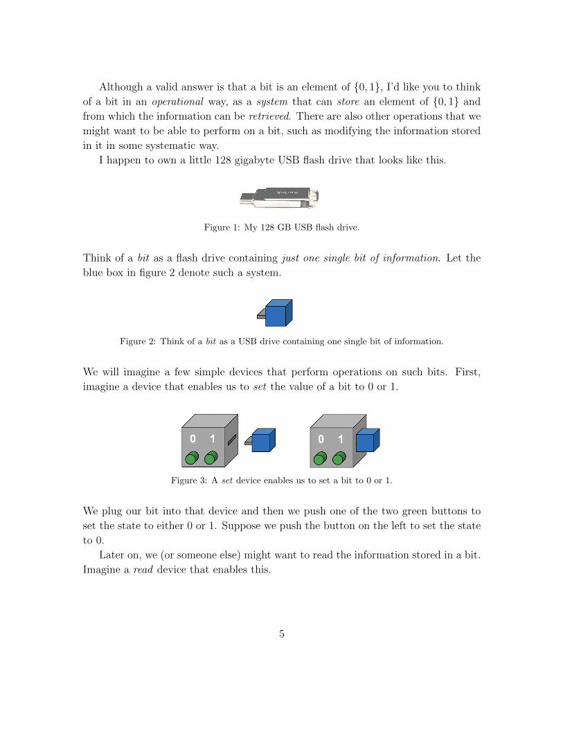
Although a valid answer is that a bit is an element of {0, 1}, I’d like you to think

of a bit in an operational way, as a system that can store an element of {0, 1} and

from which the information can be retrieved. There are also other operations that we

might want to be able to perform on a bit, such as modifying the information stored

in it in some systematic way.

I happen to own a little 128 gigabyte USB flash drive that looks like this.

Figure 1: My 128 GB USB flash drive.

Think of a bit as a flash drive containing just one single bit of information. Let the

blue box in figure 2 denote such a system.

Figure 2: Think of a bit as a USB drive containing one single bit of information.

We will imagine a few simple devices that perform operations on such bits. First,

imagine a device that enables us to set the value of a bit to 0 or 1.

Figure 3: A set device enables us to set a bit to 0 or 1.

We plug our bit into that device and then we push one of the two green buttons to

set the state to either 0 or 1. Suppose we push the button on the left to set the state

to 0.

Later on, we (or someone else) might want to read the information stored in a bit.

Imagine a read device that enables this.

5

Figure 4: Plug a bit into a read device and push the activation button to see it’s value.

We can plug the bit into that device and then push the activation button. This causes

the bit’s value to appear on a screen, so that we can see it.

A third type of device is one that transforms the state of a bit in some way. For

example, for a NOT device, we plug the bit in and, when we push the button, the

state of the bit flips (0 changes to 1 and 1 changes to 0).

Figure 5: A NOT device enables us to flip the value of a bit.

This transformation is called NOT because it performs a logical negation, where we

associate 0 with “false” and 1 with “true”. Note that, for this kind of operation,

we don’t care about seeing what the value of the bit is, as long as that value gets

negated.

OK, that’s more or less what conventional information processing is like—albeit

with many more bits in play and much more complicated operations.

2.2 A simple analog model of information

Next, let’s consider an analog information storage system. It has a continuum of

possible states (perhaps a voltage that can be anywhere within some range). We can

abstractly think of the state of the system as any real number between 0 and 1 (that

is, in the interval [0, 1]). We’ll use a different color to distinguish this from the bit.

Figure 6: An analog USB drive that stores a value in the interval [0, 1].

6

Let the red box in figure 6 represent such a system, an analog memory.

Imagine a device that sets the state of the analog memory. We plug our system

Figure 7: An analog set device.

into it. Suppose that there is some kind of dial that can be continuously rotated to

specify any number between 0 and 1. Then we press the activation button and the

state of the system becomes the value that we selected.

We can also imagine reading the state of such a system. Here the read device has

Figure 8: An analog read device.

an analog display depicted as a meter. When we press the button the needle goes to

a position between 0 and 1, corresponding to the state.

And we can also imagine an analog transformation that, when activated, applies

Figure 9: An analog f -transformation device.

some function f : [0, 1]→ [0, 1] (for example, mapping x to x2 or x to 1− x).

The real numbers are a mathematical idealization. In any implementation, there

will be a certain level of limited precision for all of the operations. But such analog

devices can be useful even if their precision isn’t perfect. Moreover, in principle,

one could make the level of precision very high. The resulting system may be very

expensive to manufacture, but it could contain a lot of information.

7

2.3 A simple probabilistic digital model of information

Before considering quantum bits, let’s introduce randomness into our notion of a bit.

Suppose that the state of our bit is the result of some random process, so there’s

a probability that the system is in state 0 and a probability that it’s in state 1. Of

course the probabilities are greater than or equal to 0 and they sum to 1. Let’s put

aside the question of what probabilities really mean. I’m going to assume that you

already have some understanding of this.

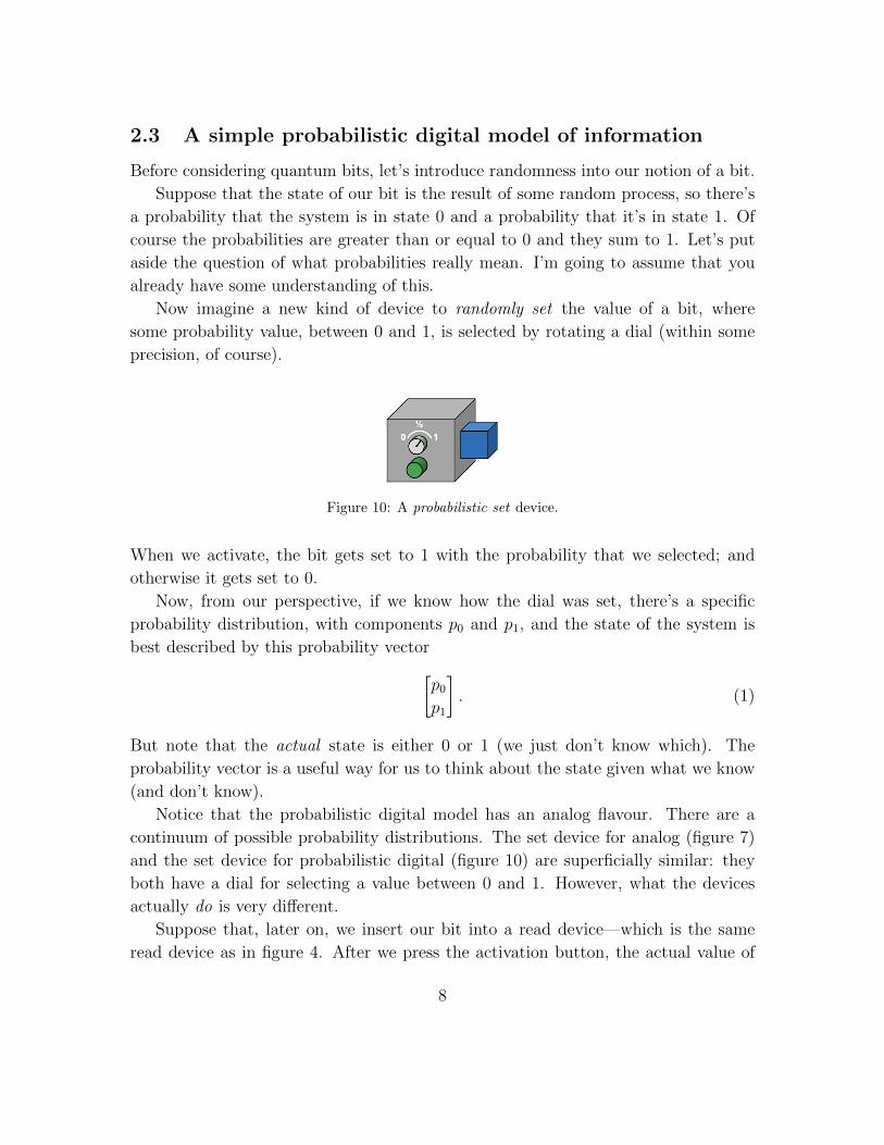
Now imagine a new kind of device to randomly set the value of a bit, where

some probability value, between 0 and 1, is selected by rotating a dial (within some

precision, of course).

Figure 10: A probabilistic set device.

When we activate, the bit gets set to 1 with the probability that we selected; and

otherwise it gets set to 0.

Now, from our perspective, if we know how the dial was set, there’s a specific

probability distribution, with components p0 and p1, and the state of the system is

best described by this probability vector[p0p1

]. (1)

But note that the actual state is either 0 or 1 (we just don’t know which). The

probability vector is a useful way for us to think about the state given what we know

(and don’t know).

Notice that the probabilistic digital model has an analog flavour. There are a

continuum of possible probability distributions. The set device for analog (figure 7)

and the set device for probabilistic digital (figure 10) are superficially similar: they

both have a dial for selecting a value between 0 and 1. However, what the devices

actually do is very different.

Suppose that, later on, we insert our bit into a read device—which is the same

read device as in figure 4. After we press the activation button, the actual value of

8

the bit appears on the screen. Once we see the value of the bit, we change whatever

probability vector we might have associated with it: the component corresponding

to what we saw becomes 1 and the other component becomes 0. Let’s refer to this

change as the “collapse of the probability vector”.

Note that, if we activate the read device a second time we will just see the same

value we saw the first time—as opposed to another independent sample. To be clear,

what the bit contains is the outcome of the original random process for setting the

bit. It does not contain information about the random process itself.

Also, if we didn’t know what probability values p0 and p1 were used when the bit

was set then reading the bit does not provide us with those values. After reading the

bit, all we can do is make some statistical inferences. For example, if the outcome

of the read operation is 1 then we can deduce that p1 could not have been 0. This

is very different from the analog model, where we can actually see the value of the

continuously varying parameter using a read device.

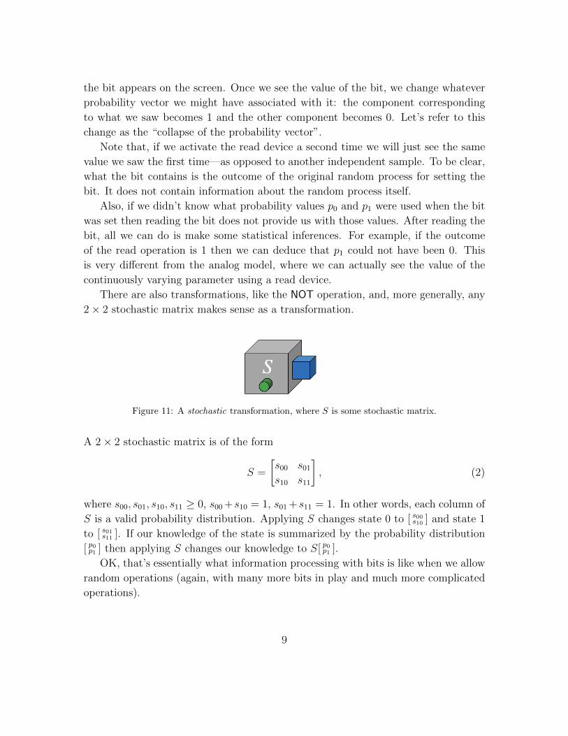
There are also transformations, like the NOT operation, and, more generally, any

2× 2 stochastic matrix makes sense as a transformation.

Figure 11: A stochastic transformation, where S is some stochastic matrix.

A 2× 2 stochastic matrix is of the form

S =

[s00 s01s10 s11

], (2)

where s00, s01, s10, s11 ≥ 0, s00 +s10 = 1, s01 +s11 = 1. In other words, each column of

S is a valid probability distribution. Applying S changes state 0 to [ s00s10 ] and state 1

to [ s01s11 ]. If our knowledge of the state is summarized by the probability distribution

[ p0p1 ] then applying S changes our knowledge to S[ p0p1 ].

OK, that’s essentially what information processing with bits is like when we allow

random operations (again, with many more bits in play and much more complicated

operations).

9

2.4 A simple quantum model of information

So how do quantum bits fit in? Are quantum bits like probabilistic bits or are they

like analog? In fact, they are neither of these. Quantum information is an entirely

different category of information. But it will be worth comparing it to probabilistic

digital and analog.

A quantum bit (or qubit) has a probability amplitude associated with 0 and with 1.

Probability amplitudes (called amplitudes for short) are different from probabilities.

They can be negative—in fact they can be complex numbers. As long as they sat-

isfy the condition that their absolute values squared sum to 1. In other words the

amplitude vector, written here with components α0 and α1, is a vector[α0

α1

]∈ C2 (3)

whose Euclidean1 length is 1 (also called a unit vector).

OK, that’s a definition, but it’s natural to ask: what do these amplitudes actually

mean? Our approach to answering this question will be operational. What I mean

by this is that we’ll consider what happens to qubits when basic operations similar

to set, read, and transform are performed. We’ll develop an understanding of qubits

by seeing them in action.

Later on, it will become clear that, unlike with probabilities, the explicit state of

a qubit is not 0 or 1; it works better to think of the amplitude vector [ α0α1 ] as the

explicit state. In this one respect, quantum digital states resemble our analog system,

where the explicit state is the continuous value.

Now, let’s see qubits in action. We have our quantum memory, which we will

denote as a purple box, containing a qubit.

Figure 12: A quantum memory containing a qubit.

To begin with, imagine a device that enables us to set the state of a qubit to any

amplitude vector.

1The Euclidean length of a vector [ α0α1

] is defined as√|α0|2 + |α1|2.

10

Figure 13: Plug the qubit into a set device, set the dials, and then push the activation button to

set the state of the qubit.

The device has two dials that we can rotate. Why two? Because there are two real

degrees of freedom for all amplitude vectors: the amplitudes α0 and α1 (which are

complex numbers) can be expressed in a polar form

α0 = sin(θ) (4)

α1 = eiφ cos(θ) (5)

which is in terms of two2 angles. So we can tune the two dials to specify any state

(within some precision), and then we press the activation button and the qubit is set

to the state that we specified.

Next, the quantum analogue of the read device is called the measure device.

Figure 14: Quantum measure device.

We’re going to consider this device carefully. Recall that the state of the qubit is

described by an amplitude vector [ α0α1 ]. What happens during a measurement is:

1. The outcome displayed on the screen is either a 0 or a 1, with respective prob-

abilities the |α0|2 and |α1|2. Note that this makes perfect sense as a probability

distribution, because these quantities sum to 1.

2. Also, the amplitude vector “collapses” towards the outcome in a manner similar

to the way that a probability vector collapses when we read the value of a bit.

The amplitude for the outcome becomes 1 and the other amplitude becomes 0.

2Perhaps you noticed that there are actually three degrees of freedom; however, it turns out that

one of them doesn’t matter (this will be explained in section 6.5).

11

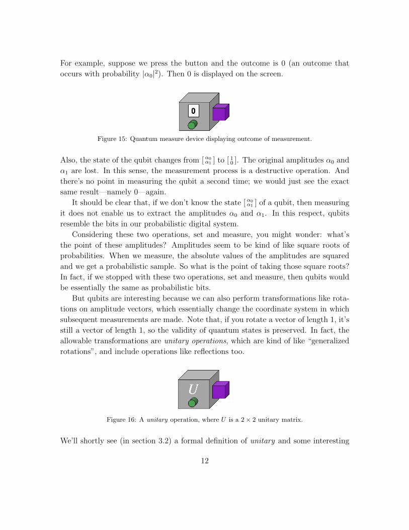
For example, suppose we press the button and the outcome is 0 (an outcome that

occurs with probability |α0|2). Then 0 is displayed on the screen.

Figure 15: Quantum measure device displaying outcome of measurement.

Also, the state of the qubit changes from [ α0α1 ] to [ 10 ]. The original amplitudes α0 and

α1 are lost. In this sense, the measurement process is a destructive operation. And

there’s no point in measuring the qubit a second time; we would just see the exact

same result—namely 0—again.

It should be clear that, if we don’t know the state [ α0α1 ] of a qubit, then measuring

it does not enable us to extract the amplitudes α0 and α1. In this respect, qubits

resemble the bits in our probabilistic digital system.

Considering these two operations, set and measure, you might wonder: what’s

the point of these amplitudes? Amplitudes seem to be kind of like square roots of

probabilities. When we measure, the absolute values of the amplitudes are squared

and we get a probabilistic sample. So what is the point of taking those square roots?

In fact, if we stopped with these two operations, set and measure, then qubits would

be essentially the same as probabilistic bits.

But qubits are interesting because we can also perform transformations like rota-

tions on amplitude vectors, which essentially change the coordinate system in which

subsequent measurements are made. Note that, if you rotate a vector of length 1, it’s

still a vector of length 1, so the validity of quantum states is preserved. In fact, the

allowable transformations are unitary operations, which are kind of like “generalized

rotations”, and include operations like reflections too.

Figure 16: A unitary operation, where U is a 2× 2 unitary matrix.

We’ll shortly see (in section 3.2) a formal definition of unitary and some interesting

12

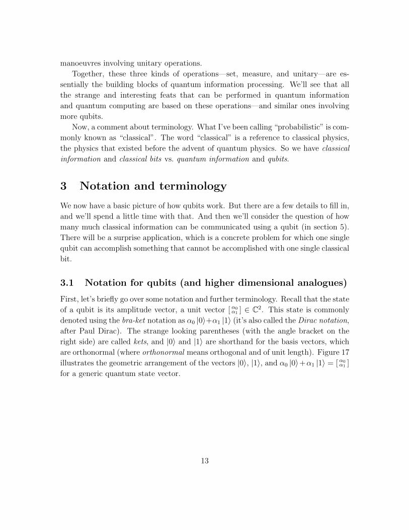
manoeuvres involving unitary operations.

Together, these three kinds of operations—set, measure, and unitary—are es-

sentially the building blocks of quantum information processing. We’ll see that all

the strange and interesting feats that can be performed in quantum information

and quantum computing are based on these operations—and similar ones involving

more qubits.

Now, a comment about terminology. What I’ve been calling “probabilistic” is com-

monly known as “classical”. The word “classical” is a reference to classical physics,

the physics that existed before the advent of quantum physics. So we have classical

information and classical bits vs. quantum information and qubits.

3 Notation and terminology

We now have a basic picture of how qubits work. But there are a few details to fill in,

and we’ll spend a little time with that. And then we’ll consider the question of how

many much classical information can be communicated using a qubit (in section 5).

There will be a surprise application, which is a concrete problem for which one single

qubit can accomplish something that cannot be accomplished with one single classical

bit.

3.1 Notation for qubits (and higher dimensional analogues)

First, let’s briefly go over some notation and further terminology. Recall that the state

of a qubit is its amplitude vector, a unit vector [ α0α1 ] ∈ C2. This state is commonly

denoted using the bra-ket notation as α0 |0〉+α1 |1〉 (it’s also called the Dirac notation,

after Paul Dirac). The strange looking parentheses (with the angle bracket on the

right side) are called kets, and |0〉 and |1〉 are shorthand for the basis vectors, which

are orthonormal (where orthonormal means orthogonal and of unit length). Figure 17

illustrates the geometric arrangement of the vectors |0〉, |1〉, and α0 |0〉+α1 |1〉 = [ α0α1 ]

for a generic quantum state vector.

13

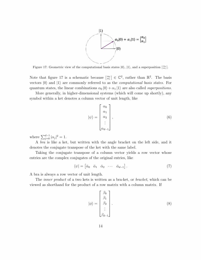
Figure 17: Geometric view of the computational basis states |0〉, |1〉, and a superposition [ α0α1

].

Note that figure 17 is a schematic because [ α0α1 ] ∈ C2, rather than R2. The basis

vectors |0〉 and |1〉 are commonly referred to as the computational basis states. For

quantum states, the linear combinations α0 |0〉+α1 |1〉 are also called superpositions.

More generally, in higher-dimensional systems (which will come up shortly), any

symbol within a ket denotes a column vector of unit length, like

|ψ〉 =

α0

α1

α2

...

αd−1

, (6)

where∑d−1

j=0 |αj|2 = 1.

A bra is like a ket, but written with the angle bracket on the left side, and it

denotes the conjugate transpose of the ket with the same label.

Taking the conjugate transpose of a column vector yields a row vector whose

entries are the complex conjugates of the original entries, like

〈ψ| =[α0 α1 α2 · · · αd−1

]. (7)

A bra is always a row vector of unit length.

The inner product of a two kets is written as a bra-ket, or bracket, which can be

viewed as shorthand for the product of a row matrix with a column matrix. If

|φ〉 =

β0β1β2...

βd−1

. (8)

14

then the inner product of |ψ〉 and |φ〉 is the bracket

〈ψ|φ〉 = 〈ψ| · |φ〉 =[α0 α1 α2 · · · αd−1

]β0β1β2...

βd−1

. (9)

Recall that, for inner products of complex-valued vectors, one takes the complex

conjugates of the entries of one of the vectors.

3.2 A closer look at unitary operations

Let U be a square matrix. Here are three equivalent definitions of unitary.

The first definition is in terms of a useful geometric property: U is unitary if it

preserves angles between unit vectors. For any two states, there is an angle between

them, which is determined by their inner product, and the property is expressed in

terms of inner products.

Definition 3.1. A square matrix U is unitary if it preserves inner products. That

is, for all |ψ1〉 and |ψ2〉, the inner product between U |ψ1〉 and U |ψ2〉 is the same as

the inner product between |ψ1〉 and |ψ2〉.

The second definition makes it easy to recognize unitary matrices.

Definition 3.2. A square matrix U is unitary if its columns are orthonormal (which

is equivalent to its rows being orthonormal).

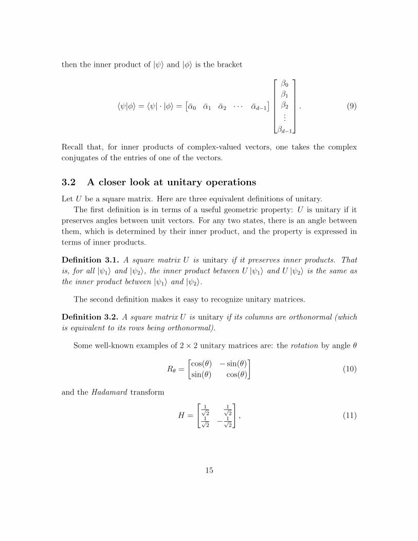
Some well-known examples of 2× 2 unitary matrices are: the rotation by angle θ

Rθ =

[cos(θ) − sin(θ)

sin(θ) cos(θ)

](10)

and the Hadamard transform

H =

[1√2

1√2

1√2− 1√

2

], (11)

15

which is not a rotation (but H is a reflection). Three further examples are the Pauli

matrices3

X =

[0 1

1 0

], Z =

[1 0

0 −1

], and Y =

[0 −ii 0

]. (12)

The PauliX is sometimes referred to as a bit flip (or NOT operation), sinceX |0〉 = |1〉and X |1〉 = |0〉. Also, Z is sometimes referred to as a phase flip.

The third definition of unitary, is useful in calculations and is commonly seen in

the literature.

Definition 3.3. A square matrix U is unitary if U∗U = I, where U∗ is the conjugate

transpose4 of U (the transpose of U with all the entries conjugated).

It remains to show that the above three definitions of unitary are equivalent:

Exercise 3.1 (fairly straightforward). Show that the above three definitions of unitary

are indeed equivalent.

3.3 A closer look at measurements

Now, let’s look at measurements again. Let our qubit be in some state α0 |0〉+α1 |1〉 =

[ α0α1 ] (where |α0|2 + |α1|2 = 1). Then the result of the measurement is the following:

• With probability |α0|2, the outcome is 0 and the state collapses to |0〉.

• With probability |α1|2, the outcome is 1 and the state collapses to |1〉.

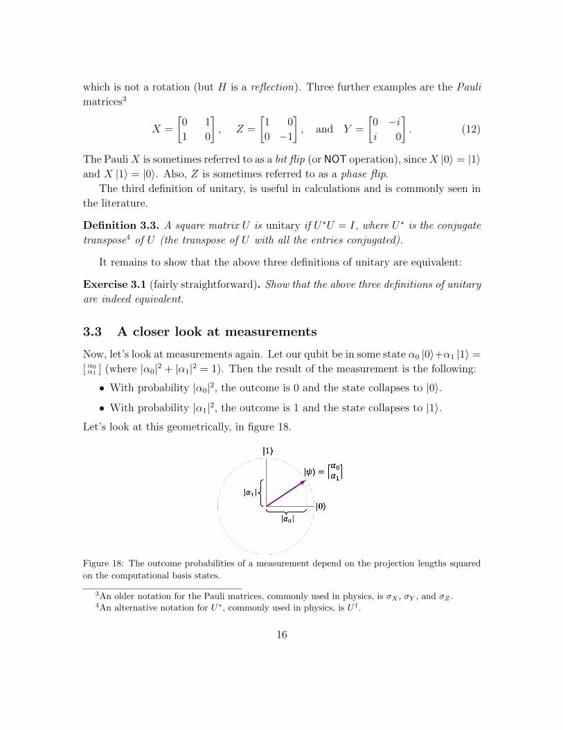
Let’s look at this geometrically, in figure 18.

Figure 18: The outcome probabilities of a measurement depend on the projection lengths squared

on the computational basis states.

3An older notation for the Pauli matrices, commonly used in physics, is σX , σY , and σZ .4An alternative notation for U∗, commonly used in physics, is U†.

16

We have a 2-dimensional space with computational basis |0〉 and |1〉. An arbitrary

state has a projection on each basis state. What happens in a measurement is that

the state collapses to each basis state with probability equal to the projection-length

squared.

The geometric perspective suggests some potential variations in our definition of

a measurement. For example, there’s no fundamental reason why the computational

basis states should have special status. We can imagine basing a measurement on

some other orthonormal basis, different from the computational basis. For example,

consider the orthonormal basis |φ0〉 and |φ1〉 in figure 19.

Figure 19: Measurement with respect to an alternative basis, |φ0〉 and |φ1〉.

Any state has a projection on each basis vector and, although the projection lengths

squared are different for this basis, they still add up to 1. We can define a new

measurement operation that projects the state being measured |ψ〉 to each these

basis vectors with probability the projection lengths squared:

• With probability |〈ψ|φ0〉|2, the outcome is 0 and the state collapses to |φ0〉.

• With probability |〈ψ|φ1〉|2, the outcome is 1 and the state collapses to |φ1〉.

One way of thinking about what unitary operations do is that they permit us to

perform measurements with respect to any alternative orthonormal basis. We have

our basic measurement operation (which is with respect to the computational basis).

If we want to perform a measurement with respect to a different orthonormal basis

|φ0〉 = U |0〉 and |φ1〉 = U |1〉 then we carry out the following procedure:

1. Apply U∗ to map the alternative basis to the computational basis (|0〉 and |1〉).

2. Perform a basic measurement (with respect to the computational basis).

3. Apply U to appropriately adjust the collapsed state (to one of |φ0〉 and |φ1〉).

17

So that’s a nice way of seeing the role of unitary operations: they change the coordi-

nate system, thereby releasing us from being tied to measuring in the computational

basis.

A final comment here is that there are more exotic measurements than this, where

the state is first embedded into a larger-dimensional space. Then a unitary operation

and measurement are made in that larger space. We’ll be seeing these types of

measurements later on, after we get to systems with multiple qubits (in section 9).

4 Introduction to state distinguishing problems

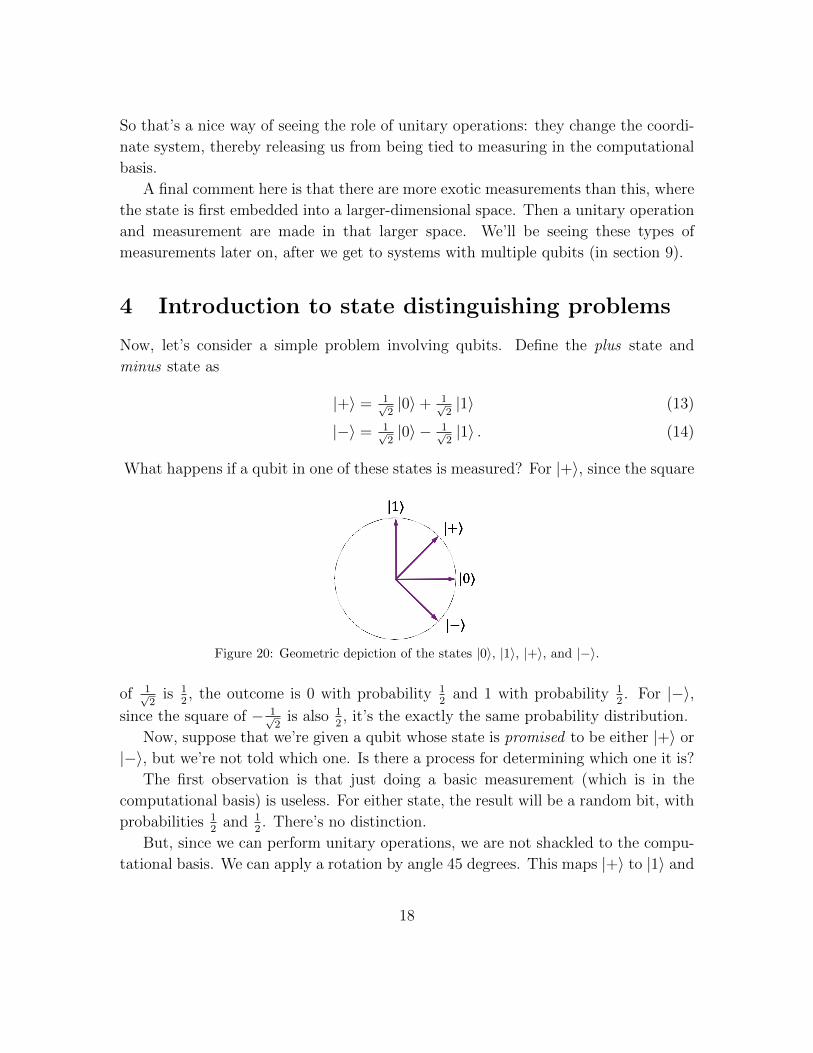
Now, let’s consider a simple problem involving qubits. Define the plus state and

minus state as

|+〉 = 1√2|0〉+ 1√

2|1〉 (13)

|−〉 = 1√2|0〉 − 1√

2|1〉 . (14)

What happens if a qubit in one of these states is measured? For |+〉, since the square

Figure 20: Geometric depiction of the states |0〉, |1〉, |+〉, and |−〉.

of 1√2

is 12, the outcome is 0 with probability 1

2and 1 with probability 1

2. For |−〉,

since the square of − 1√2

is also 12, it’s the exactly the same probability distribution.

Now, suppose that we’re given a qubit whose state is promised to be either |+〉 or

|−〉, but we’re not told which one. Is there a process for determining which one it is?

The first observation is that just doing a basic measurement (which is in the

computational basis) is useless. For either state, the result will be a random bit, with

probabilities 12

and 12. There’s no distinction.

But, since we can perform unitary operations, we are not shackled to the compu-

tational basis. We can apply a rotation by angle 45 degrees. This maps |+〉 to |1〉 and

18

|−〉 to |0〉. Then we measure in the computational basis, which perfectly distinguishes

between the two cases.

Here’s another, more subtle, state distinguishing problem to consider. Suppose

that we are given either the |0〉 state or the |+〉 state. We’re promised that the state

is one of these two, but we’re not told which one. Note that the angle between these

states is 45 degrees. Can we distinguish between these two cases?

The problem with distinguishing between the |0〉 state and the |+〉 state is that

they are not orthogonal—so there’s no unitary that takes one of them to |0〉 and the

other to |1〉 (otherwise Definition 3.1 would be violated). And, in fact, there is no

perfect distinguishing procedure.

It turns out that two states can be perfectly distinguished if and only if they are

orthogonal. I’m stating this now without proof, but when we get to the information

theory part of the course, we’ll see some tools that make it easy to prove this.

But, although we cannot perfectly distinguish between the |+〉 state and the |−〉state, we might want a procedure that at least succeeds with high probability. Let’s

consider this problem.

First note that there is a very trivial strategy, which is to output a random bit

(without even measuring the state). This succeeds with probability 12. So success

probability 12

is a baseline. Can we do better by making some measurement?

What happens if we measure in the computational basis? The sensible thing to

do in that case is to guess “0” if the outcome is 0 and guess “+” if the outcome is 1.

How well does this strategy perform? Its success probability depends on the instance:

it’s 1 for the case of |0〉 and 12

for the case of |+〉. We’ll next discuss two natural

overall measures of success probability.

One measure is the average-case success probability, which is respect to some prior

probability distribution on the instances. Suppose that this prior distribution is the

uniform distribution (so the scenario is that I flip a fair coin to determine which of the

two states to give you and your job is to perform some sort of measurement on that

state and guess which state I gave you). With respect to this performance measure,

the success probability of the above strategy is 12· 1 + 1

2· 12

= 34. Notice that this is

better than the baseline of 12.

Another overall measures of success probability is the worst-case success probabil-

ity, which is the minimum success probability with respect to all instances. Notice

that the worst-case success probability of the above strategy is 12, which is no better

than the trivial strategy.

Another strategy is to rotate by 45 degrees and then measure (and guess “0” if the

19

outcome is 0 and guess “+” if the outcome is 1). The performance of this strategy

is complementary to the strategy of measuring with respect to the computational

basis: it succeeds with probability 12

for the case of |0〉 and probability 1 for the case

of |+〉. The average-case success probability of this is 34

and it’s worse case success

probability is 12.

Can we improve on this?

Exercise 4.1 (fairly straightforward). Can you think of a simple way of combining

the two strategies above to attain a worst-case success probability of 34?

In fact, there is a better strategy than all of the strategies considered so far.

Exercise 4.2 (highly recommended if you have not seen this before). Find a strat-

egy for distinguishing between |0〉 and |+〉 whose worst-case success probability is

cos2(π/8) = 0.853...

In the information theory part of the course, we will be able to prove that cos2(π/8)

is the best worst-case performance possible for distinguishing between |0〉 and |+〉.

5 On communicating a trit using a qubit

Remember one of the questions posed at the beginning of section 2: How much

information is there in a qubit? On one hand, a qubit can be in a continuum of

explicit states, so the amount of information needed to specify a quantum state is

huge—or even infinite, when the precision is perfect. But the measurement operation

is very severe, yielding only a discrete outcome like 0 or 1, so we cannot “read out”

the continuous value.

Let’s devise a clear question about storing information that we can analyze. A

qubit can obviously store a bit (representing 0 as |0〉 and 1 as |1〉), but suppose we

want to use it to store more information than one bit. The smallest upgrade we could

ask for is to store a trit, which is an element of {0, 1, 2}. Can a qubit store a trit?

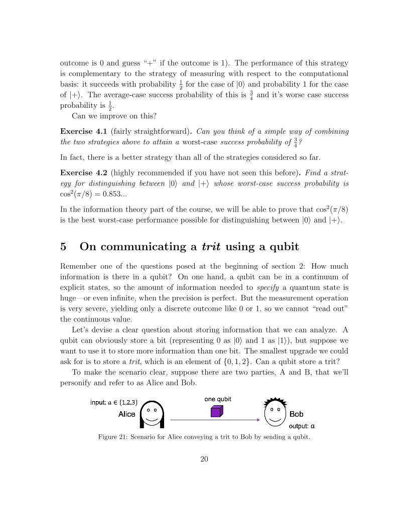
To make the scenario clear, suppose there are two parties, A and B, that we’ll

personify and refer to as Alice and Bob.

Figure 21: Scenario for Alice conveying a trit to Bob by sending a qubit.

20

Alice receives a trit a ∈ {0, 1, 2} as input and the goal is to convey this information

to Bob. Assume Alice is only allowed to send one qubit to Bob, from which he should

extract the value of the trit a. Can this be done?

To begin with, note that if Alice can only send Bob a classical bit then this is not

sufficient; please take a moment to convince yourself of this.

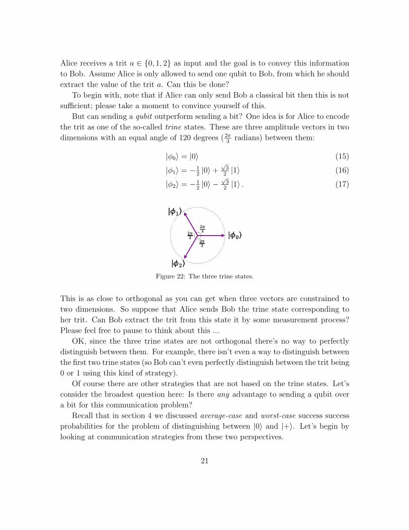
But can sending a qubit outperform sending a bit? One idea is for Alice to encode

the trit as one of the so-called trine states. These are three amplitude vectors in two

dimensions with an equal angle of 120 degrees (2π3

radians) between them:

|φ0〉 = |0〉 (15)

|φ1〉 = −12|0〉+

√32|1〉 (16)

|φ2〉 = −12|0〉 −

√32|1〉 . (17)

Figure 22: The three trine states.

This is as close to orthogonal as you can get when three vectors are constrained to

two dimensions. So suppose that Alice sends Bob the trine state corresponding to

her trit. Can Bob extract the trit from this state it by some measurement process?

Please feel free to pause to think about this ...

OK, since the three trine states are not orthogonal there’s no way to perfectly

distinguish between them. For example, there isn’t even a way to distinguish between

the first two trine states (so Bob can’t even perfectly distinguish between the trit being

0 or 1 using this kind of strategy).

Of course there are other strategies that are not based on the trine states. Let’s

consider the broadest question here: Is there any advantage to sending a qubit over

a bit for this communication problem?

Recall that in section 4 we discussed average-case and worst-case success success

probabilities for the problem of distinguishing between |0〉 and |+〉. Let’s begin by

looking at communication strategies from these two perspectives.

21

5.1 Average-case success probability

Here, the underlying assumption is that there is some known probability distribution

from which Alice’s input trit arises. For example, it could be the uniform distribu-

tion, where each trit value arises with probability 13. Then the average-case success

probability of any strategy of Alice and Bob is the weighted average of the three

success probabilities.

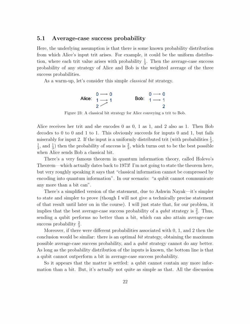
As a warm-up, let’s consider this simple classical bit strategy.

Figure 23: A classical bit strategy for Alice conveying a trit to Bob.

Alice receives her trit and she encodes 0 as 0, 1 as 1, and 2 also as 1. Then Bob

decodes to 0 to 0 and 1 to 1. This obviously succeeds for inputs 0 and 1, but fails

miserably for input 2. If the input is a uniformly distributed trit (with probabilities 13,

13, and 1

3) then the probability of success is 2

3, which turns out to be the best possible

when Alice sends Bob a classical bit.

There’s a very famous theorem in quantum information theory, called Holevo’s

Theorem—which actually dates back to 1973! I’m not going to state the theorem here,

but very roughly speaking it says that “classical information cannot be compressed by

encoding into quantum information”. In our scenario: “a qubit cannot communicate

any more than a bit can”.

There’s a simplified version of the statement, due to Ashwin Nayak—it’s simpler

to state and simpler to prove (though I will not give a technically precise statement

of that result until later on in the course). I will just state that, for our problem, it

implies that the best average-case success probability of a qubit strategy is 23. Thus,

sending a qubit performs no better than a bit, which can also attain average-case

success probability 23.

Moreover, if there were different probabilities associated with 0, 1, and 2 then the

conclusion would be similar: there is an optimal bit strategy, obtaining the maximum

possible average-case success probability, and a qubit strategy cannot do any better.

As long as the probability distribution of the inputs is known, the bottom line is that

a qubit cannot outperform a bit in average-case success probability.

So it appears that the matter is settled: a qubit cannot contain any more infor-

mation than a bit. But, it’s actually not quite as simple as that. All the discussion

22

so far has been for average-case success probability. Something surprising happens

when we consider worst-case success probability.

5.2 Worst-case success probability

For any given strategy, this is defined as lowest success probability for all inputs

(instead of the average of the success probabilities). This framework makes sense

if Alice and Bob have no idea what distribution Alice’s input trit will arise from.

Whatever strategy they come up with, the trit could be the case where their strategy

performs the worst.

Consider the classical bit strategy that we saw in figure 23, whose average-case

success probability is 23. What’s its worst-case success probability? For the worst-case

instance, the success probability is zero! If the trit is 2 then Bob produces the wrong

value for sure!

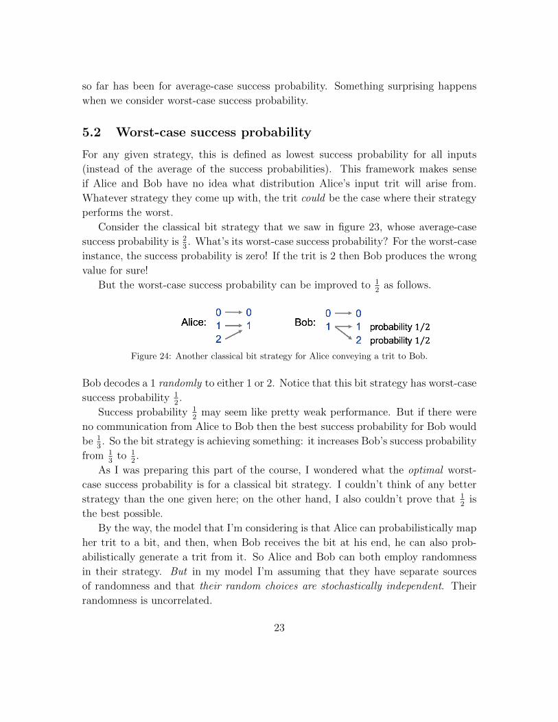
But the worst-case success probability can be improved to 12

as follows.

Figure 24: Another classical bit strategy for Alice conveying a trit to Bob.

Bob decodes a 1 randomly to either 1 or 2. Notice that this bit strategy has worst-case

success probability 12.

Success probability 12

may seem like pretty weak performance. But if there were

no communication from Alice to Bob then the best success probability for Bob would

be 13. So the bit strategy is achieving something: it increases Bob’s success probability

from 13

to 12.

As I was preparing this part of the course, I wondered what the optimal worst-

case success probability is for a classical bit strategy. I couldn’t think of any better

strategy than the one given here; on the other hand, I also couldn’t prove that 12

is

the best possible.

By the way, the model that I’m considering is that Alice can probabilistically map

her trit to a bit, and then, when Bob receives the bit at his end, he can also prob-

abilistically generate a trit from it. So Alice and Bob can both employ randomness

in their strategy. But in my model I’m assuming that they have separate sources

of randomness and that their random choices are stochastically independent. Their

randomness is uncorrelated.

23

Well, I eventually figured it out, and it was easier than I first thought. I also

thought about the optimal worst-case success probability of qubit strategies. What’s

remarkable is that the worst-case success probability can be higher for a qubit strategy

than possible with a bit strategy! The advantage is not enormous, but this shows

that there is a sense in which a qubit can store more information than a bit. We have

a scenario where a single qubit can achieve something that a single bit cannot.

OK, so what are the specific maximum success probabilities for bit strategies and

for qubit strategies, and how are they obtained? I’d like you to think about this, and

I’m posing these as challenge questions for you.

Exercise 5.1 (challenging). What’s the maximum success probability of a classical

bit strategy? (Alice and Bob can both act randomly, but their randomness must be

uncorrelated.)

Exercise 5.2 (challenging). What’s the maximum success probability of a qubit strat-

egy? (Bob is allowed to measure in a higher dimensional space.)

Remember that, for bit strategies, we’re allowing random behavior for Alice and for

Bob, but their random sources must be uncorrelated. Also, for the case of qubit

strategies, there some subtlety to this question. If you tackle exercise 5.2, you should

consider the exotic measurements that I only mentioned in passing (they are explained

in section 9). Bob can add a second qubit in state |0〉 to the qubit he receives from

Alice and then perform a two-qubit unitary operation, and then measure the two

qubit system. In the next section, we consider systems with multiple qubits.

6 Systems with multiple bits and multiple qubits

Up until now, we have considered systems of a single bit and a single qubit. Let’s

consider the case of multiple bits and qubits.

6.1 Definitions of n-bit systems and n-qubit systems

Our definitions for bits and qubits extend naturally to n-bit systems and n-qubit

systems, by taking 2n-dimensional vectors instead of 2-dimensional vectors.

For n classical bits, there are 2n possible values, and a probabilistic state has a

probability px associated with every n-bit string x ∈ {0, 1}n. Of course, since these

are probabilities, we have: for all x ∈ {0, 1}n, px ≥ 0 and∑

x∈{0,1}n px = 1. These

probabilities constitute a 2n-dimensional probability vector.

24

For n quantum bits, there are 2n amplitudes: αx ∈ C, for each x ∈ {0, 1}n(where

∑x∈{0,1}n |αx|2 = 1). These amplitudes constitute a 2n-dimensional state

vector (which is a unit vector).

Note that, although the focus of attention in quantum information processing

is usually on n-qubit systems, it’s completely valid to consider systems whose states

have dimensions other than powers of 2. For example, a quantum trit (qutrit) has a 3-

dimensional state vector of the form α0|0〉+α1|1〉+α2|2〉 (with |α0|2+|α1|2+|α2|2 = 1).

The set of all probability vectors is a simplex, which is illustrated for the case of

three dimensions as a triangular region.

Figure 25: Simplex of all possible 3-dimensional classical (probabilistic) states.

The set of all valid quantum state vectors is a hypersphere, which is all points of

distance 1 from the origin.

Figure 26: Hypersphere of all possible 3-dimensional quantum states.

There are 2n (orthonormal) computational basis states, denoted as n-bit strings

within kets. For n = 3, these states are

|000〉 , |001〉 , |010〉 , |011〉 , |100〉 , |101〉 , |110〉 , |111〉 . (18)

Note that we can write an n-qubit state vector as a linear combination of the 2n

computational basis states, as ∑x∈{0,1}n

αx |x〉 , (19)

25

where ∑x∈{0,1}n

|αx|2 = 1. (20)

As with single qubits, what’s important is the operations that can be performed

on them. We’ll consider unitary operations and measurements.

Unitary operations are 2n × 2n unitary matrices, acting on the 2n-dimensional

state vectors (unitary matrices were defined in section 3.2).

Measurements have 2n outcomes, corresponding to the 2n computational basis

states. Each basis state outcome occurs with probability the absolute squared of its

amplitude. Thus, when a measurement is applied to the state∑x∈{0,1}n

αx |x〉 , (21)

what happens is: an outcome x ∈ {0, 1}n occurs with probability |αx|2 and the state

of the system changes to the computational basis state |x〉.So far, everything is the same as for bits and qubits, except with 2n dimensions

instead of two dimensions. But there’s more to it than that. There is structure among

subsystems.

6.2 Subsystems of n-bit systems

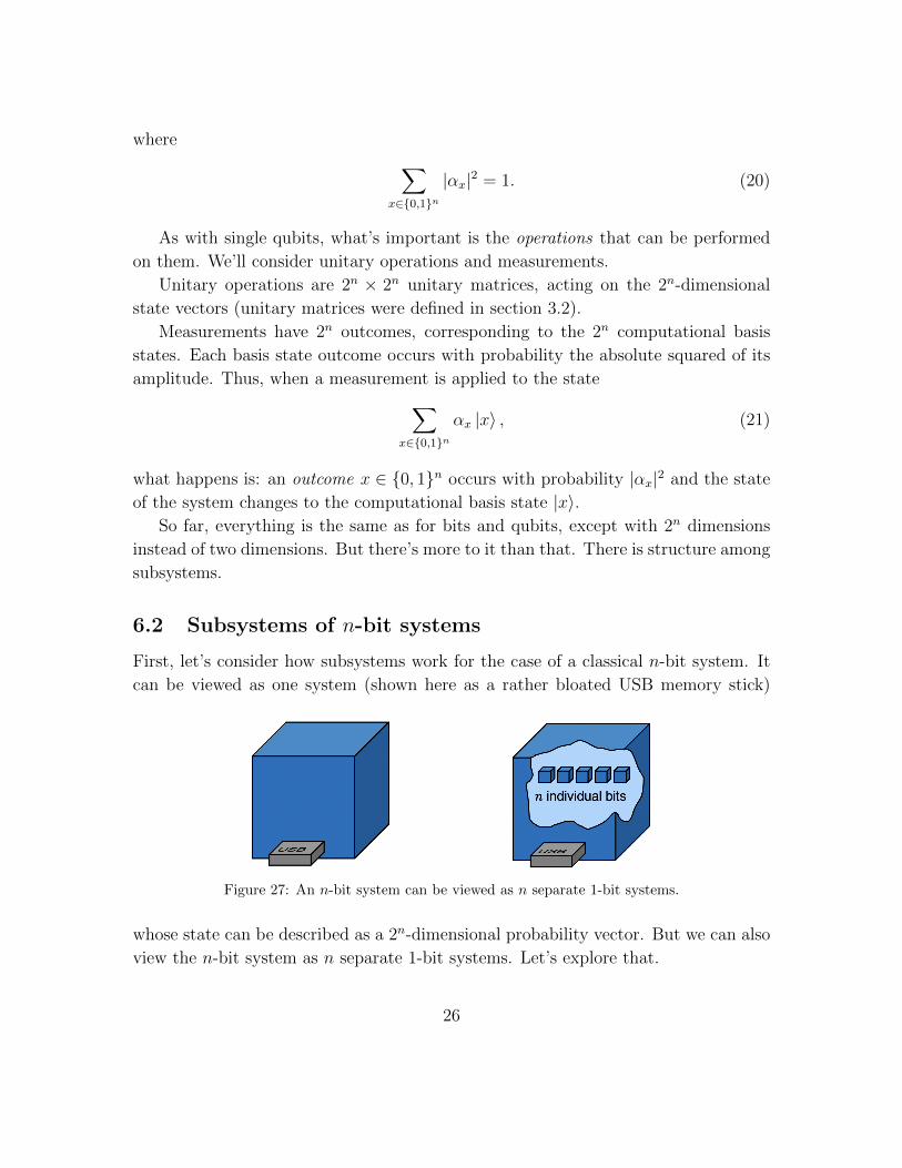
First, let’s consider how subsystems work for the case of a classical n-bit system. It

can be viewed as one system (shown here as a rather bloated USB memory stick)

Figure 27: An n-bit system can be viewed as n separate 1-bit systems.

whose state can be described as a 2n-dimensional probability vector. But we can also

view the n-bit system as n separate 1-bit systems. Let’s explore that.

26

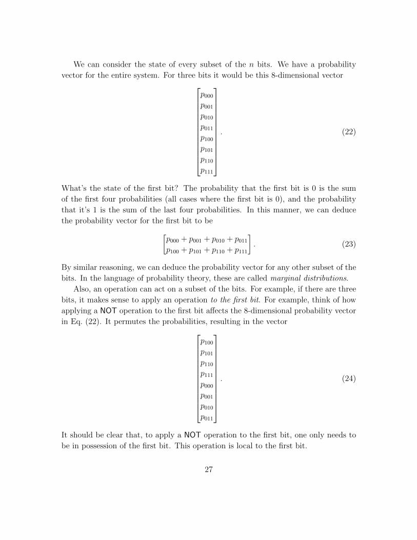
We can consider the state of every subset of the n bits. We have a probability

vector for the entire system. For three bits it would be this 8-dimensional vector

p000p001p010p011p100p101p110p111

. (22)

What’s the state of the first bit? The probability that the first bit is 0 is the sum

of the first four probabilities (all cases where the first bit is 0), and the probability

that it’s 1 is the sum of the last four probabilities. In this manner, we can deduce

the probability vector for the first bit to be[p000 + p001 + p010 + p011p100 + p101 + p110 + p111

]. (23)

By similar reasoning, we can deduce the probability vector for any other subset of the

bits. In the language of probability theory, these are called marginal distributions.

Also, an operation can act on a subset of the bits. For example, if there are three

bits, it makes sense to apply an operation to the first bit. For example, think of how

applying a NOT operation to the first bit affects the 8-dimensional probability vector

in Eq. (22). It permutes the probabilities, resulting in the vector

p100p101p110p111p000p001p010p011

. (24)

It should be clear that, to apply a NOT operation to the first bit, one only needs to

be in possession of the first bit. This operation is local to the first bit.

27

And operations can be similarly local to various other subsets of the bits. Dataflow

diagrams are a useful way of illustrating localizations of operations, and their evolu-

tion in time. Figure 28 is an example of a dataflow diagram.

Figure 28: A dataflow diagram of a 3-qubit system. First, operation S is applied to the first bit.

Then operation T is applied jointly to the second and third bits. Finally, operation U is applied to

the first and second bits.

6.3 Subsystems of n-qubit systems

Now we consider subsystems in the context of an n-qubit system. An n-qubit system

can be viewed as one system (shown as a bloated quantum USB memory). But it can

also be viewed as n separate 1-qubit systems.

Figure 29: An n-qubit system can be viewed as n separate 1-qubit systems.

Can we consider the state of every subset of the n qubits? Consider a 3-qubit system

28

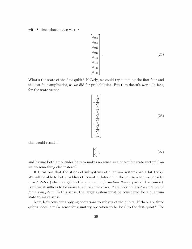
with 8-dimensional state vector

α000

α001

α010

α011

α100

α101

α110

α111

. (25)

What’s the state of the first qubit? Naıvely, we could try summing the first four and

the last four amplitudes, as we did for probabilities. But that doesn’t work. In fact,

for the state vector

1√8

− 1√81√8

− 1√81√8

− 1√81√8

− 1√8

(26)

this would result in [0

0

], (27)

and having both amplitudes be zero makes no sense as a one-qubit state vector! Can

we do something else instead?

It turns out that the states of subsystems of quantum systems are a bit tricky.

We will be able to better address this matter later on in the course when we consider

mixed states (when we get to the quantum information theory part of the course).

For now, it suffices to be aware that: in some cases, there does not exist a state vector

for a subsystem. In this sense, the larger system must be considered for a quantum

state to make sense.

Now, let’s consider applying operations to subsets of the qubits. If there are three

qubits, does it make sense for a unitary operation to be local to the first qubit? The

29

fact that the first qubit might not even have have a state vector suggests that this is

not an entirely trivial matter.

But it turns out that there is a fairly straightforward to make sense of operations

that are local to a subset of the qubits—and we’ll see how to do this shortly (in

section 6.6).

For example, if Alice possesses the first qubit and Bob the last two qubits then

Alice can perform an operation on her qubit, without touching Bob’s qubits. And

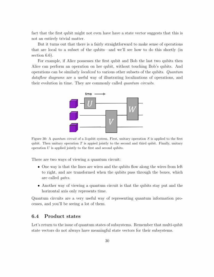
operations can be similarly localized to various other subsets of the qubits. Quantum

dataflow diagrams are a useful way of illustrating localizations of operations, and

their evolution in time. They are commonly called quantum circuits.

Figure 30: A quantum circuit of a 3-qubit system. First, unitary operation S is applied to the first

qubit. Then unitary operation T is appied jointly to the second and third qubit. Finally, unitary

operation U is applied jointly to the first and second qubits.

There are two ways of viewing a quantum circuit:

• One way is that the lines are wires and the qubits flow along the wires from left

to right, and are transformed when the qubits pass through the boxes, which

are called gates.

• Another way of viewing a quantum circuit is that the qubits stay put and the

horizontal axis only represents time.

Quantum circuits are a very useful way of representing quantum information pro-

cesses, and you’ll be seeing a lot of them.

6.4 Product states

Let’s return to the issue of quantum states of subsystems. Remember that multi-qubit

state vectors do not always have meaningful state vectors for their subsystems.

30

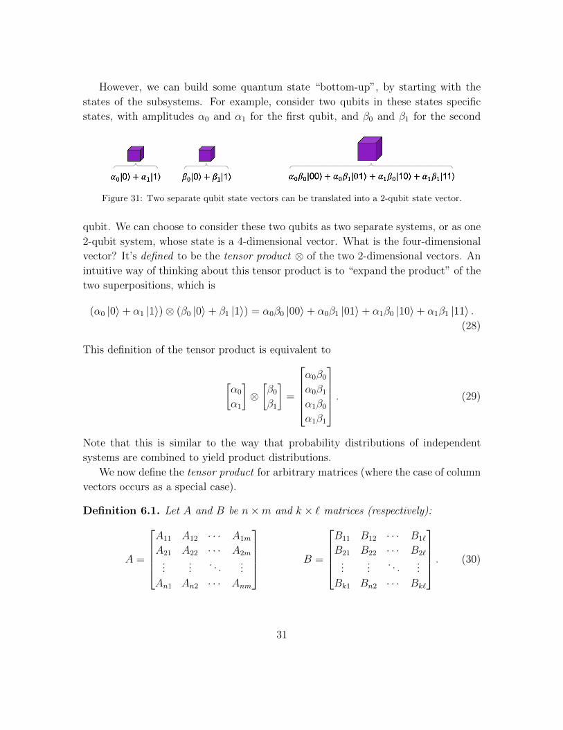
However, we can build some quantum state “bottom-up”, by starting with the

states of the subsystems. For example, consider two qubits in these states specific

states, with amplitudes α0 and α1 for the first qubit, and β0 and β1 for the second

Figure 31: Two separate qubit state vectors can be translated into a 2-qubit state vector.

qubit. We can choose to consider these two qubits as two separate systems, or as one

2-qubit system, whose state is a 4-dimensional vector. What is the four-dimensional

vector? It’s defined to be the tensor product ⊗ of the two 2-dimensional vectors. An

intuitive way of thinking about this tensor product is to “expand the product” of the

two superpositions, which is

(α0 |0〉+ α1 |1〉)⊗ (β0 |0〉+ β1 |1〉) = α0β0 |00〉+ α0β1 |01〉+ α1β0 |10〉+ α1β1 |11〉 .(28)

This definition of the tensor product is equivalent to

[α0

α1

]⊗[β0β1

]=

α0β0α0β1α1β0α1β1

. (29)

Note that this is similar to the way that probability distributions of independent

systems are combined to yield product distributions.

We now define the tensor product for arbitrary matrices (where the case of column

vectors occurs as a special case).

Definition 6.1. Let A and B be n×m and k × ` matrices (respectively):

A =

A11 A12 · · · A1m

A21 A22 · · · A2m

......

. . ....

An1 An2 · · · Anm

B =

B11 B12 · · · B1`

B21 B22 · · · B2`

......

. . ....

Bk1 Bn2 · · · Bk`

. (30)

31

The tensor product of A and B (also called the Kronecker product) is defined as

A⊗B =

A11B A12B · · · A1mB

A21B A22B · · · A2mB...

.... . .

...

An1B An2B · · · AnmB

, (31)

where each AijB denotes a k× ` block consisting of all entries of B multiplied by Aij.

Note that A⊗B is a km× `n matrix.

Definition 6.2. If one system is in state |ψ〉 and another system is in state |φ〉, then

the state of the joint system is the product state |φ〉 ⊗ |ψ〉.

Now a few words about notation for product states. Frequently |φ〉 ⊗ |ψ〉 is

abbreviated to |φ〉 |ψ〉. Also, for computational basis states, |a〉 and |b〉 (where a ∈{0, 1}n and b ∈ {0, 1}m), we have these equivalent notations: |a〉⊗|b〉 = |a〉 |b〉 = |ab〉.For example, |0〉 ⊗ |0〉 ⊗ |1〉 = |0〉 |0〉 |1〉 = |001〉.

Exercise 6.1 (straightforward, but one case is a trick question). In each case, express

the 2-qubit state as a product of two 1-qubit states:

12|00〉+ 1

2|01〉+ 1

2|10〉+ 1

2|11〉 (32)

12|00〉 − 1

2|01〉 − 1

2|10〉+ 1

2|11〉 (33)

14|00〉+

√34|01〉+

√34|10〉+ 3

4|11〉 (34)

1√2|00〉+ 1√

2|11〉 . (35)

The first three cases are straightforward. If you tried to work out the third case, you

probably realized that there is no solution! The last state cannot be expressed as a

tensor product. It is one of those states (mentioned in section 6.3) whose individual

qubits do not have state vectors.

Exercise 6.2 (fairly straightforward). Prove that the state vector 1√2|00〉 + 1√

2|11〉

cannot be written as the tensor product of two one qubit state vectors.

The state 1√2|00〉+ 1√

2|11〉 is an example of an entangled state. We’ll see that two

qubits in such a state can behave in interesting ways. It’s especially interesting when

the two qubits are physically in separate locations, say one is in Alice’s lab and one

is in Bob’s lab.

32

6.5 Aside: global phases

Now is a good time to discuss the matter of global phases. You may have noticed

that factorizations of 2-qubit states into products of 1-qubit states is not unique. For

example,

12|00〉+ 1

2|01〉+ 1

2|10〉+ 1

2|11〉 =

(1√2|0〉+ 1√

2|1〉)⊗(

1√2|0〉+ 1√

2|1〉)

(36)

=(− 1√

2|0〉 − 1√

2|1〉)⊗(− 1√

2|0〉 − 1√

2|1〉). (37)

So what’s the difference between the state 1√2|0〉 + 1√

2|1〉 and − 1√

2|0〉 − 1√

2|1〉? As

vectors they are not orthogonal, but they are certainly different. The angle between

them is 180 degrees.

Can we distinguish between them? Suppose you’re given a qubit in one of these

states but not told which one. Is there some measurement procedure for determining

which one it is? If course, you could always apply the trivial state distinguishing

procedure (from section 4) that ignores the qubit and make a random guess. This

succeeds with probability 12. Can you apply some measurement procedure that enables

you to do any better than that?

The answer is no. For any measurement (in any basis), the outcome probabilities

will be identical for both states. Since there’s no way of distinguishing between the

states, we regard them as equivalent.

Based on this, we define an equivalence relation on state vectors.

Definition 6.3. Two state vectors |ψ〉 and |φ〉 are deemed equivalent if |ψ〉 = eiθ |φ〉for some θ ∈ [0, 2π].

The factor eiθ |φ〉 is called a global phase (“global” because it’s applied to all of

the terms of the superposition).

Here’s an exercise, if you’d like to get used to this concept.

Exercise 6.3. Partition the following into sets of equivalent states:

− 1√2|0〉+ 1√

2|1〉 1√

2|0〉 − 1√

2|1〉 1√

2|0〉+ i√

2|1〉

i√2|0〉+ 1√

2|1〉 − 1√

2|0〉+ i√

2|1〉 1√

2|0〉 − i√

2|1〉

33

6.6 Local unitary operations

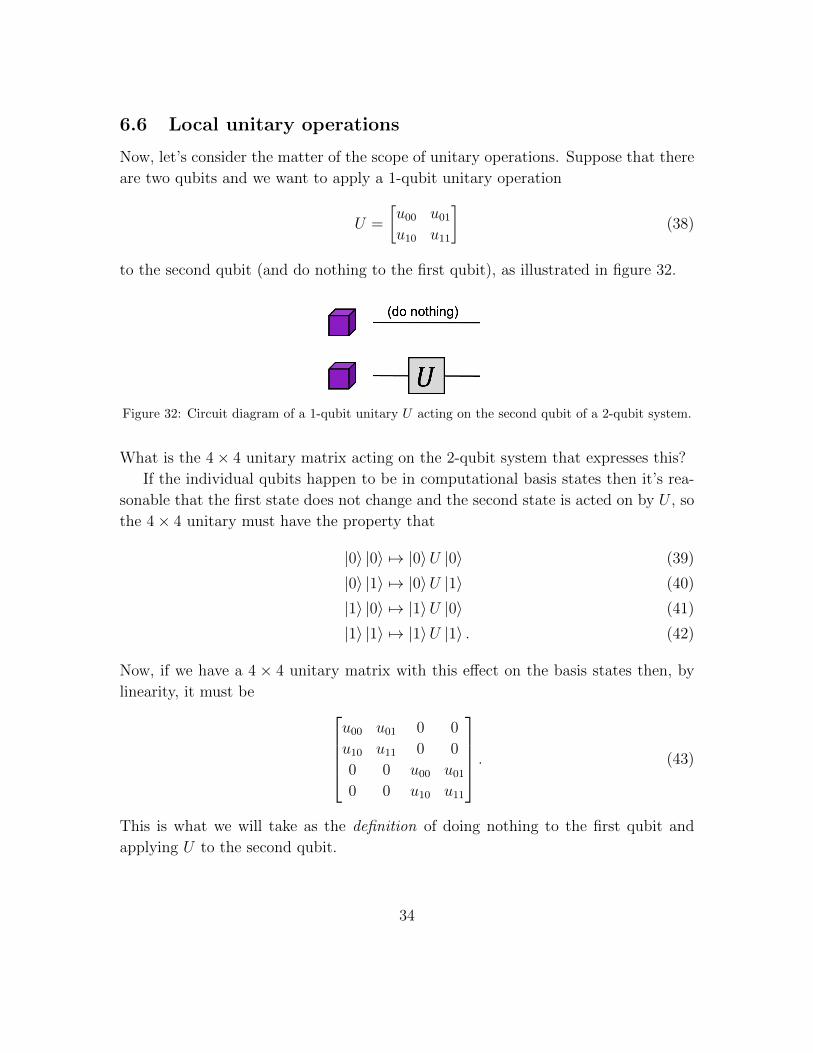
Now, let’s consider the matter of the scope of unitary operations. Suppose that there

are two qubits and we want to apply a 1-qubit unitary operation

U =

[u00 u01u10 u11

](38)

to the second qubit (and do nothing to the first qubit), as illustrated in figure 32.

Figure 32: Circuit diagram of a 1-qubit unitary U acting on the second qubit of a 2-qubit system.

What is the 4× 4 unitary matrix acting on the 2-qubit system that expresses this?

If the individual qubits happen to be in computational basis states then it’s rea-

sonable that the first state does not change and the second state is acted on by U , so

the 4× 4 unitary must have the property that

|0〉 |0〉 7→ |0〉U |0〉 (39)

|0〉 |1〉 7→ |0〉U |1〉 (40)

|1〉 |0〉 7→ |1〉U |0〉 (41)

|1〉 |1〉 7→ |1〉U |1〉 . (42)

Now, if we have a 4 × 4 unitary matrix with this effect on the basis states then, by

linearity, it must be u00 u01 0 0

u10 u11 0 0

0 0 u00 u010 0 u10 u11

. (43)

This is what we will take as the definition of doing nothing to the first qubit and

applying U to the second qubit.

34

Notice that, by this definition, it makes perfect sense to apply U to the second

qubit of any 2-qubit system, even one in an entangled state like

1√2|00〉+ 1√

2|11〉 , (44)

where the second qubit of the state does not even have a state vector! Whatever

the 2-qubit state is, it’s a 4-dimensional vector, and it makes sense to multiply that

vector by the matrix in Eq. (43).

Interestingly, the matrix in Eq. (43) can be expressed succinctly as[1 0

0 1

]⊗[u00 u01u10 u11

]= I ⊗ U, (45)

where the operation ⊗ (the tensor product) is defined in Definition 6.1. Here’s a

question to consider:

Exercise 6.4 (straightforward). What is the 4× 4 unitary corresponding to applying

U to the first qubit and doing nothing to the second qubit?

We’ve discussed 1-qubit unitary operations in 2-qubit systems. Clearly, this gen-

eralizes naturally to more qubits. For example, when there are n + m qubits and U

Figure 33: Circuit for U applied to the last m qubits of an (n+m)-qubit system.

is applied to the last m qubits, think about what the resulting 2n+m × 2n+m matrix

should be.

The resulting 2n+m×2n+m unitary matrix is I⊗U , where I is the 2n×2n identity

matrix. Also, if a unitary V is applied to the first n qubits, this is expressed as V ⊗I,

where I is the 2m × 2m identity matrix.

Furthermore, whenever U and V act on separate qubits (as in figure 34), it’s

natural to expect the two operations to commute. That is, their net effect is the

same regardless of which one applied first. It’s not too hard to prove this, and I

suggest it as an exercise.

35

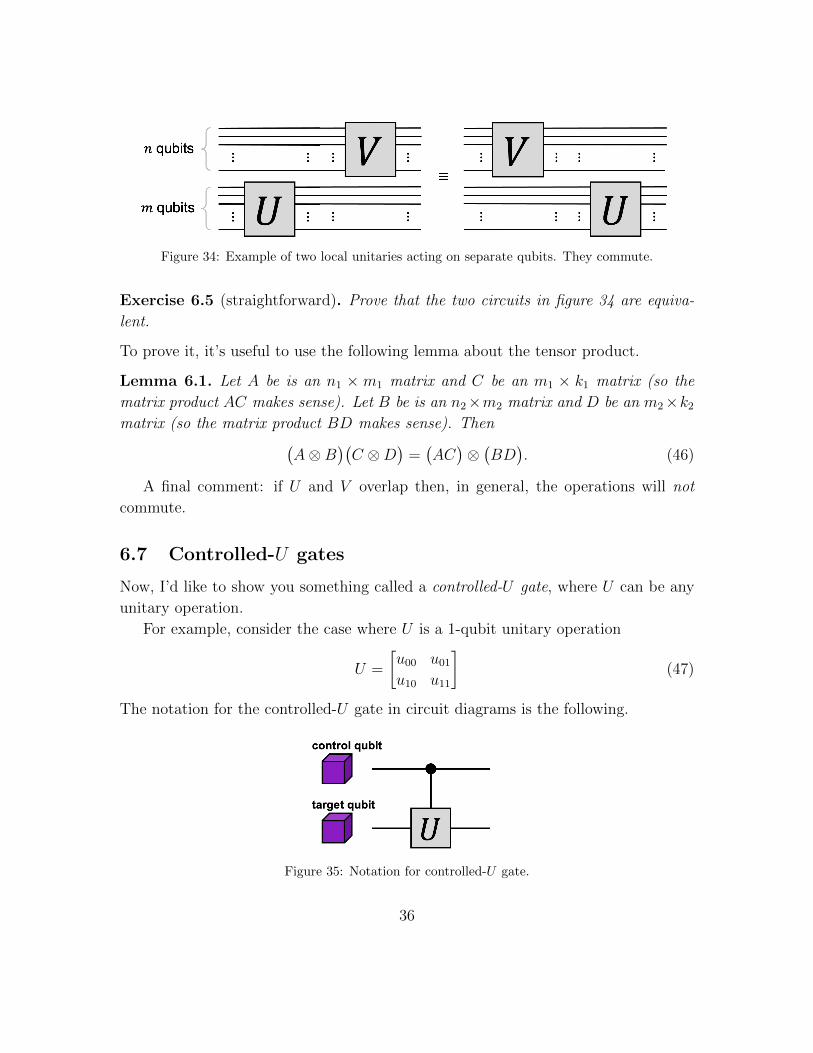
Figure 34: Example of two local unitaries acting on separate qubits. They commute.

Exercise 6.5 (straightforward). Prove that the two circuits in figure 34 are equiva-

lent.

To prove it, it’s useful to use the following lemma about the tensor product.

Lemma 6.1. Let A be is an n1 × m1 matrix and C be an m1 × k1 matrix (so the

matrix product AC makes sense). Let B be is an n2×m2 matrix and D be an m2×k2matrix (so the matrix product BD makes sense). Then(

A⊗B)(C ⊗D

)=(AC)⊗(BD

). (46)

A final comment: if U and V overlap then, in general, the operations will not

commute.

6.7 Controlled-U gates

Now, I’d like to show you something called a controlled-U gate, where U can be any

unitary operation.

For example, consider the case where U is a 1-qubit unitary operation

U =

[u00 u01u10 u11

](47)

The notation for the controlled-U gate in circuit diagrams is the following.

Figure 35: Notation for controlled-U gate.

36

where U drawn as “acting” on a target qubit and with a “wire” from a control qubit

to U .

If the control qubit is in state |0〉 then nothing happens. And, if the control qubit

is in state |1〉 then U gets applied to the target qubit. This gate has the following

effect on the four computational basis states:

|0〉 |0〉 7→ |0〉 |0〉 (48)

|0〉 |1〉 7→ |0〉 |1〉 (49)

|1〉 |0〉 7→ |1〉U |0〉 (50)

|1〉 |1〉 7→ |1〉U |1〉 . (51)

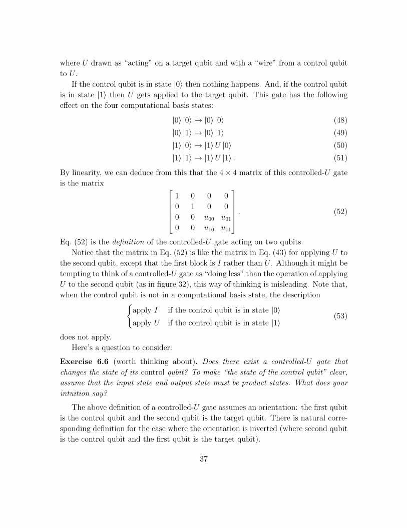
By linearity, we can deduce from this that the 4× 4 matrix of this controlled-U gate

is the matrix 1 0 0 0

0 1 0 0

0 0 u00 u010 0 u10 u11

. (52)

Eq. (52) is the definition of the controlled-U gate acting on two qubits.

Notice that the matrix in Eq. (52) is like the matrix in Eq. (43) for applying U to

the second qubit, except that the first block is I rather than U . Although it might be

tempting to think of a controlled-U gate as “doing less” than the operation of applying

U to the second qubit (as in figure 32), this way of thinking is misleading. Note that,

when the control qubit is not in a computational basis state, the description{apply I if the control qubit is in state |0〉apply U if the control qubit is in state |1〉

(53)

does not apply.

Here’s a question to consider:

Exercise 6.6 (worth thinking about). Does there exist a controlled-U gate that

changes the state of its control qubit? To make “the state of the control qubit” clear,

assume that the input state and output state must be product states. What does your

intuition say?

The above definition of a controlled-U gate assumes an orientation: the first qubit

is the control qubit and the second qubit is the target qubit. There is natural corre-

sponding definition for the case where the orientation is inverted (where second qubit

is the control qubit and the first qubit is the target qubit).

37

Exercise 6.7. Consider an inverted control-U gate, where the second qubit is the

control and the first qubit is the target. Based on the above explanations, how should

the 4× 4 matrix be defined for this (analogous to Eq. (52))?

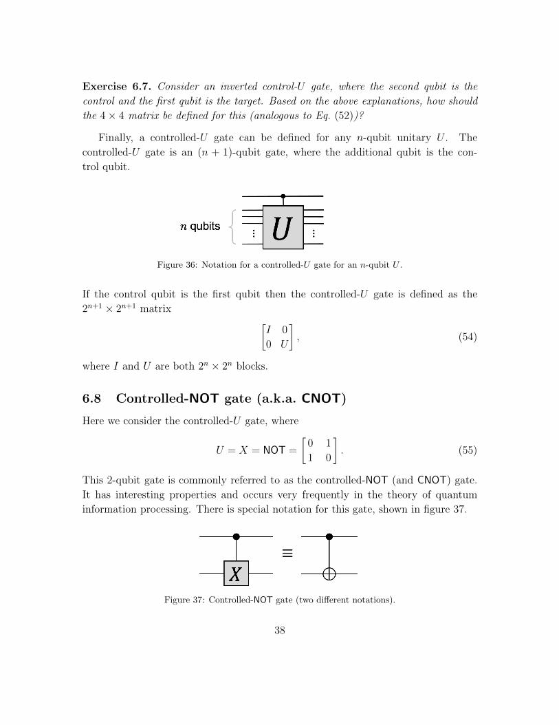
Finally, a controlled-U gate can be defined for any n-qubit unitary U . The

controlled-U gate is an (n + 1)-qubit gate, where the additional qubit is the con-

trol qubit.

Figure 36: Notation for a controlled-U gate for an n-qubit U .

If the control qubit is the first qubit then the controlled-U gate is defined as the

2n+1 × 2n+1 matrix [I 0

0 U

], (54)

where I and U are both 2n × 2n blocks.

6.8 Controlled-NOT gate (a.k.a. CNOT)

Here we consider the controlled-U gate, where

U = X = NOT =

[0 1

1 0

]. (55)

This 2-qubit gate is commonly referred to as the controlled-NOT (and CNOT) gate.

It has interesting properties and occurs very frequently in the theory of quantum

information processing. There is special notation for this gate, shown in figure 37.

Figure 37: Controlled-NOT gate (two different notations).

38

To understand where the notation comes from, consider what happens when

the inputs are computational basis states. Let the inputs be |a〉 and |b〉, where

a, b ∈ {0, 1}. For these input states, the output states are |a〉 and |a⊕ b〉. The sym-

Figure 38: Action of CNOT gate on the computational basis states (a, b ∈ {0, 1}).

bol ⊕ is the binary exclusive-OR operation (a.k.a. XOR). If you haven’t seen the ⊕operation before, here’s a table of its values, and a comparison with values of ∨ (the

standard OR).

XOR OR

ab a⊕ b a ∨ b00 0 0

01 1 1

10 1 1

11 0 1

The value of a ⊕ b is 1 and only if one of the two input bits are 1, but not both;

whereas, a ∨ b is 1 also in the case where both a and b are 1. Another, altogether

different way of thinking about the ⊕ operation is that it is the sum of the two bits in

modulo 2 arithmetic. The way that the symbol ⊕ is embedded into the gate symbol

in figure 38 is suggestive of what it does.

The above discussion of the CNOT gate is for computational basis states. The

definition of the CNOT gates is given by the 4× 4 unitary matrix in Eq. (52)

CNOT =

1 0 0 0

0 1 0 0

0 0 0 1

0 0 1 0

. (56)

This operation can be applied to any 2-qubit state—independent of any intuitive

picture that’s based on the very special case of computational basis states.

Remember, in Exercise 6.6, I asked a question about whether there is a controlled-

U gate that can change the state of its control qubit? What did you decide? Feel

free to think more about this before looking at the next page ...

39

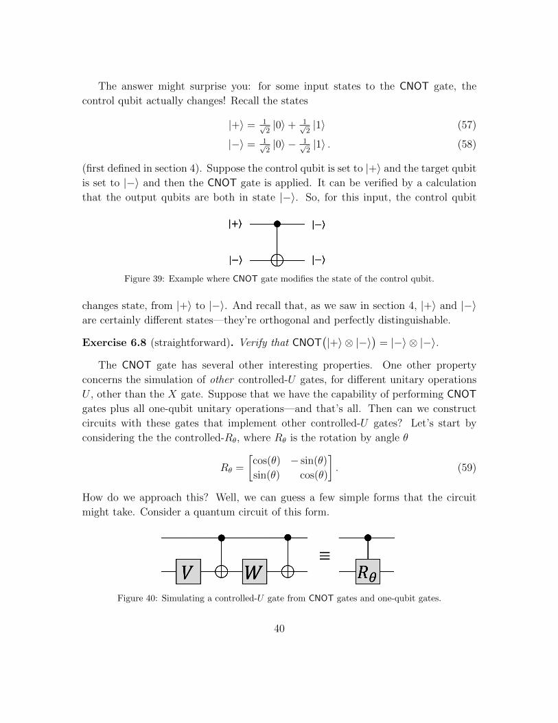
The answer might surprise you: for some input states to the CNOT gate, the

control qubit actually changes! Recall the states

|+〉 = 1√2|0〉+ 1√

2|1〉 (57)

|−〉 = 1√2|0〉 − 1√

2|1〉 . (58)

(first defined in section 4). Suppose the control qubit is set to |+〉 and the target qubit

is set to |−〉 and then the CNOT gate is applied. It can be verified by a calculation

that the output qubits are both in state |−〉. So, for this input, the control qubit

Figure 39: Example where CNOT gate modifies the state of the control qubit.

changes state, from |+〉 to |−〉. And recall that, as we saw in section 4, |+〉 and |−〉are certainly different states—they’re orthogonal and perfectly distinguishable.

Exercise 6.8 (straightforward). Verify that CNOT(|+〉 ⊗ |−〉

)= |−〉 ⊗ |−〉.

The CNOT gate has several other interesting properties. One other property

concerns the simulation of other controlled-U gates, for different unitary operations

U , other than the X gate. Suppose that we have the capability of performing CNOT

gates plus all one-qubit unitary operations—and that’s all. Then can we construct

circuits with these gates that implement other controlled-U gates? Let’s start by

considering the the controlled-Rθ, where Rθ is the rotation by angle θ

Rθ =

[cos(θ) − sin(θ)

sin(θ) cos(θ)

]. (59)

How do we approach this? Well, we can guess a few simple forms that the circuit

might take. Consider a quantum circuit of this form.

Figure 40: Simulating a controlled-U gate from CNOT gates and one-qubit gates.

40

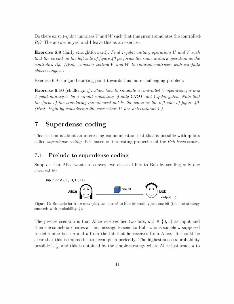
Do there exist 1-qubit unitaries V andW such that this circuit simulates the controlled-

Rθ? The answer is yes, and I leave this as an exercise.

Exercise 6.9 (fairly straightforward). Find 1-qubit unitary operations U and V such

that the circuit on the left side of figure 40 performs the same unitary operation as the

controlled-Rθ. (Hint: consider setting V and W to rotation matrices, with carefully

chosen angles.)

Exercise 6.9 is a good starting point towards this more challenging problem:

Exercise 6.10 (challenging). Show how to simulate a controlled-U operation for any

1-qubit unitary U by a circuit consisting of only CNOT and 1-qubit gates. Note that

the form of the simulating circuit need not be the same as the left side of figure 40.

(Hint: begin by considering the case where U has determinant 1.)

7 Superdense coding

This section is about an interesting communication feat that is possible with qubits

called superdense coding. It is based on interesting properties of the Bell basis states.

7.1 Prelude to superdense coding

Suppose that Alice wants to convey two classical bits to Bob by sending only one

classical bit.

Figure 41: Scenario for Alice conveying two bits ab to Bob by sending just one bit (the best strategy

succeeds with probability 12 ).

The precise scenario is that Alice receives her two bits, a, b ∈ {0, 1} as input and

then she somehow creates a 1-bit message to send to Bob, who is somehow supposed

to determine both a and b from the bit that he receives from Alice. It should be

clear that this is impossible to accomplish perfectly. The highest success probability

possible is 12, and this is obtained by the simple strategy where Alice just sends a to

41

Bob and then Bob outputs a and randomly guesses the value of b. This strategy has

success probability 12

in the average-case as well as in the worst-case.

What if Alice can send a qubit to Bob?

Figure 42: Scenario where Alice can send a qubit (the best success probability is 12 ).

It turns out that this does not help: the best success probability is still 12. We don’t

prove this here (it’s a consequence of a result of Nayak).

Now, let’s add a twist. What if we allow Bob to send a bit to Alice before Alice

sends her bit to him?

Figure 43: Scenario where Bob can send a bit to Alice and then Alice can send a bit to Bob (the

best possible success probability is 12 ).

To be clear, the scenario (depicted in figure 43) is the following:

1. Alice receives her two bits, a, b ∈ {0, 1} as input.

2. Bob sends a bit to Alice.

3. Alice sends a bit to Bob.

4. Then Bob outputs two bits (and this is successful if his output bits are ab).

That extra bit of communication from Bob to Alice does not help. The best possible

success probability is still 12. Intuitively, this is because the flow of information is in

the wrong direction. How does Bob sending a bit to Alice provide him with any more

information? To be sure that there isn’t some subtle way that Bob’s message helps,

we would need to think about this carefully. But let’s just accept, without proof, that

the best possible success probability is 12.

In fact, if Bob sends a bit the wrong way and then Alice sends a qubit to Bob,

even that does not help: the best possible success probability is still 12.

42

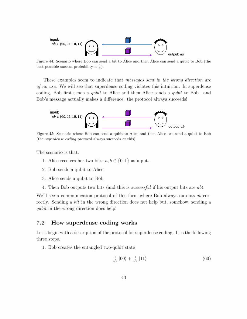
Figure 44: Scenario where Bob can send a bit to Alice and then Alice can send a qubit to Bob (the

best possible success probability is 12 ).

These examples seem to indicate that messages sent in the wrong direction are

of no use. We will see that superdense coding violates this intuition. In superdense

coding, Bob first sends a qubit to Alice and then Alice sends a qubit to Bob—and

Bob’s message actually makes a difference: the protocol always succeeds!

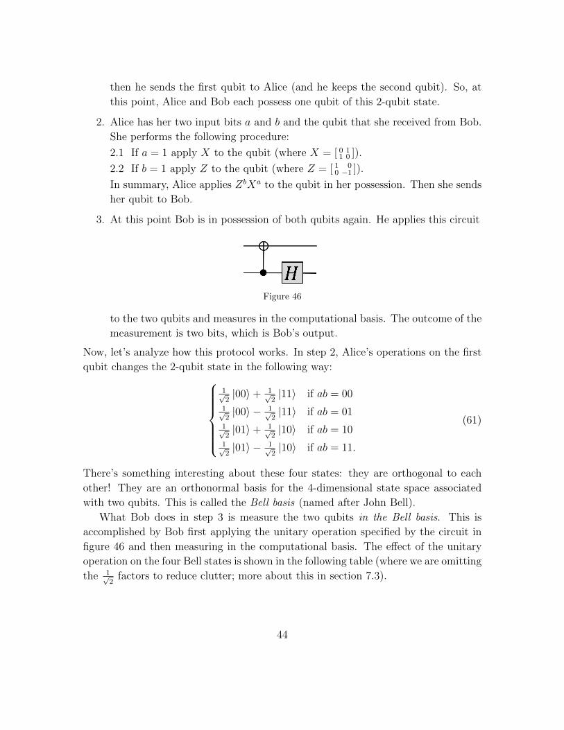
Figure 45: Scenario where Bob can send a qubit to Alice and then Alice can send a qubit to Bob

(the superdense coding protocol always succeeds at this).

The scenario is that:

1. Alice receives her two bits, a, b ∈ {0, 1} as input.

2. Bob sends a qubit to Alice.

3. Alice sends a qubit to Bob.

4. Then Bob outputs two bits (and this is successful if his output bits are ab).

We’ll see a communication protocol of this form where Bob always outouts ab cor-

rectly. Sending a bit in the wrong direction does not help but, somehow, sending a

qubit in the wrong direction does help!

7.2 How superdense coding works

Let’s begin with a description of the protocol for superdense coding. It is the following

three steps.

1. Bob creates the entangled two-qubit state

1√2|00〉+ 1√

2|11〉 (60)

43

then he sends the first qubit to Alice (and he keeps the second qubit). So, at

this point, Alice and Bob each possess one qubit of this 2-qubit state.

2. Alice has her two input bits a and b and the qubit that she received from Bob.

She performs the following procedure:

2.1 If a = 1 apply X to the qubit (where X = [ 0 11 0 ]).

2.2 If b = 1 apply Z to the qubit (where Z = [ 1 00 −1 ]).

In summary, Alice applies ZbXa to the qubit in her possession. Then she sends

her qubit to Bob.

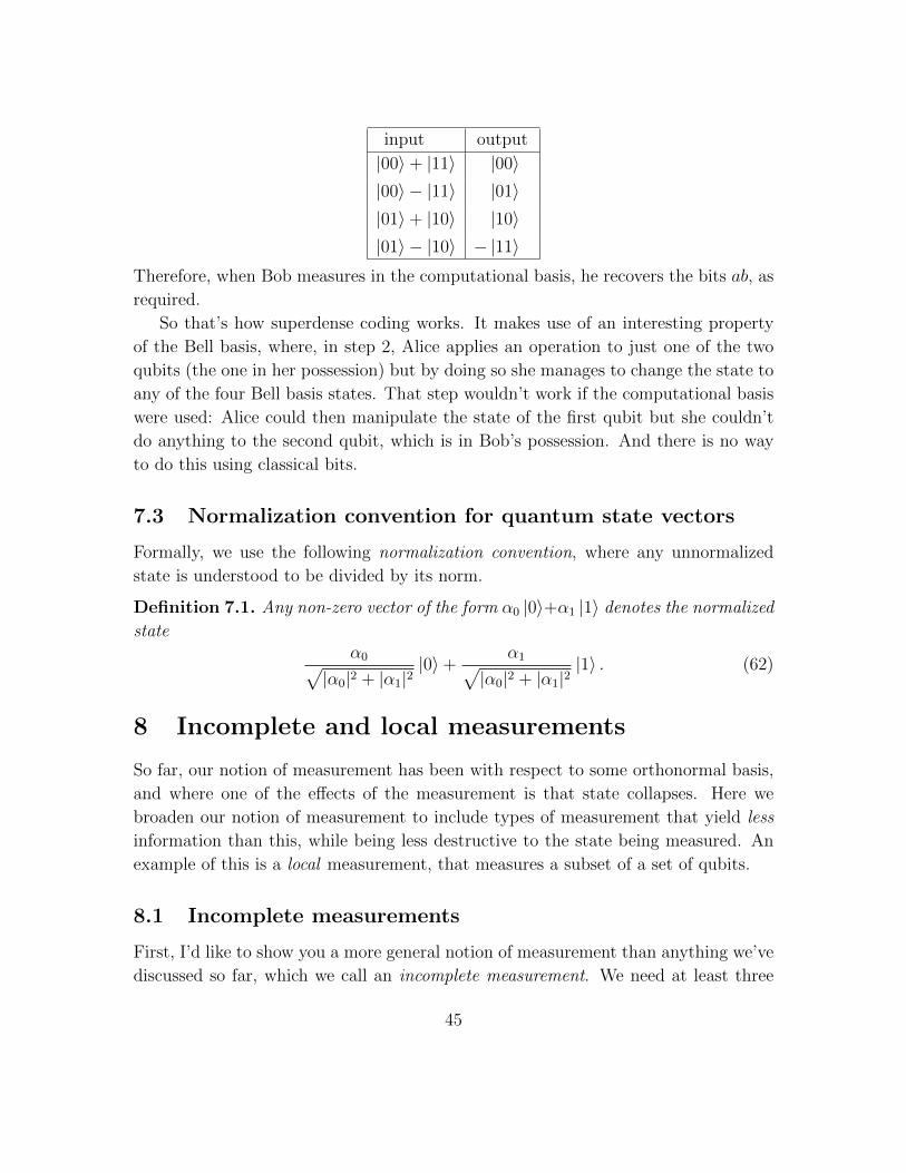
3. At this point Bob is in possession of both qubits again. He applies this circuit

Figure 46

to the two qubits and measures in the computational basis. The outcome of the

measurement is two bits, which is Bob’s output.

Now, let’s analyze how this protocol works. In step 2, Alice’s operations on the first

qubit changes the 2-qubit state in the following way:

1√2|00〉+ 1√

2|11〉 if ab = 00

1√2|00〉 − 1√

2|11〉 if ab = 01

1√2|01〉+ 1√

2|10〉 if ab = 10

1√2|01〉 − 1√

2|10〉 if ab = 11.

(61)

There’s something interesting about these four states: they are orthogonal to each

other! They are an orthonormal basis for the 4-dimensional state space associated

with two qubits. This is called the Bell basis (named after John Bell).

What Bob does in step 3 is measure the two qubits in the Bell basis. This is

accomplished by Bob first applying the unitary operation specified by the circuit in

figure 46 and then measuring in the computational basis. The effect of the unitary

operation on the four Bell states is shown in the following table (where we are omitting

the 1√2

factors to reduce clutter; more about this in section 7.3).

44

input output

|00〉+ |11〉 |00〉|00〉 − |11〉 |01〉|01〉+ |10〉 |10〉|01〉 − |10〉 − |11〉

Therefore, when Bob measures in the computational basis, he recovers the bits ab, as

required.

So that’s how superdense coding works. It makes use of an interesting property

of the Bell basis, where, in step 2, Alice applies an operation to just one of the two

qubits (the one in her possession) but by doing so she manages to change the state to

any of the four Bell basis states. That step wouldn’t work if the computational basis

were used: Alice could then manipulate the state of the first qubit but she couldn’t

do anything to the second qubit, which is in Bob’s possession. And there is no way

to do this using classical bits.

7.3 Normalization convention for quantum state vectors

Formally, we use the following normalization convention, where any unnormalized

state is understood to be divided by its norm.

Definition 7.1. Any non-zero vector of the form α0 |0〉+α1 |1〉 denotes the normalized

stateα0√

|α0|2 + |α1|2|0〉+

α1√|α0|2 + |α1|2

|1〉 . (62)

8 Incomplete and local measurements

So far, our notion of measurement has been with respect to some orthonormal basis,

and where one of the effects of the measurement is that state collapses. Here we

broaden our notion of measurement to include types of measurement that yield less

information than this, while being less destructive to the state being measured. An

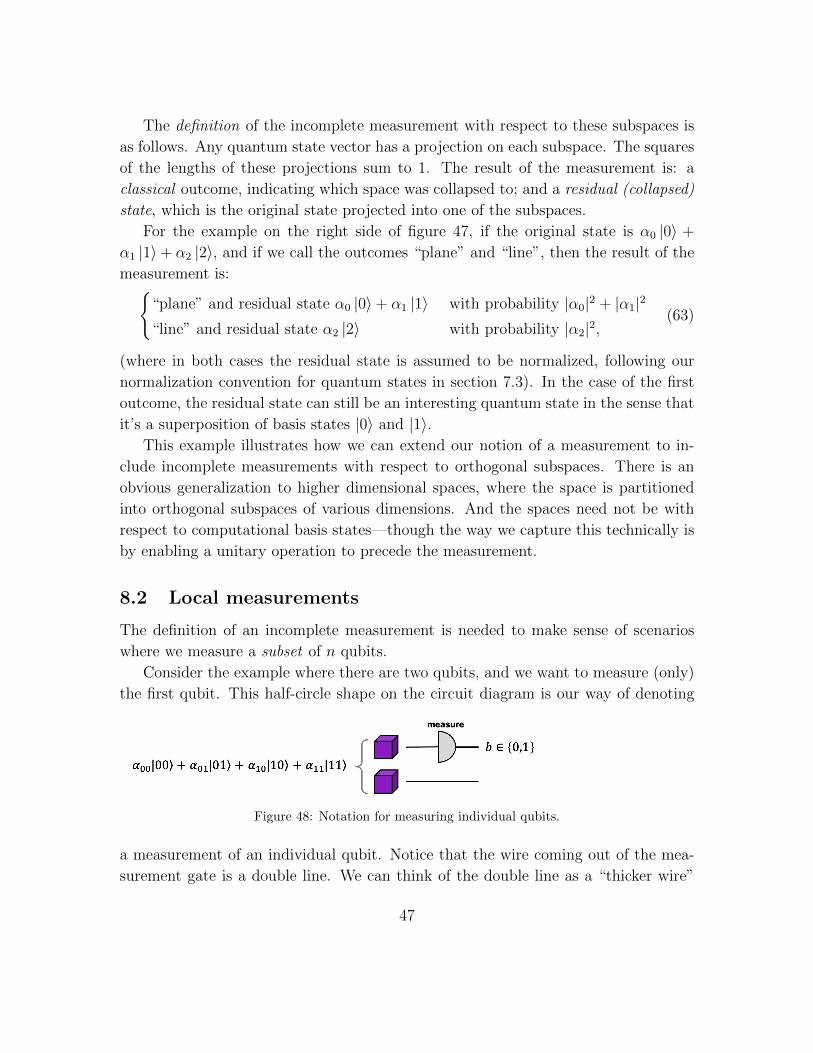
example of this is a local measurement, that measures a subset of a set of qubits.

8.1 Incomplete measurements

First, I’d like to show you a more general notion of measurement than anything we’ve

discussed so far, which we call an incomplete measurement. We need at least three

45

dimensional quantum state vectors to show this kind of measurement.

We’ll soon be talking about 2-qubit systems, whose state vectors are 4-dimensional.

But let’s start with 3-dimensional quantum systems, where the space of states is easier

to visualize. Recall that, for a quantum trit (or qutrit) there are three computational

basis states, called |0〉, |1〉, and |2〉.The measurement that we have seen so far does the following: it projects the state

to one of the computational basis states, where the probability of projecting to each

such basis state is the projection length squared. The outcome of the measurement

consists of two parts:

• Classical information indicating which basis state occurred—for qutrits, that’s

0, 1, or 2—which we can imagine is what we see on the screen.

• And there is also a residual (or collapsed) quantum state, which would be |0〉,|1〉, or |2〉.

An equivalent way of viewing this is that there are three orthogonal one-dimensional

subspaces (the span of |0〉, the span of |1〉, and the span of |2〉), and the state has

a projection onto each subspace, and the square of the length of that projection

Figure 47: A geometric view of a complete qutrit measurement (left) and an example of an incomplete

qutrit measurement (right).

determines the probability of that outcome. An incomplete measurement is like this,

except that the orthogonal subspaces need not be one-dimensional. For example, for

qutrits, consider these two subspaces (illustrated on the right side of figure 47):

• The horizontal plane spanned by |0〉 and |1〉, which is two-dimensional.

• The vertical line spanned by |2〉, which is one-dimensional.

These two subspaces are orthogonal to each other and, together, they span the entire

space.

46

The definition of the incomplete measurement with respect to these subspaces is

as follows. Any quantum state vector has a projection on each subspace. The squares

of the lengths of these projections sum to 1. The result of the measurement is: a

classical outcome, indicating which space was collapsed to; and a residual (collapsed)

state, which is the original state projected into one of the subspaces.

For the example on the right side of figure 47, if the original state is α0 |0〉 +

α1 |1〉+ α2 |2〉, and if we call the outcomes “plane” and “line”, then the result of the

measurement is:{“plane” and residual state α0 |0〉+ α1 |1〉 with probability |α0|2 + |α1|2

“line” and residual state α2 |2〉 with probability |α2|2,(63)

(where in both cases the residual state is assumed to be normalized, following our

normalization convention for quantum states in section 7.3). In the case of the first

outcome, the residual state can still be an interesting quantum state in the sense that

it’s a superposition of basis states |0〉 and |1〉.This example illustrates how we can extend our notion of a measurement to in-

clude incomplete measurements with respect to orthogonal subspaces. There is an

obvious generalization to higher dimensional spaces, where the space is partitioned

into orthogonal subspaces of various dimensions. And the spaces need not be with

respect to computational basis states—though the way we capture this technically is

by enabling a unitary operation to precede the measurement.

8.2 Local measurements

The definition of an incomplete measurement is needed to make sense of scenarios

where we measure a subset of n qubits.

Consider the example where there are two qubits, and we want to measure (only)

the first qubit. This half-circle shape on the circuit diagram is our way of denoting

Figure 48: Notation for measuring individual qubits.

a measurement of an individual qubit. Notice that the wire coming out of the mea-

surement gate is a double line. We can think of the double line as a “thicker wire”

47

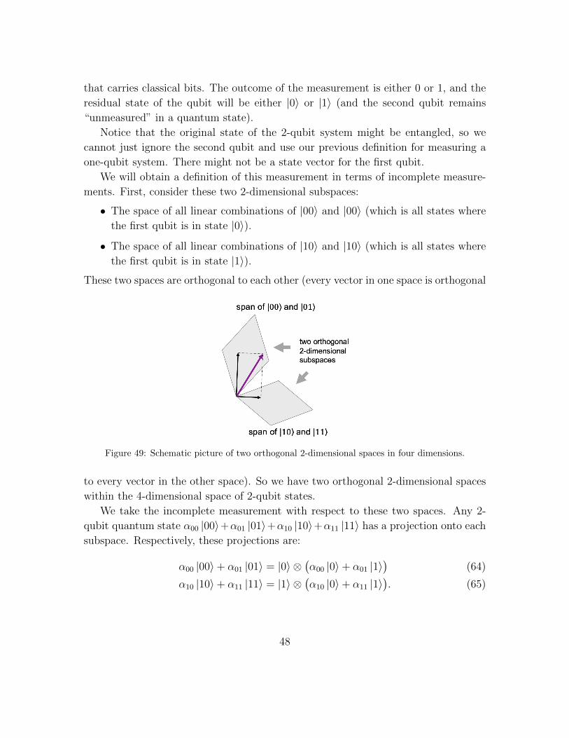
that carries classical bits. The outcome of the measurement is either 0 or 1, and the

residual state of the qubit will be either |0〉 or |1〉 (and the second qubit remains

“unmeasured” in a quantum state).

Notice that the original state of the 2-qubit system might be entangled, so we

cannot just ignore the second qubit and use our previous definition for measuring a

one-qubit system. There might not be a state vector for the first qubit.

We will obtain a definition of this measurement in terms of incomplete measure-

ments. First, consider these two 2-dimensional subspaces:

• The space of all linear combinations of |00〉 and |00〉 (which is all states where

the first qubit is in state |0〉).

• The space of all linear combinations of |10〉 and |10〉 (which is all states where

the first qubit is in state |1〉).

These two spaces are orthogonal to each other (every vector in one space is orthogonal

Figure 49: Schematic picture of two orthogonal 2-dimensional spaces in four dimensions.

to every vector in the other space). So we have two orthogonal 2-dimensional spaces

within the 4-dimensional space of 2-qubit states.

We take the incomplete measurement with respect to these two spaces. Any 2-

qubit quantum state α00 |00〉+α01 |01〉+α10 |10〉+α11 |11〉 has a projection onto each

subspace. Respectively, these projections are:

α00 |00〉+ α01 |01〉 = |0〉 ⊗(α00 |0〉+ α01 |1〉

)(64)

α10 |10〉+ α11 |11〉 = |1〉 ⊗(α10 |0〉+ α11 |1〉

). (65)

48

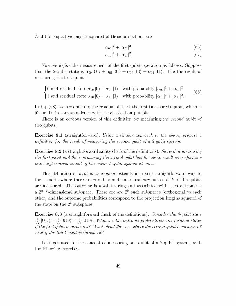
And the respective lengths squared of these projections are

|α00|2 + |α01|2 (66)

|α10|2 + |α11|2. (67)

Now we define the measurement of the first qubit operation as follows. Suppose

that the 2-qubit state is α00 |00〉 + α01 |01〉 + α10 |10〉 + α11 |11〉. The the result of

measuring the first qubit is{0 and residual state α00 |0〉+ α01 |1〉 with probability |α00|2 + |α01|2

1 and residual state α10 |0〉+ α11 |1〉 with probability |α10|2 + |α11|2.(68)

In Eq. (68), we are omitting the residual state of the first (measured) qubit, which is

|0〉 or |1〉, in correspondence with the classical output bit.

There is an obvious version of this definition for measuring the second qubit of

two qubits.

Exercise 8.1 (straightforward). Using a similar approach to the above, propose a

definition for the result of measuring the second qubit of a 2-qubit system.

Exercise 8.2 (a straightforward sanity check of the definitions). Show that measuring

the first qubit and then measuring the second qubit has the same result as performing

one single measurement of the entire 2-qubit system at once.

This definition of local measurement extends in a very straightforward way to

the scenario where there are n qubits and some arbitrary subset of k of the qubits

are measured. The outcome is a k-bit string and associated with each outcome is

a 2n−k-dimensional subspace. There are are 2k such subspaces (orthogonal to each

other) and the outcome probabilities correspond to the projection lengths squared of

the state on the 2k subspaces.

Exercise 8.3 (a straightforward check of the definitions). Consider the 3-qubit state1√2|001〉+ 1√

3|010〉+ 1√

6|010〉. What are the outcome probabilities and residual states

if the first qubit is measured? What about the case where the second qubit is measured?

And if the third qubit is measured?

Let’s get used to the concept of measuring one qubit of a 2-qubit system, with

the following exercises.

49

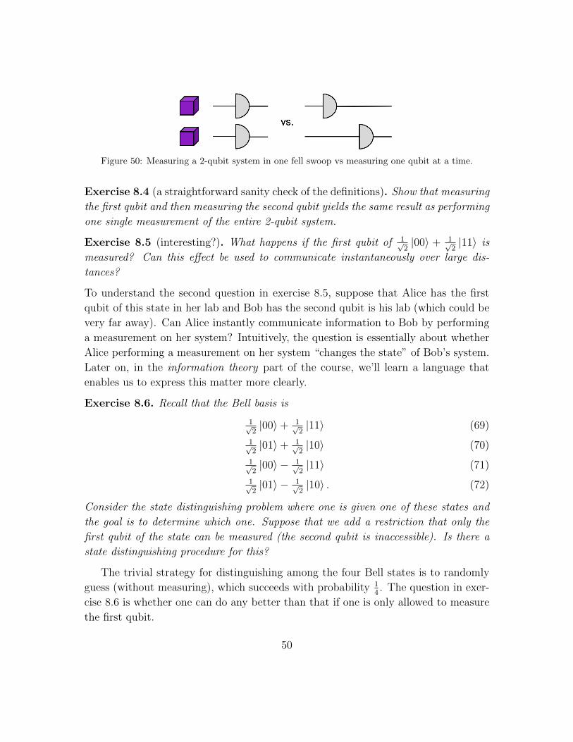
Figure 50: Measuring a 2-qubit system in one fell swoop vs measuring one qubit at a time.

Exercise 8.4 (a straightforward sanity check of the definitions). Show that measuring

the first qubit and then measuring the second qubit yields the same result as performing

one single measurement of the entire 2-qubit system.

Exercise 8.5 (interesting?). What happens if the first qubit of 1√2|00〉 + 1√

2|11〉 is

measured? Can this effect be used to communicate instantaneously over large dis-

tances?

To understand the second question in exercise 8.5, suppose that Alice has the first

qubit of this state in her lab and Bob has the second qubit is his lab (which could be

very far away). Can Alice instantly communicate information to Bob by performing

a measurement on her system? Intuitively, the question is essentially about whether

Alice performing a measurement on her system “changes the state” of Bob’s system.

Later on, in the information theory part of the course, we’ll learn a language that

enables us to express this matter more clearly.

Exercise 8.6. Recall that the Bell basis is

1√2|00〉+ 1√

2|11〉 (69)

1√2|01〉+ 1√

2|10〉 (70)

1√2|00〉 − 1√

2|11〉 (71)

1√2|01〉 − 1√

2|10〉 . (72)

Consider the state distinguishing problem where one is given one of these states and

the goal is to determine which one. Suppose that we add a restriction that only the

first qubit of the state can be measured (the second qubit is inaccessible). Is there a

state distinguishing procedure for this?

The trivial strategy for distinguishing among the four Bell states is to randomly

guess (without measuring), which succeeds with probability 14. The question in exer-

cise 8.6 is whether one can do any better than that if one is only allowed to measure

the first qubit.

50

8.3 Weirdness of the Bell basis encoding

Suppose that we have a two qubits which we want to use to encode two classical bits.

Let’s consider two different ways of encode the two classical bits: the computational

basis and the Bell basis.

ab Comp. basis

00 |00〉01 |01〉10 |10〉11 |11〉

ab Bell basis

00 |00〉+ |11〉01 |00〉 − |11〉10 |01〉+ |10〉11 |01〉 − |10〉

Now, if the two qubits are considered as one system, it doesn’t make much of a

Figure 51: A 2-qubit system can be viewed as two separate 1-qubit systems.

difference which encoding you use, because you can always convert between these

encodings by a unitary operation. However, if the two qubits are localized: say, Alice

possesses the first qubit and Bob possesses the second qubit then there’s an interesting

difference.

For the case of the computational basis encoding, Alice can determine the value

of the first bit a, but not the second bit, b. Also, Alice can flip the value first bit

(between 0 and 1) but cannot flip the second bit. She has complete control over the

first bit, but no access to the second bit.

On the other hand, for the case of the Bell basis encoding, Alice has no idea

about either bit (she cannot determine any information about the value of a nor of

b). However, Alice can flip either one of the two bits: she can flip the first bit (by

applying a Pauli X); she can flip the second bit by applying the Pauli Z); and she

can flip both bits, by applying both of these Paulis.

Informally, by using the Bell basis encoding, each party individually forgoes the

ability to read any of the bits being encoded, but gains the advantage of being able

to flip both bits by a local operation on just one of the qubits.

This weirdness of the Bell basis is the driving force behind superdense coding.

51

9 Exotic measurements

Now is a good time to see the exotic measurements that I first referred to in passing

back in section 5.2, but never actually explained.

First, to review, we have our basic measurement operation for qubits, which is

respect to the computational basis, |0〉 and |1〉.

Figure 52: Basic measurement of a qubit with respect to |0〉 and |1〉.

Then we have a notion of measuring a qubit with respect to any orthonormal

basis (for example, with respect to the |+〉, |−〉 basis), which can be simulated by

preceding a basic measurement with some unitary operation U .

Figure 53: Measurement of a qubit with respect to an arbitrary orthonormal basis (accomplished

by preceding a basic measurement with some unitary operation U).

The more exotic measurements that I want to show you are of the following form.

Figure 54: An exotic measurement of a qubit.

Let’s assume here that we are performing this measurement on one qubit (which we

refer to as the data). Upon receiving that qubit, we create a second qubit ourselves

in state |0〉. Combining the data to be measured with that second qubit, we have a

two-qubit system (with four dimensional state vectors). By the way, when a qubit is

added to a system like this, that qubit is frequently referred to an ancilla (think of

it as an “ancillary qubit”). Next we apply some four-dimensional unitary operation

52

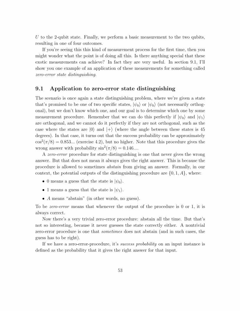
U to the 2-qubit state. Finally, we perform a basic measurement to the two qubits,

resulting in one of four outcomes.

If you’re seeing this this kind of measurement process for the first time, then you

might wonder what the point is of doing all this. Is there anything special that these

exotic measurements can achieve? In fact they are very useful. In section 9.1, I’ll

show you one example of an application of these measurements for something called

zero-error state distinguishing.

9.1 Application to zero-error state distinguishing

The scenario is once again a state distinguishing problem, where we’re given a state

that’s promised to be one of two specific states, |ψ0〉 or |ψ0〉 (not necessarily orthog-

onal), but we don’t know which one, and our goal is to determine which one by some

measurement procedure. Remember that we can do this perfectly if |ψ0〉 and |ψ1〉are orthogonal, and we cannot do it perfectly if they are not orthogonal, such as the

case where the states are |0〉 and |+〉 (where the angle between these states is 45

degrees). In that case, it turns out that the success probability can be approximately

cos2(π/8) = 0.853... (exercise 4.2), but no higher. Note that this procedure gives the

wrong answer with probability sin2(π/8) = 0.146....

A zero-error procedure for state distinguishing is one that never gives the wrong

answer. But that does not mean it always gives the right answer. This is because the

procedure is allowed to sometimes abstain from giving an answer. Formally, in our

context, the potential outputs of the distinguishing procedure are {0, 1, A}, where:

• 0 means a guess that the state is |ψ0〉.

• 1 means a guess that the state is |ψ1〉.

• A means “abstain” (in other words, no guess).

To be zero-error means that whenever the output of the procedure is 0 or 1, it is

always correct.

Now there’s a very trivial zero-error procedure: abstain all the time. But that’s

not so interesting, because it never guesses the state correctly either. A nontrivial

zero-error procedure is one that sometimes does not abstain (and in such cases, the

guess has to be right).

If we have a zero-error-procedure, it’s success probability on an input instance is

defined as the probability that it gives the right answer for that input.

53

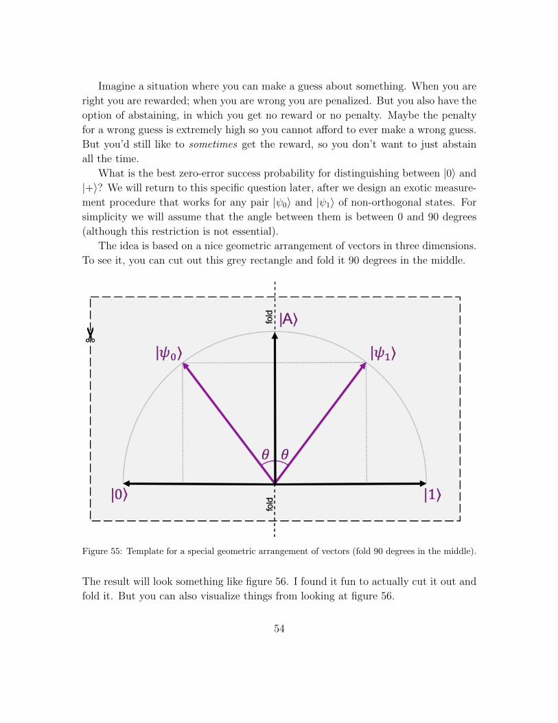
Imagine a situation where you can make a guess about something. When you are

right you are rewarded; when you are wrong you are penalized. But you also have the

option of abstaining, in which you get no reward or no penalty. Maybe the penalty

for a wrong guess is extremely high so you cannot afford to ever make a wrong guess.

But you’d still like to sometimes get the reward, so you don’t want to just abstain

all the time.

What is the best zero-error success probability for distinguishing between |0〉 and

|+〉? We will return to this specific question later, after we design an exotic measure-

ment procedure that works for any pair |ψ0〉 and |ψ1〉 of non-orthogonal states. For

simplicity we will assume that the angle between them is between 0 and 90 degrees

(although this restriction is not essential).

The idea is based on a nice geometric arrangement of vectors in three dimensions.

To see it, you can cut out this grey rectangle and fold it 90 degrees in the middle.

Figure 55: Template for a special geometric arrangement of vectors (fold 90 degrees in the middle).

The result will look something like figure 56. I found it fun to actually cut it out and

fold it. But you can also visualize things from looking at figure 56.

54

Figure 56: Special geometric arrangement of vectors.

Note that the states |0〉, |1〉, and |A〉 are three mutually orthogonal states, so it

makes sense to perform a 3-outcome measurement with respect to these states. Now,

look at the way |ψ0〉 and |ψ1〉 are arranged. |ψ0〉 and |ψ1〉 are not orthogonal (unless

θ = π2). However, |ψ1〉 is orthogonal to |0〉, so for a measurement of that state, the

outcome will never be 0; it will always be either A or 1. Similarly, |ψ0〉 is orthogonal to

|1〉, so for a measurement of that state, the outcome will never be 1. Based on this,

we have a zero-error measurement procedure for distinguishing between the states

|ψ0〉 and |ψ1〉.The probabilities of the various outcomes can be worked out to the following. For

state |ψ0〉, the outcome probabilities are0 with probability sin2(θ)

1 with probability 0

A with probability cos2(θ),

(73)

55

and, for state |ψ1〉, the outcome probabilities are0 with probability 0

1 with probability sin2(θ)

A with probability cos2(θ).

(74)

It follows that the success probability in each case is sin2(θ).

This approach can be extended to a zero-error error state distinguishing procedure

for any two states |φ0〉 and |φ1〉 as long as the angle between |φ0〉 and |φ1〉 is the same

as the angle between |ψ0〉 and |ψ1〉. The idea is to rotate the coordinate system so

that it coincides with that in figure 56.

How does the success probability depend on the angle between |ψ0〉 and |ψ1〉? Note

that this angle is not equal to 2θ, because of the fold. There is a nice relationship

between the inner product 〈ψ0|ψ1〉 and θ: namely 〈ψ0|ψ1〉 = cos2(θ).

Exercise 9.1. Prove that, for the vectors in figure 56, 〈ψ0|ψ1〉 = cos2(θ).

Note that this this implies that the success probability, sin2(θ), can be expressed as

1− 〈ψ0|ψ1〉.Now, let’s get back to the specific problem of distinguishing between |0〉 and |+〉,

whose angle is 45 degrees, and whose inner product is 1√2. The problem is that these

are qubits, so the dimension of the space is too small for a set-up like figure 56.

Here’s where the exotic measurement (figure 54) comes in. By adding an ancilla

qubit in state |0〉, input state |0〉 becomes the 2-qubit state |0〉⊗|0〉 = |00〉, and input

state |+〉 becomes |+〉 ⊗ |0〉 = 1√2|00〉+ 1√

2|10〉. These are 4-dimensional states, but

we can ignore the dimension |11〉 and view these states as being in the 3-dimensional

subspace spanned by |00〉, |01〉, |10〉. We can associate this space with that of figure 56

(associating |10〉 with |A〉, |01〉 with |0〉, and |00〉 with |1〉), where θ is set so that

cos2(θ) = 1√2. There exists a 3 × 3 unitary operation U that maps |0〉 ⊗ |0〉 to |ψ0〉

and |+〉 ⊗ |0〉 to |ψ0〉. Note that, technically, the operation performed on the 2-qubit

space is the 4× 4 unitary 0

U 0

0

0 0 0 1

. (75)

The success probability is 1 − 〈0|+〉 = 1 − 1√2

(= 0.292...). Although this is

considerably less than 0.853... from exercise 4.2, it has the advantage that it is zero-

error. If we restricted our operations to be 1-qubit unitaries and 1-qubit measurements

then the zero-error success probability would be lower than 1− 1√2.

56

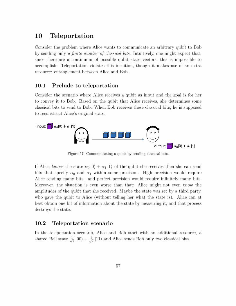
10 Teleportation

Consider the problem where Alice wants to communicate an arbitrary qubit to Bob

by sending only a finite number of classical bits. Intuitively, one might expect that,

since there are a continuum of possible qubit state vectors, this is impossible to

accomplish. Teleportation violates this intuition, though it makes use of an extra

resource: entanglement between Alice and Bob.

10.1 Prelude to teleportation

Consider the scenario where Alice receives a qubit as input and the goal is for her

to convey it to Bob. Based on the qubit that Alice receives, she determines some

classical bits to send to Bob. When Bob receives these classical bits, he is supposed

to reconstruct Alice’s original state.

Figure 57: Communicating a qubit by sending classical bits.

If Alice knows the state α0 |0〉 + α1 |1〉 of the qubit she receives then she can send

bits that specify α0 and α1 within some precision. High precision would require

Alice sending many bits—and perfect precision would require infinitely many bits.

Moreover, the situation is even worse than that: Alice might not even know the

amplitudes of the qubit that she received. Maybe the state was set by a third party,

who gave the qubit to Alice (without telling her what the state is). Alice can at

best obtain one bit of information about the state by measuring it, and that process

destroys the state.

10.2 Teleportation scenario

In the teleportation scenario, Alice and Bob start with an additional resource, a

shared Bell state 1√2|00〉+ 1√

2|11〉 and Alice sends Bob only two classical bits.

57

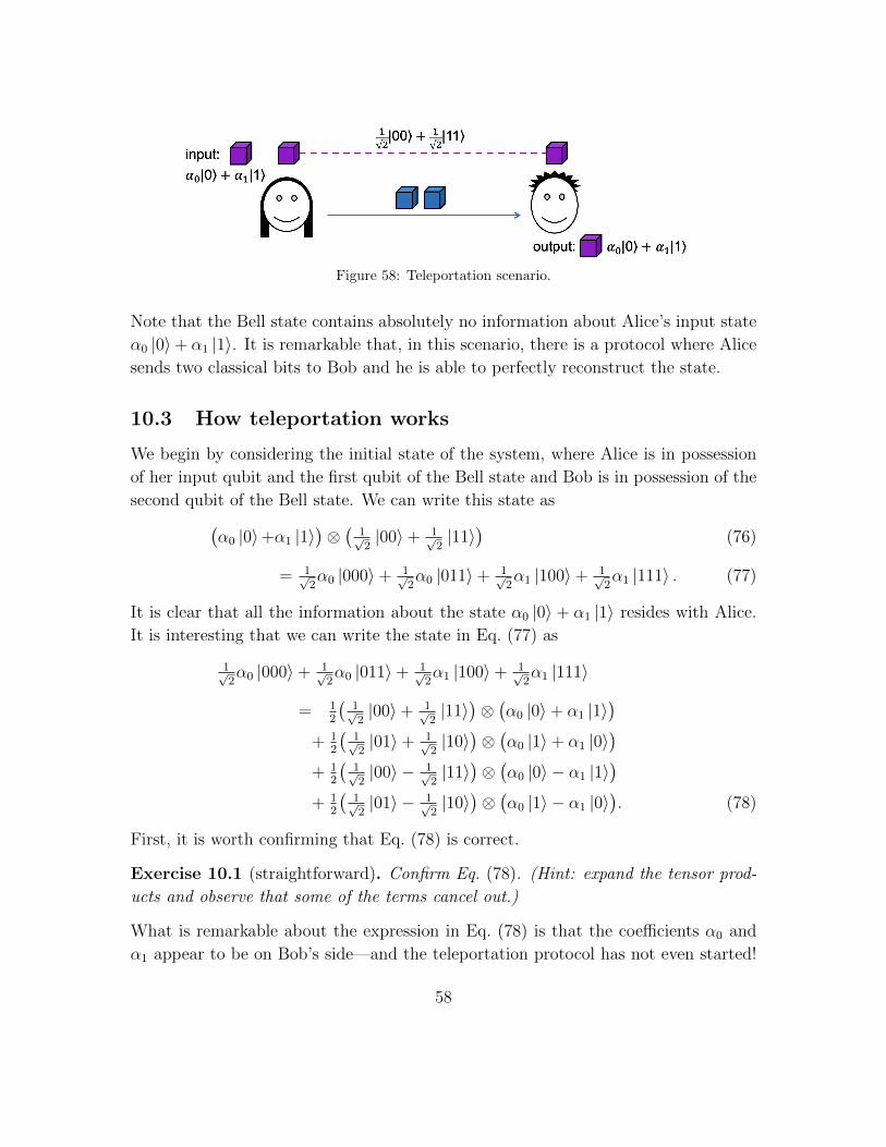
Figure 58: Teleportation scenario.

Note that the Bell state contains absolutely no information about Alice’s input state

α0 |0〉+ α1 |1〉. It is remarkable that, in this scenario, there is a protocol where Alice

sends two classical bits to Bob and he is able to perfectly reconstruct the state.

10.3 How teleportation works

We begin by considering the initial state of the system, where Alice is in possession

of her input qubit and the first qubit of the Bell state and Bob is in possession of the

second qubit of the Bell state. We can write this state as(α0 |0〉+α1 |1〉

)⊗(

1√2|00〉+ 1√

2|11〉

)(76)

= 1√2α0 |000〉+ 1√

2α0 |011〉+ 1√

2α1 |100〉+ 1√

2α1 |111〉 . (77)

It is clear that all the information about the state α0 |0〉 + α1 |1〉 resides with Alice.

It is interesting that we can write the state in Eq. (77) as

1√2α0 |000〉+ 1√

2α0 |011〉+ 1√

2α1 |100〉+ 1√

2α1 |111〉

= 12

(1√2|00〉+ 1√

2|11〉

)⊗(α0 |0〉+ α1 |1〉

)+ 1

2

(1√2|01〉+ 1√

2|10〉

)⊗(α0 |1〉+ α1 |0〉

)+ 1

2

(1√2|00〉 − 1√

2|11〉

)⊗(α0 |0〉 − α1 |1〉

)+ 1

2

(1√2|01〉 − 1√

2|10〉

)⊗(α0 |1〉 − α1 |0〉

). (78)

First, it is worth confirming that Eq. (78) is correct.

Exercise 10.1 (straightforward). Confirm Eq. (78). (Hint: expand the tensor prod-

ucts and observe that some of the terms cancel out.)

What is remarkable about the expression in Eq. (78) is that the coefficients α0 and

α1 appear to be on Bob’s side—and the teleportation protocol has not even started!

58

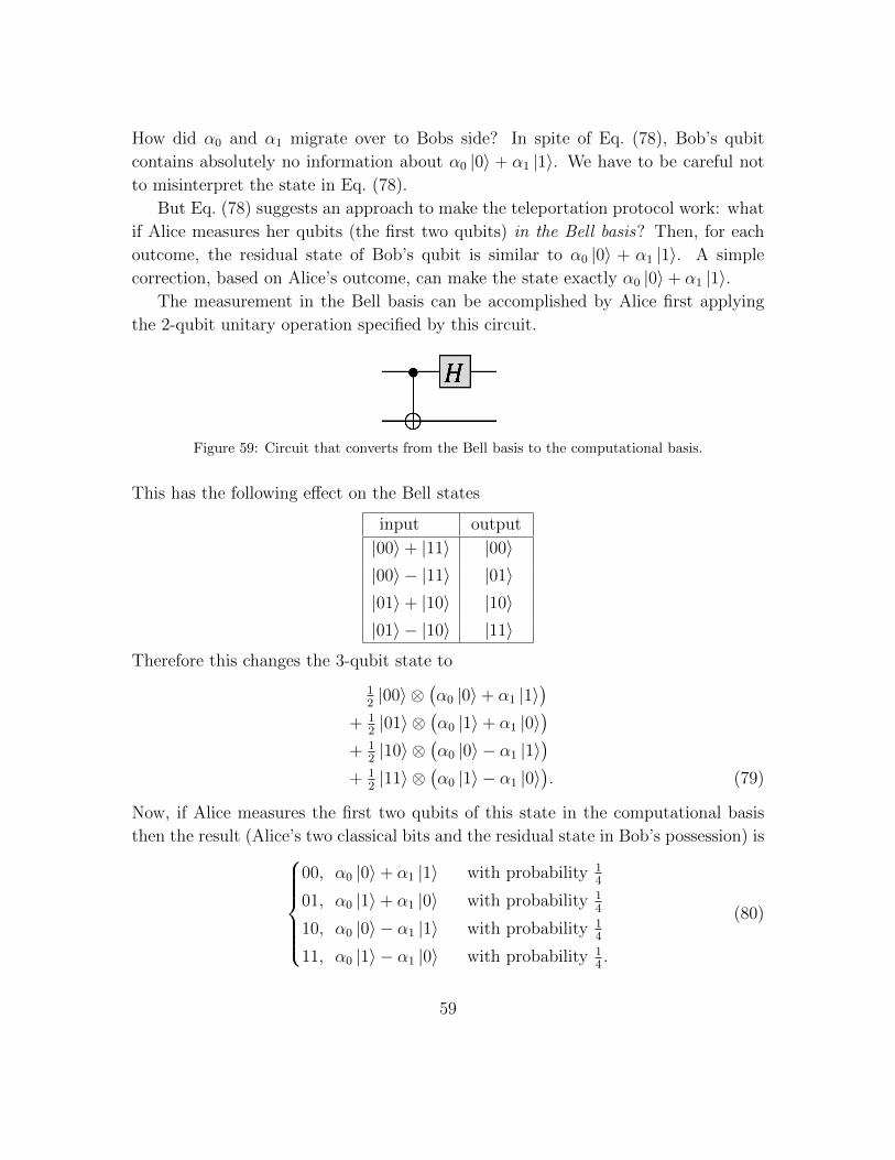
How did α0 and α1 migrate over to Bobs side? In spite of Eq. (78), Bob’s qubit

contains absolutely no information about α0 |0〉 + α1 |1〉. We have to be careful not

to misinterpret the state in Eq. (78).

But Eq. (78) suggests an approach to make the teleportation protocol work: what

if Alice measures her qubits (the first two qubits) in the Bell basis? Then, for each

outcome, the residual state of Bob’s qubit is similar to α0 |0〉 + α1 |1〉. A simple

correction, based on Alice’s outcome, can make the state exactly α0 |0〉+ α1 |1〉.The measurement in the Bell basis can be accomplished by Alice first applying

the 2-qubit unitary operation specified by this circuit.

Figure 59: Circuit that converts from the Bell basis to the computational basis.

This has the following effect on the Bell states

input output

|00〉+ |11〉 |00〉|00〉 − |11〉 |01〉|01〉+ |10〉 |10〉|01〉 − |10〉 |11〉

Therefore this changes the 3-qubit state to

12|00〉 ⊗

(α0 |0〉+ α1 |1〉

)+ 1

2|01〉 ⊗

(α0 |1〉+ α1 |0〉

)+ 1

2|10〉 ⊗

(α0 |0〉 − α1 |1〉

)+ 1

2|11〉 ⊗

(α0 |1〉 − α1 |0〉

). (79)

Now, if Alice measures the first two qubits of this state in the computational basis

then the result (Alice’s two classical bits and the residual state in Bob’s possession) is00, α0 |0〉+ α1 |1〉 with probability 1

4

01, α0 |1〉+ α1 |0〉 with probability 14

10, α0 |0〉 − α1 |1〉 with probability 14

11, α0 |1〉 − α1 |0〉 with probability 14.

(80)

59

At this point, Bob does not yet have the correct state (expect in the case of outcome

00). But, if Alice sends Bob the two bits of her measurement outcome then Bob can

apply an appropriate operation to “correct” his state.

Here’s what Bob does after receiving the two classical bits ab from Alice:

1. If b = 0 apply X.

2. If a = 0 apply Z.

The resulting state on Bob’s side is for each case is00, α0 |0〉+ α1 |1〉01, X

(α0 |1〉+ α1 |0〉

)= α0 |0〉+ α1 |1〉

10, Z(α0 |0〉 − α1 |1〉

)= α0 |0〉+ α1 |1〉

11, ZX(α0 |1〉 − α1 |0〉

)= α0 |0〉+ α1 |1〉.

(81)

This completes the description of the teleportation protocol.

The protocol can be summarized by the following circuit. Alice’s qubits and bits

Figure 60: The teleportation protocol summarized in one circuit.

are on top and Bob’s are on the bottom. The slanted classical wires denote that the

two classical bits resulting from Alice’s measurements being shifted down from Alice

towards Bob.

Exercise 10.2 (straightforward). Work through the circuit diagram in figure 60 and

confirm that it works.

It is natural to ask: What happens to Alice’s copy of her state? Is Alice’s copy

preserved? The answer is that, since Alice measures her two qubits, all the quantum

information in her possession is lost. So, while Bob ends up with a copy of the state

α0 |0〉+ α1 |1〉, Alice loses her copy of the state in the teleportation process.

60

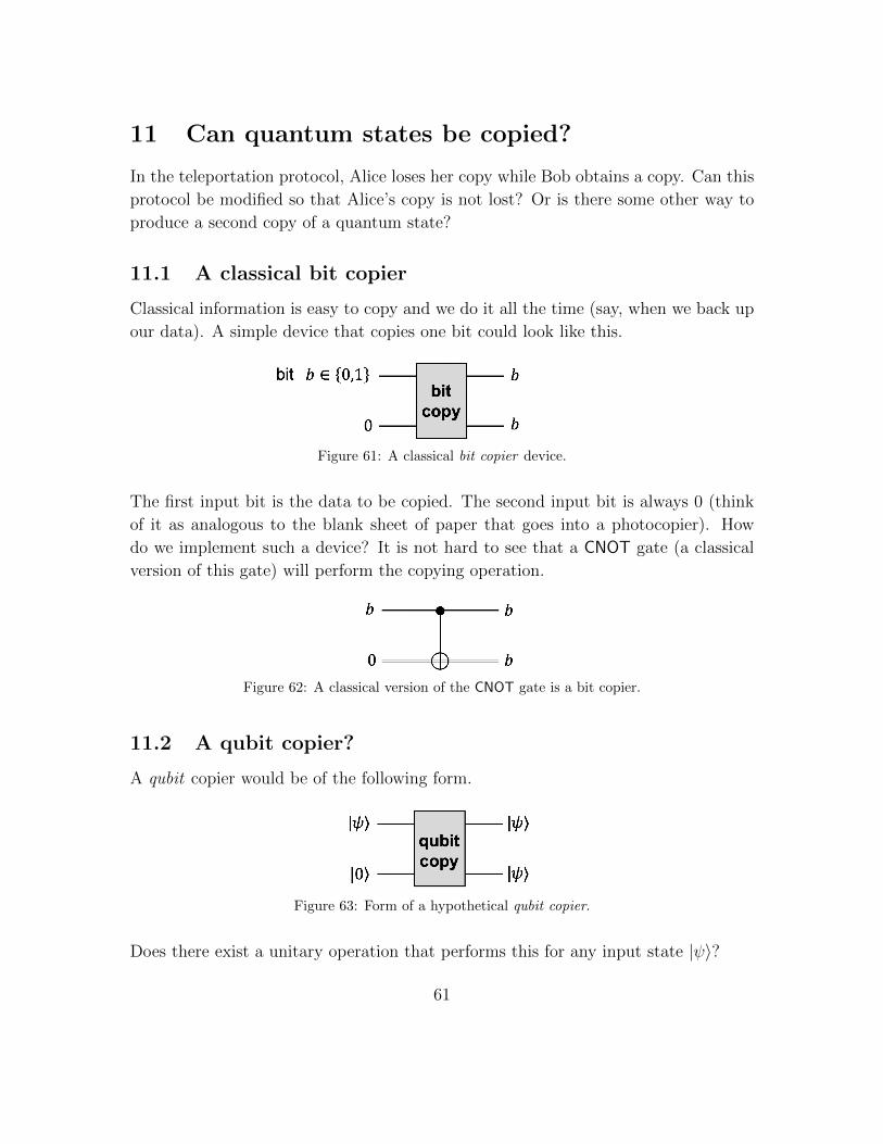
11 Can quantum states be copied?

In the teleportation protocol, Alice loses her copy while Bob obtains a copy. Can this

protocol be modified so that Alice’s copy is not lost? Or is there some other way to

produce a second copy of a quantum state?

11.1 A classical bit copier

Classical information is easy to copy and we do it all the time (say, when we back up

our data). A simple device that copies one bit could look like this.

Figure 61: A classical bit copier device.

The first input bit is the data to be copied. The second input bit is always 0 (think

of it as analogous to the blank sheet of paper that goes into a photocopier). How

do we implement such a device? It is not hard to see that a CNOT gate (a classical

version of this gate) will perform the copying operation.

Figure 62: A classical version of the CNOT gate is a bit copier.

11.2 A qubit copier?

A qubit copier would be of the following form.

Figure 63: Form of a hypothetical qubit copier.

Does there exist a unitary operation that performs this for any input state |ψ〉?

61

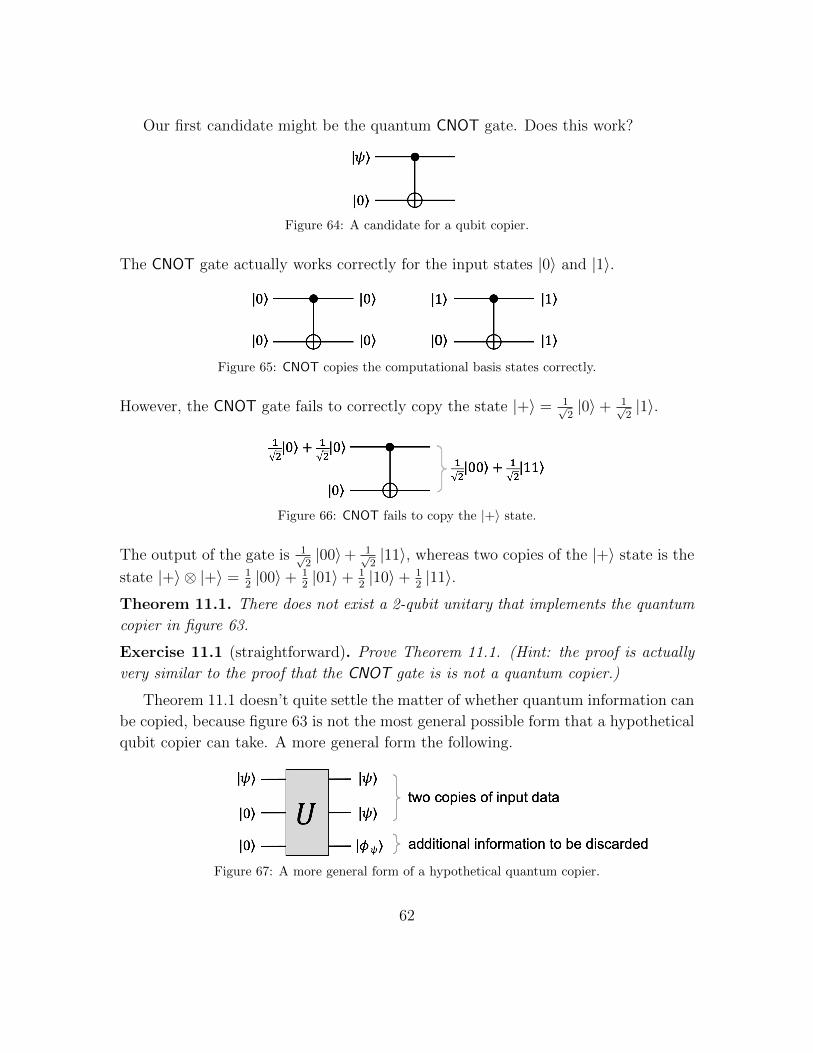
Our first candidate might be the quantum CNOT gate. Does this work?

Figure 64: A candidate for a qubit copier.

The CNOT gate actually works correctly for the input states |0〉 and |1〉.

Figure 65: CNOT copies the computational basis states correctly.

However, the CNOT gate fails to correctly copy the state |+〉 = 1√2|0〉+ 1√

2|1〉.

Figure 66: CNOT fails to copy the |+〉 state.

The output of the gate is 1√2|00〉+ 1√

2|11〉, whereas two copies of the |+〉 state is the

state |+〉 ⊗ |+〉 = 12|00〉+ 1

2|01〉+ 1

2|10〉+ 1

2|11〉.

Theorem 11.1. There does not exist a 2-qubit unitary that implements the quantum

copier in figure 63.

Exercise 11.1 (straightforward). Prove Theorem 11.1. (Hint: the proof is actually

very similar to the proof that the CNOT gate is is not a quantum copier.)

Theorem 11.1 doesn’t quite settle the matter of whether quantum information can

be copied, because figure 63 is not the most general possible form that a hypothetical

qubit copier can take. A more general form the following.

Figure 67: A more general form of a hypothetical quantum copier.

62

Think of the first qubit as the data to be copied, the second qubit as the analogue

of the blank sheet of paper that goes into a photocopier, and the third qubit as the

analogue of the toner cartridge, which is discarded at the end of the process. The

notation for the output state of the third qubit |φψ〉 is intended to indicate that it is

allowed to be a function of the data |ψ〉. In fact, this more general framework does

not help.

Theorem 11.2. There does not exist a 2-qubit unitary that implements the quantum

copier in figure 67.

Exercise 11.2 (slightly challenging). Prove Theorem 11.2.

63