arX

iv:g

r-qc

/040

5107

v2 2

1 M

ay 2

004

IFT-UAM/CSIC-04-26

gr-qc/0405107

Quantum Gravity

Enrique Alvarez

Instituto de Fısica Teorica UAM/CSIC, C-XVI, and Departamento de Fısica Teorica,

C-XI,

Universidad Autonoma de Madrid E-28049-Madrid, Spain 1

Abstract

General lectures on quantum gravity.

1 General Questions on Quantum Gravity

It is not clear at all what is the problem in quantum gravity (cf. [3] or [8] for general

reviews, written in the same spirit as the present one). The answers to the following

questions are not known, and I believe it can do no harm to think about them before

embarking in a more technical discussion.

To begin, it has been proposed that gravity should not be quantized, owing to its special

properties as determining the background on which all other fields propagate. There is a

whole line of thought on the possibility that gravity is not a fundamental theory, and this

is certainly an alternative one has to bear in mind. Indeed, even the holographic principle

of G. ’t Hooft, to be discussed later, can be interpreted in this sense.

1Lectures given in the 40th Karpacz Winter School.

1

Granting that, the next question is whether it does make any sense to consider gravi-

tons propagating in some background; that is, whether there is some useful approximation

in which there is a particle physics approach to the physics of gravitons as quanta of the

gravitational field. A related question is whether semiclassical gravity, i.e., the approxima-

tion in which the source of the classical Einstein equations is replaced by the expectation

value of the energy momentum tensor of some quantum theory has some physical ([22])

validity in some limit. We shall say more on this problems towards the end.

At any rate, even if it is possible at all, the at first sight easy problem of graviton

interactions in an otherwise flat background has withstood analysis of several generations

of physicists. The reason is that the coupling constant has mass dimension −1, so that

the structure of the perturbative counterterms involve higher and higher orders in the cur-

vature invariants (powers of the Riemann tensor in all possible independent contractions),

schematically,

S =1

2κ2R

∫

R +

∫

R2 + κ2R

∫

R4 + . . . (1)

Nobody knows how to make sense of this approach, except in one case, to be mentioned

later on.

It could be possible, sensu stricto to stop here. But if we believe that quantum gravity

should give answers to such questions as to the fate of the initial cosmological singularity,

its is almost unavoidable to speak of the wave function of the universe. This brings its own

set of problems, such as to whether it is possible to do quantum mechanics without classical

observers or whether the wave function of the Universe has a probablilistic interpretation.

Paraphrasing C. Isham [38], one would not known when to qualify a probabilistic prediction

on the whole Universe as a successful one.

The aim of the present paper is to discuss in some detail established results on the field.

In some strong sense, the review could be finished at once, because there are none. There

are, nevertheless, some interesting attempts, which look promising from certain points of

view. Perhaps the two approaches that have attracted more attention have been the loop

2

approach, on the one hand and strings on the other. We shall try to critically assess

prospects in both. Interesting related papers are [34][59].

Even if for the time being there is not (by far) consensus on the scientific community of

any quantum gravity physical picture, many great physicist have not been able to resist the

temptation of working (usually only for a while) on it. This has produced a huge spinoff

in quantum field theory; to name only a few, constrained quantization, compensating

ghosts, background field expansion and topological theories are concepts or techniques

first developped in thinking about these problems, and associated to the names of Dirac,

Pauli, Weinberg, Feynman, deWitt, Witten etc. In many cases, more or less surprising

relationships have been found with quantum gauge theories. There are probably more in

store, if one is to judge from the success of the partial implementation of holographic ideas

in Maldacena’s conjecture (more on this later).

This should be kept into account when reading the references. We have not atempted

to be comprehensive, and we have used only the references familiar to us; but in some of

the references, in particular in our own review article of 1989 ([3] there are more entry

points into the vast literature. After all, paraphrasing Feynman, we still do not know what

could be relevant in a field until the main problems are solved.

2 The issue of background independence

One of the main differences between both attacks to the quantum gravity problem is the

issue of background independence, by which it is understood that no particular background

should enter into the definition of the theory itself. Any other approach is purportedly at

variance with diffeomorphism invariance.

Work in particle physics in the second half of last century led to some understanding

of ordinary gauge theories. Can we draw some lessons from there?

Gauge theories can be formulated in the bakground field approach, as introduced by

3

B. de Witt and others (cf. [20]). In this approach, the quantum field theory depends on

a background field, but not on any one in particular, and the theory enjoys background

gauge invariance.

Is it enough to have quantum gravity formulated in such a way? 2

It can be argued that the only vacuum expectation value consistent with diffeomor-

phisms invariance is

< 0|gαβ|0 >= 0 (2)

in which case the answer to the above question ought to be in the negative, because this

is a singular background and curvature invariants do not make sense. It all boils down

as to whether the ground state of the theory is diffeomorphism invariant or not. There

is an example, namely three-dimensional gravity in which invariant quantization can be

performed [70]. In this case at least, the ensuing theory is almost topological.

In all attempts of a canonical quantization of the gravitational field, one always ends

up with an (constraint) equation corresponding physically to the fact that the total hamilto-

nian of a parametrization invariant theory should vanish. When expressed in the Schrodinger

picture, this equation is often dubbed the Wheeler-de Witt equation. This equation is

plagued by operator ordering and all other sorts of ambiguities. It is curious to notice

that in ordinary quantum field theory there also exists a Schrodinger representation, which

came recently to be controlled well enough as to be able to perform lattice computations

([42]).

Gauge theories can be expressed in terms of gauge invariant operators, such as Wilson

loops . They obey a complicated set of equations, the loop equations, which close in the

large N limit as has been shown by Makeenko and Migdal ([43]). These equations can be

properly regularized, e.g. in the lattice. Their explicit solution is one of the outstanding

challenges in theoretical physics. Although many conjectures have been advanced in this

2This was, incidentally, the way G. Hooft and M. Veltman did the first complete one-loop calculation

([65]).

4

direction, no definitive result is available.

3 The canonical approach.

It is widely acknowledged that there is a certain tension between a (3 + 1) decomposition

implicit in any canonical approach, privileging a particular notion of time, and the beautiful

geometrical structure of general relativity, with its invariance under general coordinate

transformations.

Let us now nevertheless explore how far we can go on this road, following the still very

much worth reading work of deWitt ([20]).

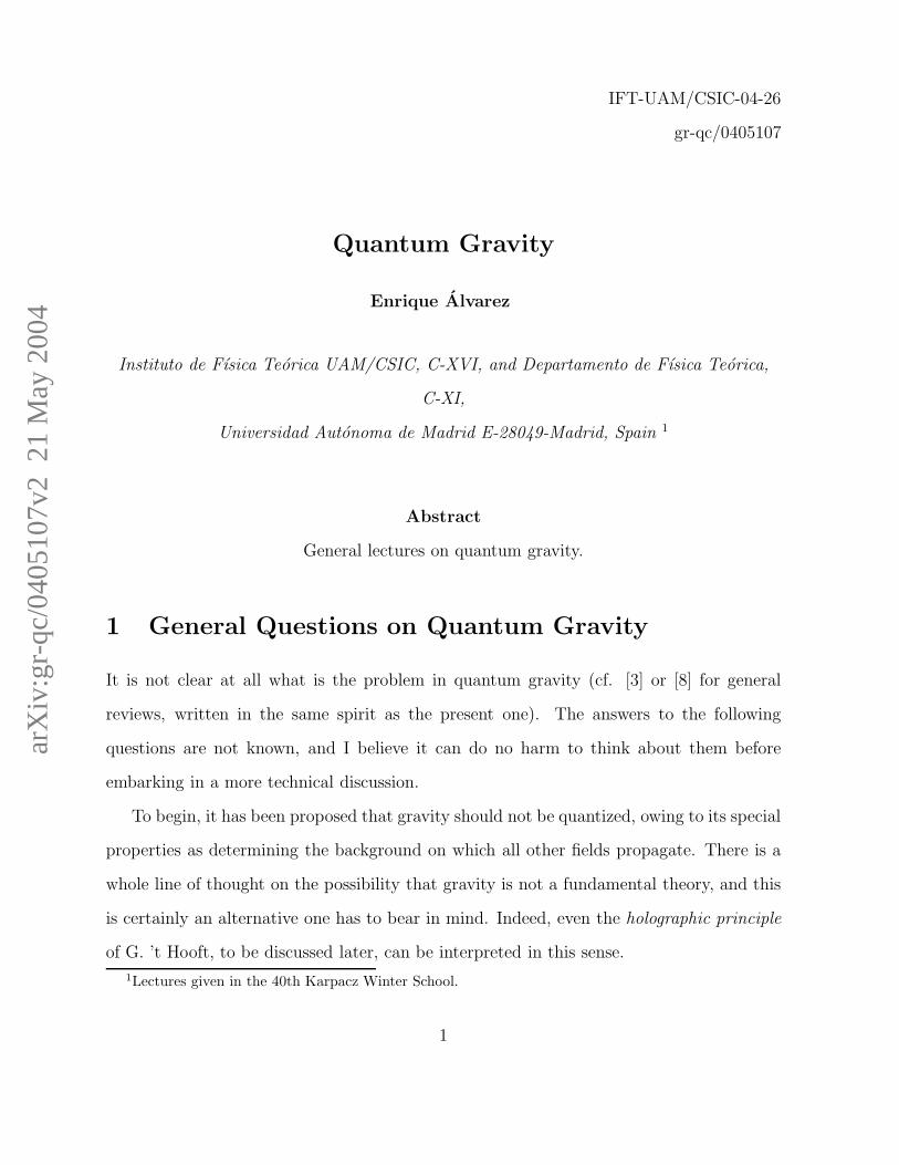
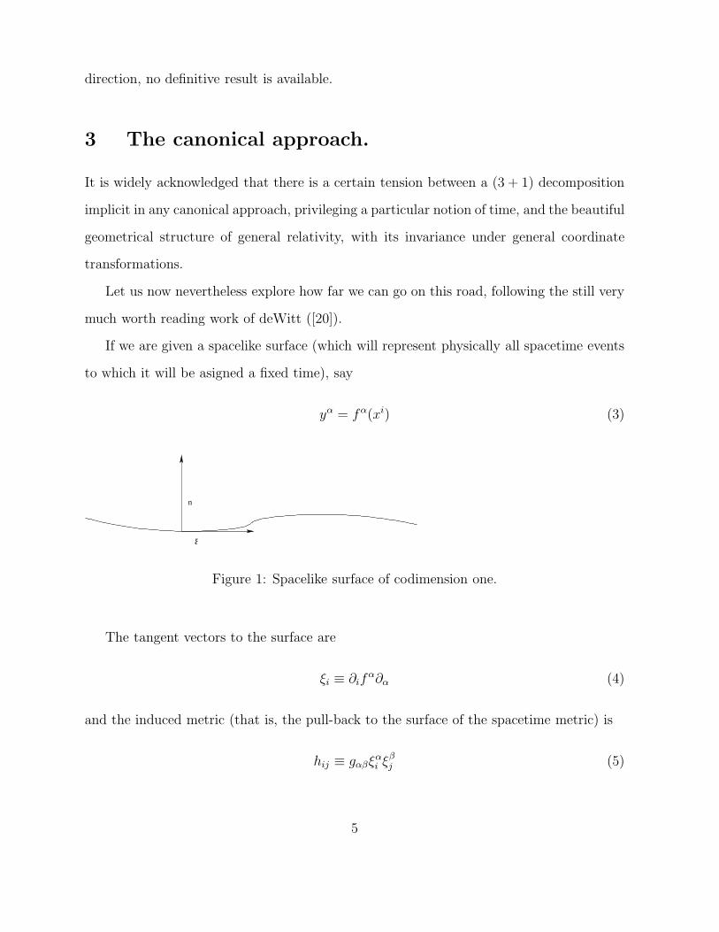
If we are given a spacelike surface (which will represent physically all spacetime events

to which it will be asigned a fixed time), say

yα = fα(xi) (3)

n

ξ

Figure 1: Spacelike surface of codimension one.

The tangent vectors to the surface are

ξi ≡ ∂ifα∂α (4)

and the induced metric (that is, the pull-back to the surface of the spacetime metric) is

hij ≡ gαβξαi ξ

βj (5)

5

The unit normal is then defined as;

gαβnαξβi = 0

n2 ≡ gαβnαnβ = 1

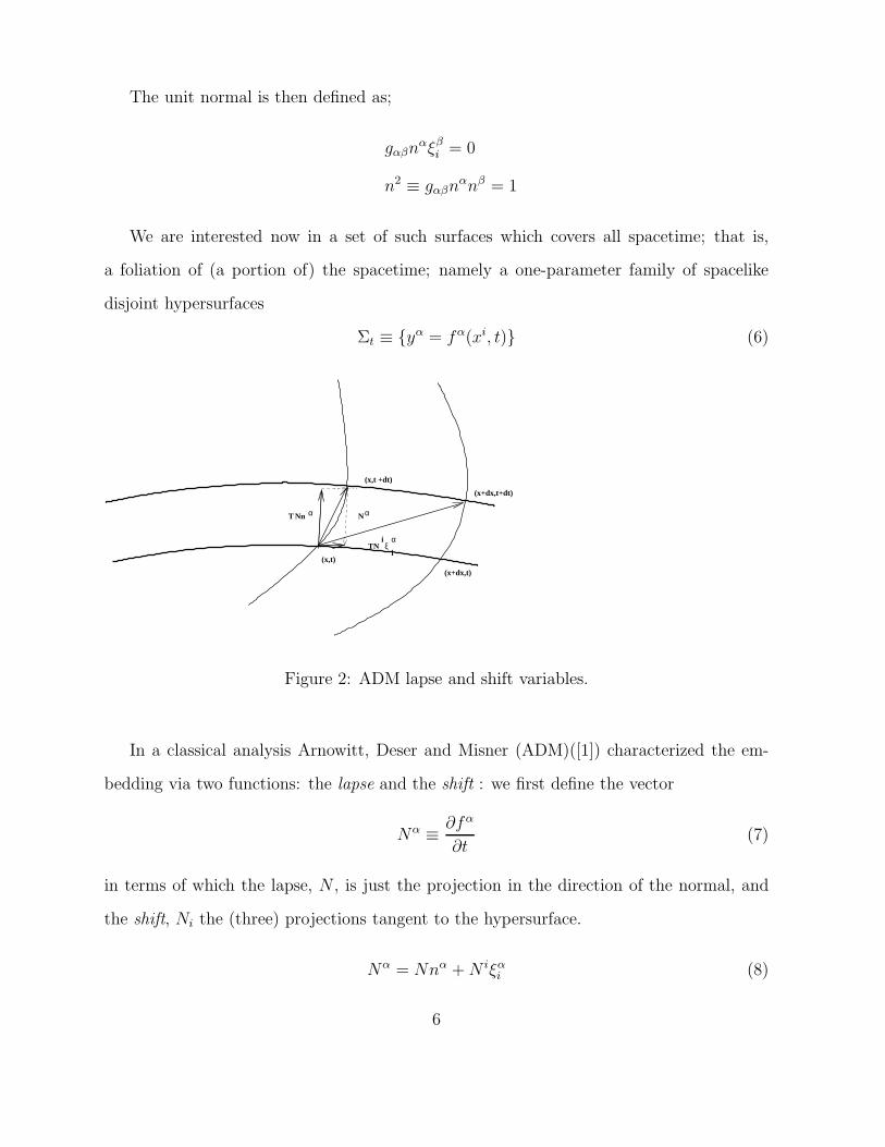
We are interested now in a set of such surfaces which covers all spacetime; that is,

a foliation of (a portion of) the spacetime; namely a one-parameter family of spacelike

disjoint hypersurfaces

Σt ≡ {yα = fα(xi, t)} (6)

T Nn α Nα

iTN ξ

i

α

(x,t)

(x,t +dt)

(x+dx,t)

(x+dx,t+dt)

Figure 2: ADM lapse and shift variables.

In a classical analysis Arnowitt, Deser and Misner (ADM)([1]) characterized the em-

bedding via two functions: the lapse and the shift : we first define the vector

Nα ≡ ∂fα

∂t(7)

in terms of which the lapse, N , is just the projection in the direction of the normal, and

the shift, Ni the (three) projections tangent to the hypersurface.

Nα = Nnα +N iξαi (8)

6

All this amounts to a particular splitting of the full spacetime metric:

ds2 = gαβdxαdxβ = gαβdf

αdfβ = gαβ(Nαdt+ξαi dx

i)(Nβdt+ξβj dxj) = N2dt2+hjk(N

jdt+dxj)(Nkdt+dxk)

(9)

or, what is the same,

gµν = hijξiµξjν + nµnν (10)

All surfaces which are equivalent from the intrinsic point of view, can be however

embedded differently; the extrinsic curvature discriminates between them:

Kij = −ξαi ∇ρnαξρj (11)

The Gauss- Codazzi equations relate intrinsic curvatures associated with the intrinsic

geometry in the hypersurface with spacetime curvatures precisely through the extrinsic

curvature:

R[h]lijk = R[g]αβσρξαl ξ

βi ξ

σj ξ

ρk −KijKlk +KikKlj (12)

and

∇[h]kKij −∇[h]jKik = Rαβσρnαξβi ξ

ρj ξ

σk (13)

whereas the curvature scalar is given by

R = Rαβαβ = 2Rni

ni +Rijij (14)

In terms of this splitting, the Einstein-Hilbert action reads:

LEH ≡ √gR[g] = N

√h(R[h] +KijK

ij −K2)− ∂αVα (15)

with

V α = 2√g(nβ∇βn

α − nα∇βnβ) (16)

Primary constraints appear when defining canonical momenta:

pµ ≡ ∂L

∂Nµ

∼ 0 (17)

7

the momenta conjugate to the spatial part of the metric is:

πij ≡ δL

δhij= −h1/2(Kij −Khij) (18)

The canonical conmutation relations yield:

{πij(~x), hkl(~x′)} = −δ(~x, ~x ′)

1

2(δikδ

jl + δjkδ

il) (19)

The total Hamiltonian reads

H ≡∫

d3x(πµNµ + πij hij − L) =

∫

d3x(NH +N iHi) (20)

where

H(h, π) = h−1/2(πijπij − 1

2π2)− h1/2R[h] (21)

and

Hi(h, π) = −2hik∂jπkj − (2∂jhki − ∂ihkj)π

kj = −2∇[h]jπij (22)

The system of constraints is now consistent (that is, that the classical time evolution

of the constraints is still a linear combination of constraints):

pµ = {pµ, H} = (H,Hi) ∼ 0 (23)

Second class constraints

Nµ = fµ (24)

can now be imposed. The whole hamiltonian analysis boils down to the two constraint

equations

H = 0

Hi = 0

8

Much of the preceding analysis is actually quite generic for generally covariant systems.

The full set of constraints obeys the Dirac-Schwinger algebra

{H(~x),H(~y)} = [Hi(~x) +Hi(~y)]∂iδ(~x, ~y)

{Hi(~x),H(~y)} = H(~x)∂iδ(~x, ~y)

{Hi(~x),Hj(~y)} = Hi(~y)∂jδ(~x, ~y) +Hj(~x)∂iδ(~x, ~y) (25)

which is nothing else than the Σ-projected algebra of the Diff(M) group.

Usually no reduction is made on the dynamical variables of the system, which amounts

to keep hij, πij as (redundant) quantum variables. It is not clear how singular metrics can

be avoided, because it is not easy to impose the condition that the metric is a positive

definite operator.

Physical states in the Hilbert space are provisionally defined a la Dirac

H|ψ >= 0

Hi|ψ >= 0

It has been realized since long that this whole approach suffers from the frozen time

problem, i.e., the Hamiltonian reads

H ≡∫

d3x(NH +N iHi) (26)

so that acting on physical states

H|ψ >= 0 (27)

in such a way that Schrodinger’s equation

i∂

∂t|ψ >= H|ψ > (28)

seemingly forbids any time dependence.

9

There are many unsolved problems in this approach, which has been kept at a formal

level. The first one is an obvious operator ordering ambiguity owing to the nonlinearity.

In the same vein, it is not clear whether it is possible to make the constraints hermitian.

Besides, it is not clear that one recovers the full Diff invariance from the Dirac- Schwinger

algebra. Actually, it is not known whether this is necessary; that is, what is the full

symmetry of the quantum theory.

We can proceed further, still formally3, using the Schrodinger representation defined in

such a way that

(hijψ)[h] ≡ hij(x)ψ[h] (29)

and

(πijψ)[h] ≡ −i~ δψ

δhij(x)[h] (30)

If we assume that diffeomorphisms act on wave functionals as:

ψ[f ∗h] = ψ[h] (31)

then the whole setup for the quantum dynamics of the gravitational field lies in Wheeler’s

superspace (nothing to do with supersymmetry) which is the set of three-dimensional met-

rics modulo three-dimensional diffs : Riem(Σ)/Diff(Σ).

The Hamiltonian constraint then implies the famous Wheeler-de Witt equation.

− ~22κ2Gijkl

δ2ψ

δhikδhjl[h]− h

2κ2R(3)[h]ψ[h] = 0 (32)

where the de Witt tensor is:

Gijkl ≡1√h

(

hijhkl −1

2hikhjl

)

(33)

3It is bound to be formal as long as the problem of the infinities is not fully addressed. We know

from the analysis of this representation for gauge theories in the lattice that those are the most difficult

problems to solve.

10

Needless to say, this equation, suggestive as it is, is plagued with ambiguities. The manifold

of positive definite metrics has been studied by deWitt. He showed that it has signature

(−1,+15), where the timelike coordinate is given by the breathing mode of the metric:

ζ =

√

32

3h1/4 (34)

and in terms of other five coordinates ζa orthogonal to the timelike coordinate, the full

metric reads

ds2 = −dζ2 + 3

32ζ2gabdζ

adζb (35)

with

gab = tr h−1∂ahh−1∂h (36)

The five dimensional submanifold with metric gab is the coset space

SL(3,R)/SO(3) (37)

It has been much speculated whether the timelike character of the dilatations lies at the

root of the concept of time. The Wheeler-deWitt equation can be written in a form quite

similar to the Klein-Gordon equation:

(

− ∂2

∂ζ2+

32

3ζ2gab∂a∂b +

3

32ζ2R(3)

)

Ψ = 0 (38)

The analogy goes further in the sense that also here there is a naturally defined scalar

product which is not positive definite:

(ψ, χ) ≡∫

Σ

ψ∗dΣijGijklδχ

iδhkl− χ∗dΣijGijkl

δψ

iδhkl(39)

4 Using Ashtekar and related variables

The whole philosophy of this approach is canonical, i.e., an analysis of the evolution of

variables defined classically through a foliation of spacetime by a family of spacelike three-

surfaces Σt. The standard choice in this case as we have just reviewed, is the three-

dimensional metric, gij, and its canonical conjugate, related to the extrinsic curvature.

11

Here, as in any canonical approach the way one chooses the canonical variables is

fundamental.

Ashtekar’s clever insight started from the definition of an original set of variables ([10])

stemming from the Einstein-Hilbert lagrangian written in the form 4

S =

∫

ea ∧ eb ∧ Rcdǫabcd (40)

where ea are the one-forms associated to the tetrad,

ea ≡ eaµdxµ. (41)

Tetrads are defined up to a local Lorentz transformation

(ea)′ ≡ Lab(x)e

b (42)

The associated SO(1, 3) connection one-form ωab is usually called the spin connection. Its

field strength is the curvature expressed as a two form:

Rab ≡ dωa

b + ωac ∧ ωc

b. (43)

Ashtekar’s variables are actually based on the SU(2) self-dual connection

A = ω − i ∗ ω (44)

Its field strength is

F ≡ dA+ A ∧ A (45)

The dynamical variables are then (Ai, Ei ≡ F 0i). The main virtue of these variables is

that constraints are then linearized. One of them is exactly analogous to Gauss’law:

DiEi = 0. (46)

There is another one related to three-dimensional diffeomorphisms invariance,

tr FijEi = 0 (47)

4Boundary terms have to be considered as well. We refer to the references for details.

12

and, finally, there is the Hamiltonian constraint,

trFijEiEj = 0 (48)

On a purely mathematical basis, there is no doubt that Astekhar’s variables are of a

great ingenuity. As a physical tool to describe the metric of space, they are not real in

general. This forces a reality condition to be imposed, which is akward. For this reason it

is usually prefered to use the Barbero-Immirzi ([13][37]) formalism in which the connexion

depends on a free parameter, γ,

Aia = ωi

a + γKia (49)

ω being the spin connection and K the extrinsic curvature. When γ = i Astekhar’s for-

malism is recovered; for other values of γ the explicit form of the constraints is more

complicated. Thiemann ([67]) has proposed a form for the Hamiltonian constraint which

seems promising, although it is not clear whether the quantum constraint algebra is iso-

morphic to the classical algebra (cf.[54]). A comprehensive reference is [66].

Some states which satisfy the Astekhar constraints are given by the loop representation,

which can be introduced from the construct (depending both on the gauge field A and on

a parametrized loop γ)

W (γ, A) ≡ tr Pe∮

γ A (50)

and a functional transform mapping functionals of the gauge field ψ(A) into functionals of

loops, ψ(γ):

ψ(γ) ≡∫

DAW (γ, A)ψ(A) (51)

When one divides by diffeomorphisms, it is found that functions of knot classes (diffeo-

morphisms classes of smooth, non self-intersecting loops) satisfy all the constraints.

Some particular states sought to reproduce smooth spaces at coarse graining are the

Weaves. It is not clear to what extent they also approach the conjugate variables ( that

is, the extrinsic curvature) as well.

13

In the presence of a cosmological constant the hamiltonian constraint reads:

ǫijkEaiEbj(F k

ab +λ

3ǫabcE

ck) = 0 (52)

A particular class of solutions of the constraint [60] are self-dual solutions of the form

F iab = −λ

3ǫabcE

ci (53)

Kodama ([41]) has shown that the Chern-Simons state

ψCS(A) ≡ e3

2λSCS(A) (54)

is a solution of the hamiltonian constraint. He even suggested that the sign of the coarse

grained, classical cosmological constant was always positive, irrespectively of the sign of

the quantum parameter λ, but it is not clear whether this result is general enough. There

is some concern [71] that this state as such is not normalizable with the usual norm. It

has been argued that this is only natural, because the physical relevant norm must be very

different from the naıve one (cf. [59]) and indeed normalizability of the Kodama state

has been suggested as a criterion for the correctness of the physical scalar product(cf. for

example the discussion in [24]) or else that a euclidean interpretation could be given to it.

Loop states in general (suitable symmetrized) can be represented as spin network ([56])

states: colored lines (carrying some SU(2) representation) meeting at nodes where inter-

twining SU(2) operators act. A beautiful graphical representation of the group theory has

been succesfully adapted for this purpose. There is a clear relationship between this repre-

sentation and the Turaev-Viro [68] invariants. Many of these ideas have been foresighted

by Penrose (cf. [48]).

There is also a path integral representation, known as spin foam (cf.[12]), a topological

theory of colored surfaces representing the evolution of a spin network. These are closely

related to topological BF theories, and many independent generalizations have been pro-

posed. Spin foams can also be considered as an independent approach to the quantization

of the gravitational field.([14])

14

In addition to its specific problems, this approach shares with all canonical approaches

to covariant systems the problem of time. It is not clear its definition, at least in the

absence of matter. Dynamics remains somewhat mysterious; the hamiltonian constraint

does not say in what sense (with respect to what) the three-dimensional dynamics evolve.

4.1 Big results of this approach.

One of the main successes of the loop approach is that the area (as well as the volume)

operator is discrete. This allows, assuming that a black hole has been formed (which is a

process that no one knows how to represent in this setting), to explain the formula for the

black hole entropy . The result is expressed in terms of the Barbero-Immirzi parameter

([57]). The physical meaning of this dependence is not well understood.

It has been pointed out [15] that there is a potential drawback in all theories in which

the area (or mass) spectrum is discrete with eigenvalues An if the level spacing between

eigenvalues δAn is uniform because of the predicted thermal character of Hawking’s radia-

tion. The explicit computations in the present setting, however, lead to an space between

(dimensionless) eigenvalues

δ An ∼ e−√An, (55)

which seemingly avoids this set of problems.

It has also been pointed out that [23] not only the spin foam, but almost all other

theories of gravity can be expressed as topological BF theories with constraints. While

this is undoubtely an intesting and potentially useful remark, it is important to remember

that the difference between the linear sigma model (a free field theory) and the nonlinear

sigma models is just a matter of constraints. This is enough to produce a mass gap and

asymptotic freedom in appropiate circumstances.

15

5 Euclidean quantum gravity

It can be boldly asserted that just by analogy with ordinary quantum field theory, the

wave functional of quantum gravity must be given by:

ψ[h] ≡∫

g(∂M)=h

Dge−SE[g] (56)

where we integrate over all riemannian metrics that obey the relevant boundary condi-

tions, and the Einstein-Hilbert action has to be supplemented with boundary terms. This

approach is problematic from the very beginning, due to the fact that the Wick analytic

continuation of a lorentzian space-time is not riemannian in general (not even real), so that

the whole setup seems to demand the study of real sections in a complex formulation. The

point of view put forward by Hawking and collaborators [32] is that the needed analytical

continuations could be hopefully made after Green’s functions are evaluated.

There however is a well-known mathematical theorem of Markov (explained for physi-

cists in [5]) asserting that there is no algorithmic way of predicting when two arbitrary

manifolds are homeomorphic :M1 ∼ M2. The problem stems essentially from the fun-

damental group: any finitely presented group can be the π1(M) of a four-dimensional

manifold, M . So one proof of the result is to simply write down a family of groups Gk

such that we cannot algorithmically recognise when G = {e}. There are, in addition, fur-

ther subtleties with the diffeomorphism class in d = 4: there is a uncountable set of non

equivalent differentiable structures in R4: the so-called exotic R

4 (cf. [18] for a physical

approach; a relevant recent reference is [50]) .

Working in lorentzian signature, a Hamiltonian path integral can be dreamt of, where

a functional integral is performed over three-dimensional geometries (cf. [6] only. Here the

situation is slightly better: it seems that there is recent progress in the proof of Thurston’s

geometrization conjecture, which implies in particular Poincare’s conjecture, and which

explains all three-dimensional manifolds in terms of eight different geometries. Incidentally,

the work of Perelman ([49]) uses what mathematicians call the Ricci flow, which is exactly

16

the flow of the renormalization group of the sigma model associated to the bosonic string

in a curved background.

Let us finally comment that even if the basic theory of Nature is topological one needs to

enumerate topologies to discriminate between different ones. Besides, topological symmetry

has to be broken al low energies.

In order to reach a probabilistic interpretation, a scalar product ought to be defined.

The one which is naturally associated to the Wheeler-de Witt equation is not positive-

definite, so this remains as an open problem in this approach.

Were somebody apply these ideas to the whole Universe (the so called Quantum Cos-

mology) there are other problems in store. It is not clear what is the physical interpretation

of probabilities associated to a single event. A related problem is the one of the physical

interpretation of Quantum Mechanics without classical observers. Many people have re-

lated this to the decoherence mechanisms (cf. for example [30]) but it seems to me that

the situation is still to be clarified.

6 Perturbative (graviton) approach

A much more modest approch is to study gravitons as ordinary (massless, spin two) par-

ticles in Minkowski space-time.

gαβ = gαβ + κhαβ (57)

It seems to many people (including the author) that this is at least a preliminary step

before embarking in more complicated adventures. As a quantum field theory, quantum

general relativity has got a dimensionful coupling : d(κ) = −1, which means that it is not

renormalizable in the usual sense of the word.

In spite of this, the theory is one loop finite on shell , as was shown in a brilliant

calculation by G. ’t Hooft and M. Veltman ([33]). They computed the counterterm:

∆L(1) =

√g

ǫ

203

80R2 (58)

17

No more miracles are expected for higher loops, and none happen. Goroff and Sagnotti

([27]) were the first to show that to two loops,

∆L(2) =209

2880(4π)41

ǫRαβ

γδRγδ

ρσRρσ

αβ (59)

The general structure of perturbation theory is governed by the fact we have just

mentioned that the coupling constant is dimensionful. A general diagram will then behave

in the s-channel as κnsn and counterterms as:

∆L ∼∑

∫

κnR(2+n/2) (60)

(where a symbolic notation has been used, packing all invariants with the same dimen-

sion; for example, R2 stands for an arbitary combination of R2, RαβRαβ and RαβγδR

αβγδ)

conveying the fact that that the theory is non-renormalizable.

It may however be pondered whether effective lagrangians are really useful for E <<

mP . This possibility has been forcefully explored by Donoghue and collaborators (cf. [21]).

There are some caveats: for example, when horizons are present, it seems necessary in order

to be able to apply these ideas, to use some particular foliations, the so called nice slices).

The mere fact that we are unable to predict the cosmological constant (which is the mother

of all infrared problems) means that our understanding has ample room for improvement.

Could it be that in spite of the fact that general relativity is not renormalizable, there

is a non perturbative sector in which the theory makes sense as a quantum theory? First

of all, were that true, it would be most remarkable: there are no known QFT which are

defined only noperturbatively. Besides, at the classical level, perturbation theory works

wonderfully, and there is indeed a whole framework, the parametrized post-newtonian

(PPN) formalism to discriminate netween alternate theories of gravity. It is then most

unclear why at the quantum (and only there) level perturbation theory should fail.

We want to mention in closing this chapter, some fascinating relationships uncovered

by Z. Berm and collaborators (cf. [16]) between purely field-theoretical S matrix elements

18

in (super)gravity and gauge theories: the so called Gravity=Gauge × Gauge conjecture.

In spite of several attempts, it is not clear how this can be understood from the Einstein-

Hilbert action. The relationship is of course automatic in strings, because closed string

amplitudes (which include the graviton) are given by products of open string amplitudes

(which contain the gauge fields).The KLT relations ([40]) are a quantitative formulation of

this fact.

In view of all this, one can try to study particular extensions of the Einstein-Hilbert

actions. Modifications quadratic in the curvature improve renormalizability ([39]), but

have problems with unitarity at a very fundamental level ([61]).

Local supersymmetry is expected to improve the ultraviolet behavior through cancel-

lations between fermionic and bosonic degrees of freedom. In spite of that, some infinities

are allowed by the symmetries of the problem, and are thus expected to appear; for ex-

ample in extended supergravities this is expected to happen at loop order L > 10D−2

in the

maximally supersymmetric case in which there are 32 supercharges.

The (sad) conclusion of all this is that ordinary QFT (with a finite number of fields)

does not work, even for describing small (quantum) ripples in Minkowski space.

7 Strings

It should be clear by now that we probably still do not know what is exactly the problem to

which string theories are the answer. At any rate, the starting point is that all elementary

particles are viewed as quantized excitations of a one dimensional object, the string, which

can be either open (free ends) or closed (a loop). Excellent books are avaliable, such as

[29][52].

String theories enjoy a convoluted history. Their origin can be traced to the Veneziano

model of strong interactions. A crucial step was the reinterpretation by Scherk and Schwarz

([58]) of the massless spin two state in the closed sector (previously thought to be related

19

to the Pomeron) as the graviton and consequently of the whole string theory as a potential

theory of quantum gravity, and potential unified theories of all interactions. Now the wheel

has made a complete turn, and we are perhaps back through the Maldacena conjecture

([44]) to a closer relationship than previously thought with ordinary gauge theories.

Figure 3: String theorist at work.

From a certain point of view, their dymamics is determined by a two-dimensional non-

linear sigma model, which geometrically is a theory of imbeddings of a two-dimensional

surface (the world sheet of the string) to a (usually ten-dimensional) target space:

xµ(ξ) : Σ2 →Mn (61)

There are two types of interactions to consider. Sigma model interactions (in a given two-

dimensional surface) are defined as an expansion in powers of momentum, where a new

dimensionful parameter, α′ ≡ l2s sets the scale. This scale is a priori believed to be of the

order of the Planck length. The first terms in the action always include a coupling to the

20

massless backgrounds: the spacetime metric, the two-index Maxwell like field known as

the Kalb-Ramond or b-field, and the dilaton. To be specific,

S =1

l2s

∫

Σ2

gµν(x(ξ))∂axµ(ξ)∂bx

ν(ξ)γab(ξ) + . . . (62)

There are also string interactions, (changing the two-dimensional surface) proportional to

the string coupling constant, gs, whose variations are related to the logarithmic variations

of the dilaton field. Open strings (which have gluons in their spectrum) always contain

closed strings (which have gravitons in their spectrum) as intermediate states in higher

string order (gs) corrections. This interplay open/closed is one of the most fascinating

aspects of the whole string theory.

It has been discovered by Friedan (cf. [25]) that in order for the quantum theory to be

consistent with all classical symmetries (diffeomorphisms and conformal invariance), the

beta function of the generalized couplings 5 must vanish:

β(gµν) = Rµν = 0 (63)

This result remains until now as one of the most important ones in string theory, hinting

at a deep relationship between Einstein’s equations and the renormalization group.

Polyakov ([53]) introduced the so called non-critical strings which have in general a

two-dimensional cosmological constant (forbidden otherwise by Weyl invariance). The

dynamics of the conformal mode (often called Liouville in this context) is, however, poorly

understood.

Fundamental strings live in D=10 spacetime dimensions, and so a Kaluza-Klein mecan-

ism of sorts must be at work in order to explain why we only see four non-compact dimen-

sions at low energies. Strings have in general tachyons in their spectrum, and the only way

to construct seemingly consistent string theories (cf. [26]) is to project out those states,

5There are corrections coming from both dilaton and Kalb-Ramond fields. The quoted result is the

first term in an expansion in derivatives, with expansion parameter α′ ≡ l2

s.

21

which leads to supersymmetry. This means in turn that all low energy predictions heavily

depend on the supersymmetry breaking mechanisms.

String perturbation theory is probably well defined although a full proof is not available.

Several stringy symmetries are believed to be exact: T-duality, relating large and small

compactification volumes, and S-duality, relating the strong coupling regime with the weak

coupling one. Besides, extended configurations (D branes); topological defects in which

open strings can end are known to be important [51]. They couple to Maxwell-like fields

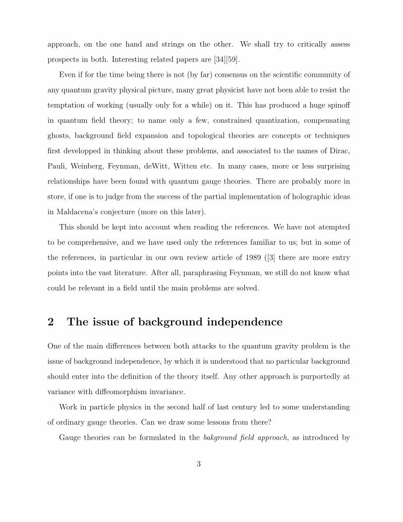
which are p-forms called Ramond-Ramond (RR) fields. These dualities [36] relate all five

string theories (namely, Heterotic E(8)× E(8), Heterotic SO(32), Tipe I, IIA and IIB)

and it is conjectured that there is an unified eleven -dimensional theory, dubbed M-theory

of which N = 1 supergravity in d = 11 dimensions is the low energy limit.

7.1 Big results

Perhaps the main result is that graviton physics in flat space is well defined for the first

time, and this is no minor accomplishment.

Besides, there is evidence that at least some geometric singularities are harmless in the

sense that strings do not feel them. Topology change amplitudes do not vanish in string

theory.

The other Big Result [62] is that one can correctly count states of extremal black holes

as a function of charges. This is at the same time astonishing and disappointing. It clearly

depends strongly on the objets being BPS states (that is, on supersymmetry), and the

result has not been extended to non-supersymmetric configurations. On the other hand,

as we have said, it exactly reproduces the entropy as a function of a sometimes large number

of charges, without any adjustable parameter.

22

7.2 The Maldacena conjecture

Maldacena [44] proposed as a conjecture that IIB string theories in a background AdS5×S5

with common radius l ∼ ls(gsN)1/4 and N units of RR flux that is,∫

S5

F5 = N (which

implies that F5 ∼ Nr5) is equivalent to a four dimensional ordinary gauge theory in flat four-

dimensional Minkowski space, namely N = 4 super Yang-Mills with gauge group SU(N)

and coupling constant g = g1/2s .

Although there is much supersymmetry in the problem and the kinematics largely

determine correlators, (in particular, the symmetry group SO(2, 4)× SO(6) is realized as

an isometry group on the gravity side and as an R-symmetry group as well as conformal

invariance on the gauge theory side) this is not fully so 6 and the conjecture has passed

many tests in the semiclassical approximation to string theory.

The action of the RR field, given schematically by∫

F 25 , scales as N2, whereas the

ten-dimensional Einstein-Hilbert∫

R, depends on the overall geometric scale as the eighth

power of the common radius, l8. The ’t Hooft coupling is λ = g2N ∼ l4

l4sand the tenth

dimensional Newton’s constant is κ210 ∼ G10 ∼ l8p = g2s l8s ∼ l8

N2 .

If we consider the effective five dimensional theory after compactifying on a five sphere

of radius r, the RR term yields a negative contribution ∼ −(Nr5)2r5 ,whereas the positive

curvature of the five sphere S5 gives a positive contribution, ∼ 1r2r5. The competition

between these two terms in the effective potential is responsible for the minimum with

negative cosmological constant.

The way the dictionary works in detail [69] is that the supergravity action corresponding

to fields with prescribed boundary values is related to gauge theory correlators of certain

gauge invariant operators corresponding to the particular field studied:

e−Ssugra[Φi]∣

∣

∣

Φi|∂AdS=φi

=< e∫

Oiφi >CFT (64)

6The only correlators that are completely determined through symmetry are the two and three-point

functions.

23

This is the first time that a precise holographic description of spacetime in terms of a

(boundary) gauge theory is proposed and, as such it is of enormous potential interest. It

has been conjectured by ’t Hooft [64] and further developed by Susskind [63] that there

should be much fewer degrees of freedom in quantum gravity than previously thought. The

conjecture claims that it should be enough with one degree of freedom per unit Planck

surface in the two-dimensional boundary of the three-dimensional volume under study.

The reason for that stems from an analysis of the Bekenstein-Hawking [15][31] entropy

associated to a black hole, given in terms of the two-dimensional area A 7 of the horizon

by

S =c3

4G~A. (66)

This is a deep result indeed, still not fully understood.

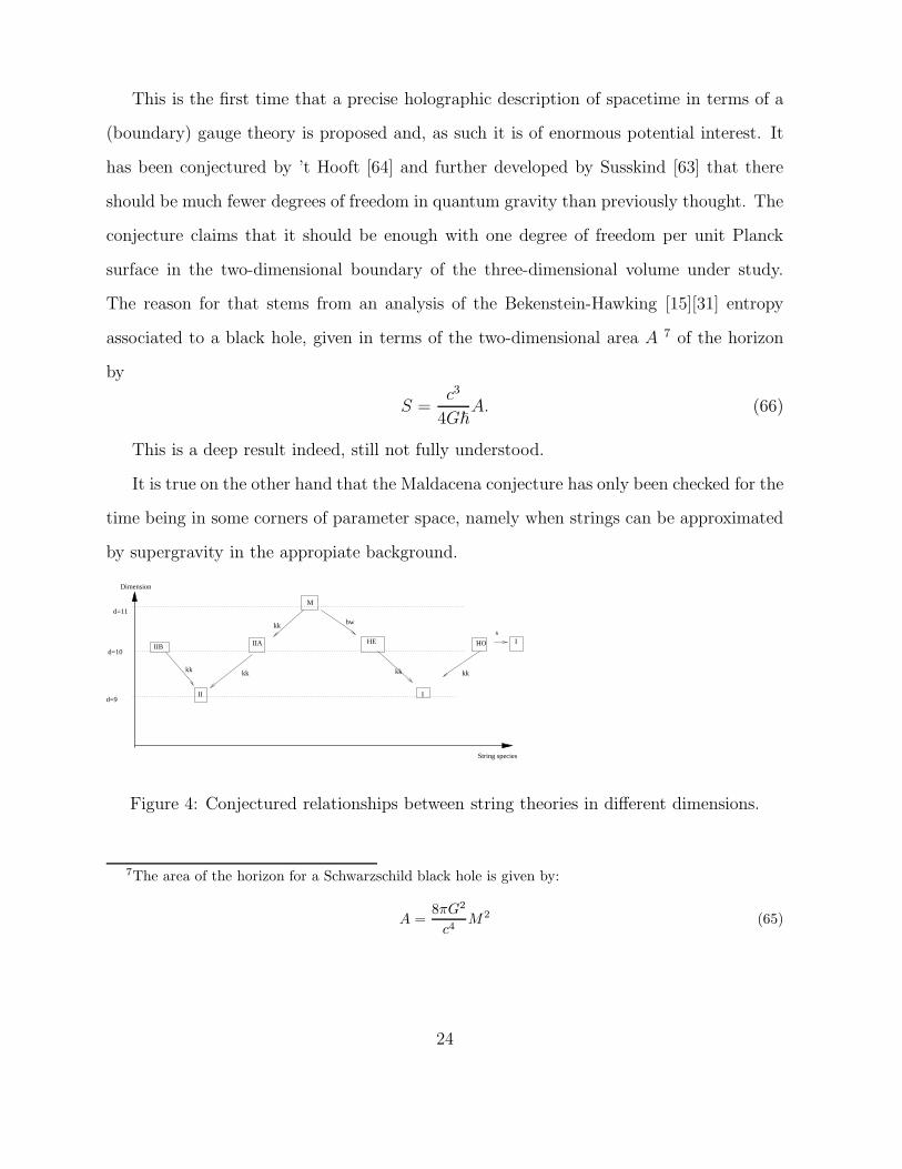
It is true on the other hand that the Maldacena conjecture has only been checked for the

time being in some corners of parameter space, namely when strings can be approximated

by supergravity in the appropiate background.

d=11

d=10

d=9

M

IIA HEIIB HO I

II I

kk

kk kk kk kk

hw

s

Dimension

String species

Figure 4: Conjectured relationships between string theories in different dimensions.

7The area of the horizon for a Schwarzschild black hole is given by:

A =8πG2

c4M

2 (65)

24

8 Dualities and branes

The so- called T-duality is the simplest of all dualities and the only one which can be shown

to be true, at least in some contexts. At the same time it is a very stringy characteristic,

and depends in an essential way on strings being extended objects. In a sense, the web of

dualities rests on this foundation, so that it is important to understand clearly the basic

physics involved. Let us consider strings living on an external space with one compact

dimension, which we shall call y, with topology S1 and radius R. The corresponding field

in the imbedding of the string, which we shall call y (i.e. we are dividing the target-

spacetime dimensions as (xµ, y), where y parametrizes the circle), has then the possibility

of winding around it:

y(σ + 2π, τ) = y(σ, τ) + 2πRm . (67)

A closed string can close in general up to an isometry of the external spacetime.

The zero mode expansion of this coordinate (that is, forgetting about oscillators) would

then be

y = yc + 2pcτ +mRσ . (68)

Canonical quantization leads to [yc, pc] = i, and single-valuedness of the plane wave eiycpc

enforces as usual pc ∈ Z/R, so that pc =nR.

The zero mode expansion can then be organized into left and right movers in the

following way

yL(τ + σ) = yc/2 +

(

n

R+mR

2

)

(τ + σ) ,

yR(τ − σ) = yc/2 +

(

n

R− mR

2

)

(τ − σ) . (69)

The mass shell conditions reduce to

m2L =

1

2

(

n

R+mR

2

)2

+NL − 1 ,

m2R =

1

2

(

n

R− mR

2

)2

+NR − 1 . (70)

25

Level matching, mL = mR, implies that there is a relationship between momentum and

winding numbers on the one hand, and the oscillator excess on the other

NR −NL = nm . (71)

At this point it is already evident that the mass formula is invariant under

R → R∗ ≡ 2/R , (72)

and exchanging momentum and winding numbers. This is the simplest instance of T-

Duality.

On the other hand, it is an old observation (which apparently originated in Schrodinger)

that Maxwell’s equations are almost symmetrical with respect to interchange between

electric and magnetic degrees of freedom. This idea was explored by Dirac and eventually

lead to the discovery of the consistency conditions that have to be fulfilled if there are

magnetic monopoles in nature. The fact that nonsingular magnetic monopoles appear as

classical solutions in some gauge theories led further support to this duality viewpoint. In

order to be able to make a consisting conjecture, first put forward by Montonen and Olive

[45], supersymmetry is needed, as first remarked by Osborn [47].

Now in strings there are the so- called Ramond-Ramond (RR) fields, which are p- forms

of different degrees. In the same way that one forms (i.e., the Maxwell field) couples to

charged particles that is, from the spacetime point of view, to objects of dimension 0 with

one-dimensional trajectories, a p-form

Aµ1...µp (73)

would couple to a (p − 1)-dimensional object, whose world history is described by a p-

dimensional hypersurface

xµ = xµ(ξ1 . . . ξp) (74)

These objects are traditionally denoted by the name p-branes (it all originated in a dubious

26

joke). That is, ordinary particles are 0-branes, a string is a 1-brane, a membrane is a 2-

brane, and so on.

Dualities relate branes of different dimensions in different theories; this means that

if one is to take this symmetry seriously, it is not clear at all that strings are the more

fundamental objects: in the so called M-theory branes appear as fundamental as strings.

If we are willing to make the hypothesis that supersymmetry is not going to be broken

whilst increasing the coupling constant, gs, some astonishing conlusions can be drawn.

Assuming this, massless quanta can become massive as gs grows only if their number,

charges and spins are such that they can combine into massive multiplets (which are all

larger than the irreducible massless ones). The only remaining issue, then, is whether any

other massless quanta can appear at strong coupling.

Now, in the IIA string theory there are states associated to the Ramond-Ramond (RR)

one form, A1, namely the D-0-branes, whose tension goes as m ∼ 1gs. This clearly gives

new massless states in the strong coupling limit.

There are reasons8 to think that this new massless states are the first level of a Kaluza-

Klein tower associated to compactification on a circle of an 11-dimensional theory. Actually,

assuming an 11-dimensional spacetime with an isometry k = ∂∂y, an Ansatz which exactly

reproduces the dilaton factors of the IIA string is

ds2(11) = e4

3φ(dy −A(1)

µ dxµ)2 + e−2

3φgµνdx

µdxν . (75)

Equating the two expressions for the D0 mass,

1

gs=

1

R11, (76)

leads to R11 = e2

3φ = g

2/3A .

This means that a new dimension appears at strong coupling, and this dimension is

related to the dilaton. The only reason why we do not see it at low energiew is precisely8In particular: The fact that there is the possibility of a central extension in the IIA algebra, related

to the Kaluza-Klein compactification of the d=11 Supergravity algebra.

27

because of the smallness of the string coupling, related directly to the dilaton field. The

other side of this is that this eleven dimensional theory, dubbed M-theory does not have

any weak coupling limit; it is always strongly coupled. Consequently, not much is known

on this theory, except for the fact that its field theory, low curvature limit is N = 1

supergravity in d = 11 dimensions.

All supermultiplets of massive one-particle states of the IIB string supersymmetry alge-

bra contain states of at least spin 4. This means that under the previous set of hypothesis,

the set of massless states at weak coupling must be exactly the same as the corresponding

set at strong coupling. This means that there must be a symmetry mapping weak coupling

into strong coupling.

There is a well-known candidate for this symmetry: Let us call, as usual, l the RR

scalar and φ the dilaton (NSNS). We can pack them together into complex scalar

S = l + ie−φ2 . (77)

The IIB supergravity action in d=10 is invariant under the SL(2,R) transformations

S → aS + b

cS + d, (78)

if at the same time the two two-forms, Bµν (the usual, ever-present, NS field), and A(2),

the RR field transform as

B

A(2)

→

d −c−b a

B

A(2)

, (79)

Both the, Einstein frame, metric gµν and the four-form A(4) are inert under this SL(2,R)

transformation.

A discrete subgroup SL(2,Z) of the full classical SL(2,R) is believed to be an exact

symmetry of the full string theory. The exact imbedding of the discrete subgroup in the

full SL(2,R) depends on the vacuum expectation value of the RR scalar.

28

The particular transformation

g =

0 1

−1 0

, (80)

maps φ into −φ (when l = 0), and B into A(2). This means that the string coupling

gs →1

gs(81)

This is a strong/weak coupling type of duality, similar to the electromagnetic duality in

that sense .The standard name for it is an S-duality type of transformation, mapping the

ordinary string with NS charge, to another string with RR charge (which then must be a

D-1-brane, and is correspondingly called a D-string), and, from there, is connected to all

other D-branes by T-duality.

Using the fact that upon compactification on S1, IIA at RA is equivalent to IIB at

RB ≡ 1/RA, and the fact that the effective action carries a factor of e−2φ we get

RAg2B = RBg

2A , (82)

which combined with our previous result, gA = R3/211 implies that gB =

R3/211

RA. Now the

Kaluza-Klein Ansatz implies that from the eleven dimensional viewpoint the compactifi-

cation radius is measured as

R210 ≡ R2

Ae−2φ/3 , (83)

yielding

gB =R11

R10. (84)

From the effective actions written above it is easy to check that there is a (S-duality

type) field transformation mapping the SO(32) Type I open string into the SO(32) Heterotic

one namely

gµν → e−φgHetµν ,

φ → −φ ,

B′ → B . (85)

29

This means that physically there is a strong/weak coupling duality, because coupling con-

stants of the compactified theories would be related by

ghet = 1/gI ,

Rhet = RI/g1/2I . (86)

9 Summary: the state of the art in quantum gravity

In the loop approach one is working with nice candidates for a quantum theory. The

theories are interesting, probably related to topological field theories ([17]) and background

independence as well as diffeomorphism invariance are clearly implemented. On the other

hand, it is not clear that their low energy limit is related to Einstein gravity.

Strings start from a perturbative approach more familiar to a particle physicist. How-

ever, they carry all the burden of supersymmetry and Kaluza-Klein. It has proved to be

very difficult to study nontrivial non-supersymmetric dynamics.

Finally, and this applies to all approaches, the holographic ideas seem intriguing; there

are many indications of a deep relationship between gravity and gauge theories.

We would like to conclude by insisting on the fact that although there is not much we

know for sure on quantum effects on the gravitational field, even the few things we know

are a big feat, given the difficulty to do physics without experiments.

Progress could be made if we could derive semiclassical gravity in such a way that

corrections to it can be reliably estimated, for example

Rµν −1

2Rgµν = 2κ2 < ψ|Tµν |ψ > +

1

L2∆, (87)

when working at a certain scale of distances, say L. In order to understand those equations,

we would had to know something about the operator of which the first member is the

expectation value; something about the state on which the expectation value is computed

(In particular, if it is the vacuum, how is it to be defined?) and finally, something about

30

the definition of the energy momentum tensor as a composite operator. A question of

obvious physical interest is the estimate of the size of the corrections: Is the expected error

at a given scale of distance L

∆ ∼ ~G

c3L2(88)

or, does it depend of the characteristic energy of the source?

∆ ∼ GE2

~c5(89)

measured with respect to what?

It is painfully clear that there is still a large margin for improving our understanding

of effective quantum field theories. For example, there is still no convincing derivation of

Hawking radiation without transplanckian modes appearing at some point (this particular

example is related to the existence of the nice slices mentioned above). Besides, we do not

understand the cosmological constant, which is clearly related to the estimate of ∆.

The observational prospects are rather poor. In many models, in particular in the loop

approach ( and also in strings, with some qualifications) deviations from the lorentzian

dispersion relations are expected:

E2 = ~p2 +m2 + E2∑

n=1

cn(E

mP)n (90)

Other contributions will undoubtly analyze those in much more detail. Let us now simply

mention that noncommutative models make similar predictions.

Winding states are stringy phenomena, and its observation would be very interesting.

Stringy predictions, however, are in general difficuly to disentangle from predictions of

supersymmetry (SUSY). Namely, SUSY has to be broken, and this scale spoils almost all

differences between strings and QFT models.

With the great triumph of particle physics at the end of the seventies, namely the

experimental discovery of the intermediate bosons related to electroweak interactions, the

standard model was confirmed in all its essential traits, waiting only for the Higgs to

31

be discovered (at LHC?) and the theoretical effort has concentrated in more and more

speculative topics, and experimental guidance has become correspondingly scarce. The

net result is that, even more so that in the old days of the hunting for the theory of strong

interactions, theoretical physics is divided in almost disconnected clans.

All this is even more true when talking about quantum gravity, a paradise of specula-

tion.

This is the reason why all efforts such as the one in the present workshop, aiming

at making contact with experiment and/or observation are welcome, and will eventually

redirect physics on a healthier track when we learn to recognise the physically relevant

facts that presumably lie in front of our eyes.

10 Acknowledgements

I am grateful to Giovanni Amelino-Camelia and to Jerzy Kowalski-Glikman for organizing

such a stimulating workshop and for allowing me to take part in it. I am also grateful to

Carlos Munoz for lending his picture of a stringer . Finally, I am indebted to Jorge Conde

for reading the manuscript.

References

[1] R. Arnowitt, S. Deser, and C. W. Misner, “ Canonical Variables for General Relativ-

ity” Phys. Rev. 117, 1595-1602 (1960)

[2] J. Alfaro and G. Palma, “Loop quantum gravity corrections and cosmic rays decays,”

Phys. Rev. D 65 (2002) 103516 [arXiv:hep-th/0111176].

“Loop quantum gravity and ultra high energy cosmic rays,” Phys. Rev. D 67 (2003)

083003 [arXiv:hep-th/0208193].

32

[3] E. Alvarez, “Quantum Gravity: A Pedagogical Introduction To Some Recent Results,”

Rev. Mod. Phys. 61 (1989) 561.

[4] E. Alvarez, “Low-Energy Effects Of Quantum Gravity,” FTUAM-89-15 Lectures given

at Mtg. on Recent Developments in Gravitation, Barcelona, Spain, Sep 5-8, 1989

[5] E. Alvarez, “Some general problems in quantum gravity,” CERN-TH-6257-91 Lec-

tures at the 22nd Gift Int. Seminar in Theoretical Physics: Quantum Gravity and

Cosmology, S. Feliu De Guixols, Jun 3-6, 1991

[6] E. Alvarez, “Some general problems in quantum gravity. 2. The Three-dimensional

case,” Int. J. Mod. Phys. D 2 (1993) 1 [arXiv:hep-th/9211050].

[7] E. Alvarez, L. Alvarez-Gaume and Y. Lozano, “An introduction to T duality in string

theory,” Nucl. Phys. Proc. Suppl. 41 (1995) 1 [arXiv:hep-th/9410237].

[8] L. Alvarez-Gaume and M. A. Vazquez-Mozo, “Topics in string theory and quantum

gravity,” arXiv:hep-th/9212006.

[9] I. Antoniadis, N. Arkani-Hamed, S. Dimopoulos and G. R. Dvali, “New dimensions

at a millimeter to a Fermi and superstrings at a TeV,” Phys. Lett. B 436 (1998) 257

[arXiv:hep-ph/9804398].

[10] A. Ashtekar, “New Hamiltonian Formulation Of General Relativity,” Phys. Rev. D

36 (1987) 1587.

[11] A. Ashtekar, “Quantum Geometry And Black Hole Entropy”, gr-qc/0005126

[=Adv.Theor.Math.Phys. 4 (2000) 1]

“Quantum Geometry Of Isolated Horizons And Black Hole Entropy”, Phys.Rev. D57

(1998) 1009 [=gr-qc/9705059]

[12] J.Baez, “An Introduction To Spin FoamModels Of Quantum Gravity And Bf Theory”,

gr-qc/0010050

33

[13] J. F. Barbero, “Real Ashtekar variables for Lorentzian signature space times,” Phys.

Rev. D 51 (1995) 5507 [arXiv:gr-qc/9410014].

[14] J. W. Barrett and L. Crane, “A Lorentzian signature model for quantum general

relativity,” Class. Quant. Grav. 17 (2000) 3101 [arXiv:gr-qc/9904025].

[15] J. Bekenstein, Black Holes And Entropy Phys.Rev. D7 (1973) 2333

(with V. Mukhanov), “Spectroscopy Of The Quantum Black Hole”, Com-

mun.Math.Phys. 125 (1989) 417

[16] Z. Bern, “Perturbative quantum gravity and its relation to gauge theory,” Living Rev.

Rel. 5 (2002) 5 [arXiv:gr-qc/0206071].

[17] M. Blau, “Topological Gauge Theories Of Antisymmetric Tensor Fields”,

hep-th/9901069 [=Adv.Theor.Math.Phys. 3 (1999) 1289]

[18] C. H. Brans, “Exotic smoothness structures in physics,” Prepared for 1st Mexican

School on Gravitation and Mathematical Physics, Guanajuato, Mexico, 12-16 Dec

1994

[19] S. R. Coleman and S. L. Glashow, “High-energy tests of Lorentz invariance,” Phys.

Rev. D 59 (1999) 116008 [arXiv:hep-ph/9812418].

[20] B. S. Dewitt, “Quantum Theory Of Gravity. 1. The Canonical Theory,” Phys. Rev.

160 (1967) 1113.

“Quantum Theory of Gravity. II. The Manifestly Covariant Theory”, Phys. Rev. 162,

1195-1239 (1967).

[21] J. F. Donoghue, “General Relativity As An Effective Field Theory: The Leading

Quantum Corrections,” Phys. Rev. D 50 (1994) 3874 [arXiv:gr-qc/9405057].

34

[22] M. J. Duff, “Inconsistency Of Quantum Field Theory In Curved Space-Time,”

ICTP/79-80/38 Talk presented at 2nd Oxford Conf. on Quantum Gravity, Oxford,

Eng., Apr 1980

[23] L. Freidel, K. Krasnov and R. Puzio, “BF description of higher-dimensional gravity

theories,” Adv. Theor. Math. Phys. 3 (1999) 1289 [arXiv:hep-th/9901069].

[24] L. Freidel and L. Smolin, “The linearization of the Kodama state,”

arXiv:hep-th/0310224.

[25] D. Friedan, “Nonlinear Models In Two Epsilon Dimensions,” Phys. Rev. Lett. 45

(1980) 1057.

[26] F. Gliozzi, J. Scherk and D. I. Olive, “Supersymmetry, Supergravity Theories And

The Dual Spinor Model,” Nucl. Phys. B 122 (1977) 253.

[27] M. H. Goroff and A. Sagnotti, “The Ultraviolet Behavior Of Einstein Gravity,” Nucl.

Phys. B 266, 709 (1986).

[28] M. B. Green and J. H. Schwarz, “Anomaly Cancellation In Supersymmetric D=10

Gauge Theory And Superstring Theory,” Phys. Lett. B 149 (1984) 117.

[29] M. B. Green, J. H. Schwarz and E. Witten, “Superstring Theory. Vol. 1: Introduction,”

“Superstring Theory. Vol. 2: Loop Amplitudes, Anomalies And Phenomenology,”

[30] J. B. Hartle, “Space-time quantum mechanics and the quantum mechanics of space-

time,” arXiv:gr-qc/9304006.

[31] S. Hawking, Particle Creation By Black Holes Commun.Math.Phys. 43 (1975) 199

[32] G. W. . Gibbons and S. W. . Hawking, “Euclidean Quantum Gravity,”

[33] G. ’t Hooft and M. J. G. Veltman, “One Loop Divergencies In The Theory Of Gravi-

tation,” Annales Poincare Phys. Theor. A 20 (1974) 69.

35

[34] G. T. Horowitz, “Quantum gravity at the turn of the millennium,”

arXiv:gr-qc/0011089.

[35] G. Horowitz,”Exactly Soluble Diffeomorphism Invariant Theories”, Annals Phys. 205

(1991) 130

[36] C. M. Hull and P. K. Townsend, “Unity of superstring dualities,” Nucl. Phys. B 438

(1995) 109 [arXiv:hep-th/9410167].

[37] G. Immirzi, “Quantum gravity and Regge calculus,” Nucl. Phys. Proc. Suppl. 57

(1997) 65 [arXiv:gr-qc/9701052].

[38] C. J. Isham, “Structural issues in quantum gravity,” arXiv:gr-qc/9510063.

[39] J. Julve and M. Tonin, “Quantum Gravity With Higher Derivative Terms,” Nuovo

Cim. B 46 (1978) 137.

[40] H. Kawai, D. C. Lewellen and S. H. H. Tye, “A Relation Between Tree Amplitudes

Of Closed And Open Strings,” Nucl. Phys. B 269 (1986) 1.

[41] H. Kodama, “Holomorphic Wave Function Of The Universe,” Phys. Rev. D 42 (1990)

2548.

[42] M. Luscher, R. Narayanan, P. Weisz and U. Wolff, “The Schrodinger functional: A

Renormalizable probe for nonAbelian gauge theories,” Nucl. Phys. B 384 (1992) 168

[arXiv:hep-lat/9207009].

[43] Y. M. Makeenko and A. A. Migdal, “Exact Equation For The Loop Average In Mul-

ticolor QCD,” Phys. Lett. B 88 (1979) 135 [Erratum-ibid. B 89 (1980) 437].

[44] J. Maldacena, The large N limit of superconformal field theories and supergravity,

Adv.Theor.Math.Phys.2:231-252,1998, hep-th/9711200.

36

[45] C. Montonen and D. I. Olive, “Magnetic Monopoles As Gauge Particles?,” Phys. Lett.

B 72 (1977) 117.

[46] R. C. Myers and M. Pospelov, “Experimental challenges for quantum gravity,”

arXiv:hep-ph/0301124.

[47] H. Osborn, “Topological Charges For N=4 Supersymmetric Gauge Theories And

Monopoles Of Spin 1,” Phys. Lett. B 83 (1979) 321.

[48] R. Penrose, Angular momentum: an approach to combinatorial spacetime,in Quantum

theory and beyond, T. Bastin ed.(Cambridge University Press, 1971)

[49] G. Perelman, “The entropy formula for the Ricci flow and its geometric applications”

[50] H. Pfeiffer, arXiv:gr-qc/0404088.

[51] J. Polchinski, “Dirichlet-Branes and Ramond-Ramond Charges,” Phys. Rev. Lett. 75

(1995) 4724 [arXiv:hep-th/9510017].

[52] J. Polchinski, “String Theory. Vol. 1: An Introduction To The Bosonic String,”

“String Theory. Vol. 2: Superstring Theory And Beyond,”

[53] A. M. Polyakov, “Quantum Geometry Of Bosonic Strings,” Phys. Lett. B 103 (1981)

207.

[54] C. Rovelli, “Loop quantum gravity,” Living Rev. Rel. 1 (1998) 1

[arXiv:gr-qc/9710008].

[55] C. Rovelli Loop Quantum Gravity gr-qc/9606088 [=Phys.Lett. B380 (1996) 257]

“The Immirzi Parameter In Quantum General Relativity”, gr-qc/9505012

[=Phys.Lett. B360 (1995) 7]

[56] C. Rovelli and L. Smolin, “Spin networks and quantum gravity,” Phys. Rev. D 52

(1995) 5743 [arXiv:gr-qc/9505006].

37

[57] C. Rovelli and L. Smolin, “Discreteness of area and volume in quantum gravity,” Nucl.

Phys. B 442 (1995) 593 [Erratum-ibid. B 456 (1995) 753] [arXiv:gr-qc/9411005].

[58] J. Scherk and J. H. Schwarz, “Dual Models For Nonhadrons,” Nucl. Phys. B 81 (1974)

118.

[59] L. Smolin, “How far are we from the quantum theory of gravity?,”

arXiv:hep-th/0303185.

[60] L. Smolin, “Quantum gravity with a positive cosmological constant,”

arXiv:hep-th/0209079.

[61] K. S. Stelle, “Renormalization Of Higher Derivative Quantum Gravity,” Phys. Rev.

D 16 (1977) 953.

[62] A. Strominger and C. Vafa, “Microscopic Origin of the Bekenstein-Hawking Entropy,”

Phys. Lett. B 379 (1996) 99 [arXiv:hep-th/9601029].

[63] L. Susskind, “The World as a hologram,” J. Math. Phys. 36 (1995) 6377

[arXiv:hep-th/9409089].

[64] G. ’t Hooft, “Dimensional Reduction In Quantum Gravity,” arXiv:gr-qc/9310026.

[65] G. ’t Hooft and M. J. Veltman, “One Loop Divergencies In The Theory Of Gravita-

tion,” Annales Poincare Phys. Theor. A 20 (1974) 69.

[66] T. Thiemann, “Introduction to modern canonical quantum general relativity,”

arXiv:gr-qc/0110034.

[67] T. Thiemann, “Anomaly-free formulation of non-perturbative, four-dimensional

Lorentzian quantum gravity,” Phys. Lett. B 380 (1996) 257 [arXiv:gr-qc/9606088].

“Gauge field theory coherent states (GCS). I: General properties,” Class. Quant. Grav.

18 (2001) 2025 [arXiv:hep-th/0005233].

38

[68] V. G. Turaev and O. Y. Viro, “State Sum Invariants Of 3 Manifolds And Quantum

6j Symbols,” Topology 31 (1992) 865.

[69] E. Witten, Anti de Sitter Space and Holography, hep-th/9802150;

Anti-de Sitter space, thermal phase transition and confinement in gauge theories

hep-th/9803131.

[70] E. Witten, “(2+1)-Dimensional Gravity As An Exactly Soluble System,” Nucl. Phys.

B 311 (1988) 46.

[71] E. Witten, “A note on the Chern-Simons and Kodama wavefunctions,”

arXiv:gr-qc/0306083.

39