JHEP08(2014)117

Published for SISSA by Springer

Received: June 13, 2014

Accepted: July 23, 2014

Published: August 21, 2014

Quantum geometry from the toroidal block

Amir-Kian Kashani-Poor and Jan Troost

Laboratoire de Physique Theorique,1 Ecole Normale Superieure,

24 rue Lhomond, 75005 Paris, France

E-mail: kashani@lpt.ens.fr, troost@lpt.ens.fr

Abstract: We continue our study of the semi-classical (large central charge) expansion

of the toroidal one-point conformal block in the context of the 2d/4d correspondence. We

demonstrate that the Seiberg-Witten curve and (ε1-deformed) differential emerge naturally

in conformal field theory when computing the block via null vector decoupling equations.

This framework permits us to derive ε1-deformations of the conventional relations govern-

ing the prepotential. These enable us to complete the proof of the quasi-modularity of

the coefficients of the conformal block in an expansion around large exchanged conformal

dimension. We furthermore derive these relations from the semi-classics of exact conformal

field theory quantities, such as braiding matrices and the S-move kernel. In the course of

our study, we present a new proof of Matone’s relation for N = 2∗ theory.

Keywords: Conformal and W Symmetry, Topological Strings, Supersymmetric gauge

theory

ArXiv ePrint: 1404.7378

1Unite Mixte du CNRS et de l’Ecole Normale Superieure associee a l’Universite Pierre et Marie Curie 6,

UMR 8549.

Open Access, c© The Authors.

Article funded by SCOAP3.doi:10.1007/JHEP08(2014)117

JHEP08(2014)117

Contents

1 Introduction 1

2 The toroidal one-point block 2

2.1 The one-point function and conformal block 3

2.2 The two-point block including one degenerate insertion 3

2.3 The variable map and limits 3

3 Seiberg-Witten geometry and S-duality from null vector decoupling 4

3.1 The null vector decoupling equation 4

3.2 The amplitudes from generalized period integrals 5

3.2.1 The generalized Seiberg-Witten differential 5

3.2.2 Seiberg-Witten data and proof of the Matone relation 6

3.2.3 Beyond leading order: quantum geometry 9

3.2.4 Comparing to the proposal in [1] for the Seiberg-Witten geometry 11

3.2.5 Bohr-Sommerfeld interpretation 12

3.3 Transformation properties and S-duality 13

4 Exact conformal field theory methods 15

4.1 The B-monodromy from braiding 15

4.2 The semi-classical S-move kernel 18

5 Conclusions 21

A The function sb 22

1 Introduction

The semi-classical limit of conformal blocks has taken on new significance with the advent

of the 2d/4d correspondence [1] between two-dimensional conformal field theory and four-

dimensional N = 2 gauge theory. Holomorphic amplitudes F (n,g) specifying the dynamics

of the gauge theory, such as the prepotential F (0,0), arise as coefficients in an asymptotic

expansion of the blocks in this limit. Several methods of computation precede the 2d/4d

correspondence: among these, the generalized holomorphic anomaly equations compute

the F (n,g) directly [2–5], while localization calculations yield their generating function,

the Nekrasov partition function [6]. The conformal field theory perspective opens up a

new avenue for the computation of the amplitudes F (n,g) based on null vector decoupling

equations. In previous work [7, 8], we demonstrated how to compute the F (n,0) in this setup,

forN = 2∗ and Nf = 4 gauge theory. Here, for the case ofN = 2∗, we will demonstrate how

– 1 –

JHEP08(2014)117

to rederive the Seiberg-Witten approach [9, 10] for computing the prepotential of the gauge

theory within this framework, and extend these techniques to the generating function F =∑F (n,0)ε2n1 . In particular, an ε1-deformed Seiberg-Witten differential will emerge naturally

in this setup. As Seiberg and Witten geometrize the problem of computing the prepotential

by relating it to an elliptic fibration over moduli space, and as deformation by ε1 can be

interpreted as a quantum deformation from an integrable systems perspective [11], such an

extension can be said to describe quantum geometry. In the course of our investigations, we

will prove the quasi-modularity of the F (n,0), a property we had observed experimentally

in [7]. Our argument includes the first proof of Matone’s relation [12] for a superconformal

theory in the Seiberg-Witten framework. A proof using localization methods has appeared

in [13].

A second theme of this work is extracting results we obtain from the semi-classical

solution of null vector decoupling equations directly from the semi-classics of known exact

relations in conformal field theory. We thus study the dual period of the ε1-deformed

Seiberg-Witten differential by using braiding matrices to compute the monodromy behavior

of the toroidal block, and also extract the transformation properties of the generating

function F under S-duality from the integral kernel implementing the S-move on the block.

Our interest in studying the amplitudes F (n,g) in the context of exact conformal field

theory results stems from their interpretation as limits of topological string amplitudes.

While the topological string partition function from a worldsheet perspective is merely a

generating function for these amplitudes, it acquires a non-perturbative definition in the

light of the 2d/4d correspondence. Our hope is therefore that a careful study of how semi-

classical results emerge from exact quantities in conformal field theory will help clarify

non-perturbative aspects of topological string theory.

Our paper is organized as follows. In section 2, we review the toroidal one-point block

of conformal field theory. In section 3, we revisit the construction of the semi-classical

conformal block through a WKB solution of the null vector decoupling equation. We

show how the Seiberg-Witten curve and (ε1-deformed) differential arise naturally in this

framework, allowing us to demonstrate that up to exceptional leading terms, the expansion

of the logarithm of the block is in terms of quasi-modular forms. We offer a proof of

Matone’s relation for N = 2∗ theory in the course of the argument. The exact formulae

for the braiding matrices and the modular S-move on the toroidal one-point block are

reviewed in section 4, and used to rederive some of the results of section 3 upon saddle

point approximation. We conclude in section 5.

2 The toroidal one-point block

In this section, we will briefly review the definition of the one-point conformal block of

two-dimensional conformal field theory, and of the two-point conformal block that includes

one degenerate insertion. These map to the instanton partition function of ε-deformed

N = 2∗ gauge theory [1], the latter in the presence of a surface operator [14].

– 2 –

JHEP08(2014)117

2.1 The one-point function and conformal block

In a two-dimensional conformal field theory, the expectation value of an operator Vhm with

conformal dimension hm inserted on a torus with complex structure parameter τ can be

decomposed in terms of the three-point functions Chhm,h of the theory and the toroidal

one-point blocks Fhhm ,

〈Vhm〉τ =∑h

Chhm,h(qq)h−c24 |Fhhm(q)|2. (2.1)

The sum here is over all the primary fields, of conformal dimensions h, in the spectrum of

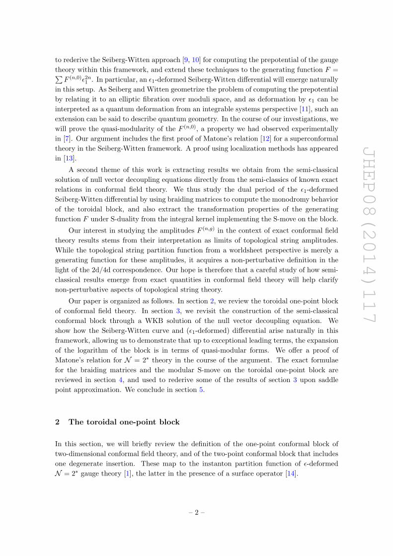
the theory. In terms of chiral vertex operators, the one-point toroidal conformal block can

be represented as the trace

qh−c24Fhhm = Trh

(qL0− c

24 hhhm

)(2.2)

=

h

hm

(2.3)

The trace is taken over the primary state |h〉 and all of its Virasoro descendants.

2.2 The two-point block including one degenerate insertion

To study the one-point conformal block, we will take advantage of the null vector decoupling

equation satisfied by the two-point toroidal block with the additional insertion chosen to

be degenerate at level two, with weight denoted h(2,1). In addition to the dependence on

the two external weights hm and h(2,1), this block requires specifying two internal momenta

h and h±, in accord with the diagram

Fh,h±hm,h(2,1)=

h±

h

hm h(2,1)

(2.4)

Note that due to the degenerate nature of the primary with weight h(2,1), this block is

non-vanishing only for two choices of internal weight h± as a function of the exchanged

conformal weight h.

2.3 The variable map and limits

Our calculations will take place purely within conformal field theory. By the 2d/4d corre-

spondence [1], the one-point toroidal block thus obtained is equal to the instanton partition

– 3 –

JHEP08(2014)117

function of N = 2∗ gauge theory, upon the following identification of variables:

c = 1 + 6Q2, Q = b+ b−1, b =

√ε2ε1

,

hm =Q2

4− m2

ε1ε2, h =

Q2

4− a2

ε1ε2. (2.5)

The central charge c of the theory is parameterized by the numbers Q or b. In gauge theory,

a and m are the vacuum expectation value of the adjoint vector multiplet scalar and the

mass parameter of the adjoint matter multiplet respectively. In the refined topological

string context [15], the εi deformation parameters are related to the string coupling g2s =

ε1ε2 and the expansion parameter s = (ε1 + ε2)2.

We will be working in the semi-classical limit of large central charge c → ∞ (b → 0)

and conformal dimensions, with h/c → ∞ and h/hm → ∞. In terms of gauge theory

parameters, this corresponds to the small εi, large vacuum expectation value limit ε2/ε1 →0, ε1/a 1, and m/a 1.

3 Seiberg-Witten geometry and S-duality from null vector decoupling

In this section, we analyze the properties of the semi-classical solutions to the second order

null vector decoupling equation satisfied by the two-point block. In particular, we identify

the Seiberg-Witten data that determine the solution within conformal field theory. This

permits us to prove the quasi-modularity of the expansion coefficients of the semi-classical

solution, observed experimentally in [7], to all orders. In the process, we provide a proof

of the Matone relation for N = 2∗ theory.

3.1 The null vector decoupling equation

Our principal strategy for computing the one-point toroidal block and determining its

transformation properties is, as in [7, 8, 16–18], to consider an additional, second order

degenerate insertion on the torus. Due to the degeneracy of the insertion, the resulting

two-point function satisfies a differential equation, the null vector decoupling equation,

which upon rescaling of the two-point function,

Ψ(z|τ) = θ1(z|τ)−b2

2 η(τ)−2(hm−b2−1)Z〈Vh(2,1)(z)Vhm(0)〉τ , (3.1)

takes the simple form [7, 18][− 1

b2∂2z −

(1

4b2− m2

ε1ε2

)℘(z)

]Ψ(z|τ) = 2πi∂τΨ(z|τ) . (3.2)

The function ℘ is the Weierstrass ℘-function associated to the torus of periods (1, τ) on

which the conformal field theory lives, and the function Z is the partition function. Im-

posing the monodromy [7, 19]

Ψ(z + 1) = e±2πi a

ε1 Ψ(z) (3.3)

– 4 –

JHEP08(2014)117

on the solution to the differential equation permits us to project onto the conformal block

Fh,h±hm,h(2,1), in the notation of (2.4). The analysis up to this point is exact. To extract the

one-point conformal block of interest from the rescaled two-point function Ψ, we need to

take the semi-classical ε2/ε1 → 0 limit, in which the degenerate insertion becomes light and

its contribution to the conformal block is multiplicative (as can be seen in a semi-classical

analysis of Liouville theory (see e.g. [20])). This motivates the factorized ansatz

Ψ(z|τ) = exp

[1

ε1ε2F(τ) +

1

ε1W(z|τ)

](3.4)

with functions F and W that are independent of ε2. In terms of this ansatz, the one-point

block is given by

limε2→0

Z 〈Vhm〉∣∣h

= exp

[1

ε1ε2

(F + 2

(−m2 +

ε214

)log η

)]. (3.5)

The null vector decoupling equation (3.2) evaluated on the ansatz (3.4) yields the equation

− 1

ε1W ′′(z|τ)− 1

ε21W ′(z|τ)2 +

(1

ε21m2 − 1

4

)℘(z) = (2πi)2

1

ε21q∂qF(τ) +

ε2ε21

2πi∂τW(z|τ) ,

(3.6)

while the boundary condition (3.3) projecting onto the desired conformal block maps to

the condition

W(z + 1)−W(z) = ±2πia . (3.7)

In [7], we solved this differential equation (dropping the linear term in ε2) in a formal

ε1-expansion of F and W,

F(τ) =

∞∑n=0

Fn(τ)εn1 , W(z|τ) =

∞∑n=0

Wn(z|τ)εn1 , (3.8)

and demonstrated to a given order that the coefficients Fn of the non-convergent expansion

reproduce the modular results obtained from the holomorphic anomaly equations [5] and

localization calculations [21, 22],

F (n,0) = F2n . (3.9)

3.2 The amplitudes from generalized period integrals

3.2.1 The generalized Seiberg-Witten differential

Combining equations (3.6) and (3.7) yields the equation∫ 1

0

√m2℘− (2πi)2q∂qF − ε1W ′′ − ε21

℘

4dz = ±2πia . (3.10)

Given that the variable a maps to the vacuum expectation value of the adjoint scalar field

in N = 2∗ gauge theory, we wish to interpret

λ :=

√m2℘− (2πi)2q∂qF − ε1W ′′ − ε21

℘

4dz (3.11)

– 5 –

JHEP08(2014)117

as a generalized ε1-dependent Seiberg-Witten differential. We will justify this interpretation

by demonstrating that the B-cycle period of λ computes the a-derivative of the generalized

prepotential F ,

2πi aD :=

∮Bλ = −1

2

∂F∂a

. (3.12)

This equation is to be interpreted as an equality of formal power series in ε1.

3.2.2 Seiberg-Witten data and proof of the Matone relation

To leading order in ε1, we find

λ0 :=√m2℘− u dz , u := 2πi ∂τF0 . (3.13)

We first determine the Riemann surface on which the square root appearing in the differ-

ential is single-valued. The Weierstrass ℘-function provides a two-to-one mapping from the

torus to the sphere. The equation m2℘ = u hence has two solutions on the torus. Single-

valuedness of the differential λ0 requires a branchcut connecting them. The natural home

of the differential is therefore a curve of genus two. The curve degenerates at um2 = ei,

with ei any of the half-periods of the domain torus of ℘. By writing

t2 = m2℘− u , y2 = 4

3∏i=1

(℘− ei) , (3.14)

we can present the genus two Riemann surface in its hyperelliptic form,

y2 = 4∏i

(t2 + u

m2− ei

)(3.15)

with holomorphic one-forms ωi

ω1 = 2dt

y=

m2dz√m2℘− u

, ω2 = 2tdt

y= m2dz . (3.16)

We will denote the cycles on the genus two surface as A± and B±, with A, B specifying

the cycle on each sheet (which has the topology of a torus) and ± specifying the sheet.

Thus, ∮A+,B+

ωi = −∮A−,B−

ωi , (3.17)

and in particular, ∮A±

λ0 = ±2πia . (3.18)

Defining the dual period

2πi a0D :=

∮B+

λ0 , (3.19)

we will prove that

2πi∂a0D∂τ

= − 1

4πi

∂u

∂a, (3.20)

where the a-dependence of u is determined by equation (3.18). Integrating this relation

with regard to τ , we will thus obtain the equality of the B+ period of the logarithm of

the semi-classical two-point conformal block and the a-derivative of the logarithm of the

one-point block, up to a τ independent function.

– 6 –

JHEP08(2014)117

The gauge theoretic point of view. From a gauge theory perspective, with the mod-

ulus u given as in (3.13) and F0 identified as the prepotential of the gauge theory via the

2d/4d correspondence, this equality demonstrates that the a-derivative of the prepotential

is the B+ period of λ0, thus justifying identifying λ0 as the Seiberg-Witten differential on

the Seiberg-Witten curve (3.15).

Note that in the original formalism of Seiberg and Witten, the curve of a rank one

gauge theory has genus one. In [23], precisely the genus two curve (3.15) appears, with a

prescription for recovering the Seiberg-Witten data from the higher dimensional Jacobian.

The interpretation of the full Jacobian is as follows: the ratio ofB+ toA+ period of ω2 yields

the ultraviolet coupling τ of the theory, while the ratio of the corresponding periods of ω1

yields the infrared coupling as determined by λ0 as Seiberg-Witten differential. Exchanging

+ for − cycles merely changes signs in accord with (3.17). In [24, 25], the Seiberg-Witten

curves of SU(2) superconformal Seiberg-Witten theories are proposed to generally arise as

the double cover of curves parametrized by the ultraviolet couplings of the theory.

The proof of equation (3.20) can also be interpreted from the conventional angle,

in which u is a coordinate on the gauge theory moduli space, a priori unrelated to the

prepotential F0. The latter is introduced via its relation to the dual period of the Seiberg-

Witten differential, ∂F0/∂a = −4πi a0D. The equation (3.20) then becomes the a-derivative

of the Matone relation for N = 2∗ gauge theory (up to an a-independent term in F0, which

carries no physical interpretation),

2πi∂F0(a, τ)

∂τ= u . (3.21)

The proof that will follow hence also provides the first demonstration of this equation for

N = 2∗ purely within the Seiberg-Witten framework. A demonstration using instanton

calculus has appeared in [13].

The proof. For simplicity of notation, we will set m2 = 1 in the following. The m depen-

dence can easily be restored via dimensional analysis, by assigning mass dimension 2 to u.

The proof we present is a variant of the proof of the Riemann bilinear identity. We

define the function

η0(z) =

∫ z 1√℘− u

dz′ . (3.22)

We will calculate the integral of

η0(z)∂τλ0 (3.23)

along the parallelogram in the complex plane spanned by 1 and τ in two ways: by inte-

grating along the edges of the parallelogram, and alternatively, by contracting the contour

inside the torus to hug the branch cut. For the first method, we will make use of the

identities (see e.g. [26])

∂τ℘(z + 1, τ) = ∂τ℘(z, τ) , ∂τ℘(z + τ, τ) = ∂τ℘(z, τ)− ℘′(z) . (3.24)

– 7 –

JHEP08(2014)117

We will denote the periods of the one-form ω1 along the cycles A+ and B+ as ΠA, ΠB

respectively. The evaluation on the parallelogram then proceeds as

2

∫η0(z)∂τλ0 =

∫ τ

0

(η0∂τ (℘− u)

)(z + 1)−

(η0∂τ (℘− u)

)(z)

√℘− u

dz

+

∫ 1

0

(η0∂τ (℘− u)

)(z)−

(η0∂τ (℘− u)

)(z + τ)

√℘− u

dz

=

∫ τ

0

(η0(z + 1)− η0(z)

)∂τ (℘− u)(z)

√℘− u

dz

+

∫ 1

0

η0(z)∂τ (℘− u)(z)−(η0(z) + ΠB

)(∂τ (℘− u)(z)− ℘′(z)

)√℘− u

dz

= ΠA

∫ τ

0

∂τ (℘− u)(z)√℘− u

dz +

∫ 1

0

(η0℘′)(z)√

℘− udz

−ΠB

∫ 1

0

∂τ (℘− u)(z)√℘− u

dz + ΠB

∫ 1

0

℘′(z)√℘− u

dz . (3.25)

The last two terms in equation (3.25) vanish. The first of these does so because a is assumed

to be τ independent. The second term in equation (3.25) can be further manipulated:

∫ 1

0

η0℘′

√℘− u

dz = 2

∫ 1

0η0∂

∂z

√℘− u dz

= 2

∫ 1

0

∂

∂z

(η0√℘− u

)dz − 2

∫ 1

0

√℘− u ∂

∂zη0 dz

= 2η0√℘− u

∣∣10− 2

= 2√℘− u (0)

(η0(1)− η0(0)

)− 2

= 2ΠA√℘− u (0)− 2 . (3.26)

We hence find

2

∫η0(z)∂τλ0 = 2ΠA∂τ

∫ τ

0

√℘− u dz − 2 , (3.27)

which contains the term we wish to evaluate.

Now, we compute the integral of the form (3.23) over the parallelgram again, this

time by first contracting the integration contour to hug the branchcut between the two

– 8 –

JHEP08(2014)117

℘-preimages of u:

2

∫η0(z)∂τλ0 dz =

∫η0(z−)∂τ

(℘(z−)− u

)√℘(z−)− u

dz− +

∫η0(z+)∂τ

(℘(z+)− u

)√℘(z+)− u

dz+

=

∫ (η0(z−) + η0(z+)

)∂τ(℘(z−)− u

)√℘(z−)− u

dz−

= 2η0(℘−1(u)1

) ∫ ∂τ(℘(z−)− u

)√℘(z−)− u

dz−

= η0(℘−1(u)1

) ∫ ∂τ(℘(z)− u

)√℘(z)− u

dz

= η0(℘−1(u)1

) ∫ 1

0

℘′√℘− u

dz

= η0(℘−1(u)1

)2√℘− u

∣∣10

= 0 , (3.28)

where ℘−1(u)1 denotes the ℘-preimage of u at the lower end of the branch cut (with regard

to the diagram). We have thus arrived at the equality

ΠA ∂τ

∮B+

λ0 = 1 ⇔ 2πi∂τaD = −1

2

∂∂τF0

∂a⇔ 2πiaD = −1

2

∂F0

∂a+ g(a) , (3.29)

with g(a) independent of τ . Note that the differential equation (3.6) and its boundary

condition (3.7) determine F only up to a τ independent piece. We are hence free to define

F and in particular F0 such that g(a) = 0, and hence

∂F0

∂a= −2

∮B+

λ0 . (3.30)

We will return to this point below after extending this equality beyond leading order in

ε1, and determine the necessary integration constant that must be included in F for the

equality (3.30) to hold.

Strictly speaking, to avoid integrating over the pole of the function ℘, we should shift

all contours in our proof by a constant amount. This will eliminate the infinities otherwise

present in intermediate steps in the calculation.

3.2.3 Beyond leading order: quantum geometry

Our results from [7] yield W ′′ as a formal power series

1

aW ′′ ∈ C[E2, E4, E6, ℘, ℘

′]

[[m

a

]][[ε1a

]]. (3.31)

– 9 –

JHEP08(2014)117

The coefficients of the formal series in ε1a are convergent power series in m

a . Interpreted

as equalities between formal power series in ε1a , the above calculation goes through almost

unchanged, with the differential λ0 replaced by the differential λ, the function η0 replaced by

η(z) =

∫ z dz√(1− ε21

4

)℘− U − ε1W ′′

, U = 2πi∂τF , (3.32)

and the periods ΠA, ΠB defined as the A+ and B+ periods of

Ω1 =dz√(

1− ε214

)℘− U − ε1W ′′

. (3.33)

The argument now relies, in addition to the quasi-periodicity properties (3.24) of the deriva-

tive of the Weierstrass function ∂τ℘, on the equality

∂τW ′′(z + τ) = ∂Eτ W ′′(z + τ) + ∂℘W ′′(z + τ)∂τ℘(z + τ) + ∂℘′W ′′(z + τ)∂τ℘′(z + τ)

= ∂τW ′′(z)− ∂℘W ′′(z)℘′(z)− ∂℘′W ′′(z)℘′′(z)= ∂τW ′′(z)−W ′′′(z) . (3.34)

The notation ∂Eτ W ′′ is used to indicate the derivative of W ′′ with regard to the τ -depen-

dence of the quasi-modular forms in the presentation (3.31) of W ′′. We can thus establish

the equality between the a-derivative of F and a period integral over a formal power series

involving the τ -derivative of F ,

∂F∂a

= −2

∮B+

√℘− 2πi∂τF − ε1W ′′ − ε21

℘

4dz +G(a) , (3.35)

with G(a) a function independent of τ . As above, we wish to define F to incorporate G(a).

To specify the ensuing integration constant in passing from ∂τF to F , note that (3.35)

can be seen as an infinite set of equalities between polynomials in the three independent

variables E2, E4, E6. Setting these to zero, the integral on the right hand side can be

evaluated in a large a expansion to give∮B+

√℘− 2πi∂τF − ε1W ′′ − ε21

℘

4dz|Ei=0 =

∮B+

√(1− ε21

4

)℘+ (2πi a)2 dz|Ei=0

= 2πi a

(τ +

1

2

1

(2πi a)2

(1− ε21

4

)2πi

)

= 2πi aτ +1

2a

(1− ε21

4

). (3.36)

We have used that W ′′|Ei=0 is a formal power series with coefficients in ℘2C[℘] ⊕ ℘′C[℘],

that∮B ℘dz|Ei=0 = 2πi,

∮B ℘

n dz|Ei=0 = 0 for n > 1 [27], and that ∂τF|Ei=0 = −2πi a2.

If we hence choose the integration constant in passing from ∂τF to F such that

∂F∂a

∣∣Ei=0

= −4πi aτ − 1

a

(1− ε21

4

), (3.37)

– 10 –

JHEP08(2014)117

we set the τ independent function G(a) in (3.35) to zero, and obtain the relation between

the ε1-deformed prepotential and Seiberg-Witten differential in the final form

∂F∂a

= −2

∮B+

√℘− 2πi∂τF − ε1W ′′ − ε21

℘

4dz . (3.38)

The equality (3.38) permits us to fill a gap in our results in [7]. There, we demonstrated

that ∂τFn are quasi-modular, and we verified experimentally at low n that this property is

inherited from Fn. As derivatives with respect to the variable a do not interfere with quasi-

modularity and the right hand side of (3.38) is manifestly quasi-modular, the relation (3.38)

proves the quasi-modularity of Fn to all orders.

Note that if the functions F andW were analytic, rather than formal power series, the

right hand side of equation (3.35) could be interpreted as the integral of a meromorphic form

over a modified (or quantum-corrected) Seiberg-Witten geometry, which would depend on

the solutions to the equation ℘ = U + ε1W ′′ + ε21℘4 .

A final remark on the null vector decoupling equation (3.2) is that we can think of

the differential equation as the quantization of a deformed Seiberg-Witten curve with the

operator ∂z and the variable z as canonically conjugate variables. The null vector decou-

pling equation on the torus can thus be interpreted as the quantum curve annihilating the

partition function.

Several other approaches to deformed Seiberg-Witten theory have appeared in the

literature. In the topological string setting, the notions of deformed periods and curves

elevated to differential operators annihilating the partition function were introduced and

studied in [28–31]. For results inspired by the relation between the ε2 → 0 limit and

integrable models, see [32, 33]. A matrix model approach is developed in [18, 34–37].

3.2.4 Comparing to the proposal in [1] for the Seiberg-Witten geometry

Above, we have demonstrated that the differential W ′ dz, defined in the semi-classical

ε2 → 0 limit via equation (3.4), can be identified with the Seiberg-Witten differential.

Defining the Seiberg-Witten curve by the requirement that this one-form be single-valued,

we obtained the hyperelliptic equation for the curve to be

t2 = (W ′)2 =

(limε2→0

d

dzlog〈Vhm(0)Vh(2,1)(z)〉τ

∣∣h,h±

)2. (3.39)

The choice of the second internal momentum h± simply determines the overall sign of W ′.The following Seiberg-Witten curve was proposed in [1]:1

t2 = limε2→0

ε1ε2〈T (z)Vhm(0)〉τ

∣∣h

〈Vhm(0)〉τ∣∣h

, (3.40)

1We have adjusted the limit to our parametrization of the variables.

– 11 –

JHEP08(2014)117

with Seiberg-Witten differential tdz. To compare the two proposals, we can evaluate the

right hand side of equation (3.40) by invoking the Ward identity [38]:

〈T (z)

n∏i=1

Vi(zi)〉 − 〈T 〉〈n∏i=1

Vi(zi)〉 = (3.41)

n∑i=1

(hi(℘(z − zi) + 2η1

)+(ζ(z − zi) + 2η1zi

)∂zi

)〈n∏i=1

Vi(zi)〉+ 2πi∂τ 〈n∏i=1

Vi(zi)〉 .

We obtain〈T (z)Vhm(0)〉〈Vhm(0)〉

= hm(℘(z) + 2η1

)+ 2πi∂τ log〈V (0)〉+ 〈T 〉 . (3.42)

Projecting this equation onto the h channel and substituting our definition of the one-point

conformal block F from equation (3.5) yields

limε2→0

ε1ε2〈T (z)Vhm(0)〉

∣∣h

〈Vhm(0)〉∣∣h

=

(ε214−m2

)℘(z) + 2πi∂τF , (3.43)

where we have used 〈T 〉 = 2πi∂τ logZ. This is to be compared to the expression (3.6) for

(W ′)2 we obtain by imposing null vector decoupling,

ε21〈(L−2V(2,1))(w)Vhm(0)〉 =1

ε22〈(L2−1V(2,1))(w)Vhm(0)〉 . (3.44)

Projecting onto the h, h± channel, dividing both sides of this equation by the two-point

block, and taking the ε2 → 0 limit yields [7]

(W ′)2 + ε1W ′′ =(ε214−m2

)℘(z) + 2πi∂τF . (3.45)

The proposals in equations (3.39) and (3.40) hence yield the same classical Seiberg-Witten

curve (defined at ε1 = 0). The additional term ε1W ′′ arising from (3.39) enters into the def-

inition of the deformed Seiberg-Witten differential (3.11) and is necessary for reproducing

the amplitudes Fn expected from gauge theory beyond the lowest order in ε1.

3.2.5 Bohr-Sommerfeld interpretation

Our analysis can be cast in the light of a Bohr-Sommerfeld evaluation of the Schrodinger-

like equation (3.2) in the ε2 → 0 limit,(− ε21 ∂2z + V (z)

)Ψ(z|τ) = uΨ(z|τ) (3.46)

with

V (z) =

(m2 − ε21

4

)℘(z) , u = 2πi∂τF . (3.47)

It was pointed out in [17, 18] that the 2d/4d correspondence permits determining Schro-

dinger equations associated to a Seiberg-Witten theory via null vector decoupling equations.

The analysis closest in spirit to ours appears in [34], where the sine-Gordon quantum

model is used to compute the ε1-deformed prepotential of pure SU(2) gauge theory. The

– 12 –

JHEP08(2014)117

authors compute the A and B periods ΠA and ΠB of the exact Bohr-Sommerfeld integral

(λ in the notation above) as functions of u, invert a = ΠA(u) to obtain u(a), and then

impose ∂F (a|ε1)∂a = ΠB(u(a)) to determine F (a|ε1). They establish to low orders in ε1 that

the F (a|ε1) thus computed coincides with the ε1-deformed prepotential, thereby providing

evidence for a claim in [11]. Given the 2d/4d correspondence, our analysis above in fact

proves to all orders that this procedure must yield the deformed prepotential: the 2d/4d

correspondence identifies the F appearing in (3.47) with this prepotential, while we proved

in subsection 3.2.3 that the B period of λ coincides with the a-derivative of F .

3.3 Transformation properties and S-duality

The quasi-modular τ -dependence of the coefficients of F in a formal ε1-expansion is clearly a

consequence of S-duality in gauge theory, through the 2d/4d correspondence. Encountering

quasi -modularity in this context may be surprising at first blush, because such forms in

fact transform in a rather messy way under the S-transformation of the modular group

SL(2,Z).

Electromagnetic duality states that the same N = 2 gauge theory expressed in terms

of electric or magnetic variables has infrared couplings related by τ IRD = −1/τ IR. The

derivatives of the corresponding prepotentials, h = F ′(a) and hD = F ′(aD), must hence

be inverse functions of each other, up to a sign [9]: hD(h(a)) = −a. Two functions whose

derivatives are inverse functions of each other are themselves related by Legendre transform,

hence FD(aD) = F (a)− aDa.

S-duality identifies superconformal theories specified by different ultraviolet data. In

the case of N = 2∗, we will demonstrate, using our conformal field theory approach, that

the prepotentials of the theories at ultraviolet couplings τ and −1/τ behave as F to FD,

in the sense that

F (aD;−1/τ) = F (a; τ)− aDa . (3.48)

We will furthermore prove that this relation persists to all orders in ε1. To this end,

we introduce the notation F(τ ; a) and W(z, τ ; a) to indicate the unique solution of the

differential equation (3.6) satisfying the boundary condition

∮A+

W ′(z, τ ; a) = 2πia (3.49)

and

∮A+

√(1− ε21

4

)℘(z, τ)− 2πi∂τF(τ ; a)− ε1∂2zW(z, τ ; a) dz = 2πia . (3.50)

– 13 –

JHEP08(2014)117

Note that as long at the ∂τ derivative on F is defined as acting only on the first argument,

we are also entitled to endow a with τ -dependence. Let us now consider

2πi aD(−1/τ) =

∮B+

√(1− ε21

4

)℘

(z,−1

τ

)− 2πi∂1F

(− 1

τ; a

)− ε1∂2zW

(z,−1

τ; a

)dz

=

∫ − 1τ

0

√(1− ε21

4

)℘

(z,−1

τ

)− 2πi∂1F

(− 1

τ; a

)− ε1∂2zW

(z,−1

τ; a

)dz

=1

τ

∫ −10

√(1− ε

21

4

)℘

(z

τ,−1

τ

)−2πi∂1F

(− 1

τ; a

)−ε1∂21W

(z

τ,−1

τ; a

)dz

= −∫ 1

0

√(1− ε21

4

)℘(z, τ)− 2πi∂τF

(− 1

τ; a

)− ε1∂2zW

(z

τ,−1

τ; a

)dz .

(3.51)

In the last line, we have used the fact that both ℘ and W ′′(z/τ,−1/τ) are invariant under

z → z + 1, the latter via (3.31). By considering the asymptotic expansion, and the lowest

order in ε1 explicitly, we conclude that

2πi∂τF(− 1

τ; a

)+ε1∂

2zW(z

τ,−1

τ; a

)=2πi∂1F

(τ ;−aD(−1/τ)

)+ε1∂

2zW(z, τ ;−aD(−1/τ)

).

(3.52)

Calculating the A+ period of both sides and invoking (3.31) finally yields

∂τF(− 1

τ; a

)= ∂1F

(τ ; aD(−1/τ)

), (3.53)

or equivalently

∂τF(τ ; a) = ∂τF(− 1/τ ; aD(τ)

), (3.54)

with the τ -derivative on the right hand side only acting on the first argument of F . We

have here used the fact that F is an even function of a. Since ∂zW is odd under (z, a)→−(z, a) [7], this allows us to conclude that

∂2zW(z, τ ; a) = ∂2zW(z

τ,−1

τ; aD(τ)

). (3.55)

To integrate (3.54), we need to pass from partial to total τ -derivatives. Assuming that a

is τ independent, this is

d

dτF(τ ; a) =

d

dτF(−1/τ ; aD)− ∂2F(−1/τ ; aD)

daDdτ

. (3.56)

– 14 –

JHEP08(2014)117

Starting from (3.38), a calculation very similar to (3.51) invoking (3.54) and (3.55) yields

∂2F(−1/τ ; aD)

= −2

∮B+

√(1− ε21

4

)℘

(z,−1

τ

)− 2πi∂1F

(− 1

τ; aD

)− ε1∂21W

(z,−1

τ; aD

)dz

= −2

∫ − 1τ

0

√(1− ε21

4

)℘

(z,−1

τ

)− 2πi∂1F

(− 1

τ; aD

)− ε1∂21W

(z,−1

τ; aD

)dz

= −2

τ

∫ −10

√(1− ε21

4

)℘

(z

τ,−1

τ

)− 2πi∂1F

(− 1

τ; aD

)− ε1∂21W

(z

τ,−1

τ; aD

)dz

= 2

∫ 1

0

√(1− ε21

4

)℘(z, τ)− 2πi∂τF

(− 1

τ; aD

)− ε1∂2zW

(z

τ,−1

τ; aD

)dz

= 2

∫ 1

0

√(1− ε21

4

)℘(z, τ)− 2πi∂τF(τ ; a)− ε1∂2zW(z, τ ; a) dz

= 4πi a . (3.57)

Hence,

F(−1/τ ; aD) = F(τ, a) + 4πi aaD + C . (3.58)

Taking the total a-derivative on both sides demonstrates that the constant C is independent

of a as well as of τ . Explicit computation shows that the contributions to the constant

stem from orders 0 and 1 in ε21, and that C = −12πi(1− ε21

4

).

The transformation properties of F under S-duality were studied in [39, 40] using

matrix model techniques, and in [21] based on the holomorphic anomaly equations.

4 Exact conformal field theory methods

In the previous section, we computed the monodromy of the two-point conformal block (2.4)

around the B-period of the torus and the transformation properties of the one-point con-

formal block (2.1) under the S-transformation τ → −1/τ by analyzing the null vector

decoupling equation in the semi-classical limit. Both computations can be performed ex-

actly in conformal field theory. By re-deriving our results from the semi-classics of these

exact relations, we demonstrate that it is consistent to take the semi-classical approxima-

tion already at the level of the null vector decoupling equations. Extracting the gauge

theory/topological string theory amplitudes from these exact results is a first step towards

moving beyond perturbation theory on this side of the 2d/4d correspondence.

4.1 The B-monodromy from braiding

We can compute the A-monodromy of the two-point toroidal block in the position of the

degenerate operator from the operator product expansions

φh(2,1)(z)|a〉= φh(2,1)(z)φa(0)|0〉

=(Ch+h(2,1),ha

zh+−h(2,1)−ha(φh+(0) + . . .

)+ C

h−h(2,1),ha

zh−−h(2,1)−ha(φh−(0) + . . .

))|0〉 ,

– 15 –

JHEP08(2014)117

or

〈a|φh(2,1)(z) = limw→∞

w2ha〈0|φha(w)φh(2,1)(z)

= limw→0

z2h(2,1)〈0|φha(w)φh(2,1)(z)

= 〈0|(Ch+ha,h(2,1)

(−z)h++h(2,1)−ha(φh+(0) + . . .

)+ C

h−ha,h(2,1)

(−z)h−+h(2,1)−ha(φh−(0) + . . .

)),

by circling the origin or infinity respectively, obtaining the same two monodromies in

the semi-classical limit. This avenue of computation is available as the operator product

expansion remains valid along the entire path associated to the monodromy. By contrast,

the B-monodromy requires exchanging the order of the two operator insertions along the

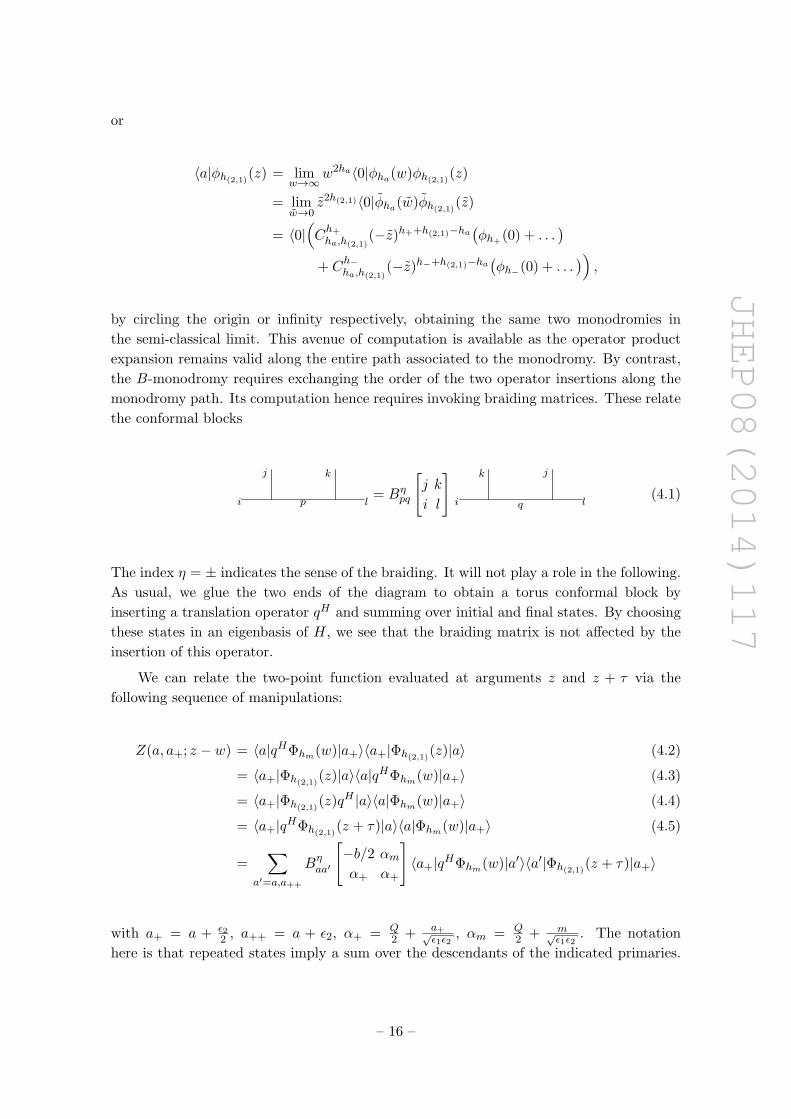
monodromy path. Its computation hence requires invoking braiding matrices. These relate

the conformal blocks

i

j

p

k

l= Bη

pq

[j k

i l

]i q

k j

l(4.1)

The index η = ± indicates the sense of the braiding. It will not play a role in the following.

As usual, we glue the two ends of the diagram to obtain a torus conformal block by

inserting a translation operator qH and summing over initial and final states. By choosing

these states in an eigenbasis of H, we see that the braiding matrix is not affected by the

insertion of this operator.

We can relate the two-point function evaluated at arguments z and z + τ via the

following sequence of manipulations:

Z(a, a+; z − w) = 〈a|qHΦhm(w)|a+〉〈a+|Φh(2,1)(z)|a〉 (4.2)

= 〈a+|Φh(2,1)(z)|a〉〈a|qHΦhm(w)|a+〉 (4.3)

= 〈a+|Φh(2,1)(z)qH |a〉〈a|Φhm(w)|a+〉 (4.4)

= 〈a+|qHΦh(2,1)(z + τ)|a〉〈a|Φhm(w)|a+〉 (4.5)

=∑

a′=a,a++

Bηaa′

[−b/2 αmα+ α+

]〈a+|qHΦhm(w)|a′〉〈a′|Φh(2,1)(z + τ)|a+〉

with a+ = a + ε22 , a++ = a + ε2, α+ = Q

2 + a+√ε1ε2

, αm = Q2 + m√

ε1ε2. The notation

here is that repeated states imply a sum over the descendants of the indicated primaries.

– 16 –

JHEP08(2014)117

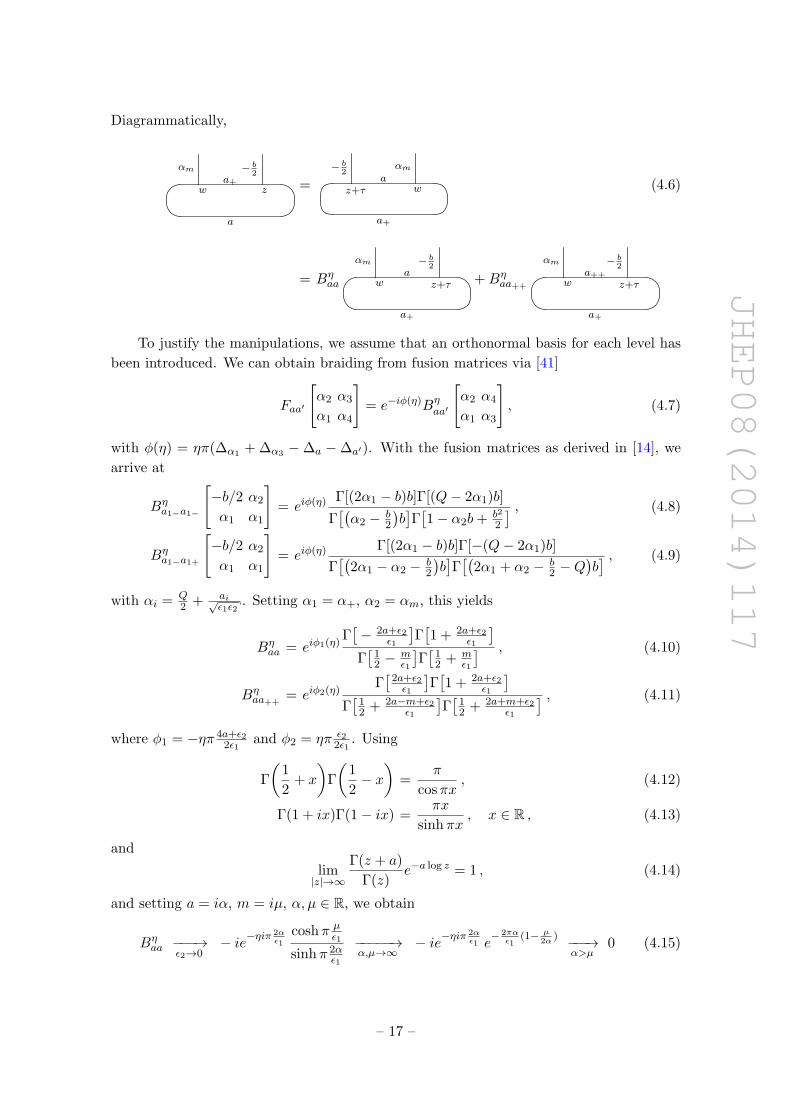
Diagrammatically,

w z

a

αma+− b

2

= z+τ w

a+

− b2

aαm

(4.6)

= Bηaa w z+τ

a+

αma− b

2

+Bηaa++ w z+τ

a+

αma++

− b2

To justify the manipulations, we assume that an orthonormal basis for each level has

been introduced. We can obtain braiding from fusion matrices via [41]

Faa′

[α2 α3

α1 α4

]= e−iφ(η)Bη

aa′

[α2 α4

α1 α3

], (4.7)

with φ(η) = ηπ(∆α1 + ∆α3 −∆a −∆a′). With the fusion matrices as derived in [14], we

arrive at

Bηa1−a1−

[−b/2 α2

α1 α1

]= eiφ(η)

Γ[(2α1 − b)b]Γ[(Q− 2α1)b]

Γ[(α2 − b

2

)b]Γ[1− α2b+ b2

2

] , (4.8)

Bηa1−a1+

[−b/2 α2

α1 α1

]= eiφ(η)

Γ[(2α1 − b)b]Γ[−(Q− 2α1)b]

Γ[(

2α1 − α2 − b2

)b]Γ[(

2α1 + α2 − b2 −Q

)b] , (4.9)

with αi = Q2 + ai√

ε1ε2. Setting α1 = α+, α2 = αm, this yields

Bηaa = eiφ1(η)

Γ[− 2a+ε2

ε1

]Γ[1 + 2a+ε2

ε1

]Γ[12 −

mε1

]Γ[12 + m

ε1

] , (4.10)

Bηaa++

= eiφ2(η)Γ[2a+ε2ε1

]Γ[1 + 2a+ε2

ε1

]Γ[12 + 2a−m+ε2

ε1

]Γ[12 + 2a+m+ε2

ε1

] , (4.11)

where φ1 = −ηπ 4a+ε22ε1

and φ2 = ηπ ε22ε1

. Using

Γ

(1

2+ x

)Γ

(1

2− x)

=π

cosπx, (4.12)

Γ(1 + ix)Γ(1− ix) =πx

sinhπx, x ∈ R , (4.13)

and

lim|z|→∞

Γ(z + a)

Γ(z)e−a log z = 1 , (4.14)

and setting a = iα, m = iµ, α, µ ∈ R, we obtain

Bηaa −−−→

ε2→0− ie−ηiπ

2αε1

coshπ µε1

sinhπ 2αε1

−−−−−→α,µ→∞

− ie−ηiπ2αε1 e− 2πα

ε1(1− µ

2α) −−−→

α>µ0 (4.15)

– 17 –

JHEP08(2014)117

and

Bηaa++

−−−→ε2→0

Γ[2aε1

]Γ[2aε1

]Γ[12 + 2a−m

ε1

]Γ[12 + 2a+m

ε1

]e( 12+mε1

) log 2aε1 e

( 12−mε1

) log 2aε1 −−−−→

|a|→∞1 . (4.16)

In the limit we are considering, we thus obtain the following relation between conformal

blocks:

Z(a, a+; z − τ) ∼ Z(a+, a++; z) . (4.17)

Defining Z(a; z) := Z(a, a+; z), dividing the above equation by Z(a; z) on both sides, and

making the semiclassical ansatz Z = exp 1ε1ε2F(a) + 1

ε1W(z; a), we arrive at

limε2→0

logZ(a; z − τ)

Z(a; z)=

1

ε1

(W(z − τ)−W(z)

)(4.18)

= limε2→0

logZ(a+; z)

Z(a; z)(4.19)

= limε2→0

1

ε1ε2

(F(a+

ε22

)−F(a)

)(4.20)

=1

2ε1∂aF(a) , (4.21)

thus reproducing the relation (3.38).

A related line of reasoning, invoking Verlinde operators, appears in [14].

4.2 The semi-classical S-move kernel

The S-move kernel relates the one-point conformal blocks with Teichmuller parameter τ and

−1/τ . It is naturally defined in conventions in which the three-point function contribution

in (2.1) is absorbed in the conformal blocks. Denoting the rescaled one-point blocks as

Fh(p)hm

, the one-point function is given by [42, 43]

〈Vhm〉τ =

∫ ∞0

dpµ(p)Fh(p)hm

(τ)Fh(p)hm

(τ) , (4.22)

where the weight h(p) is parametrized as h(p) =(Q2 + ip

)(Q2 − ip

)and µ(p) is the measure

factor

µ(p) = 4 sinh 2πpb sinh 2πb−1p . (4.23)

The integral kernel implementing the S-transformation for the block Fh(p)hm

(τ) via

Fh(p2)hm

(τ) =

∫ ∞0

dp1 µ(p1)Sp2p1(pm)Fh(p1)hm

(− 1

τ

)(4.24)

is given by [42]

Sp2p1(pm) =2

32

sb(pm)

∫Rdr∏ε=±

sb(p1 + 1

2(pm + iQ2 ) + εr)

sb(p1 − 1

2(pm + iQ2 ) + εr)e4πip2r, (4.25)

– 18 –

JHEP08(2014)117

where the function sb is defined by

log sb(x) =1

i

∫ ∞0

dt

t

(sin 2xt

2 sinh bt sinh b−1t− x

t

). (4.26)

The kernel is invariant under p1 → −p1 as well as p2 → −p2, the latter due to the functional

relation

sb(x)sb(−x) = 1 . (4.27)

We would like to compare the exact result (4.24) to the transformation properties of the

conformal block F that we derived in equation (3.58). The identification of parameters2

p1 = −i a1√ε1ε2

, (4.28)

p2 = −i a2√ε1ε2

, (4.29)

pm = −i m√ε1ε2

, (4.30)

shows that the ε2 → 0 limit corresponds to the limit in which all momenta are taken large.

In this limit, the shift relation

sb(x− ib) = 2 coshπbx sb(x) (4.31)

gives rise to a first order differential equation for the function log sb, which we can integrate

using one special value (e.g. sb(0) = 1), giving rise to the approximation

limb→0

log sb(x) ≈ i

b

∫ x

0dx′ log(2 coshπbx′) . (4.32)

We obtain an error estimate for this approximation in appendix A. The S-move kernel in

the semi-classical b→ 0 limit is thus approximated by

Sp2p1(pm) ≈ 232

sb(pm)

∫Rdr exp

[4πip2r +

i

b

∑δ,ε=±

δ

∫ p1+δ2(pm+iQ

2)+εr

0log(2 coshπby′)dy′

].

(4.33)

Introducing the variables α1 = −ia1, α2 = −ia2, µ = −im, we obtain upon the substitution

r → √ε1ε2 r

Spapb(pe) ≈

232

√ε1ε2 sb(pe)

∫Rdr exp

[1

ε2

(4πiα2r

ε1+i∑δ,ε=±

δ

∫ α1+δ2(µ+i

ε1+ε22

)+εr

0log

(2 cosh

πy

ε1

)dy

)].

We will evaluate this expression in a saddle point approximation in the limit ε2 → 0. The

saddle points of the exponent satisfy the equation [44] (see also [45])

1 = e4πα2ε1

∏δ,ε=±

[cosh

(π

ε1

(α1 +

δ

2

(µ+ i

ε1 + ε22

)+ εr

))]δε. (4.34)

2As the kernel is independent of τ , the relation (4.24) remains valid with τ replaced by −1/τ . There is

hence no natural distinction between a and aD in this context.

– 19 –

JHEP08(2014)117

By invoking

cosh

(a+ b

2+ i

π

4

)cosh

(b− a

2+ i

π

4

)=

1

2(cosh a+ i sinh b) , (4.35)

this equation can be put in the form [44]

e−4πα2ε1 =

cosh 2πα1ε1

+ i sinh π(2r+µ)ε1

cosh 2πα1ε1− i sinh π(2r−µ)

ε1

, (4.36)

yielding

cosh2πr

ε1= ±i sinh

π(2α1 ∓ µ)

ε1+O

(e−4π|Reα2|

ε1

)for Reα2 → ±∞ , (4.37)

and thus

± r = α1 ∓1

2

(µ− iε1

2

)+ ikε1 +O

(e−4π|Reα2|

ε1

), k ∈ Z , for Reα2 → ±∞ , (4.38)

where the ± on the left hand side in the last equation is not correlated with the sign of

Reα2. Let us consider the four saddle points closest to the integration path of r, which

runs along the real axis. Of these, two are zeros of the integrand of (4.25), hence do not

correspond to maxima of the real part of the exponential in (4.33). The other two lie on

poles of the integrand of (4.25). The integrand evaluated at these yields3

µ(p1)Sp2p1(pm) ≈(e

2πα1ε2 − e−

2πα1ε2

)sb(±2α1+iε12√

ε1ε2

)sb

(±2α1−µ√

ε1ε2

) cosh4πiα2

(α1 ∓ 1

2(µ− i ε12 ))

ε1ε2

for Reα2 → ±∞ . (4.39)

Using this approximation of the S-kernel, a saddle point approximation of the integral (4.24)

over p1 yields

∂a1Fr(a1,−

1

τ

)≈ ∓4πia2 for Reα2 → ±∞ , (4.40)

where Fr denotes the amplitude associated to the rescaled conformal block Fh(p)hm

introduced

above. To leading order, recalling F0(a1, τ) ≈ −2πia21τ , the relation (4.40) evaluates to

− a11

τ= ±a2 for Reα2 → ±∞ . (4.41)

3We are shifting the integration contour to run through the saddle points. As these coincide with

the poles of the integrand to O(e−4π|ReαD|

ε1

), we evaluate the principal value contribution to the integral

around these poles. Note that whether the integration path runs above or below the pole is irrelevant

for our computation, as the difference between the two is cancelled in relating the integral on the shifted

contour to the original integral.

– 20 –

JHEP08(2014)117

Given the integration region iR+ for a1, the saddle point which contributes hence depends

on the sign of Re τ . For sign(Re τ) = ±1, we obtain

Fr(τ, a2) ≈ ±4πiα1α2 + 2πi(α1 + α2)

(µ− iε1

2

)± πi

2

(µ2 +

ε214

)+ Fr

(− 1

τ, a1

)= ∓4πia1a2 − 2πi(a1 + a2)

(m+

ε12

)∓ πi

2

(m2 − ε21

4

)+ Fr

(− 1

τ, a1

),

(4.42)

where we have used

sb(y) ≈ e±πi2(y2+ 1

12b2) for Re(y)→ ±∞ , (4.43)

see appendix A. Matching to (3.58) requires the identification a2 = a, a1 = −aD at

sign(Re τ) = 1. The terms linear in ai in the exponential on the right hand side of (4.42)

cancel the rescaling of the conformal blocks. While the dependence on the sign of Re τ

is unusual, note that choosing the fundamental domain of τ such that this sign is fixed,

it is flipped by τ → − 1τ . It can hence serve to distinguish between electric and magnetic

variables, which is indeed the role it is playing in equations (4.40) and (4.42). Recall

that already in the derivation of (3.58), the argument −aD in F(− 1τ ,−aD) appeared in

the Legendre transform. As F , in contrast to Fr, is an even function in this argument,

this distinction was not relevant there. We have thus reproduced the Legendre transform

relating F at τ and − 1τ from the S-kernel.

5 Conclusions

We have seen how ε1-deformed Seiberg-Witten relations of N = 2∗ gauge theory arise

naturally within conformal field theory in the context of the 2d/4d correspondence. In

particular, we obtained an ε1-deformed Seiberg-Witten differential whose B-period eval-

uated on the classical Seiberg-Witten curve gives rise to the derivative of the deformed

prepotential. These tools allowed us to prove quasi-modularity of the coefficients of the

prepotential from first principles. In the process, we provided a proof of the Matone rela-

tion for N = 2∗ theory. We also demonstrated how the deformed relations can be extracted

from the semi-classics of exact conformal field theory quantities.

An important problem for future study is moving beyond leading order in the defor-

mation parameter ε2. Aside from recovering all amplitudes F (n,g) from within conformal

field theory, it would be important to understand what further modification of the Seiberg-

Witten data is necessary to incorporate these additional corrections. To lift the analysis

from gauge theory geometrically engineered within string theory to the topological string

proper, it would be interesting to formulate and study a q-deformed version of the null

vector decoupling equations. Finally, the exact results in conformal field theory which

complete relations among the F (n,g) non-perturbatively beg to be interpreted from a gauge

theory/topological string theory perspective.

– 21 –

JHEP08(2014)117

Acknowledgments

We would like to thank Francisco Morales and Jorg Teschner for useful conversations. Our

work is supported in part by ANR-grant ANR-13-BS05-0001.

A The function sb

The function sb has the integral representation

log sb(x) =1

i

∫ ∞0

dt

t

(sin 2xt

2 sinh bt sinh b−1t− x

t

). (A.1)

We can evaluate the x-derivative of this integral by the method of residues:

d

dxlog sb(x) =

1

i

∫ ∞0

dt

(cos 2xt

sinh bt sinh b−1t− 1

t2

)(A.2)

=1

iP

∫ ∞−∞

dt

(e2ixt

2 sinh bt sinh b−1t− 1

2t2

)(A.3)

=1

i

( ∫−∫ )

dt

(e2ixt

2 sinh bt sinh b−1t− 1

2t2

), (A.4)

where we have assumed Re(x) > 0 in the last line (else, we close the contour to the bottom).

The poles of the integrand lie at t = iπm/b and t = iπnb, m,n ∈ Z, with

Rest=iπm/b

(e2ixt

2 sinh bt sinh b−1t− 1

2t2

)= (−1)m

e−2πxm/b

2b sinh iπmb2

, (A.5)

Rest=iπnb

(e2ixt

2 sinh bt sinh b−1t− 1

2t2

)= (−1)n

b e−2πxnb

2 sinh iπnb2, (A.6)

for m,n 6= 0, and

Rest=0

(e2ixt

2 sinh bt sinh b−1t− 1

2t2

)= ix . (A.7)

Thus,

d

dxlog sb(x) =

π

i

(− x+

1

b

∞∑m=1

(−1)me−2πxm/b

sin πmb2

+ b∞∑n=1

(−1)ne−2πxnb

sinπnb2

). (A.8)

To take the semi-classical limit, we drop the first sum, and approximate the sine-function

in the second,

d

dxlog sb(x) = πix− iπb

∞∑n=1

(−1)ne−2πxnb

πnb2+O(b) (A.9)

=i

blog(2 coshπbx) +O(b) . (A.10)

Integrating and imposing the boundary condition sb(0) = 1 then yields

log sb(x) =i

b

∫ x

0dx′ log(2 coshπbx′) +O(b) . (A.11)

– 22 –

JHEP08(2014)117

21

e2i

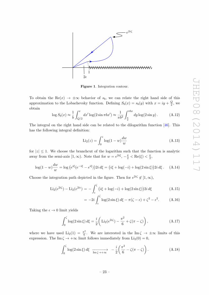
Figure 1. Integration contour.

To obtain the Re(x) → ±∞ behavior of sb, we can relate the right hand side of this

approximation to the Lobachevsky function. Defining Sb(x) = sb(y) with x = iy + Q2 , we

obtain

logSb(x) ≈ 1

b

∫ x

Q/2dx′ log(2 sinπbx′) ≈ 1

πb2

∫ πbx

π2

dy log(2 sin y) . (A.12)

The integral on the right hand side can be related to the dilogarithm function [46]. This

has the following integral definition:

Li2(z) =

∫ z

0log(1− w)

dw

w(A.13)

for |z| ≤ 1. We choose the branchcut of the logarithm such that the function is analytic

away from the semi-axis [1,∞). Note that for w = e2iξ, −π2 < Re(ξ) < π

2 ,

log(1− w)dw

w= log

(eiξ(e−iξ − eiξ)

)2i dξ =

(iξ + log(−i) + log(2 sin ξ)

)2i dξ . (A.14)

Choose the integration path depicted in the figure. Then for e2iζ 6∈ [1,∞),

Li2(e2iζ)− Li2(e

2iε) = −∫ ζ

ε

(iξ + log(−i) + log(2 sin ξ)

)2i dξ (A.15)

= −2i

∫ ζ

εlog(2 sin ξ) dξ − π(ζ − ε) + ζ2 − ε2. (A.16)

Taking the ε→ 0 limit yields∫ ζ

0log(2 sin ξ) dξ =

i

2

(Li2(e

2iζ)− π2

6+ ζ(π − ζ)

), (A.17)

where we have used Li2(1) = π2

6 . We are interested in the Im ζ → ±∞ limits of this

expression. The Im ζ → +∞ limit follows immediately from Li2(0) = 0,∫ ζ

0log(2 sin ξ) dξ −−−−−−→

Im ζ→+∞− i

2

(π2

6− ζ(π − ζ)

). (A.18)

– 23 –

JHEP08(2014)117

For the limit Im ζ → −∞, note that

Li2(z) + Li2(1/z) = −π2

6− 1

2log2(−z) , (A.19)

hence

limIm ζ→−∞

Li2(e2iζ) = −π

2

6− 1

2log2 e−iπ+2iζ =

2π2

6− 2ζ(π − ζ) . (A.20)

To arrive at this result, remember that the branchcut of log z is chosen along the negative

real axis, and that −π2 < Re(ξ) < π

2 . Thus,∫ ζ

0log(2 sin ξ) dξ −−−−−−→

Im ζ→−∞

i

2

(π2

6− ζ(π − ζ)

). (A.21)

Substituting this result into (A.12) and using∫ π2

0dy log(2 sin y) = 0 (A.22)

yields

logSb(x)b→0−−−−−−→

Imx→±∞∓ πi

2

(x

(x− 1

b

)+

1

6b2

), (A.23)

and thus

log sb(x)b→0−−−−−−→

Rex→±∞± πi

2

(x2 +

1

12b2

). (A.24)

Open Access. This article is distributed under the terms of the Creative Commons

Attribution License (CC-BY 4.0), which permits any use, distribution and reproduction in

any medium, provided the original author(s) and source are credited.

References

[1] L.F. Alday, D. Gaiotto and Y. Tachikawa, Liouville correlation functions from

four-dimensional gauge theories, Lett. Math. Phys. 91 (2010) 167 [arXiv:0906.3219]

[INSPIRE].

[2] M. Bershadsky, S. Cecotti, H. Ooguri and C. Vafa, Kodaira-Spencer theory of gravity and

exact results for quantum string amplitudes, Commun. Math. Phys. 165 (1994) 311

[hep-th/9309140] [INSPIRE].

[3] D. Krefl and J. Walcher, Extended holomorphic anomaly in gauge theory,

Lett. Math. Phys. 95 (2011) 67 [arXiv:1007.0263] [INSPIRE].

[4] M.-x. Huang and A. Klemm, Direct integration for general Ω backgrounds,

Adv. Theor. Math. Phys. 16 (2012) 805 [arXiv:1009.1126] [INSPIRE].

[5] M.-x. Huang, A.-K. Kashani-Poor and A. Klemm, The Ω deformed B-model for rigid N = 2

theories, Ann. Henri Poincare 14 (2013) 425 [arXiv:1109.5728] [INSPIRE].

[6] N.A. Nekrasov, Seiberg-Witten prepotential from instanton counting,

Adv. Theor. Math. Phys. 7 (2004) 831 [hep-th/0206161] [INSPIRE].

– 24 –

JHEP08(2014)117

[7] A.-K. Kashani-Poor and J. Troost, The toroidal block and the genus expansion,

JHEP 03 (2013) 133 [arXiv:1212.0722] [INSPIRE].

[8] A.-K. Kashani-Poor and J. Troost, Transformations of spherical blocks, JHEP 10 (2013) 009

[arXiv:1305.7408] [INSPIRE].

[9] N. Seiberg and E. Witten, Electric-magnetic duality, monopole condensation and

confinement in N = 2 supersymmetric Yang-Mills theory, Nucl. Phys. B 426 (1994) 19

[Erratum ibid. B 430 (1994) 485] [hep-th/9407087] [INSPIRE].

[10] N. Seiberg and E. Witten, Monopoles, duality and chiral symmetry breaking in N = 2

supersymmetric QCD, Nucl. Phys. B 431 (1994) 484 [hep-th/9408099] [INSPIRE].

[11] N.A. Nekrasov and S.L. Shatashvili, Quantization of integrable systems and four dimensional

gauge theories, arXiv:0908.4052 [INSPIRE].

[12] M. Matone, Instantons and recursion relations in N = 2 SUSY gauge theory,

Phys. Lett. B 357 (1995) 342 [hep-th/9506102] [INSPIRE].

[13] R. Flume, F. Fucito, J.F. Morales and R. Poghossian, Matone’s relation in the presence of

gravitational couplings, JHEP 04 (2004) 008 [hep-th/0403057] [INSPIRE].

[14] L.F. Alday, D. Gaiotto, S. Gukov, Y. Tachikawa and H. Verlinde, Loop and surface operators

in N = 2 gauge theory and Liouville modular geometry, JHEP 01 (2010) 113

[arXiv:0909.0945] [INSPIRE].

[15] A. Iqbal, C. Kozcaz and C. Vafa, The refined topological vertex, JHEP 10 (2009) 069

[hep-th/0701156] [INSPIRE].

[16] V.A. Fateev and A.V. Litvinov, Multipoint correlation functions in Liouville field theory and

minimal Liouville gravity, Theor. Math. Phys. 154 (2008) 454 [arXiv:0707.1664] [INSPIRE].

[17] K. Maruyoshi and M. Taki, Deformed prepotential, quantum integrable system and Liouville

field theory, Nucl. Phys. B 841 (2010) 388 [arXiv:1006.4505] [INSPIRE].

[18] A. Marshakov, A. Mironov and A. Morozov, On AGT relations with surface operator

insertion and stationary limit of beta-ensembles, J. Geom. Phys. 61 (2011) 1203

[arXiv:1011.4491] [INSPIRE].

[19] S.D. Mathur, S. Mukhi and A. Sen, Correlators of primary fields in the SU(2) WZW theory

on Riemann surfaces, Nucl. Phys. B 305 (1988) 219 [INSPIRE].

[20] D. Harlow, J. Maltz and E. Witten, Analytic continuation of Liouville theory,

JHEP 12 (2011) 071 [arXiv:1108.4417] [INSPIRE].

[21] M. Billo, M. Frau, L. Gallot and A. Lerda, The exact 8d chiral ring from 4d recursion

relations, JHEP 11 (2011) 077 [arXiv:1107.3691] [INSPIRE].

[22] M. Billo, M. Frau, L. Gallot, A. Lerda and I. Pesando, Deformed N = 2 theories, generalized

recursion relations and S-duality, JHEP 04 (2013) 039 [arXiv:1302.0686] [INSPIRE].

[23] R. Donagi and E. Witten, Supersymmetric Yang-Mills theory and integrable systems,

Nucl. Phys. B 460 (1996) 299 [hep-th/9510101] [INSPIRE].

[24] E. Witten, Solutions of four-dimensional field theories via M-theory,

Nucl. Phys. B 500 (1997) 3 [hep-th/9703166] [INSPIRE].

[25] D. Gaiotto, N = 2 dualities, JHEP 08 (2012) 034 [arXiv:0904.2715] [INSPIRE].

– 25 –

JHEP08(2014)117

[26] A. Zabrodin and A. Zotov, Quantum Painleve-Calogero correspondence,

J. Math. Phys. 53 (2012) 073507 [arXiv:1107.5672] [INSPIRE].

[27] M. Grosset and A. Veselov, Elliptic Faulhaber polynomials and Lame densities of states,

math-ph/0508066.

[28] M. Aganagic, R. Dijkgraaf, A. Klemm, M. Marino and C. Vafa, Topological strings and

integrable hierarchies, Commun. Math. Phys. 261 (2006) 451 [hep-th/0312085] [INSPIRE].

[29] M. Aganagic, M.C.N. Cheng, R. Dijkgraaf, D. Krefl and C. Vafa, Quantum geometry of

refined topological strings, JHEP 11 (2012) 019 [arXiv:1105.0630] [INSPIRE].

[30] M.-x. Huang, On gauge theory and topological string in Nekrasov-Shatashvili limit,

JHEP 06 (2012) 152 [arXiv:1205.3652] [INSPIRE].

[31] M.-x. Huang, A. Klemm, J. Reuter and M. Schiereck, Quantum geometry of del Pezzo

surfaces in the Nekrasov-Shatashvili limit, arXiv:1401.4723 [INSPIRE].

[32] R. Poghossian, Deforming SW curve, JHEP 04 (2011) 033 [arXiv:1006.4822] [INSPIRE].

[33] F. Fucito, J.F. Morales, D.R. Pacifici and R. Poghossian, Gauge theories on Ω-backgrounds

from non commutative Seiberg-Witten curves, JHEP 05 (2011) 098 [arXiv:1103.4495]

[INSPIRE].

[34] A. Mironov and A. Morozov, Nekrasov functions and exact Bohr-Zommerfeld integrals,

JHEP 04 (2010) 040 [arXiv:0910.5670] [INSPIRE].

[35] G. Bonelli, K. Maruyoshi and A. Tanzini, Quantum Hitchin systems via β-deformed matrix

models, arXiv:1104.4016 [INSPIRE].

[36] J.-E. Bourgine, Large-N limit of β-ensembles and deformed Seiberg-Witten relations,

JHEP 08 (2012) 046 [arXiv:1206.1696] [INSPIRE].

[37] J.-E. Bourgine, Large-N techniques for Nekrasov partition functions and AGT conjecture,

JHEP 05 (2013) 047 [arXiv:1212.4972] [INSPIRE].

[38] T. Eguchi and H. Ooguri, Conformal and current algebras on general Riemann surface,

Nucl. Phys. B 282 (1987) 308 [INSPIRE].

[39] D. Galakhov, A. Mironov and A. Morozov, S-duality as a β-deformed Fourier transform,

JHEP 08 (2012) 067 [arXiv:1205.4998] [INSPIRE].

[40] N. Nemkov, S-duality as Fourier transform for arbitrary ε1, ε2, arXiv:1307.0773 [INSPIRE].

[41] G.W. Moore and N. Seiberg, Classical and quantum conformal field theory,

Commun. Math. Phys. 123 (1989) 177 [INSPIRE].

[42] J. Teschner, From Liouville theory to the quantum geometry of Riemann surfaces,

hep-th/0308031 [INSPIRE].

[43] G. Vartanov and J. Teschner, Supersymmetric gauge theories, quantization of moduli spaces

of flat connections and conformal field theory, arXiv:1302.3778 [INSPIRE].

[44] L. Hadasz and Z. Jaskolski, Semiclassical limit of the FZZT Liouville theory,

Nucl. Phys. B 757 (2006) 233 [hep-th/0603164] [INSPIRE].

[45] T. Dimofte and S. Gukov, Chern-Simons theory and S-duality, JHEP 05 (2013) 109

[arXiv:1106.4550] [INSPIRE].

[46] J.G. Ratcliffe, Foundations of hyperbolic manifolds, vol. 149 of Graduate Texts in

Mathematics, second edition, Springer, New York U.S.A. (2006).

– 26 –