Preprint typeset in JHEP style - HYPER VERSION Michaelmas Term, 2006 and 2007

Quantum Field TheoryUniversity of Cambridge Part III Mathematical Tripos

Dr David Tong

Department of Applied Mathematics and Theoretical Physics,

Centre for Mathematical Sciences,

Wilberforce Road,

Cambridge, CB3 OWA, UK

http://www.damtp.cam.ac.uk/user/tong/qft.html

d.tong@damtp.cam.ac.uk

– 1 –

Recommended Books and Resources

• M. Peskin and D. Schroeder, An Introduction to Quantum Field Theory

This is a very clear and comprehensive book, covering everything in this course at the

right level. It will also cover everything in the “Advanced Quantum Field Theory”course, much of the “Standard Model” course, and will serve you well if you go on to

do research. To a large extent, our course will follow the first section of this book.

There is a vast array of further Quantum Field Theory texts, many of them withredeeming features. Here I mention a few very different ones.

• S. Weinberg, The Quantum Theory of Fields, Vol 1

This is the first in a three volume series by one of the masters of quantum field theory.It takes a unique route to through the subject, focussing initially on particles rather

than fields. The second volume covers material lectured in “AQFT”.

• L. Ryder, Quantum Field Theory

This elementary text has a nice discussion of much of the material in this course.

• A. Zee, Quantum Field Theory in a Nutshell

This is charming book, where emphasis is placed on physical understanding and theauthor isn’t afraid to hide the ugly truth when necessary. It contains many gems.

• M Srednicki, Quantum Field Theory

A very clear and well written introduction to the subject. Both this book and Zee’sfocus on the path integral approach, rather than canonical quantization that we develop

in this course.

There are also resources available on the web. Some particularly good ones are listedon the course webpage: http://www.damtp.cam.ac.uk/user/tong/qft.html

Contents

0. Introduction 1

0.1 Units and Scales 4

1. Classical Field Theory 7

1.1 The Dynamics of Fields 7

1.1.1 An Example: The Klein-Gordon Equation 81.1.2 Another Example: First Order Lagrangians 9

1.1.3 A Final Example: Maxwell’s Equations 101.1.4 Locality, Locality, Locality 10

1.2 Lorentz Invariance 111.3 Symmetries 13

1.3.1 Noether’s Theorem 13

1.3.2 An Example: Translations and the Energy-Momentum Tensor 141.3.3 Another Example: Lorentz Transformations and Angular Mo-

mentum 161.3.4 Internal Symmetries 18

1.4 The Hamiltonian Formalism 19

2. Free Fields 21

2.1 Canonical Quantization 212.1.1 The Simple Harmonic Oscillator 22

2.2 The Free Scalar Field 232.3 The Vacuum 25

2.3.1 The Cosmological Constant 262.3.2 The Casimir Effect 27

2.4 Particles 29

2.4.1 Relativistic Normalization 312.5 Complex Scalar Fields 33

2.6 The Heisenberg Picture 352.6.1 Causality 36

2.7 Propagators 382.7.1 The Feynman Propagator 382.7.2 Green’s Functions 40

2.8 Non-Relativistic Fields 412.8.1 Recovering Quantum Mechanics 43

– 1 –

3. Interacting Fields 47

3.1 The Interaction Picture 50

3.1.1 Dyson’s Formula 51

3.2 A First Look at Scattering 53

3.2.1 An Example: Meson Decay 55

3.3 Wick’s Theorem 56

3.3.1 An Example: Recovering the Propagator 56

3.3.2 Wick’s Theorem 58

3.3.3 An Example: Nucleon Scattering 58

3.4 Feynman Diagrams 60

3.4.1 Feynman Rules 61

3.5 Examples of Scattering Amplitudes 62

3.5.1 Mandelstam Variables 66

3.5.2 The Yukawa Potential 67

3.5.3 φ4 Theory 69

3.5.4 Connected Diagrams and Amputated Diagrams 70

3.6 What We Measure: Cross Sections and Decay Rates 71

3.6.1 Fermi’s Golden Rule 71

3.6.2 Decay Rates 73

3.6.3 Cross Sections 74

3.7 Green’s Functions 75

3.7.1 Connected Diagrams and Vacuum Bubbles 77

3.7.2 From Green’s Functions to S-Matrices 79

4. The Dirac Equation 81

4.1 The Spinor Representation 83

4.1.1 Spinors 85

4.2 Constructing an Action 87

4.3 The Dirac Equation 90

4.4 Chiral Spinors 91

4.4.1 The Weyl Equation 91

4.4.2 γ5 93

4.4.3 Parity 94

4.4.4 Chiral Interactions 95

4.5 Majorana Fermions 96

4.6 Symmetries and Conserved Currents 98

4.7 Plane Wave Solutions 100

4.7.1 Some Examples 102

– 2 –

4.7.2 Some Useful Formulae: Inner and Outer Products 103

5. Quantizing the Dirac Field 106

5.1 A Glimpse at the Spin-Statistics Theorem 1065.1.1 The Hamiltonian 107

5.2 Fermionic Quantization 1095.2.1 Fermi-Dirac Statistics 110

5.3 Dirac’s Hole Interpretation 1105.4 Propagators 112

5.5 The Feynman Propagator 1145.6 Yukawa Theory 115

5.6.1 An Example: Putting Spin on Nucleon Scattering 115

5.7 Feynman Rules for Fermions 1175.7.1 Examples 118

5.7.2 The Yukawa Potential Revisited 1215.7.3 Pseudo-Scalar Coupling 122

6. Quantum Electrodynamics 124

6.1 Maxwell’s Equations 124

6.1.1 Gauge Symmetry 1256.2 The Quantization of the Electromagnetic Field 128

6.2.1 Coulomb Gauge 1286.2.2 Lorentz Gauge 131

6.3 Coupling to Matter 1366.3.1 Coupling to Fermions 1366.3.2 Coupling to Scalars 138

6.4 QED 1396.4.1 Naive Feynman Rules 141

6.5 Feynman Rules 1436.5.1 Charged Scalars 144

6.6 Scattering in QED 1446.6.1 The Coulomb Potential 147

6.7 Afterword 149

– 3 –

Acknowledgements

These lecture notes are far from original. My primary contribution has been to borrow,steal and assimilate the best discussions and explanations I could find from the vast

literature on the subject. I inherited the course from Nick Manton, whose notes form thebackbone of the lectures. I have also relied heavily on the sources listed at the beginning,most notably the book by Peskin and Schroeder. In several places, for example the

discussion of scalar Yukawa theory, I followed the lectures of Sidney Coleman, usingthe notes written by Brian Hill and a beautiful abridged version of these notes due to

Michael Luke.

My thanks to the many who helped in various ways during the preparation of this

course, including Joe Conlon, Nick Dorey, Marie Ericsson, Eyo Ita, Ian Drummond,Jerome Gauntlett, Matt Headrick, Ron Horgan, Nick Manton, Hugh Osborn and JenniSmillie. My thanks also to the students for their sharp questions and sharp eyes in

spotting typos. I am supported by the Royal Society.

– 4 –

0. Introduction

“There are no real one-particle systems in nature, not even few-particle

systems. The existence of virtual pairs and of pair fluctuations shows thatthe days of fixed particle numbers are over.”

Viki Weisskopf

The concept of wave-particle duality tells us that the properties of electrons andphotons are fundamentally very similar. Despite obvious differences in their mass andcharge, under the right circumstances both suffer wave-like diffraction and both can

pack a particle-like punch.

Yet the appearance of these objects in classical physics is very different. Electrons

and other matter particles are postulated to be elementary constituents of Nature. Incontrast, light is a derived concept: it arises as a ripple of the electromagnetic field. If

photons and particles are truely to be placed on equal footing, how should we reconcilethis difference in the quantum world? Should we view the particle as fundamental,with the electromagnetic field arising only in some classical limit from a collection of

quantum photons? Or should we instead view the field as fundamental, with the photonappearing only when we correctly treat the field in a manner consistent with quantum

theory? And, if this latter view is correct, should we also introduce an “electron field”,whose ripples give rise to particles with mass and charge? But why then didn’t Faraday,Maxwell and other classical physicists find it useful to introduce the concept of matter

fields, analogous to the electromagnetic field?

The purpose of this course is to answer these questions. We shall see that the second

viewpoint above is the most useful: the field is primary and particles are derivedconcepts, appearing only after quantization. We will show how photons arise from thequantization of the electromagnetic field and how massive, charged particles such as

electrons arise from the quantization of matter fields. We will learn that in order todescribe the fundamental laws of Nature, we must not only introduce electron fields,

but also quark fields, neutrino fields, gluon fields, W and Z-boson fields, Higgs fieldsand a whole slew of others. There is a field associated to each type of fundamental

particle that appears in Nature.

Why Quantum Field Theory?

In classical physics, the primary reason for introducing the concept of the field is to

construct laws of Nature that are local. The old laws of Coulomb and Newton involve“action at a distance”. This means that the force felt by an electron (or planet) changes

– 1 –

immediately if a distant proton (or star) moves. This situation is philosophically un-satisfactory. More importantly, it is also experimentally wrong. The field theories of

Maxwell and Einstein remedy the situation, with all interactions mediated in a localfashion by the field.

The requirement of locality remains a strong motivation for studying field theoriesin the quantum world. However, there are further reasons for treating the quantum

field as fundamental1. Here I’ll give two answers to the question: Why quantum fieldtheory?

Answer 1: Because the combination of quantum mechanics and special relativityimplies that particle number is not conserved.

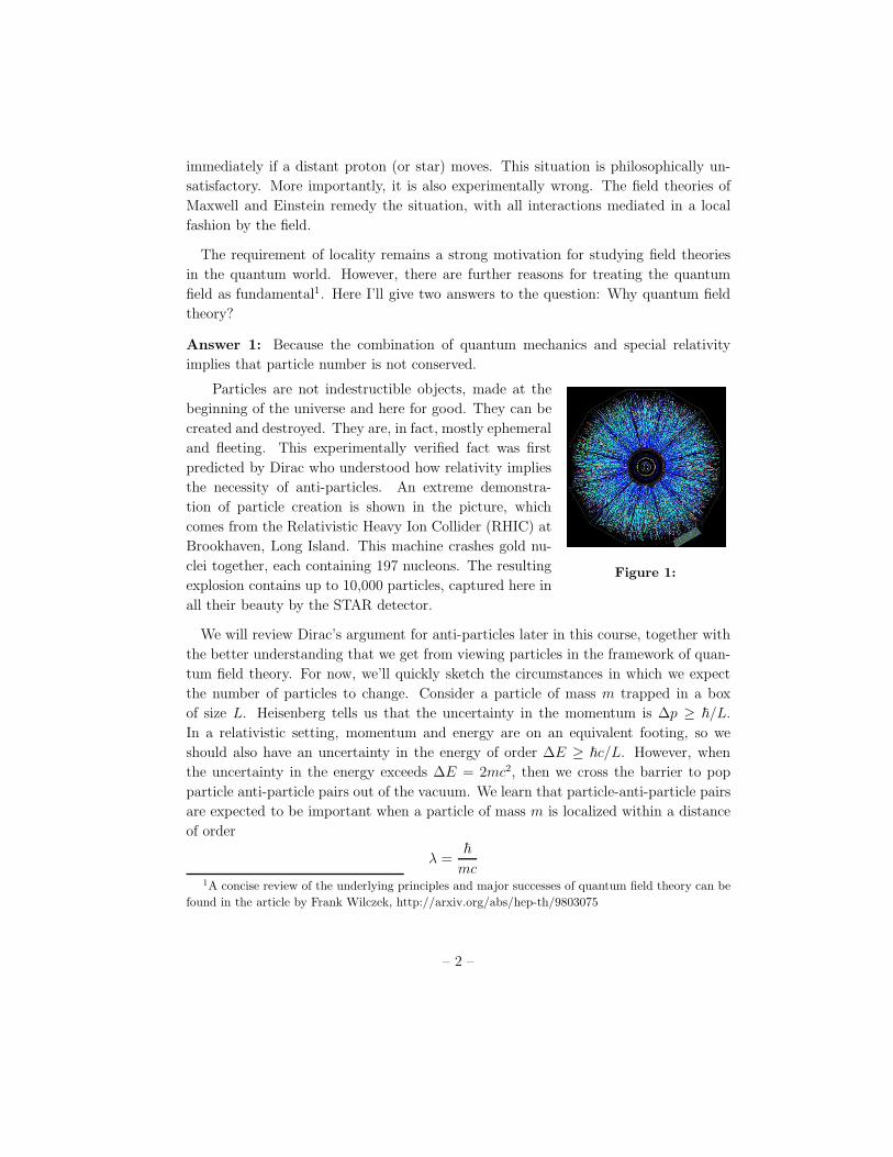
Particles are not indestructible objects, made at the

Figure 1:

beginning of the universe and here for good. They can be

created and destroyed. They are, in fact, mostly ephemeraland fleeting. This experimentally verified fact was first

predicted by Dirac who understood how relativity impliesthe necessity of anti-particles. An extreme demonstra-tion of particle creation is shown in the picture, which

comes from the Relativistic Heavy Ion Collider (RHIC) atBrookhaven, Long Island. This machine crashes gold nu-

clei together, each containing 197 nucleons. The resultingexplosion contains up to 10,000 particles, captured here in

all their beauty by the STAR detector.

We will review Dirac’s argument for anti-particles later in this course, together with

the better understanding that we get from viewing particles in the framework of quan-tum field theory. For now, we’ll quickly sketch the circumstances in which we expect

the number of particles to change. Consider a particle of mass m trapped in a boxof size L. Heisenberg tells us that the uncertainty in the momentum is ∆p ≥ !/L.

In a relativistic setting, momentum and energy are on an equivalent footing, so weshould also have an uncertainty in the energy of order ∆E ≥ !c/L. However, whenthe uncertainty in the energy exceeds ∆E = 2mc2, then we cross the barrier to pop

particle anti-particle pairs out of the vacuum. We learn that particle-anti-particle pairsare expected to be important when a particle of mass m is localized within a distance

of order

λ =!

mc1A concise review of the underlying principles and major successes of quantum field theory can be

found in the article by Frank Wilczek, http://arxiv.org/abs/hep-th/9803075

– 2 –

At distances shorter than this, there is a high probability that we will detect particle-anti-particle pairs swarming around the original particle that we put in. The distance λ

is called the Compton wavelength. It is always smaller than the de Broglie wavelengthλdB = h/|p|. If you like, the de Broglie wavelength is the distance at which the wavelikenature of particles becomes apparent; the Compton wavelength is the distance at which

the concept of a single pointlike particle breaks down completely.

The presence of a multitude of particles and antiparticles at short distances tells us

that any attempt to write down a relativistic version of the one-particle Schrodingerequation (or, indeed, an equation for any fixed number of particles) is doomed to failure.

There is no mechanism in standard non-relativistic quantum mechanics to deal withchanges in the particle number. Indeed, any attempt to naively construct a relativisticversion of the one-particle Schrodinger equation meets with serious problems. (Negative

probabilities, infinite towers of negative energy states, or a breakdown in causality arethe common issues that arise). In each case, this failure is telling us that once we

enter the relativistic regime we need a new formalism in order to treat states with anunspecified number of particles. This formalism is quantum field theory (QFT).

Answer 2: Because all particles of the same type are the same

This sound rather dumb. But it’s not! What I mean by this is that two electrons

are identical in every way, regardless of where they came from and what they’ve beenthrough. The same is true of every other fundamental particle. Let me illustrate this

through a rather prosaic story. Suppose we capture a proton from a cosmic ray whichwe identify as coming from a supernova lying 8 billion lightyears away. We compare

this proton with one freshly minted in a particle accelerator here on Earth. And thetwo are exactly the same! How is this possible? Why aren’t there errors in protonproduction? How can two objects, manufactured so far apart in space and time, be

identical in all respects? One explanation that might be offered is that there’s a seaof proton “stuff” filling the universe and when we make a proton we somehow dip our

hand into this stuff and from it mould a proton. Then it’s not surprising that protonsproduced in different parts of the universe are identical: they’re made of the same stuff.

It turns out that this is roughly what happens. The “stuff” is the proton field or, ifyou look closely enough, the quark field.

In fact, there’s more to this tale. Being the “same” in the quantum world is notlike being the “same” in the classical world: quantum particles that are the same aretruely indistinguishable. Swapping two particles around leaves the state completely

unchanged — apart from a possible minus sign. This minus sign determines the statis-tics of the particle. In quantum mechanics you have to put these statistics in by hand

– 3 –

and, to agree with experiment, should choose Bose statistics (no minus sign) for integerspin particles, and Fermi statistics (yes minus sign) for half-integer spin particles. In

quantum field theory, this relationship between spin and statistics is not somethingthat you have to put in by hand. Rather, it is a consequence of the framework.

What is Quantum Field Theory?

Having told you why QFT is necessary, I should really tell you what it is. The clue is inthe name: it is the quantization of a classical field, the most familiar example of whichis the electromagnetic field. In standard quantum mechanics, we’re taught to take the

classical degrees of freedom and promote them to operators acting on a Hilbert space.The rules for quantizing a field are no different. Thus the basic degrees of freedom in

quantum field theory are operator valued functions of space and time. This means thatwe are dealing with an infinite number of degrees of freedom — at least one for every

point in space. This infinity will come back to bite on several occasions.

It will turn out that the possible interactions in quantum field theory are governedby a few basic principles: locality, symmetry and renormalization group flow (the

decoupling of short distance phenomena from physics at larger scales). These ideasmake QFT a very robust framework: given a set of fields there is very often an almost

unique way to couple them together.

What is Quantum Field Theory Good For?

The answer is: almost everything. As I have stressed above, for any relativistic system

it is a necessity. But it is also a very useful tool in non-relativistic systems with manyparticles. Quantum field theory has had a major impact in condensed matter, high-

energy physics, cosmology, quantum gravity and pure mathematics. It is literally thelanguage in which the laws of Nature are written.

0.1 Units and Scales

Nature presents us with three fundamental dimensionful constants; the speed of light c,

Planck’s constant (divided by 2π) ! and Newton’s constant G. They have dimensions

[c] = LT−1

[!] = L2MT−1

[G] = L3M−1T−2

Throughout this course we will work with “natural” units, defined by

c = ! = 1 (0.1)

– 4 –

which allows us to express all dimensionful quantities in terms of a single scale whichwe choose to be mass or, equivalently, energy (since E = mc2 has become E = m).

The usual choice of energy unit is eV , the electron volt or, more often GeV = 109eV orTeV = 1012eV . To convert the unit of energy back to a unit of length or time, we needto insert the relevant powers of c and !. For example, the length scale λ associated to

a mass m is the Compton wavelength

λ =!

mc

With this conversion factor, the electron mass me = 106eV translates to a length scale

λe = 2× 10−12m.

Throughout this course we will refer to the dimension of a quantity, meaning the

mass dimension. If X has dimensions of (mass)d we will write [X ] = d. In particular,the surviving natural quantity G has dimensions [G] = −2 and defines a mass scale,

G =!c

M2p

=1

M2p

(0.2)

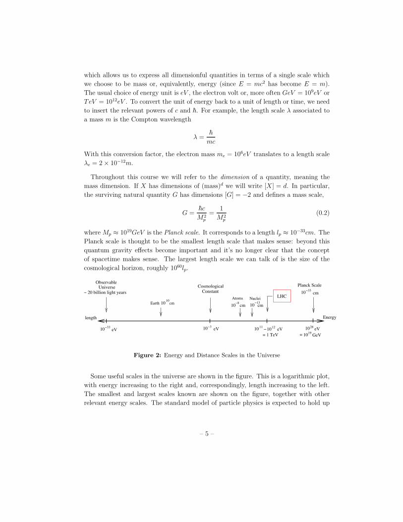
where Mp ≈ 1019GeV is the Planck scale. It corresponds to a length lp ≈ 10−33cm. ThePlanck scale is thought to be the smallest length scale that makes sense: beyond this

quantum gravity effects become important and it’s no longer clear that the conceptof spacetime makes sense. The largest length scale we can talk of is the size of the

cosmological horizon, roughly 1060lp.

−3310

28101910= GeV

121010 11−310−3310= 1 TeV

cmPlanck Scale

Energy

eV− eVeV

ConstantCosmological

eV

Observable Universe

~ 20 billion light years

length

Earth 10 10cm

Atoms−810

Nuclei10

LHC

cm cm−13

Figure 2: Energy and Distance Scales in the Universe

Some useful scales in the universe are shown in the figure. This is a logarithmic plot,with energy increasing to the right and, correspondingly, length increasing to the left.

The smallest and largest scales known are shown on the figure, together with otherrelevant energy scales. The standard model of particle physics is expected to hold up

– 5 –

to about the TeV . This is precisely the regime that is currently being probed by theLarge Hadron Collider (LHC) at CERN. There is a general belief that the framework

of quantum field theory will continue to hold to energy scales only slightly below thePlanck scale — for example, there are experimental hints that the coupling constantsof electromagnetism, and the weak and strong forces unify at around 1018 GeV.

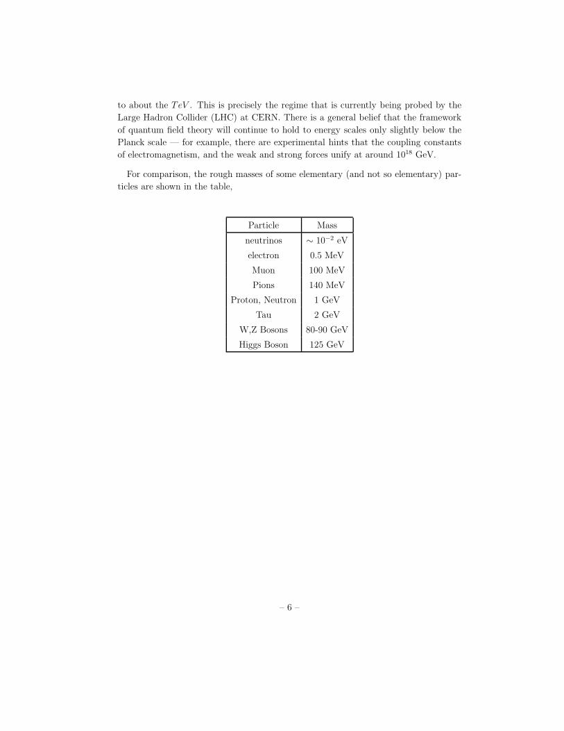
For comparison, the rough masses of some elementary (and not so elementary) par-ticles are shown in the table,

Particle Mass

neutrinos ∼ 10−2 eV

electron 0.5 MeV

Muon 100 MeV

Pions 140 MeV

Proton, Neutron 1 GeV

Tau 2 GeV

W,Z Bosons 80-90 GeV

Higgs Boson 125 GeV

– 6 –

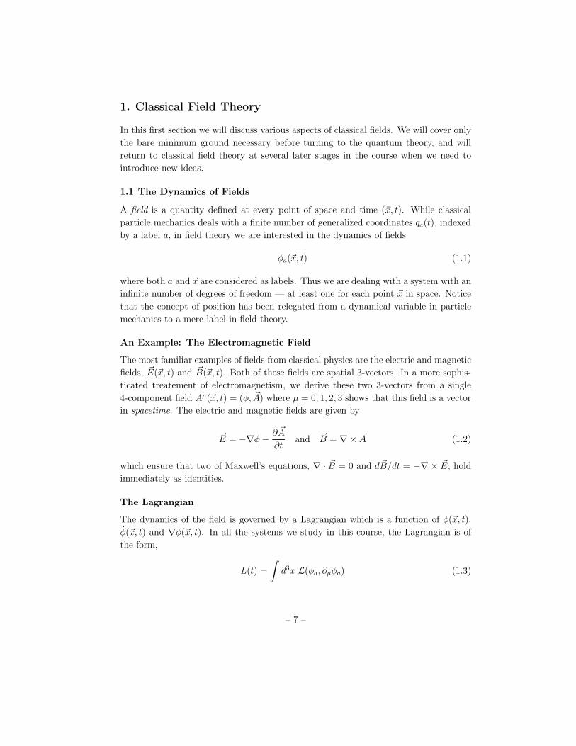
1. Classical Field Theory

In this first section we will discuss various aspects of classical fields. We will cover onlythe bare minimum ground necessary before turning to the quantum theory, and will

return to classical field theory at several later stages in the course when we need tointroduce new ideas.

1.1 The Dynamics of Fields

A field is a quantity defined at every point of space and time (x, t). While classical

particle mechanics deals with a finite number of generalized coordinates qa(t), indexedby a label a, in field theory we are interested in the dynamics of fields

φa(x, t) (1.1)

where both a and x are considered as labels. Thus we are dealing with a system with aninfinite number of degrees of freedom — at least one for each point x in space. Notice

that the concept of position has been relegated from a dynamical variable in particlemechanics to a mere label in field theory.

An Example: The Electromagnetic Field

The most familiar examples of fields from classical physics are the electric and magneticfields, E(x, t) and B(x, t). Both of these fields are spatial 3-vectors. In a more sophis-ticated treatement of electromagnetism, we derive these two 3-vectors from a single

4-component field Aµ(x, t) = (φ, A) where µ = 0, 1, 2, 3 shows that this field is a vectorin spacetime. The electric and magnetic fields are given by

E = −∇φ −∂A

∂tand B = ∇× A (1.2)

which ensure that two of Maxwell’s equations, ∇ · B = 0 and dB/dt = −∇ × E, hold

immediately as identities.

The Lagrangian

The dynamics of the field is governed by a Lagrangian which is a function of φ(x, t),

φ(x, t) and ∇φ(x, t). In all the systems we study in this course, the Lagrangian is ofthe form,

L(t) =

∫

d3x L(φa, ∂µφa) (1.3)

– 7 –

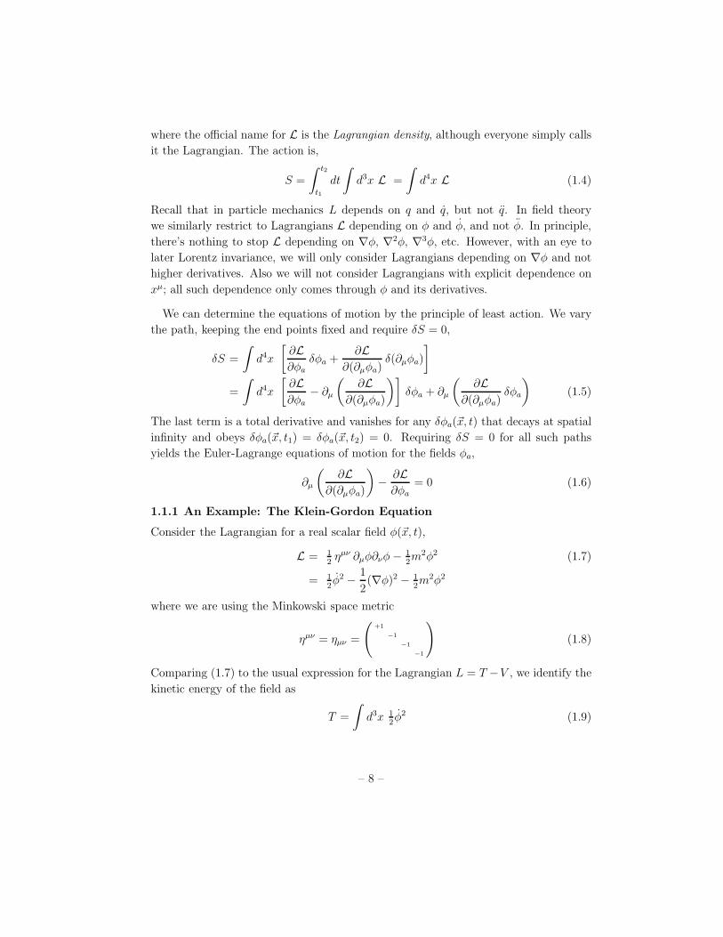
where the official name for L is the Lagrangian density, although everyone simply callsit the Lagrangian. The action is,

S =

∫ t2

t1

dt

∫

d3x L =

∫

d4x L (1.4)

Recall that in particle mechanics L depends on q and q, but not q. In field theorywe similarly restrict to Lagrangians L depending on φ and φ, and not φ. In principle,

there’s nothing to stop L depending on ∇φ, ∇2φ, ∇3φ, etc. However, with an eye tolater Lorentz invariance, we will only consider Lagrangians depending on ∇φ and nothigher derivatives. Also we will not consider Lagrangians with explicit dependence on

xµ; all such dependence only comes through φ and its derivatives.

We can determine the equations of motion by the principle of least action. We varythe path, keeping the end points fixed and require δS = 0,

δS =

∫

d4x

[

∂L∂φa

δφa +∂L

∂(∂µφa)δ(∂µφa)

]

=

∫

d4x

[

∂L∂φa

− ∂µ

(

∂L∂(∂µφa)

)]

δφa + ∂µ

(

∂L∂(∂µφa)

δφa

)

(1.5)

The last term is a total derivative and vanishes for any δφa(x, t) that decays at spatialinfinity and obeys δφa(x, t1) = δφa(x, t2) = 0. Requiring δS = 0 for all such pathsyields the Euler-Lagrange equations of motion for the fields φa,

∂µ

(

∂L∂(∂µφa)

)

−∂L∂φa

= 0 (1.6)

1.1.1 An Example: The Klein-Gordon Equation

Consider the Lagrangian for a real scalar field φ(x, t),

L = 1

2ηµν ∂µφ∂νφ− 1

2m2φ2 (1.7)

= 1

2φ2 −

1

2(∇φ)2 − 1

2m2φ2

where we are using the Minkowski space metric

ηµν = ηµν =

(

+1

−1

−1

−1

)

(1.8)

Comparing (1.7) to the usual expression for the Lagrangian L = T −V , we identify the

kinetic energy of the field as

T =

∫

d3x 1

2φ2 (1.9)

– 8 –

and the potential energy of the field as

V =

∫

d3x 1

2(∇φ)2 + 1

2m2φ2 (1.10)

The first term in this expression is called the gradient energy, while the phrase “poten-tial energy”, or just “potential”, is usually reserved for the last term.

To determine the equations of motion arising from (1.7), we compute

∂L∂φ

= −m2φ and∂L

∂(∂µφ)= ∂µφ ≡ (φ,−∇φ) (1.11)

The Euler-Lagrange equation is then

φ−∇2φ+m2φ = 0 (1.12)

which we can write in relativistic form as

∂µ∂µφ+m2φ = 0 (1.13)

This is the Klein-Gordon Equation. The Laplacian in Minkowski space is sometimes

denoted by !. In this notation, the Klein-Gordon equation reads !φ+m2φ = 0.

An obvious generalization of the Klein-Gordon equation comes from considering theLagrangian with arbitrary potential V (φ),

L = 1

2∂µφ∂

µφ− V (φ) ⇒ ∂µ∂µφ+

∂V

∂φ= 0 (1.14)

1.1.2 Another Example: First Order Lagrangians

We could also consider a Lagrangian that is linear in time derivatives, rather than

quadratic. Take a complex scalar field ψ whose dynamics is defined by the real La-grangian

L =i

2(ψ⋆ψ − ψ⋆ψ)−∇ψ⋆ ·∇ψ −mψ⋆ψ (1.15)

We can determine the equations of motion by treating ψ and ψ⋆ as independent objects,so that

∂L∂ψ⋆

=i

2ψ −mψ and

∂L∂ψ⋆

= −i

2ψ and

∂L∂∇ψ⋆

= −∇ψ (1.16)

This gives us the equation of motion

i∂ψ

∂t= −∇2ψ +mψ (1.17)

This looks very much like the Schrodinger equation. Except it isn’t! Or, at least, theinterpretation of this equation is very different: the field ψ is a classical field with none

of the probability interpretation of the wavefunction. We’ll come back to this point inSection 2.8.

– 9 –

The initial data required on a Cauchy surface differs for the two examples above.When L ∼ φ2, both φ and φ must be specified to determine the future evolution;

however when L ∼ ψ⋆ψ, only ψ and ψ⋆ are needed.

1.1.3 A Final Example: Maxwell’s Equations

We may derive Maxwell’s equations in the vacuum from the Lagrangian,

L = −1

2(∂µAν) (∂

µAν) + 1

2(∂µA

µ)2 (1.18)

Notice the funny minus signs! This is to ensure that the kinetic terms for Ai are positiveusing the Minkowski space metric (1.8), so L ∼ 1

2A2

i . The Lagrangian (1.18) has no

kinetic term A20 for A0. We will see the consequences of this in Section 6. To see that

Maxwell’s equations indeed follow from (1.18), we compute

∂L∂(∂µAν)

= −∂µAν + (∂ρAρ) ηµν (1.19)

from which we may derive the equations of motion,

∂µ

(

∂L∂(∂µAν)

)

= −∂2Aν + ∂ν(∂ρAρ) = −∂µ(∂µAν − ∂νAµ) ≡ −∂µF µν (1.20)

where the field strength is defined by Fµν = ∂µAν − ∂νAµ. You can check using (1.2)that this reproduces the remaining two Maxwell’s equations in a vacuum: ∇ · E = 0and ∂E/∂t = ∇ × B. Using the notation of the field strength, we may rewrite the

Maxwell Lagrangian (up to an integration by parts) in the compact form

L = −1

4FµνF

µν (1.21)

1.1.4 Locality, Locality, Locality

In each of the examples above, the Lagrangian is local. This means that there are noterms in the Lagrangian coupling φ(x, t) directly to φ(y, t) with x = y. For example,there are no terms that look like

L =

∫

d3xd3y φ(x)φ(y) (1.22)

A priori, there’s no reason for this. After all, x is merely a label, and we’re quitehappy to couple other labels together (for example, the term ∂3A0 ∂0A3 in the Maxwell

Lagrangian couples the µ = 0 field to the µ = 3 field). But the closest we get for thex label is a coupling between φ(x) and φ(x + δx) through the gradient term (∇φ)2.This property of locality is, as far as we know, a key feature of all theories of Nature.

Indeed, one of the main reasons for introducing field theories in classical physics is toimplement locality. In this course, we will only consider local Lagrangians.

– 10 –

1.2 Lorentz Invariance

The laws of Nature are relativistic, and one of the main motivations to develop quantumfield theory is to reconcile quantum mechanics with special relativity. To this end, we

want to construct field theories in which space and time are placed on an equal footingand the theory is invariant under Lorentz transformations,

xµ −→ (x′)µ = Λµνx

ν (1.23)

where Λµν satisfies

Λµσ η

στ Λντ = ηµν (1.24)

For example, a rotation by θ about the x3-axis, and a boost by v < 1 along the x1-axisare respectively described by the Lorentz transformations

Λµν =

⎛

⎜

⎜

⎜

⎜

⎝

1 0 0 0

0 cos θ − sin θ 0

0 sin θ cos θ 0

0 0 0 1

⎞

⎟

⎟

⎟

⎟

⎠

and Λµν =

⎛

⎜

⎜

⎜

⎜

⎝

γ −γv 0 0

−γv γ 0 0

0 0 1 0

0 0 0 1

⎞

⎟

⎟

⎟

⎟

⎠

(1.25)

with γ = 1/√1− v2. The Lorentz transformations form a Lie group under matrix

multiplication. You’ll learn more about this in the “Symmetries and Particle Physics”

course.

The Lorentz transformations have a representation on the fields. The simplest ex-

ample is the scalar field which, under the Lorentz transformation x → Λx, transformsas

φ(x) → φ′(x) = φ(Λ−1x) (1.26)

The inverse Λ−1 appears in the argument because we are dealing with an active trans-

formation in which the field is truly shifted. To see why this means that the inverseappears, it will suffice to consider a non-relativistic example such as a temperature field.

Suppose we start with an initial field φ(x) which has a hotspot at, say, x = (1, 0, 0).After a rotation x → Rx about the z-axis, the new field φ′(x) will have the hotspot at

x = (0, 1, 0). If we want to express φ′(x) in terms of the old field φ, we need to placeourselves at x = (0, 1, 0) and ask what the old field looked like where we’ve come fromat R−1(0, 1, 0) = (1, 0, 0). This R−1 is the origin of the inverse transformation. (If we

were instead dealing with a passive transformation in which we relabel our choice ofcoordinates, we would have instead φ(x) → φ′(x) = φ(Λx)).

– 11 –

The definition of a Lorentz invariant theory is that if φ(x) solves the equations ofmotion then φ(Λ−1x) also solves the equations of motion. We can ensure that this

property holds by requiring that the action is Lorentz invariant. Let’s look at ourexamples:

Example 1: The Klein-Gordon Equation

For a real scalar field we have φ(x) → φ′(x) = φ(Λ−1x). The derivative of the scalar

field transforms as a vector, meaning

(∂µφ)(x) → (Λ−1)νµ(∂νφ)(y)

where y = Λ−1x. This means that the derivative terms in the Lagrangian density

transform as

Lderiv(x) = ∂µφ(x)∂νφ(x)ηµν −→ (Λ−1)ρµ(∂ρφ)(y) (Λ

−1)σν(∂σφ)(y) ηµν

= (∂ρφ)(y) (∂σφ)(y) ηρσ

= Lderiv(y) (1.27)

The potential terms transform in the same way, with φ2(x) → φ2(y). Putting this alltogether, we find that the action is indeed invariant under Lorentz transformations,

S =

∫

d4x L(x) −→∫

d4x L(y) =∫

d4y L(y) = S (1.28)

where, in the last step, we need the fact that we don’t pick up a Jacobian factor whenwe change integration variables from

∫

d4x to∫

d4y. This follows because detΛ = 1.(At least for Lorentz transformation connected to the identity which, for now, is all we

deal with).

Example 2: First Order Dynamics

In the first-order Lagrangian (1.15), space and time are not on the same footing. (Lis linear in time derivatives, but quadratic in spatial derivatives). The theory is notLorentz invariant.

In practice, it’s easy to see if the action is Lorentz invariant: just make sure allthe Lorentz indices µ = 0, 1, 2, 3 are contracted with Lorentz invariant objects, suchas the metric ηµν . Other Lorentz invariant objects you can use include the totally

antisymmetric tensor ϵµνρσ and the matrices γµ that we will introduce when we cometo discuss spinors in Section 4.

– 12 –

Example 3: Maxwell’s Equations

Under a Lorentz transformation Aµ(x) → Λµν A

ν(Λ−1x). You can check that Maxwell’s

Lagrangian (1.21) is indeed invariant. Of course, historically electrodynamics was thefirst Lorentz invariant theory to be discovered: it was found even before the concept of

Lorentz invariance.

1.3 Symmetries

The role of symmetries in field theory is possibly even more important than in particlemechanics. There are Lorentz symmetries, internal symmetries, gauge symmetries,supersymmetries.... We start here by recasting Noether’s theorem in a field theoretic

framework.

1.3.1 Noether’s Theorem

Every continuous symmetry of the Lagrangian gives rise to a conserved current jµ(x)such that the equations of motion imply

∂µjµ = 0 (1.29)

or, in other words, ∂j 0/∂t +∇ · j = 0.

A Comment: A conserved current implies a conserved charge Q, defined as

Q =

∫

R3

d3x j 0 (1.30)

which one can immediately see by taking the time derivative,

dQ

dt=

∫

R3

d3x∂j

∂t

0

= −∫

R3

d3x ∇ · j = 0 (1.31)

assuming that j → 0 sufficiently quickly as |x| → ∞. However, the existence of a

current is a much stronger statement than the existence of a conserved charge becauseit implies that charge is conserved locally. To see this, we can define the charge in a

finite volume V ,

QV =

∫

V

d3x j 0 (1.32)

Repeating the analysis above, we find that

dQV

dt= −

∫

V

d3x ∇ · j = −∫

A

j · dS (1.33)

– 13 –

where A is the area bounding V and we have used Stokes’ theorem. This equationmeans that any charge leaving V must be accounted for by a flow of the current 3-

vector j out of the volume. This kind of local conservation of charge holds in any localfield theory.

Proof of Noether’s Theorem: We’ll prove the theorem by working infinitesimally.We may always do this if we have a continuous symmetry. We say that the transfor-

mation

δφa(x) = Xa(φ) (1.34)

is a symmetry if the Lagrangian changes by a total derivative,

δL = ∂µFµ (1.35)

for some set of functions F µ(φ). To derive Noether’s theorem, we first consider makingan arbitrary transformation of the fields δφa. Then

δL =∂L∂φa

δφa +∂L

∂(∂µφa)∂µ(δφa)

=

[

∂L∂φa

− ∂µ∂L

∂(∂µφa)

]

δφa + ∂µ

(

∂L∂(∂µφa)

δφa

)

(1.36)

When the equations of motion are satisfied, the term in square brackets vanishes. So

we’re left with

δL = ∂µ

(

∂L∂(∂µφa)

δφa

)

(1.37)

But for the symmetry transformation δφa = Xa(φ), we have by definition δL = ∂µF µ.

Equating this expression with (1.37) gives us the result

∂µjµ = 0 with jµ =

∂L∂(∂µφa)

Xa(φ)− F µ(φ) (1.38)

1.3.2 An Example: Translations and the Energy-Momentum Tensor

Recall that in classical particle mechanics, invariance under spatial translations givesrise to the conservation of momentum, while invariance under time translations is

responsible for the conservation of energy. We will now see something similar in fieldtheories. Consider the infinitesimal translation

xν → xν − ϵν ⇒ φa(x) → φa(x) + ϵν∂νφa(x) (1.39)

– 14 –

(where the sign in the field transformation is plus, instead of minus, because we’re doingan active, as opposed to passive, transformation). Similarly, once we substitute a spe-

cific field configuration φ(x) into the Lagrangian, the Lagrangian itself also transformsas

L(x) → L(x) + ϵν∂νL(x) (1.40)

Since the change in the Lagrangian is a total derivative, we may invoke Noether’stheorem which gives us four conserved currents (jµ)ν , one for each of the translations

ϵν with ν = 0, 1, 2, 3,

(jµ)ν =∂L

∂(∂µφa)∂νφa − δµνL ≡ T µ

ν (1.41)

T µν is called the energy-momentum tensor. It satisfies

∂µTµν = 0 (1.42)

The four conserved quantities are given by

E =

∫

d3x T 00 and P i =

∫

d3x T 0i (1.43)

where E is the total energy of the field configuration, while P i is the total momentumof the field configuration.

An Example of the Energy-Momentum Tensor

Consider the simplest scalar field theory with Lagrangian (1.7). From the above dis-

cussion, we can compute

T µν = ∂µφ ∂νφ− ηµνL (1.44)

One can verify using the equation of motion for φ that this expression indeed satisfies∂µT µν = 0. For this example, the conserved energy and momentum are given by

E =

∫

d3x 1

2φ2 + 1

2(∇φ)2 + 1

2m2φ2 (1.45)

P i =

∫

d3x φ ∂iφ (1.46)

Notice that for this example, T µν came out symmetric, so that T µν = T νµ. Thiswon’t always be the case. Nevertheless, there is typically a way to massage the energy

momentum tensor of any theory into a symmetric form by adding an extra term

Θµν = T µν + ∂ρΓρµν (1.47)

where Γρµν is some function of the fields that is anti-symmetric in the first two indices so

Γρµν = −Γµρν . This guarantees that ∂µ∂ρΓρµν = 0 so that the new energy-momentumtensor is also a conserved current.

– 15 –

A Cute Trick

One reason that you may want a symmetric energy-momentum tensor is to make con-tact with general relativity: such an object sits on the right-hand side of Einstein’sfield equations. In fact this observation provides a quick and easy way to determine a

symmetric energy-momentum tensor. Firstly consider coupling the theory to a curvedbackground spacetime, introducing an arbitrary metric gµν(x) in place of ηµν , and re-

placing the kinetic terms with suitable covariant derivatives using “minimal coupling”.Then a symmetric energy momentum tensor in the flat space theory is given by

Θµν = −2√−g

∂(√−gL)

∂gµν

∣

∣

∣

∣

gµν=ηµν

(1.48)

It should be noted however that this trick requires a little more care when working

with spinors.

1.3.3 Another Example: Lorentz Transformations and Angular Momentum

In classical particle mechanics, rotational invariance gave rise to conservation of angular

momentum. What is the analogy in field theory? Moreover, we now have furtherLorentz transformations, namely boosts. What conserved quantity do they correspond

to? To answer these questions, we first need the infinitesimal form of the Lorentztransformations

Λµν = δµν + ωµ

ν (1.49)

where ωµν is infinitesimal. The condition (1.24) for Λ to be a Lorentz transformation

becomes

(δµσ + ωµσ)(δ

ντ + ων

τ ) ηστ = ηµν

⇒ ωµν + ωνµ = 0 (1.50)

So the infinitesimal form ωµν of the Lorentz transformation must be an anti-symmetricmatrix. As a check, the number of different 4×4 anti-symmetric matrices is 4×3/2 = 6,which agrees with the number of different Lorentz transformations (3 rotations + 3

boosts). Now the transformation on a scalar field is given by

φ(x) → φ′(x) = φ(Λ−1x)

= φ(xµ − ωµνx

ν)

= φ(xµ)− ωµν x

ν ∂µφ(x) (1.51)

– 16 –

from which we see that

δφ = −ωµνx

ν∂µφ (1.52)

By the same argument, the Lagrangian density transforms as

δL = −ωµνx

ν∂µL = −∂µ(ωµνx

νL) (1.53)

where the last equality follows because ωµµ = 0 due to anti-symmetry. Once again,

the Lagrangian changes by a total derivative so we may apply Noether’s theorem (now

with F µ = −ωµνx

νL) to find the conserved current

j µ = −∂L

∂(∂µφ)ωρ

νxν ∂ρφ+ ωµ

ν xνL

= −ωρν

[

∂L∂(∂µφ)

xν ∂ρφ− δµρ xν L]

= −ωρν T µ

ρxν (1.54)

Unlike in the previous example, I’ve left the infinitesimal choice of ωµν in the expression

for this current. But really, we should strip it out to give six different currents, i.e. onefor each choice of ωµ

ν . We can write them as

(J µ)ρσ = xρT µσ − xσT µρ (1.55)

which satisfy ∂µ(J µ)ρσ = 0 and give rise to 6 conserved charges. For ρ, σ = 1, 2, 3,the Lorentz transformation is a rotation and the three conserved charges give the total

angular momentum of the field.

Qij =

∫

d3x (xiT 0j − xjT 0i) (1.56)

But what about the boosts? In this case, the conserved charges are

Q0i =

∫

d3x (x0T 0i − xiT 00) (1.57)

The fact that these are conserved tells us that

0 =dQ0i

dt=

∫

d3x T 0i + t

∫

d3x∂T 0i

∂t−

d

dt

∫

d3x xiT 00

= P i + tdP i

dt−

d

dt

∫

d3x xiT 00 (1.58)

But we know that P i is conserved, so dP i/dt = 0, leaving us with the following conse-quence of invariance under boosts:

d

dt

∫

d3x xiT 00 = constant (1.59)

This is the statement that the center of energy of the field travels with a constant

velocity. It’s kind of like a field theoretic version of Newton’s first law but, rathersurprisingly, appearing here as a conservation law.

– 17 –

1.3.4 Internal Symmetries

The above two examples involved transformations of spacetime, as well as transforma-

tions of the field. An internal symmetry is one that only involves a transformation ofthe fields and acts the same at every point in spacetime. The simplest example occurs

for a complex scalar field ψ(x) = (φ1(x)+ iφ2(x))/√2. We can build a real Lagrangian

by

L = ∂µψ⋆ ∂µψ − V (|ψ|2) (1.60)

where the potential is a general polynomial in |ψ|2 = ψ⋆ψ. To find the equations of

motion, we could expand ψ in terms of φ1 and φ2 and work as before. However, it’seasier (and equivalent) to treat ψ and ψ⋆ as independent variables and vary the action

with respect to both of them. For example, varying with respect to ψ⋆ leads to theequation of motion

∂µ∂µψ +

∂V (ψ⋆ψ)

∂ψ⋆= 0 (1.61)

The Lagrangian has a continuous symmetry which rotates φ1 and φ2 or, equivalently,

rotates the phase of ψ:

ψ → eiαψ or δψ = iαψ (1.62)

where the latter equation holds with α infinitesimal. The Lagrangian remains invariant

under this change: δL = 0. The associated conserved current is

j µ = i(∂µψ⋆)ψ − iψ⋆(∂µψ) (1.63)

We will later see that the conserved charges arising from currents of this type havethe interpretation of electric charge or particle number (for example, baryon or lepton

number).

Non-Abelian Internal Symmetries

Consider a theory involving N scalar fields φa, all with the same mass and the La-

grangian

L =1

2

N∑

a=1

∂µφa∂µφa −

1

2

N∑

a=1

m2φ2

a − g

(

N∑

a=1

φ2

a

)2

(1.64)

In this case the Lagrangian is invariant under the non-Abelian symmetry group G =

SO(N). (Actually O(N) in this case). One can construct theories from complex fieldsin a similar manner that are invariant under an SU(N) symmetry group. Non-Abeliansymmetries of this type are often referred to as global symmetries to distinguish them

from the “local gauge” symmetries that you will meet later. Isospin is an example ofsuch a symmetry, albeit realized only approximately in Nature.

– 18 –

Another Cute Trick

There is a quick method to determine the conserved current associated to an internalsymmetry δφ = αφ for which the Lagrangian is invariant. Here, α is a constant real

number. (We may generalize the discussion easily to a non-Abelian internal symmetryfor which α becomes a matrix). Now consider performing the transformation but where

α depends on spacetime: α = α(x). The action is no longer invariant. However, thechange must be of the form

δL = (∂µα) hµ(φ) (1.65)

since we know that δL = 0 when α is constant. The change in the action is therefore

δS =

∫

d4x δL = −∫

d4x α(x) ∂µhµ (1.66)

which means that when the equations of motion are satisfied (so δS = 0 for all varia-

tions, including δφ = α(x)φ) we have

∂µhµ = 0 (1.67)

We see that we can identify the function hµ = j µ as the conserved current. This wayof viewing things emphasizes that it is the derivative terms, not the potential terms,in the action that contribute to the current. (The potential terms are invariant even

when α = α(x)).

1.4 The Hamiltonian Formalism

The link between the Lagrangian formalism and the quantum theory goes via the pathintegral. In this course we will not discuss path integral methods, and focus instead

on canonical quantization. For this we need the Hamiltonian formalism of field theory.We start by defining the momentum πa(x) conjugate to φa(x),

πa(x) =∂L∂φa

(1.68)

The conjugate momentum πa(x) is a function of x, just like the field φa(x) itself. Itis not to be confused with the total momentum P i defined in (1.43) which is a single

number characterizing the whole field configuration. The Hamiltonian density is givenby

H = πa(x)φa(x)− L(x) (1.69)

where, as in classical mechanics, we eliminate φa(x) in favour of πa(x) everywhere in

H. The Hamiltonian is then simply

H =

∫

d3x H (1.70)

– 19 –

An Example: A Real Scalar Field

For the Lagrangian

L = 1

2φ2 − 1

2(∇φ)2 − V (φ) (1.71)

the momentum is given by π = φ, which gives us the Hamiltonian,

H =

∫

d3x 1

2π2 + 1

2(∇φ)2 + V (φ) (1.72)

Notice that the Hamiltonian agrees with the definition of the total energy (1.45) that

we get from applying Noether’s theorem for time translation invariance.

In the Lagrangian formalism, Lorentz invariance is clear for all to see since the action

is invariant under Lorentz transformations. In contrast, the Hamiltonian formalism isnot manifestly Lorentz invariant: we have picked a preferred time. For example, the

equations of motion for φ(x) = φ(x, t) arise from Hamilton’s equations,

φ(x, t) =∂H

∂π(x, t)and π(x, t) = −

∂H

∂φ(x, t)(1.73)

which, unlike the Euler-Lagrange equations (1.6), do not look Lorentz invariant. Nev-ertheless, even though the Hamiltonian framework doesn’t look Lorentz invariant, the

physics must remain unchanged. If we start from a relativistic theory, all final answersmust be Lorentz invariant even if it’s not manifest at intermediate steps. We will pause

at several points along the quantum route to check that this is indeed the case.

– 20 –