Embed Size (px)
Citation preview
QUANTUM FIELD THEORY – 230A
Eric D’Hoker
Department of Physics and Astronomy
University of California, Los Angeles, CA 90095
2004, October 3
Contents
1 Introduction 3
1.1 Relativity and quantum mechanics . . . . . . . . . . . . . . . . . . . . . . 4
1.2 Why Quantum Field Theory ? . . . . . . . . . . . . . . . . . . . . . . . . . 6
1.3 Further conceptual changes required by relativity . . . . . . . . . . . . . . 6
1.4 Some History and present significance of QFT . . . . . . . . . . . . . . . . 8
2 Quantum Mechanics – A synopsis 10
2.1 Classical Mechanics . . . . . . . . . . . . . . . . . . . . . . . . . . . . . . . 10
2.2 Principles of Quantum Mechanics . . . . . . . . . . . . . . . . . . . . . . . 12
2.3 Quantum Systems from classical mechanics . . . . . . . . . . . . . . . . . . 13
2.4 Quantum systems associated with Lie algebras . . . . . . . . . . . . . . . . 15
2.5 Appendix I : Lie groups, Lie algebras, representations . . . . . . . . . . . . 16
2.6 Functional integral formulation . . . . . . . . . . . . . . . . . . . . . . . . 19
3 Principles of Relativistic Quantum Field Theory 22
3.1 The Lorentz and Poincare groups and algebras . . . . . . . . . . . . . . . . 23
3.2 Parity and Time reversal . . . . . . . . . . . . . . . . . . . . . . . . . . . . 25
3.3 Finite-dimensional Representations of the Lorentz Algebra . . . . . . . . . 26
3.4 Unitary Representations of the Poincare Algebra . . . . . . . . . . . . . . . 29
3.5 The basic principles of quantum field theory . . . . . . . . . . . . . . . . . 32
3.6 Transformation of Local Fields under the Lorentz Group . . . . . . . . . . 34
3.7 Discrete Symmetries . . . . . . . . . . . . . . . . . . . . . . . . . . . . . . 39
3.7.1 Parity . . . . . . . . . . . . . . . . . . . . . . . . . . . . . . . . . . 39
3.7.2 Time reversal . . . . . . . . . . . . . . . . . . . . . . . . . . . . . . 39
3.7.3 Charge Conjugation . . . . . . . . . . . . . . . . . . . . . . . . . . 40
3.8 Significance of fields in terms of particle contents . . . . . . . . . . . . . . 40
3.9 Classical Poincare invariant field theories . . . . . . . . . . . . . . . . . . . 41
4 Free Field Theory 43
4.1 The Scalar Field . . . . . . . . . . . . . . . . . . . . . . . . . . . . . . . . 43
4.2 The Operator Product Expansion & Composite Operators . . . . . . . . . 51
4.3 The Gauge or Spin 1 Field . . . . . . . . . . . . . . . . . . . . . . . . . . . 54
4.4 The Casimir Effect on parallel plates . . . . . . . . . . . . . . . . . . . . . 59
4.5 Bose-Einstein and Fermi-Dirac statistics . . . . . . . . . . . . . . . . . . . 62
4.6 The Spin 1/2 Field . . . . . . . . . . . . . . . . . . . . . . . . . . . . . . . 65
4.6.1 The Weyl basis and Free Weyl spinors . . . . . . . . . . . . . . . . 66
4.7 The spin statistics theorem . . . . . . . . . . . . . . . . . . . . . . . . . . . 71
4.7.1 Parastatistics ? . . . . . . . . . . . . . . . . . . . . . . . . . . . . . 71
4.7.2 Commutation versus anti-commutation relations . . . . . . . . . . . 72
5 Interacting Field Theories – Gauge Theories 73
5.1 Interacting Lagrangians . . . . . . . . . . . . . . . . . . . . . . . . . . . . 73
5.2 Abelian Gauge Invariance . . . . . . . . . . . . . . . . . . . . . . . . . . . 74
5.3 Non-Abelian Gauge Invariance . . . . . . . . . . . . . . . . . . . . . . . . . 74
5.4 Component formulation . . . . . . . . . . . . . . . . . . . . . . . . . . . . 76
5.5 Bianchi identities . . . . . . . . . . . . . . . . . . . . . . . . . . . . . . . . 77
5.6 Gauge invariant combinations . . . . . . . . . . . . . . . . . . . . . . . . . 77
5.7 Classical Action & Field equations . . . . . . . . . . . . . . . . . . . . . . 78
5.8 Lagrangians including fermions and scalars . . . . . . . . . . . . . . . . . . 79
5.9 Examples . . . . . . . . . . . . . . . . . . . . . . . . . . . . . . . . . . . . 80
6 The S-matrix and LSZ Reduction formulas 81
6.0.1 In and Out States and Fields . . . . . . . . . . . . . . . . . . . . . 82
6.0.2 The S-matrix . . . . . . . . . . . . . . . . . . . . . . . . . . . . . . 83
6.0.3 Scattering cross sections . . . . . . . . . . . . . . . . . . . . . . . . 83
6.1 Relating the interacting and in- and out-fields . . . . . . . . . . . . . . . . 85
6.2 The Kallen-Lehmann spectral representation . . . . . . . . . . . . . . . . . 87
6.3 The Dirac Field . . . . . . . . . . . . . . . . . . . . . . . . . . . . . . . . . 89
6.4 The LSZ Reduction Formalism . . . . . . . . . . . . . . . . . . . . . . . . 90
6.4.1 In- and Out-Operators in terms of the free field . . . . . . . . . . . 90
6.4.2 Asymptotics of the interacting field . . . . . . . . . . . . . . . . . . 91
6.4.3 The reduction formulas . . . . . . . . . . . . . . . . . . . . . . . . . 92
6.4.4 The Dirac Field . . . . . . . . . . . . . . . . . . . . . . . . . . . . . 93
6.4.5 The Photon Field . . . . . . . . . . . . . . . . . . . . . . . . . . . . 94
2
1 Introduction
Quantum Field Theory (abbreviated QFT) deals with the quantization of fields. A familiar
example of a field is provided by the electromagnetic field. Classical electromagnetism
describes the dynamics of electric charges and currents, as well as electro-magnetic waves,
such as radio waves and light, in terms of Maxwell’s equations. At the atomic level,
however, the quantum nature of atoms as well as the quantum nature of electromagnetic
radiation must be taken into account. Quantum mechanically, electromagnetic waves turn
out to be composed of quanta of light, whose individual behavior is closer to that of a
particle than to a wave. Remarkably, the quantization of the electromagnetic field is in
terms of the quanta of this field, which are particles, also called photons. In QFT, this
field particle correspondence is used both ways, and it is one of the key assumptions of
QFT that to every elementary particle, there corresponds a field. Thus, the electron will
have its own field, and so will every quark.
Quantum Field Theory provides an elaborate general formalism for the field–particle
correspondence. The advantage of QFT will be that it can naturally account for the cre-
ation and annihilation of particles, which ordinary quantum mechanics of the Schrodinger
equation could not describe. The fact that the number of particles in a system can change
over time is a very important phenomenon, which takes place continuously in everyone’s
daily surroundings, but whose significance may not have been previously noticed.
In classical mechanics, the number of particles in a closed system is conserved, i.e. the
total number of particles is unchanged in time. To each pointlike particle, one associates
a set of position and momentum coordinates, the time evolution of which is governed by
the dynamics of the system. Quantum mechanics may be formulated in two stages.
1. The principles of quantum mechanics, such as the definitions of states, observables,
are general and do not make assumptions on whether the number of particles in the
system is conserved during time evolution.
2. The specific dynamics of the quantum system, described by the Hamiltonian, may or
may not assume particle number conservation. In introductory quantum mechanics,
dynamics is usually associated with non-relativistic mechanical systems (augmented
with spin degrees of freedom) and therefore assumes a fixed number of particles. In
many important quantum systems, however, the number of particles is not conserved.
A familiar and ubiquitous example is that of electromagnetic radiation. An excited
atom may decay into its ground state by emitting a single quantum of light or photon.
The photon was not “inside” the excited atom prior to the emission; it was “created” by
the excited atom during its transition to the grounds state. This is well illustrated as
3
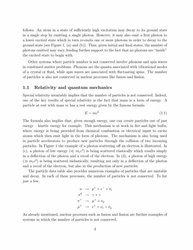
follows. An atom in a state of sufficiently high excitation may decay to its ground state
in a single step by emitting a single photon. However, it may also emit a first photon to
a lower excited state which in turn re-emits one or more photons in order to decay to the
ground state (see Figure 1, (a) and (b)). Thus, given initial and final states, the number of
photons emitted may vary, lending further support to the fact that no photons are “inside”
the excited state to begin with.
Other systems where particle number is not conserved involve phonons and spin waves
in condensed matter problems. Phonons are the quanta associated with vibrational modes
of a crystal or fluid, while spin waves are associated with fluctuating spins. The number
of particles is also not conserved in nuclear processes like fusion and fission.
1.1 Relativity and quantum mechanics
Special relativity invariably implies that the number of particles is not conserved. Indeed,
one of the key results of special relativity is the fact that mass is a form of energy. A
particle at rest with mass m has a rest energy given by the famous formula
E = mc2 (1.1)
The formula also implies that, given enough energy, one can create particles out of just
energy – kinetic energy for example. This mechanism is at work in fire and light bulbs,
where energy is being provided from chemical combustion or electrical input to excite
atoms which then emit light in the form of photons. The mechanism is also being used
in particle accelerators to produce new particles through the collision of two incoming
particles. In Figure 1 the example of a photon scattering off an electron is illustrated. In
(c), a photon of low energy (� mec2) is being scattered elastically which results simply
in a deflection of the photon and a recoil of the electron. In (d), a photon of high energy
(� mec2) is being scattered inelastically, resulting not only in a deflection of the photon
and a recoil of the electron, but also in the production of new particles.
The particle data table also provides numerous examples of particles that are unstable
and decay. In each of these processes, the number of particles is not conserved. To list
just a few,
n → p+ + e− + νe
π0 → γ + γ
π+ → µ+ + νµ
µ+ → e+ + νe + νµ
As already mentioned, nuclear processes such as fusion and fission are further examples of
systems in which the number of particles is not conserved.
4
initial
final
photon
initial
final
photon
photon
(a) (b)
photon
recoiled electron
scattered photon
photon
scattered photon
recoiled electron
new particles
(c) (d)
Figure 1: Production of particles : (a) Emission of one photon, (b) emission of two photonsbetween the same initial and final states; (c) low energy elastic scattering, (d) high energyinelastic scattering of a photon off a recoiling electron.
5
1.2 Why Quantum Field Theory ?
Quantum Field Theory is a formulation of a quantum system in which the number of
particles does not have to be conserved but may vary freely. QFT does not require a
change in the principles of either quantum mechanics or relativity. QFT requires a different
formulation of the dynamics of the particles involved in the system.
Clearly, such a description must go well beyond the usual Schrodinger equation, whose
very formulation requires that the number of particles in a system be fixed. Quantum field
theory may be formulated for non-relativistic systems in which the number of particles is
not conserved, (recall spin waves, phonons, spinons etc). Here, however, we shall concen-
trate on relativistic quantum field theory because relativity forces the number of particles
not to be conserved. In addition, relativity is one of the great fundamental principles of
Nature, so that its incorporation into the theory is mandated at a fundamental level.
1.3 Further conceptual changes required by relativity
Relativity introduces some further fundamental changes in both the nature and the for-
malism of quantum mechanics. We shall just mention a few.
• Space versus time
In non-relativistic quantum mechanics, the position x, the momentum p and the en-
ergy E of free or interacting particles are all observables. This means that each of these
quantities separately can be measured to arbitrary precision in an arbitrarily short time.
By contrast, the accurarcy of the simultaneous measurement of x and p is limited by the
Heisenberg uncertainty relations,
∆x ∆p ∼ h
There is also an energy-time uncertainty relation ∆E ∆t ∼ h, but its interpretation is quite
different from the relation ∆x ∆p ∼ h, because in ordinary quantum mechanics, time
is viewed as a parameter and not as an observable. Instead the energy-time uncertainty
relation governs the time evolution of an interacting system. In relativistic dynamics,
particle-antiparticle pairs can always be created, which subjects an interacting particle
always to a cloud of pairs, and thus inherently to an uncertainty as to which particle one
is describing. Therefore, the momentum itself is no longer an instantaneous observable,
but will be subject to the a momentum-time uncertainty relation ∆p ∆t ∼ h/c. As c→ ∞,
this effect would disappear, but it is relevant for relativistic processes. Thus, momentum
can only be observed with precision away from the interaction region.
Special relativity puts space and time on the same footing, so we have the choice of
either treating space and time both as observables (a bad idea, even in quantum mechanics)
or to treat them both as parameters, which is how QFT will be formulated.
6
• “Negative energy” solutions and anti-particles
The kinetic law for a relativistic particle of mass m is
E2 = m2c4 + p2c2
Positive and negative square roots for E naturally arise. Classically of course one may just
keep positive energy particles. Quantum mechanically, interactions induce transitions to
negative energy states, which therefore cannot be excluded arbitrarily. Following Feynman,
the correct interpretation is that these solutions correspond to negative frequencies, which
describe physical anti-particles with positive energy traveling “backward in time”.
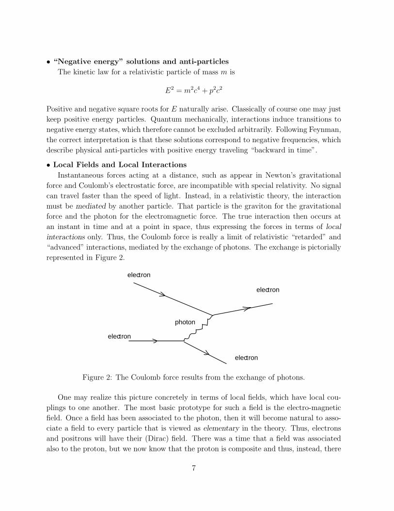
• Local Fields and Local Interactions
Instantaneous forces acting at a distance, such as appear in Newton’s gravitational
force and Coulomb’s electrostatic force, are incompatible with special relativity. No signal
can travel faster than the speed of light. Instead, in a relativistic theory, the interaction
must be mediated by another particle. That particle is the graviton for the gravitational
force and the photon for the electromagnetic force. The true interaction then occurs at
an instant in time and at a point in space, thus expressing the forces in terms of local
interactions only. Thus, the Coulomb force is really a limit of relativistic “retarded” and
“advanced” interactions, mediated by the exchange of photons. The exchange is pictorially
represented in Figure 2.
photon
electron
electron
electron
electron
Figure 2: The Coulomb force results from the exchange of photons.
One may realize this picture concretely in terms of local fields, which have local cou-
plings to one another. The most basic prototype for such a field is the electro-magnetic
field. Once a field has been associated to the photon, then it will become natural to asso-
ciate a field to every particle that is viewed as elementary in the theory. Thus, electrons
and positrons will have their (Dirac) field. There was a time that a field was associated
also to the proton, but we now know that the proton is composite and thus, instead, there
7
are now fields for quarks and gluons, which are the elementary particles that make up
a proton. The gluons are the analogs for the strong force of the photon for the electro-
magnetic force, namely the gluons mediate the strong force. Analogously, the W± and Z0
mediate the weak interactions.
1.4 Some History and present significance of QFT
The quantization of the elctro-magnetic field was initiated by Born, Heisenberg and Jor-
dan in 1926, right after quantum mechanics had been given its definitive formulation by
Heisenberg and Schrodinger in 1925. The complete formulation of the dynamics was given
by Dirac Heiseberg and Pauli in 1927. Infinities in perturbative corrections due to high
energy (or UV – ultraviolet) effects were first studied by Oppenheimer and Bethe in the
1930’s. It took until 1945-49 until Tomonaga, Schwinger and Feynman gave a completely
relativistic formulation of Quantum Electrodynamics (or QED) and evaluated the radia-
tive corrections to the magnetic moment of the electron. In 1950, Dyson showed that the
UV divergences of QED can be systematically dealt with by the process of renormalization.
In the 1960’s Glashow, Weinberg and Salam formulated a renormalizable quantum field
theory of the weak interactions in terms of a Yang-Mills theory. Yang-Mills theory was
shown to be renormalizable by ‘t Hooft in 1971, a problem that was posed to him by his
advisor Veltman. In 1973, Gross, Wilczek and Politzer discovered asymptotic freedom
of certain Yang-Mills theories (the fact that the strong force between quarks becomes
weak at high energies) and using this unique clue, they formulated (independently also
Weinberg) the quantum field theory of the strong interactions. Thus, the elctro-magnetic,
weak and strong forces are presently described – and very accurately so – by quantum
field theory, specifically Yang-Mills theory, and this combined theory is usually referred to
as the STANDARD MODEL. To give just one example of the power of the quantum field
theory approach, one may quote the experimentally measured and theoretically calculated
values of the muon magnetic dipole moment,
1
2gµ(exp) = 1.001159652410(200)
1
2gµ(thy) = 1.001159652359(282) (1.2)
revealing an astounding degree of agreement.
The gravitational force, described classically by Einstein’s general relativity theory,
does not seem to lend itself to a QFT description. String theory appears to provide
a more appropriate description of the quantum theory of gravity. String theory is an
extension of QFT, whose very formulation is built squarely on QFT and which reduces to
QFT in the low energy limit.
8
The devlopment of quantum field theory has gone hand in hand with developments
in Condensed Matter theory and Statistical Mechanics, especially critical phenomena and
phase transitions.
A final remark is in order on QFT and mathematics. Contrarily to the situation with
general relativity and quantum mechanics, there is no good “axiomatic formulation” of
QFT, i.e. one is very hard pressed to lay down a set of simple postulates from which
QFT may then be constructed in a deductive manner. For many years, physicists and
mathematicians have attempted to formulate such a set of axioms, but the theories that
could be fit into this framework almost always seem to miss the physically most relevant
ones, such as Yang-Mills theory. Thus, to date, there is no satsifactory mathematical
“definition” of a QFT.
Conversely, however, QFT has had a remarkably strong influence on mathematics over
the past 25 years, with the development of Yang-Mills theory, instantons, monopoles, con-
formal field theory, Chern-Simons theory, topological field theory and superstring theory.
Some developments is QFT have led to revolutions in mathematics, such as Seiberg-Witten
theory. It is suspected by some that this is only the tip of the iceberg, and that we are
only beginning to have a glimpse at the powerful applications of quantum field theory to
mathematics.
9
2 Quantum Mechanics – A synopsis
The basis of QFT is quantum mechanics and therefore we shall begin by reviewing the
foundations of this dsicipline. In fact, we begin with a brief summary of Lagrangian and
Hamiltonian classical mechanics as this will also be of great value.
2.1 Classical Mechanics
Consider a system of N degrees of freedom qi(t), i = 1, · · · , N . (For example n particles
in R3 has N = 3n.) Dynamics is governed by the Lagrangian function∗
L(qi, qi) qi(t) ≡dqi(t)
dt(2.1)
or by the action functional
S[qi] =∫ t2
t1dt L(qi(t), qi(t)) (2.2)
The classical time evolution of the system is determined as a solution to the variational
problem as follows{
δS[qi] = 0δqi(t1) = δqi(t1) = 0
⇒ d
dt
(∂L
∂qi
)
− ∂L
∂qi= 0 (2.3)
and these equations are the Euler-Lagrange equations. In general, the differential equations
are second order in t, and thus the Cauchy data are qi(t1) and qi(t1) at initial time t1 :
namely positions and velocities.
• Hamiltonian Formulation
The Hamiltonian formulation of classical mechanics proceeds as follows. We introduce
the canonical momenta,
pi ≡∂L
∂qi(qj, qj) ⇒ qi(q, p) (2.4)
and introduce the Hamiltonian function
H(p, q) ≡N∑
i=1
piqi(p, q) − L(qj , qj(p, q)) (2.5)
The time evolution equation can now be re-expressed as the Hamilton equations
qi =∂H
∂pipi = −∂H
∂qi(2.6)
∗For almost all the problems that we shall consider, L has no explicit time dependence and all time-dependence is implicit through qi(t) and qi(t).
10
The time evolution of any function F (p, q, t) along the classical trajectory may be expressed
as follows
d
dtF (p, q, t) = {H,F} +
∂F
∂t
{A,B} ≡N∑
i=1
(∂A
∂pi
∂B
∂qi− ∂B
∂pi
∂A
∂qi
)
(2.7)
The Poisson bracket {, } is antisymmetric and satisfies the following relations
0 = {A, {B,C}} + {B, {C,A}}+ {C, {A,B}}{A,BC} = {A,B}C + {A,C}B{pi, qj} = δij (2.8)
The second line shows that the Poisson bracket acts as a derivation.
• Symmetries
A symmetry of a classical system is a transformation on the degrees of freedom qisuch that under its action, every solution to the corresponding Euler-Lagrange equations
is transformed into a solution of these same equations. Symmetries form a group under
successive composition. An important special class consists of continuous symmetries,
where the transformation may be labeled by a parameter (or by several parameters) in a
continuous way. Denoting a transformation depending on a single parameter α ∈ R by
σ(α), the transformation may be represented as follows,
σ(α) : qi(t) −→ qi(t, α) qi(t, 0) = qi(t) (2.9)
The transformation σ(α) is a continuous symmetry of the Lagrangian L if and only if the
derivative with repect to α satisfies the following property
∂
∂αL(qi(t, α), qi(t, α)) =
d
dtX(qi, qi) (2.10)
obtained without using the Euler-Lagrange equations.
• Noether’s Theorem
The existence of a continuous symmetry implies the presence of a time independent
charge Q (also sometimes called a first integral of motion) by Noether’s theorem. An
explicit formula is available for this charge
Q =N∑
i=1
pi∂qi(t, α)
∂α
∣∣∣∣α=0
−X(pi, qi) (2.11)
11
The relation Q = 0 follows now by using the Euler-Lagrange equations. In the Hamiltonian
formulation, the charge generates the transformation in turn by Poisson bracketting,
∂qi(t, α)
∂α= {Q, qi(t, α)} (2.12)
Continuous symmetries of a given L form a Lie group. Lie groups and algebras will be
defined generally in the next section.
2.2 Principles of Quantum Mechanics
A quantum system may be defined in all generality in terms of a very small number of
physical principles.
1. Physical States are represented by rays in a Hilbert space H. Recall that a Hilbert
space H is a complex (complete) vector space with a positive definite inner product,
which we denote by 〈 | 〉 : H×H −→ C a la Dirac, and we have
• 〈φ|ψ〉 = 〈ψ|φ〉∗
• 〈φ|φ〉 ≥ 0
• 〈φ|φ〉 = 0 ⇒ |φ〉 = 0 (2.13)
A ray is an equivalence class in H by |φ〉 ∼ λ|φ〉, λ ∈ C − {0}.
2. Physical Observables are represented by self-adjoint operators on H. For the mo-
ment, we shall denote such operators with a hat, e.g. A, but after this chapter, we
drop hats. The operators are linear, so that A(a|φ〉+ b|ψ〉) = aA|φ〉+ bA|ψ〉, for all
|φ〉, |ψ〉 ∈ H and a, b ∈ C. Recall that for finite-dimensional matrices, Hermiticity
and self-adjointness are the same. For operators acting on an infinite dimensional
Hilbert space, self-adjointness requires that the domains of the operator and its ad-
joint be the same as well.
3. Measurements : A state |ψ〉 in H has a definite measured value α for some observable
A if the state is an eigenstate of A with eigenvalue α; A|ψ〉 = α|ψ〉. (Since A is
self-adjoint, states associated with different eigenvalues of A are orthogonal to one
another.) In a quantum system, what you can measure in an experiment are the
eigenvalues of various observables, e.g. the energy levels of atoms.
4. The transition probability for a given state |ψ〉 ∈ H to be found in one of a set of
orthogonal states |φn〉 is given by
P (|ψ〉 → |φn〉) = |〈ψ|φn〉|2 (2.14)
for normalized states 〈ψ|ψ〉 = 〈φn|φn〉 = 1. The quantities 〈ψ|φn〉 are referred to as
the transition amplitudes. Notice that their dependence on the state |ψ〉 is linear,
12
so that these amplitudes obey the superposition principle, while the probability
amplitudes are quadratic and cannot be linearly superimposed.
Notice that amongst the principles of quantum mechanics, there is no reference to a
Hamiltonian, a Schrodinger equation and the like. Those ingredients are dynamical and
will depend upon the specific system under consideration.
• Commuting observables – quantum numbers
If two observables A and B commute, [A, B] = 0, then they can be diagonalized
simultaneously. The associated physical observables can then be measured simultaneously,
yielding eigenvalues α and β respectively. On the other hand, if [A, B] 6= 0, the associated
physical observables cannot be measured simultaneously.
One defines a maximal set of commuting observales as a set of observables
A1, A2, · · · , An which all mutually commute, [Ai, Aj ] = 0, for all i, j = 1, · · · , n, and
such that no other operator (besides linear combinations of the Ai) commutes with all
Ai. It follows that the eigenspaces for each of the sets of eigenvalues is one-dimensional,
and therefore label the states in H in a unique manner. Given the set {Ai}i=1,···,n, the
corresponding eigenvalues are the quantum numbers.
• Symmetries in quantum systems
Symmetries in quantum mechanics are realized by unitary transformations in Hilbert
space H. Unitarity guarantees that the transition amplitudes and thus probabilities will
be invariant under the symmetry.
2.3 Quantum Systems from classical mechanics
A very large and important class of quantum systems derive from classical mechanics
systems (for example the Hydrogen atom). Given a classical mechanics system, one can
always construct an associated quantum system, using the correspondence principle. Con-
sider a classical mechanics system with degrees of freedom pi(t), qi(t) ∈ R, i = 1, · · · , Nand with Hamiltonian H(p, q). The associated quantum system is obtained by mapping
the reals pi and qi into observables in a Hilbert space H. The Hilbert space may be taken
to be L2(RN), i.e. square integrable functions of qi. The Poisson bracket is mapped into
a commutator of operators. The detailed correspondence is
pi, qi → pi, qi
{pi, qj} = δij → i
h[pi, qj ] = δij
{pi, pj} = {qi, qj} = 0 → [pi, pj] = [qi, qj ] = 0
Under the correspondence principle, the Hamiltonian H(p, q) produces a self-adjoint op-
erators H(p, q). In general, however, this correspondence will not be unique, because in
13
the classical system, p and q are commuting numbers, so their ordering in any expressing
was immaterial, while in the quantum system, p and q are operators and their ordering
will matter. If such ordering ambiguity arises in passing from the classical to the quantum
system, further physical information will have to be supplied in order to lift the ambiguity.
If the classical system had a continuous symmetry, then by Noether’s theorem, there
is an associated time-independnt charge Q. Using the correspondence principle, one may
construct an associated quantum operator Q. However, the correspondence principle, in
general, does not produce a unique Q and the question arises whether an operator Q can
be constructed at all which is time independent. If yes, the classical symmetry extends
to a quantum symmetry. If not, the classical symmetry is said to have an anomaly; this
effect does not arise in quantum mechanics but only appears in quantum field theory. A
particularly important symmetry of a system with time-independent Hamiltonian is time
translation invariance. Time-evolution is governed by the Heisenberg equation
ihdA(t)
dt= [A(t), H] (2.15)
The operators p, q and H themselves are observable, and their eigenvalues are the mo-
mentum, position and energy of the state.
The prime example, and which will be extremely ubiquitous in the practice of quantum
field theory is the Harmonic Oscillator. We consider here the simplest case with N = 1,
H =1
2p2 +
1
2ω2q2, ω > 0 (2.16)
Notice that since there are no terms involving both p and q, the passage from classical to
quantum was unambiguous here. Introducing the linear combinations,
a ≡ 1√2ωh
(+ip+ ωq)
a† ≡ 1√2ωh
(−ip + ωq) (2.17)
The system may be recast in the following fashion,
[a, a†] = 1
H = hω(a†a+1
2) (2.18)
The operators are referred to as annihilation a and creation a† operators because their ap-
plication on any state lowers and raises the energy of the state with precisely one quantum
14
of energy hω. This is shown as follows,
[H, a] = −hωa{H, a†] = +hωa† (2.19)
Thus, if |E〉 is an eigenstate with energy E, so that H|E〉 = E|E〉, then it follows that
H(a|E〉) = (E − hω)(a|E〉)H(a†|E〉) = (E + hω)(a†|E〉) (2.20)
Using this algebraic formulation, the sytem may be solved very easily. Note that H > 0,
so there must be a state |E0〉 6= 0, such that a|E0〉 = 0, whence it follows that E0 = 12hω
and the energies of the remaining states (a†)n|E0〉 are En = hω(n+ 12).
2.4 Quantum systems associated with Lie algebras
Not all quantum systems have classical analogs. For example, quantum orbital angular
momentum corresponds to the angular momentum of classical systems, but spin angular
momentum has no classical counterpart. Another example would be the color assignment
of quarks, and one may even view flavor assignments (namely whether they are up, down,
charm, strange, top or bottom) as a quantum property without classical counterpart. It is
natural to understand these quantum systems in terms of the theory of Lie groups and Lie
algebras. After all, spin appeared as a special kind of representation of the rotation group
that cannot be realized in terms of orbital angular momentum, and color will ultimately
be associated with the gauge group of the strong interactions SU(3)c. Even the quantum
system of free particles will be thought of in terms of representations of the Poincare group.
Consider a Lie group G and its associated Lie algebra G. Let ρ be a unitary represen-
tation of G acting on a Hilbert space H. (For representations of finite dimension N , we
have H = CN .) This set-up naturally defines a quantum system associated with the Lie
algebra G and the representation ρ. The quantum observables are the linear self-adjoint
operators ρ(T a). The maximal set of commuting observables is the largest set of com-
muting generators of G. For semi-simple Lie algebras this is the Cartan sub-algebra. We
conclude with a few important examples,
1. Angular momentum is associated with the group of space rotations O(3); its unitary
representations are labelled by half integers j = 0, 1/2, 1, 3/2, · · ·. Only for integer
j is there a classical realization in terms of orbital angular momentum.
2. Special relativity states that the space-time symmetry group of Nature is the
Poincare group. Elementary particles will thus be associated with unitary repre-
sentations of the Poincare group.
15
2.5 Appendix I : Lie groups, Lie algebras, representations
The concept of a group was introduced in the context of polynomial equations by Evariste
Galois, and in a more general context by Sophus Lie. Given an algebraic or differential
equation, the set of transformations that map any solution into a solution of the same
equation forms a group, where the group operation is composition of maps. As physics
is formulated in terms of mathematical equations, groups naturally enter into the under-
standing and solution of these equations.
• Definition of a group
Generally, a set G forms a group provided it is endowed with an operation, which we
denote ∗, and which satisfies the following conditions
1. Closure : g1, g2 ∈ G, then g1 ∗ g2 ∈ G;
2. Associativity : g1 ∗ (g2 ∗ g3) = (g1 ∗ g2) ∗ g3 for all g1, g2, g3 ∈ G;
3. There exists a unit I such that I ∗ g = g ∗ I = g for all g ∈ G;
4. Every g ∈ G has an inverse g−1 such that g−1 ∗ g = g ∗ g−1 = I.
Additionally, the group G,∗ is called commutative or Abelian is g1 ∗ g2 = g2 ∗ g1 for all
g1, g2 ∈ G. If on the other hand there is at least one pair g1, g2 such that g1 ∗ g2 6= g2 ∗ g1,
then the group is said to be non-commutative or non-Abelian.
Given a groupG, a subgroup H is a subset of G that contains I such that h1∗h2 ∈ H for
all h1, h2 ∈ H . An invariant subgroup or idealH of G is a subgroup such that g∗h∗g−1 ∈ H
for all g ∈ G and all h ∈ H . For example, the Poincare group has an invariant subgroup
consisting of translations alone. A group whose only invariant subgroups are {e} and G
itself is called a simple group.
• Lie groups and Lie algebras
As we have encountered already many times in physics, group elements may depend on
parameters, such as rotations depend on the angles, translations depend on the distance,
and Lorentz transformations depend on the boost velocity). A Lie group is a parametric
group where the dependence of the group elements on all its parameters is continuous (this
by itself would make it a topological group) and differentiable. The number of independent
parameters is called the dimension D of G. It is a powerful Theorem of Sophus Lie that if
the parametric dependence is differentiable just once, the additional group property makes
the dependence automatically infinitely differentiable, and thus real analytic.
16
A Lie algebra G associated with a Lie group G is obtained by expanding the group
element g around the identity element I. Assuming that a set of local parameters xi,
i = 1, · · · , D has been made, we have
g(xi) = I +D∑
i=1
xiTi + O(x2) (2.21)
The T i are the generators of the Lie algebra G and may be thought of as the tangent
vectors to the group manifold G at the identity. The fact that this structure forms a group
allows us to compose and in particular form,
g(xi)g(yi)g(xi)−1g(yi)
−1 ∈ G (2.22)
Retaining only the terms linear in xi and linear in yj, we have
g(xi)g(yi)g(xi)−1g(yi)
−1 = I +D∑
i,j=1
xiyj[Ti, T j] + O(x2, y2) (2.23)
Hence there must be a linear relation,
[T i, T j] =D∑
k=1
f ijk T k (2.24)
for a set of constants f ijk which are referred to as the structure constants, which satisfy
the Jacobi identity,
0 = [[T i, T j], T k] + [[T j , T k], T i] + [[T k, T i], T j] (2.25)
Lie’s Theorem states that, conversely, if we have a Lie algebra G, defined by generators
Ti, i = 1, · · · , D satisfying both (2.24) and (2.25), then the Lie algebra may be integrated
up to a Lie group (which is unique if connected and simply connected). Thus, except for
some often subtle global issues, the study of Lie groups may be reduced to the study of
Lie algebras, and the latter is much simpler in general ! Examples include,
1. G = U(N), unitary N ×N matrices (with complex entries); g ∈ U(N) is defined by
g†g = I; D = N2. Its Lie algebra G (often also denoted by U(N)) consists of N ×N
Hermitian matrices, (iT )† = (iT ).
2. G = O(N), orthogonal N × N matrices (with real entries); g ∈ O(N) is defined by
gtg = I; D = N(N − 1)/2. Its Lie algebra G (often also denoted by O(N)) consists
of N ×N anti-symmetric matrices, T t = −T .
17
3. Any time S appears before the name, the group elements have also unit determinant.
Thus G = SU(N) consists of g such that g†g = I and det g = 1. And G = SO(N)
consists of g such that gtg = I and det g = 1. Notice that U(N) has two invariant
subgroups : the diagonal U(1) and SU(N).
Examples 1, 2 and 3 describe compact Lie groups, which are defined to be compact
spaces, i.e. bounded and closed. A famous non-comapct group is described next.
4. G = Gl(N,R) and G = Gl(N,C) are the general linear groups of N × N matrices
g with det g 6= 0 (respectively with real and complex entries). G = Sl(N,R) and
G = Sl(N,C) are the special linear groups defined by det g = 1.
• Representations of Lie groups and Lie algebras
A (linear) representation R with dimension N of a group G is a map
R : G → GL(N,C) or Gl(N,R) (2.26)
such that the group operation ∗ is mapped onto matrix multiplication in Gl(N),
R(g1 ∗ g2) = R(g1) R(g2) & R(I) = IN (2.27)
In other words, the representation realizes the abstract group in terms of N × N ma-
trices. A representation R : G → GL(N,C) is called a complex representation, while
R : G → GL(N,R) is called a real representation. Two representations R and R′ are
equivalent if they have the same dimension and if there exists a constant invertible matrix
S such that R′(g) = S−1R(g)S for all g ∈ G. A representation is said to be reducible if
there exists a constant matrix D, which is not a scalar multiple of the identity matrix,
and which commutes with R(g) for all g. If no such matrix exists, the representation is
irreducible. A special class of representations that is especially important in physics is
that of unitary representations, for which R : G → U(N). It is a standard result that
every finite-dimensional representation of a compact (or finite) group is equivalent to a
unitary representation.
A representation of a Lie algebra G is a linear map R : G → Gl(N,C), such that
[R(T i),R(T j)] =D∑
k=1
f ijkR(T k) (2.28)
As R(T i) are matrices, the Jacobi identity is automatic.
A representation R : G → GL(N) naturally acts on an N -dimensional vector space,
which in physics is a subspace of states or wave functions. The linear space is said to
transform under the representation R, and the distiction between the representation and
the vector space on which it acts is sometimes blurred.
18
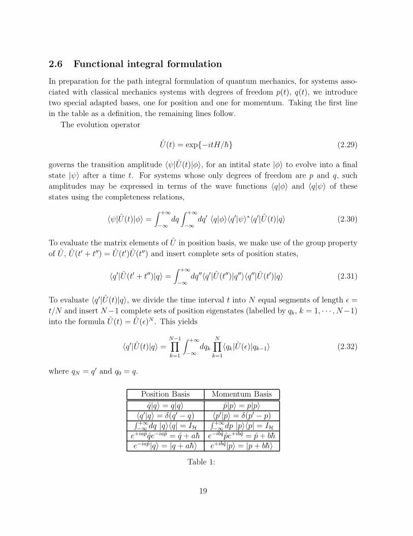
2.6 Functional integral formulation
In preparation for the path integral formulation of quantum mechanics, for systems asso-
ciated with classical mechanics systems with degrees of freedom p(t), q(t), we introduce
two special adapted bases, one for position and one for momentum. Taking the first line
in the table as a definition, the remaining lines follow.
The evolution operator
U(t) = exp{−itH/h} (2.29)
governs the transition amplitude 〈ψ|U(t)|φ〉, for an intital state |φ〉 to evolve into a final
state |ψ〉 after a time t. For systems whose only degrees of freedom are p and q, such
amplitudes may be expressed in terms of the wave functions 〈q|φ〉 and 〈q|ψ〉 of these
states using the completeness relations,
〈ψ|U(t)|φ〉 =∫ +∞
−∞dq∫ +∞
−∞dq′ 〈q|φ〉〈q′|ψ〉∗〈q′|U(t)|q〉 (2.30)
To evaluate the matrix elements of U in position basis, we make use of the group property
of U , U(t′ + t′′) = U(t′)U(t′′) and insert complete sets of position states,
〈q′|U(t′ + t′′)|q〉 =∫ +∞
−∞dq′′〈q′|U(t′′)|q′′〉〈q′′|U(t′)|q〉 (2.31)
To evaluate 〈q′|U(t)|q〉, we divide the time interval t into N equal segments of length ε =
t/N and insert N−1 complete sets of position eigenstates (labelled by qk, k = 1, · · · , N−1)
into the formula U(t) = U(ε)N . This yields
〈q′|U(t)|q〉 =N−1∏
k=1
∫ +∞
−∞dqk
N∏
k=1
〈qk|U(ε)|qk−1〉 (2.32)
where qN = q′ and q0 = q.
Position Basis Momentum Basis
q|q〉 = q|q〉 p|p〉 = p|p〉〈q′|q〉 = δ(q′ − q) 〈p′|p〉 = δ(p′ − p)∫+∞−∞ dq |q〉〈q| = IH
∫+∞−∞ dp |p〉〈p| = IH
e+iapqe−iap = q + ah e−ibq pe+ibq = p+ bhe−iap|q〉 = |q + ah〉 e+ibq|p〉 = |p+ bh〉
Table 1:
19
Each matrix element 〈qk|U(ε)|qk−1〉 may in turn be evaluated as follows. First, we
insert a complete set of states in the momentum basis (labelled by pk, k = 1, · · · , N)
〈qk|U(ε)|qk−1〉 =∫ +∞
−∞dpk〈qk|U(ε)|pk〉〈pk|qk−1〉 (2.33)
Using the overlaps of position and momentum eigenstates, we have
〈qk|pk〉 = e+ipkqk/h 〈pk|qk−1〉 = e−ipkqk−1/h (2.34)
The reason for introducing also the basis of momentum eigenstates is that now the needed
matrix elements of the quantum Hamiltonian H(p, q) can be evaluated.
In the limit N → ∞, we have ε→ 0 and thus the evolution operator over the infinites-
imal time span ε may be evaluated by expanding the exponential to first order only,
U(ε) = IH − iε
hH + O(ε2) (2.35)
We assume that H is analytic in p and q, so that upon using the commutation relation
[p, q] = −ih, we may rearrange H so as to put all p to the right and all q to the left in any
given monomial. This allows us to define a classical function H(p, q) by
H(pk, qk) ≡ 〈qk|H(p, q)|pk〉 (2.36)
and therefore, we have
〈qk|U(ε)|pk〉 = e−iεH(pk,qk)/h〈qk|pk〉 (2.37)
Assembling all results, we now find the following expression,
〈q′|U(t)|q〉 = limN→∞
N−1∏
k=1
∫ +∞
−∞dqk
N∏
l=1
∫ +∞
−∞dpl
N∏
m=1
eiSk(p,q)/h (2.38)
where
Sk(p, q) ≡ pk(qk − qk−1) − εH(pk, qk) (2.39)
In the limit N → ∞, for t fixed, the label k on pk and qk becomes continuous,
pk → p(t′) t′ = kε = kt/N, ε = dt′
qk → q(t′)
Sk(p, q) → dt′(
p(t′)q(t′) −H(p(t′), q(t′)))
(2.40)
20
As a result, the product of exponentials converges as follows
limN→∞
N∏
m=1
eiSk(p,q)/h = exp{i
h
∫ t
0dt′(
pq −H(p, q))
(t′)}
(2.41)
The measure “converges” to a random walk measure, which is denoted as follows,
limN→∞
N−1∏
k=1
∫ +∞
−∞dqk
N∏
l=1
∫ +∞
−∞dpl =
∫
Dq∫
Dp (2.42)
The final result is the path integral formulation of quantum mechanics, which gives an
expression for the position basis matrix elements of the evolution operator,
〈q′|U(t)|q〉 =∫
Dq∫
Dp exp{i
h
∫ t
0dt′(
pq −H(p, q))
(t′)}
(2.43)
with the boundary conditions that q(t′ = 0) = q and q(t′ = t) = q′. This formulation was
first proposed by Dirac and rederived by Feynman.
The quantity that enters the exponential in the path integral is really the classical
action of the system,
S[p, q] ≡∫
dt′(
pq −H(p, q))
(t′) (2.44)
Therefore, in the classical limit where one formally takes the limit h→ 0, the part integral
will be dominated by the stationnary or saddle points of the integral, which are defined
as those points at which the first order (functional derivatives of S[p, q] with respect to p
and q vanish. It is easy to work out what these equations are
0 =δS
δq= −p− ∂H
∂q
0 =δS
δp= +q − ∂H
∂p(2.45)
These are precisely the Hamilton equations of the classical Hamiltonian H . Thus, we
recover very easily in the path integral formulation that in the classical limit, quantum
mechanics receives its dominant contribution from classical solutions, as expected.
21
3 Principles of Relativistic Quantum Field Theory
The laws of quantum mechanics need to be supplemented with the principle of relativity.
We shall ignore gravity and thus general relativity throughout and assume that space-time
is flat Minkowski space-time.† The principle of relativity is then that of special relativity,
which states that in flat Minkowski space-time, the laws of physics are invariant under the
Poincare group. Recall that the Poincare group is the (semi-direct) product of the group
of translations R4 and the Lorentz group SO(1, 3),
ISO(1, 3) ≡ R4�< SO(1, 3) (3.1)
Quantum field theory is a quantum system, so we have the same definitions of states in
Hilbert space and of self-adjoint operators corresponding to observables. In addition, the
requirements that these states and operators transform consistently under the Poincare
group need to be implemented. In brief,
• The states and observables in Hilbert space will transform under unitary represen-
tations of the Poincare group.
• The fields in QFT are local observables and transform under unitary representations
of the Poincare group, which induce finite dimensional representations of the Lorentz
group on the components of the field.
• Micro-causality requires that any two local fields evaluated at points that are space-
like separated are causally unrelated and thus must commute (or anti-commute for
fermions) with one another.
Before making these principles quantitative, it is helpful to review the definitions and
properties of the Poincare and Lorentz groups and to discuss the unitary representations of
the Poincare group as well as the finite-dimensional representations of the Lorentz group.
†Henceforth, we shall work in units where c = h = 1.
22
3.1 The Lorentz and Poincare groups and algebras
In special relativity the speed of light as observed from different inertial frames is the
same, c. Inertial frames are related to one another by Poincare transformations, which in
turn may be defined as the transformations that leave the Minkowski distance between
two points invariant.‡ This distance is defined by
s2 ≡ (x0 − y0)2 − (~x− ~y)2 ≡ ηµν(xµ − yµ)(xν − yν) (3.2)
where the Minkowski metric tensor is given by
ηµν ≡ diag [1 − 1 − 1 − 1] (3.3)
Clearly, the Minkowski distance is invariant under translations by aµ and Lorentz trans-
formations by Λµν ,
R(Λ, a){xµ → x′µ = Λµ
νxν + aµ
yµ → y′µ = Λµνy
ν + aµ(3.4)
where the Lorentz transformation matrix must satisfy
ΛµρηµνΛ
νσ = ηρσ ⇔ ΛTηΛ = η ⇔ (Λ−1)µ
ν = Λνµ (3.5)
The above transformation laws form the Poincare group under the multiplication law,
R(Λ1, a1)R(Λ2, a2) = R(Λ1Λ2, a1 + Λ1a2) (3.6)
Special cases include,
1. a = 0 yields the Lorentz group, which is a subgroup of the Poincare group. The
definition (3.5) is analogous to that of an orthogonal matrix, M tIM = I; for this
reason the Lorentz group is denoted by O(1, 3).
2. A further special case of the Lorentz group is formed by the subgroup of rotations,
characterized by Λ00 = 1,Λ0
i = Λi0 = 0. Boosts do not by themselves form a
subgroup; a boost in the direction 1 leaves x′2,3 = x2,3 and
x′0
= +x0chτ − x1shτ
x′1
= −x0shτ + x1chτ chτ =√
1 − v2 (3.7)
‡Time and space coordinates are denoted by t and xi, i = 1, 2, 3 respectively. Space coordinates areoften regrouped in a 3-vector ~x, while it will be convenient to measure time in distances, using the speedof light constant c via the relation x0 ≡ ct. All four coordinates may then be conveniently regrouped intoa 4-vector xµ, µ = 0, 1, 2, 3. Throughout, we adopt the Einstein convention in which repeated upper andlower indices are summed over and the summation symbol is implicit.
23
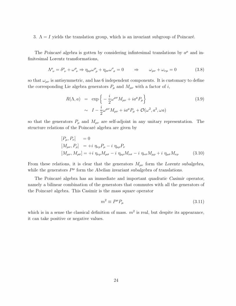
3. Λ = I yields the translation group, which is an invariant subgroup of Poincare.
The Poincare algebra is gotten by considering infintesimal translations by aµ and in-
finitesimal Lorentz transformations,
Λµν = δµν + ωµν ⇒ ηµρω
µρ + ηρνω
νσ = 0 ⇒ ωµν + ωνµ = 0 (3.8)
so that ωµν is antisymmetric, and has 6 independent components. It is customary to define
the corresponding Lie algebra generators Pµ and Mµν with a factor of i,
R(Λ, a) = exp{
− i
2ωµνMµν + iaµPµ
}
(3.9)
∼ I − i
2ωµνMµν + iaµPµ + O(ω2, a2, ωa)
so that the generators Pµ and Mµν are self-adjoint in any unitary representation. The
structure relations of the Poincare algebra are given by
[Pµ, Pν] = 0
[Mµν , Pρ] = +i ηνρPµ − i ηµρPν
[Mµν ,Mρσ] = +i ηνρMµσ − i ηµρMνσ − i ηνσMµρ + i ηµσMνρ (3.10)
From these relations, it is clear that the generators Mµν form the Lorentz subalgebra,
while the generators P µ form the Abelian invariant subalgebra of translations.
The Poincare algebra has an immediate and important quadratic Casimir operator,
namely a bilinear combination of the generators that commutes with all the generators of
the Poincare algebra. This Casimir is the mass square operator
m2 ≡ P µPµ (3.11)
which is in a sense the classical definition of mass. m2 is real, but despite its appearance,
it can take positive or negative values.
24
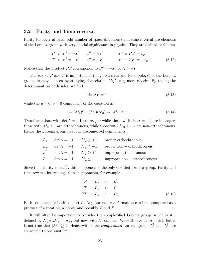
3.2 Parity and Time reversal
Parity (or reversal of an odd number of space directions) and time reversal are elements
of the Lorentz group with very special significance in physics. They are defined as follows,
P : x′0
= +x0 x′i= −xi x′
µ ≡ Pxµ = xµ
T : x′0
= −x0 x′i= +xi x′
µ ≡ Txµ = −xµ (3.12)
Notice that the product PT corresponds to x′µ = −xµ or Λ = −I.The role of P and T is important in the global structure (or topology) of the Lorentz
group, as may be seen by studying the relation ΛtηΛ = η more closely. By taking the
determinant on both sides, we find,
(det Λ)2 = 1 (3.13)
while the µ = 0, ν = 0 component of the equation is
1 = (Λ00)
2 − (Λi0)(Λ
i0) ⇒ |Λ0
0| ≥ 1 (3.14)
Transformations with det Λ = +1 are proper while those with det Λ = −1 are improper;
those with Λ00 ≥ 1 are orthochronous, while those with Λ0
0 ≤ −1 are non-orthochronous.
Hence the Lorentz group has four disconnected components.
L↑+ det Λ = +1 Λoo ≥ +1 proper orthochronous
L↓+ det Λ = +1 Λoo ≤ −1 proper non − orthochronous
L↑− det Λ = −1 Λoo ≥ +1 improper orthochronous
L↓− det Λ = −1 Λoo ≤ −1 improper non − orthochronous
Since the identity is in L↑+, this component is the only one that forms a group. Parity and
time reversal interchange these components, for example
P : L↑+ ↔ L↑−
T : L↑+ ↔ L↓−
PT : L↑+ ↔ L↓+ (3.15)
Each component is itself connected. Any Lorentz transformation can be decomposed as a
product of a rotation, a boost, and possibly T and P .
It will often be important to consider the complexified Lorentz group, which is still
defined by ΛµρηµνΛ
νσ = ηρσ, but now with Λ complex. We still have det Λ = ±1, but it
is not true that |Λoo| ≥ 1. Hence within the complexified Lorentz group, L↑+ and L↓+ are
connected to one another.
25
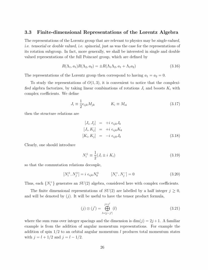
3.3 Finite-dimensional Representations of the Lorentz Algebra
The representations of the Lorentz group that are relevant to physics may be single-valued,
i.e. tensorial or double valued, i.e. spinorial, just as was the case for the representations of
its rotation subgroup. In fact, more generally, we shall be interested in single and double
valued representations of the full Poincare group, which are defined by
R(Λ1, a1)R(Λ2, a2) = ±R(Λ1Λ2, a1 + Λ1a2) (3.16)
The representations of the Lorentz group then correspond to having a1 = a2 = 0.
To study the representations of O(1, 3), it is convenient to notice that the complexi-
fied algebra factorizes, by taking linear combinations of rotations Ji and boosts Ki with
complex coefficients. We define
Ji ≡1
2εijkMjk Ki ≡Moi (3.17)
then the structure relations are
[Ji, Jj] = +i εijkJk
[Ji, Kj] = +i εijkKk
[Ki, Kj] = −i εijkJk (3.18)
Clearly, one should introduce
N±i ≡ 1
2(Ji ± i Ki) (3.19)
so that the commutation relations decouple,
[N±i , N±j ] = i εijkN
±k [N+
i , N−j ] = 0 (3.20)
Thus, each {N+i } generates an SU(2) algebra, considered here with complex coefficients.
The finite dimensional representations of SU(2) are labelled by a half integer j ≥ 0,
and will be denoted by (j). It will be useful to have the tensor product formula,
(j) ⊗ (j′) =j+j′⊕
l=|j−j′|
(l) (3.21)
where the sum runs over integer spacings and the dimension is dim(j) = 2j+1. A familiar
example is from the addition of angular momentum representations. For example the
addition of spin 1/2 to an orbital angular momentum l produces total momentum states
with j = l + 1/2 and j = l − 1/2.
26
The representation theory of the complexified Lorentz algebra is obtained as the prod-
uct of the representations of both SU(2) factors, each of which may be described by the
eigenvalue of the corresponding Casimir operator,
N+i N
+i j+(j+ + 1)
N−i N−i j−(j− + 1) j± = 0,
1
2, 1,
3
2, 2, · · · (3.22)
Thus, the finite-dimensional irreducible representations of O(1, 3) are labelled by (j+, j−).
Since J3 = N+3 +N−3 , the highest weight vector of the corresponding rotation group is just
the sum j+ + j−, which should be thought of as the spin of the representation. Complex
conjugation and parity have the same action on these representations,
(j+, j−)∗ = (j−, j+)
P (j+, j−)∗ = (j−, j+) (3.23)
and thus only the representations (j, j) or the reducible representations (j+, j−)⊕ (j−, j+)
can be real – the others are necessarily complex.
Some fundamental examples
1. (0, 0) with spin zero is the scalar; Its parity may be even orodd (scalar-pseudoscalar)
2. (12, 0) is the spin 1
2left-handed Weyl 2-component spinor (and (0, 1
2)) is the right-
handed Weyl 2-component spinor). Both are complex, and transform into one an-
other under complex and parity conjugation.
3. (12, 0) ⊕ (0, 1
2) is the Dirac spinor when the left and right spinors are independent;
it is the Majorana spinor when the left and right spinors are complex conjugates of
one another, so that the Majorana spinor is a real spinor.
4. Tensor products of the Weyl spinors yield higher (j+, j−) representations.
5. (12, 1
2) = (1
2, 0)⊗ (0, 1
2) with spin 1 and 4 components is a 4-vector, such as the E&M
gauge potential and the momentum Pµ.
6. (1, 0)⊕ (0, 1) with spin 1, is a real representation under which rank 2 antisymmetric
tensors transform. Examples are the E& M field strength tensor Fµν = −Fνµ, as
well as Mµν themselves.
7. (1, 0) (resp. (0, 1)) with spin 1 and 3 complex components is the so-called self-
dual (resp. anti self-dual) antisymmetric rank 2-tensor. To construct it in terms of
27
tensors, one defines the dual by
Fµν ≡1
2εµνρσF
ρσ ε0123 = −ε0123 = 1 (3.24)
Since ˜Fµν = −Fµν , the eigenvalues of˜are ±i, and the eigenvectors are
F±µν ≡1
2(Fµν ± iFµν) F±µν = ∓iF±µν (3.25)
The self-dual F+ corresponds to the representation (1, 0) (and the anti self-dual F−
to (0, 1). Notice that the presence of i in the definition of the dual, and therefore of
F± forces these representations to be complex. In particular N+i and N−i correspond
to the self-dual and anti self-dual part of Mµν . The precise relations are,
M±0j = ∓ i
2εjklM
±kl = ∓iN±j (3.26)
8. (1, 1) of spin 2 corresponds to the symmetric traceless rank 2 tensor, i.e. the graviton.
9. Generalizing ordinary orbital angular momentum to include time yields another rep-
resentation of the Lorentz algebra on functions of the coordinates xµ,
Lµν ≡ i(xµ∂ν − xν∂µ) ∂µ ≡ ∂
∂xµ≡(
∂
∂t, ~∇
)
(3.27)
A further generalization is to representations that include spin;
Mµν ≡ Lµν + Sµν (3.28)
where the spin representation Sµν satisfies the Lorentz structure relations by itself,
while Sµν commutes with Pµ and Lµν . Supplementing this algebra with Pµ = i∂µyields a representation of the full Poincare algebra.
28
3.4 Unitary Representations of the Poincare Algebra
Next, the unitary representations of the Poincare algebra are reviewed and constructed.
Recall the structure relations of the algebra,
[Pµ, Pν ] = 0
[Mµν , Pρ] = +iηνρPµ − iηµρPν
[Mµν ,Mρσ] = +iηνρMµσ − iηµρMνσ − iηνσMµρ + iηµσMνρ (3.29)
In any unitary representation, the generators M and P will have to be realized as self-
adjoint operators. Constructing the representations of the Poincare algebra is a bit more
tricky than those of the Lorentz algebra, because the Lorentz algebra is semi-simple, but
the Poincare algebra has the Abelian invariant subalgebra of translations, and is therefore
not semi-simple.
What are its representations? The Casimirs of the Lorentz algebra NiNi and N+i N
+i
do not commutue with Pµ any longer. However, PµPµ is a relativistic invariant, and hence
a Casimir of Poincare. If we can find another 4-vector that commute with all P ’s, its
square will also be a Casimir. The Pauli-Lubanski vector is defined by
W µ ≡ 1
2εµνρσPνMρσ (3.30)
It commutes with momentum, [W µ, P ν] = 0 and its square W µWµ commutes with the
entire Poincare algebra and is therefore a (quartic) Casimir operator for the Poincare
algebra. Now remember that the most general expression for Mµν was
Mµν = xµPν − xνPµ + Sµν (3.31)
so that the angular momentum part cancels out and we are left with
W µ =1
2εµνρσPνSρσ (3.32)
The Casimirs of the Poincare group are thus PµPµ and WµW
µ, and the states will be
labelled by Pµ and W 3. Wµ generates an SU(2) type algebra for fixed Pµ:
[W µ,W ν] = i εµναβPαWβ (3.33)
which is the so-called little group. The basic idea is to fix P µ and then to obtain the
representations of the little group.
29
• One-particle state representations
We apply the method above to the construction of the (unitary) one-particle state
representations, which are the most basic building blocks of the Hilbert space of a QFT.
We choose to diagonalize the components of the momentum operator Pµ since they mutualy
commute and commute with the mass operator m2 = P µPµ. We denote the eigenstates by
|p, ı〉, where pµ denotes the eigenvalues of the operator Pµ and the label i specifies whatever
remaining quantum numbers,
Pµ|p, i〉 = pµ|p, i〉 (3.34)
One defines a one particle state as a representation in which the range of the label i is
discrete. If one superimposes two one particle states, the index would include relative
momenta, and this index would be continuous. At fixed M2, the range of i is finite, both
in QFT and in string theory.
To obtain the action of the Lorentz group, we proceed as follows. First, we list the
transformations of the Poincare generators under Poincare transformations,
U(Λ, a)MµνU(Λ, a)−1 = (Λ−1)µα(Λ−1)ν
β(Mαβ − aαPβ + aβPα)
U(Λ, a)PµU(Λ, a)−1 = (Λ−1)µαPα (3.35)
Applying these relations to one particle states, one establishes that the state U(Λ, 0)|p, i〉indeed has momentum Λp, as expected, P µU(Λ, 0)|p, i〉 = Λµ
νpνU(Λ, 0)|p, i〉, and therefore
may be decomposed onto such states,
U(Λ, 0)|p, i〉 =∑
j
Ci,j(Λ, p)|Λp, j〉 (3.36)
To find this action and understand it, we specify a reference momentum kµ, for given M2,
so that pµ is a Lorentz transform of kµ,
pµ = Lµρ(p)kρ k2 = m2 (3.37)
Thus, the states |p, i〉 may then be reconstructed as follows,
|p, i〉 = U(L(p), 0)|k, i〉 (3.38)
Once this construction has been effected, the action of general Lorentz transformations
may be obtained as follows,
U(Λ, 0)|p, i〉 = U(Λ, 0)U(L(p), 0)|k, i〉= U(L(Λp), 0)U(W, 0)|k, i〉 (3.39)
30
Defining now the composite transformation
U(W, 0) = U(L(Λp), 0)−1U(λ, 0)U(L(p), 0) (3.40)
which represents the composite Lorentz transformation W ,
W = L(λ(p))−1ΛL(p)
Wk = L(Λp)−1ΛL(p)k = L(Λp)−1Λp = k (3.41)
Therefore, W leaves the reference momentum kµ invariant. The group of all such trans-
formations is the little group. Thus, given the reference momentum k, the unitary repre-
sentation of the one particle state is classified by the representation of the little group.
1. P µPµ = m2 > 0 : These are the massive particle states; kµ = (m, 0, 0, 0).
It follows from the explicit form of W µ that W µWµ = −m2~S2 = −m2s(s+1), where
s is the spin of the representation of the little group, and it takes the usual values
s = 0,1
2, 1, . . . (3.42)
2. PµPµ = 0 : These are the massless particle states; kµ = (κ, κ, 0, 0).
It follows from the explicit form of W µ that WµWµ = 0. Since we also have PµW
µ =
0, it follows that ~W · ~P = ±| ~W ||~P | and hence the vectors ~W and ~P must be colinear,~W = λ~P and thus
W µ = λP µ (3.43)
Again, using the explicit form of W µ, we have W 0 = PiSi = λP 0 and we see that λ
is the projection of spin onto momentum, i.e. helicity which takes values,
λ = 0,±1
2,±1, . . . (3.44)
Hence any massless particles of s 6= 0 has 2 degrees of freedom, photon ±1, neutrino
±12, graviton ±2.
3. P µPµ < 0 : These are the tachyonic particle states; kµ = (0, m, 0, 0).
These representations are unitary, and are acceptable as free particles. As soon as
interactions are turned on, however, they cause problems with micro-causality and
it is generally believed that tachyons are unacceptable in physical theories.
Note that all these unitary representations are infinite dimensional (except for the triv-
ial representation). Then there are of course also all the non-unitary representations, which
we do not consider here. A standard reference is E.P. Wigner, “Unitary Representations
of the Inhomogeneous Lorentz Group,” Ann. Math. 40 (1939) 149.
31

3.5 The basic principles of quantum field theory
A summary is presented of the fundamental principles of relativistic quantum field theory.
By analogy with quantum mechanics, these principles do not refer to any specific dynamics
(except for the fact that the dynamics is invariant under Poincare symmetry). Thus, the
principles generalize those of quantum mechanics to include the principles of relativity.
1. States of QFT are vectors in a Hilbert space H.
2. States transform under unitary representations of the Poincare group, which will be
denoted by U(Λ, a),
|state〉 → |state′〉 = U(Λ, a)|state〉 (3.45)
3. There exists a unique ground state (the vacuum), usually denoted by |0〉, which is
the singlet representation of the Poincare group,
U(Λ, a)|0〉 = |0〉 (3.46)
4. The fundamental observables in QFT are local quantum fields, which are space-
time dependent self-adjoint operators on H. They are generically denoted by φj(x);
specific notations for the fields most relevant for physics will be introduced later.§
5. Throughout, the number n of independent fields φj(x), j = 1, · · · , n will be assumed
to be FINITE. Generalizations with infinite numbers of fields can be constructed (for
example string theory), but only at the cost of severe complications, which usually
go outside the framework of standard QFT.
6. Poincare transformations on the fields are realized unitarily in H, as follows,
φ′j(x) ≡ U(Λ, a)φj(x)U(Λ, a)† =n∑
k=1
Sjk(Λ−1)φk(Λx+ a) (3.47)
Since the number of fields is assumed finite, S(Λ−1) must be a finite-dimensional
representation of the Lorentz group. Except for the trivial one, such representations
are always non-unitary. An important special case of this relation is when Λ = 1,
§Note that the operators or observables are thus time-dependent, and the states will be time-independent. This formulation is usually referred to as the Heisenberg formulation of quantum mechanics,as opposed to the Schrodinger formulation in which observables are time-independent but states are time-dependent.
32
which yields the behavior of observables under translations (this includes under time-
translation, namely dynamics),
φ′j(x) ≡ e−iaµPµφj(x)e
iaµPµ = φj(x+ a) (3.48)
since U(I, a) = exp{−iaµPµ}. The transformation law when Λ 6= I will be examined
in greater detail later.
7. Microscopic Causality or local commutativity states that any two observables φJ and
φk that have no mutual causal contact must be simultaneously observable and must
therefore commute with one another,¶
[φj(xµ), φk(y
µ)] = 0 if (x− y)2 < 0 (3.49)
Classically, as no relativistic signal can connect these two observables, it should
better be possible to assign independent initial data. Quantum mechanically, it
should be possible to measure them simultaneously to arbitrary precision and this
independently at xµ and yµ.
8. There is a relation between states in H and fields. From the fields in QFT, it is
possible to build up the Hilbert space. The simplest states (besides the vacuum)
in Hilbert space are the 1-particle states, denoted by |p, i〉. For every 1-particle
species i, there must be a corresponding field φi(x) that produces this species from
the vacuum state,
〈0|φi(x)|p, i〉 6= 0 (3.50)
9. Symmetries other than the Poincare group will be realized by unitary transformations
on Hilbert space which induce finite-dimensional transformations on the fields,
φ′j(x) ≡ U(g)φj(x)U(g)† =∑
k
S(g−1)jkφk(gx) (3.51)
When g has no action on x, namely gx = x, the transformations generate internal
symmetries; examples are flavor, color, isospin etc. On the other hand, if gx 6 x, the
transformations generate space-time symmetries; examples are Poincare invariance,
scale and conformal symmetries, parity, supersymmetry. Time-reversal is realized by
an anti-unitary transformation.
¶Fermionic fields will anti-commute.
33
3.6 Transformation of Local Fields under the Lorentz Group
Fields may be distinguished by the different finite-dimensional representations of the
Lorentz group S(Λ−1) under which they transform. It is convenient to decompose these
representations into a direct sum of irreducible representations, whose study we now initi-
ate. We apply the results of §3.3 to the general transformation rule of (3.47), specialized
to Lorentz transformations. It is convenient to let Λ → Λ−1 and x → Λx, so that
φ′j(x′) =
n∑
k=1
Sjk(Λ)φk(x) x′ = Λx (3.52)
When the transformation is continuous (we shall treat Parity and Time-reversal separately)
we may describe the transformation infinitesimally,
Λµν = δµν + ωµν + O(ω2)
φ′j(x) = φj(x) + δφj(x) + O(ω2)
S(I + ω) = I − i
2ωµνSµν + O(ω2) (3.53)
Combining these ingredients to compute δφj, we find
φ(x) + δxµ∂µφ(x) + δφ(x) = φ(x) − i
2ωµνSµνφ(x) + O(ω2) (3.54)
whence the transformation law naturally involves the total Lorentz generator L+ S,
δφ(x) = − i
2ωµν(Lµν + Sµν)φ(x) (3.55)
1. The scalar field
The scalar has spin 0, corresponding to the representation (0, 0) in the notation of §3.3.
Thus, φ′(Λx) = φ(x) for all Lorentz transformations in L↑+. Infinitesimally, we have
δφ(x) = − i
2ωµνLµνφ(x) (3.56)
All irreducible representations are 1-dimensional; a single scalar field is denoted by φ.
2. The vector field
Vector fields are generally denoted by Aµ, such as for example the electro-magnetic
potential. The transformation law of a vector field is
A′µ(x′) = Λµ
νAν(x) (3.57)
34
which corresponds to the following infinitesimal transformation law,
δAµ(x) = A′µ(x) − Aµ(x) = − i
2ωρσLρσAµ(x) + ωµ
νAν(x) (3.58)
(Using the transformation law for a scalar φ, it is easily checked that the derivative of a
scalar ∂µφ transforms as a vector with the above transformation law.) The explicit form
of the vector representation matrices may be deduced from this formula,
(Sµν)αβ = i ηµαδν
β − i ηναδµβ (3.59)
which is characteristic of the(
12, 1
2
)
representation of the Lorentz group.
3. General tensor representations
These representations may be built up by taking the tensor product of vector repre-
sentations using the tensor product formula,
(j+, j−) ⊗ (j′+, j′−) =
j±+j′±∑
s±=|j±−j′±|
(s+, s−) (3.60)
The spins s = s+ + s− are all integer. A rank n tensor Bµ1···µn transforms as
B′µ1···µn(Λx) = Λµ1
ν1 · · ·Λµn
νsBν1···νn(x) (3.61)
It is consistent with Lorentz transformations to symmetrize, anti-symmetrize or take the
trace of tensor fields. For totally symmetric tensor, the spin and the rank coincide, n = s,
but upon anti-symmetrization, n > s in general. The representation (1, 1) corresponds to
the graviton. Fields of spin higher than 2 will never be needed in QFT, and in fact we
shall always specialize to fields of spin ≤ 1.
4. The Dirac spinor field
The Dirac field, usually denoted ψ(x), is a 4-component complex column matrix, whose
transformation law is defined to be
U(Λ, a)ψ(x)U(Λ, a)† = S(Λ−1)ψ(Λx+ a) (3.62)
where S(Λ) = R(Λ, 0) is the spinor representation characterized by (12, 0) ⊕ (0, 1
2) in the
classification of Lorentz representations. To obtain an explicit construction of S(Λ), we
proceed as follows.
35
First, recall that the 2-dimensional spinor representation of the rotation group is re-
alized in terms of the 2 × 2 Pauli matrices, σi, i = 1, 2, 3, defined to satisfy the relation‖
{σi, σj} = 2δij . It is conventional to take the following basis,
σ1 =(
0 11 0
)
σ2 =(
0 −ii 0
)
σ3 =(
1 00 −1
)
(3.63)
The representation generators are Si = σi/2, and satisfy the standard rotation algebra
relations [Si, Sj] = iεijkSk.
The spinor representations of the Lorentz algebra are realized analogously in terms of
the 4 × 4 Dirac matrices γµ, defined to satisfy the Clifford-Dirac algebra,
{γµ, γν} = 2ηµν (3.64)
The 4-dimensional Dirac spinor representation is defined by the following generators,
Sµν ≡i
4[γµ, γν ] (3.65)
which satisfy the Lorentz algebra
[Sµν , Sρσ] = +i ηνρSµσ − i ηµρSνσ − i ηνσSµρ + i ηµσSνρ (3.66)
This may be verified by making use of the Clifford-Dirac algebra relations only.
As for any representation of the Lorentz group, (3.35) holds, which in this case may
be expressed as
S(Λ)SµνS(Λ)−1 = (Λ−1)µα(Λ−1)ν
βSαβ (3.67)
Furthermore, from the relation
[Sµν , γρ] = i ηνργµ − i ηµργν (3.68)
it follows that S(Λ)γµS(Λ)−1 = (Λ−1)µνγν or simply that the γµ matrices are invariant,
provided both its “vector” and “spinor” indices are transformed,
ΛµνS(Λ)γνS(Λ)−1 = γµ (3.69)
The γ-matrices are the Clebsch-Gordon coefficients for the tensor product of two Dirac
representations onto the vector representation.
‖{A, B} ≡ AB + BA is defined to be the anti-commutator of A and B.
36
The Dirac spinor representation is reducible, as may be seen from the existence of the
chirality matrix γ5 = γ5, which is defined by
γ5 = γ5 =i
4!εµνρσγ
µγνγργσ = iγ0γ1γ2γ3 (3.70)
Clearly, we have (γ5)2 = I and tr(γ5) = 0, so that γ5 is not proportional to the identity
matrix. The matrix γ5 anti-commutes with all γµ and therefore γ5 commutes with Sµν ,
{γ5, γµ} = [γ5, Sµν ] = 0 (3.71)
Thus, by Shur’s lemma, the representation S is reducible, since its generators commute
with a matrix γ5 that is not proportional to the identity matrix. (Notice that the γµ
matrices do form an irreducible representation of the Clifford algebra.)
A basis for all 4 × 4 matrices is given by the following set
I, γµ, γµν , γµνρ, γµνρσ (3.72)
where γµ1···µn is the product γµ1 · · · γµn , completely antisymmetrized in its n indices. Some
of these combinations may be reexpressed in terms of already familiar quantities,
γµν = −2i Sµν
γµνρ = −i εµνρσγ5γσ
γµνρσ = −i εµνρσγ5 (3.73)
5. The Weyl spinor fields
The irreducible components of the Dirac representation are a - chirality or left Weyl
spinor (12, 0) and an independent + chirality or right Weyl spinor (0, 1
2), corresponding to
the −1 and +1 eigenvalues of the chirality matrix γ5. In a chiral basis where γ5 is diagonal,
we have the following convenient representation of the γ-matrices,
γ5 =(−I2 0
0 +I2
)
γµ =(
0 σµ
σµ 0
)
(3.74)
where I2 is the identity matrix in 2 dimensions, and
σµ = (I2, σi) σµ = (I2,−σi) (3.75)
The Dirac representation matrices S(Λ) as well as the Dirac field ψ(x) decompose into the
Weyl spinor representation matrices SL(Λ) and SR(Λ) and the Weyl spinor fields ψL(x)
37
and ψR(x) as follows,
S(Λ) =(SL(Λ) 0
0 SR(Λ)
)
ψ(x) =(ψL(x)ψR(x)
)
(3.76)
where the Weyl representation matrices are given by
SL(Λ) = exp{
− i
2(ω+)µνM+
µν
}
= exp{i
2~σ · (~ω + i~ν)
}
SR(Λ) = exp{
− i
2(ω−)µνM−µν
}
= exp{i
2~σ · (~ω − i~ν)
}
(3.77)
Here, ω± and M± are the self-dual and anti self-dual parts of ω and M respectively, and
~ω and ~ν are real 3-vectors representing rotations and boosts respectively.
6. Equivalent representations
If Sµν in the Dirac representation satisfies the structure relations of the Lorentz algebra,
then transposition and complex conjugation automatically also produce representations of
the same dimensions, with matrices −Stµν and −S∗µν . These representations must be equiv-
alent to the Dirac representation and hence related by conjugation. These conjugations
reflect the discrete symmetries C and P (to be discussed shortly),
C − Stµν = C−1SµνC
P − S∗µν = B−1SµνB (3.78)
7. The Majorana spinor field
A Majorana spinor corresponds to a real representation (12, 0) ⊕ (0, 1
2) where the two
Weyl spinors are complex conjugates of one another. Complex conjugation by itself de-
pends upon the basis chosen, but charge conjugation, to be defined in the subsequent
subsection, is a Lorentz invariant operation. Thus, the proper requirement for a spinor to
be “real” is provided by the Majorana spinor field condition,
ψc(x) = ψ(x) (ψc(x))c = ψ(x) (3.79)
A Majorana spinor is equivalent to its left field component (or its right field component).
8. The spin 3/2 field
Spin 32
can be either(
32, 0)
or(
12, 1)
and their charge conjugates. Only the latter is
physically significant. It can be gotten from(
1
2,1
2
)
⊗(
1
2, 0)
=(
1,1
2
)
⊕(
0,1
2
)
(3.80)
The Rarita-Schwinger field ψµ precisely corresponds to the above representation plus its
complex conjugate. To project out the purely spin (1, 1/2) ⊕ (1/2, 1) part, the γ-trace
must be removed which may be achieved by suplementary condition γµψµ = 0.
38
3.7 Discrete Symmetries
We group together here the transformations under the discrete symmetries P, T and
charge conjugation C of the basic fields.
3.7.1 Parity
One distinguishes two types of scalars under parity
Pφ(x)P† = +φ(Px) scalar
Pφ(x)P† = −φ(Px) pseudo − scalar (3.81)
This distinction is important as the particles π± and π0 are for example pseudo-scalars,
while the He4 nucleus is a scalar. One also distinguished two types of vectors under parity,
PAµ(x)P† = +Aµ(Px) vector
PAµ(x)P† = −Aµ(Px) axial vector (3.82)
Again, this distinction is very important; the weak interactions are mediated by a super-
position of a vector and an axial vector. Finally, under parity, the Dirac spinor transforms
as follows,
Pψ(x)P† = eiθP γ0ψ(x) (3.83)
which amounts to an interchange of left and right spinor components, and θP is an arbitrary
angle. (Note that a theory invariant under parity will have to contain both left and right
spinors of each species.)
3.7.2 Time reversal
Time reversal symmetry is the only case which cannot be realized by a unitary transfor-
mation in Hilbert space; instead it is realized by an anti-unitary transformation T , which
has the property of changing the sign of the number i,
T i = −iT (3.84)
Its action on the scalar, vector and Dirac sprinor is given by
T φ(x)T † = φ(Tx)
T Aµ(x)T † = −Aµ(Tx)T ψ(x)T † = iCγ5ψ(Tx) (3.85)
39
3.7.3 Charge Conjugation
From the simple relation (σi)∗ = −σ2σiσ2, it follows that
SL(Λ)∗ = σ2SR(Λ)σ2 (3.86)
As a result, the charge conjugates ψcL,R of ψL,R, defined by
CψL(x)C† = ψcL(x) ≡ −σ2ψ∗L(x)
CψR(x)C† = ψcR(x) ≡ +σ2ψ∗R(x) (3.87)
transforms under SR(Λ) and SL(Λ) respectively.
Charge conjugation as defined above, was formulated in a specific basis of σ-matrices,
which is why σ2 played a special role. It is possible to produce a basis independent
definition of charge conjugation as follows. For any basis, the charge conjugation matrix
C and the charge conjugate of a Dirac spinor are defined by
γtµ = −C−1γµC ψc ≡ Cγt0ψ∗ = Cψt (3.88)
It follows that [γ5, C] = 0. In the chiral basis, the transposition equations read
γ0,2 = −C−1γ0,2C
γ1,3 = +C−1γ1,3C
which may be solved and we have
C =(−σ2 0
0 +σ2
)
(3.89)
up to a multiplicative factor, which one may choose to be unity. With this factor, the
preceding definition of charge conjugation on left and right spinors is recovered.
3.8 Significance of fields in terms of particle contents
spin 0 possible Higgs fields, pions etc.spin 1 (vector field) gauge fields, Aµ, the ρ-field
(anti-symmetric tensor) not used at presentspin 1/2 all the observed fermions
Weyl massless neutrinosDirac massive fermions e−, e+, . . .Majorana possibly massive neutrino
spin 3/2 possibly the gravitino (supergravity)spion 2 graviton
40
3.9 Classical Poincare invariant field theories
The point of departure for the construction of Poincare invariant local quantum field
theories will almost always be a classical action for a set of classical fields, which will have
to be local as well. Maxwell theory is an example of such a classical field theory where
the fundamental field is the gauge vector potential. Bosonic fields are ordinary functions
of space-time; fermionic fields, however, will have to be represented by anti-commuting or
Grassmann valued functions. These will be discussed in the next chapter.
Classical bosonic fields φi(x) (not necessarily scalars) are real or complex valued or-
dinary functions of x. We assume that the number of fields is finite, i = 1, · · · , n. The
fundamental actions in Nature appear to involve dependence on time-derivatives (and by
Lorentz invariance also space-derivatives) only of first order. Therefore, the most general
bosonic action of this type takes the form,
S[φi] =∫
d4xL L = L(
φi(x), ∂µφi(x))
(3.90)
The Euler-Lagrange equations or field equations determine the stationnary field configu-
rations of S[φi], and are given by
δS[φ]
δφi(x)=∂L∂φi
(x) − ∂µ
(∂L
∂(∂µφi)
)
(x) = 0 (3.91)
The canonical momentum πµj conjugate to φj, and the Hamiltonian are defined by
πµj (x) ≡∂L
∂(∂µφj)(x) H ≡
∫
d3x[∑
j
π0j∂0φj −L
]
(3.92)
As usual, we have Poisson brackets defined by
{A,B} =∑
j
∫
d3~x
[
δA
δπ0j (t, ~x)
δB
δφj(t, ~x)− δA
δφj(t, ~x)
δB
δπ0j (t, ~x)
]
(3.93)
In particular, we have {π0j (t, ~x), φk(t, ~x
′)} = δjkδ3(~x− ~x′).
A symmetry of the field equations is a transformation of the fields φj such that every
solution is transformed into a solution of the same field equations. For continuous sym-
metries, the usual infinitesimal criterion may be applied. The infinitesimal transformation
δφj(x) = φ′j(x) − φj(x) is a symmetry provided
δL = ∂µXµ (3.94)
without the use of the field equations. If so, Noether’s theorem may be applied, which
implies the existence of a conserved current,
jµ ≡∑
j
πµj δφj −Xµ ∂µjµ = 0 (3.95)
41
and thus of a time independent charge
Q ≡∫
d3x j0(t, ~x) (3.96)
Furthermore, the transformation is recovered by Poisson bracketing with the charge,
δφj = {Q, φj} (3.97)
Poincare covariance of the field equations and Poincare invariance of the action requires
that the Lagrangian density L transform as a scalar. As a special case, translation invari-
ance requires that L have no explicit xµ dependence. Assuming Poincare invariance of a
Lagrangian L, the conserved currents are as follows.
• Translations
δφj = aµ∂µφj ⇒ Xµ = aµLjµ = θµνa
ν
where the conserved canonical energy-momentum-stress tensor – or simply the stress
tensor – is defined by
θµν ≡∑
j
πjµ∂νφj − ηµνL (3.98)
• Lorentz transformations
δφj = ωκλ(
1
2xκ∂λφj −
1
2xλ∂κφj −
i
2Sκλφj
)
⇒ Xµ = −ωµνxνL
jµ =∑
j
πµj ωκλ(xκ∂λφj −
i
2Sκλφj) + ωµκxκL
= ωκλxκθµλ −
i
2
∑
j
π µj ω
κλSκλφj
= ωκλxκT µλ (3.99)
The conserved and symmetric improved stress tensor is given by
T µν = θµν + ∂ρBµνρ
Bµνρ = −Bνµρ = −Bµρν =i
2
∑
j
πµj Sνρφj (3.100)
A more universal interpretation of the stress tensor is that it is the quantity in a classical
(and quantum) field theory that couples to variations in the space-time metric and thus
to gravity (cfr Einstein’s equations of gravity).
42
4 Free Field Theory
Free field theory corresponds to linear equations of motion, possibly with an inhomoge-
neous driving source, and thus to an action which is quadratic in the fields. In itself, free
field theory is not so interesting, because no interactions take place at all. Free field theory
offers, however, an excellent testing ground on which to realize the basic principles of QFT,
and many of the methods needed to deal with interacting field theory may be reduced to
problems in a theory that is effectively free. We shall deal successively with scalar, spin
1 and spin 1/2 free field theories. As stated from the outset, we restrict to Lagrangians
with at most first time derivatives on the fields, and with Poincare invariance.
4.1 The Scalar Field
The most general classical Poincare invariant quadratic Lagrangian density and action of
a single real scalar field φ(x) is given by
L0(φ, ∂µφ) =1
2∂µφ∂
µφ− 1
2m2φ2 S0[φ] =
∫
d4xL0(φ, ∂µφ) (4.1)
The Euler Lagrange equations are
2φ+m2φ = 0 2 ≡ ∂µ∂µ (4.2)
The conjugate momentum π(x) is the time component of the field πµ(x),
πµ ≡ ∂L∂(∂µφ)
= ∂µφ π = π0 = ∂0φ (4.3)
The Hamiltonian is
H0 ≡∫
d3x[π∂0φ− L0] =∫
d3x[1
2π2 +
1
2(~∇φ)2 +
1
2m2φ2
]
(4.4)
The classical Poisson brackets are
{φ(t, ~x), φ(t, ~y)} = 0
{π(t, ~x), π(t, ~y)} = 0
{π(t, ~x), φ(t, ~y)} = δ3(~x− ~y) (4.5)
It is straightforward to solve the classical field equations by using either Fourrier transfor-
mation techniques, or by solving the corresponding differential equations. We shall not do
this here and directly pass to the quantization of the system; solving for the Heisenberg
field equations instead.
43
• Canonical quantization
Canonical quantization associates with the fields φ and π operators that obey the
canonical equal time commutation relations,
[φ(t, ~x), φ(t, ~y)] = [π(t, ~x), π(t, ~y)] = 0
[π(t, ~x), φ(t, ~y)] = −iδ(3)(~x− ~y) (4.6)
The Heisenberg field equations for the φ-field are obtained as follows
i∂φ
∂t(x) = [φ(x), H ] =
1
2
∫
d3~y[
φ(t, ~x), π2(t, ~y) + (~∇φ(t, ~y))2 +m2φ2(y)]
=1
2
∫
d3~y[
φ(t, ~x), π2(t, ~y)]
= iπ(x) (4.7)
while for the π-field they are derived analogously and found to be
i∂π
∂t(x) = [π(x), H ] = i∆φ(t, ~x) − im2φ(t, ~x) (4.8)
Therefore, the Heisenberg field equations for the quantum field φ(x) are the same as the
classical field equations, but now hold for the operator φ(x),
(2 +m2)φ(x) = 0 (4.9)
Although canonical quantization is not a manifestly Poincare covariant procedure, the field
equation are nonetheless Poincare invariant.
The Heisenberg equations are solved by Fourrier transformation in ~x only,
φ(t, ~x) =∫
d3~k
(2π)3a(t,~k) ei
~k·~x (4.10)
where the time-evolution of a(t,~k) is deduced from the field equations and is given by
a(t,~k) + ω2ka(t,
~k) = 0 ωk ≡√
~k2 +m2 (4.11)
which can be solved,
a(t,~k) =1
2ωk
(
a(~k)e−iωkt + a(~k)eiωkt)
(4.12)
The reality condition on the classical field translates into the self-adjointness condition on
the field φ† = φ, which in turn requires that a(~k) = a†(−~k). Once this condition has been
44
satified, we may write the complete solution in a manifestly covariant manner,
φ(x) =∫
d3k
(2π)32ωk
[
a(~k)e−ik·x + a†(~k)eik·x]
(4.13)
where kµ = (k0, ~k), k0 = ωk, and henceforth, we shall us the notations k · x = kµxµ and
k2 = kµkµ. While this expression may not look Lorentz covariant, it actually is. This may
be seen by recasting the measure in terms of a 4-dimensional integral,
d3k
(2π)32ωk=
d4k
(2π)42π δ(k2 −m2)θ(k0) (4.14)
and noticing now that it is invariant under orthochronous Lorentz transformations.
Commutation relations on φ(x) and π(x) imply the commutation relations between the
a’s, which are found to be given by a:
[a(~k), a(~k′)] = 0
[a†(~k), a†(~k′)] = 0
[a(~k), a†(~k′)] = (2π)3 2ωk δ(3)(~k − ~k′) (4.15)
Using these results, an important consistency check of the basic principles announced
earlier may be carried out. The commutator of two φ fields is,
[φ(x), φ(x′)] =∫
d3k
(2π)32ωk
[
e−ik·(x−x′) − eik·(x−x
′)]
(4.16)
which is a relativistic invariant, and depends only on (x − y)2. If (x − y)2 < 0, then one
may make x0 − y0 = 0 by a Lorentz transformation. By the equal time commutation
relations, this commutator must thus vanish. This checks out because the integral also
vanishes, since the integration measure is even under ~k → −~k, while the integrand is odd.
Thus, we have the relativistic invariant equation,
[φ(x), φ(x′)] = 0 when (x− x′)2 < 0 (4.17)
which expresses the property of microcausality of the φ(x) field.
• A Comment on UV convergence
When the classical field equations are solved, the Fourrier coefficients a(~k) are de-
termined by the initial conditions on the field. If the fields φ and π at initial time are
well-behaved, then the integration over momenta ~k will be convergent.
When the Fourrier coefficients a(~k) are operators however, UV convergence of the ~k
integral may be problematic, and indeed will be ! In those cases, the integral should be
defined with a UV regulator. We shall encounter the need for regulators soon.
45

• Fock space construction of the Hilbert space
The states of the QFT associated with the φ field are vectors in a Hilbert space, which
we shall now construct. To this end, we view the operator a(~k) as the annihilation operator
for a φ-particle with momentum ~k; similarly, its adjoint a†(~k) is the creation operator for
a φ-particle with momentum ~k. A basis of states is defined as follows,
• The ground state |0〉 or vacuum a(~k)|0〉 = 0 for all ~k;
• The 1-particle state |~k〉 |~k〉 = a†(~k)|0〉;
• The n-particle state |~k1, · · · , ~kn〉 |~k1, · · · , ~kn〉 = a†(~k1) · · ·a†(~kn)|0〉.
The ground state is unique and may be normalized to 1, while particle states form a
continuous spectrum. Their continuum normalization follows by the use of the canonical
commutation relations, and we have for example,
〈0|0〉 = 1 〈~k|~k′〉 = (2π)32ωkδ(3)(~k − ~k′) (4.18)
We can now check another basic principle : the one-particle state is obtained from the
vacuum by applying the field φ,
〈~k|φ(x)|0〉 = eikµxµ 6= 0 (4.19)
The number operator, N is defined as follows,
N ≡∫
d3k
(2π)32ωka†(~k)a(~k) (4.20)
and obeys the relations{
[N, a(~k)] = −a(~k)[N, a†(~k)] = +a†(~k)
{
N |0〉 = 0
N |~k1, · · · , ~kn〉 = n|~k1, · · · , ~kn〉(4.21)
As a result of these commutation relations, N counts the number of particles in state.
• Energy, Momentum and Angular Momentum
The Hamiltonian, momentum and angular momentum may all be derived from the
stress tensor. The classical stress tensor for a scalar is given by
T µνc = ∂µφ∂νφ− ηµνL (4.22)
and hence we have the translation and Lorentz generators
P µ =∫
d3xT 0µc Mµν =
∫
d3x(xµT 0νc − xνT 0µ
c ) (4.23)
46
Upon quantization, classical fields are replaced with quantum field operators. Carrying
out this substitution for example on the Hamiltonian and momentum,
H =∫
d3x[1
2π2 +
1
2(~∇φ)2 +
1
2m2φ2
]
~P =∫
d3xπ~∇φ (4.24)
Using the mode expansion for φ and π,
π(x) =∫ d3k
2(2π)3
[
−ia(~k)e−ik·x + ia†(~k)eik·x]
(4.25)
one finds
H =∫
d3k
(2π)32ωk
ωk2
[
a†(~k)a(~k) + a(~k)a†(~k)]
~P =∫
d3k
(2π)32ωk
~k
2
[
a†(~k)a(~k) + a(~k)a†(~k)]
(4.26)
Both operators commute with the number operator. Therefore, in free field theory the
number of particles in any state is conserved, as it was in non-relativistic quantum me-
chanics. In a fully interacting theory, particle number will of course no longer be conserved.
• The energy and momentum of the vacuum
To evaluate H|0〉 and ~P |0〉, we use the defining property of the vacuum state, a(~k)|0〉 =
0 for the first terms of the integrands of H and ~P . The second terms, however, require a
re-ordering of the operators before use can be made of a(~k)|0〉 = 0,
a(~k)a†(~k) = a†(~k)a(~k) + [a(~k), a†(~k)]
= 2ωk(2π)3δ(3)(0) (4.27)
Here, a problem is encountered as δ(3)(0) = ∞. Actually, the quantity (2π)3δ(3)(0) ≡ V
should be interpreted as the volume of space, as may be seen by considering a Fourrier
transform of 1 in finite volume V , and then letting ~k → 0. The fact that the energy of
the vacuum is proportional to the volume of space makes sense because the vacuum is
homogeneous and any vacuum energy will be distributed uniformly throughout space. For
the momentum, the integrand is now odd in ~k and therefore vanishes, ~P |0〉 = 0.
For the vacuum energy, however, a more serious problem is encountered, as may be
seen by collecting the remaining contributions,
H|0〉 = V∫
d3k
(2π)3
1
2ωk |0〉 (4.28)
This quantity is quartically divergent. The physical origin of this infinity is that there
is one oscillator for each momentum mode, contributing more energy to the vacuum as
momentum is increased.
47
Actually, we made a mistake in assuming that the quantum Hamiltonian was uniquely
determinedby the classical Hamiltonian. Indeed, to the quantum Hamiltonian, terms of
the form [π(t, ~x), φ(t, ~x)] could be added which would vanish in the classical Hamiltonian.
Such terms contribute a constant energy density and are immaterial for the time-evolution
of the system, as they will commute with any field. Thus, it would have been more general
to include a constant energy density ρ in the Hamiltonian,
Hρ =∫
d3x[1
2π2 +
1
2(~∇φ)2 +
1
2m2φ2 + ρ
]
Hρ = (2π)3δ(3)(0)ρ+∫ d3k
(2π)32ωk
ωk2
[
a†(~k)a(~k) + a(~k)a†(~k)]
(4.29)
and realizing that the constant ρ is a computable quantity that cannot be computed using
the field quantization methods advocated here.
Progress is made by realizing that the energy of the vacuum (in the absence of gravity) is
not physically observable. Instead, only differences in energy between states with different
particle contents are observable. Therefore, the constant ρ may just as well be chosen so
that the vacuum has vanishing energy, or alternatively,
H ≡∫
d3k
(2π)32ωkωk a
†(~k)a(~k) (4.30)
The process of realizing that certain quantities (such as the vacuum energy) cannot be
computed within the quantization procedure of the fields and subsequently fixing the
arbitrariness of these quantities in terms of physical conditions goes under the name of
renormalization (indicated with a subscript R on HR). The physical conditions themselves
are called renormalization conditions.
For renormalization in free field theory, it often suffices to use the operation of placing
all creation operators to the left and all annihilation operators to the right, which is referred
to as normal ordering, as was done here.
• Energy and momentum of particle states
Given the above results for the Hamiltonian and momentum operators, it is easy to
evaluate them on particle states,
H|~k1, · · · , ~kn〉 =n∑
i=1
ωki|~k1, · · · , ~kn〉
~P |~k1, · · · , ~kn〉 =n∑
i=1
~ki|~k1, · · · , ~kn〉 (4.31)
Finally, it may be verified that all the generators of the Poincare algebra, namely P µ and
Mµν will have the proper commutation relations with φ, and reproduce the basic principle
of Poincare transformations of the scalar field U(Λ, a)φ(x)U(Λ, a)† = φ(Λx+ a).
48
• Time ordered product of two operators
A key concept in QFT is that of time ordering. For any two scalar fields φ1 and φ2,
one defines their time-ordered product as follows,∗∗
Tφ1(t, ~x)φ2(t′, ~x′) = θ(t− t′)φ1(t, ~x)φ2(t
′, ~x′) + θ(t′ − t)φ2(t′, ~x′)φ1(t, ~x) (4.32)
which can obviously be generalized to the case of the product of any number of fields.
Time differentiation of the time ordered product follows a simple rule,
∂tTφ1(t, ~x)φ2(t′, ~x′) = T∂tφ1(t, ~x)φ2(t
′, ~x′) + δ(t− t′)[φ1(t, ~x), φ2(t, ~x′)] (4.33)
For a single field, the time ordered product is a Klein-Gordon Green function,
(2 +m2)xTφ(x)φ(x′) = ∂2t Tφ(x)φ(x′) + T (−∆ +m2)xφ1(x)φ(x′)
= ∂tT∂tφ(x)φ(x′) + T [−(∂t)2φ(x)φ(x′)]
= δ(t− t′)[π(x), φ(x′)] = −iδ(4)(x− x′) (4.34)
The operator 2+m2 may be supplemented with a variety of boundary conditions, so care
is needed when inverting it.
• The Feynman propagator
The Feynman propagator is defined by
GF (x− x′) ≡ 〈0|Tφ(x)φ(x′)|0〉(2 +m2)xGF (x− x′) = −iδ(4)(x− x′) (4.35)
so that GF is the inverse of the differential operator i(2 +m2). To evaluate the Feynman
propagator, we first compute
〈0|φ(x)φ(x′)|0〉 =∫
d3k
(2π)32ωk
∫d3l
(2π)32ωl〈0|
[
a(~k)e−ik·x + a†(~k)eik·x]
×[
a(~l)e−il·x′
+ a†(~l)eil·x′]
|0〉
=∫ d3k
(2π)32ωk
∫ d3l
(2π)32ωl〈0|a(~k)a†(~l)|0〉 e−ik·x+il·x′
=∫
d3k
(2π)32ωke−ik·(x−x
′) (4.36)
∗∗The Heaviside θ-function, or step-function, is defined to be θ(t) = 1 for t > 0 and θ(t) = 0 for t < 0,and θ(0) = 1/2. Its derivative, defined in the sense of distributions, is ∂tθ(t) = δ(t).
49
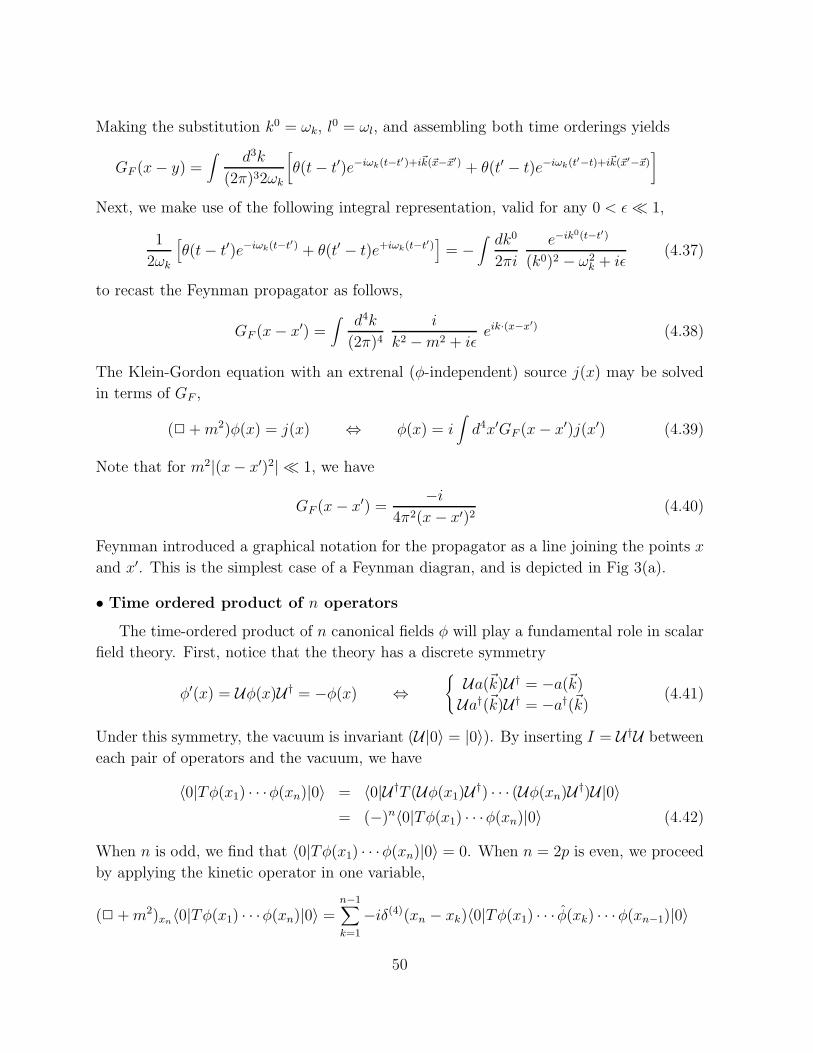
Making the substitution k0 = ωk, l0 = ωl, and assembling both time orderings yields
GF (x− y) =∫
d3k
(2π)32ωk
[
θ(t− t′)e−iωk(t−t′)+i~k(~x−~x′) + θ(t′ − t)e−iωk(t′−t)+i~k(~x′−~x)]
Next, we make use of the following integral representation, valid for any 0 < ε� 1,
1
2ωk
[
θ(t− t′)e−iωk(t−t′) + θ(t′ − t)e+iωk(t−t′)]
= −∫dk0
2πi
e−ik0(t−t′)
(k0)2 − ω2k + iε
(4.37)
to recast the Feynman propagator as follows,
GF (x− x′) =∫
d4k
(2π)4
i
k2 −m2 + iεeik·(x−x
′) (4.38)
The Klein-Gordon equation with an extrenal (φ-independent) source j(x) may be solved
in terms of GF ,
(2 +m2)φ(x) = j(x) ⇔ φ(x) = i∫
d4x′GF (x− x′)j(x′) (4.39)
Note that for m2|(x− x′)2| � 1, we have
GF (x− x′) =−i
4π2(x− x′)2(4.40)
Feynman introduced a graphical notation for the propagator as a line joining the points x
and x′. This is the simplest case of a Feynman diagran, and is depicted in Fig 3(a).
• Time ordered product of n operators
The time-ordered product of n canonical fields φ will play a fundamental role in scalar
field theory. First, notice that the theory has a discrete symmetry
φ′(x) = Uφ(x)U † = −φ(x) ⇔{
Ua(~k)U † = −a(~k)Ua†(~k)U † = −a†(~k) (4.41)
Under this symmetry, the vacuum is invariant (U|0〉 = |0〉). By inserting I = U †U between
each pair of operators and the vacuum, we have
〈0|Tφ(x1) · · ·φ(xn)|0〉 = 〈0|U †T (Uφ(x1)U †) · · · (Uφ(xn)U †)U|0〉= (−)n〈0|Tφ(x1) · · ·φ(xn)|0〉 (4.42)
When n is odd, we find that 〈0|Tφ(x1) · · ·φ(xn)|0〉 = 0. When n = 2p is even, we proceed
by applying the kinetic operator in one variable,
(2 +m2)xn〈0|Tφ(x1) · · ·φ(xn)|0〉 =n−1∑
k=1
−iδ(4)(xn − xk)〈0|Tφ(x1) · · · φ(xk) · · ·φ(xn−1)|0〉
50
x x'
1
2 3
4 1
2 3
41
2 3
4
+ +
(a) (b)
Figure 3: Free Scalar Correlation Functions; (a) The Feynman propagator GF (x − x′),(b) the 4-point function 〈0|Tφ(x1)φ(x2)φ(x3)φ(x4)|0〉.
Here, φ stands for the fact that the operators φ(xk) is to be omitted. The solution is again
obtained in terms of the Feynman propagator GF (x− x′) as follows,
〈0|Tφ(x1) · · ·φ(xn)|0〉 =n−1∑
k=1
GF (xn − xk)〈0|Tφ(x1) · · · φ(xk) · · ·φ(xn−1)|0〉 (4.43)
The solution to this recursive equation is manifest,
〈0|Tφ(x1) · · ·φ(xn)|0〉 =∑
disjoint pairs(k,l)
GF (xk1 − xl1) · · ·GF (xkp − xkp) (4.44)
where the sum is over all possible pairs without common points. The simple example of
the 4-point correlation function is given in Fig 3(b).
4.2 The Operator Product Expansion & Composite Operators
It is possible to re-analyze the issues of the vacuum energy of the free scalar field theory in
terms of a more general problem. The canonical commutation relations provide expressions
for the commutators of the canonical fields. In the construction of the Hamiltonian, mo-
mentum and Lorentz generators, composite operators enter, namely the operators φ(x)2,
π(x)2 and (~∇φ(x))2. These operators are obtained by putting two canonical fields at the
same space-time point.
From the short distance behavior of the Feynman propagator, (4.40), it is clear that
putting operators at the same point produces singularities, which ultimately result in the
infinite expression for the energy density of the vacuum. So, one very important problem
in QFT is to properly define composite operators. One of the most powerful ways is via
the use of the Operator Product Expansion (or OPE), a method that was introduced by
Ken Wilson in 1969. (Another way, which is mostly restricted to free field theory or at
best perturbation theory, is normal ordering.)
51
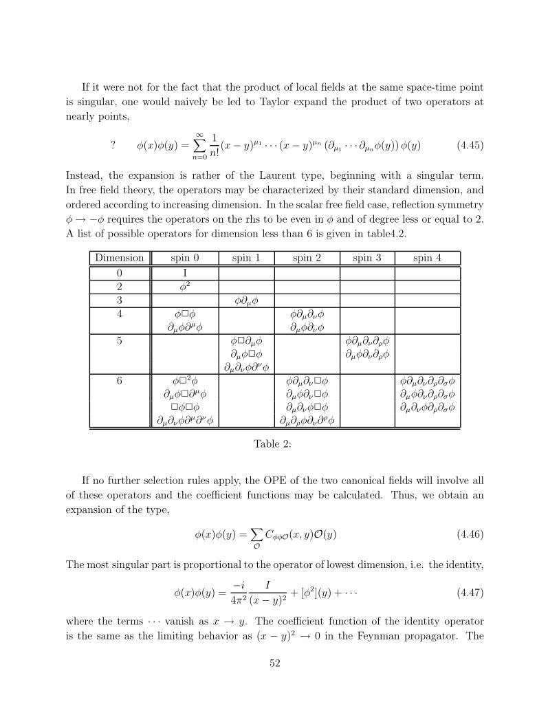
If it were not for the fact that the product of local fields at the same space-time point
is singular, one would naively be led to Taylor expand the product of two operators at
nearly points,
? φ(x)φ(y) =∞∑
n=0
1
n!(x− y)µ1 · · · (x− y)µn (∂µ1
· · ·∂µnφ(y))φ(y) (4.45)
Instead, the expansion is rather of the Laurent type, beginning with a singular term.
In free field theory, the operators may be characterized by their standard dimension, and
ordered according to increasing dimension. In the scalar free field case, reflection symmetry
φ→ −φ requires the operators on the rhs to be even in φ and of degree less or equal to 2.
A list of possible operators for dimension less than 6 is given in table4.2.
Dimension spin 0 spin 1 spin 2 spin 3 spin 4
0 I2 φ2
3 φ∂µφ4 φ2φ φ∂µ∂νφ
∂µφ∂µφ ∂µφ∂νφ
5 φ2∂µφ φ∂µ∂ν∂ρφ∂µφ2φ ∂µφ∂ν∂ρφ∂µ∂νφ∂
νφ6 φ2
2φ φ∂µ∂ν2φ φ∂µ∂ν∂ρ∂σφ∂µφ2∂µφ ∂µφ∂ν2φ ∂µφ∂ν∂ρ∂σφ2φ2φ ∂µ∂νφ2φ ∂µ∂νφ∂ρ∂σφ
∂µ∂νφ∂µ∂νφ ∂µ∂ρφ∂ν∂
ρφ
Table 2:
If no further selection rules apply, the OPE of the two canonical fields will involve all
of these operators and the coefficient functions may be calculated. Thus, we obtain an
expansion of the type,
φ(x)φ(y) =∑
O
CφφO(x, y)O(y) (4.46)
The most singular part is proportional to the operator of lowest dimension, i.e. the identity,
φ(x)φ(y) =−i4π2
I
(x− y)2+ [φ2](y) + · · · (4.47)
where the terms · · · vanish as x → y. The coefficient function of the identity operator
is the same as the limiting behavior as (x − y)2 → 0 in the Feynman propagator. The
52
operator [φ2] refers to the finite (or renormalized) operator associated with φ2. It may be
defined by the OPE in the following manner,
[φ2](y) ≡ limx→y
(
φ(x)φ(y) +i
4π2
I
(x− y)2
)
(4.48)
This limit is well-defined and unique.
More generally, but still in the scalar free field theory, the OPE of any two operators
will be a Laurent series in terms of all the operators of the theory (not neccessarily of
order 2 in the field φ), and we have
O1(x)O2(y) =∑
O
CO1O2O(x, y)O(y) (4.49)
The coefficient functions may be calculated exactly as long as we are in free field theory,
and they will have integer powers. For an interacting theory, a similar expansion exists, but
fractional expansion powers will occur, refelecting the fact that in an interacting theory,
the dimensions of the operators will received quantum corrections.
53
4.3 The Gauge or Spin 1 Field
The simplest free spin 1 field is the gauge vector potential Aµ in Maxwell theory of E&M.
This field is real and its classical Lagrangian, in the absence of sources, is given by
L = −1
4FµνF
µν Fµν ≡ ∂µAν − ∂νAµ (4.50)
The customary electric Ei and magnetic Bi fields are components of Fµν ,
Ei ≡ Fi0 Bi ≡1
2εijkFjk (4.51)
By construction, the Lagrangian L is invariant under gauge transformations by any ar-
bitary real scalar function θ(x), given by
Aµ(x) → A′µ(x) = Aµ(x) − ∂µθ(x) (4.52)
Two gauge fields related by a gauge transformation have the same electric and magnetic
fields and are thus physically equivalent.†† The canonical momenta are defined as usual,
πµ ≡ ∂L∂(∂0Aµ)
(4.53)
and are found to be
π0 = 0 πi = Ei (4.54)
The fact that π0 = 0 implies that we are dealing with a constrained system, namely the
canonical momenta and canonical fields are not independent of one another. The field A0
has vanishing canonical momentum and is therefore non-dynamical. This is an immediate
consequence of the gauge invariance of the Lagrangian and is also reflected in the structure
of the field equations,
∂µFµν = 0 ⇔
{~∇ · ~E = 0
∂t ~E − ~∇× ~B = 0(4.55)
Indeed, ~∇· ~E = 0 is a non-dynamical equation since it gives a condition that the canonical
momenta must satisfy at any time, including on the initial data. Yet a further manifesta-
tion of this phenomenon is that the second order differential operator, in terms of which
the Lagrangian may be re-expressed (up to a total derivative term) is not invertible,
L =1
2Aµ(2η
µν − ∂µ∂ν)Aν (4.56)
The operator 2ηµν − ∂µ∂ν is not invertible; it kernel are precisely gauge fields of the
form Aµ = ∂µθ, and gauge equivalent to 0. Clearly, the vanishing of one of the canonical
momenta causes complications for the quantization of the gauge field.
††Except on non-simply connected domains when there can be glovbal effects.
54
Transverse gauge quantization (Lorentz non-covariant)
A first approach in dealing with the complications that ensue from gauge invariance
and the constraints on the momenta is to make a gauge choice in which the constraint can
be solved explicitly. This will leave only dynamical fields, on which canonical quantization
may now be carried out. The drawback of this approach is that it cannot be Lorentz
covariant, as a preferred direction is chosen in space-time.
With the help of a gauge transformation, any gauge field configuration may be trans-
formed into a transverse gauge ~∇ ~A = 0. As a result of the constraint ~∇ ~E = 0, one
automatically has A0 = 0 and the Lagrangian and canonical momenta reduce to
L = +1
2(Ai)
2 − 1
2B2i
πi =∂L
∂(∂0Ai)= Ai ∂iAi = 0 (4.57)
The last equation reflects the gauge choice. The Euler-Lagrange equations are
(2ηµν − ∂µ∂ν)Aµ = 0 (4.58)
and, in transverse gauge, reduce to
2Ai = 0 ∂iAi = 0 (4.59)
The field equations are solved first by Fourier transform,
Ai(x) =∫
d3k
(2π)32ωk
(
ai(~k)e−ik·x + a†i (~k)e
ik·x)
(4.60)
after which we must further impose the radiation gauge conditions, which result in the
following transversality conditions on the oscillators,
kiai(~k) = kia†i (~k) = 0 (4.61)
It is convenient to introduce basis vectors for the two-dimensional space of transverse
polarization vectors ~ε(~k, α), α = 1, 2, which satisfy
kiεi(~k, α) = 0
εi(~k, α)∗ εi(~k, β) = δαβ∑
α εi(~k, α)εj(~k, α) = δij − kikj
k2
(4.62)
In terms of this basis, we may introduce independent field oscillators a(~k, α) in terms of
which the old oscillators may be decomposed as
ai(~k) =∑
α
a(~k, α)εi(~k, α) (4.63)
55
and the field takes the form
Ai(x) =∫ d3k
(2π)32ωk
∑
α=1,2
(
a(~k, α)εi(~k, α)e−ik·x + a†(~k, α)ε∗i (~k, α)eik·x
)
(4.64)
Clearly, the photon has two degrees of freedom, even though the field Aµ has 4 components.
The canonical commutation relations amongst the a(~k, α) and a†(~k, α) are just as for
the scalar theory, but now with two independent components,
[a(~k, α), a(~k′, β)] = [a†(~k, α), a†(~k′, β)] = 0
[a(~k, α), a†(~k′, β)] = δαβ2ωk(2π)3δ3(~k − ~k′) (4.65)
The equal time commutators may be expressed in terms of the fields Ai as follows,
[Ai(t, ~x), Aj(t, ~y)] = −iPijδ(3)(~x− ~y) Pij = δij −∂i∂j∆
(4.66)
from which it is clear again that only two degrees of freedom are independent. The
Hamiltonian is standard,
H =∫
d3x(
1
2~E2 +
1
2~B2)
(4.67)
The Hilbert space is constructed very much as in the case of the single scalar field. The
vacuum |0〉 is defined by
a(~k, α)|0〉 = 0 for all ~k, α (4.68)
The n–particle states are found to be
|k1, α1; k2, α2; · · · ; kn, αn〉 ≡ a†(k1, α1)a†(k1, α1) · · ·a†(k1, α1)|0〉 (4.69)
The (renormalized) Hamiltonian and momentum operators may be worked out,
H =∫
d3k
(2π)32ωk
∑
α
ωka†(~k, α)a(~k, α)
~P =∫
d3k
(2π)32ωk
∑
α
~ka†(~k, α)a(~k, α) (4.70)
Finally, the number operator may also be introduced,
N =∫
d3k
(2π)32ωk
∑
α
a†(~k, α)a(~k, α) (4.71)
Since this is a free theory, we have [H,N ] = [~P ,N ] = 0, so the number of photons is
conserved.
56
Gupta-Bleuler Quantization (Lorentz Covariant)
The second approach is to keep Lorentz invariance manifest at all times, possibly at
the cost of giving up manifest gauge invariance. To see exactly what goes on, we introduce
a conserved external source jµ, which we assume is independent of A. The Lagrangian is,
L = −1
4FµνF
µν − λ
2(∂µA
µ)2 − Aµjµ ∂µj
µ = 0 (4.72)
In this Lagrangian, for λ 6= 0, the time component A0 does have a non-vanishing conjugate
momentum, and the quadratic part of the Lagrangian involves an operator 2ηµν − (1 −λ)∂µ∂ν which is invertible. The Lagrangian L is, however, no longer gauge invariant, so in
the end we will have to deal with non-gauge invariant states. The canonical relations are
π0 =∂L
∂(∂0A0)= −λ∂νAν πi =
∂L∂(∂0Ai)
= F io
[πµ(t, ~x), Aν(t, ~x′)] = i ηµνδ3(~x− ~x′) (4.73)
The sign in the canonical commutation relation is chosen such that the canonical quan-
tization of the space components agree with the one derived previously. The sign for the
time-components is then forced by Lorentz invariance.
Specializing to the case λ = 1 (Feynman gauge), the field equations reduce to 2Aµ = 0.
The decomposition of Aµ(x) into modes then gives
Aµ(x) =∫
d3k
(2π)32ωk
(
aµ(~k)e−ik·x + a†µ(
~k)eik·x)
(4.74)
and the canonical commutation relations on the oscillators become,
[aµ(~k), aν(~k′)] = [a†µ(
~k), a†ν(~k′)] = 0
[aµ(~k), a†ν(~k′)] = −ηµν2ωk(2π)3δ(3)(~k − ~k′) (4.75)
We can still define the vacuum by the requirement that aµ(~k)|0〉 = 0, and one-particle
states by
|~k, µ〉 = a†µ(~k)|0〉 (4.76)
The normalization of these states may be worked out in terms of the canonical commutation
relations as usual,
〈~k, µ|~k′, ν〉 = −ηµν2ωk(2π)3δ(3)(~k − ~k′) (4.77)
While the oscillators ai create states with positive norm, as was the case in the scalar
theory, the operators a0 create states with negative norm, which cannot be physically
57
acceptable in a quantum theory. These states are unphysical, and arise because we insisted
on maintaining manifest Lorentz invariance, which forced us to carry along more degrees
of freedom than physically needed or allowed. We now investigate how these unphysical
degrees of freedom are purged from the theory.
To see how this can be done, we notice that there is a free field in the theory that is a
pure gauge artifact. Look at the equations for Aµ:
∂µFµν − λ∂ν∂µA
µ + jν = 0 (4.78)
Conservation of jµ implies that λ2∂µAµ = 0; hence ∂µA
µ is a free field with no coupling
to the source jµ. In view of the canonical quantization relations, we cannot simply set
∂µAµ = 0. However, we had way too many states created by Aµ, so we may set it be
zero on the physical states. In fact this is truly beneficial, because it implies that on the
physical states, the Heisenberg equation of motion is gauge invariant:
∂µAµ|phys〉 = 0 (4.79)
It is very important to remark that we work with two types of spaces: (1) The Fock space
for the full Aµ field, which contains states of negative norm; (2) The physical Hilbert space,
obeying the restrictions above.
To solve for the field in terms of the source,
(
2ηµν + (λ− 1)∂µ∂ν)
Aν = jµ (4.80)
we introduce the photon propagator,
(
2ηκµ + (λ− 1)∂κ∂µ)
xGµν(x− y) = −iδκν δ4(x− y) (4.81)
The propagator is related to the time-ordered product of the quantum fields,
Gµν(x− y) = 〈0|TAµ(x)Aν(y)|0〉 (4.82)
It may be obtained in terms of a Fourrier integral,
Gµν(x− y) =∫
d4k
(2π)4
[
ηµν +1 − λ
λ
kµkνk2 + iε
]
−ik2 + iε
e−ik·(x−y) (4.83)
Clearly, the propagator in Feynman gauge (λ = 1) simplifies considerably; in Landau
gauge (λ = ∞) it becomes transverse.
58
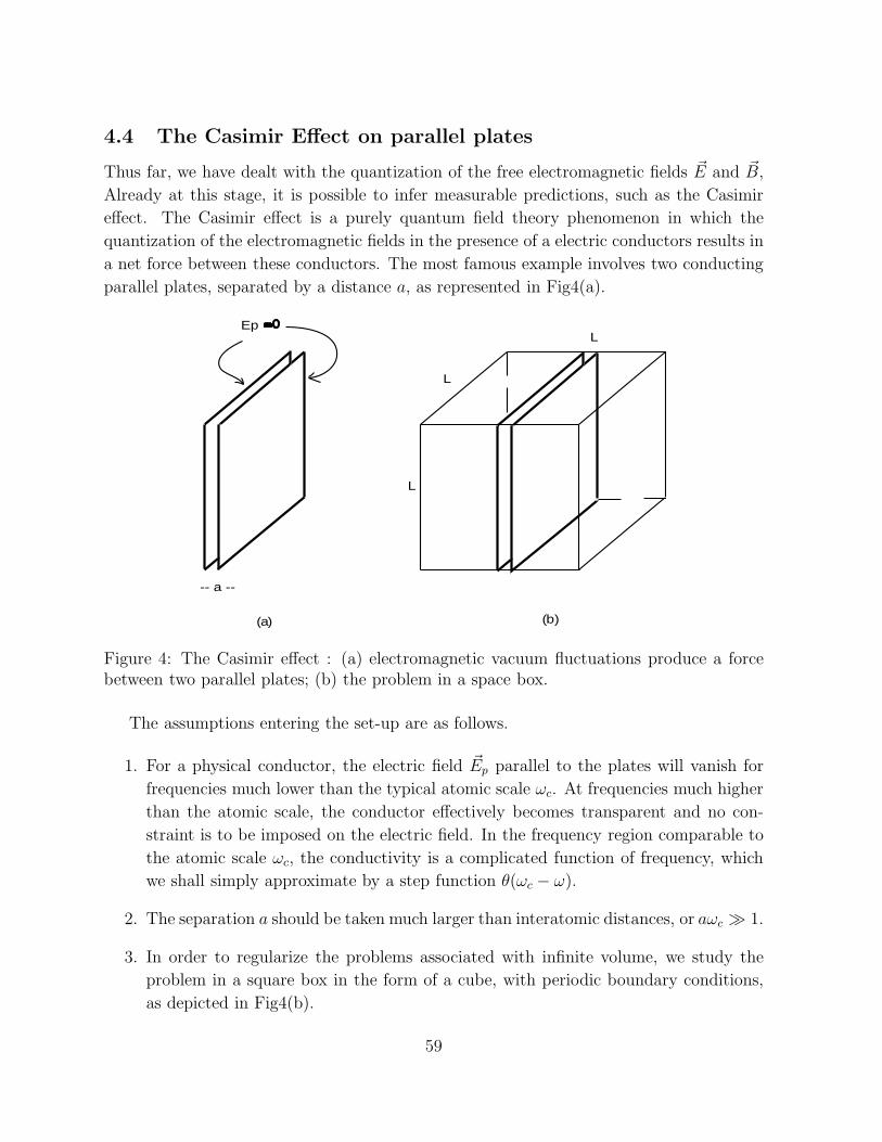
4.4 The Casimir Effect on parallel plates
Thus far, we have dealt with the quantization of the free electromagnetic fields ~E and ~B,
Already at this stage, it is possible to infer measurable predictions, such as the Casimir
effect. The Casimir effect is a purely quantum field theory phenomenon in which the
quantization of the electromagnetic fields in the presence of a electric conductors results in
a net force between these conductors. The most famous example involves two conducting
parallel plates, separated by a distance a, as represented in Fig4(a).
-- a --
(a) (b)
L
L
LEp =0
Figure 4: The Casimir effect : (a) electromagnetic vacuum fluctuations produce a forcebetween two parallel plates; (b) the problem in a space box.
The assumptions entering the set-up are as follows.
1. For a physical conductor, the electric field ~Ep parallel to the plates will vanish for
frequencies much lower than the typical atomic scale ωc. At frequencies much higher
than the atomic scale, the conductor effectively becomes transparent and no con-
straint is to be imposed on the electric field. In the frequency region comparable to
the atomic scale ωc, the conductivity is a complicated function of frequency, which
we shall simply approximate by a step function θ(ωc − ω).
2. The separation a should be taken much larger than interatomic distances, or aωc � 1.
3. In order to regularize the problems associated with infinite volume, we study the
problem in a square box in the form of a cube, with periodic boundary conditions,
as depicted in Fig4(b).
59
• Calculation of the frequencies
There are three distinct regimes in which the frequencies of the quantum oscillators
need to be computed. The momenta parallel to the plates are always of the following form,
kx =2πnxL
ky =2πnyL
nx, ny ∈ Z
Along the third direction, we distinguish three different regimes, so that the frequency has
three different branches,
ω(i) =
√
k2x + k2
y + (k(i)z )2 i = 1, 2, 3 (4.84)
The three regimes are as follows,
1. ω > ωc : the frequencies are the same as in the absence of the plates, since the plates
are acting as transparent objects,
k(1)z =
2πnzL
nz ∈ Z
2. ω < ωc & between the two plates.
k(2)z =
πnza
0 ≤ nz ∈ Z
3. ω < ωc & outside the two plates.
k(3)z =
πnzL− a
0 ≤ nz ∈ Z
• Summing up the contributions of all frequencies
Finally, we are not interested in the total energy, but rather in the enrgy in the presence
of the plates minus the energy in the absence of the plates. Thus, when the frequencies
exceed ωc, all contributions to the enrgy cancel since the plates act as transparent bodies.
Thus, we have
E(a) −E0 =∑
nx,ny,nz
(1
2ω(2)(nx, ny, nz) +
1
2ω(3)(nx, ny, nz) −
1
2ω(1)(nx, ny, nz)
)
(4.85)
When nz 6= 0, two polarization modes have ~E with 2 components along the plates, while
for nz = 0, nx, ny 6= 0, there is only one. Therefore, we isolate nz = 0,
E(a) − E0 =1
2
∑
nx,ny
ω(nx, ny, 0) (4.86)
+∑
nx,ny
∞∑
nz=1
(
ω(2)(nx, ny, nz) + ω(3)(nx, ny, nz) − 2ω(1)(nx, ny, nz))
Next, we are interested in taking the size of the box L very large compared to all other
scales in the problem. The levels in nx and ny then become very closely spaced and the
60
sums over nx and ny may be well-approximated by integrals, with the help of the following
conversion process,
dnx =Ldkx2π
dny =Lky2π
(4.87)
so that
E(a) − E0 =L2
4π2
∫ +∞
−∞dkx
∫ +∞
−∞dky
[1
2ωθ(ωc − ω)
+∞∑
nz=1
(
ω(2)θ(ωc − ω(2)) + ω(3)θ(ωc − ω(3)) − 2ω(1)θ(ωc − ω(1)))]
Now, for ω(1) and ω(3), the frequency levels are also close together and the sum over nzmay also be approximated by an integral,
∞∑
nz=1
ω(2)θ(ωc − ω(2)) =L− a
π
∫ ∞
0dkz
√
k2x + k2
y + k2z θ(ωc −
√
k2x + k2
y + k2z)
∞∑
nz=1
2ω(1) θ(ωc − ω(1)) =L
2π2∫ ∞
0dkz
√
k2x + k2
y + k2z θ(ωc −
√
k2x + k2
y + k2z)
Introducing k2 = k2x + k2
y , and in the last integral the continuous variable n = akz/π, we
have
E(a) − E0 =L2
2π
∫ ∞
0dk k
[1
2kθ(ωc − k) +
∞∑
n=1
√
k2 +π2n2
a2θ(ω2
c − k2 − π2n2
a2)
−∫ ∞
0dn
√
k2 +π2n2
a2θ(ω2
c − k2 − π2n2
a2)]
Introducing the function
f(n) ≡∫ ∞
0
dk
2πk
√
k2 +π2n2
a2θ(ω2
c − k2 − π2n2
a2) (4.88)
we have
E(a) − E0
L2=
1
2f(0) +
∞∑
n=1
f(n) −∫ ∞
0dnf(n) (4.89)
Now, there is a famous formula that relates a sum of the values of a function at integers
to the integral of this function,
∫ ∞
0dnf(n) =
1
2f(0) +
∞∑
n=1
f(n) +∞∑
p=1
B2p
(2p)!f (2p−1)(0) (4.90)
61
where the Bernoulli numbers are defined by
x
ex − 1=∞∑
n=0
Bnxn
n!B2 = −1
6, B4 = − 1
30, · · · (4.91)
Assuming a sharp cutoff, so that θ is a step function, we easily compute f(n),
f(n) =1
6π
(
ω3c −
π3n3
a3
)
(4.92)
Thus, f (2p−1)(0) = 0 as soon as p > 2, while f (3)(0) = −π2/a3, and thus we have
E(a) −E0
L2=π2
a3
B4
4!= − π2
720hcL2
a3(4.93)
This represents a universal, attractive force proportional to 1/a4. To make their depen-
dence explicit, we have restored the factors of h and c.
4.5 Bose-Einstein and Fermi-Dirac statistics
In classical mechanics, particles are distinguishable, namely each particle may be tagged
and this tagging survives throughout time evolution since particle identities are conserved.
In quantum mechanics, particles of the same species are indistinguishable, and cannot
be tagged individually. They can only be characterized by the quantum numbers of the
state of the system. Therefore, the the operation of interchange of any two particles of the
same species must be a symmetry of the quantum system. The square of the interchange
operation is the identity.‡‡ As a result, the quantum states must have definite symmetry
properties under the interchange of two particles.
All particles in Nature are either bosons or fermions;
• BOSONS : the quantum state is symmetric under the interchange of any pair of
particles and obey Bose-Einstein statistics. Bosons have integer spin. For example,
photons, W±, Z0, gluons and gravitons are bosonic elementary particles, while the
Hydrogen atom, the He4 and deuterium nuclei are composite bosons.
• FERMIONS : the quantum state is anti-symmetric under the interchange of any pair
of particles and obey Fermi-Dirac statistics. Fermions have integer plus half spin.
For example, all quarks and leptons are fermionic elementary particles, while the
proton, neutron and He3 nucleus are composite fermions.
‡‡This statement holds in 4 space-time dimensions but it does not hold generally. In 3 space-timedimensions, the topology associated with the interchange of two particles allows for braiding and thesquare of this operation is not 1. The corresponding particles are anyons.
62
Remarkably, the quantization of free scalars and free photons carried out in the pre-
ceeding subsections has Bose-Einstein statistics built in. The bosonic creation and an-
nihilation operators are denoted by a†σ(~k) and aσ(~k) for each species σ. The canonical
commutation relations inform us that all creation operators commute with one another
[a†σ(~k), a†σ′(
~k′)] = 0. As a result, two states differening only by the interchange of two
particle of the same species are identical quantum mechanically,
a†σ1(~k1) · · ·a†σi
(~ki) · · ·a†σj(~kj) · · ·a†σn
(~kn)|0〉= a†σ1
(~k1) · · ·a†σj(~kj) · · ·a†σi
(~ki) · · ·a†σn(~kn)|0〉
The famous CPT Theorem states that upon the quantization of a Poincare and CPT
invariant Lagrangian, integer spin fields will always produce particle states that obey
Bose-Einstein statistics, while integer plus half fields always produce states that obey
Fermi-Dirac statistics.
• Fermi-Dirac Statistics
It remains to establish how integer plus half spin fields are to be quantized. This will
be the subject of the subsection on the Dirac equation. Here, we shall take a very simple
approach whose point of departure is the fact that fermions obey Fermi-Dirac statistics.
First of all, a free fermion may be expected to be equivalent to a collection of oscillators,
just as bosonic free fields were. But they cannot quite be the usual harmonic oscillators,
because we have just shown above that harmonic operators produce Bose-Einstein statis-
tics. Instead, the Pauli exclusion principle states that only a single fermion is allowed to
occupy a given quantum state. This means that a fermion creation operator b† for given
quantum numbers must square to 0. Then, its repeated application to any state (which
would create a quantum state with more than one fermion particle with that species) will
produce 0.
The smallest set of operators that can characterize a fermion state is given by the
fermionic oscillators b and b†, obeying the algebra
{b, b} = {b†, b†} = 0 {b, b†} = 1 (4.94)
In analogy with the bosonic oscillator, we consider the following simple Hamiltonian,
H =ω
2
(
b†b− bb†)
= ω(
b†b− 1
2
)
(4.95)
Naturally, the ground state is defined by b|0〉 = 0 and there are just two quantum states
in this system, namely |0〉 and b†|0〉 with energies −12ω and +1
2ω respectively. A simple
63
representation of this algebra may be found by noticing that it is equivalent to the algebra
of Pauli matrices or Clifford-Dirac algebra in 2 dimensions,
σ1 = b+ b† σ2 = ib− ib† H =ω
2σ3 (4.96)
Vice-versa, the γ-matrices in 4 dimensions are equivalent to two sets of fermionic oscillators
bα and b†α, α = 1, 2. The above argumentation demsonstrates that its only irreducible
representation is 4-dimensional, and spanned by the states |0〉, b†1|0〉, b†2|0〉, b†1b†2|0〉.In terms of particles, we should affix the quantum number of momentum ~k, so that
we now have oscillators bσ(~k) and b†σ(~k), for some possible species index σ. Postulating
anti-commutation relations, we have
{bσ(~k), bσ′(~k′)} = {b†σ(~k), b†σ′(~k′)} = 0
{bσ(~k), b†σ′(~k′)} = 2ωkδσσ′(2π)3δ(3)(~k − ~k′) (4.97)
where again ωk =√
~k2 +m2. The Hamiltonian and momentum operators are naturally
H =∫
d3k
(2π)32ωkωk∑
σ
b†σ(~k)bσ(~k)
~P =∫
d3k
(2π)32ωk~k∑
σ
b†σ(~k)bσ(~k) (4.98)
The vacuum state |0〉 is defined by bσ(~k)|0〉 = 0 and multiparticle states are obtained by
applying creation operators to the vacuum,
b†σ1(~k1) · · · b†σn
(~kn)|0〉 (4.99)
Using the fact that creation operators always anti-commute with one another, it is straight-
forward to show that
b†σ1(~k1) · · · b†σi
(~ki) · · · b†σj(~kj) · · · b†σn
(~kn)|0〉= − b†σ1
(~k1) · · · b†σj(~kj) · · · b†σi
(~ki) · · · b†σn(~kn)|0〉
so that the state obeys Fermi-Dirac statistics.
64
4.6 The Spin 1/2 Field
In view of the preceeding discussion on Fermi-Dirac statistics, it is clear that the fermionic
field oscillators and thus the fermionic fields themselves should obey canonical anti-
commutation relations, such as
{ψα(t, ~x), ψβ(t, ~y)} = 0
{ψ†α(t, ~x), ψ†β(t, ~y)} = 0
{ψα(t, ~x), ψ†β(t, ~y)} = ihδαβδ(3)(~x− ~y) (4.100)
Here, α and β stand for spinor indices. The classical limit of commutation relations
(without dividing by h) confirms that classical bosonic fields are ordinary functions. The
classical limit of anti-commutation relations (also without dividing by h) for fermionic
fields informs us that classical fermionic fields must be Grassmann-valued functions, and
obey
{ψα(t, ~x), ψβ(t, ~y)} = {ψ∗α(t, ~x), ψ∗β(t, ~y)} = {ψα(t, ~x), ψ∗β(t, ~y)} = 0 (4.101)
Grassmann numbers are well-defined by the above anticommutation relations. It is also
useful, however, to obtain a concrete representation in terms of matrices. Let bj , j =
1, · · · , N be N Grassmann numbers. These algebraic objects may be realized in terms of
γ-matrices in dimension 2N , defined to obey the Clifford-Dirac algebra {γm, γn} = 2δmnI,
with m,n,= 1, · · · , 2N . The following combinations
bj ≡1
2(γj + iγj+N) j = 1, · · · , N (4.102)
will form N Grassmann numbers. Note that {bj , b†k} = δij, so Grassmann numbers may
be viewed as half of the γ-matrices.
• The Free Dirac equation
The field equations for the free Dirac field must be Poincare covariant and linear in
ψ(x). Of course, one might postulate (2 + m2)ψ(x) = 0, but it turns out that this is
neither the simplest nor the correct equation. The Dirac equation is a first order partial
differential equation,
(iγµ∂µ −mI)ψ(x) = 0 (4.103)
Here, γµ are the Dirac matrices in 4 dimensional Minkowski space-time and I is the identity
matrix in the Dirac algebra. Often, I is not written explicitly. We begin by showing that
65
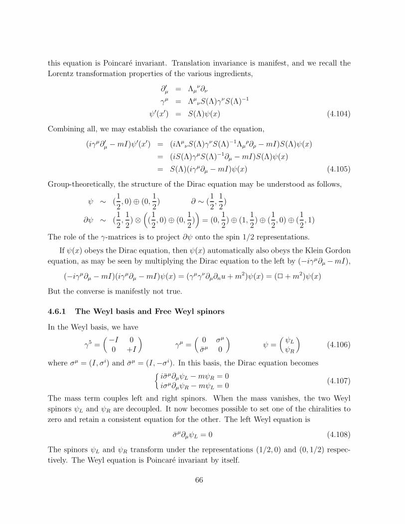
this equation is Poincare invariant. Translation invariance is manifest, and we recall the
Lorentz transformation properties of the various ingredients,
∂′µ = Λµν∂ν
γµ = ΛµνS(Λ)γνS(Λ)−1
ψ′(x′) = S(Λ)ψ(x) (4.104)
Combining all, we may establish the covariance of the equation,
(iγµ∂′µ −mI)ψ′(x′) = (iΛµνS(Λ)γνS(Λ)−1Λµ
ρ∂ρ −mI)S(Λ)ψ(x)
= (iS(Λ)γµS(Λ)−1∂µ −mI)S(Λ)ψ(x)
= S(Λ)(iγµ∂µ −mI)ψ(x) (4.105)
Group-theoretically, the structure of the Dirac equation may be understood as follows,
ψ ∼ (1
2, 0) ⊕ (0,
1
2) ∂ ∼ (
1
2,1
2)
∂ψ ∼ (1
2,1
2) ⊗
(
(1
2, 0) ⊕ (0,
1
2))
= (0,1
2) ⊕ (1,
1
2) ⊕ (
1
2, 0) ⊕ (
1
2, 1)
The role of the γ-matrices is to project ∂ψ onto the spin 1/2 representations.
If ψ(x) obeys the Dirac equation, then ψ(x) automatically also obeys the Klein Gordon
equation, as may be seen by multiplying the Dirac equation to the left by (−iγµ∂µ−mI),
(−iγµ∂µ −mI)(iγµ∂µ −mI)ψ(x) = (γµγν∂µ∂nu+m2)ψ(x) = (2 +m2)ψ(x)
But the converse is manifestly not true.
4.6.1 The Weyl basis and Free Weyl spinors
In the Weyl basis, we have
γ5 =(−I 0
0 +I
)
γµ =(
0 σµ
σµ 0
)
ψ =(ψLψR
)
(4.106)
where σµ = (I, σi) and σµ = (I,−σi). In this basis, the Dirac equation becomes{iσµ∂µψL −mψR = 0iσµ∂µψR −mψL = 0
(4.107)
The mass term couples left and right spinors. When the mass vanishes, the two Weyl
spinors ψL and ψR are decoupled. It now becomes possible to set one of the chiralities to
zero and retain a consistent equation for the other. The left Weyl equation is
σµ∂µψL = 0 (4.108)
The spinors ψL and ψR transform under the representations (1/2, 0) and (0, 1/2) respec-
tively. The Weyl equation is Poincare invariant by itself.
66
• The Free Weyl and Dirac actions
The combination ψ ≡ ψ†γ0 has a simple Lorentz transformation property in view of
the fact that ㆵ = γ0γµγ0, and we have
ψ′(x′) = S(Λ)ψ(x) ⇒ (ψ′)† = ψ†(x)S(Λ)† ⇒ ψ′(x) = ψ(x)S(Λ)−1 (4.109)
Therefore, we readily construct an invariant action,
S[ψ, ψ] =∫
d4xL L = ψ(iγµ∂µ −m)ψ (4.110)
Viewing ψ and ψ as independent fields, it is clear that the Dirac equation follows from
the variation of these fields. The canonical momenta are πψ = iψγ0 and πψ = 0 and the
Hamiltonian is given by
H =∫
d3x [πψ∂0ψ − L] =∫
d3xψ[
−i~γ · ~∇ +m]
ψ (4.111)
In the Weyl basis, the action becomes
S[ψL, ψL, ψR, ψR] =∫
d4x[
ψ†Liσµ∂µψL + ψ†Riσ
µ∂µψR −mψ†LψR −mψ†RψL]
(4.112)
• Majorana spinors
Recall that a Majorana spinor is a Dirac spinor which equals its own charge conjugate.
In the Weyl basis, it takes the form,
ψ =
(
ψL−σ2ψ∗L
)
ψc = ψ (4.113)
Hence, a Majorana spinor in 4 space-time dimensions is equivalent to a Weyl spinor. All
the properties can be deduced from this equivalence. Note that there exists an interesting
Majorana mass term,
L = ψLi 6 ∂ψL +1
2mψTLσ
2ψL =1
2ψi 6 ∂ψ − 1
2mψψ (4.114)
The Majorana mass term violates U(1) symmetry and so a spinor with Majorana mass
must be electrically neutral.
• Solutions to the Free Dirac equation
The free Dirac equation may be solved by a superposition of Fourrier modes with 4-
momentum kµ. Since any solution to the Dirac equation is also a solution to the Klein
Gordon equation, we must have k2 = m2, and there will be solutions with k0 < 0 as well
67
as k0 > 0. Just as we did in the case of bosonic fields, it is useful to separate these two
branches, and we organize all solutions in the following manner, both with k0 > 0,
ψ+(x) = u(k, r)e−ik·x (kµγµ −m)us(k) = 0
ψ−(x) = v(k, r)e+ik·x (kµγµ +m)vs(k) = 0 (4.115)
The superscript r = 1, 2 labels the linearly independent solutions. That there are precisely
two solutions for each equation may be shown as follows.
When m 6= 0, we introduce the following projection operators
Λ±(k) ≡ 1
2m(±kµγµ +m) (4.116)
which satisfy
(Λ±)2 = Λ± Λ+ + Λ− = I Λ+Λ− = 0 trΛ± = 2 (4.117)
Hence the rank of both Λ± is 2, whence there are two independent solutions. The spinors
u and v may be normalized as follows,
∑
r
u(~k, r)u(~k, r) = k/+m
∑
r
v(~k, r)v(~k, r) = k/−m (4.118)
Any bilinear in u and v may be calculated from this formula. For example, we have
u(~k, r)u(~k, s) = 2mδrsu(~k, r)v(~k, s) = 0
v(~k, r)v(~k, s) = −2mδrs
u(~k, r)γµu(~k, s) = 2kµδrsu(~k, r)γµv(~k, s) =?
v(~k, r)γµv(~k, s) = 2kµδrs
(4.119)
Explicit forms of the solutions may be obtained as follows.
u(k, r) =(
+√k · σ ξ(r)
+√k · σ ξ(r)
)
v(k, r) =(
+√k · σ η(r)
−√k · σ η(r)
)
(4.120)
with
ξ†(r)ξ(s) = η†(r)η(s) = δrs (4.121)
so that we may choose for example,
ξ(1) = η(1) =(
10
)
ξ(2) = η(2) =(
01
)
(4.122)
When m = 0, there are still two solutions u and two solutions v, but the preceeding
normalization becomes degenerate. Choose kµ = (k0, 0, 0,±k0), so that the equations
68
become (γ0 − γ3)u(k, r) = 0 and (γ0 + γ3)v(k, r) = 0, each of which has again two
solutions. It suffices to take k · σξ(r) = k · ση(r) = 0 to obtain normalized left and right
handed spinors. The above normalizations still hold good.
• Quantization of the Dirac Field
We are now ready to quantize the Dirac field. Since the field is complex valued, we
must introduce two sets of operators in the decomposition of the field solution,
ψ(x) =∫ d3k
(2π)32ωk
∑
r
(
u(k, r) b(k, r)e−ik·x + v(k, r) d†(k, r)e+ik·x)
(4.123)
The anti-commutation relations for ψ and ψ† translate into anti-commutation relations
between the b and d oscillators,
{b(~k, r), b†(~k′, r′)} = 2ωkδrr′(2π)3δ2(~k − ~k′)
{d(~k, r), d†(~k′, r′)} = 2ωkδrr′(2π)3δ3(~k − ~k′) (4.124)
while all others vanish. The time-ordered product is defined by
Tψα(x)ψβ(y) = θ(xo − yo)ψα(x)ψβ(y) − θ(yo − xo)ψβ(y)ψα(x) (4.125)
It is straightforward to compute the Green function:
SF (x− y) = 〈0|Tψ(x)ψ(y)|0〉 (4.126)
= (i 6 ∂ +m)xGF (x− y) =∫ d4k
(2π)4
i
6 k −m+ iεe−ik(x−y)
• Mode expansion of energy and momentum
These expansions are obtained as soon as the quantized fiels is available and we find,
P µ =∫
d3k
(2π)32ωk
∑
r
kµ[b†(~k, r)b(~k, r) + d†(~k, r)d(~k, r)] (4.127)
where k0 = ωk is always positive. Using canonical anti-commutation relations, we find the
commutators of P µ with the oscillators,
[P µ, b(~k, r)] = −kµb(~k, r) [P µ, b†(~k, r)] = +kµb†(k, r)
[P µ, d(~k, r)] = −kµd(~k, r) [P µ, d†(~k, r)] = +kµd†(~k, r) (4.128)
Note that the positive signs on the right hand side for creation operators confirms indeed
that b† and d† create particles with positive energy only, while b and d annihilate particles
with positive energy.
69
• Internal symmetries
The massive or massless Dirac action is invariant under phase rotations of the Dirac
field, which form a U(1) group of transformations,
U(1)V ψ(x) → ψ′(x) = eiθV ψ(x) (4.129)
The associated conserved Noether current jµ and the time independent charge Q are
obtained as usual,
jµ(x) = ψ(x)γµψ(x) Q =∫
d3xj0 (4.130)
In the quantum theory, the operator Q may be expressed in terms of the oscillators,
Q =∫
d3k
(2π)32ωk
∑
r
[b†(~k, r)b(~k, r) − d†(~k, r)d(~k, r)] (4.131)
Thus, we have the following commutation relations of Q with the individual oscillators,
[Q, b(~k, r)] = −b(~k, r) [Q, b†(~k, r)] = +b†(k, r)
[Q, d(~k, r)] = +d(~k, r) [Q, d†(~k, r)] = −d†(~k, r) (4.132)
Thus the particles created by b† and by d† have opposite charge. It will turn out that
this quantity is electric charge and that b corresponds to electrons, while d corresponds to
positrons.
The massless Dirac action has a chiral symmetry, which consists of a phase rotation
independently on the left and right handed chirality fields,
U(1)L
{ψL(x) → ψ′L(x) = eiθLψL(x)ψR(x) → ψ′R(x) = ψR(x)
(4.133)
U(1)R
{ψL(x) → ψ′L(x) = ψL(x)ψR(x) → ψ′R(x) = eiθRψR(x)
By taking linear combinations of the phases, θV = θL + θR and θA = θL − θR, we may
equivalently rewrite the transformations in terms of Dirac spinors,
U(1)V ψ(x) → ψ′(x) = eiθV ψ(x)
U(1)A ψ(x) → ψ′(x) = eiθAγ5
ψ(x) (4.134)
The U(1)A is referred to as axial symmetry, and the associated conserved current is the
axial (vector) current and the and time independent charge is the axial charge, given by
jµ5 (x) = ψ(x)γmuγ5ψ(x) Q5 =∫
d3xj05 (4.135)
70
4.7 The spin statistics theorem
The spin statistics theorem states that in any QFT invariant under CPT symmetry, integer
spin fields must be quantized with commutation relations, while half plus integer spin fields
must be quantized with anti-commutation relations. This is in fact what we have assumed
so far. We now show that this is necessary by studying some counterexamples.
4.7.1 Parastatistics ?
The first question to be answered is why we should have commutation or anticommutation
relations at all, instead of some mixture of the two. To see this concretely, consider the
case of Dirac spinors. Time translation invariance requires that [H, b(~k, α)] = −k0b(~k, α)
and thus for free field theory, we must have
[H, b(~k, α)] =∑
α′
∫d3k′
(2π)3
1
2[b+(~k′, α′)b(~k′, α′), b(~k, α)] (4.136)
The only way to realize this for all ~k is to have the following relation amongst the b’s,
∑
α′
1
2[b†(~k′, α′)b(~k′, α′), b(~k, α)] = −2ωkb(~k, α)(2π)3δ3(~k − ~k′) (4.137)
Let us now postulate not the usual commutation or anti-commutation relations, but gen-
eralization thereof which allows for some mixture of the two. For simplicity, we shall retain
a structure that is bilinear in the operators,
b(~k, α)b†(~k′, α′) + F+ b†(~k′, α′)b(~k, α) = G+(~k,~k′)
b(~k, α)b(~k′, α′) + F− b(~k′, α′)b(~k, α) = G−(~k,~k′) (4.138)
We always require these relations to be local in space-time so that F± are independent
of ~k and ~k′. When F± 6= ±1, these relations are some-times referred to as parastatistics.
Working out the cubic equation now yields
G− = 0 F+ = F− G+ = (2π)32ωk δ3(~k − ~k′) (4.139)
Now look at the last equation and interchange ~k and ~k′,
b(~k)b(~k′) + F−b(~k′)b(~k) = 0 (4.140)
b(~k′)b(~k) + F−b(~k)b(~k′) = 0 (4.141)
Combining the two, we find F 2− = +1. Therefore, the only possibilities are commutation
relations or anticommutation relations. This can be done similarly for any field.
71
4.7.2 Commutation versus anti-commutation relations
The next question to be addressed is how one decides between commutation relations
and anticommutation relations. For a change, let’s work with a complex scalar field and
attempt quantization with anticommutation relations:
φ(t, ~x) =∫
d3x
(2π)32ωk
[
a(~k)e−ikx + c†(~k)eikx]
φ+(t, ~x) =∫
d3k
(2π)32ωk
[
c(~k)e−ikx + a†(~k)e+ikx]
(4.142)
and postulate anticommutation relations between the fields φ and φdagger,
{φ†(t, ~x), φ(t, ~y)} = −i δ3(~x− ~y) etc. (4.143)
Anticommutation relations also follow on the oscillators,
{a+(~k), a(~k′)} = −(2π)3ωkδ(3)(~k − ~k′)
{c†(~k), c(~k′)} = +(2π)32ωkδ(3)(~k − ~k′) (4.144)
The fact that the two signs are opposite means that particle and antiparticle together
cannot have both positive norm. If we attempt to quantize the fermion theory with
equal time commutation relations, we get similar violations of known and well-established
physical principles.
72
5 Interacting Field Theories – Gauge Theories
Free field theories were described by quadratic Lagrangians, so that the equations of motion
are linear. Interactions will occur when the fields are coupled to external sources or to
one another. As for free field theory, we shall insist on the interactions being Poincare
invariant (when the source is external, it should be also transformed under the Poincare
transformatiions) and local. In a fundamental theory of Nature, there is no room for
external sources, since the descriptions of all phenomena is to be given in a single theory.
Often, however, the effects of a certain sector of the theory may be summarized in the
form of external sources, thereby simplifying the practical problems involved.
5.1 Interacting Lagrangians
We begin by presenting a brief list of some of the most important fundamental interacting
field theories for elementary particles whose spin is less or equal to 1. These interacting
field theories are described by local Poincare invariant Lagrangians.
1. Scalar field theory
The simplest case involves a free kinetic term plus an interaction potential.
L =1
2∂µφ∂
µφ− V (φ) (5.1)
2. The linear σ-model
This is a theory of N real scalar fields with quartic self-couplings,
L =1
2
N∑
a=1
∂µσa∂µσa − λ
4
(N∑
a=1
σaσa − v2)2
)
(5.2)
3. Electrodynamics
This theory governs most of the world that we see,
L = −1
4Fµν + ψ(i 6 ∂ −m)ψ − eAµψγ
µψ (5.3)
4. Yang-Mills theory
Yang-Mills theory describes the electro-weak and strong interactions. It is associated
with a simple Lie algebra G, with generators T a, a = 1, 2, · · · , dimG and structure
constants fabc. The Lagrangian is
L = −1
4
∑
a
F aµνF
aµν F aµν = ∂µA
aν − ∂νA
aµ + g
∑
c
fabcAbµAcν (5.4)
It is also possible to couple these various theories to one another.
73
5.2 Abelian Gauge Invariance
Consider a charged complex field ψ(x), which transforms non-trivially under U(1) gauge
transformations:
ψ(x) −→ ψ′(x) = U(x) ψ(x) U(x) = eiqθ(x) (5.5)
Bilinears, such as the current, are invariant under these transformations
ψΓψ(x) −→ ψΓψ(x) Γ = I,Γµ,Γµν . . .Γ5 (5.6)
Derivatives of the field, however, do not transform well,
∂µψ(x) −→ U(x) ∂µψ(x) + ∂µU(x) ψ(x) (5.7)
so that the standard kinetic term ψ 6 ∂ψ is not invariant.
In QED, we have also a gauge field Aµ, whose transformation law involves an in-
homogeneous piece in U , in such a way that the covariant derivative Dµψ transforms
homogeneously,
Dµ ≡ ∂µ + iqAµ
D′µψ′(x) = U(x) Dµψ(x)
(5.8)
Working out the required transformation law of Aµ, we find
A′µ = Aµ +i
qU−1∂µU = Aµ − ∂µθ (5.9)
We are now guaranteed that ψ 6 Dψ is invariant.
In additiion,
[Dµ, Dν ]ψ = iqFµνψ (5.10)
which may be used to define the field strength Fµν . (Comparing with general relativity,
one has Aµ ∼ Γkµν is a connection, while Fµν ∼ Rµνκλ is a curvature).
5.3 Non-Abelian Gauge Invariance
On a multiplet of fields ψi i = 1, . . . , N , we are free to consider a larger set of transfor-
mations
ψ(x) −→ ψ′(x) ≡ U(x)ψ(x) matrix form
ψi(x) −→ ψ′i(x) ≡ Uij(x)ψj(x) component form (5.11)
where U(x) ∈ G`(N,R) or G`(N,C) depending on whether the fields ψi are real or com-
plex.
74
While it is possible (and sometimes useful, such as in supergravity) to consider ab-
solutely general gauge groups, for our purposes, we shall always be interested in groups
with finite-dimensional unitary representations, i.e. compact groups. We denote these
generically by G, and so U(x) ∈ G, for any x. This guarantees that bilinears of ψ are
gauge-invariant
ψΓψ → ψΓψ Γ = I, γµ, γµν , γ5 . . . (5.12)
Just as in QED, covariant derivatives are again defined so that their transformation law
is homogeneous. This requires introducing a non-Abelian gauge field Aµ(x), which is an
N ×N matrix so that
Dµ ≡ ∂µ + iAµ
D′µψ′(x) ≡ U(x) Dµψ(x)
(5.13)
To work out the proper transformation law of Aµ, we need to be careful and take into
account that the fields are now all (non-commuting) matrices.
(∂µ + igA′µ)U(x)ψ(x) = U(x)(∂µ + iAµ)ψ(x) (5.14)
or
U−1(x)(∂µ + iA′µ(x))U(x)ψ(x) = (∂µ + iAµ)ψ(x) (5.15)
Working this out, and expressing A′µ in terms of Aµ and U , we have
A′µ(x) = U(x)Aµ(x)U−1(x) + i(∂µU)(x)U−1(x) (5.16)
We proceed to compute the analogue of the field strength:
[Dµ, Dν ]ψ = [∂µ + iAµ, ∂ν + iAν ]ψ = i(∂µAν − ∂νAµ + i[Aµ, Aν ])ψ (5.17)
and therefore the object analogous to the field strength is
Fµν ≡ ∂µAν − ∂νAµ + i[Aµ, Aν ] F ′µν(x) = U(x)Fµν(x)U−1(x) (5.18)
Notice that while for QED, the relation between field strength and field was linear, here
it is non-linear. Thus, the requirement of non-Abelian gauge invariance has produced a
novel interaction.
75
5.4 Component formulation
We assume that the gauge transformation belong to a Lie group G (compact), and that ψ
transforms under a representation T of G, which is unitary. At the level of the Lie algebra,
we have the expansion
U(ωa) = I + iωaTa +O(ω2) a = 1, . . . , dimG (5.19)
where ωa are the generators of the Lie group and T a are the representation matrices of Gin the representation T . They satisfy (T a)† = T a and the structure relations
[T a, T b] = i fabcT c (5.20)
where fabc is totally antisymmetric and real.
The transformation laws in components now take the form
{
δψ(x) = ψ′(x) − ψ(x) = iωa(x)Taψ(x)
δAµ(x) = A′µ(x) −Aµ(x) = −T a∂µωa + iωc[Tc, Aµ]
(5.21)
Therefore Aµ transforms under the adjoint representation of G. The matrix Aµ itself acts
in the representations T on ψ. Thus, we may decompose Aµ as follows:
Aµ = Aaµ Ta a = 1, . . . , dimG (5.22)
The transformation law of the component is
δAaµ = −∂µωa − f cbaωcAbµ (5.23)
= −(∂µωa − fabcAbµω
c) (5.24)
Recalling that fabc are the representation matrices for the adjoint representation, and that
ωa itself transforms under the adjoint representation, we have
δAaµ = −(Dµω)a (Dµω)a ≡ ∂µωa − fabcAnµω
c (5.25)
The field strength in components is
{
Fµν ≡ F aµνT
a
F aµν = ∂µA
aν − ∂νA
aµ − fabcAbµA
cν
(5.26)
Of course, Fµν also transforms under the adjoint rep. of G.
76
5.5 Bianchi identities
Dµ is an operator on the space of fields and therefore must satisfy the Jacobi identity
[Dµ, [Dν , Dρ]] + [Dν , [Dρ, Dµ]] + [Dρ, [Dµ, Dν ]] = 0 (5.27)
In 4-dimension, this equality is equivalent to
εµνρσ[Dν , [Dρ, Dσ]] = 0 (5.28)
Using [Dρ, Dσ] = iFρσ, we get the Bianchi identity,
εµνρσDνFρσ = DνFµν = 0 (5.29)
It generalizes the case of QED: ∂νFµν = 0.
5.6 Gauge invariant combinations
{
tr FµνFµν
tr FµνFµν F µν ≡ 1
2εµναβFαβ
(5.30)
To pass to components, use the fact that the Cartan-Killing form is positive-definite and
use the normalization
tr T aT b =1
2δab (5.31)
We then have
tr FµνFµν = 1
2F aµνF
aµν
tr FµνFµν = ∂µK
µ
Kµ ∼ εµαβγ(
∂αFβγ − 13AαAβAγ
)
= “Chern-Simons term”(5.32)
When G is a simple group, these invariants are the only ones possible. When G is not
simple, it must be of the form of a product of simple groups times a product of U(1)
factors.
G = G1 x . . . x Gp x U(1)1 x . . . x U(1)qA1µ . . . Apµ B1µ . . . Bqµ
F1µν . . . Fpµν G1µν . . . Gqµν
g1 . . . gp e1 . . . eq
(5.33)
and we have independent invariants for each:{
tr FiµνFiµν
tr FiµνFiµν (5.34)
77
The Abelian factors in general may mix; they can however be diagolized,
q∑
i,j=1
CijGiµνGµνj −→
q∑
i=1
1
e2iGiµνG
µνi (5.35)
and for the simple parts
p∑
j=1
1
g2j
tr FjµνFµνj (5.36)
5.7 Classical Action & Field equations
A suitable action for the Yang-Mills field is given by the expression (dimension 4), for each
simple group component
S[A, J ] ≡ − 1
2g2
∫
d4x tr FµνFµν +
θ
8π2g2
∫
d4x tr FµνFµν − 2
g
∫
d4x(JAµ) (5.37)
where Jµ ≡ JµaT a is a gauge current coupling to the Yang-Mills field Aµ and g is a coupling
constant. It is often convenient to change normalization of the field by factoring out the
coupling constant g.
Aµ −→ gAµ1
gFµν −→ Fµν = ∂µAν − ∂νAµ + ig[Aµ, Aν ] (5.38)
The action is then
S[A, J ] = −1
2
∫
d4x tr FµνFµν +
θ
8π2
∫
d4x tr FµνFµν − 2
∫
d4x tr JµAµ (5.39)
and its variation is given by
δS = −∫
d4x tr(F µνδFµν + 2JµδAµ) (5.40)
To evaluate this variation, one makes use of the following relations,
igFµν = [Dµ, Dν ]
δDµ = igδAµigδFµ = ig[δAµ, Dν ] + ig[Dµ, δAν ] (5.41)
which imply that the variation of the field strength is very simple,
δFµν = DµδAν −DνδAµ (5.42)
78
δS = −2∫
d4x tr(F µνDµδAν + JνδAν) (5.43)
We’d like to integrate by parts, but Dµ is not quite a derivative in the usual sense. Non-
theless, all proceeds as if it were.
tr F µνDµδAν = tr F µν(∂µδAν + ig[Aµ, δAν ])
= ∂µ(tr FµνδAν) − tr ∂µF
µνδAν + ig tr(F µνAµδAν − F µνδAνAµ)
= ∂µ(tr FµνδAν) − tr δAνDµF
µν (5.44)
Hence, we have
δS = −2∫
d4x tr(−DµFµν + Jν)δAν (5.45)
Thus, the field equations are
DµFµν = Jν (5.46)
As a consequence, the current Jν is covariantly conserved.
DνDµFµν =
1
2[Dν , Dµ]F
µν =1
2[Fνµ, F
µν ] = 0 (5.47)
DνJν = ∂νJ
ν + ig[Aν , Jν ] = 0 (5.48)
5.8 Lagrangians including fermions and scalars
The basic Lagrangian for a gauge field Aµ associated with a simple gauge group G, in the
presence of “matter fields”
• fermions in representations TL and TR of G;
• scalars in representation TS of G.
Then the Lagrangians of relevance are of the form
L = − 1
2g2tr FµνF
µν + ψLγµ(i∂µ − gAaµT
aL)ψL + ψRγ
µ(i∂µ − gAaµTaR)ψR
+Dµφ+Dµφ− V (φ) (5.49)
where V (φ) is invariant under G and
Dµφ ≡ ∂µφ+ igAaµTas φ (5.50)
79
Actually, when T ?L ⊗ TR ⊗ TS contains one or more singlets, one may also have Yukawa
terms
λ(ψLφψR + ψRφ+ψL) (5.51)
In addition, if T ?L ⊗ TR contains singlets, one may also have a “Dirac mass term”
M(ψLψR + ψRψL) (5.52)
Finally, if TL = TR, then the theory is parity conserving, while it is parity violating when
TL 6= TR.
5.9 Examples
1. QCD (ignoring the weak interactions); G = SU(3)c
ψt = (u d c s t b)c (5.53)
• c = color SU(3)
• each flavor is in fundamental representation SU(3)
• TL = TR = 3 ⊕ . . .⊕ 3︸ ︷︷ ︸
6 times
= T
L = − 1
2g23
tr FµνFµν +
6∑
f=1
qfγµ(i∂µ − g3A
aµT
a)qf −6∑
f=1
mf qfqf (5.54)
2. SU(2)L weak interactions U(1)Y (no QCD);
q =
(
ud
)
`L =
(
e−
νe
)
L
`R = e−R (5.55)
L = − 1
2g22
tr FµνFµν + qLγ
µ(i∂µ − g2AaµT
aL − g1BµY
qL)qL + qRγ
µ(i∂µ − g1BµYR)qR
+Dµφ+Dµφ+ ¯
Lγµ(i∂µ − g2A
aµT
a − g1Y`LBµ)`L + ¯
Rγµ(i∂µ − g1Bµ)`R
−V (φ+φ) − qLφqR − ¯Lφ`R − qLφqR (5.56)
80
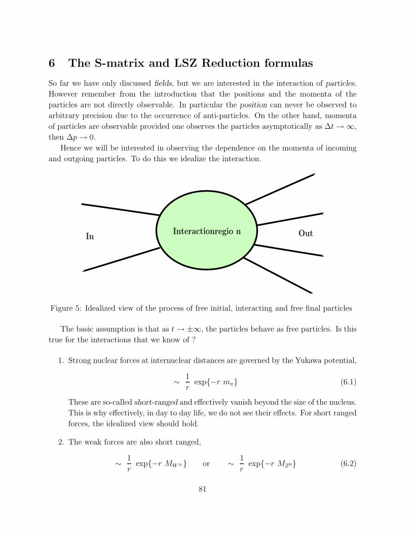
6 The S-matrix and LSZ Reduction formulas
So far we have only discussed fields, but we are interested in the interaction of particles.
However remember from the introduction that the positions and the momenta of the
particles are not directly observable. In particular the position can never be observed to
arbitrary precision due to the occurrence of anti-particles. On the other hand, momenta
of particles are observable provided one observes the particles asymptotically as ∆t→ ∞,
then ∆p→ 0.
Hence we will be interested in observing the dependence on the momenta of incoming
and outgoing particles. To do this we idealize the interaction.
In OutInteraction regio n
Figure 5: Idealized view of the process of free initial, interacting and free final particles
The basic assumption is that as t→ ±∞, the particles behave as free particles. Is this
true for the interactions that we know of ?
1. Strong nuclear forces at internuclear distances are governed by the Yukawa potential,
∼ 1
rexp{−r mπ} (6.1)
These are so-called short-ranged and effectively vanish beyond the size of the nucleus.
This is why effectively, in day to day life, we do not see their effects. For short ranged
forces, the idealized view should hold.
2. The weak forces are also short ranged,
∼ 1
rexp{−r MW±} or ∼ 1
rexp{−r MZ0} (6.2)
81
3. The electro-magnetic force falls off at infinity as well,
∼ 1
r2(6.3)
By contrast with the weak and strong forces however, this fall-off is only power-like
and such forces are referred to as long-ranged. This means that electro-magnetic
fields can extend over long distances and will not be confined to some small interac-
tion region. For example, the galactic magnetic fields extend over many parsecs. The
idealized picture may or may not hold. We should foresee difficulties at low energies
and low momenta (so-called IR propblems) when we apply the idealized view here.
4. The force of gravity behaves in the same manner as the electro-magnetic force and is
also long-ranged. Fortunately, the force of gravity is not on the menu for this course.
5. The most problematic of all – and the most interesting – is QCD which describes the
strong forces at a fundamental level. The force between two quarks is constant, even
for large distances (ignoring quark pair creation) and the quarks are confined, as it
would require an infinite amount of energy to separate two quarks that are subject
to a law of attraction that is constant. This effect is so dramatic that the spectrum
is altered to a hadronic spectrum.
6.0.1 In and Out States and Fields
If at t → −∞ the particles are free, then we better introduce a free field for them, which
are the so-called in-field, denoted generically by ΦIin(x). The Fock space associated with
Φin is Hin, and the states are labelled exactly as the free field states were. If at t → +∞the particles are free, we introduce free out-fields ΦJ
out(x) and the Fock space is Hout.
Of course we also have the Hilbert space of the full quantum field theory, which we
denote by H. Axiomatic field theory requires Hin = Hout = H. Here, however, we shall
attempt to define these different theories, to link them and then to check the nature of the
various Hilber spaces. Obviously, we should have the property Hin = Hout, which is called
asymptotic completeness.
The n-particle in-states created by in fields are denoted by
|in, p1, · · · , pn; I1, · · · , In〉 (6.4)
with particle momenta p1, · · · , pn and internal indices I1, · · · , In. The out-states created
by the out fiels are of the form
|out, q1 . . . qm, J1 · · ·Jm〉 (6.5)
82
where the m-particle out state has particle momenta q1 . . . qm, and internal indices
J1 . . . Jm. Note that it makes sense to label states in this way since momenta are ob-
servable to arbitrary precision in the t = to±∞ limit.
6.0.2 The S-matrix
The fundamental question in scattering theory and in quantum field theory is going to be
as follows. Given an initial in-state (the state of the system at t→ −∞),
|in p1, . . . pn; I1, . . . In〉 (6.6)
what is the probability (given the dynamics of the theory) for the final out-state (the state
at t→ +∞) to be
|out q1 . . . qm; J1, · · · , Jm〉 (6.7)
The answer is given by the inner product of the two states, as always
Sf←i = 〈out q1 . . . qm; J1 · · ·Jm|in p1, . . . pn, I1 · · · In〉 (6.8)
and the probability is
Wf←i = |Sf←i|2 (6.9)
Clearly, this question can be asked for every state in Hin onto every state in Hout. Assuming
asymptotic completeness, Hin = Hout, then there should exist a matrix S that relates the
in-states to the out-states,
|out〉 = S|in〉 (6.10)
The equivalence of the two Hilbert spaces requires that S be unitary. This may also be
seen from the fact that for a given initial state, a summation over all possible final states
must give unit probability. Thus, the S-matrix must be unitary ! Consequently, we may
describe all these overlap probabilities in terms of |in〉 or |out〉 states and the S-matrix.
6.0.3 Scattering cross sections
From the probability, one can compute the thing the experimental high energy physicist
talks about all day and dreams about: the scattering cross section. We shall limit ourselves
to an initial state with only 2 particles.
83
The incoming state is now in general a wave packet with distribution ρ, so
|in〉 =∫
d3p1
(2π)32po1
∫d3p2
(2π)32po2ρ1(p1)ρ2(p2)|in p1, p2〉 (6.11)
This wave packet is associated with a distribution ρ(x) (for a free particle) and positive
energy
ρ(x) =∫ d3p
(2π)32ωpe−ip·xρ(p) (6.12)
The flux is given by
Φρ ≡∫ d3p
(2π)32po|ρ(p)|2 =
# of particles
unit of time(6.13)
To isolate the interaction part from the free part, it is useful to decompose the S-matrix
into an identity part and a T matrix part, describing interaction
S = I + iT (6.14)
Energy momentum conservation then implies that
〈f |T |p1, p2〉 = (2π)4δ4(Pf − p1 − p2)〈f |T |p1, p2〉 (6.15)
In general, one will be interested in scattering cross sections for which 〈f |i〉 = 0. (If
|i〉 = |f〉, one deals with so-called forward scattering, and we shall not deal with it here.)
In the above case
〈f |S|i〉 = 〈f |i〉 − i〈f |T |i〉 = −i〈f |T |i〉 (6.16)
and
Wf←i = |〈f |S|i〉|2 = |〈f |T |i〉|2 (6.17)
Wf←i =∫
dp1
∫
dp2
∫
dp′1
∫
dp′2 ρ∗1(p1)ρ1(p
′1)ρ∗2(p2)ρ2(p
′2)(2π)4δ(p1 + p2 − Pf)
×(2π)4δ(p1 + p2 − p′1 − p′2)〈f |T |p1, p2〉∗〈f |T |p′1, p′2〉 (6.18)
Using now the fact that
(2π)4δ4(k) =∫
d4xe−ikx (6.19)
we may represent the second momentum conservation δ-function as a Fourrier integral,
Wf←i =∫
d4x∫
dp1
∫
dp2dp′1
∫
dp′2ρ∗1(p1)ρ1(p
′1)ρ∗2(p2)ρ2(p
′2)
×(2π)4δ4(p1 + p2 − Pf )e−ip1+p2−p′1−p
′2)·x〈f |T |p1, p2〉∗〈f |τ |p′1, p′2〉 (6.20)
Now we assume that the distributions ρ1 and ρ2 are very narrow, and sharply peaked
about momenta p1 and p2. We assume that the variation of the ρ’s is so small over this
84
distribution that the matrix elements of T are essentially constant over that variation. We
then have
〈f |T |p1, p2〉 ∼ 〈f |T |p′1, p′1〉 ' 〈f |T |p1, p2〉 (6.21)
Hence
Wf←i =∫
d4x|ρ1(x)|2|ρ2(x)|2(2π)4δ4(p1 + p2 − Pf)|〈f |T |p1, p2〉|2 (6.22)
Now to get the cross section, we want the transition probability per unit volume and per
unit time:
dWp←i
dtdV= |ρ1(x)|2|ρ2(x)|2(2π)4δ4(p1 + p2 − Pf)|〈f |T |p1, p2〉|2 (6.23)
Now the relative flux between distributions ρ1 and ρ2 is given by
4|m2γ2p1 −m1γ1p2||f1(x)|2|f2(x)|2 (6.24)
and therefore, the differential cross section is given by
dσ = (2π)4δ4(Pf − p1 − p2)1
2E12E2|~v1 − ~v2||〈f |T |p1, p2〉|2 (6.25)
The normalization holds for scalar, photons and spin 1/2 particles all the same!
6.1 Relating the interacting and in- and out-fields
The quantum field theory is formulated in terms of interacting fields φ(x) instead of the
free fields φin(x) and φout(x). To compute elements of the S matrix, we need to connect
the states |in〉 and |out〉 to the interacting fields in the theory. We carry this out here for
the case of a single scalar field φ. Other cases are completely analogous.
The in and out-fields satify the free field equations
(2 +m2)φin(x) = 0
(2 +m2)φout(x) = 0 (6.26)
as well as the canonical commutation relations
[φin(x), φin(y)]δ(x0 − y0) = −i δ(x− y)
85
[φout(x), φout(y)]δ(x0 − y0) = −i δ(x− y) (6.27)
The in and out states are now built with the help of the Fourier mode operators:
|in p1, · · · , pn〉 = a†in(~p1)a†in(~p2) · · ·a†in(pn)|0〉
|out q1, · · · , qm〉 = a†out(~q1)a†out(~q2) · · ·a†out(qm)|0〉 (6.28)
Recall the normalizations of the free in and out-fields with the 1-particle states,
〈in p|φin(x)|0〉 = eip·x
〈out q|φout(x)|0〉 = eiq·x (6.29)
Note that the normalization on the rhs is 1.
As remarked above, the dynammics of the theory is described by neither φin nor φout,
but rather by the interacting field φ. In some sense, the field φ should behave like φin or
φout according to whether t→ −∞ or t→ +∞.
To see concretely how this happens, consider the overlap of the field φ with the 1-
particle states. Accoding to general principles, the field φ should have non-zero overlap
with |in p〉. The x- and p-dependence of this overlap is determined by Poincare symmetry
in the following manner,
〈in p|φ(x)|0〉 = 〈in p|eix·Pφ(0)e−ix·P |0〉 = eip·x〈in p|φ(0)|0〉=
√Zeip·x (6.30)
Z is indepedent of p. We therefore conclude that
〈in p|φ(x)|0〉 =√Z〈in p|φin(x)|0〉
〈out p|φ(x)|0〉 =√Z〈out p|φin(x)|0〉 (6.31)
Therefore, we have – in a somewhat formal sense – the following limits
limt→−∞
φ(x) =√Zφin(x)
limt→+∞
φ(x) =√Zφout(x) (6.32)
This limit cannot really be understood in the sense of a limit of operators, but rather must
be viewed as a limit that will hold when matrix elements are taken with states containing
a finite number of particles.
86
6.2 The Kallen-Lehmann spectral representation
To evaluate Z, we construct the Kallen-Lehmann representation for the interacting theory.
The starting point is the commutator,
i ∆(x, x′) = 〈0|[φ(x), φ(x′)]|0〉 (6.33)
Let us collectively denote all the states of the theory |n〉. Then, using completeness of the
states |n〉, we insert a complete set of normalized states,
i ∆(x, x′) =∑
n
(
〈0|φ(x)|n〉〈n|φ(x′)|0〉 − 〈0|φ(x′)|n〉〈n|φ(x)|0〉)
(6.34)
Translation symmetry of the theory allows us to pull out the x-dependence using φ(x) =
eix·Pφ(0)e−ix·P so that
i ∆(x, x′) =∑
n
|〈0|φ(0)|n〉|2(
e−ipn·(x−x′) − eipn·(x−x′))
(6.35)
Using 1 =∫
d4qδ(q − pn), we have
i ∆′(x, x′) =∫
d4q
(2π)3ρ(q)
(
e−iq(x−x′) − eiq(x−x
′))
(6.36)
where the spectral density is defined to be
ρ(q) ≡ (2π)3∑
n
δ4(q − pn)|〈0|φ(0)|n〉|2 (6.37)
Notice that ρ is positive, and vanishes when either q2 < 0 or q0 < 0. Also it is Lorentz
invariant, and therefore can only depend upon q2. Thus, it is convenient to introduce the
function σ(q2) as follows,
ρ(q) = θ(q0)σ(q2) σ(q2) = 0 if q2 < 0 (6.38)
Recall the free commutator,
i ∆0(x− y,m2) =∫
d4q
(2π)3θ(q0)δ(q2 −m2)
(
e−iq(x−y) − eiq(x−y))
(6.39)
Hence we may express the commutator of the fully interacting fields as,
∆(x− x′) =∫ ∞
0dµ2σ(µ2)∆0(x− x′;µ2) (6.40)
This is the Kallen-Lehmann representation for the commutator.
87
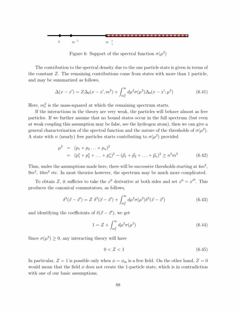
0 m 2 m 2t
Figure 6: Support of the spectral function σ(µ2)
The contribution to the spectral density due to the one particle state is given in terms of
the constant Z. The remaining contributions come from states with more than 1 particle,
and may be summarized as follows,
∆(x− x′) = Z∆0(x− x′, m2) +∫ ∞
m2
t
dµ2σ(µ2)∆0(x− x′;µ2) (6.41)
Here, m2t is the mass-squared at which the remaining spectrum starts.
If the interactions in the theory are very weak, the particles will behave almost as free
particles. If we further assume that no bound states occur in the full spectrum (but even
at weak coupling this assumption may be false, see the hydrogen atom), then we can give a
general characterization of the spectral function and the nature of the thresholds of σ(µ2).
A state with n (nearly) free particles starts contributing to σ(µ2) provided
µ2 = (p1 + p2 . . .+ pn)2
= (po1 + po2 + . . .+ pon)2 − (~p1 + ~p2 + . . .+ ~pn)
2 ≥ n2m2 (6.42)
Thus, under the assumptions made here, there will be successive thresholds starting at 4m2,
9m2, 16m2 etc. In most theories however, the spectrum may be much more complicated.
To obtain Z, it sufficies to take the x0 derivative at both sides and set x0 = x′0. This
produces the canonical commutators, as follows,
δ3(~x− ~x′) = Z δ3(~x− ~x′) +∫ ∞
m2
t
dµ2σ(µ2)δ3(~x− ~x′) (6.43)
and identifying the coefficients of δ(~x− ~x′), we get
1 = Z +∫ ∞
m2
t
dµ2σ(µ2) (6.44)
Since σ(µ2) ≥ 0, any interacting theory will have
0 < Z < 1 (6.45)
In particular, Z = 1 is possible only when φ = φin is a free field. On the other hand, Z = 0
would mean that the field φ does not create the 1-particle state, which is in contradiction
with one of our basic assumptions.
88
One may also obtain a Kallen-Lehmann representation for the two-point function in
terms of similar methods,
〈0|Tφ(x)φ(x′)|0〉 =∫ ∞
0dµ2σ(µ2)GF (x− y, µ2) (6.46)
Notice that the field φ which governs the dynammics and which obeys canonical com-
mutation relations is not the field that obeys a canonical normalization on one-particle
states. There is a multiplicative factor between the two fields. This is the first non-trivial
example of the phenomenon of renormalization: the parameter that govern the dynamics
in the theory like the field, the mass, the coupling constants are not the parameters that
are observable in the asymptotic regime. Later on it will be convenient to work directly
with this renormalized field
φR(x) ≡ 1√Zφ(x) (6.47)
Of course the field φR will no longer satisfy canonical commutation relations.
6.3 The Dirac Field
A similar treatment is available for the Dirac field ψ(x). We restrict to quoting the results
here. The normalizations of the in and out fields and of the interacting field are as follows,
〈0|ψin(x)|in p, λ〉 = u(p, λ)e−ip·x
〈0|ψ(x)|in|p, λ〉 =√
Z2〈0|ψin(x)in p, λ〉=
√
Z2〈0|ψout(x)|out p, λ〉 (6.48)
The Kallen-Lehmann representation is obtained by introducing the spectral density
ρβα(q) = (2π)3∑
n
δ4(pn − q)〈0|ψα(0)|n〉〈ψβ(0)|0〉 (6.49)
so that, using Lorentz invariance, one gets
ρβα(q) = θ(q0)(
σ1(q2)( 6 q) β
α + σ2(q2)δ β
α
)
(6.50)
The result is most easily expressed in terms of the free scalar propagator,
〈0{ψα(x)ψβ(x′)}|0〉 =∫ ∞
0dµ2
(
iσ1(µ2) 6 ∂x + σ2(µ
2))
α
βGF (x− x′;µ2) (6.51)
Properties of σ1 and σ2 are as follows, σ1(µ2) ≥ 0, σ2(µ
2) ≥ 0, and µσ1(µ2) − σ2(µ
2) ≥ 0.
The spectral representation for Z2 is obtained again via the equal time commutators,
i〈0|{ψα(x)ψβ(x′)}|0〉 = Z2S(x− x′) +∫ ∞
m2
t
dµ2(
iσ1(µ2) 6 ∂x + σ2(µ
2))
α
βGF (x− x′;µ2)
and we get
1 = Z2 +∫ ∞
4m2
dµ2σ1(µ2) (6.52)
89
6.4 The LSZ Reduction Formalism
It is now our task to evaluate the S-matrix elements in terms of quantities which can be
expressed in terms of the dynammics of the QFT. We shall treat in detail here the case
of the real scalar field; the other cases may be handled analogously. The key object of
interest is the transition amplitude
〈out q1 · · · qm|in p1 · · ·pn〉 (6.53)
We shall work out a recursion formula which decreases the number of particles in the in
and out states and replaces the overlap with expectation values of the fully interacting
quantum field φ. To this end, we isolate the in-particle with momentum pn, and write
〈out q1 · · · qm|in p1 · · ·pn〉 = 〈out β|in α pn〉|in α〉 = |in p1 · · · pn−1〉
|out β〉 = |out q1 · · · qm〉|in p1 · · ·pn〉 = a†in(pn)|in α〉 (6.54)
6.4.1 In- and Out-Operators in terms of the free field
The decomposition into creation and annihilation operators of a free scalar field ϕ(x) with
mass m and its canonical momentum ∂0φ(t, ~x) are given in terms by
ϕ(t, ~x) =∫
d3k
(2π)32ωk
(
a(~k)e−k·x + a†(~k)eik·x)
∂0ϕ(t, ~x) =∫ d3k
(2π)32
(
−ia(~k)e−ik·x + ia†(~k)eik·x)
(6.55)
The creation and annihilation operators may be recovered by by taking the space Fourier
transforms
a†(~k) = −i∫
d3x(
e−ik·x↔
∂ 0 ϕ(x))
a(~k) = +i∫
d3x(
e+ik·x↔
∂ 0 ϕ(x))
(6.56)
Here, the symbol↔
∂ stands for the antisymmetrixed derivative u↔
∂ 0 v ≡ u∂0v− ∂0uv. The
left hand side is independent of the time coordinate x0 at which the field ϕ(x) is evaluated
on the left hand side as long as the momentum satisfies k2 = m2.
90
6.4.2 Asymptotics of the interacting field
Next, we make use of the fact that, when evaluated between states, where it is to play the
role of creation operator, the field tends towards free field expectation values,
limx0→+∞
〈out|φ(x)|in〉 ∼ Z−1
2 〈out|φout(x)|in〉
limx0→−∞
〈out|φ(x)|in〉 ∼ Z−1
2 〈out|φin(x)|in〉 (6.57)
Combining this result with the free field formulas for the creation operators for in- and
out-operators, we obtain (omitting now the in- and out-states matrix elements),
a†in(~k) = − i√Z
limx0→−∞
∫
d3x(
e−ik·x↔
∂ 0 φ(x))
a†out(~k) = − i√
Zlim
x0→+∞
∫
d3x(
e−ik·x↔
∂ 0 φ(x))
ain(~k) = +i√Z
limx0→−∞
∫
d3x(
e+ik·x↔
∂ 0 φ(x))
aout(~k) = +
i√Z
limx0→+∞
∫
d3x(
e+ik·x↔
∂ 0 φ(x))
(6.58)
Using the fact that the difference between the same quantity evaluated at x0 → ±∞ may
be expressed as an integral,
limx0→+∞
ψ(x) − limx0→−∞
ψ(x) =∫ +∞
−∞dx0∂0ψ(x) (6.59)
we obtain the following difference formulas between in- and out-operators,
a†in(~k) − a†out(~k) = +
i√Z
∫
d4x∂0
(
e−ik·x↔
∂ 0 φ(x))
ain(~k) − aout(~k) = − i√
Z
∫
d4x∂0
(
e+ik·x↔
∂ 0 φ(x))
(6.60)
These combinations admit further simplifications which may be seen by working out the
integrand and using the fact that k2 = m2,∫
d4x∂0
(
e±ik·x↔
∂ 0 φ(x))
=∫
d4x(
(k0)2φ(x) + ∂20φ(x)
)
e±ik·x
=∫
d4xe±ik·x(2 +m2)φ(x) (6.61)
Thus, we obtain the following formulas,
a†in(~k) − a†out(~k) = +
i√Z
∫
d4x e−ik·x(2 +m2)φ(x)
ain(~k) − aout(~k) = − i√
Z
∫
d4x e+ik·x(2 +m2)φ(x) (6.62)
Clearly, for a free field, satisfying (2 + m2)φ = 0, there is no difference between the in-
and out-operators, but as soon as interactions are turned on, they are no longer equal.
91
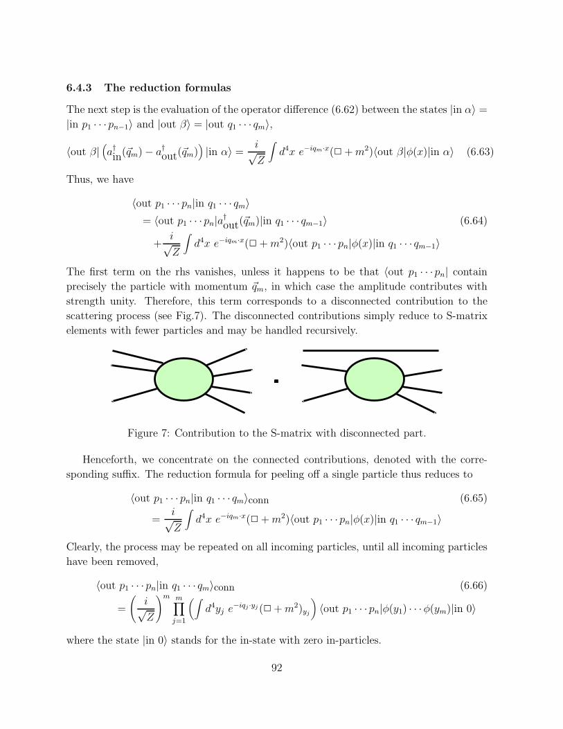
6.4.3 The reduction formulas
The next step is the evaluation of the operator difference (6.62) between the states |in α〉 =
|in p1 · · · pn−1〉 and |out β〉 = |out q1 · · · qm〉,
〈out β|(
a†in(~qm) − a†out(~qm))
|in α〉 =i√Z
∫
d4x e−iqm·x(2 +m2)〈out β|φ(x)|in α〉 (6.63)
Thus, we have
〈out p1 · · · pn|in q1 · · · qm〉= 〈out p1 · · · pn|a†out(~qm)|in q1 · · · qm−1〉 (6.64)
+i√Z
∫
d4x e−iqm·x(2 +m2)〈out p1 · · · pn|φ(x)|in q1 · · · qm−1〉
The first term on the rhs vanishes, unless it happens to be that 〈out p1 · · ·pn| contain
precisely the particle with momentum ~qm, in which case the amplitude contributes with
strength unity. Therefore, this term corresponds to a disconnected contribution to the
scattering process (see Fig.7). The disconnected contributions simply reduce to S-matrix
elements with fewer particles and may be handled recursively.
=
Figure 7: Contribution to the S-matrix with disconnected part.
Henceforth, we concentrate on the connected contributions, denoted with the corre-
sponding suffix. The reduction formula for peeling off a single particle thus reduces to
〈out p1 · · · pn|in q1 · · · qm〉conn (6.65)
=i√Z
∫
d4x e−iqm·x(2 +m2)〈out p1 · · · pn|φ(x)|in q1 · · · qm−1〉
Clearly, the process may be repeated on all incoming particles, until all incoming particles
have been removed,
〈out p1 · · · pn|in q1 · · · qm〉conn (6.66)
=
(
i√Z
)m m∏
j=1
(∫
d4yj e−iqj ·yj (2 +m2)yj
)
〈out p1 · · · pn|φ(y1) · · ·φ(ym)|in 0〉
where the state |in 0〉 stands for the in-state with zero in-particles.
92
It remains to remove also the out-particles. However, now there is a new issue to be
dealt with. The removal of the out particles must always occur to the left of the removal of
the in-particles, since the two operator types will not have simple commutation relations.
This ordering is achieved by ordering the later times to the left of the earlier times, since
out-states correspond to x0 → +∞ while in-states correspond to x0 → −∞. Since out-
states will have to be removed using annihilation operators, there is also an adjoint to be
taken. Thus, the final formula is
〈out p1 · · · pn|in q1 · · · qm〉conn (6.67)
=im(−i)n√Zm+n
n∏
k=1
(∫
d4xk e+ipk·xk(2 +m2)xk
)
×m∏
j=1
(∫
d4yj e−iqj ·yj(2 +m2)yj
)
〈out 0|Tφ(x1) · · ·φ(xn)φ(y1) · · ·φ(ym)|in 0〉
The key lesson to be learned from this formula is that the calculation of any scattering
matrix element requires the calculation in QFT of only a single type of object, namely the
time ordered correlation function, or correlator,
〈0|Tφ(x1) · · ·φ(xn)|0〉 (6.68)
Much of the remainder of the subject of quantum field theory will be concerned with the
calculation of these quantities.
6.4.4 The Dirac Field
The derivation for the Dirac field is completely analogous, though the precise 1-particle
wave functions are of course those associated with the Dirac equation instead of with
the Klein-Gordon equation. Furthermore, one will have to be careful about taking the
anti-commutative nature of the field ψ into account. For example, for in-fields we have
ψin(x) =∫
d3k
(2π)32ωk
∑
λ=±
(
bin(k, λ)u(k, λ) e−ik·x + d†in(k, λ)v(k, λ) eik·x)
(6.69)
which gives rise to the following expressions for the in- and out-operators,
bin(k, λ) =∫
d3xu(k, λ) eik·xγ0ψin(x)
d†in(k, λ) =∫
d3xv(k, λ) e−ik·xγ0ψin(x)
b†in(k, λ) =∫
d3xψ(x)γ0 e−ik·xu(k, λ)
din(k, λ) =∫
d3xψ(x)γ0 e−ik·xv(k, λ) (6.70)
93
The 1-particle state normalizations with the in-field ψin and with the fully interacting field
ψ are as follows,
〈0|ψin(x)|in p λ〉 = u(p, λ)e−ip·x
〈0|ψ(x)|in p λ〉 =√
Z2u(p, λ)e−ip·x (6.71)
You see that one can get a similar formula as for the bosonic scalar case, but now you have
to be careful about where the spinor indices are contracted. Clearly, everything is again
expressed in terms of time-ordered correlators for the fully interacting fermion fields,
〈0|Tψα1(x1)ψα2
(x2) . . . ψαn(xn)ψβ1(y1) . . . ψβp(yp)|0〉 (6.72)
6.4.5 The Photon Field
Since the lontgitudinal photons are free, we are only interested in scattering transverse
photons. kµεµ(k) = 0
〈β(k1ε)out|α in〉 = β out|α− (kε) in〉+ 〈β out|ε · aout(k) − ε · aout(k) − ε · ain(k)|α in〉
= −i∫
td3xeikx
↔
∂ o 〈β out|ε(k) · AT out(x) − ε(k)AR in(x)|α in〉
= −i Z1/23
∫
t→∞d3xeikx
↔
∂ o 〈β out|ε(k) · AT (x)|α in〉
+ i Z−1/23
∫
t→−∞d3xeikx
↔
∂ o 〈β out|ε(k)AT (x)|α in〉
= −i Z−1/23
∫
d4x{
eikx∂2o 〈β out|ε(k) ·AT (x)|α in〉
−(∂2oeikx)〈β out|ε(k) ·AT (x)|α in〉
}
= −i Z−1/23
∫
d4x{
eikx(2 + µ2)x〈β out|ε(k) · AT (x)α in〉}
(6.73)
Now:
ATµ (x) = Aµ(x) +1
m2∂µ∂ · A (6.74)
(2 + µ2)xATµ (x) = (2 + µ2)Aµ +
1
m22∂µ(∂ · A) +
µ2
m2∂µ∂ · A
= (2 + µ2)Aµ − ∂µ(∂ · A) + λ∂µ(∂ · A)
= jµ , our best friend! (6.75)
Hence, in the non-forward regime, we have the simple formula:
〈β(k, ε) out|α in〉 == i Z1/23
∫
d4xeikx〈β out|εµ(k)jµ(x)|α in〉 (6.76)
Now let’s play this game over with two photons:
〈β(kf , εf)out|α(ki, εi)in〉
94
= −Z−13
∫
d4x∫
d4yei(kfx−kiy)(2 + µ2)y
〈β out|Tεf · j(x)[
εi · (A(y)) +1
m2∂(∂A)(y)
]
|α in〉 (6.77)
You see that this is not just the time ordered product of the currents, there will be some
additional terms, arising however only at xo = yo. By locality, the contribution must now
be entirely localized at ~x = ~y = ~y as well. One can show, after a lot of work that one
exactly gets the T ∗ product. What else could it be?
〈β(kf , εf ) out|α(ki, εi) in〉= −Z−1
3
∫
d4x∫
d4yei(kfx−kiy)
〈β out|T ∗εf · j(x)εi · j(y)|α in〉 (6.78)
It is straightforward to generalize this formula.
95
QUANTUM FIELD THEORY – 230B
Eric D’Hoker
Department of Physics and Astronomy
University of California, Los Angeles, CA 90095
Contents
1 Functional Methods in Scalar Field Theory 2
1.1 Functional integral formulation of quantum mechanics . . . . . . . . . . . . 2
1.2 The functional integral for scalar fields . . . . . . . . . . . . . . . . . . . . 3
1.3 Time ordered correlation functions . . . . . . . . . . . . . . . . . . . . . . 4
1.4 The generating functional of correlators . . . . . . . . . . . . . . . . . . . 5
1.5 The generating Functional for free scalar field theory . . . . . . . . . . . . 5
2 Perturbation Theory for Scalar Fields 8
2.1 Scalar Field Theory with potential interactions . . . . . . . . . . . . . . . . 8
2.2 Feynman rules for φ4-theory . . . . . . . . . . . . . . . . . . . . . . . . . . 10
2.3 The cancellation of vacuum graphs. . . . . . . . . . . . . . . . . . . . . . . 11
2.4 General Position Space Feynman Rules for scalar field theory . . . . . . . . 12
2.5 Momentum Space Representation . . . . . . . . . . . . . . . . . . . . . . . 13
2.6 Does perturbation theory converge ? . . . . . . . . . . . . . . . . . . . . . 14
2.7 The loop expansion . . . . . . . . . . . . . . . . . . . . . . . . . . . . . . . 15
2.8 Truncated Diagrams . . . . . . . . . . . . . . . . . . . . . . . . . . . . . . 15
2.9 Connected graphs . . . . . . . . . . . . . . . . . . . . . . . . . . . . . . . . 16
2.10 One-Particle Irreducible Graphs and the Effectice Action . . . . . . . . . . 17
2.11 Schwinger Dyson Equations . . . . . . . . . . . . . . . . . . . . . . . . . . 19
2.12 The Background Field Method for Scalars . . . . . . . . . . . . . . . . . . 20
3 Basics of Perturbative Renormalization 22
3.1 Feynman parameters . . . . . . . . . . . . . . . . . . . . . . . . . . . . . . 22
3.2 Integrations over internal momenta . . . . . . . . . . . . . . . . . . . . . . 23
3.3 The basic idea of renormalization . . . . . . . . . . . . . . . . . . . . . . . 24
3.3.1 Mass renormalization . . . . . . . . . . . . . . . . . . . . . . . . . . 25
3.3.2 Coupling Constant Renormalization . . . . . . . . . . . . . . . . . . 26
3.3.3 Field renormalization . . . . . . . . . . . . . . . . . . . . . . . . . . 28
3.4 Renormalization point and renormalization conditions . . . . . . . . . . . . 30
3.5 Renormalized Correlators . . . . . . . . . . . . . . . . . . . . . . . . . . . 31
3.6 Summary of regularization and renormalization procedures . . . . . . . . . 33
4 Functional Integrals for Fermi Fields 35
4.1 Integration over Grassmann variables . . . . . . . . . . . . . . . . . . . . . 36
4.2 Grassmann Functional Integrals . . . . . . . . . . . . . . . . . . . . . . . . 37
4.3 The generating functional for Grassmann fields . . . . . . . . . . . . . . . 38
4.4 Lagrangian with multilinear terms . . . . . . . . . . . . . . . . . . . . . . 39
5 Quantum Electrodynamics : Basics 40
5.1 Feynman rules in momentum space . . . . . . . . . . . . . . . . . . . . . . 40
5.2 Verifying Feynman rules for one-loop Vacuum Polarization . . . . . . . . 41
5.3 General fermion loop diagrams . . . . . . . . . . . . . . . . . . . . . . . . . 43
5.4 Pauli-Villars Regulators . . . . . . . . . . . . . . . . . . . . . . . . . . . . 43
5.5 Furry’s Theorem . . . . . . . . . . . . . . . . . . . . . . . . . . . . . . . . 43
5.6 Ward-Takahashi identities for the electro-magnetic current . . . . . . . . . 44
5.7 Regularization and gauge invariance of vacuum polarization . . . . . . . . 46
5.8 Calculation of vacuum polarization . . . . . . . . . . . . . . . . . . . . . . 47
5.9 Resummation and screening effect . . . . . . . . . . . . . . . . . . . . . . . 49
5.10 Physical interpretation of the effective charge . . . . . . . . . . . . . . . . 50
5.11 Renormalization conditions and counterterms . . . . . . . . . . . . . . . . 51
5.12 The Gell-Mann – Low renormalization group . . . . . . . . . . . . . . . . . 52
6 Quantum Electrodynamics : Radiative Corrections 54
6.1 A first look at the Electron Self-Energy . . . . . . . . . . . . . . . . . . . . 54
6.2 Photon mass and removing infrared singularities . . . . . . . . . . . . . . . 56
6.3 The Electron Self-Energy for a massive photon . . . . . . . . . . . . . . . . 57
6.4 The Vertex Function : General structure . . . . . . . . . . . . . . . . . . . 57
6.5 Calculating the off-shell Vertex . . . . . . . . . . . . . . . . . . . . . . . . 59
6.6 The Electron Form Factor and Structure Functions . . . . . . . . . . . . . 61
6.7 Calculation of the structure functions . . . . . . . . . . . . . . . . . . . . . 62
6.8 The One-Loop Anomalous Magnetic Moment . . . . . . . . . . . . . . . . 64
2
7 Functional Integrals For Gauge Fields 66
7.1 Functional integral for Abelian gauge fields . . . . . . . . . . . . . . . . . . 66
7.2 Functional Integral for Non-Abelian Gauge Fields . . . . . . . . . . . . . . 68
7.3 Canonical Quantization . . . . . . . . . . . . . . . . . . . . . . . . . . . . . 69
7.4 Functional Integral Quantization . . . . . . . . . . . . . . . . . . . . . . . 71
7.5 The redundancy of integrating over gauge copies . . . . . . . . . . . . . . . 72
7.6 The Faddeev-Popov gauge fixing procedure . . . . . . . . . . . . . . . . . . 74
7.7 Calculation of the Faddeev-Popov determinant . . . . . . . . . . . . . . . . 77
7.8 Faddeev-Popov ghosts . . . . . . . . . . . . . . . . . . . . . . . . . . . . . 78
7.9 Axial and covariant gauges . . . . . . . . . . . . . . . . . . . . . . . . . . . 78
8 Anomalies in QED 80
8.1 Massless 4d QED, Gell-Mann–Low Renormalization . . . . . . . . . . . . . 80
8.2 Scale Invariance of Massless QED . . . . . . . . . . . . . . . . . . . . . . . 81
8.3 Chiral Symmetry . . . . . . . . . . . . . . . . . . . . . . . . . . . . . . . . 82
8.4 The axial anomaly in 2-dimensional QED . . . . . . . . . . . . . . . . . . . 83
8.5 The axial anomaly and regularization . . . . . . . . . . . . . . . . . . . . . 85
8.6 The axial anomaly and massive fermions . . . . . . . . . . . . . . . . . . . 87
8.7 Solution to the massless Schwinger Model . . . . . . . . . . . . . . . . . . 88
8.8 The axial anomaly in 4 dimensions . . . . . . . . . . . . . . . . . . . . . . 89
3
1 Functional Methods in Scalar Field Theory
The essential information of a quantum field theory is contained in its time ordered cor-
relation functions. From these, the scattering matrix elements, the transition amplitudes
and probabilities for any process may be computed.
In the preceding sections we have evaluated the correlation functions exactly for the
free field theories containing scalar, spin 1/2 and spin 1 fields. The evaluation of the
correlation functions in any interacting theory is a very difficult problem that can only
rarely be carried out exactly. Frequently, one will have to resort to an approximate or
perturbative treatment, for example based on an expansion in powers of the coupling
constants. Even the perturbative series is quite complicated because the combinatorics as
well as the space-time properties give rise to involved problems. Historically, perturbative
calculations were first carried out in the operator formalism of QFT, by recasting each of
the expansion coefficients in terms of free field theory correlation functions. For scalar field
theory problems, these calculations were involved but manageable. For gauge theories,
however, the operator methods very quickly become unmanageable. For non-Abelian
Yang-Mills theory, operator methods are seldom useful.
The functional integral formulation (already derived for quantum mechanics in SA2)
provides an alternative way of dealing with QFT. Historically, the functional integral for-
mulation of QFT was regarded foremost merely as an efficient way of organizing perturba-
tion theory. Its indispensible value was established permanently, however, with the advent
of non-Abelian Yang-Mills theory. Its direct connection with statistical mechanics led Wil-
son and others to use the functional integral formulation as a non-perturbative formulation
of QFT, and to a much deeper understanding of the properties of renormalization.
1.1 Functional integral formulation of quantum mechanics
In SA.2.6, the functional integral formulation of quantum mechanics was derived for a
Hamiltonian H(p, q) and the following formula was obtained,
〈q′|e−itH |q〉 =∫Dp
∫Dq exp
{i∫ t
0dt′(pq −H(p, q)
)(t′)
}(1.1)
with the boundary conditions q(t′ = 0) = q and q(t′ = t) = q′, and free boundary conditions
on p(t′). Recall that the measure arose from a discretisation of the time interval [0, t], for
t > 0, into N segments [ti, ti+1], t0 = 0, tN = t, i = 0, N − 1, and was formally defined by
DpDq ≡ limN→∞
N−1∏i=1
dp(ti)dq(ti)
2π(1.2)
4
Notice that the intermediate times are ordered, t = t0 < t1 < · · · < tN−1 < tN = t, so that
the integral is really over paths rather than over functions.
1.2 The functional integral for scalar fields
We now generalize the above discussion to the case of one real scalar field φ, thus to an
infinite number of degrees of freedom. We denote the momentum canonically conjugate
to φ by π and the Hamiltonian by H[φ, π]. The analogue of the position basis of states
|q〉 and |p〉 is given by |φ(~x)〉 and by |π(~x)〉. Remark that these states do not depend on
~x; instead they are functionals of φ. The completeness relations are now
I =∫Dφ(~x) |φ(~x)〉〈φ(~x)|
I =∫Dπ(~x) |π(~x)〉〈π(~x)| (1.3)
Clearly, the derivation is formal and we shall postpone all issues of cutoff and renormal-
ization until later. The derivation then follows identically the same path as we had for
quantum mechanics and therefore, we have the following result,
〈φ′|e−itH |φ〉 =∫DφDπ exp{iI[φ, π]}
{φ(t, ~x) = φ′(~x)φ(0, ~x) = φ(~x)
(1.4)
where the action is defined by
I[φ, π] ≡∫ t
0dt′(∫
d3xπφ−H[π, φ])
(t′) (1.5)
In the special case of the following simple but useful Hamiltonian,
H[φ, π] =∫d3x
(1
2π2 +
1
2(~∇φ)2 + V (φ)
)(1.6)
one gets after performing the Gaussian integration over π
〈φ′|e−itH |φ〉 =∫Dφ exp
{i∫ t
0dt′∫d3xL(φ, ∂φ)
} {φ(t, ~x) = φ′(~x)φ(0, ~x) = φ(~x)
(1.7)
Notice that, as an added bonus, this formulation is now manifestly Lorentz covariant, as
it is given in terms of the Lorentz invariant Lagrangian
L(φ, ∂φ) =1
2∂µφ∂
µφ− V (φ) (1.8)
Preserving Lorentz invariance will prove invaluable later on.
5
1.3 Time ordered correlation functions
The above result may be applied directly to the calculation of the vacuum expectation
value of the time ordered product of a string of fields φ,
〈0|Tφ(x1)φ(x2) · · ·φ(xn)|0〉 (1.9)
Notice that this object is a completely symmetric function of x1, · · ·xn. Hence, without
loss of generality, the points xi may be time-ordered, xo1 ≥ xo2 ≥ xo3 · · · ≥ xon so that
〈0|Tφ(x1)φ(x2) · · ·φ(xn)|0〉 = 〈0|φ(x1)φ(x2) · · ·φ(xn)|0〉 (1.10)
Next, one uses the evolution operator to bring out the time-dependence of the field oper-
ators φ(xi) given by the following expression,
φ(xoi , ~xi) = eixoiHφ(0, ~xi)e
−ixoiH (1.11)
Using this formula for the time-dependence of every inserted operator, we obtain,
〈0|φ(x1)φ(x2) · · ·φ(xn)|0〉 (1.12)
= 〈0|eixo1Hφ(0, ~x1)e
−i(xo1−x
o2)Hφ(0, ~x2)e
−i(xo2−x
o3)H · · · e−i(xo
n−1−xon)Hφ(0, ~xn)e
−ixonH |0〉
Next, we insert the identity operator exactly n times and express the identity as a com-
pleteness relation in the position basis of states |φ(~x)〉 Since the insertions have to be
carried out n times, we introduce n integration fields , which we denote by φ(xoi , ~xi),
i = 1, · · · , n. The operator insertions φ(0, ~xi) are diagonal in this basis and we obtain,
=∫Dφ(xo1, ~x1) · · ·
∫Dφ(xon, ~xn)〈0|eix
o1H |φ(xo1, ~x1)〉φ(xo1, ~x1) (1.13)
×〈φ(xo1, ~x1)|e−i(xo1−x
o2)H |φ(xo2, ~x2)〉φ|xo2, ~x2〉
×〈φ(xo2, ~x2)|e−i(xo2−x
o3)H |φ(xo3, ~x3)〉 · · · 〈φ(xon, ~xn)|e−ix
onH |0〉
At this stage, we use the functional integral form for the matrix elements in the field basis
of the evolution operator, as derived in (). It is immediately realized that the boundary
conditions at each integration over φ(xoi , ~xi) simply requires integration over a path in time
that is continuous. Furthermore, since the Hamiltonian acts on the ground state, assumed
to have zero energy, the time integrations may be taken to ±∞ on both ends. Finally,
there is a normalization factor Z[0] that will guarantee that the ground state is properly
6
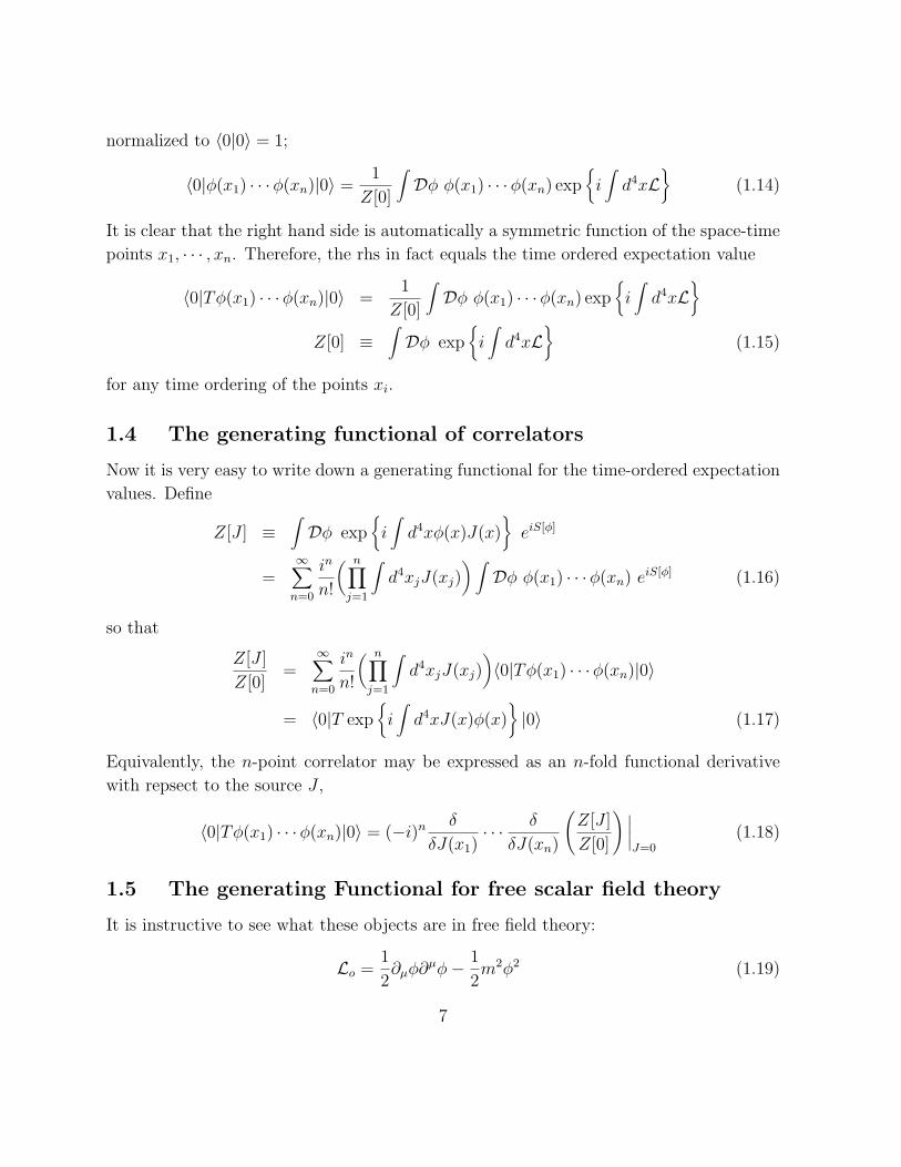
normalized to 〈0|0〉 = 1;
〈0|φ(x1) · · ·φ(xn)|0〉 =1
Z[0]
∫Dφ φ(x1) · · ·φ(xn) exp
{i∫d4xL
}(1.14)
It is clear that the right hand side is automatically a symmetric function of the space-time
points x1, · · · , xn. Therefore, the rhs in fact equals the time ordered expectation value
〈0|Tφ(x1) · · ·φ(xn)|0〉 =1
Z[0]
∫Dφ φ(x1) · · ·φ(xn) exp
{i∫d4xL
}Z[0] ≡
∫Dφ exp
{i∫d4xL
}(1.15)
for any time ordering of the points xi.
1.4 The generating functional of correlators
Now it is very easy to write down a generating functional for the time-ordered expectation
values. Define
Z[J ] ≡∫Dφ exp
{i∫d4xφ(x)J(x)
}eiS[φ]
=∞∑n=0
in
n!
( n∏j=1
∫d4xjJ(xj)
) ∫Dφ φ(x1) · · ·φ(xn) e
iS[φ] (1.16)
so that
Z[J ]
Z[0]=
∞∑n=0
in
n!
( n∏j=1
∫d4xjJ(xj)
)〈0|Tφ(x1) · · ·φ(xn)|0〉
= 〈0|T exp{i∫d4xJ(x)φ(x)
}|0〉 (1.17)
Equivalently, the n-point correlator may be expressed as an n-fold functional derivative
with repsect to the source J ,
〈0|Tφ(x1) · · ·φ(xn)|0〉 = (−i)n δ
δJ(x1)· · · δ
δJ(xn)
(Z[J ]
Z[0]
) ∣∣∣∣J=0
(1.18)
1.5 The generating Functional for free scalar field theory
It is instructive to see what these objects are in free field theory:
Lo =1
2∂µφ∂
µφ− 1
2m2φ2 (1.19)
7
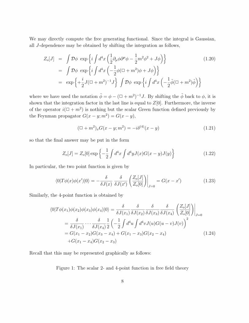
We may directly compute the free generating functional. Since the integral is Gaussian,
all J-dependence may be obtained by shifting the integration as follows,
Zo[J ] =∫Dφ exp
{i∫d4x
(1
2∂µφ∂
µφ− 1
2m2φ2 + Jφ
)}(1.20)
=∫Dφ exp
{i∫d4x
(−1
2φ(2 +m2)φ+ Jφ
)}= exp
{+i
2J(2 +m2)−1J
} ∫Dφ exp
{i∫d4x
(−1
2φ(2 +m2)φ
)}
where we have used the notation φ = φ− (2 +m2)−1J . By shifting the φ back to φ, it is
shown that the integration factor in the last line is equal to Z[0]. Furthermore, the inverse
of the operator i(2 +m2) is nothing but the scalar Green function defined previously by
the Feynman propagator G(x− y;m2) = G(x− y),
(2 +m2)xG(x− y;m2) = −iδ(4)(x− y) (1.21)
so that the final answer may be put in the form
Zo[J ] = Zo[0] exp{−1
2
∫d4x
∫d4yJ(x)G(x− y)J(y)
}(1.22)
In particular, the two point function is given by
〈0|Tφ(x)φ(x′)|0〉 = − δ
δJ(x)
δ
δJ(x′)
(Zo[J ]
Zo[0]
)∣∣∣∣∣J=0
= G(x− x′) (1.23)
Similarly, the 4-point function is obtained by
〈0|Tφ(x1)φ(x2)φ(x3)φ(x4)|0〉 =δ
δJ(x1)
δ
δJ(x2)
δ
δJ(x3)
δ
δJ(x4)
(Zo[J ]
Zo[0]
)∣∣∣∣∣J=0
=δ
δJ(x1)· · · δ
δJ(x4)
1
2
(−1
2
∫d4u
∫d4vJ(u)G(u− v)J(v)
)2
= G(x1 − x2)G(x3 − x4) +G(x1 − x3)G(x2 − x4) (1.24)
+G(x1 − x4)G(x2 − x3)
Recall that this may be represented graphically as follows:
Figure 1: The scalar 2- and 4-point function in free field theory
8
More generally, the n-point function vanishes when n is odd (by φ → −φ symmetry),
while 2n-point functions are given by
〈0|Tφ(x1) · · ·φ(x2n)|0〉 =1
2n n!
∑σ
G(xσ(1) − xσ(2)) · · ·G(xσ(2n−1) − xσ(2n)) (1.25)
The summation is effectively over all possible inequivalent pairings of the 2n points, in
which each inequivalent term then appears with coefficient 1.
9
2 Perturbation Theory for Scalar Fields
For a general interacting theory, none of the Green functions can be computed exactly.
Recall that in ordinary quantum mechanics, one can do this only in the cases where extra
symmetries decouple the degrees of freedom, which is exceedingly rare. It is even more rare
in quantum field theory and is known to take place in some 1+1-dimensional space-time
field theories. Short of exact solutions, one needs to make approximations. In perturbation
theory, one regards one or several parameters as small and such that the theory can be
solved exactly (in practice this is always free field theory) when all these parameters are
set to 0. Next, one expands in powers of these small parameters.
2.1 Scalar Field Theory with potential interactions
The prototypical scalar field theory we shall be interested in has an action of the form,
S[φ] =∫d4z
(1
2∂µφ∂
µφ− 1
2m2φ2 − λV (φ)
)(2.1)
where the potential V (φ) is an analytic function of φ admitting a powers series expansion
in φ, and λ is a small parameter. It is convenient to isolate from V (φ) the terms that are
linear and quadratic in φ, to shift φ so as to cancel the linear terms and to regroup the
quadratic terms into a mass term, which may be treated exactly. Thus, we may assume
that V ′(0) = V ′′(0) = 0.
We consider the example of the quartic potential first, and set V (φ) = φ4/4!. The
correlation functions of interest are
〈0|Tφ(x1) · · ·φ(xn)|0〉 =
∫Dφ φ(x1) · · ·φ(xn) e
iS[φ]∫Dφ eiS[φ]
(2.2)
The simplest thing to compute is the denominator assuming that λ is small,∫Dφ eiS[φ] =
∫Dφ exp
{iSo[φ]− iλ
4!
∫d4zφ4(z)
](2.3)
=∞∑p=0
1
p!
(−iλ4!
)p ∫Dφ
∫d4z1 · · ·
∫d4zpφ
4(z1) · · ·φ4(zp) eiSo[φ]
This is now a problem of free φ-fields, governed by the free action So[φ]. Therefore, the
expansion may be expressed in terms of free field vacuum expectation values,∫Dφ eiS[φ]∫Dφ eiSo[φ]
=∞∑p=0
1
p!
(−iλ4!
)p ∫d4z1 · · · d4zp〈0|Tφ4(z1) · · ·φ4(zp)|0〉o (2.4)
10
Similarly, the numerator is expanded in powers of λ as well, and we have∫Dφ φ(x1) · · ·φ(xn) e
iS[φ]∫Dφ eiSo[φ]
(2.5)
=∞∑p=0
1
p!
(−iλ4!
)p ∫d4z1 · · · d4zp〈0|Tφ(x1) · · ·φ(xn)φ
4(z1) · · ·φ4(zp)|0〉o
Again this has become a problem in free field theory. Therefore, the problem that we set
out to solve is basically solved by this formula.
It is useful to generalize this formula to any potential. It is also convenient to recast the
result in terms of the generating functional, from which any correlator may be obtained.
Thus, the quantity we are interested in is as follows,
Z[J ] ≡∫Dφ exp
{iS[φ] + i
∫d4xJ(x)φ(x)
}(2.6)
Just as before, we expand the action into its free part and the interacting part,
S[φ] = So[φ]− λ∫d4xV (φ) (2.7)
This allows us to expand also the generating functional in powers of λ,
Z[J ] =∞∑p=0
1
p!
∫Dφ
(−iλ
∫d4xV (φ)
)pexp
{iSo[φ] + i
∫d4xJ(x)φ(x)
}(2.8)
=∞∑p=0
1
p!
{−iλ
∫d4xV
(−i δ
δJ(x)
)}p ∫Dφ exp
{iSo[φ] + i
∫d4xJ(x)φ(x)
}
Hence we have a very neat shorthand for the expansion, as follows,
Z[J ] = exp
{−iλ
∫d4xV
(−i δ
δJ(x)
)}Zo[J ] (2.9)
and of course the generating functional for the free theory was known exactly in terms of
the scalar Feynman propagator G,
Zo[J ] = exp{−1
2
∫d4x
∫d4yJ(x)G(x− y)J(y)
}(2.10)
Again, the problem of perturbation theory has been completely reformulated in terms of
problems in free scalar field theory.
11
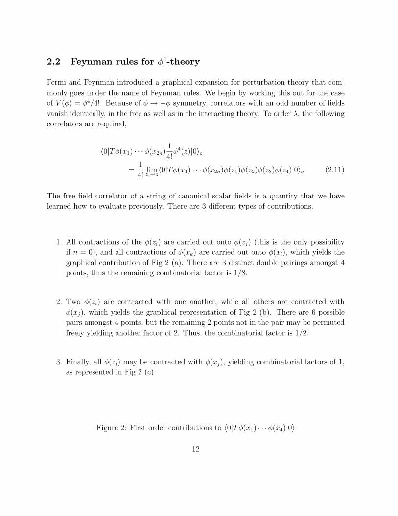
2.2 Feynman rules for φ4-theory
Fermi and Feynman introduced a graphical expansion for perturbation theory that com-
monly goes under the name of Feynman rules. We begin by working this out for the case
of V (φ) = φ4/4!. Because of φ→ −φ symmetry, correlators with an odd number of fields
vanish identically, in the free as well as in the interacting theory. To order λ, the following
correlators are required,
〈0|Tφ(x1) · · ·φ(x2n)1
4!φ4(z)|0〉o
=1
4!limzi→z
〈0|Tφ(x1) · · ·φ(x2n)φ(z1)φ(z2)φ(z3)φ(z4)|0〉o (2.11)
The free field correlator of a string of canonical scalar fields is a quantity that we have
learned how to evaluate previously. There are 3 different types of contributions.
1. All contractions of the φ(zi) are carried out onto φ(zj) (this is the only possibility
if n = 0), and all contractions of φ(xk) are carried out onto φ(xl), which yields the
graphical contribution of Fig 2 (a). There are 3 distinct double pairings amongst 4
points, thus the remaining combinatorial factor is 1/8.
2. Two φ(zi) are contracted with one another, while all others are contracted with
φ(xj), which yields the graphical representation of Fig 2 (b). There are 6 possible
pairs amongst 4 points, but the remaining 2 points not in the pair may be permuted
freely yielding another factor of 2. Thus, the combinatorial factor is 1/2.
3. Finally, all φ(zi) may be contracted with φ(xj), yielding combinatorial factors of 1,
as represented in Fig 2 (c).
Figure 2: First order contributions to 〈0|Tφ(x1) · · ·φ(x4)|0〉
12
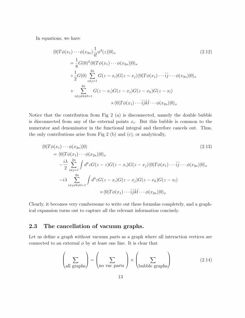
In equations, we have
〈0|Tφ(x1) · · ·φ(x2n)1
4!φ4(z)|0〉o (2.12)
=1
8G(0)2〈0|Tφ(x1) · · ·φ(x2n)|0〉o
+1
2G(0)
2n∑i6=j=1
G(z − xi)G(z − xj)〈0|Tφ(x1) · · · ij · · ·φ(x2n)|0〉o
+2n∑
i6=j 6=k 6=l=1
G(z − xi)G(z − xj)G(z − xk)G(z − xl)
×〈0|Tφ(x1) · · · ijkl · · ·φ(x2n)|0〉o
Notice that the contribution from Fig 2 (a) is disconnected, namely the double bubble
is disconnected from any of the external points xi. But this bubble is common to the
numerator and denominator in the functional integral and therefore cancels out. Thus,
the only contributions arise from Fig 2 (b) and (c), or analytically,
〈0|Tφ(x1) · · ·φ(x2n)|0〉 (2.13)
= 〈0|Tφ(x1) · · ·φ(x2n)|0〉o
−iλ2
2n∑i6=j=1
∫d4zG(z − z)G(z − xi)G(z − xj)〈0|Tφ(x1) · · · ij · · ·φ(x2n)|0〉o
−iλ2n∑
i6=j 6=k 6=l=1
∫d4zG(z − xi)G(z − xj)G(z − xk)G(z − xl)
×〈0|Tφ(x1) · · · ijkl · · ·φ(x2n)|0〉o
Clearly, it becomes very cumbersome to write out these formulas completely, and a graph-
ical expansion turns out to capture all the relevant information concisely.
2.3 The cancellation of vacuum graphs.
Let us define a graph without vacuum parts as a graph where all interaction vertices are
connected to an external φ by at least one line. It is clear that ∑all graphs
=
∑no vac parts
× ∑
bubble graphs
(2.14)
13
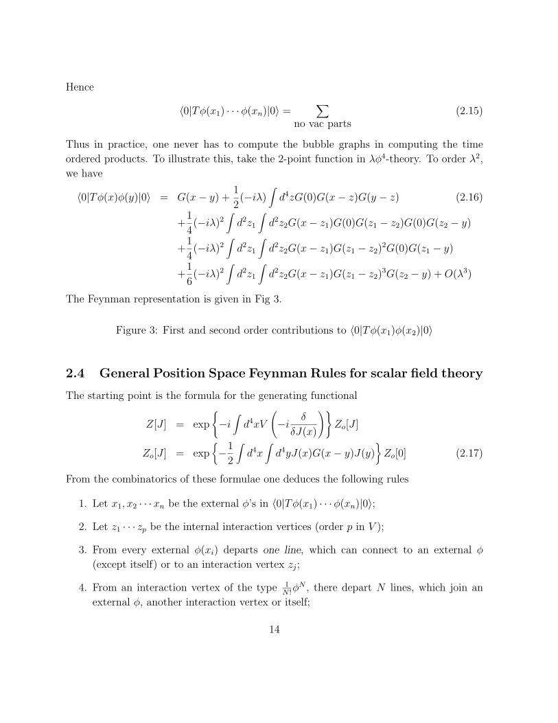
Hence
〈0|Tφ(x1) · · ·φ(xn)|0〉 =∑
no vac parts(2.15)
Thus in practice, one never has to compute the bubble graphs in computing the time
ordered products. To illustrate this, take the 2-point function in λφ4-theory. To order λ2,
we have
〈0|Tφ(x)φ(y)|0〉 = G(x− y) +1
2(−iλ)
∫d4zG(0)G(x− z)G(y − z) (2.16)
+1
4(−iλ)2
∫d2z1
∫d2z2G(x− z1)G(0)G(z1 − z2)G(0)G(z2 − y)
+1
4(−iλ)2
∫d2z1
∫d2z2G(x− z1)G(z1 − z2)
2G(0)G(z1 − y)
+1
6(−iλ)2
∫d2z1
∫d2z2G(x− z1)G(z1 − z2)
3G(z2 − y) +O(λ3)
The Feynman representation is given in Fig 3.
Figure 3: First and second order contributions to 〈0|Tφ(x1)φ(x2)|0〉
2.4 General Position Space Feynman Rules for scalar field theory
The starting point is the formula for the generating functional
Z[J ] = exp
{−i∫d4xV
(−i δ
δJ(x)
)}Zo[J ]
Zo[J ] = exp{−1
2
∫d4x
∫d4yJ(x)G(x− y)J(y)
}Zo[0] (2.17)
From the combinatorics of these formulae one deduces the following rules
1. Let x1, x2 · · ·xn be the external φ’s in 〈0|Tφ(x1) · · ·φ(xn)|0〉;
2. Let z1 · · · zp be the internal interaction vertices (order p in V );
3. From every external φ(xi) departs one line, which can connect to an external φ
(except itself) or to an interaction vertex zj;
4. From an interaction vertex of the type 1N !φN , there depart N lines, which join an
external φ, another interaction vertex or itself;
14
5. To every line is associated GF (x− y) between points x and y;
6. Every interaction vertex 1N !φN has a coupling constant factor of igN ;
7. Every interaction vertex is integrated over∫d4zi;
8. There is an overall symmetry factor.
2.5 Momentum Space Representation
We begin by defining the Fourier transform of the n-point function,
〈0|Tφ(x1) · · ·φ(xn)|0〉 =n∏j=1
(∫ d4pj(2π)4
eipj ·xj
)G(p1, · · · , pn) (2.18)
as well as the inverse Fourier transform relation,
G(p1, · · · , pn) =n∏j=1
(∫d4xj e
−ipj ·xj
)〈0|Tφ(x1) · · ·φ(xn)|0〉 (2.19)
Recall, however, that the scalar field theory action S[φ], as well as the vacuum |0〉 are
translation invariant. Therefore, the time ordered expectation value 〈0|Tφ(x1) · · ·φ(xn)|0〉only depends on the differences of the arguments. As a consequence, the Fourier transform
G(p1, · · · , pn) is non-vanishing only when overall momentum is conserved, p1 + · · ·+pn = 0
and is proportional to an overall δ-function,
G(p1, · · · , pn) = (2π)4δ4(p1 + · · ·+ pn)G(p1, · · · , pn) (2.20)
The Feynman rules in momentum space are easily derived, and are customarily formulated
for the quantities G(p1, · · · , pn).
1. Draw all topologically distinct connected diagrams with n external legs of incoming
momenta p1, · · · pn. Denote by k1, · · · k` the momenta of internal lines.
2. To the j-th external line, assign the value of the propagator,
GF (pj) =i
p2j −m2 + iε
, j = 1, · · · , n (2.21)
3. To every internal line, assign∫ d4k`(2π)4
i
k2` −m2 + iε
(2.22)
15
4. To each interaction vertex, assign
−igN(2π)4δ4(q) (2.23)
where q is the sum of incoming momenta to the vertex.
5. Integrate over the internal momenta, and multiply by the combinatorial factor.
2.6 Does perturbation theory converge ?
Having produced a perturbative expansion in the coupling constant, the question arises
as to whether the corresponding power series is convergent or not. As a caricature of the
perturbative expansion of the functional integral is to take an ordinary integral of the same
type. Thus, we consider
Z(m,λ) ≡∫ +∞
−∞dφ exp
{−m2φ2 − λ2φ4
}(2.24)
There are now two possible expansions; the first in power of m, the second in powers of λ.
The expansion in powers of m yields
Z(m,λ) =∞∑n=0
1
n!(−m2)n
∫ +∞
−∞dφ φ2n exp
{−λ2φ4
}
=∞∑n=0
1
2√λ
Γ(n2
+ 14)
Γ(n+ 1)
(−m
2
λ
)n(2.25)
while the expansion in powers of λ yields,
Z(m,λ) =∞∑n=0
1
n!(−λ2)n
∫ +∞
−∞dφ φ4n exp
{−m2φ2
}
=∞∑n=0
1
m
Γ(2n+ 12)
Γ(n+ 1)
(− λ2
m4
)n(2.26)
Clearly, from analyzing the n-dependence of the ratios of Γ functions, the expansion in
m is convergent (with ∞ radius of convergence) while the expansion in power of λ has
zero radius of convergence. This comes as no surprise. If we had flipped the sign of
m2, the integral itself would still be fine and convergent. On the other hand, if we had
flipped the sign of λ2, the integral badly diverges, and therefore, it cannot have a finite
radius of convergence around 0. The moral of the story is that perturbation theory around
free field theory is basically always given by an asymptotic series which has zero radius
of convergence. Nonetheless, and it is one of the most remarkable things about QFT,
perturbation theory gives astoundingly accurate answers when it is applicable.
16
2.7 The loop expansion
We now derive the h-dependence of the various orders of perturbation theory:
〈0|Tφ(x1) · · ·φ(xn)|0〉 =∫Dφφ(x1) · · ·φ(xn)e
ihS[φ] (connected) (2.27)
A general diagram has E external legsI internal linesV vertices
(2.28)
The number of loops L is equal to the number of independent internal momenta, after all
comservatioins have been imposed on vertices, minus one overall momentum conservation
L = I − (V − 1). Now calculate to what order in h this graph contributes:
• each propagator contributes one power of h;
• each vertex contributes one power of 1/h.
Hence a graph contributes
hE+I−V = h(E+L−1) (2.29)
For fixed number of external lines, the h expansiion is a loop expansion, provided all the
couplings in the classical actioin are independent of h.
2.8 Truncated Diagrams
To simplify and systematize the enumeration of all diagrams that contribute to a given
process, it is useful to identify special sub-categories of diagrams. We have already dis-
cussed the connected diagrams, from which all others may be recovered. We now introduce
truncated and 1-particle irreducible diagrams which allow to further cut down the number
of key diagrams.
In the calculation of the S-matrix, the full Green function is not required; instead we
only use it in the combination (scalar field)
n∏i=1
(∫d4xie
−ipi·xi(2 +m2)xiZ−1/2
)〈0|Tφ(x1) · · ·φ(xn)|0〉
= Z−n/2n∏i=1
(−p2i +m2)G(n)(p1, · · · , pn) (2.30)
17
Here pi are on-shell external momentum. As we have deduced from the spectral represen-
tation, the two-point function behaves like
G(2)(p,−p) =Z
p2 −m2+ reg. as p2 → m2 (2.31)
Hence what really comes in the reduction formula is
limp2i→m2
Zn/2n∏i=1
[G(2)c (pi,−pi)
]−1G(n)(p1, p2 · · · pn) (2.32)
One defines the truncated correlator by
G(n)trun(p1, · · · , pn) =
n∏i=1
G(2)c (pi,−pi)−1G(n)(p1, · · · , pn) (2.33)
So that the S-matrix elements are given by
〈q1 · · · qm out|p1 · · · pn in〉c= (Z1/2)m+n(2π)4δ4(q − p)G
(n+m)trun (q1, · · · , qm; p1, · · · , pn) (2.34)
where δ(q − p) stands for an overall momentum conservation δ-function. Truncation of
the n-point correlator reduces the n-point function in that the entire set of diagrams that
corresponds to the self-energy corrections of the external legs is to be omitted. Therefore, it
is much simpler to enumerate the truncated diagrams than it is to enumerate all connected
diagrams.
2.9 Connected graphs
A connected diagram is such that its graph is connected. The generating functional for
connected graphs is the log of Z[J ];
Z[J ] = Z[0] exp{iGc[J ]} (2.35)
and its expansion in powers of J yields the connected n-point functions,
Gc[J ] = −i∞∑n=0
in
n!
∫d4x1 · · · d4xnJ(x1) · · · J(xn)G
(n)c (x1, · · · , xn) (2.36)
Often, connected vacuum expectation values are simply denoted by a subscript c as well,
and thus we have
G(n)c (x1, · · · , xn) = 〈0|Tφ(x1) · · ·φ(xn)|0〉c (2.37)
18
The proof of the relation between Z[J ] and Gc[J ] is purely combinatorial. Denoting each
separate connected contribution of degree i in J by Xi, i = 1, · · · ,∞, we have
exp∞∑i=1
Xi =∞∑p=0
1
p!
∑n1+2n2···+pnp=p
p!
n1! · · ·np!Xn1
1 Xn22 · · ·Xnp
p (2.38)
which indeed reproduces the correct combinatorics for the full expansion order by order p
in the power of J , appropriate for Z[J ].
2.10 One-Particle Irreducible Graphs and the Effectice Action
A one-particle irreducible diagram is a connected truncated graph which remains connected
after any one internal line is cut. The Legendre transform of the generating functional for
connected graphs Gc[J ] is the generating functional for 1PIR’s. The Legendre transform
is defined as follows. One begins by defining the vacuum expectation value ϕ(x; J) of the
field φ in the presence of the source J ,
ϕ(x; J) ≡ δ
δJ(x)Gc(J) = 〈0|φ(x)|0〉J (2.39)
Now we assume that the relationship defining ϕ is invertible, and that J may be eliminated
in terms of ϕ in a unique manner,
ϕ(x; J) = ϕ(x) ⇐⇒ J(x) = J(x;ϕ) (2.40)
The Legendre transform Γ[ϕ] of Gc[J ] is then defined by
Γ[ϕ] ≡ Gc[J ]−∫d4xJ(x)ϕ(x)
∣∣∣∣J=J(x;ϕ)
(2.41)
where it is understood that J is eliminated in terms of ϕ. As always, it follows that
δΓ[ϕ]
δϕ(x)= −J(x) (2.42)
Now J(x) should be thought of as a source which must be applied from the outside in
order that the vacuum expectation value of φ be ϕ. When J = 0, we recover the original
theory, without source, so that
δΓ[ϕ]
δϕ(x)
∣∣∣∣ϕc
= 0 at J(x;ϕc) = 0 (2.43)
19
Next we investigate which diagrams are generated by Γ[ϕ]: For simplicity, we assume for
the moment that ϕc = 0 (the case of no spontaneous symmetry breaking)
Γ[ϕ] =∞∑n=1
1
n!
∫d4x1 · · ·
∫d4xn Γ(n)(x1, · · ·xn)ϕ(x1) · · ·ϕ(xn) (2.44)
The effective field equation (2.43) then implies that Γ(1)(x) = 0. In other words, the 1PIR
1-point function vanishes.
To obtain relations for more general Γ(n)’s, we differentiate the relation defining ϕ with
respect to ϕ. We use the functional chainrule to express the derivation with respect to ϕ
in terms of the differentiation with respect to J ,
δ4(x− y) =δ
δϕ(y)
(δGc[J ]
δJ(x)
)=∫d4z
δJ(z)
δϕ(y)
δ2Gc[J ]
δJ(z)δJ(x)(2.45)
However, from (2.42), we have
−δJ(z)
δϕ(y)=
δ2Γ[ϕ]
δϕ(z)δϕ(y)(2.46)
Evaluating this relation at ϕ = J = 0, we find a relation between the connected and 1PIR
2-point functions,
−δ4(x− y) =∫d4zΓ(2)(x, z)G(2)
c (z, y) or Γ(2) = −{G(2)c
}−1(2.47)
It is useful to illustrate this relation by working out schematically the corrections to the
2-point function. If we denote the 1PIR corrections to the self-energy by Σ(p), then the
full 2-point function is given by
G(2)c (p) =
1
p2 −m2+
1
p2 −m2Σ(p)
1
p2 −m2+
1
p2 −m2Σ(p)
1
p2 −m2Σ(p)
1
p2 −m2+ · · ·
=1
p2 −m2 − Σ(p)= Γ(2)(p)−1 (2.48)
which confirms our assertion that Γ generates 1PIR only. A graphical representation is
given in Fig 5.
Figure 4: Relations between connected and 1PIR graphs in a theory with cubic and quarticcouplings, and vanishing 1-point function.
20
By differentiating once more, and setting ϕ = J = 0, we obtain information on the
3-point function,∫d4uΓ(3)(u, y, z)G(2)
c (x, u) =∫ ∫
d4ud4vΓ(2)(u, y)Γ(2)(v, z)G3c(x, u, v) (2.49)
By multiplying by G(2)(y, ·)G(2)(z, ·), we obtain
G(3)(x, y, z) =∫d4ud4vd4wG(2)(x, u)G(2)(y, v)G(2)(z, w)Γ(3)(u, v, w) (2.50)
So, for the three-point function, the 1PIR part arises from truncating the graph. One may
repeat the exercise for 4 legs. Graphical representations are given in Fig 4.
Clearly, the expansion is in terms of the tree-level graphs, Γ(n) used as generalized
vertices. This is the skeleton expansion of any graph in terms of 1PIR’s.
Γ[ϕ] is the so-called effective action of the system. Why action? Here, it is useful to
make a loop expansion
Z[J ] =∫Dφ exp
i
h
{S[φ] +
∫Jφ}
= exp{i
hGc[J ]
}(2.51)
(note, here we have kept the J-independent term in G[J]). Now, keep only the leading
term in h→ 0, then the integral will be dominated by its saddle points. Let’s assume that
the saddle point is unique and denote it by φs, then we have
δS[φs]
δφ(x)+ J(x) = 0 (2.52)
But this is precisely the same equation as was satisfied by Γ itself. Thus, to leading order
in h, we have Γ[ϕ] = S[ϕ]. All Green functions can be reconstructed from it by the skeleton
expansion so that Γ[ϕ] is the essential quantity in a quantum field theory.
2.11 Schwinger Dyson Equations
We concentrate on a scalar field theory, with Lagrangian,
L =1
2∂µφ∂
µφ− 1
2m2φ2 − V (φ) (2.53)
Now we use the fact that the functional integral of a functional derivative vanishes,∫Dφ δ
δφ(z)
{φ(x1) · · ·φ(xn)e
iS[φ]}
= 0 (2.54)
21
Working out the actual derivatives under the integral, we obtain an hierarchy of equations,
involving the correlators,
n∑i=1
δ4(xi − z)〈0|Tφ(x1) · · · φ(xi) · · ·φ(xn)|0〉 (2.55)
−i(2 +m2)z〈0|Tφ(x1) · · ·φ(xn)φ(z)|0〉 − i〈0|Tφ(x1) · · ·φ(xn)∂V
∂φ(z)|0〉 = 0
providing a recursive type of relationship that expresses the quantum equations of motion.
These are the Schwinger-Dyson equations.
2.12 The Background Field Method for Scalars
Feynman diagrams and standard perturbation theory do not always provide the most
efficient calculational methods. This is especially true for theories with complicated lo-
cal invariances, such as gauge and reparametrization invariances. But the method also
provides important short-cuts for scalar field theories.
The background field method is introduced first for a theory with a single scalar field
φ. The classical action is denoted S0[φ], and the full quantum action, including all renor-
malization counterterms is denoted by S[φ]. The generating functional for connected
correlators is given by
exp{i
hGc[J ]
}≡∫Dφ exp
{i
hS[φ] +
i
h
∫d4xJ(x)φ(x)
}(2.56)
By the very construction of the renormalized action S[φ], Gc[J ] is a finite functional of J .
The Legendre transform is defined by
Γ[ϕ] ≡∫d4xJ(x)ϕ(x)−Gc[J ] (2.57)
where J and ϕ are related by
ϕ(x) =δGc[J ]
δJ(x)J(x) = − δΓ[ϕ]
δϕ(x)(2.58)
Recall that Γ[ϕ] is the generating functional for 1-particle irreducible correlators.
To obtain a recursive formula for Γ, one proceeds to eliminate J from (2.56) using the
above relations,
expi
h
(Γ[ϕ] +
∫Jϕ)
=∫Dφ exp
i
h
(S[φ]−
∫dxφ(x)
δΓ[ϕ]
δϕ(x)
)(2.59)
22
Moving the J-dependence from the left to the right side, and expressing J in terms of Γ
in the process, we obtain,
expi
hΓ[φ] =
∫Dφ exp
i
h
(S[φ]−
∫dx(φ− ϕ)(x)
δΓ[ϕ]
δϕ(x)
)(2.60)
The final formula is obtained by shifting the integration field φ→ ϕ+√hφ,
expi
hΓ[ϕ] =
∫Dφ exp
i
h
(S[ϕ+
√hφ]−
√h∫dxφ(x)
δΓ[ϕ]
δϕ(x)
)(2.61)
At first sight, it may seem that little has been gained since both the left and right hand
sides involve Γ. Actually, the power of this formula is revealed when it is expanded in
powers of h, since on the rhs, Γ enters to an order higher by√h than it enters on the lhs.
The h-expansion is performed as follows,
S[φ] = S0[φ] + hS1[φ] + h2S2[φ] +O(h3)
Γ[ϕ] = Γ0[ϕ] + hΓ1[ϕ] + h2Γ2[ϕ] +O(h3) (2.62)
The recursive equation to lowest order clearly shows that Γ0[ϕ] = S0[ϕ]. The interpretation
of the terms Si[φ] for i ≥ 1 is clearly in terms of counterterms to loop order i, while that
of Γi[ϕ] is that of i-loop corrections to the effective action. The 1-loop correction is readily
evaluated for example,
exp iΓ1[ϕ] = eiS1[ϕ]∫Dφ exp
{i
2
∫d4x φ(x)
∫d4y φ(y)
δ2S0[ϕ]
δϕ(x)δϕ(y)
}(2.63)
For example, if S0 describes a field φ with mass m and interaction potential V (φ), we have
S0[φ] =∫dx(
1
2∂µφ∂
µφ− 1
2m2φ2 − V (φ)
)(2.64)
then we have
eiΓ1[ϕ] = eiS1[ϕ]∫Dφ exp
{i
2
∫d4xφ
(2 +m2 + V ′′(ϕ)
)φ}
Γ1[ϕ] = S1[ϕ] +i
2ln Det
[2 +m2 + V ′′(ϕ)
](2.65)
Upon expanding this formula in perturbation theory, the standard expressions may be
recovered,
Γ1[ϕ] = S1[ϕ] + Γ1[0] +i
2ln Det
[1 + V ′′(ϕ)
1
2 +m2
](2.66)
which clearly reproduces the standard 1-loop expansion. Therefore, for scalar theories, the
gain produced by the use of the background field method is usually only minimal.
23
3 Basics of Perturbative Renormalization
In this section, we begin by presenting some useful techniques for the calculation of Feyn-
man diagrams. Next, we introduce some of the basic ideas and techniques of renormal-
ization in perturbation theory. Finally, we study the analytic behavior of the 4-point
diagrams to one loop order in λφ4 as a function of external momenta.
3.1 Feynman parameters
One will often be confronted with loop integrals over internal momenta that involve a
product of momentum space propagators. It would not be totally straightforward to do
these integrals, if it were not for the use of Feynman parameters. The simplest type of
integrals of this type may be taken to be
Id(p) =∫ ddk
(2π)d1
(k + p)2 −m2 + iε× 1
k2 −m2 + iε(3.1)
We have considered this integral in any dimension of space-time d. Feynman’s trick for
dealing with the product of propagators is to represent the product in terms of an integral.
The basic formula is as follows,
1
ab=∫ 1
0dα
1
[aα+ b(1− α)]2(3.2)
Applying this formula to the integral Id(p), we obtain
Id(p) =∫ 1
0dα∫ ddk
(2π)d1
[(k + αp)2 + α(1− α)p2 −m2 + iε]2(3.3)
For d ≥ 4, this integral actually diverges for any p due to the contributions at large k. We
shall temporarily ignore this problem and consider d < 4. In a convergent integral, one
may now safely shift k → k − αp, so that we end up with
Id(p) =∫ 1
0dα∫ ddk
(2π)d1
[k2 + α(1− α)p2 −m2 + iε]2(3.4)
The great advantage of this form of the integral is that all momenta enter through k2 and
p2, which are Lorentz scalars.
More generally, the product of several propagator denominators may be treated with
multiple integrals. The easiest is to use the exponential representation first,
1
aµ11 · · · aµn
n=∫ ∞
0dλ1 · · ·
∫ ∞
0dλn
λµ1−11 · · ·λµn−1
n
Γ(µ1) · · ·Γ(µn)e−λ1a1−···−λnan (3.5)
24
Putting λi = λαi, we recover the Feynman parametrization,
1
aµ11 a
µ22 · · · aµn
n=
Γ(µ1 + µ2 + · · ·+ µn)
Γ(µ1)Γ(µ2) · · ·Γ(µn)
∫ 1
0dα1 · · ·
∫ 1
0dαnδ(α1 + · · ·+ αn − 1)
× αµ1−11 · · ·αµn−1
n
[α1a1 + · · ·+ αnan]µ1+···+µn(3.6)
It is of course possible to integrate out one of the αi by using the δ-function, but the result
is then less symmetrical in the ai. For n = 2 and µ1 = µ2 = 1, we recover the earlier result
this way.
3.2 Integrations over internal momenta
It remains to evaluate the integrations over internal momenta. First, we shall assume that
Feynman parameters have been employed to put the integration into standard form,
I(M ; d, n) ≡∫ ddk
(2π)d1
(k2 −M2 + iε)n(3.7)
We shall now evaluate this integral for all values of d and n where it converges and then
analytically continue the result throughout the complex planes for both d and n. As
k →∞, the integrals converge as long as d < 2n, and we assume this bound satisfied.
The first step is to analytically continue to Euclidean internal momenta, ko → ikoEm
leaving M alone. This is possible, because the singularities in the complex ko plane may
be completely avoided during this process thanks to the iε prescription of the propagator.
As a result, we have k2 → −k2E and dko → idkoE, so that
I(M ; d, n) = i2n+1∫ ddkE
(2π)d1
(k2E +M2)n
(3.8)
where k2E is the Euclidean momentum square. To carry out this integration, we use d-
dimensional spherical coordinates and the formula for the volume of the sphere Sd−1,
V (Sd−1) =2πd/2
Γ(d/2)(3.9)
This formula is most easily proven as follows. Consider the Gaussian inetgral in d dimen-
sions, which is just a product of d Gaussian inetgrals in 1 dimension,∫dd~k e−
~k2
= πd/2 (3.10)
25
Working out the same formula in spherical coordinates, we have∫dd~k e−
~k2
= V (Sd−1)∫ ∞
0dk kd−1 e−k
2
=1
2V (Sd−1)Γ(d/2) (3.11)
which upon combination with the first yields the desired expression for V (Sd−1). It is easy
to check that V (S1) = 2π, V (S2) = 4π and V (S3) = 2π2 as expected. The above formula
is, however, valid for any d. Introducing real positive k such that k2E = k2, we have
I(M ; d, n) =2 i2n+1
(4π)d/2Γ(d/2)
∫ ∞
0dk
kd−1
(k2 +M2)n(3.12)
The remaining integral may be carried out as follows. First, we let k2 = M2t, so that∫ ∞
0dk
kd−1
(k2 +M2)n=
1
2
1
(M2)n−d/2
∫ ∞
0dt
td/2−1
(t+ 1)n(3.13)
Next, we let x = 1/(t+ 1), so that∫ ∞
0dk
kd−1
(k2 +M2)n=
1
2
1
(M2)n−d/2
∫ 1
0dx (1− x)d/2−1xn−d/2−1
=1
2
1
(M2)n−d/2Γ(d/2)Γ(n− d/2)
Γ(n)(3.14)
Therefore, we find
I(M ; d, n) =i2n+1Γ(n− d/2)
(4π)d/2Γ(n)
1
(M2)n−d/2(3.15)
The calculation was carried out there where the integral was convergent. We see now how-
ever, that the analytic continuation of the expression that we have obtained is straightfor-
ward since the analytic continuation of the Γ-function is well-known. Thus, we view the
result obtained above as THE answer !
3.3 The basic idea of renormalization
As soon as loops occur, the diagram is potentially divergent when the internal momen-
tum integration fails to converge in the limit of large momenta. It would seem that the
appearance of divergences renders the quantum field theory meaningless. Actually, the
procedure of renormalization is required to organize and properly interpret the loop cor-
rections that arise. We shall illustrate the salient features and ideas of renormalization
within the context of λφ4 theory, with Lagrangian,
L =1
2∂µφ∂
µφ− 1
2m2φ2 − λ
4!φ4 (3.16)
26
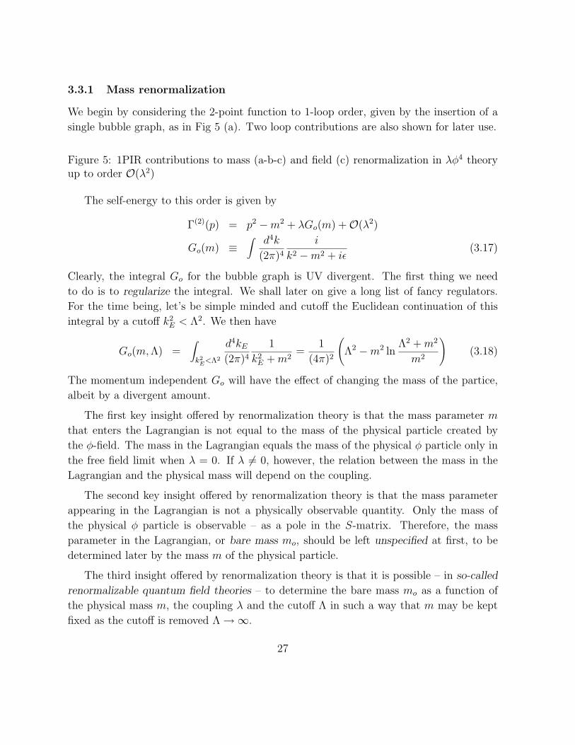
3.3.1 Mass renormalization
We begin by considering the 2-point function to 1-loop order, given by the insertion of a
single bubble graph, as in Fig 5 (a). Two loop contributions are also shown for later use.
Figure 5: 1PIR contributions to mass (a-b-c) and field (c) renormalization in λφ4 theoryup to order O(λ2)
The self-energy to this order is given by
Γ(2)(p) = p2 −m2 + λGo(m) +O(λ2)
Go(m) ≡∫ d4k
(2π)4
i
k2 −m2 + iε(3.17)
Clearly, the integral Go for the bubble graph is UV divergent. The first thing we need
to do is to regularize the integral. We shall later on give a long list of fancy regulators.
For the time being, let’s be simple minded and cutoff the Euclidean continuation of this
integral by a cutoff k2E < Λ2. We then have
Go(m,Λ) =∫k2
E<Λ2
d4kE(2π)4
1
k2E +m2
=1
(4π)2
(Λ2 −m2 ln
Λ2 +m2
m2
)(3.18)
The momentum independent Go will have the effect of changing the mass of the partice,
albeit by a divergent amount.
The first key insight offered by renormalization theory is that the mass parameter m
that enters the Lagrangian is not equal to the mass of the physical particle created by
the φ-field. The mass in the Lagrangian equals the mass of the physical φ particle only in
the free field limit when λ = 0. If λ 6= 0, however, the relation between the mass in the
Lagrangian and the physical mass will depend on the coupling.
The second key insight offered by renormalization theory is that the mass parameter
appearing in the Lagrangian is not a physically observable quantity. Only the mass of
the physical φ particle is observable – as a pole in the S-matrix. Therefore, the mass
parameter in the Lagrangian, or bare mass mo, should be left unspecified at first, to be
determined later by the mass m of the physical particle.
The third insight offered by renormalization theory is that it is possible – in so-called
renormalizable quantum field theories – to determine the bare mass mo as a function of
the physical mass m, the coupling λ and the cutoff Λ in such a way that m may be kept
fixed as the cutoff is removed Λ →∞.
27
To illustrate the points made above on φ4 theory to order λ, we are thus instructed to
take as a starting point the Lagrangian with bare mass m0,
L =1
2∂µφ∂
µφ− 1
2m2oφ
2 − λ
4!φ4 (3.19)
and to recompute all of the above up to order λ. The slef-energy corrections are given by
Γ(2)(p) = p2 −m2o + λGo(mo) +O(λ2)
Go(mo,Λ) =1
(4π)2
(Λ2 −m2
o lnΛ2 +m2
o
m2o
)(3.20)
In order for the mass of the φ particle to be m – to this order λ – it suffices to set
m2 = m2o −
λ
(4π)2
(Λ2 −m2
o lnΛ2 +m2
o
m2o
)+O(λ2) (3.21)
Actually, this relation may be solved to this order by workin iteratively,
m2o = m2 +
λ
(4π)2
(Λ2 −m2 ln
Λ2 +m2
m2
)+O(λ2) (3.22)
The key lesson learned from this simple example is that as the cutoff Λ is sent to ∞, it is
necessary to keep on adjusting mo so that the physical mass m can remain constant. As
Λ →∞, this actually requires mo →∞ as well.
3.3.2 Coupling Constant Renormalization
The lowest 1PIR corrections to the 4-point function arise at order O(λ2) and are depicted
in Fig 6. The three diagrams are permutations in the external legs of the single basic
diagram. In the study of any 4-point, it is very useful to introduce the Mandelstam
variables, s, t, u, which are the Lorentz invariant combinations one can form out of the (all
incoming) external momenta pi, i = 1, 2, 3, 4. They are defined by
s ≡ (p1 + p2)2 = (p3 + p4)
2
t ≡ (p1 + p4)2 = (p2 + p3)
2
u ≡ (p1 + p3)2 = (p2 + p4)
2 (3.23)
The Mandelstam relations obey s+ t+ u = p21 + p2
2 + p23 + p2
4, and if the external particles
are on-shell then the rhs equals 4m2.
28
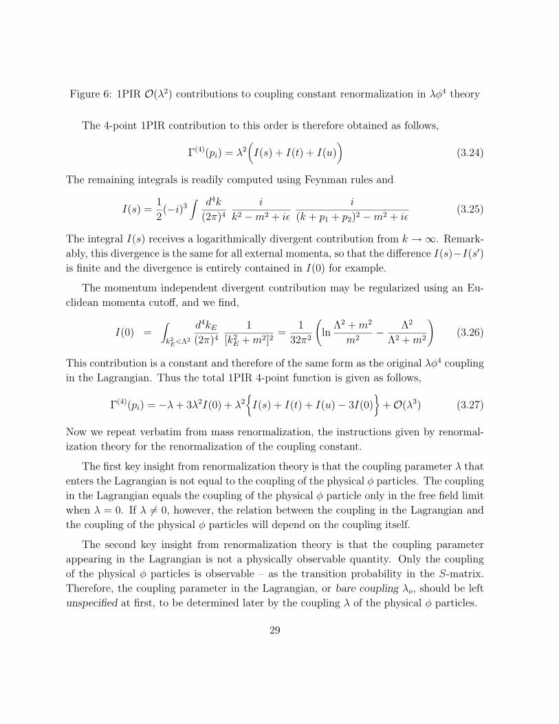
Figure 6: 1PIR O(λ2) contributions to coupling constant renormalization in λφ4 theory
The 4-point 1PIR contribution to this order is therefore obtained as follows,
Γ(4)(pi) = λ2(I(s) + I(t) + I(u)
)(3.24)
The remaining integrals is readily computed using Feynman rules and
I(s) =1
2(−i)3
∫ d4k
(2π)4
i
k2 −m2 + iε
i
(k + p1 + p2)2 −m2 + iε(3.25)
The integral I(s) receives a logarithmically divergent contribution from k →∞. Remark-
ably, this divergence is the same for all external momenta, so that the difference I(s)−I(s′)is finite and the divergence is entirely contained in I(0) for example.
The momentum independent divergent contribution may be regularized using an Eu-
clidean momenta cutoff, and we find,
I(0) =∫k2
E<Λ2
d4kE(2π)4
1
[k2E +m2]2
=1
32π2
(ln
Λ2 +m2
m2− Λ2
Λ2 +m2
)(3.26)
This contribution is a constant and therefore of the same form as the original λφ4 coupling
in the Lagrangian. Thus the total 1PIR 4-point function is given as follows,
Γ(4)(pi) = −λ+ 3λ2I(0) + λ2{I(s) + I(t) + I(u)− 3I(0)
}+O(λ3) (3.27)
Now we repeat verbatim from mass renormalization, the instructions given by renormal-
ization theory for the renormalization of the coupling constant.
The first key insight from renormalization theory is that the coupling parameter λ that
enters the Lagrangian is not equal to the coupling of the physical φ particles. The coupling
in the Lagrangian equals the coupling of the physical φ particle only in the free field limit
when λ = 0. If λ 6= 0, however, the relation between the coupling in the Lagrangian and
the coupling of the physical φ particles will depend on the coupling itself.
The second key insight from renormalization theory is that the coupling parameter
appearing in the Lagrangian is not a physically observable quantity. Only the coupling
of the physical φ particles is observable – as the transition probability in the S-matrix.
Therefore, the coupling parameter in the Lagrangian, or bare coupling λo, should be left
unspecified at first, to be determined later by the coupling λ of the physical φ particles.
29
The third insight from renormalization theory is that it is possible – in so-called renor-
malizable quantum field theories – to determine the bare coupling λo as a function of the
physical coupling λ, the mass m and the cutoff Λ in such a way that λ may be kept fixed
as the cutoff is removed Λ →∞.
To illustrate the points made above on φ4 theory to order λ2, we are thus instructed
to take as a starting point the Lagrangian with bare mass m0 and bare coupling λo,
L =1
2∂µφ∂
µφ− 1
2m2oφ
2 − λo4!φ4 (3.28)
and to recompute all of the above up to order λ2. The 4-point corrections are given by
Γ(4)(pi) = −λo + 3λ2oI(0) +O(λ3
o) (3.29)
In order for the coupling of the φ particles to be λ – to this order λ2 – it suffices to set
−λ = −λo + 3λ2oI(0) +O(λ3
o) (3.30)
Actually, this relation may be solved to this order by working iteratively, (it is customary
to omit terms that vanish in the limit Λ →∞, and we shall also do so here)
λo = λ+3λ2
32π2ln
Λ2
m2+O(λ3) (3.31)
The key lesson learned from this simple example is that as the cutoff Λ is sent to ∞, it
is necessary to keep on adjusting λo so that the physical coupling λ can remain constant.
As Λ → ∞, this actually requires λo → ∞ as well. Notice that to higher orders, the
renormalization of the mass and of the coupling will be intertwined and greater care will
be required to extract the correct procedure.
3.3.3 Field renormalization
Considering the 2-point function still in λφ4 theory, but now to order O(λ2), we have the
additional 1PIR diagrams of Fig 5 (b), (c). We encounter further mass renormalization
effects, which may be dealt with by the methods explained above as well. We also en-
counter, through the diagram (c) in Fig 5, also a new type of divergence. This may be
seen from the explicit expression of the diagram, (the iε prescription is understood)
Γ(2)2 (p) =
λ2
6
∫ d4k
(2π)4
∫ d4`
(2π)4
1
(k + p)2 −m2
1
(k + `)2 −m2
1
`2 −m2(3.32)
This integral is quadratically divergent, but the quadratic divergence is p-independent.
Thus, the differences Γ(2)2 (p)−Γ
(2)2 (p′) are less divergent. By Lorentz invariance, we expect
30
Γ(2)2 (p) to vanish to second order as p→ 0. The second derivative is easily computed,
∂2Γ(2)2 (p)
∂pµ∂pµ=λ2
6
∫ d4k
(2π)4
∫ d4`
(2π)4
8m2
[(k + p)2 −m2]31
(k + `)2 −m2
1
`2 −m2(3.33)
This integral is indeed logarithmically divergent because the sub-integration over ` is loga-
rithmically divergent. Recognizing the integration over ` as the integral I(k2) encountered
at the time of coupling constant renormalization, we may write the above as
∂2Γ(2)2 (p)
∂pµ∂pµ= i
λ2
3
∫ d4k
(2π)4
8m2
[(k + p)2 −m2]3
(I(0) + {I(k2)− I(0)}
)(3.34)
The integral over {I(k2)− I(0)} is convergent. The integral multiplying I(0) is convergent
and yields
∂2Γ(2)2 (p)
∂pµ∂pµ
∣∣∣∣I(0)
=λ2
6π2I(0) =
λ2
3(4π)4ln
Λ2
m2(3.35)
Thus, we see that a divergent contribution arises which is proportional to p2. At first
sight, it would not appear that there is a coupling in the Lagrangian capable of absorbing
this divergence. But in fact there is : the kinetic term is customarily normalized to 1/2
by choosing an appropriate normalization of the canonical field. The divergent correction
found here indicates that quantum effects change this nromalization, and give rise to field
renormalization, also sometimes improperly referred to as wave-function renormlization.
Therefore, the starting point ought to be the bare Lagrangian in which the field nor-
malization, the mass and the coupling have all been left at their bare values. One often
uses the following convention for the bare Lagrangian
LB =1
2Z∂µφ∂µφ−
1
2Zm2
oφ2 − λo
4!Z2φ4 (3.36)
which, when re-expressed in terms of the bare field
φo(x) ≡√Zφ(x) (3.37)
takes the form of the classical Lagrangian, but now with bare mass and coupling,
LB =1
2∂µφo∂µφo −
1
2m2oφ
2o −
λo4!φ4o (3.38)
The constant Z, to this order is given by
Z = 1− λ2
3(4π)4ln
Λ2
m2+O(λ3) (3.39)
Unlike mass and coupling renormalization in λφ4 theory, field renormalization has no
contributions to first order in the coupling.
31
3.4 Renormalization point and renormalization conditions
Now that we have understood how to extract finite answers from calculations involving
divergent cutoffs, we need to make precise how to extract physical answers as well. This is
achieved by imposing renormalization conditions on some of the correlators in the theory.
To completely deteremine the theory, there are to be exactly as many independent renor-
malization conditions as there are bare parameters in the bare Lagrangian. For scalar λφ4
theory, there are 3 parameters and thus there must be three independent renormalization
conditions.
Mass and field renormalization will require two independent renormalization condi-
tions of the 2-point function Γ(2)(p) while coupling constant renormalization will require
one renormalization condition on the 4-point function Γ(4)(p1, p2, p3, p4). The resulting
correlators will depend upon these renormalization condition and therefore they will have
been renormalized, a fact that is shown by suffixing the letter R.
Clearly, there is freedom in choosing the momenta at which the renormalization con-
ditions are to be imposed. This choice of momenta is referred to as the renormalization
point. It may seem most natural to relate the renormalization conditions to the properties
of the physical particles. For example, if m is to be the mass of the physical φ particle (the
position of the pole in the S-matrix corresponding to the exchange of a s ingle particle),
then the appropriate condition is an on-shell renormalization condition,
Γ(2)R (p)
∣∣∣∣p2=m2
= 0 (3.40)
But Lorentz invariance allows for a more general choice, such as for example this off-shell
renormalization condition,
Γ(2)R (p)
∣∣∣∣p2=µ2
= µ2 −m2 (3.41)
The same choice of renormalization points arise when dealing with field renormalization.
Coupling constant renormalization, which involves the 4-point function, and thus 3
independent momenta, offers even more freedom of choice of renormalization points. Since
s+t+u = p21+p
22+p
23+p
24, and on-shell renormalization consition with maximum symmetry
amongst the momenta would be
Γ(4)R (p1, p2, p3, p4)
∣∣∣∣s=t=u=4m2/3
= −λ (3.42)
32
but it is equally easy to take this condition off-shell to the point µ,
Γ(4)R (p1, p2, p3, p4)
∣∣∣∣s=t=u=4µ2/3
= −λ (3.43)
On-shell versus off-shell condition may be of use in turn in a variety of circumstances as
we shall see later.
3.5 Renormalized Correlators
Let us impose the on-shell renormalization conditions
Γ(2)R (p)
∣∣∣∣p2=m2
= 0
∂Γ(2)R (p)
∂p2
∣∣∣∣p2=m2
= 1
Γ(4)R (p1, p2, p3, p4)
∣∣∣∣s=t=u=4m2/3
= −λ (3.44)
The full expressions of the renormalized correlators are then found to be given by
Γ(2)R (p) = p2 −m2 +
Γ(4)R (pi) = −λ+ λ2
{I(s) + I(t) + I(u)− 3I
(4m2
3
)}(3.45)
It remains to evaluate more explicitly the function I(s)− I(so).
The quantity I(s) − I(so) may be evaluated using a single Feynman parameter, and
may be recovered from setting so = 0. It is convenient to set s = p2, and to omit the iε
symbols, so that
I(s)− I(0) = − i2
∫ 1
0dα∫ d4k
(2π)4
{1
[(k + αp)2 + α(1− α)s−m2]2− 1
[k2 −m2]2
}(3.46)
This integral is convergent. We would like to shift the k-integration in the first inte-
gral. Since this integral is divergent, however, it is unclear that this procedure would be
legitimate. Thus, we begin by proving a lemma.
Lemma 1 One may shift under logarithmically divergent integrations;
∫ d4k
(2π)4
{1
[k2 −m2 + iε]2− 1
[(k + p)2 −m2 + iε]2
}= 0 (3.47)
33
To prove this, notice that the equality holds at p = 0. Then, differentiating with respect
to pµ for general p, we obtain∫ d4k
(2π)4
4(k + p)µ[(k + p)2 −m2 + iε]3
(3.48)
But this integral is convergent and after shifting k+p→ k is odd in k → −k and therefore
vanishes automatically. This proves the lemma for all p.
Using lemma 1, carrying out the analytic continuation ko → ikoE, and carrying out the
kE integration, we find
I(s)− I(0) =1
2
∫ 1
0dα∫ d4kE
(2π)4
{1
[k2E − α(1− α)s+m2]2
− 1
[k2E +m2]2
}
=1
32π2
∫ 1
0dα ln
m2
m2 − α(1− α)s(3.49)
We shall now study this integral as a function of s. It is convenient to change integration
variables to 2α = 1 + x, so that
I(s)− I(0) =1
32π2ln
4m2
s− 1
32π2
∫ 1
0dx ln(x2 + σ2) (3.50)
where
σ2 ≡ 4m2
s− 1 (3.51)
Using the relation∫ 1
0dx ln(x+ iσ) = (1 + iσ) ln(1 + iσ)− iσ ln(iσ)− 1 (3.52)
we find
I(s)− I(0) =1
32π2iσ ln
iσ − 1
iσ + 1=
i
32π2
√4m2
s− 1 ln
i√
4m2
s− 1− 1
i√
4m2
s− 1 + 1
(3.53)
The integral is real as long as m2 and s are real and s < 4m2. When s > 4m2, however,
there is a branch cut, whose discontinuity is actuually most easily computed from the
integral representation that we started from,
Im(I(s)− I(0)
)= 2πi
1
32π2
∫ 1
0dαθ(α(1− α)s−m2)
=i
16πθ(s− 4m2)
√1− 4m2
s(3.54)
34
3.6 Summary of regularization and renormalization procedures
Quantum field theories expanded in perturbation theory, will develop UV divergences.
The first step in the process of defining the theory properly – without UV divergences –
is to regularize it. Over the 80 years of dealing with quantum field theories, physicists
have introduced and invented myriad regulators. Of course, it will be advantageous to
regularize theories by preserving as many symmetries of the original theory as possible
(e.g. Poincare invariance, gauge invariance, conformal invariance). Here, we give a brief
list. Regulators may be grouped according to whether they respect Poincare invariance.
• Poincare non-invariant regulators
1. The lattice formulation of quantum field theory is an example of a short space-time
distance cutoff. As we shall see later, the lattice is best formulated for Euclidean
QFT, and provides a perturbative and non-perturbative regularization of the theory.
There is a gauge invariant formulation.
2. Cutoff on momentum space at high momenta. This regulator is perhaps the most
intuitive one for qualitative studies in perturbation theory. It provides a perturbative
or non-perturbative regularization. Gauge invariance is not maintained in general.
• Poincare invariant Regulators
1. Dimensional regularization in which the dimension d of space-time is analytically
continued throughout the complex d plane. This regularization is only applicable
to Feynman diagrams and is thus in essence perturbative. It is very convenient and
preserves gauge invariance and reparametrization invariance.
• Tensor algebra, δµνδνµ = ηµνη
νµ = d.
• Spinor algebra
There are some difficulties with fermions, essentially because spinor representations
cannot naturally be continued to fractional dimensions. Therefore, the rules for
spinors are a bit ad hoc. Here are some of the key rules,
{γµ, γν} = 2ηµνI
γµγµ = d · I
γµγνγµ = (2− d)γν
γµγνγκγµ = 2γκγν + (d− 2)γνγκ
tr I = f(d) as long as f(4) = 4 (3.55)
35
There is no good definition of γ5. Deeper significance for these problems will be
derived when discussing the chiral anomaly.
2. Pauli-Villars regulators require introducing extra degrees of freedom with high masses
(and the wrong causality kinetic term). This works well to one-loop order and
preserves gauge invariance.
3. Heat-kernel and ζ-function regularizations are very powerful methods applicable
mostly only to 1-loop, but which preserve gauge invariance as well as reparametriza-
tion invariance when formulated on general manifolds !
• Renormalization
Once the theory has been regularized, we have a UV finite, but regulator dependent
theory. The question that renormalization theory addresses is whether one can make sense
out of this theory, so as to get a predictive theory. The key to renormalization theory is that
in renormalizable theories, all the divergences are of a special form, namely proportional
to terms already present in the Lagrangian. Even when one has renormalized the theory to
all orders in perturbatiion theory, the question still remains as to whether the full theory
is renormalizable (non-perturbatively). Most of these theories are not resolved to this day,
such as φ4-theory, theories with broken symmetries with monopoles and so on. The next
steps are those of renormalization.
1. Keeping the bare couplings and masses in the Lagrangian undetermined as a function
of the physical parameters and the cutoff.
2. Imposition of certain regulator independent renormalization conditions at a renor-
malization point. There should be as many renormalization conditions as indepen-
dent couplings in the Lagrangian.
3. Derive the bare coupling constants in the Lagrangian as a function of the cutoff and
the physical couplings and masses.
4. Take the limit where the cutoff is removed.
36
4 Functional Integrals for Fermi Fields
Consider a theory of Dirac fermions whose Lagrangian of the Dirac type, i.e. it is bilinear
in the Dirac fields and given in terms of a first order differential operator D by
L = ψDψ
D = i∂/−M (4.1)
M(x) = mI + φ(x)I + φ′(x)γ5 + gA/(x) + g′A/′(x)γ5
Here, M is a matrix-valued function that may include mass terms m, scalar fields φ and
φ′ and gauge fields amongst others. The operator D will be required to be self-adjoint.
Can one construct a functional integral representation for the time ordered Green
functions, in analogy to the construction we had given for the scalar field ?
〈0|Tψα1(x1) · · ·ψαn(xn)ψβ1(y1) · · · ψβn(yn)|0〉 (4.2)
There is a fundamental difference with the bosonic case: the correlation function is anti-
symmetric in the ψ fields. Any functional integral based on an integration over commuting
fields will yields a result that is symmetric in the points xi. The natural way out is via
the use of anti-commuting or Grassmann variables, already encountered previously. A set
of n anti-commuting variables may be defined as follows,
θ1, θ2 · · · θn so that {θi, θj} = 0 (4.3)
In particular the most general analytic functiion of one θ is F (θ) = Fo + θF1. One may
now define differentiation
∂
∂θF (θ) ≡ F1
{∂
∂θ, θ
}= 1 (4.4)
Grassmann numbers i.e. functions of ordinary x1 · · ·xp and θn, form a graded ring,
(1) Even grading : those which commute with all θ’s. Example are the bosonic variables
x1, · · · , xp, the bilinears θiθj, the quadrilinears θiθjθkθl etc.
(2) Odd grading : those which anti-commute with all θ’s. Examples are the θi, the
trilinears θiθjθk, etc.
Leibnitz’s rule of differentiation has to be adapted. Let F and G be two functions of
grading f and g, then
∂
∂θ(FG) =
∂F
∂θG+ (−)fF
∂G
∂θ(4.5)
so that ∂∂θ
should be viewed as odd grading.
37
4.1 Integration over Grassmann variables
Integration over Grassmann variables is defined by the following rules:
(1) linearity ∫dθF (θ) =
(∫dθ 1
)Fo +
(∫dθ θ
)F1 (4.6)
(2) integral of a total derivative vanishes
Thus, only two integrals are required,∫dθ 1 =
∫dθ
∂
∂θθ = 0
∫dθ θ = 1 (4.7)
We may now state things more generally, and introduce a space of n Grassmann variable
θi, i = 1, · · · , n,
{θi, θj} =
{∂
∂θi,
∂
∂θj
}= 0
{∂
∂θi, θj
}= δij (4.8)
So one may view the set of θi’s and ∂∂θi
’s as a set of Clifford generators.
Consider θ1 · · · θn and their complex conjugates θ1, · · · θn and calculate the following
Gaussian integral,∫dnθ
∫dnθ eθiMijθj =
∫dθ1 · · · dθn
∫dθ1 · · · dθn eθiMijθj
=∫dθ1 · · · dθn
∫dθ1 · · · dθn
1
n!
(θiMijθj
)n(4.9)
To calculate this, we use the anti-symmetry of the product of θi, and we obtain
θi1 · · · θin = εi1···in θ1θ2 · · · θn (4.10)
Therefore, the integrations may be carried out explicitly and we have∫dnθdnθ eθiMijθj =
1
n!εi1···inεj1···jnMi1j1Mi2j2 · · ·Minjn = detM (4.11)
Compare this result with the analogous Gaussian integrals for commuting variables,∫dz1 · · · dzn
∫dz1 · · · dzneziMijzj = (detM)−1 (4.12)
Similarly, correlation functions may also be evaluated explicitly,∫dnθdnθ θkθ` e
θiMijθj = (detM)(M−1)k` (4.13)∫dnθdnθ θk1θk2 θ`1 θ`2 e
θiMijθj = (detM)[(M−1)k1`1(M
−1)k2`2 − (M−1)k1`2(M−1)k2`1
]So we have constructed time ordered products that are antisymmetric in these indistin-
guishable arguments.
38
4.2 Grassmann Functional Integrals
With the above tools in hand, functional integrals over Grassmann fields may be computed.
The first object of interest is the 2-point function,∫DψDψ ψα(x)ψ
β(y) ei∫d4xL (4.14)
The arguments used to calculate this object are identical for any Lagrangian that is of
the Dirac type, so we shall treat the general case. To calculate (4.14), we diagonalize D,
which is possible in terms of real eigenvalues since D† = D. We denote the eigenvalues
by λn and the corresponding ortho-normalized eigenfunctions by ψn. The index n may
have continuous and discrete parts and degenerate eigenvalues will be labelled by distinct
n. The field may then be decomposed in terms of the basis of eigenfunctions ψn with
Grassmann odd coefficients cn as follows,
ψ(x) =∑n
cnψn(x)∫d4xL =
∑n
cncnλn (4.15)
Next, we change variables in the functional integral from the field ψ(x) to the coefficients
cn. Since the eigenfunctions satisfy (ψm, ψn) = δmn, the Jacobian of this change of variables
is unity. Actually, the expression in terms of the coefficients cn may be viewed as the proper
definition of the measure, ∫DψDψ ≡
∫ ∏n
dcndcn (4.16)
Calculating the vacuum amplitude is now starightforward,
∫DψDψ ei
∫d4xL =
∫ ∏n
dcndcn exp
{i∑n
cncnλn
}= Det(iD) (4.17)
The 2-point function may be computed by the same methods,
∫DψDψψα(x)ψβ(y) ei
∫d4xL =
∑m,n
∏p
∫dcpdcp ψmα(x)ψ
βn(y) cmcn exp
{i∑n
cncnλn
}
= (DetiD)∑n
ψnα(x)ψβn(y)
iλn(4.18)
39
The object multiplying Det(iD) on the rhs is recognized to be the Dirac propagator,
namely the inverse of the operator iD,
SF (x, y;M) ≡∑n
ψnα(x)ψβn(y)
iλn(4.19)(
DSF (x, y;M))α
β = −i∑n
ψnα(x)ψβn(y) = −iδαβδ(4)(x− y)
This is as should be expected. Since the field equations for ψ are (i∂/ −M)ψ = 0, the
2-point function satisfies
(i∂/−M)αγ〈0|Tψγ(x)ψβ(y)|0〉 = −iδαβδ(4)(x− y) (4.20)
For the higher point-functions, the same techniques may be employed and we have
〈0|Tψα1(x1) · · ·ψαn(xn)ψβ1(y1) · · · ψβn(yn)|0〉 (4.21)
=1∫
DψDψeiS[ψ]
∫DψDψψα1(x1) · · ·ψαn(xn)ψ
β1(y1) · · · ψβn(yn)eiS(ψ)
4.3 The generating functional for Grassmann fields
In particular, one may again derive a generating functional. The source term cannot how-
ever be taken to be an ordinary function, since the time ordered product is antisymmetric.
One has to use a new set of Grassmann valued functions:
Z[η, η] ≡∫DψDψ exp
{iS[ψ] +
∫d4x(ψη + ηψ)
}(4.22)
Note that we used Lorentz invariant combinations. By expanding the generating functional
in powers of the source terms, we have
Z[η, η] =∞∑
m,n=0
1
m!
1
n!
∫d4x1 · · · d4xm
∫d4y1 · · · d4ynη
α1(x1) · · · ηαn(xm)ηβ1(y1) · · · ηβn(yn)
×∫DψDψψα1(x1) · · ·ψαm(xm)ψβ1(y1) · · · ψβn(yn)e
iS[ψ] (4.23)
If the action is purely quadratic in ψ, then the number of ψ and ψ’s must be equal
Z[η, η]
Z[0, 0]=
∞∑n=0
1
(n!)2
∫d4x1 · · · d4xn
∫d4y1 · · · d4ynη
α1(x1) · · · ηαn(xn)ηβ1(y1) · · · ηβn(yn)
×〈0|Tψα1(x1) · · ·ψαn(xn)ψβ1(y1) · · · ψβn(yn)|0〉 (4.24)
40
For the free theory, the generating functional Zo may be computed by completing the
square in the Grassmann functional integral,
iS[ψ] +∫d4x(ψη + ηψ) =
∫d4x
(ψiDψ + ψη + ηψ
)(4.25)
=∫d4x
{(ψ − iD−1η)iD(ψ − iD−1η) + η(iD)−1η
}Hence the generating functional may be evaluated in terms of the Feynman propagator,
Z[η, η]
Z[0, 0]= exp
{∫d4x
∫d4y η(x)SF (x, y;M)η(y)
}(4.26)
The time-ordered expectation value of the n-point functions are recovered analogously.
4.4 Lagrangian with multilinear terms
When the Lagrangian is not just quadratic in ψ one proceeds as follows. Say it also has
quartic terms, e.g.
L = ψ(i∂/−m)ψ − 1
2g2(ψψ)2 (4.27)
It is always possible to introduce a non-dynamical bosonic “auxiliary field” σ as well as
a new Lagrangian L′, such that elimination of the field σ using the field equations for σ
yields the old Lagrangian. In the quartic case,
L′ = ψ(i∂/−m)ψ +1
2(σ − gψψ)2 − 1
2g2(ψψ)2
= ψ(i∂/−m)ψ +1
2σ2 − gσψψ (4.28)
When we compute a vacuum expectatiion value with the first Lagrangian
〈0|Tψα1(x1) · · ·ψαn(xn)ψβ1(y1) · · · ψβn(yn)|0〉 (4.29)
=1∫
DψDψ ei∫L
∫DψDψ ψα1(x1) · · ·ψαn(xn)ψ
β1(yn) · · · ψβn(yn)ei∫L
we may clearly replace it with
=1
DψDψDσ ei∫L′
∫DψDψDσ ψα1(x1) · · ·ψαn(xn)ψ
β1(y1) · · · ψβn(yn)ei∫L′ (4.30)
The Lagrangian L′ is now quadratic in ψ and can be treated with the preceding methods.
41
5 Quantum Electrodynamics : Basics
This is the theory of an Abelian gauge field, coupled to charged Dirac spinor fields. Here,
we take the case of a single spinor field ψ, which may be thought of as the field decribing
the electron and positron. We include the usual gauge fixing term. The action is as follows,
S[A,ψ] = So[A,ψ] + SI [A,ψ]
So[A,ψ] =∫d4x
(−1
4FµνF
µν − λ
2(∂µA
µ)2 + ψ(i∂/−m)ψ
)
SI [A,ψ] = −∫d4x eAµψγ
µψ (5.1)
The electric charge e enters via the fine structure constant
α =e2
4πhc∼ 1
137.04(5.2)
which may be viewed as small. Thus, we expand directly in powers of the interaction SI .
The free propagators were computed previously,∗
Sαβ(x− y) ≡ 〈0|Tψα(x)ψβ(y)|0〉o =
∫ d4k
(2π)4
(i
k/−m
) β
α
e−ik·(x−y)
(5.3)
Gµν(x− y) ≡ 〈0|TAµ(x)Aν(y)|0〉o =∫ d4k
(2π)4
−ik2
(ηµν + ξ
kµkνk2
)e−ik(x−y)
It is convenient to use the abbreviation ξ ≡ (1− λ)/λ when dealing with the gauge choice
parameter λ.
5.1 Feynman rules in momentum space
The Feynman rules are completely analogous to (and much simpler than) the ones for the
scalar field. The vertex is simply the multiplicative factor −ie(γµ)αβ. Propagators and
vertex are represented in Fig 4. Note that ψ and ψ are distinct fields (their change is
opposite), so that the counting factors are modified. In addition, for closed fermion loops,
∗Henceforth, the iε contributions to the propagators will be understood in all expressions.
42
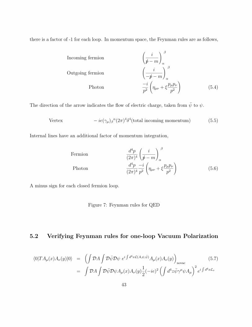
there is a factor of -1 for each loop. In momentum space, the Feynman rules are as follows,
Incoming fermion
(i
p/−m
) β
α
Outgoing fermion
(i
−p/−m
) β
α
Photon−ip2
(ηµν + ξ
pµpνp2
)(5.4)
The direction of the arrow indicates the flow of electric charge, taken from ψ to ψ.
Vertex − ie(γµ)βα(2π)4δ4(total incoming momentum) (5.5)
Internal lines have an additional factor of momentum integration,
Fermiond4p
(2π)4
(i
p/−m
) β
α
Photond4p
(2π)4
−ip2
(ηµν + ξ
pµpνp2
)(5.6)
A minus sign for each closed fermion loop.
Figure 7: Feynman rules for QED
5.2 Verifying Feynman rules for one-loop Vacuum Polarization
〈0|TAµ(x)Aν(y)|0〉 =(∫
DA∫DψDψ ei
∫d4xL(A,ψ,ψ)Aµ(x)Aν(y)
)novac
(5.7)
=∫DA
∫DψDψAµ(x)Aν(y)
1
2(−ie)2
(∫d4zψγµψAµ
)2
ei∫d4xLo
43
The purely fermionic part that has to be computed here is∫DψDψ ψγµψ(z1) ψγ
νψ(z2) ei∫d4xLo
/∫DψDψ ei
∫d4xLo
=δ
δηβ(z1)(γµ) α
β
δ
δηα(z1)
δ
δηγ(z2)(γν) δ
γ
δ
δηδ(z2)exp
{∫x
∫yη(x)S(x− y)η(y)
}=
δ
δηβ(z1)(γµ) α
β
δ
δηα(z1)
δ
δηγ(z2)(γν) δ
γ
∫uSρδ (z2 − u)ηρ(u)
∫x
∫yη(x)S(x− y)η(y)
=δ
δηβ(z1)(γµ) α
β
δ
δηα(z1)(γν) δ
γ Sγδ (0)
∫x
∫yη(x)S(x− y)η(y)
+δ
δηβ(z1)(γµ) α
β
δ
δηα(z1)(γν) δ
γ
∫yS ρδ (z2 − y)ηρ(y)
∫xησ(x)Sγσ(x− z2) (5.8)
The first term on the rhs of the last expression above must vanish by Lorentz invariance.
The cancellation may also be seen directly from the expression for the propagator,
(γν) δγ Sδ
γ(0) =∫ d4k
(2π)4
tr{γµ(6 k +m)}k2 −m2 + iε
= 0 (5.9)
The remainder of the calculation proceeds as follows,
= − δ
δηβ(z1)(γµ) α
β (γν) δγ
∫ySδ
ρ(z2 − y)ηρ(y) S γα (z1 − z2)
= −(γµ) αβ (γν) δ
γ Sδβ(z2 − z1) S
γα (z1 − z2)
= −tr(γµS(z1 − z2)γ
νS(z2 − z1))
(5.10)
Hence
〈0|TAµ(x)Aν(y|0〉 =1
2e2∫d2z1
∫d2z2 〈0|TAµ(x)Aν(y)Aκ(z1)Aλ(z2)|0〉o
×tr(γκS(z1 − z2)γλS(z2 − z1)) (5.11)
Of the three possible contributions to the tree level 4-point function for the gauge fields,
one is disconnected and corresponds to a vacuum graph which does not contribute to the
correlator. The remaining two connected contributions are equal and yield
〈0|TAµ(x)Aν(y)|0〉 = Gµν(x− y) + e2∫d4z1
∫d4z2Gµκ(x− z1)Gνλ(y − z2)
×tr(γκS(z1 − z2)γλS(z2 − z1)) (5.12)
44
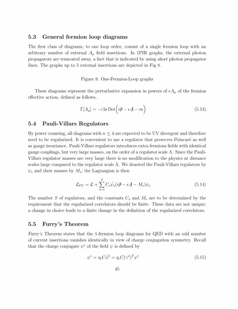
5.3 General fermion loop diagrams
The first class of diagrams, to one loop order, consist of a single fermion loop with an
arbitrary number of external Aµ field insertions. In 1PIR graphs, the external photon
propagators are truncated away, a fact that is indicated by using short photon propagator
lines. The graphs up to 5 external insertions are depicted in Fig 8.
Figure 8: One-Fermion-Loop graphs
These diagrams represent the perturbative expansion in powers of eAµ of the fermion
effective action, defined as follows,
Γ[Aµ] = −i ln Det(i∂/− eA/−m
)(5.13)
5.4 Pauli-Villars Regulators
By power counting, all diagrams with n ≤ 4 are expected to be UV divergent and therefore
need to be regularized. It is convenient to use a regulator that preserves Poincare as well
as gauge invariance. Pauli-Villars regulators introduces extra fermions fields with identical
gauge couplings, but very large masses, on the order of a regulator scale Λ. Since the Pauli-
Villars regulator masses are very large there is no modification to the physics at distance
scales large compared to the regulator scale Λ. We denoted the Pauli-Villars regulators by
ψs and their masses by Ms; the Lagrangian is then
LPV = L+S∑s=1
Csψs(i∂/− eA/−Ms)ψs (5.14)
The number S of regulators, and the constants Cs and Ms are to be determined by the
requirement that the regularized correlators should be finite. These data are not unique;
a change in choice leads to a finite change in the definition of the regularized correlators.
5.5 Furry’s Theorem
Furry’s Theorem states that the 1-fermion loop diagrams for QED with an odd number
of current insertions vanishes identically in view of charge conjugation symmetry. Recall
that the charge conjugate ψc of the field ψ is defined by
ψc = ηcCψt = ηcC(γo)Tψ∗ (5.15)
45
where the charge conjugation matrix is defined to satisfy
CγtµC−1 = −γµ C†C = I (5.16)
As a result, the charge conjugate of the electric current reverses its sign, as might be
expected. The fermion propagator in momentum space transforms as follows,
C
(1
k/−m
)tC−1 =
1
−k/−m(5.17)
and this implies that its transformation in position space is given by Hence
C S(x, y)tC−1 = S(y, x) (5.18)
For a given ordering of momenta and µ labels, two graphs with opposite charge flow
(opposite orientation of the arrow) contribute and must be added up. They are given by
Γ(n) = tr(γµ1S(x1, x2)γ
µ2S(x2, x3)γµ3 · · · γµnS(xn, x1)
)(5.19)
+tr(γµ1S(x1, xn)γ
µnS(xn, xn−1)γµn−1 · · · γµ2S(x2, x1)
)Taking the transpose inside the trace leaves this expression invariant, and re-expressing
the transposes with the help of the charge conjugation matrix C yields
Γ(n) = tr(S(xn, x1)
t(γµn)t · · · (γµ3)tS(x2, x3)t(γµ2)tS(x1, x2)
t(γµ1)t)
(5.20)
+tr(S(x2, x1)
t(γµ2)t · · · (γµn−1)tS(xn, xn−1)t(γµn)tS(x1, xn)
t(γµ1)t)
= (−)ntr(S(x1, xn)γ
µn · · · γµ3S(x3, x2)γµ2S(x2, x1)γ
µ1
)(5.21)
+(−)ntr(S(x1, x2)γ
µ2 · · · γµn−1S(xn−1, xn)γµnS(xn, x1)γ
µ1
)= (−)nΓ(n) (5.22)
This completes the proof of Furry’s theorem. Therefore, diagrams (b) and (d) in Fig 8
vanish identically, leaving only those with even n.
5.6 Ward-Takahashi identities for the electro-magnetic current
Whenever there exists a current jµ(x) which is satisfies the conservation equation ∂µjµ =
0, certain special relations, generally called Ward identities, will hold between certain
46
correlation functions of local operators. In the case at hand, the relevant conserved current
is the electro-magnetic current jµ(x) ≡ ψ(x)γµψ(x). Our derivation of the Ward identities
will, however, be more general than this case.
The conservation of the current jµ implies the existence of a time-independent charge
Q. Local observables may be organized in eigenspaces of definite Q-charge, and it suffices
to examine correlators of operators of definite charges
[Q,Oi(y)] = qiOi(y) Q =∫d3~x j0(t, ~x) (5.23)
Since the commutator [j0(t, ~x),Oi(t, ~y)] can receive contributions only from ~x = ~y in
view of the locality of the operators, the above commutator with the charge requires the
following local commutator to hold,
[j0(x),Oi(y)] δ(x0 − y0) = qiδ
(4)(x− y)Oi(y) (5.24)
In specific theories, this relation will in fact result from the explicit form of the current
jµ and the local operators Oi(y) in terms of canonical fields and the use of the canonical
commutation relations of the canonical fields. For example in QED, the relation may be
worked out for the commutator [j0(x), ψα(y)]δ(x0 − y0).
Next, consider a correlator of a product of local operators and the conserved current
jµ(x). The interesting quantity to consider is the divergence of this correlator,†
∂(x)µ 〈∅|Tjµ(x)O1(y1) · · · On(yn)|∅〉 (5.25)
Were it not for the time-ordering instruction, this divergence would be identically 0 as
long as the current is conserved. From the time ordering Heaviside functions on x0 − y0i ,
however, one picks up non-vanishing terms. This may be seen first from the time-ordering
on two fields,
∂(x)µ Tjµ(x)Oi(yi) = δ(x0 − y0
i )[j0(x),Oi(y)] = qiδ(x− y)Oi(yi) (5.26)
and readily generalizes to n fields. Inserting this result in the correlator of interest yields,
∂(x)µ 〈∅|Tjµ(x)O1(y1) · · · On(yn)|∅〉 =
n∑i=1
qi δ(x− yi)〈∅|TO1(y1) · · · On(yn)|∅〉 (5.27)
This is a very important equation, as it states that the longitudinal part of the current
correlator is expressed in terms of correlators without the insertion of the current.
†Here and elsewhere, the superscript (x) will indicate that the derivatve is applied in the variable x.
47
We give two examples in QED. The first applies to the correlator of electro-magnetic
currents only. Since the electric charge of the current itself vanishes, one has
∂(x)µ 〈∅|Tjµ(x)jν1(y1) · · · jνn(yn)|∅〉 = 0 (5.28)
In other words, the current correlators are transverse in each external leg. The second
example involves one current and two fermions,
∂(x)µ 〈∅|Tjµ(x)ψα(y)ψβ(z)|∅〉 = +δ(x− y)〈∅|Tψα(y)ψβ(z)|∅〉
−δ(x− z)〈∅|Tψα(y)ψβ(z)|∅〉 (5.29)
Feynman diagrammatic representations of both equations are given in Fig.
5.7 Regularization and gauge invariance of vacuum polarization
The vacuum polarization graph corresponds to n = 2 and contributes to Γ(2). The unreg-
ularized Feynman diagram for vacuum polarization is given by
Γµνo (k,m) ≡ (−)(−i)(−ie)2∫ d4p
(2π)4tr
(γµ
i
p/−mγν
i
p/+ k/−m
)(5.30)
The overall − sign is for a closed fermion loop; the factor of (−i) from thedefinition of Γ;
the factors of (−ie) from two vertex insertions. This integral is quadratically divergent.
We introduce s = 1, · · · , S Pauli-Villars regulators with masses Ms ∼ Λ and define the
regularized vacuum polarization tensor by
Γµν(k,m; Λ) ≡ ie2∫ d4p
(2π)4
S∑s=0
Cstr
(γµ
1
p/−Ms
γν1
p/+ k/−Ms
)(5.31)
where M0 = m and C0 = 1. In practice, it suffices to take S = 3, but we shall leave this
number arbitrary at this stage.
Gauge invariance requires conservation of the electro-magnetic current and by the
Ward identities derived in the preceding subsection, transversality of the 2-point function,
kµΓµν(k,m; Λ) = 0. This property is readily checked using the following simple, but very
useful general formula,
1
p/−Ms
k/1
p/+ k/−Ms
=1
p/−Ms
{(p/+ k/−Ms)− (p/−Ms)
}1
p/+ k/−Ms
=1
p/−Ms
− 1
p/+ k/−Ms
(5.32)
48
As a result,
kνΓµν(k,m; Λ) = ie2
∫ d4p
(2π)4
S∑s=0
Cstr γµ
(1
p/−Ms
k/1
p/+ k/−Ms
)
= ie2∫ d4p
(2π)4
S∑s=0
Cstr γµ
(1
p/−Ms
− 1
p/+ k/−Ms
)(5.33)
Since the integrals have been rendered convergent by the Pauli-Villars regulators, one may
shift the momentum integration by k in the second term so that the difference of the two
integrals vanishes, confirming gauge invariance.
Gauge invariance thus amounts to transversality of the 2-point function. This property
in turn leads to a dramatic simplification of the expression for vacuum polarization. Since
Γµν is a Lorentz tensor which depends only on the vector kµ, its general form must be
Γµν(k,m; Λ) = Aηµν +Bkµkν (5.34)
Transversality requires A + k2B = 0, so that vacuum polarization is proportional to a
single scalar function,
Γµν(k,m; Λ) = (k2ηµν − kµkν)Γ(k2,m; Λ) (5.35)
The fact that two powers of momentum are extracted by gauge invariance implies, just
on dimensional grounds, that the remaining vacuum polarization function ω will be only
logarithmically divergent. Thus, we encounter for the first time, a general paradigm that
gauge invariance improves UV convergence.
5.8 Calculation of vacuum polarization
The first step is to rationalize the fermion propagators.
Γµν(k,m; Λ) = ie2∫ d4p
(2π)4
S∑s=0
Cstr γµ(p/+Ms)γ
ν(k/+ p/+Ms)
(p2 −M2s )((k + p)2 −M2
s )(5.36)
The second step is to introduce a Feynman parameter,
Γµν(k,m; Λ) = ie2∫ 1
0dα∫ d4p
(2π)4
S∑s=0
Cstr γµ(p/+Ms)γ
ν(k/+ p/+Ms)
(p2 −M2s + 2αk · p+ αk2)2
(5.37)
The third step is to combine the denominator as follows,
p2 + 2αk · p+ αk2 = (p+ αk)2 + α(1− α)k2 (5.38)
49
The fourth step is to shift p+αk → p, which is permitted because the combined integrand
leads to a convergent integral,
Γµν(k,m; Λ) = ie2∫ 1
0dα∫ d4p
(2π)4
S∑s=0
Cstr γµ(p/− αk/+Ms)γ
ν((1− α)k/+ p/+Ms)
(p2 −M2s + α(1− α)k2)2
(5.39)
The fifth step is to work out the trace, discard terms odd in p since those cancel by p→ −psymmetry of the remaining integrand, and replace
pµpν → 1
4p2ηµν (5.40)
by using Lorentz symmetry of the integrand,
tr γµp/γνp/ → − 2p2ηµν (5.41)
Combining these result,
Γµν(k,m; Λ) = −ie2∫ 1
0dα∫ d4p
(2π)4
S∑s=0
Cs2p2ηµν − α(1− α)[4k2ηµν − 8kµkν ]− 4M2
s ηµν
(p2 + α(1− α)k2 −M2s )
2
(5.42)
This result is not manifestly transverse and we shall now show that the longitudinal piece
vanishes by intgeration by part. To do so, we split this up as follows,
Γµν(k,m; Λ) = (ηµνk2 − kµkν)Γ(k2,m; Λ) (5.43)
−ie2ηµν∫ 1
0dα∫ d4p
(2π)4
S∑s=0
Cs2p2 + 4k2α(1− α)− 4M2
s
(p2 + α(1− α)k2 −M2s )
2
The integrand of the second term is a total derivative,
2p2 + 4k2α(1− α)− 4M2s
(p2 + α(1− α)k2 −M2s )
2=
∂
∂pµ
(pµ
p2 + α(1− α)k2 −M2s
)(5.44)
and therefore the p-integral vanishes since the sum over all Pauli-Villars regulator contri-
butions is convergent. The remaining scalar integral is given as follows,
Γ(k2,m; Λ) = 8ie2∫ 1
0dα∫ d4p
(2π)4
S∑s=0
Csα(1− α)
(p2 + α(1− α)k2 −M2s )
2(5.45)
It suffices to take S = 1, M1 = Λ. The p-integral encountered are scalar and may be
carried out easily with the help of the formulas derived earlier,
Γ(k2,m,Λ) =8e2
(4π)2
∫ 1
0dα α(1− α) ln
m2 − α(1− α)k2
Λ2(5.46)
Next, we shall derive a physical interpretation for this result and carry out the required
renormalizations.
50
5.9 Resummation and screening effect
Repeated insertion of the 1-loop vacuum polarization effect into the photon propagator is
easily carried out. The tree level photon propagator is given by,
Goµν(k) =
−ik2
(ηµν +
1− λ
λ
kµkνk2
)(5.47)
Figure 9: Resummation of 1-loop vacuum polarization
Since the vacuum polarization effect is transverse, it is clear that the longitudinal part
of the photon propagator is unmodified to all orders. A single insertion therefore produces
a purely transverse effect,
G1µν(k) =
(−ik2
)2
(k2ηµν − kµkν)iΓ(k2,m; Λ)
=−ik2
(ηµν −
kµkνk2
)Γ(k2,m; Λ) (5.48)
Hence the full propagator becomes
Gµν(k) =−ik2
(ηµν −
kµkνk2
)1
1− Γ(k2,m; Λ)(5.49)
The effect of this correction is to modify Coulomb’s law. In the limit where k → 0, for
example, we have
e2
~k2→ e2eff
~k2≡ e2
~k2× 1
1− Γ(0,m; Λ)
1− Γ(0,m; Λ) = 1 +e2
12π2ln
Λ2
m2+O(e4) (5.50)
Starting out with the charge e in the Lagrangian, we see that the effective charge observed
in the Coulomb law is reduced, at distances long compared to 1/Λ. Quantitatively, the
effective charge is given by
e2eff =e2
1 + e2
12π2 ln Λ2
m2
(5.51)
51
5.10 Physical interpretation of the effective charge
Vacuum polarization is produced by the screening effects of virtual electron-positron pairs.
We now explain how this can come about. As is shown schematically by the vacuum
polarization Feynman diagram itself, the presence of the photon gives rise to an electro-
magnetic field which creates a virtual pair. The QED vacuum is therefore not quite
an empty space. Instead, in the QED vacuum, electron positron pairs are continuously
beeing created and annihilated. Each pair acts like a small short-lived electric dipole.
The presence of these electric dipoles makes the QED vacuum into a di-electric medium,
analogous to the di-electric media created by matter, such as water, air etc.
It is a well-known effect of a di-electric medium that an electric charge is screened by
the presence of the electric dipoles in the medium. Qualitatively, in the presence of a +
charge, the dipoles will align their negative ends towards the + charge and the net effect
of this is that the effective charge decreases with distance. This is schematically depicted
in Fig 10.
Figure 10: Polarization of a charge by virtual electron-positron pairs
The electric charge observed in the Coulomb law is the effective charge at long distances,
much larger than 1/me. If the charge at long distances is to be e, then the charge placed at
the center must be larger. We shall denote that charge by e0. The relation now becomes
e2 =e2o
1 + e2o12π2 ln Λ2
m2
or e2o = e2 +e4
12π2ln
Λ2
m2+O(e6) (5.52)
The k-dependent part of Γ(k,m,Λ) also affects the Coulomb interaction in a computable
way. The value of the charge will now depend on the momentum. For example in the
approximation of momenta large compared to m, we shall have
e2eff(k) =e2o
1− Γ(k2,m,Λ)=
e2o1− Γ(0,m,Λ) +−ΓR(k2,m,Λ)
=e2
1− ΓR(k2,m; Λ)(5.53)
with
ΓR(k2,m,Λ) =e2
2π2
∫ 1
0dα α(1− α) ln
m2 − α(1− α)k2
m2(5.54)
52
In the regime −k2 � m2, referred to as the deep inelastic scattering region, we have
ΓR(k2,m,Λ) =e2
12π2ln−k2
m2+O(e4) (5.55)
and the effective charge as a function of k2 is given by
e2eff(k) =e2
1− e2
12π2 ln −k2
m2
(5.56)
This formula confirms yet once more that as one probes smaller and smaller distances (large
−k2), the effective charge increases; this is again consistent with our physical picture for
vacuum polarization.
5.11 Renormalization conditions and counterterms
Our key conclusion is that vacuum polarization modifies the large distance Coulomb law
behavior of the photon propagator. But the Coulomb law provides the standard definition
of the electric charge. Thus, we shall reverse the order in which we impose known data.
1. We normalize the Coulomb law at long distances to be governed by the standard
electric charge e;
2. Therefore, the bare parameters in the Lagrangian will not be the ones observed at
long distance;
3. Imposing the condition that the Coulomb law at long distances is standard amounts
to a renormalization condition, imposed at the zero momentum renormalization
point. The modified Lagrangian used as a starting point is the bare Lagrangian.
Its derivation from the physical Lagrangian is given by counterterms.
In the bare Lagrangian Lo, the charge is replaced by the bare charge eo, the fermion
mass is replaced by the bare mass mo and the fields Aµ and ψ are subject to field renormal-
ization factors√Z3 and
√Z2 respectively. It is custormary to introduce a renormalization
constant Z1 for the vertex as well,
Lo = −1
4Z3FµνF
µν − λ
2(∂µA
µ)2 + Z2ψ(i∂/−mo)ψ − eZ1ψA/ψ (5.57)
Lct = −1
4(Z3 − 1)FµνF
µν + (Z2 − 1)ψi∂/ψ − (Z2mo −m)ψψ − e(Z1 − 1)ψA/ψ
From vacuum polarization the only term we have encountered so far is Z3.
53
The renormalization condition suitable to recovering the physical Coulomb law is that
at long distance (i.e. zero momentum k), the full truncated 2-point function
ΓµνR (k,m) = (ηµνk2 − kµkν)ΓR(k2,m)
ΓR(0,m) = 1 (5.58)
We know the contributions to ΓR(k,m). The bare coefficient is Z3 = 1 + O(e2); the
one-loop correction of vacuum polarization Γ(k,m,Λ)
Γ(k,m) = Z3 − Γ(k2,m,Λ) +O(e4) (5.59)
The renormalization condition implies the requirement
Z3 = 1 + Γ(0,m,Λ) = 1− e2
12π2ln
Λ2
m2+O(e4) (5.60)
Notice that the Ward-Takahashi identities relating the electron propagator and the vertex
function imply the relation Z1 = Z2. In other words, the combination eAµ = e0A0µ is not
renormalized.
5.12 The Gell-Mann – Low renormalization group
We shall deal in detail with the renormalization group later on, but historically, the subject
started with the following key observation by Gell-Mann and Low. One really is not forced
to renormalize the photon 2-point function at zero photon momentum. In fact, when one
imagines a theory with vanishing fermion mass m = 0, it is impossible to renormzalize
at zero momentum. To solve this problem, Gell-Mann and Low propose to choose an
arbitrary scale, called the renormalizatiion scale µ such that
ΓR(k2,m;µ)∣∣∣∣k2=−µ2
= 1 (5.61)
Using the explicit form of Z3:
Z3 = 1 +e2
2π2
∫ 1
0dα α(1− α) ln
m2 + α(1− α)µ2
Λ2+O(e4) (5.62)
Now if the bare charge is eo, we have
e(µ) = Z1/23 (µ,Λ,m)eo(Λ) (5.63)
The charge e(µ), for given bare charge eo, and given cutoff, now depends upon µ. The
limit m→ 0 is now regular.
54
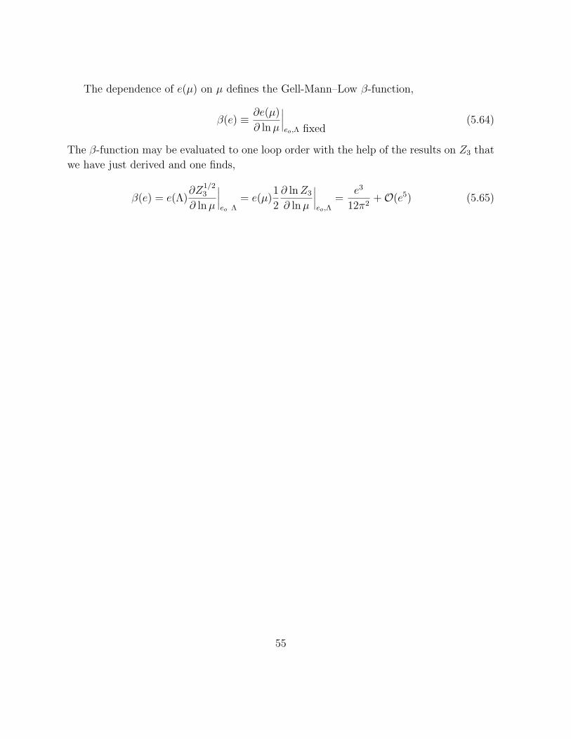
The dependence of e(µ) on µ defines the Gell-Mann–Low β-function,
β(e) ≡ ∂e(µ)
∂ lnµ
∣∣∣∣eo,Λ fixed
(5.64)
The β-function may be evaluated to one loop order with the help of the results on Z3 that
we have just derived and one finds,
β(e) = e(Λ)∂Z
1/23
∂ lnµ
∣∣∣∣eo Λ
= e(µ)1
2
∂ lnZ3
∂ lnµ
∣∣∣∣eo,Λ
=e3
12π2+O(e5) (5.65)
55
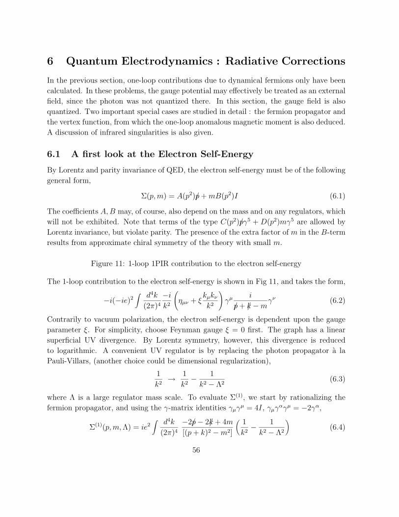
6 Quantum Electrodynamics : Radiative Corrections
In the previous section, one-loop contributions due to dynamical fermions only have been
calculated. In these problems, the gauge potential may effectively be treated as an external
field, since the photon was not quantized there. In this section, the gauge field is also
quantized. Two important special cases are studied in detail : the fermion propagator and
the vertex function, from which the one-loop anomalous magnetic moment is also deduced.
A discussion of infrared singularities is also given.
6.1 A first look at the Electron Self-Energy
By Lorentz and parity invariance of QED, the electron self-energy must be of the following
general form,
Σ(p,m) = A(p2)p/+mB(p2)I (6.1)
The coefficients A,B may, of course, also depend on the mass and on any regulators, which
will not be exhibited. Note that terms of the type C(p2)p/γ5 + D(p2)mγ5 are allowed by
Lorentz invariance, but violate parity. The presence of the extra factor of m in the B-term
results from approximate chiral symmetry of the theory with small m.
Figure 11: 1-loop 1PIR contribution to the electron self-energy
The 1-loop contribution to the electron self-energy is shown in Fig 11, and takes the form,
−i(−ie)2∫ d4k
(2π)4
−ik2
(ηµν + ξ
kµkνk2
)γµ
i
p/+ k/−mγν (6.2)
Contrarily to vacuum polarization, the electron self-energy is dependent upon the gauge
parameter ξ. For simplicity, choose Feynman gauge ξ = 0 first. The graph has a linear
superficial UV divergence. By Lorentz symmetry, however, this divergence is reduced
to logarithmic. A convenient UV regulator is by replacing the photon propagator a la
Pauli-Villars, (another choice could be dimensional regularization),
1
k2→ 1
k2− 1
k2 − Λ2(6.3)
where Λ is a large regulator mass scale. To evaluate Σ(1), we start by rationalizing the
fermion propagator, and using the γ-matrix identities γµγµ = 4I, γµγ
αγµ = −2γα,
Σ(1)(p,m,Λ) = ie2∫ d4k
(2π)4
−2p/− 2k/+ 4m
[(p+ k)2 −m2]
(1
k2− 1
k2 − Λ2
)(6.4)
56
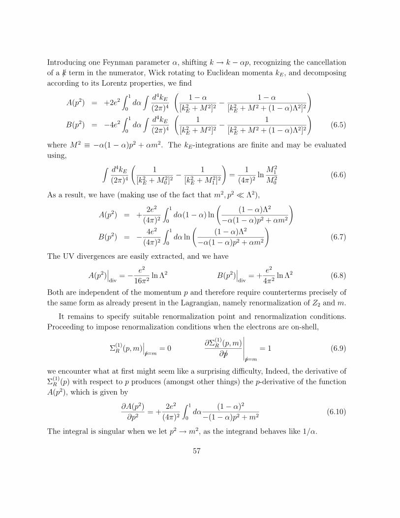
Introducing one Feynman parameter α, shifting k → k − αp, recognizing the cancellation
of a k/ term in the numerator, Wick rotating to Euclidean momenta kE, and decomposing
according to its Lorentz properties, we find
A(p2) = +2e2∫ 1
0dα∫ d4kE
(2π)4
(1− α
[k2E +M2]2
− 1− α
[k2E +M2 + (1− α)Λ2]2
)
B(p2) = −4e2∫ 1
0dα∫ d4kE
(2π)4
(1
[k2E +M2]2
− 1
[k2E +M2 + (1− α)Λ2]2
)(6.5)
where M2 ≡ −α(1 − α)p2 + αm2. The kE-integrations are finite and may be evaluated
using, ∫ d4kE(2π)4
(1
[k2E +M2
0 ]2− 1
[k2E +M2
1 ]2
)=
1
(4π)2lnM2
1
M20
(6.6)
As a result, we have (making use of the fact that m2, p2 � Λ2),
A(p2) = +2e2
(4π)2
∫ 1
0dα(1− α) ln
((1− α)Λ2
−α(1− α)p2 + αm2
)
B(p2) = − 4e2
(4π)2
∫ 1
0dα ln
((1− α)Λ2
−α(1− α)p2 + αm2
)(6.7)
The UV divergences are easily extracted, and we have
A(p2)∣∣∣div
= − e2
16π2ln Λ2 B(p2)
∣∣∣div
= +e2
4π2ln Λ2 (6.8)
Both are independent of the momentum p and therefore require counterterms precisely of
the same form as already present in the Lagrangian, namely renormalization of Z2 and m.
It remains to specify suitable renormalization point and renormalization conditions.
Proceeding to impose renormalization conditions when the electrons are on-shell,
Σ(1)R (p,m)
∣∣∣p/=m
= 0∂Σ
(1)R (p,m)
∂p/
∣∣∣∣∣∣p/=m
= 1 (6.9)
we encounter what at first might seem like a surprising difficulty, Indeed, the derivative of
Σ(1)R (p) with respect to p produces (amongst other things) the p-derivative of the function
A(p2), which is given by
∂A(p2)
∂p2= +
2e2
(4π)2
∫ 1
0dα
(1− α)2
−(1− α)p2 +m2(6.10)
The integral is singular when we let p2 → m2, as the integrand behaves like 1/α.
57
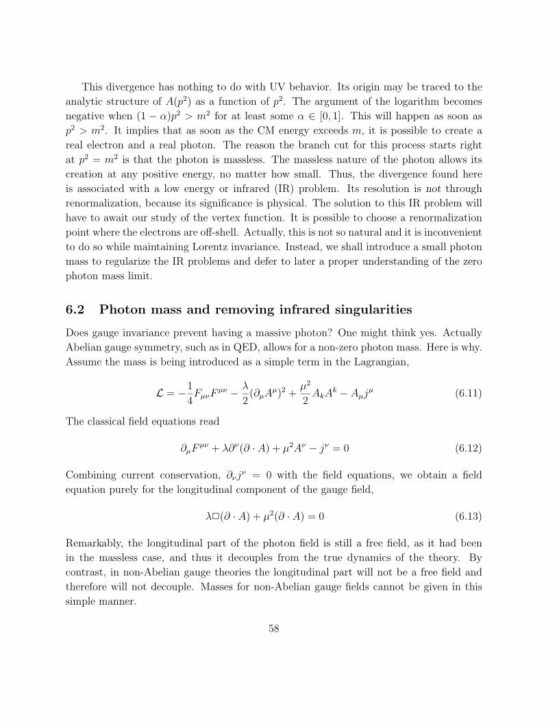
This divergence has nothing to do with UV behavior. Its origin may be traced to the
analytic structure of A(p2) as a function of p2. The argument of the logarithm becomes
negative when (1 − α)p2 > m2 for at least some α ∈ [0, 1]. This will happen as soon as
p2 > m2. It implies that as soon as the CM energy exceeds m, it is possible to create a
real electron and a real photon. The reason the branch cut for this process starts right
at p2 = m2 is that the photon is massless. The massless nature of the photon allows its
creation at any positive energy, no matter how small. Thus, the divergence found here
is associated with a low energy or infrared (IR) problem. Its resolution is not through
renormalization, because its significance is physical. The solution to this IR problem will
have to await our study of the vertex function. It is possible to choose a renormalization
point where the electrons are off-shell. Actually, this is not so natural and it is inconvenient
to do so while maintaining Lorentz invariance. Instead, we shall introduce a small photon
mass to regularize the IR problems and defer to later a proper understanding of the zero
photon mass limit.
6.2 Photon mass and removing infrared singularities
Does gauge invariance prevent having a massive photon? One might think yes. Actually
Abelian gauge symmetry, such as in QED, allows for a non-zero photon mass. Here is why.
Assume the mass is being introduced as a simple term in the Lagrangian,
L = −1
4FµνF
µν − λ
2(∂µA
µ)2 +µ2
2AkA
k − Aµjµ (6.11)
The classical field equations read
∂µFµν + λ∂ν(∂ · A) + µ2Aν − jν = 0 (6.12)
Combining current conservation, ∂νjν = 0 with the field equations, we obtain a field
equation purely for the longitudinal component of the gauge field,
λ2(∂ · A) + µ2(∂ · A) = 0 (6.13)
Remarkably, the longitudinal part of the photon field is still a free field, as it had been
in the massless case, and thus it decouples from the true dynamics of the theory. By
contrast, in non-Abelian gauge theories the longitudinal part will not be a free field and
therefore will not decouple. Masses for non-Abelian gauge fields cannot be given in this
simple manner.
58
The associated massive photon propagator is considerably more complicated than the
massless one,
−ik2 − µ2
(ηµν + ξ
kµkνk2 − µ2/λ
)(6.14)
Here, we continue to use the abbreviation ξ = (1− λ)/λ. Clearly, for the massive theory,
it is very advantageous to choose Feynman gauge λ = 1 and thus ξ = 0.
6.3 The Electron Self-Energy for a massive photon
The Lorentz decomposition of the electron self-energy in (6.1) is unmodified by the intro-
duction of a photon mass. The functions A,B become,
A(p2) = +2e2
(4π)2
∫ 1
0dα(1− α) ln
((1− α)Λ2
−α(1− α)p2 + αm2 + (1− α)µ2
)
B(p2) = − 4e2
(4π)2
∫ 1
0dα ln
((1− α)Λ2
−α(1− α)p2 + αm2 + (1− α)µ2
)(6.15)
It is readily verified that ∂A(p2)/∂p2 now has a finite limit as p2 → m2. The branch cut is
now supported at p2 > m2/(1−α)+µ2/α, (with α ∈ [0, 1]), which starts at p2 = (m+µ)2.
This is as expected : physical particles can be produced as soon as the rest energy m+ µ
is available.
6.4 The Vertex Function : General structure
The 1-loop 1PIR contribution to the vertex function is shown in Fig 12. Its unregularized
Feynman integral expression is given by
Γ(1)µ (p′, p) = −ie3
∫ d4k
(2π)4
1
k2
(ηρσ + ξ
kρkσk2
)γρ
1
p/′ − k/−mγµ
1
p/− k/−mγσ (6.16)
The k-integral has a logarithmic UV divergence, which will be regularized by a Pauli
Villars regulator on the photon propagator, just as we had used already for the electron-
self-energy. The divergence itself is clearly proportional to the bare interaction vertex γµ,
consistent with 1-loop renormalizability.
Figure 12: 1-loop 1PIR contribution to the vertex function
59
Assuming that this regularization has been carried out, it is instructive to verify ex-
plicitly the Ward identity between the vertex function and the electron self-energy Σ(1).
The Ward identity takes the form,
(p′ − p)µ Γ(1)µ (p′, p) = +e
(Σ(1)(p′)− Σ(1)(p)
)(6.17)
It is proven to one-loop using the simple fact that (p′−p)µγµ = (p/′+k/−m)− (p/+k/−m).
Substituting this relation into the integrand of the vertex function one finds,
(p′ − p)µ1
p/′ + k/−mγµ
1
p/+ k/−m= −e
(1
p/+ k/−m− 1
p/′ + k/−m
)(6.18)
Actually, the result holds to all orders in e. To see how this works, let S(p) be the full
fermion propagator, whose inverse is related to the regularized electron self-energy,
S(p)−1 = −i(p/−m)− iΣ(p) (6.19)
and Γµ(p′, p) be the full vertex function, then we have
(p′ − p)µΓµ(p′, p) = −ie[S−1(p)− S−1(p′)] (6.20)
The Ward identities imply that the renormalizations of Γ(1)µ (p′, p) and Σ(1)(p) are related
to one another. Actually, the mass renormalization does not involve the momenta, so only
Z2 should affect Γ(1)µ (p′, p).
We can make this connection explicit to one-loop order, where we have already estab-
lished the structure of the divergences and required renormalization counterterms,
Γ(1)µ (p′, p) = −eγµZ1 + Γ
(1)Rµ(p
′, p)
Σ(1)(p) = Z2(p/−m) + (Z2mo −m) + Σ(1)R (p) (6.21)
Recall the standard on-shell renormalization conditions on the electron self-energy,
Σ(1)R (p)
∣∣∣∣p/=m
= 0∂Σ
(1)R
∂p/(p)∣∣∣∣p/=m
= 1 (6.22)
For the vertex, the standard renormalization condition is also on-shell for the electrons,
and imposes the vanishing of ΓR(1)µ at vanishing photon momentum,
u(p′)Γ(1)Rµ(p
′, p)u(p)∣∣∣∣p′=p;p2=m2
= 0 (6.23)
60
Next, letting p′ → p in the Ward identity (6.17) provides the following relation,
Γ(1)µ (p, p) = −e∂Σ(1)(p)
∂pµ(6.24)
In terms of the renormalized quantities, we have
−eγµZ1 + Γ(1)Rµ(p, p) = −eγµZ2 − e
∂Σ(1)R (p)
∂pµ(6.25)
Evaluating this relation on-shell for the electrons, at zero momentum for the photon and
using the renormalization conditions, it is immediate that the contributions of Γ(1)Rµ and
Σ(1)R cancel, leaving the famous Ward identity
Z1 = Z2 (6.26)
a result which is valid to all orders in e.
6.5 Calculating the off-shell Vertex
We begin by calculating the vertex function for general off-shell momenta p, p′. For the
sake of generality, and because the result will be needed later as well, we shall include a
non-zero photon mass µ in the calculation from the start,
Γ(1)µ (p′, p) = −ie3
∫Λ
d4k
(2π)4
1
k2 − µ2
ηρσ + ξkρkσ
k2 − µ2
λ
γρ 1
p/′ − k/−mγµ
1
p/− k/−mγσ (6.27)
It will always be assumed that the vertex integral has been UV regularized by using a
Pauli Villars regulator Λ on the photon, just as was used for the electron self-energy. This
fact will be indicated by the subscript Λ on the k-integral. To begin, we work in Feynman
gauge with ξ = 0; we shall later also discuss the contributions from ξ 6= 0. Rationalizing
the fermion propagators gives,
Γ(1)µ (p′, p) = −ie3
∫Λ
d4k
(2π)4
γσ(p/′ − k/+m)γµ(p/− k/+m)γσ(k2 − µ2)((p′ − k)2 −m2)((p− k)2 −m2)
(6.28)
Introducing two Feynman parameters α, β for the 3 factors in the denominator, and using
the following formula,
1
ABC= 2
∫ 1
0dα∫ 1−α
0dβ
1
[(1− α− β)A+ αB + βC]3(6.29)
61
we obtain
Γ(1)µ (p′, p) = −2ie3
∫ 1
0dα∫ 1−α
0dβ∫Λ
d4k
(2π)4
γσ(p/′ − k/+m)γµ(p/− k/+m)γσ((k − αp′ − βp)2 −M2(µ))3
(6.30)
where we have defined the function
M2(µ) = (α+ β)m2 + (1− α− β)µ2 − αp′2 − βp2 + (αp′ + βp)2 (6.31)
Upon shifting k → k + αp′ + βp, we find
Γ(1)µ (p′, p) = −2ie3
∫ 1
0dα∫ 1−α
0dβ∫Λ
d4k
(2π)4
Nµ
(k2 −M2(µ))3(6.32)
where the numerator is abbreviated by
Nµ = γσ((1− α)p/′ − βp/− k/+m
)γµ
((1− β)p/− αp/′ − k/+m
)γσ (6.33)
The numerator may be simplified by using the following identities,
γσγµγσ = −2γµ
γσγµγνγσ = +4ηµνI
γσγµγνγργσ = −2γσγνγµ (6.34)
After regrouping and using the result of angular averaging kµkν → 1/4k2ηµν , one finds the
following numerator
Nµ = −k2γµ +Nµ (6.35)
Nµ = −2m2γµ + 4m(1− 2β)pµ + 4m(1− 2α)p′µ
+2β(1− β) p/γµp/+ 2α(1− α) p/′γµp/′
−2(1− α)(1− β) p/γµp/′ − 2αβ p/′γµp/
The k-integrals are readily evaluated,∫Λ
d4k
(2π)4
1
(k2 −M2(µ))3= − i
32π2M2(µ)∫Λ
d4k
(2π)4
k2
(k2 −M2(µ))3=
i
16π2lnM2(Λ)
M2(µ)(6.36)
In the last integral, one may use m, p, p′ � Λ to carry out the following simplification,
M2(Λ) ∼ (1− α− β)Λ2. In summary, the full off-shell vertex function is given by
Γ(1)µ (p′, p) = − e3
(4π)2
∫ 1
0dα∫ 1−α
0dβ
(2γµ ln
M2(Λ)
M2(µ)+
Nµ
M2(µ)
)(6.37)
The integration over the Feynman parameters is fairly involved. Fortunately, it will not
be needed here in full.
62
It remains to make a suitable choice of renormalization conditions. It is natural to take
the fermions to be on-shell and the photon to have zero momentum, which implies p′ = p,
u(p)(−eZ1γµ + Γ(1)
µ (p, p))u(p)
∣∣∣∣p2=m2
= u(p)(−eγµ)u(p)∣∣∣∣p2=m2
+O(e5) (6.38)
Substituting the data of the renormalization point in the function M2, we find,
M2(µ) = (1− α− β)µ2 + (α+ β)2m2 (6.39)
It is clear that the integration over α, β would fail to converge for zero photon mass µ = 0,
where an IR divergence occurs. As is the case of the electron self-energy, the physical origin
of this IR divergence resides in the diverging probability for producing ultra-low energy
photons. With µ 6= 0, however, the integrals are convergent and the regulator dependent
part of Z1 may be deduced, (it arises only from the ln term),
Z1 = 1− e2
16π2ln Λ2 +O(e4) (6.40)
The finite renormalization parts may also be computed by carrying out the α, β-integrals,
and the dependence on the gauge parameter may be incorporated as well, (Itzykson and
Zuber)
Z1 = 1− e2
(4π)2
(1
λln
Λ2
m2+ 3 ln
µ2
m2− 1
λln
µ2
λm2+
9
4
)+O(e4) (6.41)
6.6 The Electron Form Factor and Structure Functions
The renormalized vertex function resulting from the preceding subsection is quite a com-
plicated object. In particular, the numerator Nµ generates 7 different spinor/tensor struc-
tures. Depending on the ultimate purpose of the calculations, not all of this information
may actually be required. Such is the case for the calculation of the anomalous magnetic
moment of the electron, on which we shall now focus attention.
A simpler object than the full vertex function is obtained when both electrons are
restricted to being specific on-shell electron states. Equivalently, one is then evaluating
not the full correlator 〈∅|jµ(x)ψα(y)ψβ(z)|∅〉 but rather the electron form factor,
〈u(p′)|jµ(q)|u(p)〉 = u(p′)Γµ(p′, p)u(p) (6.42)
Here, |u(p)〉 stands for an (on-shell) electron state with wave function u(p), and we have
q = p′−p and p2 = p′2 = m2. The photon is not on-shell, i.e. q2 is left general. The reason
63
this object is called a form factor is because it parametrizes the distributions of charge
and current “inside” the electron. Even though the electron is assumed to be a “point-like
particle”, renormalization effects spread out its charge and gives the electron structure.
Despite these restrictions, the form factor actually still contains a wealth of information,
such as the anomalous magnetic moment, and yet its form is much simpler than that of
the full vertex. This may be seen by listing all possible Lorentz invariant structures that
may occur. The Lorentz structure is determined by the Dirac matrix insertion between
u(p′) and u(p), as well as by the explicit dependence on the external momenta. The
matrix elements u(p′)γ5u(p) and u(p′)γ5Sµnuu(p) violate parity symmetry and are not
allowed in QED. This leaves the matrix elements u(p′)u(p), u(p′)γµu(p) and u(p′)Sµνu(p)
only. The dependence on momenta also significantly simplifies, since p2 = p′2 = m2 and
2p · p′ = 2m2 − q2. Thus, the general Lorentz structure of the form factor is
u(p′)Γµ(p′, p)u(p) = u(p′)
(γµf1(q
2) + Sµνqνf2(q
2) + (pµ + p′µ)f3(q2))u(p) (6.43)
Actually, the Gordon identity provides a relation between all three coefficients,
(p+ p′)µu(p′)u(p) = 2mu(p′)γµu(p)− 2iqν u(p′)Sµνu(p) (6.44)
the identity may be proven using
γµp/ = pµ − 2iSµνpν Sµν =
i
4[γµ, γν ]
p/′γµ = p′µ + 2iSµνp′ν [γµ, γν ] = −4iSµν (6.45)
It is convenient to eliminate the term in u(p′)u(p) in favor of the other two. It is customary
to define the form factor in terms of the two structure functions F1(q2) and F2(q
2),
u(p′)Γµ(p′, p)u(p) = u(p′)γµu(p)F1(q
2) +iqν
mu(p′)Sµνu(p)F2(q
2) (6.46)
In the following subsection, it will be shown that the anomalous magnetic moment can be
computed solely from the value of F2(0).
6.7 Calculation of the structure functions
The ξ-dependent part of the form factor gives a contribution F(ξ)1 (q2) to the structure
function F1(q2) and does not contribute to F2(q
2). Indeed, carrying out the contraction of
64
kρkσ, we have the following simplification,
u(p′)k/1
p/′ − k/−mγµ
1
p/− k/−mk/u(p) = u(p′)γµu(p) (6.47)
This is established using the Dirac equations (p/−m)u(p) = 0 and u(p′)(p/′−m) = 0, with
the help of which we have k/u(p) = −(p/− k/−m)u(p) and u(p′)k/ = −u(p′)(p/′− k/−m). As
a result, we have,
F(ξ)1 (q2) = −ie3ξ
∫Λ
d4k
(2π)4
1
(k2 − µ2)(k2 − µ2/λ)=
e3ξ
(4π)2ln
Λ2
µ2(6.48)
The remainder of the form factor may be evaluated for ξ = 0.
To calculate the remaining form factor, one evaluates the full off-shell vertex on shell
and sorts the various Lorentz invariants according to the decomposition (??). The function
M2(µ) simplifies considerably by putting the electrons on-shell and we have
M2(µ) = (1− α− β)µ2 + (α+ β)2m2 − αβq2 (6.49)
This requires evaluation of the matrix element u(p′)Nµu(p), which follows from the follow-
ing simple results,
u(p′) p/γµp/ u(p) = u(p′)(m2γµ −mqµ − 2imqνSµν
)u(p)
u(p′) p/′γµp/′ u(p) = u(p′)
(m2γµ +mqµ − 2imqνSµν
)u(p)
u(p′) p/′γµp/ u(p) = u(p′)(m2γµ
)u(p)
u(p′) p/γµp/′ u(p) = u(p′)
(m2γµ + q2γµ − 4miqνSµν
)u(p) (6.50)
Therefore, the matrix elements of Nµ are found to be,
u(p′)Nµu(p) = u(p′)(2mqµ {α(1− α)− β(1− β)} − 2(1− α)(1− β)q2γµ
+m2γµ{4− 4(α+ β)− 2(α+ β)2
}−4i(α+ β)(1− α− β)mqνSµν
)u(p) (6.51)
Since the function M2(µ) is a symmetric function of α and β and since the integration
measure is symmetric as well, the numerator is effectively symmetrized, which cancels the
65
term in mqµ. The remainder is readily decomposed onto the structure functions F1 and
F2, and we have
F1(q2) = − e3
8π2
∫ 1
0dα∫ 1−α
0dβ
(lnM2(Λ)
M2(µ)
+m2{2− 2α− 2β − (α+ β)2} − q2(1− α)(1− β)
(1− α− β)µ2 + (α+ β)2m2 − αβq2
)
F2(q2) =
e3
4π2
∫ 1
0dα∫ 1−α
0dβ
m2(α+ β)(1− α− β)
(1− α− β)µ2 +m2(α+ β)2 − αβq2(6.52)
The function F1 is singular as µ → 0 signaling an IR divergence. If the renormalization
conditions are taken on-shell for the electrons and at q2 = 0 for the photons (which is
actually off-shell since µ 6= 0), then the renormalized structure function is given by
F1(q2) = − e3
8π2
∫ 1
0dα∫ 1−α
0dβ
(ln
(1− α− β)µ2 + (α+ β)2m2
(1− α− β)µ2 + (α+ β)2m2 − αβq2
+m2{2− 2α− 2β − (α+ β)2} − q2(1− α)(1− β)
(1− α− β)µ2 + (α+ β)2m2 − αβq2
−m2{2− 2α− 2β − (α+ β)2}
(1− α− β)µ2 + (α+ β)2m2
)(6.53)
The interpretation of the infrared divergence will be given later. The physical interpreta-
tion of F1 is to describe the charge distribution of the electron.
In F2(q2), the limit µ2 → 0 is finite and may be taken. This quantity is properly
renormalized all by itself. Important is the q2 → 0 limit, corresponding to low energy
photons and homogeneous static fields,
F2(0) =e3
4π2
∫ 1
0dα∫ 1−α
0dβ
(1
α+ β− 1
)=
e3
8π2(6.54)
The physical interpretation of F2 is to describe the distribution of magnetic dipole moments
of the electron. Next, this result is applied to the calculation of the anomalous magnetic
moment of the electron, viewed customarily in response to a constant magnetic field, i.e.
at q = 0.
6.8 The One-Loop Anomalous Magnetic Moment
The form of the renormalized vertex function, evaluated on-shell for the electrons, is in
the small q approximation,
u(p′)Γµ(p′, p)u(p) = u(p′)
(eγµ +
e3
8π2
iqν
mSµν
)u(p) (6.55)
66
To compute the anomalous magnetic moment, we need to incorporate the effect of the
above correction in the Dirac equation and extract the proper magnetic moment term.
First, multiply by the gauge field Aµ. Translating to position space, we use
iqνAµSµν =i
2(qνAµ − qµAν)Sµν →
1
2F µνSµν (6.56)
The modified Dirac equation is therefore,(i∂/− eA/− e3
8π2
1
2mF µνSµν −m
)ψ = 0 (6.57)
To extract the magnetic moment, we use a standard spinor formula,
(i∂/− eA/)2 = (i∂µ − eAµ)(i∂µ − eAµ)− eF µνSµν (6.58)
which may be derived by decomposing the product of two γ-matrices on the lhs into a
sum of their commutator and anti-commutator. Multiplying the effective Dirac equation
to the left by (i∂/− eA/+m) and using the fact that in the absence of A we have ip/ = m,
we have
(i∂/− eA/+m)
(i∂/− eA/− e3
8π2
1
2mF µνSµν −m
)ψ
=
((i∂µ − eAµ)
2 −m2 −(e+
e3
8π2
)F µνSµν
)ψ = 0 (6.59)
Thus, the electron magnetic moment receives a finite correction:
µ =e
m
(1 +
α
2π
)+O(α2) α =
e2
4πα
2π= 0.0011614 · · ·
expt . : 0.0011597 : other effects; QCD, weak · · ·
67
7 Functional Integrals For Gauge Fields
The functional methods appropriate for gauge fields present a number of complications,
especially for non-Abelian gauge theories. In this chapter, we begin with a rapid and some-
what sketchy discussion of the Abelian case and then move onto a systematic functional
integral quantization of the Abelian and nonAbelian cases.
7.1 Functional integral for Abelian gauge fields
The starting point will be taken to be the Hamiltonian, supplemented by Gauss’ law. It
is easiest to describe the system in temporal gauge A0 = 0, where we have,
H =∫d3x
(1
2~E2 +
1
2~B2 − ~A · ~J
)(7.1)
where ~J is a conserved external current and we the following expressions for electric and
magnetic fields,
~E =∂ ~A
∂t~B = ~∇× ~A (7.2)
Furthermore, configuration space is described by all Ai(~x), hence a “position basis” of
Fock space consists of all states of the form
F ≡{|Ai(~x)〉 for all Ai(~x)
}(7.3)
The Hilbert space of physical states (recall the difference between the Fock space and the
physical Hilbert space, as discussed for free spin 1 fields) is obtained by enforcing on the
states the constraint of Gauss’ law
G(A) ≡ ~∇ · ~E − Jo (7.4)
Thus, we have
Hphys ≡{|ψ〉 ∈ F such that G(A)|ψ〉 = 0
}(7.5)
Of course, we are only interested in the physical states. In particular, we are interested
only in time-evolution on the subspace of physical states. Therefore, we introduce the
68
projection operator onto Hphys as follows,
P ≡∑
|ψ〉∈Hphys
|φ〉〈ψ| (7.6)
and the projected evolution operator may be decomposed as follows,
e−itH∣∣∣∣Hphys
= limN→∞
(P e−itH/N
)N(7.7)
We always assume that the full Hamiltonian, using the dynammics of j is used, so that it
is time independent. Otherwise T -order!
The projection operator onto physical states may also be constructed as a functionla
intgeral, though admittedly, this construction is a bit formal,
P =1∫DΛ
∫DΛ exp
(i∫d3xΛ(~x)(~∇ · ~E − Jo)(~x)
)(7.8)
Clearly P is the identity on Hphys, and zero anywhere else! Summing over only physical
states is equivalent to summing over all states |Ai(~x)〉 and using the projector P to project
the sum onto physical states only.
e−itH∣∣∣∣Hphys
=1∫DΛ
∫DAi
∫DEi
∫DΛ (7.9)
exp{i∫ t
0dt∫d3x
(~E · ∂0
~A− 1
2~E2 − 1
2~B2 + Λ(~∇ · ~E − Jo) + ~A · ~J
)}where it is understood that the usual boundary conditions on the functional integral vari-
ables are implemented at time 0 and t. Now rebaptize Λ as Ao, and express the result in
terms of a generating functional for the source Jµ,
Z[J ] ≡ 1∫DΛ
∫DAµ exp
{i∫d4x
(−1
4FµνF
µν − JµAµ)}
(7.10)
However, this is really only a formal expression. In particular, the volume∫DΛ of the
space of all gauge transformation is wildly infinite and must be dealt with before one can
truly make sense of this expression.
Recall that the expressions that came in always assumed the form Z[Jµ]/Z[0] so that
an overall factor of the volume of the gauge transformations cancels out. Thus in the
expression for Z[Jµ] itself, we may ab initio fix a gauge, so that the volume of the gauge
orbit is eliminated. We shall give a full discussion of this phenomenon when dealing with
69
the non-Abelian case in the next subsection; here we take an informal approach. One of
the most convenient choices is given by a linear gauge condition,∫DAµ
∏x
δ(∂µAµ − c) exp{i∫d4x
(−1
4FµνF
µν − JµAµ
)}(7.11)
Since no particular slice is preferred, it is natural to integrate with respect to c, say with
a Gaussian damping factor,∫Dc e−iλ/2
∫d4xc2(x)
∏x
δ(∂µAµ(x)− c(x)) = e−iλ/2∫d4x(∂µAµ)2 (7.12)
and we recover our good old friend:
Z[J ] =∫DAµ exp
{i∫d4x
(−1
4FµνF
µν − 1
2λ(∂ · A)2 − JµAµ
)}(7.13)
The J-dependence of Z[Jµ] is independent of λ, so we can formally take λ→ 0 and regain
our original gauge invariant theory. It is straightforward to evaluate the free field result,
〈0|TAµ(x)Aν(y)|0〉 = i∫ d4k
(2π)4
(ηµν +
1− λ
λ
kµkνk2 + iε
)e−ik(x−y)
k2 + iε
= Gµν(x− y) (7.14)
So that
Z[j]
Z[0]= exp
{1
2
∫d4x
∫d4yJµ(x)Gµν(x− y)Jν(y)
}(7.15)
which, provided Jµ is conserved, is independent of λ. In particular when any gauge
independent quantity is evaluated, the dependence on λ will disappear. When λ→∞ one
recovers Landau gauge, which is manifestly transverse; when λ→ 1, one recovers another
very convenient Feynman gauge.
7.2 Functional Integral for Non-Abelian Gauge Fields
We consider a Yang-Mills theory based on a compact gauge group G with structure con-
stants fabc, a, b, c = 1, · · · , dimG. As discussed previously, if G is a direct product of n
simple and n′ U(1) factors, then there will be n + n′ independent coupling constants de-
scribing n+n′ different gauge theories. Here, we shall deal with only one such component.
Thus, we assume that G is simple or that it is just an Abelian theory with G = U(1).
70
The basic field in the theory is the Yang-Mills field Aaµ. The starting point is the classical
action,
S[A; J ] = −1
4
∫d4xF a
µνFaµν −
∫d4xJaµAaµ
F aµν = ∂µA
aν − ∂νA
aµ + gfabcAbµA
cν (7.16)
where summation over repeated gauge indices a is assumed.
For this action to be gauge invariant, the current must be covariantly conserved
DµJµ = 0, which may render the Jµ dependent on the field Aµ itself. This compli-
cates the discussion, as compared to the Abelian case. Actually, we shall make one of two
possible assumptions.
1. The current Jµ arises from the coupling of other fields (such as fermions or scalars)
in a complete theory that is fully gauge invariant.
2. The current Jµ is an external source, but will be used to produce correlation functions
of gauge invariant operators, such as trFµνFµν .
In both cases, the full theory will really be gauge invariant.
7.3 Canonical Quantization
Canonical quantization is best carried out in temporal gauge with A0 = 0. To choose this
gauge, the equation ∂0U = igUA0 must be solved, which may always be done in terms of
the time-ordered exponential
U(t, ~x) = T exp{ig∫ t
t0dt′A0(t
′, ~x)}U(t0, ~x) (7.17)
In flat space-time with no boundary conditions in the time direction, this solution always
exists. If time is to be period (as in the case of problems in statistical mechanics at finite
temperature) then one cannot completely set A0 = 0.
It is customary to introduce Yang-Mills electric and magnetic fields by
Bai ≡ 1
2εijkF
ajk
Eai ≡ F a
0i = ∂0Aai (7.18)
71
and Eai is the canonical momentum conjugate to Aai . The Hamiltonian and Gauss’ law are
given by
H[E,A; J ] =∫d3x
{1
2Eai E
ai +
1
2Bai B
ai − Jai A
ai
}Ga(E,A) = ∂iE
ai + gfabcAbiE
ci (7.19)
The canonical commutation relations are
[Eai (x), A
bj(y)]δ(x
0 − y0) = −iδabδijδ(4)(x− y) (7.20)
The operator Ga commutes with the Hamiltonian (for a covariantly conserved Jµ). The
action of Ga on the fields is by gauge transformation, as may be seen by taking the relevant
commutator,
[Ga(x), Abi(y)]δ(x0 − y0) = ∂iδ
(4)(x− y)δab + fabcAciδ(4)(x− y) (7.21)
or better even in terms of the the integrated form of Ga,
Gω ≡∫d3xGa(x)ωa(x)
[Gω, Abi(y)] = (Diω)b(y) (7.22)
Gauge transformations form a Lie algebra as usual,
[Ga(x), Gb(y)]δ(x0 − y0) = ifabcGc(x)δ(4)(x− y) (7.23)
Thus, the operator Ga generates infinitesimal gauge transformations.
As in the case of the Abelian gauge field, Gauss’ law cannot be imposed as an operator
equation because it would contradict the canonical commutation relations between Ai and
Ei. Thus, it is a constraint that should be imposed as an initial condition. In quantum
field theory, it must be imposed on the physical states. The Fock and physical Hilbert
spaces are defined in turn by
F ≡{|Aai (~x)〉
}Hphys ≡
{|ψ〉 ∈ F such that Ga(E,A)|ψ〉 = 0
}(7.24)
It is interesting to note the physical significance of Gauss’ law.
72
7.4 Functional Integral Quantization
This proceeds very similarly to the case of the quantization of the Abelian gauge field.
The starting points are the Hamiltonian in A0 = 0 gauge and the constraint of Gauss’ law
which commuted with the Hamiltonian. We construct the evolution operator projected
onto the physical Hilbert space by repeated (and redundant) insertions of the projection
operator. Recall the definition and functional integral representation of this projector,
P ≡∑
|ψ〉∈Hphys
|ψ〉〈ψ|
=1∫DΛa
∫DΛa(~x) exp
{i∫d3xΛa(~x)
(DiE
ai − Ja0 )
}(7.25)
As in the case of the Abelian gauge fields, we construct the evolution operator projected
onto the physical Hilbert space by repeated insertions of P ,
e−itH∣∣∣∣phys
= limN→∞
(P e−i
tNH)N
(7.26)
=1∫DΛa
∫DΛa
∫DAai
∫DEa
i
× exp{i∫ t
0dt′∫d3x
(Eai ∂0A
ai −
1
2Eai E
ai −
1
2Bai B
ai
+Aai Jai + Λa(DiE
ai − Ja0 )
)}together with the customary boundary conditions on the field Aai and free boundary con-
ditions on the canonically conjugate momentum Eai .
Next, we recall that Gauss’ law resulted from the variation of the non-dynamical field
A0, which had been set to 0 in this gauge. But here, Λa plays again the role of a non-
dynamical Lagrange multiplier and we rebaptize it as follows,
Λa(x) → Aa0(x) (7.27)
The integration over the non-dynamical canonical momentum Eai may be carried out in
an algebraic way by completing the square of the Gaussian,
Eai ∂0A
ai −
1
2Eai E
ai −
1
2Bai B
ai + Aai J
ai −DiA
a0E
ai − Aa0J
a0 (7.28)
= −1
2(Ea
i − ∂0Aai +DiA0)
2 +1
2(∂0A
ai −DiA0)
2 − 1
2Bai B
ai − AaµJ
aµ
The intgeration measure over DEai is invariant under (functional) shifts in Ea
i , and we use
this property to realize that the remaining Gaussian integral over Eai is independent of
73
Aaµ and Jaµ , and therefor produces a constant. The remainder is easily recognized as the
Lagrangian density with source that was used as a starting point.
As a concrete formula, we record the matrix element of the evolution operator taken
between (non-physical) states in the Fock space,
〈A2(~x)|e−itH |A1(~x)〉 = c∫DAaµ exp
{i∫ t
0dt′∫d3x
(−1
4F aµνF
aµν − AaµJaµ)}
boundary conditions{A(0, ~x) = A1(~x)A(t, ~x) = A2(~x)
(7.29)
Time ordered correlation functions are deduced as usual and may be summarized by the
following generating functional,
eiG[J ] ≡∫DAaµ exp
{−1
4F aµνF
aµν − JaµAaµ
}(7.30)
Of course, this integral is formal, since gauge invariance leads to the integration of equiva-
lent copies of Aaµ. Therefore, we need to gauge fix, a process outlined in the next subsection.
7.5 The redundancy of integrating over gauge copies
We wish to make sense out of the functional intgeral of any gauge invariant combination
of operators which we shall collectively denote by O. For example, the following operators
are gauge invariant,
O+(x) ≡ F aµνF
aµν(x)
O−(x) ≡ F aµνF
aµν(x) (7.31)
An infinite family of operators O may be formed out of a time ordered product of a string
of O+ and O− opertors,
O = TO+(x1) · · · O+(xm)O−(y1) · · · O+(yn) (7.32)
We have the general formula
〈0|O|0〉 =
∫DAaµ O eiS[A]∫DAaµ eiS[A]
(7.33)
The key characteristic of this formula is that O is a gauge invariant operator.
The measure DAaµ is also gauge invariant. The way to see this is to notice that a
measure results from a metric on the space of all gauge fields. Once this metric has been
74
found and properly defined, the measure will forllow. The metric may be taken to be given
by the following norm,
|| δAaµ ||2 ≡∫d4x δAaµ δA
aµ (7.34)
The variation of a gauge field transforms homogeneously and thus the metric is invariant.
Therefore, we can construct an invariant measure.
Thus, we realize now that all pieces of the functional integral for 〈|O|0〉 are invariant
under local gauge transformations. But this renders the numerator and the denominator
infinite, since in each the integration extends over all gauge copies of each gauge field.
However, since the integrations are over gauge invariant integrands, the full integrations
will factor out a volume factor of the space of all gauge transformations times the integral
over the quotient of all gauge fields by all gauge transformations. Concretely,
A ≡ { all Aaµ(x) }G ≡ { all Λa(x) } (7.35)
Thus we have symbolically,∫ADAaµ O eiS[A] = Vol(G)
∫A/G
DAaµ O eiS[A] (7.36)
and inparticular, the volume of the space of all gauge transformations cancels out in the
formula for 〈0|O|0〉,
〈0|O|0〉 =
∫ADAaµ O eiS[A]∫ADAaµ eiS[A]
=
∫A/G DAaµ O eiS[A]∫A/G DAaµ eiS[A]
(7.37)
The second formula does not have the infinite redundancy integrating over all gauge trans-
formations of any gauge field.
In the case of the Abelian gauge theories, the problem was manifested through the
fact that the longitudinal part of the gauge field does not couple to the FµνFµν term in
the action, a fact that renders the kinetic operator non-invertible. A gauge fixing term
λ(∂µAµ)2 was added; its effect on the physical dynamics of the theory is none since the
current is conserved. For the non-Abelian theory, things are not as simple. First of all there
are now interaction terms in the F aµνF
aµν term, but also, the current is only covariantly
conserved. The methods used for the Abelian case do not generalize to the non-Abelian
case and we have to invoke more powerful methods.
75
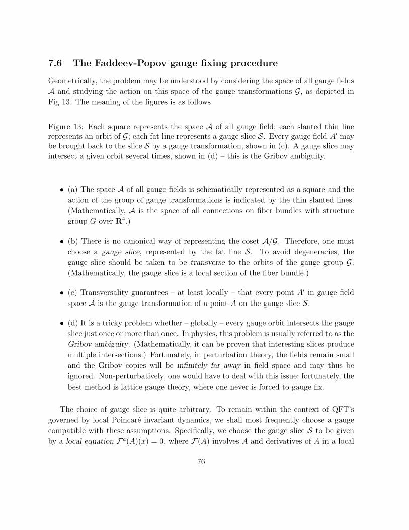
7.6 The Faddeev-Popov gauge fixing procedure
Geometrically, the problem may be understood by considering the space of all gauge fields
A and studying the action on this space of the gauge transformations G, as depicted in
Fig 13. The meaning of the figures is as follows
Figure 13: Each square represents the space A of all gauge field; each slanted thin linerepresents an orbit of G; each fat line represents a gauge slice S. Every gauge field A′ maybe brought back to the slice S by a gauge transformation, shown in (c). A gauge slice mayintersect a given orbit several times, shown in (d) – this is the Gribov ambiguity.
• (a) The space A of all gauge fields is schematically represented as a square and the
action of the group of gauge transformations is indicated by the thin slanted lines.
(Mathematically, A is the space of all connections on fiber bundles with structure
group G over R4.)
• (b) There is no canonical way of representing the coset A/G. Therefore, one must
choose a gauge slice, represented by the fat line S. To avoid degeneracies, the
gauge slice should be taken to be transverse to the orbits of the gauge group G.
(Mathematically, the gauge slice is a local section of the fiber bundle.)
• (c) Transversality guarantees – at least locally – that every point A′ in gauge field
space A is the gauge transformation of a point A on the gauge slice S.
• (d) It is a tricky problem whether – globally – every gauge orbit intersects the gauge
slice just once or more than once. In physics, this problem is usually referred to as the
Gribov ambiguity. (Mathematically, it can be proven that interesting slices produce
multiple intersections.) Fortunately, in perturbation theory, the fields remain small
and the Gribov copies will be infinitely far away in field space and may thus be
ignored. Non-perturbatively, one would have to deal with this issue; fortunately, the
best method is lattice gauge theory, where one never is forced to gauge fix.
The choice of gauge slice is quite arbitrary. To remain within the context of QFT’s
governed by local Poincare invariant dynamics, we shall most frequently choose a gauge
compatible with these assumptions. Specifically, we choose the gauge slice S to be given
by a local equation Fa(A)(x) = 0, where F(A) involves A and derivatives of A in a local
76
manner. Possible choices are
Fa(A) = ∂µAaµ Fa = Aa0 (7.38)
But many other choices could be used as well.
To reduce the functional integral to an integral along the gauge slice, we need to
factorize the measure DAaµ into a measure along the gauge slice S times a measure along
the orbits of the gauge transformations G. There is a nice gauge-invariant measure DU on
G resulting from the following gauge invariant metric on G,
|| δU ||2 ≡ −∫d4xtr
(U−1δU U−1δU
)(7.39)
If the orbits G were everywhere orthogonal to S, then the factorization would be easy
to carry out. In general it is not possible to make such a choice for S and a non-trivial
Jacobian factor will emerge. To compute it, we make use of the Faddeev-Popov trick.
Denote a gauge transformation U of a gauge field Aµ by
AUµ ≡ UAµU−1 +
i
g∂µUU
−1 (7.40)
Notice that the action of gauge transformations on Aµ satisfies the group composition law
of gauge transformations,
(AVµ )U = U(V AµV
−1 +i
g∂µV V
−1)U−1 +
i
g∂µUU
−1
= (UV )Aµ(UV )−1 +i
g∂µ(UV )(UV )−1
= AUVµ (7.41)
which will be useful later on.
Let F(A) denote the loval gauge slice function, the gauge slice being determined by
Fa(A) = 0. The quantity Fa(AU) will vanish when AU belongs to S, and will be non-zero
otherwise. We define the quantity J [A] by
1 = J [A]∫DU
∏x
δ(Fa(AU)(x)
)(7.42)
The functional δ-function looks a bit menacing, but should be understood as a Fourier
integral, ∏x
δ(Fa(AU)(x))≡∫DΛa exp
{i∫d4xΛa(x)Fa(AU)(x)
}(7.43)
77
Using the composition law (AUµ )V = AUVµ and the gauge invariance of the measure DU , it
follows that J is gauge invariant. This is shown as follows,
J [AV ]−1 =∫DU
∏x
δ(Fa((AV )U)(x)
)=
∫DU
∏x
δ(Fa(AUV )(x)
)=
∫D(U ′V −1)
∏x
δ(Fa(AU
′)(x)
)= J [A]−1 (7.44)
The deinition of the Jacobian J readily allows for a factorization of the measure of Ainto a measure over the splice S times a measure over the gauge orbits G. This is done as
follows, ∫ADAµ O eiS[A] =
∫ADAµ
∫GDU
∏x
(Fa(AU)(x)
)J [A] O eiS[A]
=∫GDU
∫ADAµ
∏x
(Fa(AU)(x)
)J [A] O eiS[A]
=(∫
GDU
) ∫ADAµ
∏x
(Fa(A)(x)
)J [A] O eiS[A] (7.45)
In passing from the first to the second line, we have simply inverted the orders of integration
over A and G; from the second to the third, we have used the gauge invariance of the
measure DAµ, of O and S[A]; from the third to the fourth, we have used the fact that
the functional δ-function restricts the integration over all of A to one just over the slice S.
Notice that the integration over all gauge transformation function∫DU is independent of
A and is an irrelevant constant.
The gauge fixed formula is independent of the gauge function F .
Therefore, we end up with the following final formula for the gauge-fixed functional
intgeral for Abelian or non-Abelian gauge fields,
〈0|O|0〉 =
∫ADAµ
∏x
(Fa(A)(x)
)J [A] O eiS[A]
∫ADAµ
∏x
(Fa(A)(x)
)J [A] eiS[A]
(7.46)
It remains to compute J and to deal with the functional δ-function.
78
7.7 Calculation of the Faddeev-Popov determinant
At first sight, the Jacobian J would appear to be given by a very complicated functional
integral over U . The key observation that makes a simple evaluation of J possible is that
Fa(A) only vanishes (i.e. its functional δ-function makes a non-vanishing contribution) on
the gauge slice. To compute the Jacobian, it suffices to linearlize the action of the gauge
transformations around the gauge slice. Therefore, we have
U = I + iωaT a +O(ω2)
AUµ = Aµ −Dµω +O(ω2)
Dµωa = ∂µω
a − gfabcAbµωc (7.47)
and the gauge function also linearizes,
Fa(AU) = Fa(Aµ −Dµω)(x) +O(ω2)
= Fa(A)(x)−∫d4y
(δFa(A)(x)
δAbµ(y)
)Dµω
b(y) +O(ω2)
= Fa(A)(x) +∫d4yMab(x, y)ωb(y) +O(ω2) (7.48)
where the operator M is defined by
Mab(x, y) ≡ Dyµ
(δFa(A)(x)
δAbµ(y)
)(7.49)
Now the calculation of J becomes feasible.
J [A]−1 =∫GDU
∏x
δ(Fa(AU)(x)
)=
∫Dωa
∏x
δ(Fa(A)(x) +
∫d4yMab(x, y)ωb(y)
)= (DetM)−1 (7.50)
Inverting this relation, we have
J [A] = DetM = Det
(Dyµ
δF(A)(x)
δAµ(y)
)(7.51)
Given a gauge slice function F , this is now a quite explicit formula. In QFT, however, we
were always dealing with local actions, local operators and these properties are obscured
in the above determinant formula.
79
7.8 Faddeev-Popov ghosts
We encountered a determinant expression in the numerator once before when delaing with
intgerations over fermions. This suggests that the Faddeev-Popov determinant may also
be cast in the form of a functional intgeration over two complex conjugate Grassmann odd
fields, which are usually referred to as the Faddeev-Popov ghost fields and are denoted by
ca(x) and ca(x). The expression for the determinant is then given by a functional integral
over the ghost fields,
DetM =∫DcaDca exp
{iSghost[A; c, c]
}Sghost[A; c, c] ≡
∫d4x
∫d4y ca(x)Mab(x, y)cb(y) (7.52)
If the function F is a local function of Aµ, then the support of Mab(x, y) is at x = y and
the above double integral collapses to a single and thus local intgeral involving the ghost
fields.
7.9 Axial and covariant gauges
First of all, there is a class of axial gauges where no ghosts are ever needed ! The gauge
function must be linear in Aaµ and involve no derivatives on Aµ. They involve a constant
vector nµ, and are therefore never Lorentz covariant, Fa(A)(x) = Aaµ(x)nµ,
δF a(A)(x)
δAbµ(y)= δabδ(4)(x− y)nµ
Dyµ
δF (A)(x)
δAµ(y)= ∂yµδ
(4)(x− y)nµ = M(x, y) (7.53)
Therefore, in axial gauges, the operator M is independent of A and thus a constant which
may be ignored. Thus, no ghost are required as the Faddeev-Popov formula would just
inform us that they decouple. Actually, since axial gauges are not Lorentz covariant, they
are much less useful in practice than it might appear.
It turns out that Lorentz covariant gauges are much more useful. The simplest such
gauges are specified by a function fa(x) as follows,
Fa(A)(x) ≡ ∂µAaµ(x)− fa(x) (7.54)
This choice gives rise to the following functional integral,
ZO =∫ADAµ
∏x
δ(∂µAaµ − fa) DetM O eiS[A] (7.55)
80
Since this functional integral is independent of the choice of fa, we may actually integrate
over all fa with any weight factor we wish. A convenient choice is to take the weight factor
to be Gaussian in fa,
ZO =
∫Dfa exp
{− i
2
∫d4xfafa
} ∫ADAµ
∏x δ(∂µA
aµ − fa) DetM O eiS[A]
∫Dfa exp
{− i
2
∫d4xfafa
} (7.56)
The denominator is just again a Aµ-independent constant which may be omitted. The
fa-intgeral in the numerator may be carried out since the functional δ-function instructs
us to set fa = ∂µAaµ, so that
ZO =∫ADAµ
∫Dca
∫DcaO exp
{iS[A] + iSgf [A] + iSghost[A; c, c]
}(7.57)
where the gauge fixing terms in the action are given by
Sgf [A] =∫d4x
{− 1
2ξ(∂µA
aµ)2}
(7.58)
It remains to obtain a more explicit form for the ghost action. To this end, we first compute
M.
Mab(x, y) = Dyµ
(δ∂νxAν(x)
δAµ(y)
)ab= (Dy
µ)ab∂µxδ
(4)(x− y) (7.59)
Inserting this operator into the expression for the ghost action, we obtain,
Sghost[A; c, c] ≡∫d4x
∫d4y ca(x)Mab(x, y)cb(y)
=∫d4x
∫d4yc(x)Dy
µ∂µxδ(x− y)c(y)
=∫d4x∂µc
a(x)(Dµc)a (7.60)
Thus, the total action for these gauges is given as follows,
Stot[A; c, c] = −1
4F aµνF
aµν − 1
2ξ(∂µA
aµ)2 + ∂µca(Dµc)a (7.61)
and we have the following general formula for vacuum expectation values of gauge invariant
operators,
〈0|O|0〉 =
∫DAµ
∫DcDc O eiStot[A;c,c]∫
DAµ∫DcDc eiStot[A;c,c]
(7.62)
In the section on perturbation theory, we shall show how to use this formula in practice.
81
8 Anomalies in QED
Initial exposure to renormalization may give the impression that the procedure is an ad hoc
remedy for a putative ill of QFT, that should not be required in some better formulation
of the theory. This is not true. The presence of anomalies and the existence of the
renormalization group will prove that the renormalization procedure has deep, physically
relevant meaning. Questions that are often posed in this context are
1. Are UV divergences a consequence of the perturbative expansion ?
2. If so, is it possible to re-sum them to finite results in the full theory?
3. Are there any physical consequences of renormalization ?
To answer these questions, we are taking a detour to anomalies.
8.1 Massless 4d QED, Gell-Mann–Low Renormalization
Recall the form of the 2-point vacuum polarization tensor to one-loop order
Πµν(k,m,Λ) = (k2ηµν − kµkν)Π(k,m,Λ) (8.1)
Π(k,m,Λ) = 1− e2
2π2
∫ 1
0dαα(1− α) ln
m2 − α(1− α)k2
Λ2+O(e4)
When the electron mass m 6= 0, it is natural (though not necessary) to renormalize at 0
photon momentum, and to require ΠR(0,m) = 1, so that
ΠR(k,m) = 1− Π(0,m,Λ) + Π(k,m,Λ) (8.2)
However, when m = 0, Π(0,m,Λ) = ∞, and this renormalization is not possible. This led
Gell-Mann–Low to renormalize “off-shell”, at a mass-scale µ that has no direct relation
with the electron mass or photon mass,
ΠR(k,m, µ)∣∣∣∣k2=−µ2
= 1 (8.3)
So that
ΠR(k,m, µ) = 1− e2
2π2
∫ 1
0dα(1− α)α ln
m2 − α(1− α)k2
m2 + α(1− α)µ2+O(e4) (8.4)
Now, we may safely let m→ 0,
ΠR(k, 0, µ) = 1− e2
12π2ln
(−k2
µ2
)+O(e4) (8.5)
The cost of renormalizing the massless theory is the introduction of a new scale µ, which
was not originally present in the theory.
82
8.2 Scale Invariance of Massless QED
But now think for a moment about what this means in terms of scaling symmetry. When
m = 0, classical electrodynamics is scale invariant,
L = −1
4FµνF
µν +ξ
2(∂µA
µ)2 + ψ(i∂/− eA/)ψ (8.6)
A scale transformation xµ → x′µ = λxµ, transforms a field φ∆(x) of dimension ∆ as follows
φ∆(x) → φ′∆(x′) = λ−∆φ∆(x)
{Aµ : ∆ = 1ψ : ∆ = 3
2
(8.7)
The classical theory will be invariant since the effects of scale transformations on the
various terms in the Lagrangian are as follows,
FµνFµν(x) → λ−4FµνF
µν(x)
(∂µAµ)2 → λ−4(∂µA
µ)2
ψ(i∂/− eA/)ψ → λ−4ψ(i∂/− eA/)ψ (8.8)
where we have assumed that e and ξ do not transform under scale transformations. Thus
L → λ−4L, and the action S =∫d4xL is invariant. Actually, you can show that L is
invariant under all conformal transformations of xµ; infinitesimally δxµ = δλxµ for a scale
transformation; δxµ = x2δcµ − xµ(δc · x) for a special conformal transformation. Thus,
classical massless QED is scale invariant; nothing in the theory sets a scale.
A fermion mass term, however, spoils scale invariance since ψψ → λ−3ψψ, assuming
that m is being kept fixed. Similarly, a photon mass would also spoil scale invariance.
Now, think afresh of the one-loop renormalization problem: when m = 0, one-loop
renormalization forced us to introduce a scale µ in order to carry out renormalization. One
cannot quantize QED without introducing a scale, and thereby breaking scale invariance.
What we have just identified is a field theory, massless QED, whose classical scale
symmetry has been broken by the process of renormalization, i.e. by quantum effects.
Whenever a symmetry of the classical Lagrangian is destroyed by quantum effects
caused by UV divergences, this classical symmetry is said to be anomalous. In this case,
it is the scaling anomaly, also referred to as the conformal anomaly.
83
8.3 Chiral Symmetry
In case the above result is insufficiently convincing at this time, we give an example of
another symmetry that has an anomaly, seen in a calculation that is finite. Take again
massless QED,
L = −1
4FµνF
µν + ψ(i∂/− eA/)ψ (8.9)
Setting m = 0 has enlarged the symmetry to include conformal invariance (classically).
It also produces another new symmetry: chiral symmetry. To see this, decompose ψ into
left and right spinors, in a chiral basis where γ5 is diagonal,
ψ = ψL ⊕ ψR γ5ψL = +ψL, γ5ψR = −ψR (8.10)
The Lagrangian then becomes,
L = −1
4FµνF
µν + ψL(i∂/− eA/)ψL + ψR(i∂/− eA/)ψR (8.11)
Clearly, ψL and ψR may be rotated by two independent phases,
U(1)L × U(1)R
{ψL → eiθLψLψR → eiθRψR
(8.12)
and the Lagrangian is invariant.‡ Now, we re-arrange these transformations as follows
U(1)V :
{ψL → eiθ+ψLψR → eiθ+ψR
2θ+ = θL + θR (8.13)
U(1)A :
{ψL → eiθ−ψLψR → e−θ−ψR
2θ− = θL − θR (8.14)
or, in 4-component spinor notation{U(1)V : ψ → eiθ+ψU(1)A : ψ → eiγ5θ−ψ
(8.15)
As symmetries, they have associated conserved currents.
• the vector current jµ ≡ ψγµψ
• the axial vector current jµ5 ≡ ψγµγ5ψ
‡Any symmetry that transforms left and right spinors differently is referred to as chiral.
84
Conservation of these currents may be checked directly by using the Dirac field equations,
in the following form,
iγµ∂µψ = eγµAµψ
−i∂µψγµ = eψγµAµ (8.16)
One then has,
∂µjµ5 = ∂µψγ
µγ5ψ − ψγ5γµ∂µψ = ieψγµAµγ5ψ + ieψγ5γ
µAµψ = 0 (8.17)
8.4 The axial anomaly in 2-dimensional QED
It is very instructive to consider the fate of chiral symmetry in the much simpler 2-
dimensional version of QED, given by the same Lagrangian,
L = −1
4FµνF
µν + ψ(i∂/− eA/)ψ (8.18)
Contrarily to 4-dim QED, this theory is not scale invariant, even for vanishing fermion
mass, since the dimensions of the various fields and couplings are given as follows, [e] = 1,
[A] = 0, [ψ] = 1/2. But it is chiral invariant, just as 4-dim QED was, and we have two
classically conserved currents,
jµ ≡ ψγµψ jµ5 ≡ ψγµγ5ψ (8.19)
A considerable simplification arises from the fact that the Dirac matrices are much simpler:
γ0 = σ1 =(
0 11 0
)γ1 = iσ2 =
(0 1−1 0
)γ5 = σ3 =
(1 00 −1
)(8.20)
As a result of this simplicity, the axial and vector currents are related to one another. This
fact may be established by computing the products γµγ5 explicitly,{γ0γ5 = σ1σ3 = −iσ2 = −γ1 = +γ1
γ1γ5 = iσ2σ3 = −σ1 = −γ0 = −γ0(8.21)
Introducing the rank 2 antisymmetric tensor εµν = −ενµ, normalized to ε01 = 1, the above
relations may be recast in the following form,
γµγ5 = εµνγν =⇒ jµ5 = εµνjν (8.22)
Consider the calculation of the vacuum polarization to one-loop, but this time in 2-dim
QED. The vacuum polarization diagram is just the correlator of the two vector currents
85
in the free theory, Πµν(k) = e〈∅|Tjµ(k)jν(−k)|∅〉, and is given by,
Πµν(k) = −e∫ d2p
(2π)2tr
(γµ
i
k/+ p/γνi
p/
)(8.23)
A priori, the integral is logarithmically divergent, and must be regularized. We choose to
regularize in a manner that preserves gauge invariance and thus conservation of the current
jµ. As a result, we have Πµν(k) = (k2ηµν − kµkν)Π(k2). Gauge invariant regularization
may be achieved using a single Pauli-Villars regulator with mass M , for example. Just as
in 4-dim QED, current conservation lowers the degree of divergence and in 2-dim, vacuum
polarization is actually finite.
Π(k2) = 4e∫ 1
0dα∫ d2p
(2π)2
[α(1− α)
(p2 + α(1− α)k2)2− α(1− α)
(p2 + α(1− α)k2 −M2)2
](8.24)
Carrying out the p-integration,
Π(k2) =ie
π
∫ 1
0dα
[α(1− α)
−α(1− α)k2− α(1− α)
−α(1− α)k2 +M2
](8.25)
Clearly, as M →∞, the limit is finite and the contribution from the Pauli-Villars regulator
actually cancels. One finds the finite result,
Π(k2) = − ie
πk2(8.26)
Notice that, even though the final result for vacuum polarization is finite, the Feynman
integral was superficially logarithmically divergent and requires regularization. It is during
this regularization process that we ensure gauge invariance by insisting on the conservation
of the vector current jµ. Later, we shall see that one might have chosen NOT to conserve
the vector current, yielding a different result.
Next, we study the correlator of the axial vector current, Πµν5 (k) = e〈∅|jµ5 (k)jν(−k)|∅〉.
Generally, Πµν5 and Πµν would be completely independent quantities. In 2-dim, however,
the axial current is related to the vector current by (8.22), and we have
Πµν5 (k) = εµρΠ ν
ρ (k) = (εµνk2 − εµρkρkν)Π(k2) (8.27)
Conservation of the vector current requires that kνΠµν5 (k) = 0, which is manifest in view
of the transversality of Πµν(k). The divergence of the axial vector current may also be
86
calculated. The contribution from the correlator with a single vector current insertion is
kµΠµν5 (k) = kµε
µνk2Π(k2) = −ieπkµε
µν (8.28)
which is manifestly non-vanishing. As a result, the axial vector is not conserved and chiral
symmetry in 2-dim QED is not a symmetry at the quantum level : chiral symmetry suffers
an anomaly. Translating this into an operator statement:
∂µjµ5 = − e
2πFµνε
µν (8.29)
Remarkably, this result is exact (Adler-Bardeen theorem). Higher point correlators are
convergent and classical conservation valid.
8.5 The axial anomaly and regularization
The above calculation of the axial anomaly was based on our explicit knowledge of the
vector current two-point function (or vacuum polarization) to one-loop order. Actually,
the anomaly equation (8.29) is and exact quantum field theory operator equation, which
in particular is valid to all orders in perturbation theory. To establish this stronger result,
there must be a more direct way to proceed than from the vacuum polarization result.
First, consider the issue of conservation of the axial vector current when only the
fermion is quantized and the gauge field is treated as a classical background. The correlator
〈∅|jµ5 |∅〉A is then given by the sum of all 1-loop diagrams shown in figure xx. Consider
first the graphs with n ≥ 2 external A-fields. Their contribution to 〈∅|jµ5 |∅〉A is given by
Πµ;ν1···νn5 (k; k1, · · · , kn) = −en
∫ d2p
(2π)2tr
(γµγ5
1
p/+ /1
γν1 · · · 1
p/+ /nγνn
1
p/+ /n+1
)(8.30)
where we use the notation li+1 − li = ki, As we assumed n ≥ 2, this integral is UV
convergent, and may be computed without regularization. In particular, the conservation
of the axial vector current may be studied by using the following simple identity, (and the
fact that ln+1 − l1 = −k by overall momentum conservation k + k1 + · · ·+ kn = 0),
1
p/+ /n+1
k/γ51
p/+ /1
γν1 = −γ51
p/+ /1
+ γ51
p/+ /n+1
(8.31)
Hence the divergence of the axial vector current correlator becomes,
kµΠµ;ν1···νn5 (k; k1, · · · , kn) = en
∫ d2p
(2π)2tr
(γ5
1
p/+ /1
γν1 · · · 1
p/+ /nγνn
)(8.32)
−en∫ d2p
(2π)2tr
(γ5
1
p/+ /2
γν2 · · · 1
p/+ /nγνn
1
p/+ /n+1
γν1)
87
When n ≥ 3, each term separately is convergent. Using boson symmetry in the external
A-field (i.e. the symmetry under the permutations on i of (ki, νi)), combined with shift
symmetry in the integration variable p, all contributions are found to cancel one another.
When n = 2, each term separately is logarithmically divergent, and shift symmetry still
applies. Thus, we have shown that ∂µjµ5 receives contributions only from terms first order in
A, which are precisely the ones that we have computed already in the preceding subsection.
To see how the contribution that is first order in A arises, we need to deal with a
contribution that is superficially logarithmically divergent, and requires regularization.
One possible regularization scheme is by Pauli-Villars, regulators. The logarithmically
divergent integral requires just a single regulator with mass M , and we have
Πµν5 (k,M) = −e
∫ d2p
(2π)2tr
(γµγ5
{1
p/+ k/γν
1
p/− 1
p/+ k/−Mγν
1
p/−M
})(8.33)
The conservation of the vector current, i.e. gauge invariance, is readily verified, using the
identity
1
p/+ k/k/1
p/− 1
p/+ k/−Mk/
1
p/−M=
1
p/− 1
p/+ k/− 1
p/+ k/−M+
1
p/−M(8.34)
and the fact that one may freely shift p in a logarithmically divergent integral. The
divergence of the axial vector current is investigated using a similar identity,
trk/γ5
{1
p/+ k/γν
1
p/− 1
p/+ k/−Mγν
1
p/−M
}
= trγ5γν
(1
p/+ k/− 1
p/− 1
p/+ k/−M+
1
p/−M
)
+2Mtr
(γ5
1
p/+ k/−Mγν
1
p/−M
)(8.35)
The first line of the integrand on the rhs may be shifted in the integral and cancels. The
second part remains, and we have
kµΠµν5 (k,M) = −2eM
∫ d2p
(2π)2tr
(γ5
1
p/+ k/−Mγν
1
p/−M
)(8.36)
Of course, this integral is superficially UV divergent, because we have used only a single
Pauli-Villars regulator. To obtain a manifestly finite result, at least two PV regulators
88
should be used; it is understood that this has been done. To evaluate (8.36), introduce a
single Feynman parameter, α and shift the internal momentum p accordingly,
kµΠµν5 (k,M) = −2eM
∫ 1
0dα∫ d2p
(2π)2
trγ5(p/+ (1− α)k/+M)γν(p/− αk/+M)
(p2 −M2 + α(1− α)k2)2(8.37)
The trace trγ5γµ1 ·γµn vanishes whenever n is odd, while for n = 2, we have trγ5γ
µγν = 2εµν .
In the numerator of (8.37), the contributions quadratic in p, those quadratic in k and those
quadratic in M cancel because they involve traces with odd n; those linear in p cancel
because of p→ −p symmetry of the denominator. This leaves only terms linear in M and
linear in k. Finally, using trγ5k/γν = 2εµνkµ and the familiar integral
∫ d2p
(2π)2
1
(p2 −M2 + α(1− α))2=
i
4π
1
M2 − α(1− α)k2(8.38)
we have
kµΠµν5 (k,M) = −ie
πεµνkµ
∫ 1
0dα
M2
M2 − α(1− α)k2(8.39)
As M is viewed as a Pauli-Villars regulator, we consider the limit M → ∞, which is
smooth, and we find,
limM→∞
kµΠµν5 (k,M) = −ie
πεµνkµ (8.40)
which is in precise agreement with (8.28). Clearly, the anomaly contribution arises here
solely from the Pauli-Villars regulator.
8.6 The axial anomaly and massive fermions
If a fermion has a mass, then chiral symmetry is violated by the mass term. This may be
seen directly from the Dirac equation for a massive fermion in QED,
iγµ∂µψ = mψ + eγµAµψ
−i∂µψγµ = mψ + eψAµγµ (8.41)
Chiral transformations may still be defined on the fermion fields and the axial vector
current may still be defined by the same expression. For massive fermions, however,
chiral transformations are not symmetries any more and the axial vector current fails
to be conserved. Its divergence is easy to compute classically from the Dirac equation,
89
∂µjµ5 = 2imψγ5ψ. Hence the Pauli-Villars regulators violate the conservation of jµ5 , and
this effect survives as M →∞. In fact, one readily establishes the axial anomaly equation
for a fermion of mass m,
∂µjµ5 = 2imψγ5ψ −
e
2πεµνFµν (8.42)
In fact, it is impossible to find a regulator of UV divergences which is gauge invariant and
preserves chiral symmetry. Dimensional regularization makes 2 → d, but now we have a
problem defining γ5 = γ0γ1.
8.7 Solution to the massless Schwinger Model
Two-dimensional QED is a theory of electrically charged fermions, interacting via a static
Coulomb potential, with no dynamical photons. The potential is just the Green function
G(x, y) for the 1-dim Laplace operator, satisfying ∂2xG(x, y) = δ(x, y), and given by
G(x, y) =1
2|x− y| (8.43)
The force due to this potential is constant in space. It would take an infinite amount of
energy to separate two charges by an infinite distance, which means that the charges will
be confined. Interestingly, this simple model of QED in 2-dim is a model for confinement !
Remarkably, 2-dim QED was completely solved by Schwinger in 1958. To achieve this
solution, one proceeds from the equations for the conservation of the vector current, the
anomaly of the axial vector current, and Maxwell’s equations,
∂µjµ = 0
∂µjµ5 = εµν∂µjν = − e
2πεµνFµν
∂µFµν = ejν (8.44)
Of course, it is crucial to the general solution that these equations hold exactly. Notice
that this is a system of linear equations, a fact that is at the root for the existence of an
exact solution. We recast the axial anomaly equation in the following form,
∂µjν − ∂νjµ = − eπFµν (8.45)
Finally, taking the divergence in ∂µ, using ∂µjµ = 0 and Maxwell’s equations, we obtain,
2jν = − e
2π∂µF
µν = −e2
πjν (8.46)
which is the field equation for a free massive boson, with mass m2 = e2/π. Actually, this
boson is a single real scalar φ, which may be obtained by solving explicitly the conservation
90
equation ∂µjµ = 0 in terms of φ by jµ = εµν∂νφ. Notice that the gauge field may also be
expressed in terms of this scalar, (or the current), by solving the chiral anomaly equation,
Aµ = −πejµ + ∂µθ = −π
eεµν∂
νφ+ ∂µθ (8.47)
where θ is any gauge transformation. This is just the London equation of superconductiv-
ity, expressing the fact that the photon field is massive now. This last equation is at the
origin of the boson-fermion correspondence in 2-dim.
Remarkably, the physics of the (massless) Schwinger model is precisely what we would
expect from a theory describing confined fermions. The salient features are as follows,
• The asymptotic spectrum contains neither free quarks, nor free gauge particles;
• The spectrum contains only fermion bound states, which are gauge neutral;
• The spectrum has a mass gap, even though the fermions were massless.
It is also interesting to include a mass to the fermions, but this model is much more
complicated, and no longer exactly solvable. Its bosonized counterpart is the massive
Sine-Gordon theory.
8.8 The axial anomaly in 4 dimensions
In d=4, the 2-point function 〈∅|Tjµ5 jν |∅〉 vanishes. However, there are now triangle dia-
grams, which do not vanish. The same problems arise with regularization and insisting on
gauge invariance, one derives the anomaly equation for the axial vector current,
∂µjµ5 =
e2
16π2FµνF
µν + 2imψγ5ψ Fµν ≡1
2εµνκλF
κλ (8.48)
Its calculation is analogous to that in two dimensions.
91
QUANTUM FIELD THEORY – 230C
Eric D’Hoker
Department of Physics and Astronomy
University of California, Los Angeles, CA 90095
Version QFT-2016v11.tex
22 May 2016
Contents
1 Classical Yang-Mills Theory 4
1.1 Interacting Lagrangians . . . . . . . . . . . . . . . . . . . . . . . . . . . . 4
1.2 Abelian gauge invariance . . . . . . . . . . . . . . . . . . . . . . . . . . . . 5
1.3 Non-Abelian gauge invariance . . . . . . . . . . . . . . . . . . . . . . . . . 7
1.4 General gauge groups and general representations . . . . . . . . . . . . . . 10
1.5 Yang-Mills theory for a simple gauge group . . . . . . . . . . . . . . . . . . 12
1.6 Gauge invariant Lagrangians for simple gauge groups . . . . . . . . . . . . 15
1.7 Bianchi identities and gauge field equations . . . . . . . . . . . . . . . . . . 18
1.8 Gauge-invariant Lagrangians for general gauge groups . . . . . . . . . . . . 21
2 Functional Integrals For Gauge Fields 22
2.1 Functional integral for Abelian gauge fields . . . . . . . . . . . . . . . . . . 22
2.2 Functional Integral for Non-Abelian Gauge Fields . . . . . . . . . . . . . . 24
2.3 Canonical Quantization . . . . . . . . . . . . . . . . . . . . . . . . . . . . . 25
2.4 Functional Integral Quantization . . . . . . . . . . . . . . . . . . . . . . . 26
2.5 The redundancy of integrating over gauge copies . . . . . . . . . . . . . . . 28
2.6 The Faddeev-Popov gauge fixing procedure . . . . . . . . . . . . . . . . . . 29
2.7 Calculation of the Faddeev-Popov determinant . . . . . . . . . . . . . . . . 32
2.8 Faddeev-Popov ghosts . . . . . . . . . . . . . . . . . . . . . . . . . . . . . 33
2.9 Axial and covariant gauges . . . . . . . . . . . . . . . . . . . . . . . . . . . 34
3 Perturbative Non-Abelian Gauge Theories 36
3.1 Feynman rules for Non-Abelian gauge theories . . . . . . . . . . . . . . . . 37
3.2 Renormalization, gauge invariance and BRST symmetry . . . . . . . . . . 40
3.3 Slavnov-Taylor identities . . . . . . . . . . . . . . . . . . . . . . . . . . . . 41
4 Anomalies 43
4.1 Massless 4d QED, Gell-Mann–Low Renormalization . . . . . . . . . . . . . 43
4.2 Scale Invariance of Massless QED . . . . . . . . . . . . . . . . . . . . . . . 44
4.3 Chiral Symmetry . . . . . . . . . . . . . . . . . . . . . . . . . . . . . . . . 45
4.4 The axial anomaly in 2-dimensional QED . . . . . . . . . . . . . . . . . . . 46
4.5 The axial anomaly and regularization . . . . . . . . . . . . . . . . . . . . . 48
4.6 The axial anomaly and massive fermions . . . . . . . . . . . . . . . . . . . 50
4.7 Solution to the massless Schwinger Model . . . . . . . . . . . . . . . . . . 51
4.8 The axial anomaly as an operator equation . . . . . . . . . . . . . . . . . . 52
4.9 The non-Abelian axial anomaly in 2 dimensions . . . . . . . . . . . . . . . 53
4.10 The Polyakov - Wiegmann calculation of the effective action . . . . . . . . 55
4.11 The Wess-Zumino-Witten term . . . . . . . . . . . . . . . . . . . . . . . . 57
4.12 The Abelian axial anomaly in 4 dimensions . . . . . . . . . . . . . . . . . . 58
4.13 Anomalies in gauge currents . . . . . . . . . . . . . . . . . . . . . . . . . . 60
4.14 Non-Abelian axial anomalies . . . . . . . . . . . . . . . . . . . . . . . . . . 62
4.15 Non-Abelian chiral anomaly . . . . . . . . . . . . . . . . . . . . . . . . . . 63
4.16 Properties of the d-symbols . . . . . . . . . . . . . . . . . . . . . . . . . . 64
5 One-Loop renormalization of Yang-Mills theory 66
5.1 Calculation of Two-Point Functions . . . . . . . . . . . . . . . . . . . . . . 66
5.2 Indices and Casimir Operators . . . . . . . . . . . . . . . . . . . . . . . . . 69
5.3 Summary of two-point functions . . . . . . . . . . . . . . . . . . . . . . . . 70
5.4 Three-Point Functions . . . . . . . . . . . . . . . . . . . . . . . . . . . . . 71
5.5 Four-Point Functions . . . . . . . . . . . . . . . . . . . . . . . . . . . . . . 71
5.6 One-Loop Renormalization . . . . . . . . . . . . . . . . . . . . . . . . . . . 73
5.7 Asymptotic Freedom . . . . . . . . . . . . . . . . . . . . . . . . . . . . . . 75
6 Use of the background field method 77
6.1 Background field method for scalar fields . . . . . . . . . . . . . . . . . . . 77
6.2 Background field method for Yang-Mills theories . . . . . . . . . . . . . . . 79
6.3 Calculation of the one-loop β-function for Yang-Mills . . . . . . . . . . . . 81
7 Lattice field theory – Lattice gauge Theory 84
7.1 Lattices . . . . . . . . . . . . . . . . . . . . . . . . . . . . . . . . . . . . . 84
7.2 Scalar fields on a lattice . . . . . . . . . . . . . . . . . . . . . . . . . . . . 85
7.3 Lattice gauge theory . . . . . . . . . . . . . . . . . . . . . . . . . . . . . . 87
7.4 The integration measure for the gauge gauge field . . . . . . . . . . . . . . 89
7.5 Wilson loops . . . . . . . . . . . . . . . . . . . . . . . . . . . . . . . . . . . 90
7.6 Lattice gauge dynamics for U(1) and SU(N) . . . . . . . . . . . . . . . . . 92
2
8 Global Internal Symmetries 948.1 Symmetries in quantum mechanics . . . . . . . . . . . . . . . . . . . . . . 958.2 Symmetries in quantum field theory . . . . . . . . . . . . . . . . . . . . . . 968.3 Continuous internal symmetry with two scalar fields . . . . . . . . . . . . . 968.4 Spontaneous symmetry breaking in massless free field theory . . . . . . . . 1008.5 Why choose a vacuum ? . . . . . . . . . . . . . . . . . . . . . . . . . . . . 1038.6 Generalized spontaneous symmetry breaking (scalars) . . . . . . . . . . . . 1048.7 The non-linear sigma model . . . . . . . . . . . . . . . . . . . . . . . . . . 1078.8 The general G/H nonlinear sigma model . . . . . . . . . . . . . . . . . . . 1088.9 Algebra of charges and currents . . . . . . . . . . . . . . . . . . . . . . . . 1098.10 Proof of Goldstone’s Theorem . . . . . . . . . . . . . . . . . . . . . . . . . 1118.11 The linear sigma model with fermions . . . . . . . . . . . . . . . . . . . . . 112
9 The Higgs Mechanism 1159.1 The Abelian Higgs mechanism . . . . . . . . . . . . . . . . . . . . . . . . . 1159.2 The Non-Abelian Higgs Mechanism . . . . . . . . . . . . . . . . . . . . . . 117
10 Topological defects, solitons, magnetic monopoles 11810.1 Topological defects - domain walls . . . . . . . . . . . . . . . . . . . . . . . 118
3
1 Classical Yang-Mills Theory
Free field theories were described by quadratic Lagrangians, so that the equations of motionare linear. Interacting field theories will be described by Lagrangians which are polynomialin the fields of degree higher than two, or which are non-polynomial in the fields. Weshall insist on Poincare invariance, though it will sometimes be interesting to consider fieldtheories with higher symmetry (such as conformal field theories) or with less or differentsymmetries (such as Galilean or Schrodinger invariance, but we shall not do so here.)Sometimes, the effects of a certain sector of the theory may be summarized in the form ofexternal sources, thereby simplifying the practical problems involved. When we do so, theexternal sources will be assumed to be subject to definite transformation properties underPoincare transformations.
1.1 Interacting Lagrangians
We begin by presenting a brief list of some of the most important fundamental interactingfield theories for elementary particles whose spin is less or equal to 1. These interactingfield theories are described by local Poincare invariant Lagrangians.
1. Scalar field theory
The simplest interacting Lagrangian is for a single real scalar field φ, and it involvesa kinetic term plus an interaction potential V (φ),
L =1
2∂µφ∂
µφ− V (φ) (1.1)
2. The linear σ-model
This is a theory of N real scalar fields φa subject to quartic self-couplings,
L =1
2
N∑
a=1
∂µφa∂µφa − λ
4
(
N∑
a=1
φaφa − v2
)2
(1.2)
The denomination ”linear sigma model” is somewhat misleading as clearly neitherthe Lagrangian nor the field equations are linear. The term arose historically fromthe fact that this theory has an SO(N) internal symmetry which is realized linearly
on the fields φa. This realization, along with its non-linear σ-model counterpart, willbe explained in detail later. Instead of the quartic interaction potential, one couldhave a more general non-derivative interaction potential with or without significantinternal symmetries.
4
3. Electrodynamics
This theory governs most of the world that we see, namely of electrons interactingwith electro-magnetic fields. It involves a single gauge field Aµ, which accounts forthe electro-magnetic field, and a single Dirac fermion ψ of electric charge e, whichaccounts for the electron and the positron. Its Lagrangian is given by,
L = −1
4Fµν + ψ(iγµDµ −m)ψ Dµψ = ∂µψ − eAµψ (1.3)
Electrically charge scalar fields may be included as well, giving rise to scalar electro-dynamics.
4. Yang-Mills theory
Yang-Mills theory is the subject of the present section, and will be the most importantinteracting field theory for the understanding of the standard model of strong andelectro-weak interactions, as well as for virtually any topic in modern quantum fieldtheory. Here, we shall just present its Lagrangian, and defer to later the propermotivation and construction of the theory. Yang-Mills theory is associated with a Liealgebra G with structure constants fabc for a, b, c = 1, 2, · · · , dim(G). The Lagrangianfor pure Yang-Mills theory is given by,
L = −1
4
∑
a
F aµνF
aµν F aµν = ∂µA
aν − ∂νA
aµ + g
∑
c
fabcAbµAcν (1.4)
It is possible to couple these various theories to one another, as we shall see later.
1.2 Abelian gauge invariance
To motivate Yang-Mills theory, which is also referred to as non-Abelian gauge theory, wereturn briefly to the theory of electrodynamics which we know well and which is based ongauge symmetry. Consider a charged complex field ψ(x), which transforms non-triviallyunder U(1) gauge transformations, denoted here by g(x),
ψ(x) −→ ψ′(x) = g(x) ψ(x) (1.5)
The transformation g(x) satisfies the unitarity condition g(x)†g(x) = 1 at every point x inspace-time, and may alternatively be represented by a real-valued phase field θ(x),
g(x) = eiθ(x) (1.6)
These U(1) gauge transformations are internal symmetries which commute with the Lorentzgroup, as is clear from the fact that the gauge transformation fields g(x) and θ(x) are scalars
5
under Lorentz transformations. As a result, any local bilinear of the type ψ(x)γψ(x) isinvariant under U(1) gauge transformations,
ψγψ(x) −→ ψ′γψ′(x) = ψγψ(x) (1.7)
where γ stands for any one of the 16 γ-matrices,
γ = I, γµ, γµν , γµνγ5, γµγ5, γ5 (1.8) {C1b1}
The derivative of the field does not transform homogeneously, but instead we have,
∂µψ(x) −→ g(x) ∂µψ(x) + ∂µg(x) ψ(x) (1.9)
so that the kinetic term iψγµ∂µψ is not invariant under U(1) gauge transformations.
In QED, the ordinary derivative which appears in the kinetic term is upgraded to acovariant derivative which involves the gauge field Aµ, and transforms under gauge trans-formations in exactly the same way the original field does,
Dµψ(x) = ∂µψ(x) + iAµψ(x)
D′µψ
′(x) = g(x) Dµψ(x)(1.10)
This requirement on the covariant derivative then implies a definite transformation law forthe gauge field Aµ, which is easily obtained from the above formulas, and we find,
A′µ = Aµ + i g−1∂µg = Aµ − ∂µθ (1.11) {C1b2}
We are now guaranteed that iψγµDµψ is invariant, and this kinetic term (up to a redefini-tion of the field Aµ → eAµ, to be discussed in more detail later) is indeed the key buildingblock of QED, and gives the only interaction in the theory.
By the Schwarz identity [∂µ, ∂ν ] = 0, ordinary derivatives commute with one another.Covariant derivatives, however, do not generally commute, and instead yield the fieldstrength Fµν of the gauge field Aµ,
[Dµ, Dν ] = iFµν (1.12)
This equation may be used to define the field strength Fµν . By construction, and using thefact that the U(1) gauge transformations form an Abelian group, the field strength Fµν isgauge invariant.
6
1.3 Non-Abelian gauge invariance
Instead of considering a single Dirac fermion field ψ, we shall now consider a multipletψ(x) of N Dirac fermion fields whose components are ψa(x) for a = 1, · · · , N . It will beconvenient to think of the multiplet ψ(x) as a column vector,
ψ(x) =
ψ1(x)ψ2(x)· · ·
ψN(x)
(1.13) {psi:mult}
A natural kinetic term LK for these fields is given by adding the kinetic fields of eachcomponent, and we have,
LK = iψγµ∂µψ =N∑
a=1
iψaγµ∂µψa (1.14)
Note that the multiplet field ψ is defined by ψ = ψ†γ0 where ψ† now includes the transpo-sition of the column matrix (1.13).
Besides Poincare invariance, the kinetic term LK is invariant under constant, i.e. space-time independent, unitary transformations g under which the multiplet ψ transforms by,
ψ(x) −→ ψ′(x) = gψ(x)
ψa(x) −→ ψ′a(x) =
N∑
b=1
gab ψb(x) (1.15)
Here g is an arbitrary N×N matrix satisfying g†g = I, with components gab. The set of all
unitary N×N matrices is denoted by U(N) and forms a group under matrix multiplication.This group is non-Abelian as soon as N ≥ 2, and reduces to the Abelian U(1) group whenN = 1. These groups are all Lie groups, i.e. parametric groups with analytic dependenceon the parameters. They are also compact in the since the equation g†g = I that definesthe set U(N) guarantees that U(N) is closed and bounded.1
We now wish to construct a Lagrangian for the multiplet field ψ which is invariantunder local U(N) gauge transformations, where the transformations are upgraded to beingarbitrary x-dependent functions. Specifically, the transformation laws are as follows,
ψ(x) −→ ψ′(x) = g(x)ψ(x)
ψa(x) −→ ψ′a(x) =
N∑
b=1
gab(x)ψb(x) (1.16) {C1c1}
1The other compact Lie groups that we shall need belong to the the so-called classical series and consistsof the infinite series SO(N) and Sp(2N) (see my classical mechanics course).
7
where g(x) ∈ U(N) at every point x in space-time. As in the case of Abelian gaugesymmetries, the non-Abelian transformations g(x) are Lorentz scalars and commute withthe Lorentz group. Therefore, local fermion bilinears of the type ψ(x)γψ(x) with γ as in(1.8) are invariant under U(N) gauge transformations,
ψ(x)γψ(x) −→ ψ′(x)γψ′(x) = ψ(x)γψ(x) (1.17)
A covariant derivative Dµ is defined so that the transformation law of Dµψ coincides withthe transformation law of ψ. This requires introducing a non-Abelian gauge field Aµ(x),which is an N ×N matrix valued field, so that
Dµψ = ∂µψ + iAµψ
D′µψ
′(x) = g(x) Dµψ(x)(1.18)
To work out the proper transformation law of Aµ, we need to take careful account of thenovelty that the fields are now all non-commuting matrices,
(∂µ + iA′µ) g(x)ψ(x) = g(x)(∂µ + iAµ)ψ(x) (1.19)
A term g(x)∂µψ(x) is common on both left and right sides of the equation and may beomitted. After this simplification, all dependence on the derivatives of ψ has cancelled,and we are left with the equation,
(
∂µg(x) + iA′µg(x)
)
ψ(x) = g(x) iAµψ(x) (1.20)
The equation holds for all ψ(x), and this field may therefore be deleted from the equation,
∂µg(x) + iA′µg(x) = g(x) iAµ (1.21)
Expressing the transformed field A′µ in terms of the original field Aµ and the gauge trans-
formation g, we find, we have,
A′µ(x) = g(x)Aµ(x)g
−1(x) + i∂µg(x) g−1(x) (1.22) {C1c2}
In the special case where N = 1, the gauge field Aµ has just one component, and the gaugetransformation g commutes with Aµ, so that in this case we simply recover (1.11).
We proceed to compute the field strength Fµν of the non-Abelian gauge field Aµ byacting with the commutator of the covariant derivatives,
[Dµ, Dν ]ψ =[
∂µ + iAµ, ∂ν + iAν
]
ψ = iFµνψ (1.23)
where Fµν takes the following form,
Fµν ≡ ∂µAν − ∂νAµ + i[Aµ, Aν ] (1.24)
8
The transformation properties of the field strength may be read off from those of thecovariant derivatives, namely,
[D′µ, D
′ν ]ψ
′ = g[Dµ, Dν ]ψ (1.25)
which implies F ′µνg = gFµν and hence also,
Fµν −→ F ′µν(x) = g(x)Fµν(x) g
−1(x) (1.26)
Notice that while for QED, where N = 1, the relation between field strength and fieldwas linear, here it is non-linear. Thus, the requirement of non-Abelian gauge invarianceproduces a novel interaction. another way to say this is that in QED the photon doesnot carry electric charge and thus will not have a basic interaction with itself, while inYang-Mills theory the gauge particle will carry charge, and thus will couple to itself.
1.3.1 The reality condition for physical Yang-Mills fields
Next, we address the nature of the gauge field Aµ. The gauge field Aµ is an N ×N matrixwith complex entries. Any such matrix-valued field may be decomposed with the help oftwo Hermitian matrix-valued fields A
(1)µ , A
(2)µ , where
Aµ = A(1)µ + iA(2)
µ (1.27)
Under U(N) gauge transformations of (1.22), the fields transform as follows,
A′µ(1)
+ iA′µ(2)
= g(
A(1)µ + iA(2)
µ
)
g† + i(∂µg) g† (1.28)
where we have suppressed the dependence on x, and made use of the fact that g g† = I. Nowthe matrix i(∂µg) g
† is Hermitian by construction, as may be seen by taking the derivativeof the relation g g† = I,
(∂µg)g† + g(∂µg
†) = 0 (1.29)
and then using this result to compute the Hermitian conjugate of i(∂µg) g†,
(
i (∂µg) g†)†
=(
−i g(∂µg†))†
= i(∂µg) g† (1.30)
As a result, the transformation rules for A(1)µ , A
(1)µ are as follows,
A′µ(1)
= gA(1)µ g† + i(∂µg) g
†
A′µ(2)
= gA(2)µ g† (1.31)
Now A(2)µ must vanish for a variety of reasons. First of all, incorporating it in the Dirac
Lagrangian, its contribution will fail to be CPT invariant, and in fact will give an imaginarypart to the Lagrangian. Second, we know that a quantum theory of a vector field requiresgauge invariance to eliminate the negative norm states produced by quantizing the vectorfield. But A
(2)µ is not a gauge field, and the associated negative norm states created by
this field cannot be eliminated. Therefore, and henceforth, we set A(2)µ = 0, so that Aµ is
Hermitian.
9
1.3.2 Lagrangian of U(N) Yang-Mills theory
We are now in a position to write down a fully Lorentz and gauge invariant kinetic termfor the multiplet field ψ, with the help of the U(N) gauge field Aµ,
iψγµDµψ (1.32)
provided ψ transforms under the rules of (1.16) and Aµ transforms under the rules of (1.22).In addition the following pure gauge part is Lorentz-invariant and is invariant also underU(N) gauge transformations,
− 1
4g22tr(
FµνFµν)
− 1
4g21tr(Fµν)tr(F
µν) (1.33)
Combining these two ingredients, we may now write down a basic Lagrangian for Yang-Mills theory with gauge group U(N) and gauge field Aµ coupled to a multiplet of N Diracfermions ψ. We do this by assembling all the invariants that we have obtained so far,including the kinetic term for the fermions, and the F 2 term for the gauge field,
L = − 1
4g22tr(
FµνFµν)
− 1
4g21tr(Fµν)tr(F
µν) + ψ(
iγµDµ −m)
ψ (1.34)
Here, we have included a Dirac mass term for the fermions, which is both Lorentz andgauge invariant. (Terms like ψγµψ are gauge invariant, but of course not, by themselves,Lorentz invariant.) The mass parameter m and the gauge couplings g21 and g22 must be realin order to have CPT invariance, but are otherwise arbitrary.
1.4 General gauge groups and general representations
Although the Yang-Mills theory for the gauge group U(N) developed in the previous sectionis perfectly consistent, it is both too restrictive and too general for physically significantapplications. For example, in the theory of strong interactions, all quarks couple to thestrong interaction Yang-Mills field, but they do not do so as proposed in this earlier model.From the point of view of the strong interactions he quarks are organized as follows,
uc, dc, cc, sc, tc, bc (1.35)
where the index c runs over the three colors c = 1, 2, 3 or more prosaically red white blue.If we had followed the model of the preceding paragraph, we would have organized thequarks into a big multiplet with N = 3×6 = 18 Dirac fermion fields and coupled an U(18)Yang-Mills field to these fermions. But this is not how Nature is structured. Instead, itis only a SU(3) Yang-Mills theory that couples in an identical manner to all six flavors ofquarks, and acts only on the color indices a = 1, 2, 3.
10
Therefore, when we have a multiplet of N fermions, it is not necessary to have full U(N)gauge invariance. All that is required is that we have a gauge group G with the fermionmultiplet transforming under a N -dimensional unitary representation of G. In other words,if the group composition in G is denoted by ⋆, the a unitary representation of dimensionN is a map T ,
T : G → U(N) such that T (g1 ⋆ g2) = T (g1)T (g2) (1.36)
for any g1, g2 ∈ G. If the representation T is faithful, then G must be a subgroup of U(N),but this is not necessary. For example, if we included also leptons in the fermion multiplet,then the strong interaction SU(3) would leave those invariance.
To proceed, we need to know a little bit more about Lie groups. For all practicalpurposes, we shall need only compact Lie groups, which are such that every one of its finitedimensional representations is equivalent to a unitary representation. That’s a good setting,because we will always be dealing with a finite number of fields, so the representation mustbe finite dimensional, and also it must be unitary in order to fit into U(N).
An invariant subgroup H of a group G is a subset of G such that g ⋆ H ⋆ g−1 = H forany g ∈ G. The group G itself, and the identity group {I} are always invariant subgroupsunder the above definition. If G = U(N1) × U(N2), then H = U(N1) is a non-trivialinvariant subgroup of G, and so is H = U(N2). Also, for N ≥ 2 we have the decompositionU(N) = SU(N) × U(1) so that G has non-trivial invariant subgroups U(1) and SU(N).A group G is said to be simple if it has no invariant subgroups, other than itself and theidentity subgroup {I}. The groups SU(N) are simple for N ≥ 2, but the Abelian groupU(1) is not simple. Simple compact Lie groups are the building blocks of all compact Liegroups. In fact, Elie Cartan classified all simple Lie groups (actually more precisely allsemi-simple simple Lie groups) in the 1920’s. The Cartan classification includes,
the classical series SU(N), N ≥ 2, SO(N), N ≥ 5, Sp(2N)
the exceptional series E8, E7, E6, F4, G2 (1.37)
Note that we have the identifications Sp(2) = SU(2), as well as SO(3) = SU(2)/Z2,SO(4) = SU(2) × SU(2)/Z2, SO(5) = Sp(4)/Z2 and SO(6) = SU(4)/Z2, which all haveto do with spinors. The groups in the exceptional series will not concern us here.
The main theorem we shall use here is that any compact Lie group G is the product ofa number r of simple compact Lie groups G1, · · · , Gr with a number s of U(1)-factors,
G = G1 × · · · ×Gr × U(1)1 × · · · × U(1)s (1.38)
up to possible factors of discrete groups, which we shall ignore here. The semi-simplefactors are taken from the Cartan classification. As you already know, the fundamentalgauge group of the Standard Model of Particle Physics takes the form,
SU(3)c × SU(2)L × U(1)Y (1.39)
where the subscripts refer respectively to “color”, “left”, and “hyper-charge”.
11
1.5 Yang-Mills theory for a simple gauge group
Let G be simple compact Lie group, and let T be an N -dimensional representation of G.Since any finite-dimensional representation of a compact group is equivalent to a unitaryrepresentation, T is unitary without loss of generality. Elements of the group G will bedenoted by g, and the corresponding N -dimensional representation matrix of G at theelement g will be denoted by T (g). The action of a gauge transformation g(x) valued in Gon an N -component Dirac spinor ψ is now specified by the representation T under whichψ transforms,
ψ(x) −→ ψ′(x) = T (g(x))ψ(x) (1.40)
The covariant derivative Dµ = DTµ depends on the representation T and is defined by,
DTµ ψ = ∂µψ + iAT
µψ (1.41)
The matrix field ATµ depends not only on the gauge group G, but also on the specific
representation T under which the spinor ψ transforms, and the superscript T on ATµ is
there to indicate this dependence. In particular, it will be our task to disentangle thedependences of AT
µ on G and on T . To do so, we use the transformation law of thecovariant derivative, which by definition is given as follows,
(DTµ )
′ψ′(x) = T (g(x))DTµ ψ(x) (1.42)
By an argument analogous to the one we used for the case of G = U(N), this implies thefollowing transformation law for the gauge field for an simple arbitrary gauge group G,
(ATµ )
′ = T (g)ATµ T (g)−1 + i ∂µT (g) T (g)−1 (1.43)
To analyze this equation, we need a little Lie group and Lie algebra theory.
1.5.1 A little Lie group and Lie algebra theory
It is convenient to restrict to infinitesimal gauge transformations and to deal with the Liealgebra G of the Lie group G. Thus, we expand the Lie group element g(x) near the identityI ∈ G, so that in the representation T we have,
T (g(x)) = IN + idimG∑
a=1
ua(x)T a +O(u2) (1.44)
where ua are real-valued functions which parametrize the group elements near the identity.The generators T a are representation matrices of the Lie algebra G in the representation T .Since G is a Lie group, the T a span its associated Lie algebra G. Using the fact that for
12
any pair of elements g1, g2 ∈ G the group commutator T (g1)T (g2)T (g−11 )T (g−1
1 ) must beof the form T (g) for some g ∈ G, one deduces the existence of the structure relations of G,
[T a, T b] = idimG∑
c=1
fabc T c (1.45) {struct}
Here, fabc are the structure constants of G, which are real and anti-symmetric in its firsttwo indices. In view of the Jacobi identity of its representation matrices, [[T a, T b], T c] +[[T b, T c], T a] + [[T c, T a], T b] = 0, the structure constants satisfy the Lie identity,
dimG∑
α=1
(
fabαfαcd + f bcαfαad + f caαfαbd)
= 0 (1.46) {fjac}
This identity is crucial in Lie algebra theory. Supposing a set of relations (1.45) were givenfor some arbitrary assignment of constants fabc. The relations (1.45) actually correspondto a Lie algebra if and only if the constants fabc satisfy (1.46).
Since the representation T is unitary, it follows that the generators T a are Hermitian,
(T a)† = T a (1.47)
The normalization of the generators T a depends on the normalization of the coefficientfunctions ua, which is arbitrary. A convenient normalization may be imposed as follows.Assuming that the representation T is non-trivial and unitary, the dimG× dimG matrixtr(T aT b) is real symmetric, and positive definite. Therefore, we may choose a basis for ua,and thus a basis for T a, in which tr(T aT b) is diagonal, and its positive eigenvalues may bescaled to a common value, so that we fix the following normalization,2
tr(T aT b) = I(T )δab (1.48)
The coefficient I(T ) is referred to as the quadratic index of the representation T . Grouptheory actually allows one to calculate the index for all representations, but we shall post-pone this problem to later. With this normalization, the structure constants fabc obey onefurther property: fabc is totally anti-symmetric in the three indices a, b, c.
The structure constants themselves are representation matrices of G, as may be seen byexpressing the generators as follows,
(Fa)αβ = −ifaαβ (1.49) {calF}Note the factor of i needed to convert the real anti-symmetric matrices f to Hermitiangenerators F . The size of this matrix is dimG × dimG so that the dimension of thecorresponding representation is dimG. This representation exists for any Lie group (or Liealgebra) and is referred to as the adjoint representation. It is always real, and always hasthe same dimension as the Lie algebra itself.
2Note that if G had been non-compact, then some of the generators T a will be non-hermitian andtr(T aT b) will not be a positive definite matrix, so that one cannot choose the above normalization.
13
1.5.2 Returning to gauge fields
Restricting the transformation law of ATµ to infinitesimal gauge transformations gives the
following relation to first order in the gauge transformation parameters ua,3
(ATµ )
′ = ATµ +
∑
a
(
i ua[
T a, ATµ
]
− ∂µuaTa)
(1.50)
The only part ofATµ that transforms as a gauge field is a linear combination of T a generators,
which is the part that must live in the Lie algebra G (by an argument analogous to the
one we used earlier to rule out the anti-Hermitian part iA(2)µ when we discussed the U(N)
case). Any other contributions to ATµ must vanish. Therefore, we must have,
ATµ (x) =
∑
a
Aaµ(x) Ta (1.51)
and the gauge transformation rule reduces to,
(Aaµ)′ = Aaµ − ∂µu
a −∑
b,c
fabcubAcµ (1.52)
Note that the gauge transformation rule on the gauge field depends only on the gauge Liealgebra G and is independent of the representation T of the fermions. In fact, the gaugefield always transforms under the adjoint representation of G, as may be seen by just thecontribution from the non-derivative part.
It is often convenient to recast transformations in infinitesimal form, so that we have,
δψ = ψ′ − ψ = i∑
a
ua T a ψ
δAaµ = (Aaµ)′ − Aaµ = −(DG
µu)a (1.53)
where DGµ is the covariant derivative acting on the adjoint representation,
(DGµu)
a = ∂µua −
∑
b,c
fabcAbµuc =
(
∂µu+ i∑
b
AbµF bu
)a
(1.54)
where F b are the Hermitian matrices of the adjoint representation given in (1.49).
Finally, we compute the field strength. We may do this using the covariant derivativeDTµ in any representation T of the gauge group. Thus, we have,
[
DTµ , D
Tν
]
= iF Tµν (1.55)
3Henceforth, we shall denote the summation∑dimG
a=1simply by
∑
a.
14
where
F Tµν =
∑
a
F aµν T
a (1.56)
and the components F aµν are given by,
F aµν = ∂µA
aν − ∂νA
aµ −
∑
b,c
fabcAbµAcν (1.57)
1.6 Gauge invariant Lagrangians for simple gauge groups
In this subsection, we shall construct general gauge invariant Lagrangians for a simplegauge group G, with Lie algebra G. We assume that the theory has a Dirac spinor fieldψ transforming under a unitary representation Tψ of G, and a scalar field φ transformingunder a unitary representation Tφ of G, with respective Lie algebra generators T aψ and T aφ .The corresponding covariant derivatives on these fields then take the following form,4
Dµψ = DTψµ ψ = ∂µψ + i
∑
a
Aaµ Taψ ψ
Dµφ = DTφµ φ = ∂µφ+ i
∑
a
Aaµ Taφ φ (1.58)
The basic invariant Lagrangian for the fields Aaµ, ψ, and φ is given as follows,
L = − 1
4g2
∑
a
F aµν F
aµν + ψ iγµDµψ + (Dµφ)†Dµφ− V (φ, ψ) (1.59)
where g is the gauge coupling and V (φ, ψ) is a potential which involves only the fields φand ψ, but not their derivatives. To have gauge invariance, it suffices for the potential tobe invariant under global (i.e. constant) transformations of G. The terms allowed in thepotential depend to a large degree on the group G and the representations Tψ and Tφ. Forany gauge group G, mass terms are allowed for the fermion field and for the scalar field,giving the allowed quadratic part of the potential,
V2(φ, ψ) = mψψψ +mφφ†φ (1.60)
More generally for any gauge group, we can have arbitrary functions of these quadraticcombinations, V (φ, ψ) = v(φ†φ, ψψ). Gauge invariant Yukawa interactions, of the typeψφψ, are allowed when the tensor product of the corresponding representations T ∗
ψ ⊗Tφ⊗Tψ
4Having specified the transformation law of the field on which the covariant derivative acts, it is cus-tomary to no longer explicitly exhibit the representation dependence of the covariant derivative.
15
contains the singlet representation. Interactions of the quartic order and higher may beanalyzed by the same criterion.
The above Lagrangian exists for these fields in any space-time dimension d. The couplingof the gauge field to the Dirac spinor field ψ is parity conserving. The entire Lagrangianwill be parity conserving provided the potential, including the Yukawa couplings, is alsoparity conserving. In generic odd dimension d, the above Lagrangian is the most generalone, given the gauge group and the field content.
A nice example is the QCD Lagrangian for which G = SU(3) which is a simple group.There is no scalar field, and we have the well-known quark contents,
uc, dc, cc, sc, tc, bc c = 1, 2, 3 (1.61)
Each quark transforms under the defining representation of SU(3) which has dimension3, sometimes denoted by 3. We may denote the six flavors of quarks instead by ψaf forf = u, d, c, s, t, b. The Lagrangian in four dimensions is very simple,
LQCD = − 1
4g2
∑
a
F aµν F
aµν + θ∑
a
F aµν F
aµν +∑
f
ψf (iγµDµ −mf )ψf (1.62)
where g is the QCD strong coupling constant, and mf are the quark masses. Note theaddition of the FF term, which exists in d = 4 but which dos not exist in other dimensions.The corresponding coupling θ is real, and periodic for reasons that will be explained later.The Lagrangian preserves parity, but the θF F term violates CP. Note that we could haveassembled the 18 Dirac fermion fields of the quarks, including all colors and flavors, into asingle 18-dimensional representation of SU(3). Of course, this representation is reducibleinto the direct sum of the six quark flavors, which is what allows us to have different valuesfor the quark masses.
1.6.1 Chiral gauge theories
In even space-time dimension d, the above Lagrangian is not the most general one. Thereason is that for even d, the Dirac spinor representation of the Lorentz group (or of theEuclidean rotation group for Euclidean signature) is reducible into the direct sum of twoWeyl spinors, usually referred to as “left” and “right” Weyl spinors. We shall denote thecorresponding projection operators onto left and right spinors by PL and PR respectively,
I = PL + PR PLPR = 0 (1.63)
Denoting the chirality matrix in arbitrary even dimension d by γd+1 (cfr. γ5 in d = 4),with the normalization (γd+1)2 = I, the projection operators are given as follows,
PL =1
2
(
I + γd+1)
PR =1
2
(
I − γd+1)
(1.64)
16
It is customary to use the following notations,
ψ = ψL + ψR ψL = PLψ ψR = PRψ (1.65)
Since gauge transformations are Lorentz scalars, the separation into left and right spinorsdoes not interfere with gauge invariance. Therefore, the representations of G under whichψL and ψR transform do not have to be the same, and we shall denote them respectivelyby TL and TR with associated representation matrices T aL and T aR. This decoupling of leftand right chiralities allows for further generalization of the Lagrangian in even space-timedimension d. We shall denote the corresponding covariant derivatives by,
DµψL = ∂µψL + i∑
a
Aaµ TaL ψL
DµψR = ∂µψR + i∑
a
Aaµ TaR ψR (1.66)
The basic invariant Lagrangian for the fields Aaµ, ψL, ψR, and φ is given as follows,
L = − 1
4g2
∑
a
F aµν F
aµν + ψL iγµDµψL + ψR iγ
µDµψR + (Dµφ)†Dµφ− V (φ, ψL, ψR) (1.67)
Whether the Dirac mass term is allowed will now depend upon whether the tensor productT ∗L⊗TR contains the singlet representation or not. Similarly for other terms in the potential.
A nice example of a chiral gauge theory is provided by the SU(2)L part of the weakinteractions, in which we ignore color quantum numbers. The quarks may then be arrangedinto doublets, corresponding to the three generations,
ψ1 =
(
ud
)
ψ2 =
(
cs
)
ψ3 =
(
tb
)
(1.68)
which we may collectively denote by ψi with i = 1, 2, 3. The SU(2)L of the weak interactionscouples only to left-chirality quarks, which transform as doublets under SU(2)L, but not tothe right chirality quarks, which therefore transform as singlets under SU(2)L. The theoryalso has a scalar field φ (the Higgs field) which transforms also as a doublet under SU(2)L.The Lagrangian is given as follows,
L = − 1
4g2
∑
a
F aµν F
aµν +3∑
i=1
(
ψiL iγµDµψiL + ψiR iγ
µ∂µψiR)
+ (Dµφ)†Dµφ− V (1.69)
Dirac mass terms, given by ψiLψjR + ψRjψLi, are not gauge invariant, and therefore notallowed. This is where the Higgs field comes to the rescue. It allows for a Yukawa potential
17

and a quartic potential,
V (φ, ψiL, ψiR) = m2φφ
†φ+ λ2(φ†φ)2 +
3∑
i,j=1
(
(ψiLφ)MijψjR + c.c.)
(1.70)
The combination ψiLφ represents the contraction of the SU(2)L doublets of the Higgs fieldφ and the left spinor ψiL and the resulting combination is gauge invariant. Furthermore,λ2 is the Higgs self-coupling, and m2
φ is the Higgs mass term. In the Standard Model, wewill have λ2 > 0 and m2
φ < 0, which will lead to the Higgs effect and to giving masses tothe gauge fields and to the quarks, as we shall discuss later. The matrix M is the so-calledCabbibo-Kobayashi-Maskawa matrix, which is responsible for mixing the couplings andmasses of weak doublets (once the Higgs effect will have taken place).
1.7 Bianchi identities and gauge field equations
The covariant derivative Dµ = DTµ is a differential operator on the space of fields and
therefore must satisfy the Jacobi identity,
[Dµ, [Dν , Dρ]] + [Dν , [Dρ, Dµ]] + [Dρ, [Dµ, Dν ]] = 0 (1.71)
Using [Dρ, Dσ] = iFρσ, the equation is equivalent to,
[Dµ, Fνρ] + [Dν , Fρµ] + [Dρ, Fµν ] = 0 (1.72)
These commutators reduce to just evaluating the covariant derivative, and give rise to theBianchi identities for the field strength,
DµFνρ +DνFρµ +DρFµν = 0 (1.73)
In 4-dimension, this equality is equivalent to a more familiar form of the Bianchi identities,
ǫµνρσDνFρσ = DνFµν = 0 F µν =
1
2εµνρσFρσ (1.74)
where εµνρσ is the totally antisymmetric tensor in four dimensions. The Bianchi identitiesgeneralize two of the four Maxwell equations of QED, ∂νF
µν = 0.
1.7.1 The action in terms of a current
The action for the Yang-Mills field is given by the integral over the Lagrangian (density).For any simple gauge group G, we may express the gauge field and the field strength in the
18

adjoint representation where the representation matrices Fa are normalized by the indexof the adjoint representation,
tr(
FaF b)
= I(G)δab (1.75)
In any space-time dimension d, the action for the Yang-Mills field is then given by,
S[A, J ] =1
I(G)
∫
ddx
(
− 1
4g2tr (FµνF
µν)− tr(JµAµ)
)
(1.76)
where g is the coupling constant. The current also transforms under the adjoint represen-tation, Jµ =
∑
a JµaFa and for example for a Dirac fermion ψ which transforms under a
representation T of G with representation matrices T a, takes the form,5
Jaµ = ψγµT aψ (1.77)
One may express the same action in terms of component fields by,
S[A, J ] =
∫
ddx∑
a
(
− 1
4g2F aµνF
aµν − JaµAaµ
)
(1.78)
In the special case where the space-time dimension if four, namely d = 4, one may adda further topological term, namely θtrFµνF
µν . This is possible only in four dimensionsbecause only then does the ε tensor exist. The term is topological, because one can easilyprove the following identity,
tr(
FµνFµν)
= ∂µKµ (1.79)
where Kµ is the so-called Chern-Simons term,
Kµ = εµνρσtr
(
2Aν∂σAρ +4i
3AνAρAσ
)
(1.80)
So, trFF is a total derivative on space-time – but of a gauge non-invariant object Kµ. Asa result, this term will have vanishing variations at any finite point in space-time, and willtherefore not contribute to the field equations. It will have, however, important quantumeffects due to tunneling effects generated by instanton configurations.
5For a scalar field φ, a term of the type AAφφ is present in the action, and produces a more complicatedform for the current which depends on A.
19
1.7.2 Deriving the field equations from the action
Assuming that the current Jµ is independent of Aµ, the variation of the action with respectto Aµ takes the following form,
δS[A, J ] =1
I(G)
∫
ddx
(
− 1
2g2tr (δFµνF
µν)− tr(JµδAµ)
)
(1.81)
To derive the field equations, we use the following straightforward identities,
δDµ = i δAµ
δFµν = DµδAν −DνδAµ (1.82)
The gauge transformation rule for δAµ is homogeneous even though the transformationrule for Aµ is inhomogeneous. More generally and more mathematically familiar from GR,the difference between two connections acting on the same fields transforms as a tensor.Thus the variation of the trFF term will now involve tr((DµδAν)F
µν). We would like tointegrate by parts and, to do so, we need a new formula,
tr(
(DµδAν)Fµν)
= ∂µtr(
δAν Fµν)
− tr(
δAν DµFµν)
(1.83)
To prove this formula, it suffices to write out the ingredients,
tr(
(DµδAν)Fµν)
= tr(
{∂µδAν + i[Aµ, δAν ]}F µν)
= ∂µtr(δAνFµν)− tr
(
δAν (∂µFµν + i[Aµ, F
µν ]))
(1.84)
which gives the result announced above. Omitting the total derivative term in the variation,
δS[A, J ] =1
I(G)
∫
ddx
(
1
g2tr (δAνDµF
µν)− tr(JµδAµ)
)
(1.85)
and requiring the action to be stationary gives the field equations,
DµFµν = g2Jν (1.86)
Note that consistency of the field equations requires the current to be covariantly conserved,since we have,
g2DνJν = DνDµF
µν =1
2[Dν , Dµ]F
µν = − i
2[Fµν , F
µν ] = 0 (1.87)
For the Dirac fermi field ψ, the current Jaµ = ψγµT aψ is indeed covariantly conserved, asay be established by using the Dirac equation for ψ in the presence of the gauge field.
20
1.8 Gauge-invariant Lagrangians for general gauge groups
Finally, we put together all that we have learned to construct Lagrangians for generalcompact gauge groups. Recall that, up to finite discrete subgroups whose effects we shallignore for the moment, a general compact gauge group may be decomposed into simplefactors Gi and U(1) factors, with associated gauge fields listed underneath,
G = G1 ×G2 × · · · ×Gr × U(1)1 × U(1)2 × · · · × U(1)s
A1µ A2µ · · · Arµ B1µ B2µ · · · Bsµ (1.88)
We have fermion multiplets of left and right Weyl spinors ψL and ψR which transformunder representations TL and TR of G with respective representation matrices (T aiL, TjL)and (T aiR, TjR), for i = 1, · · · , r and j = 1, · · · , s. We also have a scalar φ which transformsunder a representation S of G with representation matrices Si. The Lagrangian is thengiven as follows,
L = −r∑
i=1
1
4g2i I(Gi)tr(F µν
i Fiµν)−s∑
j=1
1
4e2jHjµνH
µνj
+ψLiγµDµψL + ψRiγ
µDµψR + (Dµφ)†(Dµφ)− V (φ, ψL, ψR) (1.89)
where
DµψL = ∂µψL +r∑
i=1
dimGi∑
a=1
i AaiµTaiLψL +
s∑
j=1
i BiµTjLψL
DµψR = ∂µψR +
r∑
i=1
dimGi∑
a=1
i AaiµTaiRψR +
s∑
j=1
i BiµTjRψR
Dµφ = ∂µφ+
r∑
i=1
dimGi∑
a=1
i AaiµSai φ+
s∑
j=1
i BiµSjφ (1.90)
The potential V depends only on φ and ψL, ψR, and does not involve derivatives of thesefields. It must be gauge invariant, a condition that reduces to requiring that V be invariantunder global G transformations.
The best example is of course the Standard Model, which has r = 2 and s = 1, andgauge group
G = SU(3)c × SU(2)L × U(1)Y (1.91)
We shall give it in detail when we discuss the Higgs mechanism.
21
2 Functional Integrals For Gauge Fields
The functional methods appropriate for gauge fields present a number of complications,especially for non-Abelian gauge theories. In this chapter, we begin with a rapid and some-what sketchy discussion of the Abelian case and then move on to a systematic functionalintegral quantization of the Abelian and non-Abelian cases.
2.1 Functional integral for Abelian gauge fields
The starting point will be taken to be the Hamiltonian, supplemented by Gauss’s law. Itis convenient to describe the system in temporal gauge A0 = 0, where we have,
H =
∫
dd−1x
(
1
2E2 +
1
2B2 −A · J
)
(2.1)
where J is a conserved external current and we the following expressions for electric andmagnetic fields,
E =∂A
∂tB = ∇×A (2.2)
Configuration space is described by allA(x), hence a “position basis” of Fock space consistsof all states of the form
F ≡{
|A(x)〉 for all A(x)}
(2.3)
The Hilbert space of physical states (recall the difference between the Fock space and thephysical Hilbert space, as discussed for free spin 1 fields) is obtained by enforcing on thestates the constraint of Gauss’s law,
G(A) = ∇ · E− J0 (2.4)
which commutes with the Hamiltonian so that [H,G(A)] = 0. Thus, we have
Hphys ={
|ψ〉 ∈ F such that G(A)|ψ〉 = 0}
(2.5)
Of course, we are only interested in the physical states. In particular, we are interested onlyin time-evolution on the subspace of physical states. Therefore, we introduce the projectionoperator onto Hphys as follows,
P =∑
|ψ〉∈Hphys
|ψ〉〈ψ| (2.6)
and the projected evolution operator may be decomposed as follows,
e−itH∣
∣
∣
Hphys
= limN→∞
(
P e−itH/N)N
(2.7)
The repeated insertion of the projection operator in the above formula is of course redun-dant since G commutes with H , but this redundant form will ultimately prove to be the
22
most useful one. We always assume that the full Hamiltonian, using the dynamics of J isused, so that it is time independent. Otherwise T -order !
The projection operator onto physical states may also be constructed as a functionalintegral, though admittedly, this construction is a bit formal,
P =1
∫
DΛ
∫
DΛ exp
(
i
∫
dd−1xΛ(x)(∇ ·E− J0)(x)
)
(2.8)
Clearly P is the identity on Hphys, and zero anywhere else. Summing over only physicalstates is equivalent to summing over all states |A(x)〉 and using the projector P to projectthe sum onto physical states only.
e−itH∣
∣
∣
Hphys
=1
∫
DΛ
∫
DA
∫
DE
∫
DΛ (2.9)
exp
{
i
∫ t
0
dt
∫
dd−1x
(
E · ∂0A− 1
2E2 − 1
2B2 + Λ(∇ ·E− J0) +A · J
)}
where it is understood that the usual boundary conditions on the functional integral vari-ables are implemented at times 0 and t. Now re-baptize Λ as A0, and express the result interms of a generating functional for the source Jµ,
Z[J ] ≡ 1∫
DΛ
∫
DAµ exp
{
i
∫
ddx
(
−1
4FµνF
µν − JµAµ
)}
(2.10)
However, this is really only a formal expression. In particular, the volume∫
DΛ of thespace of all gauge transformation is wildly infinite and must be dealt with before one cantruly make sense of this expression.
Recall that the expressions that came in always assumed the form Z[Jµ]/Z[0] so thatan overall factor of the volume of the gauge transformations cancels out. Thus in theexpression for Z[Jµ] itself, we may ab initio fix a gauge, so that the volume of the gaugeorbit is eliminated. We shall give a full discussion of this phenomenon when dealing withthe non-Abelian case in the next subsection; here we take an informal approach. One ofthe most convenient choices is given by a linear gauge condition,
∫
DAµ∏
x
δ(∂µAµ − c) exp
{
i
∫
ddx
(
−1
4FµνF
µν − JµAµ
)}
(2.11)
Since no particular slice is preferred, it is natural to integrate with respect to c, say with aGaussian damping factor,
∫
Dc e−iλ/2∫ddxc2(x)
∏
x
δ(∂µAµ(x)− c(x)) = e−iλ/2∫ddx(∂µAµ)2 (2.12)
23
and we recover our good old friend:
Z[J ] =
∫
DAµ exp
{
i
∫
ddx
(
−1
4FµνF
µν − 1
2λ(∂ · A)2 − JµAµ
)}
(2.13)
The J-dependence of Z[J ] is independent of λ, so we can formally take λ → 0 and regainour original gauge invariant theory. It is straightforward to evaluate the free field result,
〈0|TAµ(x)Aν(y)|0〉 = Gµν(x− y) (2.14)
where the Green function G is te inverse of the differential operator ηµν✷ − (1 − λ)∂µ∂ν ,and may be calculated by taking the Fourier transform,
Gµν(x− y) = i
∫
d4k
(2π)d
(
ηµν +1− λ
λ
kµkνk2 + iǫ
)
e−ik(x−y)
k2 + iǫ(2.15)
As a result, the ratio,
Z[J ]
Z[0]= exp
{
1
2
∫
ddx
∫
ddyJµ(x)Gµν(x− y)Jν(y)
}
(2.16)
is independent of λ provided Jµ is conserved. In particular when any gauge independentquantity is evaluated, the dependence on λ will disappear. When λ → ∞ one recoversLandau gauge, which is manifestly transverse; when λ → 1, one recovers another veryconvenient Feynman gauge.
2.2 Functional Integral for Non-Abelian Gauge Fields
We consider a Yang-Mills theory based on a compact gauge group G with structure con-stants fabc, a, b, c = 1, · · · , dimG. As discussed previously, if G is a direct product of rsimple and s U(1) factors, then there will be r + s independent coupling constants. Here,we shall deal with only one simple, compact, non-Abelian group G. The basic field in thetheory is the Yang-Mills field Aaµ. The starting point is the classical action,
S[A; J ] = − 1
4g2
∫
ddxF aµνF
aµν −∫
ddxJaµAaµ
F aµν = ∂µA
aν − ∂νA
aµ − fabcAbµA
cν (2.17)
where summation over repeated gauge indices a is assumed.
For this action to be gauge invariant, the current must be covariantly conserved DµJµ =
0, which may render Jµ dependent on the field Aµ itself. This complicates the discussion,as compared to the Abelian case. Actually, we shall make one of two possible assumptions.
24
1. The current Jµ arises from the coupling of other fields (such as fermions or scalars)in a complete theory that is fully gauge invariant.
2. The current Jµ is an external source, but will be used to produce correlation functionsof gauge invariant operators, such as trFµνF
µν .
In both cases, the full theory will really be gauge invariant.
2.3 Canonical Quantization
Canonical quantization is best carried out in temporal gauge with A0 = 0. To choose thisgauge, the equation ∂0U = igUA0 must be solved, which may always be done in terms ofthe time-ordered exponential,
U(t,x) = T exp{
ig
∫ t
t0
dt′A0(t′,x)
}
U(t0,x) (2.18)
In flat space-time with no boundary conditions in the time direction, this solution alwaysexists. If time is to be period (as in the case of problems in statistical mechanics at finitetemperature) then one cannot completely set A0 = 0.
It is customary to introduce Yang-Mills electric and magnetic fields by
Bai ≡ 1
2ǫijkF
ajk
Eai ≡ 1
g2F a0i =
1
g2∂0A
ai (2.19)
and Eai is the canonical momentum conjugate to Aai . The Hamiltonian and Gauss’ law are
given by,
H [E,A; J ] =
∫
dd−1x
(
g2
2Eai E
ai +
1
2g2Bai B
ai − Jai A
ai
)
Ga(E,A) = ∂iEai − fabcAbiE
ci (2.20)
The canonical commutation relations are
[Eai (x), A
bj(y)]δ(x
0 − y0) = −iδabδijδ(d)(x− y) (2.21)
The operator Ga commutes with the Hamiltonian (for a covariantly conserved Jµ). Theaction of Ga(E,A) = Ga(x) on the fields is by gauge transformation, as may be seen bytaking the relevant commutator,
[Ga(x), Abi(y)]δ(x0 − y0) = ∂iδ
(4)(x− y)δab − fabcAci(x)δ(d)(x− y) (2.22)
25
To clarify we integrating Ga against an infinitesimal gauge transformation ωa,
Gω =
∫
dd−1xGa(x)ωa(x) (2.23)
in terms of which the above gauge transformation formula takes the form,
[Gω, Abi(y)] = (Diω)
b(y) (2.24)
Gauge transformations form a Lie algebra as usual,
[Ga(x), Gb(y)]δ(x0 − y0) = ifabcGc(x)δ(d)(x− y) (2.25)
Thus, the operator Ga generates infinitesimal gauge transformations.
As in the case of the Abelian gauge field, Gauss’s law cannot be imposed as an operatorequation because it would contradict the canonical commutation relations between Ai andEi. Thus, it is a constraint that should be imposed as an initial condition. In quantum fieldtheory, it must be imposed on the physical states. The Fock and physical Hilbert spacesare defined in turn by
F ≡{
|Aai (x)〉}
Hphys ≡{
|ψ〉 ∈ F such that Ga(E,A)|ψ〉 = 0}
(2.26)
It is interesting to note the physical significance of Gauss’s law.
2.4 Functional Integral Quantization
This proceeds very similarly to the case of the quantization of the Abelian gauge field.The starting points are the Hamiltonian in A0 = 0 gauge and the constraint of Gauss’slaw which commuted with the Hamiltonian. We construct the evolution operator projectedonto the physical Hilbert space by repeated (and redundant) insertions of the projectionoperator. Recall the definition and functional integral representation of this projector,
P ≡∑
|ψ〉∈Hphys
|ψ〉〈ψ|
=1
∫
DΛa
∫
DΛa(x) exp{
i
∫
dd−1xΛa(x)(
DiEai − Ja0 )
}
(2.27)
As in the case of the Abelian gauge fields, we construct the evolution operator projectedonto the physical Hilbert space by repeated insertions of P,
e−itH∣
∣
∣
phys= lim
N→∞
(
P e−itNH)N
(2.28)
26
Its functional integral representation is obtained in analogy with the Abelian case,
e−itH∣
∣
∣
phys=
1∫
DΛa
∫
DΛa∫
DAai∫
DEai
× exp{
i
∫ t
0
dt′∫
dd−1x(
Eai ∂0A
ai −
g2
2Eai E
ai −
1
2g2Bai B
ai
+Aai Jai + Λa(DiE
ai − Ja0 )
)}
together with the customary boundary conditions on the field Aai and free boundary con-ditions on the canonically conjugate momentum Ea
i .
Next, we recall that Gauss’s law resulted from the variation of the non-dynamical fieldA0, which had been set to 0 in this gauge. But here, Λa plays again the role of a non-dynamical Lagrange multiplier and we rebaptize it as follows,
Λa(x) → Aa0(x) (2.29)
The integration over the non-dynamical canonical momentum Eai may be carried out in an
algebraic way by completing the square of the Gaussian,
Eai ∂0A
ai −
g2
2Eai E
ai −
1
2g2Bai B
ai + Aai J
ai −DiA
a0E
ai −Aa0J
a0 (2.30)
= − 1
2g2(g2Ea
i − ∂0Aai +DiA0)
2 +1
2g2(∂0A
ai −DiA0)
2 − 1
2g2Bai B
ai − AaµJ
aµ
The integration measure over DEai is invariant under (functional) shifts in Ea
i , and we usethis property to realize that the remaining Gaussian integral over Ea
i is independent ofAaµ and Jaµ, and therefor produces a constant. The remainder is easily recognized as theLagrangian density with source that was used as a starting point.
As a concrete formula, we record the matrix element of the evolution operator takenbetween (non-physical) states |A1〉 and |A2〉 in the Fock space,
〈A2|e−itH |A1〉 = N∫
DAaµ exp{
i
∫ t
0
dt′∫
dd−1x(
− 1
4g2F aµνF
aµν −AaµJaµ)
}
(2.31)
with the following boundary conditions,
A(0,x) = A1(x)
A(t,x) = A2(x) (2.32)
Time ordered correlation functions are deduced as usual and may be summarized by thefollowing generating functional,
eiW [J ] =
∫
DAaµ eiS[A,J ] S[A, J ] =
∫
ddx
(
− 1
4g2F aµνF
aµν − JaµAaµ
)
(2.33)
Of course, this integral is formal, since gauge invariance leads to the integration of equivalentcopies of Aaµ. Therefore, we need to gauge fix, a process outlined in the next subsection.
27
2.5 The redundancy of integrating over gauge copies
We wish to make sense out of the functional integral of any gauge invariant combinationof operators which we shall collectively denote by O. For example, the following operatorsare gauge invariant,
O+(x) = F aµνF
aµν(x)
O−(x) = F aµνF
aµν(x) (2.34)
An infinite family of operators O may be formed out of a time ordered product of a stringof O+ and O− operators,
O = O+(x1) · · ·O+(xm)O−(y1) · · ·O+(yn) (2.35)
We have the general formula,
〈0|TO|0〉 =∫
DAaµ O eiS[A]∫
DAaµ eiS[A](2.36)
where the action is evaluated at vanishing current, S[A] = S[A, 0], and is therefore gaugeinvariant. The key characteristic of this formula is that O is a gauge invariant operator.
The measure DAaµ is also gauge invariant. The way to see this is to notice that ameasure results from a metric on the space of all gauge fields. Once this metric has beenfound and properly defined, the measure will follow. The metric may be taken to be givenby the following norm,
‖δAaµ‖2 ≡∫
d4x δAaµ δAaµ (2.37)
The variation δAaµ of a gauge field transforms homogeneously and thus the metric is invari-ant. Therefore, we can construct an invariant measure.
Thus, we realize now that all pieces of the functional integral for 〈0|O|0〉 are invariantunder local gauge transformations. But this renders the numerator and the denominatorinfinite, since in each the integration extends over all gauge copies of each gauge field.However, since the integrations are over gauge invariant integrands, the full integrationswill factor out a volume factor of the space of all gauge transformations times the integralover the quotient of all gauge fields by all gauge transformations. Concretely,
A = { all Aaµ(x) }G = { all Λa(x) } (2.38)
Thus we have symbolically,∫
A
DAaµ O eiS[A] = Vol(G)∫
A/G
DAaµ O eiS[A] (2.39)
28
and in particular, the volume of the space of all gauge transformations cancels out in theformula for 〈0|O|0〉,
〈0|O|0〉 =∫
ADAaµ O eiS[A]∫
ADAaµ eiS[A]
=
∫
A/GDAaµ O eiS[A]
∫
A/GDAaµ eiS[A]
(2.40)
The second formula does not have the infinite redundancy integrating over all gauge trans-formations of any gauge field.
In the case of the Abelian gauge theories, the problem was manifested through thefact that the longitudinal part of the gauge field does not couple to the FµνF
µν term inthe action, a fact that renders the kinetic operator non-invertible. A gauge fixing termλ(∂µA
µ)2 was added; its effect on the physical dynamics of the theory is none since thecurrent is conserved. For the non-Abelian theory, things are not as simple. First of all thereare now interaction terms in the F a
µνFaµν term, but also, the current is only covariantly
conserved. The methods used for the Abelian case do not generalize to the non-Abeliancase and we have to invoke more powerful methods.
2.6 The Faddeev-Popov gauge fixing procedure
Geometrically, the problem may be understood by considering the space of all gauge fieldsA and studying the action on this space of the gauge transformations G, as depicted inFig 1. The meaning of the figures is as follows
• (a) The space A of all gauge fields is schematically represented as a square. Theaction of the group of gauge transformations on A is indicated by the thin slantedlines with arrows. (Mathematically, A is the space of all connections in a fiber bundlewith structure group G over R4.)
• (b) There is no canonical way of representing the coset A/G. Therefore, one mustchoose a gauge slice, represented by the fat line S. To avoid degeneracies, the gaugeslice should be taken to be transverse to the orbits of the gauge group G. (Mathe-matically, the gauge slice is a section of the fiber bundle.)
• (c) Transversality guarantees – at least locally – that every point A′ in gauge fieldspace A is the gauge transformation of a point A on the gauge slice S.
• (d) It is a tricky problem whether – globally – every gauge orbit intersects the gaugeslice just once or more than once. In physics, this problem is usually referred toas the Gribov ambiguity. (Mathematically, it can be proven that interesting slicesproduce multiple intersections.) Fortunately, in perturbation theory, the fields remainsmall and the Gribov copies will be infinitely far away in field space and may thus beignored. Non-perturbatively, one would have to deal with this issue; fortunately, thebest method is lattice gauge theory, where one never is forced to gauge fix.
29
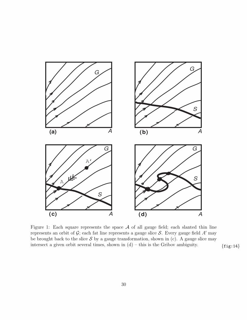
(a) (b)
(c) (d)
A A
A A
S
S
S
GG
G G
A’
A
Figure 1: Each square represents the space A of all gauge field; each slanted thin linerepresents an orbit of G; each fat line represents a gauge slice S. Every gauge field A′ maybe brought back to the slice S by a gauge transformation, shown in (c). A gauge slice mayintersect a given orbit several times, shown in (d) – this is the Gribov ambiguity. {fig:14}
30
The choice of gauge slice is quite arbitrary. To remain within the context of QFT’sgoverned by local Poincare invariant dynamics, we shall most frequently choose a gaugecompatible with these assumptions. Specifically, we choose the gauge slice S to be givenby a local equation Fa(A)(x) = 0, where F(A) involves A and derivatives of A in a localmanner. Possible choices are
Fa(A) = ∂µAaµ Fa = Aa0 (2.41)
But many other choices could be used as well.
To reduce the functional integral to an integral along the gauge slice, we need to factorizethe measure DAaµ into a measure along the gauge slice S times a measure along the orbitsof the gauge transformations G. There is a nice gauge-invariant measure Dg on G resultingfrom the following gauge invariant metric on G,
‖δg‖2 ≡ −∫
ddx tr(
g−1δg g−1δg)
(2.42)
If the orbits G were everywhere orthogonal to S, then the factorization would be easyto carry out. In general it is not possible to make such a choice for S and a non-trivialJacobian factor will emerge. To compute it, we make use of the Faddeev-Popov trick.
Denote a gauge transformation g of a gauge field Aµ by
Agµ = gAµg
−1 + i(∂µg)g−1 (2.43)
Notice that the action of gauge transformations on Aµ satisfies the group composition lawof gauge transformations,
(Ahµ)
g = g(
hAµh−1 + i(∂µh)h
−1)
g−1 + i(∂µg)g−1
= (gh)Aµ(gh)−1 + i∂µ(gh)(gh)
−1 = Aghµ (2.44)
which will be useful later on.
Let Fa(A) denote the loval gauge slice function, the gauge slice being determined byFa(A) = 0. The quantity Fa(Ag) will vanish when Ag belongs to S, and will be non-zerootherwise. We define the quantity J [A] by
1 = J [A]
∫
Dg∏
x
δ(
Fa(Ag)(x))
(2.45)
The functional δ-function looks a bit menacing, but should be understood as a Fourierintegral,
∏
x
δ(
Fa(Ag)(x))
≡∫
DΛa exp{
i
∫
ddxΛa(x)Fa(Ag)(x)}
(2.46)
31
Using the composition law (Agµ)
h = Aghµ and the gauge invariance of the measure Dg, it
follows that J is gauge invariant. This is shown as follows,
J [Ah]−1 =
∫
Dg∏
x
δ(
Fa((Ah)g)(x))
=
∫
Dg∏
x
δ(
Fa(Agh)(x))
=
∫
D(g′h−1)∏
x
δ(
Fa(Ag′)(x))
= J [A]−1 (2.47)
The definition of the Jacobian J readily allows for a factorization of the measure of Ainto a measure over the splice S times a measure over the gauge orbits G. This is done asfollows,
∫
A
DAµ O eiS[A] =
∫
A
DAµ∫
G
Dg∏
x
(
Fa(Ag)(x))
J [A] O eiS[A]
=
∫
G
Dg
∫
A
DAµ∏
x
(
Fa(AU)(x))
J [A] O eiS[A]
=(
∫
G
Dg)
∫
A
DAµ∏
x
(
Fa(A)(x))
J [A] O eiS[A] (2.48)
In passing from the first to the second line, we have simply inverted the orders of integrationover A and G; from the second to the third, we have used the gauge invariance of themeasure DAµ, of O and S[A]; from the third to the fourth, we have used the fact thatthe functional δ-function restricts the integration over all of A to one just over the slice S.Notice that the integration over all gauge transformation function
∫
DU is independent ofA and is an irrelevant constant.
The gauge fixed formula is independent of the gauge function F .
Therefore, we end up with the following final formula for the gauge-fixed functionalintegral for Abelian or non-Abelian gauge fields,
〈0|O|0〉 =∫
ADAµ
∏
x
(
Fa(A)(x))
J [A] O eiS[A]
∫
ADAµ
∏
x
(
Fa(A)(x))
J [A] eiS[A](2.49)
It remains to compute J and to deal with the functional δ-function.
2.7 Calculation of the Faddeev-Popov determinant
At first sight, the Jacobian J would appear to be given by a very complicated functionalintegral over U . The key observation that makes a simple evaluation of J possible is that
32
Fa(A) only vanishes (i.e. its functional δ-function makes a non-vanishing contribution) onthe gauge slice. To compute the Jacobian, it suffices to linearlize the action of the gaugetransformations around the gauge slice. Therefore, we have
g = I + iωaT a +O(ω2)
Agµ = Aµ −Dµω +O(ω2)
Dµωa = ∂µω
a − fabcAbµωc (2.50)
and the gauge function also linearizes,
Fa(Ag) = Fa(Aµ −Dµω)(x) +O(ω2)
= Fa(A)(x)−∫
ddy
(
δFa(A)(x)
δAbµ(y)
)
Dµωb(y) +O(ω2)
= Fa(A)(x) +
∫
ddyMab(x, y)ωb(y) +O(ω2) (2.51)
where the operator M is defined by
Mab(x, y) ≡ Dyµ
(
δFa(A)(x)
δAbµ(y)
)
(2.52)
Now the calculation of J becomes feasible.
J [A]−1 =
∫
G
DU∏
x
δ(
Fa(AU)(x))
=
∫
Dωa∏
x
δ
(
Fa(A)(x) +
∫
ddyMab(x, y)ωb(y)
)
= (DetM)−1 (2.53)
Inverting this relation, we have
J [A] = DetM = Det
(
Dyµ
δF(A)(x)
δAµ(y)
)
(2.54)
Given a gauge slice function F , this is now a quite explicit formula. In QFT, however, wewere always dealing with local actions, local operators and these properties are obscuredin the above determinant formula.
2.8 Faddeev-Popov ghosts
We encountered a determinant expression in the numerator once before when delaing withintgerations over fermions. This suggests that the Faddeev-Popov determinant may also
33
be cast in the form of a functional intgeration over two complex conjugate Grassmann oddfields, which are usually referred to as the Faddeev-Popov ghost fields and are denoted byca(x) and ca(x). The expression for the determinant is then given by a functional integralover the ghost fields,
DetM =
∫
DcaDca exp{
iSghost[A; c, c]}
Sghost[A; c, c] ≡∫
ddx
∫
d4y ca(x)Mab(x, y)cb(y) (2.55)
If the function F is a local function of Aµ, then the support of Mab(x, y) is at x = y andthe above double integral collapses to a single local integral involving the ghost fields.
2.9 Axial and covariant gauges
First of all, there is a class of axial gauges where no ghosts are ever needed ! The gaugefunction must be linear in Aaµ and involve no derivatives on Aµ. They involve a constantvector nµ, and are therefore never Lorentz covariant, Fa(A)(x) = Aaµ(x)n
µ,
δF a(A)(x)
δAbµ(y)= δabδ(d)(x− y)nµ
Dyµ
δF (A)(x)
δAµ(y)= ∂yµδ
(d)(x− y)nµ = M(x, y) (2.56)
Therefore, in axial gauges, the operator M is independent of A and thus a constant whichmay be ignored. Thus, no ghost are required as the Faddeev-Popov formula would justinform us that they decouple. Actually, since axial gauges are not Lorentz covariant, theyare much less useful in practice than it might appear.
It turns out that Lorentz covariant gauges are much more useful. The simplest suchgauges are specified by a function fa(x) as follows,
Fa(A)(x) ≡ ∂µAaµ(x)− fa(x) (2.57)
This choice gives rise to the following functional integral,
ZO =
∫
A
DAµ∏
x
δ(∂µAaµ − fa) DetM O eiS[A] (2.58)
Since this functional integral is independent of the choice of fa, we may actually integrateover all fa with any weight factor we wish. A convenient choice is to take the weight factor
34
to be Gaussian in fa,
ZO =
∫
Dfa exp{
− i2
∫
ddxfafa}
∫
ADAµ
∏
x δ(∂µAaµ − fa) DetM O eiS[A]
∫
Dfa exp{
− i2
∫
ddxfafa} (2.59)
The denominator is just again a Aµ-independent constant which may be omitted. Thefa-intgeral in the numerator may be carried out since the functional δ-function instructsus to set fa = ∂µA
aµ, so that
ZO =
∫
A
DAµ∫
Dca∫
DcaO exp{
iS[A] + iSgf [A] + iSghost[A; c, c]}
(2.60)
where the gauge fixing terms in the action are given by
Sgf [A] =
∫
ddx{
− 1
2ξ(∂µA
aµ)2}
(2.61)
We obtain a more explicit form for the ghost action by computing M,
Mab(x, y) = Dyµ
(δ∂νxAν(x)
δAµ(y)
)ab
= (Dyµ)ab∂µxδ
(4)(x− y) (2.62)
Inserting this operator into the expression for the ghost action, we obtain,
Sghost[A; c, c] ≡∫
ddx
∫
ddy ca(x)Mab(x, y)cb(y)
=
∫
ddx
∫
ddyc(x)Dyµ∂
µx δ(x− y)c(y)
=
∫
ddx∂µca(x)(Dµc)
a (2.63)
Thus, the total action for these gauges is given as follows,
Stot[A; c, c] =
∫
ddx
(
−1
4F aµνF
aµν − 1
2ξ(∂µA
aµ)2 + ∂µca(Dµc)a
)
(2.64)
and we have the following general formula for vacuum expectation values of gauge invariantoperators,
〈0|O|0〉 =∫
DAµ∫
DcDc O eiStot[A;c,c]
∫
DAµ∫
DcDc eiStot[A;c,c](2.65)
In the section on perturbation theory, we shall show how to use this formula in practice.
35
3 Perturbative Non-Abelian Gauge Theories
In this section, the Feynman rules will be derived for a gauge theory based on a simplegroup G, governed by a single gauge coupling constant g. To carry out perturbation theory,we rescale the gauge field.
Aµ → gAµ (3.1)
The pure gauge action, and the gauge fixing terms and Faddeev-Popov ghost contributionmay be expressed in terms of the fundamental fields as follows,
Lgauge = −1
2(∂µA
aν − ∂νA
aµ)∂
µAνa +1
2g(∂µA
aν − ∂νA
aµ)f
abcAµbAνc
−1
4g2fabcfadeAbµA
cνA
µdAνe
Lghost = −λ2∂µA
µa∂νAνa + ∂µc
a∂µca − gfabc∂µcaAµbcc (3.2)
Fermions ψ and (complex) bosons φ, minimally coupled to the gauge field in representationsTψ and Tφ respectively, may also be included. The corresponding actions are
Lψ = ψi(
i∂/δij − gA/a(T aψ)i
j −mψδij)
ψj (3.3)
Lφ = ∂µφ∗i∂µφi + igAaµ
(
∂µφ∗i(T aφ )ijφj − φ∗i(T aφ )i
j∂µφj)
−g2AaµAµbφ∗i(T aφ )ij(T bφ)j
kφk − V (φ)
Here, fabc are the structure constants of the Lie algebra of G and T aφ and T aψ are therepresentation matrices corresponding to the representations Tφ and Tψ of G under whichφ and ψ transform. They obey the structure relations,
[T aφ , Tbφ] = ifabcT cφ
[T aψ , Tbψ] = ifabcT cψ (3.4)
Finally, V (φ) is a potential which we shall assume to be bounded from below. In thissection, we shall specialize to developing perturbation theory in a so-called unbroken phase,characterized by the fact that the minimum of the potential we choose to expand about issymmetric under the group G. (The spontaneously broken, or Higgs phase will be discussedin later sections.) By a suitable shift in φi by constants, this minimum may be chosen tobe at φi = 0, so that
∂V
∂φi(0) =
∂V
∂φ∗i(0) = 0 (3.5)
Furthermore, by adding an unobservable constant shift to the Lagrangian, the potentialat the minimum may be chosen to vanish, V (0) = 0. Invariance of the minimum under G
36
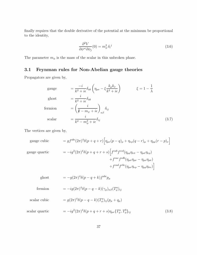
finally requires that the double derivative of the potential at the minimum be proportionalto the identity,
∂2V
∂φ∗i∂φj(0) = m2
φ δij (3.6)
The parameter mφ is the mass of the scalar in this unbroken phase.
3.1 Feynman rules for Non-Abelian gauge theories
Propagators are given by,
gauge =−i
k2 + iǫδab
(
ηµν − ξkµkνk2 + iǫ
)
ξ = 1− 1
λ
ghost =i
k2 + iǫδab
fermion =
(
i
k/−mψ + iǫ
)
αβ
δij
scalar =i
k2 −m2φ + iǫ
δij (3.7)
The vertices are given by,
gauge cubic = gfabc(2π)4δ(p+ q + r)[
ηµν(p− q)ρ + ηνρ(q − r)µ + ηρµ(r − p)ν
]
gauge quartic = −ig2(2π)4δ(p+ q + r + s)[
f eabf ecd(ηµρηνσ − ηµσηνρ)
+f eacf edb(ηµσηρν − ηµνηρσ)
+f eadf ebc(ηµνηνρ − ηµρησν)]
ghost = −g(2π)4δ(p− q + k)fabcpµ
fermion = −ig(2π)4δ(p− q − k)(γµ)αβ(Taψ)ij
scalar cubic = g(2π)4δ(p− q − k)(T aφ )ij(pµ + qµ)
scalar quartic = −ig2(2π)4δ(p+ q + r + s)ηµν{T aφ , T bφ}ij (3.8)
37
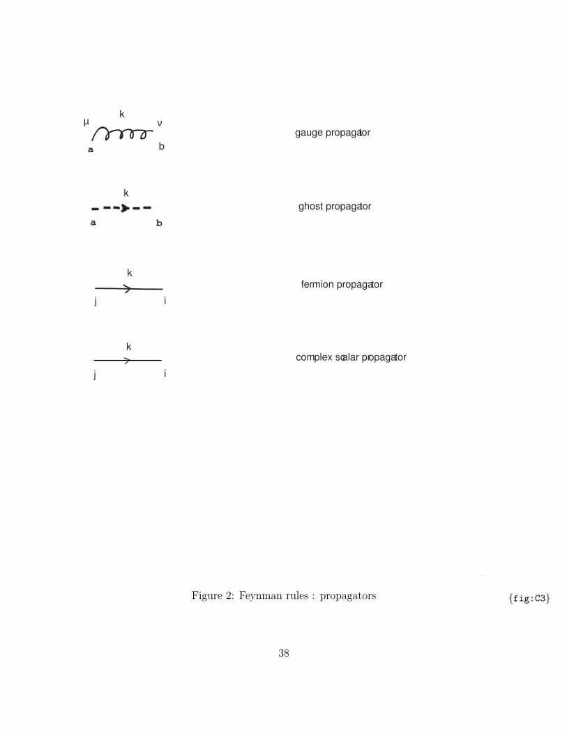
gauge propagator
ghost propagator
fermion propagator
complex scalar propagator
k
k
k
k
µ ν
ba
a b
j i
j i
Figure 2: Feynman rules : propagators {fig:C3}
38
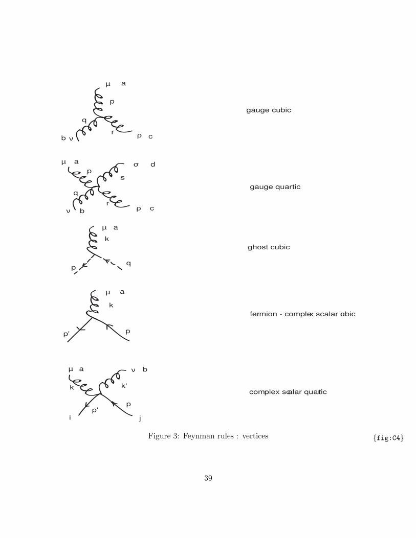
µ
ν ρ
µ
ν ρ
σ
µ
µ
µ ν
a
b c
p
q
r
a
b c
dp
q
r
s
a
a
k
k
qp
pp'
a b
ji
k k'
pp'
gauge cubic
gauge quartic
ghost cubic
fermion - complex scalar cubic
complex scalar quartic
Figure 3: Feynman rules : vertices {fig:C4}
39
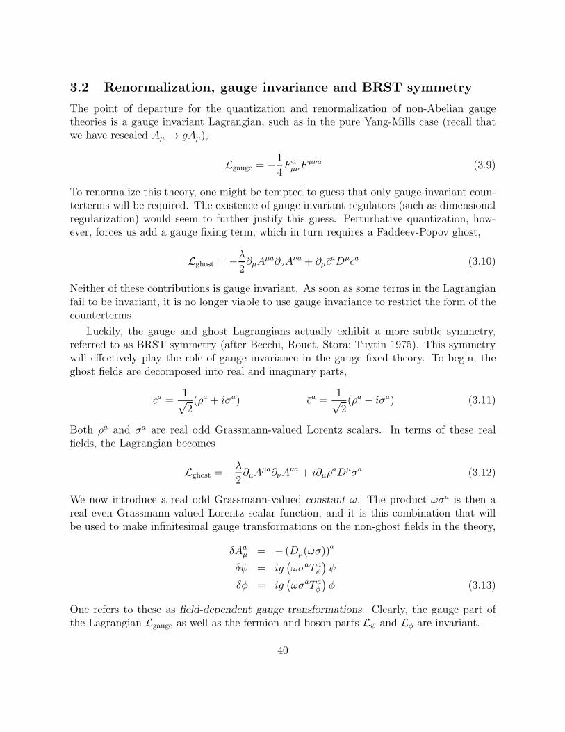
3.2 Renormalization, gauge invariance and BRST symmetry
The point of departure for the quantization and renormalization of non-Abelian gaugetheories is a gauge invariant Lagrangian, such as in the pure Yang-Mills case (recall thatwe have rescaled Aµ → gAµ),
Lgauge = −1
4F aµνF
µνa (3.9)
To renormalize this theory, one might be tempted to guess that only gauge-invariant coun-terterms will be required. The existence of gauge invariant regulators (such as dimensionalregularization) would seem to further justify this guess. Perturbative quantization, how-ever, forces us add a gauge fixing term, which in turn requires a Faddeev-Popov ghost,
Lghost = −λ2∂µA
µa∂νAνa + ∂µc
aDµca (3.10)
Neither of these contributions is gauge invariant. As soon as some terms in the Lagrangianfail to be invariant, it is no longer viable to use gauge invariance to restrict the form of thecounterterms.
Luckily, the gauge and ghost Lagrangians actually exhibit a more subtle symmetry,referred to as BRST symmetry (after Becchi, Rouet, Stora; Tuytin 1975). This symmetrywill effectively play the role of gauge invariance in the gauge fixed theory. To begin, theghost fields are decomposed into real and imaginary parts,
ca =1√2(ρa + iσa) ca =
1√2(ρa − iσa) (3.11)
Both ρa and σa are real odd Grassmann-valued Lorentz scalars. In terms of these realfields, the Lagrangian becomes
Lghost = −λ2∂µA
µa∂νAνa + i∂µρ
aDµσa (3.12)
We now introduce a real odd Grassmann-valued constant ω. The product ωσa is then areal even Grassmann-valued Lorentz scalar function, and it is this combination that willbe used to make infinitesimal gauge transformations on the non-ghost fields in the theory,
δAaµ = − (Dµ(ωσ))a
δψ = ig(
ωσaT aψ)
ψ
δφ = ig(
ωσaT aφ)
φ (3.13)
One refers to these as field-dependent gauge transformations. Clearly, the gauge part ofthe Lagrangian Lgauge as well as the fermion and boson parts Lψ and Lφ are invariant.
40
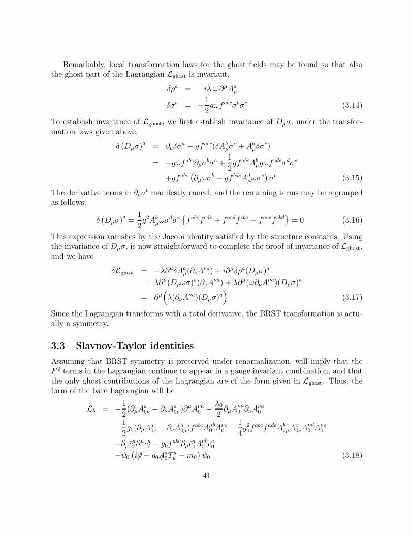
Remarkably, local transformation laws for the ghost fields may be found so that alsothe ghost part of the Lagrangian Lghost is invariant,
δρa = −iλ ω ∂µAaµδσa = −1
2gωfabcσbσc (3.14)
To establish invariance of Lghost, we first establish invariance of Dµσ, under the transfor-mation laws given above,
δ (Dµσ)a = ∂µδσ
a − gfabc(δAbµσc + Abµδσ
c)
= −gωfabc∂µσbσc +1
2gfabcAbµgωf
cdeσdσe
+gfabc(
∂µωσb − gf bdeAdµωσ
e)
σc (3.15)
The derivative terms in ∂µσb manifestly cancel, and the remaining terms may be regrouped
as follows,
δ (Dµσ)a =
1
2g2Abµωσ
dσe{
fabcf cde + facdf cbe − facef cbd}
= 0 (3.16)
This expression vanishes by the Jacobi identity satisfied by the structure constants. Usingthe invariance of Dµσ, is now straightforward to complete the proof of invariance of Lghost,and we have
δLghost = −λ∂µδAaµ(∂νAνa) + i∂µδρa(Dµσ)a
= λ∂µ(Dµωσ)a(∂νA
νa) + λ∂µ(ω∂νAνa)(Dµσ)
a
= ∂µ(
λ(∂νAνa)(Dµσ)
a)
(3.17)
Since the Lagrangian transforms with a total derivative, the BRST transformation is actu-ally a symmetry.
3.3 Slavnov-Taylor identities
Assuming that BRST symmetry is preserved under renormalization, will imply that theF 2 terms in the Lagrangian continue to appear in a gauge invariant combination, and thatthe only ghost contributions of the Lagrangian are of the form given in Lghost. Thus, theform of the bare Lagrangian will be
Lb = −1
2(∂µA
a0ν − ∂νA
a0µ)∂
µAνa0 − λ02∂µA
µa0 ∂νA
νa0
+1
2g0(∂µA
a0ν − ∂νA
a0µ)f
abcAµb0 Aνc0 − 1
4g20f
abcfadeAb0µAc0νA
µd0 A
νe0
+∂µca0∂
µca0 − g0fabc∂µc
a0A
µb0 c
c0
+ψ0
(
i∂/ − g0A/a0T
aψ −m0
)
ψ0 (3.18)
41
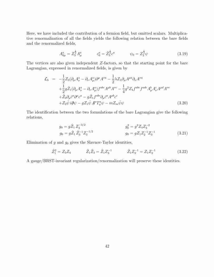
Here, we have included the contribution of a fermion field, but omitted scalars. Multiplica-tive renormalization of all the fields yields the following relation between the bare fieldsand the renormalized fields,
Aa0µ = Z12
3 Aaµ ca0 = Z
12
3 ca ψ0 = Z
12
2 ψ (3.19)
The vertices are also given independent Z-factors, so that the starting point for the bareLagrangian, expressed in renormalized fields, is given by
Lb = −1
2Z3(∂µA
aν − ∂νA
aµ)∂
µAνa − 1
2λZλ∂µA
µa∂νAνa
+1
2gZ1(∂µA
aν − ∂νA
aµ)f
abcAµbAνc − 1
4g2Z4f
abcfadeAbµAcνA
µdAνe
+Z3∂µca∂µca − gZ1f
abc∂µcaAµbcc
+Z2ψ i∂/ψ − gZ1ψ A/aT aψψ −mZmψψ (3.20)
The identification between the two formulations of the bare Lagrangian give the followingrelations,
g0 = gZ1Z−3/23 g20 = g2Z4Z
−23
g0 = gZ1 Z−13 Z
−1/23 g0 = gZ1Z
−12 Z−1
3 (3.21)
Elimination of g and g0 gives the Slavnov-Taylor identities,
Z21 = Z3Z4 Z1Z3 = Z1Z
−13 Z1Z
−13 = Z1Z
−12 (3.22)
A gauge/BRST-invariant regularization/renormalization will preserve these identities.
42
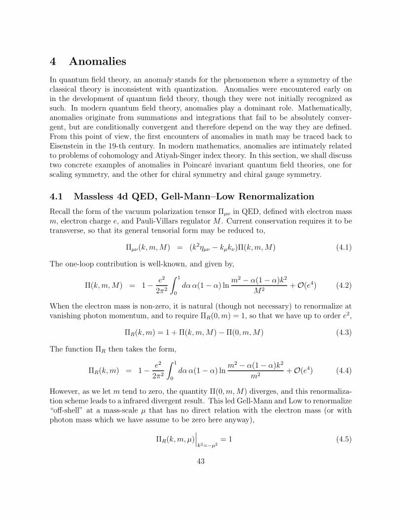
4 Anomalies
In quantum field theory, an anomaly stands for the phenomenon where a symmetry of theclassical theory is inconsistent with quantization. Anomalies were encountered early onin the development of quantum field theory, though they were not initially recognized assuch. In modern quantum field theory, anomalies play a dominant role. Mathematically,anomalies originate from summations and integrations that fail to be absolutely conver-gent, but are conditionally convergent and therefore depend on the way they are defined.From this point of view, the first encounters of anomalies in math may be traced back toEisenstein in the 19-th century. In modern mathematics, anomalies are intimately relatedto problems of cohomology and Atiyah-Singer index theory. In this section, we shall discusstwo concrete examples of anomalies in Poincare invariant quantum field theories, one forscaling symmetry, and the other for chiral symmetry and chiral gauge symmetry.
4.1 Massless 4d QED, Gell-Mann–Low Renormalization
Recall the form of the vacuum polarization tensor Πµν in QED, defined with electron massm, electron charge e, and Pauli-Villars regulatorM . Current conservation requires it to betransverse, so that its general tensorial form may be reduced to,
Πµν(k,m,M) = (k2ηµν − kµkν)Π(k,m,M) (4.1)
The one-loop contribution is well-known, and given by,
Π(k,m,M) = 1− e2
2π2
∫ 1
0
dαα(1− α) lnm2 − α(1− α)k2
M2+O(e4) (4.2)
When the electron mass is non-zero, it is natural (though not necessary) to renormalize atvanishing photon momentum, and to require ΠR(0, m) = 1, so that we have up to order e2,
ΠR(k,m) = 1 + Π(k,m,M)−Π(0, m,M) (4.3)
The function ΠR then takes the form,
ΠR(k,m) = 1− e2
2π2
∫ 1
0
dαα(1− α) lnm2 − α(1− α)k2
m2+O(e4) (4.4)
However, as we let m tend to zero, the quantity Π(0, m,M) diverges, and this renormaliza-tion scheme leads to a infrared divergent result. This led Gell-Mann and Low to renormalize“off-shell” at a mass-scale µ that has no direct relation with the electron mass (or withphoton mass which we have assume to be zero here anyway),
ΠR(k,m, µ)∣
∣
∣
k2=−µ2= 1 (4.5)
43
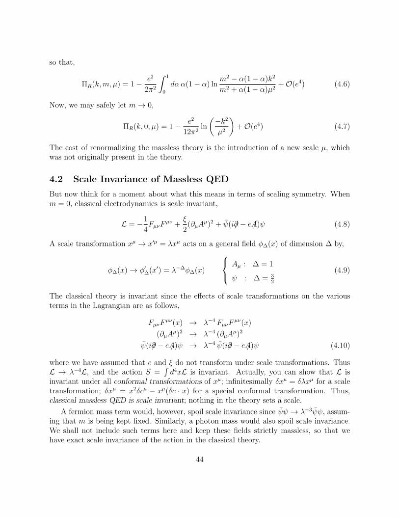
so that,
ΠR(k,m, µ) = 1− e2
2π2
∫ 1
0
dαα(1− α) lnm2 − α(1− α)k2
m2 + α(1− α)µ2+O(e4) (4.6)
Now, we may safely let m→ 0,
ΠR(k, 0, µ) = 1− e2
12π2ln
(−k2µ2
)
+O(e4) (4.7)
The cost of renormalizing the massless theory is the introduction of a new scale µ, whichwas not originally present in the theory.
4.2 Scale Invariance of Massless QED
But now think for a moment about what this means in terms of scaling symmetry. Whenm = 0, classical electrodynamics is scale invariant,
L = −1
4FµνF
µν +ξ
2(∂µA
µ)2 + ψ(i∂/− eA/)ψ (4.8)
A scale transformation xµ → x′µ = λxµ acts on a general field φ∆(x) of dimension ∆ by,
φ∆(x) → φ′∆(x
′) = λ−∆φ∆(x)
Aµ : ∆ = 1
ψ : ∆ = 32
(4.9)
The classical theory is invariant since the effects of scale transformations on the variousterms in the Lagrangian are as follows,
FµνFµν(x) → λ−4 FµνF
µν(x)
(∂µAµ)2 → λ−4 (∂µA
µ)2
ψ(i∂/− eA/)ψ → λ−4 ψ(i∂/− eA/)ψ (4.10)
where we have assumed that e and ξ do not transform under scale transformations. ThusL → λ−4L, and the action S =
∫
d4xL is invariant. Actually, you can show that L isinvariant under all conformal transformations of xµ; infinitesimally δxµ = δλxµ for a scaletransformation; δxµ = x2δcµ − xµ(δc · x) for a special conformal transformation. Thus,classical massless QED is scale invariant; nothing in the theory sets a scale.
A fermion mass term would, however, spoil scale invariance since ψψ → λ−3ψψ, assum-ing that m is being kept fixed. Similarly, a photon mass would also spoil scale invariance.We shall not include such terms here and keep these fields strictly massless, so that wehave exact scale invariance of the action in the classical theory.
44

Now, think afresh of the one-loop renormalization problem: when m = 0, one-looprenormalization forced us to introduce a scale µ in order to carry out renormalization. Onecannot quantize QED without introducing a scale, and thereby breaking scale invariance.This effect is sometimes referred to as dimensional transmutation. What we have justidentified is a field theory, massless QED, whose classical scale symmetry has been brokenby the process of renormalization, i.e. by quantum effects.
Whenever a symmetry of the classical Lagrangian is destroyed by quantum effects causedby UV divergences, this classical symmetry is said to be anomalous. In this case, it is thescaling anomaly. In fact, you can think of
4.3 Chiral Symmetry
The next example is chiral symmetry. The anomaly that will appear for this symmetry isreferred to as the chiral anomaly or also the Adler-Bell-Jackiw (ABJ) anomaly, and washistorically in 1969 the first instance where one started thinking of anomalies as classicalsymmetries being destroyed by quantization.
We consider again massless QED,
L = −1
4FµνF
µν + ψ(i∂/− eA/)ψ (4.11)
Setting m = 0 has enlarged the symmetry of the classical Lagrangian to include conformalinvariance. But setting m = 0 also produces another symmetry enhancement: chiral
symmetry. To see this, decompose ψ into left and right spinors, in a chiral basis where thechirality matrix γ5 is diagonal,
ψ = ψL + ψR
{
γ5ψL = +ψLγ5ψR = −ψR (4.12)
The Lagrangian then becomes,
L = −1
4FµνF
µν + ψL(i∂/ − eA/)ψL + ψR(i∂/ − eA/)ψR (4.13)
Clearly, ψL and ψR may be rotated by two independent constant phases,
U(1)L × U(1)R
{
ψL → eiθLψLψR → eiθRψR
(4.14)
and the Lagrangian is invariant. Any symmetry that transforms left and right spinorsdifferently is referred to as a chiral symmetry. Now, we re-arrange these transformations
45
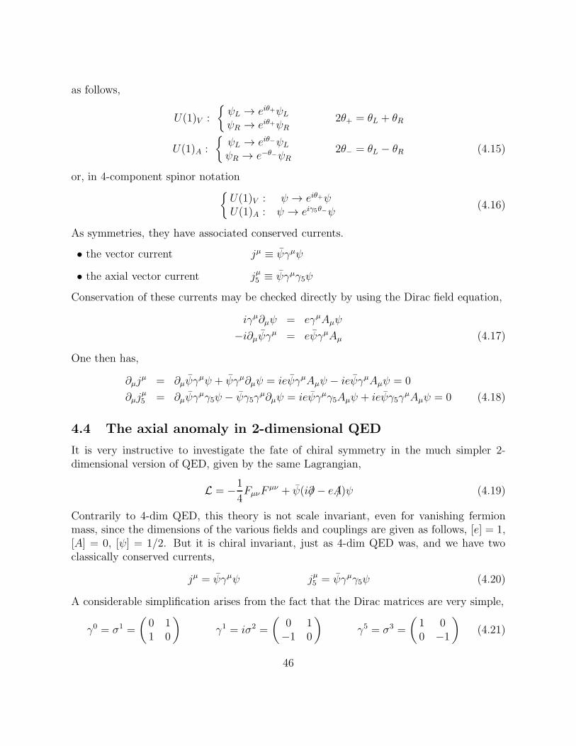
as follows,
U(1)V :
{
ψL → eiθ+ψLψR → eiθ+ψR
2θ+ = θL + θR
U(1)A :
{
ψL → eiθ−ψLψR → e−θ−ψR
2θ− = θL − θR (4.15)
or, in 4-component spinor notation{
U(1)V : ψ → eiθ+ψU(1)A : ψ → eiγ5θ−ψ
(4.16)
As symmetries, they have associated conserved currents.
• the vector current jµ ≡ ψγµψ
• the axial vector current jµ5 ≡ ψγµγ5ψ
Conservation of these currents may be checked directly by using the Dirac field equation,
iγµ∂µψ = eγµAµψ
−i∂µψγµ = eψγµAµ (4.17)
One then has,
∂µjµ = ∂µψγ
µψ + ψγµ∂µψ = ieψγµAµψ − ieψγµAµψ = 0
∂µjµ5 = ∂µψγ
µγ5ψ − ψγ5γµ∂µψ = ieψγµγ5Aµψ + ieψγ5γ
µAµψ = 0 (4.18)
4.4 The axial anomaly in 2-dimensional QED
It is very instructive to investigate the fate of chiral symmetry in the much simpler 2-dimensional version of QED, given by the same Lagrangian,
L = −1
4FµνF
µν + ψ(i∂/− eA/)ψ (4.19)
Contrarily to 4-dim QED, this theory is not scale invariant, even for vanishing fermionmass, since the dimensions of the various fields and couplings are given as follows, [e] = 1,[A] = 0, [ψ] = 1/2. But it is chiral invariant, just as 4-dim QED was, and we have twoclassically conserved currents,
jµ = ψγµψ jµ5 = ψγµγ5ψ (4.20)
A considerable simplification arises from the fact that the Dirac matrices are very simple,
γ0 = σ1 =
(
0 11 0
)
γ1 = iσ2 =
(
0 1−1 0
)
γ5 = σ3 =
(
1 00 −1
)
(4.21)
46
As a result of this simplicity, the axial and vector currents are related to one another. Thisfact may be established by computing the products γµγ5 explicitly,
γ0γ5 = σ1σ3 = −iσ2 = −γ1 = +γ1
γ1γ5 = iσ2σ3 = −σ1 = −γ0 = −γ0(4.22)
Introducing the rank 2 antisymmetric tensor ǫµν = −ǫνµ, normalized to ǫ01 = 1, the aboverelations may be recast in the following form,
γµγ5 = ǫµνγν =⇒ jµ5 = ǫµνjν (4.23) {vectoraxial2d
Consider the calculation of the vacuum polarization to one-loop, but this time in 2-dimQED. The vacuum polarization diagram is just the correlator of the two vector currents inthe free theory, Πµν(k) = e2〈0|Tjµ(k)jν(−k)|0〉, and is given by,
Πµν(k) = −e2∫
d2p
(2π)2tr
(
γµi
k/+ p/γνi
p/
)
(4.24)
A priori, the integral is logarithmically divergent, and must be regularized. We choose toregularize in a manner that preserves gauge invariance and thus conservation of the currentjµ. As a result, we have Πµν(k) = (k2ηµν − kµkν)Π(k2). Gauge invariant regularizationmay be achieved using a single Pauli-Villars regulator with mass M , for example. Just asin 4-dim QED, current conservation lowers the degree of divergence and in 2-dim, vacuumpolarization is actually finite.
Π(k2) = 4e2∫ 1
0
dα
∫
d2p
(2π)2
[
α(1− α)
(p2 + α(1− α)k2)2− α(1− α)
(p2 + α(1− α)k2 −M2)2
]
(4.25)
Carrying out the p-integration,
Π(k2) =ie2
π
∫ 1
0
dα
[
α(1− α)
−α(1− α)k2− α(1− α)
−α(1− α)k2 +M2
]
(4.26)
Clearly, asM → ∞, the limit is finite and the contribution from the Pauli-Villars regulatoractually cancels. One finds the finite result,
Π(k2) = − ie2
πk2(4.27)
Notice that, even though the final result for vacuum polarization is finite, the Feynmanintegral was superficially logarithmically divergent and requires regularization. It is duringthis regularization process that we ensure gauge invariance by insisting on the conservationof the vector current jµ. Later, we shall see that one might have chosen NOT to conservethe vector current, yielding a different result.
47
Next, we study the correlator of the axial vector current, Πµν5 (k) = e〈0|jµ5 (k)jν(−k)|0〉.
Generally, Πµν5 and Πµν would be completely independent quantities. In 2-dim, however,
the axial current is related to the vector current by (4.23), and we have
eΠµν5 (k) = ǫµρΠ ν
ρ (k) = (ǫµνk2 − ǫµρkρkν)Π(k2) (4.28)
Conservation of the vector current requires that kνΠµν5 (k) = 0, which is manifest in view
of the transversality of Πµν(k). The divergence of the axial vector current may also becalculated. The contribution from the correlator with a single vector current insertion is
kµeΠµν5 (k) = kµǫ
µνk2Π(k2) = −ie2
πkµǫ
µν (4.29) {kpi0}
which is manifestly non-vanishing. As a result, the axial vector is not conserved and chiralsymmetry in 2-dim QED is not a symmetry at the quantum level : chiral symmetry suffers
an anomaly. Translating this into an operator statement:
∂µjµ5 = − e
2πFµνǫ
µν (4.30) {anomeq}
Remarkably, this result is exact (Adler-Bardeen theorem). Higher point correlators areconvergent and classical conservation valid.
4.5 The axial anomaly and regularization
The above calculation of the axial anomaly was based on our explicit knowledge of thevector current two-point function (or vacuum polarization) to one-loop order. Actually,the anomaly equation (4.30) is an exact quantum field theory operator equation, which in
particular is valid to all orders in perturbation theory. To establish this stronger result,there must be a more direct way to proceed than from the vacuum polarization result.
First, consider the issue of conservation of the axial vector current when only thefermion is quantized and the gauge field is treated as a classical background. The correlator〈0|jµ5 |0〉A is then given by the sum of all 1-loop diagrams shown in figure xx. Consider firstthe graphs with n ≥ 2 external A-fields. Their contribution to 〈0|jµ5 |0〉A is given by
Πµ;ν1···νn5 (k; k1, · · · , kn) = −en
∫
d2p
(2π)2tr
(
γµγ51
p/+ ℓ/1γν1 · · · 1
p/ + ℓ/nγνn
1
p/+ ℓ/n+1
)
(4.31)
where we use the notation li+1 − li = ki, As we assumed n ≥ 2, this integral is UVconvergent, and may be computed without regularization. In particular, the conservationof the axial vector current may be studied by using the following simple identity, (and thefact that ln+1 − l1 = −k by overall momentum conservation k + k1 + · · ·+ kn = 0),
1
p/+ ℓ/n+1k/γ5
1
p/+ ℓ/1γν1 = −γ5
1
p/ + ℓ/1+ γ5
1
p/+ ℓ/n+1(4.32)
48
Hence the divergence of the axial vector current correlator becomes,
kµΠµ;ν1···νn5 (k; k1, · · · , kn) = en
∫
d2p
(2π)2tr
(
γ51
p/+ ℓ/1γν1 · · · 1
p/+ ℓ/nγνn)
(4.33)
−en∫
d2p
(2π)2tr
(
γ51
p/+ ℓ/2γν2 · · · 1
p/+ ℓ/nγνn
1
p/+ ℓ/n+1γν1)
When n ≥ 3, each term separately is convergent. Using boson symmetry in the externalA-field (i.e. the symmetry under the permutations on i of (ki, νi)), combined with shiftsymmetry in the integration variable p, all contributions are found to cancel one another.When n = 2, each term separately is logarithmically divergent, and shift symmetry stillapplies. Thus, we have shown that ∂µj
µ5 receives contributions only from terms first order in
A, which are precisely the ones that we have computed already in the preceding subsection.
To see how the contribution that is first order in A arises, we need to deal with acontribution that is superficially logarithmically divergent, and requires regularization. Onepossible regularization scheme is by Pauli-Villars, regulators. The logarithmically divergentintegral requires just a single regulator with mass M , and we have,
Πµν5 (k,M) = −e
∫
d2p
(2π)2tr
(
γµγ5
{
1
p/+ k/γν
1
p/− 1
p/+ k/−Mγν
1
p/−M
})
(4.34)
The conservation of the vector current, which is a necessary condition to have U(1)V gaugeinvariance, is readily verified, using the following identity,
1
p/+ k/k/1
p/− 1
p/+ k/−Mk/
1
p/−M=
1
p/− 1
p/+ k/− 1
p/+ k/−M+
1
p/−M(4.35)
and the fact that one may freely shift p in a logarithmically divergent integral. The diver-gence of the axial vector current is investigated using a similar identity,
trk/γ5
{
1
p/+ k/γν
1
p/− 1
p/+ k/−Mγν
1
p/−M
}
= trγ5γν
(
1
p/+ k/− 1
p/− 1
p/+ k/−M+
1
p/−M
)
+2Mtr
(
γ51
p/+ k/−Mγν
1
p/−M
)
(4.36)
The first line of the integrand on the rhs may be shifted in the integral and cancels. Thesecond part remains, and we have
kµΠµν5 (k,M) = −2eM
∫
d2p
(2π)2tr
(
γ51
p/ + k/−Mγν
1
p/−M
)
(4.37) {kpi1}
Of course, this integral is superficially UV divergent, because we have used only a singlePauli-Villars regulator. To obtain a manifestly finite result, at least two PV regulators
49
should be used; it is understood that this has been done. To evaluate (4.37), introduce asingle Feynman parameter, α and shift the internal momentum p accordingly,
kµΠµν5 (k,M) = −2eM
∫ 1
0
dα
∫
d2p
(2π)2trγ5(p/+ (1− α)k/+M)γν(p/− αk/+M)
(p2 −M2 + α(1− α)k2)2(4.38) {kpi2}
The trace trγ5γµ1 ·γµn vanishes whenever n is odd, while for n = 2, we have trγ5γ
µγν = 2ǫµν .In the numerator of (4.38), the contributions quadratic in p, those quadratic in k and thosequadratic in M cancel because they involve traces with odd n; those linear in p cancelbecause of p→ −p symmetry of the denominator. This leaves only terms linear in M andlinear in k. Finally, using trγ5k/γ
ν = 2ǫµνkµ and the familiar integral
∫
d2p
(2π)21
(p2 −M2 + α(1− α))2=
i
4π
1
M2 − α(1− α)k2(4.39)
we have
kµΠµν5 (k,M) = −ie
πǫµνkµ
∫ 1
0
dαM2
M2 − α(1− α)k2(4.40)
AsM is viewed as a Pauli-Villars regulator, we consider the limitM → ∞, which is smooth,and we find,
limM→∞
kµΠµν5 (k,M) = −ie
πǫµνkµ (4.41)
which is in precise agreement with (4.29). Clearly, the anomaly contribution arises heresolely from the Pauli-Villars regulator. Note that if we restored factors of ~, the right handside would have exactly one factor of ~, since its effect is purely quantum mechanical andhas no classical counterpart.
4.6 The axial anomaly and massive fermions
If a fermion has a mass, then chiral symmetry is violated by the mass term. This may beseen directly from the Dirac equation for a massive fermion in QED,
iγµ∂µψ = mψ + eγµAµψ
−i∂µψγµ = mψ + eψAµγµ (4.42)
Chiral transformations may still be defined on the fermion fields and the axial vectorcurrent may still be defined by the same expression. For massive fermions, however, chiraltransformations are not symmetries any more and the axial vector current fails to beconserved. Its divergence is easy to compute classically from the Dirac equation, ∂µj
µ5 =
2imψγ5ψ. Hence the Pauli-Villars regulators violate the conservation of jµ5 , and this effect
50
survives as M → ∞. In fact, one readily establishes the axial anomaly equation for afermion of mass m,
∂µjµ5 = 2imψγ5ψ − e
2πǫµνFµν (4.43)
In fact, it is impossible to find a regulator of UV divergences which is gauge invariant andpreserves chiral symmetry. Dimensional regularization makes 2 → d, but now we have aproblem defining γ5 = γ0γ1.
4.7 Solution to the massless Schwinger Model
Two-dimensional QED is a theory of electrically charged fermions, interacting via a staticCoulomb potential, with no dynamical photons. The potential is just the Green functionG(x, y) for the 1-dim Laplace operator, satisfying ∂2xG(x, y) = δ(x, y), and given by
G(x, y) =1
2|x− y| (4.44)
The force due to this potential is constant in space. It would take an infinite amount ofenergy to separate two charges by an infinite distance, which means that the charges willbe confined. Interestingly, this simple model of QED in 2-dim is a model for confinement !
Remarkably, 2-dim QED was completely solved by Schwinger in 1958. To achieve thissolution, one proceeds from the equations for the conservation of the vector current, theanomaly of the axial vector current, and Maxwell’s equations,
∂µjµ = 0
∂µjµ5 = ǫµν∂µjν = − e
2πǫµνFµν
∂µFµν = ejν (4.45)
Of course, it is crucial to the general solution that these equations hold exactly. Noticethat this is a system of linear equations, a fact that is at the root for the existence of anexact solution. We recast the axial anomaly equation in the following form,
∂µjν − ∂νjµ = − e
πFµν (4.46)
Finally, taking the divergence in ∂µ, using ∂µjµ = 0 and Maxwell’s equations, we obtain,
✷jν = − e
2π∂µF
µν = −e2
πjν (4.47)
which is the field equation for a free massive boson, with mass m2 = e2/π. Actually, thisboson is a single real scalar φ, which may be obtained by solving explicitly the conservation
51
equation ∂µjµ = 0 in terms of φ by jµ = ǫµν∂νφ. Notice that the gauge field may also be
expressed in terms of this scalar, (or the current), by solving the chiral anomaly equation,
Aµ = −πejµ + ∂µθ = −π
eǫµν∂
νφ+ ∂µθ (4.48)
where θ is any gauge transformation. This is just the London equation of superconductivity,expressing the fact that the photon field is massive now. This last equation is at the originof the boson-fermion correspondence in 2-dim.
Remarkably, the physics of the (massless) Schwinger model is precisely what we wouldexpect from a theory describing confined fermions. The salient features are as follows,
• The asymptotic spectrum contains neither free quarks, nor free gauge particles;
• The spectrum contains only fermion bound states, which are gauge neutral;
• The spectrum has a mass gap, even though the fermions were massless.
It is also interesting to include a mass to the fermions, but this model is much morecomplicated, and no longer exactly solvable. Its bosonized counterpart is the massive Sine-Gordon theory.
4.8 The axial anomaly as an operator equation
How can we understand that the anomaly equation is an operator equation ? Both thevector and the axial vector currents are composite operators, and they need to be properlydefined starting from the canonical fields in the theory. Generally in the definition ofcomposite operators, one splits the points at which they are inserted, and then takes thelimit. For the axial vector current, a first attempt at doing so would be,
jµ5 (x) = limy→x
(
ψ(y)γµγ5ψ(x)− 〈0|ψ(y)γµγ5ψ(x)|0〉)
(4.49)
The problem is, however, that as the operators are now inserted at distinct points, theoperator defined in this way is no longer gauge invariant, since under a gauge transformationwe would have,
ψ(x) → eie θ(x)ψ(x)
ψ(y) → eie θ(y)ψ(y) (4.50)
To obtain a gauge-invariant operator, we need to modify the regularization used here. Oneway to do this is by inserting the line integral of the gauge field between the points x and
52
y, defined by,
U(y, x) = exp
{
ie
∫ y
x
Aµ(z)dzµ
}
(4.51)
which transforms as follows under the gauge transformation θ,
U(y, x) → exp {ie θ(y)− ıe θ(x)} (4.52)
and define the gauge-invariant version of the axial current as follows,
jµ5 (x) = limy→x
(
ψ(y)U(y, x)γµγ5ψ(x)− 〈0|ψ(y)U(y, x)γµγ5ψ(x)|0〉)
(4.53)
Now, however, the equation for the divergence of the current is modified due to the insertionof U(y, x) in conjunction with the divergence of the correlator 〈0|ψ(y)γµγ5ψ(x)|0〉 as y → x.This effect may be calculated explicitly, and precisely reproduces the anomaly equation,yet once again.
4.9 The non-Abelian axial anomaly in 2 dimensions
So far, we have dealt only with Abelian symmetries and their possible anomalies. In fact,it is not very difficult to generalize our calculations to the case of non-Abelian symmetries.To begin, let us consider a multiplet of N massless Dirac fermions in 1+1 dimensions. Thefree Lagrangian is,
L0 =
N∑
a=1
ψaiγµ∂µψa =
N∑
a=1
{
ψ†aL i∂+ψ
aL + ψ†a
R i∂−ψaR
}
The manifest classical symmetry of this Lagrangian (but, as we shall see later, not in factthe largest symmetry of L0) is U(N)L × U(N)R, under which ψL and ψR each transformswith its U(N). This set of fermions may be thought of – in a 4 dimensional analogy – as Nflavors of massless quarks, and the SU(N)L × SU(N)R part of the symmetry group wouldbe chiral symmetry. We shall discuss the role of the extra U(1) components later. A simpleinteraction to introduce is by minimally coupling these fermions to an SU(N)V gauge field,where SU(N)V is the diagonal subgroup of SU(N)L×SU(N)R. This coupling is explicitlywritten as follows (Henceforth we consider a matrix notation for the N components of ψa
and group them into a column matrix which we again denote by ψ; also, we absorb thegauge coupling constant into the gauge field.)
LA = ψγµ(i∂µ −Aµ)ψ = ψ†L(i∂+ −A+)ψL + ψ†
R(i∂− − A−)ψR
Here, we have also used a matrix notation for Aµ =∑N
a=1AaµT
a and T a are the (Hermitian)representation matrices of the Lie algebra of SU(N). Recall that they satisfy the following
53
structure relations[T a, T b] = ifabcT c
where the structure constants fabc are real and completely anti-symmetric in all indices.
The SU(N)V gauge current is just the vector current; classical SU(N)L × SU(N)Rinvariance also produces an axial vector current
jµa = ψγµT aψ
jµa5 = ψγµγ5Taψ (4.54)
These currents transform in a non-trivial way under SU(N)V . Thus, in the presence of anexternal gauge field Aµ as we have here, there is no sense to having a conserved current,since this type of equation would not be invariant under SU(N)v. Instead, it is easy to see(using the Dirac equation), that the above currents are covariantly conserved :
(Dµjµ)a = ∂µj
µa − fabcAbµjµc = 0
(Dµjµ5 )a = ∂µj
µa5 − fabcAbµj
µc5 = 0 (4.55)
The SU(N)V gauge symmetry can be maintained at the quantum level. In fact thereis again a multitude of UV regulators that preserve the symmetry such as dimensionalregularization, Pauli-Villars regulators, or heat-kernel methods. (You may wish to work outan example or establish the Ward identities !) We shall thus assume that all Green functionsare regularized and renormalized in an SU(N)V -invariant way, and we have Dµj
µ = 0 asan exact operator equation which may be used in all Green functions.
What happens to the (covariant) conservation of the axial vector current upon quantiza-tion ? We may first look at the contribution that comes from ∂µj
µa5 . The lowest non-trivial
Green function is 〈0|T ∗jµa5 jνb|0〉 and the Feynman integral corresponding to it is exactlythe same as in the Abelian case (with the additional factor of trT aT b = 1
2δab). Thus, to
first order in the gauge field, we have
∂µjaµ5 =
e2
4πǫµν(∂µA
aν − ∂νA
aµ) +O(A2)
This equation is of course not SU(N)v gauge invariant (though it is invariant under globalSU(N)v !), and we now have to find out how to make it gauge invariant. Since the axialvector current transforms as a tensor in the adjoint representation of SU(N)v, we knowthat there must be a gauge invariant formulation of the covariant derivative of jµ5 . Thismust of course agree order by order in powers of the gauge field, and the lowest non-trivialorder is uniquely fixed by the above equation for ∂µj
aµ5 . Thus – without doing any further
Feynman diagram calculations – we find that we must have,
(Dµjµ5 )a =
e2
4πǫµνF a
µν (4.56)
54
where F is the field strength of the SU(N)V gauge field Aµ
F aµν = ∂µA
aν − ∂νA
aµ − fabcAbµA
cν (4.57)
The above anomaly equation can again be shown to be exact, i.e. there are no contributionsfrom higher graphs with more insertions of the gauge field.
To conclude this subsection we make a comment about an often repeated confusion. Inthe case of the Schwinger model, we had U(1)V gauge invariance and global U(1)A axialsymmetry. Both these transformations form groups, as just indicated by the notation. Infact any combination of the two also forms a group. The reason for this is that all thesesymmetries just act by commuting phase rotations. In the non-Abelian case, this ceases tobe the case. The invariance groups are SU(N)L×SU(N)R, and the subgroups are SU(N)L,SU(N)R and the diagonal (vector) subgroup SU(N)V . As soon as N ≥ 2 however, the setof axial generators γ5T
a does not form a closed Lie algebra, as can be seen from the factthat their commutator belongs to SU(N)V .
4.10 The Polyakov - Wiegmann calculation of the effective action
In the preceding discussion, we have found the non-Abelian generalization of the axialanomaly equations that we studied in the Schwinger model for the Abelian case. In theSchwinger model, the anomaly equations were sufficient to compute the entire effectiveaction for fermions in the presence of a gauge field. In this subsection, we follow a calcu-lation of Polyakov and Wiegmann and show that also here the complete effective actionfor the fermions in the presence of an SU(N)V gauge field can be computed. The effectiveaction for the fermions in the presence of a background gauge field in SU(N)V is definedas follows,
e−iW [Aµ] =
∫
DψDψ exp{
i
∫
dx2ψiγµDµψ}
= Det(γµDµ) (4.58)
The fundamental object is the vacuum expectation value of the gauge current, in thepresence of the gauge field Aµ, which is given by
jµa(x) = 〈0|ψγµT aψ(x)|0 =δW [Aµ]
δAaµ(x)(4.59)
In view of the two-dimensional identity that we also used in the Abelian case,
jµa5 = ǫµνjaν (4.60)
we may eliminate the axial vector current in favor of the vector current, for which we willnow have the following two identities, which are exact,
∂µjµ + i[Aµ, j
µ] = 0
ǫµν(∂µjν + i[Aµ, jν ]) =1
4πǫµνFµν
55
These equations are much more complicated than in the Abelian case since they are nolonger linear. Nevertheless, they can be solved exactly and in closed form.
To see this, we work in light-cone coordinates x± = (x0±x1)/√2 for the two-dimensional
space-time under consideration. Next, we parametrize the gauge field by two SU(N)-valuedfunctions, g, h, in the following way,
A+ = −ig−1∂+g A− = −ih−1∂−h
Notice that this looks pure gauge, but is not as long as h 6= g. By making an SU(N)Vgauge transformation by h, we choose a gauge in which A− = 0, and only A+ = −ig−1∂+gis non-vanishing. Under these conditions, the equations for the vector current become,
∂+j+ + ∂−j
− + i[A+, j+] = 0
∂+j+ − ∂−j
− + i[A+, j+] = − 1
4π∂−A+
The difference of these equations is given by,
∂−j− =
1
8π∂−A+ (4.61)
and is easily solved by j− = A+/(8π). The remaining equation is one for j+, and takes thefollowing form in this gauge,
∂+j+ + [g−1∂+g, j
+] =i
8π∂−(
g−1∂+g)
(4.62)
Multiplication to the left by g and to the right by g−1 allows us to recast the equation inthe following form,
∂+(
g j+g−1)
=i
8π∂+(
∂−g g−1)
(4.63)
This equation in turn is also easily integrated, and we find,
j+ =i
8πg−1∂−g j− = − i
8πg−1∂+g (4.64)
which gives the complete solution for the vector current in this gauge. Restoring both hand g by using SU(N)V gauge covariance of the vector current, we obtain,
j+ =i
8π(−h−1∂−h+ g−1∂−g)
j− =i
8π(+h−1∂+h− g−1∂+g) (4.65)
56
4.11 The Wess-Zumino-Witten term
Can we find the effective action from the expression for these currents ? Again, we shallrestrict to the gauge choice A− = 0, and attempt to integrate up the current equations.
δW [Aµ] =
∫
d2x tr(j+δA+) =1
8π
∫
d2x tr(
(
g−1∂−g)
δ(
g−1∂+g)
)
The variation of the derivative is easily found
δ(g−1∂+g) = ∂+(g−1δg) + [g−1∂+g, g
−1δg]
Putting the above equations together, we have
δW [Aµ] =1
8π
∫
d2x tr(
(g−1δg)∂−(g−1∂+g)
)
Can this variation come from a local action ? Well, there are not that many possibilities.For example, consider the variation of the standard kinetic term for a scalar field
δtr(
g−1∂+gg−1∂−g
)
= −tr∂+(g−1δg)g−1∂−g − tr∂−(g
−1δg)g−1∂+g
With the help of this equality, one may split up the change in the effective action in termsof the kinetic term (symmetric in the interchange of + and -) and another part which isanti-symmetric under the interchange of + and -. We obtain,
W [Aµ] =1
16π
∫
d2x tr(
g−1∂−g g−1∂+g)
)
+ δSWZ [g]
Here SWZ [g] is given by its variation,
δSWZ [g] =1
16π
∫
d2xtr(
g−1δg∂−(g−1∂+g)− g−1δg∂+(g
−1∂−g))
=1
32π
∫
d2x ǫµνtr(
g−1δg∂µ(g−1∂νg)
)
(4.66)
Using symmetry of the double derivative contribution, this expression can be simplified,and we obtain
δSWZ[g] =1
32π
∫
d2x ǫµνtr(
(g−1δg)(g−1∂µg)(g−1∂νg)
)
There is in fact no way that this equation can be integrated up to a local and manifestlySU(N)L×SU(N)R invariant action. Instead, we shall have the following construction. Aswe know the variation of SWZ , we may always write down the full action as an integral
57
over an interpolating field. We introduce a continuous function γ(τ, x) and 0 ≤ τ ≤ 1 andsuch that,
γ(0, x) = 1 γ(1, x) = g(x)
The action SWZ is now obtained by integrating the equation for δSWZ along the interpo-lating field,
SWZ [g]− SWZ [1] =1
32π
∫ 1
0
dτ
∫
d2xǫµνtr
(
γ−1∂γ
∂τγ−1∂µγγ
−1∂νγ
)
(4.67)
This term is called the Wess-Zumino-Witten term.
If we view the two-dimensional space-time as a sphere S2, then, we may think of thedomain of integration of the above three dimensional integral as that of a disk D whichis just a half three sphere, whose only boundary is the two-sphere of space-time. We maythen write the entire Wess-Zumino integrand in a simple geometrical fashion
SWZ [g] =1
96π
∫
D
d3x ǫαβγtr(
γ−1∂αγγ−1∂βγγ
−1∂γγ)
where ǫαβγ is the three dimensional completely anti-symmetric tensor.We shall see many properties of the WZW action a little later. Here, the main point
is that using the anomaly equations in the non-Abelian fermion case, we have again beenable to solve for the effective action completely.
4.12 The Abelian axial anomaly in 4 dimensions
In four-dimensional QED the 2-point function of the vector and axial vector currents〈0|Tjρ5(z)jµ(x)|0〉 vanishes by Lorentz invariance and parity conservation of QED. How-ever, there are now triangle diagrams associated with the correlator 〈0|Tjρ5(z)jµ(x)jν(y)|0〉,which do not vanish, as their existence is allowed by Lorentz invariance and parity in QED.The triangle graph again fails to be absolutely convergent in four dimensions, as its integralbehaves superficially as ∈ d4k/k3. Regularizing, for example with Pauli-Villars regulators,makes the triangles finite, uniquely defined, and gauge invariant. We first define the Fouriertransform of the triangle graph by,
i(2π)4δ(p− q1 − q2)Mρµν5 (p, q1, q2)
=
∫
d4z
∫
d4x
∫
d4y e−ipz+iq1x+iq2y〈0|Tjρ5(z)jµ(x)jν(y)|0〉 (4.68)
Formally, the Fourier transform is given by the Feynman rules for the triangle graph,
iMρµν5 (p, q1, q2) = −
∫
d4k
(2π)4tr(
γµi
k/γν
i
k/+ q/2γργ5
i
k/− q/1+ γν
i
k/γµ
i
k/+ q/1γργ5
i
k/− q/2
)
(4.69)
But this integral is only conditionally convergent, and will be uniquely determined by Pauli-Villars regularization, which by construction preserves the vector current and thus gauge
58
invariance. The regularized interal takes the form,
iMρµν5 (p, q1, q2) = −
∫
d4k
(2π)4
N∑
n=0
Cntr(
γµi
k/−Mnγν
i
k/+ q/2 −Mnγργ5
i
k/− q/1 −Mn
+γνi
k/−Mn
γµi
k/+ q/1 −Mn
γργ5i
k/− q/2 −Mn
)
(4.70)
The contribution n = 0 is just from the original massless fermion, for which we have,
M0 = 0 C0 = 1 (4.71)
To eliminate the linear superficial divergence, we need,
N∑
n=0
Cn = 0 (4.72)
after which the integral is logarithmically superficially divergent. We shall use N = 3, withsuitably chosenMn and Cn to render the integrals convergent, and allow pρMρµν
5 to be splitinto a difference of convergent integrals, as we did in two dimensions. Using p = q1+ q2, wemay write the contribution on the first line above with the help of the following identity,
pργργ5 = (k/+ q/2 −Mn)γ5 + γ5(k/− q/1 −Mn) + 2Mnγ5 (4.73)
with a similar identity for the second line in which µ and ν are interchanged at the sametime that q1 and q2 are. The contributions from the first two terms on the right of the aboveidentity then cancel with similar contributions from the second line, after suitably shiftingthe integration momentum in these convergent integrals, and only the contributions fromthe regulator terms remain, so that we have (after simplifying signs and factors of i),
pρMρµν5 = −
∫
d4k
(2π)4
N∑
n=0
2CnMntr(
γµ1
k/−Mn
γν1
k/+ q/2 −Mn
γ51
k/− q/1 −Mn
+γν1
k/−Mnγµ
1
k/+ q/1 −Mnγ5
1
k/− q/2 −Mn
)
(4.74)
Rationalizing and using Feynman parameters converts the first term in the integrand to,
2
∫ 1
0
dα
∫ 1−α
0
dβtr(
γµ(k/+Mn)γν(k/+ q/2 +Mn)γ5(k/− q/1 +Mn)
)
(
(k + αq2 − βq1)2 + αq22 + βq21 − (αq2 − βq1)2 −M2n
)3 (4.75)
Shifting the integration momentum k → k − αq2 + βq1, the integrand becomes,
tr(
γµ(k/− αq/2 + βq/1 +Mn)γν(k/+ q/2 − αq/2 + βq/1 +Mn)γ5(k/− q/1 − αq/2 + βq/1 +Mn)
)
(
k2 + αq22 + βq21 − (αq2 − βq1)2 −M2n
)3
In view of the γ5 factor, the only terms which contribute in the numerator are linear inMn.Since the denominator is even in k, all terms odd in k in the numerator lead to a vanishing
59
contribution to the integral over k. Finally, all terms quadratic in k in the numerator alsovanish in view of the γ5 factor. The resulting k-integral is then finite by power counting,so that only a single Pauli-Villars regular is needed so that we may set N = 1, M1 = Mand C1 = −1. Since the integrals are convergent, we shall take M → ∞ at the end of thecalculation, so that the momentum dependence of the denominator may be omitted. Wethen have,
pρMρµν5 = −4M2
∫ 1
0
dα
∫ 1−α
0
dβ
∫
d4k
(2π)4tr(γ5γ
µγνq/1q/2)
(k2 −M2)3(4.76)
The integral over α, β is readily carried out giving a factor of 1/2. The integral over k isgiven as follows,
∫
d4k
(2π)4M2
(k2 −M2)3= − i
32π2(4.77)
and the trace over spinor space is evaluated using,
γ5 = iγ0γ1γ2γ3 tr(γ5γµγνγργσ) = −4iεµνρσ (4.78)
to give
pρMρµν5 =
1
4π2εµνρσqρ1q
σ2 (4.79)
Upon Fourier transforming back to position space, we convert the momentum factor q1and q2 into derivatives on the gauge field, and therefore into field strengths times an extrafactor of 1/2 to account for anti-symmetrization. Keeping careful track of factors of i andminus signs, we obtain the final anomaly equation,
∂µjµ5 =
e2
16π2FµνF
µν F µν ≡ 1
2εµνρσFρσ (4.80)
The Adler-Bardeen theorem states that this result is exact at 1-loop, and may be viewedas an equation valid at the operator level for both ψ and Aµ. It may again be derivedalternatively by point-splitting the fermion operators when defining the axial vector current,and retaining the effects of the singularity as the two fermions come close together.
4.13 Anomalies in gauge currents
Consider a classical Lagrangian for a massless Dirac fermion ψ coupled to a vector gaugefield Aµ with field strength Fµν as in QED, but also coupled to an axial vector gauge field
60
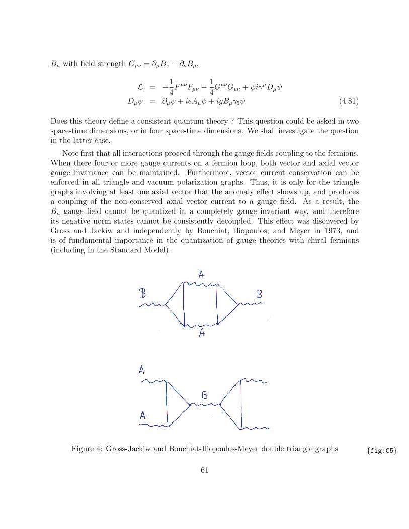
Bµ with field strength Gµν = ∂µBν − ∂νBµ,
L = −1
4F µνFµν −
1
4GµνGµν + ψiγµDµψ
Dµψ = ∂µψ + ieAµψ + igBµγ5ψ (4.81)
Does this theory define a consistent quantum theory ? This question could be asked in twospace-time dimensions, or in four space-time dimensions. We shall investigate the questionin the latter case.
Note first that all interactions proceed through the gauge fields coupling to the fermions.When there four or more gauge currents on a fermion loop, both vector and axial vectorgauge invariance can be maintained. Furthermore, vector current conservation can beenforced in all triangle and vacuum polarization graphs. Thus, it is only for the trianglegraphs involving at least one axial vector that the anomaly effect shows up, and producesa coupling of the non-conserved axial vector current to a gauge field. As a result, theBµ gauge field cannot be quantized in a completely gauge invariant way, and thereforeits negative norm states cannot be consistently decoupled. This effect was discovered byGross and Jackiw and independently by Bouchiat, Iliopoulos, and Meyer in 1973, andis of fundamental importance in the quantization of gauge theories with chiral fermions(including in the Standard Model).
Figure 4: Gross-Jackiw and Bouchiat-Iliopoulos-Meyer double triangle graphs {fig:C5}
61
In the Gross-Jackiw two-point function, gauge invariance is maintained on the A-propagators, but the anomaly then implies that gauge-invariance fails on the B-propagators,so that the negative norm states in the B-field no longer decouple. In the Bouchiat-Iliopoulos-Meyer four-point function, negative norm states are allowed to propagate in theB-propagator. The upshot is that the axial anomaly can destroy gauge invariance in anycurrent coupled to a dynamical gauge field, and consistent unitary theories must be free ofsuch anomalies. Two comments are in order.
1. Note that there is an easy modification of the A− B model in which both A and Bgauge invariance are preserved: introduce two Dirac fermions with the same electriccharge, but opposite chiral charge. The triangle graphs contributing to the anomalythen add up to zero.
2. Since the Dirac fermion is massless in this theory, its left and right chirality contribu-tions separate, and we may choose to set Aµ = Bµ and gauge only the left chirality.But this cannot be done because the left current always contains the axial vector andone cannot make the left current by itself conserved.
4.14 Non-Abelian axial anomalies
We begin by considering a Dirac fermion ψ in a representation T of the gauge group Gwith representation matrices T a of the Lie algebra coupled to a vector gauge field Aµ,
Lψ = ψγµ(i∂µ − gAµ)ψ (4.82)
and define the vector and axial vector currents as usual,
jµa = ψγµT aψ jµ = jµaT a
jµa5 = ψγµγ5Taψ jµ5 = jµa5 T a (4.83)
Assuming covariant conservation of the vector current, and therefore exact gauge invariance,the lowest order contribution to the anomaly in the axial vector current is given by thetriangle graphs for the Abelian anomaly supplemented by the insertion of the matrices T a,
i(2π)4δ(p− q1 − q2)Mρµν cab5 (p, q1, q2)
=
∫
d4z
∫
d4x
∫
d4y e−ipz+iq1x+iq2y〈0|Tjρc5 (z)jµa(x)jνb(y)|0〉 (4.84)
Formally, the Fourier transform is given by the Feynman rules for the triangle graph,
iMρµν cab5 (p, q1, q2) = −
∫
d4k
(2π)4tr(
γµT ai
k/γνT b
i
k/+ q/2γργ5T
c i
k/− q/1
+γνT bi
k/γµT a
i
k/+ q/1γργ5T
c i
k/− q/2
)
(4.85)
where the trace now also includes the trace over the representation space of T . Recall thatthe Abelian anomaly was already symmetric under Bose exchange of (µ, q1) and (ν, q2). The
62
insertion of the additional representation matrices produces a contribution antisymmetricin a, b which is finite and does not contribute to the anomaly, as well as a contributionwhich is symmetric in a, b and which does contribute to the anomaly. As a result, there isa simple relation between the Abelian and non-Abelian anomalies to this order, given by,
pρMρµν cab5 (p, q1, q2) = dcab(T ) pρMρµν
5 (p, q1, q2) (4.86)
where the symbol dcab is defined as follows,
dcab(T ) =1
2tr(
T c{T a, T b})
(4.87)
Without proof, we state here the full axial vector anomaly equation,
Dµjµ5 =
g2
16π2FµνF
µν (4.88)
We shall give some of the properties of the d-symbol in the next section.
4.15 Non-Abelian chiral anomaly
Suppose we had only a Weyl fermion ψL of left chirality in a representation T of the gaugegroup G. By charge conjugation for four space-time dimensions, one can actually expressa right chiral fermion field ψR in a representation TR of G in terms of a left chiral fermionfield ψcR transforming in the complex conjugate representation TL = T ∗
R . So, using only leftchirality fermions represents no loss of generality. The Lagrangian is then,
Lψ = ψLγµ(i∂µ − gAµ)ψL (4.89)
There is now only the left current, jµaL = ψLγµT aψL, and the triangle graph of three left
currents must be Bose symmetric under the permutation of its legs. This fixes the graphuniquely. Note that when no vector current is available, there is no sense in which we canpreserve the conservation of the vector current. All the anomaly effects here must be inthe left current alone. The anomaly equation is then given by,
(DµjµL)c =
g2
24π2εµνρσ∂µtr T
c
(
Aν∂ρAσ −i
2gAνAρAσ
)
(4.90)
Note that the right side is again proportional to dcab(T ). The 1/3 in the pre-factor arisesfrom the Bose-symmetrization of the three left currents. Finally, the right side manifestlyfails to be gauge-invariant, which is the manifestation of the anomaly in this context.
63
4.16 Properties of the d-symbols
Of particular interest is to know for which representations, and which groups G the d-symbol vanishes. Recall that we have restricted from the beginning T to be a unitaryrepresentation of a compact group G. When the representation T is real, the representationmatrices T a must be purely imaginary (since we have extracted a factor of i to make themHermitian), and therefore they must be anti-symmetric, (T a)t = −T a. As a result, thed-symbol vanishes, since we have,
2dabc(T ) = tr(
T aT bT c + T aT cT b)
= tr(
T aT bT c + T aT cT b)t
= −tr(
T cT bT a + T bT cT a)
= −2dabc(T ) (4.91)
Thus, dabc(T ) can be non-zero only for complex representation. The groups that have com-plex representations are U(1), SU(N), and possibly the spinor representations of SO(N).All other representations are real or pseudo-real and have vanishing d-symbol.
In particular, one very important case is when G contains a U(1)-factor, G = U(1)×Hand H is semi-simple. The d-symbol evaluated on the index c corresponding to the U(1)-generator while the other two indices a, b correspond to generators of H gives,
dcab = tr(T c)× tr(T aT b) (4.92)
But tr(T aT b) 6= 0 for generators of a semi-simple algebra, so the only way this anomalycan be absent is that,
tr(T c) = 0 (4.93)
This is the case for the SU(2)L×U(1)Y anomaly, where the U(1)Y charges in the StandardModel are indeed traceless and sum up to zero within the multiplet of left fermions in eachfamily. On left fermions, U(1)Y is proportional to electric charge. The multiplets are,
(
νee−
) (
uα
dα
)
(4.94)
where α is the color index α = 1, 2, 3. While the electric charge +e/3 of u and −e/3 of donly add up to +e/3, there are three colors of each, adding the charges up to +e, which isprecisely cancelled by the negative charge of the electron.
Having dispensed with the U(1) factors in G, we next consider the case where G is asemi-simple Lie algebra, given by the product of r simple factors,
G = G1 ×G2 × · · · ×Gr (4.95)
The Lie algebra generators T ai in factor Gi must be traceless trGi(Tai ) = 0 for all values of
i = 1, · · · , r, since otherwise the algebra Gi would contain a commuting U(1) factor andthis is in contradiction with the assumption of being simple.
64
• When all three Lie algebra generators belong to mutually distinct simple factors, thevanishing of the trace in each factor guarantees that d vanishes;
• When two Lie algebra generators belong to the same simple factor, and the thirdto a distinct factor, then the traceless property in the last factor guarantees thatthe d-symbol vanishes. This applies for example for the SU(2)L generators to havevanishing anomaly with SU(3)c on left fermions, since the generators of SU(2)L aremanifestly traceless.
• This leaves only the case where all three generators belong to the same simple factor,which we address next.
When G is simple, the tensor dabc(T ) has the following properties (including a summaryof the properties already stated above for general Lie algebras)
1. dabc(T ) is invariant under the action of G in the adjoint representation;
2. dabc(T ∗) = −dabc(T );
3. dabc(T1 ⊕ T2) = dabc(T1) + dabc(T2);
4. dabc(T1 ⊗ T2) = dabc(T1) dim(T2) + dabc(T2) dim(T1);
5. dabc(T ) is unique, up to overall normalization, so that we may define a numericalvalue d(T ) by dabc(T ) = d(T )dabc where dabc is the value of the d-symbol in somefixed faithful representation of G;
6. dabc(T ) = 0 in all representations of SO(N), N 6= 6; all representations of Sp(2N);and all representations of E6, E7, E8, G2, F4;
7. dabc(T ) 6= 0 in the defining representation of SU(N) for N ≥ 3, and in the spinorrepresentation of SO(6) = SU(4)/Z2, which is the defining representation of SU(4).
Properties 6 and 7 follow from the structure of the De Rham cohomology group H5(G,R).
65
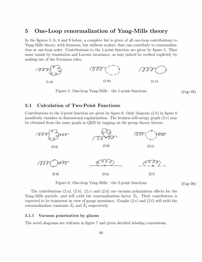
5 One-Loop renormalization of Yang-Mills theory
In the figures 5, 6, 8 and 9 below, a complete list is given of all one-loop contributions toYang-Mills theory, with fermions, but without scalars, that can contribute to renormaliza-tion at one-loop order. Contributions to the 1-point function are given by figure 5. Theymust vanish by translation and Lorentz invariance, as may indeed be verified explicitly bymaking use of the Feynman rules.
(1.a) (1.b) (1.c)
Figure 5: One-loop Yang-Mills : the 1-point functions {fig:C5}
5.1 Calculation of Two-Point Functions
Contributions to the 2-point function are given by figure 6. Only diagram (2.b) in figure 6manifestly vanishes in dimensional regularization. The fermion self-energy graph (2.e) maybe obtained from the same graph in QED by tagging on the group theory factors.
(2.a) (2.b) (2.c)
(2.d) (2.e) (2.f )
Figure 6: One-loop Yang-Mills : the 2-point functions {fig:C6}
The contributions (2.a), (2.b), (2.c) and (2.d) are vacuum polarization effects for theYang-Mills particle, and will yield the renormalization factor Z3. Their contribution isexpected to be transverse in view of gauge invariance. Graphs (2.e) and (2.f) will yield therenormalization constants Z2 and Z3 respectively.
5.1.1 Vacuum polarization by gluons
The novel diagrams are redrawn in figure 7 and given detailed labeling conventions.
66
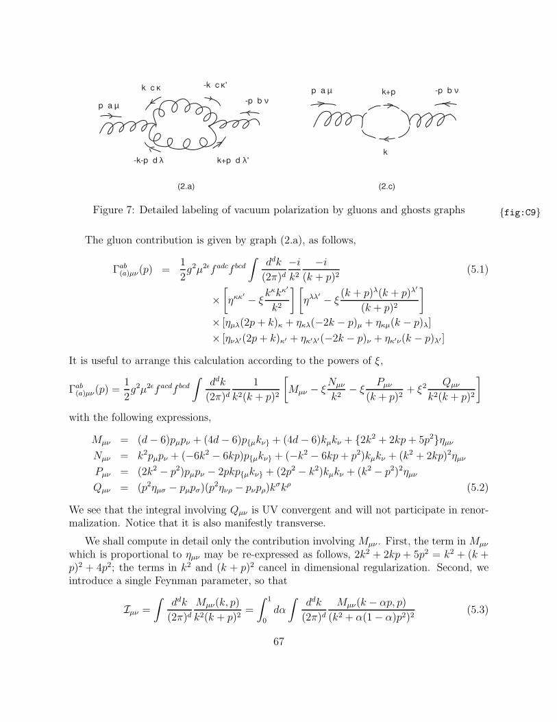
p a µ -p b ν
-k-p d λ k+p d λ'
k c κ -k c κ'p a µ -p b νk+p
k
(2.a) (2.c)
Figure 7: Detailed labeling of vacuum polarization by gluons and ghosts graphs {fig:C9}
The gluon contribution is given by graph (2.a), as follows,
Γab(a)µν(p) =1
2g2µ2ǫfadcf bcd
∫
ddk
(2π)d−ik2
−i(k + p)2
(5.1)
×[
ηκκ′ − ξ
kκkκ′
k2
] [
ηλλ′ − ξ
(k + p)λ(k + p)λ′
(k + p)2
]
× [ηµλ(2p+ k)κ + ηκλ(−2k − p)µ + ηκµ(k − p)λ]
× [ηνλ′(2p+ k)κ′ + ηκ′λ′(−2k − p)ν + ηκ′ν(k − p)λ′ ]
It is useful to arrange this calculation according to the powers of ξ,
Γab(a)µν(p) =1
2g2µ2ǫfacdf bcd
∫
ddk
(2π)d1
k2(k + p)2
[
Mµν − ξNµν
k2− ξ
Pµν(k + p)2
+ ξ2Qµν
k2(k + p)2
]
with the following expressions,
Mµν = (d− 6)pµpν + (4d− 6)p{µkν} + (4d− 6)kµkν + {2k2 + 2kp+ 5p2}ηµνNµν = k2pµpν + (−6k2 − 6kp)p{µkν} + (−k2 − 6kp+ p2)kµkν + (k2 + 2kp)2ηµν
Pµν = (2k2 − p2)pµpν − 2pkp{µkν} + (2p2 − k2)kµkν + (k2 − p2)2ηµν
Qµν = (p2ηµσ − pµpσ)(p2ηνρ − pνpρ)k
σkρ (5.2)
We see that the integral involving Qµν is UV convergent and will not participate in renor-malization. Notice that it is also manifestly transverse.
We shall compute in detail only the contribution involving Mµν . First, the term in Mµν
which is proportional to ηµν may be re-expressed as follows, 2k2 + 2kp + 5p2 = k2 + (k +p)2 + 4p2; the terms in k2 and (k + p)2 cancel in dimensional regularization. Second, weintroduce a single Feynman parameter, so that
Iµν =∫
ddk
(2π)dMµν(k, p)
k2(k + p)2=
∫ 1
0
dα
∫
ddk
(2π)dMµν(k − αp, p)
(k2 + α(1− α)p2)2(5.3)
67
Terms odd in Mµν(k − αp, p) which are odd in k do not contribute to the integral, and weare left with
Mµν(k − αp, p) ∼ (d− 6− α(1− α)(4d− 6))pµpν + 4ηµνp2 + (4d− 6)kµkν (5.4)
The integration is now Lorentz invariant and we may replace kµkν by ηµνk2/d. The re-
maining k-integrations may be carried out by first analytically continuing to Euclideantime k0 → ik0E and then using the Euclidean integral formulas,
∫
ddk
(2π)d1
(k2 +M2)n=
Γ(n− d/2)
(4π)d/2Γ(n)
1
(M2)n−d/2(5.5)
As a result, we have
Iµν = iΓ(2− d/2)
(4π)d/2
∫ 1
0
dα(
− α(1− α)p2)d/2−2
(5.6)
×(
(d− 6)pµpν − α(1− α)(4d− 6)pµpν + 4p2ηµν +4d− 6
2− dα(1− α)p2ηµν
)
The α-integration may be carried out using the Euler B-function, and we obtain,
Iµν = iΓ(2− d/2)
(4π)d/2(−p2)d/2−2
{
(
(d− 6)pµpν + 4p2ηµν) Γ(d/2− 1)2
Γ(d− 2)(5.7)
+
(
−(4d− 6)pµpν +4d− 6
2− dp2ηµν
)
Γ(d/2)2
Γ(d)
}
Picking up only the pole part in ε where d = 4 − 2ε, and using Γ(2 − d/2) = Γ(ε) ∼ 1/ε,we get
Iµν =i
(4π)2 ε(−p2)−ε
{
19
6p2ηµν −
22
6pµpν
}
(5.8)
The entire diagram is evaluated using analogous calculations, and we find,
Γab(a)µν(p) =ig2(−p2/µ2)−ε
32π2 εfacdf bcd
{
19
6p2ηµν −
22
6pµpν + ξ(p2ηµν − pµpν)
}
(5.9)
Notice that the gluon exchange graph by itself fails to be transverse, for any choice of gaugeξ.
5.1.2 Vacuum polarization by ghosts
The ghost contribution is given as follows,
Γab(c)µν(p) = −g2µ2ǫfadcf bcd∫
ddk
(2π)di
k2i
(k + p)2kµ(k + p)ν
= −g2µ2ǫfacdf bcd∫ 1
0
dα
∫
ddk
(2π)dηµνk
2/d− α(1− α)pµpν(k2 + α(1− α)p2)2
(5.10)
68
Retaining only the pole parts in ε, we find,
Γab(c)µν(p) =ig2(−p2/µ2)−ε
32π2εfacdf bcd
{
1
6p2ηµν +
2
6pµpν
}
(5.11)
Putting together the gluon and ghost contributions to vacuum polarization, we obtain,
Γab(a,b,c)µν(p) =ig2(−p2/µ2)−ε
32π2εfacdf bcd
(
p2ηµν − pµpν)
{
13
3− (1− ξ)
}
(5.12)
5.1.3 Vacuum polarization by fermions
The vacuum polarization contribution due to fermions is given by graph (2.d) of figure 6,and is proportional to the value in QED. We express this as follows,
Γab(d)µν(p) = g2tr(iT aψ)(iTbψ)Γµν(p)
Γµν(p) = −∫
ddk
(2π)di
k/−m
i
k/+ p/−m(5.13)
The pole part of this contribution is given by
Γab(d)µν(p) =−ig2(−p2/µ2)−ε
32π2ε
8
3tr(T aψT
bψ)(
p2ηµν − pµpν)
(5.14)
5.2 Indices and Casimir Operators
Some group theory is helpful in organizing the final presentation of the renormalizationeffects, to one-loop order and beyond. First, the generators of a simple Lie algebra G in aunitary representation T will be denoted by T aT = T a. They satisfy the Lie algebra structurerelations, [T a, T b] = ifabcT c, and will be normalized as follows. We begin by denoting thedimension of T by dim(T ). For any simple Lie algebra, G, and any representation T , thetrace tr(T aT b) is proportional to δab, and the sum T aT a is proportional to the identitymatrix IT in the representation space of T . The corresponding coefficient are referred toas the quadratic index I(T ), and the quadratic Casimir C(T ),
tr(IT ) = dim(T )
tr(T aT b) = I(T ) δab
T aT a = C(T ) IT (5.15)
It suffices to normalize either I(T ) or C(T ) is a single representation of G to fix thenormalizations of the structure constants fabc and I(T ) and C(T ) for all T . For Lie algebrasSU(N), SO(N) and Sp(2N), it is customary to use the defining representations T = Dof dimensions N , N , and 2N respectively, and we require I(D) = 1/2. For exceptionalgroups, one uses one of the fundamental representations to fix the normalization.
69
The index and the Casimir are related to one another, as may be derived by evaluatingtr(T aT a) respectively from the equations defining I(T ) and C(T ), and we obtain,
I(T ) dim(G) = C(T ) dim(T ) (5.16)
where dim(G) denotes the dimension of the Lie algebra, which is, of course, the dimensionof the adjoint representation. Under direct sums and tensor products, the dimension, indexand Casimir behave as follows,
dim(T1 ⊕ T2) = dim(T1) + dim(T2)
dim(T1 ⊗ T2) = dim(T1)× dim(T2)
I(T1 ⊕ T2) = I(T1) + I(T2)
I(T1 ⊗ T2) = I(T1) dim(T2) + I(T2) dim(T1) (5.17)
from which we deduce that
C(T1 ⊕ T2) =dim(T1)C(T1) + dim(T2)C(T2)
dim(T1) + dim(T2)
C(T1 ⊗ T2) = C(T1) + C(T2) (5.18)
Using these rules, we may evaluate some of these quantities for G = SU(N), the definingrepresentation D, and the adjoint representation G, related by D ⊗D∗ = G⊕ 1,
dim(D) = N I(D) =1
2C(D) =
N2 − 1
2Ndim(G) = N2 − 1 I(G) = N C(G) = N (5.19)
The representation matrices of the adjoint representation are just the structure constants(T aG)b
c = (−i fa)bc. Here, we have been careful to include a factor of −i in order to makeTG hermitian, as required by our earlier conventions. As a result, we have
tr(T aGTbG) = (−i fa)cd(−i f b)dc = facdf bcd = I(G)δab (5.20)
We recognize the combination that entered the one-loop vacuum polarization correctionsby gluons and ghosts.
5.3 Summary of two-point functions
We collect the pole contributions to the renormalization factors for 2-point functions,
Z2 = 1 +g2
32π2ε{−(2− 2ξ)C(ψ)}+O(g4)
Z3 = 1 +g2
32π2ε
{(
13
3− (1− ξ)
)
C(G)− 8
3T (ψ)
}
+O(g4)
Z3 = 1 +g2
32π2ε
{(
1 +1
2ξ
)
C(G)
}
+O(g4) (5.21)
70
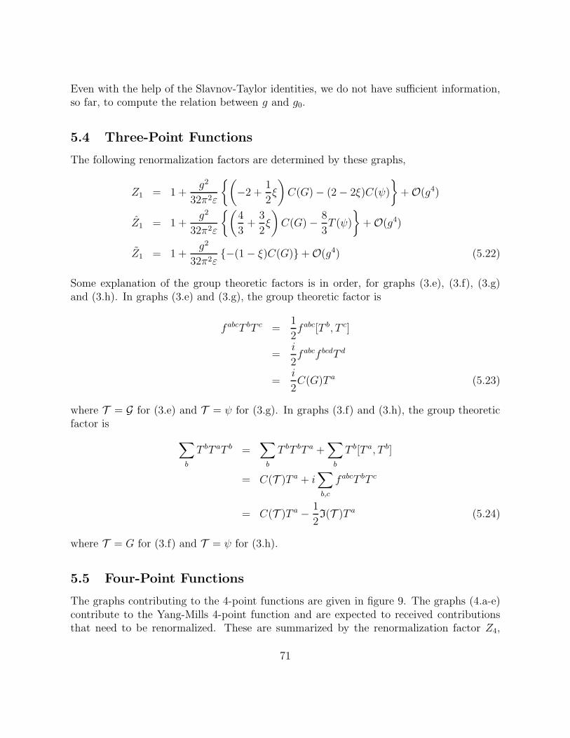
Even with the help of the Slavnov-Taylor identities, we do not have sufficient information,so far, to compute the relation between g and g0.
5.4 Three-Point Functions
The following renormalization factors are determined by these graphs,
Z1 = 1 +g2
32π2ε
{(
−2 +1
2ξ
)
C(G)− (2− 2ξ)C(ψ)
}
+O(g4)
Z1 = 1 +g2
32π2ε
{(
4
3+
3
2ξ
)
C(G)− 8
3T (ψ)
}
+O(g4)
Z1 = 1 +g2
32π2ε{−(1− ξ)C(G)}+O(g4) (5.22)
Some explanation of the group theoretic factors is in order, for graphs (3.e), (3.f), (3.g)and (3.h). In graphs (3.e) and (3.g), the group theoretic factor is
fabcT bT c =1
2fabc[T b, T c]
=i
2fabcf bcdT d
=i
2C(G)T a (5.23)
where T = G for (3.e) and T = ψ for (3.g). In graphs (3.f) and (3.h), the group theoreticfactor is
∑
b
T bT aT b =∑
b
T bT bT a +∑
b
T b[T a, T b]
= C(T )T a + i∑
b,c
fabcT bT c
= C(T )T a − 1
2I(T )T a (5.24)
where T = G for (3.f) and T = ψ for (3.h).
5.5 Four-Point Functions
The graphs contributing to the 4-point functions are given in figure 9. The graphs (4.a-e)contribute to the Yang-Mills 4-point function and are expected to received contributionsthat need to be renormalized. These are summarized by the renormalization factor Z4,
71
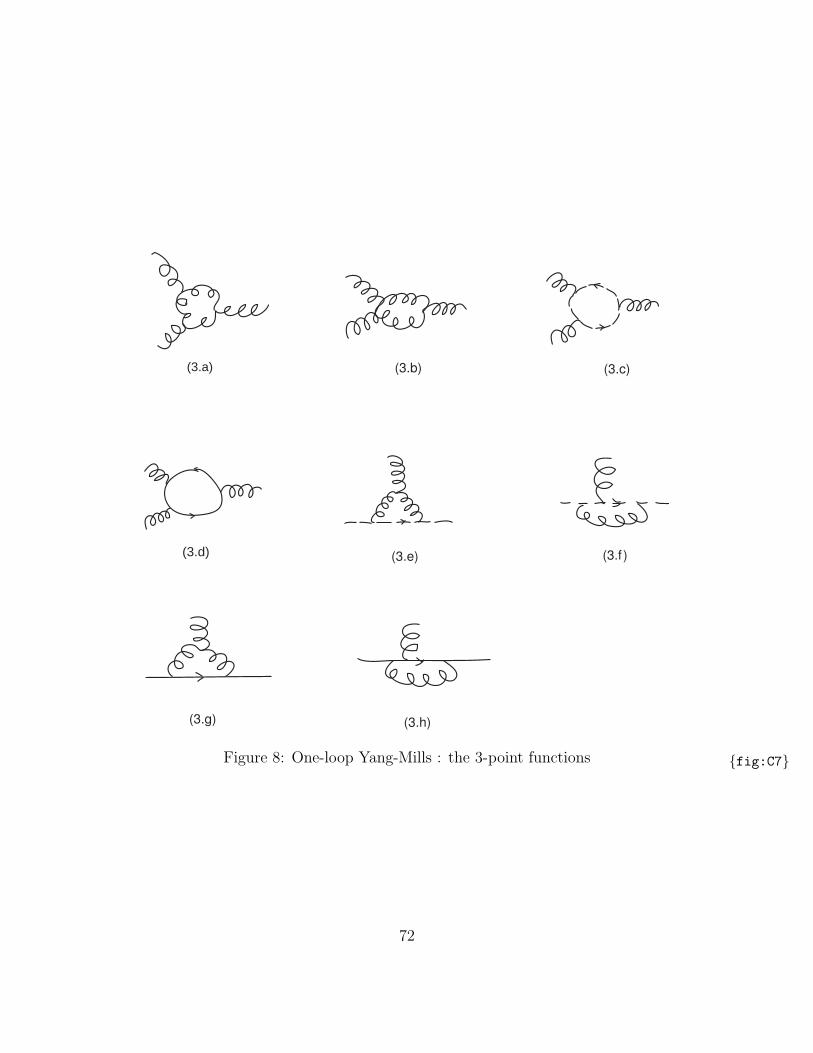
(3.a)
(3.d)
(3.b) (3.c)
(3.e) (3.f )
(3.g) (3.h)
Figure 8: One-loop Yang-Mills : the 3-point functions {fig:C7}
72
which is
Z4 = 1 +g2
32π2ε
{(
−2
3+ 2ξ
)
C(G)− 8
3I(ψ)
}
+O(g4) (5.25)
On the other hand, the graphs (4.f-i), as well as (4.j-k) are superficially log divergent, yetwould require counterterms not already represented in the Lagrangian. These contributionsare actually UV convergent, essentially because on at least one ghost vertex, the vertex mo-mentum factor is acting on the external leg and does not contribute to the loop momentumcounting. Finally, the graphs (4.l-o) are UV convergent because their superficial degree ofdivergence is -2. Thus, Z4, listed above, is in fact the only required renormalization for4-point functions.
5.6 One-Loop Renormalization
The above results for the renormalization factors verify the Slavnov-Taylor identities, asmay be seen by explicit calculation. There are 3 identities to be checked, which we shallexpress in terms of 3 combinations predicted to be 1 by the Slavnov-Taylor identities,
Z21 Z
−13 Z−1
4 = 1 +O(g4)
Z1 Z−13 Z−1
1 Z3 = 1 +O(g4)
Z1 Z−12 Z−1
1 Z3 = 1 +O(g4) (5.26)
The quantity Zλ is not renormalized at all.
Next, we derive the relation between the bare coupling g0 and the renormalized couplingg. The starting point is the relation
g0 = g µε Z1 Z−3/23 (5.27)
Using the expressions found above to one-loop order, we get
g0 = g µε(
1 +g2 b132π2 ε
+O(g4)
)
b1 = −11
3C(G) +
4
3I(ψ) (5.28)
Inverting and squaring both sides, up to this order in g gives an equivalent relation,
1
g20=µ−2ε
g2− µ−2ε
16π2 εb1 +O(g2) (5.29)
The proper interpretation of this relation is as follows. If the bare coupling g0 and theregulator ε are kept fixed, then the relation gives the dependence of the renormalized
73
(4.a) (4.b) (4.c)
(4.d) (4.e) (4.f )
(4.g) (4.h) (4.i)
(4.j) (4.k) (4.l)
(4.m) (4.n) (4.o)
Figure 9: One-loop Yang-Mills : the 4-point functions {fig:C8}
74
coupling g on the renormalization scale µ. Therefore, it is appropriate to denote therenormalized coupling by g(µ) instead of by g. The renormalized coupling should have afinite limit as ε → 0, keeping µ fixed. This requires a special choice for the dependence ofthe bare coupling g0 on the regulator ε,
1
g20= Λ−2ε
(
− b116π2ε
+ c
)
(5.30)
Here, the pole in ε is required by the requirement that g(µ) should have a finite limit asε→ 0, but the constant c is arbitrary. A scale Λ is required on dimensional grounds. Noticethat the choice of g0 is independent of µ and does not involve g(µ). Using this choice andmultiplying through by µ2ε gives
1
g(µ)2=
b116π2 ε
{
1−(µ
Λ
)2ε}
+ c(µ
Λ
)2ε
(5.31)
This expression for g(µ) now has a finite limit as ε → 0, but it involves the unknownconstant c. Taking the difference for two different values of µ eliminates this unknown andwe get,
1
g(µ)2− 1
g(µ′)2= lim
ε→0
(
b116π2 ε
{
(µ
Λ
)2ε
−(
µ′
Λ
)2ε})
(5.32)
The dependence on Λ drops out, and we find,
1
g(µ)2− 1
g(µ′)2=
b18π2
ln
(
µ
µ′
)
+O(g2)
b1 = −11
3C(G) +
4
3I(ψ) (5.33)
As a check, the coupling constant renormalization of QED may be recovered from thisrelation by setting the gauge group to be G = U(1), and g = e, so that C(G) = 0 andI(ψ) =
∑
j q2j , for Dirac fermions j with charge qje. We indeed recover,
1
e(µ)2− 1
e(µ′)2=
1
12π2
∑
j
q2j ln
(
µ
µ′
)2
+O(e2) (5.34)
This agrees precisely with the formulas derived in the section on QED.
5.7 Asymptotic Freedom
For a genuinely non-Abelian Yang-Mills theory, with simple gauge algebra G, the CasimirC(G) is positive, so that, unlike in QED, the coefficient b1 may become negative. When
75
b1 < 0, the above equation implies that
µ > µ′ ⇒ g(µ) < g(µ′) (5.35)
This means that as the energy scale at which the coupling g is probed is increased, thecoupling decreases. This effect is the opposite of electric screening which took place inQED. In particular, it implies that as the energy is taken to be asymptotically high, thecoupling will vanish, hence the name asymptotic freedom. Notice that the perturbativecalculations in an asymptotically free theory should become more reliable as the energy isincreased.
Conversely, as the energy is lowered, the coupling increases. Of course, at some point,the coupling will then fail to be in the perturbative regime and higher order corrections,as well as truly non-perturbative effects will have to be included. Nonetheless, the trendis indicative that the theory may develop a genuinely large coupling as the energy scaleis lowered. For the strong interactions, such increase in coupling is certainly a necessarycondition to have quark confinement. The phenomenon of growing coupling with lowerenergy scales is often referred to as infrared slavery.
To get a quantitative insight into the theories which are asymptotically free, we shallexamine more closely the case of Yang-Mills theory for the gauge group G = SU(N) withNf Dirac fermions in the defining representation of SU(N), which is of dimension N . Grouptheory informs us that,
C(G) = N I(ψ) =1
2Nf (5.36)
so that
b1 = −11
3N +
2
3Nf (5.37)
Asymptotic freedom is realized as long as b1 < 0, or
11N − 2Nf > 0 (5.38)
in other words, when there are not too many fermions. Specifically for the color gaugegroup of QCD, we have N = 3, and the number of quark flavors is Nf = 6, namely, theu, d, c, s, t, b. We see that 11N − 2Nf = 21 > 0 and QCD with 6 flavors of quarks isindeed asymptotically free.
76
6 Use of the background field method
Feynman diagrams and standard perturbation theory do not always provide the most ef-ficient calculational methods. This is especially true for theories with complicated localinvariances, such as gauge and reparametrization invariances. In this chapter, the back-ground field method will be introduced and discussed. It will be utilized to provide acomplete calculation of the renormalization effects of the Yang-Mills coupling.
6.1 Background field method for scalar fields
The background field method is introduced first for a theory with a single scalar field φ,in arbitrary dimension of space-time d. The classical action is denoted S0[φ], and thefull quantum action, including all renormalization counterterms is denoted by S[φ]. Thegenerating functional for connected correlators is given by,6
exp{
− i
~W [J ]
}
≡∫
Dφ exp{ i
~S[φ]− i
~
∫
ddx J(x)φ(x)}
(6.1) {back1}
By the very construction of the renormalized action S[φ], W [J ] is a finite functional of J .The Legendre transform is defined by
Γ[φ] ≡∫
ddx J(x)φ(x)−W [J ] (6.2)
where J and φ are related by
φ(x) =δW [J ]
δJ(x)J(x) =
δΓ[φ]
δφ(x)(6.3)
Recall that Γ[φ] is the generating functional for 1-particle irreducible correlators.
To obtain a recursive formula for Γ, one proceeds to eliminate J from (6.1) using theabove relations,
expi
~
(
Γ[φ]−∫
ddx J(x)φ(x))
=
∫
Dφ expi
~
(
S[φ]−∫
ddxφ(x)δΓ[φ]
δφ(x)
)
(6.4) {back2}
Moving the J-dependence from the left to the right side, and expressing J in terms of Γ inthe process, we obtain,
expi
~Γ[φ] =
∫
Dφ expi
~
(
S[φ]−∫
ddx (φ− φ)(x)δΓ[φ]
δφ(x)
)
(6.5) {back3}
6To clearly exhibit the order in the loop expansion of various contributions, we shall in this sectionexhibit Planck’s constant ~ explicitly.
77
The final formula is obtained by shifting the integration field φ→ φ+√~ϕ,
expi
~Γ[φ] =
∫
Dϕ expi
~
(
S[φ+√~ϕ]−
√~
∫
dxϕ(x)δΓ[φ]
δφ(x)
)
(6.6)
At first sight, it may seem that little has been gained since both the left and right handsides involve Γ. Actually, the power of this formula is revealed when it is expanded inpowers of ~, since on the rhs, Γ enters to an order higher by
√~ than it enters on the lhs.
The ~-expansion is performed as follows,
S[φ] = S0[φ] + ~S1[φ] + ~2S2[φ] +O(~3)
Γ[φ] = Γ0[φ] + ~Γ1[φ] + ~2Γ2[φ] +O(~3) (6.7)
The recursive equation to lowest order shows that Γ0[φ] = S0[φ]. The interpretation of theterms Si[φ] for i ≥ 1 is in terms of counter-terms to loop order i, while that of Γi[ϕ] is thatof i-loop corrections to the effective action. The 1-loop contribution is readily evaluated,
exp iΓ1[φ] = eiS1[φ]
∫
Dϕ exp
{
i
2
∫
ddxϕ(x)
∫
ddy ϕ(y)δ2S0[φ]
δφ(x)δφ(y)
}
(6.8)
For example, if S0 describes a field φ with mass m and interaction potential V (φ), we have
S0[φ] =
∫
ddx
(
1
2∂µφ∂
µφ− 1
2m2φ2 − V (φ)
)
(6.9)
As a result, the one-loop effective action is given by,
exp iΓ1[φ] = eiS1[φ]
∫
Dϕ exp
{
i
2
∫
ddxϕ(
✷+m2 + V ′′(φ))
ϕ
}
(6.10)
The Gaussian integral over ϕ may be carried out in terms of a functional determinant,
Γ1[φ] =i
2lnDet
{
✷+m2 + V ′′(φ)}
+ S1[φ] (6.11)
Upon expanding this formula in perturbation theory, the standard expressions may berecovered,
Γ1[φ] = Γ1[0] +i
2lnDet
[
1 + V ′′(φ)(✷+m2)−1]
+ S1[φ] (6.12)
which clearly reproduces the standard 1-loop expansion. Therefore, for scalar theories, thegain produced by the use of the background field method is usually only minimal.
78
6.2 Background field method for Yang-Mills theories
For gauge theories, the background field method presents important calculational advan-tages, which we illustrate by working out the coupling constant renormalization effects inYang-Mills theory. The starting point is the classical Yang-Mills action,
S0[A] = − 1
2g2trFµνF
µν Fµν = ∂µAν − ∂νAµ + i[Aµ, Aν ] (6.13)
We begin by expanding the quantum field Aµ around a non-dynamical background Aµ,
Aµ = Aµ + g√~aµ
Fµν = Fµν + g√~(Dµaν − Dνaµ) + ig2~[aµ, aν ] (6.14)
where the background field covariant derivative is defined by
Dµaν = ∂µaν + i[Aµ, aν ] (6.15)
The expansion of the classical action is given by
1
~S0[A]−
1
~S0[A] = −
∫
tr(
21√~gFµνD
µaν)
(6.16)
+
∫
tr(
−(Dµaν − Dνaµ)Dµaν − iF µν [aµ, aν ]
)
+
∫
tr(
−2i√~gDµaν [a
µ, aν ] +1
2~g2[aµ, aν ][aµ, aν ]
)
The action of gauge transformations on Aµ is unique, but its action on Aµ and aµ is not.The most useful way of decomposing the gauge invariance of Aµ is to let the quantum fieldaµ transform homogeneously,
Aµ → A′µ = UAµU
−1 + i∂µU U
aµ → a′µ = UaµU−1 (6.17)
Notice that under this action of the gauge transformation each term in the expansionsabove transform homogeneously. As a result, the structure of the counter-terms is uniquelyfixed by this background field gauge invariance.
To one-loop order, we have
S1[A] = c
∫
trFµνFµν (6.18)
where c is to be determined by the renormalization conditions.
79
6.2.1 Background gauge fixing and ghosts
In analogy with the quantization of Yang-Mills theory in trivial background, here also thekinetic part for the aµ field fails to be invertible and therefore gauge fixing is required. It isconvenient to work in background field Lorentz covariant gauges, such as the one definedby the following gauge function,
F(A) = Dµaµ − f
δF(A)(x)
δaµ(y)= Dµδ(x− y) (6.19)
where all terms are valued in the adjoint representation of the gauge algebra. The externalfunction f is to be integrated over. The Faddeev-Popov operator is defined by
M(x, y) = DµDµδ(x− y) (6.20)
Notice that the first covariant derivative is with respect to the full gauge field Aµ, whilethe second one is only with respect to the background gauge field Aµ. The correspondingFaddeev-Popov ghost Lagrangian is thus given by
Sgh[A, c, c] = 2
∫
tr(
Dµc Dµc)
= 2
∫
tr(
Dµc Dµc+ ig
√~ [aµ, c] D
µc)
(6.21)
while the gauge fixing Lagrangian that results from integrating out f gives rise to
Sgf [A] =1
ξ
∫
tr(
Dµaµ)2
(6.22)
The kinetic term for aµ may now be combined with the gauge fixing term, using thefollowing identities,
∫
tr(
DνaµDµaν)
= −∫
tr(
aµDνDµaν)
=
∫
tr(
aµ[Dµ, Dν ]aν
)
−∫
tr(
aµDµDνaν
)
= −i∫
tr(
F µν [aµ, aν ])
+
∫
tr(Dµaµ)2 (6.23)
Finally, it is convenient to choose Feynman gauge, where ξ = 1, so that
1
~S0[A]−
1
~S0[A] = −
∫
tr[
21√~gFµνD
µaν]
(6.24)
+
∫
tr[
−DµaνDµaν − 2iF µν [aµ, aν ]
]
+
∫
tr[
−2i√~gDµaν [a
µ, aν ] +1
2~g2[aµ, aν ][aµ, aν ]
]
80
Notice that the kinetic term for the aµ field may be viewed as the kinetic term for 4 scalarbosons, indexed by the Lorentz label ν.
6.2.2 Coupling scalars and spinors
Let T as , Taf , and T aG denote representation matrices in the representations of the gauge
algebra for the scalars (s), spinors (f) and gauge fields (i.e. the adjoint representation G).We denote the associated background covariant derivatives, acting on Lorentz scalars, by
DRµ = ∂µ + iAaµTaR R = s, f, G (6.25)
The Lagrangians for scalars and fermions coupled to the gauge field A are then given by
Ss[φ,A] =
∫
(1
2(Dµ
sφ)tDsµφ+ ig
√~aaµφ
tT as Dµsφ− 1
2g2~aaµabµφ
tT as Tbsφ)
Sf [ψ, ψ, A] =
∫
(
ψ(iγµDfµ −m)ψ − g√~aaµψγ
µT af ψ)
(6.26)
6.3 Calculation of the one-loop β-function for Yang-Mills
The 1-loop contributions are all given by Gaussian integrals, and thus may be calculatedin terms of functional determinants,
iΓscalar1 = −1
2lnDet(−Dµ
s Dsµ)
iΓfermion1 = + lnDet(iγµDfµ)
iΓgauge1 = −1
2lnDet(−Dµ
GDGµδνκ + 2iF [·, ·])
iΓghost1 = + lnDet(−Dµ
GDGµ) (6.27)
The fermion determinant may be put into a form more akin of the gauge contribution bysquaring the background Dirac operator,
(iγµDfµ)2 = −DfµD
µf −
i
4[γµ, γν ]F a
µνTaf (6.28)
and thus
iΓfermion1 =
1
2lnDet
(
−DfµDµf −
i
4[γµ, γν ]F a
µνTaf ))
(6.29)
The interpretation of the various contributions to the effective action are then as follows.The square of the background covariant derivative on scalar represents the coupling of acharged scalar particle to the Yang-Mills field. The effect on the coupling is diamagnetic.The term coupling F to spin is paramagnetic.
81
In the renormalization of the coupling, we shall only be interested in the contributionsproportional to S0[A]. Therefore, the contributions of the diamagnetic and paramagneticpieces do not interfere, and we may expand the corrections as follows.
iΓfermion1 = 2 lnDet(−Dµ
f Dfµ)
− 1
64
∫
dx
∫
dx′F aµν(x)F
a′
µ′ν′(x′)〈ψ[γµ, γν ]T af ψ(x)ψ[γµ
′
, γν′
]T a′
f ψ(x′)〉
iΓgauge1 = −2 lnDet(−Dµ
GDGµ)
−1
2
∫
dx
∫
dx′F aµν(x)F
a′
µ′ν′(x′)〈fabcabµacν(x)fa
′b′c′ab′
µac′
ν (x′)〉 (6.30)
The coefficients in front of the double integrals arise as follows. Γf1 has a − sign because itcontains a closed fermion loop; it has a factor i2/2 from second order perturbation theory; afactor of (−i/4)2 from the F -spin coupling in the action and an overall factor of 1/2 becausewe took the square. Γgauge1 has a factor i2/2 from second order perturbation theory; a factorof (2i)2 from the F -spin coupling in the action and a factor of (i/2)2 from the normalizationof the structure constants fabc.
The correlators are easily evaluated,
〈ψ[γµ, γν ]T af ψ(x)ψ[γµ′
, γν′
]T a′
f ψ(x′)〉 (6.31)
= −I(f)δaa′
tr[γµ, γν ][γµ′
, γν′
]
∫
ddk
(2π)de−ik(x−x
′)
∫
ddp
(2π)di
p2· i
(p+ k)2
Using the γ-trace formula,
tr[γµ, γν ][γµ′
, γν′
] = −16(ηµµ′
ηνν′ − ηµν
′
ηνµ′
) (6.32)
evaluating the Feynman integral in dimensional regularization, and retaining only the di-vergent part, we have,
〈ψ[γµ, γν ]T af ψ(x)ψ[γµ′
, γν′
]T a′
f ψ(x′)〉 = 2i
π2ǫI(f)δaa
′
(ηµµ′
ηνν′ − ηµν
′
ηνµ′
)δ(x− x′) (6.33)
The correlator of the aµ-fields is similarly evaluated,
〈fabcabµacν(x)fa′b′c′ab
′
µac′
ν (x′)〉 = − i
8π2ǫI(G)δaa′(ηµµ′ηνν′ − ηµν
′
ηνµ′
)δ(x− x′) (6.34)
Furthermore, the group theory dependence of the scalar determinants may be factoredout as follows. For any representation r of G, we have
iI(r)Γd = −1
2lnDet(−Dµ
r Drµ) (6.35)
82
where the reduced effective action Γd is independent of the representation r. Combiningthe above result, we have
Γscalar1 = I(s)Γd (6.36)
Γghost1 = −2I(G)Γd
Γfermion1 = −4I(f)Γd −
1
16π2ǫI(f)
∫
F aµνF
aµν
Γgauge1 = +4t2(G)Γd +
1
8π2ǫI(G)
∫
F aµνF
aµν
The normalization of the fermion vacuum polarization graph was computed long ago, andwe have
Γfermion1 =
1
4g2δZ3
∫
F aµνF
aµν
δZ3 = − g2
6π2ǫI(f) (6.37)
Therefore,
Γd = − i
192π2ǫ
∫
F aµνF
aµν (6.38)
From this we calculate,
1
g2− 1
g20=
1
48π2ǫ
(
+2I(G)− 4I(f) + I(s))
(diamagnetic)
+1
48π2ǫ
(
−24I(G) + 12I(f))
(paramagnetic)
=1
48π2ǫ
(
−22I(G) + 8I(f) + I(s))
(6.39)
These results are exactly the ones found by direct, but painful, Feynman diagram calcula-tions.
83
7 Lattice field theory – Lattice gauge Theory
Although most phenomena in electro-weak interactions at sufficiently low energy, and mostphenomena in the strong interactions at high energy are well-approximated by a pertur-bative evaluation in quantum field theory, there is also a host of phenomena that requireunderstanding the dynamics at strong coupling beyond perturbation theory. Confinementin the strong interactions is one such non-perturbative effect, while dynamical symmetrybreaking, the triviality of λφ4, pair production in strong electric fields, and the dynamicsof solitons and magnetic monopoles provide further examples.
In very rare examples are exact solutions available. This happens almost exclusivelyin two space-time dimensions, where their exact solutions often provides invaluable guid-ance for understanding non-perturbative phenomena in higher dimensions. The Schwingermodel, sine-Gordon theory (including solitons), the Gross-Neveu model of dynamical sym-metry breaking, and the ‘t Hooft model of two-dimensional QCD are all such examplesthat are either integrable, or very close to integrable.
In supersymmetric Yang-Mills theories in four space-time dimensions, powerful methodswhich result from the holomorphic dependence on chiral superfields, and various dualitysymmetries, may be used compute the leading parts of the low energy effective action. ofthe theory in an exact manner. Modern methods of AdS/CFT allow one to access theultra-strong coupling regime for field theories with large numbers of fields (the so-calledlarge N -limit).
When integrability, supersymmetry, or any other special circumstances are not available,however, one resorts to lattice approximations of field theory. In this section, we shallformulate field theories, including Yang-Mills theories on lattices, and develop some basicanalytical and numerical techniques to study their dynamics.
7.1 Lattices
To formulate a QFT in d space-time dimensions on a lattice, we first reformulate the QFTin Euclidean space-time by analytically continuing to imaginary time. This procedure hasalready been used when computing Feynman diagrams, and Euclidean correlators. Next,we need to choose a lattice to approximate R
d. There are of course zillions of possiblechoices. Any choice of lattice will break the translational and rotational symmetries ofRd. Some lattices, however, will preserve a discrete subgroup of translations and rotations,
and it will almost always be advantageous to choose a lattice that has as large a discretesymmetry group as possible. The square lattice (a generic term used for the lattice in R
d
generated by an orthonormal frame of vectors) is about as good as one can get for genericdimension d, and we shall restrict attention here to square lattices only.
The square lattice Λ = Zd in R
d has a single length scale, the so-called lattice spacing
a which sets the distance between any two nearest neighbors on the lattice. The lattice
84
spacing a should be thought of as a UV cutoff on the theory, as distance scales smaller thana do not exist on such a lattice. The symmetries of this lattice are the discrete translationswhich form the group Z
d, along with the symmetry group of reflections and rotations of thed-dimensional hypercube, Dd. Actually, it will often be useful to consider not the infinite-size lattice, but rather a finite, but very large, chunk of the lattice, say of linear length N.Restricting the lattice in this way is important for example in numerical work since thenumber of variables a computer can deal with must generally be finite. Thus, the latticemay be wrapped by imposing, for example, periodic boundary conditions. The lattice thenbecomes Λ = (Z/NZ)d and now has an infrared cutoff scale as well given by Na. Otherboundary conditions can also be used, but preserve fewer symmetries.
•
•
•
•
•
•
•
•
•
•
•
•
•
•
•
•
•
•
•
•
•
•
•
•
•
•
•
•
•
•
x
n1x
n2x
Lattice points x are labelled by d integers x = (m1a,m2a, · · · , mda). The d unit vectorsemanating at a point x will be denoted by nµx. For the two-dimensional case, the lattice isshown in the above figure. By translation invariance on a square lattice the vectors nµx arein fact independent of x, so we shall drop the subscript x, and simply use nµ.
7.2 Scalar fields on a lattice
A scalar field on the lattice is a function of the lattice points, also referred to as lattice
sites, and will be denoted φ(x). A lattice derivative ∂µ acting on φ(x) in direction µ isdefined as follows,
∂µφ(x) = φ(x+ anµ)− φ(x) (7.1)
It is now straightforward to write down the action for a canonical real field φ,
SΛ[φ] =∑
x∈Λ
(
a2
2
∑
µ
∂µφ(x)∂µφ(x) + a4V (φ(x))
)
(7.2)
85
As the lattice spacing a tends to 0, and assuming that φ(x) varies slowly as a function ofx, the classical lattice action SΛ[φ] tends to the continuum action,
S[φ] =
∫
ddx
(
1
2∂µφ∂µφ+ V (φ)
)
(7.3)
using the following relations,
∑
x∈Λd
a4 →∫
ddx1
a∂µφ(x) → ∂µφ(x) (7.4)
The lattice partition function is defined by,
ZΛ =
(
∏
x∈Λ
∫
dφ(x)
)
e−SΛ[φ] (7.5)
and lattice correlators of φ are given by,
〈φ(x1) · · ·φ(xp)〉Λ =1
ZΛ
(
∏
x∈Λ
∫
dφ(x)
)
φ(x1) · · ·φ(xp) e−SΛ[φ] (7.6)
It will be understood that this prescription for the correlators is for the bare correlators.
To renormalize the correlators, counter-terms will need to be added to the bare action.In continuum Lorentz-invariant QFT, these counter-terms are subject to the symmetries ofthe action and the measure. The same is true for the lattice formulation, but the amountof symmetry has now been reduced. There remains discrete translation invariance, whichrequires the counter-terms to have no explicit dependence on x. But there also remainsdiscrete rotations and reflections, which are very helpful in constraining possible counter-terms. Consider for example kinetic terms. Since we no longer have the symmetry ofcontinuous rotations in R
d, one may wonder how the counter-terms for the kinetic term arerestricted. Take for example,
∂µφ ∂νφ (7.7)
When µ 6= ν, such terms are forbidden by reflection in the direction µ, leaving ν alone.In turn, all terms with µ = ν must be equal because of discrete rotations. But thenwe actually will have full rotation invariance in the continuum, so the restrictions by thediscrete symmetries are very powerful.
Although space-time symmetries of translations and rotations are broken by the lattice,internal continuous symmetries are naturally maintained. For example, take a theory with
86
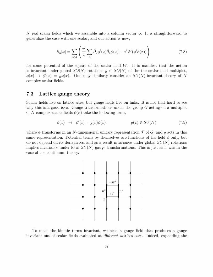
N real scalar fields which we assemble into a column vector φ. It is straightforward togeneralize the case with one scalar, and our action is now,
SΛ[φ] =∑
x∈Λ
(
a2
2
∑
µ
∂µφt(x)∂µφ(x) + a4W (φtφ(x))
)
(7.8)
for some potential of the square of the scalar field W . It is manifest that the actionis invariant under global SO(N) rotations g ∈ SO(N) of the the scalar field multiplet,φ(x) → φ′(x) = gφ(x). One may similarly consider an SU(N)-invariant theory of Ncomplex scalar fields.
7.3 Lattice gauge theory
Scalar fields live on lattice sites, but gauge fields live on links. It is not that hard to seewhy this is a good idea. Gauge transformations under the group G acting on a multipletof N complex scalar fields φ(x) take the following form,
φ(x) → φ′(x) = g(x)φ(x) g(x) ∈ SU(N) (7.9)
where φ transforms in an N -dimensional unitary representation T of G, and g acts in thissame representation. Potential terms by themselves are functions of the field φ only, butdo not depend on its derivatives, and as a result invariance under global SU(N) rotationsimplies invariance under local SU(N) gauge transformations. This is just as it was in thecase of the continuum theory.
•
•
•
•
•
•
•
•
•
•
•
•
•
•
•
•
•
•
•
•
x
nµ−nν nν
−nµ
To make the kinetic terms invariant, we need a gauge field that produces a gaugeinvariant out of scalar fields evaluated at different lattices sites. Indeed, expanding the
87
lattice kinetic term gives,
∂µφ†∂µφ = (φ(x+ nµ)† − φ(x)†)(φ(x+ nµ)− φ(x))
= (φ(x+ nµ)†φ(x+ nµ) + φ(x)†φ(x)
−φ(x+ nµ)†φ(x)− φ(x)†φ(x+ nµ) (7.10)
The two terms on the second line above are gauge invariant, since they only involve scalarfields evaluated at the same lattice sites. In fact, they are equivalent to scalar mass terms.The two terms on the last line are not gauge invariant, as the scalar fields are evaluated atdifferent lattice sites. What we need is a variable U(x, nµ) that lives on the link betweenx and x+ nµ, and transforms inversely of the scalars in the representation T at the latticesite x and T † at the site x+ nµ,
φ(x) → φ′(x) = g(x)φ(x)
U(x, nµ) → U ′(x, nµ) = g(x)U(x, nµ)g(x+ nµ)† (7.11)
It is natural to identify the hermitian conjugate as follows,
U(x+ nµ,−nµ) = U(x, nµ)† (7.12)
We shall shortly identify U with the gauge field in the continuum limit. We are now readyto write down a fully gauge invariant coupling of a scalar to the variable U(x, nµ),
∑
x∈Λ
(
d∑
µ=1
φ(x)†U(x, nµ)φ(x+ nµ) + φ(x+ nµ)†U(x, nµ)†φ(x) + a4W (φ†φ(x))
)
(7.13)
The mass term parts of the original version of the kinetic term have here been absorbed intothe potential, without loss of generality. It remains to construct a gauge invariant actionfor the variable U itself. Clearly the trace of product of link variables U(x, nµ) around anyclosed loop on the lattice will be gauge invariant. The simplest, and most local choice is totake that loop to be a single plaquette, so that the pure gauge action is given by,
SΛ[U ] = − c
g2
∑
x∈Λ
∑
ν 6=µ
tr(
U(x, nµ)U(x+ nµ, nν)U(x+ nµ + nν ,−nµ)U(x + nν ,−nν))
(7.14)
with a normalization factor c that we shall determine from the a → 0 limit of the action.Next, we need to make contact with the continuum action for the gauge field and scalarsas a→ 0. In the continuum, we know one object that transforms exactly as U(x, nµ) does,and it is given by the following formula,
P exp
{
i
∫ x+nµ
x
dyαAα(y)
}
(7.15)
integrated over yα(τ) along the straight line segment from x to x + nµ, parametrizedby τ . Here the symbol P preceding the exponential stands for path-ordering. In the
88
approximation where the lattice spacing a is small (compared to the typical length scale ofvariations of the gauge field Aµ, we may identify U with A as follows,
U(x, nµ) = exp{
iaAµ(x) +O(a2)}
(7.16)
Within the same approximation, the plaquette variable is obtained as follows,
U(x, nµ)U(x+ nµ, nν)U(x+ nµ + nν ,−nµ)U(x+ nν ,−nν)= exp
{
i a2 Fµν(x) +O(a3)}
= I + i a2 Fµν(x)−1
2a4Fµν(x)
2 +O(a5) (7.17)
Taking the trace in group space cancels out the term linear in Fµν but retains the termquadratic in Fµν , so that we obtain,
tr(
U(x, nµ)U(x+ nµ, nν)U(x+ nµ + nν ,−nµ)U(x+ nν ,−nν))
= dim T − 1
2I(T )a4F a
µν(x)Faµν(x) +O(a5) (7.18)
Hence the normalization constant c should be chosen as follows,
c =1
2 I(T )(7.19)
In the standard normalization of representation matrices of SU(N) or SO(N) in the defin-ing N -dimensional representations, we have I(T ) = 1
2, and the normalization constant
reduces to c = 1.
7.4 The integration measure for the gauge gauge field
The integration measure for the link variables U(x, nµ), which take values in G, must beinvariant under the gauge transformations acting on U(x, nµ), namely a transformationg(x) acting to the left of U , and an independent transformation g(x + nµ) acting to itsright. The problem is thus to find an integration measure for U ∈ G that is invariant underboth left and right transformations,7
U → U ′ = gLUg−1R (7.20)
To construct an invariant measure, it suffices to have an invariant metric since, by standardRiemannian geometry, a measure gives rise to a unique volume form, and the symmetries
7For unitary representations, g−1 = g†, but we shall provide here a general discussion without makingthis assumption.
89
of the metric are preserved by the measure. The metric may be constructed from eitherleft or right-invariant differential forms, defined respectively by U−1 dU and dU U−1. Byinspection, it is clear that U−1 dU is invariant under U → U ′ = gU , while dU U−1 isinvariant under U → U ′ = Ug−1. The following metric on G is invariant under both leftand right transformations,
ds2 = − 1
I(T )tr(
U−1dU U−1dU)
(7.21)
The corresponding measure, denoted [dU ] is the GL × GR-invariant volume form on G,and is referred to as the Haar measure. It will often be convenient to normalize the Haarmeasure so that the volume of G is one,
∫
G
[dU ] = 1 (7.22)
although this normalization is by no means standard.
In the special case of G = U(1), the Haar measure is simply dθ, where θ is the angleparametrizing the circle S1 = U(1). For SU(2) the metric ds2 will be identical to the roundmetric on the sphere S3 = SU(2), and the Haar measure is the standard volume form onS3. For higher compact Lie groups, the Haar measure is more complicated, but one usuallydoes not need its explicit form.
7.5 Wilson loops
In a theory with only gauge fields, i.e. link variables U(x, nµ), all gauge-invariant observ-ables may be constructed as follows. Take a closed path C on the lattice, and take the traceof the product of all oriented link variables U(x, nµ) along the path C. This is an infiniteset of operators, which tends to be a bit unwieldy. On a square lattice, one may restrictthe paths to rectangles of sides Lt, Lx ∈ N links. One may think of one of the directionsbeing time-like while the other direction is space-like. the corresponding observables arereferred to as Wilson loops,
W (C) = tr
∏
(x,nµ)∈C
U(x, nµ)
(7.23)
The significance of the Wilson loop in a theory with scalars and fermions which couple tothe gauge field may be seen as follows. We take scalars for simplicity. Consider a scalarfield φ with very large mass (compared to the scale of the dynamics of the gauge field). Ifits mass is large, then it will remain virtually immobile on the lattice for the time span of
90
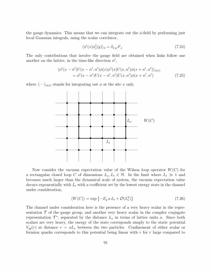
the gauge dynamics. This means that we can integrate out the φ-field by performing justlocal Gaussian integrals, using the scalar correlator,
〈φi(x)φ†j(y)〉φ = δx,y δ
ij (7.24)
The only contributions that involve the gauge field are obtained when links follow oneanother on the lattice, in the time-like direction nt,
〈φ†(x− nt)U(x− nt, nt)φ(x)φ†(x)U(x, nt)φ(x+ nt, nt)〉φ(x)= φ†(x− nt)U(x− nt, nt)U(x, nt)φ(x+ nt, nt) (7.25)
where 〈· · ·〉φ(x) stands for integrating out φ at the site x only.
•
•
•
•
•
•
•
•
•
•
•
•
•
•
•
•
•
•
•
•
•
•
•
•
•
•
•
•
•
•
Lx
Lt
W (C)
Now consider the vacuum expectation value of the Wilson loop operator W (C) fora rectangular closed loop C of dimensions Lx, Lt ∈ N. In the limit where Lt ≫ 1 andbecomes much larger than the dynamical scale of system, the vacuum expectation valuedecays exponentially with Lt with a coefficient set by the lowest energy state in the channelunder consideration,
〈W (C)〉 = exp{
−Eg aLt +O(L0t )}
(7.26)
The channel under consideration here is the presence of a very heavy scalar in the repre-sentation T of the gauge group, and another very heavy scalar in the complex conjugaterepresentation T ∗, separated by the distance Lx in terms of lattice units a. Since bothscalars are very heavy, the energy of the state corresponds simply to the static potentialVqq(r) at distance r = aLx between the two particles. Confinement of either scalar orfermion quarks corresponds to this potential being linear with r for r large compared to
91
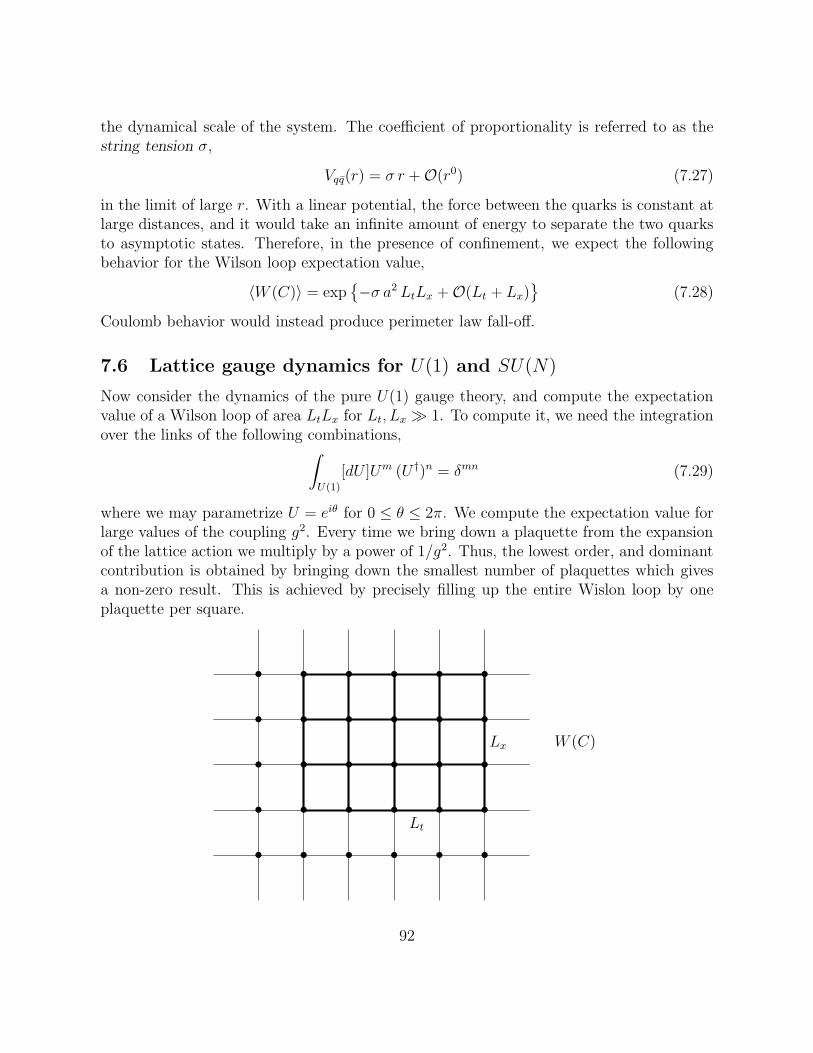
the dynamical scale of the system. The coefficient of proportionality is referred to as thestring tension σ,
Vqq(r) = σ r +O(r0) (7.27)
in the limit of large r. With a linear potential, the force between the quarks is constant atlarge distances, and it would take an infinite amount of energy to separate the two quarksto asymptotic states. Therefore, in the presence of confinement, we expect the followingbehavior for the Wilson loop expectation value,
〈W (C)〉 = exp{
−σ a2 LtLx +O(Lt + Lx)}
(7.28)
Coulomb behavior would instead produce perimeter law fall-off.
7.6 Lattice gauge dynamics for U(1) and SU(N)
Now consider the dynamics of the pure U(1) gauge theory, and compute the expectationvalue of a Wilson loop of area LtLx for Lt, Lx ≫ 1. To compute it, we need the integrationover the links of the following combinations,
∫
U(1)
[dU ]Um (U †)n = δmn (7.29)
where we may parametrize U = eiθ for 0 ≤ θ ≤ 2π. We compute the expectation value forlarge values of the coupling g2. Every time we bring down a plaquette from the expansionof the lattice action we multiply by a power of 1/g2. Thus, the lowest order, and dominantcontribution is obtained by bringing down the smallest number of plaquettes which givesa non-zero result. This is achieved by precisely filling up the entire Wislon loop by oneplaquette per square.
•
•
•
•
•
•
•
•
•
•
•
•
•
•
•
•
•
•
•
•
•
•
•
•
•
•
•
•
•
•
Lx
Lt
W (C)
92
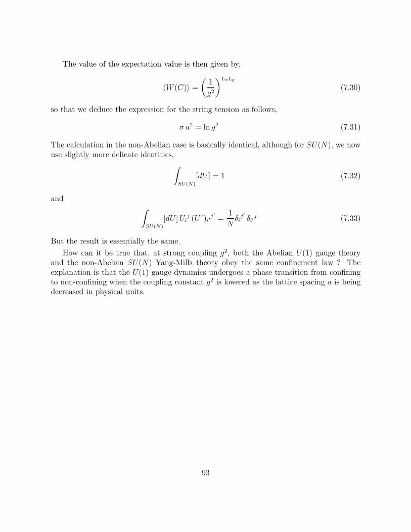
The value of the expectation value is then given by,
〈W (C)〉 =(
1
g2
)LxLy
(7.30)
so that we deduce the expression for the string tension as follows,
σ a2 = ln g2 (7.31)
The calculation in the non-Abelian case is basically identical, although for SU(N), we nowuse slightly more delicate identities,
∫
SU(N)
[dU ] = 1 (7.32)
and∫
SU(N)
[dU ]Uij (U †)i′
j′ =1
Nδij′ δi′
j (7.33)
But the result is essentially the same.
How can it be true that, at strong coupling g2, both the Abelian U(1) gauge theoryand the non-Abelian SU(N) Yang-Mills theory obey the same confinement law ? Theexplanation is that the U(1) gauge dynamics undergoes a phase transition from confiningto non-confining when the coupling constant g2 is lowered as the lattice spacing a is beingdecreased in physical units.
93
8 Global Internal Symmetries
In Nature, different quantum states may have similar physical properties and therefore maybe grouped together into a multiplet of states which are transformed into one another underthe action of a certain group. This procedure is familiar, of course, from space rotationsor Poincare transformations. In both of these cases, the group transformations actuallycorrespond to exact symmetries of space-rotations and Poincare transformations. But thesymmetries need not always be exact to provide a useful framework for assembling differentstates and fields into a single multiplet, and this is often the case with internal symmetries.
Internal symmetries were considered by Heisenberg, who noticed that – from the pointof view of the strong interactions – there is little distinction between a proton and a neutron.For one, their masses are surprisingly close. This led Heisenberg to assemble the protonand neutron states and fields into a doublet,
(
pn
) {
mp = 938.2 MeVmn = 939.5 MeV
(8.1)
The group acting on this doublet is referred to as isospin SU(2)I . The strong interactionsare insensitive to SU(2)I isospin rotations of the proton - neutron doublet. This observationleads one to postulate that the group SU(2)I is a global symmetry of the strong interactions,either exact, or approximate.
From the point of view of electromagnetism, the proton and neutron are very different,since the proton is electrically charged while the neutron is neutral, and therefore SU(2)Iisospin is not a symmetry of the electromagnetic interactions. Global symmetries may beuseful even if they are only approximate. In the case of SU(2)I , the symmetry is brokenby mass and by electromagnetic interactions. It is also broken by the weak interactions.
More modern examples are found by considering quarks instead of hadrons. Thepresently known quarks form the following array,
uc cc tc c = color ∈ {r, w, b}dc sc bc (8.2)
The strong interactions are sensitive only to the color of the quarks and not to their flavor.Extending the notion of isospin to six quarks, the symmetry group would naturally beSU(6). Given that the masses of the quarks are approximately as follows,
mu = 5 MeV mc = 1.5 GeV mt = 170 GeV
md = 7 MeV ms = 100 MeV mb = 4.9 GeV (8.3)
it is clear that SU(6) is very badly broken and little or no trace of it is left in physics.The u, d and s quarks may still be considered alike from the point of view of the strong
94
interactions as their masses are small compared to the typical strong interaction scale ofthe proton for example, and the associated SU(3) symmetry is useful.
In quantum field theory, elementary particles are described by local fields, whose dynam-ics is governed by a Lagrangian (or when there is no Lagrangian by the operator productalgebra). Thus, to describe the above type of internal symmetries, we shall consider fieldtheories that are invariant under global symmetries.
In classical field theory, a symmetry is a transformation of the fields that maps anysolution of the Euler-Lagrange equations into a solution of the same equations. Generally,the symmetry will map a solution to a different solution. A specific solution may, however,be mapped into itself and be invariant under the transformation. Two distinct conceptsof symmetry emerge from the above discussion; the symmetry of an equation versus thesymmetry of a solution to the equation.
At the much more elementary level of algebraic equations, for example, the simpleequation x3 − x = 0 has solutions x = 0,±1, and has the following symmetry properties,
• the symmetry of the equation is given by the transformation P : x→ −x;• P maps the solution x = 0 into itself, so that x = 0 is invariant under P ;
• P maps the solution x = +1 into the third solution x = −1 and vice-versa, so thatthe solution x = +1 is not invariant under the symmetry P of the equation.
The concept of symmetry for an object, such as a circle, a triangle, a square, a cube andso on, dates back to ancient Greek times, and probably to even earlier times. The conceptof a symmetry of an equation, however, was considered only in relatively recent times byLagrange and Galois in the early 19-th century.
8.1 Symmetries in quantum mechanics
In quantum mechanics, for systems with a finite number of degrees of freedom, a symmetryis realized via a unitary operator U in Hilbert space. This holds for continuous as well asdiscrete symmetries, with the exception of time-reversal which is realized by an anti-unitarytransformation. Internal symmetries commute with the Hamiltonian and obey,
U †HU = H (8.4)
Under an internal symmetry, the eigenstates of the Hamiltonian associated with a giveneigenvalue E of H transform under a unitary representation U(E). To see this, consider theeigenspace of eigenstates |E, α〉 of the HamiltonianH with given energy eigenvalue E, and αlabeling the different states with the same eigenvalue E, so that we haveH|E, α〉 = E|E, α〉.Next, calculate the action of the symmetry transformation U ,
H U |E, α〉 = U H|E, α〉 = E U |E, α〉 (8.5)
95
It follows that U |E, α〉 has energy E, and must therefore be a linear combination of thestates |E, β〉, given as follows,
U |E, α〉 =∑
β
U(E)αβ |E, β〉 (8.6)
Unitarity of U then guarantees unitarity of U(E) which satisfies U(E)†U(E) = I, where Iis the identity operator in the eigenspace of H for eigenvalue E. Thus internal symmetriesorganize the quantum states at given energy into unitary representations of the symmetrygroup. This fact is often referred to as the symmetry is realized in the Wigner mode, orthe symmetry is realized linearly.
8.2 Symmetries in quantum field theory
In quantum field theory, there are essentially three possibilities. The starting point may be aclassical Lagrangian assumed to have a symmetry in the classical sense. Upon quantization,it may be that this symmetry survives quantization, or alternatively that it suffers ananomaly and therefore ceases to be a symmetry of the system at the quantum level. U(1)gauge invariance in QED is an example of the first case, while U(1)A symmetry in QED is anexample of the second case. Recall that anomalies manifest themselves when regularizationand renormalization effects necessarily destroy the symmetry.
When the symmetry survives quantization, there are two further possibilities, which aredistinguished by the properties of the vacuum.
1. The symmetry leaves the vacuum invariant. This case is very much like the Wignermode in quantum mechanics : the states in Hilbert space transform under unitarytransformations. Global U(1) symmetry in QED is again an example of this mode;Poincare invariance is another, since all states are unitary multiplets of ISO(1,3).
2. The symmetry does not leave the vacuum invariant. This case has no counterpart inquantum mechanics (except when supersymmetry is considered). The symmetry issaid to be spontaneously broken or in the Nambu-Goldstone mode.
The spontaneously broken case is similar to classical solutions of a given classical Euler-Lagrange equations never realizing the symmetries of the equation, though the differenceis of course that there is no concept of vacuum in classical physics other than it being thesolution with the largest amount of symmetry.
8.3 Continuous internal symmetry with two scalar fields
A system with a single real field and a polynomial potential does not have interestingcontinuous internal symmetries. The case with two real fields φ1, φ2, or equivalently a
96
complex field φ = (φ1 + iφ2)/√2, subject to the discrete symmetries,
R1
{
φ1 → −φ1
φ2 → +φ2R2
{
φ1 → +φ1
φ2 → −φ2(8.7)
and renormalizability in four space-time dimensions gives,
L =1
2∂µφ1∂
µφ1 +1
2∂µφ2∂
µφ2 −1
2m2
1φ21 −
1
2m2φ
22 −
λ214!φ41 −
λ2
12φ21φ
22 −
λ224!φ42 (8.8)
The symmetries R1, R2 are mutually commuting involutions, so that the symmetry groupis Z2 × Z2 where Z2 is the group Z2 = {1,−1}.
For special arrangements of masses and couplings, however, the symmetry is actuallylarger than Z2 ×Z2. Specifically, if we require m2
1 = m22 and λ21 = λ22, we have a further Z2
which acts by interchanging φ1 and φ2. Furthermore, when m21 = m2
2 and λ1 = λ = λ2, theLagrangian has a continuous SO(2) ∼ U(1) global symmetry as well,
(
φ1
φ2
)
→(
φ′1
φ′2
)
=
(
cosα − sinαsinα cosα
)(
φ1
φ2
)
(8.9)
where α is independent of x, but otherwise arbitrary. One way of seeing the presence ofthe symmetry more explicitly is by noticing that L may be written in terms of a potentialwhich only depends on the φ2
1 + φ22. More generally, any Lagrangian of the form,
L =1
2∂µφ1∂
µφ1 +1
2∂µφ2∂
µφ2 − V (φ1, φ2) (8.10)
where the potential is invariant under SO(2), and is therefore of the form V (φ1, φ2) =W (φ2
1 + φ22) for some function W . Alternatively, one may regroup the two real fields
φ1, φ2 into a single complex field φ = (φ1 + iφ2)/√2, in terms of which the U(1) acts by
φ→ φ′ = eiαφ and the Lagrangian take the form,
L = ∂µφ ∂µφ−W (2φφ) (8.11)
Henceforth, the following SO(2)-invariant potential will be considered,
V (φ1, φ2) =1
2m2(φ2
1 + φ22) +
λ2
4!(φ2
1 + φ22)
2 (8.12)
For real λ2 and λ2 < 0, the potential is unbounded from below, which is physically unac-ceptable. Henceforth, we shall assume that λ2 and m2 are real, and that λ2 > 0, so thatthe potential is bounded from below for all values of m2, including m2 < 0. Next, thesemi-classical vacuum configuration will be determined and its symmetry properties willbe examined in light of the preceding discussion.
97
8.3.1 The symmetric or unbroken phase m2 > 0
The form of the potential for m2 > 0 is represented in Fig 1 (a). The potential has aunique minimum at φ1 = φ2 = 0. This configuration is the semi-classical approximationto the vacuum of the theory, and is invariant under SO(2) rotations. Thus, the systemhas unbroken symmetry. To study the spectrum, the field is decomposed into creationand annihilation operators, and the Fock space construction is used. The starting pointis the vacuum, corresponding here to the classical configuration φi = 0. The field is thendecomposed as follows,
φi(x) =
∫
ddk
(2π)d1
2ωk
(
ai(k)e−ik·x + a†i (k)e
ik·x)
i = 1, 2 (8.13)
where ωk =√k2 +m2, kµ = (ωk,k) and k · x = kµx
µ, with the commutation relations,[
ai(k), a†j(l)]
= 2ωk(2π)d−1δijδ(k− l) (8.14)
The generator of SO(2) rotations is defined by,
Q =
∫
dd−1k
(2π)d−1
(
a†2(k)a1(k)− a†1(k)a2(k))
(8.15)
and acts upon the creation and annihilation operators as follows,
[Q, ai(k)] = −εijaj(k)[Q, a†i (k)] = +εija
†j(k) (8.16)
where ε12 = 1. The generator Q commutes with the Hamiltonian.
The ground state is defined by ai(k)|0〉 = 0 for all k ∈ Rd, and for both i = 1, 2. The
equations defining |0〉 are invariant under SO(2) and so is |0〉, which satisfies Q|0〉 = 0.The excited states (to lowest order in the interaction) are constructed by applying creationoperators to the vacuum,
a†i1(k1) · · ·a†in(kn)|0〉 (8.17)
Since |0〉 is invariant under SO(2) it is manifest that the states transform under unitaryrepresentations of SO(2). This is the Wigner mode.
8.3.2 The spontaneously broken phase m2 < 0
The form of the potential for m2 < 0 is represented in Fig. 1 (b). The extrema of thepotential are governed by the equations,
∂V
∂φi= m2φi +
λ2
6(φ2
1 + φ22)φi = 0 i = 1, 2 (8.18)
98
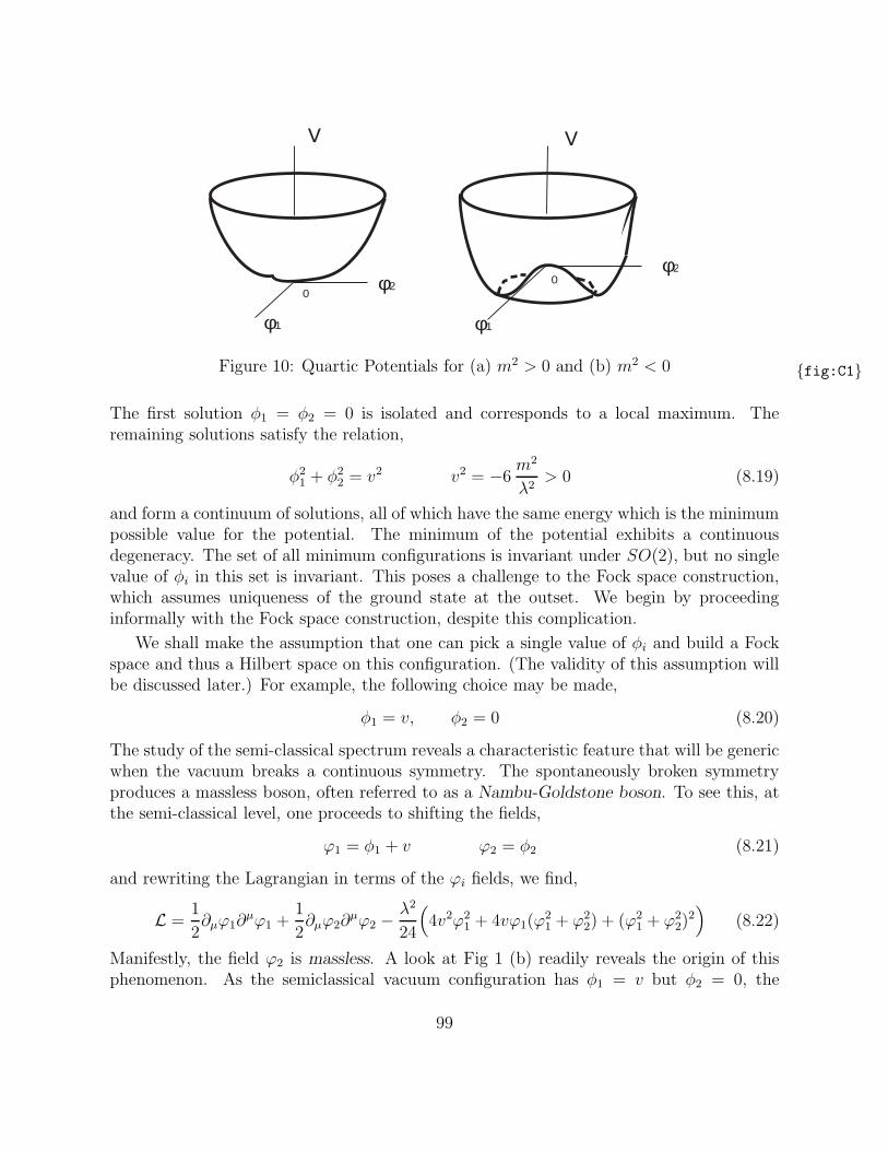
V V
φ1
φ2
φ1
φ2
00
Figure 10: Quartic Potentials for (a) m2 > 0 and (b) m2 < 0 {fig:C1}
The first solution φ1 = φ2 = 0 is isolated and corresponds to a local maximum. Theremaining solutions satisfy the relation,
φ21 + φ2
2 = v2 v2 = −6m2
λ2> 0 (8.19)
and form a continuum of solutions, all of which have the same energy which is the minimumpossible value for the potential. The minimum of the potential exhibits a continuousdegeneracy. The set of all minimum configurations is invariant under SO(2), but no singlevalue of φi in this set is invariant. This poses a challenge to the Fock space construction,which assumes uniqueness of the ground state at the outset. We begin by proceedinginformally with the Fock space construction, despite this complication.
We shall make the assumption that one can pick a single value of φi and build a Fockspace and thus a Hilbert space on this configuration. (The validity of this assumption willbe discussed later.) For example, the following choice may be made,
φ1 = v, φ2 = 0 (8.20)
The study of the semi-classical spectrum reveals a characteristic feature that will be genericwhen the vacuum breaks a continuous symmetry. The spontaneously broken symmetryproduces a massless boson, often referred to as a Nambu-Goldstone boson. To see this, atthe semi-classical level, one proceeds to shifting the fields,
ϕ1 = φ1 + v ϕ2 = φ2 (8.21)
and rewriting the Lagrangian in terms of the ϕi fields, we find,
L =1
2∂µϕ1∂
µϕ1 +1
2∂µϕ2∂
µϕ2 −λ2
24
(
4v2ϕ21 + 4vϕ1(ϕ
21 + ϕ2
2) + (ϕ21 + ϕ2
2)2)
(8.22)
Manifestly, the field ϕ2 is massless. A look at Fig 1 (b) readily reveals the origin of thisphenomenon. As the semiclassical vacuum configuration has φ1 = v but φ2 = 0, the
99
fluctuations around this point purely in the direction of φ2 = ϕ2 encounter no potentialbarrier at all and proceed along the flat direction of the potential, remaining at its minimum.This is the Nambu-Goldstone boson. The treatment so far has been semi-classical.
In the full quantum field theory, one is concerned with the full ground state of theHamiltonian. In terms of the energy expectation value of any given state |ψ >,
E(ψ) ≡ 〈ψ|H|ψ〉〈ψ|ψ〉 (8.23)
the ground state |ψ0〉 is defined by the requirement E(ψ0) ≤ E(ψ) for all |ψ〉 ∈ H. Thefollowing possibilities arise,
1. U |ψ0〉 = |ψ0〉 Wigner mode
2. U |ψ0〉 6= |ψ0〉 Goldstone mode
The analysis of the full quantum spectrum is more involved than the semi-classical approx-imation shows. We first treat an exactly solvable example to illustrate the general ideasand to arrive at the important Coleman-Mermin-Wagner Theorem.
8.4 Spontaneous symmetry breaking in massless free field theory
Consider massless free field theory of a single scalar field φ(x) in flat d dimensional space-time Rd, with Lagrangian,
L0 =1
2∂µφ ∂µφ (8.24)
The Lagrangian is invariant under shifts of φ by a real constant c,
φ(x) → φ′(x) = φ(x) + c (8.25)
The corresponding Noether current and charge are
jµ = ∂µφ P =
∫
dd−1x j0 =
∫
dd−1x ∂0φ (8.26)
Since the theory is massless, it is also invariant under scale and conformal transformations.
As usual, we expect that the Hilbert space will arise from the Fock space construction ona unique Poincare invariant vacuum, say |0〉. Is this vacuum invariant under the translationsof φ ? Consider the 1-point function 〈0|φ(x)|0〉. By Poincare invariance, this is an x-independent real constant φ0. If |0〉 were invariant under a translation φ→ φ+ c, then φ0
should also be invariant under this transformation. The transformation is by φ0 → φ0 + c,which leaves no finite φ0 invariant.
100
8.4.1 Adding a small explicit symmetry breaking term
The nature of the vacuum is always an IR problem. It is natural to try and modify ourtheory in the IR by a term in the Lagrangian that breaks the symmetry φ→ φ+c explicitly.In this case, we can actually add a small mass term that will preserve the free field natureof the problem and hence allow for an exact solution. The new Lagrangian will be (forEuclidean metric),
Lm,ϕ =1
2∂µφ∂µφ+
1
2m2(φ− φ0)
2 (8.27)
where φ0 is a real constant and m2 > 0. The original L0 may be recovered by lettingm2 → 0, in which limit the Lagrangian becomes independent of φ0. For given φ0, theminimum of the potential of Lm,ϕ is at φ0 for all m
2 > 0. Thus, for any finite value m2 > 0,the one-point function is well-defined and given by,
〈0|φ(x)|0〉 = φ0 (8.28)
The two-point function is given by,
〈0|φ(x)φ(y)|0〉 = (φ0)2 +Gd(r) r2 = (x− y)2 (8.29)
where the Green function is given by,
Gd(r) =
∫
ddk
(2π)d1
k2 +m2eik·(x−y)
=
∫ ∞
0
dτ
∫
ddk
(2π)deik·(x−y)e−τ(k
2+m2) (8.30)
Carrying out the Gaussian integration in k, we find,
Gd(r) =1
(4π)d/2
∫ ∞
0
dτ τ−d/2e−τm2−r2/4τ =
1
(2π)d/2
(m
r
)d/2−1
Kd/2−1(mr) (8.31)
Actually, Gd(r) always decays exponentially when r → ∞ for fixed m > 0. We are mostinterested, however, in the regime which is closest to the massless regime : this is when0 < mr ≪ 1 instead. The leading behavior in this regime for the cases is given by
G1(r) =1
2me−mr
G2(r) ∼ − 1
2πln(mr/2)
Gd(r) ∼ Γ(d/2)
2(d− 2)πd/2 rd−2d ≥ 3 (8.32)
We recognize the harmonic oscillator case with d = 1 and the Yukawa potential for d = 3.The cases d ≥ 3 actually admit finite limits when m → 0 for fixed r, and the resulting
101
limits fall off to 0 as r → ∞. This behavior demonstrates that as d ≥ 3, the system getslocked into the vacuum expectation value 〈0|φ(x)|0〉 = φ0 and thus breaks the translationsymmetry in the field φ at all m and also in the limit m→ 0.
The cases d = 1 and d = 2 do not obey this pattern, as no finite limits exist. Thecase d = 1 is ordinary quantum mechanics. The ground state for m = 0 is indeed a stateuniformly spread out in φ, which will produce divergent 〈0|φ|0〉. The case d = 2 is alsoimportant. The failure of being able to take the limitm→ 0 is at the origin of the Coleman-Mermin-Wagner Theorem that no continuous symmetry can be spontaneously broken in 2space-time dimensions.
8.4.2 Canonical analysis
To determine the vacuum of the theory, we construct the Hamiltonian H0 in terms of thefield φ and its canonical momentum π. Upon quantization, UV divergences may be renor-malized by normal ordering. Decomposing the field in creation and annihilation operators,
φ(x) =
∫
k
(
a†(k)e−ik·x + a(k)e+ik·x)
H0 =
∫
k
|k| a†(k)a(k)
P =1
2i
(
a(0)− a†(0))
(8.33)
Here, a general notation is used for the summation over the momenta k. In d-dimensionalflat space, the summation corresponds to an integral over the continuous variable k,
∫
k
=
∫
dd−1k
(2π)d−1 2|k| (8.34)
but we shall also consider quantization on a torus, where the sum will be discrete.
The Hamiltonian is positive and lowest energy is achieved when a state is annihilatedby the operators a(k). But, we observe a variant of the usual (for example for massivefields) situation, since the operator a(0) corresponds to zero energy. Thus, minimum, i.e.zero energy, requires only that all the operators a(k) with k 6= 0 annihilate the minimumenergy state. Its behavior under a(0) is undetermined by the minimum energy condition.
The translation charge P only depends upon a(0) − a†(0) and commutes with H0.Therefore, the zero energy states are distinguished by their P -charge and may be labeledby this charge, p. The conjugate variable is Q = (a(0)+a†(0))/2, and satisfies [Q,P ] = iV ,where V is the volume of space.
102
8.5 Why choose a vacuum ?
This question is justified because in ordinary quantum mechanics such degeneracies getlifted. For example, in the one-dimensional Hamiltonian,
H =1
2mp2 +
1
2mλ2(x2 − v2)2 (8.35)
a state localized around x = −v has a non-zero probability to tunnel to a state localizedaround x = +v. In fact the transition probability is given by the imaginary time pathintegral, familiar from the WKB approximation,
〈x = +v|x = −v〉 =∫
Dx(t) e−S[x]/~ (8.36)
with the boundary conditions x(−∞) = −v and x(+∞) = +v. The Euclidean action isgiven by,
S[x] =
∫ ∞
−∞
dt
(
1
2mx2 +
1
2mλ2(x2 − v2)2
)
(8.37)
Semi-classically, ~ is small and the integral will be dominated by extrema of S (satisfyingthe initial and final boundary conditions). Solutions are given by the first integral,
1
2mx2 − mλ2
2(x2 − v2)2 = 0 (8.38)
whose solutions are
xc(t) = ±v tanh(
λv(t− to))
(8.39)
The corresponding action is finite and given by S[xc] = 4/3mλv3; the transition amplitudein this approximation is non-zero and given by,
〈x = +v|x = −v〉 ≈ e−S[xc]/~ = exp
{
4mλv3
3~
}
(8.40)
These objects are called instantons. The true ground state is a superposition of the stateslocalized at v and −v. It would thus be absurd to choose one configuration above the other.
What happens in QFT? Can one still tunnel from one configuration to the other? Let’sinvestigate this with the help of the semi-classical approximation to the imaginary timepath integral.
S[φ] =
∫
ddx
{
1
2∂µφ∂
µφ+λ2
4(φ2 − v2)2
}
(8.41)
103
Assume there exists a solution φc(x), which is a minimum of the classical action. Considerits scaled version φσ(x) = φc(σx),
S[φσ] =
∫
ddx
{
1
2σ2−d∂µφc∂
µφc +λ2
4σ−d(φ2
c − v2)2}
(8.42)
Now σ = 1 better be a stationary point.
∂S[φσ]
∂σ
∣
∣
∣
∣
σ=1
=
∫
ddx
{
∂µφc∂µφc(2− d)− d
λ2
4(φ2
c − v2)2}
(8.43)
But for d ≥ 2, both terms are negative, and cancellation would require,
∂µφc∂µφc = 0 and φ2
c = v2 (8.44)
Only for d = 1 can there be non-trivial solutions. This result is often referred to as Derrick’s
theorem. Thus, for a scalar potential theory with d ≥ 2, it is impossible to tunnel fromone localized state to the other via instantons.
Even when vacuum degeneracy occurs for space-time dimension larger than 1, it maystill be possible to have tunneling between the degenerate vacua. Famous examples of thisphenomenon are precisely when instantons with finite action exist in space-time dimensionlarger than one,
• Non-linear σ-models in d = 2;
• Higgs model with U(1) gauge symmetry in d = 2;
• QCD in d = 4 with θ-vacua.
Finally, the Mermin-Wagner-Coleman Theorem states that in d = 2, a continuous(bosonic) symmetry can never be spontaneously broken. The reason for this resides in thefact that the massless Goldstone bosons that would arise through this breaking cannotdefine a properly interacting field theory, since their infrared behavior is too singular.
8.6 Generalized spontaneous symmetry breaking (scalars)
Consider a field theory of n real scalar fields φi, with i = 1, · · · , n, arranged in a columnvector φ. For simplicity, assume that the Lagrangian has a standard kinetic term as wellas a potential V ,
L =1
2∂µφ
t∂µφ− V (φ) (8.45)
It will be further assumed that V (φ) is bounded from below, and has its minima at finitevalues of φ. (Runaway potentials such as eφ generate special problems.)
104
• It is assumed that L is invariant under a continuous symmetry group G acting linearlyon φ; for this reason, these models are often referred to as linear σ-models;
• Invariance of the kinetic term requires that G be a subgroup of SO(N);
• The potential V (φ) must be invariant under the action of G;
• The ground state of V (φ) is assumed to be degenerate, and all ground states aremapped into one another under the action of G. When any given minimum φ0
is invariant under a subgroup H of G, which is strictly smaller than G, then thesymmetry group G of the Lagrangian is spontaneously broken to the symmetry groupH of the vacuum. Note that H may be the identity group.
8.6.1 Goldstone’s Theorem
The Goldstone bosons associated with the spontaneous symmetry breaking from G → Hare described by the coset space G/H , and their number is dimG/H = dimG− dimH .
To prove the theorem, we use the fact that G acts transitively on G/H ; i.e. withoutfixed points. Every point in G/H may be obtained by applying some g ∈ G to any givenreference point in G/H . Actually, this is true for the action of G on G (a special case withH = 1). Indeed, take a reference point g0 in G then to reach a point g ∈ G, it suffices tomultiply to the left by g g−1
0 . Thus, it suffices to analyze the problem around any point onG/H , and then carry the result to all of G/H .
Take the reference point in G/H to be φ0 which satisfies,
∂V
∂φi
∣
∣
∣
∣
φi=φ0i
= 0 (8.46)
Now the set of all solutions transform under G. Decompose the Lie algebra G of G into itssubalgebra H and the orthogonal complement under the Cartan-Killing form, M :
G = H⊕M
ρ(T a)φ0 = 0 T a ∈ Hρ(T a)φ0 6= 0 T a ∈ M
(8.47)
The Goldstone boson fields now correspond to the directions of the potential from φ0
where φ0 is charged, but the potential is still at its minimum value. These are preciselythe directions in G/H represented here by its tangent space M.
8.6.2 Example 1
The N scalar fields φi, for i = 1, · · · , N , are grouped into a column vector φ, subject to thefollowing Lagrangian,
L =1
2∂µφ
t∂µφ−W (φtφ) (8.48)
105
invariant under SO(N). Assume the minimum of v occurs at φtφ = v2 > 0. The symmetryof the Lagrangian is G = SO(N), but the symmetry of any vacuum configuration is onlyH = SO(N − 1) so that G/H = SN−1 and there are N − 1 Goldstone Bosons.
8.6.3 Example 2
The N2 scalar fields Mij for i, j = 1, · · · , N may be regrouped into a real square matrix Mvalued field subject to the Lagrangian,
L =1
2tr ∂µM
T∂µM − 1
2m2trMTM − λ2
4!tr(MTM)2 (8.49)
This Lagrangian is invariant under the following G = O(N)L × O(N)R transformations,
M → gLMgTR gL ∈ O(N)L, gR ∈ O(N)R (8.50)
Any stationary point M of the potential obeys the equation
(
MTM − v2IN
)
MT = 0 v2 = −6m2
λ2(8.51)
When m2 > 0, the solution M = 0 is unique and the full G symmetry leaves the vacuuminvariant. The interesting case is when m2 < 0, which we now analyze systematically.
The eigenvalues of MTM must either vanish or equal v2. The general solution tothis equation may be organized according to the number n of vanishing eigenvalues, with0 ≤ n ≤ N , and MTM = v2In. For each n, the configuration defines a stationary pointof the potential, but only one case n = N is an absolute minimum of the potential, whichcorresponds to the vacuum for the theory. This may be verified by substituting the solutionsfor MTM into the potential and evaluating the potential. The general solution for Mto the equation MTM = v2IN is given by M = vg with g ∈ SO(N), which under anO(N)L × O(N)R transformation is equivalent to M = vIN . The residual symmetry ofM = vIN is calculated as follows,
gL (vIN) gTR = (vIN) ⇒ gL = gR ∈ O(N)D (8.52)
Hence the dynamics of this model shows the following pattern,
O(N)L ×O(N)R → O(N)D +1
2N(N − 1) Goldstone bosons (8.53)
The Goldstone boson fields parametrize the coset G/H = (O(N)L × O(N)R)/O(N)D,following the general pattern announced earlier. Other examples of field theories may beanalyzed with the same semi-classical methods.
106
8.7 The non-linear sigma model
Often one is interested in describing only the dynamics of the Goldstone bosons at lowenergy/momentum. All other excitations are then massive and decouple. In this limit, theremaining Lagrangian consists of the kinetic term on the scalar fields φa, subject to theconstraint that the potential on these fields equals its minimum value,
L =1
2∂µφ
t∂µφ V (φ) = V (φ0) (8.54)
The Lagrangian is still invariant under G, and so is the condition for the minimum. ButG is spontaneously broken to H , and the model only describes the Goldstone bosons.
The true dynamical fields are no longer the fields φ, since they are related to one anotherby the constraint V (φ) = V (φ0). Introducing true dynamical fields may be done by solvingthe constraint.
It is best to illustrate the procedure with an example. Consider a vector φ of n realscalar fields φi, i = 1, · · · , N with a quartic potential,
V (φ) =1
2m2(φtφ) +
λ
4!(φtφ)2 v2 = −6m2
λ> 0 (8.55)
Let the vacuum expectation value of φi be φ0i = vδi,N , and denote the vector of the remain-
ing N − 1 fields by πi = φi for i = 1, · · · , N − 1. The constraint V (φ) = V (φ0) is givenby φtφ = v2. Eliminating the only non-Goldstone field φN using φN =
√v2 − πtπ. The
resulting Lagrangian is now a nonlinear sigma model, with Lagrangian
LGB =1
2∂µπ
t∂µπ +1
2
(πt∂µπ)(πt∂µπ)
v2 − πtπ(8.56)
A number of remarks:
1. G/H = SN−1; indeed there are N − 1 independent fields π.
2. H = SO(N − 1) is realized linearly on π by rotations.
3. The Lagrangian is now non-polynomial in π.
4. This implies that it is non-renormalizable (in d = 4). This is no surprise since wediscarded higher energy parts of the theory.
5. Before eliminating φN , the Lagrangian L was invariant under SO(N). What hashappened with this symmetry? Has it completely disappeared or is its presence justmore difficult to detect ?
We shall now address the last point. Since SO(N−1) leaves φN invariant, the only concernis with the transformations in SO(N) modulo those in SO(N−1) which leave φN invariant.
107
Using SO(N − 1) symmetry, these are equivalent to rotations g between π1 and φN , whichleave πi, i = 2, 3, · · · , N − 1 invariant,
g
(
π1φN
)
=
(
cosα sinα− sinα cosα
)(
π1φN
)
(8.57)
Since φN has been eliminated from the Lagrangian LGB, only the action of g on π1 is ofinterest in examining the symmetries of LGB,
g(π1) = π1 cosα+√v2 − πtπ sinα (8.58)
As a result, the Lagrangian is still invariant g(LGB) = LGB. But, the novelty is that thesymmetry is realized in a nonlinear fashion; hence the name.
8.8 The general G/H nonlinear sigma model
The wonderful thing about Goldstone boson dynamics is that, given the symmetries G andH , the corresponding Lagrangian LGB is unique up to an overall constant. The basic as-sumption producing this uniqueness is that LGB has a total of two derivatives. Thus, withinthis approximation, the dynamics of Goldstone bosons is independent of the precise mi-croscopic theory and mechanism that produced the symmetry breaking and the Goldstonebosons. In other words, given G/H , the Goldstone boson dynamics is universal.
The construction is as follows. The group G is realized in terms of matrices for which westill use the notation g. The Lie algebra G admits the following orthogonal decomposition,G = H ⊕ M. The (independent) Goldstone fields in the theory are taken to be φi withi = 1, · · · , dimM = dimG− dimH . Instead of working with the independent fields φi, itis much more convenient to parametrize the Goldstone fields by the group elements g ∈ G,g(φi). Of course, g contains too many fields, which will have to be projected out. To dothis, one proceeds geometrically.
The combinations g−1∂µg take values in G. In fact, they are left-invariant 1-forms on
G, since under left-multiplication of the field g by a constant element γ ∈ G we have,
ωµ(g) ≡ g−1∂µg ωµ(γg) = g−1γ−1∂µγg = ωµ(g) (8.59)
On the other hand, under right-multiplication by a function h ∈ H , ωµ(g) transforms as a
connection or gauge field,
ωµ(gh) = h−1g−1∂µ(gh) = h−1ωµ(g)h+ h−1∂µh (8.60)
Therefore, the ortogonal projection of ωµ(g) onto M transforms homogeneously under H ,
ωMµ (g) ≡ g−1∂µg
∣
∣
∣
M(8.61)
108
and the following universal sigma model Lagrangian is
LGB =f 2
2tr(
ωMµ (g)ωMµ(g)
)
(8.62)
is invariant under left multiplication of the field g by constant γ ∈ G and under rightmultiplication of g by any function in h. Therefore, LGB precisely describes the dynamicsof Goldstone bosons in the right coset G/H . The parameter f is a constant with thedimensions of mass in d = 4 but dimension 0 in the important case of d = 2.
8.9 Algebra of charges and currents
A local classical Lagrangian is invariant under a continuous symmetry δaφi provided theLagrangian changes by a total divergence of a local quantity Xµ, i.e. δaL = ∂µX
µa . There
exists an associated conserved current constructed as follows,
jµa =∑
i
∂L∂µφi
δaφi −Xµa ∂µj
µa = 0 (8.63)
and the associated Noether charge is time-independent,
Qa(t) =
∫
dd−1x j0a(t,x) Qa = 0 (8.64)
The commutator with the charge reproduces the field transformation,
δaφi(x) = [Qa, φi(x)] (8.65)
When the symmetry has no anomalies, all these results generalize to the full QFT. Thesymmetry charges form a representation of a Lie algebra G acting on the field operatorsand on the Hilbert space. We have the following structure relations where fabc are thestructure constants of G,
[Qa, Qb] = i fabcQc
[Qa, jµb (x)] = i fabcj
µc (x)
[joa(t,x), φi(t,y)] = δ(d−1)(x− y)(Ta)ijφj(t,y) (8.66)
One may ask what the algebra of the currents is. The form of the time components ofthe currents was conjectured by Gell-Mann; that of a time and a space component of thecurrent was worked out by Schwinger,
[j0a(t,x), j0b (t,y)] = i fabcδ
(d−1)(x,y) j0c (t,x)
[j0a(t,x), jib(t,y)] = i fabcδ
(d−1)(x− y) jic(t,x) + Sijab ∂jδ(d−1)(x− y) (8.67)
Sijab is a set of constants, referred to as the Schwinger terms.
109
8.9.1 Example 1 : Free massless fermions
We consider N fermion fields ψi for i = 1, · · · , N arranged into a column matrix ψ. For amassless Dirac fermion ψ in even space-time dimension, we may decompose ψ into left andright fermions ψL and ψR, and we have the Lagrangian,
L0 = ψiγµ∂µψ = ψLiγµ∂µψL + ψRiγ
µ∂µψR (8.68)
is invariant under
1. UL ∈ SU(N)L ψiL → ψ′L = ULψL ψR → ψR
2. UR ∈ SU(N)R ψR → ψR = URψR ψL → ψL
3. eiθL ∈ U(1)L ψL → ψ′L = eiθLψL ψR → ψR
4. eiθR ∈ U(1)R ψR → ψ′R = eiθRψR ψL → ψL
The corresponding currents are
SU(N)L jµaL ≡ ψLTaγµψL
SU(N)R jµaR ≡ ψRTaγµψR
U(1)L jµL ≡ ψLγµψL
U(1)R jµR = ψRγµψR (8.69)
8.9.2 Example 2 : Free massive fermions
A non-zero mass term will always spoil the full chiral symmetries. For example, if equalmass m 6= 0 is given to all components of ψ,
Lm = L −mψψ (8.70)
then Lm is invariant only under SU(n)V × U(1)V , defined by UL = UR and θL = θR.
8.9.3 Example 3 : Real scalars
Next, we consider a theory with N real scalar fields φi grouped into a column matrix φ,governed by the following Lagrangian,
L =1
2∂µφ
t∂µφ−W (φtφ) (8.71)
the Lagrangian is invariant under SO(N) rotations, with infinitesimal generators T a,
δaφ(x) = T a φ(x) (T a)t = −T ajµa (x) = ∂µφ
t T a φ(x) (8.72)
110
8.10 Proof of Goldstone’s Theorem
We denote the fields collectively as φi(x), with i = 1, · · · , N , and the symmetry acts by,
δaφi(x) = [Qa, φi(x)] (8.73)
The transformation properties of correlation functions are now readily investigated. Weconsider a correlator of n fields,
δa〈0|Tφi1(x1) · · ·φin(xn)|0〉= 〈0|Tδaφi1(x1) · · ·φin(xn)|0〉+ · · ·+ 〈0|Tφi1(x1) · · · δaφin(xn)|0〉= 〈0|T [Qa, φi1(x1)] · · ·φin(xn)|0〉+ · · ·+ 〈0|Tφi1(x1) · · · [Qa, φin(xn)]|0〉= 〈0|TQaφi1(x1) · · ·φin(xn)|0〉 − 〈0|Tφi1(x1) · · ·φin(xn)Qa|0〉 (8.74)
The above results are generally valid, whether the symmetry generated by Qa is realizedlinearly or is spontaneously broken. We shall now analyze these two cases separately.
1. If Qa|0〉 = 0 expresses the fact that the vacuum is invariant under the symmetrygenerated by Qa. The symmetry is unbroken, and we have,
δa〈0|Tφi1(x1) · · ·φin(xn)|0〉 = 0 (8.75)
Therefore, the correlator is invariant under the symmetry transformation Qa.
2. If Qa|0〉 6= 0, there will exist at least one correlator that is not invariant (otherwiseone can show that Qa = 0).
So now, let Qa|0〉 6= 0, and
δa〈0|Tφi1(x1) · · ·φin(xn)|0〉 6= 0 (8.76)
Consider the associated correlator with the current jµa inserted, and take its divergence,
∂zµ〈0|Tjµa (z)φi1(x1) · · ·φin(xn)|0〉 (8.77)
Since the current is conserved, the only non-zero contributions come from the T product.This may be seen by working out the effect on a single φik(xk) as follows,
∂zµ
(
T jµa (z)φik(xk))
= ∂zµ
(
θ(zo − xok)jµa (z)φik(xk)− θ(xok − zo)φi(xk)j
µa (z)
)
= δ(zo − xok)[joa(z), φik(xk)] = δ(4)(z − xk)(Ta)
jikφj(tixk)
= δ(4)(z − xk)[Qa, φik(xk)] (8.78)
111
Thus
∂zµ〈0|Tjµa (z)φi1(x1) · · ·φin(xn)|0〉
=
n∑
k=1
δ(4)(z − xk)〈0|Tφi1(x1) · · · [Qa, φik(xk)] · · ·φin(xn)|0〉 (8.79)
Fourier transform in z
iqµ〈0|Tjµa (q)φi1(x1) · · ·φin(xn)|0〉
=n∑
k=1
e−iq·xk〈0|Tφi1(x1) · · · [Qa, φik(xk)] · · ·φin(xn)|0〉 (8.80)
The right-hand side admits a finite, and non-vanishing, limit at q → 0:
limq→0
iqµ〈0|Tjµa (q)φi1 · · ·φin|0〉 = δa〈0|Tφi1 · · ·φin |0〉 6= 0 (8.81)
How can the left-hand side be 6= 0? Only if the correlators
〈0|Tjµa (q)φi1 · · ·φin|0〉 (8.82)
has a pole in q as q → 0:
〈0|Tjµa (q)φi1 · · ·φin |0〉 = −iqµ
q2δa〈0|Tφi1(x1) · · ·φin(xn)|0〉+O(q0) (8.83)
This necessarily signals the presence of a massless bosonic particle with the same internalquantum numbers as the current jµa whose couplings necessarily involve a first derivative.
8.11 The linear sigma model with fermions
This model, invented by Gell-Mann and Levy (1960) provides a simple and beautiful il-lustration of the spontaneous symmetry breaking mechanisms, both for bosons and forfermions. The model served as a prototype for the later construction of the Weinberg-Salam model (1967).
ψ =
(
pn
)
(π+, π0, π−, σ) (8.84)
Under strong isospin, SU(2)I , the (p, n), (π+, π0, π−) and (σ) multiplets transform respec-tively as a doublet, a triplet and a singlet. The Lagrangian is the sum of the bosonic Lσ
112
and fermionic Lψ parts,
Lσ ≡ 1
2∂µσ∂
µσ + ∂µ~π · ∂µ~π − λ2
4!
(
(σ2 + ~π2)− f 2π
)2
Lψ = ψ(
iγµ∂µ + g(σ + iπaτaγ5))
ψ (8.85)
It is convenient to recast this in a more compact and transparent way, by defining the 2×2matrix-valued fields Σ,
Σ = σI2 + iπaτa =
(
σ + iπ3 iπ1 + π2
iπ1 − π2 σ − iπ3
)
(8.86)
Clearly, we have Σ†Σ = (σ2 + ~π2)I2, det(Σ) = σ2 + ~π2, and
Lσ =1
4tr(
∂µΣ†∂µΣ
)
− λ2
48tr(
Σ†Σ− f 2πI2)2
Lψ = ψLiγµ∂µψL + ψRiγ
µ∂µψR + gψRΣ†ψL + gψLΣψR (8.87)
Both Lagrangians are manifestly invariant under chiral symmetry:
Σ → gLΣg+R gL ∈ SU(2)L gR ∈ SU(2)R
ψL → gL ψL
ψR → gR ψR (8.88)
The diagonal U(1)V of fermion number (or baryon number for a model of nucleons) actson both ψL and ψR but does not act on Σ. The associated currents may be arranged invector and axial vector currents:
jµa =1
2(jµLa + jµRa) = ǫabcπb∂
µπc + ψγµτa2ψ
jµ5a =1
2(jµLa − jµRa) = σ∂µπa − πa∂
µσ + ψγµγ5τa2ψ (8.89)
Notice that σ is a singlet under SU(2)V , so jµa cannot involve σ. Both currents are classically
conserved ∂µjµa = ∂µj
µa5 = 0, although, depending upon the theory, there may be anomalies
in the axial currents.
8.11.1 Unbroken phase
When f 2π < 0, the symmetry is unbroken, and the system is in the unbroken phase, where
we have 〈0|σ|0〉 = 〈0|πa|0〉 = 0. The structure of the spectrum is as follows,
• the σ-field and the πa are massive with the same mass square given by − λ12f 2π ;
• the ψ-field is massless.
113
8.11.2 Spontaneously broken phase
When f 2π > 0, the symmetry is spontaneously broken, and the system is in the sponta-
neously broken phase, where we have 〈0|σ|0〉 = fπ 6= 0 and 〈0|πa|0〉 = 0. The structure ofthe spectrum is as follows,
• σ-field is massive;
• πa are massless Goldstone bosons of SU(2)L × SU(2)R → SU(2)V ;
• ψ are massive: Mψ = gfπ.
8.11.3 Small explicit breaking
Finally, it is useful to exhibit the effects of small explicit symmetry breaking as well. Forexample, one may introduce a term that conserves SU(2)V but breaks the axial symmetry,
Lb = −cσ c constant (8.90)
which is not invariant under SU(2)L×SU(2)R. Thus, the vector current is still conserved,but not the axial vector current is not. Its violation may be evaluated classically,
∂µjµa = 0 ∂µj
µ5a = cπa (8.91)
Before this linear σ-model Lagrangian had been proposed, theories were developed usingthe dynamics only of symmetry currents. The above results in the linear model were thenadvocated as basic independent assumptions. These hypotheses went under the names ofthe conserved vector current hypothesis (CVC) and the partially conserved axial vector
current (PCAC) respectively, and were proposed as such by Feynman and Gell-Mann.Computing the mass of the πa field proceeds as follows. One starts with the axial vectorcurrent,
jµ5a = σ∂µπa − πa∂µσ + ψγµγ5
τa2ψ (8.92)
Its matrix element between the vacuum and the one-π state is obatined using the approx-imation that 〈0|σ∂µπa|πb(p)〉 = 〈0|σ|0〉〈0|∂µπa|πb(p)〉, so that
〈0|jµ5a(x)|πb(p)〉 = i pµfπ δabe−ipx (8.93)
Taking the divergence of this equation,
〈0|∂µjµ5a(x)|πb(p)〉 = δab p2fπe
−ipx = 〈0|cπa(x)|πb(p)〉 = c δab e−ipx (8.94)
As a result, we find
m2πfπ = c (8.95)
This expression gives an explicit relation between the mass of the π pseudo-Goldstonebosons and the amount c of explicit symmetry breaking. Clearly, the use of approximate
symmetries is still very helpful in solving certain quantum field theory problems.
114
9 The Higgs Mechanism
In an Abelian gauge theory, massive gauge particles and fields may be achieved by simplyadding a mass term m2AµA
µ to the Lagrangian. This addition is not gauge invariant. Yet,the longitudinal part of the gauge particle decouples from any conserved external currentand the on-shell theory is effectively gauge invariant.
In a non-Abelian gauge theory, the addition of a mass term m2AaµAµa has a more
dramatic effect and the resulting gauge theory fails to be unitary. Therefore, the problemof producing massive gauge fields and particles in a manner consistent with unitarity isan important and incompletely settled problem. The Higgs mechanism is one such wayto render gauge particles massive. It requires the addition of elementary scalar fields tothe theory. It was invented by Brout, Englert (1960) and Higgs (1960). As we shalldiscuss later, it is also possible to produce massive gauge particles with scalar fields thatare not elementary, but rather arise as composites out of a more basic interaction. Thismechanism has a very long history, starting with Anderson (1958), Jackiw and Johnson(1973), Cornwall and Norton (1973), andWeinberg (1976). Susskind revived the mechanismin a simpler and more general setting (1978) and the mechanism is usually referred to as”Technicolor” now.
9.1 The Abelian Higgs mechanism
The simplest model originates in the theory of superconductivity. The Landau-Ginzburgmodel uses a U(1) gauge field Aµ and a complex scalar field φ. The gauge field maybe thought of as the photon field while the scalar arises as the order parameter associatedwith the condensation of Cooper pairs (which are electrically charged). A simple relativisticLagrangian that encompasses these properties is as follows,
L = −1
4FµνF
µν + |i∂µφ− eAµφ|2 −λ2
4
(
|φ|2 − v2)2
(9.1)
We assume that λ2, v2 > 0. When e = 0, the model is easily analyzed, since it separates intoa free Maxwell theory and a complex scalar theory which exhibits spontaneous symmetrybreaking. The particle contents is thus
1. Two massless photon states;
2. One massless Goldstone scalar, corresponding to the phase of φ;
3. One massive scalar, corresponding to the modulus of φ.
The scalar fields do mutually interact.
When e 6= 0, the gauge and scalar fields interact, and we want to determine the massesof the various particles. To isolate the Goldstone field, we assume that the scalar takes
115
on a vacuum expectation value in a definite direction of the minimum of the potential,〈0|φ|0〉 = v, and we introduce associated real fields ϕ1, ϕ2 as follows.
φ = v +1√2(ϕ1 + iϕ2) 〈0|ϕ1,2|0〉 = 0 (9.2)
In terms of these fields, the Lagrangian becomes
L = −1
4FµνF
µν +1
2(∂µϕ1 − eAµϕ2)
2 +1
2(∂µϕ2 + ev
√2Aµ + eAµϕ1)
2
−λ2
4(√2vϕ1 +
1
2ϕ21 +
1
2ϕ22)
2 (9.3)
The spectrum of masses is governed by the quadratic approximation to the full action,which is readily identified,
Lquad = −1
4FµνF
µν +1
2∂µϕ1∂µϕ1 +
1
2(∂µϕ2 + ev
√2Aµ)
2 − λ2v2
2ϕ21 (9.4)
Effectively, the field ϕ2 becomes unphysical, as any ϕ2 bat be changed into any other ϕ′2
by a gauge transformation. One particular gauge choice is ϕ2 = 0, in which case, we have
Lquad = −1
4FµνF
µν +1
2∂µϕ1∂µϕ1 + e2v2AµA
µ − λ2v2
2ϕ21 (9.5)
The gauge field has mass√2ev, the scalar ϕ1 remains a massive scalar and the Goldstone
field ϕ2 has disappeared completely. Actually, to make the gauge field Aµ massive, a thirddegree of polarization was required and this is provided precisely by the field ϕ2. One saysthat the Goldstone boson has been eaten by the gauge field. Thus, for e 6= 0, the particlecontents is given by,
1. three massive photon states with mass mγ =√2ev;
2. no Goldstone bosons;
3. one massive scalar.
To avoid the impression that the above conclusions might be an artifact of the quadraticapproximation, we shall treat the problem now more generally. To this end, we use thefollowing decomposition
φ(x) = ρ(x)eiθ(x) 〈0|ρ|0〉 = v (9.6)
The Lagrangian in terms of these fields is
L = −1
4FµνF
µν + ∂µρ∂µρ+ (∂µθ − eAµ)2 − λ2
4(ρ2 − v2)2 (9.7)
It is clear now that, to all orders in perturbation theory, the phase θ(x) is a gauge artifactand may be rotated away freely.
116

9.2 The Non-Abelian Higgs Mechanism
Instead of analyzing this problem in general, we first concentrate on a representative specificexample. Let
117
10 Topological defects, solitons, magnetic monopoles
Spontaneous symmetry breaking (either of a continuous or of a discrete symmetry) gener-ically implies the existence of topological defects. The minimum energy configuration isa vacuum state in which the symmetry breaking expectation value is pointed in the samedirection throughout space. However, excited states appear when the symmetry breakingexpectation value points in one direction in one part of space, but in a different directionin a different part of space. In between the two phase regions, the scalar field must varyaway from its minimum energy values, and this type variation costs total energy. Theconfiguration is generally referred to as a domain wall. Higher topological defects includevortices, Skyrmions, and magnetic monopoles.
10.1 Topological defects - domain walls
In any dimension of space-time d ≥ 3, we consider the two-dimensional subspace-time con-sisting of the time direction, and the direction transverse or perpendicular to the separatingline between the two adjacent phases. For simplicity, we examine the theory correspondingto broken φ4-theory, with effective two-dimensional Lagragian given by,
L =1
2∂µφ∂
µφ− λ2
2(φ2 − v2)2 (10.1)
Look for static domain-wall solutions that are time-independent and interpolate betweenthe ground state configurations φ → −v and φ → +v. (cf. instanton problem in onespace-time dimension.) The Euler-Lagrange equation admits an integral of motion,
∂2xφ− 2λ2φ(φ2 − v2) = 0
(∂xφ)2 − λ2(φ2 − v2)2 = const. (10.2)
Solutions for which φ → ±v as x → ±∞ correspond to the above constant being exactlyzero. When this is the case, the integral of motion is easily solved by elementary methods,and we find a one-parameter family of solutions,
dφ(x)
φ2 − v2= ±λdx φ0(x) = ±v tanh
(
vλ(x− x0))
(10.3)
where x0 is an arbitrary integration constant which corresponds to the central location ofthe solution. The energy of the static solution is finite, corresponds to the mass density Mof the domain wall, and is given by,
M =
∫ ∞
−∞
dx
(
1
2(∂xφ0)
2 +λ2
4(φ2
0 − v2)2)
≈ v3
λ2(10.4)
118
Since the field equations are Poincare invariant, it is clear that a boosted solution movingwith velocity u is also a solution to the field equations. It is given by,
φu(x, t) = φ0
(
γ(x− ut))
γ =1√
1− u2(10.5)
The energy density of the moving domain wall is then given by the relativistic relation,
E = γMc2 (10.6)
This behavior is of course analogous to that of elementary particles. For weak couplingλ2v4−d ≪ 1, these solutions correspond to semi-classical particles with very large masses.
10.1.1 Topological defects of higher order
More generally, topological defects are classified by the vanishing of a scalar field alongsome sub-space-time. For example, considering the situation in four space-time dimensions,d = 4, we have the following classes of topological defects,
φ(x) = 0 at a point ∼ particle
φ(x) = 0 along a line ∼ vortex
φ(x) = 0 along plane ∼ domain wall
By ignoring one of the space-like dimensions, we decrease the dimension from d = 4 tod = 3. The domain wall of d = 4 becomes a vortex in d = 3, the vortex of d = 4 appearsas a point-like particle in d = 3.
119