Quantum Control of Finite-time Disentanglement inQubit-Qubit and Qubit-Qutrit Systems

Vom Fachbereich Physikder Technischen Universitat Darmstadt

zur Erlangung der Wurdeeines Doktors der Naturwissenschaften

(Dr. rer. nat.)genehmigte

D i s s e r t a t i o n

von

Mazhar Ali, M. Phil.,

aus Mansehra (Pakistan)

Darmstadter DissertationDarmstadt 2009

D17

Referent: Prof. Dr. rer. nat. Gernot AlberKorreferent: Prof. Dr. Robert RothTag der Einreichung: 25. Mai 2009Tag der mundlichen Prufung: 13. Juli 2009

ii

Dedicated to the loving memory of my mother (Ammi):Pari Jaan Jhanghiri.

&To my dearest brother and wellwisher (Bhai jaan):

Dr. Liaqat Ali.

iii

iv

Abstract

This thesis is a theoretical study of entanglement dynamics and its controlof qubit-qubit and qubit-qutrit systems. In particular, we focus onthe decay of entanglement of quantum states interacting with dissipativeenvironments. Qubit-qubit entanglement may vanish suddenly whileinteracting with statistically independent vacuum reservoirs. Such finite-time disentanglement is called sudden death of entanglement (ESD). Weinvestigate entanglement sudden death of qubit-qubit and qubit-qutritsystems interacting with statistically independent reservoirs at zero- andfinite-temperature. It is shown that for zero-temperature reservoirs, someentangled states exhibit sudden death while others lose their entanglementonly after infinite time. Thus, there are two possible routes of entanglementdecay, namely sudden death and asymptotic decay. We demonstrate thatstarting with an initial condition which leads to finite-time disentanglement,we can alter the future course of entanglement by local unitary actions.In other words, it is possible to put the quantum states on other track ofdecay once they are on a particular route of decay. We show that one canaccelerate or delay sudden death. However, there is a critical time such thatif local actions are taken before that critical time then sudden death can bedelayed to infinity. Any local unitary action taken after that critical timecan only accelerate or delay sudden death.

In finite-temparature reservoirs, we demonstrate that a whole class ofentangled states exhibit sudden death. This conclusion is valid if at leastone of the reservoirs is at finite-temperature. However, we show that we canstill hasten or delay sudden death by local unitary transformations up tosome finite time.

We also study sudden death for qubit-qutrit systems. Similar toqubit-qubit systems, some states exhibit sudden death while others do not.However, the process of disentanglement can be effected due to existenceof quantum interference between excited levels of qutrit. We show that itis possible to hasten, delay, or avoid sudden death by local unitary actionstaken later in time.

v

vi

Zusammenfassung

Diese Arbeit ist eine theoretische Untersuchung der Verschrankungsdynamikund ihrer Steuerung fur Qubit-Qubit- und Qubit-Qutrit-Systeme. Ins-besondere haben wir unseren Blick auf den Zerfall der Verschrankung inQuantensystemen gerichtet, wenn sie mit dissipativen Umgebungen wech-selwirken. Qubit-Qubit-Verschrankung kann bei einer Wechselwirkung mitstatistisch unabhangigen Vakuumreservoirs plotzlich verschwinden. DieseAufhebung der Verschrankung in endlicher Zeit wird plotzlicher Ver-schrankungstod genannt. Wir haben den plotzlichen Verschrankungstod furQubit-Qubit- und Qubit-Qutrit-Systeme untersucht, die mit statistisch un-abhangigen Reservoirs am absoluten Nullpunkt und bei endlicher Tempaturwechselwirken. Wir haben festgestellt, daß fur Reservoirs am absolutenNullpunkt einige Quantenzustande den plotzlichen Verschrankungstod er-leiden, wahrend andere ihre Verschrankung erst nach unendlicher Zeitverlieren. Dies bedeutet, daß es zwei mogliche Wege fur den Zerfallder Verschrankung gibt, d. h. der plotzliche Verschrankungstod und derasymptotische Zerfall. Wir haben gezeigt, dass wir den zukunftigen Wegder Verschrankung mittels lokal-unitarer Operationen verandern konnen,auch wenn die Anfangsbedingungen zu einem Aufheben der Verschrankungin endlicher Zeit fuhren wurden. Es ist mit anderen Worten moglich, dieQuantenzustande auf einen anderen Weg zu schicken, wenn sie sich bereitsauf einem bestimmten Zerfallsweg befinden. Interessanterweise konnen wirden plotzlichen Verschrankungstod beschleunigen oder verzogern. Es gibtjedoch einen kritischen Zeitpunkt derart, daß, wenn die lokal-unitare Opera-tionen vor diesem Zeitpunkt angewendet werden, der Verschrankungstod bisins Unendliche hinausgezogert werden kann. Jede lokal-unitare Operationnach diesem kritischen Zeitpunkt kann den plotzlichen Verschrankungstodnur beschleunigen oder verzogern.

Fur Reservoirs mit endlicher Temperatur haben wir festgestellt, daß alleX-Zustande den plotzlichen Verschrankungstod erleiden. Diese Ergebnis istgultig, wenn mindestens eines der Reservoirs eine endliche Temperatur be-sitzt. Wir haben jedoch gezeigt, daß wir den plotzlichen Verschrankungstod

vii

immer noch bis zu einer endlichen Zeit beschleunigen oder hinauszogernkonnen.

Wir haben den plotzlichen Verschrankungstod auch fur Qubit-Qutrit-Systeme untersucht. Ahnlich wie bei Qubit-Qubit-Systemen erleiden einigeZustande den plotzlichen Verschrankungstod. Der Verlauf des Zerfalls derVerschrankung kann durch das Vorliegen von Quanteninterferenz zwischenden angeregten Zustanden des Qutrits erfolgen. Wir haben gezeigt,daß es moglich ist, den plotzlichen Verschrankungstod durch lokal-unitareOperationen zu einem spateren Zeitpunkt zu beschleunigen, zu verzogernoder vollstandig zu vermeiden.

viii

Contents

1 Introduction 1

2 Entanglement: From philosophy to technology 5

2.1 Entangled and separable quantum states . . . . . . . . . . . . 6

2.2 Measures of entanglement . . . . . . . . . . . . . . . . . . . . 8

3 Dynamics of open quantum systems 13

3.1 Dynamics of a quantum system . . . . . . . . . . . . . . . . . 14

3.1.1 The Liouville-Von Neumann equation . . . . . . . . . . 14

3.1.2 Interaction picture . . . . . . . . . . . . . . . . . . . . 15

3.1.3 Dynamics of open systems . . . . . . . . . . . . . . . . 16

3.2 Quantum Markov processes . . . . . . . . . . . . . . . . . . . 18

3.2.1 Quantum dynamical semigroups . . . . . . . . . . . . . 18

3.2.2 The Markovian quantum master equation . . . . . . . 20

3.2.3 Born and Markov approximations . . . . . . . . . . . . 23

3.3 The quantum optical master equation . . . . . . . . . . . . . . 25

3.3.1 Matter-field interaction Hamiltonian . . . . . . . . . . 25

3.3.2 Atomic decay by thermal reservoirs . . . . . . . . . . . 28

4 Entanglement sudden death 31

4.1 Sudden death via amplitude damping . . . . . . . . . . . . . . 32

4.2 Sudden death via phase damping . . . . . . . . . . . . . . . . 34

4.2.1 Disentanglement due to global collective noise . . . . . 34

4.2.2 Disentanglement due to local noise . . . . . . . . . . . 37

4.3 Further recent investigations . . . . . . . . . . . . . . . . . . . 38

5 Hastening, delaying or avoiding entanglement sudden deathof qubit-qubit systems 43

5.1 Numerical evidence for hastening, delaying or avoiding suddendeath . . . . . . . . . . . . . . . . . . . . . . . . . . . . . . . . 44

ix

5.2 Manipulating entanglement sudden death in zero- and finite-temperature reservoirs . . . . . . . . . . . . . . . . . . . . . . 505.2.1 Open-system dynamics of two-qubits coupled to sta-

tistically independent thermal reservoirs . . . . . . . . 505.2.2 The Peres-Horodecki criterion and entanglement sud-

den death . . . . . . . . . . . . . . . . . . . . . . . . . 535.2.3 Two-qubit X-states and quantum control of entangle-

ment sudden death . . . . . . . . . . . . . . . . . . . . 585.3 Delaying, hastening, and avoiding sudden death of entangle-

ment in statistically independent vacuum reservoirs . . . . . . 595.4 Hastening and delaying sudden death in statistically indepen-

dent thermal reservoirs . . . . . . . . . . . . . . . . . . . . . . 62

6 Manipulating entanglement sudden death of qubit-qutrit sys-tems 676.1 Entanglement sudden death of qubit-qutrit systems by

amplitude damping . . . . . . . . . . . . . . . . . . . . . . . . 676.1.1 Maximally entangled pure states for 2 ⊗ 3 systems . . . 686.1.2 Three-level atom and quantum interference . . . . . . . 696.1.3 Physical Model . . . . . . . . . . . . . . . . . . . . . . 726.1.4 Dynamical process of disentanglement . . . . . . . . . 73

6.2 Delaying, hastening and avoiding sudden death . . . . . . . . 786.2.1 Effect of local unitary operations on entanglement

dynamics . . . . . . . . . . . . . . . . . . . . . . . . . 796.2.2 Werner-like states . . . . . . . . . . . . . . . . . . . . . 816.2.3 Avoiding finite-time disentanglement during the inter-

action process . . . . . . . . . . . . . . . . . . . . . . . 866.3 Asymptotic states and interference . . . . . . . . . . . . . . . 886.4 Sudden death of qubit-qutrit systems by phase damping . . . 89

7 Summary and conclusion 95

Bibliography 97

Acknowledgments 105

Curriculum Vitae 107

x

Chapter 1

Introduction

Quantum physics is an accurate description of Nature. The predictions ofquantum mechanics have been realized in numerous experiments. Despiteits growing success, quantum mechanics offer certain intriguing and counter-intuitive features, e. g. quantum interference and quantum entanglement.These two fundamental notions have no classical analog and are at theheart of quantum mechanics. In early 1980s, it was discovered that it isnot possible to clone an unknown quantum state (no-cloning theorem). Thisresult is one of the earliest results of recently emerging field of quantuminformation and quantum computation. This field promises new technologieslike quantum cryptography, quantum teleportation, quantum dense coding,and quantum computation. All these effect are not possible in classicalphysics. Quantum computation and quantum information is mainly basedon the ability to have control over single quantum systems. For example,many techniques have been developed for trapping a single atom (ion) in atrap, and probing its different aspects with precision. After having controlover single quantum systems, the task of information transmission andprocessing can be accomplished.

Many applications of quantum information rely on quantum entangle-ment. Entanglement is one of the surprising features of quantum mechanics,which gives us a description for multipartite quantum systems whereas suchdescription does not exist for each individual system alone [1, 2]. Entangle-ment has turned out to be a precious resource for quantum technology. Thetype of correlation associated with entanglement is qualitatively differentfrom any other known correlations. Entanglement may be shared amongpairs of atoms, photons, etc., even though they may be remotely located anddo not interact with each other. However, all quantum systems interact withtheir respective surroundings. Such unavoidable interactions cause the decayof coherence. Such decay has been recognized as decoherence. Decoherence

1

may result in the degradation of quantum entanglement shared by two ormore parties. It is important to study and understand the dynamics ofentanglement under the influence of dissipative environments for realisticquantum information processing. Ideally, we demand that entanglementshould be maintained for sufficiently long times to allow designed tasks ofquantum information processing.

The main phenomenon investigated in this thesis is a special typeof decoherence. It is well known that decoherence gradually eliminatesquantum coherence of single quantum systems such as a spin, or an atom.The coherence of multipartite quantum systems is called global coherenceand it is related to quantum entanglement. Decoherence leads to lossof entanglement and consequently entanglement-dependent applications ofquantum information may not be realized experimentally. It has beenobserved that two-qubits entanglement may be lost in a very differentway compared to local decoherence measured by the decay of off-diagonalelements of the density matrix of either qubit. Yu and Eberly have reportedthe surprising observation that the presence of either pure vacuum noiseor even classical noise can cause entanglement to decay to zero in finitetime although local coherences decay in infinite time [61, 63]. This effect iscalled “entanglement sudden death” (ESD), or finite-time disentanglement,or early-stage disentanglement. Such dissipation is a special form ofdecay which attacks only quantum entanglement as it has not beenpreviously encountered in the dissipation of other physical correlations [130].Entanglement sudden death has been predicted in numerous theoreticalstudies in a wide variety of cases, such as atomic qubits [83], photonicand spin qubits [89], continuous Gaussian states [58, 59], finite spin chains[81], multipartite systems [117], etc. This effect has been detected inlaboratory in two optical setups [64, 65] and in an atomic ensemble [66],confirming its experimental relevance. Despite numerous theoretical studiesand experimental observations, we still lack a deep understanding of suddendeath dynamics.

Similar studies for qubit-qutrit systems, qutrit-qutrit systems and somespecial states of qudit-qudit systems indicate that sudden death is a genericphenomenon. We need to think of some measures to protect quantuminformation processing from this possible threat. In this regard it isimportant to understand the behavior of decoherence and the dynamics ofentanglement in various physical situations. In addition, it is desired to havea control on dynamics of entanglement for quantum information processing.

Clearly, sudden death of entanglement can seriously affect variousapplications of quantum information processing. Therefore, it would be ofinterest if we could take suitable actions when faced with the prospect of loss

2

of entanglement to postpone that end. We restrict ourselves here to finitedimensions and bipartite quantum states. More specifically, we considerqubit-qubit and qubit-qutrit systems to study such a possibility. Somestudies on changing the initial state into an equivalent but more robustentangled state have been carried out. However, we deal with the more directquestion that for a given initial state and a setup which will disentangle in afinite time, can we take suitable actions later to change the future dynamicsof entanglement? Indeed we can do that. We show that simple local unitaryoperations can alter the time of disentanglement. We demonstrate that forcertain two-qubit entangled states namely X-states (properties of X-statesare described in Chapter 5) interacting with statistically independentvacuum reservoirs, simple local unitary operations can completely avoidsudden death of entanglement. However, there is always some critical timefor taking such local actions and if local actions are taken before that criticaltime then sudden death can be completely averted. For local actions takenafter this critical time, two interesting possibilities exist i. e., either suddendeath is delayed up to some finite time or it is accelerated.

We show that all X-states interacting with statistically independentthermal reservoirs exhibit finite-time disentanglement. In this case theredoes not exist any local unitary operation which can completely avoidsudden death. However, depending upon the time of applying local unitaryoperations, sudden death can be accelerated or delayed only up to somefinite time. Such manipulation of the time of sudden death depends onthe amount of temperature in reservoirs. If we lower the temperature thensudden death can be delayed to longer times and vice versa.

We study entanglement sudden death of qubit-qutrit systems as well.We found that similar to qubit-qubit systems, some states exhibit suddendeath while others do not. We show that it is always possible to manipulatesudden death via local unitary actions.

The outlines of this thesis are as follows: In Chapter 2, we discussthe history and importance of entanglement for quantum computation andquantum information. We describe the separability (entanglement) problemin a simple way. We mention some measures of entanglement for bipartitestates. In Chapter 3, we build the mathematical machinery to study thedynamics of open systems, i. e., we describe the theory of open systems andderive the general form of the master equation. We also discuss variousapproximations used in this thesis and derive the quantum optical masterequation. The approximations bring much simplicity to the master equationand make it possible to handle analytically some bipartite quantum systems.Chapter 4 deals with the introduction of entanglement sudden death intwo particular cases, i. e., via amplitude damping and phase damping. In

3

Chapter 5, we analyze sudden death of qubit-qubit systems interacting withstatistically independent reservoirs at zero- and finite-temperature. We alsodiscuss that we can hasten, delay, or avoid sudden death if we apply suitablychosen unitary transformations to both subsystems. In Chapter 6, we studythe similar analysis as in Chapter 5 for qubit-qutrit systems. We concludeour thesis in Chapter 7 and provide references at the end.

4

Chapter 2

Entanglement: Fromphilosophy to technology

Entanglement is one of the surprising and counter-intuitive phenomena ofquantum mechanics. Schrodinger coined the term “Verschrankung” [1] forthis nonclassical feature of multipartite physical systems. Entanglement isa purely quantum mechanical phenomenon and has no analog in classicalphysics. Historically, Einstein et al. [2] questioned the legitimacy ofquantum mechanics due to entangled states. They could not apprehend thispeculiar trait of quantum states and concluded that quantum mechanicsis not a complete physical theory. Bohr criticized their arguments bypresenting a different interpretation of locality and reality and stressed thecompleteness of quantum theory [3]. Entanglement was considered as afancy mathematical entity, which could only be a subject of discussionbetween philosophers. In 1964, Bell succeeded to show that the statisticalpredictions of quantum mechanics, for certain spatially separated butcorrelated two-particle systems, are incompatible with a large class ofdeterministic local theories [4]. Bell was able to construct a mathematicalrelation for all correlations that can exist between the two outcomes of twodistant systems, which satisfy the assumptions of locality and reality. Certainentangled states violate this mathematical relation and hence establish thenon-local nature of quantum states. Bell’s theorem (also called Bell’sinequality) was later extended by Clauser et al. [5] in a form more suitablefor providing an experimental test for all local hidden-variable theories.With the advancement of technology, soon it was possible to test this ideain laboratory. The world was surprized by the experimental results infavor of quantum mechanics. The pioneer experimental results testing Bell’sinequalities were in excellent agreement with the predictions of quantummechanics [6, 7, 8, 9, 10]. The experimental evidences with improved

5

techniques (hence closing nearly all loopholes) continue to support quantummechanics up to this day. More recently, the violation of local realism withfreedom of choices has been shown to support quantum mechanics [11].

In the last two decades of the 20th century the philosophical discussionon entanglement turned into its technological aspects. In 1984, Bennettand Brassard introduced the interesting field of quantum cryptography[12]. Deutsch and others came up with the idea of quantum computation[13, 14, 15, 16]. Moreover, quantum cryptography based on Bell’s theorem[17], quantum dense coding [18], and quantum teleportation [19] werealso predicted. All these quantum effects are based on entangled statesof two qubits. All these effects have been demonstrated in laboratory[20, 21, 22, 23, 24, 25, 26, 27].

All of the above mentioned discoveries supported with numerousexperimental evidences lead to a new interdisciplinary area of researchcalled quantum information [28, 29, 30, 31, 32, 33]. Quantum informationdeals with entanglement as a central resource. The theory of entanglementgenerally deals with central problems like: i) detection of entanglement bothin theory and in laboratory; ii) characterization, control and quantificationof entanglement; iii) addressing the unavoidable process of disentanglement[34]. In this thesis we investigate the degradation of entanglement interactingwith independent dissipative environments.

2.1 Entangled and separable quantum states

A fundamental question in quantum information may be the identificationof correlations existing between different quantum systems. How canone say with certainty that a given multipartite quantum state containsentanglement? The answer to this question is non-trivial. Even for thesimpler case of bipartite systems, classification of quantum states intoseparable and entangled states is not easy. To determine separability(entanglement) of a given quantum state is itself an area of research whichhas been extensively explored, see Refs. [34, 35] and references therein.We will provide a simple definition of entanglement and restrict ourselvesto bipartite quantum systems, in particular qubit-qubit and qubit-qutritsystems which are relevant for our work.

The simplest definition of separability (entanglement) is for pure bipartitequantum states. Let H be a Hilbert space such that H = HA⊗HB

∼= Cd1⊗Cd2

(with integers d1, d2 ≥ 2). Any bipartite pure state |ΨAB〉 ∈ H is calledseparable (entangled) if and only if it can be (cannot be) written as adirect product of two vectors corresponding to the Hilbert spaces of the

6

subsystems, i. e.,

|ΨAB〉 = |ψA〉 ⊗ |φB〉, (2.1)

where |ψA〉 ∈ HA, and |φB〉 ∈ HB.Another simple way to determine the separability of pure states is based

on the Schmidt decomposition. We only provide the main theorem as theproof can be found in any standard text on quantum information [29].

Schmidt decomposition 2.1.1 Let |ΨAB〉 ∈ H be a bipartite pure state,then there exist orthonormal states |ei〉 ∈ HA and |fi〉 ∈ HB such that

|ΨAB〉 =∑

i

λi|ei〉 ⊗ |fi〉, (2.2)

with λi ≥ 0 and∑

i |λi|2 = 1. The coefficients λi are the Schmidt coefficients.The number of nonzero Schmidt coefficients is referred to as Schmidt rank of|ΨAB〉. The state |ΨAB〉 is separable if and only if it has Schmidt rank one.

Due to decoherence, we usually deal with mixed states rather than purestates. For mixed states, the characterization of separability is not soeasy. However, it is defined that any bipartite mixed state ρAB defined onH = HA ⊗HB is separable [36] if and only if it can be written as

ρAB =

n∑

i=1

piρiA ⊗ ρi

B , (2.3)

where pi ≥ 0 and∑

i pi = 1, ρiA ∈ HA and ρi

B ∈ HB. For a given mixed stateρAB, it is very hard to check its separability (entanglement) directly. It isquite difficult to determine separability of a given mixed state and simplecriteria exist only in some special cases. In this thesis, we are dealing withquantum states defined in the Hilbert spaces of dimensions 4 and 6, namelyqubit-qubit (2 ⊗ 2) and qubit-qutrit (2 ⊗ 3) systems, respectively. For thesedimensions of the Hilbert spaces, there exists an operational criterion, whichis both necessary and sufficient to check separability (entanglement) ofquantum states. This criterion provided by Peres [37] is called the positivepartial transpose (PPT) criterion. It states that if a quantum state ρAB isseparable then the matrix ρPT

AB, obtained after taking the partial transpose ofρAB, is also a valid quantum state. It was shown by Horodecki et al [38]that for qubit-qubit and qubit-qutrit systems, the Peres criterion is bothnecessary and sufficient. This criterion is often called the Peres-Horodeckicriterion for separability. The partial transpose means that we take thetranspose with respect to indices of any one of the subsystems A or B.

7

For some fixed orthonormal product basis, the matrix elements of ρTB

AB aredefined by:

〈m|〈µ|ρTB

AB|n〉|ν〉 ≡ 〈m|〈ν|ρAB|n〉|µ〉 , (2.4)

where the operation TB means transposition of indices corresponding to thesubsystem B.

The Peres-Horodecki criterion was also shown to be necessary andsufficient for low rank states [39], pure states [40], rank two states [41], andrank three states [39]. However, for Hilbert spaces of dimension (≥ 8), thereare some entangled states having positive partial transpose [35, 42]. Suchpeculiar entangled states are called bound entangled states (BES), becausetheir entanglement cannot be distilled to pure entangled states. Theseobservations imply that the set of PPT states contain both separable andentangled states. However, it is certain that if a quantum state has negativepartial transpose (NPT) then the state is entangled. NPT means thatthe matrix after taking partial transpose must have at least one negativeeigenvalue. There is a conjecture (on the basis of numerical evidence) forthe existence of bound entangled states having negative partial transpose[43, 44]. However, the conclusive analytical evidence is still missing.

As mentioned earlier, our main discussion in this thesis will focus onqubit-qubit and qubit-qutrit systems and the Peres-Horodecki criterionguarantees that for these systems all PPT states are separable. Afterrecognition of all entangled (separable) states for our systems of interest, wecan now move to quantify entanglement.

2.2 Measures of entanglement

To quantify the amount of entanglement of a given quantum state is oneof the central and important issues of quantum information. Much efforthas been devoted to this area of research and several useful measures ofentanglement have been worked out for bipartite and multipartite quantumsystems. We will restrict our discussion only to bipartite quantum systemsby providing some references for multipartite systems. There exist severalproposed measures of entanglement. However, this discussion is not themain theme of this thesis therefore we briefly discuss some measures ofentanglement.

A general measure of entanglement has to be an entanglement monotone(E). An entanglement monotone is a positive functional that maps entangledstates to positive real numbers. For separable states, an entanglementmonotone must be zero and it must have maximum value for maximally

8

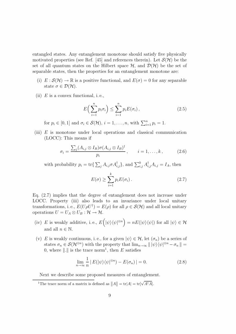
entangled states. Any entanglement monotone should satisfy five physicallymotivated properties (see Ref. [45] and references therein). Let S(H) be theset of all quantum states on the Hilbert space H, and D(H) be the set ofseparable states, then the properties for an entanglement monotone are:

(i) E : S(H) → R is a positive functional, and E(σ) = 0 for any separablestate σ ∈ D(H).

(ii) E is a convex functional, i. e.,

E(

n∑

i=1

piσi

)

≤n

∑

i=1

piE(σi) , (2.5)

for pi ∈ [0, 1] and σi ∈ S(H), i = 1, . . . , n, with∑n

i=1 pi = 1.

(iii) E is monotone under local operations and classical communication(LOCC): This means if

σi =

∑

j(Ai,j ⊗ IB)σ(Ai,j ⊗ IB)†

pi, i = 1, . . . , k , (2.6)

with probability pi = tr∑

j Ai,jσA†i,j, and

∑ki,j A

†i,jAi,j = IA, then

E(σ) ≥k

∑

i=1

piE(σi) . (2.7)

Eq. (2.7) implies that the degree of entanglement does not increase underLOCC. Property (iii) also leads to an invariance under local unitarytransformations, i. e., E(UρU †) = E(ρ) for all ρ ∈ S(H) and all local unitaryoperations U = UA ⊗ UB : H → H.

(iv) E is weakly additive, i. e., E(

|ψ〉〈ψ|⊗n)

= nE(|ψ〉〈ψ|) for all |ψ〉 ∈ Hand all n ∈ N.

(v) E is weakly continuous, i. e., for a given |ψ〉 ∈ H, let (σn) be a series ofstates σn ∈ S(H⊗n) with the property that limn→∞ ‖ |ψ〉〈ψ|⊗n−σn ‖ =0, where ‖.‖ is the trace norm1, then E satisfies

limn→∞

1

n|E(|ψ〉〈ψ|⊗n) − E(σn) | = 0. (2.8)

Next we describe some proposed measures of entanglement.

1The trace norm of a matrix is defined as∥

∥A∥

∥ = tr|A| = tr[√

A†A].

9

Von Neumann entropy

Von Neumann entropy of the reduced quantum state ρB = trA(|ψ〉〈ψ|) is theuniquely defined entanglement measure for pure states of bipartite quantumsystems [29]. It is defined by

E(|ψ〉〈ψ|) = S(trA|ψ〉〈ψ|) = S(trB|ψ〉〈ψ|) , (2.9)

where trA(B) is partial trace over indices of system A(B) and S is the VonNeumann entropy.

Distillable entanglement

Distillable entanglement is defined as the maximal number of maximallyentangled states that can be extracted from many copies of a given entangledstate σ by means of local operations and classical communication (LOCC).We can transform a certain number of non-maximally entangled states intoa smaller number of approximately maximally entangled states with the useof LOCC [46, 47]. Such an extraction is similar to “distilling”. Let D↔denote distillable entanglement [48, 49] with respect to LOCC, also calledtwo-way distillable entanglement.

For pure states S(trA|ψ〉〈ψ|) quantifies the amount of EPR pairscontained asymptotically in the state |ψ〉〈ψ|, i. e.,

D↔ = S(trA|ψ〉〈ψ|) = S(trB|ψ〉〈ψ|) . (2.10)

For a general mixed state, it is hard to evaluate this measure [48, 49]. Forbound entangled states, D↔ = 0.

Entanglement of formation

Entanglement of formation is defined as the number of maximally entangledstates required to prepare copies of a particular state in the asymptotic limitof many copies [50]. For pure states, it is given by

EF (|ψ〉〈ψ|) = S(trA|ψ〉〈ψ|) . (2.11)

This definition can be extended to mixed states by

EF (σ) = min∑

i

µiE(|ψi〉〈ψi|) , (2.12)

where the minimum is taken over all possible decompositions

σ =∑

i

µi|ψi〉〈ψi| . (2.13)

10

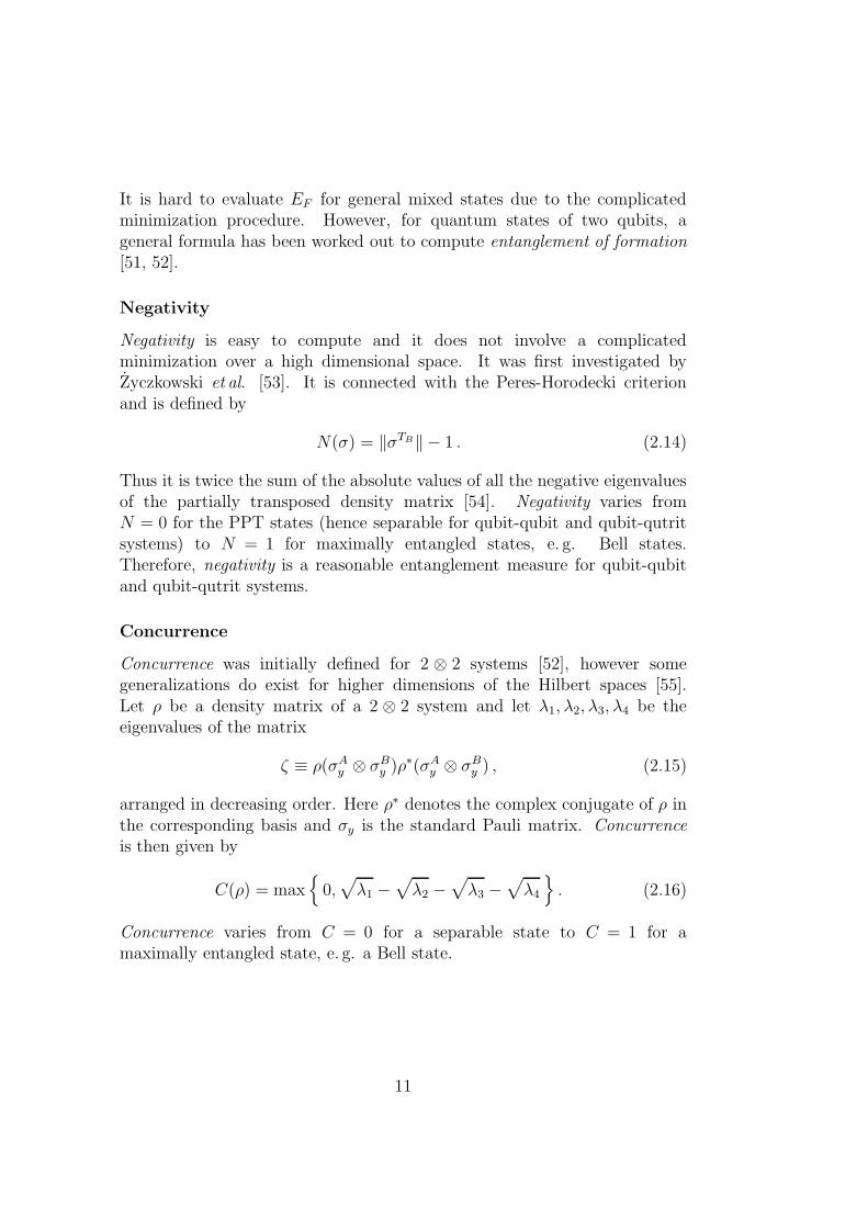
It is hard to evaluate EF for general mixed states due to the complicatedminimization procedure. However, for quantum states of two qubits, ageneral formula has been worked out to compute entanglement of formation[51, 52].

Negativity

Negativity is easy to compute and it does not involve a complicatedminimization over a high dimensional space. It was first investigated byZyczkowski et al. [53]. It is connected with the Peres-Horodecki criterionand is defined by

N(σ) = ‖σTB‖ − 1 . (2.14)

Thus it is twice the sum of the absolute values of all the negative eigenvaluesof the partially transposed density matrix [54]. Negativity varies fromN = 0 for the PPT states (hence separable for qubit-qubit and qubit-qutritsystems) to N = 1 for maximally entangled states, e. g. Bell states.Therefore, negativity is a reasonable entanglement measure for qubit-qubitand qubit-qutrit systems.

Concurrence

Concurrence was initially defined for 2 ⊗ 2 systems [52], however somegeneralizations do exist for higher dimensions of the Hilbert spaces [55].Let ρ be a density matrix of a 2 ⊗ 2 system and let λ1, λ2, λ3, λ4 be theeigenvalues of the matrix

ζ ≡ ρ(σAy ⊗ σB

y )ρ∗(σAy ⊗ σB

y ) , (2.15)

arranged in decreasing order. Here ρ∗ denotes the complex conjugate of ρ inthe corresponding basis and σy is the standard Pauli matrix. Concurrenceis then given by

C(ρ) = max

0,√

λ1 −√

λ2 −√

λ3 −√

λ4

. (2.16)

Concurrence varies from C = 0 for a separable state to C = 1 for amaximally entangled state, e. g. a Bell state.

11

12

Chapter 3

Dynamics of open quantumsystems

An open system is defined as one which has interactions with an environmentwhose dynamics we want to average over. The system of interest is calledthe principal system while any other system is called the environment.Those quantum systems which do not suffer any unwanted interactions withan environment are called closed systems. However, a closed system is anidealization and there does not exist any closed system in Nature exceptprobably the universe itself. Many interesting and fascinating applicationsof quantum information deal with closed quantum systems where theefficiency of information processing reaches its maximum value. Examplesare quantum key distribution [17] and quantum teleportation [19]. Theidealistic conclusions about these quantum feats are effected by the fact thatreal quantum systems always suffer from unwanted interactions with theirenvironments [29]. These unwanted interactions appear as quantum noise.Quantum noise can seriously effect applications of quantum informationprocessing. To understand and control such noise processes is one of thecentral issue in quantum information and quantum computation [29].

The theory of open quantum systems has been discussed extensivelyin the literature (see Ref. [56] and references therein). Contrary to thecase of a closed system, quantum dynamics of an open system does not, ingeneral, follow unitary time evolution. The dynamics of an open system cansometimes be formulated by an appropriate differential equation of motionfor its density operator. This equation is called the quantum master equationwhich may be quite useful in many cases. We will restrict ourselves togeneral Markovian dynamics in which the environmental excitations decayover short times and information regarding past time evolution is destroyed.

This Chapter is organized as follows. In Section 3.1, we discuss the

13

dynamics of quantum systems. The quantum Markov processes and theMarkovian quantum master equation along with the Born- and Markov-approximations are discussed in Section 3.2. The quantum optical masterequation is derived in Section 3.3, where we concentrate on the limiting caseof weak-coupling between radiation and matter.

3.1 Dynamics of a quantum system

3.1.1 The Liouville-Von Neumann equation

Quantum mechanics tells us that the time evolution of a state vector |ψ(t)〉of a closed quantum system is governed by the Schrodinger equation

i ~d

dt|ψ(t)〉 = H |ψ(t)〉 , (3.1)

where H is the Hamiltonian of the system. The solution of Eq. (3.1) maybe written by

|ψ(t)〉 = exp [ − i

~H(t− t0)] |ψ(t0)〉 . (3.2)

For mixed states, the corresponding statistical ensemble is characterizedby a density operator ρ. Let the state of the system at an initial time t0 begiven by the density operator

ρ(t0) =∑

j

pj |ψj(t0)〉〈ψj(t0)| , (3.3)

where pj are the positive weights and |ψj(t0)〉 are the corresponding statevectors. The time evolution of the density operator is given by

ρ(t) = U(t, t0) ρ(t0)U †(t, t0) . (3.4)

The equation of motion for the density operator is given by

d

dtρ(t) = − i

~[H, ρ(t)] . (3.5)

Eq. (3.5) is often called the Liouville or Von Neumann equation of motion.The square brackets on the right hand side of Eq. (3.5) define thecommutator1 between operators H and ρ(t).

1The commutator between two arbitrary operators A and B is defined as[

A, B]

:=AB − BA.

14

In analogy to the equation of motion for probability distribution inclassical statistical mechanics, the Von Neumann equation is sometimewritten as

d

dtρ(t) = L ρ(t) , (3.6)

where L is the Liouville operator defined through the condition that Lρis equal to −i/~ times the commutator of H with ρ(t). L is also calleda Liouville super-operator because it acts on an operator to yield anotheroperator. For a time-independent Hamiltonian the Liouville super-operatoris also time-independent and we have

ρ(t) = exp[L(t− t0)] ρ(t0) . (3.7)

3.1.2 Interaction picture

The interaction picture is a general picture and the Schrodinger picture is alimiting case of it. We can write the Hamiltonian of the system as the sumof two parts

H(t) = H0 + HI(t) . (3.8)

Here, H0 is the time independent sum of energies of two systems in theabsence of interaction. HI(t) is the Hamiltonian describing the interactionbetween the systems. The expectation value of a Schrodinger observableO(t) at time t is given by

〈O(t)〉 = trO(t)U(t, t0)ρ(t0)U †(t, t0) , (3.9)

where ρ(t0) is the state of the system at time t0.Introducing the unitary time evolution operators

U0(t, t0) ≡ exp [ − i

~H0(t− t0)] , (3.10)

and

UI(t, t0) ≡ U †0 (t, t0)U(t, t0) , (3.11)

the expectation value Eq. (3.9) can be written as

〈O(t)〉 = trU †0(t, t0)O(t)U0(t, t0)UI(t, t0)ρ(t0)U †

I (t, t0) ≡ trOI(t)ρI(t) , (3.12)

15

where we have introduced OI(t) as the interaction picture operator

OI(t) ≡ U †0 (t, t0)O(t)U0(t, t0) , (3.13)

and ρI(t) as the interaction picture density operator

ρI(t) ≡ UI(t, t0)ρ(t0)U†I (t, t0) . (3.14)

For the case of vanishing free Hamiltonian H0 = 0, we have H(t) = HI(t)such that U0(t, t0) = I and UI(t, t0) = U(t, t0), and we obtain the Schrodingerpicture.

The interaction picture time-evolution operator UI(t, t0) is the solutionof the differential equation

i ~δ

δtUI(t, t0) = HI(t)UI(t, t0) , (3.15)

with the initial condition UI(t0, t0) = I. In Eq. (3.15), we have denoted theinteraction Hamiltonian in the interaction picture by

HI(t) ≡ U †0(t, t0)HI(t)U0(t, t0) . (3.16)

The corresponding Von Neumann equation in the interaction picture is givenby

d

dtρI(t) = − i

~[HI(t), ρI(t)] . (3.17)

The integral form of the Von Neumann equation in the interaction pictureis given by

ρI(t) = ρI(t0) − i

~

∫ t

t0

dx [HI(x), ρI(x)] . (3.18)

3.1.3 Dynamics of open systems

An open system is a quantum system S which is coupled to another quantumsystem E called environment. An open system represents a subsystem ofthe combined system S + E. In most of the cases, it is assumed that thetotal system is closed and follows the Hamiltonian dynamics. The stateof the system S changes as a consequence of its internal dynamics anddue to interaction with the environment. This interaction leads to certainsystem-environment correlations and corresponding changes of the systemS can no longer be represented in terms of unitary time evolution. Thedynamics of the system S is often called as the reduced system dynamics.

16

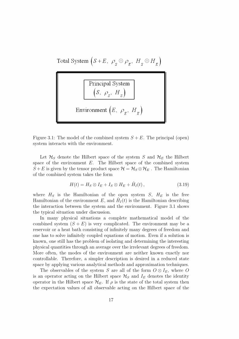
Figure 3.1: The model of the combined system S +E. The principal (open)system interacts with the environment.

Let HS denote the Hilbert space of the system S and HE the Hilbertspace of the environment E. The Hilbert space of the combined systemS+E is given by the tensor product space H = HS ⊗HE . The Hamiltonianof the combined system takes the form

H(t) = HS ⊗ IE + IS ⊗HE + HI(t) , (3.19)

where HS is the Hamiltonian of the open system S, HE is the freeHamiltonian of the environment E, and HI(t) is the Hamiltonian describingthe interaction between the system and the environment. Figure 3.1 showsthe typical situation under discussion.

In many physical situations a complete mathematical model of thecombined system (S + E) is very complicated. The environment may be areservoir or a heat bath consisting of infinitely many degrees of freedom andone has to solve infinitely coupled equations of motion. Even if a solution isknown, one still has the problem of isolating and determining the interestingphysical quantities through an average over the irrelevant degrees of freedom.More often, the modes of the environment are neither known exactly norcontrollable. Therefore, a simpler description is desired in a reduced statespace by applying various analytical methods and approximation techniques.

The observables of the system S are all of the form O ⊗ IE , where Ois an operator acting on the Hilbert space HS and IE denotes the identityoperator in the Hilbert space HE . If ρ is the state of the total system thenthe expectation values of all observable acting on the Hilbert space of the

17

open system S alone are determined by

〈O〉 = tr OρS , (3.20)

where ρS is the reduced density operator of the open system S obtainedby taking trace over the degrees of freedom of the environment E, i. e.,ρS = trEρ. The reduced density operator ρS is of central importance inthe description of the open quantum systems.

The time-dependent reduced density operator ρS(t) at time t is obtainedfrom the density operator ρ(t) of the total system. As the combined systemevolves unitarily, we have

ρS(t) = trE U(t, t0) ρ(t0)U †(t, t0) . (3.21)

Similarly the equation of motion for the reduced density operator is obtainedby taking trace over the environment on both sides of the Von Neumannequation of motion

d

dtρS(t) = − i

~trE [H(t), ρ(t)] . (3.22)

3.2 Quantum Markov processes

An important property of a classical, homogeneous Markov process is thesemigroup property, which is formulated in terms of a differential equationinvolving a time-independent generator. The extension of this idea toquantum mechanics leads to the concept of quantum dynamical semigroupsand quantum Markov processes. In this section, we introduce these conceptsand derive the general form of a quantum Markov master equation.

3.2.1 Quantum dynamical semigroups

The dynamics of the reduced system S (Eq. (3.22)) is in practice quitedifficult to solve. However, with the condition of short environmentalcorrelation time, we may neglect memory effects and formulate the reducedsystem dynamics in terms of a quantum dynamical semigroup.

First we define a dynamical map. Let us prepare the state of the totalsystem (S + E) at time t = 0 in an uncorrelated state ρ(0) = ρS(0) ⊗ ρE.Here, ρS(0) is the initial state of the open system and ρE is the referencestate of the environment. The transformation changing the reduced systemfrom time t = 0 to some later time t > 0 may be written in the form

ρS(0) 7→ ρS(t) = T (t)ρS(0) ≡ trE U(t, 0)[ρS(0) ⊗ ρE ]U †(t, 0) . (3.23)

18

Considering the state ρE and the final time t to be fixed, Eq. (3.23) definesa map from the space S(HS) of density matrices of the reduced system intoitself,

T (t) : S(HS) → S(HS) . (3.24)

This map, describing the state change of an open system over time t, iscalled a dynamical map. A dynamical map can be characterized completelyin terms of operators acting on the Hilbert space HS of the open system S.We use the spectral decomposition of the environment density operator by

ρE =∑

i

λi|ψi〉〈ψi| , (3.25)

where |ψi〉 form an orthonormal basis in HE and λi are non-negative realnumbers satisfying

∑

i λi = 1.Eq. (3.23) yields the following representation

T (t)ρS =∑

i,j

Kij(t)ρSK†ij(t) , (3.26)

where the operators Kij in HS are defined by

Kij(t) =√

λj〈ψi|U(t, 0)|ψj〉 . (3.27)

The dynamical map T (t) is of the form of an operation describing ageneralized quantum measurement and satisfies the condition

∑

i,j

K†ij(t)Kij(t) = IS . (3.28)

Based on this observation, we deduce that

trS T (t) ρS = trS ρS = 1 . (3.29)

Therefore, a dynamical map represents a convex-linear, completely positiveand trace preserving quantum operation.

Eq. (3.26) defines a dynamical map for a fixed time t ≥ 0. However,a complete one-parameter family of maps can be constructed by allowingthe time t to vary. This family of maps with T (0) = I describes the wholefuture time evolution of the open system. If the characteristic time scalesover which the reservoir correlation functions decay are much smaller thanthe characteristic time scale of the system evolution, it is justified to neglectmemory effects in the reduced system dynamics. Similar to classical theory,

19

we expect the Markovian-type behavior. The Markovian-type dynamics maybe formulated using the semigroup property

T (t1)T (t2) = T (t1 + t2) , t1, t2 ≥ 0 . (3.30)

Hence a quantum dynamical semigroup is a continuous, one-parameterfamily of dynamical maps satisfying the semigroup property Eq. (3.30).

3.2.2 The Markovian quantum master equation

For a given quantum dynamical semigroup, a linear map L under certainconditions (discussed below), allows to represent the dynamical map in theform

T (t) = exp(Lt) . (3.31)

This equation yields a first order differential equation for the reduced densityoperator of the open system,

d

dtρS(t) = LρS(t) , (3.32)

called the Markovian quantum master equation. The generator L of thesemigroup is a super-operator.

We can construct the most general form for the generator L. Let usconsider a finite dimensional Hilbert space HS with dim HS = N . Thecorresponding Liouville space 2 is a complex space of dimension N2 and wechoose a complete basis of orthonormal operators Fm, m = 1, 2, . . . , N2, inthis space such that

(Fm, Fn) ≡ tr F †mFn = δmn . (3.33)

Let one of the basis operators be chosen to proportional to the identity,FN2 = (1/

√N)IS, such that the other basis operators are traceless, i. e.,

trFm = 0 for m = 1, 2, . . . , N2 − 1. Applying the completeness relation toeach of the operators in Eq. (3.27), we have

Kij(t) =

N2∑

m=1

Fm(Fm, Kij(t)) . (3.34)

2Given some Hilbert space H the Liouville space is the space of Hilbert-Schmidtoperators, that is the space of operators A ∈ H for which tr(A†A) is finite.

20

Eq. (3.26) in terms of these operators is given by

T (t)ρS =N2∑

m,n=1

cmn(t)FmρSF†n , (3.35)

where

cmn(t) ≡∑

ij

(Fm, Kij(t))(Fn, Kij(t))∗ . (3.36)

The coefficient matrix c = (cij) is easily seen to be Hermitian and positive.Utilizing Eq. (3.35) for small time δt evolution, Eq. (3.32) can be written as

LρS = limδt→0

1

δtT (δt)ρS − ρS

= limδt→0

1

N

cN2N2(δt) −N

δtρS +

1√N

N2−1∑

m=1

(cmN2(δt)

δtFmρS +

cN2m(δt)

δtρSF

†m) +

N2−1∑

m,n=1

cmn(δt)

δtFmρSF

†n

. (3.37)

We can define the coefficients amn by

aN2N2 = limδt→0

cN2N2(δt) −N

δt, (3.38)

amN2 = limδt→0

cmN2(δt)

δt, m = 1, . . . , N2 − 1 , (3.39)

amn = limδt→0

cmn(δt)

δt, m, n = 1, . . . , N2 − 1 , (3.40)

and introduce the quantities

F =1√N

N2−1∑

m=1

amN2Fm , (3.41)

and

G =1

2NaN2N2IS +

1

2(F † + F ) , (3.42)

and the Hermitian operator

H =~

2i(F † − F ) . (3.43)

21

Again the matrix formed by the coefficients amn, m,n = 1, 2, . . . , N2 − 1, isHermitian and positive. With these definitions, we can write the generatoras

LρS = − i

~[H, ρS] + G, ρS +

N2−1∑

m,n=1

amnFmρSF†n . (3.44)

The middle term on the right hand side of Eq. (3.44) defines the anti-commutator3 between the operators G and ρS. As the semigroup is a tracepreserving operator we have

0 = trSLρS = trS

(

2G+N2−1∑

m,n=1

amnF†nFm

)

ρS

, (3.45)

from which we deduce that

G = −1

2

N2−1∑

m,n=1

amnF†nFm . (3.46)

The standard form of the generator (3.44) is given by

LρS = − i

~[H, ρS] +

N2−1∑

m,n=1

amn

(

FmρSF†n − 1

2F †

nFm, ρS)

. (3.47)

Since the coefficient matrix a = (amn) is positive, it may be diagonalized byan appropriate unitary transformation u,

uau† =

γ1 0 · · · 00 γ2 · · · 0

0 0. . . 0

0 0 · · · γN2−1

, (3.48)

where the eigenvalues γm are non-negative. We introduce a new set ofoperators Ak by

Fm =

N2−1∑

k=1

ukmAk , (3.49)

3The anti-commutator between two arbitrary operators A and B is defined as

A, B

:= AB + BA.

22

and the diagonal form of the generator is obtained as

LρS = − i

~[H, ρS] +

N2−1∑

k=1

γk

(

AkρSA†k −

1

2A†

kAkρS − 1

2ρSA

†kAk

)

. (3.50)

This is the most general form for the generator of a quantum dynamicalsemigroup. The first term represents the unitary part of the dynamicsgenerated by the Hamiltonian H . The operators Ak are usually referred asLindblad operators. The non-negative quantities γk have the dimension ofan inverse time provided the Ak are taken dimensionless. We will discusslater that γk are given in terms of certain environment correlation functionsand play the role of relaxation rates for different decay modes of the opensystem.

It is convenient sometimes to introduce the dissipator

D(ρS) ≡∑

k

γk

(

AkρSA†k −

1

2A†

kAkρS − 1

2ρSA

†kAk

)

, (3.51)

and write the quantum master equation (3.32) in the form

d

dtρS(t) = − i

~[H, ρS(t)] + D(ρS(t)) . (3.52)

3.2.3 Born and Markov approximations

The generator of a quantum dynamical semigroup is desired to derive fromthe Hamiltonian of the total system. This derivation can be achieved undercertain assumptions discussed in this section. Let us consider a quantumsystem S weakly coupled to an environment E. The Hamiltonian of thetotal system is given by

H = HS +HE +HI , (3.53)

where HS (HE) denotes the free Hamiltonian of the system (environment)and HI is the Hamiltonian responsible for the interaction between thesystem and the environment. In the interaction picture, the Von Neumannequation for the total density operator ρ(t) is given by

d

dtρ(t) = − i

~[HI(t), ρ(t)] , (3.54)

and its integral form is

ρ(t) = ρ(0) − i

~

∫ t

0

dx [HI(x), ρ(x)] . (3.55)

23

Substituting Eq. (3.55) back into Eq. (3.54), we find the equation of motion

d

dtρ(t) = − i

~[HI(t), ρ(0)] − 1

~2

∫ t

0

dx [HI(t), [HI(x), ρ(x)] ] . (3.56)

If the interaction energy HI(t) is zero, the system and the environment areindependent and the density operator ρ would factor as a direct productρ(t) = ρS(t)⊗ρE(0), where the environment is assumed to be at equilibrium.As the interaction is weak, we look for a solution of the form [57]

ρ(t) = ρS(t) ⊗ ρE(0) + ρc(t) , (3.57)

where ρc(t) is of higher order in HI(t). As the reduced density operatorfor the system ρS is obtained by taking a trace over the environmentcoordinates, therefore trρc(t) = 0. This approximation is called the Bornapproximation, which assumes that the coupling between the system andthe environment is weak, such that the influence of the system on theenvironment is small. Therefore, the density operator ρE of the environmentis negligibly affected by the interaction and the state of the total systemat time t may be approximately described by a tensor product. InsertingEq. (3.57) into Eq. (3.56) and taking the trace over the environmentcoordinates and retaining terms up to order H2

I (t), we obtain

d

dtρS(t) = − i

~trE [HI(t), ρS(0) ⊗ ρE(0)]

− 1

~2trE

∫ t

0

dx[

HI(t), [HI(x), ρS(x) ⊗ ρE(0)]]

. (3.58)

The Born approximation does not imply that there are no excitationsin the environment. The Markov approximation provides a descriptionon a coarse-grained time scale and the assumption that environmentalexcitations decay over short times which can not be resolved. In the Markovapproximation, ρS(x) is replaced by ρS(t). This is a reasonable assumptionsince damping destroys memory of the past. We can write Eq. (3.58) as

d

dtρS(t) = − i

~trE [HI(t), ρS(0) ⊗ ρE(0)]

− 1

~2trE

∫ t

0

dx[

HI(t), [HI(x), ρS(t) ⊗ ρE(0)]]

. (3.59)

This is a valid equation for a system represented by ρS interacting with areservoir represented by ρE.

24

3.3 The quantum optical master equation

Quantum dynamical semigroups and quantum Markovian master equationare easily realized in quantum optics as the physical conditions underlyingthe Markovian approximation are very well satisfied. We discuss belowatom-field interaction as an example relevant for our work.

3.3.1 Matter-field interaction Hamiltonian

We consider a quantum system e. g. an atom interacting with a quantizedradiation field. The radiation field represents an environment with infinitenumber of degrees of freedom and the quantum atomic system is our systemof interest. The quantized electric field [57] is given by

E(r, t) =∑

k

ǫkEk(ake−iνkt+ik·r + a†keiνkt−ik·r) . (3.60)

The electric field operator is evaluated in the dipole approximation at theposition of the point atom. For the atom at the origin (taking the center ofmass at origin), Eq. (3.60) reduces to

E =∑

k

ǫk Ek (ak + a†k) , (3.61)

where Ek = (~νk/2ǫ0V )1/2. The interaction of a radiation field E with asingle-electron atom can be written [57] in the dipole approximation by

H = HA +HF − e r · E , (3.62)

where HA and HF are the energies of the atom and the field respectively,when there is no interaction and r is the position vector of the electron. Inthe dipole approximation, the field is taken to be uniform over the wholeatom.

The energy HF is given in terms of creation a†k and destruction ak

operators by

HF =∑

k

~νk

(

a†kak +1

2

)

, (3.63)

here νk is the frequency of kth mode. The atomic energy HA and e rcan be written in terms of the atomic transition operators σij = |i〉〈j|.This operator takes an atom from level |j〉 to level |i〉. Let |i〉 denotes

25

a complete set of atomic energy eigenstates, such that∑

i |i〉〈i| = 1 andHA |i〉 = Ei |i〉. It then follows that

HA =∑

i

Ei |i〉〈i| =∑

i

Ei σii , (3.64)

and

e r =∑

i,j

e |i〉〈i| r |j〉〈j| =∑

i,j

℘ij σij , (3.65)

where ℘ij = e 〈i| r |j〉 is the electric-dipole transition matrix element.Substituting expressions of HA, HF , e r, and E into Eq. (3.62), we get

H =∑

k

~νk a†kak +

∑

i

Ei σii + ~

∑

i,j

∑

k

gijk σij (ak + a†k) , (3.66)

where

gijk = −(℘ij · ǫk Ek)/~ , (3.67)

and we have subtracted the zero-point energy. For simplicity, we havedecomposed the radiation field into Fourier modes in a box of volume V ,with periodic boundary conditions.

We discuss the case of a two level atom with |a〉 and |b〉 defined as theexcited and the ground states, respectively. For simplicity, we assume ℘ab tobe real, i. e., ℘ab = ℘ba and gk = gab

k = gbak . Eq. (3.66) can be written as

H =∑

k

~νk a†kak + (Eaσaa + Ebσbb) + ~

∑

k

gk(σab + σba)(ak + a†k) .(3.68)

We can simplify this relation by rewritting the second term as

Eaσaa + Ebσbb =1

2~ω(σaa − σbb) +

1

2(Ea + Eb) , (3.69)

where ~ω = (Ea −Eb) and σaa + σbb = 1. We can ignore the constant energyterm (Ea + Eb)/2. We introduce the notation

σz = σaa − σbb = |a〉〈a| − |b〉〈b| , (3.70)

σ+ = σab = |a〉〈b| , (3.71)

σ− = σba = |b〉〈a| , (3.72)

26

where σ+ takes an atom in the ground state |b〉 to the excited state |a〉and σ− takes an atom from the excited state |a〉 to the ground state |b〉.Eq. (3.68) can be written in the form

H =∑

k

~νk a†kak +

1

2~ωσz + ~

∑

k

gk(σ+ + σ−)(ak + a†k) . (3.73)

This Hamiltonian contains four interacting terms. The term a†kσ− describesa process where atom makes a transition from the upper to the lower energystate and a photon of mode k is created. The term akσ+ is the oppositeprocess. In both processes the energy is conserved. However, the term akσ−represents a process where atom makes transition from the upper to thelower level and a photon of mode k is absorbed. This leads to a loss of 2~ωenergy. Similarly the term a†kσ+ represents a gain of 2~ω energy. We canignore these two energy nonconserving terms. This approximation is calledthe rotating-wave approximation. The Hamiltonian after this approximationcan be written as

H =∑

k

~νk a†kak +

1

2~ωσz + ~

∑

k

gk(σ+ak + a†kσ−) . (3.74)

This Hamiltonian describes the interaction of a single two-level atom with amulti-mode radiation field. We can split this Hamiltonian in two parts as

H = H0 +H1 , (3.75)

where

H0 =∑

k

~νk a†kak +

1

2~ωσz , (3.76)

H1 =∑

k

gk(σ+ak + a†kσ−) . (3.77)

The Hamiltonian (3.74) in the interaction picture is given as

HI(t) = eiH0t/~H1 e−iH0t/~ . (3.78)

We use the relation

eαAB e−αA = B + α[A,B] +α2

2![A, [A,B]] + . . . , (3.79)

to calculate the following relations

ei νka†kakt a e−i νka†

kakt = ake−i νkt , (3.80)

ei ωσzt/2 σ+ e−i ωσzt/2 = σ+ei ωt . (3.81)

27

Combining these relations, Eq. (3.78) can be given as

HI(t) = ~

∑

k

gk

[

a†k σ− e−i(ω−νk)t + ak σ+ ei(ω−νk)t]

. (3.82)

Now our system corresponds to the two-level atom i. e., ρS ≡ ρatom. Weinsert the interaction energy HI(t) (Eq. (3.82)) into the equation of motion(3.59) and obtain

d

dtρatom(t) = −i

∑

k

gk〈a†k〉[σ−, ρatom(0)]e−i(ω−νk)t −∫ t

0

dx∑

k,kx

gkgkx

[σ−σ−ρatom(x) − 2σ−ρatom(x)σ− + ρatom(x)σ−σ−]

×e−i(ω−νk)t−i(ω−νkx )x〈a†ka†kx〉 + [σ−σ+ρatom(x) − σ+ρatom(x)σ−]

×e−i(ω−νk)t+i(ω−νkx )x〈a†kakx〉 + [σ+σ−ρatom(x) − σ−ρatom(x)σ+]

×ei(ω−νk)t−i(ω−νkx )x〈aka†kx〉

+ H.c. , (3.83)

where H.c. stands for the Hermitian conjugate and the expectation valuesrefer to the initial state of the reservoir.

3.3.2 Atomic decay by thermal reservoirs

Let us take the reservoir variables in the uncorrelated thermal equilibriummixture of states. The reduced density operator is the multi-mode extensionof the thermal operator, given by

ρE =∏

k

[

1 − exp(

− ~νk

kβT

)]

exp(

− ~νk a†kak

kβT

)

, (3.84)

where kβ is the Boltzmann constant and T is the temperature. It can beshown easily that

〈ak〉 = 〈a†k〉 = 0 , (3.85)

〈a†kakx〉 = nk δkkx , (3.86)

〈aka†kx〉 = (nk + 1) δkkx , (3.87)

〈akakx〉 = 〈a†ka†kx〉 = 0 , (3.88)

where nk is the mean thermal photon number given by

nk =1

exp ( ~νk

kβT) − 1

. (3.89)

28

We substitute these expectation values in Eq. (3.83) and get

d

dtρatom(t) = −

∫ t

0

dx∑

k

g2k

[σ−σ+ρatom(x) − σ+ρatom(x)σ−]

×nke−i(ω−νk)(t−x) + [σ+σ−ρatom(x) − σ−ρatom(x)σ+]

×(nk + 1)ei(ω−νk)(t−x)

+ H.c. , (3.90)

We replace the sum over k by an integral

∑

k

→ 2V

(2π)3

∫ 2π

0

dφ

∫ π

0

dθ sin θ

∫ ∞

o

dk k2 , (3.91)

where V is the quantization volume. From Eq. (3.67) follows that

g2k =

νk

2~ǫ0V℘2

ab cos2 θ , (3.92)

where θ is the angle between the atomic dipole moment ℘ab and the electricfield polarization vector ǫk. Substituting relations (3.91) and (3.92) inEq. (3.90), we get

d

dtρatom(t) = − 1

4πǫ0

4℘2ab

3~c3

∫ ∞

0

dνk ν3k

∫ t

0

dx

[σ−σ+ρatom(x) − σ+ρatom(x)σ−]

×nke−i(ω−νk)(t−x) + [σ+σ−ρatom(x) − σ−ρatom(x)σ+]

×(nk + 1)ei(ω−νk)(t−x)

+ H.c. , (3.93)

where we have carried out integrations over θ and φ and used k = νk/c. Theintensity of light related with the emitted radiation is centred about theatomic transition frequency ω. The frequency ν3

k varies little around νk = ωand the time integral for it in Eq. (3.93) can not be ignored. We can replaceν3

k by ω3 and the lower limit in the νk integral by −∞. With the integral

∫ ∞

−∞dνk ei(ω−νk)(t−x) = 2π δ(t− x) , (3.94)

Eq. (3.93) can be written by

d

dtρatom(t) = −(nth + 1)

Γ

2[σ+σ−ρatom(t) − σ−ρatom(t)σ+]

−nthΓ

2[σ−σ+ρatom(t) − σ+ρatom(t)σ−] + H.c. , (3.95)

29

where nth ≡ nk0(k0 = ω/c) and

Γ =1

4πǫ0

4℘2ab

3~c3(3.96)

is the atomic decay rate.The equations of motion for the atomic density matrix are given by

ρaa = 〈a| ρatom |a〉= −(nth + 1) Γ ρaa + nth Γ ρbb , (3.97)

ρab = ρ∗ba = −(nth +1

2) Γ ρab (3.98)

ρbb = (nth + 1)Γ ρaa − nth Γ ρbb . (3.99)

For the special case of vacuum reservoirs, i. e., the reservoir atzero-temperature (nth = 0), the equations of motion reduces to

ρaa = −Γ ρaa , (3.100)

ρab = −Γ

2ρab , (3.101)

ρbb = Γ ρaa . (3.102)

30

Chapter 4

Entanglement sudden death

We have argued in Chapter 1 that quantum entanglement is a resource formany applications of quantum information processing. For example, thefields of quantum computing [13, 14, 15, 16], quantum key distribution [17],and quantum teleportation [19, 21] all rely on having entangled states of atleast two qubits. To accomplish the various quantum feats, the presence ofentanglement among the parties sharing quantum states is both necessaryand important. It was soon realized that entanglement is a dynamic resourceand dynamics of entanglement depends on the choice of a physical systemand an environment. The unavoidable interaction of entangled states withenvironments usually causes a decrement in the amount of entanglement.This unavoidable interaction is called decoherence. Decoherence is a seriouslimitation to quantum information processing. In addition, a deeperunderstanding of quantum decoherence is also necessary for bringing newinsights into the foundations of quantum mechanics, in particular quantummeasurement and quantum to classical transitions [58, 59, 60].

For entangled states with the subsystems coupled to their own individualenvironments, decoherence affects both the local and the global coherences.Since each qubit is inevitably subject to decoherence and decay processes,no matter how much they may be screened from the external environment,it is important to consider possible degradation of any initially establishedentanglement. It is no surprise that decoherence leads to a gradual decay(taking infinite time for complete disentanglement) of initially preparedentanglement. Yu and Eberly reported the surprising phenomenon thatalthough local coherence is lost asymptotically there are some situationswhen global coherence (entanglement) is completely lost in a finite time [61].Such finite-time disentanglement process is called entanglement sudden death.Yu and Eberly have studied a particular case where two initially entangledqubits are located inside two statistically independent vacuum reservoirs.

31

They showed that the simple phenomenon of spontaneous emission causedby vacuum fluctuations have different effect on local and global coherences.Some quantum states undergo finite-time disentanglement while others donot. Soon after this study, Jakobczyk and Jamroz showed that certainentangled states of two qubits interacting with two independent thermalbaths at very high temperatures exhibit finite-time disentanglement [62].Dodd and Halliwell showed the existence of sudden death for continuous-variable systems [58, 59]. Later, Yu and Eberly demonstrated this effectunder classical noise [63]. Below we demonstrate this phenomenon bothin amplitude damping and in phase damping environments. Experimentalevidences for this effect have been reported recently [64, 65, 66]. Clearly,such finite-time disappearance of entanglement can seriously affect itsapplications in quantum information processing.

This chapter is organized as follows. In Section 4.1, we describesudden death caused by amplitude damping. In Section 4.2, we discusssudden death via phase damping. Other investigations regarding finite-timedisentanglement are discussed in Section 4.3.

4.1 Sudden death via amplitude damping

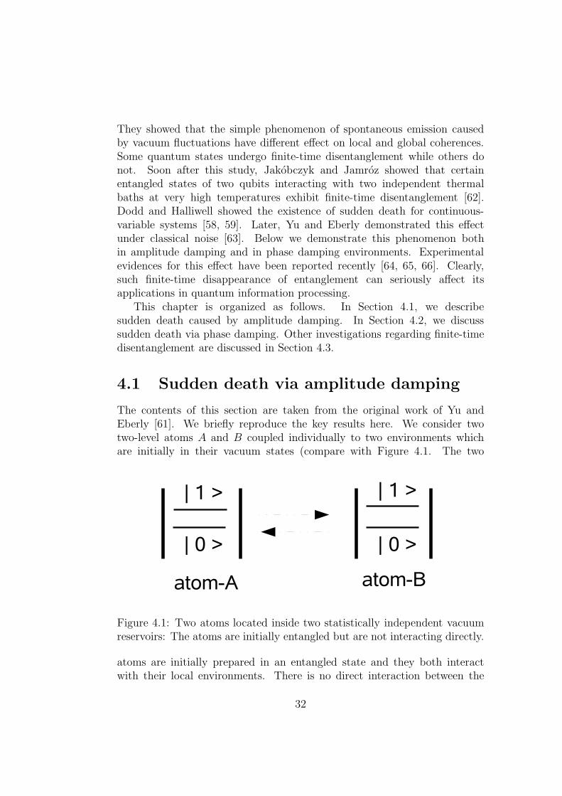
The contents of this section are taken from the original work of Yu andEberly [61]. We briefly reproduce the key results here. We consider twotwo-level atoms A and B coupled individually to two environments whichare initially in their vacuum states (compare with Figure 4.1. The two

Figure 4.1: Two atoms located inside two statistically independent vacuumreservoirs: The atoms are initially entangled but are not interacting directly.

atoms are initially prepared in an entangled state and they both interactwith their local environments. There is no direct interaction between the

32

atoms anymore. The interaction between each atom and its environmentleads to a loss of both local coherence and quantum entanglement of the twoatoms. The total Hamiltonian of the combined system is given by

Htot = Hat +Henv +Hint , (4.1)

where Hat is the Hamiltonian of the two atoms, Henv is the Hamiltonianof the environments, and Hint is the Hamiltonian describing the interactionbetween the atoms and the reservoirs. The standard two-qubit productbasis is denoted |1〉AB = |1, 1〉AB, |2〉AB = |1, 0〉AB, |3〉AB = |0, 1〉AB, and|4〉AB = |0, 0〉AB, where |1, 1〉AB describes the state in which both atoms arein their excited states, etc.

Following the standard methods of averaging over reservoirs degrees offreedom, using the dipole- and rotating-wave approximations, and solvingthe master equation, one obtains the complete dynamics of system of thetwo atoms (see Chapter 3). We demonstrate finite-time disentanglement inthis particular setup by choosing an initially entangled state

ρ =1

3

a 0 0 00 1 1 00 1 1 00 0 0 1 − a

, (4.2)

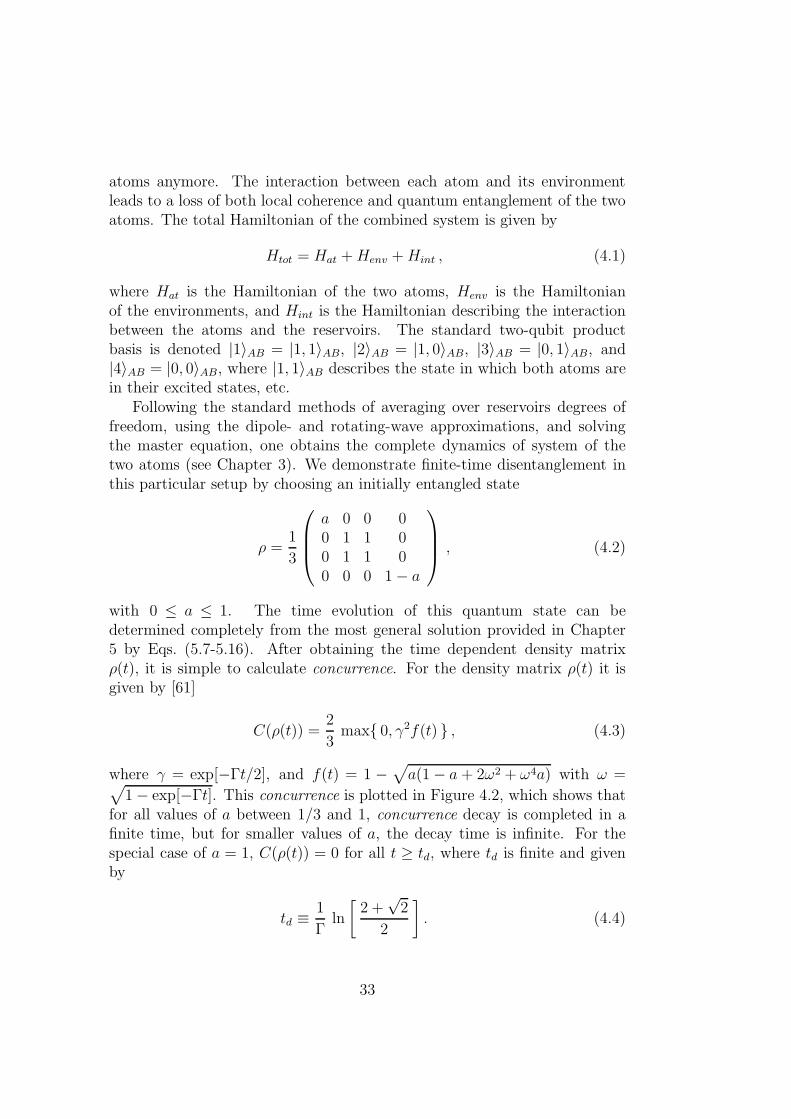
with 0 ≤ a ≤ 1. The time evolution of this quantum state can bedetermined completely from the most general solution provided in Chapter5 by Eqs. (5.7-5.16). After obtaining the time dependent density matrixρ(t), it is simple to calculate concurrence. For the density matrix ρ(t) it isgiven by [61]

C(ρ(t)) =2

3max 0, γ2f(t) , (4.3)

where γ = exp[−Γt/2], and f(t) = 1 −√

a(1 − a + 2ω2 + ω4a) with ω =√

1 − exp[−Γt]. This concurrence is plotted in Figure 4.2, which shows thatfor all values of a between 1/3 and 1, concurrence decay is completed in afinite time, but for smaller values of a, the decay time is infinite. For thespecial case of a = 1, C(ρ(t)) = 0 for all t ≥ td, where td is finite and givenby

td ≡ 1

Γln

[

2 +√

2

2

]

. (4.4)

33

01

2Gt

13

1

a

23CHΡL

01

2Gt

Figure 4.2: Concurrence is plotted against the decay parameter Γt and thesingle parameter a: Finite-time disentanglement takes place for a > 1/3,whereas for a ≤ 1/3, entanglement decays only asymptotically.

4.2 Sudden death via phase damping

Phase damping or classical noise is another type of decoherence responsiblefor decay of both local and global coherences. In this section, we describethe possibility of entanglement sudden death arising from the influence ofclassical noise on two qubits which are initially prepared in an entangledstate but have no direct interaction. The discussion of decoherence due toclassical noise can be further divided into two classes. In Section 4.2.1, wedescribe the effects of global collective noise on both qubits. The effects ofexposing each qubit separately to local noise are discussed in Section 4.2.2.

4.2.1 Disentanglement due to global collective noise

We consider two qubits initially prepared in an entangled state which areaffected collectively by a single stochastic field. The Hamiltonian of thequbits plus the classical noisy field is given by

H(t) = −1

2µB(t) (σA

z + σBz ) , (4.5)

34

where µ is the gyromagnetic ratio, and σA,Bz are the Pauli matrices in the

standard basis defined in Section 4.1. We assume that B(t) is a Gaussianfield and satisfies the Markov condition

〈B(t)〉 = 0 ,

〈B(t)B(t′)〉 =Γ

µ2δ(t− t′) , (4.6)

where 〈. . .〉 stands for an ensemble average and Γ is the dephasing dampingrate due to the collective interaction with B(t).

The solution for the reduced system under the Hamiltonian (4.5) can beobtained by various methods, e. g. master equation, stochastic Schrodingerequation, and the operator sum representation. The reduced density matrixfor the two qubits can be obtained from the statistical density operatorρst(t) for both qubits and a classical Gaussian field by taking the ensembleaverage over the noisy field B(t) given by

ρ(t) = 〈 ρst(t) 〉 , (4.7)

where the statistical density operator ρst(t) is given by

ρst(t) = U(t) ρ(0)U †(t) , (4.8)

with the unitary operator U(t) = exp[−i∫ t

0dt′H(t′)] . The explicit form of

the unitary operator is given by

U(t) = exp[ iµ

2

∫ t

0

dt′B(t′) (σAz + σB

z ) ] . (4.9)

We can average over noise degrees of freedom in Eq. (4.8) and can write themost general solution in terms of the Kraus operators [67]

ρ(t) =

3∑

j=1

K†j (t) ρ(0)Kj(t) , (4.10)

where the Kraus operators describing the collective interaction are given by

K1 =

γ 0 0 00 1 0 00 0 1 00 0 0 γ

,

K2 =

ω1 0 0 00 0 0 00 0 0 00 0 0 ω2

,

35

K3 =

0 0 0 00 0 0 00 0 0 00 0 0 ω3

, (4.11)

where γ = e−Γt/2, ω1 =√

1 − γ2, ω2 = −γ2√

1 − γ2, ω3 = (1 − γ2)√

1 + γ2.Let us consider a special class of mixed states namely X-states, where the

only non-zero matrix elements are on diagonal and anti-diagonal positions.The density matrix for X-states is given by

ρX =

ρ11 0 0 ρ14

0 ρ22 ρ23 00 ρ32 ρ33 0ρ41 0 0 ρ44

. (4.12)

Eq. (4.10) leads to

ρX(t) =

ρ11 0 0 γ4ρ14

0 ρ22 ρ23 00 ρ32 ρ33 0

γ4ρ41 0 0 ρ44

. (4.13)

From Eq. (4.13), it is clear that the collective noise only affects theoff-diagonal elements ρ14 and ρ41 and leaves all other elements intact. Inparticular the diagonal elements remain constant in time. This is in contrastto amplitude damping, where all matrix elements are affected. For purephase damping, the collective global field allows certain phase combinationsto cancel out and generates a decoherence-free subspace [68, 69] spannedby |1, 0〉 and |0, 1〉. However, we avoid such protection by assumingρ23 = ρ32 = 0. Concurrence of ρX(t) is given by

C(ρX(t)) = 2 max 0, |ρ14(t)| − √ρ22ρ33 , |ρ23(t)| − √

ρ11ρ44 . (4.14)

Therefore ρX(t) is separable if and only if |ρ14(t)| − √ρ22ρ33 ≤ 0, and

|ρ23(t)| −√ρ11ρ44 ≤ 0. Concurrence of the density matrix (4.13) with

ρ23 = ρ32 = 0 is given as

C(ρX(t) = 2 max 0, |ρ14| e−2Γt −√ρ22ρ33 . (4.15)

The critical time for finite-time disentanglement is given as

tc =1

2Γln

|ρ14|√ρ22ρ33

(4.16)

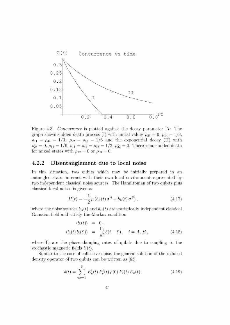
with C(ρX(t)) = 0 for t ≥ tc. It is clear from Eq. (4.16) that for ρ22 6= 0 andρ33 6= 0, sudden death will occur at time tc. If any of these matrix elementsis zero, then entanglement decays asymptotically. These features are shownin Figure 4.3.

36

0.2 0.4 0.6 0.8Gt

0.05

0.1

0.15

0.2

0.25

0.3

CHΡL Concurrence vs time

III

Figure 4.3: Concurrence is plotted against the decay parameter Γt: Thegraph shows sudden death process (I) with initial values ρ23 = 0, ρ14 = 1/3,ρ11 = ρ44 = 1/3, ρ22 = ρ33 = 1/6 and the exponential decay (II) withρ23 = 0, ρ14 = 1/6, ρ11 = ρ44 = ρ33 = 1/3, ρ22 = 0. There is no sudden deathfor mixed states with ρ22 = 0 or ρ33 = 0.

4.2.2 Disentanglement due to local noise

In this situation, two qubits which may be initially prepared in anentangled state, interact with their own local environment represented bytwo independent classical noise sources. The Hamiltonian of two qubits plusclassical local noises is given as

H(t) = −1

2µ (bA(t) σA + bB(t) σB) , (4.17)

where the noise sources bA(t) and bB(t) are statistically independent classicalGaussian field and satisfy the Markov condition

〈bi(t)〉 = 0 ,

〈bi(t) bi(t′)〉 =Γi

µ2δ(t− t′) , i = A, B , (4.18)

where Γi are the phase damping rates of qubits due to coupling to thestochastic magnetic fields bi(t).

Similar to the case of collective noise, the general solution of the reduceddensity operator of two qubits can be written as [63]

ρ(t) =2

∑

u,v=1

E†u(t)F †

v (t) ρ(0)Fv(t)Eu(t) , (4.19)

37

where the Kraus operators describing the interaction with local environmentsare given by

E1 =

(

1 00 γA

)

⊗ I , E2 =

(

0 00 ωA

)

⊗ I , (4.20)

F1 = I ⊗(

1 00 γB

)

, F2 = I ⊗(

0 00 ωB

)

, (4.21)

with γA = e−ΓAt/2, γB = e−ΓBt/2, ωA =√

1 − γ2A, ωB =

√

1 − γ2B.

For X-states (4.12), the general solution is given by

ρ(t) =

ρ11 0 0 γAγBρ14

0 ρ22 γAγBρ23 00 γAγBρ32 ρ33 0

γAγBρ41 0 0 ρ44

. (4.22)

This means that when both qubits are exposed to local dephasing separately,there is no decoherence-free subspace. Comparing Eq. (4.22) with Eq. (4.13),we observe that sudden death may appear in this case as well. However, thetime of disentanglement is different due to the change of noise but suddendeath appears for all non-zero diagonal elements.

4.3 Further recent investigations

In this section, we shortly review recent results of investigations on suddendeath of entanglement in various situations. The work of Yu-Eberly [61, 63]and Jakobczyk-Jamroz [62] attracted a lot of people to this problem.Dodd-Halliwell [58, 59] investigated the process of disentanglement for thecontinuous variables systems. The dynamics of two-qubits entanglementwas explored in symmetry-broken environment [70]. It was shown [71] thatfor pure decoherence the decay of two-qubit entanglement is approximatelygoverned by the product of the suppression factors describing docoherence ofsubsystems, if they are subjected to uncorrelated noise. Liang showed that ifthe initial state is not a maximally entangled state then entanglement decaysfaster than the product of the suppression factors describing decoherence ofqubits [72]. Entanglement sudden death of two-qubits in Jaynes-Cummingsmodel was investigated as well [73]. The time evolution of entanglement forbipartite systems of arbitrary dimensions was also investigated [74]. Theanalysis of sudden death of two-qubit X-states under amplitude damping,phase damping and state-equalizing noise was done in [75]. It was alsoshown that the partial dephasing induced by a super-Ohmic reservoir, may

38

also lead to sudden death [76]. The phase-induced collapse and revivalof entanglement of two-qubit entangled states interacting in a trap waspredicted [77]. Ban investigated decoherence of the Gaussian states underthe influence of non-Markovian quantum channels [78] and the correlated andcollective stochastic dephasing of two-qubit entanglement [79]. The directmeasurement of ESD was proposed [80] through the measurement of a singleobservable invariant with respect to decay process. This was an additionaleffort to give physical meaning to measures of entanglement. Decoherenceof entanglement of two-qubits interacting via a Heisenberg XY chaininteraction was studied in [81]. Lamata et al. showed that entanglementbetween two-qubits decreases when the correlations are transferred locallyto the momentum degree of freedom of one of the qubit [82]. Jamrozstudied local aspects of ESD induced by spontaneous emission and showedthat locally equivalent entangled states exhibit different behavior in theirdisentanglement process [83]. Yu-Eberly demonstrated another surprisingresult that if a single qubit is exposed to both amplitude damping andphase damping, the decay rate is additive, however for the simplest caseof entangled two-qubits this additivity of decay rate breaks down [84].Ficek and Tanas showed that when two qubits are coupled collectively to amultimode field, the irreversible spontaneous decay can lead to a revival ofentanglement that has already been destroyed [85]. The effect of quantuminterference [86] on entanglement of two three level atoms has been studied[87]. It was shown that quantum interference can slow down the process ofdisentanglement and for maximum interference this system (qutrit-qutrit)has non-trivial asymptotic entangled states.

Cui et al. studied ESD for bipartite systems subjected to differentscenarios [88]. Sun et al. investigated the dynamics of entanglement fortwo-qubits and two-qutrits coupled to an Ising spin chain in a transversefield [89]. Huang and Zhu worked out the necessary and sufficient conditionsfor sudden death of entanglement of two-qubits via phase dampingand amplitude damping [90]. Ann and Jaeger demonstrated finite-timedisentanglement due to multi-local dephasing noise for a class of bipartitestates in finite-dimensional systems [91]. We studied disentanglement dueto amplitude damping in qubit-qutrit systems [92] (see Section 6.1). Annand Jaeger studied finite-time disentanglement for qubit-qutrit systemsdue to phase damping [93]. Ikram et al. studied the time evolution ofvarious entangled states of two-qubits exposed to thermal and squeezedreservoirs. They numerically showed that maximally entangled state (Bellstate) exhibits sudden death interacting with independent thermal reservoirsand conjectured that all quantum states exhibit sudden death in thermalreservoirs [94]. Cunha discussed the geometrical point of view for sudden

39

death [95]. Eberly-Yu mentioned the implications of sudden death forquantum information processing [96]. Lastra et al. investigated the abruptchanges in disentanglement in qutrit-qutrit systems [97]. The story took animportant turn by the experimental verification of sudden death. Suddendeath has been reported in laboratory for optical setups [64, 65] and for anatomic ensemble [66]. Fanchini and Napolitano studied protection of suddendeath of two-qubits using continuous dynamical decoupling [98].

Another parallel investigation focused on non-locality of quantum statesvia violation of Bell inequalities. The quantum states which initially violatesa Bell inequality may not violate it after some finite time. Such studieshave been extensively done for different scenarios, see for example Refs.[99, 100, 101] and references therein.

We have extended the discussion of sudden death towards its hastening,delaying, and avoiding. We have shown that simple local unitary actionscan delay or even completely avoid sudden death of two-qubits interactingwith independent reservoirs at zero-temperature [102]. Al-Qasimi andJames studied disentanglement of two-qubits interacting with independentreservoirs at finite-temperature. Similar to our analytical conclusions [129],they showed that large number of quantum states exhibit sudden death atfinite-temperature [103]. Bellomo et al. studied entanglement dynamics oftwo-qubits interacting with independent reservoirs at zero-temperature withnon-Markovian assumption. They also considered the effect of two-qubitsentanglement dynamics interacting with statistically independent finite-temperature reservoirs without memory [104]. Cao and Zheng investigateddisentanglement process for certain classes of two-qubits entangled statesin non-Markovian approach. They have shown that entanglement decaysasymptotically only in the case of weak coupling between a system and anenvironment. For strong coupling between a qubit and an environment,entanglement sudden death always appear even if the reservoirs are atzero-temperature [105]. Lastra et al. studied the time evolution of aclass of entangled coherent states of two electromagnetic fields underdissipation. They concluded that asymptotic decay and sudden death canbe found depending on the initial condition and phase space distancesamong the component of each mode [106]. Hernandes and Orszag studieddisentanglement for two qubits in a common squeezed reservoir and workedout the relation between sudden death and revival of entanglement [107].Sainz and Bjork suggested a scheme to delay, cause and combat suddendeath with non-local quantum error correction [108, 109]. Tahira et al.investigated entanglement dynamics of a pure bipartite system subjectedto dissipative environments. They found that doubly excited component(means both atoms are in excited states) is a necessary condition for

40

sudden death in vacuum reservoirs, while all pure states exhibit suddendeath in finite-temperature reservoirs [110]. Derkacz and Jakobczyk studiedthe dynamics of entanglement between two three-level atoms coupledto the common vacuum reservoir [111]. Jian Li et al. analyzed theenhancement of sudden death for driven qubits and shown that the timeof sudden death decreases due to driving [112]. Wang et al. exploreddecoherence of two-qubits in a non-Markovian reservoir without rotatingwave approximation [113]. Yamamoto et al. have shown that suddendeath appearing in a linear quantum network can be avoided via directmeasurement feedback method [114]. Scala et al. analyzed entanglementdynamics of two coupled qubits while interacting with two independentbosonic baths [115]. Shan et al. investigated entanglement properties fortwo-qubits in the Heisenberg XY interaction and subjected to a magneticfield. They found that sudden death and sudden birth of entanglementappear during the evolution process for particular initial states [116]. Peng Liet al. shown that for composite noise environment, two-qubits Hilbert spacecan be divided into two parts: a 3-dimensional subspace in which all statesdisentangle asymptotically and that in which all states exhibit finite-timedisentanglement [?]. Cole observed that sudden death of entanglementappears when bipartite entanglement is shared among multiparties. Hencefor a particular partition of this multipartite entangled system, ESD mayappear [118]. Chan et al. investigated entanglement dynamics of two distantbut non-identical atoms interacting independently a cavity field as in theJaynes-Cummings model [119]. Dajka and Luczka studied the originationand survival of qudit-qudit (two d-dimensional systems) entanglement forvarious environments [120]. Marek et al. derived a sufficient conditionfor infinite dimensional systems which do not exhibit sudden death whileinteracting with vacuum environments. They clarified a class of bipartiteentangled states which are tolerant against decoherence in a vacuum[121]. Drumond and Cunha analyzed entanglement dynamics of two-qubitsinteracting with several relaxing environments in the light of geometry[122]. Dubi and Ventra studied two interacting qubits in a magnetic fieldand a thermal Markovian environment, presenting nonmonotonic relaxationrates as functions of the magnetic field and temperature [123]. Al-Qasimiand James showed that for the continuous variable quantum systems,two-mode-N -photon states undergoing pure dephasing never exhibit suddendeath [124]. Lastra et al. studied disentanglement of two distinguishableatoms and quantum recoil effects [125]. Paz and Roncaglia studied twoharmonic oscillators coupled to a common environment also modelled asoscillators [126]. Sudden death of entanglement and entanglement revivalare examined as well as non-Markovian environments. Lopez et al. found

41

that for two-qubits interacting with independent reservoirs, sudden deathof entanglement necessarily means sudden birth of entanglement (ESB) inreservoirs [127]. Mazzola et al. studied entanglement dynamics of two-qubitsin a common structured reservoir. They have shown that both sudden deathand sudden birth of entanglement appear for certain states [128].

Quite recently, we have analyzed entanglement dynamics of a completeset of two-qubit X-states interacting with vacuum and thermal reservoirs(Section 5.2). We have also demonstrated hastening, delaying, and avoidingsudden death of entanglement in zero- and finite-temperature reservoirs[129]. Yu-Eberly have reviewed the recent progress on sudden death [130].An and Kim studied entanglement dynamics of multipartite Greenberger-Horne-Zeilinger-type (GHZ) states exposed to phase damping and amplitudedamping simultaneously. They have reported the existence of sudden deathfor such states, however local operations can circumvent such finite-timedisentanglement [131]. More recently, Ann and Jaeger have reviewedtheoretical and experimental work for sudden death of entanglement [132].

42

Chapter 5

Hastening, delaying or avoidingentanglement sudden death ofqubit-qubit systems

We have mentioned in Chapter 1 that several applications of quantuminformation rely on entangled states of two-qubits. In this Chapterwe address the problem of sudden death of qubit-qubit systems. Inparticular, we want to prevent this unwanted phenomenon. Sudden deathof entanglement has been investigated initially for two-qubits theoretically[61, 63]. Experimental evidences of this phenomenon have been providedonly recently [64, 65, 66].

It is well known in the context of spontaneous emission processes [133, 134]or delayed choice experiments [135], for example, that characteristic quantumphenomena and effects of decoherence can be influenced significantly bymeasurements. Therefore, it would be of interest if Alice and Bob, the twoholders of an entangled pair, can take suitable individual actions to postponesudden death of entanglement. Some preliminary studies on changing theinitial state into an equivalent more robust entangled state have been carriedout recently [73, 75, 83].

In this Chapter, we deal with the question that, even given an initialstate and a setup which exhibits finite-time disentanglement, can we takesuitable actions later to change the dynamics of entanglement? We answer inthe affirmative. In particular, we show that simple local unitary operationscan change the time of sudden death. This is even possible if these localoperations are separated in space so that they are space-like and cannotbe connected by any causal relation. The operations we consider caneither hasten or delay that time depending on their time of application. Asuitable window for this application can even avert completely finite-time

43

disentanglement. In that case, entanglement will persist and decay onlyasymptotically. Similar results will apply also to other systems such asqubit-qutrit [92, 100] and qutrit-qutrit systems [87, 97] where also questionsof the finite end of entanglement have been considered. We will discussthese results in detail in Chapter 6.

In this Chapter we consider entangled states of two-qubits interactingwith statistically independent vacuum and thermal reservoirs [102, 129].In Section 5.1, we study hastening, delaying or avoiding sudden deathof two entangled qubits interacting with statistically independent vacuumreservoirs. In Section 5.2, we discuss our physical model and the masterequation along with its solution. In Section 5.3, we present analytical resultsfor hastening, delaying, or avoiding sudden death of two qubits entangledstates interacting with statistically uncorrelated zero-temperature reservoirs.Analytical results for the appearance of sudden death valid for so calledX-states are provided in Section 5.4. We also provide numerical evidence forthe possibility of hastening, and delaying sudden death in finite-temperaturereservoirs.

5.1 Numerical evidence for hastening, delay-

ing or avoiding sudden death

We consider a model consisting of two two-level atoms each interactingwith its own independent reservoir. We take both reservoirs to be in theirground states (compare with Figure 5.4). “Amplitude damping” in theform of spontaneous (pure exponential) decay into statistically independentreservoirs from the excited to the ground state is the particular dynamicswe want to investigate [61, 68, 69, 96]. In this special case, the final state isa product state of the two ground-state qubits with no entanglement. It isa pure state with zero entropy. Let us restrict ourselves in the subsequentdiscussion to mixed initial states with a density matrix of the form

ρ(t) =1

3

a(t) 0 0 00 b(t) z(t) 00 z(t) c(t) 00 0 0 d(t)

. (5.1)

The coefficients (a, b, c, d, z) are real-valued and non-negative exceptz, which may possibly be negative and tr(ρ) = (a + b + c + d)/3 =1. The four orthonormal basis states of two-qubits are denoted by(|1, 1〉, |1, 0〉, |0, 1〉, |0, 0〉) and |1〉/|0〉 denotes the excited/ground state.

44

The states in Eq. (5.1) are of interest because they maintain theirbasic structure during interaction with independent reservoirs as shown inSection 5.2. This implies that all off-diagonal density matrix elementswhich are absent at t = 0, remain zero throughout the dynamical evolution.The dynamics of this particular model is governed by the master equation(5.6) with m = n = 0. Let Γ be the spontaneous decay rate of bothatoms, i. e., γ1 = γ2 = Γ in Eq. (5.6). The initial condition chosen, ofb(0) = c(0) = z(0) = 1, along with the only evolution, that |1〉 decays to |0〉at a steady rate exp(−Γt/2) in amplitude, keeps b(t) = c(t) throughout.

The off-diagonal density matrix element z(t) is a solution of thedifferential equation z(t) = −Γz(t) (an overhead dot indicates differentiationwith respect to time). The diagonal elements are obtained as

d

dt

ρ11

ρ22

ρ33

ρ44

=

−2Γ 0 0 0Γ −Γ 0 0Γ 0 −Γ 00 Γ Γ 0

ρ11

ρ22

ρ33

ρ44

. (5.2)

These equations have an obvious structure dictated by the “decay” fromthe excited state |1〉 to “feed” into the ground state |0〉. Their solutions interms of a logarithmic, dimensionless time parameter, γ = exp(−Γt/2), aregiven as

ρ11(t) = a(t) = a(0)γ4

ρ22(t) = ρ33(t) = b(t) = [b(0) + a(0)]γ2 − a(0)γ4

ρ44(t) = d(t) = 3 + a(0)(γ4−γ2)−[3−d(0)]γ2

z(t) = z(0)γ2. (5.3)

Were (b, c, z) the only non-zero elements in Eq. (5.1), we would have anentangled pure state of the form 1/

√2(|1, 0〉+ |0, 1〉). The coefficients would

all decay with a factor γ2, and entanglement would decay only asymptotically.A choice of either (a(0) = 1, d(0) = 0) or (a(0) = 0, d(0) = 1) yields a mixedstate which is non-separable. Both choices give the same Von Neumannentropy of magnitude ln(3/41/3) at t = 0. It decreases to zero asymptoticallywhen the system is in the pure state |0, 0〉. Nevertheless, their evolution ofentanglement is very different [61, 62, 68, 69, 80, 94, 96, 103].

The second choice of d(0) = 1 leads to non-separability only asymptoti-cally at infinite times t, whereas the first choice with a(0) = 1 leads to afinite-time end of entanglement, i. e., “sudden death” [61, 68, 69, 96]. Wechoose negativity [37, 38] as an indicator of non-separability. For 2 ⊗ 2systems, there can be at most one possible negative eigenvalue [136]. After

45

taking the partial transpose of Eq. (5.1), the only possible negative eigen-

value is given by[

a(t) + d(t) −√

[a(t) − d(t)]2 + 4z2(t)]

/6. This value can

take negative values as long as a(t) d(t) < z2(t). When a(0) = 0, a(t) fromEq. (5.3) remains zero at all times. Thus the system retains non-separabilityfor all finite times t. However, for the choice (d(0) = 0, a(0) = 1), the systemstarts as non-separable or entangled but when a(t)d(t) becomes larger thanz2(t) during the subsequent evolution, entanglement is lost. It can be seenthat the time t0 at which this happens is given as

t0 =1

Γln(1/γ2

0) =1

Γln(1 + 1/

√2). (5.4)

This is the time of “sudden death” [61, 68, 69, 96]. At this point, we havea = 6 − 4

√2, b = 2

√2 − 2, d = 1, z = 2 −

√2.

Previous research has examined the evolution of entanglement fordifferent initial choices of the above parameters. The evolution of Wernerstates [36] has also been studied [61, 62, 68, 69, 80, 94, 96, 103]. It has beennoted that different “initializations”, wherein an initial given state such asin Eq. (5.1) is switched to another state with equivalent entanglement, canlead to a change in the time of non-separability [73, 75, 83]. Recent work hasestablished necessary and sufficient conditions for this phenomenon underboth amplitude and phase damping [90].

Another observation is that spontaneous emission can also lead to arevival of entanglement from a separable configuration [85]. In three-levelatoms or qutrits, finite-end of entanglement for pairs and abrupt changesin lower bounds on entanglement have been noted [97]. For qutrit-qutritsystems, it was noted that quantum interference between different excitedlevels may create an asymptotic entanglement [87]. Sudden death ofentanglement has been noted for mixed qubit-qutrit states [92, 100] as welland it seems to be a generic phenomenon for all entangled-pair systems.

We turn, however, to a different question. Given the qubit-qubit systemabove and the initial conditions that lead to separability in finite time,can a suitable intervention alter this time? This question is of practicalinterest because, as noted in [76], “finite-end of entanglement may affect thefeasibility of solid-state based quantum computing”. Therefore, a simpleintervention that prolongs entanglement in quantum states can be of broadinterest. Indeed, the above discussion and, especially, the two choices ofwhether it is a or d that is initially zero in Eq. (5.1), suggests a way for suchan intervention. If a(t) = 0, non-separability of the mixed state because ofthe presence of d(t) simply continues as the states that are entangled “decaydown” to enhance d(t). The other situation of a(0) = 1 and, therefore, a

46

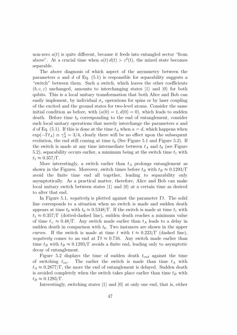
non-zero a(t) is quite different, because it feeds into entangled sector “fromabove”. At a crucial time when a(t) d(t) > z2(t), the mixed state becomesseparable.

The above diagnosis of which aspect of the asymmetry between theparameters a and d of Eq. (5.1) is responsible for separability suggests a“switch” between them. Such a switch, which leaves the other coefficients(b, c, z) unchanged, amounts to interchanging states |1〉 and |0〉 for bothqubits. This is a local unitary transformation that both Alice and Bob caneasily implement, by individual σx operations for spins or by laser couplingof the excited and the ground states for two-level atoms. Consider the sameinitial condition as before, with (a(0) = 1, d(0) = 0), which leads to suddendeath. Before time t0 corresponding to the end of entanglement, considersuch local unitary operations that merely interchange the parameters a andd of Eq. (5.1). If this is done at the time tA when a = d, which happens whenexp(−ΓtA) ≡ γ2

A = 3/4, clearly there will be no effect upon the subsequentevolution, the end still coming at time t0 (See Figure 5.1 and Figure 5.2). Ifthe switch is made at any time intermediate between tA and t0 (see Figure5.2), separability occurs earlier, a minimum being at the switch time t1 witht1 ≈ 0.357/Γ.

More interestingly, a switch earlier than tA prolongs entanglement asshown in the Figures. Moreover, switch times before tB with tB ≈ 0.1293/Γavoid the finite time end all together, leading to separability onlyasymptotically. As a practical matter, therefore, Alice and Bob can makelocal unitary switch between states |1〉 and |0〉 at a certain time as desiredto alter that end.

In Figure 5.1, negativity is plotted against the parameter Γt. The solidline corresponds to a situation when no switch is made and sudden deathappears at time t0 with t0 ≈ 0.5348/Γ. If the switch is made at time t1 witht1 ≈ 0.357/Γ (dotted-dashed line), sudden death reaches a minimum valueof time t< ≈ 0.48/Γ. Any switch made earlier than tA leads to a delay insudden death in comparison with t0. Two instances are shown in the uppercurves. If the switch is made at time t with t ≈ 0.223/Γ (dashed line),negativity comes to an end at Γt ≈ 0.716. Any switch made earlier thantime tB with tB ≈ 0.1293/Γ avoids a finite end, leading only to asymptoticdecay of entanglement.

Figure 5.2 displays the time of sudden death tend against the timeof switching tsw. The earlier the switch is made than time tA withtA ≈ 0.2877/Γ, the more the end of entanglement is delayed. Sudden deathis avoided completely when the switch takes place earlier than time tB withtB ≈ 0.1293/Γ.

Interestingly, switching states |1〉 and |0〉 at only one end, that is, either

47

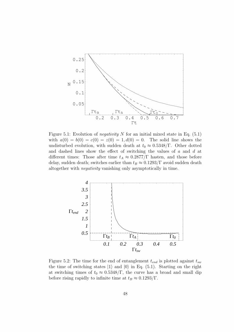
0.2 0.3 0.4 0.5 0.6 0.7Gt

0.05

0.1

0.15

0.2

0.25

N

GtAGtB Gt0

Figure 5.1: Evolution of negativity N for an initial mixed state in Eq. (5.1)with a(0) = b(0) = c(0) = z(0) = 1, d(0) = 0. The solid line shows theundisturbed evolution, with sudden death at t0 ≈ 0.5348/Γ. Other dottedand dashed lines show the effect of switching the values of a and d atdifferent times: Those after time tA ≈ 0.2877/Γ hasten, and those beforedelay, sudden death; switches earlier than tB ≈ 0.1293/Γ avoid sudden deathaltogether with negativity vanishing only asymptotically in time.

0.1 0.2 0.3 0.4 0.5Gtsw

0.5

1

1.5

2

2.5

3

3.5

4

Gtend

GtB GtA Gt0

Figure 5.2: The time for the end of entanglement tend is plotted against tswthe time of switching states |1〉 and |0〉 in Eq. (5.1). Starting on the rightat switching times of t0 ≈ 0.5348/Γ, the curve has a broad and small dipbefore rising rapidly to infinite time at tB ≈ 0.1293/Γ.

48

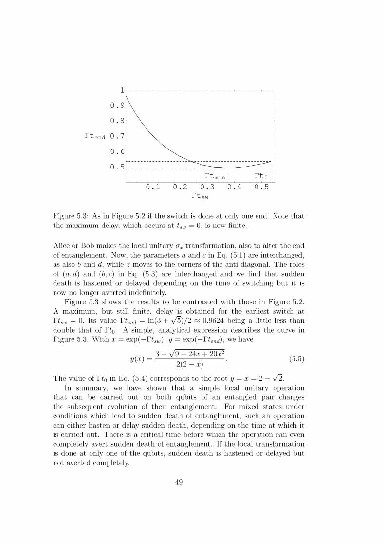
0.1 0.2 0.3 0.4 0.5Gtsw

0.5

0.6

0.7

0.8

0.9

1

Gtend

Gtmin Gt0

Figure 5.3: As in Figure 5.2 if the switch is done at only one end. Note thatthe maximum delay, which occurs at tsw = 0, is now finite.

Alice or Bob makes the local unitary σx transformation, also to alter the endof entanglement. Now, the parameters a and c in Eq. (5.1) are interchanged,as also b and d, while z moves to the corners of the anti-diagonal. The rolesof (a, d) and (b, c) in Eq. (5.3) are interchanged and we find that suddendeath is hastened or delayed depending on the time of switching but it isnow no longer averted indefinitely.

Figure 5.3 shows the results to be contrasted with those in Figure 5.2.A maximum, but still finite, delay is obtained for the earliest switch atΓtsw = 0, its value Γtend = ln(3 +

√5)/2 ≈ 0.9624 being a little less than

double that of Γt0. A simple, analytical expression describes the curve inFigure 5.3. With x = exp(−Γtsw), y = exp(−Γtend), we have

y(x) =3 −

√9 − 24x+ 20x2

2(2 − x). (5.5)

The value of Γt0 in Eq. (5.4) corresponds to the root y = x = 2 −√

2.In summary, we have shown that a simple local unitary operation

that can be carried out on both qubits of an entangled pair changesthe subsequent evolution of their entanglement. For mixed states underconditions which lead to sudden death of entanglement, such an operationcan either hasten or delay sudden death, depending on the time at which itis carried out. There is a critical time before which the operation can evencompletely avert sudden death of entanglement. If the local transformationis done at only one of the qubits, sudden death is hastened or delayed butnot averted completely.

49

5.2 Manipulating entanglement sudden death

in zero- and finite-temperature reservoirs

Sudden death of entanglement is a serious limiting factor for the useof entangled qubits in quantum information processing. It would seemimportant to stabilize quantum systems against this unwanted phenomenon.In Section 5.1, we have addressed the practically relevant question whether itis possible to delay or even avert sudden death by application of particularlychosen local unitary transformations for a given initial state and a givenopen-system dynamics [102]. We have demonstrated that this is indeedpossible for the special two-qubit system investigated first by Yu-Eberly [61]and have found similar effects in qubit-qutrit systems [137] (See Chapter 6).

In this section, we generalize our results of Section 5.1 and investigatefinite-time disentanglement of two-qubits interacting with statisticallyindependent (bosonic) reservoirs at finite temperatures. We demonstratethat based on the Peres-Horodecki criterion [37, 38] and on recent results ofHuang and Zhu [90], it is possible to develop systematically a simple criterioncapable of characterizing delay and avoidance of finite-time disentanglementof initially prepared two-qubit X-states in this open quantum system. Withthe help of this criterion we prove that, in agreement with recent conjecturesbased on numerical case studies [94], all initially prepared two-qubit X-statesexhibit sudden death if at least one of the statistically independent reservoirsis at finite-temperature. However, if both reservoirs are at zero-temperature,there are always some X-states for which sudden death does not occur.Based on this criterion, we demonstrate that even at finite-temperaturesof the reservoirs it is possible to hasten or to delay sudden death ofentanglement. The characteristic time of sudden death can be controlled bythe time when appropriate local unitary operations are applied. However,unlike in the zero-temperature case, when at least one of the reservoirs isat finite-temperature it is not possible to avoid sudden death completely byany choice of local unitary transformations.

5.2.1 Open-system dynamics of two-qubits coupled tostatistically independent thermal reservoirs

In this section, we briefly summarize the basic equations of motion governingour open quantum system of interest. In order to put the problem offinite-time disentanglement, its delay, and avoidance into perspective, letus consider two non-interacting qubits which are spatially well separated sothat each of them interacts with its own thermal reservoir (see Figure 5.4).

50

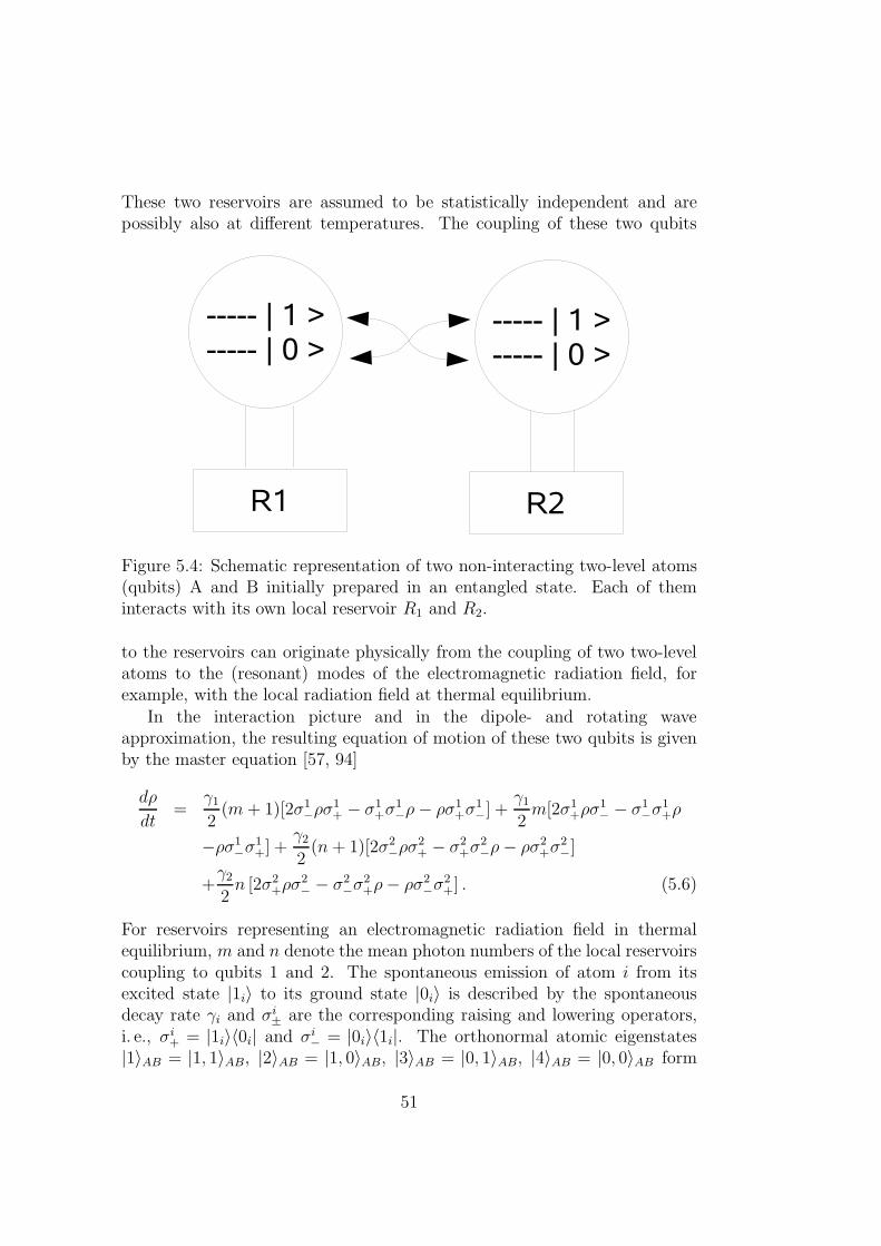
These two reservoirs are assumed to be statistically independent and arepossibly also at different temperatures. The coupling of these two qubits

Figure 5.4: Schematic representation of two non-interacting two-level atoms(qubits) A and B initially prepared in an entangled state. Each of theminteracts with its own local reservoir R1 and R2.

to the reservoirs can originate physically from the coupling of two two-levelatoms to the (resonant) modes of the electromagnetic radiation field, forexample, with the local radiation field at thermal equilibrium.

In the interaction picture and in the dipole- and rotating waveapproximation, the resulting equation of motion of these two qubits is givenby the master equation [57, 94]

dρ

dt=

γ1

2(m + 1)[2σ1

−ρσ1+ − σ1

+σ1−ρ− ρσ1

+σ1−] +

γ1

2m[2σ1

+ρσ1− − σ1

−σ1+ρ

−ρσ1−σ

1+] +

γ2

2(n + 1)[2σ2

−ρσ2+ − σ2

+σ2−ρ− ρσ2

+σ2−]

+γ2

2n [2σ2

+ρσ2− − σ2

−σ2+ρ− ρσ2

−σ2+] . (5.6)

For reservoirs representing an electromagnetic radiation field in thermalequilibrium, m and n denote the mean photon numbers of the local reservoirscoupling to qubits 1 and 2. The spontaneous emission of atom i from itsexcited state |1i〉 to its ground state |0i〉 is described by the spontaneousdecay rate γi and σi

± are the corresponding raising and lowering operators,i. e., σi

+ = |1i〉〈0i| and σi− = |0i〉〈1i|. The orthonormal atomic eigenstates

|1〉AB = |1, 1〉AB, |2〉AB = |1, 0〉AB, |3〉AB = |0, 1〉AB, |4〉AB = |0, 0〉AB form

51

the (computational) basis of the four dimensional Hilbert space of thetwo qubits. The derivation of Eq. (5.6) also assumes the validity of theBorn-Markov approximation. The most general solution of Eq. (5.6) for anyinitially prepared two-qubit quantum state ρ with density matrix elementsρij in the computational basis is given as

ρ11(t) =1

(2m+ 1)(2n+ 1)

mn +m [ (n+ 1)ρ11 + ρ33 − n(ρ22 − ρ33

+ρ44) ] e−(2n+1)γ2t + n[ (m + 1)ρ11 + (m+ 1)ρ22 −m (ρ33 + ρ44) ]

×e−(2m+1)γ1t + [ (m+ 1) (n+ 1)ρ11 −mρ33 − n (ρ22 +mρ22

+mρ33 −mρ44 ) ] e−[ (2m+1)γ1+(2n+1)γ2 ]t

, (5.7)

ρ22(t) =1

(2m+ 1)(2n+ 1)

m (n + 1) −m [ (n+ 1)ρ11 + ρ33 − n (ρ22 − ρ33

+ρ44) ] e−(2n+1)γ2t + (n+ 1) [ (m+ 1)ρ11 + (m+ 1)ρ22 −m (ρ33

+ρ44) ] e−(2m+1)γ1t + [−(m + 1)(n+ 1)ρ11 +mρ33 + n ((m + 1)ρ22

+mρ33 −mρ44 ) ] e−[ (2m+1)γ1+(2n+1)γ2 ]t

, (5.8)

ρ33(t) =1

(2m+ 1)(2n+ 1)

n(m+ 1) + (m + 1)[(n+ 1) ρ11 + ρ33 − n

(ρ22 − ρ33 + ρ44) ] e−(2n+1)γ2t − n [ (m+ 1) ρ11 + (m + 1) ρ22

−m (ρ33 + ρ44 ) ] e−(2m+1)γ1t + [−(m + 1)(n+ 1) ρ11 +mρ33

+n ( (m+ 1) ρ22 +mρ33 −mρ44 ) ] e−[(2m+1)γ1+(2n+1)γ2]t

, (5.9)

ρ44(t) =1

(2m+ 1)(2n+ 1)

(m+ 1)(n+ 1) − (m+ 1) [(n+ 1)ρ11 + ρ33 −

n(ρ22 − ρ33 + ρ44) ] e−(2n+1)γ2t − (n+ 1) [ (m+ 1) ρ11 + (m + 1) ρ22

−m (ρ33 + ρ44) ] e−(2m+1)γ1t + [ (m+ 1)(n+ 1) ρ11 −mρ33

−n ((m+ 1) ρ22 +mρ33 −mρ44) ] e−[(2m+1)γ1+(2n+1)γ2]t

, (5.10)

ρ12(t) =1

2m+ 1

m (ρ12 + ρ34) e−12

(2n+1)γ2t + [ (m+ 1)ρ12 −mρ34 ]

×e−12

[2(2m+1)γ1+(2n+1)γ2]t

, (5.11)

52

ρ13(t) =1

2n+ 1

n (ρ13 + ρ24) e−12

(2m+1)γ1t + [ (n+ 1) ρ13 − n ρ24 ]

×e−12

[(2m+1)γ1+2(2n+1)γ2]t

, (5.12)

ρ24(t) =1

2n + 1

(n + 1) (ρ13 + ρ24) e−12

(2m+1)γ1t + [n ρ24 − (n+ 1) ρ13]

×e−12

[(2m+1)γ1+2(2n+1)γ2]t

, (5.13)

ρ34(t) =1

2m+ 1

(m+ 1)(ρ12 + ρ34) e−12

(2n+1)γ2t + [mρ34 − (m+ 1)ρ12]

×e−12

[2(2m+1)γ1+(2n+1)γ2]t

, (5.14)

ρ14(t) = ρ14 e−[(m+ 12)γ1+(n+ 1

2)γ2]t, (5.15)

ρ23(t) = ρ23 e−[(m+ 12)γ1+(n+ 1

2)γ2]t. (5.16)

There is some numerical evidence [94] that the presence of non-zeromean thermal photon numbers in Eq. (5.6) may be responsible for suddendeath. However, systematic exploration of these phenomena which is capableof proving the sufficiency of non-zero photon numbers for sudden deathand of providing a systematic analytical understanding of sudden death inzero-temperature reservoirs has been missing so far. A major purpose ofthis section is to close this gap. In particular, we shall develop a simpleanalytical criterion for finite-time disentanglement which allows a systematicunderstanding of sudden death and its delay and avoidance for initiallyprepared entangled X-states.

5.2.2 The Peres-Horodecki criterion and entanglement

sudden death

In this section, we analyze conditions under which initially prepared entan-gled two-qubit states evolving according to Eq. (5.6) exhibit entanglementsudden death. Starting from the general time dependent solution of these

53

equations, sudden death is analyzed with the help of the Peres-Horodeckicriterion [37, 38] and with the help of all principal minors of the partiallytransposed time-dependent two-qubit quantum state.

Recently, Huang and Zhu [90] studied the Peres-Horodecki criterionby focussing on the principal minors of the partially transposed densitymatrix. The principal minor [ρPT (ijkl...)] of the partially transposed densityoperator ρPT is the determinant of the submatrix M(ijkl...) formed bythe matrix elements of the i, j, k, l, ...-th rows and columns of the partialtranspose ρPT , i. e.,

M(ijkl...) =

ρPTii , ρPT

ij , ρPTik , ρPT

il , · · ·ρPT

ji , ρPTjj , ρPT

jk , ρPTjl , · · ·

ρPTki , ρPT

kj , ρPTkk , ρPT

jl , · · ·ρPT

li , ρPTlj , ρPT

lk , ρPTll , · · ·

· · · · · · · · · · · · · · ·

. (5.17)

In general, if a matrix is positive semidefinite, then all its principalminors are non-negative, and vice versa [138]. Therefore, for an entangledtwo-qubit state ρ, the smallest principal minor of its partially transposeddensity operator must be negative. For two-qubit states non-negativityof the principal minors [ρPT (1)], [ρPT (2)], [ρPT (3)], [ρPT (4)], [ρPT (12)],[ρPT (13)], [ρPT (24)], and [ρPT (34)] is guaranteed already by non-negativityof the original density matrix ρ. As a consequence, a general two-qubitstate is entangled if and only if the minimum value of the remaining sevenprincipal minors P (ρPT ) is negative, i. e.,

P (ρPT ) ≡ min [ρPT (14)], [ρPT (23)], [ρPT (123)], [ρPT (124)], [ρPT (134)],

[ρPT (234)], [ρPT (1234)] < 0. (5.18)

Typically, the investigation of these seven principal minors for generalsolutions ρ(t) of the density operator equation (5.6) is cumbersome. How-ever, significant simplifications are possible for identical zero-temperaturereservoirs with m = n = 0, and γ1 = γ2 = γ in Eq. (5.6). Thus, Huangand Zhu [90] could demonstrate that for asymptotically long times t−∞ withγt−∞ ≫ 1, the separability of ρ(t−∞) is determined by the initial state ρ. Inparticular, these authors showed that the matrix

ρ =

ρ11 ρ21 ρ13 ρ23

ρ12 ρ11 + ρ22 ρ14 ρ13 + ρ24

ρ31 ρ41 ρ11 + ρ33 ρ21 + ρ43

ρ32 ρ31 + ρ42 ρ12 + ρ34 1

, (5.19)

which is defined in terms of the matrix elements of the initially preparedtwo-qubit quantum state ρ, determines the asymptotic separability of the

54

two qubits and thus the presence or absence of sudden death. The derivationof this result Eq. (5.19) is summarized in the following.

Derivation of Eq. (5.19)

For the simple case of vacuum reservoirs, i. e., m = n = 0, and γ1 = γ2 = γthe time evolution of the two-qubit state ρ(t) under amplitude damping canbe written as [90]

ρ(t) =

p2 ρ11 p√p ρ12 p

√p ρ13 p ρ14

p√p ρ21 ρ22(t) p ρ23 ρ24(t)

p√p ρ31 p ρ32 ρ33(t) ρ34(t)

p ρ41 ρ42(t) ρ43(t) ρ44(t)

, (5.20)

where p = e−γt, and ρ22(t) = p( (1−p)ρ11+ρ22 ), ρ24(t) =√p( (1−p)ρ13+ρ24 ),

ρ33(t) = p( (1 − p)ρ11 + ρ33 ), ρ34(t) =√p( (1 − p)ρ12 + ρ34 ), and ρ44(t) =

1 − p ρ22 − p ρ33 − (2p− p2) ρ11. As t → ∞, p→ 0 and the final state of thetwo-qubit system will always be in the ground |0, 0〉 state, irrespective of itsinitial state.

The partial transpose of Eq. (5.20) is given by

ρPT (t) =

p2 ρ11 p√p ρ21 p

√p ρ13 p ρ23

p√p ρ12 ρ22(t) p ρ14 ρ24(t)

p√p ρ31 p ρ41 ρ33(t) ρ43(t)

p ρ32 ρ42(t) ρ34(t) ρ44(t)

. (5.21)

Due to exponential decay the probability p tends to zero for large timesand the positivity or negativity of each principal minor of Eq. (5.21) isdetermined by its nonvanishing terms of lowest order in p. Based on thisobservation Eq. (5.21) can be written as

ρPT (t) = ρ+ ρ , (5.22)

with

ρ =

p2 ρ11 p√p ρ21 p

√p ρ13 p ρ23

p√p ρ12 p(ρ11 + ρ22) p ρ14

√p(ρ13 + ρ24)

p√p ρ31 p ρ41 p(ρ11 + ρ33)

√p(ρ21 + ρ43)

p ρ32√p(ρ31 + ρ42)

√p(ρ12 + ρ34) 1

, (5.23)

and

ρ =

0 0 0 00 −p2ρ11 0 −p√pρ13

0 0 −p2ρ11 −p√pρ21

0 −p√pρ31 −p√pρ12 −ρ44

, (5.24)

55

and with ρ44 = p(ρ11 + ρ22) + p(ρ11 + ρ33) − p2ρ11. The matrix ρ is negativesemidefinite, i. e., ρ ≤ 0.

Let us first of all assume that the minimum principal minor of thematrix (5.23) is nonzero, P (ρ) 6= 0. Because the contributions of thematrix elements of ρ are of higher order in

√p in comparison with ρ, the

minimum principal minor of the matrix (5.21) has the same sign as P (ρ).Consequently, the matrix ρ plays no role in determining the separability ofρ(t). It is found that every principal minor of the matrix

ρ′ =

ρ11 ρ21 ρ13 ρ23

ρ12 ρ11 + ρ22 ρ14 ρ13 + ρ24

ρ31 ρ41 ρ11 + ρ33 ρ21 + ρ43

ρ32 ρ31 + ρ42 ρ12 + ρ34 1

, (5.25)

is equal to the corresponding principal minor of matrix (5.23) apart frommultiplication by a suitable positive coefficient, such as

[ρ(23)] = p2 [ (ρ11 + ρ22)(ρ11 + ρ33) − |ρ14|2 ] = p2 [ρ′(23)] . (5.26)

Hence the separability of ρ(t) is determined by the matrix ρ′ which isindependent of the decay parameter p.

If the minimum principal minor of the matrix (5.23) is zero, thehigher order terms in matrix (5.24) must be taken into account andthe corresponding principal minors of matrix (5.21) are either zero ornonpositive. For example, suppose [ρ(23)] = 0, then the correspondingprincipal minor [ρPT (23)] is given by

[ρPT (23)] = [ρ(23)] − p2 ρ11 [ρ(2)] − p2 ρ11 [ρ(3)] + (p2 ρ11)2 . (5.27)

For ρ11 > 0, [ρPT (23)] is negative and for ρ11 = 0, [ρPT (23)] = 0. Similarlyall seven principal minors are nonpositive if the corresponding principalminors of ρ are zero.

If P (ρ) < 0, the two-qubit state ρ(t−∞) is entangled and sudden deathdoes not occur. If P (ρ) > 0, the asymptotic quantum state ρ(t−∞) isseparable and sudden death takes place. In summary, Huang and Zhu[90] showed that for identical zero-temperature reservoirs the necessary andsufficient condition for sudden death is given by

P (ρ) > 0, (5.28)

and is determined by the initially prepared two-qubit quantum state.The derivation carried out to reach Eq. (5.28) is for the simplest case

of vacuum reservoirs and by taking γ1 = γ2 = γ. For γ1 6= γ2, it is not

56

easy to arrive at the similar result (5.28). The situation becomes evenmore cumbersome for cases with m 6= 0 and n 6= 0, i. e., for thermalreservoirs. However, in the case of initially prepared X-states of the form ofEq. (5.1) the calculation of principal minors simplifies considerably as shownin the following. For initially prepared X-states, i. e., quantum states withρ12 = ρ13 = ρ24 = ρ34 = 0 in the basis of Section 5.2.1, the condition (5.28)can be simplified considerably. In the subsequent subsection, all relevantseven principal minors for X-states ρX are evaluated.

Principal minors for X-states

For X-states the dependence of all seven principal-minors of Eq. (5.18) isgiven by

[ρPT (14)] =

∣

∣

∣

∣

ρ11 ρ23

ρ32 ρ44

∣

∣

∣

∣

= ρ11 ρ44 − |ρ23|2 ,

[ρPT (23)] =

∣

∣

∣

∣

ρ22 ρ14

ρ41 ρ33

∣

∣

∣

∣

= ρ22 ρ33 − |ρ14|2 ,

[ρPT (123)] =

∣

∣

∣

∣

∣

∣

ρ11 0 00 ρ22 ρ14

0 ρ41 ρ33

∣

∣

∣

∣

∣

∣

= ρ11 [ρPT (23)] ,

[ρPT (124)] =

∣

∣

∣

∣

∣

∣

ρ11 0 ρ23

0 ρ22 0ρ32 0 ρ44

∣

∣

∣

∣

∣

∣

= ρ22 [ρPT (14)] ,

[ρPT (134)] =

∣

∣

∣

∣

∣

∣

ρ11 0 ρ23

0 ρ33 0ρ32 0 ρ44

∣

∣

∣

∣

∣

∣

= ρ33 [ρPT (14)] ,

[ρPT (234)] =

∣

∣

∣

∣

∣

∣

ρ22 ρ14 0ρ41 ρ33 00 0 ρ44

∣

∣

∣

∣

∣

∣

= ρ44 [ρPT (23)] ,

57

[ρPT (1234)] =

∣

∣

∣

∣

∣

∣

∣

∣

ρ11 0 0 ρ23

0 ρ22 ρ14 00 ρ41 ρ33 0ρ32 0 0 ρ44

∣

∣

∣

∣

∣

∣

∣

∣

= [ρPT (14)] [ρPT (23)] . (5.29)

From these expressions it is apparent that for initially prepared X-states,all the seven relevant principal minors are positive if and only if the twoprincipal minors are positive, i. e.,

[ρPTX (14)] , [ρPT

X (23)] > 0. (5.30)

It is apparent from the general solution of the density operator of Eq. (5.6)as given by Eqs. (5.7-5.16) that an initially prepared two-qubit X-stateremains an X-state for all times. This fact is valid for both vacuum andthermal reservoirs. However, for thermal reservoirs, the corresponding twoprincipal minors can not be written in terms of matrix elements of theinitial state alone but they also involve the quantities m, n, γ1, and γ2, in anon-trivial way.

Combining this observation with the results of Eq. (5.29) leads to thegeneral conclusion that initially prepared two-qubit X-states exhibit suddendeath if and only if at asymptotic times t−∞ the principal minors are bothpositive, i. e.,

[ρPTX (14)(t−∞)] , [ρPT

X (23)(t−∞)] > 0 , (5.31)

which are defined in terms of the matrix elements of the initially preparedtwo-qubit quantum state ρ. This condition determines the asymptoticseparability of the two qubits and thus the presence or absence of suddendeath.

5.2.3 Two-qubit X-states and quantum control of en-tanglement sudden death

In this section, we specialize our discussion of sudden death to initiallyprepared arbitrary two-qubit X-states. Delay and avoidance of suddendeath of initially prepared two-qubit X-states coupled to two statisticallyindependent zero-temperature reservoirs is discussed in Section 5.3. InSection 5.4 these results are generalized to reservoirs at finite temperatures.In particular, it is proved that if at least one of the reservoirs has non-zerotemperature, all initially prepared X-states exhibit sudden death.

58

Let us first of all briefly summarize some basic properties of X-states.The density matrix of a two-qubit X-state is of the general form

ρX =

ρ11 0 0 ρ14

0 ρ22 ρ23 00 ρ32 ρ33 0ρ41 0 0 ρ44

, (5.32)

i. e., ρ12 = ρ13 = ρ24 = ρ34 = 0. These states are not unusual but arisesnaturally in a wide variety of physical situations [81, 139, 140]. In particular,Werner states [36] are special cases of such X-states and some aspects oftheir sudden death have been discussed already [62, 75, 80, 84]. Eq. (5.32)describes a quantum state provided the unit trace and positivity conditions∑4

i=1 ρii = 1, ρ22ρ33 ≥ |ρ23|2, and ρ11ρ44 ≥ |ρ14|2 are fulfilled. X-statesare entangled if and only if either ρ22ρ33 < |ρ14|2 or ρ11ρ44 < |ρ23|2. Bothconditions cannot hold simultaneously as there can be at most one negativeeigenvalue for two-qubit states [136].

5.3 Delaying, hastening, and avoiding sudden

death of entanglement in statistically in-

dependent vacuum reservoirs

As discussed in the previous section, for zero-temperature reservoirs thecriterion for sudden death is given by Eq. (5.30) which together with theresult of Eq. (5.25) yields the necessary and sufficient conditions for suddendeath:

[ρ(14)] = ρ11 − |ρ23|2 > 0,

[ρ(23)] = (ρ11 + ρ22)(ρ11 + ρ33) − |ρ14|2 > 0 . (5.33)

Depending on the degree of entanglement of the initially prepared two-qubitstate, two different cases can be distinguished.

Case 1

For initially prepared entangled two-qubit states fulfilling the condition,

ρ11ρ44 < |ρ23|2, (5.34)

59

the analytical expression for negativity of the quantum state ρ(t) satisfyingEq. (5.6) for γ1 = γ2 = γ and m = n = 0 is given by

N1(ρX(t)) = max

0,

√

F 2(p, ρii) − 4p2(

ρ11F (p, ρii) − p2ρ211 − |ρ23|2

)

−F (p, ρii)

, (5.35)

with F (p, ρii) = (1−2p+2p2)ρ11 +(1−p)(ρ22 +ρ33)+ρ44, p = exp(−γt). Forany initially entangled two-qubit state ρ, Eq. (5.34) implies ρ22ρ33 ≥ |ρ14|2so that one of the conditions of Eq. (5.33) is satisfied. Thus, provided alsothe other condition, namely ρ11 > |ρ23|2, is satisfied, an initially preparedentangled two-qubit state exhibits sudden death and its negativity becomeszero at a finite time, say t1.

Provided both conditions of Eq. (5.33) are fulfilled, sudden death ofentanglement can be delayed or even avoided by local unitary operationsacting on the two qubits involved. In particular, let us concentrate on localunitary operations which exchange the density matrix elements ρ11(t) andρ44(t) of the quantum state at a time t < t1 in such a way that their product,i. e., ρ11(t) ρ44(t), remains constant but that the condition ρ44(t) > |ρ23(t)|2is violated. According to Eq. (5.33), in such a case sudden death will beavoided. The matrix element ρ44(t) is the probability of finding both qubitsin their ground states. Thus, as a consequence of the dynamics of Eq. (5.6),the density matrix element ρ44(t) increases monotonically. There will bea limiting time tsw for any possible switching of these matrix elements forwhich sudden death can still be avoided. If the local operation is appliedafter this limiting time, sudden death may possibly be delayed but it isunavoidable.

This simple consequence of the criterion of Eq. (5.33) explains recentnumerical work on this problem [102] (see Section 5.1). In fact, operationsof this type can avoid sudden death for any initially prepared two-qubitX-state provided they are applied at a time t such that t < tsw, wheretsw is the time of switching states |0〉 and |1〉. In particular, this appliesto the subset of Werner states with ρ14 = 0 which are mixtures of asinglet state with probability a and a completely unpolarized (chaotic)state. These Werner states exhibit sudden death in the parameter rangea ∈ [1/3, (−1 +

√5)/2) [83] where ρ11(t) > |ρ23(t)|2 while entanglement

decays asymptotically for values of a in the range a ∈ ((−1+√

5)/2, 1] whichcorresponds to ρ11(t) < |ρ23(t)|2.

Let us now deal with the question of which unitary transformations canachieve such a switch between ρ44(t) and ρ11(t). The most general 2 × 2

60

unitary matrix acting on a qubit is given by

U(2) =

(

cos(θ)ei α − sin(θ)ei(α−ω)

sin(θ)ei(β+ω) cos(θ)ei β

)

, (5.36)

which is a linear superposition of the Pauli matrices σx, σy, σz, andthe Identity matrix σ0. Exchanging the matrix elements ρ11 and ρ44

can be achieved by applying two appropriately chosen unitaries UA andUB of the form of Eq. (5.36) on qubits A and B at a suitably chosentime, say t, so that the X-state ρX(t) is transformed into another X-state(UA ⊗ UB)ρX(t)(U †

A ⊗ U †B), for example.

The most general local unitary operations transforming an arbitraryX-state into another one fulfill the conditions

sin(2θA) = sin(2θB) = 0 −→ θA = rAπ/2, θB = rBπ/2, (5.37)

with rA, rB ∈ Z. X-state preserving local unitary transformations with evenvalues of rA and rB do not have any significant effect on the density matrixelements except multiplying ρ14(t) by a constant phase factor. Odd valuesof rA and rB serve the purpose of exchanging ρ11(t) and ρ44(t). For any oddvalue of rA = rB, for example, the corresponding unitary two-qubit operatoris given by

U =

0 0 0 e2 i(α−ω)

0 0 −ei(α+β) 00 −ei(α+β) 0 0

e2 i(β+ω) 0 0 0

. (5.38)

A case in which such a X-state-preserving local unitary transformation isapplied only onto qubit B can be described by parameters θA = αA = βA =ωA = 0, for example. They lead to the transformations ρ11(t) ⇔ ρ22(t),ρ33(t) ⇔ ρ44(t), and ρ14(t) ⇔ ρ23(t). In view of the characteristic timeevolution of ρ22(t) in zero-temperature reservoirs and the criterion ofEq. (5.33), this implies that such a switch of matrix elements may delaysudden death but it cannot be avoided.

Case 2

For initially prepared entangled two-qubit X-states satisfying the alternativecondition

ρ22ρ33 < |ρ14|2, (5.39)

61

the expression for negativity of the resulting quantum state ρX(t) is given by

N2(ρX(t)) = max

0, p (√

(ρ22 − ρ33)2 + 4|ρ14|2 − (ρ22 + ρ33)

−(2 − 2 p) ρ11)

. (5.40)

Eq. (5.39) implies ρ11ρ44 ≥ |ρ23|2. Thus, the first condition of Eq. (5.33)is always satisfied so that finite-time disentanglement occurs whenever alsothe second condition is satisfied. The simplest case arises for ρ23 = 0 wherethe initially prepared state is a Werner state, i. e., an incoherent mixtureof a triplet state with probability a and the completely unpolarized state.Sudden death takes place in the parameter regime a ∈ [1/3, 1) where bothconditions are satisfied during the time evolution. In the case of an initiallyprepared Bell state, i. e., for a = 1, the second condition of Eq. (5.33) failsand entanglement decays asymptotically.

As discussed above, the first condition of Eq. (5.33) is always fulfilled inthe cases considered here so that sudden death takes place always exceptin the particular case of an initially prepared Bell state which fulfills thecondition (ρ11(t) + ρ22(t))(ρ11(t) + ρ33(t)) = |ρ14(t)|2. As a consequence anyswitch capable of exchanging ρ23(t) and ρ14(t) will be sufficient to avoid ordelay sudden death. Such a switch can be implemented by a local unitaryX-state-preserving transformation acting on qubit A or B only. As a resultthe second condition of Eq. (5.33) remains always true, while the validityof the first condition depends on the choice of the switching time t. Ifρ33(t) > |ρ14(t)|2 sudden death is unavoidable. However, for all switchingtimes violating this condition sudden death is averted completely. As anexample, let us consider Werner states with ρ23(0) = 0. In the parameterrange a ∈ [1/3, (−1+

√5)/2) the condition ρ33(t) > |ρ14(t)|2 is fulfilled for all

times so that ESD takes place. In the parameter regime a ∈ ((−1+√

5)/2, 1]this condition is violated so that entanglement decays asymptotically.

5.4 Hastening and delaying sudden death in

statistically independent thermal reser-

voirs

According to Eq. (5.30), sudden death takes place if and only if the twoprincipal minors

[ρPT (14)] = m2(m+ 1)2 + e−(2m+1)γt[F (1)] + e−2(2m+1)γt[F (2)]

+e−3(2m+1)γt[F (3)] + e−4(2m+1)γt[F (4)], (5.41)

62

and

[ρPT (23)] = m2(m+ 1)2 + e−(2m+1)γt[G(1)] + e−2(2m+1)γt[G(2)]

+e−3(2m+1)γt[G(3)] + e−4(2m+1)γt[G(4)], (5.42)

are positive in the limit of very long interaction times. For simplicity, wehave taken m = n and γ1 = γ2 = γ in Eq. (5.41) and Eq. (5.42). Thequantities F (i) and G(i) are functions of m and of the initial matrix elementsof the initially prepared quantum state. Their explicit forms are given by

F (1) = m (m+ 1) [ (2m+ 1) ρ11 + ρ22 + ρ33 − 2mρ44 ] ,

F (2) = −2m4 [2 ρ244 − ρ44 + ρ22 + 8 |ρ23|2 + ρ33 ] + 2m3 [−2 ρ2

44 + 2 ρ33 ρ44

+ρ44 − 16 |ρ23|2 − 2 ρ33 + 2 ρ22 (ρ44 − 1) ] −m2 [ ρ222 + (2 ρ33

−4 ρ44 + 3) ρ22 + ρ233 + 24 |ρ23|2 + 3 ρ33 − 4 ρ33 ρ44 − ρ44 ]

−4m (m + 1)3 ρ211 −m [ρ2

22 + 2 ρ33 ρ22 + ρ22 + ρ233 + 8 |ρ23|2

+ρ33 ] − |ρ23|2 + (m+ 1)2ρ11[ (8 ρ44 + 2)m2 +

(−4ρ22 − 4ρ33 + 2)m + 1 ] ,

F (3) = −2 ρ211 (m + 1)3 + (m + 1) ρ11 [(2m2 +m− 1)(ρ22 + ρ33) + 2mρ44 ]

+m [ (m+ 1) ρ222 + (2(m+ 1) ρ33 −m (2m+ 3) ρ44) ρ22 +

(m+ 1) ρ233 + 2m2 ρ2

44 −m (2m + 3) ρ33 ρ44 ] ,

F (4) = [m2 (ρ11 − ρ22 − ρ33 + ρ44) +m (2 ρ11 − ρ22 − ρ33) + ρ11]2 . (5.43)

Similarly, the expressions for G(i) in Eq. (5.42) are given by

G(1) = m (m+ 1) [ (2m+ 1) ρ11 + ρ22 + ρ33 − 2mρ44 ] ,

G(2) = −2m4 [ 2ρ222 − 4ρ33 ρ22 − ρ22 + 2ρ2

33 + ρ11 − ρ33 + 8|ρ14|2 + ρ44 ]

−2m3 [ 4ρ222 − 8ρ33 ρ22 − 2ρ22 + 4ρ2

33 + 3ρ11 − 2ρ33 + 16|ρ14|2

+ρ44 ] +m2[ρ211 − 2(ρ44 + 3) ρ11 − 6ρ2

22 − 6ρ233 + ρ2

44 + 2ρ22

+12 ρ22 ρ33 + 2 ρ33 − 24 |ρ14|2 ] +m [2 ρ211 + (ρ22 + ρ33 − 2 ρ44

−2) ρ11 − 2 ρ222 − 2 ρ2

33 + 4 ρ22 ρ33 − 8|ρ14|2 − ρ22 ρ44 − ρ33 ρ44 ]

+ρ211 + ρ22 ρ33 + ρ11 (ρ22 + ρ33) − |ρ14|2 ,

G(3) = −2 ρ211 (m + 1)3 + (m + 1) ρ11 [ (2m2 +m− 1)(ρ22 + ρ33) +

2mρ44 ] +m [ (m+ 1) ρ222 + ( 2(m+ 1) ρ33 −m (2m+ 3) ρ44 ) ρ22

+(m+ 1) ρ233 + 2m2 ρ2

44 −m (2m+ 3) ρ33 ρ44 ] ,

63

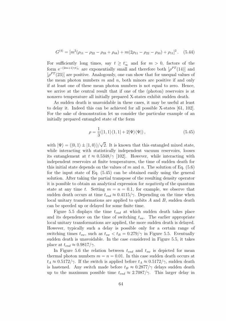
G(4) = [m2(ρ11 − ρ22 − ρ33 + ρ44) +m(2ρ11 − ρ22 − ρ33) + ρ11]2 . (5.44)

For sufficiently long times, say t ≥ t−∞ and for m > 0, factors of the

form e−(2m+1)γt−∞ are exponentially small and therefore both [ρPT (14)] and[ρPT (23)] are positive. Analogously, one can show that for unequal values ofthe mean photon numbers m and n, both minors are positive if and onlyif at least one of these mean photon numbers is not equal to zero. Hence,we arrive at the central result that if one of the (photon) reservoirs is atnonzero temperature all initially prepared X-states exhibit sudden death.

As sudden death is unavoidable in these cases, it may be useful at leastto delay it. Indeed this can be achieved for all possible X-states [61, 102].For the sake of demonstration let us consider the particular example of aninitially prepared entangled state of the form

ρ =1

3(|1, 1〉〈1, 1| + 2|Ψ〉〈Ψ|) , (5.45)

with |Ψ〉 = (|0, 1〉 ± |1, 0〉)/√

2. It is known that this entangled mixed state,while interacting with statistically independent vacuum reservoirs, loosesits entanglement at t ≈ 0.5348/γ [102]. However, while interacting withindependent reservoirs at finite temperatures, the time of sudden death forthis initial state depends on the values of m and n. The solution of Eq. (5.6)for the input state of Eq. (5.45) can be obtained easily using the generalsolution. After taking the partial transpose of the resulting density operatorit is possible to obtain an analytical expression for negativity of the quantumstate at any time t. Setting m = n = 0.1, for example, we observe thatsudden death occurs at time tend ≈ 0.4115/γ. Depending on the time whenlocal unitary transformations are applied to qubits A and B, sudden deathcan be speeded up or delayed for some finite time.

Figure 5.5 displays the time tend at which sudden death takes placeand its dependence on the time of switching tsw. The earlier appropriatelocal unitary transformations are applied, the more sudden death is delayed.However, typically such a delay is possible only for a certain range ofswitching times tsw, such as tsw < tB = 0.279/γ in Figure 5.5. Eventuallysudden death is unavoidable. In the case considered in Figure 5.5, it takesplace at tend ≈ 0.9817/γ.

In Figure 5.6 the relation between tend and tsw is depicted for meanthermal photon numbers m = n = 0.01. In this case sudden death occurs attA ≈ 0.5172/γ. If the switch is applied before tA ≈ 0.5172/γ, sudden deathis hastened. Any switch made before tB ≈ 0.2877/γ delays sudden deathup to the maximum possible time tend ≈ 2.7087/γ. This larger delay in

64

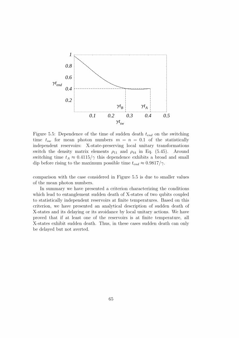
0.1 0.2 0.3 0.4 0.5Γtsw

0.2

0.4

0.6

0.8

1

Γtend

ΓtAΓtB

Figure 5.5: Dependence of the time of sudden death tend on the switchingtime tsw for mean photon numbers m = n = 0.1 of the statisticallyindependent reservoirs: X-state-preserving local unitary transformationsswitch the density matrix elements ρ11 and ρ44 in Eq. (5.45). Aroundswitching time tA ≈ 0.4115/γ this dependence exhibits a broad and smalldip before rising to the maximum possible time tend ≈ 0.9817/γ.

comparison with the case considered in Figure 5.5 is due to smaller valuesof the mean photon numbers.

In summary we have presented a criterion characterizing the conditionswhich lead to entanglement sudden death of X-states of two qubits coupledto statistically independent reservoirs at finite temperatures. Based on thiscriterion, we have presented an analytical description of sudden death ofX-states and its delaying or its avoidance by local unitary actions. We haveproved that if at least one of the reservoirs is at finite temperature, allX-states exhibit sudden death. Thus, in these cases sudden death can onlybe delayed but not averted.

65

0.1 0.2 0.3 0.4 0.5Γtsw

0.5

1

1.5

2

2.5

3

Γtend

ΓtAΓtB

Figure 5.6: Dependence of the time of sudden death tend on the switchingtime tsw for mean photon numbers m = n = 0.01: The local unitarytransformations are the same as in Figure 5.5. For switching times belowtA ≈ 0.5172/γ this dependence has a broad and small dip before rising tothe maximum possible time tend ≈ 2.7087/γ.

66

Chapter 6

Manipulating entanglementsudden death of qubit-qutritsystems

In Chapter 5, we have demonstrated that we can indeed hasten, delay,or even completely avoid sudden death of two qubits interacting withstatistically independent reservoirs. In this Chapter, we slightly enlargethe dimension of the Hilbert space to six, i. e., qubit (two dimensionalquantum system) times qutrit (three dimensional quantum system). Wefirst demonstrate the existence of sudden death in these systems due toamplitude damping and phase damping. We then discuss the possibility ofaccelerating, delaying or avoiding sudden death of entanglement by localunitary transformations.

This Chapter is organized as follows. In Section 6.1, we study thepure entangled states of qubit-qutrit systems and investigate the existenceof sudden death of different initially entangled pure and mixed statesinteracting with statistically independent reservoirs at zero-temperature. InSection 6.4, we discuss sudden death due to phase damping. Hastening,delaying or completely avoiding sudden death is provided in Section 6.2. Wediscuss the resulting asymptotic states in Section 6.3.

6.1 Entanglement sudden death of qubit-qutrit

systems by amplitude damping

So far two investigations on sudden death of entanglement of qubit-qutritsystems exist in the literature. Our investigation of this effect is foramplitude damping [92], while the second investigation deals with phase

67

damping [100]. We first discuss the results for amplitude damping and laterbriefly comment on the work for phase damping.

6.1.1 Maximally entangled pure states for 2⊗3 systems

As discussed before, negativity [54] is a computable measure of entanglementand it completely describes all entangled states in the Hilbert space ofqubit-qutrit systems. The Peres-Horodecki criterion tells us that for 2 ⊗ 2and 2 ⊗ 3 Hilbert spaces all states having positive partial transpose (PPT)(therefore, zero negativity) are separable [37, 38].

Maximally entangled pure states in 2 ⊗ 3 Hilbert space are extensions ofthe Bell states. To describe the set of pure entangled states in this Hilbertspace, an arbitrary pure state can be represented in terms of its Schmidtdecomposition [29]

|Ψ〉 =∑

ij

aij |i, j〉 , (6.1)

where i = 0, 1 denotes the qubit indices and j = 0, 1, 2 represent the qutritindices. For |Ψ〉 to be a valid state vector we need

∑

ij |aij |2 = 1, where theamplitudes aij are complex numbers in general. The density operator ρ isdefined by ρ = |Ψ〉〈Ψ|. We take the partial transpose of ρ with respect tothe qutrit basis. (Taking partial transpose with respect to the qubit basisgives the same result.) The spectrum of the partially transposed matrix ρTB

is given by

0, 0,−√

f(ax),√

f(ax),1

2(1 −

√

1 − 4f(ax)),1

2(1 +

√

1 − 4f(ax) ,(6.2)

where ax = aij corresponds to the six combinations i. e., a1 = a00, a2 = a01,a3 = a02, a4 = a10, a5 = a11, and a6 = a12.

Surprisingly, all the eigenvalues depend on the single function f(ax). Theexpression for f(ax) is given by

f(ax) = |a2|2|a4|2 + |a3|2|a4|2 − 2Re(a1a2a4a5) − 2Re(a1a3a4a6) + |a1|2 |a5|2+|a3|2|a5|2 + |a1|2|a6|2 + |a2|2|a6|2 − 2Re(a2a3a5a6) , (6.3)

where ai are the complex conjugates of ai. As the partially transposedmatrix of a Hermitian operator is also Hermitian, all its eigenvalues must bereal. This implies that 0 ≤ f(ax) ≤ 1/4. At the lower bound, the pure statesare separable, while at the upper bound, the pure states are maximallyentangled. For 0 < f(ax) < 1/4, the pure states are non-maximally

68

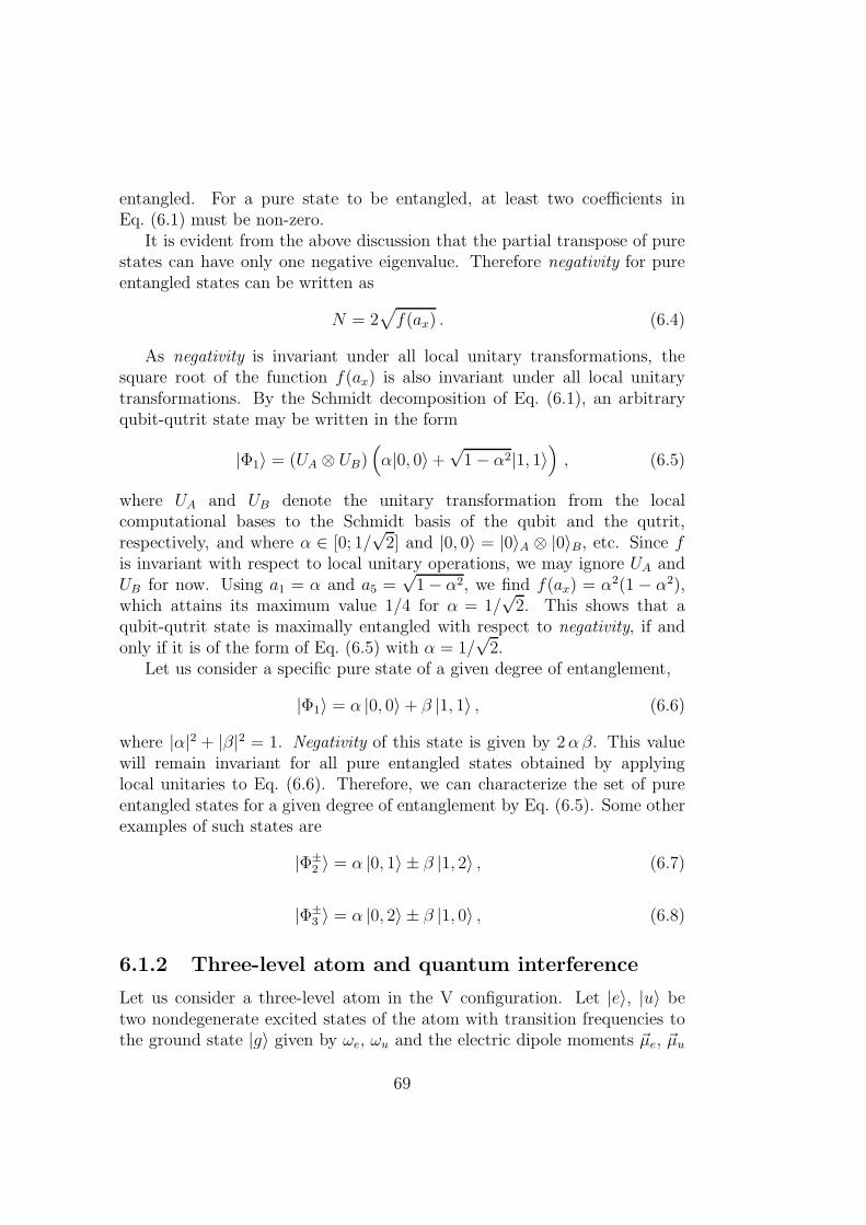
entangled. For a pure state to be entangled, at least two coefficients inEq. (6.1) must be non-zero.

It is evident from the above discussion that the partial transpose of purestates can have only one negative eigenvalue. Therefore negativity for pureentangled states can be written as

N = 2√

f(ax) . (6.4)

As negativity is invariant under all local unitary transformations, thesquare root of the function f(ax) is also invariant under all local unitarytransformations. By the Schmidt decomposition of Eq. (6.1), an arbitraryqubit-qutrit state may be written in the form

|Φ1〉 = (UA ⊗ UB)(

α|0, 0〉 +√

1 − α2|1, 1〉)

, (6.5)

where UA and UB denote the unitary transformation from the localcomputational bases to the Schmidt basis of the qubit and the qutrit,respectively, and where α ∈ [0; 1/

√2] and |0, 0〉 = |0〉A ⊗ |0〉B, etc. Since f

is invariant with respect to local unitary operations, we may ignore UA andUB for now. Using a1 = α and a5 =

√1 − α2, we find f(ax) = α2(1 − α2),

which attains its maximum value 1/4 for α = 1/√

2. This shows that aqubit-qutrit state is maximally entangled with respect to negativity, if andonly if it is of the form of Eq. (6.5) with α = 1/

√2.

Let us consider a specific pure state of a given degree of entanglement,

|Φ1〉 = α |0, 0〉 + β |1, 1〉 , (6.6)

where |α|2 + |β|2 = 1. Negativity of this state is given by 2αβ. This valuewill remain invariant for all pure entangled states obtained by applyinglocal unitaries to Eq. (6.6). Therefore, we can characterize the set of pureentangled states for a given degree of entanglement by Eq. (6.5). Some otherexamples of such states are

|Φ±2 〉 = α |0, 1〉 ± β |1, 2〉 , (6.7)

|Φ±3 〉 = α |0, 2〉 ± β |1, 0〉 , (6.8)

6.1.2 Three-level atom and quantum interference

Let us consider a three-level atom in the V configuration. Let |e〉, |u〉 betwo nondegenerate excited states of the atom with transition frequencies tothe ground state |g〉 given by ωe, ωu and the electric dipole moments ~µe, ~µu

69

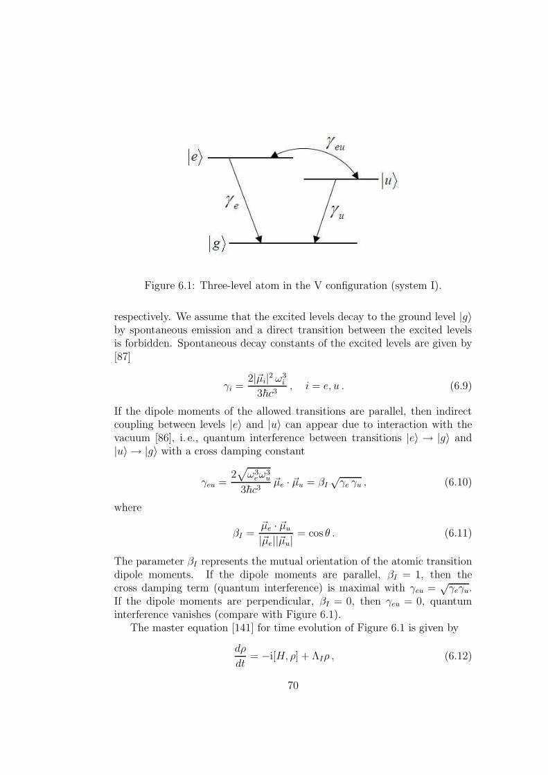
Figure 6.1: Three-level atom in the V configuration (system I).

respectively. We assume that the excited levels decay to the ground level |g〉by spontaneous emission and a direct transition between the excited levelsis forbidden. Spontaneous decay constants of the excited levels are given by[87]

γi =2|~µi|2 ω3

i

3~c3, i = e, u . (6.9)

If the dipole moments of the allowed transitions are parallel, then indirectcoupling between levels |e〉 and |u〉 can appear due to interaction with thevacuum [86], i. e., quantum interference between transitions |e〉 → |g〉 and|u〉 → |g〉 with a cross damping constant

γeu =2√

ω3eω

3u

3~c3~µe · ~µu = βI

√γe γu , (6.10)

where

βI =~µe · ~µu

|~µe||~µu|= cos θ . (6.11)

The parameter βI represents the mutual orientation of the atomic transitiondipole moments. If the dipole moments are parallel, βI = 1, then thecross damping term (quantum interference) is maximal with γeu =

√γeγu.

If the dipole moments are perpendicular, βI = 0, then γeu = 0, quantuminterference vanishes (compare with Figure 6.1).

The master equation [141] for time evolution of Figure 6.1 is given by

dρ

dt= −i[H, ρ] + ΛIρ , (6.12)

70

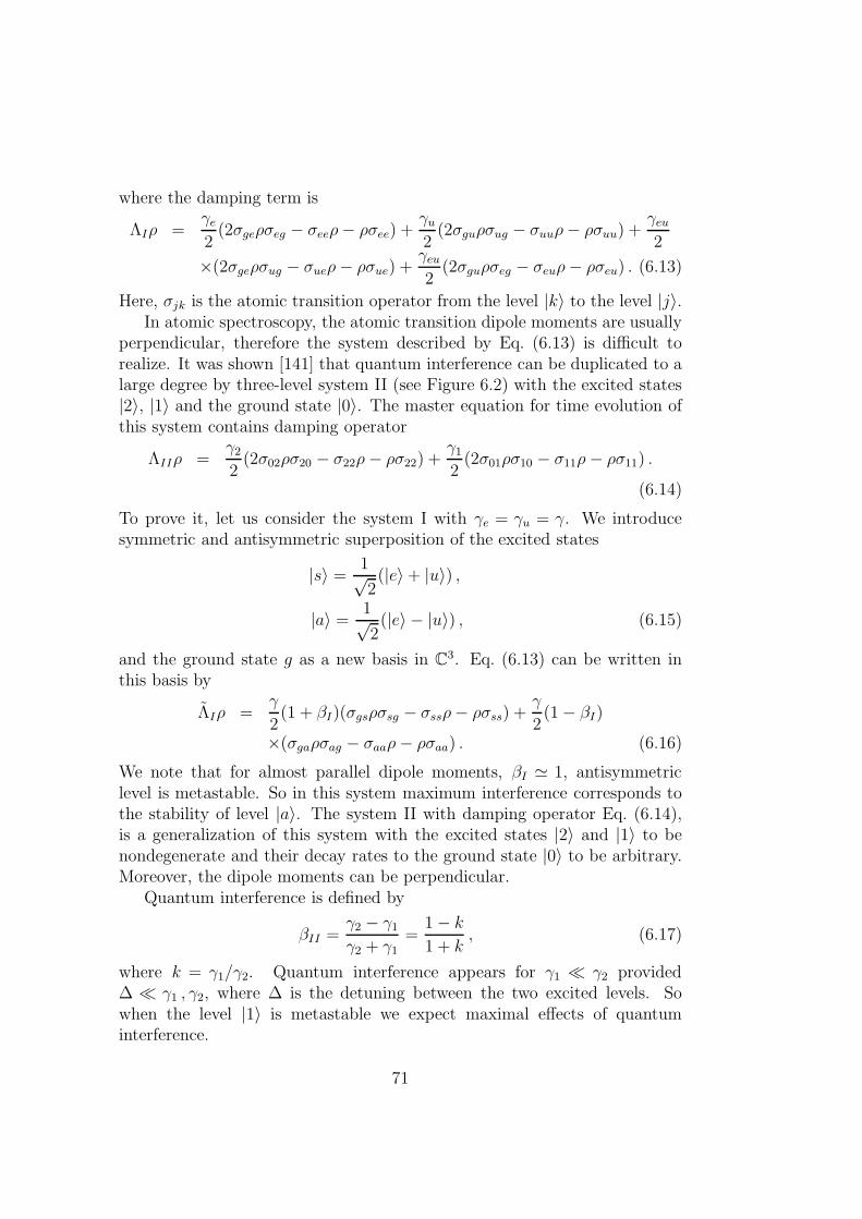
where the damping term is

ΛIρ =γe

2(2σgeρσeg − σeeρ− ρσee) +

γu

2(2σguρσug − σuuρ− ρσuu) +

γeu

2

×(2σgeρσug − σueρ− ρσue) +γeu

2(2σguρσeg − σeuρ− ρσeu) . (6.13)

Here, σjk is the atomic transition operator from the level |k〉 to the level |j〉.In atomic spectroscopy, the atomic transition dipole moments are usually

perpendicular, therefore the system described by Eq. (6.13) is difficult torealize. It was shown [141] that quantum interference can be duplicated to alarge degree by three-level system II (see Figure 6.2) with the excited states|2〉, |1〉 and the ground state |0〉. The master equation for time evolution ofthis system contains damping operator

ΛIIρ =γ2

2(2σ02ρσ20 − σ22ρ− ρσ22) +

γ1

2(2σ01ρσ10 − σ11ρ− ρσ11) .

(6.14)

To prove it, let us consider the system I with γe = γu = γ. We introducesymmetric and antisymmetric superposition of the excited states

|s〉 =1√2

(|e〉 + |u〉) ,

|a〉 =1√2

(|e〉 − |u〉) , (6.15)

and the ground state g as a new basis in C3. Eq. (6.13) can be written inthis basis by

ΛIρ =γ

2(1 + βI)(σgsρσsg − σssρ− ρσss) +

γ

2(1 − βI)

×(σgaρσag − σaaρ− ρσaa) . (6.16)

We note that for almost parallel dipole moments, βI ≃ 1, antisymmetriclevel is metastable. So in this system maximum interference corresponds tothe stability of level |a〉. The system II with damping operator Eq. (6.14),is a generalization of this system with the excited states |2〉 and |1〉 to benondegenerate and their decay rates to the ground state |0〉 to be arbitrary.Moreover, the dipole moments can be perpendicular.

Quantum interference is defined by

βII =γ2 − γ1

γ2 + γ1=

1 − k

1 + k, (6.17)

where k = γ1/γ2. Quantum interference appears for γ1 ≪ γ2 provided∆ ≪ γ1 , γ2, where ∆ is the detuning between the two excited levels. Sowhen the level |1〉 is metastable we expect maximal effects of quantuminterference.

71

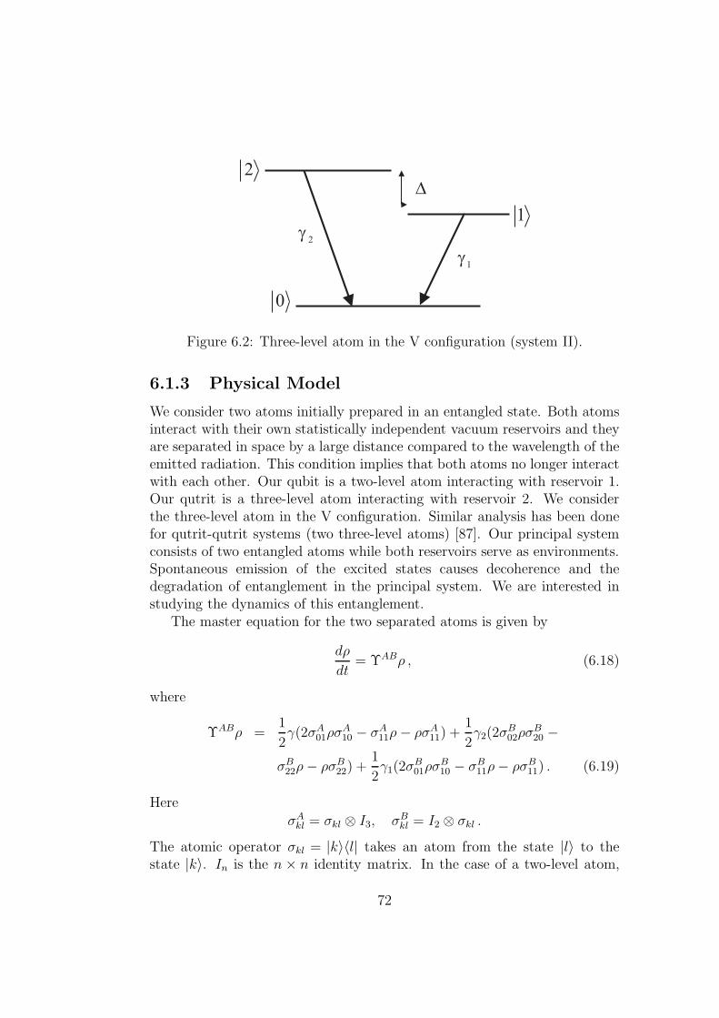
0

2

1

D

2g

1g

Figure 6.2: Three-level atom in the V configuration (system II).

6.1.3 Physical Model

We consider two atoms initially prepared in an entangled state. Both atomsinteract with their own statistically independent vacuum reservoirs and theyare separated in space by a large distance compared to the wavelength of theemitted radiation. This condition implies that both atoms no longer interactwith each other. Our qubit is a two-level atom interacting with reservoir 1.Our qutrit is a three-level atom interacting with reservoir 2. We considerthe three-level atom in the V configuration. Similar analysis has been donefor qutrit-qutrit systems (two three-level atoms) [87]. Our principal systemconsists of two entangled atoms while both reservoirs serve as environments.Spontaneous emission of the excited states causes decoherence and thedegradation of entanglement in the principal system. We are interested instudying the dynamics of this entanglement.

The master equation for the two separated atoms is given by

dρ

dt= ΥABρ , (6.18)

where

ΥABρ =1

2γ(2σA

01ρσA10 − σA

11ρ− ρσA11) +

1

2γ2(2σ

B02ρσ

B20 −

σB22ρ− ρσB

22) +1

2γ1(2σ

B01ρσ

B10 − σB

11ρ− ρσB11) . (6.19)

Here

σAkl = σkl ⊗ I3, σB

kl = I2 ⊗ σkl .

The atomic operator σkl = |k〉〈l| takes an atom from the state |l〉 to thestate |k〉. In is the n × n identity matrix. In the case of a two-level atom,

72

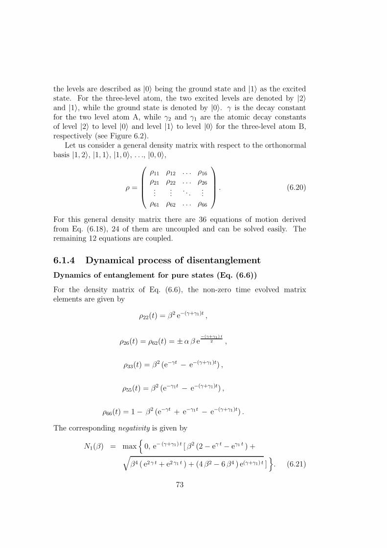
the levels are described as |0〉 being the ground state and |1〉 as the excitedstate. For the three-level atom, the two excited levels are denoted by |2〉and |1〉, while the ground state is denoted by |0〉. γ is the decay constantfor the two level atom A, while γ2 and γ1 are the atomic decay constantsof level |2〉 to level |0〉 and level |1〉 to level |0〉 for the three-level atom B,respectively (see Figure 6.2).

Let us consider a general density matrix with respect to the orthonormalbasis |1, 2〉, |1, 1〉, |1, 0〉, . . ., |0, 0〉,

ρ =

ρ11 ρ12 . . . ρ16

ρ21 ρ22 . . . ρ26...

.... . .

...ρ61 ρ62 . . . ρ66

. (6.20)

For this general density matrix there are 36 equations of motion derivedfrom Eq. (6.18), 24 of them are uncoupled and can be solved easily. Theremaining 12 equations are coupled.

6.1.4 Dynamical process of disentanglement

Dynamics of entanglement for pure states (Eq. (6.6))

For the density matrix of Eq. (6.6), the non-zero time evolved matrixelements are given by

ρ22(t) = β2 e−(γ+γ1)t ,

ρ26(t) = ρ62(t) = ±αβ e−(γ+γ1) t

2 ,

ρ33(t) = β2 (e−γt − e−(γ+γ1)t) ,

ρ55(t) = β2 (e−γ1t − e−(γ+γ1)t) ,

ρ66(t) = 1 − β2 (e−γt + e−γ1t − e−(γ+γ1)t) .

The corresponding negativity is given by

N1(β) = max

0, e− (γ+γ1) t [ β2 (2 − eγ t − eγ1 t ) +√

β4 ( e2 γ t + e2 γ1 t ) + (4 β2 − 6 β4 ) e(γ+γ1) t ]

. (6.21)

73

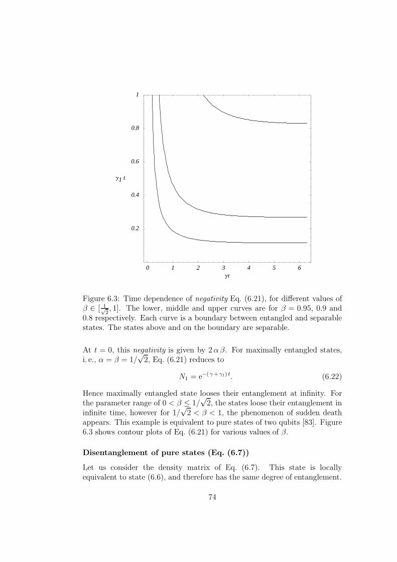
0 1 2 3 4 5 6Γt

0.2

0.4

0.6

0.8

1

Γ1 t

Figure 6.3: Time dependence of negativity Eq. (6.21), for different values ofβ ∈ [ 1√

2, 1]. The lower, middle and upper curves are for β = 0.95, 0.9 and

0.8 respectively. Each curve is a boundary between entangled and separablestates. The states above and on the boundary are separable.

At t = 0, this negativity is given by 2αβ. For maximally entangled states,i. e., α = β = 1/

√2, Eq. (6.21) reduces to

N1 = e−( γ + γ1) t. (6.22)

Hence maximally entangled state looses their entanglement at infinity. Forthe parameter range of 0 < β ≤ 1/

√2, the states loose their entanglement in

infinite time, however for 1/√

2 < β < 1, the phenomenon of sudden deathappears. This example is equivalent to pure states of two qubits [83]. Figure6.3 shows contour plots of Eq. (6.21) for various values of β.

Disentanglement of pure states (Eq. (6.7))

Let us consider the density matrix of Eq. (6.7). This state is locallyequivalent to state (6.6), and therefore has the same degree of entanglement.

74

After the interaction with both reservoirs, its non-zero matrix elements aregiven by

ρ11(t) = β2 e−( γ + γ2) t ,

ρ15(t) = ρ51(t) = ±α β e−( γ + γ1 + γ2) t

2 ,

ρ33(t) = β2 ( e− γ t − e− ( γ + γ2) t) ,

ρ44(t) = β2 (e− γ2 t − e−( γ + γ2) t) ,

ρ66(t) = 1 − α2 ( e−γ1 t − β2 ( e− γ t + e− γ2 t − e−( γ + γ2) t) . (6.23)

The appearance of decay factors γ1 and γ2, simply reflects the fact that bothupper levels of the three-level atom are now involved. As we discussed earlier,the transitions |2〉 → |0〉 and |1〉 → |0〉 may cause quantum interference.This interference has a profound effect on the process of disentanglement insystems of two entangled qutrits [87]. In our qubit-qutrit systems, it alsoaffects the process of disentanglement in a similar manner. For k = 1, thereis no quantum interference. As k decreases, quantum interference increasesand it is maximum for k = 0.

Negativity of the time evolved state is given by

N2 = e−γ2 t β2(e−γ t − 1) +√

β4(−1 + e−γ t)2 + 4α2β2e−(γ+γ1−γ2)t . (6.24)

We note that for α = β = 1/√

2 this negativity has the maximum value of 1at t = 0, and states become separable at t = ∞. Nevertheless the processof disentanglement is different from Eq. (6.21). Sudden death never occursfor any value of β. However, quantum interference may be used to controlthe process of disentanglement. Figure 6.4 shows the behavior of negativity(Eq. (6.24)) for zero and maximum interference. The locally equivalent purestate |Φ′

2〉 = α|02〉 + β|11〉 exhibits the same dynamics.

We have shown that certain pure entangled states for a given degreeof entanglement exhibit sudden death of entanglement, while other locallyequivalent pure states do not. However, quantum interference is anadditional feature of higher dimensions of the Hilbert spaces, which cancontrol the dynamics of entanglement.

75

k = 1

02

46

Γ2t0

2

4

6

Γt

N

k = 0

02

46

Γ2t0

2

4

6

Γt

N

Figure 6.4: Time dependence of negativity for a maximally entangled statefor zero and maximum interference, i. e., k = 1 and 0, respectively.

Disentanglement of mixed states

In this section, we consider an important class of mixed states of 2 ⊗ Nsystems [142]. It has been shown that an arbitrary state ρ of 2 ⊗ 3 systemscan be transformed to a state of the form in Eq. (6.25) by local unitarytransformations. These states form a two-parameter class of states. Forqubit-qutrit systems, they are given by

ρa,c = c |Ψ−〉〈Ψ−| + b ( |Ψ+〉〈Ψ+| + |0, 0〉〈0, 0| + |1, 1〉〈1, 1| )+a ( |0, 2〉〈0, 2| + |1, 2〉〈1, 2| ) , (6.25)

where |Ψ±〉 = 1/√

2( |0, 1〉 ± |1, 0〉), and the unit trace constrains theparameters to satisfy the relation

2a+ 3b+ c = 1 .

If the state ρa,c interacts with statistically independent reservoirs atzero-temperature, its time evolved non-zero matrix elements are given by

ρ11(t) = a e− (γ + γ2) t ,

ρ22(t) = b e− (γ + γ1) t ,

ρ33(t) =e−γ t

2

(

1 − 2 (b e−γ1 t + a e−γ2 t ))

,

ρ35(t) = ρ53(t) =

(

b − c

2

)

e− (γ + γ1) t

2 ,

76

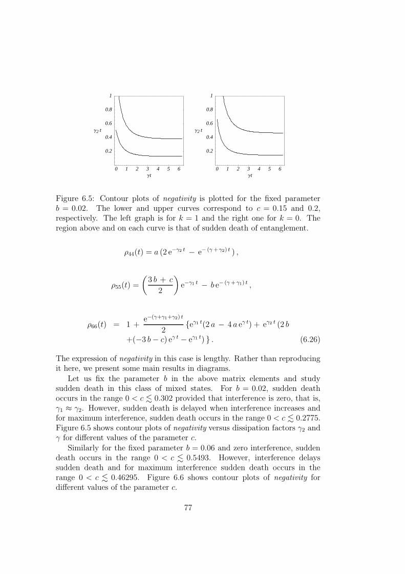
0 1 2 3 4 5 6Γt

0.2

0.4

0.6

0.8

1

Γ2 t

0 1 2 3 4 5 6Γt

0.2

0.4

0.6

0.8

1

Γ2 t

Figure 6.5: Contour plots of negativity is plotted for the fixed parameterb = 0.02. The lower and upper curves correspond to c = 0.15 and 0.2,respectively. The left graph is for k = 1 and the right one for k = 0. Theregion above and on each curve is that of sudden death of entanglement.

ρ44(t) = a (2 e−γ2 t − e− (γ + γ2) t ) ,

ρ55(t) =

(

3 b + c

2

)

e−γ1 t − b e− (γ + γ1) t ,

ρ66(t) = 1 +e−(γ+γ1+γ2) t

2eγ1 t(2 a − 4 a eγ t) + eγ2 t (2 b

+(−3 b− c) eγ t − eγ1 t) . (6.26)

The expression of negativity in this case is lengthy. Rather than reproducingit here, we present some main results in diagrams.

Let us fix the parameter b in the above matrix elements and studysudden death in this class of mixed states. For b = 0.02, sudden deathoccurs in the range 0 < c . 0.302 provided that interference is zero, that is,γ1 ≈ γ2. However, sudden death is delayed when interference increases andfor maximum interference, sudden death occurs in the range 0 < c . 0.2775.Figure 6.5 shows contour plots of negativity versus dissipation factors γ2 andγ for different values of the parameter c.

Similarly for the fixed parameter b = 0.06 and zero interference, suddendeath occurs in the range 0 < c . 0.5493. However, interference delayssudden death and for maximum interference sudden death occurs in therange 0 < c . 0.46295. Figure 6.6 shows contour plots of negativity fordifferent values of the parameter c.

77

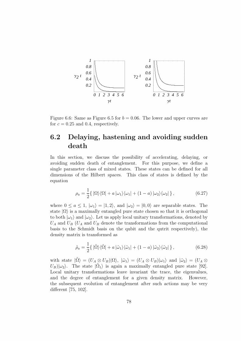
0 1 2 3 4 5 6Γt

0.2

0.4

0.6

0.8

1

Γ2 t

0 1 2 3 4 5 6Γt

0.2

0.4

0.6

0.8

1

Γ2 t

Figure 6.6: Same as Figure 6.5 for b = 0.06. The lower and upper curves arefor c = 0.25 and 0.4, respectively.

6.2 Delaying, hastening and avoiding sudden

death

In this section, we discuss the possibility of accelerating, delaying, oravoiding sudden death of entanglement. For this purpose, we define asingle parameter class of mixed states. These states can be defined for alldimensions of the Hilbert spaces. This class of states is defined by theequation

ρa =1

2 |Ω〉〈Ω| + a |ω1〉〈ω1| + (1 − a) |ω2〉〈ω2| , (6.27)

where 0 ≤ a ≤ 1, |ω1〉 = |1, 2〉, and |ω2〉 = |0, 0〉 are separable states. Thestate |Ω〉 is a maximally entangled pure state chosen so that it is orthogonalto both |ω1〉 and |ω2〉. Let us apply local unitary transformations, denoted byUA and UB (UA and UB denote the transformations from the computationalbasis to the Schmidt basis on the qubit and the qutrit respectively), thedensity matrix is transformed as

ρa =1

2 |Ω〉〈Ω| + a |ω1〉〈ω1| + (1 − a) |ω2〉〈ω2| , (6.28)

with state |Ω〉 = (UA ⊗ UB)|Ω〉, |ω1〉 = (UA ⊗ UB)|ω1〉 and |ω2〉 = (UA ⊗UB)|ω2〉. The state |Ω1〉 is again a maximally entangled pure state [92].Local unitary transformations leave invariant the trace, the eigenvalues,and the degree of entanglement for a given density matrix. However,the subsequent evolution of entanglement after such actions may be verydifferent [75, 102].

78

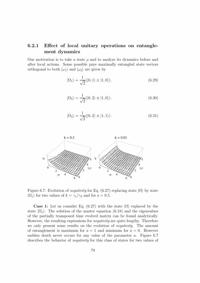
6.2.1 Effect of local unitary operations on entangle-ment dynamics

Our motivation is to take a state ρ and to analyze its dynamics before andafter local actions. Some possible pure maximally entangled state vectorsorthogonal to both |ω1〉 and |ω2〉 are given by

|Ω1〉 =1√2

(|0, 1〉 ± |1, 0〉) . (6.29)

|Ω2〉 =1√2

(|0, 2〉 ± |1, 0〉) . (6.30)

|Ω3〉 =1√2

(|0, 2〉 ± |1, 1〉) . (6.31)

k = 0.3

02

46

Γt0

2

4

6

Γ2t

N

k = 0.01

02

46

Γt0

2

4

6

Γ2t

N

Figure 6.7: Evolution of negativity for Eq. (6.27) replacing state |Ω〉 by state|Ω1〉 for two values of k = γ1/γ2 and for a = 0.5.

Case 1: Let us consider Eq. (6.27) with the state |Ω〉 replaced by thestate |Ω1〉. The solution of the master equation (6.18) and the eigenvaluesof the partially transposed time evolved matrix can be found analytically.However, the resulting expressions for negativity are quite lengthy. Thereforewe only present some results on the evolution of negativity. The amountof entanglement is maximum for a = 1 and minimum for a = 0. Howeversudden death never occurs for any value of the parameter a. Figure 6.7describes the behavior of negativity for this class of states for two values of

79

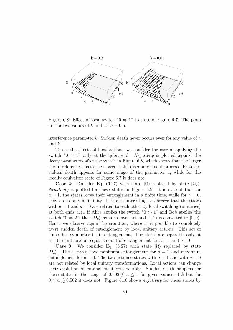
k = 0.3

02

46

Γt0

2

4

6

Γ2t

N

k = 0.01

02

46

Γt0

2

4

6

Γ2t

N

Figure 6.8: Effect of local switch “0 ⇔ 1” to state of Figure 6.7. The plotsare for two values of k and for a = 0.5.

interference parameter k. Sudden death never occurs even for any value of aand k.

To see the effects of local actions, we consider the case of applying theswitch “0 ⇔ 1” only at the qubit end. Negativity is plotted against thedecay parameters after the switch in Figure 6.8, which shows that the largerthe interference effects the slower is the disentanglement process. However,sudden death appears for some range of the parameter a, while for thelocally equivalent state of Figure 6.7 it does not.

Case 2: Consider Eq. (6.27) with state |Ω〉 replaced by state |Ω2〉.Negativity is plotted for these states in Figure 6.9. It is evident that fora = 1, the states loose their entanglement in a finite time, while for a = 0,they do so only at infinity. It is also interesting to observe that the stateswith a = 1 and a = 0 are related to each other by local switching (unitaries)at both ends, i. e., if Alice applies the switch “0 ⇔ 1” and Bob applies theswitch “0 ⇔ 2”, then |Ω2〉 remains invariant and |1, 2〉 is converted to |0, 0〉.Hence we observe again the situation, where it is possible to completelyavert sudden death of entanglement by local unitary actions. This set ofstates has symmetry in its entanglement. The states are separable only ata = 0.5 and have an equal amount of entanglement for a = 1 and a = 0.

Case 3: We consider Eq. (6.27) with state |Ω〉 replaced by state|Ω3〉. These states have minimum entanglement for a = 1 and maximumentanglement for a = 0. The two extreme states with a = 1 and with a = 0are not related by local unitary transformations. Local actions can changetheir evolution of entanglement considerably. Sudden death happens forthese states in the range of 0.502 . a ≤ 1 for given values of k but for0 ≤ a . 0.502 it does not. Figure 6.10 shows negativity for these states by

80

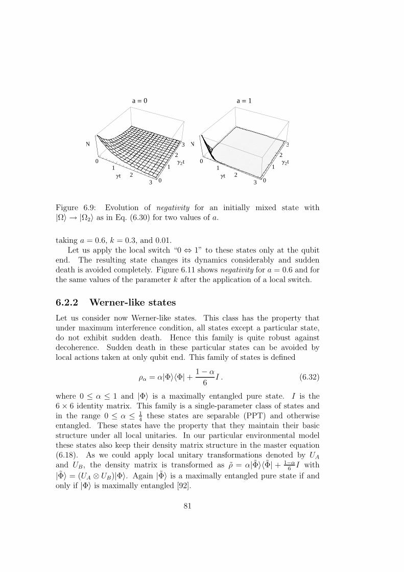
a = 0

01

23

Γt0

1

2

3

Γ2t

N

a = 1

01

23

Γt0

1

2

3

Γ2t

N

Figure 6.9: Evolution of negativity for an initially mixed state with|Ω〉 → |Ω2〉 as in Eq. (6.30) for two values of a.

taking a = 0.6, k = 0.3, and 0.01.Let us apply the local switch “0 ⇔ 1” to these states only at the qubit

end. The resulting state changes its dynamics considerably and suddendeath is avoided completely. Figure 6.11 shows negativity for a = 0.6 and forthe same values of the parameter k after the application of a local switch.

6.2.2 Werner-like states

Let us consider now Werner-like states. This class has the property thatunder maximum interference condition, all states except a particular state,do not exhibit sudden death. Hence this family is quite robust againstdecoherence. Sudden death in these particular states can be avoided bylocal actions taken at only qubit end. This family of states is defined

ρα = α|Φ〉〈Φ| +1 − α

6I . (6.32)

where 0 ≤ α ≤ 1 and |Φ〉 is a maximally entangled pure state. I is the6 × 6 identity matrix. This family is a single-parameter class of states andin the range 0 ≤ α ≤ 1

4these states are separable (PPT) and otherwise

entangled. These states have the property that they maintain their basicstructure under all local unitaries. In our particular environmental modelthese states also keep their density matrix structure in the master equation(6.18). As we could apply local unitary transformations denoted by UA

and UB, the density matrix is transformed as ρ = α|Φ〉〈Φ| + 1−α6I with

|Φ〉 = (UA ⊗ UB)|Φ〉. Again |Φ〉 is a maximally entangled pure state if andonly if |Φ〉 is maximally entangled [92].

81

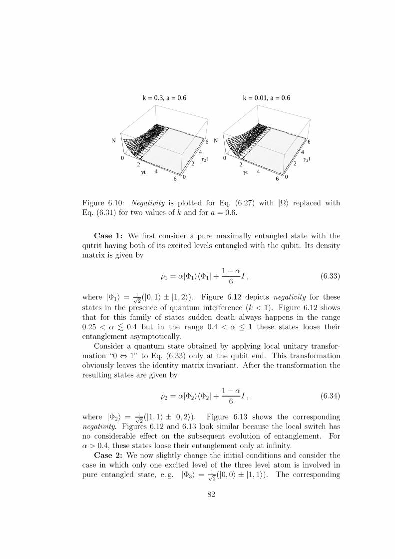
k = 0.3, a = 0.6

02

46

Γt0

2

4

6

Γ2t

N

k = 0.01, a = 0.6

02

46

Γt0

2

4

6

Γ2t

N

Figure 6.10: Negativity is plotted for Eq. (6.27) with |Ω〉 replaced withEq. (6.31) for two values of k and for a = 0.6.

Case 1: We first consider a pure maximally entangled state with thequtrit having both of its excited levels entangled with the qubit. Its densitymatrix is given by

ρ1 = α|Φ1〉〈Φ1| +1 − α

6I , (6.33)

where |Φ1〉 = 1√2(|0, 1〉 ± |1, 2〉). Figure 6.12 depicts negativity for these

states in the presence of quantum interference (k < 1). Figure 6.12 showsthat for this family of states sudden death always happens in the range0.25 < α . 0.4 but in the range 0.4 < α ≤ 1 these states loose theirentanglement asymptotically.

Consider a quantum state obtained by applying local unitary transfor-mation “0 ⇔ 1” to Eq. (6.33) only at the qubit end. This transformationobviously leaves the identity matrix invariant. After the transformation theresulting states are given by

ρ2 = α|Φ2〉〈Φ2| +1 − α

6I , (6.34)

where |Φ2〉 = 1√2(|1, 1〉 ± |0, 2〉). Figure 6.13 shows the corresponding

negativity. Figures 6.12 and 6.13 look similar because the local switch hasno considerable effect on the subsequent evolution of entanglement. Forα > 0.4, these states loose their entanglement only at infinity.

Case 2: We now slightly change the initial conditions and consider thecase in which only one excited level of the three level atom is involved inpure entangled state, e. g. |Φ3〉 = 1√

2(|0, 0〉 ± |1, 1〉). The corresponding

82

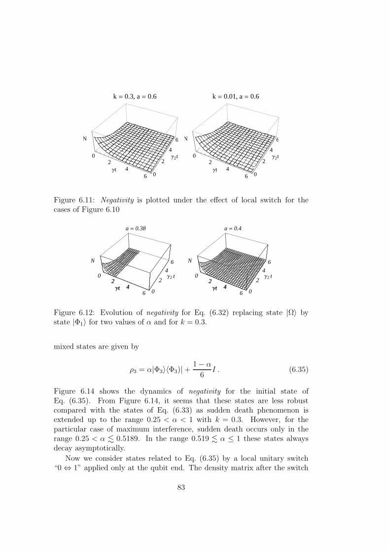
k = 0.3, a = 0.6

02

46

Γt0

2

4

6

Γ2t

N

k = 0.01, a = 0.6

02

46

Γt0

2

4

6

Γ2t

N

Figure 6.11: Negativity is plotted under the effect of local switch for thecases of Figure 6.10

a = 0.38

02

46

Γt0

2

4

6

Γ2 t

N

02

46

Γt

a = 0.4

02

46

Γt0

2

4

6

Γ2 t

N

02

46

Γt

Figure 6.12: Evolution of negativity for Eq. (6.32) replacing state |Ω〉 bystate |Φ1〉 for two values of α and for k = 0.3.

mixed states are given by

ρ3 = α|Φ3〉〈Φ3)| +1 − α

6I . (6.35)

Figure 6.14 shows the dynamics of negativity for the initial state ofEq. (6.35). From Figure 6.14, it seems that these states are less robustcompared with the states of Eq. (6.33) as sudden death phenomenon isextended up to the range 0.25 < α < 1 with k = 0.3. However, for theparticular case of maximum interference, sudden death occurs only in therange 0.25 < α . 0.5189. In the range 0.519 . α ≤ 1 these states alwaysdecay asymptotically.

Now we consider states related to Eq. (6.35) by a local unitary switch“0 ⇔ 1” applied only at the qubit end. The density matrix after the switch

83

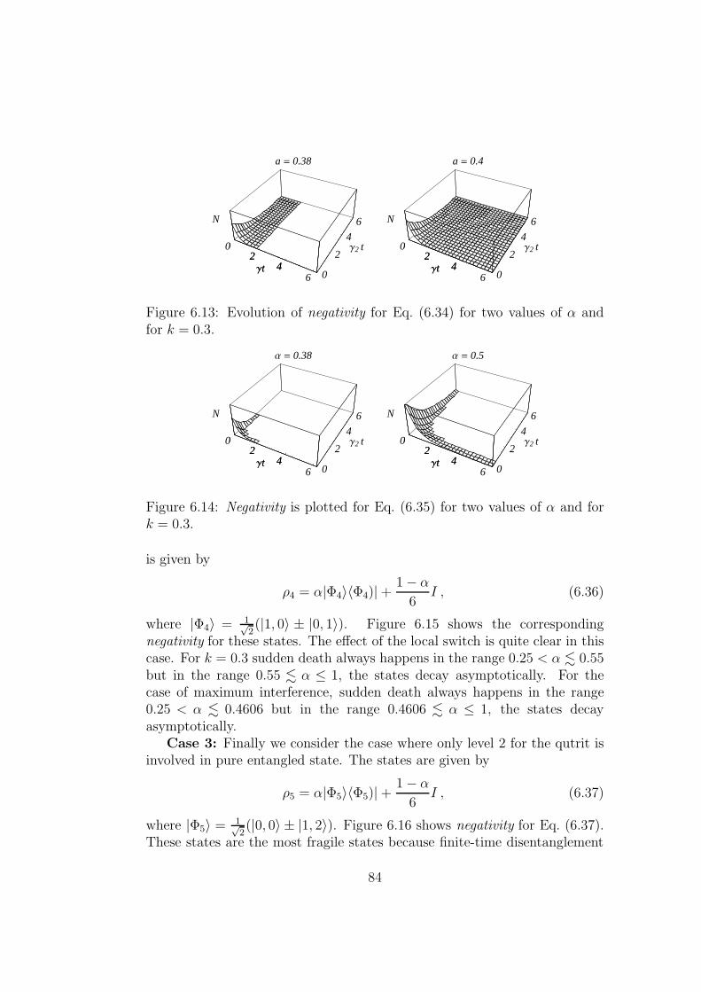
a = 0.38

02

46

Γt0

2

4

6

Γ2 t

N

02

46

Γt

a = 0.4

02

46

Γt0

2

4

6

Γ2 t

N

02

46

Γt

Figure 6.13: Evolution of negativity for Eq. (6.34) for two values of α andfor k = 0.3.

Α = 0.38

02

46

Γt0

2

4

6

Γ2 t

N

02

46

Γt

Α = 0.5

02

46

Γt0

2

4

6

Γ2 t

N

02

46

Γt

Figure 6.14: Negativity is plotted for Eq. (6.35) for two values of α and fork = 0.3.

is given by

ρ4 = α|Φ4〉〈Φ4)| +1 − α

6I , (6.36)

where |Φ4〉 = 1√2(|1, 0〉 ± |0, 1〉). Figure 6.15 shows the corresponding

negativity for these states. The effect of the local switch is quite clear in thiscase. For k = 0.3 sudden death always happens in the range 0.25 < α . 0.55but in the range 0.55 . α ≤ 1, the states decay asymptotically. For thecase of maximum interference, sudden death always happens in the range0.25 < α . 0.4606 but in the range 0.4606 . α ≤ 1, the states decayasymptotically.

Case 3: Finally we consider the case where only level 2 for the qutrit isinvolved in pure entangled state. The states are given by

ρ5 = α|Φ5〉〈Φ5)| +1 − α

6I , (6.37)

where |Φ5〉 = 1√2(|0, 0〉 ± |1, 2〉). Figure 6.16 shows negativity for Eq. (6.37).

These states are the most fragile states because finite-time disentanglement

84

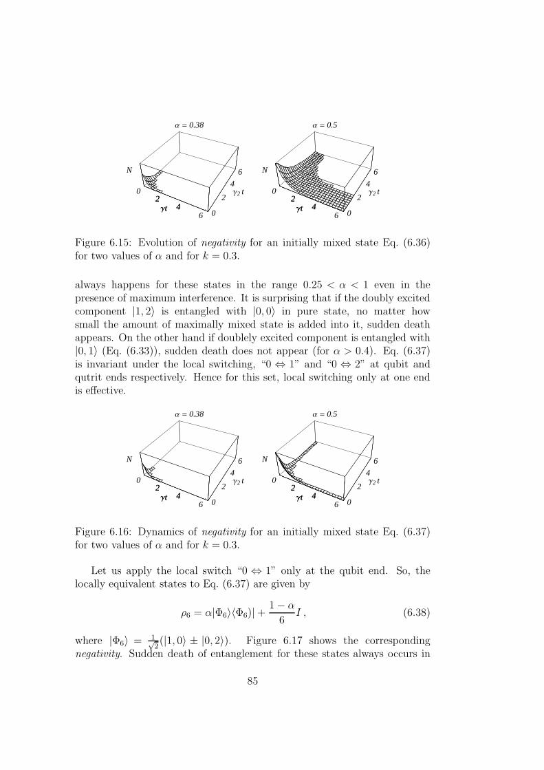
Α = 0.38

02

46

Γt0

2

4

6

Γ2 t

N

02

46

Γt

Α = 0.5

02

46

Γt0

2

4

6

Γ2 t

N

02

46

Γt

Figure 6.15: Evolution of negativity for an initially mixed state Eq. (6.36)for two values of α and for k = 0.3.

always happens for these states in the range 0.25 < α < 1 even in thepresence of maximum interference. It is surprising that if the doubly excitedcomponent |1, 2〉 is entangled with |0, 0〉 in pure state, no matter howsmall the amount of maximally mixed state is added into it, sudden deathappears. On the other hand if doublely excited component is entangled with|0, 1〉 (Eq. (6.33)), sudden death does not appear (for α > 0.4). Eq. (6.37)is invariant under the local switching, “0 ⇔ 1” and “0 ⇔ 2” at qubit andqutrit ends respectively. Hence for this set, local switching only at one endis effective.

Α = 0.38

02

46

Γt0

2

4

6

Γ2 t

N

02

46

Γt

Α = 0.5

02

46

Γt0

2

4

6

Γ2 t

N

02

46

Γt

Figure 6.16: Dynamics of negativity for an initially mixed state Eq. (6.37)for two values of α and for k = 0.3.

Let us apply the local switch “0 ⇔ 1” only at the qubit end. So, thelocally equivalent states to Eq. (6.37) are given by

ρ6 = α|Φ6〉〈Φ6)| +1 − α

6I , (6.38)

where |Φ6〉 = 1√2(|1, 0〉 ± |0, 2〉). Figure 6.17 shows the corresponding

negativity. Sudden death of entanglement for these states always occurs in

85

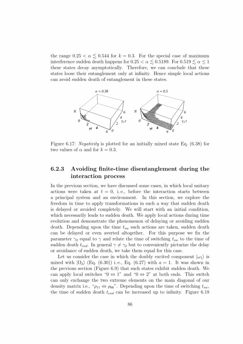
the range 0.25 < α . 0.544 for k = 0.3. For the special case of maximuminterference sudden death happens for 0.25 < α . 0.5189. For 0.519 . α ≤ 1these states decay asymptotically. Therefore, we can conclude that thesestates loose their entanglement only at infinity. Hence simple local actionscan avoid sudden death of entanglement in these states.

Α = 0.38

02

46

Γt0

2

4

6

Γ2 t

N

02

46

Γt

Α = 0.5

02

46

Γt0

2

4

6

Γ2 t

N

02

46

Γt

Figure 6.17: Negativity is plotted for an initially mixed state Eq. (6.38) fortwo values of α and for k = 0.3.

6.2.3 Avoiding finite-time disentanglement during theinteraction process

In the previous section, we have discussed some cases, in which local unitaryactions were taken at t = 0, i. e., before the interaction starts betweena principal system and an environment. In this section, we explore thefreedom in time to apply transformations in such a way that sudden deathis delayed or avoided completely. We will start with an initial condition,which necessarily leads to sudden death. We apply local actions during timeevolution and demonstrate the phenomenon of delaying or avoiding suddendeath. Depending upon the time tsw such actions are taken, sudden deathcan be delayed or even averted altogether. For this purpose we fix theparameter γ2 equal to γ and relate the time of switching tsw to the time ofsudden death tend. In general γ 6= γ2 but to conveniently picturize the delayor avoidance of sudden death, we take them equal for this case.

Let us consider the case in which the doubly excited component |ω1〉 ismixed with |Ω2〉 (Eq. (6.30)) i. e., Eq. (6.27) with a = 1. It was shown inthe previous section (Figure 6.9) that such states exhibit sudden death. Wecan apply local switches “0 ⇔ 1” and “0 ⇔ 2” at both ends. This switchcan only exchange the two extreme elements on the main diagonal of ourdensity matrix i.e., “ρ11 ⇔ ρ66”. Depending upon the time of switching tsw,the time of sudden death tend can be increased up to infinity. Figure 6.18

86

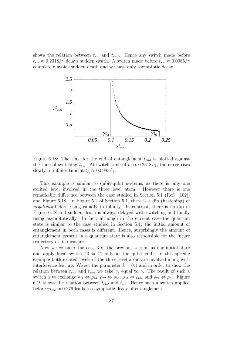
shows the relation between tsw and tend. Hence any switch made beforetsw ≈ 0.2318/γ delays sudden death. A switch made before tsw ≈ 0.0985/γcompletely avoids sudden death and we have only asymptotic decay.

0.05 0.1 0.15 0.2 0.25Γtsw

0.5

1

1.5

2

2.5

Γtend

ΓtA Γt0

Figure 6.18: The time for the end of entanglement tend is plotted againstthe time of switching tsw. At switch time of t0 ≈ 0.2318/γ, the curve risesslowly to infinite time at tA ≈ 0.0985/γ.

This example is similar to qubit-qubit systems, as there is only oneexcited level involved in the three level atom. However there is oneremarkable difference between the case studied in Section 5.1 (Ref. [102])and Figure 6.18. In Figure 5.2 of Section 5.1, there is a dip (hastening) ofnegativity before rising rapidly to infinity. In contrast, there is no dip inFigure 6.18 and sudden death is always delayed with switching and finallyrising asymptotically. In fact, although in the current case the quantumstate is similar to the case studied in Section 5.1, the initial amount ofentanglement in both cases is different. Hence, surprisingly the amount ofentanglement present in a quantum state is also responsible for the futuretrajectory of its measure.

Now we consider the case 3 of the previous section as our initial stateand apply local switch “0 ⇔ 1” only at the qubit end. In this specificexample both excited levels of the three level atom are involved along withinterference feature. We set the parameter k = 0.1 and in order to show therelation between tend and tsw, we take γ2 equal to γ. The result of such aswitch is to exchange ρ11 ⇔ ρ44, ρ22 ⇔ ρ55, ρ33 ⇔ ρ66, and ρ24 ⇔ ρ51. Figure6.19 shows the relation between tend and tsw. Hence such a switch appliedbefore γtsw ≈ 0.279 leads to asymptotic decay of entanglement.

87

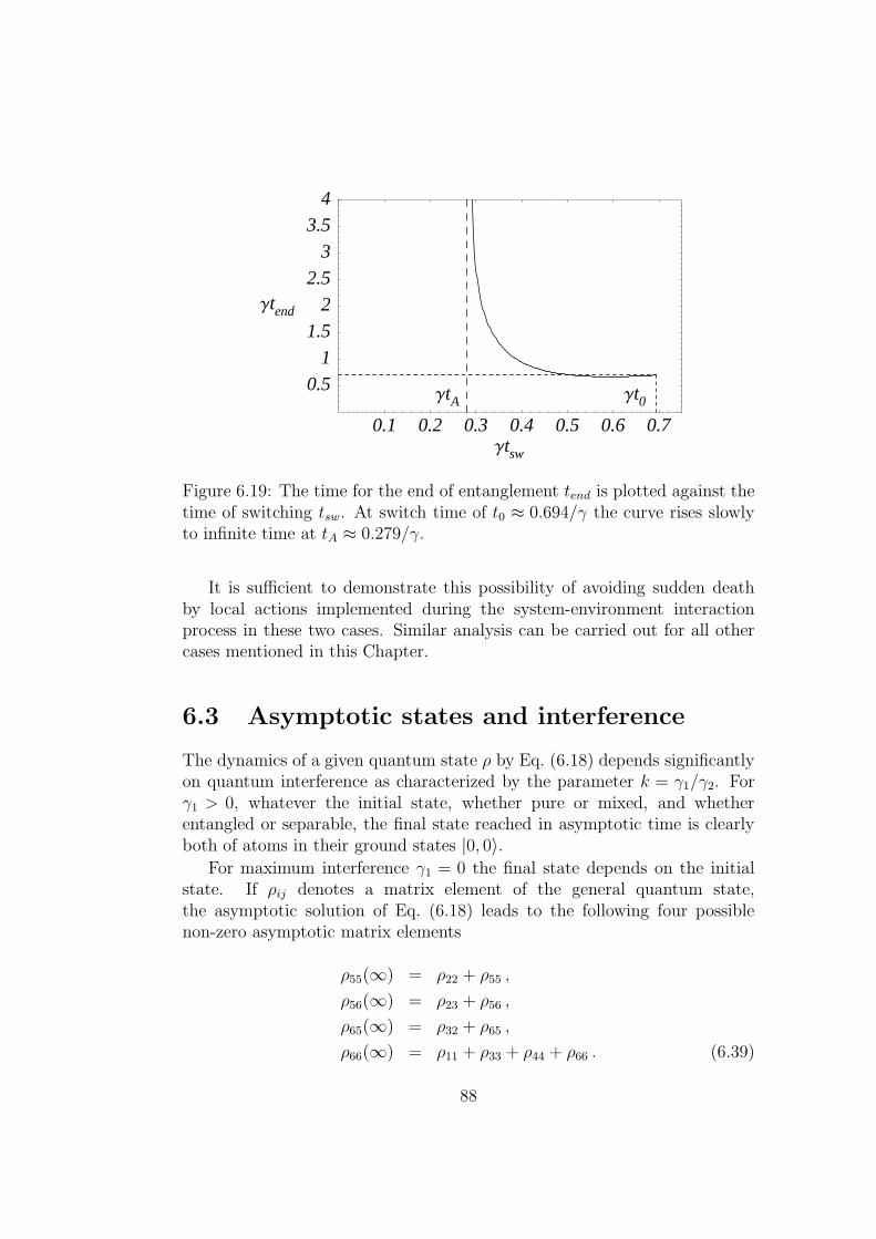
0.1 0.2 0.3 0.4 0.5 0.6 0.7Γtsw

0.5

1

1.5

2

2.5

3

3.5

4

Γtend

ΓtA Γt0

Figure 6.19: The time for the end of entanglement tend is plotted against thetime of switching tsw. At switch time of t0 ≈ 0.694/γ the curve rises slowlyto infinite time at tA ≈ 0.279/γ.

It is sufficient to demonstrate this possibility of avoiding sudden deathby local actions implemented during the system-environment interactionprocess in these two cases. Similar analysis can be carried out for all othercases mentioned in this Chapter.

6.3 Asymptotic states and interference

The dynamics of a given quantum state ρ by Eq. (6.18) depends significantlyon quantum interference as characterized by the parameter k = γ1/γ2. Forγ1 > 0, whatever the initial state, whether pure or mixed, and whetherentangled or separable, the final state reached in asymptotic time is clearlyboth of atoms in their ground states |0, 0〉.

For maximum interference γ1 = 0 the final state depends on the initialstate. If ρij denotes a matrix element of the general quantum state,the asymptotic solution of Eq. (6.18) leads to the following four possiblenon-zero asymptotic matrix elements

ρ55(∞) = ρ22 + ρ55 ,

ρ56(∞) = ρ23 + ρ56 ,

ρ65(∞) = ρ32 + ρ65 ,

ρ66(∞) = ρ11 + ρ33 + ρ44 + ρ66 . (6.39)

88

Hence whatever the values of these four matrix elements, the asymptoticstates ρ(t = ∞) are definitely separable (non-entangled). This is in contrastwith qutrit-qutrit systems, where some of the asymptotic states can beentangled [87]. Hence, quantum interference present only in qutrit part ofqubit-qutrit entangled system is not enough for the possibility of havingasymptotic entangled states. The reduced density matrix for the qubit onlyis

ρA(∞) =

(

0 00 1

)

, (6.40)

whereas the reduced density matrix for the qutrit is given by

ρB(∞) =

0 0 00 ρ55(∞) ρ56(∞)0 ρ65(∞) ρ66(∞)

. (6.41)

The qutrit part always remains in a superposition of ground and firstexcited level, i. e., (|0〉 + |1〉). In a qutrit-qutrit system, both reduceddensity matrices are always of the form of Eq. (6.41). Hence we expectthat in bipartite M ⊗N -systems, the possibility of asymptotically entangledstates in the presence of maximum interference is only possible if at leastM,N ≥ 3. Thus qutrit-qutrit systems are the minimal dimensional systemswith such a possibility. Both qubit-qubit and qubit-qutrit states always endup with separable asymptotic states in this particular model.

6.4 Sudden death of qubit-qutrit systems by

phase damping

In this section we summarize some of the results of the recent investigationon phase damping [100]. Let the general density matrix of the compositequbit-qutrit system be given by ρAB = [ρij ], where ρ∗ij = ρji,

∑

i ρii = 1, withi, j = 1, . . . , 6. This matrix contains the terms responsible for subsystemcoherence and joint-system coherence. The joint-system coherent terms areassociated with quantum entanglement. The individual subsystem can berepresented by a reduced density matrix by tracing out the variables of othersubsystem. The general reduced density matrix ρA for the qubit is given by

ρA =

(

(ρ11 + ρ22 + ρ33) (ρ14 + ρ25 + ρ36)(ρ41 + ρ52 + ρ63) (ρ44 + ρ55 + ρ66)

)

. (6.42)

Quantum states in which the subsystems are incoherent can be thosein which the composite system possesses high joint-state coherence and

89

are entangled. Therefore to study the effect of local dephasing noise onentanglement, we take all off-diagonal terms in the reduced density matricesto be zero. Therefore the incoherent reduced qubit state is given by

ρA =

(

(ρ11 + ρ22 + ρ33) 00 (ρ44 + ρ55 + ρ66)

)

. (6.43)

Similarly, the reduced density matrix for the qutrit ρB is given by

ρB =

(ρ11 + ρ44) (ρ12 + ρ45) (ρ13 + ρ46)(ρ21 + ρ54) (ρ22 + ρ55) (ρ23 + ρ56)(ρ31 + ρ64) (ρ32 + ρ65) (ρ33 + ρ66)

, (6.44)

with the incoherent qutrit reduced state

ρB =

(ρ11 + ρ44) 0 00 (ρ22 + ρ55) 00 0 (ρ33 + ρ66)

. (6.45)

Composite density matrices that yield reduced states of the form ρA andρB are given by

ρAB =

ρ11 0 0 0 ρ15 ρ16

0 ρ22 0 ρ24 0 ρ26

0 0 ρ33 ρ34 ρ35 00 ρ42 ρ43 ρ44 0 0ρ51 0 ρ53 0 ρ55 0ρ61 ρ62 0 0 0 ρ66

. (6.46)

For simplicity, consider the specific one-parameter class of states givenby

ρAB(x) =

14

0 0 0 0 x0 1

80 0 0 0

0 0 18

0 0 00 0 0 1

80 0

0 0 0 0 18

0x 0 0 0 0 1

4

, (6.47)

where 0 ≤ x ≤ 1/4.

90

Noise model

Let us consider local dephasing noise acting on subsystems that are nolonger interacting with each other. The most general time evolved densitymatrix in the operator-sum representation can be written as

ρ(t) = ε(ρ(0)) =∑

µ

Kµ(t)ρ(0)K†µ(t) , (6.48)

where the linear operators Kµ(t) satisfy a completeness relation givenby

∑

µK†µKµ = I and guarantee that the evolution is trace-preserving.

It represents the influence of noise which may be global or local. Forlocal and multi-local dephasing, the operators Kµ(t) are of the formKµ(t) = Fj(t) ⊗Ei(t), so that

ρAB(t) = ε(ρ(0)) =

2∑

i=1

3∑

j=1

Fj(t) ⊗ Ei(t)ρAB(0)E†i (t) ⊗ F †

j (t) , (6.49)

where

E1(t) = diag(1, γA) ⊗ diag(1, 1, 1) = diag(1, 1, 1, γA, γA, γA) , (6.50)

E2(t) = diag(0, ωA) ⊗ diag(1, 1, 1) = diag(0, 0, 0, ωA, ωA, ωA) , (6.51)

F1(t) = diag(1, 1) ⊗ diag(1, γB, γB) = diag(1, γB, γB, 1, γB, γB) ,(6.52)

F2(t) = diag(1, 1) ⊗ diag(0, ωB, 0) = diag(0, ωB, 0, 0, ωB, 0) , (6.53)

F3(t) = diag(1, 1) ⊗ diag(0, 0, ωB) = diag(0, 0, ωB, 0, 0, ωB) , (6.54)

with

γA(t) = exp−ΓAt/2, γB(t) = exp−ΓBt/2,ωA(t) =

√

1 − γ2A(t), ωB(t) =

√

1 − γ2B(t) , (6.55)

and diag(1, γA) is a diagonal matrix with elements 1 and γA, etc. Theoperators Ei(t) and Fj(t) individually satisfy the completeness relation, i. e.∑

iE†i (t)Ei(t) = I and

∑

j F†j (t)Fj(t) = I and induce local dephasing in the

qubit and the qutrit states, respectively. Now we can consider three noisesituations. i. e., the qubit dephasing only, the qutrit dephasing only, andthe combined local dephasing. In the first case, Fj(t) = I, and the timeevolution of the density matrix (6.47) is given as

ρAB(x, t) =

14

0 0 0 0 xγA

0 18

0 0 0 00 0 1

80 0 0

0 0 0 18

0 00 0 0 0 1

80

xγA 0 0 0 0 14

. (6.56)

91

Negativity for this matrix is given as

N(ρAB(x, t)) = max0, xγA − 1/8 . (6.57)

This function is zero for a finite time. Hence the global coherencevanishes in a finite time, i. e., sudden death, while decoherence occurs onlyasymptotically in the large-time limit.

Similarly, for noise acting on the qutrit B alone, the time evolved densitymatrix is given as

ρAB(x, t) =

14

0 0 0 0 xγB

0 18

0 0 0 00 0 1

80 0 0

0 0 0 18

0 00 0 0 0 1

80

xγB 0 0 0 0 14

. (6.58)

In this case negativity is given as

N(ρAB(x, t)) = max0, xγB − 1/8 . (6.59)

Hence sudden death of entanglement also takes place in this case of localdephasing noise acting on the qutrit alone. However, the full decoherence ofthe composite system occurs only in the large time limit, i. e., t→ ∞.

For the third situation where both subsystems are affected by local noise,the time evolved density matrix is given as

ρAB(x, t) =

14

0 0 0 0 xγAγB

0 18

0 0 0 00 0 1

80 0 0

0 0 0 18

0 00 0 0 0 1

80

xγAγB 0 0 0 0 14

. (6.60)

In this case negativity is given as

N(ρAB(x, t)) = max0, xγAγB − 1/8 . (6.61)

By the same arguments, multi-local dephasing induces sudden death evenmore quickly than in the case of single local dephasing noise.

92

Summary of Chapter 6

In summary we have investigated the effects of local unitary actionson sudden death of entanglement in two classes of quantum states ofqubit-qutrit systems. It has been demonstrated that such operations cancompletely avoid sudden death. We have also discussed the possibility ofdelaying or avoiding sudden death with local actions taken later when thedissipative dynamics has already degraded entanglement. We have shownthat up to a critical time, sudden death can be delayed and if local actionsare taken before that critical value of interaction time, sudden death can beavoided. The pursuit of robust quantum states, which can tolerate effects ofnoise and which do not undergo the peculiar phenomenon of sudden death,is vital for quantum information processing. In this regard we considered asingle parameter class of states, namely Werner-like states, which are quiterobust against sudden death. Except for a pair of quantum states, all statesin this class do not undergo sudden death. Moreover, it is also possibleto avoid sudden death in this pair by applying local action at the qubitend. We have also studied asymptotic states in the presence of maximuminterference. We point out that while it is possible for qutrit-qutrit systemsto have entangled asymptotic states, however, for qubit-qutrit system it isimpossible. All entangled quantum states in qubit-qutrit systems, whileinteracting with vacuum at two distant locations, end up in separable states.We expect similar results for qubit-qudit systems.

93

94

Chapter 7

Summary and conclusion

This thesis is concerned with dynamics of quantum entanglement. Itsmain motivation is to stabilize entanglement against decoherence effects.Entanglement is a dynamical quantity and it is very important to know itstime evolution in various physical systems. Since quantum systems interactwith environments and this unwanted interaction leads to decoherence.Docoherence leads to decay of entanglement. Recently, a special typeof decoherence is observed which attacks quantum entanglement only andfinishes it in finite time. This type of decoherence is named as suddendeath of entanglement. Sudden death of entanglement has been predictedfor many physical systems. It has been observed in laboratory as well. Weneed to take some measures to prevent quantum systems from this effect.This thesis is an effort in this regard. In particular, this thesis focuseson controlling finite-time disentanglement of bipartite entangled states ofqubit-qubit and qubit-qutrit systems.

In the theory of open quantum systems, dynamics of a principalsystem is obtained by taking trace over an environment. Under realisticconditions open quantum systems interact with environments and dynamicsof the combined system is unitary. However, dynamics of open systems isnot describable by unitary transformations due to their interactions withenvironments. The dynamics of open systems can be described by the masterequations under certain circumstances. We have studied entanglementsudden death of two non-interacting qubits interacting with their ownstatistically independent reservoirs at zero- and finite-temperatures. Wehave shown that in zero-temperature reservoirs, sudden death may appeardepending on the initial preparation of quantum states. We have analyzeda particular set of entangled states, namely X-states which preserve theirform under time evolution. We have shown that all those X-states whichexhibit sudden death can be converted to X-states which do not exhibit

95

sudden death. We have shown that such conversion is possible not onlybefore the interaction process but also during the interaction with theenvironment. However, there is always some critical time, after which it is nolonger possible to avert finite-time disentanglement. Interestingly, we haveobserved that it is possible to hasten, delay and even avert sudden deathof entanglement by local unitary transformations. However, the completeavertion of sudden death is only possible in zero-temperature reservoirs.In finite-temperature reservoirs, it is still possible to accelerate or delayfinite-time disentanglement up to some finite time. We have analyticallyshown that all X-states exhibit sudden death in finite-temperature reservoirs.We have analyzed the set of unitary operations and found the conditions onlocal unitary transformations which map X-states to X-states.

We have enlarged the dimension of the Hilbert space to 6 and consideredqubit-qutrit systems. We have studied dynamics of entanglement for variousinitial qubit-qutrit states. We have first provided the evidence of suddendeath due to amplitude damping and phase damping. Then we have studiedthe possibility of delaying, hastening, and avoiding sudden death. Again itis possible to hasten, delay, and avoid finite-time disentanglement via localunitary transformations. We have studied qubit-qutrit systems interactingwith two independent reservoirs at zero-temperature only. However, weremark that quantum interference is an additional feature which can controlthe disentanglement process. In contrast to qutrit-qutrit systems, allasymptotic states in qubit-qutrit systems are separable.

96

Bibliography

[1] E. Schrodinger, die Naturwissenschaften 23, 807 (1935).

[2] A. Einstein, B. Podolsky, and N. Rosen, Phys. Rev. 47, 777 (1935).

[3] N. Bohr, Phys. Rev. 48, 696 (1935).

[4] J. S. Bell, Physics 1(3), 195 (1964).

[5] J. F. Clauser, M. A. Horne, A. Shimony, and R. A. Holt, Phys. Rev.Lett. 23, 880 (1969).

[6] J. F. Clauser and M. A. Horne, Phys. Rev. D 10, 526 (1974).

[7] A. Aspect, P. Grangier, and G. Roger, Phys. Rev. Lett. 47, 460 (1981).

[8] A. Aspect, P. Grangier, and G. Roger, Phys. Rev. Lett. 49, 91 (1982).

[9] A. Aspect, J. Dalibard, and G. Roger, Phys. Rev. Lett. 49, 1804(1982).

[10] R. Garcıa-Patron, J. Fiurasek, N. J. Cerf, J. Wenger, R. Tualle-Brouri,and P. Grangier, Phys. Rev. Lett. 93, 130409 (2004).

[11] T. Scheidl, R. Ursin, J. Kofler, S. Ramelow, X-S Ma, T. Herbst,L. Ratschbacher, A. Fedrizzi, N. Langford, T. Jennewein, and A.Zeilinger, arXiv:quant-ph/0811.3129.

[12] C. H. Bennett and G. Brassard, in Proceedings of the IEEEInternational conference on Computers, Systems and Signal Processing(IEEE Computer Society Press, Bangalore, India, December 1984) pp.175-179

[13] D. Deutsch, Proc. R. Soc. London, Ser. A 400, 97 (1985).

[14] R. P. Feynman, Int. J. Theor. Phys. 21, 467 (1982).

97

[15] P. W. Shor, Phys. Rev. A 52, 2493 (1995).

[16] A. Steane, Phys. Rev. Lett. 77, 793 (1996).

[17] A. K. Ekert, Phys. Rev. Lett. 67, 661 (1991).

[18] C. H. Bennett and S. J. Wiesner, Phys. Rev. Lett. 69, 2881 (1992).

[19] C. H. Bennett, G. Brassard, C. Crepeau, R. Josza, A. Peres, and W.K. Wootters, Phys. Rev. Lett. 70, 1895 (1993).

[20] K. Mattle, H. Weinfurter, P. G. Kwiat, and A. Zeilinger, Phys. Rev.Lett. 76, 4656 (1996).

[21] D. Bouwmeester, J. W. Pan, K. Mattle, M. Eibl, H. Weinfurter, andA. Zeilinger, Nature 390, 575 (1997).

[22] D. Boschi, S. Branca, F. D. Martini, L. Hardy, and S. Popescu, Phys.Rev. Lett. 80, 1121 (1998).

[23] J. W. Pan, D. Bouwmeester, H. Weinfurter, and A. Zeilinger, Phys.Rev. Lett. 80, 3891 (1998).

[24] A. Furusawa, J. L. Sorensen, S. L. Braunstein, C. A. Fuchs, H. J.Kimble, and E. S. Polzik, Science 282, 706 (1998).

[25] T. Jennewein, C. Simon, G. Weihs, H. Weinfurter, and A. Zeilinger,Phys. Rev. Lett. 54, 4729 (2000).

[26] D. S. Naik, C. G. Peterson, A. G. White, A. J. Berglund, and P. G.Kwiat, Phys. Rev. Lett. 84, 4733 (2000).

[27] W. Tittel, J. Brendel, H. Zbinden, and N. Gisin, Phys. Rev. Lett. 84,4737 (2000).

[28] H-K. Lo, T. Spiller, and S. Popescu, Introduction to quantumcomputation and information (World Scientific, 1999).

[29] M. A. Nielsen and I. L. Chuang, Quantum Computation and QuantumInformation (Cambridge Univ. Press, Cambridge, 2000).

[30] D. Bouwmeester, A. K. Ekert, and A. Zeilinger, The physics ofquantum information: quantum cryptography, quantum teleportation,quantum computation (Springer, New York, 2000).

98

[31] G. Alber, T. Beth, M. Horodecki, P. Horodecki, R. Horodecki, M.Rotteler, H. Weinfurter, R. Werner, and A. Zeilinger, QuantumInformation (Springer-Verlag, Berlin, 2001).

[32] S. L. Braunstein, and A. K. Pati, Quantum Information withContinuous Variables (Kluwer Academics Publishers, 2003).

[33] D. Bruß and G. Leuchs, Lectures on Quantum Information (Wiley-VchGmbH & Co. KGaA, 2007).

[34] R. Horodecki, P. Horodecki, M. Horodecki, and K. Horodecki, Rev.Mod. Phys. 81, 865 (2009).

[35] L. Clarisse, PhD thesis, University of York, England, arXiv:quant-ph/0612072.

[36] R. F. Werner, Phys. Rev. A 40, 4277 (1989).

[37] A. Peres, Phys. Rev. Lett. 77, 1413 (1996).

[38] M. Horodecki, P. Horodecki, and R. Horodecki, Phys. Lett. A 223, 1(1996).

[39] P. Horodecki, M. Lewenstein, G. Vidal, and I. Cirac, Phys. Rev. A 62,032310 (2000).

[40] B. M. Terhal, Theo. Comp. Sc. 287, 313 (2001).

[41] P. Horodecki, Theo. Comp. Sc. 293, 589 (2003).

[42] M. Horodecki, P. Horodecki, and R. Horodecki, Phys. Rev. Lett. 80,5239 (1998).

[43] D. P. DiVincenzo, P. W. Shor, J. A. Smolin, B. M. Terhal, and A. V.Thapliyal, Phys. Rev. A 61, 062312 (2000).

[44] W. Dur, J. I. Cirac, M. Lewenstein, and D. Bruß, Phys. Rev. A 61,062313 (2000).

[45] J. Eisert, PhD thesis, University of Potsdam, Germany, arXiv:quant-ph/0610253.

[46] H. J. Briegel, W. Dur, J. I. Cirac, and P. Zoller, Phys. Rev. Lett. 81,5932 (1998).

99

[47] D. Deutsch, A. Ekert, C. Macchiavello, S. Popescu, and A. Sanpera,Phys. Rev. Lett. 77, 2818 (1996).

[48] M. Horodecki, P. Horodecki, and R. Horodecki, Phys. Rev. Lett. 84,4260 (2000).

[49] M. Horodecki, P. Horodecki, and R. Horodecki, Phys. Rev. Lett. 85,433 (2000).

[50] C. H. Bennett, D. P. DiVincenzo. J. A. Smolin, and W. K. Wootters,Phys. Rev. A 54, 3824 (1996).

[51] S. Hill and W. K. Wootters, Phys. Rev. Lett. 78, 5022 (1997).

[52] W. K. Wootters, Phys. Rev. Lett. 80, 2245 (1998).

[53] K. Zyczkowski, P. Horodecki, A. Sanpera, and M. Lewenstein, Phys.Rev. A 58, 883 (1998).

[54] G. Vidal and R. F. Werner, Phys. Rev. A 65, 032314 (2002).

[55] P. Rungta, PhD thesis, The University of New Mexico, USA (2002).

[56] H-P. Breuer, and F. Petruccione, The Theory of Open QuantumSystems (Oxford University Press, Oxford, 2002).

[57] M. O. Scully and M. S. Zubairy, Quantum Optics (CambridgeUniversity Press, London, 1997).

[58] P. J. Dodd and J. J. Halliwel, Phys. Rev. A 69, 052105 (2004).

[59] P. J. Dodd, Phys. Rev. A 69, 052106 (2004).

[60] L. Diosi, Irreversible Quantum Dynamics, edited by F. Benatti and R.Floreanini (Springer, New York, 2003).

[61] T. Yu and J. H. Eberly, Phys. Rev. Lett. 93, 140404 (2004).

[62] L. Jakobczyk and A. Jamroz, Phys. Lett. A 333, 35 (2004).

[63] T. Yu and J. H. Eberly, Opt. Commun. 264, 393 (2006).

[64] M. P. Almeida, F. de Melo, M. Hor-Meyll, A. Salles, S. P. Walborn, P.H. Souto Ribeiro, and L. Davidovich, Science 316, 579 (2007).

[65] A. Salles, F. de Melo, M. P. Almeida, M. Hor-Meyll, S. P. Walborn, P.H. Souto Ribeiro, and L. Davidovich, Phys. Rev. A 78, 022322 (2008).

100

[66] J. Laurat, K. S. Choi, H. Deng, C. W. Chou, and H. J. Kimble, Phys.Rev. Lett. 99, 180504 (2007).

[67] K. Kraus, States, Effect, and Operations: Fundamental Notions inQuantum Theory (Springer-Verlag, Berlin, 1983).

[68] T. Yu and J. H. Eberly, Phys. Rev. B 66, 193306 (2002).

[69] T. Yu and J. H. Eberly, Phys. Rev. B 68, 165322 (2003).

[70] M. Lucamarini, S. Paganelli, and S. Mancini, Phys. Rev. A 69, 062308(2004).

[71] D. Tolkonov, V. Privman, and P. K. Aravind, Phys. Rev. A 71, 060308(2005).

[72] Xian-Ting Liang, Phys. Lett. A 349, 98 (2006).

[73] M. Yonac, T. Yu, and J. H. Eberly, J. Phys. B 39, S621 (2006).

[74] A. R. R. Carvalho, F. Mintert, S. Palzer, and A. Buchleitner, Eur.Phys. J. D 41, 425 (2007).

[75] T. Yu and J. H. Eberly, Quantum Information and Computation 7,459 (2007).

[76] K. Roszak and P. Machnikowski, Phys. Rev. A 73, 022313 (2006).

[77] V. S. Malinovsky and I. R. Sola, Phys. Rev. Lett. 96, 050502 (2006).

[78] M. Ban, J. Phys. A 39, 1927 (2006).

[79] M. Ban and F. Shibata, Phys. Lett. A 354, 35 (2006).

[80] M. Franca Santos, P. Milman, L. Davidovich, and N. Zagury, Phys.Rev. A 73, 040305(R) (2006).

[81] J. Wang, H. Batelaan, J. Podany, and A. F. Starace, J. Phys. B 39,4343 (2006).

[82] L. Lamata, J. Leon, and D. Salgado, Phys. Rev. A 73, 052325 (2006).

[83] A. Jamroz, J. Phys. A 39, 7727 (2006).

[84] T. Yu and J. H. Eberly, Phys. Rev. Lett. 97, 140403 (2006).

[85] Z. Ficek and R. Tanas, Phys. Rev. A 74, 024304 (2006).

101

[86] G. S. Agarwal, Quantum Statistical Properties of Spontaneous Emissionand their Relation to Other Approaches (Springer, Berlin, 1974).

[87] L. Derkacz and L. Jakobczyk, Phys. Rev. A 74, 032313 (2006).

[88] H. T. Cui, K. Li, and X. X. Yi, Phys. Lett. A 365, 44 (2007).

[89] Z. Sun, X. Wang, and C. P. Sun, Phys. Rev A 75, 062312 (2007).

[90] Jie-Hui Huang and Shi-Yao Zhu, Phys. Rev. A 76, 062322 (2007).

[91] K. Ann and G. Jaeger, Phys. Rev. A 76, 044101 (2007).

[92] M. Ali, A. R. P. Rau, and K. Ranade, arXiv:quant-ph/0710.2238.

[93] K. Ann and G. Jaeger, Phys. Lett. A 372, 579 (2008).

[94] M. Ikram, Fu-li Li, and M. S. Zubairy, Phys. Rev. A 75, 062336(2007).

[95] M. O. T. Cunha, N. J. Phys. 9, 237 (2007).

[96] J. H. Eberly and T. Yu, Science 316, 555 (2007).

[97] F. Lastra, G. Romero, C. E. Lopez, M. Franca Santos and J. C.Retamal, Phys. Rev A 75, 062324 (2007).

[98] F. F. Fanchini and R. d. J. Napolitano, arXiv:quant-ph/0707.4092.

[99] G. Jaeger and K. Ann, Phys. Lett. A 372, 2212 (2008).

[100] K. Ann and G. Jaeger, Phys. Lett. A 372, 6853 (2008).

[101] A. G. Kofman and A. N. Korotkov, Phys. Rev. A 77, 052329 (2008).

[102] A. R. P. Rau, M. Ali, and G. Alber, Eur. Phys. Lett. 82, 40002 (2008).

[103] A. Al-Qasimi and D. F. V. James, Phys. Rev. A 77, 012117 (2008).

[104] B. Bellomo, R. Lo Franco, and G. Compagno, Phys. Rev. A 77,032342 (2008).

[105] X. Cao and H. Zheng, Phys. Rev. A 77, 022320 (2008).

[106] F. Lastra, G. Romero, C. E. Lopez, N. Zagury, and J. C. Retamal,arXiv:quant-ph/0801.1664.

[107] M. Hernandez and M. Orszag, Phys. Rev. A 78, 042114 (2008).

102

[108] I. Sainz and G. Bjork, Phys. Rev. A 77, 052307 (2008).

[109] I. Sainz and G. Bjork, arXiv:quant-ph/0806.2102.

[110] R. Tahira, M. Ikram, T. Azim, and M. S. Zubairy, J. Phys. B 41,205501 (2008).

[111] L. Derkacz and L. Jakobczyk, arXiv:quant-ph/0806.2537.

[112] J. Li, K. Chalapat, and G. S. Paraoanu, J. Low Temp. Phys. 153, 294(2008).

[113] Fa-Qiang Wang, Zhi-Ming Zhang, and Rui-Sheng Liang, Phys. Rev. A78, 062318 (2008).

[114] N. Yamamoto, H. I. Nurdin, M. R. James, and I. R. Petersen, Phys.Rev. A 78, 042339 (2008).

[115] M. Scala, R. Migliore, and A. Messina, J. Phys. A 41, 435304 (2008).

[116] C. J. Shan, W. W. Cheng, T. K Liu, J. B. Liu, and H. Wei, Chin.Phys. Lett. 25, 3115 (2008).

[117] P. Li, Q. Zhang, and J. Q. You, Phys. Rev. A 79, 014303 (2009).

[118] J. H. Cole, arXiv:quant-ph/0809.1746.

[119] S. Chan, M. D. Reid, and Z. Ficek, arXiv:quant-ph/0810.3050.

[120] J. Dajka and J. Luczka, Phys. Rev. A 77, 062303 (2008).

[121] P. Marek, J. Lee, and M. S. Kim, Phys. Rev. A 77, 032302 (2008).

[122] R. C. Drumond and M. O. Terra Cunha, arXiv:quant-ph/0809.4445.

[123] Y. Dubi and M. Ventra, Phys. Rev. A 79, 012328 (2009).

[124] A. Al-Qasimi and D. F. V. James, arXiv:quant-ph/0810.0550.

[125] F. Lastra, S. Wallentowitz, M. Orszag, and M. Hernandez, arXiv:quant-ph/0811.4399.

[126] J. P. Paz and A. J. Roncaglia, Phys. Rev. Lett. 100, 220401 (2008).

[127] C. E. Lopez, G. Romero, F. Lastra, E. Solano, and J. C. Retamal,Phys. Rev. Lett. 101, 080503 (2008).

103

[128] L. Mazzola, S. Maniscalco, J. Piilo, K.-A. Suominen, and B. M.Garraway, arXiv:quant-ph/0812.3546.

[129] M. Ali, G. Alber, and A. R. P. Rau, J. Phys. B 42, 025501 (2009).

[130] T. Yu and J. H. Eberly, Science 323, 598 (2009).

[131] N. B. An and J. Kim, Phys. Rev. A 79, 022303 (2009).

[132] K. Ann and G. Jaeger, arXiv:quant-ph/0903.0009.

[133] P. Meystre, M. O. Scully, and H. Walther, Opt. Commun 33, 153(1980).

[134] F. Shimizu, K. Shimizu, and H. Takauma, Phys. Rev. A 28, 2248(1983).

[135] T. Hellmuth, H. Walther, A. Zajonc, and W. Schleich, Phys. Rev. A35, 2532 (1987).

[136] A. Sanpera, R. Tarrach and G. Vidal, Phys. Rev. A 58, 826 (1998).

[137] M. Ali, A. R. P. Rau, and G. Alber, in preparation.

[138] R. A. Horn and C. R. Johnson, Matrix Analysis (Cambridge UniversityPress, Cambridge, 1985), Chap. 7.

[139] S. Bose, I. Fuentes-Guridi, P. L. Knight, and V. Vedral, Phys. Rev.Lett. 87, 050401 (2001).

[140] J. S. Pratt, Phys. Rev. Lett. 93, 237205 (2004).

[141] Z. Ficek and S. Swain, Phys. Rev. A 69, 023401 (2004).

[142] D. P. Chi and S. Lee, J. Phys. A 36, 11503 (2003).

104

Acknowledgments

The completion of a PhD and writing the thesis is usually the outcomeof individual hard work and cooperation of several personalities. It wascertainly not possible for me to accomplish this task without the roles ofmany individuals who have directly or indirectly influenced this work. Firstof all, I would like to submit thanks to my supervisor Prof. Dr. GernotAlber. He has certainly played a key role in the completion of this thesis.He always encouraged me to think and work independently. His penetratingquestions and criticism always opened the closed doors to me. I am indebtedto him for accepting me in his group, for being patient, kind and alwaysopening his doors to me.

I would also like to express my deepest regards to my collaborator Prof.Dr. A. R. P. Rau. In fact he introduced me to the main subject of thisthesis. Almost all of my PhD work is in collaboration with him. I havebenefited a lot from this collaboration. I am indeed thankful for his openmindness, encouragement, and always giving me many precious advises. Inaddition, I have learned professional ethics from him as well.

I am thankful to all present and past members of the TheoretischeQuantenphysik group at TU Darmstadt for providing all sort of technicalassistance to me. In particular, I thank Kedar Ranade and Oliver Kernwho were not only always willing for discussions but they always gave theirprecious time and technical assistance whenever I needed it. In particular, Ithank Oliver Kern for a nice drive to Innsbruck. I am thankful to AeyshaKhalique for her useful suggestions at some early stage of my PhD. I amthankful to Kedar Ranade for translating the abstract into German languageand for reading this manuscript and pointing out several corrections. Iam thankful to Ulrich Seyfarth for reviewing the German abstract. I amgrateful to Sameer Varyani for providing a useful Mathematica code besideshis valuable friendship.

I am thankful to Irmgard Praclik, Dietrich Praclik, Ute Stewart, BarbaraStowasser, and other members of IGM (International Generation Meeting)for exposing the German way of life and culture to me. Indeed I really

105

enjoyed my stay in Germany due to these nice, kind and friendly people. Ialso appreciate ISO (International Students Organization) in this regard.

I acknowledge the financial support from Higher Education Commission(HEC), Pakistan and German Educational Exchange Service (DAAD).

I am unable to express my appreciation for my family members. Allmy brothers and sisters pushed me forward to achieve this goal. Indeedwithout their love, encouragement, taking care, moral and financial supportat every stage of my life, I could never be able to reach this day. I amparticularly indebted to my eldest brother Dr. Liaqat Ali and my dearestsister Ms. Farzana Anjum. I am thankful to my wife Qurat Ul Ann for herunderstanding and love. Although she entered in my life at the final stagesof this work, nevertheless she managed to contribute by providing usefulsuggestions and Figures 3.1, 6.1, and 6.2.

Finally, I am thankful to Prof. Dr. R. Roth for being a referee for mythesis.

106

Curriculum Vitae

Personal Data

Name: Mazhar Ali

Email: mazhar.ali@physik.tu-darmstadt.de

Born: December 20th, 1976 in Mansehra (Pakistan)

Language Skills

Hindko: Mother language

Urdu: National language

English: very good command on reading, writing,speaking and listening

German: good command on reading, writing, speakingand listening

Education

03/1991–03/1993 Secondary School Certificate (S. S. C.), GovernmentHigh School 3, Mansehra (Pakistan)

07/1993–08/1996 Higher Secondary School Certificate (H. S. S. C.),Government Degree College, Abbottabad (Pakistan)

09/1996–09/1998 Bachelors of Science (B. Sc) in Maths and Physics, Gov-ernment Post Graduate College, Mansehra (Pakistan)

03/1999–03/2001 Masters in Physics (M. Sc), Government Post GraduateCollege, Abbottabad (Pakistan)

03/2001–03/2002 Bachelors of Education (B. Ed) in Maths and Physics,Allama Iqbal Open University, Islamabad (Pakistan)

107

03/2002–03/2004 Masters in Philosophy (M. Phil.), Electronics Depart-ment, Quaid-I-Azam University, Islamabad (Pakistan)(Thesis on Quantum Information)

04/2006– Doctoral student at Institut fur Angewandte Physik,Technische Universitat Darmstadt, (Germany) undersupervision of Prof. Dr. Gernot Alber. (Thesis onQuantum Information)

Conferences Attended

11 - 14 April 07 Informal Quantum Information Gathering 5 (IQING5),Innsbruck, Austria

27 - 31 August 07 First European Young Scientists Conference on Quan-tum Information (EYSQI), Vienna, Austria

10 - 14 March 08 German Physical Society Annual Meeting (DPG-Tagung),Darmstadt, Germany

2 - 6 March 09 German Physical Society Annual Meeting (DPG-Tagung),Hamburg, Germany

List of Publications

[1] Mazhar Ali, Quantum Cloning via Bragg Scattering, M. Phil. thesis,Quaid-I-Azam University, Islamabad (2004).

[2] K. S. Ranade and Mazhar Ali, The Jamio lkowski Isomorphism and aSimplified Proof for the Correspondence Between Vectors Having SchmidtNumber k and k−Positive Maps, Open. Sys. & Information Dyn. 14,371-378 (2007). arXiv:quant-ph/0702255v1.

[3] Mazhar Ali, A. R. P. Rau, and K. Ranade, Disentanglement inqubit-qutrit systems, arXiv:quant-ph/0710.2238v1.

[4] A. R. P. Rau, Mazhar Ali, and G. Alber, Hastening, delaying, oraverting sudden death of quantum entanglement, Eur. Phys. Lett. 82,40002 (2008). arXiv:quant-ph/0711.0317v2.

[5] Mazhar Ali, G. Alber, and A. R. P. Rau, Manipulating entanglementsudden death of two-qubit X-states in zero- and finite-temperaturereservoirs, J. Phys. B 42, 025501 (2009). arXiv:quant-ph/0810.2936v1.

108

Erklarung

Hiermit erklare ich an Eides Statt, daß ich die vorliegende Dissertationselbstandig, nur unter Verwendung der angegebenen Quellen und Hilfsmittelverfaßt habe. Ich habe bisher keinen Versuch unternommen, an eineranderen Hochschule das Promotionsverfahren einzuleiten.

Darmstadt, den 25. Mai 2009 Mazhar Ali

109