© Think You?! The Proceedings of the Bay Honors Research Symposium, 2020. All Rights Reserved.

Quantum Computing Simulation of Quantum Interrogation

by Shiloh Andersson, College of San Mateo Mentor: Alexander Wong

Abstract Quantum interrogation is the technique for measuring a quantum system without interacting with or disturbing the system. In 1995, Paul Kwiat, along with a group of physicists, devised a method for quantum interrogation that allows for successful interaction-free measurements, and the success rate depends on the number of times, N, a photon passes through a beam splitter. For the case of N = 3, the success rate is about 42%. Using software provided by IBM, we design and implement a quantum computing algorithm that performs the Kwiat’s method for quantum interrogation, and we perform a t-test to assess the validity of the hypothesized success rate.

1 Introduction Imagine two people, Alice and Bob. Alice presents Bob with a sealed box containing a photon- sensitive bomb, and she asks him to determine whether or not the bomb will explode. If Bob answers correctly, Alice will reward him with several bars of gold. However, if Bob opens the box and the bomb is alive, the bomb will explode and Bob will die. Is there a way for Bob to win the gold without risking his life? Physics says yes.

The problem above can be solved with quantum interrogation, a technique for measuring quantum systems without disturbing the system. In this case, Bob measures the state of the bomb without opening the box and exposing the bomb to light. There exists a method for quantum interrogation, proposed by Avshalom Elitzur and Lev Vaidman (Tan-Holmes, 2016). With this method, there is a 25% chance that Bob can successfully determine the state of the bomb without detonating the bomb. But can we achieve a success rate that is higher than 25%?

In 1995, researchers at the University of Illinois proposed a new method that builds upon the Elitzur-Vaidman scheme (Kwiat et al., 1995). For the case of N = 3, where N denotes the number of times a photon passes through a beam splitter, the Kwiat et. al scheme predicts that the success rate becomes 42.1875%.

In early 2019, researchers at the Indian Institute of Science Education and Research Kolkata used IBM’s quantum computing software, QISKit, in order to create a quantum computing simulation of the Elitzur-Vaidman scheme. We will extend their work to design and implement a quantum computing algorithm for a simulation of the Kwiat et al. scheme, and we will use statistical testing to assess the hypothesized 42.1875% success rate.

2 General Background 2.1 Quantum Interrogation Quantum interrogation is the technique for measuring a quantum system (that is, a system com- posed of atoms or subatomic particles) without disturbing or interacting with the system. In essence, one takes a measurement on a quantum system, but there is no interaction with the system. For this reason, quantum interrogation is also called “interaction-free measurement.” Naturally, one may wonder what constitutes as a measurement. For this paper, we will define “measurement” using the

Andersson 2

definition given by Mithuna Yoganathan, a PhD student studying quantum computing at the University of Cambridge, in her video on the difference between measurement and interaction. According to Yogonathan, a measurement is, in essence, an action that provides information about a system to an observer outside of the system (Yoganathan, 2018). As for the definition of “interaction,” we will take an interaction to be a bomb explosion (Raj et al, 2019). Thus, an interaction-free measurement for Bob would be determination of the state of the existence of a bomb in the box without causing an explosion.

2.2 A Brief Introduction to Quantum Mechanics Quantum interrogation is possible due to key principles in quantum mechanics, the branch of physics that is concerned with atoms and subatomic particles. A key feature of quantum mechanics is wave- particle duality: quantum objects can behave both like waves1 and particles. One consequence of the wave-like nature of particles is quantum superposition, the idea that particles can exist in multiple states at once prior to measurement. Before we examine the concept of quantum superposition, we will first discuss wave superposition in classical physics.

In classical physics, the principle of wave superposition states that when two waves overlap, their wave functions add together to form a new wave. The function that represents each wave is a multivariable function in terms of position x and time t. If we had two waves, which are modeled by the functions f0(x, t) and f1(x, t), then the resulting wave f(x, t) would be

f 𝑥, 𝑡 𝑓 𝑥, 𝑡 𝑓 𝑥, 𝑡 .

(2.1)

In general, when we have n waves overlapping, the resulting wave due to superposition would be

f 𝑥, 𝑡 𝑓 𝑥, 𝑡 ,

(2.2)

where fi(x,t) represents each of the n waves. We will see a very similar equation when we discuss the superposition of quantum states and the relevant mathematics for quantum mechanics.

Now we can transition to quantum physics. Quantum physics says that the state of a quantum system or object, much like classical waves, can experience superposition before measurement of the state. That is, if the state of a quantum system remains unknown to an observer outside the system, then the system exists in all possible states at once; when an outside observer attempts to measure the system, then quantum superposition is broken and the system collapses to a single state. Let’s look at quantum superposition through an example with a photon and beam splitter (a device that reflects a portion of a beam of light and allows the rest of the light to transmit through the beam splitter). Suppose there is a closed system containing a photon and a beam splitter. The photon is shot at the

beam splitter, and it has an equal probability of taking one of two paths, |horizontal⟩2 and |vertical⟩.

1 It should be noted that quantum particles do not behave like literal waves; rather, these particles can be mathematically modeled by wave functions (Yoganathan, 2019).

2 Notation for a quantum state.

Andersson 3

(Figure 1). Classical physics would predict that prior to measurement, the photon is either in one state or the other. However, because quantum states behave like waves, these states can experience superposition. As long as the photon’s path is unknown to any object outside the system, then the photon is in a superposition of both |horizontal⟩ and |vertical⟩.The photon’s ability to exist in a superposition of both states is the mechanism that allows quantum interrogation to occur, as we will see in the quantum interrogation technique proposed by Elitzur and Vaidman (Tan-Holmes, 2016).

Figure 1: An example of quantum superposition. The photon is aimed horizontally at the beam splitter, and once it passes through the

beam splitter, it is in a superposition of traveling vertically and horizontally, so long as the photon’s path is indeterminate.

Similar to classical waves, we can represent a superposition state as a linear combination of quantum states, which we will further explore in Section 2.3. For now, we will discuss the implications of superposition in both classical and quantum mechanics.

The property of superposition is vital to physics because this principle allows for wave interference. In classical physics, waves can constructively and destructively interfere with each other (see Figure 2). Constructive interference occurs when the peaks of two waves align, allowing the waves to “add up” so that the resulting wave has an amplitude that is the sum of each of the two waves’ amplitude. Destructive interference occurs when the peaks of one wave align with the troughs of another wave, making the two waves “cancel out.”

Figure 2: The two waves on the left demonstrate constructive interference. The two waves on the right demonstrate destructive

interference.

Andersson 4

Extending the idea from classical mechanics to quantum mechanics, the wave properties of quantum objects allow a quantum object to interfere with itself. Interference effects allow us to determine the state of the system which we wish to measure, which is, in our case, the state of the bomb. We will explore the importance of superposition in Section 2.4.

2.3 Mathematics for Quantum Mechanics Let us imagine a quantum system whose state |Ψ⟩ is the superposition of |Ψ ⟩ and |Ψ ⟩. Much like classical waves, we can express the superposition state |Ψ⟩ as a linear combination of |Ψ ⟩ and |Ψ ⟩, giving us:

|Ψ⟩ α|Ψ ⟩ β|Ψ ⟩

The coefficients in front of each state is related to the probability of measuring the state. To

calculate the probabilities, we square the absolute value of the coefficients3:

P |Ψ ⟩ |α|

𝑃 |Ψ ⟩ |𝛽|

Furthermore, the sum of the probabilities must add up to 1, so

|α| |β| 1.

Now let us generalize for a quantum system that is in a superposition of n states, where n is some positive integer. The state |Ψ⟩ is

|Ψ⟩ ρ |Ψ ⟩ ,

(2.3)

where ρi is the coefficient for each state |Ψ ⟩. The resulting probability of some state |Ψ ⟩ is

𝑃 |Ψ ⟩ |ρ | ,

3 Sometimes, coefficients contain negative or complex values, so we must take the square modulus of the coefficient in order to avoid the chance of negative probabilities.

Example: There is some system whose state is

|Ψ⟩𝑖

√2|0⟩

12

|1⟩

The probabilities of measuring each state are

P |0⟩𝑖

√2 12

𝑃 |1⟩1

√2 12

,

and these probabilities sum up to 1, so the coefficients for each state are valid.

Andersson 5

(2.4)

and the sum of the probabilities is

|𝜌 | 1 .

(2.5)

Notice that Equation (2.3) resembles Equation (2.2). This is unsurprising because while one equation represents quantum states and the other represents classical waves, both equations describe the phenomena of superposition.

Now that we have discussed the necessary mathematics and key concepts of quantum mechanics, let us see how these ideas permit quantum interrogation.

2.4 The Elitzur-Vaidman Scheme There are several ways to perform quantum interrogation. A simple technique for quantum interrogation was developed by Avshalom Elitzur and Lev Vaidman (Tan-Holmes, 2016). The setup for their technique (pictured in Figure 3) consists of two beam splitters, two mirrors, two detectors, the bomb, and a photon.

Figure 3: General setup for the Elitzur-Vaidman scheme. The blue rectangles represent the beam splitters; the grey rectangles

represent the mirrors; A and B denote the detectors; the black rectangle is the bomb; the black circle is our photon.

To understand how their setup permits quantum interrogation, we will begin by imagining two cases: there is a dead bomb, and there is a live bomb.

Case 1: Dead Bomb Our photon will enter the setup horizontally. Then it will approach the beam splitter. The photon can move vertically, or it can move horizontally and approach the bomb. Because the bomb is dead, the photon will not detonate the bomb; the photon will move through the bomb and toward the mirror on the bottom (see Figure 4). If the bomb is dead and the photon moves horizontally, the photon will move toward the mirror. Likewise, if the photon moves vertically, then it will move toward the mirror on the top (see Figure 4). In either case, once the photon reflects off either mirror, it will approach the second beam splitter and hit a detector.

Andersson 6

In such a setup, there is no way of figuring out whether the photon had initially moved horizontally or vertically. Though the detectors indicate the presence of a photon, they do not give any information about the photon’s path. Therefore, quantum superposition and interference are permitted in such a case. When the photon passes through the first beam splitter, the photon will then exist in a superposition of moving horizontally and vertically. As it reflects off the mirrors and approaches the second beam splitter, the photon will then interfere with itself. It constructively interferes to move toward detector B and destructively interferes toward detector A, so the photon always appear on detector B.

Figure 4: Case 1 of the Elitzur-Vaidman Scheme: The bomb is dead. The photon enters horizontally, and quantum superposition and

interference cause the photon to always appear on detector B.

Case 2: Live Bomb Unlike the first case, superposition is not permitted, and interference will not occur. In this case, if the photon continues to move horizontally, then it will certainly cause the bomb to explode. A bomb explosion guarantees that the photon moved horizontally, giving the observer information about its path. So if the photon moves horizontally, a bomb explosion occurs, and the photon is “scattered” and never appears on either detector (Elitzur & Vaidman, 1993).

If, however, the photon is reflected off the beam splitter, it will then move vertically and hit the mirror, and them it has an equal chance of hitting either detector. Because of the reflectivity of the beam splitters, there is a 50% chance the bomb explodes, and a 50% chance it does not explode. In the case that it does not explode, the photon is equally likely to hit either detector, which means a 25% chance of hitting detector A and a 25% chance of hitting detector B.

Figure 5: Case 2 of the Elitzur-Vaidman Scheme: The bomb is alive. The photon still enters horizontally, but superposition and

interference no longer occur; the photon will either detonate the bomb, or it will have an equal probability of showing up on either detector.

Andersson 7

In summation, if the bomb is dead, it will always appear on detector B. If the bomb is alive, then it has a 50% chance of exploding the bomb (failure), a 25% chance of appearing on detector B (neither success nor failure, as bomb could be dead or alive if photon appears on B), and a 25% chance of appearing on detector A (success).

2.5 The Kwiat et al. Scheme Paul Kwiat and a group of physicists devised a new method for quantum interrogation, which builds upon the EV scheme. If we look back at the EV scheme, we see that the steps in their method are:

1. Pass through beam splitter. 2. Possibly detonate the bomb. 3. If the bomb has not exploded: Reflect off the mirror. 4. Pass through second beam splitter. 5. Measure state of photon to determine state of bomb.

The Kwiat et al. scheme is quite similar, but there are a few modifications. While this method still uses a photon, bomb, and two mirrors, the Kwiat et al. scheme actually only uses one beam splitter. The setup for this method appears as follows:

Figure 6: Kwiat et al. scheme setup: A photon is placed in the left side of the cavity. The bomb lies in the right side.

Instead of using multiple beam splitters, this method simply allows the photon to pass through the same beam splitter over and over again. Let us examine the path of the photon when we let the photon pass through 3 times. That is, when N = 3. (Note: The following figures depicts the time evolution of the photon traveling through the Kwiat et al. setup, not multiple bombs/beam splitters/pairs of mirrors.)

Figure 7: When the bomb is dead. Photon always ends “up” (actually ends right, but this image has been rotated 90º).

Andersson 8

Figure 8: When the bomb is alive. If the photon ends “down” (actually ends left, but this image has been rotated 90º), we know the

bomb is alive without detonating it; otherwise, the photon is scattered and will not be measured.

Note: If the photon hits the bomb, that is the end of its path. Figure 8 merely portrays all possible paths.

Based on the above figures, we find that the steps for the Kwiat et al. scheme are as follows:

1. Pass through beam splitter. 2. Possibly detonate the bomb. 3. If the bomb has not exploded and if this cycle is not the Nth cycle: Reflect off the mirror. 4. Repeat steps 1-3 until the photon passes through the beam splitter N times/until the bomb

explodes. 5. Measure state of photon to determine state of bomb.

In order for the Kwiat et al. scheme to work, the reflectivity of the beam splitter (that is, the proportion of light the beam splitter reflects or the probability a photon is reflected) has to be adjusted accordingly for N cycles. Furthermore, the success rate will be adjusted based on the reflectivity according to these equations:

𝑅 𝑐𝑜𝑠π

2𝑁 ,

(2.6)

𝑃 𝑅 𝑐𝑜𝑠π

2𝑁,

(2.7)

where R is the reflectivity and P is the success rate (Kwiat et al., 1995). For the case of N = 3, we find that we have a reflectivity of:

𝑅 𝑐𝑜𝑠𝜋

2 30.75

(2.8)

𝑃 𝑐𝑜𝑠𝜋

2 30.75 0.421875 42.1875 %

(2.9)

Andersson 9

But this 42.1875% is only a hypothesized value, proposed by Kwiat et al. If one were to perform an experiment of the Kwiat et al. scheme for N = 3, would they observe a 42.1875% success rate?

2.6 Quantum Computing Simulation of the EV Scheme In early 2019, researchers at the Indian Institute of Science Education and Research Kolkata developed a quantum computing algorithm to verify the 25% success rate for the EV scheme (Raj et al., 2019). Like Raj et. al, we intend to use quantum computing to assess the validity of the hypothesized 42.1875% success rate by creating our own quantum computing simulation of the Kwiat et al. scheme.

3 Methodology Using IBM’s quantum computing software QISKit (2019), we will extend the work done by Raj et al. by designing and implementing a quantum computing algorithm that will simulate the Kwiat et al. scheme for the case of N = 3. Then we will run the simulation 40 times, where each simulation runs the circuit 5000 times, in order to obtain the mean and standard deviation of the success rate. Using the mean and standard deviation, we will then perform a t-test in order to assess the hypothesis that the success rate is 42.1875% for N = 3.

3.1 Qubits for this Simulation Our quantum computing simulation will have three qubits: photon0, photon1, and bomb0. photon0 represents the direction of our photon, where |0⟩ indicates that the photon moves to the left and |1⟩ indicated that it moves to the right. photon1 represents whether the photon has “scattered” or not (Elitzur & Vaidman, 1993), where |0⟩ means the bomb did not explode and the photon has not scattered, and |1⟩ means that the bomb exploded and the photon has scattered. Finally, the qubit bomb0 indicates the presence of a bomb, where |0⟩ means that the bomb is dead and |1⟩ means that the bomb is alive. At the end of our circuit, we will measure the state of qubits photon0 and photon1 in a combined state |photon0photon1⟩.

Our photon will begin by moving to the right. If the bomb is dead, then we should measure the photon’s direction to be toward the right, which is a state of |10⟩. However, if the bomb is alive, then when the bomb passes through the beam splitter, it will either continue moving right and hit the bomb, or it will move left and not detonate the bomb. This means that we should expect two possible states: |00⟩ and |11⟩. Based on Equation (2.9), we should expect to see |00⟩ measured in about 42% of the simulations.

3.2 Quantum Gates Used in the Simulation Listed below are the matrix forms of the quantum gates used to represent the components of our setup for quantum.

Beam splitter Equation (2.8) tells us that our beam splitter should have a 0.75 reflectivity. Thus, when light passes through our beam splitter, 75% of the light wave will be reflected and undergo a phase shift, while 25% of the wave will pass through without any reflection or phase shift. However, we are interested in a single photon. When a photon passes through our beam splitter, we should observe a 75% probability of measuring the photon in the opposite state with a phase shift, and a 25% chance of measuring the photon in its original state. The following matrix will represent such a beam splitter:

Andersson 10

𝐵𝑆

⎝

⎜⎛

12

𝑖√32

𝑖√32

12 ⎠

⎟⎞

Let us examine the effect of applying BS onto some quantum states.

Now that we have a matrix to model our beam splitter, we will need a quantum gate to represent such a matrix so that we can utilize IBM’s quantum computing software, QISKit. QISKit has no matrix of the form BS, but QISKit has a U3 gate that can represent any matrix, depending on the parameters that we feed into the gate. The general U3 gate is given by:

𝑼𝟑 𝛉,𝛟,𝛌𝒄𝒐𝒔 𝛉/𝟐 𝒆𝒊𝝀 𝒔𝒊𝒏 𝛉/𝟐

𝒆𝒊𝛟 𝒔𝒊𝒏 𝛉/𝟐 𝒆𝒊 𝛌 𝛟 𝒄𝒐𝒔 𝛉/𝟐 .

If we pick θ, ϕ, and λ to be 2π/3, π/2, and −π/2 for our U3 gate, we will obtain:

𝑈 2π/3,π/2, π/2cos π/3 𝑒 / sin π/3

𝑒 / sin π/3 𝑒 cos π/3

⎝

⎜⎛

12

𝑖√32

𝑖√32

12 ⎠

⎟⎞

.

As can be seen, these values for the parameters generates a matrix that matches our beam splitter BS. From now on, we will refer to BS as U3.

Examples of Applying Our Beam Splitter, BS, onto Qubits: 1. BS on |0⟩

𝐵𝑆|0⟩

⎝

⎜⎛

12

𝑖√32

𝑖√32

12 ⎠

⎟⎞ 1

0⎝

⎛

12𝑖√3

2 ⎠

⎞ 12

10

𝑖√32

01

12

|0⟩𝑖√3

2|1⟩

Squaring the modulus of the coefficients, we find that there is a 0.25 probability of |0⟩ and 0.75 probability of |1⟩. Since we started with |0⟩, these probabilities tell us that there is a 75% chance that we measure the qubit to be in the opposite state, which corresponds to a reflectivity of 0.75.

2. BS on |1⟩

𝐵𝑆|1⟩

⎝

⎜⎛

12

𝑖√32

𝑖√32

12 ⎠

⎟⎞ 0

1𝑖√3

210

12

01

𝑖√32

|0⟩12

|1⟩

Again, we square the modulus of the coefficients, and we find that there is a 0.75 probability of measuring |0⟩ and 0.25 probability of |1⟩. Similar to example 1, we observe a 0.75 probability of measuring a qubit in the opposite state (in this case, the qubit is |1⟩ and the opposite state is |0⟩) after applying the beam splitter.

Andersson 11

Mirrors When light hits a mirror, the light wave is reflected, and the wave undergoes a phase change. The following matrix represents a mirror:

𝑀 0 𝑖𝑖 0

,

and we will explore the consequence of letting a photon hit the mirror.

QISKit, once again, has no gate whose matrix representation is M. However, in order to avoid confusion, with the beam splitter, we will not use the U3 gate to generate a matrix for the mirror effect. Instead, we will utilize different quantum gates and the associative property of matrix multiplication to obtain a matrix representation for the mirrors. We will use the following gates:

𝑋 0 11 0

,𝑌 0 𝑖𝑖 0

,𝑍 1 00 1

We will apply the gates on a qubit in this order: Y, X, Z, and X, which mathematically looks like:

𝑋𝑍𝑋𝑌|state⟩4 .

Because of the associative property of matrix multiplication, we can multiply the first four matrices into a single matrix

𝑋𝑍𝑋𝑌 0 11 0

1 00 1

0 11 0

0 𝑖𝑖 0

0 𝑖𝑖 0

,

which is our mirror M.

Bomb Effect When the bomb is dead (that is, when bomb0 measures |0⟩), then the photon is completely unaffected by the presence of the bomb. However, in the case that the bomb is alive (bomb0 measure |1⟩) and the photon moves to the right (photon0 measures |1⟩), then the photon will detonate the bomb, and the photon will scatter (photon1 flips from |0⟩ to |1⟩). The ccx gate takes in three qubits as its parameters. If the first two parameters are both |1⟩, then it

4 In this mathematical statement, the closer a gate is to the qubit, the earlier the gate is applied onto the qubit.

Examples of Applying the Mirror, M, onto Qubits: 1. Applying the mirror on |0⟩

𝑀|0⟩ 0 𝑖𝑖 0

10

0𝑖

𝑖 01

𝑖|1⟩

When we apply the mirror on |0⟩, we see that the state flips, and the i term represents a phase shift.

2. Applying the mirror on |1⟩

𝑀|1⟩ 0 𝑖𝑖 0

01

𝑖0

𝑖 10

𝑖|0⟩

Much like the first case, we find that applying the mirror on |1⟩ flips the state and shifts its phase.

Andersson 12

will flip the third qubit, like from |0⟩ to |1⟩. For our bomb effect, we will apply the ccx gate with the parameters photon0, bomb0, and photon1 in that order.

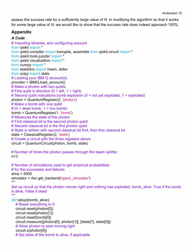
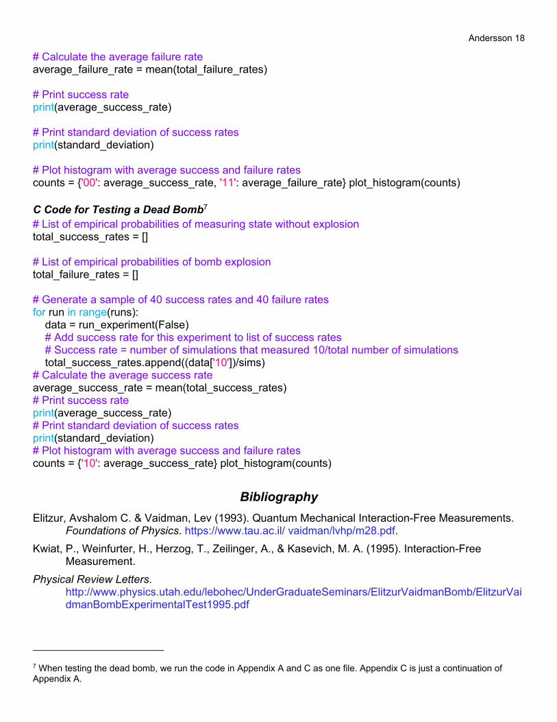
3.3 Quantum Computing Algorithm The code for our algorithm can be found in the Appendix. Appendix A contains the general algorithm for the Kwiat et al. scheme. Appendix B contains the code we run to test a live bomb, and Appendix C contains the code we run to test a dead bomb.

4 Results

Figure 9: Results when the bomb is dead. The state |10⟩ is measured 100% of the time, which is expected.

Quantity Numerical Value

Average Success Rate

1

Standard Deviation 0

Table 1: Results from Testing the Dead Bomb

Figure 10: Results when the bomb is alive. The state |00⟩ is measured about 42.1% of the time, and the state |11⟩ is measured about

57.9% of the time; these probabilities add up to 100%.

Andersson 13

Quantity Numerical Value

Average Success Rate

0.42077

Standard Deviation 0.008374264606059908

Table 2: Results from Testing the Live Bomb

5 Analysis In order to determine if the success rate of interaction-free measurements is 42.1875% based on the data from the quantum computing simulation, we will use statistical hypothesis testing. Specifically, we will perform a t-test.

Our null hypothesis, H0, is: The success rate of interaction-free measurements for the Kwiat et al scheme with three cycles is 42.1875%.

Our alternative hypothesis, Ha, is: The success rate of interaction-free measurements for the Kwiat et al scheme with three cycles is less than 42.1875%.

For our hypothesis test, we will choose an alpha value of α = 0.1. We pick a high value for α in order to reduce the probability of a type II error. A type II error in this case implies that we erroneously failed to reject the null hypothesis that the success rate is 42.1875%. Thus, the reality would be that the success rate is lower, which, in the example in the introduction, would suggest that Bob has a lower chance of survival than anticipated.

In addition to choosing a high value for alpha, we also chose to run 40 simulations in order to obtain 40 samples of the success rate. By increasing the sample size, we have further reduced the probability of a type II error.

Below is the data used to perform the t-test on a TI-84 PLUS CE calculator. The table also includes the resulting p-value.

Quantity Numerical Value

μ 0.421875

�̅� 0.42077

𝑠 0.0083743

𝑛 40

p-value 0.20453

Table 3: Data and Results from the t-test

The p-value of 0.20453 is much greater than the alpha value of α = 0.1. This means that we fail to reject the null hypothesis that the success rate is 42.1875% (that is, we lack the evidence to disprove the success rate of 42.1875% for N = 3). More testing would need to be done (either a different form

Andersson 14

of hypothesis testing or varying the parameters of the t-test) before we can generally “accept”5 this value.

As of now, we find that the 42.1875% success rate is not false. If we do accept this value through further testing, one may realize that, going back to the problem in the introduction, Bob has about a 58% chance of exploding the bomb. For N = 3, Bob is more likely to die than survive if the bomb is alive. Can we improve the success rate so that it is at least 50%? Yes.

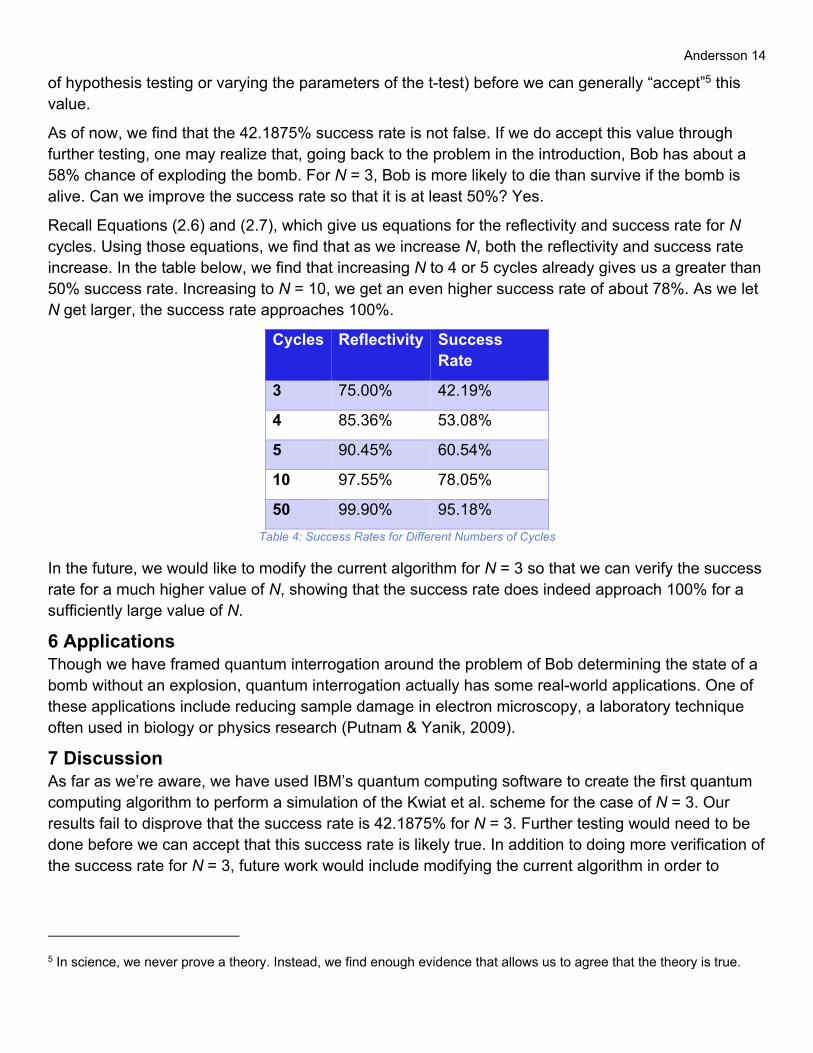
Recall Equations (2.6) and (2.7), which give us equations for the reflectivity and success rate for N cycles. Using those equations, we find that as we increase N, both the reflectivity and success rate increase. In the table below, we find that increasing N to 4 or 5 cycles already gives us a greater than 50% success rate. Increasing to N = 10, we get an even higher success rate of about 78%. As we let N get larger, the success rate approaches 100%.

Cycles Reflectivity Success Rate

3 75.00% 42.19%

4 85.36% 53.08%

5 90.45% 60.54%

10 97.55% 78.05%

50 99.90% 95.18%

Table 4: Success Rates for Different Numbers of Cycles

In the future, we would like to modify the current algorithm for N = 3 so that we can verify the success rate for a much higher value of N, showing that the success rate does indeed approach 100% for a sufficiently large value of N.

6 Applications Though we have framed quantum interrogation around the problem of Bob determining the state of a bomb without an explosion, quantum interrogation actually has some real-world applications. One of these applications include reducing sample damage in electron microscopy, a laboratory technique often used in biology or physics research (Putnam & Yanik, 2009).

7 Discussion As far as we’re aware, we have used IBM’s quantum computing software to create the first quantum computing algorithm to perform a simulation of the Kwiat et al. scheme for the case of N = 3. Our results fail to disprove that the success rate is 42.1875% for N = 3. Further testing would need to be done before we can accept that this success rate is likely true. In addition to doing more verification of the success rate for N = 3, future work would include modifying the current algorithm in order to

5 In science, we never prove a theory. Instead, we find enough evidence that allows us to agree that the theory is true.

Andersson 15

assess the success rate for a sufficiently large value of N. In modifying the algorithm so that it works for some large value of N, we would like to show that the success rate does indeed approach 100%.

Appendix A Code # Importing libraries, and configuring account from qiskit import * from qiskit.compiler import transpile, assemble from qiskit.circuit import * from qiskit.tools.jupyter import * from qiskit.visualization import * from numpy import * from statistics import mean, stdev from scipy import stats # Loading your IBM Q account(s) provider = IBMQ.load_account() # Make a photon with two qubits # First qubit is direction (0 = left, 1 = right) # Second qubit indications bomb explosion (0 = not yet exploded, 1 = exploded) photon = QuantumRegister(2, 'photon') # Make a bomb with one qubit # (0 = dead bomb, 1 = live bomb) bomb = QuantumRegister(1, 'bomb') # Measures the state of the photon # First classical bit is the second photon qubit # Second classical bit is the first photon qubit # State is written with second classical bit first, then first classical bit state = ClassicalRegister(2, 'state') # Create a circuit with the three registers above circuit = QuantumCircuit(photon, bomb, state) # Number of times the photon passes through the beam splitter n=3 # Number of simulations used to get empirical probabilities # for the successes and failures sims = 5000 simulator = Aer.get_backend('qasm_simulator') """ Set up circuit so that the photon moves right and nothing has exploded. bomb_alive: True if the bomb is alive, False if dead """ def setup(bomb_alive): # Reset everything to 0 circuit.reset(photon[0]) circuit.reset(photon[1]) circuit.reset(bomb[0]) circuit.measure([photon[0], photon[1]], [state[1], state[0]]) # Allow photon to start moving right circuit.x(photon[0]) # Set state of the bomb to alive, if applicable

Andersson 16

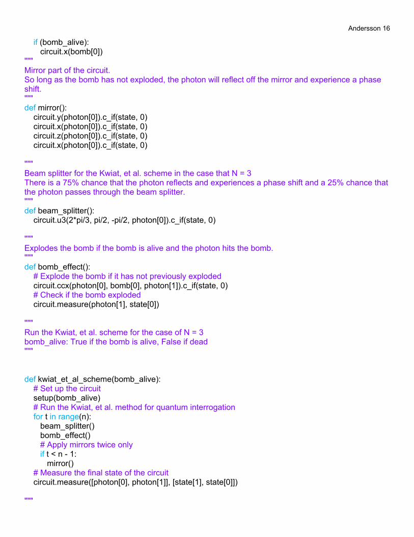
if (bomb_alive): circuit.x(bomb[0]) """ Mirror part of the circuit. So long as the bomb has not exploded, the photon will reflect off the mirror and experience a phase shift. """ def mirror(): circuit.y(photon[0]).c_if(state, 0) circuit.x(photon[0]).c_if(state, 0) circuit.z(photon[0]).c_if(state, 0) circuit.x(photon[0]).c_if(state, 0) """ Beam splitter for the Kwiat, et al. scheme in the case that N = 3 There is a 75% chance that the photon reflects and experiences a phase shift and a 25% chance that the photon passes through the beam splitter. """ def beam_splitter(): circuit.u3(2*pi/3, pi/2, -pi/2, photon[0]).c_if(state, 0) """ Explodes the bomb if the bomb is alive and the photon hits the bomb. """ def bomb_effect(): # Explode the bomb if it has not previously exploded circuit.ccx(photon[0], bomb[0], photon[1]).c_if(state, 0) # Check if the bomb exploded circuit.measure(photon[1], state[0]) """ Run the Kwiat, et al. scheme for the case of N = 3 bomb_alive: True if the bomb is alive, False if dead """ def kwiat_et_al_scheme(bomb_alive): # Set up the circuit setup(bomb_alive) # Run the Kwiat, et al. method for quantum interrogation for t in range(n): beam_splitter() bomb_effect() # Apply mirrors twice only if t < n - 1: mirror() # Measure the final state of the circuit circuit.measure([photon[0], photon[1]], [state[1], state[0]]) """

Andersson 17

Run the Kwiat, et al. scheme. Return the number of successes (measured state of bomb without explosion) and failures (bomb exploded) for a given experiment. bomb_alive: True if the bomb is alive, False if dead """ def run_experiment(bomb_alive): # Run the experiment kwiat_et_al_scheme(bomb_alive) # Execute on IBM's quantum computer experiment = execute(circuit, simulator, shots=sims) # Retrieve the results of the experiment result = experiment.result() # Get the results in the form of a dictionary # Key is the measured state # Value of the key is the number of times the key was measured counts = result.get_counts(circuit) return counts # Sample size for t-test runs = 40 B Code for Testing a Live Bomb6 # List of empirical probabilities of measuring state without explosion total_success_rates = [] # List of empirical probabilities of bomb explosion total_failure_rates = [] # Generate a sample of 40 success rates and 40 failure rates for run in range(runs): data = run_experiment(True) # Add success rate for this experiment to list of success rates # Success rate = number of simulations that measured 00/total number of simulations total_success_rates.append((data['00'])/sims) # Add failure rate for this experiment to list of failure rates # Failure rate = number of simulations that measured 11/total number of simulations total_failure_rates.append((data['11'])/sims) # Calculate the average success rate average_success_rate = mean(total_success_rates) # Calculate the standard deviation standard_deviation = stdev(total_success_rates)

6 When testing the live bomb, we run the code in Appendix A and B as one file. Appendix B is just a continuation of Appendix A.

Andersson 18

# Calculate the average failure rate average_failure_rate = mean(total_failure_rates) # Print success rate print(average_success_rate) # Print standard deviation of success rates print(standard_deviation) # Plot histogram with average success and failure rates counts = {'00': average_success_rate, '11': average_failure_rate} plot_histogram(counts) C Code for Testing a Dead Bomb7 # List of empirical probabilities of measuring state without explosion total_success_rates = [] # List of empirical probabilities of bomb explosion total_failure_rates = [] # Generate a sample of 40 success rates and 40 failure rates for run in range(runs): data = run_experiment(False) # Add success rate for this experiment to list of success rates # Success rate = number of simulations that measured 10/total number of simulations total_success_rates.append((data['10'])/sims) # Calculate the average success rate average_success_rate = mean(total_success_rates) # Print success rate print(average_success_rate) # Print standard deviation of success rates print(standard_deviation) # Plot histogram with average success and failure rates counts = {'10': average_success_rate} plot_histogram(counts)

Bibliography

Elitzur, Avshalom C. & Vaidman, Lev (1993). Quantum Mechanical Interaction-Free Measurements. Foundations of Physics. https://www.tau.ac.il/ vaidman/lvhp/m28.pdf.

Kwiat, P., Weinfurter, H., Herzog, T., Zeilinger, A., & Kasevich, M. A. (1995). Interaction-Free Measurement.

Physical Review Letters. http://www.physics.utah.edu/lebohec/UnderGraduateSeminars/ElitzurVaidmanBomb/ElitzurVaidmanBombExperimentalTest1995.pdf

7 When testing the dead bomb, we run the code in Appendix A and C as one file. Appendix C is just a continuation of Appendix A.

Andersson 19

Putnam, William P., Yanik, Mehmet Fatih (2009). Noninvasive electron microscopy with interaction- free quantum measurements. Physical Review A. https://ui.adsabs.harvard.edu/abs/2009PhRvA..80d0902P/abstract

QISkit [Computer Softare]. (2019). https://qiskit.org

Raj, A., Das, B., Behera, B.K., Panigrahi, P.K. (2019). Demonstration of Bomb Detection Using the IBM Quantum Computer. 10.13140/RG.2.2.15894.60481.

Tan-Holmes, Jade [Up and Atom]. (2016, November 10). The Quantum Bomb-Tester! [Video file]. https://youtu.be/wiW7jhdKDVA

Yoganathan, Mithuna [Looking Glass Universe]. (2018, April 24). Comment response video for Understanding Quantum Mechanics [Video file]. https://youtu.be/YBcQ0PeFsx4

Yoganathan, Mithuna [Looking Glass Universe]. (2019, June 9). Electrons aren’t actual waves [Video file]. https://www.youtube.com/watch?v=XV46ALr3OMg