Embed Size (px)
Citation preview

An Introduction to Quantum Computing for Non-Physicists
ELEANOR RIEFFELFX Palo Alto Laboratory
ANDWOLFGANG POLAK
Richard Feynman’s observation that certain quantum mechanical effects cannot besimulated efficiently on a computer led to speculation that computation in general couldbe done more efficiently if it used these quantum effects. This speculation provedjustified when Peter Shor described a polynomial time quantum algorithm for factoringintegers.
In quantum systems, the computational space increases exponentially with the sizeof the system, which enables exponential parallelism. This parallelism could lead toexponentially faster quantum algorithms than possible classically. The catch is thataccessing the results, which requires measurement, proves tricky and requires newnontraditional programming techniques.
The aim of this paper is to guide computer scientists through the barriers thatseparate quantum computing from conventional computing. We introduce basicprinciples of quantum mechanics to explain where the power of quantum computerscomes from and why it is difficult to harness. We describe quantum cryptography,teleportation, and dense coding. Various approaches to exploiting the power of quantumparallelism are explained. We conclude with a discussion of quantum error correction.
Categories and Subject Descriptors: A.1 [Introductory and Survey]
General Terms: Algorithms, Security, Theory
Additional Key Words and Phrases: Quantum computing, complexity, parallelism
1. INTRODUCTION
Richard Feynman observed in the early1980s [Feynman 1982] that certain quan-tum mechanical effects cannot be simu-lated efficiently on a classical computer.This observation led to speculation thatperhaps computation in general could bedone more efficiently if it made use of thesequantum effects. But building quantumcomputers, computational machines thatuse such quantum effects, proved tricky,
Authors’ address: E. Rieffel, FX Palo Alto Laboratory, 3400 Hillview Av., Palo Alto, CA 94304; W. Polak,Consultant.
Permission to make digital or hard copies of part or all of this work for personal or classroom use is grantedwithout fee provided that copies are not made or distributed for profit or direct commercial advantage andthat copies show this notice on the first page or initial screen of a display along with the full citation.Copyrights for components of this work owned by others than ACM must be honored. Abstracting withcredit is permitted. To copy otherwise, to republish, to post on servers, to redistribute to lists, or to use anycomponent of this work in other works, requires prior specific permission and/or a fee. Permissions maybe requested from Publications Dept, ACM Inc., 1515 Broadway, New York, NY 10036 USA, fax +1 (212)869-0481, or [email protected]©2001 ACM 0360-0300/01/0900-0000 $5.00
and as no one was sure how to use thequantum effects to speed up computation,the field developed slowly. It wasn’t until1994, when Peter Shor surprised the worldby describing a polynomial time quan-tum algorithm for factoring integers [Shor1994; 1997], that the field of quantumcomputing came into its own. This discov-ery prompted a flurry of activity amongexperimentalists trying to build quan-tum computers and theoreticians try-ing to find other quantum algorithms.
ACM Computing Surveys, Vol. 32, No. 3, September 2000, pp. 300–335.

Introduction to Quantum Computing 301
Additional interest in the subject has beencreated by the invention of quantum keydistribution and, more recently, popularpress accounts of experimental successesin quantum teleportation and the demon-stration of a 3-bit quantum computer.
The aim of this paper is to guide com-puter scientists and other nonphysiciststhrough the conceptual and notationalbarriers that separate quantum comput-ing from conventional computing and toacquaint them with this new and excit-ing field. It is important for the computerscience community to understand thesenew developments since they may radi-cally change the way we have to thinkabout computation, programming, andcomplexity.
Classically, the time it takes to do cer-tain computations can be decreased byusing parallel processors. To achieve anexponential decrease in time requires anexponential increase in the number ofprocessors, and hence an exponential in-crease in the amount of physical spaceneeded. However, in quantum systems theamount of parallelism increases exponen-tially with the size of the system. Thus,an exponential increase in parallelism re-quires only a linear increase in the amountof physical space needed. This effect iscalled quantum parallelism [Deutsch andJozsa 1992].
There is a catch, and a big catch atthat. While a quantum system can per-form massive parallel computation, accessto the results of the computation is re-stricted. Accessing the results is equiva-lent to making a measurement, which dis-turbs the quantum state. This problemmakes the situation, on the face of it, seemeven worse than the classical situation; wecan only read the result of one parallelthread, and because measurement is prob-abilistic, we cannot even choose which onewe get.
But in the past few years, various peo-ple have found clever ways of finessingthe measurement problem to exploit thepower of quantum parallelism. This sortof manipulation has no classical analogand requires nontraditional programmingtechniques. One technique manipulates
the quantum state so that a commonproperty of all of the output values suchas the symmetry or period of a functioncan be read off. This technique is usedin Shor’s factorization algorithm. Anothertechnique transforms the quantum stateto increase the likelihood that output ofinterest will be read. Grover’s search algo-rithm makes use of such an amplificationtechnique. This paper describes quantumparallelism in detail, and the techniquescurrently known for harnessing its power.
Section 2, following this introduction,explains of the basic concepts of quan-tum mechanics that are important forquantum computation. This section can-not give a comprehensive view of quan-tum mechanics. Our aim is to provide thereader with tools in the form of mathemat-ics and notation with which to work withthe quantum mechanics involved in quan-tum computation. We hope that this paperwill equip readers well enough that theycan freely explore the theoretical realm ofquantum computing.
Section 3 defines the quantum bit, orqubit. Unlike classical bits, a quantum bitcan be put in a superposition state that en-codes both 0 and 1. There is no good classi-cal explanation of superpositions: a quan-tum bit representing 0 and 1 can neitherbe viewed as “between” 0 and 1 nor canit be viewed as a hidden unknown statethat represents either 0 or 1 with a certainprobability. Even single quantum bits en-able interesting applications. We describethe use of a single quantum bit for securekey distribution.
But the real power of quantum compu-tation derives from the exponential statespaces of multiple quantum bits: just as asingle qubit can be in a superposition of0 and 1, a register of n qubits can be ina superposition of all 2n possible values.The “extra” states that have no classicalanalog and lead to the exponential size ofthe quantum state space are the entangledstates, like the state leading to the famousEPR1 paradox (see Section 3.4).
We discuss the two types of opera-tions a quantum system can undergo:
1 EPR = Einstein, Podolsky, and Rosen
ACM Computing Surveys, Vol. 32, No. 3, September 2000.

302 E. Rieffel and W. Polak
measurement and quantum state trans-formations. Most quantum algorithms in-volve a sequence of quantum state trans-formations followed by a measurement.For classical computers there are setsof gates that are universal in the sensethat any classical computation can be per-formed using a sequence of these gates.Similarly, there are sets of primitive quan-tum state transformations, called quan-tum gates, that are universal for quantumcomputation. Given enough quantum bits,it is possible to construct a universal quan-tum Turing machine.
Quantum physics puts restrictions onthe types of transformations that can bedone. In particular, all quantum statetransformations, and therefore all quan-tum gates and all quantum computations,must be reversible. Yet all classical algo-rithms can be made reversible and canbe computed on a quantum computer incomparable time. Some common quantumgates are defined in Section 4.
Two applications combining quantumgates and entangled states are describedin Section 4.2: teleportation and densecoding. Teleportation is the transfer of aquantum state from one place to anotherthrough classical channels. That telepor-tation is possible is surprising, since quan-tum mechanics tells us that it is not pos-sible to clone quantum states or evenmeasure them without disturbing thestate. Thus, it is not obvious what informa-tion could be sent through classical chan-nels that could possibly enable the recon-struction of an unknown quantum stateat the other end. Dense coding, a dual toteleportation, uses a single quantum bit totransmit two bits of classical information.Both teleportation and dense coding relyon the entangled states described in theEPR experiment.
It is only in Section 5 that we seewhere an exponential speed-up over clas-sical computers might come from. The in-put to a quantum computation can be putin a superposition state that encodes allpossible input values. Performing the com-putation on this initial state will result insuperposition of all of the correspondingoutput values. Thus, in the same time it
takes to compute the output for a single in-put state on a classical computer, a quan-tum computer can compute the values forall input states. This process is known asquantum parallelism. However, measur-ing the output states will randomly yieldonly one of the values in the superposition,and at the same time destroy all of theother results of the computation. Section 5describes this situation in detail. Sections6 and 7 describe techniques for taking ad-vantage of quantum parallelism inspite ofthe severe constraints imposed by quan-tum mechanics on what can be measured.
Section 6 describes the details of Shor’spolynomial time factoring algorithm. Thefastest known classical factoring algo-rithm requires exponential time, and it isgenerally believed that there is no classi-cal polynomial time factoring algorithm.Shor’s is a beautiful algorithm that takesadvantage of quantum parallelism by us-ing a quantum analog of the Fourier trans-form.
Lov Grover developed a technique forsearching an unstructured list of n itemsin O(
√n) steps on a quantum computer.
Classical computers can do no better thanO(n), so unstructured search on a quan-tum computer is provably more efficientthan search on a classical computer. How-ever, the speed-up is only polynomial, notexponential, and it has been shown thatGrover’s algorithm is optimal for quan-tum computers. It seems likely that searchalgorithms that could take advantage ofsome problem structure could do better.Tad Hogg, among others, has exploredsuch possibilities. We describe variousquantum search techniques in Section 7.
It is as yet unknown whether the powerof quantum parallelism can be harnessedfor a wide variety of applications. One tan-talizing open question is whether quan-tum computers can solve NP-completeproblems in polynomial time.
Perhaps the biggest open question iswhether useful quantum computers canbe built. There are a number of propos-als for building quantum computers us-ing ion traps, nuclear magnetic resonance(NMR), and optical and solid-state tech-niques. All of the current proposals have
ACM Computing Surveys, Vol. 32, No. 3, September 2000.

Introduction to Quantum Computing 303
scaling problems, so a breakthrough willbe needed to go beyond tens of qubitsto hundreds of qubits. While both opticaland solid-state techniques show promise,NMR and ion trap technologies are themost advanced so far.
In an ion trap quantum computer [Circand Zoller 1995; Steane 1996] a linear se-quence of ions representing the qubits areconfined by electric fields. Lasers are di-rected at individual ions to perform single-bit quantum gates. Two-bit operations arerealized by using a laser on one qubit tocreate an impulse that ripples through achain of ions to the second qubit, whereanother laser pulse stops the ripplingand performs the 2-bit operation. The ap-proach requires that the ions be kept inextreme vacuum and at extremely lowtemperatures.
The NMR approach has the advantagethat it will work at room temperature andthat NMR technology in general is alreadyfairly advanced. The idea is to use macro-scopic amounts of matter and encode aquantum bit in the average spin state ofa large number of nuclei. The spin statescan be manipulated by magnetic fields,and the average spin state can be mea-sured with NMR techniques. The mainproblem with the technique is that itdoesn’t scale well; the measured signalscales as 1/2n with the number of qubitsn. However, a recent proposal [Schulmanand Vazirani 1998] has been made thatmay overcome this problem. NMR com-puters with three qubits have been builtsuccessfully [Cory et al. 1998; Gershenfeldand Chuang 1997; Laflamme et al. 1997;Vandersypen et al. 1999]. This paper willnot discuss further the physical and en-gineering problems of building quantumcomputers.
The greatest problem for building quan-tum computers is decoherence, the distor-tion of the quantum state due to interac-tion with the environment. For some timeit was feared that quantum computerscould not be built because it would be im-possible to isolate them sufficiently fromthe external environment. The break-through came from the algorithmic ratherthan the physical side, through the in-
vention of quantum error correction tech-niques. Initially people thought quantumerror correction might be impossible be-cause of the impossibility of reliably copy-ing unknown quantum states, but it turnsout that it is possible to design quantumerror correcting codes that detect certainkinds of errors and enable the reconstruc-tion of the exact error-free quantum state.Quantum error correction is discussed inSection 8.
Appendices provide background infor-mation on tensor products and continuedfractions.
2. QUANTUM MECHANICS
Quantum mechanical phenomena are dif-ficult to understand, since most of oureveryday experiences are not applicable.This paper cannot provide a deep un-derstanding of quantum mechanics (seeFeynman et al. [1965], Liboff [1997], andGreenstein and Zajonc [1997] for expo-sitions of quantum mechanics). Instead,we will give some feeling as to the na-ture of quantum mechanics and some ofthe mathematical formalisms needed towork with quantum mechanics to the ex-tent needed for quantum computing.
Quantum mechanics is a theory in themathematical sense: it is governed by a setof axioms. The consequences of the axiomsdescribe the behavior of quantum systems.The axioms lead to several apparent para-doxes: in the Compton effect it appears asif an action precedes its cause; the EPRexperiment makes it appear as if actionover a distance faster than the speed oflight is possible. We will discuss the EPRexperiment in detail in Section 3.4. Ver-ification of most predictions is indirect,and requires careful experimental designand specialized equipment. We will begin,however, with an experiment that requiresonly readily available equipment and thatwill illustrate some of the key aspects ofquantum mechanics needed for quantumcomputation.
2.1. Photon Polarization
Photons are the only particles that wecan observe directly. The following simple
ACM Computing Surveys, Vol. 32, No. 3, September 2000.
304 E. Rieffel and W. Polak
experiment can be performed with mini-mal equipment: a strong light source, suchas a laser pointer, and three polaroids(polarization filters), which can be pickedup at any camera supply store. The ex-periment demonstrates some of the prin-ciples of quantum mechanics through pho-tons and their polarization.
2.1.1 The Experiment. A beam of lightshines on a projection screen. Filters A,B, and C are polarized horizontally, at45◦, and vertically, respectively, and can beplaced so as to intersect the beam of light.
First, insert filter A. Assuming the in-coming light is randomly polarized, theintensity of the output will have half ofthe intensity of the incoming light. Theoutgoing photons are now all horizontallypolarized.
The function of filter A cannot be ex-plained as a “sieve” that only lets thosephotons pass that happen to be alreadyhorizontally polarized. If that were thecase, few of the randomly polarized incom-ing electrons would be horizontally polar-ized, so we would expect a much larger at-tenuation of the light as it passes throughthe filter.
Next, when filter C is inserted, the in-tensity of the output drops to zero. Noneof the horizontally polarized photons canpass through the vertical filter. A sievemodel could explain this behavior.
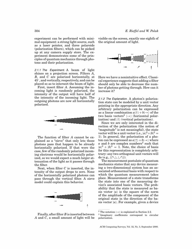
Finally, after filter B is inserted betweenA and C, a small amount of light will be
visible on the screen, exactly one eighth ofthe original amount of light.
Here we have a nonintuitive effect. Classi-cal experience suggests that adding a filtershould only be able to decrease the num-ber of photons getting through. How can itincrease it?
2.1.2 The Explanation. A photon’s polariza-tion state can be modeled by a unit vectorpointing in the appropriate direction. Anyarbitrary polarization can be expressedas a linear combination a|↑〉 + b|→〉 of thetwo basis vectors2 |→〉 (horizontal polar-ization) and |↑〉 (vertical polarization).
Since we are only interested in the di-rection of the polarization (the notion of“magnitude” is not meaningful), the statevector will be a unit vector (i.e., |a|2+|b|2 =1). In general, the polarization of a pho-ton can be expressed as a|↑〉+b|→〉 wherea and b are complex numbers3 such that|a|2 + |b|2 = 1. Note, the choice of basisfor this representation is completely arbi-trary: any two orthogonal unit vectors willdo (e.g., {|↖〉, |↗〉}).
The measurement postulate of quantummechanics states that any device measur-ing a two-dimensional system has an as-sociated orthonormal basis with respect towhich the quantum measurement takesplace. Measurement of a state transformsthe state into one of the measuring de-vice’s associated basis vectors. The prob-ability that the state is measured as ba-sis vector |u〉 is the square of the normof the amplitude of the component of theoriginal state in the direction of the ba-sis vector |u〉. For example, given a device
2 The notation |→〉 is explained in Section 2.2.3 Imaginary coefficients correspond to circularpolarization.
ACM Computing Surveys, Vol. 32, No. 3, September 2000.
Introduction to Quantum Computing 305
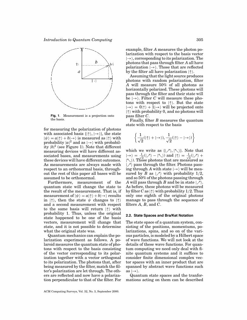
Fig. 1. Measurement is a projection ontothe basis.
for measuring the polarization of photonswith associated basis {|↑〉, |→〉}, the state|ψ〉 = a|↑〉 + b|→〉 is measured as |↑〉 withprobability |a|2 and as |→〉 with probabil-ity |b|2 (see Figure 1). Note that differentmeasuring devices will have different as-sociated bases, and measurements usingthese devices will have different outcomes.As measurements are always made withrespect to an orthonormal basis, through-out the rest of this paper all bases will beassumed to be orthonormal.
Furthermore, measurement of thequantum state will change the state tothe result of the measurement. That is, ifmeasurement of |ψ〉 = a|↑〉 + b|→〉 resultsin |↑〉, then the state ψ changes to |↑〉and a second measurement with respectto the same basis will return |↑〉 withprobability 1. Thus, unless the originalstate happened to be one of the basisvectors, measurement will change thatstate, and it is not possible to determinewhat the original state was.
Quantum mechanics can explain the po-larization experiment as follows. A po-laroid measures the quantum state of pho-tons with respect to the basis consistingof the vector corresponding to its polar-ization together with a vector orthogonalto its polarization. The photons that, afterbeing measured by the filter, match the fil-ter’s polarization are let through. The oth-ers are reflected and now have a polariza-tion perpendicular to that of the filter. For
example, filter A measures the photon po-larization with respect to the basis vector|→〉, corresponding to its polarization. Thephotons that pass through filter A all havepolarization |→〉. Those that are reflectedby the filter all have polarization |↑〉.
Assuming that the light source producesphotons with random polarization, filterA will measure 50% of all photons ashorizontally polarized. These photons willpass through the filter and their state willbe |→〉. Filter C will measure these pho-tons with respect to |↑〉. But the state|→〉 = 0|↑〉 + 1|→〉 will be projected onto|↑〉 with probability 0, and no photons willpass filter C.
Finally, filter B measures the quantumstate with respect to the basis
{1√2
(|↑〉 + |→〉), 1√2
(|↑〉 − |→〉)}
which we write as {|↗〉, |↖〉}. Note that|→〉 = 1√
2(|↗〉 − |↖〉) and |↑〉 = 1√
2(|↗〉 +
|↖〉). Those photons that are measured as|↗〉 pass through the filter. Photons pass-ing through A with state |→〉 will be mea-sured by B as |↗〉 with probability 1/2,and so 50% of the photons passing throughA will pass through B and be in state |↗〉.As before, these photons will be measuredby filter C as |↑〉 with probability 1/2. Thusonly one eighth of the original photonsmanage to pass through the sequence offilters A, B, and C.
2.2. State Spaces and Bra/Ket Notation
The state space of a quantum system, con-sisting of the positions, momentums, po-larizations, spins, and so on of the vari-ous particles, is modeled by a Hilbert spaceof wave functions. We will not look at thedetails of these wave functions. For quan-tum computing we need only deal with fi-nite quantum systems and it suffices toconsider finite dimensional complex vec-tor spaces with an inner product that arespanned by abstract wave functions suchas |→〉.
Quantum state spaces and the tranfor-mations acting on them can be described
ACM Computing Surveys, Vol. 32, No. 3, September 2000.

306 E. Rieffel and W. Polak
in terms of vectors and matrices or inthe more compact bra/ket notation in-vented by Dirac [1958]. Kets like |x〉 de-note column vectors and are typically usedto describe quantum states. The match-ing bra, 〈x|, denotes the conjugate trans-pose of |x〉. For example, the orthonor-mal basis {|0〉, |1〉} can be expressed as{(1, 0)T , (0, 1)T }. Any complex linear com-bination of |0〉 and |1〉, a|0〉 + b|1〉, can bewritten (a, b)T . Note that the choice of theorder of the basis vectors is arbitrary. Forexample, representing |0〉 as (0, 1)T and |1〉as (1, 0)T would be fine as long as this isdone consistently.
Combining 〈x| and | y〉 as in 〈x|| y〉, alsowritten as 〈x| y〉, denotes the inner prod-uct of the two vectors. For instance, since|0〉 is a unit vector we have 〈0|0〉 = 1 andsince |0〉 and |1〉 are orthogonal we have〈0|1〉 = 0.
The notation |x〉〈 y | is the outer productof |x〉 and 〈 y |. For example, |0〉〈1| is thetransformation that maps |1〉 to |0〉 and |0〉to (0, 0)T , since
|0〉〈1||1〉 = |0〉〈1|1〉 = |0〉
|0〉〈1||0〉 = |0〉〈1|0〉 = 0|0〉 =(
00
).
Equivalently, |0〉〈1| can be written in ma-trix form, where |0〉 = (1, 0)T , 〈0| = (1, 0),|1〉 = (0, 1)T , and 〈1| = (0, 1). Then
|0〉〈1| =(
10
)(0, 1) =
(0 10 0
).
This notation gives us a convenient wayof specifying transformations on quantumstates in terms of what happens to the ba-sis vectors (see Section 4). For example,the transformation that exchanges |0〉 and|1〉 is given by the matrix
X = |0〉〈1| + |1〉〈0|.
In this paper we prefer the slightly moreintuitive notation
X : |0〉 → |1〉|1〉 → |0〉,
which explicitly specifies the result of atransformation on the basis vectors.
3. QUANTUM BITS
A quantum bit, or qubit, is a unit vectorin a two-dimensional complex vector spacefor which a particular basis, denoted by{|0〉, |1〉}, has been fixed. The orthonormalbasis |0〉 and |1〉 may correspond to the |↑〉and |→〉 polarizations of a photon respec-tively, or to the polarizations |↗〉 and |↖〉.Or |0〉 and |1〉 could correspond to the spin-up and spin-down states of an electron.When talking about qubits, and quantumcomputations in general, a fixed basis withrespect to which all statements are madehas been chosen in advance. In particular,unless otherwise specified, all measure-ments will be made with respect to thestandard basis for quantum computation,{|0〉, |1〉}.
For the purposes of quantum computa-tion, the basis states |0〉 and |1〉 are takento represent the classical bit values 0 and 1respectively. Unlike classical bits however,qubits can be in a superposition of |0〉 and|1〉 such as a|0〉 + b|1〉, where a and b arecomplex numbers such that |a|2 +|b|2 = 1.Just as in the photon polarization case, ifsuch a superposition is measured with re-spect to the basis {|0〉, |1〉}, the probabilitythat the measured value is |0〉 is |a|2 andthe probability that the measured value is|1〉 is |b|2.
Even though a quantum bit can be putin infinitely many superposition states, itis only possible to extract a single classi-cal bit’s worth of information from a sin-gle quantum bit. The reason that no moreinformation can be gained from a qubitthan in a classical bit is that informa-tion can only be obtained by measurement.When a qubit is measured, the measure-ment changes the state to one of the basisstates in the way seen in the photon po-larization experiment. As every measure-ment can result in only one of two states,one of the basis vectors associated to thegiven measuring device, so, just as in theclassical case, there are only two possi-ble results. As measurement changes thestate, one cannot measure the state of a
ACM Computing Surveys, Vol. 32, No. 3, September 2000.

Introduction to Quantum Computing 307
qubit in two different bases. Furthermore,as we shall see in Section 4.1.2, quantumstates cannot be cloned, so it is not possibleto measure a qubit in two ways, even indi-rectly by, say, copying the qubit and mea-suring the copy in a different basis fromthe original.
3.1. Quantum Key Distribution
Sequences of single qubits can be used totransmit private keys on insecure chan-nels. In 1984 Bennett and Brassard de-scribed the first quantum key distribu-tion scheme [Bennett and Brassard 1987;Bennett et al. 1992]. Classically, public keyencryption techniques (e.g., RSA) are usedfor key distribution.
Consider the situation in which Aliceand Bob want to agree on a secret keyso that they can communicate privately.They are connected by an ordinary bidirec-tional open channel and a unidirectionalquantum channel, both of which can be ob-served by Eve, who wishes to eavesdrop ontheir conversation. This situation is illus-trated in the figure that follows. The quan-tum channel allows Alice to send individ-ual particles (e.g., photons) to Bob who canmeasure their quantum state. Eve can at-tempt to measure the state of these parti-cles and can resend the particles to Bob.
To begin the process of establishing asecret key, Alice sends a sequence of bits toBob by encoding each bit in the quantumstate of a photon as follows. For each bit,Alice randomly uses one of the followingtwo bases for encoding each bit:
0 → |↑〉1 → |→〉
or0 → |↖〉1 → |↗〉.
Bob measures the state of the photons hereceives by randomly picking either ba-sis. After the bits have been transmitted,Bob and Alice communicate the basis theyused for encoding and decoding of each bitover the open channel. With this informa-tion both can determine which bits havebeen transmitted correctly, by identifyingthose bits for which the sending and re-ceiving bases agree. They will use thesebits as the key and discard all the others.On average, Alice and Bob will agree on50% of all bits transmitted.
Suppose that Eve measures the stateof the photons transmitted by Alice andre-sends new photons with the measuredstate. In this process she will use thewrong basis approximately 50% of thetime, in which case she will re-send the bitwith the wrong basis. So when Bob mea-sures a re-sent qubit with the correct ba-sis, there will be a 25% probability thathe measures the wrong value. Thus anyeavesdropper on the quantum channel isbound to introduce a high error rate thatAlice and Bob can detect by communicat-ing a sufficient number of parity bits oftheir keys over the open channel. So, notonly is it likely that Eve’s version of thekey is 25% incorrect, but the fact thatsomeone is eavesdropping will be appar-ent to Alice and Bob.
Other techniques for exploiting quan-tum effects for key distribution have beenproposed. See, for example, Ekert et al.[1992], Bennett [1992], and Lo and Chau[1999]. But none of the quantum key dis-tribution techniques are substitutes forpublic key encryption schemes. Attacksby eavesdroppers other than the one de-scribed here are possible. Security againstall such schemes is discussed in bothMayers [1998] and Lo and Chau [1999].
Quantum key distribution has been re-alized over a distance of 24 km usingstandard fiber optical cables [Hughes et al.
ACM Computing Surveys, Vol. 32, No. 3, September 2000.

308 E. Rieffel and W. Polak
1997] and over 0.5 km through the atmo-sphere [Hughes et al. 1999].
3.2. Multiple Qubits
Imagine a macroscopic physical objectbreaking apart and multiple pieces flyingoff in different directions. The state of thissystem can be described completely by de-scribing the state of each of its compo-nent pieces separately. A surprising andunintuitive aspect of the state space ofan n-particle quantum system is that thestate of the system cannot always be de-scribed in terms of the state of its compo-nent pieces. It is when examining systemsof more than one qubit that one first gets aglimpse of where the computational powerof quantum computers could come from.
As we saw, the state of a qubitcan be represented by a vector in thetwo-dimensional complex vector spacespanned by |0〉 and |1〉. In classical physics,the possible states of a system of n par-ticles, whose individual states can be de-scribed by a vector in a two-dimensionalvector space, form a vector space of 2n di-mensions. However, in a quantum systemthe resulting state space is much larger; asystem of n qubits has a state space of 2n
dimensions.4 It is this exponential growthof the state space with the number of par-ticles that suggests a possible exponentialspeed-up of computation on quantum com-puters over classical computers.
Individual state spaces of n particlescombine classically through the cartesianproduct. Quantum states, however, com-bine through the tensor product. Detailson properties of tensor products and theirexpression in terms of vectors and matri-ces are given in Appendix A. Let us lookbriefly at distinctions between the carte-sian product and the tensor product thatwill be crucial to understanding quantumcomputation.
Let V and W be 2 two-dimensional com-plex vector spaces with bases {v1, v2} and
4 Actually, as we shall see, the state space is the setof normalized vectors in this 2n dimensional space,just as the state a|0〉 + b|1〉 of a qubit is normalizedso that |a|2 + |b|2 = 1.
{w1, w2} respectively. The cartesian prod-uct of these two spaces can take as itsbasis the union of the bases of its com-ponent spaces {v1, v2, w1, w2}. Note thatthe order of the basis was chosen arbi-trarily. In particular, the dimension of thestate space of multiple classical particlesgrows linearly with the number of parti-cles, since dim(X ×Y ) = dim(X )+dim(Y ).The tensor product of V and W has ba-sis {v1 ⊗ w1, v1 ⊗ w2, v2 ⊗ w1, v2 ⊗ w2}.Note that the order of the basis, again,is arbitrary.5 So the state space for twoqubits, each with basis {|0〉, |1〉}, has ba-sis {|0〉 ⊗ |0〉, |0〉 ⊗ |1〉, |1〉 ⊗ |0〉, |1〉 ⊗ |1〉},which can be written more compactly as{|00〉, |01〉, |10〉, |11〉}. More generally, wewrite |x〉 to mean |bnbn−1 . . . b0〉 where biare the binary digits of the number x.
A basis for a 3-qubit system is
{|000〉, |001〉, |010〉, |011〉,|100〉, |101〉, |110〉, |111〉}
and in general an n-qubit system has 2n
basis vectors. We can now see the expo-nential growth of the state space with thenumber of quantum particles. The tensorproduct X ⊗ Y has dimension dim(X ) ×dim(Y ).
The state |00〉 + |11〉 is an example of aquantum state that cannot be described interms of the state of each of its components(qubits) separately. In other words, wecannot find a1, a2, b1, b2 such that (a1|0〉 +b1|1〉) ⊗ (a2|0〉 + b2|1〉) = |00〉 + |11〉, since
(a1|0〉 + b1|1〉) ⊗ (a2|0〉 + b2|1〉) = a1a2|00〉+ a1b2|01〉 + b1a2|10〉 + b1b2|11〉
and a1b2 = 0 implies that either a1a2 = 0or b1b2 = 0. States that cannot be decom-posed in this way are called entangledstates. These states represent situationsthat have no classical counterpart and forwhich we have no intuition. These are alsothe states that provide the exponentialgrowth of quantum state spaces with thenumber of particles.
5 It is only when we use matrix notation to describestate transformations that the order of basis vectorsbecomes relevant.
ACM Computing Surveys, Vol. 32, No. 3, September 2000.

Introduction to Quantum Computing 309
Note that it would require vast re-sources to simulate even a small quan-tum system on traditional computers. Theevolution of quantum systems is exponen-tially faster than their classical simula-tions. The reason for the potential powerof quantum computers is the possibility ofexploiting the quantum state evolution asa computational mechanism.
3.3. Measurement
The experiment in Section 2.1.2 illus-trates how measurement of a single qubitprojects the quantum state on to one of thebasis states associated with the measur-ing device. The result of a measurement isprobabilistic and the process of measure-ment changes the state to that measured.
Let us look at an example of measure-ment in a two-qubit system. Any two-qubitstate can be expressed as a|00〉 + b|01〉 +c|10〉+d |11〉, where a, b, c, and d are com-plex numbers such that |a|2 + |b|2 + |c|2 +|d |2 = 1. Suppose we wish to measurethe first qubit with respect to the stan-dard basis {|0〉, |1〉}. For convenience wewill rewrite the state as follows:
a|00〉 + b|01〉 + c|10〉 + d |11〉= |0〉 ⊗ (a|0〉 + b|1〉) + |1〉 ⊗ (c|0〉 + d |1〉)= u|0〉 ⊗ (a/u|0〉 + b/u|1〉) + v|1〉
⊗ (c/v|0〉 + d/v|1〉).
For u =√
|a|2 + |b|2 and v =√
|c|2 + |d |2the vectors a/u|0〉 + b/u|1〉 and c/v|0〉 +d/v|1〉 are of unit length. Once the statehas been rewritten as above, as a tensorproduct of the bit being measured and asecond vector of unit length, the probabal-istic result of a measurement is easy toread off. Measurement of the first bit willwith probability u2 = |a|2 + |b|2 return|0〉, projecting the state to |0〉 ⊗ (a/u|0〉 +b/u|1〉), or with probability v = |c|2 + |d |2yield |1〉, projecting the state to |1〉 ⊗(c/v|0〉 + d/v|1〉). As |0〉 ⊗ (a/u|0〉 + b/u|1〉)and |1〉 ⊗ (c/v|0〉 + d/v|1〉) are both unitvectors, no scaling is necessary. Measur-ing the second bit works similarly.
For the purposes of quantum computa-tion, multibit measurement can be treated
as a series of single-bit measurements inthe standard basis. Other sorts of mea-surements are possible, such as measur-ing whether two qubits have the samevalue without learning the actual valueof the two qubits. But such measurementsare equivalent to unitary transformationsfollowed by a standard measurement of in-dividual qubits, and so it suffices to lookonly at standard measurements.
In the two-qubit example, the statespace is a cartesian product of the sub-space consisting of all states whose firstqubit is in the state |0〉 and the orthog-onal subspace of states whose first qubitis in the state |1〉. Any quantum statecan be written as the sum of two vectors,one in each of the subspaces. A measure-ment of k qubits in the standard basishas 2k possible outcomes mi. Any devicemeasuring k qubits of an n-qubit systemsplits of the 2n-dimensional state space Hinto a cartesian product of orthogonal sub-spaces S1, . . . , S2k with H = S1 × · · ·× S2k ,such that the value of the k qubits be-ing measured is mi and the state aftermeasurement is in space the space Si forsome i. The device randomly chooses oneof the Si ’s, with probability the square ofthe amplitude of the component of ψ inSi, and projects the state into that com-ponent, scaling to give length 1. Equiva-lently, the probability that the result of themeasurement is a given value is the sumof the squares of the the absolute valuesof the amplitudes of all basis vectors com-patible with that value of the measure-ment.
Measurement gives another way ofthinking about entangled particles. Par-ticles are not entangled if the measure-ment of one has no effect on the other.For instance, the state 1√
2(|00〉 + |11〉) is
entangled, since the probability that thefirst bit is measured to be |0〉 is 1/2 if thesecond bit has not been measured. How-ever, if the second bit had been measured,the probability that the first bit is mea-sured as |0〉 is either 1 or 0, depending onwhether the second bit was measured as|0〉 or |1〉 respectively. Thus the probableresult of measuring the first bit is changedby a measurement of the second bit. On
ACM Computing Surveys, Vol. 32, No. 3, September 2000.

310 E. Rieffel and W. Polak
the other hand, the state 1√2(|00〉 + |01〉)
is not entangled: since 1√2(|00〉 + |01〉) =
|0〉⊗ 1√2(|0〉+|1〉), any measurement of the
first bit will yield |0〉 regardless of whetherthe second bit was measured. Similarly,the second bit has a fifty-fifty chance of be-ing measured as |0〉 regardless of whetherthe first bit was measured or not. Notethat entanglement, in the sense that mea-surement of one particle has an effecton measurements of another particle, isequivalent to our previous definition of en-tangled states as states that cannot bewritten as a tensor product of individualstates.
3.4. The EPR Paradox
Einstein, Podolsky, and Rosen proposed agedanken experiment that uses entangledparticles in a manner that seemed to vi-olate fundamental principles of relativity.Imagine a source that generates two maxi-mally entangled particles 1√
2|00〉+ 1√
2|11〉,
called an EPR pair, and sends one eachto Alice and Bob.
Alice and Bob can be arbitrarily farapart. Suppose that Alice measures herparticle and observes state |0〉. This meansthat the combined state will now be |00〉,and if now Bob measures his particle hewill also observe |0〉. Similarly, if Alicemeasures |1〉, so will Bob. Note that thechange of the combined quantum state oc-curs instantaneously even though the twoparticles may be arbitrarily far apart. Itappears that this would enable Alice andBob to communicate faster than the speedof light. Further analysis, as we shall see,shows that even though there is a couplingbetween the two particles, there is no wayfor Alice or Bob to use this mechanism tocommunicate.
There are two standard ways that peo-ple use to describe entangled states andtheir measurement. Both have their posi-tive aspects, but both are incorrect and canlead to misunderstandings. Let us exam-ine both in turn.
Einstein, Podolsky, and Rosen proposedthat each particle has some internal statethat completely determines what the re-sult of any given measurement will be.This state is, for the moment, hidden fromus, and therefore the best we can currentlydo is to give probabilistic predictions. Sucha theory is known as a local hidden vari-able theory. The simplest hidden variabletheory for an EPR pair is that the par-ticles are either both in state |0〉 or bothin state |1〉, we just don’t happen to knowwhich. In such a theory no communicationbetween possibly distant particles is nec-essary to explain the correlated measure-ments. However, this point of view can-not explain the results of measurementswith respect to a different basis. In fact,Bell showed that any local hidden vari-able theory predicts that certain measure-ments will satisfy an inequality, known asBell’s inequality. However, the result of ac-tual experiments performing these mea-surements show that Bell’s inequality isviolated. Thus quantum mechanics cannotbe explained by any local hidden variabletheory. See Greenstein and Zajonc [1997]for a highly readable account of Bell’s the-orem and related experiments.
The second standard description is interms of cause and effect. For example,we said earlier that a measurement per-formed by Alice affects a measurementperformed by Bob. However, this view isincorrect also, and results, as Einstein,Podolsky, and Rosen recognized, in deepinconsistencies when combined with rela-tivity theory. It is possible to set up theEPR scenario so that one observer seesAlice measure first, then Bob, while an-other observer sees Bob measure first,then Alice. According to relativity, physicsmust equally well explain the observa-tions of the first observer as the second.While our terminology of cause and ef-fect cannot be compatible with both ob-servers, the actual experimental values
ACM Computing Surveys, Vol. 32, No. 3, September 2000.
Introduction to Quantum Computing 311
are invariant under change of observer.The experimental results can be explainedequally well by Bob’s measuring first andcausing a change in the state of Alice’s par-ticle, as the other way around. This sym-metry shows that Alice and Bob cannot, infact, use their EPR pair to communicatefaster than the speed of light, and thus re-solves the apparent paradox. All that canbe said is that Alice and Bob will observethe same random behavior.
As we will see in the section on densecoding and teleportation, EPR pairs canbe used to aid communication, albeitcommunication slower than the speed oflight.
4. QUANTUM GATES
So far we have looked at static quantumsystems, which change only when mea-sured. The dynamics of a quantum system,when not being measured, are governedby Schrodinger’s equation; the dynamicsmust take states to states in a way thatpreserves orthogonality. For a complexvector space, linear transformations thatpreserve orthogonality are unitary trans-formations, defined as follows. Any lineartransformation on a complex vector spacecan be described by a matrix. Let M ∗ de-note the conjugate transpose of the ma-trix M . A matrix M is unitary (describesa unitary transformation) if M M ∗ = I .Any unitary transformation of a quan-tum state space is a legitimate quan-tum transformation, and vice versa. Onecan think of unitary transformationsas being rotations of a complex vectorspace.
One important consequence of thefact that quantum transformations areunitary is that they are reversible.Thus quantum gates must be reversible.Bennett, Fredkin, and Toffoli had al-ready looked at reversible versions of stan-dard computing models showing that allclassical computations can be done re-versibly. See Feynman’s Lectures on Com-putation [Feynman 1996] for an accountof reversible computation and its rela-tion to the energy of computation andinformation.
4.1. Simple Quantum Gates
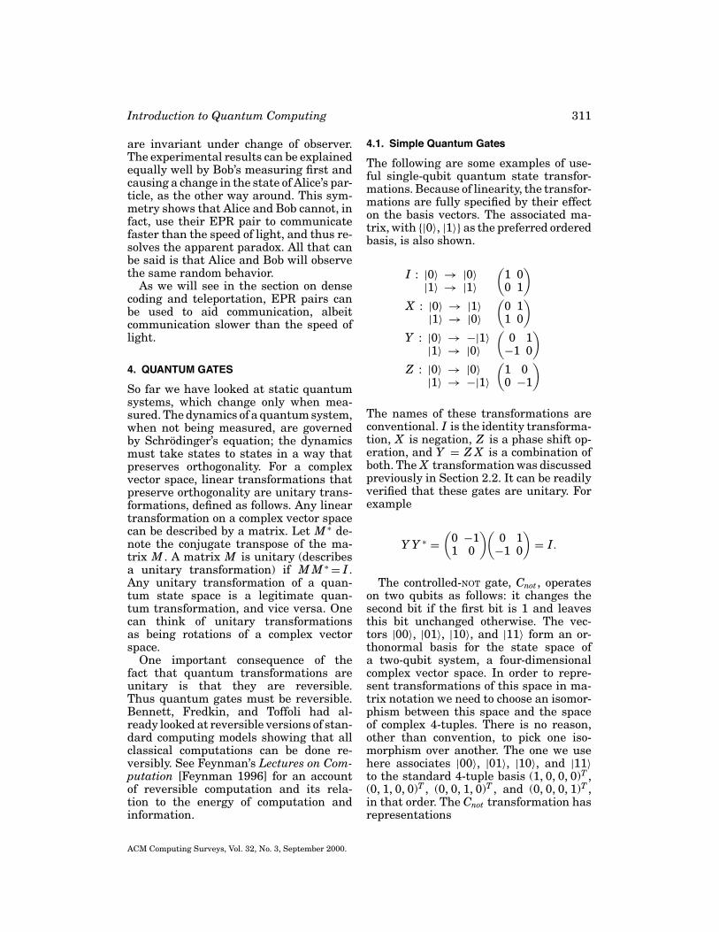
The following are some examples of use-ful single-qubit quantum state transfor-mations. Because of linearity, the transfor-mations are fully specified by their effecton the basis vectors. The associated ma-trix, with {|0〉, |1〉} as the preferred orderedbasis, is also shown.
I : |0〉 → |0〉|1〉 → |1〉
(1 00 1
)
X : |0〉 → |1〉|1〉 → |0〉
(0 11 0
)
Y : |0〉 → −|1〉|1〉 → |0〉
(0 1
−1 0
)
Z : |0〉 → |0〉|1〉 → −|1〉
(1 00 −1
)
The names of these transformations areconventional. I is the identity transforma-tion, X is negation, Z is a phase shift op-eration, and Y = Z X is a combination ofboth. The X transformation was discussedpreviously in Section 2.2. It can be readilyverified that these gates are unitary. Forexample
Y Y ∗ =(
0 −11 0
)(0 1
−1 0
)= I.
The controlled-NOT gate, Cnot , operateson two qubits as follows: it changes thesecond bit if the first bit is 1 and leavesthis bit unchanged otherwise. The vec-tors |00〉, |01〉, |10〉, and |11〉 form an or-thonormal basis for the state space ofa two-qubit system, a four-dimensionalcomplex vector space. In order to repre-sent transformations of this space in ma-trix notation we need to choose an isomor-phism between this space and the spaceof complex 4-tuples. There is no reason,other than convention, to pick one iso-morphism over another. The one we usehere associates |00〉, |01〉, |10〉, and |11〉to the standard 4-tuple basis (1, 0, 0, 0)T ,(0, 1, 0, 0)T , (0, 0, 1, 0)T , and (0, 0, 0, 1)T ,in that order. The Cnot transformation hasrepresentations
ACM Computing Surveys, Vol. 32, No. 3, September 2000.

312 E. Rieffel and W. Polak
Cnot : |00〉 → |00〉|01〉 → |01〉|10〉 → |11〉|11〉 → |10〉
1 0 0 00 1 0 00 0 0 10 0 1 0
.
The transformation Cnot is unitary sinceC∗
not = Cnot and CnotCnot = I . The Cnot gatecannot be decomposed into a tensor prod-uct of two single-bit transformations.
It is useful to have graphical represen-tations of quantum state transformations,especially when several transformationsare combined. The controlled-NOT gate Cnotis typically represented by a circuit of theform
The open circle indicates the control bit,and the × indicates the conditional nega-tion of the subject bit. In general there canbe multiple control bits. Some authors usea solid circle to indicate negative control,in which the subject bit is toggled whenthe control bit is 0.
Similarly, the controlled-controlled-NOT,which negates the last bit of three if andonly if the first two are both 1, has thefollowing graphical representation.
Single bit operations are graphicallyrepresented by appropriately labeledboxes as shown.
4.1.1 The Walsh–Hadamard Transformation.Another important single-bit transfor-mation is the Hadamard transformation,defined by
H : |0〉 → 1√2(|0〉 + |1〉)
|1〉 → 1√2(|0〉 − |1〉).
The transformation H has a numberof important applications. When appliedto |0〉, H creates a superposition state
1√2(|0〉 + |1〉). Applied to n bits individu-
ally, H generates a superposition of all 2n
possible states, which can be viewed asthe binary representation of the numbersfrom 0 to 2n − 1.
(H ⊗ H ⊗ · · · ⊗ H)|00 . . . 0〉
= 1√2n
((|0〉 + |1〉) ⊗ (|0〉 + |1〉)
⊗ · · · ⊗ (|0〉 + |1〉))
= 1√2n
2n−1∑
x=0
|x〉.
The transformation that applies H ton bits is called the Walsh, or Walsh–Hadamard, transformation W . It can bedefined as a recursive decomposition of theform
W1 = H, Wn+1 = H ⊗ Wn.
4.1.2 No Cloning. The unitary property im-plies that quantum states cannot be copiedor cloned. The no cloning proof givenhere, originally due to Wootters and Zurek[1982], is a simple application of the lin-earity of unitary transformations.
Assume that U is a unitary transforma-tion that clones, in that U (|a0〉) = |aa〉for all quantum states |a〉. Let |a〉 and |b〉be two orthogonal quantum states. SayU (|a0〉) = |aa〉 and U (|b0〉) = |bb〉. Con-sider |c〉 = (1/
√2)(|a〉 + |b〉). By linearity,
U (|c0〉) = 1√2
(U (|a0〉) + U (|b0〉))
= 1√2
(|aa〉 + |bb〉).
ACM Computing Surveys, Vol. 32, No. 3, September 2000.

Introduction to Quantum Computing 313
But if U is a cloning transformation then
U (|c0〉) = |cc〉 = 1/2(|aa〉 + |ab〉+ |ba〉 + |bb〉),
which is not equal to (1/√
2)(|aa〉 + |bb〉).Thus there is no unitary operation thatcan reliably clone unknown quantumstates. It is clear that cloning is not possi-ble by using measurement, since measure-ment is both probabalistic and destructiveof states not in the measuring device’s as-sociated subspaces.
It is important to understand what sortof cloning is and isn’t allowed. It is pos-sible to clone a known quantum state.What the no cloning principle tells usis that it is impossible to reliably clonean unknown quantum state. Also, it ispossible to obtain n particles in an en-tangled state a|00 . . . 0〉 + b|11 . . . 1〉 froman unknown state a|0〉 + b|1〉. Each ofthese particles will behave in exactly thesame way when measured with respect tothe standard basis for quantum compu-tation {|00 . . . 0〉, |00 . . . 01〉, . . . , |11 . . . 1〉},but not when measured with respect toother bases. It is not possible to create then-particle state (a|0〉 + b|1〉) ⊗ . . . ⊗ (a|0〉 +b|1〉) from an unknown state a|0〉 + b|1〉.
4.2. Examples
The use of simple quantum gates can bestudied with two simple examples: densecoding and teleportation.
Dense coding uses one quantum bit to-gether with an EPR pair to encode andtransmit two classical bits. Since EPRpairs can be distributed ahead of time,only one qubit (particle) needs to be physi-cally transmitted to communicate two bitsof information. This result is surprisingsince, as was discussed in Section 3, onlyone classical bit’s worth of information canbe extracted from a qubit. Teleportationis the opposite of dense coding, in that ituses two classical bits to transmit a singlequbit. Teleportation is surprising in lightof the no cloning principle of quantum me-chanics, in that it enables the transmis-sion of an unknown quantum state.
The key to both dense coding and tele-portation is the use of entangled particles.The initial set up is the same for both pro-cesses. Alice and Bob wish to communi-cate. Each is sent one of the entangled par-ticles making up an EPR pair,
ψ0 = 1√2
(|00〉 + |11〉).
Say Alice is sent the first particle, andBob the second. Until a particle is trans-mitted, only Alice can perform transfor-mations on her particle, and only Bob canperform transformations on his.
4.2.1 Dense Coding. Alice. Alice receivestwo classical bits, encoding the num-bers 0 through 3. Depending on thisnumber Alice performs one of the trans-formations {I, X , Y , Z } on her qubit of the
entangled pair ψ0. Transforming just onebit of an entangled pair means performingthe identity transformation on the otherbit. The resulting state is shown in thetable.
Value Transformation New state0 ψ0 = (I ⊗ I )ψ0
1√2(|00〉 + |11〉)
1 ψ1 = (X ⊗ I )ψ01√2(|10〉 + |01〉)
2 ψ2 = (Y ⊗ I )ψ01√2(−|10〉 + |01〉)
3 ψ3 = (Z ⊗ I )ψ01√2(|00〉 − |11〉)
Alice then sends her qubit to Bob.
Bob. Bob applies a controlled-NOT to thetwo qubits of the entangled pair.
ACM Computing Surveys, Vol. 32, No. 3, September 2000.

314 E. Rieffel and W. Polak
Initial state Controlled-NOT First bit Second bitψ0 = 1√
2(|00〉 + |11〉) 1√
2(|00〉 + |10〉) 1√
2(|0〉 + |1〉) |0〉
ψ1 = 1√2(|10〉 + |01〉) 1√
2(|11〉 + |01〉) 1√
2(|1〉 + |0〉) |1〉
ψ2 = 1√2(−|10〉 + |01〉) 1√
2(−|11〉 + |01〉) 1√
2(−|1〉 + |0〉) |1〉
ψ3 = 1√2(|00〉 − |11〉) 1√
2(|00〉 − |10〉) 1√
2(|0〉 − |1〉) |0〉
Note that Bob can now measure the sec-ond qubit without disturbing the quantumstate. If the measurement returns |0〉 thenthe encoded value was either 0 or 3, if themeasurement returns |1〉 then the encodedvalue was either 1 or 2.
Bob now applies H to the first bit:
Initial state First bit H(First bit)ψ0
1√2(|0〉 + |1〉) 1√
2
( 1√2(|0〉 + |1〉) + 1√
2(|0〉 − |1〉)
)= |0〉
ψ11√2(|1〉 + |0〉) 1√
2
( 1√2(|0〉 − |1〉) + 1√
2(|0〉 + |1〉)
)= |0〉
ψ21√2(−|1〉 + |0〉) 1√
2
(− 1√
2(|0〉 − |1〉) + 1√
2(|0〉 + |1〉)
)= |1〉
ψ31√2(|0〉 − |1〉) 1√
2
( 1√2(|0〉 + |1〉) − 1√
2(|0〉 − |1〉)
)= |1〉
Finally, Bob measures the resulting bit,which allows him to distinguish between0 and 3, and 1 and 2.
4.2.2 Teleportation. The objective is totransmit the quantum state of a particleusing classical bits and reconstruct theexact quantum state at the receiver.Since quantum state cannot be copied,the quantum state of the given particlewill necessarily be destroyed. Single-bitteleportation has been realized experi-mentally [Boschi et al. 1998; Bouwmeesteret al. 1997; Nielsen et al. 1998].
Alice. Alice has a qubit whose state shedoesn’t know. She wants to send the stateof ths qubit
φ = a|0〉 + b|1〉
to Bob through classical channels. As with
dense coding, Alice and Bob each possessone qubit of an entangled pair
ψ0 = 1√2
(|00〉 + |11〉).
Alice applies the decoding step of densecoding to the qubit φ to be transmitted andher half of the entangled pair. The startingstate is quantum state
φ ⊗ ψ0 = 1√2
(a|0〉 ⊗ (|00〉 + |11〉)
+ b|1〉 ⊗ (|00〉 + |11〉))
= 1√2
(a|000〉 + a|011〉 + b|100〉
+ b|111〉),
of which Alice controls the first two bitsand Bob controls the last one. Alice nowapplies Cnot ⊗ I and H ⊗ I ⊗ I to thisstate:
ACM Computing Surveys, Vol. 32, No. 3, September 2000.

Introduction to Quantum Computing 315
(H ⊗ I ⊗ I )(Cnot ⊗ I )(φ ⊗ ψ0)
= (H ⊗ I ⊗ I )(Cnot ⊗ I )1√2
(a|000〉
+ a|011〉 + b|100〉 + b|111〉)
= (H ⊗ I ⊗ I )1√2
(a|000〉 + a|011〉
+ b|110〉 + b|101〉)
= 12
(a(|000〉 + |011〉 + |100〉 + |111〉)
+ b(|010〉 + |001〉 − |110〉 − |101〉))
= 12
(|00〉(a|0〉 + b|1〉) + |01〉(a|1〉
+ b|0〉) + |10〉(a|0〉 − b|1〉)+ |11〉(a|1〉 − b|0〉))
Alice measures the first two qubits to getone of |00〉, |01〉, |10〉, or |11〉 with equalprobability. Depending on the result of themeasurement, the quantum state of Bob’squbit is projected to a|0〉+b|1〉, a|1〉+b|0〉,a|0〉−b|1〉, or a|1〉−b|0〉 respectively. Alicesends the result of her measurement astwo classical bits to Bob.
Note that when she measured it, Aliceirretrievably altered the state of her orig-inal qubit φ, whose state she is in the pro-cess of sending to Bob. This loss of the orig-inal state is the reason teleportation doesnot violate the no cloning principle.
Bob. When Bob receives the two classi-cal bits from Alice he knows how the stateof his half of the entangled pair comparesto the original state of Alice’s qubit.
Bits received State Decoding00 a|0〉 + b|1〉 I01 a|1〉 + b|0〉 X10 a|0〉 − b|1〉 Z11 a|1〉 − b|0〉 Y
Bob can reconstruct the original state ofAlice’s qubit, φ, by applying the appropri-ate decoding transformation to his part ofthe entangled pair. Note that this is theencoding step of dense coding.
5. QUANTUM COMPUTERS
This section discusses how quantum me-chanics can be used to perform compu-tations and how these computations arequalitatively different from those per-formed by a conventional computer. Re-call from Section 4 that all quantum statetransformations have to be reversible.While the classical NOT gate is reversible,AND, OR, and NAND gates are not. Thusit is not obvious that quantum trans-formations can carry out all classicalcomputations. The first subsection de-scribes complete sets of reversible gatesthat can perform any classical computa-tion on a quantum computer. Further-more, it describes sets of gates with whichall quantum computations can be done.The second subsection discusses quantumparallelism.
5.1. Quantum Gate Arrays
The bra/ket notation is useful in definingcomplex unitary operations. For two arbi-trary unitary transformations U1 and U2,the “conditional” transformation |0〉〈0| ⊗U1 + |1〉〈1| ⊗ U2 is also unitary. Thecontrolled-NOT gate can be defined by
Cnot = |0〉〈0| ⊗ I + |1〉〈1| ⊗ X .
The three-bit controlled-controlled-NOTgate or Toffoli gate of Section 4 is also aninstance of this conditional definition:
T = |0〉〈0| ⊗ I ⊗ I + |1〉〈1| ⊗ Cnot .
The Toffoli gate T can be used to constructcomplete set of boolean connectives, as canbe seen from the fact that it can be used toconstruct the AND and NOT operators in thefollowing way:
T |1, 1, x〉 = |1, 1, ¬x〉T |x, y , 0〉 = |x, y , x ∧ y〉
The T gate is sufficient to construct arbi-trary combinatorial circuits.
The following quantum circuit, for ex-ample, implements a 1 bit full adder usingToffoli and controlled-NOT gates:
ACM Computing Surveys, Vol. 32, No. 3, September 2000.
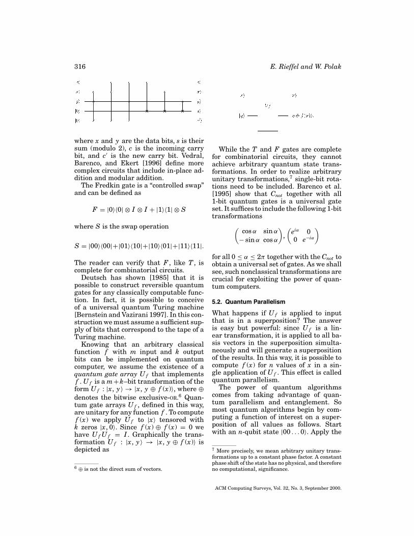
316 E. Rieffel and W. Polak
where x and y are the data bits, s is theirsum (modulo 2), c is the incoming carrybit, and c′ is the new carry bit. Vedral,Barenco, and Ekert [1996] define morecomplex circuits that include in-place ad-dition and modular addition.
The Fredkin gate is a “controlled swap”and can be defined as
F = |0〉〈0| ⊗ I ⊗ I + |1〉〈1| ⊗ S
where S is the swap operation
S = |00〉〈00|+|01〉〈10|+|10〉〈01|+|11〉〈11|.
The reader can verify that F , like T , iscomplete for combinatorial circuits.
Deutsch has shown [1985] that it ispossible to construct reversible quantumgates for any classically computable func-tion. In fact, it is possible to conceiveof a universal quantum Turing machine[Bernstein and Vazirani 1997]. In this con-struction we must assume a sufficient sup-ply of bits that correspond to the tape of aTuring machine.
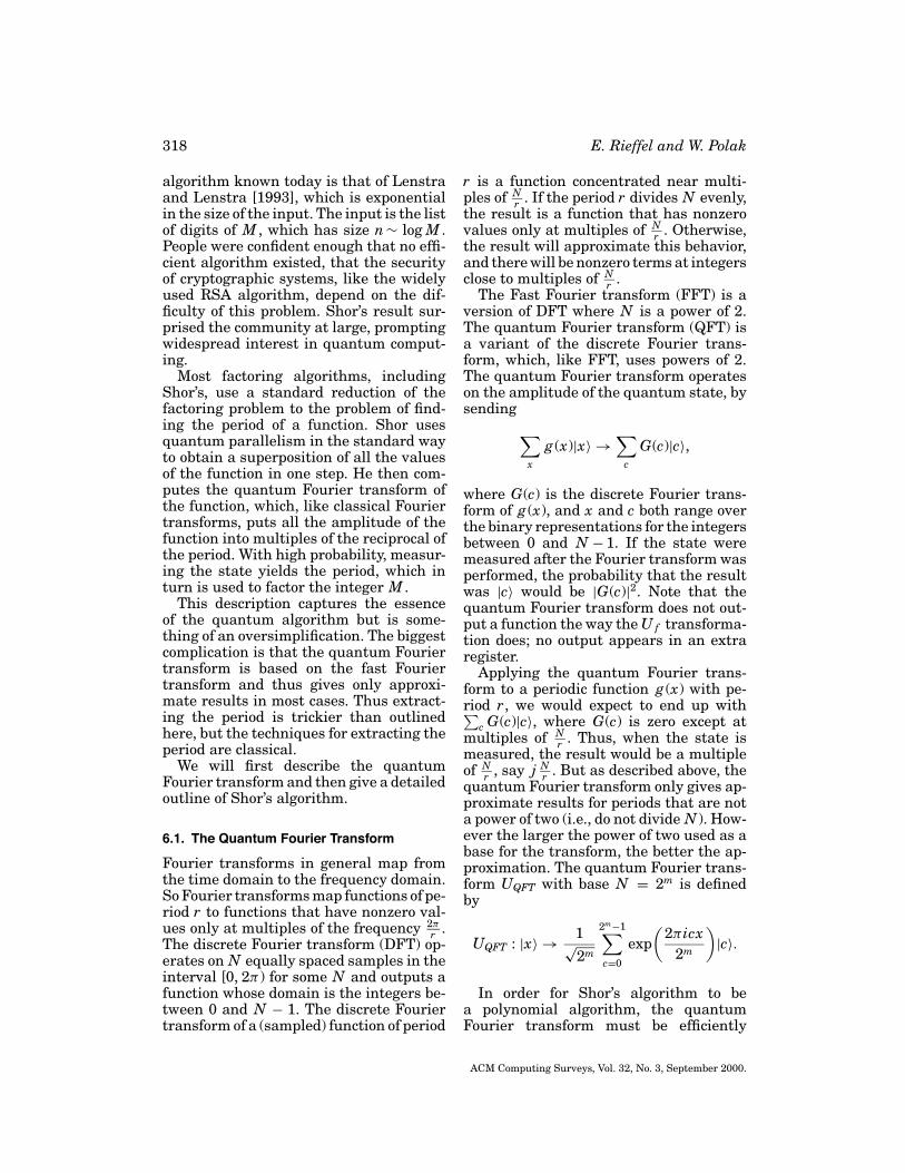
Knowing that an arbitrary classicalfunction f with m input and k outputbits can be implemented on quantumcomputer, we assume the existence of aquantum gate array U f that implementsf . U f is a m+k–bit transformation of theform U f : |x, y〉 → |x, y ⊕ f (x)〉, where ⊕denotes the bitwise exclusive-OR.6 Quan-tum gate arrays U f , defined in this way,are unitary for any function f . To computef (x) we apply U f to |x〉 tensored withk zeros |x, 0〉. Since f (x) ⊕ f (x) = 0 wehave U f U f = I . Graphically the trans-formation U f : |x, y〉 → |x, y ⊕ f (x)〉 isdepicted as
6 ⊕ is not the direct sum of vectors.
While the T and F gates are completefor combinatorial circuits, they cannotachieve arbitrary quantum state trans-formations. In order to realize arbitraryunitary transformations,7 single-bit rota-tions need to be included. Barenco et al.[1995] show that Cnot together with all1-bit quantum gates is a universal gateset. It suffices to include the following 1-bittransformations
(cos α sin α
− sin α cos α
),(
eiα 00 e−iα
)
for all 0 ≤ α ≤ 2π together with the Cnot toobtain a universal set of gates. As we shallsee, such nonclassical transformations arecrucial for exploiting the power of quan-tum computers.
5.2. Quantum Parallelism
What happens if U f is applied to inputthat is in a superposition? The answeris easy but powerful: since U f is a lin-ear transformation, it is applied to all ba-sis vectors in the superposition simulta-neously and will generate a superpositionof the results. In this way, it is possible tocompute f (x) for n values of x in a sin-gle application of U f . This effect is calledquantum parallelism.
The power of quantum algorithmscomes from taking advantage of quan-tum parallelism and entanglement. Somost quantum algorithms begin by com-puting a function of interest on a super-position of all values as follows. Startwith an n-qubit state |00 . . . 0〉. Apply the
7 More precisely, we mean arbitrary unitary trans-formations up to a constant phase factor. A constantphase shift of the state has no physical, and thereforeno computational, significance.
ACM Computing Surveys, Vol. 32, No. 3, September 2000.

Introduction to Quantum Computing 317
Walsh–Hadamard transformation W ofSection 4.1.1 to get a superposition
1√2n
(|00 . . . 0〉 + |00 . . . 1〉 + · · · + |11 . . . 1〉)
= 1√2n
2n−1∑
x=0
|x〉
which should be viewed as the superposi-tion of all integers 0 ≤ x < 2n. Add a k-bitregister |0〉 then by linearity
U f
(1√2n
2n−1∑
x=0
|x, 0〉)
= 1√2n
2n−1∑
x=0
U f (|x, 0〉)
= 1√2n
2n−1∑
x=0
|x, f (x)〉
where f (x) is the function of interest. Notethat since n qubits enable working simul-taneously with 2n states, quantum paral-lelism circumvents the time/space trade-off of classical parallelism through itsability to provide an exponential amountof computational space in a linear amountof physical space.
Consider the trivial example of acontrolled-controlled-NOT (Toffoli) gate, T ,that computes the conjunction of two val-ues:
Now take as input a superposition of allpossible bit combinations of x and y to-gether with the necessary 0:
H|0〉 ⊗ H|0〉 ⊗ |0〉
= 1√2
(|0〉 + |1〉) ⊗ 1√2
(|0〉 + |1〉) ⊗ |0〉
= 12
(|000〉 + |010〉 + |100〉 + |110〉).
Apply T to the superposition of inputs toget a superposition of the results, namely
T (H|0〉 ⊗ H|0〉 ⊗ |0〉) = 12
(|000〉 + |010〉
+ |100〉 + |111〉).
The resulting superposition can be viewedas a truth table for the conjunction, ormore generally as the graph of a function.In the output the values of x, y , and x ∧ yare entangled in such a way that measur-ing the result will give one line of the truthtable, or more generally one point of graphof the function. Note that the bits can bemeasured in any order: measuring the re-sult will project the state to a superposi-tion of the set of all input values for whichf produces this result, and measuring theinput will project the result to the corre-sponding function value.
Measuring at this point gives no ad-vantage over classical parallelism becauseonly one result is obtained, and worse stillone cannot even choose which result onegets. The heart of any quantum algorithmis the way in which it manipulates quan-tum parallelism so that desired resultswill be measured with high probability.This sort of manipulation has no classicalanalog and requires nontraditional pro-gramming techniques. We list a couple ofthe techniques currently known.! Amplify output values of interest. The
general idea is to transform the state insuch a way that values of interest havea larger amplitude and therefore havea higher probability of being measured.Examples of this approach will be de-scribed in Section 7.! Find common properties of all the val-ues of f (x). This idea is exploited inShor’s algorithm, which uses a quantumFourier transformation to obtain the pe-riod of f .
6. SHOR’S ALGORITHM
In 1994, inspired by work of Daniel Si-mon (later published in Simon [1997]),Peter Shor found a bounded probabil-ity polynomial time algorithm for fac-toring n-digit numbers on a quantumcomputer. Since the 1970s people havesearched for efficient algorithms for factor-ing integers. The most efficient classical
ACM Computing Surveys, Vol. 32, No. 3, September 2000.
318 E. Rieffel and W. Polak
algorithm known today is that of Lenstraand Lenstra [1993], which is exponentialin the size of the input. The input is the listof digits of M , which has size n∼ log M .People were confident enough that no effi-cient algorithm existed, that the securityof cryptographic systems, like the widelyused RSA algorithm, depend on the dif-ficulty of this problem. Shor’s result sur-prised the community at large, promptingwidespread interest in quantum comput-ing.
Most factoring algorithms, includingShor’s, use a standard reduction of thefactoring problem to the problem of find-ing the period of a function. Shor usesquantum parallelism in the standard wayto obtain a superposition of all the valuesof the function in one step. He then com-putes the quantum Fourier transform ofthe function, which, like classical Fouriertransforms, puts all the amplitude of thefunction into multiples of the reciprocal ofthe period. With high probability, measur-ing the state yields the period, which inturn is used to factor the integer M .
This description captures the essenceof the quantum algorithm but is some-thing of an oversimplification. The biggestcomplication is that the quantum Fouriertransform is based on the fast Fouriertransform and thus gives only approxi-mate results in most cases. Thus extract-ing the period is trickier than outlinedhere, but the techniques for extracting theperiod are classical.
We will first describe the quantumFourier transform and then give a detailedoutline of Shor’s algorithm.
6.1. The Quantum Fourier Transform
Fourier transforms in general map fromthe time domain to the frequency domain.So Fourier transforms map functions of pe-riod r to functions that have nonzero val-ues only at multiples of the frequency 2π
r .The discrete Fourier transform (DFT) op-erates on N equally spaced samples in theinterval [0, 2π ) for some N and outputs afunction whose domain is the integers be-tween 0 and N − 1. The discrete Fouriertransform of a (sampled) function of period
r is a function concentrated near multi-ples of N
r . If the period r divides N evenly,the result is a function that has nonzerovalues only at multiples of N
r . Otherwise,the result will approximate this behavior,and there will be nonzero terms at integersclose to multiples of N
r .The Fast Fourier transform (FFT) is a
version of DFT where N is a power of 2.The quantum Fourier transform (QFT) isa variant of the discrete Fourier trans-form, which, like FFT, uses powers of 2.The quantum Fourier transform operateson the amplitude of the quantum state, bysending
∑
x
g (x)|x〉 →∑
c
G(c)|c〉,
where G(c) is the discrete Fourier trans-form of g (x), and x and c both range overthe binary representations for the integersbetween 0 and N − 1. If the state weremeasured after the Fourier transform wasperformed, the probability that the resultwas |c〉 would be |G(c)|2. Note that thequantum Fourier transform does not out-put a function the way the U f transforma-tion does; no output appears in an extraregister.
Applying the quantum Fourier trans-form to a periodic function g (x) with pe-riod r, we would expect to end up with∑
c G(c)|c〉, where G(c) is zero except atmultiples of N
r . Thus, when the state ismeasured, the result would be a multipleof N
r , say j Nr . But as described above, the
quantum Fourier transform only gives ap-proximate results for periods that are nota power of two (i.e., do not divide N ). How-ever the larger the power of two used as abase for the transform, the better the ap-proximation. The quantum Fourier trans-form UQFT with base N = 2m is definedby
UQFT : |x〉 → 1√2m
2m−1∑
c=0
exp(
2πicx2m
)|c〉.
In order for Shor’s algorithm to bea polynomial algorithm, the quantumFourier transform must be efficiently
ACM Computing Surveys, Vol. 32, No. 3, September 2000.
Introduction to Quantum Computing 319
computable. Shor shows that the quan-tum Fourier transform with base 2m can beconstructed using only m(m+1)
2 gates. Theconstruction makes use of two types ofgates. One is a gate to perform the famil-iar Hadamard transformation H. We willdenote by Hj the Hadamard transforma-tion applied to the j th bit. The other typeof gate performs 2-bit transformations ofthe form
Sj ,k =
1 0 0 00 1 0 00 0 1 00 0 0 eiθk− j
,
where θk− j = π/2k− j . This transformationacts on the kth and j th bits of a largerregister. The quantum Fourier transformis given by
H0S0,1 . . . S0,m−1 H1 . . . Hm−3
Sm−3,m−2Sm−3,m−1 Hm−2Sm−2,m−1 Hm−1
followed by a bit reversal transformation.If FFT is followed by measurement, as inShor’s algorithm, the bit reversal can beperformed classically. See Shor [1997] formore details.
6.2. A Detailed Outline of Shor’s algorithm
The detailed steps of Shor’s algorithm areillustrated with a running example wherewe factor M = 21.
Step 1. Quantum parallelism. Choose aninteger a arbitrarily. If a is not relativelyprime to M , we have found a factor of M .Otherwise apply the rest of the algorithm.
Let m be such that M 2 ≤ 2m < 2M 2.[This choice is made so that the approxi-mation used in Step 3 for functions whoseperiod is not a power of 2 will be goodenough for the rest of the algorithm towork.] Use quantum parallelism as de-scribed in Section 5.2 to compute f (x) =ax mod M for all integers from 0 to 2m − 1.The function is thus encoded in the quan-tum state
1√2m
2m−1∑
x=0
|x, f (x)〉. (1)
Example. Suppose a = 11 were ran-domly chosen. Since M 2 = 441 ≤ 29 <882 = 2M 2, we find m = 9. Thus, a totalof 14 quantum bits, 9 for x and 5 for f (x),are required to compute the superpositionof equation 1.
Step 2. A state whose amplitude has the sameperiod as f . The quantum Fourier trans-form acts on the amplitude function as-sociated with the input state. In order touse the quantum Fourier transform to ob-tain the period of f , a state is constructedwhose amplitude function has the sameperiod as f .
To construct such a state, measure thelast 3log2 M 4 qubits of the state of Eq. 1that encode f (x). A random value u is ob-tained. The value u is not of interest in it-self; only the effect the measurement hason our set of superpositions is of inter-est. This measurement projects the statespace onto the subspace compatible withthe measured value, so the state aftermeasurement is
C∑
x
g (x)|x, u〉,
for some scale factor C where
g (x) ={
1 if f (x) = u0 otherwise.
Note that the x ’s that actually appear inthe sum, those with g (x) 5= 0, differ fromeach other by multiples of the period; thusg (x) is the function we are looking for. Ifwe could measure two successive x ’s in thesum, we would have the period. Unfortu-nately the laws of quantum physics permitonly one measurement.
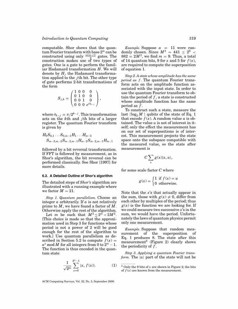
Example. Suppose that random mea-surement of the superposition ofEq. 1 produces 8. The state after thismeasurement8 (Figure 2) clearly showsthe periodicity of f .
Step 3. Applying a quantum Fourier trans-form. The |u〉 part of the state will not be
8 Only the 9 bits of x are shown in Figure 2; the bitsof f (x) are known from the measurement.
ACM Computing Surveys, Vol. 32, No. 3, September 2000.

320 E. Rieffel and W. Polak
Fig. 2. Probabilities for measuring x when measuring the state C&x∈X |x, 8〉obtained in Step 2, where X = {x|211x mod 21 = 8}}.
used, so we will no longer write it. Ap-ply the quantum Fourier transform to thestate obtained in Step 2.
UQ F T :∑
x g (x)|x〉 →∑
c G(c)|c〉
Standard Fourier analysis tells us thatwhen the period r of the function g (x)defined in Step 2 is a power of 2, the re-sult of the quantum Fourier transform is
∑
j
c j
∣∣∣∣ j2m
r
⟩,
where the amplitude is 0 except at multi-ples of 2m/r. When the period r does notdivide 2m, the transform approximates theexact case, so most of the amplitude is at-tached to integers close to multiples of 2m
r .
Example. Figure 3 shows the result ofapplying the quantum Fourier transformto the state obtained in Step 2. Notethat Figure 3 is the graph of the fastFourier transform of the function shownin Figure 2. In this particular example theperiod of f does not divide 2m.
Step 4. Extracting the period. Measure thestate in the standard basis for quantumcomputation, and call the result v. In thecase where the period happens to be apower of 2, so that the quantum Fouriertransform gives exactly multiples of 2m/r,the period is easy to extract. In this case,v = j 2m
r for some j . Most of the time j andr will be relatively prime, in which case
reducing the fraction v2m (= j
r ) to its lowestterms will yield a fraction whose denom-inator q is the period r. The fact thatin general the quantum Fourier trans-form only approximately gives multiplesof the scaled frequency complicates theextraction of the period from the measure-ment. When the period is not a powerof 2, a good guess for the period can beobtained using the continued fractionexpansion of v
2m . This classical techniqueis described in Appendix B.
Example. Say that measurement of thestate returns v = 427. Since v and 2m
are relatively prime, the period r willmost likely not divide 2m and the contin-ued fraction expansion described in Ap-pendix B needs to be applied. The follow-ing is a trace of the algorithm described inAppendix B:
i ai pi qi εi0 0 0 1 0.83398441 1 1 1 0.19906322 5 5 6 0.023529413 42 211 253 0.5
which terminates with 6 = q2 < M ≤ q3.Thus, q = 6 is likely to be the period of f .
Step 5. Finding a factor of M. When ourguess for the period, q, is even, use theEuclidean algorithm to efficiently checkwhether either aq/2 + 1 or aq/2 − 1 has anontrivial common factor with M .
ACM Computing Surveys, Vol. 32, No. 3, September 2000.

Introduction to Quantum Computing 321
Fig. 3. Probability distribution of the quantum state after Fourier transfor-mation.
The reason why aq/2 + 1 or aq/2 − 1 islikely to have a nontrivial common fac-tor with M is as follows. If q is indeedthe period of f (x) = ax mod M , thenaq = 1 mod M, since aqax = ax mod M forall x. If q is even, we can write
(aq/2 + 1)(aq/2 − 1) = 0 mod M .
Thus, as long as neither aq/2+1 nor aq/2−1is a multiple of M , either aq/2+1 or aq/2−1has a nontrivial common factor with M .
Example. Since 6 is even either a6/2−1 =113 − 1 = 1330 or a6/2 + 1 = 113 + 1 =1332 will have a common factor with M. Inthis particular example we find two factorsgcd(21, 1330) = 7 and gcd(21, 1332) = 3.
Step 6. Repeating the algorithm, if necessary.Various things could have gone wrong sothat this process does not yield a factor ofM :
1. The value v was not close enough to amultiple of 2m
r .2. The period r and the multiplier j could
have had a common factor so that thedenominator q was actually a factor ofthe period, not the period itself.
3. Step 5 yields M as M ’s factor.4. The period of f (x) = ax mod M is odd.
Shor shows that few repetitions of this al-gorithm yields a factor of M with highprobability.
6.2.1 A Comment on Step 2 of Shor’s Algorithm.The measurement in Step 2 can be skippedentirely. More generally Bernstein andVazirani [1997] show that measurementsin the middle of an algorithm can alwaysbe avoided. If the measurement in Step 2is omitted, the state consists of a superpo-sitions of several periodic functions all ofwhich have the same period. By the linear-ity of quantum algorithms, applying thequantum Fourier transformation leads toa superposition of the Fourier transformsof these functions, each of which is entan-gled with the corresponding u and there-fore do not interfere with each other. Mea-surement gives a value from one of theseFourier transforms. Seeing how this argu-ment can be formalized illustrates someof the subtleties of working with quan-tum superpostions. Apply the quantumFourier transform tensored with the iden-tity, UQ F T ⊗ I, to C&2n−1
x=0 |x, f (x)〉 to get
C ′2n−1∑
x=0
2m−1∑
c=0
exp(
2πicx2m
)|c, f (x)〉,
which is equal to
C ′∑
u
∑
x| f (x)=u
∑
c
exp(
2πicx2m
)|c, u〉
for u in the range of f (x). What resultsis a superposition of the results of Step 3for all possible u’s. The quantum Fourier
ACM Computing Surveys, Vol. 32, No. 3, September 2000.

322 E. Rieffel and W. Polak
transform is being applied to a familyof separate functions gu indexed by uwhere
gu ={
1 if f (x) = u0 otherwise,
all with the same period. Note that the am-plitudes in states with different u’s neverinterfere (add or cancel) with each other.The transform UQ F T ⊗ I as applied abovecan be written
UQ F T ⊗ I : C∑
u∈R
2n−1∑
x=0
gu(x)|x, f (x)〉
→ C ′∑
u∈R
2n−1∑
x=0
2n−1∑
c=0
Gu(c)|c, u〉,
where Gu(c) is the discrete Fourier trans-form of gu(x) and R is the range of f (x).
Measure c and run Steps 4 and 5 asbefore.
7. SEARCH PROBLEMS
A large class of problems can be speci-fied as search problems of the form “findsome x in a set of possible solutions suchthat statement P (x) is true.” Such prob-lems range from database search to sort-ing to graph coloring. For example, thegraph coloring problem can be viewed as asearch for an assignment of colors to ver-tices so that the statement “all adjacentvertices have different colors” is true. Sim-ilarly, a sorting problem can be viewed asa search for a permutation for which thestatement “the permutation x takes theinitial state to the desired sorted state” istrue.
An unstructured search problem is onewhere nothing is know (or no assumptionare used) about the structure of the solu-tion space and the statement P . For exam-ple, determining P (x0) provides no infor-mation about the possible value of P (x1)for x0 5= x1. A structured search problemis one where information about the searchspace and statement P can be exploited.
For instance, searching an alphabet-ized list is a structured search problem
and the structure can be exploited toconstruct efficient algorithms. In othercases, like constraint satisfaction prob-lems such as 3-SAT or graph colorabil-ity, the problem structure can be exploitedfor heuristic algorithms that yield effi-cient solution for some problem instances.But in the general case of an unstruc-tured problem, randomly testing the truthof statements P (xi) one by one is thebest that can be done classically. For asearch space of size N , the general un-structured search problem requires O(N )evaluations of P . On a quantum computer,however, Grover showed that the unstruc-tured search problem can be solved withbounded probability within O(
√N ) eval-
uations of P . Thus Grover’s search algo-rithm [Grover 1996] is provably more ef-ficient than any algorithm that could runon a classical computer.
While Grover’s algorithm is optimal[Bennett et al. 1997; Boyer et al. 1996;Zalka 1997] for completely unstructuredsearches, most search problems involvesearching a structured solution space.Just as there are classical heuristic al-gorithms that exploit problem structure,one would expect that there are moreefficient quantum algorithms for cer-tain structured problem instances. Cerfet al. [1998] use Grover’s search al-gorithm in place of classical searcheswithin a heuristic algorithm to show thata quadratic speed-up is possible overa particularly simple classical heuristicfor solving NP-hard problems. Brassardet al. [1998], using the techniques ofGrover’s search algorithm in a less obviousway, show that general heuristic searcheshave quantum analogs with quadraticspeed-up.
There is hope that for certain struc-tured problems a speed-up greater thanquadratic is possible. Such algorithms willlikely require new approaches that are notmerely quantum implementations of clas-sical algorithms. Shor’s algorithm, whenviewed as a search for factors, is an ex-ample of an algorithm that achieves expo-nential speed-up by using problem struc-ture (number theory) in new ways uniqueto quantum computation.
ACM Computing Surveys, Vol. 32, No. 3, September 2000.

Introduction to Quantum Computing 323
Tad Hogg has developed heuristic quan-tum search algorithms that exploit prob-lem structure. His approach is distinclynonclassical and uses unique properties ofquantum computation. One problem withthis approach is that, like most heuristicalgorithms, the use of problem structureis complicated enough that it is hard todetermine the probability that a singleexecution of an algorithm will give a cor-rect answer. Therefore, it is unknown howefficient Hogg’s algorithms are. Classi-cally the efficiency of heuristic algorithmsis estimated by empirically testing thealgorithm. But as there is an exponentialslowdown when simulating a quantumcomputer on a classical one, empirical test-ing of quantum algorithms is currently in-feasible except in small cases. Small casesindicate that Hogg’s algorithms are moreefficient than Grover’s algorithm appliedto structured search problems, but thatthe speed-up is likely to be only polyno-mial. While less interesting theoretically,even a small polynomial speed-up on av-erage for these computationally difficultproblems is of significant practical inter-est. Until sufficiently large quantum com-puters are built, or better techniques foranalyzing such algorithms are found, theefficiency cannot be determined for sure.
7.1. Grover’s Search Algorithm
Grover’s algorithm searches an unstruc-tured list of size N for an x that makes astatement true. Let n be such that 2n ≥ N ,and let Up be the quantum gate that im-plements the classical function P (x) thattests the truth of the statement, wheretrue is encoded as 1.
UP : |x, 0〉 → |x, P (x)〉
The first step is the standard onefor quantum computing described inSection 5.2. Compute P for all possible in-puts xi, by applying UP to a register con-taining the superposition 1√
2n &n−1x=0 |x〉 of all
2n possible inputs x together with a regis-ter set to 0, leading to the superposition
1√2n
2n−1∑
x=0
|x, P (x)〉. (2)
The difficult step is to obtain a useful re-sult from this superposition.
For any x0 such that P (x0) is true, |x0, 1〉will be part of the superposition of Eq. 2.Since the amplitude of such a state is 1√
2n ,the probability that a random measure-ment of the superposition produces x0 isonly 2−n. The trick is to change the quan-tum state in Eq. 2 so as to greatly increasethe amplitude of vectors |x0, 1〉 for whichP is true and decrease the amplitude ofvectors |x, 0〉 for which P is false.
Once such a transformation of the quan-tum state has been performed, one cansimply measure the last qubit of the quan-tum state which represents P (x). Becauseof the amplitude change, there is a highprobability that the result will be 1. Ifthis is the case, the measurement has pro-jected the state of Eq. 2 onto the subspace
1√k&k
i=1|xi, 1〉 where k is the number of so-lutions. Further measurement of the re-maining bits will provide one of these so-lutions. If the measurement of qubit P (x)yields 0, then the whole process is startedover and the superposition of Eq. 2 mustbe computed again.
Grover’s algorithm then consists of thefollowing steps:
1. Prepare a register containing a super-position of all possible values xi ∈[0 . . . 2n − 1].
2. Compute P (xi) on this register.3. Change amplitude aj to −aj for x j such
that P (x j ) = 1. An efficient algorithmfor changing selected signs is describedin Section 7.1.2. A plot of the ampli-tudes after this step is shown here.
4. Apply inversion about the average to in-crease amplitude of x j with P (x j ) = 1.The quantum algorithm to efficientlyperform inversion about the average is
ACM Computing Surveys, Vol. 32, No. 3, September 2000.
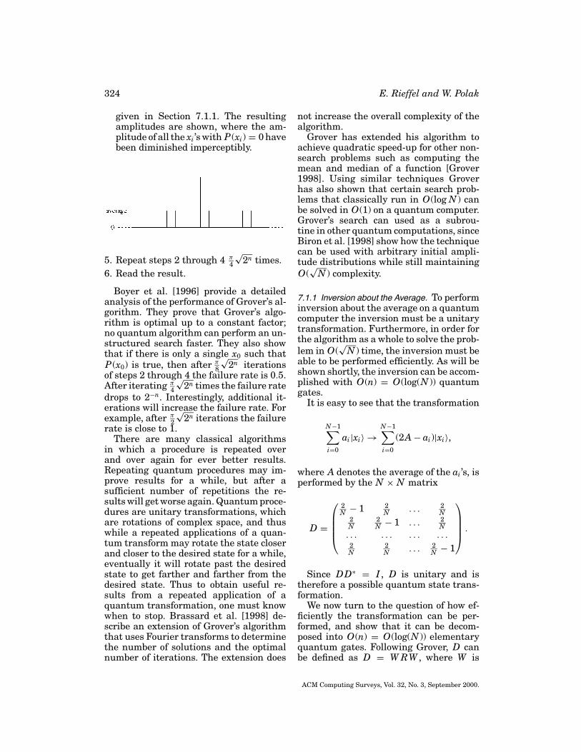
324 E. Rieffel and W. Polak
given in Section 7.1.1. The resultingamplitudes are shown, where the am-plitude of all the xi ’s with P (xi) = 0 havebeen diminished imperceptibly.
5. Repeat steps 2 through 4 π4
√2n times.
6. Read the result.
Boyer et al. [1996] provide a detailedanalysis of the performance of Grover’s al-gorithm. They prove that Grover’s algo-rithm is optimal up to a constant factor;no quantum algorithm can perform an un-structured search faster. They also showthat if there is only a single x0 such thatP (x0) is true, then after π
8
√2n iterations
of steps 2 through 4 the failure rate is 0.5.After iterating π
4
√2n times the failure rate
drops to 2−n. Interestingly, additional it-erations will increase the failure rate. Forexample, after π
2
√2n iterations the failure
rate is close to 1.There are many classical algorithms
in which a procedure is repeated overand over again for ever better results.Repeating quantum procedures may im-prove results for a while, but after asufficient number of repetitions the re-sults will get worse again. Quantum proce-dures are unitary transformations, whichare rotations of complex space, and thuswhile a repeated applications of a quan-tum transform may rotate the state closerand closer to the desired state for a while,eventually it will rotate past the desiredstate to get farther and farther from thedesired state. Thus to obtain useful re-sults from a repeated application of aquantum transformation, one must knowwhen to stop. Brassard et al. [1998] de-scribe an extension of Grover’s algorithmthat uses Fourier transforms to determinethe number of solutions and the optimalnumber of iterations. The extension does
not increase the overall complexity of thealgorithm.
Grover has extended his algorithm toachieve quadratic speed-up for other non-search problems such as computing themean and median of a function [Grover1998]. Using similar techniques Groverhas also shown that certain search prob-lems that classically run in O(log N ) canbe solved in O(1) on a quantum computer.Grover’s search can used as a subrou-tine in other quantum computations, sinceBiron et al. [1998] show how the techniquecan be used with arbitrary initial ampli-tude distributions while still maintainingO(
√N ) complexity.
7.1.1 Inversion about the Average. To performinversion about the average on a quantumcomputer the inversion must be a unitarytransformation. Furthermore, in order forthe algorithm as a whole to solve the prob-lem in O(
√N ) time, the inversion must be
able to be performed efficiently. As will beshown shortly, the inversion can be accom-plished with O(n) = O(log(N )) quantumgates.
It is easy to see that the transformation
N−1∑
i=0
ai|xi〉 →N−1∑
i=0
(2A − ai)|xi〉,
where A denotes the average of the ai ’s, isperformed by the N × N matrix
D =
2N − 1 2
N . . . 2N
2N
2N − 1 . . . 2
N. . . . . . . . . . . .2N
2N . . . 2
N − 1
.
Since DD∗ = I , D is unitary and istherefore a possible quantum state trans-formation.
We now turn to the question of how ef-ficiently the transformation can be per-formed, and show that it can be decom-posed into O(n) = O(log(N )) elementaryquantum gates. Following Grover, D canbe defined as D = W RW , where W is
ACM Computing Surveys, Vol. 32, No. 3, September 2000.

Introduction to Quantum Computing 325
the Walsh–Hadamard transform definedin Section 4 and
R =
1 0 . . . 00 −1 0 . . .0 . . . . . . 00 . . . 0 −1
.
To see that D = W RW , consider R =R ′ − I where I is the identity and
R ′ =
2 0 . . . 00 0 0 . . .0 . . . . . . 00 . . . 0 0
.
Now W RW = W (R ′ − I )W = W R ′W − I .It is easily verified that
W R ′W =
2N
2N . . . 2
N2N
2N
2N . . .
2N . . . . . . 2
N2N . . . 2
N2N
and thus W R ′W − I = D.
7.1.2 Changing the Sign. We still have to ex-plain how to invert the amplitude of thedesired result. We show, more generally, asurprisingly simple way to invert the am-plitude of exactly those states with P (x) =1 for a general P .
Let UP be the gate array that per-forms the computation UP : |x, b〉 →|x, b ⊕ P (x)〉. Apply UP to the superposi-tion |ψ〉 = 1√
2n
∑n−1x=0 |x〉 and choose b =
1√2|0〉 − |1〉 to end up in a state where
the sign of all x with P (x) = 1 has beenchanged, and b is unchanged.
To see this, let X 0 = {x|P (x) = 0} andX 1 = {x|P (x) = 1}, and consider the ap-plication of UP .
UP (|ψ, b〉)
= 1√2n+1
UP
(∑
x∈X 0
|x, 0〉 +∑
x∈X 1
|x, 0〉
−∑
x∈X 0
|x, 1〉 −∑
x∈X 1
|x, 1〉)
= 1√2n+1
(∑
x∈X 0
|x, 0 ⊕ 0〉
+∑
x∈X 1
|x, 0 ⊕ 1〉 −∑
x∈X 0
|x, 1 ⊕ 0〉
−∑
x∈X 1
|x, 1 ⊕ 1〉)
= 1√2n+1
(∑
x∈X 0
|x, 0〉 +∑
x∈X 1
|x, 1〉
−∑
x∈X 0
|x, 1〉 −∑
x∈X 1
|x, 0〉)
= 1√2n
(∑
x∈X 0
|x〉 −∑
x∈X 1
|x〉)
⊗ b
Thus the amplitude of the states in X 1have been inverted as desired.
7.2. Heuristic Search
7.2.1 A Note on the Walsh–Hadamard Trans-form. Another representation for theWalsh–Hadamard transformation of Sec-tion 4.1.1 is useful for understanding howto use the Walsh–Hadamard transforma-tion in constructing quantum algorithms.The n-bit Walsh–Hadamard transforma-tion is a 2n × 2n matrix W with entriesWrs where both r and s range from 0 to2n − 1. We will show that
Wrs = 1√2n
(−1)r·s
where r · s is the number of common 1bits in the the binary representations of rand s.
To see this equality, note that
W (|r〉) =∑
s
Wrs|s〉.
Let rn−1 . . . r0 be the binary representationof r and sn−1 . . . s0 be the binary represen-tation of s.
ACM Computing Surveys, Vol. 32, No. 3, September 2000.
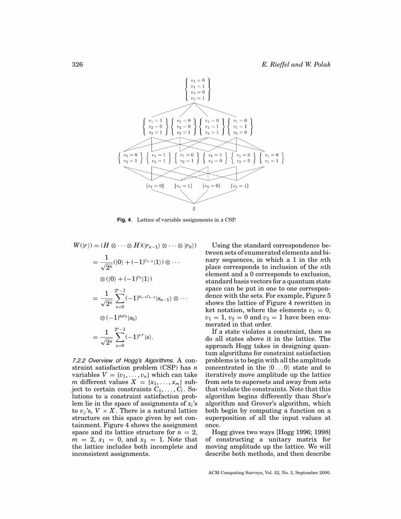
326 E. Rieffel and W. Polak
Fig. 4. Lattice of variable assignments in a CSP.
W (|r〉) = (H ⊗ · · · ⊗ H)(|rn−1〉 ⊗ · · · ⊗ |r0〉)
= 1√2n
(|0〉 + (−1)rn−1 |1〉) ⊗ · · ·
⊗ (|0〉 + (−1)r0 |1〉)
= 1√2n
2n−1∑
s=0
(−1)sn−1rn−1 |sn−1〉 ⊗ · · ·
⊗ (−1)s0r0 |s0〉
= 1√2n
2n−1∑
s=0
(−1)s·r |s〉.
7.2.2 Overview of Hogg’s Algorithms. A con-straint satisfaction problem (CSP) has nvariables V = {v1, . . . , vn} which can takem different values X = {x1, . . . , xm} sub-ject to certain constraints C1, . . . , Cl . So-lutions to a constraint satisfaction prob-lem lie in the space of assignments of xi ’sto vj ’s, V × X . There is a natural latticestructure on this space given by set con-tainment. Figure 4 shows the assignmentspace and its lattice structure for n = 2,m = 2, x1 = 0, and x2 = 1. Note thatthe lattice includes both incomplete andinconsistent assignments.
Using the standard correspondence be-tween sets of enumerated elements and bi-nary sequences, in which a 1 in the nthplace corresponds to inclusion of the nthelement and a 0 corresponds to exclusion,standard basis vectors for a quantum statespace can be put in one to one correspon-dence with the sets. For example, Figure 5shows the lattice of Figure 4 rewritten inket notation, where the elements v1 = 0,v1 = 1, v2 = 0 and v2 = 1 have been enu-merated in that order.
If a state violates a constraint, then sodo all states above it in the lattice. Theapproach Hogg takes in designing quan-tum algorithms for constraint satisfactionproblems is to begin with all the amplitudeconcentrated in the |0 . . . 0〉 state and toiteratively move amplitude up the latticefrom sets to supersets and away from setsthat violate the constraints. Note that thisalgorithm begins differently than Shor’salgorithm and Grover’s algorithm, whichboth begin by computing a function on asuperposition of all the input values atonce.
Hogg gives two ways [Hogg 1996; 1998]of constructing a unitary matrix formoving amplitude up the lattice. We willdescribe both methods, and then describe
ACM Computing Surveys, Vol. 32, No. 3, September 2000.
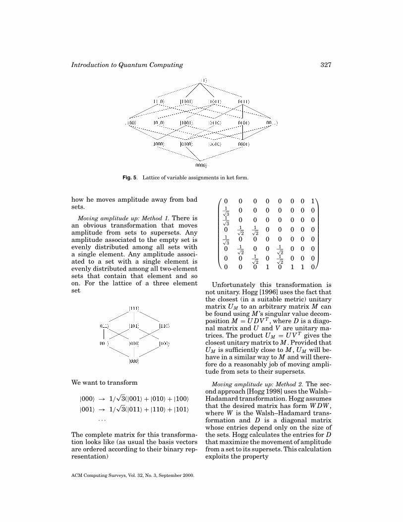
Introduction to Quantum Computing 327
Fig. 5. Lattice of variable assignments in ket form.
how he moves amplitude away from badsets.
Moving amplitude up: Method 1. There isan obvious transformation that movesamplitude from sets to supersets. Anyamplitude associated to the empty set isevenly distributed among all sets witha single element. Any amplitude associ-ated to a set with a single element isevenly distributed among all two-elementsets that contain that element and soon. For the lattice of a three elementset
We want to transform
|000〉 → 1/√
3(|001〉 + |010〉 + |100〉|001〉 → 1/
√3(|011〉 + |110〉 + |101〉
. . .
The complete matrix for this transforma-tion looks like (as usual the basis vectorsare ordered according to their binary rep-resentation)
0 0 0 0 0 0 0 11√3
0 0 0 0 0 0 01√3
0 0 0 0 0 0 00 1√
21√2
0 0 0 0 01√3
0 0 0 0 0 0 00 1√
20 0 1√
20 0 0
0 0 1√2
0 1√2
0 0 00 0 0 1 0 1 1 0
Unfortunately this transformation isnot unitary. Hogg [1996] uses the fact thatthe closest (in a suitable metric) unitarymatrix UM to an arbitrary matrix M canbe found using M ’s singular value decom-position M = U DV T , where D is a diago-nal matrix and U and V are unitary ma-trices. The product UM = U V T gives theclosest unitary matrix to M . Provided thatUM is sufficiently close to M , UM will be-have in a similar way to M and will there-fore do a reasonably job of moving ampli-tude from sets to their supersets.
Moving amplitude up: Method 2. The sec-ond approach [Hogg 1998] uses the Walsh–Hadamard transformation. Hogg assumesthat the desired matrix has form W DW ,where W is the Walsh–Hadamard trans-formation and D is a diagonal matrixwhose entries depend only on the size ofthe sets. Hogg calculates the entries for Dthat maximize the movement of amplitudefrom a set to its supersets. This calculationexploits the property
ACM Computing Surveys, Vol. 32, No. 3, September 2000.

328 E. Rieffel and W. Polak
Wrs = 1√N
(−1)|r·s| = 1√N
(−1)|r∩s|
shown in Section 7.2.1.
Moving amplitude away from bad sets. Toeffect moving amplitude away from setsthat violate the constraints, Hogg suggestsadjusting the phases of the sets, depend-ing on the extent to which they violate theconstraints, in such a way that the am-plitude distributed to sets that have badsubsets cancels, whereas the amplitudedistributed to sets from all good subsetsadds. Different choices here will workmore or less effectively depending on theparticular problem. One choice he sug-gests is inverting the phase of all badsets which will result in some cancela-tion in the amplitude of supersets be-tween the amplitude coming from goodsubsets and bad subsets. This phase in-version can be done as in Grover’s al-gorithm (Section 7.1.2) with a P thattests whether a given state satisfies allof the constraints or not. Another sug-gestion is to give random phases to thebad sets so that on average the contribu-tion to the amplitude of a superset frombad subsets is zero. Other choices arepossible.
Because the canceling resulting fromthe phase changes varies from problemto problem, the probability of obtaininga solution is difficult to analyze. A fewsmall experiments have been done, andthe guess is that the cost of the searchstill grows exponentially, but consider-ably more slowly than in the unstructuredcase. But until sufficiently large quantumcomputers are built or better techniquesfor analyzing such algorithms are found,the efficiency cannot be determined forsure.
8. QUANTUM ERROR CORRECTION
One fundamental problem in buildingquantum computers is the need to isolatethe quantum state. An interaction of parti-cles representing qubits with the externalenvironment disturbs the quantum stateand causes it to decohere, or transform
in an unintended and often nonunitaryfashion.
Steane [1998] estimates that the deco-herence of any system likely to be builtis 107 times too large to be able to runShor’s algorithm as it stands on a 130-digitnumber. However, adding error correctionalgorithms to Shor’s algorithm mitigatesthe effect of decoherence, making it againlook possible that a system could be builton which Shor’s algorithm could be run forlarge numbers.
On the surface, quantum error correc-tion is similar to classical error correct-ing codes in that redundant bits are usedto detect and correct errors, but the sit-uation for quantum error correction issomewhat more complicated than in theclassical case, since we are not deal-ing with binary data but with quantumstates.
Quantum error correction must recon-struct the exact encoded quantum state.Given the impossibility of cloning or copy-ing the quantum state, this reconstructionappears harder than in the classical case.However, it turns out that classical tech-niques can be modified to work for quan-tum systems.
8.1. Characterization of Errors
In the following it is assumed that all er-rors are the result of quantum interactionbetween a set of qubits and the environ-ment. The possible errors for each singlequbit considered are linear combinationsof no errors (I ), bit flip errors (X ), phaseerrors (Z ), and bit flip phase errors (Y ).A general single bit error is thus a trans-formation e1 I + e2 X + e3Y + e4 Z . Interac-tion with the environment transforms sin-gle qubits according to
|ψ〉 → (e1 I + e2 X + e3Y + e4 Z )|ψ〉
=∑
i
ei Ei|ψ〉.
For the general case of quantum regis-ters, possible errors are expressed as lin-ear combinations of unitary error opera-tors Ei. These could be combinations ofsingle-bit errors, such as tensor products
ACM Computing Surveys, Vol. 32, No. 3, September 2000.

Introduction to Quantum Computing 329
of the single-bit error transformations{I, X , Y , Z }, or more general multibittransformations. In any case, an error canbe written as &iei Ei for some error opera-tors Ei and coefficients ei.
8.2. Recovery of Quantum State
An error correcting code for a set of er-rors Ei consists of a mapping C that em-beds n data bits in n+k code bits togetherwith a syndrome extraction operator SCthat maps n + k code bits to the set ofindices of correctable errors Ei such thati = SC(Ei(C(x))). If y = E j (C(x)) for someunknown but correctable error, then er-ror SC( y) can be used to recover a prop-erly encoded value C(x) (i.e., E−1
SC( y)( y) =C(x)).
Now consider the case of a quantum reg-ister. First, the state of the register canbe in a superposition of basis vectors. Fur-thermore, the error can be a combinationof correctable error operators Ei. It turnsout that it is still possible to recover theencoded quantum state.
Given an error correcting code C withsyndrome extraction operator SC, ann-bit quantum state |ψ〉 is encoded ina n+ k–bit quantum state |φ〉 = C|ψ〉.Assume that decoherence leads to anerror state &iei Ei|φ〉 for some combina-tion of correctable errors Ei. The origi-nal encoded state |φ〉 can be recovered asfollows:
1. Apply the syndrome extraction opera-tor SC to the quantum state paddedwith sufficient |0〉 bits:
SC
(∑
i
ei Ei|φ〉)
⊗ |0〉
=∑
i
ei(Ei|φ〉 ⊗ |i〉).
Quantum parallelism gives a superpo-sition of different errors each associatedwith their respective error index i.
2. Measure the |i〉 component of the result.This yields some (random) value i0 andprojects the state to
Ei0 |φ, i0〉
3. Apply the inverse error transformationE−1
i0 to the first n + k qubits of Ei0 |φ, i0〉to get the corrected state |φ〉.
Note that Step 2 projects a superposi-tion of multiple error transformations intoa single error. Consequently, only one in-verse error transformation is required inStep 3.
8.3. Error Correction Example
Consider the trivial error correcting codeC that maps |0〉 → |000〉 and |1〉 → |111〉.C can correct single bit flip errors
E = {I⊗I⊗I, X ⊗I⊗I, I⊗X ⊗I, I⊗I⊗X }.
The syndrome extraction operator is
S : |x0, x1, x2, 0, 0, 0〉 → |x0, x1, x2, x0
XOR x1, x0 XOR x2, x1XOR x2〉,
with the corresponding error correctionoperators shown in the table. Note thatEi = E−1
i for this example.
Bit flipped Syndrome Error correctionnone |000〉 none
0 |110〉 X ⊗ I ⊗ I1 |101〉 I ⊗ X ⊗ I2 |011〉 I ⊗ I ⊗ X
Consider the quantum bit |ψ〉 = 1√2(|0〉−
|1〉), which is encoded as
C|ψ〉 = |φ〉 = 1√2
(|000〉 − |111〉),
and the error
E = 45
X ⊗ I ⊗ I + 35
I ⊗ X ⊗ I.
The resulting error state is
ACM Computing Surveys, Vol. 32, No. 3, September 2000.

330 E. Rieffel and W. Polak
E|φ〉 =(
45
X ⊗ I ⊗ I + 35
I ⊗ X ⊗ I)
×(
1√2
(|000〉 − |111〉))
= 45
X ⊗ I ⊗ I(
1√2
(|000〉 − |111〉))
+ 35
I ⊗ X ⊗ I(
1√2
(|000〉 − |111〉))
= 45√
2X ⊗ I ⊗ I (|000〉 − |111〉)
+ 35√
2I ⊗ X ⊗ I (|000〉 − |111〉)
= 45√
2(|100〉 − |011〉)
+ 35√
2(|010〉 − |101〉).
Next apply the syndrome extraction to(E|φ〉) ⊗ |000〉 as follows:
SC((E|φ〉) ⊗ |000〉)
= SC(4
5√
2(|100000〉 − |011000〉)
+ 35√
2(|010000〉 − |101000〉))
= 45√
2(|100110〉 − |011110〉)
+ 35√
2(|010101〉 − |101101〉)
= 45√
2(|100〉 − |011〉) ⊗ |110〉
+ 35√
2(|010〉 − |101〉) ⊗ |101〉.
Measuring the last three bits of this stateyields either |110〉 or |101〉. Assuming themeasurement produces the former, thestate becomes
1√2
(|100〉 − |011〉) ⊗ |110〉.
The measurement has the almost mag-ical effect of causing all but one summandof the error to disappear. The remaining
part of the error can be removed by ap-plying the inverse error operator X ⊗ I ⊗I , corresponding to the measured value|110〉, to the first three bits, to produce
1√2
(|000〉 − |111〉) = C|ψ〉 = |φ〉.
9. CONCLUSIONS
Quantum computing is a new, emergingfield that has the potential to dramaticallychange the way we think about computa-tion, programming, and complexity. Thechallenge for computer scientists and oth-ers is to develop new programming tech-niques appropriate for quantum comput-ers. Quantum entanglement and phasecancellation introduce a new dimension tocomputation. Programming no longer con-sists of merely formulating step-by-stepalgorithms but requires new techniques ofadjusting phases and mixing and diffusingamplitudes to extract useful output.
We have tried to give an accurateaccount of the state-of-the-art of quan-tum computing for computer scientistsand other nonphysicists. We have de-scribed some of the quantum mechani-cal effects, such as the exponential statespace, the entangled states, and the lin-earity of quantum state transformations,that make quantum parallelism possi-ble. Even though quantum computationsmust be linear and reversible, any clas-sical algorithm can be implemented on aquantum computer. But the real power ofthese new machines, the exponential par-allelism, can only be exploited using new,innovative programming techniques. Peo-ple have only recently begun to researchsuch techniques.
We have described Shor’s polynomial-time factorization algorithm, which stim-ulated the field of quantum computing.Given a practical quantum computer,Shor’s algorithm would make manypresent cryptographic methods obsolete.Grover’s search algorithm, while only pro-viding a polynomial speed-up, proves thatquantum computers are strictly more pow-erful than classical ones. Even though
ACM Computing Surveys, Vol. 32, No. 3, September 2000.

Introduction to Quantum Computing 331
Grover’s algorithm has been shown to beoptimal, there is hope that faster algo-rithms can be found by exploiting prop-erties of the problem structure. We havedescribed one such approach taken byHogg.
There are a few other known quantumalgorithms that we did not discuss. Jonesand Mosca [1998] describe the implemen-tation on a 2-bit quantum computer ofa constant time algorithm [Deutsch andJozsa 1992] that can distinguish whethera function is balanced or constant. Grover[1998] describes an efficient algorithm forestimating the median of a set of valuesand both Grover [1998] and Terhal andSmolin [1997], using different methods,can solve the coin weighing problem in asingle step.
Beyond these algorithms not much moreis known about what could be done witha practical quantum computer. It is anopen question whether or not we canfind quantum algorithms that provide ex-ponential speed-up for problems otherthan factoring. There is some speculationamong physicists that quantum transfor-mations might be slightly nonlinear. Sofar all experiments that have been doneare consistent with the standard linearquantum mechanics, but a slight nonlin-earity is still possible. Abrams and Lloyd[1998] show that even a very slight nonlin-earity could be exploited to solve all NP-hard problems on a quantum computer inpolynomial time. This result further high-lights the fact that computation is funda-mentally a physical process, and that whatcan be computed efficiently may depend onsubtle issues in physics.
The unique properties of quantum com-puters give rise to new kinds of complex-ity classes. For instance, BQP is the setof all languages accepted by a quantumTuring machine in polynomial time withbounded probability of error. Details ofthe extensive research done in the fieldof quantum complexity theory is beyondthe scope of this paper. The interestedreader may start by consulting Bennettet al. [1997] and Watrous [1998] respec-tively for analyses of time and space com-plexity of quantum computation. Williams
and Clearwater [1998] contains an in-troduction to early results in quantumcomplexity.
Of course, there are daunting physicalproblems that must be overcome if any-one is ever to build a useful quantumcomputer. Decoherence, the distortion ofthe quantum state due to interaction withthe environment, is a key problem. A bigbreakthrough for dealing with decoher-ence came from the algorithmic, ratherthan the physical, side of the field with thedevelopment of quantum error correctiontechniques. We have described some of theprinciples involved. Further advances inquantum error correction and the devel-opment of robust algorithms will be as im-portant for the development of practicalquantum computers as advances in thehardware side.
9.1. Further Reading
Andrew Steane’s survey article “Quan-tum Computing” [Steane 1998] is aimed atphysicists. We recommend reading his pa-per for his viewpoint on this subject, par-ticularly for his description of connectionsbetween information theory and quantumcomputing and for his discussion of er-ror correction, of which he was one of themain developers. He also has an overviewof the physics involved in actually build-ing quantum computers and a survey ofwhat had been done up to July 1997. Hisarticle contains a more detailed historyof the ideas related to quantum comput-ing than the present paper, and has morereferences as well. Another shorter andvery readable tutorial can be found inBerthiaume [1997].
Richard Feynman’s Lectures on Compu-tation [Feynman 1996] contains a reprintof the lecture “Quantum Mechanical Com-puters” [Feynman 1985], which began thewhole field. It also discusses the thermo-dynamics of computations, which is closelytied with reversible computing and infor-mation theory.
Colin Williams and Scott Clearwater’sbook Explorations in Quantum Comput-ing [Williams and Clearwater 1998] comeswith software, in the form of Mathematica
ACM Computing Surveys, Vol. 32, No. 3, September 2000.
332 E. Rieffel and W. Polak
notebooks, that simulates some quantumalgorithms such as Shor’s algorithm.
The second half of the October 1997 is-sue of the SIAM Journal of Computingcontains six seminal articles on quantumcomputing, including four we have alreadycited [Bennett et al. 1997; Bernstein andVazirani 1997; Shor 1997; Simon 1997].
Most of the articles referenced in thispaper, and many more, can be found atthe Los Alamos preprint server: http://xxx.lanl.gov/archive/quant-ph. Linksto research projects and other informa-tion about quantum computing can befound on our web site http://www.fxpal.xerox.com/Quantum Computing.
APPENDIX
A. TENSOR PRODUCTS
The tensor product (⊗) of a n-dimensionaland a k-dimensional vector is a nk-dimensional vector. Similarly, if A andB are transformations on n-dimensionaland k-dimensional vectors respectively,then A ⊗ B9 is a transformation on nk-dimensional vectors.
The exact mathematical details of ten-sor products are beyond the scope of thispaper (see Hungerford [1974] for a com-prehensive treatment). For our purposesthe following algebraic rules are sufficientto calculate with tensor products. For ma-trices A, B, C, D, U , vectors u, x, y , andscalars a, b, the following hold:
(A ⊗ B)(C ⊗ D) = AC ⊗ BD(A ⊗ B)(x ⊗ y) = Ax ⊗ B y
(x + y) ⊗ u = x ⊗ u + y ⊗ uu ⊗ (x + y) = u ⊗ x + u ⊗ y
ax ⊗ by = ab(x ⊗ y)(
A BC D
)⊗ U =
(A ⊗ U B ⊗ UC ⊗ U D ⊗ U
),
which is specialized for scalars a, b, c, d to(
a bc d
)⊗ U =
(aU bUcU dU
).
9 Technically, this is a right Kronecker product.
The conjugate transpose distributesover tensor products; that is,
(A ⊗ B)∗ = A∗ ⊗ B∗.
A matrix U is unitary if its conjugatetranspose is its inverse: U ∗U = I.
The tensor product of several matricesis unitary if and only if each one of thematrices is unitary up to a constant. LetU = A1 ⊗ A2 ⊗ · · ·⊗ An. Then U is unitaryif A∗
i Ai = ki I and (iki = 1.
U ∗U =(
A∗1 ⊗ A∗
2 ⊗ · · · ⊗ A∗n)
× (A1 ⊗ A2 ⊗ · · · ⊗ An)
= A∗1 A1 ⊗ A∗
2 A2 ⊗ · · · ⊗ A∗n An
= k1 I ⊗ · · · ⊗ knI
= I
where each I refers to the identity matrixof appropriate dimension.
For example, the distributive law allowscomputations of the form:
(a0|0〉 + b0|1〉) ⊗ (a1|0〉 + b1|1〉)
= (a0|0〉 ⊗ a1|0〉) + (b0|1〉 ⊗ a1|0〉)
+ (a0|0〉 ⊗ b1|1〉) + (b0|1〉 ⊗ b1|1〉)
= a0a1((|0〉 ⊗ |0〉) + b0a1(|1〉 ⊗ |0〉)
+ a0b1(|0〉 ⊗ |1〉) + b0b1(|1〉 ⊗ |1〉)
= a0a1(|00〉 + b0a1|10〉 + a0b1|01〉
+ b0b1|11〉
B. CONTINUED FRACTIONS ANDEXTRACTING THE PERIOD FROM THEMEASUREMENT IN SHOR’S ALGORITHM
In the general case where the period r doesnot divide 2m; the value v measured inStep 4 of Shor’s algorithm will be, withhigh probability, close to some multiple of2m
r , say j 2m
r .The aim is to extract the period r from
the measured value v. Shor shows that,with high probability, v is within 1
2 of somej 2m
r . Thus
ACM Computing Surveys, Vol. 32, No. 3, September 2000.

Introduction to Quantum Computing 333
∣∣∣∣v − j2m
r
∣∣∣∣ <12
for some j , which implies that
∣∣∣∣v
2m − jr
∣∣∣∣ <1
2 · 2m <1
2M 2 .
The difference between two distinct frac-tions p
q and p′
q′ with denominators less thanM is bounded
∣∣∣∣pq
− p′
q′
∣∣∣∣ =∣∣∣∣
pq′ − p′qqq′
∣∣∣∣ >1
M 2 .
Thus there is at most one fraction pq with
denominator q < M such that | v2m − p
q | <1
M 2 . In the high-probability case that v iswithin 1
2 of j 2m
r , this fraction will be jr .
The unique fraction with denominatorless than M that is within 1
M 2 of v2m can
be obtained efficiently from the continuedfraction expansion of v
2m as follows. Usingthe sequences
a0 =[
v2m
]
ε0 = v2m − a0
an =[
1εn−1
]
εn = 1εn−1
− an
p0 = a0
p1 = a1a0 + 1pn = an pn−1 + pn−2
q0 = 1q1 = a1
qn = anqn−1 + qn−2,
compute the first fraction pnqn
such thatqn < M ≤ qn+1. See any standard num-ber theory text, such as Hardy and Wright[1979], for why this procedure works.
In the high probability case when v2m is
within 1M 2 of a multiple j
r of 1r , the frac-
tion obtained from the above procedure is
jr , because it has denominator less thanM . We take the denominator q of the ob-tained fraction as our guess for the period,which will work when j and r are rela-tively prime.
ACKNOWLEDGMENTS
The authors would like to thank Tad Hogg andCarlos Mochon for many enjoyable conversationsabout quantum computing and for their feedbackon an earlier draft of this paper. We are also grate-ful to Lee Corbin, David Goldberg, Lov Grover,Norman Hardy, Vaughan Pratt, Marc Rieffel, andthe anonymous referees for detailed comments onearlier drafts of this paper. Finally, we would liketo thank FXPAL for enthusiastically supporting thiswork.
REFERENCESABRAMS, D. S. AND LLOYD, S. 1998. Nonlinear quan-
tum mechanics implies polynomial-time solutionfor NP-complete and #p problems. Los AlamosPhysics Preprint Archive, http://xxx.lanl.gov/abs/quant-ph/9801041.
BARENCO, A., BENNETT, C. H., CLEVE, R., DIVINCENZO,D. P., MARGOLUS, N. H., SHOR, P. W., SLEATOR,T., SMOLIN, J. A., AND WEINFURTER, H. 1995.Elementary gates for quantum computation.Physical Review A 52, 5, 3457–3467. Preprint atLos Alamos Physics Preprint Archive, http://xxx.lanl.gov/abs/quant-ph/9503016 and athttp://vesta.physics.ucla.edu/cgi-bin/uncompress ps cgi?torgats1.ps.
BENNETT, C. H. 1992. Quantum cryptography usingany two nonorthogonal states. Physical ReviewLetters 68, 3121–3124.
BENNETT, C. H., BERNSTEIN, E., BRASSARD, G., AND
VAZIRANI, U. V. 1997. Strengths and weak-nesses of quantum computing. Society for In-dustrial and Applied Mathematics Journalon Computing 26, 5, 1510–1523. Preprintat Los Alamos Physics Preprint Archive,http://xxx.lanl.gov/abs/quant-ph/9701001.
BENNETT, C. H. AND BRASSARD, G. 1987. Quantumpublic key distribution reinvented. SIGACTNews (ACM Special Interest Group on Automataand Computability Theory) 18, 51–53.
BENNETT, C. H., BRASSARD, G., AND EKERT, A. K.1992. Quantum cryptography. Scientific Amer-ican 267, 4 (Oct.), 50.
BERNSTEIN, E. AND VAZIRANI, U. V. 1997. Quantumcomplexity theory. Society for Industrial and Ap-plied Mathematics Journal on Computing 26, 5,1411–1473. A preliminary version of this paperappeared in the Proceedings of the 25th Associ-ation for Computing Machinery Symposium onthe Theory of Computing.
ACM Computing Surveys, Vol. 32, No. 3, September 2000.

334 E. Rieffel and W. Polak
BERTHIAUME. 1997. Quantum computation. In ALAN
L. SELMAN, ED., Complexity Theory Retrospective,In Honor of Juris Hartmanis on the Occasion ofHis Sixtieth Birthday, (July 5, 1988), Vol. 2, 23–51.
BIRON, D., BIHAM, O., BIHAM, E., GRASSEL, M., AND LI-DAR, D. A. 1998. Generalized grover search al-gorithm for arbitrary initial amplitude distri-bution. Los Alamos Physics Preprint Archive,http://xxx.lanl.gov/abs/quant-ph/9801066.
BOSCHI, D., BRANCA, S., MARTINI, F. D., HARDY, L., AND
POPESCU, S. 1998. Experimental realization ofteleporting an unknown pure quantum state viadual classical and einstein-podolski-rosen chan-nels. Physical Review Letters 80, 1121–1125.
BOUWMEESTER, D., PAN, J.-W., MATTLE, K., EIBL,M., WEINFURTER, H., AND ZEILINGER, A.1997. Experimental quantum teleportation.Nature 390, 575.
BOYER, M., BRASSARD, G., HøYER, P., AND TAPP, A. 1996.Tight bounds on quantum search. In Proceed-ings of the Workshop on Physics of Computation:PhysComp ’96 (Los Alamitos, CA, 1996), 36–43.Institute of Electrical and Electronic EngineersComputer Society Press. Preprint at Los AlamosPhysics Preprint Archive, http://xxx.lanl.gov/abs/quant-ph/9605034.
BRASSARD, G., HøYER, P., AND TAPP, A. 1998.Quantum counting. Preprint at Los AlamosPhysics Preprint Archive, http://xxx.lanl.gov/abs/quant-ph/9805082.
CERF, N. J., GROVER, L. K., AND WILLIAMS, C. P. 1998.Nested quantum search and np-complete prob-lems. Preprint at Los Alamos Physics PreprintArchive, http://xxx.lanl.gov/abs/quant-ph/9806078.
CIRAC, J. I. AND ZOLLER, P. 1995. Quantum compu-tations with cold trapped ions. Physical ReviewLetters 74, 4091–4094.
CORY, D. G., MASS, W., PRICE, M., KNILL, E.,LAFLAMME, R., ZUREK, W. H., HAVEL, T. F., AND
SOMAROO, S. S. 1998. Experimental quantumerror correction. Preprint at Los Alamos PhysicsPreprint Archive, http://xxx.lanl.gov/abs/quant-ph/9802018.
DEUTSCH, D. 1985. Quantum theory, the Church-Turing principle and the universal quantumcomputer. Proceedings of the Royal Society ofLondon Series A A400, 97–117.
DEUTSCH, D. AND JOZSA, R. 1992. Rapid solution ofproblems by quantum computation. Proceedingsof the Royal Society of London Series A A439,553–558.
DIRAC, P. 1958. The Principles of Quantum Mechan-ics (4th ed.). Oxford University Press.
EKERT, A. K., RARITY, J., TAPSTER, P., AND PALMA, G.1992. Practical quantum cryptography basedon two-photon interferometry. Physical ReviewLetters 69, 1293–1295.
FEYNMAN, R. 1982. Simulating physics with com-puters. International Journal of TheoreticalPhysics 21, 6&7, 467–488.
FEYNMAN, R. 1985. Quantum mechanical comput-ers. Optics News 11, 11–20. Also in Foundationsof Physics, 16(6), 507–531, 1986.
FEYNMAN, R. 1996. In Feynman Lectures on Compu-tation. A. J. HEY AND R. W. ALLEN EDS., Addison-Wesley.
FEYNMAN, R. P., LEIGHTON, R. B., AND SANDS, M.1965. Lectures on Physics, Vol. III. Addison-Wesley.
GERSHENFELD, N. A. AND CHUANG, I. L. 1997.Bulk spin resonance quantum computing. Sci-ence 275, 350–356.
GREENSTEIN, G. AND ZAJONC, A. G. 1997. The Quan-tum Challenge. Jones and Bartlett Publishers,Sudbury, Mass.
GROVER, L. K. 1996. A fast quantum mechanical al-gorithm for database search. In Proceedings ofthe 28th Annual ACM Symposium on the The-ory of Computing (Philadelphia, Pennsylvania,22–24 May 1996), pp. 212–219.
GROVER, L. K. 1998. A framework for fast quan-tum mechanical algorithms. Proceedings of the30th Annual ACM Symposium on the The-ory of Computing, 53–62. Preprint at LosAlamos Physics Preprint Archive, http://xxx.lanl.gov/abs/quant-ph/9711043.
HARDY, G. H. AND WRIGHT, E. M. 1979. An Introduc-tion to the Theory of Numbers. Oxford UniversityPress.
HOGG, T. 1996. Quantum computing and phasetransitions in combinatorial search. Journalof Artificial Intelligence Research 4, 91–128. Preprint at Los Alamos Physics PreprintArchive, http://xxx.lanl.gov/abs/quant-ph/9508012.
HOGG, T. 1998. Highly structured searches withquantum computers. Physical Review Letters 80,2473–2473.
HUGHES, R. J., BUTTLER, W. T., KWIAT, P. G.,LAMOREAUX, S. K., MORGAN, G. L., NORDHOLT,J. E., AND PETERSON, C. G. 1999. Practical Quan-tum Cryptography for Secure Free-Space Com-munications. Preprint at Los Alamos PhysicsPreprint Archive, http://xxx.lanl.gov/abs/quant-ph/9905009.
HUGHES, R. J., BUTTLER, W. T., KWIAT, P. G., LUTHER,G. G., MORGAN, G. L., NORDHOLT, J. E., PETERSON,C. G., AND SIMMONS, C. M. 1997. Secure commu-nications using quantum cryptography. In S. P.HOTALING AND A. R. PIRICH EDS., Photonic Quan-tum Computing, Vol. 3076, 2–11.
HUNGERFORD, T. A. 1974. Algebra. Springer Verlag,New York, Heidelberg, Berlin.
JONES, J. A. AND MOSCA, M. 1998. Implementationof a quantum algorithm on a nuclear mag-netic resonance quantum computer. Journal ofChemical Physics 109, 5, 1648–1653. Preprintat Los Alamos Physics Preprint Archive,http://xxx.lanl.gov/abs/quant-ph/9801027.
LAFLAMME, R., KNILL, E., ZUREK, W., CATASTI, P., AND
MARIAPPAN, S. 1997. NMR GHZ. Los Alamos
ACM Computing Surveys, Vol. 32, No. 3, September 2000.

Introduction to Quantum Computing 335
Physics Preprint Archive, http://xxx.lanl.gov/abs/quant-ph/9709025.
LENSTRA, A. AND LENSTRA, H. EDS. 1993. The Devel-opment of the Number Field Sieve, Vol. 1554 ofLecture Notes in Mathematics. Springer Verlag.
LIBOFF, R. L. 1997. Introductory Quantum Mechan-ics (3rd ed.). Addison-Wesley, Reading, Mass.
LO, H.-K. AND CHAU, H. F. 1999. Unconditional secu-rity of quantum key distribution over arbitrarilylong distances. Science 283, 2050–2056.
MAYERS, D. 1998. Unconditional Security in Quan-tum Cryptography. Preprint at Los AlamosPhysics Preprint Archive, http://xxx.lanl.gov/abs/quant-ph/9802025.
NIELSEN, M. A., KNILL, E., AND LAFLAMME, R. 1998.Complete Quantum Teleportation using NuclearMagnetic Resonance. Preprint at Los AlamosPhysics Preprint Archive, http://xxx.lanl.gov/abs/quant-ph/9811020.
SCHULMAN, L. J. AND VAZIRANI, U. 1998. ScalableNMR Quantum Computation. Los AlamosPhysics Preprint Archive, http://xxx.lanl.gov/abs/quant-ph/9804060.
SHOR, P. W. 1994. Algorithms for quantum compu-tation: Discrete log and factoring. In Proceedingsof the 35th Annual Symposium on Foundationsof Computer Science (Nov.), 124–134. Instituteof Electrical and Electronic Engineers ComputerSociety Press. ftp://netlib.att.com/netlib/att/math/shor/quantum.algorithms.ps.Z.
SHOR, P. W. 1997. Polynomial-time algorithms forprime factorization and discrete logarithms ona quantum computer. Society for Industrialand Applied Mathematics Journal on Comput-ing 26, 5, 1484–1509. Expanded version of Shor[1994].
SIMON, D. R. 1997. On the power of quantum compu-tation. Society for Industrial and Applied Math-ematics Journal on Computing 26, 5, 1474–1483. A preliminary version of this paper ap-
peared in the Proceedings of the 35th AnnualSymposium on Foundations of Computer Sci-ence.
STEANE, A. 1996. The Ion Trap Quantum Informa-tion Processor. Los Alamos Physics PreprintArchive, http://xxx.lanl.gov/abs/quant-ph/9608011.
STEANE, A. 1998. Quantum computing. Reports onProgress in Physics 61, 2, 117–173. Preprint atLos Alamos Physics Preprint Archive, http://xxx.lanl.gov/abs/quant-ph/9708022.
TERHAL, B. M. AND SMOLIN, J. A. 1997. Single Quan-tum Querying of a Database. Los Alamos PhysicsPreprint Archive, http://xxx.lanl.gov/abs/quant-ph/9705041.
VANDERSYPEN, L. M. K., YANNONI, C. Y., SHERWOOD,M. H., AND CHUANG, I. L. 1999. Realizationof Effective Pure States for Bulk QuantumComputation. Preprint at Los Alamos PhysicsPreprint Archive, http://xxx.lanl.gov/abs/quant-ph/9905041.
VEDRAL, V., BARENCO, A., AND EKERT, A. K. 1996.Quantum Networks for Elementary ArithmeticOperations. Physical Review A. Preprint at LosAlamos Physics Preprint Archive, http://xxx.lanl.gov/abs/quant-ph/9511018.
WATROUS, J. 1998. Relationships between quan-tum and classical space-bounded complexityclasses. In 13th Annual IEEE Conference onComputational Complexity (June 1998), 210–227.
WILLIAMS, C. P. AND CLEARWATER, S. H. 1998. Explo-rations in Quantum Computing. Telos, Springer-Verlag.
WOOTTERS, W. K. AND ZUREK, W. H. 1982. A singlequantum cannot be cloned. Nature 299, 802.
ZALKA, C. 1997. Grover’s Quantum SearchingAlgorithm is Optimal. Los Alamos PhysicsPreprint Archive, http://xxx.lanl.gov/abs/quant-ph/9711070.
Accepted September 1999
ACM Computing Surveys, Vol. 32, No. 3, September 2000.


![UniversiteitLeiden OpleidingInformaticalak [1], Quantum Computing for Computer Scientists by Noson S. Yanofsky and Mirco A. Mannucci [2], Quantum Computation and Quantum Information](https://img.pdfslide.us/doc/110x75/60bab71a70cde41d8314f9d5/universiteitleiden-opleidinginformatica-lak-1-quantum-computing-for-computer.jpg)