Embed Size (px)
Citation preview
Quantum Computation Through theEyes of a Computer Scientist
Leon Philip SandersZürich, CH
Student ID: 07-610-397
Supervisor: Thomas Bocek, Ben KeitchDate of Submission: February 4, 2016
University of ZurichDepartment of Informatics (IFI)Binzmühlestrasse 14, CH-8050 Zürich, Switzerland ifi
BA
CH
ELO
RA
RB
EIT
–C
omm
unic
atio
nS
yste
ms
Gro
up,P
rof.
Dr.
Bur
khar
dS
tille
r

Bachelor ThesisCommunication Systems Group (CSG)Department of Informatics (IFI)University of ZurichBinzmühlestrasse 14, CH-8050 Zürich, SwitzerlandURL: http://www.csg.uzh.ch/

Contents
1 Introduction 1
2 Related Work 3
2.1 Quantum Mechanics . . . . . . . . . . . . . . . . . . . . . . . . . . . . . . 3
2.2 Quantum Information . . . . . . . . . . . . . . . . . . . . . . . . . . . . . 3
2.3 Quantum Algorithms . . . . . . . . . . . . . . . . . . . . . . . . . . . . . . 4
2.4 Tabular Overview of used Sources and their Accessibility . . . . . . . . . . 4
3 Quantum Information Theory 7
3.1 A Classical System . . . . . . . . . . . . . . . . . . . . . . . . . . . . . . . 7
3.2 Probabilistic System . . . . . . . . . . . . . . . . . . . . . . . . . . . . . . 11
3.3 Complex System . . . . . . . . . . . . . . . . . . . . . . . . . . . . . . . . 15
3.3.1 The Double Slit Experiment . . . . . . . . . . . . . . . . . . . . . . 17
4 Quantum Mechanics 21
4.1 Quantum States . . . . . . . . . . . . . . . . . . . . . . . . . . . . . . . . . 21
4.1.1 The Basics . . . . . . . . . . . . . . . . . . . . . . . . . . . . . . . . 21
4.1.2 Spin . . . . . . . . . . . . . . . . . . . . . . . . . . . . . . . . . . . 22
4.1.3 Transition Amplitudes . . . . . . . . . . . . . . . . . . . . . . . . . 24
4.2 Observables . . . . . . . . . . . . . . . . . . . . . . . . . . . . . . . . . . . 25
4.3 Measurements . . . . . . . . . . . . . . . . . . . . . . . . . . . . . . . . . . 27
4.4 Evolution of Quantum Systems . . . . . . . . . . . . . . . . . . . . . . . . 28
4.4.1 The Schrodinger Equation . . . . . . . . . . . . . . . . . . . . . . . 30
4.4.2 Multiparticle Systems and Entanglement . . . . . . . . . . . . . . . 30
i

ii CONTENTS
5 Architecture of a Quantum Computer 33
5.1 QRAM Model . . . . . . . . . . . . . . . . . . . . . . . . . . . . . . . . . . 33
5.2 Bits and QuBits . . . . . . . . . . . . . . . . . . . . . . . . . . . . . . . . . 34
5.3 Gates . . . . . . . . . . . . . . . . . . . . . . . . . . . . . . . . . . . . . . 37
5.3.1 Classical . . . . . . . . . . . . . . . . . . . . . . . . . . . . . . . . . 37
5.3.2 Reversible . . . . . . . . . . . . . . . . . . . . . . . . . . . . . . . . 39
5.3.3 Quantum Gates . . . . . . . . . . . . . . . . . . . . . . . . . . . . . 40
6 Quantum Algorithms 43
6.1 Deutsch’s Quantum Algorithm . . . . . . . . . . . . . . . . . . . . . . . . . 43
6.2 Grover’s Search Algorithm . . . . . . . . . . . . . . . . . . . . . . . . . . . 49
6.3 Shor’s Prime Factorization . . . . . . . . . . . . . . . . . . . . . . . . . . . 56
7 Why, or Why Not, a Quantum Computer? 59
8 Future Work and Conclusions 61
Bibliography 61
A Experiment Program 67

Chapter 1
Introduction
Quantum mechanics is unintuitive and difficult to grasp. According to the theoreticalphysicist and mathematician Roger Penrose: ”Quantum mechanics makes absolutely nosense” [34].
Classical physics assumes that objects encounterd are larger than atoms (among otherthings). Quantum mechanics takes into account elementary particles such as electronswhere actions happen on the scale of the Planck-constant on a scale smaller than atoms.Therefore quantum physics describes the entirety of the universe more accurately [37](with the exception of gravity; though people are working on that [27]). Indeed it ispossible to infer the rules of classical physics through quantum physics [11].
The reason physicists still use the classical interpretations is obvious; they are mucheasier. And relatively accurate. The bigger the system the better their predictions. Theprobability that a car can go through a wall (or any potential barrier) is so small thatin everday life it may be assumed to be 0 [33]. Quantum mechanics though teaches thatthrough the effect of quantum tunneling the actual probability is not 0 [36].
Just as classical physics the classical theory of information is an approximation as well:Quantum information theory and with it quantum computation removes the abstractionthat the elements of information are independent of each other and can therefore bechanged independently [24]. Information is a physical concept [33]. The implications ofthis fact will be discussed in this thesis.
The following chapter will present an overview of used sources and related articles. Thetarget audience of this thesis is computer scientists. This thesis presents an abstractionitself as a full treatment of quantum mechanics goes over the scope of this thesis. Ascomputer scientists are adept at working with graphs the transition from the classicalto the quantum world will aided by graphs: A classical followed by a probabilistic anda complex or quantum system will be represented by graphs. The subsequent chapterwill treat some of the rules necessary for the understanding of quantum computation.Afterwards the architecture of a possible quantum computer will be treated. At thispoint quantum algorithms can be introduced: Two algorithms, namely Deutsch’s andGrover’s will be treated in detail whereas Shor’s prime factorization will be presented
1

2 CHAPTER 1. INTRODUCTION
from a bird’s eye perspective. Finally the merits of a possible quantum computer will bepresented.
The effects at subatomic scale are strange but have great potential as will be shown. In thefollowing thesis, an emulator for a quantum computer, to be run on a classical computer,will be built. This emulator will be constructed through the aforementioned chapters andthe algorithms will be constructed within its framework.
Chapter 2
Related Work
The texts regarded as the founding documents of quantum computation are given byBenioff [8] and Manin [32]. Richard Feynman developed similar ideas and opened themto a wider audience [20].
In general the modern bible of quantum computation is given by Nielsen & Chuang [33].This books treats every aspect of this thesis in more detail. Additionally it treats everyother aspect of quantum computation and even further develops some algorithms, which issometimes difficult to follow. For this purpose the introduction to quantum computationby Yanofsky was invaluable [48].
2.1 Quantum Mechanics
Quantum mechanics is a vast field and there is a wealth of research regarding the topic.This thesis will only cover a very shallow view of this fascinating field. For the inclined thefollowing sources go into more detail but mostly require previous knowledge of physics.
An brief introduction, accessible also to computer scientists, as well as a review of someof the important aspects is given by David Sherrill in [39].
Richard Feynmann’s Lectures on Physics specifically Volume III go into more detail [21].One of the modern standard textbooks often cited is “Modern quantum mechanics” bySakurai et al. [37]. Furthermore Mika Hirvensalo treats the topic in [24].
2.2 Quantum Information
The concept that information is physical is presented by Rolf Landauer together with anoverview of reversible computation in [31]. A basic overvirw of QuBits and the necessaryquantum gates for quantum computation may be found in [24], [33] and [48]. Theywere introduced by David Deutsch in 1989 [16]. Bennet et al. gives an overview of the
3
4 CHAPTER 2. RELATED WORK
limitations associated with quantum computing in [9]. The QRAM model is introducedby Knull in [29] and the different possible architectures of a quantum computer are treatedby Rodney van Meter et al. in [44].
2.3 Quantum Algorithms
Aaronson talks about complexity theory behind quantum algorithms in [5]
Deutsch‘s algorithm was first stated in [15]. It is further developed to the Deutsch-Jozsa-Algorithm in [17].
Grover‘s quantum search algorithm was published by Lov Grover in [23]. Chapter 6 of[33] further develops the algorithm.
Shor‘s algorithm was first announced in [40]. The most understandable overview of it iswritten by Scott Aaronson in [2]. Nielsen and Chuang [33] treat the algorithm in greatdetail in Chapter 6.
2.4 Tabular Overview of used Sources and their Ac-
cessibility
The following references in Table 2.1 are rated on a scale from 1 to 5 for their readabilityfor computer scientists where 5 means a very difficult text. They are added to the tablein the same order that they appear in the bibliography.

2.4. TABULAR OVERVIEW OF USED SOURCES AND THEIR ACCESSIBILITY 5
Title Difficulty
Limits on efficient computation in the physical world [1] 3Shor, i will do it [2] 2Quantum computing since Democritus [4] 3Strengths and weaknesses of quantum computing [9] 4Evidence for quantum annealing with more than one hundred qubits [12] 5Quantum theory, the church-turing principle and the universal quantum computer [15] 4Modeling a quantum processor using the qram model [18] 3Simulating physics with computers [20] 3The Feynman Lectures on Physics, Desktop Edition Volume III [21] 3Grovers quantum search algorithm. [22] 1A fast quantum mechanical algorithm for database search. [23] 3Quantum computing. [24] 2Conventions for quantum pseudocode. [29] 3Quantum computation and quantum information. [33] 3Quantisierung als eigenwertproblem. [38] 5A brief review of elementary quantum chemistry. [39] 2Algorithms for quantum computation: Discrete logarithms and factoring. [40] 5Modern quantum mechanics. [37] 4Programming the quantum future. [43] 1Quantum computing for computer scientists [48] 1
Table 2.1: Table of difficulties of used references

6 CHAPTER 2. RELATED WORK

Chapter 3
Quantum Information Theory
The following chapter will treat the transition from a classical view on computers to aquantum mechanical view by employing graphs and matrices well known to computerscientists.
3.1 A Classical System
Computer scientists are adept at working with graphs and matrices. Therefore an entrypoint may be a graph representing a classical system. In order to make it possible tojump from classical to quantum mechanics later on it is necessary that the initial graphsatisfies certain conditions: It is limited to exactly one edge per vertex. Additionally thevertices have weights as are displayed by the numbers in the vertices. It may be imaginedas billiard balls moving along an edge from one vertex to another. This is a very commonand often used example in quantum computation research, among others by [33] and [48].
An example graph may be the following the one in Figure 3.1.
Figure 3.1 satisfies the conditions given previously. Graphs are easily store-able as vec-tors and matrices in computers, which will also be important in the quantum emulatordeveloped later in the text. The weights can move from one vertex to another and do soin accordance with the shown arrows. These weights may be represented by the followingvector [48]:
X =
6215310
(3.1)
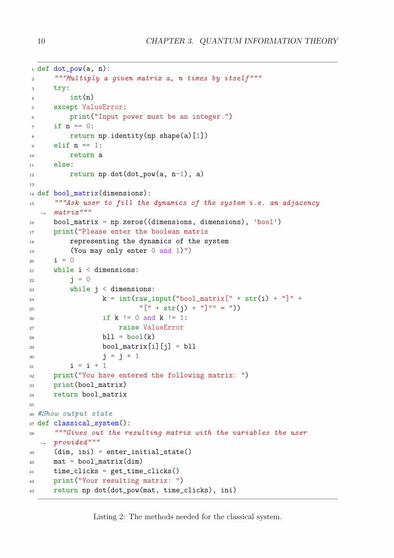
In order to start writing a program which makes it possible to reason about this graphalgorithmically a simple input method was written and is shown here.
7

8 CHAPTER 3. QUANTUM INFORMATION THEORY
Figure 3.1: An example graph for a classical system. The vertices are numbered from 0to 5 from top to bottom and left to right. Their weights are displayed inside the vertices.E.g vertex 5 has weight 10. Adapted from [48]
1 def enter_initial_state():
2 """Ask user to enter initial state vector"""
3 while True:
4 dimensions = int(raw_input(
5 "Please enter the number of Dimensions: "))
6 break
7 initial_state = np.zeros((dimensions, 1))
8 print("Please enter the initial state
9 of the system one after the other: ")
10 i = 0
11 while i < dimensions:
12 k = int(raw_input("initial_state[" + str(i) + "] = "))
13 initial_state[i] = k
14 i = i + 1
15 print(initial_state)
16 return (dimensions, initial_state)
Listing 1: An input method for the initial state of a classical system.
Python was chosen as the language to illustrate the programmatic representation of theprevious system as it is easy to read and has a powerful numerical library i.e numpy.
Represented as a boolean adjacency matrix the edges of the graph in Figure 3.1 look like

3.1. A CLASSICAL SYSTEM 9
this:
M =
0 1 2 3 4 5
0 0 0 0 0 0 01 0 0 0 0 0 02 0 1 0 0 0 13 0 0 0 1 0 04 0 0 1 0 0 05 1 0 0 0 1 0
(3.2)
M [i, j] = 1 if and only if there is an arrow from vertex j to vertex i. This is in contrastto how adjacency matrices are normally represented in computer science texts [48] whereM [i, j] = 1 if and only if there is an arrow from vertex i to vertex j. This invertedrepresentation is important for using these systems for quantum mechanics later on. Ad-ditionally as there are as many columns as there are rows in every case all such adjacencymatrices for the classical system and similar graphs are square.
The state of the system is represented by the vector Equation 3.1 and its dynamics arerepresented by matrix Equation 6.3. Therefore it is possible to show how the systemchanges over time by multiplying the dynamics with the initial state vector [48]:
MX =
0 0 0 0 0 00 0 0 0 0 00 1 0 0 0 10 0 0 1 0 00 0 1 0 0 01 0 0 0 1 0
·
6215310
=
0012519
= Y (3.3)
Vertex 0 and vertex 1 get no weights at all after one iteration, or one time unit [48].This figures as there are no edges going to vertex 0 or 1. Finite-dimensional quantummechanics adheres to similar laws as have been used in this classical system [33].
It is possible to carry out the multiplication once more to yield the state of the systemafter two time clicks (i.e MY = (0, 0, 9, 5, 12, 1)T , where M and Y are the variables used inEquation 3.3 and T stands for the transpose of the vector used for legibility). A quantumcomputer will similarly take known states and apply certain dynamics to them to yieldother states [37].
Represented as a simple computer program these relationships might look like the follow-ing:
10 CHAPTER 3. QUANTUM INFORMATION THEORY
1 def dot_pow(a, n):
2 """Multiply a given matrix a, n times by itself"""
3 try:
4 int(n)
5 except ValueError:
6 print("Input power must be an integer.")
7 if n == 0:
8 return np.identity(np.shape(a)[1])
9 elif n == 1:
10 return a
11 else:
12 return np.dot(dot_pow(a, n-1), a)
13
14 def bool_matrix(dimensions):
15 """Ask user to fill the dynamics of the system i.e. an adjacency
matrix"""→
16 bool_matrix = np.zeros((dimensions, dimensions), ’bool’)
17 print("Please enter the boolean matrix
18 representing the dynamics of the system
19 (You may only enter 0 and 1)")
20 i = 0
21 while i < dimensions:
22 j = 0
23 while j < dimensions:
24 k = int(raw_input("bool_matrix[" + str(i) + "]" +
25 "[" + str(j) + "]"" = "))
26 if k != 0 and k != 1:
27 raise ValueError
28 bll = bool(k)
29 bool_matrix[i][j] = bll
30 j = j + 1
31 i = i + 1
32 print("You have entered the following matrix: ")
33 print(bool_matrix)
34 return bool_matrix
35
36 #Show output state
37 def classical_system():
38 """Gives out the resulting matrix with the variables the user
provided"""→
39 (dim, ini) = enter_initial_state()
40 mat = bool_matrix(dim)
41 time_clicks = get_time_clicks()
42 print("Your resulting matrix: ")
43 return np.dot(dot_pow(mat, time_clicks), ini)
Listing 2: The methods needed for the classical system.

3.2. PROBABILISTIC SYSTEM 11
This is the first step on the way to a quantum computer emulator which will be detailedin the following chapters.
The requirement to only have one edge makes the system deterministic because the weightscan only move to one place [48]. A quantum system though is not deterministic. Inorder to get one step closer to a quantum system a simple probabilistic system will beinvestigated in the next chapter.
3.2 Probabilistic System
In quantum mechanics there is an inherent uncertainty about the position of an object.Quantum states change with probabilistic laws, as has been proven many times experi-mentally [34], [11]. Therefore the classical system will be changed in the following manner:Probabilities will be added to the edges. As in any probabilistic system the probabilitieswill have to add up to 1.
The conditions of this explanatory system will be labeled as “Conditions” whereas thereare certain “Postulates” in quantum mechanics that are true in nature as well and will belabeled by that name in the chapters coming. These are connected but the distinction ismade to separate this introductory from actual quantum systems.
Condition 1. The systems probabilities have to add up to 1.
Consequently all probabilities or edge weights that leave a vertex add up to 1 [48]. Con-versely the same will go for the incoming edges. Regarding the billiard ball analogy ofthe previous graph the new one will only feature 1 ball.
Another example graph is shown here:
The corresponding adjacency matrix is the following [48]:
M =
0 1
212
012
0 0 12
12
0 0 12
0 12
12
0
(3.4)
The mathematical property that all columns as well as rows in this matrix add up to 1 iscalled a doubly stochastic matrix [33] . An interesting and important property of doublystochastic matrices is that, multiplied by another such matrix again produce a doublystochastic matrix [48]. This implies, that also if the initial matrix is multiplied multipletimes the probabilities will still add up to 1 [48].
The billiard ball will start on one vertex in this case vertex 0. This initial state can bemodeled with the following vector: X1 = (1, 0, 0, 0)T [48]. Multiplying the vector with M ,similarly to the classical system, after one time click the system is in the following state:Y1 = (0, 1
2, 12, 0)T [48]. Carrying out this calculation once more MY1 = (1
2, 0, 0, 1
2)T , it is

12 CHAPTER 3. QUANTUM INFORMATION THEORY
Figure 3.2: An example graph for the probabilistic system [48]
apparent that the billiard ball bounces back and forth between the vertices. In the nextchapter a quantum version of this example will be built.
To model the uncertainty mentioned previously it will not be entirely certain were thissingle billiard ball will start. Again the probabilities have to add up to one because theball has to be somewhere. An arbitrary input state might be X2 = (1
6, 112, 23, 112
)T [48].This means that the ball will have a 1
6probability of starting on vertex 0, one of 1
12to
start on vertex 1 as well as 3 and a probability of 23
that it will start on vertex 2 [48]. Theprobabilities for moving between the vertices have been defined previously. Therefore itis now possible to, similarly to a classical system, calculate the possibility, where the ballwill find itself after one time click [48]:
MX2 =
0 1
212
012
0 0 12
12
0 0 12
0 12
12
0
·
1611223112
=
38181838
= Y2
The resulting vector corresponds to the probability of finding the billiard ball on a certainvertex after one time click (or t+1)[48]. This is for example PV 3 = 3
8to find it on vertex 3
given the previous input state X2 [48]. Also the probabilities of Y2 add up to one: Againafter one time click the billiard ball has to be somewhere.
To illustrate how the ball bounces back and forth a calculation of Y 3 and Y 4 in Pythonfollows:

3.2. PROBABILISTIC SYSTEM 13
1 In : M
2 Out:
3 array([[ 0. , 0.5, 0.5, 0. ],
4 [ 0.5, 0. , 0. , 0.5],
5 [ 0.5, 0. , 0. , 0.5],
6 [ 0. , 0.5, 0.5, 0. ]])
7
8 In : Y2
9 Out:
10 array([[ 0.375],
11 [ 0.125],
12 [ 0.125],
13 [ 0.375]])
14
15 In : Y3 = np.dot(M, Y2)
16
17 In : Y3
18 Out:
19 array([[ 0.125],
20 [ 0.375],
21 [ 0.375],
22 [ 0.125]])
23
24 In : Y4 = np.dot(M, Y3)
25
26 In : np.alltrue(Y4 == Y2)
27 Out: True
Listing 3: The output of Y 3 and Y 4 for the probabilistic system.
Y 4 equals Y 2 so the probabilities after four time clicks is equal to the one after two: Itbounces back and forth.
Naturally the probabilistic system built in this Section can be represented in a programas well. With only slight alterations to the original program:

14 CHAPTER 3. QUANTUM INFORMATION THEORY
1 def frac_matrix(dimensions):
2 """Ask user to fill the dynamics of the system i.e. a
3 doubly stochastic matrix"""
4 frac_matrix = np.zeros((dimensions, dimensions), ’float’)
5 print("")
6 print("Please enter the fractional matrix representing the dynamics
")→
7 print("of the system (You may only enter values between 0 and 1)")
8 i = 0
9 while i < dimensions:
10 j = 0
11 #try:
12 while j < dimensions:
13 k = float(raw_input("frac_matrix[" + str(i) + "]" +
14 "[" + str(j) + "]"" = "))
15 if k < 0 or k > 1:
16 raise ValueError
17 frac = bool(k)
18 frac_matrix[i][j] = frac
19 j = j + 1
20 #except sum(frac_matrix[i]) > 1
21 # print("Row " + str(i) + " is not doubly stochastic!")
22 i = i + 1
23
24 print("You have entered the following matrix: ")
25 print(frac_matrix)
26 return frac_matrix
27
28 #Show output state
29 def classical_system():
30 """Gives out the resulting matrix with the variables the user
provided"""→
31 (dim, ini) = enter_initial_state()
32 mat = frac_matrix(dim)
33 time_clicks = get_time_clicks()
34 print("Your resulting matrix: ")
35 return np.dot(dot_pow(mat, time_clicks), ini)
Listing 4: The probabilistic system represented as a program.
A probabilistic system is one step closer to a simple representation of a quantum mechan-ical system. In the next Section, such a system will be built on the building blocks of thepreceding chapters.

3.3. COMPLEX SYSTEM 15
3.3 Complex System
An easy explanation of what quantum mechanics is might be, that it is just like a prob-abilistic system only with complex numbers. In contrast to the probabilities encounteredup to now quantum mechanics works with complex numbers. This is not something whichcan be explained. It is known through experiment that nature just is like that [33], [37],[24].
In order to represent this fact the edge weights of the probabilistic system will be changedto complex numbers. A real number is obtained from this complex number by taking thesquared modulus which again has to be between 0 and 1 [48]. The difference between thetwo representations is that that real numbers are always added whereas complex numbersdon’t necessarily. For two real probabilities p1 and p2 the following is true [48]:
p1 ≤ (p1 + p2) ≥ p2 (3.5)
To obtain real probabilities from complex ones the squared modulus needs to be taken.This will be further explained in following chapters. If the probabilities are complexthey may cancel each other out as the following example shows. The complex numbersc1 = 3 + 2i and c2 = 1 − 4i are given. The squared modulus is easily calculated: |c1|2 =13, |c2|2 = 17. In stark contrast to addition in real numbers the following inequality holds:
|c1|2 + |c2|2 = 30 > |c1 + c2|2 = 20 (3.6)
Because the squared modulus of c1 + c2 = 4 − 2i is less than the individual squaredmoduli of c1 and c2 it could be said that they cancel each other out. This effect is calledinterference in quantum as well as classical wave mechanics [21]. In order to still satisfy theconditions of the probabilistic system complex numbers have to be chosen whose squaredmodulus will again add up to 1.
Condition 2. The squared modulus of the complex weights has to add up to one: |c0|2 +|c1|2 + ...+ |cn|2 = 1
This type of complex matrix has a name: It is unitary [24]. All unitary matrices aresquare and invertible [48]. Mathematically a matrix is unitary if the following equationholds [37].
U∗U = UU∗ = I (3.7)
where U∗ is the conjugate transpose or self-adjoint and I is the identity matrix [48].
A more approachable expression of a 2x2 unitary matrices is given by [33]:
U = eiφ(
a b−b∗ −a∗
)(3.8)

16 CHAPTER 3. QUANTUM INFORMATION THEORY
Figure 3.3: The quantum version of the simple graph [48]
Where the factors a and b stand for arbitrary complex numbers and are normalized i.e.|a|2+ |b|2 = 1.This fact ensures that unitary matrices “preserve the geometry” of the spaceon which it is acting [33]. This will be important later on while building the emulator.
In programmatic terms this condition may be written as:
1 def is_unitary(a):
2 """Produces True if the given matrix is unitary"""
3 try:
4 identity_a = np.identity(np.shape(a)[1])
5 #Due to allclose: Rounding error up to 1*e-8 allowed
6 return np.allclose(np.dot(a, self_adjoint(a)) == identity_a)
7 except (TypeError, NotImplemented):
8 print(’Please enter a valid matrix.’)
Listing 5: The unitarity constraint as a method on Python.
Unitary matrices are related to the doubly stochastic matrices from the foregoing chapter.If the squared modulus of a unitary matrix is taken the result is a doubly stochastic one[48].
Considering this example in a manner which is closer to that of a quantum system theweights of the aforementioned graph are changed to complex numbers that satisfy all theconditions as can be seen in Figure 3.3.
The numbers have been chosen for simplicity and therefore do not contain an imaginary
3.3. COMPLEX SYSTEM 17
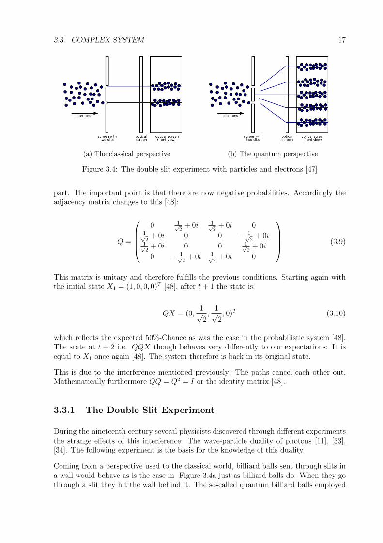
(a) The classical perspective (b) The quantum perspective
Figure 3.4: The double slit experiment with particles and electrons [47]
part. The important point is that there are now negative probabilities. Accordingly theadjacency matrix changes to this [48]:
Q =
0 1√
2+ 0i 1√
2+ 0i 0
1√2
+ 0i 0 0 − 1√2
+ 0i1√2
+ 0i 0 0 1√2
+ 0i
0 − 1√2
+ 0i 1√2
+ 0i 0
(3.9)
This matrix is unitary and therefore fulfills the previous conditions. Starting again withthe initial state X1 = (1, 0, 0, 0)T [48], after t+ 1 the state is:
QX = (0,1√2,
1√2, 0)T (3.10)
which reflects the expected 50%-Chance as was the case in the probabilistic system [48].The state at t + 2 i.e. QQX though behaves very differently to our expectations: It isequal to X1 once again [48]. The system therefore is back in its original state.
This is due to the interference mentioned previously: The paths cancel each other out.Mathematically furthermore QQ = Q2 = I or the identity matrix [48].
3.3.1 The Double Slit Experiment
During the nineteenth century several physicists discovered through different experimentsthe strange effects of this interference: The wave-particle duality of photons [11], [33],[34]. The following experiment is the basis for the knowledge of this duality.
Coming from a perspective used to the classical world, billiard balls sent through slits ina wall would behave as is the case in Figure 3.4a just as billiard balls do: When they gothrough a slit they hit the wall behind it. The so-called quantum billiard balls employed
18 CHAPTER 3. QUANTUM INFORMATION THEORY
in equation Equation 3.10 behave much more like the electrons in Figure 3.4b. This isdue to the wave-nature of particles at subatomic levels [24], [33]. This is how quantummechanics were discovered and this is how it is known that relationships at this level aretruly governed by the complex numbers used previously [21].
It may be argued that Max Planck constituted that there are quanta of light [33]. Evena single photon can interfere with itself, meaning that at a certain level where particlesare small enough something utterly strange happens: The aforementioned photon (oran electron for that matter) is seemingly in multiple places at once until it is measuredwhere it is, as it can have multiple impact sites. Therefore it is not in one position butin a superposition [48], [37], [39], [21], [33]. Richard Feynman [21] noted the followingregarding this relationship:
We choose to examine a phenomenon which is impossible, absolutely im-possible, to explain in any classical way, and which has in it the heart ofquantum mechanics. In reality, it contains the only mystery. We cannot makethe mystery go away by ‘’explaining” how it works. We will just tell you howit works. In telling you how it works we will have told you about the basicpeculiarities of all quantum mechanics.
After measuring, this superposition collapses though and the probability of finding itin position i is |ci|2 [33]. The superposition principle is what gives potential quantumcomputers their power: A classical computer cannot be put into many states at once,a quantum computer can. It is in all states at once. It is like “the ultimate parallelprocessor” [48].
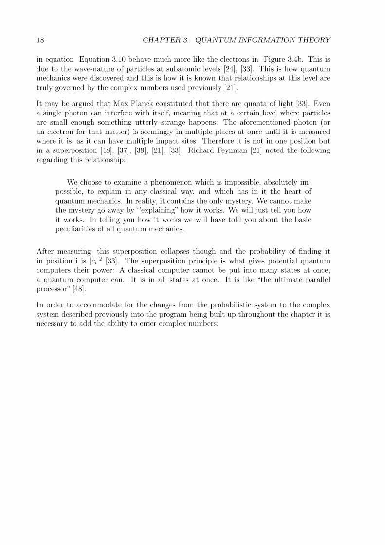
In order to accommodate for the changes from the probabilistic system to the complexsystem described previously into the program being built up throughout the chapter it isnecessary to add the ability to enter complex numbers:

3.3. COMPLEX SYSTEM 19
1 def enter_complex_state(dimensions = None):
2 """Ask user to enter complex state vector"""
3 if dimensions == None: #&& !dimensions:
4 try:
5 dimensions = int(raw_input("Please enter
6 the number of Dimensions: (max: 20)"))
7 except ValueError:
8 print("Oops! That was no valid number. Try again...")
9 initial_state = np.zeros((dimensions, 1), ’D’)
10 print("")
11 print("Please enter the initial state of the " + str(dimensions)
12 + "-dimensional system one after the other
13 (You may only enter complex values without
14 spaces i.e (int)(+/-)(int)j ): ")
15 i = 0
16 while i < dimensions:
17 try:
18 c = complex(raw_input("initial_state[" + str(i) + "] = "))
19 initial_state[i] = c
20 i = i + 1
21 except ValueError:
22 print("Oops! That was no valid complex number. Try
again...")→
23 print("")
24 print("This is your complex start state vector: ")
25 print(initial_state)
26 return (dimensions, initial_state)
Listing 6: The complex system as a program.
20 CHAPTER 3. QUANTUM INFORMATION THEORY
27 def complex_matrix(dimensions):
28 """Ask user to fill the dynamics of the system i.e. a complex
matrix"""→
29 #Initiliazie matrix; D stands for complex entries
30 complex_matrix = np.zeros((dimensions, dimensions), ’D’)
31 print("")
32 print("Please enter the complex matrix representing the dynamics of
the system→
33 (You may only enter complex values without spaces i.e
(int)(+/-)(int)j ")→
34 i = 0
35 while i < dimensions:
36 j = 0
37 #try:
38 while j < dimensions:
39 try:
40 c = complex(raw_input("complex_matrix[" + str(i) + "]" +
41 "[" + str(j) + "]"" = "))
42 complex_matrix[i][j] = c
43 j = j + 1
44 except ValueError:
45 print("Oops! That was no valid number. Try again...")
46 i = i + 1
47
48 print("You have entered the following matrix: ")
49 print(complex_matrix)
50 return complex_matrix
Listing 7: The complex system as a program (continued).
The first step in the direction of away from classical and towards quantum mechanics hasbeen made and it was shown that quantum mechanics can be thought of as probabilitytheory with complex numbers.
Chapter 4
Quantum Mechanics
4.1 Quantum States
The following Section will go into detail regarding quantum states building on the simpleexamples of the previous chapter.
4.1.1 The Basics
In any state of a classical universe it would be enough to describe a particle x via aninfinite basis. This is actually what quantum physicists do: They use infinite dimensionalfunction spaces, to be exact the Hilbert space [33]. This space may be imagined with avector for every point in space x0 to x(n−1) [48]. They are equally spaced in the discussedsystem. If every point is covered individually they could be written as vectors
x0 = [1, 0, ..., 0]T , x(n−1) = [0, 0, ..., 1]T . (4.1)
These vectors must form a basis [24]. In other words the particle has to be somewhere inthe universe.
Any arbitrary quantum state can be written as |ψ〉. This notation is called Dirac ketNotation [37]. As an example of its use consider the vector (0, 0, 3
5, 0, 0, 0, 4
5, 0)T . The ket
notation may be used to write 35|3〉+ 4
5|7〉 in a more simple manner, omitting all of the 0
entries [4].
Therefore the basis vectors from Equation 4.1 may also be written as:
|x0〉, ..., |xn−1〉 (4.2)
These vectors are the positions in the state space.
21
22 CHAPTER 4. QUANTUM MECHANICS
Considering a quantum universe though the experimentally proven complex weights andinterference mentioned before must be accounted for. This is why complex amplitudes c0to cn − 1 are needed in front of every vector. Therefore
|ψ〉 = c0|x0〉+ ...+ cn−1|xn−1〉 (4.3)
ergo the particle is somewhere in the complex vector space Cn. The Dirac notation is justan easier way of describing this. Because of the wave nature of particles (first shown by[14]) Equation 4.3 may be visualized as n waves, |x0〉 to |xn−1〉, that all contribute withintensity ci to |ψ〉 [48].
Kets have certain properties [33]:
1. Kets may be added: (c0 + c′0) · |x0〉.
2. Kets may be multiplied by scalar c.
The state |ψ〉 is said to be the superposition of the basic states from Equation 4.1. Itstands for a particle x being in all positions x0 to x(n−1) at once. The complex amplitudesc0 to cn − 1 denote which superposition it currently occupies.
After observing the state |ψ〉 it will be found in one of the basic states [21]. The squaredmodulus of the complex number ci divided by the norm squared of ψ〉 will give theprobability of finding particle in position xi after measurement [37]:
p(xi) =|ci|2
||ψ〉|2=|ci|2
Σj|cj|2(4.4)
Interestingly due to Equation 4.3, a ket is its own superposition: As any ket may bemultiplied by scalar c and this scalar gets factored out according to Equation 4.4 theydescribe the same physical state. Therefore the normalized vector
|ψ〉||ψ〉|
(4.5)
which has length 1, can be used. Consequently the probability in Equation 4.4 boils downto: p(xi) = |ci|2.
4.1.2 Spin
In order to build a quantum computer an equivalent of classical bits is needed. As shalllater be explained these are quantum bits or QuBits. To be able to understand QuBitsfirst of all the spin of a subatomic particle will be discussed.

4.1. QUANTUM STATES 23
Figure 4.1: The Stern-Gerlach Experiment adapted from [21]
As Richard Feynman describes Stern-Gerlach the following experiment showed at thebeginning of the 20th century that electrons under the influence of a magnetic field willhave a spin [21]:
Figure Figure 4.1 shows the experimental setup of a Stern-Gerlach experiment. Theatomic beam shoots electrons in direction of y. This thesis will only treat electrons butneutrons, protons [35] atoms and even molecules have be shown to behave in a similarway [7]. The magnetic field is in direction z. The figure shows furthermore how the beamsplits into two beams. Depending on the atom and its state it could be less or more - theoriginal figure shows three but for the purpose of this paper two will suffice.
If electrons are subjected to a magnetic field in this way they behave somewhat like smallmagnets trying to align themselves to this field [21]. The magnetic field splits the beamof electrons in two streams with opposite spin. Some electrons spin one way and othersthe other way round. In contrast to the little magnets though there are no electrons inthe middle of the screen [48]. If it is measured in a given direction an electron will be inone of two states: Spinning clockwise or counter-clockwise [33].
It is important to note, that the property of a spin does not correlate to the spin of abilliard ball for example. The speed of the rotation cannot be changed for example. Anelectron is a charged point, and the spin is not caused by the movement of a mass [21] butit still behaves very similarly: Elementary particles, such as the electron have an intrinsicangular momentum [37]. For each given direction in space there are only two spin states.Its direction can be changed [37]. For the z-axis they were given the name spin up | ↑〉and spin down | ↓〉 [48]. Before a measurement, the following superposition of up anddown fully describes a quantum state for the z-axis of one elementary particle [33]:
|ψ〉 = c0| ↑〉+ c1| ↓〉 (4.6)
These two states may also be written as vectors [48]:
| ↑〉 = 1 0 (4.7)
| ↓〉 = 0 1 (4.8)

24 CHAPTER 4. QUANTUM MECHANICS
4.1.3 Transition Amplitudes
Quantum mechanics also makes it possible to extract the probability of two different states,|ψ〉 and |ψ′〉, to transition into another. This property is called a transition amplitude[48]. It stands for the probability that the state of the system before a measurement is tochange to another after the measurement has taken place. This amplitude is calculatedin the following way:
The complex conjugate of the end-state denoted |ψ′〉 [48] is taken. This is done bychanging the sign of the imaginary part of a complex number: If c = a+bi is any complexnumber, the conjugate of c is c∗ = a − bi [24]. The conjugate is thereafter multipliedwith the start-state. The notation physicists use for this relation is 〈ψ′|ψ〉 which is calledbra-ket notation [33]. The bra is the complex conjugate of a state’s ket vector [48] i.e.〈ψ′| = |ψ′〉∗.
To illustrate the following examples will be employed: The ket |ψ〉 = [3, 1− 2i]T is given[48]. The bra corresponding to this ket is the complex conjugate of the individual entries:〈ψ| = [3, 1 + 2i]T [48].
Similarly the transition amplitude of two states can be computed: The state |ψ〉 =√22
[1, i]T to |ϑ〉 =√22
[i,−1]T [48]. First of all the bra corresponding to the end state
is 〈ϑ| =√22
[−i,−1]T [48]. Now their inner product is taken [48]:
〈ϑ, ψ〉 = −i (4.9)
The mathematical operation which this notation stands for is the inner product of the twovectors. This inner product may be zero. If this is the case the transition amplitude iszero or in other words, it is impossible that |ψ〉 will transition to |ψ′〉 [48]. In geometricalterms the vectors are orthogonal. The state space described by this inner product of thepossible states of a system e.g. the two spin states described previously stands for thelikelihood of the states to transition into one another [33].
To formalize these relationships in a way that is more easily graspable to computer scien-tists again a simple program representing a first quantum system will be devised:

4.2. OBSERVABLES 25
1 import numpy as np
2
3 def self_adjoint(a):
4 """Calculate the self-adjoint of a given matrix.
5 If it is a ket vector the output will be its bra"""
6 return np.conjugate(np.transpose(a))
7
8 def inner_product(a, b):
9 bra_b = self_adjoint(b)
10 return np.dot(bra_b, a)[0][0]
11
12 def quantum_system():
13 #Enter ket vector
14 (dim, ini) = enter_complex_state()
15 b = enter_complex_state(dim)
16 print(’The probabilty of transitioning from the first to the second
state is: ’ + inner_product(ini, b))→
Listing 8: An initial take on quantum systems in the emulator.
4.2 Observables
In real life many different properties of the world around us may be observed: What is thetemperature outside? How fast does this car go? Where am I on earth? etc. Observablesare specific questions to the system. In classical systems these could be mass, momentum,radioactivity and many others. As described previously there can be different states in asystem. Likewise different observables show different physical properties of these states.
Observables are the mathematical representation of the aforementioned questions to asystem. Just as when an observer asks for the temperature and will get a real number it canassumed that observables in quantum mechanics have real expectation values [33]. Thisimplies that they must have special mathematical properties: Observables are operatorson states. The operator Ω to a state |ψ〉 may be applied, so that the state changes to Ω|ψ〉[48]. After this calculation the state has changed as the original state has been modified.
One of the postulates of quantum mechanics, whose proof goes beyond the scope of thispaper, is the following:
Postulate 1. To each physical observable there corresponds a hermitian operator [39]
An operator is hermitian if it fulfills the condition that it is equal to its own conjugatetranspose i.e. A = A∗. In programmatic terms this can be captured in the following way:

26 CHAPTER 4. QUANTUM MECHANICS
1 def is_hermitian(a):
2 """Produces True if the given matrix is hermitian"""
3 #Due to allclose: Rounding error up to 1*e-8 allowed
4 return np.allclose(a == self_adjoint(a))
Listing 9: A method to check if a certain matirx a is hermitian.
The following matrix is an example for a hermitian matrix [48]:
ω =
[7 6 + 5i
6− 5i −3
](4.10)
One of the properties of hermitian operators is that their eigenvalues are real [33]. Theseeigenvalues form the set of possible valid answers to the question the observable may give[48].
Postulate 2. The eigenvalues of a hermitian operator ω associated with a physical ob-servable are the only possible values that observable can take as a result of measuring it.Furthermore, the eigenvectors of ω form a basis for the state space [48].
The position state vectors from Equation 4.2 are the eigenvalues of the observable an-swering the question ‘Where is the particle?’ [48]. This observable may be written as
P (ψ〉) = P (|xi〉) = xi|xi〉 (4.11)
Therefore the position operator acts as multiplication by position [48]. Another questionthe system may be asked is its momentum. Both of these possible questions namely whereis the particle and how quickly is it moving are both observables and therefore hermitianoperators. Interestingly most observables used in quantum mechanics may be expressedthrough these two operators [33].
The quantum system may be asked regarding the aforementioned spin as well. As wasmentioned this property of elementary particles is not concerned with changing velocitiesbut a valid question to the system might be, which direction is the particle spinning in. Isit spinning up or down in z-direction? Left or right in x-direction? In or out in y-direction?The following three operators stand for the observables regarding these questions [37].
Sz =~2
(1 00 −1
)(4.12) Sy =
~2
(0 −ii 0
)(4.13) Sx =
~2
(0 11 0
)(4.14)
The factor ~ stands for the reduced planck constant but may be ignored for the purposeof this thesis. These three matrices without the factor ~
2are called the Pauli matrices
usually denoted σx to σz [33] . They are hermitian and unitary. They are importantoperators for single-QuBit systems [33].
4.3. MEASUREMENTS 27
Properties of observables include the following [39]:
1. May be added to each other
2. May be multiplied by a real number
3. May be multiplied by each other
4. May be multiplied by itself
5. The commutator of two observables Ω1 and Ω2 is [Ω1,Ω2] = Ω1Ω2 − Ω2Ω1
The commutator has to be 0 for the observable to be hermitian. This is true for all thematrices mentioned in this Section.
4.3 Measurements
In the previous Section questions to a system i.e. observables were treated. The cor-responding answers to those questions in quantum mechanics are measurements. Thebig difference between a classical and a quantum system regarding measurement is, thatwhen something is measured it does not alter the system. After all, when someone weighshimself he does not change in weight. In quantum systems this is different: there is adistinction between projective and general measurements [33]. General measurements arenot repeatable and happen in open quantum systems [33]. The projective measurementsstand for the measurements that are known from everyday life. It can be mathematicallyshown that these are repeatable.
Interestingly within the mathematical framework of quantum mechanics this does not havebe the case and e.g a photon gets destroyed when its position is measured with a silveredscreen[33] [48]. This measurement cannot be carried out twice. For the purposes of thisthesis though it is enough to concentrate on projective measurement. The emulator beingbuilt in the thesis is only concerned with observables which are hermitian and satisfy thepreviously stated rules. The following is true for any measurement of such an observable[33]:
Postulate 3. The possible outcomes of the measurement correspond to the eigenvalues,m, of the observable.
Upon measuring the state |ψ〉, the probability of getting a specific eigenvector |e〉 as aresult is similar to the transition amplitude described previously: The squared modulusof the inner product of the two vectors, in this case |〈ψ|ψ〉|2. For the general case thisformula may be written as [33]:
p(m) = 〈ψ|Pm|ψ〉 (4.15)

28 CHAPTER 4. QUANTUM MECHANICS
This notation is commonly used for the transition amplitude described before. Thisoperation is called the projection of |ψ〉, along |e〉.
A function to be added to the program being written is accordingly the following:
1 def projection(phi, e):
2 """Calculates the projection of the quantum state phi
3 along a given eigenvector e of its observable
4 i.e. the probability of the measured value being e"""
5 return squared_modulus(np.inner_product(phi, e))
Listing 10: The calculation of the transition amplitude in Python.
The result being an eigenvalue e, the state after the measurement will be the associatedeigenvector e [33]. This state is called an eigenstate. An eigenstate is the state after thewave-function of the input state has collapsed [48]. This means that the superposition ofthe quantum state has been reduced to a single vector: The eigenstate. This is one ofthe two ways a quantum system evolves [48]. The other one will be treated in the nextSection. If the state has collapsed and there is no superposition anymore then a secondmeasurement will always yield the same result [37].
As was mentioned earlier the double slit experiment opened the door to a more differen-tiated way of looking at the universe i.e. quantum mechanics. These experiments andtheir alterations showed that an imaginary number lies at the heart of phenomena thatare happening every day.
4.4 Evolution of Quantum Systems
Quantum dynamics is concerned with the change of a quantum system with regard tochanges in motion, spin, momentum and others over time [37]. Up to now measurementswere discussed as a change within a quantum system but they were not time-dependent.
Another important postulate of quantum mechanics, regarding its evolution is the follow-ing [33]:
Postulate 4. The evolution of a closed quantum system is described by a unitary trans-formation. [...]
Any operation on a quantum state that is done through unitary matrices is a unitarytransformation. Closed in this case means that the system may not interact with anothersystem. No system except for the universe as a whole is really totally closed though [24].Nevertheless physicists trying to devise a quantum computer go to great lengths to ensurethat the system they are interacting with has as little room for interaction as possiblesuch as cooling down the system to almost 0K[33].
4.4. EVOLUTION OF QUANTUM SYSTEMS 29
Taking Postulate 4 into account there must exist a matrix U that stands for the changeover time in a quantum system. Put into a formula this might look like the following [48]:
|ψ(t+ 1)〉 = U |ψ(t)〉 (4.16)
which shows the change in the quantum state |ψ〉 from t to t+ 1. Unitary matrices werealready briefly mentioned in Equation 3.7. The same rules hold for quantum systemsas in the complex system discussed previously [48]. Unitary matrices have importantmathematical properties [48]:
1. The product of two unitary matrices is unitary
2. Furthermore multiplication by U preserves the inner product i.e. 〈Ux, Uy〉 = 〈x, y〉
3. The inverse of a unitary matrix is unitary
4. Multiplicative identity between unitary matrices is given by the identity matrix I
These properties mean that transformations on unitary matrices form a transformationgroup with respect to composition [48]. An orbit of the quantum state |ψ〉 in time i.e. t1to tn−1 under the unitary action G in the may be constructed in the following manner
|ψ〉tn−1 = G(tn−1)G(tn−2)...G(t0)|ψ〉
This means that to get to t1 the action for that point in time needs to be applied as wellas the ones before to the original state.
|ψ〉t1 = G(t1)G(t0)|ψ〉 (4.17)
Because of property item 3 another strange characteristic of quantum systems emerges:It can be calculated back in time. By applying the inverse of the previously action to thestate for t1:
|ψ〉t0 = G−1(t0)|ψ〉t1 (4.18)
This aspect of possible time reversal is called t-symmetry in physics [25]. Until a mea-surement is made this time symmetry holds. As has been discussed before, after a mea-surement is carried out, the state has collapsed and hence this time symmetry is broken[21]. Some argue that if it is broken then it is not time symmetry [25] but for the purposeof this paper this view suffices.

30 CHAPTER 4. QUANTUM MECHANICS
4.4.1 The Schrodinger Equation
By now the necessary parts of a basic quantum computation have been presented: Aunitary matrix U or a sequence of Us will be applied to an initial quantum state. After-wards the state will be measured to yield the final state. This perspective though is verysimplified. In real-life the quantum systems dynamics are described by the Schrodingerequation [33]:
The Schrodinger equation may give a probability density for the position of an electronthrough |ψ〉|2. Indeed this is solvable analytically on paper: For the hydrogen atomErwin hinmself [38] showed how. This is a very complex equation though and only fewsuch equations can be solved by man. Indeed PAM Dirac is cited as saying that chemistryhas come to an end as its content is encapsulated in the Schrodinger equation but it cannotbe solved but for the simplest of atoms (as cited in [30]).
Numerically though it is possible using a computer[33]. As soon as there are multipleparticles involved, i.e. with most atoms except the simplest ones e.g. H2 or He aninsurmountable barrier appears: In the case of n particles the wave function has to bedetermined in a 3n-dimensional vector space [30]. The number of values of the wavefunction that have to be determined depends on the number of parameters p: This numberis given by p3n. Already for a small system such as a single carbon atom where p = 5 andn = 6 this is very complex [30]. Using only two parameters, e.g. spin-up and spin-down,to simulate a quantum system of just 100 atoms 2100 values would need to be determined.Walter Kohn called this the ‘exponential wall’ [30]. Indeed this wall is the reason thatRichard Feynman and others originally proposed a quantum computer [20].
4.4.2 Multiparticle Systems and Entanglement
A single or multiple particles can interfere in quantum systems as was explained previously.This is their wave functions may overlap and cancel or intensify each other. They are notdependent on they can just influence each other though.
Multiple particles can be entangled as well as shall be explained in this Section. In shortproperties of entangled particles are correlated or depend on each other. In order tounderstand a quantum system for multiple particles and entanglement, another postulateof quantum mechanics is needed [33]:
Postulate 5. The state space of a composite physical system is the tensor product of thestate spaces of the component physical systems.
Given two state spaces A and B, A having m possible positions, B having n, the combinedstate space is the inner product of the old vector spaces [48]. Therefore it is a subset ofthe complex vector space Cm×n [33]. Moreover, given systems |ψ1〉 to |ψn〉, the joint stateof the total system is |ψ1〉 ⊗ |ψ2〉 ⊗ |ψn〉 [33]. The probabilities in multiparticle-systemsare calculated in a similar manner to one-particle systems i.e. according to Equation 4.4[33].
4.4. EVOLUTION OF QUANTUM SYSTEMS 31
For a simple multiparticle system the following state is considered where xi stands for theposition of the first particle and likewise yi stands for the one of the second particle [48]:
|ψ〉 = c0|x0〉 ⊗ |y0〉+ c1|x0〉 ⊗ |y1〉+ c2|x1〉 ⊗ |y0〉+ c3|x1〉 ⊗ |y1〉 (4.19)
If now c0 = c3 = 1 and c1 = c2 = 0 the probability of particle 1 being in position x0 maybe calculated:
p(xo) =|1|2
|1|2 + |0|2 + |0|2 + |1|2=
1
2(4.20)
Consequently the probability is 50% to find it in x0 and likewise 50% for x1. If it is indeedfound at x1 and interesting fact arises: The experimenter, without a measurement, alreadyknows with certainty that the second particle will be in position y1 because c2 = 0. Similarknowledge is gained if the first particle is found in x0 as the two cases are symmetrical. Iftwo states are intertwined this way they are called entangled. If they are entangled thismeans that the outcome of one measurement determines the state of the other.
This is even true for particles which are light years away [33]. But information cannotbe transfered in this way [48]. Given an entangled pair of particles, A and B, making ameasurement on some entangled property of A will give a random result and B will havethe complementary result [33]. The key point is that no control over the state of A maybe had, and once a measurement is made entanglement is lost [33].
These entangled states cannot be rewritten through the tensor products of two statesof its subsystems. Non-entangled states for which this is possible are called separablestates [24]. Entanglement is one of the reasons why quantum computers are so difficultto realize: For example an electron will try to interact with its neighbors. If this happensthe quantum state has changed in an unexpected way. This is called decoherence and willbe touched again in Chapter 7.

32 CHAPTER 4. QUANTUM MECHANICS

Chapter 5
Architecture of a QuantumComputer
This following Section will discuss a theoretical approach of how quantum computerscould be used in the future. It is not meant as a blueprint for its engineering but as abasis to reason about how such a device would be programmed. It is also to introducecomputer scientists with a tangible architecture as it is connected to a classical computerwell known to this audience.
5.1 QRAM Model
Even though they could, as they are Turing machines [33], quantum computers will mostprobably not replace classical computers: They will enhance them. As was pointed outbefore, quantum computers must adhere to certain restrictions. For many problems theyare not even better suited than classical computers. For example sorting is mathemati-cally proven to be optimal on classical computers [26]. Grover’s algorithm which will bediscussed in the next chapter is only for searching through an unordered set. As there areonly those limited problems it seems natural to combine the two. A schematic showingsuch a possible hybrid is shown in Figure 5.1.
This coprocessor model is called Knill’s QRAM model [29] and is regarded as the mostpromising model of a realization of commercial quantum computers [44] [43] [18]. As canbe seen in Figure 5.1 the hybrid approach would employ a quantum unit or ”qALU” as itis called by Eloushi et al. [18]. This is shown in orange in Figure 5.1. Such a quantumunit would need a way of communicating with the classical components: The quantumfirmware. This quantum firmware would need to be independent of the algorithms to berun. This means that there should be some kind of assembly language that would abstractthe quantum hardware [18].
The source code for quantum programs would still reside and be compiled on the classicalunit shown in green in Figure 5.1. This classical unit could communicate with the quantumunit via a message queue. The message queue would be used for elementary instructions
33

34 CHAPTER 5. ARCHITECTURE OF A QUANTUM COMPUTER
Figure 5.1: A schematic of a possible coprocessor model [43]
to the quantum unit such as ”allocate a QuBit”or ”measure QuBit y” [43]. Also the resultsof a computation on the quantum unit would be made available to the classical unit viathis message queue. In this sense the control flow of an algorithm is classical in that loopsand tests are performed on the classical device [18]. As Valiron et al. [43] envision bothclassical and quantum data are first-class objects.
As hinted at the quantum firmware and the compiler on the classical device would toa certain degree abstract the physical representation of the quantum hardware. Thelogical representations of the QuBits and the algorithms would be done similarly to theconventional programming model. They would be mapped to phyiscal QuBits on thequantum unit via the quantum firmware.
5.2 Bits and QuBits
Definition 1. A bit is a unit of transformation describing a two-dimensional classicalsystem. [48]

5.2. BITS AND QUBITS 35
A bit may be represented in different ways: High or low voltage or electricity or noelectricity running through a circuit or a switch being turned on and off or true and falseetc. This means that it is a two-state system which can be represented as a a matrix [48]:
|0〉 =
[ ]0 11 0 (5.1) |1〉 =
[ ]0 01 1 (5.2)
The difference between a quantum two-state system and the classical bit is that it is noteither on or off but as could be shown before it can be in both states at the same timedue to the superposition principle [33]. Consequently the definition for a QuBit has to bedifferent than the one for the bit:
Definition 2. A quantum bit is a unit of transformation describing a two-dimensionalquantum system [48]
This QuBit is represented similarly to the classical one but with complex numbers:
[ ]0 c01 c1 (5.3)
The complex number c1 stands for the probability of the QuBit collapsing to |1〉 as wasmentioned previously. The QuBit has to be unitary as all quantum systems which werediscussed and therefore |c0|2 + |c1|2 = 1. The bit described in Equation 5.1 is a basis forC2. Consequently every value in C2 and therefore any QuBit may be written as [48]:
(c0c1
)= c0
(10
)c1
(01
)= c0|0〉+ c1|1〉 (5.4)
A bit is just a special case of the QuBit where a measurement has taken place and thecomplex amplitudes have collapsed to real numbers [33].
Qubits may be implemented in different ways [24]:
1. An electron’s orbit around an atoms nucleus
2. The two polarized states of a photon
3. A subatomic particles spin
Classical computers with only one bit are not very powerful. Therefore a byte will bediscussed next. It has become convention to call eight bits one byte. A random bytemight look like this:
01101011 (5.5)

36 CHAPTER 5. ARCHITECTURE OF A QUANTUM COMPUTER
Or in matrix representation:
(10
)(01
)(01
)(10
)(01
)(10
)(01
)(10
)(10
)(5.6)
Assembled quantum systems are combined with the tensor product so a similar represen-tation of this byte system may look like this:
|0〉 ⊗ |1〉 ⊗ |1〉 ⊗ |0〉 ⊗ |1〉 ⊗ |0〉 ⊗ |1〉 ⊗ |1〉 (5.7)
As this is the tensor product of eight two-dimensional complex vector spaces the afore-mentioned vector space has 28 = 256 dimensions or is isomorphic to C256 [33].
It follows that a qubyte, what eight QuBits are called, has to be written by using 256complex numbers [48]. For a 64-QuBit register, 264 complex numbers would be needed,which by far exceeds the memory capacity of classical computers [48] This is another wayof getting at the “exponential wall” mentioned previously.
Two QuBits can be written in the following way [48]:
|0〉 ⊗ |1〉 (5.8)
which means that the first QuBit is in state |0〉 and the second on in |1〉. Equivalentlythis may be denoted |01〉 [4]. Therefore the general case of a two-QuBit system may bewritten as:
|ψ〉 = c0,0|00〉+ c0,1|01〉+ c1,0|10〉+ c1,1|11〉 (5.9)
If the QuBits are entangled this state is reduced to:
|ψ〉 = c0,0|00〉+ c1,1|11〉 (5.10)
For single QuBits there is a nice and intuitive way of representation called the Blochsphere. A normalized complex number can be visualized by an arrow from the origin ofa circle of radius one and therefore identified by the angle φ [33]. A normalized QuBit ofthe form as in 5.4 can be rewritten accordingly in canonical representation. The visualrepresentation of a QuBit accordingly looks like Figure 5.2
A QuBit may be written in the following way [48]:
|ψ〉 = cos(θ)|0〉+ eiϕsin(θ)|1〉 (5.11)
The meaning of these two angles is the following: ϕ is the angle of |ψ〉 from x along theequator and θ is half the angle it makes along the z-axis [33]. As the Bloch sphere is arepresentation of this QuBit and it is normalized, trigonometry tells us that a range of0 ≤ ϕ < 2π and 0 ≤ θ < π
2is enough to cover all possible QuBits [24]. Consequently
the arrow denoted |ψ〉 represents a single QuBit [33]. The two angles can be thought ofas the latitude and longitude used e.g. in the GPS to locate a position on earth [48].Furthermore the north and the south pole of the sphere in Figure 5.2 stand for the twostates |0〉 and |1〉 [33]. They can be seen as representations of the classical bit.

5.3. GATES 37
Figure 5.2: The QuBit represented on the Bloch sphere [33]
5.3 Gates
The following subSections will treat different realizations of logical gates starting withclassical ones used in the everyday computer, being followed by reversible gates and finallya discussion of quantum gates.
5.3.1 Classical
In order to manipulate classical bits logical gates are used. These logical gates, well-knownto computer scientists, will be studied from the point of view of matrices. The easiestclassical gate is the NOT -gate. The matrix
NOT =
(0 11 0
)(5.12)
represents such a NOT -gate [48]. It is evident that the bits are flipped by the gate (onlyshown for |0〉):
(0 11 0
)·(
10
)= NOT · |0〉 =
(01
)= |1〉 (5.13)

38 CHAPTER 5. ARCHITECTURE OF A QUANTUM COMPUTER
The AND-gate on the other hand accepts two input bits and produces one output. There-fore a 21-by-22 matrix will be needed for the AND-gate [48]:
AND =
(1 1 1 00 0 0 1
)(5.14)
This matrix acts in the same way on a bit as the classical AND-gate and hence is equiv-alent [48]:
(1 1 1 00 0 0 1
)0001
=
[01
](5.15)
As was discussed in Section 4.4.2 in order to combine two bits in matrix-representationtheir inner product is taken. The vector [0, 0, 0, 1] is just the inner product of two bitsinitialized to 1. In quantum computation the Equation 5.15 can also be written as [48]:
AND|11〉 = |1〉 (5.16)
The NAND-gate is of special importance in the context of classical computing as alllogical gates can be composed of NAND-gates. To construct a NAND-gate in matrixform, the possible input states (00, 01, 10, 11) may be taken as a basis and for whichof these the output will be 1 (for : 00, 01, 10) or0(for : 11). Thus a NAND-gate inmatrix-form may be written as [48]:
NAND =
(0 0 0 11 1 1 0
)(5.17)
The column names correspond to the inputs and the rows to the output. The NAND-gatecan just be written as NOT · AND which produces the same result [48]:
(0 11 0
)(1 1 1 00 0 0 1
)=
(0 0 0 11 1 1 0
)(5.18)
As an example the NAND-gate will be applied to the same state used with the AND-gate:
(0 0 0 11 1 1 0
)0001
=
[10
](5.19)

5.3. GATES 39
Figure 5.3: The CNOT gate [48]
The same is true for the NOR-gate [48]. It is apparent that gates may be sequentialized.In the general case any gate matrix has to be of size 2n-by-2m where m is the number ofinputs and n is the number of outputs [33]. Consequently if the gates are sequentializedas before and the second matrix in sequence is taking the n outputs of the first one asinput, it produces p outputs. Therefore the combined matrix will be of size 2p-by-2m[48].There can be parallel operations as well and together with the sequential ones these formcircuits [48].
5.3.2 Reversible
The aforementioned classical gates do not all work in quantum computers. In quan-tum mechanics all actions must be reversible (see Equation 3.7) given that they are notmeasuring the state. The AND-gate for example is not reversible as it is impossible todetermine if for the output 0 the input was 00, 01, or 10. Rolf Landauer [31] could showthat writing is reversible whereas erasing is not. The act of erasing is what causes energyto dissipate and this causes heat in a computer [31]. This fact is now known as Landauer’sprinciple [33]. This caused Bennett [10] to explore the notion of reversible gates long be-fore anyone thought about building quantum computers. If a computer would not eraseit would not use any energy [10]. The NOT -gate for example is completely reversible asNOT ·NOT = I. There are other reversible gates such as the controlled-NOT gate:
The controlled-NOT is a two-qubit gate. The two inputs determine the two outputs of thisgate: If the top input, i.e. the |x〉 in Figure 5.3, is |0〉 then the bottom input is unchanged[48]. If it is |1〉 then |y〉 is changed. Formally what happens is that |x, y〉 → |x, x ⊕ y〉where ⊕ is the binary exclusive or operation. This gate may be written as a matrix aswell:
CNOT =
00 01 10 11
00 1 0 0 001 0 1 0 010 0 0 0 111 0 0 1 0
(5.20)
It may easily be verified, that this is a reversible gate as, multiplied by itself, it equals theidentity matrix.

40 CHAPTER 5. ARCHITECTURE OF A QUANTUM COMPUTER
Figure 5.4: The Toffoli gate [48]
Another reversible gate is the Toffoli gate:
which is similar to the controlled-NOT except that it has two control bits. Both need tobe |1〉 in order for |z〉 to be flipped, i.e. a NOT -gate may be realized with a Toffoli gate.
What is interesting about the Toffoli gate is that it is universal: Any logical gate canbe constructed out of a combination of Toffoli gates [10], [48]. Therefore a reversiblecomputer may be constructed entirely out of Toffoli gates. In theory such a computerwould not use any energy or produce heat [33], [10].
5.3.3 Quantum Gates
The reversible gates discussed before work are all quantum gates as they fulfill the require-ment of being unitary as well as being reversible [48]. Additionally the Identity matrixfulfills this condition [24]. There are naturally other quantum gates. Three important onesare the Pauli matrices that were already briefly met in Equation 4.12 to Equation 4.14.
σx =
(0 11 0
)(5.21) σy =
(0 −ii 0
)(5.22) σz =
(1 00 −1
)(5.23)
The σx matrix is equal to the NOT -gate discussed before. Two other important matricesused a lot in quantum mechanics and quantum computing are:
S =
(1 00 i
)(5.24) T =
(1 00 eiπ/4
)(5.25)
the S-gate is the phase gate and the gate denoted T is the π/8-gate. All these matricesare unitary.
As discussed before measurements are very important for quantum computation as theyhave to happen in every calculation done by a quantum computer in order to see a result.In quantum mechanics a measurement is normally denoted as:
5.3. GATES 41
Figure 5.5: The measurement symbol [33]
Figure 5.6: The visualized change of basis done by the Hadamard gate [48]
As was discussed before a measurement is not reversible as the quantum state has col-lapsed. It has collapsed to the aforementioned north or south pole of the Bloch sphere inFigure 5.2. The angle θ in Equation 5.11 stands for the probability of the quantum statecollapsing to either |0〉 or |1〉 [33]. It follows that this probability depends on the latitudeof the arrow on the Bloch sphere in Figure 5.2[33]. If this arrow is on the equator thechance of the QuBit to collapse to one of the basic states is therefore 50/50 [33].
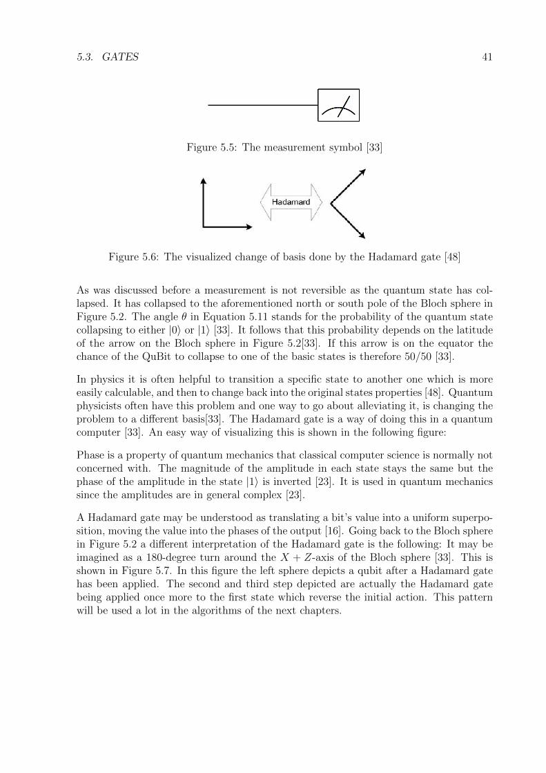
In physics it is often helpful to transition a specific state to another one which is moreeasily calculable, and then to change back into the original states properties [48]. Quantumphysicists often have this problem and one way to go about alleviating it, is changing theproblem to a different basis[33]. The Hadamard gate is a way of doing this in a quantumcomputer [33]. An easy way of visualizing this is shown in the following figure:
Phase is a property of quantum mechanics that classical computer science is normally notconcerned with. The magnitude of the amplitude in each state stays the same but thephase of the amplitude in the state |1〉 is inverted [23]. It is used in quantum mechanicssince the amplitudes are in general complex [23].
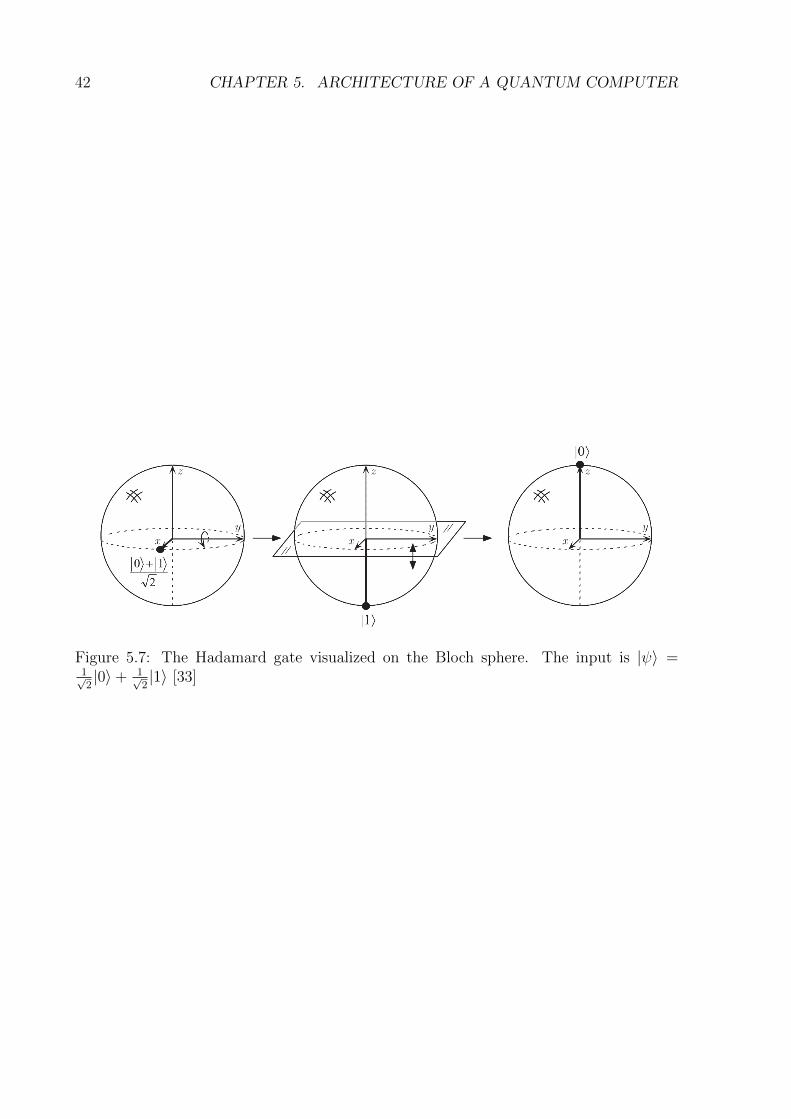
A Hadamard gate may be understood as translating a bit’s value into a uniform superpo-sition, moving the value into the phases of the output [16]. Going back to the Bloch spherein Figure 5.2 a different interpretation of the Hadamard gate is the following: It may beimagined as a 180-degree turn around the X + Z-axis of the Bloch sphere [33]. This isshown in Figure 5.7. In this figure the left sphere depicts a qubit after a Hadamard gatehas been applied. The second and third step depicted are actually the Hadamard gatebeing applied once more to the first state which reverse the initial action. This patternwill be used a lot in the algorithms of the next chapters.
42 CHAPTER 5. ARCHITECTURE OF A QUANTUM COMPUTER
Figure 5.7: The Hadamard gate visualized on the Bloch sphere. The input is |ψ〉 =1√2|0〉+ 1√
2|1〉 [33]

Chapter 6
Quantum Algorithms
Many problems are solvable in principle on classical computers but due to the huge amountof resources needed they are for all practical purposes intractable. A example of one suchproblem is prime factorization and indeed this fact is one the bases of modern cryptogra-phy. Quantum computers promise new algorithms that would make it possible to rendersuch problems feasible [33].
There are two broad classes of quantum algorithms. The first one was hinted at previously:It is the quantum version of the Fourier transform originally developed by Peter Shor[41]. It opens the door for interesting algorithms regarding the problems of factoring anddiscrete logarithm. They provide an exponential speedup over classical algorithms [33].The second class of algorithms is based upon Grover’s quantum search algorithm: Thesealgorithms have a smaller but still noteworthy quadratic speedup over classical algorithms[24]. A short outline of Shor’s algorithm will be given at the end of this chapter. First thesimple quantum algorithm by Deutsch will be developed in detail followed by a treatmentof Grover’s algorithm.
All quantum algorithms employ the following basic steps [48]:
Step 1 The computers QuBits are put into a certain classical state
Step 2 The system is put into a superposition of many states.
Step 3 This superposition is acted upon with unitary operations
Step 4 The QuBits are measured
6.1 Deutsch’s Quantum Algorithm
At the beginning of the 1980s quantum computing was just being invented. The firstactual algorithm to use its power was developed by David Deutsch [15]. It was influentialin that it was a case study that worked as a basis for Shor’s algorithm and generally for
43
44 CHAPTER 6. QUANTUM ALGORITHMS
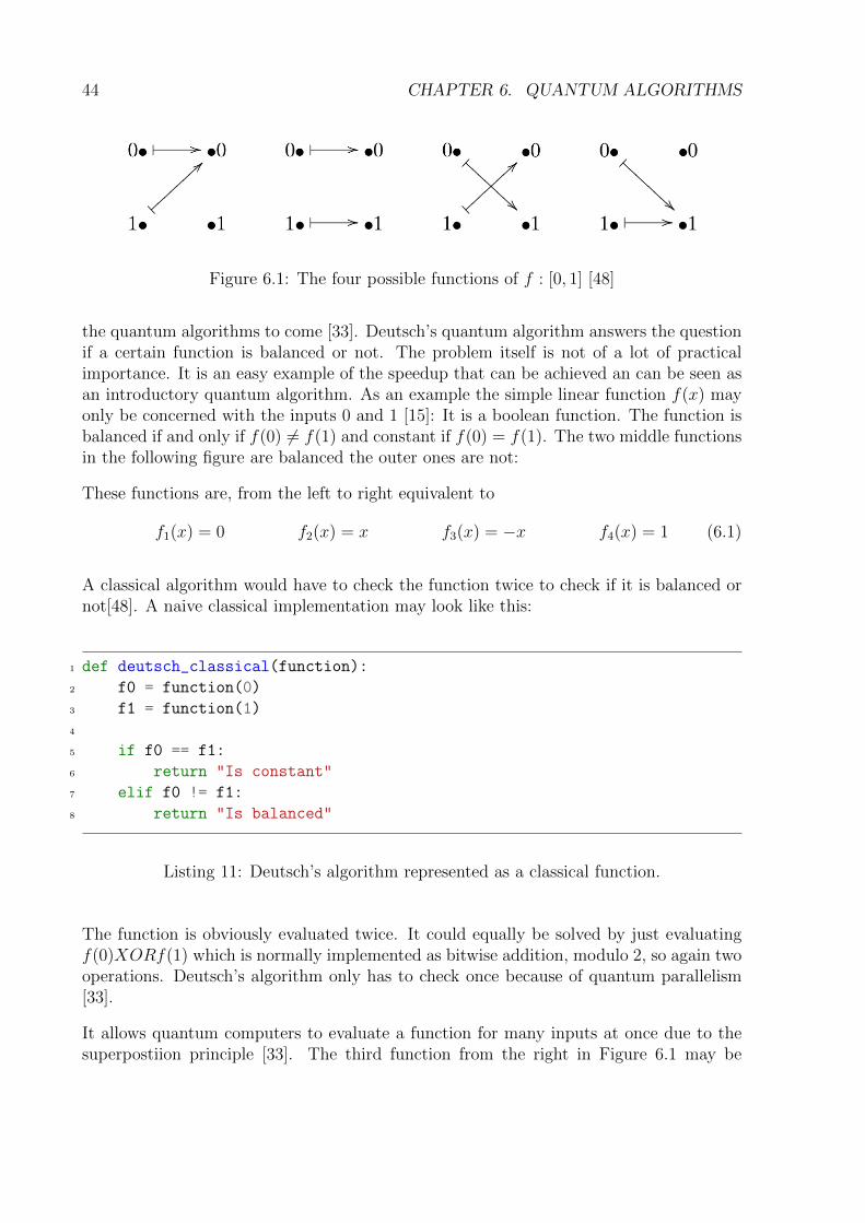
Figure 6.1: The four possible functions of f : [0, 1] [48]
the quantum algorithms to come [33]. Deutsch’s quantum algorithm answers the questionif a certain function is balanced or not. The problem itself is not of a lot of practicalimportance. It is an easy example of the speedup that can be achieved an can be seen asan introductory quantum algorithm. As an example the simple linear function f(x) mayonly be concerned with the inputs 0 and 1 [15]: It is a boolean function. The function isbalanced if and only if f(0) 6= f(1) and constant if f(0) = f(1). The two middle functionsin the following figure are balanced the outer ones are not:
These functions are, from the left to right equivalent to
f1(x) = 0 f2(x) = x f3(x) = −x f4(x) = 1 (6.1)
A classical algorithm would have to check the function twice to check if it is balanced ornot[48]. A naive classical implementation may look like this:
1 def deutsch_classical(function):
2 f0 = function(0)
3 f1 = function(1)
4
5 if f0 == f1:
6 return "Is constant"
7 elif f0 != f1:
8 return "Is balanced"
Listing 11: Deutsch’s algorithm represented as a classical function.
The function is obviously evaluated twice. It could equally be solved by just evaluatingf(0)XORf(1) which is normally implemented as bitwise addition, modulo 2, so again twooperations. Deutsch’s algorithm only has to check once because of quantum parallelism[33].
It allows quantum computers to evaluate a function for many inputs at once due to thesuperpostiion principle [33]. The third function from the right in Figure 6.1 may be
6.1. DEUTSCH’S QUANTUM ALGORITHM 45
written as the following matrix:
f3(X) =
[ 0 1
0 0 11 1 0
](6.2)
This looks like the NOT -gate encountered previously as the function acts in a similarmanner as well. The column names may be thought of as the input and the row namesas the output of the function [48]. The quantum equivalent of the classical function inEquation 6.2 has to be reversible. It is the following matrix [48]:
Uf3 =
00 01 10 11
00 0 1 0 001 1 0 0 010 0 0 1 011 0 0 0 1
(6.3)
This operation is reversible as applying it to a given input twice, outputs the originalinput as is true for unitary matrices in general. The matrix Equation 6.2 had to grow inorder to become Equation 6.3. This is the reason that not one but two QuBits are neededfor the algorithm later on.
Deutsch’s algorithm solves the problem without knowing the function [15], [24]. This iscalled a quantum oracle: It may only test inputs and receive the corresponding outputsand may be arbitrarily complex. Such oracles are often used by cryptographers to reasonabout an algorithm without being concerned by a part of it that a constant function. Thefunction in Equation 6.3 is given in order to test the algorithm. Interestingly it is noteasier for a quantum computer to find out what f is than for a classical one, as bothwill have to evaluate the function twice [28]. The quantum algorithm shall start with twoclassical states apply the function and measure the output.
The algorithms circuit looks like this:
First of all four states |ψ〉0 to |ψ〉3 are visible. Furthermore the quantum oracle can beseen in between state 1 and 2. The two QuBits are initially in states |0〉 and |1〉 or incombined state |ψ〉0 = |01〉. In matrix representation this would be: [0, 1, 0, 0]T which isthe inner product of the two states as discussed in Section 4.4.2. In terms of the quantumemulator the input would be:
1 psi0 = inner_product(QuBit(0), QuBit(1))
Listing 12: ψ0 in the emulator.
In order to get into the superposition of states, mentioned in Step 2 the Hadamard gateis employed. It puts the QuBit in the following state:
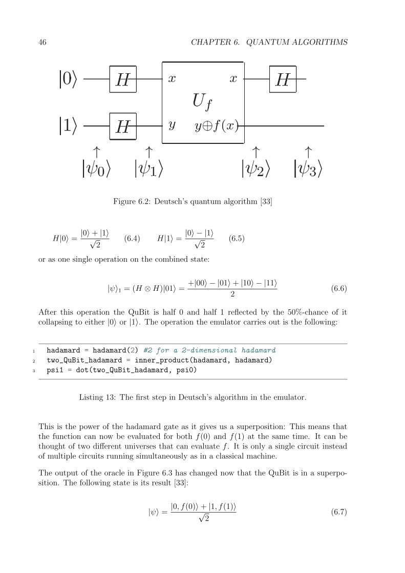
46 CHAPTER 6. QUANTUM ALGORITHMS
Figure 6.2: Deutsch’s quantum algorithm [33]
H|0〉 =|0〉+ |1〉√
2(6.4) H|1〉 =
|0〉 − |1〉√2
(6.5)
or as one single operation on the combined state:
|ψ〉1 = (H ⊗H)|01〉 =+|00〉 − |01〉+ |10〉 − |11〉
2(6.6)
After this operation the QuBit is half 0 and half 1 reflected by the 50%-chance of itcollapsing to either |0〉 or |1〉. The operation the emulator carries out is the following:
1 hadamard = hadamard(2) #2 for a 2-dimensional hadamard
2 two_QuBit_hadamard = inner_product(hadamard, hadamard)
3 psi1 = dot(two_QuBit_hadamard, psi0)
Listing 13: The first step in Deutsch’s algorithm in the emulator.
This is the power of the hadamard gate as it gives us a superposition: This means thatthe function can now be evaluated for both f(0) and f(1) at the same time. It can bethought of two different universes that can evaluate f . It is only a single circuit insteadof multiple circuits running simultaneously as in a classical machine.
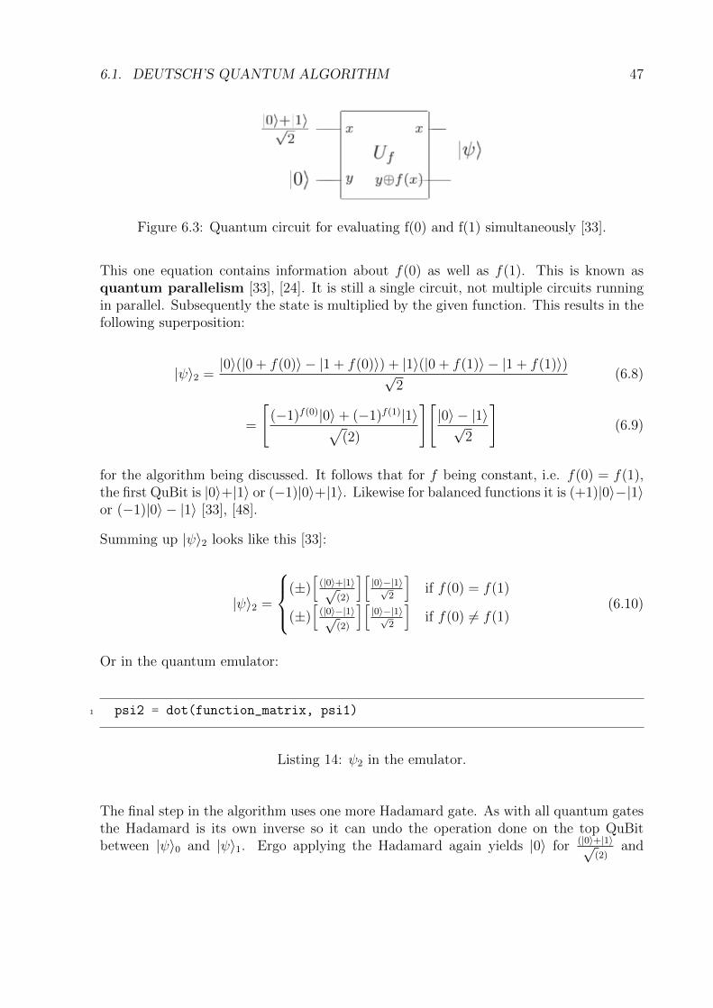
The output of the oracle in Figure 6.3 has changed now that the QuBit is in a superpo-sition. The following state is its result [33]:
|ψ〉 =|0, f(0)〉+ |1, f(1)〉√
2(6.7)
6.1. DEUTSCH’S QUANTUM ALGORITHM 47
Figure 6.3: Quantum circuit for evaluating f(0) and f(1) simultaneously [33].
This one equation contains information about f(0) as well as f(1). This is known asquantum parallelism [33], [24]. It is still a single circuit, not multiple circuits runningin parallel. Subsequently the state is multiplied by the given function. This results in thefollowing superposition:
|ψ〉2 =|0〉(|0 + f(0)〉 − |1 + f(0)〉) + |1〉(|0 + f(1)〉 − |1 + f(1)〉)√
2(6.8)
=
[(−1)f(0)|0〉+ (−1)f(1)|1〉√
(2)
][|0〉 − |1〉√
2
](6.9)
for the algorithm being discussed. It follows that for f being constant, i.e. f(0) = f(1),the first QuBit is |0〉+|1〉 or (−1)|0〉+|1〉. Likewise for balanced functions it is (+1)|0〉−|1〉or (−1)|0〉 − |1〉 [33], [48].
Summing up |ψ〉2 looks like this [33]:
|ψ〉2 =
(±)[(|0〉+|1〉√
(2)
][|0〉−|1〉√
2
]if f(0) = f(1)
(±)[(|0〉−|1〉√
(2)
][|0〉−|1〉√
2
]if f(0) 6= f(1)
(6.10)
Or in the quantum emulator:
1 psi2 = dot(function_matrix, psi1)
Listing 14: ψ2 in the emulator.
The final step in the algorithm uses one more Hadamard gate. As with all quantum gatesthe Hadamard is its own inverse so it can undo the operation done on the top QuBitbetween |ψ〉0 and |ψ〉1. Ergo applying the Hadamard again yields |0〉 for (|0〉+|1〉√
(2)and

48 CHAPTER 6. QUANTUM ALGORITHMS
likewise |1〉 for (|0〉−|1〉√(2)
. This means after the last operation before the measurement the
state is:
|ψ〉3 =
(±)|0〉[|0〉−|1〉√
2
]if f(0) = f(1)
(±)|1〉[|0〉−|1〉√
2
]if f(0) 6= f(1)
(6.11)
The bottom QuBit has not changed but the top QuBit is again in the classical state.This classical state though depends on the function now. If for example the function isconstant and f(0) = 1 as well as f(1) = 0 the resulting state is:
|ψ〉3 = −1|0〉[ |0〉 − |1〉√
2
](6.12)
To conclude: By measuring the first QuBit i.e. one operation it is possible to derive aglobal property of the function [33]. This is faster than is possible on a classical computerthat needs two operations as mentioned previously.
The final state before the measurement in the quantum emulator looks like this:
1 hadamard_identity = inner_product(hadamard,
2 np.identity(np.shape(hadmard)[1]))
3 psi3 = dot(hadamard_identity, psi2)
Listing 15: ψ3 in the emulator.
As a concrete example of this is the output of the quantum emulator during the afore-mentioned computation using f3 from Figure 6.1:
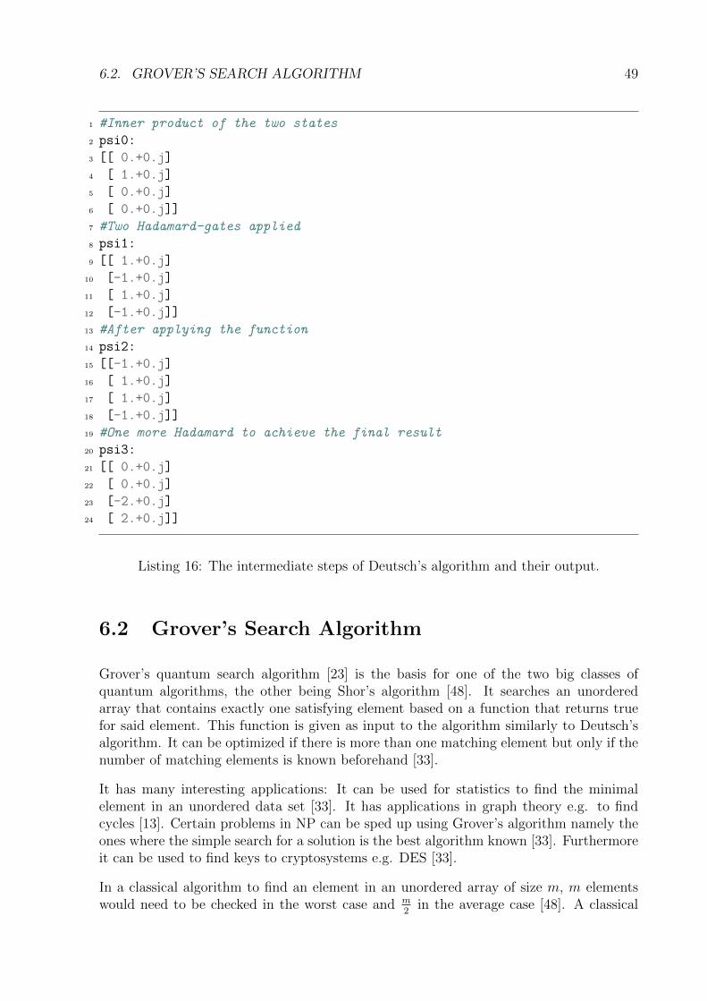
6.2. GROVER’S SEARCH ALGORITHM 49
1 #Inner product of the two states
2 psi0:
3 [[ 0.+0.j]
4 [ 1.+0.j]
5 [ 0.+0.j]
6 [ 0.+0.j]]
7 #Two Hadamard-gates applied
8 psi1:
9 [[ 1.+0.j]
10 [-1.+0.j]
11 [ 1.+0.j]
12 [-1.+0.j]]
13 #After applying the function
14 psi2:
15 [[-1.+0.j]
16 [ 1.+0.j]
17 [ 1.+0.j]
18 [-1.+0.j]]
19 #One more Hadamard to achieve the final result
20 psi3:
21 [[ 0.+0.j]
22 [ 0.+0.j]
23 [-2.+0.j]
24 [ 2.+0.j]]
Listing 16: The intermediate steps of Deutsch’s algorithm and their output.
6.2 Grover’s Search Algorithm
Grover’s quantum search algorithm [23] is the basis for one of the two big classes ofquantum algorithms, the other being Shor’s algorithm [48]. It searches an unorderedarray that contains exactly one satisfying element based on a function that returns truefor said element. This function is given as input to the algorithm similarly to Deutsch’salgorithm. It can be optimized if there is more than one matching element but only if thenumber of matching elements is known beforehand [33].
It has many interesting applications: It can be used for statistics to find the minimalelement in an unordered data set [33]. It has applications in graph theory e.g. to findcycles [13]. Certain problems in NP can be sped up using Grover’s algorithm namely theones where the simple search for a solution is the best algorithm known [33]. Furthermoreit can be used to find keys to cryptosystems e.g. DES [33].
In a classical algorithm to find an element in an unordered array of size m, m elementswould need to be checked in the worst case and m
2in the average case [48]. A classical

50 CHAPTER 6. QUANTUM ALGORITHMS
algorithm for this problem may look like this:
1 #self, the instance object, omitted for clarity
2 def grover_classical(function_classical, N):
3 solution = 0
4 for x in xrange(N):
5 if function_classical(x) == True:
6 solution = x
7 return solution
Listing 17: A classical representation of Grover’s algorithm.
Quantum computers can do better as Lov Grover showed [23]: It can be done in√m
queries. This speedup is not exponential, as is realized Shor’s algorithm and others basedon the Quantum Fourier Transform [33] but for the specific problem it is optimal as Bennetet al. could show [9]. This means that a quantum computer actually brings us closer tothe best mathematically possible solution to a problem, in this case as close as possible.This is one of the most interesting aspects of quantum computers: They test the limitsof complexity.
Similarly to Deutsch’s algorithm from the last section, Grover’s algorithm (GA) starts ofwith a binary function given to the quantum computer. This function that maps a binarystring of arbitrary length to a 0 or 1 as illustrated in Equation 6.14. It is one if and onlyif the input is equal to the target binary string x0 [48].
f(x) =
1, if x = x0
0, if x 6= x0(6.13)
So all in all there are 2n different binary numbers which a classical computer would haveto check in the worst case. GA on the other hand only needs
√2n = 2
n2 evaluations as
shown in this chapter.
As in Deutsch’s algorithm f will be given to the method in form of a black box function.As always in quantum computations the function will have to be a unitary matrix. Asjust one number needs to be found one can easily construct such a function in form ofa matrix. Indeed it is possible to “even without knowing the prime factors of m, we canexplicitly construct an oracle which recognizes a solution to the search problem when itsees one” [33]. For every value that is not the element that is being searched, the state ismultiplied by one, so it does not change. For the wanted value it is then multiplied byminus one. For a function that searches for the value 102 = 210 this matrix may look like
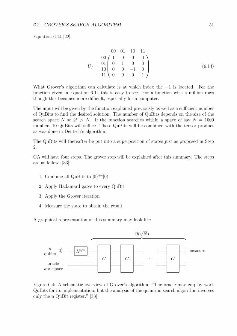
6.2. GROVER’S SEARCH ALGORITHM 51
Equation 6.14 [22].
Uf =
00 01 10 11
00 1 0 0 001 0 1 0 010 0 0 −1 011 0 0 0 1
(6.14)
What Grover’s algorithm can calculate is at which index the −1 is located. For thefunction given in Equation 6.14 this is easy to see. For a function with a million rowsthough this becomes more difficult, especially for a computer.
The input will be given by the function explained previously as well as a sufficient numberof QuBits to find the desired solution. The number of QuBits depends on the size of thesearch space N so 2x > N . If the function searches within a space of say N = 1000numbers 10 QuBits will suffice. These QuBits will be combined with the tensor productas was done in Deutsch’s algorithm.
The QuBits will thereafter be put into a superposition of states just as proposed in Step2.
GA will have four steps. The grover step will be explained after this summary. The stepsare as follows [33]:
1. Combine all QuBits to |0〉⊗n|0〉
2. Apply Hadamard gates to every QuBit
3. Apply the Grover iteration
4. Measure the state to obtain the result
A graphical representation of this summary may look like
Figure 6.4: A schematic overview of Grover’s algorithm. “The oracle may employ workQuBits for its implementation, but the analysis of the quantum search algorithm involvesonly the n QuBit register.” [33]
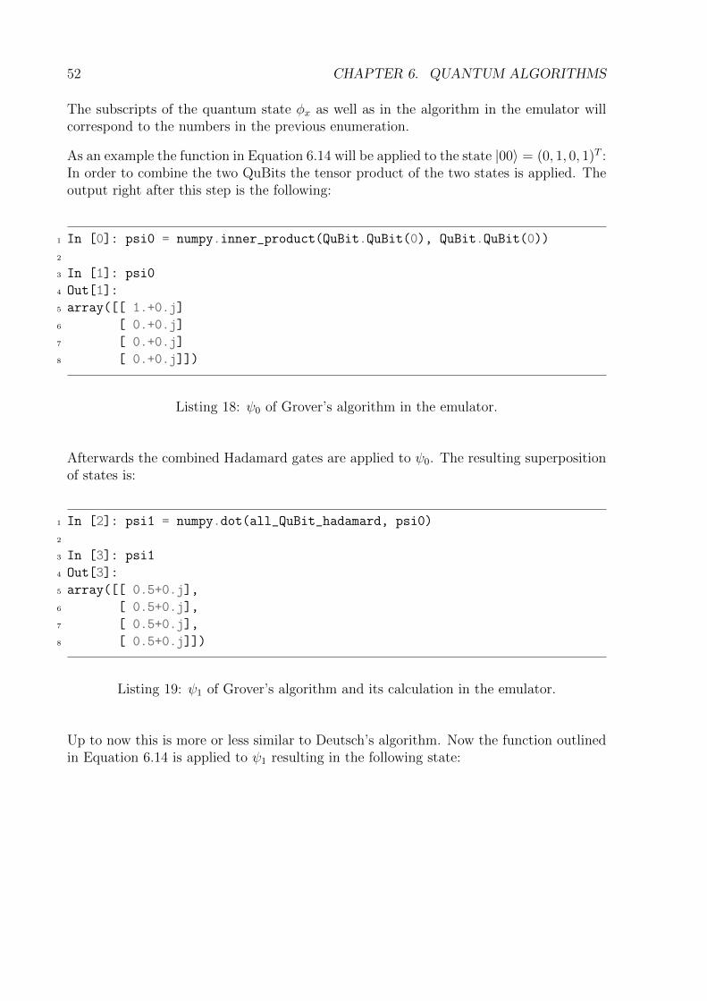
52 CHAPTER 6. QUANTUM ALGORITHMS
The subscripts of the quantum state φx as well as in the algorithm in the emulator willcorrespond to the numbers in the previous enumeration.
As an example the function in Equation 6.14 will be applied to the state |00〉 = (0, 1, 0, 1)T :In order to combine the two QuBits the tensor product of the two states is applied. Theoutput right after this step is the following:
1 In [0]: psi0 = numpy.inner_product(QuBit.QuBit(0), QuBit.QuBit(0))
2
3 In [1]: psi0
4 Out[1]:
5 array([[ 1.+0.j]
6 [ 0.+0.j]
7 [ 0.+0.j]
8 [ 0.+0.j]])
Listing 18: ψ0 of Grover’s algorithm in the emulator.
Afterwards the combined Hadamard gates are applied to ψ0. The resulting superpositionof states is:
1 In [2]: psi1 = numpy.dot(all_QuBit_hadamard, psi0)
2
3 In [3]: psi1
4 Out[3]:
5 array([[ 0.5+0.j],
6 [ 0.5+0.j],
7 [ 0.5+0.j],
8 [ 0.5+0.j]])
Listing 19: ψ1 of Grover’s algorithm and its calculation in the emulator.
Up to now this is more or less similar to Deutsch’s algorithm. Now the function outlinedin Equation 6.14 is applied to ψ1 resulting in the following state:

6.2. GROVER’S SEARCH ALGORITHM 53
1 In [4]: numpy.dot(function_matrix, psi1)
2 Out[4]:
3 matrix([[ 0.5+0.j],
4 [ 0.5+0.j],
5 [-0.5+0.j],
6 [ 0.5+0.j]])
Listing 20: ψ2 of Grover’s algorithm and its calculation in the emulator.
The sign, or the phase as quantum physicists would say, of the correct solution wasinverted by the function just as predicted. This does not help in discovering the answer.The reason is that normally the complex numbers depicted can not be accessed. Theemulator still is an approximation. If the states would be measured, the squared moduluswould have to be taken first. After doing so all outcomes are equally likely i.e. |± 1
2|2 = 1
4.
Here the special nature of GA comes into play: There must be a way to somehow increasethe difference between the correct solution. This is exactly what GA does. It does soby using interference [48], [33], [23]. Here the Grover step mentioned before starts. Thefollowing Figure 6.5 illustrates this step:
Figure 6.5: The circuit representing the Grover step.
The first step of applying the oracle function was already undertaken. Afterwards anotherHadamard gate is applied to the state. The operation that follows is commonly called“inversion around the mean” [48], [33], [22], [23]. It is easiest to understand through asimple example. It starts with 10, 10, 10, 10, 10, 10. The sign of the second to last 10 willbe changed as would be done by the oracle function in the algorithm so the sequencebecomes the one in Equation 6.15. This means that the number at index 3 is beingsearched for. It will be inverted around its average of 6 [48]:
6 =(10, 10, 10,−10, 10)
5(6.15)
The formula for this inversion about the mean is 6 + (6 − ±10) or in the general casev‘ = a+ (a− v) = −v + 2a [48]. A corresponding method in Python may look like this:

54 CHAPTER 6. QUANTUM ALGORITHMS
1 def invert_around_mean_classical(sequence):
2 mean = sum(sequence)/len(sequence)
3 inversion_function = lambda x: -x + 2*mean
4 result = []
5 for v in sequence:
6 result.append(inversion_function(v))
7 return result
Listing 21: The method to illustrate the inversion about the mean in Python.
Applying this method to all the elements of the sequence in Equation 6.15 one obtains:
(2, 2, 2, 22, 2) (6.16)
or in python:
1 In : invert_around_mean_classical([10, 10, 10, -10, 10])
2 Out: [2, 2, 2, 22, 2]
Listing 22: An example for the inversion around the mean
The distance between the elements where the sign was not changed and the solution haschanged [48]. It is now 20. Therefore this operation may be used as well in GA in orderto find the correct solution in a huge matrix. What if the function is applied once more?
1 In : invert_around_mean_classical([2, 2, 2, 22, 2])
2 Out: [10, 10, 10, -10, 10]
Listing 23: The example continued.
The sequence is again in its original state. This means the function is reversible and is ahint that it is a unitary operation that can be used in a quantum computer. What wouldhappen though if the oracle function is applied again before the inversion is calculated?
1 In : invert_around_mean_classical([2, 2, 2, -22., 2])
2 Out: [-7.6, -7.6, -7.6, 16.4, -7.6]
Listing 24: The example continued.
6.2. GROVER’S SEARCH ALGORITHM 55
The distance between the numbers has increased again. It is now 16.4 − (−7.6) = 24.Applying the oracle function followed by the inversion once more to the sequence yields:
1 In : invert_around_mean_classical([-7.6, -7.6, -7.6, -16.4, -7.6])
2 Out: [-11.12, -11.12, -11.12, -2.32, -11.12]
Listing 25: The inversion is applied one last time to finish the example.
The distance between the sought index and the other elements is now −2.32− (−11.12) =8.8. This goes to show that this operation to amplify the correct solution can be overdone[33]. Seemingly there is an optimal number of times this operation should be applied.This number was shown to be O(
√n) [9]. The proof of this relation goes over the scope
of this thesis. Further work on the correct number of steps has yielded the result inEquation 6.17 [33] which will be used in the emulator.
R ≤ π
4
√n (6.17)
In the emulator:
1 # Determine the amount of times to run
2 # the amplification of the correct result
3 nr_of_steps = math.floor(math.pi/4. * math.sqrt(n))
Listing 26: Determine the needed inversion steps.
The operation illustrated by this simple example still has to be converted to matrices inorder to be able to use it in a quantum computer. Finding the mean is essentially multi-plying all values of the sequence by 1
mwhere m is the number of elements in the sequence.
As in a quantum computer given n QuBits there are 2n possible values consequently amatrix to find the mean of all the values in the matrix will look like this [48]:
A =
12n
12n· · · 1
2n12n
12n· · · 1
2n...
.... . .
...12n
12n· · · 1
2n
(6.18)
How to map the formula v‘ = −v+2a to matrices becomes obvious now: |ψ‘〉 = (−I+2A)·|ψ〉 [48] [33]. This operation is often called the Grover diffusion operator, as it diffuses thedistance between the correct and the wrong solutions [33]. In the emulator this operationis also easy to represent:

56 CHAPTER 6. QUANTUM ALGORITHMS
1 # 2) Average around mean
2 diffusion_operator = numpy.identity(2**n, dtype=complex)
3 diffusion_operator[0][0] = -1 + 0j
Listing 27: The diffusion operator.
By now all the necessary parts for GA were presented. The actual implementation ofGrover’s algorithm in the quantum emulator is rather straightforward:
1 # Actual algorithm
2 psi0 = numpy.kron(QuBit.QuBit(0), QuBit.QuBit(0))
3
4 psi1 = numpy.dot(all_QuBit_hadamard, psi0)
5
6 result = psi1
7 for x in xrange(int(nr_of_steps)):
8 phase_inverted = numpy.dot(function_matrix, result)
9
10 prepare_diffusion = numpy.dot(all_QuBit_hadamard, phase_inverted)
11 inverted_around_mean = numpy.dot(diffusion_operator,
prepare_diffusion)→
12 result = numpy.dot(all_QuBit_hadamard, inverted_around_mean)
Listing 28: All the steps of Grover’s algorithm combined.
In order to understand it though a convenient way of imagining GA is geometrically. TheFigure 6.6 shows what happens to the quantum state during one Grover step:
In Figure 6.5 the state |β〉 depicts the sought solution [33]. First of all the Oracle functionis applied to the current state |ψ〉. It is thereby reflected around |α〉 [33]. |α〉 depictsall the wrong answers. Even though the operation O has brought the state further awayfrom the correct solution the inversion about the mean reflects the state O|ψ〉 around |ψ〉to G|ψ〉 which is closer to |β〉. This step is repeated until |ψ〉 is as close as possible to |β〉.
6.3 Shor’s Prime Factorization
Shor’s algorithm can be used to solve the discrete logarithm and factoring problems [40].The Fourier transform also turns out to be closely related to an important problem inmathematics, finding a hidden subgroup (a generalization of finding the period of a peri-odic function)[33].
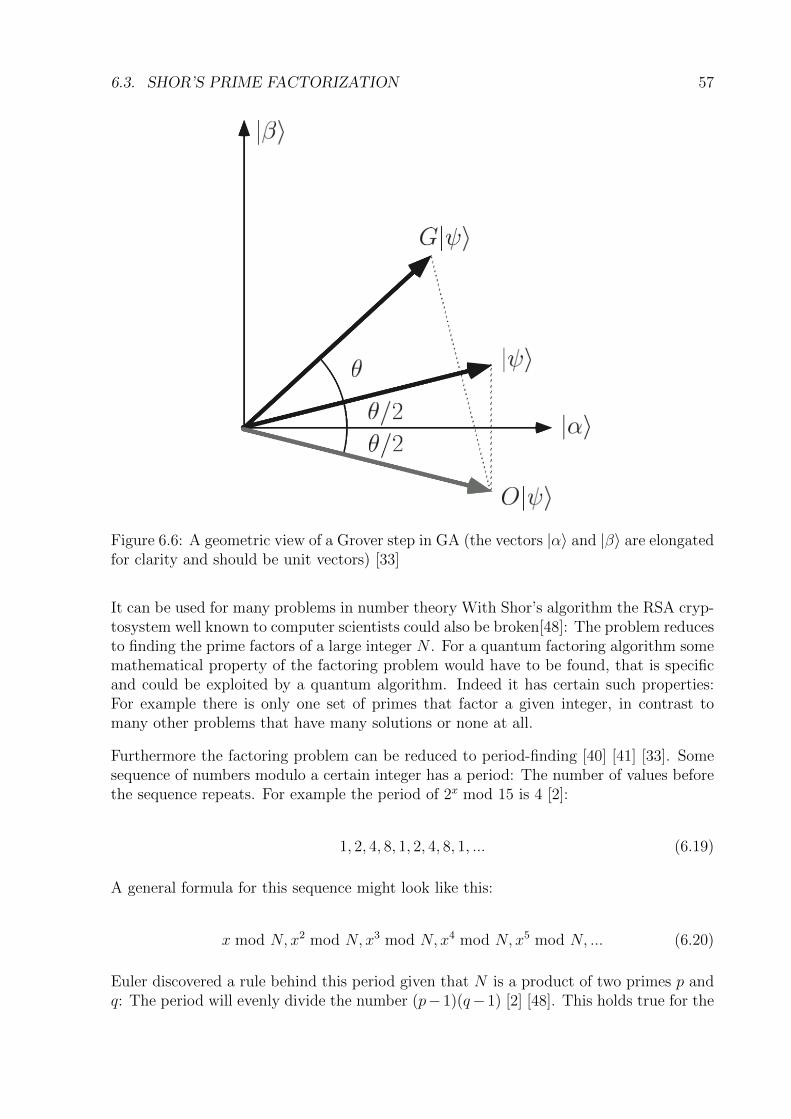
6.3. SHOR’S PRIME FACTORIZATION 57
Figure 6.6: A geometric view of a Grover step in GA (the vectors |α〉 and |β〉 are elongatedfor clarity and should be unit vectors) [33]
It can be used for many problems in number theory With Shor’s algorithm the RSA cryp-tosystem well known to computer scientists could also be broken[48]: The problem reducesto finding the prime factors of a large integer N . For a quantum factoring algorithm somemathematical property of the factoring problem would have to be found, that is specificand could be exploited by a quantum algorithm. Indeed it has certain such properties:For example there is only one set of primes that factor a given integer, in contrast tomany other problems that have many solutions or none at all.
Furthermore the factoring problem can be reduced to period-finding [40] [41] [33]. Somesequence of numbers modulo a certain integer has a period: The number of values beforethe sequence repeats. For example the period of 2x mod 15 is 4 [2]:
1, 2, 4, 8, 1, 2, 4, 8, 1, ... (6.19)
A general formula for this sequence might look like this:
x mod N, x2 mod N, x3 mod N, x4 mod N, x5 mod N, ... (6.20)
Euler discovered a rule behind this period given that N is a product of two primes p andq: The period will evenly divide the number (p−1)(q−1) [2] [48]. This holds true for the

58 CHAPTER 6. QUANTUM ALGORITHMS
example of Equation 6.19 as p and q for N = 15 are 3 and 5, so (p− 1)(q− 1) = 4 ∗ 2 = 8which indeed is evenly divided by the period 4.
Even though the sequence will repeat, the period may be almost as large as N itself [33].This is the reason that there is no classical algorithm solving the problem. A quantumcomputer though could create a superposition over all the numbers in Equation 6.20.Quantum computation cannot magically find the single universe out of all the ones thesuperposition created that satisfies the problem [2]. But because the property of the periodexplained before is a global property, this joint property of all the parallel universes maybe detected. All universes must contribute to this computation.
It is possible to create a superposition of the integers from 1 to N [48]. In order to quicklycompute one element of Equation 6.20 the exponentiation by squaring would be used. Asan example xr where r is 14 and x is 3 is considered[2].
314 = 323+22+21 = ((32)2)2) · (32)2) · 32 (6.21)
Additionally all multiplications can be done moduloN so the numbers become manageable[2]. If such a superposition can be created, the period of the sequence needs to be found.
This is the part of Shor’s algorithm that needs a quantum computer: The quantumfourier transform (QFT) is used [40]. It is similar to the discrete fourier transform usedfor example in signal processing in classical computers, with the difference that it workson the amplitudes of the quantum state i.e. complex numbers [48]. A detailed explanationof QFT goes beyond the scope of this thesis.
The problem might be looked at from the angle of interference: As was mentioned beforethis is the source of all the advantage a quantum computer has over a classical one.Because the amplitudes of the quantum state can cancel each other out. The problem isset up in a way that from a geometrical perspective the periods that are the wrong answerswill cancel each other out [2] [37]. All the parallel universes which contribute somethingto the wrong answer point into different directions whereas the ones that contribute tothe right answer will point into the same direction [2]. So the probability to get a rightanswer after the measurement is high.

Chapter 7
Why, or Why Not, a QuantumComputer?
The reason quantum computers were invented was that classical computers are incapableof simulating a quantum system fully in a reasonable amount of time. The reasons forthis were mentioned in Section 4.4.1.
Actually interference as mentioned in Figure 3.4 is the only thing they are better at [4].At the beginning of the 80s when quantum computing was first proposed physicists didnot know what to do with it except to simulate quantum systems [20]. What quantumcomputers are much better at is matrix multiplication through the advantage of interfer-ence. They could multiply matrices that classic computers would take hundreds of yearsfor in a single step [48]. This makes quantum computation a good candidate for solvingproblems in machine learning or even very complicated ray-tracing [4].
There are severe limitations though: The inputs have to be prepared by humans [33].Every operation has to be unitary (see Postulate 4) which is not always easy to map fromclassical algorithms. Decoherence makes building an actual quantum computer exceed-ingly difficult, as every QuBit tries to interact with its surroundings in an uncontrolledmanner [33]. Nevertheless researchers have decided that the advantages of building areworth the effort.
The advantage of interference can be put to use for classical problems: The most importantreal application of quantum computing is probably simulating quantum systems on aquantum level [3]. Simulating all electrons of only a single carbon atom is intractable onclassical computers [30]. Therefore quantum chemistry would benefit largely. In additionapplications in Biology such as protein folding can be imagined or in physics high energyphysics and superconductivity are possible areas where a quantum computer could benefit.
As was briefly discussed there are other classical problems such as factoring, made possibleby the Quantum Fourier Transform, which would be much more easily solvable on aquantum computer. Additionally Grover’s algorithm has many applications as was shownpreviously.
59
60 CHAPTER 7. WHY, OR WHY NOT, A QUANTUM COMPUTER?
In general solutions to NP-complete problems are not known to exist. This is true for aquantum computer as well. For some problems it could be shown mathematically thatthere is a speedup as was shown previously. One of the problems that researchers face isthat it is not clear for which class of problems there is this speedup [1]. Some problems canbe solved exponentially faster on a quantum computer. For some problems both classicaland quantum computers get stuck on the way to a global optimum [1]. There are evensome problems where classical computers are faster [1].
The only machines sold as quantum computers commercially as of 2015, are produced byD-wave. Prof. Troyer of ETH Zurich could show though that D-Wave’s machine is not areal quantum computer [12]. It is just adiabatic. This means that it is capable of solvingcertain optimization problems exponentially faster but not all the quantum algorithmspresented in this thesis. It is a very specialized processor but no quantum computer [12].
For quantum computers a new complexity class called BQP was introduced [1]. It could beshown mathematically that the maximum speedup that quantum computers can achieveis exponential. This does not affect computability theory though [1]. It is not yet clearif BQP is larger than P or in other words if it striclty contains P. Scott Aaronson et allcould show though that it does contain factoring as well as sampling [5]
One field where quantum effects are already in use today is random number generation:By using quantum effects the highest quality random number generator known to manwas created [3]. Why is its quality so high? It is provable that they are really random,through entanglement and violation of bell inequalities, given that they are not fasterthan light [46].
Similarly quantum cryptography is already in use between two offices of a bank in Switzer-land [42]. The messages exchanged between these two offices are encrypted by help ofthe laws of physics: It is provable that if eavesdropping happens, it is detectable easilybecause measurement changes the quantum state [45]. Quantum cryptography requiresspecial hardware though to work [3].
Another interesting application of the research in quantum computation is Quantummoney which was already put forth in the 70s [3]. The idea is that money would have aserial number but also QuBits. The No-cloning theorem leads to the fact that it is notcounterfeitable [19] [6]. On the same line of thought it would be possible to make quantumcopy-protected software [3].
Some things are impossible in the classic world of computation, some of those are tractablein the quantum world. This is difficult to prove though as impossibility needs to be proven.The researchers working in the field will deepen insight into quantum mechanics whetherthey find more solutions to these intractable problems or not.

Chapter 8
Future Work and Conclusions
This thesis presented a brief overview of a very deep, fascinating and complicated topic.Unfortunately the extent to which this matters can be treated within this short thesis doesnot cover some important aspects of quantum mechanics: The Heisenberg UncertaintyPrinciple which would be important to understand entanglement. A deeper explanation ofdecoherence which was hinted at above, Schrodinger’s Wave equation and its predictionsas well as Bell’s EPR Theorem, Hilbert Spaces, Hamiltonians, the behavior of multiplequbits, the universal quantum computer, quantum algorithms, quantum information the-ory, quantum error correction and quantum cryptography. In general there is too muchto say to fit within this thesis.
The effect of interference of subatomic particles was shown by the help of short programs.Some connections between computer science and quantum computation as well as themost basic of quantum gates could also be shown here in this thesis.
In the future it would be interesting to develop this knowledge further and use such gates insimilar programs as have been illustrating the experiments, and maybe more complicatedones.
61
62 CHAPTER 8. FUTURE WORK AND CONCLUSIONS

Bibliography
[1] Scott Aaronson. Limits on efficient computation in the physical world. arXiv preprintquant-ph/0412143, 2004.
[2] Scott Aaronson. Shor, i will do it. Shtetl-Optimized: The Blog of Scott Aaronson.http://www.scottaaronson.com/blog, 2007.
[3] Scott Aaronson. Quantum copy-protection and quantum money. In ComputationalComplexity, 2009. CCC’09. 24th Annual IEEE Conference on, pages 229–242. IEEE,2009.
[4] Scott Aaronson. Quantum computing since Democritus. Cambridge University Press,2013.
[5] Scott Aaronson and Alex Arkhipov. The computational complexity of linear optics.In Proceedings of the forty-third annual ACM symposium on Theory of computing,pages 333–342. ACM, 2011.
[6] Scott Aaronson and Paul Christiano. Quantum money from hidden subspaces. InProceedings of the forty-fourth annual ACM symposium on Theory of computing,pages 41–60. ACM, 2012.
[7] Markus Arndt, Olaf Nairz, Julian Vos-Andreae, Claudia Keller, Gerbrand Van derZouw, and Anton Zeilinger. Wave–particle duality of c60 molecules. nature,401(6754):680–682, 1999.
[8] Paul Benioff. The computer as a physical system: A microscopic quantum mechan-ical hamiltonian model of computers as represented by turing machines. Journal ofStatistical Physics, 22(5):563–591, 1980.
[9] Charles H Bennett, Ethan Bernstein, Gilles Brassard, and Umesh Vazirani. Strengthsand weaknesses of quantum computing. SIAM journal on Computing, 26(5):1510–1523, 1997.
[10] Chartes H Bennett. Notes on the history of reversible computation. ibm Journal ofResearch and Development, 32(1):16–23, 1988.
[11] David Bohm. Quantum theory. Courier Corporation, 2012.
[12] Sergio Boixo, Troels F Rønnow, Sergei V Isakov, Zhihui Wang, David Wecker,Daniel A Lidar, John M Martinis, and Matthias Troyer. Evidence for quantumannealing with more than one hundred qubits. Nature Physics, 10(3):218–224, 2014.
63
64 BIBLIOGRAPHY
[13] Jill Cirasella. Classical and Quantum Algorithms for Finding Cycles. PhD thesis,Universiteit van Amsterdam, 2006.
[14] Louis De Broglie. Waves and quanta. Nature, 112(2815):540–540, 1923.
[15] David Deutsch. Quantum theory, the church-turing principle and the universal quan-tum computer. In Proceedings of the Royal Society of London A: Mathematical,Physical and Engineering Sciences, volume 400, pages 97–117. The Royal Society,1985.
[16] David Deutsch. Quantum computational networks. In Proceedings of the RoyalSociety of London A: Mathematical, Physical and Engineering Sciences, volume 425,pages 73–90. The Royal Society, 1989.
[17] David Deutsch and Richard Jozsa. Rapid solution of problems by quantum compu-tation. In Proceedings of the Royal Society of London A: Mathematical, Physical andEngineering Sciences, volume 439, pages 553–558. The Royal Society, 1992.
[18] Mostafa Elhoushi, M Watheq El-Kharashi, and Hatem Elrefaei. Modeling a quan-tum processor using the qram model. In Communications, Computers and SignalProcessing (PacRim), 2011 IEEE Pacific Rim Conference on, pages 409–415. IEEE,2011.
[19] Edward Farhi, David Gosset, Avinatan Hassidim, Andrew Lutomirski, and PeterShor. Quantum money from knots. In Proceedings of the 3rd Innovations in Theo-retical Computer Science Conference, pages 276–289. ACM, 2012.
[20] Richard P Feynman. Simulating physics with computers. International journal oftheoretical physics, 21(6):467–488, 1982.
[21] Richard P Feynman, Robert B Leighton, and Matthew Sands. The Feynman Lectureson Physics, Desktop Edition Volume III, volume 3. Basic Books, 2013.
[22] Craig Gidney. Grovers quantum search algorithm. The Blog of Twisted Oak Studios.http://twistedoakstudios.com/blog/, 2013.
[23] Lov K Grover. A fast quantum mechanical algorithm for database search. In Pro-ceedings of the twenty-eighth annual ACM symposium on Theory of computing, pages212–219. ACM, 1996.
[24] Mika Hirvensalo. Quantum computing. Springer, 2013.
[25] Arthur T. Holster. The criterion for time symmetry of probabilistic theories and thereversibility of quantum mechanics. New Journal of Physics, 5(1):130, 2003.
[26] Peter Høyer, Jan Neerbek, and Yaoyun Shi. Quantum complexities of ordered search-ing, sorting, and element distinctness. Algorithmica, 34(4):429–448, 2002.
[27] Claus Kiefer. Why Quantum Gravity? Springer, 2007.
[28] Alexei Yu Kitaev, Alexander Shen, and Mikhail N Vyalyi. Classical and quantumcomputation, volume 47. American Mathematical Society Providence, 2002.

BIBLIOGRAPHY 65
[29] Emmanuel Knill. Conventions for quantum pseudocode. Technical report, Citeseer,1996.
[30] Walter Kohn. Electronic structure of matter: Wave functions and density functionals.CHIMIA-ZURICH-, 54(1/2):50–50, 2000.
[31] Rolf Landauer. Information is physical. IBM Thomas J. Watson Research Division,1992.
[32] Yu I Manin. Vychislimoe i nevychislimoe (computable and noncomputable), moscow:Sov, 1980.
[33] Michael A Nielsen and Isaac L Chuang. Quantum computation and quantum infor-mation. Cambridge university press, 2010.
[34] Roger Penrose and Chris J Isham. Quantum concepts in space and time. ClarendonPress, 1986.
[35] Helmut Rauch and Samuel A Werner. Neutron interferometry: lessons in experimen-tal quantum mechanics. Oxford University Press, 2014.
[36] Mohsen Razavy. Quantum theory of tunneling, volume 1222445599. World Scientific,2003.
[37] Jun John Sakurai and Jim Napolitano. Modern quantum mechanics. Addison-Wesley,2011.
[38] Erwin Schrodinger. Quantisierung als eigenwertproblem. Annalen der physik,385(13):437–490, 1926.
[39] C David Sherrill. A brief review of elementary quantum chemistry. Georgia Instituteof Technology, School of Chemistry and Biochemistry, 2001.
[40] Peter W Shor. Algorithms for quantum computation: Discrete logarithms and factor-ing. In Foundations of Computer Science, 1994 Proceedings., 35th Annual Symposiumon, pages 124–134. IEEE, 1994.
[41] Peter W Shor. Polynomial-time algorithms for prime factorization and discrete log-arithms on a quantum computer. SIAM journal on computing, 26(5):1484–1509,1997.
[42] Damien Stucki, Nicolas Gisin, Olivier Guinnard, Gregoire Ribordy, and HugoZbinden. Quantum key distribution over 67 km with a plug&play system. NewJournal of Physics, 4(1):41, 2002.
[43] Benoıt Valiron, Neil J Ross, Peter Selinger, D Scott Alexander, and Jonathan MSmith. Programming the quantum future. Communications of the ACM, 58(8):52–61, 2015.
[44] Rodney Van Meter and Clare Horsman. A blueprint for building a quantum com-puter. Communications of the ACM, 56(10):84–93, 2013.
66 BIBLIOGRAPHY
[45] Umesh Vazirani and Thomas Vidick. Certifiable quantum dice: or, true randomnumber generation secure against quantum adversaries. In Proceedings of the forty-fourth annual ACM symposium on Theory of computing, pages 61–76. ACM, 2012.
[46] Umesh V Vazirani and Thomas Vidick. Certifiable quantum dice-or, testable expo-nential randomness expansion. arXiv preprint arXiv:1111.6054, 2011.
[47] Wikibooks. Materials in electronics, 2007.
[48] Noson S Yanofsky and Mirco A Mannucci. Quantum computing for computer scien-tists, volume 20. Cambridge University Press Cambridge, 2008.

67

68 APPENDIX A. EXPERIMENT PROGRAM
Appendix A
Experiment Program
1 import random
2 from numpy.ma import absolute, nonzero, cumsum, asarray
3 from numpy.matlib import rand
4 from scipy.linalg import hadamard
5 import math_functions as qmath
6 import sys
7 import numpy
8 import qubit
9 import math
10
11
12 class QuantumEmulator(object):
13 """A simple emulator for a quantum computer written for
illustrative purposes"""→
14
15 def __init__(self):
16 super(QuantumEmulator, self).__init__()
17
18 @staticmethod
19 def enter_initial_state():
20 """Ask user to enter initial state vector"""
21 while True:
22 try:
23 dimensions = int(
24 raw_input("Please enter the number of Dimensions:
"))→
25 break
26 except ValueError:
27 print("Oops! That was no valid number. Try again...")
28 initial_state = numpy.zeros((dimensions, 1))
29 print("")
30 print(
31 "Please enter the initial state of the system one after the
other: ")→
32 i = 0
Listing 29: The quantum emulator including the presented algorithms.
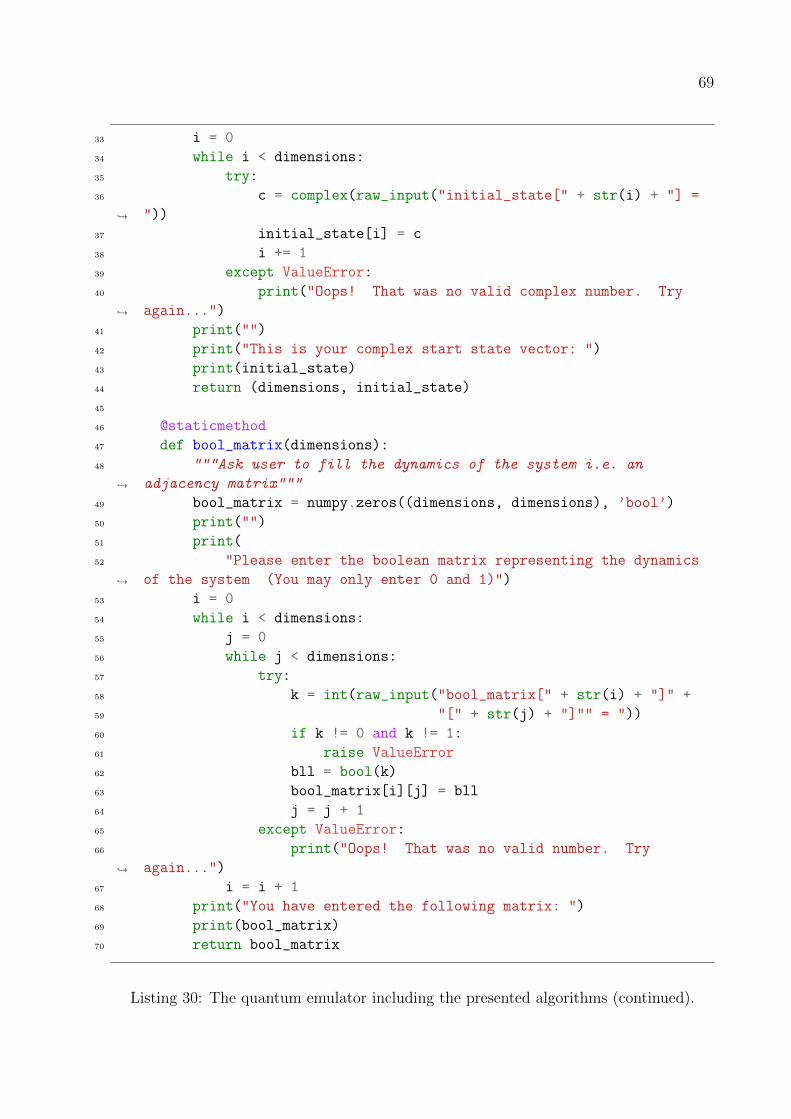
69
33 i = 0
34 while i < dimensions:
35 try:
36 c = complex(raw_input("initial_state[" + str(i) + "] =
"))→
37 initial_state[i] = c
38 i += 1
39 except ValueError:
40 print("Oops! That was no valid complex number. Try
again...")→
41 print("")
42 print("This is your complex start state vector: ")
43 print(initial_state)
44 return (dimensions, initial_state)
45
46 @staticmethod
47 def bool_matrix(dimensions):
48 """Ask user to fill the dynamics of the system i.e. an
adjacency matrix"""→
49 bool_matrix = numpy.zeros((dimensions, dimensions), ’bool’)
50 print("")
51 print(
52 "Please enter the boolean matrix representing the dynamics
of the system (You may only enter 0 and 1)")→
53 i = 0
54 while i < dimensions:
55 j = 0
56 while j < dimensions:
57 try:
58 k = int(raw_input("bool_matrix[" + str(i) + "]" +
59 "[" + str(j) + "]"" = "))
60 if k != 0 and k != 1:
61 raise ValueError
62 bll = bool(k)
63 bool_matrix[i][j] = bll
64 j = j + 1
65 except ValueError:
66 print("Oops! That was no valid number. Try
again...")→
67 i = i + 1
68 print("You have entered the following matrix: ")
69 print(bool_matrix)
70 return bool_matrix
Listing 30: The quantum emulator including the presented algorithms (continued).

70 APPENDIX A. EXPERIMENT PROGRAM
71 @staticmethod
72 def frac_matrix(dimensions):
73 """Ask user to fill the dynamics of the system i.e. a
74 doubly stochastic matrix"""
75 frac_matrix = numpy.zeros((dimensions, dimensions), ’float’)
76 print("")
77 print(
78 "Please enter the fractional matrix representing the
dynamics of the system (You may only enter values between 0 and 1)")→
79 i = 0
80 while i < dimensions:
81 j = 0
82 # try:
83 while j < dimensions:
84 try:
85 k = float(raw_input("frac_matrix[" + str(i) + "]" +
86 "[" + str(j) + "]"" = "))
87 if k < 0 or k > 1:
88 raise ValueError
89 frac = bool(k)
90 frac_matrix[i][j] = frac
91 j = j + 1
92 except ValueError:
93 print("Oops! That was no valid number. Try
again...")→
94 # except sum(frac_matrix[i]) > 1
95 # print("Row " + str(i) + " is not doubly stochastic!")
96 i = i + 1
97 """column_sums = frac_matrix.sum(axis=0)
98 for i in range(len(column_sums)):
99 if column_sums[i] < 0 or column_sums[i] > 1:
100 print("Column " + str(i) + " is not doubly stochastic
as its sum is " + str(column_sums[i]))"""→
101 print("You have entered the following matrix: ")
102 print(frac_matrix)
103 return frac_matrix
104
105 @staticmethod
106 def complex_matrix(dimensions):
107 """Ask user to fill the dynamics of the system i.e. a complex
matrix"""→
108 # Initiliazie matrix; D stands for complex entries
109 complex_matrix = numpy.zeros((dimensions, dimensions), ’D’)
110 print("")
Listing 31: The quantum emulator including the presented algorithms (continued).
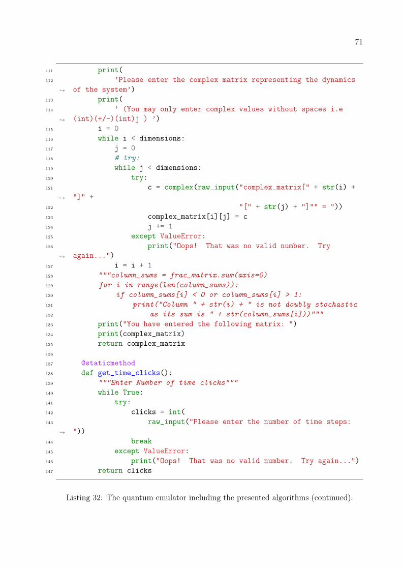
71
111 print(
112 ’Please enter the complex matrix representing the dynamics
of the system’)→
113 print(
114 ’ (You may only enter complex values without spaces i.e
(int)(+/-)(int)j ) ’)→
115 i = 0
116 while i < dimensions:
117 j = 0
118 # try:
119 while j < dimensions:
120 try:
121 c = complex(raw_input("complex_matrix[" + str(i) +
"]" +→
122 "[" + str(j) + "]"" = "))
123 complex_matrix[i][j] = c
124 j += 1
125 except ValueError:
126 print("Oops! That was no valid number. Try
again...")→
127 i = i + 1
128 """column_sums = frac_matrix.sum(axis=0)
129 for i in range(len(column_sums)):
130 if column_sums[i] < 0 or column_sums[i] > 1:
131 print("Column " + str(i) + " is not doubly stochastic
132 as its sum is " + str(column_sums[i]))"""
133 print("You have entered the following matrix: ")
134 print(complex_matrix)
135 return complex_matrix
136
137 @staticmethod
138 def get_time_clicks():
139 """Enter Number of time clicks"""
140 while True:
141 try:
142 clicks = int(
143 raw_input("Please enter the number of time steps:
"))→
144 break
145 except ValueError:
146 print("Oops! That was no valid number. Try again...")
147 return clicks
Listing 32: The quantum emulator including the presented algorithms (continued).
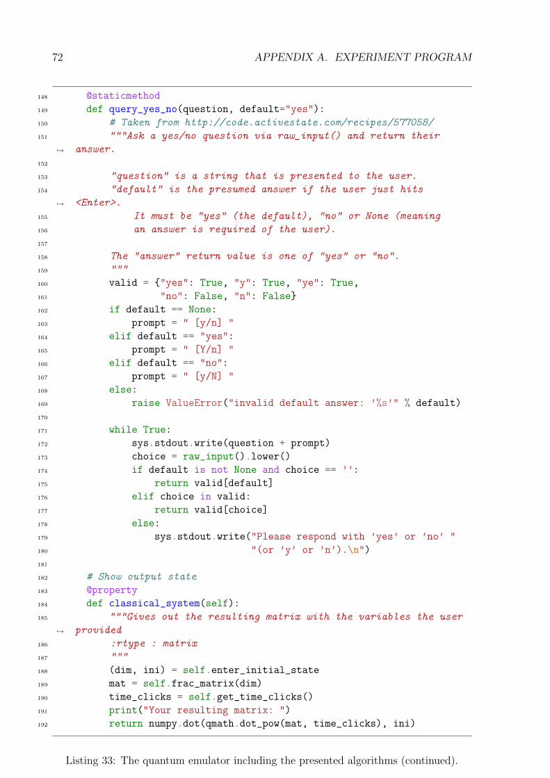
72 APPENDIX A. EXPERIMENT PROGRAM
148 @staticmethod
149 def query_yes_no(question, default="yes"):
150 # Taken from http://code.activestate.com/recipes/577058/
151 """Ask a yes/no question via raw_input() and return their
answer.→
152
153 "question" is a string that is presented to the user.
154 "default" is the presumed answer if the user just hits
<Enter>.→
155 It must be "yes" (the default), "no" or None (meaning
156 an answer is required of the user).
157
158 The "answer" return value is one of "yes" or "no".
159 """
160 valid = "yes": True, "y": True, "ye": True,
161 "no": False, "n": False
162 if default == None:
163 prompt = " [y/n] "
164 elif default == "yes":
165 prompt = " [Y/n] "
166 elif default == "no":
167 prompt = " [y/N] "
168 else:
169 raise ValueError("invalid default answer: ’%s’" % default)
170
171 while True:
172 sys.stdout.write(question + prompt)
173 choice = raw_input().lower()
174 if default is not None and choice == ’’:
175 return valid[default]
176 elif choice in valid:
177 return valid[choice]
178 else:
179 sys.stdout.write("Please respond with ’yes’ or ’no’ "
180 "(or ’y’ or ’n’).\n")
181
182 # Show output state
183 @property
184 def classical_system(self):
185 """Gives out the resulting matrix with the variables the user
provided→
186 :rtype : matrix
187 """
188 (dim, ini) = self.enter_initial_state
189 mat = self.frac_matrix(dim)
190 time_clicks = self.get_time_clicks()
191 print("Your resulting matrix: ")
192 return numpy.dot(qmath.dot_pow(mat, time_clicks), ini)
Listing 33: The quantum emulator including the presented algorithms (continued).

73
193 def observables(self, dim, ini):
194 # Observables
195 try:
196 print(’Enter a valid observable’)
197 observable = self.complex_matrix(dim)
198 except not qmath.is_hermitian(observable):
199 print("Please enter a hermitian matrix!")
200 observable_eigvals = numpy.linalg.linalg.eigvals(observable)
201 print("Eigenvalues of observable (i.e. the possible results of
a measurement): " +→
202 str(observable_eigvals))
203 print("The average value of the observable on the given initial
state is: " +→
204 str(qmath.average(observable, ini)))
205 print("The variance of the observable on the given initial
state is: " +→
206 str(qmath.variance(observable, ini)))
207 ps = list()
208 for i in range(len(observable_eigvals)):
209 ps.append(qmath.projection(ini, observable_eigvals[i]))
210 print("The probabilty of the initial state to transition to
eigenvalue " +→
211 str(observable_eigvals[i]) + " amounts to: " + ps[i])
212 # TODO: plot ps distribution
213
214 def quantum_system(self):
215 # Enter ket vector
216 (dim, ini) = self.enter_complex_state()
217 if self.query_yes_no(’Would you like to enter another quantum
state?’, ’no’):→
218 b = self.enter_complex_state(dim)
219 print(’The probabilty of transitioning from the first to
the second state is: ’ +→
220 qmath.inner_product(ini, b))
221 return ’Thank you’
222 self.observables(dim, ini)
223 # Dynamics
224 ts = self.get_time_clicks()
225 print(’Please enter the dynamics of the system’)
226 dynamics = list()
227 dynamics.append(self.complex_matrix(dim))
228 while self.query_yes_no(’Would you like to add another gate to
the sequence?’, ’no’):→
229 dynamics.append(self.complex_matrix(dim))
230 print(’t0: ’ + str(ini))
231 tmp = numpy.dot(dynamics.pop(), ini)
232 print(’t1: ’ + tmp)
233 i = 2
Listing 34: The quantum emulator including the presented algorithms (continued).

74 APPENDIX A. EXPERIMENT PROGRAM
234 while dynamics:
235 print("t" + i + ": ")
236 i += 1
237 numpy.dot(dynamics.pop(), tmp)
238
239 return qmath.normalize(ini)
240
241 def is_balanced_quantum(self, function_matrix):
242 """ Deutsch’s quantum algorithm: Answers the question if a
given function is balanced or not"""→
243 """
244 Test for balanced:
245 U_f_3 = np.matrix(’0 1 0 0; 1 0 0 0; 0 0 1 0; 0
0 0 1’)→
246 Test for constant:
247 np.identity(4)
248 """
249 # function_matrix = numpy.fromfunction(function, (2,2))
250 unitary = qmath.is_unitary(function_matrix)
251 if unitary == False:
252 raise ValueError("not unitary!")
253 psi0 = numpy.kron(qubit.QuBit(0), qubit.QuBit(1))
254 print "psi0:\n", psi0
255
256 # For clarity; the kronecker product of two hadamard(2, ...)
would be→
257 # equivalent to following hadamard gate
258 qhadamard = 1 / math.sqrt(2) * hadamard(2, dtype=complex)
259 # qhadamard(4, dtype=complex)
260 two_qubit_hadamard = numpy.kron(qhadamard, qhadamard)
261
262 psi1 = numpy.dot(two_qubit_hadamard, psi0)
263 print "psi1:\n", psi1
264
265 psi2 = numpy.dot(function_matrix, psi1)
266 print "psi2:\n", psi2
267
268 hadamard_identity = numpy.kron(
269 qhadamard,
270 numpy.identity(2)
271 )
272 print hadamard_identity
Listing 35: The quantum emulator including the presented algorithms (continued).

75
273 psi3 = numpy.dot(hadamard_identity, psi2)
274 print "psi3:\n", psi3
275
276 result = self.measure(psi3)
277 print(result)
278
279 @staticmethod
280 def is_balanced_classical(function):
281 f0 = function(0)
282 f1 = function(1)
283
284 if f0 == f1:
285 return False
286 elif f0 != f1:
287 return True
288
289 def grover_classical(self, function_classical, N):
290 solution = 0
291 for x in xrange(N):
292 if function_classical(x) == True:
293 solution = x
294 return solution
295
296 def grovers(self, function_matrix):
297 """
298 One grover step equals multiplying the state by the following
matrices in order→
299 [function_matrix, all_qubit_hadamard, diffusion_operator,
all_qubit_hadamard]→
300
301 :param function_matrix:
302 :return:
303 """
304 assert isinstance(function_matrix, numpy.ndarray)
305 if qmath.is_unitary(function_matrix) == False:
306 raise ValueError("not unitary!")
307
308 # Number of qubits
309 n = function_matrix.shape[0] / 2
310
311 # Prepare gates
312 # 1) Hadamard for superpositions
313 qhadamard = 1 / math.sqrt(2) * hadamard(2, dtype=complex)
314 all_qubit_hadamard = numpy.kron(qhadamard, qhadamard)
315 for x in xrange(1, n - 1):
316 all_qubit_hadamard = numpy.kron(all_qubit_hadamard,
qhadamard)→
Listing 36: The quantum emulator including the presented algorithms (continued).
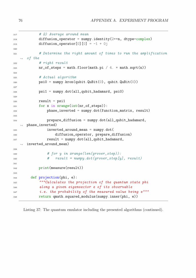
76 APPENDIX A. EXPERIMENT PROGRAM
317 # 2) Average around mean
318 diffusion_operator = numpy.identity(2**n, dtype=complex)
319 diffusion_operator[0][0] = -1 + 0j
320
321 # Determine the right amount of times to run the amplification
of the→
322 # right result
323 nr_of_steps = math.floor(math.pi / 4. * math.sqrt(n))
324
325 # Actual algorithm
326 psi0 = numpy.kron(qubit.QuBit(0), qubit.QuBit(0))
327
328 psi1 = numpy.dot(all_qubit_hadamard, psi0)
329
330 result = psi1
331 for x in xrange(int(nr_of_steps)):
332 phase_inverted = numpy.dot(function_matrix, result)
333
334 prepare_diffusion = numpy.dot(all_qubit_hadamard,
phase_inverted)→
335 inverted_around_mean = numpy.dot(
336 diffusion_operator, prepare_diffusion)
337 result = numpy.dot(all_qubit_hadamard,
inverted_around_mean)→
338
339 # for y in xrange(len(grover_step)):
340 # result = numpy.dot(grover_step[y], result)
341
342 print(measure(result))
343
344 def projection(phi, e):
345 """Calculates the projection of the quantum state phi
346 along a given eigenvector e of its observable
347 i.e. the probability of the measured value being e"""
348 return qmath.squared_modulus(numpy.inner(phi, e))
Listing 37: The quantum emulator including the presented algorithms (continued).
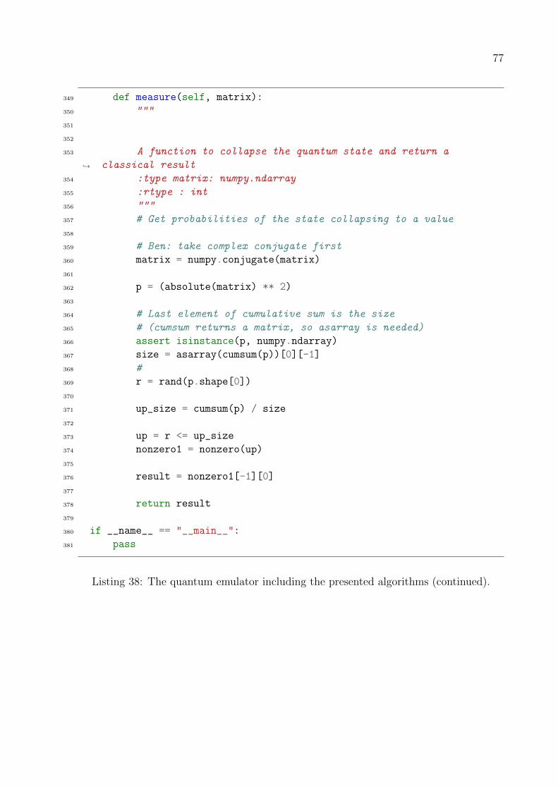
77
349 def measure(self, matrix):
350 """
351
352
353 A function to collapse the quantum state and return a
classical result→
354 :type matrix: numpy.ndarray
355 :rtype : int
356 """
357 # Get probabilities of the state collapsing to a value
358
359 # Ben: take complex conjugate first
360 matrix = numpy.conjugate(matrix)
361
362 p = (absolute(matrix) ** 2)
363
364 # Last element of cumulative sum is the size
365 # (cumsum returns a matrix, so asarray is needed)
366 assert isinstance(p, numpy.ndarray)
367 size = asarray(cumsum(p))[0][-1]
368 #
369 r = rand(p.shape[0])
370
371 up_size = cumsum(p) / size
372
373 up = r <= up_size
374 nonzero1 = nonzero(up)
375
376 result = nonzero1[-1][0]
377
378 return result
379
380 if __name__ == "__main__":
381 pass
Listing 38: The quantum emulator including the presented algorithms (continued).

78 APPENDIX A. EXPERIMENT PROGRAM
1 import numpy
2
3
4 class QuBit(numpy.ndarray):
5 """Constructs a qubit (single column matrix) with the given
amplitudes→
6 QuBit(0) => c * |0> = [1 0]T
7 QuBit(1) => c * |1> = [0 1]T
8
9 c1/2 normalized!
10
https://www.mathworks.com/matlabcentral/newsreader/view_thread/19684→
11 """
12
13 def __new__(cls, i=2):
14 cls.i = i
15 qubit = numpy.zeros((2, 1), ’D’)
16 if i == 0:
17 qubit[0] = 1
18 elif i == 1:
19 qubit[1] = 1
20 else:
21 print(’A qubit is binary: Please supply either a 0 or a 1
as parameter’)→
22 return qubit
Listing 39: The implementation of the qubit.
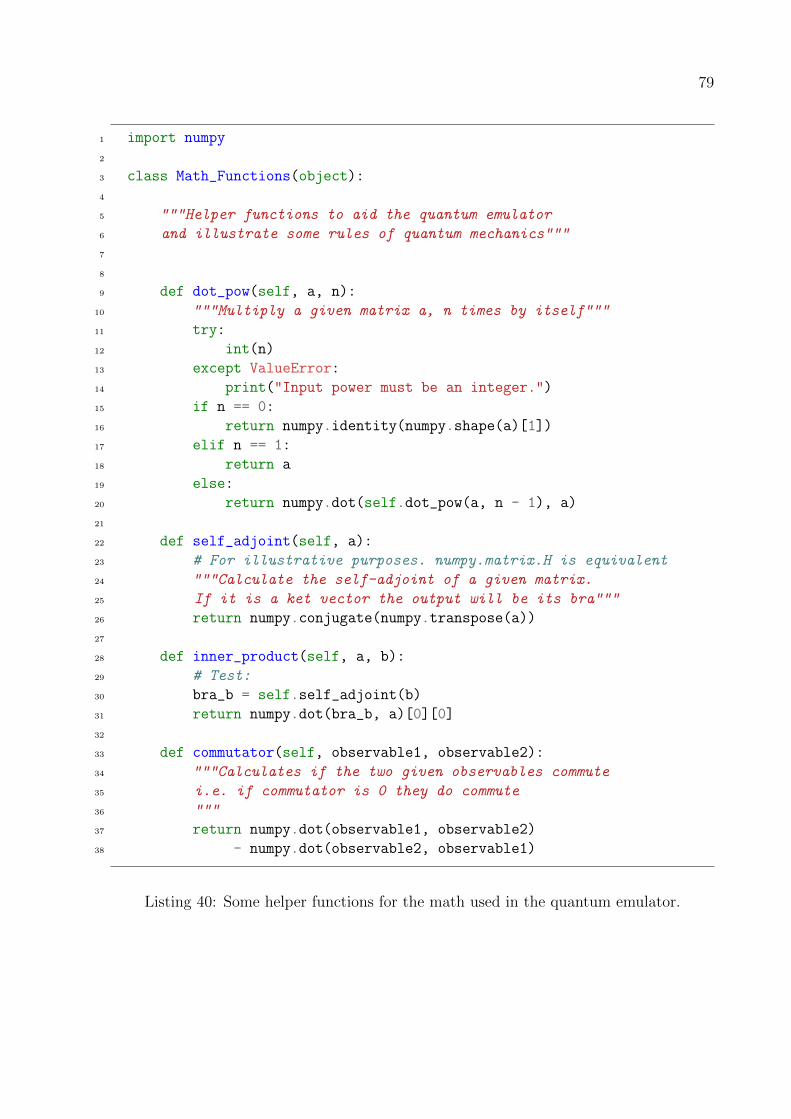
79
1 import numpy
2
3 class Math_Functions(object):
4
5 """Helper functions to aid the quantum emulator
6 and illustrate some rules of quantum mechanics"""
7
8
9 def dot_pow(self, a, n):
10 """Multiply a given matrix a, n times by itself"""
11 try:
12 int(n)
13 except ValueError:
14 print("Input power must be an integer.")
15 if n == 0:
16 return numpy.identity(numpy.shape(a)[1])
17 elif n == 1:
18 return a
19 else:
20 return numpy.dot(self.dot_pow(a, n - 1), a)
21
22 def self_adjoint(self, a):
23 # For illustrative purposes. numpy.matrix.H is equivalent
24 """Calculate the self-adjoint of a given matrix.
25 If it is a ket vector the output will be its bra"""
26 return numpy.conjugate(numpy.transpose(a))
27
28 def inner_product(self, a, b):
29 # Test:
30 bra_b = self.self_adjoint(b)
31 return numpy.dot(bra_b, a)[0][0]
32
33 def commutator(self, observable1, observable2):
34 """Calculates if the two given observables commute
35 i.e. if commutator is 0 they do commute
36 """
37 return numpy.dot(observable1, observable2)
38 - numpy.dot(observable2, observable1)
Listing 40: Some helper functions for the math used in the quantum emulator.

80 APPENDIX A. EXPERIMENT PROGRAM
39 def projection(self, phi, e):
40 # Actually sum(projection(phi, e)[0])
41 """Calculates the projection of the quantum state phi
42 along a given eigenvector e of its observable
43 i.e. the probability of the measured value being e"""
44 return self.squared_modulus(numpy.inner(phi, e))
45
46 def average(self, observable, phi):
47 """Calculates the average value of observable on quantum state
phi"""→
48 return numpy.dot(self.self_adjoint(numpy.dot(observable, phi)),
phi)→
49
50 def variance(self, observable, phi):
51 """ BLA """
52 demeanedObservable = observable - self.average(observable, phi)
53 return numpy.dot(numpy.dot(self.self_adjoint(phi),
54 self.dot_pow(demeanedObservable, 2)), phi)
55
56 def is_unitary(self, a):
57 """Produces True if the given matrix is unitary"""
58 try:
59 identity_a = numpy.identity(numpy.shape(a)[1])
60 # Due to allclose: Rounding error up to 1*e-8 allowed
61 self_adjoint = self.self_adjoint(a)
62 dot = numpy.dot(a, self_adjoint)
63 result = numpy.array_equal(dot, identity_a)
64 return result
65 except (TypeError, NotImplemented):
66 print(’Please enter a valid matrix.’)
67
68 def is_hermitian(self, a):
69 """Produces True if the given matrix is hermitian"""
70 # Due to allclose: Rounding error up to 1*e-8 allowed
71 return numpy.allclose(a, self.self_adjoint(a))
72
73 def squared_modulus(self, a):
74 """Returns the squared modulus of a matrix or number"""
75 try:
76 return abs(a)**2
77 except TypeError:
78 print("You cannot take the absolute of this value.")
Listing 41: Some helper functions for the math used in the quantum emulator (continued).

81
79 def normalize(self, a):
80 """Returns the normalized representation of vector a"""
81 try:
82 len_a = numpy.norm(a) # ==.
numpy.sqrt(sum(squared_modulus(a)))→
83 return 1. / len_a * a
84 except (TypeError, RuntimeWarning, AttributeError):
85 print(str(a) + " cannot be normalized!")
86
87 def particle_position_probability(self, a, pos):
88 """Returns an array of the probabilities of finding a particle
89 at a certain position within the given state described by
a"""→
90 self.normalize(a)[pos]
91
92 _inst = Math_Functions()
93 is_unitary = _inst.is_unitary
94 inner_product = _inst.inner_product
95 self_adjoint = _inst.self_adjoint
96 is_hermitian = _inst.is_hermitian
97 normalize = _inst.normalize
98 squared_modulus = _inst.squared_modulus
99 dot_pow = _inst.dot_pow
100
101 if __name__ == ’__main__’:
102 pass
Listing 42: Some helper functions for the math used in the quantum emulator (continued).


![CPS 590 4:CPS 590.4: Computational Microeconomics: Game ... · computation and its applications. […] A computer scientist specializes in the theory of computation and the design](https://img.pdfslide.us/doc/110x75/5e979a4e2ab3d9666b33c72e/cps-590-4cps-5904-computational-microeconomics-game-computation-and-its.jpg)