Quantum Computation andits Applications to AI

James McGivernComputer Science BSc.

August 23, 2005

scs2jsm@comp.leeds.ac.uk

School of Computing,University of Leeds,

Leeds,United Kingdom,

LS2 1HE

The candidate confirms that the work submitted is their own and the appropriate credit hasbeen given where reference has been made to the work of others.

I understand that failure to attribute material which is obtained from another source may beconsidered as plagiarism.

(Signed by Candidate)

Precis

The aim of this paper is to motivate the hypothesis that the model of computation derivedfrom quantum mechanics is comparable but not equal to the Turing, or “classical”, model.Instead, that Quantum Computation has features which do not correspond to any of theTuring model. And, as such, is the equivalent of Einstein’s relativity to Newton’s dynamics,a refinement of the existing theory. Foremost in this discussion is the concept of Quantum

Complexity Classes analogous to the classical complexity classes. We demonstrate by exam-ple problems, topical to the field of artificial intelligence, that there exist quantum algorithmswhich are more efficient than any current classical algorithm.

i

Foreword

The theory of computation has traditionally been studied almost entirely in the ab-stract, as a topic in pure mathematics. This is to miss the point of it. Computersare physical objects, and computations are physical processes. What computers canor can not compute is determined by the laws of physics alone, and not by puremathematics.

–David Deutsch

This dissertation concludes my Bachelor of Science in Computer Science at the Universityof Leeds. Many of the references in the bibliography are cited as appearing in the Los AlamosePrint journal, while this is not incorrect it may be somewhat misleading since the majority ofthose papers have been published in other journals also. The reason behind this is that, unlikemany of the electronic copies of traditional journals (e.g Physical Review A), the documentsheld at arXiv.org are free to access anonymously. It is felt that by doing this interested readersare able to easily attain original sources.

ii

Contents

Precis i

Foreword ii

Table of Contents iii

1 Introduction 1

1.1 Mathematics of Quantum Mechanics . . . . . . . . . . . . . . . . . . . . . . . . . 11.1.1 Dirac Notation . . . . . . . . . . . . . . . . . . . . . . . . . . . . . . . . . 21.1.2 Tensor Products . . . . . . . . . . . . . . . . . . . . . . . . . . . . . . . . 3

1.2 The Axioms of Quantum Mechanics . . . . . . . . . . . . . . . . . . . . . . . . . 3

2 Elements of Quantum Computation 5

2.1 Qubits And Operators . . . . . . . . . . . . . . . . . . . . . . . . . . . . . . . . . 52.1.1 The Qubit . . . . . . . . . . . . . . . . . . . . . . . . . . . . . . . . . . . . 52.1.2 Measurement of Single Qubits . . . . . . . . . . . . . . . . . . . . . . . . . 6

2.2 Single Qubit Operators . . . . . . . . . . . . . . . . . . . . . . . . . . . . . . . . 62.2.1 The Pauli Operators . . . . . . . . . . . . . . . . . . . . . . . . . . . . . . 62.2.2 The Hadamard Transform . . . . . . . . . . . . . . . . . . . . . . . . . . . 7

2.3 Quantum Registers . . . . . . . . . . . . . . . . . . . . . . . . . . . . . . . . . . . 82.4 Quantum Measurement . . . . . . . . . . . . . . . . . . . . . . . . . . . . . . . . 82.5 Multiple Qubit Operators . . . . . . . . . . . . . . . . . . . . . . . . . . . . . . . 9

2.5.1 The Hadamard Transform... Again . . . . . . . . . . . . . . . . . . . . . . 92.5.2 The Controlled NOT & Other Controlled Gates . . . . . . . . . . . . . . . 10

2.6 Entanglement . . . . . . . . . . . . . . . . . . . . . . . . . . . . . . . . . . . . . . 102.7 Laws of Quantum Information . . . . . . . . . . . . . . . . . . . . . . . . . . . . 11

2.7.1 No-deleting Principle . . . . . . . . . . . . . . . . . . . . . . . . . . . . . . 122.7.2 No-cloning Principle . . . . . . . . . . . . . . . . . . . . . . . . . . . . . . 12

2.8 Errors in Quantum Computation . . . . . . . . . . . . . . . . . . . . . . . . . . . 132.9 Summary . . . . . . . . . . . . . . . . . . . . . . . . . . . . . . . . . . . . . . . . 14

iii

3 Quantum Algorithms and Complexity 15

3.1 Quantum Turing Machines . . . . . . . . . . . . . . . . . . . . . . . . . . . . . . 153.2 Classes of Quantum Problems . . . . . . . . . . . . . . . . . . . . . . . . . . . . . 163.3 A Circuit Model of Quantum Computation . . . . . . . . . . . . . . . . . . . . . 18

3.3.1 Black Boxes And Oracles . . . . . . . . . . . . . . . . . . . . . . . . . . . 183.3.2 Universal Families of Quantum Gates . . . . . . . . . . . . . . . . . . . . 183.3.3 Quantum Circuits and QTMs . . . . . . . . . . . . . . . . . . . . . . . . . 18

3.4 Significant Quantum Algorithms . . . . . . . . . . . . . . . . . . . . . . . . . . . 183.4.1 Quantum Teleportation . . . . . . . . . . . . . . . . . . . . . . . . . . . . 183.4.2 Quantum Fourier Transform . . . . . . . . . . . . . . . . . . . . . . . . . 183.4.3 Grover’s Search Algorithm . . . . . . . . . . . . . . . . . . . . . . . . . . . 19

4 Introduction to Quantum Artificial Intelligence 21

4.1 Fundamentals of AI . . . . . . . . . . . . . . . . . . . . . . . . . . . . . . . . . . 224.1.1 Agents . . . . . . . . . . . . . . . . . . . . . . . . . . . . . . . . . . . . . . 224.1.2 The SAT Problem . . . . . . . . . . . . . . . . . . . . . . . . . . . . . . . 22

4.2 Quantum Neurocomputing . . . . . . . . . . . . . . . . . . . . . . . . . . . . . . . 234.2.1 Biological Neurons . . . . . . . . . . . . . . . . . . . . . . . . . . . . . . . 234.2.2 Artificial Neurons . . . . . . . . . . . . . . . . . . . . . . . . . . . . . . . 244.2.3 Neural Networks . . . . . . . . . . . . . . . . . . . . . . . . . . . . . . . . 254.2.4 Neural Networks as Graphs . . . . . . . . . . . . . . . . . . . . . . . . . . 25

5 Utilising Quantum Algorithms in AI 27

5.1 Phase Estimation . . . . . . . . . . . . . . . . . . . . . . . . . . . . . . . . . . . . 275.2 Amplitude Amplification . . . . . . . . . . . . . . . . . . . . . . . . . . . . . . . . 285.3 Quantum Searching . . . . . . . . . . . . . . . . . . . . . . . . . . . . . . . . . . 285.4 Assailing NP . . . . . . . . . . . . . . . . . . . . . . . . . . . . . . . . . . . . . . 285.5 Constraint Satisfaction Problems . . . . . . . . . . . . . . . . . . . . . . . . . . . 285.6 Quantum Planning . . . . . . . . . . . . . . . . . . . . . . . . . . . . . . . . . . . 28

6 Physical Realisations of Quantum Computers 29

6.1 Quantum Physics and Qubits . . . . . . . . . . . . . . . . . . . . . . . . . . . . . 296.1.1 Nuclear Spin . . . . . . . . . . . . . . . . . . . . . . . . . . . . . . . . . . 30

6.2 The DiVincenzo Criteria . . . . . . . . . . . . . . . . . . . . . . . . . . . . . . . . 306.3 Emergent Quantum Technologies . . . . . . . . . . . . . . . . . . . . . . . . . . . 33

6.3.1 Bulk Spin NMR . . . . . . . . . . . . . . . . . . . . . . . . . . . . . . . . 336.3.2 Solid State Quantum Devices . . . . . . . . . . . . . . . . . . . . . . . . . 346.3.3 Summary . . . . . . . . . . . . . . . . . . . . . . . . . . . . . . . . . . . . 36

7 Quantum Robotics 37

7.1 Quantum Robots . . . . . . . . . . . . . . . . . . . . . . . . . . . . . . . . . . . . 377.2 Q-Bots . . . . . . . . . . . . . . . . . . . . . . . . . . . . . . . . . . . . . . . . . . 387.3 A Hybrid System Architecture . . . . . . . . . . . . . . . . . . . . . . . . . . . . 39

7.3.1 Quantum Processing Units . . . . . . . . . . . . . . . . . . . . . . . . . . 39

iv

7.3.2 A Quantum Communication Unit . . . . . . . . . . . . . . . . . . . . . . 407.3.3 Agent Function . . . . . . . . . . . . . . . . . . . . . . . . . . . . . . . . . 427.3.4 Vision, Other Sensors and Actuators . . . . . . . . . . . . . . . . . . . . . 42

8 Discussion & Concluding Remarks 43

8.1 Quantum Computation . . . . . . . . . . . . . . . . . . . . . . . . . . . . . . . . 438.2 Quantum Technologies . . . . . . . . . . . . . . . . . . . . . . . . . . . . . . . . . 448.3 Quantum Algorithms for Classical AI Problems . . . . . . . . . . . . . . . . . . . 458.4 Prospects for Quantum AI . . . . . . . . . . . . . . . . . . . . . . . . . . . . . . . 45

9 Disserting a Dissertation 46

9.1 Storming . . . . . . . . . . . . . . . . . . . . . . . . . . . . . . . . . . . . . . . . 469.2 Forming . . . . . . . . . . . . . . . . . . . . . . . . . . . . . . . . . . . . . . . . . 479.3 Norming . . . . . . . . . . . . . . . . . . . . . . . . . . . . . . . . . . . . . . . . . 489.4 Disseminating . . . . . . . . . . . . . . . . . . . . . . . . . . . . . . . . . . . . . . 48

Appendix.

A Personal Reflection of Project 50

A.1 Quantum Computation and Quantum Information is Hard . . . . . . . . . . . . . 50A.2 Presenting Your Own Work is Hard . . . . . . . . . . . . . . . . . . . . . . . . . 50A.3 Presenting Other Peoples’ Work is Hard . . . . . . . . . . . . . . . . . . . . . . . 51A.4 Sagely Advice . . . . . . . . . . . . . . . . . . . . . . . . . . . . . . . . . . . . . . 51

B Writing a Technical Paper 52

B.1 Conception and Research . . . . . . . . . . . . . . . . . . . . . . . . . . . . . . . 52B.2 Developing and Reporting . . . . . . . . . . . . . . . . . . . . . . . . . . . . . . . 53

C Notes on Mathematics 55

C.1 Abstract Algebra . . . . . . . . . . . . . . . . . . . . . . . . . . . . . . . . . . . . 55C.1.1 Groups and Fields . . . . . . . . . . . . . . . . . . . . . . . . . . . . . . . 55

C.2 Linear Algebra . . . . . . . . . . . . . . . . . . . . . . . . . . . . . . . . . . . . . 56C.2.1 Vector Spaces . . . . . . . . . . . . . . . . . . . . . . . . . . . . . . . . . . 56C.2.2 Linear Operators . . . . . . . . . . . . . . . . . . . . . . . . . . . . . . . . 58C.2.3 Hilbert Spaces . . . . . . . . . . . . . . . . . . . . . . . . . . . . . . . . . 59C.2.4 Tensor Products . . . . . . . . . . . . . . . . . . . . . . . . . . . . . . . . 59C.2.5 Unitary Operators . . . . . . . . . . . . . . . . . . . . . . . . . . . . . . . 60

D Notes on Quantum Topics 61

D.1 History of Quantum Mechanics . . . . . . . . . . . . . . . . . . . . . . . . . . . . 61D.1.1 The Ultraviolet Catastrophe . . . . . . . . . . . . . . . . . . . . . . . . . . 61D.1.2 The Photoelectric Effect . . . . . . . . . . . . . . . . . . . . . . . . . . . . 62D.1.3 Wave-Particle Duality . . . . . . . . . . . . . . . . . . . . . . . . . . . . . 63D.1.4 A Note On Quantum Physics . . . . . . . . . . . . . . . . . . . . . . . . . 63

v

D.2 Matrix Representations of Quantum Transforms . . . . . . . . . . . . . . . . . . 64D.2.1 The Controlled Not . . . . . . . . . . . . . . . . . . . . . . . . . . . . . . 64

D.3 The No-Deleting Theorem . . . . . . . . . . . . . . . . . . . . . . . . . . . . . . . 64D.4 Quantum Fourier Transform . . . . . . . . . . . . . . . . . . . . . . . . . . . . . . 64

D.4.1 Unitary . . . . . . . . . . . . . . . . . . . . . . . . . . . . . . . . . . . . . 64D.5 The Local Hamiltonian Problem . . . . . . . . . . . . . . . . . . . . . . . . . . . 65D.6 Quantum Computation and Physical Systems . . . . . . . . . . . . . . . . . . . . 65

D.6.1 A Square-Well Qubit . . . . . . . . . . . . . . . . . . . . . . . . . . . . . . 65D.6.2 Trapped Ion Quantum Computers . . . . . . . . . . . . . . . . . . . . . . 66

E Notes on Artificial Intelligence 68

E.1 Backus-Naur Form . . . . . . . . . . . . . . . . . . . . . . . . . . . . . . . . . . . 68E.2 Boolean Logic . . . . . . . . . . . . . . . . . . . . . . . . . . . . . . . . . . . . . . 68

Bibliography 71

vi

Chapter 1Introduction

The aim of this paper was fourfold; to introduce a theory of computation based on the physicallaws of quantum mechanics, consider the construction of devices capable of quantum computa-tion, study the potential use of quantum algorithms in artificial intelligence, and to augment aclassical agent with quantum computation and technologies. In order to analyse the potentialoffered by the synthesis of quantum computation and artificial intelligence we must considernot just the model of computation but also the motivation of the physical laws that led toquantum mechanics. A brief history of quantum mechanics is provided in §D.1 which may pro-vide additional understanding of the physical connection between quantum computation andquantum mechanics. Although this report does not intend to provide a deep background foreither classical or quantum physics1 where it is thought appropriate such material is included.The reason for considering any such material at all is that quantum mechanics demonstrates asignificant concept best surmised by Nielsen and Chuang [77, page 98]:

Information is physical, and surprising physical theories such as quantum mechanicsmay predict surprising information processing abilities.

This is based on Landauers Insight that information must be encoded into physical systems, andthat information must be processed using physical laws of microscopic dynamics. Therefore,all limitations on information processing follow from the restrictions of the underlying physicallaws. The quantum laws of physics are fundamentally different from classical and so is thereforethe resulting information processing.

1.1 Mathematics of Quantum Mechanics

In contrast to the majority of the physical theories prior to the 1900s quantum mechanics hasbeen formalised using abstract mathematical structures, such as vector spaces and operators,drawn from the field of functional analysis. Instead of considering properties like temperatureand energy as a function of the phase-space2 we consider them as operators3

1Classical physics is sometimes referred to as deterministic physics.2A phase space is the set of all possible values for each property possessed by a system3Although the word operator has been subsumed by the term function it is used to draw attention to the

domain and the codomain of the function. In quantum mechanics an operator is generally a linear transform from

1

Another potential difficulty is the unusual notation used in quantum mechanics, the so calledbra-ket notation, developed and used by Paul Dirac. We shall introduce this notation after wedefine some fundamental algebra of quantum mechanics, those unfamiliar with linear algebrashould refer to Appendix C which contains a brief summary.

Definition 1.1.1: (Hilbert Space). Suppose that His an inner product space over a field F .Suppose further that His a complete normed vector space under the norm induced by its innerproduct. Then we say that His a Hilbert space.

Proposition 1.1.2:. The field Cn together with an inner product defined by the dot product ofvectors is a finite dimensional Hilbert space.

The proof of proposition 1.1.2 is left to the diligent reader or may be found in [47].

Remark 1.1.3:. We will adopt a notation of inner products which is more common to physiciststhan mathematicians. Instead of writing the inner product of x and y as 〈x, y〉 we write 〈x|y〉for reasons that will shortly become clear.

An important group of operators for quantum mechanics are the functionals which are linearoperators (§C.2.2) whose range is the complex field, i.e. f : U 7→ C. The functionals of a Hilbertspace Hform another Hilbert space H∗which is called the dual space of H.

1.1.1 Dirac Notation

The elements of the space Hare denoted by |v〉 for some v ∈ H, the symbol |·〉 is called a“ket”. An element of the dual space H∗, v∗ say, is denoted by 〈v∗| where the symbol 〈·| ispronounced “bra”. For a justification of Dirac’s notation see Riesz Representation Theorem(Theorem C.2.14).

Corollary 1.1.4: (of Theorem C.2.14). Every ket in Hcorresponds to exactly one bra indual space.

The Dirac notation also has the following properties:

〈ϕ1| (α|v1〉+ β|v2〉) = α〈ϕ|v1〉+ β〈ϕ|v2〉 (1.1.1)

(α〈ϕ1|+ β〈ϕ2|) |v1〉 = α〈ϕ1|v1〉+ β〈ϕ1|v1〉 (1.1.2)

〈ϕ1|v1〉 = 〈v1|ϕ1〉∗ (1.1.3)

α|v1〉+ β|v2〉 is dual to α∗〈v1|+ β∗〈v2| (1.1.4)

for 〈ϕ1|, 〈ϕ2| ∈ H∗, |v1〉, |v2〉 ∈ H and complex numbers α, β. In simplistic terms a ket is acomplex column vector and a bra is the conjugate-transpose of a ket, i.e the adjoint of a ket.Definitions C.2.11 and C.2.12 show that matrix theory and operator theory are equivalent viewsin quantum mechanics and hence allow us to change between them freely.

Definition 1.1.5:. Let U ∈ Cn×n be a linear operator. Then U is self-adjoint, or Hermitian,if U † = U . An operator T is unitary if T †T = I, where I is the n× n identity matrix.

a Hilbert space to itself (A more rigorous formulation of quantum mechanics derived by J. von Neumann extendsour simplistic Hilbert space to a structure called a C*-algebra. Von Neumann’s algebrae are fully presented inhis seminal work [106].

2

1.1.2 Tensor Products

Tensors are a geometrical abstraction which extend the concept of vectors by being definedso as to be independent of any chosen coordinate system. Traditionally tensors have beenconsidered as n-dimensional extensions of scalars, e.g. 1-dimensional tensors are vectors, and2-dimensional tensors are matrices. However it is possible to provide an intrinsic definition oftensors and their products using Hilbert spaces; suppose U is an n-dimensional Hilbert spaceand V is a m-dimensional Hilbert space which have bases v0, . . . , vn−1 and |v0〉, . . . , |vm−1〉respectively, then the tensor product of U and V is an nm-dimensional Hilbert space U ⊗ Vwhich is spanned by elements of the form |u〉 ⊗ |v〉 known as (elementary) tensors. The tensorproduct is bilinear4 hence has the following properties:

(i) λ(|u〉 ⊗ |v〉) = (λ|u〉)⊗ |v〉 = |u〉 ⊗ (λ|v〉)

(ii) (|u〉 ⊗ |v〉) + (|w〉 ⊗ |v〉) = (|u〉+ |w〉)⊗ |v〉

(iii) (|u〉 ⊗ |v〉) + (|u〉 ⊗ |w〉) = |u〉 ⊗ (|v〉+ |w〉)

The basis of U ⊗V consists of the vectors |ui〉 ⊗ |vj〉 | 0 ≤ i < n, o ≤ j < m, thus any elementin U⊗V can be expressed in the form

∑i,j λij |ui〉 ⊗ |vj〉. It is important to note that in general

the tensor product is not commutative, that is u⊗ v 6= v ⊗ u. The tensor product of two vectorspaces is itself a vector space and, since the tensor product is left-associative, we can define then-fold tensor product of vector spaces by

(((v0 ⊗ v1)⊗ v2

)· · · ⊗ vn−1

)≡ v0 ⊗ v1 · · · ⊗ vn−1 ≡

n−1⊗i=0

vi (1.1.5)

In Appendix C there are examples of the tensor product for vectors (C.2.15) and matrices(C.2.16), further details on tensors can be found in [14].

1.2 The Axioms of Quantum Mechanics

There are many variants on the axioms, or postulates, of quantum mechanics and often thereis little difference between them. The ones presented here are based on those appearing in[77, 47, 114] which themselves are based on the von Neumann axioms [107].

Axiom 1:. Associated to any isolated physical system is a Hilbert space Hknown as the state

space of the system. We say that the system is completely described by a unit vector, |ψ〉 ∈ H,called the state vector.

Axiom 2:. The time evolution of the state of a closed quantum system, say from time t1 to t2,is given by:

i~∂

∂t|ψ〉 = H|ψ〉 (1.2.1)

This is Schrodinger’s equation, where ~ is Planck’s constant, h, divided by 2π, and H is aHermitian operator known as the Hamiltonian of the system.

4A form of generalised multiplication that satisfies the distributive law.

3

It can be shown [77] that by solving Schrodinger’s equation we find:

|ψ(t2)〉 = exp[−iH(t2 − t1)

~

]|ψ(t1)〉 (1.2.2)

= U(t2, t1)|ψ(t1)〉 (1.2.3)

But by (C.2.17) U is a unitary operator since:

U(t2, t1) = e

h−iH(t2−t1)

~

i≡ e[iK] (1.2.4)

We shall generally use the unitary transform approach, since this is a discrete time formulation,rather than the continuous time representation in equation (1.2.1). A startling consequenceof this axiom is that all quantum transforms are reversible and hence so must be quantumcomputing. Other significant implications are discussed in §2.7.

Remark 1.2.1:. In equation (1.2.1) it is common practice to incorporate the constant factor ~into H.

Axiom 3:. Quantum measurements are described by a collection Mm of measurement oper-

ators. These are operators acting on a state space of the system being measured. The indexm refers to the measurement outcomes that may occur in the experiment. If the state of thequantum system immediately before the measurement is |ψ〉, then the probability that result moccurs is given by:

p(m) = 〈ψ|Mm†Mm|ψ〉 (1.2.5)

and the state of the system after the measurement is:

Mm|ψ〉√〈ψ|Mm

†Mm|ψ〉(1.2.6)

The measurement operators satisfy the completeness equation, ΣmMm†Mm = I. The complete-

ness equation expresses the fact that probabilities sum to one: 1 = Σm = 〈ψ|Mm†Mm|ψ〉.

Axiom 4:. The state space of a composite quantum system is the tensor product of the statespaces of the component physical systems. Moreover, if we have systems numbered 1 throughn, and system number i is prepared in the state |ψi〉, then the joint state of the total system is|ψ1 . . . ψn〉 ≡ |ψ1〉 ⊗ |ψ2〉 ⊗ · · · ⊗ |ψn〉.

4

Chapter 2Elements of Quantum Computation

Quantum computation and quantum information is the study of the informationprocessing tasks that can be accomplished using quantum mechanical systems. Soundspretty simple and obvious doesn’t it? [77, pages 1–2]

In this section we will define the fundamental components of quantum computation, moredetailed introductions to quantum computation can be found in [114, 5, 77, 47, 17].

2.1 Qubits And Operators

2.1.1 The Qubit

In classical computation the elementary unit of information is a bit which has two states 0and 1, its equivalent in quantum computation is the qubit1 which, like the bit, also has twostates. Unlike its classical counterpart, a qubit can exist in a superposition of these states,however there are limits as to the amount of information we can obtain about the state of aqubit.

Definition 2.1.1: (Computational Basis). Given a two dimensional Hilbert space, H2,we define the computational basis as the set of orthonormal vectors Vb = |0〉, |1〉. Where|0〉 = [1 0]T and |1〉 ≡ [0 1]T. Clearly V is a linearly independent set of vectors which span H2,hence V is a basis of H2.

Definition 2.1.2: (The Qubit). A qubit, |ψ〉, is a unit vector in a two dimensional Hilbertspace, H2, which can exist in a superposition of states. When expressed in the computationalbasis the state of an arbitrary qubit can be written as

|ψ〉 = α|0〉+ β|1〉 (2.1.1)

for α, β ∈ C and |α|2 + |β|2 = 1. Often this is written in shorthand as a two dimensionalcomplex column vector [α β]T.

1The term qubit is attributed to Benjamin Schumacher who also developed many fundamental theorems inquantum information, see [89].

5

2.1.2 Measurement of Single Qubits

Although a qubit can exist in a superposition of the basis states if we try an measure a qubit,|ψ〉 = α|0〉 + β|1〉, we will observe it either in the state |0〉 with a probability of |α|2, or thestate |1〉 with probability |β|2. We will defer a complete description to §2.4, but we shouldnote that obviously the measurement transform is not unitary. In fact Axiom 3 is one of thefundamental mysteries of quantum mechanics for which no interpretation of the theory has yetfully accounted [47].

2.2 Single Qubit Operators

In classical computation there is only one possible, non-trivial, single bit transform which is theNot operator. The Not operator acts by “flipping” the bit, that is the Not operator performsthe following transform: Not(0) = 1, Not(1) = 0. The quantum equivalent of Not invertsthe states |0〉 and |1〉. Formally the quantum Not is a unitary transform, σx, such that

σx|0〉 7→ |1〉 and σx|1〉 7→ |0〉

The σx operator, so called for historic reasons, is therefore given by |1〉〈0| + |0〉〈1|. Hence thematrix representation of the operator and its action on an arbitrary qubit is:

σx(α|0〉+ β|1〉) ≡

[0 11 0

][α

β

]=

[β

α

]≡ β|0〉+ α|1〉 (2.2.1)

The Bloch sphere is a useful visual abstraction of a single qubit which we will use in the followingsections. We can represent a single qubit as a point (θ, λ) on a unit sphere since |α|2 + |β|2 = 1.We can thus rewrite (2.1.1) as

|ψ〉 = eiγ(

cosθ

2|0〉+ eiλ sin

θ

2|1〉), (2.2.2)

where γ, θ, and λ are real numbers. The factor eiγ is called a global phase factor, and we say:the states |ψ〉and eiγ |ψ〉 are equal up to the global phase factor eiγ . To show this suppose thatMm is a measurement operator associated to some quantum measurement, then by Axiom 3 therespective probabilities of outcome m occuring are 〈ψ|M †

mMm|ψ〉, and 〈ψ|e−iγM †mMme

iγ |ψ〉 =〈ψ|M †

mMm|ψ〉 [77]. Therefore, from an observational point of view these two states are equal,and hence the global phase can be ignored for the most part. This allows us to further simplify(2.2.2) to |ψ〉 = cos θ

2 |0〉+ eiλ sin θ2 |1〉, this is shown graphically in Figure 2.1.

2.2.1 The Pauli Operators

The quantum Not belongs a group of single qubit operators known as the Pauli operators inhonour of Wolfgang Pauli. His work on the quantum property nuclear spin, which we discussin §6.1.1, lead to the development of this group of operators. The matrix representations of the

6

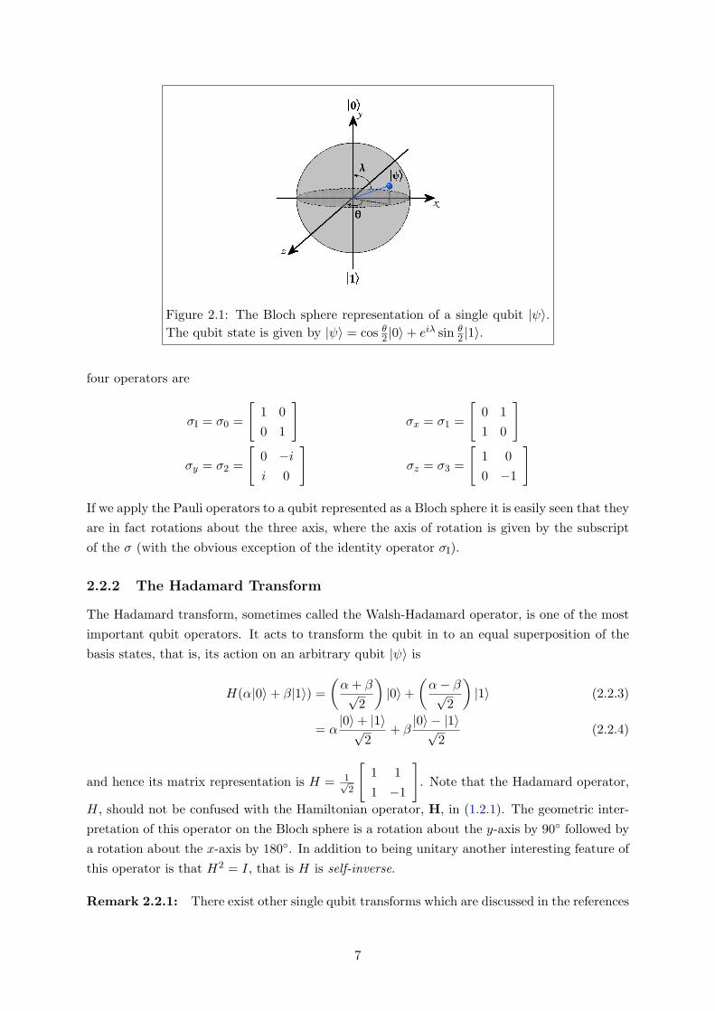
Figure 2.1: The Bloch sphere representation of a single qubit |ψ〉.The qubit state is given by |ψ〉 = cos θ

2 |0〉+ eiλ sin θ2 |1〉.

four operators are

σI = σ0 =

[1 00 1

]σx = σ1 =

[0 11 0

]

σy = σ2 =

[0 −ii 0

]σz = σ3 =

[1 00 −1

]

If we apply the Pauli operators to a qubit represented as a Bloch sphere it is easily seen that theyare in fact rotations about the three axis, where the axis of rotation is given by the subscriptof the σ (with the obvious exception of the identity operator σI).

2.2.2 The Hadamard Transform

The Hadamard transform, sometimes called the Walsh-Hadamard operator, is one of the mostimportant qubit operators. It acts to transform the qubit in to an equal superposition of thebasis states, that is, its action on an arbitrary qubit |ψ〉 is

H(α|0〉+ β|1〉) =(α+ β√

2

)|0〉+

(α− β√

2

)|1〉 (2.2.3)

= α|0〉+ |1〉√

2+ β|0〉 − |1〉√

2(2.2.4)

and hence its matrix representation is H = 1√2

[1 11 −1

]. Note that the Hadamard operator,

H, should not be confused with the Hamiltonian operator, H, in (1.2.1). The geometric inter-pretation of this operator on the Bloch sphere is a rotation about the y-axis by 90 followed bya rotation about the x-axis by 180. In addition to being unitary another interesting feature ofthis operator is that H2 = I, that is H is self-inverse.

Remark 2.2.1: There exist other single qubit transforms which are discussed in the references

7

given at the start of this chapter. We shall later introduce any further single qubit transformsif the need arises.

2.3 Quantum Registers

So far we have considered only singular qubits but in order to perform more useful calcu-lations it is necessary to consider ensembles of qubits. Axiom 4 describes how compositequantum systems may be formed by the tensor product of other quantum systems. Sup-pose we have two qubits, that is two 2-dimensional Hilbert spaces, in the computational basis|0〉, |1〉, then the 4-dimensional composite system H4 ≡ H⊗2

2 = H2⊗H2 has orthonormal basis|00〉, |01〉, |10〉, |11〉. The state of a two qubit system is described by a unit length vector:

(α0|0〉+ β0|1〉)⊗ (α1|0〉+ β1|1〉) = α0α1|00〉+ α0β1|01〉+ β0α1|10〉+ β0β1|11〉 (2.3.1)

= γ1|00〉+ γ2|01〉+ γ3|10〉+ γ4|11〉 (2.3.2)

where∑|γi|2 = 1. Using Hilbert spaces of larger dimension allows us to extend to the general

case of an n-qubit system which we call a quantum register. The state space of an n-qubitregister is given by H2n =

⊗n−1i=0 H2 and the basis states are |x〉|x ∈ 0, 1n. We should also

note that since the tensor product is, in general, non-commutative the ordering of the elementsin the quantum register is crucial. We can now show why simulating any quantum system, notjust those for quantum computation, on classical computers is so resource intensive; a generalstate of a n qubit system is

2n−1∑i=0

γi|i〉, where2n−1∑i=0

|γi|2 = 1 (2.3.3)

hence we require 2n classical variables2 to represent this system. Due to this exponential growthin the number of variables for linear increases of system size even simulating “31 qubits we need32GB of memory, and every additional qubit will double the required resources: time, memory,power and space” [38]. For this reason quantum computers are of use not only to computerscientists and mathematicians but for integrated circuit designers, material scientists, chemicalengineers and anyone else studying systems where quantum phenomena have significant impact.

2.4 Quantum Measurement

We now turn our attention to a general quantum measurement method called positive operator-valued measurement ; often physicists employ projective measurements as these more naturallyconsider the resultant state of the system post-measurement.

2E.g integers, reals, etc.

8

2.5 Multiple Qubit Operators

Suppose that U1 and U2 are arbitrary single qubit transforms acting on |ψ1〉 and |ψ2〉 respec-tively. Furthermore suppose U is a transform acting on a two qubit system |φ1φ2〉 such thatU |φ1φ2〉 = U1|φ1〉 ⊗ U2|φ2〉, therefore U = U1 ⊗ U2. Using this technique it is possible toconstruct an n-qubit transform as the tensor product of single qubit transforms. However, notall n-qubit operators can be constructed in this way, c.f §2.5.2. To perform the same singlequbit transform U on n qubits we can form the n-fold tensor product U⊗n =

⊗n−10 U . For

example: the set of Pauli operators ±σI,±σx,±σy,±σz form a group of order 8; the n-foldtensor product of these operators also forms a group Gn = ±±σI,±σx,±σy,±σz of order22n+1 called the n-qubit Pauli group.

2.5.1 The Hadamard Transform... Again

While the n-fold Hadamard operator is, like the n-fold Pauli operators, simply the action ofn single qubit Hadamard operators on n qubits it exposes a significant feature of quantumcomputation. Let us consider an example:

Example 2.5.1:. Suppose we have three input qubits in the state |0〉 and apply the trinaryHadamard operator thus

H⊗3 (|0〉 ⊗ |0〉 ⊗ |0〉) = H|0〉 ⊗H|0〉 ⊗H|0〉 (2.5.1)

=|0〉+ |1〉√

2⊗ |0〉+ |1〉√

2⊗ |0〉+ |1〉√

2(2.5.2)

=

(|000〉+ |001〉+ |010〉+ |011〉+ |100〉+ |101〉+ |110〉+ |111〉

)√

23(2.5.3)

then the input qubits are now in an equal superposition of the basis states for the Hilbert spaceH2⊗H2⊗H2 ≡ H8. Should we try to measure the state we observe one of the eight basis vectorswith equal probability.

But what properties do these types of state possess? Suppose that we rewrite (2.5.3) usingintegers instead of binary indices for the elements of H8 and omitting the scalar constant:

|ψ〉 = |0〉+ |1〉+ |2〉+ |3〉+ |4〉+ |5〉+ |6〉+ |7〉 (2.5.4)

Suppose now that we have some function f : 0, . . . , 7 7→ 0, . . . , 7 which can be implementedas a unitary transform Uf : H8 7→ H8. Applied to (2.5.4) this gives

Uf |ψ〉 = Uf |0〉+ Uf |1〉+ Uf |2〉+ Uf |3〉+ Uf |4〉+ Uf |5〉+ Uf |6〉+ Uf |7〉 (2.5.5)

= |f(0)〉+ |f(1)〉+ |f(2)〉+ |f(3)〉+ |f(4)〉+ |f(5)〉+ |f(6)〉+ |f(7)〉 (2.5.6)

Notice that every value of f(x) is evaluated in parallel, however should we try to measure thestate in (2.5.6) we are able to observe, with equal probability, only one of the values. Thisconcept is known as quantum parallelism and appears in the majority of quantum algorithms;we address the idea of performing functions via unitary transforms further in §3.3.1. Crudely

9

speaking quantum algorithms often attempt to adjust the amplitudes of the superposition3 sothat when measured the probability of finding the state(s) you seek is not equal but higher thanthose you are not.

2.5.2 The Controlled NOT & Other Controlled Gates

The controlled-Not, or CNot, is a binary quantum operator. However, unlike the previousmulti-qubit transforms, the CNot can not be decomposed as the tensor product of unaryoperators, see §D.2.1. A more intuitive name for this operator might be the conditional Not

since its action is to “flip” the second qubit if the first qubit is true, and nothing otherwise.The action on the basis states is:

|0〉|0〉 7→ |0〉|0〉 |1〉|0〉 7→ |1〉|1〉

|0〉|1〉 7→ |0〉|1〉 |1〉|1〉 7→ |1〉|0〉

The matrix of this operator is given in §D.2.1.

2.6 Entanglement

Suppose we have the following 2-qubit systems:

|B00〉 =|00〉+ |11〉√

2|B10〉 =

|00〉 − |11〉√2

|B01〉 =|01〉+ |10〉√

2|B11〉 =

|01〉 − |10〉√2

these are known as the Bell states or EPR-pairs following work by Einstein, Podolsky and Rosen.Suppose we have a system in the state |B00〉 and, without loss of generality, suppose further thatmeasurement of the first qubit returns |0〉. Then the system must be in the state |00〉 implyingthat the state of the second qubit is fixed by measurement of the first. This self-adjustment ofthe system to maintain consistency is instantaneous even if the qubits are separated by somephysical distance, making quantum mechanics a non-local theory. This appears to contradictEinstein’s theory of special relativity - no information may be transmitted faster than light -so called local realism. He, together with others, proposed a thought experiment known as theEPR-paradox to demonstrate that quantum mechanics might be an incomplete physical theory.At the moment the general consensus is that in fact this paradox highlights how quantummechanics violates our more classical intuitions [77]. The Bell states are an example of amore general quantum principle known as entanglement. Entanglement is an entirely quantumphenomenon and is the key to many quantum communication algorithms including quantumcryptograph and quantum teleportation.

Definition 2.6.1: (Entangled States). A quantum state |ψ〉 ∈ H2n is pure iff it can bedecomposed as the tensor product of states in two-dimensional Hilbert spaces. Any state which

3Physicists often called this process interference since they often use continuous wave functions instead ofdiscretised unitary transforms.

10

is not pure is said to be entangled.

For example, the following state is decomposable:

12

(|00〉+ |01〉+ |10〉+ |11〉) =1√2

(|0〉+ |1〉)⊗ 1√2

(|0〉+ |1〉) (2.6.1)

whereas 1√2(|00〉+ |11〉) is entangled. To see this we try to write the system in the form of

(2.3.1) we find the values of the coefficients are given by the following system of equations:

α0α1 =1√2, α0β0 = 0, α1β0 = 0, β0β1 =

1√2

(2.6.2)

These are obviously unsatisfiable and hence we can not decompose the quantum state, it istherefore entangled. We can create an entangled state of two qubits; suppose we have a twoqubit system |00〉 and apply the operator H ⊗ I, where I is the identity matrix, to obtain thestate |00〉+|10〉√

2. If we now perform a CNot transform using the first qubit as the control the

system becomes |00〉+|11〉√2

, the positive Bell state. Similarly if we start with the initial state |10〉we obtain the negative Bell state; this demonstrates that we are able to create entanglementusing local operations, however there has been significant advancement in methods of non-localentanglement [95, 25] and entangled qubit distribution [56, 91]. Since, like qubits, entanglementis a physical resource we define an ebit as an entangled quantum system, e.g. each Bell stateis an ebit with bipartite4 entanglement. Entanglement is not restricted to qubit pairs, it ispossible to construct an entangled n qubit state [77].

2.7 Laws of Quantum Information

In classical physics the study of energy, work, and entropy is called thermodynamics, which isbased upon a group of postulates known as the four Laws of Thermodynamics5. The physicistRichard Feynman presents thermodynamics beautifully in his lectures on physics [37], should thereader wish further information, however our only interest is the second law. In thermodynamicsentropy is a measure of the amount of energy in a physical system that cannot be used to dowork. The 2ndLaw of Thermodynamics] states that : Entropy within a closed system can notdecrease. Based on thermodynamics Shannon, in his 1948 paper “A Mathematical Theory ofCommunication” [94], introduces (classical) Information Theory, a mathematical formalisationof communication. Showing the connection between information theory and thermodynamicsis a complex task, however, the 2ndlaw of information is identical to that of thermodynamicsexcept the definition of entropy changes. Information entropy is a measure of the lack of exactinformation about a system and so the second law of classical information is known as the Lawof Conservation of Information. In fact this law goes further and includes both no-increasingand no-decreasing of entropy.

In Quantum systems the thermodynamic second law holds but can be expressed using quan-tum equivalents of Shannon’s information theory. Quantum Information theory is a rich source

4Bipartite systems consist of two parts A and B that are too far apart to interact, and whose state, pure ormixed, lies in a Hilbert space HAB = HA ⊗HB .

5From the Greek: thermos meaning heat and dynamic meaning change.

11

of research, see [77] for a detailed discussion. In [52] it is shown that in a quantum mechanicalsystem the second law gives rise to two significant principles concerning both open and closedsystems. We are only concerned with implications of those principles for closed systems as thisis a constituent of Axiom 1 from §1.2.

Definition 2.7.1: (The Principle of Conservation of Quantum Information) In aclosed quantum mechanical system the entanglement of the states is a form of quantum in-formation [51]. For a compound quantum system the sum of information contained in thesubsystems and the information contained in entanglement is conserved by unitary operators.Furthermore entanglement cannot increase under local quantum operations and classical com-munication [13].

2.7.1 No-deleting Principle

The no-deleting principle states that in a closed system, one cannot destroy quantum informa-tion. In closed systems, quantum information can only be moved from one place (subspace)to another. We must be careful to distinguish between classical erasure and quantum deletion.The former is achievable by expending a certain amount of energy and hence is irreversible,this is known as Lauder’s Principle of Erasure. It is possible [80] to express the no-deletingprinciple as a theorem, as is done in §D.3, however there is a somewhat stronger corollary forclosed systems.

Corollary 2.7.2:. For any closed quantum system there exists no unitary operator U suchthat U deletes a quantum state, that is take it to some fixed state say |0〉, using a system ofauxillary or ancilla qubits |ψ〉, i.e.

U |0〉|ψ〉 = |0〉|ψ1〉 (2.7.1)

U |1〉|ψ〉 = |0〉|ψ2〉 (2.7.2)

then 〈ψ1|ψ2〉 = 0.

We omit the proof of Corollary 2.7.2 since it is similar to the proof provided for Theorem 2.7.3below.

2.7.2 No-cloning Principle

Classical information can quite clearly be copied, however this is not true for quantum infor-mation. The no-cloning principle states that in either an open or closed quantum system it isimpossible to gain sufficient information about the exact state of a qubit for an exact copy tobe made [58]. As for no-deleting the no-cloning principle can be expressed as a theorem.

Theorem 2.7.3: (No-cloning Theorem). Suppose that there exists a unitary operator Uwhich copies two quantum states |ψ〉and |φ〉, i.e.

U |ψ〉|0〉 = |ψ〉|ψ〉 (2.7.3)

U |φ〉|0〉 = |φ〉|φ〉 (2.7.4)

12

then 〈ψ|φ〉 is either 1 or 0.

Proof.

〈ψ|φ〉 = (〈ψ|〈0|)(|φ〉|0〉) by (2.7.4) and (2.7.3) (2.7.5)

= (〈ψ|〈ψ|)(|φ〉|φ〉) since U is unitary (2.7.6)

= 〈ψ|φ〉2 (2.7.7)

In the proof of (2.7.6) above we utilise the fact that since U is unitary it preserves the innerproduct. As a result of this theorem we see that we can only copy qubits in the (computational)basis, however despite this limitation several significant applications that exploit this restrictedcopying have been developed. Such applications include the CNot-gate, which we discussedin §2.5.2, and quantum error correction (see [96, 19]).

2.8 Errors in Quantum Computation

With classical bits there is only one possible error for a single bit b, a bit flip, which is equivalentto applying a Not-gate to b. One method of reducing the effect of errors is to introduceredundancy to the system by replacing the single bit, b, by n bits and performing the samecomputation on each of them individually, the value of the original bit b is then determined bythe modal value of the other n bits. Provided that there are less than bn/2c errors this methodwill preserve the information of the single bit, obviously if the error rate is higher than this thenthis error correction scheme will fail.

For a single qubit the situation is much more complex since there are an infinite numberof single qubit transforms, each of which represents the perturbation of the qubit state causedby some error. Understandably it was first thought that errors in quantum states could not becorrected due to the limited amount of information of the total system state, however this doubtwas dispelled in 1995 when Shor proposed the first quantum error correction code (QECC) andsoon after a more general theory of quantum error correction [19]. Since then a cornucopia ofquantum error correction techniques have been developed, each optimised for different purposes,however we shall not consider them in this paper although their use is discussed again in §6.2.

While we are not interested in discussing particular instances of errors or correction tech-niques it is important to bear in mind how a general error affects an arbitrary qubit. A generalmodel of qubit errors, based on those appearing in [42, 96, 63, 77], which considers the state ofboth the qubit and its environment. While it is, in principle, physically possible to determinethe exact state of the environment, doing so in practice is prohibitively demanding. It is thislack of information of the environment state that causes decoherence of the quantum state, aswe see in Chapter 6 decoherence poses problems for constructing quantum computers.

We assume that both our qubit, |ψ〉, and the environment, |E〉, are initially pure uncorrelatedstates. Hence the total state of the system is given by |S〉 = |ψ〉 ⊗ |E〉. As the system evolves,the qubit interacts with the environment. In general this interaction can be modelled by a joint

13

unitary transform. Since this is a unitary transform it can be decomposed to a sum of Paulitransforms, §2.2.1, thus the total state of the system is given by [77]:

|S〉 = σI|ψ〉ΓI|E〉+ σx|ψ〉Γx|E〉+ σy|ψ〉Γy|E〉+ σz|ψ〉Γz|E〉 (2.8.1)

where each Γi is a unitary transformation acting on the environment state only, and σi are thePauli transforms. The first term on the right hand side of (2.8.1) represents the instance whenno perturbation to the qubit state is made, the other terms allow us to classify the errors in tothree types: bit-flip (σx), imaginary-flip(σy), and phase-flip6(σz). The total system is howeverstill in a pure state and therefore it should be possible to recover the initial state of the qubit.But, and such is the case, it is impossible to do this without information of the environmentstate, hence we are unable to determine what error has occurred nor are we able to correct it.From this it is easy to see why some doubted that quantum error correction was possible, butit is now an excellent example of utilising features of quantum mechanics to solve a problemin quantum computation. To combat the decoherence of the qubit |ψ〉 it is entangled witha number of other ancilla qubits so that the information is distributed across them all. Bypreparing these ancilla qubits to known value states we can use this information to “patch-up”the state of our original qubit |ψ〉, see [96] for the full details.

2.9 Summary

In this chapter we have introduced the basic element of quantum information, the qubit, anddemonstrated a number of methods for interacting with it. These methods include the unitarytransforms and measurement operators. We have also seen how to work with ensembles ofqubits which allowed to consider entanglement, a purely quantum phenomenon. Finally weconsidered the law of conservation of quantum information and the no-deleting and no-cloningtheorems that are derived from it.

6Note that this is not the phase gate.

14

Chapter 3Quantum Algorithms and Complexity

While Alan Turing is considered the progenitor of modern computer science, as well as asignificant figure in the development of artificial intelligence, the impetus for his research incomputability is the quantum pioneer David Hilbert. Hilbert is perhaps the most influentialmathematician of the early 20th Century, a proponent of axiomatisation1 whose work appearsquantum mechanics, general relativity, and automata theory. In 1928 Hilbert also proposed theEntscheidungsproblem: given a set of statements from first order logic is there a generalisedalgorithm which proves their logical validity [45]. Using Hilbert’s automata theory and earlierwork by Godel on the limitations of proof and computation Turing defined a mathematicalmodel of an algorithm, a Turing machine (TM), which allowed him to prove that the questionwas undecidable2. Turing continued and proposed the universal Turing machine (UTM) whichis capable of efficiently simulating any other Turing machine. There are now many variationsof Turing machines such as non-deterministic Turing machines, and probabilistic Turing ma-chines. Possibly Turing’s most audacious work led to the Church-Turing Thesis (CTT) which,surmised in his own words, is “Every function which would naturally be regarded as computablecan be computed by a Turing machine”. The thesis in this form is impalpable and hence cannot be proved true, placing it on the same footing as a physical law. Many refinements havebeen made and currently the most commonly used form is the Strong Church-Turing Thesis(SCTT) which states: “Any ‘reasonable’ model of computation can be efficiently simulated ona probabilistic Turing machine” [11]. A rigourous treatment of classical computation is givenin [48].

3.1 Quantum Turing Machines

The development of a quantum complexity theory is predominantly due to Vazirani and Bern-stein [11], however the concept of quantum Turing machines (QTM) is generally attributed toDavid Deutsch [33], as are quantum circuits (§3.3). The following definition is an abridgementof those appearing in Vazirani and Bernstein’s “Quantum Complexity Theory” [11] and “ASurvey of Quantum Complexity Theory” [103].

1The construction of formal systems based upon a (finite) set of axioms.2A problem is decidable if there exists an algorithm which solves it in a finite amount of time.

15

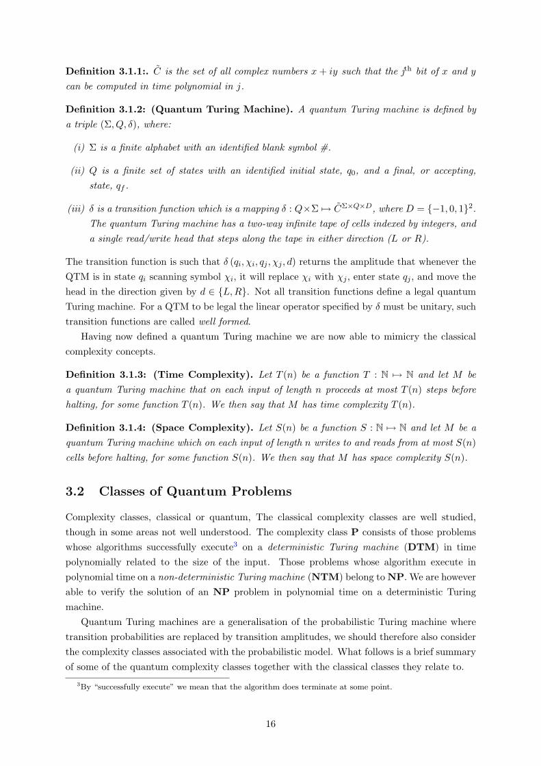
Definition 3.1.1:. C is the set of all complex numbers x+ iy such that the jth bit of x and ycan be computed in time polynomial in j.

Definition 3.1.2: (Quantum Turing Machine). A quantum Turing machine is defined bya triple (Σ, Q, δ), where:

(i) Σ is a finite alphabet with an identified blank symbol #.

(ii) Q is a finite set of states with an identified initial state, q0, and a final, or accepting,state, qf .

(iii) δ is a transition function which is a mapping δ : Q×Σ 7→ CΣ×Q×D, where D = −1, 0, 12.The quantum Turing machine has a two-way infinite tape of cells indexed by integers, anda single read/write head that steps along the tape in either direction (L or R).

The transition function is such that δ (qi, χi, qj , χj , d) returns the amplitude that whenever theQTM is in state qi scanning symbol χi, it will replace χi with χj , enter state qj , and move thehead in the direction given by d ∈ L,R. Not all transition functions define a legal quantumTuring machine. For a QTM to be legal the linear operator specified by δ must be unitary, suchtransition functions are called well formed.

Having now defined a quantum Turing machine we are now able to mimicry the classicalcomplexity concepts.

Definition 3.1.3: (Time Complexity). Let T (n) be a function T : N 7→ N and let M bea quantum Turing machine that on each input of length n proceeds at most T (n) steps beforehalting, for some function T (n). We then say that M has time complexity T (n).

Definition 3.1.4: (Space Complexity). Let S(n) be a function S : N 7→ N and let M be aquantum Turing machine which on each input of length n writes to and reads from at most S(n)cells before halting, for some function S(n). We then say that M has space complexity S(n).

3.2 Classes of Quantum Problems

Complexity classes, classical or quantum, The classical complexity classes are well studied,though in some areas not well understood. The complexity class P consists of those problemswhose algorithms successfully execute3 on a deterministic Turing machine (DTM) in timepolynomially related to the size of the input. Those problems whose algorithm execute inpolynomial time on a non-deterministic Turing machine (NTM) belong to NP. We are howeverable to verify the solution of an NP problem in polynomial time on a deterministic Turingmachine.

Quantum Turing machines are a generalisation of the probabilistic Turing machine wheretransition probabilities are replaced by transition amplitudes, we should therefore also considerthe complexity classes associated with the probabilistic model. What follows is a brief summaryof some of the quantum complexity classes together with the classical classes they relate to.

3By “successfully execute” we mean that the algorithm does terminate at some point.

16

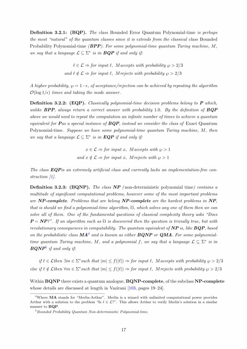
Definition 3.2.1: (BQP). The class Bounded Error Quantum Polynomial-time is perhapsthe most “natural” of the quantum classes since it is extends from the classical class BoundedProbability Polynomial-time (BPP). For some polynomial-time quantum Turing machine, M ,we say that a language L ⊆ Σ∗ is in BQP if and only if:

` ∈ L ⇒ for input `, Maccepts with probability ℘ > 2/3

and ` /∈ L ⇒ for input `, Mrejects with probability ℘ > 2/3

A higher probability, ℘ = 1−ε, of acceptance/rejection can be achieved by repeating the algorithmO(log 1/ε) times and taking the mode answer.

Definition 3.2.2: (EQP). Classically polynomial-time decision problems belong to P which,unlike BPP, always return a correct answer with probability 1.0. By the definition of BQP

above we would need to repeat the computation an infinite number of times to achieve a quantumequivalent for Pas a special instance of BQP, instead we consider the class of Exact QuantumPolynomial-time. Suppose we have some polynomial-time quantum Turing machine, M , thenwe say that a language L ⊆ Σ∗ is in EQP if and only if:

x ∈ L ⇒ for input x, Maccepts with ℘ > 1

and x /∈ L ⇒ for input x, Mrejects with ℘ > 1

The class EQPis an extremely artificial class and currently lacks an implementation-free con-struction [1].

Definition 3.2.3: (BQNP). The class NP (non-deterministic polynomial time) contains amultitude of significant computational problems, however some of the most important problemsare NP-complete. Problems that are belong NP-complete are the hardest problems in NP,that is should we find a polynomial-time algorithm, f, which solves any one of them then we cansolve all of them. One of the fundamental questions of classical complexity theory asks “DoesP = NP?”. If an algorithm such as f is discovered then the question is trivially true, but withrevolutionary consequences in computability. The quantum equivalent of NP is, like BQP, basedon the probabilistic class MA4 and is known as either BQNP or QMA. For some polynomial-time quantum Turing machine, M , and a polynomial f , we say that a language L ⊆ Σ∗ is inBQNP5 if and only if:

if ` ∈ Lthen ∃m ∈ Σ∗such that |m| ≤ f(|`|)⇒ for input `, Maccepts with probability ℘ > 2/3

else if ` /∈ Lthen ∀m ∈ Σ∗such that |m| ≤ f(|`|)⇒ for input `, Mrejects with probability ℘ > 2/3

Within BQNP there exists a quantum analogue, BQNP-complete, of the subclass NP-complete

whose details are discussed at length in Vazirani [103, pages 19–24].

4Where MA stands for “Merlin-Arthur”. Merlin is a wizard with unlimited computational power providesArthur with a solution to the problem “Is ` ∈ L?”. This allows Arthur to verify Merlin’s solution in a similarmanner to BQP.

5Bounded Probability Quantum Non-deterministic Polynomial-time.

17

3.3 A Circuit Model of Quantum Computation

3.3.1 Black Boxes And Oracles

3.3.2 Universal Families of Quantum Gates

3.3.3 Quantum Circuits and QTMs

3.4 Significant Quantum Algorithms

quantum parallelism

3.4.1 Quantum Teleportation

3.4.2 Quantum Fourier Transform

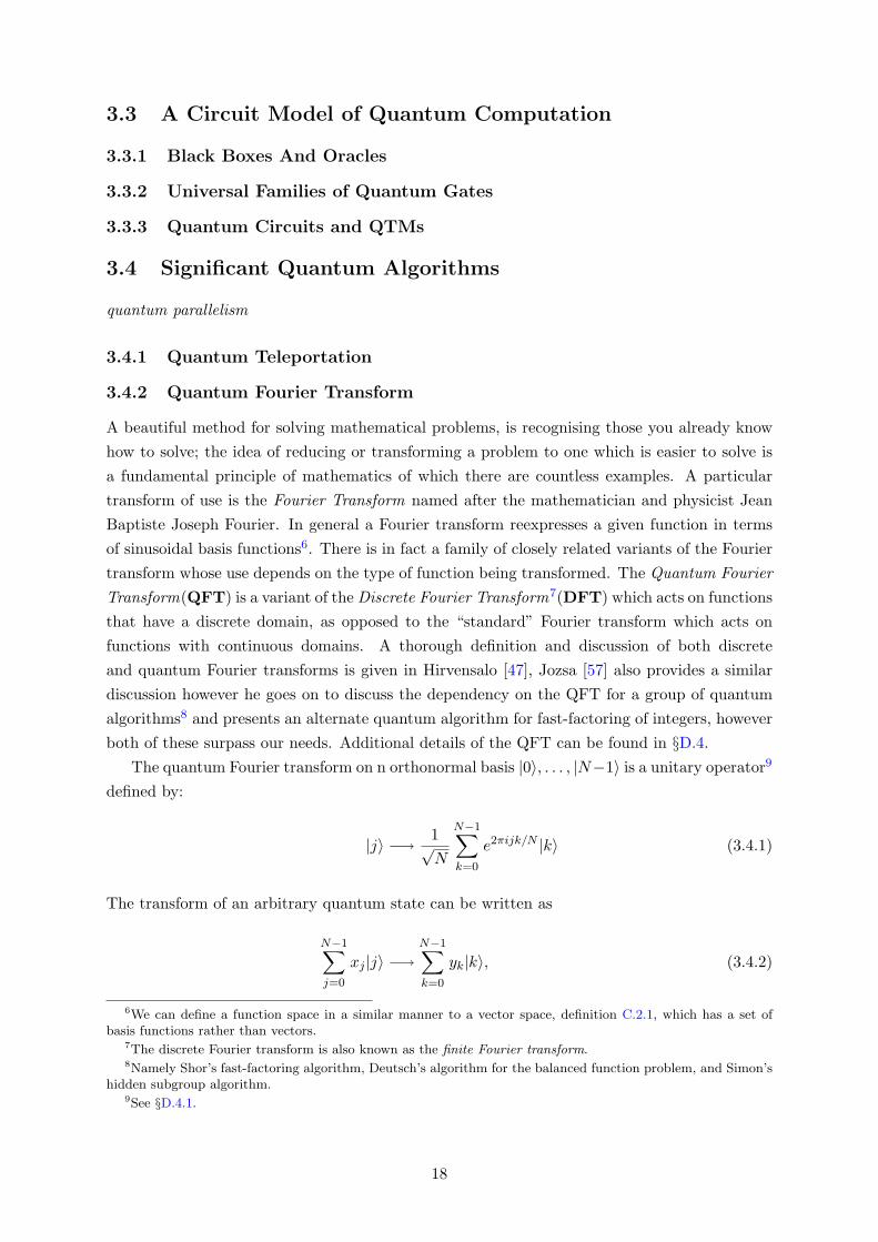
A beautiful method for solving mathematical problems, is recognising those you already knowhow to solve; the idea of reducing or transforming a problem to one which is easier to solve isa fundamental principle of mathematics of which there are countless examples. A particulartransform of use is the Fourier Transform named after the mathematician and physicist JeanBaptiste Joseph Fourier. In general a Fourier transform reexpresses a given function in termsof sinusoidal basis functions6. There is in fact a family of closely related variants of the Fouriertransform whose use depends on the type of function being transformed. The Quantum FourierTransform(QFT) is a variant of the Discrete Fourier Transform7(DFT) which acts on functionsthat have a discrete domain, as opposed to the “standard” Fourier transform which acts onfunctions with continuous domains. A thorough definition and discussion of both discreteand quantum Fourier transforms is given in Hirvensalo [47], Jozsa [57] also provides a similardiscussion however he goes on to discuss the dependency on the QFT for a group of quantumalgorithms8 and presents an alternate quantum algorithm for fast-factoring of integers, howeverboth of these surpass our needs. Additional details of the QFT can be found in §D.4.

The quantum Fourier transform on n orthonormal basis |0〉, . . . , |N−1〉 is a unitary operator9

defined by:

|j〉 −→ 1√N

N−1∑k=0

e2πijk/N |k〉 (3.4.1)

The transform of an arbitrary quantum state can be written as

N−1∑j=0

xj |j〉 −→N−1∑k=0

yk|k〉, (3.4.2)

6We can define a function space in a similar manner to a vector space, definition C.2.1, which has a set ofbasis functions rather than vectors.

7The discrete Fourier transform is also known as the finite Fourier transform.8Namely Shor’s fast-factoring algorithm, Deutsch’s algorithm for the balanced function problem, and Simon’s

hidden subgroup algorithm.9See §D.4.1.

18

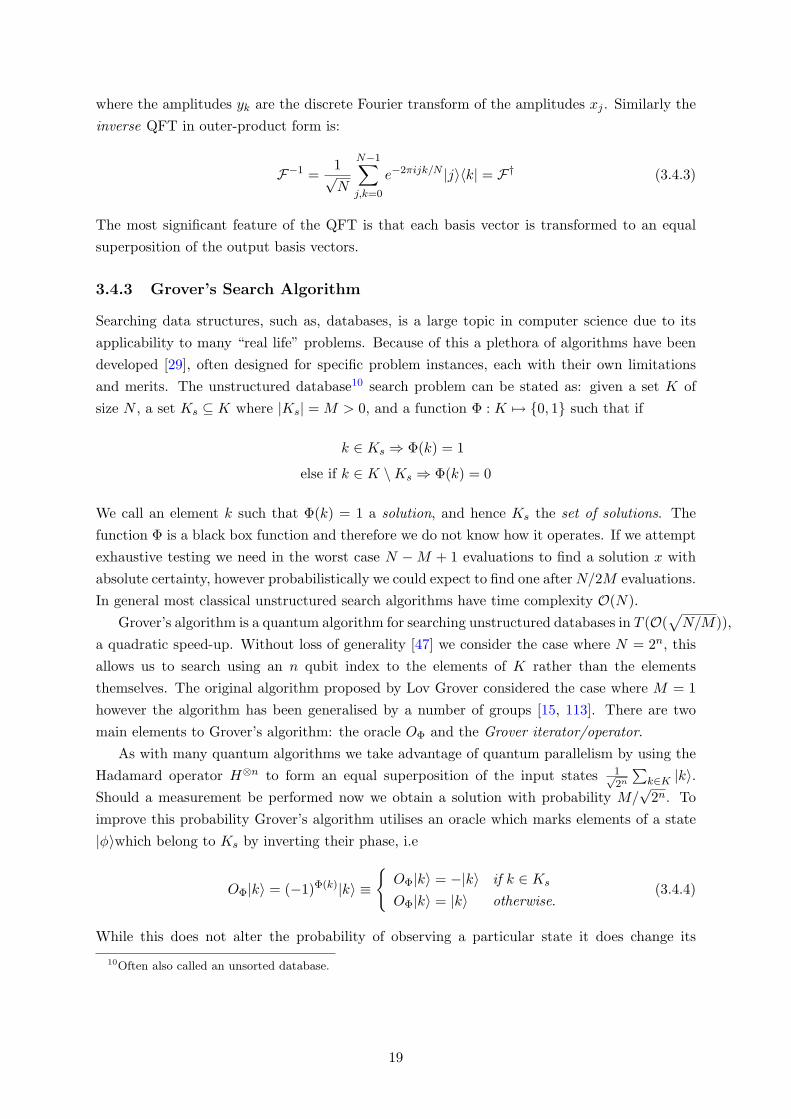
where the amplitudes yk are the discrete Fourier transform of the amplitudes xj . Similarly theinverse QFT in outer-product form is:

F−1 =1√N

N−1∑j,k=0

e−2πijk/N |j〉〈k| = F† (3.4.3)

The most significant feature of the QFT is that each basis vector is transformed to an equalsuperposition of the output basis vectors.

3.4.3 Grover’s Search Algorithm

Searching data structures, such as, databases, is a large topic in computer science due to itsapplicability to many “real life” problems. Because of this a plethora of algorithms have beendeveloped [29], often designed for specific problem instances, each with their own limitationsand merits. The unstructured database10 search problem can be stated as: given a set K ofsize N , a set Ks ⊆ K where |Ks| = M > 0, and a function Φ : K 7→ 0, 1 such that if

k ∈ Ks ⇒ Φ(k) = 1

else if k ∈ K \Ks ⇒ Φ(k) = 0

We call an element k such that Φ(k) = 1 a solution, and hence Ks the set of solutions. Thefunction Φ is a black box function and therefore we do not know how it operates. If we attemptexhaustive testing we need in the worst case N −M + 1 evaluations to find a solution x withabsolute certainty, however probabilistically we could expect to find one afterN/2M evaluations.In general most classical unstructured search algorithms have time complexity O(N).

Grover’s algorithm is a quantum algorithm for searching unstructured databases in T (O(√N/M)),

a quadratic speed-up. Without loss of generality [47] we consider the case where N = 2n, thisallows us to search using an n qubit index to the elements of K rather than the elementsthemselves. The original algorithm proposed by Lov Grover considered the case where M = 1however the algorithm has been generalised by a number of groups [15, 113]. There are twomain elements to Grover’s algorithm: the oracle OΦ and the Grover iterator/operator.

As with many quantum algorithms we take advantage of quantum parallelism by using theHadamard operator H⊗n to form an equal superposition of the input states 1√

2n

∑k∈K |k〉.

Should a measurement be performed now we obtain a solution with probability M/√

2n. Toimprove this probability Grover’s algorithm utilises an oracle which marks elements of a state|φ〉which belong to Ks by inverting their phase, i.e

OΦ|k〉 = (−1)Φ(k)|k〉 ≡

OΦ|k〉 = −|k〉 if k ∈ Ks

OΦ|k〉 = |k〉 otherwise.(3.4.4)

While this does not alter the probability of observing a particular state it does change its

10Often also called an unsorted database.

19

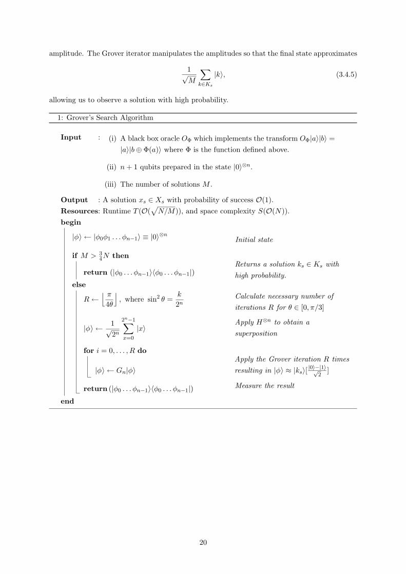
amplitude. The Grover iterator manipulates the amplitudes so that the final state approximates

1√M

∑k∈Ks

|k〉, (3.4.5)

allowing us to observe a solution with high probability.

1: Grover’s Search Algorithm

Input : (i) A black box oracle OΦ which implements the transform OΦ|a〉|b〉 =|a〉|b⊕ Φ(a)〉 where Φ is the function defined above.

(ii) n+ 1 qubits prepared in the state |0〉⊗n.

(iii) The number of solutions M .

Output : A solution xs ∈ Xs with probability of success O(1).Resources: Runtime T (O(

√N/M)), and space complexity S(O(N)).

begin

|φ〉 ← |φ0φ1 . . . φn−1〉 ≡ |0〉⊗nInitial state

if M > 34N then

return (|φ0 . . . φn−1〉〈φ0 . . . φn−1|)Returns a solution ks ∈ Ks withhigh probability.

else

R←⌊ π4θ

⌋, where sin2 θ =

k

2nCalculate necessary number ofiterations R for θ ∈ [0, π/3]

|φ〉 ← 1√2n

2n−1∑x=0

|x〉Apply H⊗n to obtain asuperposition

for i = 0, . . . , R do

|φ〉 ← Gn|φ〉Apply the Grover iteration R timesresulting in |φ〉 ≈ |ks〉[ |0〉−|1〉√

2]

return (|φ0 . . . φn−1〉〈φ0 . . . φn−1|) Measure the result

end

20

Chapter 4Introduction to Quantum Artificial

Intelligence

Artificial Intelligence, like quantum computing, draws together many diverse areas of research: phi-losophy, economics, neuroscience, engineering, and many mathematical disciplines. The embod-iment of an artificial intelligence is often referred to as an agent, but it is important to notethat a program executing on a computer can also be considered an agent.

In order that AI be considered science it was necessary to provide a mathematical formalisa-tion, of which three of the most fundamental disciplines were logic, computation, and probability.The first significant mathematical treatment of logic is generally attributed to George Boole[12]and is called Boolean logic in his honour. Boolean logic is a system of syllogistic logic, a syl-logism is an inference in which one proposition (the conclusion) follows of necessity from twoothers (known as premises), for this reason Boolean logic is often also called propositional logicor propositional calculus. Later Gottlob Frege extended Boolean logic to include objects andrelationships/quantification, this new logic is known as first-order logic (or predicate calculus).The next significant development is due to Alfred Tarski who used set theory to define Truthand model-theoretic satisfaction1. His work allows us to relate objects in our logic to objects inthe real world. This material is discussed with more detail in [87]

Another difficulty to face is that even in the instance where there exists a method of solu-tion for a problem the information available maybe imperfect or uncertain, hence we requiremethods that enable our agents to act rationally despite the lack of exact solutions and perfectinformation. Gerolamo Cardano, an italian, proposed the idea of probability and since then ithas been extended by a number of significant mathematicians such as Fermat, Bernoulli andLaplace and is now an invaluable tool for dealing with uncertain or incomplete information.

Traditionally much of artificial intelligence is based upon reductionism: complex systemscan be reduced to fundamental subsystems thereby explaining the complex by the compositionof the simple. This in turn has been reflected by a change in approach of human cogitationtheory and neuroscience, a change to support the view of logical computation.

1Model theory considers languages, their interpretations, and the kinds of classification they are able to make.See [100, 101].

21

4.1 Fundamentals of AI

NOT YET COMPLETE

4.1.1 Agents

NOT YET COMPLETE

4.1.2 The SAT Problem

The Boolean satisfiability problem (SAT) holds the distinguished position of being the firstproblem proved to be in NP-complete independently by Cook and Levin in 1971 and 1974respectively. The satisfiability problem originates from the field of Boolean Logic which isdefined in §E.2.

Definition 4.1.1: (Literals). A Boolean variable, ω, is a Symbol in the Boolean grammarwhich can be assigned to either True or False. A literal is either a variable or the negation ofa variable and is called a positive literal or negative literal correspondingly.

Definition 4.1.2: (Clauses). Let Ωk = ω0, . . . , ωk−1 be the set of k Boolean variables andLΩk

= ω0,¬ω0, . . . , υk−1,¬ωk−1 be the set of all literals. The powerset of LΩkis denoted by

P (LΩk) and an element C ∈ (LΩk

) is a clause. If clause c has at least one of its literals is true,c is said to be satisfiable. When c is satisfiable the truth value, T (c), of c is considered True,and otherwise False. Let x be a literal in c whose true value is given by T (x), then the truth ofa clause can be expressed as T (c) =

∨x∈cT (x).

Definition 4.1.3: (Conjunctive Normal Form). Given a set of clauses Cn = c0, . . . , cn−1

then C is satisfiable if and only if T (Cn) =n−1∧i=0

ci is True. An arbitrary (finite) Boolean

sentence, or formula, is said to be in conjunctive normal form (CNF) if it can be expressed asthe conjunction of clauses, i.e. c0 ∧ · · · ∧ ck. Hence a formula is satisfiable if its set of clausesis satisfiable. A formula is said to be in k-CNF if all its clauses are of size k.

It is possible to write any Boolean formula in CNF, further more is also possible to convertany CNF formula to k-CNF. Many classical algorithms require that the input be in this formatalthough others require similar ones such as Disjoint Normal Form (DNF), however we shallsee that the quantum algorithms have no such restriction.

Definition 4.1.4: (SAT). Given a set Ωk = ω0, . . . , ωk−1 and a set Cn = c0, . . . , cn−1 ofclauses, determine whether Cn is satisfiable or not.

There are several variants of the SAT problem, for example k-SAT requires each clause of Ωk

is in k-CNF. It has also been shown that 3-SAT is also in NP-complete and hence, due to itsstructural properties, is often “used in place” of the general SAT problem. The problems havebeen extensively studied and many algorithms have been developed, all which have exponentialrunning time. It is known that some subsets of the Boolean logic are known to have polynomial-time satisfiability algorithms, e.g. Horn [50], 2-SAT, SLUR [88].

22

Remark 4.1.5: The is a BQNP-complete problem which is the quantum extension of SATcalled QSAT which is frequently called the Local Hamiltonian Problem which, again in parallelwith SAT, has related problems in the form of k-local Hamiltonian problems. More surprisingis that 2-local Hamiltonian is both in NP-hard and BQNP-complete, this leads to thesupposition that there is a class QCMA which “is the class of problems that can be verifiedby a quantum verifier with a classical proof” [60]. For interested readers the local Hamiltonianproblem is stated in §D.5 as it is not required in the remainder of this paper.

4.2 Quantum Neurocomputing

Although it was long supposed that the brain was implicated in thought and consciousness,mainly due to the correlation between head trauma and mental impairment, very little wasknow about even general brain functions. In 1861 Paul Broca proposed the idea the certaincognitive functions were localised phenomena to certain regions of the brain. Biologists of thetime believed that the brain was composed of the same cells2 that formed nerves throughoutour body which they named neurons (see figure 4.1). However this was not ratified until 1873when Carmillo Golgi developed a staining technique that allowed the observation of individualneurons.

It is possible that by understanding how our own brains operate we may advance our devel-opment of artificial intelligence. This is equivalent to a bottom-up construction of consciousnesswhich compliments the top-down approach of psychology. The conjecture that intelligence isintrinsic to the structure of the brain is not an new idea and is still popular, as a recent re-mark from Searle shows: “[Since] a collection of simple cells can lead to thought, action, andconsciousness [it is reasonable to assert] brains cause minds” [90, page 14].

Neurocomputing is based on the biology of neuroscience which is, strictly speaking, the studyof the nervous system including the brain. However neuroscience encompasses not only the studyof the composition of the brain, in terms of its cellular structure and other biological factors,biochemistry for example, but also in terms of its functional structure, including learning.Neurocomputing attempts to create artificial computational models based on those developedin neuroscience. Detailed accounts, especially of the biological topics, can be found in [39, 108]and [68].

4.2.1 Biological Neurons

The neuron is the primary cell in the nervous system and its structure is given in Figure 4.1;inter-connections between individual neurons are formed by synapses. Synapses generally occurwhere a terminal button from one neuron is in close proximity to a dendrite of another neuron.The behaviour of the synapse is regulated by substances known as neurochemicals. Neuronsare able to undergo electrical excitation and they transmit this energy along their axons as inimpulse known as an action potential. The arrival of an action potential at a terminal buttonstimulates the release of neurotransmitters into the synapse, which, depending on the particularneurochemicals present, either relay or suppress the action potential along the dendrite of

2There are in actuality many different neural cells but for our purposes we shall ignore this fact.

23

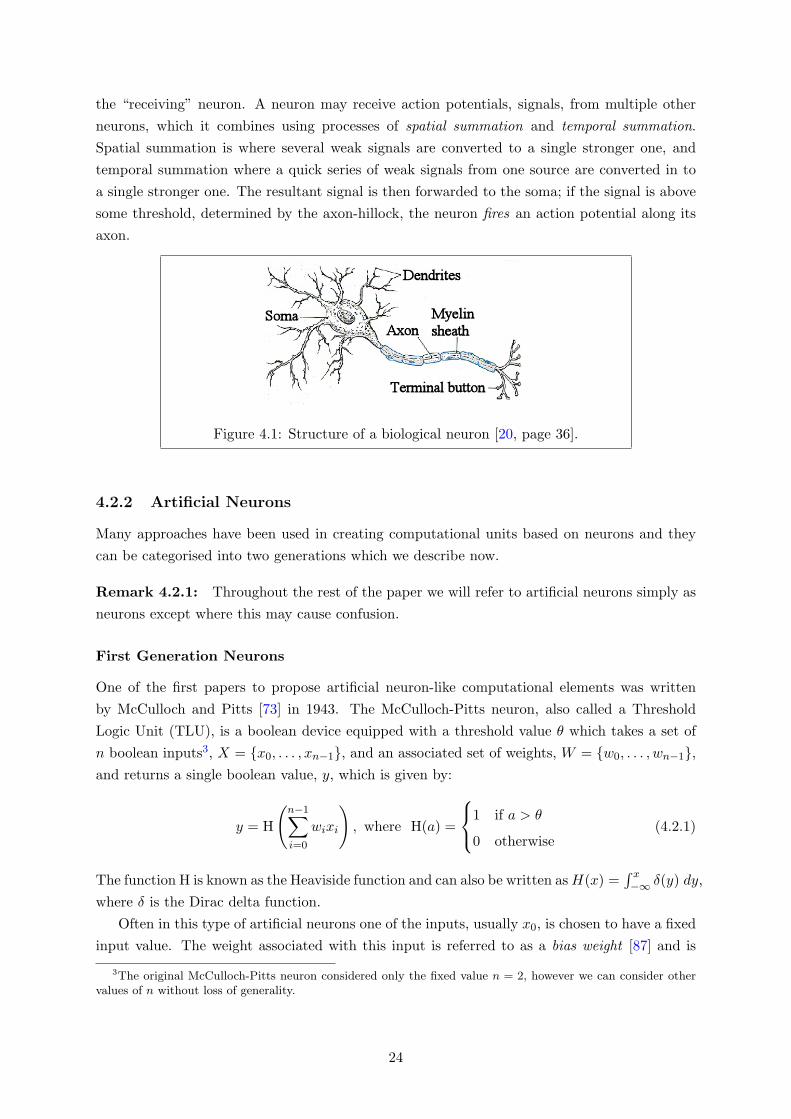
the “receiving” neuron. A neuron may receive action potentials, signals, from multiple otherneurons, which it combines using processes of spatial summation and temporal summation.Spatial summation is where several weak signals are converted to a single stronger one, andtemporal summation where a quick series of weak signals from one source are converted in toa single stronger one. The resultant signal is then forwarded to the soma; if the signal is abovesome threshold, determined by the axon-hillock, the neuron fires an action potential along itsaxon.

Figure 4.1: Structure of a biological neuron [20, page 36].

4.2.2 Artificial Neurons

Many approaches have been used in creating computational units based on neurons and theycan be categorised into two generations which we describe now.

Remark 4.2.1: Throughout the rest of the paper we will refer to artificial neurons simply asneurons except where this may cause confusion.

First Generation Neurons

One of the first papers to propose artificial neuron-like computational elements was writtenby McCulloch and Pitts [73] in 1943. The McCulloch-Pitts neuron, also called a ThresholdLogic Unit (TLU), is a boolean device equipped with a threshold value θ which takes a set ofn boolean inputs3, X = x0, . . . , xn−1, and an associated set of weights, W = w0, . . . , wn−1,and returns a single boolean value, y, which is given by:

y = H

(n−1∑i=0

wixi

), where H(a) =

1 if a > θ

0 otherwise(4.2.1)

The function H is known as the Heaviside function and can also be written asH(x) =∫ x−∞ δ(y) dy,

where δ is the Dirac delta function.Often in this type of artificial neurons one of the inputs, usually x0, is chosen to have a fixed

input value. The weight associated with this input is referred to as a bias weight [87] and is

3The original McCulloch-Pitts neuron considered only the fixed value n = 2, however we can consider othervalues of n without loss of generality.

24

utilised in training neural networks, however, this requirement is easily incorporated in to thegeneral equation (4.2.1).

Second Generation Neurons

The second generation of artificial neurons attempts to model even more accurately the prop-erties of biological neurons, in particular by extending the model to include neuron firing rates.Research suggests [70, 36] that some biological neural systems utilise the timing of single actionpotentials, “spikes”, to encode information. Artificial neurons that conform to this model arecalled “integrate and fire” neurons, or spiking neurons. It has been shown [69] that the compu-tational power of spiking neurons is far greater than first generation neurons, in particular thatthere exist “realistic” functions4 that can be computed by a single spiking neuron which wouldrequire hundreds of units of certain first generation neurons. The spiking neuron model is afascinating research area but beyond the scope of this paper, for further details consult [40] and,although we will not discuss them here, there already are several quantum models of artificialspiking neurons, see [93, 92, 32, 75].

4.2.3 Neural Networks

Neural networks are interconnected structures consisting of neural processing units, such asneurons, which may have a finite amount of local memory and communicate by encoding numericvalues in their output channels. This definition allows us to subsume both biological andartificial neural networks. A alternate description for artificial models given in [31, page 60]:

[An artificial] neural network is a system composed of many simple processing el-ements operating in parallel whose function is determined by network structure,connection strengths, and the processing performed at computing elements or nodes.

Artificial neural networks, and a group of related models, play a primary role in contemporaryartificial intelligence and machine learning [36, 87, 76]. While being able to compute anycomputable function [4], though this is not confirmed for all quantum models, they often provideoptimal performance in tasks such as pattern recognition [85], classification [87], and datamining [30] while also possessing many pre-existing learning algorithms.

4.2.4 Neural Networks as Graphs

We classify neural networks by considering their topology, that is the configuration of theconnections between neurons. We perform a simple classification of neural networks in to twogroups: forward feed networks or recurrent networks. Often we use the word “layer” whendealing with neural networks, generally speaking a layer is a collection of neurons with noconnections between them.

Definition 4.2.2: Forward Feed Network Forward feed networks are formed by n layersof neurons, ρ0, . . . , ρn−1, connected such that for any layer ρi the set of layers to which

4By this we mean biologically realistic.

25

connections are allowed, Li, is given by:

Li = ρj |j ≥ i where i ∈ [0, n− 1] (4.2.2)

The layers ρ1, . . . , ρn−1 are called hidden layers and ρn−1 the output layer and ρ0 the inputlayer.

The most renowned forward feed network is based on Rosenblat’s single layered perceptron [86].Its weakness was the ability to solve only separable linear problems however this was overcomedue to the introduction of the multi-layer perceptron(MLP) by Rumelhart, Hinton, and Mc-Clelland [72].

Definition 4.2.3: Recurrent Network Recurrent networks, in contrast to forward feednetworks, consist of n layers of neurons where any combination of connections are allowed.Often the dynamical properties of the network are important; in some cases modifications tothe activation values, relaxation, permit the network to enter a stable state, while in others thefinal values of activation are themselves the outputs.

Examples of recurrent networks are the Hopfield model [49] and the Kohonen model; as men-tioned there already exist quantum models based on recurrent networks, [76, 93, 105, 82].

26

Chapter 5Utilising Quantum Algorithms in AI

NOT YET COMPLETE

5.1 Phase Estimation

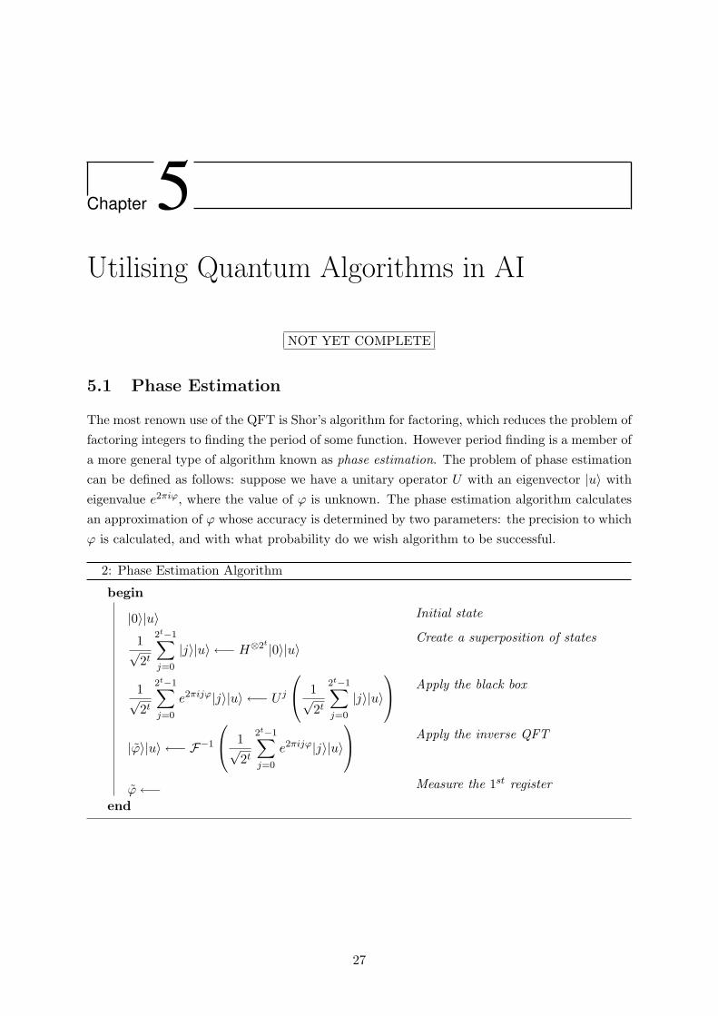
The most renown use of the QFT is Shor’s algorithm for factoring, which reduces the problem offactoring integers to finding the period of some function. However period finding is a member ofa more general type of algorithm known as phase estimation. The problem of phase estimationcan be defined as follows: suppose we have a unitary operator U with an eigenvector |u〉 witheigenvalue e2πiϕ, where the value of ϕ is unknown. The phase estimation algorithm calculatesan approximation of ϕ whose accuracy is determined by two parameters: the precision to whichϕ is calculated, and with what probability do we wish algorithm to be successful.

2: Phase Estimation Algorithm

begin

|0〉|u〉 Initial state

1√2t

2t−1∑j=0

|j〉|u〉 ←− H⊗2t |0〉|u〉Create a superposition of states

1√2t

2t−1∑j=0

e2πijϕ|j〉|u〉 ←− U j

1√2t

2t−1∑j=0

|j〉|u〉

Apply the black box

|ϕ〉|u〉 ←− F−1

1√2t

2t−1∑j=0

e2πijϕ|j〉|u〉

Apply the inverse QFT

ϕ←− Measure the 1st register

end

27

5.2 Amplitude Amplification

5.3 Quantum Searching

5.4 Assailing NP

5.5 Constraint Satisfaction Problems

5.6 Quantum Planning

Planning is a feature that we often require our agents to utilise, furthermore Chapman [22]states that any problem can be transformed to a planning problem. He also believes that “[i]tmakes no more sense to talk about [a] planning problem than it does [a] computational [one]”.

28

Chapter 6Physical Realisations of Quantum Computers

Until now all the discussions so far have been based upon a mathematical model of quantummechanics from which are derived the models quantum computation. Therefore, in order to per-form any quantum computations it is necessary to understand how the abstractions from thecomputational model, such as qubits, are manifested in the physical world. Without physicalrealisation quantum computation would be merely a mathematical curiosity. However, experi-mental realisations of quantum circuits and algorithms have proved challenging, and large-scalequantum computation may not yet be possible for quite some time. The basic requirements foran instance of a quantum computer(Quanputer [71]) consist of a closed quantum mechanicalsystem, mechanisms for altering/controlling the system state and, typically, methods of mea-suring all or some subset of the system properties. There exists a more refined set of criteriafor the construction of a quantum computer, described in §6.2, which requires some additionalaspects of quantum physics related to those detailed in §D.1.

6.1 Quantum Physics and Qubits

The most basic component in quantum computation is the qubit and was defined in §2.1.1 asa two-level quantum system, to perform computations we need to identify corresponding two-level physical systems. Fortuitously many such systems do exist but using any one has its ownadvantages and disadvantages. Any two state system consists of a ground state and an excitedstate which are separated by an energy gap [65].

Quantum physics attempts to create “quantised” physical models within the framework ofquantum mechanics, for example quantum field theories noted in §D.1.4. In addition to QEDother theories include: Quantum Chromodynamics (QCD) studies the interaction between sub-nuclear particles called quarks and gluons1, and a number of incomplete theories of quantumgravity. Each of the physical systems has a number of properties, e.g momentum and posi-tion, as physics is an empirical science it is concerned only with observables, properties whichare measurable. Observables of a Hilbert space, H, are self-adjoint operators on that space,

1Unlike electrons, protons and neutrons are not atomic but consist of a triplet of quarks, and interact witheach other via gluons. Gluons are the “messenger” particles [81] for the subnuclear forces, the strong and theweak force, just as photons are for the electromagnetic force.

29

however not all self-adjoint operators are physically meaningful observables [47]. As outlinedin [109], any physically meaningful observables must also satisfy transformation laws that relateobservations made by different observers in different frames of reference, the transform lawsare automorphisms, that is they are bijective transforms that preserve certain mathematicalproperties. In quantum mechanics the automorphisms are unitary linear transforms on theHilbert space H. In general the set of physically meaningful observables is chiefly restricted bythe principle of relativity which claims that the laws of physics are the same for all observers.

6.1.1 Nuclear Spin

For our purposes the most useful and simple example of an observable is the property of nuclearspin which is associated with microscopic particles. Spin can be conceptualised as a type ofangular momentum of the particle, not related to classical angular momentum, but is a purelyquantum mechanical phenomenon which has no analogy in classical physics. Since spin is aquantum mechanical property it can only posses discrete values, in the case of electrons theseare ~

2 ,−~2 which are referred to as spin-up and spin-down respectively. Particles with spin

possess a magnetic moment, just like a rotating electrically charged body in classical physics,which can be manipulated to perform quantum computation. Generally we refer to spin-upas the excited state and spin-down the ground state. A mathematical model of a prototypicaltwo-state quantum system, presented in [77, page 280], is included in §D.6 which demonstratehow a systems’s observables allow us to realise a qubit.

6.2 The DiVincenzo Criteria

In [34] Divincenzo describes in detail seven criteria that must be met by any physical implemen-tation if it is to perform any reliable computation, for reasons we will explain later Divincenzooften calls these seven criteria five-plus-two criteria. We now present these criteria with de-scriptions of how they relate to each other, together with brief comments on the theoretical andexperimental work surrounding them.

Criterion 1: A scalable physical system with well characterised qubits. A qubitbeing “well characterised” means several things including accurately known physical parameters,including the internal Hamiltonian of the qubit, and its interactions with itself, other qubits,and environment. By scalability we mean that it should be possible to work with ensembles ofqubits.

Criterion 2: The ability to initialise the state of the qubits to a simple fiducial

state. This criterion arises from requirements in computing, since we desire to prepare theinitial state of the registers to known values. An additional reason is that quantum errorcorrection techniques require a continuous source of prepared qubits.

Criterion 3: Long relevant decoherence times. “Decoherence times characterize the dy-namics of a qubit (or any quantum system) in contact with its environment. The (somewhatoverly) simplified definition of this time is that it is the characteristic time for a generic qubitstate, |ψ〉 = α|0〉+β|1〉, to be transformed into the mixture ρ = |α|2|0〉〈0|+ |β|2|1〉〈1|”[34], this

30

mixture represents the single qubit subsystem |ψ〉of (2.8.1). Also excluded from this definitionis the possibility that decoherence of neighbouring qubits are correlated. In quantum physicsdecoherence is identified as the basal mechanism by which classical behaviour emerges fromquantum behaviour [116], and for this reason presents an enormous threat to quantum comput-ing. Over time the effects of decoherence can reduce the capability of a quanputer to that akinto classical machines. In order to utilise the features of quantum system the decoherence timemust be of sufficient length to permit multiple quantum operations on the system. The lengthof time it take to execute an individual quantum gate is the clock-time of the quanputer. Thetheory of quantum information processing shows that, by means of quantum error correctioncodes (QECC), the decoherence time necessary for successful computations need not increaseas the size of the system does [42, 63], reducing the requirement on the decoherence time to amore reasonable, though still exacting, quantity. Furthermore it is known that QECC can bemade fully fault tolerant, protecting computation from unbounded proliferation of errors, how-ever to achieve this the decoherence time must be of the order of 104–105 times the clock-time.This suggests that once we have this threshold time decoherence will not impede scalability.

Criterion 4: A universal set of quantum gates. Many of the physically implementedqubit transforms are limited to unary, binary, and occasionally trinary operators [34]. In §3.3.2it was shown that there exits finite sets of binary qubit operators which are capable of approx-imating arbitrary quantum transforms. Of these known sets only two of them consist solely ofoperators that are implementable in a fault-tolerant way. Therefore to be of universal use aquanputer must implement not just universal gates but a finite set of universal fault-tolerantquantum gates. In [41] Gottesman shows that sometimes the error correction coding schemecan actually reduce the repertoire of gates required. He goes on to develop a methods of gen-eral quantum computation utilising only two-qubit exchange interactions, a simplification whichmight prove useful in quantum dot technologies such as quantum cellular automata.

Furthermore, since quantum algorithms are typically specified by a finite sequence of unitarytransforms, U0, . . . , Un−1, each acting on a (small) number of qubits to transcribe them to aphysical specification we identify the Hamiltonians which generate these transforms. The Hamil-

tonian of each transform, UT, is given by (1.2.2) such that UT = e

hitHT

~

ifor T = 0, . . . , n− 1.

Ideally the quanputer design permits the transform on the system, U(t), executed in the timeinterval t ∈ (tn, tn+1) to be U(t) = Un. Unfortunately, to date, such well defined manipulationof the quantum system is far from perfect as, among other reasons, it is difficult to switch thetransforms on and off in this ideal way. These problems pose further difficulties on implementinga set of universal fault-tolerant transforms.

Criterion 5: A qubit-specific measurement capability. An ideal measurement of a qubitstate, |ψ〉 = α|0〉+ β|1〉, in the computational basis |0〉, |1〉 returns |0〉 with probability |α|2,and |1〉 with probability |β|2 = 1− |α|2. In addition the measurement should:

(i) be independent of any other system parameters including the states of proximate qubits.

(ii) not alter the state of any non-measured qubit in the system.

31

Such an ideal measurement is said to have “100% quantum efficiency2” [34]. While it is de-sirable to have such efficiency much less is needed for practical computing, which is fortuitousas real measurements have efficiencies much lower than an ideal one. Suppose that we havea computation which returns a single qubit output (a decision problem) and is absent of im-perfections except for that of the quantum measurement efficiency, then the reliability of theprocess is the efficiency of the measurement. If we require higher reliability than the efficiencywe can achieve this by repeatedly running the computation [77]. An alternative solution [34]ivolves using the original single output qubit as the control bit in a modified CNot-gate whichoperates on p qubits in the state |0〉. This has the effect of “copying” the qubit in the compu-tational basis, c.f Theorem 2.7.3. By measuring all the output qubits including the origonalsingle output qubit, which is unchanged by the operation, we gain the same result as rerunningthe computation. The value of p depends on the efficiency of the measurement, q, but generallya reliable outcome can be achieved by setting p ≥ 1/q. We shall examine this possibility againin §6.3.1 when we discuss Nuclear Magnetic Resonance (NMR).

The criteria presented so far are sufficient for performing quantum computation however, thefeatures of quantum information processing are not typified by computation alone. There existinformation processing tasks, such as communication, for which quantum information processingprovides a unique advantage over classical methods, e.g. secret key distribution, multipartyfunction evaluation, and game playing. We informally define quantum communication as: thetransmission of intact qubits from one location to another. The requirements of communicationgive cause to pose two further criteria on the composition of a quanputer:

Criterion 6: The ability to interconvert stationary and flying qubits. In the discus-sions of quantum communication the term “flying qubit” [54] is used to emphasise that theoptimal physical implementation of qubits which are readily transmitted from locale to anothermay not be optimal for reliable local computations as discussed in the first five criteria. Thiscriterion is proving difficult to satisfy, so far only one theoretical proposal [26] is sufficientlytangible which utilises a technique from QED called cavity-QED and uses photons for flyingbits.

Criterion 7: The ability faithfully to transmit flying qubits between specified loca-

tions. Very little is actually said about this criterion in DiVincenzo’s paper except concerningits motivation from, predominantly, quantum cryptography. Therefore by “faithfully” we mustassume that this means that the “quantum-ness” must be preserved and not that the trans-mission be error free, since we could compensate this by using error correction codes. Therehave been many experiments [83, 111] based on photons as flying qubits but recently severalhave proposals [55, 115] consider using electrons moving through solid-state devices such as theimplanted ion scheme introduced in §6.3.2.

DiVincenzo avoid’s summarising his work and instead emphasises that quantum computa-tion is still in its infancy and such it is not proper to prematurely question what the “winning”

2The fidelity of a quantum measurement can not be captured by a single parameter, however this parameterprovides a useful pragmatism.

32

technology will be, nor its limitations. He also makes speculative comments on several differ-ent quantum technologies, some of which are purely theoretical, while others utilise yet othercomputational paradigms (such as Quantum Cellular Automata [78]).

Definition 6.2.1: We divide the criteria in to two groups: the computation criteria whichconsists of the first five criteria (1,2,3,4,5), and the communication criteria which consist of theremaining two (6,7). It is possible that DiVincenzo used a similar notion of grouping when hedescribes his work as “5 + 2 criteria” [34].

6.3 Emergent Quantum Technologies

Any particular instance of a quanputer has, by criterion 1, an associated physical system how-ever, existing quantum manipulative technologies lack the ability to be scaled-up to sizes suitablefor practical computations. Obviously the phrase “practical computations” is ill defined but toinclude the QECC described in criterion 3 we would need at least 10 qubits to characterise 1.The best current techniques are only able to reliably manipulate at most 7 qubits [53] but thishas still allowed us the experimentally verify a number of quantum algorithms. IBM signif-icantly performed the simplest non-trivial instance of Shor’s algorithm, utilising 7 qubits tofactorise 15 in to 3 and 5. This result was achieved by using a variant of NMR to control andobserve nuclear spin properties. What follows is a non-technical outline of some of the currenttrends in quantum technology, and some of their potential capabilities, and limitations.

6.3.1 Bulk Spin NMR

Nuclear magnetic resonance exploits the property of nuclear spin, introduced in §6.1.1. Itspractical uses originate in chemistry, where it was used to analyse the structure of molecules3.NMR essentially works by applying a strong magnetic field to the molecule, this causes themagnetic moment of each atom to align with the field. The magnetic moment of an atom canbe thought of as a summation of all its constituent particles’ moments and is still describedonly by quantum mechanics, that is the values of atomic spin are also quantised. The stateof the atoms in the molecule can then be controlled by bursts of radio frequency pulses (RF-

pulses), which alters their spin, and measured by the perturbation of the magnetic field thatthis causes, with the usual limitations of quantum measurement. The atoms within the moleculeinteract weakly, but reliably, with each other and their interaction with the environment areoften “sufficiently small” [65] enough to satisfy DiVincenzo’s computation criteria.

This description is insufficient to demonstrate exactly how NMR could manipulate a quan-tum system in a way that would allow us to perform computations and the exact details areunnecessary for our purposes, but full descriptions are given in [65, 77]. If we accept that eachatom in the molecule represents a suitable two-level quantum system then, together with theNMR apparatus, we can in principle form a quanputer from some molecule. There are howeverseveral difficulties and limitations faced by this technology, of which we note two.

3A composite of various atoms.

33

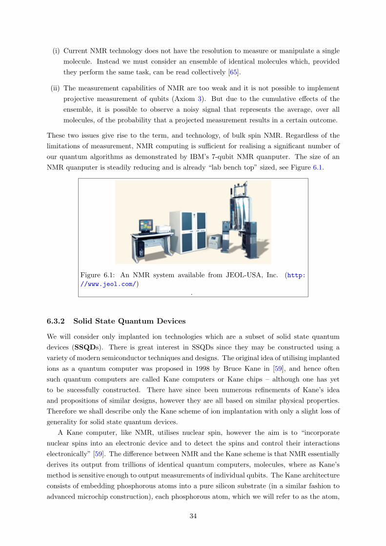
(i) Current NMR technology does not have the resolution to measure or manipulate a singlemolecule. Instead we must consider an ensemble of identical molecules which, providedthey perform the same task, can be read collectively [65].

(ii) The measurement capabilities of NMR are too weak and it is not possible to implementprojective measurement of qubits (Axiom 3). But due to the cumulative effects of theensemble, it is possible to observe a noisy signal that represents the average, over allmolecules, of the probability that a projected measurement results in a certain outcome.

These two issues give rise to the term, and technology, of bulk spin NMR. Regardless of thelimitations of measurement, NMR computing is sufficient for realising a significant number ofour quantum algorithms as demonstrated by IBM’s 7-qubit NMR quanputer. The size of anNMR quanputer is steadily reducing and is already “lab bench top” sized, see Figure 6.1.

Figure 6.1: An NMR system available from JEOL-USA, Inc. (http://www.jeol.com/)

.

6.3.2 Solid State Quantum Devices

We will consider only implanted ion technologies which are a subset of solid state quantumdevices (SSQDs). There is great interest in SSQDs since they may be constructed using avariety of modern semiconductor techniques and designs. The original idea of utilising implantedions as a quantum computer was proposed in 1998 by Bruce Kane in [59], and hence oftensuch quantum computers are called Kane computers or Kane chips – although one has yetto be sucessfully constructed. There have since been numerous refinements of Kane’s ideaand propositions of similar designs, however they are all based on similar physical properties.Therefore we shall describe only the Kane scheme of ion implantation with only a slight loss ofgenerality for solid state quantum devices.

A Kane computer, like NMR, utilises nuclear spin, however the aim is to “incorporatenuclear spins into an electronic device and to detect the spins and control their interactionselectronically” [59]. The difference between NMR and the Kane scheme is that NMR essentiallyderives its output from trillions of identical quantum computers, molecules, where as Kane’smethod is sensitive enough to output measurements of individual qubits. The Kane architectureconsists of embedding phosphorous atoms into a pure silicon substrate (in a similar fashion toadvanced microchip construction), each phosphorous atom, which we will refer to as the atom,

34

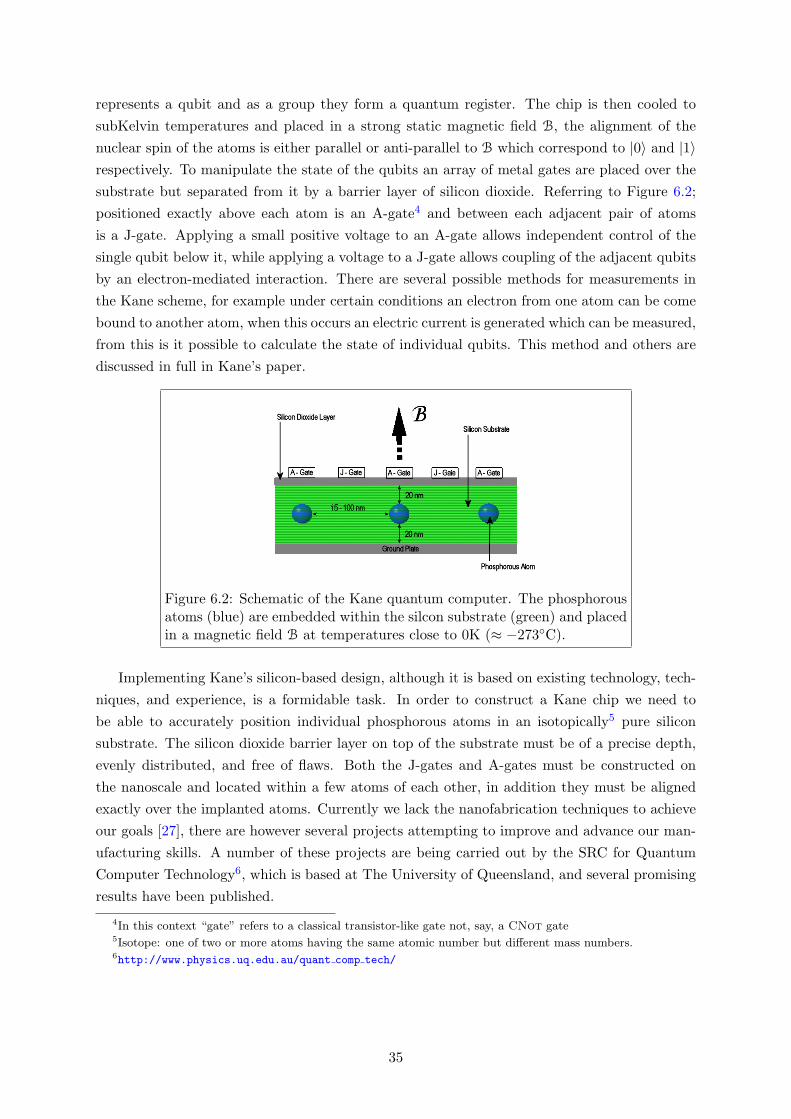
represents a qubit and as a group they form a quantum register. The chip is then cooled tosubKelvin temperatures and placed in a strong static magnetic field B, the alignment of thenuclear spin of the atoms is either parallel or anti-parallel to B which correspond to |0〉 and |1〉respectively. To manipulate the state of the qubits an array of metal gates are placed over thesubstrate but separated from it by a barrier layer of silicon dioxide. Referring to Figure 6.2;positioned exactly above each atom is an A-gate4 and between each adjacent pair of atomsis a J-gate. Applying a small positive voltage to an A-gate allows independent control of thesingle qubit below it, while applying a voltage to a J-gate allows coupling of the adjacent qubitsby an electron-mediated interaction. There are several possible methods for measurements inthe Kane scheme, for example under certain conditions an electron from one atom can be comebound to another atom, when this occurs an electric current is generated which can be measured,from this is it possible to calculate the state of individual qubits. This method and others arediscussed in full in Kane’s paper.

Figure 6.2: Schematic of the Kane quantum computer. The phosphorousatoms (blue) are embedded within the silcon substrate (green) and placedin a magnetic field B at temperatures close to 0K (≈ −273C).

Implementing Kane’s silicon-based design, although it is based on existing technology, tech-niques, and experience, is a formidable task. In order to construct a Kane chip we need tobe able to accurately position individual phosphorous atoms in an isotopically5 pure siliconsubstrate. The silicon dioxide barrier layer on top of the substrate must be of a precise depth,evenly distributed, and free of flaws. Both the J-gates and A-gates must be constructed onthe nanoscale and located within a few atoms of each other, in addition they must be alignedexactly over the implanted atoms. Currently we lack the nanofabrication techniques to achieveour goals [27], there are however several projects attempting to improve and advance our man-ufacturing skills. A number of these projects are being carried out by the SRC for QuantumComputer Technology6, which is based at The University of Queensland, and several promisingresults have been published.

4In this context “gate” refers to a classical transistor-like gate not, say, a CNot gate5Isotope: one of two or more atoms having the same atomic number but different mass numbers.6http://www.physics.uq.edu.au/quant comp tech/

35

6.3.3 Summary

In this chapter we have described the various challenges that must be overcome in order thatquantum computation and quantum information are of practical use. The DiVincenzo compu-tation criteria (excluding the first criterion) highlight the problems in maintaining and manip-ulating the state of the quantum system. Errors can arise from decoherence and gate noise,however there are methods to combat these sorts of problems. In addition there are also familiesof universal gate which operate on quantum error correction coded inputs, hence it is theoreti-cally possible to build fully fault-tolerant quanputers. Constructing a scalable physical systemto satisfy the first computation criterion, while being necessary for practical computation, iscurrently an open problem in quantum physics since the complexity of mathematical modelincreases in proportion to the size of the system. In bulk-spin NMR the fifth criterion is theleast satisfied constraint since we measure the average value of a specific qubit, but in implantedion technology it is essential that we have such ”fine grained” responses. Both of the communi-cation constraints are problems in the field of “quantum mechanical engineering” and thereforeare not technically an issue in theoretical quantum computation and quantum information butit is possible that QECC will be necessary for reliable transmission of quantum informationprocessing.

There are a plethora of proposals for the construction of quantum architecture, of which weintroduced two based on manipulating nuclear spins: NMR, and solid-state devices. In additionthere is a description in §D.6.2 of another quantum technology - an ion trap - which has beenexperimentally realised, albeit with many shortcomings. It is difficult to compare these threetechnologies however, since there are few experimental results of ion trap quanputers and a solid-state one has yet to be built. Bulk-spin NMR is currently the most frequently used technologyand has executed a number of significant quantum algorithms, adding weight to the argumentthat our theories are correct7. Unfortunately it seems likely that bulk-spin NMR is not theoptimal implementation of a quanputer since its methods of measurement and manipulationrequire an ensemble of qubits, nor is it known if it is possible to increase the scale the processsufficiently; it remains to be seen which technology will prove most fruitful. Even if quantumcomputation proves only to be equally powerful as Turing computation quantum technology hasthe potential to vastly reduce the physical size of quanputers compared to today’s computers.

7Obviously we are unable to prove our theory of reality is correct, by “correct” we mean that expectedobservations match experimental ones.

36

Chapter 7Quantum Robotics

We have thus far discussed several aspects of artificial intelligence and how they may be ac-commodated in the paradigm of quantum computation however, AI is a holistic discipline thatconsiders not just the individual intellectual mechanisms of computation but also the construc-tion of autonomous agents. Given that quantum computation is more powerful than classicalcomputation, in certain situations, it is natural to ask what advantages could be gained byconstructing agents which utilise quantum resources?.

Robots are physical agents that perform tasks by interacting with the real world. Generallythese interactions can be either an input type or an output type. Hardware designed for input isknown as sensors, while that of output is effectors. The purpose of effectors is to assert physicalforces on the environment corresponding to the output of the agent’s actuators. Examplesof effectors include robotic arms, wheels/engines, and etching lasers on microchip assemblies.Modern robots have a diverse set of sensors to enable them to perceive the environment suchas cameras, laser range-finders, and accelerometers to measure the robot’s own motion.

7.1 Quantum Robots

The original concept of a quantum robot was proposed by Paul Benioff [6] and later expandedupon in [10, 8, 7]. Benioff’s quantum robots (BQ-Robots) are “mobile systems that have aquantum computer on board and any other needed ancillary systems. Quantum robots movein and interact (locally) with environments of quantum systems. Since quantum robots aremobile, they are limited to be quantum systems with finite numbers of degrees of freedom” [6],a robot is also equipped with a memory register |m〉, an output system |o〉 and a control qubit|c〉. The environments consist of an arbitrary number of quantum systems propagating withina 1,2,3-dimensional space which are able to interact with other systems or be interaction free.Environments may be either open or closed; if the environment is open there exist systems whichnever interact directly with the quantum robot yet establish correlations with other elementsof the environment within the domain of the robot [7]. The dynamics of BQ-robot consist oftwo alternating phases: the “computation phase” and the “action phase”.

When the control qubit |c〉 is equal to |1〉 the BQ-robot is in the computation or planningphase. The purpose of the computation phase is to determine the function to execute in the

37

next action phase. In doing this the BQ-robot may use any combination of the memory |m〉,the output |o〉, and the local environment. Actions are represented by a set, A, of N basisstates each of which corresponds to a particular action, hence a successful1 computation as-signs/transforms |o〉 to some state of A. During this phase the BQ-robot does not move norinteract with the environment (save for measurement like entanglement [10]). The final step ofthis phase is to apply the σx transform to the control bit |c〉 leaving it in the state |0〉.

While the control qubit is in the state |o〉 the BQ-robot is in the action phase. The actionphase is independent of |m〉 and the state of the robot’s on-board computer, furthermore thestate |o〉 is unchanging. Examples of actions include moving the robot, performing measure-ments, and otherwise locally interacting with the environment.

Benioff’s quantum robots utilise cyclic quantum circuits, as we have done, and an example ofan instance of a complete BQ-robot can be found in [8]. He points out that the main differencebetween his quantum robots and a quantum computer is that “for quantum computers thestates of the qubits must not change spontaneously in the absence of interactions related to thecomputation” whereas the environment of the robot may change independently of its actions.

It is hoped that BQ-robots will allow us to “validate” quantum mechanics [9] since if quan-tum mechanics is universally valid then any computational or physical construct must be them-selves be described entirely by quantum mechanics. There is no existing quantum technologywhich is capable of constructing a BQ-robot nor is any proposed by Benioff, however once con-struction is possible BQ-robots may prove to be the basis of quantum systems which are able tomake decisions, perceive, and interact with their environment. In [8] Benioff exposes his beliefin computationalism by inferring that such systems will give rise to “intelligence”.

7.2 Q-Bots

Suppose that some solid state quantum technology, such as Kane’s §6.3.2, will be achieved withinthe near future2. The physical size of these devices will be relatively small but undoubtedlyscalability will still limit the system size. However, as we shall demonstrate, these restrictionscan be, at least, reduced. While we are currently unable to construct purely quantum robots,like Benioff’s, it will soon be possible to integrate quantum computational devices with current(classical) computing technology. An alternate or intermediate possibility for quantum robots isa hybridisation of existing robotic technology and quantum technologies - a Q-Bot. We define aQ-bot to be a mobile robot that utilises quantum information, computation and/or phenomenonequipped with sensors and/or effectors that has the ability to make decisions, perceive, andinteract with its environment. In following sections we show how the material from the previouschapters can be composted to construct a Q-bot both in terms of system architecture and(agent) software, however it not intended to satisfy a complete specification of all hardware andsoftware elements.

1By successful we mean that the computation terminates not that the action taken is the best possible action.2Maybe a decade!

38

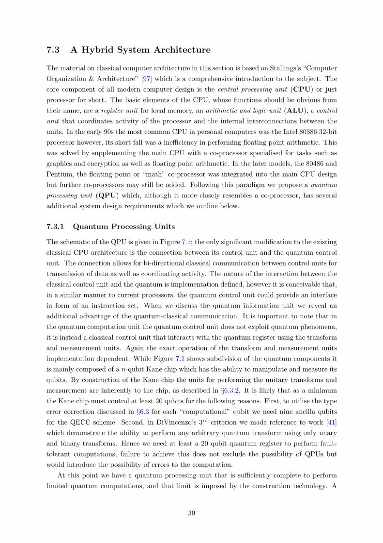
7.3 A Hybrid System Architecture

The material on classical computer architecture in this section is based on Stallings’s “ComputerOrganization & Architecture” [97] which is a comprehensive introduction to the subject. Thecore component of all modern computer design is the central processing unit (CPU) or justprocessor for short. The basic elements of the CPU, whose functions should be obvious fromtheir name, are a register unit for local memory, an arithmetic and logic unit (ALU), a controlunit that coordinates activity of the processor and the internal interconnections between theunits. In the early 90s the most common CPU in personal computers was the Intel 80386 32-bitprocessor however, its short fall was a inefficiency in performing floating point arithmetic. Thiswas solved by supplementing the main CPU with a co-processor specialised for tasks such asgraphics and encryption as well as floating point arithmetic. In the later models, the 80486 andPentium, the floating point or “math” co-processor was integrated into the main CPU designbut further co-processors may still be added. Following this paradigm we propose a quantumprocessing unit (QPU) which, although it more closely resembles a co-processor, has severaladditional system design requirements which we outline below.

7.3.1 Quantum Processing Units

The schematic of the QPU is given in Figure 7.1; the only significant modification to the existingclassical CPU architecture is the connection between its control unit and the quantum controlunit. The connection allows for bi-directional classical communication between control units fortransmission of data as well as coordinating activity. The nature of the interaction between theclassical control unit and the quantum is implementation defined, however it is conceivable that,in a similar manner to current processors, the quantum control unit could provide an interfacein form of an instruction set. When we discuss the quantum information unit we reveal anadditional advantage of the quantum-classical communication. It is important to note that inthe quantum computation unit the quantum control unit does not exploit quantum phenomena,it is instead a classical control unit that interacts with the quantum register using the transformand measurement units. Again the exact operation of the transform and measurement unitsimplementation dependent. While Figure 7.1 shows subdivision of the quantum components itis mainly composed of a n-qubit Kane chip which has the ability to manipulate and measure itsqubits. By construction of the Kane chip the units for performing the unitary transforms andmeasurement are inherently to the chip, as described in §6.3.2. It is likely that as a minimumthe Kane chip must control at least 20 qubits for the following reasons. First, to utilise the typeerror correction discussed in §6.3 for each “computational” qubit we need nine ancilla qubitsfor the QECC scheme. Second, in DiVincenzo’s 3rd criterion we made reference to work [41]which demonstrate the ability to perform any arbitrary quantum transform using only unaryand binary transforms. Hence we need at least a 20 qubit quantum register to perform fault-tolerant computations, failure to achieve this does not exclude the possibility of QPUs butwould introduce the possibility of errors to the computation.

At this point we have a quantum processing unit that is sufficiently complete to performlimited quantum computations, and that limit is imposed by the construction technology. A

39

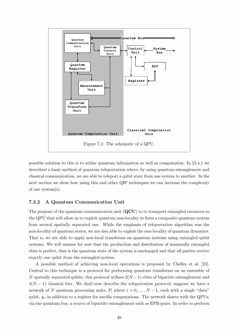
Figure 7.1: The schematic of a QPU..

possible solution to this is to utilise quantum information as well as computation. In §3.4.1 wedescribed a basic method of quantum teleportation where, by using quantum entanglement andclassical communication, we are able to teleport a qubit state from one system to another. In thenext section we show how using this and other QIP techniques we can increase the complexityof our system(s).

7.3.2 A Quantum Communication Unit

The purpose of the quantum communication unit (QCU) to to transport entangled resources tothe QPU that will allow us to exploit quantum non-locality to form a composite quantum systemfrom several spatially separated one. While the emphasis of teleportation algorithm was thenon-locality of quantum states, we are also able to exploit the non-locality of quantum dynamics.That is, we are able to apply non-local transforms on quantum systems using entangled qubitsystems. We will assume for now that the production and distribution of maximally entangledebits is perfect, that is the quantum state of the system is unchanged and that all parties receiveexactly one qubit from the entangled system.

A possible method of achieving non-local operations is proposed by Chefles et al. [23].Central to this technique is a protocol for performing quantum transforms on an ensemble ofN spatially separated qubits, this protocol utilises 2(N −1) ebits of bipartite entanglement and4(N − 1) classical bits. We shall now describe the teleportation protocol; suppose we have anetwork of N quantum processing units, Pi where i = 0, . . . , N − 1, each with a single “data”qubit, qi, in addition to a register for ancilla computations. The network shares with the QPUs,via the quantum bus, a source of bipartite entanglement such as EPR-pairs. In order to perform

40

an arbitrary transform to the qi we teleport all the qi states to a single QPU, say P0, applythe transform and teleport the final states of the qubits back to their originating processors.Since the teleportation from one QPU to another require 1 ebit and 2 classical bits each QPUP1, . . . , PN−1 utilises 2 ebits and 4 classical bits during the procedure, and hence 2(N − 1) ebitsand 4(N − 1) classical bits in total. This protocol is proved to be asymptotically optimal inclassical and quantum resources for even N , this is done by establishing a lower bound usingthe principle of conservation of quantum information (definition 2.7.1). Asymptotically optimalmeans that, given a large number of sets of separated qubits and a quantum transform to beapplied to each set, the protocol “uses the minimum average entanglement”. A further paperby Chefles et al., [24], investigates the instances when N is odd rather than even.

The final aspect of the QCU is intrinsically linked to the quantum bus which we have thusfar ignored. Nearly every feature of quantum information processing utilises the resource of en-tanglement, and while we have seen how we can create local entanglement using CNot-gates itis necessary to share this resource with the spatially separated system. The quantum bus is re-sponsible for the transmission and reception of quantum states via entangled qubits. Techniquesfor the distribution of entangled pairs are not a new occurrence since they were fundamental inestablishing the validity of Bell’s theorem on non-local correlations. The most well establishedof these techniques are optical; recent work by Resch et al. [84] aptly demonstrates technologicalachievements made thus far. In their experiment Alice and her telescope are located at the 15mabove ground on the roof of the Kuffner Sternwarte observatory, meanwhile Bob is 150m aboveground on the 46th floor of the Millennium Tower 7.8km away from Alice across the city centerof Vienna. Alice has a device capable of creating an entangled pair of photons which are passedthrough a 50/50 mirror and into fibre optic channels. One photon remains with Alice whilethe other is transmitted by the telescope to Bob, this is known as free-space transmission; theclassical communication between Alice and Bob is mediated by the Internet. Unfortunatelythis process is extremely noisy resulting in only a 1.4% average efficiency of detection rate,the reasons for this include losses in both receiving and transmitting lenses as well as the fibreoptics but not in the single photon detectors. It is possible that we can adapt this experimentto our needs as follows; Using the same entanglement source as above individual photons areinjected in to a fibre optic network and routed to their destination by careful use of fibre in-terchange stations that utilise common optic components to channel a photon in to a differentfibre. Finally the qubit is recieved by single photon detector which swaps its state with a qubitin the QPU register. The timing for the application of these components is synchronised withthe entanglement source in the same manner as the original experiment. The limitation of thisdesign is that which limits its parent, the inefficiency of transmission.

An alternate theoretical solution to the distribution problem is proposed by Brennen etal. [16] is to create “channels” of communication between blocks of computational qubits whichthe authors also name a quantum bus - we will refer to it as the quantum channel to avoidconfusion with our model. Non-local operations on the computational qubits are performedby creating entanglement between two neighbouring qubits in the quantum channel, then bycarefully timed operations the qubit states of the pair are successively swapped with their neigh-bours until each is adjacent to one of the target computational qubits. The non-local operation

41

can now be applied in a similar manner to the protocol of Chefles et al. This architecture hasthe advantage of surmounting the problem of interconverting flying to stationary qubits, oneof DiVincenzo’s criteria, in addition it appears that the requirements for the quantum channelsare less stringent than those for a quantum computer.

7.3.3 Agent Function

7.3.4 Vision, Other Sensors and Actuators

42

Chapter 8Discussion & Concluding Remarks

The aim of this paper was fourfold; to introduce a theory of computation based on the physicallaws of quantum mechanics, consider the construction of devices capable of quantum computa-tion, study the potential use of quantum algorithms in artificial intelligence, and to augment aclassical agent with quantum computation and technologies.

8.1 Quantum Computation

We have seen that using the mathematical framework of quantum mechanics it is possible toconstruct a computational model which is at least equal in “computational power” to the Turingmodel. This was crudely done by presenting construction of quantum Turing machines. Thestudy of the potential power of quanputers is still a theoretical challenge, the allure of greatercomputational power however provides additional incentive for the constructions of quantumcomputing devices. Further incentives include known quantum algorithms for computationallyimportant problems which offer significant speedups over the best known1 classical algorithms.

These algorithms include Deutsch’s Algorithm, allows us to determine whether a Booleanfunction is balanced or constant in time O(1) giving an exponential speed-up over the classicalinstance which requires time O(2n). Unfortunately there are very few practical applications ofDeutsch’s Algorithm but it contains all the main features of successful quantum algorithms, itis also shown [28] that all quantum computations are merely more complicated variations ofDeutsch’s algorithm. The two main phases of computation, according to this view, are based onthe quantum phenomena of entanglement, whereby data is encoded multi-qubit superpositions,and interference, which modifies the multi-qubit system by evolving it from the set of inputstates to the set of output states. There are no classical analogues of either entanglement ormulti-qubit interference making them inherently quantum processes. Deutsch’s algorithm isa solution to a specific instance of more generalised problem known as the hidden subgroupproblem. In this paper we introduced the basics of entanglement, which is in its own right alarge field of research both theoretically and experimentally. It is thought [77] that as we learnmore about entanglement we are refining a physical theory of information. Furthermore, some

1The word “known” is used here to indicate that the classical algorithm may not be optimal or lacks suchproof. In such cases we can compare only relative algorithm efficiencies not absolute.

43

believe that such a physical theory will redefine many of our concepts of what information isand provide insight to quantum physics.

One limitation of the approach taken in this paper is that we constrained ourselves, by ourdefinition of the axioms of quantum mechanics, to closed quantum systems. But as we laterdiscussed, this is not experimentally realistic since the quantum system will interact with itsenvironment leading to decoherence. An alternative would be to adopt the quantum densityoperator formulation of quantum mechanics which would allow us to consider open systems.However, a drawback with this approach is that it is significantly more intimidating to a novicemathematician.

8.2 Quantum Technologies

It is still uncertain whether the development of quantum technology will be accurately modelledby Moore’s law, as it has been for traditional computer technology. But asking this questionhas a number of flaws, one of which is that Moore’s law concerns the diminishing size of thesurface areas of transistors yet, loosely speaking, we consider qubits which are objects of pointmass (i.e. zero size), like particles, or they are described by localised wave functions that havepossibly infinite size. If we consider the number of bits per square nanometer that transistorscan manipulate then it is possible to compare this to the number of qubits per square nanometer.While this may seem unfair, consider the size of a 7-qubit NMR computer even compared to a10-bit pocket calculator (e.g. the first scientific pocket calculator HP-35), it does highlight thetwo biggest current technological barriers: the size of the quantum system, and the size of thecontrolling machinery. While bulk spin NMR has provided an excellent platform for refiningand refuting our ideas of quantum computation it is likely that due to the limitations on itsscalability and measuring it will soon become an inadequate quantum technology.

The solid state quantum devices are perhaps the most promising technologies at the moment,yet even within this group are a plethora of differing implementations. We discussed the mostrenown of these, the Kane chip, in §6.3.2. The advantage of the “microchip” style of constructionis that built into the device are the components to measure and transform its quantum system,this results in a small device size and would reduce our reliance on large, bulky NMR computers.However, in order to build these devices reliably an advancement in nano-fabrication techniquesis required because quantum mechanics demands a high level of precision. In fact Leonid Levinstates [t]he major problem [with quantum computing] is the requirement that basic quantumequations hold to multi-hundredth if not millionth decimal positions where the significant digitsof the relevant quantum amplitudes reside. We have never seen a physical law valid to over adozen decimals [67].

44

8.3 Quantum Algorithms for Classical AI Problems

8.4 Prospects for Quantum AI

Bylander advocates that “[i]f the relationship between intelligence and computation is takenseriously, then intelligence cannot be explained by intractable theories because no intelligentcreature has the time to perform intractable computations. Nor can intractable theories pro-vide any guarantees about the performance of engineered systems. Presumably, [agents]/robotsdon’t have the time to perform intractable computations either” [18]. What is not clear is howthis should be interpreted in a quantum setting; what are the implications of physical compu-tation? Can we claim that intelligence cannot be explained by intractable physical theories?But all (good) physical theories are intractable since they are true insofar as they agree withall experimental results. Regardless of the accuracy our mathematical models may possess, acertain ambiguity remains until our mathematics is integrated with a complete physical under-standing, whether such an understanding is achievable is a fervently debated topic throughoutphilosophy, mathematics, and the physical sciences.

More practical applications of quantum AI are severely retarded by the limitations of ourquantum technologies. None of the quantum robots designs in §7, including the quantum-classical hybrid Q-bot, can be currently implemented, nor can any experimental proof of concept.Until we have more fine grained control of quantum systems determining whether the exoticquantum technology suggested in §7 is achievable remains unanswerable.

More generally it seems that, like many other areas of computer science, quantum compu-tation and quantum information processing can offer greater computing power. But there arelimitations; the difficultly in preparing quantum states makes encoding, say a simple databasefor Grover’s algorithm, currently such computations result are less efficient than classical meth-ods. However this does not necessarily extend to more complex problems; the SAT problem,being NP-complete, is intractable on a classical computer yet quantum computers achieve apolynomial speed-up. On its own this, although useful, is not enough to motivate quantumAI but additional techniques such as phase estimation allow us to determine whether certainproblems have no solution, or how many solutions there are. Clearly quantum computation andinformation can enhance and improve our existing artificial intelligence models and techniques,but until such time as technology permits quantum AI will remain an intellectual curiosity.

45

Chapter 9Disserting a Dissertation

“Mathematics is not a spectator sport!” – Dr. Linda White (Imperial College 2000)

It may seem unconventional to include new material after the conclusion of the paper andwhich is not an appendix, however this section fulfils particular requirements on the content ofan undergraduate dissertation. At the time of writing the full requirements are stipulated at

http://www.comp.leeds.ac.uk/fyproj/

Some of these requirements seem to be slightly biased toward problems whose solution canbe achieved using some methodology, for example the waterfall model in software engineering.However, unlike software design there does not exist any complete formal methodology forwriting a dissertation, therefore it was necessary to attempt to devise guidelines based on theavailable information (see §B.1); these are included in Appendix B.

In order to present the project development we divide it into four phases1: storming, form-ing, norming and disseminating. Generally progression through the phases is sequential butsometimes there is cause to return, perhaps just a section of work, to an earlier phase and restartfrom there. This might be necessary if some branch of research proves fruitless, unrelated tothe original problem, or simply too hard.

We now informally define the phases and identify the project development within them.Following this additional comments on particular developments of this project, not coveredelsewhere, will be presented. While the initial phases might occupy a higher proportion of theproject life-span their influence maybe less obvious in the final stages where completed workemerges. Perhaps the reason for this is that often “mathematical scientists” tend to publishtheir solution of a problem together the proof of correctness, if applicable, but not necessarilywhy they started thinking a certain way. Because of this however, just like measurement inquantum algorithms, it appears as if most of the work occurs at the end of the process.

9.1 Storming

The first phase of a project forms a significant proportion of the project conception §B.1. Thename of the phase, “Storming”, could come from brainstorming but this would exclude any

1The names of some of the phases are not coincidentally similar to phases in the the Tuckman model of groupdynamics [102].

46

research and learning that may be necessary for both general understanding of the topic andproblem specific information. The aim of this phase to terminate with idea(s) which showpromise.

My initial reading material consisted mainly of two comprehensive books. The first Nielsenand Chuang [77] which provides not only a through introduction of quantum computation butalso quantum mechanics, mathematics, and computer sciences followed by in depth descrip-tions and explanations of many applications for quantum computation and information. Mostimportantly of all however, is that the authors included many exercises to reinforce the infor-mation they impart; the quote from Linda White at the beginning of this chapter captures howimportant completing these exercises were to my understanding. The second book was Hirven-salo [47] which is a more terse mathematical book that I found allowed much quicker access ofinformation once I was already familiar, but not necessarily comfortable, with the topic.

As my understanding of the material developed my reading expanded to periodicals, andother books. Also there is a profusion of resources available on-line, the most useful of whichwere electronic copies of the major periodicals and arXiv.org. The initial direction of the projectwas pointed toward quantum complexity, specifically possible methods for the solution of NP

problems in polynomial time using quantum search algorithms. In turn this lead me to questionwhat benefits quantum search would impart to search problems in artificial intelligence.

9.2 Forming

In the forming stage the ideas collated in the Storming phase are transcribed to formal state-ments. Often in this phase some ideas have to be modified to varying degrees and in extremecases discarded altogether. The aim of forming is to produce a precise description of the tasksyou intend to accomplish but not how you intend to execute them.

By continuing the investigation of search algorithms, both classical and quantum, withapplications within AI, e.g. unordered search, solution counting, and constraint satisfactionproblems, it became apparent that the theory of quantum search is well developed leaving thepossibility of my being able to contribute something novel much less probable. This promptedme to consider developing an artificial intelligent agent which utilised, to some degree, quantumcomputation and quantum information. The classical basis of the project is a agent usingpropositional logic, similar to that defined in Norvig and Russell [87], hence the developmentof certain ideas came quite naturally by a process similar to a translation between the classicaland quantum.

This idea was then extended to consider an autonomous mobile physical agent utilisingquantum technology for both computation and interactions, e.g. communication and “quantumsensors”, which we later call Q-bots. Thus the purpose of the paper would be an analysis ofthe quantum elements necessary to construct such an agent. The elements of the original Q-botidea were grouped into four categories: symbolic (Turing) computation, connected computation(neural networks), communication, and hardware. It was instantly obvious that due to thediversity of these fields, not just in the quantum setting but also the classical, uniting them inan undergraduate paper would be impossible; to reduce the complexity of the project it was

47

decided that the applicability of quantum communication in artificial intelligence should receivelittle attention except when necessary for concept completion.

Some of these elements form part of the project minimum requirements and the remainingwork on Q-bots (§7) form an extension of these requirements. It was quite obvious, even atthis early stage, that a significant task in this project would be presenting some introductionto quantum computation and is associate physics and mathematics, since without this is waslikely that very few would be able to appreciate the content.

9.3 Norming

Although this phase includes a significant amount of work its description is deceptively short, itis a natural continuation of the work produced in the previous forming stage; norming involvesexecuting the solutions to the tasks using the specified method. It is highly probable that duringthis phase further research is necessary as “knowledge gaps” may appear, nor is it uncommonto return to the forming phase as new avenues of though are encountered. Before proceedingto the next phase the goal its to have addressed every stated task.

Many complications arose during this phase, they included finding the material beyond lev-els of understanding and capability, discovering other research material that invalidates an ideaor already proposes the same or similar solutions/conclusions. An example of this is the sectionon quantum neurocomputing §4.2. The preliminary investigation into quantum neural networkssuggested that they are still relatively undeveloped when compared to symbolic methods; themajority of the relevant papers concerned recurrent quantum networks like the Hopfield modelrather than the circuit-oriented perceptron. It was therefore more logical to attempt the con-struction of a quantum perceptron, however the proposed design had a number of inherentflaws for which no easy solutions were visible. At this point work on this topic was suspendedwhile attention focused on the physical requirements for performing quantum computation andinformation. At this point I decided that I would not be able to fix the problems in quantumneurocomputing, rather than discard all the work a revised version was incorporated into thereport to outline the idea and its shortcomings. Finally before being able to define a Q-bot andits construction work was required to relate quantum search algorithms, the SAT problem, andlogical agents. Due to the abortion of the work on quantum neural networks the construction ofthe Q-bot was reduced to just three components; (symbolic) quantum computation, quantumhardware, and communication both classical and quantum.

9.4 Disseminating

The purpose of any academic research, in a general sense, is to produce new material. In orderto achieve this it is necessary to present some sort of written report which conveys the tasks,their solutions, and conclusions of the work. It is likely that this phase will commence sometimeafter storming and the product co-evolves with the results of forming and norming, however allother phases must be concluded before dissemination is complete. There is no compulsion forthe work to be complete in the sense that all questions are answered or avenues of possibility

48

exhausted.The results of this project are contained entirely within this paper and hence every aspect

of the marking criteria should be evident in it, however this is not so. The preparation of thesolution is given to have two parts, methodology and scheduling. However, as discussed atthe start of the chapter, the methodology used was developed along side the actual research, sonaturally they correlate. And, since this is an undergraduate paper, the inclusion of introduction(§B.2-(2)), research (§B.2-(3)), conclusions (§B.2-(4)), and so on, is entirely unsurprising. Moresignificant is the lack of a well defined schedule for the plan. Formulating a plan for thisproject was initially impeded by the lack of a priori knowledge on the subject of quantumcomputation, since to some degree you must be aware of the “locations” in order to placemilestones. Therefore the initial plan, and minimum requirements, centered predominately onlearning the fundamentals of quantum computation and its mathematics. It resulted that itwas not possible to progress through the project in a linear fashion. Rather, once having gainedenough information to understand generally the meaning of material, it was more productive toadvance to topics more relevant to the project, returning to “fill in the gaps” of basic knowledgewhen necessary.

Similarly the evaluation of this project, no doubt due to its ambiguous title and aims,required significant consideration. While it is possible to assess whether the specified minimumrequirements have been achieved this is not a good measure for evaluating the overall project.Within the introductory chapter is an outline of the aims of the paper and its results. Should wesee this as a set of criteria then analysis of their validity in the conclusion could be seen as theresult of evaluating the whole project by them. This being the case then the appropriatenessof the criteria implies logical deductions arriving at sound conclusions. Hence the evaluation ofthe project is contained Chapter 8.

49

Appendix

Appendix APersonal Reflection of Project

A.1 Quantum Computation and Quantum Information is Hard

The first difficulty in writing this dissertation was the lack of diversity of introductory material,especially for someone without a background in physics. Many books on quantum mechanics forphysicists tend to include vast amounts of information about particular quantum systems, andwhile necessary for any practical quantum computing, these books lack just that: computing.The result is that the number of books which introduce quantum computation, even at graduatelevel, is small. Often it is quite obvious which book has been used as a course textbook simplyby material in its lecture notes which underscores the

However, this is not the end; the second, and by far the largest, difficulty arises whenapplying quantum computation to classically established fields. One must have a firm grip ofthe theory and mathematics of both quantum and the classical disciplines. Unfortunately I nowfeel that it is improbable to expect that an undergraduate can synergise topics in this way, butnot impossible. My motivation behind this statement is based on the fact that undergraduates,even mathematicians, generally have only a limited range of mathematical knowledge and crudetools for problem dissolution. It is also reenforced by my personal experience; for example inaddition to the state vector formalism of quantum mechanics used in this paper, quantummechanics can be represented in other ways such as the von Neumann’s density operator, orthe adiabatic approach to quantum computation. All these representations are equivalent sonaturally it is possible to use only one of them, however it is highly likely that during researchmaterial is presented using another representation. This makes understanding, applying, orextending that material somewhat more challenging, alternatively all such material could beignored but this could lead to gross inaccuracies.

A.2 Presenting Your Own Work is Hard

The depth and breadth of quantum computation is such that there is great temptation toover-explain, or over-simplify, the fundamental elements of the topic. At the same time a/thisdissertation is not meant to be an encyclopedic introduction to quantum computation in general,rather every statement, such as definitions, theorems, should be relevant to the project aims.

50

Consider this, it is possible to picture some kind of dependency tree of the statements wherethe most basic statements form the leaves; by removing leaves, pruning, there is an increase inthe amount of knowledge it is assumed a reader has. This is not necessarily detrimental to theproject since it reduces the space consumed by the introduction, however the introduction alsoallows readers to become accustomed to the author’s writing style. Should an introduction betoo short it may impede the reader’s appreciation and understanding of the remainder of thedissertation.

Of paramount concern is maintaining a cohesive and coherent argument throughout thedissertation. Since final year projects at the University of Leeds project potentially resultin lengthy report excessive irrelevant tangential discussions may cause the reader to “loosethe thread of the argument”. A potential solution to this is to include a brief summary ofthe key points at the end of each chapter, perhaps excluding that which contains the projectconclusion(s).

A.3 Presenting Other Peoples’ Work is Hard

Further difficulties may arise when including and/or utilising work done by others in a report;many of the articles/abstracts presented in journals or published papers are already in a veryconcise and complete form. To include the results of such material another report simply re-hashing or paraphrasing may lead to over-simplification, and without proper citation plagiarism.It is usually more appropriate to include the work by means of reference and explanation. Thisis even more prominent when considering mathematical work since, often by its nature, math-ematics is tersely and elegantly written and hence difficult to rewrite in a form other than theauthor’s. By this we mean such tactics as changing variable symbols, sub- and super-scripts, andreordering the equation not techniques such as changing from a Cartesian coordinate systemto a spherical polar one.

A.4 Sagely Advice

Finally I want to express two pieces of advice given to me by my supervisor to which I shouldhave paid more heed.

(i) Don’t try and write your report starting at the introduction and ending at the conclusions.A consequence not following this is that rather than a report the dissertation may tendtoward the style of a book. That is, an in depth introduction with excessive irrelevantinformation which, although not “wrong”, consumes a large amount of space.

(ii) Don’t attempt to learn and understand everything before you start writing. For under-graduates the most typical style of learning is to absorb everything presented in lectures;then they are able to answer coursework assignments and exam papers. Perhaps repeatedreenforcement like this gives rise to the notion that you have to total understand beforebeing able to commence work. Due to the proliferation of new research, should this beattempted then total understanding is unobtainable.

51

Appendix BWriting a Technical Paper

Throughout this chapter we restrict the discussion by considering only mathematical scientificresearch papers. By this we mean any paper from a scientific discipline which has a mathematicalbasis, for example: physics, computer science, and obviously mathematics. In addition we willuse the terms: report, paper, and dissertation interchangeably to refer to any technical paper.

B.1 Conception and Research

The first milestone in many projects is inspiration; it is impossible to describe how one gets anidea so we will not attempt to do so, instead we discuss how one might be stumbled upon. Itis often helpful if you have an interest in field you must research but not necessary.

A brief aside; the physicist Richard Feynman, who first proposed the idea of a quantumcomputer, was renown for the diversity of his knowledge and his unorthodox method of solvingcomplex problems in his head. A colleague of his, Murray Gell-mann, suggested that Feynmanused the following problem solving algorithm:

(1) Write down the problem.

(2) Think very hard.

(3) Write down the answer.

Obviously this does not work for everybody, and most of us need at least to write down someof our working out.

There are many resources and guides, mainly targeted at graduate and postgraduate audi-ences, for researching and writing scientific papers [74, 66, 79]. The general advice, or informalmethodology, offered at these resources can be surmised as follows:

(i) Become a dynamic academic. The traditional undergraduate-style lecture coursestend to encourage passive learning by supplying all the material necessary to complete thecourse, however this is generally insufficient to produce a dissertation of suitable quality.In order to progress to active learning additional academic skills are required, among themself-motivated reading and techniques to analyse the content.

52

(ii) Be familiar with relevant research materials. This should include not only currentresearch but also material in older volumes of journals and periodicals from the chosenfield. Time should be set aside each week solely for research and reading especially in theearly phases of the project. In addition, if it is possible, attend seminars and colloquia oreven lectures of interest (with the relevant permissions of course).

(iii) Utilise all academic resources. Although it is likely that a project will be assigned tojust one supervisor it does not follow that they are an expert on any one aspect of yourproject. Investigate the research being undertaken at your institution but do not “bug”researchers with trivial questions.

(iv) Locate a niche. Once the general background reading has begun hopefully some topic ofinterest will be found and research should focus more on that area. This may occur severaltime, each time narrowing the diversity of the research material, however it is essential toavoid assiduous research!

(v) Remain active. Throughout the project you should continue reading a diverse section ofmaterial relevant to the field not just the topic, as well as continuing to attend seminars.

B.2 Developing and Reporting

Giving a methodology for evolving the germ of an idea in to a complete dissertation is, as itwas for conception, very hard. In some sense the content of any non-review style paper is inprinciple a coherent argument, one states the presuppositions and shows how the answer maybe deduced from them. Frequently we may take advantage of the formalisms of mathematics inarguments, these should be familiar to any scientific undergraduate. They include: definitions,lemmas, propositions, theorems, and most importantly methods of formal proof. There aremany resources for mathematical proof, the ones used in writing this paper include [2, 35, 3].

Remark B.2.1: It should be noted that we assume the use of LATEX which eases the pains ofwriting structured technical documents by offering facilities for citing and referencing, automaticsection numbering, mathematical typesetting, and more.

Although there are few methodologies on the explicit process of writing a dissertation thereare a plethora of guidelines for writing a well formed one. The resources referenced in §B.1 alsocontain material of this type, they advocate the following structure and caveats:

(1) Forematter. This includes the front page, acknowledgements, an abstract or summary,and tables of contents. The title of the paper should consist of only alphanumeric charac-ters1. Use of mathematical symbols is generally frowned upon, although this is not alwaysadhered to, especially in terse research papers. The abstract should be no more than a fewparagraphs, it should identify the subject of the paper by repeating words and/or phrasesfrom the title to asseverate the reader’s first impression and provide a brief, but carefully

1It is important to only use symbols that appear on the keyboard so that it is can be easily searched for in adatabase.

53

phrased, account of the central issues and and convey the direction(s), and end point, of thediscussion. All the information should be drawn from within the report and no backgroundmaterial should appear in the abstract.

(2) Introduction. The introduction may consist of two main components. The first is anoptional section introducing the background material of the paper, It is generally includedif the paper involves material from multiple fields of research. The other section is essentialand a strong introduction identifies the subject and instils interest by answering severalquestions, among them:

. What, by elaborating on the abstract, is the purpose of the paper?

. Why are the results of importance?

. Is there any currently existing similar research and who are the authors?

. How the material in the rest of the paper is organised.

(3) Body of document: The body should discuss the aspects of the work in detail and shouldsatisfy, or enable the satisfaction of, the purpose of the paper. It is important to establisha strategy for dividing and subdividing, or sectioning, the report so that the amount ofinformation presented in any one division does not overwhelm the reader, while at the sametime allows the material to be presented in a logical order that is the most conducive tounderstanding.

The style of writing a mathematical document is somewhat different from other papers; onemust consider language, typesetting mathematics, typographical customs (e.g. the AMS2

format), and mathematical style [62].

(4) Conclusion(s). The conclusions can generally be separated in to three sections:

1. A concise summary of the work presented in the paper.

2. A summary of the new knowledge contributed to the field (this may overlap with 41.

3. Suggestions for future research.

(5) Bibliography. Any report without a bibliography is incomplete and may contain pla-giarism. All material cited or referenced from other sources must have an entry in thebibliography. The precise method of citation varies with each institution but the AMSformat is widely accepted.

(6) Appendices. Any material which impedes the smoothness of presentation but is nescessaryto justify the results should be placed in the appendices. Generally this is material such aslarge tables of data, lengthy mathematical proofs and derivations, or program listings.

2American Mathematics Society (http://www.ams.org/)

54

Appendix CNotes on Mathematics

C.1 Abstract Algebra

C.1.1 Groups and Fields

Definition C.1.1:. Given a set F and the binary operators + and · on F , the tuple (F, +, ·)is a field iff, for any x, y, z ∈ F , the following hold:

(i) x+ y = y + x (Commutative law of addition)

(ii) (x+ y) + z = x+ (y + z) (Associative law of addition)

(iii) ∃ 0 ∈ F s.t x+ 0 = x = 0 + x (Additive identity)

(iv) For each x ∈ F, ∃(−x) s.t x+ (−x) = 0 = (−x) + x (Additive inverse)

(v) x · y = y · x (Commutative law of multiplication)

(vi) (x · y) · z = x · (y · z) (Associative law of multiplication)

(vii) ∃ 1 ∈ F s.t x · 1 = x = 1 · x (Multiplicative identity)

(viii) For each x ∈ F, ∃x−1 s.t x · x−1 = 1 = x−1 · x (Multiplicative inverse)

(ix) x · (y + z) = (x · y) + (x · z) and(x+ y) · z = (x · z) + (y · z) (Distributive laws)

(x) if x · y = 0 then x = 0 or y = 0 (or both) (Zero-divisors)

Remark C.1.2:. It is usual to require that 1 6= 0 so that all fields have size at least two.

It is sometimes customary to use alternate notation for the identity elements, namely: 0 = z

for zero, and 1 = e for the german word einheit.

Proposition C.1.3:. (C, +, ·) is a field.

Definition C.1.4:. The Cartesian Product, ×, of two sets X and Y is the set of all possibleordered pairs such that:

X × Y = (x, y) |x ∈ X, y ∈ Y

55

This is the binary form of the Cartesian product, but it can be extended to an n-ary operationover n sets:

X0 ×X1 . . .×Xn =n∏

i=0

Xi

= (x0, x1, . . . , xn) |xi ∈ Xi ∀i ∈ Zn

If in the above n-ary operation if the sets are identical, X0 = . . . = Xn, we denote this by:

n∏i=0

X = Xn

C.2 Linear Algebra

C.2.1 Vector Spaces

Definition C.2.1: (Vector Space). Given a field F , a non-empty set V , a binary operator⊕ : V ×V 7→ V and an external binary operator : F ×V 7→ V , then the tuple (V,⊕,) formsa vector space over F providing the following properties hold ∀u, v, w ∈ V and ∀a, b ∈ F :

(i) u⊕ v = v ⊕ u (Commutative law of vector addition)

(ii) (u⊕ v)⊕ w = u⊕ (v ⊕ w) (Associative law of vector addition)

(iii) ∃ 0 ∈ V s.t v ⊕ 0 = v = 0⊕ v (Additive vector identity)

(iv) For each v ∈ V, ∃ (−v) ∈ F s.t v ⊕ (−v) = 0 = (−v)⊕ v (Additive vector inverse)

(v) a v = v a (Commutative law of scalar multiplication)

(vi) a (b v) = (a · b) v (Associative law of scalar multiplication)

(vii) v (a+ b) = (v a)⊕ (v b) (Distributive laws)(a+ b) v = (a v)⊕ (b v)a (u⊕ v) = (a u)⊕ (a v)(u⊕ v) a = (u a)⊕ (v u)

(viii) ∃ 1 ∈ F s.t v 1 = v = 1 v (Scalar multiplicative identity)

Remark C.2.2:. The elements of the set V are called vectors, the binary operators ⊕ and are called vector addition and scalar multiplication. 0 is often called the zero vector orthe null vector. It is also customary to write u+ v in place of u⊕ v, and kv instead of k v,whenever the context is clear. Similarly we write v − u as shorthand for v + (−u).

Quite often we will refer to the vector space (V,⊕,) as the vector space V since our intuitivesense of the additive and multiplicative operators for complex vectors and numbers should becorrect (for any undergraduate computer scientist).

56

Proposition C.2.3:. (Cn, +, ·) is a vector space over C where vector addition and scalarmultiplication on x,y ∈ Cn and k ∈ C are defined by:

x⊕ y = (x0, x1, . . . , xn)⊕ (y0, y1, . . . , yn)

= (x0 + y0, x1 + y1, . . . , xn + yn)

k x = k · (x0, x1, . . . , xn)

= (kx0, kx1, . . . , kxn)

As for proposition (C.1.3) the proof of (C.2.3) is trivial, it is sufficient to show that the propertiesof C.2.1 hold.

Definition C.2.4:. LINEAR INDEPENDENCE

Definition C.2.5:. DIMENSION

Definition C.2.6:. SPAN

Definition C.2.7:. BASIS

Definition C.2.8: (Normed vector space). Given a vector space V over a field F we definea norm on V as a function ‖·‖ : V 7→ R such that ∀u, v ∈ V and k ∈ F the following propertieshold:

(i) ‖u‖ ≥ 0, with equality iff u = 0

(ii) ‖ku‖ = |k| · ‖u‖

(iii) ‖u+ v‖ ≤ ‖u‖+ ‖v‖

Then V is a normed vector space.

Definition C.2.9:. Let V be a normed vector space. If, for any sequence of vectors vi∞i=0

where∀ε > 0, ∃N > 0, ∀m,n ≥ N, ‖vm − vn‖ < ε

then there exists a vector v such that

limi→∞‖v − vi‖ = 0

we say V is complete.

Definition C.2.10: (Inner product space). Let V be a vector space. Then V is an innerproduct space if ∀u, v ∈ V there is a complex number 〈u, v〉, called the inner product of u and vsuch that:

(i) 〈u, u〉 ∈ R and 〈u, u〉 ≥ 0.

(ii) 〈u, u〉 if and only if u = 0.

57

(iii) 〈u, v〉 = 〈v, u〉∗.

(iv) 〈αu1 + βu2, v〉 = α 〈u1, v〉+ β 〈u2, v〉.

Each inner product determines a norm by ‖u‖ =√〈u, u〉. Hence any inner product space is

also a normed vector space.

C.2.2 Linear Operators

Definition C.2.11:. Let M be a matrix such that M ∈ Cm×n. Then M is a linear operator iff

M

(∑i

αi|vi〉

)=∑

i

αiM |vi〉.

Definition C.2.12:. Let A be a linear operator such that A : U 7→ V . Suppose |u1〉, . . . , |um〉is a basis of U , and |v1〉, . . . , |vn〉 is a basis of V . Then for j = 1, . . . ,m there exist complexnumbers A1j , . . . , Anj such that

A|uj〉 =∑

i

Aij |vi〉.

The matrix whose values correspond to the values Aij is called the matrix representation of thelinear operator A

An eigenvector of a linear operator A on a vector space is a non-zero vector |v〉 such that

A|v〉 = λ|v〉 (C.2.1)

where λ ∈ C is the corresponding eigenvalue of |v〉. The properties of eigenvectors and eigen-values are well documented, e.g [112, 46, 44], and will therefore not be discussed in detail. Theeigenvectors and eigenvalues are given by the characteristic polynomial which is defined as:

c(λ) = det |A− λI|, (C.2.2)

where det | • | is the determinant function1 and I the identity matrix. The eigenvalues aredetermined by solving (C.2.2) for c(λ) = 0, the eigenvectors can then be calculated by rear-ranging (C.2.1) thus

A|v〉 = λ|v〉 (C.2.3)

IA|v〉 = Iλ|v〉 (C.2.4)

A|v〉 − λI|v〉 = 0 (C.2.5)

(A− λI)|v〉 = 0 (C.2.6)

1The most common method of calculating the determinant is the Leibniz formula:

det |A| =X

σ∈Sn

sgn(σ)

nY

i=1

Ai,σ(i)

where Sn is the group of all permutations, σ, of the set of numbers 1, . . . , n, and sgn(σ) denotes the signatureof the permunation σ and is equal to 1 if the permutation is even or −1 if the permutation is odd.

58

and solving for all eigenvalues. It is easily seen that the characteristic polynomial depends onlyon the operator A not its matrix representation.

Lemma C.2.13:. A self-adjoint operator M has real eigenvalues.

Proof (from [47]). If Mx = λx, then

λ∗〈x|x〉 = 〈λx|x〉 = 〈Mx|x〉 = 〈x|Mx〉 = λ〈x|x〉.

Since x 6= 0 is an eigenvector it follows that λ∗ = λ.

C.2.3 Hilbert Spaces

The following theorem is one of several in functional analysis [112] and establishes an importantconnection between a Hilbert space and its dual space. Let Hbe a Hilbert space, and H∗ be itsdual space consisting of all functionals. Then for x ∈ H the function ϕx, which is defined by:

ϕx(y) = 〈y|x〉, ∀y ∈ Hn, (C.2.7)

is an element in H∗. The Riesz representation states that every element in H∗n can be writtenuniquely in the form of (C.2.7).

Theorem C.2.14: Riesz Representation Theorem. Let Hbe a Hilbert space and Φ be amapping such that Φ : H 7→ H∗ and Φ(v) = ϕv. Then the following are true:

(i) Φ is bijective.

(ii) ‖v‖ = ‖Φ(v)‖.

(iii) Φ(v1 + v2) = Φ(v1) + Φ(v2).

(iv) Φ(λv) = λ∗Φ(v).

That is Φ is an isometric anti-isomorphism.

C.2.4 Tensor Products

Example C.2.15: Tensor product of vectors.

A⊗B =

[a1

a2

]⊗

b1

b2

b3

=

a1b1

a1b2

a1b3

a2b1

a2b2

a2b3

(C.2.8)

59

Example C.2.16: Tensor product of matrices.

A⊗B =

[a11 a12

a21 a22

]⊗

[b11 b12

b21 b22

](C.2.9)

≡

[a11B a12B

a21B a22B

](C.2.10)

=

a11b11 a11b12 a12b11 a12b12

a11b21 a11b22 a12b21 a12b22

a21b11 a21b12 a22b11 a22b12

a21b21 a21b22 a22b21 a22b22

(C.2.11)

C.2.5 Unitary Operators

Proposition C.2.17:. Any unitary operator U can be rewritten in the form:

U = exp[iK] (C.2.12)

for some hermitian operator K.

60

Appendix DNotes on Quantum Topics

D.1 History of Quantum Mechanics

In the early part of the 20th century the physical model of the world included waves of light,based on experiments such as those by Young, involving interference and diffraction, and thetheory of electromagnetism developed by Maxwell. This, now considered a classical theory oflight, had a number of inherent problems the most significant of which are the “UltravioletCatastrophe” and the photoelectric effect. However the view held by a majority of scientistwas that, up to refinement, the existing physical theories would perfectly describe the world,to such a degree that when joining the physics department of the Munich University the thenhead said to a student, “The important discoveries [in physics] have been made. It is hardlyworth entering physics any more...”[64, page 320]. That student happened to be Max Planckand it was his discovery that eventuated the birth of quantum physics.

D.1.1 The Ultraviolet Catastrophe

To introduce this problem we must first present the idea of a “blackbody”. A blackbody is anidealised object which emits and absorbs all frequencies of electromagnetic radiation (light). TheRaleigh-Jeans law is a classical construct that describes the intensity of blackbody radiation,P , as a function of frequency for a fixed temperature.

P (λ, T ) =8πkTλ4

(D.1.1)

where λ is the wave length, T the temperature, and k is the Boltzmann constant which wasdetermined by experiment in 1879 by Josef Stefan and later verified by Ludwig Boltzmann in1884 [21]. Raleigh and Jeans law was derived from electromagnetism and accurately predictsP values for large λ, but the function has an asymptote at λ = 0, which implies that as thewavelength decreases the intensity increases to infinity (see Figure D.1). One of the shortwavelength regions is the ultraviolet region and hence the name of the crux. Max Planckpublished a paper explaining blackbody radiation in 1900 [47, page 113] and his theory predictedvalues in agreement with experimental results. Planck initially considered the molecules of theblackbody, he theorised that instead of being able have arbitrary energies they must take discrete

61

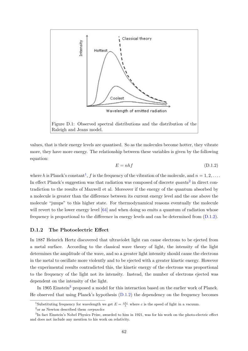
Figure D.1: Observed spectral distributions and the distribution of theRaleigh and Jeans model.

values, that is their energy levels are quantised. So as the molecules become hotter, they vibratemore, they have more energy. The relationship between these variables is given by the followingequation:

E = nhf (D.1.2)

where h is Planck’s constant1, f is the frequency of the vibration of the molecule, and n = 1, 2, . . . .In effect Planck’s suggestion was that radiation was composed of discrete quanta2 in direct con-tradiction to the results of Maxwell et al. Moreover if the energy of the quantum absorbed bya molecule is greater than the difference between its current energy level and the one above themolecule “jumps” to this higher state. For thermodynamical reasons eventually the moleculewill revert to the lower energy level [64] and when doing so emits a quantum of radiation whosefrequency is proportional to the difference in energy levels and can be determined from (D.1.2).

D.1.2 The Photoelectric Effect

In 1887 Heinrich Hertz discovered that ultraviolet light can cause electrons to be ejected froma metal surface. According to the classical wave theory of light, the intensity of the lightdetermines the amplitude of the wave, and so a greater light intensity should cause the electronsin the metal to oscillate more violently and to be ejected with a greater kinetic energy. Howeverthe experimental results contradicted this, the kinetic energy of the electrons was proportionalto the frequency of the light not its intensity. Instead, the number of electrons ejected wasdependent on the intensity of the light.

In 1905 Einstein3 proposed a model for this interaction based on the earlier work of Planck.He observed that using Planck’s hypothesis (D.1.2) the dependency on the frequency becomes

1Substituting frequency for wavelength we get E = nhcλ

where c is the speed of light in a vacuum.2or as Newton described them corpuscles3In fact Einstein’s Nobel Physics Prize, awarded to him in 1921, was for his work on the photo-electric effect

and does not include any mention to his work on relativity.

62

natural: “...the radiation should be regarded as a stream of particles whose energy is propor-tional to frequency...” [77]. A particle of light is now often referred to as a photon, from theGreek photo - light and on - unit, following a letter by Gilbert Lewis in 1926.

D.1.3 Wave-Particle Duality

As illustrated at the turn of the century there was great uncertainty as to whether light wasa (electromagnetic) wave or corpuscular, and this was summarised most eloquently by Luis deBroglie:

There are not two worlds, one of light and waves, one of matter and corpuscles.There is only a single universe. Some of its properties can be accounted for by wavetheory[s], and others by the corpuscular theory[s].

(Nobel prize award ceremony, 1929)

De Broglie’s contribution to physics, for which he was awarded the Nobel prize, did nothing tosolve this conundrum. He speculated that all particles (matter) experienced this duality, notjust light. This has subsequently been shown true, but don’t expect to defract yourself whenyou walk through doorways as they would need to be somewhere in the order of 10−43m wide.

Currently it is the belief, and all evidence agrees, that Nature is symmetric, so that every-thing we can describe with waves has a particle counterpart. However there is a lack of evidencefor a number of cases, significantly gravity whose elusive particle is called a graviton. Never-theless, as we shall show, quantum computation is an abstraction separable from the quantummechanical system which represents it, thus separating quantum computation from quantumphysics.

D.1.4 A Note On Quantum Physics

To be accurate the history of quantum mechanics that we have provided is false, it is in factthe history of Quantum Electrodynamics(QED). Quantum Mechanics is actually an abstractmathematical framework from which it is possible to derive models of particle interaction, suchas QED. Quantum Electrodynamics is a quantum field theory4 which describes all phenom-ena involving electrically charged particles interacting by means of the electromagnetic force.Section D.1 is the historical development of QED, from which quantum mechanics co-evolved.For the remainder of this paper, except where noted, we draw no distinction between quantummechanics and the quantum field theories.

4Quantum electrodynamics was the first quantum field theory, where instead of a fixed number of particlesquantisation is applied to a field allowing a relativistic formulation of quantum mechanics.

63

D.2 Matrix Representations of Quantum Transforms

D.2.1 The Controlled Not

UCNot =

1 0 0 00 1 0 00 0 0 10 0 1 0

(D.2.1)

≡

[I 0

0 σx

](D.2.2)

D.3 The No-Deleting Theorem

Theorem D.3.1: No-deleting Theorem. Suppose that there exists a unitary operator Uwhich deletes one copy of a quantum state against another then the two state must be orthogonal.That is if U is able to perform the following:

U |ψ1〉|ψ1〉 = |ψ〉|0〉 (D.3.1)

U |ψ2〉|ψ2〉 = |ψ〉|0〉 (D.3.2)

then 〈ψ1|ψ2〉 6= 0.

This theorem is valid regardless of whether the quantum system is open or closed

D.4 Quantum Fourier Transform

To perform the QFT described in §3.4.2 we apply the discrete Fourier transform to the ampli-tudes of the quantum state, i.e.

∑j

αj |〉j −→∑

k

βk|〉k, where βk =N∑

j=0

e2πijk/Nαj (D.4.1)

D.4.1 Unitary

There are many ways to show that the QFT is achievable through unitary transforms; Nielsonand Chuang [77] offer a constructive proof using quantum circuits, whereas Hirvensalo [47] doesso by decomposing the transform to the product of unitary matrices. A more simplistic prooftakes advantage of the outer product representation of the transform.

Theorem D.4.1:. The quantum Fourier transform operator

F =1√N

N−1∑j,k=0

e2πijk/N |k〉〈j|

is unitary.

64

Proof.

F†F =1N

N−1∑j′,k′=0

e−2πi(j′k−jk)′/N |j′〉〈j|δk′k (D.4.2)

=1N

N−1∑j′,k′=0

e−2πi(j′−j′)k/N |j′〉〈j| (D.4.3)

=∑j′,j

|j′〉〈j|δj′j (D.4.4)

=∑j′

|j′〉〈j′| (D.4.5)

= I (D.4.6)

∴ by definition 1.1.5F is a unitary transform.

The advantage of using either of the other two above-mentioned proofs over the one providedhere is that they both progenerate a quantum circuit which implements the QFT.

D.5 The Local Hamiltonian Problem

This section is an based on material from Kempe and Regev [61]; an operator H : H⊗n2 7→ H⊗n

2

on n qubits is a k-local Hamiltonian if it can be expressed as H =∑j

i=0Hi where each Hi is aHermitian operator acting on at most k qubits.

Definition D.5.1: (The k-Local Hamiltonian Problem). Given

(i) a k-local Hamiltonian H =∑j

i=0Hi where j is some polynomial p(n), and each Hi has abounded operator norm ‖Hi‖ ≤ q(n) for some polynomial q(n) whose entries are specifiedby a number of bits polynomial in n.

(ii) two numbers, a and b, with precision polynomial in n and such that a − b > 1/r(n) forsome polynomial r(n)

(iii) a promise that the smallest eigenvalue of H is either at most a or large than b

we must return either 1 if there is an eigenvalue of H exceeding a, or 0 if all the eigenvalues ofH are larger than b.

D.6 Quantum Computation and Physical Systems

D.6.1 A Square-Well Qubit

Suppose we have a particle in a one-dimensional box behaving according to Schrodinger’s equa-tion (1.2.1). The Hamiltonian of the system is given by:

H − p2

2m+ V (x) where V (x) =

0 for 0 < x < L

∞ otherwise(D.6.1)

65

for some constant L. The eigenstates5 of the system in the position basis are

|ψn〉 =

√2L

sin(nπLx), n ∈ N. (D.6.2)

The time evolution of the eigenstates is

|ψn(t)〉 = e−iEnt|ψn〉 (D.6.3)

where

En =n2π2m

2L2

We are only interested in a two-state system such that |ψ〉 = α|ψ0〉 + β|ψ1〉. Substituting thisin to (D.6.3) gives

|ψn(t)〉 = e−i(E1+E2)

2t

(αe

−i(E1−E2)2t |ψ0〉+ βe

i(E1−E2)2t |ψ〉1

)(D.6.4)

The state of the system can be written abstractly as a two dimensional complex vector, |ψ〉 =[α, β]T, which corresponds to a single qubit with one observable state, |ψ〉. If we denote thestates |ψ0〉 ≡ |0〉 and |ψ1〉 ≡ |1〉 then it is easily seen how we might use this system for quantumcomputation.

Since we do not wish to delve further in to physics, considering this skeleton prototypicalsystem is sufficient for our needs. However [77] provides both a more rigours formulation ofthis system and methods by which linear transforms may be performed on the state via theHamiltonian.

D.6.2 Trapped Ion Quantum Computers

The following outline of an ion trap is predominantly based on the description given in [104]but [98, 99] provide more extensive accounts. In both cases it is an ion that can be consideredas a qubit.

A typical linear ion trap consists of a number of ions within a time dependent electromagneticfield which is generated by an alternating current. For suitable ion masses and current strengththe ions experience an force attractive force towards the center of the axis of the trap. While ateither end of the trap is a ring of negatively charged metal which prevents the ions “escaping”from the ends of the trap. It is this combination of forces that effectively traps the ions withinthe apparatus. The mutually repulsive electrostatic force of the ions causes the ions to spreadout along the axis forming a string, the separation of the ions is determined by both the strengthof the current and the electrostatic force. The magnitude of the separation can be manipulatedso that it is the size of a few wavelengths of light, in turn this allows us to address the ionsindividually using lasers to alter their state. Measurement6 is performed by detecting emitted

5This can be read as just “states” without significant loss of concept.6We avoid talking about the actual techniques of measurement as they are beyond the quantum physics pre-

sented in this paper, however they are based on a principle known as electron shelving. An excellent explanation

66

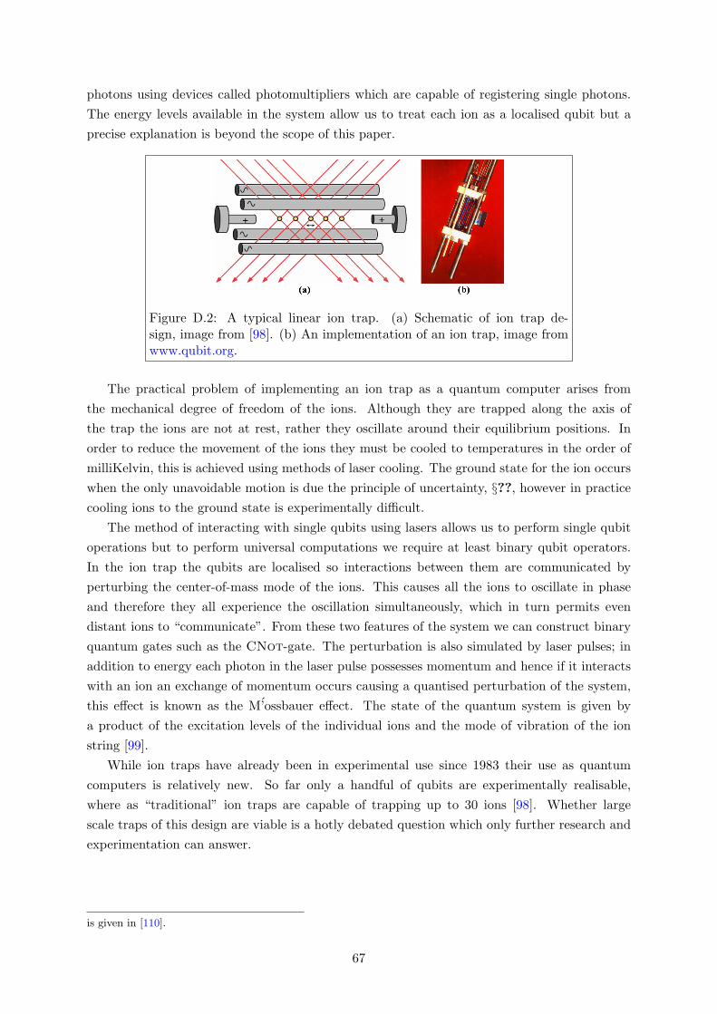
photons using devices called photomultipliers which are capable of registering single photons.The energy levels available in the system allow us to treat each ion as a localised qubit but aprecise explanation is beyond the scope of this paper.

Figure D.2: A typical linear ion trap. (a) Schematic of ion trap de-sign, image from [98]. (b) An implementation of an ion trap, image fromwww.qubit.org.

The practical problem of implementing an ion trap as a quantum computer arises fromthe mechanical degree of freedom of the ions. Although they are trapped along the axis ofthe trap the ions are not at rest, rather they oscillate around their equilibrium positions. Inorder to reduce the movement of the ions they must be cooled to temperatures in the order ofmilliKelvin, this is achieved using methods of laser cooling. The ground state for the ion occurswhen the only unavoidable motion is due the principle of uncertainty, §??, however in practicecooling ions to the ground state is experimentally difficult.

The method of interacting with single qubits using lasers allows us to perform single qubitoperations but to perform universal computations we require at least binary qubit operators.In the ion trap the qubits are localised so interactions between them are communicated byperturbing the center-of-mass mode of the ions. This causes all the ions to oscillate in phaseand therefore they all experience the oscillation simultaneously, which in turn permits evendistant ions to “communicate”. From these two features of the system we can construct binaryquantum gates such as the CNot-gate. The perturbation is also simulated by laser pulses; inaddition to energy each photon in the laser pulse possesses momentum and hence if it interactswith an ion an exchange of momentum occurs causing a quantised perturbation of the system,this effect is known as the M’ossbauer effect. The state of the quantum system is given bya product of the excitation levels of the individual ions and the mode of vibration of the ionstring [99].

While ion traps have already been in experimental use since 1983 their use as quantumcomputers is relatively new. So far only a handful of qubits are experimentally realisable,where as “traditional” ion traps are capable of trapping up to 30 ions [98]. Whether largescale traps of this design are viable is a hotly debated question which only further research andexperimentation can answer.

is given in [110].

67

Appendix ENotes on Artificial Intelligence

E.1 Backus-Naur Form

The Backus-Naur Form (BNF) is a metasyntax, that is a syntax for languages, and is widelyused in the grammar of computer programming languages. BNF was originally concieved byJohn Backus and Peter Naur to express context-free grammars within compiler design, princi-pally for Algol60. A BNF grammar consists of four components:

(i) Terminal Symbols:. These are the characters/symbols which form the strings of the lan-guage, e.g. ’A’, ’B’, ’0’, ’1’, ’♣’, etc. Terminal symbols represent constant values.

(ii) Nonterminal Symbols:. A nonterminal symbol can be expressed in terms of other terminalsor nonterminals.

(iii) Inital Symbol :. A nonterminal symbol which represents complete strings within a language,for example in definition E.2.1 Sentence is the inital symbol.

(iv) Rules:. Using derivation rules we can substitute a nonterminal symbol for another symbol,terminal or nonterminal, from a list of alternatives separated by |s, e.g.

BooleanV ariable → True | False

We can also create a nonterminal symbol from a composite of other symbols, a productrule, e.g.

NumberedSentence→ Number Sentence

Or we can use a repetition rule to create a nonterminal symbol from zero or more repeti-tions of a symbol which we denote by , e.g.

Collection→ Object

E.2 Boolean Logic

George Boole (1815–1864), mathematician and philosopher, was, in hindsight, one of thefounders of computer science. He did not regard logic as a field of mathematics but rather

68

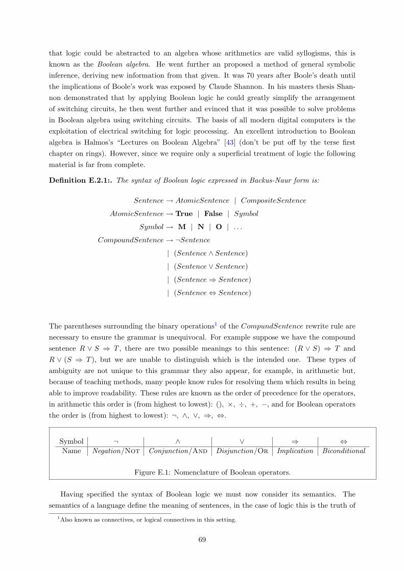
that logic could be abstracted to an algebra whose arithmetics are valid syllogisms, this isknown as the Boolean algebra. He went further an proposed a method of general symbolicinference, deriving new information from that given. It was 70 years after Boole’s death untilthe implications of Boole’s work was exposed by Claude Shannon. In his masters thesis Shan-non demonstrated that by applying Boolean logic he could greatly simplify the arrangementof switching circuits, he then went further and evinced that it was possible to solve problemsin Boolean algebra using switching circuits. The basis of all modern digital computers is theexploitation of electrical switching for logic processing. An excellent introduction to Booleanalgebra is Halmos’s “Lectures on Boolean Algebra” [43] (don’t be put off by the terse firstchapter on rings). However, since we require only a superficial treatment of logic the followingmaterial is far from complete.

Definition E.2.1:. The syntax of Boolean logic expressed in Backus-Naur form is:

Sentence→ AtomicSentence | CompositeSentence

AtomicSentence→ True | False | Symbol

Symbol→ M | N | O | . . .

CompoundSentence→ ¬Sentence

| (Sentence ∧ Sentence)

| (Sentence ∨ Sentence)

| (Sentence⇒ Sentence)

| (Sentence⇔ Sentence)

The parentheses surrounding the binary operations1 of the CompundSentence rewrite rule arenecessary to ensure the grammar is unequivocal. For example suppose we have the compoundsentence R ∨ S ⇒ T , there are two possible meanings to this sentence: (R ∨ S) ⇒ T andR ∨ (S ⇒ T ), but we are unable to distinguish which is the intended one. These types ofambiguity are not unique to this grammar they also appear, for example, in arithmetic but,because of teaching methods, many people know rules for resolving them which results in beingable to improve readability. These rules are known as the order of precedence for the operators,in arithmetic this order is (from highest to lowest): (), ×, ÷, +, −, and for Boolean operatorsthe order is (from highest to lowest): ¬, ∧, ∨, ⇒, ⇔.

Symbol ¬ ∧ ∨ ⇒ ⇔Name Negation/Not Conjunction/And Disjunction/Or Implication Biconditional

Figure E.1: Nomenclature of Boolean operators.

Having specified the syntax of Boolean logic we must now consider its semantics. Thesemantics of a language define the meaning of sentences, in the case of logic this is the truth of

1Also known as connectives, or logical connectives in this setting.

69

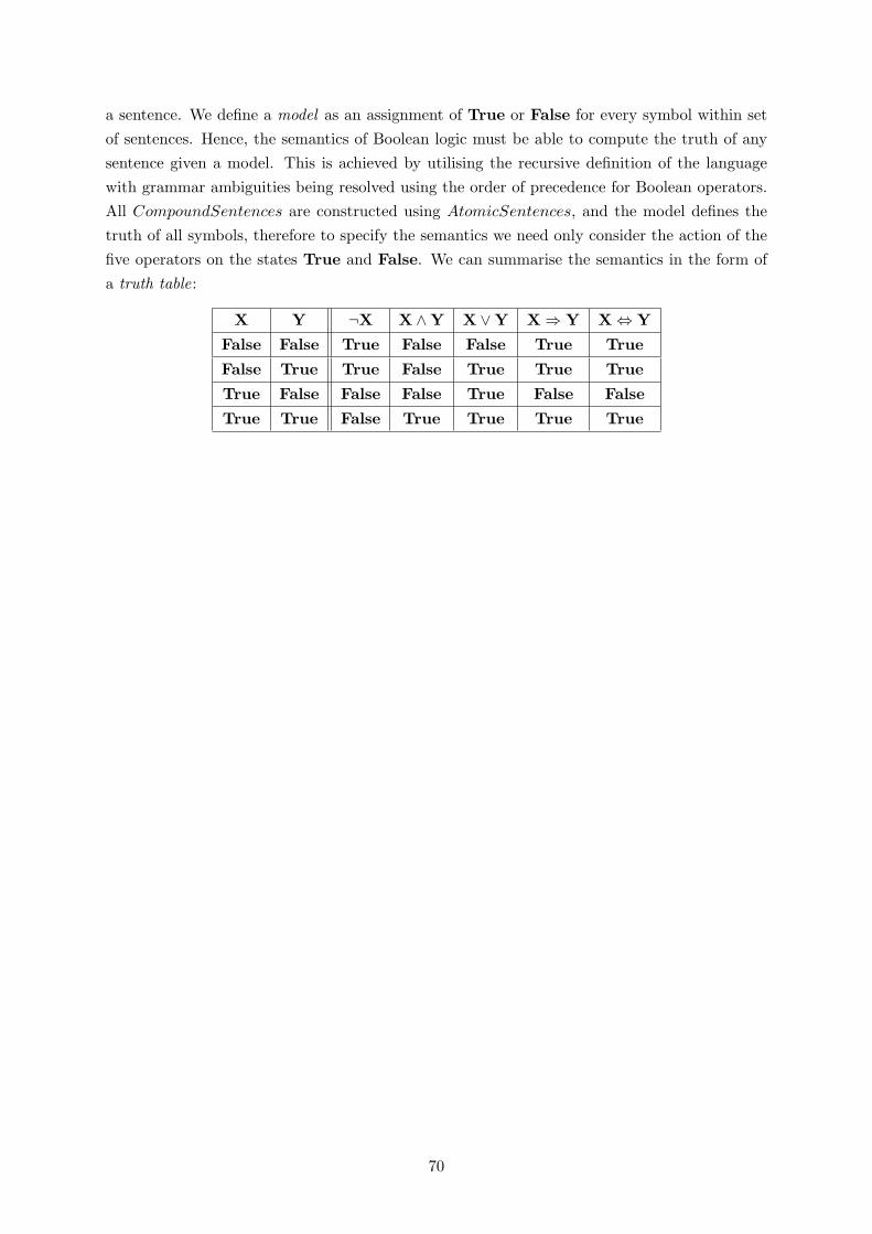
a sentence. We define a model as an assignment of True or False for every symbol within setof sentences. Hence, the semantics of Boolean logic must be able to compute the truth of anysentence given a model. This is achieved by utilising the recursive definition of the languagewith grammar ambiguities being resolved using the order of precedence for Boolean operators.All CompoundSentences are constructed using AtomicSentences, and the model defines thetruth of all symbols, therefore to specify the semantics we need only consider the action of thefive operators on the states True and False. We can summarise the semantics in the form ofa truth table:

X Y ¬X X ∧Y X ∨Y X⇒ Y X⇔ Y

False False True False False True True

False True True False True True True

True False False False True False False

True True False True True True True

70

Bibliography

[1] Scott Joel Aaronson. Limits on efficient computation in the physical world. Los AlamosePrint ArXiv.org, http://ArXiv.org/quant-ph/0412143, 2000.

[2] R. B. J. T. Allenby. Rings, Fields, and Groups. Butterworth Heinemann, 2000.

[3] R.B.J.T. Allenby and E.J. Redfern. Introduction to Number Theory with Computing.Hodder Arnold, 1989.

[4] Martin Anthony. Discrete Mathematics of Neural Networks: Selected Topics. SIAMMonographs on Discrete Mathematics and Applications. SIAM, 1st edition, 2001.

[5] M. Batty, S. L. Braunstein, A. J. Duncan, and S. Rees. Quantum algorithms in grouptheory. Los Alamos ePrint Arxiv.org, http://arxiv.org/quant-ph/0310133, 2003.

[6] Paul Benioff. Quantum robots and quantum computers. Los Alamos ePrint arXiv.org,http://arxiv.org/quant-ph/9706012, 1997.

[7] Paul Benioff. Quantum robots and environments. Los Alamos ePrint arXiv.org, http://arxiv.org/quant-ph/, 1998.

[8] Paul Benioff. Quantum robots plus environments. Los Alamos ePrint arXiv.org, http://arxiv.org/quant-ph/9807032, 1998.

[9] Paul Benioff. A simple example of definitions of truth, validity, consistency, and complete-ness in quantum mechanics. Los Alamos ePrint arXiv.org, http://arxiv.org/quant-ph/9811055, 1998.

[10] Paul Benioff. Space searches with a quantum robot. Los Alamos ePrint arXiv.org, http://arxiv.org/quant-ph/0003006, 2000.

[11] Ethan Bernstein and Umesh Vazirani. Quantum complexity theory. In Proceedings ofthe 25th ACM Symposium on the Theory of Computation, pages 11–20. New York: ACMPress, 1993.

[12] George Boole. The Mathematical Analysis of Logic: Being an Essay Toward a Calculusof Deductive Reasoning. MacMillan, Barclay, and MacMillan, 1st edition, 1847.

71

[13] S. Bose, V. Vedral, and P.L. Knight. A multiparticle generalization of entanglementswapping. Physical Revue A, A(57):1619, 1998.

[14] D.E. Bourne and P.C. Kendall. Vector Analysis and Cartesian Tensors. CRC Press, 1992.

[15] Michel Boyer, Gilles Brassard, Peter Hoyer, and Alain Tapp. Tight bounds on quantumsearching. Los Alamos ePrint ArXiv.org, http://arxiv.org/quant-ph/9605034, 1998.

[16] Gavin K. Brennen, Daegene Song, and Carl J. Williams. A quantum computer architec-ture using nonlocal interactions. Los Alamos ePrint arXiv.org, http://arxiv.org/abs/quant-ph/0301012, 2003.

[17] Michael Brooks. Quantum Computing and Communications. Springer-Verlag, 1st edition,1999.

[18] Tom Bylander. The computational complexity of propositional STRIPS planning. Arti-ficial Intelligence, 69(1-2):165–204, 1994.

[19] A. R. Calderbank and Peter W. Shor. Good quantum error-correcting codes exist. LosAlamos ePrint Arxiv.org, http://arxiv.org/quant-ph/9512032, 1995.

[20] Neil R. Carlson. Foundations of Physiological Psychology. Allyn & Bacon, 6th edition,2004.

[21] Giuseppe Castagnoli and David Finkelstein. Stefan-boltzmann law. Junior IndependentStudy Articles, 2004.

[22] D. Chapman. Planning for conjunctive goals. Artificial Intelligence, 32(3):333–377, 1987.

[23] Anthony Chefles, Claire R. Gilson, and Stephen M. Barnett. Entanglement and collec-tive quantum operations. Los Alamos ePrint arXiv.org, http://arxiv.org/quant-ph/0003062, 2000.

[24] Anthony Chefles, Claire R. Gilson, and Stephen M. Barnett. Entanglement, informationand multiparticle quantum operations. Los Alamos ePrint arXiv.org, http://arxiv.org/quant-ph/0006106, 2000.

[25] Grzegorz Chimczak. Efficient generation of distant atom entanglement. Los Alamos ePrintarXiv.org, http://arxiv.org/quant-ph/0409072, 2004.

[26] J. I. Cirac, P. Zoller, H. J. Kimble, and H. Mabuchi. Quantum state transfer and en-tanglement distribution among distant nodes in a quantum network. Los Alamos ePrintArxiv.org, http://arxiv.org/quant-ph/9611017, 1996.

[27] Robert G. Clark, P. Chris Hammel, Andrew Dzurak, Alexander Hamilton, Lloyd Hol-lenberg, David Jamieson, and Christopher Pakes. Toward a silicon-based nuclear-spinquantum computer. Los Alamos Science, 27:284 – 301, 2002.

[28] R. Cleve, A. Ekert, C. Macchiavello, and M. Mosca. Quantum algorithms revisited.Proceedings of the Royal Society of London, A(454):339–354, 1998.

72

[29] T. H. Cormen, C. E. Leiserson, R. L. Rivest, and C. Stein. Introduction to Algorithms.MIT Cambridge, 2001.

[30] Mark W. Craven and Jude W. Shavlik. Using neural networks for data mining. FutureGeneration Computer Systems, 13(2–3):211–229, 1997.

[31] DARPA. Neural Network Study. AFCEA International Press, 1988.

[32] Hugo de Garis, Ravichandra Sriram, and Zijun Zhang. Quantum generation of neuralnetworks. International Joint Conference on Neural Networks, 2003.

[33] David Deutsch. Quantum theory, the church-turing principle and the universal quantumcomputer. In Proceedings of the Royal Society of London A, volume 400, pages 97–119,1985.

[34] David P. DiVincenzo. The physical implementation of quantum computation. Los AlamosePrint Arxiv.org, http://arxiv.org/abs/quant-ph/0002077, 2004.

[35] Peter J. Eccles. An Introduction to Mathematical Reasoning. Cambridge University Press,1997.

[36] Chris Eliasmith and Charles H. Anderson. Neural Engineering: Computation, Represen-tation, and Dynamics in Neurobiological Systems. MIT Press, 1st edition, 2004.

[37] Richard P. Feynamn. Lectures on Physics. Addison Wesley, 1989.

[38] Fraunhofer FIRST. Quantum computation services. http://www.qc.fraunhofer.de/,2005.

[39] Stan Franklin. Artificial Minds. MIT Press, 2nd edition, 1999.

[40] Wolfram Gestner and Weiner M. Kistler. Spiking Neuron Models - Single Neurons, Pop-ulations, Plasticity. Cambridge University Press, 2002.

[41] Daniel Gottesman. Fault-tolerant quantum computation with local gates. Los AlamosePrint Arxiv.org, http://arxiv.org/quant-ph/9903099, 1999.

[42] Daniel Gottesman. An introduction to quantum error correction. In Samuel J. Lomonaco,editor, Proceedings of Symposia in Applied Mathematics (AMS Short Course 2000), 2000.

[43] Paul R. Halmos. Lectures on Boolean Algebras. Springer, 1974.

[44] Alan G. Hamilton. Linear Algebra. Cambridge University Press, 1990.

[45] Jean Van Heijenoort. From Frege to Godel: Mathematical Logic, 1879-1931 (Source Booksin History of Sciences). Harvard University Press, 1977.

[46] Mika Hirvensalo. Mathematical Foundations of Quantum Mechanics. Princeton UniversityPress, 2nd edition, 1955. First published in German in 1932: Mathematische Grundlagender Quantenmechank, Berlin: Springer.

73

[47] Mika Hirvensalo. Quantum Computing. Springer-Verlag, 1st edition, 2003.

[48] J. E. Hopcroft, R. Motwani, and J. D. Ullman. Introduction to Automata Theory, Lan-guages, and Computation. Addison-Wesley, 2000.

[49] J. J. Hopfield. Neural networks and physical systems with emergent collective compu-tational abilities. In Proceedings of the National Academy of Sciences, volume 79, pages2554–2558, 1982.

[50] Alfred Horn. On sentences which are true of direct unions of algebras. Journal of SymbolicLogic, 16:14–21, 1951.

[51] MichaImage Horodecki and Ryszard Horodecki. Are there basic laws of quantum infor-mation processing? Physics Letters A, 244(6):473–481, 1998.

[52] Michal Horodecki, Ryszard Horodecki, Aditi Sen De, and Ujjwal Sen. No-deleting and no-cloning principles as consequences of conservation of quantum information. Los AlamosePrint arXiv.org, http://arxiv.org/abs/quant-ph/0306044, 2003.

[53] IBM. Test-tube quantum computer makes history. Internet Press Release: http://

domino.research.ibm.com/comm/pr.nsf/pages/news.20011219 quantum.html, 2001.

[54] A. Imamoglu, D. D. Awschalom, G. Burkard, D. P. DiVincenzo, D. Loss, M. Sherwin,and A. Small. Quantum information processing using quantum dot spins and cavity-qed.Los Alamos ePrint Arxiv.org, http://arxiv.org/quant-ph/9904096, 1999.

[55] Radu Ionicioiu, Gehan Amaratunga, and Florin Udrea. Ballistic single-electron quputer.Los Alamos ePrint Arxiv.org, http://arxiv.org/quant-ph/9907043, 1999.

[56] S. J. Jones, H. M. Wiseman, and D. T. Pope. Entanglement distribution by an arbitrar-ily inept delivery service. Los Alamos ePrint arXiv.org, http://arxiv.org/quant-ph/0504112, 2005.

[57] R Jozsa. Quantum algorithms and the fourier transform. Proc Roy Soc Lond A, pages323–337, 1998.

[58] Richard Jozsa. A stronger no-cloning theorem. Los Alamos ePrint arXiv.org, http:

//arxiv.org/quant-ph/0204153, 2002.

[59] B.E. Kane. A silicon-based nuclear spin quantum computer. Nature (London), 393:133–137, 1998.

[60] Julia Kempe, Alexei Kitaev, and Oded Regev. The complexity of the local hamiltonianproblem. Los Alamos ePrint ArXiv.org, http://arxiv.org/abs/quant-ph/0406180,2004.

[61] Julia Kempe and Oded Regev. 3-local hamiltonian is qma-complete. Los Alamos ePrintArXiv.org, http://arxiv.org/quant-ph/0302079, 2005.

74

[62] Steve L. Kleiman and Glenn P. Tesler. Writing a math phase two paper. http: // www.

mit. edu/ afs/ athena. mit. edu/ course/ other/ mathp2/ www/ piil. html , 1999.

[63] E. Knill. Quantum computing with very noisy devices. Los Alamos ePrint Arxiv.org,http://arxiv.org/quant-ph/0410199, 2004.

[64] John Kotz and Paul Treichel. Chemistry and Chemical Reactivity. Harcourt Brace & Co.,3rd edition, 1996.

[65] R. Laflamme, E. Knill, E. M. Cory, D. G. amd Fortunato, T. Havel, C. Miquel, R. Mar-tinez, C. Negrevergne, G. Ortiz, M. A. Pravia, Y. Sharf, S. Sinha, R. Somma, and L. Viola.Introduction to nmr quantum information processing,. Los Alamos Science, 27:226–259,2002.

[66] M. Leone. Advice on researching and writing (for computer scientists). http://www-2.

cs.cmu.edu/afs/cs.cmu.edu/user/mleone/web/how-to.html, 2005.

[67] Leonid A. Levin. The tale of one-way functions. Problems of Information Transmission,39:92–103, 2003.

[68] Irwin B. Levitan and Leonard K. Kaczmarek. The Neuron : Cell and Molecular Biology.Oxford University Press, 3rd edition, 2001.

[69] W. Maass. Networks of spiking neurons: The third generation of neural network models. InPeter Bartlett, Anthony Burkitt, and Robert Williamson, editors, Australian Conferenceon Neural Networks, volume citeseer.ist.psu.edu/article/maass96network.html,pages 1–10. Australian National University, 1996.

[70] Wolfgang Maass and Christopher M. Bishop. Pulsed Neural Networks. MIT Press, 1stedition, 1998.

[71] Nugzar Makhaldiani. Classical and quantum problems for quanputers. Los Alamos ePrintArxiv.org, http://arxiv.org/abs/quant-ph/0210184, 2002.

[72] J. McClelland, D. Rumelhart, and the PDP Research Group. Parallel Distributed Processing: Explorations in the Microstructure of Cognition. Vol. 1: Foundations. Cambridge,MA: MIT Press, 1986.

[73] W McCuloch and W. Pits. A logical calculus of the ideas immanent in nervous activity.In Buletin of Mathematical Biophysics, volume 7, pages 115 – 133, 1943.

[74] Dr I. McIntosh. Mathematical writing: Some guidelines for writing a project. http:

//www.york.ac.uk/depts/maths/teaching/im/mathwriting.html, 2004.

[75] T. Menneer and A. Narayanan. Quantum-inspired neural networks. citeseer.ist.psu.edu/menneer95quantuminspired.html, 1995.

[76] Ajit Narayanan and Tammy Menneer. Quantum artificial neural network architecturesand components. Information Sciences, 128:231 – 255, 2000.

75

[77] M. A. Nielsen and I. L. Chuang. Quantum Computation and Quantum Information.Cambridge University Press, 3rd edition, 2003.

[78] Michael T. Niemier and Peter M. Kogge. Origins and motivations for design rules in qca.In Nano, Quantum and Molecular Computing. Kluwer Academic Publishers, 2004.

[79] Dianne P. O’Leary. Graduate Study in the Computer and Mathematical Sciences: ASurvival Manual. http://www.cs.umd.edu/ oleary/, 1999.

[80] Arun K. Pati and Samuel L. Braunstein. Quantum no-deleting principle and some of itsimplications. Los Alamos ePrint arXiv.org, http://arxiv.org/abs/quant-ph/0007121,2000.

[81] Roger Penrose. The Emperor’s New Mind. Oxford University Press, 2nd edition, 1999.

[82] Mitja Perus and Horst Bischof. A neural-network-like quantum information processingsystem. Los Alamos ePrint Arxiv.org, http://arxiv.org/quant-ph/0305072, 2003.

[83] Deepak Sethu Rao, Thomas Szkopek, Hans Daniel Robinson, Eli Yablonovitch, and Hong-Wen Jiang. Single photo-electron trapping, storage, and detection in a one-electronquantum dot. Los Alamos ePrint Arxiv.org, http://arxiv.org/abs/quant-ph/0410094,2004.

[84] K J Resch, M Lindenthal, B Blauensteiner, H R Boehm, A Fedrizzi, C Kurtsiefer,A Poppe, T Schmitt-Manderbach, M Taraba, R Ursin, P Walther, H Weier, H Weinfurter,and A Zeilinger. Distributing entanglement and single photons through an intra-city, free-space quantum channel. Optics Express, 13:202, 2005.

[85] B. D. Ripley. Pattern Recognition and Neural Networks. Cambridge University Press,1996.

[86] F Rosenblat. Principles of Neurodynamics. NewYork: Spartan Books, 1959.

[87] Stuart Russell and Peter Norvig. Artificial Intelligence: A Modern Approach. PrenticeHall, 2nd edition, 2003.

[88] J. S. Schlipf, F. Annexstein, J. Franco, and R. P. Swaminathan. On finding solutions forextended horn formulas. Information Processing Letters, 54:133–137, 1995.

[89] Benjamin Schumacher. Lecture notes in quantum information theory. University of Inns-bruck, 1998.

[90] John Searle. The Rediscovery of the Mind. Cambridge MIT Press, 1992.

[91] Alessio Serafini, Stefano Mancini, and Sougato Bose. Distributed quantum computationvia optical fibres. Los Alamos ePrint arXiv.org, http://arxiv.org/quant-ph/0507204,2005.

[92] Fariel Shafee. Neural network with semiclassical excitation. Los Alamos ePrint Arxiv.org,http://arxiv.org/quant-ph/0202015, 2004.

76

[93] Fariel Shafee. Neural networks with c-not gated nodes. Los Alamos ePrint Arxiv.org,http://arxiv.org/quant-ph/0202016, 2004.

[94] C. E. Shannon. A mathematical theory of communication. Bell System Technical Journal,27:379–423, 623–656, 1948.

[95] J. Sherson, B. Julsgaard, and E. S. Polzik. Distant entanglement of macroscopic gassamples. Los Alamos ePrint arXiv.org, http://arxiv.org/quant-ph/0408146, 2004.

[96] Peter W. Shor. Fault-tolerant quantum computation. Los Alamos ePrint Arxiv.org,http://arxiv.org/quant-ph/9605011, 1997.

[97] William Stallings. Computer Organization & Architecture: Designing for. Prentice Hall,2002.

[98] A. Steane. Quantum computing. Reports on Progress in Physics, 61:117–173, 1998.

[99] A. M. Steane and D. M. Lucas. Quantum computing with trapped ions, atoms and light.Los Alamos ePrint arXiv.org, http://arxiv.org/quant-ph/0004053, 2000.

[100] A. Tarski. Contributions to the theory of models, i. Indagationes Mathematicae, 16, 1954.

[101] A. Tarski. On the concept of logical consequence. Logic, Semantics, Metamathematics,1983.

[102] B. W Tucman. Developmental sequence in small groups. Psychological Bulletin, 63(6):384–399, 1965.

[103] Umesh V. Vazirani. A survey of quantum computational complexity theory. In QuantumComputation: A Grand Mathematical Challenge for the Twenty-first Century and theMillennium (Proceedings of Symposia in Applied Mathematics), pages 58–83. AmericanMathematical Society, 2000.

[104] Vlatko Vedral and Martin B. Plenio. Basics of quantum computation. Los Alamos ePrintarXiv.org, http://arxiv.org/quant-ph/9802065, 1998.

[105] Alexander Yu. Vlasov. Analogue quantum computers for data analysis. Los Alamos ePrintArxiv.org, http://arxiv.org/quant-ph/9802028, 1998.

[106] J. von Neumann. Collected Works, Vol 1 – 6. New York: Pergamon Press, 1st edition,1961-1963.

[107] John von Neumann. Mathematical Foundations of Quantum Mechanics. Princeton Uni-versity Press, 1932.

[108] Douglas B. Webster. Neuroscience of Communication. Thomson Delmar Learning, 1998.

[109] Wikipedia.org. http://en.wikipedia.org/wiki/Observable. Internet encylopedia, vis-ited: March 2005.

77

[110] D. J. Wineland, J. C. Bergquist, J. J. Bollinger, and W. M. Itano. Quantum effects inmeasurements on trapped ions. Physica Scripta, T(59):286–293, 1995.

[111] Wang Yao, Ren-Bao Liu, and L. J. Sham. Theory of control of spin/photon interfacefor quantum networks. Los Alamos ePrint Arxiv.org, http://arxiv.org/quant-ph/

0407060, 2004.

[112] N. Young. An Introduction to Hilbert Spaces. Cambridge University Press, 1998.

[113] Christof Zalka. Grover’s quantum searching algorithm is optimal. Los Alamos ePrintArXiv.org, http://arxiv.org/quant-ph/9711070, 1997.

[114] Christof Zalka. Introduction to quantum computers and quantum algorithms. Los AlamosePrint Arxiv.org, http://arxiv.org/quant-ph/0305053, 2003.

[115] Shi-Liang Zhu, Z. D. Wang, and Kaiyu Yang. Quantum information processing usingjosephson junctions coupled through cavities. Los Alamos ePrint Arxiv.org, http://

arxiv.org/quant-ph/0304173, 2003.

[116] Wojciech H. Zurek. Decoherence and the transition from quantum to classicalrevisited.Los Alamos Science, 27:86–109, 2002.

78