Quantitative Relations between S-N Curve Parameters and ... · Quantitative Relations between S-N Curve Parameters and Tensile Strength for Two Steels: AISI 4340 and SCM 435 Duan

Quantitative Relations between S-N Curve Parameters andTensile Strength for Two Steels: AISI 4340 and SCM 435

Duan QQ1,2, Pang JC1*, Zhang P1, Li SX1 and Zhang ZF1*

1Shenyang National Laboratory for Materials Science, Institute of Metal Research, Chinese Academy ofSciences, Shenyang 110016, P. R. China

2University of Chinese Academy of Sciences, 19 Yuquan Road, Beijing 100049, China

*For Correspondence: Pang JC, Shenyang National Laboratory for Materials Science, Institute of MetalResearch, Chinese Academy of Sciences, Shenyang 110016, P. R. China, Tel: +862483978226; E-mail:

[email protected]

Zhang ZF, Shenyang National Laboratory for Materials Science, Institute of Metal Research, Chinese Academy ofSciences, Shenyang 110016, P. R. China, Tel: +862483978226; E-mail: [email protected]

Received date: Dec 08, 2017, Accepted date: Dec 27, 2017, Published date: Jan 9, 2018

Copyright: 2018 © Duan QQ, et al. This is an open-access article distributed under the terms of the CreativeCommons Attribution License, which permits unrestricted use, distribution, and reproduction in any medium, provided

the original author and source are credited.

Research Article

ABSTRACT

S-N curves of AISI 4340 and SCM 435 steels were determined according to the qualifications and systematicallyinvestigated by Basquin relation. The change of parameters (fatigue strength coefficients and exponents) of these S-Ncurves with increasing tensile strength was analyzed and summarized. For the steels with the same type of S-N curves,as tensile strength increases, their fatigue strength coefficients linearly increase and fatigue strength exponents almostkeep unchanging at first and then decrease linearly. In addition, the fatigue mechanisms controlling the parameters of S-N curves with tensile strength increasing were discussed. It is briefly explained that the fatigue strength coefficient canbe improved by strengthening mechanisms, and the change of fatigue strength exponent with tensile strength may beinfluenced by the change of fatigue crack initiation sites, the microstructures and fatigue fractographies of steels treatedby different heat treatments. Through properly adjusting fatigue strength coefficients and fatigue strength exponents thefatigue strength can be improved in the course of the selection and preparation of steels.

Keywords: Steels, Parameters of S-N curve, Tensile strength, Fatigue mechanism

INTRODUCTIONFatigue curve, named S-N curve, is defined as the regression of stress range with increasing fatigue lifetime. For high/

very high cycle fatigue, S-N curve is a principal reference to determine fatigue strength and design criterion. In the middle1800s, fatigue failures obviously increased because of the industrial revolution, S-N curve was initially developed byW hler, therefore, in honor of him, S-N curve was also called W hler curve since 1936 [1,2]. Incidentally, his experimentalresults were expressed in the form of tables at that time, only his successor Spangenberg plotted them as curves in theunusual form of linear abscissa and ordinate [2]. Not until 1910 did Basquin represented them in the form of logarithmordinate and abscissa and found the simply linear formula such thatlog�� = log��′ + �log(2��)�� = ��′ (2��)� (2)

e-ISSN: 2321-6212p-ISSN: 2347-2278www.rroij.com

Research & Reviews: Journal of Material Science

RRJOMS | Volume 6 | Issue 1 | January, 2018 1

Where, σa is stress amplitude, is the fatigue strength coefficient, N f is the number of cycles to failure, 2Nf is thenumber of reservals to failure and b is the fatigue strength exponent on a log-log plot and also named as Basquinexponent. Eqn. (1) can be written as an exponential format:

��′

öö

(1)

DOI: 10.4172/2321-6212.1000207

mailto:[email protected]

mailto:[email protected]

Table 1. Summary of the fatigue strength coefficients and exponents.

� = −�′1 + 5�′ (3)From representative data for different types of steels with n’<0.2, Ellyin [6] detected that eqn. (3) cannot predict b well,

however, Landgraf [7] found that eqn. (3) can fit generally the experimental trend. In a word, the analysis results of fatiguecurves mentioned above show that those existing functions predicting fatigue curves are phenomenological descriptionrelated with the materials properties.

In recent years, the very high-cycle fatigue (>107 cycles, VHCF) behaviors of steels have arisen a great interest of manyinvestigators. It was found that many factors such as inclusion size [11-13], sample surface treatment [14-18], experimentalenvironment [16,19-21] and loading type [14,22] etc. can change the shape of S-N curve, and hence change the values of and b. Especially, Akiniwa et al. [23], Chapetti et al. [24], Mayer et al. [25] and Liu et al. [26] developed some new quantitativeexpressions of and b in the VHCF regime as shown in Table 1 and the corresponding Basquin relations are as followsrespectively:

�� = 2� 4��(�� − 2)1�� 1�� − 12 2�� 1�� (4)

�� = 2.5 ��+ 120�� 1/6 2�� − 148 (5)�� = 2� 1� �� −16 2�� −1� (6)

e-ISSN: 2321-6212p-ISSN: 2347-2278


This is the well-known Basquin relation and has been still widely used even today, which indicates that it is veryimportant to choose a suitable method of handling data. It is noted that there are some relations between the fatigueparameters (fatigue strength coefficients and exponents) of the S-N curves and mechanical properties [3-5] . For instance,the fatigue strength coefficient , refined as the true stress required to cause fracture in one reversal, equals to thestress intercept at 2Nf=1 and is chosen as the tensile strength or the true fracture strength . However, there aremany different debates: the differences among σf, and σb sometimes are small [3]; to a good approximation, it ischosen for most materials [5-7] that equals to . The fatigue strength exponent b is defined as the power to which thelife in reversal must be raised to be proportional to the stress amplitude and taken as the slope of the logarithm ordinateand abscissa. Moreover, different references reported different value ranges for b such as -0.125~-0.2 [8], -0.05~-0.12[5,9], -0.05~-0.2 [3] and -0.05~-0.15 [6]. Morrow et al. [10] proposed a quantitative relation between b and cyclic strainhardening exponent n (Table 1) as follows

��′ ��σb ��′��′ ��

Fatigue strength coefficient /MPa Fatigue strength exponent b Eqn. Ref.

σf ---- [6-8]

---- Eqn. (3) [12]

Eqn. (4) [25]

Eqn. (5) [26]

Eqn. (6) [27]

Eqn. (7) [28]

α+βσb C or φ+ϕσb Present

−�′1 + 5�′2� 4�� − 2 �� 1�� − 12 − 1��2.5 ��+ 120�� 1/6 − 1482� 1� �� −16 − 1�1.12 ��+ 120 9/8�� 1/8 13 lg 1.35 ��+ 120 − 116�� 148

��′

��′��′

�� = 1.12 ��+ 120 9/8�� 1/8 2�� 13lg 1.35 ��+ 120 − 116 �� − 148 (7)Here, is the square root of inner inclusion area perpendicular to the applied stress axis (μm), HV is the Vickers

hardness (kgfmm-2); mA (14.2, JIS SUJ2 [23]), CA (3.44 x 10-21, JIS SUJ2 [23]), C (6.47 x 1098, 100Cr6 [25]) and n (28.82,100Cr6 [25]) are material constants.

It is shown that from eqns. (4)-(7) and Table 1 that the most fatigue str ength coef f icients have r elations withinclusion size and two coefficients in eqns. (5) and (7) also have relations with HV; only one fatigue strengthexponent b in eqn. (7) has relation with inclusion size and HV, the other exponents are constant. This arises twoquestions of great concern: 1) for the same material with almost the same size of inclusion and wide range of tensilestrength, what on earth are the relations between tensile strength and parameters of S-N curves ( and b)? 2) What isthe fatigue mechanism determining and b? To find them, two typical high-strength steels with a wide range of tensilestrength including AISI 4340 steel (tensile strengths ranged from 1300 MP to 2400 MPa) under push-pull load and SCM435 steel (tensile strengths ranged from 990 MPa to 1900 MPa) under rotating-bending load were chosen to investigatethe parameters of S-N curves.

Assortment and Definition of S-N Curve

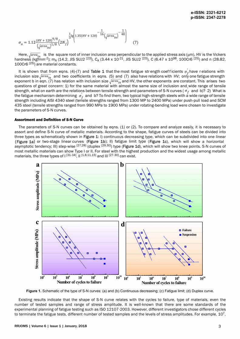
The parameters of S-N curves can be obtained by eqns. (1) or (2). To compare and analyze easily, it is necessary toassort and define S-N curve of metallic materials. According to the shape, fatigue curves of steels can be divided intothree types as schematically shown in Figure 1: I) continuous decreasing type, which can be subdivided into one linear

or two-stage linear curves (Figure 1b); II) fatigue limit type (Figure 1c), which will show a horizontalasymptotic tendency; III) step-wise [27,28] (duplex [29,30]) type (Figure 1d), which will show two knee points. S-N curves ofmost metallic materials can show Type I or II. For steel with the highest production and the widest usage among metallicmaterials, the three types of I [31-34], II [1,8,11,15] and III [27-30] can exist.

Figure 1. Schematic of the type of S-N curves: (a) and (b) Continuous decreasing; (c) Fatigue limit; (d) Duplex curve.

Existing results indicate that the shape of S-N curve relates with the cycles to failure, type of materials, even thenumber of tested samples and range of stress amplitude. It is well-known that there are some standards of theexperimental planning of fatigue testing such as ISO 12107-2003. However, different investigators chose different cyclesto terminate the fatigue tests, different number of tested samples and the levels of stress amplitudes. For example, 107,

e-ISSN: 2321-6212p-ISSN: 2347-2278


��

��′��′��′

Figure 1a)(

108, 5 x 108, 109, even 1010 can be chosen as the terminated cycles. An S-N curve has five fatigue data, however, theother has more than 100 data. The same S-N curve may be thought as continuous decreasing type by some people,however as duplex curve by others. Some materials show continuous decreasing type within 108 cycles but maybe showfatigue limit type beyond 1010 cycles. To normalize and simply compare, it is necessary to define the testing parametersthat influence the shape of S-N curve.

In this paper, the terminated cycle is identical (VHCF: 109 cycles); in each group, the total number of tested samples isalmost the same (not less than 20 or 10); the number of stress amplitude levels is almost the same (not less than 5); themaximum stress amplitude is not very high (not more than 1.5~2 times of fatigue strength). The S-N curve can be fittedas a line with the slope of nonzero, most data distribute within a certain error band (Figure 1a), this is a typicalcontinuously decreasing type; besides, in its lower part, the S-N curve may be fitted as another line with the slopenonzero, this is also a continuous decreasing type (Figure 1b). In its lower part, the S-N curve seems to be as a horizontalasymptotic line and can be fitted as a line with the slope of near zero, which is defined as fatigue limit type (Figure 1c).Some parts of S-N curve can be fit as two lines with the slopes nonzero, the third as a line with the slope of near zero,which is defined as duplex curve (or step-wise curve) (Figure 1d).

Two typical steels were chosen to figure out the type of S-N curves and to study the relation between their types andcorresponding fatigue mechanisms.

Analysis of S-N Curves of Steels with a Wide Strength Range

AISI 4340 steel with a wide strength range under push-pull loading: AISI4340 steel with a very wide range of tensilestrength, one of the excellent quenched and tempered low-alloy steels [14,17,35-41], was chosen to study the relationbetween S-N curves and tensile strength. The ingredient of current AISI 4340 [42]. To obtain a wider range of strength, sixheat-treatment procedures: heated to 850°C for 10 min and quenched in oil, did not temper and tempered at 180°C,250°C and 350°C for 120 min and at 420°C, 500°C for 30 min respectively, were employed and the specimens weredefined as A, B, C, D, E and F, correspondingly. The main microstructure of sample A is needle- or plate-shapedmartensites; those of samples B-D are tempered martensites; those of samples E and F are tempered troostites, whichwas shown in detail [42]. The tensile strengths of samples A-F were listed in Table 2. The S-N features were analyzed bythe widely used method of Basquin relation as following:

Table 2. The data of AISI 4340 steel and the parameters of Basquin relation for the very high-cycle fatigue S-N curves.

Sample A B C D E F

Tempering treatment no 180°C 250°C 350°C 420°C 500°C

Tensile strength, MPa 2363 2127 1830 1574 1390 1285

FSC , , Mpa 1190 1123 805 730 691 672

Basquin exponent, b -0.03 -0.026 -0.0078 -0.0074 -0.0052 -0.0064

σw, MPa, Exp. - 655 693 634 628 594

σw, MPa [eqn.(2)] 631 645 681 623 618 586

Error, % -1.53 -1.73 -1.74 -1.59 -1.35

FSC: Fatigue Strength Coefficient. Error= (σw.eq. - σw.exp.)/ σw.exp.

Exp: Experimental Result.

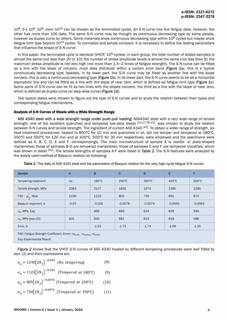
Figure 2 shows that the VHCF S-N curves of AISI 4340 treated by different tempering procedures were well fitted byeqn. (2) and their expressions are�� = 1190 2�� −0.030 (�� (8)�� = 1123 2�� −0.026 (�� 180°C) (9)�� = 805 2�� −0.0078 (�� 250°C) (10)�� = 730 2�� −0.0074 (�� 350°C) (11)

e-ISSN: 2321-6212p-ISSN: 2347-2278


��′

)

�� = 691 2�� −0.0052 (�� 420°C) (12)�� = 673 2�� −0.0064 (�� 500°C) (13)As shown in Figure 2, fatigue data of samples without tempering are within the 15% error band; however, others are

within the 5% error band. This indicates that Basquin relation can express well the VHCF S-N curves of AISI 4340 steeltempered at different temperatures and those S-N curves show decreasing type, of which step-wise or duplex typereported [29,30,43,44] was not found. Murakami et al. [45,46] carried out push-pull tests using JIS-SCM435 and JIS-SUJ2 andalso found the same results. The reason may be that for AISI 4340, the average diameter of the inclusion, which ofsamples A-F is 27, 28, 27, 32, and 41 μm respectively, is greater than 20 μm [11].

Figure 2. Basquin relation fitting of VHCF S-N curves of AISI 4340 steel treated at different tempering temperatures. (a)untempered; (b) 180°C; (c) 250°C; (d) 350°C; (e) 420°C; (f) 500°C. (Data in (b)-(f) collected from ref. [42])

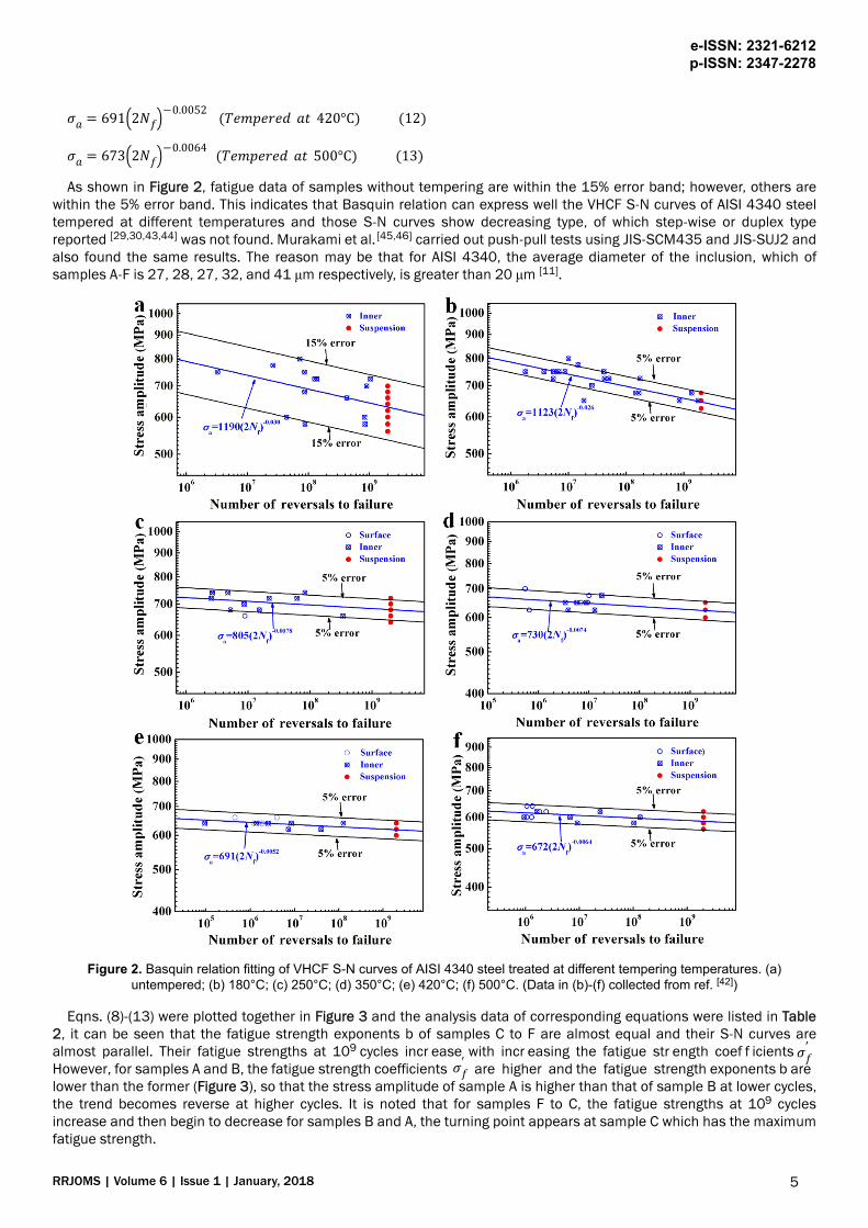
Eqns. (8)-(13) were plotted together in Figure 3 and the analysis data of corresponding equations were listed in Table2, it can be seen that the fatigue strength exponents b of samples C to F are almost equal and their S-N curves arealmost parallel. Their fatigue strengths at 109 cycles incr ease with incr easing the fatigue str ength coef f icients However, for samples A and B, the fatigue strength coefficients are higher and the fatigue strength exponents b arelower than the former (Figure 3), so that the stress amplitude of sample A is higher than that of sample B at lower cycles,the trend becomes reverse at higher cycles. It is noted that for samples F to C, the fatigue strengths at 109 cyclesincrease and then begin to decrease for samples B and A, the turning point appears at sample C which has the maximumfatigue strength.

e-ISSN: 2321-6212p-ISSN: 2347-2278


��′��′

Figure 3. Six VHCF S-N curves expressed by Basquin relation for AISI 4340 steel samples.

Figure 4. S-N curve analysis of AISI 4340 steel by Basquin relation: (a) true tensile strength and fatigue strength (FS) coefficient;(b) tensile strength and true tensile strength; (c) tensile strength and fatigue strength (FS) coefficient; (d) tensile strength and

Basquin exponent.

Figure 4 displays the relation between analysis results of S-N curves and tensile strength. In Figure 4a, with true tensilestrength increasing, fatigue strength (FS) coefficient under VHCF load increases linearly and the relation can befitted as follows:��′ = 0.49��− 259

The data are within the 15% error band, this illustrates that the relation between fatigue strength coefficient and truetensile strength is linear, which is different from the relation mentioned [5-7] . It is also found in Figure 4b thatthere is a linear relation between true tensile strength and tensile strength, i.e.

e-ISSN: 2321-6212p-ISSN: 2347-2278


(��′ = ��)�� ′(14)

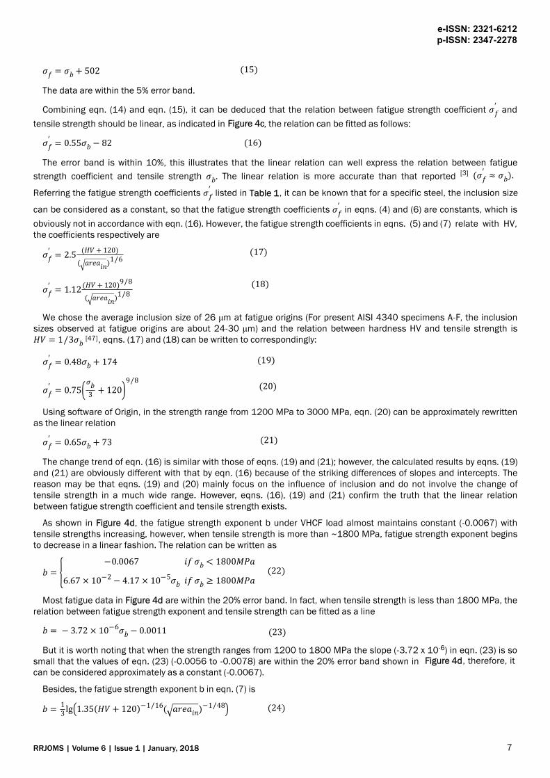
�� = ��+ 502The data are within the 5% error band.

Combining eqn. (14) and eqn. (15), it can be deduced that the relation between fatigue strength coefficient ��′ and

tensile strength should be linear, as indicated in , the relation can be fitted as follows:��′ = 0.55��− 82The error band is within 10%, this illustrates that the linear relation can well express the relation between fatigue

strength coefficient and tensile strength ��. The linear relation is more accurate than that reported (��′ ≈ ��).Referring the fatigue strength coefficients ��′ listed in , it can be known that for a specific steel, the inclusion size

can be considered as a constant, so that the fatigue strength coefficients ��′ in eqns. (4) and (6) are constants, which is

obviously not in accordance with eqn. (16). However, the fatigue strength coefficients in eqns. (5) and (7) relate with HV,the coefficients respectively are��′ = 2.5 (��+ 120)( ��)1/6 (17)��′ = 1.12 (��+ 120)9/8( ��)1/8 (18)We chose the average inclusion size of 26 μm at fatigue origins (For present AISI 4340 specimens A-F, the inclusion

sizes observed at fatigue origins are about 24-30 μm) and the relation between hardness HV and tensile strength is�� = 1/3�� , eqns. (17) and (18) can be written to correspondingly:��′ = 0.48��+ 174��′ = 0.75 ��3 + 120 9/8 (20)Using software of Origin, in the strength range from 1200 MPa to 3000 MPa, eqn. (20) can be approximately rewritten

as the linear relation��′ = 0.65��+ 73The change trend of eqn. (16) is similar with those of eqns. (19) and (21); however, the calculated results by eqns. (19)

and (21) are obviously different with that by eqn. (16) because of the striking differences of slopes and intercepts. Thereason may be that eqns. (19) and (20) mainly focus on the influence of inclusion and do not involve the change oftensile strength in a much wide range. However, eqns. (16), (19) and (21) confirm the truth that the linear relationbetween fatigue strength coefficient and tensile strength exists.

As shown in Figure 4d, the fatigue strength exponent b under VHCF load almost maintains constant (-0.0067) withtensile strengths increasing, however, when tensile strength is more than ~1800 MPa, fatigue strength exponent beginsto decrease in a linear fashion. The relation can be written as

� = −0.0067 �� < 1800��6.67 × 10−2− 4.17 × 10−5�� ≥ 1800�� (22)Most fatigue data in Figure 4d are within the 20% error band. In fact, when tensile strength is less than 1800 MPa, the

relation between fatigue strength exponent and tensile strength can be fitted as a line� = − 3.72 × 10−6��− 0.0011But it is worth noting that when the strength ranges from 1200 to 1800 MPa the slope (-3.72 x 10-6) in eqn. (23) is so

small that the values of eqn. (23) (-0.0056 to -0.0078) are within the 20% error band shown in Figure 4d , therefore, itcan be considered approximately as a constant (-0.0067).

Besides, the fatigue strength exponent b in eqn. (7) is� = 13 lg 1.35 ��+ 120 −1/16( ��)−1/48 (24)

e-ISSN: 2321-6212p-ISSN: 2347-2278


(15)

(16)

(19)

(21)

(23)

Figure 4c

[3]

Table 1

[47]

By substituting average inclusion size 26 μm at fatigue origins and the relation between hardness HV and tensilestrength mentioned above, eqn. (24) becomes to� = − 148 lg 8.11 × 10−3 × ��+ 360 (25)

In the strength range from 1200 MPa to 2400 MPa, eqn. (25) can be approximately rewritten as the linear relation� = − 4.17 × 10−6��− 0.018The values of b in eqn. (22) also are more than those in eqns. (25) or (26). This may be because S-N curve in VHCF

regime becomes gradually varying, as shown schematically in Figure 1c. But it is worth noting that the slope (-4.17 x 10-6)in eqn. (26) is so small that the values of eqn. (26) are -0.023 to -0.028 when the strength are from 1200 MPa to 2400MPa, hence it can be considered approximately as a constant (-0.026).

When σb<1800 MPa, the fatigue strength exponent b almost keeps unchanging and fatigue strength coefficientincreases with tensile strength increasing so that fatigue strength increases with tensile strength; when σb ≥ 1800 MPa,the fatigue strength coefficient σf increases, however the fatigue strength exponent b substantially decreases with tensilestrength increasing (Figure 4d) which leads to decreasing of fatigue strength. Therefore, maximum fatigue strength couldexist at an adequate tensile strength. In addition, very high cycle fatigue strengths of samples B to F at 109 cycles can becalculated by eqns. (8)-(13), respectively. It can be concluded from Table 2 that the errors between calculated fatiguestrength by Basquin relation and experimental value obtained by staircase method are less than 2%, which is quitesatisfactory for fatigue testing. Compared with samples B-F, fatigue data of sample A were too scattered to obtain fatiguestrength by staircase method.

In summary, it can be concluded that there are some quantitative relations between parameters of S-N curve (fatigue

strength coefficient ��′ and exponent b) and tensile strength ( ). By using those parameters changing tendency of

S-N curves and fatigue strength can be predicted ( ) .

SCM 435 steel with a wide strength range under rotating-bending loading: For AISI 4340 steel, the relations betweenthe features of S-N curves and tensile strength with a wide range under push-pull loading were discussed. It is necessaryto study those relations under rotating-bending loading, especially, step-wise or duplex type S-N curve [29,30,43,44] oftenappears under this condition. However, there are very rare fatigue data for a specific steel with a wide range of tensilestrength, luckily, fatigue data of SCM435 steel with 5 different strength levels were found [48]. Five heat-treatmentprocedures: heated to 855°C for 30 min and quenched in oil, did not temper and tempered at 160°C, 300°C, 500°C and600°C for 60 min were employed and the specimens were defined as A, B, C, D and E, respectively. The tensile strengthsof samples A-E are 1898, 1785, 1734, 1303 and 991 MPa. The S-N curve features of SCM 435 steel were studied by theBasquin relation as below:

The VHCF S-N curves of SCM 435 steel treated by different tempering procedures were fitted by eqn. (2) and shown inFigure 5. Their fitting equations can be written as�� = 1760 2�� −0.041 (�� )�� = 1577 2�� −0.036 (�� 160°C)�� = 1413 2�� −0.032 (�� 300°C)�� = 1291 2�� −0.033 (�� 500°C)�� = 882 2�� −0.036 (�� 600°C)

From , it is found that fatigue data of all samples are within the 15% error band. This implicates thatBasquin relation can describe well the S-N curves of SCM 435 steel tempered at different temperatures, and those S-Ncurves also show continuous decreasing type, similar to AISI 4340 steel, of which step-wise or duplex type reported[29,30,43,44] was also not found. However, S-N curves of samples A and B are considered as duplex type [48], this isbecause the number of stress amplitude levels [48] for samples A and B is more than that in present treatment.

Eqns. (27)-(31) were plotted together in Figure 5f, it can be found that the fatigue strength exponents b of samples B toE are almost equal and their S-N curves are almost parallel, their fatigue strengths at 109 cycles increase with increasingthe fatigue strength coefficients σf. However, for samples A and B, the fatigue strength coefficients are higher and thefatigue strength exponents are lower than the former (Figure 5f), so that the stress amplitude of sample A is higher thanthat of sample B at lower cycles, their stress amplitudes are almost equal, even the former trend becomes reverse at

e-ISSN: 2321-6212p-ISSN: 2347-2278


(26)

(27)(28)(29)(30)(31)

Table 1

Table 2

Figure 5a-5e

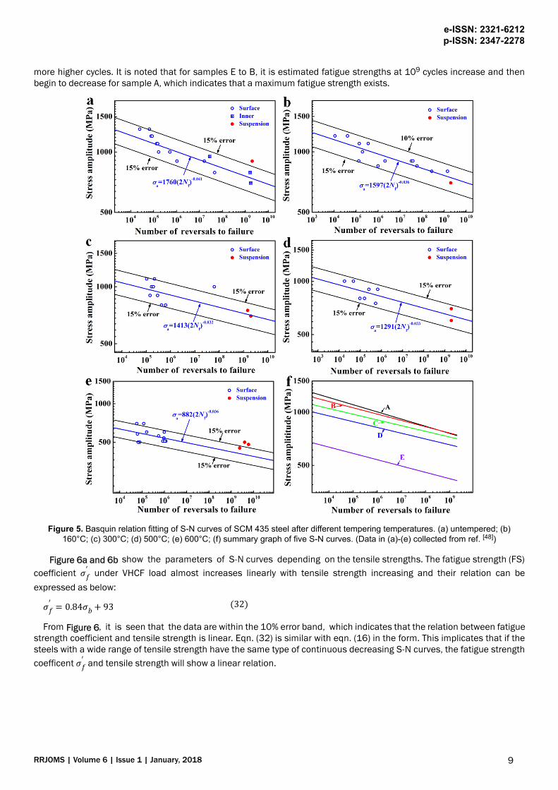
more higher cycles. It is noted that for samples E to B, it is estimated fatigue strengths at 109 cycles increase and thenbegin to decrease for sample A, which indicates that a maximum fatigue strength exists.

Figure 5. Basquin relation fitting of S-N curves of SCM 435 steel after different tempering temperatures. (a) untempered; (b)160°C; (c) 300°C; (d) 500°C; (e) 600°C; (f) summary graph of five S-N curves. (Data in (a)-(e) collected from ref. [48])

show the parameters of S-N curves depending on the tensile strengths. The fatigue strength (FS)

coefficient ��′ under VHCF load almost increases linearly with tensile strength increasing and their relation can be

expressed as below:��′ = 0.84��+ 93From , it is seen that the data are within the 10% error band, which indicates that the relation between fatigue

strength coefficient and tensile strength is linear. Eqn. (32) is similar with eqn. (16) in the form. This implicates that if thesteels with a wide range of tensile strength have the same type of continuous decreasing S-N curves, the fatigue strength

coefficent ��′ and tensile strength will show a linear relation.

e-ISSN: 2321-6212p-ISSN: 2347-2278


(32)Figure 6a and 6b

Figure 6

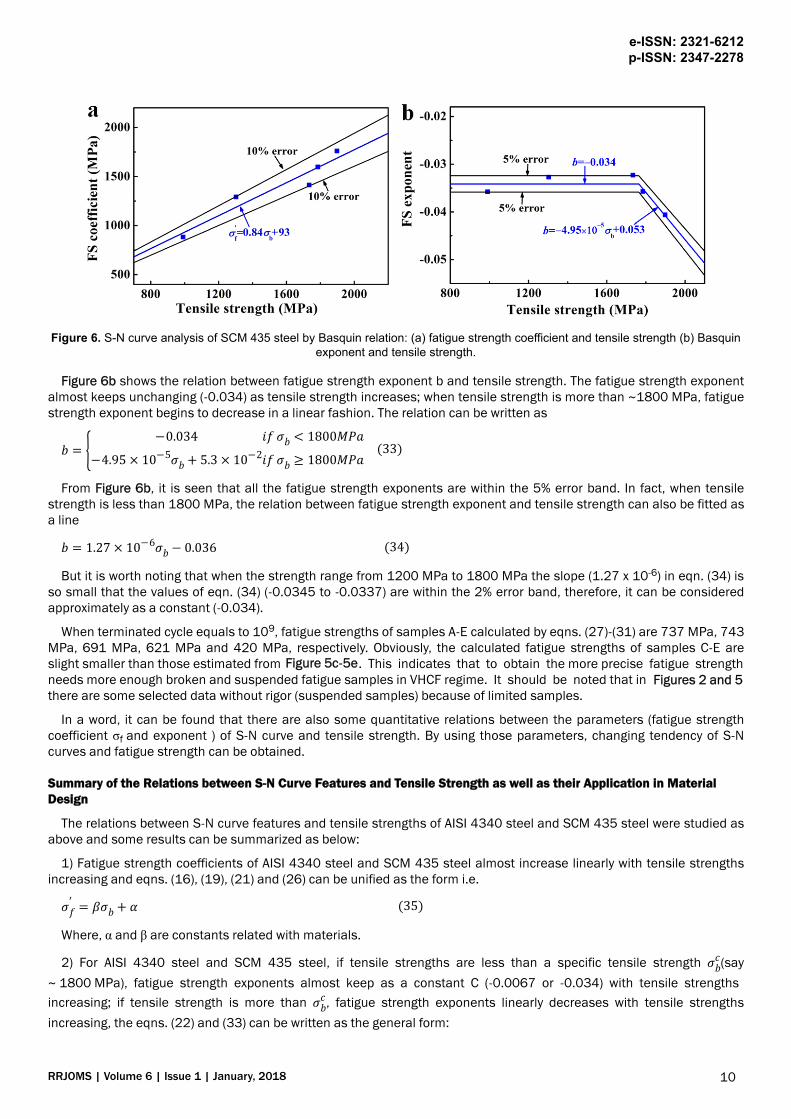
Figure 6. S-N curve analysis of SCM 435 steel by Basquin relation: (a) fatigue strength coefficient and tensile strength (b) Basquinexponent and tensile strength.

Figure 6b shows the relation between fatigue strength exponent b and tensile strength. The fatigue strength exponentalmost keeps unchanging (-0.034) as tensile strength increases; when tensile strength is more than ~1800 MPa, fatiguestrength exponent begins to decrease in a linear fashion. The relation can be written as

� = −0.034−4.95 × 10−5��+ 5.3 × 10−2�� < 1800�� ≥ 1800�� (33)From Figure 6b, it is seen that all the fatigue strength exponents are within the 5% error band. In fact, when tensile

strength is less than 1800 MPa, the relation between fatigue strength exponent and tensile strength can also be fitted asa line� = 1.27 × 10−6��− 0.036

But it is worth noting that when the strength range from 1200 MPa to 1800 MPa the slope (1.27 x 10-6) in eqn. (34) isso small that the values of eqn. (34) (-0.0345 to -0.0337) are within the 2% error band, therefore, it can be consideredapproximately as a constant (-0.034).

When terminated cycle equals to 109, fatigue strengths of samples A-E calculated by eqns. (27)-(31) are 737 MPa, 743MPa, 691 MPa, 621 MPa and 420 MPa, respectively. Obviously, the calculated fatigue strengths of samples C-E areslight smaller than those estimated from . This indicates that to obtain the more precise fatigue strengthneeds more enough broken and suspended fatigue samples in VHCF regime. It should be noted that in there are some selected data without rigor (suspended samples) because of limited samples.

In a word, it can be found that there are also some quantitative relations between the parameters (fatigue strengthcoefficient σf and exponent ) of S-N curve and tensile strength. By using those parameters, changing tendency of S-Ncurves and fatigue strength can be obtained.

Summary of the Relations between S-N Curve Features and Tensile Strength as well as their Application in MaterialDesign

The relations between S-N curve features and tensile strengths of AISI 4340 steel and SCM 435 steel were studied asabove and some results can be summarized as below:

1) Fatigue strength coefficients of AISI 4340 steel and SCM 435 steel almost increase linearly with tensile strengthsincreasing and eqns. (16), (19), (21) and (26) can be unified as the form i.e.��′ = ��+ � (35)

Where, α and β are constants related with materials.

2) For AISI 4340 steel and SCM 435 steel, if tensile strengths are less than a specific tensile strength ��(say

~ 1800 MPa), fatigue strength exponents almost keep as a constant C (-0.0067 or -0.034) with tensile strengths

increasing; if tensile strength is more than ��, fatigue strength exponents linearly decreases with tensile strengths

increasing, the eqns. (22) and (33) can be written as the general form:

e-ISSN: 2321-6212p-ISSN: 2347-2278


(34)

Figure 5c-5eFigures 2 and 5

� = ��+ � �� < �� ≥ �� (36)Where, φ and ψ are constants related with materials.

But it is worth noting that all S-N curves of AISI 4340 and SCM 435 are continuous decreasing type ( ). Itcan be deduced that if the types of S-N curves are not the same, eqns. (35) and (36) may be not necessarily suitable.

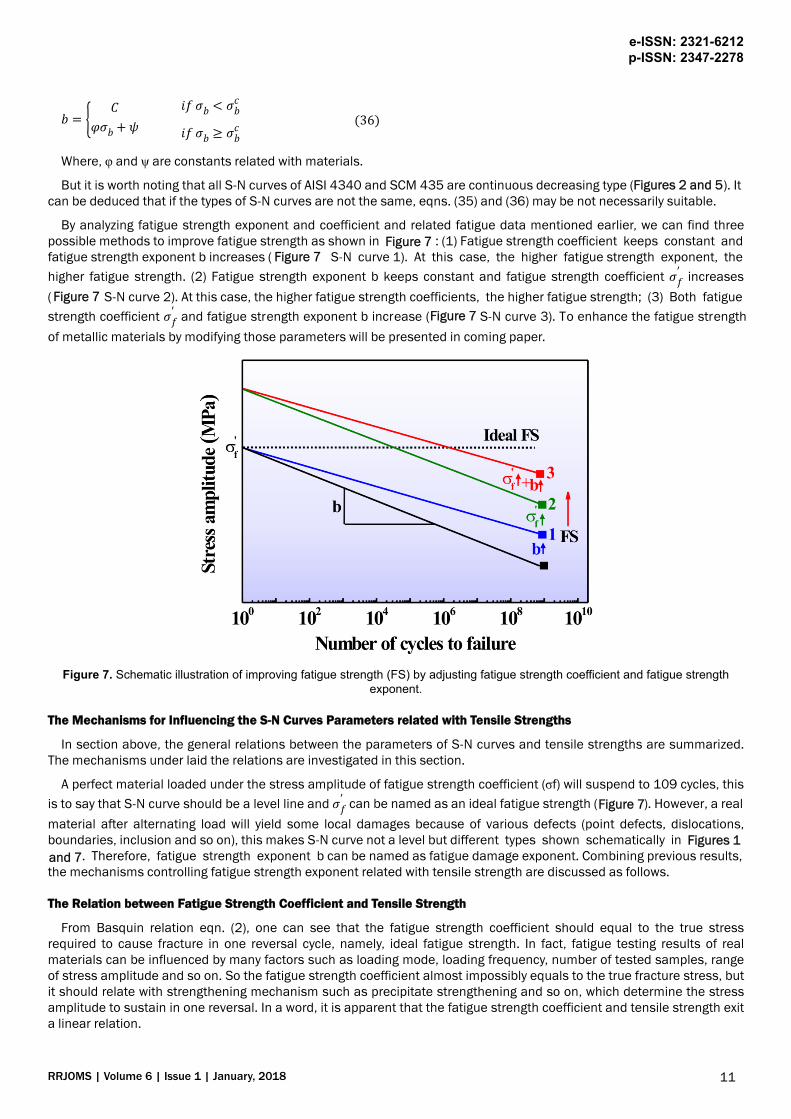
By analyzing fatigue strength exponent and coefficient and related fatigue data mentioned earlier, we can find threepossible methods to improve fatigue strength as shown in : (1) Fatigue strength coefficient keeps constant andfatigue strength exponent b increases ( S-N curve 1). At this case, the higher fatigue strength exponent, the

higher fatigue strength. (2) Fatigue strength exponent b keeps constant and fatigue strength coefficient ��′ increases

( S-N curve 2). At this case, the higher fatigue strength coefficients, the higher fatigue strength; (3) Both fatigue

strength coefficient ��′ and fatigue strength exponent b increase ( S-N curve 3). To enhance the fatigue strength

of metallic materials by modifying those parameters will be presented in coming paper.

Figure 7. Schematic illustration of improving fatigue strength (FS) by adjusting fatigue strength coefficient and fatigue strengthexponent.

The Mechanisms for Influencing the S-N Curves Parameters related with Tensile Strengths

In section above, the general relations between the parameters of S-N curves and tensile strengths are summarized.The mechanisms under laid the relations are investigated in this section.

A perfect material loaded under the stress amplitude of fatigue strength coefficient (σf) will suspend to 109 cycles, this

is to say that S-N curve should be a level line and ��′ can be named as an ideal fatigue strength ( ). However, a real

material after alternating load will yield some local damages because of various defects (point defects, dislocations,boundaries, inclusion and so on), this makes S-N curve not a level but different types shown schematically in . Therefore, fatigue strength exponent b can be named as fatigue damage exponent. Combining previous results,the mechanisms controlling fatigue strength exponent related with tensile strength are discussed as follows.

The Relation between Fatigue Strength Coefficient and Tensile Strength

From Basquin relation eqn. (2), one can see that the fatigue strength coefficient should equal to the true stressrequired to cause fracture in one reversal cycle, namely, ideal fatigue strength. In fact, fatigue testing results of realmaterials can be influenced by many factors such as loading mode, loading frequency, number of tested samples, rangeof stress amplitude and so on. So the fatigue strength coefficient almost impossibly equals to the true fracture stress, butit should relate with strengthening mechanism such as precipitate strengthening and so on, which determine the stressamplitude to sustain in one reversal. In a word, it is apparent that the fatigue strength coefficient and tensile strength exita linear relation.

e-ISSN: 2321-6212p-ISSN: 2347-2278


Figures 2 and 5

Figure 7Figure 7

Figure 7

Figure 7

Figure 7

Figures 1and 7

The Relation between Fatigue Strength Exponent and Tensile Strength

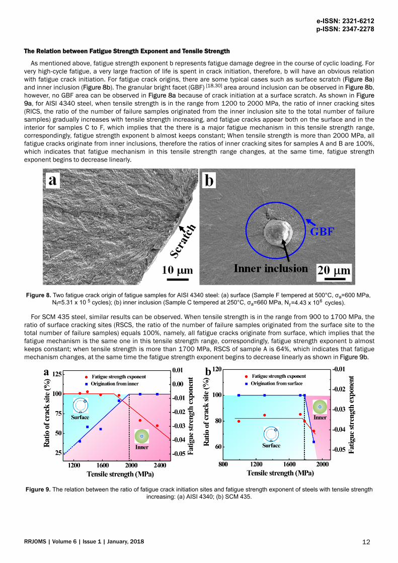
As mentioned above, fatigue strength exponent b represents fatigue damage degree in the course of cyclic loading. Forvery high-cycle fatigue, a very large fraction of life is spent in crack initiation, therefore, b will have an obvious relationwith fatigue crack initiation. For fatigue crack origins, there are some typical cases such as surface scratch (Figure 8a)and inner inclusion (Figure 8b). The granular bright facet (GBF) [18,30] area around inclusion can be observed in Figure 8b,however, no GBF area can be observed in Figure 8a because of crack initiation at a surface scratch. As shown in Figure9a, for AISI 4340 steel, when tensile strength is in the range from 1200 to 2000 MPa, the ratio of inner cracking sites(RICS, the ratio of the number of failure samples originated from the inner inclusion site to the total number of failuresamples) gradually increases with tensile strength increasing, and fatigue cracks appear both on the surface and in theinterior for samples C to F, which implies that the there is a major fatigue mechanism in this tensile strength range,correspondingly, fatigue strength exponent b almost keeps constant; When tensile strength is more than 2000 MPa, allfatigue cracks originate from inner inclusions, therefore the ratios of inner cracking sites for samples A and B are 100%,which indicates that fatigue mechanism in this tensile strength range changes, at the same time, fatigue strengthexponent begins to decrease linearly.

Figure 8. Two fatigue crack origin of fatigue samples for AISI 4340 steel: (a) surface (Sample F tempered at 500°C, σa=600 MPa,Nf=5.31 x 10 5 cycles); (b) inner inclusion (Sample C tempered at 250°C, σa=660 MPa, Nf=4.43 x 106 cycles).

For SCM 435 steel, similar results can be observed. When tensile strength is in the range from 900 to 1700 MPa, theratio of surface cracking sites (RSCS, the ratio of the number of failure samples originated from the surface site to thetotal number of failure samples) equals 100%, namely, all fatigue cracks originate from surface, which implies that thefatigue mechanism is the same one in this tensile strength range, correspondingly, fatigue strength exponent b almostkeeps constant; when tensile strength is more than 1700 MPa, RSCS of sample A is 64%, which indicates that fatiguemechanism changes, at the same time the fatigue strength exponent begins to decrease linearly as shown in Figure 9b.

Figure 9. The relation between the ratio of fatigue crack initiation sites and fatigue strength exponent of steels with tensile strengthincreasing: (a) AISI 4340; (b) SCM 435.

e-ISSN: 2321-6212p-ISSN: 2347-2278


In a word, the changing of fatigue cracking sites leads to the variation tendency of fatigue strength exponent. Inaddition, there are some changes in microstructure and fractographs of AISI 4340 steel tempered at differenttemperatures. The corresponding mechanism can be roughly explained as following:

Untempered sample A has the indistinct dividing line between crack growth area and final fracture area and flatfracture surface (Figure 10a); samples C-F tempered at 180, 250 350, 420 and 500°C have the obvious dividing linesand growth ridges (Figure 10b-10f), especially sample C shows some regular fan shaped zones as shown in Figure 10c.This implicates that their plastic deformation abilities are different. The reason maybe that sample A with full martensitemicrostructure has so many defects such as supersaturated interstitial carbon atoms, high density dislocations [49,50],subgrain boundaries and so on that the ability of plastic deformation is very weak and the tensile strength is very high; atthis case, the fatigue sensitivity to defects is much higher [42] and fatigue damage degree in the cause of fatigue crackinitiation becomes very high, therefore sample A has the lowest fatigue strength exponent b (Figure 9a).

Figure 10. The macroscopic morphologies of fatigue samples for AISI 4340 steel processed at different tempering temperatures:(a) untempered (σa=680 MPa, N f =4.34 x 107 cycles); (b) 180°C (σa=750 MPa, N f=2.05 x 107 cycles); (c) 250°C (σa=660 MPa, N f

=4.43 x 106 cycles); (d) 350°C (σa=650 MPa, Nf =4.72 x 106 cycles); (e) 420°C (σa =640 MPa, Nf =4. 23 x 106 cycles); (f) 500°C(σa=620 MPa, N f =9.14 x 105 cycles).

Martensite gradually decomposes with tempered temperature increasing (150~350°C). Compared with sample A,sample B with tempered martensite has less defects, smaller tensile strength and higher plastic deformation, which leadto the formation of obvious dividing lines and growth ridges (Figure 10b-10f); at this time, the fatigue sensitivity to defectsis lower [42] and fatigue damage degree decreases, therefore fatigue strength exponent b increases (Figure 9a; sample Cwith the microstructure of decomposed martensite and rod shaped carbides has no much high tensile strength, butbetter plastic deformation and lower fatigue sensitivity, distinct regular fan shaped zones and higher fatigue strengthexponent b.

When tempered temperature reaches 250~400°C, the decomposition of martensite is essentially over, typicaltempered martensite in sample D tempered 350°C forms; when tempered temperature is over 400°C, cementite appearsand gradually grows with tempered temperature increasing and the microstructures of the samples E and F, respectivelytempered at 420 and 500°C, are tempered troostites. For samples D-E, tensile strengths are not high, hence the plasticdeformation ability is better, fatigue sensitivity is lower, and fatigue damage degree is not high, finally, their fatiguestrength exponents keep unchanging.

In summary, for AISI 4340 steel treated by different heat treatment procedures, fatigue strength exponent firstly keepsconstant and then deceases obviously with tensile strength increasing as shown in Figure 9a. The above mechanisms tocontrol parameters of S-N curves may hint that enhancing the fatigue strength coefficient by using adequatestrengthening mechanisms and/or lowering fatigue strength exponent by decreasing harmful defects can improve thefatigue strength of the steels.

CONCLUSIONSThe S-N curves of typical high strength steels such as AISI 4340 and SCM 435 were investigated by using Basquin

relation.

e-ISSN: 2321-6212p-ISSN: 2347-2278


The changes of fatigue strength coefficient ��′ and exponent b lead to the corresponding changes of S-N curves. If the

steels have a wide range of tensile strength and the S-N curves have continuous decreasing type, the relation between

fatigue strength coefficient and tensile strength is linear, i.e. ��′ = �+ ��; the relation between fatigue strength

exponent and tensile strength almost shows a horizontal line within certain range of tensile strength and then declinesand becomes linear as b=φ+ϕσ . Basic fatigue mechanisms controlling S-N curve parameters with increasing tensile

strength were briefly investigated. Fatigue strength coefficient ��′ relates with strengthening mechanisms of materials.The

change of fatigue cracking sites, the variations of microstructures and fatigue fractographys of steels treated by differentheat treatments lead to the change of fatigue strength exponent b with tensile strength increasing.

ACKNOWLEDGEMENTSThis work is supported by National Natural Science Foundation of China (NSFC) under Grant Nos. 51301179,

51331007. Dr. Pang JC would like to thank Prof. Sakai T for sending the important reference.

REFERENCES1. Andresen P, et al. ASM Handbook Fatigue and Fracture. ASM international, the United States of America, 1997;19.

2. Schütz W. A history of fatigue. Eng Fract Mech 1996;54:263-300.

3. Stephens RI and Fuchs HO. Metal Fatigue in Engineering. Wiley, New York 2001.

4. Zheng XL, et al. Fatigue theory and engineering application, Science Press, Beijing, China 2013.

5. Suresh S. Fatigue of Materials. Cambridge University Press, Cambridge, New York 1998.

6. Ellyin F. Fatigue Damage, Crack Growth and Life Prediction. Chapman & Hall, London 1997.

7. Landgraf RW. The resistance of metals to cyclic deformation, Achievement of High Fatigue Resistance in Metals andAlloys. ASTM STP 1970;467:3-36.

8. Meyers MA and Chawla KK. Mechanical Behavior of Materials. Cambridge University Press, Cambridge, New York2008.

9. Raske DT and Morrow JD. Mechanics of materials in low cycle fatigue testing, Manual on Low Cycle Fatigue Testing.ASTM STP 1969;465:1-25.

10. Morrow JD. Cyclic plastic strain energy and fatigue of metals, Internal Friction Damping and Cyclic Plasticity. ASTMSTP 1965;378:45-84.

11. Li SX. Effects of inclusions on very high cycle fatigue properties of high strength steels. Int Mater Rev2012;57:92-114.

12. Wang QY, et al. Effect of inclusion on subsurface crack initiation and gigacycle fatigue strength. Int J Fatigue2002;24:1269-1274.

13. Zhang JM, et al. Influence of inclusion size on fatigue behavior of high strength steels in the gigacycle fatigue regime.Int J Fatigue 2007;29:765-771.

14. Aggen G, et al. ASM Handbook Properties and Selection: Irons, Steels, and High-Performance Alloys. ASMInternational, the United States of America, 1990;1.

15. Boyer HE. Atlas of Fatigue Curves, ASM International, Materials Park, Ohio 1986.

16. Bannantine JA, et al. Fundamentals of Metal Fatigue Analysis, Prentice Hall, Englewood Cliffs, New Jersey 1990.

17. Lee YL, et al. Fatigue Testing and Analysis (Theory and Practice), Elsevier Butter-worth Heinemann, Amsterdam,Boston, Heidelberg 2005.

18. Shiozawa K and Lu L. Very high-cycle fatigue behaviour of shot-peened high-carbon-chromium bearing steel. FatigueFract Eng Mater Struct 2002;25:813-822.

19. Schijve J. Fatigue of Structures and Materials (2 edn.). Springer, Delft 2009.

20. Petit J and Sarrazin-Baudoux C. An overview on the influence of the atmosphere environment on ultra-high-cyclefatigue and ultra-slow fatigue crack propagation. Int J Fatigue 2006;28:1471-1478.

e-ISSN: 2321-6212p-ISSN: 2347-2278


�

21. Tokaji K, et al. Effects of humidity on crack initiation mechanism and associated S-N characteristics in very highstrength steels. Mater Sci Eng A 2003;345:197-206.

22. Hirukawa H, et al. Gigacycle fatigue properties of V-added steel with an application of modified gaussforming. JSMEInt J Ser A 2006;49:337-344.

23. Akiniwa Y, et al. Notch effect on fatigue strength reduction of bearing steel in the very high cycle regime. Int J Fatigue2006;28:1555-1565.

24. Chapetti MD, et al. Ultra-long cycle fatigue of high-strength carbon steels part II: estimation of fatigue limit for failurefrom internal inclusions. Mater Sci Eng A 2003;356:236-244.

25. Mayer H, et al. Very high cycle fatigue properties of bainitic high carbon-chromium steel. Int J Fatigue2009;31:242-249.

26. Liu YB, et al. Prediction of the S-N curves of high-strength steels in the very high cycle fatigue regime. Int J Fatigue2010;32:1351-1357.

27. Murakami Y, et al. Factors influencing the mechanism of superlong fatigue failure in steels. Fatigue Fract Eng MaterStruct 1999;22:581-590.

28. Naito T, et al. Fatigue behavior of carburized steel with internal oxides and nonmartensitic microstructure near thesurface. Metall Mater Trans A 1984;15:1431-1436.

29. Sakai T, et al. Characteristic S-N properties of high-carbon-chromium-bearing steel under axial loading in long-lifefatigue. Fatigue Fract Eng Mater Struct 2002;25:765-773.

30. Shiozawa K, et al. S–N curve characteristics and subsurface crack initiation behaviour in ultra-long life fatigue of ahigh carbon-chromium bearing steel. Fatigue Fract Eng Mater Struct 2001;24:781-790.

31. Li W, et al. Effect of loading type on fatigue properties of high strength bearing steel in very high cycle regime. MaterSci Eng A 2011;528:5044-5052.

32. Furuya Y. Specimen size effects on gigacycle fatigue properties of high-strength steel under ultrasonic fatiguetesting. Scripta Mater 2008;58:1014-1017.

33. Bathias C and Paris PC. Gigacycle Fatigue in Mechanical Practice, Marcel Dekker, New York 2005.

34. Chen SM, et al. Fatigue Strengths of The 54SiCr6 Steel Under Different Cyclic Loading Conditions. Acta Metall Sin2009;45:428-433.

35. Murakami Y. Metal Fatigue - Effects of Small Defects and Nonmetallic Inclusions, Elsevier Science Ltd, Oxford 2000.

36. Frorrest PG. Fatigue of Metals, Pergamon Press, Oxford 1962.

37. Shi CX, et al. China Materials Engineering Canon, Vol. 1, Fundamentals of Materials Engineering, Chemical IndustryPress, Beijing 2005.

38. Totten GE. Steel Heat Treatment: Metallurgy and Technologies, CRC Press Taylor & Francis Group, Boca Raton,London, New York 2007.

39. Budynas RG and Nisbett JK. Shigley's Mechanical Engineering Design (8th edn.). McGraw-Hill 2008.

40. Gan Y, et al. China Materials Engineering Canon Steel materials Engineering. Chemical Industry Press, Beijing2005;3.

41. Callister WD. Materials Science and Engineering: An Introductin, John Wiley & Sons, Inc., the United States ofAmerica 2007.

42. Pang JC, et al. General relation between tensile strength and fatigue strength of metallic materials. Mater Sci Eng A2013;564:331-341.

43. Nishijima S and Kanazawa K. Stepwise S-N curve and fish-eye failure in gigacycle fatigue. Fatigue Fract Eng MaterStruct 1999;22:601-607.

44. Sakai T, et al. Statistical duplex S-N characteristics of high carbon chromium bearing steel in rotating bending in veryhigh cycle regime. Int J Fatigue 2010;32:497-504.

45. Murakami Y, et al. On the mechanism of fatigue failure in the superlong life regime (N>10(7) cycles). Part I: influenceof hydrogen trapped by inclusions. Fatigue Fract Eng Mater Struct 2000;23:893-902.

e-ISSN: 2321-6212p-ISSN: 2347-2278


46. Murakami Y, et al. Mechanism of fatigue failure in ultralong life regime, Fatigue Fract Eng Mater Struct2002;25:735-746.

47. Zhang P, et al. General relationship between strength and hardness. Mater Sci Eng A 2011;529:62-73.

48. Sakai T, et al. Effect of Tempering Temperature on Gigacycle Fatigue Characteristics of SCM435 Steel in RotatingBending. Proceeding of EcoDesign 2006: CD-ROM 2006.

49. Sharma RC. Principles of heat treatment of steels. New Age International 1996.

50. Pan JS, et al. Materials Science and Engineering. Revised edn., Tsinghua University Press, Beijing 2011.

e-ISSN: 2321-6212p-ISSN: 2347-2278


Documents

Quantitative Relations between S-N Curve Parameters and ... · Quantitative Relations between S-N Curve Parameters and Tensile Strength for Two Steels: AISI 4340 and SCM 435 Duan