Embed Size (px)
Citation preview
1
Quantitative price tests
in antitrust market definition
with an application to the savory snacks markets1
Forthcoming the Journal of Agricultural & Food Industrial Organization
Yannis Katsoulacos2, Ioanna Konstantakopoulou
3, Eleni Metsiou
4 &
Efthymios G. Tsionas5
ABSTRACT
In this paper we utilize the complete set of quantitative tests at the disposal of
economists for delineating antitrust markets. This includes the Small but Significant
Increase in Price (SSNIP) test but also a large number of traditional and newer price
co-movement tests. We apply these tests to the Savory Snacks Market using Greek
bi-monthly data. This market has been subject to many antitrust investigations
because of its market structure and its important implications for consumer
welfare. However, no dominant view has yet emerged regarding the appropriate
definition of the relevant market. Our results indicate that a wide relevant market
definition is appropriate.
Keywords: market definition, quantitative price-comovement tests, savory snacks
market.
JEL Code: K21, L40, L66
1 Prof. Y. Katsoulacos and E. Metsiou acknowledge support by the European Union (European Social
Fund – ESF) and Greek national funds through the Operational Program "Education and Lifelong
Learning" of the National Strategic Reference Framework (NSRF) - Research Funding Program:
Thalis – Athens University of Economics and Business - Thalis – Athens University of Economics
and Business - NEW METHODS IN THE ANALYSIS OF MARKET COMPETITION:
OLIGOPOLY, NETWORKS AND REGULATION. 2 Professor of Economics, Athens University of Economics and Business, Address: Patission 76, 104
34, Athens, GREECE, Tel: +30 210 8203348, Fax: +30 2108223259, e-mail: [email protected],
[email protected], http://www.aueb.gr/users/katsoulacos/ 3 Researcher, Center of Planning and Economic Research (KEPE).
4 PhD Candidate, Athens University of Economics and Business.
5 Professor of Economics, Athens University of Economics and Business.
2
1. Introduction and Comparative Assessment of Alternative Tests
A critical step in the assessment of Competition Law (or, antitrust) cases by
Competition Authorities is to measure the market power that firms under
investigation enjoy. Measuring market power requires estimating correctly market
shares6. In turn this requires the estimation of the relevant market (market definition)
that consists of all the products and geographical areas that exercise competitive
constraints to the product(s) of the investigated firm7.
In this paper we provide, for the first time, an application and comparison of
the complete set of quantitative tests at the disposal of economists for delineating
antitrust markets. Another very important contribution of the paper is that through
the application of these tests we delineate what is the relevant market for a very
important sector for antitrust purposes, that of Savory Snacks products.
Quantitative tests are generally considered to be an essential element in the
assessment of market definition in antitrust cases, their use increasing substantially
the quality and reliability of assessments that would otherwise rely purely on
qualitative evidence and judgments8. The most commonly used quantitative test is
the Small but Significant Non-Transitory Increase in Price (SSNIP) test which
assesses if a small (5%-10%) increase in price would result in higher profits for a
hypothetical monopolist of a product or a set of products9. If the own price elasticity
is low this would indicate that there are no close substitutes to the product (or set of
products) under investigation, so a 5%-10% price increase by a hypothetical
monopolist would be profitable, and so this product (or set of products) should be
considered as a separate market. On the other hand, if the elasticity of demand is
high, this would indicate that consumers can buy substitutes, a 5%-10% increase in
price would be unprofitable and the substitutes should be considered as parts of a
wider antitrust market. In that case we should also look at cross-price elasticities to
find the closest substitutes that should be included in the antitrust market.
To undertake the SSNIP test in practice we need to estimate the elasticity of
demand and compare it to the “critical elasticity”10
. The estimated elasticity of
demand gives the loss in sales as a result of the increase in price. To examine, when
conducting the test, whether the price increase will be profitable we have to check
6When it is not possible to measure directly market power, i.e. without defining a relevant market, market share is
an important indicator of market power. The other important indicator is barriers to entry. Competition
Authorities throughout the world continue to rely on market definition to assess the extent of market power. 7The set of products that exercise competitive constraints constitutes what is called the “relevant product market”.
The geographical area in which the undertakings concerned provide their products according to sufficiently
homogenous conditions of competition is what is called the “relevant geographical market”. It is sometimes
important to also define, for example, whether a given distribution channel constitutes a distinct market or is part
of a whole market made up of this and other distribution channels. This is true for the case examined below
regarding the savory snacks market. If different distribution channels constitute different relevant markets the
market power may be different in each. 8For a Review see O’Donoghue R and Padilla J. 2007. The Law and Economics of Article 82 EC. Oxford: Hart
Publishing. Chapter 2, Market Definition. Also Motta (2004). 9 Also referred to as the Hypothetical Monopolist (HM) test. 10 Defined as the “critical percentage loss in sales” (see below) divided by the percentage price increase. At the
critical elasticity the loss in sales just compensates the price increase so profits remain constant.

3
whether the real (estimated) loss in sales will be greater than the “critical loss” in
sales, which is the loss in sales that makes the profits before the same as the profits
after the price increase. If the price increase is profitable (i.e. the real loss in sales as
given by the estimated elasticity, is smaller than the critical loss in sales) then the
product is considered a distinct market. In the opposite case the product must be part
of a wider market. The calculation of the critical loss in sales is described in Section
3.2.
Even though the SSNIP test and associated critical-loss analysis is considered
particularly useful11 it might suffer from a number of problems, discussed in detail
below, in market definition analyses. An additional problem that emerges when
applying the SSNIP test to the current price set by a firm that already has dominant
position, is that in such a case price could have been set so high at the first place so
that a further increase would definitely lead to lower profits (the so-called
Cellophane Fallacy12) even though there are no close substitutes to the product at the
competitive price.
An alternative approach has been proposed by a number of authors over the
years, an approach that does not rely on the estimation of demand functions and
hence a knowledge of own and cross-elasticities, and argues that products can be
thought of as belonging to the same relevant market if their prices “move together”
in some well defined sense – the price comovement approach. What matters when
applying this approach is to examine the extent to which the relative prices of the
products change over time. As will be also analysed below the level of prices plays
no role in the analysis, since differences in prices may reflect differences in quality,
but what really matters is whether consumers are willing to substitute one product
with the other if the price of the first increases.
In empirical applications of this approach a number of econometric tests (for
short, price-tests) have been proposed and utilized. These include price correlation
tests (Stigler and Sherwin 1985), Granger-causality tests, stationarity or unit-root
tests and co-integration tests (for recent reviews, see Forni 2004; Coe and Krause
2008; and Boshoff, 2007 and 2012). These tests are described in detail in the sections
that follow. For the purposes of this introduction we note that price correlation
analysis examines whether the relative price of two products does not change
significantly when the price of one product increases. High degree of price
correlation indicates the existence of a single market since an increase in the price of
one product would trigger demand substitution which would in turn increase the
price of the substitute leaving the relative price of the two products unchanged. Co-
integrations tests provide valid estimates of the relation between non stationary price
series and can be used to examine whether the difference (or other linear
combination) of the two time series is stationary and if there exists a long-run trend13
.
11See Baker and Bresnahan (1988); Kamerschen and Kohler (1993); Muris, Scheffman and Spiller (1993); and
Werden and Froeb (1993). 12The fallacy that may emerge if the elasticity estimate relies on data on prices that are very high due to the
already existing market power of firms (see, for example, O’Donoghue R. and J. Padilla 2007). 13Co-integration tests do not suffer from problems created by external shocks that affect the prices of the products
in question, since by looking at two different price series the changes that reflect external shocks are cancelled
4
If the price series of different products are co-integrated this indicates that these
products may be substitutes and belong to the same relevant market. As Forni (2004)
also mentions if the price series of different products are not cointegrated this means
that these products belong to different markets14
.
The need for the use of price tests has been stressed most forcefully by Forni
(2004). Nevertheless price co-movement tests have been criticized too (e.g. Bishop
and Walker 2002)15
, though to some extent the more recent criticisms may be due to
inadequate understanding of the latest improvements in econometric theory and
techniques (e.g. in relation to estimation using small samples16
).
In our current study we apply the SSNIP test as well as price correlation,
Granger Causality and unit root and cointegration tests to the savory snacks
market using Greek bi-monthly data. Our research was triggered by the recent
TASTY (a subsidiary of PepsiCo) case of the Hellenic Competition Commission,
further analyzed in section 2.1, for infringements of Art. 102 of the Treaty of the
Functioning of European Union (TFEU)17
regarding potential abuse of dominant
position. Because of its important implications for consumer welfare and its market
structure, the savory snacks market is one of the most interesting markets from the
point of view of competition policy enforcement worldwide. Anticompetitive
practices or mergers, that could result in price increases, are likely to have a
significant adverse impact on consumer welfare as this is a very large market and its
segments, especially chips and nuts and seeds, constitute important parts of the daily
diets of significant consumer groups (such as the younger age groups)18
. The
market’s global value in 2009 was 68 billion USD, growing at an average yearly rate
of 5,1% between 2004 and 2009. The market is forecast to have a value of 87 billion
USD in 201419
. It is also a market characterized by high levels of concentration in
most countries, with just one US multinational (PepsiCo) controlling almost 30% of
the total world market20
, as well as high levels of product differentiation. Given these
facts, it is no wonder that the market has been subject to a very large number of
antitrust investigations worldwide and, given the market’s structure, this trend is
most likely to continue.
out. This is not happening when we use price-correlation analysis in which case prices might be subject to
spurious correlation (see O’Donoghue and Padilla 2007, chapter 2). 14
Moreover, panel cointegration analysis is followed to estimate the price elasticities of the demand function.
Based on the estimated elasticities that arise, we subsequently perform the SNIPP test to the savory snacks market
using Greek bi-monthly data. 15Thus it has been pointed out that price tests are subject to spurious correlation and can, at best, define an
“economic market” and not an “antitrust market”. See Coe and Krause (2008) and Boshoff (2012). The latter
argues that this is not a valid criticism. 16 As mentioned also by Boshoff (2912). Boshoff argues against «the continued practice of criticizing price co-
movement for market definition on the basis of the poor performance of conventional price tests: many
conventional tests have long been shown to suffer from small-sample power and size problems, but critics fail to
account for recent improvements in this regard». He concludes that «while no single price test offers conclusive
evidence on the market, the combination of results offer a rich picture useful for market definition purposes». 17This is the European Union Competition (or antitrust) Law that regulates the behavior of dominant firms (or
firms with significant market power). 18The market is usually thought of as composed of the following product segments: chips, nuts and seeds,
processed snacks, other savory snacks and popcorn. 19Source: Datamonitor Research Store. 20Source: Datamonitor Research Store.
5
We identified 18 different antitrust investigations of this market in the last 20
years or so21
. What is most interesting is that despite the very large number of
investigations there is still no dominant view regarding the appropriate definition of
the relevant market: in half of the investigations, the competition authorities go for a
wide definition of the market and in the other half they go for a narrow definition!
The savory snacks market is usually thought of as consisting of salty snacks
and sweet snacks. Savory Salty Snacks is made up of three main segments:
- The Core Salty Snack (CSS) segment (consisting of salty potato-based
snacks, mainly chips, and salty snacks based on potato derivatives).
- The Nuts segment.
- The Other Salty Snacks segment consisting of salty flour-based snacks (such
as salty biscuits, bake rolls, bake bars, crackers etc.).
A strong position in the CSS section, as in the case of PepsiCo (TASTY) in
Greece where the company has had a high market share of about 75% in this
segment, would be characterized as a position of dominance or even super-
dominance, if it is decided that CSS constitutes a distinct relevant market. However,
even the inclusion of one of the other segments/categories of Salty Snacks would
often lower market share to below 50%, and if all three segments were included the
market share could fall to something close to 30%. Of course, market shares would
usually be below 20% if Salty and Sweet Savory Snacks were categorized in the
same relevant market.
In our study of the savory snacks market in Greece we faced most of the
typical problems of obtaining reliable demand elasticity estimates or estimates that
could permit us to identify the relevant markets by using the SSNIP test. The
potential problems are:
(a) Insufficient data.
(b) The elasticity estimates are rarely robust, being sensitive to the functional
specification of demand. Here, there are serious dilemmas that an analyst
faces. Using linear or log linear specifications is the least satisfactory
theoretically22
but the Almost Ideal Demand System (AIDS) specification
that is better requires a much richer set of data as it requires the estimation of
a very large number of parameters. The logit model at least in its tractable
form embodies the very restrictive assumption of the independence of
irrelevant alternatives23
.
(c) Contrary to intuition and perhaps even contrary to qualitative marketing
information, demand estimation can result in cross-elasticities with the wrong
sign or that are statistically insignificant. As Hausman and Leonard have
pointed out “this is not unusual” (Hausman and Leonard 2005, 293) and in
the empirical example that they provide (for the market of health and beauty
aid) using Almost Ideal Demand System (AIDS), they do indeed get a
number of statistically insignificant cross-elasticities.
(d) Own price elasticity estimates may lack credibility due to the Cellophane
Fallacy.
21
A summary of all these cases and of the decisions taken is available from the authors on request. 22
See Hosken at al. (2002). 23
This implies that if the price of a good increases, consumers switch to other goods in proportion to
the latter’s market shares – a highly restrictive assumption that will not be valid in many instances.
(see Hosken at al., 2002).

6
For this reason, in our analysis, we complemented the SSNIP test and
traditional qualitative analysis with a battery of other quantitative tests including
price correlation, Granger causality and other (unit root and cointegration) price-
tests, looking at both short-run and long-run relationships and then tried to delineate
markets on the basis of the results obtained from all these tests24. We would argue as
our methodological proposition that, if it is the case that all these tests point in the
same direction then this provides a strong prima facie reason to think that this
direction is the right one.
What must be stressed here is that the price co-movement tests do not
constitute an alternative to SSNIP that can deal with all the potential problems of the
SSNIP test. Thus, it is clear that the price co-movement tests cannot eliminate the
problem due to the Cellophane Fallacy: if prices are already high, a high degree of
price correlation may be found though this will not necessarily mean that goods
belong in the same antitrust market25
. However, the SSNIP test and specifically the
estimation of elasticities, as already mentioned above, suffer from a number of other
problems that can make elasticity estimate unreliable. In our case these problems are
also present and these reduce the reliability of the SSNIP test results even if there was
not a serious problem due to the Cellophane Fallacy. It is for this reason and in order
to undertake the best market definition exercise possible, subject to the constraints
imposed on all tests by the Cellophane Fallacy, that our methodology involves
complementing the SSNIP with the price co-movement tests.
The paper is organized as follows: in Section 2 we describe the Greek Savory
Snacks market that has been the subject of our investigation and provide some details
of the case, for Abuse of Dominant position by PepsiCo, examined in 2010-12 by the
Hellenic Competition Commission. In Section 3 we describe the approach we
followed in assessing the extent of the relevant market, the data used, the problems
we faced and the tests we performed as well as the results of these tests. In Section 4
we conclude.
2. Brief description of the Greek savory snacks
market and qualitative evidence on market definition
2.1. Introduction and background to the case
In 2007 TASTY FOODS (a subsidiary of the PepsiCo Inc Group) was
accused by TSAKIRIS (which belongs to the Coca Cola 3E Group) of infringements
of Articles 1 and 2 of the Greek Competition Law 703/77 and of Articles 101 and
102 TFEU of EU Competition Law in connection with commercial practices
employed. By its Decision No. 520/VI/2011, the Hellenic Competition Commission
found that TASTY FOODS, infringed Articles 2 of Greek Law 703/77 and 102
24We should stress that we certainly do not disagree with those economists arguing that the SSNIP test is the most
appropriate test in market delineation cases. However, at the same time, we do not think that one should abandon
all attempts to delineate relevant markets when the SSNIP cannot guarantee credible results. See also study
prepared for OFT by National Economic Research Associates (July 2001). 25
We are grateful to a referee for explicitly making this point.
7
TFEU (abuse of dominance) and fines of €16.177.514 million were imposed on the
company26
.
To assess the dominance of TASTY in the relevant market, and by extension
the possible abuse of it, the Hellenic Competition Commission decided that the
relevant market should include only chips and potato derivatives. In other words it
was decided that the Core Salty Sector constitutes a distinct relevant market. The
Hellenic Competition Commission further stated that the market can also be
segmented according to the distribution channels to the Organised Trade (OT)
channel, that includes Super Markets, and the Small Drop Outlets (SDOs) or Down-
The-Street (DTS) channel, that includes kiosks, mini markets, bakeries and special
channels.
As noted above, TASTY has a high market share in the Core Salty Sector
exceeding 70%. However, even the inclusion of one of the other segments/categories
of Salty Snacks would lower market share to below 50%. This is indicative of the
high importance of the right definition of the relevant market since market share is
one of the main indicators used by Competition Authorities in order to determine if a
firm’s position is dominant.
In our investigation of the right boundaries we examined whether Core Salty
Snacks (chips, extruded, corn chips) and Nuts constitute distinct markets or if
alternatively these sectors are parts of a wider market that includes both. We also
examine whether distribution channels are distinct markets since, if this is so, it is
more likely that there will be market power in at least one channel (see also below).
In this section, we first describe the qualitative evidence regarding the
substitution between different Salty Snacks and then we examine the possibility that
the two different distribution channels (OT and DTS) are distinct relevant markets.
2.2 Qualitative evidence
According to the EC’s Guidance27
for the definition of the Relevant Markets,
qualitative factors that affect the demand substitution should also be taken into
account and analysed. These factors include switching costs, natural characteristic of
the products, intended use and differences in price.
However, it should be noted that these factors should be strictly examined
within the framework of substitution effects, and not merely as factors that can
define per se the relevant market. For example price differences can be high as a
result of different costs but this does not mean that an increase of 5-10% in the
relative price of a product will not lead to a higher percentage demand switch to
another product.
First of all, it is apparent that in the case of the savory snacks market there are
no transaction or learning switching costs. The Statement of Objections28
made a
vague reference regarding the differences in natural characteristics of the products,
26 This was reduced latter by 40% by the Appeals Court. 27 Commission Notice on the definition of relevant market for the purposes of Community Competition Law
(97/C 372/03), 09.12.97 available in http://europa.eu/legislation_summaries/competition/firms/l26073_en.htm. 28The Statement of Objections is the Report that has to be prepared by the Competition Commission explaining
why it considers a firm’s action as anticompetitive.

8
the natural ingredients, to exclude dry nuts from the relevant market. However, even
though natural ingredients is an important index for the degree of substitution
between two products the information has to be used strictly within the framework of
the SSNIP test - reference to product characteristics per se does not suffice for the
purpose of defining the market. What really matters is whether consumers view these
products as close substitutes and if the switch of the consumers from the one product
to the other restricts the possibility of a price increase.
Another reason that the Hellenic Competition Commission invoked to
exclude dry nuts from the relevant market was the high difference in prices.
However, as it was clearly noted in the example above, absolute price discrepancy
does not provide credible information of how demand will be affected by a price
increase. Further, substantially different price levels are realized even among Salty
Snacks which belong to the same relevant market according to the Hellenic
Competition Commission definition i.e. chips, extruded snacks and corn snacks.
Moreover, all Salty Snacks are considered as substitutable from the consumers’ point
of view with regard to the need that these products cover together with the time and
motive of consumption. Regarding the intended use of the products at least some
studies show that Salty Snacks sector should be considered as the relevant market.
For example the study by Salvetti and Llombart29 in Greece during 2004
found that Salty Snacks and dry nuts are substitutable and interchangeable from the
consumers’ point of view since the time, the place, the nature and the motive of
consumption match. Specifically Salvetti and Llombart research found that both
Salty Snacks as well as nuts are usually consumed under the same conditions, for
“chilling out” and “socialising”, usually in the afternoon, at home, together with
friends while watching TV films or sports in order to fulfill hunger or “nibble”.
Euromonitor and European Snack Association30 reach similar conclusions and define
an even broader relevant market that includes all Salty Snacks. Finally, the high
degree of substitutability between Core Salty Snacks and Nuts is also confirmed by
the Research of “Kantar World Panel” with title “Core Salty & Nuts Interaction” in
2009. The research has led to two basic results. First, an inverse influence to the
volumes of the two products was observed. If the volume of Core Salty Snacks was
decreasing the volume of Nuts would increase and vice versa. Second, the higher
shifts in volume of the savory snacks can be observed in the nuts sector. Another
indication that all Salty Snacks belong to the same market is that chips, extruded,
corn snacks, dry nuts, bake rolls, bake bars and salty biscuits in Greece are placed on
the same Super Market shelves (OT channel).
2.3 Distribution channels (OT & DTS)
The Hellenic Competition Commission (for short, Commission) also
examined whether the relevant product market may be distinct according to the
distribution channel, specifically organized trade (OT) and down-the-street (DTS)
channels. The importance of this distinction is that a finding that channels are distinct
29Salvetti & Llombart research for the delineation of the Savory Snacks market in Greece (December 2004). 30International databases EUROMONITOR (www.euromonitor.com) and European Snack Association
(www.esa.org).

9
markets may increase the likelihood that there is significant market power in at least
one market (since companies’ market shares will generally not be the same across
channels). The Commission stated that these channels may constitute different
product markets by just noting that the market share of TASTY and its main
competitor vary between the channels. However, the variation in market shares does
not suffice for the distinction of separate markets. In particular, this difference in
market shares should be expected even if the markets are not distinct if TASTY’s
efficiency relative to that of its competitors is higher in one of the channels31.
Confirming the above, an important recent decision of the British Office of Fair
Trading32
, considering whether there might be separate relevant markets identified
with respect to different supply channels (mainly grocery and «impulse» channels)
decided to proceed on the basis that the relevant market was likely to comprise both
channels.
2.4 Market shares under alternative market definitions
The diagrams below show the importance of the market definition in the
TASTY case. We can see that the market share of TASTY FOODS in the Core Salty
Sector expressed in volumes exceeded 70% throughout the period under
examination.
Diagram 1: Core Salty Market – TASTY Market Share in Total Market Volume (%)
But the situation is completely different when we consider that Nuts (both in
packaged and bulk form) are considered to belong in the same market. As we can see
below this would lower the market share of TASTY FOODS to less than 30%.
Diagram 2: Core Salty and Nuts Market – TASTY Market Share in Total Market Volume (%)
3. Market definition of the Greek savory snacks
market: Results from quantitative (SSNIP and price-
comovement) tests
3.1 Description of the data
For our quantitative tests we use bi-monthly data33 provided by Nielsen34
on
average prices and volumes for (Core) Salty Snacks and Nuts for the period 2005 –
2010. The data concern the total Greek market and 10 Greek regions35. These were
the best data available given that there were comparability problems with data
collected from previous years and that Nielsen does not collect data for “smaller”
31As claimed by TASTY for the DTS market. 32 Walkers Snacks Limited, OFT Decision on 3.5.2007. 33Scanner data on retail prices. 34Nielsen is the company that collects information from supermarkets regarding the consumption and prices of
goods over time (www.nielsen.com). 35Of course, we never use the “total” and the “regional” data simultaneously.
10
geographical areas than the “regions” just mentioned. More specifically, our
empirical analysis has been based on panel data concerning 300 independent regional
observations and 36 (total market) time series observations on prices and volumes.
3.2 Demand estimation and the SSNIP test
In order to estimate the price elasticities of the demand function, we use the
Fully Modified OLS (FMOLS) estimator. This estimator developed by Pedroni
(2000) does not have the drawbacks of the standard panel OLS estimator (see also
section 3.3.4 below). These drawbacks are associated with the fact that a standard
panel OLS estimator is asymptotically biased and its standardized distribution is
dependent on nuisance parameters associated with the dynamics underlying the data
generating processes of variables. To eliminate the problem of bias due to the
endogeneity of the regressors, Pedroni suggested the group-means FMOLS
estimator, by incorporating the Phillips and Hansen (1990) semi-parametric
correction into the OLS estimator. The results of applying the FMOLS procedure in
estimating demand functions are shown in the Table 1 below.
Concerning the functional form of the demand functions we assume, after
imposing zero homogeneity, this is:
mpmpq 221101 βββ ++= (1)
mpmpq 221102 ααα ++= (2)
where: )log( 11 Qq = , )log( 22 Qq = , )/log( 11 Μ= Pmp , )/log( 22 Μ= Pmp , 1Q and
2Q are quantities, 1P and 2P are prices and 2211 QPQPM += is income (total
expenditure).
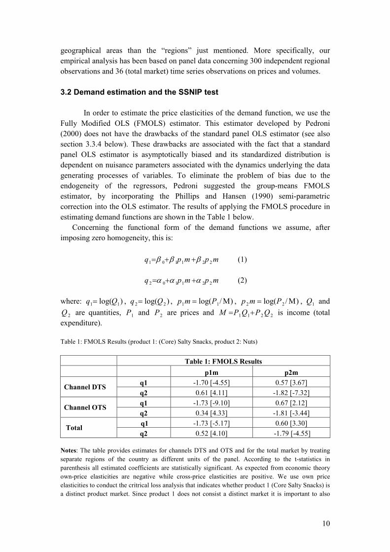
Table 1: FMOLS Results (product 1: (Core) Salty Snacks, product 2: Nuts)
Table 1: FMOLS Results
p1m p2m
Channel DTS q1 -1.70 [-4.55] 0.57 [3.67]
q2 0.61 [4.11] -1.82 [-7.32]
Channel OTS q1 -1.73 [-9.10] 0.67 [2.12]
q2 0.34 [4.33] -1.81 [-3.44]
Total q1 -1.73 [-5.17] 0.60 [3.30]
q2 0.52 [4.10] -1.79 [-4.55]
Notes: The table provides estimates for channels DTS and OTS and for the total market by treating
separate regions of the country as different units of the panel. According to the t-statistics in
parenthesis all estimated coefficients are statistically significant. As expected from economic theory
own-price elasticities are negative while cross-price elasticities are positive. We use own price
elasticities to conduct the critrical loss analysis that indicates whether product 1 (Core Salty Snacks) is
a distinct product market. Since product 1 does not consist a distinct market it is important to also
11
examine cross-price elasticities, which in this case are positive and statistically significant indicating
that the two products are substitutes and so belong to the same market.
3.2.1 Critical loss analysis and conclusions from the SSNIP test
Having estimated elasticities, to find the critical loss associated with a given
price increase let us denote by m = [(p – c)/c] the percentage margin of a
hypothetical monopolist where c is the unit variable cost and p the original (pre-
increase) price level and assume that the price increases by a percentage τ (between
5%-10%) reducing output sales by π. The critical loss denoted by π*, is then given by
π* = τ/(τ+m)36
and the critical elasticity is ε* = π*/τ. We can see that critical loss and
critical elasticity depend on the variable cost of the firm (c). According to the SSNIP
test, as described in the introduction, the Core Salty Sector does not constitute a
distinct product market if the critical elasticity is less than the elasticity estimate
(obtained from the demand estimation). Given a statistically significant elasticity
estimate of –1,73 that we found above, the critical loss analysis based on information
of the unit variable cost of TASTY37, indicates that certainly the segment of Core
Salty Snacks products cannot be considered a distinct relevant product market38. This
is because the critical elasticity is below our elasticity estimate39
. Our elasticity
estimates of the OT and DTS channels are also such that the critical loss analysis
with respect to these channels leads to the conclusion that they cannot be considered
distinct relevant markets. Further, we find positive and statistically significant cross-
elasticities also indicating that Core Salty Snacks and Nuts belong to the same
market.
However, the credibility of the SSNIP test results potentially suffers from
most of the problems mentioned above, specifically, data limitations, non-robust
elasticities estimates and the problem of the Cellophane Fallacy. For these reasons
and in order to verify the credibility of the SSNIP results we proceeded to
undertaking a large number of other quantitative (price) tests. These tests do not
themselves solve the problem of the Cellophane Fallacy, if such a problem does
exist. But, in case such a problem does not exist or is not very serious, then the price
co-movement tests can provide a very useful complementary check that lends
support or refutes the results of the SSNIP. This is especially so when, as explained
below, panel data on prices are available as is true in the present case.
36So �∗ is the percentage loss in sales for which profit after the price increase is equal to profit before the price
increase. 37 The results mentioned here hold for price increases between 5% and 10% and for a range of values of the unit
variable cost (i.e. they are robust to standard sensitivity analysis). See also O’Donoghue R. and J. Padilla (2007),
for further information on the critical loss analysis and the Cellophane Fallacy. 38We assume that the relevant geographic market is the Greek market - the assumption that is always made in
investigations of the savory snacks market. We considered this to be a reasonable assumption in view of the very
high supply side substitutability between different regions in Greece. 39For reasons of confidentiality (regarding the value of m) we cannot report the value of the critical elasticity.
12
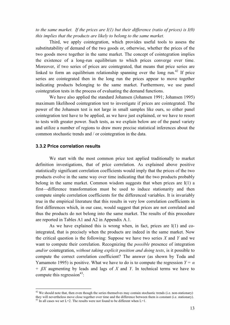
3.3 Price-tests
3.3.1 Econometric methodology and implications for market definition
Our econometric methodology concerning the price tests is conducted as
follows.
First, we undertake the most common tests, the price correlation tests. Price
correlation tests look at how the price of the two products in question change over
time. The idea is that if the two products are regarded by consumers as substitutes
then an increase in the price of one product will increase the demand of the other
leading also to an increase in the price of the second product. So finding a positive
statistically significant correlation coefficient could indicate that the two products
belong in the same market.
We then conduct Granger causality tests to investigate whether lags of Yt are
statistically significant for Xt and vice versa. Granger causality tests examine the
possibility that lagged values of one variable contain predictive content for another
variable above and beyond what is contained in the variable’s own lags40
. Phillips
(1998) has noted that Granger causality tests were used in the context of vector
autoregressions (particularly after the influential paper of Sims, 1980) to discover
causality structures without formally specifying and estimating structural,
simultaneous equations models41
.
Next we detect the nature of the underlying time-series properties using
individual unit root tests and panel unit root tests. A very important feature of our
study is that, we have panel data on prices where the different units are regions. This
opens up the possibility to strengthen the power of individual unit root tests by using
panel tests, such as IPS (Im et al. 2003), LLC (Levin et al. 2002), PP (Phillips and
Perron 1988), ADF-Fisher (Maddala and Wu 1999) and Breitung (2000). Of course
with panel data the possibility of heterogeneity arises in that constant terms and/or
autoregressive coefficients in unit root regressions can be different for each region.
Our panel unit root tests are robust to such heterogeneity (that is, the heterogeneity is
formally taken into account). Since the power of panel unit root tests is expected to
be much larger compared to individual unit root tests, such as ADF-Augmented
Dickey-Fuller (Dickey and Fuller 1979), KPSS-Kwiatkowski-Philips-Schmidt-Shin
(Kwiatkowski et al. 1992) and ERS (Elliott et al. 1996) etc, their application is
recommended in our context. The unit roots test (individual and panel) is very
important for the results of our analysis. We conduct individual unit root tests on the
price series and on the log ratios of prices to examine whether the two goods belong
40
We assume that we have two time series, Xt and Yt; when the past and present values of Xt provide some
useful information to forecast Yt+1 at time t, it is said that Xt Granger causes Yt. For Granger causality, the
common practice is testing the significance (with the F-statistics) of the coefficients of explanatory variable
(lagged Xt ). 41
Ironically, as Phillips (1998) mentioned, if the underlying time series are I(1) and cointegrated, VARs in first
differences are misspecified in that they do not include the necessary so called error correction terms which are
simply ���� − � − ���, that is the deviations from the long run relationship. We note in passing that the
practice of using first differences in VARs or Granger causality tests when time series are I(1) “to induce
stationarity” is incorrect for precisely this reason.
13
to the same market. If the prices are I(1) but their difference (ratio of prices) is I(0)
this implies that the products are likely to belong to the same market.
Third, we apply cointegration, which provides useful tools to assess the
substitutability of demand of the two goods or, otherwise, whether the prices of the
two goods move together in the same market. The concept of cointegration implies
the existence of a long-run equilibrium to which prices converge over time.
Moreover, if two series of prices are cointegrated, that means that price series are
linked to form an equilibrium relationship spanning over the long run.42
If price
series are cointegrated then in the long run the prices appear to move together
indicating products belonging to the same market. Furthermore, we use panel
cointegration tests in the process of evaluating the demand functions.
We have also applied the standard Johansen (Johansen 1991; Johansen 1995)
maximum likelihood cointegration test to investigate if prices are cointegrated. The
power of the Johansen test is not large in small samples like ours, so either panel
cointegration test have to be applied, as we have just explained, or we have to resort
to tests with greater power. Such tests, as we explain below are of the panel variety
and utilize a number of regions to draw more precise statistical inferences about the
common stochastic trends and / or cointegration in the data.
3.3.2 Price correlation results
We start with the most common price test applied traditionally to market
definition investigations, that of price correlation. As explained above positive
statistically significant correlation coefficients would imply that the prices of the two
products evolve in the same way over time indicating that the two products probably
belong in the same market. Common wisdom suggests that when prices are I(1) a
first—difference transformation must be used to induce stationarity and then
compute simple correlation coefficients for the differenced variables. It is invariably
true in the empirical literature that this results in very low correlation coefficients in
first differences which, in our case, would suggest that prices are not correlated and
thus the products do not belong into the same market. The results of this procedure
are reported in Tables A1 and A2 in Appendix A.1.
As we have explained this is wrong when, in fact, prices are I(1) and co-
integrated, that is precisely when the products are indeed in the same market. Now
the critical question is the following: Suppose we have two series X and Y and we
want to compute their correlation. Recognizing the possible presence of integration
and/or cointegration, without taking explicit position and doing tests, is it possible to
compute the correct correlation coefficient? The answer (as shown by Toda and
Yamamoto 1995) is positive. What we have to do is to compute the regression Y = α
+ βX augmenting by leads and lags of Χ and Y. In technical terms we have to
compute this regression43
:
42 We should note that, then even though the series themselves may contain stochastic trends (i.e. non-stationary)
they will nevertheless move close together over time and the difference between them is constant (i.e. stationary). 43 In all cases we set L=2. The results were not found to be different when L=1.
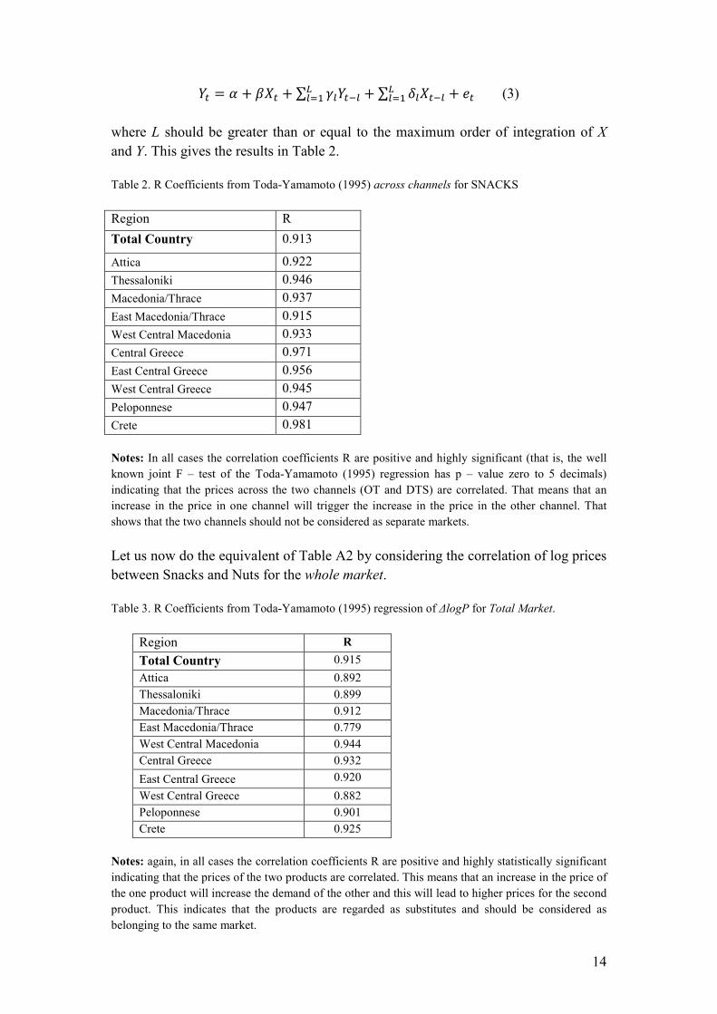
14
�� = � + �� + � ������ + � ������ + ������
���� (3)
where L should be greater than or equal to the maximum order of integration of X
and Y. This gives the results in Table 2.
Table 2. R Coefficients from Toda-Yamamoto (1995) across channels for SNACKS
Region R
Total Country 0.913
Attica 0.922
Thessaloniki 0.946
Macedonia/Thrace 0.937
East Macedonia/Thrace 0.915
West Central Macedonia 0.933
Central Greece 0.971
East Central Greece 0.956
West Central Greece 0.945
Peloponnese 0.947
Crete 0.981
Notes: In all cases the correlation coefficients R are positive and highly significant (that is, the well
known joint F – test of the Toda-Yamamoto (1995) regression has p – value zero to 5 decimals)
indicating that the prices across the two channels (OT and DTS) are correlated. That means that an
increase in the price in one channel will trigger the increase in the price in the other channel. That
shows that the two channels should not be considered as separate markets.
Let us now do the equivalent of Table A2 by considering the correlation of log prices
between Snacks and Nuts for the whole market.
Table 3. R Coefficients from Toda-Yamamoto (1995) regression of ∆logP for Total Market.
Region R
Total Country 0.915
Attica 0.892
Thessaloniki 0.899
Macedonia/Thrace 0.912
East Macedonia/Thrace 0.779
West Central Macedonia 0.944
Central Greece 0.932
East Central Greece 0.920
West Central Greece 0.882
Peloponnese 0.901
Crete 0.925
Notes: again, in all cases the correlation coefficients R are positive and highly statistically significant
indicating that the prices of the two products are correlated. This means that an increase in the price of
the one product will increase the demand of the other and this will lead to higher prices for the second
product. This indicates that the products are regarded as substitutes and should be considered as
belonging to the same market.

15
In Table 3 we provide the R coefficients for the regression logPSNACKS = α +
βlogPNUTS no matter whether there is non-stationarity or co-integration. Apparently
the correlations are on the whole very large. Indeed the minimum R is 0.75 and the
maximum R is about 0.94.
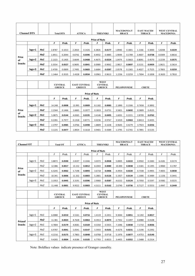
3.3.3 Granger causality results
Granger causality tests have a long history in applied econometrics. With I(1)
variables the Granger test is expected to reject causality and under cointegration it
will indicate the presence of causality, as it should, in the right direction (that is,
from X to Y if that is indeed the direction of causation). Our results, reported in Table
A.3 (in Appendix A.2) show that in most cases we do indeed have causality which
accords with the claim that the products are in the same market. Of course the
sample size is small but such findings are at least re-assuring in the sense that OLS-
Granger estimates converge at the fast rate of T-1
.
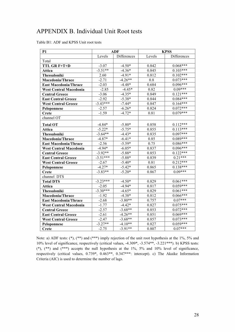
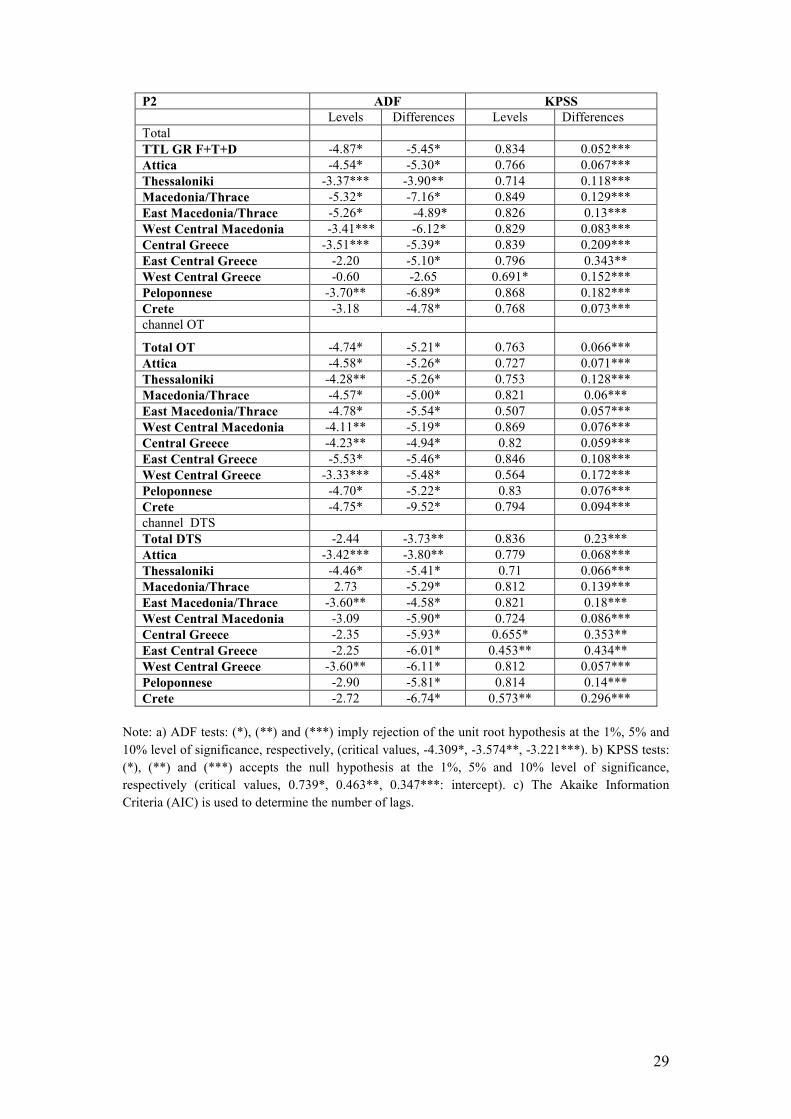
3.3.4 Unit root tests results
In a first step, we conduct the Individual time series unit root tests at the
prices of the two goods. The results for the ADF and KPSS tests are reported in
Appendix B (Table B1). These results indicate that the null hypothesis (non-
stationarity) of the ADF test is accepted at levels of the price of the snack (P1) in the
channel DTS only for the following regions: Macedonia/Thrace, East
Macedonia/Thrace, West Central Macedonia, Central Greece, East Central Greece,
West Central Greece and for the Total in the regions: Thessaloniki,
Macedonia/Thrace, East Macedonia/Thrace, West Central Macedonia, Central
Greece and East Central Greece. While for the price of nuts (P2) the results indicate
the existence of unit roots in levels for the channel DTS in the region of
Macedonia/Thrace, West Central Macedonia, Central Greece, East Central Greece,
the same is observed in the regions of the total, as follows: East Central Greece,
West Central Greece. In the first differences of the price variables, the results of the
ADF unit root tests indicate that the null hypothesis is rejected; thus, the prices of the
two goods are I(0).
Moreover, the null hypothesis of stationarity of the KPSS tests is accepted in
the first differences of variables. Therefore, based on the results of the two tests, we
conclude that the time series of prices in the first differences is I(0).
Furthermore, we also report in Appendix B (Table B2), the results from the
more powerful Elliott, Rothenberg and Stock (1996) DF-GLS test and the ERS-Point
Optimal Root Test (Table B3). Again, the message is the same as with the others unit
root tests in the sense that individual price series are I(1) but their differences, more
often than not, are stationary, indicating that the two goods belong to the same
market.
In next step, we conduct panel unit root tests using regions as different units
of the panel. All these panel unit root tests assume non-stationarity as the null

16
hypothesis and test against alternatives involving stationarity. The results of the
panel unit root tests in the log of prices and the ratio of prices are reported in Tables
4 and 5, respectively. The Tables report the p-values of the tests. From the panel
results, it is clear that the two products belong in the same market since log prices
are I(1) – Table 4 - but their difference (the log ratio of the two prices) is stationary
(Table 5). Therefore, the results of price stationarity provide evidence supporting that
the two goods are substitutes in the market. More specifically, the stationarity of the
prices ratio guarantees that short-run fluctuations in the prices will have only
temporary effects44
.
Table 4. Panel Unit Root tests (p-values)
logP1 logP2 logQ1 logQ2
Levin, Li and,Chu total market 0.159 0.0569 0.000 0.992
OT channel 0.040 0.057 0.000 0.942
DTS channel 0.679 0.455 0.000 0.001
DTS & OT 0.263 0.136 0.000 0.211
Breitung total market 0.480 0.539 0.000 0.661
OT channel 0.973 0.088 0.000 0.700
DTS channel 0.314 0.641 0.000 0.013
DTS & OT 0.753 0.263 0.000 0.171
Im, Pesaran and Shin W total market 0.998 0.913 0.000 0.221
OT channel 0.985 0.381 0.000 0.118
DTS channel 0.999 0.919 0.000 0.000
DTS & OT 1.000 0.759 0.000 0.000
Fisher ADF total market 0.999 0.636 0.000 0.389
OT channel 0.999 0.381 0.000 0.184
DTS channel 1.000 0.517 0.000 0.000
DTS & OT 1.000 0.455 0.000 0.000
Fisher PP total market 1.000 0.787 0.000 0.000
OT channel 0.998 0.009 0.000 0.000
DTS channel 1.000 0.597 0.000 0.001
DTS & OT 1.000 0.052 0.000 0.000
Notes: Bold face values indicate rejection of I(1). The Table reports p-values of the tests. In all tests,
the null hypothesis is I(1). DTS & OT indicates combination (not summation) of the DTS and OT
channels for 10 regions. All tests are panel based and are conducted in the 11 regions of the country.
Lags are selected according to the Schwarz criterion.
44 Graphs, not reported here (but available on editor’s request) indicate that we should allow for a different
regional constant but no trend.
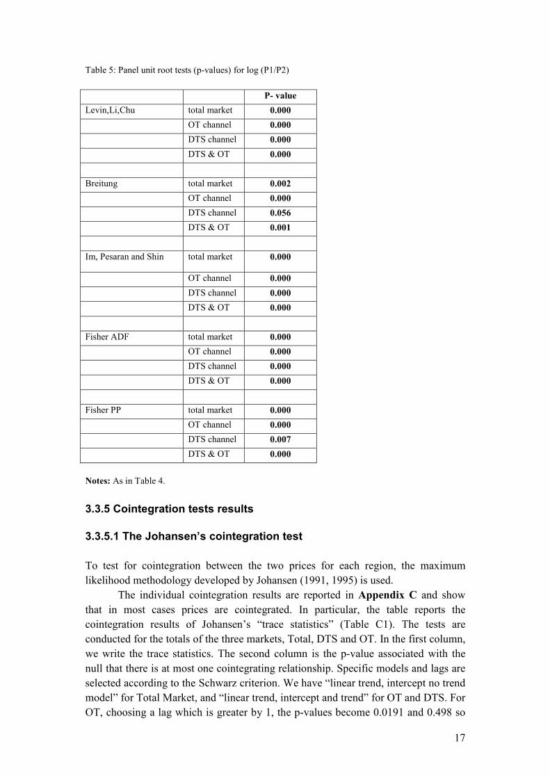
17
Table 5: Panel unit root tests (p-values) for log (P1/P2)
P- value
Levin,Li,Chu total market 0.000
ΟT channel 0.000
DTS channel 0.000
DTS & OT 0.000
Breitung total market 0.002
OT channel 0.000
DTS channel 0.056
DTS & OT 0.001
Im, Pesaran and Shin total market 0.000
OT channel 0.000
DTS channel 0.000
DTS & OT 0.000
Fisher ADF total market 0.000
OT channel 0.000
DTS channel 0.000
DTS & OT 0.000
Fisher PP total market 0.000
OT channel 0.000
DTS channel 0.007
DTS & OT 0.000
Notes: As in Table 4.
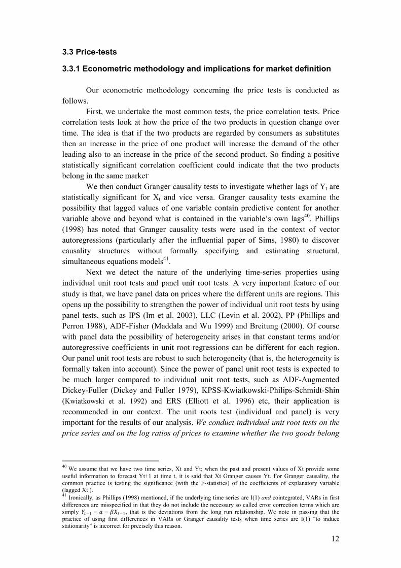
3.3.5 Cointegration tests results
3.3.5.1 The Johansen’s cointegration test
To test for cointegration between the two prices for each region, the maximum
likelihood methodology developed by Johansen (1991, 1995) is used.
The individual cointegration results are reported in Appendix C and show
that in most cases prices are cointegrated. In particular, the table reports the
cointegration results of Johansen’s “trace statistics” (Table C1). The tests are
conducted for the totals of the three markets, Total, DTS and OT. In the first column,
we write the trace statistics. The second column is the p-value associated with the
null that there is at most one cointegrating relationship. Specific models and lags are
selected according to the Schwarz criterion. We have “linear trend, intercept no trend
model” for Total Market, and “linear trend, intercept and trend” for OT and DTS. For
OT, choosing a lag which is greater by 1, the p-values become 0.0191 and 0.498 so
18
the result that we have cointegration is strengthened. The overall result is that prices
are cointegrated and therefore products and distribution channels belong to the
same market.
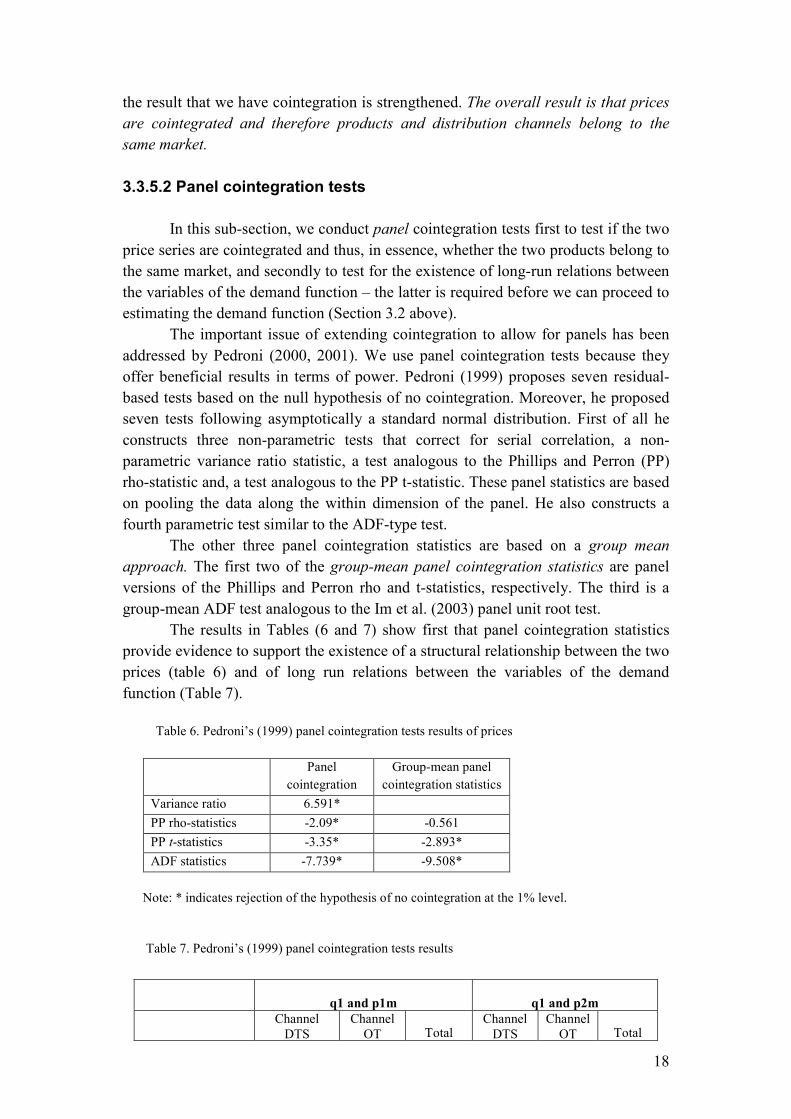
3.3.5.2 Panel cointegration tests
In this sub-section, we conduct panel cointegration tests first to test if the two
price series are cointegrated and thus, in essence, whether the two products belong to
the same market, and secondly to test for the existence of long-run relations between
the variables of the demand function – the latter is required before we can proceed to
estimating the demand function (Section 3.2 above).
The important issue of extending cointegration to allow for panels has been
addressed by Pedroni (2000, 2001). We use panel cointegration tests because they
offer beneficial results in terms of power. Pedroni (1999) proposes seven residual-
based tests based on the null hypothesis of no cointegration. Moreover, he proposed
seven tests following asymptotically a standard normal distribution. First of all he
constructs three non-parametric tests that correct for serial correlation, a non-
parametric variance ratio statistic, a test analogous to the Phillips and Perron (PP)
rho-statistic and, a test analogous to the PP t-statistic. These panel statistics are based
on pooling the data along the within dimension of the panel. He also constructs a
fourth parametric test similar to the ADF-type test.
The other three panel cointegration statistics are based on a group mean
approach. The first two of the group-mean panel cointegration statistics are panel
versions of the Phillips and Perron rho and t-statistics, respectively. The third is a
group-mean ADF test analogous to the Im et al. (2003) panel unit root test.
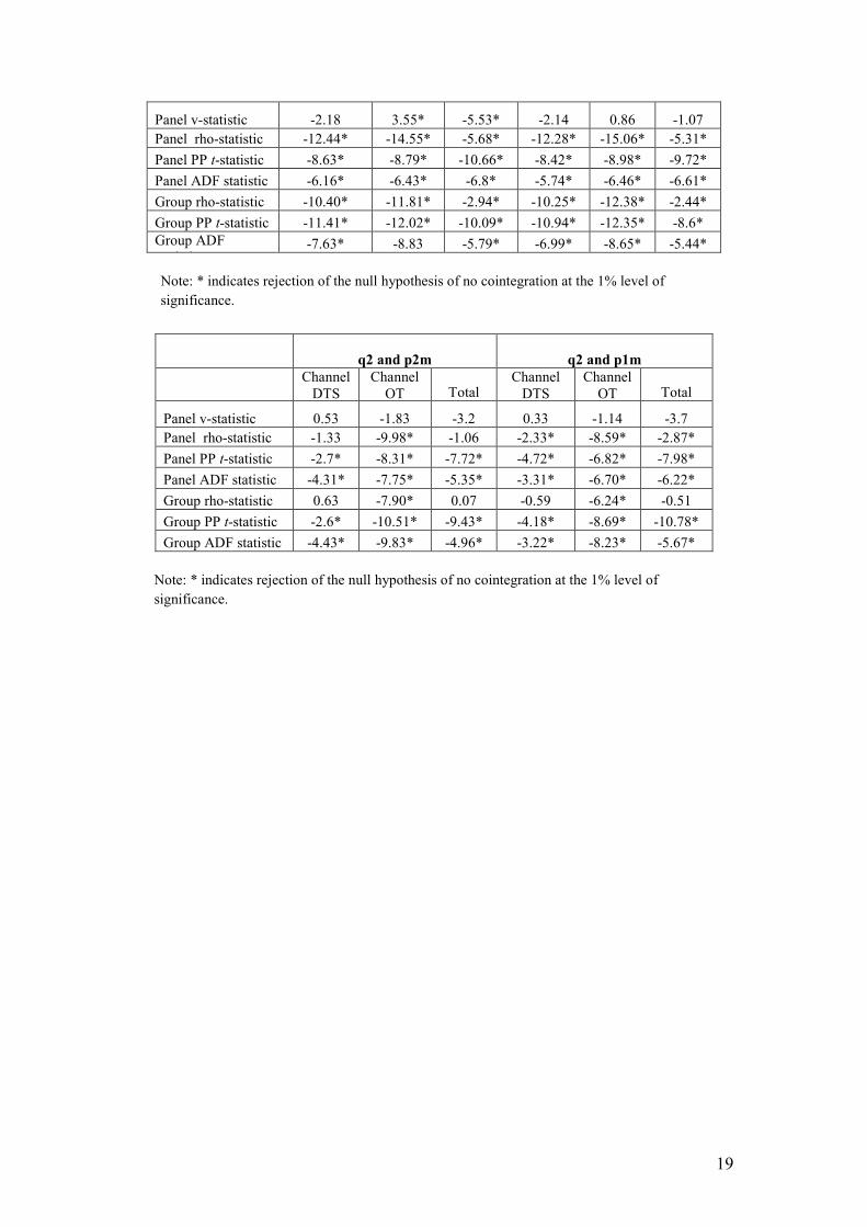
The results in Tables (6 and 7) show first that panel cointegration statistics
provide evidence to support the existence of a structural relationship between the two
prices (table 6) and of long run relations between the variables of the demand
function (Table 7).
Table 6. Pedroni’s (1999) panel cointegration tests results of prices
Panel
cointegration
statistics
Group-mean panel
cointegration statistics
Variance ratio 6.591*
PP rho-statistics -2.09* -0.561
PP t-statistics -3.35* -2.893*
ADF statistics -7.739* -9.508*
Note: * indicates rejection of the hypothesis of no cointegration at the 1% level.
Table 7. Pedroni’s (1999) panel cointegration tests results
q1 and p1m
q1 and p2m
Channel
DTS
Channel
OT Total Channel
DTS
Channel
OT Total
19
Panel v-statistic -2.18 3.55* -5.53* -2.14 0.86 -1.07
Panel rho-statistic -12.44* -14.55* -5.68* -12.28* -15.06* -5.31*
Panel PP t-statistic -8.63* -8.79* -10.66* -8.42* -8.98* -9.72*
Panel ADF statistic -6.16* -6.43* -6.8* -5.74* -6.46* -6.61*
Group rho-statistic -10.40* -11.81* -2.94* -10.25* -12.38* -2.44*
Group PP t-statistic -11.41* -12.02* -10.09* -10.94* -12.35* -8.6*
Group ADF
statistic -7.63* -8.83 -5.79* -6.99* -8.65* -5.44*
Note: * indicates rejection of the null hypothesis of no cointegration at the 1% level of
significance.
q2 and p2m
q2 and p1m
Channel
DTS
Channel
OT Total Channel
DTS
Channel
OT Total
Panel v-statistic 0.53 -1.83 -3.2 0.33 -1.14 -3.7
Panel rho-statistic -1.33 -9.98* -1.06 -2.33* -8.59* -2.87*
Panel PP t-statistic -2.7* -8.31* -7.72* -4.72* -6.82* -7.98*
Panel ADF statistic -4.31* -7.75* -5.35* -3.31* -6.70* -6.22*
Group rho-statistic 0.63 -7.90* 0.07 -0.59 -6.24* -0.51
Group PP t-statistic -2.6* -10.51* -9.43* -4.18* -8.69* -10.78*
Group ADF statistic -4.43* -9.83* -4.96* -3.22* -8.23* -5.67*
Note: * indicates rejection of the null hypothesis of no cointegration at the 1% level of
significance.

20
4. Concluding remarks
Market share is the most important indicator of market power used by
Competition Authorities. To measure it correctly it is absolutely essential to define
accurately relevant products and geographical markets. To do so, it is standard to use
the SSNIP test, but as explained in the introductory section of this paper, this has a
number of limitations. While in this paper we have undertaken the SSNIP test we
also have proposed and then applied a large number of other quantitative tests at the
disposal of economists in an effort to delineate the relevant antitrust market of
Savory Snacks - one of the most investigated markets worldwide. Our analysis
provides for the first time a detailed application and comparison of the complete set
of all the quantitative tests that have been proposed at various times by economists
for defining antitrust markets. In particular, we undertook apart from the SSNIP,
price correlation and Granger causality tests a large number of price co-movement
tests, in the light of developments in econometric techniques, using Greek bimonthly
data for this market for the period 2005 – 2010. During this period, PepsiCo has been
the largest player in Greece with market shares of over 70% in narrowly defined
markets but less than 50% in widely defined markets. The results of our extensive
tests indicate that a wide market definition is more appropriate in the Savory Snacks
market.

21
APPENDIX A.1. Values of correlation coefficients
In Table A1 below, we consider the regression ∆logPΟΤ = α + β∆logPDTS for
Snacks and also for Nuts, for the different regions. The correlation coefficient R (or
equivalently here, R2) is not significant for the total channels or for channels OT and
DTS with very few exceptions.
In Table A2 we consider the regression ∆logPSNACKS = α + β∆logPNUTS for the
whole market and the different regions. Here we see that for the market as a whole
and certain regional markets (three out of ten) the differences of log prices are
statistically significantly correlated with a negative relationship.
All p-values are derived from the p-value of regression coefficient β. In Table
A2 we also examine autocorrelation – robust standard errors (and thus p-values)
according to the well known methodology of Newey – West. The same has been
performed for Table A1 but we did not reach different results.
Table A1: R2 Coefficients from a regression of ∆logP across channels:
SNACKS NUTS
Region
Total 0.007 (-) 0.00002
Attica 0.010 0.049
Thessaloniki 0.0005 0.014 (-)
Macedonia/Thrace 0.004 0.017 (-)
East Macedonia/Thrace 0.002 (-) 0.059 (-)
West Central Macedonia 0.020 0.081
Central Greece 0.006 (-) 0.012
East Central Greece 0.420 (**) 0.105 (*)
West Central Greece 0.005 0.022 (-)
Peloponnese 0.01 (-) 0.014 (-)
Crete 0.096 (*) 0.031
Notes: (-) denotes a negative R, (*) is significance at 10% and (**) significance at 1% or higher. The
regression is ∆logPΟΤ = α + β∆logPDTS.
Table A2. R2 Coefficients from a regression of ∆logP for the Whole Market:
Region R2 p-value p-value (AR)
Total 0.108 (-) 0.075 0.0017
Attica 0.111 (-) 0.072 0.0152
Thessaloniki 0.067 0.170 0.056
Macedonia/Thrace 0.021 (-) 0.440 0.282
East Macedonia/Thrace 0.102 (-) 0.085 0.001
West Central Macedonia 0.00 (-) 0.96 0.95
Central Greece 0.004 (-) 0.73 0.60
East Central Greece 0.01 (-) 0.60 0.302
West Central Greece 0.00 0.97 0.98
Peloponnese 0.00 (-) 0.85 0.783

22
Crete 0.036 0.31 0.129
Notes: (-) denotes a negative R The regression is ∆logPSNACKS = α + β∆logPNUTS. Boldface values
indicate significance at the level indicated or higher (e.g. 0.075 denotes significance at level 7,5%,
10% etc). AR means autocorrelation – robust.
One important question in empirical Industrial Organisation is what values of
correlation coefficients are “small”. From the data on total market we get the
following results.
Dependent Variable: LD1P1
Method: Least Squares
Sample (adjusted): 2000Q2 2007Q3
Included observations: 30 after adjustments
Variable Coefficient Std.
Error t-Statistic
C 0.102893 0.115276 0.892582
LD1P1(-1) 0.959204 0.048430 19.80613
R-squared 0.933378
Adjusted R-squared 0.930999
Durbin-Watson stat 1.698816
Mean dependent var 2.385368
S.D. dependent var 0.058937
Prob (F-statistic) 0.000000
The constant term is not statistically significant while the value of ρ is close to 1.
according to the ADF test the series is I(1). Suppose we construct a series X as
1 0,015t t tX X e−= + , where ( )~ 0,1te IIDN . Let us also construct the second price
(logP2, orΥ) as 0,03t t tY X v= + , and ( )~ 0,1tv IIDN , as our estimates show. The
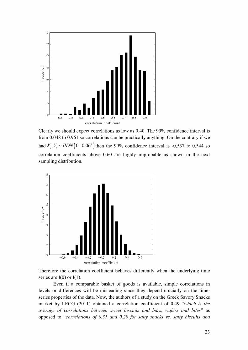
question is then what kinds of correlation coefficients we should expect. Given our
sample size, n=30, 100,000 Monte Carlo simulations provide the results shown in the
figures below.
23
Clearly we should expect correlations as low as 0.40. The 99% confidence interval is
from 0.048 to 0.961 so correlations can be practically anything. On the contrary if we
had ( )2, ~ 0, 0.06t t
X Y IIDN then the 99% confidence interval is -0,537 to 0,544 so
correlation coefficients above 0.60 are highly improbable as shown in the next
sampling distribution.
Therefore the correlation coefficient behaves differently when the underlying time
series are I(0) or I(1).
Even if a comparable basket of goods is available, simple correlations in
levels or differences will be misleading since they depend crucially on the time-
series properties of the data. Now, the authors of a study on the Greek Savory Snacks
market by LECG (2011) obtained a correlation coefficient of 0.49 “which is the
average of correlations between sweet biscuits and bars, wafers and bites” as
opposed to “correlations of 0.31 and 0.29 for salty snacks vs. salty biscuits and

24
crackers, respectively”. The authors of LECG claim that correlations like 0.30 are
“substantially lower” than 0.50.
Why are they substantially lower? How different can be a correlation
coefficient of 0.30 say, compared to 0.49 in sample sizes N=36? No statistical test is
provided here so we have to return to statitistical principles and wonder whether in
samples of size N=36 correlations like 0.30 and 0.50 are compatible. From Kendall
and Stuart45
(1977) (page 261) the standard error of the correlation coefficient is 21
N
ρ−. Given that ρ=0.5 the standard error is (1-0.5
2)/6=0.125, so the 95%
confidence interval would be 0.5 1.96 0.125± × , that is [0.255, 0.745]. Therefore, the
“basket estimate” of a correlation coefficient about 0.50 cannot reject the hypothesis
that, in fact, this correlation coefficient is as low as 0.255. Therefore, it can be 0.30.
To put it in another way, if ρ=0, then the standard error would be 1/ N = 0.17,
approximately so the estimate r=0.50 would come with a standard error se=0.17 and
a 95% confidence interval 0.50 1.96 0.17± × = [0.17, 0.833]. This asymptotic 95%
confidence interval, apparently rationalizes values of the correlation coefficient like
0.30 or as low as 0.17.
The normal approximation in small samples is known to be inaccurate and
Kendall and Stuart mention that. They provide a closer approximation in pages 417-
418 of their classical book. Suppose 12
1log
1
rz
r
+=
− which in our case, with r=0.5,
becomes z=0.5493. If the true value of ρ=0.3, then 12
1log
1
ρζ
ρ
+=
−=0.3095. The
question then is whether z and ζ are statistically close. As Kendall and Stuart
mention (p. 419) one can take as standard error of z-ζ the expression
( )
2
2
1 4
1 2 1n n
ρ−+
− −=0.1737, much like as before. The z-transformation tends to
normality fast, so we can use the 95% confidence interval 0.5 1.96 0.1737± × which
gives us a wider estimate: [0.159, 0.840].
This means that to the estimate of the correlation coefficient r=0.5 one must
attach a standard error, se=0.1737, and thus given the estimate a good approximation
to a 95% confidence interval is simply 0.5 1.96 se± × (see Kendall and Stuart, p.
419).
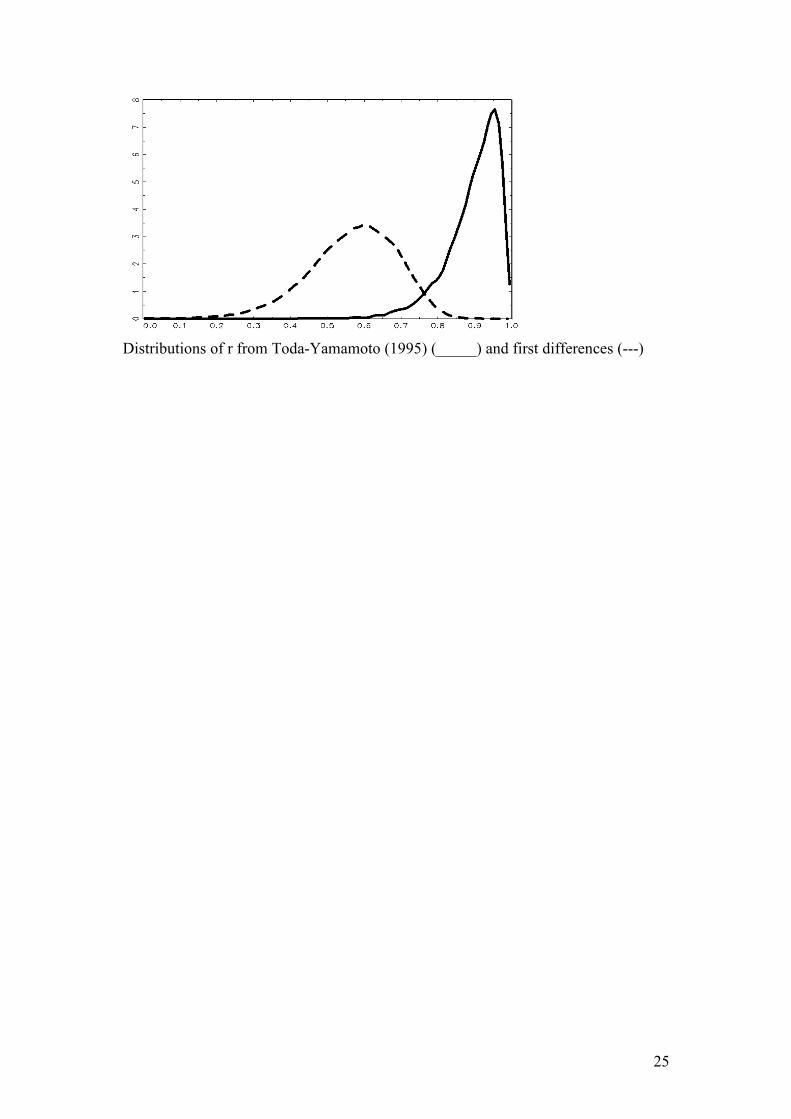
Of course the correct way would be to use the Toda-Yamamoto (1995) in the
context of I(1) processes. The difference in terms of the sampling distributions is
shown in the next figure.
45 Sir Maurice Kendall and Alan Stuart, “The Advanced Theory of Statistics”, volume 1, 4th edition, 1977,
Charles Griffin and Co.
25
Distributions of r from Toda-Yamamoto (1995) (_____) and first differences (---)

26
APPENDIX A.2. Results of Granger Causality tests
Table A3. Granger causality tests
TOTAL TTL GR F+T+D ATTICA THES/NIKI
MACEDONIA/T
HRACE
EAST MACED/
THRACE
WEST CENTRAL
MACEDONIA
Price of Nuts
F Prob. F Prob. F Prob. F Prob. F Prob. F Prob.
Price
of
Snacks
lags=1
Ho1 9.451 0.0048 4.1590 0.0513
5.752
2 0.0236 4.4334 0.0447 1.4955 0.2319 9.5683 0.0046
Ho2 2.123 0.1566 5.8950 0.0221
0.000
5 0.9822 1.9567 0.1732 3.0854 0.0903 0.0027 0.9585
lags=2 Ho1 15.929 0.000 20.386 0.000
3.301
8 0.0541 2.0582 0.1496 1.1863 0.3226 3.8966 0.0342
Ho2 2.883 0.0755 5.5140 0.0107
0.095
1 0.9096 2.8944 0.0748 1.8690 0.1760 1.5297 0.2370
lags=3 Ho1 6.625 0.0025 8.9365 0.0005
2.277
6 0.1092 1.1683 0.3454 1.2552 0.3152 2.0637 0.1357
Ho2 9.515 0.0004 17.275 0.00006
0.062
1 0.9792 2.3755 0.0989 1.8667 0.1662 1.5552 0.2299
CENTRAL
GREECE
EAST CENTRAL
GREECE
WEST
CENTRAL
GREECE PELOPONNESE CRETE
Price of Nuts
Price
of
Snacks
F Prob. F Prob. F Prob. F Prob. F Prob.
lags=1
Ho1 12.083 0.0017 8.0277 0.0086
2.838
9 0.1035 6.8902 0.0141 13.573 0.0010
Ho2 0.5028 0.4843 0.0621 0.8050
1.005
8 0.3248 2.3317 0.1384 0.8531 0.3638
lags=2 Ho1 7.5647 0.0028 4.2758 0.0258
0.930
5 0.4081 3.4610 0.0478 8.8415 0.0013
Ho2 0.2229 0.8018 0.6667 0.5226
0.630
7 0.5408 0.6652 0.5234 0.2674 0.7676
lags=3 Ho1 2.7274 0.0698 1.6180 0.2153
0.500
7 0.6858 1.6087 0.2173 3.8200 0.0250
Ho2 3.8525 0.0243 3.5211 0.0328
2.280
0 0.1089 4.5516 0.0131 0.7681 0.5247
27
Channel DTS Total DTS ATTICA THES/NIKI
MACEDONIA/T
HRACE
EAST MACED/
THRACE
WEST CENTRAL
MACEDONIA
Price of Nuts
F Prob. F Prob. F Prob. F Prob. F Prob. F Prob.
Price
of
Snacks
lags=1
Ho1 2.8787 0.1013 2.2810 0.1426 6.3826 0.0177 1.8940 0.1801 1.1166 0.3000 5.8208 0.0229
Ho2 1.6911 0.2044 4.6742 0.0396 0.4932 0.4885 1.9049 0.1789 3.4607 0.0738 0.0309 0.8616
lags=2 Ho1 2.1323 0.1405 3.6649 0.0408 4.4675 0.0224 1.0474 0.3663 0.8091 0.4570 3.2239 0.0575
Ho2 3.3354 0.0527 6.9695 0.0041 0.0989 0.9062 2.9817 0.0697 3.5131 0.0459 1.0621 0.3614
lags=3 Ho1 2.4709 0.0899 2.7495 0.0683 3.6684 0.0287 2.0578 0.1365 0.4027 0.7525 3.7803 0.0259
Ho2 1.1464 0.3535 2.4328 0.0934 0.0961 0.9613 1.2236 0.3259 1.7694 0.1838 0.3620 0.7810
CENTRAL
GREECE
EAST CENTRAL
GREECE
WEST
CENTRAL
GREECE PELOPONNESE CRETE
Price of Nuts
Price
of
Snacks
F Prob. F Prob. F Prob. F Prob. F Prob.
lags=1
Ho1 14.248 0.0008 13.995 0.0009 8.1182 0.0083 2.1890 0.1506 0.7658 0.3892
Ho2 2.2344 0.1466 1.6665 0.2077 0.1819 0.6731 3.5821 0.0692 0.5809 0.4525
lags=2 Ho1 5.0875 0.0144 4.6565 0.0195 3.4146 0.0495 1.6031 0.2221 2.8709 0.0762
Ho2 0.2281 0.7977 0.1318 0.8771 0.0236 0.9767 3.5019 0.0463 0.8413 0.4435
lags=3 Ho1 2.3797 0.0985 3.0766 0.0498 1.8809 0.1638 0.9645 0.4279 3.7923 0.0256
Ho2 3.1225 0.0477 1.8924 0.1618 0.9401 0.4389 1.3795 0.2765 0.7891 0.5135
Channel OT Total OT ATTICA THES/NIKI
MACEDONIA/T
HRACE
EAST MACED/
THRACE
WEST CENTRAL
MACEDONIA
Price of Nuts
F Prob. F Prob. F Prob. F Prob. F Prob. F Prob.
Price
of
Snacks
lags=1
Ho1 3.8872 0.0590 2.8197 0.1046 3.0372 0.0928 5.8905 0.0222 0.9502 0.3383 6.4181 0.0174
Ho2 12.086 0.0017 13.152 0.0012 8.2043 0.0080 10.000 0.0038 2.3181 0.1395 1.9060 0.1787
lags=2 Ho1 6.3245 0.0062 5.7198 0.0093 3.6718 0.0406 4.4954 0.0220 0.7338 0.4905 7.4835 0.0030
Ho2 10.341 0.0006 11.332 0.0003 5.2801 0.0126 5.1927 0.0134 1.1006 0.3489 1.1156 0.3441
lags=3 Ho1 3.1953 0.0445 3.3191 0.0396 2.9060 0.0587 4.6152 0.0124 0.7050 0.5597 3.9382 0.0225
Ho2 11.448 0.0001 9.9522 0.0003 4.3111 0.0162 2.6740 0.0736 0.7127 0.5553 1.4947 0.2449
CENTRAL
GREECE
EAST CENTRAL
GREECE
WEST
CENTRAL
GREECE PELOPONNESE CRETE
Price of Nuts
Priceof
Snacks
F Prob. F Prob. F Prob. F Prob. F Prob.
lags=1
Ho1 6.0080 0.0210 3.5161 0.0716 1.4119 0.2451 9.3044 0.0051 12.202 0.0017
Ho2 11.381 0.0023 8.7628 0.0063 8.3913 0.0074 2.7352 0.1097 0.6980 0.4108
lags=2 Ho1 4.7804 0.0179 4.8581 0.0169 0.5350 0.5925 7.1046 0.0038 7.1710 0.0036
Ho2 6.9787 0.0041 5.0541 0.0147 5.5933 0.0101 4.4276 0.0231 1.5190 0.2392
lags=3 Ho1 4.2216 0.0175 5.7863 0.0048 0.0768 0.9718 5.1976 0.0077 4.4753 0.0140
Ho2 9.4265 0.0004 4.8186 0.0105 6.7703 0.0023 3.4455 0.0352 1.5488 0.2314
Note: Boldface values indicate presence of Granger causality.
28
APPENDIX B. Individual Unit Root tests
Table B1: ADF and KPSS Unit root tests
P1 ADF KPSS
Levels Differences Levels Differences
Total
TTL GR F+T+D -3.07 -4.50* 0.842 0.068***
Attica -3.51** -4.36* 0.845 0.103***
Thessaloniki 2.60 -4.91* 0.812 0.102***
Macedonia/Thrace -2.71 -4.26** 0.8 0.073***
East Macedonia/Thrace -2.03 -4.48* 0.684 0.096***
West Central Macedonia -2.85 -4.45* 0.82 0.09***
Central Greece -3.06 -4.35* 0.849 0.121***
East Central Greece -2.92 -5.38* 0.844 0.084***
West Central Greece -3.43*** -7.44* 0.847 0.164***
Peloponnese -2.57 -6.26* 0.824 0.072***
Crete -1.59 -4.72* 0.81 0.079***
channel ΟΤ
Total OT -4.84* -5.80* 0.858 0.112***
Attica -5.22* -5.75* 0.855 0.113***
Thessaloniki -3.64** -4.43* 0.835 0.097***
Macedonia/Thrace -4.87* -6.41* 0.85 0.089***
East Macedonia/Thrace -2.56 -5.59* 0.75 0.086***
West Central Macedonia -4.94* -6.05* 0.837 0.096***
Central Greece -3.92** -5.88* 0.853 0.122***
East Central Greece -3.51*** -5.88* 0.839 0.21***
West Central Greece -2.67 -5.40* 0.81 0.212***
Peloponnese -4.27* -5.42* 0.865 0.138***
Crete -3.83** -5.20* 0.867 0.09***
channel DTS
Total DTS -3.23*** -4.50* 0.829 0.061***
Attica -2.05 -4.94* 0.817 0.059***
Thessaloniki -3.30*** -4.65* 0.829 0.061***
Macedonia/Thrace -1.92 -4.38* 0.812 0.066***
East Macedonia/Thrace -2.68 -3.80** 0.757 0.07***
West Central Macedonia -1.77 -4.42* 0.827 0.075***
Central Greece -2.57 -3.68** 0.853 0.072***
East Central Greece -2.61 -4.26** 0.851 0.069***
West Central Greece -2.47 -3.68** 0.857 0.073***
Peloponnese -3.27** -4.10** 0.827 0.059***
Crete -2.75 -3.91** 0.807 0.07***
Note: a) ADF tests: (*), (**) and (***) imply rejection of the unit root hypothesis at the 1%, 5% and
10% level of significance, respectively (critical values, -4.309*, -3.574**, -3.221***). b) KPSS tests:
(*), (**) and (***) accepts the null hypothesis at the 1%, 5% and 10% level of significance,
respectively (critical values, 0.739*, 0.463**, 0.347***: intercept). c) The Akaike Information
Criteria (AIC) is used to determine the number of lags.
29
P2 ADF KPSS
Levels Differences Levels Differences
Total
TTL GR F+T+D -4.87* -5.45* 0.834 0.052***
Attica -4.54* -5.30* 0.766 0.067***
Thessaloniki -3.37*** -3.90** 0.714 0.118***
Macedonia/Thrace -5.32* -7.16* 0.849 0.129***
East Macedonia/Thrace -5.26* -4.89* 0.826 0.13***
West Central Macedonia -3.41*** -6.12* 0.829 0.083***
Central Greece -3.51*** -5.39* 0.839 0.209***
East Central Greece -2.20 -5.10* 0.796 0.343**
West Central Greece -0.60 -2.65 0.691* 0.152***
Peloponnese -3.70** -6.89* 0.868 0.182***
Crete -3.18 -4.78* 0.768 0.073***
channel ΟΤ
Total OT -4.74* -5.21* 0.763 0.066***
Attica -4.58* -5.26* 0.727 0.071***
Thessaloniki -4.28** -5.26* 0.753 0.128***
Macedonia/Thrace -4.57* -5.00* 0.821 0.06***
East Macedonia/Thrace -4.78* -5.54* 0.507 0.057***
West Central Macedonia -4.11** -5.19* 0.869 0.076***
Central Greece -4.23** -4.94* 0.82 0.059***
East Central Greece -5.53* -5.46* 0.846 0.108***
West Central Greece -3.33*** -5.48* 0.564 0.172***
Peloponnese -4.70* -5.22* 0.83 0.076***
Crete -4.75* -9.52* 0.794 0.094***
channel DTS
Total DTS -2.44 -3.73** 0.836 0.23***
Attica -3.42*** -3.80** 0.779 0.068***
Thessaloniki -4.46* -5.41* 0.71 0.066***
Macedonia/Thrace 2.73 -5.29* 0.812 0.139***
East Macedonia/Thrace -3.60** -4.58* 0.821 0.18***
West Central Macedonia -3.09 -5.90* 0.724 0.086***
Central Greece -2.35 -5.93* 0.655* 0.353**
East Central Greece -2.25 -6.01* 0.453** 0.434**
West Central Greece -3.60** -6.11* 0.812 0.057***
Peloponnese -2.90 -5.81* 0.814 0.14***
Crete -2.72 -6.74* 0.573** 0.296***
Note: a) ADF tests: (*), (**) and (***) imply rejection of the unit root hypothesis at the 1%, 5% and
10% level of significance, respectively, (critical values, -4.309*, -3.574**, -3.221***). b) KPSS tests:
(*), (**) and (***) accepts the null hypothesis at the 1%, 5% and 10% level of significance,
respectively (critical values, 0.739*, 0.463**, 0.347***: intercept). c) The Akaike Information
Criteria (AIC) is used to determine the number of lags.

30
Q1 ADF KPSS
Levels Differences Levels Differences
Total
TTL GR F+T+D -4.88* -5.61* 0.161*** 0.057***
Attica -4.27** -4.57* 0.097*** 0.064***
Thessaloniki -4.56* -4.76* 0.146*** 0.061***
Macedonia/Thrace -4.82* -6.50* 0.537* 0.082***
East Macedonia/Thrace -4.57* -6.07* 0.591* 0.081***
West Central Macedonia -4.62* -6.45* 0.437** 0.081***
Central Greece -4.16* -5.96* 0.394*** 0.07***
East Central Greece -3.77** -5.99* 0.495* 0.076***
West Central Greece -4.70* -4.73* 0.096*** 0.062***
Peloponnese -4.11** -6.41* 0.161*** 0.07***
CRETE -3.89** -7.96* 0.145*** 0.067***
channel ΟΤ
TOTAL OΤ -4.66* -6.20* 0.348** 0.058***
Attica -4.44* -5.78* 0.191*** 0.057***
Thessaloniki -1.53 -2.53 0.44** 0.311***
Macedonia/Thrace -5.14* -7.24* 0.705 0.061***
East Macedonia/Thrace -4.96* -6.88* 0.788 0.066***
West Central Macedonia -4.39* -7.07* 0.373** 0.069***
Central Greece -4.57* -6.37* 0.554* 0.063***
East Central Greece -4.99* -6.24* 0.393** 0.06***
West Central Greece -4.51* -6.29* 0.683* 0.071***
Peloponnese -6.02* -7.00* 0.585* 0.07***
Crete -4.75* -6.40* 0.409** 0.05***
channel DTS
Total DTS -4.11** -4.62* 0.101*** 0.07***
Attica -4.42* -5.32* 0.112*** 0.089***
Thessaloniki -4.04** -4.67* 0.285*** 0.071***
Macedonia/Thrace -4.59* -5.74* 0.327*** 0.083***
East Macedonia/Thrace -4.26** -8.61* 0.319*** 0.092***
West Central Macedonia -4.45* -5.63* 0.32*** 0.078***
Central Greece -3.97** -4.57* 0.26*** 0.084***
East Central Greece -3.31*** -6.59* 0.433* 0.087***
West Central Greece -4.81* -5.10* 0.365** 0.068***
Peloponnese -3.57** -7.93* 0.323 0.083***
Crete -3.32*** -7.49* 0.109 0.077***
Note: a) ADF tests: (*), (**) and (***) imply rejection of the unit root hypothesis at the 1%, 5% and
10% level of significance, respectively, (critical values, -4.309*, -3.574**, -3.221***). b) KPSS tests:
(*), (**) and (***) accepts the null hypothesis at the 1%, 5% and 10% level of significance,
respectively (critical values, 0.739*, 0.463**, 0.347***: intercept). c) The Akaike Information
Criteria (AIC) is used to determine the number of lags.
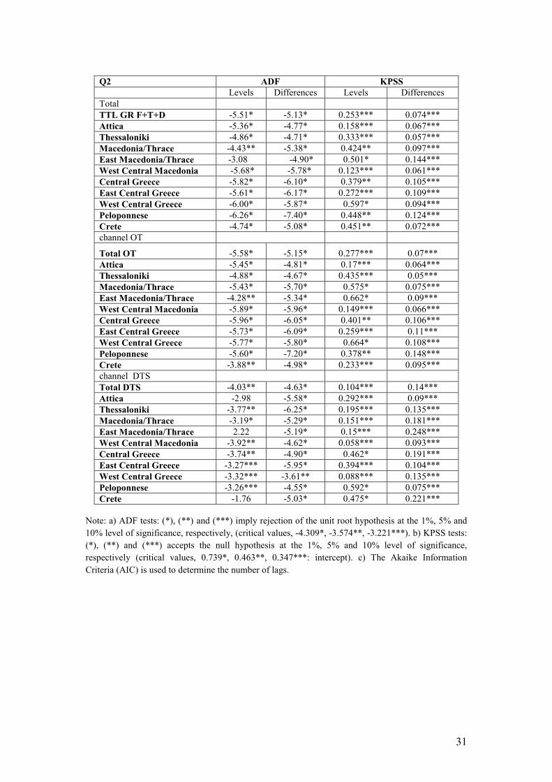
31
Q2 ADF KPSS
Levels Differences Levels Differences
Total
TTL GR F+T+D -5.51* -5.13* 0.253*** 0.074***
Attica -5.36* -4.77* 0.158*** 0.067***
Thessaloniki -4.86* -4.71* 0.333*** 0.057***
Macedonia/Thrace -4.43** -5.38* 0.424** 0.097***
East Macedonia/Thrace -3.08 -4.90* 0.501* 0.144***
West Central Macedonia -5.68* -5.78* 0.123*** 0.061***
Central Greece -5.82* -6.10* 0.379** 0.105***
East Central Greece -5.61* -6.17* 0.272*** 0.109***
West Central Greece -6.00* -5.87* 0.597* 0.094***
Peloponnese -6.26* -7.40* 0.448** 0.124***
Crete -4.74* -5.08* 0.451** 0.072***
channel ΟΤ
Total OT -5.58* -5.15* 0.277*** 0.07***
Attica -5.45* -4.81* 0.17*** 0.064***
Thessaloniki -4.88* -4.67* 0.435*** 0.05***
Macedonia/Thrace -5.43* -5.70* 0.575* 0.075***
East Macedonia/Thrace -4.28** -5.34* 0.662* 0.09***
West Central Macedonia -5.89* -5.96* 0.149*** 0.066***
Central Greece -5.96* -6.05* 0.401** 0.106***
East Central Greece -5.73* -6.09* 0.259*** 0.11***
West Central Greece -5.77* -5.80* 0.664* 0.108***
Peloponnese -5.60* -7.20* 0.378** 0.148***
Crete -3.88** -4.98* 0.233*** 0.095***
channel DTS
Total DTS -4.03** -4.63* 0.104*** 0.14***
Attica -2.98 -5.58* 0.292*** 0.09***
Thessaloniki -3.77** -6.25* 0.195*** 0.135***
Macedonia/Thrace -3.19* -5.29* 0.151*** 0.181***
East Macedonia/Thrace 2.22 -5.19* 0.15*** 0.248***
West Central Macedonia -3.92** -4.62* 0.058*** 0.093***
Central Greece -3.74** -4.90* 0.462* 0.191***
East Central Greece -3.27*** -5.95* 0.394*** 0.104***
West Central Greece -3.32*** -3.61** 0.088*** 0.135***
Peloponnese -3.26*** -4.55* 0.592* 0.075***
Crete -1.76 -5.03* 0.475* 0.221***
Note: a) ADF tests: (*), (**) and (***) imply rejection of the unit root hypothesis at the 1%, 5% and
10% level of significance, respectively, (critical values, -4.309*, -3.574**, -3.221***). b) KPSS tests:
(*), (**) and (***) accepts the null hypothesis at the 1%, 5% and 10% level of significance,
respectively (critical values, 0.739*, 0.463**, 0.347***: intercept). c) The Akaike Information
Criteria (AIC) is used to determine the number of lags.
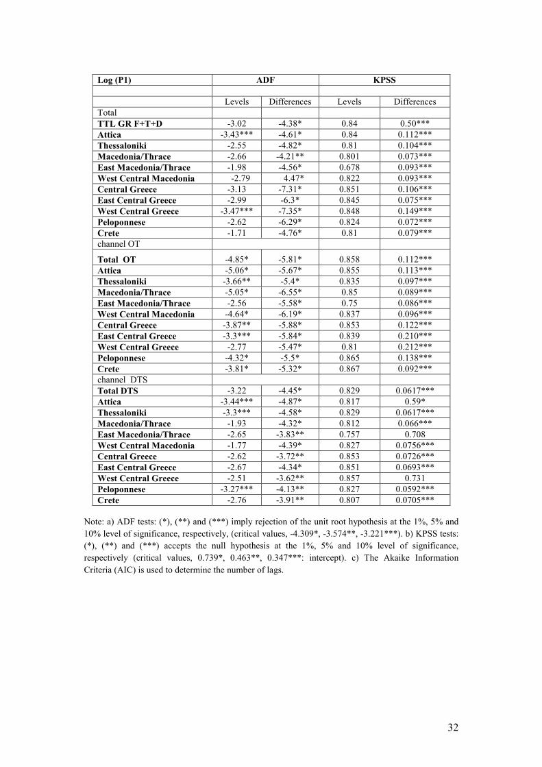
32
Log (P1) ADF KPSS
Levels Differences Levels Differences
Total
TTL GR F+T+D -3.02 -4.38* 0.84 0.50***
Attica -3.43*** -4.61* 0.84 0.112***
Thessaloniki -2.55 -4.82* 0.81 0.104***
Macedonia/Thrace -2.66 -4.21** 0.801 0.073***
East Macedonia/Thrace -1.98 -4.56* 0.678 0.093***
West Central Macedonia -2.79 4.47* 0.822 0.093***
Central Greece -3.13 -7.31* 0.851 0.106***
East Central Greece -2.99 -6.3* 0.845 0.075***
West Central Greece -3.47*** -7.35* 0.848 0.149***
Peloponnese -2.62 -6.29* 0.824 0.072***
Crete -1.71 -4.76* 0.81 0.079***
channel ΟΤ
Total OT -4.85* -5.81* 0.858 0.112***
Attica -5.06* -5.67* 0.855 0.113***
Thessaloniki -3.66** -5.4* 0.835 0.097***
Macedonia/Thrace -5.05* -6.55* 0.85 0.089***
East Macedonia/Thrace -2.56 -5.58* 0.75 0.086***
West Central Macedonia -4.64* -6.19* 0.837 0.096***
Central Greece -3.87** -5.88* 0.853 0.122***
East Central Greece -3.3*** -5.84* 0.839 0.210***
West Central Greece -2.77 -5.47* 0.81 0.212***
Peloponnese -4.32* -5.5* 0.865 0.138***
Crete -3.81* -5.32* 0.867 0.092***
channel DTS
Total DTS -3.22 -4.45* 0.829 0.0617***
Attica -3.44*** -4.87* 0.817 0.59*
Thessaloniki -3.3*** -4.58* 0.829 0.0617***
Macedonia/Thrace -1.93 -4.32* 0.812 0.066***
East Macedonia/Thrace -2.65 -3.83** 0.757 0.708
West Central Macedonia -1.77 -4.39* 0.827 0.0756***
Central Greece -2.62 -3.72** 0.853 0.0726***
East Central Greece -2.67 -4.34* 0.851 0.0693***
West Central Greece -2.51 -3.62** 0.857 0.731
Peloponnese -3.27*** -4.13** 0.827 0.0592***
Crete -2.76 -3.91** 0.807 0.0705***
Note: a) ADF tests: (*), (**) and (***) imply rejection of the unit root hypothesis at the 1%, 5% and
10% level of significance, respectively, (critical values, -4.309*, -3.574**, -3.221***). b) KPSS tests:
(*), (**) and (***) accepts the null hypothesis at the 1%, 5% and 10% level of significance,
respectively (critical values, 0.739*, 0.463**, 0.347***: intercept). c) The Akaike Information
Criteria (AIC) is used to determine the number of lags.
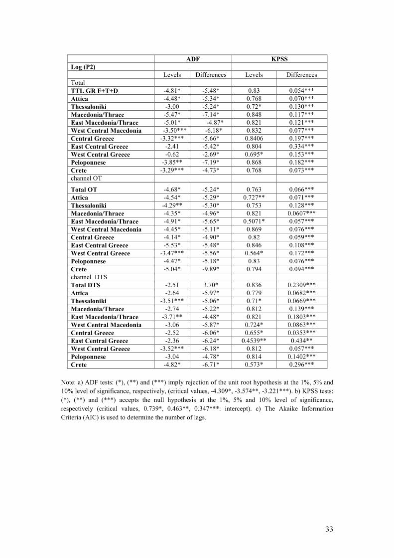
33
Note: a) ADF tests: (*), (**) and (***) imply rejection of the unit root hypothesis at the 1%, 5% and
10% level of significance, respectively, (critical values, -4.309*, -3.574**, -3.221***). b) KPSS tests:
(*), (**) and (***) accepts the null hypothesis at the 1%, 5% and 10% level of significance,
respectively (critical values, 0.739*, 0.463**, 0.347***: intercept). c) The Akaike Information
Criteria (AIC) is used to determine the number of lags.
ADF KPSS
Log (P2)
Levels Differences Levels Differences
Total
TTL GR F+T+D -4.81* -5.48* 0.83 0.054***
Attica -4.48* -5.34* 0.768 0.070***
Thessaloniki -3.00 -5.24* 0.72* 0.130***
Macedonia/Thrace -5.47* -7.14* 0.848 0.117***
East Macedonia/Thrace -5.01* -4.87* 0.821 0.121***
West Central Macedonia -3.50*** -6.18* 0.832 0.077***
Central Greece -3.32*** -5.66* 0.8406 0.197***
East Central Greece -2.41 -5.42* 0.804 0.334***
West Central Greece -0.62 -2.69* 0.695* 0.153***
Peloponnese -3.85** -7.19* 0.868 0.182***
Crete -3.29*** -4.73* 0.768 0.073***
channel ΟΤ
Total OT -4.68* -5.24* 0.763 0.066***
Attica -4.54* -5.29* 0.727** 0.071***
Thessaloniki -4.29** -5.30* 0.753 0.128***
Macedonia/Thrace -4.35* -4.96* 0.821 0.0607***
East Macedonia/Thrace -4.91* -5.65* 0.5071* 0.057***
West Central Macedonia -4.45* -5.11* 0.869 0.076***
Central Greece -4.14* -4.90* 0.82 0.059***
East Central Greece -5.53* -5.48* 0.846 0.108***
West Central Greece -3.47*** -5.56* 0.564* 0.172***
Peloponnese -4.47* -5.18* 0.83 0.076***
Crete -5.04* -9.89* 0.794 0.094***
channel DTS
Total DTS -2.51 3.70* 0.836 0.2309***
Attica -2.64 -5.97* 0.779 0.0682***
Thessaloniki -3.51*** -5.06* 0.71* 0.0669***
Macedonia/Thrace -2.74 -5.22* 0.812 0.139***
East Macedonia/Thrace -3.71** -4.48* 0.821 0.1803***
West Central Macedonia -3.06 -5.87* 0.724* 0.0863***
Central Greece -2.52 -6.06* 0.655* 0.0353***
East Central Greece -2.36 -6.24* 0.4539** 0.434**
West Central Greece -3.52*** -6.18* 0.812 0.057***
Peloponnese -3.04 -4.78* 0.814 0.1402***
Crete -4.82* -6.71* 0.573* 0.296***
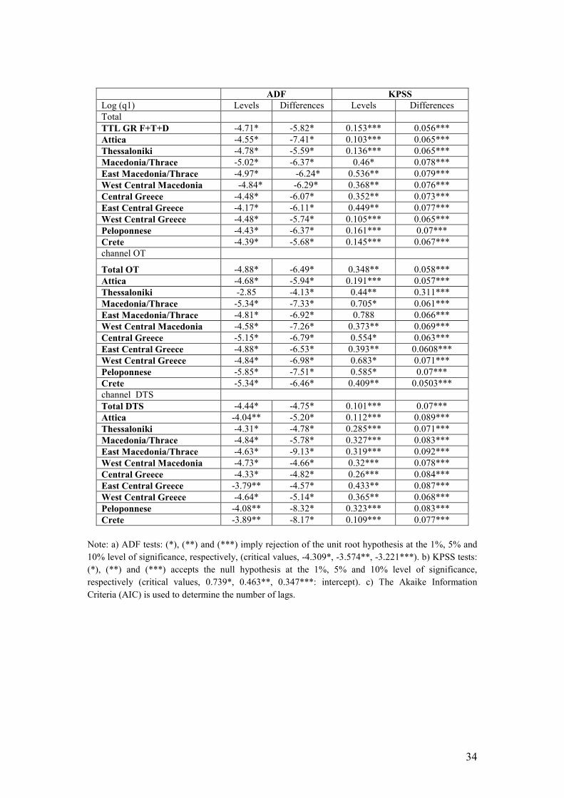
34
ADF KPSS
Log (q1) Levels Differences Levels Differences
Total
TTL GR F+T+D -4.71* -5.82* 0.153*** 0.056***
Attica -4.55* -7.41* 0.103*** 0.065***
Thessaloniki -4.78* -5.59* 0.136*** 0.065***
Macedonia/Thrace -5.02* -6.37* 0.46* 0.078***
East Macedonia/Thrace -4.97* -6.24* 0.536** 0.079***
West Central Macedonia -4.84* -6.29* 0.368** 0.076***
Central Greece -4.48* -6.07* 0.352** 0.073***
East Central Greece -4.17* -6.11* 0.449** 0.077***
West Central Greece -4.48* -5.74* 0.105*** 0.065***
Peloponnese -4.43* -6.37* 0.161*** 0.07***
Crete -4.39* -5.68* 0.145*** 0.067***
channel ΟΤ
Total OT -4.88* -6.49* 0.348** 0.058***
Attica -4.68* -5.94* 0.191*** 0.057***
Thessaloniki -2.85 -4.13* 0.44** 0.311***
Macedonia/Thrace -5.34* -7.33* 0.705* 0.061***
East Macedonia/Thrace -4.81* -6.92* 0.788 0.066***
West Central Macedonia -4.58* -7.26* 0.373** 0.069***
Central Greece -5.15* -6.79* 0.554* 0.063***
East Central Greece -4.88* -6.53* 0.393** 0.0608***
West Central Greece -4.84* -6.98* 0.683* 0.071***
Peloponnese -5.85* -7.51* 0.585* 0.07***
Crete -5.34* -6.46* 0.409** 0.0503***
channel DTS
Total DTS -4.44* -4.75* 0.101*** 0.07***
Attica -4.04** -5.20* 0.112*** 0.089***
Thessaloniki -4.31* -4.78* 0.285*** 0.071***
Macedonia/Thrace -4.84* -5.78* 0.327*** 0.083***
East Macedonia/Thrace -4.63* -9.13* 0.319*** 0.092***
West Central Macedonia -4.73* -4.66* 0.32*** 0.078***
Central Greece -4.33* -4.82* 0.26*** 0.084***
East Central Greece -3.79** -4.57* 0.433** 0.087***
West Central Greece -4.64* -5.14* 0.365** 0.068***
Peloponnese -4.08** -8.32* 0.323*** 0.083***
Crete -3.89** -8.17* 0.109*** 0.077***
Note: a) ADF tests: (*), (**) and (***) imply rejection of the unit root hypothesis at the 1%, 5% and
10% level of significance, respectively, (critical values, -4.309*, -3.574**, -3.221***). b) KPSS tests:
(*), (**) and (***) accepts the null hypothesis at the 1%, 5% and 10% level of significance,
respectively (critical values, 0.739*, 0.463**, 0.347***: intercept). c) The Akaike Information
Criteria (AIC) is used to determine the number of lags.
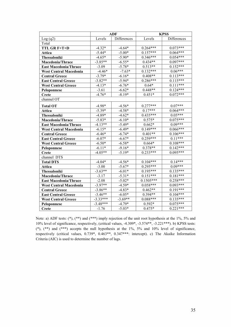
35
ADF KPSS
Log (q2) Levels Differences Levels Differences
Total
TTL GR F+T+D -4.32* -4.64* 0.264*** 0.073***
Attica -5.44* -5.00* 0.157*** 0.064***
Thessaloniki -4.65* -5.90* 0.346*** 0.054***
Macedonia/Thrace -3.85** -6.55* 0.434** 0.097***
East Macedonia/Thrace -3.09 -5.78* 0.513** 0.152***
West Central Macedonia -4.46* -7.63* 0.132*** 0.06***
Central Greece -3.79* -6.16* 0.408** 0.113***
East Central Greece -3.82** -5.94* 0.286*** 0.115***
West Central Greece -4.13* -6.76* 0.64* 0.111***
Peloponnese -3.61 -6.62* 0.448** 0.124***
Crete -4.76* -8.19* 0.451* 0.072***
channel ΟΤ
Total OT -4.98* -4.56* 0.277*** 0.07***
Attica -5.39* -4.58* 0.17*** 0.064***
Thessaloniki -4.89* -4.62* 0.435*** 0.05***
Macedonia/Thrace -5.83* -6.10* 0.575* 0.075***
East Macedonia/Thrace -4.13** -5.49* 0.662* 0.09***
West Central Macedonia -6.15* -6.49* 0.149*** 0.066***
Central Greece -6.46* -6.74* 0.401** 0.106***
East Central Greece -6.07* -6.67* 0.259*** 0.11***
West Central Greece -6.50* -6.58* 0.664* 0.108***
Peloponnese -6.11* -9.16* 0.378** 0.142***
Crete -4.05** -5.19* 0.233*** 0.095***
channel DTS
Total DTS -4.04* -4.56* 0.104*** 0.14***
Attica -3.00 -5.67* 0.295*** 0.09***
Thessaloniki -3.63** -6.01* 0.195*** 0.135***
Macedonia/Thrace -3.17 -5.31* 0.151*** 0.181***
East Macedonia/Thrace -2.08 -5.02* 0.1505*** 0.258***
West Central Macedonia -3.97** -4.59* 0.058*** 0.093***
Central Greece -3.86** -4.83* 0.462** 0.191***
East Central Greece -3.46** -6.05* 0.394** 0.104***
West Central Greece -3.33*** -3.69** 0.088*** 0.135***
Peloponnese -3.48*** -4.79* 0.592* 0.075***
Crete -1.76 -5.03* 0.475* 0.221***
Note: a) ADF tests: (*), (**) and (***) imply rejection of the unit root hypothesis at the 1%, 5% and
10% level of significance, respectively, (critical values, -4.309*, -3.574**, -3.221***). b) KPSS tests:
(*), (**) and (***) accepts the null hypothesis at the 1%, 5% and 10% level of significance,
respectively (critical values, 0.739*, 0.463**, 0.347***: intercept). c) The Akaike Information
Criteria (AIC) is used to determine the number of lags.

36
Table Β2: DF-GLS Unit Root Test
DF-GLS Unit Root Test
Levels First Differences
P1
Without
Trend With Trend
Without
Trend With Trend
Total
TTL GR F+T+D -0.140 -2.474 -4.435* -4.615*
Attica -0.720 -3.617** -4.744* -4.744*
Thessaloniki -0.829 -2.746 -3.620** -3.765**
Macedonia/Thrace -0.79 -2.784 -3.667** -3.848*
East Macedonia/Thrace -0.895 -2.053 -2.949*** -3.205**
West Central Macedonia -0.706 -2.962 -4.074* -4.208*
Central Greece 0.147 -3.030*** -5.622* -6.744*
East Central Greece -0.37 -2.719 -2.365 -4.325*
West Central Greece 0.269 -2.342 -4.027* -4.182*
Peloponnese 0.004 -2.317 -3.534** -3.896*
Crete 0.371 -1.805 -4.620* -4.839*
Channel OT
Total OT -0.344 -4.780* -5.987* -5.977*
Attica -0.436 -4.961* -5.831* -5.86*
Thessaloniki -0.494 -3.651** -5.602* -5.618*
Macedonia/Thrace -0.506 -4.703* -6.631* -6.702*
East Macedonia/Thrace -0.877 -2.803 -5.675* -5.768*
West Central Macedonia -0.609 -4.426* -6.371* -6.241*
Central Greece -0.307 -3.931* -5.941* -6.125*
East Central Greece -0.578 -3.327** -5.313* -6.034*
West Central Greece -0.0192 -2.387 -5.385* -5.520*
Peloponnese -0.224 -4.335* -5.408* -5.427*
Crete -0.08 -3.967* -5.16* -4.991*
channel DTS
Total DTS -0.511 -3.347** -4.59* -4.583*
Attica -0.703 -3.581** -5.004* -4.999*
Thessaloniki -0.594 -3.428** -4.751* -4.736*
Macedonia/Thrace -0.724 -3.262** -4.437* -4.454*
East Macedonia/Thrace -0.719 -2.756 -3.930* -3.942*
West Central Macedonia -0.675 -3.242** -4.489* -4.551*
Central Greece -0.094 -2.716 -3.697* -3.818*
East Central Greece -0.174 -2.792 -4.094* -4.375*
West Central Greece -0.003 -2.560 -3.743* -3.762*
Peloponnese -0.473 -3.39** -4.172* -4.231*
Crete -0.388 -2.895 -3.870* -3.939*
Note: a) DF-GLS tests: (*), (**) and (***) signify rejection of the unit root hypothesis at the 1%, 5%
and 10% levels, respectively. b) The asymptotical critical values for with trend (without trend) -3.77, -
3.19 and -2.89 (-2.64, -1.95 and -1.61) at the 1%, 5% and 10% levels, respectively.
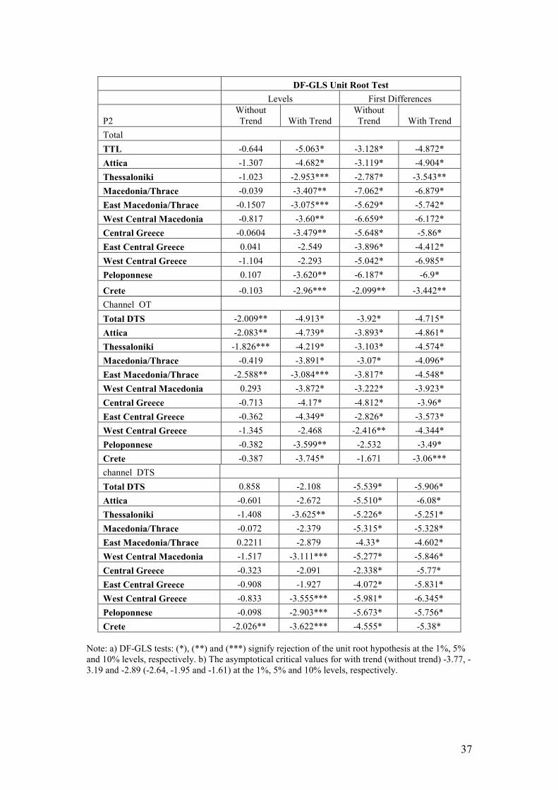
37
DF-GLS Unit Root Test
Levels First Differences
P2
Without
Trend With Trend
Without
Trend With Trend
Total
TTL -0.644 -5.063* -3.128* -4.872*
Attica -1.307 -4.682* -3.119* -4.904*
Thessaloniki -1.023 -2.953*** -2.787* -3.543**
Macedonia/Thrace -0.039 -3.407** -7.062* -6.879*
East Macedonia/Thrace -0.1507 -3.075*** -5.629* -5.742*
West Central Macedonia -0.817 -3.60** -6.659* -6.172*
Central Greece -0.0604 -3.479** -5.648* -5.86*
East Central Greece 0.041 -2.549 -3.896* -4.412*
West Central Greece -1.104 -2.293 -5.042* -6.985*
Peloponnese 0.107 -3.620** -6.187* -6.9*
Crete -0.103 -2.96*** -2.099** -3.442**
Channel OT
Total DTS -2.009** -4.913* -3.92* -4.715*
Attica -2.083** -4.739* -3.893* -4.861*
Thessaloniki -1.826*** -4.219* -3.103* -4.574*
Macedonia/Thrace -0.419 -3.891* -3.07* -4.096*
East Macedonia/Thrace -2.588** -3.084*** -3.817* -4.548*
West Central Macedonia 0.293 -3.872* -3.222* -3.923*
Central Greece -0.713 -4.17* -4.812* -3.96*
East Central Greece -0.362 -4.349* -2.826* -3.573*
West Central Greece -1.345 -2.468 -2.416** -4.344*
Peloponnese -0.382 -3.599** -2.532 -3.49*
Crete -0.387 -3.745* -1.671 -3.06***
channel DTS
Total DTS 0.858 -2.108 -5.539* -5.906*
Attica -0.601 -2.672 -5.510* -6.08*
Thessaloniki -1.408 -3.625** -5.226* -5.251*
Macedonia/Thrace -0.072 -2.379 -5.315* -5.328*
East Macedonia/Thrace 0.2211 -2.879 -4.33* -4.602*
West Central Macedonia -1.517 -3.111*** -5.277* -5.846*
Central Greece -0.323 -2.091 -2.338* -5.77*
East Central Greece -0.908 -1.927 -4.072* -5.831*
West Central Greece -0.833 -3.555*** -5.981* -6.345*
Peloponnese -0.098 -2.903*** -5.673* -5.756*
Crete -2.026** -3.622*** -4.555* -5.38*
Note: a) DF-GLS tests: (*), (**) and (***) signify rejection of the unit root hypothesis at the 1%, 5%
and 10% levels, respectively. b) The asymptotical critical values for with trend (without trend) -3.77, -
3.19 and -2.89 (-2.64, -1.95 and -1.61) at the 1%, 5% and 10% levels, respectively.
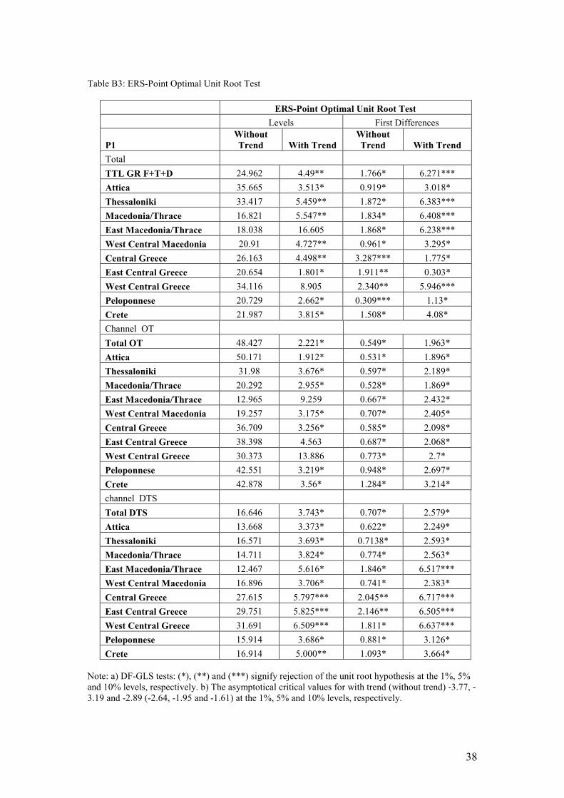
38
Table Β3: ERS-Point Optimal Unit Root Test
ERS-Point Optimal Unit Root Test
Levels First Differences
P1
Without
Trend With Trend
Without
Trend With Trend
Total
TTL GR F+T+D 24.962 4.49** 1.766* 6.271***
Attica 35.665 3.513* 0.919* 3.018*
Thessaloniki 33.417 5.459** 1.872* 6.383***
Macedonia/Thrace 16.821 5.547** 1.834* 6.408***
East Macedonia/Thrace 18.038 16.605 1.868* 6.238***
West Central Macedonia 20.91 4.727** 0.961* 3.295*
Central Greece 26.163 4.498** 3.287*** 1.775*
East Central Greece 20.654 1.801* 1.911** 0.303*
West Central Greece 34.116 8.905 2.340** 5.946***
Peloponnese 20.729 2.662* 0.309*** 1.13*
Crete 21.987 3.815* 1.508* 4.08*
Channel OT
Total OT 48.427 2.221* 0.549* 1.963*
Attica 50.171 1.912* 0.531* 1.896*
Thessaloniki 31.98 3.676* 0.597* 2.189*
Macedonia/Thrace 20.292 2.955* 0.528* 1.869*
East Macedonia/Thrace 12.965 9.259 0.667* 2.432*
West Central Macedonia 19.257 3.175* 0.707* 2.405*
Central Greece 36.709 3.256* 0.585* 2.098*
East Central Greece 38.398 4.563 0.687* 2.068*
West Central Greece 30.373 13.886 0.773* 2.7*
Peloponnese 42.551 3.219* 0.948* 2.697*
Crete 42.878 3.56* 1.284* 3.214*
channel DTS
Total DTS 16.646 3.743* 0.707* 2.579*
Attica 13.668 3.373* 0.622* 2.249*
Thessaloniki 16.571 3.693* 0.7138* 2.593*
Macedonia/Thrace 14.711 3.824* 0.774* 2.563*
East Macedonia/Thrace 12.467 5.616* 1.846* 6.517***
West Central Macedonia 16.896 3.706* 0.741* 2.383*
Central Greece 27.615 5.797*** 2.045** 6.717***
East Central Greece 29.751 5.825*** 2.146** 6.505***
West Central Greece 31.691 6.509*** 1.811* 6.637***
Peloponnese 15.914 3.686* 0.881* 3.126*
Crete 16.914 5.000** 1.093* 3.664*
Note: a) DF-GLS tests: (*), (**) and (***) signify rejection of the unit root hypothesis at the 1%, 5%
and 10% levels, respectively. b) The asymptotical critical values for with trend (without trend) -3.77, -
3.19 and -2.89 (-2.64, -1.95 and -1.61) at the 1%, 5% and 10% levels, respectively.

39
ERS-Point Optimal Unit Root Test
Levels First Differences
P2 Without
Trend
With Trend Without
Trend
With Trend
Total
TTL GR F+T+D 11.374 3.585 2.944* 5.201*
Attica 7.963 3.505*** 2.971*** 4.921**
Thessaloniki 16.994 7.392 3.28*** 7.094
Macedonia/Thrace 33.445 9.065 2.381** 6.946
East
Macedonia/Thrace
26.208 11.511 1.619* 5.953***
West Central
Macedonia
14.33 6.817 3.426*** 7.292
Central Greece 12.684 9.084 0.744* 2.605*
East Central Greece 14.231 6.933 1.914** 5.919**
West Central Greece 13.496 7.973 2.215** 2.572*
Peloponnese 21.983 7.929 1.995** 6.950
Crete 14.771 7.805 9.198
Channel OT
Total OT 7.212 3.541 3.169*** 5.441**
Attica 6.707 3.424 3.060*** 4.92**
Thessaloniki 11.696 5.791 5.041 3.381*
Macedonia/Thrace 18.802 5.848 4.839 1.559*
East
Macedonia/Thrace 3.976 6.827 1.982** 6.830
West Central
Macedonia 27.648 6.061 3.262*** 3.324*
Central Greece 8.887 6.278 2.544** 7.041
East Central Greece 10.207 3.8708 2.208** 7.236
West Central Greece 6.513 8.611 3.478*** 5.196**
Peloponnese 17.423 6.084 6.914 1.748*
Crete 27.133 6.855 17.684 3.605*
channel DTS
Total DTS 58.113 17.625 2.604** 6.557**
Attica 24.167 8.476 3.115*** 6.608***
Thessaloniki 8.148 3.695 1.596* 5.898***
Macedonia/Thrace 33.582 15.22 1.866* 6.312***
East
Macedonia/Thrace 35.972 8.280 2.063* 6.105***
West Central
Macedonia 6.943 7.93 1.55* 2.878*
Central Greece 12.138 20.65 5.419 6.927
East Central Greece 9.576 23.33 3.586*** 7.039
West Central Greece 14.763 7.119 1.757* 6.331***
Peloponnese 23.785 10.158 1.676* 6.092***
Crete 19.276 16.607 2.546** 3.426*
Note: a) DF-GLS tests: (*), (**) and (***) signify rejection of the unit root hypothesis at the 1%, 5%
and 10% levels, respectively. b) The asymptotical critical values for with trend (without trend) -3.77, -
3.19 and -2.89 (-2.64, -1.95 and -1.61) at the 1%, 5% and 10% levels, respectively.
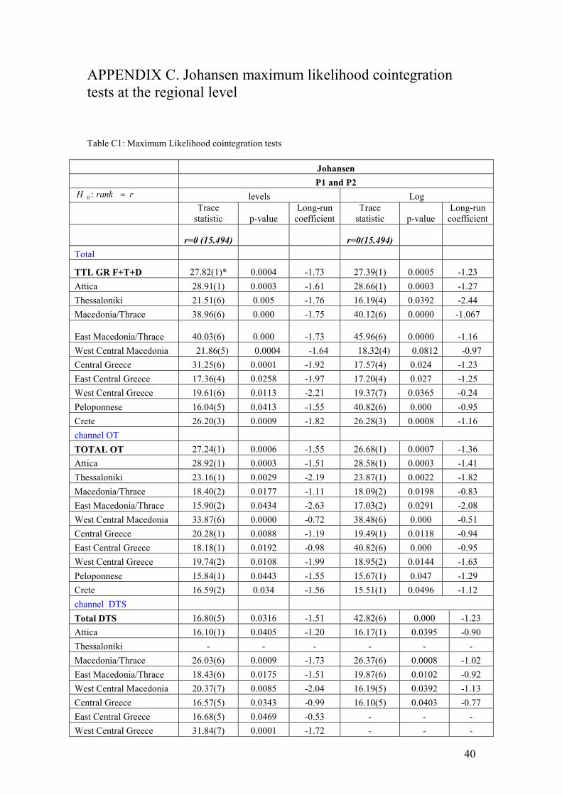
40
APPENDIX C. Johansen maximum likelihood cointegration
tests at the regional level
Table C1: Maximum Likelihood cointegration tests
Johansen
P1 and P2
rrankH =:0 levels Log
Trace
statistic p-value
Long-run
coefficient
Trace
statistic p-value
Long-run
coefficient
r=0 (15.494) r=0(15.494)
Total
TTL GR F+T+D 27.82(1)* 0.0004 -1.73 27.39(1) 0.0005 -1.23
Attica 28.91(1) 0.0003 -1.61 28.66(1) 0.0003 -1.27
Thessaloniki 21.51(6) 0.005 -1.76 16.19(4) 0.0392 -2.44
Macedonia/Thrace 38.96(6) 0.000 -1.75 40.12(6) 0.0000 -1.067
East Macedonia/Thrace 40.03(6) 0.000 -1.73 45.96(6)
0.0000 -1.16
West Central Macedonia 21.86(5) 0.0004 -1.64 18.32(4) 0.0812 -0.97
Central Greece 31.25(6) 0.0001 -1.92 17.57(4) 0.024 -1.23
East Central Greece 17.36(4) 0.0258 -1.97 17.20(4) 0.027 -1.25
West Central Greece 19.61(6) 0.0113 -2.21 19.37(7) 0.0365 -0.24
Peloponnese 16.04(5) 0.0413 -1.55 40.82(6) 0.000 -0.95
Crete 26.20(3) 0.0009 -1.82 26.28(3) 0.0008 -1.16
channel ΟΤ
TOTAL OΤ 27.24(1) 0.0006 -1.55 26.68(1) 0.0007 -1.36
Attica 28.92(1) 0.0003 -1.51 28.58(1) 0.0003 -1.41
Thessaloniki 23.16(1) 0.0029 -2.19 23.87(1) 0.0022 -1.82
Macedonia/Thrace 18.40(2) 0.0177 -1.11 18.09(2) 0.0198 -0.83
East Macedonia/Thrace 15.90(2) 0.0434 -2.63 17.03(2) 0.0291 -2.08
West Central Macedonia 33.87(6) 0.0000 -0.72 38.48(6) 0.000 -0.51
Central Greece 20.28(1) 0.0088 -1.19 19.49(1) 0.0118 -0.94
East Central Greece 18.18(1) 0.0192 -0.98 40.82(6) 0.000 -0.95
West Central Greece 19.74(2) 0.0108 -1.99 18.95(2) 0.0144 -1.63
Peloponnese 15.84(1) 0.0443 -1.55 15.67(1) 0.047 -1.29
Crete 16.59(2) 0.034 -1.56 15.51(1) 0.0496 -1.12
channel DTS
Total DTS 16.80(5) 0.0316 -1.51 42.82(6) 0.000 -1.23
Attica 16.10(1) 0.0405 -1.20 16.17(1) 0.0395 -0.90
Thessaloniki - - - - - -
Macedonia/Thrace 26.03(6) 0.0009 -1.73 26.37(6) 0.0008 -1.02
East Macedonia/Thrace 18.43(6) 0.0175 -1.51 19.87(6) 0.0102 -0.92
West Central Macedonia 20.37(7) 0.0085 -2.04 16.19(5) 0.0392 -1.13
Central Greece 16.57(5) 0.0343 -0.99 16.10(5) 0.0403 -0.77
East Central Greece 16.68(5) 0.0469 -0.53 - - -
West Central Greece 31.84(7) 0.0001 -1.72 - - -

41
Peloponnese 15.74(4) 0.0459 -1.23 30.03(5) 0.0002 -0.82
Crete - - - - - -
Note: r denotes the number of cointegrating vectors. p-values in excess of 0.01 or 0.05 imply that
cointegration is rejected. P-values less than 0.01 and close to zero imply that cointegration holds.
Numbers in parentheses denote the optimal number of lags selected by Schwarz Bayesian Information
Criterion.

42
Explanation of symbols
��: quantity of product 1
��: quantity of product 2
�� = log�(Q�)
�� = log(Q")
#�: price of product 1
#�:�price of product 2
M: income
$�% = log�(P�
M)
$�% = log�(P"
M)
m: percentage margin of a hypothetical monopolist
c: unit variable cost
p: original (pre-increase) price level of the product
τ: percentage price increase
π: reduction in output sales
(∗: critical loss in sales
ε: elasticity of demand
)∗: critical elasticity of demand

43
References
Baker, Jonathan B., and Timothy F. Bresnahan. 1988. “Estimating the residual
demand curve facing a single firm.” International Journal of Industrial
Organization 6:283-300. doi: 10.1016/S0167-7187(88)80012-2
Bishop, Simon, and Mike Walker. 2002. The economics of EC competition law,
concepts, application and measurement. London: Sweet and Maxwell.
Boshoff, Willem. 2007. “Stationarity Tests in Geographic Market Definition: An
Application to South African Milk Markets”, South African Journal of
Economics, Vol. 75, No. 1, pp. 52-65, 2007
Boshoff, Willem. 2012. “Advances in price-time-series tests for market definition.”
Stellenbosh Economic Working Papers: 01/11
Breitung, Jörg. 2000. “The local power of some unit root tests for panel data.” In:
Nonstationary panels, panel cointegration, and dynamic panels, Advances in
Econometrics 15, edited by Badi Baltagi, 161-178. Amsterdam: JAI Press.
Commission Notice on the definition of relevant market for the purposes of
Community Competition Law (97/C 372/03), 09.12.97,
http://europa.eu/legislation_summaries/competition/firms/l26073_en.htm.
Coe, Patrick, and David Krause. 2008. “An analysis of price-based tests of antitrust
market delineation.” Journal of Competition Law & Economics 4:983-1007.
Dickey, David, and Wayne Fuller. 1979. “Distribution of the estimators for
autoregressive time series with a unit root.” Journal of the American Statistical
Association 74:427-431.
Elliot, Graham, Thomas J. Rothenberg, and James H. Stock. 1996. “Efficient tests for
an autoregressive unit root.” Econometrica 64:813-836.
Engle, Robert F., and Clive W.J. Granger. 1987. “Co-integration and error
correction: representation, estimation, and testing.” Econometrica 55:251–276.
Euromonitor international database. www.euromonitor.com.
European Snack Association international database. www.esa.org.
Forni, Mario. 2004. “Using stationarity tests in antitrust market definition.”
American Law and Economics Review 6:441-464. doi:10.1093/aler/ahh007.

44
Hadri, Kaddour. 2000. “Testing for stationarity in heterogeneous panel data.”
Econometrics Journal 3:148-161. doi: 10.1111/1368-423X.00043.
Hausman, Jerry, and Gregory Leonard. 2005. “Competitive analysis using a flexible
demand specification.” Journal of Competition Law and Economics 1:279–
301. doi: 10.1093/joclec/nhi008.
Hosken, Daniel, and Christopher Taylor. 2004. Discussion of “Using stationarity
tests in antitrust market definition.” American Law and Economics Review
6:465-475. doi: 10.1093/aler/ahh008
Hosken, Daniel, Daniel O’Brien, David Scheffman and Michael Vita. 2002.
“Demand system estimation and its application to horizontal merger analysis.”
In The Use of Econometrics in Antitrust, edited by J. Harkrider, American Bar
Association Section on Antitrust.
Im, Kyung So, Hashem M. Pesaran, and Yongcheol Shin. 2003. “Testing for unit
roots in heterogeneous panels.” Journal of Econometrics 115:53-74.
Johansen, Soren. 1991. “Estimation and hypothesis testing of cointegration vectors in
Gaussian vector autoregressive models.” Econometrica 59:1551–1580.
Johansen, Soren. 1995. Likelihood-based inference in cointegrated vector
autoregressive models. Oxford: Oxford University Press.
doi:10.1093/0198774508.001.0001.
Kamerschen, David R., and Johannes Kohler. 1993. “Residual demand analysis of
the ready-to-eat breakfast cereal market.” The Antitrust Bulletin 38: 903-42.
Kantar World Panel. 2009. Research: Core salty & nuts Interaction.
Kendall, Maurice, and Alan Stuart. 1977. The advanced theory of statistics. Vol. 1.
Fourth edition. London: Griffin.
Kwiatkowski, Denis, Peter C.B. Phillips, Peter Schmidt, and Yongcheol Shin. 1992.
“Testing the null hypothesis of stationarity against the alternative of a unit root:
How sure are we that economic time series have a unit root?” Journal of
Econometrics 54:159-178.
Levin, Andrew, Chien-Fu Lin, and Chia-Shang James Chu. 2002. “Unit root tests in
panel data: asymptotic and finite sample properties.” Journal of Econometrics
108:1-24.

45
MacKinnon, James. 1996. “Numerical distribution functions for unit root and
cointegration tests.” Journal of Applied Econometrics 11:601-618. doi:
10.1002/(SICI)1099-1255(199611)11:6<601::AID-JAE417>3.0.CO;2-T
Maddala, G.S., and Shaowen Wu. 1999. “A comparative study of unit root tests with
panel data and a new simple test.” Oxford Bulletin of Economics and Statistics
61:631-652. doi: 10.1111/1468-0084.0610s1631.
Motta, Massimo. 2004. Competition policy. Theory and practice. Cambridge:
Cambridge University Press.
Muris, Timothy, David Scheffman, and Pablo Spiller. 1993. Strategy, structure, and
antitrust in the carbonated soft-drink industry. Westport CT: Quorum Books.
Newey, Whitney, and Kenneth West. 1994. “Automatic lag selection in covariance
matrix estimation.” Review of Economic Studies 61:631–653.
O’Donoghue, Robert, and Jorge Padilla. 2007. The law and economics of Article 82
EC. Oxford: Hart Publishing.
Office of Fair Trading Report. 2001. “The Role of Market Definition in monopoly
and dominance inquiries”, Economic Discussion Paper 2 prepared for the
Office of Fair Trading by National Economic Research Associates.
Pedroni, Peter. 1999. “Critical Values for Cointegration Tests in Heterogeneous
Panels with Multiple Regressors”, Oxford Bulletin of Economics and Statistics
61 (4), 653-670
Pedroni, Peter. 2000. “Fully modified OLS for heterogeneous cointegrated panels.”
In Nonstationary panels, panel cointegration and dynamic panels. Advances in
Econometrics. Vol. 15, edited by Badi H. Baltagi, T.B. Fomby and R.C. Hill,
93-130. Amsterdam: Elsevier Science. doi: 10.1016/S0731-9053(00)15004-2.
Phillips, Peter C.B., and Bruce E. Hansen. 1990. “Statistical inference in
instrumental variable regression with I(1) processes.” Review of Economic
Studies 57: 99-125.
Pedroni, Peter. 2001. “Purchasing power parity tests in cointegrated panels.” Review
of Economics and Statistics 83:727-731.
Pesaran Hashem M. and Yongcheol Shin. 1999. “An autoregressive distributed lag
modelling approach to cointegration analysis.” In Econometrics and Economic
Theory in the 20th
Century: The Ragnar Frisch Centennial Symposium, edited
by Steinar Strøm, 371-413. Cambridge: Cambridge University Press.

46
Pesaran, Hashem M. Yongcheol Shin, and Richard Smith. 2001. “Bounds testing
approaches to the analysis of level relationships.” Journal of Applied
Econometrics 16:289-326. doi: 10.1002/jae.616.
Phillips, Peter C.B. 1998. “New tools for understanding spurious regressions.”
Econometrica 66:1299-1326.
Phillips, Peter C.B., and Pierre Perron. 1988. “Testing for a unit root in a time series
regression.” Biometrika 75:335-346. doi: 10.1093/biomet/75.2.335.
Salvetti & Llombart research (December 2004) on the delineation of the Savory
Snacks market, Greece.
Sims, Christopher A. 1980. “Macroeconomics and reality.” Econometrica 48:1-48.
Stigler, George J., and Robert A. Sherwin. 1985. “The extent of the market.” The
Journal of Law and Economics 28:555-585.
Stock, James H., and Mark W. Watson. 1993. “A simple estimator of cointegrating
vectors in higher order integrated systems.” Econometrica 61:783-820.
Toda, Hiro Y., and Peter C.B. Phillips. 1993. “Vector autoregressions and causality.”
Econometrica 61:1367-1393.
Toda, Hiro Y., and Taku Yamamoto. 1995. “Statistical inference in vector
autoregressions with possibly integrated processes.” Journal of Econometrics
66:225-250.
Werden, Gregory J., and Luke M. Froeb. 1993. “Correlation, causality and All that
jazz: The inherent shortcomings of price tests for antitrust market delineation.”
Review of Industrial Organization 8:329-353.