Embed Size (px)
Citation preview
GOLDSMITHS/QUEEN MARY
UNIVERSITY OF LONDON
ESRC Doctoral Training Centre
Basic Quantitative Methods
Computer Exercises and
Reference Information
2011-12
Mike Griffiths

Quantitative Methods 2011-12 Mike Griffiths Page 1
QUANTITATIVE METHODS, 2011-12 COMPUTER EXERCISES
AND REFERENCE INFORMATION
Contents 1 Foreword ...................................................................................................... 4
1.1 How to use this booklet ........................................................................... 4
1.2 SPSS, PASW Statistics and older versions ............................................ 4
1.3 Charts and graphs; Chart Builder ........................................................... 4
1.4 Overview of inferential tests .................................................................... 5 2 Introduction to SPSS ................................................................................... 6
2.1 Data entry – numerical variables ............................................................ 6
2.2 Descriptive statistics – numerical variables ............................................ 8
2.3 Data entry – categorical variables......................................................... 10
2.4 Descriptive statistics – categorical variables ......................................... 11
3 Introduction to Excel (up to version 2002) .............................................. 12
3.1 Simple statistics in Excel ...................................................................... 13
3.2 Graphs in Excel .................................................................................... 14
3.2.1 Creating graphs ............................................................................. 14
3.2.2 Editing and changing graphs ......................................................... 15
3.2.3 Bar charts with two independent variables .................................... 16
3.2.4 Further reading .............................................................................. 16 4 Introduction to Excel (version 2007) ........................................................ 17
4.1 Simple statistics in Excel ...................................................................... 17
4.2 Graphs in Excel .................................................................................... 19
4.2.1 Creating graphs ............................................................................. 19
4.2.2 Editing and changing graphs ......................................................... 19
4.2.3 Bar charts with two independent variables .................................... 20 5 Histograms; Chart Editor .......................................................................... 21
5.1 Histograms ........................................................................................... 21
5.2 Changing the appearance of a chart using the Chart Editor ................. 22
6 t-tests, Anovas and their non-parametric equivalents ........................... 24
6.1 Introduction ........................................................................................... 24
6.2 Which test to use? ................................................................................ 24
6.3 Entering Repeated Measures data ....................................................... 25
6.4 Paired samples t-test ............................................................................ 26
6.5 Wilcoxon (Signed Ranks) test ............................................................... 29
6.6 Repeated Measures Anova .................................................................. 30
6.7 Friedman test. ....................................................................................... 36
6.8 Independent-samples data - general .................................................... 37
6.8.1 Entering independent-samples data .............................................. 37
6.8.2 Descriptive statistics and histograms ............................................. 39
Quantitative Methods 2011-12 Mike Griffiths Page 2
6.9 Independent-samples t-test .................................................................. 40
6.10 Mann-Whitney U test ............................................................................ 42
6.11 Independent-samples Anova ................................................................ 42
6.12 Kruskal-Wallis test ................................................................................ 45
7 Factorial Anovas ........................................................................................ 46
7.1 Introduction ........................................................................................... 46
7.2 Outcomes ............................................................................................. 46
7.3 If the factorial Anova shows significant effects ..................................... 47
7.4 Effect sizes ........................................................................................... 48
7.5 Two way independent-samples Anova ................................................. 48
7.6 Two way repeated measures Anova..................................................... 54
7.7 Two way mixed Anova .......................................................................... 59
7.8 Anovas with more than two factors ....................................................... 64 8 Chi-square tests of association ................................................................ 65
8.1 Introduction; when they are used .......................................................... 65
8.2 The possible outcomes of a chi-square test ......................................... 65
8.3 Example 1: entering individual cases into SPSS .................................. 65
8.4 Example 2: using the Weighted Cases procedure in SPSS .................. 69
8.5 Effect sizes ........................................................................................... 72
8.6 Showing percentages ........................................................................... 72
8.7 Constraints on chi-squared tests .......................................................... 73 9 Chi-square tests of a single categorical variable .................................... 74
9.1 When they are used .............................................................................. 74
9.2 Whether a categorical variable is evenly distributed ............................. 74
9.3 Whether a categorical variable is split in a given proportion ................. 75
9.4 Constraints ........................................................................................... 78
10 CoChran’s and McNemar’s tests .............................................................. 78
10.1 When to use Cochran‘s and McNemar‘s tests ...................................... 78
10.2 Cochran‘s Q .......................................................................................... 78
10.3 McNemar‘s test ..................................................................................... 80
11 Simple regression and correlation ........................................................... 81
11.1 Scatterplots. .......................................................................................... 81
11.2 Correlation ............................................................................................ 82
11.2.1 Parametric test of correlation (Pearson‘s r) ................................... 83
11.2.2 Non-parametric test of correlation (Spearman‘s rho) ..................... 83
11.3 Simple linear regression ....................................................................... 84
11.3.1 Carrying out a regression .............................................................. 84
11.3.2 Regression output ......................................................................... 84
11.3.3 Writing up regression ..................................................................... 86
11.3.4 What it means................................................................................ 86
12 Multiple regression and correlation ......................................................... 87
13 Introduction to statistics for questionnaires ........................................... 91
13.1 Entering the data .................................................................................. 91
13.1.1 Introduction: example data ............................................................ 91
13.1.2 Variable view ................................................................................. 92
13.1.3 Entering data ................................................................................. 93
Quantitative Methods 2011-12 Mike Griffiths Page 3
13.1.4 File control and excluding data ...................................................... 93
13.2 Checking the data file; missing data ..................................................... 94
13.2.1 Check your data entry ................................................................... 94
13.2.2 Detecting missing data .................................................................. 94
13.2.3 Dealing with missing data .............................................................. 94
13.2.4 Finding major errors in the data ..................................................... 95
13.3 Calculating overall scores on a questionnaire ...................................... 96
13.3.1 Introduction .................................................................................... 96
13.3.2 Reverse-scored questions: what they are ..................................... 96
13.3.3 Reverse-scored questions: How to deal with them ........................ 96
13.3.4 Adding up scores. .......................................................................... 98
13.3.5 Mean scores .................................................................................. 98
13.4 Your own scales: a very brief introduction ........................................... 98
13.4.1 Checking for problematic questions ............................................... 99
13.4.2 Cronbach‘s alpha: how to calculate it .......................................... 100
13.4.3 How Cronbach‘s alpha is affected by individual questions .......... 101
14 Operations on the data file...................................................................... 102
14.1 Calculating z scores ............................................................................ 102
14.2 Calculations using Compute Variable ................................................. 103
14.3 Combining variables fairly ................................................................... 104
14.4 Categorising data................................................................................ 104
14.4.1 Predefined split point(s): e.g. pass/fail ......................................... 104
14.4.2 Splitting into equal groups: e.g. median splits.............................. 105
14.5 Excluding cases from the analysis ...................................................... 105
15 Data screening and cleaning .................................................................. 107
15.1 Introduction ......................................................................................... 107
15.2 Suggested steps. ................................................................................ 107
15.2.1 Boxplots ....................................................................................... 109
15.2.2 Multivariate outliers ...................................................................... 109
15.3 Suggested actions .............................................................................. 110
Appendices...................................................................................................... 112
A Reporting results ....................................................................................... 112
(i) Statistical significance ............................................................................ 112
(ii) Reporting in APA Style ......................................................................... 112
(iii) Formatting hints in Word ...................................................................... 112
(iv) Rounding numbers............................................................................... 113
B Converting bar charts to black and white .................................................. 113
C Copying graphs and other objects into Word (or other applications)......... 114
D Help in SPSS ............................................................................................ 114
E Understanding boxplots and percentiles ................................................... 115
F Areas under the normal distribution........................................................... 117
G Overview of statistical tests ...................................................................... 119
Quantitative Methods 2011-12 Mike Griffiths Page 4
1 FOREWORD
1.1 How to use this booklet This booklet contains computer exercises for use in class and as examples of how to carry out various kinds of analysis. It should be read in conjunction with:
the lectures; please print off the PowerPoint presentations. These will be posted on grad.gold.
the Module Handbook, which gives details of recommended reading, content of classes, etc.
The order of material in this booklet has been chosen to make it read logically as a permanent reference book. For teaching reasons, the material will be covered in a different order in class. The booklet also includes a few sections which will not be covered in class at all, but which could be useful for future reference.
Information in boxes (like this) can be ignored on first reading, and may require an understanding of material which is covered later in the course. However, it may be useful when referring to the booklet later.
Unless otherwise specified, all the examples in this booklet use invented data.
1.2 SPSS, PASW Statistics and older versions For a while, SPSS was known as PASW. These names tend to be used interchangeably, or even together. We will use SPSS version 19. However, from version 15 onwards there have been very few changes relevant to this course.
1.3 Charts and graphs; Chart Builder In version 15 onwards of SPSS there is a versatile facility called Chart Builder. You may like to experiment with this. However, these versions also retain the previous methods of creating charts under Graphs – Legacy Dialogues. I will use these, for compatibility with anyone who is using an old version of SPSS (and also because I think they are easier, especially to get started with).
Quantitative Methods 2011-12 Mike Griffiths Page 5
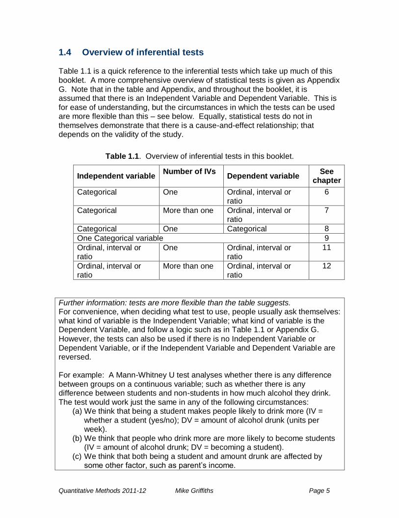
1.4 Overview of inferential tests Table 1.1 is a quick reference to the inferential tests which take up much of this booklet. A more comprehensive overview of statistical tests is given as Appendix G. Note that in the table and Appendix, and throughout the booklet, it is assumed that there is an Independent Variable and Dependent Variable. This is for ease of understanding, but the circumstances in which the tests can be used are more flexible than this – see below. Equally, statistical tests do not in themselves demonstrate that there is a cause-and-effect relationship; that depends on the validity of the study.
Table 1.1. Overview of inferential tests in this booklet.
Independent variable Number of IVs
Dependent variable See
chapter
Categorical One Ordinal, interval or ratio
6
Categorical More than one Ordinal, interval or ratio
7
Categorical One Categorical 8
One Categorical variable 9
Ordinal, interval or ratio
One Ordinal, interval or ratio
11
Ordinal, interval or ratio
More than one Ordinal, interval or ratio
12
Further information: tests are more flexible than the table suggests. For convenience, when deciding what test to use, people usually ask themselves: what kind of variable is the Independent Variable; what kind of variable is the Dependent Variable, and follow a logic such as in Table 1.1 or Appendix G.
However, the tests can also be used if there is no Independent Variable or Dependent Variable, or if the Independent Variable and Dependent Variable are reversed. For example: A Mann-Whitney U test analyses whether there is any difference between groups on a continuous variable; such as whether there is any difference between students and non-students in how much alcohol they drink. The test would work just the same in any of the following circumstances:
(a) We think that being a student makes people likely to drink more (IV = whether a student (yes/no); DV = amount of alcohol drunk (units per week).
(b) We think that people who drink more are more likely to become students (IV = amount of alcohol drunk; DV = becoming a student).
(c) We think that both being a student and amount drunk are affected by some other factor, such as parent‘s income.
Quantitative Methods 2011-12 Mike Griffiths Page 6
(d) We don‘t have any fixed ideas about how the relationship arises, we just think that students drink more.
The reverse side of this coin is that if there is a difference, we will get the same result whatever the reason is for it. If we think that being a student makes people drink more and the Mann-Whitney test is significant, that does not prove our hypothesis. It could be significant for any of the above reasons1. Whether there is a cause-and-effect relationship depends on the validity of your study.
2 INTRODUCTION TO SPSS 2.1 Data entry – numerical variables Open SPSS 19. (This may appear on the menu as SPSS and/or PASW. In the RISB, it is under Start – Goldsmiths – Departmental Software – SPSS – PASW Statistics 19). A dialogue box will appear – click on ‗Cancel‘. The Data Editor opens. This uses the file extension .sav. Notice that it has two tabs:
Data View where you enter the data.
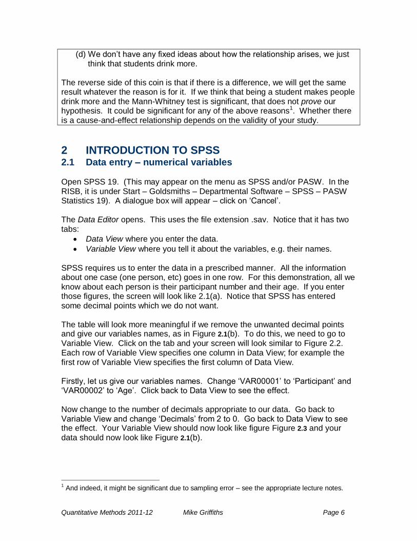
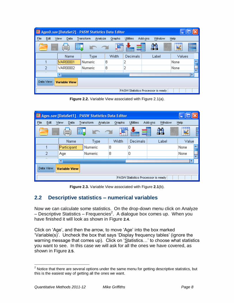
Variable View where you tell it about the variables, e.g. their names. SPSS requires us to enter the data in a prescribed manner. All the information about one case (one person, etc) goes in one row. For this demonstration, all we know about each person is their participant number and their age. If you enter those figures, the screen will look like 2.1(a). Notice that SPSS has entered some decimal points which we do not want. The table will look more meaningful if we remove the unwanted decimal points and give our variables names, as in Figure 2.1(b). To do this, we need to go to Variable View. Click on the tab and your screen will look similar to Figure 2.2. Each row of Variable View specifies one column in Data View; for example the first row of Variable View specifies the first column of Data View.
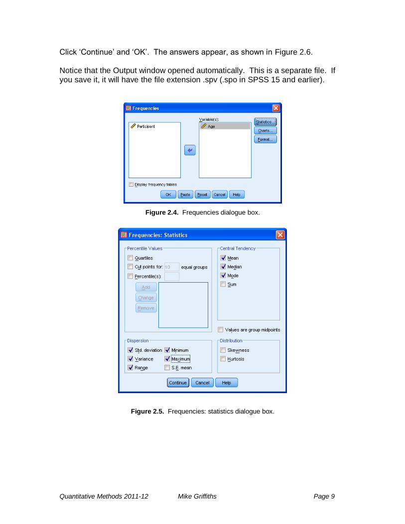
Firstly, let us give our variables names. Change ‗VAR00001‘ to ‗Participant‘ and ‗VAR00002‘ to ‗Age‘. Click back to Data View to see the effect. Now change to the number of decimals appropriate to our data. Go back to Variable View and change ‗Decimals‘ from 2 to 0. Go back to Data View to see the effect. Your Variable View should now look like figure Figure 2.3 and your data should now look like Figure 2.1(b).
1 And indeed, it might be significant due to sampling error – see the appropriate lecture notes.
Quantitative Methods 2011-12 Mike Griffiths Page 7
A few points to note if you come back to this section for future reference: 1. SPSS has some restrictions on the names you can give your variables; for
example they cannot include spaces. You can add a more meaningful name in the ‗labels‘ field (see section 6.8.1).
2. We changed the number of decimals to 0 because we were using whole numbers. If there are decimals in the data, keep the appropriate number of decimals in SPSS.
3. We entered the data first in Data View, and then set up the variables in Variable View. Once they are used to entering data, most people find it easier to set up the variables in Variable View first. You can swap between the two views as you please.
Save the file on your n: drive as Ages.sav so we can use it again next week.
(a) as first entered (b) after editing
Figure 2.1. Data for first exercise in Data View.
Quantitative Methods 2011-12 Mike Griffiths Page 8
Figure 2.2. Variable View associated with Figure 2.1(a).
Figure 2.3. Variable View associated with Figure 2.1(b).
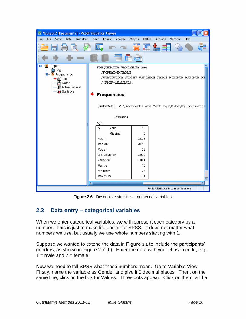
2.2 Descriptive statistics – numerical variables Now we can calculate some statistics. On the drop-down menu click on Analyze – Descriptive Statistics – Frequencies2. A dialogue box comes up. When you have finished it will look as shown in Figure 2.4.
Click on ‗Age‘, and then the arrow, to move ‗Age‘ into the box marked ‗Variable(s)‘. Uncheck the box that says ‗Display frequency tables‘ (ignore the warning message that comes up). Click on ‗Statistics…‘ to choose what statistics you want to see. In this case we will ask for all the ones we have covered, as shown in Figure 2.5.
2 Notice that there are several options under the same menu for getting descriptive statistics, but
this is the easiest way of getting all the ones we want.
Quantitative Methods 2011-12 Mike Griffiths Page 9
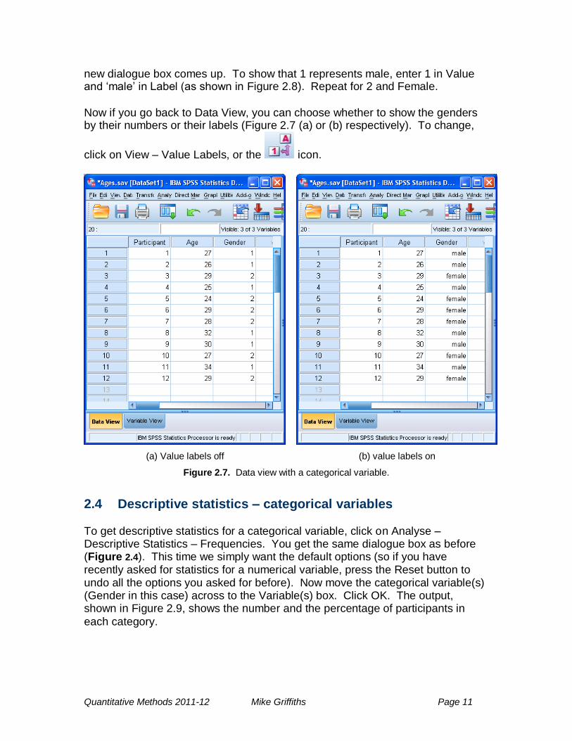
Click ‗Continue‘ and ‗OK‘. The answers appear, as shown in Figure 2.6.
Notice that the Output window opened automatically. This is a separate file. If you save it, it will have the file extension .spv (.spo in SPSS 15 and earlier).
Figure 2.4. Frequencies dialogue box.
Figure 2.5. Frequencies: statistics dialogue box.
Quantitative Methods 2011-12 Mike Griffiths Page 10
Figure 2.6. Descriptive statistics – numerical variables.
2.3 Data entry – categorical variables When we enter categorical variables, we will represent each category by a number. This is just to make life easier for SPSS. It does not matter what numbers we use, but usually we use whole numbers starting with 1. Suppose we wanted to extend the data in Figure 2.1 to include the participants‘ genders, as shown in Figure 2.7 (b). Enter the data with your chosen code, e.g.
1 = male and 2 = female. Now we need to tell SPSS what these numbers mean. Go to Variable View. Firstly, name the variable as Gender and give it 0 decimal places. Then, on the same line, click on the box for Values. Three dots appear. Click on them, and a
Quantitative Methods 2011-12 Mike Griffiths Page 11
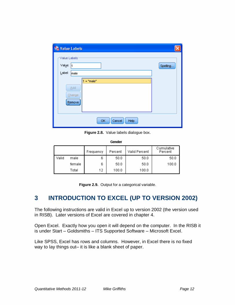
new dialogue box comes up. To show that 1 represents male, enter 1 in Value and ‗male‘ in Label (as shown in Figure 2.8). Repeat for 2 and Female.
Now if you go back to Data View, you can choose whether to show the genders by their numbers or their labels (Figure 2.7 (a) or (b) respectively). To change,
click on View – Value Labels, or the icon.
(a) Value labels off (b) value labels on
Figure 2.7. Data view with a categorical variable.
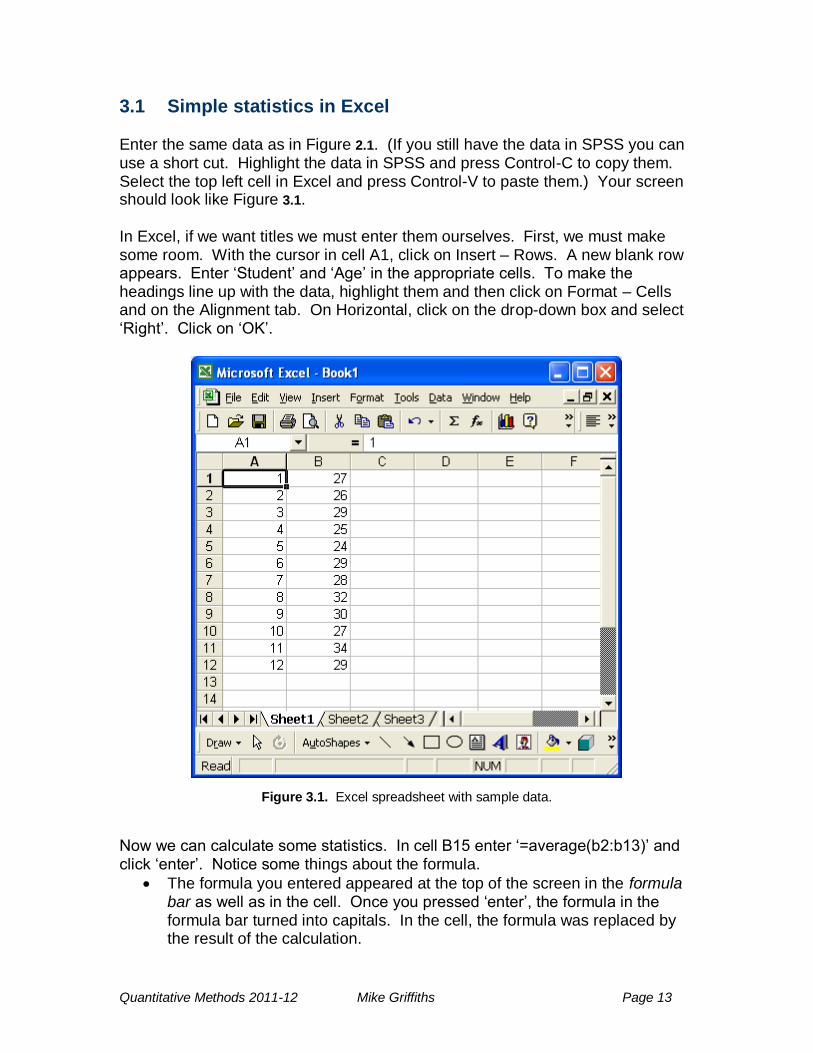
2.4 Descriptive statistics – categorical variables To get descriptive statistics for a categorical variable, click on Analyse – Descriptive Statistics – Frequencies. You get the same dialogue box as before (Figure 2.4). This time we simply want the default options (so if you have recently asked for statistics for a numerical variable, press the Reset button to undo all the options you asked for before). Now move the categorical variable(s) (Gender in this case) across to the Variable(s) box. Click OK. The output, shown in Figure 2.9, shows the number and the percentage of participants in
each category.
Quantitative Methods 2011-12 Mike Griffiths Page 12
Figure 2.8. Value labels dialogue box.
Figure 2.9. Output for a categorical variable.
3 INTRODUCTION TO EXCEL (UP TO VERSION 2002) The following instructions are valid in Excel up to version 2002 (the version used in RISB). Later versions of Excel are covered in chapter 4.
Open Excel. Exactly how you open it will depend on the computer. In the RISB it is under Start – Goldsmiths – ITS Supported Software – Microsoft Excel. Like SPSS, Excel has rows and columns. However, in Excel there is no fixed way to lay things out– it is like a blank sheet of paper.
Quantitative Methods 2011-12 Mike Griffiths Page 13
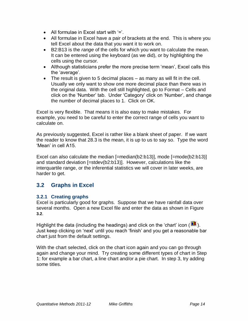
3.1 Simple statistics in Excel Enter the same data as in Figure 2.1. (If you still have the data in SPSS you can use a short cut. Highlight the data in SPSS and press Control-C to copy them. Select the top left cell in Excel and press Control-V to paste them.) Your screen should look like Figure 3.1.
In Excel, if we want titles we must enter them ourselves. First, we must make some room. With the cursor in cell A1, click on Insert – Rows. A new blank row appears. Enter ‗Student‘ and ‗Age‘ in the appropriate cells. To make the headings line up with the data, highlight them and then click on Format – Cells and on the Alignment tab. On Horizontal, click on the drop-down box and select ‗Right‘. Click on ‗OK‘.
Figure 3.1. Excel spreadsheet with sample data.
Now we can calculate some statistics. In cell B15 enter ‗=average(b2:b13)‘ and click ‗enter‘. Notice some things about the formula.
The formula you entered appeared at the top of the screen in the formula bar as well as in the cell. Once you pressed ‗enter‘, the formula in the formula bar turned into capitals. In the cell, the formula was replaced by the result of the calculation.
Quantitative Methods 2011-12 Mike Griffiths Page 14
All formulae in Excel start with ‗=‘.
All formulae in Excel have a pair of brackets at the end. This is where you tell Excel about the data that you want it to work on.
B2:B13 is the range of the cells for which you want to calculate the mean. It can be entered using the keyboard (as we did), or by highlighting the cells using the cursor.
Although statisticians prefer the more precise term ‗mean‘, Excel calls this the ‗average‘.
The result is given to 5 decimal places – as many as will fit in the cell. Usually we only want to show one more decimal place than there was in the original data. With the cell still highlighted, go to Format – Cells and click on the ‗Number‘ tab. Under ‗Category‘ click on ‗Number‘, and change the number of decimal places to 1. Click on OK.
Excel is very flexible. That means it is also easy to make mistakes. For example, you need to be careful to enter the correct range of cells you want to calculate on. As previously suggested, Excel is rather like a blank sheet of paper. If we want the reader to know that 28.3 is the mean, it is up to us to say so. Type the word ‗Mean‘ in cell A15. Excel can also calculate the median [=median(b2:b13)], mode [=mode(b2:b13)] and standard deviation [=stdev(b2:b13)]. However, calculations like the interquartile range, or the inferential statistics we will cover in later weeks, are harder to get.
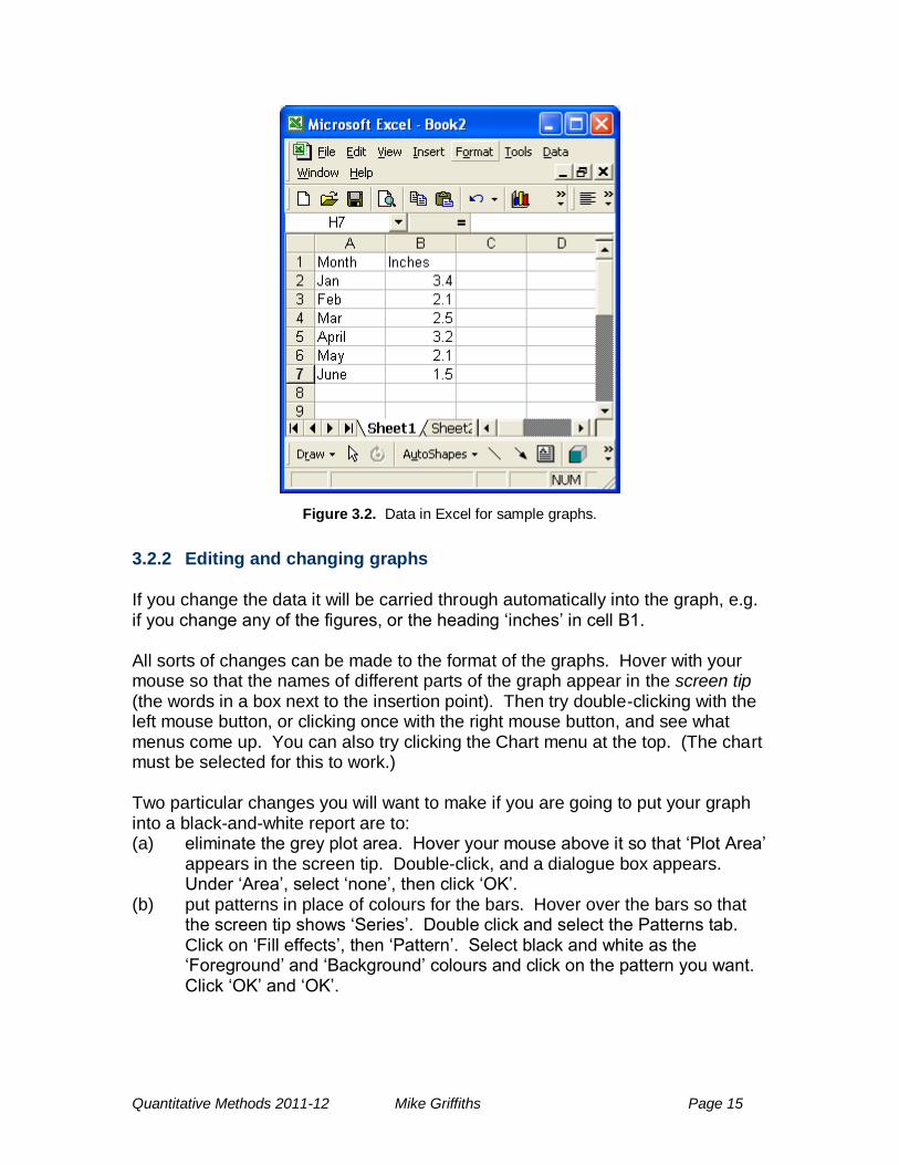
3.2 Graphs in Excel 3.2.1 Creating graphs Excel is particularly good for graphs. Suppose that we have rainfall data over several months. Open a new Excel file and enter the data as shown in Figure 3.2.
Highlight the data (including the headings) and click on the ‗chart‘ icon ( ). Just keep clicking on ‗next‘ until you reach ‗finish‘ and you get a reasonable bar chart just from the default settings. With the chart selected, click on the chart icon again and you can go through again and change your mind. Try creating some different types of chart in Step 1: for example a bar chart, a line chart and/or a pie chart. In step 3, try adding some titles.
Quantitative Methods 2011-12 Mike Griffiths Page 15
Figure 3.2. Data in Excel for sample graphs.
3.2.2 Editing and changing graphs
If you change the data it will be carried through automatically into the graph, e.g. if you change any of the figures, or the heading ‗inches‘ in cell B1. All sorts of changes can be made to the format of the graphs. Hover with your mouse so that the names of different parts of the graph appear in the screen tip (the words in a box next to the insertion point). Then try double-clicking with the left mouse button, or clicking once with the right mouse button, and see what menus come up. You can also try clicking the Chart menu at the top. (The chart must be selected for this to work.) Two particular changes you will want to make if you are going to put your graph into a black-and-white report are to: (a) eliminate the grey plot area. Hover your mouse above it so that ‗Plot Area‘
appears in the screen tip. Double-click, and a dialogue box appears. Under ‗Area‘, select ‗none‘, then click ‗OK‘.
(b) put patterns in place of colours for the bars. Hover over the bars so that the screen tip shows ‗Series‘. Double click and select the Patterns tab. Click on ‗Fill effects‘, then ‗Pattern‘. Select black and white as the ‗Foreground‘ and ‗Background‘ colours and click on the pattern you want. Click ‗OK‘ and ‗OK‘.
Quantitative Methods 2011-12 Mike Griffiths Page 16
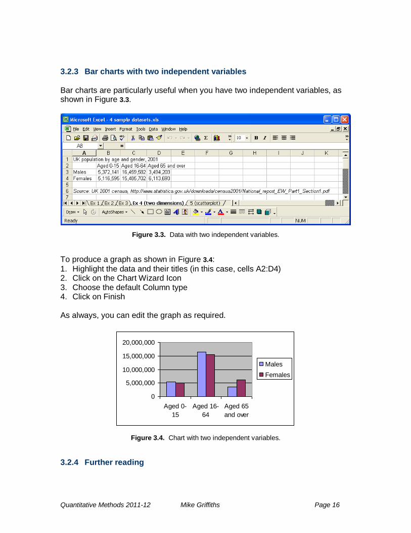
3.2.3 Bar charts with two independent variables Bar charts are particularly useful when you have two independent variables, as shown in Figure 3.3.
Figure 3.3. Data with two independent variables.
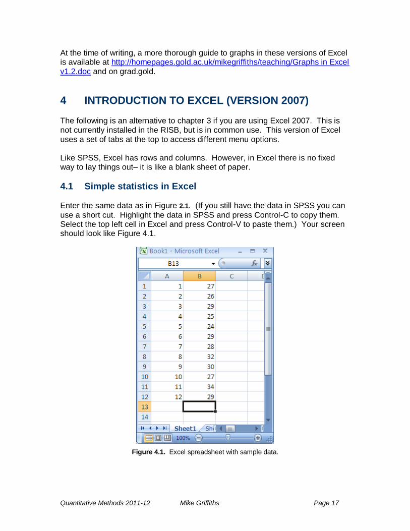
To produce a graph as shown in Figure 3.4:
1. Highlight the data and their titles (in this case, cells A2:D4) 2. Click on the Chart Wizard Icon 3. Choose the default Column type 4. Click on Finish As always, you can edit the graph as required.
0
5,000,000
10,000,000
15,000,000
20,000,000
Aged 0-
15
Aged 16-
64
Aged 65
and over
Males
Females
Figure 3.4. Chart with two independent variables.
3.2.4 Further reading
Quantitative Methods 2011-12 Mike Griffiths Page 17
At the time of writing, a more thorough guide to graphs in these versions of Excel is available at http://homepages.gold.ac.uk/mikegriffiths/teaching/Graphs in Excel v1.2.doc and on grad.gold.
4 INTRODUCTION TO EXCEL (VERSION 2007) The following is an alternative to chapter 3 if you are using Excel 2007. This is not currently installed in the RISB, but is in common use. This version of Excel uses a set of tabs at the top to access different menu options. Like SPSS, Excel has rows and columns. However, in Excel there is no fixed way to lay things out– it is like a blank sheet of paper.
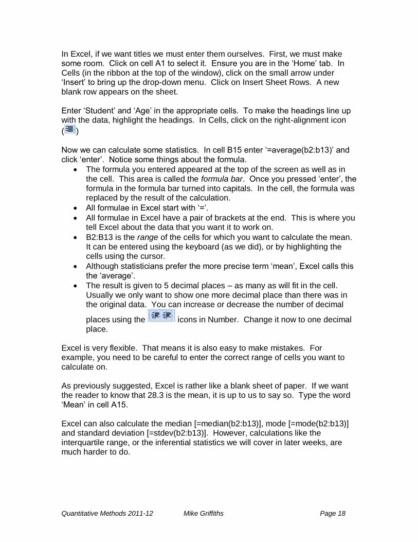
4.1 Simple statistics in Excel Enter the same data as in Figure 2.1. (If you still have the data in SPSS you can
use a short cut. Highlight the data in SPSS and press Control-C to copy them. Select the top left cell in Excel and press Control-V to paste them.) Your screen should look like Figure 4.1.
Figure 4.1. Excel spreadsheet with sample data.
Quantitative Methods 2011-12 Mike Griffiths Page 18
In Excel, if we want titles we must enter them ourselves. First, we must make some room. Click on cell A1 to select it. Ensure you are in the ‗Home‘ tab. In Cells (in the ribbon at the top of the window), click on the small arrow under ‗Insert‘ to bring up the drop-down menu. Click on Insert Sheet Rows. A new blank row appears on the sheet. Enter ‗Student‘ and ‗Age‘ in the appropriate cells. To make the headings line up with the data, highlight the headings. In Cells, click on the right-alignment icon
( ) Now we can calculate some statistics. In cell B15 enter ‗=average(b2:b13)‘ and click ‗enter‘. Notice some things about the formula.
The formula you entered appeared at the top of the screen as well as in the cell. This area is called the formula bar. Once you pressed ‗enter‘, the formula in the formula bar turned into capitals. In the cell, the formula was replaced by the result of the calculation.
All formulae in Excel start with ‗=‘.
All formulae in Excel have a pair of brackets at the end. This is where you tell Excel about the data that you want it to work on.
B2:B13 is the range of the cells for which you want to calculate the mean. It can be entered using the keyboard (as we did), or by highlighting the cells using the cursor.
Although statisticians prefer the more precise term ‗mean‘, Excel calls this the ‗average‘.
The result is given to 5 decimal places – as many as will fit in the cell. Usually we only want to show one more decimal place than there was in the original data. You can increase or decrease the number of decimal
places using the icons in Number. Change it now to one decimal place.
Excel is very flexible. That means it is also easy to make mistakes. For example, you need to be careful to enter the correct range of cells you want to calculate on. As previously suggested, Excel is rather like a blank sheet of paper. If we want the reader to know that 28.3 is the mean, it is up to us to say so. Type the word ‗Mean‘ in cell A15. Excel can also calculate the median [=median(b2:b13)], mode [=mode(b2:b13)] and standard deviation [=stdev(b2:b13)]. However, calculations like the interquartile range, or the inferential statistics we will cover in later weeks, are much harder to do.
Quantitative Methods 2011-12 Mike Griffiths Page 19
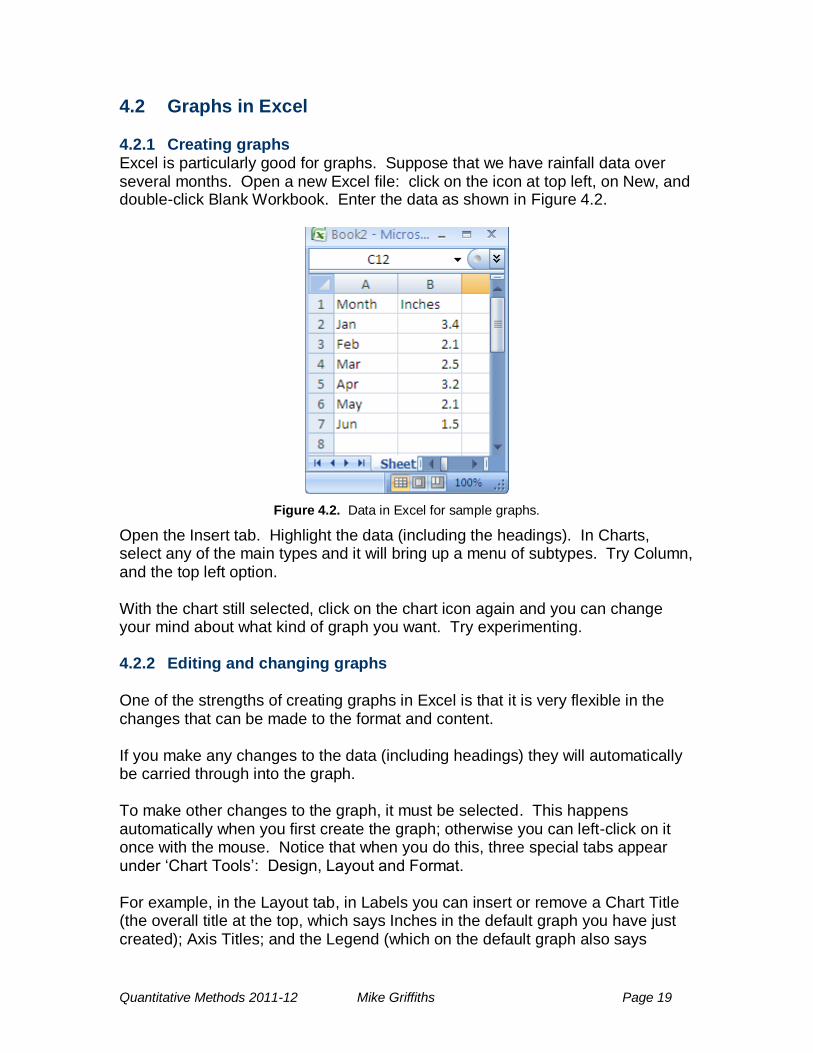
4.2 Graphs in Excel 4.2.1 Creating graphs Excel is particularly good for graphs. Suppose that we have rainfall data over several months. Open a new Excel file: click on the icon at top left, on New, and double-click Blank Workbook. Enter the data as shown in Figure 4.2.
Figure 4.2. Data in Excel for sample graphs.
Open the Insert tab. Highlight the data (including the headings). In Charts, select any of the main types and it will bring up a menu of subtypes. Try Column, and the top left option. With the chart still selected, click on the chart icon again and you can change your mind about what kind of graph you want. Try experimenting. 4.2.2 Editing and changing graphs
One of the strengths of creating graphs in Excel is that it is very flexible in the changes that can be made to the format and content. If you make any changes to the data (including headings) they will automatically be carried through into the graph. To make other changes to the graph, it must be selected. This happens automatically when you first create the graph; otherwise you can left-click on it once with the mouse. Notice that when you do this, three special tabs appear under ‗Chart Tools‘: Design, Layout and Format. For example, in the Layout tab, in Labels you can insert or remove a Chart Title (the overall title at the top, which says Inches in the default graph you have just created); Axis Titles; and the Legend (which on the default graph also says
Quantitative Methods 2011-12 Mike Griffiths Page 20
Inches, and is on the right of the graph). For some of these, the wording can be changed by clicking on them and typing your new wording in; others simply reflect the headings in the original data. Another way of making changes (with the chart selected) is to hover with your mouse so that the names of different parts of the graph appear in the screen tip (the words in a box next to the insertion point). Right-clicking with the mouse will bring up menus which allow you to make changes to the format. For example, in the chart area, in our default chart there is no fill. Suppose you wanted a red fill. Right-click on the plot area, click on Format Plot Area, and change Fill to Solid Fill. Additional buttons appear that allow you to choose a colour. Unfortunately, one specific feature that is not available in Excel 2007 (unlike earlier versions, and even SPSS) is the ability to create patterns like those in Figure 5.1 (b). There are some fixes on the Internet which claim to reinstate this
feature (e.g. http://www.dailydoseofexcel.com/archives/2007/11/17/chart-pattern-fills-in-excel-2007/) but I have not tested them. 4.2.3 Bar charts with two independent variables
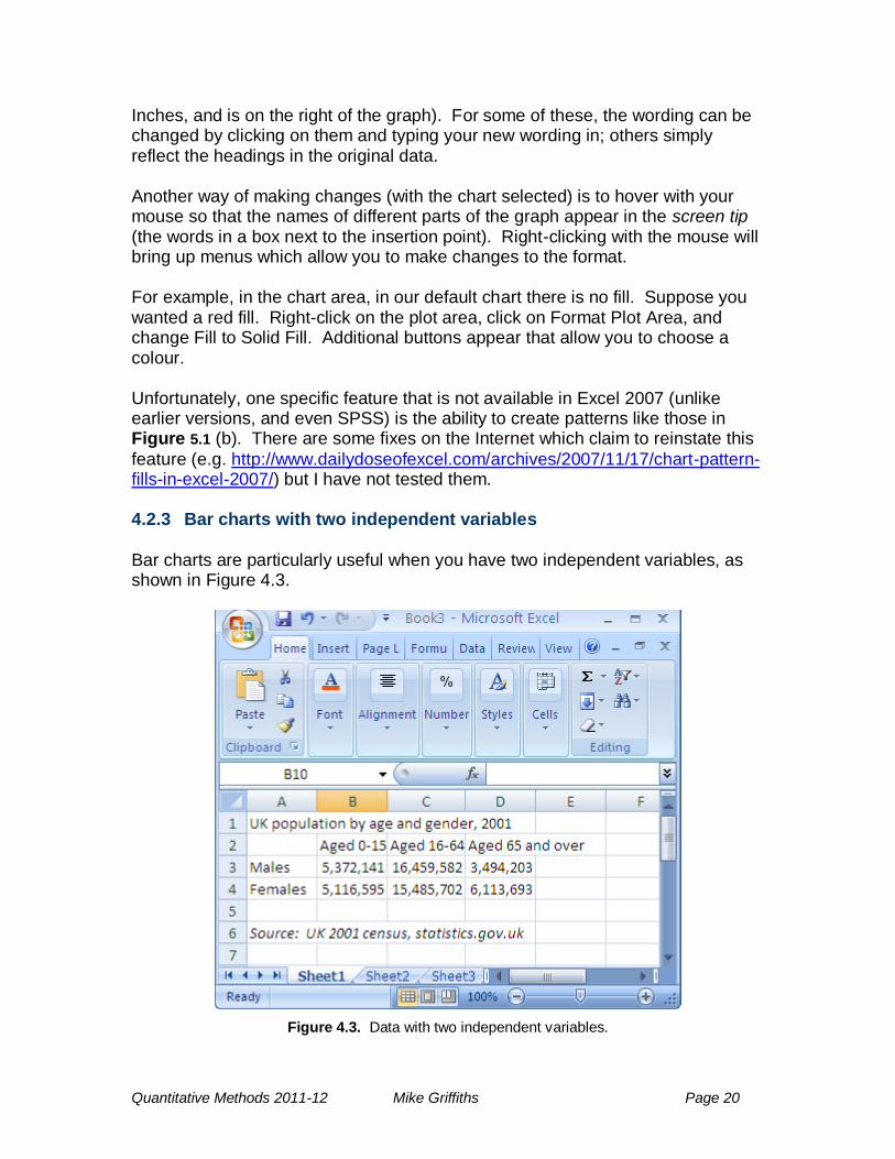
Bar charts are particularly useful when you have two independent variables, as shown in Figure 4.3.
Figure 4.3. Data with two independent variables.
Quantitative Methods 2011-12 Mike Griffiths Page 21
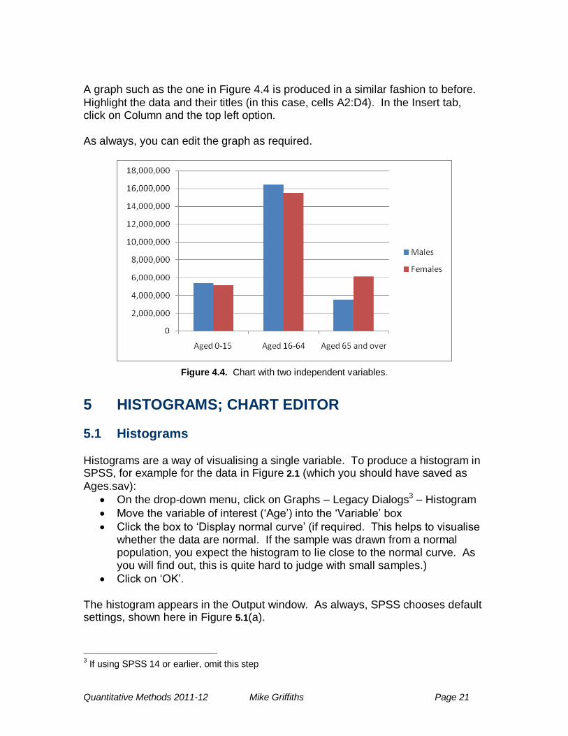
A graph such as the one in Figure 4.4 is produced in a similar fashion to before.
Highlight the data and their titles (in this case, cells A2:D4). In the Insert tab, click on Column and the top left option. As always, you can edit the graph as required.
Figure 4.4. Chart with two independent variables.
5 HISTOGRAMS; CHART EDITOR
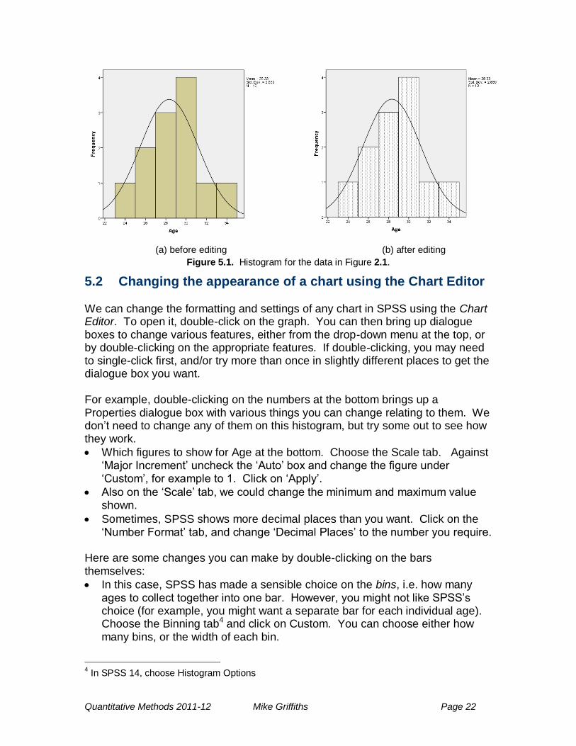
5.1 Histograms Histograms are a way of visualising a single variable. To produce a histogram in SPSS, for example for the data in Figure 2.1 (which you should have saved as
Ages.sav):
On the drop-down menu, click on Graphs – Legacy Dialogs3 – Histogram
Move the variable of interest (‗Age‘) into the ‗Variable‘ box
Click the box to ‗Display normal curve‘ (if required. This helps to visualise whether the data are normal. If the sample was drawn from a normal population, you expect the histogram to lie close to the normal curve. As you will find out, this is quite hard to judge with small samples.)
Click on ‗OK‘. The histogram appears in the Output window. As always, SPSS chooses default settings, shown here in Figure 5.1(a).
3 If using SPSS 14 or earlier, omit this step
Quantitative Methods 2011-12 Mike Griffiths Page 22
(a) before editing (b) after editing
Figure 5.1. Histogram for the data in Figure 2.1.
5.2 Changing the appearance of a chart using the Chart Editor We can change the formatting and settings of any chart in SPSS using the Chart Editor. To open it, double-click on the graph. You can then bring up dialogue boxes to change various features, either from the drop-down menu at the top, or by double-clicking on the appropriate features. If double-clicking, you may need to single-click first, and/or try more than once in slightly different places to get the dialogue box you want. For example, double-clicking on the numbers at the bottom brings up a Properties dialogue box with various things you can change relating to them. We don‘t need to change any of them on this histogram, but try some out to see how they work.
Which figures to show for Age at the bottom. Choose the Scale tab. Against ‗Major Increment‘ uncheck the ‗Auto‘ box and change the figure under ‗Custom‘, for example to 1. Click on ‗Apply‘.
Also on the ‗Scale‘ tab, we could change the minimum and maximum value shown.
Sometimes, SPSS shows more decimal places than you want. Click on the ‗Number Format‘ tab, and change ‗Decimal Places‘ to the number you require.
Here are some changes you can make by double-clicking on the bars themselves:
In this case, SPSS has made a sensible choice on the bins, i.e. how many ages to collect together into one bar. However, you might not like SPSS‘s choice (for example, you might want a separate bar for each individual age). Choose the Binning tab4 and click on Custom. You can choose either how many bins, or the width of each bin.
4 In SPSS 14, choose Histogram Options
Quantitative Methods 2011-12 Mike Griffiths Page 23
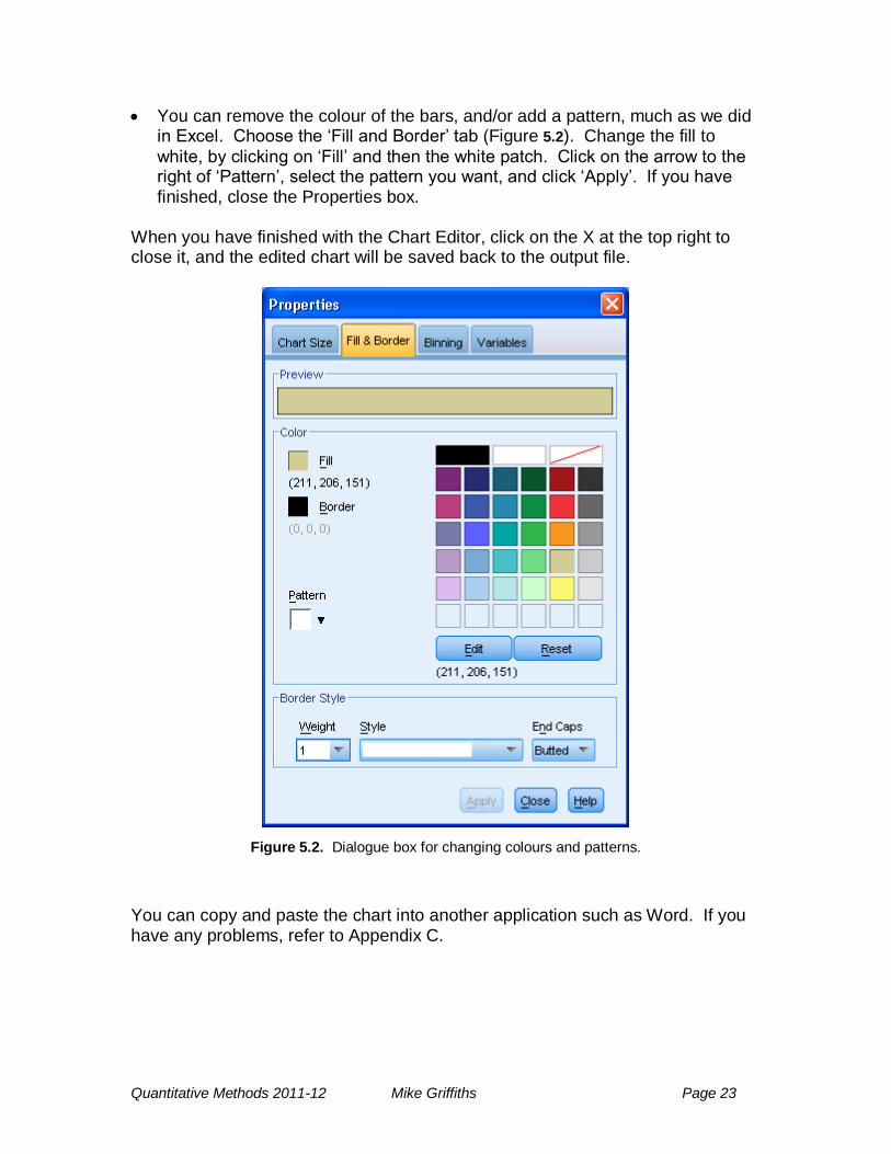
You can remove the colour of the bars, and/or add a pattern, much as we did in Excel. Choose the ‗Fill and Border‘ tab (Figure 5.2). Change the fill to
white, by clicking on ‗Fill‘ and then the white patch. Click on the arrow to the right of ‗Pattern‘, select the pattern you want, and click ‗Apply‘. If you have finished, close the Properties box.
When you have finished with the Chart Editor, click on the X at the top right to close it, and the edited chart will be saved back to the output file.
Figure 5.2. Dialogue box for changing colours and patterns.
You can copy and paste the chart into another application such as Word. If you have any problems, refer to Appendix C.
Quantitative Methods 2011-12 Mike Griffiths Page 24
6 T-TESTS, ANOVAS AND THEIR NON-PARAMETRIC EQUIVALENTS
6.1 Introduction
This section deals with tests when
the Independent Variable is categorical, and
the Dependent Variable is ordinal, interval or ratio. For example
the IV might be the amount of alcohol consumed (no alcohol, 1 unit, 2 units)
the DV might be performance on a test (measured as a score) Note: For this kind of test it is usually recommended that you have at least 20 cases (e.g. participants) for within-subjects designs, and 20 per condition for between-subject designs. This is just a rule of thumb – the best number of participants depends on various things including how big the effects are. I have used fewer cases to make the data entry easier.
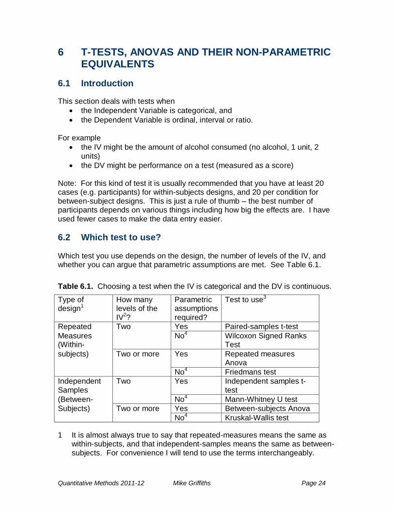
6.2 Which test to use? Which test you use depends on the design, the number of levels of the IV, and whether you can argue that parametric assumptions are met. See Table 6.1.
Table 6.1. Choosing a test when the IV is categorical and the DV is continuous.
Type of design1
How many levels of the IV2?
Parametric assumptions required?
Test to use3
Repeated Two Yes Paired-samples t-test
Measures (Within-
No4 Wilcoxon Signed Ranks Test
subjects) Two or more Yes Repeated measures Anova
No4 Friedmans test
Independent Samples
Two Yes Independent samples t-test
(Between- No4 Mann-Whitney U test
Subjects) Two or more Yes Between-subjects Anova
No4 Kruskal-Wallis test
1 It is almost always true to say that repeated-measures means the same as within-subjects, and that independent-samples means the same as between-subjects. For convenience I will tend to use the terms interchangeably.
Quantitative Methods 2011-12 Mike Griffiths Page 25
There are a few exceptions, which are quite rare. For example, if there are control participants who are individually matched to each participant in the experimental condition, a repeated measures analysis is applicable.
2 You may wonder why we bother with tests for two levels. Surely you can use the tests that are for ‗two or more‘ levels? Yes, you can. However, if there are only two levels, most people still use the separate tests (essentially for historical reasons) so you still need to understand them.
3 Unfortunately, most of these tests have more than one name. These are the names that SPSS uses.
4 These tests can be used whether parametric assumptions are met or not. However they are less powerful than the parametric tests, so researchers prefer to use the parametric tests if possible.
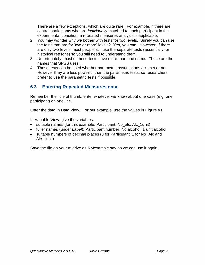
6.3 Entering Repeated Measures data Remember the rule of thumb: enter whatever we know about one case (e.g. one participant) on one line. Enter the data in Data View. For our example, use the values in Figure 6.1.
In Variable View, give the variables:
suitable names (for this example, Participant, No_alc, Alc_1unit)
fuller names (under Label): Participant number, No alcohol, 1 unit alcohol.
suitable numbers of decimal places (0 for Participant, 1 for No_Alc and Alc_1unit).
Save the file on your n: drive as RMexample.sav so we can use it again.
Quantitative Methods 2011-12 Mike Griffiths Page 26
Figure 6.1. Data for paired samples t-test
6.4 Paired samples t-test (also known as related, matched pairs, within-subjects or repeated measures t-test) Within-subjects, two levels of the IV, parametric assumptions met.
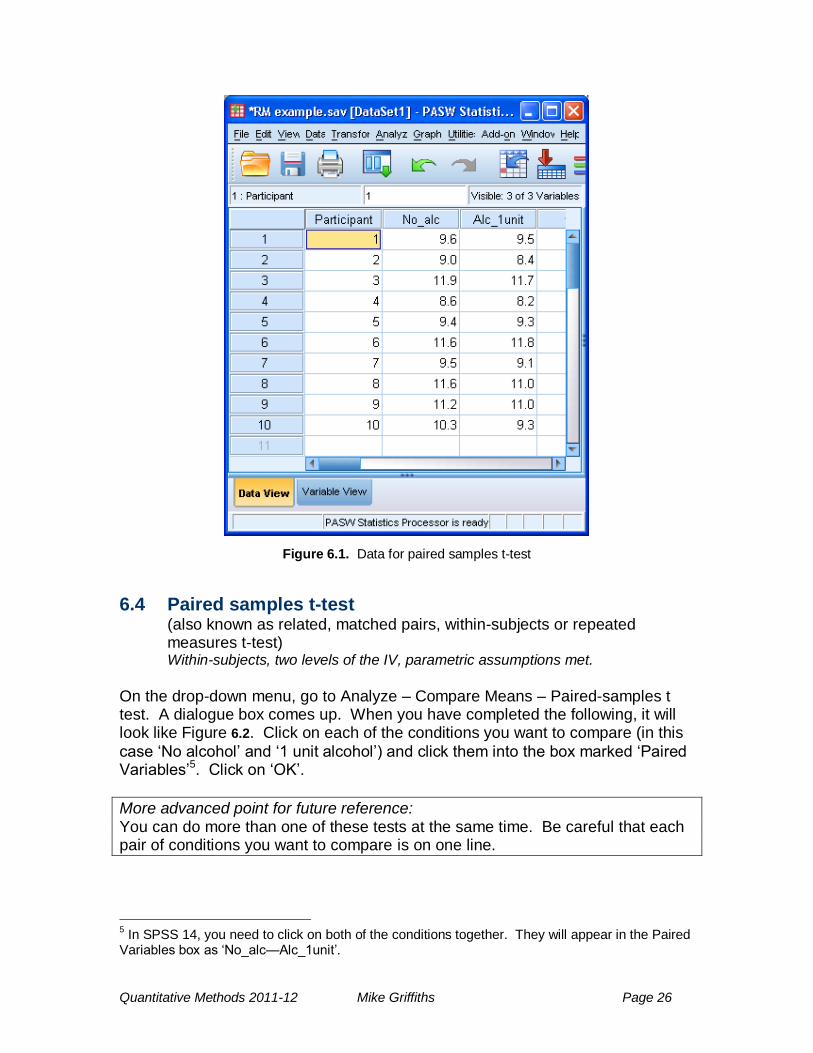
On the drop-down menu, go to Analyze – Compare Means – Paired-samples t test. A dialogue box comes up. When you have completed the following, it will look like Figure 6.2. Click on each of the conditions you want to compare (in this
case ‗No alcohol‘ and ‗1 unit alcohol‘) and click them into the box marked ‗Paired Variables‘5. Click on ‗OK‘.
More advanced point for future reference: You can do more than one of these tests at the same time. Be careful that each pair of conditions you want to compare is on one line.
5 In SPSS 14, you need to click on both of the conditions together. They will appear in the Paired
Variables box as ‗No_alc—Alc_1unit‘.
Quantitative Methods 2011-12 Mike Griffiths Page 27
Figure 6.2. Dialogue box for paired samples t-test.
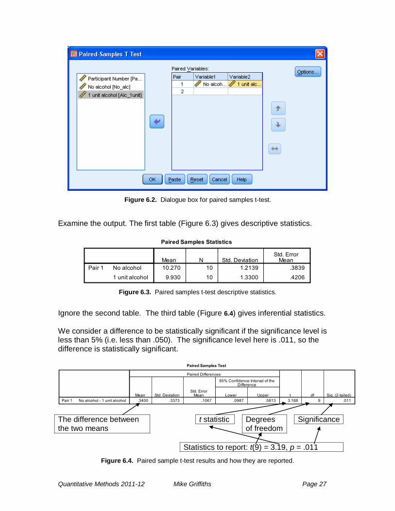
Examine the output. The first table (Figure 6.3) gives descriptive statistics.
Figure 6.3. Paired samples t-test descriptive statistics.
Ignore the second table. The third table (Figure 6.4) gives inferential statistics. We consider a difference to be statistically significant if the significance level is less than 5% (i.e. less than .050). The significance level here is .011, so the difference is statistically significant.
The difference between the two means
t statistic Degrees of freedom
Significance
Statistics to report: t(9) = 3.19, p = .011
Figure 6.4. Paired sample t-test results and how they are reported.
Quantitative Methods 2011-12 Mike Griffiths Page 28
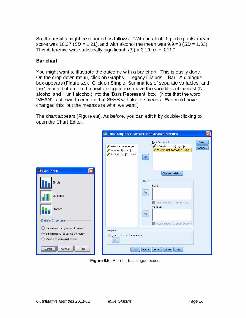
So, the results might be reported as follows: ―With no alcohol, participants‘ mean score was 10.27 (SD = 1.21), and with alcohol the mean was 9.9.=3 (SD = 1.33). This difference was statistically significant, t(9) = 3.19, p = .011.‖ Bar chart You might want to illustrate the outcome with a bar chart. This is easily done. On the drop down menu, click on Graphs – Legacy Dialogs – Bar. A dialogue box appears (Figure 6.5). Click on Simple; Summaries of separate variables; and
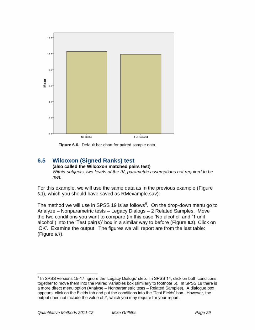
the ‗Define‘ button. In the next dialogue box, move the variables of interest (No alcohol and 1 unit alcohol) into the ‗Bars Represent‘ box. (Note that the word ‗MEAN‘ is shown, to confirm that SPSS will plot the means. We could have changed this, but the means are what we want.) The chart appears (Figure 6.6). As before, you can edit it by double-clicking to
open the Chart Editor.
Figure 6.5. Bar charts dialogue boxes.
Quantitative Methods 2011-12 Mike Griffiths Page 29
Figure 6.6. Default bar chart for paired sample data.
6.5 Wilcoxon (Signed Ranks) test (also called the Wilcoxon matched pairs test) Within-subjects, two levels of the IV, parametric assumptions not required to be met.
For this example, we will use the same data as in the previous example (Figure 6.1), which you should have saved as RMexample.sav): The method we will use in SPSS 19 is as follows6. On the drop-down menu go to Analyze – Nonparametric tests – Legacy Dialogs – 2 Related Samples. Move the two conditions you want to compare (in this case ‗No alcohol‘ and ‗1 unit alcohol‘) into the ‗Test pair(s)‘ box in a similar way to before (Figure 6.2). Click on
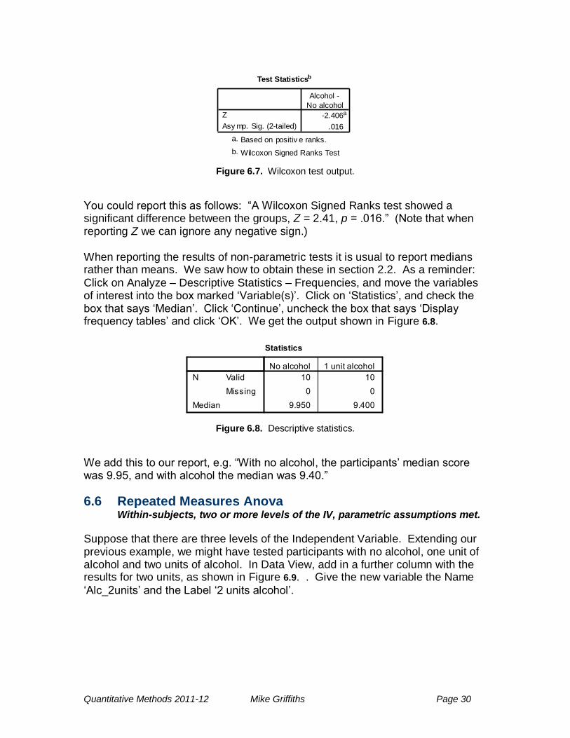
‗OK‘. Examine the output. The figures we will report are from the last table: (Figure 6.7).
6 In SPSS versions 15-17, ignore the ‗Legacy Dialogs‘ step. In SPSS 14, click on both conditions
together to move them into the Paired Variables box (similarly to footnote 5). In SPSS 18 there is a more direct menu option (Analyse – Nonparametric tests – Related Samples). A dialogue box appears; click on the Fields tab and put the conditions into the ‗Test Fields‘ box. However, the output does not include the value of Z, which you may require for your report.
Quantitative Methods 2011-12 Mike Griffiths Page 30
Test Statisticsb
-2.406a
.016
Z
Asy mp. Sig. (2-tailed)
Alcohol -
No alcohol
Based on positiv e ranks.a.
Wilcoxon Signed Ranks Testb.
Figure 6.7. Wilcoxon test output.
You could report this as follows: ―A Wilcoxon Signed Ranks test showed a significant difference between the groups, Z = 2.41, p = .016.‖ (Note that when reporting Z we can ignore any negative sign.) When reporting the results of non-parametric tests it is usual to report medians rather than means. We saw how to obtain these in section 2.2. As a reminder:
Click on Analyze – Descriptive Statistics – Frequencies, and move the variables of interest into the box marked ‗Variable(s)‘. Click on ‗Statistics‘, and check the box that says ‗Median‘. Click ‗Continue‘, uncheck the box that says ‗Display frequency tables‘ and click ‗OK‘. We get the output shown in Figure 6.8.
Figure 6.8. Descriptive statistics.
We add this to our report, e.g. ―With no alcohol, the participants‘ median score was 9.95, and with alcohol the median was 9.40.‖
6.6 Repeated Measures Anova Within-subjects, two or more levels of the IV, parametric assumptions met.
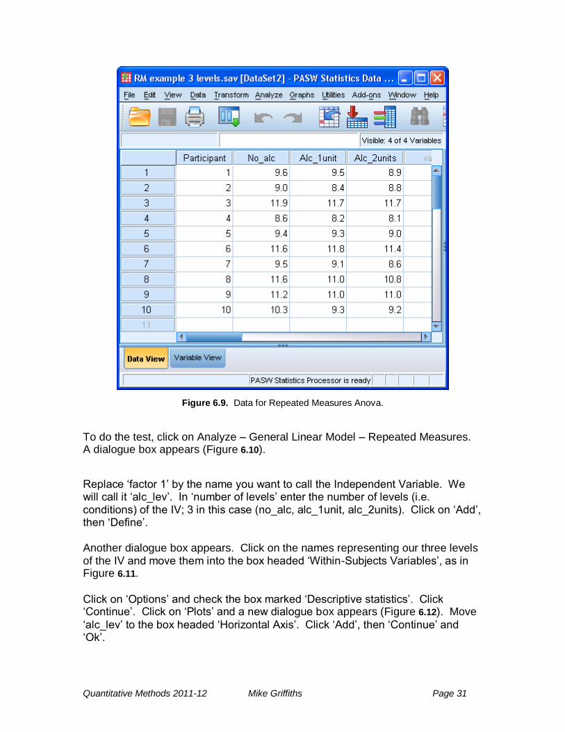
Suppose that there are three levels of the Independent Variable. Extending our previous example, we might have tested participants with no alcohol, one unit of alcohol and two units of alcohol. In Data View, add in a further column with the results for two units, as shown in Figure 6.9. . Give the new variable the Name
‗Alc_2units‘ and the Label ‗2 units alcohol‘.
Quantitative Methods 2011-12 Mike Griffiths Page 31
Figure 6.9. Data for Repeated Measures Anova.
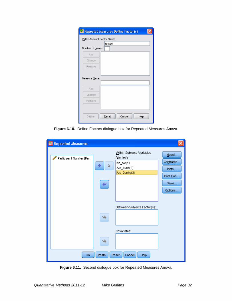
To do the test, click on Analyze – General Linear Model – Repeated Measures. A dialogue box appears (Figure 6.10).
Replace ‗factor 1‘ by the name you want to call the Independent Variable. We will call it ‗alc_lev‘. In ‗number of levels‘ enter the number of levels (i.e. conditions) of the IV; 3 in this case (no_alc, alc_1unit, alc_2units). Click on ‗Add‘, then ‗Define‘. Another dialogue box appears. Click on the names representing our three levels of the IV and move them into the box headed ‗Within-Subjects Variables‘, as in Figure 6.11.
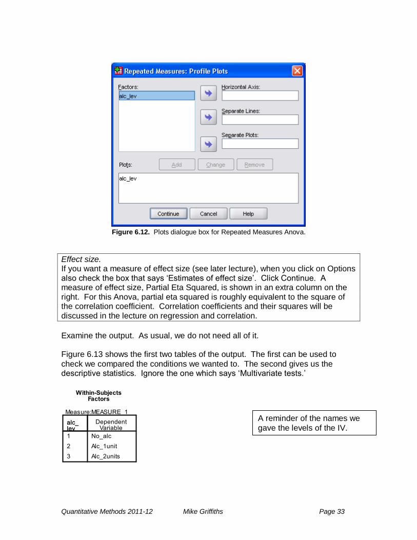
Click on ‗Options‘ and check the box marked ‗Descriptive statistics‘. Click ‗Continue‘. Click on ‗Plots‘ and a new dialogue box appears (Figure 6.12). Move
‗alc_lev‘ to the box headed ‗Horizontal Axis‘. Click ‗Add‘, then ‗Continue‘ and ‗Ok‘.
Quantitative Methods 2011-12 Mike Griffiths Page 32
Figure 6.10. Define Factors dialogue box for Repeated Measures Anova.
Figure 6.11. Second dialogue box for Repeated Measures Anova.
Quantitative Methods 2011-12 Mike Griffiths Page 33
Figure 6.12. Plots dialogue box for Repeated Measures Anova.
Effect size. If you want a measure of effect size (see later lecture), when you click on Options also check the box that says ‗Estimates of effect size‘. Click Continue. A measure of effect size, Partial Eta Squared, is shown in an extra column on the right. For this Anova, partial eta squared is roughly equivalent to the square of the correlation coefficient. Correlation coefficients and their squares will be discussed in the lecture on regression and correlation.
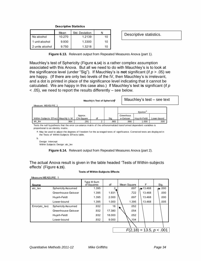
Examine the output. As usual, we do not need all of it. Figure 6.13 shows the first two tables of the output. The first can be used to
check we compared the conditions we wanted to. The second gives us the descriptive statistics. Ignore the one which says ‗Multivariate tests.‘
A reminder of the names we
gave the levels of the IV.
Quantitative Methods 2011-12 Mike Griffiths Page 34
Figure 6.13. Relevant output from Repeated Measures Anova (part 1).
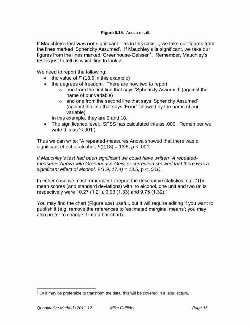
Mauchley‘s test of Sphericity (Figure 6.14) is a rather complex assumption associated with this Anova. But all we need to do with Mauchley‘s is to look at the significance level (under ―Sig‖). If Mauchley‘s is not significant (if p > .05) we are happy. (If there are only two levels of the IV, then Mauchley‘s is irrelevant, and a dot is printed in place of the significance level indicating that it cannot be calculated. We are happy in this case also.) If Mauchley‘s test is significant (if p
< .05), we need to report the results differently – see below.
Mauchly's Test of Sphericityb
Measure: MEASURE_1
.964 .291 2 .865 .966 1.000 .500
Within Subjects Ef f ect
alc_lev
Mauchly 's W
Approx.
Chi-Square df Sig.
Greenhous
e-Geisser Huynh-Feldt Lower-bound
Epsilona
Tests the null hypothesis that the error cov ariance matrix of the orthonormalized transf ormed dependent variables is
proportional to an identity matrix.
May be used to adjust the degrees of f reedom f or the av eraged tests of signif icance. Corrected tests are displayed in
the Tests of Within-Subjects Ef f ects table.
a.
Design: Intercept
Within Subjects Design: alc_lev
b.
Figure 6.14. Relevant output from Repeated Measures Anova (part 2).
The actual Anova result is given in the table headed ‗Tests of Within-subjects effects‘ (Figure 6.15).
F(2,18) = 13.5, p < .001
Mauchley‘s test – see text
Descriptive statistics.
Quantitative Methods 2011-12 Mike Griffiths Page 35
Figure 6.15. Anova result.
If Mauchley‘s test was not significant – as in this case –, we take our figures from the lines marked ‗Sphericity Assumed‘. If Mauchley‘s is significant, we take our
figures from the lines marked ‗Greenhouse-Geisser‘7. Remember, Mauchley‘s test is just to tell us which line to look at. We need to report the following:
the value of F (13.5 in this example)
the degrees of freedom. There are now two to report o one from the first line that says ‗Sphericity Assumed‘ (against the
name of our variable) o and one from the second line that says ‗Sphericity Assumed‘
(against the line that says ‗Error‘ followed by the name of our variable).
In this example, they are 2 and 18.
The significance level. SPSS has calculated this as .000. Remember we write this as ‗<.001‘).
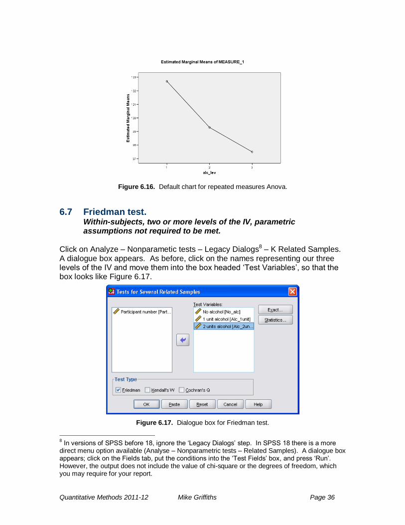
Thus we can write: ―A repeated-measures Anova showed that there was a significant effect of alcohol, F(2,18) = 13.5, p < .001.‖ If Mauchley’s test had been significant we could have written “A repeated-measures Anova with Greenhouse-Geisser correction showed that there was a significant effect of alcohol, F(1.9, 17.4) = 13.5, p < .001). In either case we must remember to report the descriptive statistics, e.g. ―The mean scores (and standard deviations) with no alcohol, one unit and two units respectively were 10.27 (1.21), 9.93 (1.33) and 9.75 (1.32).‖ You may find the chart (Figure 6.16) useful, but it will require editing if you want to
publish it (e.g. remove the references to ‗estimated marginal means‘; you may also prefer to change it into a bar chart).
7 Or it may be preferable to transform the data; this will be covered in a later lecture.
Quantitative Methods 2011-12 Mike Griffiths Page 36
Figure 6.16. Default chart for repeated measures Anova.
6.7 Friedman test. Within-subjects, two or more levels of the IV, parametric assumptions not required to be met.
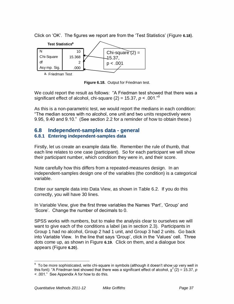
Click on Analyze – Nonparametic tests – Legacy Dialogs8 – K Related Samples. A dialogue box appears. As before, click on the names representing our three levels of the IV and move them into the box headed ‗Test Variables‘, so that the box looks like Figure 6.17.
Figure 6.17. Dialogue box for Friedman test.
8 In versions of SPSS before 18, ignore the ‗Legacy Dialogs‘ step. In SPSS 18 there is a more
direct menu option available (Analyse – Nonparametric tests – Related Samples). A dialogue box appears; click on the Fields tab, put the conditions into the ‗Test Fields‘ box, and press ‗Run‘. However, the output does not include the value of chi-square or the degrees of freedom, which you may require for your report.
Quantitative Methods 2011-12 Mike Griffiths Page 37
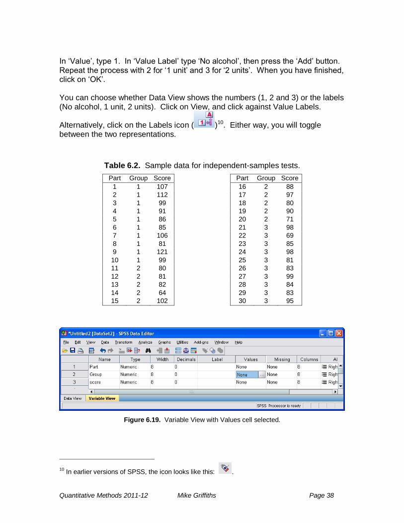
Click on ‗OK‘. The figures we report are from the ‗Test Statistics‘ (Figure 6.18).
Test Statisticsa
10
15.368
2
.000
N
Chi-Square
df
Asy mp. Sig.
Friedman Testa.
Figure 6.18. Output for Friedman test.
We could report the result as follows: ―A Friedman test showed that there was a significant effect of alcohol, chi-square (2) = 15.37, p < .001.‖9 As this is a non-parametric test, we would report the medians in each condition: ―The median scores with no alcohol, one unit and two units respectively were 9.95, 9.40 and 9.10.‖ (See section 2.2 for a reminder of how to obtain these.)
6.8 Independent-samples data - general 6.8.1 Entering independent-samples data
Firstly, let us create an example data file. Remember the rule of thumb, that each line relates to one case (participant). So for each participant we will show their participant number, which condition they were in, and their score. Note carefully how this differs from a repeated-measures design. In an independent-samples design one of the variables (the condition) is a categorical variable. Enter our sample data into Data View, as shown in Table 6.2. If you do this
correctly, you will have 30 lines. In Variable View, give the first three variables the Names ‗Part‘, ‗Group‘ and ‗Score‘. Change the number of decimals to 0. SPSS works with numbers, but to make the analysis clear to ourselves we will want to give each of the conditions a label (as in section 2.3). Participants in
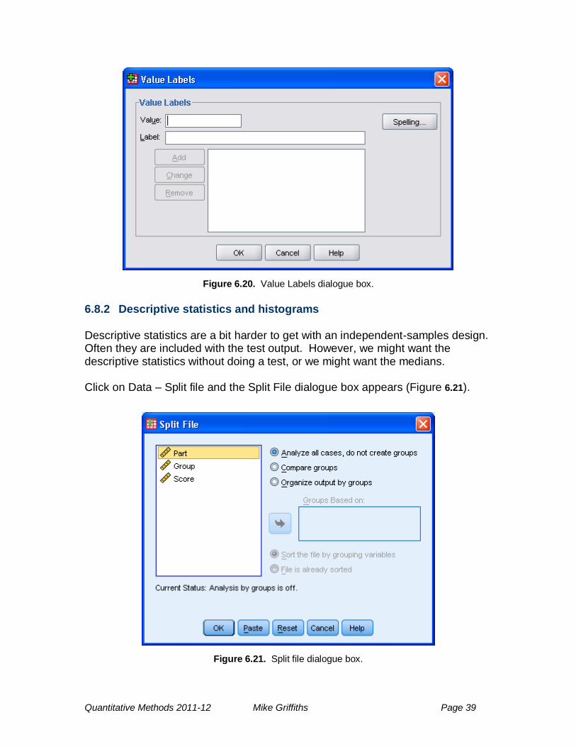
Group 1 had no alcohol, Group 2 had 1 unit, and Group 3 had 2 units. Go back into Variable View. In the line that says ‗Group‘, click in the ‗Values‘ cell. Three dots come up, as shown in Figure 6.19. Click on them, and a dialogue box appears (Figure 6.20).
9 To be more sophisticated, write chi-square in symbols (although it doesn‘t show up very well in
this font): ―A Friedman test showed that there was a significant effect of alcohol, χ2 (2) = 15.37, p
< .001.‖ See Appendix A for how to do this.
Chi-square (2) = 15.37,
p < .001
Quantitative Methods 2011-12 Mike Griffiths Page 38
In ‗Value‘, type 1. In ‗Value Label‘ type ‗No alcohol‘, then press the ‗Add‘ button. Repeat the process with 2 for ‗1 unit‘ and 3 for ‗2 units‘. When you have finished, click on ‗OK‘. You can choose whether Data View shows the numbers (1, 2 and 3) or the labels (No alcohol, 1 unit, 2 units). Click on View, and click against Value Labels.
Alternatively, click on the Labels icon ( )10. Either way, you will toggle between the two representations.
Table 6.2. Sample data for independent-samples tests.
Part Group Score Part Group Score
1 1 107 16 2 88
2 1 112 17 2 97
3 1 99 18 2 80
4 1 91 19 2 90
5 1 86 20 2 71
6 1 85 21 3 98
7 1 106 22 3 69
8 1 81 23 3 85
9 1 121 24 3 98
10 1 99 25 3 81
11 2 80 26 3 83
12 2 81 27 3 99
13 2 82 28 3 84
14 2 64 29 3 83
15 2 102 30 3 95
Figure 6.19. Variable View with Values cell selected.
10 In earlier versions of SPSS, the icon looks like this: .
Quantitative Methods 2011-12 Mike Griffiths Page 39
Figure 6.20. Value Labels dialogue box.
6.8.2 Descriptive statistics and histograms Descriptive statistics are a bit harder to get with an independent-samples design. Often they are included with the test output. However, we might want the descriptive statistics without doing a test, or we might want the medians. Click on Data – Split file and the Split File dialogue box appears (Figure 6.21).
Figure 6.21. Split file dialogue box.
Quantitative Methods 2011-12 Mike Griffiths Page 40
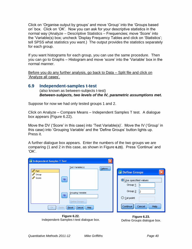
Click on ‗Organise output by groups‘ and move ‗Group‘ into the ‗Groups based on‘ box. Click on ‗OK‘. Now you can ask for your descriptive statistics in the normal way (Analyze – Descriptive Statistics – Frequencies; move ‗Score‘ into the ‗Variable(s) box; uncheck ‗Display Frequency Tables and click on ‗Statistics‘; tell SPSS what statistics you want.) The output provides the statistics separately for each group. If you want histograms for each group, you can use the same procedure. Then you can go to Graphs – Histogram and move ‗score‘ into the ‗Variable‘ box in the normal manner. Before you do any further analysis, go back to Data – Split file and click on ‗Analyze all cases‘.
6.9 Independent-samples t-test (also known as between-subjects t-test) Between-subjects, two levels of the IV, parametric assumptions met.
Suppose for now we had only tested groups 1 and 2. Click on Analyze – Compare Means – Independent Samples T test. A dialogue box appears (Figure 6.22).
Move the DV (‗Score‘ in this case) into ‗Test Variable(s)‘. Move the IV (‗Group‘ in this case) into ‗Grouping Variable‘ and the ‗Define Groups‘ button lights up. Press it. A further dialogue box appears. Enter the numbers of the two groups we are comparing (1 and 2 in this case, as shown in Figure 6.23). Press ‗Continue‘ and ‗OK‘.
Figure 6.22. Independent-Samples t-test dialogue box.
Figure 6.23. Define Groups dialogue box.
Quantitative Methods 2011-12 Mike Griffiths Page 41
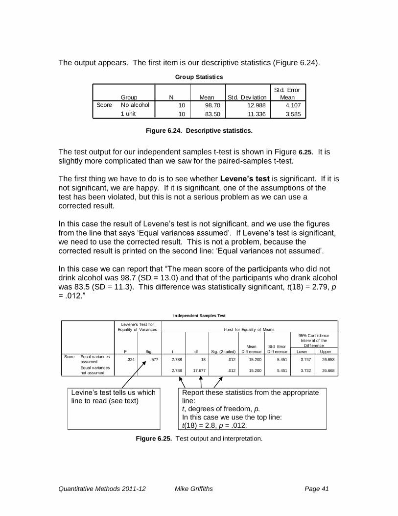
The output appears. The first item is our descriptive statistics (Figure 6.24).
Group Statistics
10 98.70 12.988 4.107
10 83.50 11.336 3.585
Group
No alcohol
1 unit
Score
N Mean Std. Dev iation
Std. Error
Mean
Figure 6.24. Descriptive statistics.
The test output for our independent samples t-test is shown in Figure 6.25. It is slightly more complicated than we saw for the paired-samples t-test. The first thing we have to do is to see whether Levene’s test is significant. If it is not significant, we are happy. If it is significant, one of the assumptions of the test has been violated, but this is not a serious problem as we can use a corrected result. In this case the result of Levene‘s test is not significant, and we use the figures from the line that says ‗Equal variances assumed‘. If Levene‘s test is significant, we need to use the corrected result. This is not a problem, because the corrected result is printed on the second line: ‗Equal variances not assumed‘. In this case we can report that ―The mean score of the participants who did not drink alcohol was 98.7 (SD = 13.0) and that of the participants who drank alcohol was 83.5 (SD = 11.3). This difference was statistically significant, t(18) = 2.79, p = .012.‖
Independent Samples Test
.324 .577 2.788 18 .012 15.200 5.451 3.747 26.653
2.788 17.677 .012 15.200 5.451 3.732 26.668
Equal variances
assumed
Equal variances
not assumed
Score
F Sig.
Levene's Test f or
Equality of Variances
t df Sig. (2-tailed)
Mean
Dif f erence
Std. Error
Dif f erence Lower Upper
95% Conf i dence
Interv al of the
Dif f erence
t-test for Equality of Means
Levine‘s test tells us which
line to read (see text) Report these statistics from the appropriate
line: t, degrees of freedom, p.
In this case we use the top line: t(18) = 2.8, p = .012.
Figure 6.25. Test output and interpretation.
Quantitative Methods 2011-12 Mike Griffiths Page 42
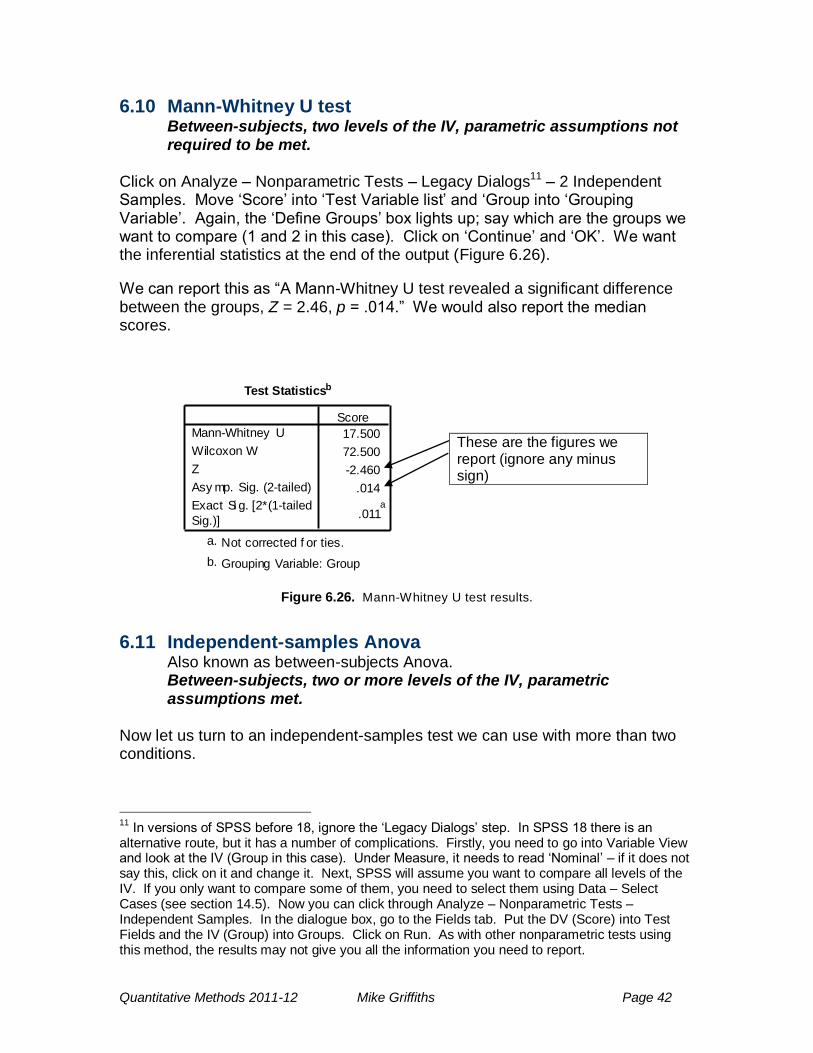
6.10 Mann-Whitney U test Between-subjects, two levels of the IV, parametric assumptions not required to be met.
Click on Analyze – Nonparametric Tests – Legacy Dialogs11 – 2 Independent Samples. Move ‗Score‘ into ‗Test Variable list‘ and ‗Group into ‗Grouping Variable‘. Again, the ‗Define Groups‘ box lights up; say which are the groups we want to compare (1 and 2 in this case). Click on ‗Continue‘ and ‗OK‘. We want the inferential statistics at the end of the output (Figure 6.26).
We can report this as ―A Mann-Whitney U test revealed a significant difference between the groups, Z = 2.46, p = .014.‖ We would also report the median scores.
Test Statisticsb
17.500
72.500
-2.460
.014
.011a
Mann-Whitney U
Wilcoxon W
Z
Asy mp. Sig. (2-tailed)
Exact Si g. [2*(1-tailed
Sig.)]
Score
Not corrected f or ties.a.
Grouping Variable: Groupb.
These are the figures we report (ignore any minus sign)
Figure 6.26. Mann-Whitney U test results.
6.11 Independent-samples Anova Also known as between-subjects Anova. Between-subjects, two or more levels of the IV, parametric assumptions met.
Now let us turn to an independent-samples test we can use with more than two conditions.
11
In versions of SPSS before 18, ignore the ‗Legacy Dialogs‘ step. In SPSS 18 there is an alternative route, but it has a number of complications. Firstly, you need to go into Variable View and look at the IV (Group in this case). Under Measure, it needs to read ‗Nominal‘ – if it does not say this, click on it and change it. Next, SPSS will assume you want to compare all levels of the IV. If you only want to compare some of them, you need to select them using Data – Select Cases (see section 14.5). Now you can click through Analyze – Nonparametric Tests – Independent Samples. In the dialogue box, go to the Fields tab. Put the DV (Score) into Test Fields and the IV (Group) into Groups. Click on Run. As with other nonparametric tests using this method, the results may not give you all the information you need to report.
Quantitative Methods 2011-12 Mike Griffiths Page 43
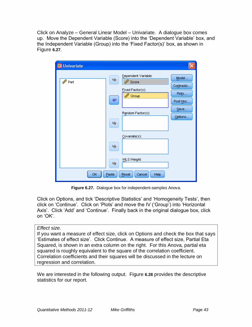
Click on Analyze – General Linear Model – Univariate. A dialogue box comes up. Move the Dependent Variable (Score) into the ‗Dependent Variable‘ box, and the Independent Variable (Group) into the ‗Fixed Factor(s)‘ box, as shown in Figure 6.27.
Figure 6.27. Dialogue box for independent-samples Anova.
Click on Options, and tick ‗Descriptive Statistics‘ and ‗Homogeneity Tests‘, then click on ‗Continue‘. Click on ‗Plots‘ and move the IV (‗Group‘) into ‗Horizontal Axis‘. Click ‗Add‘ and ‗Continue‘. Finally back in the original dialogue box, click on ‗OK‘.
Effect size. If you want a measure of effect size, click on Options and check the box that says ‗Estimates of effect size‘. Click Continue. A measure of effect size, Partial Eta Squared, is shown in an extra column on the right. For this Anova, partial eta squared is roughly equivalent to the square of the correlation coefficient. Correlation coefficients and their squares will be discussed in the lecture on regression and correlation.
We are interested in the following output. Figure 6.28 provides the descriptive statistics for our report.
Quantitative Methods 2011-12 Mike Griffiths Page 44
Descriptive Statistics
Dependent Variable: Score
98.70 12.988 10
83.50 11.336 10
87.50 9.733 10
89.90 12.823 30
Group
No alcohol
1 unit
2 units
Total
Mean Std. Dev iat ion N
Figure 6.28. Descriptive statistics.
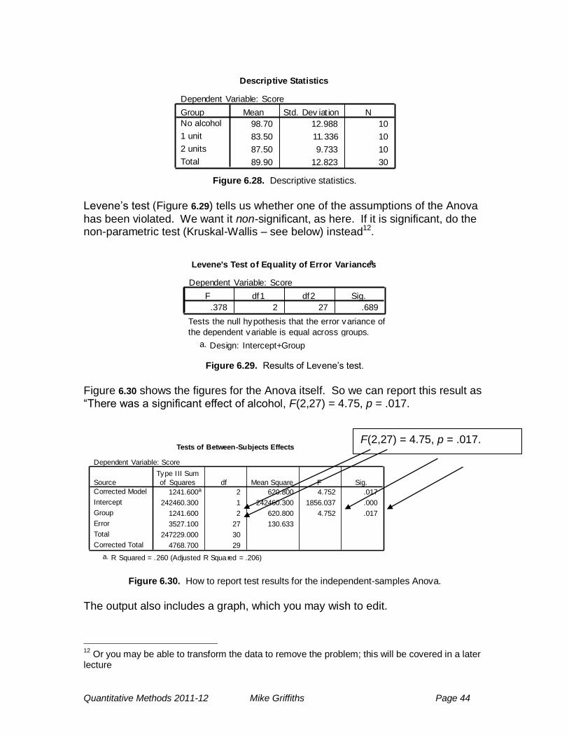
Levene‘s test (Figure 6.29) tells us whether one of the assumptions of the Anova
has been violated. We want it non-significant, as here. If it is significant, do the non-parametric test (Kruskal-Wallis – see below) instead12.
Levene's Test of Equality of Error Variancesa
Dependent Variable: Score
.378 2 27 .689
F df1 df2 Sig.
Tests the null hypothesis that the error variance of
the dependent variable is equal across groups.
Design: Intercept+Groupa.
Figure 6.29. Results of Levene‘s test.
Figure 6.30 shows the figures for the Anova itself. So we can report this result as ―There was a significant effect of alcohol, F(2,27) = 4.75, p = .017.
Tests of Between-Subjects Effects
Dependent Variable: Score
1241.600a 2 620.800 4.752 .017
242460.300 1 242460.300 1856.037 .000
1241.600 2 620.800 4.752 .017
3527.100 27 130.633
247229.000 30
4768.700 29
Source
Corrected Model
Intercept
Group
Error
Total
Corrected Total
Type I II Sum
of Squares df Mean Square F Sig.
R Squared = .260 (Adjusted R Squared = .206)a.
Figure 6.30. How to report test results for the independent-samples Anova.
The output also includes a graph, which you may wish to edit.
12
Or you may be able to transform the data to remove the problem; this will be covered in a later lecture
F(2,27) = 4.75, p = .017.
Quantitative Methods 2011-12 Mike Griffiths Page 45
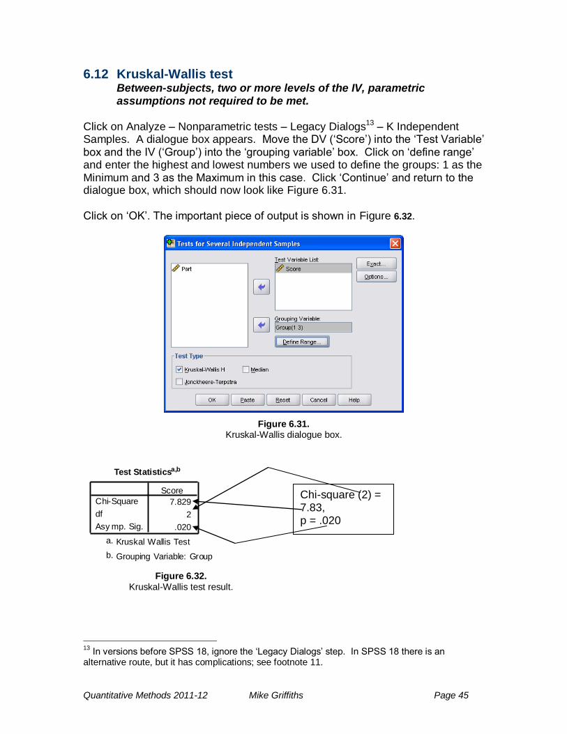
6.12 Kruskal-Wallis test Between-subjects, two or more levels of the IV, parametric assumptions not required to be met.
Click on Analyze – Nonparametric tests – Legacy Dialogs13 – K Independent Samples. A dialogue box appears. Move the DV (‗Score‘) into the ‗Test Variable‘ box and the IV (‗Group‘) into the ‗grouping variable‘ box. Click on ‗define range‘ and enter the highest and lowest numbers we used to define the groups: 1 as the Minimum and 3 as the Maximum in this case. Click ‗Continue‘ and return to the dialogue box, which should now look like Figure 6.31.
Click on ‗OK‘. The important piece of output is shown in Figure 6.32.
Figure 6.31. Kruskal-Wallis dialogue box.
Test Statisticsa,b
7.829
2
.020
Chi-Square
df
Asy mp. Sig.
Score
Kruskal Wallis Testa.
Grouping Variable: Groupb.
Figure 6.32. Kruskal-Wallis test result.
13
In versions before SPSS 18, ignore the ‗Legacy Dialogs‘ step. In SPSS 18 there is an alternative route, but it has complications; see footnote 11.
Chi-square (2) = 7.83, p = .020
Quantitative Methods 2011-12 Mike Griffiths Page 46
We could report the result as follows: ―A Kruskal-Wallis test showed that there was a significant effect of alcohol, chi-square (2) = 7.83, p = .020.‖14 As this is a non-parametric test, again we would report the medians in each condition.
7 FACTORIAL ANOVAS 7.1 Introduction A ‗factorial Anova‘ is an Anova with more than one independent variable (but still one Dependent Variable). For example, a ‗two way Anova‘ means that there are two Independent Variables: e.g. the effect of gender and alcohol on performance. In Anova, an alternative name for the IVs is factors. (Do not get confused by the fact that this word also has other meanings.) Each of the IVs could either be repeated-measures or independent-samples. For example, in a two way Anova, any of the following combinations can occur. Each requires a different procedure in SPSS. (a) both IVs are independent-samples: requires a two way independent-
samples Anova (section 7.5) (b) both IVs are repeated-measures: requires a two way repeated-measures
Anova (section 7.6)
(d) one IV is independent-samples and the other is repeated-measures: requires a two way mixed Anova (section 7.7).
As before, a rule of thumb is that there should be at least 20 participants (20 in each group for between-subjects variables) but for illustrative purposes we will use fewer. Each of the IVs can have two levels (categories), or more. In the following examples each will two, but the principles are the same if they have more.
7.2 Outcomes The Anova calculates the effect of each IV on the DV: for example, the effect of alcohol on performance, and the effect of gender on performance. These are called main effects. However, the main point of a two way Anova is that it enables us to see whether the effect of one IV is different depending on the level of the other IV. For example, is the effect of alcohol on performance different for men and women? This is called an interaction. The main effects and interactions are generically known as effects.
14
To be more sophisticated, write the χ2 in symbols: ―A Kruskall-Wallis test showed that there
was a significant effect of alcohol, χ2 (2) = 7.83, p = .020.‖ See Appendix A for how to do this.
Quantitative Methods 2011-12 Mike Griffiths Page 47
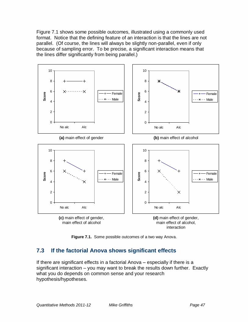
Figure 7.1 shows some possible outcomes, illustrated using a commonly used
format. Notice that the defining feature of an interaction is that the lines are not parallel. (Of course, the lines will always be slightly non-parallel, even if only because of sampling error. To be precise, a significant interaction means that the lines differ significantly from being parallel.)
0
2
4
6
8
10
No alc Alc
Sco
re Female
Male
0
2
4
6
8
10
No alc Alc
Sco
re Female
Male
(a) main effect of gender (b) main effect of alcohol
0
2
4
6
8
10
No alc Alc
Sco
re Female
Male
0
2
4
6
8
10
No alc Alc
Sco
re Female
Male
(c) main effect of gender,
main effect of alcohol (d) main effect of gender,
main effect of alcohol, interaction
Figure 7.1. Some possible outcomes of a two way Anova.
7.3 If the factorial Anova shows significant effects If there are significant effects in a factorial Anova – especially if there is a significant interaction – you may want to break the results down further. Exactly what you do depends on common sense and your research hypothesis/hypotheses.
Quantitative Methods 2011-12 Mike Griffiths Page 48
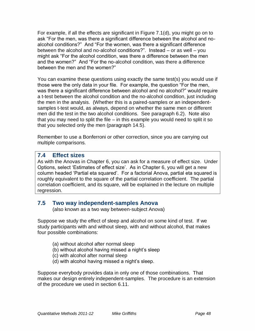
For example, if all the effects are significant in Figure 7.1(d), you might go on to
ask ―For the men, was there a significant difference between the alcohol and no-alcohol conditions?‖ And ―For the women, was there a significant difference between the alcohol and no-alcohol conditions?‖. Instead – or as well – you might ask ―For the alcohol condition, was there a difference between the men and the women?‖ And ―For the no-alcohol condition, was there a difference between the men and the women?‖ You can examine these questions using exactly the same test(s) you would use if those were the only data in your file. For example, the question ―For the men, was there a significant difference between alcohol and no alcohol?‖ would require a t-test between the alcohol condition and the no-alcohol condition, just including the men in the analysis. (Whether this is a paired-samples or an independent-samples t-test would, as always, depend on whether the same men or different men did the test in the two alcohol conditions. See paragraph 6.2). Note also
that you may need to split the file – in this example you would need to split it so that you selected only the men (paragraph 14.5).
Remember to use a Bonferroni or other correction, since you are carrying out multiple comparisons.
7.4 Effect sizes As with the Anovas in Chapter 6, you can ask for a measure of effect size. Under Options, select ‗Estimates of effect size‘. As in Chapter 6, you will get a new column headed ‗Partial eta squared‘. For a factorial Anova, partial eta squared is roughly equivalent to the square of the partial correlation coefficient. The partial correlation coefficient, and its square, will be explained in the lecture on multiple regression.
7.5 Two way independent-samples Anova (also known as a two way between-subject Anova)
Suppose we study the effect of sleep and alcohol on some kind of test. If we study participants with and without sleep, with and without alcohol, that makes four possible combinations:
(a) without alcohol after normal sleep (b) without alcohol having missed a night‘s sleep (c) with alcohol after normal sleep (d) with alcohol having missed a night‘s sleep.
Suppose everybody provides data in only one of those combinations. That makes our design entirely independent-samples. The procedure is an extension of the procedure we used in section 6.11.
Quantitative Methods 2011-12 Mike Griffiths Page 49
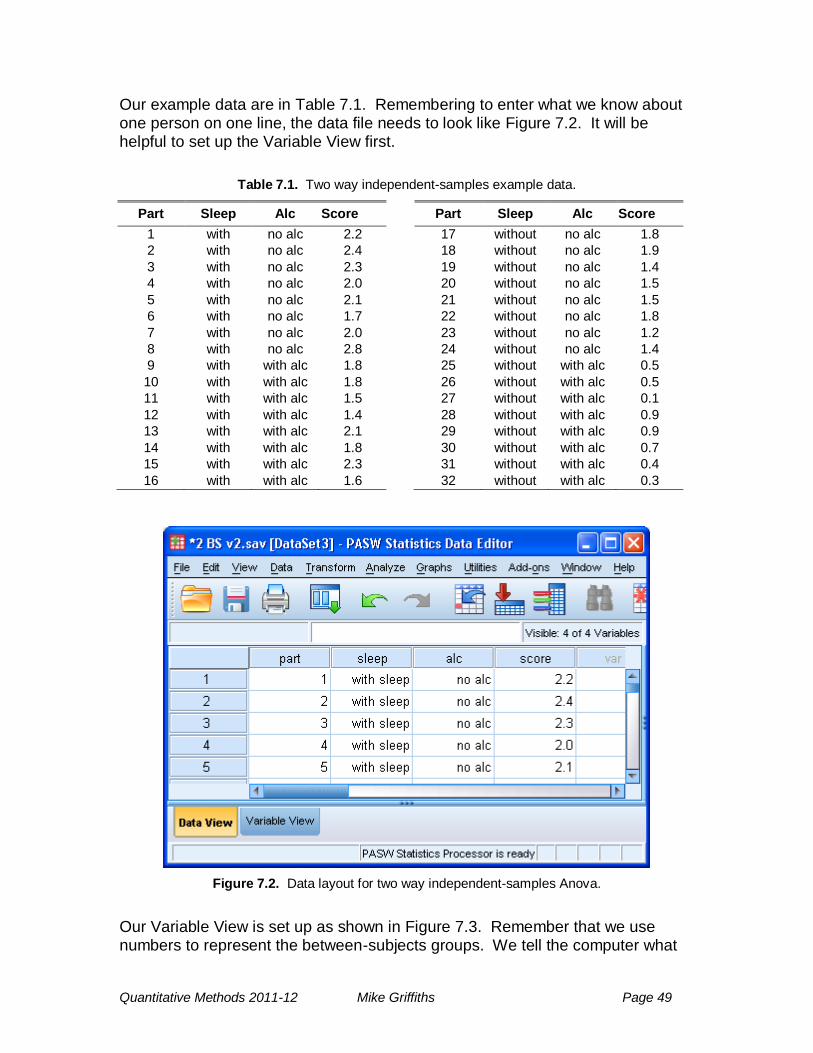
Our example data are in Table 7.1. Remembering to enter what we know about one person on one line, the data file needs to look like Figure 7.2. It will be helpful to set up the Variable View first.
Table 7.1. Two way independent-samples example data.
Part Sleep Alc Score Part Sleep Alc Score
1 with no alc 2.2 17 without no alc 1.8
2 with no alc 2.4 18 without no alc 1.9
3 with no alc 2.3 19 without no alc 1.4
4 with no alc 2.0 20 without no alc 1.5
5 with no alc 2.1 21 without no alc 1.5
6 with no alc 1.7 22 without no alc 1.8
7 with no alc 2.0 23 without no alc 1.2
8 with no alc 2.8 24 without no alc 1.4
9 with with alc 1.8 25 without with alc 0.5
10 with with alc 1.8 26 without with alc 0.5
11 with with alc 1.5 27 without with alc 0.1
12 with with alc 1.4 28 without with alc 0.9
13 with with alc 2.1 29 without with alc 0.9
14 with with alc 1.8 30 without with alc 0.7
15 with with alc 2.3 31 without with alc 0.4
16 with with alc 1.6 32 without with alc 0.3
Figure 7.2. Data layout for two way independent-samples Anova.
Our Variable View is set up as shown in Figure 7.3. Remember that we use numbers to represent the between-subjects groups. We tell the computer what
Quantitative Methods 2011-12 Mike Griffiths Page 50
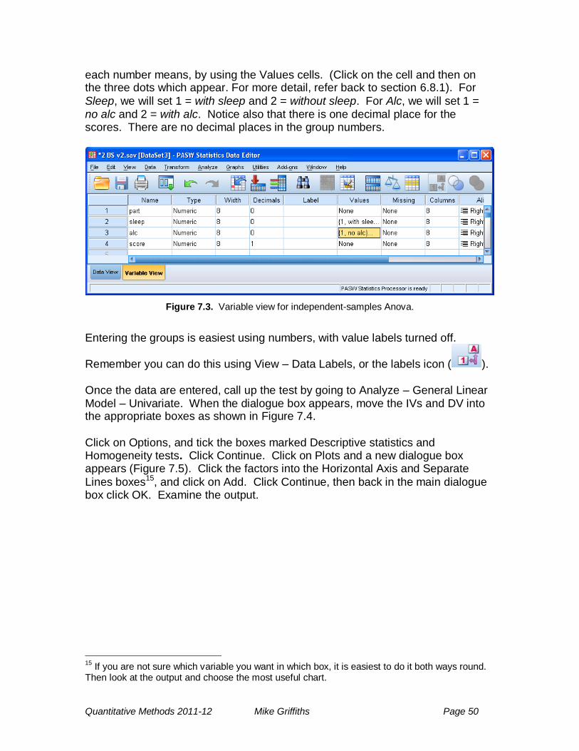
each number means, by using the Values cells. (Click on the cell and then on the three dots which appear. For more detail, refer back to section 6.8.1). For
Sleep, we will set 1 = with sleep and 2 = without sleep. For Alc, we will set 1 = no alc and 2 = with alc. Notice also that there is one decimal place for the scores. There are no decimal places in the group numbers.
Figure 7.3. Variable view for independent-samples Anova.
Entering the groups is easiest using numbers, with value labels turned off.
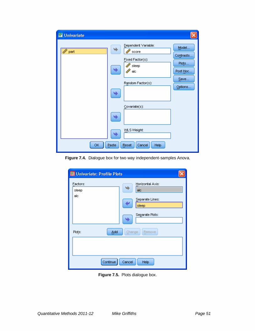
Remember you can do this using View – Data Labels, or the labels icon ( ). Once the data are entered, call up the test by going to Analyze – General Linear Model – Univariate. When the dialogue box appears, move the IVs and DV into the appropriate boxes as shown in Figure 7.4.
Click on Options, and tick the boxes marked Descriptive statistics and Homogeneity tests. Click Continue. Click on Plots and a new dialogue box appears (Figure 7.5). Click the factors into the Horizontal Axis and Separate
Lines boxes15, and click on Add. Click Continue, then back in the main dialogue box click OK. Examine the output.
15
If you are not sure which variable you want in which box, it is easiest to do it both ways round. Then look at the output and choose the most useful chart.
Quantitative Methods 2011-12 Mike Griffiths Page 51
Figure 7.4. Dialogue box for two way independent-samples Anova.
Figure 7.5. Plots dialogue box.
Quantitative Methods 2011-12 Mike Griffiths Page 52
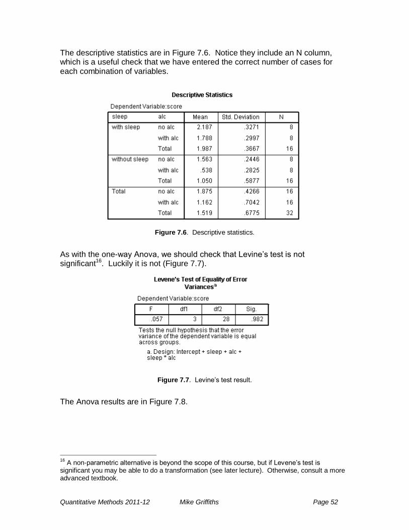
The descriptive statistics are in Figure 7.6. Notice they include an N column, which is a useful check that we have entered the correct number of cases for each combination of variables.
Figure 7.6. Descriptive statistics.
As with the one-way Anova, we should check that Levine‘s test is not significant16. Luckily it is not (Figure 7.7).
Figure 7.7. Levine‘s test result.
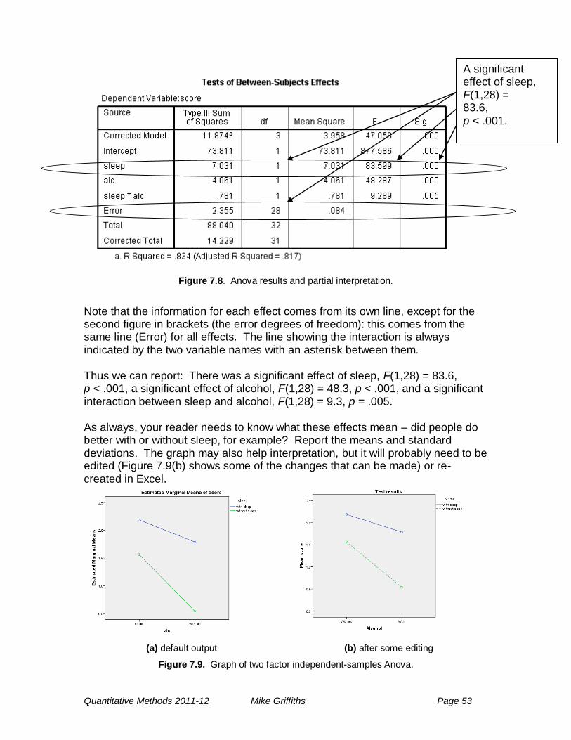
The Anova results are in Figure 7.8.
16
A non-parametric alternative is beyond the scope of this course, but if Levene‘s test is significant you may be able to do a transformation (see later lecture). Otherwise, consult a more advanced textbook.
Quantitative Methods 2011-12 Mike Griffiths Page 53
Figure 7.8. Anova results and partial interpretation.
Note that the information for each effect comes from its own line, except for the second figure in brackets (the error degrees of freedom): this comes from the same line (Error) for all effects. The line showing the interaction is always indicated by the two variable names with an asterisk between them. Thus we can report: There was a significant effect of sleep, F(1,28) = 83.6, p < .001, a significant effect of alcohol, F(1,28) = 48.3, p < .001, and a significant interaction between sleep and alcohol, F(1,28) = 9.3, p = .005. As always, your reader needs to know what these effects mean – did people do better with or without sleep, for example? Report the means and standard deviations. The graph may also help interpretation, but it will probably need to be edited (Figure 7.9(b) shows some of the changes that can be made) or re-
created in Excel.
(a) default output (b) after some editing
Figure 7.9. Graph of two factor independent-samples Anova.
A significant effect of sleep, F(1,28) = 83.6,
p < .001.
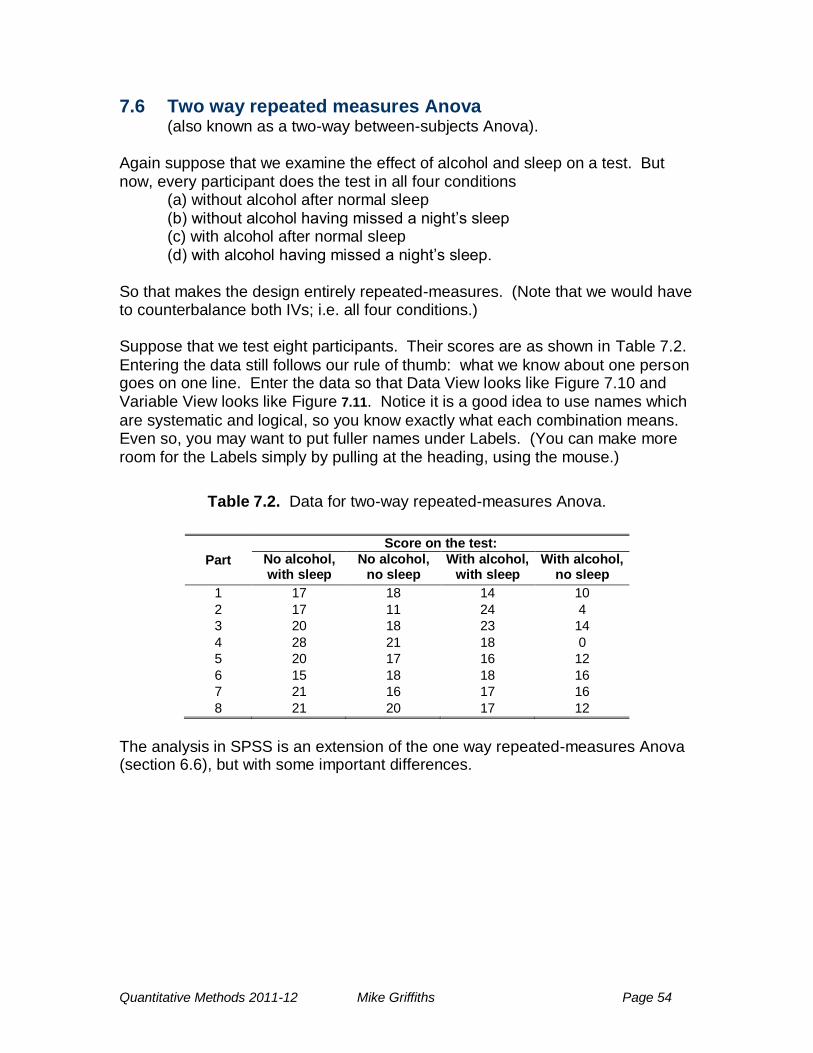
Quantitative Methods 2011-12 Mike Griffiths Page 54
7.6 Two way repeated measures Anova (also known as a two-way between-subjects Anova).
Again suppose that we examine the effect of alcohol and sleep on a test. But now, every participant does the test in all four conditions
(a) without alcohol after normal sleep (b) without alcohol having missed a night‘s sleep (c) with alcohol after normal sleep (d) with alcohol having missed a night‘s sleep.
So that makes the design entirely repeated-measures. (Note that we would have to counterbalance both IVs; i.e. all four conditions.) Suppose that we test eight participants. Their scores are as shown in Table 7.2.
Entering the data still follows our rule of thumb: what we know about one person goes on one line. Enter the data so that Data View looks like Figure 7.10 and Variable View looks like Figure 7.11. Notice it is a good idea to use names which
are systematic and logical, so you know exactly what each combination means. Even so, you may want to put fuller names under Labels. (You can make more room for the Labels simply by pulling at the heading, using the mouse.)
Table 7.2. Data for two-way repeated-measures Anova.
Part
Score on the test:
No alcohol, with sleep
No alcohol, no sleep
With alcohol, with sleep
With alcohol, no sleep
1 17 18 14 10
2 17 11 24 4
3 20 18 23 14
4 28 21 18 0
5 20 17 16 12
6 15 18 18 16
7 21 16 17 16
8 21 20 17 12
The analysis in SPSS is an extension of the one way repeated-measures Anova (section 6.6), but with some important differences.
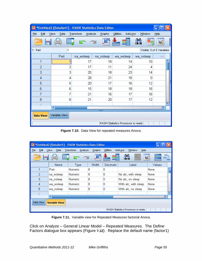
Quantitative Methods 2011-12 Mike Griffiths Page 55
Figure 7.10. Data View for repeated measures Anova.
Figure 7.11. Variable view for Repeated Measures factorial Anova.
Click on Analyze – General Linear Model – Repeated Measures. The Define Factors dialogue box appears (Figure 7.12). Replace the default name (factor1)
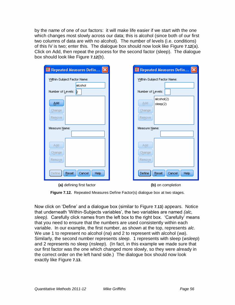
Quantitative Methods 2011-12 Mike Griffiths Page 56
by the name of one of our factors: it will make life easier if we start with the one which changes most slowly across our data; this is alcohol (since both of our first two columns of data are with no alcohol). The number of levels (i.e. conditions) of this IV is two; enter this. The dialogue box should now look like Figure 7.12(a).
Click on Add, then repeat the process for the second factor (sleep). The dialogue box should look like Figure 7.12(b).
(a) defining first factor (b) on completion
Figure 7.12. Repeated Measures Define Factor(s) dialogue box at two stages.
Now click on ‗Define‘ and a dialogue box (similar to Figure 7.13) appears. Notice
that underneath ‗Within-Subjects variables‘, the two variables are named (alc, sleep). Carefully click names from the left box to the right box. ‗Carefully‘ means that you need to ensure that the numbers are used consistently within each variable. In our example, the first number, as shown at the top, represents alc. We use 1 to represent no alcohol (na) and 2 to represent with alcohol (wa). Similarly, the second number represents sleep. 1 represents with sleep (wsleep) and 2 represents no sleep (nsleep). (In fact, in this example we made sure that our first factor was the one which changed more slowly, so they were already in the correct order on the left hand side.) The dialogue box should now look exactly like Figure 7.13.
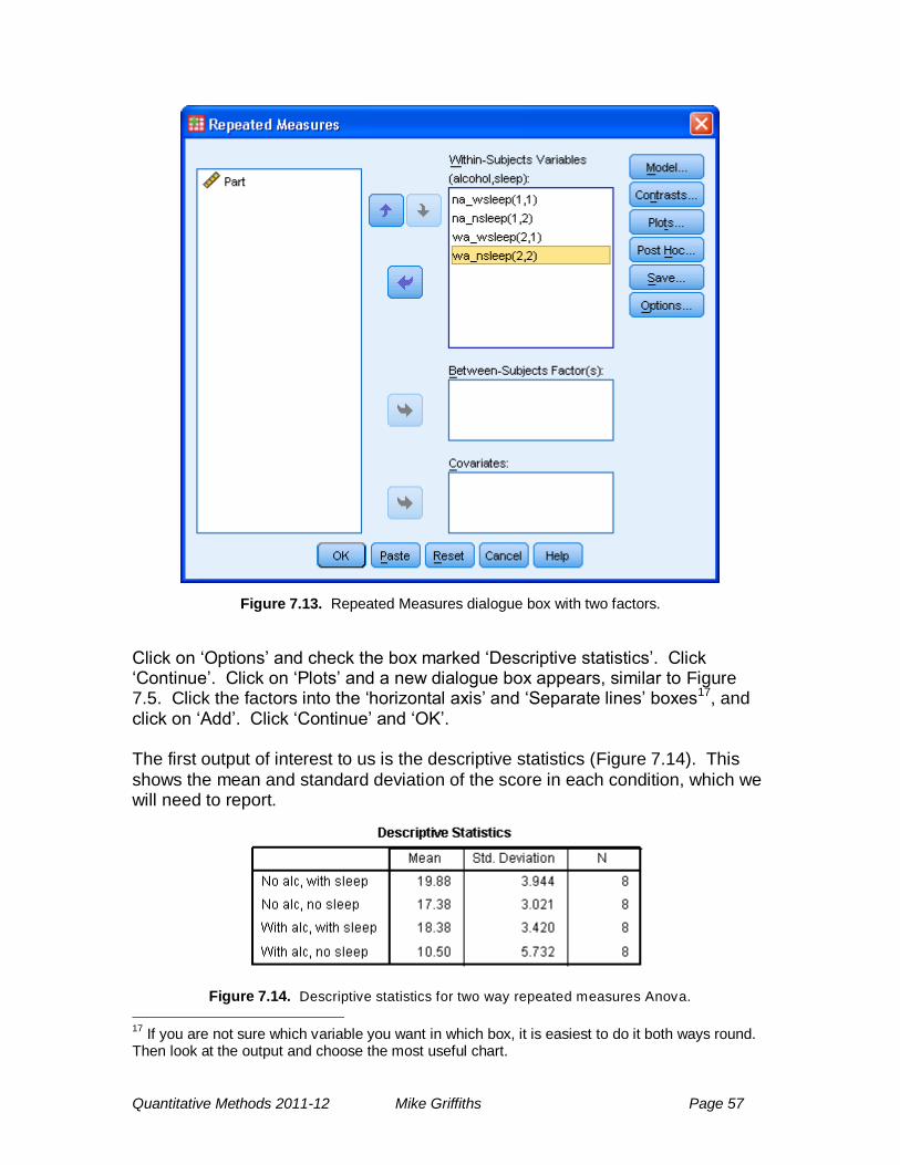
Quantitative Methods 2011-12 Mike Griffiths Page 57
Figure 7.13. Repeated Measures dialogue box with two factors.
Click on ‗Options‘ and check the box marked ‗Descriptive statistics‘. Click ‗Continue‘. Click on ‗Plots‘ and a new dialogue box appears, similar to Figure 7.5. Click the factors into the ‗horizontal axis‘ and ‗Separate lines‘ boxes17, and click on ‗Add‘. Click ‗Continue‘ and ‗OK‘. The first output of interest to us is the descriptive statistics (Figure 7.14). This
shows the mean and standard deviation of the score in each condition, which we will need to report.
Figure 7.14. Descriptive statistics for two way repeated measures Anova.
17
If you are not sure which variable you want in which box, it is easiest to do it both ways round. Then look at the output and choose the most useful chart.
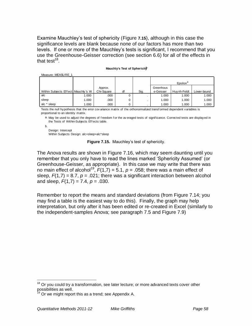
Quantitative Methods 2011-12 Mike Griffiths Page 58
Examine Mauchley‘s test of sphericity (Figure 7.15), although in this case the
significance levels are blank because none of our factors has more than two levels. If one or more of the Mauchley‘s tests is significant, I recommend that you use the Greenhouse-Geisser correction (see section 6.6) for all of the effects in that test18.
Mauchly's Test of Sphericityb
Measure: MEASURE_1
1.000 .000 0 . 1.000 1.000 1.000
1.000 .000 0 . 1.000 1.000 1.000
1.000 .000 0 . 1.000 1.000 1.000
Within Subjects Ef f ect
alc
sleep
alc * sleep
Mauchly 's W
Approx.
Chi-Square df Sig.
Greenhous
e-Geisser Huynh-Feldt Lower-bound
Epsilona
Tests the null hypothesis that the error cov ariance matrix of the orthonormalized transf ormed dependent variables is
proportional to an identity matrix.
May be used to adjust the degrees of f reedom f or the av eraged tests of signif icance. Corrected tests are displayed in
the Tests of Within-Subjects Ef f ects table.
a.
Design: Intercept
Within Subjects Design: alc+sleep+alc*sleep
b.
Figure 7.15. Mauchley‘s test of sphericity.
The Anova results are shown in Figure 7.16, which may seem daunting until you remember that you only have to read the lines marked ‗Sphericity Assumed‘ (or Greenhouse-Geisser, as appropriate). In this case we may write that there was no main effect of alcohol19, F(1,7) = 5.1, p = .058; there was a main effect of sleep, F(1,7) = 8.7, p = .021; there was a significant interaction between alcohol and sleep, F(1,7) = 7.4, p = .030.
Remember to report the means and standard deviations (from Figure 7.14; you
may find a table is the easiest way to do this). Finally, the graph may help interpretation, but only after it has been edited or re-created in Excel (similarly to the independent-samples Anova; see paragraph 7.5 and Figure 7.9)
18
Or you could try a transformation, see later lecture; or more advanced texts cover other possibilities as well. 19
Or we might report this as a trend; see Appendix A.
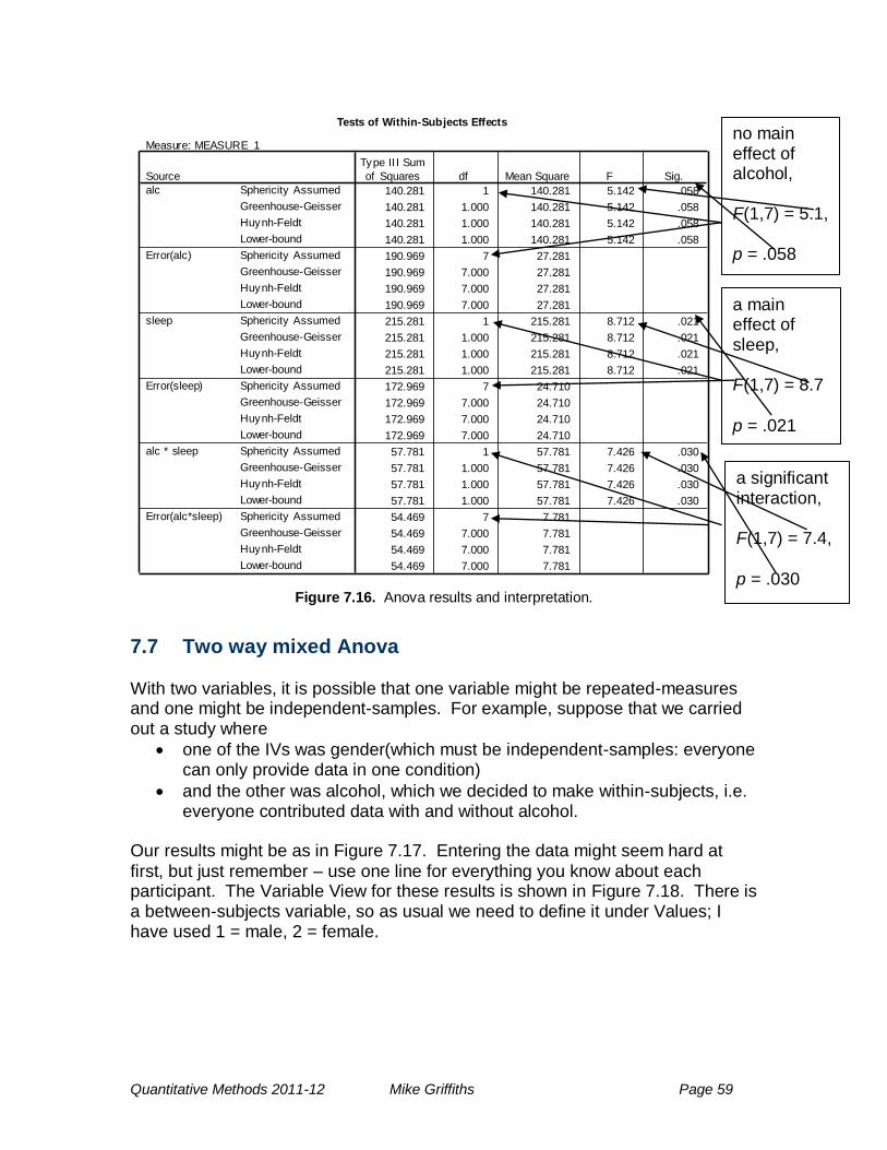
Quantitative Methods 2011-12 Mike Griffiths Page 59
Tests of Within-Subjects Effects
Measure: MEASURE_1
140.281 1 140.281 5.142 .058
140.281 1.000 140.281 5.142 .058
140.281 1.000 140.281 5.142 .058
140.281 1.000 140.281 5.142 .058
190.969 7 27.281
190.969 7.000 27.281
190.969 7.000 27.281
190.969 7.000 27.281
215.281 1 215.281 8.712 .021
215.281 1.000 215.281 8.712 .021
215.281 1.000 215.281 8.712 .021
215.281 1.000 215.281 8.712 .021
172.969 7 24.710
172.969 7.000 24.710
172.969 7.000 24.710
172.969 7.000 24.710
57.781 1 57.781 7.426 .030
57.781 1.000 57.781 7.426 .030
57.781 1.000 57.781 7.426 .030
57.781 1.000 57.781 7.426 .030
54.469 7 7.781
54.469 7.000 7.781
54.469 7.000 7.781
54.469 7.000 7.781
Sphericity Assumed
Greenhouse-Geisser
Huynh-Feldt
Lower-bound
Sphericity Assumed
Greenhouse-Geisser
Huynh-Feldt
Lower-bound
Sphericity Assumed
Greenhouse-Geisser
Huynh-Feldt
Lower-bound
Sphericity Assumed
Greenhouse-Geisser
Huynh-Feldt
Lower-bound
Sphericity Assumed
Greenhouse-Geisser
Huynh-Feldt
Lower-bound
Sphericity Assumed
Greenhouse-Geisser
Huynh-Feldt
Lower-bound
Source
alc
Error(alc)
sleep
Error(sleep)
alc * sleep
Error(alc*sleep)
Type II I Sum
of Squares df Mean Square F Sig.
Figure 7.16. Anova results and interpretation.
7.7 Two way mixed Anova With two variables, it is possible that one variable might be repeated-measures and one might be independent-samples. For example, suppose that we carried out a study where
one of the IVs was gender(which must be independent-samples: everyone can only provide data in one condition)
and the other was alcohol, which we decided to make within-subjects, i.e. everyone contributed data with and without alcohol.
Our results might be as in Figure 7.17. Entering the data might seem hard at
first, but just remember – use one line for everything you know about each participant. The Variable View for these results is shown in Figure 7.18. There is a between-subjects variable, so as usual we need to define it under Values; I have used 1 = male, 2 = female.
no main effect of alcohol, F(1,7) = 5.1, p = .058
a main effect of sleep, F(1,7) = 8.7
p = .021
a significant interaction, F(1,7) = 7.4,
p = .030
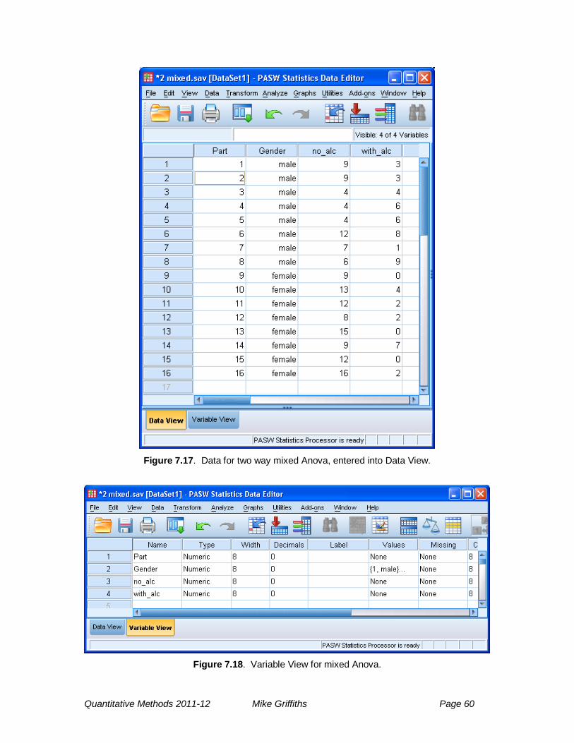
Quantitative Methods 2011-12 Mike Griffiths Page 60
Figure 7.17. Data for two way mixed Anova, entered into Data View.
Figure 7.18. Variable View for mixed Anova.
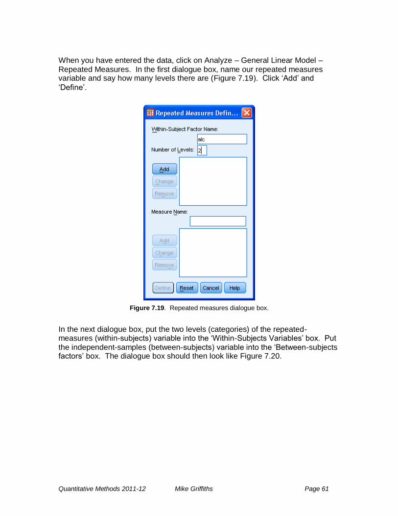
Quantitative Methods 2011-12 Mike Griffiths Page 61
When you have entered the data, click on Analyze – General Linear Model – Repeated Measures. In the first dialogue box, name our repeated measures variable and say how many levels there are (Figure 7.19). Click ‗Add‘ and
‗Define‘.
Figure 7.19. Repeated measures dialogue box.
In the next dialogue box, put the two levels (categories) of the repeated-measures (within-subjects) variable into the ‗Within-Subjects Variables‘ box. Put the independent-samples (between-subjects) variable into the ‗Between-subjects factors‘ box. The dialogue box should then look like Figure 7.20.
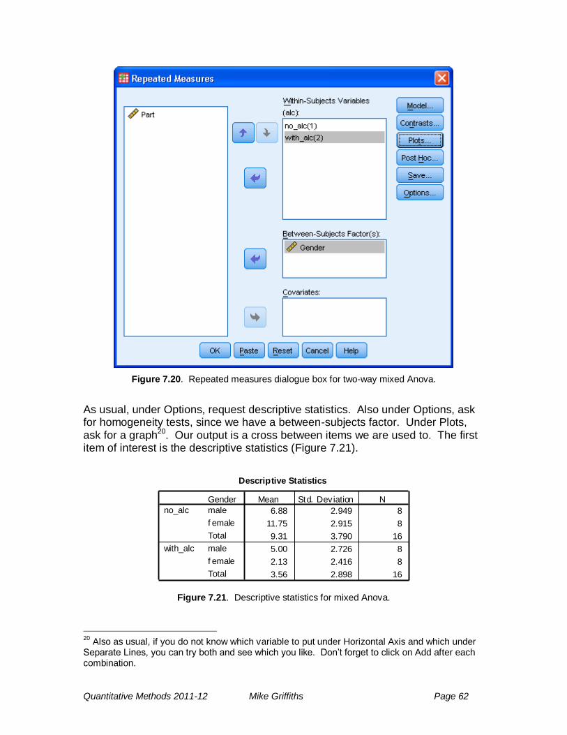
Quantitative Methods 2011-12 Mike Griffiths Page 62
Figure 7.20. Repeated measures dialogue box for two-way mixed Anova.
As usual, under Options, request descriptive statistics. Also under Options, ask for homogeneity tests, since we have a between-subjects factor. Under Plots, ask for a graph20. Our output is a cross between items we are used to. The first item of interest is the descriptive statistics (Figure 7.21).
Descriptive Statistics
6.88 2.949 8
11.75 2.915 8
9.31 3.790 16
5.00 2.726 8
2.13 2.416 8
3.56 2.898 16
Gender
male
f emale
Total
male
f emale
Total
no_alc
with_alc
Mean Std. Deviation N
Figure 7.21. Descriptive statistics for mixed Anova.
20
Also as usual, if you do not know which variable to put under Horizontal Axis and which under Separate Lines, you can try both and see which you like. Don‘t forget to click on Add after each combination.
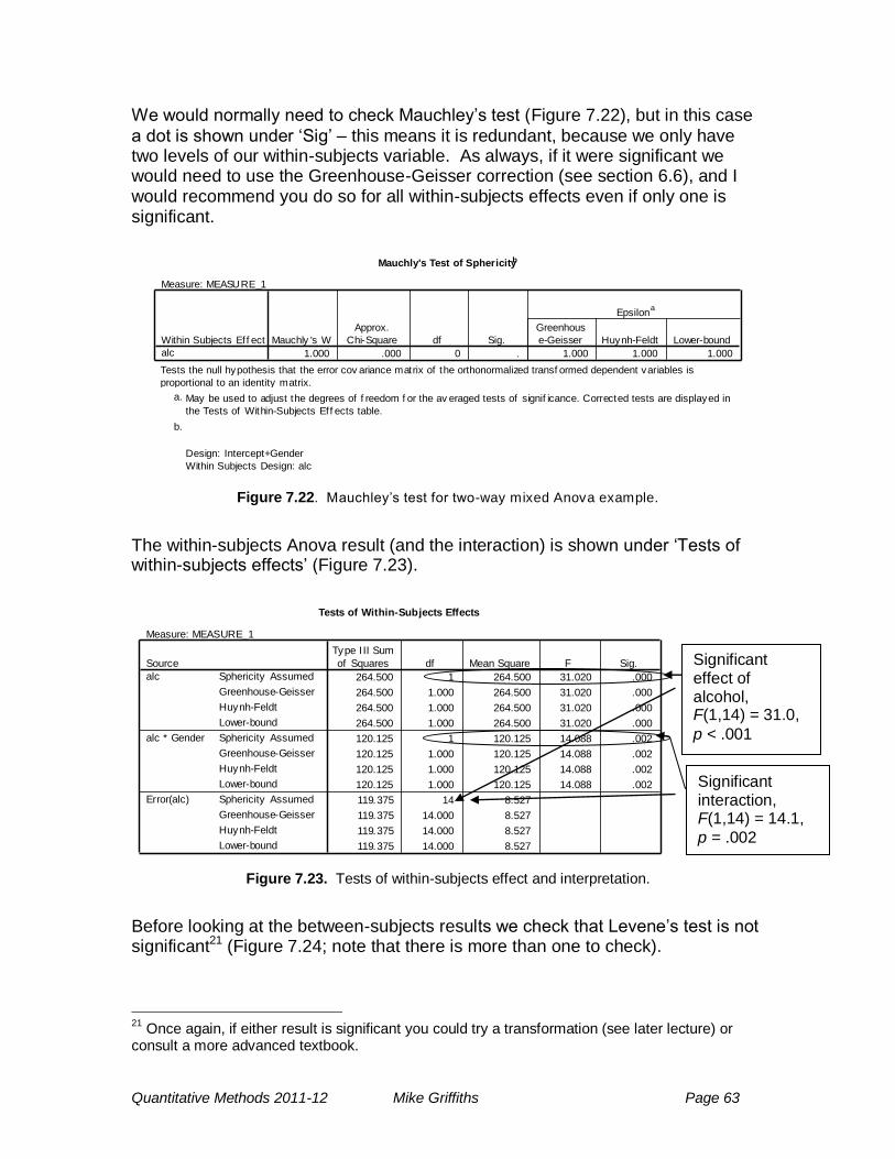
Quantitative Methods 2011-12 Mike Griffiths Page 63
We would normally need to check Mauchley‘s test (Figure 7.22), but in this case
a dot is shown under ‗Sig‘ – this means it is redundant, because we only have two levels of our within-subjects variable. As always, if it were significant we would need to use the Greenhouse-Geisser correction (see section 6.6), and I would recommend you do so for all within-subjects effects even if only one is significant.
Mauchly's Test of Sphericityb
Measure: MEASURE_1
1.000 .000 0 . 1.000 1.000 1.000
Within Subjects Ef f ect
alc
Mauchly 's W
Approx.
Chi-Square df Sig.
Greenhous
e-Geisser Huynh-Feldt Lower-bound
Epsilona
Tests the null hypothesis that the error cov ariance matrix of the orthonormalized transf ormed dependent variables is
proportional to an identity matrix.
May be used to adjust the degrees of f reedom f or the av eraged tests of signif icance. Corrected tests are displayed in
the Tests of Within-Subjects Ef f ects table.
a.
Design: Intercept+Gender
Within Subjects Design: alc
b.
Figure 7.22. Mauchley‘s test for two-way mixed Anova example.
The within-subjects Anova result (and the interaction) is shown under ‗Tests of within-subjects effects‘ (Figure 7.23).
Tests of Within-Subjects Effects
Measure: MEASURE_1
264.500 1 264.500 31.020 .000
264.500 1.000 264.500 31.020 .000
264.500 1.000 264.500 31.020 .000
264.500 1.000 264.500 31.020 .000
120.125 1 120.125 14.088 .002
120.125 1.000 120.125 14.088 .002
120.125 1.000 120.125 14.088 .002
120.125 1.000 120.125 14.088 .002
119.375 14 8.527
119.375 14.000 8.527
119.375 14.000 8.527
119.375 14.000 8.527
Sphericity Assumed
Greenhouse-Geisser
Huynh-Feldt
Lower-bound
Sphericity Assumed
Greenhouse-Geisser
Huynh-Feldt
Lower-bound
Sphericity Assumed
Greenhouse-Geisser
Huynh-Feldt
Lower-bound
Source
alc
alc * Gender
Error(alc)
Type I II Sum
of Squares df Mean Square F Sig.
Figure 7.23. Tests of within-subjects effect and interpretation.
Before looking at the between-subjects results we check that Levene‘s test is not significant21 (Figure 7.24; note that there is more than one to check).
21
Once again, if either result is significant you could try a transformation (see later lecture) or consult a more advanced textbook.
Significant effect of alcohol, F(1,14) = 31.0,
p < .001
Significant interaction, F(1,14) = 14.1,
p = .002
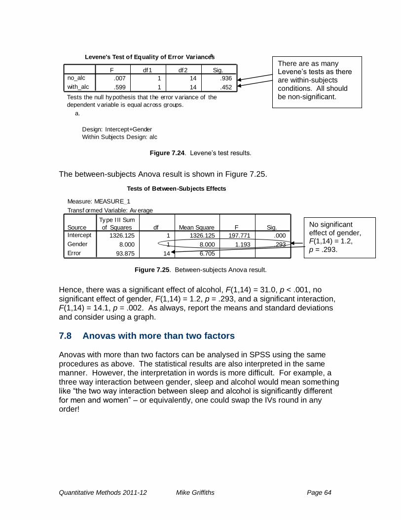
Quantitative Methods 2011-12 Mike Griffiths Page 64
Levene's Test of Equality of Error Variancesa
.007 1 14 .936
.599 1 14 .452
no_alc
with_alc
F df1 df2 Sig.
Tests the null hypothesis that the error variance of the
dependent variable is equal across groups.
Design: Intercept+Gender
Within Subjects Design: alc
a.
Figure 7.24. Levene‘s test results.
The between-subjects Anova result is shown in Figure 7.25.
Tests of Between-Subjects Effects
Measure: MEASURE_1
Transf ormed Variable: Av erage
1326.125 1 1326.125 197.771 .000
8.000 1 8.000 1.193 .293
93.875 14 6.705
Source
Intercept
Gender
Error
Type I II Sum
of Squares df Mean Square F Sig.
Figure 7.25. Between-subjects Anova result.
Hence, there was a significant effect of alcohol, F(1,14) = 31.0, p < .001, no significant effect of gender, F(1,14) = 1.2, p = .293, and a significant interaction, F(1,14) = 14.1, p = .002. As always, report the means and standard deviations and consider using a graph.
7.8 Anovas with more than two factors Anovas with more than two factors can be analysed in SPSS using the same procedures as above. The statistical results are also interpreted in the same manner. However, the interpretation in words is more difficult. For example, a three way interaction between gender, sleep and alcohol would mean something like ―the two way interaction between sleep and alcohol is significantly different for men and women‖ – or equivalently, one could swap the IVs round in any order!
No significant effect of gender, F(1,14) = 1.2,
p = .293.
There are as many Levene‘s tests as there are within-subjects conditions. All should be non-significant.
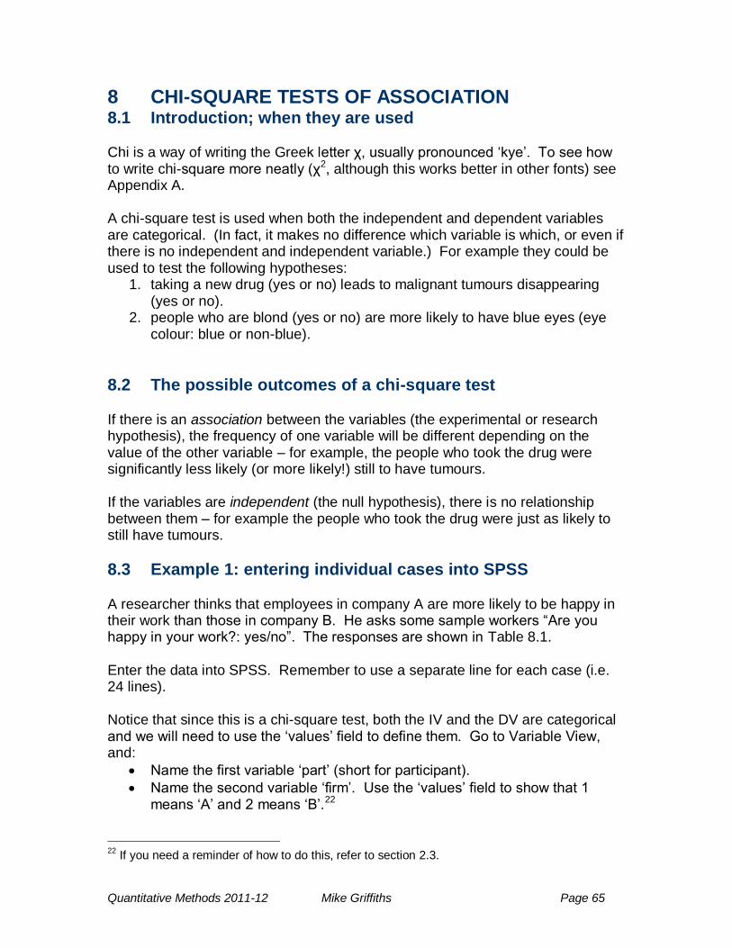
Quantitative Methods 2011-12 Mike Griffiths Page 65
8 CHI-SQUARE TESTS OF ASSOCIATION 8.1 Introduction; when they are used Chi is a way of writing the Greek letter χ, usually pronounced ‗kye‘. To see how to write chi-square more neatly (χ2, although this works better in other fonts) see Appendix A. A chi-square test is used when both the independent and dependent variables are categorical. (In fact, it makes no difference which variable is which, or even if there is no independent and independent variable.) For example they could be used to test the following hypotheses:
1. taking a new drug (yes or no) leads to malignant tumours disappearing (yes or no).
2. people who are blond (yes or no) are more likely to have blue eyes (eye colour: blue or non-blue).
8.2 The possible outcomes of a chi-square test If there is an association between the variables (the experimental or research hypothesis), the frequency of one variable will be different depending on the value of the other variable – for example, the people who took the drug were significantly less likely (or more likely!) still to have tumours. If the variables are independent (the null hypothesis), there is no relationship between them – for example the people who took the drug were just as likely to still have tumours.
8.3 Example 1: entering individual cases into SPSS A researcher thinks that employees in company A are more likely to be happy in their work than those in company B. He asks some sample workers ―Are you happy in your work?: yes/no‖. The responses are shown in Table 8.1. Enter the data into SPSS. Remember to use a separate line for each case (i.e. 24 lines). Notice that since this is a chi-square test, both the IV and the DV are categorical and we will need to use the ‗values‘ field to define them. Go to Variable View, and:
Name the first variable ‗part‘ (short for participant).
Name the second variable ‗firm‘. Use the ‗values‘ field to show that 1 means ‗A‘ and 2 means ‗B‘.22
22
If you need a reminder of how to do this, refer to section 2.3.
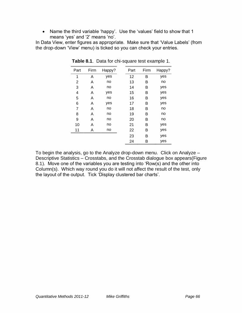
Quantitative Methods 2011-12 Mike Griffiths Page 66
Name the third variable ‗happy‘. Use the ‗values‘ field to show that 1 means ‗yes‘ and ‗2‘ means ‗no‘.
In Data View, enter figures as appropriate. Make sure that ‗Value Labels‘ (from the drop-down ‗View‘ menu) is ticked so you can check your entries.
Table 8.1. Data for chi-square test example 1.
Part Firm Happy? Part Firm Happy?
1 A yes 12 B yes
2 A no 13 B no
3 A no 14 B yes
4 A yes 15 B yes
5 A no 16 B yes
6 A yes 17 B yes
7 A no 18 B no
8 A no 19 B no
9 A no 20 B no
10 A no 21 B yes
11 A no 22 B yes
23 B yes
24 B yes
To begin the analysis, go to the Analyze drop-down menu. Click on Analyze – Descriptive Statistics – Crosstabs, and the Crosstab dialogue box appears(Figure 8.1). Move one of the variables you are testing into ‗Row(s) and the other into Column(s). Which way round you do it will not affect the result of the test, only the layout of the output. Tick ‗Display clustered bar charts‘.
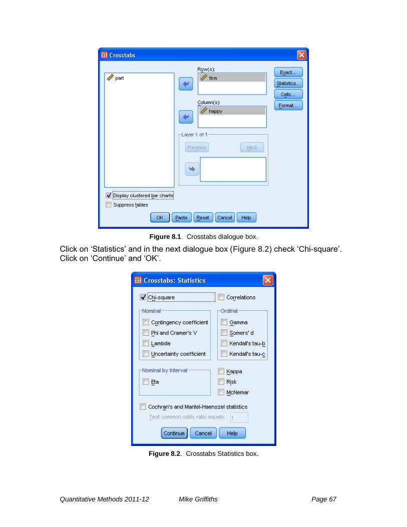
Quantitative Methods 2011-12 Mike Griffiths Page 67
Figure 8.1. Crosstabs dialogue box.
Click on ‗Statistics‘ and in the next dialogue box (Figure 8.2) check ‗Chi-square‘. Click on ‗Continue‘ and ‗OK‘.
Figure 8.2. Crosstabs Statistics box.
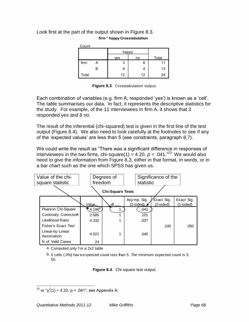
Quantitative Methods 2011-12 Mike Griffiths Page 68
Look first at the part of the output shown in Figure 8.3.
Figure 8.3. Crosstabulation output.
Each combination of variables (e.g. firm A, responded ‗yes‘) is known as a ‗cell‘. The table summarises our data. In fact, it represents the descriptive statistics for the study. For example, of the 11 interviewees in firm A, it shows that 3 responded yes and 8 no. The result of the inferential (chi-squared) test is given in the first line of the test output (Figure 8.4). We also need to look carefully at the footnotes to see if any of the ‗expected values‘ are less than 5 (see constraints, paragraph 8.7).
We could write the result as ―There was a significant difference in responses of interviewees in the two firms, chi-square(1) = 4.20, p = .041.‖23 We would also need to give the information from Figure 8.3, either in that format, in words, or in
a bar chart such as the one which SPSS has given us.
Value of the chi-square statistic
Degrees of freedom
Significance of the statistic
Chi-Square Tests
4.196b 1 .041
2.685 1 .101
4.332 1 .037
.100 .050
4.021 1 .045
24
Pearson Chi-Square
Continuity Correctiona
Likelihood Ratio
Fisher's Exact Test
Linear-by-Linear
Association
N of Valid Cases
Value df
Asy mp. Sig.
(2-sided)
Exact Sig.
(2-sided)
Exact Sig.
(1-sided)
Computed only f or a 2x2 tablea.
0 cells (.0%) hav e expected count l ess than 5. The minimum expected count is 5.
50.
b.
Figure 8.4. Chi-square test output.
23
or ―χ2(1) = 4.20, p = .041‖; see Appendix A.
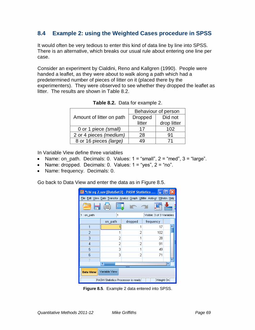
Quantitative Methods 2011-12 Mike Griffiths Page 69
8.4 Example 2: using the Weighted Cases procedure in SPSS It would often be very tedious to enter this kind of data line by line into SPSS. There is an alternative, which breaks our usual rule about entering one line per case. Consider an experiment by Cialdini, Reno and Kallgren (1990). People were handed a leaflet, as they were about to walk along a path which had a predetermined number of pieces of litter on it (placed there by the experimenters). They were observed to see whether they dropped the leaflet as litter. The results are shown in Table 8.2.
Table 8.2. Data for example 2.
Amount of litter on path
Behaviour of person
Dropped litter
Did not drop litter
0 or 1 piece (small) 17 102
2 or 4 pieces (medium) 28 91
8 or 16 pieces (large) 49 71
In Variable View define three variables
Name: on_path. Decimals: 0. Values: 1 = ―small‖, 2 = ―med‖, 3 = ―large‖.
Name: dropped. Decimals: 0. Values: 1 = ―yes‖, 2 = ―no‖.
Name: frequency. Decimals: 0. Go back to Data View and enter the data as in Figure 8.5.
Figure 8.5. Example 2 data entered into SPSS.
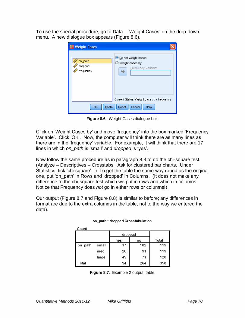
Quantitative Methods 2011-12 Mike Griffiths Page 70
To use the special procedure, go to Data – ‗Weight Cases‘ on the drop-down menu. A new dialogue box appears (Figure 8.6).
Figure 8.6. Weight Cases dialogue box.
Click on ‗Weight Cases by‘ and move ‗frequency‘ into the box marked ‗Frequency Variable‘. Click ‗OK‘. Now, the computer will think there are as many lines as there are in the ‗frequency‘ variable. For example, it will think that there are 17 lines in which on_path is ‗small‘ and dropped is ‗yes‘. Now follow the same procedure as in paragraph 8.3 to do the chi-square test. (Analyze – Descriptives – Crosstabs. Ask for clustered bar charts. Under Statistics, tick ‗chi-square‘. ) To get the table the same way round as the original one, put ‗on_path‘ in Rows and ‗dropped‘ in Columns. (It does not make any difference to the chi-square test which we put in rows and which in columns. Notice that Frequency does not go in either rows or columns!) Our output (Figure 8.7 and Figure 8.8) is similar to before; any differences in
format are due to the extra columns in the table, not to the way we entered the data).
Figure 8.7. Example 2 output: table.

Quantitative Methods 2011-12 Mike Griffiths Page 71
Chi-Square Tests
22.433a 2 .000
22.463 2 .000
21.706 1 .000
358
Pearson Chi-Square
Likelihood Ratio
Linear-by-Linear
Association
N of Valid Cases
Value df
Asy mp. Sig.
(2-sided)
0 cells (.0%) hav e expected count l ess than 5. The
minimum expected count is 31.25.
a.
Figure 8.8. Example 2 output: test results.
Check the footnote to see whether there are any problems with expected counts being less than 5 (see section 8.7). In this case there are not. So whether people dropped litter was significantly affected by whether there was already litter on the path, chi-square (2) = 22.4, p < .001. Again, we would include the descriptive statistics in our report, and you may find the bar chart useful (Figure 8.9).
Figure 8.9. Clustered bar graph.
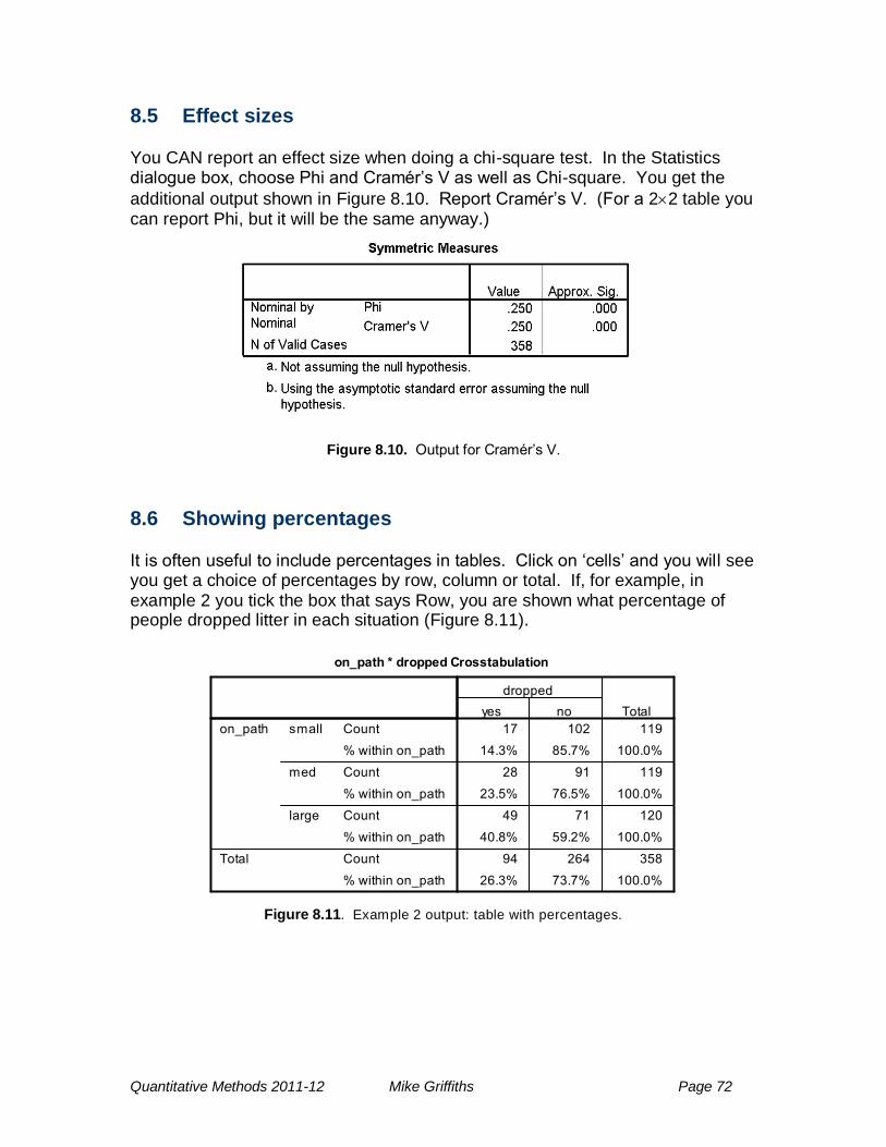
Quantitative Methods 2011-12 Mike Griffiths Page 72
8.5 Effect sizes You CAN report an effect size when doing a chi-square test. In the Statistics dialogue box, choose Phi and Cramér‘s V as well as Chi-square. You get the
additional output shown in Figure 8.10. Report Cramér‘s V. (For a 22 table you can report Phi, but it will be the same anyway.)
Figure 8.10. Output for Cramér‘s V.
8.6 Showing percentages It is often useful to include percentages in tables. Click on ‗cells‘ and you will see you get a choice of percentages by row, column or total. If, for example, in example 2 you tick the box that says Row, you are shown what percentage of people dropped litter in each situation (Figure 8.11).
Figure 8.11. Example 2 output: table with percentages.
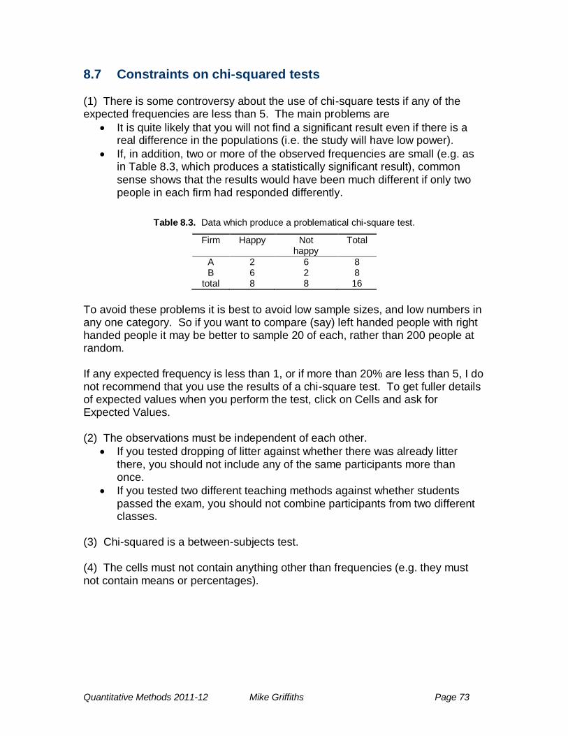
Quantitative Methods 2011-12 Mike Griffiths Page 73
8.7 Constraints on chi-squared tests (1) There is some controversy about the use of chi-square tests if any of the expected frequencies are less than 5. The main problems are
It is quite likely that you will not find a significant result even if there is a real difference in the populations (i.e. the study will have low power).
If, in addition, two or more of the observed frequencies are small (e.g. as in Table 8.3, which produces a statistically significant result), common
sense shows that the results would have been much different if only two people in each firm had responded differently.
Table 8.3. Data which produce a problematical chi-square test.
Firm Happy Not happy
Total
A 2 6 8 B 6 2 8
total 8 8 16
To avoid these problems it is best to avoid low sample sizes, and low numbers in any one category. So if you want to compare (say) left handed people with right handed people it may be better to sample 20 of each, rather than 200 people at random. If any expected frequency is less than 1, or if more than 20% are less than 5, I do not recommend that you use the results of a chi-square test. To get fuller details of expected values when you perform the test, click on Cells and ask for Expected Values. (2) The observations must be independent of each other.
If you tested dropping of litter against whether there was already litter there, you should not include any of the same participants more than once.
If you tested two different teaching methods against whether students passed the exam, you should not combine participants from two different classes.
(3) Chi-squared is a between-subjects test. (4) The cells must not contain anything other than frequencies (e.g. they must not contain means or percentages).
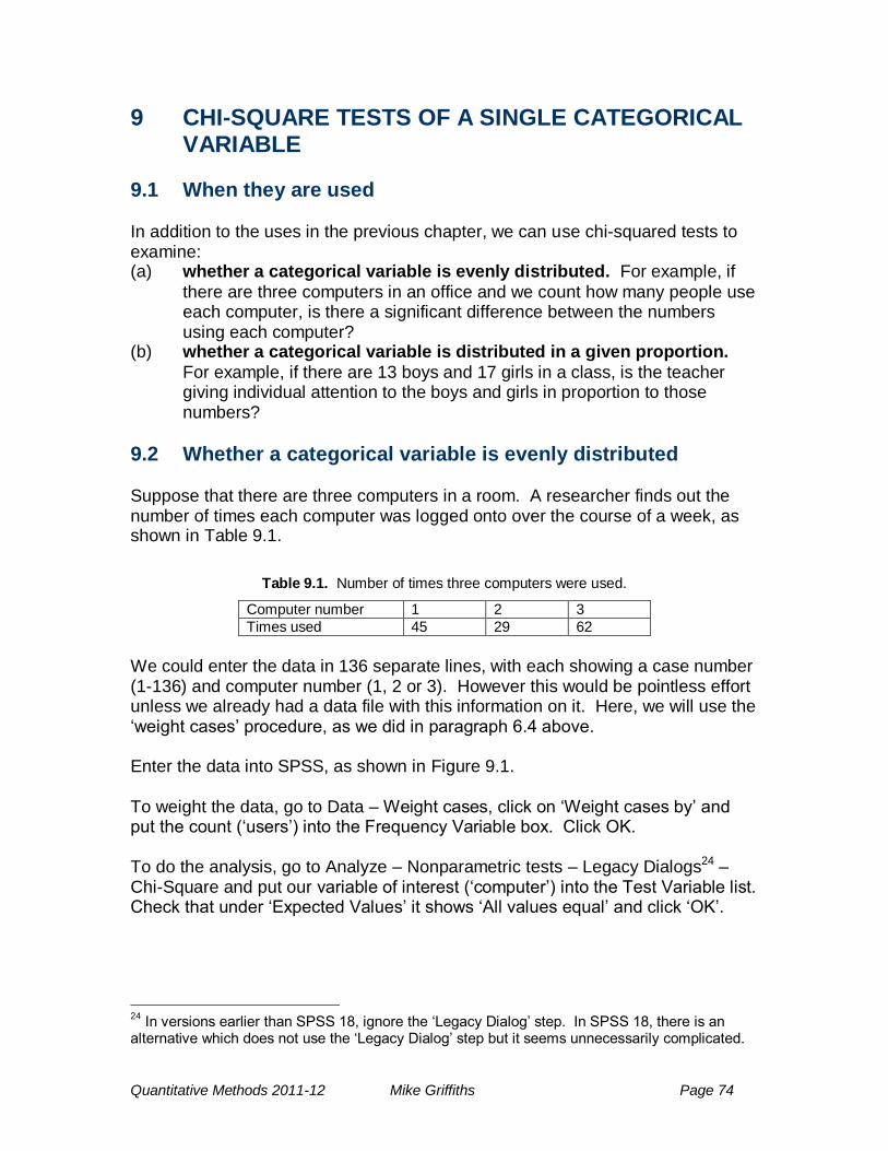
Quantitative Methods 2011-12 Mike Griffiths Page 74
9 CHI-SQUARE TESTS OF A SINGLE CATEGORICAL VARIABLE
9.1 When they are used In addition to the uses in the previous chapter, we can use chi-squared tests to examine: (a) whether a categorical variable is evenly distributed. For example, if
there are three computers in an office and we count how many people use each computer, is there a significant difference between the numbers using each computer?
(b) whether a categorical variable is distributed in a given proportion.
For example, if there are 13 boys and 17 girls in a class, is the teacher giving individual attention to the boys and girls in proportion to those numbers?
9.2 Whether a categorical variable is evenly distributed Suppose that there are three computers in a room. A researcher finds out the number of times each computer was logged onto over the course of a week, as shown in Table 9.1.
Table 9.1. Number of times three computers were used.
Computer number 1 2 3
Times used 45 29 62
We could enter the data in 136 separate lines, with each showing a case number (1-136) and computer number (1, 2 or 3). However this would be pointless effort unless we already had a data file with this information on it. Here, we will use the ‗weight cases‘ procedure, as we did in paragraph 6.4 above. Enter the data into SPSS, as shown in Figure 9.1. To weight the data, go to Data – Weight cases, click on ‗Weight cases by‘ and put the count (‗users‘) into the Frequency Variable box. Click OK. To do the analysis, go to Analyze – Nonparametric tests – Legacy Dialogs24 – Chi-Square and put our variable of interest (‗computer‘) into the Test Variable list. Check that under ‗Expected Values‘ it shows ‗All values equal‘ and click ‗OK‘.
24
In versions earlier than SPSS 18, ignore the ‗Legacy Dialog‘ step. In SPSS 18, there is an alternative which does not use the ‗Legacy Dialog‘ step but it seems unnecessarily complicated.
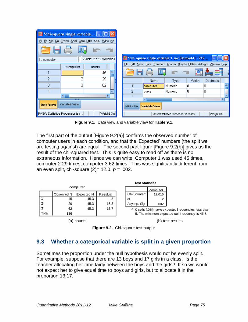
Quantitative Methods 2011-12 Mike Griffiths Page 75
Figure 9.1. Data view and variable view for Table 9.1.
The first part of the output [Figure 9.2(a)] confirms the observed number of
computer users in each condition, and that the ‗Expected‘ numbers (the split we are testing against) are equal. The second part figure [Figure 9.2(b)] gives us the result of the chi-squared test. This is quite easy to read off as there is no extraneous information. Hence we can write: Computer 1 was used 45 times, computer 2 29 times, computer 3 62 times. This was significantly different from an even split, chi-square (2)= 12.0, p = .002.
computer
45 45.3 -.3
29 45.3 -16.3
62 45.3 16.7
136
1
2
3
Total
Observed N Expected N Residual
Test Statistics
12.015
2
.002
Chi-Square a
df
Asy mp. Sig.
computer
0 cells (.0%) hav e expected f requencies less than
5. The minimum expected cell f requency is 45.3.
a.
(a) counts (b) test results
Figure 9.2. Chi-square test output.
9.3 Whether a categorical variable is split in a given proportion Sometimes the proportion under the null hypothesis would not be evenly split. For example, suppose that there are 13 boys and 17 girls in a class. Is the teacher allocating her time fairly between the boys and the girls? If so we would not expect her to give equal time to boys and girls, but to allocate it in the proportion 13:17.
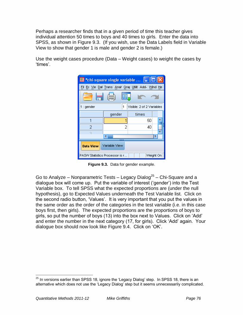
Quantitative Methods 2011-12 Mike Griffiths Page 76
Perhaps a researcher finds that in a given period of time this teacher gives individual attention 50 times to boys and 40 times to girls. Enter the data into SPSS, as shown in Figure 9.3. (If you wish, use the Data Labels field in Variable
View to show that gender 1 is male and gender 2 is female.) Use the weight cases procedure (Data – Weight cases) to weight the cases by ‗times‘.
Figure 9.3. Data for gender example.
Go to Analyze – Nonparametric Tests – Legacy Dialog25 – Chi-Square and a dialogue box will come up. Put the variable of interest (‗gender‘) into the Test Variable box. To tell SPSS what the expected proportions are (under the null hypothesis), go to Expected Values underneath the Test Variable list. Click on the second radio button, ‗Values‘. It is very important that you put the values in the same order as the order of the categories in the test variable (i.e. in this case boys first, then girls). The expected proportions are the proportions of boys to girls, so put the number of boys (13) into the box next to Values. Click on ‗Add‘ and enter the number in the next category (17, for girls). Click ‗Add‘ again. Your dialogue box should now look like Figure 9.4. Click on ‗OK‘.
25
In versions earlier than SPSS 18, ignore the ‗Legacy Dialog‘ step. In SPSS 18, there is an alternative which does not use the ‗Legacy Dialog‘ step but it seems unnecessarily complicated.
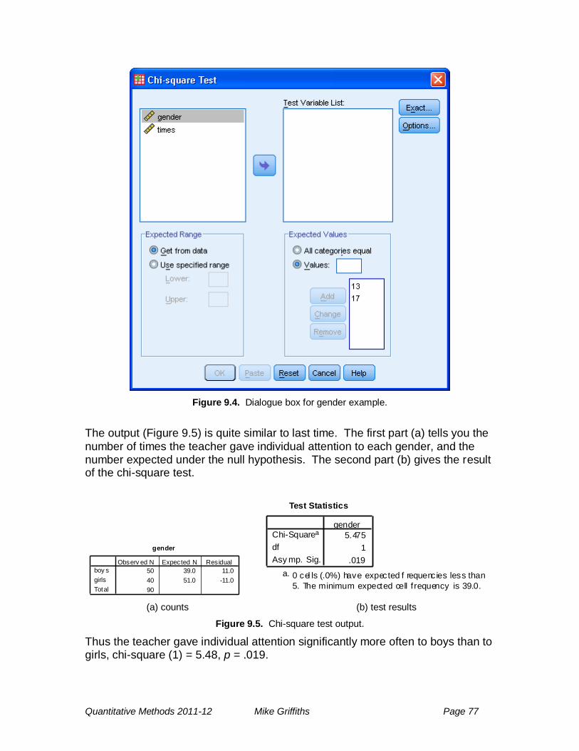
Quantitative Methods 2011-12 Mike Griffiths Page 77
Figure 9.4. Dialogue box for gender example.
The output (Figure 9.5) is quite similar to last time. The first part (a) tells you the
number of times the teacher gave individual attention to each gender, and the number expected under the null hypothesis. The second part (b) gives the result of the chi-square test.
gender
50 39.0 11.0
40 51.0 -11.0
90
boy s
girls
Total
Observ ed N Expected N Residual
Test Statistics
5.475
1
.019
Chi-Squarea
df
Asy mp. Sig.
gender
0 cel ls (.0%) have expected f requencies less than
5. The minimum expected cell f requency is 39.0.
a.
(a) counts (b) test results
Figure 9.5. Chi-square test output.
Thus the teacher gave individual attention significantly more often to boys than to girls, chi-square (1) = 5.48, p = .019.
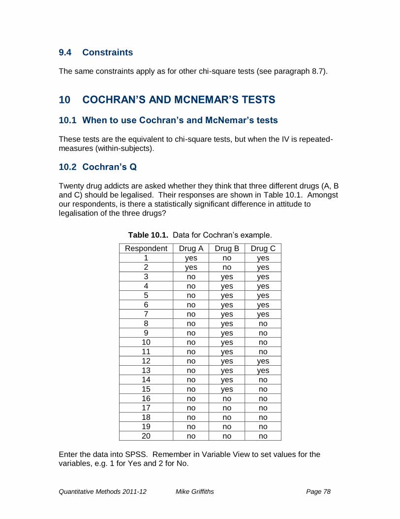
Quantitative Methods 2011-12 Mike Griffiths Page 78
9.4 Constraints The same constraints apply as for other chi-square tests (see paragraph 8.7).
10 COCHRAN’S AND MCNEMAR’S TESTS
10.1 When to use Cochran’s and McNemar’s tests These tests are the equivalent to chi-square tests, but when the IV is repeated-measures (within-subjects).
10.2 Cochran’s Q Twenty drug addicts are asked whether they think that three different drugs (A, B and C) should be legalised. Their responses are shown in Table 10.1. Amongst our respondents, is there a statistically significant difference in attitude to legalisation of the three drugs?
Table 10.1. Data for Cochran‘s example.
Respondent Drug A Drug B Drug C
1 yes no yes
2 yes no yes
3 no yes yes
4 no yes yes
5 no yes yes
6 no yes yes
7 no yes yes
8 no yes no
9 no yes no
10 no yes no
11 no yes no
12 no yes yes
13 no yes yes
14 no yes no
15 no yes no
16 no no no
17 no no no
18 no no no
19 no no no
20 no no no
Enter the data into SPSS. Remember in Variable View to set values for the variables, e.g. 1 for Yes and 2 for No.
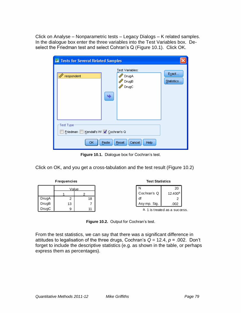
Quantitative Methods 2011-12 Mike Griffiths Page 79
Click on Analyse – Nonparametric tests – Legacy Dialogs – K related samples. In the dialogue box enter the three variables into the Test Variables box. De-select the Friedman test and select Cohran‘s Q (Figure 10.1). Click OK.
Figure 10.1. Dialogue box for Cochran‘s test.
Click on OK, and you get a cross-tabulation and the test result (Figure 10.2)
Frequencies
2 18
13 7
9 11
DrugA
DrugB
DrugC
1 2
Value
Test Statistics
20
12.400a
2
.002
N
Cochran's Q
df
Asy mp. Sig.
1 is t reated as a success.a.
Figure 10.2. Output for Cochran‘s test.
From the test statistics, we can say that there was a significant difference in attitudes to legalisation of the three drugs, Cochran‘s Q = 12.4, p = .002. Don‘t forget to include the descriptive statistics (e.g. as shown in the table, or perhaps express them as percentages).
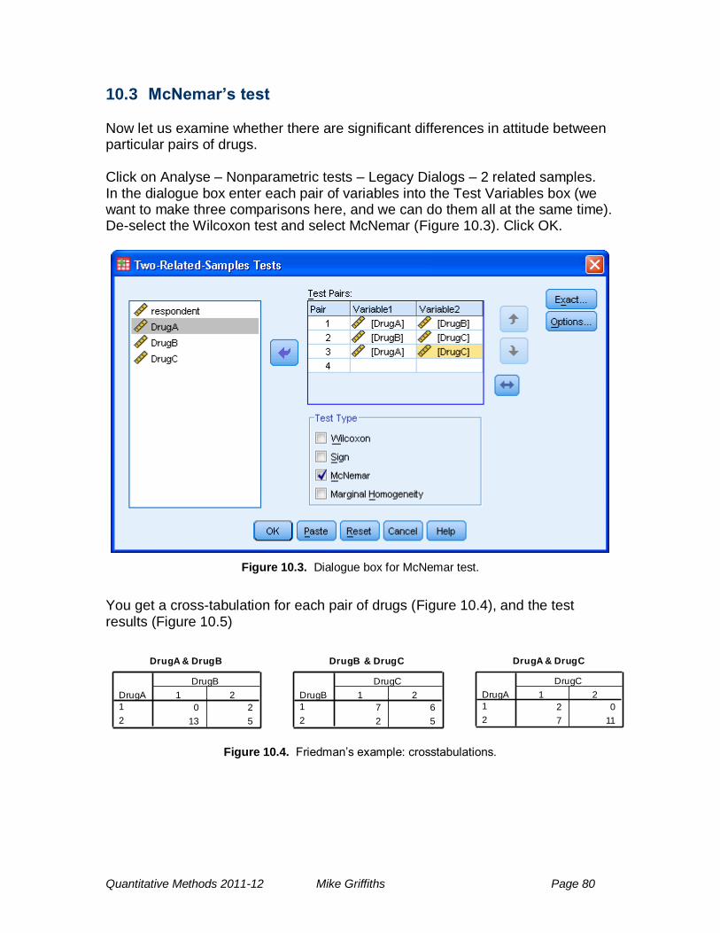
Quantitative Methods 2011-12 Mike Griffiths Page 80
10.3 McNemar’s test Now let us examine whether there are significant differences in attitude between particular pairs of drugs. Click on Analyse – Nonparametric tests – Legacy Dialogs – 2 related samples. In the dialogue box enter each pair of variables into the Test Variables box (we want to make three comparisons here, and we can do them all at the same time). De-select the Wilcoxon test and select McNemar (Figure 10.3). Click OK.
Figure 10.3. Dialogue box for McNemar test.
You get a cross-tabulation for each pair of drugs (Figure 10.4), and the test results (Figure 10.5)
DrugA & DrugB
0 2
13 5
DrugA
1
2
1 2
DrugB
DrugB & DrugC
7 6
2 5
DrugB
1
2
1 2
DrugC
DrugA & DrugC
2 0
7 11
DrugA
1
2
1 2
DrugC
Figure 10.4. Friedman‘s example: crosstabulations.

Quantitative Methods 2011-12 Mike Griffiths Page 81
Test Statisticsb
20 20 20
.007a .289a .016a
N
Exact Sig. (2-tailed)
DrugA &
DrugB
DrugB &
DrugC
DrugA &
DrugC
Binomial dis tribution used.a.
McNemar Testb.
Figure 10.5. Friedman‘s example: test results.
Remembering to use a Bonferroni correction, we could report: McNemar tests (Bonferroni-corrected for three comparisons) showed that there was a significant difference between attitudes to drugs A and B (p = .021) and drugs A and C (p = .048) but not between drugs B and C (p = .867).
11 SIMPLE REGRESSION AND CORRELATION ―Simple‖ in this context means that there is only one independent variable. We will work with the example data in Table 11.1: the length of time that eleven students studied for a test and their scores. Enter them into SPSS.
Table 11.1. Example data for correlation and regression.
Student Hours studying
Test score
1 0 5
2 1 16
3 2 23
4 3 26 5 4 24
6 5 25
7 6 38
8 7 41
9 8 53
10 9 48
11 10 56
11.1 Scatterplots. To do a scatterplot
From the drop-down menu, click on Graphs – Legacy Dialogs – Scatter/Dot
In the dialogue box, choose ‗Simple Scatter‘ and click ‗Define‘
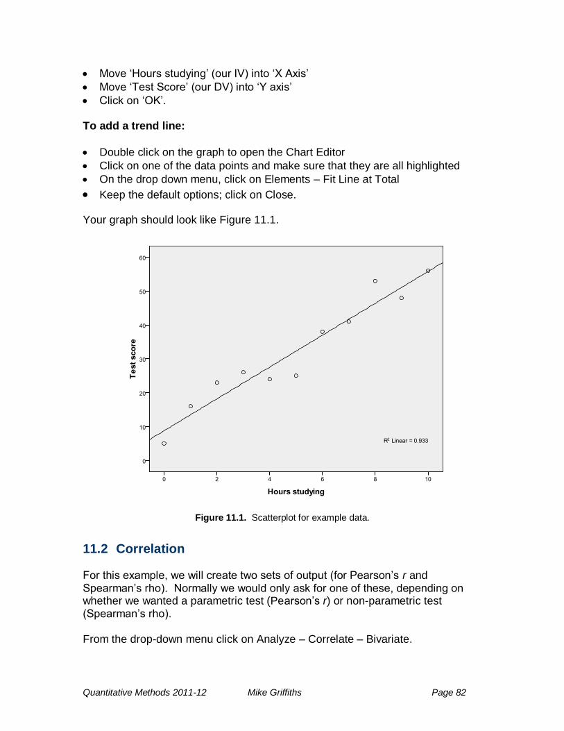
Quantitative Methods 2011-12 Mike Griffiths Page 82
Move ‗Hours studying‘ (our IV) into ‗X Axis‘
Move ‗Test Score‘ (our DV) into ‗Y axis‘
Click on ‗OK‘. To add a trend line:
Double click on the graph to open the Chart Editor
Click on one of the data points and make sure that they are all highlighted
On the drop down menu, click on Elements – Fit Line at Total
Keep the default options; click on Close. Your graph should look like Figure 11.1.
Figure 11.1. Scatterplot for example data.
11.2 Correlation For this example, we will create two sets of output (for Pearson‘s r and Spearman‘s rho). Normally we would only ask for one of these, depending on whether we wanted a parametric test (Pearson‘s r) or non-parametric test (Spearman‘s rho).
From the drop-down menu click on Analyze – Correlate – Bivariate.
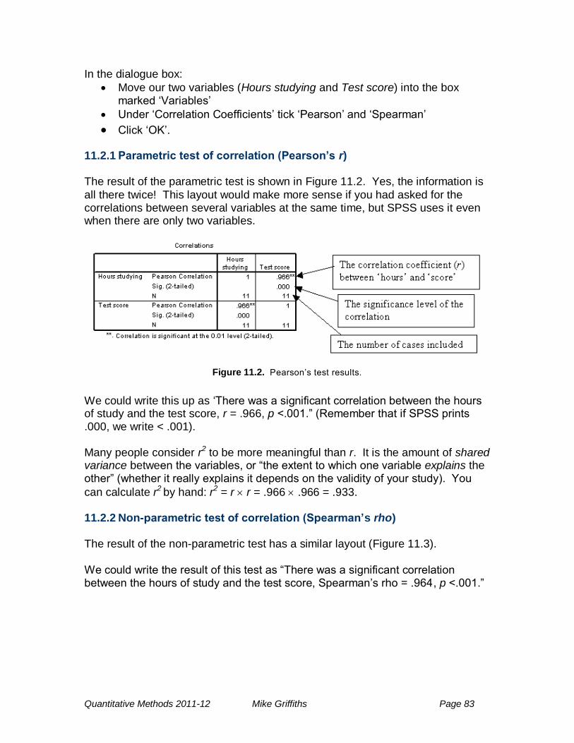
Quantitative Methods 2011-12 Mike Griffiths Page 83
In the dialogue box:
Move our two variables (Hours studying and Test score) into the box marked ‗Variables‘
Under ‗Correlation Coefficients‘ tick ‗Pearson‘ and ‗Spearman‘
Click ‗OK‘. 11.2.1 Parametric test of correlation (Pearson’s r)
The result of the parametric test is shown in Figure 11.2. Yes, the information is
all there twice! This layout would make more sense if you had asked for the correlations between several variables at the same time, but SPSS uses it even when there are only two variables.
Figure 11.2. Pearson‘s test results.
We could write this up as ‗There was a significant correlation between the hours of study and the test score, r = .966, p <.001.‖ (Remember that if SPSS prints .000, we write < .001). Many people consider r2 to be more meaningful than r. It is the amount of shared variance between the variables, or ―the extent to which one variable explains the other‖ (whether it really explains it depends on the validity of your study). You
can calculate r2 by hand: r2 = r r = .966 .966 = .933. 11.2.2 Non-parametric test of correlation (Spearman’s rho)
The result of the non-parametric test has a similar layout (Figure 11.3).
We could write the result of this test as ―There was a significant correlation between the hours of study and the test score, Spearman‘s rho = .964, p <.001.‖
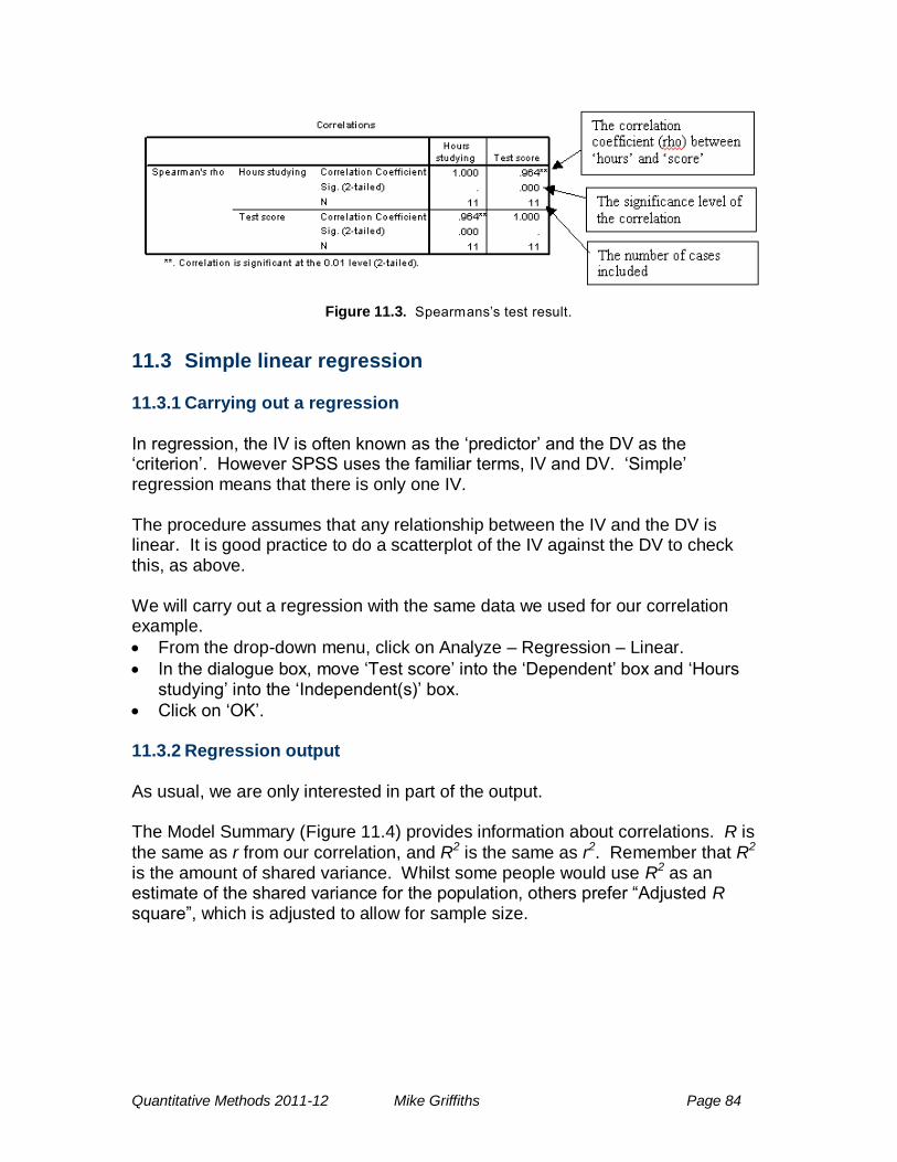
Quantitative Methods 2011-12 Mike Griffiths Page 84
Figure 11.3. Spearmans‘s test result.
11.3 Simple linear regression 11.3.1 Carrying out a regression In regression, the IV is often known as the ‗predictor‘ and the DV as the ‗criterion‘. However SPSS uses the familiar terms, IV and DV. ‗Simple‘ regression means that there is only one IV. The procedure assumes that any relationship between the IV and the DV is linear. It is good practice to do a scatterplot of the IV against the DV to check this, as above. We will carry out a regression with the same data we used for our correlation example.
From the drop-down menu, click on Analyze – Regression – Linear.
In the dialogue box, move ‗Test score‘ into the ‗Dependent‘ box and ‗Hours studying‘ into the ‗Independent(s)‘ box.
Click on ‗OK‘. 11.3.2 Regression output
As usual, we are only interested in part of the output. The Model Summary (Figure 11.4) provides information about correlations. R is
the same as r from our correlation, and R2 is the same as r2. Remember that R2 is the amount of shared variance. Whilst some people would use R2 as an estimate of the shared variance for the population, others prefer ―Adjusted R square‖, which is adjusted to allow for sample size.
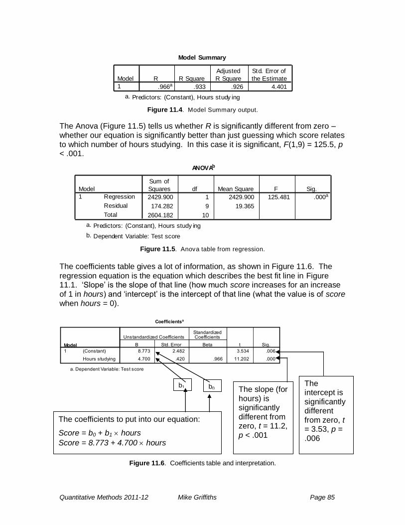
Quantitative Methods 2011-12 Mike Griffiths Page 85
Model Summary
.966a .933 .926 4.401
Model
1
R R Square
Adjusted
R Square
Std. Error of
the Estimate
Predictors: (Constant), Hours study inga.
Figure 11.4. Model Summary output.
The Anova (Figure 11.5) tells us whether R is significantly different from zero – whether our equation is significantly better than just guessing which score relates to which number of hours studying. In this case it is significant, F(1,9) = 125.5, p < .001.
ANOVAb
2429.900 1 2429.900 125.481 .000a
174.282 9 19.365
2604.182 10
Regression
Residual
Total
Model
1
Sum of
Squares df Mean Square F Sig.
Predictors: (Constant), Hours study inga.
Dependent Variable: Test scoreb.
Figure 11.5. Anova table from regression.
The coefficients table gives a lot of information, as shown in Figure 11.6. The
regression equation is the equation which describes the best fit line in Figure 11.1. ‗Slope‘ is the slope of that line (how much score increases for an increase of 1 in hours) and ‗intercept‘ is the intercept of that line (what the value is of score when hours = 0).
Figure 11.6. Coefficients table and interpretation.
b0 b1
The coefficients to put into our equation:
Score = b0 + b1 hours
Score = 8.773 + 4.700 hours
The slope (for hours) is significantly different from zero, t = 11.2, p < .001
The intercept is significantly different from zero, t = 3.53, p = .006
Quantitative Methods 2011-12 Mike Griffiths Page 86
11.3.3 Writing up regression
You could say ―A linear regression showed that the number of hours studying was a significant predictor of the score, R = .966, R2 = .933, adjusted R2 = .926, F(1,9) = 125.5, p < .001. Coefficients are shown in table xxx‖, where table xxx reproduces the SPSS coefficients table. Depending on what you were investigating, you might want to write out the regression equation, and/or explain it (e.g. ―The equation estimates that each extra hour‘s studying results in an increase of 4.7 in the score achieved in the test.‖) 11.3.4 What it means
The regression equation was Score = 8.773 + 4.700 Hours. We can use this to predict the score for any given number of hours. For example, if somebody had studied for 2 hours we predict that their score
would be 8.773 + 4.700 2 = 8.773 + 9.400 = 18.173, which we can round to 18.226. Actually, the student who did study for 2 hours has a score of 23. The difference (23-18.173, = 4.827) is known as a residual. This difference might arise because:
Students‘ performance may vary for reasons other than hours of study (e.g. ability of the student, mood, random fluctuations)
The regression is not exact: for example, the relationship between hours of study and score is not exactly a straight line.
Similarly, you can estimate how much someone would score if they studied for 2.5 hours (20.55). Because this is in between two values of the IV that we have (2 and 3) it is known as interpolation. The equation also allows you to estimate a score if someone had studied beyond the number of hours that were in the study (e.g. 11 hours). This is known as extrapolation and you need to beware of it. Can you rely on it? Would the score really go on increasing at the same rate for ever? For example, there is probably a maximum score on the test.
26
There is a slightly difficult issue about rounding here. If you are going on to use a figure in subsequent calculations, it makes sense to keep as many decimal places as possible. If you are reporting a figure to somebody else, you do not want to suggest that it is more accurate than it really is by giving too many decimal places. You just need to apply common sense and decide what the figure is being used for.
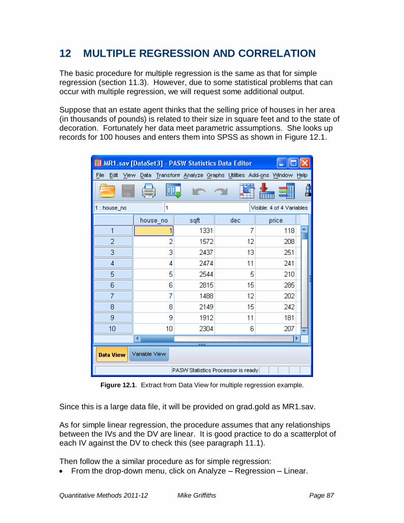
Quantitative Methods 2011-12 Mike Griffiths Page 87
12 MULTIPLE REGRESSION AND CORRELATION The basic procedure for multiple regression is the same as that for simple regression (section 11.3). However, due to some statistical problems that can occur with multiple regression, we will request some additional output. Suppose that an estate agent thinks that the selling price of houses in her area (in thousands of pounds) is related to their size in square feet and to the state of decoration. Fortunately her data meet parametric assumptions. She looks up records for 100 houses and enters them into SPSS as shown in Figure 12.1.
Figure 12.1. Extract from Data View for multiple regression example.
Since this is a large data file, it will be provided on grad.gold as MR1.sav. As for simple linear regression, the procedure assumes that any relationships between the IVs and the DV are linear. It is good practice to do a scatterplot of each IV against the DV to check this (see paragraph 11.1). Then follow the a similar procedure as for simple regression:
From the drop-down menu, click on Analyze – Regression – Linear.
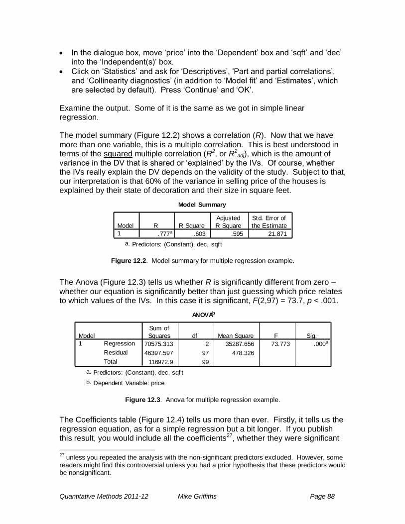
Quantitative Methods 2011-12 Mike Griffiths Page 88
In the dialogue box, move ‗price‘ into the ‗Dependent‘ box and ‗sqft‘ and ‗dec‘ into the ‗Independent(s)‘ box.
Click on ‗Statistics‘ and ask for ‗Descriptives‘, ‗Part and partial correlations‘, and ‗Collinearity diagnostics‘ (in addition to ‗Model fit‘ and ‗Estimates‘, which are selected by default). Press ‗Continue‘ and ‗OK‘.
Examine the output. Some of it is the same as we got in simple linear regression. The model summary (Figure 12.2) shows a correlation (R). Now that we have
more than one variable, this is a multiple correlation. This is best understood in terms of the squared multiple correlation (R2, or R2
adj), which is the amount of variance in the DV that is shared or ‗explained‘ by the IVs. Of course, whether the IVs really explain the DV depends on the validity of the study. Subject to that, our interpretation is that 60% of the variance in selling price of the houses is explained by their state of decoration and their size in square feet.
Model Summary
.777a .603 .595 21.871
Model
1
R R Square
Adjusted
R Square
Std. Error of
the Estimate
Predictors: (Constant), dec, sqf ta.
Figure 12.2. Model summary for multiple regression example.
The Anova (Figure 12.3) tells us whether R is significantly different from zero –
whether our equation is significantly better than just guessing which price relates to which values of the IVs. In this case it is significant, F(2,97) = 73.7, p < .001.
ANOVAb
70575.313 2 35287.656 73.773 .000a
46397.597 97 478.326
116972.9 99
Regression
Residual
Total
Model
1
Sum of
Squares df Mean Square F Sig.
Predictors: (Constant), dec, sqf ta.
Dependent Variable: priceb.
Figure 12.3. Anova for multiple regression example.
The Coefficients table (Figure 12.4) tells us more than ever. Firstly, it tells us the regression equation, as for a simple regression but a bit longer. If you publish this result, you would include all the coefficients27, whether they were significant
27
unless you repeated the analysis with the non-significant predictors excluded. However, some readers might find this controversial unless you had a prior hypothesis that these predictors would be nonsignificant.
Quantitative Methods 2011-12 Mike Griffiths Page 89
or not. Secondly, it tells us which coefficients were in fact significant. If you are carrying out an exploratory study you can use this information to say which IVs were in fact significant predictors of the DV (but read the rest of this section first!). Some of the extra information we asked for is at the end of this table. If there are any big differences between the zero-order and the partial correlations, this shows that there are correlations between the Independent Variables. The zero-order correlations are the ordinary ones we have come across before, the correlation between each IV and the DV. The partial correlations are the unique correlation of that IV with the DV, that is to say how much of their relationship with the DV is not shared by any of the other IVs. If the two correlations are very different, you should tell your readers both. Check the figures against each variable under VIF (Variance Inflation Factor). If any of them are too big (say, greater than 428), that IV has too much shared variance with the other IVs – that is to say, it has a high correlation with one or more of them29. This messes up the maths and stops the regression from working properly. Think about whether you can re-run the analysis with one of the IVs removed – the high correlation may mean it is measuring something very similar to one of the other IVs anyway. If more than one VIF is too high, you can experiment with removing one IV at a time. It is also a good idea to look at the correlations table (Figure 12.5), which was
produced because we checked the ‗Descriptive statistics‘ box. Check the significance of the correlations of each IV against the DV (notice that the significance levels are given as one-tailed; I recommend doubling them to give the two-tailed significance). If any of them are significant in this table, but those IVs are not significant in the Coefficients table, this is caused by correlations between the IVs. Again you should report both and be particularly careful to check the VIFs. Also, if the table showed a significant correlation between the IVs, we would report this and take the same precautions. However, in this case there is no significant correlation between the IVs sqft and dec (r = .112, p = .134).
28
Some people will allow higher figures, such as 10, but that takes us into matters of opinion best left to people who are experienced at this kind of analysis. 29
Strictly speaking, what is too high is the squared multiple correlation with the other IVs.
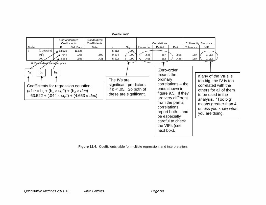
Quantitative Methods 2011-12 Mike Griffiths Page 90
Coefficientsa
63.522 11.525 5.512 .000
.044 .005 .600 9.324 .000 .648 .687 .596 .987 1.013
4.653 .695 .431 6.692 .000 .498 .562 .428 .987 1.013
(Constant)
sqf t
dec
Model
1
B Std. Error
Unstandardized
Coeff icients
Beta
Standardized
Coeff icients
t Sig. Zero-order Part ial Part
Correlat ions
Tolerance VIF
Collinearity Stat istics
Dependent Variable: pricea.
Figure 12.4. Coefficients table for multiple regression, and interpretation.
b0 b1 b2
Coefficients for regression equation:
price = b0 + (b1 sqft) + (b2 dec)
= 63.522 + (.044 sqft) + (4.653 dec)
The IVs are significant predictors if p < .05. So both of
these are significant.
‗Zero-order‘ means the ordinary correlations – the ones shown in figure 9.5. If they are very different from the partial correlations, report both – and be especially careful to check the VIFs (see
next box).
If any of the VIFs is too big, the IV is too correlated with the others for all of them to be used in the analysis. ―Too big‖ means greater than 4, unless you know what
you are doing.
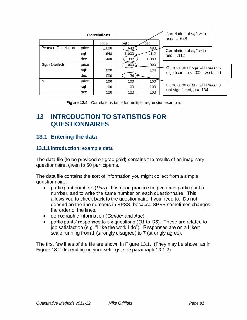
Quantitative Methods 2011-12 Mike Griffiths Page 91
Correlations
1.000 .648 .498
.648 1.000 .112
.498 .112 1.000
. .000 .000
.000 . .134
.000 .134 .
100 100 100
100 100 100
100 100 100
price
sqf t
dec
price
sqf t
dec
price
sqf t
dec
Pearson Correlation
Sig. (1-tailed)
N
price sqf t dec
Figure 12.5. Correlations table for multiple regression example.
13 INTRODUCTION TO STATISTICS FOR QUESTIONNAIRES
13.1 Entering the data 13.1.1 Introduction: example data
The data file (to be provided on grad.gold) contains the results of an imaginary questionnaire, given to 60 participants. The data file contains the sort of information you might collect from a simple questionnaire:
participant numbers (Part). It is good practice to give each participant a number, and to write the same number on each questionnaire. This allows you to check back to the questionnaire if you need to. Do not depend on the line numbers in SPSS, because SPSS sometimes changes the order of the lines.
demographic information (Gender and Age)
participants‘ responses to six questions (Q1 to Q6). These are related to job satisfaction (e.g. ―I like the work I do‖). Responses are on a Likert scale running from 1 (strongly disagree) to 7 (strongly agree).
The first few lines of the file are shown in Figure 13.1. (They may be shown as in Figure 13.2 depending on your settings; see paragraph 13.1.2).
Correlation of sqft with price = .648
Correlation of sqft with price is
significant, p < .002, two-tailed
Correlation of sqft with
dec = .112
Correlation of dec with price is
not significant, p = .134
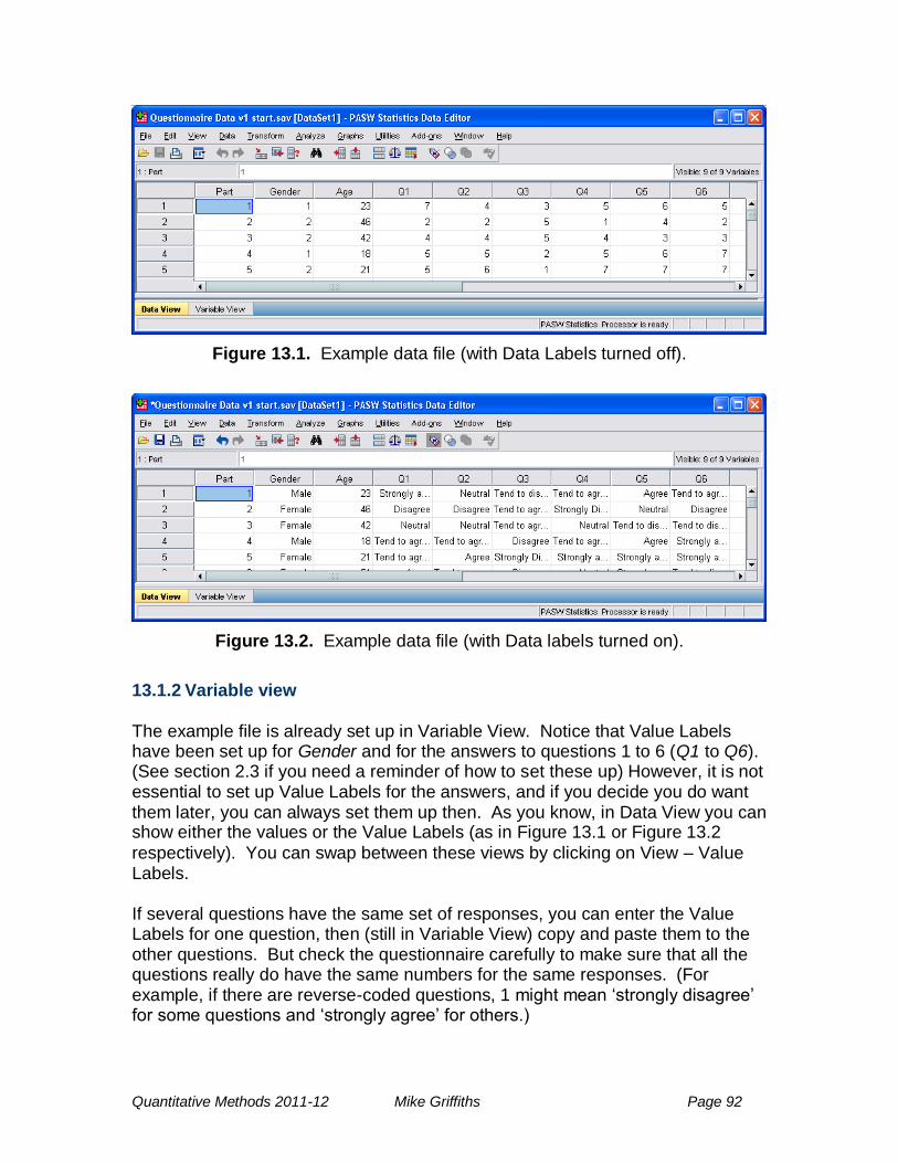
Quantitative Methods 2011-12 Mike Griffiths Page 92
Figure 13.1. Example data file (with Data Labels turned off).
Figure 13.2. Example data file (with Data labels turned on).
13.1.2 Variable view The example file is already set up in Variable View. Notice that Value Labels have been set up for Gender and for the answers to questions 1 to 6 (Q1 to Q6). (See section 2.3 if you need a reminder of how to set these up) However, it is not essential to set up Value Labels for the answers, and if you decide you do want them later, you can always set them up then. As you know, in Data View you can show either the values or the Value Labels (as in Figure 13.1 or Figure 13.2
respectively). You can swap between these views by clicking on View – Value Labels. If several questions have the same set of responses, you can enter the Value Labels for one question, then (still in Variable View) copy and paste them to the other questions. But check the questionnaire carefully to make sure that all the questions really do have the same numbers for the same responses. (For example, if there are reverse-coded questions, 1 might mean ‗strongly disagree‘ for some questions and ‗strongly agree‘ for others.)
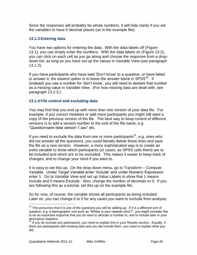
Quantitative Methods 2011-12 Mike Griffiths Page 93
Since the responses will probably be whole numbers, it will help clarity if you set the variables to have 0 decimal places (as in the example file). 13.1.3 Entering data
You have two options for entering the data. With the data labels off (Figure 13.1), you can simply enter the numbers. With the data labels on (Figure 13.2),
you can click on each cell as you go along and choose the response from a drop-down list, as long as you have set up the values in Variable View (see paragraph 13.1.2). If you have participants who have said ‗Don‘t know‘ to a question, or have failed to answer it, the easiest option is to leave the answer blank in SPSS30. If (instead) you use a number for ‗don‘t know‘, you will need to declare that number as a missing value in Variable View. (For how missing data are dealt with, see paragraph 13.2.3.)
13.1.4 File control and excluding data
You may find that you end up with more than one version of your data file. For example, if you correct mistakes or add more participants you might still want a copy of the previous version of the file. The best way to keep control of different versions is to add a version number to the end of the file name, e.g. ―Questionnaire data version 1.sav‖ etc. If you need to exclude the data from one or more participants31, e.g. ones who did not answer all the questions, you could literally delete those lines and save the file as a new version. However, a more sophisticated way is to create an extra variable to show which participants (or cases, as SPSS calls them) are to be included and which are to be excluded. This makes it easier to keep track of changes, and to change your mind if you want to. It is easy to set this up. On the drop-down menu, go to Transform – Compute Variable. Under Target Variable enter ‗Include‘ and under Numeric Expression enter 1. Go to Variable View and set up Value Labels to show that 1 means Include and 0 means Exclude. Also, change the number of decimals to 0. If you are following this as a tutorial, set this up on the example file. So for now, of course, the variable shows all participants as being included. Later on, you can change it to 0 for any cases you want to exclude from analysis.
30
This presumes that it is one of the questions you will be adding up. If it is a different sort of question, e.g. a demographic one such as ―Where is your nearest clinic?‖, you might consider this to be an important response that you do want to allocate a number to, and to include later in your descriptive statistics. 31
If you do exclude any participants, you need to explain this in your Results section. Equally, if there are participants with missing data and you did include them, you need to explain what you did.
Quantitative Methods 2011-12 Mike Griffiths Page 94
If you use this method, note that you will have to select these participants before doing any analysis, whenever you exclude any more cases, and again every time you open the file. To do this, go to Data – Select Cases.
Click on ‗If condition is satisfied‘ and the ‗If‘ button. In the dialogue box that comes up, type ‗Include = 1‘. (Remember, here you are specifying which cases to include, not which ones to exclude.) Click on Continue and OK. In Data View, check that SPSS has put a cross through the line numbers of the cases which are to be excluded.
13.2 Checking the data file; missing data 13.2.1 Check your data entry
Always check over your data to ensure that you have entered it correctly. However, if you have a lot of data, it is easy to miss mistakes. Here are a few tips. 13.2.2 Detecting missing data If any of the data have no value against them at all, they will be shown in the data file as a dot. This may be because the participant really did not answer, but it may be that you made a mistake in data entry. You can of course try to spot any missing data by looking at the file. If the file is too big for that, you can call up a Missing Value Analysis. This is done from the drop-down menu: Analyse – Missing Value Analysis. Note that this dialogue box requires you to specify variables as Quantitative (ones with meaningful numbers, including answers to questions on a Likert scale) or Categorical (ones where the numbers simply define categories). In the example file, the Quantitative variables are Part, Age, Q1, Q2, Q3, Q4, Q5 and Q6. The only Categorical variable is Gender. (There is no point in entering Include, because we know it will not have any missing values.) Click the ‗Patterns‘ button and select ‗Cases with missing values‘. Click Continue and OK. In the table headed Missing Patterns, ‗S‘ indicates a missing value. In the example file, they are cases 44 and 52. Note that the ‗Case‘ number relates to the line number, not to any number you may have given to the participants. 13.2.3 Dealing with missing data If possible, check the original questionnaires to fill in any missing data. If this is not possible (e.g. if the questionnaires are not available, or the participant did not
Quantitative Methods 2011-12 Mike Griffiths Page 95
answer that question) there are a number of options as to what to do32. The simplest options are:
1. Carry on and ignore the missing data. SPSS will exclude those participants from any analysis that needs those figures.
2. Delete the case (e.g. by using the Include variable, see section 13.1.4)
If you are following this document as a tutorial, use the Include variable on the example file. Change Include to 0 for cases 44 and 52, and use the Select Cases procedure. See section 13.1.4 for how to do this.
13.2.4 Finding major errors in the data
There are a couple of short cuts to looking for figures which are grossly wrong. For continuous variables (the ones we referred to as ‗quantitative‘ in the last paragraph: Part, Age, Q1, Q2, Q3, Q4, Q5 and Q6 in the example file), go to Analyse – Descriptive Statistics – Descriptives and put the variables into the Variable(s) box. You can then look for variables which are obviously wrong, because the minimum or maximum are not in the range we expect. For example, in the example questionnaire we know that the answers to questions must be between 1 and 7. You may be able to spot similar problems with other variables; for example a maximum age of 222 would obviously be wrong. In the example file, the descriptive statistics show that at least one score for Q3 is 55. Now you can go back to the data file and find it (it is line 53). Presume you go back to the original questionnaire and confirm that it should be 5. Change the score accordingly. Similarly for categorical variables, go to Analyse – Descriptive Statistics – Frequencies and put the variable into the Variables box (Gender in the example). In the example file, there is an incorrect value of 22. Again, let us suppose that you go back to the original data and confirm that it should have read 2 (it is case 45). Correct it accordingly.
32
Some textbooks cover other options, but there is no perfect answer and these are the ones to use unless you have studied advanced statistics. They are likely to give similar results, unless you have a lot of missing data (more than 5% of cases, say) or particular reason to believe that the missing data is non-random, in which case it would be wise to take further advice. Whatever you do, describe it in your Results section.
Quantitative Methods 2011-12 Mike Griffiths Page 96
13.3 Calculating overall scores on a questionnaire 13.3.1 Introduction If the questions constitute a scale, you will need to add up (or average) the answers to different questions. For example, if the questions are all about job satisfaction (as in the example), we might have to add them up to get a total score for job satisfaction. There may be just one total, or sometimes different questions have to be added up to make sub-scales. If using a published questionnaire, make sure you find the instructions. These may be in a manual or in a journal article. They will give important information on how to calculate the overall score (e.g. whether it is a total or an average, whether there are subscales, whether there are any reverse-scored questions, whether certain questions need to be ignored for any reason). The same source will also tell you who the questionnaire was tested on (the so-called norm group) and what their mean score was; you may wish to compare your own participants‘ mean against the norm group. 13.3.2 Reverse-scored questions: what they are We will see how to add up scores in SPSS in a minute, but first you may have to deal with reverse-scored questions. If the questions are about how happy people are in their job, a typical question might ask people how much they agree with the statement ―I enjoy coming to work.‖ Obviously the more people agree with this statement, the happier they are in their job. The people who most strongly agree with the statement get the highest score. However there might be some questions such as ―If I could give up work tomorrow, I would.‖ In this case, the more people agree with the statement, the less they are happy in their job. If the questionnaire has been devised and published by someone else, they should have made it clear if there are any such questions. 13.3.3 Reverse-scored questions: How to deal with them
If you entered the data with the data labels on (see section 13.1.3) you may have
already taken account of the reverse-scoring, and given a score of 1 to the people who most agree with the statement. If not, the score needs to be amended so that low scores are changed into high scores, and vice versa.
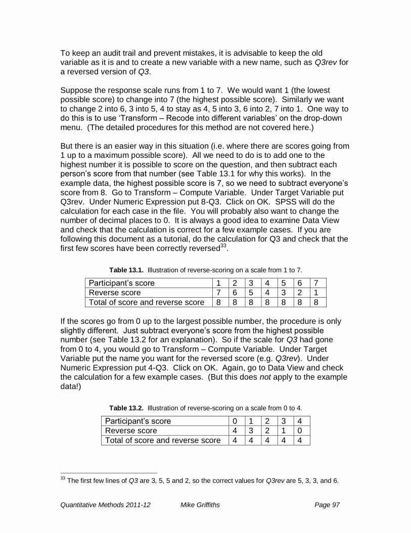
Quantitative Methods 2011-12 Mike Griffiths Page 97
To keep an audit trail and prevent mistakes, it is advisable to keep the old variable as it is and to create a new variable with a new name, such as Q3rev for a reversed version of Q3. Suppose the response scale runs from 1 to 7. We would want 1 (the lowest possible score) to change into 7 (the highest possible score). Similarly we want to change 2 into 6, 3 into 5, 4 to stay as 4, 5 into 3, 6 into 2, 7 into 1. One way to do this is to use ‗Transform – Recode into different variables‘ on the drop-down menu. (The detailed procedures for this method are not covered here.) But there is an easier way in this situation (i.e. where there are scores going from 1 up to a maximum possible score). All we need to do is to add one to the highest number it is possible to score on the question, and then subtract each person‘s score from that number (see Table 13.1 for why this works). In the
example data, the highest possible score is 7, so we need to subtract everyone‘s score from 8. Go to Transform – Compute Variable. Under Target Variable put Q3rev. Under Numeric Expression put 8-Q3. Click on OK. SPSS will do the calculation for each case in the file. You will probably also want to change the number of decimal places to 0. It is always a good idea to examine Data View and check that the calculation is correct for a few example cases. If you are following this document as a tutorial, do the calculation for Q3 and check that the first few scores have been correctly reversed33.
Table 13.1. Illustration of reverse-scoring on a scale from 1 to 7.
Participant‘s score 1 2 3 4 5 6 7
Reverse score 7 6 5 4 3 2 1
Total of score and reverse score 8 8 8 8 8 8 8
If the scores go from 0 up to the largest possible number, the procedure is only slightly different. Just subtract everyone‘s score from the highest possible number (see Table 13.2 for an explanation). So if the scale for Q3 had gone
from 0 to 4, you would go to Transform – Compute Variable. Under Target Variable put the name you want for the reversed score (e.g. Q3rev). Under Numeric Expression put 4-Q3. Click on OK. Again, go to Data View and check the calculation for a few example cases. (But this does not apply to the example data!)
Table 13.2. Illustration of reverse-scoring on a scale from 0 to 4.
Participant‘s score 0 1 2 3 4
Reverse score 4 3 2 1 0
Total of score and reverse score 4 4 4 4 4
33
The first few lines of Q3 are 3, 5, 5 and 2, so the correct values for Q3rev are 5, 3, 3, and 6.
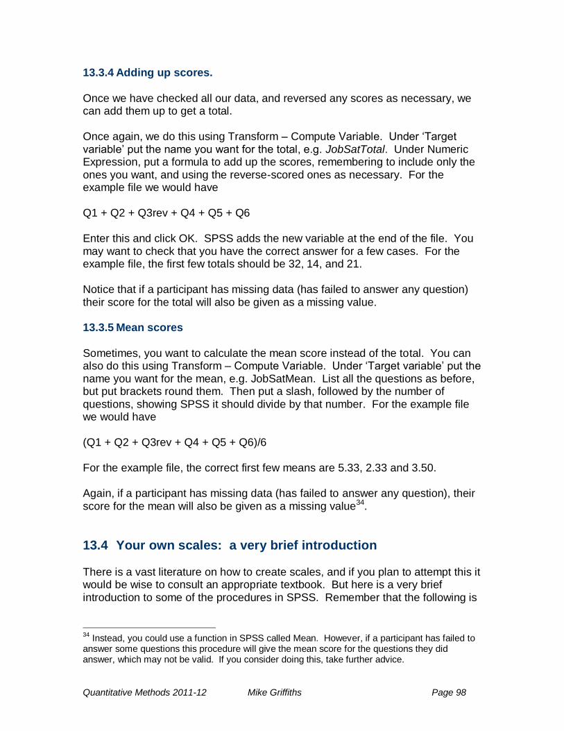
Quantitative Methods 2011-12 Mike Griffiths Page 98
13.3.4 Adding up scores. Once we have checked all our data, and reversed any scores as necessary, we can add them up to get a total. Once again, we do this using Transform – Compute Variable. Under ‗Target variable‘ put the name you want for the total, e.g. JobSatTotal. Under Numeric Expression, put a formula to add up the scores, remembering to include only the ones you want, and using the reverse-scored ones as necessary. For the example file we would have Q1 + Q2 + Q3rev + Q4 + Q5 + Q6 Enter this and click OK. SPSS adds the new variable at the end of the file. You may want to check that you have the correct answer for a few cases. For the example file, the first few totals should be 32, 14, and 21. Notice that if a participant has missing data (has failed to answer any question) their score for the total will also be given as a missing value. 13.3.5 Mean scores Sometimes, you want to calculate the mean score instead of the total. You can also do this using Transform – Compute Variable. Under ‗Target variable‘ put the name you want for the mean, e.g. JobSatMean. List all the questions as before, but put brackets round them. Then put a slash, followed by the number of questions, showing SPSS it should divide by that number. For the example file we would have (Q1 + Q2 + Q3rev + Q4 + Q5 + Q6)/6 For the example file, the correct first few means are 5.33, 2.33 and 3.50. Again, if a participant has missing data (has failed to answer any question), their score for the mean will also be given as a missing value34.
13.4 Your own scales: a very brief introduction There is a vast literature on how to create scales, and if you plan to attempt this it would be wise to consult an appropriate textbook. But here is a very brief introduction to some of the procedures in SPSS. Remember that the following is
34
Instead, you could use a function in SPSS called Mean. However, if a participant has failed to answer some questions this procedure will give the mean score for the questions they did answer, which may not be valid. If you consider doing this, take further advice.
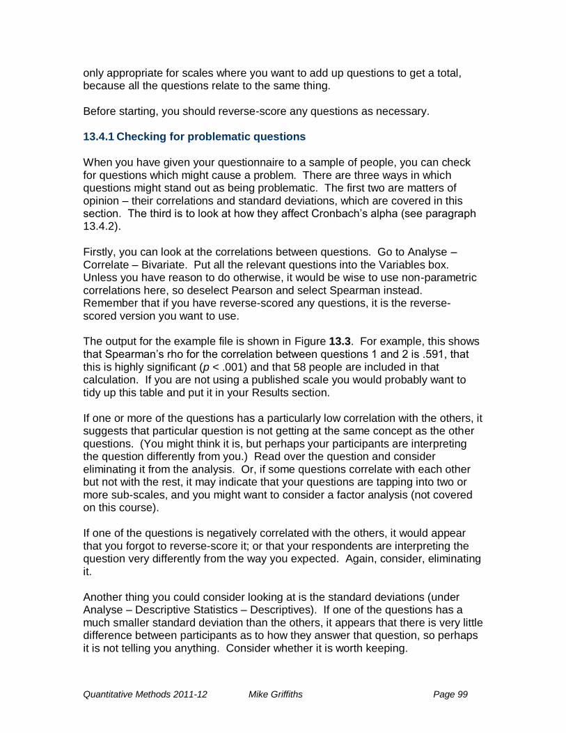
Quantitative Methods 2011-12 Mike Griffiths Page 99
only appropriate for scales where you want to add up questions to get a total, because all the questions relate to the same thing. Before starting, you should reverse-score any questions as necessary. 13.4.1 Checking for problematic questions
When you have given your questionnaire to a sample of people, you can check for questions which might cause a problem. There are three ways in which questions might stand out as being problematic. The first two are matters of opinion – their correlations and standard deviations, which are covered in this section. The third is to look at how they affect Cronbach‘s alpha (see paragraph 13.4.2).
Firstly, you can look at the correlations between questions. Go to Analyse – Correlate – Bivariate. Put all the relevant questions into the Variables box. Unless you have reason to do otherwise, it would be wise to use non-parametric correlations here, so deselect Pearson and select Spearman instead. Remember that if you have reverse-scored any questions, it is the reverse-scored version you want to use. The output for the example file is shown in Figure 13.3. For example, this shows that Spearman‘s rho for the correlation between questions 1 and 2 is .591, that this is highly significant (p < .001) and that 58 people are included in that calculation. If you are not using a published scale you would probably want to tidy up this table and put it in your Results section. If one or more of the questions has a particularly low correlation with the others, it suggests that particular question is not getting at the same concept as the other questions. (You might think it is, but perhaps your participants are interpreting the question differently from you.) Read over the question and consider eliminating it from the analysis. Or, if some questions correlate with each other but not with the rest, it may indicate that your questions are tapping into two or more sub-scales, and you might want to consider a factor analysis (not covered on this course). If one of the questions is negatively correlated with the others, it would appear that you forgot to reverse-score it; or that your respondents are interpreting the question very differently from the way you expected. Again, consider, eliminating it. Another thing you could consider looking at is the standard deviations (under Analyse – Descriptive Statistics – Descriptives). If one of the questions has a much smaller standard deviation than the others, it appears that there is very little difference between participants as to how they answer that question, so perhaps it is not telling you anything. Consider whether it is worth keeping.
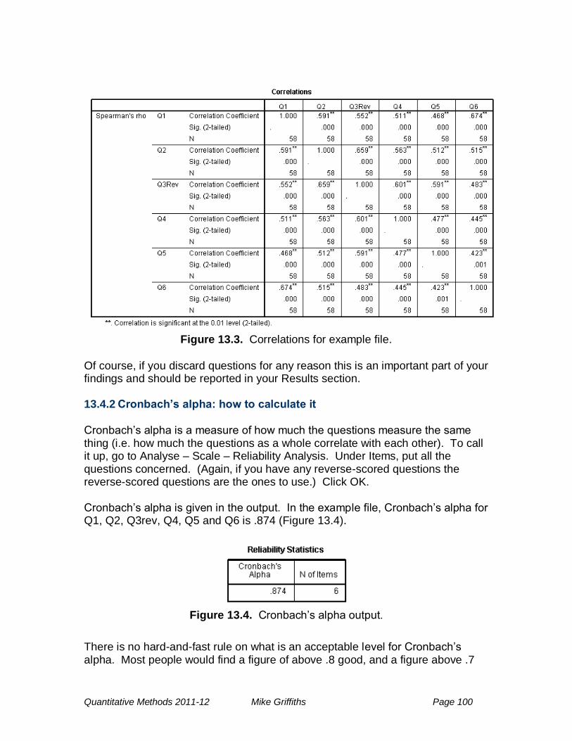
Quantitative Methods 2011-12 Mike Griffiths Page 100
Figure 13.3. Correlations for example file.
Of course, if you discard questions for any reason this is an important part of your findings and should be reported in your Results section. 13.4.2 Cronbach’s alpha: how to calculate it
Cronbach‘s alpha is a measure of how much the questions measure the same thing (i.e. how much the questions as a whole correlate with each other). To call it up, go to Analyse – Scale – Reliability Analysis. Under Items, put all the questions concerned. (Again, if you have any reverse-scored questions the reverse-scored questions are the ones to use.) Click OK. Cronbach‘s alpha is given in the output. In the example file, Cronbach‘s alpha for Q1, Q2, Q3rev, Q4, Q5 and Q6 is .874 (Figure 13.4).
Figure 13.4. Cronbach‘s alpha output.
There is no hard-and-fast rule on what is an acceptable level for Cronbach‘s alpha. Most people would find a figure of above .8 good, and a figure above .7
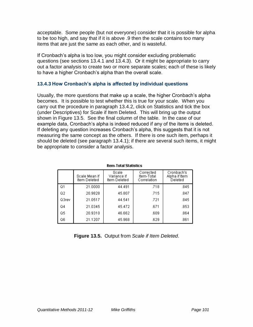
Quantitative Methods 2011-12 Mike Griffiths Page 101
acceptable. Some people (but not everyone) consider that it is possible for alpha to be too high, and say that if it is above .9 then the scale contains too many items that are just the same as each other, and is wasteful. If Cronbach‘s alpha is too low, you might consider excluding problematic questions (see sections 13.4.1 and 13.4.3). Or it might be appropriate to carry
out a factor analysis to create two or more separate scales; each of these is likely to have a higher Cronbach‘s alpha than the overall scale. 13.4.3 How Cronbach’s alpha is affected by individual questions Usually, the more questions that make up a scale, the higher Cronbach‘s alpha becomes. It is possible to test whether this is true for your scale. When you carry out the procedure in paragraph 13.4.2, click on Statistics and tick the box (under Descriptives) for Scale if Item Deleted. This will bring up the output shown in Figure 13.5. See the final column of the table. In the case of our
example data, Cronbach‘s alpha is indeed reduced if any of the items is deleted. If deleting any question increases Cronbach‘s alpha, this suggests that it is not measuring the same concept as the others. If there is one such item, perhaps it should be deleted (see paragraph 13.4.1); if there are several such items, it might
be appropriate to consider a factor analysis.
Figure 13.5. Output from Scale if Item Deleted.
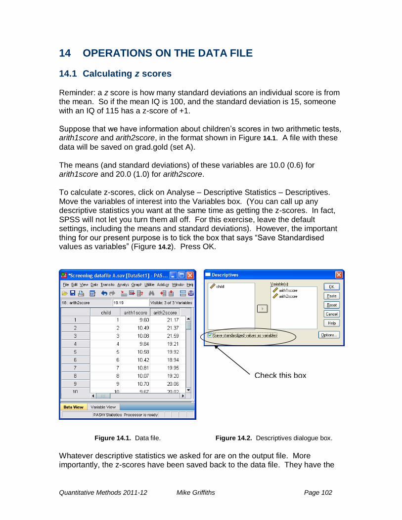
Quantitative Methods 2011-12 Mike Griffiths Page 102
14 OPERATIONS ON THE DATA FILE
14.1 Calculating z scores Reminder: a z score is how many standard deviations an individual score is from the mean. So if the mean IQ is 100, and the standard deviation is 15, someone with an IQ of 115 has a z-score of +1. Suppose that we have information about children‘s scores in two arithmetic tests, arith1score and arith2score, in the format shown in Figure 14.1. A file with these
data will be saved on grad.gold (set A). The means (and standard deviations) of these variables are 10.0 (0.6) for arith1score and 20.0 (1.0) for arith2score. To calculate z-scores, click on Analyse – Descriptive Statistics – Descriptives. Move the variables of interest into the Variables box. (You can call up any descriptive statistics you want at the same time as getting the z-scores. In fact, SPSS will not let you turn them all off. For this exercise, leave the default settings, including the means and standard deviations). However, the important thing for our present purpose is to tick the box that says ―Save Standardised values as variables‖ (Figure 14.2). Press OK.
Figure 14.1. Data file. Figure 14.2. Descriptives dialogue box.
Whatever descriptive statistics we asked for are on the output file. More importantly, the z-scores have been saved back to the data file. They have the
Check this box
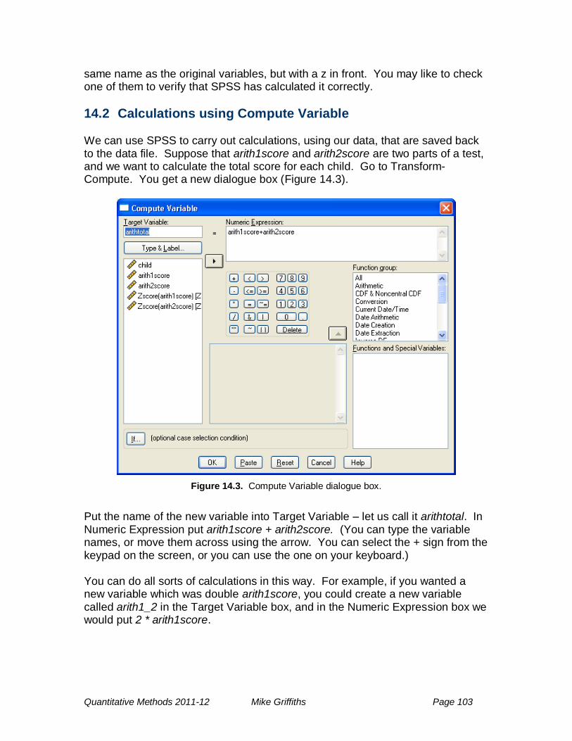
Quantitative Methods 2011-12 Mike Griffiths Page 103
same name as the original variables, but with a z in front. You may like to check one of them to verify that SPSS has calculated it correctly.
14.2 Calculations using Compute Variable We can use SPSS to carry out calculations, using our data, that are saved back to the data file. Suppose that arith1score and arith2score are two parts of a test, and we want to calculate the total score for each child. Go to Transform-Compute. You get a new dialogue box (Figure 14.3).
Figure 14.3. Compute Variable dialogue box.
Put the name of the new variable into Target Variable – let us call it arithtotal. In Numeric Expression put arith1score + arith2score. (You can type the variable names, or move them across using the arrow. You can select the + sign from the keypad on the screen, or you can use the one on your keyboard.) You can do all sorts of calculations in this way. For example, if you wanted a new variable which was double arith1score, you could create a new variable called arith1_2 in the Target Variable box, and in the Numeric Expression box we would put 2 * arith1score.
Quantitative Methods 2011-12 Mike Griffiths Page 104
It is always advisable to go back to the data file and check on a couple of lines that the new variable has been calculated the way you expected – especially if your calculation is at all complicated!
14.3 Combining variables fairly We might want the score on both tests to count equally toward the final mark. arithtotal does not do this – arith2score has a bigger standard deviation than arith1score, so it makes a bigger contribution to the total score. To get a combined variable where both variables contribute equally, we could add up the z-scores. Try this as an exercise.
14.4 Categorising data 14.4.1 Predefined split point(s): e.g. pass/fail
Suppose we wanted to divide the children up into those who had passed the test and those who had failed it. (Perhaps we want a categorical variable for a chi-squared test, or for an Anova; or we just want to make a list of who has passed). We have calculated the total score (arithtotal); suppose that the passmark is 30. Let us create a new variable, with the value 1 if the child has passed, and 2 if they have failed. To start, click on Transform – Compute and put a suitable name (e.g. passfail) in Target Variable. To set it up, we will start by giving everyone the same value (e.g. 1). Just type 1 in Numeric Expression and click ‗OK‘. Examine the data file – you have the new variable you asked for, and it is 1 for everybody for now. Now let us change passfail to 2 for the children who failed. Click on Transform – Compute and leave the Target Variable as passfail. Change Numeric Expression to 2. Click on ―If…‖ at the bottom left, and a new dialogue box comes up. Click on ―Include if case satisfies condition‖ and enter a formula that defines who failed. In this case enter arithtotal < 30, meaning arithtotal is less than 30. Click Continue and OK. A dialogue box comes up asking whether you want to change an existing variable – click on OK. Examine the data file. It should now show the value 1 for the children with scores of at least 30, and 2 for children with scores below 30. You can of course go on to create even more categories if you want to. When you have finished, you will probably want to tidy up the variable in Variable View, for example giving names to the categories under Values. Warning. SPSS will remember the ―If…‖ condition for as long as the file is open. If you do other calculations you probably do not want to restrict them to these cases. Click on ―If…‖ and re-check ―Include all cases‖.
Quantitative Methods 2011-12 Mike Griffiths Page 105
14.4.2 Splitting into equal groups: e.g. median splits Sometimes we want to split a variable up into two, but there is no specific pass mark. In particular, it is often useful to split a variable up into equal-sized groups of high and low scores. This is known as a median split. To do this, go to Transform – Rank Cases. Put the variable of interest (e.g. arithtotal) into the Variables box. Click on Rank Types and uncheck Rank. Check Ntiles and change the figure to 2. Click Continue and OK. The new variable is automatically added to the file, with the name Narithto (i.e. N followed by as much of the original name as there is room for). You can use a similar procedure to split a variable into any other number of equally sized groups– just put the number of groups you want in place of 2.
14.5 Excluding cases from the analysis You may find something wrong with some of the data, or you may simply want to work on a part of the data. Of course you could simply make a copy of the file and delete the unwanted cases, but there is a more sophisticated way. (This is also covered, slightly differently, in section 13.1.4.)
Open sample dataset B. Suppose that we only want to include cases where members is greater than 0. Click on Data – Select Cases and you get a dialogue box (Figure 14.4). Click on ―If condition is satisfied‖ and then on ―If…‖. You get another dialogue box (Figure 14.5). Type in the rule for the cases you want
included. Note that you specify what cases you want included, not the ones you want excluded. Press Continue and OK. Examine the effect on the data file. The excluded cases have lines through the row numbers. Warning. SPSS will remember your rule until you close the file, but only until
then. If you close the file and re-open it, you need to go through the procedure again. If your rule is complicated, it may be easier to set up a variable specially for the purpose. Use Transform – Compute to create a variable called include with the value 1. Then change the value to 0 for those cases you want to exclude (either by hand, or by using the Transform – Compute command). Whenever you open the file, use the Select Cases command to select those cases whose value of include is 1.
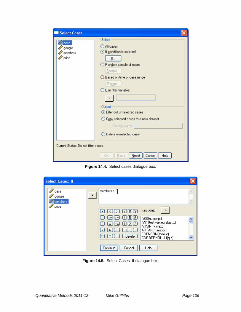
Quantitative Methods 2011-12 Mike Griffiths Page 106
Figure 14.4. Select cases dialogue box.
Figure 14.5. Select Cases: If dialogue box.
Quantitative Methods 2011-12 Mike Griffiths Page 107
15 DATA SCREENING AND CLEANING 15.1 Introduction I am dealing with this subject at the end because (a) some people find some of it contentious (b) you need an understanding of statistics to appreciate it. However, it is something you should think about at the beginning of your analysis. Everyone would agree that it is important to check that your data have been entered accurately. What is more contentious is what to do if your data are accurate but are not well-behaved (e.g. they include outliers). This is one of the subjects that more advanced courses deal with in more detail. The vital rule is that if you tinker with your data in any way (other than correcting data entry errors), you must say in your write-up exactly what you did and what effect this had on the data.
15.2 Suggested steps. Note. If your data are between-subject, ensure that your file is split (See section 6.8.2. Split by all of the between-subject variables if there is more than one).
Remember to cancel this at the end of your analysis. 1. As far as possible, check your data by re-reading the data file against the
original data. 2. It is a good idea to check for out-of range numbers. For example, if one of the
variables is the age of the participants, and somebody‘s age is shown as –2 or 150, they must be mistakes. Go on the drop-down menu to Analyze – Descriptive Statistics – Descriptives. Under ‗Options‘ ensure that ‗minimum‘ and ‗maximum‘ are selected. In the output, check that the minima and maxima in your data file are sensible. (In this example the minimum might be shown as –2 or the maximum as 150, showing up these obvious mistakes).
3. Check for missing data (see paragraph 13.2).
4. See whether your data are normally distributed by producing histograms (section 5.1). You can also do a formal test35. On the drop-down menu, select Analyze – Nonparametric tests – Legacy Dialogs – 1-sample K-S, and move the variable(s) of interest into Test Variable List. Click on OK and look at the output (Figure 15.1). If the bottom figure, Asymp. Sig (2-tailed), is less
than .05 the distribution of the sample is significantly different from normal.
35
However, some people regard this test as not sensitive enough when the sample is small (and non-normality is more important) and too sensitive when the sample is large (and non-normality is less important).
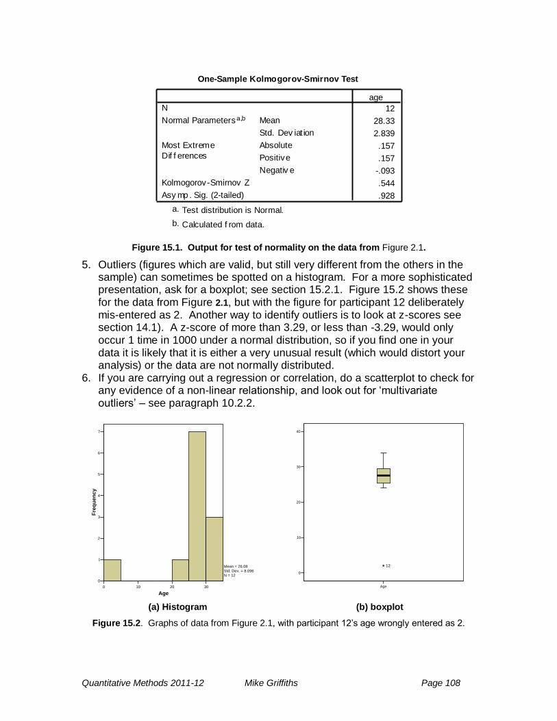
Quantitative Methods 2011-12 Mike Griffiths Page 108
One-Sample Kolmogorov-Smirnov Test
12
28.33
2.839
.157
.157
-.093
.544
.928
N
Mean
Std. Dev iat ion
Normal Parametersa,b
Absolute
Positive
Negativ e
Most Extreme
Dif f erences
Kolmogorov-Smirnov Z
Asy mp . Sig. (2-tailed)
age
Test distribution is Normal.a.
Calculated f rom data.b.
Figure 15.1. Output for test of normality on the data from Figure 2.1.
5. Outliers (figures which are valid, but still very different from the others in the sample) can sometimes be spotted on a histogram. For a more sophisticated presentation, ask for a boxplot; see section 15.2.1. Figure 15.2 shows these for the data from Figure 2.1, but with the figure for participant 12 deliberately mis-entered as 2. Another way to identify outliers is to look at z-scores see section 14.1). A z-score of more than 3.29, or less than -3.29, would only occur 1 time in 1000 under a normal distribution, so if you find one in your data it is likely that it is either a very unusual result (which would distort your analysis) or the data are not normally distributed.
6. If you are carrying out a regression or correlation, do a scatterplot to check for any evidence of a non-linear relationship, and look out for ‗multivariate outliers‘ – see paragraph 10.2.2.
0 10 20 30
Age
0
1
2
3
4
5
6
7
Fre
qu
en
cy
Mean = 26.08Std. Dev. = 8.096N = 12
Age
0
10
20
30
40
12
(a) Histogram (b) boxplot
Figure 15.2. Graphs of data from Figure 2.1, with participant 12‘s age wrongly entered as 2.
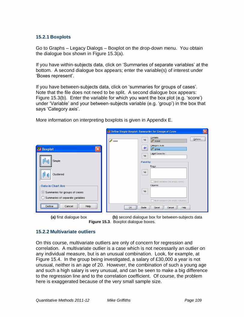
Quantitative Methods 2011-12 Mike Griffiths Page 109
15.2.1 Boxplots
Go to Graphs – Legacy Dialogs – Boxplot on the drop-down menu. You obtain the dialogue box shown in Figure 15.3(a).
If you have within-subjects data, click on ‗Summaries of separate variables‘ at the bottom. A second dialogue box appears; enter the variable(s) of interest under ‗Boxes represent‘. If you have between-subjects data, click on ‗summaries for groups of cases‘. Note that the file does not need to be split. A second dialogue box appears: Figure 15.3(b). Enter the variable for which you want the box plot (e.g. ‗score‘)
under ‗Variable‘ and your between-subjects variable (e.g. ‗group‘) in the box that says ‗Category axis‘. More information on interpreting boxplots is given in Appendix E.
(a) first dialogue box (b) second dialogue box for between-subjects data Figure 15.3. Boxplot dialogue boxes.
15.2.2 Multivariate outliers On this course, multivariate outliers are only of concern for regression and correlation. A multivariate outlier is a case which is not necessarily an outlier on any individual measure, but is an unusual combination. Look, for example, at Figure 15.4. In the group being investigated, a salary of £30,000 a year is not
unusual, neither is an age of 20. However, the combination of such a young age and such a high salary is very unusual, and can be seen to make a big difference to the regression line and to the correlation coefficient. Of course, the problem here is exaggerated because of the very small sample size.
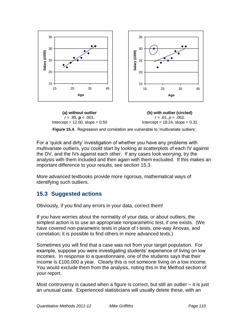
Quantitative Methods 2011-12 Mike Griffiths Page 110
15
20
25
30
35
15 25 35 45
Age
Sala
ry (
£000)
15
20
25
30
35
15 25 35 45
Age
Sala
ry (
£000)
(a) without outlier r = .95, p < .001.
Intercept = 12.00, slope = 0.50
(b) with outlier (circled) r = .61, p = .063.
Intercept = 18.24, slope = 0.31
Figure 15.4. Regression and correlation are vulnerable to ‗multivariate outliers‘.
For a ‗quick and dirty‘ investigation of whether you have any problems with multivariate outliers, you could start by looking at scatterplots of each IV against the DV, and the IVs against each other. If any cases look worrying, try the analysis with them included and then again with them excluded. If this makes an important difference to your results, see section 15.3.
More advanced textbooks provide more rigorous, mathematical ways of identifying such outliers.
15.3 Suggested actions Obviously, if you find any errors in your data, correct them! If you have worries about the normality of your data, or about outliers, the simplest action is to use an appropriate nonparametric test, if one exists. (We have covered non-parametric tests in place of t-tests, one-way Anovas, and correlation; it is possible to find others in more advanced texts.) Sometimes you will find that a case was not from your target population. For example, suppose you were investigating students‘ experience of living on low incomes. In response to a questionnaire, one of the students says that their income is £100,000 a year. Clearly this is not someone living on a low income. You would exclude them from the analysis, noting this in the Method section of your report. Most controversy is caused when a figure is correct, but still an outlier – it is just an unusual case. Experienced statisticians will usually delete these, with an
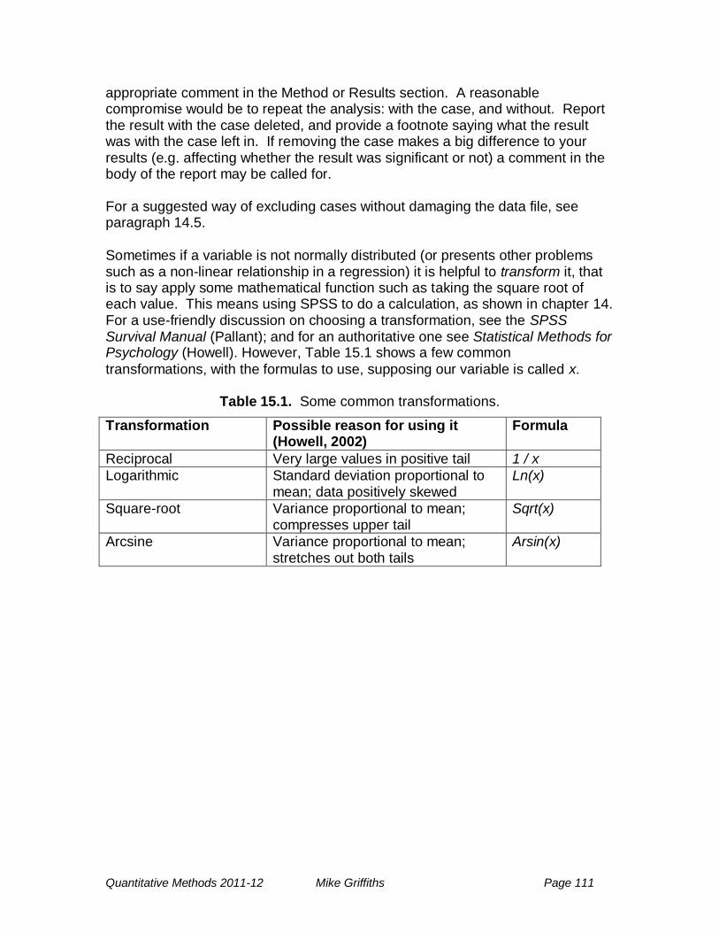
Quantitative Methods 2011-12 Mike Griffiths Page 111
appropriate comment in the Method or Results section. A reasonable compromise would be to repeat the analysis: with the case, and without. Report the result with the case deleted, and provide a footnote saying what the result was with the case left in. If removing the case makes a big difference to your results (e.g. affecting whether the result was significant or not) a comment in the body of the report may be called for. For a suggested way of excluding cases without damaging the data file, see paragraph 14.5.
Sometimes if a variable is not normally distributed (or presents other problems such as a non-linear relationship in a regression) it is helpful to transform it, that is to say apply some mathematical function such as taking the square root of each value. This means using SPSS to do a calculation, as shown in chapter 14. For a use-friendly discussion on choosing a transformation, see the SPSS Survival Manual (Pallant); and for an authoritative one see Statistical Methods for Psychology (Howell). However, Table 15.1 shows a few common
transformations, with the formulas to use, supposing our variable is called x.
Table 15.1. Some common transformations.
Transformation Possible reason for using it (Howell, 2002)
Formula
Reciprocal Very large values in positive tail 1 / x
Logarithmic Standard deviation proportional to mean; data positively skewed
Ln(x)
Square-root Variance proportional to mean; compresses upper tail
Sqrt(x)
Arcsine Variance proportional to mean; stretches out both tails
Arsin(x)
Quantitative Methods 2011-12 Mike Griffiths Page 112
APPENDICES A Reporting results (i) Statistical significance
In the social sciences we usually regard a result as significant if p is less than .05. (You may find it easiest to think of this as .050 so it has the same number of decimal places as the SPSS output.) Some researchers/journals report p values between .05 and .10 as a ‗trend‘, implying that they think there may have been an effect but their study was not quite powerful enough to find it. (ii) Reporting in APA Style
You should always report the descriptive statistics as well as the inferential statistics. Styles of reporting statistics differ, even between journals in the same discipline. However, APA (American Psychological Association) style is used by many journals. Here are some of its main features:
if a Roman letter (e.g. t, F, p, r) is used for a statistic it is printed in italics
degrees of freedom are put in brackets after the statistic. For example t(3) = 3.12
if a statistic cannot take a value higher than 1 (e.g. p, r), the 0 before the decimal point is omitted (e.g. p = .011)
Even within APA style, journals differ in whether one reports the exact level of the significance (e.g. p = .011) or just that it is less than .05 (p < .05, as in this case) or greater than .05 (p > .05).
if we are reporting exact values and SPSS prints the level of significance as .000, we write it as p < .001.
N or n represent the number of participants. In strict APA style, N means the total number of participants in the study and n means the number in a subgroup, but not all journals follow this rule.
(iii) Formatting hints in Word
To insert a Greek letter (e.g. χ) go on the drop-down menu to Insert, then Symbol. In the dialogue box, choose ‗(normal text)‘ in the Font drop-down box (top left), then scroll down until you find the letter you want. To insert a superscript (e.g. the 2 in χ2) go on the drop-down menu to Format, Font, then in the drop-down box ensure that the Font tab is selected. Tick the Superscript box. Repeat and untick the box before typing the next character.
Quantitative Methods 2011-12 Mike Griffiths Page 113
(iv) Rounding numbers
It is often sensible to report figures to fewer decimal places than are given by SPSS or your computer. For example, when reporting a mean it is usually only meaningful to report one more decimal place than there was in the original data. How you do it. Take the number you wish to round (e.g. 2.361) and decide how many decimal places you wish to report (e.g. one). Cross out all the figures after that (in this case after the 3; 2.361). If the first crossed-out figure is 0, 1, 2, 3, or 4) leave the result unchanged. If the first crossed-out figure is 5, 6, 7, 8, or 9, add one to the last uncrossed-out figure. So here, the rounded result is 2.4. Why you do it.
Readers are likely to think that the number of decimal places reflects how confident you are in your result. Suppose Anna and Bob give some children a test. Anna reports that her children‘s mean score is 5. Bob reports that his children‘s mean is 5.00. Bob‘s score sounds more accurate than Anna‘s. This is because Anna‘s if children had a mean score anywhere between 4.5000 and 5.4999, she would still have reported it as 5 (as a round number). In other words, there could have been a range of 1 in the mean score and Anna would have reported it the same way. Bob‘s children would need an average between 4.9950 and 5.0050 for him to report it as 4.00 (to two decimal places). In other words there is only a range of 0.01 in the mean score for which Bob can have legitimately given the score he did. So if the calculator (or SPSS) gives a mean score of 2.361, why not report it as 2.361? The reason is that we are not usually calculating numbers for the fun of it: we are using them to represent something. When we report the children‘s mean score, we are suggesting that this is our best estimate of something, for example what the likely score would be of other children who had the same learning experience. If we report it as 2.361 this suggests that we would expect other children to have a very similar score. This is known as spurious accuracy.
B Converting bar charts to black and white The default bar charts provided by SPSS and Excel are in colour, which may not be appropriate for published work. To change them to black and white, see section 3.2.2 (Excel) or 5.2 (SPSS).
Quantitative Methods 2011-12 Mike Griffiths Page 114
C Copying graphs and other objects into Word (or other applications) Often, copying something from one programme to another is as simple as this:
Click on it in the original program and ensure it is selected (sometimes this means it changes appearance in some way)
Select Edit – Copy from the drop-down menu (or enter Control-C)
Open the programme you want to move it to, and ensure that the cursor is at the point you want the object to appear
Click on Edit – Paste (or enter Control-V). If this does not work, or if the object does not behave itself in the new programme, read on. To change the way that an object is copied, especially how much of its appearance it retains from the original, try one or more of the following.
See if the application you are copying from has any other way of copying. For example,
o to copy a graph from SPSS, you can open the Chart Editor first by double-clicking the chart, then select Edit - Copy Chart
o When copying from SPSS 15 or earlier, try Edit – Copy Objects instead of simply Edit – Copy.
In the application you are copying to, try Edit – Paste Special instead of Edit – Paste. Experiment with all the options until you get the one you want. (For example, if you want a table in Word 2002 to look just like it did in SPSS, try Edit – Paste Special – Files.) Or in Word 2000, try Paste Special – Enhanced Metafile.
Having copied any object into Word, it is advisable to right-click on it, click on ‗Format Objects‘ on the drop-down menu, click on the ‗layout‘ tab, and under ‗Wrapping style‘ select ‗In line with text‘. This ensures that it remains exactly where you placed it in relation to the text on the page.
D Help in SPSS SPSS has the usual Help facilities. It also has (under Help) tutorials and case studies. There are also quite substantial screen tips in many places. For example, on the output for the a chi-square test, double-click on the Chi-Square Tests table so that it is surrounded by a shaded box. Click once on ‗Pearson Chi-square‘, right-click and a drop-down menu appears. Click on ‗What‘s this?‘ and an explanation appears. Similarly, when using a dialogue box (e.g. Crosstabs), right-click on a part of it (e.g. ‗Row(s)‘) and an explanation appears.
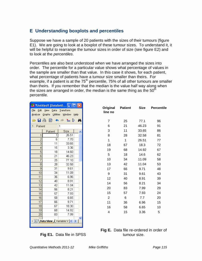
Quantitative Methods 2011-12 Mike Griffiths Page 115
E Understanding boxplots and percentiles Suppose we have a sample of 20 patients with the sizes of their tumours (figure E1). We are going to look at a boxplot of these tumour sizes. To understand it, it will be helpful to rearrange the tumour sizes in order of size (see figure E2) and to look at the percentiles. Percentiles are also best understood when we have arranged the sizes into order. The percentile for a particular value shows what percentage of values in the sample are smaller than that value. In this case it shows, for each patient, what percentage of patients have a tumour size smaller than theirs. For example, if a patient is at the 75th percentile, 75% of all other tumours are smaller than theirs. If you remember that the median is the value half way along when the sizes are arranged in order, the median is the same thing as the 50th percentile.
Original
line no
Patient Size Percentile
7 25 77.1 96
6 21 46.23 91
3 11 33.65 86
8 28 32.58 81
1 1 26.51 77
18 67 18.3 72
19 68 14.92 67
5 18 14.6 62
10 34 11.09 58
13 42 11.04 53
17 66 9.71 48
9 31 9.61 43
12 40 8.91 39
14 56 8.21 34
20 83 7.99 29
15 57 7.93 24
2 6 7.7 20
11 36 6.96 15
16 58 6.65 10
4 15 3.36 5
Fig E1. Data file in SPSS Fig E. Data file re-ordered in order of
tumour size.
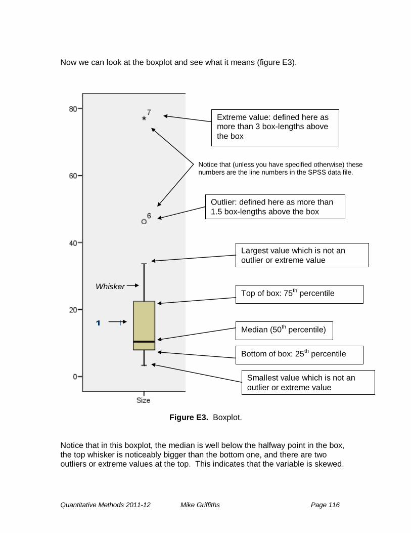
Quantitative Methods 2011-12 Mike Griffiths Page 116
Now we can look at the boxplot and see what it means (figure E3).
Figure E3. Boxplot.
Notice that in this boxplot, the median is well below the halfway point in the box, the top whisker is noticeably bigger than the bottom one, and there are two outliers or extreme values at the top. This indicates that the variable is skewed.
Median (50th percentile)
Bottom of box: 25th percentile
Smallest value which is not an
outlier or extreme value
Top of box: 75th percentile
Largest value which is not an
outlier or extreme value
Outlier: defined here as more than
1.5 box-lengths above the box
Extreme value: defined here as more than 3 box-lengths above
the box
Notice that (unless you have specified otherwise) these numbers are the line numbers in the SPSS data file.
1 BOX
Whisker
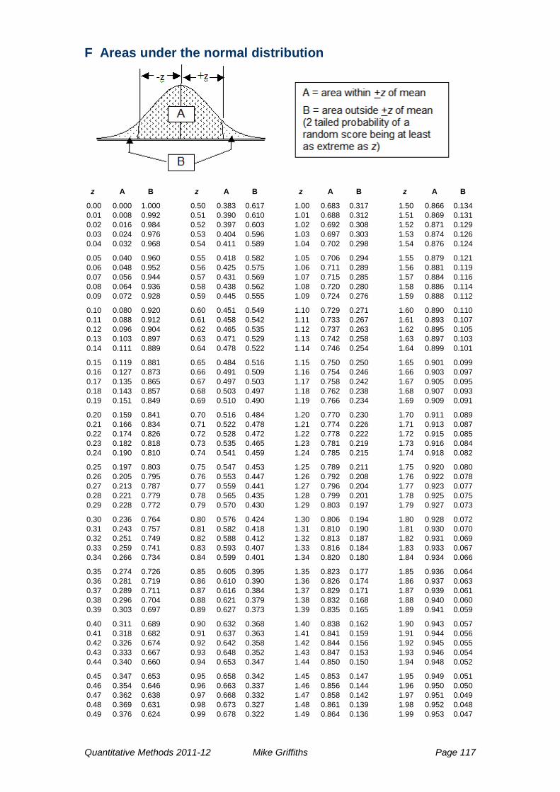
Quantitative Methods 2011-12 Mike Griffiths Page 117
F Areas under the normal distribution
z A B z A B z A B z A B
0.00 0.000 1.000 0.50 0.383 0.617 1.00 0.683 0.317 1.50 0.866 0.134
0.01 0.008 0.992 0.51 0.390 0.610 1.01 0.688 0.312 1.51 0.869 0.131
0.02 0.016 0.984 0.52 0.397 0.603 1.02 0.692 0.308 1.52 0.871 0.129
0.03 0.024 0.976 0.53 0.404 0.596 1.03 0.697 0.303 1.53 0.874 0.126
0.04 0.032 0.968 0.54 0.411 0.589 1.04 0.702 0.298 1.54 0.876 0.124
0.05 0.040 0.960 0.55 0.418 0.582 1.05 0.706 0.294 1.55 0.879 0.121
0.06 0.048 0.952 0.56 0.425 0.575 1.06 0.711 0.289 1.56 0.881 0.119
0.07 0.056 0.944 0.57 0.431 0.569 1.07 0.715 0.285 1.57 0.884 0.116
0.08 0.064 0.936 0.58 0.438 0.562 1.08 0.720 0.280 1.58 0.886 0.114
0.09 0.072 0.928 0.59 0.445 0.555 1.09 0.724 0.276 1.59 0.888 0.112
0.10 0.080 0.920 0.60 0.451 0.549 1.10 0.729 0.271 1.60 0.890 0.110
0.11 0.088 0.912 0.61 0.458 0.542 1.11 0.733 0.267 1.61 0.893 0.107
0.12 0.096 0.904 0.62 0.465 0.535 1.12 0.737 0.263 1.62 0.895 0.105
0.13 0.103 0.897 0.63 0.471 0.529 1.13 0.742 0.258 1.63 0.897 0.103
0.14 0.111 0.889 0.64 0.478 0.522 1.14 0.746 0.254 1.64 0.899 0.101
0.15 0.119 0.881 0.65 0.484 0.516 1.15 0.750 0.250 1.65 0.901 0.099
0.16 0.127 0.873 0.66 0.491 0.509 1.16 0.754 0.246 1.66 0.903 0.097
0.17 0.135 0.865 0.67 0.497 0.503 1.17 0.758 0.242 1.67 0.905 0.095
0.18 0.143 0.857 0.68 0.503 0.497 1.18 0.762 0.238 1.68 0.907 0.093
0.19 0.151 0.849 0.69 0.510 0.490 1.19 0.766 0.234 1.69 0.909 0.091
0.20 0.159 0.841 0.70 0.516 0.484 1.20 0.770 0.230 1.70 0.911 0.089
0.21 0.166 0.834 0.71 0.522 0.478 1.21 0.774 0.226 1.71 0.913 0.087
0.22 0.174 0.826 0.72 0.528 0.472 1.22 0.778 0.222 1.72 0.915 0.085
0.23 0.182 0.818 0.73 0.535 0.465 1.23 0.781 0.219 1.73 0.916 0.084
0.24 0.190 0.810 0.74 0.541 0.459 1.24 0.785 0.215 1.74 0.918 0.082
0.25 0.197 0.803 0.75 0.547 0.453 1.25 0.789 0.211 1.75 0.920 0.080
0.26 0.205 0.795 0.76 0.553 0.447 1.26 0.792 0.208 1.76 0.922 0.078
0.27 0.213 0.787 0.77 0.559 0.441 1.27 0.796 0.204 1.77 0.923 0.077
0.28 0.221 0.779 0.78 0.565 0.435 1.28 0.799 0.201 1.78 0.925 0.075
0.29 0.228 0.772 0.79 0.570 0.430 1.29 0.803 0.197 1.79 0.927 0.073
0.30 0.236 0.764 0.80 0.576 0.424 1.30 0.806 0.194 1.80 0.928 0.072
0.31 0.243 0.757 0.81 0.582 0.418 1.31 0.810 0.190 1.81 0.930 0.070
0.32 0.251 0.749 0.82 0.588 0.412 1.32 0.813 0.187 1.82 0.931 0.069
0.33 0.259 0.741 0.83 0.593 0.407 1.33 0.816 0.184 1.83 0.933 0.067
0.34 0.266 0.734 0.84 0.599 0.401 1.34 0.820 0.180 1.84 0.934 0.066
0.35 0.274 0.726 0.85 0.605 0.395 1.35 0.823 0.177 1.85 0.936 0.064
0.36 0.281 0.719 0.86 0.610 0.390 1.36 0.826 0.174 1.86 0.937 0.063
0.37 0.289 0.711 0.87 0.616 0.384 1.37 0.829 0.171 1.87 0.939 0.061
0.38 0.296 0.704 0.88 0.621 0.379 1.38 0.832 0.168 1.88 0.940 0.060
0.39 0.303 0.697 0.89 0.627 0.373 1.39 0.835 0.165 1.89 0.941 0.059
0.40 0.311 0.689 0.90 0.632 0.368 1.40 0.838 0.162 1.90 0.943 0.057
0.41 0.318 0.682 0.91 0.637 0.363 1.41 0.841 0.159 1.91 0.944 0.056
0.42 0.326 0.674 0.92 0.642 0.358 1.42 0.844 0.156 1.92 0.945 0.055
0.43 0.333 0.667 0.93 0.648 0.352 1.43 0.847 0.153 1.93 0.946 0.054
0.44 0.340 0.660 0.94 0.653 0.347 1.44 0.850 0.150 1.94 0.948 0.052
0.45 0.347 0.653 0.95 0.658 0.342 1.45 0.853 0.147 1.95 0.949 0.051
0.46 0.354 0.646 0.96 0.663 0.337 1.46 0.856 0.144 1.96 0.950 0.050
0.47 0.362 0.638 0.97 0.668 0.332 1.47 0.858 0.142 1.97 0.951 0.049
0.48 0.369 0.631 0.98 0.673 0.327 1.48 0.861 0.139 1.98 0.952 0.048
0.49 0.376 0.624 0.99 0.678 0.322 1.49 0.864 0.136 1.99 0.953 0.047
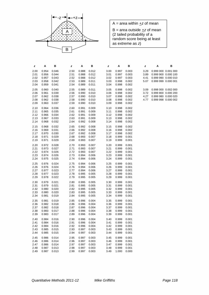
Quantitative Methods 2011-12 Mike Griffiths Page 118
+z
A
B
A = area within +z of mean
B = area outside +z of mean
(2 tailed probability of a random score being at least
as extreme as z)
-z
z A B z A B z A B z A B
2.00 0.954 0.046 2.50 0.988 0.012 3.00 0.997 0.003 3.29 0.999 000 0.001 000
2.01 0.956 0.044 2.51 0.988 0.012 3.01 0.997 0.003 3.89 0.999 900 0.000 100
2.02 0.957 0.043 2.52 0.988 0.012 3.02 0.997 0.003 4.41 0.999 990 0.000 010
2.03 0.958 0.042 2.53 0.989 0.011 3.03 0.998 0.002 5.07 0.999 999 0.000 001
2.04 0.959 0.041 2.54 0.989 0.011 3.04 0.998 0.002
2.05 0.960 0.040 2.55 0.989 0.011 3.05 0.998 0.002 3.09 0.998 000 0.002 000
2.06 0.961 0.039 2.56 0.990 0.010 3.06 0.998 0.002 3.72 0.999 800 0.000 200
2.07 0.962 0.038 2.57 0.990 0.010 3.07 0.998 0.002 4.27 0.999 980 0.000 020
2.08 0.962 0.038 2.58 0.990 0.010 3.08 0.998 0.002 4.77 0.999 998 0.000 002
2.09 0.963 0.037 2.59 0.990 0.010 3.09 0.998 0.002
2.10 0.964 0.036 2.60 0.991 0.009 3.10 0.998 0.002
2.11 0.965 0.035 2.61 0.991 0.009 3.11 0.998 0.002
2.12 0.966 0.034 2.62 0.991 0.009 3.12 0.998 0.002
2.13 0.967 0.033 2.63 0.991 0.009 3.13 0.998 0.002
2.14 0.968 0.032 2.64 0.992 0.008 3.14 0.998 0.002
2.15 0.968 0.032 2.65 0.992 0.008 3.15 0.998 0.002
2.16 0.969 0.031 2.66 0.992 0.008 3.16 0.998 0.002
2.17 0.970 0.030 2.67 0.992 0.008 3.17 0.998 0.002
2.18 0.971 0.029 2.68 0.993 0.007 3.18 0.999 0.001
2.19 0.971 0.029 2.69 0.993 0.007 3.19 0.999 0.001
2.20 0.972 0.028 2.70 0.993 0.007 3.20 0.999 0.001
2.21 0.973 0.027 2.71 0.993 0.007 3.21 0.999 0.001
2.22 0.974 0.026 2.72 0.993 0.007 3.22 0.999 0.001
2.23 0.974 0.026 2.73 0.994 0.006 3.23 0.999 0.001
2.24 0.975 0.025 2.74 0.994 0.006 3.24 0.999 0.001
2.25 0.976 0.024 2.75 0.994 0.006 3.25 0.999 0.001
2.26 0.976 0.024 2.76 0.994 0.006 3.26 0.999 0.001
2.27 0.977 0.023 2.77 0.994 0.006 3.27 0.999 0.001
2.28 0.977 0.023 2.78 0.995 0.005 3.28 0.999 0.001
2.29 0.978 0.022 2.79 0.995 0.005 3.29 0.999 0.001
2.30 0.979 0.021 2.80 0.995 0.005 3.30 0.999 0.001
2.31 0.979 0.021 2.81 0.995 0.005 3.31 0.999 0.001
2.32 0.980 0.020 2.82 0.995 0.005 3.32 0.999 0.001
2.33 0.980 0.020 2.83 0.995 0.005 3.33 0.999 0.001
2.34 0.981 0.019 2.84 0.995 0.005 3.34 0.999 0.001
2.35 0.981 0.019 2.85 0.996 0.004 3.35 0.999 0.001
2.36 0.982 0.018 2.86 0.996 0.004 3.36 0.999 0.001
2.37 0.982 0.018 2.87 0.996 0.004 3.37 0.999 0.001
2.38 0.983 0.017 2.88 0.996 0.004 3.38 0.999 0.001
2.39 0.983 0.017 2.89 0.996 0.004 3.39 0.999 0.001
2.40 0.984 0.016 2.90 0.996 0.004 3.40 0.999 0.001
2.41 0.984 0.016 2.91 0.996 0.004 3.41 0.999 0.001
2.42 0.984 0.016 2.92 0.996 0.004 3.42 0.999 0.001
2.43 0.985 0.015 2.93 0.997 0.003 3.43 0.999 0.001
2.44 0.985 0.015 2.94 0.997 0.003 3.44 0.999 0.001
2.45 0.986 0.014 2.95 0.997 0.003 3.45 0.999 0.001
2.46 0.986 0.014 2.96 0.997 0.003 3.46 0.999 0.001
2.47 0.986 0.014 2.97 0.997 0.003 3.47 0.999 0.001
2.48 0.987 0.013 2.98 0.997 0.003 3.48 0.999 0.001
2.49 0.987 0.013 2.99 0.997 0.003 3.49 1.000 0.000
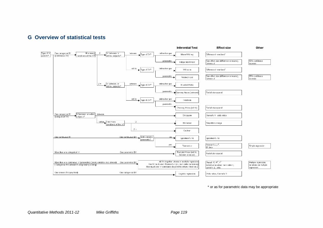
Quantitative Methods 2011-12 Mike Griffiths Page 119
G Overview of statistical tests
* or as for parametric data may be appropriate