Embed Size (px)
Citation preview
Journal of International Economics 70 (2006) 82–114
www.elsevier.com/locate/econbase
Quantitative implications of a debt-deflation theory of
Sudden Stops and asset prices
Enrique G. Mendoza a,*, Katherine A. Smith b
a Department of Economics, University of Maryland and NBER, College Park, MD 20742, United Statesb U.S. Naval Academy, United States
Received 21 April 2003; received in revised form 3 November 2004; accepted 6 June 2005
Abstract
This paper shows that the quantitative predictions of an equilibrium asset-pricing model with financial
frictions are consistent with key features of the Sudden Stop phenomenon. Foreign traders incur costs in
trading assets with domestic agents, and a collateral constraint limits external debt to a fraction of the
market value of domestic equity holdings. When this constraint does not bind, standard productivity shocks
cause typical real-business-cycle effects. When it binds, the same shocks cause strikingly different effects
depending on the leverage ratio and asset market liquidity. With high leverage and a liquid market, the
shocks force bfire salesQ of assets and Fisher’s debt-deflation mechanism amplifies the responses of asset
prices, consumption and the current account. Precautionary saving makes these Sudden Stops infrequent in
the long run.
D 2005 Elsevier B.V. All rights reserved.
Keywords: Emerging markets; Sudden Stops; Collateral constraints; Margin calls; Trading costs; Asset-pricing; Fisherian
debt-deflation
JEL classification: F41; F32; E44; D52
1. Introduction
A significant fraction of the literature dealing with the emerging markets crises of the last ten
years focuses on an intriguing phenomenon referred to as a bSudden StopQ. A Sudden Stop is
defined by three stylized facts: sudden, sharp reversals in capital inflows and the current account,
0022-1996/$ -
doi:10.1016/j.
* Correspon
E-mail add
see front matter D 2005 Elsevier B.V. All rights reserved.
jinteco.2005.06.016
ding author.
ress: [email protected] (E.G. Mendoza).
1 See, for example, Auernheimer and Garcia-Saltos (2000), Aghion et al. (2000), Calvo (1998), Calvo and Mendoza
(2000a), Cespedes et al. (2001), Choi and Cook (2004), Gopinath (2003), Martin and Rey (2002), and Paasche (2001)
Table 1
Sudden stops in four emerging economies
Real equity prices
(% change)
Current account/GDP ratio
(%change)
Industrial production
(%change)
Private consumption
(%change)
Argentina (94.4–95.1) �27.82 4.05 �9.26 �4.12Korea (97.4–98.1) �9.79 10.97 �7.2 �9.48Mexico (94.4–95.1) �28.72 5.24 �9.52 �6.44Russia (98.3–98.4) �59.37 9.46 �5.2 �3.12Real equity prices are deflated by the CPI, except Russian equity prices which are in U.S. dollar terms. The change in the
current account/GDP ratio for Argentina corresponds to the second quarter of 1995. Industrial production for Korea and
Russia and private consumption for Argentina, Korea, and Russia are annual rates.
E.G. Mendoza, K.A. Smith / Journal of International Economics 70 (2006) 82–114 83
large declines in absorption and production, and collapses in real asset prices and in the price of
non-tradable goods relative to tradables.
Table 1 summarizes the stylized facts of Sudden Stops using quarterly data from the IMF for
four well-known cases: Mexico 1994, Argentina 1995, Korea 1997 and Russia 1998. In the
Mexican crisis, real equity prices in units of the CPI fell by 29 percent, the current account rose
by 5.2 percentage points of GDP, industrial output fell nearly 10 percent and consumption
declined by 6.5 percent. Argentina’s 1995 bTequilaQ crisis resulted in collapses in real equity
prices and industrial output similar to Mexico’s, a current account reversal of 4 percentage points
of GDP, and a decline in consumption of 4 percent. The Korean and Russian crises stood out for
their large current account reversals of 11 and 9.5 percentage points of GDP, respectively, and for
the widespread contagion across world financial markets. Equity prices fell simultaneously
across emerging markets in South East Asia in 1997, even in countries where there was no
devaluation of the currency, as in Hong Kong where equity prices fell by 20 percent.
Since the current account reversals that occur during Sudden Stops reflect an emerging
economy’s loss of access to international capital markets, there is growing consensus on the view
that financial frictions are important for explaining Sudden Stops. Several theoretical studies
have shown how a variety of financial frictions could potentially explain this phenomenon.1 In
contrast, the quantitative predictions of this class of models are largely unknown. In particular,
there is little evidence showing whether the effects of financial frictions are strong enough to
account for the observed empirical regularities of Sudden Stops. Moreover, the current account
reversal itself is modeled often as an exogenous shock rather than as an endogenous outcome of
financial frictions (see for example Calvo, 1998). Hence, it is yet unknown whether this class of
models can produce endogenous Sudden Stops caused by the standard underlying sources of
business cycles in emerging markets, without relying on large, unanticipated shocks that impose
the loss of access to capital markets by assumption. This paper attempts to address these issues
by studying the quantitative predictions of an equilibrium asset-pricing model with financial
frictions in which Sudden Stops are an endogenous response to productivity shocks identical to
those that drive a frictionless real-business-cycle model.
The model considers two financial frictions widely used in studies of emerging markets crises
(see the survey by Arellano and Mendoza, 2003): (1) collateral constraints, in the form of a
margin requirement that limits the ability of agents to leverage foreign debt on domestic asset
holdings, and (2) asset trading costs, intended to capture the effects of informational or
.
E.G. Mendoza, K.A. Smith / Journal of International Economics 70 (2006) 82–11484
institutional frictions affecting the ability of foreign traders to trade the equity of emerging
economies (see Frankel and Schmukler, 1996; Calvo and Mendoza, 2000b). Collateral
constraints and trading costs interact with the mechanisms at work in RBC models of the
small open economy and equilibrium asset-pricing models with frictions: uncertainty, risk
aversion and incomplete insurance markets.
The transmission mechanism that causes Sudden Stops in the model operates as follows.
When the economy’s debt is bsufficiently highQ, an adverse productivity shock of standard
magnitude has an effect that it does not have in other states of nature: it triggers collateral
constraints on domestic agents. How high debt needs to be for this to occur is an endogenous
outcome of the analysis. If the asset market is liquid, in the sense that the asset holdings of
domestic agents are above short-selling limits, collateral constraints force domestic agents to
fire-sell assets to foreign traders. These traders are slow to adjust their portfolios because of
trading costs, and as a result asset prices fall. The price fall sets in motion Fisher’s debt-deflation
mechanism, as domestic agents engage in further fire sales of assets to comply with increasingly
tight collateral constraints.2 At high leverage ratios (i.e., high ratios of debt to the market value
of equity), these fire sales cannot prevent a correction in the economy’s net foreign asset
position, and as a result the price decline is accompanied by reversals in consumption and the
current account. Thus, a Sudden Stop takes place.
The analysis of the above financial transmission mechanism as a feature of a dynamic,
stochastic general equilibrium model is difficult because equilibrium asset prices are forward-
looking objects that represent conditional expected present values of the stream of dividends
discounted with stochastic intertemporal marginal rates of substitution. These stochastic
discount factors vary depending on whether collateral constraints bind or not, and this in turn
depends on portfolio choice and equilibrium equity prices. Thus, equilibrium dynamics
feature a nonlinear feedback between equity prices, portfolio choice, stochastic discount
factors, and collateral constraints. The paper develops a numerical solution method to explore
these nonlinear dynamics using a recursive representation of the model’s competitive
equilibrium.
The quantitative results show that a baseline scenario calibrated to Mexican data and with
minimal trading costs can produce reversals in consumption and the current account similar to
those observed in actual Sudden Stops. However, low trading costs imply a high price elasticity
for the foreign traders’ asset demand function, and as a result the fall in asset prices is small.
Still, the drop in asset prices is much larger than in the absence of financial frictions.
The model’s ability to produce larger (and more realistic) asset price collapses hinges on the
size of per-trade asset trading costs. The elasticity of the foreign traders’ asset demand function
with respect to percent deviations of the fundamentals price from the market price is equal to the
inverse of the coefficient that controls the size of these costs. With zero per-trade costs, the
foreign trader’s demand is infinitely elastic at the fundamentals price, and even in the presence of
binding collateral constraints asset prices cannot deviate from their fundamentals level.
Sensitivity analysis shows that the model produces Sudden Stops with realistic responses in
consumption, the current account and asset prices when per trade costs are set so as to yield a
less-than-unitary demand elasticity.
The economy can be inside the high-debt region of the state space in which Sudden Stops
occur (i.e., the bSudden Stop regionQ) because its initial conditions are in that region (for
2 Fisher (1933) and Keynes (1932) provided the first characterizations of the debt-deflation process.
E.G. Mendoza, K.A. Smith / Journal of International Economics 70 (2006) 82–114 85
example, if the economy liberalizes its capital account when its foreign debt is high, or if an
unanticipated shock increases its debt burden) or because the endogenous long-run stochastic
dynamics of the model lead to some of the states inside that region with positive probability. In
the latter case, states in the Sudden Stop region are reached as a result of optimal saving and
portfolio choices in the face of particular sequences of productivity shocks. Precautionary
saving, however, works to minimize the likelihood that these states are reached in the long run.
As a result, long-run business cycle moments for economies with and without financial frictions
display minimal differences and the long-run probability of observing binding margin
requirements is low, consistent with the fact that Sudden Stops are rare events. In addition,
changes in the economic environment that lead to increases in the volatility of asset prices and
income, which strengthen incentives for precautionary saving (such as increases in the variability
or persistence of productivity shocks) make Sudden Stops larger but reduce their long-run
probability.
The transmission mechanism triggering Sudden Stops in this paper differs from others
examined in the literature on emerging markets crises based on the closed-economy bfinancialacceleratorQ models of Kiyotaki and Moore (1997) and Bernanke et al. (1998). Our model differs
in that it introduces elements of equilibrium asset-pricing theory in the presence of aggregate,
non-diversifiable risk, boccasionally-bindingQ collateral constraints and asset trading costs. Most
models of Sudden Stops with collateral constraints feature borrowing constraints that are always
binding at equilibrium or that emerge as an unanticipated, exogenous shock. In contrast, in the
model examined here, collateral constraints become endogenously binding in states of nature in
which the economy’s debt is sufficiently high and agents formulate optimal plans factoring in the
possibility of observing these states. Moreover, in contrast with models that adopt the Bernanke–
Gertler setup of costly monitoring, in which the external financing premium is unaffected by
aggregate risk and is a smooth function of the net worth/debt ratio, the equilibrium dynamics of
our model are influenced by non-insurable risk and the risk premium jumps when collateral
constraints bind.
The asset-pricing features of the model are similar to those studied in the closed-economy
equilibrium asset-pricing literature by Aiyagari (1993), Lucas (1994), Heaton and Lucas (1996),
Krusell and Smith (1997), and Aiyagari and Gertler (1999). These authors examined the asset-
pricing implications of borrowing constraints, trading costs and short-selling constraints with the
aim to explain facts of U.S. capital markets, particularly the equity premium. The quantitative
results were mixed. Yet, financial frictions can still be important for explaining Sudden Stops
because empirical regularities like the equity premium relate to moments of the stochastic steady
state of a model economy but Sudden Stops are features of equilibrium dynamics when
occasionally binding financial frictions bind, even if in the long run these are rare events.
The rest of the paper proceeds as follows. Section 2 presents the model and discusses the
financial transmission mechanism. Section 3 reviews key properties of the model’s deterministic
competitive equilibrium. Section 4 defines the stochastic competitive equilibrium in recursive
form and describes the numerical solution method. Section 5 calibrates the model to Mexican
data and studies the model’s quantitative predictions. Section 6 concludes.
2. An equilibrium model of Sudden Stops and debt-deflations
The model can be summarized as a general equilibrium asset-pricing model with financial
frictions and two sets of agents: foreign and domestic. Domestic agents are modeled as a
representative-agent small open economy subject to non-diversifiable productivity shocks. The
E.G. Mendoza, K.A. Smith / Journal of International Economics 70 (2006) 82–11486
residents of this economy are risk averse and trade bonds and equity with the rest of the world.
They face a margin requirement that limits their ability to borrow and a short-selling constraint
on their equity holdings. Foreign agents are made of two entities: a set of foreign securities firms
specialized in trading equity of the small open economy, and the usual global credit market of
non-state-contingent, one-period bonds that determines the world’s real interest rate via the
standard small open economy assumption. Foreign traders face higher costs than domestic
agents in trading the small open economy’s equity.
Margin requirements and trading costs are modeled following Aiyagari and Gertler (1999).
They examined a closed economy in which households face portfolio adjustment costs,
securities firms face margin requirements, and income, consumption, and the risk-free real
interest rate are exogenous random processes.3 In contrast, in the small open economy examined
here, domestic households face margin requirements, foreign traders are subject to trading costs,
and consumption and income are endogenous.
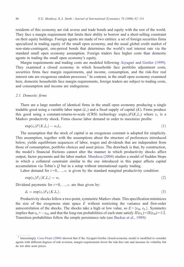
2.1. Domestic firms
There are a large number of identical firms in the small open economy producing a single
tradable good using a variable labor input (Lt) and a fixed supply of capital (K). Firms produce
this good using a constant-returns-to-scale (CRS) technology exp(Et)F(K,Lt) where Et is a
Markov productivity shock. Firms choose labor demand in order to maximize profits:
exp etð ÞF K;Ltð Þ � wtLt: ð1Þ
The assumption that the stock of capital is an exogenous constant is adopted for simplicity.
This assumption, together with the assumptions about the structure of preferences introduced
below, yields equilibrium sequences of labor, wages and dividends that are independent from
those of consumption, portfolio choices and asset prices. The drawback is that, by construction,
the model’s financial frictions cannot alter the manner in which productivity shocks affect
output, factor payments and the labor market. Mendoza (2004) studies a model of Sudden Stops
in which a collateral constraint similar to the one introduced in this paper affects capital
accumulation via Tobin’s Q but in a setup without international equity trading.
Labor demand for t=0,. . .,l is given by the standard marginal productivity condition:
exp etð ÞFL K;Ltð Þ ¼ wt ð2Þ
Dividend payments for t =0,. . .,l are thus given by:
dt ¼ exp etð ÞFK K;LtÞ:ð ð3Þ
Productivity shocks follow a two-point, symmetricMarkov chain. This specificationminimizes
the size of the exogenous state space E without restricting the variance and first-order
autocorrelation of the shocks. The shocks take a high or low value, so E ={EH, EL}. Symmetry
implies that EL=�EH, and that the long-run probabilities of each state satisfy P(EL)=P(EH)=1/2.
Transition probabilities follow the simple persistence rule (see Backus et al., 1989):
3 Interestingly, Coen-Pirani (2000) showed that if the Aiyagari-Gertler closed-economy model is modified to consider
agents with different degrees of risk aversion, margin requirements lower the risk-free rate and increase its volatility but
do not alter asset prices.
E.G. Mendoza, K.A. Smith / Journal of International Economics 70 (2006) 82–114 87
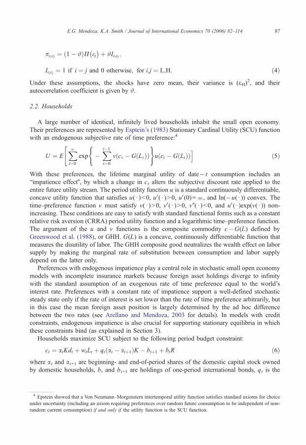
peiej ¼ 1� #ð ÞP ej� �þ #Ieiej ;
Ieiej ¼ 1 if i ¼ j and 0 otherwise; for i;j ¼ L;H: ð4Þ
Under these assumptions, the shocks have zero mean, their variance is (EH)2, and their
autocorrelation coefficient is given by #.
2.2. Households
A large number of identical, infinitely lived households inhabit the small open economy.
Their preferences are represented by Esptein’s (1983) Stationary Cardinal Utility (SCU) function
with an endogenous subjective rate of time preference:4
U ¼ EXlt¼0
exp �Xt�1s¼0
v cs � G Lsð Þð Þ)u ct � G Ltð Þð Þ
i("ð5Þ
With these preferences, the lifetime marginal utility of date� t consumption includes an
bimpatience effectQ, by which a change in ct alters the subjective discount rate applied to the
entire future utility stream. The period utility function u is a standard continuously differentiable,
concave utility function that satisfies u(d )b0, uV(d )N0, uV(0)=l, and ln(�u(d )) convex. The
time–preference function v must satisfy v(d )N0, vV(d )N0, vU(d )b0, and uV(d )exp(v(d )) non-
increasing. These conditions are easy to satisfy with standard functional forms such as a constant
relative risk aversion (CRRA) period utility function and a logarithmic time–preference function.
The argument of the u and v functions is the composite commodity c�G(L) defined by
Greenwood et al. (1988), or GHH. G(L) is a concave, continuously differentiable function that
measures the disutility of labor. The GHH composite good neutralizes the wealth effect on labor
supply by making the marginal rate of substitution between consumption and labor supply
depend on the latter only.
Preferences with endogenous impatience play a central role in stochastic small open economy
models with incomplete insurance markets because foreign asset holdings diverge to infinity
with the standard assumption of an exogenous rate of time preference equal to the world’s
interest rate. Preferences with a constant rate of impatience support a well-defined stochastic
steady state only if the rate of interest is set lower than the rate of time preference arbitrarily, but
in this case the mean foreign asset position is largely determined by the ad hoc difference
between the two rates (see Arellano and Mendoza, 2003 for details). In models with credit
constraints, endogenous impatience is also crucial for supporting stationary equilibria in which
these constraints bind (as explained in Section 3).
Households maximize SCU subject to the following period budget constraint:
ct ¼ atKdt þ wtLt þ qt at � atþ1ð ÞK � btþ1 þ btR ð6Þ
where at and at+1 are beginning- and end-of-period shares of the domestic capital stock owned
by domestic households, bt and bt+1 are holdings of one-period international bonds, qt is the
4 Epstein showed that a Von Neumann–Morgenstern intertemporal utility function satisfies standard axioms for choice
under uncertainty (including an axiom requiring preferences over random future consumption to be independent of non
random current consumption) if and only if the utility function is the SCU function.
-
E.G. Mendoza, K.A. Smith / Journal of International Economics 70 (2006) 82–11488
price of equity, and R is the world’s gross real interest rate (which is kept constant for
simplicity).
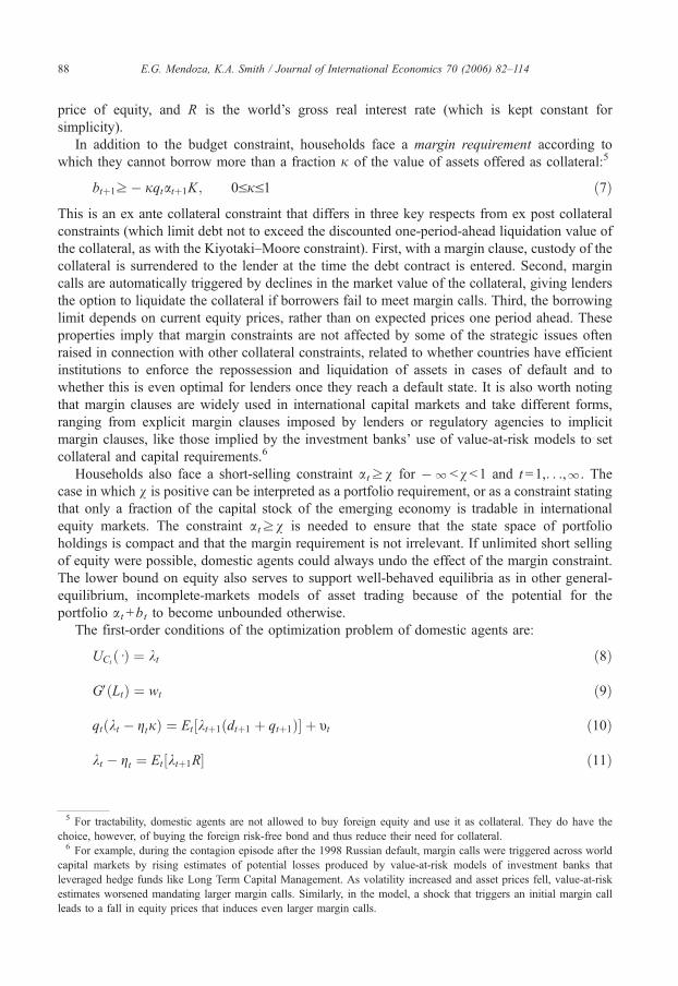
In addition to the budget constraint, households face a margin requirement according to
which they cannot borrow more than a fraction j of the value of assets offered as collateral:5
btþ1z� jqtatþ1K; 0VjV1 ð7Þ
This is an ex ante collateral constraint that differs in three key respects from ex post collateral
constraints (which limit debt not to exceed the discounted one-period-ahead liquidation value of
the collateral, as with the Kiyotaki–Moore constraint). First, with a margin clause, custody of the
collateral is surrendered to the lender at the time the debt contract is entered. Second, margin
calls are automatically triggered by declines in the market value of the collateral, giving lenders
the option to liquidate the collateral if borrowers fail to meet margin calls. Third, the borrowing
limit depends on current equity prices, rather than on expected prices one period ahead. These
properties imply that margin constraints are not affected by some of the strategic issues often
raised in connection with other collateral constraints, related to whether countries have efficient
institutions to enforce the repossession and liquidation of assets in cases of default and to
whether this is even optimal for lenders once they reach a default state. It is also worth noting
that margin clauses are widely used in international capital markets and take different forms,
ranging from explicit margin clauses imposed by lenders or regulatory agencies to implicit
margin clauses, like those implied by the investment banks’ use of value-at-risk models to set
collateral and capital requirements.6
Households also face a short-selling constraint atzv for �lbv b1 and t=1,. . .,l. The
case in which v is positive can be interpreted as a portfolio requirement, or as a constraint stating
that only a fraction of the capital stock of the emerging economy is tradable in international
equity markets. The constraint atzv is needed to ensure that the state space of portfolio
holdings is compact and that the margin requirement is not irrelevant. If unlimited short selling
of equity were possible, domestic agents could always undo the effect of the margin constraint.
The lower bound on equity also serves to support well-behaved equilibria as in other general-
equilibrium, incomplete-markets models of asset trading because of the potential for the
portfolio at +bt to become unbounded otherwise.
The first-order conditions of the optimization problem of domestic agents are:
UCtdð Þ ¼ kt ð8Þ
GV Ltð Þ ¼ wt ð9Þ
qt kt � gtjð Þ ¼ Et ktþ1 dtþ1 þ qtþ1ð Þ½ � þ yt ð10Þ
kt � gt ¼ Et ktþ1R½ � ð11Þ
5 For tractability, domestic agents are not allowed to buy foreign equity and use it as collateral. They do have the
choice, however, of buying the foreign risk-free bond and thus reduce their need for collateral.6 For example, during the contagion episode after the 1998 Russian default, margin calls were triggered across world
capital markets by rising estimates of potential losses produced by value-at-risk models of investment banks that
leveraged hedge funds like Long Term Capital Management. As volatility increased and asset prices fell, value-at-risk
estimates worsened mandating larger margin calls. Similarly, in the model, a shock that triggers an initial margin call
leads to a fall in equity prices that induces even larger margin calls.
E.G. Mendoza, K.A. Smith / Journal of International Economics 70 (2006) 82–114 89
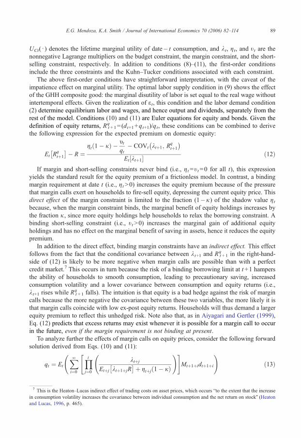
UCt(d ) denotes the lifetime marginal utility of date� t consumption, and kt, gt, and tt are the
nonnegative Lagrange multipliers on the budget constraint, the margin constraint, and the short-
selling constraint, respectively. In addition to conditions (8)–(11), the first-order conditions
include the three constraints and the Kuhn–Tucker conditions associated with each constraint.
The above first-order conditions have straightforward interpretation, with the caveat of the
impatience effect on marginal utility. The optimal labor supply condition in (9) shows the effect
of the GHH composite good: the marginal disutility of labor is set equal to the real wage without
intertemporal effects. Given the realization of Et, this condition and the labor demand condition
(2) determine equilibrium labor and wages, and hence output and dividends, separately from the
rest of the model. Conditions (10) and (11) are Euler equations for equity and bonds. Given the
definition of equity returns, Rqt + 1= (dt+1+qt+1)/qt, these conditions can be combined to derive
the following expression for the expected premium on domestic equity:
Et Rqtþ1
� �� R ¼
gt 1� jð Þ � yt
qt� COVt ktþ1; R
qtþ1
� �Et ktþ1½ � ð12Þ
If margin and short-selling constraints never bind (i.e., gt =tt=0 for all t), this expression
yields the standard result for the equity premium of a frictionless model. In contrast, a binding
margin requirement at date t (i.e., gt N0) increases the equity premium because of the pressure
that margin calls exert on households to fire-sell equity, depressing the current equity price. This
direct effect of the margin constraint is limited to the fraction (1�j) of the shadow value gtbecause, when the margin constraint binds, the marginal benefit of equity holdings increases by
the fraction j, since more equity holdings help households to relax the borrowing constraint. A
binding short-selling constraint (i.e., tt N0) increases the marginal gain of additional equity
holdings and has no effect on the marginal benefit of saving in assets, hence it reduces the equity
premium.
In addition to the direct effect, binding margin constraints have an indirect effect. This effect
follows from the fact that the conditional covariance between kt+1 and Rqt + 1 in the right-hand-
side of (12) is likely to be more negative when margin calls are possible than with a perfect
credit market.7 This occurs in turn because the risk of a binding borrowing limit at t +1 hampers
the ability of households to smooth consumption, leading to precautionary saving, increased
consumption volatility and a lower covariance between consumption and equity returns (i.e.,
kt+1 rises while Rqt +1 falls). The intuition is that equity is a bad hedge against the risk of margin
calls because the more negative the covariance between these two variables, the more likely it is
that margin calls coincide with low ex-post equity returns. Households will thus demand a larger
equity premium to reflect this unhedged risk. Note also that, as in Aiyagari and Gertler (1999),
Eq. (12) predicts that excess returns may exist whenever it is possible for a margin call to occur
in the future, even if the margin requirement is not binding at present.
To analyze further the effects of margin calls on equity prices, consider the following forward
solution derived from Eqs. (10) and (11):
qt ¼ Et
Xli¼0
Yij¼0
ktþjEtþj ktþ1þjR
� �þ gtþj 1� jð Þ
!" #Mtþ1þidtþ1þi
!ð13Þ
7 This is the Heaton–Lucas indirect effect of trading costs on asset prices, which occurs bto the extent that the increase
in consumption volatility increases the covariance between individual consumption and the net return on stockQ (Heatonand Lucas, 1996, p. 465).
E.G. Mendoza, K.A. Smith / Journal of International Economics 70 (2006) 82–11490
where Mt+1+i =kt+1+i/kt for i =0,. . ., 4, is the stochastic intertemporal marginal rate of
substitution between ct+1+i and ct. If the margin requirement never binds, this expression
collapses again to a standard asset-pricing formula. If margin calls are possible at any date, the
rates at which domestic agents discount future dividends are altered by the direct and indirect
effects of margin constraints. The net effect on the price of equity is easier to interpret by solving
forward the expression Et[Rqt +1] =Et[(dt+1+qt+1)/qt] to obtain:
qt ¼ Et
Xli¼0
Yij¼0
Et Rqtþ1þj
h i� ��1" #dtþ1þi
!ð14Þ
where the sequence of Et[Rqt + 1+ j] is given by (12). Hence, if the direct and indirect effects of
margin calls lead to excess equity returns, a margin requirement that binds at present or is
expected to bind in the future implies that some of the expected returns used to discount the
future stream of dividends increase, and thus the current price of equity bid by households falls.
It is important to note that at equilibrium the direct and indirect effects of margin calls are
amplified by the Fisherian debt-deflation process that results from the interaction between
domestic agents and foreign traders in the equity market. A productivity shock triggers an initial
margin call. Domestic agents then try to liquidate equity to meet the call, which puts downward
pressure on the equilibrium equity price because domestic agents trade with foreign traders who
incur trading costs and are thus slow to adjust their portfolios. The resulting fall in equity prices
tightens the margin constraint, which leads to further equity sales and further tightening of the
margin constraint.
2.3. Foreign securities firms
Foreign securities firms maximize the present discounted value of dividends paid to their global
shareholders, facing trading costs that are quadratic in the volume of trades (as in Aiyagari and
Gertler, 1999) and in a fixed recurrent cost.8 These costs represent the disadvantaged position
from which foreign traders operate relative to domestic agents, which may result from
informational frictions (i.e., domestic residents may be better informed on economic and
political variables relevant for determining the earnings prospects of local firms),9 or from
country-specific institutional features or government policies that favor domestic residents. The
recurrent cost represents fixed costs for participating in an emerging equity market that foreign
traders incur just to be ready to trade, even if they do not actually trade in any given period.
Foreign traders choose a*t+1 for t=0, . . ., 4, so as to maximize the value of foreign securities
firms per unit of capital:
D=K ¼ E0
Xlt¼0
Mt4 at4 dt þ qtð Þ � qtatþ14 � qta
2
� �atþ14 � at4þ hð Þ2
� �" #h;az0 ð15Þ
8 Trading costs are often modeled as quadratic in the value of trades (see Heaton and Lucas, 1996). The Aiyagari–
Gertler specification, in which the equity price enters in linear form, yields a more tractable recursive specification of the
trader’s optimality conditions.9 Foreign traders may be less informed because they cannot access or process country-specific information as easily as
domestic agents or because they optimally choose not to do so (Calvo and Mendoza (2000b) provide two arguments for
why the latter can occur).
E.G. Mendoza, K.A. Smith / Journal of International Economics 70 (2006) 82–114 91
where M0*=1 and Mt* for t =1,. . ., 4 are the exogenous marginal rates of substitution between
date� t consumption and date�0 consumption for the world’s representative consumer. For
simplicity, these marginal rates of substitution are set to match the world real interest rate, so
Mt*=Rt. Trading costs are given by qt(a/2)(at+1* �at*+h)2. The recurrent entry cost is h and a is
an adjustment cost coefficient that determines the price elasticity of the foreign trader’s demand
for equity, as shown below. Note that h induces an asymmetry in the manner in which trading
costs operate. With h =0, the total cost of increasing or reducing equity holdings by a given
amount is the same, but with h N0 the total cost of reducing equity holdings is higher.
At an interior solution, the first-order conditions for the above optimization problem imply
that the foreign traders’ demand for equity follows the following partial adjustment rule:
atþ14 � at4ð Þ ¼ 1
a
qftqt� 1
� � h ð16Þ
where qtf is defined as the bfundamentalsQ price:
qftuEt
Xli¼0
Mtþ1þi4 dtþ1þi
!ð17Þ
Note that this price is not equivalent to the asset price that would prevail in the absence of
collateral constraints, because even then equilibrium equity prices would reflect the premium
that risk-averse domestic agents would demand for holding equity (whereas the fundamentals
price as defined in (17) implies zero equity premia since Mt*=Rt).
According to (16), foreign traders increase their demand for equity by a factor 1/a of the
percent deviation of the date� t fundamentals price above the actual price (i.e., 1/a is the
elasticity of their demand for equity with respect to the percent deviation of qtf relative to qt). If
there were no per-trade trading costs, their demand for equity would be infinitely elastic at qtf and
domestic agents could liquidate the shares needed to meet margin calls at an infinitesimal
discount below qtf.
An important implication of the incompleteness of asset markets is that, despite asset trading
between foreign and domestic agents, the stochastic sequences of their discount factors, M*t+1+iand Mt+1+i for i =0,. . .,l, are not equalized. With complete markets, or under perfect foresight,
both sequences are equal to the reciprocal of the world interest rate (compounded i periods).
Under uncertainty and incomplete markets, however, this is not the case even with an
exogenous, risk-free world interest rate. In particular, domestic stochastic discount factors are
endogenous and reflect the effects of margin calls.
2.4. Competitive equilibrium
Given the Markov process of productivity shocks and the initial conditions (b0, a0, a*0), acompetitive equilibrium is defined by stochastic sequences of allocations [ct, Lt, bt+1, at+1,a*t+1]t=0
l and prices [wt, dt, qt, Rqt]t=0l such that: (a) domestic firms maximize dividends subject to
the CRS technology, taking factor and goods prices as given; (b) households maximize SCU
subject to the budget constraint, the margin constraint, and the short-selling constraint, taking as
given factor prices, goods prices, the world interest rate and asset prices; (c) foreign securities
firms maximize the expected present value of dividends net of trading costs, taking as given asset
prices; and (d) the market-clearing conditions for equity, labor, and goods markets hold.
E.G. Mendoza, K.A. Smith / Journal of International Economics 70 (2006) 82–11492
3. Deterministic stationary equilibrium with and without financial frictions
Under perfect foresight, conditions (12) and (13) reduce to the following:
Rqtþ1 � R ¼ gt 1� jð Þ
ktþ1ð18Þ
qt ¼Xli¼0
Yij¼0
1þ 1� jð Þgtþj
ktþj � gtþj
" #�1R�idtþ1þi
0@
1A ð19Þ
As these expressions show, under perfect foresight there is a premium on domestic equity only if
the margin requirement binds at date t, and this premium reflects only the direct effect of margin
calls.
The above expressions can be used to compare the asset-pricing implications of the margin
constraint with those of the Kiyotaki–Moore (KM) collateral constraint, which requires
Rbt+1z�qt+1at+1K. In this case, the forward solution for asset prices yields qt ¼Pl
i¼0�1�
gtþiktþi
��1R�idtþ1þi (using g now for the multiplier on the KM constraint). The KM constraint is
similar to the margin constraint in that: (a) if it binds at present, the equity price is lower
than the fundamentals price because of higher effective discounting of future dividends;10
and (b) if it binds in the future, the current equity price is lower than the fundamentals price.
The quantitative implications of the two constraints differ, however, because a margin
requirement binding at t alters the discount rates domestic agents apply to both dividends and
capital gains at t+1, while a binding KM constraint alters only the discount rate applied to
dividends.
We examine next the implications of margin requirements and trading costs for the
deterministic steady state. At steady state, it follows from (18) and (19) that the fundamentals
price is qf= d/(R�1). The foreign traders’ demand function implies then that asset prices and the
return on equity must satisfy:
qq ¼ qqf
1þ ahð Þ V qqf ð20Þ
RRq ¼ 1þ dd
qqz1þ dd
qqf¼ R ð21Þ
These steady-conditions include two scenarios: a frictionless steady state, with zero trading
costs and non-binding margin constraints, and a steady state with financial frictions.
Consider first the frictionless steady state. The above steady-state conditions state that in
the long run the equity price will equal the fundamentals price, and the equity premium will
vanish, only if per-trade or recurrent trading costs are zero. However, this is necessary but not
sufficient to support the stationary equilibrium because the domestic agents’ asset-pricing
condition will hold at q = qf only if it is also true that the margin constraint does not bind (see
Eq. (19)).
10 Note that the Euler equation for bonds (Eq. (11)) implies that 0V1�g t/k t V1.
E.G. Mendoza, K.A. Smith / Journal of International Economics 70 (2006) 82–114 93
In this frictionless steady state, there is a unique level of steady-state consumption
independent of initial conditions. Since the margin constraint does not bind (i.e., g/k=0), theEuler equations imply that steady-state consumption satisfies exp(v(c)�G(L))=R. The stock of
savings, Su b + qaK, also has a unique steady state because savings and consumption are related
by the budget constraint c = wL + S(R�1). The steady-state portfolio, however, is undetermined.
Any portfolio with vV a V S/((1�j)qf ) and b = S� qa¯K supports the unique level of steady-state
savings.
The multiplicity of steady state portfolios vanishes if financial frictions matter in the long
run. Supporting this steady-state equilibrium requires: (a) positive per trade and recurrent
trading costs and (b) a binding margin constraint. By conditions (20) and (21), positive per
trade and recurrent trading costs imply a steady-state equity price below the fundamentals price
and a long-run equity premium equal to ha(R�1). Since the Euler equations imply that steady-
state consumption satisfies exp(v(c)�G(L))=R/(1� g/k), it follows that the margin constraint
must bind (otherwise c and q would be the same as in the frictionless equilibrium, which is a
contradiction). The implicit solution for steady-state consumption can also be written as
exp(v(c)�G(L))=R +(R�1)[(ah)/(1�j)]. Hence, the beffectiveQ gross real interest rate that
agents face in the steady state with frictions exceeds the gross world interest rate by the factor
[(ah)/(1�j)]. Higher trading costs (higher ah) or tighter margin requirements (lower j) are akinto an increase in the real interest rate in terms of their effect on steady-state consumption. Note
that the model can support this stationary equilibrium at a higher interest rate because the
endogenous rate of time preference increases accordingly. Preferences with a constant rate of
time preference cannot support this equilibrium.
The steady-state portfolio is now uniquely determined and is independent of initial
conditions. The unique portfolio is given by a = S/((1�j)q) and b =�jqaK. Domestic agents
hold more equity than in the frictionless case because the margin constraint increases long-run
savings and because the trading costs make the equity price fall.11
4. Recursive equilibrium and numerical solution method
The model’s competitive equilibrium is solved by reformulating it in recursive form and
applying a numerical solution method. The algorithm is designed to deal with four key
features of the model: incomplete markets of contingent claims, portfolio choice in a two-
agent equilibrium setting, forward-looking asset prices, and occasionally binding margin
constraints.
To represent the equilibrium in recursive form, define a and b as the endogenous state
variables and e as the exogenous state. Since wages, dividends and factor payments depend only
on e, they are represented by the functions w(e), d(e) and L(e) that solve jointly Eqs. (2), (3), and(9). The state space of equity positions spans the interval [v,amax] with NA discrete nodes and
the state space of bond positions spans the interval [bmin,bmax] with NB discrete nodes. The state
space of endogenous states is thus given by the set Z =[v,amax]� [bmin,bmax] of NA�NB
elements.
The recursive asset-pricing function is defined as q(a,b,e): E�ZYR+. For any state
(a,b,e)aE�Z, this pricing function must satisfy the condition that q(a,b,e)a [ qmin(a,e),qmax
11 These results imply that trading costs and credit constraints that bind at steady state produce bhome biasQ in portfolio
holdings and excess returns on emerging markets in the long run.
E.G. Mendoza, K.A. Smith / Journal of International Economics 70 (2006) 82–11494
(a,e)], where qmin (a,e)=qf(e)/[1+a(a�v+h)] and qmax(a,e)=qf(e)/[1+a(a�amax+h)] are
bounds of the pricing function that follow from the fact that when domestic equity holdings
hit either v or amax, the foreign traders’ price prevails because they are at the bshort sideQ ofthe market.
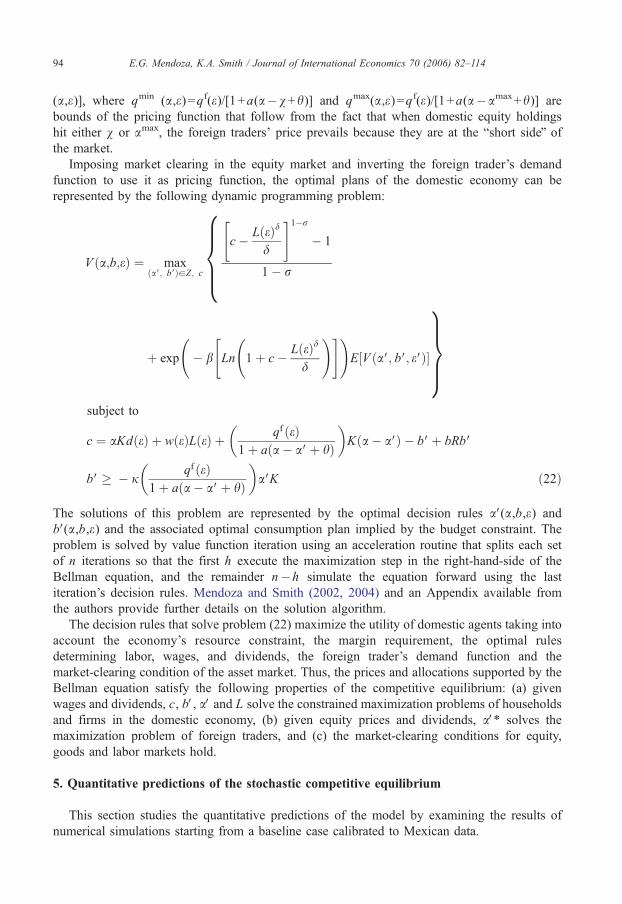
Imposing market clearing in the equity market and inverting the foreign trader’s demand
function to use it as pricing function, the optimal plans of the domestic economy can be
represented by the following dynamic programming problem:
V a;b;eð Þ ¼ maxa V; b Vð ÞaZ; c
(c� L eð Þd
d
" #1�r
� 1
1� r
þ exp � b Ln 1þ c� L eð Þd
d
!" # !E V aV; b V; e Vð Þ½ �
)subject to
c ¼ aKd eð Þ þ w eð ÞL eð Þ þ qf eð Þ1þ a a� aVþ hð Þ
� K a� aVð Þ � b Vþ bRb V
bV � � jqf eð Þ
1þ a a� aVþ hð Þ
� aVK ð22Þ
The solutions of this problem are represented by the optimal decision rules aV(a,b,e) and
bV(a,b,e) and the associated optimal consumption plan implied by the budget constraint. The
problem is solved by value function iteration using an acceleration routine that splits each set
of n iterations so that the first h execute the maximization step in the right-hand-side of the
Bellman equation, and the remainder n�h simulate the equation forward using the last
iteration’s decision rules. Mendoza and Smith (2002, 2004) and an Appendix available from
the authors provide further details on the solution algorithm.
The decision rules that solve problem (22) maximize the utility of domestic agents taking into
account the economy’s resource constraint, the margin requirement, the optimal rules
determining labor, wages, and dividends, the foreign trader’s demand function and the
market-clearing condition of the asset market. Thus, the prices and allocations supported by the
Bellman equation satisfy the following properties of the competitive equilibrium: (a) given
wages and dividends, c, bV, aV and L solve the constrained maximization problems of households
and firms in the domestic economy, (b) given equity prices and dividends, aV* solves the
maximization problem of foreign traders, and (c) the market-clearing conditions for equity,
goods and labor markets hold.
5. Quantitative predictions of the stochastic competitive equilibrium
This section studies the quantitative predictions of the model by examining the results of
numerical simulations starting from a baseline case calibrated to Mexican data.
E.G. Mendoza, K.A. Smith / Journal of International Economics 70 (2006) 82–114 95
5.1. Functional forms and baseline calibration
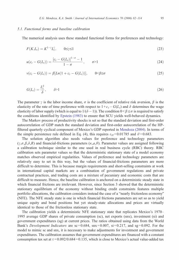
The numerical analysis uses these standard functional forms for preferences and technology:
F K;Ltð Þ ¼ K1�cLct ; 0VcV1 ð23Þ
u ct � G Ltð Þð Þ ¼ ct � G Ltð Þ½ �1�r � 1
1� r; rN1 ð24Þ
v ct � G Ltð Þð Þ ¼ b Ln 1þ ct � G Ltð Þð Þ½ �; 0bbVr ð25Þ
G Ltð Þ ¼Ldt
d; dN1 ð26Þ
The parameter c is the labor income share, r is the coefficient of relative risk aversion, b is the
elasticity of the rate of time preference with respect to 1+ct�G(Lt) and d determines the wage
elasticity of labor supply (which is equal to 1/(d�1)). The condition 0bbVr is required to satisfy
the conditions identified by Epstein (1983) to ensure that SCU yields well-behaved dynamics.
The Markov process of productivity shocks is set so that the standard deviation and first-order
autocorrelation of GDP match the standard deviation and first-order autocorrelation of the HP-
filtered quarterly cyclical component of Mexico’s GDP reported in Mendoza (2004). In terms of
the simple persistence rule defined in Eq. (4), this requires eH =0.01785 and # =0.683.The solution algorithm also needs values for preference and technology parameters
(c,r,b,d,R) and financial-frictions parameters (j,a,h). Parameter values are assigned following
a calibration technique similar to the one used in real business cycle (RBC) theory. RBC
calibration sets parameter values so that the deterministic stationary state of a model economy
matches observed empirical regularities. Values of preference and technology parameters are
relatively easy to set in this way, but the values of financial-frictions parameters are more
difficult to determine. This is because margin requirements and short-selling constraints at work
in international capital markets are a combination of government regulations and private
contractual practices, and trading costs are a mixture of pecuniary and economic costs that are
difficult to measure. Hence, the baseline calibration is anchored on a deterministic steady state in
which financial frictions are irrelevant. However, since Section 3 showed that the deterministic
stationary equilibrium of the economy without binding credit constraints features multiple
portfolio allocations, the calibration considers instead the case of a bnearly frictionless economyQ(NFE). The NFE steady state is one in which financial frictions parameters are set so as to yield
unique equity and bond positions but yet steady-state allocations and prices are virtually
identical to those of the frictionless stationary state.
The calibration yields a deterministic NFE stationary state that replicates Mexico’s 1970–
1995 average GDP shares of private consumption (sc), net exports (snx), investment (si) and
government expenditures (sg) at current prices. The ratios obtained using data from the World
Bank’s Development Indicators are sc=0.684, snx=0.007, si=0.217, and sg=0.092. For the
model to mimic sc and snx, it is necessary to make adjustments for investment and government
expenditures. The calibration assumes that government expenditures are financed with a constant
consumption tax set at s =0.092/0.684=0.135, which is close to Mexico’s actual value-added tax
E.G. Mendoza, K.A. Smith / Journal of International Economics 70 (2006) 82–11496
rate. This tax vanishes from the Euler equations but it does distort labor supply. Still, keeping the
tax state- and time-invariant implies that its effects on the stochastic dynamics are minimal. To
adjust for investment expenditures, the calibration adds an autonomous (time and state invariant)
level of private expenditures equal to the fraction si of steady-state output.
The capital stock is normalized at K =1 without loss of generality. Mexican data from the
System of National Accounts yield an average labor income share for the period 1988–1996 of
0.341. However, this is a low labor share compared to evidence from other countries, as has been
noted in the controversy surrounding measures of labor income shares in some developing
countries (see Mendoza, 2004 for the case of Mexico). Hence, we adopted instead a labor share
of c =0.65, which in line with international evidence. Lacking information on the wage elasticity
of labor supply, the calibration assumes unitary elasticity, so d =2. Given c, K, s and d, thesteady-state allocations of labor and output and the associated wage and dividend rates are
computed using the production function in (24) and the optimality conditions (2), (3), and (9),
adjusted for the presence of the consumption tax. Steady-state consumption is then calculated
using steady-state output and the requirement that the consumption/GDP ratio matches the
average from Mexican data (0.684).
The coefficient of relative risk aversion and the gross real interest rate are set to standard RBC
values: r =2 and R =(1.065)1/4. The interest rate and the dividend rate determine then the steady-
state fundamentals price qf =d/(R�1)=16.9. Finally, given c, L and d, the value of the time
preference elasticity b is derived from the steady-state Euler equation for bonds, which implies
b =Ln(R)/Ln(1+c�Ld/d)=0.0593.Applying the preference and technology parameters set in the previous three paragraphs to the
frictionless stationary equilibrium of Section 3, we obtain allocations and prices that match the
target national accounts ratios taken from the data, but we also obtain the range of multiple steady
states of equity and bonds described there. The economy borrows from abroad (i.e., holds a
negative bond position) only in the solutions in this range in which domestic agents own more
than 90 percent of the capital stock. Bond holdings become positive and unrealistically large
when domestic agents own less than 90 percent of the capital. This is because, with the calibrated
parameters, the market value of the capital stock is large relative to steady-state savings (about 11
percent larger). Since bond holdings at the frictionless steady state are given by b = S� qfaK, ittakes only a small reduction in equity holdings (relative to 100 percent ownership) to leave
households with a positive gap between their desired savings and the value of their equity
holdings, which they fill by holding a large bond position. It also follows from this result that it
will take low values of j to obtain a binding margin constraint in the NFE steady state. In the
frictionless stationary state, the ratio of debt to the value of capital is less than 9.7 percent even in
the extreme case in which domestic agents own all the capital. Thus, only values of j below 9.7
percent can result in binding margin constraints in a deterministic stationary equilibrium.
The above findings lead to two important observations. First, the low ratio of debt to capital
does not preclude large debt/output ratios. When domestic agents own all the domestic capital
stock, the debt ratio is 215 percent of GDP, which is much higher than typical debt ratios of
emerging economies (see Lane and Milesi-Ferretti, 2001). Second, a low j can be rationalized as
the combined outcome of two features that limit the ability of emerging economies to leverage
foreign debt on domestic physical capital: (1) as documented below, the shares of the physical
capital stock of an emerging economy traded in liquid equity markets often represent a small
fraction of the economy’s total capital, and (2) of this residual bmarketableQ portion of the capitalstock, only a fraction may be busefulQ collateral for external borrowing due to institutional or
contractual frictions (see Caballero and Krishnamurthy, 2001; Paasche, 2001).
E.G. Mendoza, K.A. Smith / Journal of International Economics 70 (2006) 82–114 97
The values of the financial frictions parameters that approximate the frictionless steady-state
equilibrium in the NFE case are a =0.01, h =0.04, and j =0.09. In the NFE steady state, the
equity price is only 0.04 percent below the fundamentals price, consumption is less than 0.03
percent higher than in the frictionless equilibrium, and the excess return on equity is less than
0.0007 percent. The unique portfolio allocations are a =0.993 and b =�1.51.
The choice of j at 9 percent follows from the previous result showing that, in the frictionless
steady state, the largest ratio of debt to market value of capital is 9.7 percent. The value of
a =0.01 was chosen to set a high elasticity for the foreign traders’ demand curve, so as to
approximate an environment without per-trade costs. Given a =0.01, h =0.04 implies a low ratio
of steady-state total trading costs to foreign traders’ earnings of 7 percent. Thus, foreign traders
make substantial gains despite the existence of trading costs.
Before ending the discussion of the calibration procedure, it is important to note that, because
the stochastic model is influenced by precautionary saving effects and (if binding) the effects of
margin constraints and trading costs, the deterministic stationary equilibria of equity and bonds
in the NFE can differ widely from the long-run averages obtained with its stochastic counterpart.
For example, the debt ratio in the deterministic NFE is 197 percent but in the stochastic NFE it
falls to 130 percent, and in an economy with identical parameters but j set at 4 percent, it falls to
only 18 percent. This is not a feature particular to this model. It is a general feature of
incomplete-markets models with state-contingent wealth distributions. In calibrating parameter
values for models in this class, a deterministic steady state is useful for imposing some discipline
in the manner in which parameters are selected, but should not be expected to match closely the
mean values of state variables in the stochastic steady state as in standard RBC models.
5.2. State space for baseline simulations
The baseline simulation results compare the NFE with an economy identical in all respects
except for a lower value of j that makes the margin constraint bind in some states of nature. The
margin coefficient in the economy with binding margin constraints (BME) is set to j =0.04.
These simulations use a grid of bond positions with 150 evenly spaced nodes. The lower
bound, bmin, is the largest debt position that the margin constraint can support for all triples (aV,a, e) in the state space (i.e., bmin=�j qmax(v,eH)a
maxK =�1.52). The upper bound bmax=1.43
was determined by setting an initial value and rising it gradually until the grid supported the
limiting distribution of bonds in both the NFE and BME (see Fig. 1b). The grid of equity
positions has 90 evenly spaced nodes and bounds set at v =0.75 and amax=1. The lower bound
at 0.75 is higher than the conventional short-selling limit set at 0 but is consistent with the
national aggregates targeted in the calibration. In Mexico, the average ratio of stock market
capitalization to GDP during 1988–2000 was 27.6 percent. Since the capital/output ratio is about
2.5 (see Mendoza, 2004), the value of Mexican publicly traded firms constitutes just 11 percent
of Mexico’s capital. Thus, a large fraction of Mexico’s capital is owned by non-publicly-traded
private and government firms and residential property owners, and therefore does not have a
liquid market in which shares are traded with foreign residents. Moreover, as Fig. 1a shows,
v =0.75 is a non-binding lower bound in the stochastic stationary states of the NFE and BME
(i.e., the long-run probability of hitting v is zero in both cases).
The 4-percent margin coefficient of the BME is close to a rough estimate of the 1994 ratio of
the debt of Mexico’s listed corporations as a fraction of the country’s capital stock inferred from
firm-level data. Calculations based on data from Worldscope show that the median ratio of debt
to market value of equity of these corporations was about 30 percent. Since the stock market
0.00
0.02
0.04
0.06
0.08
0.10
0.83 0.85 0.86 0.87 0.89 0.90 0.92 0.93 0.94 0.96 0.97 0.99 1.00
0.00
0.01
0.02
0.03
0.04
0.05
-1.52 -1.36 -1.20 -1.05 -0.89 -0.73 -0.57 -0.41 -0.25 -0.09 0.06 0.22 0.38 0.54 0.70 0.86 1.01 1.17 1.33
nearly frictionless economy economy with binding margin constraints
a.
b.
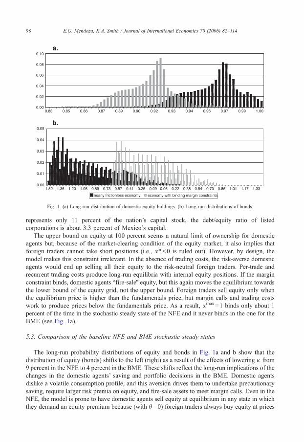
Fig. 1. (a) Long-run distribution of domestic equity holdings. (b) Long-run distributions of bonds.
E.G. Mendoza, K.A. Smith / Journal of International Economics 70 (2006) 82–11498
represents only 11 percent of the nation’s capital stock, the debt/equity ratio of listed
corporations is about 3.3 percent of Mexico’s capital.
The upper bound on equity at 100 percent seems a natural limit of ownership for domestic
agents but, because of the market-clearing condition of the equity market, it also implies that
foreign traders cannot take short positions (i.e., a*b0 is ruled out). However, by design, the
model makes this constraint irrelevant. In the absence of trading costs, the risk-averse domestic
agents would end up selling all their equity to the risk-neutral foreign traders. Per-trade and
recurrent trading costs produce long-run equilibria with internal equity positions. If the margin
constraint binds, domestic agents bfire-saleQ equity, but this again moves the equilibrium towards
the lower bound of the equity grid, not the upper bound. Foreign traders sell equity only when
the equilibrium price is higher than the fundamentals price, but margin calls and trading costs
work to produce prices below the fundamentals price. As a result, amax=1 binds only about 1
percent of the time in the stochastic steady state of the NFE and it never binds in the one for the
BME (see Fig. 1a).
5.3. Comparison of the baseline NFE and BME stochastic steady states
The long-run probability distributions of equity and bonds in Fig. 1a and b show that the
distribution of equity (bonds) shifts to the left (right) as a result of the effects of lowering j from
9 percent in the NFE to 4 percent in the BME. These shifts reflect the long-run implications of the
changes in the domestic agents’ saving and portfolio decisions in the BME. Domestic agents
dislike a volatile consumption profile, and this aversion drives them to undertake precautionary
saving, require larger risk premia on equity, and fire-sale assets to meet margin calls. Even in the
NFE, the model is prone to have domestic agents sell equity at equilibrium in any state in which
they demand an equity premium because (with h =0) foreign traders always buy equity at prices
E.G. Mendoza, K.A. Smith / Journal of International Economics 70 (2006) 82–114 99
that reflect a positive excess return on equity (which are prices below qtf). Domestic agents then
seek to self-insure by building up a large enough bond position. The fire-sales of assets in response
to margin calls, and the diminished ability to leverage debt and smooth consumption, in the BME
add to the forces driving domestic agents to reduce equity holdings and increase bond holdings.
Precautionary saving behavior produces stochastic stationary states for economies with
financial frictions that feature a low probability of observing pairs (a,b) such that a productivity
shock can trigger binding margin constraints causing large drops in consumption. The long-run
probability of states with binding margin constraints in the BME is 2.45 percent. Moreover,
states that combine very large debt positions with low equity positions are ruled out by a version
of Aiyagari’s (1994) natural debt limit: since long sequences of adverse shocks are a non-zero
probability event, domestic agents never hold portfolios that leave them exposed to the
possibility of c�G(L) becoming non-positive.
The above findings provide an interesting interpretation of the dynamics of emerging
economies after the creation of emerging equity markets in the late 1980s, which took place in an
environment of high external debts. During the early periods of this financial globalization, in
which the model would view the stock of precautionary saving as low relative to its long-run
average, emerging economies would be highly vulnerable to suffer endogenous Sudden Stops in
response to the bnormalQ shocks that drive their business cycles. Economies that go through
these early periods with favorable realizations of these shocks would reach the area of debt–
equity positions in which Sudden Stops are very unlikely more rapidly than those that experience
adverse shocks. In these early periods, the model also predicts high excess returns on emerging
markets equity because of the direct, indirect and debt-deflation effects of margin constraints.
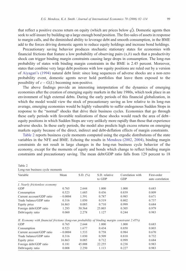
Table 2 reports business cycle moments computed using the ergodic distributions of the state
variables in the NFE and BME. Echoing the results in Mendoza (2002, 2004), binding margin
constraints do not result in large changes in the long-run business cycle behavior of the
economy, except for the moments of equity and bonds which change to reflect binding margin
constraints and precautionary saving. The mean debt/GDP ratio falls from 129 percent to 18
Table 2
Long-run business cycle moments
Variable Mean S.D. (%) S.D. relative
to GDP
Correlation with
GDP
First-order
auto correlation
I. Nearly frictionless economy
GDP 0.765 2.644 1.000 1.000 0.683
Consumption 0.523 1.685 0.436 0.839 0.809
Current account/GDP ratio �0.0004 1.591 0.787 0.985 0.671
Trade balance/GDP ratio 0.316 1.050 0.519 0.802 0.737
Equity price 16.863 0.085 0.710 0.999 0.684
Foreign debt/GDP ratio 1.293 50.564 25.003 0.305 0.979
Debt/equity ratio 0.060 2.278 1.127 0.244 0.983
II. Economy with financial frictions (long-run probability of binding margin constraint 2.45%)
GDP 0.765 2.644 1.000 1.000 0.683
Consumption 0.523 1.677 0.434 0.850 0.803
Current account/GDP ratio �0.0004 1.533 0.758 0.984 0.670
Trade balance/GDP ratio 0.316 1.030 0.509 0.810 0.732
Equity price 16.863 0.085 0.712 0.999 0.684
Foreign debt/GDP ratio 0.181 45.008 22.255 0.238 0.983
Debt/equity ratio 0.008 2.250 1.113 0.227 0.983
E.G. Mendoza, K.A. Smith / Journal of International Economics 70 (2006) 82–114100
percent, and the leverage ratio (the ratio of debt to the value of domestic equity holdings) falls
from 6 to 0.8 percent. In contrast, the variability, co-movement and persistence of consumption,
asset prices and the current account/GDP ratio are almost the same in the two economies,
indicating that domestic agents can reshuffle their portfolio and accumulate enough
precautionary saving to maintain similar consumption allocations in the long run. Hence, the
effects of Sudden Stops are hard to observe in long-run moments and need to be studied by
examining short-run dynamics.
Relative to classic RBC models of the small open economy, this model does not produce a
stochastic steady state with a counter-cyclical current account. This is a well-known limitation of
dynamic general equilibrium models of small open economies that do not consider endogenous
capital accumulation, which typically yield pro-cyclical external accounts driven by consump-
tion smoothing (see Mendoza, 1991). The model is also unable to generate endogenous
persistence in output fluctuations because the assumptions used to separate the bsupply sideQfrom consumption and portfolio choices imply that the persistence of GDP is the same as the
persistence of the exogenous productivity shocks. However, the aim of this quantitative analysis
is to examine the magnitude of the short-run Sudden Stop effects that can result from margin
constraints and trading costs, rather than to develop a full-fledge RBC model. Moreover, since
long-run business cycle moments differ little across the NFE and BME, and since this result
holds also in RBC models with endogenous investment and financial frictions (as shown in
Mendoza, 2004), the inability of this model to produce counter-cyclical external accounts in the
long run and to generate endogenous persistence in GDP is not necessarily a major shortcoming.
In the short-run Sudden Stop dynamics studied next, there is a strong counter-cyclical response
of the current account to adverse productivity shocks.
5.4. Short-run dynamics: leverage, liquidity and Sudden Stops
The previous results showing that the model’s financial frictions do not have significant
effects on long-run business cycle statistics, and that states with binding margin constraints are
low probability events in the stochastic steady state because of precautionary saving, are
consistent with the observation that countries do not experience Sudden Stops very often.
However, we still need to determine whether the dynamics of the model when the economy does
experience a Sudden Stop resemble Sudden Stops observed in the data. This question is
examined next by studying the dynamics around the bSudden Stop regionQ in which margin
constraints bind in the BME.
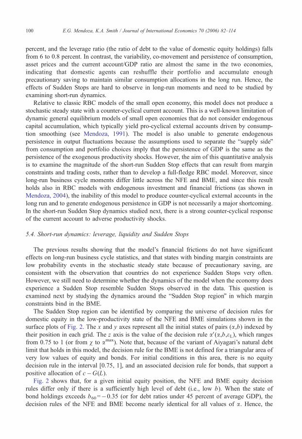
The Sudden Stop region can be identified by comparing the universe of decision rules for
domestic equity in the low-productivity state of the NFE and BME simulations shown in the
surface plots of Fig. 2. The x and y axes represent all the initial states of pairs (a,b) indexed by
their position in each grid. The z axis is the value of the decision rule aV(a,b,eL), which ranges
from 0.75 to 1 (or from v to amax). Note that, because of the variant of Aiyagari’s natural debt
limit that holds in this model, the decision rule for the BME is not defined for a triangular area of
very low values of equity and bonds. For initial conditions in this area, there is no equity
decision rule in the interval [0.75, 1], and an associated decision rule for bonds, that support a
positive allocation of c�G(L).
Fig. 2 shows that, for a given initial equity position, the NFE and BME equity decision
rules differ only if there is a sufficiently high level of debt (i.e., low b). When the state of
bond holdings exceeds b60=�0.35 (or for debt ratios under 45 percent of average GDP), the
decision rules of the NFE and BME become nearly identical for all values of a. Hence, the
1.000
0.938
0.875
0.813
1.000
0.938
0.875
0.813
0.750
0.750
8165
4933
17
equity
equity decision rule
1
81654933
14512911397
17 bonds1
1.000
0.938
0.875
0.813
1.000
0.938
0.875
0.813
0.750
0.750
8165
4933
17
equity
equity decision rule
1
81654933
14512911397
17 bonds1
a. b.
Fig. 2. Equity decision rules in the low productivity state: (a) nearly frictionless economy; (b) economy with binding
margin constraints.
E.G. Mendoza, K.A. Smith / Journal of International Economics 70 (2006) 82–114 101
Sudden Stop region is defined by the subset of high-debt bond position bminVbVb60 for
which there is at least one equity position such that the margin constraint binds. Fig. 2 shows
that in this region the equity and bond decision rules differ sharply across the NFE and
BME.
The differences in the equity decision rules inside the Sudden Stop region illustrate the
magnitude of the combined direct, indirect, and debt-deflation effects of margin calls.
Domestic agents reduce their equity positions significantly more in the BME than in the NFE
in response to the same one-standard-deviation productivity shocks and for the same initial
bond and equity positions. The largest difference between the two economies is about 6
percent of the capital stock, which occurs for initial states with the highest debt (the smallest
b position).
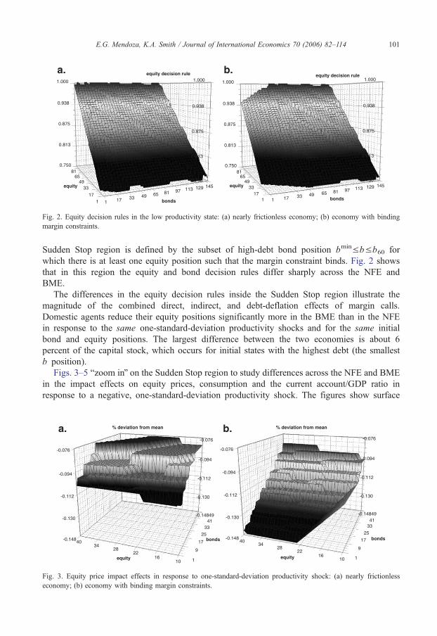
Figs. 3–5 bzoom inQ on the Sudden Stop region to study differences across the NFE and BME
in the impact effects on equity prices, consumption and the current account/GDP ratio in
response to a negative, one-standard-deviation productivity shock. The figures show surface
-0.076
-0.094
-0.112
-0.130
-0.148
-0.076
-0.094
-0.112
-0.130
4034
2822
1610
9
17
3341
-0.14849
25
1equity
% deviation from mean
bonds
-0.076
-0.094
-0.112
-0.130
-0.148
-0.076
-0.094
-0.112
-0.130
4034
2822
1610
9
17
3341
-0.14849
25
1equity
% deviation from mean
bonds
a. b.
Fig. 3. Equity price impact effects in response to one-standard-deviation productivity shock: (a) nearly frictionless
economy; (b) economy with binding margin constraints.
-6.
-12.
-18.
-24.
-30.
-6.
-12.
-18.
-24.
-30.40
34
28
22
16
10
917
3341
49
25
1
equity
% deviation from mean
bonds
-6.
-12.
-18.
-24.
-30.
-6.
-12.
-18.
-24.
-30.40
34
28
22
16
10
9
17
3341
49
25
1
equity bonds
% deviation from mean
a. b.
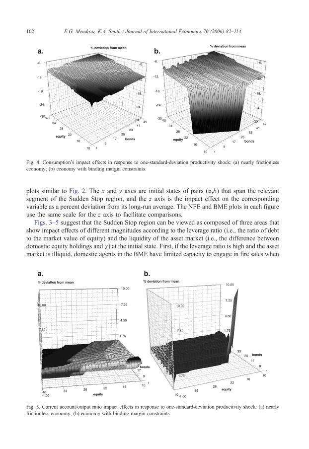
Fig. 4. Consumption’s impact effects in response to one-standard-deviation productivity shock: (a) nearly frictionless
economy; (b) economy with binding margin constraints.
E.G. Mendoza, K.A. Smith / Journal of International Economics 70 (2006) 82–114102
plots similar to Fig. 2. The x and y axes are initial states of pairs (a,b) that span the relevant
segment of the Sudden Stop region, and the z axis is the impact effect on the corresponding
variable as a percent deviation from its long-run average. The NFE and BME plots in each figure
use the same scale for the z axis to facilitate comparisons.
Figs. 3–5 suggest that the Sudden Stop region can be viewed as composed of three areas that
show impact effects of different magnitudes according to the leverage ratio (i.e., the ratio of debt
to the market value of equity) and the liquidity of the asset market (i.e., the difference between
domestic equity holdings and v) at the initial state. First, if the leverage ratio is high and the assetmarket is illiquid, domestic agents in the BME have limited capacity to engage in fire sales when
7.25
4.50
1.75
17
-1.0040 34 28 22 16 10
9
1
10.00
7.25
4.50
1.75
10.00
equity
% deviation from mean
bonds
7.25
4.50
1.75
17
2533
1
-1.00
3440
2822
1610
9
1
10.00
7.25
4.50
1.75
10.00
equity
bonds
% deviation from mean
a. b.
Fig. 5. Current account/output ratio impact effects in response to one-standard-deviation productivity shock: (a) nearly
frictionless economy; (b) economy with binding margin constraints.
-6
-5
-4
-3
-2
-1
0
1
2 4 6 8 10 12 14 16 18 20
-1
0
1
2
3
4
5
2 4 6 8 10 12 14 16 18 20
-0.04
-0.03
-0.02
-0.01
0.00
0.01
2 4 6 8 10 12 14 16 18 20
high leverage ratio (-10.9%) low leverage ratio (-7.4%)
consumption
current account-GDP ratio
equity price
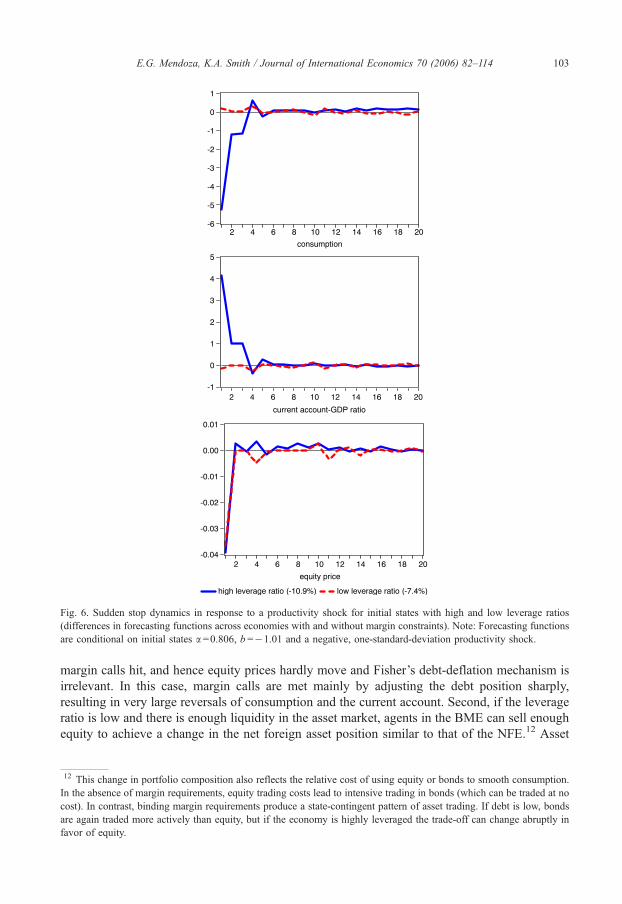
Fig. 6. Sudden stop dynamics in response to a productivity shock for initial states with high and low leverage ratios
(differences in forecasting functions across economies with and without margin constraints). Note: Forecasting functions
are conditional on initial states a =0.806, b =�1.01 and a negative, one-standard-deviation productivity shock.
E.G. Mendoza, K.A. Smith / Journal of International Economics 70 (2006) 82–114 103
margin calls hit, and hence equity prices hardly move and Fisher’s debt-deflation mechanism is
irrelevant. In this case, margin calls are met mainly by adjusting the debt position sharply,
resulting in very large reversals of consumption and the current account. Second, if the leverage
ratio is low and there is enough liquidity in the asset market, agents in the BME can sell enough
equity to achieve a change in the net foreign asset position similar to that of the NFE.12 Asset
12 This change in portfolio composition also reflects the relative cost of using equity or bonds to smooth consumption
In the absence of margin requirements, equity trading costs lead to intensive trading in bonds (which can be traded at no
cost). In contrast, binding margin requirements produce a state-contingent pattern of asset trading. If debt is low, bonds
are again traded more actively than equity, but if the economy is highly leveraged the trade-off can change abruptly in
favor of equity.
.
E.G. Mendoza, K.A. Smith / Journal of International Economics 70 (2006) 82–114104
prices fall by more in the BME than in the NFE, but consumption and the current account
display very similar responses. Third, if the leverage ratio is high and the asset market has
enough liquidity, the direct, indirect and debt-deflation effects of margin calls lead the BME to
produce larger price collapses than the NFE together with larger declines in consumption and
sizable current account reversals.
Fig. 3 shows that the impact effects on asset prices of an adverse productivity shock are
significantly more negative in the BME than in the NFE, but the price declines are quantitatively
small compared to those observed in actual Sudden Stops. However, this is to be expected
because of the high elasticity set for the foreign traders’ demand curve in the calibration. For the
same reason, equity premia are small compared to observed equity premia, although they are
much larger in the BME than in the NFE. These excess returns display the same pattern of the
asset price collapses. They are the largest in the area of the Sudden Stop region in which
domestic agents liquidate the largest amount of equity.
Figs. 3–5 show all the spectrum of possible impact effects at date 1 in response to a negative
productivity shock that hits the NFE and BMEwhen the state of equity and bond holdings is inside
the Sudden Stop region. The baverageQ times-series dynamics for 20 quarters after the shock hits
are illustrated in Fig. 6 for two initial conditions in the relevant areas of the Sudden Stop region: a
high-leverage state (a =0.806, b =�1.481, with a leverage ratio b/[ q(a,b, e)a]=�10.9 percent)
and a low-leverage state (a =0.806, b =�1.01, with a leverage ratio of �7.4 percent). Since in
these two scenarios a is the same, the level of asset market liquidity is also the same.
Fig. 6 plots the differences between the NFE and BME in the forecast functions of
consumption, equity prices, and the current account/GDP ratio, as a percent of the long-run
averages of each in the NFE. The forecast functions are induced by a negative, one-standard-
deviation productivity shock at date 1, theMarkov process of productivity shocks, and the decision
rules aV(a,b,e) and bV(a,b,e). These forecast functions are analogous to impulse-response functions
conditional on starting the NFE and BME at either the high- or low-leverage states and hitting them
with the same negative productivity shock. The forecast functions have the advantage that they
preserve all the non-linear aspects of the model’s stochastic competitive equilibrium captured in
the decision rules. The figures plot the difference in the forecast functions between the NFE and
BME to remove low-frequency dynamics common to both economies. Since the high- and low-
leverage states are far below the long-run averages of equity and bond holdings, the two economies
display low-frequency transitional dynamics to revert all variables to their long-run means.
Fig. 6 shows that, in the high-leverage state, consumption falls by 5.2 percentage points more
in the BME than in the NFE, the current account reversal is equivalent to an increase of
4.1 percentage points of GDP, and asset prices in the BME fall by about four-tenths of a
percentage point more than in the NFE. The low-leverage state shows markedly different
responses to the same productivity shock. Domestic agents in the BME still liquidate assets to
meet margin calls, but now they manage to re-balance their portfolios by replacing debt with
reduced equity holdings, and hence they can maintain a net foreign asset position close to the
desired one in the NFE. As a result, there is no collapse in consumption and no current account
reversal. The asset price decline is slightly smaller than in the high-leverage case. The significant
differences in the Sudden Stop dynamics of the high- and low-leverage cases suggest that Fisher’s
debt-deflation mechanism is a powerful mechanism for inducing strong business cycle
amplification even for small asset price changes.
Fig. 6 also shows that Sudden Stops are short-lived. In the high-leverage case, it takes about
four quarters for the dynamics of consumption, the current account and asset prices of the BME
to converge to the patterns of the NFE, and there is already after the first quarter a substantial
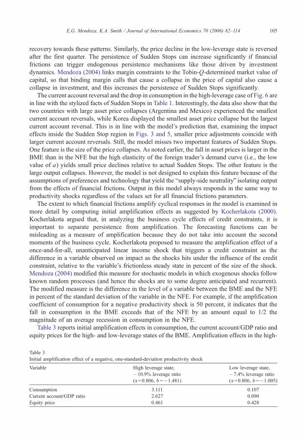
E.G. Mendoza, K.A. Smith / Journal of International Economics 70 (2006) 82–114 105
recovery towards these patterns. Similarly, the price decline in the low-leverage state is reversed
after the first quarter. The persistence of Sudden Stops can increase significantly if financial
frictions can trigger endogenous persistence mechanisms like those driven by investment
dynamics. Mendoza (2004) links margin constraints to the Tobin-Q-determined market value of
capital, so that binding margin calls that cause a collapse in the price of capital also cause a
collapse in investment, and this increases the persistence of Sudden Stops significantly.
The current account reversal and the drop in consumption in the high-leverage case of Fig. 6 are
in line with the stylized facts of Sudden Stops in Table 1. Interestingly, the data also show that the
two countries with large asset price collapses (Argentina and Mexico) experienced the smallest
current account reversals, while Korea displayed the smallest asset price collapse but the largest
current account reversal. This is in line with the model’s prediction that, examining the impact
effects inside the Sudden Stop region in Figs. 3 and 5, smaller price adjustments coincide with
larger current account reversals. Still, the model misses two important features of Sudden Stops.
One feature is the size of the price collapses. As noted earlier, the fall in asset prices is larger in the
BME than in the NFE but the high elasticity of the foreign trader’s demand curve (i.e., the low
value of a) yields small price declines relative to actual Sudden Stops. The other feature is the
large output collapses. However, the model is not designed to explain this feature because of the
assumptions of preferences and technology that yield the bsupply-side neutralityQ isolating outputfrom the effects of financial frictions. Output in this model always responds in the same way to
productivity shocks regardless of the values set for all financial frictions parameters.
The extent to which financial frictions amplify cyclical responses in the model is examined in
more detail by computing initial amplification effects as suggested by Kocherlakota (2000).
Kocherlakota argued that, in analyzing the business cycle effects of credit constraints, it is
important to separate persistence from amplification. The forecasting functions can be
misleading as a measure of amplification because they do not take into account the second
moments of the business cycle. Kocherlakota proposed to measure the amplification effect of a
once-and-for-all, unanticipated linear income shock that triggers a credit constraint as the
difference in a variable observed on impact as the shocks hits under the influence of the credit
constraint, relative to the variable’s frictionless steady state in percent of the size of the shock.
Mendoza (2004) modified this measure for stochastic models in which exogenous shocks follow
known random processes (and hence the shocks are to some degree anticipated and recurrent).
The modified measure is the difference in the level of a variable between the BME and the NFE
in percent of the standard deviation of the variable in the NFE. For example, if the amplification
coefficient of consumption for a negative productivity shock is 50 percent, it indicates that the
fall in consumption in the BME exceeds that of the NFE by an amount equal to 1/2 the
magnitude of an average recession in consumption in the NFE.
Table 3 reports initial amplification effects in consumption, the current account/GDP ratio and
equity prices for the high- and low-leverage states of the BME. Amplification effects in the high-
Table 3
Initial amplification effect of a negative, one-standard-deviation productivity shock
Variable High leverage state,
�10.9% leverage ratio
(a =0.806, b =�1.481)
Low leverage state,
�7.4% leverage ratio
(a =0.806, b =�1.005Consumption 3.111 0.107
Current account/GDP ratio 2.627 0.090
Equity price 0.461 0.428
)
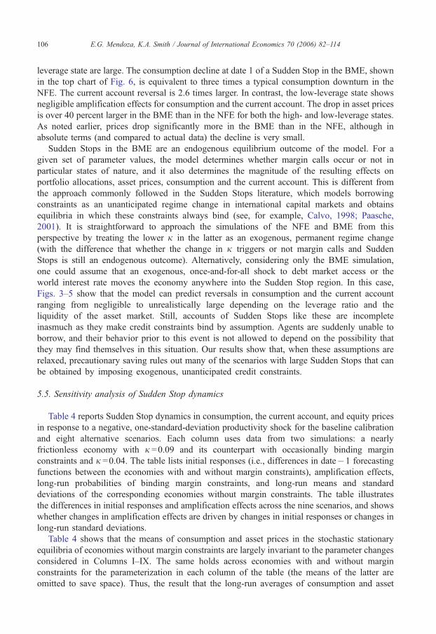
E.G. Mendoza, K.A. Smith / Journal of International Economics 70 (2006) 82–114106
leverage state are large. The consumption decline at date 1 of a Sudden Stop in the BME, shown
in the top chart of Fig. 6, is equivalent to three times a typical consumption downturn in the
NFE. The current account reversal is 2.6 times larger. In contrast, the low-leverage state shows
negligible amplification effects for consumption and the current account. The drop in asset prices
is over 40 percent larger in the BME than in the NFE for both the high- and low-leverage states.
As noted earlier, prices drop significantly more in the BME than in the NFE, although in
absolute terms (and compared to actual data) the decline is very small.
Sudden Stops in the BME are an endogenous equilibrium outcome of the model. For a
given set of parameter values, the model determines whether margin calls occur or not in
particular states of nature, and it also determines the magnitude of the resulting effects on
portfolio allocations, asset prices, consumption and the current account. This is different from
the approach commonly followed in the Sudden Stops literature, which models borrowing
constraints as an unanticipated regime change in international capital markets and obtains
equilibria in which these constraints always bind (see, for example, Calvo, 1998; Paasche,
2001). It is straightforward to approach the simulations of the NFE and BME from this
perspective by treating the lower j in the latter as an exogenous, permanent regime change
(with the difference that whether the change in j triggers or not margin calls and Sudden
Stops is still an endogenous outcome). Alternatively, considering only the BME simulation,
one could assume that an exogenous, once-and-for-all shock to debt market access or the
world interest rate moves the economy anywhere into the Sudden Stop region. In this case,
Figs. 3–5 show that the model can predict reversals in consumption and the current account
ranging from negligible to unrealistically large depending on the leverage ratio and the
liquidity of the asset market. Still, accounts of Sudden Stops like these are incomplete
inasmuch as they make credit constraints bind by assumption. Agents are suddenly unable to
borrow, and their behavior prior to this event is not allowed to depend on the possibility that
they may find themselves in this situation. Our results show that, when these assumptions are
relaxed, precautionary saving rules out many of the scenarios with large Sudden Stops that can
be obtained by imposing exogenous, unanticipated credit constraints.
5.5. Sensitivity analysis of Sudden Stop dynamics
Table 4 reports Sudden Stop dynamics in consumption, the current account, and equity prices
in response to a negative, one-standard-deviation productivity shock for the baseline calibration
and eight alternative scenarios. Each column uses data from two simulations: a nearly
frictionless economy with j =0.09 and its counterpart with occasionally binding margin
constraints and j =0.04. The table lists initial responses (i.e., differences in date�1 forecasting
functions between the economies with and without margin constraints), amplification effects,
long-run probabilities of binding margin constraints, and long-run means and standard
deviations of the corresponding economies without margin constraints. The table illustrates
the differences in initial responses and amplification effects across the nine scenarios, and shows
whether changes in amplification effects are driven by changes in initial responses or changes in
long-run standard deviations.
Table 4 shows that the means of consumption and asset prices in the stochastic stationary
equilibria of economies without margin constraints are largely invariant to the parameter changes
considered in Columns I–IX. The same holds across economies with and without margin
constraints for the parameterization in each column of the table (the means of the latter are
omitted to save space). Thus, the result that the long-run averages of consumption and asset
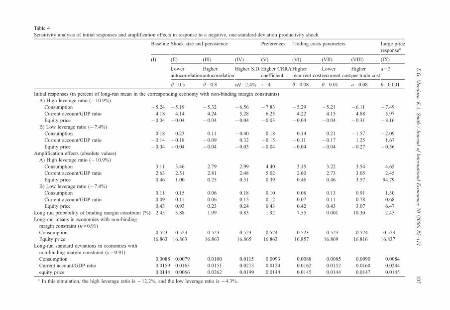
Table 4
Sensitivity analysis of initial responses and amplification effects in response to a negative, one-standard-deviation productivity shock
Baseline Shock size and persistence Preferences Trading costs parameters Large price
responsea
(I) (II) (III) (IV) (V) (VI) (VII) (VIII) (IX)
Lower
autocorrelation
Higher
autocorrelation
Higher S.D.Higher CRRA
coefficient
Higher
recurrent cost
Lower
recurrent cost
Higher
per-trade cost
a =2
# =0.5 # =0.8 eH =2.4% c =4 h =0.08 h =0.01 a =0.08 h =0.001
Initial responses (in percent of long-run mean in the corresponding economy with non-binding margin constraints)
A) High leverage ratio (�10.9%)
Consumption �5.24 �5.19 �5.32 �6.56 �7.83 �5.29 �5.21 �6.11 �7.49Current account/GDP ratio 4.18 4.14 4.24 5.28 6.25 4.22 4.15 4.88 5.97
Equity price �0.04 �0.04 �0.04 �0.04 �0.03 �0.04 �0.04 �0.31 �8.16B) Low leverage ratio (�7.4%)
Consumption 0.18 0.23 0.11 �0.40 0.18 0.14 0.21 �1.57 �2.09Current account/GDP ratio �0.14 �0.18 �0.09 0.32 �0.15 �0.11 �0.17 1.25 1.67
Equity price �0.04 �0.04 �0.04 �0.03 �0.04 �0.04 �0.04 �0.27 �0.56Amplification effects (absolute values)
A) High leverage ratio (�10.9%)
Consumption 3.11 3.46 2.79 2.99 4.40 3.15 3.22 3.54 4.65
Current account/GDP ratio 2.63 2.51 2.81 2.48 5.02 2.60 2.73 3.05 2.45
Equity price 0.46 1.00 0.25 0.31 0.39 0.46 0.46 3.57 94.79
B) Low leverage ratio (�7.4%)
Consumption 0.11 0.15 0.06 0.18 0.10 0.08 0.13 0.91 1.30
Current account/GDP ratio 0.09 0.11 0.06 0.15 0.12 0.07 0.11 0.78 0.68
Equity price 0.43 0.93 0.23 0.24 0.43 0.42 0.43 3.07 6.47
Long run probability of binding margin constraint (%) 2.45 3.88 1.99 0.83 1.92 7.55 0.001 10.30 2.45
Long-run means in economies with non-binding
margin constraint (j =0.91)
Consumption 0.523 0.523 0.523 0.523 0.524 0.523 0.523 0.524 0.523
Equity price 16.863 16.863 16.863 16.865 16.863 16.857 16.869 16.816 16.837
Long-run standard deviations in economies with
non-binding margin constraint (j =0.91)
Consumption 0.0088 0.0079 0.0100 0.0115 0.0093 0.0088 0.0085 0.0090 0.0084
Current account/GDP ratio 0.0159 0.0165 0.0151 0.0213 0.0124 0.0162 0.0152 0.0160 0.0244
equity price 0.0144 0.0066 0.0262 0.0199 0.0144 0.0145 0.0144 0.0147 0.0145
a In this simulation, the high leverage ratio is �12.2%, and the low leverage ratio is �4.3%.
E.G.Mendoza,K.A.Smith
/JournalofIntern
atio
nalEconomics
70(2006)82–114
107
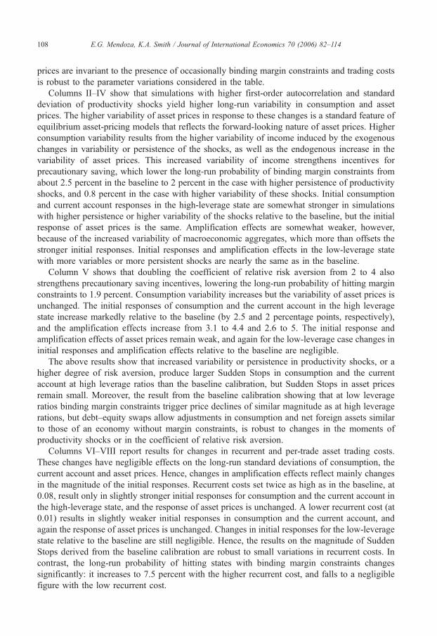
E.G. Mendoza, K.A. Smith / Journal of International Economics 70 (2006) 82–114108
prices are invariant to the presence of occasionally binding margin constraints and trading costs
is robust to the parameter variations considered in the table.
Columns II–IV show that simulations with higher first-order autocorrelation and standard
deviation of productivity shocks yield higher long-run variability in consumption and asset
prices. The higher variability of asset prices in response to these changes is a standard feature of
equilibrium asset-pricing models that reflects the forward-looking nature of asset prices. Higher
consumption variability results from the higher variability of income induced by the exogenous
changes in variability or persistence of the shocks, as well as the endogenous increase in the
variability of asset prices. This increased variability of income strengthens incentives for
precautionary saving, which lower the long-run probability of binding margin constraints from
about 2.5 percent in the baseline to 2 percent in the case with higher persistence of productivity
shocks, and 0.8 percent in the case with higher variability of these shocks. Initial consumption
and current account responses in the high-leverage state are somewhat stronger in simulations
with higher persistence or higher variability of the shocks relative to the baseline, but the initial
response of asset prices is the same. Amplification effects are somewhat weaker, however,
because of the increased variability of macroeconomic aggregates, which more than offsets the
stronger initial responses. Initial responses and amplification effects in the low-leverage state
with more variables or more persistent shocks are nearly the same as in the baseline.
Column V shows that doubling the coefficient of relative risk aversion from 2 to 4 also
strengthens precautionary saving incentives, lowering the long-run probability of hitting margin
constraints to 1.9 percent. Consumption variability increases but the variability of asset prices is
unchanged. The initial responses of consumption and the current account in the high leverage
state increase markedly relative to the baseline (by 2.5 and 2 percentage points, respectively),
and the amplification effects increase from 3.1 to 4.4 and 2.6 to 5. The initial response and
amplification effects of asset prices remain weak, and again for the low-leverage case changes in
initial responses and amplification effects relative to the baseline are negligible.
The above results show that increased variability or persistence in productivity shocks, or a
higher degree of risk aversion, produce larger Sudden Stops in consumption and the current
account at high leverage ratios than the baseline calibration, but Sudden Stops in asset prices
remain small. Moreover, the result from the baseline calibration showing that at low leverage
ratios binding margin constraints trigger price declines of similar magnitude as at high leverage
rations, but debt–equity swaps allow adjustments in consumption and net foreign assets similar
to those of an economy without margin constraints, is robust to changes in the moments of
productivity shocks or in the coefficient of relative risk aversion.
Columns VI–VIII report results for changes in recurrent and per-trade asset trading costs.
These changes have negligible effects on the long-run standard deviations of consumption, the
current account and asset prices. Hence, changes in amplification effects reflect mainly changes
in the magnitude of the initial responses. Recurrent costs set twice as high as in the baseline, at
0.08, result only in slightly stronger initial responses for consumption and the current account in
the high-leverage state, and the response of asset prices is unchanged. A lower recurrent cost (at
0.01) results in slightly weaker initial responses in consumption and the current account, and
again the response of asset prices is unchanged. Changes in initial responses for the low-leverage
state relative to the baseline are still negligible. Hence, the results on the magnitude of Sudden
Stops derived from the baseline calibration are robust to small variations in recurrent costs. In
contrast, the long-run probability of hitting states with binding margin constraints changes
significantly: it increases to 7.5 percent with the higher recurrent cost, and falls to a negligible
figure with the low recurrent cost.
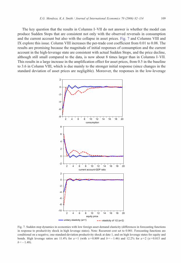
E.G. Mendoza, K.A. Smith / Journal of International Economics 70 (2006) 82–114 109
The key question that the results in Columns I–VII do not answer is whether the model can
produce Sudden Stops that are consistent not only with the observed reversals in consumption
and the current account but also with the collapse in asset prices. Fig. 7 and Columns VIII and
IX explore this issue. Column VIII increases the per-trade cost coefficient from 0.01 to 0.08. The
results are promising because the magnitude of initial responses of consumption and the current
account in the high-leverage state are consistent with actual Sudden Stops, and the price decline,
although still small compared to the data, is now about 8 times larger than in Columns I–VII.
This results in a large increase in the amplification effect for asset prices, from 0.5 in the baseline
to 3.6 in Column VIII, which is due mainly to the stronger initial response (since changes in the
standard deviation of asset prices are negligible). Moreover, the responses in the low-leverage
-8
-6
-4
-2
0
2
2 4 6 8 10 12 14 16 18 20
-2
0
2
4
6
8
2 4 6 8 10 12 14 16 18 20
-10
-8
-6
-4
-2
0
2
2 4 6 8 10 12 14 16 18 20
unitary elasticity (a=1) elasticity of 1/2 (a=2)
consumption
current account-GDP ratio
equity price
Fig. 7. Sudden stop dynamics in economies with low foreign asset demand elasticity (differences in forecasting functions
in response to productivity shock in high leverage states). Note: Recurrent cost set to 0.001. Forecasting functions are
conditional on a negative, one-standard-deviation productivity shock at date 1, and on high leverage states for equity and
bonds. High leverage ratios are 11.4% for a =1 (with a =0.809 and b =�1.46) and 12.2% for a =2 (a =0.815 and
b =�1.48).
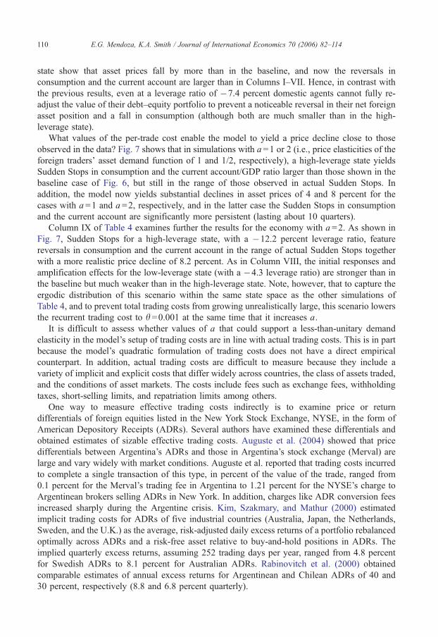
E.G. Mendoza, K.A. Smith / Journal of International Economics 70 (2006) 82–114110
state show that asset prices fall by more than in the baseline, and now the reversals in
consumption and the current account are larger than in Columns I–VII. Hence, in contrast with
the previous results, even at a leverage ratio of �7.4 percent domestic agents cannot fully re-
adjust the value of their debt–equity portfolio to prevent a noticeable reversal in their net foreign
asset position and a fall in consumption (although both are much smaller than in the high-
leverage state).
What values of the per-trade cost enable the model to yield a price decline close to those
observed in the data? Fig. 7 shows that in simulations with a =1 or 2 (i.e., price elasticities of the
foreign traders’ asset demand function of 1 and 1/2, respectively), a high-leverage state yields
Sudden Stops in consumption and the current account/GDP ratio larger than those shown in the
baseline case of Fig. 6, but still in the range of those observed in actual Sudden Stops. In
addition, the model now yields substantial declines in asset prices of 4 and 8 percent for the
cases with a =1 and a =2, respectively, and in the latter case the Sudden Stops in consumption
and the current account are significantly more persistent (lasting about 10 quarters).
Column IX of Table 4 examines further the results for the economy with a =2. As shown in
Fig. 7, Sudden Stops for a high-leverage state, with a �12.2 percent leverage ratio, feature
reversals in consumption and the current account in the range of actual Sudden Stops together
with a more realistic price decline of 8.2 percent. As in Column VIII, the initial responses and
amplification effects for the low-leverage state (with a �4.3 leverage ratio) are stronger than in
the baseline but much weaker than in the high-leverage state. Note, however, that to capture the
ergodic distribution of this scenario within the same state space as the other simulations of
Table 4, and to prevent total trading costs from growing unrealistically large, this scenario lowers
the recurrent trading cost to h =0.001 at the same time that it increases a.
It is difficult to assess whether values of a that could support a less-than-unitary demand
elasticity in the model’s setup of trading costs are in line with actual trading costs. This is in part
because the model’s quadratic formulation of trading costs does not have a direct empirical
counterpart. In addition, actual trading costs are difficult to measure because they include a
variety of implicit and explicit costs that differ widely across countries, the class of assets traded,
and the conditions of asset markets. The costs include fees such as exchange fees, withholding
taxes, short-selling limits, and repatriation limits among others.
One way to measure effective trading costs indirectly is to examine price or return
differentials of foreign equities listed in the New York Stock Exchange, NYSE, in the form of
American Depository Receipts (ADRs). Several authors have examined these differentials and
obtained estimates of sizable effective trading costs. Auguste et al. (2004) showed that price
differentials between Argentina’s ADRs and those in Argentina’s stock exchange (Merval) are
large and vary widely with market conditions. Auguste et al. reported that trading costs incurred
to complete a single transaction of this type, in percent of the value of the trade, ranged from
0.1 percent for the Merval’s trading fee in Argentina to 1.21 percent for the NYSE’s charge to
Argentinean brokers selling ADRs in New York. In addition, charges like ADR conversion fees
increased sharply during the Argentine crisis. Kim, Szakmary, and Mathur (2000) estimated
implicit trading costs for ADRs of five industrial countries (Australia, Japan, the Netherlands,
Sweden, and the U.K.) as the average, risk-adjusted daily excess returns of a portfolio rebalanced
optimally across ADRs and a risk-free asset relative to buy-and-hold positions in ADRs. The
implied quarterly excess returns, assuming 252 trading days per year, ranged from 4.8 percent
for Swedish ADRs to 8.1 percent for Australian ADRs. Rabinovitch et al. (2000) obtained
comparable estimates of annual excess returns for Argentinean and Chilean ADRs of 40 and
30 percent, respectively (8.8 and 6.8 percent quarterly).
E.G. Mendoza, K.A. Smith / Journal of International Economics 70 (2006) 82–114 111
A roughly comparable measure of effective trading costs can be obtained from the model by
computing total trading costs in percent of quarterly equity returns. Trading costs are negligible,
at less than one-fifth of a percent of equity returns, outside the Sudden Stop region. Trading costs
increase rapidly as the leverage ratio rises inside the Sudden Stop region, reaching a maximum
of about 6.4 percent of equity returns when debt is at its maximum (i.e., b =b1). Thus, the model
yields realistic Sudden Stop dynamics in asset prices, as well as in consumption and the current
account, in the presence of frictions in asset markets that translate into effective costs of at most
6.4 percent of asset returns. Trading costs of this magnitude are in line with the estimates
obtained by Kim et al. (2000) and Rabinovitch et al. (2000).
Griffin et al. (2004) provided further evidence of the potential relevance of trading costs.
Using weekly data for 46 industrial and emerging economies for the 1993–2003 period, they
found that in emerging economies, a one-standard-deviation shock to returns is followed by a
0.60-standard-deviation increase in trading after five weeks, and that the delayed response of
asset trading is likely due to participation and trading costs in stock markets. This slow
adjustment of asset positions is qualitatively consistent with the model’s partial-adjustment
portfolio rule of foreign traders induced by trading costs. The forecasting functions of the
baseline NFE and BME in the high-leverage state showed little persistence of asset prices in
response to a negative productivity shock (see Fig. 6), but asset holdings in the BME drop
4 percentage points below those in the NFE on impact, and take about 20 quarters to converge to
the NFE path.
6. Conclusions
This paper studies the quantitative predictions of a dynamic, stochastic, general equilibrium
asset-pricing model with financial frictions to determine if they can rationalize the Sudden Stop
phenomenon. The underlying source of uncertainty in the model is a productivity shock of the
standard magnitude used in RBC analysis, against which domestic agents cannot hedge because
asset markets are incomplete. Two financial frictions are considered. First, domestic residents
face a collateral constraint in international debt markets, in the form of a margin requirement that
limits debt not to exceed the market value of asset holdings used as collateral. Second, foreign
traders face trading costs that reflect institutional or informational frictions they encounter in
trading the equity of an emerging economy.
A binding collateral constraint triggers margin calls that have direct, indirect and debt-
deflation effects working to depress equity prices and increase excess returns. The direct effect is
driven by fire sales of equity in which domestic agents engage to meet margin calls. The indirect
effect is induced by the larger negative covariance between consumption and equity returns that
results from the reduced ability to smooth consumption in the presence of current or expected
future margin calls. When domestic agents rush to sell equity to meet margin calls, they deal
with foreign traders that have a less-than-infinitely-elastic demand for equity because of trading
costs. As a result, equity prices drop and the equity premium rises. In turn, the margin call and
price drop trigger Fisher’s debt-deflation mechanism, as the fall in asset prices leads to
subsequent rounds of margin calls. These results require both collateral constraints and trading
costs. The former alone cannot induce Sudden Stops because without trading costs the foreign
traders’ demand function is infinitely elastic at a fundamentals price that discounts dividends at
the world interest rate.
If the economy has a low leverage ratio (i.e., a low debt/equity ratio), and if the asset market
is sufficiently liquid, the asset–price deflation and a large portfolio re-allocation across bonds
E.G. Mendoza, K.A. Smith / Journal of International Economics 70 (2006) 82–114112
and equity occur without impairing too much the domestic agents’ ability to adjust net foreign
assets and smooth consumption. In contrast, if the leverage ratio is high for the same level of
asset market liquidity, asset prices still fall but portfolio shifts cannot prevent large reversals in
consumption and the current account.
Quantitative simulations calibrated to Mexican data show that, even with very small trading
costs, the direct, indirect and debt-deflation effects of collateral constraints produce Sudden
Stops with large consumption and current account reversals. Asset price declines are small,
however, because small per-trade costs imply a high price elasticity for the foreign traders’ asset
demand function. With trading costs high enough to produce a demand function with less-than-
unitary price elasticity, the model produces Sudden Stops that feature realistic asset price
collapses together with reversals in consumption and the current account in the ranges of those
observed in the data. Empirical evidence on indirect measures of trading costs, in the form of
return differentials, is roughly in line with the model’s predicted ratio of trading costs to asset
returns obtained with a demand function featuring a less-than-unitary price elasticity. Yet, it is
important to recognize that actual trading costs take various forms that differ from the model’s
formulation, and that these costs vary with market conditions and affect traders regardless of
residence (for example, rising in times of turbulence to reflect reduced market liquidity).
Moreover, the price elasticity of demand for an emerging economy’s assets is influenced by
factors other than trading costs (such as informational frictions or government policies) and these
can also affect foreign and domestic residents. However, the model can also be interpreted more
generally: the key to trigger the debt-deflation mechanism is a less-than-perfectly-elastic demand
for domestic equity, which can result from trading costs, or from other frictions, affecting foreign
or domestic agents.
The analysis considered only productivity shocks but Sudden Stops can be caused by a
variety of foreign and domestic shocks that could trigger collateral constraints (such as policy
shocks or shocks to the terms of trade and the world interest rate, as in Mendoza (2002, 2004)).
One important finding of this paper is that these shocks need not be unusually large and
unanticipated to cause Sudden Stops: Adverse shocks of standard magnitude that hit highly
leveraged economies can be sufficient to trigger Sudden Stops, and economies can reach high-
leverage states as a result of endogenous equilibrium dynamics. Moreover, to the extent that
foreign shocks can trigger margin calls, the model embodies a financial transmission mechanism
for the international contagion of capital markets crises. These shocks could be in the form of
typical world-interest-rate shocks or shocks like the global margin calls triggered by the Russian
default in 1998.
The model predicts that Sudden Stops become rare in the long run, after economies build up
buffer stocks of saving. This is an interesting finding because emerging equity markets were
created only a decade ago in an environment in which emerging economies were highly
indebted, and in recent years, many of them have accumulated large stocks of foreign reserves.
The model also predicts that in the early stages of globalization, emerging economies are
vulnerable to Sudden Stops even in the absence of large systemic shocks to world capital
markets, and that during this time, emerging economies should command large excess returns.
Further research in the class of models of the one examined here is proceeding in several
directions. Cavallo et al. (2002) introduce the bliability dollarizationQ feature of foreign debt
contracts of emerging economies, for which debt is largely denominated in units of tradable
goods but leveraged in part on the income and assets of the non-tradables sector. Mendoza
(2004) studies a model with endogenous capital accumulation to explore output collapses and
the investment transmission channel of Sudden Stops. Durdu and Mendoza (in press) study the
E.G. Mendoza, K.A. Smith / Journal of International Economics 70 (2006) 82–114 113
potential benefits of ex ante official asset price guarantees targeted at offsetting the distortions
induced by margin calls and trading costs.
Acknowledgements
We thank Fernando Alvarez, Cristina Arellano, Leonardo Auernheimer, Guillermo Calvo,
Daniele Coen-Pirani, Jonathan Heatcote, Urban Jermann, Fabrizio Perri, Tony Smith, Diego
Valderrama, Kirk White and Stan Zin for helpful comments. We also thank seminar participants
at the University of Chicago GSB, Georgetown, IDB, Iowa State, Wisconsin, UNC, the 2001
Meeting of the Society for Economic Dynamics and Workshop of the Duke International
Economics Group, and the Fall 2003 IFM Program Meeting of the NBER for their suggestions.
References
Aghion, Philippe, Bacchetta, Philippe, Banerjee, Abhijit, 2000. Currency crises and monetary policy with credit
constraints, mimeo, Dept. of Economics, Harvard University.
Aiyagari, S. Rao, 1993. Explaining financial market facts: the importance of incomplete markets and transaction costs.
Quarterly Review - Federal Reserve Bank of Minneapolis 17, 17–31.
Aiyagari, S. Rao, 1994. Uninsured idiosyncratic risk and aggregate saving. Quarterly Journal of Economics 109 (3),
659–684.
Aiyagari, S. Rao, Gertler, Mark, 1999. Overreaction of asset prices in general equilibrium. Review of Economic
Dynamics 2, 3–35.
Auguste, Sebastian, Dominguez, Kathryn M.E., Kamil, Herman, Tesar, Linda L., 2004. Cross-border trading as a
mechanism for implicit capital flight: ADRs, CEDEARs and the argentine crisis, mimeo, Department of Economics,
University of Michigan.
Arellano, Cristina, Mendoza, Enrique G., 2003. Credit frictions and bSudden StopsQ in Small Open Economies: An
Equilibrium Business Cycle Framework For Emerging Markets Crises. In: Altug, Chadha, Nolandynamic
macroeconomic analysis: theory and policy in general equilibrium. Cambridge University Press.
Auernheimer, Leonardo, Garcia-Saltos, Roberto, 2000. International Debt and the Price of Domestic Assets. IMF
Working Paper, vol. WP/00/177. International Monetary Fund.
Backus, David K., Gregory, Allan W., Zin, Stanley E., 1989. Risk premiums in the term structure: evidence from artificial
economies. Journal of Monetary Economies 24, 371–400.
Bernanke, Ben, Gertler, Mark, Girlchrist, Simon, 1998. The Financial Accelerator in a Quantitative Business Cycle
Framework. NBER Working Paper, vol. 6455. National Bureau of Economic Research, Cambridge, MA.
Caballero, Ricardo J., Krishnamurthy, Arvind, 2001. International and domestic collateral constraints in a model of
emerging market crises. Journal of Monetary Economics 48, 513–548.
Calvo, Guillermo A., 1998. Capital flows and capital-market crises: the simple economics of Sudden Stops. Journal of
Applied Economics 1, 35–54.
Calvo, Guillermo A., Mendoza, Enrique G., 2000a. Capital-markets crises and economic collapse in emerging markets:
an informational-frictions approach. American Economic Review: Papers and Proceedings, May.
Calvo, Guillermo A., Mendoza, Enrique G., 2000b. Rational contagion and the globalization of securities markets.
Journal of International Economics 51.
Cavallo, Michele, Kisselev, Kate, Perri, Fabrizio, Roubini, Nouriel, 2002. Exchange Rate Overshooting and the Cost of
Floating, Mimeo. New York University.
Cespedes, Luis, Chang, Roberto, Velasco, Andres, 2001. Balance sheets and exchange rate policy. Mimeo, Department of
Economics, New York University.
Choi, Woon Gyu, Cook, David, 2004. Liability dollarization and the bank balance sheet channel. Journal of International
Economics 64 (2), 247–276.
Coen-Pirani, Daniele, 2000. Margin requirements and equilibrium asset prices, mimeo, Graduate School of Industrial
Administration, Carnegie Mellon University.
Durdu, Ceyhun Bora, Mendoza, Enrique G., in press. Are asset price guarantees useful for preventing sudden stops?: A
quantitative investigation of the globalization hazard–moral hazard tradeoff. Journal of International Economics.
Epstein, Larry G., 1983. Stationary cardinal utility and optimal growth under uncertainty. Journal of Economic Theory
31, 133–152.
E.G. Mendoza, K.A. Smith / Journal of International Economics 70 (2006) 82–114114
Fisher, Irving, 1933. The debt-deflation theory of great depressions. Econometrica 1, 337–357.
Frankel, Jeffrey A., Schmukler, Sergio, 1996. Country fund discounts and the Mexican crisis of December 1994. Open
Economies Review, 7 (Suppl. 1), 551–584.
Gopinath, Gita, 2003. Lending booms, sharp reversals and real exchange rate dynamics. Journal of International
Economics.
Greenwood, Jeremy, Hercowitz, Zvi, Huffman, Gregory W., 1988. Investment, capacity utilization and the real business
cycle. American Economic Review (June).
Griffin, John M., Nardari, Federico, Stulz, Rene M., 2004. Stock Market Trading and Market Conditions. NBERWorking
Paper vol. 10719. National Bureau of Economic Research.
Heaton, John, Lucas, Deborah J., 1996. Evaluating the effects of incomplete markets on risk sharing and asset pricing.
Journal of Political Economy 104 (3), 443–487.
Keynes, John Maynard, 1932. The consequences to the banks of the collapse of money value. Ch. 7 of Essays in
Persuasion. Harcourt, Brace and Company, New York, NY.
Kim, Minho, Szakmary, Andrew C., Mathur, Ike, 2000. Price transmission dynamics between ADRs and their underlying
foreign securities. Journal of Banking and Finance 24, 1359–1382.
Kiyotaki, Nobuhiro, Moore, John, 1997. Credit cycles. Journal of Political Economy 105, 211–248.
Kocherlakota, Narayana, 2000. Creating business cycles through credit constraints. Federal Reserve Bank of Minneapolis
Quarterly Review 24 (3), 2–10 (Summer).
Krusell, Per, Smith Jr., Anthony A., 1997. Income and wealth heterogeneity, portfolio choice, and equilibrium asset
returns. Macroeconomic Dynamics 1, 387–422.
Lane, Philip R., Milesi-Ferretti, Gian Maria, 2001. The external wealth of nations: measures of foreign assets and
liabilities for industrial and developing countries. Journal of International Economics 55, 263–294.
Lucas, Deborah J., 1994. Asset pricing with undiversifiable income risk and short sales constraints. Journal of Monetary
Economics 34, 325–341.
Martin, Philippe, Helene Rey, 2002. Financial globalization and emerging markets: with or without crash?, mimeo,
Department of Economics, Princeton University.
Mendoza, Enrique G., 1991. Real business cycles in a small open economy. American Economic Review 81, 797–818.
Mendoza, Enrique G., 2002. Credit, prices, and crashes: business cycles with a Sudden Stop. In: Edwards, S., Frankel,
J. (Eds.), Preventing Currency Crises in Emerging Markets. University of Chicago Press.
Mendoza, Enrique G., 2004. dSudden StopsT in an equilibrium business cycle model with credit constraints: a fisherian
deflation of Tobin’s Q, mimeo, Department of Economics, University of Maryland.
Mendoza, Enrique G., Smith, Katherine A., 2002. Margin Calls, Trading Costs and Asset Prices in Emerging Markets:
The Financial Mechanics of the dSudden StopT Phenomenon. NBER Working Paper vol. 9286. National Bureau of
Economic Research.
Mendoza, Enrique G., Smith, Katherine A., 2004. Quantitative Implications of a Debt-Deflation Theory of Sudden Stops
and Asset Prices. NBER Working Paper vol. 10940. National Bureau of Economic Research.
Paasche, Bernhard, 2001. Credit constraints and international financial crises. Journal of Monetary Economics 28,
623–650.
Rabinovitch, Ramon, Silva, Ana C., Susmel, Raul, 2000. The Impact of Capital Controls and Transaction Costs on the
Return Distribution of Dually Traded Securities: Evidence from Chile and Argentina. Department of Finance, CBA,
University of Houston.