QUANTITATIVE ESTIMATES OF MECHANICAL PROPERTIES FROM IN VIVO TUMORS OF RODENT ANIMALS

BY

YUE WANG

THESIS

Submitted in partial fulfillment of the requirements for the degree of Master of Science in Bioengineering

in the Graduate College of the University of Illinois at Urbana-Champaign, 2012

Urbana, Illinois

Adviser: Professor Michael F. Insana

ii

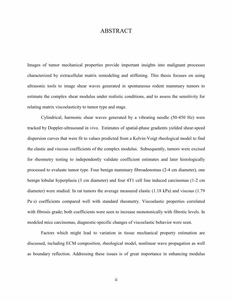
ABSTRACT

Images of tumor mechanical properties provide important insights into malignant processes

characterized by extracellular matrix remodeling and stiffening. This thesis focuses on using

ultrasonic tools to image shear waves generated in spontaneous rodent mammary tumors to

estimate the complex shear modulus under realistic conditions, and to assess the sensitivity for

relating matrix viscoelasticity to tumor type and stage.

Cylindrical, harmonic shear waves generated by a vibrating needle (50-450 Hz) were

tracked by Doppler-ultrasound in vivo. Estimates of spatial-phase gradients yielded shear-speed

dispersion curves that were fit to values predicted from a Kelvin-Voigt rheological model to find

the elastic and viscous coefficients of the complex modulus. Subsequently, tumors were excised

for rheometry testing to independently validate coefficient estimates and later histologically

processed to evaluate tumor type. Four benign mammary fibroadenomas (2-4 cm diameter), one

benign lobular hyperplasia (3 cm diameter) and four 4T1 cell line induced carcinomas (1-2 cm

diameter) were studied. In rat tumors the average measured elastic (1.18 kPa) and viscous (1.79

Pa·s) coefficients compared well with standard rheometry. Viscoelastic properties correlated

with fibrosis grade; both coefficients were seen to increase monotonically with fibrotic levels. In

modeled mice carcinomas, diagnostic-specific changes of viscoelastic behavior were seen.

Factors which might lead to variation in tissue mechanical property estimation are

discussed, including ECM composition, rheological model, nonlinear wave propagation as well

as boundary reflection. Addressing these issues is of great importance in enhancing modulus

iii

measurement accuracy and lesion image contrast by making the right decisions about mechanical

excitation methods and constitutive models.

Dynamic shear-wave estimation of complex modulus has demonstrated an ability to

describe mammary tumors. The measurable differences between lesion types are greater than

inter-animal or technique variabilities. Nevertheless, to reliably classify tumors using elasticity

imaging, more knowledge on the biological contrast mechanism in tissue mechanical properties

is needed. Future work will be on discovering how mechanical properties change with cancer

progression and the way to monitor this change by assessing mechanoenvironment.

iv

ACKNOWLEDGMENTS

This work would not have been possible without the help and support from many people. First, I

would like to thank my adviser, Dr. Michael F. Insana, for his generous support and

encouragement, for his enlightening guide throughout the project, for him to be so patient in my

tough time. I gained lots of valuable assets in this process. I must also thank Marko Orescanin,

who spent countless time with me when I first started this project. And I am also grateful to my

other lab mates, Muqeem Qayyum, Rebecca Yapp, etc. and their kind help in my experiment

design and implementation. I need to thank my collaborators Dan Weisgerber who helped me

with ECM quantification experiments. Most of all, I will give my greatest thanks to my parents

who always love me, support me. This work was funded by NIH Grant R01CA082497 and

carried out in Beckman Institute for Advanced Science and Technology.

v

TABLE OF CONTENTS

CHAPTER 1: INTRODUCTION ...................................................................................... 1

CHAPTER 2: SHEAR WAVE IMAGING TECHNOLOGY ........................................... 6

CHAPTER 3: IN VIVO IMAGING OF RODENT MAMMARY TUMORS ................ 22

CHAPTER 4: VARIATION IN MEASUREMENTS ..................................................... 45

CHAPTER 5: DISCUSSIONS ........................................................................................ 61

REFERENCES ................................................................................................................. 63

1

CHAPTER 1

INTRODUCTION

1.1 Background in biology

Pathological changes in tissues are usually accompanied by mechanical property changes.

In some pathological conditions, elastographic contrast is greater than it is from other

common imaging modalities such as MR imaging and X-ray-based methods. Many

papers have shown that tissue fibrosis stage correlates with tissue stiffness (modulus)

which motivates the use of elasticity imaging techniques for detecting diseases that

include tissue fibrosis. [1][2] Breast tumors, similar to liver fibrosis in the sense of

extracellular matrix (ECM) proteins alteration, possess a potential change in tissue

mechanical properties. The importance of fibrosis is found in recent discoveries in cancer

cell biology that mechanotransduction plays an important role in modulating cell

behaviors in response to ECM changes during cancer development. [3] By depositing

more stromal components and enhancing collagen crosslinks, cancer cells increase the

strength of focal adhesion to facilitate its growth. Accompanied with this reciprocal

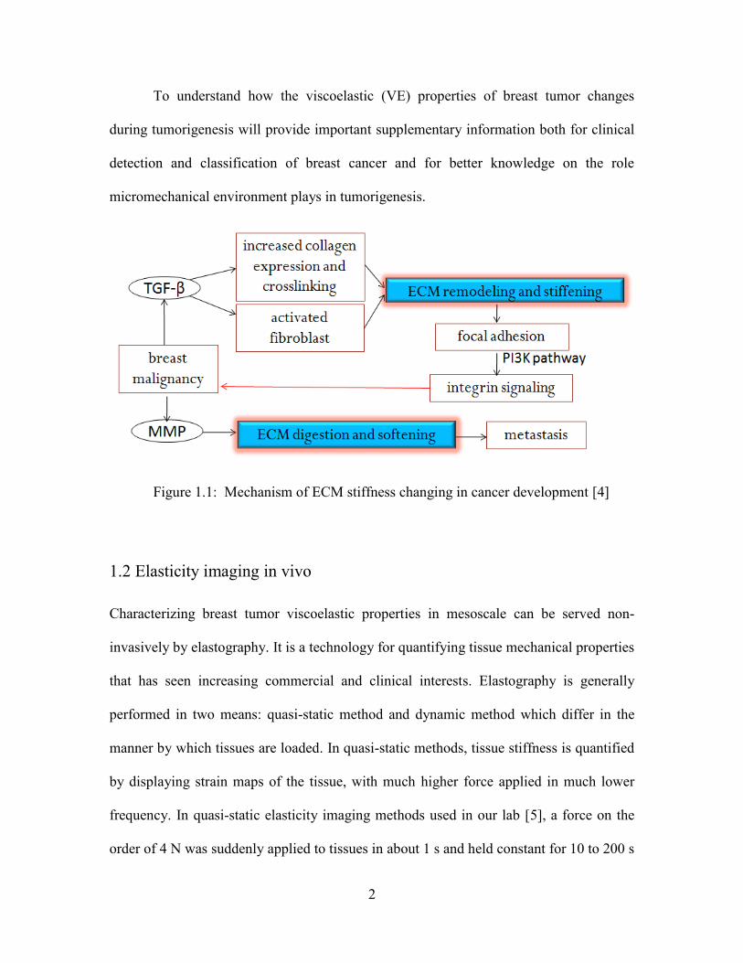
process of cancer development is the change in both elasticity and viscosity. Figure 1.1

shows one of the conjectures for the mechanism of ECM stiffness changing in cancer

development. Proper tuning of mechanical properties in cancer is very important in

restraining cancer growth. Thus, assessments of the tissue mechano-environment that are

accurate and non-invasive are being researched widely.

2

To understand how the viscoelastic (VE) properties of breast tumor changes

during tumorigenesis will provide important supplementary information both for clinical

detection and classification of breast cancer and for better knowledge on the role

micromechanical environment plays in tumorigenesis.

Figure 1.1: Mechanism of ECM stiffness changing in cancer development [4]

1.2 Elasticity imaging in vivo

Characterizing breast tumor viscoelastic properties in mesoscale can be served non-

invasively by elastography. It is a technology for quantifying tissue mechanical properties

that has seen increasing commercial and clinical interests. Elastography is generally

performed in two means: quasi-static method and dynamic method which differ in the

manner by which tissues are loaded. In quasi-static methods, tissue stiffness is quantified

by displaying strain maps of the tissue, with much higher force applied in much lower

frequency. In quasi-static elasticity imaging methods used in our lab [5], a force on the

order of 4 N was suddenly applied to tissues in about 1 s and held constant for 10 to 200 s

3

while frames of ultrasound (US) images were recorded. The VE parameters were

obtained via fitting the time-varying strain data to a rheological model. This method is

restricted by several reasons. Firstly, boundary conditions must be known exactly in order

to solve the inverse problem to obtain the elastic modulus of the tissue. Secondly, we

suspect additional diagnostic information might reside in larger frequency bandwidth of

the applied force. Thus, dynamic methods were explored.

Dynamic methods are usually associated with oscillation of the tissue either

produced by external force or by internal vibrations with frequency from ten to several

hundred Hz. The method used in this thesis work is based on shear wave imaging. We

detected and tracked the propagation of shear waves resulting from certain mechanical

vibrations of tissue. Next we inverted the shear wave speeds and attenuation

measurements to compute the complex shear modulus of the tissue. The dynamic shear

wave imaging technique was developed and extensively studied in many laboratories

during the past decade. [6][7] Most studies were conducted on the “demonstration of

principles on phantoms” and “preliminary clinic studies.” The information from those

studies is reproducible and relatively consistent, making shear wave elastography a very

promising tool in monitoring mechanical property of mass tissue. The results of one

preliminary clinical trial showed a good separation between breast cancer and benign

fibroadenoma utilizing elasticity, not viscosity. Noticeably, the variance of shear modulus

changes vastly with tumor type. [8] In another trial, when trying to classify different

kinds of tumors, the variance of each group was too large to conclude that the elastic

modulus was able to differentiate the two groups. [9] Reasons may come from two folds:

tumor microstructural characteristics determine the range of viscoelasticity; there is

4

difference in systematic error including variation of tumor homogeneity, uncontrollable

apparatus-related measurement accuracy, uncertainty of tumor geometry and boundary

conditions. Since accurate estimation of tissue mechanical property is necessary to make

this technique an effective tool in clinical diagnosis, one purpose of this study is to

examine the source of the variance in tissue mechanical property characterization,

employing rat tumor model in view of its similarity to human tumor in pathology [10]

and comparability in size and other properties.

1.3 Innovation and Significance

In this study, we correlated VE properties for different tumor types and stages to gain

more knowledge of the biological contrast mechanism of shear wave imaging, and

elucidate the source of variation in measurements. This information adds to knowledge

about the mechanical property changes during tumor formation and growth which will

eventually help in interpreting clinical elasticity images. My initial results proved that it

is feasible to adapt the technique from Marko Orescanin’s paper [11] to in vivo biological

tissue measurement. Measurements of VE properties were made in vivo of tumors in five

female Sprague-Dawley rats (non-cancerous) and four female BALB/c mice (cancerous)

using a needle-based ultrasonic shear wave imaging technique. Data reduction assumed

Kelvin-Voigt model to fit dispersion data to the model when estimating complex moduli.

The estimated VE properties correlated to histological findings and collagen density

quantification of the tumors. My initial hypothesis was that both tumor elasticity and

viscosity would increase with collagen density in a certain type of tumor, and my

5

measurements confirmed that viscoelastic behaviors are different in various types of

tumors depending on ECM properties and cellularity.

It is becoming increasingly important to measure the mechanical properties of

biological tissues to assess malignant conditions. We can measure mechanical properties

using ultrasound as well as other imaging modalities such as optical and MRI methods. In

each case, we need to improve the imaging technology to achieve diagnostic image

quality. We also need to know the biological contrast mechanisms behind these elasticity

images so we can accurately interpret clinical images. The evolution of this field has the

potential to bridge molecular, cellular, and tissue biology and lead to new approaches in

the treatment of patients, linking these pathological changes to the exact mechanical

behavior at a mesoscale tissue level larger than the cell but smaller than the organ.

In Chapter 2, theories and models used in shear wave imaging technique are

described. The technique is validated through inhomogeneous gelatin phantom

experiments and comparison to FDTD simulation results. In Chapter 3, animal models

are described in more detail. In vivo measurement procedures and results in tumors are

presented. In Chapter 4, multiple factors that could lead to the variance of measurement

results are examined, including tumor type and collagen content, and rheological model.

Additional issues associated with measurements inconsistencies such as strain bandwidth,

tissue nonlinearity and tumor geometry will be discussed.

6

CHAPTER 2

SHEAR WAVE IMAGING TECHNOLOGY

2.1 Introduction

2.1.1 Tissue mechanics and mechanoenvironment

The theory of continuum mechanics can be applied to soft tissue mechanical property

study. A tissue is a collection of cells embedded in an extracellular matrix, which consists

of fibers (e.g., the proteins collagen and elastin). Stroma cells like fibroblasts control the

structure of the tissue by manufacturing most of the tissue constituents, maintaining the

tissue and adapting the tissue structure to changed environments, including mechanical

load environments. Tissue epithelia consist of sheets of cells that line the inner and outer

surfaces of the body. In contrast to connective tissues, which may contain a great deal of

extracellular matrix between each cell, cells of the epithelium are tightly packed with

little extracellular substance between them. The epithelial cells are bound together by

cell-cell junctions to form an integrated network that gives the cell sheet mechanical

strength. Cell adhesions serve as signaling and anchoring points between cells and

between the cell cytoskeleton and its extracellular matrix to ensure appropriate integrity

and strength of the cell network and its connection to the extracellular matrix. [12]

All these molecular and structural features in tissue will reflect on tissue

mechanical parameters. The goal of studying tissue mechanics is to better understand

7

tissue function and pathology. One technique to assess tissue mechanical properties is

through shear wave imaging which will be discussed in this chapter.

2.1.2 Imaging of mechanoenvironment

The dynamic methods for measuring mechanical properties can be divided into two

groups: those that utilize motion produced from external forces on the body and those

that utilize motions of the tissue produced by internal vibrations. For internal forces, it

usually refers to passive imaging. They tried to solve the inverse problem to find

elasticity map from tissue motion induced by breathing or cardiac motion. One of the

difficulties with this approach is that the distribution of stress is unknown. For external

forces, radiation force is often chosen as an efficient and non-invasive way to exert

enough strain in tissue. However, the force profile is not uniform which depends on the

sound beam profile as well as tissue acoustic properties such as attenuation. This makes it

even harder to perform basic imaging science study. Recently, some researchers use

magnetic nanoparticles as agents to apply the desired force field. The displacement is

relatively small with magnetic nanoparticles excitation and movements from adjacent

particles are coupled. [13][14]

Shear wave imaging is one of the dynamic methods in quantitatively evaluating

the elastic parameters of the tissue. It utilizes the phase velocity and attenuation

coefficient information of the propagated shear waves in tissue to reconstruct mechanical

properties. People have been using this technique in pre-clinic studies on human breast

tumors. [9][15] Quantitative and reproducible information on solid breast lesions with

diagnostic accuracy was acquired in most studies.

8

My focus will be on exploring biological contrast mechanism of shear wave

imaging in animal breast tumor diagnosis. Thus, a needle-based external excitation

manner is chosen to give us a well-defined cylindrical wave field locally. It excludes

many factors that could bias the estimated values, such as force profile and imaging

probe angle.

2.2 Ultrasound Shear Wave Imaging Methodology

2.2.1 Shear wave imaging hardware

Mechanical stimulation: One of the most important considerations is how shear

waves are generated in the tissue of interest. We used a fine stainless-steel needle (1 mm

in diameter) driven by a mechanical actuator (SF-9324, PASCO Scientific, Roseville,

CA). The actuator was driven by an arbitrary waveform generator transmitting 400 ms

pure-tone voltage bursts in the frequency range of 50 Hz to 450 Hz. The voltage

amplitude ranged from 2 V to 10 V depending on the tissue stiffness and type. The needle

vibrated along the z axis, and generated cylindrical shear waves that propagate radially

for several millimeters. The top part of the needle body was rubbed with sandpaper to

increase friction between the tissue and needle to avoid potential slippage. This also gave

it enough scattering for the ultrasound to "see" the needle position for aligning the

transducer plane.

To ensure good coupling between the needle and the imaging medium, no

slippage should occur around the needle. In both gelatin and animal studies presented

here, energy from the needle passed through to the medium very well. Very small

9

harmonic frequency components in spectral plot can be seen in spectral plots whichh

arises from the imperfection of the actuator.

Doppler ultrasound tracking: Harmonic shear waves were tracked with a linear-

array transducer BW-14/60 (SonixRP, Ultrasonix Medical Corporation, Richmond, BC).

Data collection of the SonixRP was synchronized with the excitation wave form. In the

experiment, I set a 200 ms delay for the excitation to ensure collecting steady state data

instead of transient data. Ultrasound transducer worked in Doppler mode with a pulse

repetition frequency (PRF) of 12500 Hz which was high enough to avoid aliasing for all

vibration velocities. For each A-line, 2000 Doppler pulses were emitted which required

2000/12500=160ms to acquire. In my opinion, this yielded adequate signal-to-noise ratio

(SNR) for detecting shear wave phase changes. Fewer Doppler pulses would not greatly

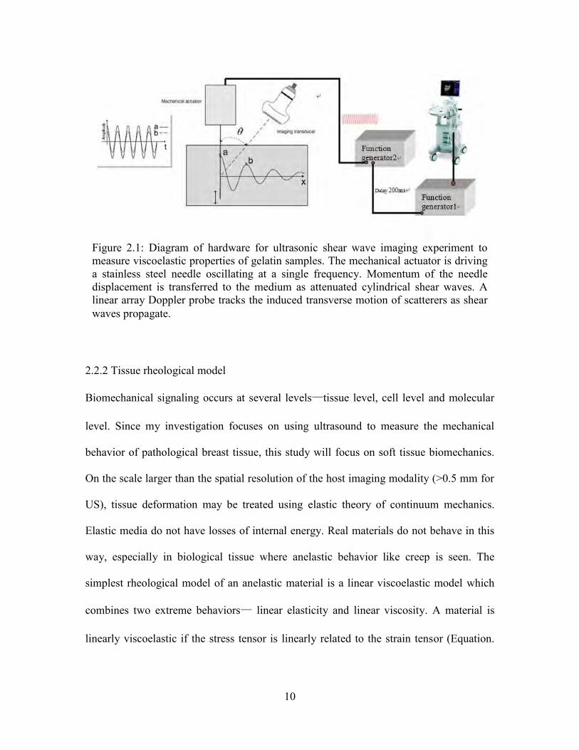
affect the SNR but decrease the post-processing time. The diagram of the equipment's set

up is shown in Figure 2.1. Displacement of each pixel was calculated by autocorrelation

using an improved version of Kasai Doppler velocity estimator (1985)—lag-k phase

velocity estimator. [11] This method will reduce velocity estimation variance for narrow-

band Doppler echoes when the echo SNR is less than 30 dB. The time-varying velocity in

space will define the wave field from which viscoelastic properties can be derived from.

10

2.2.2 Tissue rheological model

Biomechanical signaling occurs at several levels—tissue level, cell level and molecular

level. Since my investigation focuses on using ultrasound to measure the mechanical

behavior of pathological breast tissue, this study will focus on soft tissue biomechanics.

On the scale larger than the spatial resolution of the host imaging modality (>0.5 mm for

US), tissue deformation may be treated using elastic theory of continuum mechanics.

Elastic media do not have losses of internal energy. Real materials do not behave in this

way, especially in biological tissue where anelastic behavior like creep is seen. The

simplest rheological model of an anelastic material is a linear viscoelastic model which

combines two extreme behaviors— linear elasticity and linear viscosity. A material is

linearly viscoelastic if the stress tensor is linearly related to the strain tensor (Equation.

Figure 2.1: Diagram of hardware for ultrasonic shear wave imaging experiment to measure viscoelastic properties of gelatin samples. The mechanical actuator is driving a stainless steel needle oscillating at a single frequency. Momentum of the needle displacement is transferred to the medium as attenuated cylindrical shear waves. A linear array Doppler probe tracks the induced transverse motion of scatterers as shear waves propagate.

11

(2.1)) and the strain response to a linear combination of applied stresses is the same linear

combination of strain responses to individual applied stress.

ij ijkl klC (2.1)

For a linear isotropic viscoelastic material, the stress-strain relation is given by

Boltzmann superposition principle [16]. In a simple scalar notation,

0

( ) ( ) ( )

( ) ( ) ( ) ( ) ( ) ( )

t

t t d

t t t t M t t

(2.2)

where ( )t is stress, ( )t is time derivative of strain, and ( )t is stress relaxation

function (a stress response to a step function of strain). ( )M t is called the time-dependent

modulus. Its Fourier Transform is related to the complex modulus. There are many

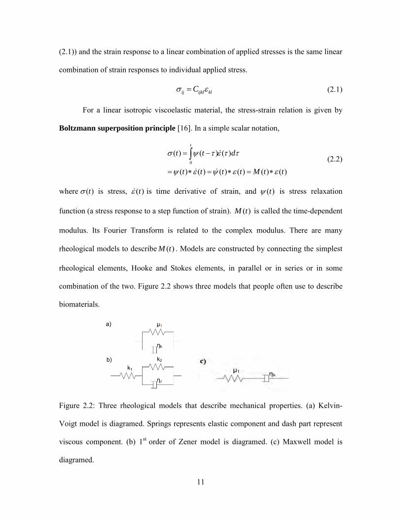
rheological models to describe ( )M t . Models are constructed by connecting the simplest

rheological elements, Hooke and Stokes elements, in parallel or in series or in some

combination of the two. Figure 2.2 shows three models that people often use to describe

biomaterials.

Figure 2.2: Three rheological models that describe mechanical properties. (a) Kelvin-

Voigt model is diagramed. Springs represents elastic component and dash part represent

viscous component. (b) 1st order of Zener model is diagramed. (c) Maxwell model is

diagramed.

12

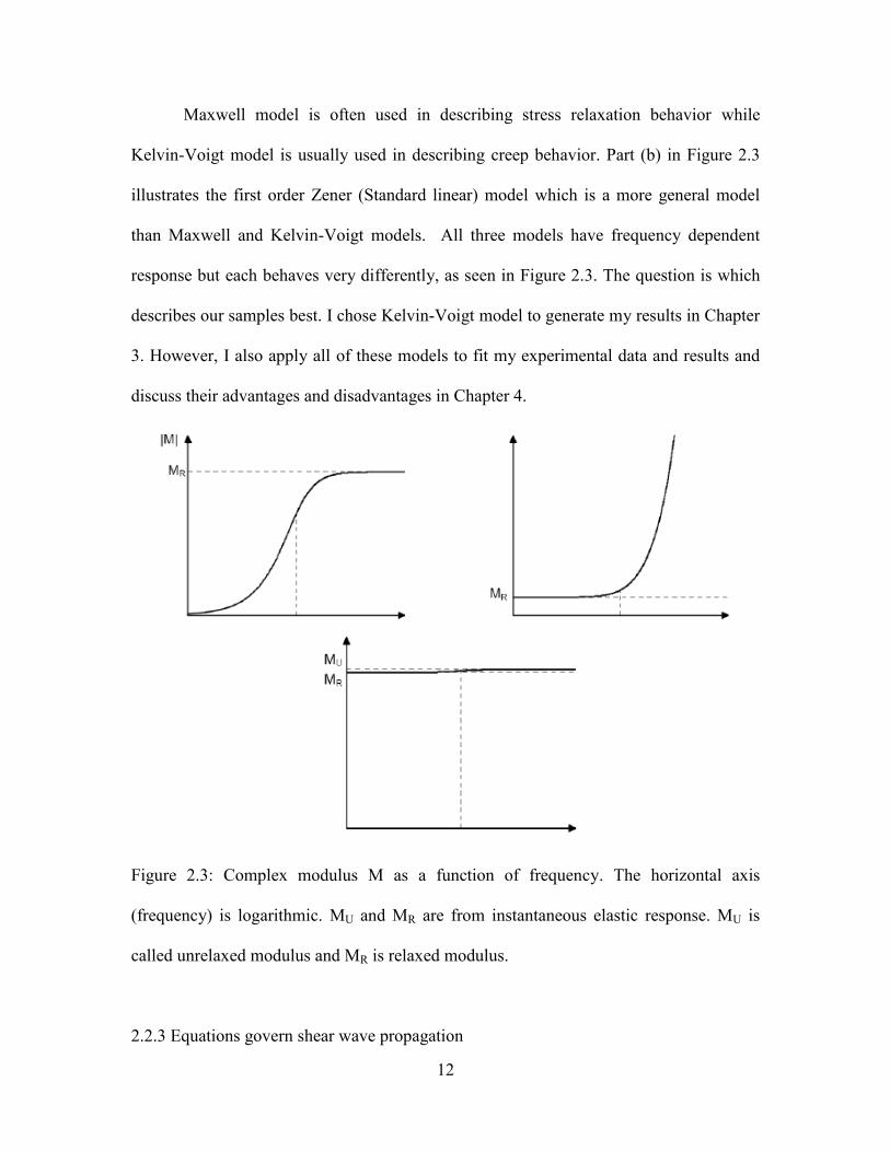
Maxwell model is often used in describing stress relaxation behavior while

Kelvin-Voigt model is usually used in describing creep behavior. Part (b) in Figure 2.3

illustrates the first order Zener (Standard linear) model which is a more general model

than Maxwell and Kelvin-Voigt models. All three models have frequency dependent

response but each behaves very differently, as seen in Figure 2.3. The question is which

describes our samples best. I chose Kelvin-Voigt model to generate my results in Chapter

3. However, I also apply all of these models to fit my experimental data and results and

discuss their advantages and disadvantages in Chapter 4.

Figure 2.3: Complex modulus M as a function of frequency. The horizontal axis

(frequency) is logarithmic. MU and MR are from instantaneous elastic response. MU is

called unrelaxed modulus and MR is relaxed modulus.

2.2.3 Equations govern shear wave propagation

13

The speed of shear wave propagation in media is closely related to the mechanical

characteristics of the medium, which is usually described as complex shear modulus G.

When the deformation of the solid media is small enough to be linear, the shear modulus

will then become a 6*6 tensor matrix relating stress matrix and strain matrix. In these 36

elastic coefficients, 21 are independent. For trigonal crystals like quartz, the number of

independent elastic coefficients reduces to six. For hexagonal crystals like ZnO, the

number of independent elastic coefficients reduces to five. For cubic crystals like GaAs,

the number of independent elastic coefficients reduces to three. Even further, for isotropic

solids like medal and glass, independent elastic coefficients can reduce to just two: the

Lame constants and μ, where μ is what we called "shear modulus"—a quantity that

could describe stiffness of a material. And if we further assume local homogeneity of the

material, and μ become constant instead of a function of position and time.

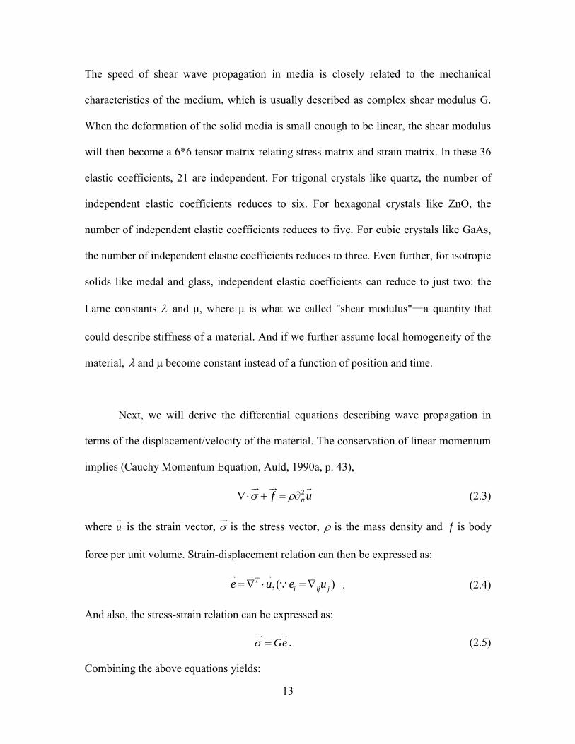
Next, we will derive the differential equations describing wave propagation in

terms of the displacement/velocity of the material. The conservation of linear momentum

implies (Cauchy Momentum Equation, Auld, 1990a, p. 43),

2ttf u

(2.3)

where u

is the strain vector,

is the stress vector, is the mass density and f is body

force per unit volume. Strain-displacement relation can then be expressed as:

, ( )T

i ij je u e u

. (2.4)

And also, the stress-strain relation can be expressed as:

Ge

. (2.5)

Combining the above equations yields:

14

2[ ( )]T

ttG u f u

. (2.6)

For isotropic materials, G matrix is given by:

2 0 0 02 0 0 0

2 0 0 00 0 0 0 00 0 0 0 00 0 0 0 0

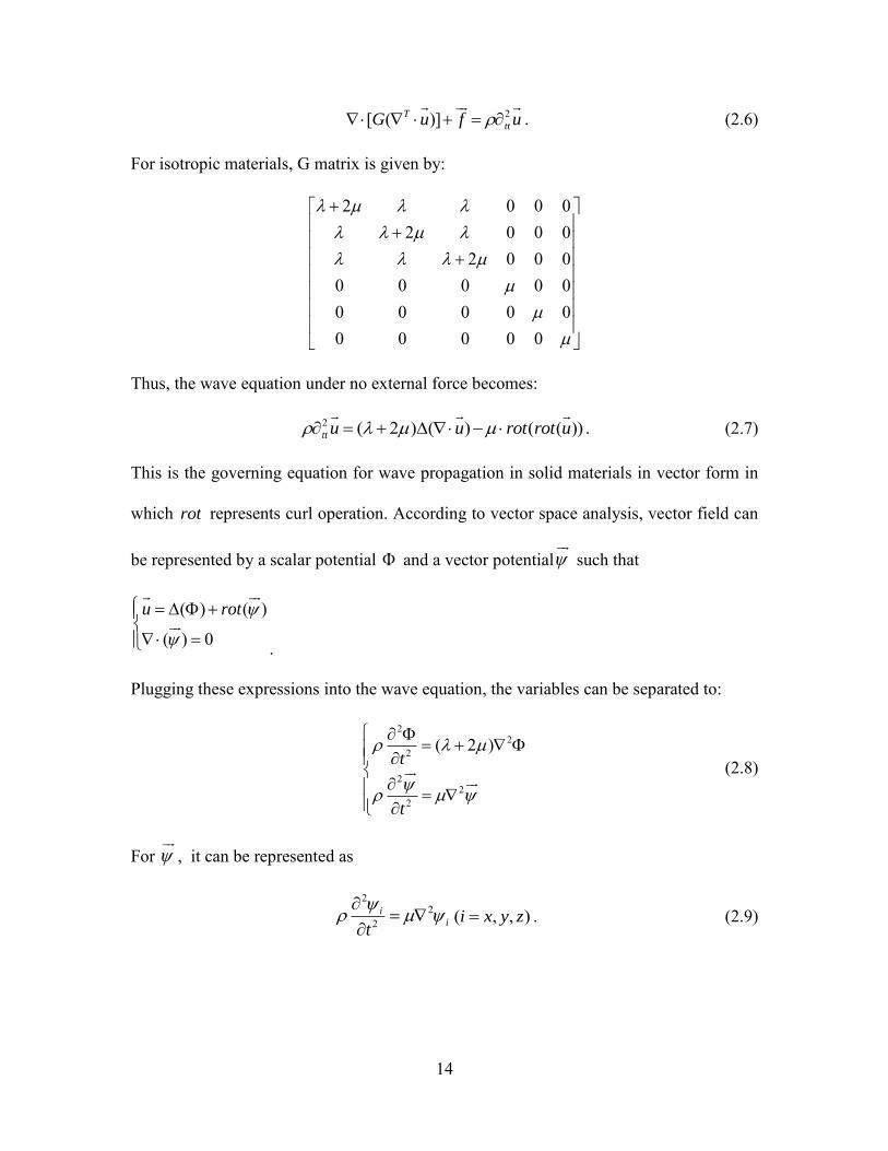
Thus, the wave equation under no external force becomes:

2 ( 2 ) ( ) ( ( ))tt u u rot rot u

. (2.7)

This is the governing equation for wave propagation in solid materials in vector form in

which rot represents curl operation. According to vector space analysis, vector field can

be represented by a scalar potential and a vector potential

such that

( ) ( )

( ) 0

u rot

.

Plugging these expressions into the wave equation, the variables can be separated to:

22

2

22

2

( 2 )t

t

(2.8)

For

, it can be represented as

22

2i

it

( , , )i x y z . (2.9)

15

In physics, corresponds to the longitudinal wave field and

corresponds to the shear

wave field. And the speed of longitudinal wave equals2

and the speed of shear

wave equals

. We only need the second equation of Equation (2.8) because 1) the

speeds of sound and wavelengths of a longitudinal wave is much larger than those for a

shear wave; 2) in the experiment, only shear waves are generated thus longitudinal wave

so we assume the longitudinal wave is ignorable.

In the frequency domain, the shear wave equation can be expressed as:

2 2i i ( , , )i x y z . (2.10)

If we combine Kelvin-Voigt model described in section 2.2.2, we can represent wave

propagation in viscoelastic media.

2 2( )i ii ( , , )i x y z . (2.11)

Here I will establish a relationship between shear wave speed and the complex shear

modulus.

A needle vibrating along its long axis will generate cylindrical waves if the

diameter of the needle is much smaller than the wavelength. If the needle is vibrating

harmonically along the z axis and the force generated is 0( , ) i t

zf r t f e , then the velocity

scalar is ( )0( , ) ( ) si k r t

z r t u r e

, in which 0 ( )u r determines the amplitude dissipation and

initial phase and ,sk determines the shear wave speed and frequency respectively.

2.2.4 Shear wave image reconstruction algorithm

16

This section will discuss the relation of shear wave phase velocity and mechanical

properties of the propagation medium so that we can reconstruct the viscoelastic

properties of tissue from shear wave velocities.

Possible factors that could influence the shear wave speed (phase velocity)

include the elasticity and density of the propagation medium, frequency of vibration and

the amplitude of the wave. Thus, we assume a plane wave at a given frequency in an

unbounded medium by using ( )0( , ) si k x t

z x t u e

. Plugged into the wave equation

(Equation (2.11)) gives:

2 2

2

z s z

s

k

k

(2.12)

The complex wave number is sk k i where is the shear wave attenuation

coefficient. Also, if we consider tissue as a viscoelastic solid under the Kelvin-Voigt

model in section 2.2.2,

1 i .

After combining these equations, we derive the relation between shear wave speed and

viscoelastic parameters:

2 2 21

2 2 21 1

2( )( )( )

sc

(2.13)

In phantom and in vivo animal experiments, the shear wave speed ( )sC for each

vibration frequency is derived from the ratio of ultrasound transducer array pitch (300

m ) and the spatial phase shift of shear wave in the direction of wave propagation.

Spatial phase shift is estimated from cross correlation of velocity estimates measured at

two adjacent lateral locations. Shear wave speed versus frequency can be mapped for

17

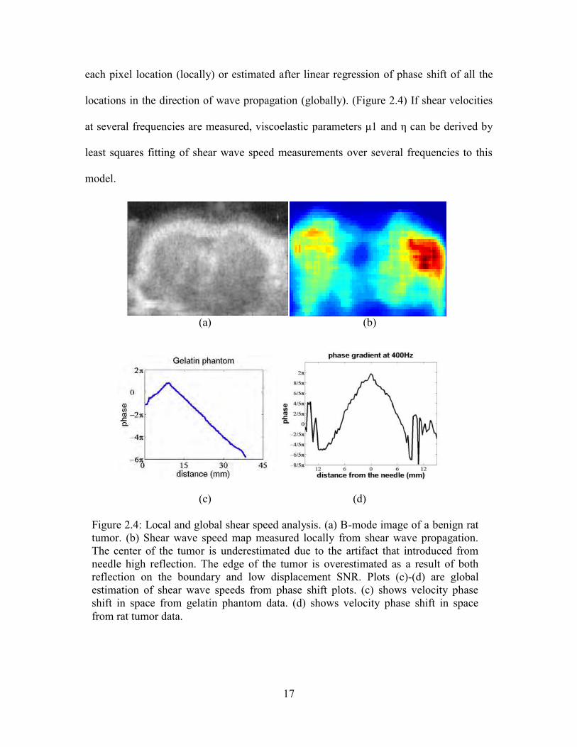
each pixel location (locally) or estimated after linear regression of phase shift of all the

locations in the direction of wave propagation (globally). (Figure 2.4) If shear velocities

at several frequencies are measured, viscoelastic parameters μ1 and η can be derived by

least squares fitting of shear wave speed measurements over several frequencies to this

model.

(a) (b)

(c) (d) Figure 2.4: Local and global shear speed analysis. (a) B-mode image of a benign rat tumor. (b) Shear wave speed map measured locally from shear wave propagation. The center of the tumor is underestimated due to the artifact that introduced from needle high reflection. The edge of the tumor is overestimated as a result of both reflection on the boundary and low displacement SNR. Plots (c)-(d) are global estimation of shear wave speeds from phase shift plots. (c) shows velocity phase shift in space from gelatin phantom data. (d) shows velocity phase shift in space from rat tumor data.

18

2.3 Simulation Validation

A numerical simulation developed by our group to simulate shear wave propagation in

viscoelastic media has been used for two purposes: First, simulations provide the 3D

velocity data comparable to the phantom measurements that enabled us to verify the

accuracy of the complex shear modulus inversion approach. Second, this activity helped

us understand how wave reflections and refractions in inhomogeneous media affect our

estimation on viscoelastic properties.

An FDTD (Finite-Difference Time-domain) method was used to solve the wave

equation in solid media. It is known to be more robust and less computationally

expensive when compared with FEM (Finite Element Methods). To minimize computing

time, we only simulate shear wave propagation. Longitudinal waves travel much faster

and thus require smaller time steps. Since they do not interfere with shear waves, they

can be ignored with little effect.

2.3.1 Finite-Difference in Time Domain (FDTD) method simulation program

Using numerical method to solve this forward problem is essential to study the

limitations imposed by various assumptions in the experiment such as homogeneity and

unlimited boundary conditions. The simulation software was developed by Marko

Orescanin for simulating shear wave propagation in time and three spatial dimensions for

heterogeneous media. [17]

Forward problem was based on the wave equations from section 2.2.3.

(Equation2.3) but solved using two first-order hyperbolic equation.

19

( , , , , )( )( )

iji ik

ij jit

v

t j ki j k x y z

vv

t j i

(2.14)

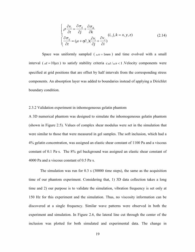
Space was uniformly sampled ( 1x mm ) and time evolved with a small

interval ( 10t s ) to satisfy stability criteria / 1c t x .Velocity components were

specified at grid positions that are offset by half intervals from the corresponding stress

components. An absorption layer was added to boundaries instead of applying a Dirichlet

boundary condition.

2.3.2 Validation experiment in inhomogeneous gelatin phantom

A 3D numerical phantom was designed to simulate the inhomogeneous gelatin phantom

(shown in Figure 2.5). Values of complex shear modulus were set in the simulation that

were similar to those that were measured in gel samples. The soft inclusion, which had a

4% gelatin concentration, was assigned an elastic shear constant of 1100 Pa and a viscous

constant of 0.1 Pa·s. The 8% gel background was assigned an elastic shear constant of

4000 Pa and a viscous constant of 0.5 Pa·s.

The simulation was run for 0.3 s (30000 time steps), the same as the acquisition

time of our phantom experiment. Considering that, 1) 3D data collection takes a long

time and 2) our purpose is to validate the simulation, vibration frequency is set only at

150 Hz for this experiment and the simulation. Thus, no viscosity information can be

discovered at a single frequency. Similar wave patterns were observed in both the

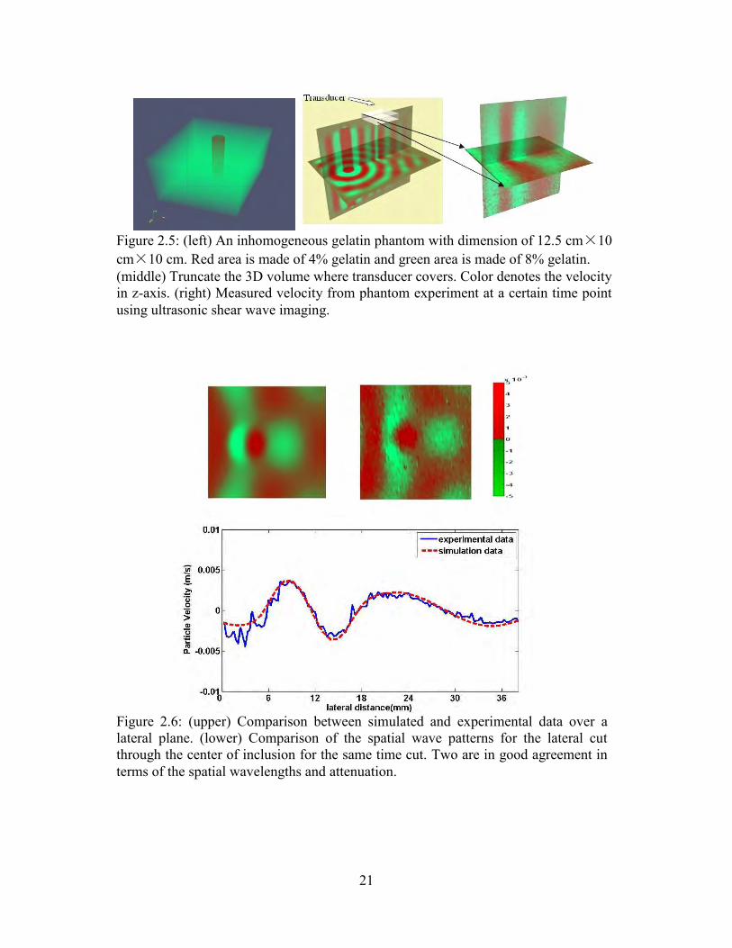
experiment and simulation. In Figure 2.6, the lateral line cut through the center of the

inclusion was plotted for both simulated and experimental data. The change in

20

wavelength of the shear wave as it propagated through the soft inclusion could be

observed in the region from 4mm to 19 mm which corresponds to the 15 mm diameter of

the inclusion in both the simulation and the experiment. Small differences between

simulated and experimental data are explained by the variability of the mechanical

properties of gelatin samples of up to 20%.

It is demonstrated that the developed 3D FDTD solver is an accurate tool for

simulating shear wave propagation through soft viscoelastic biomaterials. Furthermore,

we show the feasibility of using a 1D linear array transducer to collect 3D volumetric

velocity data. The developed simulator is the first step in solving a 3D inverse problem

for complex shear modulus reconstruction. It provides a unique opportunity to conduct

experiments in silico, and to study the effect of realistic viscoelastic biological material

properties on contrasts we observed in shear wave images.

21

Figure 2.6: (upper) Comparison between simulated and experimental data over a lateral plane. (lower) Comparison of the spatial wave patterns for the lateral cut through the center of inclusion for the same time cut. Two are in good agreement in terms of the spatial wavelengths and attenuation.

Figure 2.5: (left) An inhomogeneous gelatin phantom with dimension of 12.5 cm×10 cm×10 cm. Red area is made of 4% gelatin and green area is made of 8% gelatin. (middle) Truncate the 3D volume where transducer covers. Color denotes the velocity in z-axis. (right) Measured velocity from phantom experiment at a certain time point using ultrasonic shear wave imaging.

22

CHAPTER 3

IN VIVO IMAGING OF RODENT MAMMARY TUMORS

3.1 In vivo elastographic imaging

3.1.1 Background

In the clinical protocols, several imaging modalities are used for diagnosis and prognosis

of suspicious breast lesions. Usually, mammography and ultrasound are both useful if the

patient has a palpable mass. While MRI has significant promise as a supplemental tool to

mammography in the diagnosis of breast cancer, there are limitations associated with

MRI. MRI cannot always distinguish between cancerous and non-cancerous

abnormalities, which can lead to unnecessary breast biopsies. 18-FDG Positron emission

tomography (PET) is valuable in oncology for identifying regions of abnormally high

metabolic rates, yet is very expensive and not universally available.

Even through mammography and ultrasonograms are widely used, there are

several limitations too. Mammography cannot be used to distinguish when a mass is a

fibroadenoma, a cyst, or an early carcinoma since all of them appear as smooth masses.

On ultrasonograms, fibroadenomas may be distinguished clearly from cysts and

carcinomas; however, fibrocystic disease with complicated hypoechoic cysts and some

carcinomas may look like fibroadenoma. Also, there are atypical fibroadenomas which

23

simulate carcinomas in inhomogeneity and irregular shape. Definitive diagnosis often

requires image-guided biopsy.

3.1.2 Rational for the use of elasticity imaging

Inspired by the desire to image information normally obtained through clinical

palpation, elastogram have attracted people’s attention. It is a medical imaging

technology for describing mechanical properties of soft tissues. Results show that, under

small deformation conditions, the elastic modulus of normal breast fat and fibroglandular

tissues appear similar while fibroadenomas appeared with approximately twice the

stiffness. Fibrocystic disease and malignant tumors exhibited a 3–6-fold increase in

stiffness with high-grade invasive ductal carcinoma exhibiting up to a 13-fold increase in

stiffness compared to fibroglandular tissue. [18] A statistical analysis showed that

differences between the elastic modulus of the majority of those tissues were statistically

significant. Thus, elastogram will benefit in differentiating benign and malignant tumor

types. [14]

Apart from this, more and more evidence shows that cancer progression is

determined to large extent by the mechnoenvironment surrounding cancer cells. Only

recently have scientists recognized the essential role of the cellular mechanical

environment in regulating integrin signaling pathways during health and disease. The

formation and progression of several diseases are closely associated with mechanical

properties of the extracellular matrix (ECM) [3,4]. In cancer, for example, transformed

cells placed in a stiff mechano-environment are more likely to form tumors and

metastasize. These cancer cells also play an active role in stiffening the ECM through

protein expression and force generation [1,3]. Thus, images of the mechanical properties

24

of tissue provide physicians with vital information about conditions that promote cancer

progression.

In summary, as a quantitative, non-invasive imaging method, elastography or

equivalently elasticity imaging, provides physicians with diagnostic information not

available through other diagnostic techniques. So far, great progress has been made in

developing these imaging technologies and improving image quality for clinical

applications. Although clinical trials clearly show the vast diagnostic potential of

elastography, little is known about the underlying mechanisms linking tissue

microstructure (primarily ECM) to measured mechanical properties, which limits our

ability to correlate elastography with standard pathological metrics. My study is trying to

advance understanding of the biological contrast mechanisms of elasticity imaging.

3.2 Pathology of mammary tumors

3.2.1 Fibroadenoma and rat model (benign)

Fibroadenoma of the breast is a frequently occurring benign tumor. It can occur in

women of any age, but the peak incidence is during the second and third decades of life.

Fibroadenoma is a benign tumor which is fairly homogenous. Its collagen content is

increased by several folds. Fibroadenomas are very mobile when touching them.

Fibroadenoma is composed of two elements: epithelium and stroma. Depending on the

proportion and the relationship between these two components, there are two main

histological feature types: intracanalicular and pericanalicular. Usually, both types are

found in the same tumor. Intracanalicular fibroadenoma (Figure 3.1(a)): stromal

25

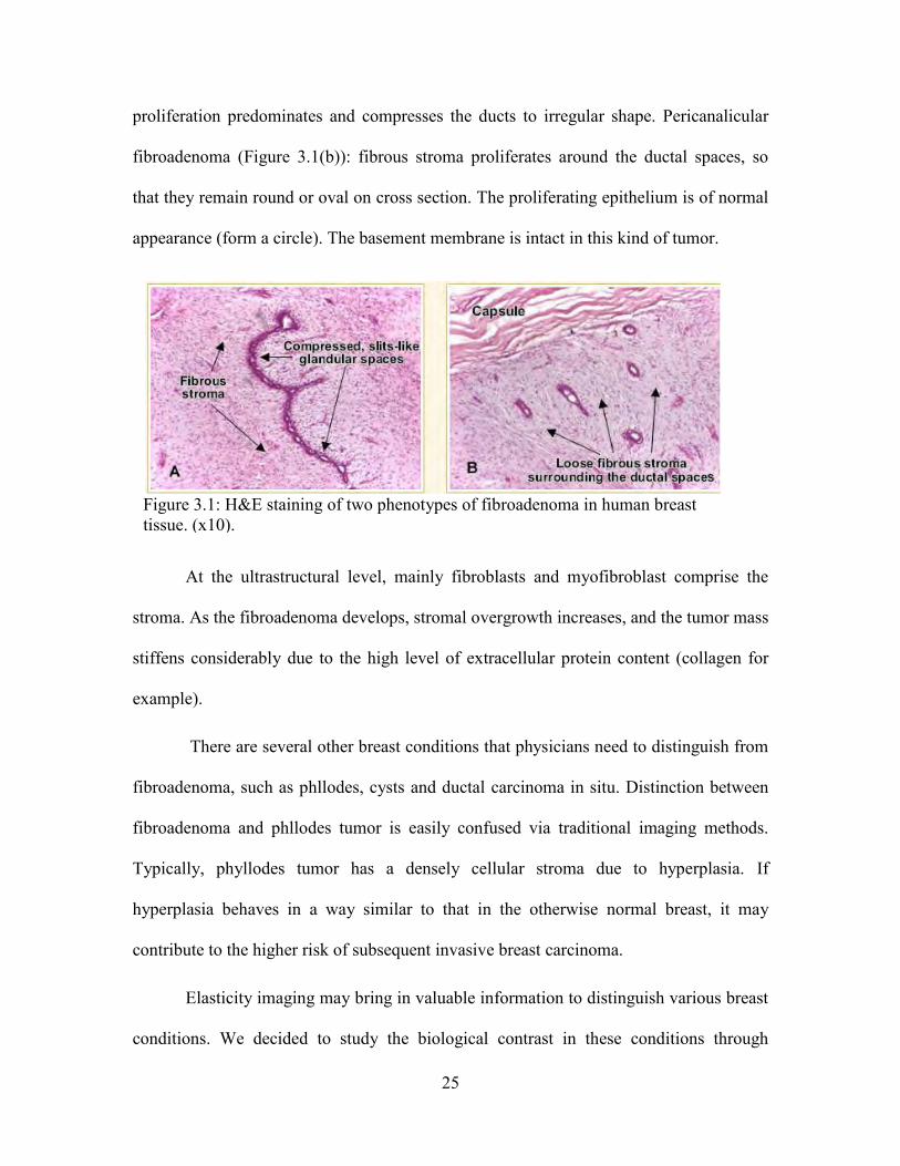
proliferation predominates and compresses the ducts to irregular shape. Pericanalicular

fibroadenoma (Figure 3.1(b)): fibrous stroma proliferates around the ductal spaces, so

that they remain round or oval on cross section. The proliferating epithelium is of normal

appearance (form a circle). The basement membrane is intact in this kind of tumor.

At the ultrastructural level, mainly fibroblasts and myofibroblast comprise the

stroma. As the fibroadenoma develops, stromal overgrowth increases, and the tumor mass

stiffens considerably due to the high level of extracellular protein content (collagen for

example).

There are several other breast conditions that physicians need to distinguish from

fibroadenoma, such as phllodes, cysts and ductal carcinoma in situ. Distinction between

fibroadenoma and phllodes tumor is easily confused via traditional imaging methods.

Typically, phyllodes tumor has a densely cellular stroma due to hyperplasia. If

hyperplasia behaves in a way similar to that in the otherwise normal breast, it may

contribute to the higher risk of subsequent invasive breast carcinoma.

Elasticity imaging may bring in valuable information to distinguish various breast

conditions. We decided to study the biological contrast in these conditions through

Figure 3.1: H&E staining of two phenotypes of fibroadenoma in human breast tissue. (x10).

26

animal models. Rat mammary tumors generally resemble many features of human breast

tumors. With the recent developments in rat genetic engineering, the rat has become an

excellent model system to study breast cancer.

Since the origin of fibroadenoma is unclear, we chose spontaneous Sprague-

Dawley rat as the tumor model. Rats were purchased from Harlan Laboratories Inc. The

tumors, which developed spontaneously, were identified by the vendor. Rat mammary

tumors in five Sprague-Dawley rats have been studied. The age of the tumors ranged

from 5 to 10 weeks, and tumor size ranged from 2 to 4 cm in diameter. Manual palpation

revealed a variation in tumor stiffness among these animals. Tumor type was determined

histologically (H&E) after imaging procedures. The experimental protocol was approved

by campus Laboratory Animal Care Advisory Committee.

3.2.2 Mammary carcinoma and mouse model (malignant)

Breast cancer is one of the most common causes of cancer death worldwide which

comprises 22.9% of all cancers in women. Malignant tumors are much more complicated

than benign ones in terms of origin, development, phenotype and the risk of metastases.

There are two main types of breast cancer. One is ductal carcinoma that begins when an

epithelial cell lining the mammary ducts becames genetically transformed. Most breast

cancers (75%-85%) are of this type. The other common type is lobular carcinoma, which

starts in the mammary lobules that produce milk. [19]

Breast cancer is extensively studied in many laboratories, including the initial

genetic mutations, the signaling pathways that allow the disease to grow and spread, and

the clinical aspects of reliable diagnosis and treatment. More and more knowledge was

27

gained about this disease during the past decades. Biopsy is now the gold standard for

diagnosing breast cancer. Biopsy samples from patients with malignant breast tumors are

assigned an SBR (Scarff-Bloom-Richardson) score. Pathologists closely observe three

features when determining a cancer’s grade: the frequency of cell mitosis (rate of cell

division), tubule formation (percentage of cancer composed of tubular structures), and

nuclear pleomorphism (change in cell size and uniformity).

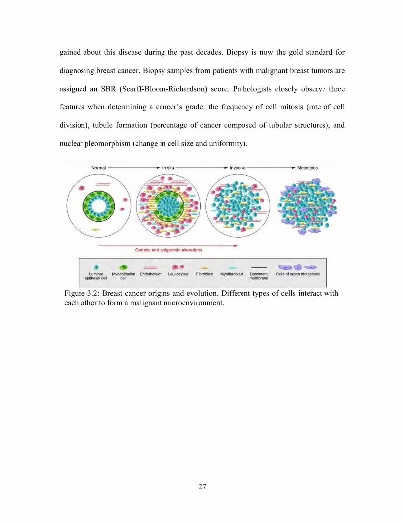
Figure 3.2: Breast cancer origins and evolution. Different types of cells interact with each other to form a malignant microenvironment.

28

In primary tumor formation, ductal carcinoma for example, cancer epithelial cells

over-proliferate inside the duct and the pressure in the duct keeps increasing. At some

point, cancer cells break the basement membrane and start to crosstalk with stromal cells.

(Figure 3.2) Cancer cells secret transcription factors such as TGF-beta to induce a stiffer

ECM. In the early stage of the disease, breast structures are mostly preserved; just the

cancer cell quantity is increased. However, as the disease progresses, cancer cells will

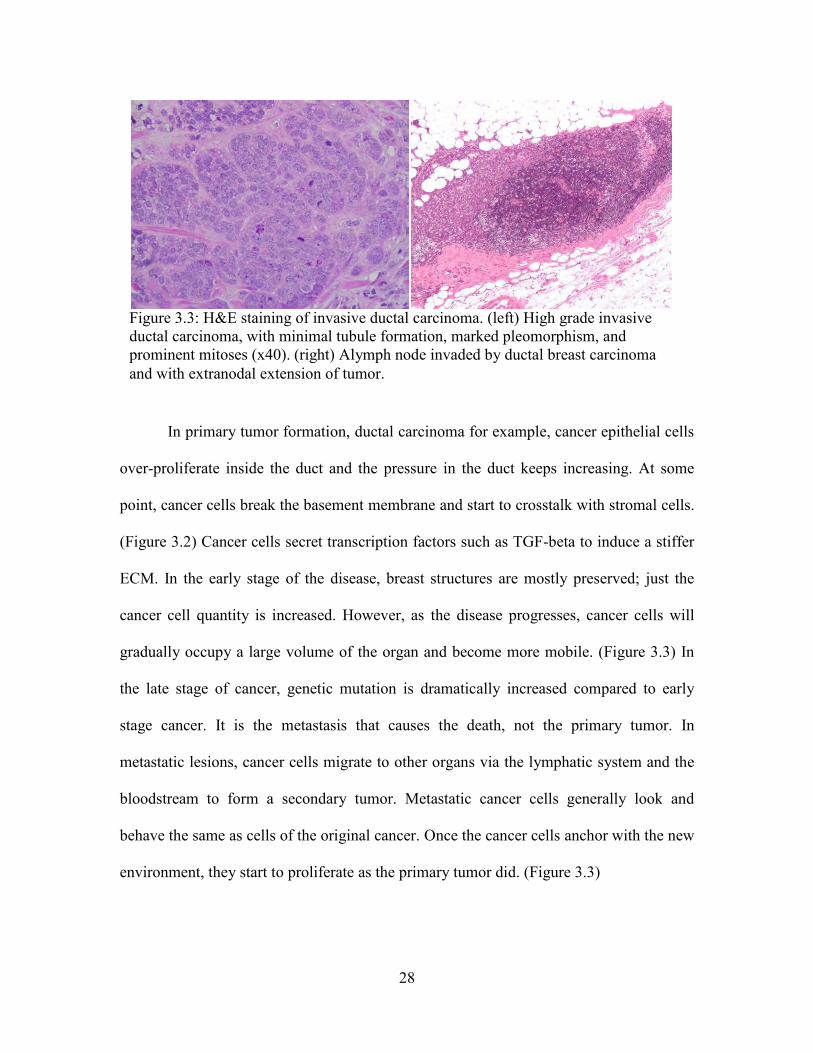
gradually occupy a large volume of the organ and become more mobile. (Figure 3.3) In

the late stage of cancer, genetic mutation is dramatically increased compared to early

stage cancer. It is the metastasis that causes the death, not the primary tumor. In

metastatic lesions, cancer cells migrate to other organs via the lymphatic system and the

bloodstream to form a secondary tumor. Metastatic cancer cells generally look and

behave the same as cells of the original cancer. Once the cancer cells anchor with the new

environment, they start to proliferate as the primary tumor did. (Figure 3.3)

Figure 3.3: H&E staining of invasive ductal carcinoma. (left) High grade invasive ductal carcinoma, with minimal tubule formation, marked pleomorphism, and prominent mitoses (x40). (right) Alymph node invaded by ductal breast carcinoma and with extranodal extension of tumor.

29

The 4T1 metastatic breast cancer model is a syngeneic xenograft model based on

a mouse mammary cancer cell line called 4T1. This cell line is a metastatic cell line,

which models properties of late stage human breast cancers (Stage IV). The 4T1 tumor

has several characteristics that make it a suitable experimental animal model for human

mammary cancer. First, tumor cells are easily transplanted into the mammary gland so

that the primary tumor grows in the anatomically correct site. Tumor growth is very

homogeneous and reproducible comparable to other cancer models. Second, many studies

use 4T1 cell line to study mechanotransduction pathways and ECM responses, which

indicate that it is suitable to use this cell line as a tumor model to study mechanical

properties of breast cancer. The disadvantage of this model for my study is that since the

cancer cell phenotype is late stage, it proliferates faster than the body can build new

blood vessels. Thus tumors have necrosis at the center which affects mechanical property

measurements of the tumor.

In the cell culture protocol, 4T1 cells were stored in liquid nitrogen. Prior to use,

they were thawed at 37oC in a water bath, grown in RPMI 1640 medium with 10% fetal

bovine serum (FBS) and antibiotic/antifungal supplements (ATCC, Manassas, VA), and

incubated at 37oC at 100% humidity and 5% CO2. Cells were grown in 75 cm2 tissue

culture flasks until cells reached 80% confluence. They were rinsed with RPMI 1640

medium lacking FBS or supplements to detach the cells from the flask. The cells were

gently and repetitively drawn through a 10-mL pipette to individualize the cells.

In the tumor implant protocol, 104 4T1 cells with 50 micro liter cell media were

injected subcutaneously into the 4th or 9th mammary pad of a normal 8-16 week-old

30

BALB/c mouse. The injection site was closely monitored (daily) and when the tumor

reached a size of approximately 1 cm, it was used for ultrasonic scanning. Irregular tumor

sizes were determined by the largest dimension. The injected cells initiated tumor growth

in 80% of the animals. In 1-2 weeks, tumor growth was very slow, probably due to the

immune system response. The 4T1 line grew rapidly at the primary site after a period of

2-3 weeks and then the growing speed slowed as the tumor mass stiffened. Although

larger tumors are easier to manipulate, image and analyze, the large necrotic regions will

affect the results. Usually, I scanned the tumor and sacrificed the mouse after about 1

month post cell injection. The mouse tumor model can simulate the pathophysiology of

common human tumors. Due to the complex nature of human breast cancer, models that

mimic all aspects of the disease are not currently available.

3.3 Imaging procedure

All rats and mice were anesthetized with a combination of ketamine

hydrochloride (87 mg/kg) and xylazine hydrochloride (13 mg/kg) administered

intraperitoneally. The anesthetized animal was shaved in the region around the tumor

before imaging. The animal was placed on an acrylic plate in a prone position and

submerged in 37 oC degassed water bath with its head outside of the water. The water

provided an acoustic window for ultrasonic scanning and it controlled body temperature

while the animal was under anesthesia. B-mode imaging of the tumor was performed

before needle insertion for the purpose of choosing a good imaging plane and direction.

Then a fine needle was inserted vertically into the tumor with the aid of real time B-mode

and Color Doppler visualization on the SonixRP ultrasonic imaging system to select

31

needle depth and to avoid damaging tumor vessels. The Doppler probe scanned the tumor

in a plane at a fixed scan angle of 30°. The transmit focus of ultrasound beam was set to

be at its intersection with the needle. The pulse repetition frequency (PRF) of Doppler

mode was 10 kHz, which was high enough to avoid aliasing for all vibration velocities.

The actuator was synchronized with the pulse series of ultrasound acquisition. The

excitation frequency ranged from 50 Hz to 450 Hz in increments of 50 Hz. The peak-to-

peak voltage of the actuator was set to 2 V to avoid nonlinearities, at the cost of velocity

SNR. Nonlinear property will be discussed in Chapter 4.

After velocity acquisition, the tumor was excised immediately after the animal

was euthanized in a CO2 tank. Three cylindrical samples were cut from each tumor for

standard shear rheometer testing within 1 hour after sacrificing the animal (0-10 Hz

sweep, 5% strain, K-V model fit G’ and G’’, average of three samples). Other parts of the

tumor were fixed, stained (H&E) and sliced for standard histological analysis that

identified tumor types. Hydroxyproline assay was performed afterwards to quantify ECM

protein contents. Assay protocols can be found in reference [20]. Results from both

assays are shown in Chapter 4. Effective scatterer diameter (ESD) was determined in

vivo using a quantitative ultrasound (QUS) with the help from Dr. Goutam Ghoshal in

Bioacoustic Research Laboratory.

Post analysis details are covered in Chapter 2. A global estimation is applied since

spatial stiffness distribution is not as interesting as the overall characteristics of a

particular tumor. Viscous behavior of tumor is also a very interesting aspect to investigate

as it may carry important information in tissue pathology.

32

The statistic analysis of the results involves some non-parametric statistical

hypothesis testing because we cannot assume normal distribution of tumor mechanical

and chemical properties or two tissue groups have the same variance. Wilcoxon signed-

rank test and Permutation tests were used to determine the collagen assay repeatability

and the property difference between cancer and non-cancer tumors. Due to the

insufficiency in the animal number, conclusion of universal significance cannot be drawn.

3.4 Results

3.4.1 Rats study result

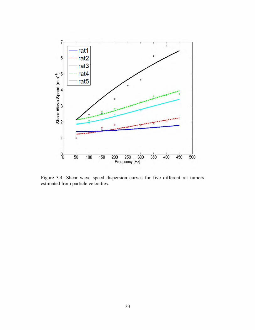
Five rats with spontaneous tumors were scanned in the way presented above. The

estimated particle velocity data in time domain was filtered using a bandpass filter to

extract the desired harmonic component of the shear wave and remove motion artifacts

from the heart beat, breathing and other tissue movements. For heterogeneous tumors, the

areas around the needle were considered homogeneous and chosen to be the region of

interest (ROI) for shear wave speed estimation. Estimated dispersion curves are shown in

Figure. 3.4.

33

Figure 3.4: Shear wave speed dispersion curves for five different rat tumors estimated from particle velocities.

34

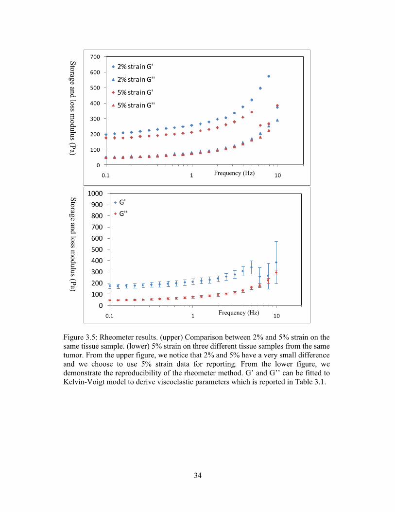
Figure 3.5: Rheometer results. (upper) Comparison between 2% and 5% strain on the same tissue sample. (lower) 5% strain on three different tissue samples from the same tumor. From the upper figure, we notice that 2% and 5% have a very small difference and we choose to use 5% strain data for reporting. From the lower figure, we demonstrate the reproducibility of the rheometer method. G’ and G’’ can be fitted to Kelvin-Voigt model to derive viscoelastic parameters which is reported in Table 3.1.

0

100

200

300

400

500

600

700

0.1 1 10

2% strain G'

2% strain G''

5% strain G'

5% strain G''

0

100

200

300

400

500

600

700

800

900

1000

0.1 1 10

G'

G''

Frequency (Hz)

Frequency (Hz) Storage and loss m

odulus (Pa) Storage and loss m

odulus (Pa)

35

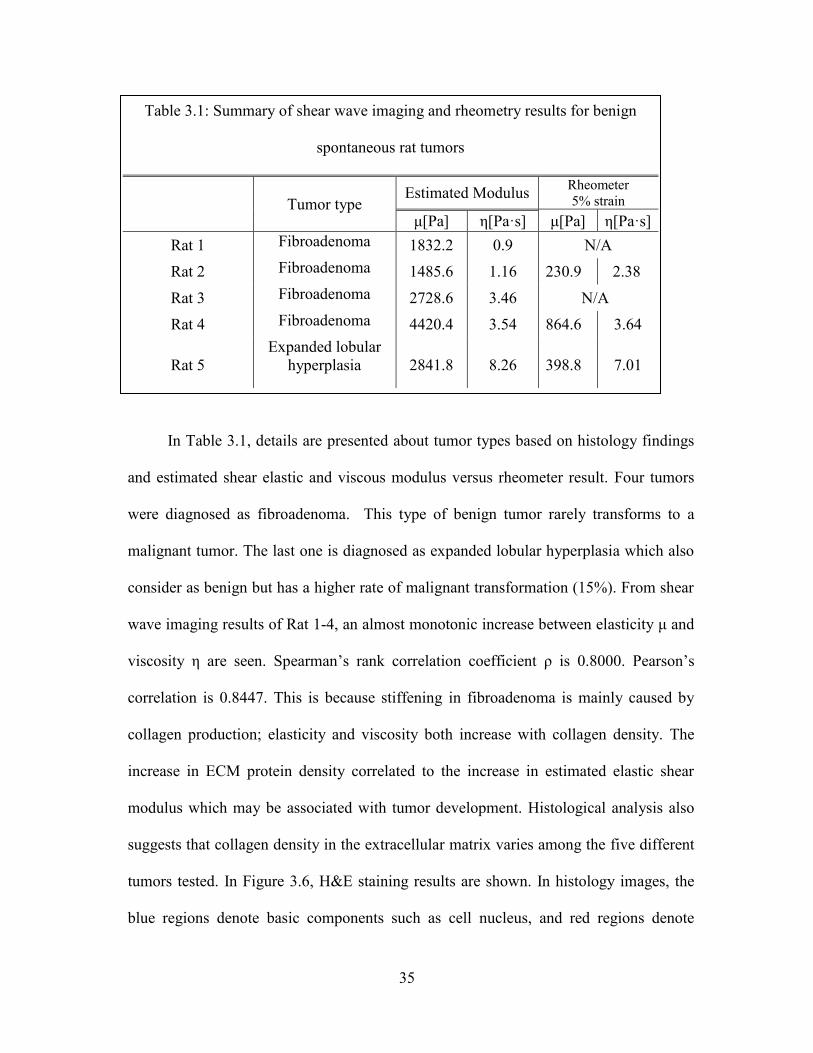
In Table 3.1, details are presented about tumor types based on histology findings

and estimated shear elastic and viscous modulus versus rheometer result. Four tumors

were diagnosed as fibroadenoma. This type of benign tumor rarely transforms to a

malignant tumor. The last one is diagnosed as expanded lobular hyperplasia which also

consider as benign but has a higher rate of malignant transformation (15%). From shear

wave imaging results of Rat 1-4, an almost monotonic increase between elasticity μ and

viscosity η are seen. Spearman’s rank correlation coefficient ρ is 0.8000. Pearson’s

correlation is 0.8447. This is because stiffening in fibroadenoma is mainly caused by

collagen production; elasticity and viscosity both increase with collagen density. The

increase in ECM protein density correlated to the increase in estimated elastic shear

modulus which may be associated with tumor development. Histological analysis also

suggests that collagen density in the extracellular matrix varies among the five different

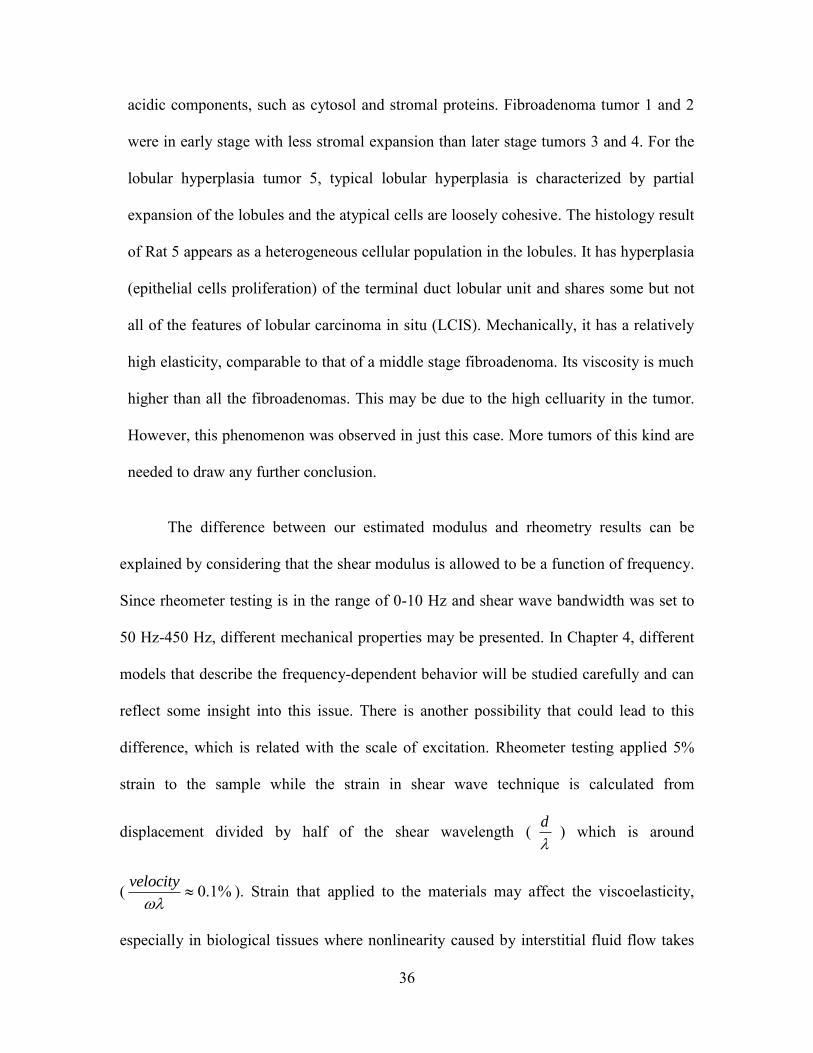
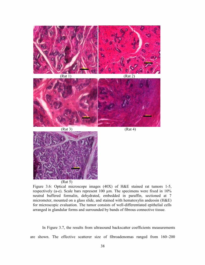
tumors tested. In Figure 3.6, H&E staining results are shown. In histology images, the

blue regions denote basic components such as cell nucleus, and red regions denote

Table 3.1: Summary of shear wave imaging and rheometry results for benign

spontaneous rat tumors

Tumor type Estimated Modulus Rheometer

5% strain μ[Pa] η[Pa·s] μ[Pa] η[Pa·s]

Rat 1 Fibroadenoma 1832.2 0.9 N/A

Rat 2 Fibroadenoma 1485.6 1.16 230.9 2.38

Rat 3 Fibroadenoma 2728.6 3.46 N/A

Rat 4 Fibroadenoma 4420.4 3.54 864.6 3.64

Rat 5 Expanded lobular

hyperplasia

2841.8 8.26 398.8 7.01

36

acidic components, such as cytosol and stromal proteins. Fibroadenoma tumor 1 and 2

were in early stage with less stromal expansion than later stage tumors 3 and 4. For the

lobular hyperplasia tumor 5, typical lobular hyperplasia is characterized by partial

expansion of the lobules and the atypical cells are loosely cohesive. The histology result

of Rat 5 appears as a heterogeneous cellular population in the lobules. It has hyperplasia

(epithelial cells proliferation) of the terminal duct lobular unit and shares some but not

all of the features of lobular carcinoma in situ (LCIS). Mechanically, it has a relatively

high elasticity, comparable to that of a middle stage fibroadenoma. Its viscosity is much

higher than all the fibroadenomas. This may be due to the high celluarity in the tumor.

However, this phenomenon was observed in just this case. More tumors of this kind are

needed to draw any further conclusion.

The difference between our estimated modulus and rheometry results can be

explained by considering that the shear modulus is allowed to be a function of frequency.

Since rheometer testing is in the range of 0-10 Hz and shear wave bandwidth was set to

50 Hz-450 Hz, different mechanical properties may be presented. In Chapter 4, different

models that describe the frequency-dependent behavior will be studied carefully and can

reflect some insight into this issue. There is another possibility that could lead to this

difference, which is related with the scale of excitation. Rheometer testing applied 5%

strain to the sample while the strain in shear wave technique is calculated from

displacement divided by half of the shear wavelength ( d

) which is around

( 0.1%velocity

). Strain that applied to the materials may affect the viscoelasticity,

especially in biological tissues where nonlinearity caused by interstitial fluid flow takes

37

effect. However, due to the limitation of our method in measuring low shear frequency

(large shear wavelength) and the limitation of the rheometer in reaching high frequency,

it is hard to quantitatively compare the two to verify the above conjectures. In future

work, other techniques with broader bandwidth may help to address the question.

38

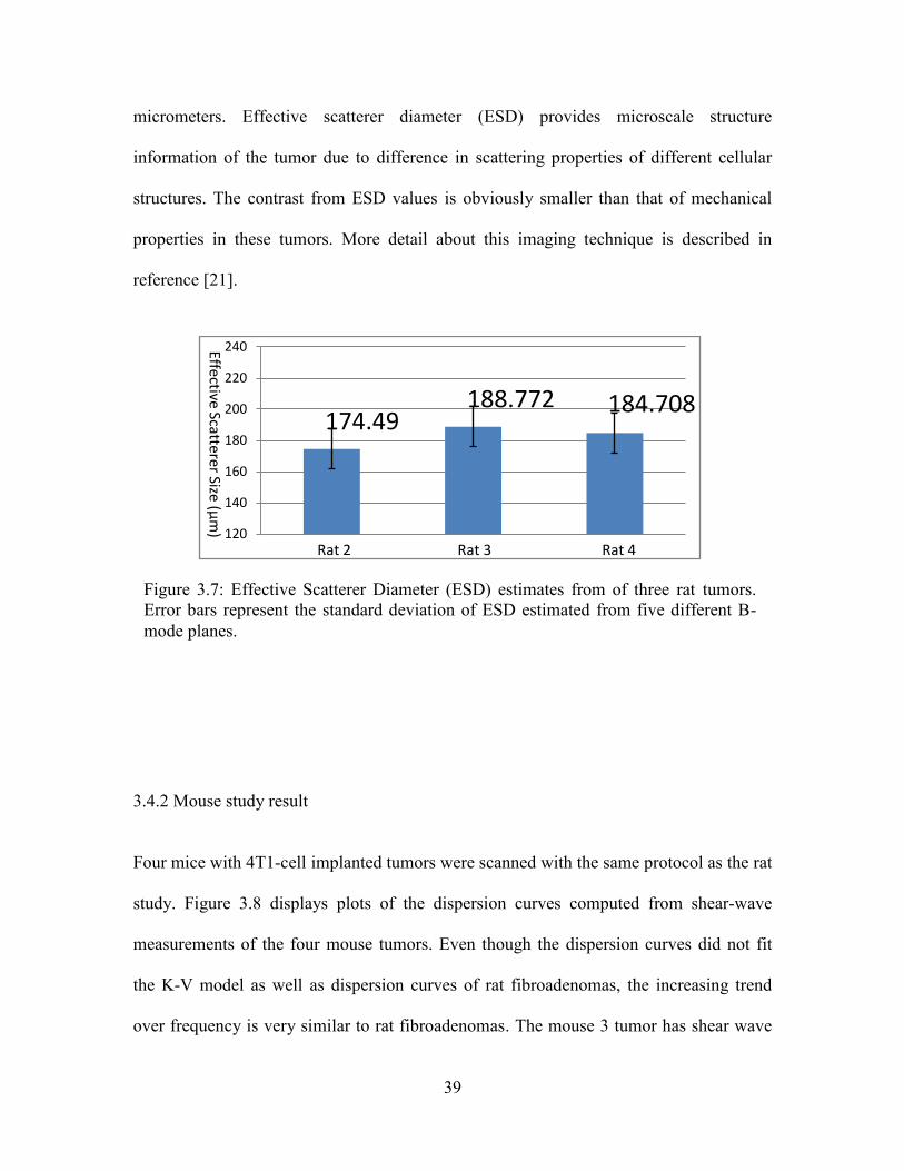
In Figure 3.7, the results from ultrasound backscatter coefficients measurements

are shown. The effective scatterer size of fibroadenomas ranged from 160~200

(Rat 1) (Rat 2)

(Rat 3) (Rat 4)

(Rat 5)

Figure 3.6: Optical microscope images (40X) of H&E stained rat tumors 1-5, respectively (a-e). Scale bars represent 100 µm. The specimens were fixed in 10% neutral buffered formalin, dehydrated, embedded in paraffin, sectioned at 7 micrometer, mounted on a glass slide, and stained with hematoxylin andeosin (H&E) for microscopic evaluation. The tumor consists of well-differentiated epithelial cells arranged in glandular forms and surrounded by bands of fibrous connective tissue.

39

micrometers. Effective scatterer diameter (ESD) provides microscale structure

information of the tumor due to difference in scattering properties of different cellular

structures. The contrast from ESD values is obviously smaller than that of mechanical

properties in these tumors. More detail about this imaging technique is described in

reference [21].

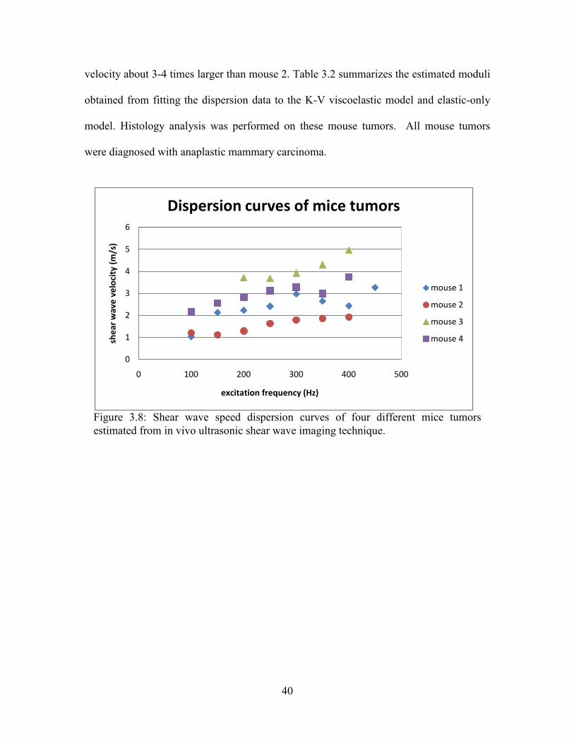
3.4.2 Mouse study result

Four mice with 4T1-cell implanted tumors were scanned with the same protocol as the rat

study. Figure 3.8 displays plots of the dispersion curves computed from shear-wave

measurements of the four mouse tumors. Even though the dispersion curves did not fit

the K-V model as well as dispersion curves of rat fibroadenomas, the increasing trend

over frequency is very similar to rat fibroadenomas. The mouse 3 tumor has shear wave

Figure 3.7: Effective Scatterer Diameter (ESD) estimates from of three rat tumors. Error bars represent the standard deviation of ESD estimated from five different B-mode planes.

174.49188.772 184.708

120

140

160

180

200

220

240EffectiveScatte

rer Size (μm

)

Rat 2 Rat 3 Rat 4

40

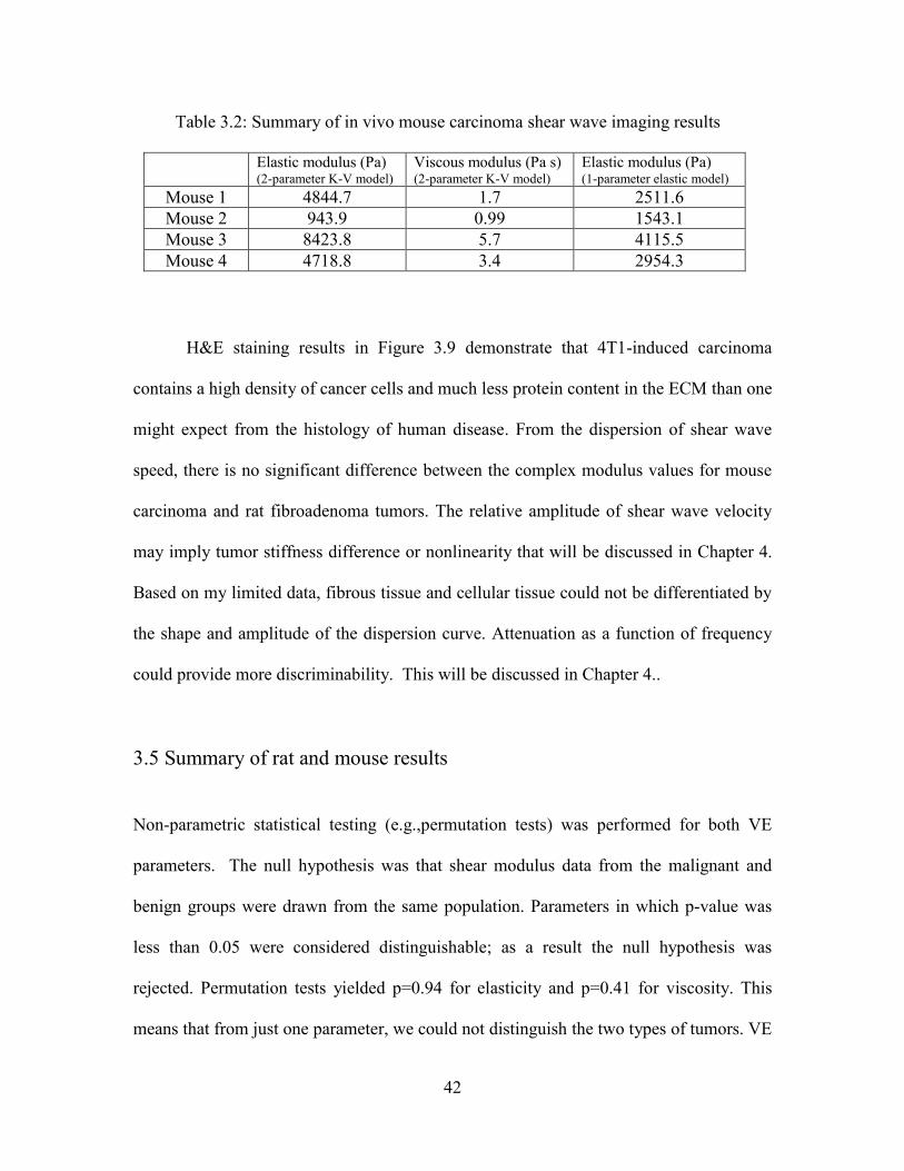
velocity about 3-4 times larger than mouse 2. Table 3.2 summarizes the estimated moduli

obtained from fitting the dispersion data to the K-V viscoelastic model and elastic-only

model. Histology analysis was performed on these mouse tumors. All mouse tumors

were diagnosed with anaplastic mammary carcinoma.

Figure 3.8: Shear wave speed dispersion curves of four different mice tumors estimated from in vivo ultrasonic shear wave imaging technique.

0

1

2

3

4

5

6

0 100 200 300 400 500

she

ar w

ave

ve

loci

ty (

m/s

)

excitation frequency (Hz)

Dispersion curves of mice tumors

mouse 1

mouse 2

mouse 3

mouse 4

41

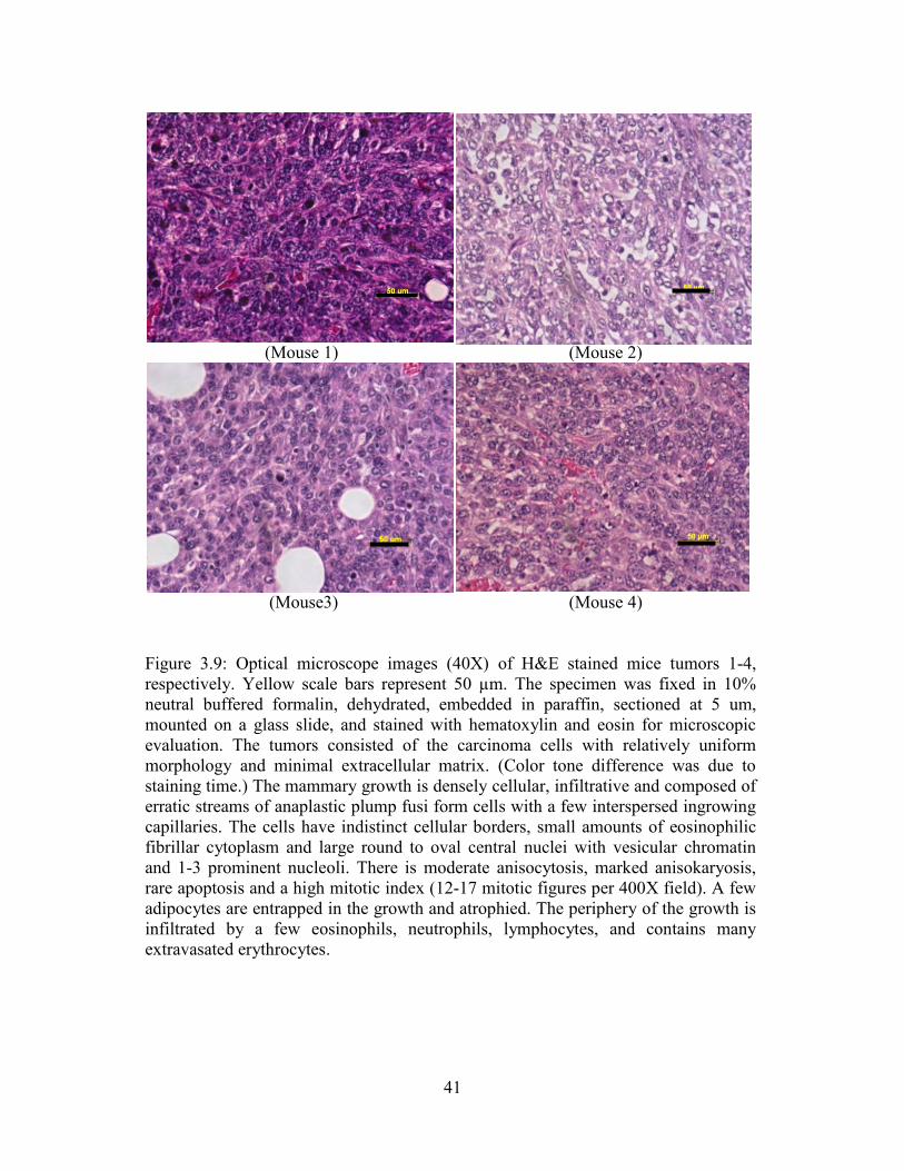
(Mouse 1) (Mouse 2)

(Mouse3) (Mouse 4)

Figure 3.9: Optical microscope images (40X) of H&E stained mice tumors 1-4, respectively. Yellow scale bars represent 50 µm. The specimen was fixed in 10% neutral buffered formalin, dehydrated, embedded in paraffin, sectioned at 5 um, mounted on a glass slide, and stained with hematoxylin and eosin for microscopic evaluation. The tumors consisted of the carcinoma cells with relatively uniform morphology and minimal extracellular matrix. (Color tone difference was due to staining time.) The mammary growth is densely cellular, infiltrative and composed of erratic streams of anaplastic plump fusi form cells with a few interspersed ingrowing capillaries. The cells have indistinct cellular borders, small amounts of eosinophilic fibrillar cytoplasm and large round to oval central nuclei with vesicular chromatin and 1-3 prominent nucleoli. There is moderate anisocytosis, marked anisokaryosis, rare apoptosis and a high mitotic index (12-17 mitotic figures per 400X field). A few adipocytes are entrapped in the growth and atrophied. The periphery of the growth is infiltrated by a few eosinophils, neutrophils, lymphocytes, and contains many extravasated erythrocytes.

42

H&E staining results in Figure 3.9 demonstrate that 4T1-induced carcinoma

contains a high density of cancer cells and much less protein content in the ECM than one

might expect from the histology of human disease. From the dispersion of shear wave

speed, there is no significant difference between the complex modulus values for mouse

carcinoma and rat fibroadenoma tumors. The relative amplitude of shear wave velocity

may imply tumor stiffness difference or nonlinearity that will be discussed in Chapter 4.

Based on my limited data, fibrous tissue and cellular tissue could not be differentiated by

the shape and amplitude of the dispersion curve. Attenuation as a function of frequency

could provide more discriminability. This will be discussed in Chapter 4..

3.5 Summary of rat and mouse results

Non-parametric statistical testing (e.g.,permutation tests) was performed for both VE

parameters. The null hypothesis was that shear modulus data from the malignant and

benign groups were drawn from the same population. Parameters in which p-value was

less than 0.05 were considered distinguishable; as a result the null hypothesis was

rejected. Permutation tests yielded p=0.94 for elasticity and p=0.41 for viscosity. This

means that from just one parameter, we could not distinguish the two types of tumors. VE

Table 3.2: Summary of in vivo mouse carcinoma shear wave imaging results

Elastic modulus (Pa) (2-parameter K-V model)

Viscous modulus (Pa s) (2-parameter K-V model)

Elastic modulus (Pa) (1-parameter elastic model)

Mouse 1 4844.7 1.7 2511.6 Mouse 2 943.9 0.99 1543.1 Mouse 3 8423.8 5.7 4115.5 Mouse 4 4718.8 3.4 2954.3

43

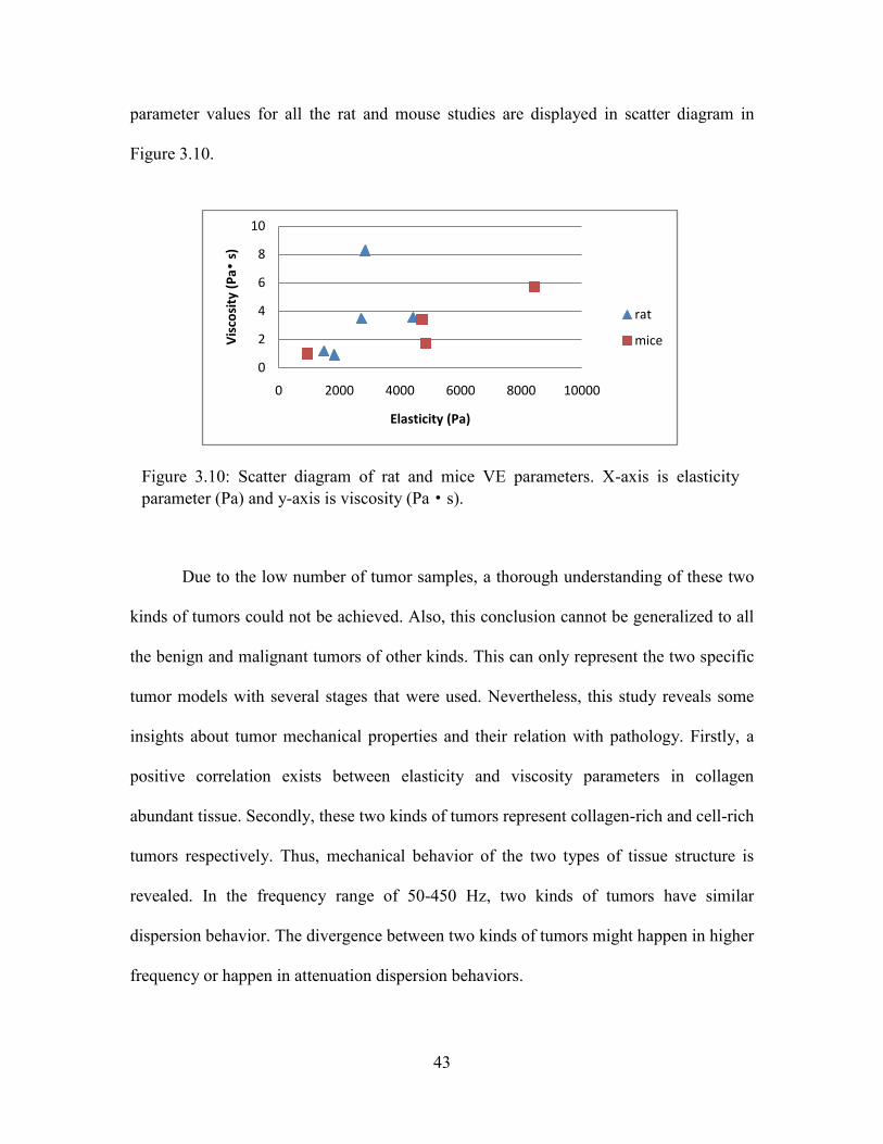
parameter values for all the rat and mouse studies are displayed in scatter diagram in

Figure 3.10.

Due to the low number of tumor samples, a thorough understanding of these two

kinds of tumors could not be achieved. Also, this conclusion cannot be generalized to all

the benign and malignant tumors of other kinds. This can only represent the two specific

tumor models with several stages that were used. Nevertheless, this study reveals some

insights about tumor mechanical properties and their relation with pathology. Firstly, a

positive correlation exists between elasticity and viscosity parameters in collagen

abundant tissue. Secondly, these two kinds of tumors represent collagen-rich and cell-rich

tumors respectively. Thus, mechanical behavior of the two types of tissue structure is

revealed. In the frequency range of 50-450 Hz, two kinds of tumors have similar

dispersion behavior. The divergence between two kinds of tumors might happen in higher

frequency or happen in attenuation dispersion behaviors.

Figure 3.10: Scatter diagram of rat and mice VE parameters. X-axis is elasticity parameter (Pa) and y-axis is viscosity (Pa·s).

0

2

4

6

8

10

0 2000 4000 6000 8000 10000

Vis

cosi

ty (

Pa•

s)

Elasticity (Pa)

rat

mice

44

Another interesting point from this study is the very different behavior between

hyperplasia and cancer, both of which have high cellularity. One conjecture is that as a

late stage metastasis cancer, 4T1 cancer epithelial cells are less adhesive to each other,

while in benign hyperplasia, epithelial cells are normal and more adhesive to each other.

Overall, this study demonstrates that measurement of mechanical properties using

ultrasound is feasible. The measurements are comparable to study results from other labs

on other tissue samples. [25][26] Data are not as perfect as gelatin phantoms since a lot of

reasons could lead to variation in measurements. The next Chapter will focus on those

factors that produce variance in tumor in vivo experiments.

45

CHAPTER 4

VARIATION IN MEASUREMENTS

Unlike gelatin experiments, in vivo measurement of complex modulus values suffers

from relatively large variability. On one hand, biological tissue is far more complicated in

structure than pure protein aggregates, with irregular boundary and texture heterogeneity

affecting the measurement. On the other hand, biological tissue could cause violations to

the assumptions made in the reconstruction model such as isotropic material, cylindrical

wave field, linear propagation, etc. In this Chapter, I will focus more on investigation of

these possible effects which could lead to variation in in vivo tissue experiments.

4.1 Tumor type and ECM protein

Tumors of different types or subtypes may exhibit very different mechanical behavior

due to the formation and structural dissimilarity. Within the three tumor phenotypes that I

examined, histology clearly showed the vast difference in the tumor structures and

composites. Further quantification of collagen content confirmed that different tumor

phenotypes contained ECM protein very differently, with benign rat breast fibroadenoma

in the range from 85-110 mg hydroxyproline/mg dry tissue and hyperplasia is a little

46

lower than fibroadenoma, which is around 60 mg hydroxyproline/mg dry tissue. This

number falls in the same range of that of human breast fibroadenoma. [22][23] On the

contrary, mice carcinoma model contains very little collagen in ECM, within the range of

1-8 mg hydroxyproline/mg dry tissue. Note that hydroxyproline constitutes 15% of total

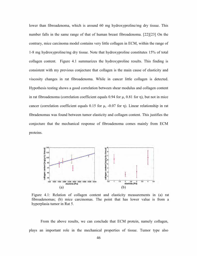
collagen content. Figure 4.1 summarizes the hydroxyproline results. This finding is

consistent with my previous conjecture that collagen is the main cause of elasticity and

viscosity changes in rat fibroadenoma. While in cancer little collagen is detected.

Hypothesis testing shows a good correlation between shear modulus and collagen content

in rat fibroadenoma (correlation coefficient equals 0.94 for μ, 0.81 for η), but not in mice

cancer (correlation coefficient equals 0.15 for μ, -0.07 for η). Linear relationship in rat

fibradenomas was found between tumor elasticity and collagen content. This justifies the

conjecture that the mechanical response of fibroadenoma comes mainly from ECM

proteins.

From the above results, we can conclude that ECM protein, namely collagen,

plays an important role in the mechanical properties of tissue. Tumor type also

(a) (b)

Figure 4.1: Relation of collagen content and elasticity measurements in (a) rat fibroadenomas; (b) mice carcinomas. The point that has lower value is from a hyperplasia tumor in Rat 5.

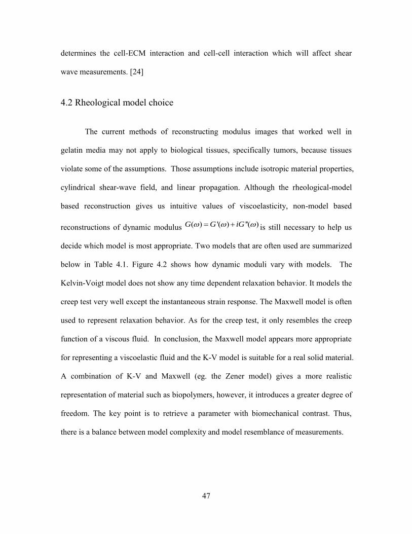
47

determines the cell-ECM interaction and cell-cell interaction which will affect shear

wave measurements. [24]

4.2 Rheological model choice

The current methods of reconstructing modulus images that worked well in

gelatin media may not apply to biological tissues, specifically tumors, because tissues

violate some of the assumptions. Those assumptions include isotropic material properties,

cylindrical shear-wave field, and linear propagation. Although the rheological-model

based reconstruction gives us intuitive values of viscoelasticity, non-model based

reconstructions of dynamic modulus ( ) '( ) ''( )G G iG is still necessary to help us

decide which model is most appropriate. Two models that are often used are summarized

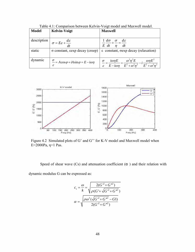
below in Table 4.1. Figure 4.2 shows how dynamic moduli vary with models. The

Kelvin-Voigt model does not show any time dependent relaxation behavior. It models the

creep test very well except the instantaneous strain response. The Maxwell model is often

used to represent relaxation behavior. As for the creep test, it only resembles the creep

function of a viscous fluid. In conclusion, the Maxwell model appears more appropriate

for representing a viscoelastic fluid and the K-V model is suitable for a real solid material.

A combination of K-V and Maxwell (eg. the Zener model) gives a more realistic

representation of material such as biopolymers, however, it introduces a greater degree of

freedom. The key point is to retrieve a parameter with biomechanical contrast. Thus,

there is a balance between model complexity and model resemblance of measurements.

48

Speed of shear wave (Cs) and attenuation coefficient (α ) and their relation with

dynamic modulus G can be expressed as:

2 2

2 2

2 2 2

2 2

2( ' '' )( ' ' '' )

( ' '' 1)2( ' '' )

s

G Gc

k G G G

G G G

G G

Figure 4.2 Simulated plots of G’ and G’’ for K-V model and Maxwell model when E=2000Pa, η=1 Pas.

Table 4.1: Comparison between Kelvin-Voigt model and Maxwell model. Model Kelvin-Voigt Maxwell

description dE

dt

1 d d

E dt dt

static σ constant, εexp decay (creep) ε constant, σexp decay (relaxation)

dynamic cos sinA iA E i

2 2 2

2 2 2 2 2 2

i E E Ei

E i E E

49

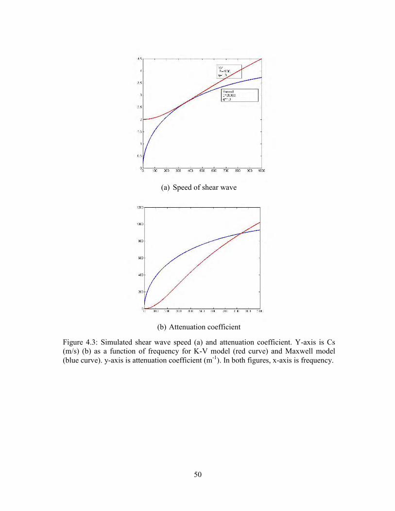
In Figure 4.3, the dispersion of shear velocity and attenuation coefficient from 0

Hz to 1000 Hz for both models are plotted at selected values. From the figure, we observe

that dispersive behaviors vary for both models, especially in low and high frequencies.

For shear wave velocity dispersion curve, note that the Maxwell model requires a larger

E value to approach the K-V model in the frequency region that we are most interested in.

This is because shear wave in a Maxwell material travels slower than a wave in the

corresponding elastic material – if this is represented by the spring. On the contrary, shear

wave in K-V material travels faster than a wave in the corresponding elastic material.

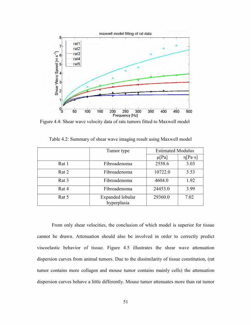
Figure 4.4 and Table 4.2 are Maxwell-model based estimations of shear velocity

dispersion and complex shear modulus based on the rat tumor data. Compared to the

measurement results from the K-V model, the Maxwell model fits better in low frequency

region (<150 Hz) and it provides larger contrast in elasticity modulus as well.

50

(a) Speed of shear wave

(b) Attenuation coefficient

Figure 4.3: Simulated shear wave speed (a) and attenuation coefficient. Y-axis is Cs (m/s) (b) as a function of frequency for K-V model (red curve) and Maxwell model (blue curve). y-axis is attenuation coefficient (m-1). In both figures, x-axis is frequency.

51

From only shear velocities, the conclusion of which model is superior for tissue

cannot be drawn. Attenuation should also be involved in order to correctly predict

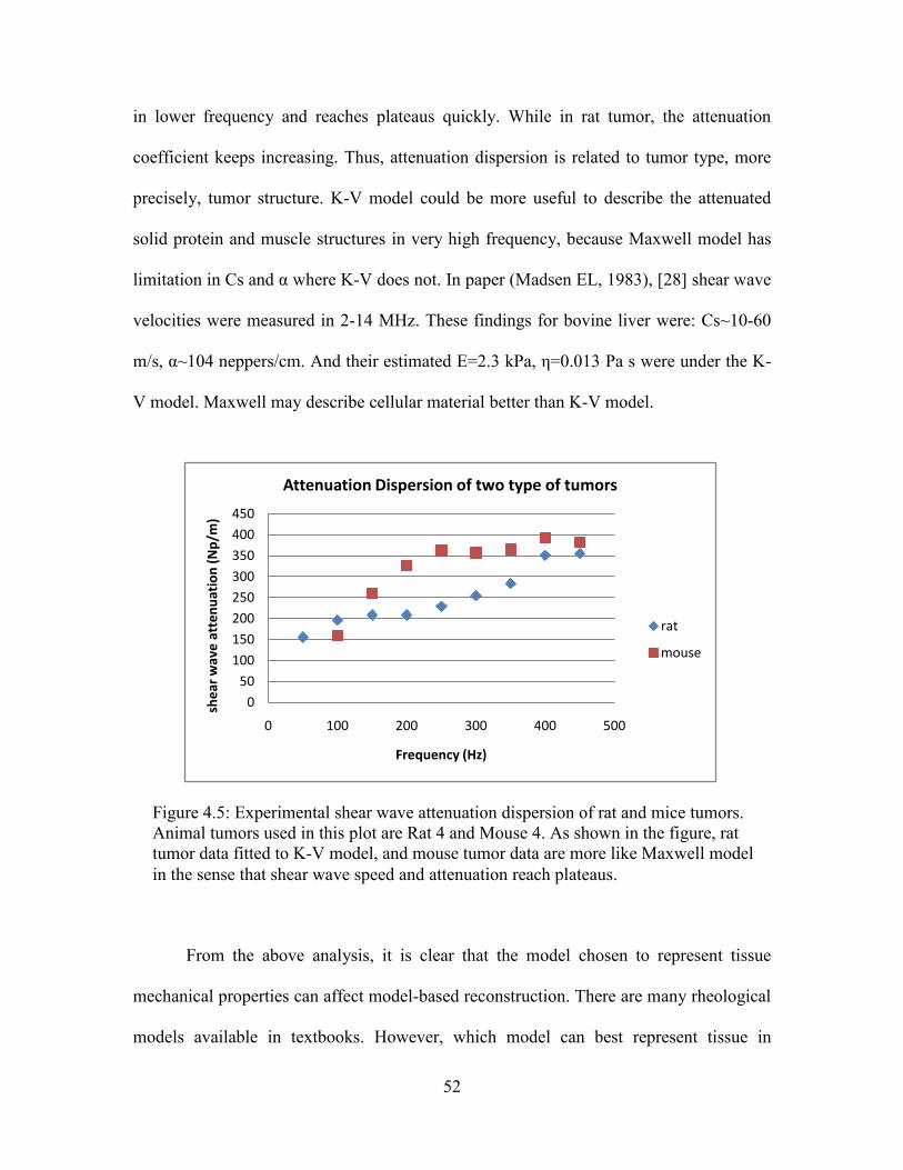
viscoelastic behavior of tissue. Figure 4.5 illustrates the shear wave attenuation

dispersion curves from animal tumors. Due to the dissimilarity of tissue constitution, (rat

tumor contains more collagen and mouse tumor contains mainly cells) the attenuation

dispersion curves behave a little differently. Mouse tumor attenuates more than rat tumor

Table 4.2: Summary of shear wave imaging result using Maxwell model

Tumor type Estimated Modulus μ[Pa] η[Pa·s]

Rat 1 Fibroadenoma 2558.6 3.03

Rat 2 Fibroadenoma 10722.0 3.53

Rat 3 Fibroadenoma 4604.0 1.92

Rat 4 Fibroadenoma 24453.0 3.99

Rat 5 Expanded lobular hyperplasia

29360.0 7.02

Figure 4.4: Shear wave velocity data of rats tumors fitted to Maxwell model

52

in lower frequency and reaches plateaus quickly. While in rat tumor, the attenuation

coefficient keeps increasing. Thus, attenuation dispersion is related to tumor type, more

precisely, tumor structure. K-V model could be more useful to describe the attenuated

solid protein and muscle structures in very high frequency, because Maxwell model has

limitation in Cs and α where K-V does not. In paper (Madsen EL, 1983), [28] shear wave

velocities were measured in 2-14 MHz. These findings for bovine liver were: Cs~10-60

m/s, α~104 neppers/cm. And their estimated E=2.3 kPa, η=0.013 Pa s were under the K-

V model. Maxwell may describe cellular material better than K-V model.

From the above analysis, it is clear that the model chosen to represent tissue

mechanical properties can affect model-based reconstruction. There are many rheological

models available in textbooks. However, which model can best represent tissue in

Figure 4.5: Experimental shear wave attenuation dispersion of rat and mice tumors. Animal tumors used in this plot are Rat 4 and Mouse 4. As shown in the figure, rat tumor data fitted to K-V model, and mouse tumor data are more like Maxwell model in the sense that shear wave speed and attenuation reach plateaus.

0

50

100

150

200

250

300

350

400

450

0 100 200 300 400 500

she

ar w

ave

att

en

uat

ion

(N

p/m

)

Frequency (Hz)

Attenuation Dispersion of two type of tumors

rat

mouse

53

appropriate frequency bandwidth remains unresolved and a very interesting topic. In

Chapter 3, I reported the estimated modulus using K-V model since it is a prevalent

model used in the field of soft tissue mechanics and I can compare results with others.

Future work with higher frequency bandwidth might help explain more on the model

selection issue.

4.3 Nonlinear wave propagation

Biological materials may have large second- and third-order nonlinear elastic moduli.

Even though strains in shear wave imaging experiments are small, nonlinear effects may

be important in the complex shear modulus estimation. If this is true, then a nonlinear

extension of the model should be considered in addition to the dispersive extension.

To investigate the nonlinear propagation effect brought from strain amplitude and

frequency bandwidth as well as to explore other excitation methods that could have

comparable accuracy to harmonic excitation, we implemented two other excitation

methods. First, we examined a broadband technique for generating shear waves in the

medium in order to estimate ( )sc . The needle actuator was driven by a one-cycle

sinusoidal voltage to produce shear-wave pulses with bandwidths of 60 to 400 Hz. The

pulsed response is decomposed in frequency via Fourier analysis to estimate shear-speed

dispersion.

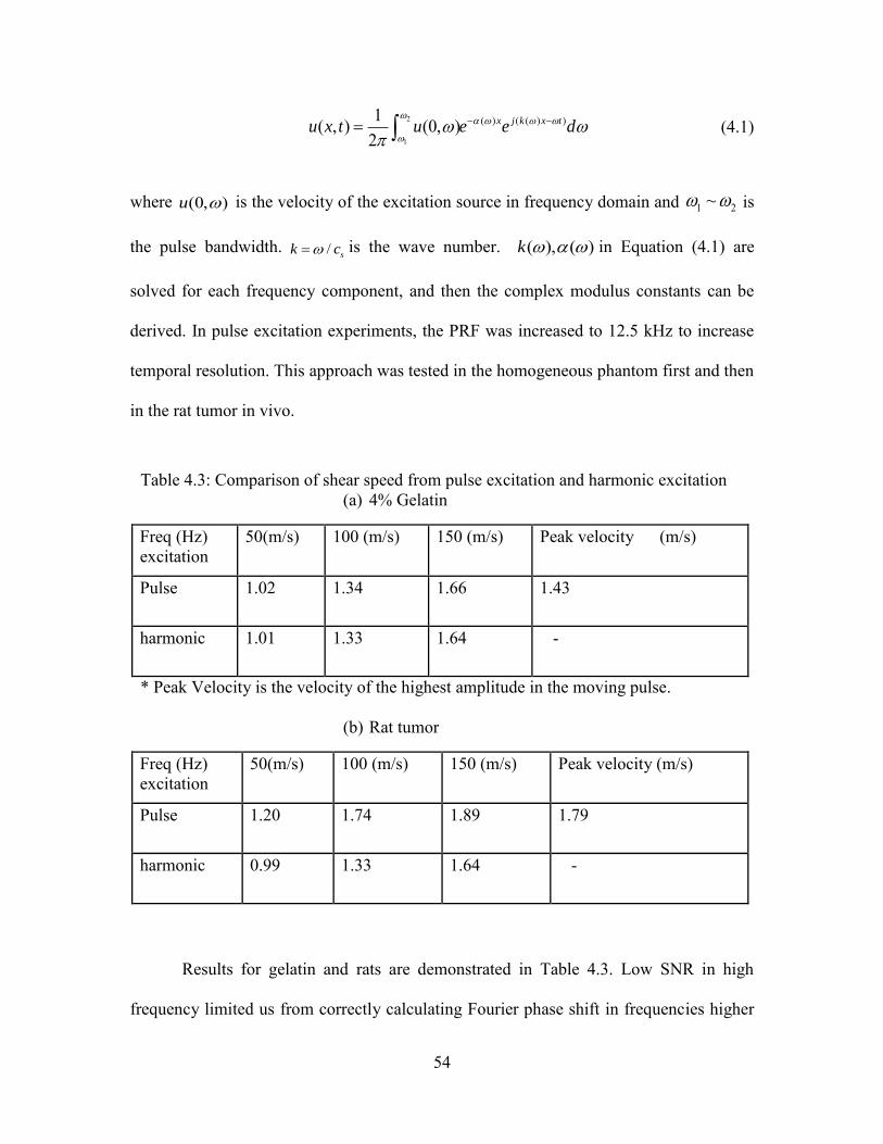
To illustrate, assume the pulsed source is a plane wave. The spatio-temporal

particle velocity can be modeled as

54

2

1

( ) ( ( ) )1( , ) (0, )2

x j k x tu x t u e e d

(4.1)

where (0, )u is the velocity of the excitation source in frequency domain and 1 2~ is

the pulse bandwidth. / sk c is the wave number. ( ), ( )k in Equation (4.1) are

solved for each frequency component, and then the complex modulus constants can be

derived. In pulse excitation experiments, the PRF was increased to 12.5 kHz to increase

temporal resolution. This approach was tested in the homogeneous phantom first and then

in the rat tumor in vivo.

Results for gelatin and rats are demonstrated in Table 4.3. Low SNR in high

frequency limited us from correctly calculating Fourier phase shift in frequencies higher

Table 4.3: Comparison of shear speed from pulse excitation and harmonic excitation (a) 4% Gelatin

Freq (Hz) excitation

50(m/s) 100 (m/s) 150 (m/s) Peak velocity (m/s)

Pulse 1.02 1.34 1.66 1.43

harmonic 1.01 1.33 1.64 -

* Peak Velocity is the velocity of the highest amplitude in the moving pulse.

(b) Rat tumor

Freq (Hz) excitation

50(m/s) 100 (m/s) 150 (m/s) Peak velocity (m/s)

Pulse 1.20 1.74 1.89 1.79

harmonic 0.99 1.33 1.64 -

55

than 200 Hz. The pulse excitation method has low sensitivity to phase after amplitude

dropping under 40 dB. Thus, only three frequencies are listed in the table. Thus, another

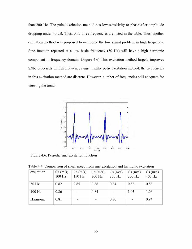
excitation method was proposed to overcome the low signal problem in high frequency.

Sinc function repeated at a low basic frequency (50 Hz) will have a high harmonic

component in frequency domain. (Figure 4.6) This excitation method largely improves

SNR, especially in high frequency range. Unlike pulse excitation method, the frequencies

in this excitation method are discrete. However, number of frequencies still adequate for

viewing the trend.

Table 4.4: Comparison of shear speed from sinc excitation and harmonic excitation

excitation Cs (m/s) 100 Hz

Cs (m/s) 150 Hz

Cs (m/s) 200 Hz

Cs (m/s) 250 Hz

Cs (m/s) 300 Hz

Cs (m/s) 400 Hz

50 Hz 0.82 0.85 0.86 0.84 0.88 0.88

100 Hz 0.86 - 0.84 - 1.03 1.06

Harmonic 0.81 - - 0.80 - 0.94

Figure 4.6: Periodic sinc excitation function

56

In both excitation methods, gelatin phantoms demonstrate linear property where

shear wave velocities do not vary with driven amplitude change. While in rat tumor tissue,

nonlinearity may occur, (Table 4.5) not only due to tissue inner structure but also a result

of other factors such as geometry.

4.4 Reflection effect

Depending on the underlying material properties, especially tumors with lower elasticity

and viscosity, reflections from the boundary cannot be ignored. These reflections can

result in phase ambiguity in shear wave speed estimation. Lower frequencies are affected

more than higher frequencies due to the longer wavelength and significantly smaller

attenuation coefficient.

Theoretically, two interfering waves with same frequency but opposite direction

will corrupt the precision of spatial phase shift. In a strict case where these two waves

have the same amplitude, and distance between source and boundary 2

nL

( n is

integer), standing wave will occur and spatial phase shift will be reduced to zero. 1D

FDTD simulation of plane wave and 3D FDTD simulation of needle-driven cylindrical

wave were performed to study the reflection induced phase ambiguity.

Table 4.5: Shear speed measurements affected by drive amplitude Drive amplitude (A) Drive amplitude (2A) 150 Hz 4.08 m/s 3.44 m/s

350 Hz 6.40 m/s 5.34 m/s

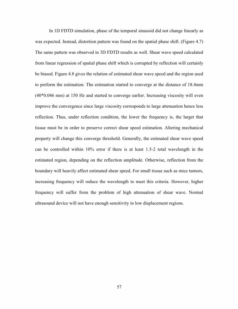
57

In 1D FDTD simulation, phase of the temporal sinusoid did not change linearly as

was expected. Instead, distortion pattern was found on the spatial phase shift. (Figure 4.7)

The same pattern was observed in 3D FDTD results as well. Shear wave speed calculated

from linear regression of spatial phase shift which is corrupted by reflection will certainly

be biased. Figure 4.8 gives the relation of estimated shear wave speed and the region used

to perform the estimation. The estimation started to converge at the distance of 18.4mm

(40*0.046 mm) at 150 Hz and started to converge earlier. Increasing viscosity will even

improve the convergence since large viscosity corresponds to large attenuation hence less

reflection. Thus, under reflection condition, the lower the frequency is, the larger that

tissue must be in order to preserve correct shear speed estimation. Altering mechanical

property will change this converge threshold. Generally, the estimated shear wave speed

can be controlled within 10% error if there is at least 1.5-2 total wavelength in the

estimated region, depending on the reflection amplitude. Otherwise, reflection from the

boundary will heavily affect estimated shear speed. For small tissue such as mice tumors,

increasing frequency will reduce the wavelength to meet this criteria. However, higher

frequency will suffer from the problem of high attenuation of shear wave. Normal

ultrasound device will not have enough sensitivity in low displacement regions.

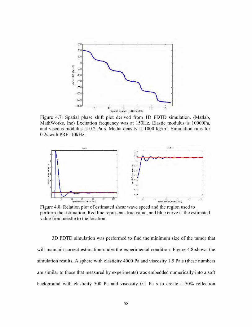
58

3D FDTD simulation was performed to find the minimum size of the tumor that

will maintain correct estimation under the experimental condition. Figure 4.8 shows the

simulation results. A sphere with elasticity 4000 Pa and viscosity 1.5 Pa s (these numbers

are similar to those that measured by experiments) was embedded numerically into a soft

background with elasticity 500 Pa and viscosity 0.1 Pa s to create a 50% reflection

Figure 4.8: Relation plot of estimated shear wave speed and the region used to perform the estimation. Red line represents true value, and blue curve is the estimated value from needle to the location.

Figure 4.7: Spatial phase shift plot derived from 1D FDTD simulation. (Matlab, MathWorks, Inc) Excitation frequency was at 150Hz. Elastic modulus is 10000Pa, and viscous modulus is 0.2 Pa s. Media density is 1000 kg/m3. Simulation runs for 0.2s with PRF=10kHz.

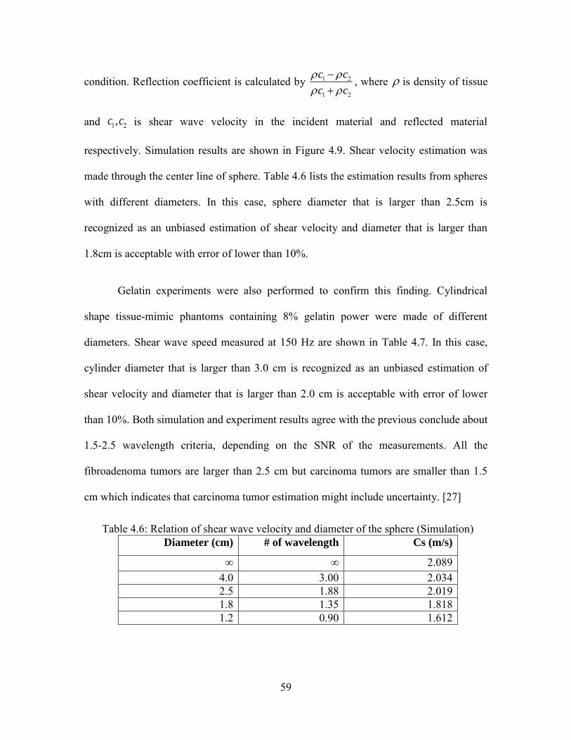
59

condition. Reflection coefficient is calculated by 1 2

1 2

c c

c c

, where is density of tissue

and 1 2,c c is shear wave velocity in the incident material and reflected material

respectively. Simulation results are shown in Figure 4.9. Shear velocity estimation was

made through the center line of sphere. Table 4.6 lists the estimation results from spheres

with different diameters. In this case, sphere diameter that is larger than 2.5cm is

recognized as an unbiased estimation of shear velocity and diameter that is larger than

1.8cm is acceptable with error of lower than 10%.

Gelatin experiments were also performed to confirm this finding. Cylindrical

shape tissue-mimic phantoms containing 8% gelatin power were made of different

diameters. Shear wave speed measured at 150 Hz are shown in Table 4.7. In this case,

cylinder diameter that is larger than 3.0 cm is recognized as an unbiased estimation of

shear velocity and diameter that is larger than 2.0 cm is acceptable with error of lower

than 10%. Both simulation and experiment results agree with the previous conclude about

1.5-2.5 wavelength criteria, depending on the SNR of the measurements. All the

fibroadenoma tumors are larger than 2.5 cm but carcinoma tumors are smaller than 1.5

cm which indicates that carcinoma tumor estimation might include uncertainty. [27]

Table 4.6: Relation of shear wave velocity and diameter of the sphere (Simulation) Diameter (cm) # of wavelength Cs (m/s)

∞ ∞ 2.089 4.0 3.00 2.034 2.5 1.88 2.019 1.8 1.35 1.818 1.2 0.90 1.612

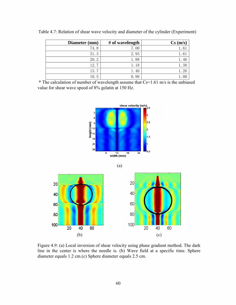
60

(a)

(b) (c) Figure 4.9: (a) Local inversion of shear velocity using phase gradient method. The dark line in the center is where the needle is. (b) Wave field at a specific time. Sphere diameter equals 1.2 cm.(c) Sphere diameter equals 2.5 cm.

Table 4.7: Relation of shear wave velocity and diameter of the cylinder (Experiment)

Diameter (mm) # of wavelength Cs (m/s)

74.8 7.00 1.61

31.3 2.93 1.61

20.2 1.88 1.46

12.7 1.18 1.38

15.7 1.46 1.26

10.5 0.98 1.00

* The calculation of number of wavelength assume that Cs=1.61 m/s is the unbiased value for shear wave speed of 8% gelatin at 150 Hz.

61

CHAPTER 5

DISCUSSIONS

Ultrasonic shear wave imaging is a new approach to image and characterize tissue

structures based on the use of shear acoustic waves. The needle-based technique benefits

in increasing SNR as well as in generating a locally uniform excitation, thus serving as a

good approach to study contrast mechanism and some concept behind this technique.

Data presented in Chapter 3 demonstrates the feasibility of assessing mechanical

parameters in rodent animals in vivo by measuring shear wave propagated in tissue and

then applying rheological models. The mechanical properties measured by shear wave

imaging technique and rheometer measurements track each other and show distinction

among different tumor types. In Chapter 4, several reasons which might lead to variation

in mechanical property estimation are discussed, including ECM composition,

rheological model as well as experimental design. Analysis suggests that both elasticity

and viscosity are sensitive to ECM protein density such as collagen. In addition to the

viscoelastic response from the protein network, a coupled viscoelastic response comes

from cellularity and loosely bounded interstitial fluid. This increases the complexity of

the modeling, however, might gain biological contrast in VE properties on various tumor

types. It is still unclear about the contrast mechanism of shear wave imaging technique in

diagnosis and prognosis in tumor detection, and models that represent the true dispersion

62

behavior are still under discovery (ie, incorporation of poroviscoelasticity and nonlinear

effect).

Since rodent animal models were used, the preliminary results were compared

with literature [8] on the complex shear modulus estimated in fibroadenoma tumors in

human subjects and found good correlation between the results. This suggests that rat

mammary tumor models are representative of the mechano-enviroment in human

fibroadenoma tumors and represent good models for studying viscoelastic contrasts in

elasticity imaging. However, presented analysis is valid under several assumptions. We

assumed that the materials are locally homogenous. This approach is valid for this study

where any inhomogeneities are considered to be much smaller than the wavelength of the

shear wave. Thus, the phase gradient approach and homeogeneity assumption is

reasonable for the proposed application. Nevertheless, in some tumors where the size of

an inhomogeneity necrosis core is comparable to the wavelength of the shear wave,

especially when high frequency is used, strong refraction effects are observed in the

boundary of the inhomogeneity. Refraction effects could bias estimated shear wave speed.

I plan to further investigate techniques capable of quantitatively reconstructing complex

shear modulus in heterogeneous media.

Preliminary results demonstrate both elastic and viscous modulus obtained using

our technique possesses insights into tumor microenvironment. Dynamic shear-wave

estimation of the complex modulus of mammary tumors demonstrates that changes in

histological features are greater than inter-animal or technique variabilities.

Consequently it is possible to reliably classify tumors using elasticity imaging.

63

REFERENCES

[1] L. Huwart, F. Peeters, R. Sinkus, L. Annet, N. Salameh, L. C. terBeek, Y. Horsmans and B. E. Van Beers, "Liver fibrosis: Non-invasive assessment with MR elastography," NMR Biomed., vol. 19, pp. 173-179, 2006.

[2] M. H. Wang, M. L. Palmeri, C. D. Guy, L. Yang, L. W. Hedlund, A. M. Diehl and K. R. Nightingale, "In vivo Quantification of Liver Stiffness in a Rat Model of Hepatic Fibrosis with Acoustic Radiation Force," Ultrasound Med. Biol., vol. 35, pp. 1709-1721, 10, 2009.

[3] H. Yu, "Forcing form and function: Biomechanical regulation of tumor evolution," Trends Cell Biol., vol. 21, pp. 47-56, 2011.

[4] K. R. Levental, "Matrix Crosslinking Forces Tumor Progression by Enhancing Integrin Signaling," Cell, vol. 139, pp. 891-906, 2009.

[5] Y. Qiu, M. Sridhar, J. Tsou, K. Lindfors and M. Insana, "Ultrasonic Viscoelasticity Imaging of Nonpalpable Breast Tumors: Preliminary Results," Acad. Radiol., vol. 15, pp. 1526-1533, 2008.

[6] S. Chen, "Shearwave dispersion ultrasound vibrometry (SDUV) for measuring tissue elasticity and viscosity," IEEE Trans. Ultrason.Ferroelectr. Freq. Control, vol. 56, pp. 55-62, 2009.

[7] T. Deffieux, "Shear wave spectroscopy for in vivo quantification of human soft tissues visco-elasticity," IEEE Trans. Med. Imaging, vol. 28, pp. 313-322, 2009.

[8] R. Sinkus, "Viscoelastic shear properties of in vivo breast lesions measured by MR elastography," Magn. Reson.Imaging, vol. 23, pp. 159-165, 2005.

[9] A. Evans, "Quantitative shear wave ultrasound elastography: Initial experience in solid breast masses," Breast Cancer Research, vol. 12, 2010.

[10] Costa, M. Solanas and E. Escrich, "Histopathologic characterization of mammary neoplastic lesions induced with 7,12 dimethylbenz(alpha)anthracene in the rat - A comparative analysis with human breast tumors," Archives of Pathology Laboratory

Medicine, vol. 126, pp. 915-927, 2002.

64

[11] M. Orescanin and M. Insana, "Shear Modulus Estimation With Vibrating Needle Stimulation," IEEE Trans. Ultrason.Ferroelectr. Freq. Control, vol. 57, pp. 1358-1367, 2010.

[12] S. C. Cowin, "How Is a Tissue Built?" J. Biomech. Eng., vol. 122, pp. 553, 12, 2000.

[13] R. John, R. Rezaeipoor, S. G. Adie, E. J. Chaney, A. L. Oldenburg, M. Marjanovic, J. P. Haldar, B. R. Sutton and S. A. Boppart, "In vivo magnetomotive Optical molecular imaging using targeted magnetic nanoprobes," Proc. Natl. Acad. Sci. U. S. A., vol. 107, pp. 8085-8090, 05/04, 2010.

[14] J. F. Greenleaf, M. Fatemi and M. Insana, "Selected Methods for Imaging Elastic Properties of Biological Tissues," Annu.Rev. Biomed.Eng., vol. 5, pp. 57-78, 08, 2003.

[15] P. Rzymski, "Factors influencing breast elasticity measured by the ultrasound shear wave elastography - Preliminary results," Archives of Medical Science, vol. 7, pp. 127-133, 2011.

[16] J. Carcione, "Wave fields in real media wave propagation in anisotropic, anelastic and porous media," Handbook of Geophysical Exploration.Section 1, Seismic

Exploration, vol. 31, 2001.

[17] M. Orescanin, Y. Wang and M. Insana, "3-D FDTD simulation of shear waves for evaluation of complex modulus imaging," IEEE Transactions on Ultrasonics

Ferroelectrics & Frequency Control, vol. 58, pp. 389-398, 02, 2011.

[18] A. Samani, J. Zubovits and D. Plewes, "Elastic moduli of normal and pathological human breast tissues: an inversion-technique-based investigation of 169 samples," Phys.

Med. Biol., vol. 52, pp. 1565-1576, MAR 21, 2007.

[19] C. Downs-Holmes and P. Silverman, "Breast cancer: overview & updates." Nurse

Pract., vol. 36, pp. 20-6; 7, 2011 Dec 16, 2011.

[20] C. S. Samuel, "Determination of collagen content, concentration, and sub-types in kidney tissue," Methods in Molecular Biology, vol. 466, pp. 223-235, 2009.

[21] M. Oelze, W. O'Brien, J. Blue and J. Zachary, "Differentiation and characterization of rat mammary fibroadenomas and 4T1 mouse carcinomas using quantitative ultrasound imaging," IEEE Trans. Med. Imaging, vol. 23, pp. 764-771, JUN, 2004.

[22] M. Cechowska-Pasko, J. Palka and M. Z. Wojtukiewicz, "Enhanced prolidase activity and decreased collagen content in breast cancer tissue," Int. J. Exp. Pathol., vol. 87, pp. 289-296, AUG 2006, 2006.

[23] F. Okano, "Study on stromal component of mastopathy--content and type of collagen," Hokkaido IgakuZasshi, vol. 60, pp. 555-570, 1985.

65

[24] M. Cechowska-Pasko, J. Pałka and M. Z. Wojtukiewicz, "Enhanced prolidase activity and decreased collagen content in breast cancer tissue," Int. J. Exp. Pathol., vol. 87, pp. 289-296, 2006.

[25] H. Xie, et al, "Shear wave Dispersion Ultrasound Vibrometry (SDUV) on an ultrasound system: In vivo measurement of liver viscoelasticity in healthy animals," Ultrasonics Symposium (IUS), 2010 IEEE, pp. 912 – 915, 2010.

[26] K. Nightingale, S. McAleavey, G. Trahey, "Shear-wave generation using acoustic radiation force: In vivo and ex vivo results," Ultrasound Med. Biol., vol. 29, pp. 1715-1723, 12, 2003.

[27] H. Lin, S. Chen, "Precision analysis of viscoelastic measurement using shear wave dispersion vibrometry method,", Proceedings-2011 ICBMI 2011, art. no. 6131724, pp. 16-18, 2011.

[28] E. L. Madsen, H. J. Sathoff, J. A. Zagzebski, "Ultrasonic shear wave properties of soft tissues and tissuelike materials," J Acoust Soc Am., Vol 74, pp. 1346-1355, 1983.