Embed Size (px)
Citation preview

Analysis of single gene effects 1
Quantitative analysis of single gene effects
Gregory Carey, Barbara J. Bowers, Jeanne M. Wehner
From the Department of Psychology (GC, JMW) and Institute for Behavioral Genetic
(GC, BJB, JMW) University of Colorado, Boulder, CO, USA.
Supported by Grant 2 M01 RR00051 from the General Clinical Research Center Program
of the National Center for Research Resources, National Institute of Health, AA-11275,
AA-03627, and R.C.A. AA-00141 to JMW.

Analysis of single gene effects 2
Abstract
Traditionally, the analysis of a quantitative phenotype as a function of a two allele
polymorphism at a single locus involves a oneway ANOVA with locus as the ANOVA
factor and the three individual genotypes (e.g., aa, Aa, and AA) as the levels of the factor.
Here, we propose a related method of analysis that is just as easy to implement as the
oneway ANOVA but has the following advantages: (1) greater statistical power; (2)
direct estimation of meaningful genetic parameters such as additive genetic variance at
the locus and both broad and narrow heritability due to the locus; (3) provides estimates
of effect size that also equal meaningful genetic parameters; (4) gives a direct test for
dominance that avoids the problems with post hoc ANOVA tests; (5) yields an omnibus
F test that is identical to that of the oneway ANOVA. The method is illustrated with data
on the protein kinase C g locus in the mouse and behavior on the elevated plus-maze.
Power calculations are also provided.

Analysis of single gene effects 3
Many designs involving genetics and neuroscience involve the comparison of the
three genotypic means for a locus with various mechanisms used to control for (or to
estimate) differences in background genetic variation. A simple and valid statistical
technique for this type of problem is a oneway ANOVA in which genetic locus is the
ANOVA factor and the individual genotypes at the locus are the three levels of the factor.
Most planned experiments of this type strive to achieve equal sample sizes for the
three cells in the ANOVA. While the resulting orthogonal design has attractive
properties, it presents a problem for calculating quantities like narrow-sense heritability
for the locus that may be of use to the researcher. Many traditional texts on quantitative
genetics deal with panmictic populations and derive their formulas for heritability
assuming, say, Hardy-Weinberg equilibrium. When an ANOVA design has equal sample
sizes, then such formulas are inappropriate.
Here, we present a simple method of analysis for single-gene problems that has
several advantages over a oneway ANOVA but is just as easy to implement. The first
advantage is that is statistically more powerful than the oneway ANOVA. The second
advantage is that it calculates and tests the significance of quantitative parameters such as
broad and narrow sense heritability due to the locus. (Note well that in this paper, the
term “heritability” applies only to the variance explained by the locus under question and
not to all polymorphic loci that influence the trait). A third advantage is that results can
be presented in terms of effect sizes instead of p values, a trend that is recommended in
contemporary statistics (Cohen, 1988). A fourth advantage is that, in addition to the
information given above, it also provides an F test identical to that of a oneway ANOVA.

Analysis of single gene effects 4
A fifth advantage is that there is no need for post hoc tests to assess for the presence of
dominant gene action.
Analytical proof of these statements (and other assertions to follow) is provided
by a technical document at http://ibgwww.colorado.edu/~carey/QAOSGE.html, and in
some standard statistical texts such as Judd and McClelland (1989). The model also
applies to observational data gathered on organisms in their natural habitat where
genotypic frequencies are not equal (see the above website for the general quantitative
equations). In this paper, however, we deal with the specific case of equal genotypic
frequencies.
Mathematical Model
The model used here assumes two alleles per locus (which we designate as A and
a), giving three genotypes—AA, Aa, and aa. The overall notation is similar to that used
in Falconer and Mackay (1996) and is presented in Table 1.
[Insert Table 1 about here]
Here m is the midpoint between the two homozygotes. The quantity a is the
additive genetic effect and has the following interpretation: if we were to substitute allele
A for allele a in a genotype, then we expect, on average, a phenotypic change of a units.
The quantity d is the parameter for dominance. It measures the extent to which the mean
of the heterozygote Aa deviates from the average of the two homozygotes. When d = 0,
there is complete additivity.

Analysis of single gene effects 5
Data Arrangement
The arrangement of data for the analysis is illustrated in Table 2. In addition to a
column for genotype and one for phenotypic scores (the values of which are fictitious in
this table), two new quantitative variables are created. The first of these is called “alpha”
in Table 2 and it is used to obtain an estimate of the additive effect of an allelic
substitution and also an estimate of narrow-sense (i.e., additive) heritability. The rule for
constructing variable alpha is simple. Alpha equals –1 for one homozygote, equals 1 for
the other homozygote, and equals 0 for the heterozygote. (Hint: let alpha equal –1 for the
homozygote with the lower mean.) The second variable is called “delta” and it is used to
assess the presence of dominance. If the genotype is a heterozygote, then the value of
delta is 1; otherwise, delta equals 0.
[Insert Table 2 about here]
Sequence of Analysis
After variables alpha and delta are constructed, two regressions are performed.
The first regression, referred to by some authors as the compact model (Judd &
McClelland, 1989), uses the phenotypic score as the dependent variable and variable
alpha as the independent variable. The second, termed the augmented model, uses both
variables alpha and delta as the independent variables.
Interpretation of the Output
The squared multiple correlation (R2) from the first regression is an estimate of
the narrow sense heritability or the proportion of additive genetic variance to phenotypic

Analysis of single gene effects 6
variance for the locus. Multiplying this R2 by the phenotypic variance gives the additive
genetic variance that this locus contributes to the trait. If there is no dominance
(discussed below), then the regression coefficient for the variable alpha is a direct
estimate of the additive effect of an allelic substitution (i.e., the quantity a in Table 1).
Also, the test of significant for this coefficient is always the most powerful statistical test
for genetic effects provided dominance is not strong.
The regression for the augmented model tests for dominance. If we reject the null
hypothesis of no dominance, then this regression gives additional important quantities;
otherwise, we return to the first regression and present and interpret those results. The
intercept from this multiple regression model equals the midpoint between the two
homozygotes (i.e., the quantity m in Table 1). The regression coefficient for variable
alpha equals the additive effect of an allelic substitution (i.e., the quantity a in Table 1).
The regression coefficient for variable delta equals the deviation of the heterozygote
mean from the midpoint (i.e., the quantity d in Table 1).
The F statistic from augmented model is an omnibus F that assesses the fit of the
whole model. It, along with its p value, will be identical to the F (and that F’s p value)
from a oneway ANOVA. For the types of sample sizes available for neuroscience
research, the t test for the regression coefficient of variable alpha in either the first or
second regression is almost always a more powerful statistic for testing the presence of
genetic effects at the locus than the omnibus F. For those few cases in which the F test is
more powerful (complete dominance, large additive effect, and large sample sizes), the
maximal difference in power is about .03. However, in the rest of the parameter space,
the difference in power favoring the t statistic can be appreciable—up to .20.

Analysis of single gene effects 7
The appropriate test for dominance is the significance of the t statistic for the
regression coefficient of variable delta. The p level for this t statistic will be identical to
that of an F statistic that tests whether adding variable delta significantly increased R2
over the first regression. This test for dominance will always be less powerful than the t
test for variable alpha’s regression coefficient.
The squared multiple correlation from the second regression is an estimate of
broad sense heritability or the proportion of phenotypic variance attributable to total
genetic variance (additive plus dominance variance) at the gene. Thus, the proportion of
phenotype variance attributable to dominance variance can be calculated by subtracting
the R2 from this regression from the R2 of the first regression. Multiplying this quantity
by the phenotypic standard deviation gives dominance variance in raw score units.
A numerical example
As an example, we analyze data collected and reported by Bowers et al. (2000) on
behavior on an elevated plus-maze for mice lacking the gene for the g isoform of protein
kinase C (PKCg knockouts) and their heterozygous and wild-type littermates. Two
phenotypes are analyzed, both derived from a principal components analysis of the
original variables presented in Table 1 of Bowers et al. (2000). These factors agree
almost perfectly with those reported by Rodgers & Johnson (1995) using a different
population of mice. The first phenotype is activity (marked by the total number of
entrances, and entrances into the closed arms of the maze). The second phenotype is
anxiety. Here, high scores are marked by a high percentage of time and of entrances into
the closed arm while low scores are indexed by a high percentage of time and entrances

Analysis of single gene effects 8
into the open arms. Descriptive statistics for these two phenotypes are presented in Table
3.
[Insert Table 3 about here]
The values of alpha were assigned so that the PKCg knock out mice were given
the value of –1, heterozygotes a value of 0, and the wild type homozygotes, a value of 1.
Code from the Statistical Analysis System (SAS) to perform the regressions for the the
anxiety phenotype is given in Appendix 1.
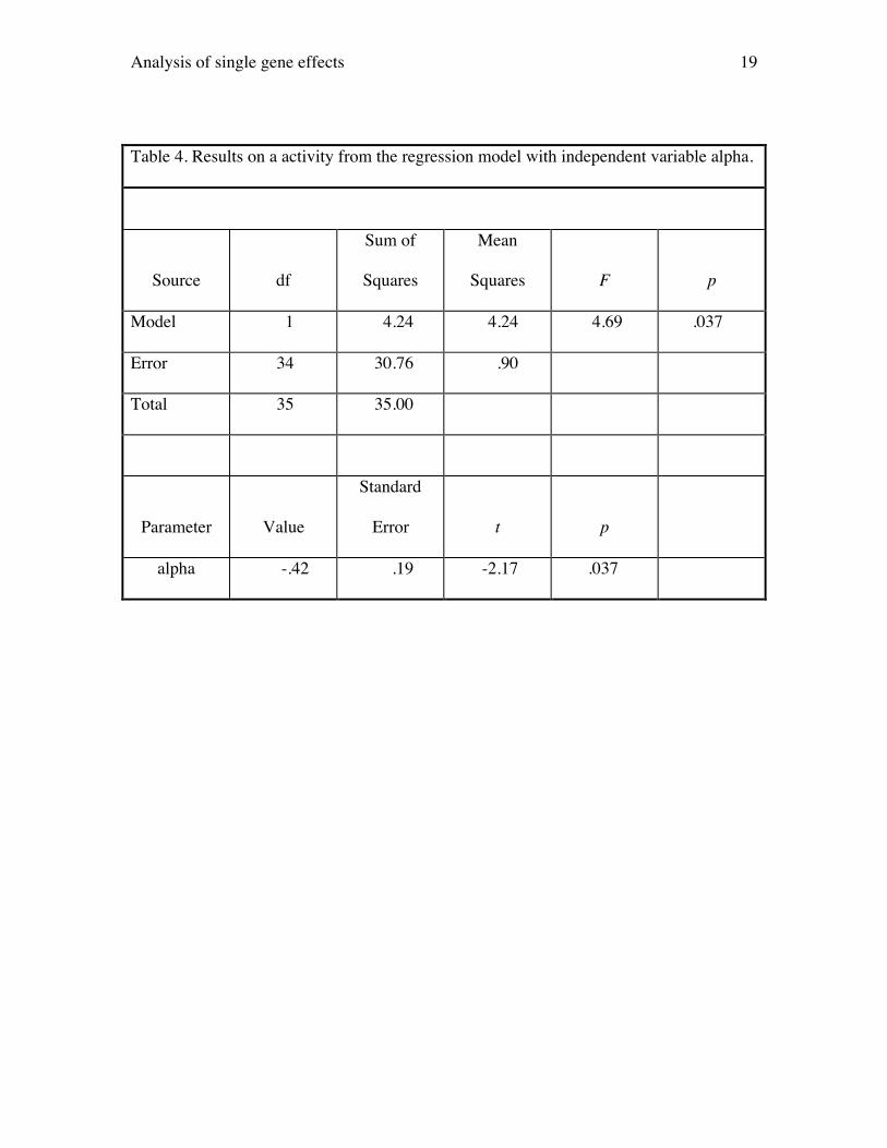
The activity phenotype illustrates how the method operates for a system with only
additive gene action. The results from the first regression, presented in Table 4, should
be used to interpret whether or not the PKCg locus has an effect on activity. Here, one
could interpret either the F statistic from the ANOVA table or the t statistic testing
whether the parameter estimate for variable alpha is significantly different from 0. (Both
statistics are equivalent because with only one independent variable the F statistic is the
square of the t statistic and both will have identical p values.) Here, t = -2.17 (p = .037),
so we reject the null hypothesis of no genetic effect and conclude that the PKCg gene has
an influence on overall activity in the elevated plus-maze. The value of the coefficient
for variable alpha (i.e., our estimate of a) is -.42 indicating that, on average, a
substitution of one wild type allele for null (i.e., knock out) allele reduces activity by .42
units. Here, the estimate of a may be viewed as an effect size expressed in the metric of
the original data.
This effect size may be standardized in one of two ways. First, the estimate of
a may be divided by the error standard deviation (i.e., the square root of the error mean
square). This gives a measure of effect size favored by statisticians such as Cohen

Analysis of single gene effects 9
(1988). In the present case, this gives
†
-.42 / .90 = -.44. Hence, the average effect of an
allelic substitution is to change activity by .44 standard deviation units. The second way
to standardize is to divide a by the phenotypic standard deviation. Because we used
scores from a principal components analysis, the phenotypic standard deviations are 1.0,
leaving a unchanged.
A second way of expressing effect size is in terms of the proportion of variance
explained. The statistic here is R2, the squared multiple correlation that will be calculated
and printed in any output. It just so happens that this quantity also equals narrow-sense
heritability or the ratio of additive genetic variance to phenotypic variance. For this
regression, the R2 is .12, implying that 12% of phenotypic variance is attributable to
additive genetic variance.
[Insert Table 4 about here]
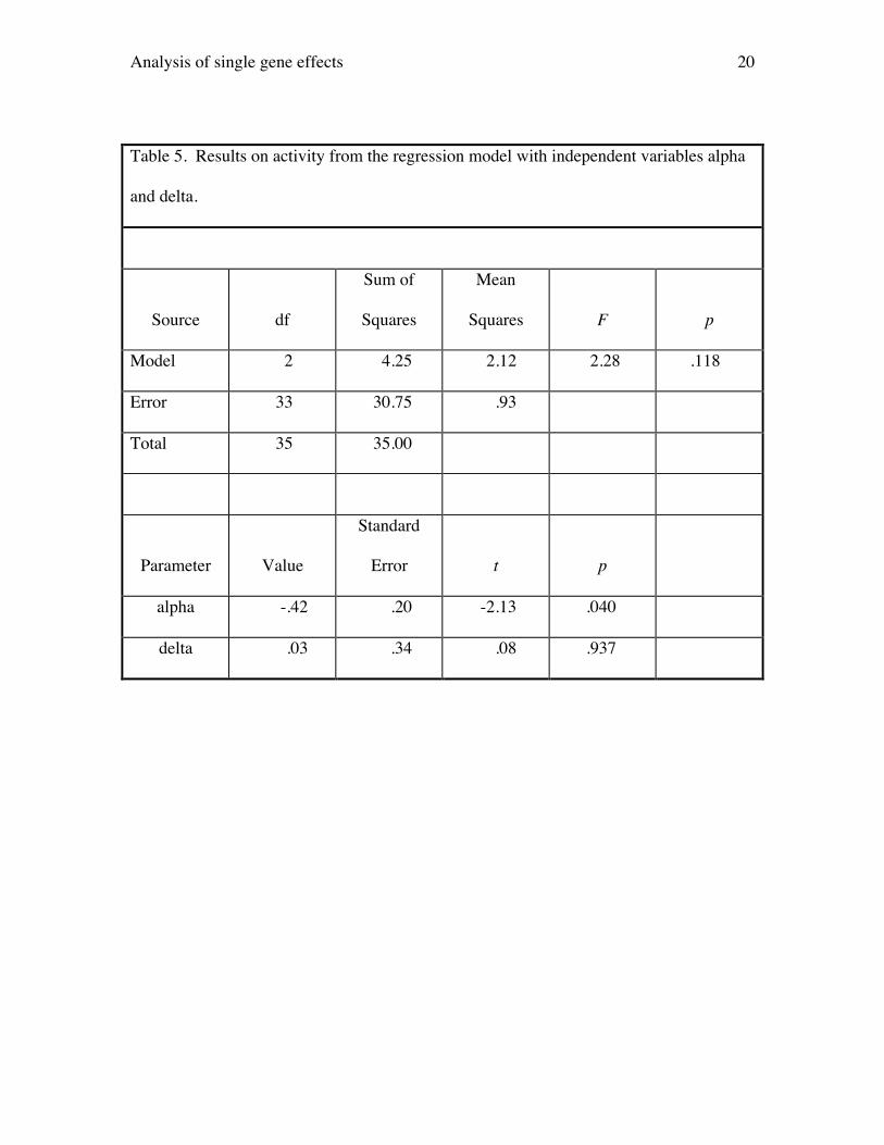
The next step is to test for dominance by regressing the activity phenotype on
both variables alpha and delta. Results are presented in Table 5. The critical statistic is
the t statistic that tests whether the parameter estimate for delta is significantly difference
from 0. Here, the value of t is .08 and its associated p value is .937. Hence, there is no
evidence for dominance on activity, and we would return and interpret the first regression
as the best model to explain the data.
[Insert Table 5 about here]
The results on activity also illustrate how the present method increases power to
detect genetic effects over a oneway ANOVA. The ANOVA table from a oneway
ANOVA is identical to that presented in Table 5. Here, the F value is 2.28 and its p
value is .118, so one would not reject the null hypothesis. The typical conclusion would
Analysis of single gene effects 10
be that there is no evidence that the PKCg locus influences activity in the elevated plus-
maze. On the other hand, we have seen that testing whether the coefficient for alpha
differs from 0 results in a statistically significant finding.
In summary, there is good evidence that the PKCg locus influences activity. All
gene action appears to be additive and the estimate of both narrow and broad-sense
heritability for the locus is .12. Whether an effect size of this magnitude is something
that is worthwhile pursuing is, of course, a matter that should be determined by the
substance of the problem and not the statistics.
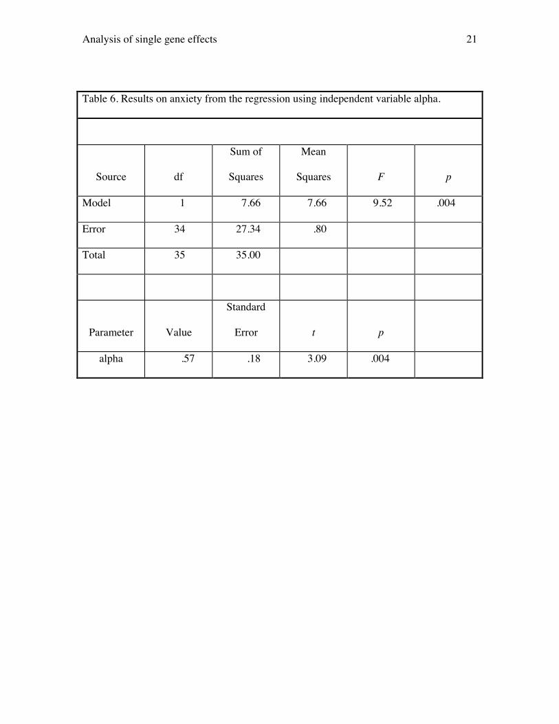
The anxiety phenotype is used to illustrate the method when dominance is
important. The results of regressing anxiety on variable alpha are presented in Table 6.
Here, the t statistic testing whether the coefficient for alpha equals is 3.09 (p = .004), so
we conclude that there is evidence that the PKCg locus also influences anxiety. The R2
from this regression (.22) equals the estimate of narrow sense heritability for anxiety.
[Insert Table 6 about here]
The results of the second regression are given in Table 7. The t statistic for the
coefficient for variable delta equals 3.25 (p = .003), so we reject the null hypothesis of no
dominance. Because there is evidence for dominance, we favor the parameter estimate
for alpha using this regression instead of that from the first regression. (The two
estimates are the same in the present case because there are equal sample sizes for the
genotypes; when sample sizes differ, the estimates of alpha may be different in the two
regressions). Here, the value of the coefficient for variable alpha is .56, implying that
substituting one wild-type allele for a null PKCg allele has the average effect of
increasing anxiety by .56 units. The value of the coefficient for variable delta (i.e., our

Analysis of single gene effects 11
estimate of d) is .91. This is larger than the value for a, so we might suspect heterosis.
Let us postpone discussion of this topic to focus on interpretation of heritability.
The R2 for this second regression is .41. This is our estimate of broad sense
heritability for anxiety. In short, variation in the PKCg locus accounts for about 41% of
the variability in this anxiety measure in this population of mice. Because the R2 from the
first regression is an estimate of narrow-sense heritability, the contribution of dominance
to broad sense heritability may be found by subtracting the R2 from the first regression
from that in the second regression. This gives .41 - .22 = .19.
Should we interpret the large estimate of d as overdominance? Certainly the
mean of the heterozygote is consistent with this possibility. Most—but not all—modern
regression software allows for a direct test of this hypothesis. When there is heterosis,
then the value for d should be significantly greater than the value of a (or significantly
less than the value of –a, depending on which allele is dominant). One can test for this
by constraining the regression coefficients for variables alpha and delta to be equal and
then testing the significance of this model against the second regression given above.
One simple SAS statement is sufficient for this test (see Appendix 1).
For the present case, the test is not significant (F(1,33) = 1.14, p = .29). Hence,
the value of d is not significantly greater than that for a, and there is no evidence for
overdominance.
Power
Calculations of power are very easy when the number of animals in each cell is
equal. Because the most powerful test is the t statistic for the regression coefficient of

Analysis of single gene effects 12
variable alpha, we base power on that statistic used in the augmented model. The
numerator for the t is the hypothesized value of the regression coefficient for variable
alpha (i.e., the quantity a in the model in Table 1). The denominator is the standard error
of the regression coefficient and equals
†
1.5s error2
N,
where
†
s error2 is the error variance and N is the total number of animals. The degrees of
freedom for this test equal (N – 2). With a little algebra, the noncentrality parameter for
the t may be written as
†
tnc =a
s error
N1.5
.
Note that the a in this equation is the parameter on Table 1 and not the probability of a
type I error. Note also the quantity a divided by the error standard deviation is the
Cohen’s standardized effect size. Power may then be calculated by finding the area
under this noncentral t distribution that exceeds the critical value of t. A program for the
calculation of power is available at http://ibgwww.colorado.edu/~carey/QAOSGE.html.
Table 8 gives estimates of power as a function of Cohen’s (1988) effect size and
sample sizes. The calculations were made assuming complete additivity. Dominance
will increase power because error variance will be reduced, but increase is so slight that
the figures in Table 8 are close approximations, even to the case of complete dominance.
The calculations suggest that 12 animals per group will result in power of .80 or better as
long as the effect size is moderately large (i.e., .60 or greater).
[Insert Table 8 about here]

Analysis of single gene effects 13
Discussion
The method advocated in this paper provides greater statistical power and more
informative quantitative estimates than traditional statistical techniques for analyzing
single gene effects. It provides two different ways to communicate effect sizes, one
expressed in mean change units (i.e., the values of a and d) and the second in terms of
variance components or heritabilities (R2) at the locus.
The major liability with the technique does not lie in the mathematics. Instead, it
resides in the incorrect interpretation and extrapolation of the quantitative estimates. In
experimental organisms, heritability estimates for a single gene are usually estimated
within the context of a limited range of genetic backgrounds and in controlled
environments. These estimates should never be extrapolated to general populations or
treated and interpreted as heritability estimates derived from, say, human twin or
adoption studies. For example, the mice used for the data examples give involved the
genetic background of C57BL/6J and 129/SvEvTac inbreds and were all reared and
tested in environmentally standardized conditions. The estimates of effect size and
heritability pertain only to this genetic background and similar environments. These
estimates can be very useful in guiding which of several future experiments to pursue, in
calculating power for other studies, and perhaps even in pointing out a suitable candidate
locus for other designs. They do not, however, imply that the PKCg locus must be
involved in individual differences in anxiety in wild mouse populations.
Finally, we offer a caveat. All statements made in this paper about power are
based on equal genotypic frequencies. They will be also apply to the case where cell size

Analysis of single gene effects 14
differs, but only by a few animals. The results on power should not be extrapolated to
natural populations in whom allele and genotypic frequencies can markedly differ.
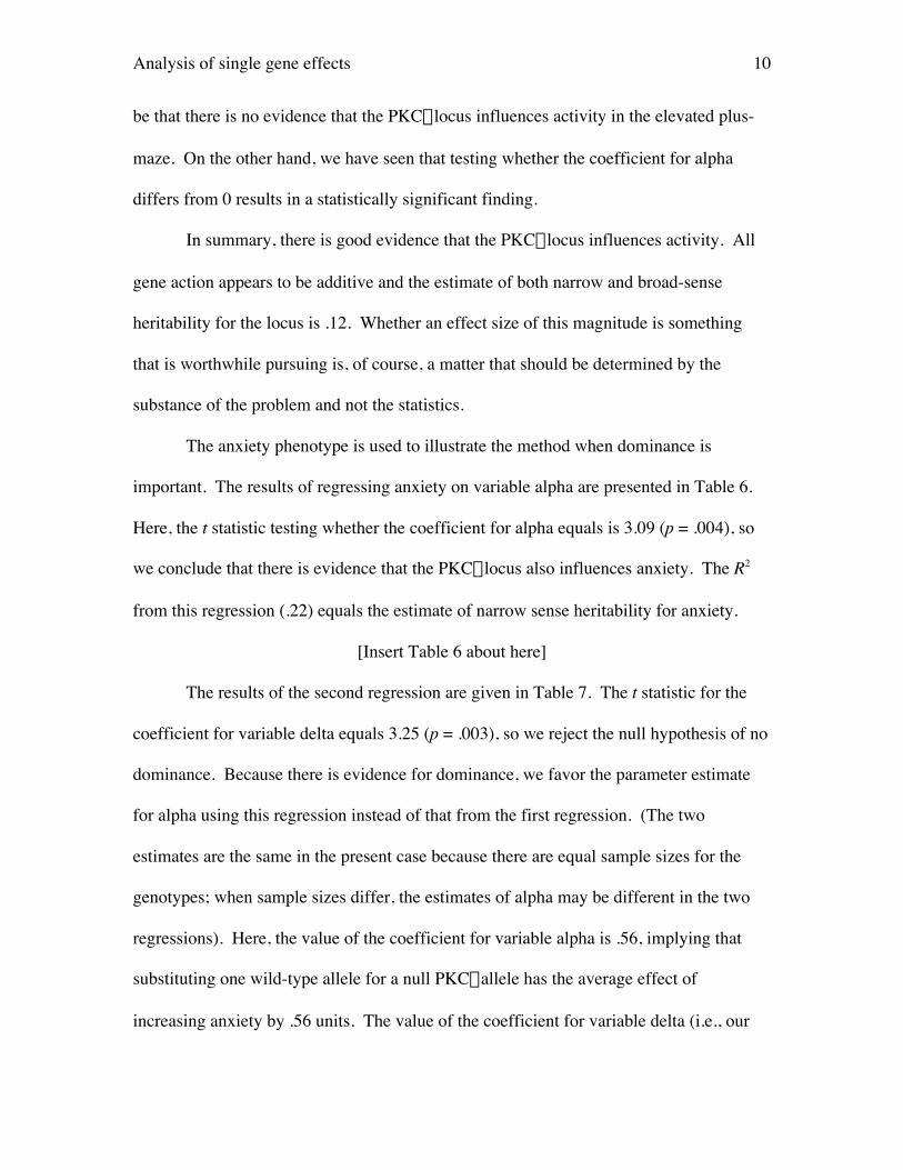
Analysis of single gene effects 15
References
Bowers,B.J., Collins,A.C., Tritto,T., & Wehner, J.M. (2000). Mice lacking PKCg exhibit
decreased anxiety. Behavior Genetics 30:111-121.
Cohen, J. (1988). Statistical power analysis for the behavioral sciences. Hillsdale NJ: L.
Erlbaum.
Falconer,D.S. & Mackay, T.F.C. (1996). Introduction to quantitative genetics, 4th edition.
Essex, England: Longman.
Judd,C.M. & McClelland,G.H. (1989) Data analysis: A model-comparison approach. San
Diego: Harcourt Brace Jovanovich.
Rodgers, R.J. & Johnson, N.J.T. (1995) Factor analysis of spatiotemporal and ethological
measures in the murine elevated plus-maze test of anxiety. Pharmacology Biochemistry
and Behavior 52: 297-303.

Analysis of single gene effects 16
Table 1. Notation for the single-gene model.
Genotype Frequency
Expected
Mean
Variance
within Genotype
aa faa m – a s
Aa fAa m + d s
AA fAA m + a s

Analysis of single gene effects 17
Table 2. Example of a data set arranged for single-gene analysis.
Phenotype Genotype alpha delta
8.3 AA 1 0
6.1 Aa 0 1
5.7 aa -1 0
.
6.5 aa -1 0
7.2 Aa 0 1
6.9 AA 1 0

Analysis of single gene effects 18
Table 3. Means and standard deviations for activity and anxiety measures on an elevated
plus-maze for mice lacking the gene for PKCg (knock outs) and their heterozygous and
wild-type littermates.
Activity Anxiety
Genotype N Mean St. Dev. Mean St. Dev.
Knock Out 12 .41 .94 -.87 .93
Heterozygote 12 .02 1.09 .61 .56
Wild Type 12 -.43 .85 .26 .85
Analysis of single gene effects 19
Table 4. Results on a activity from the regression model with independent variable alpha.
Source df
Sum of
Squares
Mean
Squares F p
Model 1 4.24 4.24 4.69 .037
Error 34 30.76 .90
Total 35 35.00
Parameter Value
Standard
Error t p
alpha -.42 .19 -2.17 .037
Analysis of single gene effects 20
Table 5. Results on activity from the regression model with independent variables alpha
and delta.
Source df
Sum of
Squares
Mean
Squares F p
Model 2 4.25 2.12 2.28 .118
Error 33 30.75 .93
Total 35 35.00
Parameter Value
Standard
Error t p
alpha -.42 .20 -2.13 .040
delta .03 .34 .08 .937
Analysis of single gene effects 21
Table 6. Results on anxiety from the regression using independent variable alpha.
Source df
Sum of
Squares
Mean
Squares F p
Model 1 7.66 7.66 9.52 .004
Error 34 27.34 .80
Total 35 35.00
Parameter Value
Standard
Error t p
alpha .57 .18 3.09 .004

Analysis of single gene effects 22
Table 7. Results on anxiety from the regression using independent variables alpha and
delta.
Source df
Sum of
Squares
Mean
Squares F p
Model 2 14.28 7.14 11.38 .0002
Error 33 20.72 .63
Total 35 35.00
Parameter Value
Standard
Error t p
alpha .56 .16 3.49 .001
delta .91 .28 3.25 .003

Analysis of single gene effects 23
Table 8. Power for single-gene analysis using the t test for the regression coefficient of
variable alpha in the full model: No dominance.
Effect Size = a/serror
Total N .2 .4 .6 .8 1.0
12 0.07 0.18 0.37 0.53 0.72
18 0.10 0.26 0.50 0.74 0.90
24 0.12 0.33 0.63 0.86 0.97
30 0.14 0.41 0.74 0.93 0.99
36 0.16 0.48 0.82 0.97 0.99
42 0.18 0.54 0.87 0.99 0.99
48 0.20 0.60 0.94 0.99 0.99
54 0.22 0.65 0.94 0.99 0.99
60 0.24 0.70 0.96 0.99 0.99

Analysis of single gene effects 24
Appendix 1. SAS code for performing the regression analyses. Code for variable
genotype: 1 = PKCg null mutant homozygotes; 2 = heterozygotes; 3 = wild-type
homozygotes. A copy of this program is available at
http://ibgwww.colorado.edu/~carey/QAOSGE.html.
data plusmaze;
input genotype activity anxiety;
if genotype=1 then alpha = -1;
else if genotype=2 then alpha = 0;
else alpha = 1;
delta = 0;
if genotype=2 then delta = 1;
datalines;
1 0.83 -0.889
1 0.274 -0.816
1 0.869 0.025
1 0.898 -2.024
1 0.257 -1.346
1 -0.429 -1.553
1 1.061 -2.557
1 -2.093 -0.573
1 1.56 0.919
1 0.976 -0.213
1 0.497 -0.693

Analysis of single gene effects 25
1 0.236 -0.699
2 -0.121 -0.174
2 -3.047 -0.396
2 0.345 0.789
2 0.739 1.234
2 0.164 1.21
2 0.561 1.118
2 0.852 -0.106
2 0.868 0.69
2 0.179 0.738
2 -0.936 0.499
2 -0.046 1.035
2 0.658 0.644
3 -0.639 1.367
3 -0.329 0.344
3 -0.746 1.32
3 -0.879 -1.053
3 0.375 0.61
3 0.667 -0.001
3 -2.484 -0.563
3 -0.479 0.144
3 -0.943 1.262
3 -0.098 -1.08
3 -0.185 0.576

Analysis of single gene effects 26
3 0.584 0.212
run;
title Bowers et al (2000) data on PKC-gamma and anxiety;
proc reg data=plusmaze;
var anxiety alpha delta;
title2 first model;
additive: model anxiety = alpha;
run;
title2 second model;
total: model anxiety = alpha delta;
run;
title3 test for overdominance;
test alpha = delta;
run;
quit;


![The effects and interaction of soybean maturity gene ...backgrounds the long juvenile trait was under the con-trol of a single gene [13, 18]. However, delayed flowering was shown in](https://img.pdfslide.us/doc/110x75/5ee1bdfcad6a402d666c832b/the-effects-and-interaction-of-soybean-maturity-gene-backgrounds-the-long-juvenile.jpg)