Embed Size (px)
Citation preview

Quantitative Analysis by the
Point-Centered Quarter Method
Kevin MitchellDepartment of Mathematics and Computer Science
Hobart and William Smith CollegesGeneva, NY [email protected]
25 June 2007
Abstract
This document is an introduction to the use of the point-centered quarter method. It brieflyoutlines its history, its methodology, and some of the practical issues that inevitably arise withits use in the field. Additionally this paper shows how data collected using point-centered quartermethod sampling may be used to determine importance values of different species of trees anddescribes several methods of estimating plant density and corresponding confidence intervals.
This paper is a significant revision of a 1999 online document intended for student use at Hobartand William Smith Colleges. A number of individuals elsewhere found the earlier version helpfuland had additional questions that I have tried to address in this revision.
1 Introduction and History
A wide variety of methods have been used to study forest structure parameters such as population density,basal area, and biomass. While these are sometimes estimated using aerial surveys or photographs, moststudies involve measurement of these characteristics for individual trees using a number of differentsampling methods. These methods fall into two broad categories: plot-based and plot-less. Plot-basedmethods begin with one or more plots (quadrats, belts) of known area in which the characteristics ofinterest are measured for each plant. In contrast, plot-less methods involve measuring distances for arandom sample of trees, typically along a transect, and recording the characteristics of interest for thissample. The point-centered quarter method is one such plot-less method.
The advantage to using plot-less methods rather than standard plot-based techniques is that theytend to be more efficient. Plot-less methods are faster, require less equipment, and may require fewerworkers. However, the main advantage is speed. The question, then, is whether accuracy is sacrificed inthe process.
Stearns (1949) indicated that the point-centered quarter method dates back a least 150 years andwas used by surveyors in the mid-nineteenth century making the first surveys of government land. Inthe late 1940s and early 1950s, several articles appeared that described a variety of plot-less methodsand compared them to sampling by quadrats. In particular, Cottam, Curtis, and Hale (1953) comparedthe point-centered quarter method to quadrat sampling and derived empirically a formula that could beused to estimate population density from the distance data collected. Since the current paper is intendedas an introduction to these methods, it is worth reminding ourselves what the goal of these methods isby recalling part of the introduction to their paper:
As our knowledge of plant communities increases, greater emphasis is being placed on themethods used to measure the characteristics of these communities. Succeeding decades haveshown a trend toward the use of quantitative methods, with purely descriptive methodsbecoming less common. One reason for the use of quantitative techniques is that the resultingdata are not tinged by the subjective bias of the investigator. The results are presumed to
1
SECTION 2: Materials and Methods 2
represent the vegetation as it actually exists; any other investigator should be able to employthe same methods in the same communities and secure approximately the same data.
Under the assumption that trees are distributed randomly throughout the survey site, Morisita (1954)provided a mathematical proof for the formula that Cottam, Curtis, and Hale (1953) had derived empir-ically for the estimation of population density using the point-centered quarter method. In other words,the point-centered quarter method could, in fact, be used to obtain accurate estimates of population den-sities with the advantage that the point-centered quarter method data could be collected more quicklythan quadrat data. Subsequently, Cottam and Curtis (1956) provided a more detailed comparison ofthe point-centered quarter method and three other plot-less methods (the closest individual, the nearestneighbor, and the random pairs methods). Their conclusion was:
The quarter method gives the least variable results for distance determinations, providesmore data per sampling point, and is the least susceptible to subjective bias.. . .
It is the opinion of the authors that the quarter method is, in most respects, superior to theother distance methods studied, and its use is recommended.
Beasom and Haucke (1975) compared the same four plotless methods and also concluded that point-centered quarter method provides the most accurate estimate of density. In a comparison of a morediverse set of methods (Engeman et al. 1994) have a more nuanced opinion of whether the point-centeredquarter method is more efficient in the field and more accurate in its density estimates, especially insituations where individuals are not distributed randomly.
In recent years, as the point-centered quarter method has been used more widely, variations havebeen proposed by Dahdouh-Guebas and Koedam (2006) to address a number of practical problems thatarise in the field (multi-stem trees, quarters where no trees are immediately present).
One use of the point-centered quarter method is to determine the relative importance of thevarious tree species in a community. The term “importance” can mean many things depending on thecontext. An obvious factor influencing the importance of a species to a community is the number oftrees present of that species. However, the importance of some number of small trees is not the sameas the importance of the same number of large trees. So the size of the trees also plays a role. Further,how the trees are distributed throughout the community also has an effect. A number of trees of thesame species clumped together should have a different importance value than the same number of treesdistributed more evenly throughout the community.
Measuring importance can aid understanding the successional stages of a forest habitat. At differentstages, different species of trees will dominate. Importance values are one objective way of measuringthis dominance.
The three factors that we will use to determine the importance value of a species are the density, thesize, and the frequency (distribution). Ideally, to estimate these factors, one would take a large sample,measuring, say, all the trees in a 100 × 100 meter square (a hectare). This can be extraordinarily timeconsuming if the trees are very dense. The point-centered quarter method provides a quick way to makesuch estimates by using a series of measurements along a transect.
2 Materials and Methods
The procedure outlined below describes how to carry out point-centered quarter method data collectionalong a 100 m transect. It can be scaled up or down, as appropriate, for longer or shorter transects.While this analysis can be carried out alone, groups of two or three can make for very efficient datacollection. Material requirements include 50 or 100 meter tape, a shorter 5 or 10 meter tape, a notebook,a calculator, and a table of random numbers (Table 15) if the calculator cannot generate them.
1. Generate a list of 15 to 20 random two-digit numbers. If the difference of any two is 4 or less, crossout the second listed number. There should be 10 or more two-digit numbers remaining; if not,generate additional ones. List the first 10 remaining numbers in increasing order. It is importantto generate this list before doing any measurements.
http://people.hws.edu/mitchell/PCQM.pdf Version 2.15
SECTION 2: Materials and Methods 3
2. Lay out a 100 m transect (or longer or shorter as required).
3. The random numbers represent the distances along the transect at which data will be collected.Random numbers are used to eliminate bias. Everyone always wants to measure that BIG treealong the transect, but such trees may not be representative of the community.1 The reason formaking sure that points are at least 5 meters apart is so that the same trees will not be measuredrepeatedly. Caution: If trees are particularly sparse, both the length of the transect and theminimum distance between points may need to be increased.
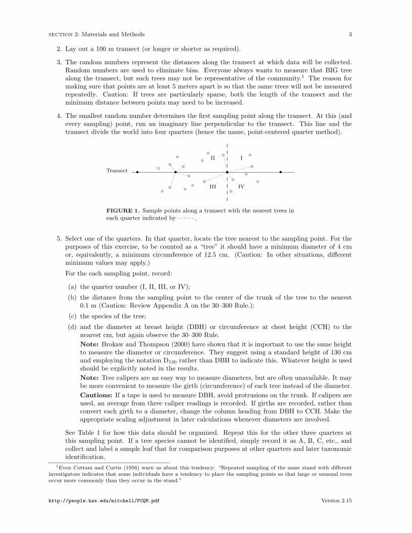
4. The smallest random number determines the first sampling point along the transect. At this (andevery sampling) point, run an imaginary line perpendicular to the transect. This line and thetransect divide the world into four quarters (hence the name, point-centered quarter method).
........
.....
........
.....
........
.....
........
.....
........
.....
........
.....
........
.....
........
.....
........
.....
• • • •◦
◦
◦ ◦......
..........
...........
...............
......
III
III IV
Transect
◦
◦◦ ◦
◦◦
◦
◦
◦◦ ◦
◦
◦◦
◦
....
..
......
.........
..........
FIGURE 1. Sample points along a transect with the nearest trees ineach quarter indicated by · · · · · · .
5. Select one of the quarters. In that quarter, locate the tree nearest to the sampling point. For thepurposes of this exercise, to be counted as a “tree” it should have a minimum diameter of 4 cmor, equivalently, a minimum circumference of 12.5 cm. (Caution: In other situations, differentminimum values may apply.)
For the each sampling point, record:
(a) the quarter number (I, II, III, or IV);
(b) the distance from the sampling point to the center of the trunk of the tree to the nearest0.1 m (Caution: Review Appendix A on the 30–300 Rule.);
(c) the species of the tree;
(d) and the diameter at breast height (DBH) or circumference at chest height (CCH) to thenearest cm, but again observe the 30–300 Rule.Note: Brokaw and Thompson (2000) have shown that it is important to use the same heightto measure the diameter or circumference. They suggest using a standard height of 130 cmand employing the notation D130 rather than DBH to indicate this. Whatever height is usedshould be explicitly noted in the results.Note: Tree calipers are an easy way to measure diameters, but are often unavailable. It maybe more convenient to measure the girth (circumference) of each tree instead of the diameter.Cautions: If a tape is used to measure DBH, avoid protrusions on the trunk. If calipers areused, an average from three caliper readings is recorded. If girths are recorded, rather thanconvert each girth to a diameter, change the column heading from DBH to CCH. Make theappropriate scaling adjustment in later calculations whenever diameters are involved.
See Table 1 for how this data should be organized. Repeat this for the other three quarters atthis sampling point. If a tree species cannot be identified, simply record it as A, B, C, etc., andcollect and label a sample leaf that for comparison purposes at other quarters and later taxonomicidentification.
1Even Cottam and Curtis (1956) warn us about this tendency: “Repeated sampling of the same stand with differentinvestigators indicates that some individuals have a tendency to place the sampling points so that large or unusual treesoccur more commonly than they occur in the stand.”
http://people.hws.edu/mitchell/PCQM.pdf Version 2.15

SECTION 3: Data Organization and Notation 4
6. Repeat this process for the entire set of sampling points.
7. Carry out the data analysis as described below.
For trees with multiple trunks at breast height, record the diameter (circumference) of each trunkseparately. What is the minimum allowed diameter of each trunk in a such multi-trunk tree? Suchdecisions should be spelled out in the methods section of the resulting report. At a minimum, oneshould ensure that the combined cross-sectional areas of all trunks meet the previously establishedminimum cross-sectional area for a single trunk tree. For example, with a 4 cm minimum diameter fora single trunk, the minimum cross-sectional area is
πr2 = π(2)2 = 4π ≈ 12.6 cm2.
3 Data Organization and Notation
The Data Layout
Table 1 illustrates how the data should be organized for the point-centered quarter method analysis.Note the multi-trunk Accacia (8 cm, 6 cm; D130) in the third quarter at the second sampling point. Theonly calculation required at this stage is to sum the distances from the sample points to each of the treesthat was measured. Note: A sample of only five points as in Table 1 is too few for most studies. Thesedata are presented only to illustrate the method of analysis in a concise way.
TABLE 1. Field data organized for point-centered quarter method analysis.
Sampling Point Quarter No. Species Distance (m) D130 (cm)
1 1 Acacia 1.1 6
2 Eucalyptus 1.6 483 Casuarina 2.3 15
4 Callitris 3.0 11
2 1 Eucalyptus 2.8 65
2 Casuarina 3.7 16
3 Acacia 0.9 8, 64 Casuarina 2.2 9
3 1 Acacia 2.8 42 Acacia 1.1 6
3 Acacia 3.2 64 Acacia 1.4 5
4 1 Callitris 1.3 19
2 Casuarina 0.8 22
3 Casuarina 0.7 124 Callitris 3.1 7
5 1 Acacia 1.5 72 Acacia 2.4 5
3 Eucalyptus 3.3 274 Eucalyptus 1.7 36
Total 40.9
Notation
We will use the following notation throughout this paper.
http://people.hws.edu/mitchell/PCQM.pdf Version 2.15
SECTION 4: Basic Analysis 5
n the number of sample points along the transect
4n the number of samples or observations
one for each quarter at each pointi a particular transect point, where i = 1, . . . , n
j a quarter at a transect point, where j = 1, . . . , 4Rij the point-to-tree distance at point i in quarter j
For example, the sum of the distances in the Table 1 is
5∑i=1
4∑j=1
Rij = 40.9.
4 Basic Analysis
The next three subsections outline the estimation of density, frequency, and cover. The most widelystudied of the three is density. In Section 5 we present a more robust way to determine the both a pointestimate and a confidence interval for population density. In this section density, frequency, and coverare defined both in absolute and relative terms. The relative measures are then combined to create ameasure of relative importance.
Density
Absolute Density
The absolute density λ of trees is defined as the number of trees per unit area. Since λ is most easilyestimated per square meter and since a hectare is 10,000 m2, λ is often multiplied by 10,000 to expressthe number of tree per hectare. The distances measured using the point-centered quarter method maybe used to estimate λ to avoid having to count every tree within such a large area.
Note that if λ is given as trees/m2, then its reciprocal 1/λ is the mean area occupied by a single tree.This observation is the basis for the following estimate of λ. (Also see Section 5.)
From the transect information, determine the mean distance r̄, which is the sum of the nearestneighbor distances in the quarters surveyed divided by the number of quarters,
r̄ =
∑ni=1
∑4j=1Rij
4n.
For the data in Table 1,
r̄ =40.920
= 2.05 m.
Cottam, Curtis, and Hale (1953) showed empirically and Morisita (1954) demonstrated mathematicallythat r̄ is actually an estimate of
√1/λ, the square root of the mean area occupied by a single tree.
Consequently, an estimate of the density is given by
Absolute density = λ̃ =1r̄2
=16n2(∑n
i=1
∑4j=1Rij
)2 . (1)
For the data in Table 1,
λ̃ =1r̄2
=1
2.052= 0.2380 trees/m2
,
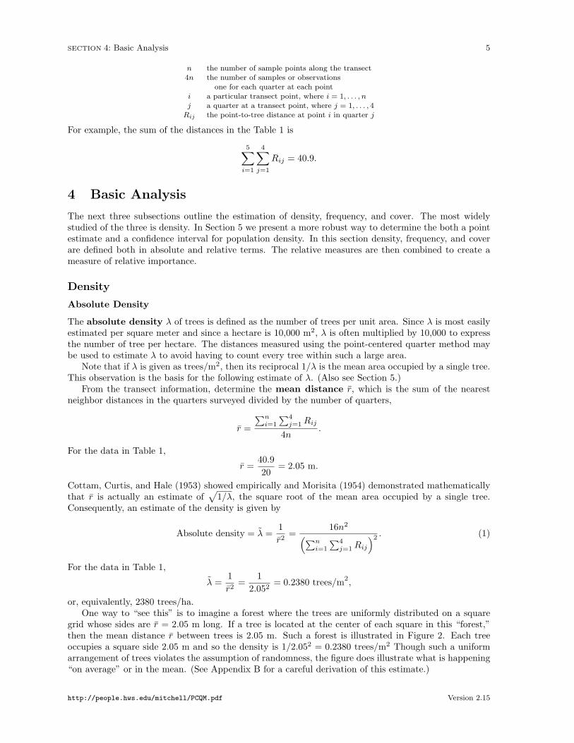
or, equivalently, 2380 trees/ha.One way to “see this” is to imagine a forest where the trees are uniformly distributed on a square
grid whose sides are r̄ = 2.05 m long. If a tree is located at the center of each square in this “forest,”then the mean distance r̄ between trees is 2.05 m. Such a forest is illustrated in Figure 2. Each treeoccupies a square side 2.05 m and so the density is 1/2.052 = 0.2380 trees/m2 Though such a uniformarrangement of trees violates the assumption of randomness, the figure does illustrate what is happening“on average” or in the mean. (See Appendix B for a careful derivation of this estimate.)
http://people.hws.edu/mitchell/PCQM.pdf Version 2.15
SECTION 4: Basic Analysis 6
0.00
2.05
4.10
6.15
8.20
10.25
0.00 2.05 4.10 6.15 8.20 10.25 12.30 14.35 16.40 18.45 20.50
•
•
•
•
•
•
•
•
•
•
•
•
•
•
•
•
•
•
•
•
•
•
•
•
•
•
•
•
•
•
•
•
•
•
•
•
•
•
•
•
•
•
•
•
•
•
•
•
•
•
FIGURE 2. A grid-like forest with trees uniformly dispersed so that the nearestneighbor is 2.05 m.
Absolute Density of Each Species
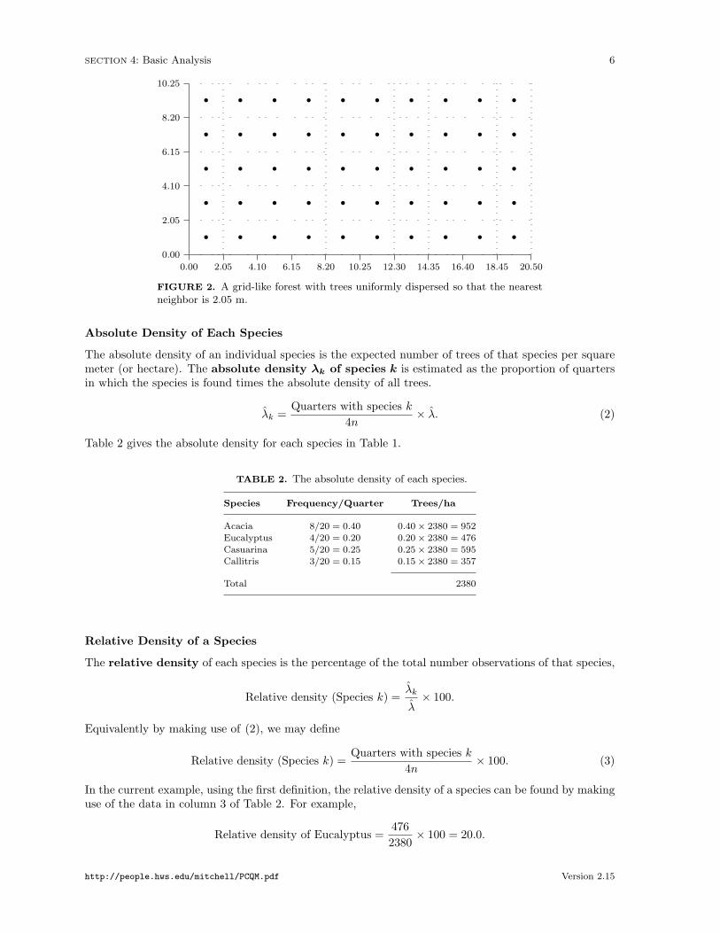
The absolute density of an individual species is the expected number of trees of that species per squaremeter (or hectare). The absolute density λk of species k is estimated as the proportion of quartersin which the species is found times the absolute density of all trees.
λ̂k =Quarters with species k
4n× λ̂. (2)
Table 2 gives the absolute density for each species in Table 1.
TABLE 2. The absolute density of each species.
Species Frequency/Quarter Trees/ha
Acacia 8/20 = 0.40 0.40× 2380 = 952
Eucalyptus 4/20 = 0.20 0.20× 2380 = 476Casuarina 5/20 = 0.25 0.25× 2380 = 595
Callitris 3/20 = 0.15 0.15× 2380 = 357
Total 2380
Relative Density of a Species
The relative density of each species is the percentage of the total number observations of that species,
Relative density (Species k) =λ̂k
λ̂× 100.
Equivalently by making use of (2), we may define
Relative density (Species k) =Quarters with species k
4n× 100. (3)
In the current example, using the first definition, the relative density of a species can be found by makinguse of the data in column 3 of Table 2. For example,
Relative density of Eucalyptus =4762380
× 100 = 20.0.
http://people.hws.edu/mitchell/PCQM.pdf Version 2.15

SECTION 4: Basic Analysis 7
Using the alternative method in (3) as a check on earlier calculations we see that the relative density isjust the proportion in column 2 of Table 2 times 100. For example,
Relative density of Eucalyptus =420× 100 = 20.0.
The relative densities should sum to 100 plus or minus a tiny round-off error.
TABLE 3. The relative density of each species.
Species Relative Density
Acacia 40.0Eucalyptus 20.0
Casuarina 25.0Callitris 15.0
Based on simulations, Cottam, Curtis, and Hale (1953) suggest that about 30 individuals of a par-ticular species must be present in the total sample before confidence can placed in any statements aboutrelative frequency.
Cover or Dominance of a Species
Absolute Cover
The cover or dominance of an individual tree is measured by its basal area or cross-sectional area. Letd, r, c, and A denote the diameter, radius, circumference, and basal area of a tree, respectively. Sincethe area of a circle is A = πr2, it is also A = π(d/2)2 = πd2/4. Since the circumference is c = 2πr,then the area is also A = c2/4π. Either A = πd2/4 or A = c2/4π can be used to determine basal area,depending on whether DBH or CCH was recorded in Table 1.
The first step is to compute the basal area for each tree sampled, organizing the data by species.This is the most tedious part of the analysis. A calculator that can handle lists of data or a spreadsheetcan be very handy at this stage. For the data in Table 1, the basal area for each tree was obtained usingthe formula A = πd2/4. For trees with multiple trunks, the basal area for each trunk was computedseparately and the results summed. (See Acacia in Table 4.)
TABLE 4. The basal area of each tree.
Acacia Eucalyptus Casuarina Callitris TotalD130 Area D130 Area D130 Area D130 Area
(cm) (cm2) (cm) (cm2) (cm) (cm2) (cm) (cm2)
6 28.3 48 1809.6 15 176.7 11 95.08, 6 78.5 65 3318.3 16 201.1 19 283.5
4 12.6 27 572.6 9 63.6 7 38.56 28.3 36 1017.9 22 380.1
6 28.3 12 113.1
5 19.67 38.55 19.6
Total BA 253.7 6718.4 934.6 417.0 8323.7
Mean BA 31.71 1679.60 186.92 139.00 416.19
Next, determine the total cover or basal area of the trees in the sample by species, and then calculatethe mean basal area for each species.2 Be careful when computing the means as the number of trees for
2Note: Mean basal area cannot be calculated by finding the mean diameter for each species and then using the formulaA = πd2/4.
http://people.hws.edu/mitchell/PCQM.pdf Version 2.15

SECTION 4: Basic Analysis 8
each species will differ. Remember that each multi-trunk tree counts as a single tree.The absolute cover or dominance of each species is expressed as its basal area per hectare. This
is obtained by taking the number of trees per species from Table 2 and multiplying by the correspondingmean basal area in Table 4. The units for cover are m2/ha (not cm2/ha), so a conversion factor isrequired. For Acacia,
Absolute Cover (Acacia) = 31.71 cm2 × 952ha× 1 m2
10, 000 cm2= 3.0
m2
ha.
TABLE 5. The total basal area of each species.
Species Mean BA Number/ha Total BA/ha
(cm2) (m2/ha)
Acacia 31.71 952 3.0
Eucalyptus 1679.60 476 79.9Casuarina 186.92 595 11.1
Callitris 139.00 357 5.0
Total Cover/ha 99.0
Finally, calculate the total cover per hectare by summing the per species covers.
Relative Cover (Relative Dominance) of a Species
The relative cover or relative dominance [see Cottam and Curtis (1956)] for a particular speciesis defined to be the absolute cover for that species divided by the total cover times 100 to express theresult as a percentage. For example, for Eucalyptus,
Relative cover (Eucalyptus) =79.9 m2/ha99.0 m2/ha
× 100 = 80.7.
The relative covers should sum to 100% plus or minus a tiny round-off error. Note that the relativecover can also be calculated directly from the transect information in Table 4.
Relative cover (Species k) =Total BA of species k along transectTotal BA of all species along transect
× 100. (4)
For example,
Relative cover (Eucalyptus) =6718.4 cm2
8323.7 cm2× 100 = 80.7.
TABLE 6. The relative cover of each species.
Species Relative Cover
Acacia 3.0
Eucalyptus 80.7Casuarina 11.2
Callitris 5.1
http://people.hws.edu/mitchell/PCQM.pdf Version 2.15

SECTION 4: Basic Analysis 9
The Frequency of a Species
Absolute Frequency of a Species
The absolute frequency of a species is the percentage of sample points at which a species occurs.Higher absolute frequencies indicate a more uniform distribution of a species while lower values mayindicate clustering or clumping. It is defined as
Absolute frequency =No. of sample points with a species
Total number of sample points× 100. (5)
For example,
Absolute frequency (Acacia) =45× 100 = 80%.
Note that absolute frequency is based on the number of sample points, not the number of quarters!
TABLE 7. The absolute cover of each species.
Species Absolute Frequency
Acacia (4/5)× 100 = 80Eucalyptus (3/5)× 100 = 60
Casuarina (3/5)× 100 = 60
Callitris (2/5)× 100 = 40
Total 240
Note that the total will sum to more than 100%.
Relative Frequency of a Species
To normalize for the fact that the absolute frequencies sum to more than 100%, the relative frequencyis computed. It is defined as
Relative frequency =Absolute frequency of a speciesTotal frequency of all species
× 100. (6)
For example,
Relative frequency (Acacia) =80240× 100 = 33.3.
The relative frequencies should sum to 100 plus or minus a tiny round-off error.
TABLE 8. The relative frequency of each species.
Species Relative Frequency
Acacia 33.3
Eucalyptus 25.0Casuarina 25.0
Callitris 16.7
What is the difference between relative frequency and relative density? A high relative frequencyindicates that the species occurs near relatively many different sampling points, in other words, thespecies is well-distributed along the transect. A high relative density indicates that the species appearsin a relatively large number of quarters. Consequently, if the relative density is high and the relativefrequency is low, then the species must appear in lots of quarters but only at a few points, i.e., thespecies appears in clumps. If both are high, the distribution is relatively even and relatively commonalong the transect. If the relative density is low (appears in few quarters) and the relative frequency ishigh(er), then the species must be sparsely distributed (few plants, no clumping).
http://people.hws.edu/mitchell/PCQM.pdf Version 2.15

SECTION 5: Population Density Reconsidered 10
The Importance Value of a Species
The importance value of a species is defined as the sum of the three relative measures:
Importance value = Relative density + Relative cover + Relative frequency. (7)
The importance value gives equal weight to the three factors of relative density, cover, and frequency.This means that small trees (i.e., with small basal area) can be dominant only if there are enough ofthem widely distributed across the transect. The importance value can range from 0 to 300.
For the data in Table 1, even though eucalypti are not very common, because of their size they turnout to be the most important species within the community.
TABLE 9. The importance value of each species.
Species Relative Density Relative Cover Relative Frequency Importance
Acacia 40.0 3.0 33.3 76.3
Eucalyptus 20.0 80.7 25.0 125.7
Casuarina 25.0 11.2 25.0 61.2Callitris 15.0 5.1 16.7 36.8
Comment. Each of the measures that make up relative importance may be calculated without knowingthe absolute density of the trees at the site (review (3), (4), and (6).) In fact, any estimate for theabsolute density of all species leads to the same relative densities for each species. Consequently, theactual value of density of the plot is not needed to determine relative importance. However, in moststudies, absolute density is one the parameters of greatest interest. Because of this, there have beena number of different methods to estimate absolute density from point-centered quarter method dataproposed in the literature. In the next section we explore one of these and others are discussed inAppendix B. Whichever method is used, relative importance is unaffected.
It has been shown by Pollard (1971) that the estimate of Cottam and Curtis (1956) of λ in (1) isbiased.3 Nonetheless, this estimate appears widely in the literature and, so, has been used here. Anotherdrawback of the estimate in (1) is that no confidence limits are available for it. The next section addressesboth of these issues.
5 Population Density Reconsidered
Pollard (1971) and Seber (1982) derived an unbiased estimate of the absolute population density usingpoint-centered quarter method data that we now present. It also has the advantage that it can be usedto determine confidence intervals for the density estimate.
Intuition
The discussion that follows is meant to inform our intuition and by no means constitutes a proof of anyof the results, which requires a substantially more sophisticated argument. See Appendix B.
The assumption of this model is that trees are randomly distributed in the survey area. Now thinkof the random points along the transect as representing “virtual trees”. The measured distance Rij isa nearest neighbor distance from a virtual to a real tree. As such, it is an estimate of the actual meannearest neighbor tree-to-tree distance.
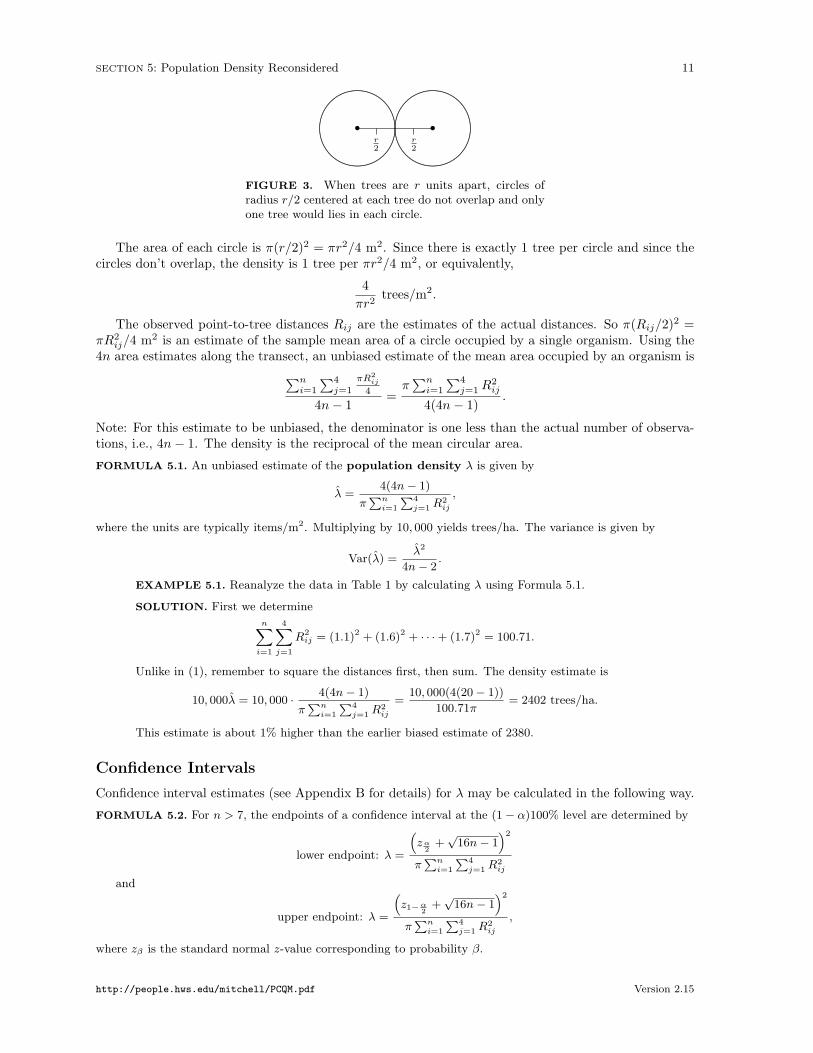
If an actual tree-to-tree distance were r meters, we could draw circles of radius r/2 centered at eachtree. See Figure 3. Notice that the circles would not overlap and that only one tree would lie in eachcircle.
3Pollard (1971) states that the reason for this is Cottam and Curtis (1956) chose to estimate the mean area A occupiedby a tree as the reciprocal of λ. Rather then estimate A directly, as we saw in (1) they estimated r̄, which is the reciprocalof the square root of A. Squaring and inverting leads to a biased estimate of A.
http://people.hws.edu/mitchell/PCQM.pdf Version 2.15
SECTION 5: Population Density Reconsidered 11
r2
r2
........
............................................
.........................
....................................................................................................................................................................................................................................................................................................
...............................................................................................................................................................................................................................
...................................................................................................................................
...........................
................................................................................................................................................• •
FIGURE 3. When trees are r units apart, circles ofradius r/2 centered at each tree do not overlap and onlyone tree would lies in each circle.
The area of each circle is π(r/2)2 = πr2/4 m2. Since there is exactly 1 tree per circle and since thecircles don’t overlap, the density is 1 tree per πr2/4 m2, or equivalently,
4πr2
trees/m2.
The observed point-to-tree distances Rij are the estimates of the actual distances. So π(Rij/2)2 =πR2
ij/4 m2 is an estimate of the sample mean area of a circle occupied by a single organism. Using the4n area estimates along the transect, an unbiased estimate of the mean area occupied by an organism is∑n
i=1
∑4j=1
πR2ij
4
4n− 1=π∑ni=1
∑4j=1R
2ij
4(4n− 1).
Note: For this estimate to be unbiased, the denominator is one less than the actual number of observa-tions, i.e., 4n− 1. The density is the reciprocal of the mean circular area.
FORMULA 5.1. An unbiased estimate of the population density λ is given by
λ̂ =4(4n− 1)
πPni=1
P4j=1 R
2ij
,
where the units are typically items/m2. Multiplying by 10, 000 yields trees/ha. The variance is given by
Var(λ̂) =λ̂2
4n− 2.
EXAMPLE 5.1. Reanalyze the data in Table 1 by calculating λ using Formula 5.1.
SOLUTION. First we determine
nXi=1
4Xj=1
R2ij = (1.1)2 + (1.6)2 + · · ·+ (1.7)2 = 100.71.
Unlike in (1), remember to square the distances first, then sum. The density estimate is
10, 000λ̂ = 10, 000 · 4(4n− 1)
πPni=1
P4j=1 R
2ij
=10, 000(4(20− 1))
100.71π= 2402 trees/ha.
This estimate is about 1% higher than the earlier biased estimate of 2380.
Confidence Intervals
Confidence interval estimates (see Appendix B for details) for λ may be calculated in the following way.
FORMULA 5.2. For n > 7, the endpoints of a confidence interval at the (1− α)100% level are determined by
lower endpoint: λ =
“zα
2+√
16n− 1”2
πPni=1
P4j=1 R
2ij
and
upper endpoint: λ =
“z1−α2 +
√16n− 1
”2
πPni=1
P4j=1 R
2ij
,
where zβ is the standard normal z-value corresponding to probability β.
http://people.hws.edu/mitchell/PCQM.pdf Version 2.15

SECTION 5: Population Density Reconsidered 12
EXAMPLE 5.2. The following data were collected at Lamington National Park in 1994. The data arethe nearest point-to-tree distances for each of four quarters at 15 points along a 200 meter transect. Themeasurements are in meters. Estimate the tree density and find a 95% confidence interval for the mean.
Point I II III IV
1 1.5 1.2 2.3 1.9
2 3.3 0.7 2.5 2.0
3 3.3 2.3 2.3 2.44 1.8 3.4 1.0 4.3
5 0.9 0.9 2.9 1.4
6 2.0 1.3 1.0 0.77 0.7 2.0 2.7 2.5
8 2.6 4.8 1.1 1.2
9 1.0 2.5 1.9 1.110 1.6 0.7 3.4 3.2
11 1.8 1.0 1.4 3.6
12 4.2 0.6 3.2 2.613 4.1 3.9 0.2 2.0
14 1.7 4.2 4.0 1.115 1.8 2.2 1.2 2.8
SOLUTION. In this example, the number of points is n = 15 and the number of samples is 4n = 60.Therefore, the density estimate is
λ̂ =4(4n− 1)
π
nXi=1
4Xj=1
R2ij
=4(59)
347.63π= 0.2161 trees/m2.
Since the number of points is greater than 7, confidence intervals may be calculated using Formula 5.2.To find a 1 − α = 0.95 confidence interval, we have α = 0.05 and so z1−α2 = z0.975 = 1.96 and z0.025 =−z0.975 = −1.96. The lower endpoint of the confidence interval is
z0.025 +√
16n− 1qπPni=1
P4j=1 R
2ij
=
“−1.96 +
p16(15)− 1
”2
347.63π= 0.1669
and the upper endpoint is`z0.975 +
√16n− 1
´2πPni=1
P4j=1 R
2ij
=
“1.96 +
p16(15)− 1
”2
347.63π= 0.2778.
Therefore, the confidence interval for the density is
(0.1669, 0.2778) trees/m2.
Using Formula 5.1, the point estimate for the density4
λ̂ =4(4n− 1)
πPni=1
P4j=1 R
2ij
=4(60− 1)√
347.63π= 0.2161 trees/ha
The units are changed to hectares by multiplying by 10, 000. Thus, λ̂ = 2161 trees/ha while the confidenceinterval is (1669, 2778) trees/ha.
Cautions
The estimates and confidence intervals for density assume that the points along the transect are spreadout sufficiently so that no organism is sampled in more than one quarter. Further, the density estimateassumes that the spatial distribution of the organisms is completely random. For example, it would beinappropriate to use these methods in an orchard or woodlot where the trees had been planted in rows.
4Instead, if (1) were used, the density estimate would be quite similar, 2205 trees/ha.
http://people.hws.edu/mitchell/PCQM.pdf Version 2.15
SECTION 6: Modifications, Adaptations, and Applications 13
Exercises
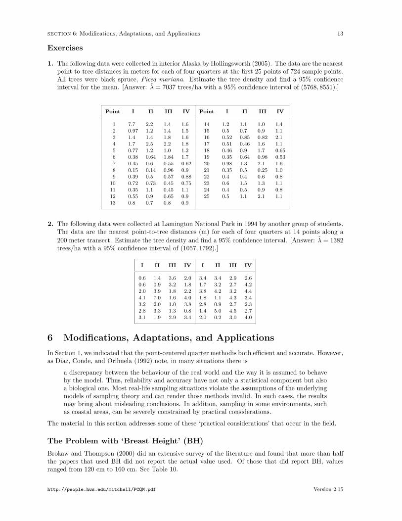
1. The following data were collected in interior Alaska by Hollingsworth (2005). The data are the nearestpoint-to-tree distances in meters for each of four quarters at the first 25 points of 724 sample points.All trees were black spruce, Picea mariana. Estimate the tree density and find a 95% confidenceinterval for the mean. [Answer: λ̂ = 7037 trees/ha with a 95% confidence interval of (5768, 8551).]
Point I II III IV Point I II III IV
1 7.7 2.2 1.4 1.6 14 1.2 1.1 1.0 1.42 0.97 1.2 1.4 1.5 15 0.5 0.7 0.9 1.1
3 1.4 1.4 1.8 1.6 16 0.52 0.85 0.82 2.14 1.7 2.5 2.2 1.8 17 0.51 0.46 1.6 1.15 0.77 1.2 1.0 1.2 18 0.46 0.9 1.7 0.65
6 0.38 0.64 1.84 1.7 19 0.35 0.64 0.98 0.537 0.45 0.6 0.55 0.62 20 0.98 1.3 2.1 1.68 0.15 0.14 0.96 0.9 21 0.35 0.5 0.25 1.0
9 0.39 0.5 0.57 0.88 22 0.4 0.4 0.6 0.810 0.72 0.73 0.45 0.75 23 0.6 1.5 1.3 1.111 0.35 1.1 0.45 1.1 24 0.4 0.5 0.9 0.812 0.55 0.9 0.65 0.9 25 0.5 1.1 2.1 1.1
13 0.8 0.7 0.8 0.9
2. The following data were collected at Lamington National Park in 1994 by another group of students.The data are the nearest point-to-tree distances (m) for each of four quarters at 14 points along a200 meter transect. Estimate the tree density and find a 95% confidence interval. [Answer: λ̂ = 1382trees/ha with a 95% confidence interval of (1057, 1792).]
I II III IV I II III IV
0.6 1.4 3.6 2.0 3.4 3.4 2.9 2.60.6 0.9 3.2 1.8 1.7 3.2 2.7 4.2
2.0 3.9 1.8 2.2 3.8 4.2 3.2 4.44.1 7.0 1.6 4.0 1.8 1.1 4.3 3.43.2 2.0 1.0 3.8 2.8 0.9 2.7 2.3
2.8 3.3 1.3 0.8 1.4 5.0 4.5 2.73.1 1.9 2.9 3.4 2.0 0.2 3.0 4.0
6 Modifications, Adaptations, and Applications
In Section 1, we indicated that the point-centered quarter methodis both efficient and accurate. However,as Dı́az, Conde, and Orihuela (1992) note, in many situations there is
a discrepancy between the behaviour of the real world and the way it is assumed to behaveby the model. Thus, reliability and accuracy have not only a statistical component but alsoa biological one. Most real-life sampling situations violate the assumptions of the underlyingmodels of sampling theory and can render those methods invalid. In such cases, the resultsmay bring about misleading conclusions. In addition, sampling in some environments, suchas coastal areas, can be severely constrained by practical considerations.
The material in this section addresses some of these ‘practical considerations’ that occur in the field.
The Problem with ‘Breast Height’ (BH)
Brokaw and Thompson (2000) did an extensive survey of the literature and found that more than halfthe papers that used BH did not report the actual value used. Of those that did report BH, valuesranged from 120 cm to 160 cm. See Table 10.
http://people.hws.edu/mitchell/PCQM.pdf Version 2.15

SECTION 6: Modifications, Adaptations, and Applications 14
TABLE 10. The distribution of values stated for ‘breast hight’ (BH)in papers published in Biotropica, Ecology, Journal of Tropical Ecology,Forest Service, and Forest Ecology and Management during the period1988–1997. Adapted from Brokaw and Thompson (2000), Table 1.
BH (cm) 120 130 135 137 140 150 160 None Total
Articles 1 113 2 28 27 10 1 258 440
Since the mode of the BH-values listed was 130 cm, Brokaw and Thompson (2000) strongly suggestadopting this as the standard BH-value. They strongly suggest denoting this value by ‘D130’ rather thanDBH while reserving ‘DBH’ as a generic term. At a minimum, the BH-value used should be explicitlystated. If a value x other than 130 cm is used, it might be denoted as ‘Dx’.
As one would expect, DBH does decrease as height increases. In a field survey of 100 trees, Brokawand Thompson (2000) found that the mean difference between D130 and D140 was 3.5 mm (s = 5.8,n = 100). This difference matters. Brokaw and Thompson (2000) report that this resulted in a 2.6%difference in total basal area. When biomass was was calculated using the equation
ln(dry weight) = −1.966 + 1.242 ln(DBH2)
there was a 4.0% difference.Using different values of BH within a single survey may lead to erroneous results. Additionally,
Brokaw and Thompson’s (2000) results show that failing to indicate the value of BH may lead toerroneous comparisons of characteristics such as diameter-class distributions, biomass, total basal area,and importance values between studies.
Vacant Quarters and Truncated Sampling
A question that arises frequently is whether there is a distance limit beyond which one no longer searchesfor a tree (or other organism of interest) in a particular quarter. The simple answer is, “No.” Wheneverpossible, it is preferable to make sure that every quadrant contains an individual, even if that requiresconsiderable effort. But as a practical matter, a major reason to use the point-centered quarter methodis its efficiency, which is at odds with substantial sampling effort. Additionally, in Section 2 we notedthat sample points along the transect should be sufficiently far apart so that the same tree is not sampledat two adjacent transect points. Dahdouh-Guebas and Koedam (2006) suggest that it may be preferableto establish a consistent distance limit for the sampling point to the nearest individual rather than toconsider the same individual twice. (Note, however, that Cottam and Curtis (1956) explicitly statethat they did not use any method to exclude resampling a tree at adjacent transect points and thatresampling did, in fact, occur.)
Whether because a distance limit is established for reasons of efficiency [often called truncated sam-pling] or to prevent resampling, in practice vacant quarters, i.e., quadrants containing no tree may occur.In such cases the calculation of the absolute density must be corrected, since a density calculated fromonly those quarters containing observations will overestimate the true density.
Warde and Petranka (1981) give a careful derivation of a correction factor (CF) to be used in suchcases. In the language of the current paper, as usual, let n denote the number of sampling points and 4nthe number of quarters. Let n0 denote the number of vacant quarters. Begin by computing the densityfor the 4n− n0 non-vacant quarters,
r̄′ =
4n−n0∑m=1
Rm
4n− n0,
where Rm is the distance from tree m to its corresponding transect sample point, which is the analogto (1). Then
Absolute Density (corrected) = λ̃c =1
(r̄′)2· CF,
http://people.hws.edu/mitchell/PCQM.pdf Version 2.15
SECTION 6: Modifications, Adaptations, and Applications 15
where CF is the correction factor from Table 11 corresponding to proportion of vacant quarters, n04n .
Note that as the proportion of vacant quarters increases, CF decreases and, consequently, so does theestimate of the density (as it should).
TABLE 11. Values of the correction factor (CF) to the density esti-mate based on the formula of Warde and Petranka (1981).
n0/4n CF n0/4n CF n0/4n CF n0/4n CF
0.005 0.9818 0.080 0.8177 0.155 0.7014 0.230 0.6050
0.010 0.9667 0.085 0.8091 0.160 0.6945 0.235 0.5991
0.015 0.9530 0.090 0.8006 0.165 0.6877 0.240 0.59320.020 0.9401 0.095 0.7922 0.170 0.6809 0.245 0.5874
0.025 0.9279 0.100 0.7840 0.175 0.6742 0.250 0.5816
0.030 0.9163 0.105 0.7759 0.180 0.6676 0.255 0.57590.035 0.9051 0.110 0.7680 0.185 0.6610 0.260 0.5702
0.040 0.8943 0.115 0.7602 0.190 0.6546 0.265 0.56450.045 0.8838 0.120 0.7525 0.195 0.6482 0.270 0.5590
0.050 0.8737 0.125 0.7449 0.200 0.6418 0.275 0.5534
0.055 0.8638 0.130 0.7374 0.205 0.6355 0.280 0.54790.060 0.8542 0.135 0.7300 0.210 0.6293 0.285 0.5425
0.065 0.8447 0.140 0.7227 0.215 0.6232 0.290 0.5370
0.070 0.8355 0.145 0.7156 0.220 0.6171 0.295 0.53170.075 0.8265 0.150 0.7085 0.225 0.6110 0.300 0.5263
Caution: Dahdouh-Guebas and Koedam (2006) propose (without mathematical justification) usinga correction factor of CF′ = 1 − n0
4n . While this correction factor also lowers the value of the densitybased on the trees actually measured, this correction differs substantially from that derived by Wardeand Petranka (1981). For example, if 5% of the quarters are vacant, then from Table 11 we findCF = 0.873681 while CF′ = 0.95.
The Problem of Unusual Trees or Tree Clusters
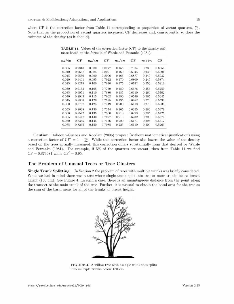
Single Trunk Splitting. In Section 2 the problem of trees with multiple trunks was briefly considered.What we had in mind there was a tree whose single trunk split into two or more trunks below breastheight (130 cm). See Figure 4. In such a case, there is an unambiguous distance from the point alongthe transect to the main trunk of the tree. Further, it is natural to obtain the basal area for the tree asthe sum of the basal areas for all of the trunks at breast height.
FIGURE 4. A willow tree with a single trunk that splitsinto multiple trunks below 130 cm.
http://people.hws.edu/mitchell/PCQM.pdf Version 2.15
SECTION 6: Modifications, Adaptations, and Applications 16
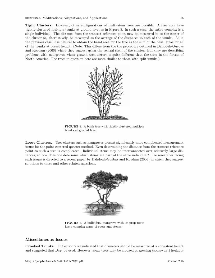
Tight Clusters. However, other configurations of multi-stem trees are possible. A tree may havetightly-clustered multiple trunks at ground level as in Figure 5. In such a case, the entire complex is asingle individual. The distance from the transect reference point may be measured in to the center ofthe cluster or, alternatively, be measured as the average of the distances to each of the trunks. As inthe previous case, it is natural to obtain the basal area for the tree as the sum of the basal areas for allof the trunks at breast height. (Note: This differs from the the procedure outlined in Dahdouh-Guebasand Koedam (2006) where they suggest using the central stem of the cluster. But they are describingproblems with mangroves whose growth architecture is quite different than the trees in the forests ofNorth America. The trees in question here are more similar to those with split trunks.)
FIGURE 5. A birch tree with tightly clustered multipletrunks at ground level.
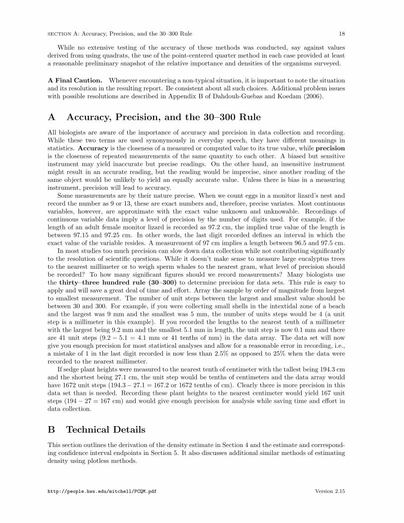
Loose Clusters. Tree clusters such as mangroves present significantly more complicated measurementissues for the point-centered quarter method. Even determining the distance from the transect referencepoint to such a tree is complicated. Individual stems may be interconnected over relatively large dis-tances, so how does one determine which stems are part of the same individual? The researcher facingsuch issues is directed to a recent paper by Dahdouh-Guebas and Koedam (2006) in which they suggestsolutions to these and other related questions.
FIGURE 6. A individual mangrove with its prop rootshas a complex array of roots and stems.
Miscellaneous Issues
Crooked Trunks. In Section 2 we indicated that diameters should be measured at a consistent heightand suggested that D130 be used. However, some trees may be crooked or growing (somewhat) horizon-
http://people.hws.edu/mitchell/PCQM.pdf Version 2.15

SECTION 6: Modifications, Adaptations, and Applications 17
tally at 130 cm above the forest floor. Dahdouh-Guebas and Koedam (2006) suggest that the diameterof such a stem or trunk always be measured at 130 cm along the stem, whether or not this is actually130 cm above the ground.
Dead Trees. The implicit but unstated assumption in Section 2 was that we were measuring livetrees in the survey. However, depending on the purpose of the survey, dead trees may be important toinclude. This might be the case if the purpose is to assess exploitable firewood. Such decisions shouldbe explicitly noted in the methods section of the resulting report.
Reversing the roles of live and dead trees, Rheinhardt et al. (1997) used the point-centered quar-ter method to determine the biomass of standing dead trees in a wetland and also the biomass ofcoarse woody debris available for nutrient recycling. In the latter case the distance, diameter (minimum4 inches), and length (minimum 3 feet) of the debris item nearest to the transect sampling point in eachquarter was recorded.
Novel Applications
Distance methods have been commonly used for vegetation surveys and are easily adapted to inventoriesof rare plants or other sessile organisms. The approach may also be useful for population studies of moremobile animal species by obtaining abundance estimates of their nests, dens, roosting sites, or scat piles.
Grasslands. The point-centered quarter method has been adapted to measure density and importancevalues when sampling grassland vegetation. Dix (1960) used the distance, measured at ground level,from the sampling point to the emergence from the soil of the nearest living herbaceous shoot in eachquarter. Since this was the only measurement recorded, importance values were determined using onlyrelative densities and relative frequencies.
Penfound (1963) modified Dix’s method to include a relative cover or weight component to bettermatch importance values of trees. In particular, once the distance to a culm or plant was measured,the plant was cut off at soil level and later its oven-dry weight was determined. The relative weight foreach species was determined as the total weight for the species divided by the total weight for all speciestimes 100 to express the result as a percentage. The importance of each species was then defined as thesum of the relative frequency, relative density, and relative weight.
On the surface of it, the aggregation often exhibited grassland populations violates the assumptionof the random distribution assumption of the point-centered quarter method. Indeed, empirical studiesby Risser and Zedler (1968) and Good and Good (1971) indicate that the point-centered quarter methodappears to underestimate species density in such cases. In particular, Rissler and Zelder (1968) suggestthat when using the point-centered quarter method on grasslands, one should check against counts madeusing quadrat samples.
Animal Surveys. The point-centered quarter method was adapted in a series of projects of studentsof mine to determine the densities and importance values of certain sessile or relatively slow movingmarine organisms.
One group carried out a project surveying holothurians (sea cucumbers) in the reef flat of a coral cay.Transects were laid out in the usual way and the distance and species of the nearest holothurian to eachsampling point was recorded for each quarter. These data allowed computation of the relative densityand relative frequency for each species. To take the place of relative cover, the volume of each holothurianwas recorded. Volume was estimated by placing each organism in a bucket full of sea water and thenremoving it. The bucket was then topped off with water from a graduated cylinder and the volume ofthis water recorded. Since volume and mass are proportional, the relative volume is an approximationof the relative biomass. The sum of the relative density, relative frequency, and relative volume for eachspecies gave its importance value.
A similar survey was conducted both in a reef flat and in an intextidal zone of a sand island forasteroidea (sea stars) using radial “arm length” instead of DBH. Another survey, this time of anemonesin the intextidal zone of a sand island was conducted. Since these organisms are more elliptical thancircular, major and minor axes were measured from which area covered could be estimated.
http://people.hws.edu/mitchell/PCQM.pdf Version 2.15
SECTION A: Accuracy, Precision, and the 30–300 Rule 18
While no extensive testing of the accuracy of these methods was conducted, say against valuesderived from using quadrats, the use of the point-centered quarter method in each case provided at leasta reasonable preliminary snapshot of the relative importance and densities of the organisms surveyed.
A Final Caution. Whenever encountering a non-typical situation, it is important to note the situationand its resolution in the resulting report. Be consistent about all such choices. Additional problem issueswith possible resolutions are described in Appendix B of Dahdouh-Guebas and Koedam (2006).
A Accuracy, Precision, and the 30–300 Rule
All biologists are aware of the importance of accuracy and precision in data collection and recording.While these two terms are used synonymously in everyday speech, they have different meanings instatistics. Accuracy is the closeness of a measured or computed value to its true value, while precisionis the closeness of repeated measurements of the same quantity to each other. A biased but sensitiveinstrument may yield inaccurate but precise readings. On the other hand, an insensitive instrumentmight result in an accurate reading, but the reading would be imprecise, since another reading of thesame object would be unlikely to yield an equally accurate value. Unless there is bias in a measuringinstrument, precision will lead to accuracy.
Some measurements are by their nature precise. When we count eggs in a monitor lizard’s nest andrecord the number as 9 or 13, these are exact numbers and, therefore, precise variates. Most continuousvariables, however, are approximate with the exact value unknown and unknowable. Recordings ofcontinuous variable data imply a level of precision by the number of digits used. For example, if thelength of an adult female monitor lizard is recorded as 97.2 cm, the implied true value of the length isbetween 97.15 and 97.25 cm. In other words, the last digit recorded defines an interval in which theexact value of the variable resides. A measurement of 97 cm implies a length between 96.5 and 97.5 cm.
In most studies too much precision can slow down data collection while not contributing significantlyto the resolution of scientific questions. While it doesn’t make sense to measure large eucalyptus treesto the nearest millimeter or to weigh sperm whales to the nearest gram, what level of precision shouldbe recorded? To how many significant figures should we record measurements? Many biologists usethe thirty–three hundred rule (30–300) to determine precision for data sets. This rule is easy toapply and will save a great deal of time and effort. Array the sample by order of magnitude from largestto smallest measurement. The number of unit steps between the largest and smallest value should bebetween 30 and 300. For example, if you were collecting small shells in the intextidal zone of a beachand the largest was 9 mm and the smallest was 5 mm, the number of units steps would be 4 (a unitstep is a millimeter in this example). If you recorded the lengths to the nearest tenth of a millimeterwith the largest being 9.2 mm and the smallest 5.1 mm in length, the unit step is now 0.1 mm and thereare 41 unit steps (9.2 − 5.1 = 4.1 mm or 41 tenths of mm) in the data array. The data set will nowgive you enough precision for most statistical analyses and allow for a reasonable error in recording, i.e.,a mistake of 1 in the last digit recorded is now less than 2.5% as opposed to 25% when the data wererecorded to the nearest millimeter.
If sedge plant heights were measured to the nearest tenth of centimeter with the tallest being 194.3 cmand the shortest being 27.1 cm, the unit step would be tenths of centimeters and the data array wouldhave 1672 unit steps (194.3− 27.1 = 167.2 or 1672 tenths of cm). Clearly there is more precision in thisdata set than is needed. Recording these plant heights to the nearest centimeter would yield 167 unitsteps (194− 27 = 167 cm) and would give enough precision for analysis while saving time and effort indata collection.
B Technical Details
This section outlines the derivation of the density estimate in Section 4 and the estimate and correspond-ing confidence interval endpoints in Section 5. It also discusses additional similar methods of estimatingdensity using plotless methods.
http://people.hws.edu/mitchell/PCQM.pdf Version 2.15
SECTION B: Technical Details 19
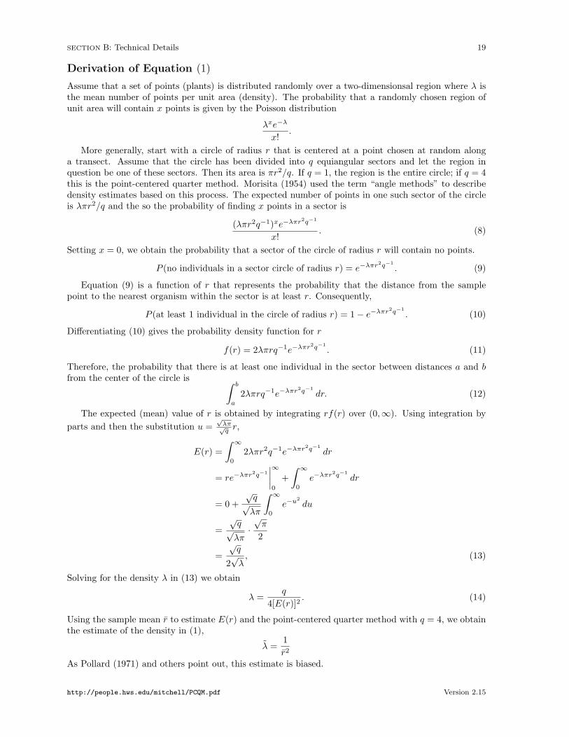
Derivation of Equation (1)
Assume that a set of points (plants) is distributed randomly over a two-dimensionsal region where λ isthe mean number of points per unit area (density). The probability that a randomly chosen region ofunit area will contain x points is given by the Poisson distribution
λxe−λ
x!.
More generally, start with a circle of radius r that is centered at a point chosen at random alonga transect. Assume that the circle has been divided into q equiangular sectors and let the region inquestion be one of these sectors. Then its area is πr2/q. If q = 1, the region is the entire circle; if q = 4this is the point-centered quarter method. Morisita (1954) used the term “angle methods” to describedensity estimates based on this process. The expected number of points in one such sector of the circleis λπr2/q and the so the probability of finding x points in a sector is
(λπr2q−1)xe−λπr2q−1
x!. (8)
Setting x = 0, we obtain the probability that a sector of the circle of radius r will contain no points.
P (no individuals in a sector circle of radius r) = e−λπr2q−1
. (9)
Equation (9) is a function of r that represents the probability that the distance from the samplepoint to the nearest organism within the sector is at least r. Consequently,
P (at least 1 individual in the circle of radius r) = 1− e−λπr2q−1
. (10)
Differentiating (10) gives the probability density function for r
f(r) = 2λπrq−1e−λπr2q−1
. (11)
Therefore, the probability that there is at least one individual in the sector between distances a and bfrom the center of the circle is ∫ b
a
2λπrq−1e−λπr2q−1
dr. (12)
The expected (mean) value of r is obtained by integrating rf(r) over (0,∞). Using integration byparts and then the substitution u =
√λπ√q r,
E(r) =∫ ∞
0
2λπr2q−1e−λπr2q−1
dr
= re−λπr2q−1
∣∣∣∣∞0
+∫ ∞
0
e−λπr2q−1
dr
= 0 +√q
√λπ
∫ ∞0
e−u2du
=√q
√λπ·√π
2
=√q
2√λ, (13)
Solving for the density λ in (13) we obtain
λ =q
4[E(r)]2. (14)
Using the sample mean r̄ to estimate E(r) and the point-centered quarter method with q = 4, we obtainthe estimate of the density in (1),
λ̃ =1r̄2
As Pollard (1971) and others point out, this estimate is biased.
http://people.hws.edu/mitchell/PCQM.pdf Version 2.15

SECTION B: Technical Details 20
Derivation of Formula 5.1
The intuition used in Sections 4 and 5 was that the density and the mean area occupied by a tree arereciprocals of each other. Assume that n random sampling points have been selected along a transectand that there are q equiangular sectors centered at each such point. For i = 1, . . . , n and j = 1, . . . , qlet rij denote the distance from the ith sample point to the nearest organism in the j sector. Since thesedistances are independent, using (11) the likelihood of their joint occurrence is the product(
2λπr11q−1e−λπr211
)(2λπr12q−1e−λπr
212
)· · ·(
2λπrnqq−1e−λπr2nq
)= (2λπq−1)nq(r11r12 · · · rnq)e−λπq
−1Pni=1
Pqj=1 r
2ij . (15)
To simplify notation, denote the nq distances rij by rm for m = 1, . . . , nq using the one-to-one corre-spondence rij ←→ r(i−1)q+j . For example, r11 ←→ r1,r1q ←→ rq, r21 ←→ rq+1, and rnq ←→ rnq. Then(15) becomes
(2λπq−1)nq(r1r2 · · · rnq)e−λπq−1Pnq
m=1 r2m . (16)
Using the nq sample distances an estimate of the mean area occupied by a tree is given by
πq−1∑nqm=1 r
2m
nq.
If our intuition is correct expectation of the reciprocal of this mean area,
E
[nq
πq−1∑nqm=1 r
2m
]=∫ ∞
0
· · ·∫ ∞
0
∫ ∞0
nq
πq−1∑nqm=1 r
2m
(2λπq−1)nq(r1r2 · · · rnq)e−λπq−1Pnq
m=1 r2m dr1dr2 · · · drnq, (17)
should be λ. To carry out this calculation, use the substitution [see Pollard (1971)]
uj = λπq−1
j∑m=1
r2m j = 1, . . . , nq
with Jacobian
J(u1, u2, . . . , unq) =
∣∣∣∣∣∣∣∣∣2λπq−1r1 0 · · · 02λπq−1r1 2λπq−1r2 · · · 0
......
......
2λπq−1r1 2λπq−1r2 · · · 2λπq−1rnq
∣∣∣∣∣∣∣∣∣ = (2λπq−1)nqr1r2 · · · rnq.
The limits of integration for unq are 0 to ∞ and for um (i = m, . . . , nq− 1) they are 0 to um+1. So (17)becomes
E
[nq
πq−1∑nqm=1 r
2m
]= E
[λnq
unq
]=∫ ∞
0
· · ·∫ u3
0
∫ u2
0
λnq
unqe−unq du1du2 · · · dunq
=∫ ∞
0
· · ·∫ u3
0
λnqu2
1 · unqe−unq du2 · · · dunq
=∫ ∞
0
· · ·∫ u4
0
λnqu23
2 · 1 · unqe−unq du3 · · · dunq
...
=∫ ∞
0
λnqunq−1nq
(nq − 1)!unqe−unq dunq
=λnq
(nq − 1)!
∫ ∞0
unq−2nq e−unq dunq
=λnq
nq − 1. (18)
http://people.hws.edu/mitchell/PCQM.pdf Version 2.15

SECTION B: Technical Details 21
So the reciprocal of the mean area occupied by a tree is also a biased estimate of λ, but the bias is easilycorrected. An unbiased estimate of the density is
λ̂ =nq − 1nq
· nq
πq−1∑nqm=1 r
2m
=q(nq − 1)
π∑ni=1
∑qj=1 r
2ij
. (19)
For the point-centered quarter method method where q = 4 we have that an unbiased estimate of thedensity is
λ̂ =4(4n− 1)
π∑ni=1
∑4j=1 r
2ij
,
which is Formula 5.1.It is worth mentioning the interpretation of (19) when q = 1. In this case the distance from each
sample point to the nearest organism is measured and an unbiased estimate of the density is given bythe simpler formula
λ̂ =n− 1
π∑ni=1 r
2i
.
Confidence Intervals and the Derivation of Formula 5.2
Next, recall that the probability density function of the chi-square distribution for x ≥ 0 is
f(x; k) =
(12
)k/2xk/2−1
Γ(k/2)e−x/2, (20)
where k denotes degrees of freedom and Γ(z) is the gamma function.5 If we let y = 2λπr2q−1, thendy = 4λπrq−1 so (12) may be written as ∫ πb2
πa2
12e−y/2 dy.
In other words, using (12) and (20) we see that 2λπr2q−1 is distributed as χ2(2).
To generalize, assume as before that we have selected n random sampling points along a transectand that there are q equiangular sectors centered at each such point. For i = 1, . . . , n and j = 1, . . . , qlet rij denote the distance from the ith sample point to the nearest organism in the j sector. From (15)the probality of their joint occurrence is the product
(2λπq−1)nq(r11r12 · · · rnq)e−λπq−1Pn
i=1Pqj=1 r
2ij .
Since the distances are independent and since each 2λπr2ijq−1 is distributed as χ2
(2), then
2λπq−1n∑i=1
q∑j=1
r2ij ∼ χ2(2nq). (21)
Consequently, a (1− α)100% confidence interval for λ is determined by the inequalities
χα2 (2nq) < 2λπq−1
n∑i=1
q∑j=1
r2ij < χ1−α2 (2nq).
Solving for λ we obtain the following result.
FORMULA B.1. Assume n random sampling points have been selected along a transect and that there are qequiangular sectors centered at each such point. For i = 1, . . . , n and j = 1, . . . , q let rij denote the distance
5In particular, if z is a positive integer, then Γ(z) = (z − 1)!.
http://people.hws.edu/mitchell/PCQM.pdf Version 2.15

SECTION B: Technical Details 22
from the ith sample point to the nearest organism in the j sector. A (1 − α)100% confidence interval for thedensity λ is given by (C1, C2), where
C1 =qχα
2 (2nq)
2πPni=1
Pqj=1 r
2ij
and C2 =qχ1−α2 (2nq)
2πPni=1
Pqj=1 r
2ij
.
In particular, for the point-centered quarter method where q = 4, we have
C1 =2χα
2 (8n)
πPni=1
P4j=1 r
2ij
and C2 =2χ1−α2 (8n)
πPni=1
P4j=1 r
2ij
.
For convenience, for 95% confidence intervals, Table 14 provides the required χ2 values for up ton = 240 sample points (960 quarters).
EXAMPLE B.1. Return to Example 5.2 and calculate a confidence interval for the density using For-mula B.1.
SOLUTION. From Formula B.1,
C1 =2χα
2 (8n)
πPni=1
P4j=1 r
2ij
=2χα
2 (120)
πP15i=1
P4j=1 r
2ij
=183.15
1092.11= 0.1677.
and
C2 =2χ1−α2 (8n)
πPni=1
P4j=1 r
2ij
=2χ1−α2 (120)
πP15i=1
P4j=1 r
2ij
=304.42
1092.11= 0.2787.
This interval is nearly identical to the one computed in Example 5.2 using a normal approximation.
Normal Approximation
A difficulty with calculating confidence intervals using Formula B.1 is that 2nq is often greater than thedegrees of freedom listed in a typical χ2-table. For larger values of 2nq, the appropriate χ2 values canbe obtained from a spreadsheet program or other statistical or mathematical software.
Alternatively, one can use a normal approximation. It is a well-known result due to Fisher that ifX ∼ χ2
(k), then√
2X is approximately normally distributed with mean√
2k − 1 and unit variance. Inother words,
√2X −
√2k − 1 has approximately a standard normal distribution.
In the case at hand, 2λπq−1∑ni=1
∑qj=1 r
2ij ∼ χ2
(2nq). Therefore, the endpoints for a a (1 − α)100%confidence interval for λ are determined as follows:
zα/2 <
√2(
2λπq−1∑ni=1
∑qj=1 r
2ij
)−√
2(2nq)− 1 < z1−α/2
⇐⇒ zα/2 +√
4nq − 1 <√
4λπq−1∑ni=1
∑qj=1 r
2ij < z1−α/2 +
√4nq − 1
⇐⇒zα/2 +
√4nq − 1√
4πq−1∑ni=1
∑qj=1 r
2ij
<√λ <
z1−α/2 +√
4nq − 1√4πq−1
∑ni=1
∑qj=1 r
2ij
.
Squaring, we find:
FORMULA B.2. For nq > 30, the endpoints of a (1 − α)100% confidence interval for the density λ are well-aproximated by
C1 =
“zα
2+√
4nq − 1”2
4πq−1Pni=1
Pqj=1 r
2ij
and C2 =
“z1−α2 +
√4nq − 1
”2
4πq−1Pni=1
Pqj=1 r
2ij
.
For the point-centered quarter method where q = 4 we obtain
C1 =
“zα
2+√
16n− 1”2
πPni=1
P4j=1 r
2ij
and C2 =
“z1−α2 +
√16n− 1
”2
πPni=1
P4j=1 r
2ij
.
Note that the later formula above is Formula 5.2.
http://people.hws.edu/mitchell/PCQM.pdf Version 2.15

SECTION B: Technical Details 23
Further Generalizations: Order Methods
Order methods describe the estimation of the density λ by measuring the distances from the samplepoint to the first, second, third, etc. closest individuals. Note: The data collected during point-centeredquarter method sampling (as in Table 1) do not necessarily measure the first through fourth closestindividuals to the sample point because any two, three, or four closest individuals may lie in a singlequadrant or at least be spread among fewer than all four quadrants.
The derivation that follows is an adaptation of Moore (1954), Seber (1982), Eberhardt (1967), andMorisita (1954). We continue to assume, as above, that the population is randomly distributed withdensity λ so that the number of individuals x in a circle of radius r chosen at random has a Poissondistribution
P (x) =(λπr2)xe−λπr
2
x!.
Let R(k) denote the distance to the kth nearest tree from a random sampling point. Then
P (R(k) ≤ r) = P (finding at least k individuals in a circle of area πr2)
=∞∑i=k
e−λπr2
[(λπr2
)ii!
]. (22)
Taking the derivative of (22), the corresponding pdf for r is
fk(r) =∞∑i=k
(−2λπre−λπr
2
[(λπr2
)ii!
]+ e−λπr
2
[2iλπr
(λπr2
)(i−1)
i!
])
= 2λπre−λπr2∞∑i=k
(−(λπr2
)ii!
+
(λπr2
)(i−1)
(i− 1)!
)
=2λπre−λπr
2 (λπr2
)(k−1)
(k − 1)!
=2(λπ)kr2k−1e−λπr
2
(k − 1)!, (23)
which generalizes (11). In other words, the probability that the kth closest tree to the sample point liesin the interval between a and b is ∫ b
a
2(λπ)kr2k−1e−λπr2
(k − 1)!dr. (24)
If we use the substitution y = 2λπr2 and dy = 4λπr dr, then (24) becomes∫ 2λπb2
2λπa2
(12
)kyk−1e−y/2
(k − 1)!dy.
In other words, the pdf for y is
gk(y) =
(12
)kyk−1e−y/2
(k − 1)!
and so it follows from (20) that2λπR2
(k) ∼ χ2(2k). (25)
Now assume that n independent sample points are chosen at random. Similar to the derivation of(19), we have that an unbiased estimate of the density is
λ̂ =kn− 1
π∑ni=1R
2(k)i
. (26)
http://people.hws.edu/mitchell/PCQM.pdf Version 2.15

SECTION B: Technical Details 24
Moreover, from (25) it follows that
2λπn∑i=1
R2(k)i ∼ χ
2(2kn). (27)
Consequently, a (1− α)100% confidence interval for λ is determined by the inequalities
χα2 (2kn) < 2λπ
n∑i=1
R2(k)i < χ1−α2 (2kn).
Solving for λ, a (1− α)100% confidence interval is given by (C1, C2), where
C1 =χα
2 (2kn)
2π∑ni=1R
2(k)i
and C2 =χ1−α2 (2kn)
2π∑ni=1R
2(k)i
. (28)
A special case. Notice that when k = 1 only the nearest organism to the sample point is beingmeasured. This is the same as taking only q = 1 sector (the entire circle) in the two preceding sections.In particular, when k = q = 1, the unbiased estimates for λ in (26) and (19) agree as do the confidenceinterval limits in (28) and Formula B.1.
EXAMPLE B.2. Use the closest trees to the 15 sample points in Example 5.2 to estimate the densityand find a 95% confidence interval for this estimate.
SOLUTION. From Example 5.2 we have
Ri 1.2 0.7 2.3 1.0 0.9 0.7 0.7 1.1 1.0 0.7 1.0 0.6 0.2 1.1 1.2
πR2(1)i
4.52 1.54 16.62 3.14 2.54 1.54 1.54 3.80 3.14 1.54 3.14 1.13 0.13 3.80 4.52
Check that πP15i=1 R
2(1)i = 52.64. Since n = 15 and k = 1, then from (26)
λ̂ =kn− 1
πPni=1 R
2(1)i
=1(15)− 1
52.64= 0.2660 trees/m2
or 2660 trees/ha. From (28) we find
C1 =χα
2 (2kn)
2πPni=1 R
2(1)i
=χ0.025(30)
2(52.64)=
16.2
105.28= 0.1596
and
C2 =χ1−α2 (2kn)
2πPni=1 R
2(1)i
=χ0.975(30)
2(52.64)=
47.0
105.28= 0.4464.
This is equivalent to a confidence interval of (1596, 4464) trees/ha. With fewer estimates this confidenceinterval is wider than the one originally calculated in Example 5.2.
Normal Approximation
For larger values of 2kn, one can use a normal approximation. In the case at hand, 2λπ∑ni=1R
2(k)i ∼
χ2(2kn). Adapting the argument that precedes Formula B.2 the endpoints for a (1 − α)100% confidence
interval for λ are determined as follows:
zα/2 <
√2(
2λπ∑ni=1R
2(k)i
)−√
2(2kn)− 1 < z1−α/2
⇐⇒ zα/2 +√
4kn− 1 <√
4λπ∑ni=1R
2(k)i < z1−α/2 +
√4kn− 1
⇐⇒zα/2 +
√4kn− 1√
4π∑ni=1R
2(k)i
<√λ <
z1−α/2 +√
4kn− 1√4π∑ni=1R
2(k)i
http://people.hws.edu/mitchell/PCQM.pdf Version 2.15
SECTION B: Technical Details 25
Squaring, we find that the endpoints of a (1− α)100% confidence interval for λ are
C1 =
(zα/2 +
√4kn− 1
)24π∑ni=1R
2(k)i
and C2 =
(z1−α/2 +
√4kn− 1
)24π∑ni=1R
2(k)i
. (29)
Typically, kn > 30 before one would use a normal approximation.Again note that when k = q = 1, (29) and Formula B.2 agree. For comparison purposes only, we
now use (29) to determine a 95% confidence interval for the density in Example B.2. We obtain
C1 =
(z0.025 +
√4kn− 1
)24π∑ni=1R
2(k)i
=
(−1.96 +
√60− 1
)24(52.64)
= 0.1554
C2 =
(z0.975 +
√4kn− 1
)24π∑ni=1R
2(k)i
=
(1.96 +
√60− 1
)24(52.64)
= 0.4414,
or (1554, 4414) trees/ha. This is not that different from the interval calculated in Example B.2
Angle-Order Methods
The angle and order methods may be combined by dividing the region about each sampling point intoq equiangular sectors and recording the distance to the kth nearest individual in each sector. Morisita(1957) seems to have been the first to propose such a method.6 Let R(k)ij denote the distance from theith sample point to the kth closest individual in the jth sector. Morisita (1957) actually proposed twounbiased estimates of the density for this situation. The first (for k > 1) is
λ̂1 =k − 1πn
n∑i=1
q∑j=1
1R2
(k)ij
. (30)
This estimate is discussed by Eberhardt (1967) and Seber (1982).Morisita’s (1957) other angle-order density estimate is
λ̂2 =kq − 1πn
n∑i=1
q∑qj=1R
2(k)ij
. (31)
Be careful to note the difference in order of operations (reciprocals and summations) in these twoestimates. In particular, note that
n∑i=1
1∑qj=1R
2(k)ij
6=n∑i=1
q∑j=1
1R2
(k)ij
.
Notice that (31) is valid for q = 4 and k = 1 (which corresponds to the using data collected in the‘standard’ point-centered quarter method) and in that case simplifies to
λ̂2 =12πn
n∑i=1
1∑4j=1R
2ij
. (32)
This equation is different from the earlier biased estimate of λ for the point-centered quarter method in(1) and the unbiased estimate in Formula 5.1. Equation (32) appears to have been rediscovered by Jost(1993).
Given our previous work, it is relatively easy to derive (31) for the case k = 1, measuring the closestorganism to the sample point in each sector (quarter). The motivating idea is to estimate the density
6This paper is in Japanese with an English summary. A number of sources indicate that it is available as USDA ForestService translation: Number 11116, Washington, D.C. However, no one I was able to contact at the USDA was familiarwith the paper.
http://people.hws.edu/mitchell/PCQM.pdf Version 2.15
SECTION B: Technical Details 26
at each point along the transect separately and then average these estimates. As usual, the density ismeasured by taking the reciprocal of the mean area occupied by organisms near each sample point. Withk = 1, the mean of the q estimates of the area occupied by an organism near the ith sample point is∑q
j=1 πq−1R2
ij
q.
The reciprocal gives an estimate of the density (near the ith point):
q
πq−1∑qj=1R
2ij
.
Averaging all n density estimates along the transect, yields the estimate
1n
n∑i=1
q
πq−1∑qj=1R
2ij
.
However, using (18), we find that
E
[1n
n∑i=1
q
πq−1∑qj=1R
2ij
]=
1n
n∑i=1
E
[q
πq−1∑qj=1R
2ij
]
=1n
n∑i=1
[∫ ∞0
· · ·∫ ∞
0
q
πq−1∑qj=1R
2ij
(2λπq−1)q(Ri1 · · ·Riq)e−λπq−1Pq
j=1 R2ij dRi1 · · · dRiq
]
=1n
n∑i=1
λq
q − 1
=λq
q − 1,
which means that the estimate is biased. An unbiased estimate of the density is
λ̂ =q − 1q
[1n
n∑i=1
q
πq−1∑qj=1R
2ij
]=q − 1n
n∑i=1
q
π∑qj=1R
2ij
.
This is the same as (31) with k = 1 or (32) with q = 4.
EXAMPLE B.3. If we use (32) and the data in Example 5.2 (where k = 1) we obtain
λ̂2 =12
15π
15Xi=1
1P4j=1 R
2ij
= 0.2078 trees/m2. (33)
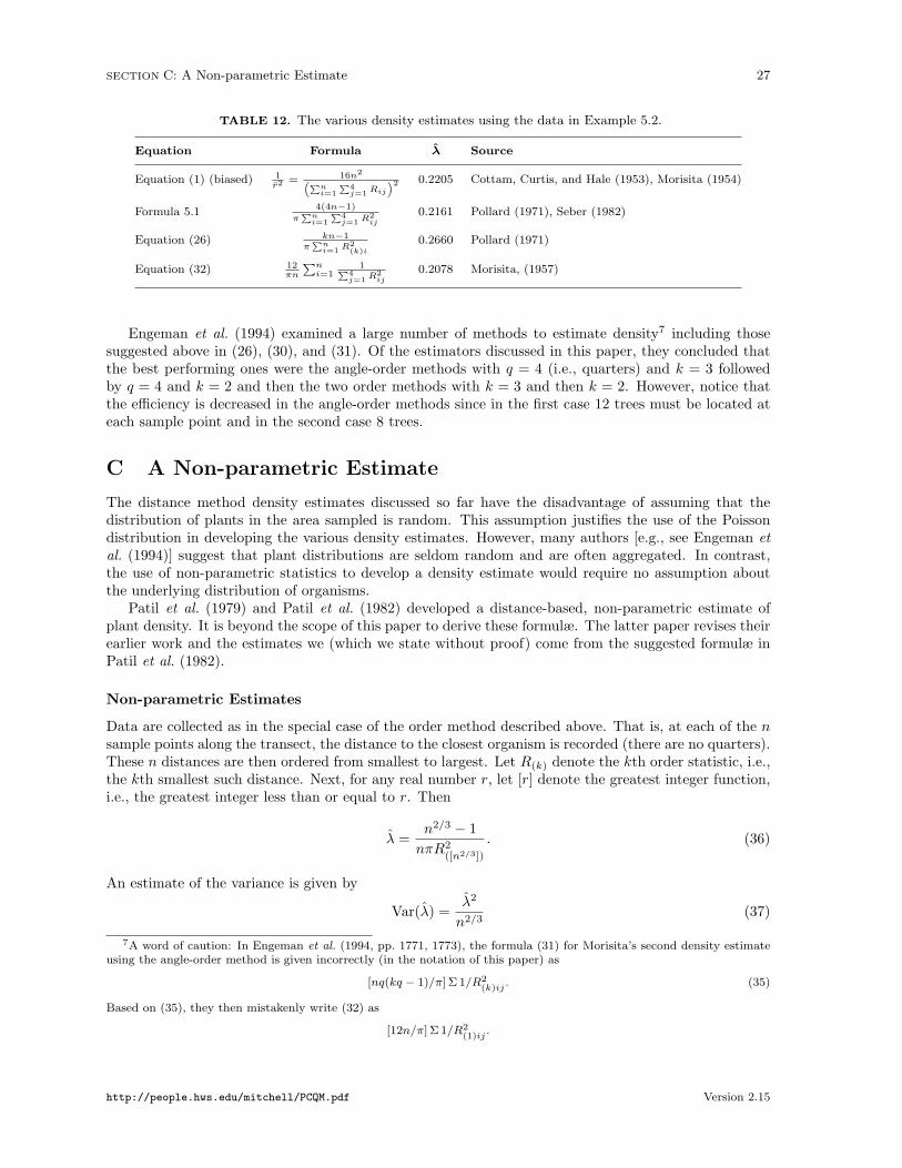
Table 12 compares this estimate to the estimates with the other applicable methods in this paper. Inshort, though most estimates are similar, it is important to specify which formula one is using to estimatedensity when the point-centered quarter method is employed.
Morisita (1957) suggests that the two estimates be averaged to form yet another density estimate
λ̂0 =λ̂1 + λ̂2
2(34)
and claims that all these estimates are “applicable to any kinds of patterns of spatial distribution ofindividuals (k ≥ 3).” Having applied the methods to a number of artificial populations, Morisita (1957)proposes the use of λ̂0 with p = 4 and n = 3 as a practical way of obtaining an accurate density estimate.
http://people.hws.edu/mitchell/PCQM.pdf Version 2.15
SECTION C: A Non-parametric Estimate 27
TABLE 12. The various density estimates using the data in Example 5.2.
Equation Formula λ̂ Source
Equation (1) (biased) 1r̄2
= 16n2“Pni=1
P4j=1 Rij
”2 0.2205 Cottam, Curtis, and Hale (1953), Morisita (1954)
Formula 5.14(4n−1)
πPni=1
P4j=1 R
2ij
0.2161 Pollard (1971), Seber (1982)
Equation (26) kn−1πPni=1 R
2(k)i
0.2660 Pollard (1971)
Equation (32) 12πn
Pni=1
1P4j=1 R
2ij
0.2078 Morisita, (1957)
Engeman et al. (1994) examined a large number of methods to estimate density7 including thosesuggested above in (26), (30), and (31). Of the estimators discussed in this paper, they concluded thatthe best performing ones were the angle-order methods with q = 4 (i.e., quarters) and k = 3 followedby q = 4 and k = 2 and then the two order methods with k = 3 and then k = 2. However, notice thatthe efficiency is decreased in the angle-order methods since in the first case 12 trees must be located ateach sample point and in the second case 8 trees.
C A Non-parametric Estimate
The distance method density estimates discussed so far have the disadvantage of assuming that thedistribution of plants in the area sampled is random. This assumption justifies the use of the Poissondistribution in developing the various density estimates. However, many authors [e.g., see Engeman etal. (1994)] suggest that plant distributions are seldom random and are often aggregated. In contrast,the use of non-parametric statistics to develop a density estimate would require no assumption aboutthe underlying distribution of organisms.
Patil et al. (1979) and Patil et al. (1982) developed a distance-based, non-parametric estimate ofplant density. It is beyond the scope of this paper to derive these formulæ. The latter paper revises theirearlier work and the estimates we (which we state without proof) come from the suggested formulæ inPatil et al. (1982).
Non-parametric Estimates
Data are collected as in the special case of the order method described above. That is, at each of the nsample points along the transect, the distance to the closest organism is recorded (there are no quarters).These n distances are then ordered from smallest to largest. Let R(k) denote the kth order statistic, i.e.,the kth smallest such distance. Next, for any real number r, let [r] denote the greatest integer function,i.e., the greatest integer less than or equal to r. Then
λ̂ =n2/3 − 1nπR2
([n2/3])
. (36)
An estimate of the variance is given by
Var(λ̂) =λ̂2
n2/3(37)
7A word of caution: In Engeman et al. (1994, pp. 1771, 1773), the formula (31) for Morisita’s second density estimateusing the angle-order method is given incorrectly (in the notation of this paper) as
[nq(kq − 1)/π] Σ 1/R2(k)ij
. (35)
Based on (35), they then mistakenly write (32) as
[12n/π] Σ 1/R2(1)ij
.
http://people.hws.edu/mitchell/PCQM.pdf Version 2.15

SECTION C: A Non-parametric Estimate 28
and so the the standard deviation is λ̂n1/3 For large samples, a confidence interval is developed in the
usual way: The endpoints of a (1 − α)100% confidence interval for the density λ are well-aproximatedby
C1 = λ̂+zα
2λ̂
n1/3and C2 = λ̂+
z1−α2 λ̂
n1/3. (38)
EXAMPLE C.1. If we use (36), (37) and the data in Example B.2 which lists the distances to the closesttrees at n = 15 sample points, the ordered data are
R(k) 0.2 0.6 0.7 0.7 0.7 0.7 0.9 1.0 1.0 1.0 1.1 1.1 1.2 1.2 2.3
πR2(k)
0.13 1.13 1.54 1.54 1.54 1.54 2.54 3.14 3.14 3.14 3.80 3.80 4.52 4.52 16.62
Since [n1/2] = [152/3] = [6.08] = 6, then R([152/3]) = R(6) = 0.7. Thus,
λ̂ =n2/3 − 1
nπR2([n2/3])
=152/3 − 1
15(1.54)= 0.2201 trees/m2.
Note that this estimate of λ compares favorably with those given by the parametric formulæ in Table 12and in (33).
An estimate of the variance is given by
Var(λ̂) =λ̂2
n2/3=
(0.2201)2
151/3= 0.0080
and for the standard deviation by
qVar(λ̂) =
√0.0800 = 0.0894. Though the sample size is not large,
we illustrate the calculation of a 95% confidence interval for λ.
C1 = λ̂+z0.025λ̂
n1/3= 0.2201− 1.96(0.0894) = 0.0449 trees/m2
and
C2 = λ̂+z0.975λ̂
n1/4= 0.2201 + 1.96(0.0894) = 0.3953 trees/m2.
This confidence interval is wider than the one calculated in Example B.2 using parametric methods. Inthe discussion section of Patil et al. (1982), the authors note that the price for a robust density estimate“is the considerable increase in variance as compared to a parametric estimator which assumes a specificspatial distribution of plants.”
Truncated Sampling
For truncated sampling (i.e., when a consistent upper limit is placed on the search radius used abouteach sample point), Patil et al. (1979) derived formulas for the density and its variance. Using theseformulas with the modifications in Patil et al. (1982) leads to the following. Let w be the upper limit forthe radius beyond which one does not search. Let n be the number of sample points and let n1 denotethe number of sample points with observations, i.e., points where the distance to the nearest organismdoes not excced w. (So there are n0 = n − n1 sample points without observations.) The data are theorder statistics R(k), where k = 1, . . . , n1.
Then
λ̂ =n1
n
n2/31 − 1
n1πR2
([n2/31 ])
. (39)
An estimate of the variance is given by
Var(λ̂t) =λ̂2t
n2/31
+ λ̂2t
(1n1− 1n
)(1 +
1
n2/31
). (40)
For large samples, the endpoints of a (1 − α)100% confidence interval for the density λ are well-aproximated by
C1 = λ̂+ zα2
√Var(λ̂t) and C2 = λ̂+ z1−α2
√Var(λ̂t). (41)
http://people.hws.edu/mitchell/PCQM.pdf Version 2.15

SECTION D: References 29
EXAMPLE C.2. To illustrate these calculations return once more to the data in Example C.1. Supposethat the students who collected the data only brought a 1 meter stick with them and so did not search fortrees beyond a meter from each sampling point. Then the data would consist of the n1 = 10 observationsthat were no greater than 1.0 m. Since there were n = 15 sampling points and [102/3] = 4, using (39),(40) we obtain
λ̂ =n1
n
0@ n2/31 − 1
n1πR2
([n2/31 ])
1A =10
15
102/3 − 1
10πR2([4])
!=
2
3
„3.6416
10π(0.7)2
«= 0.1577 trees/m2
and
Var(λ̂t) =λ̂2t
n2/31
+ λ̂2t
„1
n1− 1
n
« 1 +
1
n2/31
!
=(0.1577)2
102/3+ (0.1577)2
„1
10− 1
15
«„1 +
1
102/3
«= 0.0064.
The standard deviation is√
0.0064 = 0.080, so a 95% confidence interval for λ using these data would be
C1 = λ̂+z0.025λ̂
n1/3= 0.1577− 1.96(0.080) = 0.0009 trees/m2
and
C2 = λ̂+z0.975λ̂
n1/4= 0.1577 + 1.96(0.080) = 0.3145 trees/m2.
D References
Beasom, Samuel L. and Harry H. Haucke. 1975. A comparison of four distance sampling techniques inSouth Texas live oak mottes. J. Range Management. 28: 142–144.
Brokaw, Nicholas and Jill Thompson. 2000. The H for DBH. Forest Ecology and Management. 129:89–91.
Cottam, Grant and J. T. Curtis. 1956. The use of distance measures in phytosociological sampling.Ecology. 37: 451–460.
Cottam, Grant, J. T. Curtis, and B. W. Hale. 1953. Some sampling characteristics of a population ofrandomly dispersed individuals. Ecology. 34: 741–757.
Dahdouh-Guebas, Farid and Nico Koedam. 2006. Empirical estimate of the reliability of the use of thePoint-Centred Quarter Method (PCQM): Solutions to ambiguous field situations and descriptionof the PCQM+ protocol. Forest Ecology and Management. 228: 1–18. Available at: www.vub.ac.be/APNA/staff/FDG/pub/Dahdouh-Guebas&Koedam_2006_ForestEcolManage.pdf
Diaz, H., J. E. Conde, and B. Orihuela. 1992. Estimating the species number and cover of a mangrove-root community: a comparison of methods. Australian Journal of Marine and Freshwater Research.43(4): 707–713.
Dix, R. L. 1960. An application of the point-centered quarter method to sampling of grassland vegetation.J. Range Management. 14: 63–69.
Eberhardt, L. L. 1967. Some developments in ‘Distance Sampling’. Biometrics. 23: 207–216.
Engeman, Richard M., Robert T. Sugihara, Larry F. Pank, and William E. Dusenberry. 1994. Acomparison of plotless density estimators using Monte Carlo simulation. Ecology. 75(6): 1769–1779.
Glover, Thomas and Kevin Mitchell. 2006. An Introduction to Biostatistics. Longville, IL, WavelandPress.
http://people.hws.edu/mitchell/PCQM.pdf Version 2.15
SECTION D: References 30
Good, Ralph E. and Norma Frauendorf Good. 1971. Vegetation of a Minnesota prairie and a comparisonof methods. American Midland Naturalist, 85(1): 228–231.
Hollingsworth, T. 2005. Point-center quarter method black spruce heights, diameter, and location for150 mature black spruce sites in interior Alaska. LTER Database:BNZD:138. www.lter.uaf.edu/ascii/files138_pcqbs_ht_diam.txt. NSF awards DEB-0080609, 9810217, 9211769, 8702629 andUSDA Forest Service, Pacific Northwest Research Station RJVA-PNW-01-JV-11261952-231.
Jost, Lou. 1993. A simple distance estimator for plant density in nonuniform stands: Mathematical ap-pendix. http://www.loujost.com/Statistics%20and%20Physics/PCQ/PCQJournalArticle.htm
Kendall, M. G. and P. A. P. Moran. 1963. Geometrical Probality. New York, Hafner Publishing Co.37–41.
Krebs, C. J. 1989. Ecological Methodology. New York, Harper & Row.
Lamb, David. 1994. Lecture notes. University of Queensland, Australia.
Moore, P. G. 1954. Spacing in plant populations. Ecology. 35(2): 222–227.
Morisita, Masaaki. 1954. Estimation of population density by spacing method. Memoirs Fac. Sci.Kyushu Univ. Ser. E. 1: 187–197.
Morisita, Masaaki. 1957. A new method for the estimation of density by spacing method applicableto nonrandomly distributed populations. Physiology and Ecology 7: 134–144. (In Japanese withEnglish summary.)
Patil, S. A., K. P. Burnham, and J. L Kovner. 1979. Nonparametric estimation of plant density by thedistance method. Biometrics. 35(3): 597–604.
Patil, S. A., J. L Kovner, and K. P. Burnham. 1982. Optimum nonparametric estimation of populationdensity based on ordered distances. Biometrics. 38(1): 243-248.
Penfound, William T. 1963. A modification of the point-centered quarter method for grassland analysis.Ecology. 44(1): 175–176.
Pollard, J. H. 1971. On distance estimators of density in randomly distributed forests. Biometrics. 27:991–1002.
Rheinhardt, R., Mark M. Brinson, N. Eric Fleming, and J. Glenn Sandifer, Jr. 1997. Deciduous wetlandflats interim HGM model. www.pwrc.usgs.gov/wlistates/secoast.htm. Accessed online 1 Mar07.
Risser, Paul G. and Paul H. Zedler. 1968. An evaluation of the grassland quarter method. Ecology.49(5): 1006–1009
Seber, G. A. F. 1982. The Estimation of Animal Abundance and Related Parameters. New York,MacMillan. 41–45.
Stearns, Forest. 1949. Ninety years change in a northern hardwood forest in Wisconsin. Ecology. 30:350–358.
Warde, William and James W. Petranka. 1981. A correction factor table for missing point-center quarterdata. Ecology. 62(2): 491–494.
http://people.hws.edu/mitchell/PCQM.pdf Version 2.15

SECTION E: Reference Tables 31
E Reference Tables
TABLE 13. The cumulative standard normal distribution.
z 0.00 0.01 0.02 0.03 0.04 0.05 0.06 0.07 0.08 0.09
−3.9 0.0000 0.0000 0.0000 0.0000 0.0000 0.0000 0.0000 0.0000 0.0000 0.0000−3.8 0.0001 0.0001 0.0001 0.0001 0.0001 0.0001 0.0001 0.0001 0.0001 0.0001
−3.7 0.0001 0.0001 0.0001 0.0001 0.0001 0.0001 0.0001 0.0001 0.0001 0.0001−3.6 0.0002 0.0002 0.0001 0.0001 0.0001 0.0001 0.0001 0.0001 0.0001 0.0001
−3.5 0.0002 0.0002 0.0002 0.0002 0.0002 0.0002 0.0002 0.0002 0.0002 0.0002
−3.4 0.0003 0.0003 0.0003 0.0003 0.0003 0.0003 0.0003 0.0003 0.0003 0.0002−3.3 0.0005 0.0005 0.0005 0.0004 0.0004 0.0004 0.0004 0.0004 0.0004 0.0003
−3.2 0.0007 0.0007 0.0006 0.0006 0.0006 0.0006 0.0006 0.0005 0.0005 0.0005
−3.1 0.0010 0.0009 0.0009 0.0009 0.0008 0.0008 0.0008 0.0008 0.0007 0.0007−3.0 0.0013 0.0013 0.0013 0.0012 0.0012 0.0011 0.0011 0.0011 0.0010 0.0010
−2.9 0.0019 0.0018 0.0018 0.0017 0.0016 0.0016 0.0015 0.0015 0.0014 0.0014
−2.8 0.0026 0.0025 0.0024 0.0023 0.0023 0.0022 0.0021 0.0021 0.0020 0.0019−2.7 0.0035 0.0034 0.0033 0.0032 0.0031 0.0030 0.0029 0.0028 0.0027 0.0026
−2.6 0.0047 0.0045 0.0044 0.0043 0.0041 0.0040 0.0039 0.0038 0.0037 0.0036
−2.5 0.0062 0.0060 0.0059 0.0057 0.0055 0.0054 0.0052 0.0051 0.0049 0.0048−2.4 0.0082 0.0080 0.0078 0.0075 0.0073 0.0071 0.0069 0.0068 0.0066 0.0064
−2.3 0.0107 0.0104 0.0102 0.0099 0.0096 0.0094 0.0091 0.0089 0.0087 0.0084
−2.2 0.0139 0.0136 0.0132 0.0129 0.0125 0.0122 0.0119 0.0116 0.0113 0.0110−2.1 0.0179 0.0174 0.0170 0.0166 0.0162 0.0158 0.0154 0.0150 0.0146 0.0143
−2.0 0.0228 0.0222 0.0217 0.0212 0.0207 0.0202 0.0197 0.0192 0.0188 0.0183
−1.9 0.0287 0.0281 0.0274 0.0268 0.0262 0.0256 0.0250 0.0244 0.0239 0.0233
−1.8 0.0359 0.0351 0.0344 0.0336 0.0329 0.0322 0.0314 0.0307 0.0301 0.0294
−1.7 0.0446 0.0436 0.0427 0.0418 0.0409 0.0401 0.0392 0.0384 0.0375 0.0367−1.6 0.0548 0.0537 0.0526 0.0516 0.0505 0.0495 0.0485 0.0475 0.0465 0.0455
−1.5 0.0668 0.0655 0.0643 0.0630 0.0618 0.0606 0.0594 0.0582 0.0571 0.0559
−1.4 0.0808 0.0793 0.0778 0.0764 0.0749 0.0735 0.0721 0.0708 0.0694 0.0681−1.3 0.0968 0.0951 0.0934 0.0918 0.0901 0.0885 0.0869 0.0853 0.0838 0.0823
−1.2 0.1151 0.1131 0.1112 0.1093 0.1075 0.1056 0.1038 0.1020 0.1003 0.0985
−1.1 0.1357 0.1335 0.1314 0.1292 0.1271 0.1251 0.1230 0.1210 0.1190 0.1170−1.0 0.1587 0.1562 0.1539 0.1515 0.1492 0.1469 0.1446 0.1423 0.1401 0.1379
−0.9 0.1841 0.1814 0.1788 0.1762 0.1736 0.1711 0.1685 0.1660 0.1635 0.1611
−0.8 0.2119 0.2090 0.2061 0.2033 0.2005 0.1977 0.1949 0.1922 0.1894 0.1867
−0.7 0.2420 0.2389 0.2358 0.2327 0.2296 0.2266 0.2236 0.2206 0.2177 0.2148−0.6 0.2743 0.2709 0.2676 0.2643 0.2611 0.2578 0.2546 0.2514 0.2483 0.2451
−0.5 0.3085 0.3050 0.3015 0.2981 0.2946 0.2912 0.2877 0.2843 0.2810 0.2776
−0.4 0.3446 0.3409 0.3372 0.3336 0.3300 0.3264 0.3228 0.3192 0.3156 0.3121−0.3 0.3821 0.3783 0.3745 0.3707 0.3669 0.3632 0.3594 0.3557 0.3520 0.3483
−0.2 0.4207 0.4168 0.4129 0.4090 0.4052 0.4013 0.3974 0.3936 0.3897 0.3859−0.1 0.4602 0.4562 0.4522 0.4483 0.4443 0.4404 0.4364 0.4325 0.4286 0.4247
−0.0 0.5000 0.4960 0.4920 0.4880 0.4840 0.4801 0.4761 0.4721 0.4681 0.4641
http://people.hws.edu/mitchell/PCQM.pdf Version 2.15
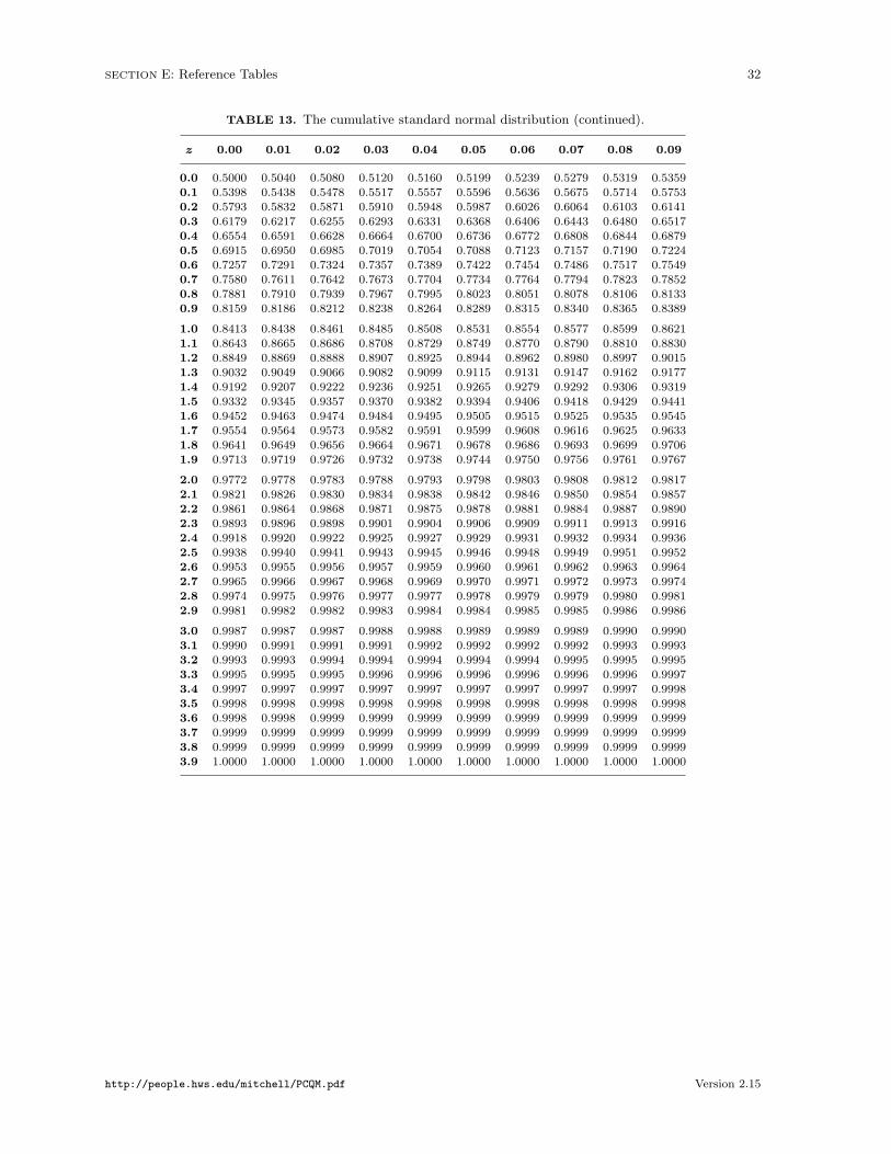
SECTION E: Reference Tables 32
TABLE 13. The cumulative standard normal distribution (continued).
z 0.00 0.01 0.02 0.03 0.04 0.05 0.06 0.07 0.08 0.09
0.0 0.5000 0.5040 0.5080 0.5120 0.5160 0.5199 0.5239 0.5279 0.5319 0.5359
0.1 0.5398 0.5438 0.5478 0.5517 0.5557 0.5596 0.5636 0.5675 0.5714 0.57530.2 0.5793 0.5832 0.5871 0.5910 0.5948 0.5987 0.6026 0.6064 0.6103 0.6141
0.3 0.6179 0.6217 0.6255 0.6293 0.6331 0.6368 0.6406 0.6443 0.6480 0.6517
0.4 0.6554 0.6591 0.6628 0.6664 0.6700 0.6736 0.6772 0.6808 0.6844 0.68790.5 0.6915 0.6950 0.6985 0.7019 0.7054 0.7088 0.7123 0.7157 0.7190 0.7224
0.6 0.7257 0.7291 0.7324 0.7357 0.7389 0.7422 0.7454 0.7486 0.7517 0.7549
0.7 0.7580 0.7611 0.7642 0.7673 0.7704 0.7734 0.7764 0.7794 0.7823 0.78520.8 0.7881 0.7910 0.7939 0.7967 0.7995 0.8023 0.8051 0.8078 0.8106 0.8133
0.9 0.8159 0.8186 0.8212 0.8238 0.8264 0.8289 0.8315 0.8340 0.8365 0.8389
1.0 0.8413 0.8438 0.8461 0.8485 0.8508 0.8531 0.8554 0.8577 0.8599 0.86211.1 0.8643 0.8665 0.8686 0.8708 0.8729 0.8749 0.8770 0.8790 0.8810 0.8830
1.2 0.8849 0.8869 0.8888 0.8907 0.8925 0.8944 0.8962 0.8980 0.8997 0.9015
1.3 0.9032 0.9049 0.9066 0.9082 0.9099 0.9115 0.9131 0.9147 0.9162 0.91771.4 0.9192 0.9207 0.9222 0.9236 0.9251 0.9265 0.9279 0.9292 0.9306 0.9319
1.5 0.9332 0.9345 0.9357 0.9370 0.9382 0.9394 0.9406 0.9418 0.9429 0.94411.6 0.9452 0.9463 0.9474 0.9484 0.9495 0.9505 0.9515 0.9525 0.9535 0.9545
1.7 0.9554 0.9564 0.9573 0.9582 0.9591 0.9599 0.9608 0.9616 0.9625 0.9633
1.8 0.9641 0.9649 0.9656 0.9664 0.9671 0.9678 0.9686 0.9693 0.9699 0.97061.9 0.9713 0.9719 0.9726 0.9732 0.9738 0.9744 0.9750 0.9756 0.9761 0.9767
2.0 0.9772 0.9778 0.9783 0.9788 0.9793 0.9798 0.9803 0.9808 0.9812 0.9817
2.1 0.9821 0.9826 0.9830 0.9834 0.9838 0.9842 0.9846 0.9850 0.9854 0.98572.2 0.9861 0.9864 0.9868 0.9871 0.9875 0.9878 0.9881 0.9884 0.9887 0.9890
2.3 0.9893 0.9896 0.9898 0.9901 0.9904 0.9906 0.9909 0.9911 0.9913 0.9916
2.4 0.9918 0.9920 0.9922 0.9925 0.9927 0.9929 0.9931 0.9932 0.9934 0.99362.5 0.9938 0.9940 0.9941 0.9943 0.9945 0.9946 0.9948 0.9949 0.9951 0.9952
2.6 0.9953 0.9955 0.9956 0.9957 0.9959 0.9960 0.9961 0.9962 0.9963 0.9964
2.7 0.9965 0.9966 0.9967 0.9968 0.9969 0.9970 0.9971 0.9972 0.9973 0.99742.8 0.9974 0.9975 0.9976 0.9977 0.9977 0.9978 0.9979 0.9979 0.9980 0.9981
2.9 0.9981 0.9982 0.9982 0.9983 0.9984 0.9984 0.9985 0.9985 0.9986 0.9986
3.0 0.9987 0.9987 0.9987 0.9988 0.9988 0.9989 0.9989 0.9989 0.9990 0.99903.1 0.9990 0.9991 0.9991 0.9991 0.9992 0.9992 0.9992 0.9992 0.9993 0.9993
3.2 0.9993 0.9993 0.9994 0.9994 0.9994 0.9994 0.9994 0.9995 0.9995 0.99953.3 0.9995 0.9995 0.9995 0.9996 0.9996 0.9996 0.9996 0.9996 0.9996 0.9997
3.4 0.9997 0.9997 0.9997 0.9997 0.9997 0.9997 0.9997 0.9997 0.9997 0.9998
3.5 0.9998 0.9998 0.9998 0.9998 0.9998 0.9998 0.9998 0.9998 0.9998 0.99983.6 0.9998 0.9998 0.9999 0.9999 0.9999 0.9999 0.9999 0.9999 0.9999 0.9999
3.7 0.9999 0.9999 0.9999 0.9999 0.9999 0.9999 0.9999 0.9999 0.9999 0.9999
3.8 0.9999 0.9999 0.9999 0.9999 0.9999 0.9999 0.9999 0.9999 0.9999 0.99993.9 1.0000 1.0000 1.0000 1.0000 1.0000 1.0000 1.0000 1.0000 1.0000 1.0000
http://people.hws.edu/mitchell/PCQM.pdf Version 2.15

SECTION E: Reference Tables 33
TABLE 14. Table of chi-square values for 95% confidence internals for n = 1 to 240 transect sample points.
n 8n χ20.025 χ2
0.975 n 8n χ20.025 χ2
0.975 n 8n χ20.025 χ2
0.975 n 8n χ20.025 χ2
0.975
1 8 2.18 17.53 61 488 428.68 551.10 121 968 883.67 1056.12 181 1448 1344.43 1555.36
2 16 6.91 28.85 62 496 436.18 559.60 122 976 891.32 1064.47 182 1456 1352.14 1563.65
3 24 12.40 39.36 63 504 443.69 568.10 123 984 898.96 1072.83 183 1464 1359.85 1571.944 32 18.29 49.48 64 512 451.20 576.59 124 992 906.61 1081.18 184 1472 1367.56 1580.23
5 40 24.43 59.34 65 520 458.71 585.08 125 1000 914.26 1089.53 185 1480 1375.27 1588.52
6 48 30.75 69.02 66 528 466.22 593.56 126 1008 921.91 1097.88 186 1488 1382.99 1596.807 56 37.21 78.57 67 536 473.74 602.04 127 1016 929.56 1106.23 187 1496 1390.70 1605.09
8 64 43.78 88.00 68 544 481.27 610.52 128 1024 937.21 1114.58 188 1504 1398.41 1613.389 72 50.43 97.35 69 552 488.79 619.00 129 1032 944.87 1122.92 189 1512 1406.13 1621.66
10 80 57.15 106.63 70 560 496.32 627.47 130 1040 952.52 1131.27 190 1520 1413.84 1629.95
11 88 63.94 115.84 71 568 503.85 635.93 131 1048 960.18 1139.61 191 1528 1421.56 1638.23
12 96 70.78 125.00 72 576 511.39 644.40 132 1056 967.84 1147.95 192 1536 1429.27 1646.51
13 104 77.67 134.11 73 584 518.93 652.86 133 1064 975.50 1156.29 193 1544 1436.99 1654.8014 112 84.60 143.18 74 592 526.47 661.31 134 1072 983.16 1164.63 194 1552 1444.71 1663.08
15 120 91.57 152.21 75 600 534.02 669.77 135 1080 990.82 1172.97 195 1560 1452.43 1671.36
16 128 98.58 161.21 76 608 541.57 678.22 136 1088 998.48 1181.31 196 1568 1460.15 1679.6417 136 105.61 170.18 77 616 549.12 686.67 137 1096 1006.15 1189.64 197 1576 1467.87 1687.92
18 144 112.67 179.11 78 624 556.67 695.11 138 1104 1013.81 1197.98 198 1584 1475.59 1696.20
19 152 119.76 188.03 79 632 564.23 703.56 139 1112 1021.48 1206.31 199 1592 1483.31 1704.4820 160 126.87 196.92 80 640 571.79 712.00 140 1120 1029.15 1214.64 200 1600 1491.03 1712.75
21 168 134.00 205.78 81 648 579.35 720.43 141 1128 1036.82 1222.97 201 1608 1498.76 1721.0322 176 141.16 214.63 82 656 586.92 728.87 142 1136 1044.49 1231.30 202 1616 1506.48 1729.31
23 184 148.33 223.46 83 664 594.49 737.30 143 1144 1052.16 1239.63 203 1624 1514.21 1737.58
24 192 155.52 232.27 84 672 602.06 745.73 144 1152 1059.83 1247.96 204 1632 1521.93 1745.8625 200 162.73 241.06 85 680 609.63 754.16 145 1160 1067.50 1256.28 205 1640 1529.66 1754.13
26 208 169.95 249.83 86 688 617.21 762.58 146 1168 1075.18 1264.61 206 1648 1537.38 1762.41
27 216 177.19 258.60 87 696 624.79 771.00 147 1176 1082.86 1272.93 207 1656 1545.11 1770.68
28 224 184.44 267.35 88 704 632.37 779.42 148 1184 1090.53 1281.26 208 1664 1552.84 1778.95
29 232 191.71 276.08 89 712 639.95 787.84 149 1192 1098.21 1289.58 209 1672 1560.57 1787.2230 240 198.98 284.80 90 720 647.54 796.25 150 1200 1105.89 1297.90 210 1680 1568.30 1795.49
31 248 206.27 293.51 91 728 655.12 804.66 151 1208 1113.57 1306.22 211 1688 1576.03 1803.7632 256 213.57 302.21 92 736 662.71 813.07 152 1216 1121.25 1314.54 212 1696 1583.76 1812.03
33 264 220.89 310.90 93 744 670.31 821.48 153 1224 1128.93 1322.85 213 1704 1591.49 1820.30
34 272 228.21 319.58 94 752 677.90 829.89 154 1232 1136.62 1331.17 214 1712 1599.22 1828.5735 280 235.54 328.25 95 760 685.50 838.29 155 1240 1144.30 1339.49 215 1720 1606.95 1836.84
36 288 242.88 336.90 96 768 693.10 846.69 156 1248 1151.99 1347.80 216 1728 1614.68 1845.10
37 296 250.23 345.55 97 776 700.70 855.09 157 1256 1159.67 1356.11 217 1736 1622.42 1853.3738 304 257.59 354.19 98 784 708.30 863.49 158 1264 1167.36 1364.43 218 1744 1630.15 1861.64
39 312 264.96 362.83 99 792 715.91 871.88 159 1272 1175.05 1372.74 219 1752 1637.89 1869.90
40 320 272.34 371.45 100 800 723.51 880.28 160 1280 1182.74 1381.05 220 1760 1645.62 1878.17
41 328 279.72 380.07 101 808 731.12 888.67 161 1288 1190.43 1389.36 221 1768 1653.36 1886.43
42 336 287.11 388.68 102 816 738.73 897.06 162 1296 1198.12 1397.67 222 1776 1661.09 1894.6943 344 294.51 397.28 103 824 746.35 905.44 163 1304 1205.81 1405.97 223 1784 1668.83 1902.96
44 352 301.92 405.87 104 832 753.96 913.83 164 1312 1213.51 1414.28 224 1792 1676.57 1911.22
45 360 309.33 414.46 105 840 761.58 922.21 165 1320 1221.20 1422.59 225 1800 1684.31 1919.4846 368 316.75 423.04 106 848 769.19 930.59 166 1328 1228.90 1430.89 226 1808 1692.05 1927.7447 376 324.17 431.62 107 856 776.81 938.97 167 1336 1236.59 1439.19 227 1816 1699.79 1936.0048 384 331.60 440.18 108 864 784.44 947.35 168 1344 1244.29 1447.50 228 1824 1707.53 1944.26
49 392 339.04 448.75 109 872 792.06 955.73 169 1352 1251.99 1455.80 229 1832 1715.27 1952.52
50 400 346.48 457.31 110 880 799.69 964.10 170 1360 1259.69 1464.10 230 1840 1723.01 1960.78
51 408 353.93 465.86 111 888 807.31 972.48 171 1368 1267.39 1472.40 231 1848 1730.75 1969.0452 416 361.38 474.40 112 896 814.94 980.85 172 1376 1275.09 1480.70 232 1856 1738.49 1977.3053 424 368.84 482.95 113 904 822.57 989.22 173 1384 1282.79 1489.00 233 1864 1746.24 1985.55
54 432 376.31 491.48 114 912 830.20 997.58 174 1392 1290.49 1497.30 234 1872 1753.98 1993.81
55 440 383.77 500.01 115 920 837.84 1005.95 175 1400 1298.20 1505.59 235 1880 1761.72 2002.0756 448 391.25 508.54 116 928 845.47 1014.32 176 1408 1305.90 1513.89 236 1888 1769.47 2010.32
57 456 398.73 517.06 117 936 853.11 1022.68 177 1416 1313.60 1522.18 237 1896 1777.21 2018.5858 464 406.21 525.58 118 944 860.75 1031.04 178 1424 1321.31 1530.48 238 1904 1784.96 2026.8359 472 413.70 534.09 119 952 868.39 1039.40 179 1432 1329.02 1538.77 239 1912 1792.70 2035.08
60 480 421.19 542.60 120 960 876.03 1047.76 180 1440 1336.72 1547.06 240 1920 1800.45 2043.34
http://people.hws.edu/mitchell/PCQM.pdf Version 2.15
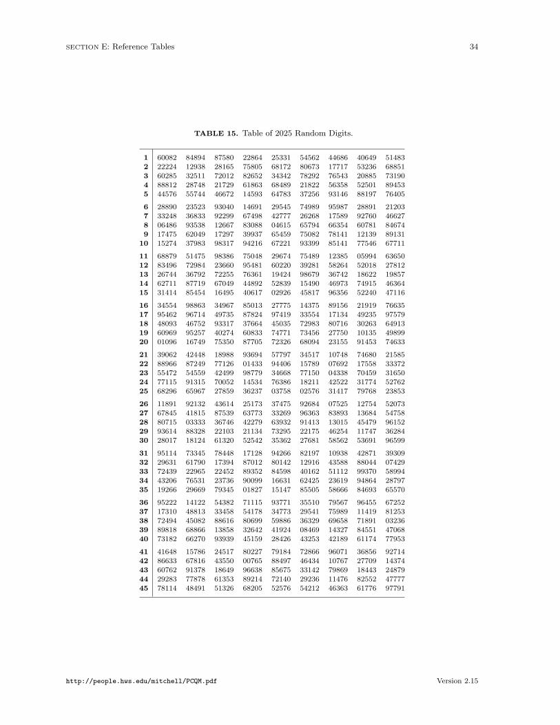
SECTION E: Reference Tables 34
TABLE 15. Table of 2025 Random Digits.
1 60082 84894 87580 22864 25331 54562 44686 40649 51483
2 22224 12938 28165 75805 68172 80673 17717 53236 68851
3 60285 32511 72012 82652 34342 78292 76543 20885 731904 88812 28748 21729 61863 68489 21822 56358 52501 89453
5 44576 55744 46672 14593 64783 37256 93146 88197 76405
6 28890 23523 93040 14691 29545 74989 95987 28891 212037 33248 36833 92299 67498 42777 26268 17589 92760 46627
8 06486 93538 12667 83088 04615 65794 66354 60781 84674
9 17475 62049 17297 39937 65459 75082 78141 12139 8913110 15274 37983 98317 94216 67221 93399 85141 77546 67711
11 68879 51475 98386 75048 29674 75489 12385 05994 6365012 83496 72984 23660 95481 60220 39281 58264 52018 27812
13 26744 36792 72255 76361 19424 98679 36742 18622 19857
14 62711 87719 67049 44892 52839 15490 46973 74915 4636415 31414 85454 16495 40617 02926 45817 96356 52240 47116
16 34554 98863 34967 85013 27775 14375 89156 21919 76635
17 95462 96714 49735 87824 97419 33554 17134 49235 9757918 48093 46752 93317 37664 45035 72983 80716 30263 64913
19 60969 95257 40274 60833 74771 73456 27750 10135 49899
20 01096 16749 75350 87705 72326 68094 23155 91453 74633
21 39062 42448 18988 93694 57797 34517 10748 74680 21585
22 88966 87249 77126 01433 94406 15789 07692 17558 33372
23 55472 54559 42499 98779 34668 77150 04338 70459 3165024 77115 91315 70052 14534 76386 18211 42522 31774 52762
25 68296 65967 27859 36237 03758 02576 31417 79768 23853
26 11891 92132 43614 25173 37475 92684 07525 12754 5207327 67845 41815 87539 63773 33269 96363 83893 13684 54758
28 80715 03333 36746 42279 63932 91413 13015 45479 9615229 93614 88328 22103 21134 73295 22175 46254 11747 36284
30 28017 18124 61320 52542 35362 27681 58562 53691 96599
31 95114 73345 78448 17128 94266 82197 10938 42871 3930932 29631 61790 17394 87012 80142 12916 43588 88044 0742933 72439 22965 22452 89352 84598 40162 51112 99370 58994
34 43206 76531 23736 90099 16631 62425 23619 94864 2879735 19266 29669 79345 01827 15147 85505 58666 84693 65570
36 95222 14122 54382 71115 93771 35510 79567 96455 67252
37 17310 48813 33458 54178 34773 29541 75989 11419 8125338 72494 45082 88616 80699 59886 36329 69658 71891 03236
39 89818 68866 13858 32642 41924 08469 14327 84551 4706840 73182 66270 93939 45159 28426 43253 42189 61174 77953
41 41648 15786 24517 80227 79184 72866 96071 36856 92714
42 86633 67816 43550 00765 88497 46434 10767 27709 1437443 60762 91378 18649 96638 85675 33142 79869 18443 24879
44 29283 77878 61353 89214 72140 29236 11476 82552 47777
45 78114 48491 51326 68205 52576 54212 46363 61776 97791
http://people.hws.edu/mitchell/PCQM.pdf Version 2.15