Embed Size (px)
DESCRIPTION
Quantitative analysis and R – (1). LING115 November 18, 2009. Some basic statistics. Reference. The basics. Measures of central tendency, dispersion Frequency distribution Hypothesis testing Population vs. sample One sample t-test Measures of association Covariance and correlation. - PowerPoint PPT Presentation
Citation preview

Quantitative analysis and R – (1)
LING115November 18, 2009

Some basic statistics
Reference

The basics
• Measures of central tendency, dispersion• Frequency distribution• Hypothesis testing– Population vs. sample– One sample t-test
• Measures of association– Covariance and correlation
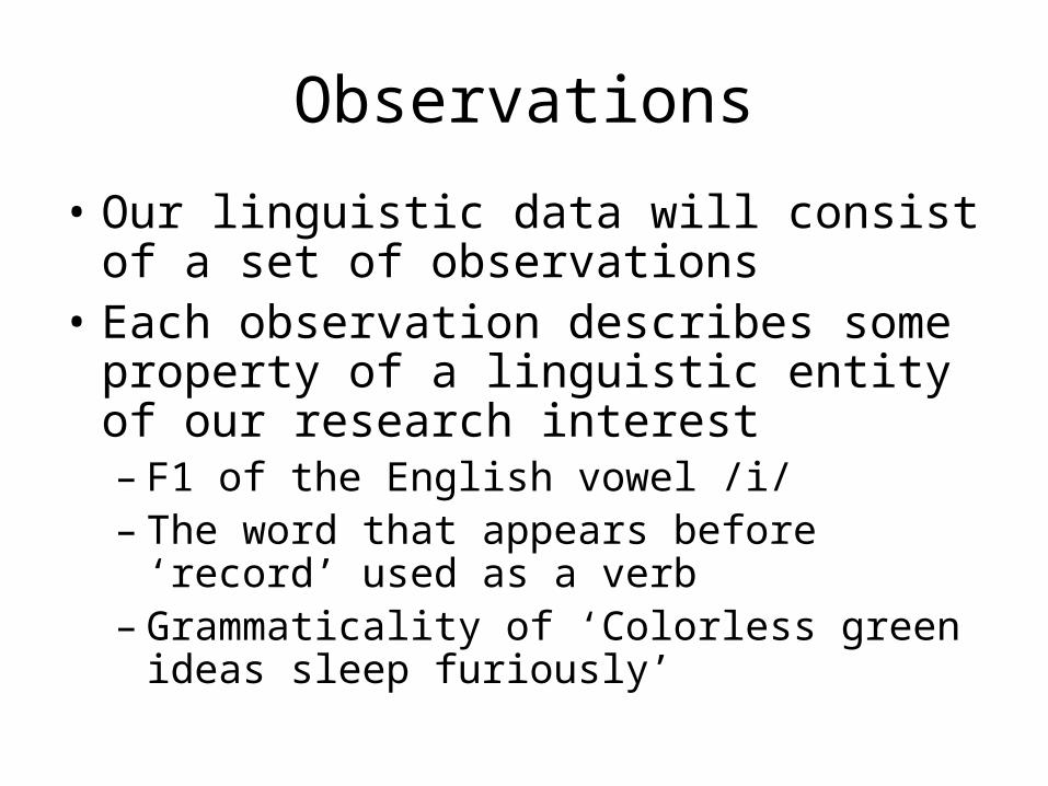
Observations
• Our linguistic data will consist of a set of observations
• Each observation describes some property of a linguistic entity of our research interest– F1 of the English vowel /i/– The word that appears before ‘record’ used as a
verb– Grammaticality of ‘Colorless green ideas sleep
furiously’

Measures of central tendency
• Median– The value in the middle assuming that the values
in the data are ordered according to their size
• Mode– The most frequent value in the data
• Mean– The arithmetic mean of values in the data
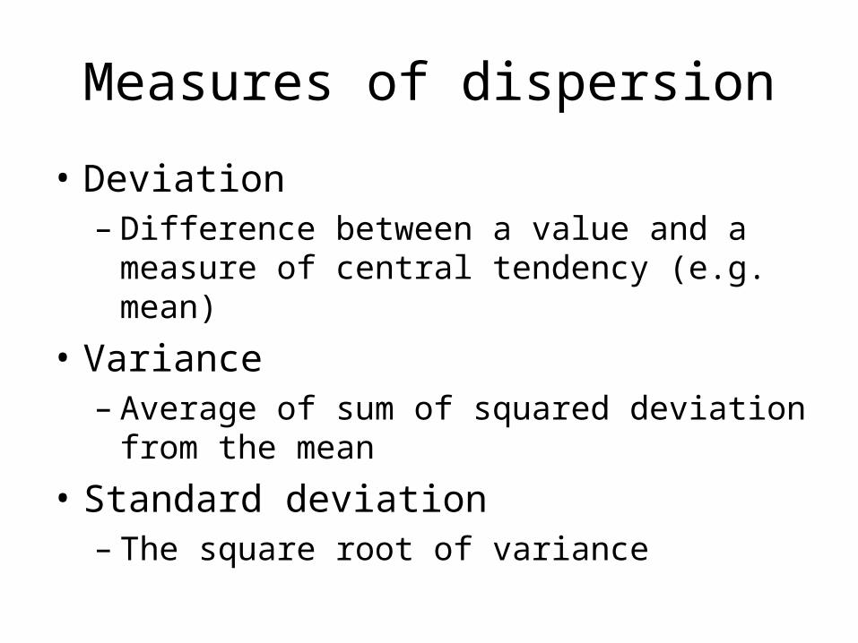
Measures of dispersion
• Deviation– Difference between a value and a measure of
central tendency (e.g. mean)
• Variance– Average of sum of squared deviation from the
mean
• Standard deviation– The square root of variance

Frequency distribution
• Distribution describing how often each value of an observation occurs in the data
• Enumerating the frequency of each value of an observation may not be informative, especially if the observations can have continuous values
• Instead we can characterize the frequency distribution in terms of ranges of value
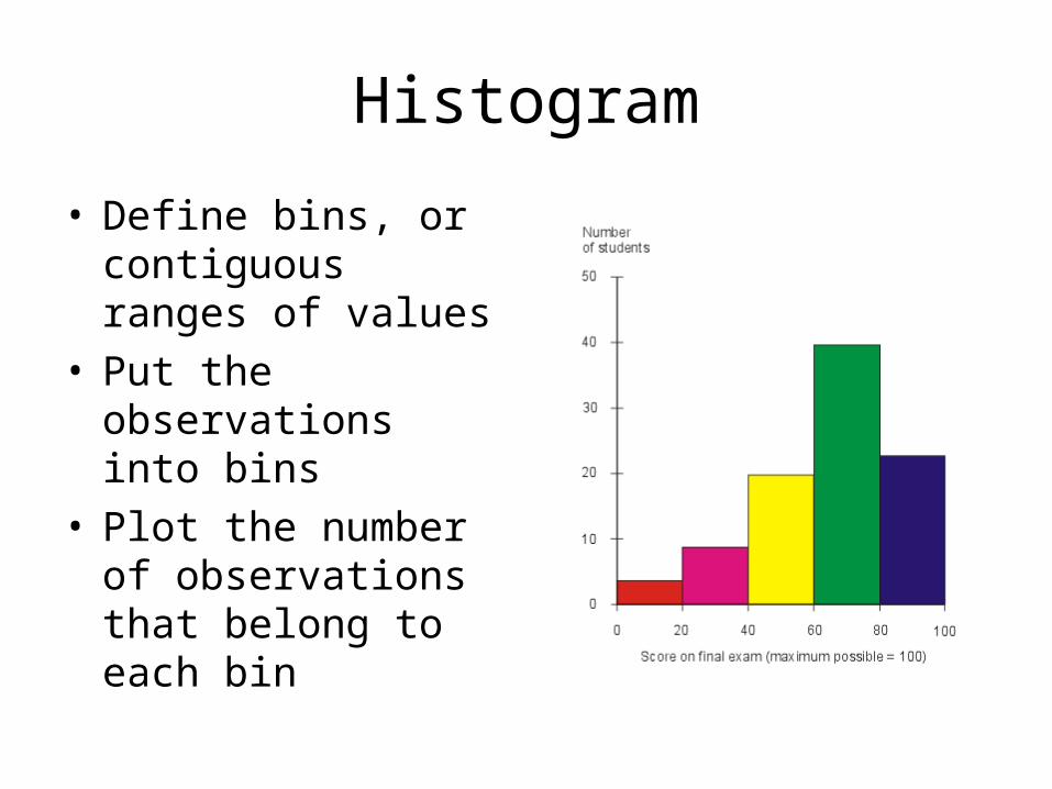
Histogram
• Define bins, or contiguous ranges of values
• Put the observations into bins
• Plot the number of observations that belong to each bin

Histograms with smaller bins
Continuous curve and probability
• As the bin gets smaller, the histogram looks more like a continuous curve
• Once we interpret a histogram as a continuous curve, it makes more sense to calculating the probability that the observations falls within a range of values rather than counting the number of such observations
• The probability is the ratio of the area under the curve within the given range to the total area under the curve

Uniform distribution

Bimodal distribution
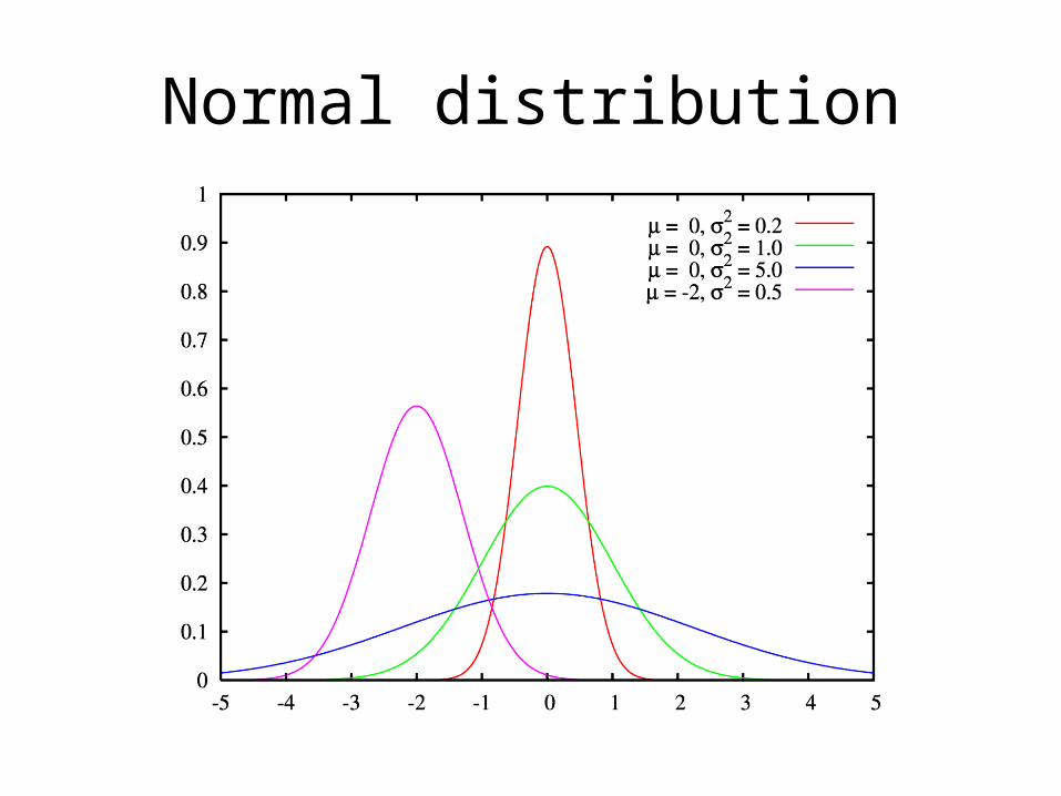
Normal distribution
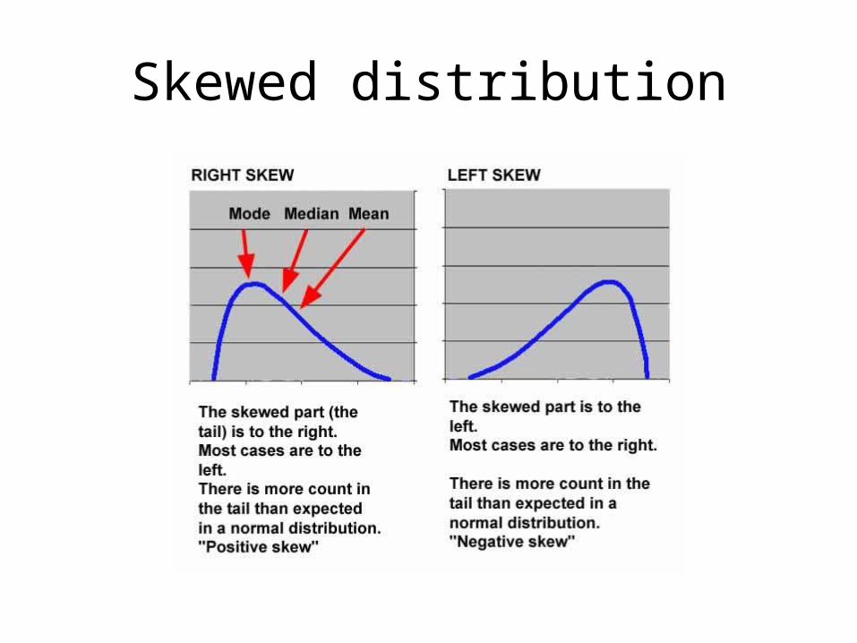
Skewed distribution
Normal distribution
• Symmetric bell-shaped curve– Mean = median = mode
• The distribution can be solely defined in terms of the mean and the standard deviation– Mean (μ) defines the center of the curve– Standard deviation (σ)defines the spread of the curve– N(μ, σ) means a normal distribution whose mean= μ,
standard deviation=σ– N(0,1) is called the standard normal distribution

Z-score
• Z-score measures the distance of a value from the mean in terms of standard deviation units– Subtract the mean from the value– Normalize the distance by the standard deviation– i.e.
• Calculating the z-score for every value of a normal distribution converts the distribution into a standard normal distribution
ixz

Standard normal (Z) table
• Recall that we calculate the probability of a value falling within a particular range by calculating the area under the curve
• To skip the calculation part, people have provided distribution tables for some popular distributions
• The standard normal distribution is one of them• http://www.statsoft.com/textbook/sttable.html

Population vs. sample
• Population– The entire set– e.g. The set of all people who live in California– e.g. The set of all sentences in English
• Sample– A subset of the population– e.g. A set of 50,000 people who live in California– e.g. The set of sentences in the WSJ corpus

Sample
• We analyze a sample when we examine a corpus
• We hope our sample is a good representation of the population
• Otherwise we cannot generalize a statistical tendency found in a corpus to make claims about the language

A good sample
• Size– The sample must be large enough
• Randomness– Members of the sample must be chosen randomly
from the population

Sample statistics
• Statistics about a sample is an estimation of the population parameter with possible errors due to sampling

Degree of freedom
• Degrees of freedom reflect how precise our estimation is– The bigger the size of a sample, the more precise
our estimation of the population parameter
• Initially, degrees of freedom is equal to the size of the sample
• Degrees of freedom decrease as we estimate more parameters with the same data

Measures – revisited
• Mean– Sample mean:
– Population mean:
• Variance– Sample variance:
– Population variance:
n
xx
n
ii
1
N
xN
ii
1
)1(
)(1
2
2
n
xxs
n
ii
N
xxN
ii
1
2
2)(
Central limit theorem
• As the number of observations in each sample increases, the means of the samples tend toward the normal distribution
• http://www.stat.sc.edu/~west/javahtml/CLT.html
• The applet actually illustrates that the sum of dice converges to normality, but this also applies to the sample means since we can divide the sum by the number of dice

Standard error (SE)
• Standard deviation of means of samples of a population• Intuitively, this would be calculated by first sampling the
data from the population many times and then calculating the standard deviation of the means
• There is a way to directly calculate the standard error from the standard deviation of the population or the sample– From population:
– From sample:
nSE
n
sSE x

Comparing means – (1)
• Question– We do expect the sample mean to be somewhat
different even if the samples are from the same population
– But then how do we tell if the mean of a data set is too different to say that the data set is from a different population?
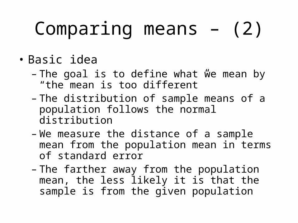
Comparing means – (2)
• Basic idea– The goal is to define what we mean by “the mean
is too different”– The distribution of sample means of a population
follows the normal distribution– We measure the distance of a sample mean from
the population mean in terms of standard error– The farther away from the population mean, the
less likely it is that the sample is from the given population
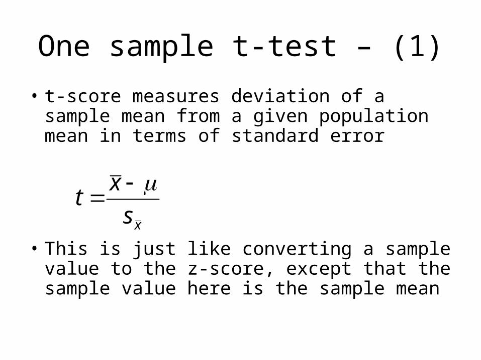
One sample t-test – (1)
• t-score measures deviation of a sample mean from a given population mean in terms of standard error
• This is just like converting a sample value to the z-score, except that the sample value here is the sample mean
xs
xt
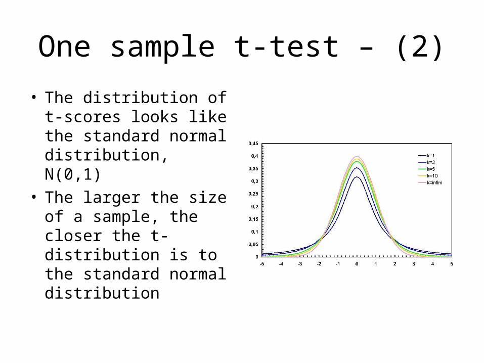
One sample t-test – (2)
• The distribution of t-scores looks like the standard normal distribution, N(0,1)
• The larger the size of a sample, the closer the t-distribution is to the standard normal distribution

One sample t-test – (3)
• Once we have the t-score (t), we ask “how likely is it to get a value less/greater than or equal to t from the t-distribution?”
• We can answer this by calculating the relevant area under the curve or looking up the t-table
• If you think the probability is too small, you have reason to suspect that your sample mean is not from the distribution of possible sample means of a population

A more typical way to put it
• Null hypothesis (H0): your sample mean is not different from the population mean (the apparent difference is simply due to error inherent in the sampling process)
• We decide whether to accept or reject the null hypothesis by performing one-sample t-test
• Let’s say α is the probability that the t-score representing the sample mean is from the t-distribution representing the distribution of sample means of the population
• If α is smaller than some threshold we predefined (e.g. 0.5) , we reject the null hypothesis

A more typical way to put it – (2)• Note that unless α is zero, we can never be
confident rejecting the null hypothesis is the right thing
• We call the error of falsely rejecting the null hypothesis “Type-I error”
• α is the probability that we will commit type-I error
• 1- α is the probability that we won’t• We can say “we are (1- α)*100 percent confident
that the null-hypothesis is wrong”

Measures of association
• Question– We want to see if two variables are related to
each other
• Basic idea– If the values of two variables fluctuate in the same
direction, in similar magnitudes, they are probably related
– Degree of fluctuation is measured in terms of the deviation from the mean

Covariance• Average sum of product of deviations
• If x and y fluctuate in the same direction, in similar magnitudes, the sum of product of deviations will be large
• The sum of product will be larger if we have more pairs to compare
• This is not desirable, so we normalize the sum by the number of pairs
n
yyxxn
iii
1
)()(

Correlation
• Same as covariance except that the deviation is measured in terms of z-scores
• The idea is to make the magnitudes of deviation comparable by putting both x and y on the same scale
n
s
yy
s
xxn
i y
i
x
i
1
)()(

A little bit of R
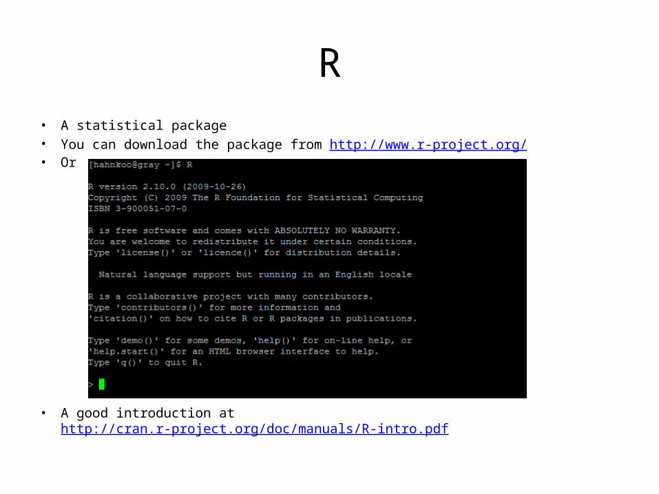
R• A statistical package• You can download the package from http://www.r-project.org/ • Or
• A good introduction at http://cran.r-project.org/doc/manuals/R-intro.pdf

Vectors
• A numeric vector is like a list of numbers in Python• Index starts from 1
Command What it does
x <- c(10,12,30,4,5) Create a vector called x consisting of 10,12,30, 4, 5
x Print out the contents of x
x[2:4] Return 2nd to 4th entry in the vector
x[-3] Return all entries in the vector except the 3rd entry
x[x<10] Return all entries whose value is less than 10

Example commands for a vectorCommand What it does
length(x) Number of values in x
mean(x) Calculate the mean of x
median(x) Calculate the median value of x
sd(x) Calculate the standard deviation of x
var(x) Calculate the variance of x
min(x) Identify the minimum value in x
max(x) Identify the maximum value in x
summary(x) Summarize descriptive statistics of x

Data frames• We often summarize our data as a table– Each row is an observation characterized in terms of a
number of variables– Each column lists values pertaining to a variable
• A data frame in R is like columns of vectors, where each column can be labeled> a <- c(1,2,3,4)> b <- c(10,20,30,40)> c <- data.frame(v1=a,v2=b)> c$a> c$b
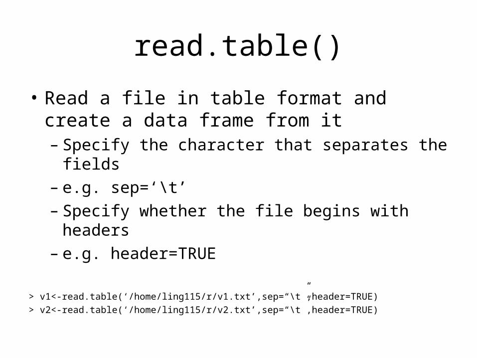
read.table()
• Read a file in table format and create a data frame from it– Specify the character that separates the fields– e.g. sep=‘\t’– Specify whether the file begins with headers– e.g. header=TRUE
> v1<-read.table(‘/home/ling115/r/v1.txt’,sep=“\t”,header=TRUE)
> v2<-read.table(‘/home/ling115/r/v2.txt’,sep=“\t”,header=TRUE)
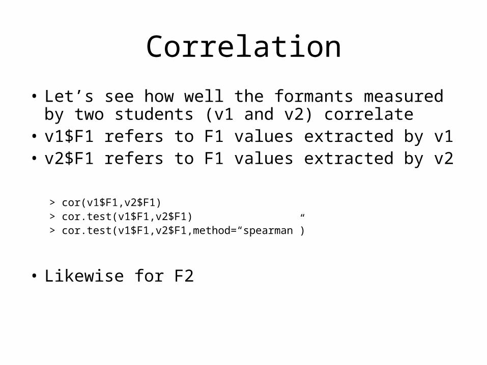
Correlation
• Let’s see how well the formants measured by two students (v1 and v2) correlate
• v1$F1 refers to F1 values extracted by v1• v2$F1 refers to F1 values extracted by v2
> cor(v1$F1,v2$F1)> cor.test(v1$F1,v2$F1)> cor.test(v1$F1,v2$F1,method=“spearman”)
• Likewise for F2