Embed Size (px)
Citation preview
QUANTISATION OF TWISTOR THEORY BY COCYCLE TWIST
S.J. BRAIN AND S. MAJID
Abstract. We present the main ingredients of twistor theory leading up to
and including the Penrose-Ward transform in a coordinate algebra form which
we can then ‘quantise’ by means of a functorial cocycle twist. The quantum
algebras for the conformal group, twistor space CP3, compactified Minkowski
space CM# and the twistor correspondence space are obtained along with their
canonical quantum differential calculi, both in a local form and in a global ∗-algebra formulation which even in the classical commutative case provides
a useful alternative to the formulation in terms of projective varieties. We
outline how the Penrose-Ward transform then quantises. As an example, we
show that the pull-back of the tautological bundle on CM# pulls back to the
basic instanton on S4 ⊂ CM# and that this observation quantises to obtain the
Connes-Landi instanton on θ-deformed S4 as the pull-back of the tautological
bundle on our θ-deformed CM#. We likewise quantise the fibration CP3 → S4
and use it to construct the bundle on θ-deformed CP3 that maps over under
the transform to the θ-deformed instanton.
1. Introduction and preliminaries
There has been a lot of interest in recent years in the ‘quantisation’ of space-time(in which the algebra of coordinates xµ is noncommutative), among them one classof examples of the Heisenberg form
[xµ, xν ] = ıθµν
where the deformation parameter is an antisymmetric tensor or (when placed incanonical form) a single parameter θ. One of the motivations here is from the effec-tive theory of the ends of open strings in a fixed D-brane[18] and in this context alot of attention has been drawn to the existence of noncommutative instantons andother nontrivial noncommutative geometry that emerges, see [15] and referencestherein to a large literature. One also has θ-versions of S4 coming out of considera-tions of cyclic cohomology in noncommutative geometry (used to characterise whata noncommutative 4-sphere should be), see notably [5, 10].
Date: January, 2007.
1991 Mathematics Subject Classification. 58B32, 58B34, 20C05.
Key words and phrases. Twistors, quantum group, flag varieties, instantons, noncommutative
geometry.
The work was mainly completed while S.M. was visiting July-December 2006 at the Isaac
Newton Institute, Cambridge, which both authors thank for support.
1
2 S.J. BRAIN AND S. MAJID
In the present paper we show that underlying and bringing together these con-structions is in fact a systematic theory of what could be called θ-deformed or‘quantum’ twistor theory. Thus we introduce noncommutative versions of conformalcomplexified space-time CM#, of twistor space CP3 as well as of the twistor corre-spondence space F12 of 1-2-flags in C4 used in the Penrose-Ward transform [17, 19].Our approach is a general one but we do make contact for specific parameter valueswith some previous ideas on what should be noncommutative twistor space, notablywith [9, 8] even though these works approach the problem entirely differently. Inour approach we canonically find not just the noncommutative coordinate algebrasbut their algebras of differential forms, indeed because our quantisation takes theform of a ‘quantisation functor’ we find in principle the noncommutative versionsof all suitably covariant constructions. Likewise, inside our θ-deformed CM# wefind (again for certain parameter values) exactly the θ-deformed S4 of [5] as wellas its differential calculus.
While the quantisation of twistor theory is our main motivation, most of thepresent paper is in fact concerned with properly setting up the classical theory fromthe ‘right’ point of view after which quantisation follows functorially. We providein this paper two classical points of view, both of interest. The first is purelylocal and corresponds in physics to ordinary (complex) Minkowski space as the flat‘affine’ part of CM#. Quantisation at this level gives the kind of noncommutativespace-time mentioned above which can therefore be viewed as a local ‘patch’ ofthe actual noncommutative geometry. The actual varieties CM# and CP3 arehowever projective varieties and cannot therefore be simply described by generatorsand relations in algebraic geometry, rather one should pass to the ‘homogeneous
coordinate algebras’ corresponding to the affine spaces CM#, CP3 = C4 that projecton removing zero and quotienting by an action of C∗ to the projective varieties ofinterest. Let us call this the ‘conventional approach’. We explain the classicalsituation in this approach in Sections 1.1, 2 below, and quantise it (including therelevant quantum group of conformal transformations and the algebra of differentialforms) in Sections 4,5. The classical Sections 1.1, 2 here are not intended to beanything new but to provide a lightning introduction to the classical theory andan immediate coordinate algebra reformulation for those unfamiliar either withtwistors or with algebraic groups. The quantum Sections 4,5 contain the newresults in this stream of the paper and provide a more or less complete solutionto the basic noncommutative differential geometry at the level of the quantum
homogeneous coordinate algebras CF [CM#], CF [CP3] etc. Here F is a 2-cocyclewhich is the general quantisation data in the cocycle twisting method [11, 12] thatwe use.
Our second approach even to classical twistor theory is a novel one suggestedin fact from quantum theory. We call this the unitary or ∗-algebraic formulation
QUANTISATION OF TWISTOR THEORY BY COCYCLE TWIST 3
of our projective varieties CM#, CP3 as real manifolds, setting aside that they areprojective varieties. The idea is that mathematically CM# is the Grassmannian of2-planes in C4 and every point in it can therefore be viewed not as a 2-plane but asa self-adjoint rank two projector P that picks out the two-plane as the eigenspace ofeigenvalue 1. Working directly with such projectors as a coordinatisation of CM#,its commutative coordinate ∗-algebra is therefore given by 16 generators Pµ
ν withrelations that P.P = P as an algebra-valued matrix, Tr P = 2 and the ∗-operationPµ
ν∗ = P ν
µ. Similarly CP3 is the commutative ∗-algebra with a matrix of genera-tors Qµ
ν , the relations Q.Q = Q, Tr Q = 1 and the ∗-operation Qµν∗ = Qν
µ. Onemay proceed similarly for all classical flag varieties. The merit of this approach isthat if one forgets the ∗-structure one has affine varieties defined simply by genera-tors and relations (they are the complexifications of our original projective varietiesviewed as real manifolds), while the ∗-structure picks out the real forms that areCM#, CP3 as real manifolds in our approach (these cannot themselves be describedsimply by generators and relations). Finally, the complex structure of our projec-tive varieties appears now in real terms as a structure on the cotangent bundle.This amounts to a new approach to projective geometry suggested by our theoryfor classical flag varieties and provides a second stream in the paper starting inSection 3. Note that there is no simple algebraic formula for change of coordinatesfrom describing a 2-plane as a 2-form and as a rank 2 projector, so the projectorcoordinates have a very different flavour from those usually used for CM#, CP3. Forexample the tautological vector bundles in these coordinates are now immediate towrite down and we find that the pull-back of the tautological one on CM# to anatural S4 contained in it is exactly the instanton bundle given by the known pro-jector for S4 (it is the analogue of the Bott projector that gives the basic monopolebundle on S2). We explain this calculation in detail in Section 3.1. The Lorentzianversion is also mentioned and we find that Penrose’s diamond compactification ofMinkowski space arises very naturally in these coordinates. In Section 3.2 we ex-plain the known fibration CP3 → S4 in our new approach, used to construct anauxiliary bundle that maps over under the Penrose-Ward transform to the basicinstanton.
The second merit of our approach is that just as commutative C∗-algebras corre-spond to (locally compact) topological spaces, quantisation has a precise meaningas a noncommutative ∗-algebra with (in principle) C∗-algebra completion. More-over, one does not need to consider completions but may work at the ∗-algebralevel, as has been shown amply in the last two decades in the theory of quantumgroups [11]. The quantisation of all flag varieties, indeed of all varieties definedby ‘matrix’ type relations on a matrix of generators is given in Section 6, withthe quantum tautological bundle looked at explicitly in Section 6.1. Our quantumalgebra CF [CM#] actually has three independent real parameters in the unitary
4 S.J. BRAIN AND S. MAJID
case and takes a ‘Weyl form’ with phase factor commutation relations (see Proposi-tion 6.3). We also show that only a 1-parameter subfamily gives a natural quantumS4 and in this case we recover exactly the θ-deformed S4 and its instanton as in[5, 10], now from a different point of view as ‘pull back’ from our θ-deformed CM#.
Finally, while our main results are about the coordinate algebras and differen-tial geometry behind twistor theory in the classical and quantum cases, we look inSection 7,8 at enough of the deeper theory to see that our methods are compatiblealso with the Penrose-Ward transform and ADHM construction respectively. Inthese sections we concentrate on the classical theory but formulated in a mannerthat is then ‘quantised’ by our functorial method. Since their formulation in non-commutative geometry is not fully developed we avoid for example the necessityof the implicit complex structures. We also expect our results to be compatiblewith another approach to the quantum version based on groupoid C∗-algebras [4].Although we only sketch the quantum version, we do show that our formulationincludes for example the quantum basic instanton as would be expected. A fullaccount of the quantum Penrose-Ward transform including an explicit treatmentof the noncommutative complex structure is deferred to a sequel.
1.1. Conformal space-time. Classically, complex Minkowski space CM is thefour-dimensional affine vector space C4 equipped with the metric
ds2 = 2(dzdz − dwdw)
written in double null coordinates [14]. Certain conformal transformations, suchas isometries and dilations, are defined globally on CM, whereas others, such asinversions and reflections, may map a light cone to infinity and vice versa. In orderto obtain a group of globally defined conformal transformations, we adjoin a lightcone at infinity to obtain compactified Minkowski space, usually denoted CM#.
This compactification is achieved geometrically as follows (and is just the Pluckerembedding, see for example [14, 20, 3]). One observes that the exterior algebra Λ2C4
can be identified with the set of 4× 4 matrices as
x =
0 s −w z
−s 0 −z w
w z 0 t
−z −w −t 0
,
the points of Λ2C4 being identified with the six entries xµν , µ < ν. Then GL4 =GL(4, C) acts from the left on Λ2C4 by conjugation,
x 7→ axat, a ∈ GL4.
We note that multiples of the identity act trivially, and that this action preserves thequadratic relation detx ≡ (st−zz+ww)2 = 0. From the point of view of Λ2C4 this
quadric, which we shall denote CM#, is the subset of the form a∧b : a, b ∈ C4 ⊂
QUANTISATION OF TWISTOR THEORY BY COCYCLE TWIST 5
Λ2C4, (the antisymmetric projections of rank-one matrices, i.e. of decomposableelements of the tensor product). We exclude x = 0. Note that x of the form
x =
0 a11a22 − a21a12 −(a31a12 − a11a32) a11a42 − a41a12
−(a11a22 − a21a12) 0 −(a31a22 − a21a32) a21a42 − a41a22
a31a12 − a11a32 a31a22 − a21a32 0 a31a42 − a41a32
−(a11a42 − a41a12) −(a21a42 − a41a22) −(a31a42 − a41a32) 0
,
or xµν = a[µbν] where a = a·1, b = a·2, automatically has determinant zero. Con-versely, if the determinant vanishes then an antisymmetric matrix has this formover C. To see this, we provide a short proof as follows. Thus, we have to solve
a1b2 − a2b1 = s, a1b3 − a3b1 = −w, a1b4 − a4b1 = z
a2b3 − a3b2 = −z, a2b4 − a4b2 = w, a3b4 − a4b3 = t.
We refer to the first relation as the (12)-relation, the second as the (13)-relationand so forth. Now if a solution for ai, bi exists, we make use of a ‘cycle’ consistingof the (12)b3, (23)b1, (13)b2 relations (multiplied as shown) to deduce that
a1b2b3 = a2b1b3 + sb3 = a3b1b2 + sb3 − zb1 = a1b3b2 + sb3 − zb1 + wb2
hence a linear equation for b. The cycles consisting of the (12)b4, (24)b1, (14)b2
relations, the (13)b4, (34)b1, (14)b3 relations, and the (23)b4, (34)b2, (24)b3 relationsgive altogether the necessary conditions
0 −s −w z
s 0 −z w
w z 0 −t
−z −w t 0
b4
b3
b2
b1
= 0.
The matrix here is not the matrix x above but it has the same determinant. Henceif det x = 0 we know that a nonzero vector b obeying these necessary conditionsmust exist. We now fix such a vector b, and we know that at least one of itsentries must be non-zero. We treat each case in turn. For example, if b2 6= 0 thenfrom the above analysis, the (12),(23) relations imply the (13) relations. Likewise(12), (24) ⇒ (14), (23), (24) ⇒ (34). Hence the six original equations to be solvedbecome the three linear equations in four unknowns ai:
a1b2 − a2b1 = s, a2b3 − a3b2 = −z, a2b4 − a4b2 = w
with general solution
a = λb + b−12
s
0z
−w
, λ ∈ C.
One proceeds similarly in each of the other cases where a single bi 6= 0. Clearly,adding any multiple of b will not change a∧ b, but we see that apart from this a is
6 S.J. BRAIN AND S. MAJID
uniquely fixed by a choice of zero mode b of a matrix with the same but permutedentries as x. It follows that every x defines a two-plane in C4 spanned by theobtained linearly independent vectors a, b.
Such matrices x with detx = 0 are the orbit under GL4 of the point wheres = 1, t = z = z = w = w = 0. It is easily verified that this point has isotropysubgroup H consisting of elements of GL4 such that a3µ = a4µ = 0 for µ = 1, 2 and
a11a22 − a21a12 = 1. Thus CM# = GL4/H where we quotient from the right.Finally, we may identify conformal space-time CM# with the rays of the above
quadric cone st = zz − ww in Λ2C4, identifying the finite points of space-timewith the rays for which t 6= 0 (which have coordinates z, z, w, w up to scale): therays for which t = 0 give the light cone at infinity. It follows that the groupPGL(4, C) = GL(4, C)/C acts globally on CM# by conformal transformations andthat every conformal transformation arises in this way. Observe that CM# is, inparticular, the orbit of the point s = 1, z = z = w = w = t = 0 under the actionof the conformal group PGL(4, C). Moreover, by the above result we have thatCM# = F2(C4), the Grassmannian of two-planes in C4.
We may equally identify CM# with the resulting quadric in the projective spaceCP5 by choosing homogeneous coordinates s, z, z, w, w and projective representa-tives with t = 0 and t = 1. In doing so, there is no loss of generality in identifyingthe conformal group PGL(4, C) with SL(4, C) by representing each equivalence classwith a transformation of unit determinant. Observing that Λ2C4 has a natural met-ric
υ = 2(−dsdt + dzdz − dwdw),
we see that CM# is the null cone through the origin in Λ2C4. This metric maybe restricted to this cone and moreover it descends to give a metric υ on CM#
[17]. Indeed, choosing a projective representative t = 1 of the coordinate patchcorresponding to the affine piece of space-time, we have
υ = 2(dzdz − dwdw),
thus recovering the original metric. Similarly, we find the metric on other coordinatepatches of CM# by in turn choosing projective representatives s = 1, z = 1, z =1, w = 1, w = 1.
Passing to the level of coordinates algebras let us denote by aµν the coordinate
functions in C[GL4] (where we have now rationalised indices so that they are raisedand lowered by the metric υ) and by s, t, z, z, w, w the coordinates in C[Λ2C4]. Thealgebra C[Λ2C4] is the commutative polynomial algebra on the these six generators
with no further relations, whereas the algebra C[CM#] is the quotient by the furtherrelation st− zz +ww = 0. (Although we are ultimately interested in the projectivegeometry of the space described by this algebra, we shall put this point aside for
QUANTISATION OF TWISTOR THEORY BY COCYCLE TWIST 7
the moment). In the coordinate algebra (as an affine algebraic variety) we do not
see the deletion of the zero point in CM#.
As explained, C[CM#] is essentially the algebra of functions on the orbit of thepoint s = 1, t = z = z = w = w = 0 in Λ2C4 under the action of GL4. The
specification of a GL4/H element that moves the base point to a point of CM#
becomes at the level of coordinate algebras the map
φ : C[CM#] ∼= C[GL4]C[H], φ(xµν) = aµ1aν
2 − aν1aµ
2 .
As shown, the relation st = zz −ww in C[Λ2C4] automatically holds for the imageof the generators, so this map is well-defined. Also in these dual terms there is aleft coaction
∆L(xµν) = aµαaν
β⊗xαβ
of C[GL4] on C[Λ2C4]. One should view the orbit base point above as a linearfunction on C[Λ2C4] that sends s = 1 and the rest to zero. Then applying this to∆L defines the above map φ. By construction, and one may easily check if in doubt,the image of φ lies in the fixed subalgebra under the right coaction ∆R = (id⊗π)∆of C[H] on C[GL4], where π is the canonical surjection to
C[H] = C[GL4]/〈a31 = a3
2 = a41 = a4
2 = 0, a11a
22 − a2
1a12 = 1〉
and ∆ is the matrix coproduct of C[GL4].Ultimately we want the same picture for the projective variety CM#. In order
to do this the usual route in algebraic geometry is to work with rational functionsinstead of polynomials in the homogeneous coordinate algebra and make the quo-tient by C∗ as the subalgebra of total degree zero. Rational functions here mayhave poles so to be more precise, for any open set U ⊂ X in a projective variety,we take the algebra
OX(U) = a/b | a, b ∈ C[X], a, b same degree, b(x) 6= 0 ∀x ∈ U
where C[X] denotes the homogeneous coordinate algebra (the coordinate algebrafunctions of the affine (i.e. non-projective) version X) and a, b are homogeneous.Doing this for any open set gives a sheaf of algebras. Of particular interest are prin-cipal open sets of the form Uf = x ∈ X | f(x) 6= 0 for any nonzero homogeneousf . Then
OX(Uf ) = C[X][f−1]0
where we adjoin f−1 to the homogeneous coordinate algebra and 0 denotes thedegree zero part. In the case of PGL4 we in fact have a coordinate algebra ofregular functions
C[PGL4] := C[GL4]C[C∗] = C[GL4]0
constructed as the affine algebra analogue of GL4/C∗. It is an affine variety and notprojective (yet one could view its coordinate algebra as OCP15(UD) where D is the
8 S.J. BRAIN AND S. MAJID
determinant). In contrast, CM# is projective and we have to work with sheaves.For example, Ut is the open set where t 6= 0. Then
OCM#(Ut) := C[CM#][t−1]0.
There is a natural inclusion
C[CM] → OCM#(Ut)
of the coordinate algebra of affine Minkowski space CM (polynomials in the fourcoordinate functions x1, x2, x3, x4 on C4 with no further relations) given by
x1 7→ t−1z, x2 7→ t−1z, x3 7→ t−1w, x4 7→ t−1w.
This is the coordinate algebra version of identifying the affine piece of space-timeCM with the patch of CM# for which t 6= 0.
2. Twistor Space and the Correspondence Space
Next we give the coordinate picture for twistor space T = CP3 = F1(C4) of linesin C4. As a partial flag variety this is also known to be a homogeneous space. Atthe non-projective level we just mean T = C4 with coordinates Z = (Zµ) and theorigin deleted. This is of course a homogeneous space for GL4 and may be identifiedas the orbit of the point Z1 = 1, Z2 = Z3 = Z4 = 0: the isotropy subgroup K
consists of elements such that a11 = 1, a2
1 = a31 = a4
1 = 0, giving the identificationT = GL4/K (again we quotient from the right).
Again we pass to the coordinate algebra level. At this level we do not see thedeletion of the origin, so we define C[T ] = C[C4]. We have an isomorphism
φ : C[T ] → C[GL4]C[K], φ(Zµ) = aµ1
according to a left coaction
∆L(Zµ) = aµα⊗Zα.
One should view the principal orbit base point as a linear function on C4 that sendsZ1 = 1 and the rest to zero: as before, applying this to the coaction ∆L definesφ as the dual of the orbit construction. It is easily verified that the image of thisisomorphism is exactly the subalgebra of C[GL4] fixed under
C[K] = C[GL4]/〈a11 = 1, a2
1 = a31 = a4
1 = 0〉
by the right coaction on C[GL4] given by projection from the coproduct ∆ ofC[GL4].
Finally we introduce a new space F , the ‘correspondence space’, as follows. Foreach point Z ∈ T we define the associated ‘α-plane’
Z = x ∈ CM# | x ∧ Z = x[µνZρ] = 0 ⊂ CM#.
QUANTISATION OF TWISTOR THEORY BY COCYCLE TWIST 9
The condition on x is independent both of the scale of x and of Z, so constructionsmay be done ‘upstairs’ in terms of matrices, but we also have a well-defined map atthe projective level. The α-plane Z contains for example all points in the quadricof the form W ∧ Z as W ∈ C4 varies. Any multiple of Z does not contribute, so Z
is a 3-dimensional space in CM# and hence a CP2 contained in CM# (the imageof a two-dimensional subspace of CM under the conformal compactification, hencethe term ‘plane’).
Explicitly, the condition x ∧ Z = 0 in our coordinates is:
zZ3 + wZ4 − tZ1 = 0, wZ3 + zZ4 − tZ2 = 0,(1)
sZ3 + wZ2 − zZ1 = 0, sZ4 − zZ2 + wZ1 = 0.
If t 6= 0 one can check that the second pair of equations is implied by the first(given the quadric relation det x = 0), so generically we have two equations forfour unknowns as expected. Moreover, at each point of a plane Z we have in theLorentzian case the property that ν(A,B) = 0 for any two tangent vectors to theplane (where ν is the aforementioned metric on CM#). One may check that theplane Z defined by x ∧ Z = 0 is null if and only if the bivector π = A ∧ B definedat each point of the plane (determined up to scale) is self-dual with respect to theHodge ∗-operator. We note that one may also construct ‘β-planes’, for which thetangent bivector is anti-self-dual: these are instead parameterized by 3-forms in therole of Z.
Conversely, given any point x ∈ CM# we define the ‘line’
x = Z ∈ T | x ∈ Z = Z ∈ T | x[µνZρ] = 0 ⊂ T.
We have seen that we may write x = a ∧ b and indeed Z = λa + µb solves thisequation for all λ, µ ∈ C. This is a plane in T = C4 which projects to a CP1
contained in CP3, thus each x is a projective line in twistor space T = CP3.
We then define F to be the set of pairs (Z, x), where x ∈ CM# and Z ∈ CP3 = T
are such that x ∈ Z (or equivalently Z ∈ x), i.e. such that x ∧ Z = 0. This spacefibres naturally over both space-time and twistor space via the obvious projections
F
CP3 CM#.
@@@R
p q
(2)
Clearly we have
Z = q(p−1(Z)), x = p(q−1(x)).
It is also clear that the defining relation of F is preserved under the action of GL4.From the Grassmannian point of view, Z ∈ CP3 = F1(C4) is a line in C4
and Z ⊂ F2(C4) is the set of two-planes in C4 containing this line. Moreover,
10 S.J. BRAIN AND S. MAJID
x ⊂ F1(C4) consists of all one-dimensional subspaces of C4 contained in x viewedas a two-plane in C4. Then F is the partial flag variety
F1,2(C4)
of subspaces C ⊂ C2 ⊂ C4. Here x ∈ CM# = F2(C4) is a plane in C4 andZ ∈ T = CP3 is a line in C4 contained in this plane. From this point of viewit is known that the homology H4(CM#) is two-dimensional and indeed one ofthe generators is given by any Z (they are all homologous and parameterized byCP3). The other generator is given by a similar construction of ‘β-planes’ [17, 14]with correspondence space F2,3(C4) and with F3(C4) = (CP3)∗. Likewise, thehomology H2(CP3) is one-dimensional and indeed any flag x is a generator (theyare all homologous and parameterized by CM#). For more details on the geometryof this construction, see [14]. More on the algebraic description can be found in [3].
This F is known to be a homogeneous space. Moreover, F (the non-projectiveversion of F) can be viewed as a quadric in (Λ2C4)⊗C4 and hence the orbit underthe action of GL4 of the point in F where s = 1, Z1 = 1 and all other coordinatesare zero. The isotropy subgroup R of this point consists of those a ∈ GL4 suchthat a2
1 = 0, a3µ = a4
µ = 0 for µ = 1, 2 and a11 = a2
2 = 1. As one should expect,R = H ∩ K.
At the level of the coordinate rings, the identification of F with the quadricin (Λ2C4) ⊗ C4 gives the definition of C[F ] as the polynomials in the coordinatefunctions xµν , Zα, modulo the quadric relations and the relations (1). That it is anaffine homogeneous space is the isomorphism
φ : C[F ] → C[GL4]C[R], φ(xµν ⊗ Zβ) = (aµ1aν
2 − aν1aµ
2 )aβ1 ,
according to the left coaction
∆L(xµν ⊗ Zσ) = aµαaν
βaσγ⊗(xαβ ⊗ Zγ).
The image of φ is the invariant subalgebra under the right coaction of
C[R] = C[GL4]/〈a21 = 0, a1
1a22 = 1, a3
1 = a32 = a4
1 = a42 = 0〉.
on C[GL4] given by projection from the coproduct ∆ of C[GL4].
3. SL4 and Unitary Versions
As discussed, the group GL4 acts on CM# = x ∈ Λ2C4 | detx = 0 by
conjugation, x 7→ axat, and since multiples of the identity act trivially on CM#,this picture descends to an action of the projective group PGL4 on the quotientspace CM#. Our approach accordingly was to work at the non-projective level inorder for the algebraic structure to have an affine form and pass at the end to theprojective spaces CM#, T and F as rational functions of total degree zero.
QUANTISATION OF TWISTOR THEORY BY COCYCLE TWIST 11
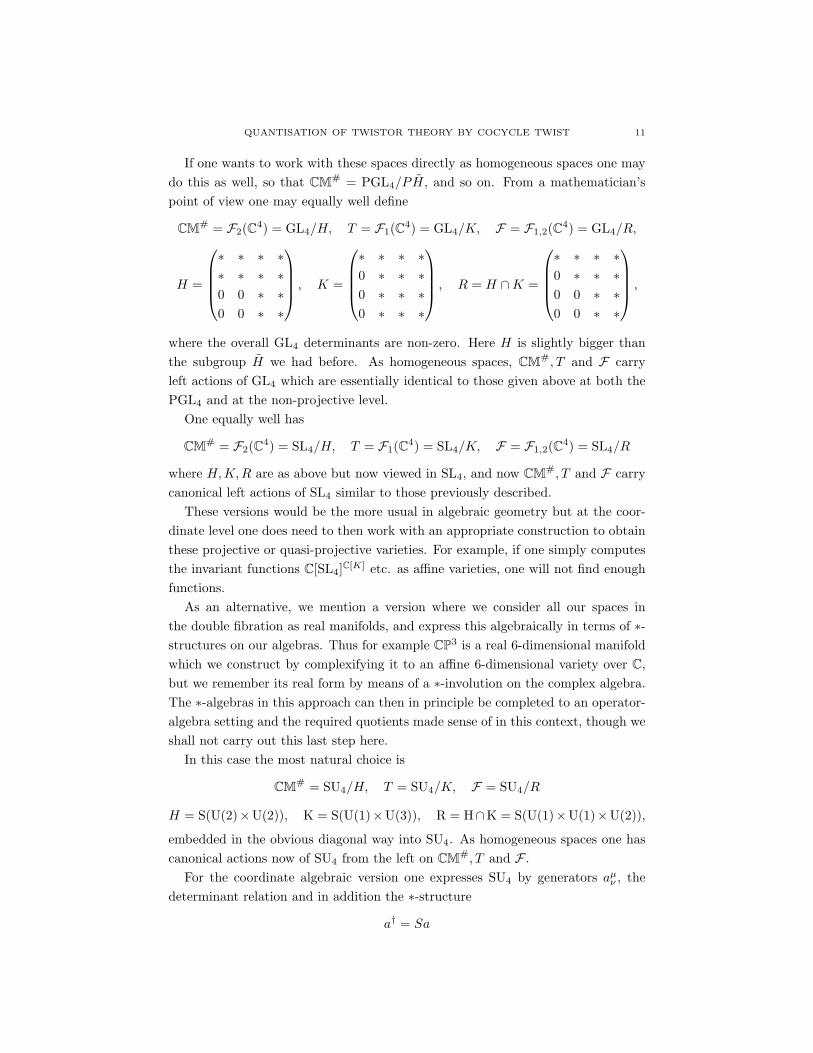
If one wants to work with these spaces directly as homogeneous spaces one maydo this as well, so that CM# = PGL4/PH, and so on. From a mathematician’spoint of view one may equally well define
CM# = F2(C4) = GL4/H, T = F1(C4) = GL4/K, F = F1,2(C4) = GL4/R,
H =
∗ ∗ ∗ ∗∗ ∗ ∗ ∗0 0 ∗ ∗0 0 ∗ ∗
, K =
∗ ∗ ∗ ∗0 ∗ ∗ ∗0 ∗ ∗ ∗0 ∗ ∗ ∗
, R = H ∩K =
∗ ∗ ∗ ∗0 ∗ ∗ ∗0 0 ∗ ∗0 0 ∗ ∗
,
where the overall GL4 determinants are non-zero. Here H is slightly bigger thanthe subgroup H we had before. As homogeneous spaces, CM#, T and F carryleft actions of GL4 which are essentially identical to those given above at both thePGL4 and at the non-projective level.
One equally well has
CM# = F2(C4) = SL4/H, T = F1(C4) = SL4/K, F = F1,2(C4) = SL4/R
where H,K,R are as above but now viewed in SL4, and now CM#, T and F carrycanonical left actions of SL4 similar to those previously described.
These versions would be the more usual in algebraic geometry but at the coor-dinate level one does need to then work with an appropriate construction to obtainthese projective or quasi-projective varieties. For example, if one simply computesthe invariant functions C[SL4]C[K] etc. as affine varieties, one will not find enoughfunctions.
As an alternative, we mention a version where we consider all our spaces inthe double fibration as real manifolds, and express this algebraically in terms of ∗-structures on our algebras. Thus for example CP3 is a real 6-dimensional manifoldwhich we construct by complexifying it to an affine 6-dimensional variety over C,but we remember its real form by means of a ∗-involution on the complex algebra.The ∗-algebras in this approach can then in principle be completed to an operator-algebra setting and the required quotients made sense of in this context, though weshall not carry out this last step here.
In this case the most natural choice is
CM# = SU4/H, T = SU4/K, F = SU4/R
H = S(U(2)×U(2)), K = S(U(1)×U(3)), R = H∩K = S(U(1)×U(1)×U(2)),
embedded in the obvious diagonal way into SU4. As homogeneous spaces one hascanonical actions now of SU4 from the left on CM#, T and F .
For the coordinate algebraic version one expresses SU4 by generators aµν , the
determinant relation and in addition the ∗-structure
a† = Sa
12 S.J. BRAIN AND S. MAJID
where † denotes transpose and ∗ on each matrix generator entry, (aµν )† = (aν
µ)∗,and S is the Hopf algebra antipode characterised by aS(a) = (Sa)a = id. This isas for any compact group or quantum group coordinate algebra. The coordinatealgebras of the subgroups are similarly defined as ∗-Hopf algebras.
There is also a natural ∗-structure on twistor space. To see this let us write itin the form
T = CP3 = Q ∈ M4(C), Q = Q†, Q2 = Q, Tr Q = 1
in terms of Hermitian-conjugation †. Thus CP3 is the space of Hermitian rankone projectors on C4. Such projectors can be written explicitly in the form Qµ
ν =ZµZν for some complex vector Z of modulus 1 and determined only up to a U(1)normalisation. Thus CP3 = S7/U(1) as a real 6-dimensional manifold. In thisdescription the left action of SU4 is given by conjugation in M4(C), i.e. by unitarytransformation of the Z and its inverse on Z. One can exhibit the identificationwith the homogeneous space picture, as the orbit of the projector diag(1, 0, 0, 0)(i.e. Z = (1, 0, 0, 0) = Z∗). The isotropy group of this is the intersection of SU4
with U(1)×U(3) as stated.The coordinate ∗-algebra version is
C[CP3] = C[Qµν ]/〈Q2 = Q, Tr Q = 1〉, Q = Q†
with the last equation now as a definition of the ∗-algebra structure via † = ( )∗t.We can also realise this as the degree zero subalgebra,
C[CP3] = C[S7]0, C[S7] = C[Zµ, Zν∗]/〈∑
µ
Zµ∗Zµ = 1〉,
where Z,Z∗ are two sets of generators related by the ∗-involution. The grading isgiven by deg(Z) = 1 and deg(Z∗) = −1, corresponding to the U(1) action on Z
and its inverse on Z∗. Finally, the left coaction is
∆L(Zµ) = aµα⊗Zα, ∆L(Zµ∗) = Saα
µ⊗Zα∗,
as required for a unitary coaction of a Hopf ∗-algebra on a ∗-algebra, as well as topreserve the relation.
We have similar ∗-algebra versions of F and CM# as well. Thus
C[CM#] = C[Pµν ]/〈P 2 = P, Tr P = 2〉, P = P †
in terms of a rank two projector matrix of generators, while
C[F ] = C[Qµν , Pµ
ν ]/〈Q2 = Q, P 2 = P, Tr Q = 1, Tr P = 2, PQ = Q = QP 〉
Q = Q†, P = P †.
We see that our ∗-algebra approach to flag varieties has a ‘quantum logic’ form. Inphysical terms, the fact that P,Q commute as matrices (or matrices of generatorsin the coordinate algebras) means that they may be jointly diagonalised, while
QUANTISATION OF TWISTOR THEORY BY COCYCLE TWIST 13
QP = Q says that the 1-eigenvectors of Q are a subset of the 1-eigenvectors ofP (equivalently, PQ = Q says that the 0-eigenvectors of P are a subset of the0-eigenvectors of Q). Thus the line which is the image of Q is contained in theplane which is the image of P : this is of course the defining property of pairs ofprojectors (Q, P ) ∈ F = F1,2(C4). Clearly this approach works for all flag varietiesFk1,···kr
(Cn) of k1 < · · · < kr-dimensional planes in Cn as the ∗-algebra with n×n
matrices Pi of generators
C[Fk1,···kr] = C[Pµ
i ν ; i = 1, · · · , r]/〈P 2i = Pi, Tr Pi = ki, PiPi+1 = Pi = Pi+1Pi, 〉
Pi = P †i .
In this setting all our algebras are now complex affine varieties (with ∗-structure)and we can expect to be able to work algebraically. Thus one may expect forexample that C[CP3] = C[SU4]C[S(U(1)×U(3))] (similarly for other flag varieties) andindeed we may identify the above generators and relations in the relevant invariantsubalgebra of C[SU4]. This is the same approach as was successfully used for theHopf fibration construction of CP1 = S2 = SU(2)/U(1) as C[SU2]C[U(1)], namely asC[SL2]C[C∗] with suitable ∗-algebra structures [13]. Note that one should not confusesuch Hopf algebra (‘GIT’) quotients with complex algebraic geometry quotients,which are more complicated to define and typically quasi-projective. Finally, weobserve that in this approach the tautological bundle of rank k over a flag varietyFk(Cn) appears tautologically as a matrix generator viewed as a projection P ∈Mn(C[Fk]). The classical picture is that the flag variety with this tautologicalbundle is universal for rank k vector bundles.
3.1. Tautological bundle on CM# and the instanton as its Grassmannconnection. Here we conclude with a result that is surely known to some, but ap-parently not well-known even at the classical level, and yet drops out very naturallyin our ∗-algebra approach. We show that the tautological bundle on CM# restrictsin a natural way to S4 ⊂ CM#, where it becomes the 1-instanton bundle, and forwhich the Grassmann connection associated to the projector is the 1-instanton.
We first explain the Grassmann connection for a projective module E over analgebra A. We suppose that E = Ane where e ∈ Mn(A) is a projection matrixacting on an A-valued row vector. Thus every element v ∈ E takes the form
v = v · e = vjej = (vk)ekjej ,
where ej = ej· ∈ An span E over A and vi ∈ A. The action of the Grassmannconnection is the exterior derivative on components followed by projection backdown to E :
∇v = ∇(v.e) = (d(v.e))e = ((dvj)ejk + vjdejk)ek = (dv + vde)e.
14 S.J. BRAIN AND S. MAJID
One readily checks that this is both well-defined and a connection in the sense that
∇(av) = da.v + a∇v, ∀a ∈ A, v ∈ E ,
and that its curvature operator F = ∇2 on sections is
F (v) = F (v.e) = (v.de.de).e
As a warm-up example we compute the Grassmann connection for the tautolog-ical bundle on A = C[CP1]. Here e = Q, the projection matrix of coordinates inour ∗-algebraic set-up:
e = Q =
(a z
z∗ 1− a
); a(1− a) = zz∗, a ∈ R, z ∈ C,
where s = a− 12 and z = x + ıy describes a usual sphere of radius 1/2 in Cartesian
coordinates (x, y, s). We note that
(1− 2a)da = dz.z∗ + zdz∗
allows to eliminate da in the open patch where a 6= 12 (i.e. if we delete the north
pole of S2). Then
de.de =
(da dz
dz∗ −da
)(da dz
dz∗ −da
)= dzdz∗
(1 − 2z
1−2a
− 2z∗
1−2a −1
)=
dzdz∗
1− 2a(1− 2e)
and henceF (v.e) = − dzdz∗
1− 2av.e.
In other words, F acts as a multiple of the identity operator on E = A2.e and thismultiple has the standard form for the charge 1 monopole connection if one convertsto usual Cartesian coordinates. We conclude that the Grassmann connection forthe tautological bundle on CP1 is the standard 1-monopole. This is surely well-known. The q-deformed version of this statement can be found in [7] providedone identifies the projector introduced there as the defining projection matrix ofgenerators for Cq[CP1] = Cq[SL2]C[t,t−1] as a ∗-algebra in the q-version of the abovepicture (the projector there obeys Trq(e) = 1 where we use the q-trace). Note that ifone looks for any algebra A containing potentially non-commuting elements a, z, z∗
and a projection e of the form above with Tr(e) = 1, one immediately finds thatthese elements commute and obey the sphere relation as above. If one performs thesame exercise with the q-trace, one finds exactly the four relations of the standardq-sphere as a ∗-algebra.
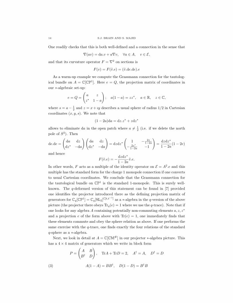
Next, we look in detail at A = C[CM#] in our projector ∗-algebra picture. Thishas a 4× 4 matrix of generators which we write in block form
P =
(A B
B† D
), TrA + TrD = 2, A† = A, D† = D
(3) A(1−A) = BB†, D(1−D) = B†B
QUANTISATION OF TWISTOR THEORY BY COCYCLE TWIST 15
(4) (A− 12)B + B(D − 1
2) = 0,
where we have written out the requirement that P be a Hermitian A-valued projec-tion without making any assumptions on the ∗-algebra A (so that these formulaealso apply to any noncommutative version of C[CM#] in our approach).
To proceed further, it is useful to write
A = a + α · σ, B = t + ıx · σ, B† = t∗ − ıx∗ · σ, D = 1− a + δ · σ
in terms of usual Pauli matrices σ1, σ2, σ3. We recall that these are traceless andHermitian, so a, α, δ are self-adjoint, whilst t, xi, i = 1, 2, 3 are not necessarily soand are subject to (3)-(4).
Proposition 3.1. The commutative ∗-algebra C[CM#] is defined by the above gen-erators a = a∗, α = α∗, δ = δ∗, t, t∗, x, x∗ and the relations
tt∗+xx∗ = a(1−a)−α.α, (1−2a)(α−δ) = 2ı(t∗x−tx∗), (1−2a)(α+δ) = 2ıx×x∗
α.α = δ.δ, (α + δ).x = 0, (α + δ)t = (α− δ)× x
Proof. This is a direct computation of (3)-(4) under the assumption that the gen-erators commute. Writing our matrices in the form above, equations (3) become
a(1− a)− α · α + (1− 2a)α · σ = tt∗ + x · σx∗ · σ + ı(xt∗ − tx∗) · σ
(1− a)a− δ · δ − (1− 2a)δ · σ = t∗t + x∗ · σx · σ + ı(t∗x− x∗t) · σ.
Taking the sum and difference of these equations and in each case the parts propor-tional to 1 (which is the same on both right hand sides) and the parts proportionalto σ (where the difference of the right hand sides is proportional to x × x∗) givesfour of the stated equations (all except those involving terms (α+δ)·x and (α+δ)t).We employ the key identity
σiσj = δij + ıεijkσk,
where ε with ε123 = 1 is the totally antisymmetric tensor used in the definition ofthe vector cross product. Meanwhile, (4) becomes
ıα.σx · σ + αt · σ + ıx · σδ · σ + tδ · σ = 0
after cancellations, and this supplies the remaining two relations using our keyidentity.
We see that in the open set where a 6= 12 we have α, δ fully determined by the
second and third relations, so the only free variables are the complex generators t, ~x,with a determined from the first equation. The complex affine variety generated bythe independent variables x, x∗, t, t∗ modulo the first three equations is reducible;the second ‘auxiliary’ line of equations makes CF [CM#] reducible (we conjecturethis).
16 S.J. BRAIN AND S. MAJID
Proposition 3.2. There is a natural ∗-algebra quotient C[S4] of C[CM#] definedby the additional relations x∗ = x, t∗ = t and α = δ = 0. The tautological projectorof C[CM#] becomes
e =
(a t + ıx · σ
t− ıx · σ 1− a
)∈ M2(C[S4]).
The Grassmann connection on the projective module E = C[S4]4e is the 1-instantonwith local form
(F ∧ F )(v.e) = −4!dtd3x
1− 2av.e
Proof. All relations in Proposition 3.1 are trivially satisfied in the quotient excepttt∗ + xx∗ = a(1 − a), which is that of a 4-sphere of radius 1
2 in usual Cartesiancoordinates (t, x, s) if we set s = a − 1
2 . The image e of the projector exhibitsS4 ⊂ CM# as a projective variety in our ∗-algebra projector approach. We interpretthis as providing a projective module over C[S4], the pull-back of the tautologicalbundle on CM# from a geometrical point of view. To compute the curvature of itsGrassmann connection we first note that
dx · σdx · σ = ı(dx× dx) · σ, (dx× dx) · (dx× dx) = 0,
(dx× dx)× (dx× dx) = dx× (dx× dx) = 0, dx · (dx× dx) = 3!d3x,
since 1-forms anticommute and since any four products of the dxi vanish. Now wehave
dede =
(da dt + ıdx · σ
dt− ıdx · σ −da
)(da dt + ıdx · σ
dt− ıdx · σ −da
)
=
(−2ıdtdx · σ + ıdx× dx · σ 2dadt + 2ıdadx · σ−2dadt + 2ıdadx · σ 2ıdtdx · σ + ıdx× dx · σ
)and we square this matrix to find that
(de)4 =
(1 − 2
1−2a (t + ıx · σ)− 2
1−2a (t− ıx · σ) −1
)4!dtd3x =
1− 2e
1− 2a4!dtd3x
after substantial computation. For example, since (da)2 = 0, the 1-1 entry is
−(dx×dx−2dtdx).σ(dx×dx−2dtdx)·σ = 2dtdx·(dx×dx)+2(dx×dx)·dtdx = 4!dtd3x
where only the cross-terms contribute on account of the second observation aboveand the fact that (dt)2 = 0. For the 1-2 entry we have similarly that
2ıda(dx× dx− 2dtdx) · σ(dt + ıdx · σ) + 2ıda(dt + ıdx · σ)(dx× dx + 2dtdx) · σ
= 12ıdadt(dx× dx) · σ − 4da(dx× dx) · σdx · σ
= − 241− 2a
2ıx · σdtd3x− 81− 2a
t3!dtd3x = − 21− 2a
(t + ıx · σ)4!dtd3x,
QUANTISATION OF TWISTOR THEORY BY COCYCLE TWIST 17
where at the end we substitute
da =2(tdt + x · dx)
1− 2a
and note that
x · dx(dx× dx) = xidxiεjkmdxjdxk = 2xmd3x,
since in the sum over i only i = m can contribute for a nonzero 3-form. The 2-2and 2-1 entries are analogous and left to the reader. We conclude that (de)4e actson C[S4]4 from the right as a multiple of the identity as stated.
One may check that F = dede.e is anti-self-dual with respect to the usual Eu-clidean Hodge ∗-operator. Note also that the off-diagonal corners of e are preciselya general quaternion q = t + ıx · σ and its conjugate, which relates our approach tothe more conventional point of view on the 1-instanton. However, that is not ourstarting point as we come from CM#, where the top right corner is a general 2× 2matrix B and the bottom left corner its adjoint.
If instead we let B be an arbitrary Hermitian matrix in the form
B = t + x · σ
(i.e. replace ıx above by x and let t∗ = t, x∗ = x) then the quotient t∗ = t, x∗ =x, α = −δ = 2tx/(1− 2a) gives us
s2 + t2 + (1 +t2
s2)x2 =
14
when s = a− 12 6= 0 and txi = 0, t2+x2+α2 = 1
4 when s = 0. We can also approachthis case directly from (3)-(4). We have to find Hermitian A,D, or equivalentlyS = A − 1
2 , T = D − 12 with Tr(S + T ) = 0 and S2 = T 2 = 1
4 − B2. Since B isHermitian it has real eigenvalues and indeed after conjugation we can rotate x to|x| times a vector in the 3-direction, i.e. B has eigenvalues t ± |x|. It follows thatsquare roots S, T exist precisely when
(5) |t|+ |x| ≤ 12
and are diagonal in the same basis as was B, hence they necessarily commute withB. In this case (4) becomes that (S + T ).B = 0. If B has two nonzero eigenvaluesthen S + T = 0. If B has one nonzero eigenvalue then S + T has a zero eigenvalue,but the trace condition then again implies S+T = 0. If B = 0 our equations reduceto those for two self-adjoint 2× 2 projectors A,D with traces summing to two. Insummary, if B 6= 0 there exists a projector of the form required if and only if (t, x)lies in the diamond region (5), with S = T and a fourfold choice (the choice ofroot for each eigenvalue) of S in the interior. These observations about the moduliof projectors with B Hermitian means that the corresponding quotient of C[CM#]is a fourfold cover of a diamond region in affine Minkowski space-time (viewed asthe space of 2 × 2 Hermitian matrices). The diamond is conformally equivalent
18 S.J. BRAIN AND S. MAJID
to a compactification of all of usual Minkowski space (the Penrose diagram forMinkowski space), while its fourfold covering reminds us of the Penrose diagramfor a black-white hole pair. It is the analogue of the disk that one obtains byprojecting S4 onto its first two coordinates. One may in principle compute theconnection associated to the pull-back of the tautological bundle to this regionas well as the 4-dimensional object of which it is a projection. The most naturalversion of this is to slightly change the problem to two 2×2 Hermitian matrices S, B
with S2 + B2 = 14 (a ‘matrix circle’), a variety which will be described elsewhere.
Note also that in both cases D = 1−A and if we suppose this at the outset ourequations including (4) and (3) simplify to
(6) [A,B] = [B,B†] = 0, A(1−A) = BB†, A = A†.
In fact this is the same calculation as for any potentially noncommutative CP1
which (if we use the usual trace) is forced to be commutative as mentioned above.Finally, returning to the general case of C[CM#], we have emphasised ‘Cartesian
coordinates’ with different signatures. From a twistor point of view it is morenatural to work with the four matrix entries of B as the natural twistor coordinates.This will also be key when we quantise. Thus equivalently to Proposition 3.1 wewrite
(7) B =
(z w
w z
), A =
(a + α3 α
α∗ a− α3
), D =
(1− a + δ3 δ
δ∗ 1− a− δ3
),
where a = a∗, α3 = α∗3, δ3 = δ∗3 as before but all our other notations are different.
In particular, α, α∗, δ, δ∗, z, z∗, w, w∗, z, z∗, w, w∗ are now complex generators.
Corollary 3.3. The relations of C[CM#] in these new notations appear as
zz∗ + ww∗ + zz∗ + ww∗ = 2(a(1− a)− αα∗ − α23)
(1− 2a)α = zw∗ + wz∗, (1− 2a)δ = −z∗w − zw∗
(1− 2a)(α3 + δ3) = ww∗ − ww∗, (1− 2a)(α3 − δ3) = zz∗ − zz∗
and the auxiliary relations
αα∗ + α23 = δδ∗ + δ2
3
(α3 + δ3)
(z
z
)=
(−α −δ∗
δ α∗
)(w
w
), (α3 − δ3)
(w
w
)=
(−α∗ −δ∗
δ α
)(z
z
).
Moreover, S4 ⊂ CM# appears as the ∗-algebra quotient C[S4] defined by w∗ = −w,z∗ = z and α = δ = 0.
Proof. It is actually easier to recompute these, but of course this is just a changeof generators from the equations in Proposition 3.1.
Note that these affine ∗-algebra coordinates are more similar in spirit but notthe same as those for CM# as a projective quadric in Section 1.
QUANTISATION OF TWISTOR THEORY BY COCYCLE TWIST 19
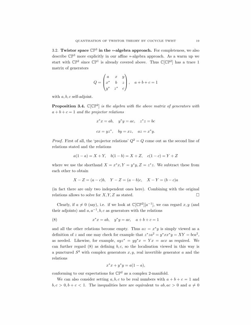
3.2. Twistor space CP3 in the ∗-algebra approach. For completeness, we alsodescribe CP3 more explicitly in our affine ∗-algebra approach. As a warm up westart with CP2 since CP1 is already covered above. Thus C[CP2] has a trace 1matrix of generators
Q =
a x y
x∗ b z
y∗ z∗ c
, a + b + c = 1
with a, b, c self-adjoint.
Proposition 3.4. C[CP2] is the algebra with the above matrix of generators witha + b + c = 1 and the projector relations
x∗x = ab, y∗y = ac, z∗z = bc
cx = yz∗, by = xz, az = x∗y.
Proof. First of all, the ‘projector relations’ Q2 = Q come out as the second line ofrelations stated and the relations
a(1− a) = X + Y, b(1− b) = X + Z, c(1− c) = Y + Z
where we use the shorthand X = x∗x, Y = y∗y, Z = z∗z. We subtract these fromeach other to obtain
X − Z = (a− c)b, Y − Z = (a− b)c, X − Y = (b− c)a
(in fact there are only two independent ones here). Combining with the originalrelations allows to solve for X, Y, Z as stated.
Clearly, if a 6= 0 (say), i.e. if we look at C[CP2][a−1], we can regard x, y (andtheir adjoints) and a, a−1, b, c as generators with the relations
(8) x∗x = ab, y∗y = ac, a + b + c = 1
and all the other relations become empty. Thus az = x∗y is simply viewed as adefinition of z and one may check for example that z∗za2 = y∗xx∗y = XY = bca2,as needed. Likewise, for example, ayz∗ = yy∗x = Y x = acx as required. Wecan further regard (8) as defining b, c, so the localisation viewed in this way isa punctured S4 with complex generators x, y, real invertible generator a and therelations
x∗x + y∗y = a(1− a),
conforming to our expectations for CP2 as a complex 2-manifold.We can also consider setting a, b, c to be real numbers with a + b + c = 1 and
b, c > 0, b + c < 1. The inequalities here are equivalent to ab, ac > 0 and a 6= 0
20 S.J. BRAIN AND S. MAJID
(with a > 0 necessarily following since if a < 0 we would need b, c < 0 and hencea + b + c < 0, which is not allowed). We then have
C[CP2]| b,c>0b+c<1
= C[S1 × S1],
so the passage to this quotient algebra is geometrically an inclusion S1×S1 ⊂ CP2
with (8) defining the two circles (recall that x, y are complex generators). As theparameters vary the circles vary in size so the general case with a inverted can beviewed in that sense as an inclusion C∗ × C∗ ⊂ CP2. This holds classically as anopen dense subset (since CP2 is a toric variety). We have the same situation forC[CP1] where there is only one relation x∗x = a(1 − a), i.e. circles S1 ⊂ CP1 ofdifferent size as 0 < a < 1. They are the circles of constant latitude and as a
varies in this range they map out C∗ (viewed as S2 with the north and south poleremoved).
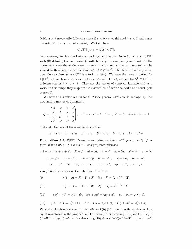
We now find similar results for CP3 (the general CPn case is analogous). Wenow have a matrix of generators
Q =
a x y z
x∗ b w v
y∗ w∗ c u
z∗ v∗ u∗ d
, a∗ = a, b∗ = b, c∗ = c, d∗ = d, a + b + c + d = 1
and make free use of the shorthand notation
X = x∗x, Y = y∗y, Z = z∗z, U = u∗u, V = v∗u , W = w∗w.
Proposition 3.5. C[CP3] is the commutative ∗-algebra with generators Q of theform above with a + b + c + d = 1 and projector relations
a(1− a) = X + Y + Z, X −U = ab− cd, Y − V = ac− bd, Z −W = ad− bc,
au = y∗z, av = x∗z, aw = x∗y, bu = w∗v, cv = wu, dw = vu∗,
cx = yw∗, by = xw, bz = xv, dx = zv∗, dy = zu∗, cz = yu.
Proof. We first write out the relations P 2 = P as
(9) a(1− a) = X + Y + Z, b(1− b) = X + V + W,
(10) c(1− c) = Y + U + W, d(1− d) = Z + U + V,
(11) yw∗ + zv∗ = x(c + d), xw + zu∗ = y(b + d), xv + yu = z(b + c),
(12) y∗z + w∗v = u(a + b), x∗z + wu = v(a + c), x∗y + vu∗ = w(a + d).
We add and subtract several combinations of (9)-(10) to obtain the equivalent fourequations stated in the proposition. For example, subtracting (9) gives (Y − V ) +(Z−W ) = (c+d)(a−b) while subtracting (10) gives (Y −V )−(Z−W ) = (c−d)(a+b)
QUANTISATION OF TWISTOR THEORY BY COCYCLE TWIST 21
and combining these gives the Y − V and Z − W relations stated. Similarly, forthe X − U relation. We can also write our three equations as
(13) (a+ c)(a+d)+X−U = (a+ b)(a+d)+Y −V = (a+ b)(a+ c)+Z−W = a
using a + b + c + d = 1.Next, we compute (12) assuming (11), for example
(a + b)(a + c)u = (a + c)(y∗z + w∗v) = (a + c)y∗z + w∗(x∗z + wu)
= (a + c)y∗z + Wu + (y∗(b + d)− uz∗)z = y∗z + (W − Z)u
which, using (13), becomes au = y∗z. We similarly obtain av = x∗z, aw = x∗y.Given these relations, clearly (12) is equivalent to the next three stated equations,which completes the first six equations of this type. Similarly for the remainingsix.
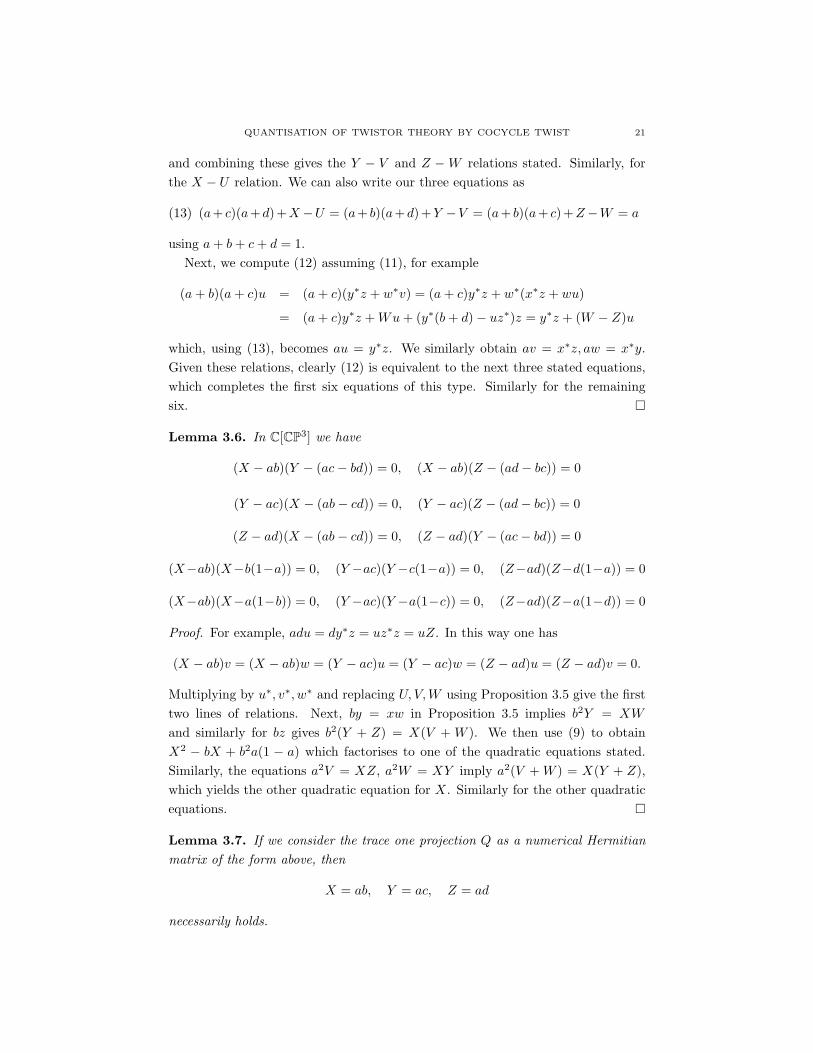
Lemma 3.6. In C[CP3] we have
(X − ab)(Y − (ac− bd)) = 0, (X − ab)(Z − (ad− bc)) = 0
(Y − ac)(X − (ab− cd)) = 0, (Y − ac)(Z − (ad− bc)) = 0
(Z − ad)(X − (ab− cd)) = 0, (Z − ad)(Y − (ac− bd)) = 0
(X−ab)(X−b(1−a)) = 0, (Y −ac)(Y −c(1−a)) = 0, (Z−ad)(Z−d(1−a)) = 0
(X−ab)(X−a(1−b)) = 0, (Y −ac)(Y −a(1−c)) = 0, (Z−ad)(Z−a(1−d)) = 0
Proof. For example, adu = dy∗z = uz∗z = uZ. In this way one has
(X − ab)v = (X − ab)w = (Y − ac)u = (Y − ac)w = (Z − ad)u = (Z − ad)v = 0.
Multiplying by u∗, v∗, w∗ and replacing U, V,W using Proposition 3.5 give the firsttwo lines of relations. Next, by = xw in Proposition 3.5 implies b2Y = XW
and similarly for bz gives b2(Y + Z) = X(V + W ). We then use (9) to obtainX2 − bX + b2a(1 − a) which factorises to one of the quadratic equations stated.Similarly, the equations a2V = XZ, a2W = XY imply a2(V + W ) = X(Y + Z),which yields the other quadratic equation for X. Similarly for the other quadraticequations.
Lemma 3.7. If we consider the trace one projection Q as a numerical Hermitianmatrix of the form above, then
X = ab, Y = ac, Z = ad
necessarily holds.
22 S.J. BRAIN AND S. MAJID
Proof. We use the preceding lemma but regarded as for real numbers (equivalentlyone can assume that our algebra has no zero divisors). Suppose without loss ofgenerality that X 6= ab. Then by the lemma, V = W = 0 or Y = ac − bd,Z = ad − bc. We also have v = w = 0 and hence from Proposition 3.5 thatx∗z = x∗y = 0. We can also deduce from the quadratic equations of X that a = b
and X = a(1 − a) or U = a(1 − 2a) + cd. We distinguish two cases: (i) x = 0 inwhich case a = b = 0 (since X = a(1 − a) 6= ab = a2) and (ii) x 6= 0, y = z = 0,in which case a = b 6= 0, 1, c + d = 0. In either case since b 6= 1 we have Y 6= ac
and Z 6= ad, hence X = ab− cd or U = 0, u = 0 and hence y∗z = 0 while c, d 6= 0.This means that at most one of x, y, z is non-zero. We can now go through all ofthe subcases and find a contradiction in every case. Similar arguments prove thatY = ac, Z = ad.
Let us denote by C−[CP3] the quotient of C[CP3] by the relations in the lemma.We call it the ‘regular form’ of the coordinate algebra for CP3 in our ∗-algebraicapproach and will work with it henceforth. The lemma means that there is nodiscernible difference (if any) between the ∗-algebras C−[CP3] and C[CP3] in thesense that if we were looking at CP3 as a set of projector matrices and the abovevariables as real or complex numbers, we would not see any distinction. (As long asthe relevant intersections are transverse the same would then be true in the algebrasalso, but it is beyond our scope to prove this here.) Moreover, if either x, y, z oru, v, w are made invertible then one can show that the solution in the lemma indeedholds and does not need to be imposed, i.e. C[CP3] and C−[CP3] have the samelocalisations in this respect.
Proposition 3.8. C−[CP3] can be viewed as having generators a, b, c, x, y, z witha + b + c + d = 1 and the relations
X = ab, Y = ac, Z = ad
as well as auxiliary generators u, v, w and auxiliary relations
U = cd, V = bd, W = bc,
au = y∗z, av = x∗z aw = x∗y, bu = w∗v, cv = wu, dw = vu∗,
cx = yw∗, by = xw, bz = xv, dx = zv∗, dy = zu∗, cz = yu.
If a 6= 0 these auxiliary variables and equations are redundant.
Proof. If a 6= 0 (i.e. if we work in the algebra with a−1 adjoined) we regard threeof the auxiliary equations as a definition of u, v, w. We then verify that the otherequations hold automatically. The first line is clear since these equations timesa2 were solved in the lemma above. For example, from the next line we havea2w∗v = y∗xx∗z = Xy∗z = aby∗z = a2bu, as required. Similarly a(yw∗ + zv∗) =yy∗x + zz∗x = (Y + Z)x = a(c + d)x as required.
QUANTISATION OF TWISTOR THEORY BY COCYCLE TWIST 23
From this we see that the ‘patch’ given by inverting a is described by just threeindependent complex variables x, y, z and one invertible real variable a with thesingle relation
x∗x + y∗y + z∗z = a(1− a)
(the relations stated can be viewed as a definition of b, c, d but we still need a+ b+c + d = 1), in other words a punctured S6 where the point x = y = z = a = 0 isdeleted. This conforms to our expectations for CP3 as a complex 3-manifold or real6-manifold. Of course, our original projector system was symmetric and we couldhave equally well analysed and presented our algebra in a form adapted to one ofb, c, d 6= 0.
Finally, we also see that if we set a, b, c, d to actual real values with a+b+c+d = 1and b, c, d > 0, b + c + d < 1 (the inequalities here are equivalent to a 6= 0 andab, ac, ad > 0) then
C−[CP3]| b,c,d>0b+c+d<1
= C[S1 × S1 × S1]
for three circles x∗x = ab, y∗y = ac, z∗z = ad and no further relations. This is theanalogue in our ∗-algebra approach of inclusions S1 × S1 × S1 ⊂ CP3 and as thecircles vary in radius we have part of the fact in the usual picture that CP3 is atoric variety (namely that C∗ × C∗ × C∗ ⊂ CP3 is open dense).
We now relate this description of twistor space to the space-time algebras inthe previous section. In particular, we note that classically there is a fibration oftwistor space over the Euclidean four-sphere, CP3 → S4, whose fibre is CP1 (see forexample [20]). This fibration arises through the observation that each α-plane inCM# intersects S4 at a unique point (essentially because there are no null lines inEuclidean signature). The double fibration (2) thus collapses to a single fibrationCP3 → S4 (making the twistor theory of the real space-time S4 much easier to studythan that of its complex counterpart). To see this we make use of the followingnondegenerate antilinear involution on C4,
J(Z) = J(Z1, Z2, Z3, Z4) := (−Z2, Z1,−Z4, Z3).
Once again we recall that points of twistor space are one-dimensional subspaces ofC4, whereas points of CM# are two-dimensional subspaces. Of course, given a 1dsubspace (spanned by Z ∈ C4), there are many 2d subspaces in which it lies, andthese constitute exactly the set Z = CP2. However, the involution J serves to pickout a unique such 2d subspace, the one spanned by Z and J(Z).
Now recall our ‘quantum logic’ interpretation of the correspondence space F , aspairs of projectors (Q,P ) on C4 with Q of rank one and P of rank two such thatQP = Q = PQ. Then since we have
CP3 = S7/U(1), S7 = Zµ, Zν |∑
ZµZµ = 1,
24 S.J. BRAIN AND S. MAJID
the involution J extends to one on CP3, given by
J(Qµν) = J(ZµZν) = J(Zν)J(Zµ).
At the level of the coordinate algebra C−[CP3] we have the following interpretation.
Lemma 3.9. There is an antilinear involution J : C−[CP3] → C−[CP3], given inthe notation of Proposition 3.8 by
J(a) = b, J(b) = a, J(c) = 1− (a + b + c),
J(x) = −x, J(y) = v∗, J(z) = −w∗, J(u) = −u, J(v) = y∗, J(w) = −z∗,
Proof. This is by direct computation, noting that if we write
Q =
Z1Z1 Z1Z2 Z1Z3 Z1Z4
Z2Z1 Z2Z2 Z2Z3 Z2Z4
Z3Z1 Z3Z2 Z3Z3 Z3Z4
Z4Z1 Z4Z2 Z4Z3 Z4Z4
, TrQ = 1,
we see that
J(Q) =
Z2Z2 −Z1Z2 Z4Z2 −Z3Z2
−Z2Z1 Z1Z1 −Z4Z1 Z3Z1
Z2Z4 −Z1Z4 Z4Z4 −Z3Z4
−Z2Z3 Z1Z3 −Z4Z3 Z3Z3
, Tr J(Q) = TrQ = 1,
and the result follows by comparing with the notation of Proposition 3.8. In par-ticular we see that J(X) = X and J(U) = U . The relations of Proposition 3.5indicate that J extends to the full algebra as an antialgebra map (indeed this needsto be the case for J to be well-defined), since then we have
J(au) = J(u)J(a) = −ub = −bu = −w∗v = J(z)J(y∗) = J(y∗z),
similarly for the remaining relations.
We remark that since the algebra is commutative here, we may treat J as analgebra map rather than as an antialgebra map as required in the notion of anantilinear involution. This will no longer be the case when we come to quantise,when it is the notion of antilinear involution that will survive.
Now J extends further to an involution on CM#: given P ∈ CM# we writeP = Q + Q′ for Q,Q′ ∈ CP3 and define
J(P ) := J(Q) + J(Q′).
Indeed, we note that the 1d subspaces defined by a pair of rank one projectorsQ1, Q2 are distinct if and only if Q1Q2 = Q2Q1 = 0, and it is easily checked thatthis is equivalent to the condition that J(Q1)J(Q2) = J(Q2)J(Q1) = 0 (computedeither by direct calculation with matrices or by working with vectors Z1, Z2 ∈ C4
which define Q1, Q2 up to scale and using the inner product on C4 induced by
QUANTISATION OF TWISTOR THEORY BY COCYCLE TWIST 25
J). Thus if P is a rank two projector with P = Q1 + Q′1 = Q2 + Q′
2, then if Q1,Q2 are distinct, so are J(Q1), J(Q2). Elementary linear algebra then tells us thatJ(Q1) + J(Q′
1) and J(Q2) + J(Q′2) must define the same projector J(P ), i.e. the
map J is well-defined on CM#.
Proposition 3.10. P ∈ CM# is invariant under J if and only if P ∈ S4.
Proof. Writing Q′ = (WµW ν), we have that
P = Q + Q′ = (ZµZν + WµW ν),
and that this supposed to be identified with the 2× 2 block decomposition
P =
(A B
B† D
), A = A†, D = D†, TrA + TrD = 2.
Here we shall use the notation of Proposition 3.1. Examining A, we have
A = a + α · σ =
(Z1Z1 + W 1W 1 Z1Z2 + Z2Z1
Z2Z1 + Z1Z2 Z2Z2 + W 2W 2
),
and hence an identification
a =12(Z1Z1 + Z2Z2 + W 1W 1 + W 2W 2),
α3 =12(Z1Z1 − Z2Z2 + W 1W 1 − W 2W 2),
as well as the off-diagonal entries
α1 =12(Z1Z2 − Z2Z1 + W 1W 2 − W 2W 1),
α2 =12ı
(Z1Z2 + Z2Z1 + W 1W 2 + W 2W 1).
Clearly the relations a = a∗, α = α∗ hold under this identification. Under theinvolution J we calculate that
J(a) = a, J(α) = −α.
Similarly we look at the block D,
D = d + δ · σ =
(Z3Z3 + W 3W 3 Z3Z4 + W 3W 4
Z4Z3 + W 4W 3 Z4Z4 + W 4W 4
).
The same computation as above shows that the relations d = d∗, δ = δ∗ hold here,and moreover the trace relation implies that d = 1− a, in agreement with Section3.1. Under the involution J we also see that
J(d) = d, J(δ) = −δ.
Finally we look at the matrix B,
B = t + ıx · σ =
(Z1Z3 + W 1W 3 Z1Z4 + W 1W 4
Z2Z3 + W 2W 3 Z2Z4 + W 2W 4
).
26 S.J. BRAIN AND S. MAJID
Solving, we have the identification of generators
t =12(Z1Z3 + Z2Z4 + W 1W 3 + W 2W 4),
x3 =12ı
(Z1Z3 − Z2Z4 + W 1W 3 − W 2W 4)
for the diagonal entries, as well as
x1 =12ı
(Z2Z3 + Z1Z4 + W 2W 3 + W 1W 4),
x2 =12(Z2Z3 − Z1Z4 + W 2W 3 − W 1W 4)
on the off-diagonal. This is in agreement with the fact as in Proposition 3.1 thatthe generators t, x are not necessarily Hermitian. Moreover, it is a simple matterto compute that under the involution J we have
J(t) = t∗, J(x) = x∗.
Overall, we see that J has fixed points in CM# consisting of those with coordinatessubject to the additional constraints α = δ = 0, t = t∗, x = x∗. Thus (uponverification of the extra relations) the fixed points of CM# under J are exactlythose lying in S4, in accordance with proposition 3.2.
In the notation of Proposition 3.3, the action of J on C[CM#] is to map
J(a) = a, J(α3) = α3, J(δ3) = δ3, J(α) = −α, J(δ) = −δ,
J(w) = −w∗, J(z) = z∗, J(w) = −w∗, J(z) = z∗.
This may either be recomputed, or obtained simply by making the same changeof variables as was made in going from Proposition 3.1 to Proposition 3.3. Thefixed points in these coordinates are those with α = δ = 0, w∗ = −w, z∗ = z, inagreement with Proposition 3.3.
Proposition 3.11. For each P ∈ CM# we have P ∈ S4 if and only if there existsQ ∈ CP3 such that P = Q + J(Q).
Proof. By the previous proposition, P ∈ S4 if and only if J(P ) = P . Of course,the reverse direction of the claim is easy, since if P = Q + J(Q), we have J(P ) =J(Q) + J2(Q) = P . Conversely, given P ∈ S4 with J(P ) = P we may writeP = Q + Q′ for some Q, Q′ ∈ CP3 (as remarked already, this is not a uniquedecomposition but given Q we have Q′ = P −Q, and J acts independently of thisdecomposition). The result is now obvious since J is nondegenerate, so Q′ = J(Q′′)for some Q′′, but we must have Q′′ = Q since J is an involution.
As promised, there is a fibration of CP3 over S4 given at the coordinate alge-bra level by an inclusion C[S4] → C−[CP3]. In terms of the C−[CP3] coordinates
QUANTISATION OF TWISTOR THEORY BY COCYCLE TWIST 27
a, b, c, x, y, z used in Proposition 3.8 and the C[S4] coordinates z, w, a of Propo-sition 3.3 we have the following (we note the overlap in notation between thesepropositions and rely on the context for clarity).
Proposition 3.12. There is an algebra inclusion
η : C[S4] → C−[CP3]
given byη(a) = a + b, η(z) = y + v∗, η(w) = w − z∗.
Proof. That this is an algebra map is a matter of rewriting the previous propositionin our explicit coordinates, for example that η(z) = y + v∗ = y + J(y). The solerelation to investigate is the image of the sphere relation zz∗ + ww∗ = a(1 − a).Applying η to the left hand side, we obtain
η(zz∗ + ww∗) = yy∗ + yv + v∗y∗ + v∗v + ww∗ − wz − z∗w∗ + z∗z.
Now using the relations of Proposition 3.5 we compute that
ayv = yav = yx∗z = x∗yz = awz,
where we have relied upon the commutativity of the algebra. Similarly one com-putes that byv = bwz, cyv = cwz, dyv = dwz, so that adding these four relationsyields that yv = wz in C−[CP3]. Then finally using the relations in Proposition 3.8we see that
η(zz∗+ww∗) = Y +V +W +Z = (a+b)(c+d) = (a+b)(1− (a+b)) = η(a(1−a)),
as required.
We now look at the typical fibre CP1 of the fibration CP3 → S4, but now in thecoordinate algebra picture.
Proposition 3.13. The quotient of the algebra C−[CP3] obtained by setting η(a),η(z), η(w) to be constant numerical values is isomorphic to the coordinate algebraof a CP1.
Proof. If we suppose that we are in the patch where a 6= 0 in C−[CP3] then we canview x, y, z as the variables and X = ab, Y = ac, Z = ad as the relations. Thegenerators u, v, w are defined by the equations in Proposition 3.8 and the rest areredundant.
Now suppose that a + b = A, a fixed real number, and y + v∗ = B, w − z∗ = C,fixed complex numbers, such that
BB∗ + CC∗ = A(1−A)
(an element of S4). Then we have just one equation
X = a(A− a) = (A/2)2 − s2
28 S.J. BRAIN AND S. MAJID
if we set s = a−A/2. This is a CP1 of radius A/2 in place of the usual radius 1/2.The equation Y = ac is viewed as a definition of c. The equation Z = ad is then
equivalent to Y + Z = a(1−A). We’ll see that this is automatic and that y, z areuniquely determined by x, a and our fixed parameters A,B,C so are not in fact freevariables.
Indeed, av = x∗z and aw = x∗y determine v and w as mentioned above, so ourquotient is
aB = ay + z∗x, aC = x∗y − az∗,
which implies that a2(BB∗ + CC∗) = (a2 + X)(Y + Z) = aA(Y + Z), so Y + Z =a(1−A) necessarily holds if A, B, C lie in S4.
We also combine the equations to find ax∗B = a2C+z∗aA and aCx = aAy−a2B
so that at least if A 6= 0 we have z,y determined. (In fact one has By∗ − z∗C =a(1−A) from the above so if z is determined then so is y if B is not zero etc). ThusC[CP1] is viewed inside C[CP3] in this patch as
(14)
a x
x∗ A− a∗
∗ ∗
, x∗x = a(A− a),
where the unspecified entries are determined as above using the relations in termsof x and a.
Similar analysis holds in the other coordinate patches, although we shall notcheck this here as this is a well-known classical result. In other patches we wouldsee the various copies of C[CP1] appearing elsewhere in the above matrix.
This situation now provides us with yet another way to view the instanton bun-dle. Let M be a finite rank projective C[CM#]-module. Then J induces a modulemap J : M → M whose fixed point submodule is a finite rank projective C[S4]-module. In particular, if we takeM to be the C[CM#]-module given by the definingtautological projector (7), then as explained above as well as in that section, thefixed point submodule is precisely the tautological bundle E = C[S4]4e of Proposi-tion 3.2 which defines the instanton bundle over S4.
Now the map η : C[S4] → C−[CP3] induces the ‘push-out’ of the C[S4]-module Ealong η to obtain an ‘auxiliary’ C−[CP3]-module E , given by viewing the projectore ∈ M4(C[S4]) as a projector e ∈ M4(C−[CP3]), so that E := C−[CP3]4e, giving a
QUANTISATION OF TWISTOR THEORY BY COCYCLE TWIST 29
bundle over twistor space. Explicitly, we have
e =
η(a) 0 η(z) η(−w∗)
0 η(a) η(w) η(z∗)η(z∗) η(w∗) η(1− a) 0η(−w) η(z) 0 η(1− a)
=
a + b 0 y + v∗ z − w∗
0 a + b w − z∗ y∗ + v
y∗ + v w∗ − z 1− (a + b) 0z∗ − w y + v∗ 0 1− (a + b)
∈ M4(C−[CP3]).
Moreover, if one sets a + b = A, y + v∗ = B, w − z∗ = C for fixed real A andcomplex B, C as in Proposition 3.13, then we have
e =
A 0 B −C∗
0 A C B∗
B∗ C∗ 1−A 0−C B 0 1−A
,
a constant projector of rank two. Then viewing the fibre C[CP1] as a subset ofC[CP3] as in (14), it is easily seen that C[CP1]4e is a free C[CP1]-module of rank two.This is just the coordinate algebra version of saying that for all x = (A,B,C) ∈ S4
the instanton bundle pulled back from S4 to CP3 is trivial upon restriction to eachfibre x = CP1, and we may thus see the instanton bundle E over C[S4] as comingfrom the bundle E over twistor space. This is an easy example of the Penrose-Wardtransform, which we shall discuss in more detail later.
4. The Quantum Conformal Group
The advantage of writing space-time and twistor space as homogeneous spaces inthe language of coordinate functions is that we are now free to apply the standardtheory of quantisation by a cocycle twist.
To this end, we recall that if H is a Hopf algebra with coproduct ∆ : H → H⊗H,counit ε : H → C and antipode S : H → H, then a two-cocycle F on H meansF : H ⊗H → C which is convolution invertible and unital (i.e. a 2-cochain) in thesense
F (h(1), g(1))F−1(h(2), g(2)) = F−1(h(1), g(1))F (h(2), g(2)) = ε(h)ε(g)
(for some map F−1) and obeys ∂F = 1 in the sense
F (g(1), f (1))F (h(1), g(1)f (2))F−1(h(2)g(3), f (3))F−1(h(3), g(4)) = ε(f)ε(h)ε(g).
We have used Sweedler notation ∆(h) = h(1)⊗h(2) and suppressed the summation.In this case there is a ‘cotwisted’ Hopf algebra HF with the same coalgebra structure
30 S.J. BRAIN AND S. MAJID
and counit as H but with modified product • and antipode SF [11]
(15) h • g = F (h(1) ⊗ g(1)) h(2)g(2) F−1(h(3) ⊗ g(3))
SF (h) = U(h(1))Sh(2)U−1(h(2)), U(h) = F (h(1), Sh(2))
for h, g ∈ H, where we use the product and antipode of H on the right hand sidesand U−1(h(1))U(h(2)) = ε(h) = U(h(1))U−1(h(2)) defines the inverse functional. If H
is a coquastriangular Hopf algebra then so is HF . In particular, if H is commutativethen HF is cotriangular with ’universal R-matrix’ and induced (symmetric) braidinggiven by
R(h, g) = F (g(1), h(1))F−1(h(2), g(2)), ΨV,W (v⊗w) = R(w(1), v(1))w(2)⊗v(2)
for any two left comodules V,W . We use the Sweedler notation for the left coactionsas well. In the cotriangular case one has Ψ2 = id, so every object on the categoryof HF -comodules inherits nontrivial statistics in which transposition is replaced bythis non-standard transposition.
The nice property of this construction is that the category of H-comodules isactually equivalent to that of HF -comodules, so there is an invertible functor which‘functorially quantises’ any construction in the first category (any H-covariant con-struction) to give an HF -covariant one. So not only is the classical Hopf algebra H
quantised but also any H-covariant construction as well. This is a particularly easyexample of the ‘braid statistics approach’ to quantisation, whereby deformation isachieved by deforming the category of vector spaces to a braided one [11].
In particular, if A is a left H-comodule algebra, we automatically obtain a leftHF -comodule algebra AF which as a vector space is the same as A, but has themodified product
(16) a • b = F (a(1), b(1))a(2)b(2),
for a, b ∈ A, where we have again used the Sweedler notation ∆L(a) = a(1) ⊗ a(2)
for the coaction ∆L : A → H⊗A. The same applies to any other covariant algebra.For example if Ω(A) is an H-covariant differential calculus (see later) then thisfunctorially quantises as Ω(AF ) := Ω(A)F by this same construction.
Finally, if H ′ → H is a homomorphism of Hopf algebras then any cocycle F onH pulls back to one on H ′ and as a result one has a homomorphism H ′
F → HF .In what follows we take H = C[C4] (the translation group of C4) and H ′ variouslythe coordinate algebras of K, H, GL4.
In particular, since the group GL4 acts on the quadric CM#, we have (as in
section 1.1) a coaction ∆L of the coordinate ring C[GL4] on C[CM#], and we shallfirst deform this picture. In order to do this we note first that the conformaltransformations of CM# break down into compositions of translations, rotations,
QUANTISATION OF TWISTOR THEORY BY COCYCLE TWIST 31
dilations and inversions. Written with respect to the aforementioned double nullcoordinates, GL4 decomposes into 2× 2 blocks
(17)
(γ τ
σ γ
)with overall non-zero determinant, where the entries of τ constitute the translationsand the entries of σ contain the inversions. The diagonal blocks γ × γ constitutethe space-time rotations as well as the dilations. Writing M2 := M2(C), GL4
decomposes as the subset of nonzero determinant
GL4 ⊂ C4 o (M2 ×M2) n C4
where the outer factors denote σ, τ and γ×γ ∈ M2×M2. In practice it is convenientto work in a ‘patch’ GL−4 where γ is assumed invertible. Then by factorising thematrix we deduce that
det
(γ τ
σ γ
)= det(γ) det(γ − σγ−1τ)
which is actually a part of a universal formula for determinants of matrices withentries in a noncommutative algebra (here the algebra is M2 and we compose withthe determinant map on this algebra). We see that as a set, GL−4 is C4 × GL2 ×GL2×C4, where the two copies of GL2 refer to γ and γ−σγ−1τ . There is of courseanother patch GL+
4 where we similarly assume γ invertible.In terms of coordinate functions for C[GL4] we therefore have four matrix gener-
ators τ, σ, γ, γ organised as above. These together have a matrix form of coproduct
∆
(γ τ
σ γ
)=
(γ τ
σ γ
)⊗
(γ τ
σ γ
).
In the classical case the generators commute and an invertible element D obeyingD = det a is adjoined. For C[GL−4 ] we instead adjoin inverses to d = det(γ) andd = det(γ − σγ−1τ).
We focus next on the translation sector H = C[C4] generated by some tAA′ ,where A′ ∈ 3, 4 and A ∈ 1, 2 to line up with our conventions for GL4. Thesegenerators have a standard additive coproduct. We let ∂A′
A be the Lie algebra oftranslation generators dual to this, so
〈∂A′
A , tBB′〉 = δA′
B′δBA
which extends to the action on products of the tAA′ by differentiation and evaluationat zero (hence the notation). In this notation the we use cocycle
F (h, g) = 〈exp(ı
2θAB
A′B′ ∂A′
A ⊗ ∂B′
B ), h⊗g〉.
Cotwisting here does not change H itself, H = HF , because its coproduct is cocom-mutative (the group C4 is Abelian) but it twists A = C[C4] as a comodule algebrainto the Moyal plane. This is by now well-known both in the module form and the
32 S.J. BRAIN AND S. MAJID
above comodule form. We now pull this cocycle back to C[GL4], where it takes thesame form as above on the generators τA
A′ (which project onto tAA′). The pairingextends as zero on the other generators. One can view the ∂A′
A in the Lie algebraof GL4 as the nilpotent 4× 4 matrices with entry 1 in the A,A′ position for someA = 1, 2, A′ = 3, 4 and zeros elsewhere, extending the above picture. Either way,one computes
Fµανβ = F (aµ
ν , aαβ) = 〈exp(
ı
2θAB
A′B′∂A′
A ⊗ ∂B′
B ), aµν⊗aα
β〉
= δµν δα
β +ı
2θAB
A′B′δµAδα
BδA′
ν δB′
β
= δµν δα
β +ı
2θµα
νβ ,
where it is understood that θµανβ is zero when µ, α 6= 1, 2, ν, β 6= 3, 4. We
also compute
U(aµν ) = F (aµ
a , Saaν) = 〈exp(− ı
2θAB
A′B′∂A′
A ⊗ ∂B′
B ), aµα⊗aα
ν 〉 = δµν −
ı
2θµa
aβ = δµν .
Then following equations (15) the deformed coordinate algebra CF [GL4] hasundeformed antipode on the generators and deformed product
aµν • aα
β = Fµαmnam
p anq F−1pq
νβ
where aµν ∈ C[GL4] are the generators of the classical algebra. The commutation
relations can be written in R-matrix form (as for any matrix coquasitriangular Hopfalgebra) as
Rµναβaα
γ • aβδ = aν
β • aµαRαβ
γδ , Rµναβ = F νµ
δγ F−1γδαβ
where in our particular case
Rµανβ = δµ
ν δαβ − ıθ−µα
νβ , θ−µανβ =
12(θµα
νβ − θαµβν )
has the same form but now with only the antisymmetric part of θ in the senseshown.
We give the resulting relations explicitly in the γ, γ, σ, τ block form (17). Theseare in fact all 2×2 matrix relations with indices A,A′ etc. as explained but when noconfusion can arise we write the indices in an apparently GL4 form. For example,in writing γµ
ν it is implicit that µ, ν ∈ 1, 2, whereas for σµν it is understood that
µ ∈ 3, 4 and ν ∈ 1, 2.
Theorem 4.1. The quantum group coordinate algebra CF [GL4] has deformed prod-uct
τµν • τα
β = τµν τα
β + ı2θµα
cd γcαγd
β − ı2γµ
c γαd θcd
νβ + 14θµα
ab σac σb
d θcdνβ ,
γµν • τα
β = γµν τα
β + ı2θµα
cd σcν γd
β , τµν • γα
β = τµν γα
β + ı2θµα
cd γcνσd
β ,
γµν • τα
β = γµν τα
β − ı2σµ
c γαd θcd
νβ , τµν • γα
β = τµν γα
β − ı2γµ
c σαd θcd
νβ ,
γµν • γα
β = γµν γα
β + ı2θµα
cd σcνσd
β , γµν • γα
β = γµν γα
β − ı2σµ
c σαd θcd
νβ
QUANTISATION OF TWISTOR THEORY BY COCYCLE TWIST 33
with the remaining relations, antipode and coproduct undeformed on the generators.The quantum group is generated by matrices γ, γ, τ, σ of generators with commuta-tion relations
[γµν , γα
β ]• = ıθ−µαcd σc
ν • σdβ , [γµ
ν , γαβ ]• = −ıσα
d • σµc θ−cd
νβ
[γµν , τα
β ]• = ıθ−µαcd σc
ν • γdβ , [γµ
ν , ταβ ]• = −ıγα
d • σµc θ−cd
νβ
[τµν , τα
β ]• = ıθ−µαcd γc
ν • γdβ − ıγα
d • γµc θ−cd
νβ
and a certain determinant inverted.
Proof. Finishing the computations above with the explicit form of F we have
aµν • aα
β = aµνaα
β +ı
2θµα
cd acνad
β −ı
2aµ
c aαd θcd
νβ +14θµα
ab aacab
dθcdνβ .
Noting that θµανβ = 0 unless µ, α ∈ 1, 2 and ν, β ∈ 3, 4 we can write these for
the 2× 2 blocks as shown. For the commutation relations we have similarly
[aµν , aα
β ]• = ıθ−µαcd ac
ν • adβ − ıaα
d • aµc θ−cd
νβ
which we similarly decompose as stated. Note that different terms here drop outdue to the range of the indices for nonzero θ−, which are same as for θ. There isin principle a formula also for the determinant written in terms of the • product.It can be obtained via braided ‘antisymmetric tensors’ from the R-matrix and willnecessarily be product of 2 × 2 determinants in the ‘patches’ where γ or γ areinvertible in the noncommutative algebra.
One may proceed to compute these more explicitly, for example
[γµν , γα
β ]• = ıθ−µα34 σ3
νσ4β + ıθ−µα
43 σ3βσ4
ν + ıθ−µα33 σ3
νσ3β + ıθ−µα
44 σ4νσ4
β
and so forth.We similarly calculate the resulting products on the coordinate algebras of the
deformed homogeneous spaces. Indeed, using equation (16), we have the followingresults.
Proposition 4.2. The covariantly twisted algebra CF [CM#] has the deformed prod-uct
xµν • xαβ = xµνxαβ +ı
2(θµβ
ad xaνxαd + θµαac xaνxcβ + θνβ
bd xµbxαd + θναbc xµbxcβ)
−14
(θνα
bc θµβad + θνβ
bd θµαac
)xabxcd
and is isomorphic to the subalgebra
CF [GL4]CF [H]
where F is pulled back to C[H]. Products of generators with t = x34 are undeformed.
34 S.J. BRAIN AND S. MAJID
Proof. The isomorphism CF [CM#] ∼= CF [GL4]CF [H] is a consequence of the functo-riality of the cocycle twist. The deformed product is simply a matter of calculating
the twisted product on CF [CM#]. The coaction ∆L(xµν) = aµaaν
b⊗xab combinedwith the formula (16) yields
xµν • xαβ = F (aµaaν
b , aαc aβ
d )xabxcd = FµαmnFmβ
ap F νnqc F qp
bd xabxcd,
using that F in our particular case is multiplicative (a Hopf algebra bicharacter onC[C4] and hence when pulled back to C[GL4]). Alternatively, one may computeit directly from the original definition as an exponentiated operator, going outto ∂∂⊗∂∂ terms before evaluating at zero in C4. Either way we have the resultstated when we recall that θµα
bd is understood to be zero unless µ, α = 1, 2,b, d = 3, 4. We note also the commutation relations
xαβ • xµν = RµαmnRmβ
ap Rνnqc Rqp
bdxab • xcd
following from b • a = R(a(1), b(1))a(2) • b(2) computed in the same was as abovebut now with R in place of F . Since R−1 = R21 these relations may be writtenin a ‘reflection’ form on regarding x as a matrix. Finally, since θ is zero whenµ, α 6= 1, 2 we see that the • product of the generator t = x34 with anyother generator is undeformed, which also implies that t is central in the deformedalgebra.
Examining the resulting relations associated to the twisted product more closely,one finds
[z, z]• = [−x23, x14]• = − ı
2θ2143x
43x34 +ı
2θ1234x
34x43 = ıθ−2143t
2,
[w, w]• = [−x13, x24]• = − ı
2θ1243x
43x34 +ı
2θ2134x
34x43 = ıθ−1243t
2,
with the remaining commutators amongst these affine Minkowski space generatorsundeformed. Since products with t are undeformed, the above can be viewed as the
commutation relations among the affine generators t, w, w, z, z of CF [CM#]. Thecommutation relations for the s generator are
[s, z]• = [x12,−x23]• = − ı
2θ12
acxa2xc3 +
ı
2θ21
acxa3xc2
= − ı
2θ1234x
32x43 − ı
2θ1244x
42x43 +ı
2θ2143x
43x32 +ı
2θ2144x
43x42
= ıθ−1234zt + ıθ−21
44wt,
for example, as well as[s, z]• = ıθ−12
33wt + ıθ−2143zt,
[s, w]• = ıθ−1243wt + ıθ−21
44zt,
[s, w]• = ıθ−1233zt + ıθ−21
34wt.
Again, we may equally well use the • product on the right hand side of each equa-tion.
QUANTISATION OF TWISTOR THEORY BY COCYCLE TWIST 35
Proposition 4.3. The twisted algebra CF [T ] has deformed product
Zµ • Zν = ZµZν +ı
2θµν
ab ZaZb.
It is isomorphic to the subalgebra
CF [GL4]CF [K]
where F is pulled back to C[K]. Products of generators with Z3, Z4 are undeformed.
Proof. The isomorphism CF [T ] ∼= CF [GL4]CF [K] is again a consequence of thetheory of cocycle twisting. An application of equation (16) gives the new product
Zν • Zµ = F νµab ZaZb = F νµ
ab F−1bacdZc • Zd = Rµν
cd Zc • Zd
and we compute the first of these explicitly. The remaining relations tell us thatthis is a ‘braided vector space’ associated to the R-matrix, see [11, Ch. 10]. Asbefore, the form of θ implies that products with Z3, Z4 are undeformed. Hencethese are central.
We conclude that the only nontrivial commutation relation is the Z1-Z2 one,which we compute explicitly as
[Z1, Z2]• = −ıθ−21abZ
a • Zb = ı(θ−1234 + θ−12
43)Z3Z4 + ıθ−12
33Z3Z3 + ıθ−12
44Z4Z4.
where we could as well use the • on the right.We remark that although our deformation of the conformal group is different
from and more general than that previously obtained in [8] (which insists on onlyfirst order terms in the deformation parameter), it is of note that the deformedcommutation relations associated to twistor space and conformal space-time arein agreement with those proposed in recent literature [15, 9, 8, 4] provided onesupposes that the four parameters
θ−1233 = θ−12
44 = θ−1134 = θ−22
34 = 0.
This says that θ−ABA′B′ as a 4×4 matrix with rows AA′ and columns BB′ (the usual
presentation) has the form
θ− =
0 0 0 θ1
0 0 −θ2 00 θ2 0 0−θ1 0 0 0
, θ1 = θ−1234, θ2 = θ−21
34.
The quantum group deformation we propose then agrees with [8] on the generatorsγµ
ν , σαβ and this in fact is the reason that the space-time and twistor algebras then
agree, since their generators may be viewed as living in the subalgebra generatedby the first two columns of a via the isomorphisms given in propositions 4.2 and4.3.
36 S.J. BRAIN AND S. MAJID
Finally we give the commutation relations in the twisted coordinate algebraCF [F ] of the correspondence space, which may be computed either by viewing it asa twisted comodule algebra for CF [GL4] or by identification with the appropriatesubalgebra of CF [GL4] and calculating there. Either way, one obtains
(18) [s, Z1]• = −ıθ−2133wZ3 − ıθ−21
34wZ4 + ıθ−2143zZ3 + ıθ−21
44zZ4 + ıθ−1134tZ
2,
[s, Z2]• = ıθ−1233zZ3 + ıθ−12
34zZ4 − ıθ−1243wZ3 − ıθ−12
44wZ4 + ıθ−2234tZ
1,
[z, Z1]• = ıθ−2143tZ
3 + ıθ−2144tZ
4, [z, Z2]• = ıθ−2243tZ
3,
[z, Z1]• = ıθ−1134tZ
4, [z, Z2]• = ıθ−1233tZ
3 + ıθ−1234tZ
4,
[w,Z1]• = ıθ−1143tZ
3, [w,Z2]• = ıθ−1243tZ
3 + ıθ−1244tZ
4,
[w, Z1]• = ıθ−2133tZ
3 + ıθ−2134tZ
4, [w, Z2]• = ıθ−2234tZ
4,
where we may equally write • on the right hand side of each relation. The generatorst, Z3, Z4 are of course central. The relations (1) twist by replacing the old productby •. In terms of the old product they become
zZ3 + wZ4 − tZ1 = 0,(19)
wZ3 + zZ4 − tZ2 = 0,
sZ3 + wZ2 +−zZ1 +ı
2((θ12
43 − θ2143)tZ
3 + θ−1244tZ
4) = 0,
sZ4 − zZ2 + wZ1 +ı
2(θ−21
33tZ3 + (θ21
34 − θ1234)tZ
4) = 0.
5. Quantum Differential Calculi on CF [GL4], CF [CM#] and CF [T ]
We recall that a differential calculus of an algebra A consists of an A-A-bimoduleΩ1A and a map d : A → Ω1A obeying the Leibniz rule such that Ω1A is spanned byelements of the form adb. Every unital algebra has a universal calculus Ω1
un = kerµ
where µ is the product map of A. The differential is dun(a) = 1⊗a − a⊗1. Anyother calculus is a quotient of Ω1
un by a sub-bimodule NA.When A is a Hopf algebra, it coacts on itself by left and right translation via
the coproduct ∆: we say a calculus on A is left covariant if this coaction extendsto a left coaction ∆L : Ω1A → A⊗ Ω1A such that d is an intertwiner and ∆L is abimodule map, that is
∆L(da) = (id⊗ d)∆(a),
a ·∆L(ω) = ∆L(a · ω), ∆L(ω) · b = ∆L(ω · b)for all a, b ∈ A,ω ∈ Ω1A, where A acts on A⊗Ω1A in the tensor product represen-tation. Equivalently, ∆L(a · ω) = (∆a) · ∆L(ω) etc., with the second product asan A⊗A-module. We then say that a one-form ω ∈ Ω1A is left invariant if it isinvariant under left translation by ∆L. Of course, similar definitions may be madewith ‘left’ replaced by ‘right’. It is bicovariant if both definitions hold and the leftand right coactions commute. We similarly have the notion of the calculus on anH-comodule algebra A being H-covariant, namely that the coaction extends to the
QUANTISATION OF TWISTOR THEORY BY COCYCLE TWIST 37
calculus such that it commutes with d and is multiplicative with respect to thebimodule product.
We now quantise the differential structures on our spaces and groups by the samecovariant twist method. For groups the important thing to know is that the classicalexterior algebra of differential forms Ω(GL4) (in our case) is a super-Hopf algebrawhere the coproduct on degree zero elements is that of C[GL4] while on degree oneit is ∆L + ∆R for the classical coactions induced by left and right translation (so∆Lda = a(1)⊗da(2) etc.) We view F as a cocycle on this super-Hopf algebra byextending it as zero, and make a cotwist in the super-algebra version of the cotwistof C[GL4]. Then Ω(CF [GL4]) has the bimodule and wedge products
aµν • daα
β = Fµαmnam
p danq F−1pq
νβ , daµν • aα
β = Fµαmn(dam
p )anq F−1pq
νβ ,
daµν • daα
β = Fµαmndam
p ∧ danq F−1pq
νβ ,
while d itself is not deformed. The commutation relations are
Rµαab aa
ν • dabβ = daα
b • aµb Rab
νβ , Rµαab daa
ν • dabβ = −daα
b • daµb Rab
νβ .
In terms of the decomposition (17) the deformed products come out as
γµν • dγα
β = γµν dγα
β +ı
2θµα
ab σaνdσb
β , dγµν • γα
β = (dγµν )γα
β +ı
2θµα
ab (dσaν )σb
β ,
dγµν • dγα
β = dγµν ∧ dγα
β +ı
2θµα
ab dσaν ∧ dσb
β ,
γµν • dγα
β = γµν dγα
β −ı
2σα
c dσαd θcd
νβ , dγµν • γα
β = (dγµν )γα
β −ı
2(dσα
c )σαd θcd
νβ ,
dγµν • dγα
β = dγµν ∧ dγα
β −ı
2dσµ
c ∧ dσαd θcd
νβ ,
γµν • dτα
β = γµν dτα
β +ı
2θµα
ab σaνdγb
β , dγµν • τα
β = (dγµν )τα
β +ı
2θµα
ab (dσaν )γb
β ,
dγµν • dτα
β = dγµν ∧ dτα
β +ı
2θµα
ab dσaν ∧ dγb
β ,
τµν • dγα
β = τµν dγα
β +ı
2θµα
ab γaνdσb
β , dτµν • γα
β = (dτµν )(γα
β ) +ı
2θµα
ab (dγaν )σb
β ,
dτµν • dγα
β = dτµν ∧ dγα
β +ı
2θµα
ab dγaν ∧ dσb
β ,
γµν • dτα
β = γµν dτα
β − ı
2σµ
c γαd θcd
νβ , dγµν • τα
β = (dγµν )τα
β − ı
2(dσµ
c )γαd θcd
νβ ,
dγµν • dτα
β = dγµν ∧ dτα
β − ı
2dσµ
c ∧ γαd θcd
νβ ,
τµν • dγα
β = τµν dγα
β −ı
2γµ
c dσdαθcd
νβ , dτµν • γα
β = (dτµν )γα
β −ı
2(dγµ
c )σdαθcd
νβ ,
dτµν • dγα
β = dτµν ∧ dγα
β −ı
2dγµ
c ∧ dσdαθcd
νβ ,
τµν • dτα
β = τµν dτα
β +ı
2θµα
ab γaνdγb
β −ı
2γµ
c dγαd θcd
νβ +14θµα
ab σac dσb
dθcdνβ ,
dτµν • τα
β = (dτµν )τα
β +ı
2θµα
ab (dγaν )γb
β −ı
2(dγµ
c )γαd θcd
νβ +14θµα
ab (dσac )σb
dθcdνβ ,
dτµν • dτα
β = dτµν ∧ dτα
β +ı
2θµα
ab dγaν ∧ dγb
β −ı
2dγµ
c ∧ dγαd θcd
νβ +14θµα
ab dσac ∧ dσb
dθcdνβ ,
38 S.J. BRAIN AND S. MAJID
with remaining relations undeformed. As before we adopt the convention that ineach set of equations, the indices α, β, µ, ν lie in the appropriate ranges for each2 × 2 block. One may also calculate the explicit commutation relations in closedform; they will be similar to the above but with θ− in place of θ.
Similarly, since the classical differential structures on CM#, T are covariant un-der GL4, we have coactions on their classical exterior algebras induced from thecoactions on the spaces themselves, such that d is equivariant. We can hence co-variantly twist these in the same way as the algebras themselves. Thus Ω(CF [T ])has structure
(20) Zν • dZµ = F νµab ZadZb, dZν • Zµ = F νµ
ab (dZa)Zb
dZν • dZµ = F νµab dZa ∧ dZb
The commutation relations are similarly
Zν • dZµ = Rµνab dZa • Zb, dZν • dZµ = −Rµν
ab dZa • dZb.
These formulae are essentially as for the coordinate algebra, but now with d in-serted, and are (in some form) standard for braided linear spaces define by anR-matrix. More explicitly,
Zµ • dZν = ZµdZν +ı
2θµν
ab ZadZb, dZµ • Zν = (dZµ)Zν +ı
2θµν
ab dZaZb
dZµ • dZν = dZµ ∧ dZν +ı
2θµν
ab dZa ∧ dZb
so that the Z3, Z4,dZ3,dZ4 products are undeformed. In terms of commutationrelations
[Zµ,dZν ]• = ıθ−µνab ZadZb, dZµ,dZν• = ıθ−µν
ab dZa ∧ dZb
where the right hand sides are for a, b ∈ 3, 4 and could be written with the bulletproduct equally well. The only nonclassical commutation relations here are thosewith µ, ν ∈ 1, 2.
Similarly, Ω(CF [CM#]) has structure
xµν • dxαβ = FµαmnFmβ
ap F νnqc F qy
bd xabdxcd, dxµν • xαβ = FµαmnFmβ
ap F νnqc F qy
bd (dxab)xcd
dxµν • dxαβ = FµαmnFmβ
ap F νnqc F qy
bd dxab ∧ dxcd.
On the affine Minkowski generators and t we find explicitly:
(21) z • dz = zdz +ı
2θ2143tdt, dz • z = (dz)z +
ı
2θ2143(dt)t,
z • dz = zdz +ı
2θ1234tdt, dz • z = (dz)z +
ı
2θ1234(dt)t,
dz • dz = dz ∧ dz +ı
2θ2143dt ∧ dt = dz ∧ dz,
w • dw = wdw +ı
2θ1243tdt, dw • w = (dw)w +
ı
2θ1243(dt)t,
w • dw = wdw +ı
2θ2134tdt, dw • w = (dw)w +
ı
2θ2134(dt)t,
QUANTISATION OF TWISTOR THEORY BY COCYCLE TWIST 39
dw • dw = dw ∧ dw +ı
2θ1243dt ∧ dt = dw ∧ dw,
with other relations amongst these generators undeformed, as are the relationsinvolving dt, whence we may equally use the • product in terms which involve t, dt.The relations in the calculus involving s,ds are more complicated. We write justthe final commutation relations for these:
[s,dz]• = − ı
2θ1234zdt +
ı
2θ2143tdz − ı
2θ1244wdt +
ı
2θ2144tdw;
[ds, z]• = − ı
2θ1234(dz)t +
ı
2θ2143(dt)z − ı
2θ1244(dw)t +
ı
2θ2144(dt)w;
[ds,dz]• = − ı
2θ1234dz ∧ dt +
ı
2θ2143dt ∧ dz − ı
2θ1244dw ∧ dt +
ı
2θ2144dt ∧ dw;
[s,dz]• = − ı
2θ2133wdt +
ı
2θ1233tdw +
ı
2θ1243 zdt− ı
2θ1234tdz;
[ds, z]• = − ı
2θ2133(dw)t +
ı
2θ1233(dt)w +
ı
2θ1243(dz)t− ı
2θ1234(dt)z;
[ds,dz]• = − ı
2θ2133dw ∧ dt +
ı
2θ1233dt ∧ dw +
ı
2θ1243dz ∧ dt− ı
2θ1234dt ∧ dz;
[s,dw]• = − ı
2θ2134wdt +
ı
2θ1243tdw +
ı
2θ2144 zdt− ı
2θ1244tdz;
[ds, w]• = − ı
2θ2134(dw)t +
ı
2θ1243(dt)w +
ı
2θ1244(dz)t− ı
2θ1244(dt)z;
[ds,dw]• = − ı
2θ2134dw ∧ dt +
ı
2θ1243dt ∧ dw +
ı
2θ2144dz ∧ dt− ı
2θ1244dt ∧ dz;
[s,dw]• =ı
2θ1233zdt− ı
2θ2133tdz − ı
2θ1243wdt +
ı
2θ2134tdw;
[ds, w]• =ı
2θ1233(dz)t− ı
2θ2133(dt)z − ı
2θ1243(dw)t +
ı
2θ2134(dt)w;
[ds,dw]• =ı
2θ1233dz ∧ dt− ı
2θ2133dt ∧ dz − ı
2θ1243dw ∧ dt +
ı
2θ2134dt ∧ dw.
The calculus of the correspondence space algebra CF [F ] is generated by dZµ,ds, dt, dz, dz, dw, dw with twisted relations given by (18) with d inserted whereappropriate, as well as the relations given by differentiating (19) using the Leibnizrule. Explicitly we have
(22) [z, dZ1]• = ıθ−2143tdZ3 + ıθ−21
44tdZ4, [z,dZ2]• = ıθ−2243tdZ3,
[dz, Z1]• = ıθ−2143(dt)Z3 + ıθ−21
44(dt)Z4, [dz, Z2]• = ıθ−2243(dt)Z3
[dz,dZ1]• = ıθ−2143dt ∧ dZ3 + ıθ−21
44dt ∧ dZ4, [dz,dZ2]• = ıθ−2243dt ∧ dZ3,
40 S.J. BRAIN AND S. MAJID
for example, where we may equally use the • product on the right-hand sides.Moreover,
(dz)Z3 + (dw)Z4 − (dt)Z1 + zdZ3 + wdZ4 − tdZ1 = 0,
(dw)Z3 + (dz)Z4 − (dt)Z2 + wdZ3 + zdZ4 − tdZ2 = 0,
(ds)Z3 + (dw)Z2 +−(dz)Z1 +ı
2((θ12
43 − θ2143)(dt)Z3 + θ−12
44(dt)Z4)
+sdZ3 + wdZ2 +−zdZ1 +ı
2((θ12
43 − θ2143)tdZ3 + θ−12
44tdZ4) = 0,
(ds)Z4 − (dz)Z2 + (dw)Z1 +ı
2(θ−21
33(dt)Z3 + (θ2134 − θ12
34)(dt)Z4)
+sdZ4 − zdZ2 + wdZ1 +ı
2(θ−21
33tdZ3 + (θ2134 − θ12
34)tdZ4) = 0.
Of course, there relations may be written much more compactly using the • product(as explained, the twisted relations are the same as the classical case, save forreplacing the old product by the twisted one). The other relations are obtainedsimilarly, hence we refrain from writing them out explicitly, although we stress thatdZ3,dZ4,dt are central in the calculus.
6. Quantisation by cotwists in the SUn ∗-algebra version
Our second setting is to work with twistor space and space-time as real manifoldsin a ∗-algebra context. To this end we gave a ‘projector’ description of our spacesCP3, CM#,F as well as their realisation as SU4 homogeneous spaces. We alsoshow that this setting too quantises nicely by a cochain twist. This approach isdirectly compatible with C∗-algebra methods, although we shall not perform theC∗-algebra completions here. We shall however simultaneously quantise all realmanifolds defined by n × n-matrices of generators with SUn-covariant conditions,a class which (as we have seen) includes all partial flag varieties based on Cn, withn = 4 the case relevant for the paper.
The main new ingredient is that in the general theory of cotwisting, we shouldadd that H is a Hopf ∗-algebra in the sense that ∆ is a ∗-algebra map and (S∗)2 =id, and that the cocycle is real in the sense [11]
F (h, g) = F ((S2g)∗, (S2h)∗).
In this case the twisted Hopf algebra acquires a new ∗-structure
h∗F =∑
V −1(S−1h(1))(h(2))∗V (S−1h(3)), V (h) = U−1(h(1))U(S−1h(2)).
(We note the small correction to the formula stated in [11]). Also, if A is a leftcomodule algebra and a ∗-algebra, we require the coaction ∆L to be a ∗-algebramap. Then AF has a new ∗-structure
a∗F = V −1(S−1a(1))(a(2))∗.
QUANTISATION OF TWISTOR THEORY BY COCYCLE TWIST 41
The twisting subgroup in our application will be S(U(1)× U(1)× U(1)× U(1))since this is contained in all relevant subgroups of SU4, or rather the larger groupSUn with twisting subgroup appearing in the Hopf ∗-algebra picture as
H = C[S(U(1)n)] = C[tµ, t−1µ ; µ = 1, · · · , n]/〈t1 · · · tn = 1〉
t∗µ = t−1µ , ∆tµ = tµ⊗tµ εtµ = 1, Stµ = t−1
µ .
This is also the group algebra of the Abelian group Zn/Z(1, 1, · · · , 1) (where thevector here has n entries, all equal to 1). We define a basis of H by
t~a = ta11 · · · tan
n , ~a ∈ Zn/Z(1, 1, · · · , 1).
Note that we could of course eliminate one of the U(1) factors and identify the groupwith U(1)n−1 and the dual group with Zn−1, and this would be entirely equivalentin what follows but not canonical. We prefer to keep manifest the natural inclusionon the diagonal of SUn. This inclusion appears now as the ∗-Hopf algebra surjection
π : C[SUn] → H, π(aµν ) = δµ
ν tµ.
Next, we define a cocycle F : H⊗H → C by
F (t~a, t~b) = eı~a·θ·~b
where θ ∈ Mn(C) is any matrix for which every row and every column adds up tozero (so that (1, 1, · · · , 1) is in the null space from either side). Such a matrix isfully determined by an arbitrary choice of (say) lower (n − 1) × (n − 1) diagonalblock. Thus the data here is an arbitrary (n − 1) × (n − 1) matrix just as wewould have if we had eliminated t1 in the first place. The reality condition and thefunctional V work out as
θ† = −θ, U(t~a) = e−ı~aθ~a, V (t~a) = 1.
The latter means that the ∗-structures do not deform.We now pull back this cocycle under π to a cocycle on C[SUn] with matrix
F = F (aµν , aα
β) = δµν δα
β F (tν , tβ) = δµν δα
β eıθνβ .
We then use these new F -matrices in place of those in Sections 4,5 since the generalformulae in terms of F -matrices are identical, being determined by the coactionsand coproducts, with the additional twist of the ∗-operation computed in the sameway. Thus we find easily that CF [SUn] has the deformed product and antipode(and undeformed ∗-structure):
aµν • aα
β = eı(θµα−θνβ)aµνaα
β = eı(θµα−θνβ−θαµ+θβν)aαβ • aµ
ν , SF aµν = e−ı(θµµ−θνν)Saµ
ν
which means that CF [SUn] has a compact form if we use new generators
aµν = e
ı2 (θµµ−θνν)aµ
ν
42 S.J. BRAIN AND S. MAJID
in the sense
∆aµν = aµ
α⊗aαν , SF aµ
α • aαν = δµ
ν = aµα • SF aα
ν , aµν∗ = SF aν
µ.
They have the same form of commutation relations as the aµν with respect to the
• product. Note that for a C∗-algebra treatment we will certainly want the com-mutation relations in ‘Weyl form’ with a purely phase factor and hence θ to bereal-valued, hence antisymmetric and hence with zeros on the diagonal. So in thiscase natural case there will be no difference between the a and the a generators.
Similarly we find by comodule cotwist that
Zµ • Zν = eıθµν ZµZν , Zµ∗ • Zν = e−ıθµν Zµ∗Zν , Zµ • Zν∗ = e−ıθµν ZµZν∗,
or directly from the unitary transformation of any projectors
Pµν •Pα
β = F (aµaSac
ν , aαb ad
β)P ac P b
d = F (tµt−1ν , tαt−1
β )Pµν Pα
β = eı(θµα−θνα+θνβ−θµβ)Pµν Pα
β .
The commutation relations for the entries of Z,P respectively have the same formas the deformation relations but with θµν replaced by 2θ−µν ≡ θµν − θνµ.
The Pµν are no longer projectors with respect to the • product but the new
generatorsPµ
ν = e−ıθµν+ ı2 (θµµ+θνν)Pµ
ν
are. They enjoy the same commutation relations as the Pµν with respect to the
bullet product. Moreover
Tr P = Tr P, Pµν∗ = P ν
µ .
Thus we see for example that CF [CP3] has quantised commutation relations forthe matrix entries of generators Q with further relations Tr Q = 1 and ∗-structureQ† = Q, i.e. exactly the same form for the matrix-• relations as in the classicalcase. Applying these computations but now with Tr P = 2 for the matrix generatorP , we obtain CF [CM#] in exactly the same way but with Tr P = 2, so that in theprojector picture we cover both cases at the same time but with different values forthe trace.
For CF [F ] we have projectors Q of trace 1 and P of trace 2. Their products aredeformed in the same manner as the P -P relations, leading to
Pµν • Qα
β = e2ı(θ−µα−θ−να+θ−νβ−θ−µβ)Qαβ • Pµ
ν
for the quantised commutation relations between entries. Moreover, P • Q = Q =Q • P by a similar computation as for P 2 = P . In particular, we see that Q ∈M4(CF [CP3]) and P ∈ M4(CF [CM#]) are projectors which define tautologicalquantum vector bundles over these quantum spaces and their pull-backs to CF [F ].
Rather than proving all these facts for each algebra, let us prove them for thequantisation of any real manifold X ⊂ Mn(C)r defined as the set of r-tuples ofmatrices P1, · · ·Pr obeying relations defined by the operations of: (a) matrix prod-uct; (b) trace; (c) the ( )† operation of Hermitian conjugation. We say that X is
QUANTISATION OF TWISTOR THEORY BY COCYCLE TWIST 43
defined by ‘matrix relations’. Clearly any such X has on it an action of SUn actingby conjugation. We define C[X] to be the (possibly ∗-) algebra defined by treatingthe matrix entries Pi
µν as polynomial generators, the matrix relations as relations
in the algebra, and P †i (when specified) as a definition of Pi
νµ∗. The coaction of
C[SUn] is
∆LPiµν = aµ
aSacν⊗Pi
ac .
We have already seen several examples of such coordinate algebras with matrixrelations.
Proposition 6.1. Let C[X] be a ∗-algebra defined by ‘matrix relations’ amongmatrices of generators Pi, i = 1, · · · , r. Its quantisation CF [X] by cocycle cotwistusing the cocycle above is the free associative algebra with matrices of generators Pi
modulo the commutation relations
Piµν • Pj
αβ = e2ı(θ−µα−θ−να+θ−νβ−θ−µβ)Pj
αβ • Pi
µν
and the matrix relations of C[X] with Pi replaced by Pi.
Proof. All the Pi have the same coaction, hence for the deformed product for anyP,Q ∈ P1, · · · , Pr we have
Pµν •Qα
β = eı(θµα−θνα+θνβ−θµβ)Pµν Qα
β
by the same computation as for the P -P relations above. This implies the commu-tation relations stated for the entries of Pi and hence of the Pi. Again motivatedby the example we define
Piµν = e−ıθµν+ ı
2 (θµµ+θνν)Piµν
and verify that
P • Q = (PQ), (P )† = (P †), Tr P = Tr P
for any P,Q taken from our collection. Thus
(P • Q)µν = Pµ
α • Pαν = e−ıθµα+ ı
2 (θµµ+θαα)−ıθαν+ ı2 (θαα+θνν)Pµ
α • Pαν
= e−ıθµα+ ı2 (θµµ+θαα)−ıθαν+ ı
2 (θαα+θνν)eı(θµα−θαα+θαν−θµν)Pµα Qα
ν
= e−ıθµν+ ı2 (θµµ+θνν)Pµ
α Qαν = (PQ)
µ
ν
P νµ∗ = eıθνµ− ı
2 (θνν+θµµ)P νµ∗ = e−ıθµν+ ı
2 (θµµ+θνν)P †µν = (P †)
µ
ν .
The proof for the trace is immediate from the definition. We also note that δµν =
δµν as the quantisation of the constant identity projector (the identity for matrix
multiplication).
For example, we now have the quantisation of all flag varieties CF [Fk1,··· ,kr (Cn)]with projectors Pi having this new form of commutation relations for their matrixentries, but with matrix-• products having the same form as in the classical case
44 S.J. BRAIN AND S. MAJID
given in Section 3. Again, the Pi define r tautological projectors with values in thequantum algebra and hence r tautological classes in the noncommutative K-theory,strictly quantising the commutative situation.
Let us also make some immediate observations from the relations in the propo-sition. We see that diagonal elements Pi
µµ (no sum) are central. We also see that
Piµν and Pi
νµ = (Pi
µν )∗ commute (so all matrix entry generators are normal in the
*-algebra sense). On the other hand nontrivial commutation relations arise whenthree of the four indices are different and that if we take the adjoint of a generatoron both sides of a commutation relation, we should also invert the commutationfactor. This means that elements of the form (Pi
µν )∗Pi
µν (no summation) are always
central.These observations mean that CF [CP1] is necessarily undeformed in the new
generators. For a nontrivial deformation the smallest example is then CF [CP2].Writing its matrix generator as
Q =
a x y
x∗ b z
y∗ z∗ c
one has a, b, c are self-adjoint and central with a + b + c = 1 and
xy = eıθyx, yz = eıθzy, xz = eıθzx, θ = 2(θ−12 + θ−23 + θ−31)
and the projection relations exactly as stated in Proposition 3.4 (whose statementand proof assumed only that a, b, c, x∗x, y∗y, z∗z are central; no other commutationrelations were actually needed). Also note that since a, b, c are central it is naturalto set them to constants even in the quantum case. In the quotient a = b = c = 1
3
we can define U = 3x, W = 3y, V = 3z. Then we have the algebra
UV = W, U∗ = U−1, V ∗ = V −1, W ∗ = W−1
UW = eıθWU, WV = eıθV W, UV = eıθV U.
Actually this is just the usual noncommutative torus Cθ[S1 × S1] with W definedby the above relations and no additional constraints. Similarly in general, for anyactual values with b, c > 0 and b + c < 1 we will have the same result but withdifferent rescaling factors for U, V,W , i.e. again noncommutative tori as quantumversions of a family of inclusions S1 × S1 ⊂ CP2. We can consider this family as aquantum analogue of C∗×C∗ ⊂ CP2. This conforms to our expectation of CF [CP2]as a ‘quantum toric variety’. Moreover, by arguments analogous to the classical casein Section 3.2 we can view the localisation CF [CP2][a−1] as a punctured quantumS4 with generators x, y, a, a−1 and the relations
xy = eıθyx, x∗x + y∗y = a(1− a),
with a central.
QUANTISATION OF TWISTOR THEORY BY COCYCLE TWIST 45
One can also check that the cotriangular Hopf ∗-algebra CF [SUn] coacts onCF [X] now as the quantum version of our classical coactions, as is required by thegeneral theory, namely that these quantised spaces may be realised as quantumhomogeneous spaces if one wishes. Again from general theory, these spaces areΨ-commutative with respect to the induced involutive braiding built from θ− andappearing in the commutation relations for the matrix entries.
Finally, the differential calculi are twisted by the same methods as in Section 5.The formulae are similar to the deformation of the coordinate algebras, with theinsertion of d just as before. Thus Ω(CF [SUn]) has structure
aµν • daα
β = eı(θµα−θνβ)aµνdaα
β , daµν • aα
β = eı(θµα−θνβ)daµνaα
β ,
daµν • daα
β = eı(θµα−θνβ)daµν ∧ daα
β
and commutation relations
aµν • daα
β = e2ı(θ−µα−θ−νβ)aµν • daα
β , daµν • daα
β = −e2ı(θ−µα−θ−νβ)daµν • daα
β .
Similarly, for the quantisation CF [X] above of an algebra with matrix relations,Ω(CF [X]) has commutation relations
Piµν • dPj
αβ = e2ı(θ−µα−θ−να+θ−νβ−θ−µβ)dPj
αβ • Pi
µν ,
dPiµν • dPj
αβ = −e2ı(θ−µα−θ−να+θ−νβ−θ−µβ)dPj
αβ • dPi
µν .
6.1. Quantum CF [CM#], CF [S4] and the quantum instanton. In this sectionwe specialise the above general theory to C[CM#] and its cocycle twist quantisa-tion. We also find a natural one-parameter family of the θµν-parameters for whichCF [CM#] has a ∗-algebra quotient CF [S4]. We find that this recovers the S4
θ pre-viously introduced by Connes and Landi [5] and that the quantum tautologicalbundle (as a projective module) on CF [CM#] pulls back in this case to a bundlewith Grassmann connection equal to the noncommutative instanton found in [10].This is very different from the approach in [10].
We start with some notations. Since here n = 4, θµν is a 4 × 4 matrix withall rows and columns summing to zero. For convenience we limit ourselves to thecase where θ is real and hence (see above) antisymmetric (only the antisymmetricpart enters into the commutation relations so this is no real loss). As a result itis equivalent to giving a 3× 3 real antisymmetric matrix, i.e. it has within it onlythree independent parameters.
Lemma 6.2.
θA = θ12 + θ23 + θ31, θB = θ23 + θ34 + θ42, θ = θ13 − θ23 + θ24 − θ14
determine any antisymmetric theta completely.
46 S.J. BRAIN AND S. MAJID
Proof. We write out the three independent equations∑
j θij = 0 for j = 1, 2, 3 as
θ12 + θ13 + θ14 = 0, −θ12 + θ23 + θ24 = 0, −θ13 − θ23 + θ34 = 0
and sum the first two, and sum the last two to give:
θ13 + θ23 + θ14 + θ24 = 0, θ24 + θ34 − θ12 − θ13 = 0.
Adding the first to θ equations tells us that θ = 2(θ13 + θ24), while adding thesecond to θA− θB tells us that θA− θB = 2(θ24− θ13). Hence, knowing (θ, θA− θB)is equivalent to knowing θ13, θ24. Finally,
θA + θB = θ12 + 2θ23 + θ34 − θ13 − θ24 = θ12 + 3θ23 − θ24 = 4(θ12 − θ24)
using the third of our original three equations to identify θ23 and then the secondof our original three equations to replace it. Hence knowing θ, θA − θB , we seethat knowing θA + θB is equivalent to knowing θ12. The remaining θ14, θ23, θ34 aredetermined from our original three equations. This completes the proof, which alsoprovides the explicit formulae:
θ24 =14(θ + θA − θB), θ13 =
14(θ − θA + θB), θ12 =
14θ +
12θA
θ14 = −12θ − 1
4θA −
14θB , θ23 =
14θA +
14θB , θ34 =
14θ +
12θB
We are now ready to compute the commutation relations between the entries of
P =
(A B
B† D
), B =
(z w
w z
)as in (7), except that now the matrix entry generators are for the quantum algebraCF [CM#] (we omit their hats). From the general remarks after Proposition 6.1we know that the generators along the diagonal, i.e. a, α3, δ3, are central (andself-conjugate under ∗). Also from general remarks we know that all matrix en-try generators P are normal (they commute with their own conjugate under ∗).Moreover, it is easy to see that if xy = λyx is a commutation relation between anytwo matrix entries then so is xy∗ = λy∗x, again due to the form of the factors inProposition 6.1.
Proposition 6.3. The nontrivial commutation relations of CF [CM#] are
αδ = e2ıθδα,
αz = e2ıθAzα, αw = e2ı(θ+θA)wα, αw = e2ıθAwα, αz = e2ı(θ+θA)zα,
δz = e−2ı(θ+θB)zδ, δw = e−2ıθBwδ, δw = e−2ı(θ+θB)wδ, δz = e−2ıθB zδ,
zw = e2ı(θ+θB)wz, zw = e2ıθAwz, zz = e2ı(θ+θA+θB)zz
ww = e2ı(θA−θB)ww, wz = e2ı(θ+θA)zw, wz = e2ıθB zw,
QUANTISATION OF TWISTOR THEORY BY COCYCLE TWIST 47
and similar relations with inverse coefficient when a generator is replaced by itsconjugate under ∗. The further (projector) relations of CF [CM#] are exactly thesame as in stated in Corollary 3.3 except for the last two auxiliary relations:
(α3 + δ3)
(z
z
)=
(−α −e−2ı(θ+θB)δ∗
e2ıθBδ α∗
)(w
w
),
(α3 − δ3)
(w
w
)=
(−α∗ −e−2ıθBδ∗
e2ı(θ+θB)δ α
)(z
z
).
Proof. Here the product is the twisted • product which we do not denote explic-itly. We use the commutation relations in Proposition 6.1, computing the variousinstances of
θijkl = θik − θjk + θjl − θil
in terms of the combinations in Lemma 6.2. This gives
αBi1 = e2ıθABi
1α, αBi2 = e2ı(θ+θA)Bi
2α, i = 1, 2
δB1i = e−2ı(θ+θB)B1
iδ, δB2i = e−2ıθB B2
iδ, i = 1, 2
B11B
12 = e2ı(θ+θB)B1
2B11, B1
1B21 = e2ıθAB2
1B11,
B11B
22 = e2ı(θ+θA+θB)B2
2B11, B1
2B21 = e2ı(θA−θB)B2
1B12,
B12B
22 = e2ı(θ+θA)B2
2B12, B2
1B22 = e2ıθB B2
2B21,
which we write out more explicitly as stated. As explained above, the diagonalelements of A,D are central and for general reasons the conjugate relations are asstated. Finally, we explicitly recompute the content of the noncommutative versionsof (3)-(4) to find the relations required for P to be a projector (this is equivalentto computing the bullet product from the classical relations). The a, α, α∗ form acommutative subalgebra, as do a, δ, δ∗, so the calculations of A(1−A) and (1−D)Dare not affected. We can compute BB† without any commutativity assumptions,and in fact we stated all results from (3) in Corollary 3.3 carefully so as to stillbe correct without such assumptions. Being similarly careful for (4) gives theremaining two auxiliary equations (without any commutativity assumptions) as
(α3 + δ3)
(z
z
)=
(−wδ∗ − αw
wδ + α∗w
), (α3 − δ3)
(w
w
)=
(zδ∗ + α∗z
−zδ − αz
)which we write in ‘matrix’ form using the above deformed commutation relations.
Note that the ‘Cartesian’ decomposition B = t + ıx · σ may also be computedbut it involves sin and cos factors, whereas the ‘twistor’ coordinates, where we workwith Bi
j directly as generators, have simple phase factors as above. Next, we lookat the possible cases where CF [CM#] has a quotient analogous to C[S4] in the
48 S.J. BRAIN AND S. MAJID
classical case. We saw in the classical case that α = δ = 0 and t, x are Hermitian,or equivalently that
(23) z∗ = z, w∗ = −w.
Now in the quantum case the ∗-operation on the entries of P are given by a multipleof the undeformed ∗-operation (as shown in the proof of Proposition 6.1). Hencethe analogous relations in CF [S4], if it exists as a ∗-algebra quotient, will have thesame form as (23) but with some twisting factors.
Proposition 6.4. The twisting quantisation CF [CM#] is compatible with the ∗-algebra quotient C[CM#] → C[S4] if and only if θA = θB = − 1
2θ. In this case
z∗ = eı2 θ z, w∗ = −e−
ı2 θw
Proof. If the twisting quantisation is compatible with the ∗-algebra quotient, wehave
B11 = e−ıθ13B1
1, B12 = e−ıθ14B1
2, B21 = e−ıθ23B2
1, B22 = e−ıθ24B2
2
from which we deduce the required ∗-operations for the quotient. For example,B1
1∗ = eıθ13+ıθ24B2
2 and use the above lemma to identify the factor here as eıθ/2.Therefore we obtain the formulae as stated for the ∗-structure necessarily in thequotient. Next, working out CF [CM#] using Proposition 6.3 we have on the onehand
zw∗ = e−2ı(θ+θB)w∗z
and on the other hand
zw = e2ıθAwz.
For these to coincide as needed by any relation of the form (23) (independently ofany deformation factors there) we need −(θ+θB) = θA. Similarly for compatibilityof the z∗w relation with the zw relation, we need θA = θB . This determines θA, θB
as stated for the required quotient to be a ∗-algebra quotient. These are alsosufficient as far as the commutation relations are concerned. The precise form of∗-structure stated allows one to verify the other relations in the quotient as well.
We see that while CF [CM#] has a 3-parameter deformation, there is only a 1-parameter deformation that pulls back to CF [S4]. The latter has only a, z, w, z∗, w∗
as generators with relations
[a, z] = [a,w] = 0, zw = e−ıθwz, zw∗ = eıθw∗z, z∗z + w∗w = a(1− a),
which after a minor change of variables is exactly the S4θ in [5]. The ‘pull-back’ of
the projector P to CF [S4] is
e =
(a B
B† 1− a
), a∗ = a, B =
(z −e
ıθ2 w∗
w e−ıθ2 z∗
)
QUANTISATION OF TWISTOR THEORY BY COCYCLE TWIST 49
which up to the change of notations is the ‘defining projector’ in the Connes-Landiapproach to S4. Whereas it is obtained in [5] from considerations of cyclic cohomol-ogy, we obtain it by a straightforward twisting-quantisation. In view of Proposi-tion 3.2 we define the noncommutative 1-instanton to be the Grassmann connectionfor the projector e on E = CF [S4]4e. This should not come as any surprise since thewhole point in [5] was to define the noncommutative S4 by a projector generatingthe K-theory as the 1-instanton bundle does classically. However, we now obtaine not by this requirement but by twisting-quantisation and as a ‘pull-back’ of thetautological bundle on CF [CM#].
Finally, our approach also canonically constructs Ω(CF [CM#]) and one maycheck that this quotients in the one-parameter case to Ω(CF [S4]), coinciding withthe calculus used in [5]. As explained above, the classical (anti)commutation re-lations are modified by the same phase factors as in the commutation relationsabove. One may then obtain explicit formulae for the instanton connection and forthe Grassmann connection on CF [CM#]4P .
6.2. Quantum twistor space CF [CP3]. In our ∗-algebra approach the classicalalgebra C[CP3] has a matrix of generators Qµ
ν with exactly the same form as forC[CM#], with the only difference being now Tr Q = 1, which significantly affectsthe content of the ‘projector’ relations of the ∗-algebra. However, the commutationrelations in the quantum case CF [CP3] according to Proposition 6.1 have exactlythe same form as CF [CM#] if we use the same cocycle F . Hence the commutationrelations between different matrix entries in the quantum case can be read off fromProposition 6.3. We describe them in the special 1-parameter case found in theprevious section where θA = θB = − 1
2θ.Using the same notations as in Section 3.2 but now with potentially noncommu-
tative generators, CF [CP3] has a matrix of generators
Q =
a x y z
x∗ b w v
y∗ w∗ c u
z∗ v∗ u∗ d
, a∗ = a, b∗ = b, c∗ = c, d∗ = d, a + b + c + d = 1
(we omit hats on the generators). We will use the same shorthand X = x∗x etc asbefore. As we know on general grounds above, any twisting quantisation CF [CP3]has all entries of the quantum matrix Q normal (commuting with their adjoints),and the diagonal elements and quantum versions of X, Y, Z, U, V, W central. More-over, all proofs and statements in Section 3.2 were given whilst being careful not toassume that x, y, z, u, v, w mutually commute, only that these elements are normaland X, Y, Z, U, V, W central. Hence the relations stated there are also exactly theprojector relations for this algebra:
50 S.J. BRAIN AND S. MAJID
Proposition 6.5. For the 1-parameter family of cocycles θA = θB = − 12θ the quan-
tisations CF [CP3] and C−F [CP3] have exactly the projection relations as in Proposi-
tions 3.5 and 3.7 but now with the commutation relations
xz = eıθzx, yx = eıθxy, yz = eıθzy,
and the auxiliary commutation relations
uv = eıθvu, uw = eıθwu, vw = eıθwv,
x(u, v, w) = (e2ıθu, eıθv, e−ıθw)x,
y(u, v, w) = (eıθu, v, e−ıθw)y, z(u, v, w) = (eıθu, eıθv, w)z,
and similar relations with inverse factor if any generator in a relation is replacedby its adjoint under ∗.
Proof. As explained, the commutation relations are the same as for the entries ofP in CF [CM#] with a different notation of the matrix entries. We read them offand specialise to the 1-parameter case of interest. The ‘auxiliary’ set are deducedfrom those among the x, y, z if a 6= 0, since in this case u, v, w are given in termsof these and their adjoints.
If we localise by inverting a, then by analogous arguments to the classical case,the resulting ‘patch’ of C−
F [CP3] becomes a quantum punctured S6 with complexgenerators x, y, z, invertible central self-adjoint generator a and commutation re-lations as above, and the relation x∗x + y∗y + z∗z = a(1 − a). Also by the samearguments as in the classical case, if we set a, b, c, d to actual fixed numbers (whichstill makes sense since they are central) then
C−F [CP3]| b,c,d>0
b+c+d=1= Cθ[S1 × S1 × S1]
where the right hand side has relations as above for three circles but now with com-mutation relations between the x, y, z circle generators as stated in the proposition.For each set of values of b, c, d we have a quantum analogue of S1×S1×S1 ⊂ CP3
and if we leave them undetermined then in some sense a quantum version ofC∗ × C∗ × C∗ ⊂ CP3, i.e. C−
F [CP3] is in this sense a ‘quantum toric variety’.We have seen the same pattern of results already for CF [CP2] and C[CP1].
Having established the quantum versions of C[S4] and twistor space C−[CP3],we now investigate the quantum version of the fibration CP3 → S4. In termsof coordinate algebras one has an antilinear involution J : C−
F [CP3] → C−F [CP3]
analogous to Lemma 3.9. The form of J , however, has to be modified by somephase factors to fit the commutation relations of Proposition 6.5, and is now givenby
J(y) = eıθv∗, J(y∗) = e−ıθv, J(v) = e−ıθy∗, J(v∗) = eıθy,
J(w) = z∗, J(w∗) = −z, J(z) = −w∗, J(z∗) = −w,
J(x) = −x, J(u) = −u, J(a) = b, J(b) = a.
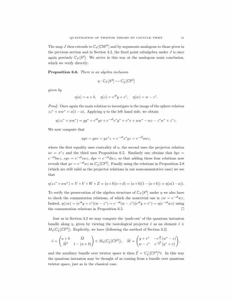
QUANTISATION OF TWISTOR THEORY BY COCYCLE TWIST 51
The map J then extends to CF [CM#] and by arguments analogous to those given inthe previous section and in Section 3.2, the fixed point subalgebra under J is onceagain precisely CF [S4]. We arrive in this way at the analogous main conclusion,which we verify directly:
Proposition 6.6. There is an algebra inclusion
η : CF [S4] → C−F [CP3]
given by
η(a) = a + b, η(z) = eıθy + v∗, η(w) = w − z∗.
Proof. Once again the main relation to investigate is the image of the sphere relationzz∗ + ww∗ = a(1− a). Applying η to the left hand side, we obtain
η(zz∗ + ww∗) = yy∗ + eıθyv + e−ıθv∗y∗ + v∗v + ww∗ − wz − z∗w∗ + z∗z.
We now compute that
ayv = yav = yx∗z = e−ıθx∗yz = e−ıθawz,
where the first equality uses centrality of a, the second uses the projector relationav = x∗z and the third uses Proposition 6.5. Similarly one obtains that byv =e−ıθbwz, cyv = e−ıθcwz, dyv = e−ıθdwz, so that adding these four relations nowreveals that yv = e−ıθwz in C−
F [CP3]. Finally using the relations in Proposition 3.8(which are still valid as the projector relations in our noncommutative case) we seethat
η(zz∗+ww∗) = Y +V +W +Z = (a+b)(c+d) = (a+b)(1− (a+b)) = η(a(1−a)).
To verify the preservation of the algebra structure of CF [S4] under η we also haveto check the commutation relations, of which the nontrivial one is zw = e−ıθwz.Indeed, η(zw) = (eıθy + v∗)(w − z∗) = e−ıθ(w − z∗)(eıθy + v∗) = η(e−ıθwz) usingthe commutation relations in Proposition 6.5.
Just as in Section 3.2 we may compute the ‘push-out’ of the quantum instantonbundle along η, given by viewing the tautological projector e as an element e ∈M4(C−
F [CP3]). Explicitly, we have (following the method of Section 3.2)
e =
(a + b M
M† 1− (a + b)
)∈ M4(C−
F [CP3]), M =
(y + v∗ −e
ıθ2 (w∗ − z)
w − z∗ e−ıθ2 (y∗ + v)
),
and the auxiliary bundle over twistor space is then E = C−F [CP3]4e. In this way
the quantum instanton may be thought of as coming from a bundle over quantumtwistor space, just as in the classical case.
52 S.J. BRAIN AND S. MAJID
7. The Penrose-Ward Transform
The main application of the double fibration (2) is to study relationships betweenvector bundles over twistor space and space-time, and between their associatedgeometric data. We begin by discussing how differential forms on these spaces arerelated, before considering more general vector bundles. Although we restrict ourattention to the special case of (2), our remarks are not specific to this example andone should keep in mind the picture of a pair of fibrations of homogeneous spaces
G/R
G/H G/K,
@@@R
p q
(24)
where G is, say, a complex Lie group with parabolic subgroups H,K,R such thatR = H ∩K. In general, the differential calculi of the coordinate algebras of thesespaces need not be compatible in any sensible way, however when there is someform of compatibility (namely a certain transversality condition on the fibrationsat the level of the correspondence space G/R) then the double fibration has somenice properties. Indeed, as we shall see, such a compatibility between calculi allowsone to ‘transform’ geometric data from G/H to G/K and vice versa.
This is the motivation behind the Penrose-Ward transform, which we shall de-scribe in this section. The idea is that certain classes of vector bundles over a givensubset of G/H correspond to vector bundles over an appropriate subset of G/K
equipped with a connection possessing anti-self-dual curvature, the correspondencegiven by pull-back along p followed by direct image along q. In fact, as discussed,we have already seen this transform in action, albeit in the simplified case whereG/H = CP3 and the given subset of G/K = CM# is S4, so that the double fibrationcollapses to a single fibration. In Section 3.2 we gave a coordinate algebra descrip-tion of this fibration, with the analogous quantum version computed in Section 6.2.In this section we outline how the transform works in a different situation, namelybetween the affine piece CM ⊂ CM# of space-time and the corresponding patch oftwistor space (so that we are utilising the full geometry of the double fibration):we also outline how it quantises under the cotwist given in Section 4.
7.1. Localised coordinate algebras. We note that classically the driving forcebehind the construction that we shall describe is the theory of holomorphic functionsand holomorphic sections of vector bundles. Of course, if one works globally thenone cannot expect to be able to say very much at all (in general, one cannot expectto find enough functions). Hence here we resort to working locally, on some open setU of space-time CM# having nice topological properties1. As remarked earlier, ofparticular interest are the principal open sets Uf , for which one can explicitly write
1Namely that the intersection of each α-plane Z with U is either empty or connected and
simply connected, so that if we write W := q−1(U) and Y := p(W ) then the fibres of the maps
QUANTISATION OF TWISTOR THEORY BY COCYCLE TWIST 53
down the coordinate algebraOCM#(Uf ) in our language and expect the constructionto go through. In what follows, however, we choose to be explicit and restrict ourattention to the case of
OCM#(Ut) = C[CM#](t−1)0,
the ‘affine’ piece of space-time, for which we have the inclusion of algebras C[CM] →
C[CM#](t−1)0 given by
x1 → t−1z, x2 → t−1z, x3 → t−1w, x4 → t−1w.
In fact we also choose to write s := t−1s, so that the quadric relation in C[CM#]
becomes s = x1x2 − x3x4. Thus in the algebra C[CM#](t−1)0 the generator s isredundant and we may as well work with C[CM].
Since the points in CM# for which t = 0 correspond to the points in T whereZ3 = Z4 = 0, the homogeneous twistor space of affine space-time C[CM] hascoordinate algebra C[T ] with the extra conditions that Z3, Z4 are not both zero.The twistor space Tt of CM is thus covered by two coordinate patches, where Z3 6= 0and where Z4 6= 0. These patches have coordinate algebras
C[TZ3 ] := C[T ]((Z3)−1)0, C[TZ4 ] := C[T ]((Z4)−1)0
respectively. Note that when both Z3 and Z4 are non-zero the two algebras areisomorphic (even in the twisted case, since Z3, Z4 remain central in the algebra),with ‘transition functions’ Zµ(Z3)−1 7→ Zµ(Z4)−1. This isomorphism simply saysthat both coordinate patches look locally like C3, in agreement that our expectationthat twistor space is a complex 3-manifold.
In passing from CM# to CM we delete the ‘region at infinity’ where t = 0, andsimilarly we obtain the corresponding twistor space Tt by deleting the region whereZ3 = Z4 = 0. At the homogeneous level this region has coordinate algebra
C[T ]/〈Z3 = Z4 = 0〉 ∼= C[Z1, Z2],
describing a line CP1 at the projective level. In the twisted framework, the gener-ators Z3, Z4 are central so the quotient still makes sense and we have
CF [T ]/〈Z3 = Z4 = 0〉 ∼= CF [Z1, Z2],
describing a noncommutative CP1.At the level of the homogeneous correspondence space we also have t−1 adjoined
and Z3, Z4 not both zero, and we write C[Ft] := C[F ](t−1)0 for the correspondingcoordinate algebra. We note that in terms of the C[CM] generators, the relations(1) now read
(25) Z1 = x2Z3 + x3Z
4, Z2 = x4Z3 + x1Z
4.
p : W → Y and q : W → U are connected, so that operations such as pull-back and direct image
are well-behaved.
54 S.J. BRAIN AND S. MAJID
At the projective level, the correspondence space is also covered by two coordinatepatches. Thus when Z3 6= 0 and when Z4 6= 0 we respectively mean
C[FZ3 ] := C[Ft]((Z3)−1)0, C[FZ4 ] := C[Ft]((Z4)−1)0.
Again when Z3 and Z4 are both non-zero these algebras are seen to be isomorphicunder appropriate transition functions. Thus at the homogeneous level, the coor-dinate algebra C[Ft] describes a local trivialisation of the correspondence space inthe form Ft
∼= C2×CM. The two coordinate patches FZ3 and FZ4 together give atrivialisation of the projective correspondence space in the form Ft = CP1 × CM.
Regarding the differential calculus of C[CM#](t−1)0, it is easy to see that sinced(t−1t) = 0, from the Leibniz rule we have d(t−1) = −t−2dt. Since dt is central evenin the twisted calculus, adjoining this extra generator t−1 causes no problems, andit remains to check that the calculus is well-defined in the degree zero subalgebra
C[CM#](t−1)0. Indeed, we see that for example
dx1 = d(t−1z) = t−1dz − (t−1z)(t−1dt),
which is again of overall degree zero. Similar statements hold regarding the differ-ential calculi of C[TZ3 ] and C[TZ4 ] as well as those of C[FZ3 ] and C[FZ4 ].
7.2. Differential aspects of the double fibration. We now consider the pull-back and direct image of one-forms on our algebras. Indeed, we shall examinehow the differential calculi occurring in the fibration (2) are related and derive thepromised ‘transversality condition’ required in order to transfer data from one sideof the fibration to the other. For now, we consider only the classical (i.e. untwisted)situation.
Initially we work at the homogeneous level, with C[T ] and C[Ft], later passingto local coordinates by adjoining an inverse for either Z3 or Z4, as described above.We define
(26) Ω1p := Ω1C[Ft]/p∗Ω1C[T ]
to be the set of relative one-forms (the one-forms which are dual to those vectorswhich are tangent to the fibres of p). Note that Ω1
p is just the sub-bimodule ofΩ1C[Ft] spanned by ds, dx1, dx2, dx3, dx4, so that
(27) Ω1C[Ft] = p∗Ω1C[T ]⊕ Ω1p.
There is of course an associated projection
πp : Ω1C[Ft] → Ω1p
and hence an associated relative exterior derivative dp : C[Ft] → Ω1p given by
composition of d with this projection,
(28) dp = πp d : C[Ft] → Ω1p.
QUANTISATION OF TWISTOR THEORY BY COCYCLE TWIST 55
Similarly, we define the relative two-forms by
Ω2p := Ω2C[Ft]/(p∗Ω1C[T ] ∧ Ω1C[Ft])
so that dp extends to a map
dp : Ω1p → Ω2
p
by composing d : Ω1C[Ft] → Ω2C[Ft] with the projection Ω1C[Ft] → Ω2p. We see
that dp obeys the relative Leibniz rule,
(29) dp(fg) = (dpf)g + f(dpg), f, g ∈ C[Ft].
It is clear by construction that the kernel of dp consists precisely of the functionsin C[Ft] which are constant on the fibres of p, whence we recover C[T ] by meansof the functions in C[Ft] which are covariantly constant with respect to dp (sincefunctions in C[T ] may be identified with those functions in C[Ft] which are constanton the fibres of p). Moreover, the derivative dp is relatively flat, i.e. its curvatured2
p is zero.The next stage is to consider the direct image of the one-forms Ω1
p along q. Inthe usual theory the direct image [20] of a vector bundle π : E′ → Ft over Ft alongthe fibration q : Ft → CM is by definition the bundle E := q∗E
′ → CM whose fibreover x ∈ CM is H0(q−1(x), E′), the space of global sections of the restriction ofE′ to q−1(x). Of course, this definition does not in general result in a well-definedvector bundle. For this, we assume that each q−1(x) is compact and connected sothat H0(q−1(x), E′) is finite dimensional, and that H0(q−1(x), E′) is of constantdimension as x ∈ CM varies. In our situation these criteria are clearly satisfied.
We recall that in the given local trivialisation, the correspondence space lookslike Ft = CP1×CM with coordinate functions ζ, x1, x2, x3, x4, where ζ = Z3(Z4)−1
or Z4(Z3)−1 (depending on which coordinate patch we are in). Writing E ′ for thespace of sections of the bundle E′ → Ft, the space of sections E of the direct imagebundle E is in general obtained by computing E ′ as a C[CM]-module. So althoughany section ξ ∈ E ′ of E′ is in general a function of the twistor coordinate ζ as wellas the space-time coordinates xj , its restriction to any fibre q−1(x) is by Liouville’stheorem independent of ζ (i.e. ζ is constant on q−1(x)). Of course, when we restrictthe section ξ to each q−1(x), its dependence on ζ varies as x ∈ CM varies (in thatalthough ζ is constant on each q−1(x), it possibly takes different values as x varies),and this means that in taking the direct image we may write ζ as a function of thespace-time coordinates xj , j = 1, . . . 4. One could also argue by by noting that CMis topologically trivial so has no cohomology, whence one has for example
H0(CP1 × CM, C) = H0(CP1, C)⊗H0(CM, C) ∼= H0(CM, C).
At the homogeneous level, although the fibres of the map q : Ft → CM arenot compact, the effect of the above argument may be achieved by regarding thetwistor coordinates Z3, Z4 as functions of the space-time coordinates under the
56 S.J. BRAIN AND S. MAJID
direct image. The upshot of this argument is that to compute the direct image of aC[Ft]-module E ′, we ‘remove’ the dependence of E ′ on the twistor coordinates Zi,hence obtaining a C[CM]-module E . In what follows, this will be our naive definitionof direct image, by analogy with the classical case. Since this argument reallybelongs in the language of cohomology, we satisfy ourselves with this definition fornow, deferring a more precise treatment to a sequel.
Proposition 7.1. There is an isomorphism q∗q∗Ω1C[CM] ∼= Ω1C[CM].
Proof. The generators dxj , j = 1, . . . 4 of Ω1C[CM] pull back to their counterpartsdxi, i = 1, . . . 4 in C[Ft] and these span q∗Ω1C[CM] as a C[Ft]-bimodule. Takingthe direct image involves computing q∗Ω1C[CM] as a C[CM]-bimodule, and assuch it is spanned by elements of the form ds, dxi, Zids, Zidxj , for i, j = 1, . . . 4.As already observed, the generator s is essentially redundant, hence so are thegenerators involving ds. Moreover, the relations (25) allow us to write Z1 and Z2
in terms of Z3, Z4, whence we are left with elements of the form dxj , Z3dxj andZ4dxj for j = 1, . . . 4.
As explained above, the direct image is given by writing the Z-coordinates asfunctions of the space-time coordinates, and it is clear that the resulting differentialcalculus q∗q
∗Ω1C[CM] of C[CM] is isomorphic to the one we first thought of. Weremark that we have used the same symbol d to denote the exterior derivative inthe different calculi Ω1C[CM], q∗Ω1C[CM] and q∗q
∗Ω1C[CM]. Although they arein principle different, our notation causes no confusion here.
Proposition 7.2. For s = 1, 2 the direct images q∗Ωsp are given by:
• q∗Ω1p∼= Ω1C[CM];
• q∗Ω2p∼= Ω2
+C[CM],
where Ω2+C[CM] denotes the space of two-forms in Ω2C[CM] which are self-dual
with respect to the Hodge ∗-operator defined by the metric η = 2(dx1dx2−dx3dx4).
Proof. We first consider the C[Ft]-bimodule Ω1p, and write q∗Ω1
p for the same vectorspace considered as a C[CM]-bimodule. Quotienting Ω1C[Ft] by the one-formspulled back from C[T ] means that Ω1
p is spanned as a C[Ft]-bimodule by ds anddxi, i = 1, . . . 4.
The direct image is computed just as before, so q∗Ω1p is as a vector space the
same calculus Ω1p but now considered as a C[CM]-bimodule. In what follows we
shall write d for the exterior derivatives in the calculi Ω1C[CM] and Ω1C[Ft] asthey are the usual operators (the ones we which we wrote down and quantised insection 5). However, in calculating the direct image q∗Ω1
p of the calculus Ω1p, we
must introduce different notation for the image of the operator dp under q∗. Tothis end, we write q∗dp := d, so that as a C[CM]-bimodule the calculus q∗Ω1
p isspanned by elements of the form ds and dxj , i, j = 1, . . . 4. As already observed,the generator s is essentially redundant, hence so is the generator ds.
QUANTISATION OF TWISTOR THEORY BY COCYCLE TWIST 57
The identity (29) becomes a Leibniz rule for d upon taking the direct image q∗,whence (q∗Ω1
p,d) is a first order differential calculus of C[CM]. We must investigateits relationship with the calculus Ω1C[CM].
Differentiating the relations (25) and quotienting by generators dZi yields therelations
(30) Z3dpx2 + Z4dpx3 = 0, Z3dpx4 + Z4dpx1 = 0
in the relative calculus Ω1p. Thus as a C[Ft]-bimodule, Ω1
p has rank two, sincethe basis elements dpxj are not independent. However, in the direct image q∗Ω1
p,which is just Ω1
p considered as a C[CM]-bimodule, these basis elements (now writtendxj) are independent. Thus it is clear that the calculus (q∗Ω1
p,d) is isomorphic to(Ω1C[CM],d) in the sense that as bimodules they are isomorphic, and that thisisomorphism is an intertwiner for the derivatives d and d.
Using the relations (30) it is easy to see that in the direct image bimoduleq∗Ω2
p := Λ2(q∗Ω1p) we have
dx1 ∧ dx4 = dx2 ∧ dx3 = dx1 ∧ dx2 + dx3 ∧ dx4 = 0,
which we recognise (since we are in double null coordinates) as the anti-self-dualtwo-forms, whence it is the self-dual two-forms which survive under the direct image.It is evident that these arguments are valid upon passing to either coordinate patchat the projective level, i.e. upon adjoining either (Z3)−1 or (Z4)−1 and taking thedegree zero part of the resulting calculus.
It is clear that the composition of maps
q∗Ω1C[CM] → Ω1C[Ft] → Ω1p
determines the isomorphism
Ω1C[CM] → q∗Ω1p
by taking direct images2 (this is also true in each of the coordinate patches). Thesequence
(31) C[Ft] → Ω1p → Ω2
p,
where the two maps are just dp, becomes the sequence
C[CM] → Ω1C[CM] → Ω2+C[CM]
upon taking direct images (the maps become d). The condition that d2p = 0 is then
equivalent to the statement that the curvature d2 is annihilated by the map
Ω2C[CM] → q∗Ω2p = Ω2
+,
2We note that for the general double fibration (24), a similar analysis will go through provided
one has the transversality condition that q∗Ω1p∼= Ω1C[G/H].
58 S.J. BRAIN AND S. MAJID
i.e. that the curvature d2 is anti-self-dual. So although the connection dp is flat, itsimage under q∗ is not. Although the derivatives d and d agree as maps C[CM] →Ω1C[CM], they do not agree beyond the one-forms. The image of d : Ω1C[CM] →Ω2C[CM] consists of all holomorphic two-forms, whereas d maps Ω1C[CM] ∼= q∗Ω1
p
onto the anti-self-dual two-forms. At the level of the correspondence space, thereason for this is that in the sequence (31), the calculus Ω1
p comes equipped withrelations (30), whereas the pull-back q∗Ω1C[CM] has no such relations.
We are now in a position to investigate how this construction behaves underthe twisting discussed in Sections 4 and 5. Of course, we need only check thatthe various steps of the procedure remain valid under the quantisation functor.To this end, our first observation is that although the relations in the first orderdifferential calculus of C[CM] are deformed, equations (21) show that the two-formsare undeformed, as is the metric υ, hence the Hodge ∗-operator is also undeformedin this case. It follows that the notion of anti-self-duality of two-forms is the sameas in the classical case.
Furthermore, the definition of relative one-forms (26) still makes sense since thedecomposition (27) is clearly unaffected by the twisting. Since we are working withthe affine piece of (now noncommutative) space-time, the relevant relations in thecorrespondence space algebra CF [Ft] are given by (25), which are unchanged undertwisting since t, Z3, Z4 remain central in the algebra.
Finally we observe that the proofs of Propositions 7.2 and 7.1 go through un-changed. The key steps use the fact that when the generators Z3, Z4 and t areinvertible, one may adjoin their inverses to the coordinate algebras and differentialcalculi and take the degree zero parts. Since these generators remain central undertwisting, this argument remains valid and we have the following twisted consequenceof Proposition 7.2.
Proposition 7.3. Let dp : CF [Ft] → Ω1p be the differential operator defined by the
composition of maps dp = π d,
dp : CF [Ft] → Ω1CF [Ft] → Ω1p.
Then the direct image d : CF [CM] → q∗Ω1p∼= Ω1CF [CM] is a differential operator
whose curvature d2 takes values in the anti-self-dual two-forms Ω2−CF [CM].
We remark that this is no coincidence: the transform between one-forms on Tt
and the operator d on the corresponding affine patch CM of space-time goes throughto this noncommutative picture precisely because of the choice of cocycle made inSection 4. Indeed, we reiterate that any construction which is covariant undera chosen symmetry group will also be covariant after applying the quantisationfunctor. In this case, the symmetry group is the subgroup generated by conformaltranslations (see Section 4), which clearly acts covariantly on affine space-time CM.By the very nature of the twistor double fibration, this translation group also acts
QUANTISATION OF TWISTOR THEORY BY COCYCLE TWIST 59
covariantly on the corresponding subsets T and Ft of (homogeneous) twistor spaceand the correspondence space respectively, and it is therefore no surprise that thetransform outlined above works in the quantum case as well.
As discussed, it is true classically that one can expect such a transform betweensubsets of CM# and the corresponding subsets of twistor space T provided therequired topological properties (such as connectedness and simple-connectedness ofthe fibres) are met. We now see, however, that the same is not necessarily true inthe quantum case. For a given open subset U of CM#, we expect the transformbetween U and its twistor counterpart U = p(q−1(U)) ⊂ T to carry over to thequantum case provided the twisting group of symmetries is chosen in a way so asto preserve U .
7.3. Outline of the Penrose-Ward transform for vector bundles. The pre-vious section described how the one-forms on twistor space give rise to a differentialoperator on forms over space-time having anti-self-dual curvature. The main featureof this relationship is that bundle data on twistor space correspond to differentialdata on space-time. The idea of the full Penrose-Ward transform is to generalisethis construction from differential forms to sections of more general vector bundles.
We begin with a finite rank C[T ]-module3 E describing the holomorphic sectionsof a (trivial) holomorphic vector bundle E over homogeneous twistor space T . Thepull-back p∗E is the C[Ft]-module
(32) E ′ := p∗E = C[Ft]⊗C[T ] E .
The key observation is then that there is a relative connection ∇p on p∗E definedby
∇p = dp ⊗ 1
with respect to the decomposition (32). Again there is a relative Leibniz rule
(33) ∇p(fξ) = f(∇pξ) + (dpf)⊗ ξ
for f ∈ C[Ft] and ξ ∈ p∗E . Moreover, ∇p extends to C[Ft]-valued k-forms bydefining
Ωkp E ′ := Ωk
p ⊗C[Ft]E ′
for k ≥ 0 and extending ∇p = dp⊗ 1 with respect to this decomposition. It is clearthat the curvature satisfies ∇2
p = 0 and we say that ∇p is relatively flat.Conversely, if the fibres of p are connected and simply connected (as they clearly
are in our situation; we assume this in the general case of (24)), then if E ′ is a finiterank C[Ft]-module admitting a flat relative connection ∇′ (that is, a complex-linear
3In this section we shall for convenience work with left modules over the algebras in question.
60 S.J. BRAIN AND S. MAJID
map ∇′ : E ′ → Ω1p⊗C[Ft]
E ′ satisfying (33) and (∇′)2 = 0), we may recover a finiterank C[T ]-module E by means of the covariantly constant sections, namely
E := ξ ∈ E ′ | ∇′ξ = 0.
This argument gives rise to the following result.
Proposition 7.4. There is a one-to-one correspondence between finite rank C[T ]-modules E and finite rank C[Ft]-modules E ′ admitting a flat relative connection∇p,
∇p(fξ) = f(∇pξ) + (dpf)⊗ ξ, ∇2p = 0
for all f ∈ C[Ft] and ξ ∈ E ′.
We remark that here we do not see the non-trivial structure of the bundlesinvolved (all of our modules describing vector bundles are free) as in our localpicture all bundles are trivial. However, given these local formulae it will be possibleat a later stage to patch together what happens at the global level.
The Penrose-Ward transform arises by considering what happens to a relativeconnection ∇p under direct image along q. We here impose the additional assump-tion that E ′ is also the pull-back of a bundle on space-time, so E ′ = p∗E = q∗E forsome finite rank C[CM]-module E . This is equivalent to assuming that the bundleE′ is trivial upon restriction to each of the fibres of the map q : Ft → CM. Thedirect image is computed exactly as described in the previous section.
Thus the direct image of E ′ is q∗E ′ = q∗q∗E ∼= E and, just as in Proposition 7.2,
equation (33) for ∇p becomes a Leibniz rule for ∇ := q∗∇, whence ∇p maps ontoa genuine connection on E . The sequence
E ′ → Ω1p⊗C[Ft]
E ′ → Ω2p⊗C[Ft]
E ′,
where the two maps are ∇p, becomes the sequence
E → Ω1C[CM]⊗C[CM]E → Ω2+⊗C[CM]E ,
where the maps here are ∇. Moreover, just as in the previous section it followsthat under direct image the condition that ∇2
p = 0 is equivalent to the conditionthat the curvature ∇2 is annihilated by the mapping
Ω2C[CM]⊗C[CM] E → q∗Ω2p ⊗C[CM] E = Ω2
+ ⊗C[CM] E ,
so that ∇ has anti-self-dual curvature.
7.4. Tautological bundle on CM and its Ward transform. We remark thatin the previous section we began with a bundle over homogeneous twistor space T ,whereas it is usual to work with bundles over the projective version T . As such,we implicitly assume that in doing so we obtain from E corresponding C[TZ3 ]- andC[TZ4 ]-modules which are compatible in the patch where Z3 and Z4 are both non-zero, as was the case for the coordinate algebras C[TZ3 ] and C[TZ4 ], C[FZ3 ] and
QUANTISATION OF TWISTOR THEORY BY COCYCLE TWIST 61
C[FZ4 ] via the transition functions Zµ(Z3)−1 7→ Zµ(Z4)−1. We similarly assumethis for the corresponding calculi on these coordinate patches.
In order to neatly capture these issues of coordinate patching, the general con-struction really belongs in the language of cohomology: as explained, the detailswill be addressed elsewhere. For the time begin we give an illustration of the trans-form in the coordinate algebra framework, as well as an indication of what happensunder twisting, through the tautological example introduced in Section 3.1.
We recall the identification of conformal space-time and the correspondence spaceas flag varieties CM# = F2(C4) and F = F1,2(C4) respectively, and the resultingfibration
q : F1,2(C4) → F2(C4),
where the fibre over a point x ∈ F2(C4) is the set of all one-dimensional subspacesof C4 contained in the two-plane x ⊂ C4, so is topologically a projective line CP1.We also have a fibration at the homogeneous level,
F → F2(C4),
where this time the fibre over x ∈ F2(C4) is the set of all vectors which lie in thetwo-plane x. As explained, there are no non-constant global holomorphic sectionsof this bundle, so as before we pass to the affine piece of space-time CM in orderto avoid this trivial case.
We identify C4 with its dual and take the basis (Z1, Z2, Z3, Z4). In the patchFt the relations in C[Ft] are
(34) Z1 = x2Z3 + x3Z
4, Z2 = x4Z3 + x1Z
4,
which may be seen as giving a trivialisation of the tautological bundle over CM#
in this coordinate patch. In this trivialisation the space E of sections of the bun-dle is just the free module over C[CM] of rank two, spanned by Z3 and Z4, i.e.E ∼= C[CM] ⊗ C2. We equip this module with the anti-self-dual connection d ⊗ 1constructed in Section 7.2.
It is now easy to see that the pull-back E ′ of E along q is just the free C[Ft]-moduleof rank two. By construction, the connection d on E pulls back to the relativeconnection dp⊗ 1 on E ′ = C[Ft]⊗C2. As discussed earlier the corresponding C[T ]-module E is obtained as the kernel of the partial connection ∇p, which is preciselythe free rank two C[T ]-module E = C[T ] ⊗ C2. It is also clear that these modulessatisfy the condition that E ′ = p∗E = q∗E (the corresponding vector bundles aretrivial in this case, whence they are automatically trivial when restricted to eachfibre of p and of q).
Lastly, it is obvious that the bundle over T described by the module E descendsto a (trivial) bundle over the twistor space Tt of CM. On the coordinate patcheswhere Z3 and Z4 are non-zero one obtains respectively a free rank two C[TZ3 ]-module EZ3 by inverting Z3 and a C[TZ4 ]-module EZ4 by inverting Z4, and since
62 S.J. BRAIN AND S. MAJID
the algebras C[TZ3 ] and C[TZ4 ] agree when Z3, Z4 are both non-zero, the sameis true of the sections in the localised modules EZ3 and EZ4 . The construction inthis example remains valid under the twisting described in Section 4.1 due to ourearlier observation that the relations (34) are unchanged.
Explicitly then, the tautological bundle of CM# in the affine patch CM is simplythe free rank two C[CM]-module E = C[CM]2 = C[CM]⊗C2, which we equip withthe anti-self-dual connection d⊗1 constructed in Section 7.2 (note that one reservesthe term instanton specifically for anti-self-dual connections over S4). Its Penrose-Ward transform is the trivial rank two holomorphic bundle over the twistor spaceTt of CM. Since these spaces are topologically trivial, we see that the Penrose-Wardtransform is here very different in flavour to the transform given in Section 3.2. Itis however clear that this example of the transform quantises in exactly the sameway as the rank one case of Section 7.2.
8. The ADHM Construction
8.1. The classical ADHM construction. We begin this section with a briefsummary of the ADHM construction for connections with anti-self-dual curvatureon vector bundles over Minkowski space CM [1, 14], with a view to dualising andthen twisting the construction.
A monad over T = C4 is a sequence of linear maps
A B C,ρ
Zτ
Z- -
between complex vector spaces A,B, C of dimensions k, 2k +n, k respectively, suchthat for all Z ∈ C4, τ
Zρ
Z: A −→ C is zero and for all Z ∈ C4, ρ
Zis injective and
τZ
is surjective. Moreover, we insist that ρZ, τ
Zeach depend linearly on Z ∈ T .
The spaces A,B,C should be thought of as typical fibres of trivial vector bundlesover CP3 of ranks k, 2k + n, k, respectively.
A monad determines a rank-n holomorphic vector bundle on T = CP3 whose fibreat [Z] is Ker τ
Z/Im ρ
Z(where [Z] denotes the projective equivalence class of Z ∈
C4). Moreover, any holomorphic vector bundle on CP3 trivial on each projectiveline comes from such a monad, unique up to the action of GL(A)×GL(B)×GL(C).For a proof of this we refer to [16], although we note that the condition τ
Zρ
Z= 0
implies Im ρZ⊂ Ker τ
Zfor all z ∈ C4 so the cohomology makes sense, and the fact
that ρZ, τ
Zhave maximal rank at every Z implies that each fibre has dimension
n. The idea behind the ADHM construction is to use the same monad data toconstruct a rank n vector bundle over CM# with second Chern class c2 = k (in thephysics literature this is usually called the topological charge of the bundle).
QUANTISATION OF TWISTOR THEORY BY COCYCLE TWIST 63
For each W,Z ∈ T we write x = W ∧ Z for the corresponding element x of
(homogeneous) conformal space-time CM# ⊂ Λ2T . Then define
Ex = Ker τZ∩Ker τ
W, Fx = (ρ
ZA) ∩ (ρ
WA), ∆x = τ
Zρ
W.
Proposition 8.1. [14] The vector spaces Ex, Fx and the map ∆x depend on x,rather than on Z,W individually.
Proof. We first consider ∆x and suppose that x = Z ∧ W = Z ∧ W ′ for someW ′ = W + λZ, λ ∈ C. Then we have
τZρ
W ′ − τZρ
W= τ
Zρ
W ′−W= τ
Zρ
λZ= λτ
Zρ
Z= 0.
Now writing Z ′ = Z + λW ′ we see that
τZ′ρW ′ − τ
Zρ
W= (τ
Z+ λτ
W ′ )ρW ′ − τZρ
W= λτ
Zρ
W ′ − τZρ
W= 0
by the first calculation, proving the claim for ∆x.Next we consider b ∈ Ker τ
Z∩Ker τ
Wand suppose x = Z ∧W = Z ∧W ′ where
W ′ = W + λZ. Thenτ
W ′ b = (τW
+ λτZ)b = 0,
so that Ker τZ∩ Ker τ
W= Ker τ
Z∩ Ker τ
W ′ . Moreover, if Z ′ = Z + λW ′ we seethat
τZ′ b = (τ
Z+ λτ
W ′ )b = 0,
so that Ker τZ∩ Ker τ
W= Ker τ
Z′ ∩ Ker τW ′ , establishing the second claim. The
third follows similarly.
As in [14], we write U for the set of x ∈ CM# on which ∆x is invertible.
Proposition 8.2. For all x ∈ U we have the decomposition,
(35) B = Ex ⊕ Im ρZ⊕ Im ρ
W.
In particular, for all x ∈ CM# we have Fx = 0.
Proof. For x ∈ U , define
Px = 1− ρW
∆−1x τ
Z+ ρ
Z∆−1
x τW
: B → B.
Now Px is linear in x and is dependent only on x and not on Z,W individually. Itis easily shown that P 2
x = Px and PxB = Ex, whence Px is the projection onto Ex.Moreover,
−ρW
∆−1x τ
Z, ρ
Z∆−1
x τW
,
are the projections onto the second and third summands respectively. Hence wehave proven the claim provided we can show that Fx = 0, since the sum Im ρ
Z⊕
Im ρW
is then direct.Suppose that Fx = (ρ
ZA)∩(ρ
WA) is not zero for some x ∈ CM#, so there exists a
non-zero b ∈ ρW ′A for all W ′ ∈ T such that x = Z∧W = Z∧W ′. Then in particular
64 S.J. BRAIN AND S. MAJID
a := ρ−1W ′ b is non-zero and defines a holomorphic section of a vector bundle over the
two-dimensional subspace of T spanned by all such W ′ (whose typical fibre is justA), and hence (at the projective level) a non-zero holomorphic section of the bundleO(−1) ⊗ A over x = CP1, where O(−1) denotes the tautological line bundle overCP1. It is however well-known that this bundle has no non-zero global sections,whence we must in fact have Fx = 0.
This procedure has thus constructed a rank n vector bundle over U whose fibreover x ∈ U is Ex (again noting that the construction is independent of the scaling of
x ∈ CM#). The bundle E is obtained as a sub-bundle of the trivial bundle U ×B:the projection Px identifies the fibre of E at each x ∈ CM# as well as defining aconnection on E by orthogonal projection of the trivial connection on U ×B.
8.2. ADHM in the ∗-algebra picture. In this section we mention how theADHM construction ought to operate in our SU4 ∗-algebra framework. In passingto the affine description of our manifolds, we encode them as real rather than com-plex manifolds, obtaining a global coordinate algebra description. Thus we expectthat the ADHM construction ought to go through at some global level in our ∗-algebra picture. For now we suppress the underlying holomorphic structure of thebundles we construct, with the complex structure to be added elsewhere.
Indeed, we observe that the key ingredient in the ADHM construction is thedecomposition (35),
B = Ex ⊕ Im ρZ⊕ Im ρ
W,
which identifies the required bundle over space-time as a sub-bundle of the trivialbundle with fibre B. We wish to give a version of this decomposition labelled bypoints at the projective level, that is in terms of points of T = CP3 and CM# =F2(C4), rather than in terms of the homogeneous representatives Z ∈ T and x ∈
CM# used above. We shall do this as before by identifying points of CP3 withrank one projectors Q in M4(C), similarly points of CM# with rank two projectorsP . Points of the correspondence space are identified with pairs of such projectors(Q,P ) such that QP = Q = PQ.
Recall that in the previous description, given x ∈ Λ2T and Z ∈ x there are manyW such that x = Z ∧ W . In the alternative description, given a projection P ∈CM#, the corresponding picture is that there are Q,Q′ ∈ T with QP = Q = PQ
and Q′P = Q′ = PQ′ such that Im P = Im Q ⊕ Im Q′. Given P ∈ CM#, Q ∈ T
with (Q,P ) ∈ F , there is a canonical choice for Q′, namely Q′ := P −Q. Indeed,P identifies a two-dimensional subspace of C4 and Q picks out a one-dimensionalsubspace of this plane. The projector Q′ = P − Q picks out a line in C4 in theorthogonal complement of the line determined by Q.
As in the monad description of the construction outlined earlier, the idea is tobegin with a trivial bundle of rank 2k + n with typical fibre B = C2k+n and to
QUANTISATION OF TWISTOR THEORY BY COCYCLE TWIST 65
present sufficient information to canonically identify a decomposition of B in theform (35). In the monad description this was done by assuming that τ
Zρ
Z= 0 and
that the maps τ, ρ were linearly dependent on Z ∈ T . Of course, this makes full useof the additive structure on T , a property which we do not have in the projectorversion: here we suggest an alternative approach.
In order to obtain such a decomposition it is necessary to determine the reason foreach assumption in the monad construction and to then translate this assumptioninto the projector picture. The first observation is that the effect of the map ρ isto identify a k-dimensional subspace of B for each point in twistor space (for eachQ ∈ T the map ρ
Qis simply the associated embedding of A into B). We note that
this may be achieved directly by specifying for each Q ∈ T a rank k projectionρ
Q: B → B.The construction then requires us to decompose each point of space-time in terms
of a pair of twistors. As observed above, given P ∈ CM# and any Q ∈ T such thatPQ = Q = QP we have P = Q+Q′, where Q′ = P −Q (it is easy to check that Q′
is indeed another projection of rank one). The claim is then that the correspondingk-dimensional subspaces of B have zero intersection and that their direct sum isindependent of the choice of decomposition of P . In the monad construction thiswas obtained using the assumed linear dependence of ρ on points Z ∈ T , althoughin terms of projectors this is instead achieved by assuming that the projectionsρ
Q,ρ
Q′ are orthogonal whenever Q,Q′ are orthogonal (clearly if Q + Q′ = P thenQ,Q′ are orthogonal), i.e.
ρQρ
Q′ = ρQ′ρQ
= 0
for all Q,Q′ such that QQ′ = Q′Q = 0. Moreover, we impose that ρQ
+ρQ′ depends
only on Q + Q′, so that the direct sum of the images of these projections dependsonly on the sum of the projections.
Then for each P ∈ CM# we define a subspace BP of B of dimension n,
B = BP ⊕ Im ρQ⊕ Im ρ
Q′
by constructing the projection
eP
:= 1− ρQ− ρ
Q′
on C4, which is well-defined since the assumptions we have made on the family ρQ
imply that the projectors eP, ρ
Qand ρ
Q′ are pairwise orthogonal. This constructsa rank n vector bundle over CM# whose fibre over P ∈ CM# is Im e
P= BP .
8.3. The tautological bundle on CM# and its corresponding monad. Weillustrate these ideas by constructing a specific example in the ∗-algebra picture. Weconstruct a ‘tautological monad’ which appears extremely naturally in the projectorversion and turns out to correspond to the 1-instanton bundle of Section 3.2.
66 S.J. BRAIN AND S. MAJID
We once again recall that compactified space-time may be identified with the flagvariety F2(C4) of two-planes in C4 and this space has its associated tautologicalbundle whose fibre at x ∈ F2(C4) is the two-plane in C4 which defines x (it isprecisely this observation which gave rise to the projector description of space-timein the first place). Then we take B = C4 in the ADHM construction: note that weexpect to take n = 2, k = 1, which agrees with the fact that dim B = 2k + n = 4.
Then for each point P ∈ CM# we are required to decompose it as the sum of apair Q, Q′ of rank one projectors (each representing a twistor). Here this is easy todo: we simply choose any one-dimensional subspace of the image of P and take Q
to be the rank one projector whose image is this line. As discussed, the canonicalchoice for Q′ is just Q′ := P −Q.
In doing so, we have tautologically specified the one-dimensional subspace ofB = C4 associated to Q ∈ T (recalling that k = 1 here), simply defining ρ
Q:= Q.
We now check that these data satisfy the conditions outlined in the previous section.It is tautologically clear that for all Q1, Q2 ∈ T we have that ρ
Q1and ρ
Q2are
orthogonal projections if and only if Q1 and Q2 are orthogonal. Moreover, if we fixP ∈ CM#, Q ∈ T such that PQ = Q = QP and take Q′ = P −Q then
ρQ
+ ρQ′ = Q + Q′ = P,
which of course depends only on Q + Q′ rather than on Q, Q′ individually.Thus we construct the subspace BP as the complement of the direct sum of the
images of ρQ
and ρQ′ . As explained, this is done by constructing the projection
eP
= 1− ρQ− ρ
Q′ = 1− P.
Thus as P varies we get a rank two vector bundle over CM#, which is easily seento be the complement in C4 of the tautological vector bundle over CM#. We equipthis bundle with the Grassmann connection obtained by orthogonal projection ofthe trivial connection on the trivial bundle CM# × C4, as discussed earlier.
This gives a monad description of the tautological bundle over CM# = F2(C4).As explained, the instanton bundle over S4 is obtained by restriction of this bun-dle to the two-planes x ∈ F2(C4) which are invariant under the map J defined inSection 3.2. Hence we consider this construction only for x ∈ S4, and by Proposi-tion 3.11 we have that Q′ = J(Q) in the above. We now wish to give the monadversion of the corresponding bundle over twistor space, for which we need the mapτ
Q. We recall that τ is meant to satisfy τ
Qρ
Q= 0 for all Q ∈ CP3, and we use this
property to construct τ by putting τQ
:= ρJ(Q) = J(Q), so that in this tautological
example we have
τQρ
Q= ρ
J(Q)ρQ= J(Q)Q = 0.
QUANTISATION OF TWISTOR THEORY BY COCYCLE TWIST 67
The bundle over twistor space corresponding to the instanton then appears as thevector bundle whose fibre over Q ∈ CP3 is the cohomology
E = Ker τQ/Im ρ
Q= Ker ρ
J(Q)/Im ρQ,
which in the case of the 1-instanton is the rank two bundle E = Ker J(Q)/Im Q,and one may easily check that this bundle over twistor space agrees with the onecomputed in Section 3.2 using the Penrose-Ward transform. Indeed, the crucialproperty is that it is trivial upon restriction to P = p(q−1(P )) for all P ∈ S4,which is straightforward to see through the observation that as Q varies with P
fixed, Q and J(Q) always span the same plane (the one defined by P ), and thefibre of E over all such Q is precisely the orthogonal complement to this plane.
Acknowledgements. We would like to thank G. Landi and S.P. Smith for help-ful comments on versions of the manuscript during their respective visits to theNoncommutative Geometry Programme at the Newton Institute.
References
[1] M.F. Atiyah, V.G. Drinfel’d, N.J. Hitchin, Y.I. Manin. Construction of Instantons. Phys.
Lett. 65A No. 3, 185-187, 1978
[2] W. Barth. Moduli of Vector Bundles on the Projective Plane. Invent. Math. 42, 63-91, 1977
[3] R.J. Baston, M.G. Eastwood. The Penrose Transform: Its Interaction with Representation
Theory, Oxford University Press, 1989
[4] S.J. Brain. The Noncommutative Penrose-Ward Transform and Self-Dual Yang-Mills Fields.
DPhil Thesis, University of Oxford, 2005
[5] A. Connes, G. Landi. Noncommutative Manifolds, the Instanton Algebra and Isospectral
Deformations. Comm. Math. Phys. 221, 141-159, 2001
[6] M.G. Eastwood. The Generalized Penrose-Ward Transform. Math. Proc. Camb. Phil. Soc.
97, 165-187, 1985
[7] S.Majid, P. Hajac. Projective Module Description of the q-Monopole. Commun. Math. Phys.
206, 246-264, 1999.
[8] K.C. Hannabuss. Noncommutative Twistor Space. Lett. Math. Phys. 58 No. 2, 153-166, 2001
[9] A. Kapustin, A. Kuznetsov, D. Orlov. Noncommutative Instantons and Twistor Transform.
Comm. Math. Phys. 221 No. 2, 385-432, 2001
[10] G. Landi, W.S. van Suijlelom. Principal Fibrations from Noncommutative Spheres. Comm.
Math. Phys. 260, 203-225, 2005
[11] S. Majid. Foundations of Quantum Group Theory, Cambridge University Press, 1995
[12] S. Majid, R. Oeckl. Twisting of Quantum Differentials and the Planck Scale Hopf Algebra.
Comm. Math. Phys. 205, 617-655, 1999
[13] S. Majid. Noncommutative Riemannian and Spin Geometry of the Standard q-Sphere. Comm.
Math. Phys. 256, 255-285, 2005
[14] L.J. Mason, N.M.J. Woodhouse. Integrability, Self-Duality and Twistor Theory, Oxford Uni-
versity Press, 1996
[15] N.A. Nekrasov, A. Schwarz. Instantons on Noncommutative R4 and (2,0) Superconformal Six
Dimensional Theory. Comm. Math. Phys. 198 No.3, 689-703, 1998
[16] C. Okonek, M. Schneider, H. Spindler. Vector Bundles on Complex Projective Spaces,
Birkhauser, Boston, 1980
68 S.J. BRAIN AND S. MAJID
[17] R. Penrose, W. Rindler. Spinors and Space-Time, vol. 2, Cambridge University Press, 1986
[18] N. Seiberg, E. Witten. String Theory and Noncommutative Geometry. JHEP 9909 No. 9,
Paper 32, 1999
[19] R.S. Ward. On Self-Dual Gauge Fields. Phys. Lett. 61A No. 2, 81-82, 1977
[20] R.S. Ward, R.O. Wells Jr. Twistor Geometry and Field Theory, Cambridge University Press,
1990
Mathematical Institute, 24-29 St Giles’, Oxford OX1 3LB, UK
School of Mathematical Sciences, Queen Mary, University of London, 327 Mile End
Rd, London E1 4NS, UK


![Twistor theory at fifty: from contour integrals to twistor ... · arXiv:1704.07464v2 [hep-th] 8 Sep 2017 Twistor theory at fifty: from contour integrals to twistor strings Michael](https://img.pdfslide.us/doc/110x75/5af45bab7f8b9a9e598c9549/twistor-theory-at-fty-from-contour-integrals-to-twistor-170407464v2-hep-th.jpg)