Quantile Cross-Spectral Measures of Dependence

between Economic Variables

⇤

Jozef Barunık†and Tobias Kley‡

October 23, 2015

Abstract

In this paper we introduce quantile cross-spectral analysis of multiple time serieswhich is designed to detect general dependence structures emerging in quantiles ofthe joint distribution in the frequency domain. We argue that this type of depen-dence is natural for economic time series but remains invisible when the traditionalanalysis is employed. To illustrate how such dependence structures can arise be-tween variables in di↵erent parts of the joint distribution and across frequencies,we consider quantile vector autoregression processes. We define new estimatorswhich capture the general dependence structure, provide a detailed analysis of theirasymptotic properties and discuss how to conduct inference for a general class ofpossibly nonlinear processes. In an empirical illustration we examine one of themost prominent time series in economics and shed new light on the dependence ofbivariate stock market returns.

Keywords: cross-spectral density, quantiles, dependence, time series, ranks, cop-ula

⇤Authors are listed in alphabetical order, as they have equally contributed to the project. Forestimation and inference of the quantile cross-spectral measures introduced in this paper, the R packagequantspec is provided (Kley, 2014, 2015). The R package is available on https://cran.r-project.

org/web/packages/quantspec/index.html

†The paper has been written during Jozef Barunık’s postdoctoral stay with the Econometric Depart-ment, IITA, The Czech Academy of Sciences. Jozef Barunık is also Assistant Professor at the Instituteof Economic Studies, Charles University in Prague, and gratefully acknowledges partial support fromthe European Union’s Seventh Framework Programme (FP7/2007-2013) under grant agreement No.FP7-SSH- 612955 (FinMaP).

‡Tobias Kley is Postdoctoral Research O�cer, Department of Statistics, London School of Economicsand Political Science, London WC2A 2AE, UK. In May 2014 he obtained a PhD from the Fakultat furMathematik, Ruhr-Universitat Bochum, 44780 Bochum, Germany. He is grateful for being partiallysupported by the EPSRC fellowship “New challenges in time series analysis” (EP/L014246/1) and bythe Collaborative Research Center “Statistical modeling of non-linear dynamic processes” (SFB 823,Teilprojekt C1) of the German Research Foundation (DFG).

1

1 Dependence structures in quantiles of the joint dis-

tribution across frequencies

One of the fundamental problems faced by a researcher in economics is how to quantifythe dependence between economic variables. Although correlated variables are rathercommonly observed phenomena in economics, it is often the case that strongly correlatedvariables under study are truly independent, and what we measure is mere spuriouscorrelation (Granger and Newbold, 1974). Conversely, but equally deluding, uncorrelatedvariables may possess dependence in the di↵erent parts of the joint distribution, and/orat di↵erent frequencies. This dependence stays hidden when classical measures based onlinear correlation and traditional cross-spectral analysis are used (Croux et al., 2001; Ningand Chollete, 2009; Fan and Patton, 2014). Hence, conventional models derived fromaveraged quantities as estimated by traditional measures may deliver rather misleadingresults.

In this paper, we introduce a new class of cross-spectral densities that characterizethe dependence in quantiles of the joint distribution across frequencies. Subsequently,related quantities to which we will refer to as quantile coherency and quantile coherenceare similarly defined and motivated as their traditional cross-spectral counterparts. Yet,instead of quantifying dependence by averaging with respect to the joint distribution,the new measures detect common behavior of variables in a specified part of their jointdistribution. Hence, they are designed to detect any general type of dependence structurethat may arise between variables under study.

Such complex dynamics may arise naturally in many (possibly multivariate) macroe-conomic, or financial time series such as growth rates, inflation, housing markets, orstock market returns. In financial markets, extremely scarce and negative events inone asset can cause irrational outcomes and panics leading investors to ignore economicfundamentals and cause similarly extreme negative outcomes in other assets. In suchsituations, markets may be connected more strongly than in calm periods of small, orpositive returns (Bae et al., 2003). Hence, the co-occurrences of large negative valuesmay be more common across stock markets than co-occurrences of large positive valuesreflecting asymmetric behavior of economic agents. Moreover, long-term fluctuations inquantiles of the joint distribution may di↵er from the ones in the short-term due to di↵er-ing risk perception of economic agents over distinct investment horizons. This behaviorproduces various degrees of persistence at di↵erent parts of the joint distribution, whileon average the stock market returns remain impersistent. In univariate macroeconomicvariables, researchers document asymmetric adjustment paths (Neftci, 1984; Enders andGranger, 1998) as firms are more liable to increase than to decrease in prices. Asym-metric business cycle dynamics at di↵erent quantiles can be caused by positive shocksto output being more persistent than negative shocks (Beaudry and Koop, 1993). Whileoutput fluctuations are known to be persistent, Beaudry and Koop (1993) document lesspersistence at longer horizons. Such asymmetric dependence at di↵erent horizons can beshared by multiple variables. Because classical, covariance-based approaches only takeaveraged information into account, these types of dependence fail to be identified by tra-ditional means. Revealing such dependence structures, quantile cross-spectral analysis

2

(a)

0.0 0.1 0.2 0.3 0.4 0.5

−1.0

−0.5

0.0

0.5

1.0

ω 2π

quantile coherency (Re)

0.05 | 0.050.95 | 0.95

0.25 | 0.250.75 | 0.75

0.5 | 0.5

(b)

0.0 0.1 0.2 0.3 0.4 0.5

−1.0

−0.5

0.0

0.5

1.0

ω 2π

quantile coherency (Re)

0.05 | 0.050.95 | 0.95

0.25 | 0.250.75 | 0.75

0.5 | 0.5

(c)

0.0 0.1 0.2 0.3 0.4 0.5

−1.0

−0.5

0.0

0.5

1.0

ω 2π

quantile coherency (Re)

0.05 | 0.050.95 | 0.95

0.25 | 0.250.75 | 0.75

0.5 | 0.5

Figure 1: Illustration of dependence between processes x

t

and y

t

with Cov(xt

, y

s

) = 0; with(✏

t

) i.i.d. N(0,1) we have in (a) x

t

= ✏

t

and y

t

= ✏

2

t

, in (b) x

t

= ✏

t

and y

t

= ✏

2

t�1

, andin (c) x

t

, y

t

⇠ N(0, 1) independent. All plots show real parts of the quantile coherency for⌧

1

= ⌧

2

2 {0.05, 0.25, 0.5, 0.75, 0.95} quantiles.

introduced in this paper can fundamentally change the way how we view the dependencebetween economic time series, and open new possibilities for the modeling of interactionsbetween economic and financial variables.

Three toy examples illustrating the potential o↵ered by quantile cross-spectral anal-ysis are depicted in Figure 1. In each example one distinct type of dependence is con-sidered: cross-sectional dependence in (a), serial dependence in (b), and independencein (c). We consider two processes that possess the desired dependence structure, butare indistinguishable in terms of traditional coherency. In the examples, (✏

t

) is an inde-pendent sequence of standard normally distributed random variables. In column (a) ofFigure 1 the dependence emerging between ✏

t

and ✏2t

is depicted. It is important to ob-serve that ✏

t

and ✏2s

are uncorrelated.1 Therefore, traditional coherency for (✏t

, ✏2t

) wouldread zero across all frequencies, even though it is obvious that ✏

t

and ✏2t

are dependent.From the newly introduced quantile coherency, this dependence can easily be observed.More precisely, we can distinguish various degrees of dependence for each “part of thedistribution”. For example, there is no dependence in the center of the distribution(i. e., 0.5|0.5), but when one of the quantile levels is di↵erent from 0.5 the dependenceis visible.2 In this example the quantile coherency is constant across frequencies, whichcorresponds to the fact that there is no serial dependence. In column (b) of Figure 1the process (✏

t

, ✏2t�1

) is studied, where we have introduced a time lag. Intuitively, thedependence in quantiles of this bivariate process will be the same as in example (a) inthe long run, referring to frequencies close to zero. With increasing frequency, depen-dence will decline or incline gradually to values with opposite signs, as high frequencymovements are in opposition due to the lag shift. This is clearly captured by quantilecoherency, while the dependence structure would stay hidden away from traditional co-herency, again, as it averages the dependence across quantiles. We can think about these

1This holds for s = t due to the symmetry of the marginal distribution and for s 6= t due to theindependence of (✏t)

2Note that all plots show real parts of the complex-valued quantities for illustratory purposes.

3

processes as being spuriously independent. To demonstrate the behavior of the quantilecoherency when the processes under consideration are truly independent, we observe incolumn (c) of Figure 1 the quantities for independent bivariate Gaussian white noise,where quantile coherency displays zero dependence at all quantiles and frequencies, asexpected. These illustrations strongly support our claim that there is need for moregeneral measures that can provide a better understanding of the dependence betweenvariables. These very simple, yet illuminating motivating examples focus on uncoveringdependence in uncorrelated variables. Later in the text, we provide a data generatingprocess based on quantile vector autoregression, which is able to generate even richerdependence structures (cf. Section 4).

Quantile cross-spectral analysis bridges two literatures focusing separately on thedependence between variables in quantiles, and across frequencies. It thus provides ageneral, unifying framework for estimating dependence between economic time series.As noted in the early work of Granger (1966), the spectral distribution of an economicvariable has a typical shape which distinguishes long-term fluctuations from short-termones. These fluctuations point to economic activity at di↵erent frequencies (after removalof trend in mean, as well as seasonal components). After Granger (1966) studied the be-havior of single time series, important literature using cross-spectral analysis to identifythe dependence between variables quickly emerged (from Granger (1969) to more recentCroux et al. (2001)). Instead of considering only cross-sectional correlations, researchersstarted to use coherency (frequency dependent correlation) to investigate short-run andlong-run dynamic properties of multiple time series, and identify business cycle synchro-nization (Croux et al., 2001). In one of his very last papers, Granger (2010) hypothesizedabout possible cointegrating relationships in quantiles, leading to the first notion of gen-eral types of dependence that quantile cross-spectral analysis is addressing. The quantilecointegration developed by Xiao (2009) partially addresses the problem, but does notallow to fully explore the frequency dependent structure of correlations in di↵erent quan-tiles of the joint distribution.

Although a powerful tool, classical (cross-)spectral analysis becomes of limited use inmany situations. Relying entirely on means and covariances, it is not robust to heavytails, cannot accommodate infinite variances, and cannot account for conditional changesin skewness or kurtosis, or dependence in extremes – features often present in economicdata. Several authors aimed at a robustification of the classical tools against outliers (seeKleiner et al. (1979) for an early contribution, or Chapter 8 of Maronna et al. (2006) foran overview; a weighted “self-normalized” periodogram was introduced by Kluppelbergand Mikosch (1994); parameter estimates in time series models, based on the traditionalspectra, were obtained from a robustified periodogram by Hill and McCloskey (2014);Katkovnik (1998) introduced a periodogram based on robust loss functions). Recently,important contributions that aim for accounting of more general dynamics emerged inthe literature.

Measures as, for example, distance correlation (Szekely et al., 2007) and martingaledi↵erence correlation (Shao and Zhang, 2014) go beyond traditional correlation and in-stead can indicate whether random quantities are independent or martingale di↵erences,respectively. For time series, in the time domain, Zhou (2012) introduced auto distancecorrelations that are zero if and only if the measured time series components are inde-

4

pendent. Linton and Whang (2007), and Davis et al. (2009) introduced the (univariate)concepts of quantilograms and extremograms, respectively. More recently, quantile cor-relation (Schmitt et al., 2015), and quantile autocorrelation functions (Li et al., 2015)together with cross-quantilograms (Han et al., 2014) have been proposed as a fundamen-tal tools for analyzing dependence in quantiles of the distribution.

In the frequency domain, Hong (1999) introduced a generalized spectral density. Inthe generalized spectral density covariances are replaced by quantities that are closelyrelated to empirical characteristic functions. In Hong (2000) the Fourier transform ofempirical copulas at di↵erent lags is considered for testing the hypothesis of pairwiseindependence. Recently, under the names of Laplace-, quantile and copula spectral den-sity and spectral density kernels, various quantile-related spectral concepts have beenproposed, for the frequency domain. The approaches by Hagemann (2013) and Li (2008,2012) are designed to consider cyclical dependence in the distribution at user-specifiedquantiles. Mikosch and Zhao (2014, 2015) define and analyze a periodogram (and itsintegrated version) of extreme events. As noted by Hagemann (2013) other approachesaim at discovering “the presence of any type of dependence structure in time series data”,referring to work of Dette et al. (2015) and Lee and Rao (2012). This comment also ap-plies to Kley et al. (2015). In the present paper our aim is to extend the most general ofthese approaches to multivariate time series, so that it can be employed in the analysis ofnot only the serial dependence of one, but also for the joint analysis of multiple economictime series.

While our main motivation for the development of the quantile cross-spectral anal-ysis was to provide a tool to measure general dependence structures between economicvariables that previously remained hidden from researchers, our results also constitutean important step in robustifying the traditional cross-spectral analysis. Quantile-basedspectral quantities are very attractive as they do not require the existence of any mo-ments, which is in sharp contrast to the classical assumptions, where moments up to theorder of the cumulants have to exist. The rank-based estimators proposed in Section 2.4of this paper are robust to many common violations of traditional assumptions found indata, including outliers, heavy tails, and changes in higher moments of the distribution.As we motivated earlier, it is even possible to reveal the dependence in uncorrelated data.As an essential ingredient for a successful applications, we provide a rigorous analysis ofasymptotic properties and show that for a very broad class of processes (including theclassical linear ARMA time series models, but also important nonlinear models such e. g.,ARCH and GARCH), properly centered and smoothed versions of the quantile-basedestimators converge in distribution to centered Gaussian processes. Based on these re-sults, generalizing univariate quantile spectral analysis of Kley et al. (2015), we constructasymptotic pointwise confidence bands for the proposed quantities.

In order to support our theoretical discussions empirically, we study the dependencein one of the most prominent time series in economics – stock market returns. Quantilecross-spectral analysis of bivariate stock market returns detects commonalities in quan-tiles of the joint distribution of stock market returns across frequencies. We documentstrong dependence of the bivariate returns series in periods of large negative returns,which varies over frequencies. Positive returns display less dependence over all frequen-cies. This result is not favorable for an investor relying on traditional pricing theories,

5

as he/she may want exactly the opposite situation: choosing to invest to a stock withindependent negative returns, but dependent positive returns. Our tool can reveal ifsuch systematic risk exists in quantiles of the joint distribution in the long-, medium-, orshort-run investment horizons.

2 Quantile cross-spectral quantities

2.1 Quantile cross-spectral density kernels

Throughout the paper (Xt

)t2Z denotes a d-variate, strictly stationary process, with com-

ponents Xt,j

, j = 1, . . . , d; i. e. Xt

= (Xt,1

, . . . , Xt,d

). The marginal distribution functionofX

t,j

will be denoted by Fj

, and by qj

(⌧) := F�1

j

(⌧) := inf{q 2 R : ⌧ Fj

(q)}, ⌧ 2 [0, 1],we denote the corresponding quantile function. We use the convention inf ; = +1, suchthat, if ⌧ = 0 or ⌧ = 1, then �1 and +1 are possible values for q

j

(⌧), respectively. Wewill write z for the complex conjugate, <z for the real part and =z for the imaginarypart of z 2 C, respectively. The transpose of a matrix A will be denoted by A0, theinverse of a regular matrix B will be denoted by B�1.

As a measure for the serial and cross-dependency structure of (Xt

)t2Z, we define the

matrix of quantile cross-covariance kernels, �k

(⌧1

, ⌧2

) := (�j1,j2k

(⌧1

, ⌧2

))j1,j2=1,...,d

, where

�j1,j2k

(⌧1

, ⌧2

) := Cov⇣

I{Xt+k,j1 q

j1(⌧1)}, I{Xt,j2 qj2(⌧2)}

⌘

, (1)

j1

, j2

2 {1, . . . , d}, k 2 Z, ⌧1

, ⌧2

2 [0, 1], and I{A} denotes the indicator function of theevent A. This quantile-based quantities and the ones to be defined in the sequel arefunctions of the two variables ⌧

1

and ⌧2

. They are thus richer in information than thetraditional counterparts. We have added the term kernel to the name for the quantities tostress this fact, but will frequently omit it in the rest of the paper, for the sake of brevity.For continuous F

j1 and Fj2 , these quantities coincide with the di↵erence of the copula of

(Xt+k,j1 , Xt,j2) and the independence copula. Thus, they provide important information

about both the serial dependence (by letting k vary) and the cross-section-dependence(by choosing j

1

6= j2

). In the frequency domain this yields (under appropriate mixingconditions) the matrix of quantile cross-spectral density kernels

f(!; ⌧1

, ⌧2

) := (fj1,j2(!; ⌧1

, ⌧2

))j1,j2=1,...,d

,

where

fj1,j2(!; ⌧1

, ⌧2

) := (2⇡)�1

1X

k=�1

�j1,j2k

(⌧1

, ⌧2

)e�ik!, (2)

j1

, j2

2 {1, . . . , d}, ! 2 R, ⌧1

, ⌧2

2 [0, 1]. Observe that f takes values in Cd⇥d (the setof all complex-valued d ⇥ d matrices). Further, note that, as a function of !, but forfixed ⌧

1

, ⌧2

, it coincides with the traditional cross-spectral density of the bivariate, binaryprocess

⇣

I{Xt,j1 q

j1(⌧1)}, I{Xt,j2 qj2(⌧2)}

⌘

t2Z. (3)

6

The time series in (3) has the bivariate time series (Xt,j1 , Xt,j2)t2Z as a “latent driver”

and indicates whether the values of the components j1

and j2

are below the respectivemarginal distribution’s ⌧

1

and ⌧2

quantile. Note that (Xt,j1 , Xt,j2)t2Z are the j

1

th andj2

th component of the time series (Xt

)t2Z under consideration.

In the special case of a univariate time series, i. e. pick one of the d components(X

t,j

)t2Z of (X

t

)t2Z, quantities as in (2), with j

1

= j2

=: j, were previously considered indi↵erent versions. An integrated version of the spectrum defined in (2) was consideredby Hong (2000) in the context of testing for independence. Li (2008) considered thespecial case of ⌧

1

= ⌧2

= 0.5 and later the more general case where ⌧1

= ⌧2

2 (0, 1) (Li,2012). Under the name of ⌧ -th quantile spectral densities Hagemann (2013) also studiedthe special case where ⌧

1

= ⌧2

is required. The general case of the spectral densitykernel as defined in (2), still for j

1

= j2

, but allowing (⌧1

, ⌧2

) 2 [0, 1]2, was discussedin Dette et al. (2015), where consistent estimation based on quantile regression in anharmonic linear model is proposed. Dette et al. (2015) refer to the univariate versionas the copula spectral density kernel to distinguish it from a weighted version that theycall the Laplace spectral density kernel. An estimator based on the Fourier transform ofindicator functions based on the ranks was recently discussed in Kley et al. (2015). Notethe substantial di↵erence between the two cases ⌧

1

= ⌧2

2 [0, 1] and (⌧1

, ⌧2

) 2 [0, 1]2.The first case corresponds to analyzing the two components of the binary, bivariate timeseries (3) separately, while in the second case the analysis is performed jointly.

In this paper, by allowing j1

6= j2

in (3), the quantile cross-spectral density kernelfurther generalizes the copula spectral density defined in Dette et al. (2015), allowing fora detailed analysis of joint dynamics in the multivariate process (X

t

)t2Z. More precisely,

note the relationZ

⇡

�⇡

fj1,j2(!; ⌧1

, ⌧2

)eik!d! + ⌧1

⌧2

= P⇣

Xt+k,j1 q

j1(⌧1), Xt,j2 qj2(⌧2)

⌘

. (4)

The quantity on the right hand side of (4), as a function of (⌧1

, ⌧2

), is the copula of the pair(X

t+k,j1 , Xt,j2). The equality (4) thus shows how any of the pair copulas can be derivedfrom the quantile cross-spectral density kernel defined in (2). Thus, the quantile cross-spectral density kernel provides a full description of all copulas of pairs in the process.Comparing these new quantities with their traditional counterparts, it can be observedthat covariances and means are essentially replaced by copulas and quantiles. Similar tothe regression setting, where this approach provides valuable extra information (Koenker,2005), the quantile-based approach to spectral analysis supplements the traditional L2-spectral analysis.

2.2 Quantile coherency and coherence

In the situation described in this paper, there exists a right continuous orthogonal incre-ment process {Z⌧

j

(!) : �⇡ ! ⇡}, for every j 2 {1, . . . , d} and ⌧ 2 [0, 1], such thatthe Cramer representation

I{Xt,j

qj

(⌧)} =

Z

⇡

�⇡

eit!dZ⌧

j

(!)

7

holds [cf., e. g., Theorem 1.2.15 in Taniguchi and Kakizawa (2000)]. Note the factthat (X

t,j

)t2Z is strictly stationary and therefore (I{X

t,j

qj

(⌧)})t2Z is second-order

stationary, as the boundedness of the indicator functions implies existence of their secondmoments.

The quantile cross-spectral density kernels are closely related to these orthogonalincrement processes [cf. (Brillinger, 1975, p. 101) and (Brockwell and Davis, 1987, p. 436)].More specifically the following relation holds:

fj1,j2(!; ⌧1

, ⌧2

)d! = Cov(dZ⌧1j1(!), dZ⌧2

j2(!)),

which is short forZ

!2

!1

fj1,j2(!; ⌧1

, ⌧2

)d! = Cov�

Z⌧1j1(!

2

)�Z⌧1j1(!

1

), Z⌧2j2(!

2

)�Z⌧2j2(!)

�

, �⇡ !1

!2

⇡.

It is important to observe that fj1,j2(!; ⌧1

, ⌧2

) is complex-valued. One way to representfj1,j2(!; ⌧

1

, ⌧2

) is to decompose it into its real and imaginary part. The real part is knownas the cospectrum (of the processes (I{X

t,j1 qj1(⌧1)})t2Z and (I{X

t,j2 qj2(⌧2)})t2Z).

The negative of the imaginary part is commonly referred to as the quadrature spectrum.We will refer to these quantities as the quantile cospectrum and quantile quadraturespectrum of (X

t,j1)t2Z and (Xt,j2)t2Z. Occasionally, to emphasize that these spectra are

functions of (⌧1

, ⌧2

), we will refer to them as the quantile cospectrum kernel and quantilequadrature spectrum kernel, respectively. The quantile quadrature spectrum vanishes ifj1

= j2

and ⌧1

= ⌧2

. More generally, as described in Kley et al. (2015), for any fixedj1

, j2

, the quadrature spectrum will vanish, for all ⌧1

, ⌧2

, if and only if (Xt�k,j1 , Xt,j2) and

(Xt+k,j1 , Xt,j2) possess the same copula, for all k.An alternative way to look at fj1,j2(!; ⌧

1

, ⌧2

) is by representing it in polar coordi-nates. The radius |fj1,j2(!; ⌧

1

, ⌧2

)| is then referred to as the amplitude spectrum (ofthe two processes (I{X

t,j1 qj1(⌧1)})t2Z and (I{X

t,j2 qj2(⌧2)})t2Z), while the angle

arg(fj1,j2(!; ⌧1

, ⌧2

)) is the so called phase spectrum, respectively. We refer to these quan-tities as the quantile amplitude spectrum and the quantile phase spectrum of (X

t,j1)t2Zand (X

t,j2)t2Z.A closely related quantity that can be used as a measure for the dynamic depen-

dence of the two processes (Xt,j1)t2Z and (X

t,j2)t2Z is the correlation between dZ⌧1j1(!)

and dZ⌧2j2(!). We will call this quantity the quantile coherency kernel of (X

t,j1)t2Z and(X

t,j2)t2Z and denote it by

Rj1,j2(!; ⌧1

, ⌧2

) := Corr(dZ⌧1j1(!), dZ⌧2

j2(!)) =

fj1,j2(!; ⌧1

, ⌧2

)⇣

fj1,j1(!; ⌧1

, ⌧1

)fj2,j2(!; ⌧2

, ⌧2

)⌘

1/2

, (5)

(⌧1

, ⌧2

) 2 (0, 1)2. Its modulus squared |Rj1,j2(!; ⌧1

, ⌧2

)|2 is referred to as the quantile co-herence kernel of (X

t,j1)t2Z and (Xt,j2)t2Z. Note the important fact that Rj1,j2(!; ⌧

1

, ⌧2

)is undefined when (⌧

1

, ⌧2

) is on the boundary of [0, 1]2, which is due to the fact thatVar dZ⌧

j

(!) = 0 if ⌧ 2 {0, 1}. By Cauchy-Schwarz inequality, we further observe thatthe range of possible values is limited to Rj1,j2(!; ⌧

1

, ⌧2

) 2 {z 2 C : |z| 1} and

8

Name Symbol

quantile cospectrum of (Xt,j1)t2Z and (X

t,j2)t2Z <fj1,j2(!; ⌧1

, ⌧2

)quantile quadrature spectrum of (X

t,j1)t2Z and (Xt,j2)t2Z -=fj1,j2(!; ⌧

1

, ⌧2

)quantile amplitude spectrum of (X

t,j1)t2Z and (Xt,j2)t2Z |fj1,j2(!; ⌧

1

, ⌧2

)|quantile phase spectrum of (X

t,j1)t2Z and (Xt,j2)t2Z arg(fj1,j2(!; ⌧

1

, ⌧2

))quantile coherency of of (X

t,j1)t2Z and (Xt,j2)t2Z Rj1,j2(!; ⌧

1

, ⌧2

)quantile coherence of of (X

t,j1)t2Z and (Xt,j2)t2Z |Rj1,j2(!; ⌧

1

, ⌧2

)|2

Table 1: Spectral quantities related to the quantile cross-spectral density kernelfj1,j2(!; ⌧

1

, ⌧2

) of (Xt,j1)t2Z and (X

t,j2)t2Z, as defined in Section 2.2.

|Rj1,j2(!; ⌧1

, ⌧2

)|2 2 [0, 1], respectively. A value of |Rj1,j2(!; ⌧1

, ⌧2

)|2 close to 1 indi-cates a strong (linear) relationship between dZ⌧1

j1(!) and dZ⌧2

j2(!). Note that, as (⌧

1

, ⌧2

)approaches the border of the unit square, the quantile cross-spectral density vanishes.Therefore, the quantile cross-spectral density (without the standardization) is not wellsuited to measure dependence of extremes. Implicitly, we take advantage of the fact thatthe quantile cross-spectral density and quantile spectral densities vanish at the same rateand therefore the quotient yields a meaningful quantity when the quantile levels (⌧

1

, ⌧2

)approaches the border of the unit square.

The quantile coherency kernel and quantile coherence kernel contain very valuableinformation about the joint dynamics of the time series (X

t,j1)t2Z and (Xt,j2)t2Z. In

contrast to the traditional case, where coherency and coherence will always equal oneif j

1

= j2

=: j, the quantile-based versions of these quantities are capable of deliveringvaluable information about one single component of (X

t

)t2Z as well. More precisely,

quantile coherency and quantile coherence then quantify the joint dynamics of (I{Xt,j

qj

(⌧1

)})t2Z and (I{X

t,j

qj

(⌧2

)})t2Z.

Note that all the quantities defined above are complex-valued, 2⇡-periodic as a func-tion of the variable !, and Hermitian in the sense that we have

fj1,j2(!; ⌧1

, ⌧2

) = fj1,j2(�!; ⌧1

, ⌧2

) = fj2,j1(!; ⌧2

, ⌧1

) = fj2,j1(2⇡ + !; ⌧2

, ⌧1

).

Similar relations hold for quantile coherency and quantile coherence.For the readers convenience, a list of the quantities and symbols introduced in this

section is provided in Table 1.

2.3 Relation between quantile and traditional spectral quanti-

ties

When applying the proposed quantities, it is important to proceed with care when relatingthem to the traditional correlation and coherency measures. In this section we examinethe case of a weakly stationary, multivariate process, where the proposed, quantile-basedquantities and their traditional counterparts are directly related. The aim of the dis-cussion is twofold. On one hand it provides assistance in how to interpret the quantilespectral quantities when the model is known to be Gaussian. On the other hand, and

9

more importantly, it provides additional insight in how the traditional quantities breakdown when the serial dependency structure is not completely specified by the secondmoments.

We start by the discussion of the general case, where the process under consideration isassumed to be stationary, but needs not to be Gaussian. We will state conditions underwhich the traditional spectra (i. e., the matrix of spectral densities and cross-spectraldensities) uniquely determines the quantile spectra (i. e., the matrix of quantile spectraldensities and cross-spectral densities). In the end of this section we will discuss threeexamples of bivariate, stationary Gaussian processes and explain how the traditionalcoherency and the quantile coherency are related.

Denote by c := {cj1,j2k

: j1

, j2

2 {1, . . . , d}, k 2 Z}. cj1,j2k

:= Cov(Xt+k,j1 , Xt,j2),

the family of auto- and cross-covariances. We will also refer to them as the secondmoment features of the process. We assume that (|cj1,j2

k

|)k2Z is summable, such that

the traditional spectra f j1,j2(!) := (2⇡)�1

P

k2Z cj1,j2k

e�ik! exist. Because of the relation

cj1,j2k

=R

⇡

�⇡

f j1,j2(!)eik!d! we will equivalently refer to f(!) := (f j1,j2(!))j1,j2=1,...,d

asthe second moment features of the process.

We now state conditions under which the traditional spectra uniquely determine thequantile spectra. Assume that the marginal distribution of X

t,j

(j 2 {1, . . . , d}), whichwe denote by F

j

, does not depend on t and is continuous. Further, the joint distributionof�

Fj1(Xt+k,j1), Fj2(Xt,j2)

�

, j1

, j2

2 {1, . . . , d}, i. e. the copula of the pair (Xt+k,j1 , Xt,j2),

shall depend only on k, but not on t, and be uniquely specified by the second momentfeatures of the process. More precisely, we assume the existence of functions Cj1,j2

k

, suchthat

Cj1,j2k

�

⌧1

, ⌧2

; c�

= P�

Fj1(Xt+k,j1) ⌧

1

, Fj2(Xt,j2) ⌧

2

�

.

Obviously, fj1,j2(!; ⌧1

, ⌧2

) is then, if it exists, uniquely determined by c [note (2) and thefact that �j1,j2

k

(⌧1

, ⌧2

) = Cj1,j2k

�

⌧1

, ⌧2

; c�

� ⌧1

⌧2

].In the case of stationary Gaussian processes the assumptions su�cient for the quantile

spectra to be uniquely identified by the traditional spectra hold with

Cj1,j2k

�

⌧1

, ⌧2

; c�

:= CGauss(⌧1

, ⌧2

; cj1,j2k

(cj1,j10

cj2,j20

)�1/2),

where we have denoted the Gaussian copula by CGauss(⌧1

, ⌧2

; ⇢).The converse can be stated under less restrictive conditions. If the marginal distri-

butions are both known and both possess second moments, then the quantile spectrauniquely determine the traditional spectra.

Assume now the previously described situation in which the second moment featuresf uniquely determine the quantile spectra, which we denote by fj1,j2f (!; ⌧

1

, ⌧2

) to stressthe fact that it is determined by f . Thus, the relation between the traditional spectraand the quantile spectra is 1-to-1. Denote the traditional coherency by Rj1,j2(!) :=f j1,j2(!)/(f j1,j1(!)f j2,j2(!))1/2 and observe that it is also uniquely determined by thesecond moment features f . Because the quantile coherency is determined by the quantilespectra which is related to the second moment features f , as previously explained, wehave established the relation of the traditional coherency and the quantile coherency.Obviously, this relation is not necessarily 1-to-1 anymore.

10

If the stationary process is from a parametric family of time series models the secondmoment features can be determined for each parameter. We now discuss three examplesof Gaussian processes. Each example will have more complex serial dependence than theprevious one. Without loss of generality we consider only bivariate examples. The firstexample is the one of non-degenerate Gaussian white noise. More precisely, we considera Gaussian process (X

t,1

, Xt,2

)t2Z, where Cov(X

t,i

, Xs,j

) = 0 and Var(Xt,i

) > 0, for allt 6= s and i, j 2 {1, 2}.

Observe that, due to the independence of (Xt,1

, Xt,2

) and (Xs,1

, Xs,2

), t 6= s, we have�1,2

k

(⌧1

, ⌧2

) = 0 for all k 6= 0 and ⌧1

, ⌧2

2 [0, 1]. It is easy to see that

R1,2(!; ⌧1

, ⌧2

) =CGauss(⌧

1

, ⌧2

;R1,2(!))� ⌧1

⌧2

p

⌧1

(1� ⌧1

)p

⌧2

(1� ⌧2

))(6)

where R1,2(!) denotes the traditional coherency, which in this case (a bivariate i. i. d.sequence) equals c1,2

0

(c1,10

c2,20

)�1/2 (for all !).By employing (6), we can thus determine the quantile coherency for any given tra-

ditional coherency and fixed combination of ⌧1

, ⌧2

2 (0, 1). In the top-center part ofFigure 2 this conversion is visualized for four pairs of quantile levels and any possibletraditional coherency. It is important to observe the limited range of the quantile co-herency. For example, there never is strong positive dependence between the ⌧

1

-quantilein the first component and the ⌧

2

-quantile in the second component when both ⌧1

and⌧2

are close to 0. Similarly, there never is strong negative dependence when one of thequantile levels is chosen close to 0 while the other one is chosen close to 1. This ob-servation is not special for the Gaussian case, but holds for any sequence of pairwiseindependent bivariate random variables. Bounds that correspond to the case of perfectpositive or perfect negative dependence (at the level of quantiles), can be derived fromthe Frechet/Hoe↵ding bounds for copulas: in the case of serial independence quantilecoherency is bounded by

max{⌧1

+ ⌧2

� 1, 0}� ⌧1

⌧2

p

⌧1

(1� ⌧1

)p

⌧2

(1� ⌧2

)) R1,2(!; ⌧

1

, ⌧2

) min{⌧1

, ⌧2

}� ⌧1

⌧2

p

⌧1

(1� ⌧1

)p

⌧2

(1� ⌧2

)).

Note that these bounds hold for any joint distribution of (Xt,i

, Xt,j

). In particular, thebound holds independent of the correlation.

In the top-left part of Figure 2 traditional coherencies are shown for this example.Because no serial dependence is present, all coherencies are flat lines. Their level is equalto the correlation between the two components. In the top-right part of Figure 2 thequantile coherency for the example is shown when the correlation is 0.6 (the correspondingcoherency is marked with a bold line in the top-left figure). Note that for fixed ⌧

1

and ⌧2

the value of the quantile coherency corresponds to the value in the top-center figure wherethe vertical gray line and the corresponding graph intersect. The quantile coherency inthe right part does not depend on the frequency, because in this example there is noserial dependence.

In the top-center part of Figure 2 it is important to observe that for correlation 0(i. e., when the components are independent, due to (X

t,1

, Xt,2

) being uncorrelated jointlyGaussian) quantile coherency is zero at all quantile levels.

11

0.0 0.1 0.2 0.3 0.4 0.5

−1.0

−0.5

0.0

0.5

1.0

ω 2π

tradi

tiona

l coh

eren

cy (R

e)

−1.0

−0.5

0.0

0.5

1.0

traditional coherency (Re)qu

antil

e co

here

ncy

(Re)

−1 −0.5 0 0.5 1

0.05 | 0.050.5 | 0.5

0.05 | 0.950.5 | 0.05

0.0 0.1 0.2 0.3 0.4 0.5

−1.0

−0.5

0.0

0.5

1.0

ω 2π

quantile coherency (Re)

0.05 | 0.050.5 | 0.5

0.05 | 0.950.5 | 0.05

0.0 0.1 0.2 0.3 0.4 0.5

−1.0

−0.5

0.0

0.5

1.0

ω 2π

tradi

tiona

l coh

eren

cy (R

e)

−1.0 −0.5 0.0 0.5 1.0

−1.0

−0.5

0.0

0.5

1.0

frequency = 2π52 512

traditional coherency (Re)

quan

tile

cohe

renc

y (R

e)

0.05 | 0.050.5 | 0.5

0.05 | 0.950.5 | 0.05

0.0 0.1 0.2 0.3 0.4 0.5

−1.0

−0.5

0.0

0.5

1.0

ω 2π

quantile coherency (Re)

0.05 | 0.050.5 | 0.5

0.05 | 0.950.5 | 0.05

0.0 0.1 0.2 0.3 0.4 0.5

−1.0

−0.5

0.0

0.5

1.0

ω 2π

tradi

tiona

l coh

eren

cy (R

e)

−1.0 −0.5 0.0 0.5 1.0

−1.0

−0.5

0.0

0.5

1.0

frequency = 2π52 512

traditional coherency (Re)

quan

tile

cohe

renc

y (R

e)

0.05 | 0.05 0.05 | 0.95

0.0 0.1 0.2 0.3 0.4 0.5

−1.0

−0.5

0.0

0.5

1.0

ω 2π

quantile coherency (Re)

0.05 | 0.05 0.05 | 0.95

Figure 2: Each row corresponds to one of the three examples in the text. Top: Gaussianwhite noise. Middle: VAR(1) with X

t

=�

0 a

a 0

�

Xt�1

+ "t

, |a| < 1, where ("t

) is Gaussian whitenoise, with E("

t

"0t

) = I2

. Bottom: VAR(1) with Xt

=�

b a

a b

�

Xt�1

+ "t

, |a + b| < 1, where("

t

) is as before. Left : traditional coherencies. For examples 1 and 2 the coherency that hasthe value of 0.6 at 2⇡51/512 is shown in bold; in example 3 three such coherencies are shown.Center : Relationship between traditional coherency and quantile coherency; gray grid linesindicate how the traditional coherency of 0.6 translate to quantile coherency. In examples 2and 3, where serial dependence is present, the cases where ! = 2⇡52/512 is shown. Right :quantile coherency for the example(s) where the traditional coherency is 0.6 (for ! = 2⇡52/512in examples 2 and 3).

12

In the next two examples we stay in the Gaussian framework, but introduce serialdependence. Consider a bivariate, stable VAR(1) process X

t

= (Xt,1

, Xt,2

)0, t 2 Z,fulfilling the di↵erence equation

Xt

= AXt�1

+ "t

, (7)

with parameter A 2 R2⇥2 and i. i. d., centered, bivariate, jointly normally distributedinnovations "

t

with unit variance E("t

"0t

) = I2

.In our second example serial dependence is introduced, by relating each component

to the lagged other component in the regression equation. In other words, we considermodel (7) where the matrix A has diagonal elements equal to 0 and some value a onthe o↵-diagonal. Assuming |a| < 1 yields a stable process. As described earlier, thetraditional spectral density matrix, which in this example is of the form

f(!) := (2⇡)�1

⇣

I2

�✓

0 aa 0

◆

e�i!

⌘�1

⇣

I2

�✓

0 aa 0

◆

ei!⌘�1

, |a| < 1,

uniquely determines the traditional coherency and, because of the Gaussian innovations,also the quantile coherency.

In the middle-left plot of Figure 2 the traditional coherencies for this model areshown when a takes di↵erent values. If we now fix a frequency [ 6= ⇡/4], then the valueof the traditional coherency for this frequency uniquely determines the value of a. InFigure 2 we have marked the frequency of ! = 2⇡52/512 and coherency value of 0.6 bygray lines and printed the corresponding coherency (as a function of !) in bold. Notethat of the many pictured coherencies [one for each a 2 (�1, 1)] only one has the valueof 0.6 at this frequency. In the center plot of the middle row we show the relationbetween the traditional coherency and quantile coherency for the considered model. Forfour combinations of quantile levels and all values of a 2 (�1, 1) the correspondingtraditional coherencies and quantile coherencies are shown. It is important to observethat the relation is shown only for one frequency [! = 2⇡52/512]. We observe that therange of values for the quantile coherency is limited and that the range depends on thecombination of quantile levels and on the frequency. While this is quite similar to thefirst example where quantile coherency had to be bounded due to the Frechet/Hoe↵dingbounds, we here also observe (for this particular model and frequency) that the range ofvalues for the traditional coherency is limited. This fact is also apparent in the middle-left plot. To relate the traditional and quantile coherency at this particular frequency,one can, using the center-middle plot, proceed as in the first example. For a givenfrequency choose a valid traditional coherency (x-axis of the middle-center plot) andcombination of quantile levels (one of the lines in the plot) and then determine the valuefor the quantile coherency (depicted in the right plot). Note that (in this example), fora given frequency and combination of quantile levels the relation is still a function of thetraditional coherency, but fails to be injective.

In our final example we consider the Gaussian VAR(1) model (7) where we now allowfor an additional degree of freedom, by letting the matrix A be of the form where thediagonal elements both are equal to b and keep the value a on the o↵-diagonal as before.Thus, compared to the previous example, where b = 0 was required, each component

13

now may also depend on its own lagged value. It is easy to see that |a + b| < 1 yields astable process. In this case the tradtional spectral density matrix is of the form

f(!) := (2⇡)�1

⇣

I2

�✓

b aa b

◆

e�i!

⌘�1

⇣

I2

�✓

b aa b

◆

ei!⌘�1

, |a+ b| < 1.

In the bottom-left part of Figure 2 a collection of traditional coherencies (as functionsof !) is shown. Due to the extra degree of freedom in the model the variety of shapesincreased dramatically. In particular, for a given frequency, the value of the traditionalcoherency does not uniquely specify the model parameter any more. We have markedthree coherencies (as functions of !) that have value 0.6 at ! = 2⇡52/512 in bold tostress this fact. The corresponding processes have (for a fixed combination of quantilelevels) di↵erent values of quantile coherency at this frequency. This fact can be seenfrom the bottom-center part of Figure 2, where the relation between traditional andquantile coherency is depicted for the frequency fixed and two combinations of quantilelevels are shown in black and gray. Note the important fact that the relation (for fixedfrequency) is not a function of the traditional coherency any more. The bottom-rightpart of the figure shows the quantile coherency curves (as a function of !) for the threemodel parameters (shown in bold in the bottom-left part of the figure) and the twocombination of quantile levels. It is clearly visible that even though, for the particularfixed frequency, the traditional coherency coincide, the value and shape of the quantilecoherency can be very di↵erent depending on the underlying process. This third exampleillustrated how a frequency-by-frequency comparison of the traditional coherency withits quantile-based counterpart may fail, even when the process is quite simple.

We have seen, from the theoretical discussion in the beginning of this section, thatfor Gaussian processes, when the marginal distributions are fixed, a relation between thetraditional spectra and the quantile spectra exists. This relation is a 1-to-1 relation be-tween the quantities as functions of frequency (and quantile levels). The three exampleshave illustrated that a comparison on a frequency-by-frequency basis may be possible inspecial cases but does not hold in general.

In conclusion we therefore advise to see the quantile cross-spectral density as a mea-sure for dependence on its own, as the quantile-based quantities focus on more generaltypes of dependence. We further point out that quantile coherency may be used in exam-ples where the conditions that make a relation possible are fulfilled, but also, for example,to analyze the dependence in the quantile vector autoregressive (QVAR) processes, de-scribed in Section 4. The QVAR processes possess more complicated dynamics, whichcannot be described only by the second order moment features.

2.4 Estimation

For the univariate case (j1

= j2

), di↵erent approaches to consistent estimation wereconsidered. Li (2008) proposed an estimator, based on least absolute deviation regression,for the special case where ⌧

1

= ⌧2

= 0.5. He later (Li, 2012) generalized the estimator,using quantile regression, to the case where ⌧

1

= ⌧2

2 (0, 1). The general case, in whichthe quantities can be related to the copulas of pairs, was first considered by Dette et al.

14

(2015). These authors also introduce a rank-based version of the quantile regression-type estimator for this case. A di↵erent approach to estimation was taken by Hagemann(2013). Again for the special cases where j

1

= j2

and ⌧1

= ⌧2

2 (0, 1), Hagemann (2013)proposed a version of the traditional L2-periodogram where the observations are replacedwith I{F

n,j

(Xt,j

) ⌧} = I{Rn;t,j

n⌧}, where Fn,j

(x) := n�1

P

n�1

t=0

I{Xt,j

x} denotesthe empirical distribution function of X

t,j

and Rn;t,j

denotes the (maximum) rank of Xt,j

amongX0,j

, . . . , Xn�1,j

. Kley et al. (2015) generalized this estimator, in the spirit of Detteet al. (2015), by considering cross-periodograms for arbitrary couples (⌧

1

, ⌧2

) 2 [0, 1]2, andproved that it converges, as a stochastic process, to a complex-valued Gaussian limit. Anestimator defined in analogy to the traditional lag-window estimator was analyzed by Birret al. (2015) in the context of non-stationary time series.

In this paper we define, in the spirit of Hagemann (2013) and Kley et al. (2015), theestimator for the quantile cross-spectral density as follows. The collection

Ij1,j2n,R

(!; ⌧1

, ⌧2

) :=1

2⇡ndj1n,R

(!; ⌧1

)dj2n,R

(�!; ⌧2

), (8)

j1

, j2

= 1, . . . , d, ! 2 R, (⌧1

, ⌧2

) 2 [0, 1]2, will be called the rank-based copula cross-periodograms, shortly, the CCR-periodograms, where

djn,R

(!; ⌧) :=n�1

X

t=0

I{Fn,j

(Xt,j

) ⌧}e�i!t =n�1

X

t=0

I{Rn;t,j

n⌧}e�i!t,

j = 1, . . . , d, ! 2 R, ⌧ 2 [0, 1]. We will denote the matrix of CCR-periodograms by

In,R

(!; ⌧1

, ⌧2

) := (Ij1,j2n,R

(!; ⌧1

, ⌧2

))j1,j2=1,...,d

. (9)

From the univariate case it is already known (cf. Proposition 3.4 in Kley et al. (2015))that the CCR-periodograms fail to estimate fj1,j2(!; ⌧

1

, ⌧2

) consistently. Consistency canbe achieved by smoothing Ij1,j2

n,R

(!; ⌧1

, ⌧2

) across frequencies. More precisely, in this paper,we will consider

Gj1,j2n,R

(!; ⌧1

, ⌧2

) :=2⇡

n

n�1

X

s=1

Wn

�

! � 2⇡s/n�

Ij1,j2n,R

(2⇡s/n, ⌧1

, ⌧2

), (10)

where Wn

denotes a sequence of weight functions, precisely to be defined in Section 3.We will denote the matrix of smoothed CCR-periodograms by

Gn,R

(!; ⌧1

, ⌧2

) := (Gj1,j2n,R

(!; ⌧1

, ⌧2

))j1,j2=1,...,d

. (11)

Estimators for the quantile cospectrum, quantile quadrature spectrum, quantile am-plitude spectrum, quantile phase spectrum, quantile coherency and quantile coherence arethen given by <Gj1,j2

n,R

(!; ⌧1

, ⌧2

), �=Gj1,j2n,R

(!; ⌧1

, ⌧2

), |Gj1,j2n,R

(!; ⌧1

, ⌧2

)|, arg(Gj1,j2n,R

(!; ⌧1

, ⌧2

)),

Rj1,j2n,R

(!; ⌧1

, ⌧2

) :=Gj1,j2

n,R

(!; ⌧1

, ⌧2

)⇣

Gj1,j1n,R

(!; ⌧1

, ⌧1

)Gj2,j2n,R

(!; ⌧2

, ⌧2

)⌘

1/2

and |Rj1,j2n,R

(!; ⌧1

, ⌧2

)|2, respectively.

15

3 Asymptotic properties of the proposed estimators

To derive the asymptotic properties of the estimators defined in Section 2.4 some as-sumptions on the underlying process (X

t

)t2Z and the weighting functions W

n

need to bemade.

Recall (cf. Brillinger (1975), p. 19) that the rth order joint cumulant cum(Z1

, . . . , Zr

)of the random vector (Z

1

, . . . , Zr

) is defined as

cum(Z1

, . . . , Zr

) :=X

{⌫1,...,⌫p}

(�1)p�1(p� 1)!(EY

j2⌫1

Zj

) · · · (EY

j2⌫p

Zj

),

with summation extending over all partitions {⌫1

, . . . , ⌫p

}, p = 1, . . . , r, of {1, . . . , r}.Regarding the range of dependence of (X

t

)t2Z we make the following assumption,

(C) There exist constants ⇢ 2 (0, 1) and K < 1 such that, for arbitrary intervalsA

1

, ..., Ap

⇢ R, arbitrary indices j1

, . . . , jp

2 {1, . . . , d} and times t1

, ..., tp

2 Z,

| cum(I{Xt1,j1 2 A

1

}, . . . , I{Xtp,jp 2 A

p

})| K⇢maxi,j |ti�tj |. (12)

Note that this assumption is a generalization of the assumption made in Kley et al.(2015) to multivariate processes. It is important to observe that Assumption (C) doesnot require the existence of any moments, which is in sharp contrast to the classicalassumptions, where moments up to the order of the respective cumulants have to exist.Furthermore, note that the sets A

j

in (12) are not required to be general Borel sets as inclassical mixing assumptions.

The relation of assumption (C) to the classical ↵-mixing assumption is summarizedin form of the following proposition.

Proposition 3.1. Assume that the process (Xt

)t2Z is strictly stationary and exponen-

tially ↵-mixing, i. e.,

↵(n) := supA2�(X0,X�1,...)

B2�(Xn,Xn+1,...)

|P(A \ B)� P(A)P(B)| Kn , n 2 N (13)

for some K < 1 and 2 (0, 1). Then Assumption (C) holds.

Proof of Proposition 3.1. The proof is almost identical to the proof of Proposi-tion 3.1 in Kley et al. (2015) and is therefore omitted.

Proposition 3.1 implies that Assumption (C) will hold for a wide range of pop-ular, linear and nonlinear, multivariate and univariate processes that are known tobe ↵- or �-mixing at an exponential rate. Examples of such processes (possibly, un-der mild additional assumptions) include the traditional (V)ARMA, general nonlin-ear scalar ARCH, vector-ARCH(1), threshold ARCH, and exponential ARCH processes[cf. Liebscher (2005)], GARCH(p,q) processes with moments [cf. Boussama (1998)] andGARCH(1,1) processes with no assumptions regarding the moments [cf. Francq andZakoıan (2006)], generalized polynomial random coe�cient vector autoregressive pro-cesses, and a family of generalized hidden Markov processes [cf. Carrasco and Chen(2002)] which include stochastic volatility models.

16

Denote by the weak convergence in the sense of Ho↵man-Jørgensen (cf. Chap-ter 1 of van der Vaart and Wellner (1996)). The estimators under consideration takevalues in the space of (element-wise) bounded functions [0, 1]2 ! Cd⇥d, which we de-note by `1Cd⇥d([0, 1]2). While results in empirical process theory are typically stated forspaces of real-valued, bounded functions, these results transfer immediately by identify-ing `1Cd⇥d([0, 1]2) with the product space `1([0, 1]2)2d

2. Note that the space `1Cd⇥d([0, 1]2)

is constructed along the same lines as the space `1C ([0, 1]2) in Kley et al. (2015).We are now ready to state the first result on the asymptotic properties of the CCR-

periodogram In,R

(!; ⌧1

, ⌧2

) defined in (8) and (9)

Proposition 3.2. Assume that (Xt

)t2Z is strictly stationary and satisfies Assumption (C).

Further assume that the marginal distributions Fj

, j = 1, . . . , d are continuous. Then,for every fixed ! 6= 0 mod 2⇡,

⇣

In,R

(!; ⌧1

, ⌧2

)⌘

(⌧1,⌧2)2[0,1]2

⇣

I(!; ⌧1

, ⌧2

)⌘

(⌧1,⌧2)2[0,1]2in `1Cd⇥d([0, 1]2). (14)

The Cd⇥d-valued limiting processes I, indexed by (⌧1

, ⌧2

) 2 [0, 1]2, is of the form

I(!; ⌧1

, ⌧2

) =1

2⇡D(!; ⌧

1

)D(!; ⌧2

)0,

where D(!; ⌧) = (Dj(!; ⌧))j=1,...,d

, ⌧ 2 [0, 1], ! 2 R is a centered, Cd-valued Gaussianprocesses with covariance structure of the following form

Cov(Dj1(!; ⌧1

),Dj2(!; ⌧2

)) = 2⇡fj1,j2(!; ⌧1

, ⌧2

).

Moreover, D(!; ⌧) = D(�!; ⌧) = D(! + 2⇡; ⌧), and the family {D(!; ·) : ! 2 [0, ⇡]}is a collection of independent processes. In particular, the weak convergence (14) holdsjointly for any finite fixed collection of frequencies !.

Proof. Deferred to the Appendix (Section 7.2).

For ! = 0 mod 2⇡ the asymptotic behavior of the CCR-periodogram is as follows:we have dj

n,R

(0; ⌧) = n⌧ + oP

(n1/2), where the exact form of the remainder term dependson the number of ties in X

j,0

, . . . , Xj,n�1

. Therefore, under the assumptions of Proposi-tion 3.2, we have I

n,R

(0; ⌧1

, ⌧2

) = n(2⇡)�1⌧1

⌧2

1d

10d

+ oP

(1), where 1d

:= (1, . . . , 1)0 2 Rd.In order to establish the convergence of the smoothed CCR-periodogram process,

defined in (10) and (11), an assumption regarding the weights Wn

in (10) is in order. Fora sequence of scaling parameters b

n

> 0, n = 1, 2, . . ., that satisfy bn

! 0 and nbn

! 1,as n ! 1, we define

Wn

(u) :=1X

j=�1

b�1

n

W (b�1

n

[u+ 2⇡j])

and assume that the function W satisfies

(W) The weight functionW is real-valued, even, has support [�⇡, ⇡], bounded variation,and satisfies

R

⇡

�⇡

W (u)du = 1.

17

Assumption (W) is quite standard in classical time series analysis [see, for example,p. 147 of Brillinger (1975)].

We now are ready to state the first main result of this paper, where the uncertaintyin estimating f(!; ⌧

1

, ⌧2

) by Gn,R

(!; ⌧1

, ⌧2

) is asymptotically described.

Theorem 3.3. Let Assumptions (C) and (W) hold. Assume that the distribution func-tions F

j

, j = 1, . . . , d are continuous and that constants > 0 and k 2 N exist, such thatbn

= o(n�1/(2k+1)) and bn

n1� ! 1. Then, for any fixed ! 2 R, the process

Gn

(!; ·, ·) :=p

nbn

⇣

Gn,R

(!; ⌧1

, ⌧2

)� f(!; ⌧1

, ⌧2

)�B(k)

n

(!; ⌧1

, ⌧2

)⌘

⌧1,⌧22[0,1]

satisfiesG

n

(!; ·, ·) H(!; ·, ·) in `1Cd⇥d([0, 1]2), (15)

where the elements of the bias matrix B(k)

n

are given by

n

B(k)

n

(!; ⌧1

, ⌧2

)o

j1,j2

:=k

X

`=2

b`n

`!

Z

⇡

�⇡

v`W (v)dvd`

d!`

fj1,j2(!; ⌧1

, ⌧2

) (16)

and fj1,j2(!; ⌧1

, ⌧2

) is defined in (2). The process H(!; ·, ·) := (Hj1,j2(!; ·, ·))j1,j2=1,...,d

in (15) is a centered, Cd⇥d-valued Gaussian process characterized by

Cov�

Hj1,j2(!; u1

, v1

�

,Hk1,k2(�; u2

, v2

)�

= 2⇡⇣

Z

⇡

�⇡

W 2(↵)d↵⌘⇣

fj1,k1(!; u1

, u2

)fj2,k2(�!; v1

, v2

)⌘(! � �)

+ fj1,k2(!; u1

, v2

)fj2,k1(�!; v1

, u2

)⌘(! + �)⌘

, (17)

where ⌘(x) := I{x = 0( mod 2⇡)} [cf. (Brillinger, 1975, p. 148)] is the 2⇡-periodicextension of Kronecker’s delta function. The family {H(!; ·, ·), ! 2 [0, ⇡]} is a collectionof independent processes and H(!; ⌧

1

, ⌧2

) = H(�!; ⌧1

, ⌧2

) = H(! + 2⇡; ⌧1

, ⌧2

).

Proof. Deferred to the Appendix (Section 7.3).

A few remarks on the result are in order. In sharp contrast to classical spectralanalysis, where higher-order moments are required to obtain smoothness of the spectraldensity [cf. Brillinger (1975), p. 27], Assumption (C) guarantees that the quantile cross-spectral density is an analytical function of ! [cf. Lemma 7.6]. Hence, the kth derivativeof ! 7! fj1,j2(!; ⌧

1

, ⌧2

) in (16) exists without further assumptions.Assume that W , for some p, satisfies

R

⇡

�⇡

vjW (v)dv = 0, for j < p, and 0 <R

⇡

�⇡

vpW (v)dv < 1. Such kernels are typically referred to as kernels of order p; theEpanechnikov kernel, for example, is of order p = 2. Then, the bias is of order bp

n

. Asthe variance is of order (nb

n

)�1, the mean squared error is minimal, if bn

⇣ n�1/(2p+1).This optimal bandwidth fulfills the assumptions of Theorem 3.3.

We can use Theorem 3.3 to construct asymptotically valid confidence intervals. Adetailed discussion of the construction of confidence intervals is deferred to Section 7.1.1.

18

The independence of the limit {H(!; ·, ·), ! 2 [0, ⇡]} has two important implications.On one hand, the weak convergence (15) holds jointly for any finite fixed collection offrequencies !. On the other hand, if one were to consider the smoothed CCR-periodogramas a function of the three arguments (!, ⌧

1

, ⌧2

), weak convergence cannot hold any more.This limitation of convergence is due to the fact that there exists no tight element in`1Cd⇥d([0, ⇡] ⇥ [0, 1]2) that has the right finite-dimensional distributions, which would berequired for process convergence in `1Cd⇥d([0, ⇡]⇥ [0, 1]2).

Fixing j1

, j2

and ⌧1

, ⌧2

the CCR-periodogram Gj1,j2n,R

(!; ⌧1

, ⌧2

) and traditional smoothedcross-periodogram determined from the unobservable, bivariate time series

�

I{Fj1(Xt,j1) ⌧

1

}, I{Fj1(Xt,j2) ⌧

2

}�

, t = 0, . . . , n� 1, (18)

are asymptotically equivalent. Theorem 3.3 thus reveals that in the context of the esti-mation of the quantile cross-spectral density the estimation of the marginal distributionhas no impact on the limit distribution.

We now turn our attention to the estimation of quantile coherency. A consistentestimator for the matrix of quantile coherencies

R(!; ⌧1

, ⌧2

) :=�

Rj1,j2(!; ⌧1

, ⌧2

)�

j1,j2=1,...,d

is given by the Cd⇥d-valued function

Rn,R

(!; ⌧1

, ⌧2

) :=�

Rj1,j2n,R

(!; ⌧1

, ⌧2

)�

j1,j2=1,...,d

.

The second main result of this paper is about the asymptotic behavior of Rn,R

(!; ⌧1

, ⌧2

)as an estimator for R(!; ⌧

1

, ⌧2

).

Theorem 3.4. Let the Assumptions for Theorem 3.3 hold. Furthermore, assume thatfor some " 2 (0, 1/2) we have

inf⌧2[",1�"]

fj,j(!; ⌧, ⌧) > 0, for all j = 1, . . . , d,

and that bn

satisfies

sup⌧1,⌧22[",1�"]

�

�

�

n

B(k)

n

(!; ⌧1

, ⌧2

)o

j1,j2

�

�

�

= o�

(nbn

)�1/4

�

, for all j1

, j2

= 1, . . . , d. (19)

Then, for any fixed ! 2 R,p

nbn

⇣

Rn,R

(!; ⌧1

, ⌧2

)�R(!; ⌧1

, ⌧2

)�B(k)

n

(!; ⌧1

, ⌧2

)⌘

(⌧1,⌧2)2[0,1]2 L(!; ·, ·), (20)

in `1Cd⇥d([", 1� "]2), where

n

L(!; ⌧1

, ⌧2

)o

j1,j2

:=1

p

f1,1

f2,2

⇣

H1,2

� 1

2

f1,2

f1,1

H1,1

� 1

2

f1,2

f2,2

H2,2

⌘

, (21)

19

n

B(k)

n

(!; ⌧1

, ⌧2

)o

j1,j2

:=1

p

f1,1

f2,2

⇣

B1,2

� 1

2

f1,2

f1,1

B1,1

� 1

2

f1,2

f2,2

B2,2

⌘

(22)

and we have written fa,b

for the quantile cross-spectral density fja,jb(!; ⌧a

, ⌧b

), Ha,b

for

the limit distribution Hja,jb(!; ⌧a

, ⌧b

�

, and Ba,b

for the bias {B(k)

n

(!; ⌧a

, ⌧b

)}ja,jb

defined inTheorem 3.3 (a, b = 1, 2).

Proof. Deferred to the Appendix (Section 7.4).

Comparing Theorem 3.4 with what is known for the traditional coherency (see,for example, Theorem 7.6.2 in Brillinger (1975)) we observe that the distribution ofR

n,R

(!; ⌧1

, ⌧2

) is asymptotically equivalent to that of the traditional estimator [for a def-inition see (7.6.14) in Brillinger (1975)] computed from the unobserved time series (18).

The convergence to a Gaussian process in (20) can be employed to obtain asymptoti-cally valid pointwise confidence bands. To this end, the covariance kernel of L can easilybe determined from (21) and (17), yielding an expression similar to (7.6.16) in Brillinger(1975). A more detailed account on how to conduct inference is given in Section 7.1.2.Note that the bound to the order of the bias given in (7.6.15) in Brillinger (1975) appliesto the expansion given in (22).

If W is a kernel of order p � 1 we have that the bias is of order bpn

. Thus, if we choosethe mean square error minimizing bandwidth b

n

⇣ n�1/(2p+1) the bias will be of ordern�p/(2p+1). With this particular choice of b

n

we obtain o�

(nbn

)�1/4

�

= o�

n�1/(4p+2)

�

andsee that (19) holds.

Regarding the restriction " > 0, note that the convergence (20) can not hold if (⌧1

, ⌧2

)is on the border of the unit square, as the quantile coherency R(!; ⌧

1

, ⌧2

) is not definedif ⌧

j

2 {0, 1}, as this implies that Var(I{Fj

(Xt,j

) ⌧j

}) = 0.

4 An example of a process generating quantile de-

pendence across frequencies: QVAR(p)

For a better understanding of the dependence structures that we study in this paper, itis illustrative to introduce a process capable of generating them. We focus on generatingdependence at di↵erent points of the joint distribution, which will vary across frequencies,but stay hidden from classical measures. In other words, we illustrate the intuition ofspuriously independent variables, a situation when two variables seem to be independentwhen traditional cross-spectral analysis is used, while they are indeed clearly dependentat di↵erent parts of their joint distribution.

We base our example on a multivariate generalization of the popular quantile au-toregression process (QAR) introduced by Koenker and Xiao (2006). Inspired by vec-tor autoregression processes (VAR), we link multiple QAR processes through their lagstructure and refer to the resulting process as a quantile vector autoregression process(QVAR). This provides a natural way of generating rich dependence structure betweentwo random variables in points of their joint distribution and over di↵erent frequencies.The autocovariance function of a stationary QVAR(p) process is that of a fixed param-eter VAR(p) process. This follows from the argument by Knight (2006), who concludes

20

that the exclusive use of autocorrelations may thus “fail to identify structure in the datathat is potentially very informative”. We will show how quantile spectral analysis revealswhat otherwise may remain invisible.

Let Xt

= (Xt,1

, . . . , Xt,d

)0, t 2 Z, be a sequence of random vectors that fulfills

Xt

=p

X

j=1

⇥

(j)(Ut

)Xt�j

+ ✓(0)(Ut

), (23)

where ⇥

(1), . . . ,⇥(p) are d ⇥ d matrices of functions, ✓(0) is a d ⇥ 1 column vector offunctions, and U

t

= (Ut,1

, . . . , Ut,d

)0, t 2 Z, is a sequence of independent vectors, withcomponents U

t,k

that are U [0, 1]-distributed. We will assume that the elements of the

`th row ✓(j)

`

(u`

) =�

✓(j)`,1

(u`

), . . . , ✓(j)`,d

(u`

)�

of ⇥(j)(u1

, . . . , ud

) =�

✓(j)

1

(u1

)0, . . . ,✓(j)

d

(ud

)0�0

and that the `th element ✓(0)`

(u`

) of ✓(0) =�

✓(0)1

(u1

), . . . , ✓(0)d

(ud

)�0

only depend on the`th variable, respectively. Note that in this design the `th component of U

t

determinesthe coe�cients for the autoregression equation of the `th component of X

t

. We refer tothe process as a quantile vector autoregression process of order p, hence QVAR(p). Inthe bivariate case (d = 2) of order p = 1, i.e. QVAR(1), (23) takes the following form

Xt,1

Xt,2

!

=

✓(1)11

(Ut,1

) ✓(1)12

(Ut,1

)

✓(1)21

(Ut,2

) ✓(1)22

(Ut,2

)

!

Xt�1,1

Xt�1,2

!

+

✓(0)1

(Ut,1

)

✓(0)2

(Ut,2

)

!

.

For the examples we assume that the components Ut,1

and Ut,2

are independent and set

the components of ✓(0) to ✓(0)1

(u) = ✓(0)2

(u) = ��1(u), u 2 [0, 1], where ��1(u) denotesthe u-quantile of the standard normal distribution. Further, we set the diagonal elementsof of ⇥(1) to zero (i. e., ✓(1)

11

(u) = ✓(1)22

(u) = 0, u 2 [0, 1]) and the o↵-diagonal elements to

✓(1)12

(u) = ✓(1)21

(u) = 1.2(u � 0.5), u 2 [0, 1]. We thus create cross-dependence by linkingthe two processes with each other through the other ones lagged contributions. Note thatthis particular choice of parameter functions leads to the existence of a unique, strictlystationary solution (Bougerol and Picard, 1992). (X

t,1

)t2Z and (X

t,2

)t2Z are uncorrelated.

In Figure 3 the dynamics of the described QVAR(1) process are depicted. In terms oftraditional coherency there appears to be no dependence across all frequencies. In termsof quantile coherency, on the other hand, rich dynamics are revealed in the di↵erentparts of the joint distribution. While, in the center of the distribution (at the 0.5|0.5level) the dependence is zero across frequencies, we see that the dependence increases ifat least one of the quantile levels (⌧

1

, ⌧2

) is chosen closer to 0 or 1. More precisely, wesee that the quantile coherency of this QVAR process resembles the shape of an VAR(1)process with coe�cient matrix ⇥

(1)(⌧1

, ⌧2

). The two processes are, for example when⌧1

= 0.05 and ⌧2

= 0.95, clearly positively connected at lower frequencies with exactlythe opposite value of quantile coherency at high frequencies, where the processes are inopposition. This also resembles the dynamics of the simple motivating examples fromthe introductory section of this paper, and highlights the importance of the quantilecross-spectral analysis as the dependence structure stays hidden if only the traditionalmeasures are used.

In a second and third example, we consider a similar structure of parameters at thesecond and third lag. For the QVAR(2) process we let ✓(j)

11

(u) = ✓(j)22

(u) = 0, for j = 1, 2,

21

0.0 0.1 0.2 0.3 0.4 0.5

−1.0

−0.5

0.0

0.5

1.0

ω 2π

traditional coherency (Re)

0.0 0.1 0.2 0.3 0.4 0.5

−1.0

−0.5

0.0

0.5

1.0

ω 2π

quantile coherency (Re)

0.05 | 0.050.95 | 0.95

0.25 | 0.250.5 | 0.5

0.5 | 0.95

0.0 0.1 0.2 0.3 0.4 0.5

−0.0

4−0

.02

0.00

0.02

0.04

ω 2π

quantile cospectrum

0.05 | 0.050.95 | 0.95

0.25 | 0.250.5 | 0.5

0.5 | 0.95

0.0 0.1 0.2 0.3 0.4 0.5

−1.0

−0.5

0.0

0.5

1.0

ω 2π

traditional coherency (Im)

0.0 0.1 0.2 0.3 0.4 0.5

−1.0

−0.5

0.0

0.5

1.0

ω 2π

quantile coherency (Im)

0.05 | 0.050.95 | 0.95

0.25 | 0.250.5 | 0.5

0.5 | 0.95

0.0 0.1 0.2 0.3 0.4 0.5

−0.0

4−0

.02

0.00

0.02

0.04

ω 2π

quantile quadrature spectrum

0.05 | 0.050.95 | 0.95

0.25 | 0.250.5 | 0.5

0.5 | 0.95

Figure 3: Example of dependence structures generated by QVAR(1) described by (23) with

✓

(0)

1

(u) = ✓

(0)

2

(u) = ��1(u), ✓(1)11

(u) = ✓

(1)

22

(u) = 0, and ✓

(1)

12

(u) = ✓

(1)

21

(u) = 1.2(u�0.5), u 2 [0, 1].Left column: traditional coherency. Middle column: quantile-coherency for some combinationsof ⌧

1

, ⌧

2

2 {0.05, 0.25, 0.5, 0.95}. Right column: quantile cospectrum and quantile quadraturespectrum. Figure shows real and imaginary parts of the complex valued quantities.

✓(1)12

(u) = ✓(1)21

(u) = 0 and ✓(2)12

(u) = ✓(2)21

(u) = 1.2(u � 0.5). In other words, here, theprocesses are connected through the second lag of the other one and, again, not directlythrough their own lagged contributions. In the QVAR(3) process, all coe�cients are

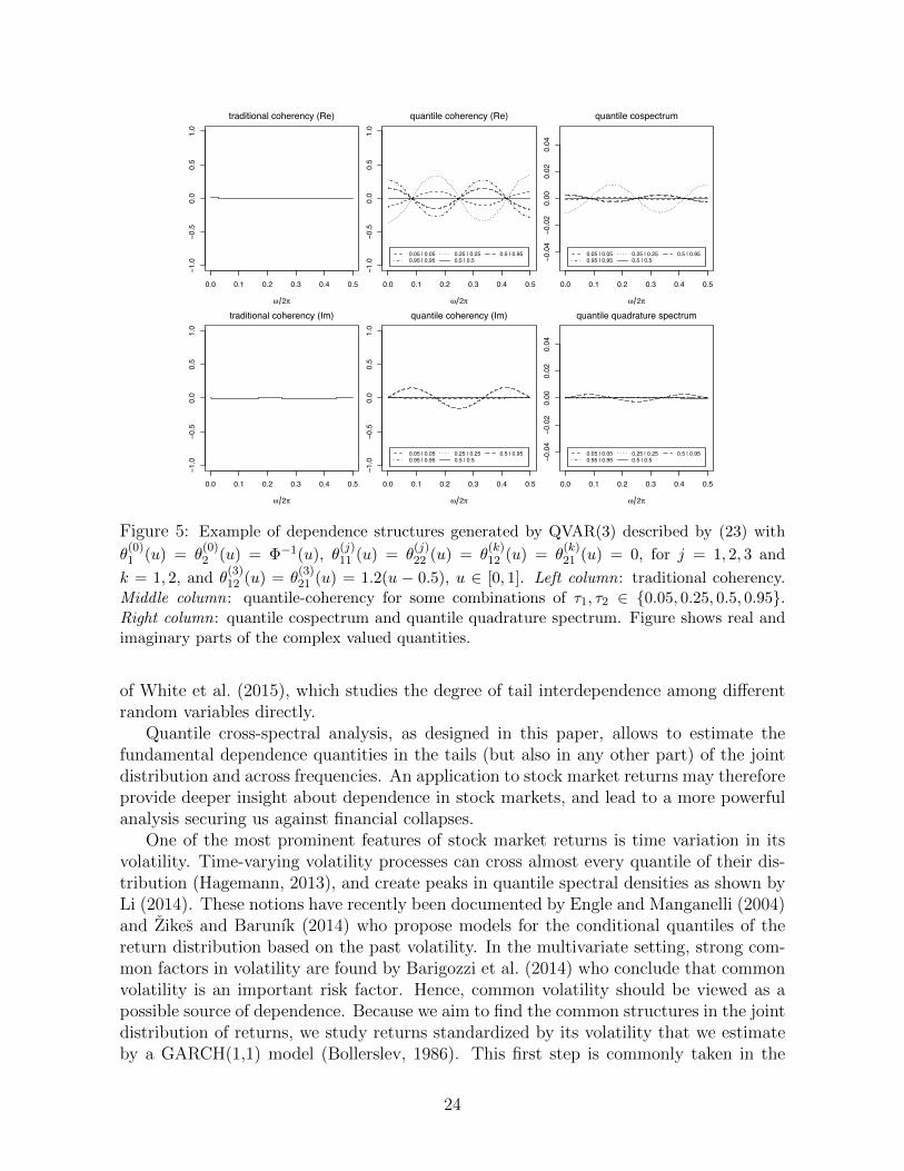
again set to zero, except for ✓(3)12

(u) = ✓(3)21

(u) = 1.2(u� 0.5), such that the processes areconnected only through the third lag of the other component and not through their owncontributions.

In Figures 4 and 5 the dynamics of the described QVAR(2) and QVAR(3) processesare shown. Connecting the quantiles of the two processes through the second and thirdlag gives us richer dependence structures across frequencies. They, again, resemble theshape of the traditional coherencies of VAR(2) and VAR(3) processes. When traditionalcoherency is used for the QVAR(2) and QVAR(3) processes, the dependence structurestays completely hidden.

These examples of the general QVAR(p) specified in (23) served to show how richdependence structures can be created across points of the joint distribution and di↵erentfrequencies. It is obvious, how more complicated structures for the coe�cient functionswould lead to even richer dynamics than in the examples shown.

22

0.0 0.1 0.2 0.3 0.4 0.5

−1.0

−0.5

0.0

0.5

1.0

ω 2π

traditional coherency (Re)

0.0 0.1 0.2 0.3 0.4 0.5

−1.0

−0.5

0.0

0.5

1.0

ω 2π

quantile coherency (Re)

0.05 | 0.050.95 | 0.95

0.25 | 0.250.5 | 0.5

0.5 | 0.95

0.0 0.1 0.2 0.3 0.4 0.5

−0.0

4−0

.02

0.00

0.02

0.04

ω 2π

quantile cospectrum

0.05 | 0.050.95 | 0.95

0.25 | 0.250.5 | 0.5

0.5 | 0.95

0.0 0.1 0.2 0.3 0.4 0.5

−1.0

−0.5

0.0

0.5

1.0

ω 2π

traditional coherency (Im)

0.0 0.1 0.2 0.3 0.4 0.5

−1.0

−0.5

0.0

0.5

1.0

ω 2π

quantile coherency (Im)

0.05 | 0.050.95 | 0.95

0.25 | 0.250.5 | 0.5

0.5 | 0.95

0.0 0.1 0.2 0.3 0.4 0.5

−0.0

4−0

.02

0.00

0.02

0.04

ω 2π

quantile quadrature spectrum

0.05 | 0.050.95 | 0.95

0.25 | 0.250.5 | 0.5

0.5 | 0.95

Figure 4: Example of dependence structures generated by QVAR(2) described by (23) with

✓

(0)

1

(u) = ✓

(0)

2

(u) = ��1(u), ✓(1)11

(u) = ✓

(1)

22

(u) = ✓

(2)

11

(u) = ✓

(2)

22

(u) = ✓

(1)

12

(u) = ✓

(1)

21

(u) = 0 and

✓

(2)

12

(u) = ✓

(2)

21

(u) = 1.2(u � 0.5), u 2 [0, 1]. Left column: traditional coherency. Middle col-

umn: quantile-coherency for some combinations of ⌧1

, ⌧

2

2 {0.05, 0.25, 0.5, 0.95}. Right column:quantile cospectrum and quantile quadrature spectrum. Figure shows real and imaginary partsof the complex valued quantities.

5 Quantile cross-spectral analysis of stock market re-

turns: A route to more accurate risk measures?

Stock market returns belong to the most prominent datasets in economics and finance.Although many important stylized facts about their behavior have been established inthe past decades, it remains a very active area of research. Despite the e↵orts, animportant direction, which has not been fully addressed is stylized facts about the jointdistribution of returns. Especially during the last turbulent decade, understanding thebehavior of joint quantiles in return distributions became particularly important, as itis essential for understanding systemic risk; “the risk that the intermediation capacity ofthe entire system can be impaired” (Adrian and Brunnermeier, 2011). Several authorsfocus on explaining tails of the bivariate market distributions in di↵erent ways. Adrianand Brunnermeier (2011) proposed to classify institutions according to the sensitivity oftheir quantiles to shocks to the market. Han et al. (2014) proposed cross-quantilogramsand used them to measure co-dependence in the tails of equity returns of an individualinstitution and of the whole system. Most closely related to the notion of how we viewthe dependence structures is the recently proposed multivariate regression quantile model

23

0.0 0.1 0.2 0.3 0.4 0.5

−1.0

−0.5

0.0

0.5

1.0

ω 2π

traditional coherency (Re)

0.0 0.1 0.2 0.3 0.4 0.5

−1.0

−0.5

0.0

0.5

1.0

ω 2π

quantile coherency (Re)

0.05 | 0.050.95 | 0.95

0.25 | 0.250.5 | 0.5

0.5 | 0.95

0.0 0.1 0.2 0.3 0.4 0.5

−0.0

4−0

.02

0.00

0.02

0.04

ω 2π

quantile cospectrum

0.05 | 0.050.95 | 0.95

0.25 | 0.250.5 | 0.5

0.5 | 0.95

0.0 0.1 0.2 0.3 0.4 0.5

−1.0

−0.5

0.0

0.5

1.0

ω 2π

traditional coherency (Im)

0.0 0.1 0.2 0.3 0.4 0.5

−1.0

−0.5

0.0

0.5

1.0

ω 2π

quantile coherency (Im)

0.05 | 0.050.95 | 0.95

0.25 | 0.250.5 | 0.5

0.5 | 0.95

0.0 0.1 0.2 0.3 0.4 0.5

−0.0

4−0

.02

0.00

0.02

0.04

ω 2π

quantile quadrature spectrum

0.05 | 0.050.95 | 0.95

0.25 | 0.250.5 | 0.5

0.5 | 0.95

Figure 5: Example of dependence structures generated by QVAR(3) described by (23) with

✓

(0)

1

(u) = ✓

(0)

2

(u) = ��1(u), ✓

(j)

11

(u) = ✓

(j)

22

(u) = ✓

(k)

12

(u) = ✓

(k)

21

(u) = 0, for j = 1, 2, 3 and

k = 1, 2, and ✓

(3)

12

(u) = ✓

(3)

21

(u) = 1.2(u � 0.5), u 2 [0, 1]. Left column: traditional coherency.Middle column: quantile-coherency for some combinations of ⌧

1

, ⌧

2

2 {0.05, 0.25, 0.5, 0.95}.Right column: quantile cospectrum and quantile quadrature spectrum. Figure shows real andimaginary parts of the complex valued quantities.

of White et al. (2015), which studies the degree of tail interdependence among di↵erentrandom variables directly.

Quantile cross-spectral analysis, as designed in this paper, allows to estimate thefundamental dependence quantities in the tails (but also in any other part) of the jointdistribution and across frequencies. An application to stock market returns may thereforeprovide deeper insight about dependence in stock markets, and lead to a more powerfulanalysis securing us against financial collapses.

One of the most prominent features of stock market returns is time variation in itsvolatility. Time-varying volatility processes can cross almost every quantile of their dis-tribution (Hagemann, 2013), and create peaks in quantile spectral densities as shown byLi (2014). These notions have recently been documented by Engle and Manganelli (2004)and Zikes and Barunık (2014) who propose models for the conditional quantiles of thereturn distribution based on the past volatility. In the multivariate setting, strong com-mon factors in volatility are found by Barigozzi et al. (2014) who conclude that commonvolatility is an important risk factor. Hence, common volatility should be viewed as apossible source of dependence. Because we aim to find the common structures in the jointdistribution of returns, we study returns standardized by its volatility that we estimateby a GARCH(1,1) model (Bollerslev, 1986). This first step is commonly taken in the

24

literature of modeling the joint market distribution using copulas (Granger et al., 2006;Patton, 2012). In these approaches the volatility in the marginal distributions is mod-eled first, and the common factors are then considered in the second step. Consequently,this will allow us to discover other possible common factors in the joint distribution ofmarket returns across frequencies, that result in spurious dependence, but which will notbe overshadowed by the strong volatility process.

0.0 0.1 0.2 0.3 0.4 0.5

0.2

0.4

0.6

0.8

ω 2π

Y M Wquantile coherency (Re)

0.5 | 0.5 0.05 | 0.05 0.95 | 0.95

0.0 0.1 0.2 0.3 0.4 0.5

−0.4

−0.2

0.0

0.2

0.4

ω 2π

Y M Wquantile coherency (Im)

0.5 | 0.5 0.05 | 0.05 0.95 | 0.95

Figure 6: Real (left) and imaginary (right) parts of the quantile coherency estimates for theportfolio formed from consumer non-durables and excess market returns for 0.05, 0.5, and 0.95quantiles together with 95% confidence intervals. W, M, and Y denotes weekly, monthly, andyearly periods. Data span years 1926 – 2015.

We choose to study the joint distribution of portfolio returns and excess returns onthe broad market, hence looking at one of the most commonly studied factor structuresin the literature as dictated by asset pricing theories (Sharpe, 1964; Lintner, 1965). As anexcess return on the market, we use value-weighted returns of all firms listed on the NYSE,AMEX, or NASDAQ from the Center for Research in Security Price (CRSP) database.For the benchmark portfolio, we use an industry portfolio formed from consumer non-durables.3 The daily data we have used runs from July 1, 1926 through to June 30, 2015.

Although very attractive due to powerful and intuitive predictions about risk mea-surement, the capital asset pricing theory (CAPM) is largely invalidated empirically byresearchers (Fama and French, 2004). In the model it is assumed that the variance of thereturns is an adequate risk measure, as implied by the assumption of the returns understudy being normally distributed. Intuitively, departures from normality are better ca-pable of capturing the investor’s preferences. Risk can be viewed as a probability of loss,

3Note to choice of the data: we use the publicly available data available and maintained by Fama andFrench at http://mba.tuck.dartmouth.edu/pages/faculty/ken.french/data_library.html. Thisdata set is popular among researchers, and while many types of portfolios can be chosen, we choseconsumer non-durables randomly for this application. Although very interesting and attractive, it isfar beyond the scope of this work to present and discuss results for wider portfolios formed on distinctcriteria.

25

hence is asymmetric, implying that we should move our focus from variability of returnsto their quantiles directly.

In Figure 6, quantile coherency estimates for the 0.05|0.05, 0.5|0.5, and 0.95|0.95 com-binations of quantile levels of the joint distribution are shown for the industry portfolioand excess market returns over frequencies. For clarity, we plot the x-axis in daily cyclesand also indicate the frequencies that correspond to yearly, monthly, and weekly periods.While we use daily data the highest possible frequency of 0.5 indicates 0.5 cycles per day(i. e., a 2-day period). While precise frequencies do not have an economic meaning, oneneeds to understand the interpretation with respect to the time domain. For example, asampling frequency of 0.2 corresponds to 0.2 cycles per day translating to a 5 days period(equivalent to one week), but the frequency of 0.3 translates to a hardly interpretable3.3 period. Hence, the upper label of the x-axis is of particular interest to an economist,as one can study how weekly, monthly, or yearly cycles are connected across quantiles ofthe joint distribution.

The real parts of the quantile coherency estimates reveal frequency dynamics in quan-tiles of the joint distribution of the returns under study. Generally, lower quantiles aremore strongly dependent than upper quantiles, which is a well documented stylized factabout stock market returns. It points us to the fact that returns are more dependentduring business cycle downturns, than upturns (Erb et al., 1994; Longin and Solnik, 2001;Ang and Chen, 2002; Patton, 2012). More importantly, lower quantiles as well as themedian are strongly related in periods longer than one week in average in comparison toshorter than weekly periods, and are even more connected at longer than monthly cy-cles. This suggests that infrequent clusters of large negative portfolio returns are betterexplained by excess market returns than small daily fluctuations. The same result holdsalso for the median, while returns in upper quantiles of the joint distribution seem to beconnected similarly across all frequencies.

While asymmetry is commonly found by researchers, we document frequency depen-dent asymmetry in the joint distribution of stock market returns. In case this behaviorwould be common across larger classes of assets, our results may have large implicationsfor one of the cornerstones of asset pricing theory assuming normal distribution of re-turns. It leads us to the call for more general models, and more importantly to the needof restating the asset pricing theory in a way that allows to distinguish between shortrun and long run behavior of investors.

Our results are also crucial for systemic risk measurement, as an investor wishing tooptimize a portfolio should focus on stocks which will not be connected at lower quantiles,in a situation of distress, but will be connected at upper quantiles, in a situation of marketupturns in a given investment period. We document behavior which is not favorable tosuch an investor using traditional pricing theories, as we show that broad stock marketreturns contain a common factor more frequently during downturns than during upturns.This suggests that the portfolio at hand might be much riskier than it were implied bycommon measures. Further, our results suggest that this e↵ect becomes even worse forlong-run investors.

An important feature of our quantile cross-spectral measures is that they enable usto measure dependence also between ⌧

1

6= ⌧2

quantiles of the joint distribution. InFigure 7 we document that the dependence between the 0.05|0.95 quantiles of the return

26

0.0 0.1 0.2 0.3 0.4 0.5

−0.2

0.0

0.2

0.4

0.6

0.8

ω 2π

Y M Wquantile coherency (Re)

0.05 | 0.95

0.0 0.1 0.2 0.3 0.4 0.5

−0.4

−0.2

0.0

0.2

0.4

ω 2π

Y M Wquantile coherency (Im)

0.05 | 0.95

Figure 7: Real (left) and imaginary (right) parts of the quantile coherency estimates for the0.05 quantile of portfolio formed from consumer non-durables and 0.95 quantile of excess marketreturns together with 95% confidence intervals. W, M, and Y denotes weekly, monthly, andyearly periods, respectively. The data spans the years 1926–2015.

distribution is not very strong. Generally speaking, no dependence can be seen betweenlarge negative returns of the stock market, and large positive returns of the portfoliounder study. This analysis may be much more interesting in case of dependence betweenindividual assets, where negative news may have strong opposite impact on the assetsunder study.

Here, we remind the reader about the interpretation of the quantities which we haveestimated. In Section 2.3 we provided a link between quantile coherency and tradi-tional measures of dependence under the assumption of normally distributed data. Thequantile-based measures are designed to capture general dependence types without re-strictive assumptions on the underlying distribution of the process. Hence, we do inten-tionally not relate it to traditional correlation which, ideally, should only be interpretedwhen the process is known to be Gaussian. The financial returns under study in thissection are known to depart from normality. Therefore, quantile coherency is not directlycomparable to traditional correlation measures. What we can see is generally very strongdependence between the portfolio returns and excess market returns at all quantiles con-firming the fact that excess returns are a strong common factor for the studied portfolioreturns. The details that the quantile-based analysis in this section revealed would haveremained hidden in an analysis based on the traditional coherency.

6 Conclusion

In this paper we introduced quantile cross-spectral analysis of economic time series pro-viding an entirely model-free, nonparametric theory for the estimation of general cross-dependence structures emerging from quantiles of the joint distribution in the frequency

27

domain. We argue that complex dynamics in time series often arise naturally in manymacroeconomic and financial time series, as infrequent periods of large negative val-ues (lower quantiles of the joint distribution) may be more dependent than infrequentperiods of large positive values (upper quantiles of the joint distribution). Moreover,the dependence may di↵er in the long-, medium, or short-run. Quantile cross-spectralanalysis hence fundamentally changes the way how we view the dependence betweeneconomic time series, and may be viewed as a precursor to the subsequent developmentsin economic research underlying many new modeling strategies.

Bridging two literatures which focus on the dependence between variables in quantilesof their joint distribution and across frequencies separately, the proposed methods maybe viewed as an important step in robustifying the traditional cross-spectral analysisas well. Quantile-based spectral quantities are very attractive as they do not requirethe existence of moments, an important relaxation to the classical assumptions, wheremoments up to the order of the cumulants involved are typically assumed to exist. Theproposed quantities are robust to many common violations of traditional assumptionsfound in data, including outliers, heavy tails, and changes in higher moments of thedistribution. By considering quantiles instead of moments the proposed methods areable to reveal the dependence even in uncorrelated data. As an essential ingredient for asuccessful applications we have provided a rigorous analysis of the asymptotic propertiesof the introduced estimators and showed that for a general class of nonlinear processes,properly centered and smoothed versions of the quantile-based estimators converge indistribution to centered Gaussian processes.

In an empirical application, we have shown that asset pricing theories may not suit thedata well, as commonly documented by researchers, because rich dependence structuresexists varying across quantiles and frequencies in the joint distribution of returns. Wedocument strong dependence of the bivariate returns series in periods of large negativereturns, while positive returns display less dependence over all frequencies. This resultis not favorable for an investor, as exactly the opposite would be desired: choosing toinvest to a stocks with independent negative returns, but dependent positive returns.Our tool reveals that systematic risk originates more strongly from lower quantiles of thejoint distribution in the long-, and medium-run investment horizons in comparison to theupper quantiles.

We believe that our work opens many exciting routes for future theoretical as wellas empirical research. From the perspective of applications, exploratory analysis basedon the quantile cross-spectral estimators can reveal new implications for improvement oreven restating of many economic problems. Dependence in many economic time seriesis of a non-Gaussian nature, calling for an escape from covariance-based methods andallowing for a detailed analysis of the dependence in the quantiles of the joint distribution.

References

Adrian, T. and M. K. Brunnermeier (2011). CoVaR. http://www.nber.org/papers/w17454. Technical report, National Bureau of Economic Research.

28

Ang, A. and J. Chen (2002). Asymmetric correlations of equity portfolios. Journal ofFinancial Economics 63 (3), 443–494.

Bae, K.-H., G. A. Karolyi, and R. M. Stulz (2003). A new approach to measuring financialcontagion. Review of Financial studies 16 (3), 717–763.

Barigozzi, M., C. Brownlees, G. M. Gallo, and D. Veredas (2014). Disentangling system-atic and idiosyncratic dynamics in panels of volatility measures. Journal of Economet-rics 182 (2), 364–384.

Beaudry, P. and G. Koop (1993). Do recessions permanently change output? Journal ofMonetary economics 31 (2), 149–163.

Birr, S., S. Volgushev, T. Kley, H. Dette, and M. Hallin (2015). Quantile spectral analysisfor locally stationary time series (arxiv:1404.4605v2). ArXiv e-prints .

Bollerslev, T. (1986). Generalized autoregressive conditional heteroskedasticity. Journalof Econometrics 31 (3), 307–327.

Bougerol, P. and N. Picard (1992). Strict stationarity of generalized autoregressive pro-cesses. The Annals of Probability 20 (4), 1714–1730.

Boussama, F. (1998). Ergodicite, melange et estimation dans le modeles GARCH. Ph.D. thesis, Universite 7 Paris.

Brillinger, D. R. (1975). Time Series: Data Analysis and Theory. New York: Holt,Rinehart and Winston, Inc.

Brockwell, P. J. and R. A. Davis (1987). Time Series: Theory and Methods. SpringerSeries in Statistics. New York: Springer.

Carrasco, M. and X. Chen (2002). Mixing and moment properties of various GARCHand stochastic volatility models. Econometric Theory 18 (1), 17–39.

Croux, C., M. Forni, and L. Reichlin (2001). A measure of comovement for economicvariables: Theory and empirics. Review of Economics and Statistics 83 (2), 232–241.

Davis, R. A., T. Mikosch, et al. (2009). The extremogram: A correlogram for extremeevents. Bernoulli 15 (4), 977–1009.

Dette, H., M. Hallin, T. Kley, and S. Volgushev (2015). Of copulas, quantiles, ranks andspectra: An L

1

-approach to spectral analysis. Bernoulli 21 (2), 781–831.

Enders, W. and C. W. J. Granger (1998). Unit-root tests and asymmetric adjustmentwith an example using the term structure of interest rates. Journal of Business &amp;Economic Statistics 16 (3), 304–311.

Engle, R. F. and S. Manganelli (2004). CAViaR: Conditional autoregressive value at riskby regression quantiles. Journal of Business & Economic Statistics 22 (4), 367–381.

29

Erb, C. B., C. R. Harvey, and T. E. Viskanta (1994). Forecasting international equitycorrelations. Financial Analysts Journal 50 (6), 32–45.

Fama, E. F. and K. R. French (2004). The capital asset pricing model: Theory andevidence. Journal of Economic Perspectives 18, 25–46.

Fan, Y. and A. J. Patton (2014). Copulas in econometrics. Annual Review of Eco-nomics 6 (1), 179–200.

Francq, C. and J.-M. Zakoıan (2006). Mixing properties of a general class of GARCH(1,1)models without moment assumptions on the observed process. Econometric The-ory 22 (05), 815–834.

Granger, C. W. (1966). The typical spectral shape of an economic variable. Econometrica,150–161.

Granger, C. W. (1969). Investigating causal relations by econometric models and cross-spectral methods. Econometrica, 424–438.

Granger, C. W. (2010). Some thoughts on the development of cointegration. Journal ofEconometrics 158 (1), 3–6.

Granger, C. W. and P. Newbold (1974). Spurious regressions in econometrics. Journalof Econometrics 2 (2), 111–120.

Granger, C. W., T. Terasvirta, and A. J. Patton (2006). Common factors in conditionaldistributions for bivariate time series. Journal of Econometrics 132 (1), 43–57.

Hagemann, A. (2013). Robust spectral analysis (arxiv:1111.1965v2). ArXiv e-prints .

Han, H., O. Linton, T. Oka, and Y.-J. Whang (2014). The cross-quantilogram: mea-suring quantile dependence and testing directional predictability between time series(arxiv:1402.1937v1). ArXiv e-prints .

Hill, J. B. and A. McCloskey (2014). Heavy tail robust frequency do-main estimation. http://www.econ.brown.edu/fac/adam_mccloskey/Research_

files/FDTTQML.pdf.

Hong, Y. (1999). Hypothesis testing in time series via the empirical characteristic func-tion: a generalized spectral density approach. Journal of the American StatisticalAssociation 94 (448), 1201–1220.

Hong, Y. (2000). Generalized spectral tests for serial dependence. Journal of the RoyalStatistical Society Series B 62 (3), 557–574.

Katkovnik, V. (1998). Robust M-periodogram. IEEE Transactions on Signal Process-ing 46 (11), 3104–3109.

Kleiner, R., R. D. Martin, and D. J. Thomson (1979). Robust estimation of powerspectra. Journal of the Royal Statistical Society Series B 41 (3), 313–351.

30

Kley, T. (2014). Quantile-based spectral analysis in an object-oriented framework anda reference implementation in R: The quantspec package (arxiv:1408.6755). ArXive-prints .

Kley, T. (2015). quantspec: Quantile-based spectral analysis functions. R package version1.2-0.

Kley, T., S. Volgushev, H. Dette, and M. Hallin (2015+). Quantile spectral processes:Asymptotic analysis and inference. Bernoulli forthcoming.

Kluppelberg, C. and T. Mikosch (1994). Some limit theory for the self-normalised peri-odogram of stable processes. Scandinavian Journal of Statistics 21, 485–491.

Knight, K. (2006). Comment on “Quantile autoregression”. Journal of the AmericanStatistical Association 101 (475), 994–996.

Koenker, R. (2005). Quantile Regression. Econometric Society Monographs. CambridgeUniversity Press.

Koenker, R. and Z. Xiao (2006). Quantile autoregression. Journal of the AmericanStatistical Association 101 (475), 980–990.

Lee, J. and S. S. Rao (2012). The quantile spectral density and comparison based testsfor nonlinear time series (arxiv:1112.2759v2). ArXiv e-prints .

Li, G., Y. Li, and C.-L. Tsai (2015). Quantile correlations and quantile autoregressivemodeling. Journal of the American Statistical Association 110 (509), 246–261.

Li, T.-H. (2008). Laplace periodogram for time series analysis. Journal of the AmericanStatistical Association 103 (482), 757–768.

Li, T.-H. (2012). Quantile periodograms. Journal of the American Statistical Associa-tion 107 (498), 765–776.

Li, T.-H. (2014). Quantile periodogram and time-dependent variance. Journal of TimeSeries Analysis 35 (4), 322–340.

Liebscher, E. (2005). Towards a unified approach for proving geometric ergodicity andmixing properties of nonlinear autoregressive processes. Journal of Time Series Anal-ysis 26 (5), 669–689.

Lintner, J. (1965). The valuation of risk assets and the selection of risky investments instock portfolios and capital budgets. The Review of Economics & Statistics , 13–37.

Linton, O. and Y.-J. Whang (2007). The quantilogram: With an application to evaluatingdirectional predictability. Journal of Econometrics 141 (1), 250–282.

Longin, F. and B. Solnik (2001). Extreme correlation of international equity markets.Journal of Finance, 649–676.

31

Maronna, R., D. Martin, and V. Yohai (2006). Robust Statistics: Theory and Methods.Wiley Series in Probability and Statistics. Wiley.

Mikosch, T. and Y. Zhao (2014). A fourier analysis of extreme events. Bernoulli 20 (2),803–845.

Mikosch, T. and Y. Zhao (2015). The integrated periodogram of a dependent extremalevent sequence. Stochastic Processes and their Applications 125 (8), 3126–3169.

Neftci, S. N. (1984). Are economic time series asymmetric over the business cycle? TheJournal of Political Economy , 307–328.

Ning, C. Q. and L. Chollete (2009). The dependence structure of macroeconomic vari-ables in the us. http://www1.uis.no/ansatt/odegaard/uis_wps_econ_fin/uis_

wps_2009_31_chollete_ning.pdf. Technical report.

Patton, A. J. (2012). A review of copula models for economic time series. Journal ofMultivariate Analysis 110, 4–18.

Schmitt, T. A., R. Schafer, H. Dette, and T. Guhr (2015). Quantile correlations: Un-covering temporal dependencies in financial time series. Journal of Theoretical andApplied Finance forthcoming.

Shao, X. and J. Zhang (2014). Martingale di↵erence correlation and its use inhigh-dimensional variable screening. Journal of the American Statistical Associa-tion 109 (507), 1302–1318.

Sharpe, W. F. (1964). Capital asset prices: A theory of market equilibrium under con-ditions of risk. The Journal of Finance 19 (3), 425–442.

Szekely, G. J., M. L. Rizzo, and N. K. Bakirov (2007, 12). Measuring and testing depen-dence by correlation of distances. Ann. Statist. 35 (6), 2769–2794.

Taniguchi, M. and Y. Kakizawa (2000). Asymptotic theory of statistical inference fortime series. Springer.

van der Vaart, A. and J. Wellner (1996). Weak Convergence and Empirical Processes:With Applications to Statistics. New York: Springer.

White, H., T.-H. Kim, and S. Manganelli (2015). VAR for VaR: Measuring tail de-pendence using multivariate regression quantiles. Journal of Econometrics 187 (1),169–188.

Xiao, Z. (2009). Quantile cointegrating regression. Journal of Econometrics 150 (2),248–260.

Zhou, Z. (2012). Measuring nonlinear dependence in time-series, a distance correlationapproach. Journal of Time Series Analysis 33 (3), 438–457.

Zikes, F. and J. Barunık (2014). Semi-parametric conditional quantile models for financialreturns and realized volatility. Journal of Financial Econometrics , forthcoming.

32

7 Technical Appendix

In the first section of the appendix we collect details on how to construct pointwiseconfidence bands. The proofs to the theorems in the paper are given in the remainingsections of the appendix.

7.1 Interval Estimators

Section 3 contained asymptotic results on the uncertainty of point estimation of the newlyintroduced quantile cross-spectral quantities. In this section we describe strategies toestimate the variances (of the real and imaginary parts) that appear in those limit resultsand describe how asymptotically valid pointwise confidence bands can be constructed.

In all three subsections the following comment is relevant. Assuming that we havedetermined the weights W

n

form a kernel W that is of order d. We will choose abandwidth b

n

= o(n�1/(2d+1)). This choice implies that compared to the variance thebias (that in some form appears in both limit results) is asymptotically negligible:pnb

n

B(k)

n

(!; ⌧1

, ⌧2

) = o(1).

7.1.1 Pointwise Confidence Bands for f

Utilizing Theorem 3.3 we now construct pointwise asymptotic (1 � ↵)-level confidencebands for the real and imaginary parts of fj1,j2(!

kn

; ⌧1

, ⌧2

), !kn

:= 2⇡k/n, as follows:

C(1)

r,n

(!kn

; ⌧1

, ⌧2

) := <Gj1,j2n,R

(!kn

; ⌧1

, ⌧2

)± <�j1,j2

(1)

(!kn

; ⌧1

, ⌧2

)��1(1� ↵/2),

for the real part, and

C(1)

i,n

(!kn

; ⌧1

, ⌧2

) := =Gj1,j2n,R

(!kn

; ⌧1

, ⌧2

)± =�j1,j2

(1)

(!kn

; ⌧1

, ⌧2

)��1(1� ↵/2),

for the imaginary part of the quantile cross-spectrum. Here,

Gj1,j2n,R

(!kn

; ⌧1

, ⌧2

) := Gj1,j2n,R

(!kn

; ⌧1

, ⌧2

)/W k

n

, W k

n

:=2⇡

n

n�1

X

s=1

Wn

(!kn

� !sn

),

and � denotes the cumulative distribution function of the standard normal distribution,4

�

<�j1,j2(!kn

; ⌧1

, ⌧2

)�

2

:= 0_(

Cov(H1,2

,H1,2

) if j1

= j2

and ⌧1

= ⌧2

,1

2

�

Cov(H1,2

,H1,2

) + <Cov(H1,2

,H2,1

)�

otherwise,

and

�

=�j1,j2(!kn

; ⌧1

, ⌧2

)�

2

:= 0_(

0 if j1

= j2

and ⌧1

= ⌧2

,1

2

�

Cov(H1,2

,H1,2

)�<Cov(H1,2

,H2,1

)�

otherwise,

4Note that for k = 0, . . . , n � 1 we have W

kn := 2⇡/n

P

0=s 6=k Wn(2⇡s/n). For k 2 Z with k < 0 ork � n we can define it as the n periodic extension.

33

where Cov(Ha,b

,Hc,d

) denotes an estimator of Cov�

Hja,jb(!kn

; ⌧a

, ⌧b

�

,Hjc,jd(!kn

; ⌧c

, ⌧d

)�

.Here, motivated by Theorem 7.4.3 in Brillinger (1975), we use

⇣ 2⇡

n ·W k

n

⌘

⇥"

n�1

X

s=1

Wn

�

2⇡(k�s)/n�

Wn

�

2⇡(k�s)/n�

Gja,jcn,R

(⌧a

, ⌧c

; 2⇡s/n)Gjb,jdn,R

(⌧b

, ⌧d

;�2⇡s/n)

+n�1

X

s=1

Wn

�

2⇡(k � s)/n�

Wn

�

2⇡(k + s)/n�

Gja,jdn,R

(⌧a

, ⌧d

; 2⇡s/n)Gjb,jcn,R

(⌧b

, ⌧c

;�2⇡s/n)

#

(24)

The definition of �j1,j2

(1)

(!kn

; ⌧1

, ⌧2

) is motivated by the fact that =Gj1,j2n,R

(!kn

; ⌧1

, ⌧2

) = 0,if j

1

= j2

and ⌧1

= ⌧2

. Furthermore, note that, for any complex-valued random variableZ, with complex conjugate Z,

Var(<Z) = 1

2

�

Var(Z) + <Cov(Z, Z)�

; Var(=Z) = 1

2

�

Var(Z)�<Cov(Z, Z)�

, (25)

and we have H1,2

= H2,1

.

7.1.2 Pointwise Confidence Bands for R

We utilize Theorem 3.4 to construct pointwise asymptotic (1�↵)-level confidence bandsfor the real and imaginary parts of Rj1,j2(!; ⌧

1

, ⌧2

) as follows:

C(2)

r,n

(!kn

; ⌧1

, ⌧2

) := <Rj1,j2n,R

(!kn

; ⌧1

, ⌧2

)± <�j1,j2

(2)

(!kn

; ⌧1

, ⌧2

)��1(1� ↵/2),

for the real part, and

C(2)

i,n

(!kn

; ⌧1

, ⌧2

) := =Rj1,j2n,R

(!kn

; ⌧1

, ⌧2

)± =�j1,j2

(2)

(!kn

; ⌧1

, ⌧2

)��1(1� ↵/2),

for the imaginary part of the quantile coherency. Here, � stands for the cdf of thestandard normal distribution,

�

<�j1,j2

(2)

(!kn

; ⌧1

, ⌧2

)�

2

:= 0_(

0 if j1

= j2

and ⌧1

= ⌧2

,1

2

�

Cov(L1,2

,L1,2

) + <Cov(L1,2

,L2,1

)�

otherwise,

and

�

=�j1,j2

(2)

(!kn

; ⌧1

, ⌧2

)�

2

:= 0_(

0 if j1

= j2

and ⌧1

= ⌧2

,1

2

�

Cov(L1,2

,L1,2

)�<Cov(L1,2

,L2,1

)�

otherwise.

The definition of �j1,j2

(2)

(!kn

; ⌧1

, ⌧2

) is motivated by (25) and the fact that we have

L1,2

= L2,1

. Furthermore, note that Rj1,j2n,R

(!kn

; ⌧1

, ⌧2

) = 1, if j1

= j2

and ⌧1

= ⌧2

..

In the definition of �j1,j2

(2)

(!kn

; ⌧1

, ⌧2

) we have used Cov(La,b

,Lc,d

) to denote an estimatorfor

Cov�

Lj1,j2(!kn

; ⌧1

, ⌧2

�

,Lj3,j4(!kn

; ⌧3

, ⌧4

)�

.

34

Recalling the definition of he limit process in Theorem 3.4 we derive the following ex-pression:

1p

f1,1

f2,2

f3,3

f4,4

Cov⇣

H1,2

� 1

2

f1,2

f1,1

H1,1

� 1

2

f1,2

f2,2

H2,2

,H3,4

� 1

2

f3,4

f3,3

H3,3

� 1

2

f3,4

f4,4

H4,4

⌘

=Cov(H

1,2

,H3,4

)p

f1,1

f2,2

f3,3

f4,4

� 1

2

f3,4

Cov(H1,2

,H3,3

)q

f1,1

f2,2

f33,3

f4,4

� 1

2

f3,4

Cov(H1,2

,H4,4

)q

f1,1

f2,2

f3,3

f34,4

� 1

2

f1,2

Cov(H1,1

,H3,4

)q

f31,1

f2,2

f3,3

f4,4

+1

4

f1,2

f3,4

Cov(H1,1

,H3,3

)q

f31,1

f2,2

f33,3

f4,4

+1

4

f1,2

f3,4

Cov(H1,1

,H4,4

)q

f31,1

f2,2

f3,3

f34,4

� 1

2

f1,2

Cov(H2,2

,H3,4

)q

f1,1

f32,2

f3,3

f4,4

+1

4

f1,2

f3,4

Cov(H2,2

,H3,3

)q

f1,1

f32,2

f33,3

f4,4

+1

4

f1,2

f3,4

Cov(H2,2

,H4,4

)q

f1,1

f32,2

f3,3

f34,4

,

where we have written fa,b

for the quantile spectral density fja,jb(!kn

; ⌧a

, ⌧b

), and Ha,b

forthe limit distribution Hja,jb(!

kn

; ⌧a

, ⌧b

�

for any a, b = 1, 2, 3, 4).Thus, considering the special case where ⌧

3

= ⌧1

and ⌧4

= ⌧2

, we have

Cov(L1,2

,L1,2

)

=1

f1,1

f2,2

⇣

Cov(H1,2

,H1,2

)�< f1,2

Cov(H1,1

,H1,2

)

f1,1

�< f1,2

Cov(H2,2

,H1,2

)

f2,2

+1

4|f1,2

|2⇣Cov(H

1,1

,H1,1

)

f21,1

+ 2<Cov(H1,1

,H2,2

)

f1,1

f2,2

+Cov(H

2,2

,H2,2

)

f22,2

⌘⌘

(26)

and for the special case where ⌧3

= ⌧1

and ⌧4

= ⌧2

we have

Cov(L1,2

,L2,1

)

=1

f1,1

f2,2

⇣

Cov(H1,2

,H2,1

)� f1,2

Cov(H1,2

,H2,2

)

f2,2

� f1,2

Cov(H1,2

,H1,1

)

f1,1

+1

4f21,2

⇣Cov(H1,1

,H1,1

)

f21,1

+ 2<Cov(H1,1

,H2,2

)

f1,1

f2,2

+Cov(H

2,2

,H2,2

)

f22,2

⌘⌘

.

We substitute consistent estimators for the unknown quantities. To do so we abusenotation using f

a,b

to denote Gja,jbn,R

(!kn

; ⌧a

, ⌧b

) and write Cov(Ha,b

,Hc,d

) for the quantitydefined in (24).

7.2 Proof of Proposition 3.2

The proof resembles the proof of Proposition 3.4 in Kley et al. (2015), where the univariatecase was handled. For j = 1, . . . , d we have, from the continuity of F

j

that the ranks ofthe random variables X

0,j

, ..., Xn�1,j

and Fj

(X0,j

), ..., Fj

(Xn�1,j

) coincide almost surely.Thus, without loss of generality, we can assume that the CCR-periodogram is computedfrom the unobservable data (F

j

(X0,j

))j=1,...,d

, ..., (Fj

(Xn�1,j

))j=1,...,d

. In particular, we canassume the marginals to be uniform.

35

Applying the Continuous Mapping Theorem afterward, it su�ces to prove⇣

n�1/2djn,R

(!; ⌧)⌘

⌧2[0,1],j=1,...,d

⇣

Dj(!; ⌧)⌘

⌧2[0,1],j=1,...,d

in `1Cd([0, 1]), (27)

where `1Cd([0, 1]) is the space of bounded functions [0, 1] ! Cd that we identify with theproduct space `1([0, 1])2d. Let

djn,U

(!; ⌧) :=n�1

X

t=0

I{Fj

(Xt,j

) ⌧}e�i!t,

j = 1, . . . , d, ! 2 R, ⌧ 2 [0, 1], and note that for (27) to hold, it is su�cient that�

n�1/2djn,U

(!; ⌧)�

⌧2[0,1],j=1,...,d

satisfies the following two conditions:

(i1) convergence of the finite-dimensional distributions, i. e.,

�

n�1/2dj`n,U

(!`

; ⌧`

)�

`=1,...,k

d�!�

Dj`(!`

; ⌧`

)�

`=1,...,k

, (28)

for any (j`

, ⌧`

) 2 {1, . . . , d}⇥ [0, 1], !`

6= 0 mod 2⇡, ` = 1, . . . , k and k 2 N;

(i2) stochastic equicontinuity: for any x > 0 and any ! 6= 0 mod 2⇡,

lim�#0

lim supn!1

P⇣

sup⌧1,⌧22[0,1]|⌧1�⌧2|�

|n�1/2(djn,U

(!; ⌧1

)� djn,U

(!; ⌧2

))| > x⌘

= 0, 8j = 1, . . . , d.

(29)

Under (i1) and (i2), an application of Theorems 1.5.4 and 1.5.7 from van der Vaart andWellner (1996) then yields

⇣

n�1/2djn,U

(!; ⌧)⌘

⌧2[0,1],j=1,...,d

⇣

Dj(!; ⌧)⌘

⌧2[0,1],j=1,...,d

in `1Cd([0, 1]). (30)

In combination with

sup⌧2[0,1]

|n�1/2(djn,R

(!; ⌧)� djn,U

(!; ⌧))| = oP

(1), for ! 6= 0 mod 2⇡, j = 1, . . . , d, (31)

which we will prove below, (30) yields the desired result: (27). For the proof of (31), wedenote by F�1

n,j

(⌧) := inf{x : Fn,j

(x) � ⌧} the generalized inverse of Fn,j

and let inf ; := 0.Then, we have, as in (7.25) of Kley et al. (2015), that

sup!2R

sup⌧2[0,1]

�

�

�

djn,R

(!; ⌧)� djn,U

(!; F�1

n,j

(⌧))�

�

�

n sup⌧2[0,1]

|Fn,j

(⌧)� Fn,j

(⌧�)| = OP

(n1/2k) (32)

where Fn,j

(⌧�) := lim⇠"0 Fn,j

(⌧ � ⇠). The OP

-bound in (32) follows from Lemma 7.8.Therefore, it su�ces to bound the terms

sup⌧2[0,1]

n�1/2|djn,U

(!; F�1

n,j

(⌧))� djn,U

(!, ⌧))|, for all j = 1, . . . , d.

36

To do so, note that, for any x > 0 and �n

= o(1) satisfying n1/2�n

! 1, we have

P⇣

sup⌧2[0,1]

n�1/2|djn,U

(!; F�1

n,j

(⌧))� djn,U

(!; ⌧))| > x⌘

P⇣

sup⌧2[0,1]

sup|u�⌧ |�n

|djn,U

(!; u)� djn,U

(!; ⌧)| > xn1/2, sup⌧2[0,1]

|F�1

n,j

(⌧)� ⌧ | �n

⌘

+ P⇣

sup⌧2[0,1]

|F�1

n,j

(⌧)� ⌧ | > �n

⌘

= o(1) + o(1).

The first o(1) follows from (29). The second one is a consequence of Lemma 7.9.It thus remains to prove (28) and (29). For any fixed j = 1, . . . , d the process

�

djn,U

(!, ⌧)�

⌧2[0,1] is determined by the univariate time series X0,j

, . . . , Xn�1,j

. Under

the assumptions made here, (29) therefore follows from (8.7) in Kley et al. (2015).Finally, we establish (28), by employing Lemma 7.7 in combination with Lemma P4.5

and Theorem 4.3.2 from Brillinger (1975). More precisely, to apply Lemma P4.5 (Brillinger,1975), we have to verify that, for any j

1

, . . . , j`

2 {1, . . . , d}, ⌧1

, . . . , ⌧`

2 [0, 1], ` 2 N,and !

1

, . . . ,!`

6= 0 mod 2⇡, all cumulants of the vector

n�1/2

�

dj1n,U

(!1

; ⌧1

), dj1n,U

(�!1

; ⌧1

), . . . , dj`n,U

(!`

; ⌧`

), dj`n,U

(�!`

; ⌧`

)�

converge to the corresponding cumulants of the vector

�

Dj1(!1

; ⌧1

),Dj1(�!1

; ⌧1

), . . . ,Dj`(!`

; ⌧`

),Dj`(�!`

; ⌧`

)�

.

For the cumulants of order one the arguments from the univariate case (cf. the proofof Proposition 3.4 in Kley et al. (2015)) apply: we have |E(n�1/2dj

n,U

(!; ⌧))| = o(1), forany j = 1, . . . , d, ⌧ 2 [0, 1] and fixed ! 6= 0 mod 2⇡. Furthermore, for the cumulants oforder two, applying Theorem 4.3.1 in Brillinger (1975) to the bivariate process (I{X

t,j1 qj1(µ1

)}, I{Xt,j2 q

j2(µ2

)}), we obtain

cum(n�1/2di1n,U

(�1

;µ1

), n�1/2di2n,U

(�2

;µ2

)) = 2⇡n�1�n

(�1

+ �2

)fi1,i2(�1

;µ1

, µ2

) + o(1)

for any (i1

,�1

, µ1

), (i2

,�2

, µ2

) 2S

k

`=1

{(i`

,!`

, ⌧`

), (j`

,�!`

, ⌧`

)}, which yields the correctsecond moment structure. The function �

n

is defined in Lemma 7.7. Finally, the cumu-lants of order J , with J 2 N and J � 3, all tend to zero, as in view of Lemma 7.7

cum(n�1/2di1n,U

(�1

;µ1

), . . . , n�1/2diJn,U

(�J

;µJ

))

Cn�J/2(|�n

(J

X

j=1

�j

)|+ 1)"(| log "|+ 1)d = O(n�(J�2)/2) = o(1),

for (i1

,�1

, µ1

), . . . , (iJ

,�J

, µJ

) 2S

k

`=1

{(i`

,!`

, ⌧`

), (i`

,�!`

, ⌧`

)}, where " := minJ

j=1

µj

.This implies that the limit Dj(⌧ ;!) is Gaussian, and completes the proof of (28). Propo-sition 3.2 follows.

37

7.3 Proof of Theorem 3.3

We proceed in a similar fashion as in the proof of the univariate estimator which wasanalyzed in Kley et al. (2015). First, we state an asymptotic representation result bywhich the estimator G

n,R

can be approximated, in a suitable uniform sense, by anotherprocess G

n,U

which is not defined as a function of the standardized ranks Fn,j

(Xt,j

), butas a function of the unobservable quantities F

j

(Xt,j

), t = 0, . . . , n�1, j = 1, . . . , d. Moreprecisely, this process is defined as

Gn,U

(!; ⌧1

, ⌧2

) := (Gj1,j2n,U

(!; ⌧1

, ⌧2

))j1,j2=1,...,d

,

where

Gj1,j2n,U

(!; ⌧1

, ⌧2

) :=2⇡

n

n�1

X

s=1

Wn

�

! � 2⇡s/n�

Ij1,j2n,U

(2⇡s/n, ⌧1

, ⌧2

)

Ij1,j2n,U

(!; ⌧1

, ⌧2

) :=1

2⇡ndj1n,U

(!; ⌧1

)dj2n,U

(�!; ⌧2

)

djn,U

(!; ⌧) :=n�1

X

t=0

I{Fj

(Xt,j

) ⌧}e�i!t. (33)

Theorem 3.3 then follows from the asymptotic representation of Gn,R

by Gn,U

(i. e.,Theorem 7.1(iii)) and the asymptotic properties of G

n,U

(i. e., Theorem 7.1(i)–(ii)), whichwe now state:

Theorem 7.1. Let Assumptions (C) and (W) hold, and assume that the distributionfunctions F

j

of X0,j

are continuous for all j = 1, . . . , d. Let bn

satisfy the assumptionsof Theorem 3.3. Then,

(i) for any fixed ! 2 R, as n ! 1,p

nbn

�

Gn,U

(!; ⌧1

, ⌧2

)� EGn,U

(!; ⌧1

, ⌧2

)�

⌧1,⌧22[0,1] H(!; ·, ·)

in `1Cd⇥d([0, 1]2), where the process H(!; ·, ·) is defined in Theorem 3.3;

(ii) still as n ! 1,

supj1,j22{1,...,d}⌧1,⌧22[0,1]

!2R

�

�

�

EGj1,j2n,U

(⌧1

, ⌧2

;!)�fj1,j2(!; ⌧1

, ⌧2

)��

B(k)

n

(!; ⌧1

, ⌧2

)

j1,j2

�

�

�

= O((nbn

)�1)+o(bkn

),

where�

B(k)

n

(!; ⌧1

, ⌧2

)

j1,j2is defined in (16);

(iii) for any fixed ! 2 R,

supj1,j22{1,...,d}⌧1,⌧22[0,1]

|Gj1,j2n,R

(⌧1

, ⌧2

;!)� Gj1,j2n,U

(⌧1

, ⌧2

;!)| = oP

�

(nbn

)�1/2 + bkn

�

;

if moreover the kernel W is uniformly Lipschitz-continuous, this bound is uniformwith respect to ! 2 R.

38

The proof of Theorem 7.1 is lengthy, technical and in many places similar to the proofof Theorem 3.6 in Kley et al. (2015). We provide the proof in Sections 7.3.1–7.3.3, withtechnical details deferred to Section 7.5. For the reader’s convenience we first give a briefdescription of the necessary steps.

Part (ii) of Theorem 7.1 can be proved along the lines of classical results from Brillinger(1975), but uniformly with respect to the arguments ⌧

1

and ⌧2

. Parts (i) and (iii) re-quire additional arguments that are di↵erent from the classical theory. These additionalarguments are due to the fact that the estimator is a stochastic process and stochasticequicontinuity of

�

Hj1,j2n

(a;!)�

a2[0,1]2 :=p

nbn

�

Gj1,j2n,U

(!; ⌧1

, ⌧2

)� EGj1,j2n,U

(!; ⌧1

, ⌧2

)�

⌧1,⌧22[0,1](34)

for all j1

, j2

= 1, . . . , d has to be proven to ensure that the convergence holds not onlypointwise, but also uniformly. The key to the proof of (i) and (iii) is a uniform boundon the increments Hj1,j2

n

(a;!) � Hj1,j2n

(b;!) of the process Hj1,j2n

. This bound is neededto show the stochastic equicontinuity of the process. To employ a restricted chainingtechnique (cf. Lemma 7.4), we require two di↵erent bounds. First, we prove a generalbound, uniform in a and b, on the moments of the increments Hj1,j2

n

(a;!)� Hj1,j2n

(b;!)(cf. Lemma 7.5). Second, we prove a sharper bound on the increments Hj1,j2

n

(a;!) �Hj1,j2

n

(b;!) when a and b are “su�ciently close” (cf. Lemma 7.11).Condition (41) which we will required for Lemma 7.5 to hold is rather general. In

Lemma 7.7 we prove that Assumption (C) implies (41).

7.3.1 Proof of Theorem 7.1(i)

It is su�cient to prove the following two claims:

(i1) convergence of the finite-dimensional distributions of the process (34), that is,

�

Hj1`,j2`n

�

(a1`

, a2`

);!j

��

j=1,...,k

d�!�

Hj1`,j2`�

(a1`

, a2`

);!j

��

j=1,...,k

(35)

for any (j1`

, j2`

, a1`

, a2`

,!`

) 2 {1, . . . , d}⇥ [0, 1]2 ⇥ R, ` = 1, . . . , k and k 2 N;

(i2) stochastic equicontinuity: for any x > 0, any ! 2 R, and any j1

, j2

= 1, . . . , d,

lim�#0

lim supn!1

P⇣

supa,b2[0,1]2ka�bk1�

|Hj1,j2n

(a;!)� Hj1,j2n

(b;!)| > x⌘

= 0. (36)

By (36) we have stochastic equicontinuity of all real parts <Hj1,j2n

(·;!) and imaginaryparts =Hj1,j2

n

(·;!). Therefore, in view of Theorems 1.5.4 and 1.5.7 in van der Vaart andWellner (1996), we will have proven part (i).

First we prove (i1). For fixed ⌧1

, ⌧2

, Gj1,j2n,U

(!; ⌧1

, ⌧2

) is the traditional smoothed peri-odogram estimator of the cross-spectrum of the clipped processes (I{F

j1(Xt,j1) ⌧1

})t2Z

and (I{Fj2(Xt,j2) ⌧

2

})t2Z [see Chapter 7.1 in Brillinger (1975)]. Thus, (35) follows from

Theorem 7.4.4 in Brillinger (1975), by which these estimators are asymptotically jointlyGaussian. The first and second moment structures of the limit are given by Theorem 7.4.1

39

and Corollary 7.4.3 in Brillinger (1975). The joint convergence (35) follows. Note thatcondition (C) implies the summability condition [i. e., Assumption 2.6.2(`) in Brillinger(1975), for every `] required for the three theorems in Brillinger (1975) to be applied.

Now to the proof of (i2). The Orlicz norm kXk

= inf{C > 0 : E (|X|/C) 1}with (x) := x6 coincides with the L

6

norm kXk6

= (E|X|6)1/6. Therefore, for any > 0and su�ciently small ka� bk

1

, we have by Lemma 7.5 and Lemma 7.7 that

kHj1,j2n

(a;!)� Hj1,j2n

(b;!)k

K⇣ka� bk

1

(nbn

)2+

ka� bk21

nbn

+ ka� bk31

⌘

1/6

.

Consequently, for all a, b with ka � bk1

su�ciently small and ka � bk1

� (nbn

)�1/� andall � 2 (0, 1) such that � < ,

kHj1,j2n

(a;!)� Hj1,j2n

(b;!)k

Kka� bk�/21

.

Note that ka � bk1

� (nbn

)�1/� if and only if d(a, b) := ka � bk�/21

� (nbn

)�1/2 =: ⌘n

/2.The packing number (van der Vaart and Wellner, 1996, p. 98)D(", d) of ([0, 1]2, d) satisfiesD(", d) ⇣ "�4/�. By Lemma 7.4, we therefore have, for all x, � > 0 and ⌘ � ⌘

n

,

P⇣

supka�bk1�

2/�

|Hj1,j2n

(a;!)� Hj1,j2n

(b;!)| > x⌘

= P⇣

supd(a,b)�

|Hj1,j2n

(a;!)� Hj1,j2n

(b;!)| > x⌘

"

8K

x

Z

⌘

⌘n/2

✏�2/(3�)d✏+ (� + 2⌘n

)⌘�4/(3�)

!#

6

+ P⇣

supd(a,b)⌘n

|Hj1,j2n

(a;!)� Hj1,j2n

(b;!)| > x/4⌘

.

Now, choosing 2/3 < � < 1 and letting n tend to infinity, the second term tends tozero by Lemma 7.11, because, by construction, 1/� > 1 and d(a, b) ⌘

n

if and only ifka� bk

1

22/�(nbn

)�1/�. All together, this yields

lim�#0

lim supn!1

P⇣

supd(a,b)�

|Hn

(a;!)� Hn

(b;!)| > x⌘

"

8K

x

Z

⌘

0

✏�2/(3�)d✏

#

6

,

for every x, ⌘ > 0. The claim then follows, as the integral on the right-hand side may bearbitrarily small by choosing ⌘ accordingly.

7.3.2 Proof of Theorem 7.1(ii)

Following the arguments which were applied in Section 8.1 of Kley et al. (2015) we canderive asymptotic expansions for E[Ij1,j2

n,U

(!; ⌧1

, ⌧2

)] and E[Gj1,j2n,U

(!; ⌧1

, ⌧2

)]. In fact, it iseasy to see that the proofs can still be applied when the Laplace cumulants

cum�

I{Xk1 x

1

}, I{Xk2 x

2

}, . . . , I{X0

xp

}�

40

which were considered in Kley et al. (2015) are replaced by their multivariate counterparts

cum�

I{Xk1,j1 x

1

}, I{Xk2,j2 x

2

}, . . . , I{X0,jp x

p

}�

.

More precisely, we now state Lemma 7.2 and 7.3 (without proof) that are multivariatecounterparts to Lemmas 8.4 and 8.5 in Kley et al. (2015). The lemmas hold under thefollowing assumption:

(CS) Let p � 2, � > 0. There exists a non-increasing function ap

: N ! R+ such that

X

k2N

k�ap

(k) < 1

and

supx1,...,xp

| cum�

I{Xk1,j1 x

1

}, I{Xk2,j2 x

2

}, . . . , I{X0,jp x

p

}�

| ap

�

maxj

|kj

|�

,

for all j1

, . . . , jp

= 1, . . . , d.

Note that condition (CS) follows from Assumption (C) but is in fact somewhat weaker.We now state the first of the two lemmas. It is a generalization of Theorem 5.2.2 inBrillinger (1975).

Lemma 7.2. Under (CS) with K = 2, � > 3,

EIj1,j2n,U

(!; ⌧1

, ⌧2

) =

8

<

:

fj1,j2(!; ⌧1

, ⌧2

) + 1

2⇡n

h

sin(n!/2)

sin(!/2)

i

2

⌧1

⌧2

+ "⌧1,⌧2n

(!) ! 6= 0 mod 2⇡

fj1,j2(!; ⌧1

, ⌧2

) + n

2⇡

⌧1

⌧2

+ "⌧1,⌧2n

(!) ! = 0 mod 2⇡

(37)with sup

⌧1,⌧22[0,1],!2R |"⌧1,⌧2n

(!)| = O(1/n).

The second of the two lemmas is a generalization of Theorem 5.6.1 in Brillinger (1975).

Lemma 7.3. Assume that (CS), with p = 2 and � > k + 1, and (W) hold. Then, withthe notation of Theorem 3.3,

sup⌧1,⌧22[0,1],!2R

�

�

�

EGj1,j2n

(!; ⌧1

, ⌧2

)�fj1,j2(!; ⌧1

, ⌧2

)��

B(k)

n

(!; ⌧1

, ⌧2

)

j1,j2

�

�

�

= O((nbn

)�1)+o(bkn

).

Because (C) implies (CS), Lemma 7.3 implies Theorem 7.1(ii).

7.3.3 Proof of Theorem 7.1(iii)

Using (31) and argument similar to the ones in the proof of Lemma 7.11 it follows that

sup!2R

sup⌧1,⌧22[0,1]

|Gj1,j2n,R

(!; ⌧1

, ⌧2

)� Gj1,j2n,U

(!; F�1

n,j1(⌧

1

), F�1

n,j2(⌧

2

))| = oP

(1).

41

It therefore su�ces to bound the di↵erences

sup⌧1,⌧22[0,1]

|Gj1,j2n,U

(!; ⌧1

, ⌧2

)� Gj1,j2n,U

(!; F�1

n,j1(⌧

1

), F�1

n,j2(⌧

2

))|

for j1

, j2

= 1, . . . , d, pointwise and uniformly in !.We first prove the statement for fixed ! 2 R in full details and will later sketch the

additional arguments needed for the proof of the uniform result. For any x > 0 andsequence �

n

we have,

P n(!):=P⇣

sup⌧1,⌧22[0,1]

|Gj1,j2n,U

(!; F�1

n,j1(⌧

1

), F�1

n,j2(⌧

2

))� Gj1,j2n,U

(!; ⌧1

, ⌧2

)| > x((nbn

)�1/2 + bkn

)⌘

P⇣

sup⌧1,⌧22[0,1]

supk(u,v)�(⌧1,⌧2)k1

supi=1,2;⌧2[0,1] | ˆF�1n,ji

(⌧)�⌧ |

|Gj1,j2n,U

(!; u, v)� Gj1,j2n,U

(!; ⌧1

, ⌧2

)| > x((nbn

)�1/2 + bkn

)⌘

P⇣

sup⌧1,⌧22[0,1]

sup|u�⌧1|�n

|v�⌧2|�n

|Gj1,j2n,U

(!; u, v)� Gj1,j2n,U

(!; ⌧1

, ⌧2

)| > x((nbn

)�1/2 + bkn

),

supi=1,2;⌧2[0,1]

|F�1

n,ji(⌧)� ⌧ | �

n

⌘

+2

X

i=1

P⇣

sup⌧2[0,1]

|F�1

n,ji(⌧)� ⌧ | > �

n

⌘

=P n

1

+ P n

2

, say.

We choose �n

such that n�1/2 ⌧ �n

= o(n�1/2b�1/2

n

(log n)�D), where D denotes theconstant from Lemma 7.6. It then follows from Lemma 7.9 that P n

2

is o(1). For P n

1

, onthe other hand, we have the following bound:

P⇣

sup⌧1,⌧22[0,1]

sup|u�⌧1|�n

|v�⌧2|�n

|Hj1,j2n,U

(!; u, v)� Hj1,j2n,U

(!; ⌧1

, ⌧2

)| > (1 + (nbn

)1/2bkn

)x/2⌘

+ In

sup⌧1,⌧22[0,1]

sup|u�⌧1|�n

|v�⌧2|�n

|EGj1,j2n,U

(!; u, v)� EGj1,j2n,U

(!; ⌧1

, ⌧2

)| > ((nbn

)�1/2 + bkn

)x/2o

.

The first term tends to zero because of (36). The indicator vanishes for n large enough,because we have

sup⌧1,⌧22[0,1]

sup|u�⌧1|�n

|v�⌧2|�n

|EGj1,j2n,U

(!; u, v)� EGj1,j2n,U

(!; ⌧1

, ⌧2

)|

sup⌧1,⌧22[0,1]

sup|u�⌧1|�n

|v�⌧2|�n

|EGj1,j2n,U

(!; u, v)� fj1,j2(!; u, v)��

B(k)

n

(!; u, v)

j1,j2|

+ sup⌧1,⌧22[0,1]

sup|u�⌧1|�n

|v�⌧2|�n

|�

B(k)

n

(!; ⌧1

, ⌧2

)

j1,j2+ fj1,j2(!; ⌧

1

, ⌧2

)� EGj1,j2n,U

(!; ⌧1

, ⌧2

)|

+ sup⌧1,⌧22[0,1]

sup|u�⌧1|�n

|v�⌧2|�n

|fj1,j2(!; u, v) +�

B(k)

n

(!; u, v)

j1,j2

� fj1,j2(!; ⌧1

, ⌧2

)��

B(k)

n

(!; ⌧1

, ⌧2

)

j1,j2|

=o(n�1/2b�1/2

n

+ bkn

) +O(�n

(1 + | log �n

|)D),

42

where D is still the constant from Lemma 7.6. To bound the first two terms we haveapplied part (ii) of Theorem 7.1 and Lemma 7.6 for the third one. Thus, for any fixed !,we have shown P n(!) = o(1), which is the pointwise version of the claim.

Next, we outline the proof of the uniform (with respect to !) convergence. Forany y

n

> 0, by similar arguments as above, using the same �n

, we have

P⇣

sup!2R

sup⌧1,⌧22[0,1]

|Gj1,j2n,R

(!; ⌧1

, ⌧2

)� Gj1,j2n,U

(!; ⌧1

, ⌧2

)| > yn

⌘

P⇣

sup!2R

sup⌧1,⌧22[0,1]

sup|u�⌧1|�n

|v�⌧2|�n

|Hj1,j2n,U

(!; u, v)� Hj1,j2n,U

(!; ⌧1

, ⌧2

)| > (nbn

)1/2yn

/2⌘

+ In

sup!2R

sup⌧1,⌧22[0,1]

sup|u�⌧1|�n

|v�⌧2|�n

|EGj1,j2n,U

(!; u, v)� EGj1,j2n,U

(!; ⌧1

, ⌧2

)| > yn

/2o

+ o(1).

The indicator in the latter expression is o(1) by the same arguments as above [note thatLemma 7.6 and the statement of part (ii) both hold uniformly with respect to ! 2 R].For the bound of the probability, note that by Lemma 7.10,

sup⌧1,⌧2

supk=1,...,n

|Ij1,j2n,U

(2⇡k/n; ⌧1

, ⌧2

)| = OP

(n2/K), for any K > 0.

Moreover, by the uniform Lipschitz continuity ofW the functionWn

is also uniformly Lip-schitz continuous with constant of order O(b�2

n

). Combining those facts with Lemma 7.6and the assumptions on b

n

, we obtain

sup!1,!22R

|!1�!2|n

�3

sup⌧1,⌧22[0,1]

|Hj1,j2n,U

(!1

; ⌧1

, ⌧2

)� Hj1,j2n,U

(!2

; ⌧1

, ⌧2

)| = oP

(1).

By the periodicity of Hj1,j2n,U

(with respect to !), it su�ces to show that

max!=0,2⇡n

�3,...,2⇡

sup⌧1,⌧22[0,1]

sup|u�⌧1|�n

|v�⌧2|�n

|Hj1,j2n,U

(!; u, v)� Hj1,j2n,U

(!; ⌧1

, ⌧2

)| = oP

(1).

By Lemmas 7.4 and 7.11 there exists a random variable S(!) such that

sup⌧1,⌧22[0,1]

sup|u�⌧1|�n

|v�⌧2|�n

|Hj1,j2n,U

(!; u, v)� Hj1,j2n,U

(!; ⌧1

, ⌧2

)| |S(!)|+Rn

(!),

for any fixed ! 2 R, with sup!2R |Rn

(!)| = oP

(1) and

max!=0,2⇡n

�3...,2⇡

E[|S2L(!)|] K2L

L

Z

⌘

0

✏�4/(2L�)d✏+ (��/2n

+ 2(nbn

)�1/2)⌘�8/(2L�)

!

2L

for any 0 < � < 1, L 2 N, 0 < ⌘ < �n

, and a constant KL

depending on L only. Forappropriately chosen L and �, this latter bound is o(n�3). Note that the maximum iswith respect to a set of cardinality O(n3), which completes the proof of part (iii).

43

7.4 Proof of Theorem 3.4

By a Taylor expansion we have, for every x, x0

> 0,

1px=

1px0

� 1

2

1p

x3

0

(x� x0

) +3

8⇠�5/2

x,x0(x� x

0

)2,

where ⇠x,x0 is between x and x

0

. Let Rn

(x, x0

) := 3

8

⇠�5/2

x,x0 (x� x0

)2, then

xpyz

� x0p

y0

z0

=1

py0

z0

⇣

(x� x0

)� 1

2

x0

y0

(y � y0

)� 1

2

x0

z0

(z � z0

)⌘

+ rn

, (38)

where

rn

= (x� x0

)⇣

� 1

2

1

y0

(y � y0

)� 1

2

1

z0

(z � z0

)⌘

+ x⇣

Rn

(y, y0

)py0

�

1� 1

2

1

z0

(z � z0

)�

+Rn

(z, z0

)pz0

�

1� 1

2

1

y0

(y � y0

)�

+1

4

1

y0

(y � y0

)1

z0

(z � z0

) +py0

z0

Rn

(y, y0

)Rn

(z, z0

)⌘

Write fa,b

for fja,jb(!; ⌧a

, ⌧b

), Ga,b

for Gja,jbn,R

(!; ⌧a

, ⌧b

), and Ba,b

for {B(k)

n

(!; ⌧a

, ⌧b

)}ja,jb

(a, b = 1, 2, 3, 4). We want to employ (38) and to this end let

x := Ga,b

y := Ga,a

z := Gb,b

x0

:= fa,b

+Ba,b

y0

:= fa,a

+Ba,a

z0

:= fb,b

+Bb,b

By Theorem 3.3 the di↵erences x�x0

, y� y0

, and z� z0

are in OP

((nbn

)�1/2), uniformlywith respect to ⌧

1

, ⌧2

. Under the assumption that nbn

! 1, as n ! 1, this entailsG

a,a

�Ba,a

! fa,a

, in probability. For " ⌧1

, ⌧2

1� ", we have fa,a

> 0, such that, by

the Continuous Mapping Theorem we have (Ga,a

�Ba,a

)�5/2 ! f�5/2

a,a

, in probability. As

Ba,a

= o(1), we have y�5/2 � y�5/2

0

= oP

(1). Finally, due to

⇠�5/2

y,y0 y�5/2

n

_ y�5/2

0

(y�5/2

n

� y�5/2

0

) _ 0 + y�5/2

0

= oP

(1) +O(1) = OP

(1),

we have thatRn

(y, y0

) = OP

((nbn

)�1). Analogous arguments yieldsRn

(z, z0

) = OP

((nbn

)�1).Thus we have shown that

Rj1,j2n,R

(!; ⌧1

, ⌧2

)� fa,b

+Ba,b

p

fa,a

+Ba,a

p

fb,b

+Bb,b

=1

p

f1,1

f2,2

⇣

[G1,2

� f1,2

�B1,2

]� 1

2

f1,2

f1,1

[G1,1

� f1,1

�B1,1

]� 1

2

f1,2

f2,2

[G2,2

� f2,2

�B2,2

]⌘

+OP

�

1/(nbn

)�

,

with the OP

holding uniformly with respect to ⌧1

, ⌧2

. Further more, note that

fa,b

+Ba,b

p

fa,a

+Ba,a

p

fb,b

+Bb,b

=fa,b

p

fa,a

fb,b

+1

p

fa,a

fb,b

⇣

Ba,b

� 1

2

fa,b

fa,a

Ba,a

� 1

2

fa,b

fb,b

Bb,b

⌘

+O(|Ba,b

|(Ba,a

+Bb,b

) +B2

a,a

+B2

b,b

+Ba,a

Bb,b

),

44

where we have used (38) again. Condition (19) implies that the remainder is of ordero�

(nbn

)�1/2

�

. Therefore,

p

nbn

⇣

Rj1,j2n,R

(!; ⌧1

, ⌧2

)�Rj1,j2(!; ⌧1

, ⌧2

)� 1p

fa,a

fb,b

⇣

Ba,b

� 1

2

fa,b

fa,a

Ba,a

� 1

2

fa,b

fb,b

Bb,b

⌘⌘

⌧1,⌧22[0,1]

andpnb

n

p

f1,1

f2,2

⇣

[G1,2

� f1,2

�B1,2

]� 1

2

f1,2

f1,1

[G1,1

� f1,1

�B1,1

]� 1

2

f1,2

f2,2

[G2,2

� f2,2

�B2,2

]⌘

(39)

are asymptotically equivalent in the sense that if one of the two converges weakly in`1Cd⇥d([0, 1]2), then so does the other. The assertion then follows by Theorem 3.3, Slutzky’slemma and the Continuous Mapping Theorem.

7.5 Auxiliary Lemmas

In this section we state multivariate versions of the auxiliary lemmas from Section 7.4in Kley et al. (2015). Note that Lemma 7.4 is unaltered and therefore stated withoutproof. The remaining lemmas are adapted to the multivariate quantities and proofs ordirections on how to adapt the proofs in Kley et al. (2015) are collected in the end ofthis section.

For the statement of Lemma 7.4, we define the Orlicz norm [see e.g. van der Vaartand Wellner (1996), Chapter 2.2] of a real-valued random variable Z as

kZk

= infn

C > 0 : E ⇣

|Z|/C⌘

1o

,

where : R+ ! R+ may be any non-decreasing, convex function with (0) = 0.For the statement of Lemmas 7.5, 7.7, and 7.10 we define, for any Borel set A,

djn

(!;A) :=n�1

X

t=0

I{Xt,j

2 A}e�it!. (40)

Lemma 7.4. Let {Gt

: t 2 T} be a separable stochastic process with kGs

� Gt

k

Cd(s, t) for all s, t with d(s, t) � ⌘/2 � 0. Denote by D(✏, d) the packing number of themetric space (T, d). Then, for any � > 0, ⌘ � ⌘, there exists a random variable S

1

anda constant K < 1 such that

supd(s,t)�

|Gs

�Gt

| S1

+ 2 supd(s,t)⌘,t2 ˜

T

|Gs

�Gt

| and

kS1

k

Kh

Z

⌘

⌘/2

�1

�

D(✏, d)�

d✏+ (� + 2⌘) �1

�

D2(⌘, d)�

i

,

where the set T contains at most D(⌘, d) points. In particular, by Markov’s inequality[cf. van der Vaart and Wellner (1996), p. 96],

P⇣

|S1

| > x⌘

⇣

⇣

x⇥

8K�

Z

⌘

⌘/2

�1

�

D(✏, d)�

d✏ + (� + 2⌘) �1

�

D2(⌘, d)��⇤�1

⌘⌘�1

.

for any x > 0.

45

Lemma 7.5. Let X0

, ...,Xn�1

, where Xt

= (Xt,1

, . . . , Xt,d

), be the finite realizationof a strictly stationary process with X

0,j

⇠ U [0, 1], j = 1, . . . , d. Let (W) hold. Forx = (x

1

, x2

) let Hj1,j2n

(x;!) :=pnb

n

(Gj1,j2n

(x1

, x2

;!)� E[Gj1,j2n

(x1

, x2

;!)]). Let djn

(!;A)be defined as in (40). Assume that, for p = 1, . . . , P , there exist a constant C and afunction g : R+ ! R+, both independent of !

1

, ...,!p

2 R, n and A1

, ..., Ap

, such that

�

�

�

cum(dj1n

(!1

;A1

), . . . , djpn

(!p

;Ap

))�

�

�

C⇣

�

�

�

�n

⇣

p

X

i=1

!i

⌘

�

�

�

+ 1⌘

g(") (41)

for any indices j1

, . . . , jp

2 {1, . . . , d} and intervals A1

, . . . , Ap

with mink

P(X0,jk

2 Ak

) ". Then, there exists a constant K (depending on C,L, g only) such that

sup!2R

supka�bk1"

E|Hj1,j2n

(a;!)� Hj1,j2n

(b;!)|2L KL�1

X

`=0

gL�`(")

(nbn

)`

for all " with g(") < 1 and all L = 1, . . . , P .

Lemma 7.6. Under the assumptions of Theorem 3.3, the derivative

(⌧1

, ⌧2

) 7! dk

d!k

fj1,j2(!; ⌧1

, ⌧2

)

exists and satisfies, for any k 2 N0

and some constants C, d that are independent ofa = (a

1

, a2

), b = (b1

, b2

), but may depend on k,

sup!2R

�

�

�

dk

d!k

fj1,j2(!; a1

, a2

)� dk

d!k

fj1,j2(!; b1

, b2

)�

�

�

Cka� bk1

(1 + | log ka� bk1

|)D.

Lemma 7.7. Let the strictly stationary process (Xt

)t2Z satisfy Assumption (C). Let

djn

(!;A) be defined as in (40). Let A1

, . . . , Ap

⇢ [0, 1] be intervals, and let

" := mink=1,...,p

P(X0,jk

2 Ak

).

Then, for any p-tuple !1

, ...,!p

2 R and j1

, . . . , jp

2 {1, . . . , d},�

�

�

cum(dj1n

(!1

;A1

), . . . , djpn

(!p

;Ap

))�

�

�

C⇣

�

�

�

�n

⇣

p

X

i=1

!i

⌘

�

�

�

+ 1⌘

"(| log "|+ 1)D,

where �n

(�) :=P

n�1

t=0

eit� and the constants C,D depend only on K, p, and ⇢ [with ⇢from condition (C)].

Lemma 7.8. Assume that (Xt

)t2Z is a strictly stationary process satisfying Assump-

tion (C) and X0,j

⇠ U [0, 1]. Denote by Fn,j

the empirical distribution function ofX

0,j

, ..., Xn�1,j

. Then, for any k 2 N, there exists a constant dk

depending only on k,such that

supx,y2[0,1],|x�y|�n

pn|F

n,j

(x)� Fn,j

(y)� (x� y)|

= OP

⇣

(n2�n

+ n)1/2k(�n

| log �n

|dk + n�1)1/2⌘

,

as �n

! 0.

46

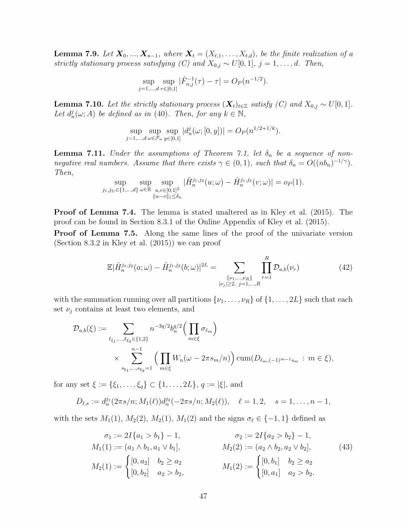
Lemma 7.9. Let X0

, ...,Xn�1

, where Xt

= (Xt,1

, . . . , Xt,d

), be the finite realization of astrictly stationary process satisfying (C) and X

0,j

⇠ U [0, 1], j = 1, . . . , d. Then,

supj=1,...,d

sup⌧2[0,1]

|F�1

n,j

(⌧)� ⌧ | = OP

(n�1/2).

Lemma 7.10. Let the strictly stationary process (Xt

)t2Z satisfy (C) and X

0,j

⇠ U [0, 1].Let dj

n

(!;A) be defined as in (40). Then, for any k 2 N,

supj=1,...,d

sup!2Fn

supy2[0,1]

|djn

(!; [0, y])| = OP

(n1/2+1/k).

Lemma 7.11. Under the assumptions of Theorem 7.1, let �n

be a sequence of non-negative real numbers. Assume that there exists � 2 (0, 1), such that �

n

= O((nbn

)�1/�).Then,

supj1,j2,2{1,...,d}

sup!2R

supu,v2[0,1]2ku�vk1�n

|Hj1,j2n

(u;!)� Hj1,j2n

(v;!)| = oP

(1).

Proof of Lemma 7.4. The lemma is stated unaltered as in Kley et al. (2015). Theproof can be found in Section 8.3.1 of the Online Appendix of Kley et al. (2015).

Proof of Lemma 7.5. Along the same lines of the proof of the univariate version(Section 8.3.2 in Kley et al. (2015)) we can proof

E|Hj1,j2n

(a;!)� Hj1,j2n

(b;!)|2L =X

{⌫1,...,⌫R}|⌫j |�2, j=1,...,R

R

Y

r=1

Da,b

(⌫r

) (42)

with the summation running over all partitions {⌫1

, . . . , ⌫R

} of {1, . . . , 2L} such that eachset ⌫

j

contains at least two elements, and

Da,b

(⇠) :=X

`⇠1,...,`⇠q2{1,2}

n�3q/2bq/2n

⇣

Y

m2⇠

�`m

⌘

⇥n�1

X

s⇠1,...,s⇠q=1

⇣

Y

m2⇠

Wn

(! � 2⇡sm

/n)⌘

cum(D`m,(�1)

m�1sm : m 2 ⇠),

for any set ⇠ := {⇠1

, . . . , ⇠q

} ⇢ {1, . . . , 2L}, q := |⇠|, and

D`,s

:= dj1n

(2⇡s/n;M1

(`))dj2n

(�2⇡s/n;M2

(`)), ` = 1, 2, s = 1, . . . , n� 1,

with the sets M1

(1), M2

(2), M2

(1), M1

(2) and the signs �`

2 {�1, 1} defined as

�1

:= 2I{a1

> b1

}� 1, �2

:= 2I{a2

> b2

}� 1,

M1

(1) := (a1

^ b1

, a1

_ b1

], M2

(2) := (a2

^ b2

, a2

_ b2

], (43)

M2

(1) :=

(

[0, a2

] b2

� a2

[0, b2

] a2

> b2

,M

1

(2) :=

(

[0, b1

] b2

� a2

[0, a1

] a2

> b2

.

47

Employing assumption (41), we can further prove, by following the arguments of theunivariate version, that

sup⇠⇢{1,...,2L}

|⇠|=q

supka�bk1"

|Da,b

(⇠)| C(nbn

)1�q/2g("), 2 q 2L.

The lemma then follows, by observing that

�

�

�

R

Y

r=1

Da,b

(⌫r

)�

�

�

CgR(")(nbn

)R�L

for any partition in (42) [note thatP

R

r=1

|⌫r

| = 2L].

Proof of Lemma 7.6. Note that

cum(I{X0,j1 q

j1(a1)}, I{Xk,j2 qj2(a2)})� cum(I{X

0,j1 qj1(b1)}, I{Xk,j2 q

j2(b2)})= �

1

cum(I{Fj1(X0,j1) 2 M

1

(1)}, I{Fj2(Xk,j2) 2 M

2

(1)})+ �

2

cum(I{Fj1(X0,j1) 2 M

1

(2)}, I{Fj2(Xk,j2) 2 M

2

(2)}),

with the sets M1

(1), M2

(2), M2

(1), M1

(2) and the signs �`

2 {�1, 1} defined in (43).From the fact that �(M

j

(j)) ka� bk1

for j = 1, 2, we conclude that

�

�

�

d`

d!`

fj1,j2(!; a1

, a2

)� d`

d!`

fj1,j2(!; b1

, b2

)�

�

�

X

k2Z

|k|`| cum(I{Fj1(X0,j1) 2 M

1

(1)}, I{Fj2(Xk,j2) 2 M

2

(1)})|

+X

k2Z

|k|`| cum(I{Fj1(X0,j1) 2 M

1

(2)}, I{Fj2(Xk,j2) 2 M

2

(2)})|

41X

k=0

k`

⇣

(K⇢`) ^ ka� bk1

⌘

.

The assertion then follows by after some algebraic manipulations.

Proof of Lemma 7.7. Similar to (8.27) in Kley et al. (2015) we have, by the definitionof cumulants and strict stationarity,

cum(dj1n

(!1

;A1

), . . . , djpn

(!p

;Ap

))

=n

X

u2,...,up=�n

cum(I{X0,j1 2 A

1

}, I{Xu2,j2 2 A

2

} . . . , I{Xup,jp 2 A

p

}) exp⇣

� ip

X

j=2

!j

uj

⌘

⇥n�1

X

t1=0

exp⇣

� it1

p

X

j=1

!j

⌘

I{0t1+u2<n} · · · I{0t1+up<n}. (44)

By Lemma 8.1 in Kley et al. (2015),

�

�

�

�n

(p

X

j=1

!j

)�n�1

X

t1=0

exp⇣

�it1

p

X

j=1

!j

⌘

I{0 t1

+ u2

< n} · · · I{0 t1

+ up

< n}�

�

�

2p

X

j=2

|uj

|.

(45)

48

Following the arguments for the proof of (8.29) in Kley et al. (2015), we further have, forany p + 1 intervals A

0

, . . . , Ap

⇢ R, any indices j0

, . . . , jp

2 {1, . . . , d}, and any p-tuple := (

1

, ...,p

) 2 Rp

+

, p � 2, that

1X

k1,...,kp=�1

⇣

1 +p

X

`=1

|k`

|`

⌘

�

� cum�

I{Xk1,j1 2 A

1

}, . . . , I{Xkp,jp 2 A

p

}, I{X0,j0 2 A

0

}�

�

�

C"(| log "|+ 1)d. (46)

To this end, define k0

= 0, consider the set

Tm

:=�

(k1

, ..., kp

) 2 Zp| maxi,j=0,...,p

|ki

� kj

| = m

,

and note that |Tm

| cp

mp�1 for some constant cp

. From the definition of cumulants andsome simple algebra we get the bound

| cum(I{Xt1,j1 2 A

1

}, ..., I{Xtp,jp 2 A

p

})| C mini=1,...,p

P (X0,ji 2 A

i

).

With this bound and condition (C) we obtain, employing the above notation, that

1X

k1,...,kp=�1

⇣

1 +p

X

j=1

|k`

|`

⌘

�

� cum�

I{Xk1,j1 2 A

1

}, . . . , I{Xkp,jp 2 A

p

}, I{X0,j02A0}�

�

�

=1X

m=0

X

(k1,...,kp)2Tm

⇣

1+p

X

`=1

|k`

|`

⌘

�

� cum�

I{Xk1,j1 2 A

1

}, . . . , I{Xkp,jp 2 A

p

}, I{X0,j0 2 A

0

}�

�

�

1X

m=0

X

(k1,...,kp)2Tm

⇣

1 + pmmaxj j

⌘⇣

⇢m ^ "⌘

Kp

Cp

1X

m=0

⇣

⇢m ^ "⌘

|Tm

|mmaxj j .

For " � ⇢, (46) then follows trivially. For " < ⇢, set m"

:= log "/ log ⇢ and note that⇢m " if and only if m � m

"

. Thus,

1X

m=0

⇣

⇢m ^ "⌘

mu X

mm"

mu"+X

m>m"

mu⇢m C⇣

"mu+1

"

+ ⇢m"

1X

m=0

(m+m"

)u⇢m⌘

.

The fact that ⇢m" = " completes the proof of the desired inequality (46). The assertionfollows from (44), (45), (46) and the triangle inequality.

Proofs of Lemmas 7.8, 7.9 and 7.10. Note that the component processes (Xt,j

) arestationary and fulfill assumption (C) in Kley et al. (2015), for every j = 1, . . . , d. Theassertion then follow from the univariate versions (i. e., Lemma 8.6, 7.5 and 7.6 in Kleyet al. (2015), respectively), as the dimension d does not depend on n.

Proof of Lemma 7.11. Assume, without loss of generality, that n�1 = o(�n

) [otherwise,enlarge the supremum by considering �

n

:= max(n�1, �n

)]. With the notation a = (a1

, a2

)and b = (b

1

, b2

), we have

Hj1,j2n

(a;!)� Hj1,j2n

(b;!) = b1/2n

n�1/2

n�1

X

s=1

Wn

(! � 2⇡s/n)(Ks,n

(u, v)� EKs,n

(u, v))

49

where, with djn,U

defined in (33),

Ks,n

(a, b) := n�1

�

dj1n,U

(2⇡s/n; u1

)dj2n,U

(�2⇡s/n; u2

)� dj1n,U

(2⇡s/n; v1

)dj2n,U

(�2⇡s/n; v2

)�

= dj1n,U

(2⇡s/n; u1

)n�1

⇥

dj2n,U

(�2⇡s/n; u2

)� dj2n,U

(�2⇡s/n; v2

)⇤

+ dj2n,U

(�2⇡s/n; v2

)n�1

⇥

dj1n,U

(2⇡s/n; u1

)� dj1n,U

(2⇡s/n; v1

)⇤

.

By Lemma 7.10, we have, for any k 2 N,

supy2[0,1]

sup!2Fn

|djn,U

(!; y)| = OP

⇣

n1/2+1/k

⌘

. (47)

Employing Lemma 7.8, we have, for any ` 2 N and j = 1, . . . , d,

sup!2R

supy2[0,1]

supx:|x�y|�n

n�1|djn,U

(!; x)� djn,U

(!; y)|

supy2[0,1]

supx:|x�y|�n

n�1

n�1

X

t=0

|I{Fj

(Xt,j

) x}� I{Fj

(Xt,j

) y}|

supy2[0,1]

supx:|x�y|�n

|Fn,j

(x _ y)� Fn,j

(x ^ y)� x _ y + x ^ y|+ C�n

= OP

�

⇢n

(�n

, `) + �n

�

,

with ⇢n

(�n

, `) := n�1/2(n2�n

+ n)1/2`(�n

| log �n

|D` + n�1)1/2, Fn,j

denoting the empiricaldistribution function of F

j

(X0,j

), . . . , Fj

(Xn�1,j

), and d`

being a constant depending onlyon `. Combining these arguments and observing that

sup!2R

n�1

X

s=1

�

�

�

Wn

(! � 2⇡s/n)�

�

�

= O(n) (48)

yields

sup!2R

supu,v2[0,1]2ku�vk1�n

�

�

�

n�1

X

s=1

Wn

(! � 2⇡s/n)Ks,n

(u, v)�

�

�

= OP

�

n3/2+1/k(⇢(�n

, `) + �n

)�

. (49)

With Mi

(j), i, j = 1, 2, as defined in (43), we have

supka�bk1�n

sups=1,...,n�1

|EKs,n

(a, b)|

n�1 supka�bk1�n

sups=1,...,n�1

�

� cum(dj1n,U

(2⇡s/n;M1

(1)), dj2n,U

(�2⇡s/n;M2

(1)))�

�

+ n�1 supka�bk1�n

sups=1,...,n�1

�

� cum(dj1n,U

(2⇡s/n;M1

(2)), dj2n,U

(�2⇡s/n;M2

(2)))�

�

(50)

where we have used Edjn,U

(2⇡s/n;M) = 0. Lemma 7.7 and �(Mj

(j)) �n

, for j = 1, 2(with � denoting the Lebesgue measure over R) yield

supka�bk1�n

sups=1,...,n�1

| cum(dj1n

(2⇡s/n;M1

(j)), dj2n

(�2⇡s/n;M2

(j)))| C(n+1)�n

(1+| log �n

|)D,

50

It follows that the right-hand side in (50) is O(�n

| log �n

|D). Therefore, by (48), we obtain

sup!2R

supka�bk1�n

�

�

�

b1/2n

n�1/2

n�1

X

s=1

Wn

(! � 2⇡s/n)EKs,n

(a, b)�

�

�

= O�

(nbn

)1/2�n

| log n|D�

.

In view of the assumption that n�1 = o(�n

), we have �n

= O(n1/2⇢n

(�n

, `)), which, incombination with (49), yields

sup!2R

supka�bk1�n

|Hj1,j2n

(a;!)� Hj1,j2n

(b;!)|

= OP

⇣

(nbn

)1/2[n1/2+1/k(⇢n

(�n

, `) + �n

) + �n

| log �n

|D]⌘

= OP

⇣

(nbn

)1/2n1/2+1/k⇢n

(�n

, `)⌘

= OP

⇣

(nbn

)1/2n1/k+1/`(n�1 _ �n

(log n)D`)1/2⌘

= oP

(1).

The oP

(1) holds, as we have, for arbitrary k and `,

O((nbn

)1/2n1/k+1/`�1/2n

(log n)D`/2) = O((nbn

)1/2�1/2�n1/k+1/`(log n)D`/2).

The assumptions on bn

imply (nbn

)1/2�1/2� = o(n�) for some > 0, such that this latterquantity is o(1) for k, ` su�ciently large. The term (nb

n

)1/2n1/k+1/`n�1/2 is handled in asimilar fashion. This concludes the proof.

51