Embed Size (px)
Citation preview

Quantifying uncertainties in projections of extremes—a perturbedland surface parameter experiment
Erich M. Fischer • David M. Lawrence •
Benjamin M. Sanderson
Received: 20 May 2010 / Accepted: 14 September 2010
� Springer-Verlag 2010
Abstract Uncertainties in the climate response to a dou-
bling of atmospheric CO2 concentrations are quantified in a
perturbed land surface parameter experiment. The ensemble
of 108 members is constructed by systematically perturbing
five poorly constrained land surface parameters of global
climate model individually and in all possible combina-
tions. The land surface parameters induce small uncertain-
ties at global scale, substantial uncertainties at regional and
seasonal scale and very large uncertainties in the tails of the
distribution, the climate extremes. Climate sensitivity varies
across the ensemble mainly due to the perturbation of the
snow albedo parameterization, which controls the snow
albedo feedback strength. The uncertainty range in the
global response is small relative to perturbed physics
experiments focusing on atmospheric parameters. However,
land surface parameters are revealed to control the response
not only of the mean but also of the variability of temper-
ature. Major uncertainties are identified in the response of
climate extremes to a doubling of CO2. During winter the
response both of temperature mean and daily variability
relates to fractional snow cover. Cold extremes over high
latitudes warm disproportionately in ensemble members
with strong snow albedo feedback and large snow cover
reduction. Reduced snow cover leads to more winter
warming and stronger variability decrease. As a result
uncertainties in mean and variability response line up, with
some members showing weak and others very strong
warming of the cold tail of the distribution, depending on
the snow albedo parametrization. The uncertainty across the
ensemble regionally exceeds the CMIP3 multi-model range.
Regarding summer hot extremes, the uncertainties are lar-
ger than for mean summer warming but smaller than in
multi-model experiments. The summer precipitation
response to a doubling of CO2 is not robust over many
regions. Land surface parameter perturbations and natural
variability alter the sign of the response even over sub-
tropical regions.
Keywords Climate extremes � Uncertainties �Heat waves � Land–atmosphere interactions �Snow albedo feedback � Parametrization
1 Introduction
Changes in the frequency and intensity of climate extremes
have socio-economic impacts that reach far beyond the
effects of mean warming. Numerous studies have explored
changes in extreme temperature events during the obser-
vational period (e.g. Kunkel et al. 1999; Easterling et al.
2000; Meehl et al. 2000; Tebaldi et al. 2006). The most
robust changes include a significant trend towards fewer
cold nights and frost days and a tendency for more warm
nights and heat waves (e.g. Frich et al. 2002; Alexander
et al. 2006). Scenarios project an intensification of these
Electronic supplementary material The online version of thisarticle (doi:10.1007/s00382-010-0915-y) contains supplementarymaterial, which is available to authorized users.
E. M. Fischer (&) � D. M. Lawrence � B. M. Sanderson
National Center for Atmospheric Research,
P.O. Box 3000, Boulder, CO 80302, USA
e-mail: [email protected]
D. M. Lawrence
e-mail: [email protected]
B. M. Sanderson
e-mail: [email protected]
E. M. Fischer
Institute for Atmospheric and Climate Science,
ETH Zurich, Zurich 8092, Switzerland
123
Clim Dyn
DOI 10.1007/s00382-010-0915-y
trends leading to more frequent, intense and longer lasting
heat waves if atmospheric greenhouse gas concentrations
continue to rise (e.g. Meehl and Tebaldi 2004; Schar et al.
2004; Beniston 2004; Weisheimer and Palmer 2005;
Tebaldi et al. 2006; Kharin et al. 2007).
The magnitude of these projected changes in extremes,
however, involves large uncertainties, particularly at
regional scale. Uncertainties in climate projections arise
from three distinct sources: (1) uncertainties in emissions
of greenhouse gases and aerosols, and land use changes
(scenario uncertainties), (2) the resulting atmospheric
radiative forcing and the representation of the numerous
feedbacks on the climate system in models (model uncer-
tainties), and (3) natural variability (initial condition
uncertainties). The latter two sources of uncertainty have
mostly been addressed by considering the spread across an
ensemble of opportunity, e.g. a relatively small ensemble
of Global Climate Model (GCM) results (Tebaldi and
Knutti 2007). However, such multi-model ensembles may
substantially underestimate the actual uncertainty, since
they are not designed to sample the full range of possible
behaviours (Allen et al. 2000; Knutti et al. 2008; Hawkins
and Sutton 2009). Moreover, it is difficult to determine
whether differences identified in a multi-model ensemble
arise from different initial conditions, structural uncer-
tainties (such as grid resolution and the representation of
processes) or uncertainties in the parameterization of sub-
grid scale processes (such as cloud formation).
Parameter uncertainties can be systematically quantified
in perturbed physics ensembles (PPE), which are con-
structed by varying model parameters whose values cannot
be accurately constrained by observations (e.g. Allen et al.
2000; Murphy et al. 2004; Piani et al. 2005; Stainforth
et al. 2005). Using PPE it has been demonstrated that
uncertainty range of climate sensitivity (the equilibrium
response of global temperatures to a doubling of CO2)
induced by parameter choices in some GCMs is nearly as
large or even larger than it is for a multi-model ensemble
sampling across different GCMs (Murphy et al. 2004;
Stainforth et al. 2005). PPE have further been used to
quantify uncertainties in climate extremes, such as heat
waves (Clark et al. 2006; Barnett et al. 2006), wet days
(Barnett et al. 2006) and droughts (Burke and Brown
2008). While most of the available PPEs have been based
on HadSM3, Sanderson (2010) demonstrates that a corre-
sponding ensemble based on a different GCM (CCSM3.5)
may yield a substantially smaller uncertainty range.
While most of the existing PPEs emphasize the role of
atmospheric model parameterizations, we focus here on land
surface model parameterizations. To our knowledge this is
the first study systematically focusing on land surface
parameter uncertainties in a global coupled model frame-
work. Land surface parameter uncertainty analyses have
been carried out in single column model (e.g. Liu et al.
2005) and offline experiments. The PPE evaluated in this
study consists of 108 model versions (hereafter referred to as
members), which are generated by systematically perturbing
five land surface parameters in the land surface scheme of
the Community Climate System Model (CCSM 3.5). Most
of the land surface processes and their interactions with the
atmosphere act on subgrid scales and need to be parame-
terized. The land surface parameters are generally poorly
constrained by observations and represent an important
source of uncertainty, which to our knowledge has not yet
been systematically assessed in a coupled model framework.
Land surface parameterizations control the surface energy
and water budgets and are crucial for a realistic representa-
tion of the present-day climate. Feedback mechanisms
through snow albedo (e.g Qu and Hall 2006), soil moisture
(Koster et al. 2002; Seneviratne et al. 2006a; Vidale et al.
2007) or vegetation change may amplify or offset future
changes in mean temperature and its variability.
Here, we systematically quantify uncertainties induced
by land surface parameters. We specifically focus on
uncertainties in regional projections of temperature, pre-
cipitation and impact-relevant extremes. This controlled
exercise further allows us to disentangle the relevance of
individual land surface parameters. Particularly important
parameters can be identified, thereby isolating which
parameters need to be better constrained by observations to
ultimately reduce uncertainties in projections.
The paper is organized as follows: First, the experi-
mental setup, including the individual parameter pertur-
bations, is detailed and an analysis of the primary impacts
in single perturbation experiments is presented. Second,
uncertainties in simulated temperature mean and variability
are evaluated. Third, regional projections in temperature
extremes are explored and finally, the precipitation
response and related uncertainties are discussed.
2 CLMCUBE experiment
A 108-member perturbed parameter experiment (hereafter
CLMCUBE) is performed with the NCAR Community
Climate System Model (CCSM 3.5) (Gent et al. 2010)
version with a non-dynamic mixed layer (slab) ocean. The
finite volume model version used in this experiment has a
horizontal resolution of 2� latitude 9 2.5� longitude with
26 levels on hybrid vertical coordinates. The land surface
model component is the Community Land Model (CLM),
which is documented in detail in Oleson et al. (2004). The
modifications in the latest version CLM 3.5 used here and
its performance are described in Lawrence et al. (2007);
Oleson et al. (2008); Stockli et al. (2008). Subgrid-scale
land surface heterogeneity is represented in CLM through
E. M. Fischer et al.: Quantifying uncertainties in projections of extremes
123

different fractional coverage of bare soil, lake, glacier, and
vegetation. Vegetation cover is subdivided in 16 different
plant functional types (PFTs) and the soil consists of 10
layers, which extend to a total depth of 3.4 m.
The basic experimental setup of CLMCUBE is similar
to climateprediciton.net (Stainforth et al. 2005), the QUMP
experiments (Murphy et al. 2004) and CAMCUBE
(Sanderson 2010). Each CLMCUBE member simulation
consists of three stages: a calibration, a 1 9 CO2 and
2 9 CO2 stage. In the 15-year calibration stage the sea
surface temperatures are prescribed to diagnose heat con-
vergence fields, which can be applied during the two later
stages. Since the mixed layer ocean model does not
explicitly represent ocean dynamics, the ocean heat trans-
port has to be prescribed as heat convergence. The
1 9 CO2 simulations cover a 30-year period with con-
stant atmospheric CO2 concentrations of 355 ppm and the
2 9 CO2 cover 20 years, forced with atmospheric CO2
concentrations of 710 ppm.
In each ensemble member, land surface parameters were
perturbed to a high and low value relative to the standard
values used in CLM3.5. Standard parameters that are at the
low or high end of the parameter uncertainty range are only
perturbed to one side. The perturbations have been applied
to five poorly constrained land surface parameters
(described below) individually and in all possible combi-
nations to account for nonlinear interactions. In contrast to
previous experiments such as CAMCUBE, QUMP and
climateprediction.net, CLMCUBE focuses on uncertainties
induced by land surface parameters.
The five land surface parameters were selected in close
consultation with the CLM model development group.
They include two optical parameters that affect the surface
albedo (vegetation and snow reflectance), two parameters
that exert significant control on the partitioning of surface
turbulent fluxes (soil hydrology decay factor f and a pho-
tosynthetic parameter Vmax), and one parameter that affects
turbulent energy exchange (momentum roughness length).
The parameter perturbations are based on uncertainty ran-
ges found in the reference literature of the standard CLM
parameters and in the case of snow albedo and water table
on expert judgement.
The imposed perturbations to the five parameters and
their primary anticipated climate effects are illustrated in
Fig. 1 and discussed in detail in the following.
2.1 Snow albedo
Snow albedo in CLM 3.5 is calculated for the visible and
near-infrared radiative spectrum. The calculation is a
function of a prescribed fresh snow albedo and subsequent
snow aging, which accounts for dirt and soot effects as well
as for snow grain growth. The fresh snow albedo asno;^;0 is
comparatively well constrained by observations and is set
at 0.95 for visual and 0.65 for near-infrared radiation.
The actual snow albedo is calculated as
asno;^ ¼ ½1� C^Fage�asno;^;0; ð1Þ
where Fage is the snow age and C^ is a constant. In contrast
to the fresh snow albedo, C^ is a highly uncertain empirical
Control Perturbed
1. Snow albedo
4. Water table depth
2. Vegetation albedo
3. V
max
5. R
ough
ness
leng
th
2. Vegetation albedo
H
H
LE
LE
SW
SW
LW
LW
V
Fig. 1 Illustration of land surface model parameter perturbations and first order effects of shortwave (SW), longwave (LW), latent heat (LE) and
sensible heat (H) fluxes (colored arrows) as described in Sect. 2
E. M. Fischer et al.: Quantifying uncertainties in projections of extremes
123

quantity. Standard values used in CLM 3.5 and perturbed
values are given in Table 1 and S1.
As a primary effect this perturbation alters the short- and
longwave radiation absorbed by snow-covered surfaces. The
members with only this parameter perturbed, simulate an
albedo change over the Northern Hemisphere, which is
largest in mid-winter (January and February). The net radi-
ation change is largest in late winter and spring due to higher
insolation. The effect of the two-sided perturbation on all
sky albedo is non-symmetric. The surface net radiation
change is almost four times larger for the high than for the
low snow albedo perturbation. However, the resulting global
mean land temperature changes are very similar (±0.12 K).
Regional temperatures over seasonally snow-covered
regions are unsurprisingly much more sensitive (±2–4 K).
2.2 Vegetation albedo
The reflectance of vegetation is a combined measure of leaf
and stem reflectance and calculated for each PFT as
a^ ¼ aleaf^ wleaf þ astem
^ wstem; ð2Þ
where wleaf = L/(L ? S) and wstem = S/(L ? S) with L and
S being the exposed leaf/stem area index. Even though
surface albedo can be measured from satellites, the actual
values for the different vegetation types include substantial
uncertainties. To account for these uncertainties the leaf
reflectance has been perturbed by ±20% to the values
listed in Table 1 and S2.
This perturbation of leaf albedo directly alters the
radiation absorbed by the vegetation covered land surface.
The individual perturbations of vegetation albedo alter the
global land surface net radiation by -2.0 W/m2 (vegetation
albedo ?20%) and ?2.4 W/m2 (vegetation albedo -20%),
respectively. This results in a global land temperature
change of ±0.16 K, which is substantially larger at regio-
nal scale and during specific seasons, especially over the
corresponding summer hemisphere (±1–2 K). The maxi-
mum sensitivity of net radiation and temperature is found
over Central and Eastern North America, which are pre-
dominantly covered by crop and broadleaf deciduous
temperate trees.
2.3 Maximum rate of carboxylation Vmax
The rates of photosynthesis in CLM 3.5 are calculated at
the leaf scale for sunlit and shaded canopy fractions. The
leaf photosynthesis is dependent on the leaf-scale maxi-
mum carboxylation capacity of Rubisco (Vmax, lmol
CO2m-2 s-1). Vmax is formulated as a function of the leaf
area based concentration of Rubisco and the enzyme
activity as follows
Vmax ¼1
SLA� CNLFLNR
1
FNRaR; ð3Þ
where SLA is the specific leaf area, CNL the leaf car-
bon:nitrogen ratio gC gN-1, FLNR the fraction of leaf
nitrogen in Rubisco (unitless), FNR the mass ratio of
nitrogen in the Rubisco molecule to total molecular mass
(unitless) and aR the specific activity of Rubisco (lmol
CO2 gRubisco-1s-1) (Thornton and Zimmermann 2007).
Detailed observations of SLA and CNL are presented in
White et al. (2000) for different species. Measured values
differ strongly across species of the same CLM PFT. The
Table 1 Summary of land
surface model parameter
perturbations detailed in Sect. 2
Detailed values for each plant
functional type (denoted with
index i) are given in Tables
S1–S5
Parameter Lower Low Standard High Higher
Snow albedo
C^ (VIS) (empirical const., visual) 0.02 0.2 0.38
C^ (NIR) (empirical const., near-infrared) 0.05 0.5 0.85
Leaf albedo
aleafvis (leaf reflectance, visual) avis,i-20% ai avis,i?20%
aleafnir (leaf reflectance, near-infrared) anir,i-20% ai anir,i?20%
Water table
f [m-1] (decay factor) 1.0 1.75 2.5
qdrai,max [kg m-2 s-1]
(max. subsurface runoff)
8.5 9 10-4 6.5 9 10-4 4.5 9 10-4
Vmax
SLAi (specific leaf area index) SLAi SLAi ? r
CNL, i (leaf carbon:nitrogen ration) CNL, i CNL, i ? r
Momentum roughness length
Rz0m, i (ratio of momentum
roughness length)
Rz0m, i 2*Rz0m, i
E. M. Fischer et al.: Quantifying uncertainties in projections of extremes
123

standard parameter used in CLM 3.5 is typically the mean
value for each PFT. Since photosynthesis in CLM 3.5 is
generally considered to be high (Stockli et al., 2008), we
use a one-sided perturbation of SLA and CNL of one
standard deviation of the uncertainty given for each PFT in
White et al. (2000) (see Table 1 and S3), which gives a
smaller but still realistic Vmax.
The perturbation of Vmax directly affects photosynthesis
and thereby leaf stomatal resistance. In the single pertur-
bation simulation, modified Vmax regionally decreases the
ecosystem net photosynthesis by 50%. Note that here, due
to the absence of an interactive carbon cycle model, this
does not affect the atmospheric CO2 concentrations.
However, the higher stomatal resistance reduces plant
transpiration globally by 3.7 W/m2. This reduction is partly
offset (40–50%) by enhanced bare soil evaporation. As a
result, the global latent (sensible) heat flux over land is
reduced (enhanced) by about 2W/m2. Regionally the
change in partitioning of turbulent fluxes is substantially
larger, peaking at 15–20W/m2 over eastern North America
during summer (see map in Fig. S1a).
2.4 Water table depth and subsurface runoff
The surface and subsurface runoff are calculated with a
simple TOPMODEL-based runoff scheme (SIMTOP) (Niu
et al. 2005). The determination of the water table depth zOis based on a simple groundwater model by Niu et al.
(2007). The groundwater solution is dependent on whether
the water table is within or below the soil column (3.4 m).
The water table depth affects subsurface and surface runoff
generation and thereby soil hydrology, which in turn con-
trols the surface energy and water budget.
The subsurface runoff or drainage qdrai in CLM 3.5 is
defined as follows:
qdrai ¼ ð1� fimpÞqdrai;max expð�fzOÞ; ð4Þ
where fimp is the fraction of impermeable area determined
from the ice content of the soil layers, qdrai,max(kg m-2 s-1)
is the maximum subsurface runoff when the grid-averaged
water table depth equals zero (i.e. is at the surface) and f is
a decay factor, which was determined through sensitivity
analysis and comparison against observed runoff data.
Both the decay factor f and qdrai,max are perturbed in
combination. Generally an increase in f decreases the water
table depth, which results in wetter soils and lower sub-
surface runoff, whereas larger qdrai,max results in drier soils.
Since the water table depth has been found to be generally
shallow with standard parameters of CLM 3.5 (Oleson et al.
2008), one-sided perturbations are applied. The standard
values and the perturbations are given in Table S4.
The primary effect of the one-sided perturbation of the
soil hydrological parameters f and qdrai,max is an increase of
the water table depth (average ?0.6 for moderate, and
?2.4 m for maximum perturbation, respectively) and lead
to higher subsurface and lower surface runoff. On average
the drier soils lead to slightly higher surface albedo. Latent
heat flux over land is reduced by 2.8 W/m2 in the member
with maximum perturbations, mainly due to reduced bare
soil evaporation (see spatial pattern of latent heat flux
anomaly in Fig. S1a). In response, global land precipitation
is slightly reduced and precipitation minus evaporation is
substantially lower. The enhanced sensible heat flux results
in a warming of mean land temperatures by 0.28 K, the
strongest temperature signal induced by a single parameter
perturbation. The spatial temperature anomaly pattern is
more uniform than in the case of the other perturbations.
2.5 Roughness length
The roughness lengths for momentum (z0m), heat (z0h) and
water vapor flux (z0w) are equal and calculated as follows
z0m ¼ z0h ¼ z0w ¼ ztopRz0m; ð5Þ
where ztop is the canopy top height for the plant functional
type and Rz0m the ratio of momentum roughness length.
While the canopy top height is relatively well constrained
by observations, the ratio of momentum roughness length
varies substantially across GCMs. For some PFTs the
actual roughness lengths used in CLM 3.5 is less than half
of the values used in the ECMWF land surface scheme
TESSEL (ECMWF 2007). To account for this uncer-
tainty, we double the standard ratio Rz0m for each PFT
(see Table S5).
The perturbation of roughness length primarily reduces
the near surface wind speed but has a negligible effect on
global land temperatures. Global land precipitation is
slightly reduced by about 1%.
3 Extreme indices
The uncertainties in the response of climate extremes to a
doubling of CO2 are explored based on widely used indi-
ces. Most of the indices used here are introduced and
defined in Frich et al. (2002) and also used in Tebaldi et al.
(2006); IPCC (2007). The extreme indices are briefly
defined in the following:
– Tropical nights (TR): Total number of tropical nights
(i.e. days with absolute minimum temperatures[20�C).
– Heat wave duration index (HWDI): maximum period of
at least 6 consecutive days (within summer months
May–September for Northern Hemisphere, and
November–March for Southern Hemisphere, respec-
tively) with maximum temperatures more than 5�C
E. M. Fischer et al.: Quantifying uncertainties in projections of extremes
123

warmer than reference value. The reference value is a
centered mean of daily maximum temperatures over a
5-day time window derived from the corresponding
present-day (1 9 CO2) simulation.
– Heat index days warmer than 40.6�C/105�F (HI105F):
the average number of days with maximum humidity-
corrected heat index (apparent temperature) exceeding
40.6�C (105F). The heat index (Steadman 1984),
represents heat stress on the human body by accounting
for the effects of additional environmental factors
beyond temperature. Here we use an approximated
version of the heat index defined in detail in Fischer
and Schar (2010) that accounts for ambient humidity
under shaded conditions and that is commonly used by
NOAA in North America (see http://www.crh.noaa.
gov/pub/heat.php).
– Frost days (FD): Total number of frost days (i.e. days
with absolute minimum temperatures \0�C) per year.
– Growing season length (GSL): number of days between
the first occurrence of at least 6 days with mean
temperatures[5�C and the first occurrence (after July 1)
of at least 6 days with mean temperatures\5�C. GSL is
not defined and thus not shown for regions outside the
Northern extratropics.
All of the above indices are calculated on annual or
seasonal basis and then averaged over the entire 1 9 CO2
and 2 9 CO2 simulation period.
4 Land surface parameter effect on mean temperature
4.1 Sensitivity of present-day temperatures
Here, we evaluate the sensitivity of land temperatures in
present-day climate (1 9 CO2) to parameter perturbations.
The temperature range across CLMCUBE is depicted as
the local annual mean difference between the 95th and 5th
percentiles of all 108 ensemble members (Fig. 2a). The
sensitivity of present-day temperatures (annual, DJF and
JJA mean) to the perturbation is smallest in the tropics and
largest in the northern high latitudes and the Tibetan Pla-
teau. JJA temperatures are also highly sensitive over
northern mid-latitudes at about 40–50�N (not shown).
The sensitivity to each parameter is assessed by aver-
aging all members with high/low value for each parameter
(e.g. 36 low vs. 36 high vegetation albedo members). The
composite difference qualitatively agrees with the differ-
ence patterns of the individual parameter perturbations
runs. However, averaging over all members reduces the
internal variability and leads to a smoother difference field.
Composite temperature difference for each of the five
perturbed parameters are shown in Fig. S2. Snow albedo is
the dominant parameter explaining the annual mean tem-
perature differences in northern high latitudes (1–1.5 K
north of 60�N), and vegetation albedo in mid-latitudes
(0.6–1 K at 30–60�N). Vmax and water table depth have a
moderate effect on annual temperatures (*0.3–0.5 K) over
most of the continents.
The sensitivity of summer temperatures to the different
parameters is rather complex and varies across regions and
seasons. We calculate the relative variance explained by
each of the five parameters (predictor) for regional summer
temperature (predictand) based on a multiple linear
regression (see Table 2). The linearity assumption of this
approach is found to be well justified for the present-day
temperatures (in contrast to the response to 2 9 CO2, see
below).
Vegetation albedo explains the highest variance in
summer temperatures throughout northern mid-latitudes
through its control on net radiation. Summer temperatures
are also sensitive to Vmax over the Amazon Basin, and to
water table depth, particularly in dry regions (e.g. Central
Asia, the Mediterranean Basin, Western Africa and Aus-
tralia). Both these parameters control evapotranspiration,
modify the Bowen ratio and thereby affect the local sum-
mer temperatures.
Temperature range (1xCO2) Temperature response (2xCO2 vs.1xCO2) Range of response (2xCO2 vs.1xCO2)(a) (b) (c)
Fig. 2 CLMCUBE ensemble range of present-day annual mean
temperatures (left, displayed as the local difference between 5th and
95th percentile member). Ensemble mean annual temperature
response to doubling of CO2 (central) and corresponding ensemble
range (right, 5th-95th percentile)
E. M. Fischer et al.: Quantifying uncertainties in projections of extremes
123

4.2 Uncertainty in response to a doubling of CO2
The ensemble mean global land temperature response
DTANN to a doubling of atmospheric CO2 concentrations
from 355 ppm to 710 ppm is 2.65 K. The full range of land
temperature response across the land surface parameter
perturbation experiments is 2.47 to 2.87 K. The uncertainty
range of climate sensitivity (including ocean areas) across
CLMCUBE is 2.04–2.33 K. This range is substantially
smaller than in CAMCUBE (equilibrium climate sensitivity
2.2–3.2 K), the corresponding PPE with the same model but
for perturbations across four atmospheric model parameters
(Sanderson 2010). This confirms that the uncertainty in
climate sensitivity induced by atmospheric parameters
(affecting water vapour, lapse rate and cloud feedbacks)
dominate over land surface parameter uncertainties.
We find that DTANN cannot be estimated by a linear
combination of the impacts of the individual land surface
parameter perturbations (e.g. same multiple linear regres-
sion as conducted above yields low explained variances).
Since the multiple linear regression fails to explain the
variance across the ensemble, we instead use a nonpara-
metric recursive partitioning and regression method (Brei-
man et al. 1984) to identify the most important land surface
parameter for DTANN. Snow albedo is found to explain the
largest partial variance (43%) in DTANN across CLMCUBE.
Members with a higher present-day snow albedo (and
higher snow cover fraction) simulate a stronger reduction
in spring albedo and annual snow cover fraction (Fig. 3),
which leads to a larger DTANN over northern extratropics
(30�–90�N). We find a significant correlation (r = 0.67)
between present-day all-sky albedo in the extratropics
Table 2 Role of different land surface parameters in explaining ensemble range of summer (JJA for Northern Hemisphere and DJF for
Australia) temperatures derived from multiple linear regression
Total expl. var. Veg. albedo Snow albedo Water table Vmax Roughn. length
Summer temp.
AUS 63.8 12.6 0.0 32.4 19.9 0.6
AMZ 92.0 23.6 0.0 15.1 46.6 7.0
WNA 97.1 53.6 4.2 17.0 20.5 1.9
CNA 97.0 60.1 1.3 13.5 21.9 0.3
ENA 97.0 50.0 2.1 7.7 37.3 0.0
MED 97.2 59.3 1.8 23.3 12.6 0.3
NEU 92.1 44.2 3.6 14.6 29.7 0.4
WAF 80.0 21.8 0.0 33.5 22.6 2.9
SAS 67.3 16.8 0.1 9.4 21.5 21.1
CAS 97.5 56.1 2.1 27.2 11.9 0.3
NAS 97.6 45.6 13.1 12.5 26.4 0.1
The total adjusted variance [%] is given in the first column and the partial variance [%] explained by each parameter in the following columns.
Values are regionally averaged over Australia (AUS), Amazon Basin (AMZ), Western North America (WNA), Central North America (CNA),
Eastern North America (ENA), Mediterranean Basin (MED), Northern Europe (NEU), Western Africa (WAF), South Asia (SAS), Central Asia
(CAS), North Asia (NAS). The exact coordinates defining the regions are given in (IPCC 2007)
Cor = −0.88
0.21 0.23 0.25 0.27 0.29 0.31 0.21 0.23 0.25 0.27 0.29 0.31
−0.
030
−0.
020
−0.
010
Δal
l−sk
y al
bedo
(M
AM
)
All−sky albedo (MAM)
Cor = 0.67 Cor = −0.78
2.6
2.8
3.0
3.2
3.4
3.6
All−sky albedo (MAM)
Δ Tem
p (A
NN
) [K
]
−4.
6−
4.2
−3.
8−
3.4
−3.
0
ΔS
now
cov
er fr
actio
n (A
NN
) [%
](a) (b)Fig. 3 (left) Correlation
between present-day spring
(MAM) all-sky albedo and
corresponding response to a
doubling of CO2 in northern
extratropics (30–90�N) across
all CLMCUBE members.
(right) Correlation between
present-day spring (MAM)
all-sky albedo and annual
temperature response (black)
and fractional snow cover
reduction (blue) in northern
extratropics
E. M. Fischer et al.: Quantifying uncertainties in projections of extremes
123

(30�–90�N in MAM) and DTANN across the ensemble. This
is consistent with Levis et al. (2007) who suggested that
models with a high (low) snow albedo bias have a strong
(weak) snow albedo feedback and also tend to have a
higher (lower) equilibrium climate sensitivity. Qu and Hall
(2007) suggested that the snow albedo feedback in models
with high present-day snow albedo is stronger as a result of
the higher contrast between snow-covered and snow-free
surfaces.
The uncertainty range of DTANN is largest ([2 K) over
the northernmost latitudes (where the ensemble mean
response DTANN is largest) and smallest over the tropics
(Fig. 2b, c). Magnitude of response and uncertainty are not
necessarily correlated, e.g. over Antarctica DTANN is large
and the corresponding uncertainty identified here, compar-
atively small. The response in members with low present-
day snow albedo is on average 0.5–1 K weaker than in
members with high albedo (Fig. S3, upper left). Interest-
ingly CLMCUBE also suggests comparatively weak high
latitude warming in members with low vegetation albedo
and deep water table (Fig. S3 upper middle and right panel).
The uncertainty range in winter warming (DTDJF) is
particularly high over Northern Europe (?1.9–5.0 K),
Northern Asia (?3.2–6.5 K) and Alaska (?2.3–6.9 K)
(Fig. 4a). This implies that simple land surface parameter
perturbations can more than double DTDJF, at least
regionally. When compared to equilibrium climate sensi-
tivity experiments performed with 10 CMIP3 models
(Meehl et al. 2007), the uncertainty range in CLMCUBE
regionally corresponds to about 50–80% of the multi-
model ensemble range. Note that some portion of the
uncertainty in the CLMCUBE arises from internal model
variability, which due to the relatively short simulation
length inflates the uncertainty range (Fig. S4b).
The uncertainty range of the JJA response (DTJJA) is
typically smaller (2.0–3.3 K over Central North America
and 2.2–3.3 K over Northern Asia), which is only about
20–40% of the CMIP3 uncertainty range (Fig. 4b).
5 Land surface effect on temperature variability
Land surface parameters not only affect the mean state
but also the variability of several climate variables at
interannual to intraseasonal time scales (e.g. Seneviratne
et al. 2006b; Fischer and Schar 2009). Such variability
changes may affect the intensity of climate extremes
beyond a simple shift in the mean climate (e.g. Katz and
Brown 1992; Schar et al. 2004). Here we define tem-
perature variability as the standard deviation of daily
JJA and DJF temperatures over the entire simulation
length.
Observed temperature variability (based on HadGHCND,
Caesar et al. 2006) is generally small over the tropics and
large over the high-latitudes (both in winter and summer)
and over the northern mid-latitudes around 40–50� (summer
only). CCSM 3.5 captures the observed latitudinal depen-
dence of temperature variability reasonably well (not
shown). The model somewhat overestimates the local var-
iability maxima north of 60�N in DJF and over the northern
subtropical regions in JJA.
Temperature variability is highly sensitive to parameter
perturbations in CLMCUBE. In JJA the variability spread
across CLMCUBE is largest over northernmost latitudes,
the central United States as well as central and southern
Europe (Fig. 5b). In the following we explore the dominant
parameters and underlying mechanisms for selected
regions of high variability.
Over mid-latitudes, vegetation albedo and water table
depth are the dominant parameters in explaining JJA var-
iability across CLMCUBE. Latent heat, which in this
experiment is largely controlled by the water table depth,
AUS
AM
Z
WN
A
CN
A
EN
A
ME
D
NE
U
WA
F
SA
S
CA
S
NA
S
24
68
DJF mean temperature response
Diff
eren
ce 2
xCO
2 vs
. 1xC
O2
[K]
*****
***
*
*
*****
****
****
**
*
*
**
*
***
**
*
*
*
*
*
***
**
*
*
**
*
*****
**
**
* *
*
***
*
*
**
*
*****
****
*
****
*
***
*
*****
*
**
**
*
**
*
**
**
**
*
AUS
AM
Z
WN
A
CN
A
EN
A
ME
D
NE
U
WA
F
SA
S
CA
S
NA
S
12
34
56
JJA mean temperature response
Diff
eren
ce 2
xCO
2 vs
. 1xC
O2
[K]
****
*
**
**
*
***
*
*
**
*
*
*
**
**
*
*
*
*
*
*
**
*
**
*
*
**
*
*
*
*
**
*
*
**
*
**
**
*
*
*
**
*
*****
*
*
*
*
*
*
***
*
***
*
*
****
*
*
**
*
***
**
*
**
**
*
****
*
**
*
*
*
(a) (b)
Fig. 4 Response in mean (a) DJF and (b) JJA temperatures in
response to a doubling of CO2 for regions defined in Table 2. The
boxes indicate the 25th and 75th percentile of the ensemble range and
the whiskers the most extreme members. Green stars show the
corresponding response in ten CMIP3 models providing output for
this equilibrium sensitivity slab ocean experiment
E. M. Fischer et al.: Quantifying uncertainties in projections of extremes
123

acts as a damping factor of daily temperature variability
(Fischer and Schar 2009).
Gregory and Mitchell (1995) suggested that daily tem-
perature variability is determined by the ratio of latent heat
flux to the sum of the outgoing turbulent and longwave
fluxes k, which is defined as
k ¼ LE
LE þ H þ LW¼ LE
SW þ GH;
where LE is latent heat flux, H is sensible heat flux, LW is
longwave surface net radiation, SW is shortwave surface
net radiation, and GH is ground heat flux. In CLMCUBE
we find a significant anticorrelation between k and JJA
variability over the Mediterranean and Central North
America (Fig. 6a). Reduced LE (e.g. due to dry soils) tends
to enhance daily summer temperature variability and
increased LE tends to dampen it.
Diurnal temperature range (DTR) and daily variability
share the same underlying mechanisms, which is substan-
tiated by their strong correlation across CLMCUBE
members (not shown). Relative humidity is highly anti-
correlated with JJA variability and DTR over dry regions
(Fig. 6b). Members with low relative humidity and high
JJA mean temperatures simulate high daily variability (see
also Fischer and Schar 2009). We suggest that variability
and DTR are mainly linked to relative humidity through
their dependence on cloudiness (see also Dai et al. 1999).
In response to 2 9 CO2, JJA variability tends to
increase mostly over dry regions including Central North
America and Mediterranean (Fig. 5a). Over the Mediter-
ranean region more than 90% of the CLMCUBE members
simulate enhanced variability. Temporal decomposition of
the variability response reveals that the annual cycle is
strongly enhanced due to a larger temperature contrast
between early summer and the warmest period in late July
and early August (see also Fischer and Schar 2009). Fur-
thermore, the soil drying substantially increases day-to-day
temperature variations through the mechanisms discussed
above. The variability increase over the Sahel and Arabian
Peninsula should not be overinterpreted as it occurs over an
(a) (b)
(d)(c)
Fig. 5 Daily temperature variability change in JJA (upper panels)
and DJF (lower panels) in response to a doubling of CO2. Ensemble
mean response (left panels) is shown along with respective ensemble
range (5th–95th ensemble percentile, right panels). Grid points where
the response is significant (F-test) at 95% confidence level in the
majority of members are stippled
E. M. Fischer et al.: Quantifying uncertainties in projections of extremes
123

area of small present-day variability with a substantial wet
bias in precipitation.
During DJF the ensemble range of present-day variability
is largest at the edges of the area commonly covered by snow
during winter at around 45–60�N. Winter temperature var-
iability over these latitudes is significantly correlated with
snow albedo and fractional snow cover. Cold, snow-covered
regions characteristically have very low latent heat flux and
atmospheric humidity, which otherwise tend to damp vari-
ability. Thus, DJF variability in regions such as Northern
Asia is generally large in members with high albedo and low
mean temperatures (Fig. 6c and S7).
In response to a doubling of CO2 DJF variability is
strongly reduced around 60�N (Fig. 5c), associated with
the strongest reduction in fractional snow cover. This is
consistent with changes at interannual scales (Gregory and
Mitchell 1995; Raisanen, 2002). Variance decomposition
reveals that DJF variability mostly changes at intraseasonal
rather than longer time scales. CLMCUBE reveals large
uncertainties in the response (Fig. 5d). Most members
show a strong variability decrease and a few members no
change or slightly enhanced variability. Members with
strong warming and snow melt, tend to simulate a stronger
variability reduction, which is consistent with the driving
processes identified above.
6 Uncertainties in temperature extremes
Per definition the extremes have an infrequent and irregular
nature and as a consequence long simulations are required
to quantify their changes. In order to increase the robust-
ness of our estimate, we here use moderate criteria. Note
that because of their still relatively coarse resolution,
GCMs may underestimate the intensity of extreme weather
events, particularly for precipitation-related events
(Raisanen and Joelsson 2001; Tebaldi et al. 2006). Here we
first explore the intensity of hot and cold extremes, and
second, changes in widely-used extreme indices.
6.1 Intensity of cold and hot extremes
Cold extremes are defined as 5th percentile of daily winter
temperatures (T5PDJF) and hot extremes as 95th percentile
of summer temperatures (T95PJJA). These represent two
extremely cold/hot thresholds, which on average occur on
4–5 days per winter and summer, respectively.
All CLMCUBE members simulate strong temperature
increases, DT95PJJA and DT5PDJF, in response to a dou-
bling of CO2 (Fig. 7). Due to the reduced DJF variability
over high latitudes, DT5PDJF exceeds the mean winter
warming regionally by up to a factor of 2. In Northern
Europe and Northern Asia the DT5PDJF is on average 60
and 20% larger, respectively, than the DJF mean warming.
Interestingly, we find that mean warming and variability
reduction are correlated across CLMCUBE, even though
they are statistically independent. Lower snow cover
fraction in response to a doubling CO2 tends to reduce
variability and amplify DT5PDJF. Thus, members showing
a large mean warming tend to simulate a stronger vari-
ability reduction over mid- to high-latitudes. As a result,
mean and variability uncertainties tend to line up, giving
rise to very large uncertainties in DT5PDJF. Fig. 8 illus-
trates that in northern extratropics (30–90�N), and in par-
ticular in Northern Europe, members with a high DTDJF,
tend to simulate a strongly amplified DT5PDJF. In Northern
Europe DT5PDJF ranges between 1.9–8.8 K and in North
Asia between 3.0–8.3 K (Fig. 7a). Thereby the CLMCUBE
uncertainty range exceeds the spread of the six CMIP3
models (green stars), which provide daily output for this
equilibrium sensitivity experiment.
Regarding summer hot extremes, DT95PJJA is typically
15–20% larger than the mean summer warming over sub-
tropical regions due to the enhanced JJA variability. This
8.6
8.8
9.0
9.2
9.4
9.6
DJF mean temperature [C]
DJF
var
iabi
lity
[C] NAS: r = −0.65
Rel. humidity [%]
JJA
var
iabi
lity
[K]
CNA: r = −0.78
MED: r = −0.88
−22.5 −22.0 −21.5 −21.0 −20.5 −20.040 45 50 55 60 650.1 0.2 0.3 0.4 0.5
2.6
2.8
3.0
3.2
3.4
3.6
3.8
2.6
2.8
3.0
3.2
3.4
3.6
3.8
λ
JJA
var
iabi
lity
[K]
CNA: r = −0.75
MED: r = −0.76
(a) (b) (c)
Fig. 6 a Correlation between present-day JJA daily temperature
variability and k in Central North America (CNA) and the Mediter-
ranean Basin (MED). k is defined as the ratio of latent heat to the sum
of longwave, sensible and latent heat (see Sect. 5 for details). b Same
as (a) but correlation between daily variability and relative humidity.
c Correlation between present-day DJF daily temperature variability
and mean temperature in North Asia. As in many other mid- to high-
latitudinal regions, DJF mean and variability are highly correlated
through snow cover
E. M. Fischer et al.: Quantifying uncertainties in projections of extremes
123

difference in warming between highest percentile and
mean summer temperature is consistent though less pro-
nounced than in earlier PPE based on HadSM3 (Clark et al.
2006). Again, we find that the uncertainty range is larger
for DT95PJJA than DTJJA. While in present-day runs,
members with high mean temperatures tend to simulate
high JJA variability, we do not find a significant correlation
in their response. Over Central North America uncertainty
range of DT95PJJA is largest (1.6–3.6 K) (Fig. 7b), which
is still substantially smaller than the spread in the CMIP3
models (green stars).
In summary uncertainties both in cold and hot extremes
are substantially larger than the uncertainty in the mean. In
winter the CLMCUBE range regionally exceeds the
CMIP3 suite of models, whereas in summer it is substan-
tially smaller.
The extreme temperature range (ETR) expresses the
difference between hot and cold extremes discussed
above. Thus, ETR is basically an extremes measure of the
annual cycle and is highly correlated to the amplitude of
the annual cycle defined as the difference between mean
JJA and DJF temperatures. The CLMCUBE members
simulate a statistically significant decrease in ETR over
high-latitudes and a weak increase over subtropical
regions. The ensemble mean ETR response pattern is in
good agreement with the transient response of CCSM3.0
and CMIP3 multi-model mean at the end of the twenty-
first century (Tebaldi et al. 2006). Due to the high
uncertainties in both cold and hot extremes, ETR is highly
sensitive to the CLM parameter perturbations, showing
uncertainties even in the sign of the response over
numerous regions (Fig. 9b).
AUS
AM
Z
WN
A
CN
A
EN
A
ME
D
NE
U
WA
F
SA
S
CA
S
NA
S
12
34
56
Hot extremes (JJA 95P)
Diff
eren
ce 2
xCO
2 vs
. 1xC
O2
[K]
*
*
**** *
*
**
** **
*
*
*
***
**
** **
**
**
*
*
**
*
*
*
*
*
*
*
**
*
**** *
*
****
*
*
**
*
***
**
*
*AU
S
AM
Z
WN
A
CN
A
EN
A
ME
D
NE
U
WA
F
SA
S
CA
S
NA
S
02
46
8
Cold extremes (DJF 5P)
Diff
eren
ce 2
xCO
2 vs
. 1xC
O2
[K]
**
**** **
******
**
*
**
*
**
**
**
**
**
**
**
**
**
*
*
**
*
*
**** *
*
**** **
**
*
*
**
**
*
*
(a) (b)
Fig. 7 Regional change in intensity of cold extremes (DJF 5th
percentile) and hot extremes (JJA 95th percentile) in response to a
doubling of CO2 for regions defined in Table 2. The boxes indicate
the 25th and 75th percentile of the ensemble range and the whiskers
the most extreme members. Green stars show the corresponding
response in six CMIP3 models providing daily output for this
equilibrium sensitivity slab ocean experiment
Northern Europe
1.5 2.5 3.5 4.5 5.5 6.5 7.5 8.5
ΔT DJF mean [K]
ΔT D
JF p
erce
ntile
s [K
]
Northern extratropics
2.0 2.5 3.0 3.5 4.0 4.5 5.0 5.5
1.5
2.5
3.5
4.5
5.5
6.5
7.5
8.5
2.0
2.5
3.0
3.5
4.0
4.5
5.0
5.5
ΔT DJF mean [K]
ΔT D
JF p
erce
ntile
s [K
]
Fig. 8 Scatterplot of DJF mean temperature response versus DJF 5th
(blue) and 95th percentile (red). Each point marks one member of the
CLMCUBE ensemble. Temperatures are averaged over land grid
points in (left) Northern Europe (see definition in Table 2) (right)
northern extratropics (30–90�N)
E. M. Fischer et al.: Quantifying uncertainties in projections of extremes
123

6.2 Heat waves and health indicators
In this section we discuss the response of three indices (see
Sect. 3), which reflect different aspects of heat impacts on
human discomfort and mortality: (1) high night-time tem-
peratures (2) extended duration of a heat wave, and (3)
relative humidity. Statistical studies (Hemon et al. 2003;
Grize et al. 2005) suggest that the mortality increases due
to very warm nights in which the human body cannot
recover from excessive day time heat. The critical mini-
mum temperature threshold differs across regions due to
different adaptation levels. We here use a threshold of Tmin
[20�C for tropical nights (TR), which is a well-established
indicator for human discomfort during heat wave episodes.
The TR response to a doubling of CO2 is largest over the
tropical regions due to the high baseline values in present-
day climate. Over northern mid-latitudes as well as in
Australia all members simulate a severe increase of about
20–40 TR per year (Fig. 10a). Night-time temperatures are
comparatively insensitive to land surface perturbations and
thus the uncertainties identified through CLMCUBE are
rather small (Fig. 10b).
Impacts on human health relate to a heat episode of an
extended duration (several days) rather than a single
extreme day. The heat wave duration index (HWDI)
expresses the change in the longest heat wave per season.
Severely enhanced HWDI are found over western and
central North America, around the Mediterranean, in
western Australia, South Africa and parts of South America
(Fig. 10c). The increased duration is a very robust signal,
however the exact magnitude of the response differs typi-
cally by a factor of 2–3 across the ensemble (Fig. 10d).
Finally, we consider the role of humidity, a well-
established health factor during heat waves. Changes in
relative humidity may in principle either amplify or offset
the health effects of temperature extremes. The daily
maximum heat index (apparent, human-perceived tem-
perature) (Steadman 1984) accounts for the combined
effect of temperature and humidity stress under shaded
conditions.
Severe increases in dangerous heat index conditions
(heat index [105F) are found over subtropical regions in
both hemispheres. Large parts of Australia, the United
States, North Africa and South Asia experience more
dangerous health conditions in response to a doubling of
CO2 (increase by 10–40 days). Note that in the present-day
climate simulations such conditions occur only on five days
per year over most of these regions. While relative
humidity is constant or slightly reduced in some of the
above regions, the impact of the warming is not compen-
sated for. Since the same mean warming leads to a stronger
heat index increase over areas, which are humid and warm
in present-day climate (Fischer and Schar 2010), the
coastal areas experience the strongest heat index changes.
The heat index response involves substantial uncertainties,
however the uncertainties may still be regarded as sur-
prisingly low. The reason here is that members with higher
temperatures tend to simulate lower relative humidity and
vice versa (not shown). As a result their uncertainties tend
to counter each other and the uncertainty in heat index
response is smaller than if the two variables were
independent.
The above indices describe changes in the exceedance
frequency of fixed or relative (percentile-based) thresholds.
In contrast to changes in intensity, frequency changes are
comparatively insensitive to variability and mainly
dependent on mean changes (Barnett et al. 2006; Fischer
and Schar 2010).
WN
A
CN
A
EN
A
ME
D
NE
U
CA
S
NA
S
−8
−6
−4
−2
02
Extreme temperature rangeExtreme temperature range (2xCO2 vs. 1xCO2)
Diff
eren
ce 2
xCO
2 vs
. 1xC
O2
[K]
(a) (b)
Fig. 9 Ensemble mean response in extreme temperature range to a doubling of CO2 (left) and regional uncertainties (right) for regions defined in
Table 2. Grid points where the response is significant at 95% confidence level in the majority of members are stippled
E. M. Fischer et al.: Quantifying uncertainties in projections of extremes
123

AUS
AM
Z
WN
A
CN
A
EN
A
ME
D
NE
U
WA
F
SA
S
CA
S
NA
S
010
2030
4050
6070
Tropical nights (>20C)Tropical nights (2xCO2 vs. 1xCO2)
Diff
eren
ce 2
xCO
2 vs
. 1xC
O2
[day
s]
AUS
AM
Z
WN
A
CN
A
EN
A
ME
D
NE
U
WA
F
SA
S
CA
S
NA
S
05
1015
20
Heat wave duration index (HWDI)Heat wave duration (2xCO2 vs. 1xCO2)
Diff
eren
ce 2
xCO
2 vs
. 1xC
O2
[day
s]
AUS
AM
Z
WN
A
CN
A
EN
A
ME
D
NE
U
WA
F
SA
S
CA
S
NA
S
010
2030
40
Heat index >105FHeat index >105F (2xCO2 vs. 1xCO2)
Diff
eren
ce 2
xCO
2 vs
. 1xC
O2
[day
s]
(a) (b)
(c)(d)
(e)(f)
Fig. 10 Ensemble mean change in number of tropical nights (TR),
heat wave duration index (HWDI) and number of days when the heat
index exceeds 40.6�C /105�F in response to a doubling of CO2 (left)
and regional uncertainties (right) for regions defined in Table 2. Grid
points where the response is significant at 95% confidence level in the
majority of members are stippled
E. M. Fischer et al.: Quantifying uncertainties in projections of extremes
123

6.3 Frost days and growing season length
The number of frost days (FD) is relevant for impacts on
vegetation, snow melting and freezing/thawing of the soil.
The ensemble mean response to a doubling of CO2
(Fig 11a) is largest at around 60�N. The response further
north is smaller since the DJF temperatures do not exceed
freezing point despite stronger warming. The response
pattern here is consistent with transient simulations for the
twenty-first century (Tebaldi et al. 2006). CLMCUBE
reveals large uncertainties induced by the snow albedo
parametrization in particular in Western North America
and Northern Europe (Fig 11b).
Growing season length (GSL) is not an extreme index
per se. It provides a rough estimate on the length of the
period favorable for vegetation growth. Note that GSL is
temperature dependent and does not account for any
water limitation in vegetation growth. In contrast to the
other indices used here, GSL is most sensitive to spring
and autumn temperatures. Since GSL is only meaningful
for extratropical regions, we do not show any changes
between 30�N and 30�S. The entire northern mid-lati-
tudes experience a significant increase in GSL in
response to 2 9 CO2. Particularly over the western parts
of the continents the GSL is extended by more than
1.5 months. The GSL response involves large uncertain-
ties (more than 3 weeks) particularly due to the vegeta-
tion onset in spring, which is sensitive to the timing of
the snow melt and thus to the snow albedo perturbations.
Over Northern Europe the growing season under
2 9 CO2 starts 26–46 days earlier than in present-day
conditions.
AUS
AM
Z
WN
A
CN
A
EN
A
ME
D
NE
U
WA
F
SA
S
CA
S
NA
S
−40
−30
−20
−10
0
Frost days (TMIN<0C)Frost days (2xCO2 vs. 1xCO2)
Diff
eren
ce 2
xCO
2 vs
. 1xC
O2
[day
s]
AUS
AM
Z
WN
A
CN
A
EN
A
ME
D
NE
U
WA
F
SA
S
CA
S
NA
S
010
2030
40
Growing season lengthGrowing season length (2xCO2 vs. 1xCO2)
Diff
eren
ce 2
xCO
2 vs
. 1xC
O2
[day
s]
(a)(b)
(d)(c)
Fig. 11 Ensemble mean change in number of frost days (FD) and
growing season length (GSL) in response to a doubling of CO2 (left)and corresponding regional uncertainties (right) for regions defined in
Table 2. Grid points where the response is significant at 95%
confidence level in the majority of members are stippled
E. M. Fischer et al.: Quantifying uncertainties in projections of extremes
123

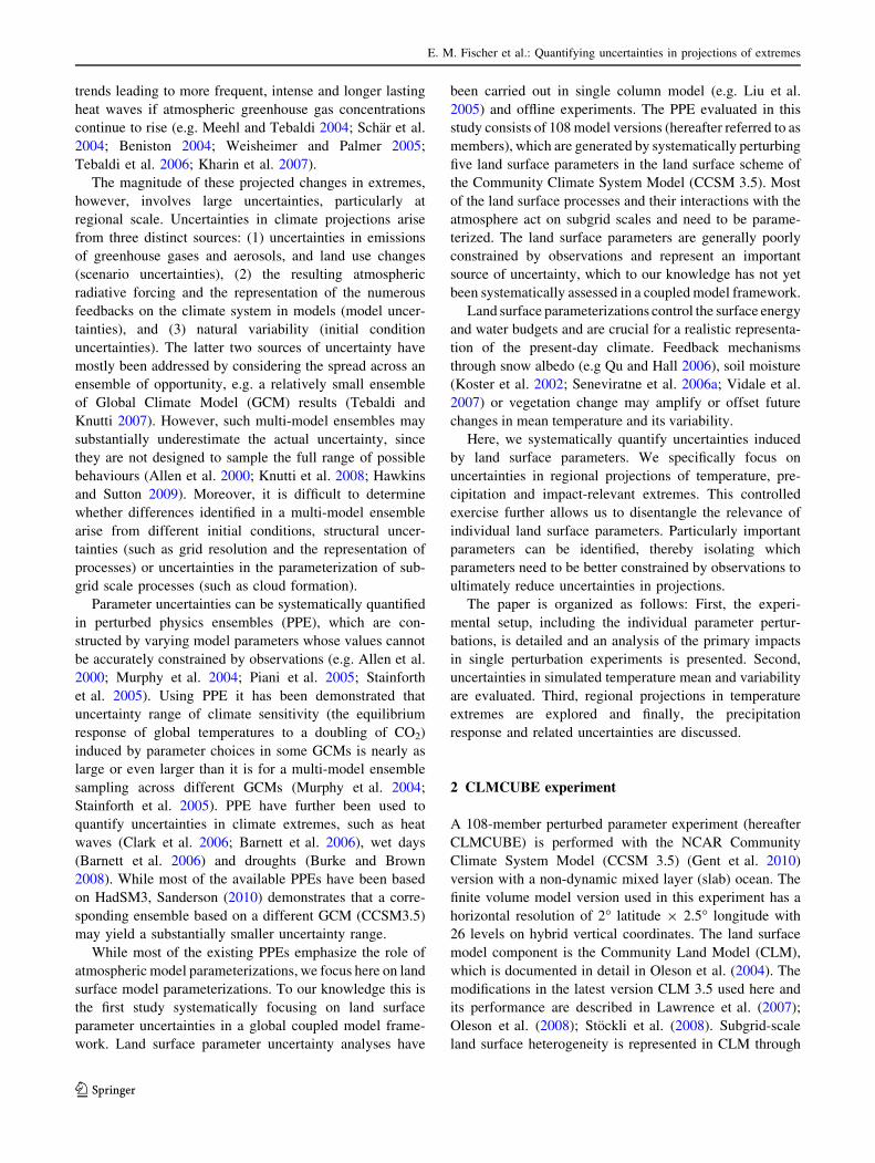
7 Sensitivity of present-day precipitation and response
Regarding precipitation, we only evaluate the ensemble
range for summer (Fig. 12a), which due to the important
role of convective processes is most sensitive to land sur-
face parameterizations. The relative ensemble range with
respect to the ensemble mean is largest over dry regions,
which to some extent is a result of the low baseline values.
Present-day summer precipitation is substantially reduced
in members with low Vmax (over vegetated mid-latitudes
e.g. Central North America) and in members with a deep
water table (over dry subtropical regions, e.g. Mediterra-
nean and Central Asia) (Fig. S5). Table 3 illustrates that
the role of the land surface parameter in explaining the
precipitation variance across CLMCUBE differs across
regions with Vmax, water table depth and vegetation albedo
being most important. The uncertainty of the mean induced
by internal variability accounts for approximately 5–30%
of the uncertainty range (Fig. S8a).
The global mean land precipitation response (DPANN) to
a doubling of CO2 ranges from ?5.4–8.4%. While present-
day precipitation and temperature are highly correlated, we
do not find a significant correlation between DPANN and
DTANN across CLMCUBE. The spatial pattern mean
response (Fig. 12b) compares well with the CMIP3
ensemble transient response. The CLMCUBE ensemble
mean is consistent in sign, wherever CMIP3 shows a highly
robust precipitation change (more than 90% agreement in
sign across models), except for some particularly dry
regions. For parts of north Africa and over south-central
Africa at about 10–20�S CLMCUBE simulates a tendency
to wetter conditions, which contrasts with the majority of
the CMIP3 models.
Note that the relative DP involves large uncertainties
particularly during JJA (Fig 12c). The range in the relative
precipitation response DPJJA is largest over the subtropical
regions of both hemispheres. Over very dry regions the
large relative range should not be overinterpreted as it is to
some extent a result of the small baseline present-day
values. However, even in many mid-latitudinal regions
parameter perturbations can change the sign of DPJJA.
DPJJA ranges between -14 and ?5% in Central North
America, -9 and ?20% in the Mediterranean region, or
-6 and ?36% in Central Asia.
Note that given the short length of the simulation
internal variability can induce large uncertainties in the
(a) (b) (c)
Fig. 12 a CLMCUBE ensemble range (95th–5th percentile member)
of present-day JJA precipitation. The range is shown as a relative
departure from the local climatology. b Ensemble mean JJA
precipitation response to doubling of CO2 and (c) corresponding
uncertainty range relative to ensemble mean response (5th–95th
percentile, right panel)
Table 3 Role of different land
surface parameter in explaining
ensemble range of summer (JJA
for Northern Hemisphere and
DJF for Australia) precipitation
derived from multiple linear
regression
The total adjusted variance [%]
is given in the first column and
the partial variance [%]
explained by each parameter in
the following columns
Total expl. var. Veg. albedo Snow albedo Water table Vmax Roughn. length
Summer precip.
AUS 62.0 52.0 0.2 0.5 5.5 5.5
AMZ 65.8 59.0 2.5 3.7 1.2 1.0
WNA 86.3 4.3 2.7 50.5 29.3 0.1
CNA 90.3 14.6 1.2 25.0 48.3 1.8
ENA 83.3 60.5 1.0 0.0 22.5 0.1
MED 84.0 12.8 0.3 48.2 19.9 3.6
NEU 89.9 12.2 0.1 27.2 50.5 0.4
WAF 53.8 42.8 0.0 11.8 1.3 0.0
SAS 74.7 59.7 4.3 6.8 2.1 3.1
CAS 45.6 0.0 9.5 31.5 4.9 2.1
NAS 92.3 16.5 8.8 11.7 55.0 0.7
E. M. Fischer et al.: Quantifying uncertainties in projections of extremes
123

mean response. We tested this by randomly sampling the
corresponding number of years for 1 9 CO2 and 2 9 CO2
with a Monte Carlo technique from a 50-year control
experiment performed with the unperturbed model. We
find that the majority of the uncertainty in DP at the grid
scale is induced by internal variability as demonstrated in
Fig. S8b. Internal variability dominates especially over the
tropics whereas over mid- to high-latitudes parameter
uncertainties play an important role. In general, the sensi-
tivity of DPJJA to the different parameters is highly
nonlinear.
8 Conclusions
We present a systematic analysis of uncertainties in the
climate response to a doubling of atmospheric CO2 con-
centrations based on CLMCUBE, a perturbed land surface
parameter experiment. CLMCUBE includes 108 versions
of CCSM 3.5 (mixed-layer ocean), in which five poorly
constrained land surface parameters are perturbed across
their nominal ranges, individually and in all possible
combinations of the the discrete parameter values sampled.
We find that land surface parameter induce small
uncertainties at global scale, substantial uncertainties at
regional and seasonal scale and very large uncertainties in
the tails of the distribution, the climate extremes. Land
surface parameters are revealed to control the response not
only of the mean but also of the variability of temperature.
– Global response: The global land temperature response
to a doubling of atmospheric CO2 concentrations ranges
between 2.47–2.87 K across CLMCUBE. Thereby the
range is substantially smaller than in equivalent ensem-
bles with perturbed atmospheric parameters. The dif-
ferences here are mainly a result of perturbations of an
empirical snow aging parameter, which controls the
snow albedo feedback. We find that members with high
present-day snow albedo show a stronger decrease in
albedo and snow cover fraction and thus a stronger
warming. This confirms an earlier hypothesis based on a
small set of GCMs (Levis et al. 2007).
– Cold extremes: The climate change signal of temper-
ature extremes varies strongly across CLMCUBE as a
result of land surface parameter and initial condition
uncertainties. The response in DJF 5th percentile, here
referred to as cold extremes, ranges between 1.9–8.8 K
in Northern Europe and 3.0–8.3 K in North Asia.
Thereby the CLMCUBE range exceeds the spread
across the CMIP3 multi-model ensemble over the two
regions. The large uncertainty range results from the
fact that the response in temperature mean and daily
variability tend to line up in winter. Both variability
and the mean response relate to the amount of snow
cover/surface albedo reduction. Members with strong
(weak) snow albedo feedback simulate strong (weak)
warming and strongly (weakly) reduced variability. As
a result mean and variability combine in some members
to a weak and in others to a very strong response of
cold extremes over northern mid- to high-latitudes.
Changes in cold extremes and frost days are highly
uncertain in these regions, where they have important
socio-economic and ecological impacts, e.g. on energy
demand (Hadley et al. 2006) or mortality of mountain
pine beetle (Stahl et al. 2006). Furthermore, the shift in
timing of spring snow melt, which affects the vegeta-
tion onset is highly sensitive to the choice of the snow
aging parameter. As are result the climate change
signal in growing season length is highly uncertain and
differs by a factor of almost 2 across CLMCUBE (i.e.
25–45 days increase).
– Hot extremes: The uncertainty in hot extremes (95th
percentile of summer temperatures) exceeds the uncer-
tainty in the mean summer warming by far. However, the
range here is smaller than the CMIP3 uncertainty range
for hot extremes. Again, variability plays an important
role, for instance, in the Mediterranean region and
central North America, where it increases in response to
2 9 CO2. More intense and frequent hot extremes may
have substantial effects on human health. Three specific
health indicators have been analysed here. Heat wave
duration and heat index response involve substantial
uncertainties (response varies by a factor 2–3), whereas
the response in tropical nights is relatively insensitive to
land surface parameter perturbations.
– Precipitation: For the precipitation response, the
CLMCUBE range is often larger than the mean signal,
especially in dry regions. Given the short simulation
length, a large portion of this precipitation uncertainty
is induced by natural variability. Over the Mediterra-
nean, Central North America and Australia even the
sign of the summer precipitation response to a doubling
of CO2 varies between ensemble members. This result
is interesting since it is not consistent with the transient
response of CCSM3.0 nor the majority of the CMIP3
models for the twenty-first century, in which robust
precipitation reductions are identified over the Medi-
terranean and parts of Australia. The uncertainty range
found here should not be overinterpreted since poten-
tially important changes in ocean circulation and SST
variability are not reflected in the mixed-layer ocean
model and the simulations are relatively short given the
natural variability of summer precipitation.
Note that this experiment only covers part of the actual
uncertainty range (i.e. uncertainties induced by land
E. M. Fischer et al.: Quantifying uncertainties in projections of extremes
123

surface model parameters). First, because feedback uncer-
tainties in other components of the climate system, such as
atmosphere feedbacks (water vapour, cloud and lapse rate),
have not been accounted for. Joint perturbations in atmo-
spheric and land surface parameters may further lead to
non-linear effects, which are not sampled here. Second,
only a subset of the land surface parameter uncertainty has
been perturbed, excluding uncertainties in the biogeo-
chemical feedbacks, which are not interactively simulated
in this model version. Uncertainties in the carbon/nitrogen
cycle may be relevant for climate-carbon cycle feedbacks
and uncertainties in the carbon uptake by the land bio-
sphere. Third, potentially important structural uncertainties
in grid resolution and fundamental physical assumptions in
the model formulation have not been considered.
CLMCUBE provides extended insight in the global and
regional uncertainties related to land surface parameter-
izations. While uncertainties are large particularly in the
case of temperature extremes, the sign of the response is
very robust for temperature-related variables.
Acknowledgments We thank Gerald Meehl, Keith Oleson and Reto
Knutti for the fruitful discussion and the anonymous reviewers for their
valuable comments on the manuscript. Erich Fischer was supported by
the Swiss National Science Foundation. Support of this dataset is
provided by the Office of Science, U.S. Department of Energy.
References
Alexander L, Zhang X, Peterson T, Caesar J, Gleason B, Tank AK,
Haylock M, Collins D, Trewin B, Rahimzadeh F, Tagipour A,
Kumar K, Revadekar J, Griffiths G, Vincent L, Stephenson D,
Burn J, Aguilar E, Brunet M, Taylor M, New M, Zhai P,
Rusticucci M, Vazquez-Aguirre J (2006) Global observed
changes in daily climate extremes of temperature and precipi-
tation. J Geophys Res 111. doi:10.1029/2005JD006290
Allen M, Stott P, Mitchell J, Schnur R, Delworth T (2000)
Quantifying the uncertainty in forecasts of anthropogenic
climate change. Nature 407:617–620
Barnett DN, Brown SJ, Murphy JM, Sexton DMH, Webb MJ (2006)
Quantifying uncertainty in changes in extreme event frequency
in response to doubled CO2 using a large ensemble of GCM
simulations. Clim Dyn 26. doi:10.1007/s00382-005-0097-1
Beniston M (2004) The 2003 heat wave in Europe: a shape of things
to come? An analysis based on Swiss climatological data and
model simulations. Geophys Res Lett 31. doi:10.1029/2003
GL018857
Breiman L, Friedman J, Olshen R, Stone C (1984) Classification and
regression trees. Wadsworth, Belmont, CA 1
Burke E and Brown S (2008) Evaluating uncertainties in the
projection of future drought. J Hydrometeorol 9:292–299
Caesar J, Alexander L, Vose R (2006) Large-scale changes in
observed daily maximum and minimum temperatures: creation
and analysis of a new gridded data set. J Geophys Res 111. doi:
10.1029/2005JD006280
Clark RT, Brown SJ, Murphy JM (2006) Modeling Northern
Hemisphere summer heat extreme changes and their
uncertainties using a physics ensemble of climate sensitivity
experiments. J Clim 19:4418–4435
Dai A, Trenberth K, and Karl T (1999) Effects of clouds, soil
moisture, precipitation, and water vapor on diurnal temperature
range. J Clim 12:2451–2473
Easterling D, Evans J, Groisman P, Karl T, Kunkel K, Ambenje P
(2000) Observed variability and trends in extreme climate
events: a brief review. Bull Am Meteorol Soc 81:417–425
ECMWF (2007) IFS documentation—Cy31r1: part IV, physical
processes. ECMWF, Full scientific and technical documentation.
http://www.ecmwf.int/research/ifsdocs/CY31r1/index.html
Fischer EM, Schar C (2009) Future changes in daily summer
temperature variability: driving processes and role for temper-
ature extremes. Clim Dyn. doi:10.1007/s00382-008-0473-8
Fischer EM, Schar C (2010) Consistent geographical patterns of
changes in high-impact european heatwaves. Nat Geosci. doi:
10.1038/NGEO866
Frich P, Alexander L, Della-Marta P, Gleason B, Haylock M, Tank A,
Peterson T (2002) Observed coherent changes in climatic
extremes during the second half of the twentieth century. Clim
Res 19:193–212
Gent P, Yeager S, Neale R, Levis S, Bailey D (2010) Improvements
in a half degree atmosphere/land version of the CCSM. Clim
Dyn 34(6):819–833
Gregory J and Mitchell J (1995) Simulation of daily variability of
surface temperature and precipitation over Europe in the current
and 2 9 CO2 climates using the UKMO climate model. Q J R
Meteorol Soc 121:1451–1476
Grize L, Huss A, Thommen O, Schindler C, Braun-Fahrlander C
(2005) Heat wave 2003 and mortality in Switzerland. Swiss Med
Wkly 135:200–205
Hadley S, Hernandez J, Broniak C, Blasing T (2006) Responses of
energy use to climate change: a climate modeling study.
Geophys Res Lett 33:L17703
Hawkins E and Sutton R (2009) The potential to narrow uncertainty
in regional climate predictions. Bull Am Meteorol Soc
90:1095–1107
Hemon D, Jougla E, Laurent CJF, Bellec S, Pavillon G (2003)
Surmortalite lieeala canicule d’aout 2003 en France. Bull
Epidemiologique Hebdomadaire 45–46:1–5
IPCC (2007) Climate change 2007: the physical science basis.
Contribution of working group i to the fourth assessment report
of the intergovernmental panel on climate change. Cambridge
University Press, Cambridge, 996 pp
Katz RW and Brown BG (1992) Extreme events in a changing
climate: variability is more important than averages. Clim
Change 21:289–302
Kharin V, Zwiers F, Zhang X, Hegerl G (2007) Changes in
temperature and precipitation extremes in the IPCC ensemble
of global coupled model simulations. J Clim 20:1419–1444
Knutti R, Allen M, Friedlingstein P, Gregory J, Hegerl G, Meehl G,
Meinshausen M, Murphy J, Plattner G, Raper S et al (2008) A
review of uncertainties in global temperature projections over
the twenty-first century. J Clim 21:2651–2663
Koster R, Dirmeyer P, Hahmann A, Ijpelaar R, Tyahla L, Cox P,
Suarez M (2002) Comparing the degree of land-atmosphere
interaction in four atmospheric general circulation models.
J Hydrometeor 3:363–375
Kunkel K, Andsager K, Easterling D (1999) Long-term trends in
extreme precipitation events over the conterminous United
States and Canada. J Clim 12:2515–2527
Lawrence D, Thornton P, Oleson K, Bonan G (2007) The partitioning
of evapotranspiration into transpiration, soil evaporation, and
canopy evaporation in a GCM: impacts on land-atmosphere
interaction. J Hydrometeor 8:862–880
E. M. Fischer et al.: Quantifying uncertainties in projections of extremes
123

Levis S, Bonan G, Lawrence P (2007) Present-day springtime high-
latitude surface albedo as a predictor of simulated climate
sensitivity. Geophys Res Lett 34:L17703
Liu Y, Gupta H, Sorooshian S, Bastidas L, Shuttleworth W (2005)
Constraining land surface and atmospheric parameters of a
locally coupled model using observational data. J Hydrometeor
6:156–172
Meehl G, Covey C, Taylor K, Delworth T, Stouffer R, Latif M,
McAvaney B, Mitchell J (2007) The WCRP CMIP3 multimodel
dataset:A new era in climate change research. Bull Am Meteorol
Soc 88:1383–1394
Meehl G, Zwiers F, Evans J, Knutson T, Mearns L, Whetton P (2000)
Trends in extreme weather and climate events: issues related to
modeling extremes in projections of future climate change. Bull
Am Meteorol Soc 81:427–436
Meehl GA and Tebaldi C (2004) More intense, more frequent, and
longer lasting heat waves in the 21st century. Science
305:994–997
Murphy J, Sexton D, Barnett D, Jones G, Webb M, Collins M,
Stainforth D (2004) Quantification of modelling uncertainties in
a large ensemble of climate change simulations. Nature
430:768–772
Niu G, Yang Z, Dickinson R, Gulden L (2005) A simple TOPMOD-
EL-based runoff parameterization (SIMTOP) for use in global
climate models. J Geophys Res 110. doi:10.1029/2005JD006111
Niu G, Yang Z, Dickinson R, Gulden L, Su H (2007) Development of
a simple groundwater model for use in climate models and
evaluation with Gravity Recovery and Climate Experiment data.
J Geophys Res 112. doi:10.1029/2006JD007522
Oleson K, Dai Y, Bonan G, Bosilovich M, Dickinson R, Dirmeyer P,
Hoffman F, Houser P, Levis S, Niu G et al (2004) Technical
description of the community land model (CLM). Tech Note
NCAR/TN-461? STR
Oleson K, Niu G, Yang Z, Lawrence D, Thornton P, Lawrence P,
Stockli R, Dickinson R, Bonan G, Levis S et al (2008)
Improvements to the Community Land Model and their impact
on the hydrological cycle. J Geophys Res 113. doi:
10.1029/2007JG000563
Piani C, Frame D, Stainforth D, Allen M (2005) Constraints on
climate change from a multi-thousand member ensemble of
simulations. Geophys Res Lett 32:23
Qu X and Hall A (2006) Assessing snow albedo feedback in
simulated climate change. J Clim 19:2617–2630
Qu X and Hall A (2007) What controls the strength of snow-albedo
feedback? J Clim 34:3971–3981
Raisanen J (2002) CO2-induced changes in interannual temperature
and precipitation variability in 19 CMIP2 experiments. J Clim
15:2395–2411
Raisanen J and Joelsson R (2001) Changes in average and extreme
precipitation in two regional climate model experiments. Tellus
A 53:547–566
Sanderson BM (2010) A multi-model study of parametric uncertainty
in predictions of climate response to rising greenhouse gas
concentrations. J Clim. doi:10.1175/2010JCLI3498.1
Schar C, Vidale PL, Luthi D, Frei C, Haberli C, Liniger MA,
Appenzeller C (2004) The role of increasing temperature
variability in European summer heatwaves. Nature 427:332–
336. doi:10.1038/nature02300
Seneviratne SI, Koster RD, Guo Z, Dirmeyer PA, Kowalczyk E,
Lawrence D, Liu P, Lu C-H, Mocko D, Oleson KW, Verseghy D
(2006a) Soil moisture memory in AGCM simulations: analysis
of global land-atmosphere coupling experiment (GLACE) data.
J Hydrometeor 7:1090–1112
Seneviratne SI, Luthi D, Litschi M, Schar C (2006b) Land-atmosphere
coupling and climate change in Europe. Nature 443:205–209
Stahl K, Moore R, McKendry I (2006) Climatology of winter cold
spells in relation to mountain pine beetle mortality in British
Columbia, Canada. Clim Res 32:13–23
Stainforth D, Aina T, Christensen C, Collins M, Faull N, Frame D,
Kettleborough J, Knight S, Martin A, Murphy J et al (2005)
Uncertainty in predictions of the climate response to rising levels
of greenhouse gases. Nature 433:403–406
Steadman RG (1984) A universal scale of apparent temperature.
J Clim Appl Meteorol 23:1674–1687
Stockli R, Lawrence D, Niu G, Oleson K, Thornton P, Yang Z, Bonan
G, Denning A, Running S (2008) Use of FLUXNET in the
Community Land Model development. J Geophys Res 113. doi:
10.1029/2007JG000562
Tebaldi C, Hayhoe K, Arblaster J, and Meehl G (2006) Going to the
extremes. Clim Change 79:185–211
Tebaldi C and Knutti R (2007) The use of the multi-model ensemble
in probabilistic climate projections. Philos Transact A Math Phys
Eng Sci 365:2053
Thornton P and Zimmermann N (2007) An improved canopy
integration scheme for a land surface model with prognostic
canopy structure. J Clim 20:3902–3923
Vidale PL, Luthi D, Wegmann R, Schar C (2007) Europea summer
climate variability in a heterogeneous multi-model ensemble.
Clim Change 81:209–232
Weisheimer A and Palmer T (2005) Changing frequency of occur-
rence of extreme seasonal temperatures under global warming.
Geophys Res Lett 32:L20721
White M, Thornton P, Running S, Ramakrishna R (2000) Parame-
terization and sensitivity analysis of the BIOME-BGC terrestrial
ecosystem model: net primary production controls. Earth Interact
4:1
E. M. Fischer et al.: Quantifying uncertainties in projections of extremes
123