ORIGINAL PAPER

Quantifying the local influence at a tall tower sitein nocturnal conditions

David Werth1& Robert Buckley1 & Gengsheng Zhang2 & Robert Kurzeja1 &

Monique Leclerc2 & Henrique Duarte2 & Matthew Parker1 & Thomas Watson3

Received: 20 August 2014 /Accepted: 24 September 2015 /Published online: 17 October 2015# Springer-Verlag Berlin Heidelberg (outside the USA) 2015

Abstract The influence of the local terrestrial environment onnocturnal atmospheric CO2 measurements at a 329-m televi-sion transmitter tower (and a component of a CO2 monitoringnetwork) was estimated with a tracer release experiment and asubsequent simulation of the releases. This was done to char-acterize the vertical transport of emissions from the surface tothe uppermost tower level and how it is affected by atmosphericstability. The tracer release experiment was conducted over twonights in May of 2009 near the Department of Energy’s Savan-nah River Site (SRS) in South Carolina. Tracer was released ontwo contrasting nights—slightly stable and moderately sta-ble—from several upwind surface locations. Measurements atthe 329-m level on both nights indicate that tracer was able tomix vertically within a relatively short (∼24 km) distance, im-plying that nocturnal stable conditions do not necessarily pre-vent vertical dispersion in the boundary layer and that CO2

measurements at the tower are at least partly influenced bynearby emissions. A simulation of the tracer release is used tocalculate the tower footprint on the two nights to estimate thedegree to which the local domain affects the tower readings.The effect of the nocturnal boundary layer on the area sampledby the tower can be seen clearly, as the footprints were affectedby changes in stability. The contribution of local sources to the

measurements at the tower was minimal, however, suggestingthat nocturnal concentrations at upper levels are contributedmostly by regional sources.

1 Introduction

In contrast with the multitude of studies of vertical transport inthe convective boundary layer (e.g., Wang et al. 2007;Barkhatov et al. 2012), vertical transport modeling and mea-surements remain scarce in the stable boundary layer(Sogachev and Leclerc 2011). This lack of robust data canhinder the interpretation of gas concentration measurementsmade at a tall tower sensor under stable conditions. Networksof towers are currently employed as platforms for making CO2

measurements, with the goal of constraining global-scale car-bon budgets (Andrews et al. 2013). Concentrations at a singletall (> 300 m) tower should be representative of continental-scale CO2 distributions (Desai et al. 2008), but the surface areaover which emissions are detected at an upper tower level isdictated by the local meteorology, especially the atmosphericstability (Gerbig et al. 2009; Sogachev and Leclerc 2011;Gloor et al. 2001). Stable conditions often prevail duringnighttime, making such periods ideal for continental-scalesampling (Gloor et al. 2001). Nocturnal turbulent conditionsdo occur, however, depending on the local terrain and meteo-rology, and the sampled area will tend to be local if there issignificant vertical mixing of respired CO2 (Gerbig et al.2009). In their paper on continental carbon exchange, Gerbiget al. (2009) describe the issues involved in the design andinterpretation of a tower network and write BIn a network oftall towers, the most important [question] is to ask: ‘what is itthat the individual tower observes?’^. We need to know moreabout nocturnal eddy transport and the influence of the nearbyenvironment on a tower.

* David Werthdavid.werth@srnl.doe.gov

1 Savannah River National Laboratory, Building 773-A,Aiken, SC 29808, USA

2 Laboratory for Atmospheric and Environmental Physics, Universityof Georgia, Griffin, GA, USA

3 Tracer Technology Group, Brookhaven National Laboratory,Upton, NY, USA

Theor Appl Climatol (2017) 127:627–642DOI 10.1007/s00704-015-1648-y

BNL-113796-2017-JA

The area sampled by a tower in any particular condition isoften described by its Bfootprint,^ a function that weights thecontribution from each point at the surface to the measuredsignal (Schmid 2002; Gerbig et al. 2009; Sogachev andLeclerc 2011; Barcza et al. 2009; Chen et al. 2013). The cal-culation of a footprint is often accomplished with a transportmodel that uses as input either a meteorological reanalysis(Gloor et al. 2001; Gerbig et al. 2009; Hegarty et al. 2013)or data from a boundary layer model (Sogachev and Leclerc2011). As the planetary boundary layer (PBL) becomes moreturbulent, the footprint will be confined to an area near thetower as vertical mixing will quickly move CO2 upwards.Gerbig et al. (2009), for example, used the Stochastic Time-Inverted Lagrangian Transport (STILT) transport model withan analyzed wind field to estimate footprints of the 30-m levelof the Harvard Forest tower in turbulent daytime conditions(when mixing leads to small differences between the 30- and300-m levels) and noted the dominant influence within 20 kmof the tower. In stable conditions, however, the footprintshould begin at a surface point well away from the towerand extend for long distances (Sogachev and Leclerc 2011).

In August 2008, the BSouth Carolina Tower^ (SCT), a 329-m television transmitter tower near Beech Island, SC, wasincorporated into the National Oceanic and Atmospheric Ad-ministration’s (NOAA) tall tower network (a subset of theAmeriflux network), which measures carbon concentrationsto quantify the terms of the global carbon flux, especiallythose dealing with the land surface (Birdsey et al. 2009; Ste-phens et al. 2007; Gourdji et al. 2012). Terrestrial ecosystemsconstitute a major sink of carbon, but their magnitude is un-certain (Birdsey et al. 2009). NOAA initiated the CarbonTracker project to process global carbon measurements andproduce a complete global carbon budget (Peters et al. 2007).The tower network is currently active in making measure-ments (Andrews et al. 2013), and this monitoring resourceforms the North American backbone of the Carbon Trackerproject.

Our goal is to determine the location of sources contribut-ing to the flux signature measured at the SCT. The objective ofthis project is to obtain detailed information about the wayeddy activity acts to move a gas emitted from the surface nearthe SCT upward to higher levels in the absence of convection.To accomplish this, a set of artificial tracers was released intothe nocturnal boundary layer (NBL) on two nights from var-ious locations within a 24-km distance upwind of the tower(Parker et al., in preparation) and time series of tracer concen-trations at three tower levels were recorded. The source areaaround a tower can be characterized by a Bnear field^ (within∼50 km) and a Bfar field^ out to the order of 1000 km (Gerbiget al. 2009), and the focus here is on the SCT near field.Therefore, a high-resolution mesoscale PBL simulation of a19 km × 26 km domain (encompassing the area of the exper-iment) is coupled to a transport model of the tracer release and

validated against the tracer signal at the tower. The coupledmodel is then used to estimate the footprints on the two nights.

Several experiments and simulations have helped elucidatevertical dispersion in the non-convective environment.Pasquill and Smith (1983) describe several tracer release fieldexperiments done under neutral and stable conditions,measuring the vertical distribution at towers within the rangeof 230 m. Sogachev and Leclerc (2011) applied the ScalarDistribution (SCADIS) boundary layer model with a Lagrang-ian transport model to estimate footprints in the stable bound-ary layer, and they found that Bthe changing atmospheric strat-ification determines the footprint which depends not only onthe height of a sensor but also on the time of measurements.^They also note that the calculation of a footprint can be mademore robust with the inclusion of actual data for comparison,and this is the goal of the current research. With a validatedsimulation of tracer transport, the plume behavior and towerfootprint in stable and neutral conditions can be quantified,allowing us to understand better the degree to which theSCT is influenced by the local environment.

2 Tracer field experiment

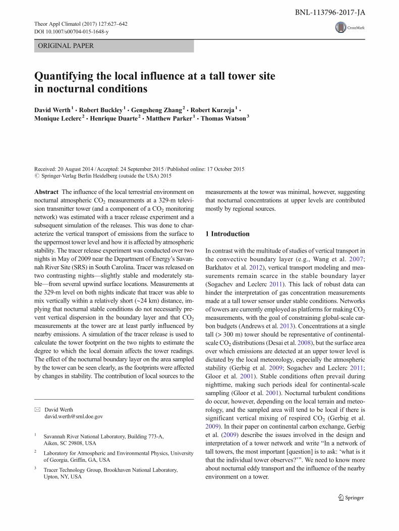
Tracer releases are a well-established method to study atmo-spheric motions (van Dop et al. 1998; Leclerc et al. 2003a, b),but their use to study stable boundary layers is less common.A nocturnal tracer study was conducted at the SCT site inMay 2009 (Parker et al. in preparation), with the goal of eval-uating the way gas released from the area near the tall tower ismixed upward into the moderately stable or slightly stableboundary layer during lateral advection. The experiment com-prised the released tracers and their detection at variousheights on the SCT, and the data was then used to validate asimulation of the release. The tracer release was conducted oneach of two nights, a slightly stable night (May 11th/12th,2009, Bnight 1^) and a second, moderately stable night(May 12th/13th, 2009, Bnight 2^), identified as such by theirtemperature profiles, the values of the friction velocity (u*),and Vaisala CL31 (Helsinki, Finland) lidar ceilometer read-ings of the boundary layer height. Compared to night 1,night 2 has a stronger late-night inversion (Fig. 1a),lower u* values (Fig. 1b) (especially at 329 m), and ashallower mixing layer (Fig. 1c). On night 1, the u*values fal l after peaking at around 0700 UTC(3:00 am EDT), while the values on night 2 rise afterreaching a minimum at around the same time (despite afalling boundary layer height (Fig. 1c)). This occursduring the release of the tracers and will affect tracerbehavior differently on the two nights. Selected tracerdata from this field experiment and local meteorologicalmeasurements are used in this study (Parker et al., inpreparation).

628 Werth D. et al.

2.1 Materials and methods

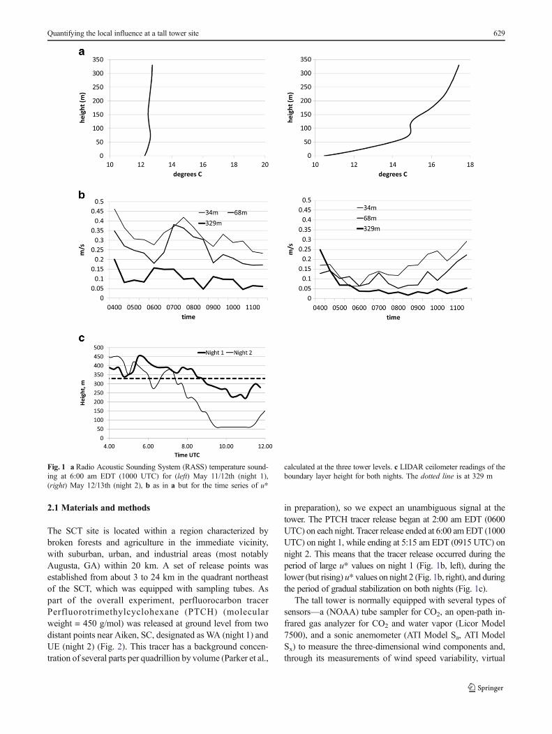
The SCT site is located within a region characterized bybroken forests and agriculture in the immediate vicinity,with suburban, urban, and industrial areas (most notablyAugusta, GA) within 20 km. A set of release points wasestablished from about 3 to 24 km in the quadrant northeastof the SCT, which was equipped with sampling tubes. Aspart of the overall experiment, perfluorocarbon tracerPerfluorotrimethylcyclohexane (PTCH) (molecularweight = 450 g/mol) was released at ground level from twodistant points near Aiken, SC, designated asWA (night 1) andUE (night 2) (Fig. 2). This tracer has a background concen-tration of several parts per quadrillion by volume (Parker et al.,

in preparation), so we expect an unambiguous signal at thetower. The PTCH tracer release began at 2:00 am EDT (0600UTC) on each night. Tracer release ended at 6:00 amEDT (1000UTC) on night 1, while ending at 5:15 am EDT (0915 UTC) onnight 2. This means that the tracer release occurred during theperiod of large u* values on night 1 (Fig. 1b, left), during thelower (but rising) u* values on night 2 (Fig. 1b, right), and duringthe period of gradual stabilization on both nights (Fig. 1c).

The tall tower is normally equipped with several types ofsensors—a (NOAA) tube sampler for CO2, an open-path in-frared gas analyzer for CO2 and water vapor (Licor Model7500), and a sonic anemometer (ATI Model Sa, ATI ModelSx) to measure the three-dimensional wind components and,through its measurements of wind speed variability, virtual

Fig. 1 a Radio Acoustic Sounding System (RASS) temperature sound-ing at 6:00 am EDT (1000 UTC) for (left) May 11/12th (night 1),(right) May 12/13th (night 2), b as in a but for the time series of u*

calculated at the three tower levels. c LIDAR ceilometer readings of theboundary layer height for both nights. The dotted line is at 329 m

Quantifying the local influence at a tall tower site 629

temperature. For the tracer release experiment, an additionaltube sampler was added to measure PTCH concentrations.The sensors and tube sampler inlets are deployed at threelevels: 34, 68, and 329 m. The tube samplers have beendiscussed in Parker et al. (in preparation), and the reader isreferred there for a detailed description.

In addition to the tower data, a sodar with a radio acousticsounding system (RASS) extension (Scintec AG, modelSFAS, Rottenburg, Germany) was installed at 33.455 N,81.7739 W, near the center of the experiment domain(Fig. 2), providing temperature and three-dimensional compo-nents of the velocity and boundary layer depth at 5 m resolu-tion up to 300 m (Parker et al., in preparation). A second sodar(Remtech PA2) was installed at 33.340 N, 81.564 W (Fig. 2),providing another source of wind data throughout the depth ofthe boundary layer.

2.2 Experimental results

2.2.1 Night 1: 11 to 12 May, 2009—slightly stable case

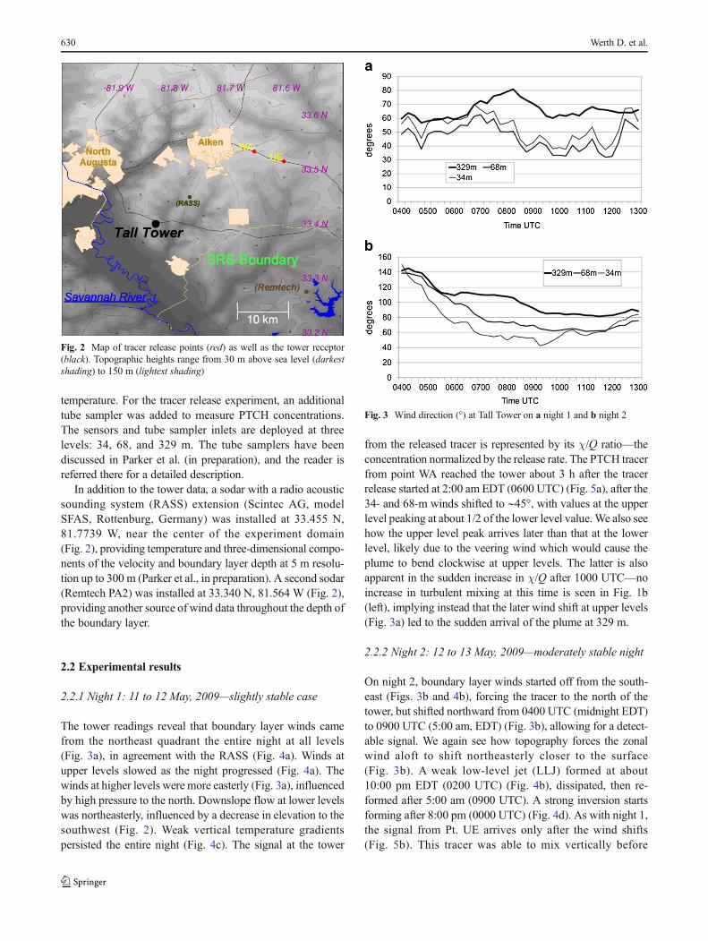
The tower readings reveal that boundary layer winds camefrom the northeast quadrant the entire night at all levels(Fig. 3a), in agreement with the RASS (Fig. 4a). Winds atupper levels slowed as the night progressed (Fig. 4a). Thewinds at higher levels were more easterly (Fig. 3a), influencedby high pressure to the north. Downslope flow at lower levelswas northeasterly, influenced by a decrease in elevation to thesouthwest (Fig. 2). Weak vertical temperature gradientspersisted the entire night (Fig. 4c). The signal at the tower

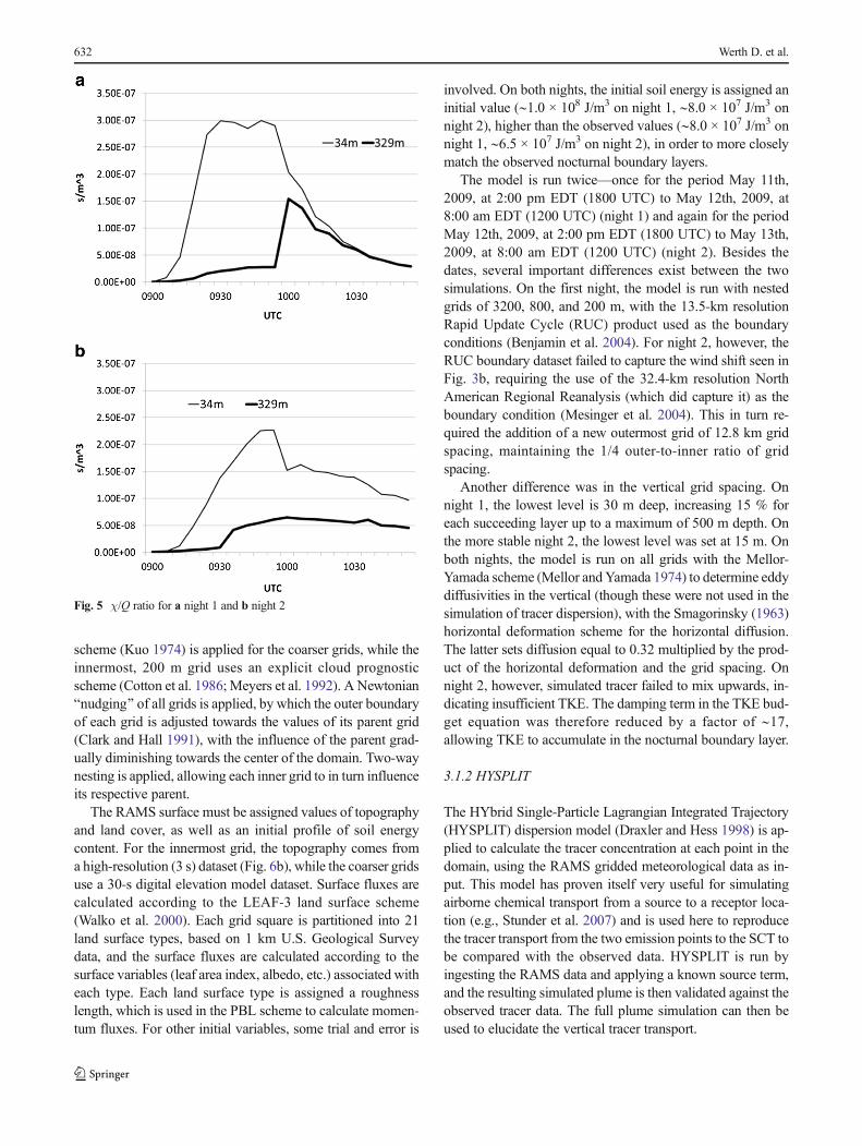
from the released tracer is represented by its χ/Q ratio—theconcentration normalized by the release rate. The PTCH tracerfrom point WA reached the tower about 3 h after the tracerrelease started at 2:00 am EDT (0600 UTC) (Fig. 5a), after the34- and 68-m winds shifted to ∼45°, with values at the upperlevel peaking at about 1/2 of the lower level value.We also seehow the upper level peak arrives later than that at the lowerlevel, likely due to the veering wind which would cause theplume to bend clockwise at upper levels. The latter is alsoapparent in the sudden increase in χ/Q after 1000 UTC—noincrease in turbulent mixing at this time is seen in Fig. 1b(left), implying instead that the later wind shift at upper levels(Fig. 3a) led to the sudden arrival of the plume at 329 m.

2.2.2 Night 2: 12 to 13 May, 2009—moderately stable night

On night 2, boundary layer winds started off from the south-east (Figs. 3b and 4b), forcing the tracer to the north of thetower, but shifted northward from 0400 UTC (midnight EDT)to 0900 UTC (5:00 am, EDT) (Fig. 3b), allowing for a detect-able signal. We again see how topography forces the zonalwind aloft to shift northeasterly closer to the surface(Fig. 3b). A weak low-level jet (LLJ) formed at about10:00 pm EDT (0200 UTC) (Fig. 4b), dissipated, then re-formed after 5:00 am (0900 UTC). A strong inversion startsforming after 8:00 pm (0000 UTC) (Fig. 4d). As with night 1,the signal from Pt. UE arrives only after the wind shifts(Fig. 5b). This tracer was able to mix vertically before

Fig. 2 Map of tracer release points (red) as well as the tower receptor(black). Topographic heights range from 30 m above sea level (darkestshading) to 150 m (lightest shading)

Fig. 3 Wind direction (°) at Tall Tower on a night 1 and b night 2

630 Werth D. et al.

reaching the tower (despite the low boundary layer heightspresent on both nights as seen in Fig. 1c), but on night 2, themost distant tracer peaks at only about 1/3 its surface value,whereas on night 1 the tracer is able to mix upward in quan-tities sufficient to cause the ratio of the peaks to be over half(albeit briefly), implying the vertical mixing of the tracer wasweaker on the more stable second night. The 329 m χ/Qvalues are lower on the second night, reflecting the greaterstability during this time.

3 Tracer simulation

3.1 Materials and methods

Calculating the motion of the tracer and inferring the relation-ship between the vertical transport and the turbulent propertiesof the atmosphere requires knowing the emission rate of thesource as well as estimates of the advection and turbulenttransport terms. While the emission rate in this study isknown, modeling must be used to estimate the advectionand turbulent terms. Similar to the work of Sogachev andLeclerc (2011), a meteorological model was coupled to a

dispersion model to explicitly calculate the tracer concentra-tions at each point. Coupled dispersion simulations often lackobserved concentrations of tracer for comparison to the modelresults (Sogachev and Leclerc 2011), but our tracer data can beused to validate our coupled simulation.

3.1.1 RAMS

The Regional Atmospheric Modeling System (RAMS, Pielkeet al. 1992) has been used previously to simulate fine-scalemotions within the nocturnal boundary layer (e.g., Werth et al.2011) and is selected to recreate the meteorology from the twonights of the tracer experiment, centered over the domain inFig. 6a. RAMS solves the non-hydrostatic equations of mo-tion for velocity and potential temperature on a staggered po-lar stereographic C grid (Mesinger and Arakawa 1976). Themodel also employs a terrain-following sigma coordinate sys-tem in the vertical. For our purposes, an innermost domain of200 m grid spacing was designed covering the area of theexperiment (25.8 km × 19.4 km) (Fig. 6b). This grid is nestedwithin coarser grids as described below. The Harrington radi-ation scheme (Harrington 1997) is applied for both shortwaveand longwave radiative transfer. For convection, the Kuo

Fig. 4 Radio Acoustic Sounding System (RASS) profiles of a night 1 wind speed and direction, b night 2 wind speed and direction, c night 1temperature, d night 2 temperature

Quantifying the local influence at a tall tower site 631

scheme (Kuo 1974) is applied for the coarser grids, while theinnermost, 200 m grid uses an explicit cloud prognosticscheme (Cotton et al. 1986; Meyers et al. 1992). A NewtonianBnudging^ of all grids is applied, by which the outer boundaryof each grid is adjusted towards the values of its parent grid(Clark and Hall 1991), with the influence of the parent grad-ually diminishing towards the center of the domain. Two-waynesting is applied, allowing each inner grid to in turn influenceits respective parent.

The RAMS surface must be assigned values of topographyand land cover, as well as an initial profile of soil energycontent. For the innermost grid, the topography comes froma high-resolution (3 s) dataset (Fig. 6b), while the coarser gridsuse a 30-s digital elevation model dataset. Surface fluxes arecalculated according to the LEAF-3 land surface scheme(Walko et al. 2000). Each grid square is partitioned into 21land surface types, based on 1 km U.S. Geological Surveydata, and the surface fluxes are calculated according to thesurface variables (leaf area index, albedo, etc.) associated witheach type. Each land surface type is assigned a roughnesslength, which is used in the PBL scheme to calculate momen-tum fluxes. For other initial variables, some trial and error is

involved. On both nights, the initial soil energy is assigned aninitial value (∼1.0 × 108 J/m3 on night 1, ∼8.0 × 107 J/m3 onnight 2), higher than the observed values (∼8.0 × 107 J/m3 onnight 1, ∼6.5 × 107 J/m3 on night 2), in order to more closelymatch the observed nocturnal boundary layers.

The model is run twice—once for the period May 11th,2009, at 2:00 pm EDT (1800 UTC) to May 12th, 2009, at8:00 am EDT (1200 UTC) (night 1) and again for the periodMay 12th, 2009, at 2:00 pm EDT (1800 UTC) to May 13th,2009, at 8:00 am EDT (1200 UTC) (night 2). Besides thedates, several important differences exist between the twosimulations. On the first night, the model is run with nestedgrids of 3200, 800, and 200 m, with the 13.5-km resolutionRapid Update Cycle (RUC) product used as the boundaryconditions (Benjamin et al. 2004). For night 2, however, theRUC boundary dataset failed to capture the wind shift seen inFig. 3b, requiring the use of the 32.4-km resolution NorthAmerican Regional Reanalysis (which did capture it) as theboundary condition (Mesinger et al. 2004). This in turn re-quired the addition of a new outermost grid of 12.8 km gridspacing, maintaining the 1/4 outer-to-inner ratio of gridspacing.

Another difference was in the vertical grid spacing. Onnight 1, the lowest level is 30 m deep, increasing 15 % foreach succeeding layer up to a maximum of 500 m depth. Onthe more stable night 2, the lowest level was set at 15 m. Onboth nights, the model is run on all grids with the Mellor-Yamada scheme (Mellor andYamada 1974) to determine eddydiffusivities in the vertical (though these were not used in thesimulation of tracer dispersion), with the Smagorinsky (1963)horizontal deformation scheme for the horizontal diffusion.The latter sets diffusion equal to 0.32 multiplied by the prod-uct of the horizontal deformation and the grid spacing. Onnight 2, however, simulated tracer failed to mix upwards, in-dicating insufficient TKE. The damping term in the TKE bud-get equation was therefore reduced by a factor of ∼17,allowing TKE to accumulate in the nocturnal boundary layer.

3.1.2 HYSPLIT

The HYbrid Single-Particle Lagrangian Integrated Trajectory(HYSPLIT) dispersion model (Draxler and Hess 1998) is ap-plied to calculate the tracer concentration at each point in thedomain, using the RAMS gridded meteorological data as in-put. This model has proven itself very useful for simulatingairborne chemical transport from a source to a receptor loca-tion (e.g., Stunder et al. 2007) and is used here to reproducethe tracer transport from the two emission points to the SCT tobe compared with the observed data. HYSPLIT is run byingesting the RAMS data and applying a known source term,and the resulting simulated plume is then validated against theobserved tracer data. The full plume simulation can then beused to elucidate the vertical tracer transport.

Fig. 5 χ/Q ratio for a night 1 and b night 2

632 Werth D. et al.

HYSPLIT uses turbulence kinetic energy (TKE) takenfrom the mesoscale model to calculate a Gaussian distributionof turbulent wind values, which are randomly added to themean wind values (taken from the 200 m RAMS grid) to getthe transport of each Lagrangian tracer particle. As they arereleased into the atmosphere, the particles will begin as aconcentrated cloud that gradually disperses as the particlesare assigned different turbulent velocities.

3.2 Results: night 1 (11 to 12 May, 2009)

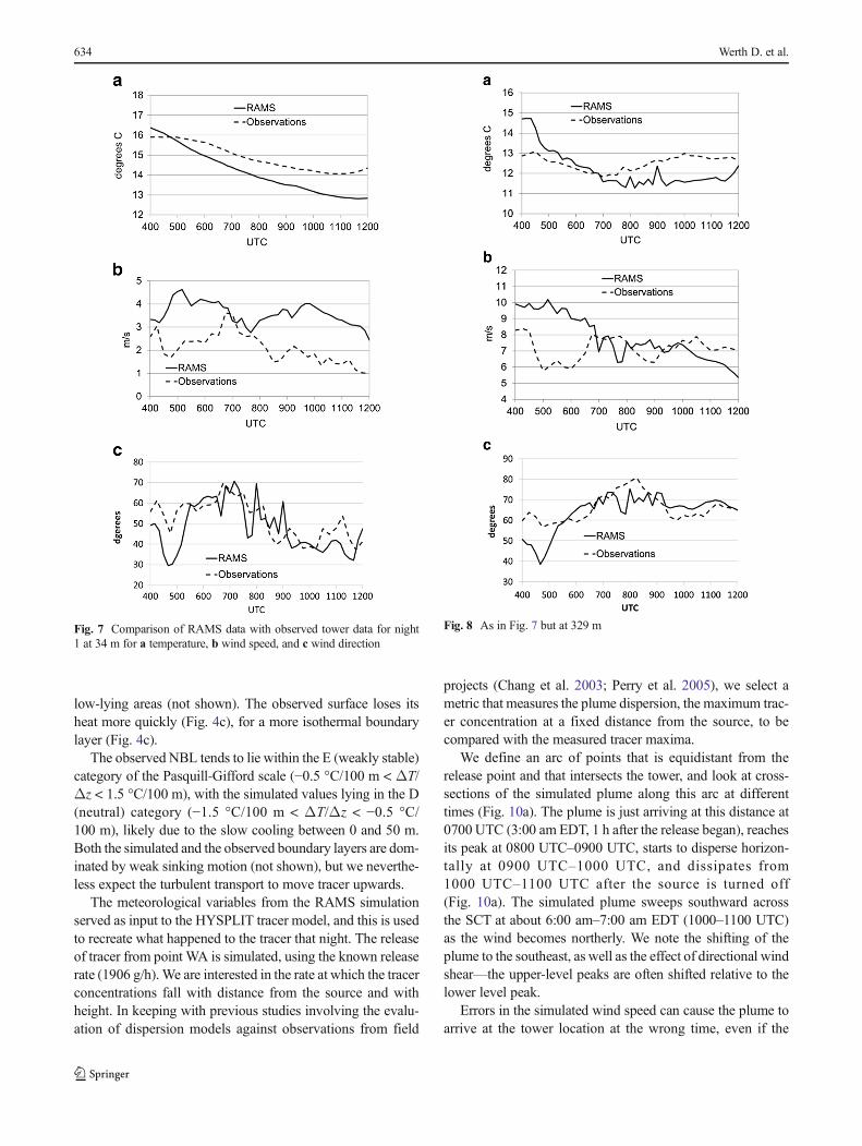
The model wind directions and temperature on the first night(Figs. 7 and 8) approximate the observed values at two levelsat the tall tower. Temperatures agree to within about 1 °C.Both levels experience a gradual cooling, with winds out of

the northeast. The model captures the wind shifts and verticalshear during the night (Figs. 7c and 8c), with errors usuallyless than 10°. At both levels, however, the RAMSwind speedsshow large errors (Figs. 7b and 8b).

The simulated PBL (Fig. 9a) and the RASS (Fig. 4a) fea-ture winds out of the NE to ENE up to the tower level(Fig. 9a), with faster winds above 200 m from 0000 UTC(8:00 pm EDT) to 0400 UTC (midnight) that decrease after-ward. Simulated cooling at the surface occurs at a slow rate(Fig. 9b), precluding the formation of an inversion in the 0–350-m range, with TKE remaining large (with a gradual de-crease) within a deep layer (Fig. 9b). This has the effect ofmaintaining vertical turbulent transport (and preventing theLLJ from forming) throughout most of the night. We alsosee a weak effect of drainage flow as convergence in the

SC

GA

Grid 1

Grid 2

WA

UE

a

b

Fig. 6 Topography (m above sealevel) for a grids 1 and 2, and bgrid 3. The star indicates thetower location, and the circlesindicate the release points

Quantifying the local influence at a tall tower site 633

low-lying areas (not shown). The observed surface loses itsheat more quickly (Fig. 4c), for a more isothermal boundarylayer (Fig. 4c).

The observed NBL tends to lie within the E (weakly stable)category of the Pasquill-Gifford scale (−0.5 °C/100 m < ΔT/Δz < 1.5 °C/100 m), with the simulated values lying in the D(neutral) category (−1.5 °C/100 m < ΔT/Δz < −0.5 °C/100 m), likely due to the slow cooling between 0 and 50 m.Both the simulated and the observed boundary layers are dom-inated by weak sinking motion (not shown), but we neverthe-less expect the turbulent transport to move tracer upwards.

The meteorological variables from the RAMS simulationserved as input to the HYSPLIT tracer model, and this is usedto recreate what happened to the tracer that night. The releaseof tracer from point WA is simulated, using the known releaserate (1906 g/h). We are interested in the rate at which the tracerconcentrations fall with distance from the source and withheight. In keeping with previous studies involving the evalu-ation of dispersion models against observations from field

projects (Chang et al. 2003; Perry et al. 2005), we select ametric that measures the plume dispersion, the maximum trac-er concentration at a fixed distance from the source, to becompared with the measured tracer maxima.

We define an arc of points that is equidistant from therelease point and that intersects the tower, and look at cross-sections of the simulated plume along this arc at differenttimes (Fig. 10a). The plume is just arriving at this distance at0700 UTC (3:00 am EDT, 1 h after the release began), reachesits peak at 0800 UTC–0900 UTC, starts to disperse horizon-tally at 0900 UTC–1000 UTC, and dissipates from1000 UTC–1100 UTC after the source is turned off(Fig. 10a). The simulated plume sweeps southward acrossthe SCT at about 6:00 am–7:00 am EDT (1000–1100 UTC)as the wind becomes northerly. We note the shifting of theplume to the southeast, as well as the effect of directional windshear—the upper-level peaks are often shifted relative to thelower level peak.

Errors in the simulated wind speed can cause the plume toarrive at the tower location at the wrong time, even if the

Fig. 7 Comparison of RAMS data with observed tower data for night1 at 34 m for a temperature, b wind speed, and c wind direction

Fig. 8 As in Fig. 7 but at 329 m

634 Werth D. et al.

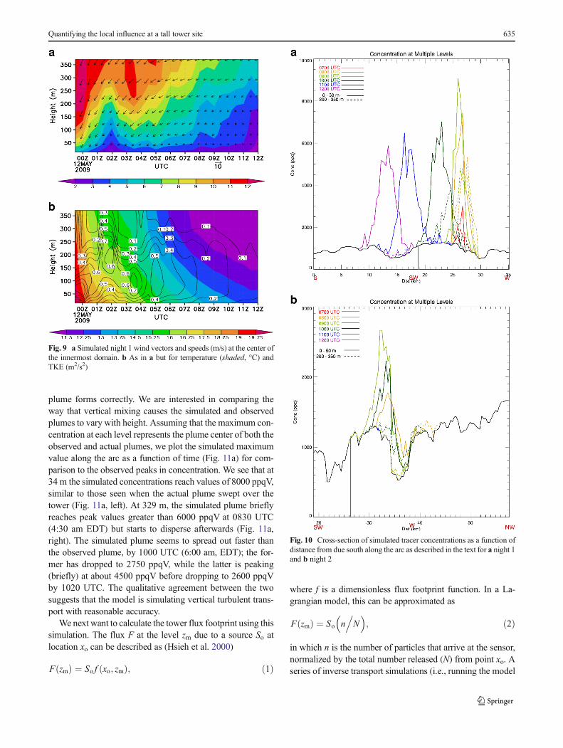
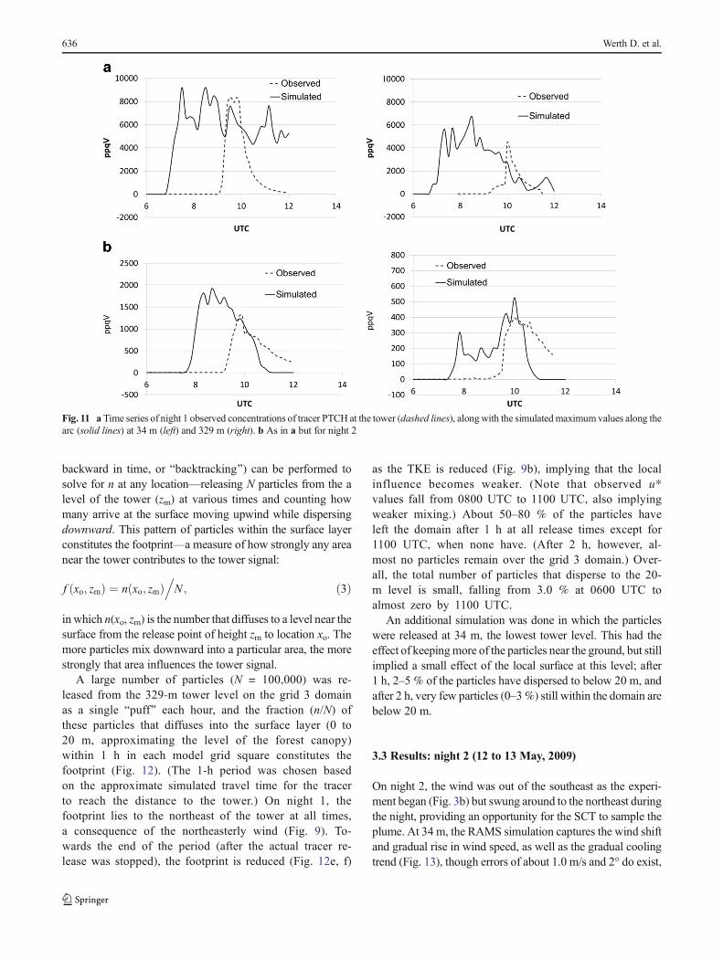
plume forms correctly. We are interested in comparing theway that vertical mixing causes the simulated and observedplumes to vary with height. Assuming that the maximum con-centration at each level represents the plume center of both theobserved and actual plumes, we plot the simulated maximumvalue along the arc as a function of time (Fig. 11a) for com-parison to the observed peaks in concentration. We see that at34 m the simulated concentrations reach values of 8000 ppqV,similar to those seen when the actual plume swept over thetower (Fig. 11a, left). At 329 m, the simulated plume brieflyreaches peak values greater than 6000 ppqV at 0830 UTC(4:30 am EDT) but starts to disperse afterwards (Fig. 11a,right). The simulated plume seems to spread out faster thanthe observed plume, by 1000 UTC (6:00 am, EDT); the for-mer has dropped to 2750 ppqV, while the latter is peaking(briefly) at about 4500 ppqV before dropping to 2600 ppqVby 1020 UTC. The qualitative agreement between the twosuggests that the model is simulating vertical turbulent trans-port with reasonable accuracy.

We next want to calculate the tower flux footprint using thissimulation. The flux F at the level zm due to a source So atlocation xo can be described as (Hsieh et al. 2000)

F zmð Þ ¼ So f xo; zmð Þ; ð1Þ

where f is a dimensionless flux footprint function. In a La-grangian model, this can be approximated as

F zmð Þ ¼ So n.N

� �; ð2Þ

in which n is the number of particles that arrive at the sensor,normalized by the total number released (N) from point xo. Aseries of inverse transport simulations (i.e., running the model

Fig. 9 a Simulated night 1 wind vectors and speeds (m/s) at the center ofthe innermost domain. b As in a but for temperature (shaded, °C) andTKE (m2/s2)

Fig. 10 Cross-section of simulated tracer concentrations as a function ofdistance from due south along the arc as described in the text for a night 1and b night 2

Quantifying the local influence at a tall tower site 635

backward in time, or Bbacktracking^) can be performed tosolve for n at any location—releasing N particles from the alevel of the tower (zm) at various times and counting howmany arrive at the surface moving upwind while dispersingdownward. This pattern of particles within the surface layerconstitutes the footprint—a measure of how strongly any areanear the tower contributes to the tower signal:

f xo; zmð Þ ¼ n xo; zmð Þ.N ; ð3Þ

in which n(xo, zm) is the number that diffuses to a level near thesurface from the release point of height zm to location xo. Themore particles mix downward into a particular area, the morestrongly that area influences the tower signal.

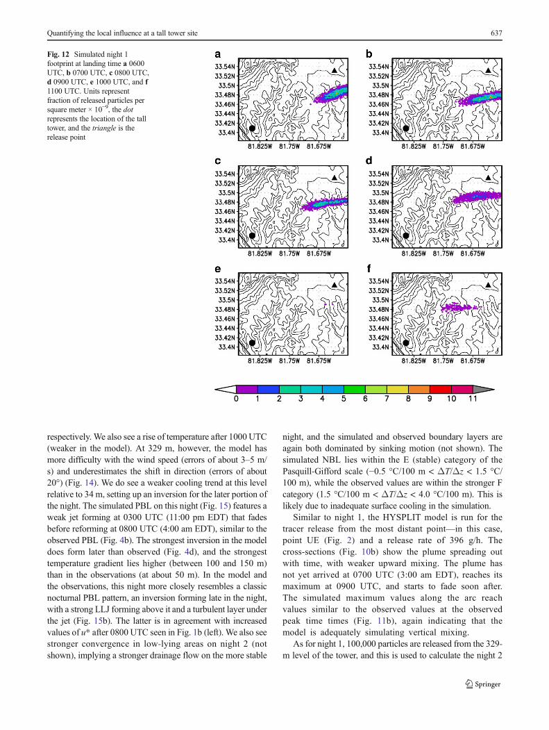
A large number of particles (N = 100,000) was re-leased from the 329-m tower level on the grid 3 domainas a single Bpuff^ each hour, and the fraction (n/N) ofthese particles that diffuses into the surface layer (0 to20 m, approximating the level of the forest canopy)within 1 h in each model grid square constitutes thefootprint (Fig. 12). (The 1-h period was chosen basedon the approximate simulated travel time for the tracerto reach the distance to the tower.) On night 1, thefootprint lies to the northeast of the tower at all times,a consequence of the northeasterly wind (Fig. 9). To-wards the end of the period (after the actual tracer re-lease was stopped), the footprint is reduced (Fig. 12e, f)

as the TKE is reduced (Fig. 9b), implying that the localinfluence becomes weaker. (Note that observed u*values fall from 0800 UTC to 1100 UTC, also implyingweaker mixing.) About 50–80 % of the particles haveleft the domain after 1 h at all release times except for1100 UTC, when none have. (After 2 h, however, al-most no particles remain over the grid 3 domain.) Over-all, the total number of particles that disperse to the 20-m level is small, falling from 3.0 % at 0600 UTC toalmost zero by 1100 UTC.

An additional simulation was done in which the particleswere released at 34 m, the lowest tower level. This had theeffect of keepingmore of the particles near the ground, but stillimplied a small effect of the local surface at this level; after1 h, 2–5 % of the particles have dispersed to below 20 m, andafter 2 h, very few particles (0–3%) still within the domain arebelow 20 m.

3.3 Results: night 2 (12 to 13 May, 2009)

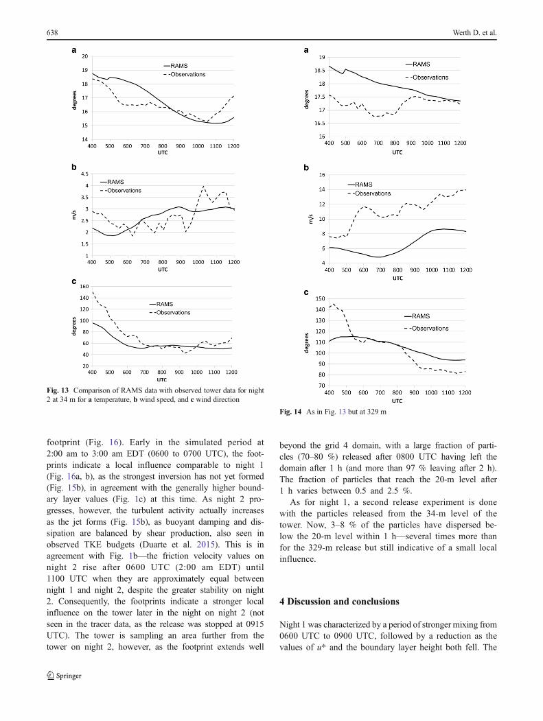
On night 2, the wind was out of the southeast as the experi-ment began (Fig. 3b) but swung around to the northeast duringthe night, providing an opportunity for the SCT to sample theplume. At 34 m, the RAMS simulation captures the wind shiftand gradual rise in wind speed, as well as the gradual coolingtrend (Fig. 13), though errors of about 1.0 m/s and 2° do exist,

Fig. 11 a Time series of night 1 observed concentrations of tracer PTCH at the tower (dashed lines), alongwith the simulated maximumvalues along thearc (solid lines) at 34 m (left) and 329 m (right). b As in a but for night 2

636 Werth D. et al.

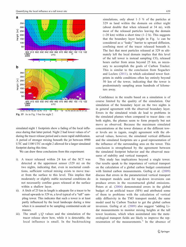
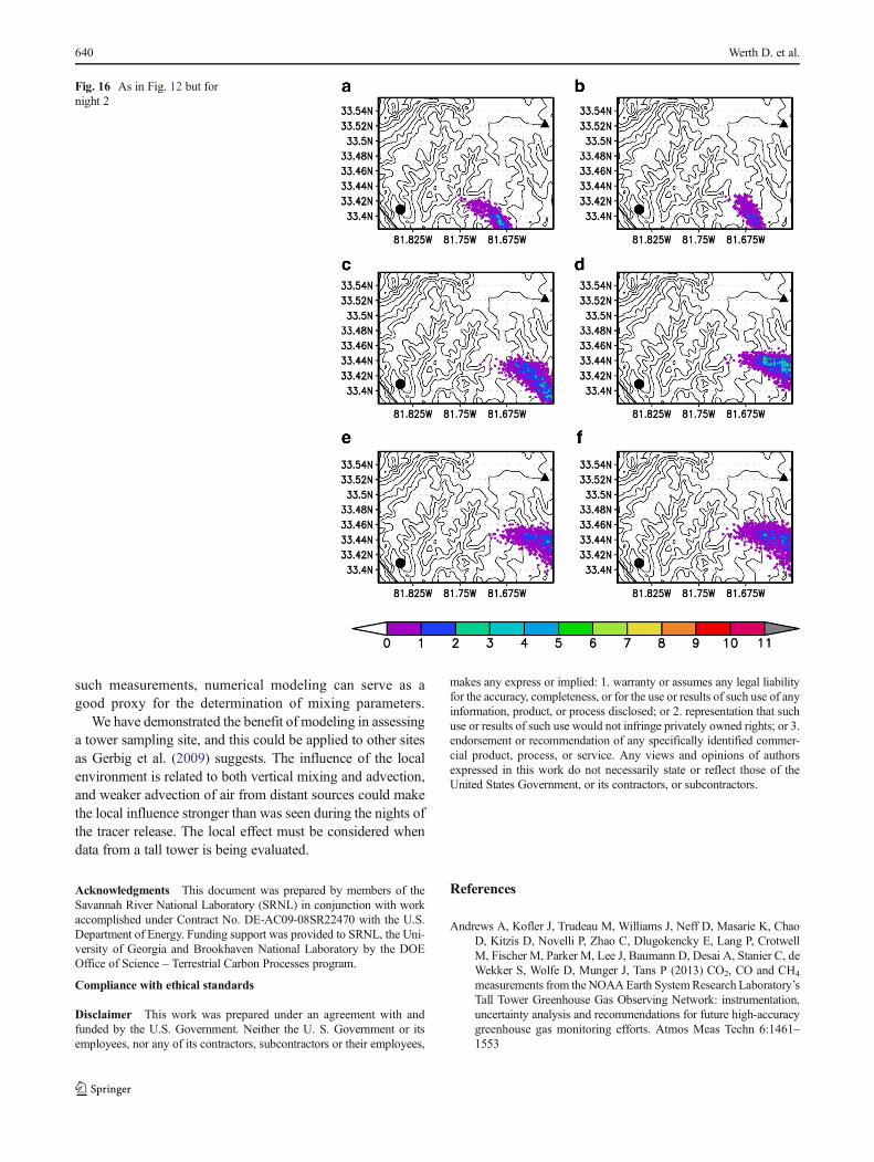
respectively. We also see a rise of temperature after 1000 UTC(weaker in the model). At 329 m, however, the model hasmore difficulty with the wind speed (errors of about 3–5 m/s) and underestimates the shift in direction (errors of about20°) (Fig. 14). We do see a weaker cooling trend at this levelrelative to 34 m, setting up an inversion for the later portion ofthe night. The simulated PBL on this night (Fig. 15) features aweak jet forming at 0300 UTC (11:00 pm EDT) that fadesbefore reforming at 0800 UTC (4:00 am EDT), similar to theobserved PBL (Fig. 4b). The strongest inversion in the modeldoes form later than observed (Fig. 4d), and the strongesttemperature gradient lies higher (between 100 and 150 m)than in the observations (at about 50 m). In the model andthe observations, this night more closely resembles a classicnocturnal PBL pattern, an inversion forming late in the night,with a strong LLJ forming above it and a turbulent layer underthe jet (Fig. 15b). The latter is in agreement with increasedvalues of u* after 0800 UTC seen in Fig. 1b (left). We also seestronger convergence in low-lying areas on night 2 (notshown), implying a stronger drainage flow on the more stable

night, and the simulated and observed boundary layers areagain both dominated by sinking motion (not shown). Thesimulated NBL lies within the E (stable) category of thePasquill-Gifford scale (−0.5 °C/100 m < ΔT/Δz < 1.5 °C/100 m), while the observed values are within the stronger Fcategory (1.5 °C/100 m < ΔT/Δz < 4.0 °C/100 m). This islikely due to inadequate surface cooling in the simulation.

Similar to night 1, the HYSPLIT model is run for thetracer release from the most distant point—in this case,point UE (Fig. 2) and a release rate of 396 g/h. Thecross-sections (Fig. 10b) show the plume spreading outwith time, with weaker upward mixing. The plume hasnot yet arrived at 0700 UTC (3:00 am EDT), reaches itsmaximum at 0900 UTC, and starts to fade soon after.The simulated maximum values along the arc reachvalues similar to the observed values at the observedpeak time times (Fig. 11b), again indicating that themodel is adequately simulating vertical mixing.

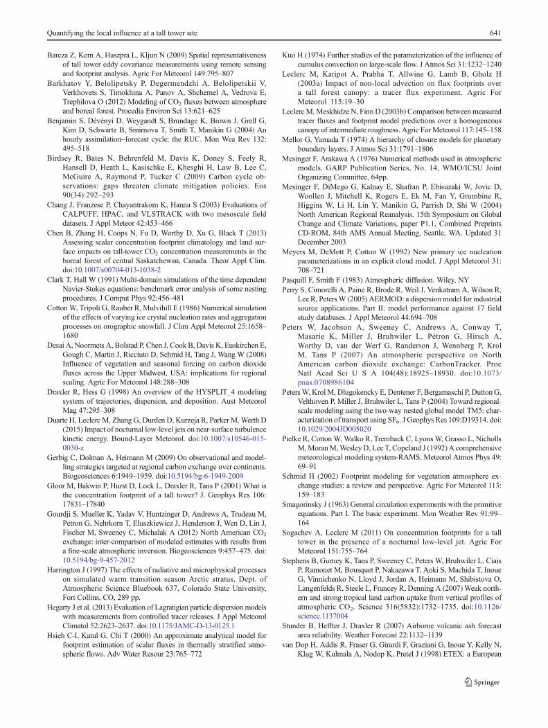
As for night 1, 100,000 particles are released from the 329-m level of the tower, and this is used to calculate the night 2

Fig. 12 Simulated night 1footprint at landing time a 0600UTC, b 0700 UTC, c 0800 UTC,d 0900 UTC, e 1000 UTC, and f1100 UTC. Units representfraction of released particles persquare meter × 10−9, the dotrepresents the location of the talltower, and the triangle is therelease point

Quantifying the local influence at a tall tower site 637

footprint (Fig. 16). Early in the simulated period at2:00 am to 3:00 am EDT (0600 to 0700 UTC), the foot-prints indicate a local influence comparable to night 1(Fig. 16a, b), as the strongest inversion has not yet formed(Fig. 15b), in agreement with the generally higher bound-ary layer values (Fig. 1c) at this time. As night 2 pro-gresses, however, the turbulent activity actually increasesas the jet forms (Fig. 15b), as buoyant damping and dis-sipation are balanced by shear production, also seen inobserved TKE budgets (Duarte et al. 2015). This is inagreement with Fig. 1b—the friction velocity values onnight 2 rise after 0600 UTC (2:00 am EDT) until1100 UTC when they are approximately equal betweennight 1 and night 2, despite the greater stability on night2. Consequently, the footprints indicate a stronger localinfluence on the tower later in the night on night 2 (notseen in the tracer data, as the release was stopped at 0915UTC). The tower is sampling an area further from thetower on night 2, however, as the footprint extends well

beyond the grid 4 domain, with a large fraction of parti-cles (70–80 %) released after 0800 UTC having left thedomain after 1 h (and more than 97 % leaving after 2 h).The fraction of particles that reach the 20-m level after1 h varies between 0.5 and 2.5 %.

As for night 1, a second release experiment is donewith the particles released from the 34-m level of thetower. Now, 3–8 % of the particles have dispersed be-low the 20-m level within 1 h—several times more thanfor the 329-m release but still indicative of a small localinfluence.

4 Discussion and conclusions

Night 1 was characterized by a period of stronger mixing from0600 UTC to 0900 UTC, followed by a reduction as thevalues of u* and the boundary layer height both fell. The

Fig. 13 Comparison of RAMS data with observed tower data for night2 at 34 m for a temperature, b wind speed, and c wind direction

Fig. 14 As in Fig. 13 but at 329 m

638 Werth D. et al.

simulated night 1 footprints show a fading of the local influ-ence during that latter period. Night 2 had lower values of u*during the tracer release period and a more rapid stabilization.A period of stronger mixing beneath the jet between 0900UTC and 1100 UTC on night 2 allowed for a larger simulatedfootprint during this time.

We can draw three conclusions from this experiment:

i). A tracer released within 24 km of the SCT wasdetected at the uppermost sensor (329 m) on thetwo nights, indicating that, even in nocturnal condi-tions, sufficient vertical mixing exists to move trac-er from the surface to this level. This implies thatmoderately or slightly stable nocturnal conditions donot necessarily confine gases released at the surfacewithin a shallow layer.

ii). A fetch of 25 km in length is adequate for a tracer to bemixed upwards to 329 m, a level typical of a Btall^ sam-pling tower. This indicates that such a tower is at leastpartly influenced by the local landscape during a timewhen it is assumed to be sampling continental-scale airmasses.

iii). The small χ/Q values and the simulation of thetracer release show how, while it is detectable, thelocal influence is small. In the backtracking

simulations, only about 1–3 % of the particles at329 m land within the domain on either night(about double that when released at 34 m), withmost of the released particles leaving the domain(∼20 km) within a short time (1–2 h). This suggeststhat the boundary layer height in Fig. 1c can beconsidered as a Bleaky^ barrier to upward diffusion,confining most of the tracer released beneath it.The fact that most particles released at 329 m ulti-mately left the local domain implies that this levelof the tall tower is instead sampling CO2 releasedhours earlier from areas beyond 25 km, as neces-sary to accomplish the goals of Carbon Tracker.This is similar to the conclusion from Sogachevand Leclerc (2011), in which calculated tower foot-prints in stable conditions often lay entirely beyond50 km of the tower, indicating that the tower ispredominately sampling areas hundreds of kilome-ters away.

Confidence in the results based on a simulation is ofcourse limited by the quality of the simulation. Oursimulation of the boundary layer on the two nights isin general agreement with the observed boundary layer.Errors in the simulated winds do lead to problems inthe simulated plumes when compared to tracer data—onboth nights, the plumes seem to form properly but notmove as observed. Because the maximum simulatedconcentrations at the tower distance at the different tow-er levels are in (again, rough) agreement with the ob-served values, however, the simulated vertical diffusionand the simulated footprints are a good representation ofthe influence of the surrounding area on the tower. Thisconclusion is strengthened by the agreement betweenthe simulated footprint behavior and the observed mea-sures of stability and vertical transport.

This study has implications beyond a single tower.Our results speak to the importance of vertical transporton the calculation of a global carbon budget constrainedwith limited carbon measurements. Gerbig et al. (2009)discuss that errors in the parameterized vertical transportin transport models used for top-down inversions canproduce errors in the reconstructed global emissions.Peters et al. (2004) demonstrated errors in the globalbudget of an artificial tracer (SF6) and attributed someof them to problems with the calculation of verticaleddy diffusivity in the TM5 transport model, the samemodel used by Carbon Tracker to get the global carboninversion. Gerbig et al. (2009) also suggest Badding Li-dar measurements to monitor mixing heights at the talltower locations, which when assimilated into the mete-orological transport fields are likely to improve the rep-resentation of the measurements.^ In the absence of

Fig. 15 As in Fig. 9 but for night 2

Quantifying the local influence at a tall tower site 639

such measurements, numerical modeling can serve as agood proxy for the determination of mixing parameters.

We have demonstrated the benefit of modeling in assessinga tower sampling site, and this could be applied to other sitesas Gerbig et al. (2009) suggests. The influence of the localenvironment is related to both vertical mixing and advection,and weaker advection of air from distant sources could makethe local influence stronger than was seen during the nights ofthe tracer release. The local effect must be considered whendata from a tall tower is being evaluated.

Acknowledgments This document was prepared by members of theSavannah River National Laboratory (SRNL) in conjunction with workaccomplished under Contract No. DE-AC09-08SR22470 with the U.S.Department of Energy. Funding support was provided to SRNL, the Uni-versity of Georgia and Brookhaven National Laboratory by the DOEOffice of Science – Terrestrial Carbon Processes program.

Compliance with ethical standards

Disclaimer This work was prepared under an agreement with andfunded by the U.S. Government. Neither the U. S. Government or itsemployees, nor any of its contractors, subcontractors or their employees,

makes any express or implied: 1. warranty or assumes any legal liabilityfor the accuracy, completeness, or for the use or results of such use of anyinformation, product, or process disclosed; or 2. representation that suchuse or results of such use would not infringe privately owned rights; or 3.endorsement or recommendation of any specifically identified commer-cial product, process, or service. Any views and opinions of authorsexpressed in this work do not necessarily state or reflect those of theUnited States Government, or its contractors, or subcontractors.

References

Andrews A, Kofler J, Trudeau M, Williams J, Neff D, Masarie K, ChaoD, Kitzis D, Novelli P, Zhao C, Dlugokencky E, Lang P, CrotwellM, Fischer M, Parker M, Lee J, Baumann D, Desai A, Stanier C, deWekker S, Wolfe D, Munger J, Tans P (2013) CO2, CO and CH4

measurements from theNOAAEarth SystemResearch Laboratory’sTall Tower Greenhouse Gas Observing Network: instrumentation,uncertainty analysis and recommendations for future high-accuracygreenhouse gas monitoring efforts. Atmos Meas Techn 6:1461–1553

Fig. 16 As in Fig. 12 but fornight 2

640 Werth D. et al.

Barcza Z, Kern A, Haszpra L, Kljun N (2009) Spatial representativenessof tall tower eddy covariance measurements using remote sensingand footprint analysis. Agric For Meteorol 149:795–807

Barkhatov Y, Belolipetsky P, Degermendzhi A, Belolipetskii V,Verkhovets S, Timokhina A, Panov A, Shchemel A, Vedrova E,Trephilova O (2012) Modeling of CO2 fluxes between atmosphereand boreal forest. Procedia Environ Sci 13:621–625

Benjamin S, Dévényi D, Weygandt S, Brundage K, Brown J, Grell G,Kim D, Schwartz B, Smirnova T, Smith T, Manikin G (2004) Anhourly assimilation–forecast cycle: the RUC. Mon Wea Rev 132:495–518

Birdsey R, Bates N, Behrenfeld M, Davis K, Doney S, Feely R,Hansell D, Heath L, Kasischke E, Khesghi H, Law B, Lee C,McGuire A, Raymond P, Tucker C (2009) Carbon cycle ob-servations: gaps threaten climate mitigation policies. Eos90(34):292–293

Chang J, Franzese P, Chayantrakom K, Hanna S (2003) Evaluations ofCALPUFF, HPAC, and VLSTRACK with two mesoscale fielddatasets. J Appl Meteor 42:453–466

Chen B, Zhang H, Coops N, Fu D, Worthy D, Xu G, Black T (2013)Assessing scalar concentration footprint climatology and land sur-face impacts on tall-tower CO2 concentration measurements in theboreal forest of central Saskatchewan, Canada. Theor Appl Clim.doi:10.1007/s00704-013-1038-2

Clark T, Hall W (1991) Multi-domain simulations of the time dependentNavier-Stokes equations: benchmark error analysis of some nestingprocedures. J Comput Phys 92:456–481

Cotton W, Tripoli G, Rauber R, Mulvihill E (1986) Numerical simulationof the effects of varying ice crystal nucleation rates and aggregationprocesses on orographic snowfall. J Clim Appl Meteorol 25:1658–1680

Desai A, Noormets A, Bolstad P, Chen J, CookB,Davis K, Euskirchen E,Gough C, Martin J, Ricciuto D, Schmid H, Tang J, Wang W (2008)Influence of vegetation and seasonal forcing on carbon dioxidefluxes across the Upper Midwest, USA: implications for regionalscaling. Agric For Meteorol 148:288–308

Draxler R, Hess G (1998) An overview of the HYSPLIT_4 modelingsystem of trajectories, dispersion, and deposition. Aust MeteorolMag 47:295–308

Duarte H, Leclerc M, Zhang G, Durden D, Kurzeja R, Parker M,Werth D(2015) Impact of nocturnal low-level jets on near-surface turbulencekinetic energy. Bound-Layer Meteorol. doi:10.1007/s10546-015-0030-z

Gerbig C, Dolman A, Heimann M (2009) On observational and model-ling strategies targeted at regional carbon exchange over continents.Biogeosciences 6:1949–1959. doi:10.5194/bg-6-1949-2009

Gloor M, Bakwin P, Hurst D, Lock L, Draxler R, Tans P (2001) What isthe concentration footprint of a tall tower? J. Geophys Res 106:17831–17840

Gourdji S, Mueller K, Yadav V, Huntzinger D, Andrews A, Trudeau M,Petron G, Nehrkorn T, Eluszkiewicz J, Henderson J, Wen D, Lin J,Fischer M, Sweeney C, Michalak A (2012) North American CO2

exchange: inter-comparison of modeled estimates with results froma fine-scale atmospheric inversion. Biogeosciences 9:457–475. doi:10.5194/bg-9-457-2012

Harrington J (1997) The effects of radiative and microphysical processeson simulated warm transition season Arctic stratus, Dept. ofAtmospheric Science Bluebook 637, Colorado State University,Fort Collins, CO, 289 pp.

Hegarty J et al. (2013) Evaluation of Lagrangian particle dispersion modelswith measurements from controlled tracer releases. J Appl MeteorolClimatol 52:2623–2637. doi:10.1175/JAMC-D-13-0125.1

Hsieh C-I, Katul G, Chi T (2000) An approximate analytical model forfootprint estimation of scalar fluxes in thermally stratified atmo-spheric flows. Adv Water Resour 23:765–772

Kuo H (1974) Further studies of the parameterization of the influence ofcumulus convection on large-scale flow. J Atmos Sci 31:1232–1240

Leclerc M, Karipot A, Prabha T, Allwine G, Lamb B, Gholz H(2003a) Impact of non-local advection on flux footprints overa tall forest canopy: a tracer flux experiment. Agric ForMeteorol 115:19–30

LeclercM,MeskhidzeN, FinnD (2003b) Comparison betweenmeasuredtracer fluxes and footprint model predictions over a homogeneouscanopy of intermediate roughness. Agric ForMeteorol 117:145–158

Mellor G, Yamada T (1974) A hierarchy of closure models for planetaryboundary layers. J Atmos Sci 31:1791–1806

Mesinger F, Arakawa A (1976) Numerical methods used in atmosphericmodels. GARP Publication Series, No. 14, WMO/ICSU JointOrganizing Committee, 64pp.

Mesinger F, DiMego G, Kalnay E, Shafran P, Ebisuzaki W, Jovic D,Woollen J, Mitchell K, Rogers E, Ek M, Fan Y, Grumbine R,Higgins W, Li H, Lin Y, Manikin G, Parrish D, Shi W (2004)North American Regional Reanalysis. 15th Symposium on GlobalChange and Climate Variations, paper P1.1, Combined PreprintsCD-ROM, 84th AMS Annual Meeting, Seattle, WA. Updated 31December 2003

Meyers M, DeMott P, Cotton W (1992) New primary ice nucleationparameterizations in an explicit cloud model. J Appl Meteorol 31:708–721

Pasquill F, Smith F (1983) Atmospheric diffusion. Wiley, NYPerry S, Cimorelli A, Paine R, Brode R, Weil J, Venkatram A, Wilson R,

Lee R, PetersW (2005) AERMOD: a dispersionmodel for industrialsource applications. Part II: model performance against 17 fieldstudy databases. J Appl Meteorol 44:694–708

Peters W, Jacobson A, Sweeney C, Andrews A, Conway T,Masarie K, Miller J, Bruhwiler L, Pétron G, Hirsch A,Worthy D, van der Werf G, Randerson J, Wennberg P, KrolM, Tans P (2007) An atmospheric perspective on NorthAmerican carbon dioxide exchange: CarbonTracker. ProcNatl Acad Sci U S A 104(48):18925–18930. doi:10.1073/pnas.0708986104

PetersW, KrolM, Dlugokencky E, Dentener F, Bergamaschi P, Dutton G,Velthoven P, Miller J, Bruhwiler L, Tans P (2004) Toward regional-scale modeling using the two-way nested global model TM5: char-acterization of transport using SF6. J Geophys Res 109:D19314. doi:10.1029/2004JD005020

Pielke R, Cotton W, Walko R, Tremback C, LyonsW, Grasso L, NichollsM,MoranM,WesleyD, Lee T, Copeland J (1992) A comprehensivemeteorological modeling system-RAMS. Meteorol Atmos Phys 49:69–91

Schmid H (2002) Footprint modeling for vegetation atmosphere ex-change studies: a review and perspective. Agric For Meteorol 113:159–183

Smagorinsky J (1963) General circulation experiments with the primitiveequations. Part I. The basic experiment. Mon Weather Rev 91:99–164

Sogachev A, Leclerc M (2011) On concentration footprints for a talltower in the presence of a nocturnal low-level jet. Agric ForMeteorol 151:755–764

Stephens B, Gurney K, Tans P, Sweeney C, Peters W, Bruhwiler L, CiaisP, Ramonet M, Bousquet P, Nakazawa T, Aoki S, Machida T, InoueG, Vinnichenko N, Lloyd J, Jordan A, Heimann M, Shibistova O,Langenfelds R, Steele L, Francey R, Denning A (2007)Weak north-ern and strong tropical land carbon uptake from vertical profiles ofatmospheric CO2. Science 316(5832):1732–1735. doi:10.1126/science.1137004

Stunder B, Heffter J, Draxler R (2007) Airborne volcanic ash forecastarea reliability. Weather Forecast 22:1132–1139

van Dop H, Addis R, Fraser G, Girardi F, Graziani G, Inoue Y, Kelly N,Klug W, Kulmala A, Nodop K, Pretel J (1998) ETEX: a European

Quantifying the local influence at a tall tower site 641

tracer experiment; observations, dispersion modelling and emergen-cy response. Atmos Environ 32:4089–4094

Walko R, Band L, Baron J, Kittel T, Lammers R, Lee T, Ojima D, PielkeR, Taylor C, Tague C, Tremback C, Vidale P (2000) Coupled atmo-sphere–biophysics–hydrology models for environmental modeling.J Appl Meteorol 39:931–944

Wang W, Davis K, Cook B, Yi C, Butler M, Ricciuto D, Bakwin P(2007) Estimating daytime CO2 fluxes over a mixed forest from

tall tower mixing ratio measurements. J Geophys Res V112,2006JD007770

Werth D, Kurzeja R, Luís Dias N, Zhang G, Duarte H, Fischer M, ParkerM, Leclerc M (2011) The simulation of the southern great plainsnocturnal boundary layer and the low-level jet with a high-resolutionmesoscale atmospheric model. J Appl Meteorol Climatol 50:1497–1513

642 Werth D. et al.