Quantifying the Interest Rate Risk of Bonds by Simulation

QUANTIFYING THE INTEREST RATE RISK OF BONDS BY SIMULATION

by

Cagatay Dagıstan

B.S., Industrial Engineering, Istanbul Technical University, 2008

Submitted to the Institute for Graduate Studies in

Science and Engineering in partial fulfillment of

the requirements for the degree of

Master of Science

Graduate Program in Industrial Engineering

Bogazici University

2010

ii

QUANTIFYING THE INTEREST RATE RISK OF BONDS BY SIMULATION

APPROVED BY:

Assoc. Prof. Wolfgang Hormann . . . . . . . . . . . . . . . . . . .

(Thesis Supervisor)

Prof. Refik Gullu . . . . . . . . . . . . . . . . . . .

Assist. Prof. Emrah Sener . . . . . . . . . . . . . . . . . . .

DATE OF APPROVAL: 07.07.2010

iii

ACKNOWLEDGEMENTS

I would like to thank my advisor, Assoc. Prof. Wolfgang Hormann for his guid-

ance, support and consistent interest throughout this study. I am also grateful to him

for introducing me to the field of quantitative finance.

I thank to my friend Kemal Dincer Dingec for his valuable comments and sig-

nificant assistance during this study. Besides, I am also thankful to TUBITAK for

providing financial support during my graduate study.

I would also like to thank Prof. Refik Gullu and Assist. Prof. Emrah Sener for

their interest and joining to my thesis committee.

Finally, I thank to my family for their support and care throughout my life.

iv

ABSTRACT

QUANTIFYING THE INTEREST RATE RISK OF BONDS

BY SIMULATION

Managing interest rate risk of bonds is very important in practice. Therefore,

many methods have been developed to measure the interest rate risk. In this thesis,

simulation is used to quantify the interest rate risk of bonds. Only government bonds

are considered, which are often assumed to have “0” default risk. So, the only relevant

risk is the interest rate risk.

In this thesis popular interest rate models are analyzed in a practical framework.

Bond pricing, interest rate simulation, parameter estimation and risk simulation princi-

ples are explained for six different short-rate models. For each model, the exact method

for simulating the short-rate is given; the analytical bond prices of the models and the

bond prices obtained by simulation are compared; MLE is used to estimate the model

parameters and risk simulations are made including a sensitivity analysis of VaR with

respect to the model parameters.

In the last part of this thesis, the risk estimation performance of the different

models is compared. The US, German and the Canadian bond market data are used

for analysis. The quality of the risk estimates of the models for different maturities is

assessed. It is observed that for all models and data that the arbitrage-free and the

equilibrium versions lead to the same Value at Risk results. For all implementations

we use R, which is a programming language for statistical computing.

v

OZET

TAHVILLERIN FAIZ ORANI RISKININ SIMULASYONLA

OLCULMESI

Tahvillerin faiz oranı riskini yonetmek, uygulamada cok onemlidir. Bu nedenle,

faiz oranı riskini olcmek icin bircok metod gelistirilmistir. Bu calısmada, tahvillerin

faiz oranı riskini hesaplamak icin simulasyon kullanılmıstır. Sadece devlet tahvilleri,

batma riski genellikle “0” kabul edilen, incelenmistir. Dolayısıyla, ilgili tek risk faiz

oranı riskidir.

Bu tezde, yaygın faiz haddi modelleri uygulamaya donuk bir cercevede analiz

edilmistir. Altı farklı kısa donem faiz haddi modeli icin, tahvil fiyatlama, faiz oranı

simulasyonu, parametre tahmini ve risk simulasyonu esasları acıklanmıstır. Her model

icin, kısa donem faiz oranı simulasyonunun kesin metodu verilmistir; modellerin analitik

tahvil fiyatlarıyla simulasyon ile hesaplanan tahvil fiyatları karsılastırılmıstır; model

parametreleri maksimum olabilirlik tahmin (MLE) yontemi kullanılarak elde edilmistir

ve risk simulasyonları, riske maruz degerin model parametrelerine duyarlılık analizi ile

birlikte, yapılmıstır.

Tezin son bolumunde, farklı modellerin risk tahmin performansı karsılastırılmıstır.

Analizlerde, Amerikan, Alman ve Kanada tahvil piyasası verileri kullanılmıstır. Mod-

ellerin risk tahmin kaliteleri, farklı vadeler icin degerlendirilmıstır. Modellerin arbi-

trajı engelleyen ya da denge versiyonlarını kullanmanın risk olcumunu etkilemedigi

gosterilmistir. Tum uygulamalar icin, programlama dili ve istatiksel hesaplama ortamı

olan R kullanılmıstır.

vi

TABLE OF CONTENTS

ACKNOWLEDGEMENTS . . . . . . . . . . . . . . . . . . . . . . . . . . . . . iii

ABSTRACT . . . . . . . . . . . . . . . . . . . . . . . . . . . . . . . . . . . . . iv

OZET . . . . . . . . . . . . . . . . . . . . . . . . . . . . . . . . . . . . . . . . . v

LIST OF FIGURES . . . . . . . . . . . . . . . . . . . . . . . . . . . . . . . . . xi

LIST OF TABLES . . . . . . . . . . . . . . . . . . . . . . . . . . . . . . . . . . xvii

LIST OF SYMBOLS/ABBREVIATIONS . . . . . . . . . . . . . . . . . . . . . xix

1. INTRODUCTION . . . . . . . . . . . . . . . . . . . . . . . . . . . . . . . . 1

2. BONDS . . . . . . . . . . . . . . . . . . . . . . . . . . . . . . . . . . . . . . 3

2.1. Definitions . . . . . . . . . . . . . . . . . . . . . . . . . . . . . . . . . . 3

2.2. Pricing Zero-Coupon Bonds . . . . . . . . . . . . . . . . . . . . . . . . 4

2.2.1. Yield in Simple-Compounding . . . . . . . . . . . . . . . . . . . 4

2.2.2. Yield in Periodic-Compounding . . . . . . . . . . . . . . . . . . 5

2.2.3. Yield in Continuous Compounding . . . . . . . . . . . . . . . . 5

2.2.3.1. An Example . . . . . . . . . . . . . . . . . . . . . . . 6

2.3. Yield Curve . . . . . . . . . . . . . . . . . . . . . . . . . . . . . . . . . 7

2.4. The Forward Rate . . . . . . . . . . . . . . . . . . . . . . . . . . . . . 9

2.4.1. Simply-Compounded Forward Rate . . . . . . . . . . . . . . . . 10

2.4.2. Continuously-Compounded Forward Rate . . . . . . . . . . . . 10

2.4.3. Instantaneous Forward Interest Rate . . . . . . . . . . . . . . . 12

2.5. Risk in Bond Investments . . . . . . . . . . . . . . . . . . . . . . . . . 12

3. INTEREST RATE MODELS . . . . . . . . . . . . . . . . . . . . . . . . . . 16

3.1. Fundamentals of Interest Rate Modeling . . . . . . . . . . . . . . . . . 16

3.1.1. The Short Rate . . . . . . . . . . . . . . . . . . . . . . . . . . . 16

3.2. Equilibrium Interest Rate Models . . . . . . . . . . . . . . . . . . . . . 17

3.3. No-Arbitrage Interest Rate Models . . . . . . . . . . . . . . . . . . . . 18

3.4. Bond Pricing . . . . . . . . . . . . . . . . . . . . . . . . . . . . . . . . 19

3.5. Risk Quantification . . . . . . . . . . . . . . . . . . . . . . . . . . . . . 20

4. EQUILIBRIUM INTEREST RATE MODELS . . . . . . . . . . . . . . . . . 22

4.1. The Vasicek Model . . . . . . . . . . . . . . . . . . . . . . . . . . . . . 22

vii

4.1.1. The Short-Rate Dynamics . . . . . . . . . . . . . . . . . . . . . 22

4.1.1.1. Objective Measure (Real-World) Dynamics . . . . . . 23

4.1.2. Simulating the Short Rate . . . . . . . . . . . . . . . . . . . . . 23

4.1.2.1. Exact Simulation . . . . . . . . . . . . . . . . . . . . . 23

4.1.2.2. Approximate Euler Scheme Simulation . . . . . . . . . 24

4.1.3. Maximum Likelihood Estimation of Parameters . . . . . . . . . 26

4.1.4. Bond Pricing . . . . . . . . . . . . . . . . . . . . . . . . . . . . 29

4.1.4.1. Analytical Bond Pricing . . . . . . . . . . . . . . . . . 29

4.1.4.2. Bond Pricing by Simulation . . . . . . . . . . . . . . . 30

4.1.5. Vasicek Yield Curve . . . . . . . . . . . . . . . . . . . . . . . . 32

4.1.6. Risk Simulation . . . . . . . . . . . . . . . . . . . . . . . . . . . 33

4.1.6.1. Sensitivity Analysis . . . . . . . . . . . . . . . . . . . 35

4.2. The Cox, Ingersoll and Ross (CIR) Model . . . . . . . . . . . . . . . . 37





4.2.3. Maximum Likelihood Estimation of Parameters . . . . . . . . . 39

4.2.4. Bond Pricing . . . . . . . . . . . . . . . . . . . . . . . . . . . . 41



4.2.5. CIR Yield Curve . . . . . . . . . . . . . . . . . . . . . . . . . . 43

4.2.6. Risk Simulation . . . . . . . . . . . . . . . . . . . . . . . . . . . 44


4.3. The Two-Factor Equilibrium Vasicek Model . . . . . . . . . . . . . . . 47

4.3.1. Motivation . . . . . . . . . . . . . . . . . . . . . . . . . . . . . . 47





4.3.4. Selecting the Parameters of the Model . . . . . . . . . . . . . . 49

4.3.5. Bond Pricing . . . . . . . . . . . . . . . . . . . . . . . . . . . . 50

viii



4.3.6. Two Factor Equilibrium Vasicek Yield Curve . . . . . . . . . . . 52

4.3.7. Risk Simulation . . . . . . . . . . . . . . . . . . . . . . . . . . . 54


5. ARBITRAGE-FREE INTEREST RATE MODELS . . . . . . . . . . . . . . 58

5.1. The Hull-White Extended Vasicek Model . . . . . . . . . . . . . . . . . 58




5.1.3. Fitting the Instantaneous Forward Rates to the Bond Prices . . 60


5.1.5. Bond Pricing . . . . . . . . . . . . . . . . . . . . . . . . . . . . 64



5.1.6. Hull-White Yield Curve . . . . . . . . . . . . . . . . . . . . . . 67

5.1.7. Risk Simulation . . . . . . . . . . . . . . . . . . . . . . . . . . . 68


5.2. The CIR++ Model . . . . . . . . . . . . . . . . . . . . . . . . . . . . . 70






5.2.4. Bond Pricing . . . . . . . . . . . . . . . . . . . . . . . . . . . . 73



5.2.5. CIR++ Yield Curve . . . . . . . . . . . . . . . . . . . . . . . . 74

5.2.6. Risk Simulation . . . . . . . . . . . . . . . . . . . . . . . . . . . 75


5.3. The Two Factor Arbitrage-Free Vasicek Model . . . . . . . . . . . . . . 78


ix





5.3.4. Bond Pricing . . . . . . . . . . . . . . . . . . . . . . . . . . . . 82



5.3.5. Two Factor Arbitrage-Free Vasicek Yield Curve . . . . . . . . . 84

5.3.6. Risk Simulation . . . . . . . . . . . . . . . . . . . . . . . . . . . 85


6. AN EMPIRICAL COMPARISON OF DIFFERENT MODELS FOR QUAN-

TIFYING THE RISK . . . . . . . . . . . . . . . . . . . . . . . . . . . . . . 89

6.1. Which model should we use? . . . . . . . . . . . . . . . . . . . . . . . . 89

6.2. Historic Risk Assesment of the Quality of the VaR Estimates . . . . . . 89

6.3. Historical Risk Simulation Results . . . . . . . . . . . . . . . . . . . . . 93

7. CONCLUSIONS . . . . . . . . . . . . . . . . . . . . . . . . . . . . . . . . . 105

APPENDIX A: R CODES . . . . . . . . . . . . . . . . . . . . . . . . . . . . . 107

A.1. R Codes for the Exact Simulation of the Vasicek Model . . . . . . . . . 107

A.2. R Codes for the Approximate Simulation of the Vasicek Model . . . . . 107

A.3. R Codes for the MLE of the Parameters of the Vasicek Model . . . . . 108

A.4. R Codes for the Bond Price and the Yield Calculations for the Vasicek

Model . . . . . . . . . . . . . . . . . . . . . . . . . . . . . . . . . . . . . 108

A.5. R Codes for Risk Simulation for the Vasicek Model . . . . . . . . . . . 108

A.6. R Codes for the Exact Simulation of the CIR Model . . . . . . . . . . . 109

A.7. R Codes for the Approximate Simulation of the CIR Model . . . . . . . 110

A.8. R Codes for Calculating the Log-Likelihood Function of the CIR Model 110

A.9. R Codes for the Bond Price and Yield Calculations for the CIR Model 111

A.10.R Codes for Risk Simulation for the CIR Model . . . . . . . . . . . . . 111

A.11.R Codes for the Exact Simulation of the Two Factor Equilibrium Vasicek

Model . . . . . . . . . . . . . . . . . . . . . . . . . . . . . . . . . . . . . 112

A.12.R Codes for the Approximate Simulation of the Two Factor Equilibrium

Vasicek Model . . . . . . . . . . . . . . . . . . . . . . . . . . . . . . . . 113

x

A.13.R Codes for the Bond Price and the Yield Calculations for the Two

Factor Equilibrium Vasicek Model . . . . . . . . . . . . . . . . . . . . . 114

A.14.R Codes for Risk Simulation for the Two Factor Equilibrium Vasicek

Model . . . . . . . . . . . . . . . . . . . . . . . . . . . . . . . . . . . . . 115

A.15.R Codes for the Exact Simulation of the Hull-White Model . . . . . . . 115

A.16.R Codes for the Bond Price and the Yield Calculations for the Hull-

White Model . . . . . . . . . . . . . . . . . . . . . . . . . . . . . . . . . 116

A.17.R Codes for Risk Simulation for the Hull-White Model . . . . . . . . . 116

A.18.R Codes for the Exact Simulation of the CIR++ Model . . . . . . . . . 117

A.19.R Codes for the Approximate Simulation of the CIR++ Model . . . . . 118

A.20.R Codes for the Bond Price and the Yield Calculations for the CIR++

Model . . . . . . . . . . . . . . . . . . . . . . . . . . . . . . . . . . . . . 119

A.21.R Codes for Risk Simulation for the CIR++ Model . . . . . . . . . . . 119

A.22.R Codes for the Exact Simulation of the Two Factor Arbitrage-Free

Vasicek Model . . . . . . . . . . . . . . . . . . . . . . . . . . . . . . . . 120

A.23.R Codes for the Approximate Simulation of the Two Factor Arbitrage-

Free Vasicek Model . . . . . . . . . . . . . . . . . . . . . . . . . . . . . 121

A.24.R Codes for the Bond Price and the Yield Calculations for the Two

Factor Arbitrage-Free Vasicek Model . . . . . . . . . . . . . . . . . . . . 122

A.25.R Codes for Risk Simulation for the Two Factor Arbitrage-Free Vasicek

Model . . . . . . . . . . . . . . . . . . . . . . . . . . . . . . . . . . . . . 123

A.26.R Codes for Historic Loss Calculations . . . . . . . . . . . . . . . . . . 123

A.27.R Codes for Historical Risk Simulations . . . . . . . . . . . . . . . . . 124

A.28.R Codes for Fitting Instantaneous Forward Rates to the Bond Prices . 127

REFERENCES . . . . . . . . . . . . . . . . . . . . . . . . . . . . . . . . . . . . 130

xi

LIST OF FIGURES

Figure 2.1. R-codes for plotting the yield curve . . . . . . . . . . . . . . . . . 8

Figure 2.2. A Sample Yield Curve . . . . . . . . . . . . . . . . . . . . . . . . 8

Figure 4.1. Comparison of the approximate and the exact distribution of the

short-rate in the Vasicek model. . . . . . . . . . . . . . . . . . . . 25

Figure 4.2. Simulated paths of the short rate in the Vasicek model . . . . . . 26

Figure 4.3. US 3-month maturity monthly yields for 1952-2004 . . . . . . . . 27

Figure 4.4. EURIBOR 3-month period daily rates for 1999-2007 . . . . . . . . 27

Figure 4.5. R-codes for calculating the MLE’s of the Vasicek model for US and

European data . . . . . . . . . . . . . . . . . . . . . . . . . . . . . 28

Figure 4.6. R-codes for calculating the MLE’s of the Vasicek model for US data

(1980-1990) . . . . . . . . . . . . . . . . . . . . . . . . . . . . . . 29

Figure 4.7. R-codes for calculating the analytical bond prices of the Vasicek

model . . . . . . . . . . . . . . . . . . . . . . . . . . . . . . . . . . 30

Figure 4.8. R-codes for obtaining the bond price by simulation for the Vasicek

model . . . . . . . . . . . . . . . . . . . . . . . . . . . . . . . . . . 31

Figure 4.9. R-codes for plotting the yield curve of the Vasicek model . . . . . 32

Figure 4.10. Comparison of the yield curves of the Vasicek model and the market 32

xii

Figure 4.11. R-codes for estimating the parameters of the Vasicek model for risk

simulations . . . . . . . . . . . . . . . . . . . . . . . . . . . . . . . 34

Figure 4.12. R-codes for calculating the VaR for the Vasicek model . . . . . . . 35

Figure 4.13. Parameter sets for the sensitivity analysis of VaR for the Vasicek

model . . . . . . . . . . . . . . . . . . . . . . . . . . . . . . . . . . 37


short-rate in the CIR model . . . . . . . . . . . . . . . . . . . . . 39

Figure 4.15. R-codes for estimating the parameters of the CIR model . . . . . . 41

Figure 4.16. R-codes for obtaining the bond price by simulation for the CIR model 43

Figure 4.17. R-codes for plotting the yield curve of the CIR model . . . . . . . 44

Figure 4.18. Comparison of the yield curves of the CIR and the Vasicek model

and the market . . . . . . . . . . . . . . . . . . . . . . . . . . . . 45

Figure 4.19. R-codes for estimating the parameters of the CIR model for risk

simulations . . . . . . . . . . . . . . . . . . . . . . . . . . . . . . . 45

Figure 4.20. R-codes for calculating the VaR for the CIR model . . . . . . . . . 45

Figure 4.21. Parameters sets for the sensitivity of VaR analysis for the CIR model 46


short-rate in the Two Factor Equilibrium Vasicek model . . . . . . 49

Figure 4.23. R-codes for selecting the parameters of the Two Factor Equilibrium

Vasicek model . . . . . . . . . . . . . . . . . . . . . . . . . . . . . 50

xiii

Figure 4.24. R-codes for calculating the analytical bond prices of the Two Factor

Equilibrium Vasicek model . . . . . . . . . . . . . . . . . . . . . . 51

Figure 4.25. R-codes for obtaining the bond price by simulation for Two Factor

Equilibrium Vasicek model . . . . . . . . . . . . . . . . . . . . . . 52

Figure 4.26. R-codes for plotting the yield curve of the Two Factor Equilibrium

Vasicek model . . . . . . . . . . . . . . . . . . . . . . . . . . . . . 53

Figure 4.27. Different yield curves of the Two Factor Equilibrium Vasicek model 53

Figure 4.28. Comparison of the yield curves of the Two Factor Equilibrium Va-

sicek model and the market . . . . . . . . . . . . . . . . . . . . . . 54

Figure 4.29. R-codes for estimating the parameters of the Two Factor Equilib-

rium Vasicek model for risk simulations . . . . . . . . . . . . . . . 55

Figure 4.30. R-codes for calculating the VaR for the Two Factor Equilibrium

Vasicek model . . . . . . . . . . . . . . . . . . . . . . . . . . . . . 55

Figure 5.1. R-codes for plotting the instantaneous forward rate and the bond

price curve for the Hull-White model . . . . . . . . . . . . . . . . 63

Figure 5.2. Hull-White January 2000 forward rate curve . . . . . . . . . . . . 63

Figure 5.3. Hull-White January 2000 bond price curve . . . . . . . . . . . . . 64

Figure 5.4. R-codes for obtaining the bond price by simulation for the Hull-

White model . . . . . . . . . . . . . . . . . . . . . . . . . . . . . . 66

Figure 5.5. R-codes for plotting the yield curve of the Hull-White model . . . 67

xiv

Figure 5.6. Comparison of the yield curves of the Hull-White model and the

market . . . . . . . . . . . . . . . . . . . . . . . . . . . . . . . . . 68

Figure 5.7. R-codes for estimating the parameters of the Hull-White model for

risk simulations . . . . . . . . . . . . . . . . . . . . . . . . . . . . 68

Figure 5.8. R-codes for calculating the VaR for the Hull-White model . . . . . 69


short-rate in the CIR++ model . . . . . . . . . . . . . . . . . . . 73

Figure 5.10. R-codes for obtaining the bond price by simulation for the CIR++

model . . . . . . . . . . . . . . . . . . . . . . . . . . . . . . . . . . 75

Figure 5.11. R-codes for plotting the yield curve of the CIR++ model . . . . . 76

Figure 5.12. Comparison of the yield curves of the CIR++ model and the market 76

Figure 5.13. R-codes for calculating the VaR for the CIR++ model . . . . . . . 77


short-rate in the Two Factor Arbitrage-Free Vasicek model . . . . 81

Figure 5.15. R-codes for selecting the parameters of the Two Factor Arbitrage-

Free Vasicek model . . . . . . . . . . . . . . . . . . . . . . . . . . 82

Figure 5.16. R-codes for the Bond Price and Yield Calculations for the Two

Factor Arbitrage-Free Vasicek Model . . . . . . . . . . . . . . . . 83

Figure 5.17. R-codes for obtaining the bond price by simulation for the Two

Factor Arbitrage-Free Vasicek model . . . . . . . . . . . . . . . . . 84

xv

Figure 5.18. R-codes for plotting the yield curve of the Two Factor Arbitrage-

Free Vasicek model . . . . . . . . . . . . . . . . . . . . . . . . . . 85

Figure 5.19. Comparison of the yield curves of the Two Factor Arbitrage-Free

Vasicek model and the market . . . . . . . . . . . . . . . . . . . . 86

Figure 5.20. R-codes for estimating the parameters of the Two Factor Arbitrage-

Free Vasicek model for risk simulations . . . . . . . . . . . . . . . 86

Figure 5.21. R-codes for calculating the VaR for the Two Factor Arbitrage-Free

Vasicek model . . . . . . . . . . . . . . . . . . . . . . . . . . . . . 87

Figure 6.1. 3-month maturity bond yield for the US, German and the Canadian

data . . . . . . . . . . . . . . . . . . . . . . . . . . . . . . . . . . 90

Figure 6.2. R-codes for calculating the binomial probabilities for the US, Ger-

man and the Canadian data . . . . . . . . . . . . . . . . . . . . . 92

Figure 6.3. VaR and historical loss results for 1-year maturity bonds for the

US data . . . . . . . . . . . . . . . . . . . . . . . . . . . . . . . . 98


US data . . . . . . . . . . . . . . . . . . . . . . . . . . . . . . . . 98


US data . . . . . . . . . . . . . . . . . . . . . . . . . . . . . . . . 99


US data . . . . . . . . . . . . . . . . . . . . . . . . . . . . . . . . 99


German data . . . . . . . . . . . . . . . . . . . . . . . . . . . . . . 100

xvi


German data . . . . . . . . . . . . . . . . . . . . . . . . . . . . . . 100


German data . . . . . . . . . . . . . . . . . . . . . . . . . . . . . . 101


German data . . . . . . . . . . . . . . . . . . . . . . . . . . . . . . 101


Canadian data . . . . . . . . . . . . . . . . . . . . . . . . . . . . . 102


Canadian data . . . . . . . . . . . . . . . . . . . . . . . . . . . . . 102


Canadian data . . . . . . . . . . . . . . . . . . . . . . . . . . . . . 103

xvii

LIST OF TABLES

Table 3.1. Summary of one-factor short rate models . . . . . . . . . . . . . . 19

Table 3.2. Risk quantification algorithm . . . . . . . . . . . . . . . . . . . . . 21

Table 4.1. Comparison of bond prices obtained by the analytical formula and

the simulation for the Vasicek model . . . . . . . . . . . . . . . . . 31

Table 4.2. VaR results for the Vasicek model . . . . . . . . . . . . . . . . . . 35

Table 4.3. Sensitivity analysis of the VaR in the Vasicek model . . . . . . . . 36


the simulation for the CIR model . . . . . . . . . . . . . . . . . . . 43

Table 4.5. VaR results for the CIR model . . . . . . . . . . . . . . . . . . . . 46

Table 4.6. Sensitivity analysis of the VaR in the CIR model . . . . . . . . . . 46


the simulation for the Two Factor Equilibrium Vasicek model . . . 51

Table 4.8. VaR results for the Two Factor Equilibrium Vasicek model . . . . 56

Table 4.9. Sensitivity analysis of the VaR in the Two Factor Equilibrium Va-

sicek model . . . . . . . . . . . . . . . . . . . . . . . . . . . . . . . 57

Table 5.1. Comparison of market bond prices and the prices obtained by the

simulation for the Hull-White model . . . . . . . . . . . . . . . . . 67

xviii

Table 5.2. VaR results for the Hull-White model . . . . . . . . . . . . . . . . 69

Table 5.3. Sensitivity analysis of the VaR in the Hull-White model . . . . . . 70


simulation for the CIR++ model . . . . . . . . . . . . . . . . . . . 74

Table 5.5. VaR results for the CIR++ model . . . . . . . . . . . . . . . . . . 78

Table 5.6. Sensitivity analysis of the VaR in the CIR++ model . . . . . . . . 78

Table 5.7. Comparison of the market bond prices and the prices obtained by

the simulation for the Two Factor Arbitrage-Free Vasicek model . 85

Table 5.8. VaR results for the Two Factor Arbitrage-Free Vasicek model . . . 88

Table 5.9. Sensitivity analysis of the VaR in the Two Factor Arbitrage-Free

Vasicek model . . . . . . . . . . . . . . . . . . . . . . . . . . . . . 88

Table 6.1. Summary of parameter estimation methods and estimation periods

for the different models . . . . . . . . . . . . . . . . . . . . . . . . 91

Table 6.2. Historic risk assessment results for 1-year maturity bonds . . . . . 93




xix

LIST OF SYMBOLS/ABBREVIATIONS

d Number of time steps

dt Length of time steps

dWt Brownian Motion

F (t; T, S) Simply compounded forward rate at time t for the expiry T

and maturity S

f(t; T, S) Continuously compounded forward rate at time t for the ex-

piry T and maturity S

f(t, T ) Instantaneous forward rate at time t for maturity T

fM(t, T ) Market instantaneous forward rate at time t for maturity T

L(t, T ) Simply-compounded yield from time t for maturity T

n Sample size

P (t, T ) Bond price at time t for maturity T

PM(t, T ) Market bond price at time t for maturity T

R(t, T ) Continuously compounded yield from time t for maturity T

r(t) Short-rate at time t

r0 Initial short-rate

T maturity

t time

Y k(t, T )) K-times-per-year compounded yield from time t for maturity

T

α Type-I error

β Mean-reversion parameter

µ Long-term mean parameter

λ Market price of risk

ρ Correlation coefficient

σ Volatility parameter

ϕ(t) Deterministic shift function at time t

xx

AF Arbitrage-free

BDT Black-Derman-Toy

BP Bond price

CIR Cox-Ingersoll-Ross

EURIBOR Euro Interbank Offered Rate

MLE Maximum likelihood estimation

VAR Value-at-risk

1

1. INTRODUCTION

A bond is a financial debt instrument requiring the issuer (borrower) to repay to

the lender/investor the amount borrowed plus interest over a specified period of time

(maturity). The size of the bond market (also called debt or fixed income market) in

2009 was an estimated of $82.2 trillion of which the size of the USA bond market debt

was $31.2 trillion according to “Bank for International Settlements” [1]. Bond prices

are less volatile than stock prices, which makes them safer investments. However, they

also have some risks, such as the default risk and the interest rate risk. In this thesis

we will consider the interest rate risk.

Fundamental features of bonds and some classic interest rate risk measures (e.g.

duration and convexity) are well explained in a lot of sources [2–6]. However, prac-

titioners need more explicit methods for both pricing and risk measuring. For this

reasons, interest rate models (i.e. short rate models) were developed. There are a

lot of books on interest rate modeling, such as Brigo and Mercurio [7], Filipovic [8],

Cairns [9], Rebonato [10], Tuckman [11] and Shreve [12]. However, these books are

very mathematical and thus it is difficult to understand the models not only for prac-

titioners.

The aim of this thesis is to explain and analyze popular interest rate models in a

practical, simulation and risk oriented, framework. We also try to answer the questions,

how to quantify the interest rate risk of bonds and more importantly which model or

models should be used to quantify the risk correctly. These questions, especially the

second one, are not discussed much in the literature. Although some papers compare

different short-rate models empirically, most of them are pricing, forecasting or calibra-

tion oriented rather than risk oriented [13–16]. In this thesis, we use the US, German

and the Canadian bond market data to compare the risk estimation performance of

the different models.

The thesis is organized as follows. Chapter 2 gives general information about

2

bonds and risk in bond investments. Fundamentals of interest rate modeling are ex-

plained in Chapter 3. Interest rate simulation, parameter estimation, bond pricing

and risk simulation principles are explained for the equilibrium and the arbitrage-free

models in Chapter 4 and in Chapter 5, respectively. In chapter 6, the risk estimation

performance of the different models is compared by using the market data. The last

chapter gives our conclusions.

3

2. BONDS

In this chapter bonds are described in general. After that we summarize the

different compounding methods that are used for bond pricing. We also explain the

notion of forward rates. Finally, risk in bond investments is explained. Lyuu [2] and

Brigo & Mercurio [7] are references generally used in this chapter.

2.1. Definitions

A bond is a contract between the issuer (borrower) and the bondholder (lender).

The issuer promises to pay the bondholder interest. In other words, the issuer of the

bond will repay to the lender/investor the amount borrowed (principal) plus interest

over a specified period of time (maturity). There are two main types of bonds: govern-

ment and corporate. We will only consider government bonds as the majority of the

bonds in the world and all bonds in Turkey are government bonds. Government bond

contracts can be considered as credits given to a government. Basically, governments

borrow money to finance their treasury and promise to repay this money plus an in-

terest rate at a fixed time called maturity. Generally bonds of stable governments are

considered to have no default risk. Some important definitions about bonds are given

below [2].

• The Par-Value (Face Value, Stated Value, Principal Value, Redemption Value or

Maturity Value) is the amount (borrowed money+interest) the issuer will pay to

the bond holder at maturity.

• Coupon Bonds are bonds for which the issuer promises to pay the investor (bond

holder) coupon paying (of the interests) at periodic intervals before maturity. We

will only consider zero-coupon bonds, since they are easier to implement.

• Zero-Coupon Bonds do not have any periodic coupon payments. Instead there

exists only the single payment at maturity. A zero-coupon bond can be considered

as a long-term bank account where the investor withdraws his initial investment

+ interest at maturity.

4

• Yield (Yield to Maturity) is the interest rate that bond holders earn for buying

the bond. The issuer of the bond will make the interest payment according to

the specified yield.

2.2. Pricing Zero-Coupon Bonds

The price of any financial instrument is equal to the present value of the expected

cash flows of that financial instrument. As zero-coupon bonds have only a single

future payment, we only have to discount this payment with the specified yield to

obtain the price of the bond. As a convention, year is used as time scale in the bond

market. However different compounding methods for interest rates are used. Note that

yield is an interest rate itself. So different compounding methods for interest rates

define different notions of yield. The three main compounding methods are: simple-

compounding, periodic-compounding and continuous compounding. The formulas for

the compounding methods are taken from Brigo and Mercurio [7].

2.2.1. Yield in Simple-Compounding

Here the yield L(t, T ) is defined as the simply-compounded constant interest rate

from time t for the maturity T . It is the rate at which the bond price P (t, T ) has to

carry interest proportional to the investment time T − t to produce an amount of one

unit at maturity T . This definition easily leads to the yield formula:

L(t, T ) =1 − P (t, T )

(T − t)P (t, T ).

Equivalently the bond price is

P (t, T ) =1

1 + L(t, T )(T − t).

At the Istanbul Stock Exchange bond market, simple-compounding is used to obtain

bond prices from yields.

5

2.2.2. Yield in Periodic-Compounding

This method is also called k-times-per-year compounding. Here the yield is de-

fined similar to the section above, the only difference is, that a k-times-per-year com-

pounding is used. Thus using the same principle as above we equate the bond price

plus the total value of the interest paying to the Par-Value (value at maturity) 1 and

thus get the equation

P (t, T )

(

1 +Y k(t, T )

k

)k(T−t)

= 1 .

Elementary manipulations of that equation lead to the formula for the bond price

P (t, T ) =1

(

1 + Y k(t,T )k

)k(T−t),

and to the yield formula:

Y k(t, T ) = k

(

1

P (t, T )

)1/(k(T−t))

− k .

In the US Treasury bond market and in many European countries semi-annual com-

pounding (ie. periodic compounding with k = 2) is used as standard.

2.2.3. Yield in Continuous Compounding

Again the principle remains the same but the compounding method is now con-

tinuous compounding. Again equating the bond price plus the interest paying to the

Par-Value 1 we have

P (t, T ) eR(t,T )(T−t) = 1 .

6

Elementary manipulations of that equation lead to the formula for the bond price

P (t, T ) = e−R(t,T )(T−t) ,

and to the yield formula:

R(t, T ) = − ln P (t, T )

(T − t). (2.1)

Note that k-times-per year compounding is equivalent to continuous compounding

when k approaches infinity.

limk→+∞

(

1 +Y

k

)k(T−t)

= eY (T−t).

2.2.3.1. An Example. Consider a zero-coupon bond traded in the IMKB bond market

on the 07.09.2009 that matures 611 days later. Its simple yield is 9.73% and has a

par-value of 100 units. Since we have the simply-compounded yield, the bond price

according to simple-compounding method will be:

P (0, 611/365) =100

(1 + 0.0973 ∗ 611/365),

= 85.994.

So the investor invests 85.994 for buying the bond and her investment becomes 100 in

611 days with simple compounding. Interest payment is 100 − 85.994 = 14.006. Note

that yield is the interest rate that equates the bond’s price (present value) with its

par-value

7

Corresponding periodic compounded yield, 1-time-per year compounded, will be:

Y k(t, T ) = k

(

1

P (t, T )

)1/(k(T−t))

− k,

Y 1(0, 611/365) = 1 ∗(

100

85.994

)1/(611/365)

− 1,

= 0.0943,

Note that k = 1 and we used yearly time scale. So the annually compounded yield is

9.43%.

Corresponding continuously-compounded yield is:

R(t, T ) = − ln P (t, T )/1

(T − t),

R(0, 611/365) = − ln 85.994/100

(611/365),

= 0.0901,

And the continuosly compounded yield is 9.01%. Continuous compounding has many

advantages and we will use it in this thesis.

2.3. Yield Curve

Also referred as zero-coupon curve or term structure of interest rates, is the

plot of yields to maturity for bonds of equal quality differing solely in their time

to maturity [2]. Different compounding methods can be used for the yield curve.

Continuous-compounding is applicable for arbitrary maturity and is therefore widely

used in practice.

Consider 4 US zero-coupon bonds with unit par-value and maturities 6 month, 1

year, 18 month and 2 years. They are traded in the US bond market with the prices:

0.987, 0.962, 0.931, 0.902 respectively. First we calculate the continuous yields, for plot-

ting the yield curve. R-code that calculates the yields (with continuous-compounding)

and plots the yield curve is given in Figure 2.1.

8

cont_yield<-function(price,matur){

yield= -log(price)/matur

yield

}

c(0.987,0.962,0.931,0.902)

matur= c(0.5,1,1.5,2)

yields=cont_yield(price,matur)

yields

#[1] 0.02617048 0.03874083 0.04766400 0.05157038

plot(matur,yields,"l",main="Sample Yield Curve")

smooth=spline(matur,yields)

points(smooth$x,smooth$y,"l",col="red")

Figure 2.1. R-codes for plotting the yield curve

Note that, we use R’s spline function to get a smooth curve.

As it can be seen from Figure 2.2, yield curves are usually upward sloping as a

longer maturity leads to a higher yield. This is reasonable as longer maturities entail

a greater risk for the investor. So, a risk premium is needed by the market, since there

is more uncertainty till the end of the investment.

0.5 1.0 1.5 2.0

0.03

00.

035

0.04

00.

045

0.05

0

Sample Yield Curve

matur

yiel

ds

Figure 2.2. A Sample Yield Curve

9

2.4. The Forward Rate

Future interest rates, currently expected by the market are called forward rates.

To understand the notion of forward rates, consider the following explanation that is

taken from Fabozzi [5]. Suppose there are two investment alternatives,

• Alternative 1 Buy a one-year instrument.

• Alternative 2 Buy a six-month instrument and when it matures re-invest it to

another six-month instrument.

With Alternative 1 the investor will realize the one-year yield and this rate is known.

In contrast, with alternative 2, the investor will realize the six-month yield, but the

six-month yield six months from now is unknown. Therefore, for alternative 2 the rate

that will be earned one year from now is not known with certainty.

The future rate currently expected by the market, which makes the two alterna-

tives indifferent is called the forward rate and given as:

f(0; 0.5, 1) =1

1 − 0.5

(

(1 + z2)2

1 + z1

− 1

)

.

where z1 is the 6-month rate for period [0, 0.5], z2 is the 6-month rate for period [0, 1]

and f is the annual forward rate for period [0.5, 1]. So, if the six-month yield six

months from now is less (greater) than f in the market, then investing in alternative 1

(alternative 2) would be more profitable. If the six-month yield six months from now

is the forward rate, then the two investment alternatives are indifferent.

10

2.4.1. Simply-Compounded Forward Rate

More formally, with T denoting the expiry and S the maturity, the simply com-

pounded forward interest rate prevailing at time t is defined by,

F (t; T, S) =1

(S − T )

(

P (t, T )

P (t, S)− 1

)

.

So, the investor first realizes the yield with maturity T then at time T he re-

invests his money at forward rate F between times S and T . Note that when T = 0

the forward rate at t = 0 will be the S-year yield, since P (0, 0) = 1 and

F (0; 0, S) =1

S

(

P (0, 0)

P (0, S)− 1

)

,

=1 − P (0, S)

SP (0, S),

So that F (0; 0, S) = L(0, S), since the simply-compounded yield is given as

L(t, S) =1 − P (t, S)

(S − t)P (t, S).

2.4.2. Continuously-Compounded Forward Rate

The logic is the same as for the simply-compounded forward rate. Again we

compare two investment alternatives and the forward rate is the rate that makes these

two alternatives indifferent.

Then, with T denoting the expiry and S the maturity, the first alternative consists

of holding a bond with maturity S; the second alternative is holding a bond with

maturity T and at time T re-investing into a bond with maturity S−T and yield equal

to the forward rate.

11

More formally, if we invest 1-unit amount at both investments and equate them

at time S we get,

1 exp {R(t, S)(S − t)} = 1 exp {R(t, T )(T − t)} exp {f(t; T, S)(S − T )}

R(t, S)(S − T ) = R(t, T )(T − t) + f(t; T, S)(S − T )

f(t; T, S) =R(t, S)(S − T ) − R(t, T )(T − t)

S − T.

The continoulsy-compounded yield is given in Formula 2.1, then the continuously-

compounded forward rate will be,

f(t; T, S) =− ln P (t, S) + ln P (t, T )

S − T

f(t; T, S) =ln {P (t, T )/P (t, S)}

S − T.

Consider the example in the yield curve section above. We have 4 zero-coupon

bonds with prices 0.987, 0.962, 0.931, 0.902 and maturities 0.5 year, 1 year, 1.5 year

and 2 years respectively. Then, the continuously-compounded forward rates in the

intervals (0, 0.5), (0.5, 1), (1, 1.5) and (1.5, 2) are given by,

f(0; 0, 0.5) =ln P (0, 0)/P (0, 0.5)

0.5 − 0= 0.02617.

f(0; 0.5, 1) =ln P (0, 0.5)/P (0, 1)

1 − 0.5= 0.0513.

f(0; 1, 1.5) =ln P (0, 1)/P (0, 1.5)

1.5 − 1= 0.0655.

f(0; 1.5, 2) =ln P (0, 1.5)/P (0, 2)

2 − 1.5= 0.0633.

We know from the forward rate definition that investing into 2-year yield is equivalent

to first investing into 0.5 year yield and re-investing continuously to (0.5, 1) year, (1, 1.5)

years and (1.5, 2) years forward rates. Note that 0.5 year yield is equal to the forward

rate f(0; 0, 0.5). Therefore, if we discount the unit par-value of the 2 year bond with

12

forward rates back to time t = 0 we should get the 2-year bond price.

P (0, 2) =1 exp{−f(0; 1.5, 2)0.5} exp{−f(0; 1, 1.5)0.5} exp{−f(0; 0.5, 1)0.5}

exp{−f(0; 0, 0.5)0.5} = 0.902.

Note that forward rates can be seen as future interest rates currently expected by the

market in the “risk-neutral world”. So we can’t expect them to be equal to the market

interest rates (short rate) in the “real-world”. The notion of the short rate will be

explained in the next chapter.

2.4.3. Instantaneous Forward Interest Rate

If we consider the definition of the forward rate f(t, T, S) above, if (S − T ) gets

very short we can obtain a forward rate for very short termed bonds. This is called

the instantaneous forward interest rate and defined by the limit

f(t, T ) = limS→T

f(t, T, S) .

2.5. Risk in Bond Investments

In bond contracts, it is guaranteed that investors will get their principal in-

vestment plus a constant interest payment at the maturity of the bond. However,

if investors want to sell their bonds before maturity, they may be faced with a dis-

counted market price. This is due to the fact that the bond prices are inversely related

to the interest rates. As it can be seen from the bond price formula in continuous

compounding,

P (t, T ) = e−R(t,T )(T−t) ,

13

So, when interest rates go up, bond prices go down, and vice versa. As a result,

investors can be exposed to interest rate risk if they want to sell their bonds before

maturity.

More formally, if we denote the price of a zero-coupon bond at time t with the

maturity T by P (t, T ) then the initial bond price at time t = 0 is P (0, T ) and the loss

at time t > 0 will be,

Loss(t) = P (0, T ) − P (t, T ) (2.2)

According to 2.2, a bond investor will pay P (0, T ) to buy the bond and receive

P (t, T ) at time t by selling the bond to the bond market. Therefore, if the interest

rate level is higher at time t than at time 0, then the investor will be exposed to a

loss. Note that at time t = T , the bond investor will receive the par-value of the bond

independent from the level of the interest rates.

We should also include the opportunity cost of buying a bond in our loss function

for more realistic loss computation. To do that, we can assume that a bond investor

will put his money into a risk less bank account at time t = 0 rather than buying a

bond. If we assume constant interest rates in the investment period (i.e. [0, t]) and use

continuous compounding, then the profit from that alternative investment will be,

Pbank(t) = P (0, T ) ert − P (0, T ) (2.3)

where r > 0 ensures that Pbank(t) > 0.

Finally, we can calculate the profit difference between the two investments as the

opportunity cost of investing in a bond. The profit from the bond investment will be

14

negative of (2.2), then the opportunity cost can be written as,

Opp(t) = Pbank(t) − (−Loss(t))

= P (0, T ) ert − P (t, T )(2.4)

which shows how much better we are doing than a risk less investment. If (2.4) is

negative, investing in a bond is more profitable, otherwise investing to a bank account

is better.

In order to quantify the risk efficiently, we need a coherent risk measure. In this

thesis, we will use the value-at-risk (VAR) method, which is the most popular risk

measure in practice. VAR is defined as a percentile of the loss distribution over a

fixed time horizon ∆t (see, e.g., Glasserman [17]). Then, the 95% VAR is the point lp

satisfying,

1 − FL(lp) = P (Loss > lp) = α (2.5)

with α = 0.05. In other words, the 95% VAR is the 95% quantile of the loss distribution.

This means practically that the bond investor will, compared to investing in to a bank

account, not lose more than lp with 95 percent probability.

In the literature, relatively little attention has been directed to measuring the

interest rate risk of bonds by using interest rate models, while default risk is discussed

a lot. Numerous articles and books have been published on measuring default risk,

especially for corporate bonds, [18–21].

However, banks generally hold government bonds (e.g. almost all of the bond

market in Turkey consists of government bonds), which is often, at least for strong

economies like US and Germany, assumed to have “0” default risk. The development

of the debt crisis in Iceland, Ireland and recently Greece shows that the default of

a government is more likely than thought before. In this thesis, we only consider

zero-coupon government bonds and assume that they have no default risk.

15

Measuring interest rate risk is very important for banks. Also, the Basel Com-

mittee on Banking Supervision stress the importance of managing interest rate risk for

banks [22]. In the market, duration and convexity are the most commonly used risk

measures by practitioners for measuring the bond price volatility, interest rate risk,

(i.e. the sensitivity of the bond price to changes in the interest rates). Duration and

convexity use today’s yield curve to measure the risk of changes in interest rate levels.

Therefore, interest rate risk is also called yield curve risk in this concept [23]. How-

ever, these measures can not quantify the risk of holding a bond portfolio for a certain

period, they can be used just for comparing the relative risk of different bonds. They

are explained in various sources such as Lyuu [2]; Nawalkha, Gloria and Beliaeva [3];

Tuckman [4] and Fabozzi [5, 6].

In the last decade, some articles have been published on measuring the interest

rate and default risk of bonds together by using simulation techniques [24–26]. How-

ever, the question, which short rate models should be used to quantify the interest rate

risk correctly is not answered in the literature. Answering this question is the main

aim of our thesis.

16

3. INTEREST RATE MODELS

Interest rates are highly volatile in today’s markets. This calls for stochastic

interest rate models to model the movements of the interest rates [2]. Interest rate

models are also needed for quantifying the interest rate risk of bonds and other interest

rate securities.

The first stochastic interest rate model was proposed by Merton in 1973 [27].

Merton’s model was followed by the pioneering model of Vasicek in 1977 [28] and some

other classical models, such as Dothan in 1978 [29], Cox-Ingersoll and Ross in 1985 [30],

Ho-Lee in 1986 [31], Hull-White Extended Vasicek in 1990 [32], Black-Derman-Toy in

1990 [33] and CIR++ in 2001 [34].

3.1. Fundamentals of Interest Rate Modeling

Brigo and Mercurio [7] state that the notion of interest rate modeling is based

on the specific dynamics of the instantaneous interest rate process r. This process is

called the short rate process. In this chapter, most of the formulas were taken from

Brigo and Mercurio [7].

3.1.1. The Short Rate

The short rate is the limit of the bond interest rate for maturity tending to

zero [8]. Therefore, we can not directly observe the short rate in the market. However,

we can think of the short rate as the overnight interest rate of reserve banks, since it

has the shortest maturity in the market. It is also possible to use the yield of very

short termed bonds (eg. 1 month or 3 months to maturity) as approximate value of the

short rate. The short rate changes over time so we write rt for the short rate process.

The short rate is also defined as the rate at which the bank account grows [7].

Consider a bank account which holds one unit at time zero. We use B(t) to denote the

17

value of the bank account over time and have of course B(0) = 1. Then, for continuous

compounding the value of the bank account at any time can be calculated as:

B(t) = exp

(∫ t

0

rs ds

)

Note that all definitions of interest rates are equivalent for very short time inter-

vals. Indeed, it is easy to show that the short rate can be written as the limit of all

the different rates that were defined above [7].

r(t) = limT→t+

R(t, T )

= limT→t+

L(t, T )

= limT→t+

Y (t, T )

= limT→t+

Y k(t, T ) for each k.

It is of greatest importance to have a stochastic model that describes the dynamics

of the short rate process rt. Since, all fundamental quantities (yields, forward rates

and bond prices) are defined by the short rate. In fact most stochastic interest rate

models characterize the dynamics of the short rate and are therefore also called short

rate models. Interest rate models or term structure models are grouped in to two main

categories: Equilibrium models and no-arbitrage models.

3.2. Equilibrium Interest Rate Models

Hull [35] states that equilibrium models are based on some assumptions about

economic variables and they define a process for the short rate r. The name equilibrium

comes from the fact that these models aim to achieve a balance between the supply of

bonds and other interest rate derivatives and the demand of investors [9].

Equilibrium models take only the initial short rate as input and they produce

18

the current term structure of interest rates as output. Therefore, they are also called

endogenous term-structure models [7]. Since their input doesn’t take enough informa-

tion, the bond prices of the equilibrium models differ from the market bond prices.

This means that, these models are not arbitrage free, they allow arbitrage between

bond prices. In other words, equilibrium models can’t be perfectly calibrated to the

yield curve.

Note that, equilibrium models are also arbitrage-free in the sense that bond prices

produced from these models will not allow arbitrage [36]. However, in the context of

interest rate modelling arbitrage-free means that model bond prices are consistent with

the market prices. In that sense, equilibrium models are not arbitrage-free. The term

structure of these models is inconsistent with the current market term structure.

Merton, Vasicek, Dothan and CIR are the most popular equilibrium models.

3.3. No-Arbitrage Interest Rate Models

No-arbitrage or arbitrage-free models use the full information of the term struc-

ture. They take the current term structure (i.e. yield curve) as input rather than

producing it as output like the equilibrium models. In that sense, arbitrage-free mod-

els are exogenous term structure models.

For no-arbitrage models, bond prices of the model are equivalent to the market

bond prices (i.e. the model yield curve perfectly fits to the market one). Ho-Lee, Hull-

White Extended Vasicek , Hull-White Extended CIR and Black-Derman-Toy are some

classical no-arbitrage models.

Properties of the equilibrium and no-arbitrage interest rate models mentioned

above are summarized in Table 3.1, where N , LN , NC2χ, SNC2

χ stands for normal, log-

normal, non-central χ2 and shifted non-central χ2 distributions, respectively; “Equil”.

and “Ar. free” denote equilibrium and arbitrage-free, respectively; and AB stands for

analytical bond price [7].

19

Table 3.1. Summary of one-factor short rate models

Model Dynamics r AB Type

Merton drt = αdt + σdWt N Yes Equil

Vasicek drt = β(µ − rt)dt + σdWt N Yes Equil

Dothan drt = artdt + σrtdWt LN Yes Equil

CIR drt = β(µ − rt)dt + σ√

rtdWt NC2χ Yes Equil

Ho-Lee drt = µt + σdWt N Yes Ar. free

Hull-White drt = β(µt − rt)dt + σdWt N Yes Ar. free

BDT d(ln rt) =(

φ(t) + σ′

(t)σ(t)

)

dt + σ(t)dWt LN No Ar. free

CIR++ rt = xt + ϕt, dxt = β(µ − xt)dt + σ√

xtdWt SNC2χ Yes Ar. free

3.4. Bond Pricing

As stated in the previous sections, there are various interest rate models in the

literature that define the dynamics of the short rate. Bond prices can be directly

computed for these models, as it is possible to show in a very general setting the

following principle:

The arbitrage free bond price is equal to the expected value of its maturity value

(par value) discounted by the short rate process. Therefore, Shreve [12] defines the unit

par-value zero-coupon bond price given the information up to time t for the maturity

T as,

P (t, T ) = Et

exp

−T

∫

t

rsds

. (3.1)

In this formula, continuous-compounding is used and expectation is taken over rt; since,

r is random. This formula is similar to the bond price formula with continuously-

compounded yield. But as the short rate is random we have to take the expectation of

the integral.

20

From (3.1) it is clear that whenever we define the distribution of exp

(

−T∫

t

rsds

)

in terms of the short rate rs, we can compute the bond prices and from bond prices all

rates can be computed [7].

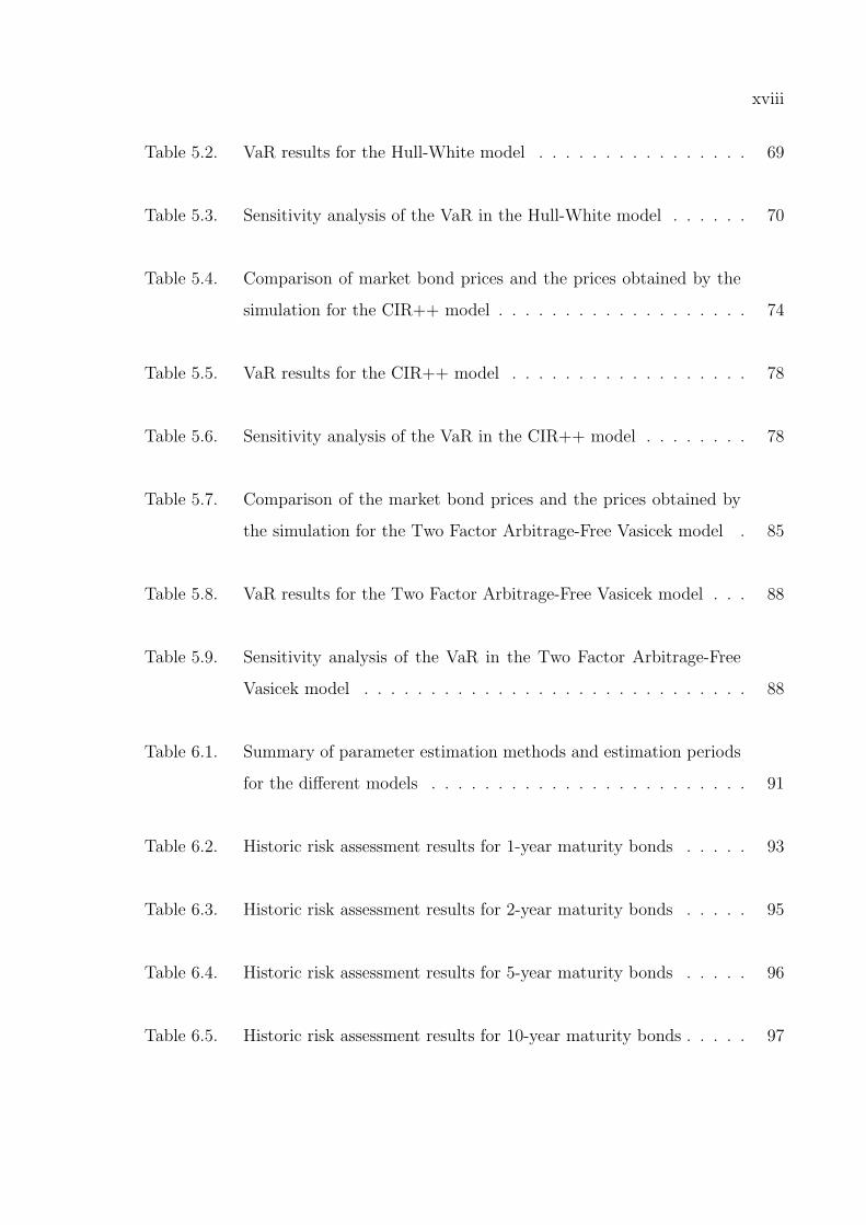
3.5. Risk Quantification

In section 2.5, we have argued why it is best to use VaR of opportunity losses

as risk measure. In this section, we will explain our risk quantification methodology.

According to the VaR definition in (2.5), the loss distribution is needed for computing

the VaR (i.e. 95% quantile value for α = 0.05). We will use the short rate models

that are explained in Section 3 for simulating the loss distribution. Then, we will

demonstrate how the VaR is computed by simulation.

In the opportunity loss formula defined in 2.4, we used constant interest rates.

Now, since we have short rate models to simulate the interest rates, we can use these

simulated interest rates in the loss formula. Then, the final relative loss formula is,

Relloss = 1 − P (t, T )

P (0, T ) exp

{(

t∫

0

ru du

)} (3.2)

Notice that the integral of the interest rates in continuous compounding is taken

from 0 to t, since the investment period is [0, t] (i.e. the bond investor will sell his

bonds at time t).

Our risk quantification methodology is explained in the algorithm presented in

Table 3.2.

Note that in the simulations, we use 1 day as the step size and 1000 as the

sample size. Since we will use exact simulation algorithms for each model, using large

step size is not a problem. However, the integral of the short rate in Formula 3.2 is

only approximated. Additionally, variance is very small in simulations, which leads to

21

Table 3.2. Risk quantification algorithm

Algorithm 1 Risk Quantification

1: Calibrate model parameters using Maximum Likelihood Estimation (MLE) from

historic market data.

2: if Model==Equilibrium Model then

3: Use shortest maturity bond yield in the market as the short rate and calculate

the initial bond price (i.e. P (0, T )) from model’s closed form bond price formula.

4: else if Model==Arbitrage-Free Model then

5: Take directly the bond price in the market as the initial bond price.

6: end if

7: Simulate the t time ahead short rates with dt = 1 day and sample size n = 1000.

8: Calculate the t time ahead bond prices (i.e. P (t, T ) with maturity (T − t)) from

model’s bond price formula.

8: Compute the losses for each simulated bond price according to the loss formula

in (3.2).

10: Compute the VaR as 95 percent quantile value of the losses.

narrow confidence intervals. Therefore, we can use small sample size like 1000 which

saves computation time.

22

4. EQUILIBRIUM INTEREST RATE MODELS

In Chapter 3, we explained the fundamentals of interest rate modelling and we

analyzed the two main types of interest rate models: Equilibrium models and arbitrage-

free models. In this chapter, we will explain popular equilibrium models. Namely, the

Vasicek, the CIR and the Two Factor Equilibrium Vasicek models.

4.1. The Vasicek Model

The Vasicek model [28] is one of the earliest short rate models. It is based upon

the idea of mean reverting interest rates. In this section, most of the formulas were

taken from Brigo and Mercurio [7].

4.1.1. The Short-Rate Dynamics

Vasicek [28] assumed that the instantaneous short rate, r, evolves under risk-

neutral measure by the following dynamics:

drt = β(µ − rt)dt + σdWt, r(0) = r0 (4.1)

where r0, β, µ and σ are positive constants.

The parameters of the model are β (mean-reversion), µ (long-term mean) and σ

(volatility of the short rate). dWt denotes the standard Brownian motion. The idea of

mean-reversion implies that in the long run all trajectories of r will evolve around a

mean level µ. This can also be inferred from the dynamics (4.1). Whenever the short

rate is below µ the drift of the process, µ − rt, is positive; whenever the short rate is

above µ the drift of the process, µ − rt, is negative. Thus, in every case rt is pushed

towards the level µ.

23

4.1.1.1. Objective Measure (Real-World) Dynamics. As we noted before the process

(4.1) is modelled in the risk-neutral world. However, the relevant distribution in risk

management is the distribution under objective measure (real-world) rather than the

risk-neutral measure, which is used for pricing (see, e.g. Glasserman [17]).

We can make the change of risk-neutral measure to real-world measure by setting,

dW o(t) = dW (t) + λ r(t)dt

which leads to,

drt = [β µ − (β + λ σ)r(t)] dt + σdW ot (4.2)

where λ is a new parameter that is defined as the market price of risk. According to

Brigo and Mercurio [7] market price of risk can be explained as the “excess return with

respect to a risk-free investment per unit of risk”.

In (4.2) it is assumed that λ(t) has the functional form,

λ(t) = λ r(t)

in the short rate. However, also different choices for λ exists in the literature. Indeed,

the market price of risk parameter is usually chosen to be constant (i.e. λ(t) = λ) in

the Vasicek model [7]. Morever, there is no consensus in the literature on the selection

of λ (see, e.g. Cheridito and Filipovic and Kimmel [37]). Therefore, we assume λ = 0

for all models that we analyze in this thesis. Note that, for λ = 0 the two dynamics

(i.e. (4.1) and (4.2)) coincide.

4.1.2. Simulating the Short Rate

4.1.2.1. Exact Simulation. For the Vasicek model, given the value rs at time s the

exact distribution of rt is known. It can be shown that it is normal with mean and

24

variance given by:

rt ∼ N

(

rs e−β(t−s) + µ(

1 − e−β(t−s))

,σ2

2β

[

1 − e−2β(t−s)]

)

To simulate rt at times 0 = t0 < t1 < · · · < tn, we can thus easily use the recursion:

rti+1= e−β(ti+1−ti)rti + µ

(

1 − e−β(ti+1−ti))

+ σ

√

1

2β(1 − e−2β(ti+1−ti))Zi+1 (4.3)

where Z is a vector of iid. standard normal variates. Note that this simple simulation

is the simulation of the exact process. A R-function that simulates the Vasicek process

by using exact simulation is given in Appendix A.1.

4.1.2.2. Approximate Euler Scheme Simulation. We want to demonstrate that we can

also use the simple Euler Scheme to simulate the process in (4.1) without knowing its

exact distribution. We simply replace dt in the equation (4.1) by short time steps ∆t

and dWt by a normal random variate with mean 0 and variance t. Using this principle

the stochastic differential equation for the Vasicek model can be rewritten as

rt+∆t − rt = β(µ − rt)∆t + σ√

∆tZ,

where Z denotes a standard normal variate. Thus we get the simple recursion:

rt+∆t = rt + β(µ − rt)∆t + σ√

∆tZ . (4.4)

This simulation principle is called as the Euler scheme. To balance the size of the

simulation error and the discretisation error it is suggested to select the number of

time steps d approximately equal to the square root of the sample size n. A R-function

that simulates the short rate process by using the Euler scheme is given in Appendix

A.2.

We can assess the quality of the approximate Euler scheme by comparing it with

25

−0.05 0.00 0.05 0.10 0.15

02

46

810

1214

1 Time Step

N = 10000 Bandwidth = 0.00411

Den

sity

EulerExact

−0.05 0.00 0.05 0.10 0.15

02

46

810

1214

10 Time Step

N = 10000 Bandwidth = 0.004024

Den

sity

EulerExact

−0.05 0.00 0.05 0.10 0.15 0.20

02

46

810

1214

100 Time Step

N = 10000 Bandwidth = 0.004054

Den

sity

EulerExact


short-rate in the Vasicek model.

the exact method. For comparison, density plots of the simulated short rates of both

simulation methods will be used. We will use the function cmttdensity in R, which

can estimate the probability distribution directly from the data. Parameters were set

to: µ = 0.052, β = 0.181, σ = 0.017, which are the parameters of the Vasicek model

estimated for US data as we will explain in the next section.

The plots of the densities for using the exact and the approximate simulation and

different number of time steps d are given in Figure 4.1. Note that the two densities

are very close for 100 time steps, which shows that the approximation is good and that

our simulation algorithms seem to be correct.

Furthermore, four different simulated paths of the short rate are with the same

parameters presented in Figure 4.2. Note that the process is mean reverting. The

speed of the mean reversion depends on the parameter β of the Vasicek model. We

can also see that the short rate can become negative in the Vasicek model. This is a

drawback of the model as negative interest rates can not occur.

26

0 500 1000 15000.

020.

030.

040.

050.

06

Different Paths of the Short Rate

5 years time

Sho

rt R

ate

0 500 1000 1500

−0.

020.

000.

02


5 years time

Sho

rt R

ate

0 500 1000 1500

0.02

0.04

0.06

0.08


5 years time

Sho

rt R

ate

0 500 1000 1500

0.02

0.04

0.06

0.08


5 years time

Sho

rt R

ate

Figure 4.2. Simulated paths of the short rate in the Vasicek model

4.1.3. Maximum Likelihood Estimation of Parameters

Historic short rate data can be used to estimate the parameters of the Vasicek

model with maximum likelihood estimation (MLE). As we do not have instantenous

short-rate data in the market, we will use 3 months maturity US monthly yield data

from 1952 to 2004 (1952-1999 from [38, 39] and 1999-2004 from [40]) and 3 months

period daily “Euro Interbank Offered Rate” (EURIBOR), which is based on the average

interest rates at which a panel of more than 50 European banks borrow funds from

one another, data from 1999 to 2007 [41] to estimate the standard parameters for the

Vasicek model for the US and the European markets. US 3-months maturity yield

data and 3 months period EURIBOR interest rate data are shown in Figure 4.3 and

Figure 4.4, respectively. Closed-form maximum likelihood estimates for functions of

the parameters of the Vasicek model are given in Brigo and Mercurio [7] as:

α =n

∑ni=1 riri−1 −

∑ni=1 ri

∑ni=1 ri−1

n∑n

i=1 r2i−1 − (

∑ni=1 ri−1)2

µ =

∑ni [ri − αri−1]

n(1 − α)

V 2 =1

n

n∑

i=1

[ri − αri−1 − µ(1 − α)]2

27

1950 1960 1970 1980 1990 2000

0.00

0.05

0.10

0.15

US 3−month Maturity Monthly Yields for 1952−2004

Date

3m Y

ield

s

Figure 4.3. US 3-month maturity monthly yields for 1952-2004

2000 2002 2004 2006

0.02

00.

025

0.03

00.

035

0.04

00.

045

0.05

0

EURIBOR 3−month Period Daily Rates for 1999−2007

Date

3m R

ates

Figure 4.4. EURIBOR 3-month period daily rates for 1999-2007

28

where dt is the time step between observed proxies r0, r1, ..., rn of r and,

β =− log(α)

dt

σ2 =2βV 2

(1 − e−2βdt)

R-function for calculating the MLE of the parameters of the Vasicek model is

given in Appendix A.3. By using that function, we can calculate the MLE’s for US

and European data as in Figure 4.5. So, for our American bond data with 3-months

MLE_Vas_US=Vasicek_MLE(data=USyields$B3month,dt=1/12)

MLE_Vas_US

#[1] 0.05215587 0.18171718 0.01759183

MLE_VAS_EU=Vasicek_MLE(data=EUrates$B3M,dt=1/365)

MLE_VAS_EU

#[1] 0.047513000 0.050692963 0.003891468

Figure 4.5. R-codes for calculating the MLE’s of the Vasicek model for US and

European data

time to maturity we obtained as parameter estimates:

µ = 0.05215587 β = 0.18171718 σ = 0.01759183

and for our European interest rate with 3-months period:

µ = 0.047513000 β = 0.050692963 σ = 0.003891468

Note that µ estimates are close for both the American and the European data. The

estimates are also close to the standard parameter values that are used in the literature

(see, e.g. Hull and White [42]) especially for US data.

It is important to mention here that the parameters of the Vasicek model may

be not constant over time. If we look at Figure 4.3 it seems obvious that in the early

eighties the mean value µ and the volatility σ were much higher than in the rest of the

29

time. So, probably taking for example just the data from 1990 would lead to clearly

different parameter estimates. For instance, taking the data between “1980-1” and

“1991-1” would lead to the estimates in Figure 4.6.

Vasicek_MLE(data=USyields$B3month[337:469],dt=1/12)

#[1] 0.07855993 0.59740640 0.02983012

Figure 4.6. R-codes for calculating the MLE’s of the Vasicek model for US data

(1980-1990)

4.1.4. Bond Pricing

As mentioned in Section 3 the Vasicek model does not lead to arbitrage free bond

prices. Still it is of interest to calculate these prices. For instance, the question of which

goverment bonds are over-priced in the market can be answered by using a equilibrium

model like the Vasicek model.

4.1.4.1. Analytical Bond Pricing. It is possible to calculate the expectation of the

integral in formula (3.1) for the Vasicek model defined in (4.1). Thus the price of a

zero coupon bond when using the Vasicek model as short rate model is given by:

P (t, T ) = A(t, T )e−B(t,T )rt , (4.5)

where,

A(t, T ) = exp

{(

µ − σ2

2β2

)

[B(t, T ) − T + t] − σ2

4βB(t, T )2

}

B(t, T ) =1

β

[

1 − e−β(T−t)]

.

(4.6)

It is easy to see that in the above bond price formula only the current value of

the short rate rt, the parameters of the Vasicek model and the time to maturity T are

required. Using that bond price formula, it is also easy to calculate the yield curve

30

implied by the Vasicek model. As the continuously-compounded yield R(t) is defined

by,

P (t, T ) = e−R(t,T )(T−t)

we can simply plug the bond price of the vasicek model into the above equation to get,

A(t, T )e−B(t,T )r(t) = e−R(t,T )(T−t)

Simple algebra then leads to the yield function

R(t, T ) =(r(t)B − log(A))

(T − t)(4.7)

R-function for bond price and yield calculations for the Vasicek model is given in

Appendix A.4. By using that function, we can calculate analytica bond prices of the

Vasicek model as in Figure 4.7

para=MLE_Vas_US

VasicekPriceYield(r=0.025,tau=1,Param=para,priceyn=T)

#[1] 0.9730894 price of a 1-year maturity bond





Figure 4.7. R-codes for calculating the analytical bond prices of the Vasicek model

4.1.4.2. Bond Pricing by Simulation. To test our implementation of the bond price

formula and our path simulation of the Vasicek model, we try to obtain the bond

price by simulation and compare it with the analytical bond price. For calculating

the bond price by simulation, we have to use the recursion of the Vasicek model given

in (4.3) together with the general bond price formula of (3.1). Of course we evaluate

the expectation in that formula by taking simply the average of the results of the n

31

generated paths of the daily rates. So, the daily discount factor is exp(−rdaily/360) and

we have to multiply all the discount factors of a path. To evaluate that in an efficient

way we can simply sum up the rates and divide them by 365 and exponentiate them

in the end. The details are given in the short R-code in Figure 4.8 for both the exact

res=Vasicek_simul_exact(para=para,r0=0.025,n=1000,dt=1/360,d=360)

y=exp(rowSums(-res)/360)

mean(y)

#[1] 0.973086 1-year Bond Price by exact sim.

1.96*sd(y)/sqrt(1000)

#[1] 0.0005757755 Error Bound

res1=Vasicek_simul_euler(para=para,r0=0.025,n=1000,dt=1/360,d=360)

y1=exp(rowSums(-res1)/360)

mean(y1)

#[1] 0.97313 1-year Bond Price by Euler Scheme sim.

1.96*sd(y1)/sqrt(1000)

#[1] 0.0006027706 Error Bound

Figure 4.8. R-codes for obtaining the bond price by simulation for the Vasicek model

path simulation and the Euler scheme. Note that n = 1000 paths are enough to obtain

a quite precise result. 2 and 3 year bond prices can be calculated similarly.

The analytical bond prices and the bond prices obtained by simulation are com-

pared in Table 4.7. Note that simulation error is small and the analytical prices fall

into the confidence interval produced by simulation. Also notice that one error bound

is given for both simulations, since it is almost the same for the exact and the approx-

imate method.

Table 4.1. Comparison of bond prices obtained by the analytical formula and the

simulation for the Vasicek model

Analytical BP Exact Sim. BP Euler Sim. BP Error Bound

1-year bond 0.97308 0.97308 0.97327 0.00057

2-year bond 0.94321 0.94312 0.94249 0.00145

3-year bond 0.91144 0.91235 0.91087 0.00246

32

4.1.5. Vasicek Yield Curve

As we have mentioned above bond prices or equivalently bond yields are fully

determined by the Vasicek model, they are only influenced by the current short rate

rt and by the time to maturity T − t. Therefore the yield curve of the Vasicek model

is just influenced by the current value of the short rate. It is therefore not astonishing

that the market yield curve is in many cases not similar to that of the Vasicek model.

We demonstrate this fact by comparing the US market yield curve of Jannuary 2000

with the yield curve obtained from the Vasicek model. The R-code in Figure 4.9 shows

the commands to plot the two yield curves together.

maturities=c(0.25,0.5,1,2,5,10)

plot(maturities,USyields["2000-1",2:7],type=’l’,ylab="yield",

ylim=c(0.03,0.07),xlim=c(0,13),main="January 2000 Yield Curve")

lines(maturities,VasicekPriceYield(r=USyields["2000-1",2],

tau=maturities,Param=para),type="l",lty=2)

legend("topright",legend=c("Vasicek","Market"),

lwd=c(1,1),lty=c(2,1),bty="n")

Figure 4.9. R-codes for plotting the yield curve of the Vasicek model

0 2 4 6 8 10 12

0.03

0.04

0.05

0.06

0.07

January 2000 Yield Curve

maturities

yiel

d

VasicekMarket

Figure 4.10. Comparison of the yield curves of the Vasicek model and the market

The result of the R-commands is shown as Figure 4.10. Note that in the Vasicek

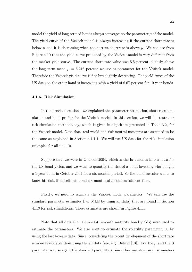
33

model the yield of long termed bonds always converges to the parameter µ of the model.

The yield curve of the Vasicek model is always increasing if the current short rate is

below µ and it is decreasing when the current shortrate is above µ. We can see from

Figure 4.10 that the yield curve produced by the Vasicek model is very different from

the market yield curve. The current short rate value was 5.5 percent, slightly above

the long term mean µ = 5.216 percent we use as parameter for the Vasicek model.

Therefore the Vasicek yield curve is flat but slightly decreasing. The yield curve of the

US-data on the other hand is increasing with a yield of 6.67 percent for 10 year bonds.

4.1.6. Risk Simulation

In the previous sections, we explained the parameter estimation, short rate sim-

ulation and bond pricing for the Vasicek model. In this section, we will illustrate our

risk simulation methodology, which is given in algorithm presented in Table 3.2, for

the Vasicek model. Note that, real-world and risk-neutral measures are assumed to be

the same as explained in Section 4.1.1.1. We will use US data for the risk simulation

examples for all models.

Suppose that we were in October 2004, which is the last month in our data for

the US bond yields, and we want to quantify the risk of a bond investor, who bought

a 1-year bond in October 2004 for a six months period. So the bond investor wants to

know his risk, if he sells his bond six months after the investment time.

Firstly, we need to estimate the Vasicek model parameters. We can use the

standard parameter estimates (i.e. MLE by using all data) that are found in Section

4.1.3 for risk simulations. These estimates are shown in Figure 4.11.

Note that all data (i.e. 1952-2004 3-month maturity bond yields) were used to

estimate the parameters. We also want to estimate the volatility parameter, σ, by

using the last 5-years data. Since, considering the recent development of the short rate

is more reasonable than using the all data (see, e.g. Buhrer [13]). For the µ and the β

parameter we use again the standard parameters, since they are structural parameters

34

MLE_VAS_US=Vasicek_MLE(data=USyields$B3month,dt=1/12)

MLE_VAS_US

#[1] 0.05215587 0.18171718 0.01759183

Sig_Last5y=Vasicek_MLE(data=USyields$B3month[575:634],dt=1/12)[3]

Sig_Last5y

#[1] 0.007279803

Figure 4.11. R-codes for estimating the parameters of the Vasicek model for risk

simulations

of the model [13]. So, R-code for calculating the σ estimate from last 5-years data

is given also in Figure 4.11. Note that the σ estimate from last 5-years data is only

around half of the estimate from all data. This is expected, as we can see from Figure

4.3 that the volatility is smaller for the last years in the data.

Secondly, we calculate the initial 1-year bond price (i.e. P (0, 1)) from (4.6) by

using 3-month yield as the short rate. Then, we simulate the 6-month ahead daily

short rates by using the recursion in (4.3) and we calculate the 6-month ahead bond

prices (i.e. P (0.5, 1)) from (4.6). Finally, we compute the losses for each simulated

bond price according to the loss formula in (3.2) and then we will compute the VaR as

95 percent quantile value of these losses. Briefly, we will follow the steps in algorithm

presented in Table (3.2) in Section 3.5.

Of course, we will use the exact simulation method in risk simulations. R-code

for risk simulation using the Vasicek model is given in Appendix A.5.

Then, the VaR of buying a 1-year maturity bond in October 2004 and selling it

after 6-months can be calculated by the R-code in Figure 4.12.

We use d = 180, since we need only the short-rate path up to 6-month. Note

that we have to store the short rate path in a matrix for opportunity loss calculation.

If we use the volatility parameter that is estimated from last 5-years data, VaR will be

estimated as in Figure 4.12. Note that V aR2 is approximately half of the V aR1, since

the σ estimate of the last 5-years data is about half of the standard σ estimate.

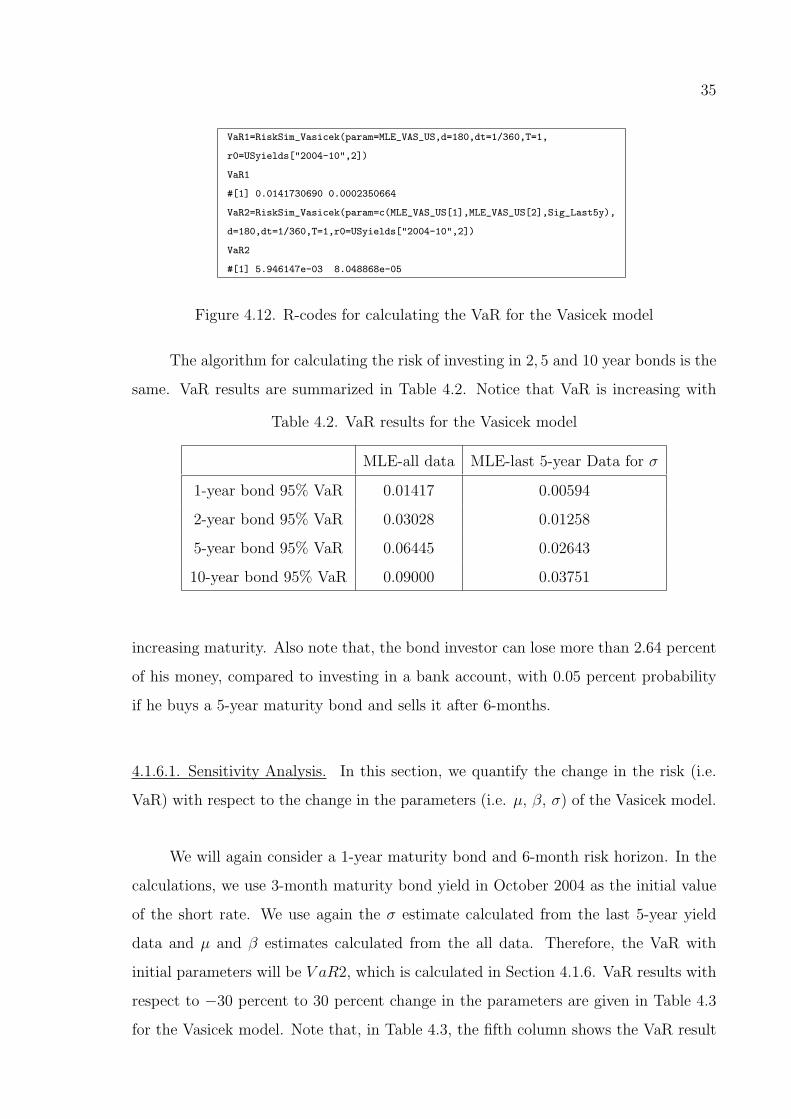
35

VaR1=RiskSim_Vasicek(param=MLE_VAS_US,d=180,dt=1/360,T=1,

r0=USyields["2004-10",2])

VaR1

#[1] 0.0141730690 0.0002350664

VaR2=RiskSim_Vasicek(param=c(MLE_VAS_US[1],MLE_VAS_US[2],Sig_Last5y),

d=180,dt=1/360,T=1,r0=USyields["2004-10",2])

VaR2

#[1] 5.946147e-03 8.048868e-05

Figure 4.12. R-codes for calculating the VaR for the Vasicek model

The algorithm for calculating the risk of investing in 2, 5 and 10 year bonds is the

same. VaR results are summarized in Table 4.2. Notice that VaR is increasing with

Table 4.2. VaR results for the Vasicek model

MLE-all data MLE-last 5-year Data for σ

1-year bond 95% VaR 0.01417 0.00594

2-year bond 95% VaR 0.03028 0.01258

5-year bond 95% VaR 0.06445 0.02643

10-year bond 95% VaR 0.09000 0.03751

increasing maturity. Also note that, the bond investor can lose more than 2.64 percent

of his money, compared to investing in a bank account, with 0.05 percent probability

if he buys a 5-year maturity bond and sells it after 6-months.

4.1.6.1. Sensitivity Analysis. In this section, we quantify the change in the risk (i.e.

VaR) with respect to the change in the parameters (i.e. µ, β, σ) of the Vasicek model.

We will again consider a 1-year maturity bond and 6-month risk horizon. In the

calculations, we use 3-month maturity bond yield in October 2004 as the initial value

of the short rate. We use again the σ estimate calculated from the last 5-year yield

data and µ and β estimates calculated from the all data. Therefore, the VaR with

initial parameters will be V aR2, which is calculated in Section 4.1.6. VaR results with

respect to −30 percent to 30 percent change in the parameters are given in Table 4.3

for the Vasicek model. Note that, in Table 4.3, the fifth column shows the VaR result

36

for the initial parameter values.

Table 4.3. Sensitivity analysis of the VaR in the Vasicek model

−%30 −%20 −%10 Initial Values +%10 +%20 +%30

VaR-µ −%1.56 −%0.36 −%0.40 0.00594 +%0.4 +%0.48 +%0.81

VaR-β +%2.49 +%1.92 +%0.75 0.00594 −%0.32 −%1.27 −%1.53

VaR-σ −%30 −%20 −%10 0.00594 +%10 +%20 +%30

Note that, VaR is increasing (decreasing) with increasing (decreasing) long-term

mean (i.e. µ) and increasing (decreasing) with decreasing (increasing) mean-reversion

(i.e. β). This is due to the fact that the Vasicek process always pushes the short rate

towards the long-term mean value. So, short rate is pulled to a much smaller value

when the long-term mean is decreasing and pulled to a much larger value when it is

increasing. Moreover, we know that bond prices are inversely related to the interest

rates. So, investors will have a higher risk when interest rates go up. This explains

why the VaR is increasing with increasing long-term mean.

Mean-reversion parameter shows the speed that the short rate is pushed to the

long-term mean. When β increases, short rate will pushed to the long-term mean

faster, which decreases the volatility of the process. Therefore, risk is decreasing with

increasing mean-reversion parameter.

Risk is increasing (decreasing) with increasing (decreasing) volatility parameter as

expected. Note that, the VaR is mainly influenced by σ, from Table 4.3 we can see that

µ and β have a very small effect on VaR compared to σ. Therefore, it seems reasonable

to estimate the volatility from the last 5-years data and structural parameters (i.e. µ

and β) from all data for risk simulations. Parameter sets that were used in the table

are given in Figure 4.13.

37

# -%30 -%20 -%10 +%10 +%20 +%30

#mu 0.036505 0.041720 0.046935 0.057365 0.062580 0.067795

#beta 0.127190 0.145360 0.163530 0.199870 0.218040 0.236210

#sigma 0.005089 0.005816 0.006543 0.007997 0.008724 0.009451

Figure 4.13. Parameter sets for the sensitivity analysis of VaR for the Vasicek model

4.2. The Cox, Ingersoll and Ross (CIR) Model

The CIR model [30] was developed to overcome the problem of possible negative

interest rates of the Vasicek model. Therefore, a “square-root” term is introduced

in to the diffusion coefficient of the instantaneous short-rate dynamics proposed by

Vasicek [28]. The resulting model has been used as a benchmark for many years

because of its analytical tractability and the positivity of the instantaneous short rate.

In this section most of the formulas were taken from Brigo and Mercurio [7].


The stochastic differential equation describing the CIR model under the risk-

neutral measure Q is

drt = β(µ − rt)dt + σ√

rtdWt, r(0) = r0, (4.8)

with r0, β, µ, σ positive constants. Like for the Vasicek model, the parameters of the

model are β (mean-reversion), µ (long-term mean) and σ (volatility of the short rate).

dWt denotes the standard Brownian motion. The model is mean-reverting like the

Vasicek model.


4.2.2.1. Exact Simulation. In the CIR model the increments of the short-rate follows

a non-central chi-square distribution. More formally, as stated in the Glasserman [17]

38

the transition density of r(t) in (4.8) can be written as

r(t) =σ2

(

1 − e−β(t−u))

4βχ2

d

(

4βe−β(t−u)

σ2 (1 − e−β(t−u))r(u)

)

, t > u, (4.9)

where,

d =4µβ

σ2. (4.10)

This shows that, given r(u), r(t) is distributed as σ2(

1 − e−β(t−u))

/(4β) times a

non-central chi-square random variable with d degrees of freedom and non-centrality

parameter

λ =4βe−k(t−u)

σ2 (1 − e−β(t−u))r(u). (4.11)

Thus, to simulate rt at times 0 = t0 < t1 < · · · < tn , we can easily use the

recursion:

r(ti+1) =σ2

(

1 − e−β(t−u))

4βχ2

d

(

4βe−β(t−u)

σ2 (1 − e−β(t−u))r(ti)

)

, (4.12)

The R-function that simulates the CIR process by using exact simulation is given in

Appendix A.6.

4.2.2.2. Approximate Euler Scheme Simulation. As the exact simulation method re-

quires sampling from the non-central chi-square distribution, we can use again the

simple Euler scheme to simulate the process in (4.8) like for the Vasicek model. The

Euler discretization of (4.8) suggests simulating r(t) at times 0 = t0 < t1 < · · · < tn by

setting

r(ti+1) = r(ti) + β(µ − r(ti)) [ti+1 − ti] + σ√

r(ti)√

ti+1 − tiZi+1, (4.13)

39

with Z1, . . . , Zn idependent N(0, 1) random variables.

A R-function that simulates the CIR process by using the approximate Euler

scheme is given in Appendix A.7. We can again assess the quality of the approximate

Euler scheme by comparing the density plots of the simulated short rates of both

simulation methods as we have done for the Vasicek model. Parameters were set to:

µ = 0.052, β = 0.128, σ = 0.066, which are standard parameters of the CIR model

for US data as we will see in the next section. The plots of the densities for using the

exact and the approximate simulation and different number of time steps d are given

in Figure 4.14. Note that densities are again very close for 100 time steps.

0.03 0.04 0.05 0.06 0.07

010

2030

4050

60

1 Time Step

N = 10000 Bandwidth = 0.0009017

Den

sity

EulerExact

0.03 0.04 0.05 0.06 0.07 0.08

010

2030

4050

6010 Time Step

N = 10000 Bandwidth = 0.0009181

Den

sity

EulerExact

0.03 0.04 0.05 0.06 0.07 0.08

010

2030

4050

60

100 Time Step

N = 10000 Bandwidth = 0.0009111

Den

sity

EulerExact


short-rate in the CIR model

4.2.3. Maximum Likelihood Estimation of Parameters

We will use again the 3 month maturity US monthly yield data and the 3 month

period EURIBOR daily interest rate data to estimate the parameters of the CIR model.

However, different to the Vasicek model we do not have closed form formulas for the

maximum likelihood estimate for the parameters in the CIR model. This is mainly

40

due to the non-Gaussian distribution of the short rate in the CIR model. Therefore,

we have to use a numerical optimization to obtain the MLE’s.

To do that we need the likelihood function of the CIR model. Note that the

transition density of the short rate in the CIR model is given in (4.9). From that we

can write the cumulative distribution function of r(t) as

P (r(t) ≤ y|r(u)) = Fχ2(d,λ)

(

4βy

σ2 (1 − e−β(t−u))

)

, (4.14)

with d as in (4.10) and λ as in (4.11).

Then the probability density function is:

Pr(t)(y|r(u)) = cpχ2(d,λ)

(cy), (4.15)

where pχ2(d,λ)

(cy) is the density of the non-central chi-square distribution and where,

c =4β

σ2 (1 − e−β(t−u)).

From that we can write the likelihood and log-likelihood functions as:

L(µ, β, σ; y) =n

∏

i=2

cpχ2(d,λ)

(cyi|yi−1),

l(µ, β, σ; y) =n

∑

i=2

log(c) +n

∑

i=2

log(

pχ2(d,λ)

(cyi|yi−1))

,

where y = r1, r2, · · · , rn. Note that dt = 1 month in our data.

As we have found the log-likelihood function of the model we use numerical

optimization to find the MLE’s. The R-function that calculates the log-likelihood

function of the CIR model for a given data set is given in Appendix A.8.

To test our implementation of the MLE method, we can simulate a single short

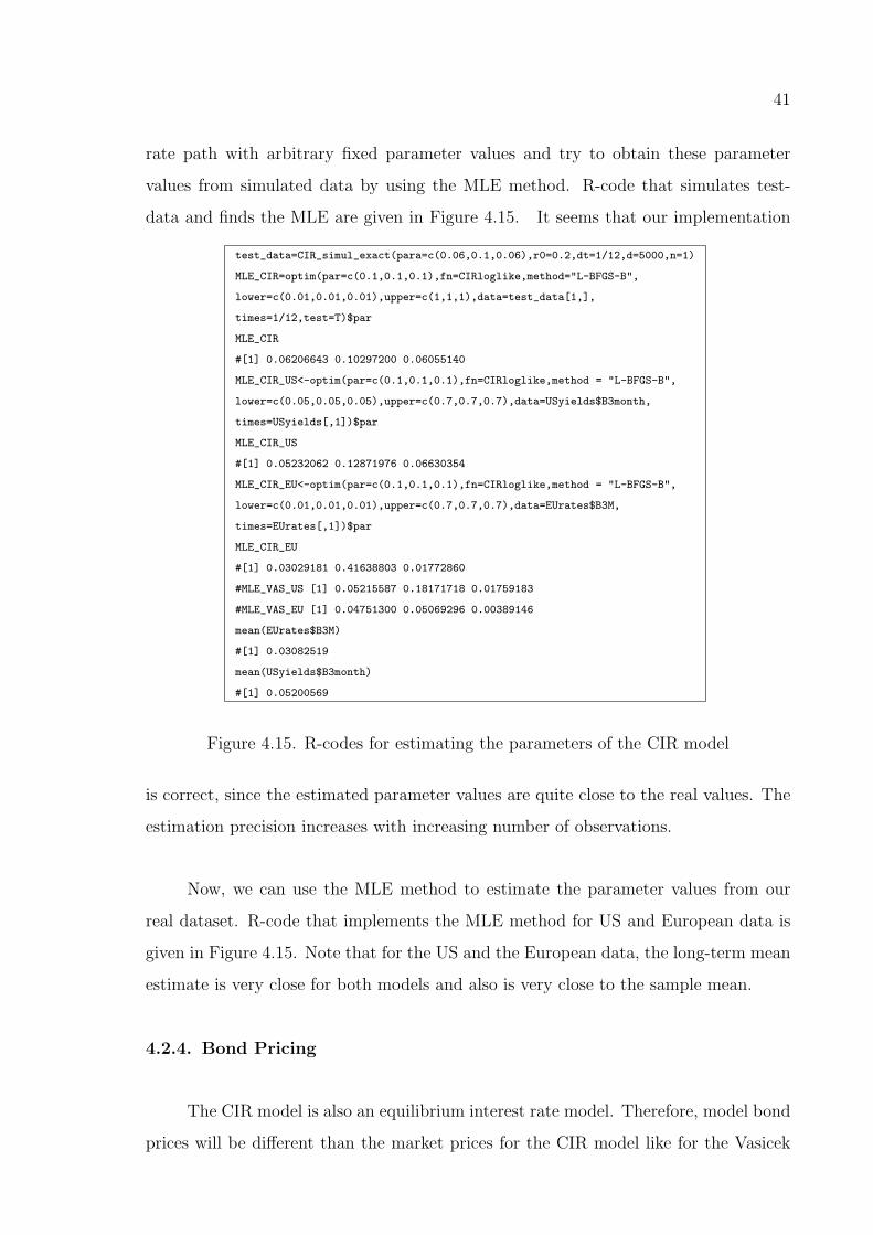
41

rate path with arbitrary fixed parameter values and try to obtain these parameter

values from simulated data by using the MLE method. R-code that simulates test-

data and finds the MLE are given in Figure 4.15. It seems that our implementation

test_data=CIR_simul_exact(para=c(0.06,0.1,0.06),r0=0.2,dt=1/12,d=5000,n=1)

MLE_CIR=optim(par=c(0.1,0.1,0.1),fn=CIRloglike,method="L-BFGS-B",

lower=c(0.01,0.01,0.01),upper=c(1,1,1),data=test_data[1,],

times=1/12,test=T)$par

MLE_CIR

#[1] 0.06206643 0.10297200 0.06055140

MLE_CIR_US<-optim(par=c(0.1,0.1,0.1),fn=CIRloglike,method = "L-BFGS-B",

lower=c(0.05,0.05,0.05),upper=c(0.7,0.7,0.7),data=USyields$B3month,

times=USyields[,1])$par

MLE_CIR_US

#[1] 0.05232062 0.12871976 0.06630354

MLE_CIR_EU<-optim(par=c(0.1,0.1,0.1),fn=CIRloglike,method = "L-BFGS-B",

lower=c(0.01,0.01,0.01),upper=c(0.7,0.7,0.7),data=EUrates$B3M,

times=EUrates[,1])$par

MLE_CIR_EU

#[1] 0.03029181 0.41638803 0.01772860

#MLE_VAS_US [1] 0.05215587 0.18171718 0.01759183

#MLE_VAS_EU [1] 0.04751300 0.05069296 0.00389146

mean(EUrates$B3M)

#[1] 0.03082519

mean(USyields$B3month)

#[1] 0.05200569

Figure 4.15. R-codes for estimating the parameters of the CIR model

is correct, since the estimated parameter values are quite close to the real values. The

estimation precision increases with increasing number of observations.

Now, we can use the MLE method to estimate the parameter values from our

real dataset. R-code that implements the MLE method for US and European data is

given in Figure 4.15. Note that for the US and the European data, the long-term mean

estimate is very close for both models and also is very close to the sample mean.

4.2.4. Bond Pricing

The CIR model is also an equilibrium interest rate model. Therefore, model bond

prices will be different than the market prices for the CIR model like for the Vasicek

42

model.

4.2.4.1. Analytical Bond Pricing. We use the same general principle of bond pricing

like for the Vasicek model. Therefore, we have to calculate the expectation of the

integral in the formula (3.1) for the CIR model defined in (4.8). It is possible to show

that (see, e.g. Brigo and Mercurio [7]), the price at time t of a zero-coupon bond with

maturity T is

p(t, T ) = A(t, T )e−B(t,T )r(t),

where

A(t, T ) =

[

2h exp {(β + h)(T − t)/2}2h + (β + h)(exp {(T − t)h} − 1)

]2βµ/σ2

,

B(t, T ) =2(exp {(T − t)/h} − 1)

2h + (β + h)(exp {(T − t)/h} − 1),

(4.16)

with

h =√

β2 + 2σ2.

From the bond prices we can easily calculate the continuously-compounded yield by

using Formula 2.1 like for the Vasicek model. R-function for bond price and yield

calculations for the CIR model is given in Appendix A.9.

4.2.4.2. Bond Pricing by Simulation. We can again test our simulation algorithm and

bond price formula by trying to obtain a bond price by simulation and comparing it

with the analytical price. The principle is the same as for the Vasicek model. The R-

code in Figure 4.16 shows the commands to calculate the 1-year maturity bond prices

by using the analytical formula of the CIR model and the simulation .

2 and 3 year bond prices can be calculated similarly. Bond prices that are obtained

by using the analytical formula and the simulation, both the exact simulation and the

43

param=MLE_CIR_US

CirPriceYield(r=0.05,tau=1,Param=param,priceyn=T)

#[1] 0.951125 #1-year analytical price

#Vasicek 1y Price

#[1] 0.9730894

res=CIR_simul_exact(para=param,r0=0.05,n=1000,dt=1/360,d=360)


mean(y)

#[1] 0.9510627 # Simulation (Exact) Price

1.96*sd(y)/sqrt(1000)

#[1] 0.0004696053

res=CIR_simul_euler(para=param,r0=0.05,n=1000,dt=1/360,d=360)


mean(y)

#[1] 0.9511621 # Simulation (Euler) Price

1.96*sd(y)/sqrt(1000)

#[1] 0.0004895801

Figure 4.16. R-codes for obtaining the bond price by simulation for the CIR model

Euler scheme, are given in Table 4.4. Analytical prices fall into the confidence interval

produced by simulations.


simulation for the CIR model


1-year bond 0.95112 0.95106 0.95116 0.00046

2-year bond 0.90456 0.90406 0.90465 0.00123

3-year bond 0.86032 0.85879 0.86044 0.00200

4.2.5. CIR Yield Curve

As we have mentioned above, the CIR model is an equilibrium interest rate model.

Therefore, we expect that the market yield curve will not be similar to the CIR yield

curve. We will again demonstrate this fact by comparing the US market yield curve

of January 2000 with the yield curve obtained from the CIR model. We also plot the

Vasicek yield curve for comparison. The R-code in Figure 4.17 shows the commands

to plot the three yield curves together.

44

param=MLE_CIR_US

maturities=c(0.25,0.5,1,2,5,10)

plot(maturities,USyields["2000-1",2:7],type=’l’,ylab="yield",lwd=2,

ylim=c(0.03,0.07),xlim=c(0,13),main="January 2000 Yield Curves")

lines(maturities,CirPriceYield(r=USyields["2000-1",2],

tau=maturities,Param=param),type=’l’,lwd=2,lty=2)

lines(maturities,VasicekPriceYield(r=USyields["2000-1",2],

tau=maturities,Param=MLE_VAS_US),type=’l’,lwd=2,lty=3)

legend("topright",legend=c("Market","CIR","Vasicek"),

lwd=c(2,2,2),lty=c(1,2,3),bty="n")

Figure 4.17. R-codes for plotting the yield curve of the CIR model

From Figure 4.18, we can see that CIR and Vasicek yield curves are almost the

same.


The risk simulation methodology is same as for the Vasicek model. Note that, it

is possible to select λ = 0 for the CIR model similar to the Vasicek model. We again

calculate the risk of a bond investor, who buys a bond in October 2004 and sells it

after 6-months. We use the standard parameter estimates, which were estimated from

all US data, and also the volatility estimate calculated from the last 5-years data. If

we use all the data (i.e. 1952-2004 3-month maturity bond yields), the standard model

parameter estimates using MLE are given in Figure 4.19. Furthermore, the σ estimate

calculated from the last 5-years data is also given in Figure 4.19. Note that the σ

estimate from last 5-years data is around half of the estimate from all data like for the

Vasicek model. R-code for risk simulation using the CIR model is given in Appendix

A.10.

By using the risk simulation function, the VaR of buying a 1-year maturity bond

in October 2004 and selling it 6-months later can be estimated as in Figure 4.20 If

we use the volatility parameter that is estimated from last 5-years data, VaR will be

calculated as VaR2 in Figure 4.20. Note that V aR2 is approximately half of the V aR1,

since the σ estimate from the last 5-years data is also half of the standard σ estimate.

Risk of investing in 2, 5 and 10 year bonds can be calculated similarly. VaR results are

45

0 2 4 6 8 10 12

0.03

0.04

0.05

0.06

0.07

January 2000 Yield Curves

maturities

yiel

d

MarketCIRVasicek

Figure 4.18. Comparison of the yield curves of the CIR and the Vasicek model and

the market

MLE_CIR_US

#[1] 0.05232062 0.12871976 0.06630354

x<-function(mu,beta,sigma,data,times,test)CIRloglike(param=c(mu,beta,

sigma),data,times)

cirsig_last5y=optim(par=c(0.011),fn=x,method="L-BFGS-B",lower=0.01,

upper=0.90,mu=MLE_CIR_US[1],beta=MLE_CIR_US[2],

data=EUrates$B3M[575:634],times=EUrates[,1])$par

cirsig_last5y

#[1] 0.03215337

Figure 4.19. R-codes for estimating the parameters of the CIR model for risk

simulations

VaR1=RiskSim_CIR(param=MLE_CIR_US,d=180,dt=1/360,T=1,

r0=USyields["2004-10",2])

VaR1

#[1] 0.0081063178 0.0001364939

VaR2=RiskSim_CIR(param=c(MLE_CIR_US[1],MLE_CIR_US[2],sig_last5y),

d=180,dt=1/360,T=1,r0=USyields["2004-10",2])

VaR2

#[1] 0.0038334866 0.0000630276

Figure 4.20. R-codes for calculating the VaR for the CIR model

46

Table 4.5. VaR results for the CIR model


1-year bond 95% VaR 0.00810 0.00383

2-year bond 95% VaR 0.01748 0.00827

5-year bond 95% VaR 0.03953 0.01880

10-year bond 95% VaR 0.05931 0.02922

summarized in Table 4.5. VaR is increasing with the increasing maturity as expected.

4.2.6.1. Sensitivity Analysis. In this section, we quantify the change in the VaR with

respect to the change in the parameters (i.e. µ, β, σ) of the CIR model. We will use

again a 1-year maturity bond and 6-month risk horizon. Analysis is the same as for

the Vasicek model in Section 4.1.6.1. VaR results with respect to −30 percent to 30

percent change in the parameters are given in Table 4.6 for the CIR model. Note that

Table 4.6. Sensitivity analysis of the VaR in the CIR model

−%30 −%20 −%10 Initial Values +%10 +%20 +%30

VaR-µ −%2.6 −%2.3 −%1.2 0.00464 +%0.8 +%1.9 +%2.7

VaR-β +%2.1 +%1.0 +%0.6 0.00464 −%0.8 −%1.2 −%3.0

VaR-σ −%30 −%20 −%10 0.00464 +%9.6 +%20 +%29

long-term mean and mean-reversion parameters affect the VaR in a similar way as for

the Vasicek model. In both models, the VaR is mainly influenced by σ. The parameter

sets that were used in the calculations are given in Figure 4.21.

# -%30 -%20 -%10 +%10 +%20 +%30

#mu 0.0366247 0.0418568 0.0470889 0.0575531 0.0627852 0.0680173

#beta 0.0901040 0.1029760 0.1158480 0.1415920 0.1544640 0.1673360

#sigma 0.0225071 0.0257224 0.0289377 0.0353683 0.0385836 0.0417989

Figure 4.21. Parameters sets for the sensitivity of VaR analysis for the CIR model

47

4.3. The Two-Factor Equilibrium Vasicek Model

4.3.1. Motivation

One-factor short rate models have several shortcomings. For instance, they just

use the short rate and ignore the information from other rates on the yield curve [2].

Also some yield curve shapes (e.g. inverted shape) can not be generated by using

one-factor models such as the Vasicek and the CIR model [7].

Moreover, one-factor models assume a perfect correlation between different rates

of the yield curve. At every time instant, interest rates for all maturities are perfectly

correlated. This means that a shock to the interest rate curve at time t is transmitted

equally through all maturities [7]. However, this may not be the case in the market

(e.g. 30-year yield and 3-month yield may not change in the same direction). For this

reasons, multi-factor models are developed. It is shown that two-factor models can

explain up to %90 percent variation in the yield curve [43]. In this section we will

analyze the Two Factor Equilibrium Vasicek Model (also called Two Factor Vasicek

Model or G2 Model [7]) and use it in risk simulation. We use the name Equilibrium to

make clear that the model is not an arbitrage-free model.


Brigo and Mercurio [7] state that, for the Two Factor Equilibrium Vasicek Model

(Two Factor Vasicek, hereafter), the instantaneous interest rate process under the risk-

neutral measure Q is given by

rt = xt + yt, r(0) = x0 + y0,

dxt = βx(µx − xt)dt + σxdW1(t), x(0) = x0,

dyt = βy(µy − yt)dt + σydW2(t), y(0) = y0,

(4.17)

48

where (W1,W2) is a two-dimensional Brownian motion with instantaneous correlation

ρ as from

dW1(t)dW2(t) = ρdt,

where x0, y0, βx, βy, µx, µy, σx, σy are positive constants, and where −1 ≤ ρ ≤ 1.

In the literature, the xt and yt processes are generally modeled as the short-rate

and the long-rate in order to explain the variation of the interest rates better. Note

that, the question of which process is modeled as the short rate or the long rate is not

important, since both processes are modeled identically.


4.3.3.1. Exact Simulation. Since the Two Factor Vasicek model is defined as the sum

of the two processes, which follow the Vasicek model, we will use the Vasicek recursion

in (4.3) to simulate the processes xt and yt and then we sum them up to get the

short rate process rt. A R-function that generates the process (4.17) by using exact

simulation is given in Appendix A.11.

4.3.3.2. Approximate Euler Scheme Simulation. For demonstration and comparison

purposes, we can also use the Euler scheme to simulate the Two Factor Vasicek model.

We will use the Euler discretion of Vasicek in (4.4) to simulate the xt and yt processes.

A R-function that generates the process by using approximate Euler scheme simulation

is given in Appendix A.12.

Density plots of the simulated short rates of both simulation methods are given

in Figure 4.22. Different number of time steps, d, are used in the simulations for

comparison. Parameters were set to the standard short-rate and long-rate parameters

of the Two Factor Vasicek model, which will be explained in the next section. Note that

densities are again very close for 100 time steps, which shows that the approximation

49

0.00 0.05 0.10 0.15 0.200

24

68

1012

1 Time Step

N = 10000 Bandwidth = 0.004346

Den

sity

EulerExact

0.00 0.05 0.10 0.15 0.20

02

46

810

12

10 Time Step

N = 10000 Bandwidth = 0.004359

Den

sity

EulerExact

0.00 0.05 0.10 0.15 0.20 0.25

02

46

810

12

100 Time Step

N = 10000 Bandwidth = 0.004321

Den

sity

EulerExact


short-rate in the Two Factor Equilibrium Vasicek model

is good and that our simulation algorithms seem to be correct.

4.3.4. Selecting the Parameters of the Model

As noted before, the Two Factor Vasicek model is defined as the sum of the short-

rate and the long-rate processes, which both follow the Vasicek model. Therefore, we

can use the maximum likelihood estimates of the short rate and the long-rate in the

Vasicek model as the standard parameter estimates for the Two Factor Vasicek model.

3-month and 10-year maturity bond yields are used to estimate the short-rate and the

long-rate, respectively. Then, for the short-rate (say xt) and the long-rate (yt) process

of the Two Factor Vasicek model, the standard parameter estimates are given in Figure

4.23.

Note that long rate process has a small mean-reversion speed, which makes it a

long-lived factor [4]. For the parameter ρ, we use the correlation between the historical

short and the long rate. In R we can calculate this correlation as in Figure 4.23. Note

that rates are highly correlated.

50

ShortR_MLE=Vasicek_MLE(data=USyields$B3month,dt=1/12)

ShortR_MLE

#[1] 0.05215587 0.18171718 0.01759183

LongR_MLE=Vasicek_MLE(data=USyields$B10year,dt=1/12)

LongR_MLE

#[1] 0.06829182 0.08606587 0.01025833

corr=cor(USyields$B3month,USyields$B10year)

corr

#[1] 0.903111

Figure 4.23. R-codes for selecting the parameters of the Two Factor Equilibrium

Vasicek model

4.3.5. Bond Pricing

4.3.5.1. Analytical Bond Pricing. Bond pricing method remains the same for the Two

Factor Vasicek model. We have to calculate the expectation of the integral in the

formula (3.1) for the Two Factor Vasicek model defined in (4.17). Therefore, it can be

shown that the yield at time t of a zero-coupon bond with maturity T is given by [44]

R(t, T ) =µx +

(

1 − eβxτ)

βxτ(xt − µx) + µy +

(

1 − eβyτ)

βyτ(yt − µy),

− σ2x

2β2x

(

1 +1 − e−2 βxτ

2βxτ− 2

1 − e−βxτ

βxτ

)

,

−σ2

y

2β2y

(

1 +1 − e−2 βyτ

2βyτ− 2

1 − e−βyτ

βyτ

)

,

− ρσxσy

βx + βy

(

1 − 1 − e−βxτ

βxτ− 1 − e−βyτ

βyτ+

1 − e−(βx+βy)τ

(βx + βy)τ

)

, (4.18)

where τ = (T − t).

Using that yield formula, it is also easy to calculate the bond prices. As the bond

price P (t, T ) is defined by,

P (t, T ) = e−R(t,T )(T−t)

R-code for bond price and yield calculations for the Two Factor Vasicek model is in

Appendix A.13.

51

param=c(ShortR_MLE,LongR_MLE,corr)

Vas_2fPriceYield(t=0,param=param,x0=USyields["2000-1",2],

y0=USyields["2000-1",7],tau=1,priceyn=T)

#[1] 0.8857535 #1-year analytical bond price

Vas_2fPriceYield(t=0,param=param,x0=USyields["2000-1",2],y0=0,

tau=1,priceyn=T)

#[1] 0.9703777 #1-year price with long_rate=0

VasicekPriceYield(r=0.025,tau=1,Param=MLE_VAS_US,priceyn=T)

#[1] 0.9730894 #1-year Vasicek bond price

Figure 4.24. R-codes for calculating the analytical bond prices of the Two Factor

Equilibrium Vasicek model

The analytical model bond prices in January 2000 can be calculated by the R-

code in Figure 4.24. Note that 1-year bond prices are very close for the Two Factor

Vasicek and the Vasicek model, when the initial long-rate is assumed to be 0 in the

Two Factor Vasicek model.

4.3.5.2. Bond Pricing by Simulation. To test our simulation algorithm and the bond

price formula, we can again try to obtain a bond price by simulation and compare it

with the analytical price. The principle remains the same for the Two Factor Vasicek

model. January 2000 term structure is used for the initial short and the long-rate.

R-code for calculating the 1-year maturity bond price by simulation is given in Figure

4.25. 2 and 3 year maturity bond prices can be calculated similarly. Analytical

bond prices and bond prices obtained by simulation, both using the exact and the

approximate method, are shown in Table 4.7. Analytical prices fall into the confidence

interval produced by simulations.


simulation for the Two Factor Equilibrium Vasicek model


1-year bond 0.88575 0.88567 0.88582 0.000858

2-year bond 0.78524 0.78488 0.78521 0.002081

3-year bond 0.69696 0.69373 0.69851 0.003570

52

res=Vas2f_sim_exact(param=param,x0=USyields["2000-1",2],

y0=USyields["2000-1",7],dt=1/360,n=1000,d=360)

y=exp(rowSums(-res$rt)/360)

mean(y)

#[1] 0.8856709 #1-year sim price by exact method

1.96*sd(y)/sqrt(1000)

#[1] 0.000858667 #error bound

res=Vas2f_sim_euler(param=param,x0=USyields["2000-1",2],

y0=USyields["2000-1",7],dt=1/360,n=1000,d=360)


mean(y)

#[1] 0.8858207 #1-year sim price by approximate method

1.96*sd(y)/sqrt(1000)

#[1] 0.0009086509 #error bound

Figure 4.25. R-codes for obtaining the bond price by simulation for Two Factor

Equilibrium Vasicek model

4.3.6. Two Factor Equilibrium Vasicek Yield Curve

As we have mentioned in above various yield curve shapes can be generated with

the Two Factor Vasicek model. However, perfect fit to the initial term structure is not

possible, since the Two Factor Vasicek model is not an arbitrage-free model.

We can see from Figure 4.27 that different yield curve shapes (e.g. inverted shape)

can be generated with the Two Factor Vasicek model. We can also plot the yield curve

of the Two Factor Vasicek model in January 2000 with the market yield curve and

the yield curve implied by the Vasicek model together for comparison. The R-code in

Figure 4.26 shows the commands to plot the yield curves together. From Figure

4.28, we can see that Two Factor Vasicek yield curve fits better to the market yield

curve than the Vasicek. Note that for the Two Factor Vasicek model, the short rate is

set to the 3 month yield in January 2000 and the long rate is assumed to be zero for a

better fit.

53

maturities=c(0.25,0.5,1,2,5,10)

plot(maturities,USyields["2000-1",2:7],type="l",

ylab="yield", ylim=c(0.03,0.07),xlim=c(0,13),main="January 2000 Yield

Curves",lwd=2)

lines(maturities,VasicekPriceYield(r=USyields

["2000-1",2],tau=maturities,Param=MLE_VAS_US),type="l",lwd=2,lty=2)

lines(maturities,Vas_2fPriceYield(t=0,param=param,tau=maturities,

x0=USyields["2000-1",2],y0=0,priceyn=F),

type="l",lwd=2,lty=3)

legend("topright",legend=c("Market","Vasicek","2f Vasicek"),

lwd=c(2,2,2),lty=c(1,2,3),bty="n")

Figure 4.26. R-codes for plotting the yield curve of the Two Factor Equilibrium

Vasicek model

0 5 10 15 20 25 30

0.00

0.05

0.10

0.15

maturities

Yie

ld

x0=0,y0=0.1

x0=0,y0=0

x0=0.1,y0=0

x0=0.04,y0=0.02

Figure 4.27. Different yield curves of the Two Factor Equilibrium Vasicek model

54

0 2 4 6 8 10 12

0.03

0.04

0.05

0.06

0.07

January 2000 Yield Curves

maturities

yiel

d

MarketVasicek2f Vasicek

Figure 4.28. Comparison of the yield curves of the Two Factor Equilibrium Vasicek

model and the market


The risk simulation methodology is the same as for the Vasicek model. We use the

standard parameter estimates that are given in Section 4.3.4 as well as the σ estimate

that is calculated from last 5-years of the US data. Note that, we estimate two σ values

for the short and the long rate. Also, we estimate the correlation between the short

and the long rate by using last 5-years data. Then, the standard parameter estimates

for the Two Factor Vasicek model are given in Figure 4.29.

The σ estimate of the short and the long rate as well as the correlation estimate

using last 5-year data are given also in Figure 4.29. Note that we have used 10-year

bond yields to estimate the volatility of the long rate. We will use these estimates for

the following risk simulations. R-code for risk simulation for the Two Factor Vasicek

model is given in Appendix A.14. So, the VaR of buying a 1-year maturity bond in

October 2004 and selling it after 6-months can be estimated by using the r-code given

in Figure 4.30.

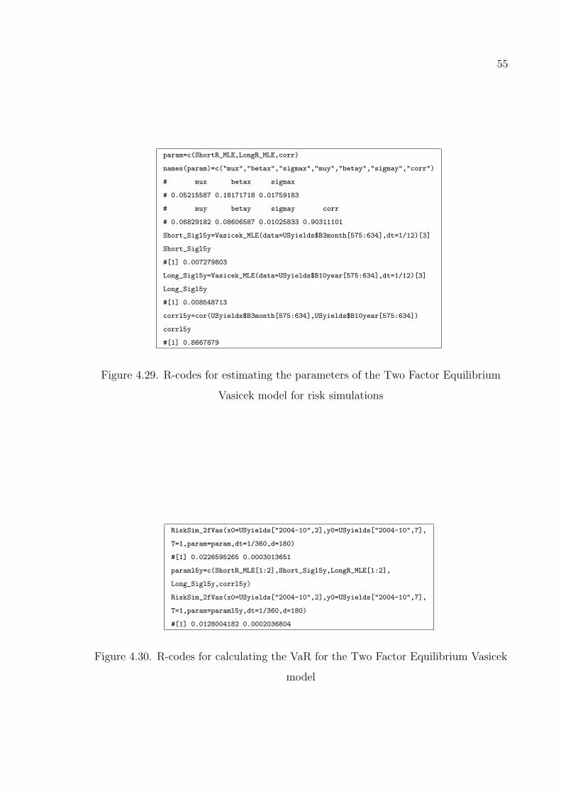
55

param=c(ShortR_MLE,LongR_MLE,corr)

names(param)=c("mux","betax","sigmax","muy","betay","sigmay","corr")

# mux betax sigmax

# 0.05215587 0.18171718 0.01759183

# muy betay sigmay corr

# 0.06829182 0.08606587 0.01025833 0.90311101

Short_Sigl5y=Vasicek_MLE(data=USyields$B3month[575:634],dt=1/12)[3]

Short_Sigl5y

#[1] 0.007279803

Long_Sigl5y=Vasicek_MLE(data=USyields$B10year[575:634],dt=1/12)[3]

Long_Sigl5y

#[1] 0.008548713

corrl5y=cor(USyields$B3month[575:634],USyields$B10year[575:634])

corrl5y

#[1] 0.8667879

Figure 4.29. R-codes for estimating the parameters of the Two Factor Equilibrium

Vasicek model for risk simulations

RiskSim_2fVas(x0=USyields["2004-10",2],y0=USyields["2004-10",7],

T=1,param=param,dt=1/360,d=180)

#[1] 0.0226595265 0.0003013651

paraml5y=c(ShortR_MLE[1:2],Short_Sigl5y,LongR_MLE[1:2],

Long_Sigl5y,corrl5y)

RiskSim_2fVas(x0=USyields["2004-10",2],y0=USyields["2004-10",7],

T=1,param=paraml5y,dt=1/360,d=180)

#[1] 0.0128004182 0.0002036804

Figure 4.30. R-codes for calculating the VaR for the Two Factor Equilibrium Vasicek

model

56

Table 4.8. VaR results for the Two Factor Equilibrium Vasicek model

MLE-all data MLE-last 5-year data for σ and ρ

1-year bond 95% VaR 0.02265 0.01280

2-year bond 95% VaR 0.05062 0.03071

5-year bond 95% VaR 0.11012 0.06739

10-year bond 95% VaR 0.16738 0.10570

Note that initial value of the long rate is taken as the 10-year bond yield in

October 2004. If we use the volatility parameters and the correlation parameter that

are estimated from last 5-years data, VaR of investing in a 1-year maturity bond can

also be calculated as in Figure 4.30. Risk of investing in 2, 5 and 10 year maturity

bonds can also be quantified similarly. VaR results are summarized in Table 4.8.

Note that VaR results are much higher than the results of the Vasicek model.

This is mainly due to the additive modeling of the short and the long rate in the Two

Factor Vasicek model as the risk is increasing with increasing interest rates (i.e. price

of the bond at time t = 0.5 year decreases).


respect to the change in the parameters (i.e. µ, β, σ, ρ) of the Two Factor Vasicek

model.

1-year maturity bond and 6-month risk horizon will be used. Last 5-year data

are used for estimating σ and ρ. Analysis is the same as for the Vasicek model in

Section 4.1.6.1. Of course, we use the exact simulation method like for the Vasicek and

the CIR model. VaR results with respect to −30 percent to 30 percent change in the

parameters are given in Table 4.9 for the Two Factor Vasicek model. For the ρ the

change is limited to 20 percent, since −1 ≤ ρ ≤ 1.

Note that long-term mean and mean-reversion parameters affect the VaR in the

same way as for the Vasicek model, and they have a very small effect on VaR. In both

57

Table 4.9. Sensitivity analysis of the VaR in the Two Factor Equilibrium Vasicek

model

−%30 −%20 −%10 Initial Val. +%10 +%20 +%30

VaR-µx −%0.3 −%0.2 −%0.1 0.0128 +%0.4 +%0.64 +%0.7

VaR-βx +%1.1 +%0.78 +%0.50 0.0128 −%0.2 −%0.6 −%1.2

VaR-σx −%14 −%8.7 −%5.3 0.0128 +%4.5 +%11 +%14

VaR-µy −%0.42 −%0.26 −%0.12 0.0128 +%0.3 +%0.56 +%0.68

VaR-βy +%1.8 +%1.1 +%0.12 0.0128 −%0.11 −%1 −%1.5

VaR-σy −%14.6 −%10.2 −%5.8 0.0128 +%5 +%10.3 +%15

VaR-ρ −%6.8 −%5.0 −%2.1 0.0128 +%2.4 +%2.7 −

models, σ is the main parameter that affects the VaR. Also notice that the effect of σ is

divided equally for the short rate and the long rate and risk is increasing (decreasing)

with increasing (decreasing) correlation as the variance of the short rate increases with

increasing correlation.

58

5. ARBITRAGE-FREE INTEREST RATE MODELS

In chapter 4 we explained the Vasicek, the CIR and the Two-Factor Equilibrium

Vasicek equilibrium models. In this chapter, we will explain popular arbitrage-free in-

terest rate models. Namely, the Hull-White Extended Vasicek (Hull-White, hereafter),

CIR++ and Two-Factor Arbitrage Free Vasicek models. In this chapter, most of the

formulas were taken from Brigo and Mercurio [7].

5.1. The Hull-White Extended Vasicek Model

Hull and White (1990) assumed that the instantaneous short-rate process evolves

under the risk-neutral measure according to

dr(t) = (θ(t) − β(t)r(t)) dt + σ(t)dW (t), (5.1)

where θ,β and σ are deterministic functions of time.

This model can be fitted to the term structure of interest rates and term structure

of volatilities. However, fitting the volatilities can be problematic as finding enough

and accurate volatility data is hard in the market [7].

Therefore, we consider the following simpler extension of the Vasicek model pro-

posed by Hull and White [45],

dr(t) = (θ(t) − βr(t)) dt + σdW (t), (5.2)

where β and σ are the constant mean reversion and volatility parameters, respectively.

The time-dependent mean parameter, θ, is chosen in order to exactly fit the term

structure of the interest rates currently observed in the market. Since, the model

ensures an exact fit to the current term structure it is an arbitrage-free model. The

Hull-White model implies a normal distribution for the short-rate process at each time

59

point. Moreover, the model is analytically tractable and thus bonds can be priced

easily.


It can be shown that the Hull-White process in (5.2) provides an exact fit to the

term structure of the interest rates by setting,

θ(t) =∂fM(0, t)

∂T+ βfM(0, t) +

σ2

2β(1 − e−2βt), (5.3)

where fM(0, T ) denotes the market instantaneous forward rate at time 0 for the ma-

turity T , i.e.,

fM(0, T ) = −∂ ln PM(0, T )

∂T. (5.4)

Integrating (5.2) leads to,

r(t) = r(s)e−β(t−s) +

∫ t

s

e−β(t−u)θ(u) du + σ

∫ t

s

e−β(t−u)dW (u),

= r(s)e−β(t−s) + α(t) − α(s)e−β(t−s) + σ

∫ t

s

e−β(t−u)dW (u),

(5.5)

where

α(t) = fM(0, t) +σ2

2β2

(

1 − e−βt)2

. (5.6)

60


5.1.2.1. Exact Simulation. From (5.5), it is easy to show that, given the value rs at

time t the distribution of rt is normal with mean and variance given by:

rt ∼ N

(

rs e−β(t−s) + α(t) − α(s)e−β(t−s),σ2

2β

[

1 − e−2β(t−s)]

)

.

Thus knowing α(t) is enough to simulate the short rate process in (5.5). A R-function

that simulates the Hull-White process by using exact simulation is given in Appendix

A.15.

5.1.3. Fitting the Instantaneous Forward Rates to the Bond Prices

As it can be seen from (5.5) and (5.6), we need the market instantaneous forward

rates to simulate the rt process of the Hull-White model. However, we do not have

instantaneous forward rate data in the market. Instead of forward rates, generally we

have only bond price and maturity data. Therefore, we have to use bond prices to

obtain forward rates.

Bond prices can be expressed as the integral of the instantaneous forward rates

by using the fact that forward rates are future interest rates, currently expected by the

market in the risk neutral world, and using equation (3.1). So, if the time intervals

between expiry and maturity dates for the forward rate is infinitesimal we can define

the bond price as

P (t, T ) = exp

{(

−∫ s

t

f(t, u) du

)}

. (5.7)

We can use this equation to obtain forward rates from bond prices. Like for the

Vasicek case we again use January 2000 term structure as our dataset, which consists of

6 zero-coupon bonds with 0.25, 0.5, 1, 2, 5, 10 year maturites and 0.055, 0.0576, 0.0612,

0.0644, 0.0658, 0.0666 yields, respectively.

61

By using only this dataset and (5.7) we can use constant forward rates for the

time intervals 0−0.25, 0.25−0.5, 0.5−1, 1−2, 2−5 and 5−10 year. However, we need

instantaneous forward rates at each time t to correctly simulate the short rate process.

To obtain that, we can use linear interpolation and fit the forward rate function such

that we obtain correct bond prices.

Firstly, we assume that the short rate at time t = 0 is the 3-month yield. Then

the forward rate at time t = 0 is 0.055, as the initial forward rate is by definition equal

to the initial short rate. The forward rate curve is linear and defined by,

fi(t) = ait + bi,

where t denotes time and ai, bi are the slope and intercept parameters, respectively.

There will be a separate line segment for each time interval (i.e. 0 − 0.25, 0.25 − 0.5,

0.5 − 1, 1 − 2, 2 − 5 and 5 − 10). Therefore, index i runs from 1 to 6.

We need to select ai and bi for each time interval to obtain a fully defined instan-

taneous forward rate. We will illustrate the calculations for the first 2 intervals.

We know that b1 = 0.055, since initial short rate is 0.055, and by using (5.7) we

can write

P (0, 0.25) =exp

−0.25∫

0

f(u) du

=exp

−0.25∫

0

(a1x + 0.055) dx

=exp

{(

−a10.252

2− 0.055 ∗ 0.25

)}

.

From that a1 is found as,

a1 = −32 (log(P (0, 0.25)) + 0.055 ∗ 0.25) ≃ 0

62

By finding a1 and b1 we have fully specified the forward rate line for the interval 0−0.25

year. For the second interval (i.e. 0.25 − 0.5) we have to use again equation (5.7), as

we have two unknown parameters a2 and b2.

Note that the starting point of the second line must be the same as the end point

of the first line. Denoting with t1 the end point of the first interval (i.e. 0.25) we must

have

f2(t1) =f1(t1)

a2t1 + b2 =a1t1 + b1.

Then, b2 is t1(a1 − a2) + b1. Since, we have found t1, b1 and a1 the only unknown

parameter remaining is a2. Therefore, we obtain a2 by solving,

P (0, 0.5) =exp

−t2=0.5∫

0

(ax + b) dx

=exp

−t1=0.25∫

0

(a1x + b1) dx

exp

−t2=0.5∫

t1=0.25

(a2x + b2) dx

=P (0, 0.25) exp

{(

−a2(0.52 − 0.252)

2− b2(0.5 − 0.25)

)}

.

After writing b2 in terms of a2 we can find a2 as 0.0416. Then b2 is t1(a1 − a2) + b1 =

0.25 ∗ (0 − 0.0416) + 0.055 = 0.0446. Since we found a2 and b2, we have fully specified

the forward rate for the interval 0.25−0.5 year. The methodology is the same for other

intervals.

After finding the instantaneous forward rates we can find bond prices by using

(5.7). The R-function, HW forwPrice, that calculates the slope and intercept param-

eters for all intervals and returns the daily instantaneous forward rate and bond price

vector is given in Appendix A.28. In the calculations, we have used linear interpolation

for the given yields (i.e. January 2000 term structure) and we calculated recursively

the forward rates and bond prices for [0, 10] year. Instantaneous forward rate and the

63

bond price curves are shown in Figure 5.2 and 5.3, respectively. R-code that plots these

curves is given in Figure 5.1.

matur=c(0.25,0.5,1,2,5,10)

yield=c(0.0550,0.0576,0.0612,0.0644,0.0658,0.0666)

forward=HW_forwPrice(matur=matur,yield=yield)

prices=HW_forwPrice(matur=matur,yield=yield,forwardyn=F)

i=1:length(forward)

plot(i,forward,"l",main="Instantaneous Forward Rate Curve",

ylab="Forward Rates",xlab="Time in Days")

plot(i,prices,"l",main="Bond Price Curve",xlab="Time in Days",

ylab="Bons Prices")

Figure 5.1. R-codes for plotting the instantaneous forward rate and the bond price

curve for the Hull-White model

0 500 1000 1500 2000 2500 3000 3500

0.05

50.

060

0.06

50.

070

Instantaneous Forward Rate Curve

Time in Days

For

war

d R

ates

Figure 5.2. Hull-White January 2000 forward rate curve


The Hull and White [32] model has the same short rate dynamics as the Vasicek

model, only the long-term mean parameter is defined as time-dependent in the Hull-

White model. Therefore, for the mean-reversion and volatility parameters of the Hull-

White model we will use the maximum likelihood estimates of these parameters in

64

0 500 1000 1500 2000 2500 3000 3500

0.5

0.6

0.7

0.8

0.9

1.0

Bond Price Curve

Time in Days

Bon

s P

rices

Figure 5.3. Hull-White January 2000 bond price curve

the Vasicek model. Note that, the time-dependent mean parameter of the Hull-White

model is defined by the instantaneous forward rates as explained in Section 5.1.3.

5.1.5. Bond Pricing

As noted in the previous sections, Hull-White is an arbitrage-free model. There-

fore, initial model bond prices are equivalent to the market prices in the Hull-White

model. We will demonstrate this principle in the following sections.

5.1.5.1. Analytical Bond Pricing. Bond pricing is the same as for the Vasicek and the

CIR model. We will again calculate the expectation of the integral in the formula (3.1)

for the Hull-White model defined in (5.2). Therefore, it can be shown that the price

of a zero coupon bond in the Hull-White model is given by:

P (t, T ) = A(t, T )e−B(t,T )rt, (5.8)

65

where

A(t, T ) =PM(0, T )

PM(0, t)exp

{

B(t, T )fM(0, t) − σ2

4β

(

1 − e−2βt)

B(t, T )2

}

B(t, T ) =1

β

[

1 − e−β(T−t)]

. (5.9)

Note that market bond prices are required for that bond price formula. Thus,

the whole term structure is used for calculating bond prices in the Hull-White model.

Moreover, when calculating the current bond price, i.e t = 0, the formula for A(t, T )

reduces to:

A(0, T ) = PM(0, T )exp{

B(0, T )fM(0, 0)}

where fM(0, 0) is the market instantaneous forward rate at time 0 (i.e. short rate

at time 0). The yield calculation is the same as for the Vasicek model. R-code for

bond price and yield calculations for general time t is given in Appendix A.16.

5.1.5.2. Bond Pricing by Simulation. We again test our simulation algorithm and

bond price formula by trying to obtain bond prices by simulation and comparing it

with the analytical price. The principle is the same as for the Vasicek and the CIR

models.

Note that to simulate (5.2) we have to calculate α(t) values using (5.6). We can

use the instantaneous forward rate, which were found in the previous section by fitting

them to the bond price data, to calculate the α(t).

Moreover, as noted before the Hull-White model always leads to the market price

at time 0, since the forward rate at time 0 is equal to the short rate at time 0. We can

66

prove that easily using the Hull-White bond price Formula 5.9.

B(0, T ) =1

β

[

1 − e−βT]

A(0, T ) =PM(0, T )exp{

B(0, T )fM(0, 0)}

= PM(0, T )exp {B(0, T )r(0)}

P (0, T ) =A(0, T )exp (−B(0, T )r(0)) = PM(0, T )exp {B(0, T )r(0)} exp (−B(0, T )r(0))

=PM(0, T ).

Therefore, we will compare the bond prices found by simulation directly with the

market bond prices. Again we use January 2000 term structure to test our simulation

code. We choose daily simulation steps, since we have daily instantaneous forward

rates. R-code for calculating 1 and 2 year maturity bond prices are given in Figure

5.4.

param=c(MLE_VAS_US[2],MLE_VAS_US[3])

forward=HW_forwPrice(matur=matur,yield=yield)

R=yield #Market yields in January 2000.

Pm1y=exp(-R[3]*1)

Pm1y

#[1] 0.940635 # 1-year market bond price

res<-HullW_simul_exact(param=param,r0=R[1],n=1000,dt=1/360,

d=360,fm=forward)

y<-exp(rowSums(-res)/360)

mean(y)

#[1] 0.940513 # 1-year price by simulation

1.96*sd(y)/sqrt(1000)

#[1] 0.0001696594 #error bound

Pm2y=exp(-R[4]*2)

Pm2y


res<-HullW_mc(param=param,r0=R[1],n=1000,dt=1/360,d=2*360,fm=forward)


mean(y)

#[1] 0.8788417 # 2-year price by simulation

1.96*sd(y)/sqrt(1000)

#[1] 0.0004328625 #error bound

Figure 5.4. R-codes for obtaining the bond price by simulation for the Hull-White

model

67

The principle remains the same for 5 and 10 year maturity bonds. Comparison

of market prices and prices obtained by simulation are given in Table 5.1. Note that

thr simulation error is small for n = 1000 and the market prices fall into the confidence

intervals produced by simulation.


simulation for the Hull-White model

Jan. 2000 Market BP Simulation BP Error Bound

1-year bond 0.94063 0.94051 0.000169

2-year bond 0.87914 0.87884 0.000432

5-year bond 0.71964 0.71863 0.001166

10-year bond 0.51375 0.51537 0.001815

5.1.6. Hull-White Yield Curve

As we have shown in the previous section, the bond prices of the Hull-White are

equivalent to the market bond prices. Therefore, we expect that market and model

yield curves are the same. We again demonstrate this fact by comparing the US market

yield curve of January 2000 with the yield curve obtained from the Hull-White model.

The R-code in Figure 5.5 shows the commands to plot the two yield curves together.

maturities=c(0.25,0.5,1,2,5,10)

Pmarket=exp(-maturities*USyields["2000-1",2:7])


ylim=c(0.03,0.07),xlim=c(0,13),main="January 2000 Market

and Hull-White Yield Curve",lty=2,lwd=2)

lines(maturities,HwPriceYield(r=USyields["2000-1",2], T=maturities,t=0,

Param=param,Pm0=Pmarket,Pmt=1, fmt=USyields["2000-1",2],priceyn=F),

type=’l’,lty=4,lwd=2,col="red")

legend("topright",legend=c("Market","Hull-White"),

lwd=c(2,2),lty=c(2,4),col=c("black","red"),bty="n")

Figure 5.5. R-codes for plotting the yield curve of the Hull-White model

The result of the R-commands is shown in Figure 5.6. Note that two curves are

identical as expected. Also notice that, initial market prices are input to the Hull-White

bond price formula.

68

0 2 4 6 8 10 12

0.03

0.04

0.05

0.06

0.07

January 2000 Market and Hull−White Yield Curve

maturities

yiel

d

MarketHull−White

Figure 5.6. Comparison of the yield curves of the Hull-White model and the market


The risk simulation methodology is the same as for the Vasicek and the CIR

models. As noted in Section 5.1.4, we use the standard parameter estimates of the

Vasicek model and also the σ estimate of the Vasicek model that is calculated from

last 5-years data. So, the standard mean-reversion and volatility estimates of the Hull-

White model are given in Figure 5.7. These are standard parameter estimates for

MLE_VAS_US=Vasicek_MLE(data=USyields$B3month,dt=1/12)

MLE_HW=c(MLE_VAS_US[2],MLE_VAS_US[3])

MLE_HW

[1] 0.18171718 0.01759183

Sig_Last5y=Vasicek_MLE(data=USyields$B3month[575:634],dt=1/12)[3]

Sig_Last5y

#[1] 0.007279803

Figure 5.7. R-codes for estimating the parameters of the Hull-White model for risk

simulations

the Hull-White model. Notice that, Hull and White [42] use β = 0.1 and σ = 0.01 as

standard parameters. The volatility estimate using the last 5-years data is also given

in Figure 5.7.

69

We will use these estimates for the below risk simulations. R-code for risk simula-

tion for the Hull-White model is given in Appendix A.17. Note that we use directly the

market price as initial bond price, since Hull-White is an arbitrage-free model. Also

notice that, the market prices (i.e. PM(0, T ) and PM(0, t)) are input to the Hull-White

bond price formula. So, the VaR of buying a 1-year maturity bond in October 2004

and selling it after 6-months can be calculated by the R-code in Figure 5.8. Note that

USyields2=as.matrix(USyields,rownames.force=NA)

forward=HW_forwPrice(matur=matur,yield=USyields2["2004-10",2:7])

RiskSim_HwVas(param=MLE_HW,r0=USyields["2004-10",2],

Pm=exp(-1*USyields["2004-10",4]),fm=forward,matur=2,

yield6m=USyields["2004-10",3],dt=1/360,d=180)

#[1] 0.0143081401 0.0001484025

RiskSim_HwVas(param=c(MLE_HW[1],Sig_Last5y),r0=USyields["2004-10",2],



#[1] 0.0124677411 0.0002103328

Figure 5.8. R-codes for calculating the VaR for the Hull-White model

we have calculated the forward rates using the October 2004 term structure. If we use

the volatility parameter that is estimated from last 5-years data, the VaR of investing

in a 2-year maturity bond is given in Figure 5.8. The risk of investing in 5 and 10 year

maturity bonds can be quantified easily using the same principles. Our VaR results

are summarized in Table 5.2. Note that the VaR results are very close to the results

of the Vasicek model.

Table 5.2. VaR results for the Hull-White model


1-year bond 95% VaR 0.01430 0.00583

2-year bond 95% VaR 0.03002 0.01246

5-year bond 95% VaR 0.06322 0.02657

10-year bond 95% VaR 0.08960 0.03744


subject to the changes in the parameters (i.e. β, σ) of the Hull-White model.

70

We will use again a 1-year maturity bond and 6-month risk horizon. Last 5-year

data are used for estimating σ. The analysis is the same as for the Vasicek model

in Section 4.1.6.1. VaR results with respect to −30 percent to 30 percent change in

the parameters are given in Table 5.3 for the Hull-White model. Note that the mean-

Table 5.3. Sensitivity analysis of the VaR in the Hull-White model

−%30 −%20 −%10 Initial Values +%10 +%20 +%30

VaR-β +%3.72 +%2.2 +%0.85 0.0583 −%1.4 −%2.5 −%4.01

VaR-σ −%30 −%21 −%10 0.0583 +%10 +%18 +%30

reversion parameter affect the VaR in the same way as the Vasicek model. In both

models, the VaR is mainly influenced by σ.

5.2. The CIR++ Model

Hull and White [32] proposed an extension of the Cox-Ingersoll and Ross [30]

model based on the same idea of considering time dependent coefficients like for the

Vasicek model [7]:

dr(t) = [θ(t) − β(t)r(t)] dt + σ(t)√

r(t)dW (t) (5.10)

where β, σ and θ are deterministic functions of time. However, this model is not

analytically tractable. Indeed, no analytical solution exist for zero-coupon bond prices.

The same drawback holds for the simplified dynamics with constant mean reversion

and volatility parameters,

dr(t) = [θ(t) − βr(t)] dt + σ√

r(t)dW (t) (5.11)

where β and σ are now positive constants, and only θ(t), the time dependent mean

parameter is chosen in order to to exactly fit the term structure of the interest rates.

No analytical expression for θ(t) is available in the literature.

71

A different approach is described by Brigo and Mercurio [34] to extend any time-

homogeneous short-rate model, in order to exactly fit the initial term structure. In this

approach, a deterministic shift function is added to the short rate process such that

“the extended version preserves the analytical tractability of the initial model while

exactly fitting the observed term structure of interest rates” [34].

In the case of the Vasicek model, the extension is equivalent to the Hull and

White model, which is explained in Section 5.1. In the case of the Cox-Ingersoll-Ross

model, however, the extension is analytically more tractable than the model given in

(5.10) and (5.11). This extension for the CIR model is called CIR++ model [34].


Brigo and Mercurio [34] assumed that the instantaneous short-rate process evolves

under the risk-neutral measure according to,

dx(t) =β(µ − x(t))dt + σ√

x(t)dW (t), x(0) = x0

r(t) =x(t) + ϕ(t; α),(5.12)

where x0, β, µ and σ are positive constants and ϕ(t; α) is the deterministic shift func-

tion depending on the parameter vector, α, and time. The CIR++ model provides

an exact fit to the current term structure of the interest rates by setting ϕ(t; α) =

ϕCIR(t; α) where

ϕCIR(t; α) =fM(0, t) − fCIR(0, t; α),

fCIR(0, t; α) =2βθ (exp{th} − 1)

2h + (β + h)(exp{th} − 1)+ x0

4h2exp{th}[2h + (β + h)(exp{th} − 1)]2

,(5.13)

with h =√

β2 + 2σ2 and fM(0, t) is the market instantaneous forward rate.

72


5.2.2.1. Exact Simulation. Note that the process (5.12) is equivalent to the original

CIR process in (4.8) without the deterministic shift. Thus, we can simulate the CIR++

process (5.12) exactly by simulating the CIR process (4.12) and adding the determin-

istic shift, which is given in (5.13). The R-function that simulates the CIR++ model

by using exact simulation is given in Appendix A.18

5.2.2.2. Approximate Euler Scheme Simulation. We can also use the Euler discretiza-

tion of the CIR model (4.8) to simulate the x(t) process (5.12), so that we do not have

to sample from the non-central chi-square distribution like for the CIR model. Then,

we add the deterministic shift to get the CIR++ process. We give a R-function that

simulates the CIR++ process by using the approximate Euler scheme in Appendix

A.19.

We can again assess the quality of the approximate Euler scheme by comparing

the density plots of the simulated short rates of both simulation methods. Parameters

were set to: µ = 0.052, β = 0.128, σ = 0.066, which are standard parameters of the

CIR model for US data.

The plots of the densities for using the exact and the approximate simulation and

different number of time steps d are given in Figure 5.9. Note that the two densities

are again very close for 100 time steps.


As we noted before, CIR and CIR++ models have the same dynamics for the

short rate, except for the deterministic shift parameter that is added to the short rate

process in the CIR++ model. Therefore, for the CIR++ model parameters, we will

use the same maximum likelihood estimates of the parameters that were found for the

CIR model.

73

0.00 0.04 0.08 0.120

510

1520

25

1 Time Step

N = 10000 Bandwidth = 0.001973

Den

sity

EulerExact

0.02 0.04 0.06 0.08 0.10

05

1015

2025

30

10 Time Step

N = 10000 Bandwidth = 0.001977

Den

sity

EulerExact

0.02 0.04 0.06 0.08 0.10 0.12

05

1015

2025

100 Time Step

N = 10000 Bandwidth = 0.001999

Den

sity

EulerExact


short-rate in the CIR++ model

5.2.4. Bond Pricing

As noted before, CIR++ is an arbitrage-free model like the Hull-White model.

Therefore, the initial model bond prices are equivalent to the market prices in the

CIR++ model. We will demonstrate this principle in the following sections.

5.2.4.1. Analytical Bond Pricing. The bond pricing method remains the same for the

CIR++ model. We will again calculate the expectation of the integral in the formula

(3.1) for the CIR++ model defined in (5.12). Therefore, it is possible to show that the

price of a zero-coupon bond at time t maturing at time T is given by

P (t, T ) = A(t, T )e−B(t,T )r(t),

where

A(t, T ) =PM(0, T ) A(0, t) exp {−B(0, t) x0}PM(0, t) A(0, T ) exp {−B(0, T ) x0}

A(t, T ) eB(t,T ) ϕCIR(t;α),

74

and A(t, T ) and B(t, T ) are defined as in (4.16). After some algebra, one can show that

the market bond price at time t = 0 is equal to the model bond price at time t = 0,

which is expected since the CIR++ model is an arbitrage-free model. R-code for bond

price and yield calculations for any time t is given in Appendix A.20.

5.2.4.2. Bond Pricing by Simulation. To test our implementation of the bond price

formula and our simulation algorithm, we can try to obtain bond prices by simulation

and compare them with the market price. The principle is the same as for the Hull-

White model. We will compare the bond prices found by simulation directly with the

market bond prices, since CIR++ is an arbitrage-free model.

We again use January 2000 term structure to test our simulation code. We choose

daily simulation steps, since we have daily instantaneous forward rates. Forward rates

that are calculated in Section 5.1.3 will be used. R-code for calculating 1 and 2 year

maturity bond prices are given in Figure 5.10. Note that, the model’s 1-year bond

price is equivalent to the 1-year market bond price. 5 and 10 year bond prices can be

calculated similarly. Market prices and the prices obtained by simulation are given in

Table 5.4. Note that the simulation error is small for n = 1000 and market prices fall

into the confidence intervals produced by simulation.


simulation for the CIR++ model

Market BP Exact Sim. BP Euler Sim. BP Error Bound

1-year bond 0.94063 0.94050 0.94079 0.00050

2-year bond 0.87914 0.87953 0.87955 0.00126

5-year bond 0.71964 0.71744 0.71764 0.00347

10-year bond 0.51375 0.51681 0.50924 0.00535

5.2.5. CIR++ Yield Curve

As noted before, CIR++ is an arbitrage-free model. Therefore, we expect that

market and model yield curves are the same. We again demonstrate this fact by

75

param=MLE_CIR_US

R=yield #Market yields in January 2000.

Pm1y=exp(-R[3]*1)

Pm1y


Ex_CIR_PriceYield(x0=R[1],T=1,t=0,Param=MLE_CIR_US,Pm0=exp(-1*R[3]),

Pmt=1,fmt=R[1])

#[1] 0.940635 # 1-year model price

res<-Ex_CIR_simul_exact(param=param,x0=R[1],n=1000,dt=1/360,d=360,

fm=forward)


mean(y)

#[1] 0.9405054 # 1-year price by exact simulation

1.96*sd(y)/sqrt(1000)

#[1] 0.0005049458#error bound

Pm2y=exp(-R[4]*2)

Pm2y


res<-Ex_CIR_simul_euler(param=param,x0=R[1],n=1000,dt=1/360,d=2*360,

fm=forward)


mean(y)

#[1] 0.8795593 # 2-year price by Euler simulation

1.96*sd(y)/sqrt(1000)

#[1] 0.001334085 #error bound

Figure 5.10. R-codes for obtaining the bond price by simulation for the CIR++ model

comparing the US market yield curve of January 2000 with the yield curve obtained

from the CIR++ model. The R-code in Figure 5.11 shows the commands to plot the

two yield curves together.

The result of the R-commands is shown in Figure 5.12. Note that two curves are

identical as expected.


The risk simulation methodology is the same as for the previous models. We

use the standard parameter estimates of the CIR model, which are estimated by using

all US data, and also the σ estimate that is calculated by using last 5-years US data.

The standard mean-reversion and volatility estimates of the CIR++ model are given

76

maturities=c(0.25,0.5,1,2,5,10)




and CIR++ Yield Curve",lty=2,lwd=2)

lines(maturities,Ex_CIR_PriceYield(x0=USyields["2000-1",2],

T=maturities,t=0,Param=param,Pm0=Pmarket,Pmt=1,

fmt=USyields["2000-1",2],priceyn=F),type=’l’,lty=4,lwd=2,col="red")

legend("topright",legend=c("Market","Hull-White"),


Figure 5.11. R-codes for plotting the yield curve of the CIR++ model

0 2 4 6 8 10 12

0.03

0.04

0.05

0.06

0.07

January 2000 Market and CIR++ Yield Curve

maturities

yiel

d

MarketHull−White

Figure 5.12. Comparison of the yield curves of the CIR++ model and the market

77

MLE_ExCIR=MLE_CIR_US

MLE_ExCIR

#[1] 0.05232062 0.12871976 0.06630354

cirsig_last5y

#[1] 0.03215337



RiskSim_ExCIR(param=MLE_ExCIR,r0=USyields["2004-10",2],



#[1] 0.0080990082 0.0002623806

RiskSim_ExCIR(param=c(MLE_ExCIR[1],MLE_ExCIR[2],cirsig_last5y),

r0=USyields["2004-10",2],Pm=exp(-2*USyields["2004-10",5]),

fm=forward,matur=2,yield6m=USyields["2004-10",3],dt=1/360,d=180)

#[1] 0.0084750073 0.0002412596

Figure 5.13. R-codes for calculating the VaR for the CIR++ model

in Figure 5.13. The volatility estimate when using the last 5-years data is also given

in Figure 5.13. We use these estimates for the below risk simulations. R-code for the

risk simulation for the CIR++ model is given in Appendix A.21.

Note that in the risk simulation function, we use directly the market price as

initial bond price. Also notice that the market prices (i.e. PM(0, T ) and PM(0, t)) are

input to the CIR++ bond price formula. So, the VaR of buying a 1-year maturity

bond in October 2004 and selling it after 6-months can be estimated using the R-code

in Figure 5.13. Note that we have calculated the forward rates using the October

2004 term structure. If we use the volatility parameter that is estimated from the last

5-years data, the VaR of investing in a 2-year maturity bond is can also be calculated

by the R-code in Figure 5.13. The risk of investing in 5 and 10 year maturity bonds can

also be quantified easily with the same principles. The VaR results are summarized in

Table 5.5.

Note that the VaR results are very close to the results of the CIR model. This

was to be expected as the underlying dynamics of the short rate is the same for both

models and the same parameter estimates were used.

78

Table 5.5. VaR results for the CIR++ model


1-year bond 95% VaR 0.00809 0.00385

2-year bond 95% VaR 0.01760 0.00847

5-year bond 95% VaR 0.04052 0.01880

10-year bond 95% VaR 0.06074 0.02957


subject to the change in the parameters (i.e. µ, β, σ) of the CIR++ model. We will use

again a 1-year maturity bond and 6-month risk horizon. The last 5-year data are used

for estimating σ. The analysis here is the same as for the CIR model in Section 4.2.6.1.

VaR results with respect to −30 percent to 30 percent change in the parameters are

given in Table 5.6 for the CIR++ model.

Table 5.6. Sensitivity analysis of the VaR in the CIR++ model

−%30 −%20 −%10 Initial Values +%10 +%20 +%30

VaR-µ −%1.4 −%0.51 −%0.08 0.00385 +%1.7 +%3.6 +%3.8

VaR-β +%2.1 +%1 +%0.6 0.00385 −%0.8 −%1.2 −%3.0

VaR-σ −%31 −%20 −%10 0.00385 +%8.9 +%20 +%29

Note that the long-term mean and mean-reversion parameters affect the VaR in

the same way as for the CIR model. VaR is again mainly influenced byσ.

5.3. The Two Factor Arbitrage-Free Vasicek Model

In Section 4.3 we explained the advantages of the two factor models and we

analyzed the Two Factor Equilibrium Vasicek model. In this section, we analyze the

arbitrage-free version of the Two Factor Vasicek model. Most of the formulas were

taken from [7].

79


The dynamics of the instantaneous-short-rate process under the risk-neutral mea-

sure Q is given by

r(t) = x(t) + y(t) + ϕ(t), r(0) = r0, (5.14)

where the processes {x(t) : t ≥ 0} and {y(t) : t ≥ 0} satisfy

dx(t) = −βxx(t)dt + σxdW1(t), x(0) = 0,

dy(t) = −βyy(t)dt + σydW2(t), y(0) = 0,(5.15)

where (W1,W2) is a two-dimensional Brownian motion with instantaneous correlation

ρ such that

dW1(t)dW2(t) = ρdt.

where r0, βx, βy, σx, σy are positive constants, and we have −1 ≤ ρ ≤ 1. The function

ϕ is deterministic and defined in the time interval [0, T ], with T denoting the maturity

of the bonds. In particular, ϕ(0) = r0.


5.3.2.1. Exact Simulation. Integration of equations (5.15) implies that for each s < t

r(t) =x(s)e−βx(t−s) + y(s)e−βy(t−s)

+ σx

∫ t

s

e−βx(t−u)dW1(u) + σy

∫ t

s

e−βy(t−u)dW2(u) + ϕ(t),

80

Then it is easy to show that r(t) conditional on Fs is normally distributed with mean

and variance given respectively by

E {r(t)|Fs} = x(s)e−βx(t−s) + y(s)e−βy(t−s) + ϕ(t),

V ar {r(t)|Fs} =σ2

x

2βx

[

1 − e−2βx(t−s)]

+σ2

y

2βy

[

1 − e−2βy(t−s)]

+ 2ρσxσy

βx + βy

[

1 − e−(βx+βy)(t−s)]

.

(5.16)

To simulate rt at times 0 = t0 < t1 < · · · < tn, we can thus easily use the following

recursions:

xi+1 = xi e−βx dt + σx

√

1

2βx

(1 − e−2βxdt)Z1i+1

yi+1 = yi e−βy dt + σy

√

1

2βy

(1 − e−2βydt)Z2i+1

ri+1 = xi+1 + yi+1 + ϕ(t),

(5.17)

where Z1 and Z2 are correlated Brownian motions and ϕ is a deterministic function

defined in the time interval [0, T ] as:

ϕ(t) = fM(0, t) +σ2

x

2β2x

(

1 − e−βxt)2

+σ2

y

2β2y

(

1 − e−βyt)2

+ ρσxσy

βxβy

(

1 − e−βxt) (

1 − e−βyt)

.

(5.18)

It is necessary to exactly fit the term structure of interest rates being currently observed

in the market. Note that market instantaneous forward rates, fM(0, t), are fitted as in

Section 5.1.3. A R-function that simulates the Two Factor Arbitrage-Free Vasicek (Two

Factor AF Vasicek, hereafter) process by using exact simulation is given in Appendix

A.22.

5.3.2.2. Approximate Euler Scheme Simulation. We want to demonstrate that we can

also use the simple Euler scheleme to simulate the Two Factor AF Vasicek model. We

81

will use the Euler discretization of Vasicek in (4.4) to simulate the xt and yt processes.

Note that the x(t) and y(t) processes are equivalent to the Vasicek short rate process

with 0 long-term mean value. Finally, we add the deterministic shift function that is

given in (5.18). Therefore, we use the following recursions:

xi+1 = xi + βx(−xi)dt + σx

√dtZ1

i+1

yi+1 = yi + βy(−yi)dt + σy

√dtZ2

i+1

ri+1 = xi+1 + yi+1 + ϕ(t).

(5.19)

A R-function that generates the process by using approximate Euler scheme simulation

is given in Appendix A.23. Density plots of the simulated short rates of both simulation

methods for different number of time steps d are given in Figure 4.22. Parameters were

set to standard short-rate and long-rate parameters of the Two Factor AF Vasicek

model, which will be explained in the next section. Note that densities are again very

close for d = 100 time steps, which shows that the approximation is good and that our

simulation algorithms seem to be correct.

−0.10 0.00 0.10 0.20

02

46

810

1 Time Step

N = 10000 Bandwidth = 0.005144

Den

sity

EulerExact

−0.10 0.00 0.10 0.20

02

46

810

10 Time Step

N = 10000 Bandwidth = 0.005121

Den

sity

EulerExact

−0.10 0.00 0.10 0.20

02

46

810

100 Time Step

N = 10000 Bandwidth = 0.005094

Den

sity

EulerExact


short-rate in the Two Factor Arbitrage-Free Vasicek model

82


As noted in Section 4.3, the Two Factor Equilibrium Vasicek model is defined as

the sum of the short-rate and the long-rate processes, which follow the Vasicek model.

Therefore, in section 4.3.4, we note that we use MLE of the parameters of the Vasicek

model as standard parameter estimates for the equilibrium version of the Two Factor

Vasicek model. For the arbitrage-free version of the model, the principle remains the

same. However, as we do not have a mean parameter in the Two Factor AF Vasicek

model, we will only use MLE of β and σ of the Vasicek model. 3-month and 10-

year maturity bond yields will be used to estimate the short-rate and the long-rate,

respectively. Then, for the short-rate (say xt) and the long-rate (yt) process of the

Two Factor AF Vasicek model, standard parameter estimates (i.e. MLE by using all

data) are given in Figure 5.15. Note that, for the parameter ρ, we use the correlation

AFShortR_MLE=Vasicek_MLE(data=USyields$B3month,dt=1/12)[2:3]

AFShortR_MLE

#[1] 0.18171718 0.01759183

AFLongR_MLE=Vasicek_MLE(data=USyields$B10year,dt=1/12)[2:3]

AFLongR_MLE

#[1] 0.08606587 0.01025833

AFcorr=cor(USyields$B3month,USyields$B10year)

AFcorr

#[1] 0.903111

Figure 5.15. R-codes for selecting the parameters of the Two Factor Arbitrage-Free

Vasicek model

between the historical short (3-month yield) and the long rate (10-year yield). In R we

calculate this correlation by as in Figure 5.15.

5.3.4. Bond Pricing

5.3.4.1. Analytical Bond Pricing. Bond pricing method remains the same for the Two

Factor AF Vasicek model. We have to calculate the expectation of the integral in the

formula (3.1) for the Two Factor Vasicek model defined in (5.15). Therefore, it can be

shown that the price at time t of a zero-coupon bond maturing at time T and with

83

unit par-value is

P (t, T ) =PM(0, T )

PM(0, t)exp {A(t, T )}

A(t, T ) =1

2[V (t, T ) − V (0, T ) + V (0, t)]

− 1 − e−βx(T−t)

βx

x(t) − 1 − e−βy(T−t)

βy

y(t),

(5.20)

where PM(0, T ) and PM(0, t) are market bond prices for maturity T and t, respectively

and V (t, T ) is given as

V (t, T ) =σ2

x

β2x

[

T − t +2

βx

e−βx(T−t) − 1

2βx

e−2βx(T−t) − 3

2βx

]

+σ2

y

β2y

[

T − t +2

βy

e−βy(T−t) − 1

2βy

e−2βy(T−t) − 3

2βy

]

+ 2ρσxσy

βxβy

[

T − t +e−βx(T−t) − 1

βx

+e−βy(T−t) − 1

βy

− e−(βy+βx)(T−t) − 1

βx + βy

]

.

(5.21)

From the bond prices, it is easy to calculate the continuously-compounded yield

using (2.1). R-code for bond price and yield calculations for the Two Factor AF Vasicek

model is given in Appendix A.24. Then, 1 and 2 year maturity bond prices in January

2000 can be calculated by the R-code in Figure 5.16. Note that market and the model

AFparam=c(AFShortR_MLE,AFLongR_MLE,AFcorr)

AF_vas2f_PriceYield(T=1,t=0,Param=AFparam,PmT=exp(-USyields["2000-1",

4]*1),Pmt=1)

#[1] 0.940635 #1-year model bond price

AF_vas2f_PriceYield(T=1,t=0,Param=AFparam,PmT=exp(-USyields["2000-1",

5]*2),Pmt=1,fmt=forward)

#[1] 0.8791498 #2-year model bond price

exp(-USyields["2000-1",4]*1)

#[1] 0.940635 #1-year bond price in the market

exp(-USyields["2000-1",5]*2)

#[1] 0.8791498 #2-year bond price in the market

Figure 5.16. R-codes for the Bond Price and Yield Calculations for the Two Factor

Arbitrage-Free Vasicek Model

84

bond prices are exactly the same for the Two Factor AF Vasicek model.

5.3.4.2. Bond Pricing by Simulation. We can again test our simulation algorithm and

bond price formula by trying to obtain a bond price by simulation and comparing

it with the market price. Note that initial model bond prices are equivalent to the

market prices, since the Two Factor AF Vasicek is an arbitrage-free model. We again

use January 2000 term structure for calculations. Moreover, forward rates that are

calculated in Section 5.1.3 will be used. R-code for calculating the 1 year maturity

bond price by simulation is given below in Figure 5.17. 2, 5 and 10-year bond prices


res=AFVas2f_sim_exact(Param=AFparam,n=1000,d=360,dt=1/360,fm=forward)


mean(y)

#[1] 0.9409452 #1-year sim price by exact method

1.96*sd(y)/sqrt(1000)

#[1] 0.000863276 #error bound

res=AFVas2f_sim_euler(Param=AFparam,n=1000,d=360,dt=1/360,fm=forward)


mean(y)

#[1] 0.9409747 #1-year sim price by approximate method

1.96*sd(y)/sqrt(1000)

#[1] 0.0008675287 #error bound

exp(-USyields["2000-1",4]*1)

#[1] 0.940635 #1-year market bond price

Figure 5.17. R-codes for obtaining the bond price by simulation for the Two Factor

Arbitrage-Free Vasicek model

can be calculated similarly. Market bond prices and bond prices obtained by simulation,

both using the exact and the approximate method, are compared in Table 5.7. Market

bond prices fall into the confidence interval produced by simulations.

5.3.5. Two Factor Arbitrage-Free Vasicek Yield Curve

As we have shown in the previous section, Two Factor AF Vasicek model bond

prices are equivalent to the market bond prices. Therefore, we expect that market and

model yield curves are the same. We again demonstrate this fact by comparing the US

85

Table 5.7. Comparison of the market bond prices and the prices obtained by the

simulation for the Two Factor Arbitrage-Free Vasicek model

Market BP Exact Sim. BP Euler Sim. BP Error Bound

1-year bond 0.94063 0.94094 0.94097 0.00086

2-year bond 0.87914 0.87868 0.88050 0.00218

5-year bond 0.71964 0.7203 0.71610 0.00613

10-year bond 0.51375 0.51674 0.50984 0.01011

market yield curve of January 2000 with the yield curve obtained from the Two Factor

AF Vasicek model. The R-code in Figure 5.18 shows the commands to plot the two

yield curves together. The result of the R-commands is shown in Figure 5.19. As

maturities=c(0.25,0.5,1,2,5,10)




and Two Factor AF Vasicek Yield Curve",lty=2,lwd=2)

lines(maturities,AF_vas2f_PriceYield(T=maturities,t=0,

Param=AFparam,PmT=Pmarket,Pmt=1,fmt=USyields["2000-1",2],priceyn=F),

type=’l’,lty=4,lwd=2,col="red")

legend("topright",legend=c("Market","AF_Vas2f"),


Figure 5.18. R-codes for plotting the yield curve of the Two Factor Arbitrage-Free

Vasicek model

expected the two yield curves are exactly the same.


The risk simulation methodology is the same as for the Two Factor Equilibrium

Vasicek model. We use the standard parameter estimates that are given in Section 5.3.3

as well as the σ estimate that is calculated by using last 5-years US data. Note that, we

estimate two σ values one for the short and one for the long rate. Also, we estimate the

correlation between the short and the long rate by using last 5-years data. Standard

parameter estimates for the Two Factor AF Vasicek model are shown in Figure 5.20.

Moreover, the σ estimate of the short and the long rate and the correlation estimate

86

0 2 4 6 8 10 12

0.03

0.04

0.05

0.06

0.07

January 2000 Market and Two Factor AF Vasicek Yield Curve

maturities

yiel

d

MarketAF_Vas2f

Figure 5.19. Comparison of the yield curves of the Two Factor Arbitrage-Free

Vasicek model and the market

AFparam=c(AFShortR_MLE,AFLongR_MLE,AFcorr)

names(AFparam)=c("betax","sigmax","betay","sigmay","rho")

AFparam

# betax sigmax betay sigmay rho

#0.18171718 0.01759183 0.08606587 0.01025833 0.90311101

AFShort_Sigl5y=Vasicek_MLE(data=USyields$B3month[575:634],dt=1/12)[3]

AFShort_Sigl5y

#[1] 0.007279803

AFLong_Sigl5y=Vasicek_MLE(data=USyields$B10year[575:634],dt=1/12)[3]

AFLong_Sigl5y

#[1] 0.008548713

AFcorrl5y=cor(USyields$B3month[575:634],USyields$B10year[575:634])

AFcorrl5y

#[1] 0.8667879

Figure 5.20. R-codes for estimating the parameters of the Two Factor Arbitrage-Free

Vasicek model for risk simulations

87


forward_2004=HW_forwPrice(matur=matur,yield=USyields2["2004-10",2:7])

RiskSim_AF_2fVas(x0=USyields["2004-10",2],y0=USyields["2004-10",7],

T=1,Param=AFparam,Pm=exp(-USyields["2004-10",4]*1),yield6m=USyields

["2004-10",3],fm=forward_2004)

#[1] 0.0223408413 0.0003099921

AFparaml5y=c(AFparam[1],AFShort_Sigl5y,AFparam[2],AFLong_Sigl5y,

AFcorrl5y)

names(AFparaml5y)=c("betax","sigmaxl5y","betay","sigmayl5y","rhol5y")

AFparaml5y

# betax sigmaxl5y betay sigmayl5y rhol5y

#0.181717182 0.007279803 0.017591831 0.008548713 0.866787878

RiskSim_AF_2fVas(x0=USyields["2004-10",2],y0=USyields["2004-10",7],

T=1,Param=AFparaml5y,Pm=exp(-USyields["2004-10",4]*1),yield6m=

USyields["2004-10",3],fm=forward_2004)

#[1] 0.0128580797 0.0001933881

Figure 5.21. R-codes for calculating the VaR for the Two Factor Arbitrage-Free

Vasicek model

calculated from last 5-years data are also shown in Figure 5.20. Note that we have

used 10-year bond yields to estimate the volatility of the long rate. We will use these

estimates in the following risk simulations. R-code for risk simulation for the Two

Factor AF Vasicek model is given in Appendix A.25. So, R-code for calculating the

VaR of buying a 1-year maturity bond in October 2004 and selling it 6-months later

can be calculated by the R-code given in Figure 5.21

Note that 1-year maturity bond price and 6-month yield in October 2004 is input

to the risk simulation function, since we need the 6-month and 1-year maturity bond

prices (i.e. P (0, T ) = P (0, 1) and P (0, t) = P (0, 0.5)) for the bond price formula of the

Two Factor AF Vasicek Model defined in (5.20). If we use the volatility parameters

and the correlation parameter that are estimated from last 5-years data, then the

VaR of investing in a 1-year maturity bond calculated as in Figure 5.21. The risk of

investing in 2, 5 and 10 year maturity bonds can be quantified similarly. VaR results

are summarized in Table 5.8.

Note that the VaR results are very close to the results of the Two Factor Equi-

librium Vasicek model as the underlying dynamics of the short rate are the same for

88

Table 5.8. VaR results for the Two Factor Arbitrage-Free Vasicek model

MLE-all data MLE-last 5-year fata for σ and ρ

1-year bond 95% VaR 0.02234 0.01285

2-year bond 95% VaR 0.04831 0.02772

5-year bond 95% VaR 0.10434 0.06683

10-year bond 95% VaR 0.15728 0.11680

both models and same parameter estimates (e.g. for mean-reversion, volatility and

correlation) were used.


respect to the change in the parameters (i.e. β, σ, ρ) of the Two Factor AF Vasicek

model. 1-year maturity bond and 6-month risk horizon is used. Last 5-year data is used

for estimating σ and ρ. The analysis is the same as for the Two Factor Equilibrium

Vasicek model in Section 4.3.7.1. VaR results with respect to −30 percent to 30 percent

change in the parameters are given in Table 4.9 for the Two Factor AF Vasicek model.

Clearly, for ρ the change is limited to 20 percent, since −1 ≤ ρ ≤ 1.

Table 5.9. Sensitivity analysis of the VaR in the Two Factor Arbitrage-Free Vasicek

model

−%30 −%20 −%10 Initial Val. +%10 +%20 +%30

VaR-βx +%0.94 +%0.47 +%0.25 0.0128 −%0.10 −%0.14 −%0.23

VaR-σx −%13 −%8.4 −%4.0 0.0128 +%4.9 +%9.4 +%14

VaR-βy +%1.1 +%0.70 +%0.42 0.0128 −%0.20 −%0.40 −%0.82

VaR-σy −%14 −%9.90 −%3.49 0.0128 +%7.5 +%12 +%17

VaR-ρ −%6.3 −%2.4 −%0.8 0.0128 +%0.34 +%4.56 −

Note that the mean-reversion parameters have a very small effect on the VaR.

Like for the other models, VaR is mainly influenced by σ. Also notice that effect of σ

is divided equally for the short and the long rate. Also risk is increasing (decreasing)

with increasing (decreasing) correlation between the rates.

89

6. AN EMPIRICAL COMPARISON OF DIFFERENT

MODELS FOR QUANTIFYING THE RISK

6.1. Which model should we use?

In Section 2.5 we generally explained the risk of investing in bonds. Our risk

quantification methodology is given in 3.5 and we made risk simulations for the Vasicek,

CIR, Two-Factor Equilibrium Vasicek, The Hull-White Extended Vasicek, The CIR++

and the Two-Factor Arbitrage Free Vasicek model in Sections 4.1.6, 4.2.6, 4.3.7, 5.1.7,

5.2.6 and 5.3.6, respectively. In the following sections, we will try to assess the quality

of the risk estimates of these models by using historic market data. To do that, we will

analyze the models risk estimation performance for different maturities.

6.2. Historic Risk Assesment of the Quality of the VaR Estimates

We will assess the quality of the different short rate models VaR estimates by

comparing the VaR results with the historical losses in the market. For computing

the market loss, we will use US monthly yield data from 1952 to 2004 (1952-1999

from [38, 39] and 1999-2004 from [40]) , German monthly yield data from 1973 to

2009 [46] and Canadian monthly yield data from 1978-2010 [47]. The plot for US,

German and Canadian 3-month maturity bond yield is given in Figure 6.1. As it can

be seen from that plot, yield movements are similar for the US, German and Canadian

bonds. However, the volatility of the Canadian 3-month yield seems higher than the

US and the German bonds. We also have monthly yield data for 1, 2, 5 and 10 year

maturity bonds for US and German data. For Canadian data, we have monthly yield

data for 2, 5 and 10 year maturity bonds. Our methodology for historic risk assessment

is as follows:

Firstly, the historical loss in the market is calculated for 6 month risk horizon

(i.e. the historical loss of buying a T year maturity bond and selling it 6 months later).

90

1950 1960 1970 1980 1990 2000 2010

0.00

0.05

0.10

0.15

0.20

US (1952−2004), German (1973−2010) and Canadian (1978−2010) 3−month yields

USyields[, 1]

US

yiel

ds[,

2]USCanadianGerman

Figure 6.1. 3-month maturity bond yield for the US, German and the Canadian data

Moreover, investing in a 6 month maturity bond will be considered as the opportunity

cost of buying a T year bond. We directly use the historical 6 month yield data in the

market for opportunity loss calculation, which means that we do not need to simulate

the interest rates. So, historical losses are computed by using the relative opportunity

loss formula defined in (3.2) with the 6-month yield as interest rate. The final formula,

therefore is:

Rel Histloss(ti, T, 0.5) = 1 − P (ti + 0.5, ti + T )

P (ti, ti + T ) exp {(Y (ti, ti + 0.5) ((ti + 0.5) − ti))}(6.1)

where Y is the 6-month yield from time ti for maturity (ti + 0.5), P (ti + 0.5, ti + T ) is

the bond price at time (ti+0.5) for maturity (T +ti) and P (ti, ti+T ) is the initial bond

price at time ti for maturity (T +ti) where ti runs from the start date of risk simulations

to the end date and the risk horizon is 0.5 year. The (T + ti) − (ti + 0.5) = (T − 0.5)

year maturity bond price (i.e. P (ti + 0.5, ti + T )) will be computed by interpolation

91

using the method explained in Section 5.1.3. We can say that when Rel Histloss (6.1)

is negative, investing in a T year maturity bond is more profitable, otherwise investing

in a 6 month bond is better. R-code for historic loss calculations is given in Appendix

A.26.

Secondly, VaR estimates using interest rate models are computed from the risk

simulations. The risk simulation methodology follows our risk quantification algorithm

presented in Table 3.2 in Section 3.5, with the following principles and assumptions.

The risk horizon is 6 month. Sample size of n = 1000 is enough, as the confidence

interval is narrow as we observed in risk simulations. Therefore, a very small num-

ber of historical loss results will be in the confidence interval of the VaR estimates.

Parameters of the models are estimated as summarized in Table 6.1, where “2f-Vas”,

“2fAF-Vas” and “Vas” stands for Two Factor Equilibrium Vasicek, Two Factor Arbi-

trage Free Vasicek and Vasicek model, respectively. This estimation procedure follows

the procedure for our risk simulations for different models in Sections 4.1.6, 4.2.6, 4.3.7,

5.1.7, 5.2.6 and 5.3.6. Note that, 5-year yield data are used to estimate σ and ρ for

Table 6.1. Summary of parameter estimation methods and estimation periods for the

different models

µ β σ ρ

Vas MLE-all data MLE-all data MLE-5 year data -

CIR MLE-all data MLE-all data MLE-5 year data -

2f-Vas Same as Vas Same as Vas Same as Vas 5-year data

Hull-White - Same as Vas Same as Vas -

CIR++ Same as CIR Same as CIR Same as CIR -

2fAF-Vas - Same as Vas Same as Vas 5-year data

each simulation date (i.e. if we make a risk simulation for January 2000, we will use

1995-1999 data). Therefore, start and end dates for the risk simulations for the US,

German and the Canadian data will be 1957-2004, 1978-2009.5 and 1983-2009 respec-

tively (i.e. the data of the first 5 years are only used for calibration). As the interval

between two risk simulations we use 6-month, which is equal to the risk horizon so

92

US=pbinom(1:10,95,0.05)

US

#[1] 0.04590857 0.14054465 0.29495090 0.48186372 0.66090652 0.80225611

#[7] 0.89684343 0.95160450 0.97946540 0.99207613

DE=pbinom(1:10,64,0.05)

DE

#[1] 0.1639212 0.3734743 0.6014093 0.7843570 0.8999030 0.9597031

#[7] 0.9857814 0.9955607 0.9987633 0.9996904

CA=pbinom(1:10,53,0.05)

CA

#[1] 0.2499942 0.5018159 0.7271300 0.8753630 0.9518200

#[6] 0.9840124 0.9953887 0.9988315 0.9997375 0.9999473

Figure 6.2. R-codes for calculating the binomial probabilities for the US, German and

the Canadian data

that the historic risk observations are independent. So, two simulations will be made

in each year except for the last year, which leads to total of 95 simulations for the US

data, 64 for the German data and 53 for the Canadian data. In the risk simulations 1,

2, 5 and 10 year bonds are used for the US and the German bonds and 2, 5 and 10 year

bonds are used for the Canadian bonds . VaR is computed by using the 95% quantile

value of the relative losses, which are calculated using (3.2). Note that historical losses

will be calculated according to (6.1) for the same dates.

Finally, since we will compute the 95% VaR, we hope that around 5 percent of

the historical losses will be larger than the VaR estimates. More formally, we have a

straightforward binomial hypothesis. We test,

H0 : p = 0.05, (6.2)

against the two sided alternative. Then, we can find our acceptance region by cal-

culating the binomial probabilities for the US, German and the Canadian data. The

results for US, German and Canadian data are given in Figure 6.2. So, for two-sided

α ≤ 0.1 our acceptance region is [2, 8] for the US data. Then, for two-sided α ≤ 0.1 our

acceptance region is [1, 6] for the German data. Finally, our acceptance region is [1, 5]

for the Canadian data. Therefore, in our analysis we will assess the quality of the VaR

93

estimates according to this criteria, by considering which model is under-estimating

or over-estimating the risk for different maturities. The R-function, Risk Sim, that

implements historical risk simulation algorithm is given in Appendix A.27.

6.3. Historical Risk Simulation Results

The results for the historical losses and historical risk simulations for 1-year ma-

turity bonds are given in Table 6.2. There, the fifth column shows the number of times

historical losses greater than the VaR estimates were observed. We can see from the

fifth column that for the US data, the Vasicek, Hull-White and the CIR models are

in the acceptance region for the null hypothesis (6.2) and thus they are better at risk

estimation than the other models, which are over-estimating the risk. For the Ger-

man data, the Vasicek, Hull-White, CIR and CIR++ models are slightly better at risk

estimation than the two-factor models that are over-estimating the risk.

Table 6.2. Historic risk assessment results for 1-year maturity bonds

Total Sim mean(risk) histloss≥VaR

US Data

Vasicek 95 0.0122 3

Hull-White 95 0.0121 3

CIR 95 0.0128 2

CIR++ 95 0.0128 1

Vas2f Equil. 95 0.0189 0

Vas2f AF. 95 0.0189 0

German Data

Vasicek 64 0.0104 1


CIR 64 0.0122 1

CIR++ 64 0.0122 1

Vas2f Equil. 64 0.0162 0

Vas2f AF. 64 0.0157 0

94

The results for 2-year maturity bonds are given in Table 6.3. Note that for the

2-year bonds, VaR estimates of the models are higher than the 1-year bond, since

longer maturity bonds have greater risk. Also notice that, the arbitrage-free and the

equilibrium version of the models can be grouped in three pairs: the “Vasicek–Hull-

White” pair, the “CIR–CIR++” pair and the “Two Factor Equilibrium Vasicek–Two

Factor Arbitrage Free (AF) Vasicek” pair, according to the their VaR results and the

comparison with the historical losses. CIR and CIR++ models are better at risk

estimation than the other models for both the US and the German data. On the other

hand, the Vasicek and the Hull-White models results are at the upper border of the

acceptance region of the null hypothesis for the US data. However, for the German

data they are under-estimating the risk. Two factor models are over-estimating the risk

for the US data but are at the lower border of the acceptance region for the German

data. For the Canadian data, all models are correctly estimating the risk. Note that,

VaR is higher for Canadian data than the US and the German data.

The results for the 5-year and the 10-year bonds are shown in Table 6.4 and

Table 6.5, respectively. For the US data, all models are under-estimating the risk for

5 year maturity except for the two-factor models, which are over-estimating the risk.

For the German data, CIR and CIR++ models are acceptable at risk estimation for

5-year maturity. Moreover, the Vasicek and the Hull-White models under-estimate

the risk for 5 and 10 year maturities for both the German and the US data. Two-

factor models are best at risk estimation for 10-year maturity for both the US and the

German data, although they seem to slightly under-estimate the risk for the US data.

For the Canadian data, all models are again correctly estimating the risk for 5 and 10

year maturities. Also note that, once again models’ VaR estimates are higher for the

Canadian data than the US and the German data for 5 and 10 year maturities.

We can elaborate further on risk simulation results by considering the plots of

models’ VaR estimates and the historical market losses. The plots of VaR estimation

and historical loss results for the US data for 1, 2, 5 and 10-year maturity bonds are

shown in Figure 6.3, 6.4, 6.5 and 6.6, respectively, for the German data they are given

in Figure 6.3, 6.4, 6.5 and 6.6, respectively and for the Canadian data plots are given

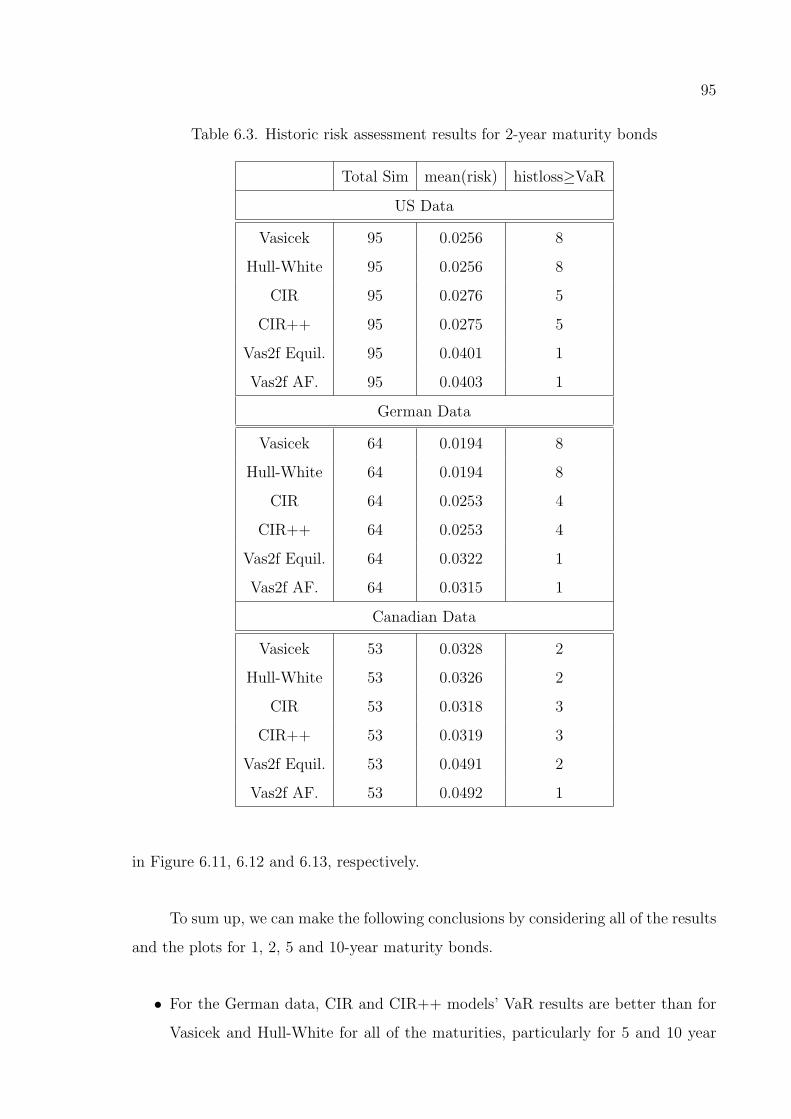
95



US Data

Vasicek 95 0.0256 8


CIR 95 0.0276 5

CIR++ 95 0.0275 5

Vas2f Equil. 95 0.0401 1

Vas2f AF. 95 0.0403 1

German Data

Vasicek 64 0.0194 8


CIR 64 0.0253 4

CIR++ 64 0.0253 4

Vas2f Equil. 64 0.0322 1

Vas2f AF. 64 0.0315 1

Canadian Data

Vasicek 53 0.0328 2


CIR 53 0.0318 3

CIR++ 53 0.0319 3

Vas2f Equil. 53 0.0491 2

Vas2f AF. 53 0.0492 1

in Figure 6.11, 6.12 and 6.13, respectively.

To sum up, we can make the following conclusions by considering all of the results

and the plots for 1, 2, 5 and 10-year maturity bonds.

• For the German data, CIR and CIR++ models’ VaR results are better than for

Vasicek and Hull-White for all of the maturities, particularly for 5 and 10 year

96



US Data

Vasicek 95 0.0537 17

Hull-White 95 0.0535 17

CIR 95 0.0606 10

CIR++ 95 0.0603 11

Vas2f Equil. 95 0.0874 1

Vas2f AF. 95 0.0878 1

German Data

Vasicek 64 0.0304 11

Hull-White 64 0.0304 10

CIR 64 0.0495 6

CIR++ 64 0.0497 6

Vas2f Equil. 64 0.0627 2

Vas2f AF. 64 0.0621 2

Canadian Data

Vasicek 53 0.0779 2


CIR 53 0.0778 1

CIR++ 53 0.0777 1

Vas2f Equil. 53 0.1161 1

Vas2f AF. 53 0.1163 1

bonds, for which Vasicek and Hull-White models are clearly under-estimating the

risk.

• For the US data, all models are under-estimating the risk for 5 and 10 year

maturities except for the two-factor models, which are over-estimating the risk

for 5-year maturity and correctly estimating the risk for 10-year maturity.

• Only two-factor models correctly estimating the risk for 10-year maturity for both

the US and the German data.

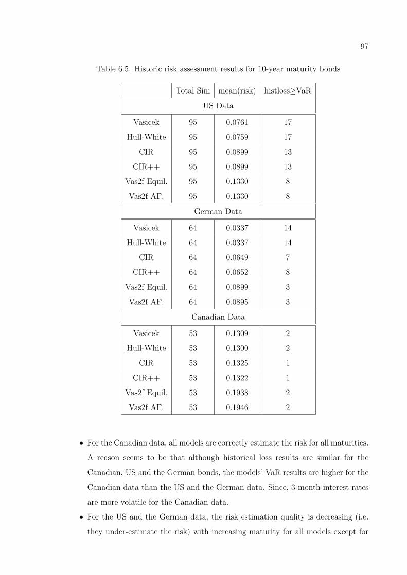
97



US Data

Vasicek 95 0.0761 17

Hull-White 95 0.0759 17

CIR 95 0.0899 13

CIR++ 95 0.0899 13

Vas2f Equil. 95 0.1330 8

Vas2f AF. 95 0.1330 8

German Data

Vasicek 64 0.0337 14

Hull-White 64 0.0337 14

CIR 64 0.0649 7

CIR++ 64 0.0652 8

Vas2f Equil. 64 0.0899 3

Vas2f AF. 64 0.0895 3

Canadian Data

Vasicek 53 0.1309 2


CIR 53 0.1325 1

CIR++ 53 0.1322 1

Vas2f Equil. 53 0.1938 2

Vas2f AF. 53 0.1946 2

• For the Canadian data, all models are correctly estimate the risk for all maturities.

A reason seems to be that although historical loss results are similar for the

Canadian, US and the German bonds, the models’ VaR results are higher for the

Canadian data than the US and the German data. Since, 3-month interest rates

are more volatile for the Canadian data.

• For the US and the German data, the risk estimation quality is decreasing (i.e.

they under-estimate the risk) with increasing maturity for all models except for

98

−0.

020.

000.

020.

040.

06

US 1−year Bond 6month Risk Horizon

dates

%V

aR R

esul

ts

1957.0 1963.0 1969.0 1975.0 1981.0 1987.0 1993.0 1999.0

VasicekHull−WhiteCIRCIR++Vas2f Equil.Vas2f AFMarket Loss

Figure 6.3. VaR and historical loss results for 1-year maturity bonds for the US data

−0.

050.

000.

050.

10

US 2−year Bond 6−month Risk Horizon

dates

%V

aR R

esul

ts

1957.0 1963.0 1969.0 1975.0 1981.0 1987.0 1993.0 1999.0



the two factor models.

After considering these results, we can conclude that:

• With increasing maturity VaR is increasing for all models.

99

−0.

10.

00.

10.

2


dates

%V

aR R

esul

ts

1957.0 1963.0 1969.0 1975.0 1981.0 1987.0 1993.0 1999.0



−0.

2−

0.1

0.0

0.1

0.2

0.3


dates

%V

aR R

esul

ts

1957.0 1963.0 1969.0 1975.0 1981.0 1987.0 1993.0 1999.0



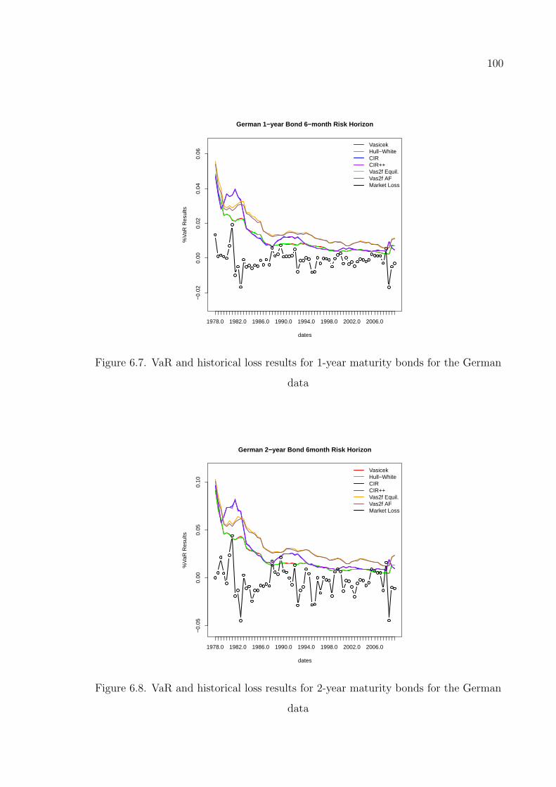
100

−0.

020.

000.

020.

040.

06

German 1−year Bond 6−month Risk Horizon

dates

%V

aR R

esul

ts

1978.0 1982.0 1986.0 1990.0 1994.0 1998.0 2002.0 2006.0


Figure 6.7. VaR and historical loss results for 1-year maturity bonds for the German

data

−0.

050.

000.

050.

10

German 2−year Bond 6month Risk Horizon

dates

%V

aR R

esul

ts

1978.0 1982.0 1986.0 1990.0 1994.0 1998.0 2002.0 2006.0



data

101

−0.

10−

0.05

0.00

0.05

0.10

0.15


dates

%V

aR R

esul

ts

1978.0 1982.0 1986.0 1990.0 1994.0 1998.0 2002.0 2006.0



data

−0.

10.

00.

10.

2


dates

%V

aR R

esul

ts

1978.0 1982.0 1986.0 1990.0 1994.0 1998.0 2002.0 2006.0



German data

102

−0.

050.

000.

050.

10

Canadian 2−year Bond 6−month Risk Horizon

dates

%V

aR R

esul

ts

1983.0 1986.0 1989.0 1992.0 1995.0 1998.0 2001.0 2004.0 2007.0



Canadian data

−0.

10.

00.

10.

2


dates

%V

aR R

esul

ts

1983.0 1986.0 1989.0 1992.0 1995.0 1998.0 2001.0 2004.0 2007.0



Canadian data

103

−0.

2−

0.1

0.0

0.1

0.2

0.3

0.4


dates

%V

aR R

esul

ts

1983.0 1986.0 1989.0 1992.0 1995.0 1998.0 2001.0 2004.0 2007.0



Canadian data

• With increasing maturity historical losses are also increasing.

• Two factor models produce greater VaR than other models, since they model

the short and long rate together by summing them up (i.e. risk increases with

increasing interest rates).

• Our three equilibrium-arbitrage free model pairs lead to very similar results for

all maturities for both the US, German and the Canadian data. Note that in the

plots, their results are so close that we can only see three lines. Therefore, we

can say that for these models using the arbitrage-free or the equilibrium version

does not influence risk quantification. A reason seems to be that the parameter

σ, which has a main influence on risk, is estimated in the same way for the

equilibrium and the arbitrage-free versions of the models.

• For all maturities except for 1-year, CIR and CIR++ models are better at risk

estimation than Vasicek and Hull-White except for the Canadian data, for which

they produce similar VaR results. This difference is more clear in the German

data. This is reasonable, since we know that the short-rate can become negative

in the Vasicek process. Especially for a small initial value like 3-month yield, this

104

can lead to unrealistic short-rate paths.

• VaR is highest in 1984.5 (i.e. July 1984) for all maturities for the US data. This

is due to the highly volatile interest rates in the early 1980’s, leading to large

volatility estimates.

• VaR is highest in late 1970’s and early 1980’s for all maturities for the German

data. Note that German 3-month yield is more volatile than the US 3-month

yield in mid 1970’s, which leads to high VaR estimates.

• For the Canadian data, VaR is again highest in early 1980’s for all maturities.

Since, 3-month rates are highly volatile in late 1970’s in Canada.

• Volatility of the losses in the market increases with increasing maturity for all

data.

• Two factor models are better at risk estimation for longer maturities , particularly

for 10 year maturity as historical losses are increasing with increasing maturity.

105

7. CONCLUSIONS

In this study, we worked on the Vasicek, CIR and the Two Factor Vasicek equilib-

rium models and also on their arbitrage free counterparts called Hull-White, CIR++

and Two Factor Arbitrage-Free Vasicek model. We explained and illustrated the short-

rate simulation, parameter estimation, bond pricing and risk simulation for all of the

models. Note that for the two factor models, we used an additive modeling framework

(i.e. the short-rate and the long-rate are added together).

We used MLE for estimating the model parameters. Note that for the Vasicek

model closed-form formulas exist for maximum likelihood estimators. We also used the

MLE of the Vasicek model for the parameter estimates of the Hull-White, Two Factor

Equilibrium Vasicek and the Two Factor Arbitrage-Free Vasicek models. For the CIR

model we have used R’s optim function to find the MLE numerically and we used the

MLE of the CIR model for the parameter estimates of the CIR++ model.

Short-rate simulation and bond pricing is not so difficult, as for all of the models

the exact distribution of rt is known and analytical formulas exist for bond pricing.

Therefore, risk simulation is easy and fast as small sample sizes are enough to obtain

quite precise results.

In the last chapter of the thesis, we made an empirical comparison of the models

for quantifying the interest rate risk. We used the US, German and the Canadian bond

market data to test six short-rate models’ risk quantification performances. We can

summarize our results as follows:

• For the three equilibrium-arbitrage free model pairs, the VaR results are almost

the same for all maturities for both the US, German and the Canadian data. So,

we conclude that for all three models using the arbitrage-free or the equilibrium

version does not influence the risk quantification.

• For 1 and 2 year maturities, Vasicek-Hull White and CIR-CIR++ pairs’ VaR

106

estimates are acceptable for the US and the German data.

• For 5 and 10 year maturities, two factor models are better at risk estimation for

the US and the German data.

• For the US and the German data, the Vasicek and the Hull-White models produce

more optimistic VaR estimates than the CIR and the CIR++ models. Two factor

models lead to the highest risk estimates.

• All models are correctly estimating the risk for all maturities for the Canadian

data.

• For the Canadian data, Vasicek-Hull White and CIR-CIR++ models’ VaR es-

timates are similar. However, two factor models again lead to the highest risk

estimates like for the US and the German data.

Which short rate model should be used to quantify bond risk? As they are

clearly easier to implement we suggest to use one of the three equilibrium models we

have tried. It also makes sense to use all three and to interpret the three results

as an interval holding the true VaR. However, also note that model’s risk estimation

performance varies for countries (e.g. 10-year bond risk in Germany is clearly above

the VaR results for three dates). Therefore, it is reasonable to use different models for

different countries to estimate the risk .

107

APPENDIX A: R CODES

A.1. R Codes for the Exact Simulation of the Vasicek Model

Vasicek_simul_exact<- function(para,r0,n,dt,d){

# exact simulation of n paths of the short rate process

# Short rate path is returned as a matrix

# para ... parameters of the Vasicek model

# r0 ... starting value of the interest rate process

# n ... number of paths that are generated

# dt ... length of time step (in years)

# d ... number of time steps that should be generated

mu=para[1]

beta=para[2]

sigma= para[3]

r=matrix(nrow=n,ncol=d)

r[,1]=r0

for(i in 1:(d-1))

r[,i+1]= r[,i]*exp(-beta*dt) + mu*(1-exp(-beta*dt))+(

sigma*sqrt((1-exp(-2*beta*dt))/(2*beta))*rnorm(n))

r

}

A.2. R Codes for the Approximate Simulation of the Vasicek Model

Vasicek_simul_euler <- function(para,r0,n,dt,d,exact=T){

# approximate simulation of n paths of the short rate process


# para ... parameters of the Vasicek model

# r0 ... starting value of the short rate process




mu=para[1]

beta=para[2]

sigma= para[3]


r[,1]=r0

for(i in 1:(d-1))

r[,i+1]= r[,i] + beta*(mu-r[,i])*dt+ sigma*sqrt(dt)*rnorm(n)

r

}

108

A.3. R Codes for the MLE of the Parameters of the Vasicek Model

Vasicek_MLE<-function(data,dt = 1/12){

#returns a vector with the estimates for the parameters mu, beta and

#sigma of the Vasicek model

#data ... vector of short rate data

#dt ... time interval (in years) between the data points given in data

N = length(data)

rate <- data[2:N]

lagrate<- data[1:(N-1)]

alpha<-(N*sum(rate*lagrate) - sum(rate)*sum(lagrate))/

(N*sum(lagrate^2)- sum(lagrate)^2)

beta_hat = -log(alpha)/dt

mu_hat = sum(rate-alpha*lagrate ) / (N*(1-alpha))

v2hat<-sum((rate-lagrate*alpha-mu_hat*(1-alpha))^2)/N

sigma_hat<-sqrt(2*beta_hat*v2hat/(1-alpha^2))

c(mu_hat,beta_hat,sigma_hat)

}

A.4. R Codes for the Bond Price and the Yield Calculations for the

Vasicek Model

VasicekPriceYield<-function(r,tau=1,Param,priceyn=F){

# r ... r(t) current value of short rate

# tau ...(T-t), time to maturity

# Param ... vector holding the parameters of the Vasicek model

mu =Param[1]

beta =Param[2]

sigma =Param[3]

B=(1-exp(-beta*tau))/beta

A=((B-tau)*(beta^2*mu-0.5*sigma^2)/beta^2 - sigma^2*B^2/(4*beta))

if(priceyn){

if(tau==0) return(1) #price is par-value(1) at maturity

else return(exp(A-B*r))

}else return((r*B-A)/tau)

}

A.5. R Codes for Risk Simulation for the Vasicek Model

RiskSim_Vasicek<-function(param,d=180,dt=1/360,r0,T,n=1000,m=10){

# evaluates the VaR value for 6m risk horizon.

# r0... initial value of the short rate

109

# T... maturity of the bond

# n... simulation size

# m... outer loop for calculating a conf. interval for VaR



Var6m=0

Init.Price=VasicekPriceYield(r=r0,tau=T,Param=param,priceyn=1)

for(i in 1:m)

{

res=Vasicek_simul_exact(para=param,r0=r0,n=n,dt=dt,d=d)

Sim.Price6m=VasicekPriceYield(r=res[,d],tau=T-1/2,

Param=param,priceyn=T)

Loss6m= 1-Sim.Price6m/(Init.Price*exp(rowSums(res)*dt))

Var6m[i]= quantile(Loss6m,0.95)

}

return(c(mean(Var6m),1.96*sd(Var6m)/sqrt(m)))

}

A.6. R Codes for the Exact Simulation of the CIR Model

CIR_simul_exact <- function(para,r0,n,dt,d,exact=T){


# para ... parameters of the CIR model





# c... multiplying term for the chi-square distribution

# df... degree of freedom

# ncp... non-centrality parameter

mu=para[1]

beta=para[2]

sigma= para[3]

c= sigma^2*(1-exp(-beta*dt))/(4*beta)

df= 4*mu*beta/sigma^2


r[,1]=r0

for(i in 1:(d-1)){

ncp= r[,i]*exp(-beta*dt)/c

r[,i+1] = c*rchisq(n,df=df,ncp=ncp)

}

r

}

110

A.7. R Codes for the Approximate Simulation of the CIR Model

CIR_simul_euler<- function(para,r0,n,dt,d){










mu=para[1]

beta=para[2]

sigma= para[3]

c= sigma^2*(1-exp(-beta*dt))/(4*beta)



r[,1]=r0

for(i in 1:(d-1))

r[,i+1]=r[,i]+beta*(mu-r[,i])*dt+sigma*sqrt(r[,i]*dt)*rnorm(n)

r

}

A.8. R Codes for Calculating the Log-Likelihood Function of the CIR

Model

CIRloglike<-function(param,data,times,test=F,addsign=T){

# CIR log-likelihood Function


# dt ... time interval (in years) between the data points given in data




mu=param[1]

beta=param[2]

sigma=param[3]

N<-length(data)

if(test==T)

dt=times

else

dt<-diff(times,1)

rate=data[1:(N-1)]

lagrate=data[2:N]

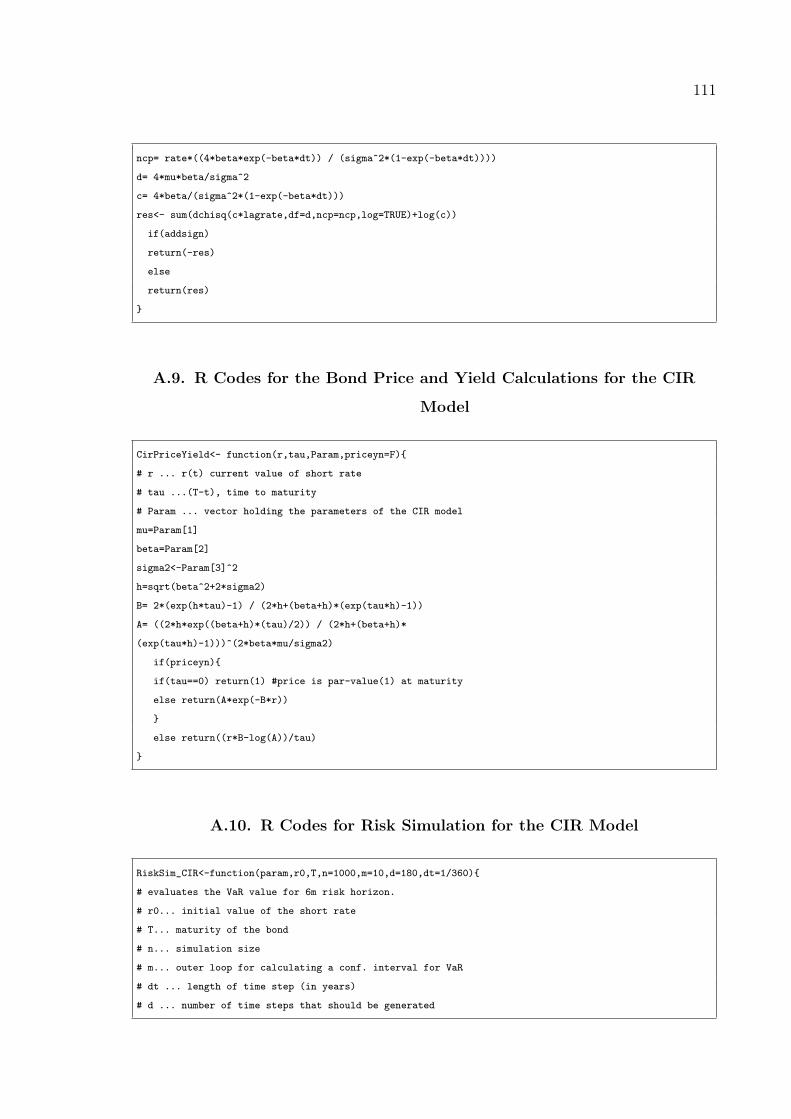
111

ncp= rate*((4*beta*exp(-beta*dt)) / (sigma^2*(1-exp(-beta*dt))))

d= 4*mu*beta/sigma^2

c= 4*beta/(sigma^2*(1-exp(-beta*dt)))

res<- sum(dchisq(c*lagrate,df=d,ncp=ncp,log=TRUE)+log(c))

if(addsign)

return(-res)

else

return(res)

}

A.9. R Codes for the Bond Price and Yield Calculations for the CIR

Model

CirPriceYield<- function(r,tau,Param,priceyn=F){



# Param ... vector holding the parameters of the CIR model

mu=Param[1]

beta=Param[2]

sigma2<-Param[3]^2

h=sqrt(beta^2+2*sigma2)

B= 2*(exp(h*tau)-1) / (2*h+(beta+h)*(exp(tau*h)-1))

A= ((2*h*exp((beta+h)*(tau)/2)) / (2*h+(beta+h)*

(exp(tau*h)-1)))^(2*beta*mu/sigma2)

if(priceyn){


else return(A*exp(-B*r))

}

else return((r*B-log(A))/tau)

}

A.10. R Codes for Risk Simulation for the CIR Model

RiskSim_CIR<-function(param,r0,T,n=1000,m=10,d=180,dt=1/360){

# evaluates the VaR value for 6m risk horizon.

# r0... initial value of the short rate

# T... maturity of the bond

# n... simulation size

# m... outer loop for calculating a conf. interval for VaR



112

Var6m=0

Init.Price=CirPriceYield(r=r0,tau=T,Param=param,priceyn=1)

for(i in 1:m)

{

res=CIR_simul_exact(para=param,r0=r0,n=n,dt=dt,d=d,exact=T)

Sim.Price6m=CirPriceYield(r=res[,d],tau=T-1/2,Param=param,priceyn=T)

Loss6m= 1-Sim.Price6m/(Init.Price*exp(rowSums(res)*dt))


}


}

A.11. R Codes for the Exact Simulation of the Two Factor Equilibrium

Vasicek Model

Vas2f_sim_exact<-function(param,x0,y0,dt,n,d){


# Short rate path and x(t),y(t) processes returned as a matrix

# param ... parameters of the 2-factor Vasicek model

# x0 ... starting value of the x (short rate) process

# y0 ... starting value of the y (long rate) process




mu_x =param[1]

beta_x =param[2]

sigma_x=param[3]

mu_y =param[4]

beta_y =param[5]

sigma_y=param[6]

rho =param[7]

x=matrix(nrow=n,ncol=d)

y=matrix(nrow=n,ncol=d)


x[,1]=x0

y[,1]=y0

r[,1]=x0+y0

R<-matrix(c(1 ,rho,rho,1),nrow=2)# Correlation Matrix

L<- t(chol(R))# Cholesky decomposition

for(i in 1:(d-1))

{

Z<- matrix(rnorm(n*2),nrow=2)

Z<- L%*%Z ## Correlated random variates

Z2=t(Z)

113

x[,i+1]=x[,i]*exp(-beta_x*dt)+mu_x*(1-exp(-beta_x*dt))+

sigma_x*sqrt((1-exp(-2*beta_x*dt))/(2*beta_x))*Z2[,1]

y[,i+1]=y[,i]*exp(-beta_y*dt)+mu_y*(1-exp(-beta_y*dt))+

sigma_y*sqrt((1-exp(-2*beta_y*dt))/(2*beta_y))*Z2[,2]

r[,i+1]=x[,i+1]+y[,i+1]

}

return(list(rt=r,xt=x,yt=y))

}

A.12. R Codes for the Approximate Simulation of the Two Factor

Equilibrium Vasicek Model

Vas2f_sim_euler<-function(param,x0,y0,dt,n,d){



# param ... parameters of the 2-factor Vasicek model

# x0 ... starting value of the x process

# y0 ... starting value of the y process




mu_x =param[1]

beta_x =param[2]

sigma_x=param[3]

mu_y =param[4]

beta_y =param[5]

sigma_y=param[6]

rho =param[7]




x[,1]=x0

y[,1]=y0

r[,1]=x0+y0



for(i in 1:(d-1))

{



Z2=t(Z)

x[,i+1]=x[,i]+beta_x*(mu_x-x[,i])*dt+sigma_x*sqrt(dt)*Z2[,1]

y[,i+1]=y[,i]+beta_y*(mu_y-y[,i])*dt+sigma_y*sqrt(dt)*Z2[,2]

114

r[,i+1]=x[,i+1]+y[,i+1]

}


}

A.13. R Codes for the Bond Price and the Yield Calculations for the Two

Factor Equilibrium Vasicek Model

Vas_2fPriceYield<-function(t,param,x0,y0,x,y,tau,priceyn=F,d){

# param ... vector holding the parameters of the 2f Vasicek model

# x0 ... initial value of short rate

# y0 ... initial value of the long rate

# x ... short rate process x(t)

# y ... long rate process y(t)

# d ... number of time steps in the simulations


# t ... time

mu_x =param[1]

beta_x =param[2]

sigma_x=param[3]

mu_y =param[4]

beta_y =param[5]

sigma_y=param[6]

rho =param[7]

yield=mu_x+(1-exp(-beta_x*tau))/(beta_x*tau)*((if(t==0){x0}else

{x[,d]})-mu_x)+mu_y+(1-exp(-beta_y*tau))/(beta_y*tau)*((if(t==0)

{y0}else{y[,d]})-mu_y)-sigma_x^2/(2*beta_x^2)*(1+(1-exp(-2*beta_x*

tau))/(2*beta_x*tau)-2*(1-exp(-beta_x*tau))/(beta_x*tau))-

sigma_y^2/(2*beta_y^2)*(1+(1-exp(-2*beta_y*tau))/(2*beta_y*tau)-

2*(1-exp(-beta_y*tau))/(beta_y*tau))-(rho*sigma_x*sigma_y)/

(beta_x*beta_y)*(1-(1-exp(-beta_x*tau))/(beta_x*tau)-

(1-exp(-beta_y*tau))/(beta_y*tau)+(1-exp(-(beta_x+beta_y)*tau))/

((beta_x+beta_y)*tau))

price=exp(-yield*tau)

if(priceyn)


else return(price)

else

return(yield)

}

115

A.14. R Codes for Risk Simulation for the Two Factor Equilibrium

Vasicek Model

RiskSim_2fVas<-function(x0,y0,T,param,n=1000,m=10,d=180,dt=1/360){

#evaluates the VaR value for 6m horizon.

#r0... initial value of the short rate

#T... maturity of the bond

#n... simulation size

#m... outer loop for calculating a conf. interval for VaR



Var6m=0

Init.Price=Vas_2fPriceYield(t=0,tau=T-0,param=param,x0,y0,priceyn=T)

for(i in 1:m)

{

res=Vas2f_sim_exact(param=param,n=n,dt=dt,d=d,x0=x0,y0=y0)

Sim.Price6m=Vas_2fPriceYield(t=1/2,tau=T-1/2,param=param,

x=res$xt,y=res$yt,priceyn=T,d=d)

Loss6m= 1-Sim.Price6m/(Init.Price*exp(rowSums(res$rt)*dt))


}


}

A.15. R Codes for the Exact Simulation of the Hull-White Model

HullW_simul_exact <- function(param,r0,n,dt,d,fm,exact=T){



# para ... parameters of the Hull-White model





beta = param[1]

sigma = param[2]


r[,1]=r0

alphat=0

alphat[1]= fm[1]

for(i in 1:(d-1)){

alphat[i+1]= fm[i] + sigma^2/(2*beta^2)*(1-exp(-beta*dt*i))^2

r[,i+1]= r[,i]*exp(-beta*dt) + alphat[i+1]-alphat[i]*exp(-beta*dt) +

116

sqrt(sigma^2/(2*beta)*(1-exp(-2*beta*dt)))*rnorm(n)

}

r

}


Hull-White Model

HwPriceYield<-function(r,T,t,Param,priceyn=T,Pm0,Pmt,fmt){


# T ... maturity

# t ... time


# Pm0 ... initial market bond price for maturity T

# Pmt ... initial market bond price for maturity t

# fmt ... initial forward rate at time t

beta = Param[1]

sigma = Param[2]

B = 1/beta*(1-exp(-beta*(T-t)))

A = Pm0/Pmt*exp(B*fmt-sigma^2/(4*beta)*(1-exp(-2*beta*t))*B^2)

if(priceyn){

if((T-t)==0) return(1) #price is par-value(1) at maturity

else return(A*exp(-B*r))

}

else return((r*B-log(A))/(T-t))

}

A.17. R Codes for Risk Simulation for the Hull-White Model

RiskSim_HwVas<-function(param,r0,n=1000,m=30,Pm,fm,matur,yield6m,d=180,dt=1/360){

#evaluates the VaR value for 6m risk horizon for the Hull-White model.




#m... outer loop for calculating a conf. interval for VaR

#dt ... length of time step (in years)

#d ... number of time steps that should be generated

Var6m=0

for(i in 1:m)

{

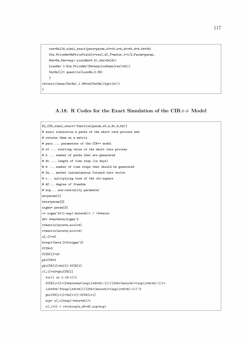
117

res=HullW_simul_exact(para=param,r0=r0,n=n,dt=dt,d=d,fm=fm)

Sim.Price6m=HwPriceYield(r=res[,d],T=matur,t=1/2,Param=param,

Pm0=Pm,Pmt=exp(-yield6m*0.5),fmt=fm[d])

Loss6m= 1-Sim.Price6m/(Pm*exp(rowSums(res)*dt))


}


}

A.18. R Codes for the Exact Simulation of the CIR++ Model

Ex_CIR_simul_exact<-function(param,x0,n,dt,d,fm){

# exact simulation n paths of the short rate process and

# returns them as a matrix

# para ... parameters of the CIR++ model



# dt ... length of time step (in days)


# fm... market instantaneous forward rate vector

# c... multiplying term of the chi-square



mu=param[1]

beta=param[2]

sigma= param[3]

c= sigma^2*(1-exp(-beta*dt)) / (4*beta)




x[,1]=x0

h=sqrt(beta^2+2*sigma^2)

fCIR=0

fCIR[1]=x0

phiCIR=0

phiCIR[1]=fm[1]-fCIR[1]

r[,1]=x0+phiCIR[1]

for(i in 1:(d-1)){

fCIR[i+1]=(2*beta*mu*(exp(i*dt*h)-1))/(2*h+(beta+h)*(exp(i*dt*h)-1))+

(x0*4*h^2*exp(i*dt*h))/(2*h+(beta+h)*(exp(i*dt*h)-1))^2

phiCIR[i+1]=fm[i+1]-fCIR[i+1]

ncp= x[,i]*exp(-beta*dt)/c

x[,i+1] = c*rchisq(n,df=df,ncp=ncp)

118

r[,i+1] = x[,i+1]+phiCIR[i+1]

}

r

}

A.19. R Codes for the Approximate Simulation of the CIR++ Model

Ex_CIR_simul_euler<-function(param,x0,n,dt,d,fm){

# exact simulation n paths of the short rate process and

# returns them as a matrix

# para ... parameters of the CIR++ model



# dt ... length of time step (in days)


# fm... market instantaneous forward rate vector

# c... multiplying term of the chi-square



mu=param[1]

beta=param[2]

sigma= param[3]

c= sigma^2*(1-exp(-beta*dt)) / (4*beta)




x[,1]=x0

h=sqrt(beta^2+2*sigma^2)

fCIR=0

fCIR[1]=x0

phiCIR=0

phiCIR[1]=fm[1]-fCIR[1]

r[,1]=x0+phiCIR[1]

for(i in 1:(d-1)){

fCIR[i+1]=(2*beta*mu*(exp(i*dt*h)-1))/(2*h+(beta+h)*(exp(i*dt*h)-1))+

(x0*4*h^2*exp(i*dt*h))/(2*h+(beta+h)*(exp(i*dt*h)-1))^2

phiCIR[i+1]=fm[i+1]-fCIR[i+1]

ncp= x[,i]*exp(-beta*dt)/c

x[,i+1]=x[,i]+beta*(mu-r[,i])*dt+sigma*sqrt(r[,i]*dt)*rnorm(n)

r[,i+1] = x[,i+1]+phiCIR[i+1]

}

r

}

119


CIR++ Model

Ex_CIR_PriceYield<-function(r,x0,T,t,Param,priceyn=T,Pm0,Pmt,fmt){

# x0 ... initial value for the x process

# r ... short rate process with shift added

# T ... maturity

# t ... time


# Pm0 ... initial market bond price for maturity T



mu=Param[1]

beta=Param[2]

sigma2<-Param[3]^2

h=sqrt(beta^2+2*sigma2)

B<-function(t,T) 2*(exp(h*(T-t))-1) / (2*h+(beta+h)*(exp((T-t)*h)-1))

A<-function(t,T) ((2*h*exp((beta+h)*(T-t)/2))/(2*h+(beta+h)*

(exp((T-t)*h)-1)))^(2*beta*mu/sigma2)

fCIRt=(2*beta*mu*(exp(t*h)-1))/(2*h+(beta+h)*(exp(t*h)-1))+

(x0*4*h^2*exp(t*h))/(2*h+(beta+h)*(exp(t*h)-1))^2

phiCIRt=fmt-fCIRt

A_bar=Pm0*A(0,t)*exp(-B(0,t)*x0)/(Pmt*A(0,T)*exp(-B(0,T)*x0))*

A(t,T)*exp(B(t,T)*phiCIRt)

#if t=0 add the shift to the x process

#else simulated r values will already be shifted

if(t==0)

r=x0+phiCIRt

else

r=r

price=A_bar*exp(-B(t,T)*r)

yield=-log(price)/(T-t)

if(priceyn){

if((T-t)==0) return(1) #price is par-value(1) at maturity

else return(price)

}else return(yield)

}

A.21. R Codes for Risk Simulation for the CIR++ Model

RiskSim_ExCIR<-function(param,r0,n=1000,m=10,Pm,fm,matur,yield6m,d=180,dt=1/360){

#evaluates the VaR value for 6m risk horizon for the CIR++ model.

#time...simulation horizon


120



#m... inner loop for calculating a conf. interval for VaR

#dt ... length of time step (in years)

#d ... number of time steps that should be generated

Var6m=0

for(i in 1:m)

{

res=Ex_CIR_simul_exact(param=param,x0=r0,n=n,dt=dt,d=d,fm=fm)

Sim.Price6m=Ex_CIR_PriceYield(r=res[,d],x0=r0,T=matur,t=1/2,

Param=param,Pm0=Pm,Pmt=exp(-yield6m*0.5),fmt=fm[d])

Loss6m= 1-Sim.Price6m/(Pm*exp(rowSums(res)*dt))


}


}

A.22. R Codes for the Exact Simulation of the Two Factor Arbitrage-Free

Vasicek Model

AFVas2f_sim_exact<-function(Param,n,d,dt,fm){


# Short rate path and x,y processes are returned as a matrix

# Param ... parameters of the 2f AF Vasicek model




betax=Param[1]

sigmax=Param[2]

betay=Param[3]

sigmay=Param[4]

rho=Param[5]




R<-matrix(c(1,rho,rho,1),nrow=2)# Correlation Matrix

L<- t(chol(R)) # Cholesky decomposition

x[,1]=0

y[,1]=0

phi=0

phi[1]=fm[1]

r[,1]=phi[1]

for(i in 1:(d-1)){


121


Z2=t(Z)

x[,i+1]=x[,i]*exp(-betax*dt)+sqrt(sigmax^2/(2*betax)*

(1-exp(-2*betax*dt)))*Z2[,1]

y[,i+1]=y[,i]*exp(-betay*dt)+sqrt(sigmay^2/(2*betay)*

(1-exp(-2*betay*dt)))*Z2[,2]

phi[i+1]=fm[i+1]+sigmax^2/(2*betax^2)*(1-exp(-betax*i*dt))^2+

sigmay^2/(2*betay^2)*(1-exp(-betay*i*dt))^2+rho*sigmax*sigmay/

(betax*betay)*(1-exp(-betax*i*dt))*(1-exp(-betay*i*dt))

r[,i+1]=x[,i+1]+y[,i+1]+phi[i+1]

}

return(list(rt=r,Xt=x,Yt=y))

}

A.23. R Codes for the Approximate Simulation of the Two Factor

Arbitrage-Free Vasicek Model

AFVas2f_sim_euler<-function(Param,dt,n,d,fm){



# param ... parameters of the 2-factor AF Vasicek model

# x0 ... starting value of the x process

# y0 ... starting value of the y process




# fm ... daily forward rates

betax=Param[1]

sigmax=Param[2]

betay=Param[3]

sigmay=Param[4]

rho=Param[5]




x[,1]=0

y[,1]=0

phi=0

phi[1]=fm[1]

r[,1]=phi[1]



for(i in 1:(d-1))

122

{



Z2=t(Z)

x[,i+1]=x[,i]+betax*(-x[,i])*dt+sigmax*sqrt(dt)*Z2[,1]

y[,i+1]=y[,i]+betay*(-y[,i])*dt+sigmay*sqrt(dt)*Z2[,2]

phi[i+1]=fm[i+1]+sigmax^2/(2*betax^2)*(1-exp(-betax*i*dt))^2+

sigmay^2/(2*betay^2)*(1-exp(-betay*i*dt))^2+rho*sigmax*sigmay/

(betax*betay)*(1-exp(-betax*i*dt))*(1-exp(-betay*i*dt))

r[,i+1]=x[,i+1]+y[,i+1]+phi[i+1]

}


}

A.24. R Codes for the Bond Price and the Yield Calculations for the Two

Factor Arbitrage-Free Vasicek Model

AF_vas2f_PriceYield<-function(x,y,T,t,Param,PmT,Pmt,fmt,d,priceyn=T){

# x ... x(t) (short-rate) process

# y ... y(t) (long-rate) process

# T ... maturity

# t ... time


# PmT ... initial market bond price for maturity T



# d ... time step used in the simulation.

betax=Param[1]

sigmax=Param[2]

betay=Param[3]

sigmay=Param[4]

rho=Param[5]

V<-function(t,T){

sigmax^2/betax^2*(T-t+2/betax*exp(-betax*(T-t))-1/(2*betax)*

exp(-2*betax*(T-t))-3/(2*betax))+sigmay^2/betay^2*(T-t+2/betay*

exp(-betay*(T-t))-1/(2*betay)* exp(-2*betay*(T-t))-3/(2*betay))+

2*rho*sigmax*sigmay/(betax*betay)*(T-t+(exp(-betax*(T-t))-1)/

betax+(exp(-betay*(T-t))-1)/betay-(exp(-(betax+betay)*(T-t))-1)/

(betax+betay))}

#if t=0 x(0)=0 and y(0)=0 else x[,t]=x[,d],y[,t]=y[,6]

#x[,d] and y[,d] will be found from simulations.

At=1/2*(V(t,T)-V(0,T)+V(0,t))-(1-exp(-betax*(T-t)))/betax*(if(t==0){0}

else{x[,d]})-(1-exp(-betay*(T-t)))/betay*(if(t==0){0}else{y[,d]})

123

Price=PmT/Pmt*exp(At)

yield=-log(Price)/(T-t)

if(priceyn)

return(Price)

else

return(yield)

}

A.25. R Codes for Risk Simulation for the Two Factor Arbitrage-Free

Vasicek Model

RiskSim_AF_2fVas<-function(x0,y0,T,Param,n=1000,m=30,d=180,dt=1/360,Pm,yield6m,fm){

#evaluates the VaR value for 6m horizon.

#x0 ... initial value of the short rate

#y0 ... initial value of the long rate

#T ... maturity of the bond

#n ... simulation size

#m ... outer loop for calculating a conf. interval for VaR

#Pm ... initial market price for maturity T

#Pmt ... initial market price for maturity t

#yield6m ... initial 6-month yield

#fm ... forward rate vector for the interval [0,10] year

Var6m=0

for(i in 1:m){

res=AFVas2f_sim_exact(Param=Param,n=n,d=d,dt=dt,fm=fm)

Sim.Price6m=AF_vas2f_PriceYield(x=res$Xt,y=res$Yt,T=T,t=1/2,

Param=Param,PmT=Pm,Pmt=exp(-yield6m*0.5),fmt=fmt,d=d)

Loss6m= 1-Sim.Price6m/(Pm*exp(rowSums(res$rt)*dt))


}


}

A.26. R Codes for Historic Loss Calculations

Historic_loss<-function(Pm_buy,Pm_sell,opp_cost,time,sim_total){

#Pm_buy ... historical prices of bonds at simulation dates.

#Pm_sell ... historical prices of bonds after risk_horizon.

#time ... time of holding the bond (i.e. 6-month).

#opp_cost ... 6-month yield at simulation dates

#sim_total ... total risk simulations

124

hist=0

hist[1]=1-(Pm_sell[1+1]/(Pm_buy[1]*exp(opp_cost[1]*time)))

for(i in 1:(sim_total-1))

hist[i+1]=1-(Pm_sell[i+2]/(Pm_buy[i+1]*exp(opp_cost[i+1]*time)))

return(hist)

}

A.27. R Codes for Historical Risk Simulations

Risk_Sim<-function(func,...,data,str_date=1957,end_date=2004,

period=2,model="vasicek",sim=T,bond="1-year",forward,datas){

#str_date ... start date of risk simulations.

#end_date ... end date of risk simulations.

#period ... number of simulations in a year.

#sim_total ... total number of simulations

#results ... matrix for storing %VaR results.

#1st column for simulation dates, 2nd for mean VaR results

#3rd for error bounds.

#yields ... yields at simulation dates.

#r0 ... initial short rate (3-month) at simulation dates.

#L0 ... initial long rate (10-year) at simulation dates.

#Pm ... Market Prices at simulation dates.

#forward .. daily forward rates at simulation dates.

#rt_MLE_vas ... MLE for short rate in the Vasicek model.

#lt_sigma_hat ... MLE for long rate in the Vasicek model.

#rt_sigma_hat ... MLE of sigma of the short rate, estimated from

#last 5-years data for each simulation date.

#For CIR and CIR++, numerical optimization is made seperately for

#the US and the German data.

#Three dots (...) is used for assigning further arguments to the risk

#simulation functions of different models.

#First 5 year data is only used for calibration (i.e. risk simulations

#start after 60 months).

data2 =as.matrix(data,rownames.force=NA)

d =length(data2[1,])

sim_total =(end_date-str_date)*period+1

results =matrix(0,nrow=sim_total,ncol=3)

yields =matrix(0,nrow=sim_total+1,ncol=(d-1))

results[1,1]=data[61,1]

yields[1,] = data2[61,2:d]

yields[sim_total+1,] = data2[(sim_total/period)*12+61,2:d]

for(i in 1:(sim_total-1))

{

results[i+1,1] =data[(12/period)*i+61,1]

125

yields[i+1,] =data2[(12/period)*i+61,2:d]

}

r0=yields[,1]

if(datas=="CA"){

Pm6m =exp(-yields[,2]*0.5)

Pm1y =0

Pm2y =exp(-yields[,3]*2)



yield6m =yields[,2]

L0 =yields[,6]

}

if(datas=="US")

{






yield6m =yields[,2]

L0 =yields[,5]

}

if(datas=="DE")

{





Pm10y =exp(-yields[,d-1]*10)

L0 =yields[,d-1]

yield6m =yields[,1]

}

if(bond=="1-year")

Pm=Pm1y

if(bond=="2-year")

Pm=Pm2y

if(bond=="5-year")

Pm=Pm5y

if(bond=="10-year")

Pm=Pm10y

rt_MLE_vas=Vasicek_MLE(data=data[,2])

lt_MLE_vas=Vasicek_MLE(data=data[,d])

rt_sigma_hat=rep(0,sim_total)

for(i in 1:(sim_total))

rt_sigma_hat[i]=Vasicek_MLE(data=data[((12/period)*(i-1)+1):

((12/period)*(i-1)+60),2])[3]

126

lt_sigma_hat=rep(0,sim_total)


lt_sigma_hat[i]=Vasicek_MLE(data=data[((12/period)*(i-1)+1):

((12/period)*(i-1)+60),d])[3]

corr=rep(0,sim_total)


corr[i]=cor(data[((12/period)*(i-1)+1):((12/period)*(i-1)+61),2],

data[((12/period)*(i-1)+1):((12/period)*(i-1)+60),d])

if(model=="vasicek"&sim==T)

{


results[i,2:3]=func(param=c(rt_MLE_vas[1],rt_MLE_vas[2],

rt_sigma_hat[i]),r0=r0[i],...)

}

if((model=="cir"||model=="cir++")&sim==T)

{

sigma_hat=rep(0,sim_total)

MLE_cir=optim(par=c(0.001,0.001,0.018),fn=CIRloglike,

method = "L-BFGS-B",lower=c(0.001,0.05,0.018),upper=c(0.9,2,0.9),

data=data[,2],times=1/12,test=T)$par

x<-function(mu,beta,sigma,data,times,test)CIRloglike(param=

c(mu,beta,sigma),data,times,test)

if(datas=="US"||datas=="CA")

{


sigma_hat[i]=optim(par=c(0.011),fn=x,method="L-BFGS-B",

lower=0.017,upper=0.90,mu=MLE_cir[1],beta=MLE_cir[2],

data=data[((12/period)*(i-1)+1):((12/period)*(i-1)+62),2],


}

if(datas=="DE")

{


sigma_hat[i]=optim(par=c(0.01),fn=x,method="L-BFGS-B",

lower=0.0199,upper=0.90,mu=MLE_cir[1],beta=MLE_cir[2],

data=data[((12/period)*(i-1)+1):((12/period)*(i-1)+63),2],


}

}

if(model=="cir"){


results[i,2:3]=func(param=c(MLE_cir[1],MLE_cir[2],sigma_hat[i]),

r0=r0[i],...)

}

if(model=="cir++"){


127

results[i,2:3]=func(param=c(MLE_cir[1],MLE_cir[2],sigma_hat[i]),

yield6m=yield6m[i], r0=r0[i],Pm=Pm[i],fm=forward[,i],...)

}

if(model=="Hull-White"&sim==T)

{


results[i,2:3]=func(param=c(rt_MLE_vas[2],rt_sigma_hat[i]),

yield6m=yield6m[i],r0=r0[i],Pm=Pm[i],fm=forward[,i],...)

}

if(model=="Vas_2f"&sim==T)

{


results[i,2:3]=func(param=c(rt_MLE_vas[1],rt_MLE_vas[2],

rt_sigma_hat[i],lt_MLE_vas[1],lt_MLE_vas[2],lt_sigma_hat[i],

corr[i]),x0=r0[i],y0=L0[i],...)

}

if(model=="AF_Vas_2f"&sim==T)

{


results[i,2:3]=func(Param=c(rt_MLE_vas[2],rt_sigma_hat[i],

lt_MLE_vas2[2],lt_sigma_hat[i],corr[i]),x0=r0[i],y0=L0[i],

Pm=Pm[i],fm=forward[,i],yield6m=yield6m[i],...)

}

if(sim)

return(results)

else

return(list(Pm6m=Pm6m,Pm1y=Pm1y,Pm2y=Pm2y,Pm5y=Pm5y,

Pm10y=Pm10y,yields=yields))

}

A.28. R Codes for Fitting Instantaneous Forward Rates to the Bond

Prices

HW_forwPrice<-function(matur,yield,data="US",forwardyn=T){

#Uses linear interpolation to find daily forward rates for each time x.

#f(x)=ax+b...forward rate line for 0 to longest matury.

#Finds all a and b values for each interval in the maturity vector.

#Uses p(0,T)=exp(-int_{0}^{T} f(x) dx ) to find daily bond prices for each time x .

#matur...bond maturities

#yield...bond yields

#USyields ... 0.25,0.5,1,2,5,10 year maturities

#Germanyields ... 0.5,1,2,3,4,5,6,7,8,9,10 year maturities

#Canadianyields ... 0.25,0.5,2,5,10 year maturities

R=yield

128

price=c(1,exp(-R*matur))

a=0;b=0

b[1]=R[1]

a[1]=uniroot(function(a) log(price[2])+a*matur[1]^2/2+b[1]*matur[1],c(-1,1))[[1]]

for(i in 2:length(matur)){

a[i]=uniroot(function(y) log(price[i+1]/price[i])+y/2*(matur[i]^2-matur[i-1]^2)+

(matur[i-1]*(a[i-1]-y)+b[i-1])*(matur[i]-matur[i-1]),c(-1,1))[[1]]

b[i]=matur[i-1]*(a[i-1]-a[i])+b[i-1]

}

# 1year=360 days

fwd=0

prices=0

for(x in 1:(360*matur[length(matur)])){

if(x<=matur[1]*360)

{

fwd[x]=a[1]*x/360+b[1]

prices[x]=exp(-a[1]*(x/360)^2/2-b[1]*x/360)

}

if(x>matur[1]*360&x<=matur[2]*360){

{

fwd[x]=a[2]*x/360+b[2]

prices[x]=price[2]*exp(-a[2]*(x/360)^2/2-b[2]*x/360+a[2]*matur[1]^2/2+

b[2]*matur[1])

}

}


{

fwd[x]=a[3]*x/360+b[3]

prices[x]=price[3]*exp(-a[3]*(x/360)^2/2-b[3]*x/360+a[3]*matur[2]^2/2+

b[3]*matur[2])

}

}


{

fwd[x]=a[4]*x/360+b[4]

prices[x]= price[4]*exp(-a[4]*(x/360)^2/2-b[4]*x/360+a[4]*matur[3]^2/2+

b[4]*matur[3])

}

}


{

fwd[x]=a[5]*x/360+b[5]


b[5]*matur[4])

}

}

129

if(data!="CA")

{


fwd[x]=a[6]*x/360+b[6]


b[6]*matur[5])

}

}

if(data=="DE")

{

if(x>matur[6]*360&x<=matur[7]*360)

{

fwd[x]=a[7]*x/360+b[7]


b[7]*matur[6])

}


{

fwd[x]=a[8]*x/360+b[8]


b[8]*matur[7])

}


{

fwd[x]=a[9]*x/360+b[9]


b[9]*matur[8])

}


{

fwd[x]=a[10]*x/360+b[10]


b[10]*matur[9])

}

if(x>matur[10]*360&x<=matur[11]*360)

{

fwd[x]=a[11]*x/360+b[11]


b[11]*matur[10])

}

}

}

if(forwardyn)

return(fwd)

else

return(prices)

}

130

REFERENCES

1. Bank for International Settlements, Outstanding World Bond Market Debt , 2009.

2. Lyuu, Y. D., Financial Engineering and Computation: Principles, Mathemat-

ics,Algorithms , Cambridge University Press, 2002.

3. Nawalkha, S. K., G. M. Soto, and N. A. Beliaeva, “Bond Price, Duration, and

Convexity”, Interest Rate Risk Modelling: The Fixed Income Valuation Course,

chapter 2, John Wiley and Sons, 2005.

4. Tuckman, B., “One-Factor Measures of Price Sensitivity”, Fixed Income Securities:

Tools for Today’s Markets, chapter 5, John Wiley and Sons, 2002.

5. Fabozzi, F. J., Bond Markets, Analysis and Strategies , Prentice Hall, fourth edi-

tion, 2000.

6. Fabozzi, F. J., “Tools for Measuring Level Interest Rate Risk”, Measuring and

Controlling Interest Rate and Credit Risk , chapter 4, John Wiley and Sons, second

edition, 2003.

7. Brigo, D. and F. Mercurio, Interest Rate Models Theory and Practice With Smile,

Inflation and Credit , Springer, second edition, 2007.

8. Filipovic, D., Term-Structure Models A Graduate Course, Springer, 2009.

9. Cairns, A. J., Interest rate models : an introduction, Princeton University Press,

2004.

10. Rebonato, R., Interest-Rate Option Models: Understanding, analysing and using

models for exotic interest-rate options, John Wiley and Sons, second edition, 1998.

11. Tuckman, B., Fixed Income Securities: Tools for Today’s Markets, John Wiley and

131

Sons, 2002.

12. Shreve, S. E., Continuous-Time Models , Springer, 2004.

13. Buhrer, W., M. Uhrig-Homburg, U. Walter, and T. Weber, “An Empirical Compar-

ison of Forward-Rate and Spot-Rate Models for Valuing Interest-Rate Options”,

The Journal of Finance, Vol. 54, pp. 269–305, 1999.

14. Chan, K. C., G. A. Karolyi, F. A. Longstaff, and A. B. Sanders, “An Empirical

Comparison of Alternative Models of the Short-Term Interest Rate”, The Journal

of Finance, Vol. 47, pp. 1209–1227, 1992.

15. Nuno, C. and L. J. Barros, “A two-factor model of the German term structure of

interest rates”, Applied Financial Economics , Vol. 13, pp. 783–806, 2003.

16. Joost, D., M. Bertrand, and N. Theo, “Common factors in international bond

returns”, Journal of International Money and Finance, Vol. 22, pp. 629–656, 2003.

17. Glasserman, P., Monte Carlo Methods in Financial Engineering (Stochastic Mod-

elling and Applied Probability), Springer, 2003.

18. Jagtiani, J., G. G. Kaufman, and C. Lemieux, “The Effect of Credit Risk on Bank

and Bank Holding Company Bond Yields:Evidence from the Post-FDICIA Period”,

Journal of Financial Research, Vol. 25, No. 4, pp. 559–575, 2002.

19. Duffie, D. and K. J. Singleton, Credit Risk: Pricing, Measurement, and Manage-

ment , Princeton University Press, 2003.

20. John Hull, M. Predescu, and A. White, “Bond prices, default probabilities and risk

premiums”, Journal of Credit Risk , Vol. 1, No. 2, pp. 53–60, 2005.

21. Fons, J. S., “Using Default Rates to Model the Term Structure of Credit Risk”,

Financial Analysts Journal , Vol. 50, No. 5, pp. 25–33, 1994.

132

22. Basel Committee on Banking Supervision, Principles for the Management and

Supervision of Interest Rate Risk , 2001, consultative document.

23. Golub, B. W. and L. M. Tilman, “Measuring Yield Curve Risk Using Principal

Components, Analysis, Value, At Risk, And Key Rate Durations”, The Journal of

Portfolio Management , Vol. 23, pp. 72–84, 1997.

24. Jobst, N. J. and S. A. Zenios, “On the simulation of portfolios of interest rate and

credit risk sensitive securities”, European Journal of Operational Research, Vol.

161, pp. 298–324, 2005.

25. Jr., T. M. B. and W. F. Maxwell, “Modeling correlated market and credit risk in

fixed income portfolios”, Journal of Banking and Finance, Vol. 26, pp. 347–374,

2002.

26. Jobst, N. J. and S. A. Zenios, “Integrating market and credit risk: A simulation

and optimisation perspective”, Journal of Banking and Finance, Vol. 30, No. 2,

pp. 717–742, 2006.

27. Merton, R. C., “Theory of Rational Option Pricing”, Bell Journal of Economics

and Management Science, Vol. 4, pp. 141–183, 1974.

28. Vasicek, O., “An Equilibrium Characterization of the Term Structure”, Journal of

Financial Economics , Vol. 5, pp. 177–188, 1977.

29. Dothan, L. U., “On the Term Structure of Interest Rates”, Journal of Financial

Economics , Vol. 6, pp. 59–69, 1978.

30. Cox, J. C., J. E. Ingersoll, and S. A. Ross, “A Theory of the Term Structure of

Interest Rates”, Econometrica, Vol. 53, pp. 385–407, 1985.

31. Ho, T. S. Y. and S. B. Lee, “Term Structure Movements and the Pricing of Interest

Rate Contingent Claims”, The Journal of Finance, Vol. 41, pp. 1011–1029, 1986.

133

32. John Hull and A. White, “Pricing Interest-Rate-Derivative Securities”, The Review

of Financial Studies , Vol. 5, pp. 573–592, 1990.

33. Black, F., E. Derman, and W. Toy, “A One-Factor Model of Interest Rates and its

Application to Treasury Bond Options”, Financial Analysts Journal , Vol. 46, pp.

33–39, 1990.

34. Brigo, D. and F. Mercurio, “A deterministic shift extension of analytically tractable

and time homogeneous short rate models”, Finance and Stochastics , Vol. 5, p.

369388, 2001.

35. John Hull, Options, Futures, and Other Derivatives , Prentice Hall, fifth edition,

2002.

36. Chance, D., Teaching Note 97-03: The Vasicek Term Structure Model , 2008.

37. Cheridito, P., D. Filipovic, and R. L. Kimmel, “Market price of risk specifications

for affine models: Theory and evidence”, Journal of Financial Economics , Vol. 83,

pp. 123–170, 2007.

38. McCulloch, J. H. and H. C. Kwon, “US term structure data, 1947-1991”, Technical

report, Ohio State University, 1993, working paper.

39. Fama, E. F. and R. R. Bliss, “The Information in Long-Maturity Forward Rates”,

The American Economic Review , Vol. 77, pp. 680–692, 1987.

40. Board of Governors of the Federal Reserve System, Federal Reserve Statistical

Release H.15 , historical data.

41. European Banking Federation, Euro Interbank Offered Rate, historical rates.

42. John Hull and A. White, “Numerical Procedures for Implementing Term Structure

Models I: Singe-Factor Models”, The Journal of Derivatives , Vol. 2, pp. 7–16, 1994.

134

43. Jamshidian, F. and Y. Zhu, “Scenario Simulation: Theory and methodology”,

Finance and Stochastics , Vol. 1, pp. 43–67, 1997.

44. Eraker, B., Two Factor Models , 2008, wisconsin school of business.

45. John Hull and A. White, “Branching Out”, Risk , Vol. 7, pp. 34–37, 1994.

46. Deutsche Bundesbank, Term structure on Listed Federal Securities, historical data.

47. Bank of Canada, Selected historical interest rates, historical data.

Documents

Quantifying the Interest Rate Risk of Bonds by Simulation