Embed Size (px)
Citation preview

The SerieS: De GruyTer STuDieS in MaTheMaTical PhySicSThe series is devoted to the publication of monographs and high-level texts in mathe- matical physics. They cover topics and methods in fields of current interest, with an emphasis on didactical presentation. The series will enable readers to understand, apply, and develop further, with sufficient rigor, mathematical methods to given problems in physics. For this reason, works with a few authors are preferred over edited volumes. The works in this series are aimed at advanced students and researchers in mathematical and theoretical physics. They can also serve as secondary reading for lectures and seminars at advanced levels.
STuDieS in MaTheMaTical PhySicS 17
This book discusses the main concepts of the Standard Model of elementary particles in a compact and straightforward way. The work illustrates the unity of modern theoretical physics by combining approaches and concepts of the quantum field theory and modern condensed matter theory. The inductive approach allows a deep understanding of ideas and methods used for solving problems in this field.
Michael V
. SadovskiiQ
ua
nTu
M FielD
Theo
ry
Michael V. Sadovskii
QuanTuM FielD Theory
www.degruyter.comISBN 978-3-11-027029-7
17GSTMP
9783110270297_Cover_Sadovskii.indd 5 * Meta Systems GmbH 30.01.2013 10:37:27

De Gruyter Studies in Mathematical Physics 17
EditorsMichael Efroimsky, Bethesda, USALeonard Gamberg, Reading, USADmitry Gitman, São Paulo, BrasilAlexander Lazarian, Madison, USABoris Smirnov, Moscow, Russia


Michael V. Sadovskii
Quantum Field Theory
De Gruyter

Physics and Astronomy Classification Scheme 2010: 03.70.+k, 03.65.Pm, 11.10.-z, 11.10.Gh,11.10.Jj, 11.25.Db, 11.15.Bt, 11.15.Ha, 11.15.Ex, 11.30. -j, 12.20.-m, 12.38.Bx, 12.10.-g,12.38.Cy.
ISBN 978-3-11-027029-7e-ISBN 978-3-11-027035-8
Library of Congress Cataloging-in-Publication Data
A CIP catalog record for this book has been applied for at the Library of Congress.
Bibliographic information published by the Deutsche Nationalbibliothek
The Deutsche Nationalbibliothek lists this publication in the Deutsche Nationalbibliografie;detailed bibliographic data are available in the Internet at http://dnb.dnb.de.
© 2013 Walter de Gruyter GmbH, Berlin/Boston
Typesetting: PTP-Berlin Protago-TEX-Production GmbH, www.ptp-berlin.dePrinting and binding: Hubert & Co. GmbH & Co. KG, Göttingen
Printed on acid-free paper
Printed in Germany
www.degruyter.com

Preface
This book is the revised English translation of the 2003 Russian edition of “Lectures onQuantum Field Theory”, which was based on much extended lecture course taught bythe author since 1991 at the Ural State University, Ekaterinburg. It is addressed mainlyto graduate and PhD students, as well as to young researchers, who are working mainlyin condensed matter physics and seeking a compact and relatively simple introductionto the major section of modern theoretical physics, devoted to particles and fields,which remains relatively unknown to the condensed matter community, largely un-aware of the major progress related to the formulation the so-called “standard model”of elementary particles, which is at the moment the most fundamental theory of matterconfirmed by experiments. In fact, this book discusses the main concepts of this fun-damental theory which are basic and necessary (in the author’s opinion) for everyonestarting professional research work in other areas of theoretical physics, not related tohigh-energy physics and the theory of elementary particles, such as condensed mattertheory. This is actually even more important, as many of the theoretical approachesdeveloped in quantum field theory are now actively used in condensed matter theory,and many of the concepts of condensed matter theory are now widely used in the con-struction of the “standard model” of elementary particles. One of the main aims of thebook is to illustrate this unity of modern theoretical physics, widely using the analogiesbetween quantum field theory and modern condensed matter theory.
In contrast to many books on quantum field theory [2, 6, 8–10, 13, 25, 28, 53, 56, 59,60], most of which usually follow rather deductive presentation of the material, herewe use a kind of inductive approach (similar to that used in [59, 60]), when one andthe same problem is discussed several times using different approaches. In the author’sopinion such repetitions are useful for a more deep understanding of the various ideasand methods used for solving real problems. Of course, among the books mentionedabove, the author was much influenced by [6, 56, 60], and this influence is obvious inmany parts of the text. However, the choice of material and the form of presentation isessentially his own. For the present English edition some of the material was rewritten,bringing the content more up to date and adding more discussion on some of the moredifficult cases.
The central idea of this book is the presentation of the basics of the gauge field the-ory of interacting elementary particles. As to the methods, we present a rather detailedderivation of the Feynman diagram technique, which long ago also became so impor-tant for condensed matter theory. We also discuss in detail the method of functional(path) integrals in quantum theory, which is now also widely used in many sections oftheoretical physics.

vi Preface
We limit ourselves to this relatively traditional material, dropping some of the moremodern (but more speculative) approaches, such as supersymmetry. Obviously, wealso drop the discussion of some new ideas which are in fact outside the domain ofthe quantum field theory, such as strings and superstrings. Also we do not discuss inany detail the experimental aspects of modern high-energy physics (particle physics),using only a few illustrative examples.
Ekaterinburg, 2012 M.V. Sadovskii

Contents
Preface v
1 Basics of elementary particles 1
1.1 Fundamental particles . . . . . . . . . . . . . . . . . . . . . . . . . . . . . . . . . . . . . 11.1.1 Fermions . . . . . . . . . . . . . . . . . . . . . . . . . . . . . . . . . . . . . . . . 21.1.2 Vector bosons . . . . . . . . . . . . . . . . . . . . . . . . . . . . . . . . . . . . . 3
1.2 Fundamental interactions . . . . . . . . . . . . . . . . . . . . . . . . . . . . . . . . . . 4
1.3 The Standard Model and perspectives . . . . . . . . . . . . . . . . . . . . . . . . 5
2 Lagrange formalism. Symmetries and gauge fields 9
2.1 Lagrange mechanics of a particle . . . . . . . . . . . . . . . . . . . . . . . . . . . . 9
2.2 Real scalar field. Lagrange equations . . . . . . . . . . . . . . . . . . . . . . . . . 11
2.3 The Noether theorem . . . . . . . . . . . . . . . . . . . . . . . . . . . . . . . . . . . . . 15
2.4 Complex scalar and electromagnetic fields . . . . . . . . . . . . . . . . . . . . 18
2.5 Yang–Mills fields . . . . . . . . . . . . . . . . . . . . . . . . . . . . . . . . . . . . . . . . 24
2.6 The geometry of gauge fields . . . . . . . . . . . . . . . . . . . . . . . . . . . . . . . 30
2.7 A realistic example – chromodynamics . . . . . . . . . . . . . . . . . . . . . . . 38
3 Canonical quantization, symmetries in quantum field theory 40
3.1 Photons . . . . . . . . . . . . . . . . . . . . . . . . . . . . . . . . . . . . . . . . . . . . . . . . 403.1.1 Quantization of the electromagnetic field . . . . . . . . . . . . . . . 403.1.2 Remarks on gauge invariance and Bose statistics . . . . . . . . . 453.1.3 Vacuum fluctuations and Casimir effect . . . . . . . . . . . . . . . . 48
3.2 Bosons . . . . . . . . . . . . . . . . . . . . . . . . . . . . . . . . . . . . . . . . . . . . . . . . 503.2.1 Scalar particles . . . . . . . . . . . . . . . . . . . . . . . . . . . . . . . . . . . . 503.2.2 Truly neutral particles . . . . . . . . . . . . . . . . . . . . . . . . . . . . . . 543.2.3 CPT -transformations . . . . . . . . . . . . . . . . . . . . . . . . . . . . . . 573.2.4 Vector bosons . . . . . . . . . . . . . . . . . . . . . . . . . . . . . . . . . . . . . 61
3.3 Fermions . . . . . . . . . . . . . . . . . . . . . . . . . . . . . . . . . . . . . . . . . . . . . . . 633.3.1 Three-dimensional spinors . . . . . . . . . . . . . . . . . . . . . . . . . . . 633.3.2 Spinors of the Lorentz group . . . . . . . . . . . . . . . . . . . . . . . . . 673.3.3 The Dirac equation . . . . . . . . . . . . . . . . . . . . . . . . . . . . . . . . . 743.3.4 The algebra of Dirac’s matrices . . . . . . . . . . . . . . . . . . . . . . . 793.3.5 Plane waves . . . . . . . . . . . . . . . . . . . . . . . . . . . . . . . . . . . . . . 81

viii Contents
3.3.6 Spin and statistics . . . . . . . . . . . . . . . . . . . . . . . . . . . . . . . . . . 833.3.7 C ,P ,T transformations for fermions . . . . . . . . . . . . . . . . . . 853.3.8 Bilinear forms . . . . . . . . . . . . . . . . . . . . . . . . . . . . . . . . . . . . 863.3.9 The neutrino . . . . . . . . . . . . . . . . . . . . . . . . . . . . . . . . . . . . . . 87
4 The Feynman theory of positron and elementary quantumelectrodynamics 93
4.1 Nonrelativistic theory. Green’s functions . . . . . . . . . . . . . . . . . . . . . . 93
4.2 Relativistic theory . . . . . . . . . . . . . . . . . . . . . . . . . . . . . . . . . . . . . . . . 96
4.3 Momentum representation . . . . . . . . . . . . . . . . . . . . . . . . . . . . . . . . . 100
4.4 The electron in an external electromagnetic field . . . . . . . . . . . . . . . . 103
4.5 The two-particle problem . . . . . . . . . . . . . . . . . . . . . . . . . . . . . . . . . . 110
5 Scattering matrix 115
5.1 Scattering amplitude . . . . . . . . . . . . . . . . . . . . . . . . . . . . . . . . . . . . . . 115
5.2 Kinematic invariants . . . . . . . . . . . . . . . . . . . . . . . . . . . . . . . . . . . . . . 118
5.3 Unitarity . . . . . . . . . . . . . . . . . . . . . . . . . . . . . . . . . . . . . . . . . . . . . . . 121
6 Invariant perturbation theory 124
6.1 Schroedinger and Heisenberg representations . . . . . . . . . . . . . . . . . . 124
6.2 Interaction representation . . . . . . . . . . . . . . . . . . . . . . . . . . . . . . . . . . 125
6.3 S -matrix expansion . . . . . . . . . . . . . . . . . . . . . . . . . . . . . . . . . . . . . . 128
6.4 Feynman diagrams for electron scattering in quantumelectrodynamics . . . . . . . . . . . . . . . . . . . . . . . . . . . . . . . . . . . . . . . . . 135
6.5 Feynman diagrams for photon scattering . . . . . . . . . . . . . . . . . . . . . . 140
6.6 Electron propagator . . . . . . . . . . . . . . . . . . . . . . . . . . . . . . . . . . . . . . 142
6.7 The photon propagator . . . . . . . . . . . . . . . . . . . . . . . . . . . . . . . . . . . . 146
6.8 The Wick theorem and general diagram rules . . . . . . . . . . . . . . . . . . 149
7 Exact propagators and vertices 156
7.1 Field operators in the Heisenberg representation and interactionrepresentation . . . . . . . . . . . . . . . . . . . . . . . . . . . . . . . . . . . . . . . . . . . 156
7.2 The exact propagator of photons . . . . . . . . . . . . . . . . . . . . . . . . . . . . 158
7.3 The exact propagator of electrons . . . . . . . . . . . . . . . . . . . . . . . . . . . 164
7.4 Vertex parts . . . . . . . . . . . . . . . . . . . . . . . . . . . . . . . . . . . . . . . . . . . . 168
7.5 Dyson equations . . . . . . . . . . . . . . . . . . . . . . . . . . . . . . . . . . . . . . . . . 172
7.6 Ward identity . . . . . . . . . . . . . . . . . . . . . . . . . . . . . . . . . . . . . . . . . . . 173

Contents ix
8 Some applications of quantum electrodynamics 175
8.1 Electron scattering by static charge: higher order corrections . . . . . . 175
8.2 The Lamb shift and the anomalous magnetic moment . . . . . . . . . . . . 180
8.3 Renormalization – how it works . . . . . . . . . . . . . . . . . . . . . . . . . . . . . 185
8.4 “Running” the coupling constant . . . . . . . . . . . . . . . . . . . . . . . . . . . . 189
8.5 Annihilation of eCe� into hadrons. Proof of the existence of quarks 191
8.6 The physical conditions for renormalization . . . . . . . . . . . . . . . . . . . 192
8.7 The classification and elimination of divergences . . . . . . . . . . . . . . . 196
8.8 The asymptotic behavior of a photon propagator at large momenta . 200
8.9 Relation between the “bare” and “true” charges . . . . . . . . . . . . . . . . 203
8.10 The renormalization group in QED . . . . . . . . . . . . . . . . . . . . . . . . . . 207
8.11 The asymptotic nature of a perturbation series . . . . . . . . . . . . . . . . . . 209
9 Path integrals and quantum mechanics 211
9.1 Quantum mechanics and path integrals . . . . . . . . . . . . . . . . . . . . . . . 211
9.2 Perturbation theory . . . . . . . . . . . . . . . . . . . . . . . . . . . . . . . . . . . . . . . 219
9.3 Functional derivatives . . . . . . . . . . . . . . . . . . . . . . . . . . . . . . . . . . . . 225
9.4 Some properties of functional integrals . . . . . . . . . . . . . . . . . . . . . . . 226
10 Functional integrals: scalars and spinors 232
10.1 Generating the functional for scalar fields . . . . . . . . . . . . . . . . . . . . . 232
10.2 Functional integration . . . . . . . . . . . . . . . . . . . . . . . . . . . . . . . . . . . . . 237
10.3 Free particle Green’s functions . . . . . . . . . . . . . . . . . . . . . . . . . . . . . 240
10.4 Generating the functional for interacting fields . . . . . . . . . . . . . . . . . 247
10.5 '4 theory . . . . . . . . . . . . . . . . . . . . . . . . . . . . . . . . . . . . . . . . . . . . . . . 250
10.6 The generating functional for connected diagrams . . . . . . . . . . . . . . 257
10.7 Self-energy and vertex functions . . . . . . . . . . . . . . . . . . . . . . . . . . . . 260
10.8 The theory of critical phenomena . . . . . . . . . . . . . . . . . . . . . . . . . . . . 264
10.9 Functional methods for fermions . . . . . . . . . . . . . . . . . . . . . . . . . . . . 277
10.10 Propagators and gauge conditions in QED . . . . . . . . . . . . . . . . . . . . . 285
11 Functional integrals: gauge fields 287
11.1 Non-Abelian gauge fields and Faddeev–Popov quantization . . . . . . . 287
11.2 Feynman diagrams for non-Abelian theory . . . . . . . . . . . . . . . . . . . . 293

x Contents
12 The Weinberg–Salam model 302
12.1 Spontaneous symmetry-breaking and the Goldstone theorem . . . . . . 302
12.2 Gauge fields and the Higgs phenomenon . . . . . . . . . . . . . . . . . . . . . . 308
12.3 Yang–Mills fields and spontaneous symmetry-breaking . . . . . . . . . . 311
12.4 The Weinberg–Salam model . . . . . . . . . . . . . . . . . . . . . . . . . . . . . . . 317
13 Renormalization 326
13.1 Divergences in '4 . . . . . . . . . . . . . . . . . . . . . . . . . . . . . . . . . . . . . . . . 326
13.2 Dimensional regularization of '4-theory . . . . . . . . . . . . . . . . . . . . . . 330
13.3 Renormalization of '4-theory . . . . . . . . . . . . . . . . . . . . . . . . . . . . . . 335
13.4 The renormalization group . . . . . . . . . . . . . . . . . . . . . . . . . . . . . . . . . 342
13.5 Asymptotic freedom of the Yang–Mills theory . . . . . . . . . . . . . . . . . 348
13.6 “Running” coupling constants and the “grand unification” . . . . . . . . 355
14 Nonperturbative approaches 361
14.1 The lattice field theory . . . . . . . . . . . . . . . . . . . . . . . . . . . . . . . . . . . . 361
14.2 Effective potential and loop expansion . . . . . . . . . . . . . . . . . . . . . . . 373
14.3 Instantons in quantum mechanics . . . . . . . . . . . . . . . . . . . . . . . . . . . . 378
14.4 Instantons and the unstable vacuum in field theory . . . . . . . . . . . . . . 389
14.5 The Lipatov asymptotics of a perturbation series . . . . . . . . . . . . . . . . 395
14.6 The end of the “zero-charge” story? . . . . . . . . . . . . . . . . . . . . . . . . . . 397
Bibliography 402
Index 406

We have no better way of describing elementary particlesthan quantum field theory. A quantum field in general isan assembly of an infinite number of interacting harmonicoscillators. Excitations of such oscillators are associatedwith particles . . . All this has the flavor of the 19th cen-tury, when people tried to construct mechanical models forall phenomena. I see nothing wrong with it, because anynontrivial idea is in a certain sense correct. The garbageof the past often becomes the treasure of the present (andvice versa). For this reason we shall boldly investigate allpossible analogies together with our main problem.
A. M. Polyakov, “Gauge Fields and Strings”, 1987 [51]

Chapter 1
Basics of elementary particles
1.1 Fundamental particles
Before we begin with the systematic presentation of the principles of quantum fieldtheory, it is useful to give a short review of the modern knowledge of the world of el-ementary particles, as quantum field theory is the major instrument for describing theproperties and interactions of these particles. In fact, historically, quantum field the-ory was developed as the principal theoretical approach in the physics of elementaryparticles. Below we shall introduce the basic terminology of particle physics, shortlydescribe the classification of elementary particles, and note some of the central ideasused to describe particle interactions. Also we shall briefly discuss some of the prob-lems which will not be discussed at all in the rest of this book. All of these problemsare discussed in more detail (on an elementary level) in a very well-written book [46]and a review [47]. It is quite useful to read these references before reading this book!Elementary presentation of the theoretical principles to be discussed below is givenin [26]. A discussion of the world of elementary particles similar in spirit can be foundin [23]. At the less elementary level, the basic results of the modern experimentalphysics of elementary particles, as well as basic theoretical ideas used to describe theirclassification and interactions, are presented in [24, 29, 50].
During many years (mainly in the 1950s and 1960s and much later in popular liter-ature) it was a common theme to speak about a “crisis” in the physics of elementaryparticles which was related to an enormous number (hundreds!) of experimentallyobserved subnuclear (“elementary”) particles, as well as to the difficulties of the the-oretical description of their interactions. A great achievement of modern physics isthe rather drastic simplification of this complicated picture, which is expressed bythe so-called “standard model” of elementary particles. Now it is a well-establishedexperimental fact, that the world of truly elementary particles1 is rather simple andtheoretically well described by the basic principles of modern quantum field theory.
According to most fundamental principles of relativistic quantum theory, all ele-mentary particles are divided in two major classes, fermions and bosons. Experimen-tally, there are only 12 elementary fermions (with spin s D 1=2) and 4 bosons (withspin s D 1), plus corresponding antiparticles (for fermions). In this sense, our worldis really rather simple!
1 Naturally, we understand as “truly elementary” those particles which can not be shown to consist ofsome more elementary entities at the present level of experimental knowledge.

2 Chapter 1 Basics of elementary particles
1.1.1 Fermions
All the known fundamental fermions (s D 1=2) are listed in Table 1.1. Of their prop-erties in this table we show only the electric charge. These 12 fermions form three“generations”2, with two leptons and two quarks3. To each charged fermion there iscorresponding antiparticle, with an opposite value of electric charge. Whether or notthere are corresponding antiparticles for neutrinos is at present undecided. It is possiblethat neutrinos are the so-called truly neutral particles.
Table 1.1. Fundamental fermions.
Generations 1 2 3 Q
Quarks u c t C2=3(“up” and “down”) d s b �1=3
Leptons �e �� �� 0(neutrino and charged) e � � �1
All the remaining subnuclear particles are composite and are built of quarks. How thisis done is described in detail, e. g., in [24,50]4, and we shall not deal with this problemin the following. We only remind the reader that baryons, i. e., fermions like protons,neutrons, and various hyperons, are built of three quarks each, while quark–antiquarkpairs form mesons, i. e., Bosons like �-mesons, K-mesons, etc. Baryons and mesonsform a large class of particles, known as hadrons – these particles take part in all typesof interactions known in nature: strong, electromagnetic, and weak. Leptons partici-pate only in electromagnetic and weak interactions. Similar particles originating fromdifferent generations differ only by their masses, all other quantum numbers are justthe same. For example, the muon � is in all respects equivalent to an electron, but itsmass is approximately 200 times larger, and the nature of this difference is unknown.In Table 1.2 we show experimental values for masses of all fundamental fermions (inunits of energy), as well as their lifetimes (or appropriate widths of resonances) forunstable particles. We also give the year of discovery of the appropriate particle5. Thevalues of quark masses (as well as their lifetimes) are to be understood with some
2 In particle theory there exists a rather well-established terminology; in the following, we use thestandard terms without quotation marks. Here we wish to stress that almost all of these acceptedterms have absolutely no relation to any common meaning of the words used.
3 Leptons, such as electron and electron neutrino, have been well known for a long time. Until recently,in popular and general physics texts quarks were called “hypothetical” particles. This is wrong –quarks have been studied experimentally for a rather long time, while certain doubts have been ex-pressed concerning their existence are related to their “theoretical” origin and impossibility of observ-ing them in free states (confinement). It should be stressed that quarks are absolutely real particleswhich have been clearly observed inside hadrons in many experiments at high energies.
4 Historical aspects of the origin of the quark model can be easily followed in older reviews [76, 77].5 The year of discovery is in some cases not very well defined, so that we give the year of theoretical
prediction

Section 1.1 Fundamental particles 3
Table 1.2. Masses and lifetimes of fundamental fermions.
�e < 10 eV (1956) �� < 170 KeV (1962) �� < 24 MeV (1975)
e D 0.5 MeV (1897) � D 105.7 MeV, 2 � 10�6 s .1937/ � D 1777 MeV, 3 � 10�13 s .1975/
u D 2.5 MeV (1964) c D 1266 MeV, 10�12 s (1974) t D 173 GeV, � D 2 GeV (1994)
d D 5 MeV (1964) s D 105 MeV (1964) b D 4.2 GeV, 10�12 s (1977)
caution, as quarks are not observed as free particles, so that these values characterizequarks deep inside hadrons at some energy scale of the order of several Gev6.
It is rather curious that in order to build the entire world around us, which consists ofatoms, molecules, etc., i. e., nuclei (consisting of protons and neutrons) and electrons(with the addition of stable neutrinos), we need only fundamental fermions of the firstgeneration! Who “ordered” two more generations, and for what purpose? At the sametime, there are rather strong arguments supporting the claim, that there are only three(not more!) generations of fundamental fermions7.
1.1.2 Vector bosons
Besides fundamental fermions, which are the basic building blocks of ordinary mat-ter, experiments confirm the existence of four types of vector (s D 1) bosons, whichare responsible for the transfer of basic interactions; these are the well-known pho-ton � , gluons g, neutral weak (“intermediate”) boson Z0, and charged weak bosonsW ˙ (which are antiparticles with respect to each other). The basic properties of theseparticles are given in Table 1.3.
Table 1.3. Fundamental bosons (masses and widths).
Boson � (1900) g (1973) Z (1983) W (1983)
Mass 0 0 91.2 GeV 80.4 GeV
Width 0 0 2.5 GeV 2.1 GeV
The most studied of these bosons are obviously photons. These are represented byradio waves, light, X-rays, and � -rays. The photon mass is zero, so that its energy
6 Precise values of these and other parameters of the Standard Model, determined during the hard ex-perimental work of recent decades, can be found in [67]
7 In recent years it has become clear that the “ordinary” matter, consisting of atoms and molecules (builtof hadrons (quarks) and leptons), corresponds to a rather small fraction of the whole universe welive in. Astrophysical and cosmological data convincingly show that most of the universe apparentlyconsists of some unknown classes of matter, usually referred to as “dark” matter and “dark” energy,both having nothing to do with the “ordinary” particles discussed here [67]. In this book we shalldiscuss only “ordinary” matter.

4 Chapter 1 Basics of elementary particles
spectrum (dispersion) is given by8 E D „cjkj. Photons with E ¤ „cjkj are calledvirtual; for example the Coulomb field in the hydrogen atom creates virtual pho-tons with „2c2k2 � E2. The source of photons is the electric charge. The corre-sponding dimensionless coupling constant is the well-known fine structure constant˛ D e2=„c � 1=137. All electromagnetic interactions are transferred by the ex-change of photons. The theory which describes electromagnetic interactions is calledquantum electrodynamics (QED).
Massive vector bosons Z andW ˙ transfer the short-range weak weak interactions.Together with photons they are responsible for the unified electroweak interaction.The corresponding dimensionless coupling constants are ˛W D g2
W =„c � ˛Z Dg2Z=„c � ˛, of the order of the electromagnetic coupling constant.Gluons transfer strong interactions. The sources of gluons are specific “color”
charges. Each of the six types (or “flavors) of quarks u, d , c, s, t , b exists in three colorstates: red r , green g, blue b. Antiquarks are characterized by corresponding the anti-colors: Nr , Ng, Nb. The colors of quarks do not depend on their flavors. Hadrons are formedby symmetric or opposite color combinations of quarks – they are “white”, and theircolor is zero. Taking into account antiparticles, there are 12 quarks, or 36 if we con-sider different colors. However, for each flavor, we are dealing simply with a differentcolor state of each quark. Color symmetry is exact.
Color states of gluons are more complicated. Gluons are characterized not by one,but by two color indices. In total, there are eight colored gluons: 3 � N3 D 8 C 1,one combination – r Nr C g Ng C b Nb – is white with no color charge (color neutral).Unlike in electrodynamics, where photons are electrically neutral, gluons possess colorcharges and interact both with quarks and among themselves, i. e., radiate and absorbother gluons (“luminous light”). This is one of the reasons for confinement: as we tryto separate quarks, their interaction energy grows (in fact, linearly with interquarkdistance) to infinity, leading to nonexistence of free quarks. The theory of interactingquarks and gluons is called quantum chromodynamics (QCD).
1.2 Fundamental interactions
The physics of elementary particles deals with three types of interactions: strong,electromagnetic, and weak. The theory of strong interactions is based on quantumchromodynamics and describes the interactions of quarks inside hadrons. Electromag-netic and weak interactions are unified within the so-called electroweak theory. Allthese interactions are characterized by corresponding dimensionless coupling con-stants: ˛ D e2=„c, ˛s D g2=„c, ˛W D g2
W =„c, ˛Z D g2Z=„c. Actually, it was
8 Up to now we are writing „ and c explicitly, but in the following we shall mainly use the naturalsystem of units, extensively used in theoretical works of quantum field theory, where „ D c D 1. Themain recipes to use such system of units are described in detail in Ref. [46]. In most cases „ and c areeasily restored in all expressions, when necessary.

Section 1.3 The Standard Model and perspectives 5
already was recognized in the 1950s that ˛ D e2=„c � 1=137 is constant only atzero (or a very small) square of the momentum q2, transferred during the interac-tion (scattering process). In fact, due to the effect of vacuum polarization, the valueof ˛ increases with the growth of q2, and for large, though finite, values of q2 caneven become infinite (Landau–Pomeranchuk pole). At that time this result was con-sidered to be a demonstration of the internal inconsistency of QED. Much later, afterthe creation of QCD, it was discovered that ˛s.q2/, opposite to the case of ˛.q2/,tends to zero as q2 ! 1, which is the essence of the so-called asymptotic freedom.Asymptotic freedom leads to the possibility of describing gluon–quark interactions atsmall distances (large q2!) by simple perturbation theory, similar to electromagneticinteractions. Asymptotic freedom is reversed at large interquark distances, where thequark–gluon interaction grows, so that perturbation theory cannot be applied: this isthe essence of confinement. The difficulty in giving a theoretical description of theconfinement of quarks is directly related to this inapplicability of perturbation theoryat large distances (of the order of hadron size and larger). Coupling constants of weakinteraction ˛W , ˛Z also change with transferred momentum – they grow approxi-mately by 1% as q2 increases from zero to q2 � 100 GeV2 (this is an experimentalobservation!). Thus, modern theory deals with the so-called “running” coupling con-stants. In this sense, the old problem of the size of an electric charge as a fundamen-tal constant of nature, in fact, lost its meaning – the charge is not a constant, but afunction of the characteristic distance at which particle interaction is analyzed. Thetheoretical extrapolation of all coupling constants to large q2 demonstrates the ten-dency for them to become approximately equal for q2 � 1015 � 1016 GeV2, where˛ � ˛s � ˛W � 8
31
137 � 140 . This leads to the hopes for a unified description of
electroweak and strong interactions at large q2, the so-called grand unification theory(GUT).
1.3 The Standard Model and perspectives
The Standard Model of elementary particles foundation is special relativity (equiva-lence of inertial frames of reference). All processes are taking place in four-dimen-sional Minkowski space-time .x, y, z, t / D .r, t /. The distance between two points(events) A and B in this space is determined by a four-dimensional interval: s2
AB Dc2.tA � tB/
2 � .xA � xB/2 � .yA � yB/
2 � .zA � zB/2. Interval s2
AB � 0 for twoevents, which can be casually connected (time-like interval), while the space-like in-terval s2
AB < 0 separates two events which cannot be casually related.At the heart of the theory lies the concept of a local quantum field – field com-
mutators in points separated by a space-like interval are always equal to zero:Œ .xA/, .xB/� D 0 for s2
AB < 0, which corresponds to the independence of thecorresponding fields. Particles (antiparticles) are considered as quanta (excitations) ofthe corresponding fields. Most general principles of relativistic invariance and stability

6 Chapter 1 Basics of elementary particles
of the ground state of the field system directly lead to the fundamental spin-statisticstheorem: particles with halfinteger spins are fermions, while particles with integer spinare bosons. In principle, bosons can be assumed to be “built” of an even number offermions; in this sense Fermions are “more fundamental”.
Symmetries are of fundamental importance in quantum field theory. Besides the rel-ativistic invariance mentioned above, modern theory considers a number of exact andapproximate symmetries (symmetry groups) which are derived from the vast exper-imental material on the classification of particles and their interactions. Symmetriesare directly related with the appropriate conservation laws (Noether theorem), such asenergy-momentum conservation, angular momentum conservation, and conservationof different “charges”. The principle of local gauge invariance is the key to the theoryof particles interactions. Last but not least, the phenomenon of spontaneous symmetry-breaking (vacuum phase transitions) leads to the mechanism of mass generation forinitially massless particles (Higgs mechanism)9. The rest of this book is essentiallydevoted to the explanation and deciphering of these and of some other statements tofollow.
The Standard Model is based on experimentally established local gauge SU.3/c ˝SU.2/W ˝U.1/Y symmetry. Here SU.3/c is the symmetry of strong (color) interac-tion of quarks and gluons, while SU.2/W ˝U.1/Y describes electroweak interactions.If this last symmetry is not broken, all fermions and vector gauge bosons are mass-less. As a result of spontaneous SU.2/W ˝ U.1/Y breaking, bosons responsible forweak interaction become massive, while the photon remains massless. Leptons alsoacquire mass (except for the neutrino?)10. The electrically neutral Higgs field acquiresa nonzero vacuum value (Bose-condensate). The quanta of this field (the notoriousHiggs bosons) are the scalar particles with spin s D 0, and up to now have not beendiscovered in experiments. The search for Higgs bosons is among the main tasks of thelarge hadron collider (LHC) at CERN. This task is complicated by rather indeterminatetheoretical estimates [67] of Higgs boson mass, which reduce to some inequalities suchas, e. g., mZ < mh < 2mZ11. There is an interesting theoretical possibility that theHiggs boson could be a composite particle built of the fermions of the Standard Model(the so-called technicolor models). However, these ideas meet with serious difficul-ties of the selfconsistency of experimentally determined parameters of the StandardModel. In any case, the problem of experimental confirmation of the existence of the
9 The Higgs mechanism in quantum field theory is the direct analogue of the Meissner effect in theGinzburg–Landau theory of superconductivity.
10 The problem of neutrino mass is somehow outside the Standard Model. There is direct evidence offinite, but very small masses of different neutrinos, following from the experiments on neutrino os-cillations [67]. The absolute values of neutrino masses are unknown, are definitely very small (incomparison to electron mass): experiments on neutrino oscillations only measure differences of neu-trino masses. The current (conservative) limitation is m�e < 2 eV [67]
11 On July 4, 2012, the ATLAS and CMS collaborations at LHC announced the discovery of a newparticle “consistent with the long-sought Higgs boson” with massmh � 125.3 ˙ 0.6 Gev. See detailsin Physics Today, September 2012, pp. 12–15. See also a brief review of experimental situation in [55].

Section 1.3 The Standard Model and perspectives 7
Higgs boson remains the main problem of modern experimental particle physics. Itsdiscovery will complete the experimental confirmation of the Standard Model. Thenondiscovery of the Higgs boson within the known theoretical limits will necessar-ily lead to a serious revision of the Standard Model. The present-day situation of theexperimental confirmation of the Standard Model is discussed in [67].
We already noted that the Standard Model (even taking into account only the firstgeneration of fundamental fermions) is sufficient for complete understanding of thestructure of matter in our world, consisting only of atoms and nuclei. All generaliza-tions of the Standard Model up to now are rather speculative and are not supportedby the experiments. There are a number of grand unification (GUT) models wheremultiplets of quarks and leptons are described within the single (gauge) symmetrygroup. This symmetry is assumed to be exact at very high transferred momenta (smalldistances) of the order of q2 � 1015 � 1016 GeV2, where all coupling constants be-come (approximately) equal. Experimental confirmation of GUT is very difficult, asthe energies needed to make scattering experiments with such momentum transfers areunlikely to be ever achievable by humans. The only verifiable, in principle, predictionof GUT models is the decay of the proton. However, the intensive search for protoninstability during the last decades has produced no results, so that the simplest versionsof GUT are definitely wrong. More elaborate GUT models predict proton lifetime oneor two orders of magnitude larger, making this search much more problematic.
Another popular generalization is supersymmetry (SUSY), which unifies fermionsand bosons into the same multiplets. There are several reasons for theorists to believein SUSY:
� cancellation of certain divergences in the Standard Model;� unification of all interactions, probably including gravitation (?);� mathematical elegance.
In the simplest variant of SUSY, each known particle has the corresponding “super-partner”, differing (in case of an exact SUSY) only by its spin: to a photon with s D 1there corresponds a photino with s D 1=2, to an electron with s D 1=2 there corre-sponds an electrino with s D 0, to quarks with s D 1=2 there corresponds squarkswith s D 0, etc. Supersymmetry is definitely strongly broken (by mass); the searchfor superpartners is also one of the major tasks for LHC. Preliminary results fromLHC produced no evidence for SUSY, but the work continues. We shall not discusssypersymmetry in this book.
Finally, beyond any doubt there should be one more fundamental particle – thegraviton, i. e., the quantum of gravitational interactions with s D 2. However, gravita-tion is definitely outside the scope of experimental particle physics. Gravitation is tooweak to be observed in particle interactions. It becomes important only for micropro-cesses at extremely high, the so-called Planck energies of the order of E � mP c
2 D.„c=G/1=2 c2 D 1.22 � 1019 GeV. Here G is the Newtonian gravitational constant,and mP is the so-called Planck mass (� 10�5 Gramm!), which determines also the

8 Chapter 1 Basics of elementary particles
characteristic Planck length: ƒP � „=mP c � p„G=c3 � 10�33 cm. Experiments atsuch energies are simply unimaginable for humans. However, the effects of quantumgravitation were decisive during the Big Bang and determined the future evolution ofthe universe. Thus, quantum gravitation is of primary importance for relativistic cos-mology. Unfortunately, quantum gravitation is still undeveloped, and for many seriousreasons. Attempts to quantize Einstein’s theory of gravitation (general relativity) meetwith insurmountable difficulties, due to the strong nonlinearity of this theory. All vari-ants of such quantization inevitably lead to a strongly nonrenormalizable theory, withno possibility of applying the standard methods of modern quantum field theory. Theseproblems have been under active study for many years, with no significant progress.There are some elegant modifications of the standard theory of gravitation, such ase. g., supergravity. Especially beautiful is an idea of “induced” gravitation, suggestedby Sakharov, when Einstein’s theory is considered as the low-energy (phenomenolog-ical) limit of the usual quantum field theory in the curved space-time. However, up tonow these ideas have not been developed enough to be of importance for experimentalparticle physics.
There are even more fantastic ideas which have been actively discussed duringrecent decades. Many people think that both quantum field theory and the StandardModel are just effective phenomenological theories, appearing in the low energy limitof the new microscopic superstring theory. This theory assumes that “real” micro-scopic theory should not deal with point-like particles, but with strings with charac-teristic sizes of the order ofƒP � 10�33 cm. These strings are moving (oscillating) inthe spaces of many dimensions and possess fermion-boson symmetry (superstrings!).These ideas are now being developed for the “theory of everything”.
Our aim in this book is a much more modest one. There is a funny terminology [47],according to which all theories devoted to particles which have been and will be dis-covered in the near future are called “phenomenological”, while theories devoted toparticles or any entities, which will never be discovered experimentally, are called“theoretical”. In this sense, we are not dealing here with “fundamental” theory atall. However, we shall see that there are too many interesting problems even at this“low” level.

Chapter 2
Lagrange formalism. Symmetries and gauge fields
2.1 Lagrange mechanics of a particle
Let us recall first of all some basic principles of classical mechanics. Consider a par-ticle (material point) with mass m, moving in some potential V.x/. For simplicity weconsider one-dimensional motion. At the time moment t the particle is at point x.t/ ofits trajectory, which connects the initial point x.t1/with the finite point x.t2/, as shownin Figure 2.1(a). This trajectory is determined by the solution of Newton’s equation ofmotion:
md 2x
dt2D F.x/ D �dV.x/
dx(2.1)
with appropriate initial conditions. This equation can be “derived” from the principleof least action. We introduce the Lagrange function as the difference between kineticand potential energy:
L D T � V D m
2
�dx
dt
�2
� V.x/ (2.2)
and the action integral
S Dt2Z
t1
dt L.x, Px/ , (2.3)
(a) (b)
Figure 2.1. (a) Trajectory, corresponding to the least action. (b) The set of arbitrary trajectoriesof the particle.

10 Chapter 2 Lagrange formalism. Symmetries and gauge fields
where as usual Px denotes velocity Px D dx=dt . The true trajectory of the particle cor-responds to the minimum (in general extremum) of the action on the whole set of arbi-trary trajectories, connecting points x.t1/ and x.t2/, as shown in Figure 2.1(b). Fromthis principle we can immediately obtain the classical equations of motion. Considerthe arbitrary small variation a.t/ of the true trajectory x.t/:
x.t/ ! x0.t/ D x.t/C a.t/ . (2.4)
At the initial and final points this variation is naturally assumed to be zero:
a.t1/ D a.t2/ D 0 . (2.5)
Substituting (2.4) into action (2.3) we obtain its variation as
S ! S 0 Dt2Z
t1
dt
�m
2. Px C Pa/2 � V.x C a/
�D
Dt2Z
t1
dt
�1
2m Px2 Cm Px Pa � V.x/ � aV 0.x/
�CO.a2/ D
D S Ct2Z
t1
dtŒm Px Pa � aV 0.x/� S C ıS , (2.6)
where V 0 D dV=dx, so that
ıS Dt2Z
t1
dtŒm Px Pa � aV 0.x/� . (2.7)
The action is extremal at x.t/ if ıS D 0. Integrating the first term in (2.7) by parts,we get
t2Z
t1
dt Px Pa D Pxaˇˇt2
t1
�t2Z
t1
dt a Rx D �t2Z
t1
dt a Rx , (2.8)
as variations at the ends of trajectory are fixed by equation (2.5). Then
ıS D �t2Z
t1
dt aŒm Rx C V 0.x/� D 0 , (2.9)
Due to the arbitrariness of variation a we immediately obtain Newton’s law (2.1):
m Rx D �V 0.x/ ,
which determines the (single!) true trajectory of the classical particle.

Section 2.2 Real scalar field. Lagrange equations 11
2.2 Real scalar field. Lagrange equations
The transition from the classical mechanics of a particle to classical field theory re-duces to the transition from particle trajectories to the space-time variations of fieldconfigurations, defined at each point in space-time. Analogue to the particle coordinateas a function of time x.t/ is the field function '.x�/ D '.x, y, z, t /.
Notes on relativistic notations
We use the following standard notations. Two space-time points (events) .x,y, z, t / and x Cdx,y C dy, z C dz, t C dt are separated by the interval
ds2 D c2dt2 � .dx2 C dy2 C dz2/ .
The interval ds2 > 0 is called time-like and the corresponding points (events) can be casuallyrelated. The interval ds2 < 0 is called space-like; corresponding points (events) can not becasually related.
The set of coordinates
x� D .x0, x1, x2, x3/ .ct , x,y, z/
determines the contravariant components of 4-vector, while
x� D .x0, x1, x2, x3/ .ct , �x, �y, �z/represents the corresponding covariant components. Then the interval can be written as
ds2 D3X
�D0
dx�dx� dx�dx� D c2dt2 � dx2 � dy2 � dz2 .
There is an obvious relation:
x� D g��x� D g�0x
0 C g�1x1 C g�2x
2 C g�3x3 ,
where we have introduced the metric tensor in Minkowski space-time:
g�� D g�� D
0
BB@
1 0 0 00 �1 0 00 0 �1 00 0 0 �1
1
CCA ; g��g
�ı D ıı� .
For differential operators we shall use the following short notations:
@� @
@x�D .@0, @1, @2, @3/ D
�1
c
@
@t,@
@x,@
@y,@
@z
�D�
1
c
@
@t, r�
,
@� D g��@� D�
1
c
@
@t, �r
�,
� @�@� D 1
c2
@2
@t2��@2
@x2C @2
@y2C @2
@z2
�D 1
c2
@2
@t2� 4 .

12 Chapter 2 Lagrange formalism. Symmetries and gauge fields
For the energy-momentum vector of a particle with mass m we have
p� D�E
c, p�
, p� D�E
c, �p
�,
p2 D p�p� D E2
c2� p2 D m2c2 .
For typical combination, usually standing in Fourier integrals, we write
px D p�x� D Et � p � r .
In the following almost everywhere we use the natural system of units with „ D c D 1.The advantages of this system, besides the obvious compactness of all expressions, and itsconnection with traditional systems of units, are well described in [46].
Consider the simplest example of a free scalar field '.x�/ D '.x, y, z, t /, which isattributed to particles with spin s D 0. This field satisfies the Klein–Gordon equation:
.� Cm2/' D 0 . (2.10)
Historically this equation was obtained as a direct relativistic generalization of theSchroedinger equation. If we consider '.x�/ as a wave function of a particle and takeinto account relativistic dispersion (spectrum)
E2 D p2 Cm2 , (2.11)
we can perform the standard Shroedinger replacement of dynamic variables by oper-ators, acting on the wave function:
p ! „i
@
@r, E ! i„ @
@t, (2.12)
which immediately gives (2.10). Naturally, this procedure is not a derivation, and amore consistent procedure for obtaining relativistic field equations is based on theprinciple of least action.
Let us introduce the action functional as
S DZd 4xL.', @�'/ , (2.13)
where L is the Lagrangian (Lagrange function density) of the system of fields. TheLagrange function is L D R
d 3rL. It is usually assumed that L depends on the field' and its first derivatives. The Klein–Gordon equation is easily derived from the fol-lowing Lagrangian:
L D 1
2.@�'/.@�'/ � m2
2'2 D 1
2
�.@0'/
2 � .r'/2 �m2'2� . (2.14)
This directly follows from the general Lagrange formalism in field theory. However,before discussing this formalism it is useful to read the following.

Section 2.2 Real scalar field. Lagrange equations 13
Notes on dimensionalities
In our system of units with „ D c D 1 dimensionalities of energy, mass, and inverse lengthare just the same: Œenergy� D Œmass� D l�1. To understand the last equality we remind that theCompton length for a particle with mass m is determined as „=mc. The action S D R
d 4xL
has the dimensionality of „, so that in our system of units it is dimensionless! Then the di-mensionality of Lagrangian is ŒL� D l�4. Accordingly, from equation (2.14) we obtain thedimensionality of the scalar field as Œ'� D l�1. This type of dimensionality analysis will beused many times in the following.
Now let us turn to the general Lagrange formalism of the field theory. Consider thefield ' filling some space-time region (volume) R in Minkowski space. As initial andfinal hypersurfaces in this space we can take time slices at t D t1 and t D t2. Considernow arbitrary (small) variations of coordinates and fields:
x� ! x0� D x� C ıx� , (2.15a)
'.x/ ! '0.x/ D '.x/C ı'.x/ . (2.15b)
Here we assume these variations ıx� and ı'.x/ to be fixed at zero at the boundariesof our space-time region QR:
ı'.x/ D 0 , ıx� D 0 , x 2 QR . (2.16)
Let us analyze the sufficiently general case, when the Lagrangian L is explicitlydependent of coordinates x�, which may correspond to the situation when our fieldsinteract with external sources. Total variation of the field can be written as
'0.x0/ D '.x/C'.x/ , (2.17)
where
' D '0.x0/ � '.x0/C '.x0/ � '.x/ D ı'.x/C ıx�.@�'/ . (2.18)
Then action variation is given by
ıS DZ
R
d 4x0 L.'0, @�'0, x0�/ �
Z
R
d 4xL.', @�', x�/ . (2.19)
Here d 4x0 D J.x=x0/d 4x, where J.x=x0/ is the Jacobian of transformation from x
to x0. From equation (2.15a) we can see that
@x0�
@x�D ı
�
�C @�ıx
� (2.20)
and for Jacobian we can write down the simple expression up to terms of the first orderin ıx�:
J.x=x0/ D Det
�@x0�
@x�
�D 1 C @�.ıx
�/ . (2.21)

14 Chapter 2 Lagrange formalism. Symmetries and gauge fields
Then
ıS DZ
R
d 4x�ıL C L@�ıx
��
, (2.22)
where
ıL D @L
@'ı' C @L
@.@�'/ı.@�'/C @L
@x�ıx� . (2.23)
From equation (2.15a) it is clear that ı.@�'/ D @�ı', so that from equations (2.22)and (2.23) it immediately follows that
ıS DZ
R
d 4x
²@L
@'ı' C @L
@.@�'/@�.ı'/C @�.Lıx
�/
³. (2.24)
The third term in figure brackets reduces to full divergence, so that this contribution istransformed (using the Gauss theorem) into the integral over the boundary surface R.The second term in equation (2.24) can also be transformed to an expression containingfull divergence:
@L
@.@�'/@�.ı'/ D @�
²@L
@.@�'/ı'
³� @�
²@L
@.@�'/
³ı' . (2.25)
As a result we rewrite the action variation (2.24) as
ıS DZ
R
d 4x
²@L
@'� @�
�@L
@.@�'/
�³ı' C
Z
QRd�
²@L
@.@�'/ı' C Lıx�
³.(2.26)
Due limitations of equation (2.16), variations ' and x� on the boundary of integrationregion R are equal to zero, so that the surface integral in equation (2.26) reduces tozero. Then, demanding ıS D 0 for arbitrary field and coordinate variations, we get
@L
@'� @
@x�
�@L
@.@�'/
�D 0 . (2.27)
This is the general form of Lagrange equations (equations of motion) for the field '1.Let us write down the Lagrangian of a scalar field (2.14) as a simplest quadratic
form of the field and its first derivatives:
L D 1
2g��.@�'/.@�'/ � 1
2m2'2 .
Then we have
@L
@'D �m2' ,
@L
@.@�'/D g��.@�'/ D @�' (2.28)
and Lagrange equation reduces to the Klein–Gordon equation:
@�@�' Cm2' �' Cm2' D 0 . (2.29)
1 This derivation is actually valid for arbitrary fields, not necessarily scalar ones. In the case of vectors,tensors, or spinor fields, this equation is satisfied by all components of the field, which are numberedby the appropriate indices.

Section 2.3 The Noether theorem 15
This is a linear differential equation, and it describes the free (noninteracting) field. Ifwe add to the Lagrangian (2.28) higher order (higher power) invariants of field ', weshall obtain a nonlinear equation for self-interacting scalar fields.
2.3 The Noether theorem
Let us return to equation (2.26) and rewrite the surface integral in a different form:
ıS DZ
R
d 4x
²@L
@'� @�
�@L
@.@�'/
�³ı' C
CZ
QRd�
²@L
@.@�'/Œı' C .@�'/ıx
� � ��
@L
@.@�'/.@�'/ � ı�� L
�ıx�
³,(2.30)
where we just added and subtracted the same term. The expression in the first squarebrackets in the surface integral represents the full variation of the field, as defined inequation (2.18). The second square bracket, as we shall demonstrate below, definesthe energy-momentum tensor:
��� D @L
@.@�'/@�' � ı�� L . (2.31)
Then ıS is rewritten as
ıSDZ
R
d 4x
²@L
@'� @
@x�
�@L
@.@�'/
�³ı' C
Z
QRd�
²@L
@.@�'/' � ��� ıx�
³.(2.32)
Note that the first integral here is equal to zero (for arbitrary variations ı') due tothe validity of the equations of motion (2.27). Consider now the second term in equa-tion (2.32). Assume that the action S is invariant with respect to some continuousgroup of transformations of x� and ' (Lie group). We can write the correspondinginfinitesimal transformations as
ıx� D X�� ı!� . ' D ˆ�ı!
� , (2.33)
where ı!� are infinitesimal parameters of group transformation (“rotation angles”),X�� is some matrix, and ˆ� are some numbers. Note that in the general case indices
here may be double, triple, etc. In particular we may consider some multiplet of fields'i , so that
'i D ˆij ı!j , (2.34)
where ˆ is now also some matrix in some abstract (“isotopic”) space.Demanding the invariance of the action ıS D 0 under transformations (2.33), from
(2.32) (taking into account (2.27)) we obtainZ
QRd�
²@L
@.@�'/ˆ� � ��� X��
³ı!� D 0 , (2.35)

16 Chapter 2 Lagrange formalism. Symmetries and gauge fields
which, due to the arbitrariness of ı!� , leads toZ
QRd�J
�� D 0 , (2.36)
where
J�� D @L
@.@�'/ˆ� � ��� X�� . (2.37)
Using the Gauss theorem, from equation (2.36) we obtain the continuity equation
@�J�� D 0 , (2.38)
so that J�� represents some conserving current. More precisely, conserving is the gen-eralized charge:
Q� DZ
�
d�J�� , (2.39)
where the integral is taken over the arbitrary space-like hypersurface . If we take as hyperplane t D const , we simply obtain the integral over the three-dimensionalvolume V :
Q� DZ
V
d 3r J 0� . (2.40)
As usual [33], integrating (2.38) over the volume V , we haveZ
V
d 3r @0J0� C
Z
V
d 3r @iJ i� D 0 . (2.41)
The second integral here is transformed, using the three-dimensional Gauss theorem,into the surface integral, which determines the flow of charge through this surface [33].For the closed system (universe) this flow is zero and we obtain
d
dt
Z
V
d 3r J 0� D dQ�
dtD 0 . (2.42)
This is the main statement of the Noether theorem: invariance of the action with re-spect to some continuous symmetry group leads to the corresponding conservationlaw.
Consider the simple example. Let symmetry transformations (2.33) be the simplespace-time translations
ıx� D "� , ' D 0 , (2.43)
so thatX�� D ı�� , ˆ� D 0 . (2.44)
Then from equation (2.37) we immediately obtain
J�� D ���� (2.45)

Section 2.3 The Noether theorem 17
and the corresponding conservation law is given by
d
dt
Z
V
d 3r �0� D 0 , (2.46)
which represents the conservation of energy and momentum, and confirms the defini-tion of the energy-momentum tensor given above. Here
P� DZ
V
d 3r �0� (2.47)
defines the 4-momentum of our field. This is also clear from the simple analogy withclassical mechanics. In particular, from definition (2.31) it follows that
Z
V
d 3r �00 D
Z
V
d 3r²@L
@ P' P' � L
³, (2.48)
which is similar to the well-known expression relating Lagrange function with theHamiltonian of classical mechanics [34]:
H DX
i
pi Pqi � L , pi D @L
@ Pqi , (2.49)
so that equation (2.48) gives the energy of the field. Similarly, the value ofRd 3r �0
i
determines the momentum of the field.Thus, energy-momentum conservation is valid for any system with the Lagrangian
(action) independent of x� (explicitly).For the Klein–Gordon Lagrangian (2.28) from (2.31) we immediately obtain the
energy-momentum tensor as
��� D .@�'/.@�'/ � g��L . (2.50)
This expression is explicitly symmetric over indices ��� D ���. However, it is notalways so if are using the definition of equation (2.31) for an arbitrary Lagrangian. Atthe same time, we can always add to (2.31) an additional term like @�f
��� , wheref ��� D �f ��� , so that @�@�f ��� 0 and conservation laws (2.38), (2.46) are notbroken. We can use this indeterminacy and introduce
T �� D ��� C @�f��� , (2.51)
choosing some specific f ��� to guarantee the symmetry condition T �� D T ��. Inthis case the energy-momentum tensor is called canonical. Naturally we have
@�T�� D @��
�� D 0 . (2.52)
The total 4-momentum in this case is also unchanged, asZ
V
d 3r @�f �0� DZ
V
d 3r @if i0� DZdif
i0� D 0 . (2.53)
18 Chapter 2 Lagrange formalism. Symmetries and gauge fields
The first equality in equation (2.53) follows from f 00� D 0, and the second one fol-lows from the Gauss theorem. The zero in the right-hand side appears when the sur-face is moved to the infinity, where fields are assumed to be absent.
Thus, both the energy and momentum of the field are determined unambiguously,despite some indeterminacy of the energy-momentum tensor.
There are certain physical reasons to require the energy-momentum tensor to always be sym-metric [33, 56]. An especially elegant argument follows from general relativity. Einstein’sequations for gravitational field (space-time metric g��) has the form [33]
R�� � 1
2g��R D �8�G
c2T�� , (2.54)
where R�� is Riemann’s curvature tensor, simplified by two indices (Ricci tensor), R is thescalar curvature of space, and G is the Newtonian gravitational constant. The left-hand sideof equation (2.54) is built of the metric tensor g�� and its derivatives, and by definition it is apurely geometric object. It can be shown to be always symmetric over indices �, � [33]. Then,the energy-momentum tensor in the right-hand side, which is the source of the gravitationalfield, should also be symmetric.
2.4 Complex scalar and electromagnetic fields
Consider now the complex scalar field, which can be conveniently written as
' D 1p2.'1 C i'2/ , (2.55a)
'� D 1p2.'1 � i'2/ . (2.55b)
In fact we are considering here two independent scalar fields '1,'2, which can berepresenting, e. g., two projections of some two-dimensional vector on axis 1 and 2in some isotopic2 space, associated with our field. Requiring the action to be real, theLagrangian of our field, similar to (2.28), can be written as
L D .@�'/.@�'�/ �m2'�' . (2.56)
Considering fields ' and '� to be independent variables, we obtain from the Lagrangeequations (2.27) two Klein–Gordon equations:
.� Cm2/' D 0 , (2.57a)
.� Cm2/'� D 0 . (2.57b)
2 The term “isotopic” as used by us is in most cases not related to the isotopic symmetry of hadronsin nuclear and hadron physics [40]. In fact, we are speaking about some space of internal quantumnumbers of fields (particles), conserving due to appropriate symmetry in this associated space (notrelated to space-time).

Section 2.4 Complex scalar and electromagnetic fields 19
The Lagrangian (2.56) is obviously invariant with respect to the so-called global3
gauge transformations:
' ! e�iƒ' , '� ! eiƒ'� , (2.58)
whereƒ is an arbitrary real constant. Equation (2.58) is the typical Lie group transfor-mation (in this case it is the U.1/ group of two-dimensional rotations), accordingly;for small ƒ we can always write
ı' D �iƒ' , ı'� D iƒ'� (2.59)
i. e., as the infinitesimal gauge transformation. Due to the independence ofƒ on space-time coordinates, the infinitesimal transformation of field derivatives has the sameform:
ı.@�'/ D �iƒ@�' , ı.@�'�/ D iƒ@�'
� . (2.60)
In the notations of equation (2.33) we have
ˆ D �i' , ˆ� D i' , X D 0 , (2.61)
so that conserving Noether current (2.37) in this case takes the following form:
J� D @L
@.@�'/.�i'/C @L
@.@�'�/.i'�/ . (2.62)
With the account of (2.56) we get
J� D i.'�@�' � '@�'�/ (2.63)
i. e., the explicit form of the current, satisfying the equation
@�J� D 0 . (2.64)
This may be checked also directly, using equations of motion (2.57). Accordingly, inthis theory we get the conserving charge
Q DZdVJ 0 D i
ZdV
�'� @'@t
� ' @'�
@t
�. (2.65)
If the field is real, i. e., ' D '�, we obviously get Q D 0, so that the concept ofconserving the charge with dQ=dt D 0 can be defined only for a complex field.This is the decisive role of U.1/ symmetry of Lagrangian (2.56), (2.58). Note that ourentire discussion up to now is purely classical; accordingly Q may acquire arbitrary(noninteger) values.
3 The term “global” means that the arbitrary phase ƒ here is the same for fields, taken at differentspace-time points.

20 Chapter 2 Lagrange formalism. Symmetries and gauge fields
Let us rewrite (2.56), using (2.55), as the additive sum of Lagrangians for fields'1,'2:
L D 1
2
�.@�'1/.@
�'1/C .@�'2/.@�'2/
� � 1
2m2.'2
1 C '22/ . (2.66)
Then, writing the field ' as a vector E' in two-dimensional isotopic space,
E' D '1Ei C '2 Ej , (2.67)
where Ei , Ej are unit vectors along axes in this space, we can write (2.66) as
L D 1
2.@� E'/.@� E'/ � 1
2m2 E' � E' , (2.68)
which clearly demonstrates the geometric meaning of this symmetry of the Lagrangian.The gauge transformations (2.58) can be written also as
'01 C i'0
2 D e�iƒ.'1 C i'2/ , '01 � i'0
2 D eiƒ.'1 � i'2/ ,
or
'01 D '1 cosƒC '2 sinƒ ,
'02 D �'1 sinƒC '2 cosƒ , (2.69)
which describes the rotation of the vector E' by angle ƒ in the 1, 2-plane. Our La-grangian is obviously invariant with respect to these rotations, described by the two-dimensional rotation groupO.2/, or the isomorphicU.1/ group. Transformation (2.58)is unitary: eiƒ.eiƒ/� D 1. Group space is defined as the set of all possible angles ƒ,determined up to 2�n (where n is an integer and the rotation by angleƒ is equivalentto rotations by ƒC 2�n), which is topologically equivalent to a circle of unit radius.
Now we going to take a decisive step! We can ask rather the formal question ofwhether or not we can make our theory invariant with respect to local gauge transfor-mations, similar to (2.58), but with a phase (angle) which is an arbitrary function ofthe space-time point, where our field is defined
'.x/ ! e�iƒ.x/'.x/ , '�.x/ ! eiƒ.x/'�.x/ . (2.70)
There are no obvious reasons for such a wish. In principle, we can only say that theglobal transformation (2.58) does not look very beautiful from the point of view of rel-ativistic “ideology”, as we are “rotating” our field by the same angle (in isotopic space)in all space-time points, including those separated by space-like interval (which cannotbe casually related to each other). At the same time, isotopic space is in no way relatedto Minkowski space-time. However, we shall see shortly that demanding the invari-ance of the theory with respect to (2.70) will immediately lead to rather remarkableresults.

Section 2.4 Complex scalar and electromagnetic fields 21
Naively, the invariance of the theory with respect to (2.70) is just impossible. Con-sider once again infinitesimal transformations withƒ.x/ 1. Then (2.70) reduces to
' ! ' � iƒ' , ı' D �iƒ' , (2.71)
which is identical to (2.59). However, for field derivatives the situation is more com-plicated due to explicit dependence ƒ.x/ on the coordinate:
@�' ! @�' � i.@�ƒ/' � iƒ.@�'/ , ı.@�'/ D �iƒ.@�'/ � i.@�ƒ/' , (2.72)
which, naturally, does not coincide with (2.60). For a complex conjugate field every-thing is similar:
'� ! '� C iƒ'� , ı'� D iƒ'� , (2.73)
@�'� ! @�'
� C i.@�ƒ/'� C iƒ.@�'
�/ , ı.@�'�/ D iƒ.@�'
�/C i.@�ƒ/'� .
(2.74)
This means that field derivatives of ' are transformed (in contrast to the field itself) in anoncovariant way, i. e., not proportionally to itself. The problem is with the derivativeof ƒ! The Lagrangian (2.56) is obviously noninvariant to these transformations. Letus look, however, whether we can somehow guarantee it.
The change of the Lagrangian under arbitrary variations of fields and field deriva-tives is written as
ıL D @L
@'ı' C @L
@.@�'/ı.@�'/C .' ! '�/ . (2.75)
Rewriting the first term using the Lagrange equations (2.27) and substituting (2.71)into (2.72), we obtain
ıL D @�
�@L
@.@�'/
�.�iƒ'/C @L
@.@�'/.�iƒ@�' � i'@�ƒ/ � .' ! '�/
D �iƒ@��
@L
@.@�'/'
�� i @L
@.@�'/.@�ƒ/' � .' ! '�/ . (2.76)
The first term here is proportional to the divergence of the conserving current (2.62)and gives zero. The second term, using the explicit form of the Lagrangian, is rewrit-ten as
ıL D i.'�@�' � '@�'�/@�ƒ D J�@�ƒ , (2.77)
where J� is again the same conserving current (2.63).Thus, the action is noninvariant with respect to local gauge transformations. How-
ever, we can guarantee such invariance of the action by introducing the new vectorfield A�, directly interacting with current J�, adding to the Lagrangian the followinginteraction term:
L1 D �eJ�A� D �ie.'�@�' � '@�'�/A� , (2.78)

22 Chapter 2 Lagrange formalism. Symmetries and gauge fields
where e is a dimensionless coupling constant. Let us require that local gauge transfor-mations of the field ' (2.70) are accompanied by the gradient transformations of A�:
A� ! A� C 1
e@�ƒ . (2.79)
Then we obtain
ıL1 D �e.ıJ�/A� � eJ�.ıA�/ D �e.ıJ�/A� � J�@�ƒ . (2.80)
Now we see that the second term in (2.80) precisely cancels (2.77). But we also needto eliminate the first term in (2.80). With the help of (2.71) and (2.73) we can get
ıJ� D iı.'�@�' � '@�'�/ D 2'�'@�ƒ , (2.81)
so thatıL C ıL1 D �2eA�.@
�ƒ/'�' . (2.82)
But let us add to L one more term:
L2 D e2A�A�'�' . (2.83)
Then, under the influence of (2.79) we have
ıL2 D 2e2A�ıA�'�' D 2eA�.@
�ƒ/'�' . (2.84)
Then, it is easily seen that
ıL C ıL1 C ıL2 D 0 , (2.85)
so that the invariance of the action with respect to local gauge transformations is guar-anteed!
Let us now take into account that the new vector field A� should also produce theappropriate “free” contribution to the Lagrangian. This term should be invariant togradient transformations (2.79). It is quite clear how we now proceed. Let us introducethe 4-vector of the curl of the field A�:
F�� D @�A� � @�A� , (2.86)
which is obviously invariant with respect to (2.79). Then we can introduce
L3 D � 1
16�F��F�� . (2.87)
Collecting all terms of the new Lagrangian, we get
Ltot D L C L1 C L2 C L3 D .@�'/.@�'�/ �m2'�'
� ie.'�@�' � '@�'�/A� C e2A�A�'�' � 1
16�F��F
�� , (2.88)

Section 2.4 Complex scalar and electromagnetic fields 23
which is rewritten as
Ltot D � 1
16�F��F
�� C .@� C ieA�/'.@� � ieA�/'� �m2'�' . (2.89)
Thus, we obtained the Lagrangian of electrodynamics of the complex scalar field '!It is easily obtained from the initial Klein–Gordon Lagrangian (2.56) by the standardreplacement [33] of the usual derivative @�' by the covariant derivative4:
D�' D .@� C ieA�/' (2.90)
and the addition of the term, corresponding to the free electromagnetic field (2.87).
The Lagrangian of an electromagnetic field (2.87) can be written as L D aF��F�� [33],
where the constant a can be chosen to be different, depending on the choice of the systemof units. In the Gaussian system of units, used e. g., by Landau and Lifshitz, it is taken asa D �1=16� . In the Heaviside system of units (see e. g., [56]) a D �1=4, In this system thereis no factor of 4� in field equations, but instead it appears in Coulomb’s law. In a Gaussiansystem, on the opposite, 4� enters Maxwell equations, but is absent in Coulomb’s law. In theliterature on quantum electrodynamics, in most cases the Heaviside system is used. However,below we shall mainly use the Gaussian system, with special remarks, when using Heavisidesystem.
In contrast to @�' the value of (2.90) is transformed under gauge transformationcovariantly, i. e., as the field ' itself:
ı.D�'/ D ı.@�'/C ie.ıA�/' C ieA�ı' D �iƒ.@�' C ieA�'/ D �iƒ.D�'/ .(2.91)
The field ' is now associated with an electric charge e, the conjugate field '� corre-sponds to the charge .�e/:
�D�'
� D .@� � ieA�/'� . (2.92)
It is clear that F�� , introduced above, represents the usual tensor of electromagneticfields [33].
Maxwell equations follow from (2.89) as Lagrange equations for the A� field:
@L
@A�� @�
�@L
@.@�A�/
�D 0 , (2.93)
which reduces to
1
4�@�F
�� D �ie.'�@�' � '@�'�/C 2e2A�j'j2 DD �ie�'�D�' � '.D�'�/
� �eJ� , (2.94)
4 The constant e means the electric charge.
24 Chapter 2 Lagrange formalism. Symmetries and gauge fields
whereJ� D i
�'�D�' � '.D�'�/
�(2.95)
is the covariant form of the current. From the antisymmetry of F�� it immediatelyfollows that
@�J� D 0 , (2.96)
so that in the presence of electromagnetic field the conserved current is J�, not J�.
Note that electromagnetic field is massless and that this is absolutely necessary – if we at-tribute to an electromagnetic field a finite massM , we have to add to the Lagrangian (2.87) anadditional term such as
LM D 1
8�M 2A�A
� . (2.97)
It is obvious that such a contribution is noninvariant with respect to local gauge transformations(2.70), (2.79).
This way of introducing an electromagnetic field was used apparently for the firsttime by Weyl during his attempts to formulate the unified field theory in the 1920s.Electrodynamics corresponds to the Abelian gauge group U.1/, and the electromag-netic field is the simplest example of a gauge field.
2.5 Yang–Mills fields
Introducing the invariance to local gauge transformations of theU.1/ group, we obtainfrom the Lagrangian of a free Klein–Gordon field the Lagrangian of scalar electrody-namics, i. e., the field theory with quite nontrivial interaction. We can say that thesymmetry “dictated” to us the form of interaction and leads to the necessity of intro-ducing the gauge fieldA�, which is responsible for this interaction. Gauge groupU.1/is Abelian. The generalization of gauge field theory to non-Abelian gauge groups wasproposed at the beginning of the 1950s by Yang and Mills. This opened the way forconstruction of the wide class of nontrivial theories of interacting quantum fields,which were quite successfully applied to the foundations of the modern theory of dy-namics of elementary particles.
The simplest version of a non-Abelian gauge group, analyzed in the first paper byYang and Mills, is the group of isotopic spin, SU.2/, which is isomorphic to the three-dimensional rotation group O.3/. Previously we considered the complex scalar fieldwhich is represented by the two-dimensional vector E' D .'1,'2/ in “isotopic” space.Consider instead the scalar field, which is simultaneously a three-dimensional vectorin some “isotopic” space: E' D .'1,'2,'3/. The Lagrangian of this Klein–Gordonfield, which is invariant to three-dimensional rotations in this “associated” space, canbe written as
L D 1
2.@� E'/.@� E'/ � 1
2m2 E' � E' , (2.98)

Section 2.5 Yang–Mills fields 25
where the field E' enters only via its scalar products. Invariance with respect to rotationshere is global – the field E' is rotated by an arbitrary angle in isotopic space, which isthe same for fields in all space-time points. For example, we can consider rotation inthe1 � 2-plane by angle ƒ3 around the axis 3:
'01 D '1 cosƒ3 C '2 sinƒ3 ,
'02 D �'1 sinƒ3 C '2 cosƒ3 , (2.99a)
'03 D '3 .
For infinitesimal rotation ƒ3 1 and we can write
'01 D '1 Cƒ3'2 ,
'02 D '2 �ƒ3'1 , (2.99b)
'03 D '3 . (2.99c)
For infinitesimal rotation around an arbitrarily oriented axis we write
E' ! E'0 D E' � Eƒ � E' , ı E' D � Eƒ � E' , (2.99d)
where vector Eƒ is directed along the rotation axis and its value is equal to the rotationangle.
Consider now the local transformation, assuming Eƒ D Eƒ.x�/. Then the field deriva-tive E' is transformed in a noncovariant way:
@� E' ! @� E'0 D @� E' � @� Eƒ � E' � Eƒ � @� E' ,
ı.@� E'/ D � Eƒ � @� E' � @� Eƒ � E' . (2.100)
Let us again try to construct the covariant derivative, writing it as
D� E' D @� E' C g EW� � E' . (2.101)
where we have introduced the gauge field (Yang–Mills field) EW�, which is the vectornot only in Minkowski space, but also in an associated isotopic space, and g is thecoupling constant.
Covariance means that
ı.D� E'/ D � Eƒ � .D� E'/ . (2.102)
What transformation rules for field EW� are necessary to guarantee covariance? Theanswer is
EW� ! EW 0� D EW� � Eƒ � EW� C 1
g@� Eƒ ,
ı EW� D � Eƒ � EW� C 1
g@� Eƒ . (2.103)

26 Chapter 2 Lagrange formalism. Symmetries and gauge fields
To check this, use (2.99d), (2.100), and (2.101) to obtain
ı.D� E'/D ı.@� E'/C g.ı EW�/ � E' C g EW� � .ı E'/D � Eƒ � @� E' � @� Eƒ � E' � g. Eƒ � EW�/ � E' C @� Eƒ � E' � g EW� � . Eƒ � E'/D � Eƒ � @� E' � gŒ. Eƒ � EW�/ � E' C EW� � . Eƒ � E'/� . (2.104)
Then use the Jacobi identity5:
. EA � EB/ � EC C . EB � EC/ � EAC . EC � EA/ � EB D 0 , (2.105)
Making here cyclic permutations we can obtain
. EA � EB/ � EC C EB � . EA � EC/ D EA � . EB � EC/ . (2.106)
Applying this identity to the expression in square brackets in (2.104), we get
ı.D� E'/ D � Eƒ � .@� E' C g EW� � E'/ D � Eƒ �D� E' , (2.107)
Q.E.D.Let us now discuss how we should write the analogue of the F�� tensor of elec-
trodynamics. We shall denote it as EW�� . In contrast to F�� , which is a scalar withrespect to O.2/ .U.1// gauge group transformations, EW�� is the vector with respectto O.3/ .SU.2//. Accordingly, transformation rules should be the same, as for thefield E':
ı EW�� D � Eƒ � EW�� . (2.108)
In fact, @� EW� � @� EW� is not transformed in this way:
ı.@� EW� � @� EW�/ D @�
�� Eƒ � EW� C 1
g@� Eƒ
�� @�
�� Eƒ � EW� C 1
g@� Eƒ
�
D � Eƒ � .@� EW� � @� EW�/ � .@� Eƒ � EW� � @� Eƒ � EW�/ .(2.109)
We have here an “extra” second term. Note now that
ı.g EW� � EW�/ D g
�� Eƒ � EW� C 1
g@� Eƒ
�� EW� C g EW� �
�� Eƒ � EW� C 1
g@� Eƒ
�,
(2.110)
The first and third terms here can be united with the use of (2.106), which gives
ı.g EW� � EW�/ D �g Eƒ � . EW� � EW�/C .@� Eƒ � EW� � @� Eƒ � EW�/ . (2.111)
5 This identity is easily proven using the well-known rule . EA � EB/ � EC D EB. EA � EC/ � EA. EB � EC/.

Section 2.5 Yang–Mills fields 27
We see that the second term here coincides with the “extra” term in (2.109). Thus, wehave to define the tensor of Yang–Mills fields as
EW�� D @� EW� � @� EW� C g EW� � EW� , (2.112)
which is transformed in a correct way, i. e., according to (2.108).Now we can write the Lagrangian of Yang–Mills theory:
L D 1
2.D� E'/.D� E'/ � 1
2m2 E' � E' � 1
16�EW�� � EW �� . (2.113)
Equations of motion are derived in the usual way from Lagrange equations:
@L
@.W i�/
D @�
´@L
@.@�W i�/
μ
, (2.114)
where i is the vector index in isotopic space. Then we have
@� EW�� C g EW � � EW�� D 4�g�.@� E'/ � E' C g. EW� � E'/ � E'� (2.115)
or, taking into account (2.101),
D� EW�� D 4�g.D� E'/ � E' 4�g EJ� . (2.116)
These equations are similar to Maxwell equations (2.94), but are nonlinear in the fieldEW�. The second equality in (2.116) in fact determines the current of the field E', which
plays the role of the “source” of the gauge (Yang–Mills) field EW�. In the absence of“matter”, i. e., for E' D 0, from (2.115), (2.116) we have
D� EW�� D 0 or @� EW�� D �g EW � � EW�� , (2.117)
so that the Yang–Mills field (non-Abelian gauge field) is the source of itself6 (“lu-minous light”)! This is radically different from the case of the Abelian gauge field(electromagnetic field), where (Maxwell) field equations are linear [33]:
@�F�� D 0 or divE D 0 ,@E@t
� rotH D 0 . (2.118)
In standard electrodynamics we also have an additional homogeneous Maxwell equa-tion [33]:
@�F�� C @�F�� C @�F�� D 0 , (2.119)
from which, in three-dimensional notations, we get the second pair of electromagneticfield equations:
divH D 0 ,@H@t
C rotE D 0 . (2.120)
6 The situation here is similar to general relativity, where the gravitational field is also the source ofitself due to the nonlinearity of Einstein’s equations [33].

28 Chapter 2 Lagrange formalism. Symmetries and gauge fields
The first of these equations, in particular, signifies the absence of magnetic charges(monopoles). Similar equations also exist in Yang–Mills theory (its derivation will bepresented a little bit later):
D� EW�� CD� EW�� CD� EW�� D 0 . (2.121)
The tensor of Yang–Mills fields EW�� can be written via corresponding non-Abelian“electric” and “magnetic” fields, in a similar way to electrodynamics [33]:
EW�� D
0
BBB@
0 EEx EEy EEz� EEx 0 � EHz EHy� EEy EHz 0 � EHx� EEz � EHy EHx 0
1
CCCA
. (2.122)
Then, it follows from (2.121) that
div EH ¤ 0 , (2.123)
which directly leads to the existence of the so-called t’Hooft–Polyakov monopoles inYang–Mills theory [56]. Due to the lack of space, we shall not further analyze theseinteresting solutions of field equations here.
The Yang–Mills field, similar to the electromagnetic field, should be massless. Forthe massive case we have to add to the Lagrangian (2.113) an additional term such as
LM D 1
8�M 2 EW� � EW � , (2.124)
which will lead to the replacement of equation (2.116) by
D� EW�� D 4�g EJ� CM 2 EW� , (2.125)
which is explicitly noninvariant with respect to local gauge transformations.
For a rather long time, the zero mass of Yang–Mills fields under conditions of strict gaugeinvariance was considered to be a primary obstacle for physical applications of gauge fieldtheories. The initial idea of these theories was [75] that, using one or another (exact or approx-imate and experimentally confirmed) internal symmetry of elementary particles (e. g., conser-vation of baryon number or isotopic spin), one can introduce local invariance with respectto appropriate group transformations and obtain quite nontrivial interaction Lagrangians withcorresponding (Abelian or non-Abelian) gauge fields.
The gauge principle was proposed as a foundation for the theory of interacting fields. Butit seems that difficulties appeared from the very beginning. The appearance of a masslessgauge field immediately leads to the existence of long range forces, associated with this field.A typical case is electrodynamics and its long range Coulomb interaction. However, it is rathereasily demonstrated that an electromagnetic field is probably the only long range force in nature(except, obviously, for gravitation!). We can see this using very simple estimates, due to Leeand Yang [39].
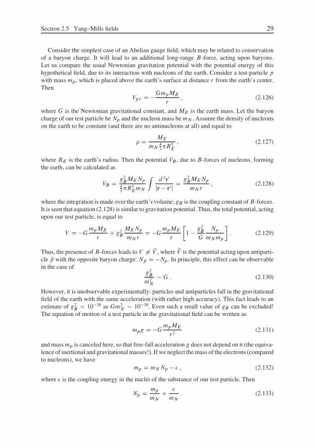
Section 2.5 Yang–Mills fields 29
Consider the simplest case of an Abelian gauge field, which may be related to conservationof a baryon charge. It will lead to an additional long-range B-force, acting upon baryons.Let us compare the usual Newtonian gravitation potential with the potential energy of thishypothetical field, due to its interaction with nucleons of the earth. Consider a test-particle pwith mass mp , which is placed above the earth’s surface at distance r from the earth’s center.Then
Vgr D �GmpME
r, (2.126)
where G is the Newtonian gravitational constant, and ME is the earth mass. Let the baryoncharge of our test particle beNp and the nucleon mass bemN . Assume the density of nucleonson the earth to be constant (and there are no antinucleons at all) and equal to
� D ME
mN43�R
3E
, (2.127)
where RE is the earth’s radius. Then the potential VB , due to B-forces of nucleons, formingthe earth, can be calculated as
VB D g2BMENp
43�R
3EmN
Zd 3r0
jr � r0j D g2BMENp
mN r, (2.128)
where the integration is made over the earth’s volume; gB is the coupling constant ofB-forces.It is seen that equation (2.128) is similar to gravitation potential. Thus, the total potential, actingupon our test particle, is equal to
V D �GmpME
rC g2
B
MENp
mN rD �GmpME
r
�1 � g2
B
G
Np
mNmp
�. (2.129)
Thus, the presence ofB-forces leads to V ¤ NV , where NV is the potential acting upon antiparti-cle Np with the opposite baryon charge: N Np D �Np . In principle, this effect can be observablein the case of
g2B
m2N
� G . (2.130)
However, it is unobservable experimentally: particles and antiparticles fall in the gravitationalfield of the earth with the same acceleration (with rather high accuracy). This fact leads to anestimate of g2
B < 10�38 as Gm2N � 10�38. Even such a small value of gB can be excluded!
The equation of motion of a test particle in the gravitational field can be written as
mpg D �GmpME
r2(2.131)
and massmp is canceled here, so that free-fall acceleration g does not depend on it (the equiva-lence of inertional and gravitational masses!). If we neglect the mass of the electrons (comparedto nucleons), we have
mp D mNNp � , (2.132)
where is the coupling energy in the nuclei of the substance of our test particle. Then
Np D mp
mNC
mN. (2.133)

30 Chapter 2 Lagrange formalism. Symmetries and gauge fields
In the presence of B-forces, the Newtonian equation of motion takes the form
mpg D �mpME
r2C C g2
B
r2
ME
m2N
, (2.134)
where C D G � g2B=m
2N can be identified with the measured gravitational constant Gexp . In
other words, equation (2.134) can be rewritten as
mpg D �mpME
r2Gexp
�1 � g2
B
Gexpm2N
mp
�. (2.135)
The second term here breaks the equivalence of inertional and gravitational masses, which isexperimentally established with an accuracy of the order of 10�8 in classical Eotvos experi-ments for different substances. A typical modern estimate from similar experiments gives
g2B
Gm2N
mp� 10�3 g2
B
Gm2N
< 10�12 , (2.136)
where we have taken into account that the difference of =mp for different substances is of theorder of 10�3. Accordingly,
g2B
Gm2N
< 10�9 . (2.137)
Thus, the experimentally established equivalence of inertional and gravitational masses leadsto the following upper bound of B-forces coupling constant: g2
B < 10�47! Accordingly, B-forces (if they exist at all) are much weaker even than gravitation! Thus, in every practicalsense, we can exclude the existence of any massless gauge fields except the electromagneticfield. Experimentally observed, vector mesons are massive and break the local gauge invari-ance. Thus, it seems that the beautiful idea of the introduction of new gauge fields becomesrather doubtful. Later we shall see how this problem is solved in modern particle theory.
2.6 The geometry of gauge fields
Let us make some generalizations. We have seen above that the rotation of the vectorin isotopic space on some small angle Eƒ .j Eƒj 1/ can be written as (cf. (2.99d))
E' ! E'0 D E' � Eƒ � E' , (2.138)
which is an infinitesimal version of the general transformation
E' ! E'0 D exp.i EI � Eƒ/ E' , (2.139)
where EI are matrix generators:
I1 D0
@0 0 00 0 �i0 i 0
1
A , I2 D0
@0 0 i
0 0 0�i 0 0
1
A , I3 D0
@0 �i 0i 0 00 0 0
1
A . (2.140)
Here the matrix elements can be written as
.Ii /mn D �i"imn , (2.141)

Section 2.6 The geometry of gauge fields 31
where "imn is the antisymmetric Levi–Civita symbol. Accordingly, by components,equation (2.138) can be written as
'0m D .1 C iIiƒi /mn'n D .ımnC "imnƒi /'n D 'm� "minƒi'n D . E'� Eƒ� E'/m .
(2.142)Local transformations have the form
E' ! E'0 D exp�i EI � Eƒ.x/ E' D S.x/ E' , (2.143)
where S.x/ denotes the operator of local rotation. Matrices I are generators of thevector representation of rotation group O.3/ (or SU.2/) and satisfy the well-known(angular momentum) commutation relations:
ŒIi , Ij � D i"ijkIk D CijkIk . (2.144)
Here Cijk denote structural constants of the SU.2/ group, in this case Cijk D i"ijk .Naturally, structural constants for other Lie groups are different, but commutation re-lations for generators are always written as in equation (2.144).
For an arbitrary Lie group, generators satisfy the Jacobi identity
ŒŒIi , Ij �, Ik�C ŒŒIj , Ik�, Ii �C ŒŒIk , Ii �, Ij � D 0 , (2.145)
which reduces (for structural constants) to
CijlClkm C CjklClim C CkilCljm D 0 . (2.146)
So far we have analyzed the isovector field. A more fundamental approach requiresintroduction of isospinors for the same SU.2/ group7. Rotation of fundamental two-
dimensional spinor D � 1 2
can be written as
0 D exp
�i
2E� � Eƒ.x/
� .x/ D S.x/ .x/ , (2.147)
where S.x/ is 2 � 2 matrix and E� are Pauli matrices in isotopic space, �i=2 satisfycommutation relations (2.144), and from the beginning we are writing the local trans-formation. For the general n-dimensional case we have
.x/ ! 0.x/ D expŒiM aƒa.x/� .x/ D S.x/ .x/ , (2.148)
where a takes the values 1, 2, 3 (SU.2/ group!); here is the n-component spinor,and M a are n � n matrices, satisfying commutation relations like (2.144).
7 Below we shall return to the detailed analysis of spinors; here it is sufficient to remember some ele-mentary information from the standard course on quantum mechanics.

32 Chapter 2 Lagrange formalism. Symmetries and gauge fields
If we consider local transformations of fields, the field derivative @� , as we haveseen above, is transformed in a noncovariant way:
@� 0 D S.@� /C .@�S/ . (2.149)
The reason for this is purely of a “geometrical” nature. The fields .x/ and .x Cdx/ D .x/ C d in nearby (infinitesimally close) points of space-time are mea-sured relative to different (rotated by local gauge transformations) axes in isotopicspace, shown in Figure 2.2(a). Thus, the value of d contains information not only onfield change with distance, as we move from point x to xCdx, but also on the appro-priate change due to the rotation of the axes in isotopic fields. To construct covariantderivative, we have to compare .x C dx/ not with .x/, but with the value whichthe field .x/ acquires due to translation from x to x C dx with fixed directions ofaxes in isotopic space, which is denoted below as Cı and called the field obtainedas a result of “parallel” transfer, as shown in Figure 2.2(b). Let us assume that ı isproportional to field itself and also to translation dx�, so that it can be written as
ı D igM aAa�dx� , (2.150)
(a)
(b)
Figure 2.2. (a) The value of d contains information both on the change of and on thetransformation of coordinate axes in isotopic space during the transfer from point x to xCdx.(b) The value of ı , determined by “parallel” transfer.

Section 2.6 The geometry of gauge fields 33
where g is some constant and Aa� is the gauge field, which in some sense determineshow axes in isotopic space change during the transfer from one point to the other. The“true” or covariant derivative of is now determined by the difference
D D . C d / � . C ı / D d � ı D d � igM aAa�dx� (2.151)
and equal toD
dx�D D� D @� � igM aAa� . (2.152)
The situation here is similar to that in the theory of gravitation [33], where the covariant deriva-tive of some vector V � is defined as
D�V� D @�V
� C ��
��V � , (2.153)
where Christoffel coefficients ����
connect the components of the vector in a given point withits components in a nearby point, from which this vector is transferred by parallel translationin Riemann space.
Equation (2.152) gives the general definition of the covariant derivative in the Yang–Mills theory for an arbitrary field , which is transformed under some irreducible rep-resentation of some gauge group with generators M a [56]. Consider the followingsimple examples:
� U.1/ group:
' ! e�iƒ' , '� ! eiƒ'� , M D �1 ,
D� D @� C igA� g D e (2.154)
– electrodynamics.
� SU.2/ group:
vector representation:
.M a/mn D �i"amn , .a,m,n D 1, 2, 3/ ,
D�'m D @�'m � ig.M a/mnAa�'n D @�'m � g"amnAa�'n (2.155)
D .@� E' C g EA� � E'/m ,
where EA is the same gauge field, which was denoted as EW above.
spinor representation:
M a D 1
2�a , .a D 1, 2, 3/ ,
D� D @� � i g2
E� � EA� (2.156)
– Yang–Mills theory.

34 Chapter 2 Lagrange formalism. Symmetries and gauge fields
Thus, under an arbitrary rotation in isotopic space the field is transformed as
! S.x�/ , (2.157)
and the covariant derivative is transformed as the field itself:
D� ! D0�
0 D S.x�/D� . (2.158)
It is convenient to introduce matrix notations
OA� D M aAa� , (2.159)
so that equation (2.152) takes the form
D� D .@� � ig OA�/ . (2.160)
Transformation to a new coordinate system in isotopic space, with the account of(2.158), gives
.@� � ig OA0�/
0 D S.@� � ig OA�/ . (2.161)
Assuming here 0 D S , we obtain
OA0� D S OA�S�1 � i
g.@�S/S
�1 , (2.162)
which gives the general form of the gauge transformations of Yang–Mills fields (gen-eralized gradient transformation). Consider again the same examples:
� U.1/ group:
S D e�iƒ , @�S D �i.@�ƒ/e�iƒ ,
A0� D A� C 1
e@�ƒ .g D e, M D �1/ , D� D @� C igA� . (2.163)
� SU.2/ group:
spinor representation:
S D exp
�i
2E� � Eƒ
�, @�S D i
2E� � @� EƒS , (2.164)
EA0� D EA� � Eƒ � EA� C 1
g@� Eƒ , (2.165)
which follows from (2.162) for j Eƒj 1, with the account of commutation relationsŒ�a, �b� D i2"abc�c , and coincides with (2.103).
Consider now the succession of “parallel transfers” of our field around the closed pathABCD, shown in Figure 2.3. Let us start from point A, where the field is assumed to

Section 2.6 The geometry of gauge fields 35
Figure 2.3
be equal to A,0. Then its change due to the transfer to point B is determined by thecovariant derivative (cf. (2.158), (2.152)), which gives
B D A,0CD� A,0x�C1
2D�D� A,0x
�x�C� � � D .1Cx�D�C� � � / A,0 .
Next, performing transfer to point C , up to the terms of first order, we get
C D B C ıx�D� B D .1 C ıx�D�/ B D .1 C ıx�D�/.1 Cx�D�/ A,0 .
Next, the transfer to point D and the return to initial point A give
D D .1 �x�D�/ C , (2.166)
A,1 D .1 � ıx�D� / DD .1 � ıx�D� /.1 �x�D�/.1 C ıx�D�/.1 Cx�D�/ A,0 (2.167)
D ®1 C ıx�x� ŒD�,D� �
¯ A,0 , (2.168)
where the commutator of operators of covariant differentiation appeared:
ŒD�,D� � D Œ@� � ig OA�, @� � ig OA� � D �ig®@� OA� � @� OA� � igŒ OA�, OA� �¯
.(2.169)
Let us introduce the field tensor
G�� D @� OA� � @� OA� � igŒ OA�, OA�� , (2.170)
so thatŒD�,D�� D �igG�,� . (2.171)
Equation (2.170), in fact, gives the general definition of the tensor of Yang–Mills fieldsfor an arbitrary gauge group. Accordingly, equation (2.168) can be written as
A,1 D .1 � igS��G��/ A,0 , S�� D ıx�x� (2.172)

36 Chapter 2 Lagrange formalism. Symmetries and gauge fields
and we obtain A,1 � A,0 D �igS��G�� A,0 . (2.173)
Thus, a nonzero gauge field tensor leads to a finite physical result as we go aroundthe closed path, which is proportional to the flux of the gauge field G�� through thepath (contour) areaS��: the field is rotated in isotopic space. It is easy to see thatthe field tensor G�� is invariant relative to gauge transformations:
G�� D SG��S�1 (2.174)
so that it cannot be reduced to zero, using only such transformations. At the same time,if G�� is zero for some gauge, it remains zero for all other gauges.
Consider again our examples:
� U.1/ group:G�� F�� D @�A� � @�A� (2.175)
– the usual field tensor of electrodynamics.
� SU.2/ group:
ŒM a,M b� D i"abcMc , Ga�� D @�A
a� � @�Aa� C g"abcA
b�A
c� , (2.176)
which in vector notations in isotopic space
EG�� D @� EA� � @� EA� C g EA� � EA� (2.177)
coincides with definition (2.112) given above.
Here we again can note an analogy to the theory of gravitation. The tensor of Yang–Mills fieldsis, in some sense, analogous to the Riemann–Christoffel curvature tensor [33]:
R���� D @����� � @����� C �
�
������ � ��
������ . (2.178)
The parallel transfer of an arbitrary vector V � around the closed contour in Riemann spaceleads to the following difference between the initial and final components of the vector:
V � D 1
2R�
���V �S�� , (2.179)
where S�� again denotes the area of the contour. The value of V � is different from zeroonly in the space of with finite curvature. In general relativity, this corresponds to the presenceof a nontrivial gravitational field.
Analyzing the transfer around the path forming the parallelepiped shown in Fig-ure 2.4, Feynman has given a simple derivation of the following identity for the fieldG��:
D�G�� CD�G�� CD�G�� D 0 , (2.180)

Section 2.6 The geometry of gauge fields 37
Figure 2.4
which in fact determines the second pair of “Maxwell equations” for the Yang–Millsfield (2.121). In the case of U.1/ gauge symmetry, this reduces simply to (2.119):
@�F�� C @�F�� C @�F�� D 0 . (2.181)
Briefly, the derivation goes as follows. In Figure 2.4 we show the path (contour)ABCDAPSRQPA. There are another two paths of the same type along the bor-ders of two pairs of opposite facets of the parallelepiped, so that along the borders ofall six facets we can draw the path .ABCDAPSRQPA/ C .ADSPABQRCBA/ C.APQBADCRSDA/. All parts of this contour are now passed twice in two oppositedirections. Accordingly, the field is not changed as we go around our closed path,which immediately gives the identity (2.180).
In the theory of gravitation there exists the similar Bianchi identity for the Riemann–Christoffeltensor:
D�R���� CD�R
���� CD�R
���� D 0 . (2.182)
The analogy of gauge field theories and the theory of gravitation can be expressed as inTable 2.1.
Table 2.1. Analogies between gauge field theories and gravitation.
Gauge theories General relativity
Gauge transformations Coordinate transformations
Gauge group Group of all coordinate transformations
Potential of gauge field A� Christoffel coefficients ����Field tensor G�� Tensor of curvature R�
���
All these analogies actually exist on a deeper level. Even during early stages of the develop-ment of gauge field theories, it was shown by Utiyama [68] that the equations of Einstein’sgeneral relativity theory can be derived using the idea and general scheme of gauge field the-ory, if we take the Lorentz group (coordinate transformations of the special theory of relativity)

38 Chapter 2 Lagrange formalism. Symmetries and gauge fields
and demand the invariance of the theory with respect to corresponding local transformations(when parameters of the Lorentz group are considered as arbitrary functions of coordinate inMinkowski space).
2.7 A realistic example – chromodynamics
Let us briefly consider the structure of quantum chromodynamics (QCD) as an exam-ple of realistic non-Abelian gauge theory. Quantum chromodynamics is based on thefundamental experimental discovery: each quark of the given “flavor” u, d , s, c, t , bpossesses an additional quantum number, which is called “color”, and which can takethree possible values (1, 2, 3 orR,G,B)8. Then, each quark field is represented by thefundamental spinor of the SU.3/ group9:
q D0
@q1
q2
q3
1
A . (2.183)
The color symmetry is exact, and QCD Lagrangian should be invariant to SU.3/ grouptransformations:
q ! Uq , (2.184)
where the 3�3-matrices U are unitary and unimodular:
UCU D 1 , DetU D 1 ,
U D eiT , T D TC , SpT D 0 . (2.185)
These matrices (transformations) depend on eight parameters (“rotation angles”) "a,and accordingly there are eight generators �i=2 .i D 1, : : : , 8/:
�1 D0
@0 1 01 0 00 0 0
1
A , �2 D0
@0 �i 0i 0 00 0 0
1
A , �3 D0
@1 0 00 �1 00 0 0
1
A ,
�4 D0
@0 0 10 0 01 0 0
1
A , �5 D0
@0 0 �i0 0 0i 0 0
1
A , �6 D0
@0 0 00 0 10 1 0
1
A ,
�7 D0
@0 0 00 0 �i0 i 0
1
A , �8 D 1p3
0
@1 0 00 1 00 0 �2
1
A (2.186)
8 The necessity of this quantum number was clear from the very beginning of the quark model, as itallowed to lift certain contradictions with the Pauli principle.
9 A rather clear and compact presentation of irreducible representations of this group, though in relationto the other problem of particle physics (approximate symmetry of hadrons and their quark structure),can be found in [40].
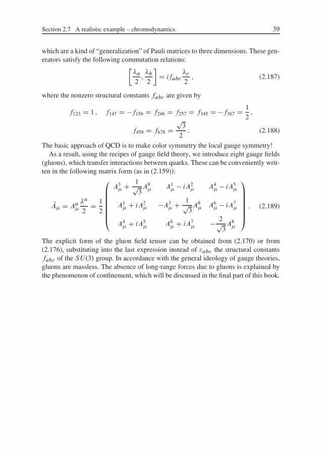
Section 2.7 A realistic example – chromodynamics 39
which are a kind of “generalization” of Pauli matrices to three dimensions. These gen-erators satisfy the following commutation relations:
��a
2,�b
2
�D ifabc
�c
2, (2.187)
where the nonzero structural constants fabc are given by
f123 D 1 , f147 D �f156 D f246 D f257 D f345 D �f367 D 1
2,
f458 D f678 Dp
3
2. (2.188)
The basic approach of QCD is to make color symmetry the local gauge symmetry!As a result, using the recipes of gauge field theory, we introduce eight gauge fields
(gluons), which transfer interactions between quarks. These can be conveniently writ-ten in the following matrix form (as in (2.159)):
OA� D Aa��a
2D 1
2
0
BBBBBB@
A3� C 1p
3A8� A1
� � iA2� A4
� � iA5�
A1� C iA2
� �A3� C 1p
3A8� A6
� � iA7�
A4� C iA5
� A6� C iA7
� � 2p3A8�
1
CCCCCCA
. (2.189)
The explicit form of the gluon field tensor can be obtained from (2.170) or from(2.176), substituting into the last expression instead of "abc the structural constantsfabc of the SU.3/ group. In accordance with the general ideology of gauge theories,gluons are massless. The absence of long-range forces due to gluons is explained bythe phenomenon of confinement, which will be discussed in the final part of this book.

Chapter 3
Canonical quantization, symmetries in quantumfield theory
3.1 Photons
3.1.1 Quantization of the electromagnetic field
Now we have to move from classical to quantum field theory. The procedure of canoni-cal field quantization is done in complete analogy to similar procedures for mechanicalsystems. First of all, we shall consider the quantum field theory of free (noninteracting)fields, and we shall start with the case of the electromagnetic field – not the simplestcase, but nonetheless physically quite important. We have already seen above that theelectromagnetic field is an example of an (Abelian) gauge field. This leads to someadditional complications related to the correct account of gauge invariance. For theelectromagnetic field these problems are solved in a relatively simple way, within thecanonical quantization procedure, while for non-Abelian Yang–Mills fields we needa much a more complicated scheme of quantization, based on functional integration,which will be discussed much later. The presentation in this chapter is essentially basedon [6].
From a mechanical point of view, the field is represented as the system with aninfinite (continuous) number of degrees of freedom. However, it is convenient to startfrom the classical description of the field, which deals with an infinite, but discrete,set of variables. We shall consider the electromagnetic field in the so-called Coulombgauge, when its vector potential A.r, t / satisfies the condition of transversality:
divA D 0 . (3.1)
The scalar potential is taken as ' D 0, while the electric E and magnetic H field aredefined as1
E D � PA , H D rotA . (3.2)
Maxwell equations reduce, in this case, to the wave equation for the vector potentialA
r2A � @2A@t2
D 0 . (3.3)
It is well known that the six components of the electromagnetic field are written in the form ofan antisymmetric tensor:
F �� D @�A� � @�A� , (3.4)
1 Let us recall that we are using the system of units with the speed of light c D 1.

Section 3.1 Photons 41
which immediately leads to homogeneous Maxwell equations:
@�F �� C @�F �� C @�F �� D 0 . (3.5)
In a vacuum (in the absence of sources) inhomogeneous Maxwell equations are written as
@�F�� D 0 (3.6)
or�A� � @�.@�A�/ D 0 . (3.7)
We know that these equations follow from the variational principle with a Lagrangian
L D � 1
16�F��F
�� , (3.8)
where A� is considered as a dynamic variable. However, for the given values of field strengthF�� , the 4-vector potential A� is not single valued, but is determined only up to the gradienttransformation
A� ! A0� D A� C @�ƒ.x/ . (3.9)
If we require forƒ.x/ the validity of an additional condition �ƒ D �@�A�, we easily obtainfor the field, transformed by (3.9), @�A�
0 D 0. Now we can just drop the prime over A� andwrite the so-called Lorentz condition:
@�A� D 0 . (3.10)
Then (3.7) is transformed to�A� D 0 (3.11)
i. e., the wave function for the 4-vector potential. The Lorentz gauge (3.10) gives one equationfor four components of the potential, reducing the number of independent components of thefield to three. However, this condition still does not make A� singly defined. For A� satis-fying Lorentz condition, we may introduce A0
� D A� C @�ƒ, which also satisfies it due to
�ƒ.x/ D 0. Let us now choose ƒ.x/ to satisfy @ƒ@t
D �', then obviously '0 D 0, so thatequation (3.10) gives r �A D divA D 0. Thus, we come to the Coulomb gauge, with only twoindependent components of the electromagnetic field (transversality condition), in agreementwith reality.
Transformation to a discrete set of field variables is achieved by considering thefield system in a finite spatial volume V (below, for shortness of notation, we just putV D 1) [33]. The vector potential is represented by a Fourier expansion over planewaves:
A DX
k
.akeikr C a�
ke�ikr/ , (3.12)
where expansion coefficients ak depend on time according to
ak � e�i!kt , !k D jkj . (3.13)

42 Chapter 3 Canonical quantization, symmetries in quantum field theory
Due to transversality condition (3.1), we have
ak � k D 0 . (3.14)
In (3.12) summation is done over the infinite discrete set of kx , ky , kz . As usual, we canmake transformation from summation to integration over kx , ky , kz , introducing d 3k
.2/3 ,as the number of possible values of k, in the infinitesimal volume of k-space d 3k Ddkxdkydkz . Finally, the state of the field is completely determined by amplitudes ak,which are considered as the set of classical field variables.
Let us introduce canonical field variables as
Qk D 1p4�.ak C a�
k/ , (3.15)
Pk D � i!kp4�.ak � a�
k/ D PQk . (3.16)
Obviously, these variables are real. Then the series (3.12) can be rewritten as
A D p4�X
k
�Qk cos kr � 1
!kPk sin kr
�. (3.17)
To determine the field Hamiltonian H , we calculate the total energy:
E D 1
8�
Zd 3r.E2 CH2/ (3.18)
and express it via the variables Qk and Pk. To do this, we find E andH from (3.2) and(3.17), substitute the appropriate expressions into (3.18) and obtain, after the integra-tion over coordinates,
H D 1
2
X
k
P2k C !2
kQ2k
�. (3.19)
From the condition of transversality, bothPk andQk are orthogonal to vector k, so thatthey, in fact, possess only two independent components. The directions of these vectorsare defined by the polarization directions of the appropriate wave. Let us denote twocomponents of Pk andQk in the plane orthogonal to k as Pk˛ andQk˛ , with ˛ D 1, 2.Then (3.19) can be rewritten as
H D 1
2
X
k˛
P 2k˛ C !2
kQ2k˛
�. (3.20)
Thus, the HamiltonianH is represented by the sum of independent terms, each havingthe form of the Hamiltonian of the harmonic oscillator.
Now we can perform quantization. The way to quantize an oscillator is well knownfrom quantum mechanics [35]. Quantization reduces to the change of the generalizedcoordinates Qk˛ and generalized momenta Pk˛ by corresponding operators, satisfy-

Section 3.1 Photons 43
ing the standard commutation relations2:
Qk˛Pk˛ � Pk˛Qk˛ ŒQk˛ ,Pk˛� D i . (3.21)
For different values of k˛, the corresponding operators just commute. Accordingly,the fields A,E,H also become operators.
The Eigenvalues of the Hamiltonian (3.20) obviously are
E DX
k˛
Nk˛ C 1
2
�!k , (3.22)
whereNk˛ are integer numbers, representing the number of photons in quantum states,characterized by k˛. The matrix elements of operator Qk˛ are also well known fromquantum mechanics [35]:
hNk˛jQk˛jNk˛ � 1i D hNk˛ � 1jQk˛jNk˛i DsNk˛
2!k. (3.23)
The matrix elements Pk˛ D PQk˛ differ from (3.23) by a factor ˙i!k.Let us introduce new operators:
ck˛ D 1p2!k
.!kQk˛ C iPk˛/ , cCk˛ D 1p
2!k.!kQk˛ � iPk˛/ . (3.24)
Then, from (3.23) and (3.24) we obtain
hNk˛ � 1jck˛jNk˛i D hNk˛jcCk˛jNk˛ � 1i D
pNk˛ . (3.25)
From (3.24) and (3.21) we immediately get commutation relations for operators ck˛and cC
k˛:ck˛c
Ck˛ � cC
k˛ck˛ Œck˛ , cCk˛� D 1 . (3.26)
For different k and ˛ these operators simply commute. The operators ck˛ and cCk˛ are
called operators of annihilation and creation of photons in the state with wave vector(momentum) k and polarization ˛. The origin of these terms is obvious from (3.25).For historical reasons, the formalism, based on the use of such operators is calledsecond quantization.
The operator of the vector potential (with the use of (3.12), (3.15), (3.16), and(3.24)) can now be written as
A DX
k˛
ck˛Ak˛ C cC
k˛A�k˛
�, (3.27)
where
Ak˛ D p4�
e.˛/p2!k
eikr , (3.28)
2 Note that here we use „ D 1.

44 Chapter 3 Canonical quantization, symmetries in quantum field theory
where e.˛/ is the unit vector of polarization for the given field oscillator. Obviously,we have e.˛/ � k D 0, so that this vector is orthogonal to the photon momentum k. Toeach value of k we have two independent directions of polarization ˛ D 1, 2.
Similarly we can write down expansions for electric E and magnetic H field opera-tors:
E DX
k˛
.ck˛Ek˛ C cCk˛E
�k˛/ , (3.29)
H DX
k˛
.ck˛Hk˛ C cCk˛H
�k˛/ , (3.30)
whereEk˛ D i!kAk˛ , Hk˛ D Œn � Ek˛� , (3.31)
where n D k=!k is the unit vector directed along photon propagation. The vectorsAk˛, introduced in (3.28), satisfy the following orthonormality condition:
Zd 3rAk˛A
�k0˛0 D 2�
!kı˛˛0ıkk0 , (3.32)
where we have taken into account that two independent polarization vectors are or-thogonal: e.˛/ � e.˛0/� D 0. In fact, the values of Ak˛ (plane waves) can be treated aswave functions of a photon with momentum k and polarization e.˛/3.
From (3.32) and (3.31) it is easy to obtain
1
4�
Zd 3r.Ek˛E
�k0˛0 CHk˛H
�k0˛0/ D !kıkk0ı˛˛0 . (3.33)
Substituting (3.29) and (3.30) into (3.18) and using (3.33), we find
H DX
k˛
1
2.ck˛c
Ck˛ C cC
k˛ck˛/1
4�
Zd 3r.Ek˛E�
k0˛0 CHk˛H�k0˛0/
DX
k˛
1
2.ck˛c
Ck˛ C cC
k˛ck˛/!k (3.34)
or, using commutation relations (3.26),
H DX
k˛
cCk˛ck˛ C 1
2
�!k (3.35)
which gives the secondary quantized Hamiltonian of the system of photons. After com-parison with (3.22) it becomes clear that
ONk˛ D cCk˛ck˛ (3.36)
3 Let us stress that these wave functions cannot be understood as probability amplitudes of spatiallocalization of photon, as there is no sense in defining the coordinate of a particle moving with thevelocity of light.

Section 3.1 Photons 45
represents the operator of the number of photons in k˛ state, which is diagonal in occu-pation number representation, with integer eigenvalues. Note that (3.33) correspondsto the wave function normalization to a “single photon per volume V D 1”.
In classical theory of electromagnetic field its momentum is defined as [33]
P D 1
4�
Zd 3r ŒE �H� . (3.37)
Replacing E and B by operators (3.29) and (3.30), we obtain
P DX
k˛
cCk˛ck˛ C 1
2
�k , (3.38)
which corresponds to each photon carrying the momentum k.The presence in (3.35) and (3.38) of the terms, independent of occupation numbers
(1=2 contribution in parenthesis), corresponds to an infinite contribution of vacuumfluctuations (“zero-level” oscillations) of the electromagnetic field. This is the firstexample we meet of a typical “field theory divergence”. In most cases, in this situationwe can simply shift the origin of an energy scale (or the origin of momentum scale)and write
H DX
k˛
cCk˛ck˛!k , P D
X
k˛
cCk˛ck˛k . (3.39)
The origin of energy or momentum scale is “renormalized” here by infinite (“vacuum”)constants, which are independent of excitations of the field system. However, we muststress that the presence of an infinite energy (momentum) of the vacuum (zero-leveloscillations) is absolutely real physically and reflects the quantum nature of the field,leading to some finite experimental effects. One of the best examples is the so-calledCasimir effect, which we shall discuss below.
3.1.2 Remarks on gauge invariance and Bose statistics
The choice of potentials in electrodynamics, as is well known, is not unique. Abovewe have used the Coulomb gauge (3.1). In the general case, components of vectorpotential A� can undergo the gradient transformation like
A� ! A� C @�ƒ . (3.40)
For plane waves, limiting ourselves to transformations, which do not change this formof potential (i. e., its proportionality to exp.�ik�x�/), this nonuniqueness reducesto the possibility of adding to the wave amplitude an arbitrary 4-vector proportionalto k�.
In the case of an arbitrary gauge, the 4-potential of the field can be written in theform, generalizing (3.27),
A� DX
k˛
.ck˛A�
k˛C cC
k˛A��k˛/ , (3.41)

46 Chapter 3 Canonical quantization, symmetries in quantum field theory
where wave functions of photon are
A�
kD p
4�e�p2!e�ik�x
�
, (3.42)
where e� is a space-like 4-vector of polarization, which satisfies the conditione�e
�� D �1. The space-like nature of the 4-vector of polarization is obvious fromthe condition of four-dimensional transversality, as the wave vector (momentum) of areal photon always belongs to the light cone. In these notations our gradient (gauge)transformation reduces to
e� ! e� Cƒk� , (3.43)
whereƒ D ƒ.k�/ is an arbitrary scalar function of k�. Transversality of polarizationmeans that we always can choose the gauge, guaranteeing three-dimensional transver-sality, when we choose
e� D .0, e/ , e � k D 0 . (3.44)
Four-dimensional transversality, equivalent to the Lorentz condition (3.10), can bewritten in an invariant form as
e�k� D 0 . (3.45)
This condition, as well as e�e�� D �1, is not violated by transformation (3.43), asfor a real photon we always have k2 D 0 (massless photon on the light-cone!). Themeasurable physical characteristics should obviously be invariant to gauge transfor-mations.
Photons are described by Bose statistics. This is obvious from the fact that the num-ber of photons Nk˛ in k˛ state may be an arbitrary integer, as well as from the formof commutation relations (3.26). A Bose field can acquire the classical limit. It is wellknown that the properties of the quantum system approach that of the classical, whenquantum numbers, determining the system state, become large. For an electromagneticfield this means that the number of photons Nk˛ is to be large enough. In this case wecan neglect unity in the right-hand side of commutation relations (3.26) (obviously,this corresponds to the limit of „ ! 0 for the usual system of units) and write
cCk˛ck˛ � ck˛c
Ck˛ , (3.46)
so that operators ck˛ , cCk˛ can be considered as classical filed amplitudes. However,
some care is needed, as in the case of all Nk˛ � 1 we shall get the infinity after thesummation over k˛ for the field energy (3.22).
In fact, from a physical point of view it is sensible to consider the values of the fields,averaged over some finite time intervals t . In Fourier expansion of a such averagedfield E the main contribution comes from the frequency region !t < 1. Now, toderive the conditions of quasiclassicality we have to consider only field oscillatorswith ! < 1=t . The number of oscillators with frequencies from zero to ! � 1=t ,

Section 3.1 Photons 47
by the order of magnitude, is equal to (V D 1):!c
�3 � 1
.ct/3. (3.47)
The energy of the field in the unit volume is of the order of E2. Dividing this energy bythe number of oscillators and by the average photon energy � „!, we get the followingestimate for the number of photons:
N � E2c3
„!4. (3.48)
Then from the condition N � 1 and (3.47) we obtain
jEj �p„c.ct/2
, (3.49)
which determines the criterion of quasiclassicality4. We see that the field is be strongenough, and stronger for smaller time intervalst . For the time-dependent fieldt �!�1, so that a sufficiently weak alternating field cannot be described quasiclassically.Only static fields, for which t ! 1, can always be treated as classical.
On the measurability of fields in quantum electrodynamics
The existence of a finite limit for velocity of propagation of interactions (speed of light) inrelativistic theory leads to a number of additional limitations for the measurability of physi-cal characteristics (variables). At the early stages of the development of quantum field theorythese limitations were discussed by Landau and Peierls. The qualitative discussion of theselimitations can be found in the Introduction to [6]. During this analysis, Landau and Peierlsformulated the fundamental question of the possibility of measuring an electromagnetic fielditself. They claimed that the measurement of any component of (say) an electric field requiresthe determination of the momentum of a charged test particle, so that the imminent action ofthe field, radiated during this operation, will always lead to unavoidable limitations of fieldmeasurements. They concluded that the precise measurement of field strength becomes im-possible, in contradiction with the basic points of quantum electrodynamics discussed above.This fact, as well as a number of similar difficulties to be discussed later, were the reason fora long period of Landau’s rather skeptical opinion on quantum field theory in general.
The problem of fields measurability was analyzed in more detail by Bohr and Rosenfeld(cf. an interesting review of this problem by Rosenfeld in [49]). It was demonstrated, that allthe difficulties are essentially solved (in the spirit of the Copenhagen interpretation of quan-tum mechanics) if we use the finite (not point-like) test particles. For example, consider themeasurement of the Ex component of an electric field, averaged over some volume and timeintervals. Let us use the test particle with volume V and homogeneous charge density � andmeasure its momenta p0
x and p00x at the beginning and end of time interval T . Making this test
particle heavy enough, we can achieve its arbitrarily small displacement during this interval,and obtain for the average value of the field NEx
NEx�V T D p00x � p0
x . (3.50)
4 For better understanding here we explicitly write down both c and „.

48 Chapter 3 Canonical quantization, symmetries in quantum field theory
However, the measurement of the momentum of the test particle inevitably leads to someerror x in the determination of its position, according to the usual indeterminacy relation:px � „=x. This leads to indeterminacy NEx for the field value NEx , which is of the order of
NEx � „�V Tx
. (3.51)
However, it is obvious that this error can be made arbitrarily small by just increasing the chargedensity of a test particle.
In a similar way, we can analyze the measurability of charges and currents [49]. In theopinion of Bohr and Rosenfeld, such arguments demonstrate the absence of any contradic-tions in the basic principle of quantum electrodynamics. However, we should note that theCopenhagen interpretation of quantum theory, using the classical concepts as its inevitablepart, at present is not commonly accepted (nor is it considered to be absolutely satisfactory bymany researchers). The modern situation with the quantum limitations of field measurementsis discussed in [44].
3.1.3 Vacuum fluctuations and Casimir effect
The reality of vacuum (“zero-level”) fluctuations of an electromagnetic field is beautifullyillustrated by the so-called Casimir effect [28]. Consider two big ideally conducting metallicplanes, placed in a vacuum, at the distance a from each other, as it is shown in Figure 3.1.Let these metallic plates be just squares with sides L and L � a. Consider the modes ofan oscillating electromagnetic field in the volume L2a. Boundary conditions require that the
Figure 3.1

Section 3.1 Photons 49
vector of electric fieldE be perpendicular, while the vector of magnetic fieldB is parallel to theinternal surface of the plate. Only transversal modes contribute to energy. If the wave vectorcomponent kz , orthogonal to the surface of plates, is nonzero, it can acquire only discretevalues kz D n�=a .n D 1, 2, : : :/, so that the nodes of the field are at the plates. We alsohave to take into account two polarization states. If kz D 0, we remain with only one mode (theelectric field component of this mode is just zero, as a tangential electric field is absent on thesurface of an ideal conductor). Then, the energy of zero-level oscillations of electromagneticfield in the volume between plates is given by
E DX
k˛
1
2„!k˛ D
X
k˛
1
2„cjk˛j D „c
2L2Z
d 2kk.2�/2
"
jkkj C 21X
nD1
r
k2k C n2�2
a2
#
. (3.52)
This expression is obviously infinite. However, let us subtract from (3.52) the similar expres-sion for the energy of vacuum fluctuations in the same volume, but in the absence of metallicplates:
E0 D „c2L2Z
d 2kk.2�/2
a
Z 1
�1dkz
2�2qk2
k C k2z D „c
2L2Z
d 2kk.2�/2
2Z 1
0dnqk2
k C n2�2=a2 .
(3.53)Then, the change of the vacuum energy due to introduction of metallic plates (per unit surfaceof the plates) is given by
E D E �E0
L2D „c
2�
Z 1
0dk k
�k
2C
1X
nD1
pk2 C n2�2=a2 �
Z 1
0dnpk2 C n2�2=a2
�.
(3.54)This expression is still infinite, due to ultraviolet (large k!) divergences. However, we cantake into account that for wavelengths smaller than atomic size, the approximation of an idealconductors (considered as continuous medium) becomes inapplicable, Thus we have to intro-duce in the integrand of (3.54) some smooth cutoff function f .k/, which is equal to unity fork < km and tends to zero for k � km, where km is of the order of the inverse atomic size.Then we can write
E D „c �2
4a3
Z 1
0du
�pu
2f�a
pu�
C1X
nD1
puC n2f
�a
puC n2
�
�Z 1
0dn
puC n2f
�a
puC n2
� �, (3.55)
where we have introduced the dimensionless integration variable u D a2k2=�2. The last ex-pression can be rewritten as
E D „c �2
4a3
�1
2F.0/C F.1/C F.2/C � � � �
Z 1
0dnF.n/
�, (3.56)
where we have defined the function
F.n/ DZ 1
0du
puC n2f
�a
puC n2
�. (3.57)
For n ! 1 we have F.n/ ! 0 due to the properties of the cutoff function. To calculate thedifference between the sum and the integral in square brackets in equation (3.56), we may use

50 Chapter 3 Canonical quantization, symmetries in quantum field theory
the Eiler–Maclaurin summation formula, writing it as
1
2F.0/C F.1/C F.2/C : : :�
Z 1
0dnF.n/ D � 1
2ŠB2F
0.0/� 1
4ŠB4F
000.0/C � � � , (3.58)
where B� are Bernoulli numbers, defined by the series
y
ey � 1D
1X
�D0
B�y�
�Š. (3.59)
In particular, B2 D 1=6, B4 D �1=30, . . . . We have
F.n/ DZ 1
n2du
puf
��
pu
a
�, F 0.n/ D �2n2f
��n
a
�. (3.60)
Assuming that f .0/ D 1 and all its derivatives are zero at the same value of its argument, wehave F 0.0/ D 0, F 000.0/ D �4, while all higher order derivatives of F are zero. Thus, thevalue of the cutoff does not enter into the final results and we get
E D „c�2
a3
B4
4ŠD � �2
720
„ca3
. (3.61)
Then, the force (per unit square) acting upon the plates are
F D � �2
240
„ca4
. (3.62)
The negative sign here corresponds to attraction. It is remarkable that the existence of this(quite weak!) attractive force, due to vacuum fluctuations of the electromagnetic field, wasexperimentally confirmed, and the theoretical expression (3.62) was directly checked. It iseven more surprising that the existence of the Casimir force has to be taken into account [32]during construction and work of modern micromachines! This proves, beyond any doubt, that“zero-level” oscillations of an electromagnetic field are quite real.
3.2 Bosons
3.2.1 Scalar particles
Consider particles with spin 0. The state of a free spinless particle is completely de-termined by its momentum p. Its energy "p is defined by
"2p D p2 Cm2 or p2 D m2 (3.63)
or, as usually expressed, the particle is on its “mass surface”. Energy-momentum con-servation follows from the homogeneity of space-time. In quantum mechanics, therequirement of the symmetry towards an arbitrary translation of a coordinate systemmeans that the wave function of a particle with 4-momentum p is multiplied (as aresult of translation) by a phase factor (with modulus 1). This requirement is obeyedonly by the plane wave:
const � e�ipx , px D "pt � pr . (3.64)

Section 3.2 Bosons 51
The wave equation for our particles should have (3.64) as a partial solution for anyp, satisfying equation (3.63). This equation should also be linear, expressing the su-perposition principle: any linear combination of solutions also describes the possiblestate of a free particle. And finally, this equation should be of a sufficiently low orderin derivatives.
The spin of a particle is its angular momentum in a coordinate system at rest, and thestate of a particle in a system at rest is described by nonrelativistic quantum mechanics.Then, if a particle spin in a resting system is equal to s, its wave function in thiscoordinate system should have 2s C 1 components (i. e., be represented by a three-dimensional spinor of rank 2s) [35]. The particle with spin s D 0 in a resting systemis described by a three-dimensional scalar. However, this three-dimensional scalar canhave a double four-dimensional “origin” [6]: it can be a four-dimensional scalar ', butit also can be a time component 0 of some time-like 4-vector �, such that in a systemat rest only a 0 component is different from zero. Tensors of higher ranks are not tobe taken into account, as they will lead to differential equations of higher orders.
For a free particle, the only differential operator which can enter the wave equationis the operator of 4-momentum p:
p� D i@� D�i@
@t, �ir
�. (3.65)
A wave equation can be written as a differential relation between ' and �, con-structed with the help of operator p�, and satisfying the condition of relativistic in-variance. Obviously, the simplest variant of such relation has the following form:
p�' D m � , p� � D m' , (3.66)
wherem is a scalar, characterizing the particle5. Substituting � from the first equationin (3.66) to the second one, we get
.p2 �m2/' D 0 , (3.67)
which coincides with the Klein–Gordon equation (2.10), (2.29) for the scalar field '.Substituting ' � e�ipx into (3.67), we obtain p2 D m2, so that (3.63) is satisfied,and the scalarm is just the rest mass of our particle. As (3.63) is valid for a relativisticparticle with arbitrary spin, the Klein–Gordon equation is obeyed, in fact, by wavefunction components of particles with any spin.
The properties of a scalar field, satisfying the Klein–Gordon equation, were alreadydiscussed in detail above. For generality we shall consider here, from the very begin-ning, the case of a complex field. Its energy-momentum tensor, similar to (2.50), isgiven by
T �� D .@�'�/.@�'/C .@�'/.@�'�/ � g��L , (3.68)
5 There is no sense in introducing two scalars m1,m2, as they can always be made equal by the appro-priate redefinition of ', �

52 Chapter 3 Canonical quantization, symmetries in quantum field theory
where the Lagrangian L is defined in (2.56). In particular,
T00 D @'�@t
@'
@tC r'� � r' Cm2'�' , (3.69)
Ti0 D @'�@t
@'
@xiC @'�@xi
@'
@t. (3.70)
Then the 4-momentum of the field is determined by the integral
P� DZd 3rT�0 . (3.71)
From (3.69) we can see that T00 > 0, so that energy is positively defined, which, infact, determines the choice of signs in the Lagrangian.
Equation (3.69) can be used to normalize the field. The plane wave, normalized to“single particle in volume V D 1” can be written as
p D 1p2"p
e�ipx . (3.72)
Calculating (3.69) with (3.72), we obtain T00 D "p, so that the total energy in thevolume V D 1 is equal to the energy of a single particle.
Let us now proceed to quantization. Let us consider an expansion of an arbitrarywave function (field) over the complete set of eigenfunctions of a free particle, e. g.,the plane waves p from (3.72):
' DX
p
ap p , '� DX
p
a�p
�p . (3.73)
Quantization reduces to the replacement of the coefficients ap, a�p by the corresponding
operators of annihilation and creation of particles Oap , OaCp .
The principal aspect of relativistic theory is the existence of two solutions for equa-tion (3.63), which gives for the energy of a particle
"p D ˙pp2 Cm2 . (3.74)
Physically sensible are only "p > 0, as the negative particle energies correspond tothe instability of the system (absence of the ground state). We cannot just drop thesolutions with "p < 0, as the general solution of the wave equation is given by thesuperposition of all independent partial solutions, and the expansion of the field shouldbe performed over the complete set of eigenfunctions. Let us write
' DX
p
1p2"p
a.C/p ei.pr�"pt/ CX
p
1p2"p
a.�/p ei.prC"pt/ , (3.75)
where in the first sum the plane waves correspond to positive, while in the second theycorrespond to negative frequencies. Here and below we take "p D p
p2 Cm2, i. e.,the positive definite energy of the physical particle.

Section 3.2 Bosons 53
The recipe for the correct transition to the second quantization can now be formu-lated in the following way:
� a.C/p ! Oap is the annihilation operator of a particle with momentum p;
� a.�/p ! ObC�p is the creation operator of an antiparticle with momentum �p.
The last change to be made is due to the time dependence in the second sum in (3.75)being ei"pt D .e�i"pt /�, which corresponds to the appearance of one “extra” particlewith energy "p in the final state (during the calculation of any matrix element, whichincludes '). Now, replacing in the second sum p ! �p, we write
O' DX
p
1p2"p
Oape�ipx C ObC
p eipx�
,
O'C DX
p
1p2"p
OaCp e
ipx C Obpe�ipx� . (3.76)
Now operators Oap and Obp in expansion (3.76) are multiplied by “correct” factors like
e�i"pt , while operators OaCp and ObC
p are multiplied by complex conjugate factors likeei"pt . Both types of particles (particles and antiparticles), represented by the creationand annihilation operators entering the field operatorb' have the same masses.
Substituting operator expansion (3.76) into (3.69) and integralRd 3rT00, determin-
ing the energy of the field, we obtain the Hamiltonian of the field as
H DX
p
"p� OaCp Oap C Obp ObC
p
. (3.77)
A physically reasonable result for the eigenvalues of this operator (positive definiteenergy) is obtained only if the creation and annihilation operators satisfy Bose com-mutation relations:
Œ Oap, OaCp � D Œ Obp, ObC
p � D 1 , Œ Oap, Obp� D Œ Oap, ObCp � D � � � D 0 . (3.78)
In fact, using these commutation relations, we can write the Hamiltonian (3.77) in thefollowing form:
H DX
p
"p.aCp ap C bC
p bp C 1/ . (3.79)
We have already seen above that in occupation number representation the eigenvaluesof Bose operators aC
p ap and bCp bp are given by nonnegative integers, which we shall
denote as Np and NNp, respectively (the numbers of particles and antiparticles in thestate with a given momentum). Then both energy and momentum of the field can be

54 Chapter 3 Canonical quantization, symmetries in quantum field theory
written (dropping the infinite energy of the vacuum) as
E DX
p
"p.Np C NNp/ , (3.80)
P DX
p
p.Np C NNp/ . (3.81)
Formal derivation of the last expression can be performed with the help of (3.70) and(3.71). Assuming anticommutation (Fermi-like) relations for creation and annihila-tion operators, we obtain, instead of (3.79), an expression like H D P
p "p.aCp ap �
bCp bp C 1/, which is not positively defined (leading to the absence of the ground state
of the system). Thus, the particles with spin 0 (scalar particles) are Bosons. This isactually a proof of the spin-statistics theorem for this simplest case of the scalar field.
We have seen above, that for complex scalar field we have charge conservation(2.65). Replacing in the expression (2.63) for current density classical fields ','� byoperators O', O'C from (3.76), and making elementary calculations, we obtain from(2.65)
Q DX
p
.aCp ap � bpbC
p / DX
p
.aCp ap � bC
p bp � 1/ , (3.82)
where, while transforming to the last equality, we have again used the commutationrelations (3.78). The eigenvalues of this operator, without the vacuum contribution,are written as
Q DX
p
.Np � NNp/ , (3.83)
so that the charges of particles and antiparticles are opposite in sign. Note that now(after quantization!) the charge can change only in a discrete way.
3.2.2 Truly neutral particles
Above we have considered operators Oap and Obp as referring to different particles. Thisis not always so – we may consider a specific case, when operators entering the ex-pansion of O' refer to the same particles (we have already met this situation in case ofphotons). Then
O' DX
p
1p2"p
Ocpe�ipx C OcC
p eipx�
, (3.84)
so that the particle just coincides with its antiparticle, and we are dealing with the so-called truly neutral particles. Now the field operator is Hermitian: O' D O'C, which is ananalogue of the real field in classical field theory. Naturally, this field possesses twiceless degrees of freedom in comparison with complex field, and its Lagrangian takesthe form as in (2.28). Accordingly, we can calculate the energy-momentum tensor and

Section 3.2 Bosons 55
obtain for the energy density the following expression:
T00 D 1
2
²�@'
@t
�2
C .r'/2 Cm2'2³
. (3.85)
Then, substituting expansion (3.84) intoRd 3rT00 we get the Hamiltonian as
H D 1
2
X
p
"p� OcCp Ocp C Ocp OcC
p
. (3.86)
Again we see the necessity to quantize using Bose rules, so that commutation relationsfor creation and annihilation operators are written as
Œ Ocp, OcCp � D 1 , Œ Ocp, Ocp� D Œ OcC
p , OcCp � D 0 . (3.87)
The Hamiltonian is
H DX
p
"p
�cCp cp C 1
2
�, (3.88)
so that, after dropping the vacuum contribution, its eigenvalues are given by
E DX
p
"pNp . (3.89)
It is obvious that for a Hermitian (real in classical limit) field both current density andcharge are zero.
Note that from previously discussed physical particles an example of a truly neu-tral particle was the photon, and the Hermiticity of corresponding quantum field wasrelevant to the measurability of quantum electric and magnetic fields.
Remarks on the Lorentz group
According to the special theory of relativity, all inertial reference systems are equivalent. Iftwo coordinate systems move relative to each other along direction x1 with velocity v, theconnection between corresponding coordinates is expressed by Lorentz transformation [33]:
x00 D �.x0 � ˇx1/ D x0chu � x1shu ,
x01 D �.x1 � ˇx0/ D x1chu � x0shu , (3.90)
x02 D x2 , x03 D x3 ,
where
� D 1p
1 � ˇ2, ˇ D v
c, thu D ˇ . (3.91)
In the general case, we postulate the invariance of physical laws with respect to linear coordi-nate transformations (inhomogeneous Lorentz transformations):
x� ! x0� D ƒ�� x� C a� , (3.92)

56 Chapter 3 Canonical quantization, symmetries in quantum field theory
which conserve the square of the interval
.x � y/2 D .x� � y�/.x� � y�/ D g��.x� � y�/.x� � y�/ . (3.93)
In (3.92) translation is performed after the homogeneous transformation. Inhomogeneous Lo-rentz transformations are also called Poincaré transformations.
Among possible coordinate transformations, we may consider not only translations and ro-tations in pseudo-Euclidean space-time, but also space and time inversions, which we shalldenote by P , T , and PT :
Pxk D �xk , Px0 D x0 ,
T xk D xk , T x0 D �x0 ,
PT x� D �x� . (3.94)
The interval (3.93) does not change under transformations (3.92) if
ƒ��ƒ�� D ı�� , ƒ�� D g��ƒ
�
ˇgˇ� . (3.95)
In matrix form the last relation is written as
Qƒgƒ D g , (3.96)
where the tilde denotes matrix transposition. Then, it is clear that
Detƒ D ˙1 . (3.97)
From (3.95) it also follows that
.ƒ00/2 �X
k
.ƒ0k/2 D 1 , (3.98)
so that .ƒ00/2 � 1. Correspondingly, there are two possibilities:
ƒ00 � 1 , ƒ00 � �1 . (3.99)
Thus, the general transformations (3.92) can be divided into four classes:
1. P"C: Detƒ D 1, ƒ00 � 1
No time and space inversions. Only rotations and translations in pseudo-Euclidean space,which form a proper orthochronous Poincare group.
2. P#C: Detƒ D 1, ƒ00 � �1
Here the T -operation is included. Due to the unimodular nature of transformations, the P -operation is also included. Any transformation from P
#C can be represented by the product
P"C èPT . In particular, 4-inversion PT 2 P
#C, whileP and T do not enter P
#C separately,
due to Detƒ D 1. P"C and P
#C transformations together form the proper Poincare group
PC.
3. P "� : Detƒ D �1, ƒ00 � 1
Corresponding transformations have the form PP"C. Together with P
"C they form an or-
thochronous Poincaré group.

Section 3.2 Bosons 57
4. P #� : Detƒ D �1, ƒ00 � �1
Time direction changes. Any transformation from this class can be written as TP"C.
The general Poincaré group can now be represented by the sum
P D P"C C PTP
"C C PP
"C C TP
"C . (3.100)
Of all these components of the Poincaré group, only P"C contains the unit transformation. Thus,
transformations from different classes cannot be connected by the continuous transformationbelonging to P
"C. Transformations from the same class can be obtained from each other by
transformations from P"C.
3.2.3 CPT -transformations
Space inversion
Discrete symmetries, like space or time inversions and charge conjugation (replace-ment particles by antiparticles), are of major importance in quantum field theory. Forexample, space inversion is defined as
P r D �r . (3.101)
Under this transformation the scalar field can be transformed as
P'.t , r/ D ˙'.t , �r/ , (3.102)
where signs correspond to the usual scalar or pseudoscalar. In nonrelativistic quantummechanics, the behavior of the wave function of the system under space inversionis related simply to its coordinate dependence, which leads to the concept of orbitalparity [35]:
.t , �r/ D ˙ .t , r/ . (3.103)
In quantum field theory we are speaking about behavior of the field at a given pointin space, and equation (3.102) defines the internal parity of corresponding particles.Total parity of the particle system is equal to the product of their internal parities andorbital parity of their relative motion. “Internal” symmetry properties of different par-ticles become manifest only in the processes of particle transmutations during reactionbetween particles.
For the second quantized fields, internal parity is expressed via appropriate behaviorofb'-operators. For scalar or pseudoscalar fields we have
Pb'.t , r/ D ˙b'.t , �r/ . (3.104)
The action of the P -operation on theb'-operator can be formulated as transformationrules for creation and annihilation operators of particles, which correspond to (3.104).

58 Chapter 3 Canonical quantization, symmetries in quantum field theory
Using (3.76) it is easy to find that these rules take the form
P :ap ! ˙a�p , bp ! ˙b�p ,
aCp ! ˙aC�p , bC
p ! ˙bC�p .(3.105)
In fact, we can write
'.t , r/ DX
p
1p2"p
�ape
�i"ptCipr C bCp e
i"pt�ipr , (3.106)
and after the operation (3.105) and the change of the summation variable p ! �p weimmediately obtain ˙'.t , �r/6. Note that transformation (3.105) is pretty obvious –inversion simply changes the sign of polar vector p.
Charge conjugation
Replacement of particles by antiparticles can be made in the field operator (3.76) byan obvious operation:
C : ap ! bp , bp ! ap . (3.107)
Then ' ! 'C , where'C .t , r/ D 'C.t , r/ . (3.108)
The meaning of this transformation does not change if we introduce an arbitrary phasefactor:
ap ! ei˛bp , bp ! e�i˛ap , (3.109)
so that' ! ei˛'C , 'C ! e�i˛' . (3.110)
If we perform the charge conjugation twice, we obtain the identical transformation' ! '. Symmetry towards the replacement of particles by antiparticles, in the generalcase, does not lead to any new particle characteristics, and operator C does not haveeigenstates and eigenvalues. The only exception is the system containing the equalnumber of particles and antiparticles. Operator C transforms such a system into itself,and in this case it has eigenvalues C D ˙1 (as C 2 D 1, which is obvious). The sameis valid for truly neutral particles, when 'C D ˙', and we can speak of charge parity.
Four-dimensional inversion and the inversion of time
Four-dimensional inversion is defined as
x ! �x , where x D .r, t / . (3.111)
6 Note that below, in most cases, we shall not use the cap-sign of operator for creation and annihilationoperators, as well as for other filed operators, hoping that this will not lead to any misunderstandings.

Section 3.2 Bosons 59
This operation can be considered as some four-dimensional rotation or, in other words,as some Lorentz transformation, because the determinant of the transformation ma-trix in both cases is equal to unity. The situation here is different from the case ofthree-dimensional (spatial) inversion, where the determinant is equal to �1. Thus, anyexpression invariant with respect to Lorentz transformations is also invariant to four-dimensional inversion. With respect to the operator of the scalar field (scalar withrespect to four-dimensional rotations) this means that
'.t , r/ ! '.�t , �r/ . (3.112)
In terms of the creation and annihilation operators, transformation (3.112) is achievedby interchanging the coefficients before e�ipx and eipx in equation (3.76), which gives
CPT : ap ! bCp , bp ! aC
p . (3.113)
Thus, this transformation includes the replacement of particles by antiparticles, so thatin relativistic field theory we automatically obtain the invariance with respect to trans-formation when we simultaneously perform P and T , and also the charge conjugationC . This is the content of the so-called CPT-theorem, which is one of the most generalstatements of quantum field theory: nothing in nature will change if we simultaneouslywith 4-inversion (inversion of both space coordinates and time) replace all particlesby antiparticles! Transformation (3.113) can be written also in the form
'CPT .t , r/ D '.�t , �r/ . (3.114)
Then it is easy to formulate the recipe for T -inversion (inversion of time). This oper-ation should be defined so that, together with CP , it reduces to CPT -transformation(3.113). Taking into account (3.105) and (3.107), we find
T : ap ! ˙aC�p , bp ! ˙bC�p , (3.115)
where the signs correspond to the signs in equation (3.105). Thus, time inversion notonly transforms the motion with momentum p to the motion with momentum �p,but also interchanges the initial and final states in all matrix elements, which leads tothe replacement of the annihilation operators of particles with momentum p by thecreation operators of particles with momentum �p (and vice versa). From (3.115) and(3.106), with replacement p ! �p, we get
'T .t , r/ D ˙'C.�t , r/ . (3.116)
In fact, here we have the full correspondence with time inversion in quantum mechan-ics [35]: if some state is described by the wave function .t , r/, the time-inverted stateis described by �.�t , r/.
Transformations T andCPT -interchange initial and final states, and for these trans-formations there are no notions like eigenstates and eigenvalues. They do not lead

60 Chapter 3 Canonical quantization, symmetries in quantum field theory
to any new characteristics of particles. Due to relativistic invariance, the operator ofCPT -transformation should commute with the arbitrary Hamiltonian (Lagrangian)of relativistic field theory. As to C and P (i. e., also T ) separately, this is not so ingeneral. In particular, weak interactions of elementary particles are not invariant withrespect to spatial inversion P , and even with respect to combined CP transformation.This last (very small!) breaking of symmetry, according to the CPT -theorem, leadsto a weak nonequivalence of time directions in nature, which leads to some signifi-cant consequences for cosmology. For example, Sakharov proposed an idea that thissymmetry-breaking can explain the overwhelming domination of matter over antimat-ter in the modern state of the universe.
Discrete transformations of current
Consider the operator of conserving current of the scalar field, which, with the help of (2.63),can be written as
j� D i.'C@�' � '@�'C/ . (3.117)
Transformation (3.104), with the obvious replacement .@0, @/ ! .@0, �@/, gives
P : .j 0, j/t ,r ! .j 0, �j/t ,�r , (3.118)
as it should be for a true 4-vector.Similarly, charge conjugation (3.108) gives
C : .j 0, j/t ,r ! .�j 0, �j/t ,r , (3.119)
if operators ' and 'C commute. Strictly speaking, they do not commute, but this is irrele-vant – this noncommutativity appears only due to the noncommutativity of the creation andannihilation operators with the same p, which leads to the appearance of terms, independent ofoccupation numbers, i. e., independent of the state of the field. Dropping these terms we stillobtain (3.119). From (3.119) it is seen that the change of particles by antiparticles leads to thechange of the sign of all the components of the current.
The operation of time inversion is accompanied by the interchange of the initial and finalstates, so that being applied to the product of operators it changes the order of the operators inthis product, for example
.'C@�'/T D .@�'/T .'C/T . (3.120)
According to the remark after equation (3.119), this is irrelevant, and the return to the initial or-der does not change the results. Taking into account that underT -inversion .@0, @/ ! .�@0, @/,with the help of (3.116), we obtain
T : .j 0, j/t ,r ! .j 0, �j/�t ,r , (3.121)
so that the three-dimensional current j changes its sign, in accordance with the classical mean-ing of the current, while the charge density j 0 does not change.
Finally, under 4-inversion (3.112) we easily obtain
CPT : .j 0, j/t ,r ! .�j 0, �j/�t ,�r (3.122)
in accordance with the CPT -nature of this transformation.

Section 3.2 Bosons 61
The operator of electromagnetic interaction is proportional to j�A� and is invariant toCPT , as any other relativistic interaction. Accordingly, using (3.118), (3.119), and (3.121)it is not difficult to obtain transformation rules for electromagnetic potential A� D .A0,A/:
C : .A0,A/t ,r ! .�A0, �A/t ,rP : .A0,A/t ,r ! .A0, �A/t ,�rT : .A0,A/t ,r ! .A0, �A/�t ,r
CPT : .A0,A/t ,r ! .�A0, �A/�t ,�r . (3.123)
Similar transformation rules are also valid for Yang–Mills gauge fields.
3.2.4 Vector bosons
The particle with spin 1 in its rest system is described by the three-component wavefunction – a three-dimensional vector (vector Boson). By its four-dimensional “origin”these may be three spatial components of 4-vector � (space-like!) or three compo-nents of the antisymmetric second rank tensor �� , for which in a rest system thecorresponding time-components 0 , 00 and spatial ik components become zero.
The wave equation can again be written as a differential relation between � and �� in the form
i �� D p� � � p� � , (3.124)
p� �� D im2 � , (3.125)
where p� D i@� is the momentum operator. These are Proca equations for a vectorfield. Applyingp� to both sides of (3.125), we obtain (due to the antisymmetry of ��)
p� � D 0 . (3.126)
Then, excluding �� from (3.124), (3.125) (substituting the first equation into thesecond) and taking into account (3.126), we obtain
.p2 �m2/ � D 0 , (3.127)
so thatm, as usual, represents the particle mass. Thus, the free particle with spin 1 is de-scribed by a single 4-vector �, the components of which satisfy the “Klein–Gordon”-like equation (3.127) and an additional condition, similar to the Lorentz condition (offour-dimensional transversality) (3.126), which excludes from � a “part, belongingto spin 0”.
In the rest system, � does not depend on spatial coordinates (p D 0), and wesimply have p0 0 D 0, at the same time taking into account that in the rest systemp0 D m we have p0 0 D m 0. Then it is clear that in the rest system 0 D 0, as itshould be for a particle with spin 1. Together with 0 in the rest system both ik and 00 also become zero.

62 Chapter 3 Canonical quantization, symmetries in quantum field theory
The particle with spin 1 may have a different internal parity, depending on � beinga true vector or pseudovector:
P � D . 0, � / or P � D .� 0, / . (3.128)
The plane wave, normalized to a single particle in volume V D 1, is written as
� D 1p2"p
u�e�ipx , u�u
�� D �1 , (3.129)
whereu� is a unit 4-vector of polarization, normalized by the requirement of the space-like nature of �, also satisfying the condition of four-dimensional transversality:
u�p� D 0 . (3.130)
Note that, in contrast to the case of photons, vector Bosons with spin 1 have threeindependent polarizations.
The Lagrangian of vector field can be written as
L D �.@� �� /.@
� �/Cm2 ��
� . (3.131)
The structure of this Lagrangian is similar to the case of a scalar field, but note the dif-ferent overall sign! The thing is that � is the space-like vector, so that �
� � < 0,
while for scalar field '�' > 0, so that the sign is chosen to guarantee the positivedefiniteness of energy in the classical limit. In fact, the practical use of the Lagrangian(3.131) reduces not only to the derivation of equations of motion, but also to the in-troduction of the energy-momentum tensor and current. It is easy to find that
T�� D �@� ��@� � � @� ��@� � � Lg�� , (3.132)
j� D �i Œ ��@�
� � .@� ��/
�� . (3.133)
These expressions are similar to those obtained for scalar field and do not requirefurther commenting.
Quantization can be performed similarly to the case of the scalar field. Again, toguarantee the physically obvious requirement of T00 > 0 and the arbitrariness of thesign of charge density j 0, we have to use Bose-like rules of quantization (commutationrelations)!
Let us stress that, due to m ¤ 0, gradient (gauge) invariance is absent. Becauseof this the massive vector field possesses three independent components. The absenceof gauge invariance of this theory is most clearly seen from the second of the Procaequations (3.125): the value of �� is invariant with respect to gradient transforma-tions, so that the left-hand side of this equation is invariant, while the right-hand sideis obviously noninvariant and changes under these transformations.

Section 3.3 Fermions 63
Particles with arbitrary integer spin
the wave function of a particle with integer spin s is represented by an irreducible 4-tensor ofthe rank s, i. e., tensor symmetric over all of its indices which becomes zero under contractionover any pair of its indices:
:::�:::�::: D :::�:::�::: , �::::::�::: D 0 . (3.134)
This tensor should satisfy any extra condition of four-dimensional transversality:
p� :::�::: D 0 , (3.135)
and any of its components should satisfy the equation
.p2 �m2/ :::�::: D 0 . (3.136)
In the rest system, equation (3.135) leads to the zeroes of all the components of the 4-tensor,with any of the indices equal to 0. Thus, in the rest system our field is reduced to irreduciblethree-dimensional tensor of rank s, with the number of independent components equal to 2sC1.
The Lagrangian, energy-momentum tensor, and current density for the field with integerspin s differ from those just written above for the case of s D 1 only by the replacement �with :::�:::�:::. The normalized plane wave is written as
��::: D 1p2"p
u��:::e�ipx , u���:::u
�� D �1 , (3.137)
withu:::�:::p� D 0 . (3.138)
There are in total 2s C 1 independent polarizations.Quantization is performed as an obvious generalization of the cases of s D 0 and s D 1.The scheme presented above is sufficient for the description of free particles with integer
spins. For the interacting case the situation becomes more complicated. For all integer spinswith s > 1 it is actually impossible to formulate a variational principle, using only one (tensor)field function, with the rank, corresponding to this spin. It becomes necessary to introduceadditional tensor (or spinor) entities of lower rank. Then the Lagrangian is chosen in such away that these additional fields reduce to zero due to the equations of motion (following fromvariational principle) for free particles.
Note that the problem of particles with spin s > 1 is of rather “academic” interest, as thereare no such elementary particles within the Standard Model (and forgetting about gravitons!).
3.3 Fermions
3.3.1 Three-dimensional spinors
Let us recall the description of particles with half-integer spin (Fermions) in nonrela-tivistic quantum mechanics [35]. A particle with spin s D 1=2 is described by a two-component wave function – the spinor, which is conveniently written as the followingcolumn:
D� 1
2
�D� .1=2/ .�1=2/
�, (3.139)

64 Chapter 3 Canonical quantization, symmetries in quantum field theory
where components 1 and 2 correspond to spin projections sz D ˙1=2. Underan arbitrary rotation of the coordinate system, spinor components are transformed bylinear transformation:
01 D a 1 C b 2 , 02 D c 1 C d 2 . (3.140)
In other words,
0 D U , U D�a b
c d
�. (3.141)
Transformation coefficients (matrix elements of U ) are, in general, complex and arefunctions of the angles of rotation.
Consider a bilinear form 1'2 � 2'1 , (3.142)
where and ' are two spinors. Simple calculation gives
01'02 � 02'01 D .ad � bc/. 1'2 � 2'1/ , (3.143)
so that (3.142) under coordinate system rotations (3.140) is transformed into itself.Consider now the bilinear form (3.142) as some wave function of the composite sys-tem. However, if we have a single component wave function, which is transformedunder rotations into itself, it obviously corresponds to spin zero, i. e., it is a scalar andcan not change under rotation at all. Thus, the coefficients of our transformation shouldsatisfy the condition
ad � bc D 1 , DetU D 1 . (3.144)
Then (3.142) is simply a wave function of a particle with spin s D 0, composed oftwo particles with spin s D 1=2. At the same time, we can introduce one more scalar,composed of spinor components (3.139):
1 1� C 2 2� (3.145)
which is just the probability density needed to find a particle in a given point of space.Transformation, which conserves the sum of squares of modules of transformed vari-ables, is unitary, so that
UC D�a� c�b� d�
�D U�1 . (3.146)
Taking (3.144) into account, the inverse transformation matrix takes the form
U�1 D�d �b�c a
�, (3.147)
so that from unitarity we obtain
a D d� , b D �c� . (3.148)

Section 3.3 Fermions 65
Due to conditions (3.144) and (3.148), of the four complex coefficients a, b, c, d (i. e.,of eight real numbers), in fact, only three (real) are independent, which correspondsto the three rotation angles of three-dimensional coordinate system.
Comparing scalars (3.142) and (3.145) we see that 1� and 2� should transformcorrespondingly as 2 and � 1.
Besides the contravariant spinor components 1, 2, introduced above, we maydefine the covariant components:
1 D 2 , 2 D � 1 . (3.149)
The invariant (3.142) can be written now as the scalar product:
�'� D 1'1 C 2'2 D 1'2 � 2'1 . (3.150)
Now, take into account that
�'� D 1'1 C 2'2 D � 2'2 � 1'
1 , (3.151)
so that the following antisymmetry condition is always valid:
�'� D � �'� . (3.152)
Then it is obvious that � � D 0 . (3.153)
We can also define spinors of a higher rank. For example, we can introduce spinors ofthe second rank as
�� � �'� , �� � �'� , �
�� �'
� . (3.154)
Higher rank spinors are defined in a similar way.Transformation from contravariant to covariant spinors can be made with the help
of a “metric tensor”:
g�� D g�� D�
0 1�1 0
�, (3.155)
as it is easily seen that we can write
� D g�� � , � D g�� � . (3.156)
Consider now the multiplication and contraction of spinors. Multiplication of twospinors of the second and third ranks �� ��� produces a spinor of the fifth rank.Construction of ���
��over the pair of indices � and � gives the spinor of third rank
���
��. In particular, contraction of �
�produces the scalar �
�. Here we have to take
into account (3.152) and (3.153), so that ��
D � ��
. Then it follows that the con-traction over two indices of any symmetric (to permutation of indices) spinor produceszero! In particular, for the symmetric spinor of the second rank �� D �� we have

66 Chapter 3 Canonical quantization, symmetries in quantum field theory
��
D 0. A spinor symmetric over all indices of any rank can always be constructedby the appropriate symmetrization (i. e., by taking the sum of the spinors with all thepermutations of the indices). We have shown that the contraction over a pair of indicesof a symmetric spinor can not produce spinors of a lower rank. From a mathematicalpoint of view these spinors realize irreducible representations of the three-dimensionalrotation group SU.2/.
By definition of the angular momentum (spin) s operator 1 C iı'.n � s/ describesthe rotation by infinitesimal angle ı' around an axis, oriented along the unit vectorn [35]. For spin s D 1=2 we have s D 1
2 , where is the set of three Pauli matrices:
x D�
0 11 0
�, y D
�0 �ii 0
�, z D
�1 00 �1
�. (3.157)
The corresponding operator for a finite angle rotation is given by
Un D exp
�i
2.n � /'
�, (3.158)
or, in another form:Un D cos
'
2C i.n � � / sin
'
2. (3.159)
Then, for rotation around z-axis we have
Uz.'/ D cos'
2C iz sin
'
2D�ei'=2 0
0 e�i'=2
�, (3.160)
so that 01 D 1ei'=2 , 02 D 2e�i'=2 . (3.161)
Now we can observe an unusual property of a spinor of the first rank – under therotation by angle 2� its components change sign (nonclassical behavior). A similarproperty is characteristic for all spinors of odd rank.
For rotations around the x-axis and y-axis in a similar way we obtain
Ux.'/ D cos'
2C ix sin
'
2D
cos '2 i sin '2i sin '2 cos '2
!
, (3.162)
Uy.'/ D cos'
2C iy sin
'
2D
cos '2 sin '2� sin '2 cos '2
!
. (3.163)
Spin properties of wave functions for a particle with spin s and the system of n D 2sparticles with spin s D 1=2, oriented to obtain the total spin 2s, are identical. Thenumber of independent components of symmetric spinor of rank 2s is equal to 2sC 1,as only those of its components are different which contain 2s indices equal to 1 and 0indices 2, 2s � 1 indices equal to 1 and one index equal to 2, : : : , 0 indices equal to 1and 2s indices equal to 2. As we noted above, symmetric spinors are transformed viairreducible representations of the rotation group.

Section 3.3 Fermions 67
In particular, spinors of even rank are transformed as tensors of the rank which ishalf of that of spinors. Components of these tensors can be explicitly expressed viacorresponding components of these spinors. As an important example we present inexplicit form the relation between the components of a second rank spinor and corre-sponding vector [35]:
12 D ip2az , 11 D � ip
2.ax C iay/ , 22 D ip
2.ax � iay/ , (3.164)
12 D � ip2az , 11 D ip
2.ax � iay/ , 22 D � ip
2.ax C iay/ (3.165)
and
az D ip
2 12 D ip2. 12 C 21/ , ax D ip
2. 22 � 11/ ,
ay D � 1p2. 11 C 22/ . (3.166)
Using Pauli matrices, these relations can be rewritten in a more transparent and com-pact form:
�
�D � ip
2a � �
�, (3.167)
a D ip2��
�
�. (3.168)
The scalar product of two vectors can be directly expressed via the scalar productof corresponding spinors as
a � b D ��'�� . (3.169)
3.3.2 Spinors of the Lorentz group
Thus, in nonrelativistic theory, a particle with spin s is described by a .2s C 1/-component symmetric spinor of rank 2s, i. e., by a mathematical object which is trans-formed according to the corresponding irreducible representation of rotation groupSU.2/. The rotation group is a subgroup of the Lorentz group (rotation group in four-dimensional space-time). Let us limit ourselves to a proper Lorentz group (withoutspatial inversions). The theory of four-dimensional spinors is constructed similarly tothe theory of spinors in three dimensions.
Spinor �˛ is a two-component object, and ˛ D 1, 2, in correspondence with twospin projections s D ˙1=2. Under the action of an arbitrary Lorentz transformation,spinor components are transformed via each other as (binary transformations):
� 01 D ˛�1 C ˇ�2 , � 02 D ��1 C ı�2 , (3.170)

68 Chapter 3 Canonical quantization, symmetries in quantum field theory
where complex coefficients ˛,ˇ, � , ı are determined by the rotation angles of four-dimensional coordinate system and satisfy the condition
˛ı � ˇ� D 1 , (3.171)
so that the determinant of transformation (3.170) is equal to 1. Thus, there is a limita-tion, determined by two equations for four complex coefficients, so that there remain8 � 2 D 6 independent real transformation parameters, corresponding to the numberof rotation angles of a coordinate system in four-dimensional space-time (rotations insix coordinate planes).
Due to (3.171) transformations (3.170) leave invariant the following bilinear form:
�1„2 � �2„1 , (3.172)
which is constructed from the components of two spinors �˛ and „˛ , which corre-sponds to a scalar particle with spin s D 0, composed of two particles with spins D 1=2.
Besides contravariant spinors �˛ , we can also introduce covariant spinors �˛ as
�˛ D g˛ˇ �ˇ , (3.173)
where the “metric tensor” g˛ˇ has the same form as (3.155):
g˛ˇ D g�� D�
0 1�1 0
�(3.174)
so that
�1 D �2 , �2 D ��1 , (3.175)
�1„2 � �2„1 D �˛„˛ D ��˛„˛ . (3.176)
Up to now all the expressions are the same as in nonrelativistic theory. The differenceappears when we consider complex conjugate spinors. In nonrelativistic theory thesum 1 1� C 2 2�, determining the probability density of particle localization inspace, is scalar. Thus, the components ˛� are to be transformed as covariant compo-nents of a spinor. The corresponding transformation (3.141), as we have seen, is uni-tary. In relativistic theory particle density is not a scalar, but the time-component of a 4-vector, so that there are no limitations on coefficients of transformation (3.170), except(3.171). Thus, in relativistic theory, complex conjugate transformations of spinors areessentially different. Correspondingly, here we are dealing with two types of spinors.The indices of the spinors, transformed by complex conjugate expressions (3.170),will be supplied by additional dots (dotted indices).
By definition we have � P � �˛� (here � means “transformed as”) and the rule oftransformation for spinors with dotted indices is written as
�0 P1 D ˛��P1 C ˇ��P2 , �0 P2 D ���P1 C ı��P2 . (3.177)

Section 3.3 Fermions 69
Operations of the lowering and lifting of indices are written as usual:
�P1 D �P2 , �P2 D ��P1 . (3.178)
With respect to three-dimensional rotations, 4-spinors behave as three-dimensionalspinors; as we already noted, that rotation group is a subgroup of the Lorentz group.However, for three-dimensional spinors � � ˛ . Thus, � P under rotations behavesas a contravariant 3-spinor ˛ .
Spinors of higher rank are defined as objects which are transformed as products ofthe components of several spinors of rank 1. For example, we can introduce three typesof second-rank spinors:
�˛ˇ � �˛„ˇ , �˛P � �˛�
P, � P P � � PH P
. (3.179)
Accordingly, the rank of a spinor in relativistic theory is denoted by the pair of numbers.k, l/, i. e., the number of nondotted and dotted indices.
Contraction of spinors can be performed only over pairs of indices of a similar type(two dotted or two nondotted), as summation over the pair of indices of different typesis not an invariant operation. Thus, taking the spinor
�˛1˛2:::˛kP1
P2::: P
l , (3.180)
symmetric over all k-dotted and l-nondotted indices, we can not obtain the spinor ofthe lower rank (contraction over the pair of indices, with respect to which the spinor issymmetric, gives zero, with the account of (3.176)). Thus, symmetric spinors realizeirreducible representations of the Lorentz group, and each of these representations ischaracterized by the pair of numbers .k, l/. As each of the spinor indices takes twovalues, we have k C 1 essentially7 different sets of numbers ˛1,˛2, : : : ,˛k in (3.180)(containing 0, 1, 2, : : : k values equal to 1 and k, k � 1, : : : , 0 values equal to 2) andlC 1 sets of numbers P
1, P2, : : : , P
l . Accordingly, the symmetric spinor of rank .k, l/has .k C 1/.l C 1/ independent components, which defines the dimensionality of thecorresponding irreducible representation.
The relationship between spinors and 4-vectors
Spinor �˛P
has 2�2 D 4 components, the same number as the 4-vector a�. Both real-ize the same irreducible representation of the proper Lorentz group, and we have thefollowing linear relations between their components:
a1 D 1
2.�1P2 C �2P1/ , a2 D i
2.�1P2 � �2P1/ ,
a3 D 1
2.�1P1 � �2P2/ , a0 D 1
2.�1P1 C �2P2/ . (3.181)
7 �˛P
and �P˛ are just the same, as transformations (3.170) and (3.177) are independent.
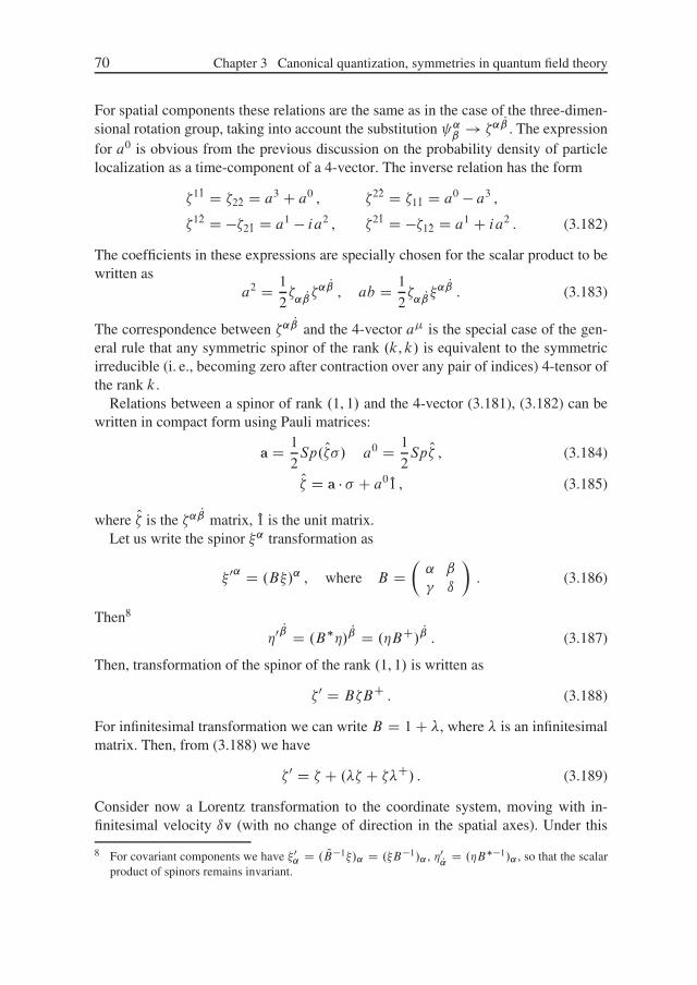
70 Chapter 3 Canonical quantization, symmetries in quantum field theory
For spatial components these relations are the same as in the case of the three-dimen-sional rotation group, taking into account the substitution ˛
ˇ! �˛
P. The expression
for a0 is obvious from the previous discussion on the probability density of particlelocalization as a time-component of a 4-vector. The inverse relation has the form
�1P1 D �2P2 D a3 C a0 , �2P2 D �1P1 D a0 � a3 ,
�1P2 D ��2P1 D a1 � ia2 , �2P1 D ��1P2 D a1 C ia2 . (3.182)
The coefficients in these expressions are specially chosen for the scalar product to bewritten as
a2 D 1
2�˛ P�˛
P, ab D 1
2�˛ P�˛
P. (3.183)
The correspondence between �˛P
and the 4-vector a� is the special case of the gen-eral rule that any symmetric spinor of the rank .k, k/ is equivalent to the symmetricirreducible (i. e., becoming zero after contraction over any pair of indices) 4-tensor ofthe rank k.
Relations between a spinor of rank .1, 1/ and the 4-vector (3.181), (3.182) can bewritten in compact form using Pauli matrices:
a D 1
2Sp. O�/ a0 D 1
2Sp O� , (3.184)
O� D a � C a0 O1 , (3.185)
where O� is the �˛P
matrix, O1 is the unit matrix.Let us write the spinor �˛ transformation as
� 0˛ D .B�/˛ , where B D�˛ ˇ
� ı
�. (3.186)
Then8
�0 P D .B��/ P D .�BC/ P. (3.187)
Then, transformation of the spinor of the rank .1, 1/ is written as
�0 D B�BC . (3.188)
For infinitesimal transformation we can write B D 1 C �, where � is an infinitesimalmatrix. Then, from (3.188) we have
�0 D � C .�� C ��C/ . (3.189)
Consider now a Lorentz transformation to the coordinate system, moving with in-finitesimal velocity ıv (with no change of direction in the spatial axes). Under this
8 For covariant components we have � 0 D . QB�1�/˛ D .�B�1/˛ , �0P D .�B��1/˛ , so that the scalar
product of spinors remains invariant.

Section 3.3 Fermions 71
transformation 4-vector a� D .a0, a/ is transformed as
a0 D a � a0ıv , a00 D a0 � a � ıv . (3.190)
Let us now use equation (3.184). First of all,
a00 D a0 � aıv D a0 � 1
2Sp.�ıv/ , (3.191)
On the other hand,
a00 D 1
2Sp�0 D a0 C 1
2Sp.�� C ��C/ D a0 C 1
2Sp�.�C �C/ . (3.192)
Comparing (3.191) and (3.192) we get
�C �C D �ıv . (3.193)
Similarly, considering the transformation of a, we obtain
�C �C D �ıv . (3.194)
Now, equations (3.193), (3.194) give
� D �C D �1
2 � ıv , (3.195)
so that the infinitesimal Lorentz transformation of spinor �˛ is done by the matrix:
B D 1 � 1
2. � n/ıv (3.196)
where n D ıv=ıv. Now we can consider finite transformations. Lorentz transforma-tion (to the coordinate system, moving with velocity v) has the geometrical meaningof a rotation of a four-dimensional coordinate system by angle ' in the .t , n/-plane,where ' is determined by velocity v: v D th' [33]. Infinitesimal transformation cor-responds to the angle ı' D ıv, and rotation by the finite angle can be achieved bymaking the ı'-rotation '=ı' times. Raising (3.196) to the power '=ı' and going tothe limit ı' ! 0, we obtain
B D exp�'
2n �
�. (3.197)
Taking into account that even powers of n � are equal to 1, while odd powers reduceto n � , we get
B D ch'
2� n � sh'
2, th' D v . (3.198)
Note that the transformation matrix B D BC is Hermitian. Equation (3.198) finallydetermines the Lorentz transformation of a 4-spinor of first rank.
Consider now an infinitesimal rotation of some vector in three-dimensional space:
a0 D a � Œı� � a� . (3.199)

72 Chapter 3 Canonical quantization, symmetries in quantum field theory
In this case we obtain
B D 1 C i
2 � ı� , (3.200)
while for the finite angle rotation
B D exp
�i�
2n �
�D cos
�
2C in � sin
�
2, (3.201)
where n determines the direction of the rotation axis. This matrix is unitary BC DB�1, as it should be for spatial rotation.
Inversion of spinors (P-reflection)
In nonrelativistic quantum mechanics, spatial inversion does not change the sign of anaxial vector such as spin. Thus, its sz-projection also does not change. It follows thenthat under inversion each component of the three-dimensional spinor ˛ transformsonly via itself:
˛ ! P ˛ (3.202)
Making inversion twice, we return to the initial coordinate system. In the case ofspinors, the return to the initial coordinates can be understood as a rotation by an-gle 0, or like a rotation by angle 2� . However, we have seen that for spinors these twooperations are not the same, since according to (3.161) spinor components ˛ changesign under rotation by 2� . Thus, we obtain two alternatives:
P 2 D 1 , i. e., P D ˙1 , (3.203)
P 2 D �1 , i. e., P D ˙i . (3.204)
Consider now 4-spinors. Inversion commutes with spatial rotations, as it only changesthe signs of x, y, z in x, y, z, t , but does not commute with transformations dealingwith the t -axis. Consider the Lorentz transformation L to a system, moving with ve-locity v, then PL D L0P , where L0 is the transformation to system, moving withvelocity �v. Thus, under the inversion components of a 4-spinor �˛ can not transformvia each other, and inversion transforms �˛ via some other objects, which may beonly � P . As inversion does not change the sign of sz , the components �1 and �2 can betransformed only into �P1 and �P2, corresponding to the same values of sz D C1=2 andsz D �1=2. Understanding inversion as an operation giving 1 being applied twice, wedefine it by
�˛ ! � P , � P ! �˛ ,
�˛ ! �� P , � P ! ��˛ (3.205)

Section 3.3 Fermions 73
for the case of P 2 D 1. For the alternative variant of P 2 D �1 we can write:
�˛ ! i� P � P ! i�˛
�˛ ! �i� P � P ! �i�˛ (3.206)
The different sign in the second row of these expressions is connected with the fact thatthe lowering or raising of the same index, according to (3.175), (3.178), is performedwith different signs. Below, for definiteness, we shall use the definition (3.206).
With respect to the subgroup of rotations, as we have seen above, �˛ and � P aretransformed in the same way. Let us construct the following combinations:
�˛ ˙ � P . (3.207)
It is easily seen that these combinations are transformed under inversion via each other,as (3.202) with P D ˙i . However, these combinations do not behave as spinors withrespect to all transformations of the Lorentz group.
Thus, the inclusion of inversion into our group of symmetry requires the simultane-ous consideration of the pair of spinors .�˛ , � P / – the so-called bispinor. Four com-ponents of the bispinor realize one of the irreducible representations of the extendedLorentz group. The scalar product of two bispinors can be constructed in two differentways. The value of
�˛„˛ C � PH P (3.208)
does not change under inversion and defines the true scalar. The value of
�˛„˛ � � PH P (3.209)
is also invariant with respect to rotations of the four-dimensional coordinate system,but it changes its sign under inversion, defining the pseudoscalar.
Also in two ways, from the components of two bispinors we can define the corre-sponding spinor of the second rank �˛
P. Defining it as
�˛P � �˛H
P C„˛�P
, (3.210)
we obtain the object, transforming under inversion as �˛P ! � Pˇ , so that the 4-vector
equivalent to this spinor is transformed as .a0, a/ ! .a0, �a/ and represents the true
4-vector (here a is the polar vector). But we can also define �˛P
in another form:
�˛P � �˛H
P �„˛� P. (3.211)
Then, under inversion �˛P ! �� Pˇ , and this spinor corresponds to the 4-vector,
transformed under inversion as .a0, a/ ! .�a0, a/, i. e., 4-pseudovector (here a is theaxial vector).
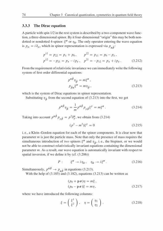
74 Chapter 3 Canonical quantization, symmetries in quantum field theory
3.3.3 The Dirac equation
A particle with spin 1/2 in the rest system is described by a two-component wave func-tion, a three-dimensional spinor. By it four-dimensional “origin” this may be both non-dotted or nondotted 4-spinor: �˛ or � P . The only operator entering the wave equationis p� D i@�, which in spinor representation is expressed via p
˛ P :
p1P1 D p2P2 D pz C p0 , p2P2 D p1P1 D p0 � pz ,
p1P2 D �p2P1 D px � ipy , p2P1 D �p1P2 D px C ipy . (3.212)
From the requirement of relativistic invariance we can immediately write the followingsystem of first order differential equations:
p˛P� P D m�˛ ,
p P˛�˛ D m� P , (3.213)
which is the system of Dirac equations in spinor representation.Substituting � P from the second equation of (3.213) into the first, we get
p˛P� P D 1
mp˛
Pp P� D m�˛ . (3.214)
Taking into account p˛Pp P D p2ı˛ , we obtain from (3.214)
.p2 �m2/� D 0 (3.215)
i. e., a Klein–Gordon equation for each of the spinor components. It is clear now thatparameterm is just the particle mass. Note that only the presence of mass requires thesimultaneous introduction of two spinors �˛ and � P , i. e., the bispinor, or we wouldnot be able to construct relativistically invariant equations containing the dimensionalparameterm. As a result, our wave equation is automatically invariant with respect tospatial inversion, if we define it by (cf. (3.206))
P : �˛ ! i� P , � P ! i�˛ . (3.216)
Simultaneously, p Pˇ ! p˛ P in equations (3.213).
With the help of (3.185) and (3.182), equations (3.213) can be written as
.p0 C p � /� D m� ,
.p0 � p � /� D m� , (3.217)
where we have introduced the following columns:
� D��1
�2
�, � D
��P1�P2
�. (3.218)

Section 3.3 Fermions 75
For complex conjugate equations it is convenient to introduce rows:
�� D .�1�, �2�/ , �� D .��P1 , ��
P2 / (3.219)
and write (taking into account p�� D �p�)
��.p0 C p � / D �m�� ,
��.p0 � p � / D �m�� . (3.220)
The inversion for complex conjugate spinors can be written as:
P : �˛� ! �i��P , ��
P ! �i�˛� . (3.221)
In the literature, it is more common to use (instead of (3.213) or (3.217)) the so-called symmetric form of the Dirac equation. To obtain it, we introduce the four-component Dirac bispinor, which is constructed from the columns of (3.218):
D��
�
�. (3.222)
Then, the system of equations (3.217) can be written as
p���
ik k D m i (3.223)
or, lowering bispinor indices, as
.��p� �m/ D 0 , i. e., .i��@� �m/ D 0 , (3.224)
where ��p� D p0�0 �p �� D i�0@0 C i� �r, and we have introduced matrices 4�4
(Dirac matrices):
�0 D�
0 O1O1 0
�, � D
�0 �OO 0
�. (3.225)
In fact, equation (3.217) can be written as�
0 p0 C p �p0 � p � 0
���
�
�D m
��
�
�, (3.226)
which coincides with (3.224) if we take � -matrices as in (3.225).In the general case � -matrices should satisfy conditions guaranteeing the identity
p2 D m2. To derive these conditions we multiply (3.224) on the left side by ��p� .Then,
.��p�/.��p�/ D m.��p�/ D m2 . (3.227)
As p�p� is a symmetric tensor (momentum components commute!), equation (3.227)can be rewritten as
1
2p�p�.�
��� C ����/ D m2 , (3.228)

76 Chapter 3 Canonical quantization, symmetries in quantum field theory
so that the necessary condition is satisfied if
���� C ���� D 2g�� . (3.229)
Thus, the pairs of different matrices �� anticommute, while their squares are
.�1/2 D .�2/2 D .�3/2 D �1 , .�0/2 D 1 . (3.230)
Under an arbitrary unitary transformation of bispinor 0 D U (where U is the uni-tary matrix 4 � 4) � -matrices transform as
� 0 D U�U�1 D U�UC , (3.231)
so that .��p� � m/ D 0 is transformed into .� 0�p� � m/ 0 D 0. Under thistransformation, as it is obvious from (3.225), the following properties are conserved:
�C D �� , �0C D �0 . (3.232)
The complex conjugate of equation (3.224) can be written as
.�p0 Q�0 � p Q� �m/ � D 0 . (3.233)
Using Q�� � D ��� and multiplying this equation from the right side by �0 (andtaking into account ��0 D ��0�), we obtain a conjugate Dirac’s equation as
N .��p� Cm/ D 0 , (3.234)
where we have introduced
N D ��0, � D N �0 (3.235)
– Dirac’s conjugate of bispinor .It is easy to see that the Dirac’s equation (3.224)
.i��@� �m/ D 0 (3.236)
can be obtained from the Euler–Lagrange equation
@L
@ N � @��
@L
@.@� N /�
D 0 (3.237)
using the following Lagrangian of Dirac’s field:
L D i
2Œ N ��.@� / � .@� N /�� � �m N i N �� $
@ � �m N , (3.238)
where$@� denotes differentiation “to the right” and “to the left”, defined by the given
identity. In Euler–Lagrange equations, N and are considered as independent fields.
Section 3.3 Fermions 77
The conjugate Dirac equation (3.234) is obtained from equation (3.237) after the re-placement N ! . Then we immediately find the canonical momentum �.x/ ofDirac’s field as
�.x/ D @L
@ P .x/ D i C.x/ . (3.239)
Then the Hamiltonian density of Dirac’s field is written as
H D � P � L D C�0.�i� i@i Cm/ D C�0.i�0@0 / D Ci @ @t
, (3.240)
where in the second equality we used the Dirac equation (3.224).
Remark on dimensionalities
Using the explicit form of Dirac’s field Lagrangian (3.238) and the standard dimensionalitiesŒL� D l�4, Œm� D l�1, Œ@� D l�1, we immediately determine the dimensionality of Dirac’sfield as
Œ � D Œ N � D l�3=2 (3.241)
This result will be used below.
The inversion (3.216) for can be written as
P : ! i�0 , N ! �i N �0 . (3.242)
The invariance of the Dirac equation with respect to (3.242) is obvious. Replacingp ! �p and ! i�0 , we get .p0�
0 C p� �m/�0 D 0, so that multiplying thisequation on the left side by �0 and taking into account anticommutativity of �0 and �we return to initial equation.
Let us multiply .��p� �m/ D 0 on the left side by N , and N .��p� Cm/ D 0on the right by , then make the sum of both and obtain
N ��.p� /C .p� N /�� D p�. N �� / D 0 (3.243)
which is the continuity equation for 4-current of Dirac’s particles:
@�j� D 0 , j� D N �� D . � , ��0� / , (3.244)
describing the charge conservation, with the charge density given by j 0 D � > 0.The Dirac equation can be written in the form of a Schroedinger equation:
i@
@tD H , (3.245)
where the Hamiltonian H has the form
H D ˛pC ˇm , (3.246)

78 Chapter 3 Canonical quantization, symmetries in quantum field theory
with Dirac’s matrices ˛ and ˇ:
˛ D �0� , ˇ D �0 , (3.247)
so that (3.246) coincides with (3.240) introduced above. The matrices (3.247) satisfythe commutation relations
˛i˛k C ˛k˛i D 2ıik , ˇ˛C ˛ˇ D 0 , ˇ2 D 1 , (3.248)
and in explicit form
˛ D� 00 �
�, ˇ D
�0 11 0
�. (3.249)
Consider the nonrelativistic limit. Performing in equation (3.217) the limit of p !0, " ! m, we get � D �, so that both spinors of the bispinor coincide, and all fourcomponents of the bispinor are nonzero. At the same time, it is clear that only twocomponents are independent. It is convenient to transform to the so-called standardrepresentation, when in the nonrelativistic limit two components of the bispinor willbe zero. Let us introduce
D�'
�
�, ' D 1p
2.� C �/ , � D 1p
2.� � �/ . (3.250)
For the particle at rest we obviously have � D 0. Adding and subtracting equa-tions (3.217) we obtain
p0' � p� D m' ,
�p0�C p' D m� , (3.251)
which allows to find the explicit form of � -matrices in the standard representation [6].Note that in equation (3.250) we separately sum the first and the second components ofspinors � and �. Accordingly, in standard representation, as in the spinor representationconsidered above, 1, 3 corresponds to spin projection sz D C1=2, while 2, 4 toprojection sz D �1=2. Matrix
1
2† D 1
2
� 00
�(3.252)
gives the three-dimensional operator of the spin in standard representation.
Helicity
In relativistic theory, the orbital moment l and spin s of a moving particle are not conservedseparately. Only the total angular moment j D lC s is conserved. Accordingly, the projectionof the spin on some direction (z-axis) is also not conserved and cannot be used to classify polar-ization (spin) states of a moving particles. However, we may introduce the helicity of a particle,i. e., the projection of its spin on the direction of motion (momentum). In fact, l D Œr � p� and

Section 3.3 Fermions 79
the product s �n, where n D pjpj , coincides with the conserving product j �n. The eigenvalues of
these spin projections are obviously given by � D �s, : : : , Cs. Accordingly, the wave func-tions of a free particle with momentum p are characterized by helicity: p�. In the rest systemthe state of a particle is characterized, as usual, by its spin (projection on z-axis).
For a particle with zero mass there is no rest system of coordinates; this particle moves withthe speed of light in any coordinate system. However, for such a particle there is always thespecial direction in space – the direction of momentum p. In this case there is no symmetrywith respect to arbitrary three-dimensional rotations, but only the axial symmetry to rotationsaround this preferred direction. Accordingly, we have only helicity conservation. If we requiresymmetry with respect to reflections in planes, passing through the p-axis, the states differingby the sign of � will be degenerate, and for � ¤ 0 we have double degeneracy. Thus, inthe limit of m ! 0 the system of equations for a particle with spin s splits into independentequations for particles with different helicities ˙s, ˙.s � 1/, : : :: for example, in the case ofphoton � D ˙1, which corresponds to right and left polarizations of light.
3.3.4 The algebra of Dirac’s matrices
For practical calculations it is important to understand algebraic properties of � -matri-ces. Here we present a short summary of the main formulas and definitions which willbe extensively used in the rest of the book. All the algebraic properties of Dirac’smatrices are derived from two basic relations:
���� C ���� D 2g�� , (3.253)
g������ D ���
� D 4 or �20 � �2
1 � �22 � �2
3 D 4 , (3.254)
i. e., from the main anticommutation relation and the scalar product.If �� and �� in the matrix product are separated by several other � -matrices, ��
and �� can be placed in neighboring positions with the help of (3.253), after which wecan perform the summation over � using (3.254). In this way we can get the followingrelations:
������ D �2�� ,
�������� D 4g�� ,
���������� D �2������ ,
������������ D 2.�������� C �������� / . (3.255)
Rather often �� appears in combination with 4-vectors. Let us introduce the standardnotation:
Oa ��a� . (3.256)
Then, from (3.253) we obtain
Oa Ob C Ob Oa D 2a�b� , Oa Oa D a2 , (3.257)

80 Chapter 3 Canonical quantization, symmetries in quantum field theory
and from (3.255) we get
�� Oa�� D �2 Oa ,
�� Oa Ob�� D 4a�b� ,
�� Oa Ob Oc�� D �2Oc Ob Oa ,
�� Oa Ob Oc Od�� D 2� Od Oa Ob Oc C Oc Ob Oa Od . (3.258)
Traces of � -matrices are widely used. In particular,
Sp�� D 0 . (3.259)
IntroducingT �� D 1
4Sp.����/ (3.260)
and calculating the trace of (3.253), we find
T �� D g�� (3.261)
and, respectively, 1
4Sp. Oa Ob/ D a�b� . (3.262)
The special case is the matrix �5 defined as
�5 D �i�0�1�2�3 (3.263)
It is easy to see that�5�� C ���5 D 0 , .�5/2 D 1 , (3.264)
so that �5 anticommutes with all other � -matrices. As to ˛ and ˇ matrices we have
˛�5 � �5˛ D 0 , ˇ�5 C �5ˇ D 0 . (3.265)
The �5-matrix is Hermitian:
�5C D i�3C�2C�1C�0C D �i�3�2�1�0 D �5 , (3.266)
as we can transform the index order 3210 to 0123 by even permutation of � -matrices.In spinor representation the explicit form of �5 is given by
�5 D� �O1 0
0 O1�
, (3.267)
while in standard representation:
�5 D�
0 �O1�O1 0
�, (3.268)
and we see thatSp�5 D 0 , (3.269)

Section 3.3 Fermions 81
which is obviously independent of the choice of representation.The set of 16 matrices
®�A¯ D ®
b1, �5, ��, i���5, i��¯
, (3.270)
where�� D 1
2.���� � ����/ (3.271)
represents the “complete set”, over which we can “expand” any 4�4-matrix. In fact,these matrices have the property:
Sp�A D 0 .A ¤ 1/ ,
�A�A D 1 ,1
4Sp�A�B D ıAB . (3.272)
Accordingly, all �A-matrices are linearly independent, and any 4�4-matrix can berepresented in the form
� DX
A
cA�A , cA D 1
4Sp�A� . (3.273)
3.3.5 Plane waves
The state of a free particle with fixed momentum is described by the plane wave, whichcan be written as
p D 1p2"p
upe�ipx , (3.274)
where up is a normalized bispinor. For the wave function with “negative frequency”(also changing the sign of p) we have
p D 1p2"p
u�peipx . (3.275)
In both cases we write "p D Cpp2 Cm2. The bispinor components up and u�p sat-
isfy the following equations, which are derived by substitution of (3.274) and (3.275)into the Dirac equation:
. Op �m/up D 0 , . Op Cm/u�p D 0 . (3.276)
For conjugated bispinors Nup D u�p�
0 we have
Nup. Op �m/ D 0 , Nu�p. Op Cm/ D 0 . (3.277)
Let us assume the invariant normalization
Nupup D 2m , Nu�pu�p D �2m . (3.278)

82 Chapter 3 Canonical quantization, symmetries in quantum field theory
Multiplying (3.276) from the left by Nu˙p we obtain . Nu˙p��u˙p/p� D 2m2 D 2p2,i. e.,
Nup��up D Nu�p��u�p D 2p� , (3.279)
so that the 4-vector of the current density for plane waves (3.274), (3.275) is equal to
j� D N ˙p�� ˙p D 1
2"pNu˙p��u˙p D p�
"p, (3.280)
i. e., j� D .1, v/, where v D p"p
is the particle velocity. We see that our choice ofnormalization corresponds to “one particle in volume V D 1”.
In standard representation, from (3.251) we get the following system of homoge-neous linear equations:
."p �m/' � p� D 0 ,
."p Cm/� � p' D 0 . (3.281)
Then,' D p
"p �m� , � D p"p Cm
' . (3.282)
The common multiplier before ' and � (which is arbitrary until we are simply dealingwith solutions of homogeneous equations) should be chosen from the normalizationcondition (3.278). Accordingly, in standard representation, spinors up and u�p takethe form
up D� p
"p Cmwp"p �m.n/w
�, u�p D
� p"p �m.n/w0p"p Cmw0
�, (3.283)
where n D pjpj , and w is an arbitrary two-component spinor, satisfying the normaliza-
tion conditionw�w D 1 . (3.284)
The second expression in (3.283) is obtained from the first one by changing the signbefore m and replacing w ! .n/w0. Similarly, we can obtain [6]
Nup Dp
"p Cmw�, �p"p �mw�.n/
�,
Nu�p Dp
"p �mw0�.n/, �p"p Cmw0�� . (3.285)
Direct multiplication givesNu˙pu˙p D ˙2m .
In the rest frame, i. e., for "p D m, we have
up D p2m
�w
0
�, u�p D p
2m
�0w0
�, (3.286)

Section 3.3 Fermions 83
so that w is the three-dimensional spinor to which our plane waves reduce in the non-relativistic limit:
w�D1=2 D�
10
�, w�D�1=2 D
�01
�. (3.287)
For fixed momentum there exist two independent states, corresponding to the two pos-sible values of spin projection. In accordance with the general statements made above,we are speaking of particle helicity �, i. e., spin projection on the direction of p. Thehelicity states correspond to the plane waves with spinor w D w.�/.n/, which is aneigenfunction of operator n :
1
2.n/w.�/ D �w.�/ . (3.288)
3.3.6 Spin and statistics
A second quantization of the Dirac field (of particles with spin s D 1=2) can be doneas follows. Let us introduce an expansion of an arbitrary Dirac field over plane waves:
DX
p�
1p2"p
ap�up�e
�ipx C bCp�u�p��eipx
�,
N C�0 DX
p�
1p2"p
aCp� Nup�eipx C bp� Nu�p��e�ipx� . (3.289)
We know Dirac’s Hamiltonian, so we do not need an energy-momentum tensor. Using(3.240), (3.245), we find the average energy of the Dirac particle in the state with wavefunction :
E DZd 3r �H D i
Zd 3r � @
@tD i
Zd 3r N �0 @
@t. (3.290)
Substituting here (3.289), taking into account the orthogonality of of the functions withdifferent p, and Nu˙p��0u˙p,� D 2"p (ñð. (3.280)), we obtain
H DX
p�
"p�aCp�ap� � bp�bC
p�
. (3.291)
This expression is obviously the direct consequence of the transformation propertiesof the Dirac field and the requirement of relativistic invariance. Now it is clear that wemust quantize our field using Fermion rules, i. e., introducing anticommutators:
®ap� , aC
p�¯ D 1 ,
®bp� , bC
p�¯ D 1 . (3.292)
For different indices, as well as for the pairs of “noncrossed” and “crossed” operators,the corresponding anticommutators are equal to zero. As a result, (3.291) is rewritten

84 Chapter 3 Canonical quantization, symmetries in quantum field theory
in the formH D
X
p�
"p.aCp�ap� C bC
p�bp� � 1/ , (3.293)
so that the eigenvalues of energy (minus the infinite energy of a vacuum) are equal to
E DX
p�
"p.Np� C NNp� / (3.294)
and are positive definite. If we had instead used Boson quantization, we would haveobtained E D P
p "p� .Np� � NNp� /, i. e., a nonpositive definite expression9.For the momentum operator, in a similar way, from
Rd 3r � Op we get
P DX
p�
p.Np� C NNp� / . (3.295)
The 4-current density operator j� D N �� in a second quantized form defines thecharge operator as
Q DZd 3r N �0 D
X
p�
�aCp�ap� C bp�b
Cp� D
X
p�
.aCp�ap� � bC
p�bp� C 1
.
(3.296)This gives the eigenvalues of charge:
Q DX
p�
.Np� � NNp� / , (3.297)
leading to the opposite charges of particles and antiparticles.Fermion anticommutation rules for creation and annihilation operators immediately
lead [35] to the validity of the Pauli principle, so that the eigenvalues of the particlenumber operator in a given state Np� can only be 0 or 1: now we see that for particleswith spin 1=2 this directly follows from the general requirements of relativistic invari-ance and positive definiteness of energy. Then, we are coming to the general theoremon spin and statistics: all particles with a half-integer spin are fermions, while parti-cles with integer spin are bosons. This becomes obvious if we take into account thatany particle with spin s can be assumed to be “composed” of 2s particles with spin1=2. For the half-integer s the number 2s is odd, while for the integer s this number iseven. “Composite” particles, consisting of an even number of fermions, is a boson, andthose consisting of an odd number of fermions are a fermion. To understand this it issufficient to consider permutations of such “composite” particles. It is understood, thatall particles with the same spin obey the same statistics. If we could have had fermionswith spin s D 0, then such fermions as well as fermions with spin 1=2 could be usedto “compose” a particle with spin 1=2, which would be a boson, in contradiction with
9 Here we are using the standard notations, assuming that the general properties of the creation andannihilation operators are known to the reader [35]

Section 3.3 Fermions 85
the general results for s D 1=2 obtained above. This remarkable theorem is amongthe most general statements of relativistic quantum field theory and was first provedby Pauli10.
3.3.7 C ,P ,T transformations for fermions
Factors of p� D up� exp.�ipx/, entering (3.289) accompanying operators ap� , represent
wave functions of free particles (e. g., electrons) with momentum p and polarization : .e/ D p� . Factors of N �p�� accompanying operators bp� are to be considered as wave functionsof the corresponding antiparticles (e. g., positrons) with the same p and . However, p� andN �p�� differ by their transformation properties, and their components satisfy different systems
of equations. To overcome this deficiency we have to perform a certain unitary transformationof N �p�� , such that the new wave function satisfies the same equation as p� . We shall callthis new wave function the wave function of antiparticles (positron) with momentum p andpolarization . Thus, we can write
.p/p� D UC N �p�� . (3.298)
This operation is called charge conjugation C . It is not limited to plane waves only; in thegeneral case we can write
C .t , r/ D UC N .t , r/ . (3.299)
Dropping the details of derivation, which can be found in [6], we quote only the final result:
UC D �2�0 . (3.300)
From N D ��0 D Q�0 � D �0 � we obtain
C D �2�0 N D �2 � . (3.301)
For plane wave solutions we can easily see that
C �p�� D p� , (3.302)
so that both electrons and positrons are described by identical wave functions .e/ D .p/ D p� , as it should be, because these functions carry information only on momentum and polar-ization of particles.
In a similar way, we may introduce the operation of time inversion. Changing the sign oftime should be accompanied by the complex conjugation of the wave function [35]. To obtainthe fermion wave function “reversed in time” T in the same representation as initial , weagain have to perform some unitary transformation of � (or N ):
T .r, t / D UT N .r, �t / . (3.303)
10 We would like to stress that in quantum field theory this theorem is really proved, starting from mostgeneral requirements of relativistic invariance (transformation properties of fields) and positive defi-niteness of energy, i. e., the stability of the ground state of a particle system, and not postulated, as itis done in nonrelativistic quantum mechanics.

86 Chapter 3 Canonical quantization, symmetries in quantum field theory
It can be shown [6] thatUT D i�3�1�0 , (3.304)
so thatT .t , r/ D i�3�1�0 N .�t , r/ D i�3�1 �.�t , r/ . (3.305)
Spatial inversion of (bi)spinors P was defined above in (3.242):
P D i�0 , P N D �i N �0 . (3.306)
Let us make T ,P ,C transformations of Dirac field one after another:
T .t , r/ D �i�1�3 �.�t , r/ ,
PT .t , r/ D i�0.T / D �0�1�3 �.�t , �r/ ,
CPT .t , r/ D �2.�0�1�3 �/� D �2�0�1�3 .�t , �r/ (3.307)
orCPT .t , r/ D i�5 .�t , �r/ . (3.308)
Applying these operations to (3.289), we can find the following transformation rules for cre-ation and annihilation operators [6]:
aCp� D bp� , bCp� D ap� ,
aP�p� D iap� , bP�p� D ibp� ,
aT�p�� D 2 iaCp� , bT�p�� D 2 ibC
p� . (3.309)
3.3.8 Bilinear forms
As bispinors and � have 4 components each, their multiplication produces 4�4 D16 independent bilinear combinations. In symmetric form these combinations can bewritten as (cf. (3.270), (3.271)
S D N , V � D N �� ,
P D i N �5 , A� D N ���5 ,
T �� D i N �� , (3.310)
where�� D 1
2.���� � ����/ . (3.311)
These bilinear forms reduce to one scalar S , one pseudoscalar P , the 4-vector V �, the4-pseudovector A�, and the antisymmetric tensor T �� .
The scalar nature of S and the pseudoscalar of P are obvious from their spinorrepresentations (cf. (3.208) and (3.209)):
S D ���C ��� , P D i.��� � ���/ . (3.312)

Section 3.3 Fermions 87
The vector nature of V � is now clear from the Dirac equation p��� D m , whichgives . N p��� / D m N , where scalars are standing in both sides.
The rule of construction of bilinear forms (3.310) is obvious: they are composed insuch a way that �� represents a 4-vector, �5 is a pseudovector, while N and , standingon both sides produce a scalar. The absence of bilinear forms reducing to a symmetric4-tensor is clear from the fact that the symmetric combination ����C���� D 2g�� ,so that the corresponding bilinear form reduces to g�� N . In practice, bilinear forms(3.310) are widely used during construction of different interaction Lagrangians ofspinor fields. The transformation rules of the bilinear forms under discrete transfor-mations C ,P ,T can be found in [6].
3.3.9 The neutrino
We have seen above that the necessity to describe a particle with spin s D 1=2 bytwo spinors � and � is directly related to the finite mass of a particle. There is no suchdemand if the particle mass is zero11. A wave equation describing such a particle canbe constructed using only one spinor, e. g., �:
p˛P� P D 0 (3.313)
or, which is the same,.p0 C p/� D 0 . (3.314)
This is the so-called Weyl equation.We have noted before, that the wave equation with massm is automatically invariant
with respect to spatial inversion (transformation � $ � (3.216)). However, if wedescribe our particle by one spinor, this symmetry is lost.
The energy and momentum of a particle with m D 0 are related by " D jpj. Thus,for a plane wave �p � e�ipx equation (3.314) gives
.n � /�p D ��p , (3.315)
where n D pjpj . The same equation holds for the wave with “negative frequency”
��p � eipx:.n � /��p D ���p . (3.316)
11 Among all the known fermions only the neutrino possesses mass, which is zero or very small: theexperimental limitation is that its mass m� < 2 eV [67]. However, experimentally observed neutrinooscillations definitely show, that neutrino mass is definitely finite [67]. Still, zero mass is a very goodapproximation to describe most of neutrino physics.
88 Chapter 3 Canonical quantization, symmetries in quantum field theory
The second quantized operators of the field � are represented by
� DX
p
.�pap C ��pbCp / ,
�C DX
p
.��pa
Cp C ���pbp/ . (3.317)
From here, as usual, we see that ���p is the wave function of an antiparticle. A neutrinois electrically neutral, but in this formalism it is not a truly neutral particle!
From the definition of operators p˛P
(3.212) it can be seen that p˛P� D �p Pˇ .
Then, the complex conjugate spinor �� satisfies the equation p Pˇ��P D 0, or, which
is the same,p Pˇ�
P� D 0 . (3.318)
Let us denote �P� D �ˇ , as complex conjugation transforms dotted spinors into non-
dotted ones. Thus, the wave functions of antiparticles satisfy the equation
p Pˇ �ˇ D 0 (3.319)
or.p0 � p � /� D 0 . (3.320)
For the plane wave we have.n � /�p D �p . (3.321)
Note that 12.n � / represents the operator of spin projection on the particle momen-
tum (helicity). Thus, equations (3.315) and (3.321) automatically describe the particleswith fixed helicities – spin projection is always oriented parallel to the momentum.The spin of the particle is opposite to the momentum (helicity is equal to �1=2, “leftscrew”), while the spin of an antiparticle is oriented along the momentum (helicityC1=2, “right screw”). Accordingly, for neutrinos and antineutrinos there is no symme-try towards reflections in the plane, orthogonal to momentum, as shown in Figure 3.2.This corresponds to the experimentally observed breaking of spatial parity in weakinteractions. However, symmetry towards CP operation persists, which correspondsto the conservations of the so-called combined parity12. This scheme represents thetwo-component theory of neutrinos first proposed by Landau.
With one spinor � (or �) we can construct only four bilinear combinations, whichtogether form a 4-vector:
j� D .���, ���/ . (3.322)
12 In fact, weak interactions weakly break also the CP -invariance, which is mainly observed in decaysofK-mesons. This obviously corresponds to the weak breaking of T -invariance. The physical natureof the breaking of CP -invariance has not been well established up to now, and our description ofneutrinos simply neglect this small effect.

Section 3.3 Fermions 89
(a) (b)
Figure 3.2. Under mirror reflection (spatial inversion) the left-hand neutrino is transformedinto a nonexistent right-hand neutrino (a). A real physical state is obtained with simultaneoustransformation from particles to antiparticles (charge conjugation), when the left-hand neutrinois transformed into the right-hand antineutrino (b).
Using .p0 Cp � /� D 0 and ��.p0 �pº � / D 0 we get the continuity equation @�j� D0, so that j� represents the 4-vector of the neutrino current density.
Neutrino plane waves are conveniently written as
�p D 1p2"upe
�ipx , ��p D 1p2"u�peipx , (3.323)
and spinor amplitudes are normalized by the invariant condition:
u�p.1, /u˙p D 2.", p/ . (3.324)
Then particle density and current density are equal to j 0 D 1, j D p"
D n.To describe neutrino interactions with other particles, it is convenient to use com-
mon notations and introduce the neutrino “bispinor”, with two components just equalto zero: D .
0�/. However, such a form of , in general, changes after the transfor-
mation to another (nonspinor) representation. We can overcome this difficulty, notingthat in spinor representation
1
2.1 C �5/ D 1
2
²� O1 00 O1
�C� �O1 0
0 O1�³
D�
0 00 O1
�,
1
2.1 � �5/ D
� O1 00 0
�, (3.325)
so that we can write the following identities:
1
2.1 C �5/
��
�
�D�
0�
�, .��, ��/1
2.1 � �5/ D .��, 0/ , (3.326)

90 Chapter 3 Canonical quantization, symmetries in quantum field theory
where � is an arbitrary “dummy” spinor. Then the condition of the true two-componentnature of a neutrino will also be satisfied in its description by the 4-component bispinor in arbitrary representation, if is understood to be the solution of Dirac’s equationwith m D 0:
bp D 0 (3.327)
with an additional condition (�5-invariance)
1
2.1 C �5/ D or �5 D . (3.328)
This condition can be taken into account automatically, if in all expressions we replaceneutrino bispinors with the following rule:
! 1
2.1 C �5/ , N ! N 1
2.1 � �5/ . (3.329)
For example, the 4-vector of the current density is written as
j� D 1
4N .1 � �5/��.1 C �5/ D 1
2N ��.1 C �5/ . (3.330)
From the previous discussion of the helicity of massless fermions, it is clear that inthe general case we can introduce “right-hand” and “left-hand” fields as
R D 1
2.1 C �5/ , L D 1
2.1 � �5/ , D R C L . (3.331)
These notations are often used not only for neutrinos, but also for any other fermionswith spin s D 1=2, while discussing problems where we can neglect fermion masses.
In recent years, because of the indirect experimental indications of neutrino mass finiteness(such as neutrino oscillations [67]), there was a revival of interest in a truly neutral model,the so-called Majorana neutrino, which is transformed to itself under charge conjugation andpossesses a finite mass which is in some sense different from the usual Dirac’s mass. We haveseen that mass term of the Dirac type in the Lagrangian mixes L and R components of thesame field:
LD D D. N L R C N R L/ D D N , (3.332)
where D denotes Dirac’s mass. The mass term of the Majorana type mixes L and R compo-nents of charge conjugate fields, so that the corresponding contributions to the Lagrangian canbe written as [13]
LMA D A. N CL L C N L CL / D A N�� ,
LMB D B. N CR R C N R CR / D B N!! , (3.333)
where the index C denotes the charge conjugation and the Hermitian (truly neutral or Majo-rana) fields we introduced:
� D L C CL , �C D � ,
! D R C CR , !C D ! . (3.334)

Section 3.3 Fermions 91
The inverse relations have the form
L D 1
2.1 � �5/� , CL D 1
2.1 C �5/� ,
R D 1
2.1 C �5/! , CR D 1
2.1 � �5/! . (3.335)
When both Dirac and Majorana terms are present in the Lagrangian, we have
LDM D D N L R C A N CL L C B N CR R C h.c
D 1
2D. N�! C N!�/C A N��C B N!! D . N�, N!/
�A 1
2D12D B
���
!
�. (3.336)
The mass matrix appearing here is easily diagonalized, and its eigenvalues give
m1,2 D 1
2.AC B/˙ 1
2
p.A � B/2 CD2 . (3.337)
Thus, the most general mass term (3.336) with 4-component fermion fields in fact describestwo Majorana particles with different masses. The corresponding fields are represented by thefollowing (diagonalizing (3.336)) linear combinations of initial fields:
�1 D � cos � � ! sin � , �2 D � sin � C ! cos � , (3.338)
where
tg2� D D
B � A . (3.339)
It is easy to see that in the case of A D B D 0 (i. e., for zero Majorana masses) we obtainthe usual formalism of a 4-component Dirac’s field, so that the Dirac’s fermion correspondsto the “degenerate” limit A D B D 0 of two Majorana particles. Majorana mass terms in theLagrangian (3.333) obviously lead to nonconservation of additive quantum numbers carried bythe field , e. g., electric charge, so that all the known elementary fermions, except neutrinos,being charged should have A D B D 0 and should be Dirac’s particles. For the neutrino thereis no such limitation, and it can be described within the more general Majorana formalism. Ifthe neutrino mass is precisely zero, Majorana neutrinos become equivalent to two-componentWeyl neutrinos, considered above. In case of finite neutrino masses, the Majorana theory leadsto a number of specific predictions which we shall not discuss here.
Particles with spin s D 3=2
Particles with spin s D 3=2 in their rest system are described by a symmetric three-dimensionalspinor of the third rank, possessing 2s C 1 D 4 independent components. Accordingly, inthe arbitrary Lorentz system of coordinates, the description of such particles should be doneusing spinors �˛ P P , � Pˇ , �˛ˇ , and � P P P , each of which is symmetric over all indices ofidentical nature (i. e., dotted or nondotted). Note that the last pair of spinors do not add anythingnew to the equations obtained with the help of the first pair. There exist several equivalentformulations of wave equations for this problem, but we shall limit ourselves to a short reviewof only one [6].
We have seen above that to a pair of spinor indices ˛ P we can associate a single 4-vector
index �. Thus, we can associate �˛ P P ! P� and � P˛ !
�, i. e., introduce the “mixed”
spinor-tensors. Then we can introduce the “vector” bispinor � (where we have dropped the

92 Chapter 3 Canonical quantization, symmetries in quantum field theory
bispinor indices). The wave equation is written as a “Dirac equation” for each of vector com-ponents �:
.bp �m/ � D 0 (3.340)
with an additional condition�� � D 0 . (3.341)
Multiplying (3.340) by ��, taking into account (3.341), we obtain ����p� � D 0, or, due tocommutation rules for ��: 2g��p� � � ���� � D 0, where the second term gives zero dueto (3.341). Then we have
p� � D 0 , (3.342)
which guarantees that four-dimensional spinors are transformed to the “right” three-dimen-sional spinors in the rest system.
The problem of the correct account of additional conditions for wave equations createssignificant difficulties during the quantization procedure. Note, however, that, as in the caseof particles with higher integer spins, there are no fundamental fermions with s � 3=2 in theStandard Model.
Chapter 4
The Feynman theory of positron and elementaryquantum electrodynamics
4.1 Nonrelativistic theory. Green’s functions
In this chapter we shall present an elementary introduction in quantum electrodynam-ics (QED), which is understood as the theory of the electromagnetic interactions ofelementary leptons, i. e., mostly of electrons and positrons. Here we mainly follow theoriginal papers of Feynman; similar presentations can be found in [18, 60]. However,we will begin with nonrelativistic quantum mechanics, so as to introduce some basicnotions which are usually not included in traditional courses like [35].
Consider the time-dependent Schroedinger equation
i„@ @t
D H . (4.1)
The standard approach to solve this differential equation starts with the wave functionat some initial moment of time .t1/, the calculation of its change during a small timeintervalt , to find .t1 Ct/, with further continuation of this process of integration.Feynman proposed writing the solution of equation (4.1) in integral form, so that attime t2 > t1 the wave function at space-time point .t2, x2/ is expressed via the wavefunction at space-time point .t1, x1/ as follows:
.x2, t2/ DZd 3x1K.x2t2; x1t1/ .x1t1/ , t2 � t1 . (4.2)
Here the integral kernel K.x2t2; x1t1/ represents the propagator (Green’s function),corresponding to the linear differential equation (4.1). The physical meaning of prop-agator is clear from the form of equation (4.2) – this is the quantum mechanical prob-ability amplitude of particle transition from point x1 at time t1 to point x2 at time t2.
For simplicity, we consider the case of time-independent Hamiltonian H . In accor-dance with the superposition principle of quantum mechanics, we can expand .x1t1/
in a series over the full set of orthonormalized eigenfunctions un.x/ of operator Hwith eigenvalues En:
Hun D Enun ,Zd 3xu�
n.x/um.x/ .un,um/ D ınm , (4.3)X
n
un.x/u�n.x
0/ D ı.x � x0/ .

94 Chapter 4 The Feynman theory of positron and elementary quantum electrodynamics
Then, .x1t1/ D
X
n
cnun.x1/e�iEnt1=„ . (4.4)
The coefficients cn can be obtained by multiplying (4.4) by u�n.x1/ and performing
integration over the whole three-dimensional space:
cn DZd 3x1u
�n.x1/ .x1t1/e
iEnt1=„ . (4.5)
The wave function at time t2 can be written as
.x2t2/ DX
n
cnun.x2/e�iEnt2=„ . (4.6)
Substituting (4.5) into (4.6), changing the order of summation and integration, andcomparing with (4.2), we get
K.x2t2; x1t1/ DX
n
un.x2/u�n.x1/e
�iEn.t2�t1/=„ , (4.7)
and introducing the notation
�n.x, t / D un.x/e�iEnt=„ , (4.8)
we obtain a shorter expression:
K.x2t2; x1t1/ DX
n
�n.x2t2/ .��n.x1t1/ (4.9)
At coinciding times t1 D t2 D t from (4.7) we obtain
K.x2t ; x1t / DX
n
un.x2/u�n.x1/ D ı.x2 � x1/ . (4.10)
This obviously transforms (4.2) for t1 D t2 into the identity. We are certainly interestedin times t2 > t1; thus it is convenient to put K.x2t2; x1t1/ D 0 for t2 < t1, whichguarantees causality, and we define
K.x2t2; x1t1/ D �.t2 � t1/X
n
�n.x2t2/��.x1t1/ , (4.11)
where we have introduced the step-function
�.t/ D²
1 for t � 00 for t < 0
. (4.12)
The derivative of the � -function is given by
d�.t/
dtD ı.t/ . (4.13)

Section 4.1 Nonrelativistic theory. Green’s functions 95
Now we can write the differential equation for Green’s function (propagator)K.r2t2; r1t1/. As �n represent the solutions of the Schroedinger equation (4.1), (4.3),using (4.10), (4.11), and (4.13), we have
�i„ @
@t2�H.x2/
�K.x2t2; x1t1/ D i„
X
n
�n.x2t2/��.x1t1/
@
@t2�.t2 � t1/
D i„X
n
un.x2/u�n.x1/e
�iEn.t2�t1/=„ı.t2 � t1/
D i„ı.t2 � t1/X
n
un.x2/u�n.x1/ D i„ı.t2 � t1/ı.x2 � x1/ . (4.14)
Thus, in the general case (even for time-dependent H ) Green’s function (propagator)K.x2t2; x1t1/ is defined as the solution of the inhomogeneous (with ı-source in theright-hand side) differential equation1
�i„ @
@t2�H.x2t2/
�K.x2t2; x1t1/ D i„ı.t2 � t1/ı.x2 � x1/ , (4.15)
with the boundary condition
K.x2t2; x1t1/ D 0 for t2 < t1 . (4.16)
For t2 ¤ t1, equation (4.15) reduces to�i„ @
@t2�H.x2t2/
�K.x2t2; x1t1/ D 0 . (4.17)
If we integrate equation (4.15) over small time interval from t2 D t1 �" to t2 D t1 C",we get
K.x2t1 C "; x1t1/ �K.x2t1 � "; x1t1/ D ı.x2 � x1/ . (4.18)
The contribution of the second term in the left-hand side of equation (4.15) drops outas " ! 0 for finite H . Now take into account that K.x2t1 � ", x1t1/ D 0 due to (4.16)and t1 � " < t1. Then,
lim"!0
K.x2t1 C "; x1t1/ D K.x2t1; x1t1/ D ı.x2 � x1/ , (4.19)
which coincides with (4.10).Thus, the use of equation (4.2) is equivalent to the standard quantum mechanical
description. Consider the problem of when we can write H D H0 C V and if forH D H0 there is an exact solution. Then we can try to construct the perturbation theoryover potential V . Let us denote K0.x2t2; x1t1/ as the Green’s function of a “free”particle, moving in the absence of perturbation V. We can easily convince ourselves
1 Actually, our definition of Green’s function of the Schroedinger equation coincides with its definitionin mathematical physics [70].

96 Chapter 4 The Feynman theory of positron and elementary quantum electrodynamics
that differential equation (4.15) and boundary condition (4.16) can be unified in asingle integral equation:
K.2, 1/ D K0.2, 1/ � i
„Zd 4x3K0.2, 3/V .3/K.3, 1/ , (4.20)
where the numbers denote space-time points, e. g., .2/ D .x1, t2/ etc., and we haveintroduced the four-dimensional integration variable x3 D .x3, t3/, where integrationover time t3 is formally done within infinite limits (the presence of � -function in thedefinition of propagator automatically guarantees the correct finite limits of integra-tion). To check the validity of equation (4.20) let us act on both of its sides by theoperator Œi„ @
@t2� H0.2/�, so that using equation (4.15) for K0 (i. e., for V D 0), we
obtain the differential equation�i„ @
@t2�H0.2/
�K.2, 1/ D i„ı.2, 1/C V.2/K.2, 1/ ,
which, after moving the second term in the right-hand side to the left-hand side, justcoincides with equation (4.15). AsK0.2, 1/ D 0 for t2 < t1, we also haveK.2, 1/ D 0for t2 < t1.
The advantage of integral equation (4.20) is that it is conveniently solved by itera-tions, so that we obtain the following perturbation series for the propagator:
K.2, 1/ D K0.2, 1/ � i
„Zd 4x3K0.2, 3/V .3/K0.3, 1/
C��i
„�2 Z
d 4x3d4x4K0.2, 3/V .3/K0.3, 4/V .4/K0.4, 1/C � � � .
(4.21)
The terms of this expansion have an obvious and graphic interpretation: the first termdescribes the propagation of a free particle from point 1 to point 2, and the seconddescribes the propagation of a free particle from point 1 to point 3, where it is scatteredby potential V and the propagates as a free particle from 3 to 2. Obviously, point 3 isarbitrary, so that we have to integrate over its coordinates. This process continues inhigher orders, so that the series describes all the multiple scattering processes up to aninfinite order in V. Such a perturbation theory can be effectively used for the solutionof concrete problems, and we shall return to it later.
4.2 Relativistic theory
Now we are going to construct a similar formalism in relativistic theory. Dirac’s equa-tion for a free particle is written as
.ibr �m/ D 0 , br D ��@� D �0@0 C � � r , (4.22)

Section 4.2 Relativistic theory 97
where, in contrast to the previous section, we returned to a “natural” system of unitswith „ D c D 1. A 4-component wave function (Dirac’s bispinor) .x2t2/ can be ob-tained from the “initial” one .x1t1/with the help of the propagator (Green’s function)K0.x2t2; x1t1/, which is a 4�4-matrix. This matrix should satisfy the Dirac’s equationwith the right-hand side, similar to equation (4.15):
.ibr2 �m/K0.2, 1/ D iı.2, 1/ , (4.23)
where, as before, we use the obvious number notations for space-time points. In anal-ogy with (4.4), (4.6), the wave function can be expanded over the complete setof eigenfunctions un, corresponding both to positive and negative energies. Insteadof u�
n, it is convenient to use conjugate spinors Nun D u��0 D u�ˇ (where we useDirac’s matrices �0 D ˇ, ˇ2 D 1). Repeating the steps used to derive (4.7), we findthe desirable propagator as
K.x2t2; x1t1/ DX
En>0
un.x2/ Nun.x1/e�iEn.t2�t1/ C
X
En<0
un.x2/ Nun.x1/e�iEn.t2�t1/ for t2 > t1 ,
K.x2t2; x1t1/ D 0 for t2 < t1 . (4.24)
It is necessary to do the expansion of over the complete set of eigenfunctions, includ-ing those corresponding to negative energies. This may seem bad for physics, as theintroduction of some external perturbation (potential) can induce quantum transitionof a particle (e. g., an electron) from positive energy states to the states with nega-tive energies, which leads to instability of the system (absence of the ground state).It is well-known that Dirac solved this problem in the following way. Let us assumethat all states with negative energies in the physical ground state (vacuum) are alreadyfilled by electrons, so that the Pauli principle prevents an electron, moving above thisvacuum, from making a transition to the filled states with negative energies. In ourformalism this reduces to the requirement that for t2 > t1 propagator K.x2t2; x1t1/
should be the sum over the eigenfunctions, corresponding to positive energies only.Mathematically we should write
K.x2t2; x1t1/ DX
En>0
un.x2/ Nun.x1/e�iEn.t2�t1/ for t2 > t1 , (4.25)
so that from (4.24) we should subtract the sum of terms like
un.x2/ Nun.x1/e�iEn.t2�t1/ (4.26)
over the states with negative energies for all moments of time. This can be done, assuch a sum represents the solution of homogeneous (i. e., without the right-hand sideof) equation (4.23). As a result, this sum is cancelled by the second half of the solution

98 Chapter 4 The Feynman theory of positron and elementary quantum electrodynamics
(4.24), and we obtain the following Green’s function for a free particle:
KC.x2t2; x1t1/ DX
En>0
un.x2/ Nun.x1/e�iEn.t2�t1/ for t2 > t1 . (4.27)
However, for this function
KC.x2t2; x1t1/ D �X
En<0
un.x2/ Nun.x1/e�iEn.t2�t1/ for t2 < t1 . (4.28)
is obviously nonzero for t2 < t1. Not the minus sign appearing here! This last expres-sion is conveniently written as
KC.x2t2; x1t1/ D �X
En<0
un.x2/ Nun.x1/e�i jEnjjt2�t1j for t2 < t1 , (4.29)
so that in the exponent we have only positive energies, and negative energies seem todisappear.
In the presence of an external potential we can again write an integral equationsimilar to equation (4.20) and its perturbation expansion of equation (4.21), but withK0 replaced everywhere by KC, and the potential V should be considered as a 4�4-matrix. The terms of this series can be graphically understood by drawing space-timeFeynman diagrams. The first term of the series (4.21)KC.2, 1/ describes free particlepropagation from point 1 to point 2 (Figure 4.1). The second term (Figure 4.2) has theform
.�i/Zd 4x3KC.2, 3/V .3/KC.3, 1/ (4.30)
Figure 4.1

Section 4.2 Relativistic theory 99
Figure 4.2
(a) (b)
Figure 4.3
and describes single scattering. In the figure the closed curve denotes the region, wherethe potential V is different from zero. The third term (Figure 4.3)
.�i/2Zd 4x3d
4x4KC.2, 3/V .3/KC.3, 4/V .4/KC.4, 1/ (4.31)
describes two scattering processes. Diagrams in Figure 4.3(a) and Figure 4.3(b) illus-trate two variants of such a scattering:
� Case (a). From point 1 to point 2 the electron propagates in such a way that timegrows along its world line, expression for KC contains only sums like (4.27), i. e.,only states with positive particle energies are accounted for. These re the usual sec-ond order scatterings of an electron with positive energy, as in nonrelativistic theory.
� Case (b). From point 4 to point 3 the electron propagates backwards in time, thenexpression forKC contains only sums over negative energy states like (4.29). In theFeynman interpretation this corresponds to a positron (i. e., antiparticle) propagation

100 Chapter 4 The Feynman theory of positron and elementary quantum electrodynamics
from point 3 to point 4. If time always grows, we can interpret this sequence ofevents in the following way: An electron–positron pair is created at point 3, withthe electron propagating in the direction of point 2, while the positron propagates topoint 4, where it annihilates with the initial electron, coming there from 1.
Thus, according to Feynman, a positron is an electron propagating backwards in time.
This interpretation can also be illustrated from the classical point of view: in equations ofmotion of a classical particle in electromagnetic field [33]
md 2x�
ds2D e
dx�
dsF �� . (4.32)
the change of proper time direction s is equivalent to the change of the charge e sign.
Note that for the process shown in Figure 4.3 we certainly have to integrate over allthe possible values of times t3 and t4, so that both cases are described by the single termof the series (4.31), which can be represented by the single diagram of Figure 4.3(a),while the diagram of Figure 4.3(b) is just identical. The scattering process shown inFigure 4.3(b) is in fact in accordance with Dirac’s theory: an electron with negativeenergy goes to the state 2 with positive energy (final state), i. e., an electron–positronpair is created, while the hole is filled by the electron coming from 1, which annihi-lates. As a result, the electron is scattered from state 1 to state 2, and the electron withpositive energy is replaced by one of the electrons from the negative “background”(vacuum). Thus, we have an exchange of identical particles, and the correspondingmatrix element acquires a negative sign, as it should be for fermions. However, wenever used the Pauli principle! The appearance of a negative sign in (4.28) was dueto a method of construction of propagator KC, thus guaranteeing the correct statis-tics! The generalization of these arguments to all higher orders of perturbation theoryproduces an alternative proof of the spin-statistics theorem [18].
4.3 Momentum representation
In practice, all calculations are most conveniently done in the momentum representa-tion. Propagator KC is determined by the equation
.ibr �m/KC.2, 1/ D iı.2, 1/ . (4.33)
Let us introduce the Fourier transform ofKC, which we shall denote as SC.p/, so that
KC.2, 1/ DZd 4pe�ip.x2�x1/SC.p/ , (4.34)

Section 4.3 Momentum representation 101
where d 4p D dp0d3p. The operator .ibr � m/ can be moved under the integral as
. Op �m/, while for the ı-function we can write
ı.x2 � x1/ DZ
d 4p
.2�/4e�ip.x2�x1/ . (4.35)
Then it is easy to find the following equation for SC.p/:
SC.p/ D i
.2�/41
Op �m . (4.36)
This expression can be rewritten as
SC.p/ D i
.2�/4Op Cm
Op Cm
1
Op �m D i
.2�/4Op Cm
p2 �m2, (4.37)
where we have taken into account that Op2 D p�p� D p2
0 � p2 D p2, so that thedenominator in (4.37) contains no matrices. Then,
KC.2, 1/ D i
.2�/4
Zd 4pe�ip.x2�x1/
Op Cm
p2 �m2. (4.38)
Let us introduce, by definition, the following integral:
IC.2, 1/ D 1
.2�/4
Zd 4p
e�ip.x2�x1/
p2 �m2. (4.39)
Then (4.38) can be written as
KC.2, 1/ D i.ibr2 Cm/IC.2, 1/ . (4.40)
Substituting (4.40) into (4.33) we find that IC satisfies the following equation:
.� Cm2/IC.2, 1/ D �ı.2, 1/ (4.41)
i. e., it represents, in fact, Green’s function of the Klein–Gordon equation. Separatingthe spatial coordinates and time, we rewrite IC as
IC.x2 � x1/ D 1
.2�/4
1Z
�1dp0
Zd 3p
e�ip0.t2�t1/eip.r2�r1/
p20 � p2 �m2
. (4.42)
Here we have a problem: the integrand contains poles at p20 � p2 �m2 D 0, i. e., for
p0 D ˙qp2 Cm2 ˙Ep. Thus, we have to introduce a certain integration path
going around these poles (the rule to encircle poles). Feynman’s rule is to replace
m ! m � iı , ı > 0 , ı ! C0 . (4.43)
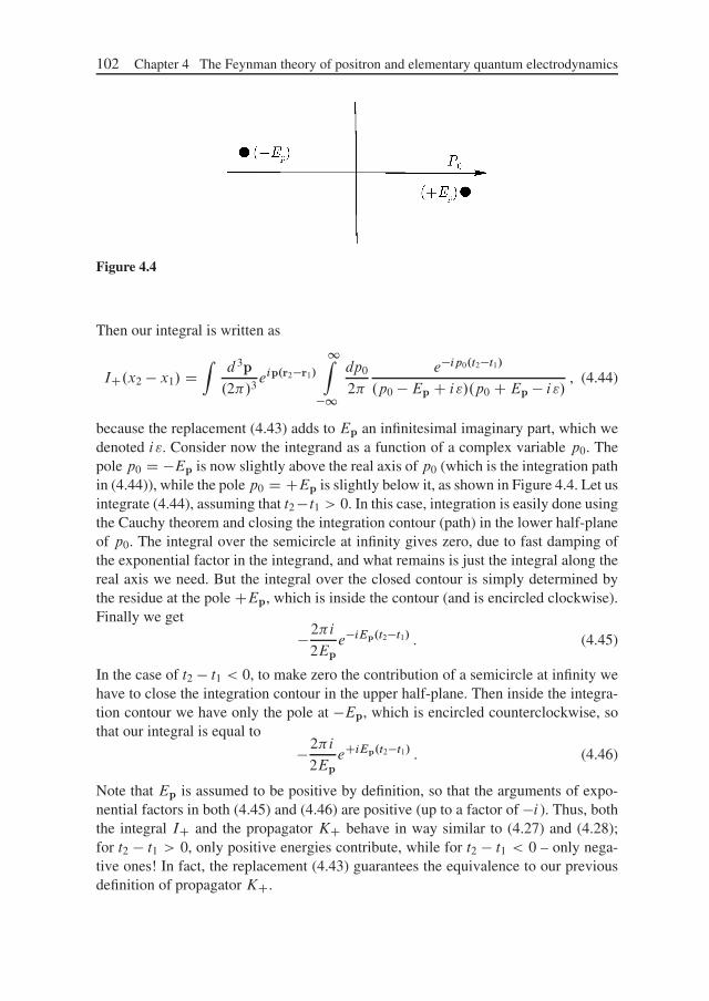
102 Chapter 4 The Feynman theory of positron and elementary quantum electrodynamics
Figure 4.4
Then our integral is written as
IC.x2 � x1/ DZ
d 3p.2�/3
eip.r2�r1/
1Z
�1
dp0
2�
e�ip0.t2�t1/.p0 �Ep C i"/.p0 CEp � i"/ , (4.44)
because the replacement (4.43) adds to Ep an infinitesimal imaginary part, which wedenoted i". Consider now the integrand as a function of a complex variable p0. Thepole p0 D �Ep is now slightly above the real axis of p0 (which is the integration pathin (4.44)), while the pole p0 D CEp is slightly below it, as shown in Figure 4.4. Let usintegrate (4.44), assuming that t2 � t1 > 0. In this case, integration is easily done usingthe Cauchy theorem and closing the integration contour (path) in the lower half-planeof p0. The integral over the semicircle at infinity gives zero, due to fast damping ofthe exponential factor in the integrand, and what remains is just the integral along thereal axis we need. But the integral over the closed contour is simply determined bythe residue at the pole CEp, which is inside the contour (and is encircled clockwise).Finally we get
� 2�i
2Epe�iEp.t2�t1/ . (4.45)
In the case of t2 � t1 < 0, to make zero the contribution of a semicircle at infinity wehave to close the integration contour in the upper half-plane. Then inside the integra-tion contour we have only the pole at �Ep, which is encircled counterclockwise, sothat our integral is equal to
� 2�i
2EpeCiEp.t2�t1/ . (4.46)
Note that Ep is assumed to be positive by definition, so that the arguments of expo-nential factors in both (4.45) and (4.46) are positive (up to a factor of �i ). Thus, boththe integral IC and the propagator KC behave in way similar to (4.27) and (4.28);for t2 � t1 > 0, only positive energies contribute, while for t2 � t1 < 0 – only nega-tive ones! In fact, the replacement (4.43) guarantees the equivalence to our previousdefinition of propagator KC.

Section 4.4 The electron in an external electromagnetic field 103
We could define integration (4.42) in another way and instead of (4.43) just add an infinitesimalimaginary part to p0:
p0 ! p0 C iı , ı ! C0 . (4.47)
Then, in the integrand of (4.42) two poles appear, both in the lower half-plane of p0. Thenfor t2 � t1 > 0, when the integration contour is naturally closed in the lower half-plane, bothpositive and negative energies contribute. At the same time, for t2 � t1 we close the contourin the upper half-plane, where there are no poles at all, so that the integral is just zero. Thisdefinition of propagator K gives, in fact, equation (4.24) (“retarded” Green’s function), i. e.,Dirac’s theory for electrons only. Feynman’s rule also has an obvious advantage of the imag-inary part being introduced into the relativistic invariant m, so that all expressions remaincovariant, while in the theory of “electrons only” the imaginary part in p0 makes it differentfrom other components of 4-momentum.
We shall return to the discussion of these rather fine details of the definition of an-alytical properties of Green’s functions several times later on, while here we just notethe most general property: poles of the propagators (Green’s functions) in momen-tum representation determine, in fact, the energy spectrum of the corresponding par-
ticles. In our discussion above, Ep Dqp2 Cm2 represents the relativistic spectrum
of an electron (positron). This property of Green’s functions is also widely used in themodern condensed matter theory. In particular, it is the basis of the whole concept ofquasiparticles – the elementary excitations in many particle systems [1].
4.4 The electron in an external electromagnetic field
Consider an electron interacting with an external electromagnetic field. This inter-action is described by the expression ej�A� D e N �� A�, so that the interaction“potential” is conveniently denoted as e��A� ebA (e is the electron charge). Dirac’sequation, taking into account interaction with the electromagnetic field, has an obviousform:
.ibr � ebA �m/ D 0 , (4.48)
where we introduced the appropriate covariant derivative of electrodynamics.Accordingly, the particle propagator in the external fieldKAC is defined by the equa-
tion.ibr2 � ebA2 �m/KAC.2, 1/ D iı.2, 1/ . (4.49)
Dirac’s equation (4.48) can also be rewritten in the form of a Schroedinger equation with theappropriate Hamiltonian:
i@
@tD H D Œ˛ � .p � eA/C e' Cmˇ� , (4.50)
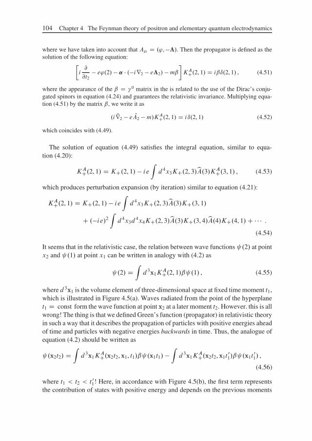
104 Chapter 4 The Feynman theory of positron and elementary quantum electrodynamics
where we have taken into account that A� D .', �A/. Then the propagator is defined as thesolution of the following equation:
�i@
@t2� e'.2/ � ˛ � .�ir2 � eA2/ �mˇ
�KAC.2, 1/ D iˇı.2, 1/ , (4.51)
where the appearance of the ˇ D �0 matrix in the is related to the use of the Dirac’s conju-gated spinors in equation (4.24) and guarantees the relativistic invariance. Multiplying equa-tion (4.51) by the matrix ˇ, we write it as
.i Or2 � e OA2 �m/KAC.2, 1/ D iı.2, 1/ (4.52)
which coincides with (4.49).
The solution of equation (4.49) satisfies the integral equation, similar to equa-tion (4.20):
KAC.2, 1/ D KC.2, 1/ � ieZd 4x3KC.2, 3/bA.3/KAC.3, 1/ , (4.53)
which produces perturbation expansion (by iteration) similar to equation (4.21):
KAC.2, 1/ D KC.2, 1/ � ieZd 4x3KC.2, 3/bA.3/KC.3, 1/
C .�ie/2Zd 4x3d
4x4KC.2, 3/bA.3/KC.3, 4/bA.4/KC.4, 1/C � � � .
(4.54)
It seems that in the relativistic case, the relation between wave functions .2/ at pointx2 and .1/ at point x1 can be written in analogy with (4.2) as
.2/ DZd 3x1K
AC.2, 1/ˇ .1/ , (4.55)
where d 3x1 is the volume element of three-dimensional space at fixed time moment t1,which is illustrated in Figure 4.5(a). Waves radiated from the point of the hyperplanet1 D const form the wave function at point x2 at a later moment t2. However. this is allwrong! The thing is that we defined Green’s function (propagator) in relativistic theoryin such a way that it describes the propagation of particles with positive energies aheadof time and particles with negative energies backwards in time. Thus, the analogue ofequation (4.2) should be written as
.x2t2/ DZd 3x1K
AC.x2t2, x1, t1/ˇ .x1t1/ �Zd 3x1K
AC.x2t2, x1t01/ˇ .x1t
01/ ,
(4.56)
where t1 < t2 < t 01! Here, in accordance with Figure 4.5(b), the first term representsthe contribution of states with positive energy and depends on the previous moments
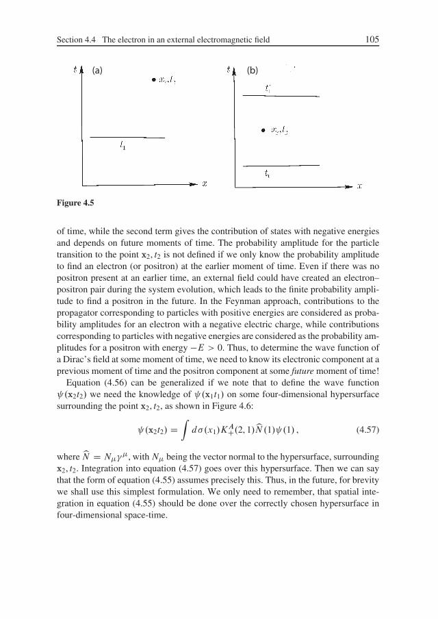
Section 4.4 The electron in an external electromagnetic field 105
(a) (b)
Figure 4.5
of time, while the second term gives the contribution of states with negative energiesand depends on future moments of time. The probability amplitude for the particletransition to the point x2, t2 is not defined if we only know the probability amplitudeto find an electron (or positron) at the earlier moment of time. Even if there was nopositron present at an earlier time, an external field could have created an electron–positron pair during the system evolution, which leads to the finite probability ampli-tude to find a positron in the future. In the Feynman approach, contributions to thepropagator corresponding to particles with positive energies are considered as proba-bility amplitudes for an electron with a negative electric charge, while contributionscorresponding to particles with negative energies are considered as the probability am-plitudes for a positron with energy �E > 0. Thus, to determine the wave function ofa Dirac’s field at some moment of time, we need to know its electronic component at aprevious moment of time and the positron component at some future moment of time!
Equation (4.56) can be generalized if we note that to define the wave function .x2t2/ we need the knowledge of .x1t1/ on some four-dimensional hypersurfacesurrounding the point x2, t2, as shown in Figure 4.6:
.x2t2/ DZd.x1/K
AC.2, 1/bN.1/ .1/ , (4.57)
where bN D N���, withN� being the vector normal to the hypersurface, surrounding
x2, t2. Integration into equation (4.57) goes over this hypersurface. Then we can saythat the form of equation (4.55) assumes precisely this. Thus, in the future, for brevitywe shall use this simplest formulation. We only need to remember, that spatial inte-gration in equation (4.55) should be done over the correctly chosen hypersurface infour-dimensional space-time.

106 Chapter 4 The Feynman theory of positron and elementary quantum electrodynamics
Figure 4.6
The formal derivation of equation (4.57) can be done as follows. Let us use the four-dimen-sional Gauss theorem:
Z
d 4x0 @F�.x0/@x0�
DZ
S
d.x0/F�.x0/n�.x0/ , (4.58)
where F�.x0/ is some 4-vector function, defined in space-time volume � limited by hyper-surface S , n�.x0/ is an external normal to surface element d.x0/ at point x0. Let .x/ be thesolution of the Dirac’s equation i�� @ .x/
@x� � m .x/ D 0. Let us choose F.x0/ D iKC.x �x0/�� .x0/, where x, x0 2 �. Then we have
@F�.x0/
@x0�
D i@
@x0�
ŒKC.x � x0/�� .x0/�
D"
[email protected] � x0/
@x0�
�� CmKC.x � x0/#
.x0/
CKC.x � x0/"
i��@ .x0/@x0�
�m .x0/#
. (4.59)
The second term here is equal to zero in accordance with Dirac’s equation. Let us substitutethis expression into the left-hand side of equation (4.58) and take into account that
[email protected] � x0/
@x0�
�� CmKC.x � x0/ D �iı.x � x0/ . (4.60)
Then we have
.x/ D �Z
S
d.x0/KC.x � x0/�� .x0/n�.x0/ , (4.61)
where n� is an external normal. If we introduce internal normal N�, we get
.x/ DZ
S
d.x0/KC.x � x0/�� .x0/N�.x0/ , (4.62)
which completes the proof. Equation (4.56) now follows if we choose hypersurface S consist-ing of two space-like hyperplanes t1 and t2, and neglect the “side” contributions, taking intoaccount that these parts of S are moved to infinity. Note that in this case N 0�0 D ˇ.

Section 4.4 The electron in an external electromagnetic field 107
The probability amplitude for an electron transition from some state with wave func-tion 0.x1t1/ of a particle with positive energy at the moment t1 to the state with wavefunction '0.x2t2/, also corresponding to states with positive energies, at the momentt2 > t1 is given by the following expression:
M DZd 3x1d
3x2'�0 .x2t2/KC.x2t2; x1t1/ˇ 0.x1t1/
DZd 3x1d
3x2 N'0.2/ˇKC.2, 1/ˇ 0.1/ . (4.63)
If between moments t1 and t2 the potential ebA acts, the function KC is replaced byKAC. In the first order, the transition amplitude, according to (4.54), is equal to
M1 D �ieZd 3x1d
3x2d4x3 N'0.2/ˇKC.2, 3/bA.3/KC.3, 1/ˇ 0.1/ . (4.64)
With the help of (4.55) we can perform integration over x1 and x2, introducing
0.3/ DZd 3x1KC.3, 1/ˇ 0.1/ , (4.65a)
N'0.3/ DZd 3x2 N'0.2/ˇKC.2, 3/ , (4.65b)
so that (4.64) becomes
M1 D �ieZd 4x N'0.x/bA.x/ 0.x/ . (4.66)
Let the initial wave function correspond to an electron with 4-momentum p1, whilethe final one corresponds to an electron with 4-momentum p2:
0.x/ D u.p1/e�ip1x , N'0.x/ D Nu.p2/e
ip2x , (4.67)
where u are spinors, corresponding to free particles with positive energy. Introducingthe Fourier transform of A�.x/,
A�.x/ DZd 4ke�ikxa�.k/ (4.68)
and substituting (4.67) and (4.68) into (4.66), we perform integration over x3 and get
M1 D �ie.2�/4Zd 4k ı.p2 � k � p1/ Nu.p2/ Oa.k/u.p1/
D �ie.2�/4 Nu.p2/ Oa.p2 � p1/u.p1/ , (4.69)
which is depicted by the diagram shown in Figure 4.7. Similarly, we can write the

108 Chapter 4 The Feynman theory of positron and elementary quantum electrodynamics
Figure 4.7 Figure 4.8
second-order matrix element for transition from the state with p1 into the state withp2 as
M2 D .�ie/2Zd 4x
Zd 4y N'0.x/bA.x/KC.x, y/bA.y/ 0.y/ . (4.70)
Then, after the substitution of the Fourier transforms ofbA andKC from (4.68), (4.38),and (4.67) we obtain
M2 D �ie2.2�/4Zd 4p
Zd 4k1
Zd 4k2ı.p2 � k1 � p/
� ı.p1 C k2 � p/ Nu.p2/ Oa.k1/1
Op �m Oa.k2/u.p1/ (4.71)
or
M2 D �ie2.2�/4Zd 4k Nu.p2/ Oa.p2 � p1 � k/ 1
Op1 C Ok �m Oa.k/u.p1/ , (4.72)
which can be associated with the diagram in Figure 4.8. It is clear that in a similar waywe can write all terms of the higher orders of perturbation theory: as a result we obtainthe following diagrammatic rules to describe electron scattering by the potential of anexternal electromagnetic field:
1. the atrix element of transition has the form M D Nu2Nu1;
2. to each virtual electron state (internal electron line) with momentum p correspondsin N by a factor i
Op�m ;
3. to each photon (wavy line) with momentum q corresponds in N by a factor of�ie Oa.q/;
4. over all momenta qi , which are not fixed by conservation laws, and which areobeyed in interaction vertices, we should perform integration d 4qi
.2/4 ;
While calculating integrals, the integration contour for the time component of the mo-mentum should br chosen according to the Feynman rule of pole encirclement: massm in the integrand is replaced by m ! m � iı .ı ! C0/.

Section 4.4 The electron in an external electromagnetic field 109
As a simple example of concrete calculating we shall briefly consider the scattering of anelectron by the Coulomb field of an atomic nuclei (Rutherford scattering) with electric chargeZe. The potential of nuclei is given by
A0 D V.r/ D Ze
r. (4.73)
Then,
Oa.q/ D 1
.2�/4
Zd 4x eiqx��A� D 1
.2�/3ı.q0/�
0Zd 3x e�iqrV.r/ D Ze
2�2q2ı.q0/�
0 .
(4.74)The first-order transition amplitude (4.69) has the form
M1 D �2�iı.E1 �E2/
�Nu.p2/
4�Ze2
jp2 � p1j2 �0u.p1/
�, (4.75)
where E1 and E2 are the initial and final energies of an electron. From (4.75) we can see thatE1 D E2 D E, i. e., we are dealing with elastic scattering (static potential!). The probabilityof scattering is determined by
jM1j2 D .2�/2ˇˇˇ Nu.p2/
4�Ze2
jp2 � p1j2 �0u.p1/
ˇˇˇ
2
ı.E1 �E2/ı.0/ . (4.76)
Here we have written Œı.E1 � E2/�2 D ı.E1 � E2/ı.0/, which creates obvious problems.
However, ı.0/ should be interpreted, according to the well-known Fermi recipe, as
ı.0/ D limT!1 lim
x!0
1
2�
T=2Z
�T=2
dt eixt D limT!1
T
2�, (4.77)
where T is the interaction time. Then we can define the transition probability per unit of timew1!2 as:
w1!2 D 2�
ˇˇˇ Nu.p2/
4�Ze2
jp2 � p1j2 �0u.p1/
ˇˇˇ
2
ı.E1 �E2/ . (4.78)
Further calculations (assuming the nonpolarized nature of the beam of initial electrons) requirethe averaging over both initial spin polarizations of electrons and the summation over the finalpolarizations. To perform this averaging and summation there exists a certain well-developedmathematical apparatus which uses the explicit form of spinors u.p/ and the properties ofDirac’s matrices. We pass over these details, which have been well-described in [60] and [6].Finally, from (4.78) it is possible to obtain a relativistic version of the Rutherford formula(Mott formula) for a differential scattering crossection to the element of solid angle d� [60]:
d
d�D Z2e4
4p2v2 sin4 �2
�1 � v2 sin2 �
2
�, (4.79)
taking into account that jp1 � p2j D 2jpj sin �=2, where � is the scattering angle, and weintroduced the velocity v D jpj=E.

110 Chapter 4 The Feynman theory of positron and elementary quantum electrodynamics
4.5 The two-particle problem
As we have seen above, in the Lorentz gauge the Maxwell equation for potentialsacquires the form
�A� D 4�j� . (4.80)
This equation is easily solved with the help of Green’s function DC, which is definedby the following equation:
�2DC.2, 1/ D 4�ı.2, 1/ . (4.81)
Making some obvious Fourier transformations, we have
DC.2, 1/ D � 4�
.2�/4
Zd 4k e�ik.x2�x1/
1
k2 C iı, ı ! C0 . (4.82)
In fact, up to a constant and sign, this expression coincides with the integral IC from(4.39) if we putm D 0 and use the rule (4.43). Now we can write the solution of (4.80)in the almost obvious form
A�.2/ DZd 4x1D.2, 1/j�.1/ . (4.83)
Here the possibly inhomogeneous term is absent, which corresponds to the boundarycondition of the absence of free electromagnetic radiation at t D ˙1 (i. e., there areno solutions A.0/� equation �A� D 0, which can always be added to the right-handside of equation (4.83)).
Consider now the case of two charged (interacting!) fermions. Each of the particlesis the source of an electromagnetic field which acts upon the motion of the other par-ticle. As a result of this interaction, each particle is scattered by the other. Let us writean expression for the current, corresponding to the transition of electron “a” from thestate ua.p1/e
�ip1x to the state ua.p2/e�ip2x:
j�.x/ D e Nua.p2/��a ua.p1/e
i.p2�p1/x . (4.84)
In accordance with equation (4.83) this current creates electromagnetic potential at thespace-time point x:
A�.x/ D e
Zd 4x0DC.x � x0/ei.p2�p1/x
0 Nua.p2/��a ua.p1/
D �4�eZd 4k
1
k2 C iıe�ikxı.k C p2 � p1/ Nua.p2/�
�a ua.p1/ . (4.85)
This potential acts upon the motion of the second electron “b”. According to equa-tion (4.66), the first-order matrix element, corresponding to the transition of electron“b” from the state with 4-momentum q1 into the state with 4-momentum q2, induced

Section 4.5 The two-particle problem 111
by potential (4.85), has the following form:
M D �ieZd 4x Nub.q2/e
iq2x��
bA�.x/ub.q1/e
�iq1x
D 4�ie2.2�/4Nub.q2/�
�
bub.q1/ Nua.p2/�a�ua.p1/
jp1 � p2j2 ı.p1 C q1 � p2 � q2/ .
(4.86)
Consider now the propagator for a system of two particles (two-particle Green’s func-tion). In a nonrelativistic approximation the system of two particles is described bythe Schroedinger wave function .xa, xb , t /, and, as in the previous case of a sin-gle particle, we can define the propagator K.xa, xb , t ; x0
a, x0b , t 0/, which determines
the probability amplitude of particle the “a” transition from point x0a at the time mo-
ment t 0 to point xa at the moment t , while particle “b” propagates from point x0b at the
moment t 0 to point xb at the moment t . If the particles do not interact, we obviouslyhave
K.xa, xb , t ; x0a, x0
b , t 0/ D K0a.xat ; x0at
0/K0b.xbt ; x0bt
0/ , (4.87)
whereK0a andK0b are the propagators of the free particles “a” and “b”. In the absenceof any interaction we can also define a more general two-particle Green’s function withdifferent time moments for particles in initial and final states:
K0.3, 4; 1, 2/ D K0a.3, 1/K0b.4, 2/ . (4.88)
Equation (4.86) can now be considered as the matrix element, appearing due to thefirst-order correction K.1/ to the propagator of two free particles, which is written as
KC.3, 4; 1, 2/ D� ie2
Zd 4x5
Zd 4x6KCa.3, 5/��a KCa.5, 1/DC.5, 6/KCb.4, 6/�b�KCb.6, 2/
(4.89)and can be represented by the Feynman diagram shown in Figure 4.9. In this expres-sion,DC can be considered as the propagator of the virtual photon. In fact, our deriva-tion is not completely satisfactory, because we did not quantize the electromagneticfield itself. However, we shall see later that the same result is reproduced in the rigor-ous theory.
In momentum representation we can rewrite the previous expressions in a more
transparent way. Assuming the validity of the Lorentz condition @A�
@x� D 0, and differ-entiating (4.85) over x�, we get
Nua.p2/��a k�ua.p1/ D Nua.p2/.�
0ak
0 � � � k/ua.p1/ D 0 . (4.90)
This relation is satisfied, because, due to the presence of ı-function in (4.85), we haveOk D Op1 � Op2, while u.p2/ and u.p1/ are free-particle spinors, so that
Nu1.p2/. Op1 � Op2/u.p1/ D Nu.p2/Œ. Op1 �m/ � . Op2 �m/�u.p1/ D 0 . (4.91)

112 Chapter 4 The Feynman theory of positron and elementary quantum electrodynamics
Figure 4.9
Thus, everywhere in (4.86) where the �0a matrix is present we can use the relation
�0a � k0 � �a � k D 0 (4.92)
and express �0a as
�0a D �al
� jkjk0
�, (4.93)
where �l is the � -matrix “projected on the direction of the propagation” k (let us stressthis the for virtual photon k0 ¤ jkj). Thus, denoting the “transverse” components of
� as � it , we can rewrite
�a
�
b
k2 in (4.86) as
��a �
�
b
k2D �0
a�0b
� � la� lb �P2iD1 �
iat�
ibt
k20 � k2
D�0a�
0b
1 � k2
0jkj2�
�P2iD1 �
iat�
ibt
k20 � k2
D ��0a�
0b
k2�P2iD1 �
iat�
ibt
k20 � k2
. (4.94)
The first term in this expression describes in (4.86) and (4.89) the instantaneous Cou-lomb interaction of two electrons, while the second one takes into account the transver-sal quanta responsible for the retarded magnetic interaction of particles. The appear-ance of instantaneous interaction is connected to the noncovariant separation of ini-tially the covariant interaction (4.94) into two terms: in fact the first term gives the maincontribution in the limit of small velocities, while the second produces corrections tothe instantaneous Coulomb interaction.
Up to now we have not taken into account that electrons are identical particles com-plying to the Pauli principle. This can be taken into account requiring antisymmetryof the wave function of the particle system, which can be achieved by introducing thetwo-particle propagator K.3, 4; 1, 2/ �K.4, 3; 1, 2/, which describes the transition oftwo particles from points 1 and 2 to points 3 and 4, including the exchange process.Thus, instead of (4.86), we obtain the matrix element for the scattering of two identical

Section 4.5 The two-particle problem 113
Figure 4.10
particles, in the first order over interaction, in the following form:
M D 4�ie2.2�/4´
Nub.q2/��
bub.q1/ Nua.p2/�a�ua.p1/
jp1 � p2j2
� Nub.p2/��
bub.q1/ Nua.q2/�a�ua.p1/
jq1 � p2j2μ
ı.p1 C q1 � p2 � q2/ ,
which determines e. g., the cross-section of the so-called Möller scattering.In higher orders of perturbation theory over interaction, an infinite number of cor-
rections appear which correspond to the exchange of a larger and larger numbers ofvirtual photons between interacting particles and particle self-interactions. All suchprocesses are described by Feynman diagrams, which correspond to the appropriatemathematical expressions. Examples of diagrams of the order of e4 are shown in Fig-ure 4.10. Additional Feynman diagram rules for two-particle scattering are formulatedas follows:
1. the probability amplitude for the radiation of a virtual photon is given by e��,which is attributed to an interaction point (vertex) on the diagram;
2. the probability amplitude for a photon transition (propagator, wavy line) from point1 to point 2 is given by DC.2, 1/ or, in momentum representation, � 4
k2Ciı .
Let us limit ourselves to the so-called “ladder” diagrams (with no intersections of in-teraction lines) shown in Figure 4.11. Introducing the probability amplitude '.x1, x2/
to find two particles at points x1 and x2 after the exchange of n virtual photons, we canwrite the same probability amplitude after the exchange of the next .nC 1/-th photonas
'nC1.1, 2/ D �ie2Zd 4x3
Zd 4x4KCa.1, 3/��a KCb.2, 4/�b�DC.3, 4/'n.3, 4/ .
(4.95)Then the total probability amplitude in the ladder approximation can be written as
.x1, x2/ D1X
nD0
'n.x1, x2/ (4.96)

114 Chapter 4 The Feynman theory of positron and elementary quantum electrodynamics
Figure 4.11
and, accordingly,
.2, 1/ D '0.2, 1/� ie2Zd 4x3
Zd 4x4KCa.1, 3/��a KCb.2, 4/�b�DC.3, 4/ .3, 4/ ,
(4.97)where '0.2, 1/ is the wave function, satisfying Dirac’s equation for the free particle (byboth variables). Applying Dirac’s differential operators for the “a” and “b” particlesto both sides of equation (4.97), we obtain the differential equation for .2, 1/
.i Ora �m/.i Orb �m/ .2, 1/ D ie2��a �b�DC.2, 1/ .2, 1/ . (4.98)
This is the so-called Bethe–Salpeter equation (in a ladder approximation), which is therelativistic wave equation for a two-particle system. In principle, it allows the completeanalysis of the bound state problem in such a system, e. g., the study of the formationand of the energy spectrum of positronium.
Chapter 5
Scattering matrix
5.1 Scattering amplitude
Most experiments in high-energy physics (physics of elementary particles) are essen-tially scattering experiments: studies of reactions between particles and their decays.Particles usually interact at very small distances and during very short time intervals(inside a target or at crossings of accelerator beams), while practically free reactionproducts are registered in detector systems which are placed rather far from the spaceregion where particles interact with each other, producing these reaction products.Thus, we are usually dealing with a rather general scattering problem: knowing theinitial state of a system of free particles, we have to find the probability of differentfinal states, which are also the sets of free particles, produced as a result of interactions.
Let jii be some initial state. The result of an interaction can be represented by asuperposition X
f
jf ihf jS jii , (5.1)
where the summation is performed over all possible final states jf i. The coefficientsSf i D hf jS jii form the so-called scattering matrix or S-matrix1. Now jSf i j2 givesthe probability of transition i ! f . In the absence of interactions, the S -matrix isobviously a unit matrix. Then it is convenient to separate this unit part and write
Sf i D ıf i C i.2�/4ı.Pf � Pi /Tf i , (5.2)
where the ı-functions simply express the conservation of the 4-momentum. For non-diagonal elements we simply have
Sf i D i.2�/4ı.Pi � Pf /Tf i . (5.3)
Here Tf i is called the scattering amplitude.While calculating the square of (5.2) we encounter the badly defined square of the
ı-function, which expresses the 4-momentum conservation law. The correct way toproceed is to introduce the Fourier transform:
ı.Pf � Pi / D 1
.2�/4
Zd 4xei.Pf �Pi /x . (5.4)
1 The notion of scattering matrix was first introduced by Heisenberg, who suggested considering it asthe most fundamental characteristic of elementary particle interactions.

116 Chapter 5 Scattering matrix
and dealing with the second such integral perform calculations for Pf D Pi , but withintegration extended to some large, but finite, volume V and time interval T , whichgives V T=.2�/4. Thus, we write
jSf i j2 D .2�/4ı.Pf � Pi /jTf i j2V T . (5.5)
Now we can introduce the well-defined probability of transition in unit time (and infinite volume)2:
wf i D .2�/4ı.Pf � Pi /jTf i j2V . (5.6)
Free particles are described by appropriate plane waves with amplitudes u, represent-ing bispinors for Dirac fermions, 4-vectors for photons, etc. Then we have
Tf i D u�1u
�2 � � �Qu1u2 � � � , (5.7)
where Q is some matrix over indices of the wave function amplitudes of all particles.Let us consider the most important cases, where there are only one or two particles
in the initial state, i. e., decays of single particles or collisions of two particles. Letus start from decays. The single particle can decay into several other particles withmomenta p0
a, belonging to an element of phase spaceQa d
3p0a (a numerates here
the particles in the final state). The number of states in this elementary phase spacevolume is
QaVd 3p0
a
.2/3 , and we have to multiply (5.6) by this number to obtain theprobability of transition into the final states:
dw D .2�/4ı.Pf � Pi /jTf i j2VY
a
Vd 3p0a
.2�/3. (5.8)
Everywhere we use normalization by a “single particle in volume V ”, so that the wavefunctions of all particles contain the factor of 1p
2"pV, where "p is the particle energy.
It is convenient to move these factors into the scattering amplitude and write the wavefunctions in the following as
D ue�ipx , Nuu D 2m (electrons) , (5.9)
A� D p4�e�e
�ikx , e�e�� D �1 , e�k
� D 0 (photons) (5.10)
etc., rewriting the scattering amplitude via the new amplitude Mf i , defined as
Tf i D Mf i
.2"1V : : : 2"01V : : :/
1=2, (5.11)
where the denominator contains one factor of .2"iV / per each initial and final particle.Then, the decay probability is written as
dw D .2�/4ı.Pf � Pi /jMf i j2 1
2"
Y
a
d 3p0a
.2�/32"0a
, (5.12)
2 As we already noted above, this recipe was first proposed by Fermi.

Section 5.1 Scattering amplitude 117
where " is an energy of the decaying particle. As should be expected, all normalizationvolumes in (5.12) has cancelled. If among final particles we have N identical ones,the phase volume of the final states should be divided by NŠ, to account for theirpermutations, producing the same state.
Consider in more detail the case of the decay into two particles with momenta p01, p0
2 andenergies "0
1, "02. In the rest frame of the decaying particle, p0
1 D �p02 p0, "0
1 C"02 D m. Then
dw D 1
.2�/2jMf i j2 1
2m
1
4"01"
02
ı.p01 C p0
2/ı."01 C "0
2 �m/d 3p01d
3p02 . (5.13)
First, the ı-function here disappears after integration over d 3p02. Then we rewrite d 3p0
1 as
d 3p0 D jp0j2d jp0jd� D jp0jd�0 "01"
02d."
01 C "0
2/
"01 C "0
2
, (5.14)
where we have taken into account "01
2 � m21 D "0
22 � m2
2 D jp0j2. Then, integrating overd."0
1 C"02/, we get rid of the second ı-function in (5.13). Accordingly, for the decay probability
into an element of the solid angle d�0 we get
dw D 1
32�2m2jMf i j2jp0jd�0 . (5.15)
Let us now consider the collision of two particles with momenta p1, p2 and energies"1, "2, producing in the final state some set of particles with momenta p0
a and energies"0a. Then,
dw D .2�/4ı.Pf � Pi /jMf i j2 1
4"1"2V
Y
a
d 3p0a
.2�/32"0a
. (5.16)
The invariant (with respect to Lorentz transformations) scattering cross-section is ob-tained from (5.16) dividing by [33]
j D I
V"1"2, where I D p
.p1p2/2 �m21m
22 . (5.17)
In the center of the mass frame we have p1 D �p2 p, so that I D jpj."1 C "2/ and
j D jpjV
�1
"1C 1
"2
�D v1 C v2
V, (5.18)
which gives the current density of the colliding particles (v1, v2 are the particle veloc-ities). Then finally
d D .2�/4ı.Pf � Pi /jMf i j2 1
4I
Y
a
d 3p0a
.2�/32"0a
. (5.19)
Let us drop the ı-functions for the case where there are two particles in the final state. Consideragain scattering in the center of the mass frame. Let " D "1 C "2 D "0
1 C "02 be the total energy

118 Chapter 5 Scattering matrix
of the colliding particles, while p1 D �p2 p and p01 D �p0
2 p0 are the initial and finalmomenta. Performing calculations similarly to the case of a decaying particle, we obtain
d D 1
64�2jMf i j2 jp0j
jpj"2d�0 (5.20)
For the case of elastic scattering we have jp0j D jpj. Let us introduce the kinematic invariant:
t .p1 � p01/
2 D m12 Cm0
12 � 2.p1p
01/ D m1
2 Cm01
2 � 2"1"01 C 2jp1jjp0
1j cos � , (5.21)
where � is the scattering angle. In the center of the mass reference frame, jp1j jpj andjp0
1j jp0j are determined only by the total energy ", so that for its given value we have
dt D 2jpjjp0jd cos � . (5.22)
Correspondingly, in equation (5.20) we can write
d�0 D �d'd cos � D d'd.�t /2jpjjp0j , (5.23)
where ' is the asimuthal angle of the vector p01 with respect to p1. Further, for brevity, we
write d.�t / as dt and obtain
d D 1
64�jMf i j2 dt
I 2
d'
2�. (5.24)
If the cross section does not depend on the asimuthal angle ', we get
d D 1
64�jMf i j2 dt
I 2. (5.25)
5.2 Kinematic invariants
Consider now the details of the kinematics of two particles scattering into two particlesin the final state. The conservation law for a 4-momentum can be written in the form(where we do not predetermine which particles are in initial and which are in finalstate)
p1 C p2 C p3 C p4 D 0 . (5.26)
The scattering amplitude for this process can be represented by a graph (diagram),as shown in Figure 5.1, where directions of the arrows correspond to the momenta“entering” the amplitude (cf. equation (5.26)). Two of the momenta correspond toinitial particles, while two others to particles in the final state (with moments �pa).In these notations, two of pa possess the time component p0
a > 0, while two otherspossess the time component p0
a < 0. For given types of particles participating inthe scattering process, the squares the 4-momenta p2
a are determined by their masses:p2a D m2
a (free particles always belong to their “mass surface”). Depending on the

Section 5.2 Kinematic invariants 119
Figure 5.1
values, which acquire time components p0a, and also on the values of particles charges,
the scattering amplitude in Figure 5.1 can describe three different reactions:
.1/ 1 C 2 ! 3 C 4 .s-channel/ ,
.2/ 1 C N3 ! N2 C 4 .t -channel/ , (5.27)
.3/ 1 C N4 ! N2 C 3 .u-channel/ ,
where the bars denote the appropriate antiparticles. These scattering processes arecalled cross-reactions, whcih can be represented graphically as in the diagrams in Fig-ure 5.2. We can also speak of three cross-channels of the same reaction, shown inFigure 5.1. We go from one reaction to another by changing the sign of the appropri-ate time component of momentum p0
a in (5.26):
p01 > 0 , p0
2 > 0 , p03 < 0 , p0
4 < 0 .s-channel) ,
p01 > 0 , p0
2 < 0 , p03 > 0 , p0
4 < 0 .t -channel/ , (5.28)
p01 > 0 , p0
2 < 0 , p03 < 0 , p0
4 > 0 .u-channel/ ,
and also the signs of the charges. All initial and final states in (5.29) obviously possesspositive energy. Transformation to the cross-channel reaction particle momentum in
Figure 5.2

120 Chapter 5 Scattering matrix
the initial state pa is replaced by the antiparticle momentum �pa in the final state,with a corresponding change of charge. Due to the CPT -invariance of the theory wecan also consider three CPT -conjugate reactions, which are obtained from (5.28) byreplacement of all particles by antiparticles and the interchange of the initial and finalstates. If the theory is invariant with respect to charge conjugation C , we can add tothese six reactions six moreC -conjugate reactions, where all the particles are replacedby the corresponding antiparticles.
From the four 4-momenta entering the reaction we can construct two independentinvariants. Due to (5.26) there are only three independent 4-vectors pa; let these bep1,p2,p3. From these we can construct six invariants: p2
1,p22,p2
3,p1p2,p1p3,p2p3.The first three reduce to the corresponding squares of masses: m2
1,m22,m2
3. The otherthree are connected by one relation, following from .p1 C p2 C p3/
2 D p24 D m2
4.Usually the following symmetric notations are used, introducing three kinematic in-variants:
s D .p1 C p2/2 D .p3 C p4/
2 ,
t D .p1 C p3/2 D .p2 C p4/
2 , (5.29)
u D .p1 C p4/2 D .p2 C p3/
2 ,
which are called Mandelstam variables. It is easily checked that
s C t C u D h m21 Cm2
2 Cm23 Cm2
4 . (5.30)
In channel (1), the invariant s represents the square of the total energy of collidingparticles 1 and 2 in their center of the mass reference frame. In fact, for p1 C p2 D 0we immediately obtain s D ."1 C "2/
2. In channel (2), a similar role is played byinvariant t , while in channel (3) it is played by invariant u. Correspondingly, we arespeaking about the s, t , and u reaction channels.
Let us consider in more detail the s-channel. Let
p1 D ."1, ps/ , p2 D ."2, �ps/ ,
p3 D .�"3, �p0s/ , p4 D .�"4, p0
s/ . (5.31)
Then it is easy to get
s D "2s , where "s D "1 C "2 D "3 C "4 , (5.32)
4sp2s D Œs � .m1 Cm2/
2�Œs � .m1 �m2/2� ,
4sp02s D Œs � .m3 Cm4/
2�Œs � .m3 �m4/2� , (5.33)
2t D h � s C 4psp0s � 1
s.m2
1 �m22/.m
23 �m2
4/ ,
2u D h � s � 4psp0s C 1
s.m2
1 �m22/.m
23 �m2
4/ . (5.34)

Section 5.3 Unitarity 121
In the case of elastic scattering (m1 D m3, m2 D m4) we have jpsj D jp0sj, so that
"1 D "3 and "2 D "4. Then equations (5.33) simplify to
t D �.ps � p0s/
2 D �2p2s.1 � cos �s/
u D �2p2s.1 C cos �s/C ."1 � "2/
2 (5.35)
where �s is an angle between ps and p0s , i. e., the scattering angle. Thus, in this case,
invariant �t represents the square of the transferred 3-momentum.Similar expressions for other channels are obtained by the obvious changes of no-
tation. The transformation to the t -channel is achieved by the replacements s $ t ,2 $ 3, while the transformation to the u-channel is made by s $ u, 2 $ 4.
If colliding particles are spinless, the scattering amplitude depends only on the kine-matic invariants s, t ,u, and in fact reduces to the single function
Mf i D f .s, t / . (5.36)
For particles with spin, besides s, t ,u there exist invariants which can be constructedfrom the amplitudes of the wave functions (bispinors, 4-vectors, 4-tensors etc.). Thenthe scattering amplitude has the form
Mf i DX
n
fn.s, t /Fn , (5.37)
where Fn are invariants, linearly dependent on wave function amplitudes of all thecolliding particles, as well as on their 4-momenta. The coefficients fn.s, t / are calledinvariant amplitudes.
5.3 Unitarity
The scattering matrix should be unitary: SSC D 1, or
.SSC/f i DX
n
Sf nS�in D ıf i , (5.38)
where n enumerates all the possible intermediate states. The unitarity condition (5.38)expresses the conservation of normalization and orthogonality of quantum states inscattering processes. In particular, the diagonal elements of (5.38) represent the sumof all transition probabilities from the fixed initial state to all the possible final states:
X
n
jSni j2 D 1 . (5.39)
Using (5.2) we obtain from (5.38)
Tf i � T �if D i.2�/4
X
n
ı.Pf � Pn/Tf nT �in . (5.40)

122 Chapter 5 Scattering matrix
The left-hand side is linear, while the right-hand side is quadratic over T . If the in-teraction contains a small parameter, the left-hand side is “larger” than the right-handside, and in the first approximation, neglecting the right-hand side, we can write
Tf i D T �if , (5.41)
so that the T -matrix in this approximation is Hermitian.Consider the collision of two particles. Only in the case of elastic scatterings are
all the intermediate states in (5.40) also two-particle states. The summation over thesestates reduces to the integration over the intermediate momenta p00
1, p002 and the sum-
mation over spins (helicities) of both particles, which we denote �00:X
n
D V 2Zd 3p00
1d3p00
2
.2�/6X
�00
(5.42)
After dropping the ı-function, in a way similar to that used above, we may obtain the“two-particle” unitarity condition as
Tf i � T �if D i
V 2
.2�/2X
�00
jpj"
ZTf nT
�in"
001"
002d�
00 , (5.43)
where p is the momentum and " is the total energy in the center of the mass referenceframe. The normalization volume disappears after transition to amplitudes Mf i :
Mf i �M �if D i
.4�/2X
�00
jpj"
ZMf nM
�ind�
00 . (5.44)
The diagonal element Ti i is called the zero-angle scattering amplitude. For this am-plitude the unitarity condition takes the form
2 ImTi i D .2�/4X
n
jTinj2ı.Pi � Pn/ . (5.45)
The right-hand side here is proportional to the total cross section of all the scatteringprocesses from the fixed initial state i , which we shall denote as tot . In fact, summing(5.6) over f and dividing by the particle current density j , we obtain
tot D .2�/4V
j
X
n
jTinj2ı.Pi � Pn/ , (5.46)
so that2V
jImTi i D tot . (5.47)
The normalization volume is cancelled after the transformation to Ti i DMi i=.2"1V 2"2V / (where "1, "2 are particle energies in the center of the mass refer-ence frame) and substitution of j from (5.18) we get
ImMi i D 2jpj"tot , (5.48)
which is called the optical theorem.

Section 5.3 Unitarity 123
Due to the CPT -theorem we have
Tf i D TNi Nf , (5.49)
where Ni and Nf are states obtained from i and f by changing all the particles with theirantiparticles. For diagonal elements,
Ti i D TNi Ni . (5.50)
Then it follows from (5.45) and (5.48) that the total cross section of all possible scatter-ing processes (with a fixed initial state) is the same for the reactions between particlesand antiparticles. In particular, this means that the total lifetime (decay probability) ofa particle and an antiparticle are equal.
During the period of the late 1950s and early 1960 where there was a certain dis-satisfaction in quantum field theory, it was proposed to limit the theory of elementaryparticles to the analysis of the general properties of the S -matrix, such as unitarity andsome general analyticity properties related to causality. This was the basis of the so-called analytical theory of the S -matrix [14]. Despite some successes and importanttheorems which are proved within this approach, it was insufficient for the construc-tion of a complete dynamical theory of elementary particles. At the same time, as weshall see below, modern quantum field theory gives the well-developed formalism forthe calculation of S -matrix via the standard perturbation theory approach.

Chapter 6
Invariant perturbation theory
6.1 Schroedinger and Heisenberg representations
Let us proceed to a systematic presentation of mathematical apparatus of perturbationtheory over interactions in quantum field theory. It is well known that there exist twomain formulations for equations of motion in quantum theory. In Schroedinger rep-resentation the quantum state at a given moment of time t is represented by the statevector ‰S .t/, containing the complete set of all possible results of measurements,applied to the system at this moment of time. The further evolution of the system isdescribed by the time dependence of this state vector (wave function), described bythe Schroedinger equation
i„@‰S@t
D HS‰S .t/ . (6.1)
In this representation, the operators of physical variables FS do not depend on time;for all t they are the same: dFS=dt D 0. At the same time, the average value of anoperator
hFS i D h‰S .t/jFS j‰S .t/i (6.2)
in the general case will depend on time as
i„ ddt
hFS i D h‰S .t/jŒFS ,H�j‰S .t/i . (6.3)
Let us make the following time-dependent unitary transformation of vector ‰S .t/:
ˆ.t/ D V.t/‰S .t/ , (6.4)
whereV.t/V C.t/ D V C.t/V .t/ D 1 , V C.t/ D V �1.t/ . (6.5)
Then the new state vector ˆ.t/ satisfies the equation1
i„@ˆ.t/@t
D�i„@V@tV �1 C VHSV
�1�ˆ.t/ . (6.6)
Let us choose V.t/ satisfying the equation
�i„@V@t
D .VHSV�1/V D VHS . (6.7)
1 We have i„ @ˆ.t/@t
D i„ @V@t‰S .t/ C i„V @‰S
@tD i„ @V
@tV �1ˆ.t/ C VHS‰S D i„ @V
@tV �1ˆ.t/ C
VHSV�1ˆ.t/, which coincides with (6.6).

Section 6.2 Interaction representation 125
Then the transformed state vector will not depend on time, which is directly seen from(6.6). Due to the unitarity of V.t/, the average value of an operator FS is expressed as
hF i D h‰S .t/jFS j‰S .t/i D hV.t/‰S .t/jV.t/FS‰S .t/iD hˆH jV.t/FSV �1.t/jˆH i , (6.8)
where we have defined ˆH as
ˆH D V.t/‰S .t/ , (6.9)
and V.t/ satisfies equation (6.7). Let us define FH .t/ as
FH .t/ D V.t/FSV�1.t/ . (6.10)
Then the time-dependent operator FH .t/ has the same average value in the state de-fined by vector ˆH , which the operator FS has in the state defined by vector ‰S .Differentiating (6.5) over time, we have
dV.t/
dtV C.t/C V.t/
dV C.t/dt
D 0 . (6.11)
Then from (6.7) and (6.10) we obtain for the time dependence of FH .t/2
@FH .t/
@tD @V
@tV CFH .t/CFH .t/V @V
C@t
D i
„ ŒVHSVC,FH .t/� D i
„ ŒHH ,FH .t/� ,(6.12)
which represents the equation of motion for the operator of the physical variable in aHeisenberg representation. The Heisenberg-state vectorˆH does not depend on time:
@ˆH
@tD 0 . (6.13)
We can assume that ˆH just coincides with ‰S .0/ at t D 0.
6.2 Interaction representation
Consider once again the usual Schroedinger equation
i„@ˆ.t/@t
D .H0 CHI /ˆ.t/ , (6.14)
where H0 is the Hamiltonian of noninteracting fields (particles), while HI is someinteraction Hamiltonian. The state vector ˆ in the absence of interactions, i. e., forHI D 0, describes the motion of the given number of free particles with fixed momentaand spins. The operator HI describes interactions of these particles.
2 To obtain (6.12) we take into account that @FH
@tD @V
@tFSV
�1 C VFS@V�1
@tD @V
@tV �1FH C
FHV@V�1
@t.

126 Chapter 6 Invariant perturbation theory
Let us introduce the state vector
‰.t/ D exp
�iH0t
„�ˆ.t/ . (6.15)
It is easy to see that ‰.t/ satisfies the equation
i„@‰.t/@t
D exp
�iH0t
„�HI exp
�� iH0t
„�‰.t/ (6.16)
or
i„@‰.t/@t
D H IRI .t/‰.t/ , (6.17)
where
H IRI .t/ D exp
�iH0t
„�HI exp
�� iH0t
„�
, (6.18)
the operator of the interaction energy in this new representation. This operator ex-plicitly depends on time, in contrast to the Schroedinger operator HI . In general, anarbitrary operatorQIR.t/ in this, the so-called interaction representation, is related tothe Schroedinger operator QS as
QIR.t/ D exp
�iH0t
„�QS exp
�� iH0t
„�
. (6.19)
Now it immediately follows that in interaction representation the dependence of oper-ators on time is determined by the Hamiltonian of free particles; differentiating (6.19)by t we obtain
i„@QIR.t/@t
D ŒQIR.t/,H0� . (6.20)
Note thatH IR0 D HS
0 . Thus, in interaction representation, field operators satisfy equa-tions of motion of free fields3, while the time-dependence of the state vector ‰.t/ isdetermined, according to (6.17), only by the interaction energy. Interaction represen-tation is quite convenient for the construction of perturbation theory.
Consider as an example the theory of Dirac fermions interacting with a scalar field. In Schroe-dinger representation the Hamiltonian of free fields has the form
H0 DZd 3r
�N .x/ .�i� � r Cm/ .x/C 1
2
�@'.x/
@t
�2
C 1
2.r'.x//2 C 1
2m2'2.x/
�,
(6.21)
and the interaction Hamiltonian (based on simplest principles of relativistic invariance) is writ-ten as
HI D g
Zd 3r N .x/ .x/'.x/ , (6.22)
3 In particular, this means that commutation relations for these operators are the same for arbitrarymoments of time.

Section 6.2 Interaction representation 127
where g is the dimensionless coupling constant. After transformation to interaction represen-tation, field operators '.x/ and .x/ satisfy the equations
.ibr �m/ IR.x/ D 0 , .� Cm2/'IR.x/ D 0 , (6.23)
and equation (6.17) reduces to
i„@‰.t/@t
D g
Z
ctDx0
d 3r N IR.x/ IR.x/'IR.x/‰.t/ . (6.24)
Equation (6.17) can be generalized to covariant form. This is achieved by introduc-tion of an arbitrary hypersurface in space-time instead of the hyperplane t D const.The only condition for this hypersurface to satisfy is that any vector normal to it n�.x/at an arbitrary point r should be time-like, i. e., n�.r/n�.r/ > 0. This means that nopoints on this hypersurface can be connected by a light signal, or that any two pointson it should br separated by a space-like interval. Let us denote such surfaces as . Atan arbitrary point r on this surface we can introduce time t .r/, which is called the localtime. In the limit when this surface becomes just a plane, all points on it possess thesame time t D const. Now we can generalize ‰.t/ by introducing ‰Œt.r/�. The basicequation (6.17)
i„@‰.t/@t
D HI .t/‰.t/ (6.25)
can now be considered to be the result of the summation of an infinite number ofequations obtained after the introduction of local time at each point of the space-likehypersurface. If the interaction Hamiltonian is expressed as the sum over small three-dimensional cells V on the space-like hypersurface , i. e.,
HI DX
�
HI .x/V , (6.26)
the equation in a small cell surrounding the space-time point r, t .r/ can be written as
i„@‰Œt.r/�@t.r/
D HI .x/V ‰Œt.r/� , (6.27)
which directly generalizes equation (6.17). The variation of ‰.t/, corresponding to arigid infinitesimal translation of hypersurface t D const as a whole, is determined bythe integral
Rt HId
3r, so that it becomes clear that the variation of ‰Œt.r/� relativeto point x is determined by the interaction energy in HI .x/V with an infinitesimalvolume surrounding x. As the product Vt is a relativistic invariant, we may in-troduce the following invariant differentiation procedure. Consider a function definedon the space-like hypersurface ‰Œt.r/� D ‰./. Let us compare the values of thisfunction on two space-like hypersurfaces and 0, which are infinitesimally differentfrom each other in the vicinity of point x, as shown in Figure 6.1. Now we define the

128 Chapter 6 Invariant perturbation theory
Figure 6.1
invariant operation ı=ı.x/ in the following way:
ı‰./
ı.x/D lim�t�V!0
‰Œt.r/Ct.r/� �‰Œt.r/�cR�V d
3rt.r/
D lim�t�V!0
‰. 0/ �‰./ct.r/V
D lim .x/!0
‰. 0/ �‰./�.x/
, (6.28)
where �.x/ is the 4-volume between and 0. Then, in the limit of �.x/ ! 0 equa-tion (6.27) can be rewritten in the form of the so-called Tomonaga–Schwinger equa-tion:
i„c ı‰./ı.x/
D HI .x/‰./ . (6.29)
This equation is covariant, as HI .x/ is relativistic invariant (scalar), and we do notneed any specific Lorentz reference frame to define the space-like surface . Thus, theTomonaga–Schwinger equation is written with no reference to any system of coordi-nates. However, in the following we shall mainly deal with equation (6.17), written inthe fixed reference frame.
6.3 S -matrix expansion
The solution of equation of motion in interaction representation (6.17) can be writtenin integral form as
‰.t/ D ‰.t0/ � i
„Z t
t0
dt 0HI .t 0/‰.t 0/ . (6.30)
Here we take into account the initial condition: for t D t0 the function ‰ reduces to‰.t0/.
Let us write the relation between ‰.t/ and ‰.t0/ as4
‰.t/ D U.t , t0/‰.t0/ ,
‰.t0/ D U�1.t , t0/‰.t/ , (6.31)
U.t0, t0/ D 1 ,
4 The formalism presented below was developed by Dyson.

Section 6.3 S -matrix expansion 129
where U.t , t0/ is a unitary (conserving normalization!) operator of evolution. Then
S D U.C1, �1/ (6.32)
defines the S-matrix (scattering matrix), which determines all the possible changes ofthe system states due to interaction:
‰.C1/ D S‰.�1/ , (6.33)
where ‰.�1/ and ‰.C1/ are asymptotic state vectors of the system, in particular,the asymptotic forms of incoming and scattered waves in a typical scattering process.
The operator U.t , t0/ satisfies the following differential equation, which is obviousfrom (6.17):
i„@U.t , t0/@t
D HI .t/U.t , t0/ . (6.34)
Similarly,
�i„@UC.t , t0/@t
D UC.t , t0/HI .t/ , (6.35)
as HI .t/ is Hermitian. From these equations it immediately follows that
@
@t.UC.t , t0/U.t , t0// D 0 , (6.36)
which is equivalent toUC.t , t0/U.t , t0/ D 1 . (6.37)
To prove unitarity we still have to show that
U.t , t0/UC.t , t0/ D 1 . (6.38)
The evolution operator satisfies the group property
U.t , t1/U.t1, t0/ D U.t , t0/ . (6.39)
In fact, from‰.t/ D U.t , t1/‰.t1/ , ‰.t1/ D U.t1, t0/‰.t0/ (6.40)
it follows that
‰.t/ D U.t , t0/‰.t0/ D U.t , t1/U.t1, t0/‰.t0/ , (6.41)
which is necessary to satisfy (6.39). If in (6.39) we set t D t0, we get
U.t0, t1/ D U�1.t1, t0/ . (6.42)
From U.t0, t1/U.t1, t0/ D 1, multiplying it from the left side by UC.t0, t1/ and using(6.37), we obtain
U.t1, t0/ D UC.t0, t1/ D U�1.t0, t1/ , (6.43)
which proves the unitarity of the evolution operator.

130 Chapter 6 Invariant perturbation theory
It follows directly from group property (6.39) that any transition of the system dur-ing the finite time interval can be represented by the multiplication of evolution oper-ators, corresponding to infinitesimal transitions:
U.t , t 0/ D U.t , t1/U.t1, t2/ � � �U.tn�1, tn/U.tn, t 0/ , (6.44)
where U.tj , tjC1/ corresponds to an infinitesimal transformation from time momenttj to tjC1.
The solution of equation (6.34) can obviously be written also in integral form:
U.t , t 0/ D 1 � i
„Z t
t 0d�HI .�/U.� , t 0/ . (6.45)
Thus, for the infinitesimal time difference tj � tjC1 we have:
U.tj , tjC1/ D 1 � i
„Z tj
tj C1
d�HI .�/U.� , tjC1/
� 1 � i
„Z tj
tj C1
dt 0HI .t 0/U.tjC1, tjC1/ D 1 � i
„Z tj
tj C1
dt 0HI .t 0/ .
(6.46)
Increasing the number of time intervals (to infinity!) and regrouping the terms in (6.44)we obtain
U.t , t0/ D 1 C��i
„�Z t
t0
dt1HI .t1/C��i
„�2 Z t
t0
dt1
Z t1
t0
dt2HI .t1/HI .t2/
C��i
„�3 Z t
t0
dt1
Z t1
t0
dt2
Z t2
t0
dt3HI .t1/HI .t2/HI .t3/C � � � . (6.47)
Consider the integral, determining the n-th order of perturbation theory:Z t
t0
dt1
Z t1
t0
dt2 � � �Z tn�1
t0
dtnHI .t1/HI .t2/ � � �HI .tn/ . (6.48)
Here integration is performed essentially over the whole time interval from t0 to t ,but with a limitation: the time moment tj is earlier than tj�1.j � n/. Of course,in equation (6.48) we can arbitrarily rename the integration variables t1, : : : , tn !tp1 , tp2 : : : tpn
, and the value of integral will not change. Making all permutations ofvariables t1, : : : , tn, summing all the expressions obtained, and dividing by the numberof permutations nŠ, we extend the integration over each of the variables to the wholetime interval from t0 to t . However, it is necessary to guarantee that operators HI .tj /under the integral are placed from left to right in the order of the growth of the timearguments. This can be achieved defining the operator T -ordering, which acts on theoperators, depending on time, and places them in chronological order, i. e., an operator

Section 6.3 S -matrix expansion 131
with a larger value of time in the product stands to the left of those with smaller times:
T�HI .t1/ � � �HI .tk/
D HI .ti /HI .tj / � � �HI .tk/ for ti > tj > � � � > tk , (6.49)
which gives the definition of the chronological or T-product of the operators. Then,using the symmetry of the integrand (6.48) mentioned above, we get:
Z t
t0
dt1
Z t1
t0
dt2 � � �Z tn�1
t0
dtnHI .t1/HI .t2/ � � �HI .tn/ D1
nŠ
Z t
t0
dt1
Z t
t0
dt2 � � �Z t
t0
dtnT�HI .t1/HI .t2/ � � �HI .tn/
. (6.50)
Let us consider in more detail the equivalence of these two forms of integral for thecase n D 2. From the definition of the T -product we have
Z t
t0
dt1
Z t
t0
dt2T�HI .t1/HI .t2/
DZ t
t0
dt1
Z t1
t0
dt2HI .t1/HI .t2/CZ t
t0
dt1
Z t
t1
dt2HI .t2/HI .t1/ . (6.51)
The integration region of the left-hand side is shown in Figure 6.2 as a square. On theother hand, in the first term in the right-hand side of (6.51), integration is extended overthe region I (nondashed triangle), while in the second term integration is performedover the dashed region II . Changing the order of integration in the second integral,
Figure 6.2

132 Chapter 6 Invariant perturbation theory
we shall first integrate over t1; then the limits of integration change, and we getZ t
t0
dt2
Z t2
t0
dt1HI .t2/HI .t1/ . (6.52)
Now, if we make the change of variables t1 ! t2 and t2 ! t1, equation (6.52) takesthe form Z t
t0
dt1
Z t1
t0
dt2HI .t1/HI .t2/ , (6.53)
so that (6.51) reduces toZ t
t0
dt1
Z t
t0
dt2T�HI .t1/HI .t2/
D 2ŠZ t
t0
dt1
Z t1
t0
dt2HI .t1/HI .t2/ , (6.54)
which proves the validity of (6.50) for the case of n D 2.Thus, expansion (6.47) can be written as
U.t , t0/ D 1 C��i
„�Z t
t0
dt1T�HI .t1/
(6.55)
C 1
2Š
��i„�2 Z t
t0
dt1
Z t
t0
dt2T�HI .t1/HI .t2/
C 1
3Š
��i„�3 Z t
t0
dt1
Z t
t0
dt2
Z t
t0
dt3T�HI .t1/HI .t2/HI .t3/
C � � �
D1X
nD0
1
nŠ
�� i„
�n Z t
t0
dt1
Z t
t0
dt2 � � �Z t
t0
dtnT�HI .t1/HI .t2/ � � �HI .tn/
,
(6.56)
which can be rewritten as
U.t , t0/ D T
²exp
�� i„
Z t
t0
HI .t0/dt 0
�³, (6.57)
where we have performed the symbolic summation of the series (6.56), which reducesit to the so-called T-exponent.
It can be directly checked that the series (6.56) gives the solution of equation (6.34). Let usdifferentiate (6.56) by time t :
@U.t , t0/
@tD
1X
nD1
1
nŠ
�� i„
�nZ t
t0
dt1
Z t
t0
dt2 � � �Z t
t0
dtn�1nHI .t/T�HI .t1/HI .t2/ � � �HI .tn�1/
.
(6.58)While writing the right-hand side of (6.58) we used the symmetry of the integrand and the factthat operator HI .t/ always depends on the time moment t , which is later, than t1, : : : , tn�1.This allows us to move operator HI .t/ outside the sign of the T -product, putting it to the left

Section 6.3 S -matrix expansion 133
of all the other factors. Then (6.58) can be rewritten as
i„@U.t , t0/@t
D HI .t/
1X
nD1
1
.n � 1/Š
�� i„
�n�1 Z t
t0
dt1
Z t
t0
dt2
� � �Z t
t0
dtn�1T�HI .t1/HI .t2/ � � �HI .tn�1/
D HI .t/
1X
nD0
1
nŠ
�� i„
�n Z t
t0
dt1
Z t
t0
dt2 � � �Z t
t0
dtnT�HI .t1/HI .t2/ � � �HI .tn/
D HI .t/U.t , t0/ , (6.59)
which proves the desired result!
Recalling that
HI .t/ DZd 3rHI .x/ , (6.60)
we can rewrite (6.56) in the form, explicitly demonstrating its covariance,
U.t , t0/ D1X
nD0
1
nŠ
�� i„
�n Z t
t0
d 4x1
Z t
t0
d 4xc
� � �Z t
t0
d 4xnT�HI .x1/HI .x2/ � � � HI .xn/
, (6.61)
where we have usedRdtRd 3r D R
d 4x=c. We can generalize (6.61), introducingintegration limits at space-like surfaces and 0, then U. , 0/ will be explicitly in-variant, as both HI and the volume element d 4x are 4-scalars.
The important point in the justification of the above formalism is the so-called adia-batic hypothesis. Following the definition of the S -matrix we have to tend the initialmoment of time t0 to �1 and the final moment t to C1. However, we have to becautious: for the n-th order term in expansion (6.56), this can be done in nŠ waysfor each of the limits. Dyson proposed to overcome this difficulty by introducing theconvergence factor e��jt j, multiplying the interaction Hamiltonian, with � ! 0 atthe end of the calculations. This procedure is equivalent to an averaging procedureover all possible nŠ ways to perform the limit of t ! ˙1. Assuming the validity ofthis adiabatic hypothesis, we can consider the initial- and final-state wave functions aseigenstates of the “free” Hamiltonian H0; these are usually called the wave functionsof “bare” particles. Then, any scattering process is considered as consisting of thefollowing stages.
1. At time t D �1 the system is in a state described by the wave functionˆ, which isan eigenstate of the operator H0. In this state, there is a given number of particleswith fixed spins and momenta, and these particles are separated from each otherand noninteracting. Vector ˆ is constant and independent of the time .HI D 0/vector in interaction representation.

134 Chapter 6 Invariant perturbation theory
2. The interaction is switched on adiabatically, so that the state with wave function ˆtransforms into a state ‰.t0/ D U.t0, �1/ˆ, which is assumed to correspond tothe real state of physical particles with the same momenta and spins. At this stage itis still assumed, that particles are well separated and do not interact with each other.However, switching onHI induces self-interaction, so that the “bare” particles are“dressed” by virtual quanta and the particles become real physical particles whichsatisfy the condition p2 D m2, where m is the observable physical mass.
3. Further on, the particles interact with each other, i. e., are scattered, transform intoother type of particles, etc. After a long enough time T D t � t0, particles separateagain, but their states are now described by the wave function‰.t/ D U.t , t0/‰.t0/,this state corresponding to the “dressed” (i. e., real physical) particles after scatter-ing.
4. Then interaction is adiabatically switched of,f and the state with wave function‰.t/ transforms into a state with the wave functionˆ0, which corresponds to “bare”particles after scattering, and ˆ0 D U.1, t /‰.t/.
Thus, the real scattering problem ‰.t0/ ! ‰.t/ is replaced by an “equivalent” prob-lem which introduces the “bare” particles at t D ˙1. Consider the relation
‰.t/ D U.t , t0/‰.t0/ (6.62)
which can be rewritten as
U�1.1, t /‰0 D U.t , t0/U.t0, �1/ˆ . (6.63)
Now we have
ˆ0 D U.1, t /U.t , t0/U.t0, �1/ˆ D U.1, �1/ˆ D Sˆ . (6.64)
This means that ˆ0 at t D C1 is the wave function of “bare” particles which appearas a result of scattering from the state described by wave function ˆ at t D �1.
The adiabatic hypothesis leads to results which are in excellent agreement with ex-periments. This may seem strange, as it is clear that interaction between real particlescan not be “switched off” (adiabatically or in any other way). In this respect, quantumfield theory is rather different from quantum mechanics, where we usually deal withpotentials with finite radius (except the Coulomb case, but there we know the exactwave functions), so that in the scattering problem the wave functions of the initial andfinal states are really corresponding to free particles.

Section 6.4 Feynman diagrams for electron scattering in quantum electrodynamics 135
6.4 Feynman diagrams for electron scattering in quantumelectrodynamics
In quantum electrodynamics (QED), interaction Hamiltonian density has the form
HI .x/ D j�.x/A�.x/ , (6.65)
where j� is the current density of Dirac electrons, while A� is the vector-potential ofthe electromagnetic field. Then the scattering matrix is written as5
S D T exp
²�ie
Zd 4xj�.x/A
�.x/
³, (6.66)
where we returned to the system of units with „ D c D 1.Let us consider some specific examples of the calculation of matrix elements of a
scattering matrix. The current density operator j contains the product of two electronic -operators. Thus, in the first order of perturbation theory only the processes involvingthree particles – two electrons and one photon – can appear, as shown by the diagramin Figure 6.3, similar to that of Figure 4.7. However, such processes with free particlesare impossible because of energy and momentum conservation. In fact, ifp1 andp2 arethe 4-momenta of electrons, and k is the 4-momentum of a photon, conservation lawis written as k D p2 �p1 or k D p1 Cp2. However, these equalities are impossible, asfor the real photon we always have k2 D 0, while the square .p2˙p1/
2 is easily shownto be nonzero. Let us calculate .p2˙p1/
2 in the rest frame of one of the electrons, e. g.,electron 1. Then .p2 ˙p1/
2 D 2.m2 ˙p1p2/ D 2.m2 ˙"1"2 �p1p2/ D 2m.m˙"2/,and because of "2 > m we have .p2 C p1/
2 > 0 or .p2 � p1/2 < 0.
Thus, the first nonzero matrix elements of the S -matrix can appear only in the sec-ond order of perturbation theory:
S .2/ D �e2
2Š
Zd 4x
Zd 4x0T
�j�.x/A�.x/j
�.x0/A�.x0/
. (6.67)
As electron and photon operators in interaction representation commute with eachother, (6.67) can be rewritten as
S .2/ D �e2
2Š
Zd 4x
Zd 4x0T
�j�.x/j �.x0/
T�A�.x/A�.x
0/
. (6.68)
Figure 6.3
5 In the following, here and in the next chapter, we mainly follow [6].

136 Chapter 6 Invariant perturbation theory
As a first example we consider the elastic scattering of two electrons. In the ini-tial state we have two electrons with momenta p1 and p2, while in the final state wehave two electrons with momenta p3 and p4. It is assumed that electrons are in someconcrete spin states, but the spin indices in the following are dropped for brevity. Wehave to calculate the matrix element between the initial and final states with appro-priate particles. As in both states photons are just absent, the required matrix elementof the T -product of the photon operators is simply h0j � � � j0i, where j0i is a photonvacuum. Accordingly, from (6.68) we obtain a tensor:
D��.x � x0/ D ih0jTA�.x/A�.x0/j0i , (6.69)
which is called the photon propagator or the photon Green’s function.From the T -product of electron operators in (6.68) the following matrix element
appears:h34jTj�.x/j �.x0/j12i , (6.70)
where j12i and j34i denote states with two electrons with the appropriate momenta.This matrix element can also be written in the form of a vacuum average, if we use therelation
h2jF j1i D h0ja2FaC1 j0i , (6.71)
where F is an arbitrary operator, while aC1 and a2 are operators of the creation of the
1-st and annihilation of 2-nd electrons. It is clear that instead of (6.70) we have tocalculate
h0ja3a4T .j�.x/j �.x0//aC
2 aC1 j0i . (6.72)
Each of the current operators is written as j D N � , and the -operators are repre-sented by
DX
p
.ap p C bCp �p/ , N D
X
p
.aCp
N p C bpN �p/ , (6.73)
where p denotes the appropriate spinors (plane waves). The second terms here con-tain positron operators, which are irrelevant for the problem under consideration. Tak-ing (6.73) into account, the product j�.x/j �.x0/ is represented by the sum of theterms, each containing the product of two operators ap and two aC
p , which are respon-sible for the annihilation of electrons 1 and 2 and the creation of electrons 3 and 4.It is clear that these should be operators a1, a2, aC
3 , aC4 , which are “paired” (or “con-
tracted”) with the “external” operators aC1 , aC
2 , a3, a4 according to an obvious equality:
h0japaCp j0i D 1 . (6.74)
The operators just disappear, and only the c-numbers remain. Depending on which of -operators provide a1, a2, aC
3 , aC4 for pairing (contraction) with external aC
1 , aC2 , a3,

Section 6.4 Feynman diagrams for electron scattering in quantum electrodynamics 137
a4, equation (6.72) produces four terms like
a���3 a
�4.
N ��� ��/. N 0����� 0����/aC��2 aC����
1 C a�3a
���4 .
N ��� ��/. N 0����� 0����/aC����2 aC��
1
C a�3a
���4 .
N ��� ��/. N 0����� 0����/aC��2 aC����
1 C a���3 a
�4.
N ��� ��/. N 0����� 0����/aC����2 aC��
1 ,
(6.75)
where D .x/ and 0 D .x0/, and the same number of dots denote paired (con-tracted) fermion operators. Now, in each of these terms it is necessary to make per-mutations of the “paired” operators a1, a2, : : : from , written as (6.73), to put themalongside their external partners aC
1 , aC2 , : : : , so that we can use (6.74) and obtain the
vacuum average as a simple product of averages, corresponding to these pairings (con-tractions). Taking into account the anticommutativity of these operators (1,2,3,4 aredifferent states!), we find, that the matrix element (6.70) is equal to 6
h34jTj�.x/j �.x0/j12i D . N 4�� 2/. N 0
3�� 0
1/C . N 3�� 1/. N 0
4�� 0
2/
� . N 3�� 2/. N 0
4�� 0
1/ � . N 4�� 1/. N 0
3�� 0
2/ , (6.76)
where the are not operators, but are the corresponding spinors (plane waves withmomenta 1,2,3,4)! The total sign here is the subject of agreement; it depends on theorder of placement of the “external” electron operators. The sign of a matrix elementfor the scattering of identical particles is, in general, arbitrary. The first and secondterms in (6.76) (as well as the third and fourth) differ from each other only by thepermutation of indices � and � and arguments x and x0. But such permutations do notchange the matrix element (6.70), where the order of all factors is determined by thesymbol of T -ordering. Thus, after multiplying (6.76) and (6.69), and integration overd 4xd 4x0, four terms from (6.76) give
Sf i D ie2Zd 4xd 4x0D��.x � x0/Œ. N 4�
� 2/. N 03�� 0
1/ � . N 4�� 1/. N 0
3�� 0
2/�
(6.77)Note that the factor of 2Š cancelled! Taking into account that the electronic wave func-tion here are plane waves, we can write the expression in square brackets in (6.77) as
. Nu4��u2/. Nu3�
�u1/e�i.p2�p4/x�i.p1�p3/x
0
� . Nu4��u1/. Nu3�
�u2/e�i.p1�p4/x�i.p2�p3/x
0 D°. Nu4�
�u2/. Nu3��u1/e
�iŒ.p2�p4/C.p3�p1/��=2
� . Nu4��u1/. Nu3�
�u2/e�iŒ.p1�p4/C.p3�p2/��=2
±e�i.p1Cp2�p3�p4/X , (6.78)
where we have introduced � D x � x0 and X D 12.x C x0/. The integration in
(6.77) over d 4xd 4x0 is now replaced by d 4�d 4X . The integral over d 4X produces
6 Due to the anticommutativity of fermion operators, the current operators j.x/ and j.x0/, composedof pairs of these operators, commute, and we can drop the symbol T -product.

138 Chapter 6 Invariant perturbation theory
Figure 6.4
Figure 6.5
ı.p1 C p2 � p3 � p4/, corresponding to the conservation of the 4-momentum. Trans-forming from Sf i toMf i according to (5.2), (5.3), (5.11), we obtain scattering ampli-tude Mf i as
Mf i D e2Œ. Nu4��u2/D��.p4 � p2/. Nu3�
�u1/ � . Nu4��u1/D��.p4 � p1/. Nu3�
�u2/� ,(6.79)
where
D��.k/ DZd 4�eik�D��.�/ (6.80)
is the photon propagator in momentum representation.Each of the contributions to the scattering amplitude in (6.79) can be represented
by an appropriate Feynman diagram. For example, the first term corresponds to thediagram in Figure 6.4, where k D p1 � p3 D p4 � p2. Similarly, the second term isrepresented by the diagram int Figure 6.5, where k0 D p1 � p4 D p3 � p2. The rulesof diagram construction are similar to those discussed in Chapter 4:
1. The full lines “entering” the diagram (incoming lines) and directed towards theinteraction vertex correspond to the initial electrons and are associated withbispinors u. The full lines “leaving” the diagram (outgoing lines) and directedoutside the vertices correspond to the final electrons and are associated withbispinors Nu. These factors are written from left to right in the order correspond-ing to the movement along the full lines against the direction of arrows.
2. To each vertex we associate the factor .�ie��/. The vertices are connected by thephoton line, to which we associate the factor �iD�� . The 4-momenta of all particles(lines) in the vertices are conserved. the direction of the photon line is irrelevant;

Section 6.4 Feynman diagrams for electron scattering in quantum electrodynamics 139
it only changes the sign of the photon momentum k, but the photon propagatorD��.k/ is an even function of k.
These two diagrams differ from each other because of the exchange of two electronswith momenta p3 and p4, which corresponds to the exchange of identical particles inthe final state, leading to a sign change of the scattering amplitude (Pauli principle!).
Consider now electron–positron scattering. We now denote the initial momenta asp� and pC, while the final momenta are denoted as p0� and p0C. The operators of thecreation and annihilation of positrons enter the field operators (6.73) together with thecorresponding creation and annihilation operators of electrons. In the previous caseof electron–electron scattering, the annihilation of initial particles was done by theoperator , while the creation of the final particle was achieved by the operator N .Now the roles of these operators change: the conjugate function N .�pC/ describes theinitial positron, while the final positron is described by .�pC/. With this differencein mind we can easily write the scattering matrix as
Mf i D �e2. Nu.p0�/��u.p�//D��.p� � p0�/. Nu.�pC/��u.�p0C//C e2. Nu.�pC/��u.p�//D��.p� C pC/. Nu.p0�/��u.�p0C// , (6.81)
which is represented by the diagrams in Figure 6.6. The rules for constructing thesediagrams remain the same as before. the incoming full lines are associated with thebispinor u, and the outgoing lines with Nu. However, now the incoming lines correspondto the final positrons, while the outgoing lines correspond to the initial positrons, andtheir momenta are taken with the opposite sign. This is in agreement with the Feynmaninterpretation of a positron (discussed in Chapter 4) being an electron propagatingbackwards in time. In the first diagram of Figure 6.6, in one the vertex cross the linesof the initial and final electrons, while in the other they cross the positron lines, sothat this diagram describes electron scattering by positron. In the second diagram ineach of the vertices the electron and positron lines meet. In the upper vertex the pair isannihilated and a virtual photon is emitted, while in the lower vertex the pair is createdby this photon. This difference is also reflected in the properties of the virtual photons.In the first diagram (scattering channel) the 4-momentum of the virtual photon is equalto the difference of the 4-momenta of two electrons (or positrons), so that k2 < 0
Figure 6.6

140 Chapter 6 Invariant perturbation theory
(cf. the footnote at the beginning of this section). In the second diagram (annihilationchannel), k0 D p� C pC, so that k02 > 0. Note that for a virtual photon we alwayshave k2 ¤ 0, in contrast to a real photon, for which we always have k2 D 0.
6.5 Feynman diagrams for photon scattering
Consider now another effect which appears in the second order of perturbation the-ory – the photon scattering by electrons (the Compton effect). In the initial state wehave a photon and electron with 4-momenta k1 and p1 respectively, while in the finalstate they have momenta k2 and p2 (for brevity, we drop the polarization indices).During the calculation of the matrix element S .2/ between the initial and final states,the following photon matrix element appears:
h2jTA�.x/A�.x/j1i D h0jc2TA�.x/A�.x0/cC
1 j0i , (6.82)
where (cf. (3.41))A� D
X
k
.ckAk� C cCk A
�k�/ . (6.83)
In (6.82) we are performing all pairings (contractions) of “external” and “internal”photon operators and obtain
c�2A
��A
0���c
C��1 C c�
2A���A
0��c
C��1 D A�
2�A01� C A1�A
0�2� . (6.84)
Here we have taken into account the commutativity of c1 and cC2 , allowing the symbol
of T -ordering to be dropped.Similarly, we can analyze the electronic part of the matrix element:
h2jTj�.x/j �.x0/j1i D h0ja2T .N �� /. N 0�� 0/aC
1 j0i . (6.85)
Here again we are dealing with four -operators. Only two of them annihilate elec-tron 1 and create electron 2, i. e., paired with operators aC
1 and a2. These may beoperators N 0, or 0, N , but not , N or 0, N 0, as the creation or annihilation at thesame point x or x0 of a pair of real electrons (together with one real photon) obviouslyproduces zero. Making all the contractions, we obtain in the matrix element (6.85) twoterms, which we first write for the case of t > t 0:
a�2.
N ��� /. N 0�� 0��/aC��1 C a�
2.N �� ��/. N 0��� 0/aC��
1 . (6.86)
Contractions in the first term give
a2N ! a2a
C2
N 2 , 0aC1 ! a1a
C1
01 . (6.87)
Products a2aC2 and a1a
C1 are diagonal and can be replaced with their vacuum aver-
ages, which, according to (6.74), reduce to unity. For the similar transformation of the

Section 6.5 Feynman diagrams for photon scattering 141
second term in (6.87) we first have to move operator aC2 to the left and a1 to the right,
which can be done using the commutation rules, which gives®ap ,
¯C D ®
aCp , N ¯C D 0 ,
®ap, N ¯C D N p ,
®aCp ,
¯C D p , (6.88)
where in the right-hand side of the last two expressions spinors appeared, correspond-ing to plane waves with 4-momentum p (cf. (6.73)). As a results (6.86) is transformedto the form
h0j. N 2�� /. N 0�� 0
1/ � . N �� 1/. N 02�� 0/j0i for t > t 0 , (6.89)
where without index are operators, while 1, 2 are again just spinors (plane waves)with the appropriate momenta. Similarly, for t < t 0 we obtain an expression whichdiffers by permutation of the primes and the indices � and �:
h0j � . N 0�� 01/.
N 2�� /C . N 0
2�� 0/. N �� 1/j0i for t < t 0 . (6.90)
Both expressions (6.89) and (6.90) can be written in a unified way, introducing thefollowing definition of chronological (T -ordered) product of Fermion operators:
T .x/ N .x0/ D´
.x/ N .x0/ , t 0 < t ,
� N .x0/ .x/ , t 0 > t .(6.91)
Then the first and second terms in (6.89) and (6.90) are written as
N 2��h0jT N 0j0i�� 0
1 C N 02��h0jT 0 N j0i�� 1 . (6.92)
Note that in accordance with definition of (6.91) the products of the operators for t < t 0and t > t 0 are taken with different signs. This is the main difference of the definitionof the T -product for fermion operators from those given previously, which is relatedto the anticommutation of these operators, in contrast to commuting bilinear forms,entering the interaction Hamiltonian.
Let us define the electron propagator (Green’s function) as a second rank bispinorof the form
G.x � x0/ D �ih0jT .x/ N .x0/j0i . (6.93)
Then the matrix element of interest to us is written as
h2jTj�.x/j �.x0/j1i D i N 2��G.x � x0/�� 0
1 C Ci N 02��G.x0 � x/�� 1 . (6.94)
After multiplication by the photon matrix element (6.82), (6.84), and integration overd 4xd 4x0, both terms in (6.94) give the same result, so that
Sf i D �ie2Zd 4x
Zd 4x0 N 2.x/�
�G.x � x0/�� 1.x0/
� �A�2�.x/A1�.x
0/C A�2�.x
0/A1�.x/�
. (6.95)

142 Chapter 6 Invariant perturbation theory
Figure 6.7
Substituting plane waves for the electron and photon wave functions and separating, asin previous examples, the ı-function, corresponding to the 4-momentum conservationlaw, we obtain the scattering amplitude as
Mf i D �4�e2 Nu2Œ.�e�2 /G.p1 C k1/.�e1/C .�e1/G.p1 � k2/.�e
�2 /�u1 , (6.96)
where e1 and e2 are 4-vectors of photon polarization and G.p/ is the electron propa-gator in momentum representation. Two terms of this expression are represented bythe Feynman diagrams shown in Figure 6.7.
To the incoming line (initial photon) we associated the factorp
4�e, to the outgoingline (final photon) the factor
p4�e�. The full internal line corresponds to the virtual
electron with 4-momentum determined by the 4-momentum conservation law in thevertices. This line is associated with the electron propagator iG.f /. In contrast to the4-momentum of a real particle, the square of the virtual electron 4-momentum doesnot belong to its mass surface, i. e., it is not equal to m2. Writing the invariant f 2 inelectron rest frame, it is easy to show that
f 2 D .p1 C k1/2 > m2 , f 02 D .p1 � k2/
2 < m2 . (6.97)
6.6 Electron propagator
Let us calculate explicitly the propagators (Green’s functions) of free particles. Bydefinition (6.93) the electron propagator is given by
G.x � x0/ D �ih0jT .x/ N .x0/j0i .
Let us act upon it from the right side by the operator ��p��m, where p� D i@�. Asthe free field .x/ satisfies the Dirac’s equation .��p� �m/ .x/ D 0, we shall get

Section 6.6 Electron propagator 143
zero in all points x except those where t D t 0. Note that G.x � x0/ tends to differentlimits as t ! t 0 C 0 and t ! t 0 � 0, and according to definition (6.93) these limits aregiven by
�ih0j .rt / N .r0t /j0i and C ih0j N .r0t / .rt /j0i , (6.98)
so that for t D t 0 the Green’s function demonstrates finite discontinuity. This leads tothe appearance of an additional term with the ı-function in the derivative @G=@t :
@G
@tD �ih0jT @
@t .x0/j0i C ı.t � t 0/ŒGjt!t 0C0 �Gjt!t 0�0� . (6.99)
Note that in ��p� �m the derivative over t enters as i�0@=@t , so that
.��p� �m/G.x � x0/ D ı.t � t 0/�0h0j ® .rt /, N .r0t /¯C j0i . (6.100)
Now calculate the anticommutator. Multiplying the field operators, which we take inthe form of .6.73/, and using commutation relations for ap and bp, we obtain
® .r, t /, N .r0t /¯C D
X
p
Œ p.r/ N p.r0/C �p.r/ N �p.r0/� , (6.101)
where ˙p.r/ are plane waves (bispinors) without a time dependent factor. Thesefunctions form the full set, so that
X
p
Œ p.r/ �p .r
0/C �p.r/ ��p.r0/� D ı.r � r0/ıik (6.102)
where ıik is the Kronecker symbol over the spinor indices. The sum in the right-handside of (6.101) differs from (6.102) by the replacement of � by ��0, so that
® .rt /, N .r0t /¯C D �0ı.r � r0/ . (6.103)
Substituting (6.103) into (6.100) we finally get
.��p� �m/G.x � x0/ D ı.x � x0/ . (6.104)
Thus, the electron propagator satisfies the Dirac’s equation with a ı-function in theright-hand side, so that it is really the Green’s function for this equation7.
Consider now the Fourier transform of Green’s function
G.p/ DZd 4�e�ip�G.�/ . (6.105)
Calculating the Fourier transforms of both sides of equation (6.104), we get
.��p� �m/G.p/ D 1 . (6.106)
7 It is easy to see that iG.x1 � x2/ just coincides with Feynman’s function KC.2, 1/ introduced inChapter 4.

144 Chapter 6 Invariant perturbation theory
Solving this equation, we obtain the result, which we already know from Chapter 4,
G.p/ D ��p� Cm
p2 �m2. (6.107)
The components of the 4-vector p in G.p/ are independent variables and are not re-stricted by any relations like p2 p2
0 � p2 D m2. If we write the denominator of(6.107) as p2
0 � .p2 C m2/, we can see, that G.p/ as the function of p0 for a givenvalue of p has two poles at p0 D ˙", where " D p
p2 Cm2. Then again, during theintegration over dp0 in
G.�/ DZ
d 4p
.2�/4e�ip�G.p/ D 1
.2�/4
Zd 3peipr
Zdp0e
�ip0�G.p/ , .� D t�t 0/(6.108)
we meet the problem of encircling these poles which we first discussed in Chapter 4.Again we shall use Feynman’s approach. Let us return definition (6.93). Substituteinto it -operators in the form given by (6.73). Note that nonzero vacuum averagesappear only from the following products of creation and annihilation operators:
h0japaCp j0i D 1 , h0jbpbC
p j0i D 1 . (6.109)
Then,
G.x � x0/ D �iX
p
p.rt / N p.r0t 0/ D �iX
p
e�i".t�t 0/ p.r/ N p.r0/ (6.110)
for t � t 0 > 0. Accordingly,
G.x � x0/ D iX
p
N �p.r0t 0/ �p.rt / D iX
p
ei".t�t 0/ �p.r/ N �p.r0/ (6.111)
for t � t 0 < 0. We see that, as in Chapter 4, for t � t 0 > 0 only electrons contribute toG, while for t � t 0 < 0 – only positrons. Comparing (6.110) and (6.111) with (6.108)we see that integral Z
dp0e�ip0�G.p/ (6.112)
in equation (6.108) must produce a factor e�i"� for � > 0 and ei"� for � < 0. Thiscan be achieved if during the calculation of (6.112) we encircle poles p0 D " andp0 D �" in the upper and lower half-planes of complex variable p0 correspondingly,as shown in Figure 6.8. In fact, for � > 0 we have (to guarantee convergence!) closedthe integration contour to a semicircle at infinity in the lower half-plane of p0, then the
Figure 6.8

Section 6.6 Electron propagator 145
Figure 6.9
value of integral (6.112) will be determined by the residue at the pole p0 D C". For� < 0 we close the contour in the upper half-plane, and integral is determined by theresidue at the pole p0 D �". Thus we achieve the desired result. The Feynman rule todeal with the poles, as we have seen in Chapter 4, can be formulated in another form:integration over p0 is performed along the real axis, but we an add infinitesimallysmall negative imaginary part to particle mass m:
m ! m � i0 . (6.113)
Then" !
pp2 C .m � i0/2 D p
p2 Cm2 � i0 D " � i0 . (6.114)
Correspondingly, the poles p0 D ˙" are moved up and down from the real axis, asshown in Figure 6.9, so that integration becomes equivalent to integration along thecontour shown in Figure 6.88.
This rule for dealing with poles is equivalent to the well-known relation
1
x ˙ i0D P
1
x� i�ı.x/ , (6.115)
which is understood in the sense that integration with some regular function f .x/ is done asfollows: Z 1
�1dx
f .x/
x ˙ i0D P
Z 1
�1dxf .x/
x� i�f .0/ , (6.116)
where P denotes the principal value of the integral.
Using Feynman’s rule we write the electron propagator in momentum representa-tion as
G.p/ D ��p� Cm
p2 �m2 C i0. (6.117)
This Green’s function is the product of the bispinor ��p� Cm and the scalar
G.0/.p/ D 1
p2 �m2 C i0. (6.118)
8 It is useful to note that this rule of pole encirclement corresponds toG.x�x0/ acquiring an infinitesimaldamping over j� j. If we write the value of p0 in displaced poles as �." � iı/ and C." � iı/, whereı ! C0, the time-dependent exponent in integral (6.112) will be equal to exp.�i"j� j � ıj� j/.

146 Chapter 6 Invariant perturbation theory
In coordinate representation G.0/.�/ satisfies the equation
.� �m2/G.0/.x � x0/ D ı.x � x0/, (6.119)
being the Green’s function of the Klein-Gordon equation. It is obvious, that it deter-mines the propagator of scalar particles and can be defined via scalar filed as
G.0/.x � x0/ D �ih0jT '.x/'C.x0/j0i , (6.120)
where
T '.x/'C.x0/ D²'.x/'C.x0/ , t 0 < t ,'C.x0/'.x/ , t 0 > t (6.121)
is the definition of the T -product for the Bose field.
6.7 The photon propagator
While analyzing the free electromagnetic field, we used the expansion of the vector-potential over transversal plane waves. This description does not apply in the case ofan arbitrary electromagnetic field. This is obvious, as for example in case of electronscattering we have to take into account Coulomb interaction, which is described bythe scalar potential and is not reduced to the exchange of transversal virtual photons.Thus, it seems that we still do not have the full definition of operators A� and cannotcalculate the photon propagator directly using the expression
D��.x � x0/ D ih0jTA�.x/A�.x0/j0i . (6.122)
Besides that, the gauge invariance makes the field operators somehow unphysical.However, below we shall present some general analysis which solves all of these prob-lems [6].
The most general form of the symmetric 4-tensor of the second rank, dependingonly on the 4-vector � D x � x0, is given by
D��.�/ D g��D.�2/ � @�@�Dl .�2/ , (6.123)
where D andDl are scalar functions of invariant �2. Then, in momentum representa-tion we have
D��.k/ D g��D.k2/C k�k�D
l.k2/ , (6.124)
where D.k2/ and Dl .k2/ are Fourier components of D.�2/ and Dl.�2/.The photon Green’s function always enters scattering amplitudes multiplied by the
matrix elements of the transition currents of a pair of electrons, i. e., in combinationslike j�21D��j
�43, which is seen, e. g., from equation (6.79). Current conservation gives
@�j� D 0, so that the matrix elements of the current satisfy the condition of four-
dimensional transversality:k�j
�21 D 0 , (6.125)

Section 6.7 The photon propagator 147
where k D p2 � p1. Thus, the physical results do not change after the replacement
D�� ! D�� C ��k� C ��k� , (6.126)
where �� are arbitrary functions of k. This arbitrariness corresponds, in fact, to differ-ent choices of the gauge for field operators. Thus, the choice of the functionDl .k2/ in(6.124) is in fact arbitrary9 and can be done to make calculations more convenient.Thus, the full definition of the Green’s function reduces to the choice of a singlegauge invariant function D.k2/. Taking the fixed value of k2 and choosing the z-axis along the direction of k, we can see that transformations (6.126) will not affectDxx D Dyy D �D.k2/. Thus, it is sufficient to calculate only one component Dxx ,using an arbitrary choice of the gauge for potentials.
It is convenient to use, as before, the Coulomb gauge divA D 0, when the operatorA is given by
A DX
k˛
r2�
!
ck˛e
.˛/e�ikx C cCk˛e
.˛/�eikx�
, (6.127)
where ! D jkj and ˛ D 1, 2 enumerates polarizations. The only nonzero vacuumaverage of the product of operators c, cC is
h0jck˛cCk˛j0i D 1 . (6.128)
Then, using the definition (6.122), we obtain
Dik.�/ DZ
d 3k.2�/3
2�i
!
�X
˛
e.˛/i e
.˛/�k
�e�i!j� jCik� , (6.129)
where i , k are three-dimensional vector indices. The presence in the exponent of themodulus of � D t � t 0 reflects the T -ordering of the field operators in (6.122). From(6.129) it is clear that the integrand without the factor of eik� represents the Fouriercomponent of Dik.rt /. For Dxx D �D it is equal to
2�i
!e�i!j� jX
˛
je.˛/x j2 D 2�i
!e�i!j� j . (6.130)
To find Dxx.k2/ we have to Fourier expand this function in time. This gives
2�i
!e�i!j� j D �
Z 1
�1dk0
2�
4�
k20 � k2 C i0
e�ik0� . (6.131)
As shown above, integration here assumes encirclement of poles k0 D ˙jkj D ˙!from below and above, correspondingly, so that for � > 0 the integral is determined
9 Consider ıDl .k2/: an arbitrary change of Dl .k2/. Then we get ıD�� D k�k�ıDl k��� , where
�� D k�ıDl .k2/.

148 Chapter 6 Invariant perturbation theory
by the residue at the pole k0 D C!, for � < 0 by the residue at the pole k0 D �!.Thus, we finally find
D.k2/ D 4�
k2 C i0. (6.132)
Now it is obvious that the corresponding function in coordinate representation satisfiesthe equation
�D.x � x0/ D �4�ı.x � x0/ , (6.133)
so that it is the Green’s function of the wave equation.In most cases it is convenient to choose Dl D 0, so that the photon propagator has
the formD�� D g��D.k
2/ D 4�
k2 C i0g�� , (6.134)
which coincides with the result obtained in Chapter 4 and corresponds to the so-calledFeynman gauge.
Sometimes it is convenient to choose Dl D �D.k2/=k2, so that
D�� D 4�
k2
�g�� � k�k�
k2
�, (6.135)
corresponding to the so-called Landau gauge. Then D��k� D 0, and this choice issimilar to the Lorentz gauge, where k�A� D 0.
The choice of the gauge divA D 0 leads to a similar gauge for the propagator:
Di ikl D 0 , D0lk
l D 0 , (6.136)
which, together with Dxx D �D D �4�=k2, gives
Dil D � 4�
!2 � k2
�ıil � kikl
k2
�, D00 D �4�
k2, D0i D 0 , (6.137)
so that D00 simply equals to the Fourier transform of the Coulomb potential.
For massive particles with spin s D 1 there is no gauge invariance, and the choice of propagatoris unique. Substituting the appropriate operators � into the definition
G��.x � x0/ D �ih0jT �.x/ C� .x
0/j0i , (6.138)
we obtain an expression which differs from (6.129) only in the form of the sum over polar-izations, which takes into account three independent polarizations of the massive vector field.Dropping the technical details [6], we only mention that in momentum representation the prop-agator of the vector field is equal to
G�� D � 1
p2 �m2 C i0
g�� � p�p�
m2
�. (6.139)

Section 6.8 The Wick theorem and general diagram rules 149
6.8 The Wick theorem and general diagram rules
From simple examples of calculations of matrix elements of scattering matrix, con-sidered above, we already can see the advantages of diagrammatic approach. Let usconsider now the general case. Matrix element of S for a transition between arbitraryinitial and final states coincides with vacuum average of operator, which is obtainedby multiplication of S from the right by creation operators of all initial particles andfrom the left by annihilation operators of all final particles. Then, in n-th order ofperturbation theory this matrix element is written as:
hf jS .n/jii D 1
nŠ.�ie/n
Zd 4x1 � � �d 4xn
D0j : : : b2f b1f � � � a1f � � � c1f T
� . N 1�A1 1/ � � � . N n�An n/cC1i � � � aC
1i � � � bC1i � � � j0
E. (6.140)
The indices 1i , 2i , : : : enumerate the initial particles (electrons, positrons, and pho-tons separately), while 1f , 2f , : : : enumerate the final ones. The indices 1, 2, : : : ofoperators and A correspond to 1 D .x1/ etc. Operators and A are representedby linear combinations of the creation and annihilation operators of the appropriateparticles in different states. Thus, in matrix element vacuum averages of products ofcreation and annihilation operators as well as their linear combinations appear. Allthese operators are taken in interaction representation, so that they satisfy the equa-tions of motion and the commutation relations for free particles. Calculation of suchaverages is done using the Wick theorem, which is proved below.
The Wick theorem
Let us define the normal product of operators
N.ABCD � � �XYZ/ , (6.141)
so that all the creation operators are to the left of the annihilation operators, with theirsign corresponding to the parity of the permutation of the Fermion operators, whichtransforms the product to the necessary form. Obviously, the vacuum average of thenormal product of operators equals zero, except in the case where under the sign ofthe normal product we have simply some c-number. Let us call the “pairing” (“con-traction”) of two operators the following difference:
A.B . D T .AB/ �N.AB/ . (6.142)
It is easy to see that this expression is a c-number, as its right-hand side is either zero orcoincides (up to a sign) with the commutator (anticommutator) of operators A and B .The main statement of the Wick theorem is that the T -product of an arbitrary number of
150 Chapter 6 Invariant perturbation theory
operators can be expressed through all possible N -products with all possible pairings(contractions):
T .ABCD � � �XYZ/ D N.ABCD � � �XYZ/CN.A�B �CD � � �XYZ/CN.A�BC �D � � �XYZ/C � � � CN.A�B ��C ���D � � �X �Y ��Z���/ , (6.143)
i. e., the chronological product of the operators is equal to the normal product plusthe sum of the normal products with one pairing (the pair can be chosen in all possi-ble ways), plus the sum of the normal products with two pairings, etc. Pairing withinthe normal product is the c-number, which is (up to a sign ˙1) determined by equa-tion (6.142). The minus sign is chosen when the permutation needed to bring pairedoperators out of the normal product is odd with respect to the Fermion operators.
To prove the theorem, we first note that the simultaneous permutation of the op-erators in both sides of (6.143) does not change this equality. Then, with no loss ofgenerality we may assume that the time ordering of operators corresponds to that in(6.143). To obtain the N -product from the T -product we have to take all the creationoperators and interchange their positions with all the annihilation operators on the leftone by one, using the definition (6.142). In this way we get the sum of theN -productsof the type written in (6.143). However, this will contain only the contractions of thoseoperators, for which the order in the T -product is different from that in theN -product.But pairings of operators for which both orders are equivalent equal to zero, and wecan say that the right-hand side of (6.143) contain normal products with all possiblepairings (contractions). This proves the Wick theorem.
The Wick theorem helps to calculate the averages of the products of the operatorsover the vacuum state j0i. The average of the normal products is obviously zero, so thata nonzero contribution comes only from those terms in the right-hand side of (6.143),where all the operators are paired:
h0jT .ABCD � � �XYZ/j0i D h0jT .AB/j0ih0jT .CD/j0i � � � h0jT .YZ/j0i˙ h0jT .AC/j0ih0jT .BD/j0i � � � h0jT .YZ/j0i ˙ � � � , (6.144)
where we have taken into account that
h0jA�B �j0i D h0jT .AB/j0i . (6.145)
Thus, the average is represented by the sum of all the possible products of the aver-ages (over the ground state) of the T -products of the pairs of operators. The sign ofeach term corresponds to the parity of permutation of the Fermion operators. From(6.144) it follows, in particular, that among the operators A,B ,C ,D, : : : there shouldnecessarily be an even number of operators of each field. Recalling the definition ofthe Green’s function, we conclude that the vacuum average of the T -product of anarbitrary (even) number of field operators is expressed via the sum of the products ofthe free Green’s functions.

Section 6.8 The Wick theorem and general diagram rules 151
Applying Wick’s theorem to the matrix element (6.140), we can represent it as thesum of terms, each being the product of some pairwise averages. Among these we shallmeet pairings of operators , N , andAwith the “external” operators of the creation ofthe initial particles or the annihilation of the final ones. These pairings can be expressedthrough the wave functions of the initial and final particles as
h0jAcCp j0i D Ap , h0jcpAj0i D A�
p ,
h0j aCp j0i D p , h0jap N j0i D �
p , (6.146)
h0jbp j0i D �p , h0j N bCp j0i D N �p ,
where Ap, p are photon and electron wave functions with momentum p. The polar-ization indices are dropped here for brevity. There will also be pairings of “internal”operators, standing under the sign of the T -product. These pairings are replaced bythe appropriate propagators.
Each of the terms in the sum for the matrix element of the S -matrix appearing as aresult of the application of Wick theorem can be represented by the appropriate Feyn-man diagram. In the diagram of the n-th order there are n vertices, each associatedwith the corresponding integration variable x1, x2, : : : . Each vertex is connected withthree lines – two full ones (electrons) and one wavy one (photon), corresponding tothe electron ( and N ) and photon (A) operators, as functions of the same variable x.The operator corresponds to the incoming line and N – to the outgoing line.
To illustrate this we show several examples of the correspondence between theterms of the matrix element of third order and the diagrams. Dropping the signs ofthe integral and T -ordering, as well as the factors �ie� and the arguments of the op-erators, we write these terms in symbolic form, as shown in Figure 6.10, where pairings(contractions) are shown, as often done, by lines connecting the appropriate field op-erators. Note that for the internal photon pairings the direction of photon lines is ofno importance, because of the even nature of the photon propagator as a function ofx � x0.
Among the terms obtained in this way there are some that are equivalent and whichdiffer only by the permutation of the numbers of vertices, reflecting the correspon-dence between the vertices and the number of variables x1, x2, : : : , i. e., by a simpleredefinition of the integration variables. The number of such permutations is nŠ. It can-cels the factor of 1=nŠ in (6.140), so that we, in fact, do not need to take into accountdiagrams with all the permutations of the vertices. For example, two diagrams of thesecond order, shown in Figure 6.11, are just equivalent. In Figure 6.10 and Figure 6.11we show only internal pairings, corresponding to internal lines in the diagrams (virtualelectrons and photons). The remaining free operators are paired with external opera-tors, which establishes the correspondence between the external “legs” of diagramsand the initial or final particles. For example, pairing N with operators af or bC
i givesthe line of the final electron or initial positron, while pairing with aC
i or bf pro-

152 Chapter 6 Invariant perturbation theory
duces the line of the initial electron or final positron. Free operator A pairing with cCi
or with cf may correspond to both the initial or final photon. In this way we obtainseveral “topologically equivalent” (i. e., consisting of the same number of lines withidentical configurations of the graphs) diagrams, differing only by the permutations ofthe initial and the final incoming and outgoing external legs. Any such permutation isequivalent to some permutation of external operators a, b, : : : . If among the initial orfinal particles there are identical fermions, the relative sign of the diagrams, differingby the odd permutation of the corresponding free legs, should be opposite.
The nonoverlapping sequence of the full lines in the diagrams forms the electronline with an arrow along it, conserving the continuous direction. It may have two freeexternal legs, or it can form a loop, as shown in Figure 6.12. The conservation ofdirection along the electronic line is a graphical expression of the charge conservationlaw: the “incoming” charge to every vertex is equal to the “outgoing’ one. Placementof the bispinor indices along the continuous electron line corresponds to writing thematrices from left to right, moving against the arrows. Bispinor indices of differentelectron lines never intermix. Along the nonclosed line, the sequence of indices endsat the free external legs on the electron (or positron) wave functions. On the closedloop the sequence of indices also closes, so that the loop corresponds to the trace ofthe product of the matrices along it. It is easy to see that this trace should always betaken with a minus sign, In fact, the loop with k vertices corresponds to the set of kpairings:
. N �A ��/. N ��A ���/ : : : . N ���A �/ (6.147)
(a)
(b)
(c)
(d)
Figure 6.10

Section 6.8 The Wick theorem and general diagram rules 153
Figure 6.11
or the other similar, differing by permutation of vertices. In the .k � 1/-th pairing theoperators and N are already in the correct order ( N to the right of ) in which theyshould stand in an electron propagator. Those operators at the edges can be movedto become neighbors with the help of an even number of permutations with other -operators, to get at the end the correct order N . As h0jT N 0 j0i D �h0jT N 0j0i,the replacement of this pairing by the corresponding propagator is related to the changeof the total sign of the whole expression.
Transformation to momentum representation leads to the general 4-momentum con-servation law and also to the similar conservation law at every vertex. However, theselaws may be insufficient for fixing momenta of all internal lines in a given diagram.In these cases we should perform the integration of all momenta of internal linesd 4p=.2�/4 which remain indeterminate.
In a similar way we may analyze the case with an external electromagnetic field (cf. Chapter 4),i. e., the field, created by “passive” particles, whose states are not changed during the scatteringprocess (these may be heavy “classical” charges). LetA.e/.x/ be the 4-potential of an externalfield. It enters the Lagrangian together with the photon operator A as a sum ACA.e/. Becauseof the classical nature of A.e/ it is actually a c-number field containing no operators, and itcannot pair with other operators. Thus, in Feynman diagrams external fields may correspondonly to external lines. Let us introduce Fourier expansion for A.e/:
A.e/.x/ DZ
d 4q
.2�/4e�iqxA.e/.q/ , A.e/.q/ D
Zd 4xeiqxA.e/.x/ . (6.148)
In expressions for matrix elements in the momentum representation 4-vector q will be presentalong the 4-momenta of other external lines, corresponding to real particles. To each line ofan external field we associate the factor A.e/.q/, with the corresponding line considered as“incoming” in accordance with the sign in the exponent e�iqx in Fourier expansion forA.e/.q/(the “outgoing” line should be associated withA.e/�.q/). If the 4-momentum conservation law,
Figure 6.12

154 Chapter 6 Invariant perturbation theory
with given values of the 4-momenta of all real particles, does not fix the 4-momenta for thelines of external field, we have to integrate over “free” d 4q=.2�/4, as well as over all othernonfixed 4-momenta in the diagram.
If external field does not depend on time,
A.e/.q/ D 2�ı.q0/A.e/.q/ , (6.149)
where A.e/.q/ is the three-dimensional Fourier component,
A.e/.q/ DZd 3rA.e/.r/e�iqr . (6.150)
The xternal line is now associated with the factor A.e/.q/ and the 4-momentum q� D .0, q/.Energies of electron lines entering (along with the line of the external field) the vertex are thesame due to the conservation law. Over the remaining nonfixed three-dimensional momenta pof the internal lines we perform the integration d 3p=.2�/3.
Let us now present the final summary of the diagrammatic rules for scattering am-plitude (more precisely for iMf i ) of QED in momentum representation.
1. Contributions of the n-th order of perturbation theory are represented by diagramswith n vertices, each with one incoming and one outgoing electron (full) line andone photon (wavy) line. The scattering amplitude is described by all diagrams withfree external legs (external lines), corresponding to the initial and final particles.
2. To each external incoming full line (leg) we associate the amplitude of initial elec-tron u.p/ or final positron u.�p/. To each outgoing full line we associate the am-plitude of final electron Nu.p/ or initial positron Nu.�p/.
3. To each vertex we associate the 4-vector �ie��.
4. To each external incoming wavy line we associate the amplitude of initial photonp4�e�, and to the outgoing wavy line the amplitude
p4�e�
� of the final photon.The vector index � coincides with index of the �� matrix in the correspondingvertex, so that we have the scalar product.
5. To each internal full line we associate the factor iG.p/, and to the internal wavyline we associate the factor of �iD��.p/. Tensor indices �� coincide with indicesof matrices ��, �� in vertices, connected by a wavy line.
6. Along the continuous sequence of electron lines the arrows have the same direction,while the positions of bispinor indices correspond to writing matrices from left toright against the arrows. A closed loop is associated with the trace of the productof the corresponding bispinor matrices.
7. In each vertex, the 4-momenta of the lines entering or leaving it satisfy the conser-vation law, i. e., the sum of the momenta of incoming lines equals the sum of the

Section 6.8 The Wick theorem and general diagram rules 155
momenta of the outgoing lines. The momenta of the external lines (legs) are fixed(and obey the total conservation law for the scattering process under discussion),with the positron line associated with the momentum �p. Integration d 4p=.2�/4 isperformed over all momenta of the internal lines, remaining nonfixed, after takinginto account the conservation laws in all vertices.
8. An incoming external line (leg), corresponding to the external field, is associatedwith factor A.e/.q/, where the 4-vector q is related to the 4-momenta of other linesin the vertex by the conservation law. If the external field does not depend on time,this external leg corresponds to the factor of A.e/.q/, and integration d 3p=.2�/3 isperformed over nonfixed three-dimensional momenta of internal lines.
9. To each closed fermion loop we associate an extra factor of .�1/. If among theinitial or final particles there are several electrons or positrons, the relative signof the diagrams, differing by odd permutations of the identical particles (i. e., thecorresponding external legs), should be opposite.
Finally, let us recall that in the presence of identical fermions the total sign of thescattering amplitude is irrelevant.

Chapter 7
Exact propagators and vertices
7.1 Field operators in the Heisenberg representation andinteraction representation
Above we have expressed the terms of a perturbation series via field operators in theinteraction representation, with time-dependence determined by the Hamiltonian H0
of free particles. Exact scattering amplitudes are more conveniently expressed via fieldoperators in the Heisenberg representation, where the time-dependence is determinedby the total Hamiltonian of interacting particles H D H0 C HI . According to thegeneral rule for Heisenberg operators we have
.x/ .rt / D exp.iHt/ .r/ exp.�iHt/ (7.1)
and similar expressions for N .x/ andA�.x/. Here .r/ are time-independent (Schroe-dinger) operators. Heisenberg operators, taken at the same moments of time, satisfythe same commutation rules as Schroedinger operators and operators in the interactionrepresentation. In fact, we have® .rt /, N .r0t /¯C D exp.iHt/
® .r/, N .r0/¯C exp.�iHt/ D �0ı.r � r0/ . (7.2)
In a similar way, .rt / and A�.rt / commute:
Œ .rt /,A�.r0t /� D 0 . (7.3)
This is not so for operators taken at different moments of time!The equation of motion for the Heisenberg -operator is written as
�i @ @t
D H .x/ � .x/H ŒH , .x/� . (7.4)
For the Hamiltonian itself the Schroedinger and Heisenberg representations coincide.
During the calculation of the right-hand side of (7.4), in the Hamiltonian we can drop the partdepending only on the operator A�.x/ (the Hamiltonian of a free electromagnetic field), as itcommutes with . Then
H DZd 3r �.rt /.˛p C ˇm/ .rt /C e
Zd 3r N .rt /��A�.rt / .rt /
DZd 3r N .rt /Œ� � pCmC e��A�.rt /� .rt / . (7.5)

Section 7.1 Field operators in Heisenberg and interaction representations 157
Calculating the commutator ŒH , .x/� using (7.2) and excluding the ı-function by d 3r inte-gration, we obtain the equation of motion for the operator in the explicit form
.��p� � e��A� �m/ .rt / D 0 , (7.6)
which naturally coincides with Dirac’s equation in an electromagnetic field.Equations of motion for electromagnetic potential A�.rt / are obvious in advance from the
correspondence with the classical limit (large occupation numbers), when operator equationsof motion should reduce to the usual Maxwell equations for potentials, so that in an arbitrarygauge we have
@�@�A�.x/ � @�@�A�.x/ D 4�ej �.x/ , (7.7)
where j �.x/ D N .x/�� .x/ is the current operator, satisfying the continuity equation
@�j� D 0 . (7.8)
The system of equations (7.6) , (7.7) is the gauge invariant
A� ! A�.x/ � @��.x/ , .x/ ! .x/eie�.x/ , N .x/ ! e�ie�.x/ N .x/ , (7.9)
where �.x/ is an arbitrary Hermitian operator, commuting (at the same moment of time)with . Here we are dealing with operators in the Heisenberg representation. In interactionrepresentation the gauge transformation of electromagnetic potential does not act on oper-ators at all!
Let us now establish the relation between operators in the Heisenberg and inter-action representations. In accordance with the adiabatic hypothesis we assume thatinteraction HI .t/ is slowly “switched on” from the time moment t D �1 to finitetimes. Then for t ! �1 both representations (Heisenberg and interaction) simplycoincide. The corresponding wave functions (state vectors) ˆ è ˆint also coincide:
ˆint .t D �1/ D ˆ . (7.10)
On the other hand, the wave function in the Heisenberg representation does not dependon time at all (all time dependence is moved to the operators!), while in the interactionrepresentation the time-dependence of the wave function has the form
ˆint .t/ D S.t , �1/ˆint .�1/ , (7.11)
where1
S.t2, t1/ D T exp
²�iZ t2
t1
dt HI .t/
³(7.12)
with the obvious properties
S.t , t1/S.t1, t0/ D S.t , t0/ , S�1.t , t1/ D S.t1, t / . (7.13)
1 Note, that similar operator in the previous Chapter was denoted as U.t2, t1/.

158 Chapter 7 Exact propagators and vertices
Comparing (7.11) and (7.10) we find
ˆint .t/ D S.t , �1/ˆ , (7.14)
which establishes the relation between the wave functions in both representations. Thecorresponding expression for the transformation of operators has the form
.rt / D S�1.t , �1/ int .rt /S.t , �1/ D S.�1, t / int .rt /S.t , �1/ (7.15)
and a similar expression also holds for N and A�.
7.2 The exact propagator of photons
The exact photon propagator is defined as
D��.x � x0/ D ih0jTA�.x/A�.x0/j0i , (7.16)
where A�.x/ are the Heisenberg field operators, while previously we considered
D��.x � x0/ D ih0jTAint� .x/Aint� .x0/j0i , (7.17)
built upon the operators in the interaction representation. Green’s function (7.17) isusually referred to as the propagator of free photons.
Let us now express the exact propagator D�� via the operators in the interactionrepresentation. Consider t > t 0; then from the relation between A� and Aint� of thetype of (7.15), we obtain
D��.x � x0/ D ih0jTA�.x/A�.x0/j0i (7.18)
D ih0jS.�1, t /Aint� .x/S.t , �1/S.�1, t 0/Aint� .x0/S.t 0, �1/j0i .
Using (7.13) we have
S.t , �1/S.�1, t 0/ D S.t , t 0/ , S.�1, t / D S.�1, C1/S.1, t / . (7.19)
Then (7.18) is written as
D��.x � x0/ D ih0jS�1ŒS.1, t /Aint� .x/S.t , t 0/Aint� .x0/S.t 0, �1/�j0i , (7.20)
where, for brevity, we introduced
S D S.C1, �1/ (7.21)
and have taken into account that S�1.1, �1/S.1, t / D S.�1, t /. As S.t2, t1/ con-tains only operators taken at the time moments between t1 and t2, placed in chrono-logical order, it becomes obvious that all operator factors in square brackets in (7.20)are placed from left to right in the order of decreasing time. Placing the T -ordering

Section 7.2 The exact propagator of photons 159
symbol before the bracket, in the following we can make any permutations of factorshere, because the T -ordering will, in any case, place everything in the correct order.Then we can rewrite the bracket as:
T�Aint� .x/Aint� .x0/S.1, t /S.t , t 0/S.t 0, �1/
� D T�Aint� .x/Aint� .x0/S
�. (7.22)
Thus, we obtain
D��.x � x0/ D ih0jS�1TAint� .x/Aint� .x0/S j0i . (7.23)
Repeating all the previous arguments, we can show that this expression is also validfor the case of t < t 0.
It can be shown that S�1 can be moved out of the averaging procedure in the formof a phase factor. In fact, a Heisenberg wave function of the vacuum ˆ0 (as any otherHeisenberg function) coincides, according to (7.10), with the value of the vacuumwave function ˆ0
int .�1/ in the interaction representation. On the other hand, wehave
Sˆ0int .�1/ S.C1, �1/ˆ0
int .�1/ D ˆ0int .C1/ . (7.24)
But a vacuum (ground state) in a stable system is strictly a stationary state in whichthere is no possibility of any spontaneous processes of creation or annihilation of par-ticles. In other words, as time goes by, the vacuum remains a vacuum. This means thatˆ0int .C1/ can differ from ˆ0
int .�1/ only by some phase factor ei˛ . Then
Sˆ0int .�1/ D ei˛ˆ0
int .�1/ D h0jS j0iˆ0int .�1/ (7.25)
or, making a complex conjugation and taking into account the unitarity of S ,
ˆ0�int .�1/S�1 D h0jS j0i�1ˆ0�
int .�1/ (7.26)
Now it is clear that (7.23) can be rewritten as
D��.x � x0/ D ih0jTAint� .x/Aint� .x0/S j0i
h0jS j0i . (7.27)
Substituting into the numerator and denominator perturbation expansion of the S -matrix defined by (6.56), and performing averaging with the help of the Wick theorem,we can obtain the expansion of D�� in powers of the coupling constant e2.
In the numerator of (7.27), the expressions being averaged differ from similar ex-pressions for the matrix elements of the scattering matrix, as analyzed in the previ-ous chapter, by the replacement of the “external” creation and annihilation operatorof photons by the operators Aint� .x/ and Aint� .x0/. As all factors here stand underthe symbol of T -product, the pairings of these operators with “internal” operatorsAint� .x1/,Aint� .x2/will produce photon propagatorsD�� . Thus, the results of averag-ing will be expressed by sets of diagrams with two external legs, which are constructedby the rules, given in the previous chapter, with the only difference that both the ex-
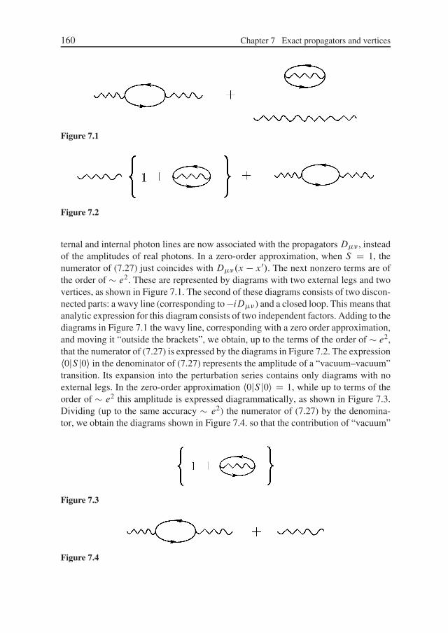
160 Chapter 7 Exact propagators and vertices
Figure 7.1
Figure 7.2
ternal and internal photon lines are now associated with the propagators D�� , insteadof the amplitudes of real photons. In a zero-order approximation, when S D 1, thenumerator of (7.27) just coincides with D��.x � x0/. The next nonzero terms are ofthe order of � e2. These are represented by diagrams with two external legs and twovertices, as shown in Figure 7.1. The second of these diagrams consists of two discon-nected parts: a wavy line (corresponding to �iD��) and a closed loop. This means thatanalytic expression for this diagram consists of two independent factors. Adding to thediagrams in Figure 7.1 the wavy line, corresponding with a zero order approximation,and moving it “outside the brackets”, we obtain, up to the terms of the order of � e2,that the numerator of (7.27) is expressed by the diagrams in Figure 7.2. The expressionh0jS j0i in the denominator of (7.27) represents the amplitude of a “vacuum–vacuum”transition. Its expansion into the perturbation series contains only diagrams with noexternal legs. In the zero-order approximation h0jS j0i D 1, while up to terms of theorder of � e2 this amplitude is expressed diagrammatically, as shown in Figure 7.3.Dividing (up to the same accuracy � e2) the numerator of (7.27) by the denomina-tor, we obtain the diagrams shown in Figure 7.4. so that the contribution of “vacuum”
Figure 7.3
Figure 7.4

Section 7.2 The exact propagator of photons 161
Figure 7.5
Figure 7.6
terms (under the figure brackets) is completely cancelled. Thus, the disconnected dia-gram in Figure 7.1(b) drops out of the answer. This result is, in fact, of a quite generalnature. A more detailed analysis of the diagrams in the numerator and denominator of(7.27) shows, that the role of the denominator h0jS j0i reduces to the general cancel-lation of all disconnected diagrams (in any order of perturbation theory), so that theexact propagator D�� is expressed only by diagrams without disconnected parts, orby connected diagrams only!
Note that diagrams without external legs (closed loops) are of no physical impor-tance, as these loops represent radiation corrections to the diagonal element of theS -matrix, describing vacuum–vacuum quantum transitions, and we already noted thatthe sum of all such loops (together with 1 from the zero-th order) produces only anirrelevant phase factor which does not influence physical results.
Transformation from coordinate to momentum representation is done in the usualway. For example, up to the terms of the order of � e2, the propagator �iD��.k/ isgiven by the diagrams shown in Figure 7.5, where the propagator itself is shown as a“fat” wavy line in the left-hand side. The analytic expression corresponding to thesediagrams is
D��.k/ D D��.k/C ie2D��.k/
�Zd 4p
.2�/4Sp��G.p C k/��G.p/
�D��.k/ .
(7.28)Terms of the higher orders are constructed in a similar way and are graphically rep-resented by diagrams with two external photon lines and the necessary number ofvertices, corresponding to the order of perturbation theory. For example, terms of theorder of � e4 are represented by diagrams with four vertices, as shown in Figure 7.6.The diagram shown in Figure 7.7 also contains four vertices, with an electron loopin its upper part. This loop corresponds to the pairing (contraction) N .x/� .x/, i. e.,simply to the vacuum average of the current h0jj.x/j0i. Even from the definition of the

162 Chapter 7 Exact propagators and vertices
Figure 7.7
Figure 7.8
Figure 7.9
vacuum itself it is obvious, that this average should identically be zero, and this factcannot be changed by any radiation (higher-order) corrections to this loop (though di-rect calculation, by the way, produces an infinite result here!). Thus, no diagrams withelectron loops of this kind should be taken into account in any order of perturbationtheory.
Part of the diagram (“block”) between two photon lines (external or internal) iscalled a photon self-energy part2. In the general case, such a block can itself be dividedinto parts connected by one photon line, as shown in Figure 7.8, where circles denoteblocks which cannot be further divided in this way. Such blocks are called irreducible(or single-particle irreducible). Let us denote the sum (of an infinite number!) of allirreducible photon self-energy parts as iP��=4� and call it the polarization operator.Classifying diagrams by the number of full irreducible self-energy parts (polarizationoperators), we can represent the exact photon propagator D�� by the diagrammaticseries shown in Figure 7.9, where each dashed circle represents iP��=4� . The orre-sponding analytic expression is written as
D D D CDP
4�D CD
P
4�D
P
4�D C � � �
D D
²1 C P
4�
�D CD
P
4�D C � � �
�³. (7.29)
2 Or, for brevity, just self-energy!
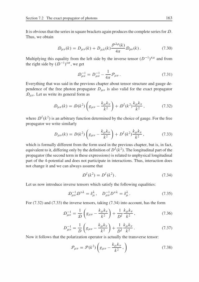
Section 7.2 The exact propagator of photons 163
It is obvious that the series in square brackets again produces the complete series for D .Thus, we obtain
D��.k/ D D��.k/CD��.k/P ��.k/
4�D��.k/ . (7.30)
Multiplying this equality from the left side by the inverse tensor .D�1/�� and fromthe right side by .D�1/�� , we get
D�1�� D D�1
�� � 1
4�P�� . (7.31)
Everything that was said in the previous chapter about tensor structure and gauge de-pendence of the free photon propagator D�� is also valid for the exact propagatorD�� . Let us write its general form as
D��.k/ D D.k2/
�g�� � k�k�
k2
�C D l.k2/
k�k�
k2, (7.32)
where D l.k2/ is an arbitrary function determined by the choice of gauge. For the freepropagator we write similarly
D��.k/ D D.k2/
�g�� � k�k�
k2
�CDl.k2/
k�k�
k2, (7.33)
which is formally different from the form used in the previous chapter, but is, in fact,equivalent to it, differing only by the definition ofDl.k2/. The longitudinal part of thepropagator (the second term in these expressions) is related to unphysical longitudinalpart of the 4-potential and does not participate in interactions. Thus, interaction doesnot change it and we can always assume that
D l.k2/ D Dl .k2/ . (7.34)
Let us now introduce inverse tensors which satisfy the following equalities:
D�1��D�� D ı�� , D�1
��D�� D ı�� . (7.35)
For (7.32) and (7.33) the inverse tensors, taking (7.34) into account, has the form
D�1�� D 1
D
�g�� � k�k�
k2
�C 1
Dl
k�k�
k2, (7.36)
D�1�� D 1
D
�g�� � k�k�
k2
�C 1
Dl
k�k�
k2. (7.37)
Now it follows that the polarization operator is actually the transverse tensor:
P�� D P .k2/
�g�� � k�k�
k2,
�(7.38)

164 Chapter 7 Exact propagators and vertices
Figure 7.10
where P .k2/ D k2 � 4�=D.k2/, so that3
D.k2/ D 4�
k2Œ1 � P .k2/=k2�. (7.39)
Thus, in contrast to the photon propagator, the polarization operator is gauge invariant!Sometimes it is useful to introduce photon self-energy, defined as the sum of all (not
only irreducible) the diagrams. Let us denote it as i…��=4�; then we have
D�� D D�� CD��…��
4�D�� , (7.40)
which is shown by the diagrams in Figure 7.10. Determining now …�� , we obtain
1
4�…�� D D�1
��D��D�1�� �D�1
�� (7.41)
and, using (7.32), (7.33), (7.36), and (7.37), we get
…�� D ….k2/
�g�� � k�k�
k2
�, … D P
1 � P=k2. (7.42)
Now we see that …�� , as well as P�� , is the gauge invariant tensor.
7.3 The exact propagator of electrons
An exact electron propagator is defined as
G .x � x0/ D �ih0jT .x/ N .x0/j0i , (7.43)
which is different from the case of the free particle propagator
G.x � x0/ D �ih0jT int .x/ N int .x0/j0i (7.44)
by replacement of the -operators in interaction representation by operators in theHeisenberg representation. Similarly to the case of photon propagator, discussedabove, equation (7.43) can be transformed to
G .x � x0/ D �i h0jT int .x/ N int .x0/S j0ih0jS j0i . (7.45)
3 It is useful to note that P .k2/ D P�� .k
2/=3.

Section 7.3 The exact propagator of electrons 165
Figure 7.11
Figure 7.12
Expansion of this expression in powers of e2 leads to a diagrammatic series for theG -function. The role of the denominator in (7.45) again reduces to the cancellation ofvacuum–vacuum transitions, so that the diagrammatic expansion for Green’s functioncontains diagrams without an isolated vacuum loops. Up to the terms of the order � e4
diagrams for G are shown in Figure 7.11, where the exact propagator itself is shownby a “fat” line. Diagrams like that in Figure 7.12, as noted before, should not be takeninto account. In momentum representation, a “fat” line corresponds to iG .p/, and theusual full and wavy lines represent propagators of free particles iG.p/ and �iD.k/.
Let us present a formal proof of the cancellation of vacuum diagrams. Consider the n-th ordercorrection to the Green’s function (propagator) of an electron, described by some disconnecteddiagram, representing two multiples. The first one includes all HI , contracted with .x/ andN .x0/, i. e., corresponds to a connected block with external legs. The second one describes the
rest of the diagram. Thus, the analytic expression for this correction looks like
� i .�i /n
nŠ
Zdt1 � � �
Zdtmh0jT � int .x/ N int .x0/HI .t1/ � � �HI .tm/
�j0ic�ZdtmC1 � � �
Zdtnh0jT .HI .tmC1/ � � �HI .tn//j0i . (7.46)
Here h0j � � � j0ic and h0j � � � j0i corresponds to some definite set of contractions (pairings) de-scribed by the Wick theorem, and the symbol h� � � ic denotes that pairings in this expressionproduce a connected diagram.
It is easily seen, that some of the diagrams give identical contributions. In fact, if we changethe pairings just by making different permutations of HI between h� � � ic and h� � � i, this willsimply correspond to the renaming integration variables and will not change the value of thecorrection to G . The number of such diagrams is equal to the number of ways to break noperators in HI into groups of m and n �m operators, i. e., it will be equal to nŠ
mŠ.n�m/Š .The total contribution of these diagrams is given by
� i .�i /m
mŠ
Zdt1 � � �
Zdtmh0jT . int .x/ N int .x0/HI .t1/ � � �HI .tm//j0ic
� .�i /n�m
.n �m/ŠZdtmC1 � � �
Zdtnh0jT .HI .tmC1/ � � �HI .tn//j0i . (7.47)

166 Chapter 7 Exact propagators and vertices
Let us sum the contributions of all diagrams of an arbitrary order, containing the definite con-nected part and the arbitrary disconnected parts. Obviously, we shall get
� i .�i /m
mŠ
Zdt1 � � �
Zdtmh0jT . int .x/ N int .x0/HI .t1/ � � �HI .tm//j0ic
�²
1 � iZdtmC1h0jHI .tmC1/j0i � 1
2
ZdtmC1
ZdtmC2h0jT .HI .tmC1/HI .tmC2//j0i
C � � � C .�i /kkŠ
ZdtmC1 � � �
ZdtmCkh0jT .HI .tmC1/ � � �HI .tmCk//j0i C � � �
³. (7.48)
Let us return to the initial expression (7.45). If we expand h0jS j0i in the denominator in a seriesin powers of HI , we shall get exactly the same expression, which stands in figure brackets in(7.48). Thus,
h0jT int .x/ N int .x0/S j0i D h0jT int .x/ N int .x0/S j0ich0jS j0i , (7.49)
so that, according to (7.45),
G .x � x0/ D �ih0jT int .x/ N int .x0/S j0ic , (7.50)
which completes our proof! This rule is valid for calculations of arbitrary expressions like(7.27) or (7.45) with an arbitrary number of field operators. In practice this means that we canjust drop the factor of h0jS j0i in the denominator, and do not take into account disconnecteddiagrams.
Further simplifications appear due to the fact that all types of pairings in
�i .�i /m
mŠ
Zdt1 � � �
Zdtmh0jT . int .x/ N int .x0/HI .t1/ � � �HI .tm//j0ic , (7.51)
differing only by permutations of HI , give the same contributions. Because of this, we candrop the factor of 1=mŠ and take into account only those pairings which lead to topologicallynonequivalent diagrams, i. e., those which can not be obtained from each other by permutationof operatorsHI . Now the contribution of each diagram does not contain a factor with relevantdependence on the order of diagram m. Due to this fact, each diagram can be separated intoelements which can be considered separately as corrections to one or another Green’s function.There may be irrelevant dependences onm, such as factors like �m, where � is some constant.Such factors do not prohibit separation of the diagram into different elements (blocks). Onthe contrary, the presence of a factor like 1=m does not allow such separation and separatesummations within different parts of the diagram.
The block between two electron lines is called the electron self-energy part. As in thecase of photons, it is called irreducible (or single particle irreducible), if it cannot be cutinto two self-energies by cutting one electron line. We denote the sum of all irreducibleself-energy parts as �iM.p/, and call M.p/ the mass operator. Up to terms of theorder of � e4 the mass operator is represented by diagrams shown in Figure 7.13.Performing summation, similar to that done during the derivation of equation (7.30),we obtain the Dyson equation,
G .p/ D G.p/CG.p/M.p/G .p/ (7.52)

Section 7.3 The exact propagator of electrons 167
Figure 7.13
or, in terms of inverse matrices,
G �1.p/ D G�1.p/ � M.p/ D ��p� �m � M.p/ . (7.53)
Equation (7.30) can also be called a Dyson equation for a photon propagator. Belowwe shall return many times to the discussion of these equations.
Heisenberg -operators (in contrast to -operators in interaction representation),as previously noted, do change under gauge transformations. In a similar way, theexact telectron propagator G is also not a gauge invariant quantity. It is clear that thechange of G under gauge transformations should be expressible via the same arbitraryfunction Dl , which is added to the photon propagator. It is clear from the fact that,during the calculations of G via a diagrammatic perturbation series, any term in thisseries is expressed via the photon Green’s functions D, and no other terms related toan electromagnetic field are present at all. We can make some assumptions about theproperties of the operator� in (7.9), with the only limitation that the result be expressedvia Dl . Under (7.9) the propagators D and G transform into
D�� ! ih0jT ŒA�.x/ � @��.x/�ŒA� � @0��.x
0/�j0i , (7.54)
G ! �ih0jT .x/eie�.x/e�ie�.x0/ N .x0/j0i . (7.55)
We shall assume that operators � are averaged over the vacuum independently of oth-ers, which is natural, as gauge invariance of electrodynamics requires that the “field” �does not take part in the interactions. Now put also h0j�.x/j0i D 0. Then, in equa-tions (7.54) and (7.55), terms containing � are separated and we obtain
D�� ! D�� C ih0jT @��.x/@0��.x
0/j0i , (7.56)
G ! G h0jTeie�.x/e�ie�.x0/j0i . (7.57)
Let us stress once again that here the � are operators. Next we consider the case ofinfinitesimal gauge transformations and introduce ı� instead of �. Transformation(7.56), independently of the smallness of ı�, can be written as
D�� ! D�� C ıD�� , ıD�� D @�@0�dl .x � x0/ , (7.58)
whered l .x � x0/ D ih0jT ı�.x/ı�.x0/j0i . (7.59)
Now we see that d l determines the change of the longitudinal part of the photon prop-agator D l under the gauge transformation.

168 Chapter 7 Exact propagators and vertices
In (7.57) we can expand the exponents in powers of ı� up to quadratic terms, sothat
h0jTeieı�.x/e�ieı�.x0/j0i � 1 � 1
2e2h0jı�2.x/C ı�2.x0/ � 2T ı�.x/ı�.x0/j0i .
(7.60)Taking into account the definition (7.59) we get
G ! G C ıG , ıG D ie2G .x � x0/Œd l .0/ � d l.x � x0/� . (7.61)
In momentum representation
ıG .p/ D ie2Z
d 4q
.2�/4ŒG .p/ � G .p � q/�d l.q/ , (7.62)
withq2d l.q/ D ıD l.q/ . (7.63)
These expressions give the general gauge transformation rules for exact propagatorsin QED.
7.4 Vertex parts
Besides the self-energy parts, in more complicated diagrams we can introduce addi-tional blocks with special physical meaning. Consider the function
K�.x1, x2, x3/ D h0jTA�.x1/ .x2/ N .x3/j0i . (7.64)
Due to the homogeneity of space-time, this function depends only on differences ofits arguments. After transformation to interaction representation we have
K�.x1, x2, x3/ D h0jTA�int .x1/ int .x2/ N int .x3/S j0i
h0jS j0i . (7.65)
In momentum representation we can write
K�.p2,p1; k/.2�/4ı.p1 C k � p2/ DZd 4x1
Zd 4x2
Zd 4x3e
�ikx1Cip2x2�ip1x3K�.x1, x2, x3/ . (7.66)
In the diagram technique function K� is described by a “three leg” graph, shown inFigure 7.14, with one photon and two electron legs, with the 4-momenta satisfying theconservation law
p1 C k D p2 . (7.67)
The zero-th order term in the perturbation expansion of this function is obviously zero,

Section 7.4 Vertex parts 169
Figure 7.14 Figure 7.15
Figure 7.16
while the first-order term in coordinate representation is
K�.x1, x2, x3/ D e
Zd 4xG.x2 � x/��G.x � x3/D
��.x1 � x/ (7.68)
or, in momentum representation
K�.p2,p1; k/ D eG.p2/��G.p1/D��.k/ , (7.69)
which is shown by the diagram in Figure 7.15. In higher orders, diagrams becomemore complicated due to the addition of extra vertices. For example, in the third orderthe diagrams shown in Figure 7.16 appear. In the first three diagrams of Figure 7.16we can separate the obvious self-energy parts of the photon and electrons. However,there are no such blocks in the fourth diagram. This is a general situation: correctionsof self-energy type simply replace in (7.69) Green’s functions G and D by G and D .The sum of the remaining terms of expansion lead to the change of the factor �� in(7.69). Denoting this quantity as �� we have, by definition,
K�.p2,p1; k/ D ¹iG .p2/Œ�ie��.p2,p1; k/�iG .p1/º Œ�iD��.k/� . (7.70)
The block connected with the other parts of diagram by a single photon and two elec-tron lines is called the vertex part, if this block can not be separated into parts, whichare connected to each other by single (electron or photon) lines. Block ��, introducedabove, representing the sum of all possible vertex parts, including the simple vertex��, is called the vertex operator (or vertex function). Up terms of the fifth order it isexpressed by the diagrams shown in Figure 7.17. All three momenta here cannot be si-multaneously related to real particles: we have already seen that absorption (emission)of a photon by the free electron is impossible because of 4-momentum conservation.

170 Chapter 7 Exact propagators and vertices
(a) (b) (c) (d)
(e) (f ) (g) (h) (i)
Figure 7.17
Figure 7.18
Thus, one of the legs in this graph can only be related a virtual particle (or externalfield).
We can now introduce the notions of compact and noncompact vertex parts. Thosevertex parts which do not contain self-energy corrections to internal lines are calledcompact, and we cannot separate the parts representing corrections to the internal ver-tices. Among the graphs shown in Figure 7.17, only diagrams (b) and (d) are compact.Diagrams (g,h,i) contain self-energy corrections either to the electron or the photonlines. In diagram (c) the upper horizontal wavy line can be considered as a correctionto the upper vertex, while the wavy lines at the sides of diagrams (e) and (f) representcorrections to vertices at these sides. Replacing internal lines in compact diagramsby “fat” lines representing exact Green’s functions, we obtain the expansion of thevertex operator in the form, shown in Figure 7.18, which is usually called a “skele-ton” diagram expansion. This expansion, in fact, produces an integral equation for � ,but with an infinite number of terms in the right-hand side; there is no closed equa-tion for the vertex parts, similar to that of the Dyson equation for Green’s functions(propagators).
We can also introduce vertices with a larger number of external legs, e. g., the “four-leg” vertex shown in Figure 7.19. We can obtain such a vertex considering the function
K.x1, x2; x3, x4/ D h0jT .x1/ .x2/ N .x3/ N .x4/j0i , (7.71)

Section 7.4 Vertex parts 171
Figure 7.19
Figure 7.20
which is usually called a two particle Green’s function. It also depends on differencesof its arguments, and its Fourier transformation can be written asZd 4x1
Zd 4x2
Zd 4x3
Zd 4x4K.x1, x2; x3, x4/e
i.p3x1Cp4x2�p1x3�p2x4/ D.2�/4ı.p1 C p2 � p3 � p4/K.p3,p4;p1,p2/ , (7.72)
where
K.p3,p4;p1,p2/ D .2�/4ı.p1 � p3/G .p1/G .p2/ � .2�/4ı.p2 � p3/G .p1/G .p2/
C G .p3/G .p4/Œ�i�.p3,p4;p1,p2/�G .p1/G .p2/ . (7.73)
The first two terms here exclude from the definition of �.p3,p4;p1,p2/ diagrams likethose shown in Figure 7.20. Similarly, in the third term in (7.73), the factors G excludefrom the definition of �-vertex those graphs which represent corrections to externalelectron lines. Using the properties of the T -product of fermion operators, we mayeasily see that �.p3,p4;p1,p2/ has the following (anti)symmetry properties:
�.p3,p4;p1,p2/ D ��.p4,p3;p1,p2/ D ��.p3,p4;p2,p1/ . (7.74)
This vertex describes, e. g., the process of scattering of two electrons; its amplitudecan be found if we associate with the external legs the amplitudes of the initial andfinal particles (instead of propagators G ):
iMf i D Nu.p3/ Nu.p4/Œ�ie�.p3,p4;p1,p2/�u.p1/u.p2/ , (7.75)
and here � describes all the possible interaction processes in all orders of perturbationtheory.

172 Chapter 7 Exact propagators and vertices
Figure 7.21
Figure 7.22
Figure 7.23
7.5 Dyson equations
Exact propagators and vertex parts are connected to each other, as we have alreadyseen, by certain integral relations. Let us analyze these relations in more detail. Con-sider diagrams for irreducible self-energies of an electron. It is easy to see that amongthe infinite number of these diagrams, only one, shown in Figure 7.21, is compact inthe sense discussed in the previous section, while the others can be considered as in-troducing corrections to one of its vertices. It is clear that all vertex corrections shouldbe attributed only to one (any of two) vertices of this diagram, while the other remains“bare” (to avoid double counting). Correspondingly, the sum of all irreducible self-energy parts (i. e., the mass operator) can be expressed by only one skeleton diagram,shown in Figure 7.22. The appropriate analytic expression has the form
M.p/ D G�1.p/� G �1.p/ D �ie2Z
d 4k
.2�/4��G .pC k/��.pC k,p; k/D��.k/ .
(7.76)Similar expression can be also written for the polarization operator. Among irreducibleself-energies for a photon, again only one is compact, and the polarization operator isrepresented by the diagram shown in Figure 7.23. the orresponding analytic expres-sion is
1
4�P��.k/ D D�1
��.k/�D�1�� .k/ D ie2Sp
Zd 4p
.2�/4��G .pCk/��.pCk,p; k/G .p/ .
(7.77)
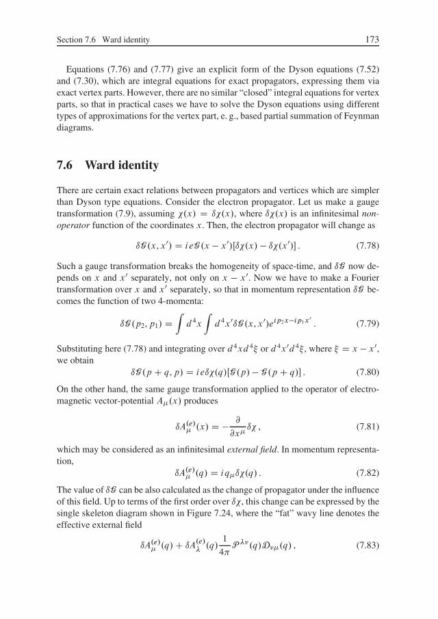
Section 7.6 Ward identity 173
Equations (7.76) and (7.77) give an explicit form of the Dyson equations (7.52)and (7.30), which are integral equations for exact propagators, expressing them viaexact vertex parts. However, there are no similar “closed” integral equations for vertexparts, so that in practical cases we have to solve the Dyson equations using differenttypes of approximations for the vertex part, e. g., based partial summation of Feynmandiagrams.
7.6 Ward identity
There are certain exact relations between propagators and vertices which are simplerthan Dyson type equations. Consider the electron propagator. Let us make a gaugetransformation (7.9), assuming �.x/ D ı�.x/, where ı�.x/ is an infinitesimal non-operator function of the coordinates x. Then, the electron propagator will change as
ıG .x, x0/ D ieG .x � x0/Œı�.x/ � ı�.x0/� . (7.78)
Such a gauge transformation breaks the homogeneity of space-time, and ıG now de-pends on x and x0 separately, not only on x � x0. Now we have to make a Fouriertransformation over x and x0 separately, so that in momentum representation ıG be-comes the function of two 4-momenta:
ıG .p2,p1/ DZd 4x
Zd 4x0ıG .x, x0/eip2x�ip1x
0
. (7.79)
Substituting here (7.78) and integrating over d 4xd 4� or d 4x0d 4� , where � D x � x0,we obtain
ıG .p C q,p/ D ieı�.q/ŒG .p/ � G .p C q/� . (7.80)
On the other hand, the same gauge transformation applied to the operator of electro-magnetic vector-potential A�.x/ produces
ıA.e/� .x/ D � @
@x�ı� , (7.81)
which may be considered as an infinitesimal external field. In momentum representa-tion,
ıA.e/� .q/ D iq�ı�.q/ . (7.82)
The value of ıG can be also calculated as the change of propagator under the influenceof this field. Up to terms of the first order over ı�, this change can be expressed by thesingle skeleton diagram shown in Figure 7.24, where the “fat” wavy line denotes theeffective external field
ıA.e/� .q/C ıA.e/
�.q/
1
4�P ��.q/D��.q/ , (7.83)

174 Chapter 7 Exact propagators and vertices
which takes into account the self-energy corrections. However, the 4-vector ıA.e/�.q/ is
longitudinal (with respect to q), while the tensor P �� is transversal (cf. (7.38, (7.42)).Thus, the second term here simply gives zero, so what remains is, in fact, the contri-bution of the diagram shown in Figure 7.24, where the line of the external field can betaken as “thin” and equal to ıA.e/� .q/. In analytic form,
ıG .p C q,p/ D eG .p C q/��.p C q,p; q/G .p/ıA.e/� .q/ . (7.84)
Substituting here (7.82) and comparing with (7.80), we find
G .p C q/ � G .p/ D �G .p C q/q���.p C q,p; q/G .p/ (7.85)
or, in terms of inverse matrices,
G �1.p C q/ � G �1.p/ D q���.p C q,p; q/ . (7.86)
For q ! 0, comparing the coefficients before infinitesimal q� in both sides of thisrelation, we get
@
@p�G �1.p/ D ��.p,p; 0/ (7.87)
which is called the Ward identity in differential form. Relation (7.86) is also called aWard identity, but for finite q. From (7.87) we can see that the derivative of G �1.p/
over the momentum coincides with a vertex operator with zero momentum transfer.The derivative of Green’s function G .p/ itself is equal to
� @
@p�iG .p/ D iG .p/Œ�i��.p,p; 0/�iG .p/ (7.88)
In zero-th approximation this identity is obvious, as from G�1 D ��p� � m weimmediately obtain @G�1
@p�D ��. Now it is easy to obtain a diagrammatic derivation of
Ward identity: from Dyson equation (7.53) it is obvious, that the differentiation of theinverse Green’s function over the momentum is equivalent to all possible insertions oflines of a fictitious external field, with zero momentum transfer, into all diagrams forirreducible self-energy, which generates all the diagrams for the corresponding vertexpart. The Ward identity is of great importance for checking the self-consistency ofconcrete approximations in different problems of quantum field theory.
A little more technical is a similar derivation of similar identities for an exact photonpropagator (polarization operator). The details of this derivation can be found in [6].
Figure 7.24

Chapter 8
Some applications of quantum electrodynamics
8.1 Electron scattering by static charge: higher ordercorrections
In this chapter we shall consider the calculations of some specific effects of quantumelectrodynamics (QED), as well as some conceptual problems related to the founda-tions of QED. It should be noted that QED is actually an example of the quite suc-cessful theory of interacting elementary particles. It allows exceptionally precise cal-culations of different effects due to electromagnetic interactions, which are in an idealagreement with current. The detailed analysis of the vast number of QED effects canbe found in [2, 6], while here we shall limit ourselves to only few of the most typicalcases. During our discussion we shall more or less skip the technical details, concen-trating on the qualitative aspects of the theory.
Let us return to the previously discussed problem (cf. Chapter 4) of electron scatter-ing by static charge of the nuclei (Rutherford scattering). In the first order of perturba-tion theory this scattering process is described by the diagram shown in Figure 8.1(a),where the static charge is denoted by a cross. According to the general rules of diagramtechnique, the corresponding scattering amplitude is written as
Mf i D �iZd 4xhf jj�.x/jiiA�.x/ , (8.1)
where the matrix element of transition current is
hf jj�.x/jii D e Nuf ��uie�iqx , (8.2)
(a) (b)
Figure 8.1

176 Chapter 8 Some applications of quantum electrodynamics
with q D pi � pf , and we introduced the spinors of an initial and final state of anelectron. Vector potential A�.x/ describes electromagnetic field of the static charge.Then we can write
Mf i D �ie Nuf ��uiA�.q/ , (8.3)
where
A�.q/ DZd 4x e�iqxA�.x/ . (8.4)
For a static charge, the value of A�.x/ is time independent, so that
A�.q/ DZdt e�i.Ei �Ef /t
Zd 3r eiqrA�.r/ D 2�ı.Ef � Ei /A�.q/ . (8.5)
The static Maxwell equation is written as
r2A�.r/ D �4�j�.r/ . (8.6)
Then we have
A�.q/ D 4�
jqj2 j�.q/ . (8.7)
Accordingly, from (8.3) and (8.5) we obtain
Mf i D �2�iı.Ef �Ei /e Nuf ��ui 4�
jqj2 j�.q/ . (8.8)
To shorten expressions to follow, we drop the ı-function for the conservation law anddefine the amplitude M as
�iM D ie Nuf ��ui 4�
jqj2 j�.q/ . (8.9)
During static charge scattering, an electron changes its momentum so that pi ¤ pf ,but energy is conserved, and Ei D Ef , or q0 D 0. Thus,
q2 D �jqj2 < 0 (8.10)
is a space-like scattering vector, and (8.9) is rewritten as
�iM D .ie Nuf ��ui /��4�ig��
q2
�.�ij �.q// . (8.11)
Here the first factor describes the vertex part, while the second represents the photonpropagator. For static nuclei with charge Ze we have
j 0.r/ D �.r/ D Zeı.r/ , j.r/ D 0 , (8.12)

Section 8.1 Electron scattering by static charge: higher order corrections 177
so that
�iM D .ie Nuf �0ui /
��4�i
q2
�.�iZe/ , (8.13)
which is expressed by the diagram in Figure 8.1(a) and coincides in fact with (4.75).These expressions describe Rutherford scattering and the corresponding crossectionis given by (4.79):
d
d�� jM j2 � q�4 � 1
sin4 �2
, (8.14)
where � is the scattering angle determined by kinematics:
q2 D .pi � pf /2 � �2k2.1 � cos �/ D �4k2 sin2 �
2, (8.15)
where we have neglected electron mass (in comparison to that of nuclei) and intro-duced k jpi j D jpf j.
This is the result of the first order perturbation theory. Let us discuss higher order(radiation) corrections. Let us consider as an example the third order diagram, shown inFigure 8.2. Using the general rules of diagram technique we obtain the corresponding
Figure 8.2

178 Chapter 8 Some applications of quantum electrodynamics
analytic expression
�iM D .�1/.ie Nuf ��ui /�
�i 4�g��0
q2
�Zd 4p
.2�/4Sp (8.16)
�².ie��
0
/i. Op Cm/
p2 �m2.ie��
0
/i. Oq � Op Cm/
.q � p/2 �m2
³��i 4�g�0�
q2
�.�ij �.q// .
In comparison to the first order result (8.11), here we observe the obvious modificationof the photon propagator by the single-loop polarization “insertion”, so that
� i 4�g��q2
! �i 4�g��q2
C�
�i 4�g��0
q2
�I�
0�0
��i 4�g�0�
q2
�D
� i 4�g��q2
C .�4�i/
q2I��.q
2/.�4�i/
q2, (8.17)
where
I��.q2/ D .�1/
Zd 4p
.2�/4Sp
².ie��/
i. Op Cm/
p2 �m2.ie��/
i. Oq � Op Cm/
.q � p/2 �m2
³. (8.18)
Immediately we see that for jpj ! 1 the integral in I�� contains the contributionof a term (from the polarization loop) like
Rdpp
3
p2 , which is seems to be quadraticallydivergent at the upper limit. This is a a typical divergence that appears in higher ordersof perturbation theory in practically every model of quantum field theory. The physicalorigin of this divergence is obviously related to the point-like (local) nature of fieldinteractions in relativistic theory. In fact, divergence here is weaker (logarithmic), butthe problem remains. Below we shall discuss its qualitative aspects.
Direct, but rather tedious, calculations show [2] that I�� can be written as
I��.q2/ D �ig��q2I.q2/C � � � , (8.19)
where
I.q2/ D e2
3�
Z 1
m2
dp2
p2� 2e2
�
Z 1
0dzz.1 � z/ ln
�1 � q2z.1 � z/
m2
�, (8.20)
and the multiple dot in (8.19) replaces the terms proportional to q�q� , which givea zero contribution after tensor contraction of the photon propagator with externalcharges (currents). The first term in (8.19) gives precisely the logarithmic divergenceof the polarization loop1.
It is useful to explicitly write expressions for I.q2/ in the limits of large and small.�q/2. To make the integral sensible we introduce in the first term of (8.20) the upperlimit cutoff ƒ2 (with dimensionality of momentum (mass) ƒ2 � m2 squared). Then,
1 Logarithmic, not quadratic, divergence here is due to some “hidden” algebra of the integrand [2].

Section 8.1 Electron scattering by static charge: higher order corrections 179
for .�q2/ m2 we have
ln
�1 � q2z.1 � z/
m2
�� �q
2z.1 � z/m2
(8.21)
and accordingly,
I.q2/ � e2
3�ln
�ƒ2
m2
�C e2
15�
q2
m2. (8.22)
For .�q2/ � m2 we have
ln
�1 � q2z.1 � z/
m2
�� ln
��q2
m2
�, (8.23)
so that
I.q2/ � e2
3�ln
�ƒ2
m2
�� e2
3�ln
��q2
m2
�D e2
3�ln
�ƒ2
�q2
�. (8.24)
Now we can write the scattering amplitude with a single-loop correction at .�q2/ m2 in the form2
�iM D .ie Nuf �0ui /
��4�i
q2
��1 � e2
3�ln
�ƒ2
m2
�� e2
15�
q2
m2CO.e4/
�.�iZe/ .
(8.25)This expression can be rewritten with the same accuracy as
�iM D .ieR Nuf �0ui /
��4�i
q2
��1 � e2
R
15�
q2
m2
�.�iZeR/ , (8.26)
where we introduced the renormalized charge
eR D e
�1 � e2
3�lnƒ2
m2
�1=2
. (8.27)
Let us assume that the value of eR from (8.27) represents the “true” (experimentallymeasurable) electric charge. Then the scattering amplitude (8.26) becomes finite, andits divergence is “concealed” in eR, which is taken from the experiment and is notcalculable within our theory. Thus we have explicitly performed the renormalizationof the divergent radiation correction. In the following we shall see that in QED alldivergences which appearing in higher orders of perturbation theory can be similarly“hidden” in the finite number of parameters, which should be determined experimen-tally. This reflects the fundamental property of the renormalizability of this theory.Only renormalizable models of quantum field theory are physically sensible.
2 Perturbation expansion here is in powers of dimensionless parameter e2 ! e2
„c � 1137 .
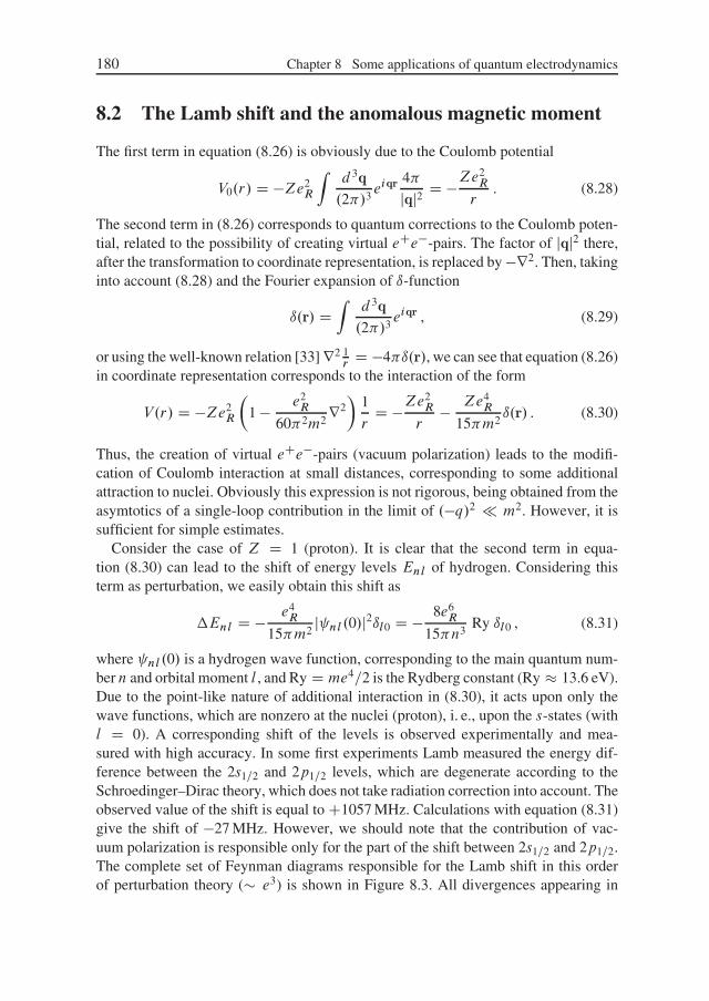
180 Chapter 8 Some applications of quantum electrodynamics
8.2 The Lamb shift and the anomalous magnetic moment
The first term in equation (8.26) is obviously due to the Coulomb potential
V0.r/ D �Ze2R
Zd 3q.2�/3
eiqr4�
jqj2 D �Ze2R
r. (8.28)
The second term in (8.26) corresponds to quantum corrections to the Coulomb poten-tial, related to the possibility of creating virtual eCe�-pairs. The factor of jqj2 there,after the transformation to coordinate representation, is replaced by �r2. Then, takinginto account (8.28) and the Fourier expansion of ı-function
ı.r/ DZ
d 3q.2�/3
eiqr , (8.29)
or using the well-known relation [33] r2 1r
D �4�ı.r/, we can see that equation (8.26)in coordinate representation corresponds to the interaction of the form
V.r/ D �Ze2R
�1 � e2
R
60�2m2r2�
1
rD �Ze
2R
r� Ze4
R
15�m2ı.r/ . (8.30)
Thus, the creation of virtual eCe�-pairs (vacuum polarization) leads to the modifi-cation of Coulomb interaction at small distances, corresponding to some additionalattraction to nuclei. Obviously this expression is not rigorous, being obtained from theasymtotics of a single-loop contribution in the limit of .�q/2 m2. However, it issufficient for simple estimates.
Consider the case of Z D 1 (proton). It is clear that the second term in equa-tion (8.30) can lead to the shift of energy levels Enl of hydrogen. Considering thisterm as perturbation, we easily obtain this shift as
Enl D � e4R
15�m2j nl .0/j2ıl0 D � 8e6
R
15�n3Ry ıl0 , (8.31)
where nl .0/ is a hydrogen wave function, corresponding to the main quantum num-ber n and orbital moment l , and Ry D me4=2 is the Rydberg constant (Ry � 13.6 eV).Due to the point-like nature of additional interaction in (8.30), it acts upon only thewave functions, which are nonzero at the nuclei (proton), i. e., upon the s-states (withl D 0). A corresponding shift of the levels is observed experimentally and mea-sured with high accuracy. In some first experiments Lamb measured the energy dif-ference between the 2s1=2 and 2p1=2 levels, which are degenerate according to theSchroedinger–Dirac theory, which does not take radiation correction into account. Theobserved value of the shift is equal to C1057 MHz. Calculations with equation (8.31)give the shift of �27 MHz. However, we should note that the contribution of vac-uum polarization is responsible only for the part of the shift between 2s1=2 and 2p1=2.The complete set of Feynman diagrams responsible for the Lamb shift in this orderof perturbation theory (� e3) is shown in Figure 8.3. All divergences appearing in
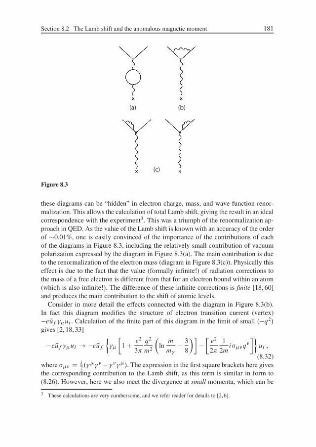
Section 8.2 The Lamb shift and the anomalous magnetic moment 181
(a) (b)
(c)
Figure 8.3
these diagrams can be “hidden” in electron charge, mass, and wave function renor-malization. This allows the calculation of total Lamb shift, giving the result in an idealcorrespondence with the experiment3. This was a triumph of the renormalization ap-proach in QED. As the value of the Lamb shift is known with an accuracy of the orderof �0.01%, one is easily convinced of the importance of the contributions of eachof the diagrams in Figure 8.3, including the relatively small contribution of vacuumpolarization expressed by the diagram in Figure 8.3(a). The main contribution is dueto the renormalization of the electron mass (diagram in Figure 8.3(c)). Physically thiseffect is due to the fact that the value (formally infinite!) of radiation corrections tothe mass of a free electron is different from that for an electron bound within an atom(which is also infinite!). The difference of these infinite corrections is finite [18, 60]and produces the main contribution to the shift of atomic levels.
Consider in more detail the effects connected with the diagram in Figure 8.3(b).In fact this diagram modifies the structure of electron transition current (vertex)�e Nuf ��ui . Calculation of the finite part of this diagram in the limit of small .�q2/
gives [2, 18, 33]
�e Nuf ��ui ! �e Nuf²��
�1 C e2
3�
q2
m2
�lnm
m� 3
8
����e2
2�
1
2mi��q
�
�³ui ,
(8.32)where �� D i
2.���� � ����/. The expression in the first square brackets here gives
the corresponding contribution to the Lamb shift, as this term is similar in form to(8.26). However, here we also meet the divergence at small momenta, which can be
3 These calculations are very cumbersome, and we refer reader for details to [2, 6].

182 Chapter 8 Some applications of quantum electrodynamics
formally avoided in (8.32) by introducing a small fictitious photon mass m . Thisdivergence is related to the so-called infrared catastrophe. In fact, the contributionconnected with the fictitious mass m is exactly cancelled by similar terms, originat-ing from diagrams in Figure 8.3(c). Infrared divergences in QED do not lead to majordifficulties like in the case of ultraviolet divergences (appearing due to the divergenceof Feynman integrals at the upper limit) discussed above. The infrared catastrophe isrelated to the ever-present possibility (for any QED process) of radiation of the largenumber of very “soft” photons with very small energy (frequency). Thus, the appear-ance of the infrared catastrophe is connected with the somehow inconsistent formula-tion of the problem: What is the probability for electron scattering by static nuclei withno photon being emitted? In reality we have to determine the scattering amplitude foran electron without a single photon emission, as well as the amplitudes with the emis-sion of one, two, three etc. “soft” photons with energies less than m . Each of theseamplitudes diverges, but an artificial introduction ofm makes them finite. The sum ofall these amplitudes does not diverge, and the fictitious parameterm just cancels. Thisproblem was analyzed in detail at the early stages of development of QED [2, 6, 18].
We are now interested in the second term in the square brackets in (8.32), whichmodifies ��, i. e., the structure of the current. In fact, we can convince ourselves [2,6, 18], that the contribution of the type ��q� describes the magnetic moment of anelectron � D � e
2m� , which is usually written as � D �g e2ms, with spin s D 1
2� , andg being the gyromagnetic ratio for an electron (in Dirac’s theory g D 2). Accordingly,the second term in (8.32) describes the additional contribution to the magnetic momentof an electron, so that
� D � e
2m
�1 C e2
2�
�� (8.33)
or
g D 2 C e2
�. (8.34)
Thus, in addition to Dirac’s magnetic moment of an electron, there appears the so-called anomalous magnetic moment e2=2� . A more precise expression for the anoma-lous contribution to the gyromagnetic ratio, obtained through very tedious calculationstaking into account terms up to the order of � e6, has the form
g � 2
2D 1
2
e2
��0.32848
�e2
�
�2
C.1.49˙0.2/
�e2
�
�3
C� � � D .1159655.4˙3.3/�10�9.
(8.35)The uncertainty shown here is related to the difficulty of calculating the very largenumber of diagrams of the order of � e6. The experimental value of the anomalousgyromagnetic ratio is
g � 2
2
ˇˇexp
D .1159657.7 ˙ 3.5/ � 10�9 . (8.36)

Section 8.2 The Lamb shift and the anomalous magnetic moment 183
This is the reason why QED is considered to be probably the most exact of the the-ories of interacting elementary particles. To the author’s knowledge, up to now nodiscrepancies between QED predictions and experiments were ever found in purelyelectrodynamic phenomena.
The analysis of the radiation corrections using Feynman diagrams, being rigorous, is rathercomplicated and requires tedious calculations. To understand the physics of these effects, it isuseful to refer to the qualitative approach proposed by Welton, which allows us to obtain theirsimple interpretation, based on the picture of the vacuum fluctuations of an electromagneticfield and the role of the electron–positron vacuum.
First of all, let us discuss the mean-square fluctuations of an electromagnetic field in thearbitrary point of a physical vacuum. Consider a field in some normalization volume V . Zero-point oscillation with frequency ! has the energy „!
2 . We can write the obvious relation
„!2
D 1
8�
ZdV.E2
! CH2!/ D 1
4�
ZdV E2
! D E20!
8�V , (8.37)
where E0! andH0! are amplitudes of electric and magnetic fields in a vacuum, correspondingto zero-point oscillation with frequency!, while the line denotes averaging over the oscillationperiod. From (8.37) we find the mean-square amplitude of a zero-point oscillation of the field,corresponding to frequency !, as
E20! D 4�„!
V. (8.38)
Consider an electron bound within an atom. It is acted upon by a Coulomb field of nucleiand also by zero-point fluctuations of the electromagnetic field in a vacuum. Thus, the orbitalmotion of an electron is superposed with additional chaotic motion due to vacuum fluctuationsof the electromagnetic field. Let V.r/ denote the potential energy of an electron at a point r. Wecan write the electron coordinate as r D r0 C r0, where r0 denotes the usual coordinate, whichis more or less regularly changing during its orbital motion, while r0 is its small displacementunder the influence of a random force from vacuum field fluctuations. Then we can write thechange of the average potential energy of an electron under these random displacements as
hV.r/i D hV.r0 C r0/ � V.r0/i ��x0i
@V
@xiC 1
2.x0ix
0k/
@2V
@xi@xk
D 1
2r2V h.x0
i /2i D 1
6r2V h.r0/2i . (8.39)
Here the angular brackets denote the average over all the possible values of the random variabler0. During this averaging we take into account that hx0
i i D 0, and hx0ix
0ki D 1
3 h.r0/2i due to thespatial isotropy of these random displacements.
For the Coulomb field of the proton we have
r2V.r0/ D 4�e2ı.r0/ , (8.40)
so that
hV.r/i D V.r0/C 2�e2
3ı.r0/hr02i . (8.41)

184 Chapter 8 Some applications of quantum electrodynamics
To estimate the Lamb shift of an atomic level, we have to average (8.41) over the electron stateof the atom, so that
ELamb D 2�
3e2ZdV j n.r0/j2ı.r0/hr02i D 2�
3e2j n.0/j2hr02i , (8.42)
where n is the wave function of the relevant atomic state.To estimate hr02i we assume that electron displacement under the influence of field fluctu-
ations is independent of its orbital motion. Let us write the classical equation of motion:
md 2r0!dt2
D eE! D eE0! sin.kr � !t/ , (8.43)
which gives
r0! D �eE0!
m!2sin.kr � !t/ . (8.44)
Accordingly,
h.r0!/2i D e2
2m2!4E2
0! D 2�e2„m2!3V
, (8.45)
where the line again denotes time averaging, and to get the last equality we used (8.38).Zero-point oscillations with different frequencies are independent, so that their contribution
to the mean square displacement of an electron can be written as a simple sum:
hr02i D V
�2c3
Zd!!2h.r0!/2i D 2e2„
�c3m2
Z !max
!min
d!
!. (8.46)
In the absence of an electron–positron vacuum, the upper integration limit here can be arbitrar-ily large, and the integral diverges. In fact, for frequencies of the order of mc2=„ zero-pointoscillations of the electromagnetic field begin to interact with the filled negative energy (“back-ground”) states of the electron–positron vacuum. We can imagine the interaction of currentfluctuations due to random displacement of electrons with positive energy and similar currentsdue to random displacement of “background” electrons from the filled states. Due to the Pauliprinciple, all electrons tend to avoid each other, and these current fluctuations should be in theopposite phase, leading to their effective compensation. This leads to the effective cutoff in(8.46) for !max � mc2. The cutoff at the lower limit in (8.46) is determined by some averagefrequency of electronic excitation in an atom, which is of the order of the Rydberg frequency:!min D !0 � Ry
„ D me4
2„3 . Then (8.46) reduces to
h.r02/i D 2e2„�c3m2
lnmc2
„!0D 2
�
e2
„c� „mc
�2
lnmc2
„!0. (8.47)
Now we obtain for the value of Lamb shift (8.42):
ELamb D 4
3
e2
„c� „mc
�2
j n.0/j2 lnmc2
„!0. (8.48)
This shift is always positive, and the s-level of hydrogen is higher in energy than predicted bythe standard Schroedinger–Dirac theory. For a hydrogen atom
j n.0/j2 D 1
na�1=3
�3, (8.49)
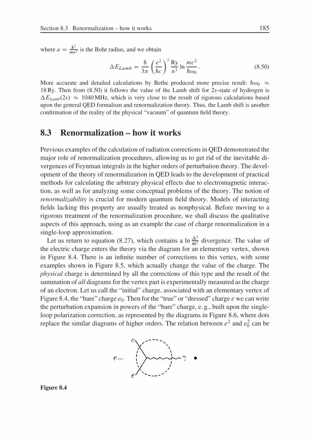
Section 8.3 Renormalization – how it works 185
where a D „2
me2 is the Bohr radius, and we obtain
ELamb D 8
3�
�e2
„c�3 Ry
n3lnmc2
„!0. (8.50)
More accurate and detailed calculations by Bethe produced more precise result: „!0 �18 Ry. Then from (8.50) it follows the value of the Lamb shift for 2s-state of hydrogen isELamb.2s/ � 1040 MHz, which is very close to the result of rigorous calculations basedupon the general QED formalism and renormalization theory. Thus, the Lamb shift is anotherconfirmation of the reality of the physical “vacuum” of quantum field theory.
8.3 Renormalization – how it works
Previous examples of the calculation of radiation corrections in QED demonstrated themajor role of renormalization procedures, allowing us to get rid of the inevitable di-vergences of Feynman integrals in the higher orders of perturbation theory. The devel-opment of the theory of renormalization in QED leads to the development of practicalmethods for calculating the arbitrary physical effects due to electromagnetic interac-tion, as well as for analyzing some conceptual problems of the theory. The notion ofrenormalizability is crucial for modern quantum field theory. Models of interactingfields lacking this property are usually treated as nonphysical. Before moving to arigorous treatment of the renormalization procedure, we shall discuss the qualitativeaspects of this approach, using as an example the case of charge renormalization in asingle-loop approximation.
Let us return to equation (8.27), which contains a ln ƒ2
m2 divergence. The value ofthe electric charge enters the theory via the diagram for an elementary vertex, shownin Figure 8.4. There is an infinite number of corrections to this vertex, with someexamples shown in Figure 8.5, which actually change the value of the charge. Thephysical charge is determined by all the corrections of this type and the result of thesummation of all diagrams for the vertex part is experimentally measured as the chargeof an electron. Let us call the “initial” charge, associated with an elementary vertex ofFigure 8.4, the “bare” charge e0. Then for the “true” or “dressed” charge e we can writethe perturbation expansion in powers of the “bare” charge, e. g., built upon the single-loop polarization correction, as represented by the diagrams in Figure 8.6, where dotsreplace the similar diagrams of higher orders. The relation between e2 and e2
0 can be
Figure 8.4

186 Chapter 8 Some applications of quantum electrodynamics
Figure 8.5
Figure 8.6
established, as shown in Figure 8.6, at some appropriate (from an experimental pointof view) value of transferred (by photon line) momentum4 q2 �Q2 D ��2. Inmost traditional methods, to determine the charge value we use the low-energy limitof Q2 m2. As a result, the expansion shown in Figure 8.6 can be schematicallywritten as
e2 D e20 Œ1 � I.Q2 D �2/CO.e4
0/� , (8.51)
where the value of I.Q2/ is determined by equations (8.17)–(8.20), i. e., by the single-loop approximation � e2
0. Taking the square root of both sides of equation (8.51), weobtain
e D e0
�1 � 1
2I.Q2 D �2/CO.e4
0/
�, (8.52)
which coincides with (8.27) after the square root expansion. Eexpansion (8.52) isshown in diagramatic form in Figure 8.7. Accordingly, taking into account all the
Figure 8.7
4 The value of Q2 is introduced here instead of .�q2/, just for convenience, to deal with Q2 > 0.

Section 8.3 Renormalization – how it works 187
Figure 8.8
Figure 8.9
orders of perturbation theory, we have
e D e0Œ1 C e20A1.Q
2/C e40A2.Q
2/C : : :�Q2D�2 . (8.53)
It is clear that A1.Q2/,A2.Q
2/, : : : are infinite in the limit of ƒ2 ! 1. Considersome physical scattering process, e. g., the one shown in the diagrams of Figure 8.8.In analytic form:
�iM.e20/ D e2
0ŒF1.Q2/C e2
0F2.Q2/CO.e4
0/� . (8.54)
Here all the terms are also divergent. But now we are taking a crucial step. Let usrenormalize the value of �iM.e2
0/, expressing e0 via e, by inversing (8.52), or, inother words, reconstructing the diagrams of Figure 8.7 with the same accuracy, asshown in Figure 8.9, and substituting this expansion into the vertices of the diagramsin Figure 8.8. Then we obtain the diagrammatic expansion shown in Figure 8.10. Thefirst two diagrams of this expansion originate from the first diagram of Figure 8.8,
Figure 8.10
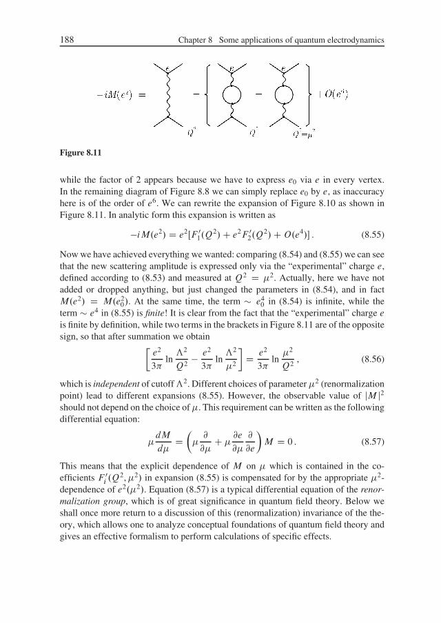
188 Chapter 8 Some applications of quantum electrodynamics
Figure 8.11
while the factor of 2 appears because we have to express e0 via e in every vertex.In the remaining diagram of Figure 8.8 we can simply replace e0 by e, as inaccuracyhere is of the order of e6. We can rewrite the expansion of Figure 8.10 as shown inFigure 8.11. In analytic form this expansion is written as
�iM.e2/ D e2ŒF 01.Q
2/C e2F 02.Q
2/CO.e4/� . (8.55)
Now we have achieved everything we wanted: comparing (8.54) and (8.55) we can seethat the new scattering amplitude is expressed only via the “experimental” charge e,defined according to (8.53) and measured at Q2 D �2. Actually, here we have notadded or dropped anything, but just changed the parameters in (8.54), and in factM.e2/ D M.e2
0/. At the same time, the term � e40 in (8.54) is infinite, while the
term � e4 in (8.55) is finite! It is clear from the fact that the “experimental” charge eis finite by definition, while two terms in the brackets in Figure 8.11 are of the oppositesign, so that after summation we obtain
�e2
3�lnƒ2
Q2� e2
3�lnƒ2
�2
�D e2
3�ln�2
Q2, (8.56)
which is independent of cutoffƒ2. Different choices of parameter�2 (renormalizationpoint) lead to different expansions (8.55). However, the observable value of jM j2should not depend on the choice of�. This requirement can be written as the followingdifferential equation:
�dM
d�D��@
@�C �
@e
@�
@
@e
�M D 0 . (8.57)
This means that the explicit dependence of M on � which is contained in the co-efficients F 0
i .Q2,�2/ in expansion (8.55) is compensated for by the appropriate �2-
dependence of e2.�2/. Equation (8.57) is a typical differential equation of the renor-malization group, which is of great significance in quantum field theory. Below weshall once more return to a discussion of this (renormalization) invariance of the the-ory, which allows one to analyze conceptual foundations of quantum field theory andgives an effective formalism to perform calculations of specific effects.

Section 8.4 “Running” the coupling constant 189
8.4 “Running” the coupling constant
The expansion of Figure 8.6 can be redrawn as shown in Figure 8.12. If we limitourselves only to loop diagrams, we obtain geometric a progression which is easilysummed, as shown in Figure 8.13. We have seen above that divergences can be elim-inated if we work with the physical (renormalized) charge e, which is determined bythe expansion shown in Figure 8.13 at Q2 D �2. Actually we can use any value of�2. Different choices of Q2 D �2
1,�22, : : : correspond to the perturbation expansion
in powers of numerically different values of the physical charge e.�2i /. In fact, from
Figure 8.13 we obtain
e2.Q2/ D e20
1 C I.Q2/, (8.58)
so that the experimentally observable charge depends on the value of transferred (dur-ing the scattering) momentumQ2. The value of e.Q2/ is called the “running” couplingconstant. In the limits of large Q2 .�q2/ the value of I.q2/ is given by (8.24), andwe get
e2.Q2/ D e20
1 � e20
3 lnQ2
ƒ2
� . (8.59)
To exclude in equation (8.59) the explicit dependence of e2.Q2/ on the cutoff param-eterƒ, we consider this expression atQ2 D �2 and express e0 via e2.�2/. As a result,
Figure 8.12
Figure 8.13

190 Chapter 8 Some applications of quantum electrodynamics
for large Q2 we can rewrite (8.59) as
e2.Q2/ D e2.�2/
1 � e2.�2/3 ln
Q2
�2
� . (8.60)
Here everything is finite! The “running” coupling constant e.Q2/ describes the de-pendence of the effective charge on the transferred momentum Q2, i. e., in fact on thedistance between the charged particles. We shall see later that it is really the observ-able effect, and the corresponding dependence is precisely logarithmic. However, theresult expressed by equation (8.60) raises a number of conceptual questions on theconsistency of QED. The thing is that from (8.60) we can see that with the growth ofQ2 (reduction of distance) the value of effective charge grows, so that sooner or laterperturbation theory becomes invalid at small distances, and for
Q2 D �2 exp
�3�
e2.�2/
�(8.61)
we obtain an obviously unphysical divergence (“ghost” pole). ForQ2 larger than thisvalue the charge becomes imaginary! For historical reasons this behavior is called“Moscow zero” (or the “zero-charge” problem). In the following we shall return sev-eral times to the discussion of this situation and related problems.
Actually, somewhat prematurely, we note that in quantum chromodynamics (QCD) situationis just the opposite. There we also obtain the “running” coupling constant of gluons and quarks,which is expressed (similarly to (8.60)) as
g2.Q2/ D g2.�/
1 C g2.�2/12 .33 � 2nf / ln
Q2
�2
� , (8.62)
where nf is the number of flavors of quarks, while the constant factor of 33 is connected tothe non-Abelian nature of gauge symmetry in QCD (in fact it is calculated as some constant,related to the properties of the matrices of generators of the color group SU.3/). Only for theworld with nf > 16, the sign in the denominator of equation (8.62) will be the same as inQED. In the real world we have nf D 6. Thus, the effective charge in QCD does not grow,but diminishes with the growth of Q2 and becomes small at small distances. This behavioris called “asymptotic freedom”. For small enough Q2 (at large distances between quarks) theeffective coupling constant (in contrast to QED!) becomes large, which is directly related tothe confinement of quarks (“infrared prison”). Let us denote the value ofQ2, corresponding tothe pole (“ghost pole” again!) in (8.62), as ƒ2, so that
ƒ2 D �2 exp
�� 12�
.33 � 2nf /g2.�2/
�. (8.63)
Then (8.62) can be rewritten as
g2.Q2/ D 12�
.33 � 2nf / lnQ2
ƒ2
� . (8.64)

Section 8.5 Annihilation of eCe� into hadrons. Proof of the existence of quarks 191
ForQ2 � ƒ2 the effective coupling constant is small, and the interaction of quarks and gluons(at small distances of large momenta) can be described by perturbation theory, similarly tointeractions of electrons and photons in QED (at large distances or small momenta). ForQ2 �ƒ2 such a description becomes impossible, while quarks and gluons form strongly coupledclusters: the hadrons. The experimental value of ƒ is somewhere in the interval between 0.1and 0.5 GeV. Then, for experiments at Q2 � .30 GeV/2 it follows from (8.64) that g2 � 0.1,so that perturbation theory is valid, like in QED. In the limits of large Q2 we can neglect allquark masses, but there is still a mass scale in the theory, given by �2, which appears in theprocess of renormalization.
8.5 Annihilation of eCe� into hadrons. Proof ofthe existence of quarks
As an interesting illustration of QED applications, let us show how purely electro-dynamic experiments prove the existence of quarks [24]. This becomes possible viastudies of the high-energy annihilation processes of electrons and positrons, with ar-bitrary hadrons in the final state. In fact, these reactions are going through the creationof quark–antiquark pairs, i. e., eCe� ! q Nq, which afterwards form hadrons. We canshow that the crossection for such processes can be obtained from an easily calculableQED cross section for electron–positron annihilation into muons: eCe� ! � N�.
To calculate the cross section of this process in QED it is sufficient to consider thesecond of the Feynman diagrams shown in Figure 6.6, where the final products of thereaction is the pair � N�5. The standard calculation, using the rules of QED diagramtechnique, gives the total cross section for such process as [24]
.eCe� ! � N�/ D 4�e2
3Q2, (8.65)
where Q2 D 4E2 is the square of energy in the center of the mass reference frame(Mandelstam variable s). Then, the cross section for annihilation into the quark–anti-quark pair is given by
.eCe� ! q Nq/ D 3e2q.e
Ce� ! � N�/ , (8.66)
where eq is the q-quark charge. An additional factor of 3 appears here due to threeseparate diagrams for different quark colors, which are to be summed, so that appro-priate cross sections are also to be summed. To find the cross section for the creationof all possible hadrons it is necessary to sum over all quark flavors q D u, d , s, : : :, sothat
.eCe� ! hadrons/ DX
q
.eCe� ! q Nq/ D 3X
q
e2q.e
Ce� ! � N�/ . (8.67)
5 We remind, that muons are just like electrons, but with larger (about 200 times) rest mass.

192 Chapter 8 Some applications of quantum electrodynamics
Thus we obtain the very important prediction
R .eCe� ! hadrons/
.eCe� ! � N�/ D 3X
q
e2q . (8.68)
As cross section .eCe� ! � N�/ is well studied (and is in excellent agreementwith equation (8.65)), the experimental measurements of the cross section for eCe�-annihilation into hadrons give direct information on the number of quarks, their fla-vors, and their colors. We have
R D
8ˆˆ<
ˆ:
3
�2
3
�2C1
3
�2C1
3
�2�
D 2 for u, d , s .
2 C 32
3
�2D 10
3for u, d , s, c ,
10
3C 3
1
3
�2D 11
3for u, d , s, c, b etc.
(8.69)
These predictions have been well confirmed by experiments! The value of R D 2is observed for Q < 2.mc C mu/ � 3.7 GeV, i. e., below the threshold for cre-ation of c-quarks. Above the threshold for creation of five quark flavors, i. e., forQ > 2mb � 10 GeV, the experimentally observed value of this ratio is R D 11=3.These experiments directly confirm the existence of three colors of quarks with theappropriate (fractional!) values of the electric charge.
Within QCD we can also take into account the contributions of diagrams with quarks (or anti-quarks) emitting gluons [24]. In the first order over g2, equation (8.68) is modified as follows:
R D 3X
q
e2q
�1 C g2.Q2/
�
�, (8.70)
so that the weak (logarithmic) dependence of R on Q2 is also observed.
8.6 The physical conditions for renormalization
Let us now discuss more rigorously the basics of renormalizability in QED. It is clearthat the general scheme of invariant perturbation theory and diagrammatic equationsfor exact propagators presented above was rather formal. We have operated with allthe entities of the theory as with the usual finite mathematical expressions, thoughexplicit calculations of D ,G, and � , using perturbation theory, inevitably producediverging integrals. We shall explicitly show below that using certain recipes in QEDallows us to perform the well-defined “subtraction” of all infinities and to obtain finiteexpressions for all the measurable physical characteristics. These recipes are basedupon the obvious physical requirements of the photon mass being exactly zero, whilethe electron charge and mass are equal to their observable values. Our presentation will

Section 8.6 The physical conditions for renormalization 193
necessarily be a bit schematic, but further details can be found in [6] and in especiallydetailed analysis in [2].
A physical photon has zero mass, so that its dispersion is given by k2 D 0. Thismeans that the exact photon propagator should always have a pole at k2 D 0, so that
D.k2/ D 4�
k2Z for k2 ! 0 , (8.71)
whereZ is some constant. According to equation (7.39), the general form of the prop-agator is expressed via the polarization operator as
D.k2/ D 4�
k2.1 � P .k2/=k2/, (8.72)
so that from (8.71) we get for polarization operator
P .0/ D 0 . (8.73)
Similarly, the constant Z in equation (8.71) can be defined as
1
ZD 1 � P .k2/
k2
ˇˇk2!0
. (8.74)
Further limitations on the behavior of P .k2/ can be obtained from the analysis of thephysical definition of electric charge. Two classical (very heavy!) particles being atrest at some large distance from each other (r � m�1, where m is electron mass),are interacting according to the Coulomb law: V.r/ D e2=r . On the other hand, thisinteraction is expressed by the diagram shown in Figure 8.14, where the “fat” wavyline denotes the exact propagator of the virtual photon and the upper and lower linescorrespond to classical particles. Self-energy corrections for the photon are taken intoaccount in its exact propagator. Any other self-energy corrections, acting upon thelines of heavy particles, lead to the corresponding diagrams being zero. In fact, an ad-dition of some internal line into the diagram of Figure 8.14, e. g., joining 1 and 3 or1 and 2 by a photon line, leads to the appearance in corresponding diagrams of heavyvirtual particles (due to particle lines under the extra photon lines), with the propa-gators containing large mass M of the classical particle in denominators, giving zerocontribution in the limit of M ! 1. Then it is clear that the facto of e2D.k2/ in
Figure 8.14

194 Chapter 8 Some applications of quantum electrodynamics
the diagram of Figure 8.14 is given (up to a sign) by the Fourier transform of the in-teraction potential of our particles. The static nature of interaction (particles at rest!)corresponds to the frequency of virtual photon ! D 0, while the large distances cor-respond to the small wave vectors k. As D depends only on k2 D !2 � k2, we arriveat the condition
e2D ! 4�e2
k2for k2 ! 0 , (8.75)
so that in equation (8.71) we have to put Z D 1. Then from equation (8.74) it imme-diately follows that
P .k2/
k2! 0 for k2 ! 0 . (8.76)
Besides the previously derived condition (8.73) it follows now that
P 0.0/ dP .k2/
dk2
ˇˇk2D0
D 0 . (8.77)
Note that the effective external line of a real photon should be associated with thefactor of
p4�Œ1 C 1
4P .k2/D.k2/�e�. However, for the real photon we always havek2 D 0, and due to (8.76) we conclude that in the lines of external photons we cansafely drop all radiation corrections.
Thus, the natural physical requirements lead to definite values (zeroes!) for P .0/and P 0.0/. At the same time, direct calculation using the diagram rules of perturba-tion theory leads here to diverging integrals. We can get rid of these divergencies ifwe attribute the finite values dictated by physical requirements to these divergent ex-pressions. This is the main idea of renormalization. Another way to formulate thisoperation e. g., for charge renormalization, is as follows. We can introduce the non-physical “bare” charge e0, as a parameter entering the initial expression for an operatorof electromagnetic interaction, which is used in formal perturbation theory. After that,the renormalization condition is formulated as the requirement of
e20D.k2/ ! 4�e2
k2for k2 ! 0 , (8.78)
where e is the true physical charge of a particle. The we find the relation
e2 D Ze20 (8.79)
Now the unphysical e0 is excluded from all expressions, determining the physical ef-fects (while divergence is “hidden” in the renormalization factor Z). If we requireZ D 1 from the very beginning, we actually perform renormalization “on the fly” [6],so that there is no need to introduce any fictitious entities into the intermediate calcu-lations.
Let us now consider the physical conditions for renormalization of the electron prop-agator. It is obvious that the exact propagator G .p/ should have a pole at p2 D m2,

Section 8.6 The physical conditions for renormalization 195
where m is the mass of physical electron. Then we can write
G .p/ � Z1��p� Cm
p2 �m2 C i0C g.p/ for p2 ! m2 , (8.80)
whereZ1 is a scalar constant (renormalization factor) and g.p/ is finite for p2 ! m2.From (8.80) we immediately obtain the inverse propagator as
G �1.p/ � 1
Z1.��p��m/� .��p��m/g.p/.��p��m/ for p2 ! m2 . (8.81)
The mass operator for p2 ! m2 now has the form
M.p/ D G�1.p/�G �1.p/ ��
1� 1
Z1
�.��p��m/C.��p��m/g.p/.��p��m/ .
(8.82)We associate the following factor with the effective external electron line (e. g.,
incoming) in the scattering diagram:
U.p/ D u.p/C G .p/M.p/u.p/ , (8.83)
where u.p/ is the usual electron bispinor, satisfying the Dirac equation .��p� �m/u D 0. Due to relativistic invariance (U is also the bispinor) the limiting valueof U(p) for p2 ! m2 can differ from u.p/ by a constant scalar factor (wave functionrenormalization)
U.p/ D Z0u.p/ . (8.84)
It is not difficult to show [6] the validity of a simple relation
Z0 DpZ1 . (8.85)
This is almost obvious, since Green’s function (propagator) is quadratic in electronoperators.
Now, after the establishment of the limiting behavior of the electron propagator,there is no need of any additional conditions for the vertex operators. Consider thediagram in Figure 8.15 and let us assume that it describes first-order electron scatteringby an external field A.e/� .k/, taking into account all radiation corrections. In the limitof k ! 0 we have p2 ! p1 p and the radiation corrections to the line of the
Figure 8.15

196 Chapter 8 Some applications of quantum electrodynamics
external field vanish (we already noted above that they vanish for arbitrary k2 D 0).Then this diagram corresponds to the amplitude
Mf i D �e NU.p/��.p,p; 0/U.p/A.e/� .k ! 0/ . (8.86)
But for k ! 0 the potential A.e/� .k/ reduces to a constant independent of coordinatesand time, which does not describe any physical field and cannot lead to any changeof transition current. In other words, in this limit, transition current NU��U shouldsimply coincide with free current Nu��u:
NU.p/��.p,p; 0/U.p/ D Z1 Nu.p/��u.p/ D Nu.p/��u.p/ . (8.87)
This relation is automatically satisfied due to Ward identity, independent of the valueof Z1. In fact, substituting G �1.p/ from (8.81) into (7.87), we obtain
��.p,p; 0/ D 1
Z1�� � ��g.p/.��p� �m/ � .��p� �m/g.p/�� (8.88)
and (8.87) is satisfied due to .��p� �m/u.p/ D 0 and Nu.p/.��p� �m/ D 0. Thisagain simply gives us the definition of the physical electron charge. We see that therenormalization factor Z1 just drops from the amplitude of the physical process. Wecan simply require
Nu.p/��.p,p; 0/u.p/ D Nu.p/��u.p/ for p2 D m2 , (8.89)
i. e., putZ1 D 1. The convenience of such a definition is that now there is no necessityto introduce any corrections to external electron lines, and we simply have U.p/ Du.p/. It is also clear also that, for Z1 D 1, for mass operator (8.82) we have
M.p/ D .��p� �m/g.p/.��p� �m/ , (8.90)
so that the second term in (8.83) obviously reduces to zero. Thus, there is no need torenormalize the external lines of all real particles, both photons and electrons.
8.7 The classification and elimination of divergences
The physical conditions of renormalization introduced above allow us, in principle.to obtain the finite and definite values for the amplitudes of any QED process in anarbitrary order of the perturbation theory.
Consider first the character of divergences appearing in different Feynman integrals.First of all we calculate the powers of the virtual 4-momenta, entering the integrand.Consider an arbitrary diagram of the n-th order (n is the number of vertices!), con-taining external lines of Ne electron and N photon. The number Ne is always even.The total number of electron lines is equal to 2n; of these Ne are external and Ie are
Section 8.7 The classification and elimination of divergences 197
internal. During the calculation of the number of lines, the internal lines are countedtwice, as each of them connects two vertices, so that
2n D Ne C 2Ie . (8.91)
Correspondingly, the total number of internal electron lines in the diagram is
Ie D n � Ne
2. (8.92)
Each vertex is connected with one photon line, and forN vertices this line is external,while for the remaining n � N vertices this line is internal. As each internal photonline connects two vertices, the total number of these lines is equal to
n �N2
. (8.93)
Each internal photon line is associated with the propagator D.k/, which contains k tothe power of �2. Each internal electron line is associated with the propagator G.p/,which behaves like p to power of �1 (for p2 � m2). Thus, the total power of the4-momenta in the denominator of the integrand is
2n �N
2C n � Ne
2D 2n � Ne
2�N . (8.94)
The number of integrations over d 4p and d 4k in the diagram is equal to the number ofinternal lines, but the conservation law of the 4-momentum in each vertex leads to anadditional n� 1 constraint on integration momenta (one of these n conservation lawsis connected with external momenta, and it corresponds to the general conservationlaw for the scattering process described by this diagram). Correspondingly, takinginto account equations (8.92) and (8.93), we conclude that the total number of internallines (both electron and photon) in the diagram is given by
n � Ne
2C n
2� N
2D 3
2n � Ne
2� N
2, (8.95)
which gives the number of integrations, not taking conservation laws into account.Then, subtracting n�1 we obtain for the number of independent integration momenta
3
2n � Ne
2� N
2� nC 1 D n
2C 1 � Ne
2� N
2. (8.96)
Multiplication by 4 gives the total number of integrations:
2.n �Ne �N C 2/ . (8.97)
The difference between the number of integrations and the power of the momenta inthe denominator of the integrand for our diagram is equal to the difference between(8.97) and (8.94):
r D 4 � 3
2Ne �N . (8.98)

198 Chapter 8 Some applications of quantum electrodynamics
This number determines whether the appropriate Feynman integral is convergent ordivergent6. Strictly speaking, the situation is more complicated, as the condition ofr < 0 for the diagram as a whole is not sufficient to guarantee its convergence. We alsohave to require the negative values of r 0 for all internal blocks which can be containedwithin our diagram. The presence of internal blocks with r 0 > 0 leads to the divergenceof the diagram as a whole, though all other integrals may be convergent. The conditionr < 0 is sufficient to guarantee the convergence of the simplest diagrams.
For r � 0 the integral is always divergent. The power of divergence is not lessthan r if r is even, and not less than r � 1 if r is odd (the drop of divergence power by1 in the last case is related to the integration of the product of odd number of 4-vectorsover the whole 4-space giving zero!). The power of divergence can grow due to thepresence of internal blocks with r 0 > 0.
Note that the divergence power of the diagram r , according to (8.98), does not de-pend on the diagram order n. This remarkable property, as we shall see later, makes thetheory renormalizable. Briefly speaking, the important thing here is that from (8.98) itbecomes immediately clear that only the finite number of types of divergence exists insuch a theory, because with positivity of bothNe andN we can obtain r � 0 for only afew pairs of the values of these integers, and thus only the finite number of the simplestprimitively diverging diagrams. Correspondingly, we can introduce the finite numberof parameters (to be determined from the experiments) to “hide” all divergences. Inthe case of n entering (with positive sign) into (8.98), the number of divergence typeswill grow with the growth of n, so that situation will become hopeless! For QED wecan explicitly list all primitively diverging diagrams. From the very beginning we canexclude the cases ofNe D N D 0 (vacuum loops) andNe D 0,N D 1 (the averagevalue of vacuum current). All other cases are shown in Figure 8.16. For the first ofthese diagrams we have r D 2, and divergence is formally quadratic; in all other casesr D 0 or r D 1, and divergence is logarithmic.
The diagram of Figure 8.16(d) represents the first correction to the vertex. It shouldsatisfy (8.89), which can be written as
Nu.p/ƒ�.p,p; 0/u.p/ D 0 for p2 D m2 , (8.99)
whereƒ� D �� � �� . (8.100)
Let us denote the Feynman integral, written according to diagram rules, asNƒ�.p2,p1; k/. This integral is logarithmically divergent and does not satisfy (8.99).However, we can obtain the expression satisfying this condition by constructing thedifference
ƒ�.p2,p2; k/ D Nƒ�.p2,p1; k/ � Nƒ�.p1,p1; 0/jp21Dm2 . (8.101)
6 Let us recall that in all cases we are dealing with divergences of integrals at the upper integrationlimit!

Section 8.7 The classification and elimination of divergences 199
(a) (b) (c)
(d) (e)
Figure 8.16
Divergence in the integral for Nƒ�.p2,p1; k/ can be separated if we consider the limit of a verylarge 4-momentum of the virtual photon f . Then we obtain
� 4�ie2Z
d 4f
.2�/4��G.p2 � f /��G.p1 � f /��D��.f / �
� 4�ie2Z
d 4f
.2�/4��.��f�/�
�.��f�/��
f 2f 2f 2, (8.102)
which is independent of the values of the 4-momentum of the external lines. Then in the dif-ference given by (8.101) divergences are cancelled, and we obtain the finite expression.
Such a procedure for cancelling divergence is called the subtraction schemeof renormalization. Let us stress that the possibility for cancelling divergence inNƒ�.p2,p1; k/ by only one subtraction is guaranteed by (the weakest possible) log-arithmic nature of the divergence.
After determining the first correction for �� (i. e., the first term of expansion forƒ�), the first correction for the electron propagator (diagram of Figure 8.16(b)) canbe calculated using the Ward identity (7.87), which can be rewritten as
�@M.p/
@p�D ƒ�.p,p; 0/ , (8.103)
introducing the mass operator M instead of G and ƒ� instead of ��. This equationcan be easily integrated with the boundary condition
Nu.p/M.p/u.p/ D 0 for p2 D m2 , (8.104)
which follows from (8.90).

200 Chapter 8 Some applications of quantum electrodynamics
In principle, in a similar (though more tedious) way we can cancel divergencesfrom the polarization operator of Figure 8.16(a) [2, 6], but here we have to make twosubtractions:
P .k2/ D NP .k2/ � NP .0/ � k2 NP 0.0/ , (8.105)
where NP denotes the Feynman integral, corresponding to this diagram. It is obviousthat (8.105) satisfies the physical requirements given by (8.73) and (8.77).
The next order of the perturbation theory for the vertex operatorƒ.2/� is determinedby the diagrams shown in Figure 7.17(c–i). Of these, only the diagrams shown in Fig-ure 7.17(d–f) are compact, which can be made finite with the help of one subtraction(8.101). Internal self-energy and vertex parts, contained within the noncompact dia-grams, can be directly replaced by the already-known (renormalized) values of the firstorder, given by P .1/, M.1/ andƒ.1/� , so that integrals are again made finite by subtrac-tion (8.101). Corrections M.2/ and P .2/ are then calculated using the Ward identity(8.103) and (8.105). The systematic application of such procedure gives, in principle,the rigorous way to obtain finite expressions for P , M, andƒ� in an arbitrary order ofthe perturbation theory [2,6]. This makes possible the calculation of the amplitudes ofthe physical scattering processes, containing blocks like P , M, andƒ�. The physicalconditions of renormalizability formulated above are sufficient to cancel divergencesfrom all Feynman integrals. This is the manifestation of the quite nontrivial propertyof renormalizability of QED. Below we shall return several times to the discussion ofrenormalizability and its use in other models of quantum field theory.
8.8 The asymptotic behavior of a photon propagatorat large momenta
Let us consider the conceptually very important problem of photon propagator asymp-totic behavior at large momenta jk2j � m2. In the lowest order of perturbation the-ory the polarization operator is determined by the simple loop diagram shown in Fig-ure 8.17. It is defined by the Feynman integral
i
4�P��.k/ D �e2
Zd 4p
.2�/4Sp��G.p/��G.p � k/ . (8.106)
However, this integral (over the whole 4-dimensional p-space) diverges (quadrati-cally, according to a simple power counting of the previous section, but actually only
Figure 8.17

Section 8.8 The asymptotic behavior of a photon propagator at large momenta 201
logarithmically due to a “hidden” algebra of the integrand). These divergence can becancelled using the renormalization recipes of the previous sections. Direct calcula-tions are rather tedious [2]. This analysis is much simplified in the asymptotic limit ofjk2j � m2, which is of major interest to us. As we shall see below, after the renor-malization 8.106), in this limit we have
P .k2/ D e2
3�k2 ln
jkj2m2
. (8.107)
In essence, this gives the first order correction inverse photon propagator 4�D�1 D k2
and it is valid until the following condition is satisfied:
e2
3�ln
jk2jm2
1 , (8.108)
which limits the validity region of our approximation at high values of jkj2. In fact,equation (8.107) can be used even under the much weaker condition of
e2
3�ln
jk2jm2
. 1 . (8.109)
Now we shall give a proof of this statement and also obtain the result (8.107) itself [6].First of all, let us note that, although for (8.109) there may be additional contributionsto P .k2/ due to the higher orders of perturbation theory, in the n-th order it is sufficientto take into account only the terms of the order of � .e2/n lnn. jkj2
m2 /, containing thelarge logarithm, appearing in the limit of jk2j � m2. This logarithm should enter withthe same power as e2, because terms with lower powers of the logarithm are obviouslysmaller due to e2 1. This is called the approximation of leading logarithms.
Consider now the Dyson equation for polarization operator (7.77)
P .k2/ D 4�ie2
3Sp
Zd 4p
.2�/4��G .p C k/��.p C k,p; k/G .p/ . (8.110)
As we have shown above, P .k2/ is gauge invariant, so that calculating it using Feyn-man diagrams we can use any gauge for the propagators and vertices. Most convenientis the Landau gauge, when the photon propagator is written as (Dl D 0):
D��.k/ D 4�
k2
�g�� � k�k�
k2
�. (8.111)
A detailed analysis of the correction diagrams for (8.106), which can be found in [6],shows that in this gauge perturbation theory series does not contain terms with therequired powers of logarithms at all.
Then in (8.110) it is sufficient to use the zero-th order approximations G D G and�� D ��. Then (8.110) reduces to the integral
P .k2/ D 4�ie2
3Sp
Zd 4p
.2�/4��G.p C k/��G.p/ , (8.112)

202 Chapter 8 Some applications of quantum electrodynamics
the same as in (8.106). Let us discuss the appearance of the logarithm in this integral.It is easily seen that it originates from the integration region
p2 � jk2j for jk2j � m2 . (8.113)
In fact, in this limit we can write7
G.p/ � 1
��p�D ��p�
p2, (8.114)
G.p � k/ �Š 1
��p� � ��k� D 1
��p�C 1
��p���k�
1
�˛p˛
C 1
��p���k�
1
�˛p˛��k�
1
�ˇpˇC � � �
D ��p�
p2C .��p�/.�
�k�/.�˛p˛/
.p2/2
C .��p�/.��k�/.�
˛p˛/.��k�/.�
ˇpˇ /
.p2/3C � � � . (8.115)
After substitution of these expressions into (8.112) the first term, independent of k,drops out due to renormalization in accordance with the condition P .0/ D 0 (the firstsubtraction in (8.105)). The second term also becomes zero after integration over thedirections of p. The third integral is logarithmically divergent over p2; it can be easilyestimated making the integration from p2 � jk2j (lower limit of the region (8.113))up to some “cutoff parameter” ƒ2:Zd 4p
p4
p8�Zdp p3p
4
p8�Z ƒ2
jk2jdp2 p2p
4
p8�Z ƒ2
jk2jdp2 1
p2� ln
ƒ2
jk2j . (8.116)
Finally we get
P .k2/ D � e2
3�k2 ln
ƒ2
jk2j . (8.117)
This is not the end of our derivation; for the final cancellation of the divergence (atƒ ! 1) we need to subtract from P .k2/=k2 its value at k2 D 0 (second subtractionin (8.105)). However, logarithmic accuracy of our calculations assumes jk2j � m2, sothat it is sufficient to subtract the value of (8.117) at jk2j � m2, andƒ2 in the argumentof logarithm is simply replaced by m2. Thus, we obtain the required result (8.107). Inthe Landau gauge there are no corrections to G and � with the “proper” powers of thelogarithm, and equation (8.107) is actually valid under the condition (8.109).
The function D.k2/, corresponding to the polarization operator (8.107), has theform
D.k2/ D 4�
k2
1
1 � e2
3 ln jk2jm2
. (8.118)
7 The signs here are determined by the properties of the � -matrices.

Section 8.9 Relation between the “bare” and “true” charges 203
Because of (8.109) there is no need to expand this expression in the powers e2. How-ever, the validity of (8.118) is limited from the side of large jk2j due to the diminishingdenominator. The derivation of (8.118) was based on logarithmic approximation andneglect of infinite sequences of the diagrams of higher orders, which do not containleading logarithms. According to (8.118) an addition of each new “fat” photon lineintroduces an additional factor of e2D , and the small parameter of the perturbationtheory instead of e2 is given by
e2
1 � e2
3 ln jk2jm2
1 , (8.119)
which coincides with the “running” coupling constant (8.60) discussed above. As jk2jgrows, this coupling becomes of the order of unity, so that the small expansion param-eter actually disappears, and perturbation theory can not be further applied.
8.9 Relation between the “bare” and “true” charges
The situation with (8.118), (8.119) can be understood more clearly if, during the deriva-tion of (8.118), we do not do renormalization “on the fly”, but introduce the first “bare”charge e0, which afterwards is fitted to obtain the correct observable value of charge e(or eR in the notations used above). If the logarithmically divergent integral is cut offat the upper limit at some ƒ2 (above we have also used the notation M 2 as the cutoffparameter), the “bare” charge can be considered to be its function: e0 D e0.ƒ
2/, andat the end we have to perform the limit ƒ ! 1. In this approach, the polarizationoperator takes the form (8.117)
P .k2/ D � e20
3�k2 ln
ƒ2
jk2j . (8.120)
Correspondingly,D.k2/ D 4�
k2
1
1 C e20
3 ln ƒ2
jk2j. (8.121)
Let us define the physical charge e according to
e20D.k2/ ! 4�e2
k2where k2 ! m2 , (8.122)
i. e., at distances of the order of m�1 (i. e., the Compton length of an electron „=mc,which in quantum field theory defines its effective size). Then we obtain
e2 D e20
1 C e20
3 ln ƒ2
m2
, (8.123)

204 Chapter 8 Some applications of quantum electrodynamics
which, in fact, coincides with (8.59) if we choose the normalization point �2 D m2.Then
e20 D e2
1 � e2
3 ln ƒ2
m2
. (8.124)
If we formally consider the limit of point-like charge ƒ ! 1 in (8.123), we shallobtain e ! 0, independently of the possible form of the function e2
0.ƒ/. This behav-ior is called the “zero charge” (or “Moscow zero”). It was first noted by Landau andPomeranchuk and independently by Fradkin in the mid-1950s. In the opinion of Lan-dau [49] this situation reflected the internal inconsistency of both the renormalizationprocedure and QED (and any other model of quantum field theory known at that time)itself.
Let us consider the arguments of Landau and Pomeranchuk, which lead them to this ratherradical conclusion. Let the ratio ƒ2
jk2j be so large that
e20
3�lnƒ2
jk2j � 1 , (8.125)
but, at the same time, we still have e0 1. Then in equation (8.121) we can neglect unity inthe denominator, so that
D.k2/ D 12�2
k2e20 ln ƒ2
jk2j(8.126)
and, correspondingly, from (8.122) we have
e2 D 3�
� ln ƒ2
m2
, (8.127)
which is independent of the value of “bare” charge e0. Note that here we divided (8.127)by an additional parameter �, which denotes the number of the fundamental fermions whichcontribute to vacuum polarization (the corresponding contributions to polarization loops areadditive!). Let us now introduce, instead of the standard 4-potential of electromagnetic fieldA�, a new 4-vector A� D e0A
�. Then the interaction Hamiltonian HI will not contain the“bare” charge e0, while the free electromagnetic field Hamiltonian H0 (quadratic in A�) willcontain e2
0 in the denominator. The function QD.k2/, defined with the help of A� in the sameway that D.k2/ is defined via A�, will be equal to
QD.k2/ D e20D.k2/ D 12�2
k2 ln ƒ2
jk2j. (8.128)
This expression does not contain e0, and this means that it corresponds to the neglect in thetotal Hamiltonian H D H0 C HI (depending of e0) of the term H0. If this neglect of H0 incomparison to HI is possible (at large ƒ) already for e2
0 1, it is natural to assume, thatit is even more justified at not so small e2
0. Then equation (8.126), and also equation (8.127),become unrelated to the condition of e2
0 1, so that the limit of ƒ ! 1 becomes feasible.Then e2 ! 0 independent of the form of the function e2
0.ƒ/.The cutoff parameter ƒ, guaranteeing the validity of (8.127), is in any case very large. At
corresponding (very small!) distances the effects of gravitation may exceed those of electro-magnetism. This leads to the very attractive idea that the “crisis” of QED happens precisely

Section 8.9 Relation between the “bare” and “true” charges 205
at those distances (energies) where gravitation coupling matches that of electromagnetism.Choosing the cutoff parameter of the order of the Planck length, we have
GNƒ2 � 1 , (8.129)
whereGN is the Newtonian gravitational constant. If we accept such a point of view, the valueof the physical charge e will be automatically determined by the theory via equations (8.127)and (8.129), which will lead to the limitation of � � 12. In fact, if � < 12, the effects ofgravitation will become important well before the effective charge becomes of the order ofunity. In the opposite case of � > 12 the effects of gravitation will not “save” electrodynam-ics, becoming important “too late”. Note that, according to the modern experimental data onelementary particles (see Chapter 1), there are precisely 12 fundamental fermions!
At the same time, we must stress the opinion of the majority of theorists, who believethat the limit of ƒ ! 1 in expressions like (8.123) and (8.124) cannot be performedwithout breaking the assumptions made during their derivation. From (8.124) it is seen,that as ƒ grows (with fixed e2) the value of e2
0 also grows and for e20 � 1 all these
expressions just become invalid, as their derivation was based on the assumption ofe2
0 1, which is simply the criterion of the applicability of perturbation theory.Note that for QED all these difficulties are of a rather “academic” importance, since
they appear at fantastically high energies of no real interest: e2
ln.E
2
m2 / D 1 is achievedfor E � 1093m, which is essentially due to the smallness of e2 D 1
137 . Much earlier,as we shall see later, electromagnetic interactions become “intermixed” with the weakand strong interactions of the elementary particles, so that “pure” electrodynamicslooses its meaning. At the end of this volume we shall return to the discussion of theproblems of consistency of quantum field theory and its asymptotic behavior.
Fora better understanding of these problems we now present a simple qualitative discussionon coordinate space [5]. We can transform our asymptotic expressions of QED to “coordinaterepresentation” by an obvious (from dimensionality arguments) replacement: m ! r�1 andƒ ! r�1
0 , where r is the characteristic distance from the “center” of an electron (which canbe taken to be of the order of its Compton wavelength), while r0 is some fundamental length,characterizing the geometric size of the “bare” charge, which can be imagined to be a smallsphere with radius r0. Then (8.123) can be written as
e2.r/ D e2.r0/
1 C 2e2.r0/32 ln r
r0
. (8.130)
Let the value of the “bare” charge e2.r0/ be fixed. Our aim now is to go to the limit of apoint-like “bare” charge, so we start to diminish r0, with a fixed value of e2
0.r0/. Then, sooneror later we obtain 2e2.r0/
32 ln rr0
� 1, and we can neglect unity in the denominator of (8.130).Correspondingly, we have
e2.r/ D 12
32 ln rr0
. (8.131)

206 Chapter 8 Some applications of quantum electrodynamics
But now, with a further diminishing of r0 we obtain e2.r/ ! 0 for r0 ! 0. This is “zerocharge” behavior (or “Moscow zero”). On this ground, Landau and Pomeranchuk claimed 8:“We are coming to the fundamental conclusion that the formal quantum electrodynamics ap-parently leads to the zero charge of an electron. The word “apparently” here is related to somelack of rigorousness in the above arguments”. The physics here is that in this approximationvacuum polarization (due to creation of virtual electron–positron pairs) is so strong at small dis-tances that on some distance the remnant charge is actually independent of the initial (“bare”)charge. In the limit of the point-like “bare” charge nothing remains of it on any finite distance:we have the complete screening. Note that this result is quite transparent; the phenomenon ofscreening is well known in plasma and solid state physics [36], where it is described by quitesimilar calculations of the polarization operator in many body systems [1]. But in this situation,how we can understand the magnificent successes of QED?
Let us write (8.130) in the form solved with respect to e2.r0/ and put r D �e D m�1 (theCompton wave length of an electron):
e2.r0/ D e2.�e/
1 � 2e2.�e/32 ln �e
r0
. (8.132)
Here e2.�e/ should be understood as the “physical” charge of an electron, i. e., that chargewhich is measured at large distances (of the order of �e) outside the effective region of vac-uum polarization (screening). When we “enter” this region (r0 < �e), the charge grows due tothe diminishing screening inside the “cloud” of electron–positron pairs9. However, we cannotreach the limit of a very large charge due to the existence of the “Landau ghost pole”, closeto which equation (8.132) simply becomes invalid. From a practical point of view all this isnot important at all, as we are speaking here about the region of r0 � �e expŒ�.137/.3�2/=2�.QED is a practical theory precisely because we are using nonexact solutions with point-likeinteraction and leave open the question of the correct behavior at small distances, where otherinteractions become quite important. And who knows; is there not some physical mechanismcutting off divergences at small distances (e. g., related to gravitation; cf. (8.129)!), which isstill unknown to us, but which makes interactions in quantum field theory effectively nonpoint-like? Thus, the pragmatic (majority!) point-of-view is that we are dealing with the experimen-tally defined “physical” charge e.�e/, such that we can work with solutions in the form of aperturbation series, though modern theory becomes invalid at small distances. Thus, the prob-lem of the asymptotic behavior of QED still remains unsolved (we shall return to this at theend of the book).
In asymptotically free field theories, e. g., in QCD, the situation is different. The sign in thedenominators of expressions similar to (8.130) and (8.132) is opposite to that in QED, andthe asymptotic behavior of the interaction “constant” (charge) is also opposite: g2.r0/ ! 0for r0 ! 0. It is not that the charge at the finite distance is becoming zero for an arbitraryvalue of the “bare” charge, but the zero point-like charge corresponds to a finite charge at thefinite distance: g2.r/ grows with the growth of r . In QCD we are dealing with an effective“antiscreening” of the “bare” charge. However, we do not know which values of r0 and g.r0/
should be fixed and up to what values of r we can use an logarithmic expression like (8.130).We cannot use it infinitely, as the diminishing (with growth of r) denominator again makes
8 Reports of the USSR Academy of Sciences 102, 489 (1955)9 In fact, this corresponds to the dependence of the “fine structure constant” on momentum, transferred
during the scattering process. We already noted that this effect is experimentally observable!

Section 8.10 The renormalization group in QED 207
perturbation theory inapplicable. Qualitatively it is clear that this growth of the charge withr corresponds to the confinement force (acting upon quarks). These dependences are nowmeasured experimentally, and we shall return later to the discussion of asymptotic freedomin QCD .
8.10 The renormalization group in QED
Let us show now how equations (8.130) and (8.124) can be derived using simple analy-sis, based on dimensional analysis and the notion of renormalizability which constitutethe essence of the so-called renormalization group introduced in QED by Gell-Mannand Low. Consider again the square of the “bare” charge as a function of cutoff pa-rameter e2
0.ƒ/ and introduce some function d which relates e20 for two different values
of its argument (cutoff):e2
0.ƒ22/ D e2
0.ƒ21/d . (8.133)
Forƒ21,ƒ2
2 � m2 the function d does not depend onm and, being dimensionless, candepend only on the dimensionless arguments e2
0.ƒ21/ andƒ2
2=ƒ21, so that we can write
e20.ƒ
22/ D e2
0.ƒ21/d
�e2
0.ƒ21/,ƒ2
2
ƒ21
�. (8.134)
This is the main relation of the renormalization group. Its physical meaning is quiteclear: in renormalizable theory any change of the cutoff parameter can be compensatedfor by the appropriate change of the “bare” charge, with no change in the physicalresults (in this case, of the physical charge!). The functional equation (8.134) can beconveniently rewritten in a differential form. Consider the infinitesimally close valuesof cutoff parametersƒ2
1 andƒ22. Let us denoteƒ2
1 D � andƒ22 D �Cd� . Then, from
(8.134) we obtain
e20.� C d�/ D e2
0.�/C de20.�/ D e2
0.�/d
�e2
0.�/, 1 C d�
�
�
D e20.�/
�d.e2
0.�/, 1/C @d.e20.�/, x/
@x
ˇˇxD1
d�
�
�, (8.135)
which gives, on account of d.e20.�/, 1/ D 1,
de20.�/ D e2
0.�/@d.e2
0.�/, x/
@x
ˇˇxD1
d�
�, (8.136)
giving the differential Gell-Mann–Low equation
de20
d ln �D .e2
0/ , (8.137)
where we have introduced the Gell-Mann–Low function
.e20/ D e2
0
�@d.e2
0, x/
@x
�
xD1. (8.138)

208 Chapter 8 Some applications of quantum electrodynamics
Writing (8.137) as de20
.e20/
D d��
and integrating it from � D ƒ21 to � D ƒ2
2, we get
lnƒ2
2
ƒ21
DZ e2
0.ƒ22/
e20.ƒ
21/
de2
.e2/. (8.139)
If in the entire integration region the value of e20 is small, we can use for .e2/ the
expression obtained from the first order of perturbation theory. From the general ex-pression D.k2/ D 4
k2 .1 � P .k2/k2 /�1 it is clear that corrections to the “bare” charge e2
0are given by e2
0k�2P .k2/. Then, using for the polarization operator its lowest order
expression (8.120), we find (cf. (8.123))
e2 D e20.ƒ
21/
�1 � e2
0.ƒ21/
3�lnƒ2
1
jk2j�
D e20.ƒ
22/
�1 � e2
0.ƒ22/
3�lnƒ2
2
jk2j�
. (8.140)
Then
d
�e2
0,ƒ2
2
ƒ21
�D
1 � e20
3 ln ƒ21jk2j
1 � e20
3 ln ƒ22jk2j
� 1 C e20
3�lnƒ2
2
ƒ21
. (8.141)
Correspondingly, using the definition (8.138), we obtain
.e20/ D e4
0
3�, (8.142)
so that the Gell-Mann–Low function is quadratically growing with its argument. Nowwe can perform integration in (8.139) explicitly:
1
3�lnƒ2
2
ƒ21
D 1
e20.ƒ
21/
� 1
e20.ƒ
22/
. (8.143)
If we define the physical charge as e2 D limƒ21!m2 e2
0.ƒ21/, the expression (8.143)
reduces to (8.123) and (8.124). Thus, the calculation of the Gell-Mann–Low functionin the lowest order of perturbation theory and the subsequent integration of the differ-ential renormalization group equation give the result obtained above by summation ofthe leading logarithms of diagrammatic expansion. In this sense, we can “overcome”the problems of the rigorous justification of this summation procedure. Sometimesit is said that the renormalization group provides an “improved” perturbation theory,where the role of the coupling constant is played by (8.119). However, all the mainquestions discussed above actually remain. The result (8.143) was obtained from anapproximate expression for the Gell-Mann–Low function (8.142), which is valid onlyfor e2
0 1. It is not clear how it is changed by higher order corrections, and no reliableanalysis of this problem is available. However, later we shall see that the qualitativeanalysis of the possible consequences of a differential equation like (8.137), based oncertain assumptions on the form of the Gell-Mann–Low function for arbitrary valuesof its argument, is actually possible and may be quite useful for the general discussionon the asymptotic properties of quantum field theory.

Section 8.11 The asymptotic nature of a perturbation series 209
8.11 The asymptotic nature of a perturbation series
The scheme of renormalization discussed above allows the total cancellation of diver-gences in separate diagrams, i. e., in separate terms of the perturbation expansion ofthe scattering matrix in powers of an electron charge, but not in the scattering matrixas a whole. The question arises of whether or not this renormalized perturbation seriesis convergent. There is an argument, due to Dyson, which proves that this series isactually divergent and belongs to the class of the so-called asymptotic expansions.
We have seen that the interaction between two electrons is determined by the func-tion e2
RD.k2/, where eR is the renormalized (physical) charge. Calculating, with thehelp of this function, some physical property F.p; e2
R/, we obtain the infinite series inpowers of e2
R
F.p; e2R/ D
1X
nD0
e2nR fn.p/ , (8.144)
where fn.p/ are some functions of the 4-momenta of the particles. Assume that thisseries (with separate terms renormalized according to the procedure discussed above)is convergent for some value of eR. Then F.p; e2
R/ F.e2R/ is an analytic function
of e2R for e2
R � 0, so that F.�e2R/ is also an analytic function, expressible as a power
series. But F.�e2R/ represents our property F for the case of particle interaction given
by �e2RD.k2/, which corresponds to particle attraction rather than repulsion.
It can be easily seen that in this case the usual definition of the vacuum does not cor-respond to the state with the lowest possible energy! In fact, imagine the creation ofNelectron–positron pairs with all electrons being concentrated in one region of space andwhile all positrons in another region. If both regions are small and well separated, forlarge enough N the negative Coulomb energy of these attracting regions will becomelarger than their rest and kinetic energies. Let us call these states “pathological”.
Assuming that charge interaction is determined by �e2RD.k2/, consider some usual
state characterized by the presence of several particles. In particular, this may be theusual vacuum state (state with no particles). This state is separated from the “patholog-ical” state with the same energy by some energy barrier, and the height of this barrieris determined by the minimal energy needed to create N pairs, i. e., by the rest energyof these N particles.
Due to quantum mechanical tunneling there is a finite probability of transition fromthe usual to the “pathological” state. This means that every physical state is actuallyunstable towards the spontaneous creation of a large number of particles. The “patho-logical” state, to which our system tunnels, will not be stationary, because more andmore particles will be created, so that the vacuum state in particular will be destroyed,and there will be no ground state for our system at all! Due to such “pathology”, wecannot assume that QED interaction �e2
RD.k2/ leads to well-defined analytic func-tions. Actually, the function F.�e2
R/ cannot be analytic and the perturbation series(8.144) can not be convergent for e2
R ¤ 0.

210 Chapter 8 Some applications of quantum electrodynamics
Again we can pose the natural questions: What is the physical meaning of perturba-tion series (8.144), and why is QED, operating with such expansions, so successful inexplaining experiments? The answer is that expansion (8.144) represents an asymp-totic series. Such expansions, under certain conditions, can be used to describe thefunctions they represent with high (but always finite!) accuracy [71]. In contrast to aconvergent series, the terms of the asymptotic series e2n
R fn.p/ first diminish with thegrowth of n, but then, starting from some number n0, start to grow (and this growth isin general unlimited). The maximal accuracy for an asymptotic series to the approx-imate function F is determined by the value of fn0 . The less this term is, the higheris this accuracy. In the case of QED, there are reasons to believe that in the series(8.144) the values of fn will diminish up to n of the order of n0 � „c=e2
R D 137. Thisvalue of n0 is so large that the accuracy of the QED series (8.144) in describing realityis very high. Apparently, the error here can be estimated as exp.�„c=e2
R/, which isimmensely small. For the practical tasks of QED, such accuracy is overwhelming!

Chapter 9
Path integrals and quantum mechanics
9.1 Quantum mechanics and path integrals
It is well known that quantum mechanics was initially formulated in two equivalentforms: matrix Heisenberg mechanics and wave mechanics, based on the Schroedingerequation. Later Feynman proposed [20] another quite elegant path integral formula-tion of quantum mechanics, which will be briefly described in this chapter. Of course,all these formulations of are equivalent and may be used to solve different practicalproblems, choosing those more convenient for the problem at hand. Conceptually, theystress different aspects of the same universal quantum theory and allow different waysof generalizing towards the appropriate quantum field theory. Feynman’s formulationis especially convenient for this kind of generalization, as we shall see later.
Let .qi , ti / be a wave function of a quantum particle at the initial moment of timeti , where qi denotes the appropriate coordinate dependence. For simplicity we shallconsider here only one-dimensional motion. We have seen in Chapter 4 that the valueof the wave function at a later moment of time t can be written as
.qf , tf / DZdqiK.qf tf ; qi ti / .qi ti / , (9.1)
where K.qf tf ; qi ti / is the appropriate propagator (Green’s function of the Schroe-dinger equation). According to standard interpretation, .qf , tf / represents the prob-ability amplitude for finding the particle at spatial point qf at time moment tf . Corre-spondingly, propagator K.qf tf ; qi ti / represents the probability amplitude of particletransition from the initial point qi at moment ti to the final point qf at moment tf . Theprobability of this transition is given by
P.qf tf ; qi ti / D jK.qf tf ; qi ti /j2 . (9.2)
Let us divide the time interval between moments ti and tf into two intervals separatedby the time moment t . Repeated use of (9.1) gives
.qf , tf / DZdqi
ZdqK.qf tf ; qt/K.qt ; qi ti / .qi ti / , (9.3)
so that
K.qf tf ; qi ti / DZdqK.qf tf ; qt/K.qt ; qi ti / . (9.4)

212 Chapter 9 Path integrals and quantum mechanics
Figure 9.1
Thus, the qi ti ! qf tf transition can be considered as the particle transition via allpossible intermediate points (states), as shown in Figure 9.1. As an example, we mayrecall the notorious experiment on two slot electron diffraction. This is schematicallyshown in Figure 9.2, where slots are placed at points 2A and 2B. In this case theanalogue of equation (9.4) can be written as
K.3; 1/ D K.3; 2A/K.2A; 1/CK.3; 2B/K.2B; 1/ . (9.5)
The intensity distribution at the screen, placed at point 3, is determined by
P.3; 1/ D jK.3; 1/j2 , (9.6)
with obvious interference contributions. It can be said that in this experiment the elec-tron simultaneously moves along both paths (trajectories). Registering it somehow atone of the slots destroys the interference picture.
Figure 9.2

Section 9.1 Quantum mechanics and path integrals 213
Let us introduce eigenvectors of the coordinate operator in Dirac’s notations:
Oqjqi D qjqi . (9.7)
Then the wave function of our particle can be written as
.qt/ D hqj t iS , (9.8)
where j t iS is the state vector in the Schroedinger representation, related to the time-independent state vector in Heisenberg representation j iH by
j t iS D e�iHt=„j iH . (9.9)
Let us define the time-dependent state vector as
jqti D eiHt=„jqi . (9.10)
Then we can rewrite (9.8) as
.qt/ D hqt j iH . (9.11)
All these relations are well known from elementary quantum mechanics. Using thecompleteness of the set of state vectors (9.7), (9.10) we can write
hqf tf j iH DZdqi hqf tf jqi ti ihqi ti j iH , (9.12)
which reduces (with the account of (9.11)) to
.qf tf / DZdqi hqf tf jqi ti i .qi ti / . (9.13)
Comparing (9.13) with (9.1) we see that the propagator can be written as
K.qf tf ; qi ti / D hqf tf jqi ti i , (9.14)
which (in a slightly different form) we already used in Chapter 4. Below we shallwidely use (9.14) in our discussion.
Let us divide the time interval between moments ti and tf into .nC 1/ equal seg-ments of duration � . Then the propagation of particle from qi ti to qf tf can be con-sidered as shown in Figure 9.3, which by repeated use of (9.4), allows us to write thetransition amplitude (propagator) as
hqf tf jqi ti i DZ
� � �Zdq1dq2 � � �dqnhqf tf jqntnihqntnjqn�1tn�1i � � � hq1t1jqi ti i ,
(9.15)where the multiple integral is taken over all possible trajectories, connecting initialpoint qi with final qf . In the limit of n ! 1 or � ! 0 equation (9.15) determines thepropagator as a Feynman’s path integral (continual or functional integral). Already at

214 Chapter 9 Path integrals and quantum mechanics
Figure 9.3
this level we can see the major difference between classical and quantum mechanics.The classical particle propagates from some initial point to the final point, movingalong the single trajectory determined by the least action principle, while in quantummechanics the particle motion involves the whole continuum of all possible trajecto-ries, connecting these points!
The propagator at a small trajectory segment is easily calculated. From equation(9.10) we get
hqjC1tjC1jqj tj i D hqjC1je�iH�=„jqj i D�qjC1
ˇˇ1 � i
„H� CO.�2/
ˇˇ qj
D ı.qjC1 � qj / � i�
„ hqjC1jH jqj i
DZ
dp
2�„ exp
�i
„p.qjC1 � qj /�
� i�
„ hqjC1jH jqj i , (9.16)
where we have used an obvious representation of the ı-function via a Fourier integral.In the general case the HamiltonianH is some function of q and p. Consider the mostcommon case of a particle moving in a potential field, when
H D p2
2mC V.q/ . (9.17)
Then the kinetic energy term can be rewritten as�qjC1
ˇˇ p
2
2m
ˇˇ qj
DZdp0
ZdphqjC1jp0i
�p0ˇˇ p
2
2m
ˇˇp
hpjqj i , (9.18)
so that using
hqjC1jp0i D 1p2�„ exp
�ip0qjC1
„�
, hpjqj i D 1p2�„ exp
�� ipqj„
�,

Section 9.1 Quantum mechanics and path integrals 215
we obtain�qjC1
ˇˇˇp2
2m
ˇˇˇ qj
D“
dpdp02�„ exp
�i
„.p0qjC1 � pqj /
�p2
2mı.p � p0/
DZ
dp
2�„ exp
�i
„p.qjC1 � qj /�p2
2m. (9.19)
Note that in the left-hand side of this expression p is represented by operator, whilein the right-hand side it is just a c-number! In a similar way we can obtain
hqjC1jV.q/jqj i D V
�qjC1 C qj
2
�hqjC1jqj i D V
�qjC1 C qj
2
�ı.qjC1 � qj /
DZ
dp
2�„ exp
�i
„p.qjC1 � qj /�V. Nqj / , (9.20)
where Nqj D 12.qjC1 C qj /. Now, from (9.19) and (9.20), we get
hqjC1jH jqj i DZ
dp
2�„ exp
�i
„p.qjC1 � qj /�H.p, Nq/ , (9.21)
so that (9.16) is rewritten as
hqjC1tjC1jqj tj i DZdpj
2�„ exp
²i
„�pj .qjC1 � qj / � �H.pj , Nqj /
�³, (9.22)
where pj is momentum at the moment between tj and tjC1 (between qj and qjC1).The corresponding segments of the trajectory in momentum space are shown in Fig-ure 9.4. Equation (9.22) defines the propagator on a small segment of one of the paths(trajectories). The complete propagator is obtained by substitution of (9.22) into (9.15),
Figure 9.4
216 Chapter 9 Path integrals and quantum mechanics
so that
hqf tf jqi ti i D limn!1
Z nY
jD1
dqj
nY
iD0
dpi
2�„ exp
´i
„nX
lD0
Œpl .qlC1 � ql/ � �H.pl , Nql/�μ
,
(9.23)where q0 D qi and qnC1 D qf . In fact we are dealing here with a multiple integral ofan infinite order. Usually equation (9.23) is written in the symbolic form
hqf tf jqi ti i DZ
Dq.t/Dp.t/
2�„ exp
²i
„Z tf
ti
dt Œp Pq �H.p, q/�
³, (9.24)
where q.ti / D qi and q.tf / D qf . This form defines the measure for integrationover all trajectories .q.t/,p.t// in the phase space of a particle, and it has no othermeaning except the compact notation for (9.23). The situation here is quite similar tothe definition of the usual integral via the limiting behavior of Riemann sums. Thisnotation (9.24) introduces the notion of a functional (continual) integral over all tra-jectories (paths) in the phase space. Variables p.t/ and q.t/ entering (9.24) are theusual c-number functions.
The definition of the propagator via the functional integral over all trajectories inphase space (9.24) is absolutely general and is valid for the arbitrary HamiltonianH.p, q/. In the case of the Hamiltonian given by (9.17) we can make further sim-plifications and transform the propagator to a functional integral over all the paths incoordinate space only. In this case we can write
hqf tf jqi ti i D
limn!1
Z nY
jD1
dqj
nY
iD0
dpi
2�„ exp
´i
„nX
lD0
�pl .qlC1 � ql/ � p2
l
2m� � V. Nql /�
�μ
.
(9.25)The integrals over pj here are easily calculated using the standard expressions pre-sented below. Then we get
hqf tf jqi ti i D
limn!1
m
2�i„��nC1
2Z nY
jD1
dqj exp
´i�
„nX
lD0
hm2
qlC1 � ql�
�2 � V. Nql /iμ
, (9.26)
so that in a continuous limit we can write
hqf tf jqi ti i D N
ZDq.t/ exp
²i
„Z tf
ti
dthm
2Pq2 � V.q/
i³
D N
ZDq.t/ exp
²i
„Z tf
ti
dtL.q, Pq/³
D N
ZDq.t/ exp
²i
„S³
,
(9.27)
where L D T � V is the classical Lagrange function of our particle, while S DR tftidtL.q, Pq/ is the classical action, calculated for an arbitrary trajectory q.t/, con-
Section 9.1 Quantum mechanics and path integrals 217
necting the initial point q.ti / with final q.tf /. The functional integral (9.27) is takenover all the possible trajectories, connecting the initial and final points. The normaliza-tion factor N introduced here is formally divergent in the limit of n ! 1, but this isirrelevant; as we shall see later it always cancels from physical transition amplitudes.
The remarkable result (9.27) allows, in particular, a qualitative understanding ofthe physical origin of the classical principle of least action. We can see that in theclassical limit of „ ! 0 the Feynman integral (9.27) contains the continuum of rapidlyoscillating factors of exp.iS=„/, which “on the average” cancel each other. The only“surviving” one is the contribution of the most slowly changing factor withSmin, whichcorresponds to the single trajectory described by the least action principle and theNewtonian equations of motion of classical mechanics.
Remarks on some useful integrals
Below we present some common integrals, which are useful for practical calculations withfunctional integrals. First of all, we have the well-known Gauss–Poisson integral:
Z 1
�1dx e�ax2 D
r�
a, a > 0 . (9.28)
This result follows immediately if we writeZ 1
�1dx
Z 1
�1dy e�a.x2Cy2/ D �
a, (9.29)
which, after the transformation to polar coordinates in the .x,y/ plane, reduces toZ 2
0d�
Z 1
0dr re�ar2 D �
Z 1
0d.r2/ e�ar2 D �
a. (9.30)
The last equality is obvious and proves (9.28).Consider now the integral of an exponent, depending on the quadratic form:
Z 1
�1dx e�ax2CbxCc
Z 1
�1dx eq.x/ , (9.31)
where we assume a > 0. Then we have q0.x/ D �2ax C b, q00.x/ D �2a, q000.x/ D 0 : : : ,and we easily find Nx, the value of x corresponding to the minimum of q.x/:
Nx D b
2a, q. Nx/ D b2
4aC c . (9.32)
Now it is convenient to rewrite q.x/ as
q.x/ D q. Nx/ � a.x � Nx/2 . (9.33)
Then, Z 1
�1dx eq.x/ D eq. Nx/
Z 1
�1dxe�a.x� Nx/2 D eq. Nx/
r�
a, (9.34)
so that finally we haveZ 1
�1dxe�ax2CbxCc
Z 1
�1eq.x/ D exp
�b2
4aC c
�r�
a. (9.35)
This expression was used to derive (9.26), (9.25).

218 Chapter 9 Path integrals and quantum mechanics
Let us quote also the generalization of (9.35) for the case of n integration variables [56]:Z 1
�1dx1 � � �
Z 1
�1dxn exp ¹i�Œ.x1 � a/2 C .x2 � x1/
2 C � � � C .b � xn/2�º D�
in�n
.nC 1/�n
�1=2
exp
�i�
nC 1.b � a/2
�, (9.36)
which will be useful in the following.
Equation (9.27), in fact, contains the whole of the quantum mechanics of a particleand is widely used to solve practical problems [20]. Let us show how the commonSchroedinger equation is derived from this representation. First of all, we write thebasic relation (9.1), which connects the wave function at moment t2 with its value atthe previous moment t1:
.x2, t2/ DZ 1
�1dx1K.x2t2; x1t1/ .x1t1/ . (9.37)
Let moments t2 and t1 be very close, so that t2 D t1 C ", where " ! 0. Then the prop-agator is determined by the contribution of a single small segment of the trajectory, sothat using (9.26) we can write (9.37) as
.x, t C "/ D A
Z 1
�1exp
�i
„m.x � y/2
2"
�exp
�� i„"V
�x C y
2, t
�� .y, t /dy ,
(9.38)whereA D �
m2i„"
1=2. Due to the first exponent, a significant contribution to the inte-
gral originates only from the values y close to x. Making the variable transformationy D x C � we rewrite (9.38) as
.x, tC"/ D A
Z 1
�1exp
�im�2
2„"�
exp
�� i"„ V
x C �
2, t�� .xC�, t /d� . (9.39)
The main contribution here comes from the small values of �, and expanding bothsides of (9.39) we have
.x, t /C "@
@tD
A
Z 1
�1exp
�im�2
2„"��
1 � i"
„ V.x, t /
� � .x, t /C �
@
@xC 1
2�2 @
2
@x2
�d� . (9.40)
Now we can take into account that
A
Z 1
�1eim�
2=2„"d� D 1 ,
A
Z 1
�1eim�
2=2„"�d� D 0 ,
A
Z 1
�1eim�
2=2„"�2d� D i„"m
.

Section 9.2 Perturbation theory 219
Then (9.40) reduces to
.x, t /C "@
@tD � i"
„ V � „"2im
@2
@x2. (9.41)
This equation is valid (for " ! 0) if satisfies the one-dimensional Schroedingerequation
i„@ @t
D � „2
2m
@2
@x2C V.x, t / . (9.42)
This completes our derivation.
9.2 Perturbation theory
Let us consider potential V.x/ as a small perturbation. More strictly speaking we re-quire the smallness (in comparison with „) of the time integral of V.x, t /. Then wecan write an expansion:
exp
²� i„
Z tf
ti
dtV .x, t /
³� 1 � i
„Z tf
ti
dtV .x, t / � 1
2Š„2
�Z tf
ti
dtV .x, t /
�2
C � � � .
(9.43)Using this type of expansion in equation (9.27), we can obtain the the perturbationexpansion for the propagator K.xf tf ; xi ti /:
K D K0 CK1 CK2 C � � � . (9.44)
The zero-th order term here represents the free particle propagator:
K0 D N
ZDx exp
�i
„Zdt
1
2m Px2
�. (9.45)
To make an explicit calculation, we return to the definition of the path integral (9.23)and write (9.45) as a limit of the multiple integral (cf. (9.26)):
K0 D limn!1
m
2�i„��nC1
2Z 1
�1
nY
jD1
dxj exp
�im
2„�nX
lD0
.xlC1 � xl/2�
. (9.46)
Denoting the multiple integral here as I , we can calculate it using (9.36) and obtain
I D 1
.nC 1/1=2
�i2�„�m
�n=2
exp
²im
2„.nC 1/�.xf � xi /2
³. (9.47)
Taking .n C 1/� D tf � ti , from (9.46) we get the explicit form of the free particlepropagator
K0.xf tf ; xi ti / D �.tf � ti /�
m
2�i„.tf � ti /�1=2
exp
²im.xf � xi /2
2„.tf � ti /³
, (9.48)

220 Chapter 9 Path integrals and quantum mechanics
where we have added a factor of �.tf � ti /, which guarantees causality. The general-ization of this expression for a particle moving in three-dimensional space is quite ob-vious: the corresponding propagator reduces to the product of free propagators (9.48)along three axes x, y, z.
In Chapter 4 we have seen the that particle propagator satisfies Schroedinger equa-tion with the ı-source:
�i„ @
@tf�H.xf /
�K.xf tf ; xi ti / D i„ı.tf � ti /ı.xf � xi / . (9.49)
For one-dimensional free particle motion H.xf / D � „2
2m@2
@x2f
. Correspondingly, thefree particle propagator satisfies the equation
�i„ @
@tfC „2
2m
@2
@x2f
�K0.xf tf ; xi ti / D i„ı.tf � ti /ı.xf � xi / . (9.50)
It can also be checked by direct substitution of (9.48) into this equation.
In equations (9.48) and (9.50) we make the replacements t ! �i„t and „2m ! D; equa-
tion (9.50) transforms into"@
@tf�D @2
@x2f
#
K0.xf tf ; xi ti / D ı.tf � ti /ı.xf � xi / , (9.51)
andK0.xf tf ; xi ti / now represents the Green’s function of the diffusion equation [70] with thediffusion coefficient D. All the imaginary terms of (9.48) disappear, and this expression de-scribes the diffusion of particles from the point-like source. In fact, path integrals first appearedin the theory of diffusion processes, where these are called Wiener integrals. The disappear-ance of oscillations from (9.48) (which are replaced by rapidly the diminishing exponents ofdiffusion theory) is quite convenient for numerical calculations, particularly for calculations ofpath integrals by Monte-Carlo algorithms. Such formal transformation to the imaginary time iswidely used in studies of different problems of quantum mechanics and quantum field theory.
There is one more aspect of transformation to imaginary time, which is even more funda-mental for physics. Equilibrium statistical mechanics is based of the use of Gibbs canonicaldistribution, with the density matrix of the following form [36]:
� D 1
Ze�ˇH , (9.52)
where H is the system Hamiltonian, Z is the partition function, and ˇ D 1T
is the inversetemperature. Then it is easy to get
@�
@ˇD �H� . (9.53)
But this equation (also called the Bloch equation) can be obtained from the usual Schroedingerequation:
i„@ @t
D H (9.54)
after the formal replacement ! �, t ! �i„ˇ. Thus we may say that all of statisticalmechanics is the same theory as quantum mechanics in “imaginary time”. The calculation of

Section 9.2 Perturbation theory 221
the equilibrium density matrix of the system of interacting particles can be performed solv-ing equation (9.53) with the help of Green’s function formalism (propagators) in imaginary(so-called “Matsubara”) time [1]. These propagators can be represented by Feynman path in-tegrals (Wiener integrals), which allows the development of an alternative general approachto problems of statistical physics [19].
Now let us calculate K1, the first order correction over the potential V.x/. From(9.26) and (9.43) we have
K1 D
� i�
„ limn!1
m
2�i„��nC1
2nX
iD1
Zdx1 � � �dxnV.xi , ti / exp
²im
2„�nX
jD0
.xjC1 �xj /2³
,
(9.55)
where we have replaced integration over t by summation over ti . As V depends hereon xi , we break the sum in the exponent in two: one performed from j D 0 to j D i�1and the other from j D i to j D n. Let us also separate the integral over xi . As aresult, equation (9.55) is rewritten as
K1 D � limn!1
i�
„nX
iD1
Z
� dxi² m
2�i„��n�iC1
2ZdxiC1 � � �dxn exp
�im
2„�nX
jDi.xjC1 � xj /2
�³
� V.xi , ti /²�
m
2�i„�� i
2Zdx1 � � �dxi�1 exp
�im
2„�i�1X
jD0
.xjC1 � xj /2�³
.
(9.56)
The terms in the figure brackets are equal to K0.xf tf ; xt/ and K0.xt ; xi ti /, so thatafter the replacement �
Pi
Rdxi by
RdxRdt equation (9.56) reduces to
K1 D � i„Z tf
ti
dt
Z 1
�1dx K0.xf tf ; xt/V .x, t /K0.xt ; xi ti / . (9.57)
Taking into account that K0.xf tf ; xt/ D 0 for t > tf , while K0.xt ; xi ti / D 0 fort < ti , we can write equation (9.57) as
K1 D � i„Z 1
�1dt
Z 1
�1dx K0.xf tf ; xt/V .x, t /K0.xt ; xi ti / , (9.58)
which is the final expression for the first order correction to the propagator (Green’sfunction) of our particle.

222 Chapter 9 Path integrals and quantum mechanics
Quite similarly, but by more tedious calculations, we can find the second-order cor-rection:
K2.xf tf ; xi ti / D�
� i„�2 Z 1
�1dt1
Z 1
�1dt2
Z 1
�1dx1
Z 1
�1dx2 (9.59)
�K0.xf tf ; x2t2/V .x2t2/K0.x2t2; x1t1/V .x1t1/K0.x1t1; xi ti / .
Now the structure of the higher orders becomes clear, and we obtain the perturbationseries for the propagator:
K.xf tf ; xi ti / D K0.xf tf ; xi ti / � i
„Zdt1dx1K0.xf tf ; x1t1/V .x1, t1/K0.x1t1; xi ti /
� 1
„2
Zdt1dt2dx1dx2K0.xf tf ; x2t2/V .x2t2/K0.x2t2; x1t1/
� V.x1t1/K0.x1t1; xi ti /C � � � . (9.60)
which coincides with the similar expansion introduced in Chapter 4. Note that in equa-tion (9.59) there is no factor of 1=2Š, which is present in expansion (9.43). This is dueto the fact that two interactions V at different moments of time are equivalent, and wecan write
1
2Š
Z 1
�1dt 0
Z 1
�1dt 00V.t 0/V .t 00/
DZ 1
�1dt 0
Z 1
�1dt 00Œ�.t 0 � t 00/V .t 0/V .t 00/C �.t 00 � t 0/V .t 0/V .t 00/
DZ 1
�1dt1
Z 1
�1dt2V.t1/V .t2/�.t1 � t2/ . (9.61)
For the same reason, the correction of the arbitrary orderKn does not contain the factorof 1=nŠ. It is clear that expansion (9.60) corresponds to the simple diagram technique:each term of the series can be expressed by a diagram, if we associate the straight linewith the propagator and the wavy lines with the potential, acting at appropriate pointsof space at appropriate moments of time (over which we perform integration).
Substitution of expansion (9.60) into (9.1) gives
.xf tf / DZdxiK.xf tf ; xi ti / .xi ti /
DZdxiK0.xf tf ; xi ti / .xi ti /
� i
„Zdt
Zdx
ZdxiK0.xf tf ; xt/V .x, t /K0.xt , xi ti / .xi ti /C � � � .
(9.62)
The contribution of higher order terms, which are not written here, obviously reducesto the replacement of the last propagator K0 by the complete propagator K. Corre-

Section 9.2 Perturbation theory 223
spondingly we obtain the exact integral equation for the wave function:
.xf tf / DZdxiK0.xf tf ; xi ti / .xi ti / � i
„Zdt
ZdxK0.xf tf ; xt/V .x, t / .xt/ ,
(9.63)which is just equivalent to the Schroedinger equation for the problem under discussion.Assuming that for ti ! �1 the wave function is the solution of the free particleSchroedinger equation (plane wave!) and denoting it by '.xt/, we may rewrite (9.63)as
.xf tf / D '.xf tf / � i
„Zdt
ZdxK0.xf tf ; xt/V .x, t / .xt/ , (9.64)
because the plane wave remains the plane wave during free particle motion.For practical tasks it is more convenient to use the momentum representation. Let
K.p1t1; p0t0/ be the probability amplitude for a particle with momentum p0 at momentt0 to be registered at a later moment t1 with momentum p1. This amplitude is given by
K.p1t1; p0t0/ DZdx0
Zdx1 exp
�� i„p1x1
�K.x1t1; x0t0/ exp
�i
„p0x0
�,
(9.65)where the free propagator K.x1t1; x0t0/ for a particle moving in three-dimensionalspace (in accordance with the remark made after equation (9.48)) has the form
K0.x1t1; x0t0/ D �.t1 � t0/�
m
2�i„.t1 � t0/�3=2
exp
²im.x1 � x0/
2
2„.t1 � t0/³
. (9.66)
Then we have
K.p1t1; p0t0/ D �.t1 � t0/�
m
2�i„.t1 � t0/�3=2
�Zdx0
Zdx1 exp
�i
„.p0x0 � p1x1/
�exp
�im.x0 � x1/
2
2„.t1 � t0/�
.
(9.67)
Let us introduce the new integration variables
x D x0 � x1 , X D x0 C x1 , p D p0 � p1 , P D p0 C p1 , (9.68)
so that 2.p0x0 � p1x1/ D PxC pX. The Jacobian of this variables transformation isequal to .1=2/3 D 1=8. Correspondingly, equation (9.67) is rewritten as
K.p1t1; p0t0/ D �.t1�t0/ ˛i�
�3=2 1
8
ZdX exp
�i
2„pX�Z
dx exp
�i
2„Px�ei˛x
2,
(9.69)

224 Chapter 9 Path integrals and quantum mechanics
where ˛ D m2„.t1�t0/ . The first integral here is equal to 8.2�„/3ı.p/ D 8.2�„/3ı.p0 �
p1/, so that
K.p1t1; p0t0/ D.2�„/3�.t1 � t0/ı.p0 � p1/
˛i�
�3=2Zdx exp
�i
2„PxC i˛x2�
, (9.70)
and using (9.35) we obtain
K.p1t1; p0t0/ D .2�„/3�.t1 � t0/ı.p0 � p1/ exp
�� iP
2.t1 � t0/8m„
�, (9.71)
where the ı-function expresses momentum conservation. Taking into account P2 D4p2
0, we get finally
K.p1t1; p0t0/ D .2�„/3�.t1 � t0/ı.p0 � p1/ exp
�� ip
20.t1 � t0/2m„
�. (9.72)
At last we can calculate the Fourier transform of the propagator over time:
K.p1E1; p0E0/ DZdt0
Zdt1 exp
�i
„E1t1
�K.p1t1; p0t0/ exp
�� i„E0t0
�
D .2�„/3ı.p0 � p1/
Zdt0
Zdt1�.�/
� exp
�� ip2
1
2m„��
exp
�i
„.E1t1 �E0t0/
�, (9.73)
where we have introduced � D t1 � t0. Considering � and t0 as independent variables,we obtain
K.p1E1; p0E0/ D .2�„/3ı.p0 � p1/
Z 1
�1dt0 exp
�i
„.E1 �E0/t0
�
�Z 1
�1d��.�/ exp
�i
„.E1 � p21
2m/�
�. (9.74)
The first integral here yields .2�„/ı.E1 � E0/, while the second one, because of thepresence of �.�/, should be understood as1
limı!C0
Z 1
0d�ei.E1�p2
1=2mCiı/�=„ D i„E1 � p2
12m C iı
. (9.75)
1 Fourier transform of �.t/ is defined by
�.t/ D limı!C0
Z 1
�1d!
2�e�i!t i
! C iı,
which can be easily checked making the integration along the real axis and closing integration contourin upper or lower half-planes of complex !, depending on the sign of t .

Section 9.3 Functional derivatives 225
Thus finally we have
K.p1E1; p0E0/ D .2�„/4ı.p0 �p1/ı.E0 �E1/i„
E1 � p21
2m C iı, ı ! C0 , (9.76)
which is the Fourier transform of the retarded Green’s function of the free particle,where ı-functions express the momentum and energy conservation laws. Note that thepole here is in fact determined by the kinetic energy of a particle, which reflects thegeneral property of Green’s functions [1]: their poles determine the energy spectrumof the corresponding particles (quasiparticles).
If we introduce the Fourier transform of potential, writing V.x, t / as
V.x, t / DZd!
2�
Zd 3q.2�/3
ei.qx�!t/V.q!/ , (9.77)
perturbation series (9.60) generates the standard diagram technique in momentum rep-resentation for the Green’s function of a particle in an external field [1].
9.3 Functional derivatives
The Green’s function (particle propagator) written in the form of Feynman path inte-gral
hqf tf jqi ti i D N
ZDq.t/ exp
²i
„Z tf
ti
dthm
2Pq2 � V.q/
i³
D N
ZDq.t/ exp
²i
„Z tf
ti
dtL.q, Pq/³
(9.78)
introduces the notion of the functional integral: integration is performed here over allfunctions (trajectories) q.t/, connecting the initial and final points. Thus, the calcu-lation of (9.78) relates the whole set of functions q.t/ with some concrete (complex)number: the amplitude of quantum mechanical transition in the left-hand side. Thus,equation (9.78) is the concrete realization of the mathematical notion of functional:the mapping of the set of functions into the set of numbers:
� Functional: function ) number
In contrast, the usual function defines the mapping of one set of numbers into anotherset of numbers:
� Function: number ) number
In particular, the functional is not simply the function of another function (this is againjust a function!).
Usually, the functional F of function f .x/ is denoted as F Œf .x/�. A typical exam-ple of a functional is the definite integral: F Œf .x/� D R b
a dxf .x/.

226 Chapter 9 Path integrals and quantum mechanics
Let us now define the functional derivative. In analogy with the the usual differen-tiation, the functional (or variational) derivative of some functional F Œf .x/� over thefunction f .y/ is defined as
ıF Œf .x/�
ıf .y/D lim"!0
F Œf .x/C "ı.x � y/� � F Œf .x/�"
. (9.79)
For example, for F Œf .x/� given by definite integral:
ıF Œf .x/�
ıf .y/D lim"!0
1
"
�ZdxŒf .x/C "ı.x � y/� �
Zdxf .x/
�DZdxı.x�y/ D 1 .
(9.80)As another example, we consider the functional
FxŒf � DZdyf .y/G.x, y/ , (9.81)
where the variable x in the left-hand side is considered as a parameter. Then we have
ıFxŒf �
ıf .z/D lim"!0
1
"
�Zdy¹G.x, y/Œf .y/C "ı.y � z/�º �
ZdyG.x, y/f .y/
�
DZdyG.x, y/ı.y � z/ D G.x, z/ . (9.82)
These expressions are sufficient for understanding all the expressions related to func-tional differentiation which will be used below.
9.4 Some properties of functional integrals
The amplitude of quantum particle transition from initial point qi ti to final qf tf isgiven by
hqf tf jqi ti i D N
Z q.tf /Dqf
q.ti /Dqi
Dq.t/ exp
²i
„Z tf
ti
dthm
2Pq2 � V.q/
i³
D N
Z q.tf /Dqf
q.ti /Dqi
Dq.t/ exp
²i
„Z tf
ti
dtL.q, Pq/³
. (9.83)
Let us derive some formal relations, which will be quite useful below during the gener-alization to quantum field theory. We can add to the Lagrange function of our particlean extra “source” term:
L ! LC „J.t/q.t/ (9.84)
where J.t/ is some arbitrary function of time. Let us assume that J.t/ is nonzero atsome time interval between moments t and t 0 (t < t 0), which is shown in Figure 9.5.Consider also the moment T , previous to t , and another moment T 0, which is later

Section 9.4 Some properties of functional integrals 227
Figure 9.5
than t 0. Then the transition amplitude of the system, interacting with source, betweenarbitrary states (points) in these moments of time is given by
hQ0T 0jQT iJ D N
ZDq.t/ exp
²i
„Z T 0
T
dt�L.q, Pq/C „Jq�
³. (9.85)
On the other hand, using (9.4) we can write
hQ0T 0jQT iJ DZdq0
ZdqhQ0T 0jq0t 0ihq0t 0jqtiJ hqt jQT i , (9.86)
where (due to our assumption on the form of J.t/) only the “intermediate” propagatoris source dependent. Using (9.10) we have
hQ0T 0jq0t 0i D�Q0ˇˇexp
�� i„HT
0�
exp
�i
„Ht0�ˇˇ q0
D
DX
m
'm.Q0/'�
m.q0/ exp
�i
„Em.t0 � T 0/
�, (9.87)
where ¹'m.q/º is the complete set of the eigenfunctions of the Hamiltonian (energyoperator). In a similar way we obtain
hqt jQT i DX
n
'n.q/'�n.Q/ exp
�� i„En.t � T /
�. (9.88)
Substituting (9.87) and (9.88) into (9.86) and making the replacement T 0 ! T 0e�iıand T ! Te�iı (“rotating” the time axis by an arbitrary angle ı < �=2 in a complexplane of “time”, as shown in Figure 9.5), we perform the limits of T 0 ! 1 andT ! �1. In this case, because of the “damping” factor ı in the transition amplitude(9.86), all the contributions of the states with En > 0,Em > 0 just vanish, while theterm with E0 D 0 survives, which gives the contribution of the ground state level of

228 Chapter 9 Path integrals and quantum mechanics
our particle in potential V.q/2. Then we get
limT 0!1e�iı
limT!�1e�iı
hQ0T 0jQT iJ D '�0 .Q/'0.Q
0/ exp
�� i„E0.T
0 � T /�
�Zdq0
Zdq'�
0 .q0t 0/hq0t 0jqtiJ'0.qt/
(9.89)
orZdq0
Zdq'�
0 .q0t 0/hq0t 0jqtiJ'0.qt/ D
limT 0!1e�iı
limT!�1e�iı
hQ0T 0jQT iJ'�
0 .Q/'0.Q0/ exp� � i
„E0.T 0 � T /� . (9.90)
The left-hand side of this expression represents the transition amplitude (in the pres-ence of the source), averaged over the ground state (“vacuum”) of the system. Nowwe can make t 0 ! 1 and t ! �1 and introduce denoting our averaged transitionamplitude (9.90) as h0, 1j0, �1iJ , which corresponds to a “vacuum–vacuum” tran-sition during the infinite interval of time. The denominator in the right-hand side of(9.90) is a simple number, and we can write
h0, 1j0, �1iJ � limT 0!1e�iı
limT!�1e�iı
hQ0T 0jQT iJ ZŒJ � , (9.91)
where we have introduced the following functional of the source:
ZŒJ � D limT 0!1e�iı
limT!�1e�iı
N
ZDQ.t/ exp
²i
„Z T 0
T
dtŒL.Q, PQ/C „JQ�³
.
(9.92)
Note that instead of time axis “rotation” in a complex plane to extract a ground statecontribution, we could just add a small negative imaginary part to the Hamiltonian ofour system (9.17), which can conveniently be written as �1
2 i"q2." ! C0/. In this
case the entire energy level will acquire small imaginary parts, which in the limit ofT 0 ! 1,T ! �1 will lead to the same effect of the exponential damping of thecontributions of levels with En > 03. In a Lagrange function this L is equivalent to
2 Here it is important that the eigenlevels of energy can be ordered:E0 < E1 < E2 < � � � < En < � � � ,so that this procedure separates the contribution of the lowest energy level, which may be set as energyzero (or left explicitly as the most slowly vanishing term). At the end we may safely go to the limit ofı ! C0, to get rid of “complex” time.
3 It is obvious that the explicit coordinate dependence � 12q
2 introduced here is just irrelevant for theseargumentation. However, later we shall see its convenience.

Section 9.4 Some properties of functional integrals 229
an addition of the term C12 i"q
2. Then we can write
ZŒJ � D N
ZDq.t/ exp
²i
„Z 1
�1dthL.q, Pq/C „Jq C 1
2i"q2
i³, " ! C0 .
(9.93)We shall see that the thusly defined functional ZŒJ � possesses a number of useful andinteresting properties.
Instead of transition amplitude hqf tf jqi ti i we may consider the matrix element ofcoordinate operator hqf tf j Oq.tn1/jqi ti i, where tf > tn1 > ti . Using the well-knowngeneral rules we can write
hqf tf j Oq.tn1/jqi ti i DZdq1 � � � dqnhqf tf jqntnihqntnjqn�1tn�1i
� � � hqn1tn1j Oq.tn1/jqn1�1tn1�1i � � � .hq1t1jqi ti i. (9.94)
Obviously,
hqn1tn1j Oq.tn1/jqn1�1tn1�1i D q.tn1/hqn1tn1jqn1�1tn1�1i , (9.95)
where in the right-hand side q.tn1/ is now not an operator, but a c-number (eigen-value). Then we can repeat all the arguments used during the transformation from(9.15) to (9.24) and write (9.94) in the form of aFeynman path integral:
hqf tf j Oq.t1/jqi ti i DZ
DqDp
2�„ q.t1/ exp
²i
„Z tf
ti
dtŒp Pq �H.p, q/�
³. (9.96)
Now let us calculate the matrix element hqf tf j Oq.tn1/ Oq.tn2/jqi ti i. For tn1 > tn2 wecan write
hqf tf j Oq.tn1/ Oq.tn2/jqi ti i DZdq1 � � �dqnhqf tf jqntnihqntnjqn�1tn�1i
� � � hqn1tn1j Oq.tn1/jqn1�1tn1�1i� � � hqn2tn2j Oq.tn2/jqn2�1tn2�1i � � � hq1t1jqi ti i , (9.97)
producing (as limiting behavior) the path integral of the form
hqf tf j Oq.t1/ Oq.t2/jqi ti i DZ
DqDp
2�„ q.t1/q.t2/ exp
²i
„Z tf
ti
dtŒp Pq �H.p, q/�
³.
(9.98)
Here we assumed t1 > t2. If we consider the case of t2 > t1, the matrix elements of thecoordinate in time moments t1 and t2 in the right-hand side of (9.94) will interchangepositions, so that this expression, as well as the path integral in the right-hand side of(9.98), reduces to hqf tf j Oq.t2/ Oq.t1/jqi ti i. Thus, in the general case the path integral inthe right-hand side of (9.98) defines the matrix element of the chronological productof operators hqf tf jT Œ Oq.t1/ Oq.t2/�jqi ti i, where the operation of the T-ordering of two

230 Chapter 9 Path integrals and quantum mechanics
operators is defined as
T ŒA.t1/B.t2/� D²A.t1/B.t2/ for t1 > t2 ,B.t2/A.t1/ for t2 > t1 .
(9.99)
Thus, in general case we can write
hqf tf jT Œ Oq.t1/ Oq.t2/ � � � Oq.tn/�jqi ti i DZ
DqDp
2�„ q.t1/q.t2/ � � � q.tn/ exp
²i
„Z tf
ti
dtŒp Pq �H.p, q/�
³, (9.100)
which gives the general expression for the average of the chronological product of theoperators via the functional (path) integral. For the case, when the Hamiltonian can bewritten in the form given by equation (9.17), we can make additional simplificationsand write
hqf tf jT Œ Oq.t1/ Oq.t2/ � � � q.tn/�jqi ti i DN
ZDq q.t1/q.t2/ � � � q.tn/ exp
²i
„Z tf
ti
dtL
³. (9.101)
Using the definition of the functional ZŒJ � (9.93) we can easily see that its functional(variational) derivative over the source J is written as
ıZŒJ �
ıJ.t1/D iN
ZDq.t/ q.t1/ exp
²i
„Z 1
�1dthL.q, Pq/C „Jq C 1
2i"q2
i ³.
(9.102)
In the general case,
ınZŒJ �
ıJ.t1/ : : : ıJ.tn/D inN
ZD q.t/q.t1/
� � � q.tn/ exp
²i
„Z 1
�1dthL.q, Pq/C „Jq C 1
2i"q2
i³.
(9.103)
Now putting J D 0 here, we get
ınZŒJ �
ıJ.t1/ : : : ıJ.tn/
ˇˇJD0
D inN
ZD q.t/q.t1/
� � � q.tn/ exp
²i
„Z 1
�1dthL.q, Pq/C 1
2i"q2
i³. (9.104)
Remembering that the term i2"q
2 allows us to extract the ground state contributionfrom the quantum averages, and using (9.101), we come to the following expression

Section 9.4 Some properties of functional integrals 231
for the “vacuum” average of chronological product of operators:
ınZŒJ �
ıJ.t1/ : : : ıJ.tn/
ˇˇJD0
� inh0, 1jT Œ Oq.t1/ � � � Oq.tn/�j0, �1i . (9.105)
Thus, the multiple functional differentiation ofZŒJ � over the source J “generates” theaverages of T -ordered products of the quantum operators, while the source itself canbe put to zero at the end of calculations. Thus, the functional ZŒJ � can be called thegenerating functional for these averages. As a byproduct, we obtain the representationof such averages in the form of functional (path) integrals.
We have seen above that vacuum averages of T -ordered products of field operatorsdetermine the whole set of Green’s functions of quantum field theory. The transitionfrom quantum mechanics to quantum field theory reduces to the generalization to thesystem with an infinite number of degrees of freedom, when the operators of coordi-nates are replaced by field operators at each point of space-time. Now it becomes clearthat the path integral formulation of quantum mechanics can be used for the directconstruction of quantum field theory, based on formalism of functional integrals overfield variables. This will be our task in the next chapters.

Chapter 10
Functional integrals: scalars and spinors
10.1 Generating the functional for scalar fields
Now we we will begin discussing the modern functional formulation of quantum fieldtheory. Let us first consider t the simplest case of the free scalar field '.x/, interactingwith an arbitrary source J.x/. Directly generalizing the analysis given in the previouschapter, we can introduce the generating functional:
ZŒJ � DZ
D'.x�/ exp
²i
Zd 4xŒL.'/C J.x/'.x/C i
2"'2.x/�
³
� h0, 1j0, �1iJ , (10.1)
which is proportional to the vacuum–vacuum transition amplitude. Here L.'/ is aKlein–Gordon Lagrangian, and we replaced integration over the trajectories of a par-ticle to integration over all possible field configurations1 in space-time: Dq.t/ !D'.x�/. The meaning of such integration is rather simple. We can represent space-time as a set of small four-dimensional cubes (cells) of volume ı4 and assume ourfield a constant within any of these cells (the average value of the field inside thecube): ' � '.xi , yj , zk , tl/. Field derivatives can be expressed via finite differencesas
@'
@xi
ˇˇˇi ,j ,k,l
� 1
ıŒ'.xi C ı, yj , zk , tl/ � '.xi , yj , zk , tl/�, (10.2)
etc. Replacing the set of indices .i , j , k, l/ by a single index n which enumerates thecells (cubes), we can write
L.'n, @�'n/ D Ln . (10.3)
In any of the indices .i , j , k, l/ takes N values; the new index n takes N 4 values, andwe can write the action as
S DZd 4xL D
N 4X
nD1
ı4Ln . (10.4)
1 In classical field theory we are dealing with only one configuration of the field in space-time, thosesatisfying the Lagrange equations (principle of the least action). In quantum field theory all kinds offield configurations are “at work”, each one entering the theory with the “weight” exp¹iSº, where Sis the classical action.

Section 10.1 Generating the functional for scalar fields 233
Then generating functional ZŒJ � takes the form
ZŒJ � D limN!1
Z N 4Y
nD1
d'n exp
²i
N 4X
nD1
ı4�
Ln C 'nJn C i
2"'2n
�³, (10.5)
which defines the meaning of the formal expression (10.1) and introduces the notionof the functional integral over field configurations (instead of the particle trajectoriesin quantum mechanics).
Let us calculate ZŒJ � for the free field, when
L ! L0 D 1
2.@�'@
�' �m2'2/ (10.6)
is a Klein–Gordon Lagrangian. Then
Z0ŒJ � DZ
D' exp
²i
Zd 4x
�1
2
�@�'@
�' � .m2 � i"/'2C 'J
�³. (10.7)
We can move further even without explicit calculation of the functional integral. Letus use the obvious identity @�.'@�'/ D @�'@
�' C '@�@�' and write
Zd 4x@�'@
�' DZd 4x@�.'@
�'/ �Zd 4x'�' . (10.8)
Then the first term in the right-hand side is transformed according to the Gauss theoreminto a surface integral, which can be made zero if we move this surface to infinity(where we assume that ' ! 0). Then,
Zd 4x@�'@
�' D �Zd 4x'�' (10.9)
and generating the functional is rewritten as
Z0ŒJ � DZ
D' exp
²� i
Zd 4x
�1
2'.� Cm2 � i"/' � 'J
�³. (10.10)
Let us stress that the field ' in this expression is arbitrary (integration variable!) anddoes not satisfy the Klein–Gordon equation at all! Now we can change the integrationvariable as
'.x/ ! '0.x/C '.x/ (10.11)
and use the relation (which is derived similarly to (10.9)):Zd 4x'0Œ� Cm2 � i"�' D
Zd 4x'.� Cm2 � i"/'0 . (10.12)

234 Chapter 10 Functional integrals: scalars and spinors
Then we haveZd 4x
�1
2'.� Cm2 � i"/' � 'J
�!Zd 4x
�1
2'.� Cm2 � i"/' C
C '.� Cm2 � i"/'0 C 1
2'0.� Cm2 � i"/'0 � 'J � '0J
�. (10.13)
And now we can require that '0.x/ satisfy the Klein–Gordon equation with the sourcein the right-hand side:
.� Cm2 � i"/'0.x/ D J.x/ . (10.14)
Then the integral of interest to us reduces toZd 4x
�1
2'.� Cm2 � i"/' � 1
2'0J
�. (10.15)
The solution of equation (10.14) has the form
'0.x/ D �Zd 4yF .x � y/J.y/ , (10.16)
where F .x � y/ is Feynman’s propagator of a scalar field, satisfying the equation(already written in Chapter 4)
.� Cm2 � i"/F .x/ D �ı.x/ . (10.17)
Substituting (10.16) into (10.15) we see that the expression in the exponent in (10.10)is equal to
�i²
1
2
Zd 4x'.� Cm2 � i"/' C 1
2
Zd 4xd 4yJ.x/F .x � y/J.y/
³. (10.18)
Thus we obtain2
Z0ŒJ � D exp
²� i
2
ZdxdyJ.x/F .x � y/J.y/
³
�Z
D' exp
²� i
2
Zdx'.� Cm2 � i"/'
³. (10.19)
However, the integral over D' is simply some number (it is taken over all the possibleconfigurations of the field ')! Denoting this number as N , we obtain finally
Z0ŒJ � D N exp
²� i
2
ZdxdyJ.x/F .x � y/J.y/
³. (10.20)
The value of N is of no special importance: this is just a normalization factor.
2 Further we write for brevity dx instead of d 4x, etc.

Section 10.1 Generating the functional for scalar fields 235
Figure 10.1
Figure 10.2
The Fourier expansion for F .x/ has the form
F .x/ DZ
d 4k
.2�/4e�ikx
k2 �m2 C i". (10.21)
The presence of i" ! i0C in the denominator here dictates the choice of the integra-tion contour in the integral over k0 in accordance with Feynman rule to deal with thepoles at k0 D ˙p
k2 Cm2. The poles are situated at the points (in the complex k0
plane) determined by equation: k20 D k2 Cm2 � i", i. e., at
k0 D ˙pk2 Cm2 � iı D ˙E � iı , (10.22)
as shown in Figure 10.1. In the limit of ı ! 0." ! 0/ these poles move to the realaxis, and the integration contour goes as shown in Figure 10.2.
We have seen above that this approach corresponds to the “rotation” of the timeaxis by a small angle ı in the complex plane for time. This guarantees us the correctboundary conditions for the vacuum–vacuum transition amplitude. The same aim canbe achieved by making finite angle rotation by ��=2, so that t ! �i t .! �i1/.

236 Chapter 10 Functional integrals: scalars and spinors
Introducing the notationx4 D i t D ix0 , (10.23)
we see that this limit corresponds to x4 ! 1. Such space-time (with imaginary time)is Euclidean, with the invariant interval (distance between two adjacent points) givenby
ds2 D �.dx0/2 � .dx/2 � .dy/2 � .dz/2 D �4X
�D1
.dx�/2 . (10.24)
In momentum space we can similarly introduce
k4 D �ik0 , (10.25)
so that
k2 D �.k21 C k2
2 C k23 C k2
4/ D �k2E , d 4kE D d 3kdk4 D �id 4k , (10.26)
where the indexE denotes Euclidean momentum space. Now the Feynman propagatortakes the form
F .x/ D �iZd 4kE
.2�/4e�ikxk2E Cm2
. (10.27)
Note that this expression3, up to a factor of �i , coincides with the Ornstein–Zernikecorrelation function of the theory of critical phenomena in four-dimensional space[3, 36, 42], if we take m2 � T � Tc , where Tc is the temperature of the second or-der phase transition (and for simplicity we are dealing with temperatures T > Tc).Here we meet for the first time the deep interconnections between quantum field the-ory and the modern theory of critical phenomena in statistical physics [3, 42]. Fromequation (10.7), taking into account d 4x D �id 4xE and .@�'/2 D �.@�E'/2, weobtain the generating functional of Euclidean field theory as
Z0E ŒJ � DZ
D' exp
²�Zd 4xE
1
2Œ.@�E'/
2 Cm2'2� � 'J�³
, (10.28)
which actually coincides with the partition function of the Gaussian model of the phasetransition (i. e., the Landau theory [36] with no � '4 and higher-order terms in Landauexpansion) for scalar-order parameter ', interacting with the external field J [3, 42].
3 There is no problem with encircling poles here: both are at the imaginary axis at points k4 D˙iqk2E
Cm2.

Section 10.2 Functional integration 237
10.2 Functional integration
Now we present the formal discussion of functional integration. Let us start from thewell-known expression for the Poisson–Gauss integral (9.28):
Z 1
�1dxe� 1
2ax2 D
r2�
a. (10.29)
In the following we assume the integration limits to be always from �1 to 1 and donot write them explicitly. Let us take the product of n such integrals:
Zdx1dx2 : : : dxn exp
�� 1
2
X
n
anx2n
�D .2�/n=2
QniD1 a
1=2i
. (10.30)
Let A be the diagonal matrix with elements a1, a2, : : : , an and x the n-dimensionalvector (column) with components x1, x2, : : : , xn. Then the expression in the exponentin (10.30) can be written as the scalar product:
.x,Ax/ DX
n
anx2n , (10.31)
The determinant of the matrix A is
DetA D a1a2 � � � an DnY
iD1
ai . (10.32)
Then (10.30) can be written asZdnxe� 1
2 .x,Ax/ D .2�/n=2.DetA/�1=2 . (10.33)
This expression is valid for any diagonal matrix; correspondingly it is also valid forany real symmetric matrix, as it can always be diagonalized by linear transformation.Let us define the integration measure as
Œdx� D .2�/�n=2dnx . (10.34)
Then (10.33) is rewritten asZŒdx�e� 1
2 .x,Ax/ D .DetA/�1=2 . (10.35)
This relation is easily generalized to the case when there is a general quadratic formin the exponent:
Q.x/ D 1
2.x,Ax/C .b, x/C c . (10.36)
We can proceed as during the derivation of (9.35). The form (10.36) reaches its mini-mum for Nx D �A�1b and can be rewritten as
Q.x/ D Q. Nx/C 1
2Œx � Nx,A.x � Nx/� . (10.37)

238 Chapter 10 Functional integrals: scalars and spinors
Then we immediately obtain the analogue of (9.35) asZŒdx� exp
�� 1
2.x,Ax/�.b, x/�c
�D exp
�1
2.b,A�1b/�c
�.DetA/�1=2 , (10.38)
where A�1 denotes the inverse matrix.Consider now the case of Hermitian matrices. Taking the square of (10.29) we write
Zdxdye� 1
2a.x2Cy2/ D 2�
a. (10.39)
Let us introduce z D x C iy and z� D x � iy, so that (calculating the Jacobian oftransformation from x, y to z, z�) we have dxdy D �idz�dz=2, so that (10.39) canbe written as Z
dz�
.2�i/1=2
dz
.2�i/1=2e�az�z D 1
a(10.40)
We can generalize this expression, similarly to the transformation from (10.30) to(10.35) and (10.38), introducing the positive definite Hermitian matrixA, the complexvector b, and the integration measure
Œdz� D .2�i/�n=2dnz . (10.41)
Then we obtainZŒdz��Œdz�e�.z�,Az/ D .DetA/�1 . (10.42a)
ZŒdz��Œdz�e�.z�,Az/�.b�,z/�.z�,b/�c D exp
�.b�,A�1b/ � c� .DetA/�1
(10.42b)
All these expressions are quite rigorous and represent the direct generalization of“one-dimensional” integrals to the case of the vector space of finite dimensionality.Let us make the formal generalization to the case of infinite-dimensional functionalspace. Consider the space of real functions '.x�/. We can define the scalar product as
.','/ DZd 4xŒ'.x/�2 . (10.43)
The generalization of equation (10.35) is written asZ
D'.x/ exp
²�1
2
Zdx'.x/A'.x/
³D .DetA/�1=2 , (10.44)
where A is some operator acting upon functions '.x/:
A'.x/ DZdy A.x, y/'.y/ , (10.45)

Section 10.2 Functional integration 239
and its determinant is naturally defined as the the corresponding product of eigen-values. Integration measure is D'.x/ D Œd'.x/�. All these expressions should beunderstood as the limiting expression like (10.5). Expression (10.44) is usually calleda Gaussian functional integral.
If '.x/ is a complex function (field), we obtain the natural generalization of (10.42a)Z
D'�.x/D'.x/ exp
²�Zdx'�.x/A'.x/
³D .DetA/�1 , (10.46)
where A is the Hermitian operator.Generalization of (10.38) for the case of real fields '.x/ has the form
ZD'.x/ exp
²�1
2
Zdx
Zdy'.x/A.x, y/'.y/ �
ZdxB.x/'.x/ � c
³D
exp
²1
2
Zdx
ZdyB.x/A�1.x, y/B.y/ � c
³.DetA/�1=2 (10.47)
where A�1.x, y/ denotes the inverse operator. A similar expression for integrationover complex fields differs from (10.47) by the presence of integration over '� and ',as well by the replacement of .DetA/�1=2 by .DetA/�1:
ZD'�.x/D'.x/ exp
²�Zdx
Zdy'�.x/A.x, y/'.y/
�Zdx�B�.x/'.x/C '�.x/B.x/
� � c³
D
exp
²Zdx
ZdyB�.x/A�1.x, y/B.y/ � c
³.DetA/�1 . (10.48)
Let us return to the discussion of the general expression for generating the functionalof a Klein–Gordon field (10.10):
Z0ŒJ � DZ
D' exp
²� i
Zd 4x
�1
2'.� Cm2 � i"/' � 'J
�³. (10.49)
Here we have precisely the Gaussian functional integral like (10.47) with A.x, y/ Di.� Cm2 � i"/ı.x � y/, B.x/ D �iJ.x/, c D 0. Then, from (10.47) we get
Z0ŒJ � D exp
²i
2
ZdxdyJ.x/.� Cm2 � i"/�1J.y/
³Œi Det.� Cm2 � i"/��1=2 .
(10.50)The determinant here can be rewritten using (10.44) as
Œi Det.� Cm2 � i"/��1=2 DZ
D'.x/ exp
²� i
2
Zdx'.x/.� Cm2 � i"/'.x/
³,
(10.51)

240 Chapter 10 Functional integrals: scalars and spinors
and the inverse operator is
.� Cm2 � i"/�1 D �F .x � y/ , (10.52)
which follows directly from (10.17). Then equation (10.50) reduces to
Z0ŒJ � D exp
²� i
2
ZdxdyJ.x/F .x � y/J.y/
³
�Z
D' exp
²� i
2
Zdx'.� Cm2 � i"/'
³, (10.53)
which coincides with (10.19). Thus, the direct calculation using the rules of functionalintegration produces the same result obtained above via “indirect” arguments.
The expressions for Gaussian functional integrals will be widely used below.
10.3 Free particle Green’s functions
Let us now show that Z0ŒJ � is the generating functional for the Green’s functions offree particles. We can expand (10.20) in the series:
Z0ŒJ � D N
²1 � i
2
ZdxdyJ.x/F .x � y/J.y/
C 1
2Š
�i
2
�2 �ZdxdyJ.x/F .x � y/J.y/
�2
� 1
3Š
�i
2
�3 �ZdxdyJ.x/F .x � y/J.y/
�3
C � � �³
. (10.54)
Introducing Fourier representation for the source
J.x/ DZd 4pJ.p/e�ipx (10.55)
and using (10.21) we easily obtain
� i2
Zd 4xd 4yJ.x/F .x � y/J.y/ D � i
2.2�/4
Zd 4p
J.�p/J.p/p2 �m2 C i"
. (10.56)
We may associate analytic expressions in these series with graphic elements as shownin Figure 10.3. Then equation (10.56) corresponds to the diagram, shown in Fig-ure 10.4. As a result, the expansion of the generating functional (vacuum–vacuumtransition amplitude) (10.54) is represented by the diagrams shown in Figure 10.54.We see that this series describes the propagation of 1, 2, 3, etc. “particles” betweensources, so that we are dealing with a many particle theory. It is clear thatZ0ŒJ � is thegenerating functional for the Green’s functions of our field theory.
4 Normalization factor N is dropped here.

Section 10.3 Free particle Green’s functions 241
Figure 10.3
Figure 10.4
Figure 10.5
Let us comment on the formal aspects of this analysis. Consider, for example, Taylor expansionof some functions F.y1, : : : ,yk/ of k variables y1, : : : ,yk :
F ¹yº F.y1, : : : ,yk/ D1X
nD0
kX
i1D1
� � �kX
inD1
1
nŠTn.i1, : : : , in/yi1 : : : yin , (10.57)
where
Tn D @nF ¹yº@yi1 : : : @yin
ˇˇˇyD0
. (10.58)
We may go to the intuitively clear limit, when variables form the continuum i ! x,yi .i D1, : : : , k/ ! y.x/,
Pi ! R
dx and obtain an expansion for the functional
F Œy� D1X
nD0
Zdx1 : : : dxn
1
nŠTn.x1, : : : , xn/y.x1/ : : : y.xn/ , (10.59)
where
Tn.x1, : : : , xn/ D ı
ıy.x1/� � � ı
ıy.xn/F Œy�
ˇˇyD0
. (10.60)
In such a case we call F Œy� the generating functional for functions Tn.x1, : : : xn/.

242 Chapter 10 Functional integrals: scalars and spinors
Our generating functional ZŒJ � should be normalized. We have seen that it is, pro-portional to vacuum-vacuum transition amplitude in the presence of a source J Naturalnormalization is ZŒJ D 0� D 1. Then we can write
ZŒJ � D h0, 1j0, �1iJ , (10.61)
so that ZŒ0� D 1 is satisfied automatically. Thus, we have to rewrite both (10.10) and(10.20) as
Z0ŒJ � D
ZD' exp
²�iZd 4x
h1
2'.� Cm2 � i"/' � 'J
i³
ZD' exp
²�iZd 4x
1
2'.� Cm2 � i"/'
³ , (10.62)
Z0ŒJ � D exp
²� i
2
ZdxdyJ.x/F .x � y/J.y/
³. (10.63)
These new definitions obviously satisfy the condition ofZŒJ D 0� D 1, justifying ourdropping of the irrelevant normalization factor N . The functional Z0ŒJ �, defined byequation (10.63) in accordance with equation (10.60), is the generating functional ofthe functions
�.x1, : : : , xn/ D 1
inınZ0ŒJ �
ıJ.x1/ : : : ıJ.xn/
ˇˇˇJD0
. (10.64)
Recalling equation (9.105), we understand that
ınZ0ŒJ �
ıJ.x1/ : : : ıJ.xn/
ˇˇJD0
D inh0jT '.x1/ : : : '.xn/j0i , (10.65)
so that�.x1, : : : , xn/ D h0jT '.x1/ � � �'.xn/j0i (10.66)
represents the vacuum average of the chronological product of the field operators, i. e.,n-point (number of coordinates) Green’s functions of our theory. This definition coin-cides with our previous definition of the Green’s functions in the operator formalismof quantum field theory. Generating the functional can now be written as
Z0ŒJ � D1X
nD0
in
nŠ
Zdx1 : : : dxnJ.x1/ : : : J.xn/�.x1, : : : , xn/ , (10.67)
which means that Z0ŒJ � is the generating functional of the Green’s functions�.x1, : : : , xn/. This expansion is shown graphically in Figure 10.5.
Let us now calculate some simplest n-point Green’s functions in our free scalar fieldtheory. We start with a 2-point function
�.x, y/ D � ı2Z0ŒJ �
ıJ.x/ıJ.y/
ˇˇˇJD0
. (10.68)

Section 10.3 Free particle Green’s functions 243
Calculations can be done explicitly, using the general definition of the functionalderivative. We have
1
i
ıZ0ŒJ �
ıJ.x/D 1
i
ı
ıJ.x/exp
�� i
2
Zdx1dx2J.x1/F .x1 � x2/J.x2/
�
D �Zdx1F .x � x1/J.x1/ exp
�� i
2
Zdx1dx2J.x1/F .x1 � x2/J.x2/
�
(10.69)
1
i
ı
ıJ.x/
1
i
ı
ıJ.y/Z0ŒJ � D iF .x � y/ exp
�� i
2
ZJF J
�
CZdx1F .x � x1/J.x1/
Zdx2F .y � x2/J.x2/ exp
�� i
2
ZJF J
�
(10.70)
where we use the shortened notations in the exponent. Putting now J D 0 we get
1
i
ı
ıJ.x/
1
i
ı
ıJ.y/Z0ŒJ �
ˇˇJD0
D iF .x � y/ (10.71)
or�.x, y/ D iF .x � y/ . (10.72)
It is clear that the 2-point Green’s function in fact coincides with the Feynman prop-agator for a scalar particle (single-particle Green’s function of a free scalar particle).Let us once more consider its physical meaning. We start with operator formalism. Bydefinition of the chronological product we have
�.x, y/ D h0jT '.x/'.y/j0iD �.x0 � y0/h'.x/'.y/i C �.y0 � x0/h'.y/'.x/j0i . (10.73)
Here the first term represents the probability amplitude of particle creation at point yat time moment y0, and its annihilation at point x at later moment x0. The second termgives the probability amplitude of particle creation at point x at moment x0 and itsannihilation at point y at time moment y0. These processes are graphically illustratedin Figure 10.6. The sum of these amplitudes gives the Feynman propagator. We knowthat in operator formalism the field ' can be written as the sum of the terms withpositive and negative frequencies (cf. Chapter 3)
'.x/ D '.C/.x/C '.�/.x/ , (10.74)
where
'.C/.x/ DZ
d 3k.2�/3
1p2!k
ake�ikx , (10.75)
'.�/.x/ DZ
d 3k.2�/3
1p2!k
aCk e
ikx , (10.76)

244 Chapter 10 Functional integrals: scalars and spinors
time time
space space
Figure 10.6
where !k D pk2 Cm2 and aC
k , ak are the corresponding creation and annihilationoperators. Taking into account the physical meaning of these operators, only termslike '.C/'.�/ remain in the vacuum average (10.73):
�.x, y/ D �.x0 � y0/h0j'.C/.x/'.�/.y/j0i C �.y0 � x0/h0j'.C/.y/'.�/.x/j0i .(10.77)
Substituting here (10.75) into (10.76) we get
�.x, y/ DZ
d 3kd 3k0.2�/6
p2!k!k0
Œ�.x0 � y0/e�i.kx�k0y/ C �.y0 � x0/e
�i.ky�k0x/�h0jakaCk0 j0i ,
(10.78)
so that interchanging operators in the vacuum average using commutation relations(to separate normal product of operators giving zero and nonzero contribution fromı-function) we obtain
�.x, y/ DZ
d 3k.2�/32!k
Œ�.x0 � y0/e�ik.x�y/ C �.y0 � x0/e
ik.x�y/� . (10.79)
Actually, this expression can be shown to coincide with iF .x�y/, whereF .x�y/is given by (10.21). and equation (10.21) can be rewritten as
F .x/ DZ
d 4k
.2�/4e�ikx
k2 �m2 C i"DZd 3kdk0
.2�/4e�ikx
k20 � .k2 Cm2/C i"
DZd 3kdk0
.2�/4e�ikx2!k
²1
k0 � !k C iı� 1
k0 C !k � iı³
. (10.80)
The integral over k0 can be calculated as usual by contour integration in a complexplane. Due to the exponential factor e�ik0x0 , for x0 > 0 we are closing the integrationcontour in the lower half-plane of k0, so that the integral is determined by the contri-bution of the pole at k0 D !k � iı. For x0 < 0 we close the integration contour in theupper half-plane, so that integral is determined by the pole at k0 D �!k C iı. Then,

Section 10.3 Free particle Green’s functions 245
using the Cauchy theorem, we have
F .x/ DZ
d 2k.2�/3
eikx
2!k
��.x0/.�i/e�i!kx0 � �.�x0/ie
i!kx0�
. (10.81)
After the replacement k ! �k in the second integral and variable transformationx ! x � y, we obtain
F .x�y/ D �iZ
d 3k.2�/32!k
��.x0�y0/e
�ik.x�y/C�.y0�x0/eik.x�y/� , (10.82)
which coincides with �i�.x, y/ from (10.79). Thus, the 2-point Green’s function ap-pearing in the functional approach coincides with single-particle propagator of theoperator formulation of quantum field theory.
But what is the 1-point function? From (10.69) we obviously have
�.x/D h0jT '.x/j0i D h0j'.x/j0i D 1
i
ıZ0ŒJ �
ıJ.x/
ˇˇJD0
D �Zdx1F .x � x1/J.x1/ exp
�� i
2
ZJF J
�ˇˇJD0
D 0, (10.83)
i. e., the vacuum average of the field itself is just zero!Let us now find the 3-point function. Differentiating (10.70) once more, we get
1
i
ı
ıJ.x1/
1
i
ı
ıJ.x2/
1
i
ı
ıJ.x3/Z0ŒJ � D
� iF .x2 � x3/
ZdxF .x1 � x/J.x/ exp
�� i
2
ZJF J
�
� iF .x2 � x1/
ZdxF .x3 � x/J.x/ exp
�� i
2
ZJF J
�
� iF .x3 � x1/
ZdxF .x2 � x/J.x/ exp
�� i
2
ZJF J
�
�ZdxF .x2 � x/J.x/
ZdyF .x3 � y/J.y/
�ZdzF .x1 � z/J.z/ exp
�� i
2
ZJF J
�, (10.84)
which for J D 0 obviously gives zero. Thus
�.x1, x2, x3/ D h0jT '.x1/'.x2/'.x3/j0i D 0 . (10.85)

246 Chapter 10 Functional integrals: scalars and spinors
Figure 10.7
Similar calculations give
1
i
ı
ıJ.x1/: : :
1
i
ı
ıJ.x4/Z0ŒJ �D �F .x2 � x3/F .x1 � x4/ exp
�� i
2
ZJF J
�
�F .x2 � x1/F .x3 � x4/ exp
�� i
2
ZJF J
�
�F .x3 � x1/F .x2 � x4/ exp
�� i
2
ZJF J
�
C � � � , (10.86)
where multiple dots denote terms giving zero for J D 0. Accordingly, we obtain
�.x1, x2, x3, x4/ D �F .x2 � x3/F .x1 � x4/ �F .x2 � x1/F .x3 � x4/
�F .x3 � x1/F .x2 � x4/ , (10.87)
which is graphically shown by the diagrams in Figure 10.7 and represents the propa-gation amplitude of two free particles. Here we have just four space-time points inter-connected in all possible ways by the lines of free particles.
Going to n-point functions, we can easily be convinced that for the odd value of nthey are just zero:
�.x1, x2, : : : , x2nC1/ D 0 . (10.88)
For even n each n-point function is factorized into the sum of the products of the 2-point functions (i. e., the sum of all “pairings” (contractions), defined by all possiblepermutations of the coordinates, entering in pairs):
�.x1, x2, : : : , x2n/ DX
P
�.xp1 , xp2/ � � � �.xp2k�1 , xp2k/ , (10.89)

Section 10.4 Generating the functional for interacting fields 247
where�.x1, x2/ D iF .x � y/ . (10.90)
This reduces to the Wick theorem we are familiar with, which is now proved in afunctional formulation of quantum field theory.
10.4 Generating the functional for interacting fields
So far we have discussed the case of a free (noninteracting) field. How can this formal-ism be generalized to the interacting case? Consider the simplest case of interactingtheory, taking the Lagrangian of a scalar field in the form
L D 1
2@�'@�' � m2
2'2 � g
4Š'4 D L0 C Lint , (10.91)
where g is some coupling constant. This is the so-called g'4-theory. The interactionLagrangian is
Lint D � g4Š'4 . (10.92)
Lagrange equations for such theory are nonlinear (containing the term � g'3), whichreflects the presence of (self)interaction. In the general case the interaction Lagrangianis some function V.'/. In principle, we could consider even nonpolynomial functions,but we shall limit ourselves here to the simplest models.
Remarks on the dimensionality of coupling constants
We have seen above that the actionS D Rd 4xL is dimensionless (we are using natural system
units with „ D 1). Correspondingly, the dimensionality of the Lagrangian ŒL� D l�4, wherel is some length. The dimensionality of energy (mass) is: ŒE� D Œm� D l�1. From the explicitexpression (10.91) for the Lagrangian it is clear that Œ'� D l�1. Then from equation (10.92) itis clear that in g'4-theory the interaction constant g is dimensionless. This is very important!Due to this property, this theory is renormalizable. Intuitively, this can be understood from thefollowing elementary arguments. Consider a more general interaction Lagrangian:
Lint D gk'4Ck k > 0 (10.93)
In this case the dimensionality of the coupling constant Œgk� D lk . However, perturbationexpansion should be always performed in powers of some dimensionless small parameter. Inour case, such a parameter is given by
gkl�k � gkm
k � gkEk (10.94)
which grows with the growth of energy E (or at small distances). This is bad and actuallyreflect the nonrenormalizability of such a theory. Roughly speaking, we may say that the di-mensionality of the coupling constant is a necessary (but not sufficient!) condition for therenormalizability of any theory of interacting particles. More precisely, it is necessary that in-teraction constant be dimensionless, or that it has the dimensionality of some negative power

248 Chapter 10 Functional integrals: scalars and spinors
of length: g � l�a, a > 0. In this last case, the dimensionless parameter of perturbation the-ory is gE�a, which is harmless at high energies. From this point of view, g'3-theory is alsosatisfactory, but it leads to other problems: it breaks the positive definiteness of energy (thereis no stable ground state). Thus, the g'4-theory is actually the only “reasonable” theory of ascalar field in 4-dimensional space-time5.
For the spinor field .s D 1=2/ we argue in a similar way. Dirac’s Lagrangian L � i N @ �m N , so that Œ � D Œ N � D l�3=2. Correspondingly, if we write the interaction Lagrangian ofDirac field with scalar fields in the obvious form (so-called Yukawa interaction)
Lint � g N ' , (10.95)
the appropriate interaction constant g is again dimensionless, and the theory is renormalizable.However, if we take the 4-Fermion interaction (Fermi)
Lint � G N N , (10.96)
the coupling constant G is dimensional: ŒG� D Œm�2� D l2. Such a theory has “bad” behaviorat high energies and is nonrenormalizable.
Modern quantum field theory deals mainly with renormalizable theories. The dimensional-ity of the coupling constant is the crude criterion for choosing between different interactionLagrangians, satisfying the general requirements of relativistic invariance.
Tje normalized generating functional for the theory with interactions is defined sim-ilarly to the case of noninteracting theory (cf.(10.1), (10.62)):
ZŒJ � DR
D' exp�iS C i
RdxJ'
R
D'eiS, (10.97)
where S D Rd 4xL is the action of our theory, including the contribution from the
interaction Lagrangian. For Lint D 0, (10.97) naturally reduces to the case of the freetheory. In the general case we can write S D S0 C Sint , where Sint D R
d 4xLint .Performing functional differentiation explicitly, we have
1
i
ıZ
ıJ.x/DR
D' exp�iS C i
RdxJ'
'.x/
RD'eiS
, (10.98)
1
i2
ı2Z
ıJ.x/ıJ.y/DR
D' exp�iS C i
RdxJ'
'.x/'.y/
RD'eiS
, (10.99)
etc. Putting here J D 0 we generate all the Green’s functions of our theory:
h0jT '.x/'.y/j0i DR
D' exp .iS/ '.x/'.y/R
D'eiS, (10.100)
h0jT '.x1/'.x2/'.x3/'.x4/j0i DR
D' exp .iS/ '.x1/'.x2/'.x3/'.x4/RD'eiS
, (10.101)
5 These arguments, including the dependence on spatial dimensionality, will be discussed later in moredetail.

Section 10.4 Generating the functional for interacting fields 249
etc. We see that Green’s functions are represented by the functional “averages” of theproducts of an even number of fields, and “averaging” is performed with “weight” eiS .If we write here S D S0 CSint and perform an expansion of the exponent in powers ofSint (i. e., consider the perturbation series in powers of the coupling constant) and useWick theorem (proven above), we can build a diagram technique for calculating arbi-trary Green’s functions, similarly to the case of operator formalism. The “averages”of the pairs of fields in different points will be “averaged” with eiS0 . These “averages”are easily calculated (Gaussian integrals!) and reduced to the appropriate free Green’sfunctions. However, below we shall use a more formal approach based on the analysisof the general relations for generating the functional of interacting theory (10.97).
Note that1
i
ı
ıJ.x/eiRdxJ' D '.x/ei
RdxJ' . (10.102)
As J and ' here are independent (functional) variables, a similar equality also is validfor an arbitrary function of ':
V
�1
i
ı
ıJ.x/
�eiRdxJ' D V .'.x// ei
RdxJ' , (10.103)
which is easily proven making Taylor expansion of V.'/. Then we have
e�i R dxV.'/eiRdxJ' D e
�i R dxV
1i
ııJ.x/
�
eiRdxJ' . (10.104)
Now, taking for V.'/ the interaction Lagrangian Lint .'/, we can write the generatingfunctional of interacting theory as
ZŒJ � D N
ZD' exp
²i
Zdxh1
2@�'@
�' � 1
2.m2 � i"/'2 C Lint .'/C J'
i³
D N
ZD' exp
²i
ZdxLint .'/
³
� exp
²i
Zdxh1
2@�'@
�' � 1
2.m2 � i"/'2 C J'
i³
D N exp
²i
ZdxLint
�1
i
ı
ıJ.x/
�³Z0ŒJ � (10.105)
or, using (10.20),
ZŒJ � D N exp
�i
ZdxLint
�1
i
ı
ıJ.x/
��exp
²� i
2
ZdxdyJ.x/F .x � y/J.y/
³.
(10.106)
Thus we have obtained the general expression for generating functional of interactingtheory, which will be used below to construct a diagram technique.

250 Chapter 10 Functional integrals: scalars and spinors
10.5 '4 theory
Let us return to the theory with interaction the Lagrangian
Lint D � g4Š'4 . (10.107)
The normalized generating functional for this theory is written as
ZŒJ � Dexp
hiRdzLint
1i
ııJ.z/
�iexp
h� i
2
RdxdyJ.x/F .x � y/J.y/
i
°exp
hiRdzLint
1i
ııJ.z/
�iexp
h� i
2
RdxdyJ.x/F .x � y/J.y/
i±ˇˇJD0
.
(10.108)
Perturbation theory is constructed by expanding this expression into the series in pow-ers of the interaction constant g. Let us write the first terms of this expansion for thenumerator:�
1 � ig
4Š
Zdz
�1
i
ı
ıJ.z/
�4
CO.g2/
�exp
�� i
2
ZdxdyJ.x/F .x � y/J.y/
�.
(10.109)
Making all the necessary differentiations we get
1
i
ı
ıJ.z/exp
�� i
2
ZdxdyJ.x/F .x � y/J.y/
�D
�ZdxF .z � x/J.x/ exp
�� i
2
ZdxdyJ.x/F .x � y/J.y/
�, (10.110)
�1
i
ı
ıJ.z/
�2
exp
�� i
2
ZdxdyJ.x/F .x � y/J.y/
�D
²iF .0/C
�ZdxF .z � x/J.x/
�2³
� exp
�� i
2
ZdxdyJ.x/F .x � y/J.y/
�, (10.111)
�1
i
ı
ıJ.z/
�3
exp
�� i
2
ZdxdyJ.x/F .x � y/J.y/
�D
²3Œ�iF .0/�
ZdxF .z � x/J.x/ �
�ZdxF .z � x/J.x/
�3³
� exp
�� i
2
ZdxdyJ.x/F .x � y/J.y/
�, (10.112)

Section 10.5 '4 theory 251
�1
i
ı
ıJ.z/
�4
exp
�� i
2
ZdxdyJ.x/F .x � y/J.y/
�D
²� 3ŒF .0/�
2 C 6iF .0/
�ZdxF .z � x/J.x/
�2
C�Z
dxF .z � x/J.x/�4 ³
exp
�� i
2
ZdxdyJ.x/F .x � y/J.y/
�.
(10.113)
These expressions can be associated with diagrams. Let us draw function �iF .x�y/(propagator) by the straight line, connecting points x and y. The value of �iF .0/ D�iF .x � x/ will be drawn as closed loop, connected with point x. Then, equa-tion (10.113) is graphically represented as shown in Figure 10.8. The origin of coef-ficients 3, 6, 1 here can be understood from symmetry considerations. For example,coefficient 3 corresponds to three ways to connect two pairs of lines to draw diagramwith two loops. Similarly, in the second term there are 6 ways to connect two linesto obtain the diagram shown in Figure 10.8. These coefficients are called symmetryfactors, and we later shall discuss the general algorithm for finding them. Note that thefirst term in (10.113) and in Figure 10.8 represents the typical vacuum contribution(diagram) with no external lines.
Consider now the denominator of (10.108). We can simply put J D 0 in (10.113),which excludes the second and third terms in Figure 10.8. Thus, up to the terms ofthe order of g, generating the functional is expressed by the diagrams shown in Fig-ure 10.9, where the second equality is obtained by expanding the denominator to thesame accuracy, so that the vacuum diagram from the denominator is “lifted upwards”and cancels the vacuum diagram from the numerator. This reflects the general rule ofcancellation of vacuum diagrams valid for normalized generating functionals in quan-tum field theory.
Figure 10.8

252 Chapter 10 Functional integrals: scalars and spinors
Figure 10.9
2-point function
2-point function is defined as
�.x1, x2/ D � ı2ZŒJ �
ıJ.x1/ıJ.x2/
ˇˇˇJD0
. (10.114)
From Figure 10.9 it is clear, that contribution of the first term of ZŒJ � into �.x1, x2/
is equal simply to iF .x1 �x2/, i. e., the free propagator. The diagram in Figure 10.9with four “legs” contains four factors of J and does not contribute .J D 0/ to the2-point function. The contribution of the diagram with lthe oop in ZŒJ � is equal to
g
4F .0/
ZdxdyF .z � x/J.x/F .z � y/J.y/ exp
�� i
2
ZJF J
�. (10.115)
Differentiating this expression twice we get
1
i
ı
ıJ.x1/.� � � / D
� ig
4F .0/2
ZdydzF .z � x1/F .z � y/J.y/ exp
�� i
2
ZJF J
�C � � � ,
(10.116)
1
i
ı
ıJ.x2/
1
i
ı
ıJ.x1/.� � � / D
� g
2F .0/
ZdzF .z � x1/F .z � x2/ exp
�� i
2
ZJF J
�C � � � , (10.117)
where we have dropped the terms giving zero for J ! 0. Finally, we have
�.x1, x2/ D iF .x1 � x2/ � g
2F .0/
ZdzF .z � x1/F .z � x2/CO.g2/ ,
(10.118)which is shown by the diagrams in Figure 10.10. For the free particle we have
�.x/ D iF .x/ D i
Zd 4k
.2�/4e�ikx
k2 �m2 C i"(10.119)

Section 10.5 '4 theory 253
Figure 10.10
and the Fourier transform of the free propagator has the pole at k2 D m2, whichdetermines the spectrum of the corresponding particle. It is easy to see that in thepresence of interactions the particle mass becomes different form m. In fact, we canwrite the second term of Figure 10.10 as
� g
2F .0/
ZdzF .x1 � z/F .x2 � z/
D �g2F .0/
Zd 4pd 4qdz
.2�/8e�ip.x1�z/p2 �m2 C i"
e�iq.x2�z/q2 �m2 C i"
D �g2F .0/
Zd 4pd 4q
.2�/4e�ip.x1�x2/
.p2 �m2 C i"/2ı.p C q/
D �g2F .0/
Zd 4p
.2�/4e�ip.x1�x2/
.p2 �m2 C i"/2, (10.120)
so that (10.118) reduces to
�.x1, x2/ D i
Zd 4p
.2�/4e�ip.x1�x2/
p2 �m2 C i"
²1 C i
2g
F .0/
p2 �m2 C i"
³. (10.121)
For g 1 the term in the figure brackets in (10.121) can be rewritten (with the sameaccuracy) as ²
1 � i g2
F .0/
p2 �m2 C i"
³�1
. (10.122)
Then
�.x1, x2/ D i
Zd 4p
.2�/4e�ip.x1�x2/
p2 �m2 � i2gF .0/C i"
. (10.123)
We see that now the Fourier transform of �.x1, x2/ has the pole at
p2 D m2 C i
2gF .0/ m2 C ım2 D m2
r , (10.124)
whereım2 D i
2gF .0/ , (10.125)
and mr here represents the physical (or renormalized) mass of the particle. Thus, in-teraction changes the mass. Unfortunately, the value of ım2 cannot be calculated, as
it is formally infinite as F .0/ � Rd 4kk2 � R
dkk3=k2 � Rdkk, and this inte-
gral is quadratically divergent at the upper limit. This is again a typical example of“ultraviolet” divergence in quantum field theory. The situation here is the same asin QED. The physical origin of divergence is the point-like nature of interaction in

254 Chapter 10 Functional integrals: scalars and spinors
local field theory. We do not know whether or not any “realistic” mechanism of the“cutoff” of these divergences exists. In the theory of condensed matter, in similar situ-ations the upper limit of integration in momentum space is usually � 1=a, where a issome “minimal” length of the order of the average interatomic distance or lattice con-stant. There is no known analogue of such “minimal” length in quantum field theory.Its introduction (e. g., by assuming a kind of lattice structure of space-time at smalldistances) explicitly breaks the relativistic invariance of the theory. The problem issolved for renormalizable theories, where all such divergences can be “hidden” in thefinite number of parameters to be determined from experiments. For renormalizableg'4-theory we shall return to the discussion of these problem later.
4-point function
We have
�.x1, x2, x3, x4/ D ı4ZŒJ �
ıJ.x1/ıJ.x2/ıJ.x3/ıJ.x4/
ˇˇJD0
. (10.126)
The term of the order of g0 was considered above, and from (10.87) we have
�.x1, x2, x3, x4/ D �F .x2 � x3/F .x1 � x4/ �F .x2 � x1/F .x3 � x4/
�F .x3 � x1/F .x2 � x4/ , (10.127)
which is shown diagrammatically in Figure 10.7 and corresponds to the free propaga-tion of two particles without any scattering. Consider the contribution of the first orderin g. From the diagrammatic form of generating a functional, shown in Figure 10.9, itis clear that one of the contributions of this type, which is due to differentiation of theloop graph in ZŒJ �, is shown in Figure 10.11 and is equal to
g
4
ı4
ıJ.x1/ıJ.x2/ıJ.x3/ıJ.x4/
²F .0/
Zdx
Zdy
ZdzF .x � z/F .y � z/
� J.y/J.x/ exp
�� i
2
ZJF J
�³ˇˇˇJD0
D
� ig
2F .0/
ZdzŒF .z � x1/F .z � x2/F .x3 � x4/
CF .z � x1/F .z � x3/F .x2 � x4/
CF .z � x1/F .z � x4/F .x2 � x3/
CF .z � x2/F .z � x3/F .x1 � x4/
CF .z � x2/F .z � x4/F .x1 � x2/
CF .z � x3/F .z � x4/F .x1 � x2/� , (10.128)
which is shown by the diagram in Figure 10.12, which replaces six terms in this ex-pression. The other contribution of the first order in g is obtained by differentiation

Section 10.5 '4 theory 255
Figure 10.11
Figure 10.12
of the “four leg” graph in ZŒJ �, which gives
� ig
4Š
ı4
ıJ.x1/ � � � ıJ.x4/
²Zdz
�ZdxF .z � x/J.x/
�4
exp
�� i
2
ZJF J
�³ˇˇˇJD0
D �igZdzF .x1 � z/F .x2 � z/F .x3 � z/F .x4 � z/ , (10.129)
which may be expressed graphically by a point with four “legs”, where the point rep-resents the elementary (“bare”) interaction vertex.
Thus, the 4-point function up to terms of the order of g is expressed by the dia-grams in Figure 10.13. Here the first term of the order g0, as we noted above, does notcontribute to scattering, the second term describes the self-interaction of one particles,and scattering itself is described only by the third term.
The numerical coefficients in Figure 10.13, as well as in other similar cases, canbe understood from simple combinatorics. Consider an arbitrary diagram of the ordergn for a 4-point function. It contains n vertices, as shown in Figure 10.14. A 4-pointfunction has 4 external “legs”, as shown in Figure 10.15 (“prediagram”). Now wehave to connect these “legs” in all possible ways with n vertices, using the rules ofdiagram technique. For example, in the first order in g there exist three topologically
Figure 10.13

256 Chapter 10 Functional integrals: scalars and spinors
Figure 10.14
Figure 10.15
(a) (b) (c)
Figure 10.16
different types of Feynman diagrams, shown in Figure 10.16. To obtain the diagram ofFigure 10.16(a) we have to connect x1 in the prediagram of Figure 10.15 with one ofthe legs of the vertex; there are four ways to do this Afterwards, there remain only threeways to connect x2 with one of the remaining legs, etc. In total, there are 4Š D 24 waysto obtain this diagram from the prediagram, leading to the corresponding coefficient inFigure 10.13. To obtain the diagram of Figure 10.16(b) we have to connect x1 with oneof the external legs x2, x3, x4, which will produce a single line: there are three waysto do this. Then we take one of the vertex legs and connect it with one of remainingexternal points: this can be done in 4 � 2 ways. After that, we connect one of thethree remaining legs of the dotted vertex to the last remaining point, which can bedone in three ways. Finally, we connect the two remaining legs with each other. Asa result, we obtain a multiplicity factor of 3 � 4 � 2 � 3 D 12 � 6, which gives thecoefficient before the diagram in Figure 10.13. It is clear that the multiplicity of thediagram in Figure 10.16(c) is equal to 3 � 3 D 9, but this (vacuum) diagram is notpresent in Figure 10.13, being cancelled by the corresponding contribution from thedenominator of the normalized functional ZŒJ �.
Finally, we formulate the following diagram rules for g'4-theory (in coordinaterepresentation).
� The free particle propagator �iF .x � y/ is associated with the continuous line,connecting points x and y.
� The elementary interaction vertex is expressed by a point, connected with four con-tinuous lines, and associated with factor �ig. There is integration over the vertexcoordinates.
Section 10.6 The generating functional for connected diagrams 257
� Each diagram is multiplied by the corresponding symmetry factor S.1=4Š/n, whereS is the number of ways to construct this diagram from the corresponding pre-diagram.
10.6 The generating functional for connected diagrams
We can introduce the generating functional W ŒJ �, which generates only connectedFeynman diagrams, i. e., diagrams which can not be represented by independent“blocks”6. Connected diagrams are important, because only these diagrams contributeto the nontrivial part of the S -matrix (scattering). The functional W ŒJ � is defined as
W ŒJ � D �i lnZŒJ � , (10.130)
so thatZŒJ � D exp .iW ŒJ �/ . (10.131)
Let us consider, for example, 2-point and 4-point functions and show that W ŒJ � gen-erates only connected diagrams. We have
ı2W
ıJ.x1/ıJ.x2/D i
Z2
ıZ
ıJ.x1/
ıZ
ıJ.x2/� i
Z
ı2Z
ıJ.x1/ıJ.x2/. (10.132)
For J D 0 we haveıZŒJ �
ıJ.x/
ˇˇˇJD0
D 0 , ZŒ0� D 1 , (10.133)
so that
ı2W
ıJ.x1/ıJ.x2/
ˇˇJD0
D �i ı2Z
ıJ.x1/ıJ.x2/
ˇˇJD0
D i�.x1, x2/ . (10.134)
We see that W determines the propagator in all orders of g.Now for 4-point function: let us differentiate (10.132) two more times and put
J D 0. Then we have
ı4W
ıJ.x1/ıJ.x2/ıJ.x3/ıJ.x4/
D i
�1
Z2
ı2Z
ıJ.x1/ıJ.x2/
ı2Z
ıJ.x3/ıJ.x4/C 1
Z2
ı2Z
ıJ.x1/ıJ.x3/
ı2Z
ıJ.x2/ıJ.x4/
C 1
Z2
ı2Z
ıJ.x1/ıJ.x4/
ı2Z
ıJ.x2/ıJ.x3/� 1
Z2
ı4Z
ıJ.x1/ıJ.x2/ıJ.x3/ıJ.x4/
�ˇˇJD0
D i Œ�.x1, x2/�.x3, x4/C�.x1, x3/�.x2, x4/C�.x1, x4/�.x2, x3/��.x1, x2, x3, x4/� .
(10.135)
6 An example of a nonconnected diagram is shown in Figure 10.16(b).

258 Chapter 10 Functional integrals: scalars and spinors
Figure 10.17
It is easily seen that this expression does not contain nonconnected diagrams. Sub-stituting (10.118) and (10.129) into (10.135), with an accuracy up to the terms of theorder g, we obtain Figure 10.17. We see that only connected diagrams contribute here.
Let us briefly discuss the n-point function
�.x1, : : : , xn/ D 1
inınZŒJ �
ıJ.x1/ : : : ıJ.xn/
ˇˇJD0
. (10.136)
The irreducible (connected) n-point function '.x1, : : : , xn/ can be defined as
'.x1, : : : , xn/ D 1
inınW ŒJ �
ıJ.x1/ � � � ıJ.xn/ˇˇJD0
. (10.137)
In fact, from Figure 10.13 and equation (10.136) directly follow the expressions, shown

Section 10.6 The generating functional for connected diagrams 259
Figure 10.18
Figure 10.19
Figure 10.20
Figure 10.21
in Figure 10.18. From (10.135) it follows that
i'.x1, : : : , x4/ D�.x1, : : : , x4/��.x1, x2/�.x3, x4/��.x1, x3/�.x2, x4/��.x1, x4/�.x2, x3/ .
(10.138)
As �.x1, x2/ D i'.x1, x2/, we have:
�.x1, : : : , x4/ D i'.x1, : : : , x4/ �X
p
'.xi1 , xi2/'.xi3 , xi4/ , (10.139)
where the sum is taken over all the possible combinations of the indices .1, : : : , 4/into the pairs .i1, i2/, .i3, i4/. Thus, the 4-point function breaks into an “irreducible”(or connected) part and reducible parts, as shown in Figure 10.19. In the first order overg we have the diagrams shown in Figure 10.20. For the case of n-points functions, theappropriate generalization has the form shown in Figure 10.21.

260 Chapter 10 Functional integrals: scalars and spinors
10.7 Self-energy and vertex functions
Let us continue our discussion of the general structure of equations in quantum fieldtheory in the functional formulation, limiting ourselves mainly to the g'4-theory.From the generating functionalZŒJ �we can determine n-point functions �.x1, : : : , xn/(Green’s functions Gn.x1, : : : , xn/):
�.x1, : : : , xn/ D G.n/.x1, : : : , xn/ D 1
inınZŒJ �
ıJ.x1/ : : : ıJ.xn/
ˇˇJD0
. (10.140)
These functions contain both connected (irreducible) and nonconnected (reducible)parts, as shown, for example, for the case of G.4/ in Figure 10.22. The scattering pro-cesses are determined only by connected diagrams, which are generated by functionalW D �i lnZ, so that the connected Green’s functions are defined as
i'.x1, : : : , xn/ D G.n/c .x1, : : : , xn/ D 1
in�1
ınW ŒJ �
ıJ.x1/ : : : ıJ.xn/
ˇˇˇJD0
. (10.141)
Then, of all the graphs shown in Figure 10.22 only the third one remains, which de-termines G.4/c in the first order over g.
Connected (irreducible) 2-point Green’s function, up to the terms g3, is determinedby the diagrams shown in Figure 10.23. The complete sum of such diagrams gives
Figure 10.22
Figure 10.23

Section 10.7 Self-energy and vertex functions 261
Figure 10.24
the “dressed” propagator G.2/c .x, y/, which is usually depicted by a “fat” line. We canperform the usual procedure, extracting single-particle irreducible diagrams (whichcannot be cut over the single-particle line), and introduce their sum, as shown in Fig-ure 10.24. This sum defines the irreducible self-energy part. The exact (dressed) prop-agator is now determined by the Dyson equation:
G.2/c .p/ D G0.p/CG0.p/1
i†.p/G0.p/CG0.p/
1
i†.p/G0.p/
1
i†.p/G0.p/C � � �
D G0
°1 C 1
i†G0 C 1
i†G0
1
i†G0 C : : :
±D
D G0
h1 � 1
i†G0
i�1DhG�1
0 .p/ � 1
i†.p/
i�1(10.142)
or
G.2/c .p/ D i
p2 �m2 �†.p/ , (10.143)
where we have taken into account that
G0.p/ D i
p2 �m2. (10.144)
The Dyson equation is shown in diagrammatic form in Figure 10.25. Defining the
Figure 10.25

262 Chapter 10 Functional integrals: scalars and spinors
physical mass of a particle mphys from the pole of the dressed propagator7
G.2/c .p/ D i
p2 �m2phys
, (10.145)
we obtainm2phys D m2 C†.p2 D m2
phys/ . (10.146)
From equation (10.142) we have
ŒG.2/c .p/��1 D G�10 .p/ � 1
i†.p/ , (10.147)
so that the inverse 2-point function contains (besides an inverse “bare” propagator)only single-particle irreducible diagrams. Formally, we can define the 2-point vertexfunction �.2/.p/ by
G.2/c .p/�.2/.p/ D i , (10.148)
which, according to (10.147), reduces to
�.2/.p/ D p2 �m2 �†.p/ . (10.149)
In fact, the nontrivial part of this construction reduces simply to †.p/, but this newnotation is convenient within the framework of some universal notation system, whichintroduces the general notion of vertex functions8.
We can also introduce the generating functional for n-point single-particle irre-ducible vertices �n. This is denoted as �Œ'� and is usually called the effective action.This functional is defined by the so-called Legendre transformation of the functionalW ŒJ �:
W ŒJ � D �Œ'�CZdxJ.x/'.x/ . (10.150)
Now we immediately obtain
ıW ŒJ �
ıJ.x/D '.x/ ,
ı�Œ'�
ı'.x/D �J.x/ . (10.151)
Then as propagator we have
G.x, y/ D � ı2W ŒJ �
ıJ.x/ıJ.y/D �ı'.x/
ıJ.y/. (10.152)
Let us define �.x, y/ as
�.x, y/ D ı2�Œ'�
ı'.x/ı'.y/D � ıJ.x/
ı'.y/, (10.153)
7 The energy spectrum of a freely propagating “dressed” particle is determined from p2 D m2phys
.8 It is convenient to exclude the imaginary i from the definition of G.2/c .p/, so that the right-hand side
of (10.148) is equal simply to 1. Correspondingly, in the Dyson equation we replace 1i † ! †. These
notations are most common in the literature.

Section 10.7 Self-energy and vertex functions 263
which is inverse to the propagator:ZdxG.x, z/�.z, y/ D �
Zdz
ı2W ŒJ �
ıJ.x/ıJ.z/
ı2�Œ'�
ı'.z/ı'.y/
DZdzı'.x/
ıJ.z/
ıJ.z/
ı'.y/D ı'.x/
ı'.y/D ı.x � y/ , (10.154)
Differentiating both sides of (10.154) by J.x00/, replacing y by z, and using the relation
ı
ıJ.x00/DZdz00 ı'.z00/
ıJ.x00/ı
ı'.z00/D �
Zdz00G.x00, z00/
ı
ı'.z00/; (10.155)
we then obtainZdz
ı3W
ıJ.x/ıJ.x00/ıJ.z/ı2�
ı'.z/ı'.z0/�Zdz
�Zdz00 ı2W
ıJ.x/ıJ.z/G.x00, z00/
ı3�
ı'.z/ı'.z0/ı'.z00/D 0 , (10.156)
so thatZdz
ı3W
ıJ.x/ıJ.x00/ıJ.z/�.z, z0/
CZdzdz00G.x, z/G.x00, z00/
ı3�
ı'.z/ı'.z0/ı'.z00/D 0 . (10.157)
Multiplying both sides of the last equation by G.x0, z0/ and integrating by z0, taking into ac-count (10.154), we get
ı3W
ıJ.x/ıJ.x0/ıJ.x00/D �
Zdzdz0dz00G.x, z/G.x0, z0/G.x00, z00/
ı3�
ı'.z/ı'.z0/ı'.z00/.
(10.158)
Thus, the connected 3-point function reduces to a single-particle irreducible 3-point vertex
function, with external lines given by exact propagators. Correspondingly, ı3�ı'.z/ı'.z0/ı'.z00/
represents the complete three-leg vertex. All this is shown graphically in Figure 10.26.Equation (10.158) can be inverted with the help of (10.154), so that
ı3�
ı'.y/ı'.y0/ı'.y00/D �
Zdxdx0dx00�.x,y/�.x0,y0/�.x00,y00/
ı3W
ıJ.x/ıJ.x0/ıJ.x00/.
(10.159)
In the right-hand side the external legs of (10.158) are “amputated”.
Figure 10.26

264 Chapter 10 Functional integrals: scalars and spinors
Figure 10.27
Differentiating (10.158) once more, we obtain the 4-point function represented by the dia-grams in Figure 10.27, where a 4-leg irreducible vertex and a three single-particle reduciblecontributions appeared, corresponding to the three cross-channels of the reaction.
Thermodynamic analogy
There is a deep analogy between quantum field theory and statistical mechanics, whichis expressed by the following table:
Quantum field theory Statistical mechanics
Z - generating functional Z - partition function
Z D eiW Z D e� FT
W ŒJ � D �Œ'�C RJ' F – free energy
In the following section we shall consider an explicit example of the application ofthe methods of quantum field theory to the theory of the critical phenomena at second-order phase transitions.
10.8 The theory of critical phenomena
Let us consider briefly one of most successful applications of quantum field theorymethods to problems of statistical physics: the theory of critical phenomena in thevicinity of the critical temperature of the second order phase transitions. This problemremained unsolved by the traditional methods of statistical physics for a long time.The essence of the problem is well known: in the rather narrow (so-called critical)region near the phase transition temperature Tc , the critical exponent describing thesingular behavior of physical properties at Tc is not satisfactory, as described by thegeneral Landau theory of second-order phase transitions [36]. The reason for this de-ficiency is also quite clear; close to a phase transition point, strong fluctuations of theorder parameter develop in the system which strongly interact with each other [36,42].Significant progress in the theory was achieved with the introduction of the importantconcept of scale invariance, or scaling [42, 48]. However, the rigorous derivation of

Section 10.8 The theory of critical phenomena 265
this concept and the explicit calculations of the critical exponents became possible onlyafter the development of the appropriate quantum field theory methods, which lead tothe successes of the modern theory of critical phenomena [3, 42, 48]. Below we shallgive a very short presentation of the main ideas and results of this theory, which illus-trate a deep relationship between quantum field theory and statistical physics. Manyimportant details of the calculations will, however, be skipped.
The Landau functional of free energy can be written in the standard form as [3, 42,48]9
1
TF Œ�.r/� D
Zdd r
´1
2
nX
jD1
h.r�j /2 C ��2
j
iC 1
8g
nX
jD1
�2j
!2μ
, (10.160)
where T is the temperature and the parameter � D T�Tc
Tcdetermines the the size
of the critical region close to the phase transition point. We shall limit ourselves tothe temperature region T > Tc (symmetric phase). The order parameter �j is rep-resented by an n-component vector in some “isotopic” space with dimensionality n.Equation (10.160) is quite general. In fact, we are dealing with anO.n/-symmetric(isotropic) model of phase transition, which well describes a rather wide class of realsystems. The case of n D 1 corresponds to the Ising model, n D 2 describes the so-called XY -model (superfluidity, superconductivity), n D 3 corresponds to isotropicHeisenberg ferromagnet, etc. [42, 48].
In the Landau theory, which completely neglects fluctuations of the order parameter(mean-field theory), � D 0 for T > Tc [36]. However, even for T > Tc , fluctuationsmay lead to the appearance of regions in the system with �.r/ ¤ 0. The probabilityof such fluctuations is defined by [36, 42]
P Œ�.r/� D 1
Zexp
°� 1
TF Œ�.r/�
±, (10.161)
where partition function Z is determined by functional integral:
Z DZ
D�.r/ exp°� 1
TF Œ�.r/�
±. (10.162)
The free energy of the whole system is given by
F D �T lnZ. (10.163)
The correlation function of the order parameter is defined as
Gjl.r , r 0/ D Z�1Z
D�.r/�j .r/�l .r0/ exp
°� 1
TF Œ�.r/�
± h�j .r/�l .r 0/i .
(10.164)
9 From the very beginning we shall consider the space of dimension d because of the important depen-dence of critical phenomena on spatial dimensionality [36, 42].

266 Chapter 10 Functional integrals: scalars and spinors
Figure 10.28
An analogy with the results of the previous sections is obvious: the theory of criticalphenomena is equivalent to the Euclidean quantum theory of an n-component scalarfield in d -dimensional space. Equation (10.164) is simply the propagator (Green’sfunction or 2-point function) of such a field theory. In the simplest variant of theso-called Gaussian model of critical phenomena we have already met this theory inconnection with equation (10.28).
The structure of the perturbation theory over the coupling constant g for fluctua-tions of the order parameter is quite similar to that in the g'4-theory with a single-component scalar field discussed above. The free Green’s function coincides withOrnstein–Zernike correlator (cf.(10.27)):
G0jl.p/ D ıjl
p2 C �. (10.165)
The correlation function of interacting fluctuations is determined by the Dyson equa-tion
G�1.p/ D G�10 .p/ �†.p/ , (10.166)
where the self-energy part †.p/ is represented by the diagrams in Figure 10.28. Thevertex part (“four-leg” vertex) determines the 4-point correlator h�i .r1/�j .r2/�l .r3/�m.r4/i etc.
Nontrivial physics of critical phenomena is connected with interaction of fluctua-tions. Let us consider the lowest-order perturbation theory corrections to the “bare”interaction, defined by the coupling constant g. In Figure 10.29 we show diagrams� g2, corresponding to the three cross-channels of “two-particle scattering”, deter-mined by three sums of incoming momenta10:
1. p1 C p2,
2. p1 � p3,
3. p1 � p4.
Naturally, we have the conservation of the total momentum
p1 C p2 D p3 C p4 . (10.167)
In the problem with an n-component field it is convenient to use the symmetrized (over“isotopic” indices) form of the “bare” interaction
D g.ıij ıkl C ıikıjl C ıilıjk/ gIijkl . (10.168)
10 Arrows on lines define the directions of incoming and outgoing momenta.

Section 10.8 The theory of critical phenomena 267
Then the interaction term in (10.160) is � Iijkl�i�j�k�l , where we assume summa-tion over the repeating indices from 1 to n.
To find the full vertex part of a two-particle scattering, we need to perform thesummation of all the diagrams like those shown in Figure 10.30. Obviously, in thegeneral case this problem is unsolvable. However, we can introduce some topologicalclassification of diagrams which allows us to write the general system of the so-called“parquet”(integral) equations, which determines this full vertex part [17]. It is clearthat the full vertex � can be written as
� D RC �1 C �2 C �3 , (10.169)
where the “blocks” �1,�2,�3 are built of diagrams which can be cut over two lines inchannels 1,2,3, while blockR consists of all diagrams which cannot be cut in this wayin either of these channels. Then for blocks �1,�2,�3 we can construct diagrammaticequations, which are shown in Figure 10.31. Here we introduced blocks
Ii D RCX
j¤i�j , (10.170)
which cannot be cut over two lines in channel i . The structure of the diagrams, deter-mining block R, is clear from the diagrams shown in Figure 10.32.
This system of integral equations is very complicated. However, there is a case,where the solution is more or less simple. This is the so-called approximation of the“leading logarithms”. To understand the main idea, let us estimate Diagram 1 in Fig-ure 10.2911. Analytically, the contribution of this diagram is determined by the fol-lowing integral:
g2.nC 8/Z
ddp
.2�/d1
p2 C �
1
.p C k/2 C �. (10.171)
Figure 10.29
11 In the following, in most cases we drop irrelevant numerical constants like symmetry factors etc.

268 Chapter 10 Functional integrals: scalars and spinors
Figure 10.30
Figure 10.31
Figure 10.32
The factor nC 8 here originates from the product of two factors (10.168), standing atthe vertices
IijmnImnkl C IikmnImnjl C IilmnImnjk D .nC 8/.ıij ıkl C ıikıjl C ıilıjk/ .(10.172)
Now consider our theory in 4-dimensional space d D 4. Then we can estimate ourintegral as
Zd 4p
1
p2 C �
1
.p C k/2 C ��Z ƒ
Max.k,p�/
dpp3
p4�Z ƒ
Max.k,p�/
dp
p
� lnƒ
Max.k,p�/
, (10.173)

Section 10.8 The theory of critical phenomena 269
where we have introduced upper limit cutoffƒ � 1a
. Here, in contrast to quantum fieldtheory, we do not have any problem with logarithmic divergence at the upper limit;Landau expansion (10.160) is valid only on the length scale, which is much largerthan the interatomic distances a, and there is simply no fluctuation with shorter wave-lengths. The value of a plays the role of “minimal length”, which is absent in quantumfield theory. However, the presence of logarithmic divergence in (10.173) is of primeimportance. This logarithm becomes very large in the vicinity of a phase transitionpoint when we are dealing with k,
p� ƒ. Here we have “infrared” divergence for
� or k tending to zero! In fact, with an accuracy up to second order terms in g we nowhave
�.k/ � g � g2.nC 8/ lnƒ
Max.k,p�/
C � � � . (10.174)
We see that the first correction to the interaction vertex for � ! 0, k ! 0 can be-come much larger than the bare coupling constant g; fluctuations become stronglyinteracting as we move to the transition point. This is the essence of the problem: weneed some everywhere relevant corrections, and this is not an easy problem to solve!For d D 3 this seems to be a hopeless task; however, for d D 4, due to the rela-tively weak logarithmic singularity, we can perform the summation of a certain setof diagrams, corresponding to the “leading logarithm” approximation. The logarithmappears from momentum integration in the loop graph. In higher orders higher pow-ers of logarithm appear, with their powers determined by the number of loops in thecorresponding diagram. For example, considering in a similar way Diagrams 2 and 3in Figure 10.30, we estimate their contribution to be � g3 ln2 ƒ
Max.k,p�/
, while for
Diagram 4 we get � g4 ln3 ƒMax.k,
p�/
. At the same time, the estimate of Diagram 6
gives � g4 ln ƒMax.k,
p�/
, while for Diagram 7 we have � g5 ln ƒMax.k,
p�/
, which ismuch smaller than contributions of 2, 3, 4 due to the assumption of weakness of the“bare” coupling g 1. Thus, we can limit ourselves to the “leading logarithms”, i. e.,take into account only those diagrams which give the power of the logarithm as equalto the power of coupling constant g minus 1; in Figure 10.30 these are Diagrams 2,3, and 4. The topology of these diagrams is quite clear: in the given order they con-tain the maximal number of loops, like Figure 10.29. This set of graphs is typicallycalled “parquet” diagrams. “Parquet” takes into account all the vertex corrections ofthe order of � gn lnn, but neglects contributions like � gnCk lnn. Moreover, we canneglect the contributions without logarithms. In particular, block R introduced abovenow reduces to the first term in Figure 10.32, i. e., simply to the “bare” interaction g.In such an approximation the “parquet” equations of Figure 10.31 can be solved. How-ever, the procedure of this solution is rather complicated, and we shall not discuss it.The correct answer for the full vertex can be obtained using a more “naïve” analysis,which will be used here. Consider the simple one-dimensional set of diagrams shownin Figure 10.33. This is a simple progression, which is easily summed (in contrast to

270 Chapter 10 Functional integrals: scalars and spinors
Figure 10.33
a two-dimensional “parquet”):
�.k/ D g � g2.nC 8/ lnƒ
Max.k,p�/
C g3.nC 8/2 ln2 ƒ
Max.k,p�/
C � � �
D g
1 C g.nC 8/ ln ƒMax.k,
p�/
. (10.175)
The rigorous solution of “parquet” equations gives the same answer (for external mo-menta of the same order of magnitude)12. “Parquet” equations for such vertices arereduced to the differential equation
d�.s/
dsD �.nC 8/�2.s/ (10.176)
with the boundary condition �.s/ ! g for s ! 0. Here we introduce the logarithmicvariable
s D lnƒ
Max.k,p�/
. (10.177)
Integration of (10.176) gives
�.s/ D g
1 C g.nC 8/s, (10.178)
which coincides with (10.175). In fact, this result is completely similar to expressionsfor physical charge obtained in Chapter 8 during our discussion on the asymptoticproperties of QED which lead to the problem of the “Moscow zero” or the Landau“ghost pole”13.
Consider the case of k D 0 (interaction of fluctuations with very long wavelengths).Then (10.175) reduces to
�.k D 0/ D g
1 C g.nC 8/ ln ƒp�
! 1
.nC 8/ ln ƒp�
for � ! 0 . (10.179)
Now, as we approach the point of phase transition, the dependence on the “bare” cou-pling constant g cancels, while the effective interaction tends to zero (typical “zero-charge” behavior!)14. But here, in contrast to relativistic field theory, this behavior
12 This coincidence with the correct answer is pretty accidental; the rigorous solution was first obtainedin [17].
13 A result of the type of (10.175) was first obtained from the analysis of “parquet” equations during thestudies of asymptotic properties of relativistic scalar field g'4-theory [17]. In the theory of criticalphenomena for d D 4 it was obtained much later by Larkin and Khmelnitskii [38].
14 Let us stress that in the theory of critical phenomena we have g > 0, so that here we have no problemslike “ghost poles”.

Section 10.8 The theory of critical phenomena 271
does not lead to any problem and, in fact, completely clarifies the situation. Equa-tion (10.179) corresponds to the effective interaction of fluctuations becoming weakeras we approach the phase transition. We can explicitly calculate the influence of thisweak interaction on all physical characteristics which are singular at the phase transi-tion point, and we can see that it leads only to some insignificant (logarithmic) temper-ature corrections to the critical behavior described by the Landau theory. These log-arithmic corrections do not change the powers of the temperature singularities, i. e.,critical exponents. Thus, for d D 4 the critical indices (exponents) are simply equalto their values of the Landau theory!
Definitions of critical exponents
The theory of critical phenomena usually considers the following standard set of physical char-acteristics of the system and critical exponents (indices), determining sthe ingular behavior ofthese characteristics for � D T�Tc
Tc! 0.
Order parameter:
N' � j� jˇ , T ! Tc � 0 , (10.180)
N' � h1ı , T D Tc , (10.181)
where h is the external field, interacting with the order parameter.
Susceptibility:
� �²�� , T ! Tc C 0 ,j� j� 0
. T ! Tc � 0 .(10.182)
Correlation function of the order parameter (d – spatial dimensionality):
G.r/ � exp .�r=�/rd�.2��/ , (10.183)
where the correlation length is
� �²��� , T ! Tc C 0 ,j� j��0
, T ! Tc � 0 .(10.184)
At the critical point itself,
G.r/ � 1
rd�.2��/ , (10.185)
G.p/ � 1
k2�� . (10.186)
In a similar way we introduce the critical index of specific heat ˛:
C.� , h D 0/ D AC
˛Œ��˛ � 1�C BC , T ! Tc C 0 , (10.187)
C.� , h D 0/ D A�
˛0 Œj� j�˛0 � 1�C B� , T ! Tc � 0 , (10.188)
so that ˛ D 0 corresponds to logarithmic singularity.

272 Chapter 10 Functional integrals: scalars and spinors
It is important to note that in Landau theory (mean-filed theory) the values of thecritical indices are [36]
� D 1
2, � D 1 , � D 0 ,
˛ D 0 , ˇ D 1
2, ı D 3 (10.189)
and satisfy the standard scaling relations [36, 42]
� D �
2 � � ,
˛ D 2 � �d , (10.190)
ˇ D 1
2�.d � 2 C �/ ,
in 4-dimensional space d D 4. In this sense we can say that Landau theory gives acorrect description of critical phenomena for d D 4. The same statement is actuallyvalid for all d > 4; it can be easily seen that corrections of the type of (10.171) donot lead to any divergences for d > 4 and are small due to the assumption of g 1.Spatial dimensionality d D 4 is called the upper critical dimension of the theory.
For the physically most interesting case of d D 3 there is no possibility of choosingthe “leading” (dominating) diagrams in a perturbation series; actually, all the diagramsare of the same order. This was the main obstacle for construction a rigorous theoryof critical phenomena. Wilson has proposed an original method for calculating crit-ical exponents, which is based on the idea of the introduction of an artificial smallparameter of the perturbation theory " D 4 � d : a deviation from the upper criticaldimensionality d D 4, for which all critical indices coincide with the predictions ofthe mean-field theory ("-expansion). The idea of “fractional” spatial dimensionality israther simple. In all the Feynman integrals above we have dealt with integration overthe volume of d -dimensional momentum space, with the volume element in sphericalcoordinates (for the integrand depending only on the absolute value of momentum)written as
ddp D �dpd�1dp , (10.191)
where �d is the surface of a d -dimensional sphere of the unit radius
�d D 2�d=2
�d2
� , (10.192)
where we use the usual definition of a�-function. In this expression we already canconsider d as an arbitrary (noninteger) real parameter. Then we can write
Zddp
.2�/d� � � D �d
.2�/d
Zdp pd�1 � � � D Kd
Zdp pd�1 � � � , (10.193)

Section 10.8 The theory of critical phenomena 273
where we introduces the standard notation
Kd D 2�.d�1/��d=2��
�d
2
���1
. (10.194)
In particular,K4 D .8�2/�1. Previously, during our estimates of (10.173) this constantwas just dropped. In the following we shall also drop it.
Let us estimate once again the contribution of Diagram 1 in Figure 10.29 for thespace dimensionality d D 4 � ". Instead of (10.173) we have
g2.nC 8/Kd
Z ƒ
Max.k,p�/
dp pd�1 1
p4� g2.nC 8/
Z ƒ
Max.k,p�/
dp pd�5
� g2.nC 8/1
d � 4pd�4
ˇˇƒ
Max.k,p�/
� g2.nC 8/1
"
°�Max.k,
p�/��" �ƒ�"± .
(10.195)
The changes in comparison to the case of d D 4 reduce the replacement of logarithm(10.173) by a “logarithmic variable”
s D 1
"
°�Max.k,
p�/��" �ƒ�"± , (10.196)
which gives the same logarithm in the limit of " ! 0. Thus, during the solution of“parquet” equations, we can again use the approximation of the “leading logarithms”,and the differential equation for the vertex (10.176) conserves its form. Its solution(10.178) for the case of k D 0 in space with d D 4 � " can now be written as
�.k D 0/ D g
1 C g.nC 8/1"Œ��"=2 �ƒ�"�
!
1
.nC 8/ 1"�"=2
D "�"=2
.nC 8/for � ! 0 . (10.197)
We see that the effective interaction of fluctuations is small due to the assumed small-ness of our artificial parameter " D 4 � d .
Equation (10.176) can also be considered as a differential equation over cutoff pa-rameter ƒ, which enters the variable s (10.196), (10.177): ds D ƒ�.1C"/dƒ. In thiscase this equation describes the renormalization of the vertex � under infinitesimaltransformation of the cutoff parameter ƒ ! ƒ0 D ƒ C dƒ. Essentially this is thedifferential equation of the renormalization group introduced first by Gell-Mann andLow and already known to us in the case of QED. Renormalization group ideology isthe basis of the modern theory of phase transitions [3, 42, 69].
Let us schematically present how critical exponents are calculated in "-expansion.Consider a correlation function of the order parameter (Green’s function) G.p�/. We

274 Chapter 10 Functional integrals: scalars and spinors
Figure 10.34
have, by definition:
G.p D 0�/ D �.�/ � �� ,
G.p� D 0/ � p�2C� . (10.198)
Let us limit ourselves to indices � aqnd�, as all others can be determined from scalingrelations like (10.190) [42, 48].
In this theory we may prove two Ward identities:
@
@p˛G�1jl .p� D 0/ D 2p˛ıjl � 2
Zddp0
.2�/dp 0 G2
mm.p00/�jlmm.ppp0p0/ ,
(10.199)@
@�G�1jl .p� D 0/ D ıjl �
Zddp0
.2�/dG2mm.p
00/�jlmm.ppp0p0/ . (10.200)
Introducing the “triangular” vertex Tjl D @@�G�1jl.p� D 0/, we can draw the second
of these identities as shown in Figure 10.34. This identity can be derived by differen-tiation of diagrams for self-energy (inverse propagator), as is shown schematically inFigure 10.35. Differentiation of the inverse free propagator (10.165) (Figure 10.35(a))gives the first term, while differentiation of the simplest contribution to self-energy(Figure 10.35(a)) gives lowest order contributions to the vertex with two linked “legs”,i. e., the lowest-order contribution to the second term. The full series of “differentiated”graphs is summed to the full vertex. The identity (10.199) is derived in a similar way,differentiating by p˛.
Let us substitute into (10.199) the “parquet” solution for �.ppp0p0/. We have notderived it explicitly, but it is sufficient to know that (similarly to �.k/ derived above)it depends only on the absolute values jpj and jp0j, so that the integral in the right-hand
(a)
(b)
Figure 10.35
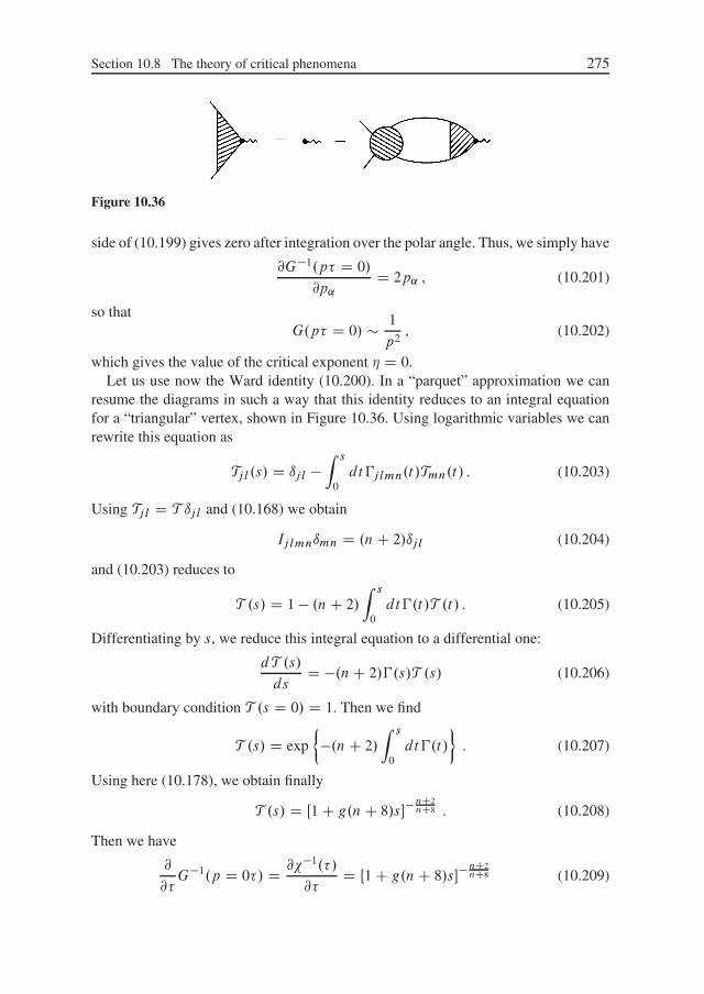
Section 10.8 The theory of critical phenomena 275
Figure 10.36
side of (10.199) gives zero after integration over the polar angle. Thus, we simply have
@G�1.p� D 0/
@p˛D 2p˛ , (10.201)
so thatG.p� D 0/ � 1
p2, (10.202)
which gives the value of the critical exponent � D 0.Let us use now the Ward identity (10.200). In a “parquet” approximation we can
resume the diagrams in such a way that this identity reduces to an integral equationfor a “triangular” vertex, shown in Figure 10.36. Using logarithmic variables we canrewrite this equation as
Tjl.s/ D ıjl �Z s
0dt�jlmn.t/Tmn.t/ . (10.203)
Using Tjl D T ıjl and (10.168) we obtain
Ijlmnımn D .nC 2/ıjl (10.204)
and (10.203) reduces to
T .s/ D 1 � .nC 2/Z s
0dt�.t/T .t/ . (10.205)
Differentiating by s, we reduce this integral equation to a differential one:
dT .s/
dsD �.nC 2/�.s/T .s/ (10.206)
with boundary condition T .s D 0/ D 1. Then we find
T .s/ D exp
²�.nC 2/
Z s
0dt�.t/
³. (10.207)
Using here (10.178), we obtain finally
T .s/ D Œ1 C g.nC 8/s��nC2nC8 . (10.208)
Then we have
@
@�G�1.p D 0�/ D @��1.�/
@�D Œ1 C g.nC 8/s��
nC2nC8 (10.209)

276 Chapter 10 Functional integrals: scalars and spinors
Integrating with the necessary accuracy, we get
�.�/ � 1
�
°1 C g.nC 8/
1
"Œ��"=2 �ƒ�"�
±nC2nC8 ! ��.1C "
2nC2nC8 / (10.210)
for � ! 0. Then, for the susceptibility critical exponent we find
� D 1 C nC 2
nC 8
"
2C � � � . (10.211)
This expression, as well as the previous result � D 0, are valid up to the terms of thefirst order in ", and represent the first terms of the "-expansion of critical indices. Moretedious calculations allow the derivation of higher order corrections.
One remarkable result of the modern theory following from these expressions is theuniversality of critical behavior; the values of the critical exponents in quite differ-ent physical systems are determined only by the dimensionality of space (or system)and the number of components n of the order parameter (i. e., in fact, the type of thesymmetry broken during the phase transition).
Expansion (10.160) may in principle contain higher powers of the order parameter.What is their role in critical behavior? Why have we limited ourselves only to g�4?Consider a possible term like ��6 and the simplest diagram due to such an interaction,shown in Figure 10.37. By the order of magnitude it is determined by the integral:
�2Zd 3p1
Zd 3p2
1
p21p
22.p
21 C p2
2/� �2
Z ƒ
p�
dp1
Z ƒ
p�
dp2p2
1p22
p21p
22.p
21 C p2
2/
� �2 lnƒp�
. (10.212)
For d > 3 this correction just converges (at the lower limit, for � ! 0), so that ford D 4 � " an interaction of the type of ��6 is actually irrelevant. Quite analogous isthe situation with the higher-order terms of the Landau expansion, which justifies theanalysis made above.
In conclusion, let us quote the values of critical indices up to the terms of the orderof � "2 for the theory with an n-component order parameter [3, 42]:
� D 1 C nC 2
nC 8
"
2C nC 2
nC 8
n2 C 22nC 52
.nC 8/2"2
4C � � � ,
Figure 10.37
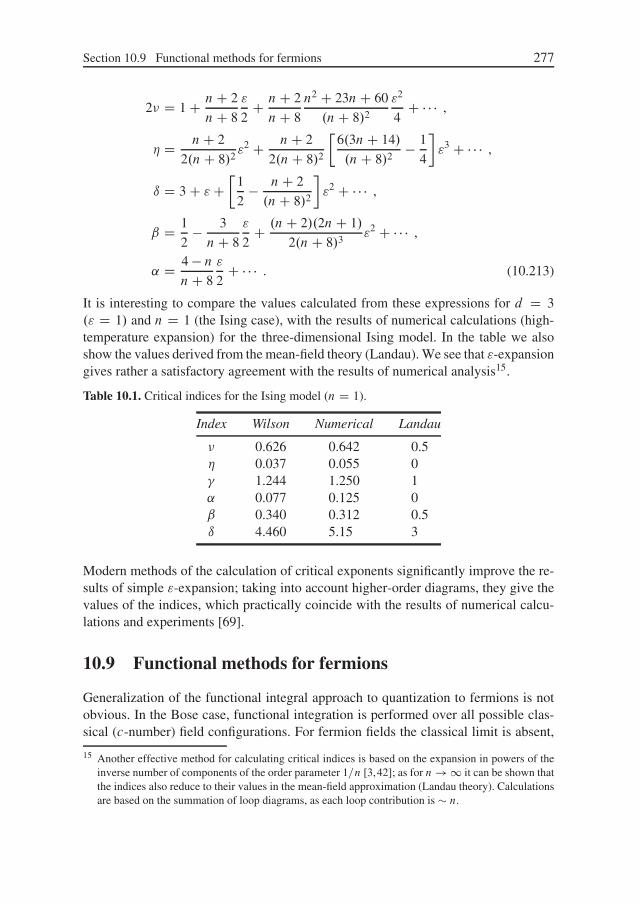
Section 10.9 Functional methods for fermions 277
2� D 1 C nC 2
nC 8
"
2C nC 2
nC 8
n2 C 23nC 60
.nC 8/2"2
4C � � � ,
� D nC 2
2.nC 8/2"2 C nC 2
2.nC 8/2
�6.3nC 14/
.nC 8/2� 1
4
�"3 C � � � ,
ı D 3 C "C�
1
2� nC 2
.nC 8/2
�"2 C � � � ,
ˇ D 1
2� 3
nC 8
"
2C .nC 2/.2nC 1/
2.nC 8/3"2 C � � � ,
˛ D 4 � nnC 8
"
2C � � � . (10.213)
It is interesting to compare the values calculated from these expressions for d D 3." D 1/ and n D 1 (the Ising case), with the results of numerical calculations (high-temperature expansion) for the three-dimensional Ising model. In the table we alsoshow the values derived from the mean-field theory (Landau). We see that "-expansiongives rather a satisfactory agreement with the results of numerical analysis15.
Table 10.1. Critical indices for the Ising model (n D 1).
Index Wilson Numerical Landau
� 0.626 0.642 0.5� 0.037 0.055 0� 1.244 1.250 1˛ 0.077 0.125 0ˇ 0.340 0.312 0.5ı 4.460 5.15 3
Modern methods of the calculation of critical exponents significantly improve the re-sults of simple "-expansion; taking into account higher-order diagrams, they give thevalues of the indices, which practically coincide with the results of numerical calcu-lations and experiments [69].
10.9 Functional methods for fermions
Generalization of the functional integral approach to quantization to fermions is notobvious. In the Bose case, functional integration is performed over all possible clas-sical (c-number) field configurations. For fermion fields the classical limit is absent,
15 Another effective method for calculating critical indices is based on the expansion in powers of theinverse number of components of the order parameter 1=n [3,42]; as for n ! 1 it can be shown thatthe indices also reduce to their values in the mean-field approximation (Landau theory). Calculationsare based on the summation of loop diagrams, as each loop contribution is � n.

278 Chapter 10 Functional integrals: scalars and spinors
and it is not clear what kind of field configurations we can introduce at all. The classi-cal limit is achieved as „ ! 0. In this case, the nontrivial right-hand side of all Bosefield operators, as considered in Chapter 2, tend to zero, and the operators becomec-numbers. For fermion fields, quantization is done with anticommutators, so that for„ ! 0 in the Fermi case we just get some anticommuting variables, with no obvious“common-sense” meaning. However, it happens that these variables lead to a correctsolution of our problem. Such variables were introduced in mathematics by Grassmannin the middle of 19th century and are called Grassmann variables. A functional formu-lation in quantum field theory for fermions, using Grassmann variables, was proposedby Berezin, who introduced the notion of integration over these variables [7].
Consider first the mathematical definitions. Generators Ci of n-dimensional Grass-mann algebra satisfy the anticommutation relations
¹Ci ,Cj º CiCj C CjCi D 0 , (10.214)
where i D 1, 2, : : : ,n. In particular,
C 2i D 0 . (10.215)
Thus, the series expansion of an arbitrary function f .Ci / can contain only a finitenumber of terms. For example, in the case of one-dimensional algebra we have
f .C / D aC bC , (10.216)
where a and b are usual numbers. The quadratic and higher-power terms of this ex-pansion are equal to zero.
For the general n-dimensional case the analogue of (10.216) takes the form
f .C / D P0 C P i1Ci C P ij2 CiCj C � � � C PnC1C2 � � �Cn , (10.217)
where each summation index takes values from 1 to n, and coefficients P are antisymmetricwith respect to the permutation of any pair of indices i , j , : : : . Expansion is cut a finite numberof terms because of (10.214).
Consider the notion of differentiation over Grassmann variables. We can introducetwo types of derivatives, left and right. The left derivative of the product C1C2 isdefined as
@L
@Ci.C1C2/ D ıi1C2 � ıi2C1 . (10.218)
Ccorrespondingly, the right derivative is given by
@R
@Ci.C1C2/ D ıi2C1 � ıi1C2 . (10.219)

Section 10.9 Functional methods for fermions 279
Then we have the following equalities:²@
@Ci,Cj
³D ıij , (10.220)
²@
@Ci,@
@Cj
³D 0 . (10.221)
In particular, for one-dimensional algebra,²d
dC,C
³D 1 (10.222)
and we always have �@
@Ci
�2
D 0 . (10.223)
All these relations are rather natural.In contrast, the definition of an integral over Grassmann variables is rather formal.
In particular, it is impossible to introduce it as the inverse operation to differentiation.However, it can be defined in such a way that it possesses some general propertiescharacteristic of the usual integral. For example, we can require our integral to beinvariant towards the shift of the integration variable by a constant:
ZdCf .C / D
ZdCf .C C ˛/ . (10.224)
This is always so for the usual integral with infinite limits of integration, but here ournew definition of integration has nothing in common with the usual definition (exceptthe notation
R), and there is no limits of integration here in the usual sense. Using the
explicit form of f .C / (10.216), we obtainZdC.aC bC / D
ZdC ŒaC b.C C ˛/� , so that
ZdC bC D
ZdC b.C C ˛/ , (10.225)
from which it follows that ZdC b˛ D 0 (10.226)
or, due to arbitrariness of b˛, ZdC D 0 . (10.227)
Here ˛ is another element of Grassmann algebra, independent of and anticommutingwith C . The remaining integral
RdC C can be just defined by the conditionZdC C D 1 . (10.228)

280 Chapter 10 Functional integrals: scalars and spinors
Equations (10.227) and (10.228) completely determine integration over Grassmannvariables.
Naturally, integration thus defined has nothing in common with the usual notionof an integral. Moreover, in the case of one-dimensional Grassmann algebra we havedfdC
D b andRdCf .C / D b, so that the operation of integration acts upon a function
in the same way as differentiation!In the n-dimensional case we assume
ZdCi D 0 ,
ZdCiCi D 1 . (10.229)
Let � and N� be independent Grassmann variables, so thatZd� D
Zd N� D 0 ,
Zd�� D
Zd N� N� D 1 . (10.230)
As �2 D N�2 D 0, we havee� N�� D 1 � N�� , (10.231)
so thatZd N�d� e� N�� D
Zd N�d� �
Zd N�d� N�� D 0 C
Zd N�d� � N� D 1 . (10.232)
Let us find the generalization of this expression for the case of a larger number ofdimensions. Consider the two-dimensional case, introducing for convenience the newnotations
� D��1
�2
�, N� D
� N�1
N�2
�. (10.233)
The exponent N�� (or more precisely N�T �) has the form
N�� D N�1�1 C N�2�2 . (10.234)
Then,
. N��/2 D . N�1�1 C N�2�2/. N�1�1 C N�2�2/
D N�1�1 N�2�2 C N�2�2 N�1�1 D 2 N�1�1 N�2�2 , (10.235)
where we have taken into account that �21 D �2
2 D N�21 N�2
2 D 0. Higher powers of N�� areequal to zero, and we get
e� N�� D 1 � . N�1�1 C N�2�2/C N�1�1 N�2�2 . (10.236)
Applying our integration rules, we see thatZd N�d�e� N�� D
Zd N�1d�1d N�2d�2 N�1�1 N�2�2 D 1 , (10.237)
as in the one-dimensional case. Let us transform the integration variables as
� D M˛ , N� D N N , (10.238)

Section 10.9 Functional methods for fermions 281
whereM andN are 2�2-matrices, while ˛ and N are new Grassmann variables. Thenwe have
�1�2 D .M11˛1 CM12˛2/.M21˛1 CM22˛2/
D .M11M22 �M12M21/˛1˛2 D .DetM/˛1˛2 , (10.239)
where we have taken into account the anticommutativity of Grassmann variables. Toconserve the integration rules
Zd�1d�2�1�2 D
Zd˛1d˛2˛1˛2 , (10.240)
we have to require that
d�1d�2 D .DetM/�1d˛1d˛2 , (10.241)
which differs from the usual rule for an integration variable change by the power ofthe determinant. Taking into account that
N�� D N NM˛ D N N˛MT D �˛MTN N D NMTN˛ , (10.242)
we write (10.237) as
.DetMN/�1Zd Nd˛e� NMTN˛ D 1 . (10.243)
As DetMN D DetMTN we obtain the general resultZd Nd˛e� NA˛ D DetA , (10.244)
which represents the Gaussian integral over Grassmann variables.To describe fermion fields we make a transition to Grassmann algebra with infinite
dimensions, with the appropriate generators denoted as C.x/:
¹C.x/,C.y/º D 0 , (10.245)
@L,RC.x/
@C.y/D ı.x � y/ , (10.246)
ZdC.x/ D 0 ,
ZdC.x/C.x/ D 1 . (10.247)
As a result we obtain functional integrals over Grassmann (Fermion) fields.As we already know, Dirac’s Lagrangian has the form
L D i N ��@� �m N . (10.248)
Then, the normalized generating functional for the free Dirac field can be written as
Z0Œ�, N�� D 1
N
ZD N D
� exp
²i
ZdxŒ N .x/.i��@� �m/ .x/C N�.x/ .x/C N .x/�.x/�
³, (10.249)
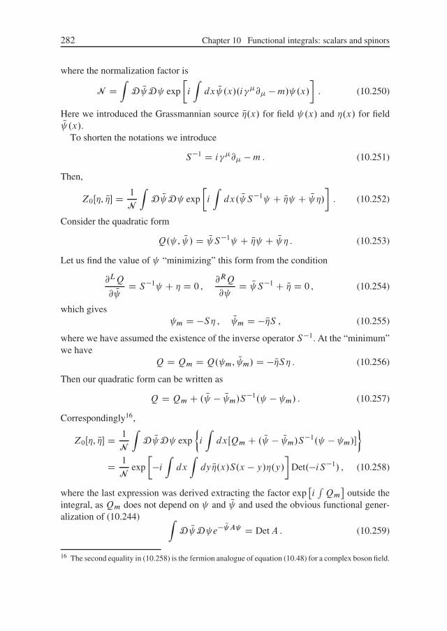
282 Chapter 10 Functional integrals: scalars and spinors
where the normalization factor is
N DZ
D N D exp
�i
Zdx N .x/.i��@� �m/ .x/
�. (10.250)
Here we introduced the Grassmannian source N�.x/ for field .x/ and �.x/ for fieldN .x/.
To shorten the notations we introduce
S�1 D i��@� �m . (10.251)
Then,
Z0Œ�, N�� D 1
N
ZD N D exp
�i
Zdx. N S�1 C N� C N �/
�. (10.252)
Consider the quadratic form
Q. , N / D N S�1 C N� C N � . (10.253)
Let us find the value of “minimizing” this form from the condition
@LQ
@ N D S�1 C � D 0 ,@RQ
@ D N S�1 C N� D 0 , (10.254)
which gives m D �S� , N m D �N�S , (10.255)
where we have assumed the existence of the inverse operator S�1. At the “minimum”we have
Q D Qm D Q. m, N m/ D �N�S� . (10.256)
Then our quadratic form can be written as
Q D Qm C . N � N m/S�1. � m/ . (10.257)
Correspondingly16,
Z0Œ�, N�� D 1
N
ZD N D exp
²i
ZdxŒQm C . N � N m/S�1. � m/�
³
D 1
Nexp
��iZdx
Zdy N�.x/S.x � y/�.y/
�Det.�iS�1/ , (10.258)
where the last expression was derived extracting the factor exp�iRQm
�outside the
integral, as Qm does not depend on and N and used the obvious functional gener-alization of (10.244) Z
D N D e� N A D DetA . (10.259)
16 The second equality in (10.258) is the fermion analogue of equation (10.48) for a complex boson field.

Section 10.9 Functional methods for fermions 283
In a similar way we may show that N D Det.�iS�1/, so that finally we obtain thegenerating functional of the free Dirac field as
Z0Œ�, N�� D exp
��iZdx
Zdy N�.x/S.x � y/�.y/
�. (10.260)
It is easy to see that operator S really exists. It has the form
S.x/ D .i��@� Cm/F .x/ , (10.261)
where F .x/ is the well-known Feynman propagator of a scalar field. In fact, using(10.251) we have
S�1S D .i��@��m/.i��@�Cm/F .x/ D .���m2/F .x/ D ı.x/ . (10.262)
Now we can define the free propagator of the Dirac field as
�.x, y/ D � ı2Z0Œ�, N��ı�.x/ı N�.y/
ˇˇ�D N�D0
D � ı
ı�.x/
ı
ı N�.y/²
�iZdx
Zdy N�.x/S.x � y/�.y/
³ˇˇ�D N�D0
D iS.x � y/ , (10.263)
where we have used exp.�N�S�/ D 1 � N�S�.Let us summarize the main expressions related to the free scalar and spinor fields.
For the scalar field we have
L0 D 1
2@�'@
�' � 1
2m2'2 D �1
2'.� Cm2/' . (10.264)
We have seen above that�.x, y/ D iF .x � y/ , (10.265)
where F is the Feynman propagator satisfying the equation
.� Cm2/F .x � y/ D �ı.x � y/ . (10.266)
For the spinor (Dirac) field we have
L0 D i N ��@� �m N D N S�1 , (10.267)
�.x, y/ D iS.x � y/ . (10.268)
In both cases we see that the propagator is inverse (operator) to the coefficient be-fore the quadratic term in the Lagrangian. We can take this as the definition of a freepropagator in the functional formulation for an arbitrary field.
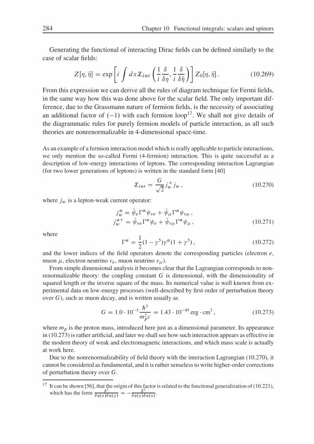
284 Chapter 10 Functional integrals: scalars and spinors
Generating the functional of interacting Dirac fields can be defined similarly to thecase of scalar fields:
ZŒ�, N�� D exp
�i
ZdxLint
�1
i
ı
ı�,
1
i
ı
ı N���Z0Œ�, N�� . (10.269)
From this expression we can derive all the rules of diagram technique for Fermi fields,in the same way how this was done above for the scalar field. The only important dif-ference, due to the Grassmann nature of fermion fields, is the necessity of associatingan additional factor of .�1/ with each fermion loop17. We shall not give details ofthe diagrammatic rules for purely fermion models of particle interaction, as all suchtheories are nonrenormalizable in 4-dimensional space-time.
As an example of a fermion interaction model which is really applicable to particle interactions,we only mention the so-called Fermi (4-fermion) interaction. This is quite successful as adescription of low-energy interactions of leptons. The corresponding interaction Lagrangian(for two lower generations of leptons) is written in the standard form [40]
Lint D Gp2jCw jw , (10.270)
where jw is a lepton-weak current operator:
j ˛w D N e�˛ �e C N ��˛ �� ,
j ˛Cw D N �e�˛ e C N ���˛ � , (10.271)
where�˛ D 1
2.1 � �5/�˛.1 C �5/ , (10.272)
and the lower indices of the field operators denote the corresponding particles (electron e,muon �, electron neutrino �e , muon neutrino ��).
From simple dimensional analysis it becomes clear that the Lagrangian corresponds to non-renormalizable theory: the coupling constant G is dimensional, with the dimensionality ofsquared length or the inverse square of the mass. Its numerical value is well known from ex-perimental data on low-energy processes (well-described by first order of perturbation theoryover G), such as muon decay, and is written usually as
G D 1.0 � 10�5 „3
m2pc
D 1.43 � 10�49 erg � cm3 , (10.273)
where mp is the proton mass, introduced here just as a dimensional parameter. Its appearancein (10.273) is rather artificial, and later we shall see how such interaction appears as effective inthe modern theory of weak and electromagnetic interactions, and which mass scale is actuallyat work here.
Due to the nonrenormalizability of field theory with the interaction Lagrangian (10.270), itcannot be considered as fundamental, and it is rather senseless to write higher-order correctionsof perturbation theory over G.
17 It can be shown [56], that the origin of this factor is related to the functional generalization of (10.221),which has the form ı2
ı�.x/ı�.y/D � ı2
ı�.y/ı�.x/.

Section 10.10 Propagators and gauge conditions in QED 285
10.10 Propagators and gauge conditions in QED
In QED we can write down the generating functional of Maxwell field as
ZŒJ � DZ
DA� exp
²i
Zdx.L C J�A�/
³, (10.274)
where J� is an external source current,
L D � 1
16�F��F
�� . (10.275)
Making partial integration over dx and dropping the surface integrals, we can rewritethis Lagrangian as
L D 1
8�A�Œg��� � @�@� �A� . (10.276)
The Lagrangian of the electromagnetic field is invariant to gradient (gauge) transfor-mations A� ! A� C @�ƒ. At the same time, the functional integral in (10.274) istaken over all A�, including those connected with each other by gauge transforma-tions. Obviously this leads to the appearance of an infinite contribution to Z and toGreen’s functions. It is clear that it is necessary to fix some gauge, so that the integralover A� is not calculated over the field configurations, which are obtained from eachother by gauge transformations. Physically these configurations are just equivalent!Here we meet a problem which becomes especially difficult for non-Abelian gaugetheories. In fact, this problem can be rigorously solved, as it will be shown in the nextchapter. Here we just limit ourselves to several technical remarks.
If we use the Lorentz gauge @�A� D 0, the Lagrangian (10.276) becomes
L D 1
8�A�g���A� . (10.277)
The inverse operator for g��� is represented by the Feynman propagator (see e. g.,Chapter 4)
DF��.x, y/ D g��4�F .x, y;m D 0/ . (10.278)
In momentum representation, the operator �g��k2, originating from (10.277), has aninverse operator written as �g�� 1
k2 , so that the Feynman propagator of the electro-magnetic field in the Lorentz gauge has the form
DF��.k/ D g��4�
k2. (10.279)
In the general case we can add to the Lagrangian an extra term, fixing the gauge, withan arbitrary coefficient ˛:
L D � 1
16�F��F
�� � 1
8�˛.@�A
�/2 D 1
8�A�
hg��� C
1
˛� 1
�@�@�
iA� .
(10.280)

286 Chapter 10 Functional integrals: scalars and spinors
In momentum representation, the coefficient before the square of the field is
�k2g�� C
1 � 1
˛
�k�k� , (10.281)
with the corresponding inverse operator produces propagator as
D��.k/ D 4�
k2
�g�� C .˛ � 1/
k�k�
k2
�. (10.282)
For ˛ ! 1 we obtain a Feynman propagator (Lorentz-Feynman gauge), while for˛ ! 0 we obtain the propagator in a Landau gauge.

Chapter 11
Functional integrals: gauge fields
11.1 Non-Abelian gauge fields and Faddeev–Popovquantization
Let us consider the quantum theory of non-Abelian gauge fields. For a long time, quan-tization of Yang-Mills fields remained an unsolved problem due to difficulties relatedto the necessity of a correct account of gauge invariance. In particular, attempts toquantize this theory along the lines of the traditional (operator) approach in quantumfield theory were mostly unsuccessful, despite the successes of Abelian QED. Thecomplete solution of the problem was achieved by Faddeev and Popov, who usedfunctional methods. In the following we mainly follow the presentation of [13].
The heuristic idea
We have seen above that the value of the generating functionalZ, defined in the usualway, in case of gauge theory (even QED) is. in general, infinite, as it contains integra-tion over all fields A�, including those connected with each other by gauge transfor-mations, which leave an integrand invariant.
Before we start the analysis, allowing separation of the corresponding infinite “vol-ume” factor from the (infinite-dimensional) functional integral over the gauge field,we shall consider a simple illustration of the main idea of our general method for thecase of the usual two-dimensional integral:
W DZdx
ZdyeiS.x,y/ D
ZdreiS.r/ , (11.1)
where r D .r , �/ defines the polar coordinates of a point on the plane. Assume thatfunction S.r/ (analogue to the action!) is invariant with respect to rotations in two-dimensional space:
S.r/ D S.r�/ (11.2)
as r D .r , �/ ! r� D .r , � C �/. This means, that S.r/ is constant at the circles(“orbits”) in the .x, y/-plane, as shown in Figure 11.1(a). In this trivial example, if wewant to take into account only contributions from nonequivalent values of S.r/, weneed to extract a “volume factor”, corresponding to integration over angular variable1
1 Angular integration is assumed to be done from 0 to 2� , and we just drop these integration limitsbelow.

288 Chapter 11 Functional integrals: gauge fields
(a) (b)
Figure 11.1
Rd� D 2� . To formalize this, we shall use the following “recipe”, to be generalized
for more complicated cases later. Let us put inside our integral a factor 1, written inthe form2
1 DZd�ı.� � �/ . (11.3)
Then we have
W DZd�
ZdreiS.r/ı.� � �/ D
Zd�W� , (11.4)
where
W� DZdrı.� � �/eiS.r/ (11.5)
is calculated for the given value of � D � . Thus, first of all we calculate W at thefixed value of � D � (constraint!), and afterwards integrate over all values of � (seeFigure 11.1(a)). Using the invariance of S (11.2), we have
W� D W�0 . (11.6)
We see that the “volume” of the orbit can be extracted as a factor:
W DZd�W� D W�
Zd� D 2�W� . (11.7)
In the eneral case, we can use a more complicated constraint (instead of � D � ), whichcan be represented by some curve g.r/ D 0, crossing each orbit only once, as shown inFigure 11.1(b), so that the equation g.r�/ D 0 has the unique solution for � at a fixedvalue of r . Taking such a general constraint, we define, instead of simple equation(11.3), the “representation of unity” of the form
1 D g.r/Zd�ıŒg.r�/� . (11.8)
In other words, we define the function g.r/ as
Œg.r/��1 DZd�ıŒg.r�/� . (11.9)
2 Here it is assumed that � is within the interval .0, 2�/.

Section 11.1 Non-Abelian gauge fields and Faddeev–Popov quantization 289
Using the general ruleZdxıŒf .x/� D
Zdf
1
df=dxı.f / D 1
df=dx
ˇˇfD0
, (11.10)
we obtain
g.r/ D @g.r� /@�
ˇˇgD0
, (11.11)
and g.r/ here is invariant with respect to two-dimensional rotations:
Œg.r�0/��1 DZd�ıŒg.r�C�0/� D
Zd�00ıŒg.r�00/� D Œg.r/��1 . (11.12)
Then, repeating arguments similar to those used during the transformation from (11.4)to (11.7), we can again extract from our integral the “volume factor” 2�:
W DZd�
Zdrg.r/ıŒg.r�/�eiS.r/ D
Zd�W� , (11.13)
where
W� DZdreiS.r/g.r/ıŒg.r�/� . (11.14)
The entire nontrivial part of the integral is here! The “volume factor” is equal just to2� , which is the formal outcome of the invariance ofW� with respect to the rotations:
W�0 DZdreiS.r/g.r/ıŒg.r�0/� D
Zdr0eiS.r0/g.r0�/ D W� , (11.15)
where we have introduced the variable r0 D .r ,�0/ and used the rotational invarianceof S.r/, g.r/ and the integration measure dr. Thus, our “recipe” for extracting the“volume factor” is to introduce into the integrand the constraining ı-function, whichis multiplied by g , defined by (11.9).
Extracting the “volume factor” in a functional integral
Now let us discuss non-Abelian gauge fields. To be concrete, we consider here thecase of Yang–Mills fields for a SU.2/ gauge group. The Lagrangian of this theory iswritten as
L D � 1
16�F a��F
a�� , a D 1, 2, 3 , (11.16)
where (cf. equation (2.112))
F a�� D @�Aa� � @�Aa� C g"abcAb�A
c� . (11.17)
Here g is the Yang–Mills coupling constant. We define the generating functional asusual:
ZŒ EJ � DZ
D EA� exp
²i
ZdxŒL.x/C EJ� � EA�.x/�
³. (11.18)

290 Chapter 11 Functional integrals: gauge fields
The action is invariant with respect to gauge transformations
EA� ! EA�� , (11.19)
where (cf. equations (2.156), (2.159), and (2.162))
EA�� � E�2
D U.�/
�EA� � E�
2C 1
igU�1.�/@�U.�/
�U�1.�/ . (11.20)
Here
U.�/ D exp
�i E�.x/ � E�
2
�(11.21)
is the spinor transformation of SU.2/. Near the unit transformation, we can writeU.�/as
U.�/ D 1 C i E� � E�2
CO.�2/ . (11.22)
The values of E�.x/ represent the group parameters, depending on the point of space-time, while E� are Pauli matrices in isotopic space.
The action of our theory is constant (invariant) on the orbit of the gauge group, con-sisting of all EA��, obtained from some fixed field configuration EA� by transformationU.�/, which encompasses all elements of the group SU.2/. For the correct quanti-zation procedure, functional integration should be done over the “hypersurface” infunctional space, which crosses each orbit only once. Thus, if we write the equationfor this hypersurface as
fa. EA�/ D 0 , a D 1, 2, 3 ; (11.23)
equationfa. EA��/ D 0 (11.24)
should have the unique solution E� for the given field configuration EA�. This conditionfixes the gauge.
Let us define integration over the gauge group parameters as
Œd E�� D3Y
aD1
d�a . (11.25)
If we make two gauge transformations E� and E� 0, the corresponding matrix is U.�/U.� 0/, and the transformation parameters are summed: E� C E� 0. Thus, the integrationmeasure defined as in (11.25) is gauge invariant; if � angles encompass all possiblevalues, the shift by a constant � 0 is irrelevant. Symbolically we write this as d.E� E� 0/ Dd E� 00 D d E� .

Section 11.1 Non-Abelian gauge fields and Faddeev–Popov quantization 291
Now we can act as above (in the case of usual integral) and introduce f Œ EA�� asfollows:
�1f Œ EA�� D
ZŒd E�.x/�ıŒfa. EA��/� . (11.26)
Then we havef Œ EA�� D DetMf (11.27)
which is called the Faddeev–Popov determinant, where
.Mf /ab D ıfa
ı�b. (11.28)
In more detail, making the usual discretization of space (followed by the continuous limit), wecan write
�1f Œ EA�� D
Z Y
x
Y
a
d�a.x/ıŒfa.x/� DY
x
Y
a
Zdfa.x/ıŒfa.x/�
@.�1.x/, �2.x/, �3.x//
@.f1.x/,f2.x/,f3.x//
DY
x
Det
�@�a.x/
@fb.x/
�
fD0D Det
�ı�a.x/
ıfb.x/
�
fD0. (11.29)
In the last equality (after transformation to continuous x) the functional determinant (Jacobian)of the matrix with continuous indices ı�a.x/
ıfb.y/, appearked which is defined as the product of
eigenstates of this matrix.
The matrix Mf is related to the infinitesimal gauge transformations of the function
faŒ EA��:faŒ EA��.x/� D faŒ EA�.x/�C
Zdyıfa.x/
ı�b.y/�b.y/CO.�2/
D faŒ EA�.x/�CZdyŒMf .x, y/�ab�b.y/CO.�2/ . (11.30)
Then, demanding the uniqueness of the solution of equation (11.24) fa. EA��/ D 0 with
respect to E� , we conclude that DetMf should be nonzero. The explicit form of Mfis naturally dependent on the choice of specific gauge condition (the form of functionfa); concrete expressions for the case for Lorentz gauge will be presented below.
The Faddeev–Popov determinant f Œ EA�� is gauge invariant. In fact, we can write
�1f Œ EA�� D
ZŒd E� 0.x/�ı
�fa. EA� 0
� /�
. (11.31)
Then
�1f Œ EA��� D
ZŒd E� 0.x/�ıŒfa. EA�� 0
� /� DZŒd E�.x/E� 0.x/�ıŒfa. EA�� 0
� /�
DZŒd E� 00.x/�ıŒfa. EA� 00
� /� D �1f Œ EA�� , (11.32)
which completes the proof. Actually, this situation is similar to (11.12)).

292 Chapter 11 Functional integrals: gauge fields
Let us substitute the “unity representation” following from (11.26)
1 DZŒd E�.x/�f Œ EA��ıŒfa. EA��/� (11.33)
into (11.18). Then, denoting the integration measure over the Yang–Mills fields asŒd EA�.x/�, we obtainZŒd EA�.x/� exp
²i
ZdxL.x/
³
DZŒd E�.x/�
ZŒd EA�.x/�f Œ EA��ıŒfa. EA��/� exp
²i
ZdxL.x/
³
DZŒd�.x/�
ZŒd EA�.x/�f Œ EA�.x/�ıŒfa. EA�/� exp
²i
ZdxL.x/
³. (11.34)
To obtain the last equality we used the invariance of f Œ EA�� and exp®iRdxL.x/
¯
to gauge transformations EA�� ! EA�. Then we see that the integrand does not depend
on E�.x/, andRŒd E�.x/� D R Q
x dE�.x/ simply gives infinite “volume” of the orbit,
which we wanted to separate! Thus, dropping this irrelevant factor, we can write thegenerating functional for gauge field EA� as
ZŒ EJ � DZŒd EA��f Œ EA��ıŒfa. EA�/� exp
²i
ZdxŒL.x/C EJ� � EA��
³
DZŒd EA��.DetMf /ıŒfa. EA�/� exp
²i
ZdxŒL.x/C EJ� � EA��
³. (11.35)
This is the essence of the so-called Faddeev–Popov Ansatz – we isolate and can-cel all the irrelevant integrations, introducing into integration measure the factor ofDetMf ıŒfa. EA�/�.
Abelian gauge theory (QED)
Consider the simplest example – QED. In this case infinitesimal gauge transformationis written as
A�� D A�.x/ � 1
g@��.x/ . (11.36)
For any choice of the gauge condition (11.23) linear over field A�.x/, the matrix Mf(11.28) is independent of field A�.x/. Then, Faddeev-Popov determinant is unimpor-tant from physical point of view and can be moved outside functional integral overA�.x/ and just dropped3. Then we can write generating functional as:
ZŒJ � DZŒdA��ıŒf .A�/� exp
²i
ZdxŒL.x/C J�.x/A
�.x/�
³, (11.37)
where ıŒf .A�/� fixes the gauge and we obtain the usual formulation of QED.
3 In terms of general case, discussed below, we can say, that in QED Faddeev-Popov “ghosts” do notinteract with field A� and are irrelevant.

Section 11.2 Feynman diagrams for non-Abelian theory 293
11.2 Feynman diagrams for non-Abelian theory
Consider now the details of the diagram technique for non-Abelian theory. Let usrewrite the generating functional (11.35) as
ZŒ EJ � DZŒd EA�� exp
²iSeff C i
Zdx EJ� � EA�
³, (11.38)
where we have rewritten the factor DetMf ıŒfa. EA�/� as exp ln.DetMf ıŒfa. EA�/�/,and included �i ln.DetMf ıŒfa. EA�/�/ into the definition of effective action Seff .Naturally, the presence of such a term in effective action complicates the constructionof the diagram technique. First we shall try to write this term in a more natural andconvenient form.
Faddeev–Popov “ghosts”
We can write DetMf as an exponential, using the expression
DetMf D expŒSp lnMf � . (11.39)
The proof of (11.39) is trivial. The equality ln DetMf D Sp lnMf is obvious for any matrix:DetMf is represented by the product of eigenvalues of Mf , so that ln DetMf gives the sumof the logarithms of all eigenvalues of Mf , i. e., precisely Sp lnMf .
Writing the matrix Mf asMf D 1 C L (11.40)
and expanding the logarithms, we have
expŒSp lnMf � D exp
�SpL � 1
2SpL2 C � � � C .�1/nC1
nSpLn C � � �
�
D exp
²ZdxLaa.x, x/ � 1
2
Zdx
ZdyLab.x, y/Lba.y, x/C � � �
³.
(11.41)
We see that the Faddeev–Popov determinant can be represented as a loop expansion4,as shown in Figure 11.2, where lines denote the propagators of some fictitious particles(Faddeev–Popov “ghosts”), forming a triplet of complex scalar (spinless) fields Ec.x/.These fields and their interactions can be described by the generating functional
DetMf DZŒd Ec�Œd EcC� exp
²i
Zdxdy
X
ab
cCa .x/ŒMf .x, y/�abcb.y/
³. (11.42)
4 This expansion is similar to the loop expansion of free energy in the theory of condensed matter [1]

294 Chapter 11 Functional integrals: gauge fields
Figure 11.2
Here integration is done over Grassmannian Ec.x/, EcC.x/, as the use of common c-number fields will lead to .DetMf /�1! Thus, our scalar fields Ec.x/, EcC.x/ obey Fermistatistics, and the Faddeev–Popov “ghosts” are fermions with spin)! There is no con-tradiction with the spin and statistics theorem here, because these “ghosts” are purelyfictitious particles which are introduced to the theory just “for convenience”. As theircontribution to the generating functional reduces to the loop series (11.41), there areno diagrams with external “ghost” lines.
Gauge-fixing terms
Now we shall transform to the exponential form the term ıŒfa. EA�/�. First of all, wegeneralize the gauge-fixing condition, writing it as
faŒ EA�� D Ba.x/ , a D 1, 2, 3 , (11.43)
where Ba.x/ is some arbitrary function of space-time point, independent of gaugefield EA�. Correspondingly we define f by the condition
f Œ EA��ZŒd E�.x/�ıŒfa. EA��/ � Ba.x/� D 1 . (11.44)
Obviously, because of the independence of Ba.x/ from EA�, this is the same functionf defined in (11.26)5; in fact there is no dependence on Ba.x/ here at all! Thus thegenerating functional (11.35) can be rewritten as
ZŒ EJ � DZŒd EA��Œd EB�.DetMf /ıŒfa. EA�/ � Ba�
� exp
²i
Zdx
�L.x/ � EJ� � EA� � 1
8��EB2.x/
�³, (11.45)
where we have included in the integrand the constant term likeZŒd EB� exp
²� i
8��
Zdx EB2.x/
³, (11.46)
5 This is simply the analogue of (11.6) in the case of usual integration.

Section 11.2 Feynman diagrams for non-Abelian theory 295
where � is an arbitrary constant coefficient which is usually called the gauge parameter.As a result, the generating functional (11.45) differs from (11.35) by an irrelevantconstant factor which can be hidden into normalization. But now, using the ı-function,entering (11.45), we can lift integration over Œd EB.x/�. Finally, taking into account also(11.42), we obtain
ZŒ EJ � DZŒd EA��Œd Ec�Œd EcC� exp.iSeff Œ EJ �/ , (11.47)
whereSeff Œ EJ � D SŒ EJ �C Sf ix C Sghost , (11.48)
where SŒ EJ � D RdxŒL.x/C EJ� � EA�� is the usual action of our theory,
Sf ix D � 1
8��
Zdx¹faŒ EA�.x/�º2 (11.49)
is the so-called gauge fixing term, and
Sghost DZdxdy
X
ab
cCa .x/ŒMf .x, y/�abcb.y/ (11.50)
is “ghosts” action.
The Lorentz gauge
In the Lorentz gauge we have
fa. EA�/ @�Aa� D 0 , a D 1, 2, 3 . (11.51)
Under infinitesimal gauge transformations
U.�/ D 1 C i E�.x/ � E�2
CO.�2/ , (11.52)
so thatAa�� D Aa�.x/ � "abc�b.x/Ac�.x/C 1
g@��
a.x/ . (11.53)
Substituting (11.53) into (11.51) we have
fa. EA��/ D fa. EA�/ � @��"abc�b.x/Ac�.x/ � 1
g@��
a.x/
�
D fa. EA�/CZdyŒMf .x, y/�ab�
b.y/ , (11.54)
where in the last equality we have used (11.30). Then we see that in this case
ŒMf .x, y/�ab D 1
g@�Œıab@� � g"abcAc��ı.x � y/ . (11.55)

296 Chapter 11 Functional integrals: gauge fields
Now, substituting everything into (11.49) and (11.50), we obtain
Sf ix D � 1
8��
Zdx.@� EA�/2 , (11.56)
Sghost D 1
g
ZdxX
ab
cCa .x/@
�Œıab@� � g"abcAc��cb.x/ . (11.57)
We see that now “ghosts” are interacting with the gauge field EA�, which is describedby the second term in square brackets in (11.57). In similar expressions in QED sucha term was just absent6.
Let us also introduce the sources �Ca , �a for “ghost” fields ca, cC
a and write thegenerating functional of gauge theory as
ZŒ EJ , E�, E�C� DZŒd EA�d Ecd EcC� exp
²i
Zdx
�L.x/ � 1
8��.@� EA�/2
C cCa @
�.ıab@� � g"abcAc�/cb C J a�Aa� C �aCca C �acaC
�³,
(11.58)
where we redefined fields ca, cCa in an obvious way by including the factor 1=g.
Perturbation expansion
Let us write the action of our theory as
Seff D S0 C SI , (11.59)
where
S0 DZdx
�� 1
16�.@�A
a� � @�Aa�/2 � 1
8��.@�Aa�/
2 C cCa @
2ca C J a�Aa�
C �aCca C �acaC�
, (11.60)
and the interaction term, containing fields in powers higher than two, has the form
SI DZdx
�� 1
8�.@�A
a� � @�Aa�/g"abcAb�Ac�
� 1
16�g2"abc"adeAb�A
c�A
d�Ae� � gcaC@�"abcAc�cb�
.
(11.61)
6 In the non-Abelian case it is also possible to choose a special, so-called axial, gauge, where “ghosts”are completely excluded [13], but this gauge is rather inconvenient for practical calculations due to avery complicated form of the gauge field propagator.

Section 11.2 Feynman diagrams for non-Abelian theory 297
Generating functional can now be written as
ZŒ EJ , E�, E�C� D exp
²iSI
�ı
iı EJ�,ı
iıE� ,ı
iıE�C
�³Z0AŒ
EJ �Z0c ŒE�, E�C� , (11.62)
where
Z0AŒ
EJ � DZŒd EA�� exp
²i
Zdx
�� 1
16�.@�A
a� � @�Aa�/2
� 1
8��.@�Aa�/
2 C J a�Aa�
�³, (11.63)
Z0c ŒE�, E�C� D
ZŒd EcC�Œd Ec� exp
²i
Zdx�caC@2ca � �aCca � �acaC�
³. (11.64)
These expressions allow the direct derivation of perturbation theory. We shall not givethe detailed derivation here, but limit ourselves to the summary of the main rules ofthe diagram technique. Readers interested in details can find everything in a numberof books , e.g., [13, 25, 28, 53, 56].
Propagators
To find the propagator of field EA� we rewrite Z0A as
Z0AŒ
EJ � DZŒd EA�� exp
²i
Zdx
�1
8�ıabA
a�
�g��@2 � � � 1
�@�@�
�Ab� C J a�A
a�
�³
DZŒd EA�� exp
²i
Zdxh1
2Aa�K
��
abAb� C J a�A
a�i³
, (11.65)
where
K��
abD�g��@2 �
�1 � 1
�
�@�@�
�ıab . (11.66)
Integration over Œd EA�� can be performed using the well-known Gaussian integral(10.47), which in this case can be written as
ZŒd'� exp
h�1
2h'K'i C hJ'i
i� .DetK/�1=2 exphJK�1J i , (11.67)
where angular brackets denote the appropriate integrals. Application of this expressionto (11.65) gives
Z0AŒ
EJ � D exp
²� i
2
ZdxdyJ a�.x/G
��
ab.x � y/J b� .y/
³, (11.68)
where
G��
ab.x � y/ D ıab
Zd 4k
.2�/4e�ik.x�y/
���g�� � k�k�
k2
�� � k
�k�
k2
�4�
k2 C i".
(11.69)

298 Chapter 11 Functional integrals: gauge fields
It is easy to check thatZdyK
��
ab.x � y/Gbc��.y � z/ D g
�
�ıcaı.x � z/ , (11.70)
so that the propagator G is the inverse of K.Similarly we find
Z0c ŒE�, E�C� D exp
²�iZdxdy�aC.x/Gab.x � y/�a.y/
³, (11.71)
where
Gab.x � y/ D �Z
d 4k
.2�/4e�ik.x�y/k2 C i"
ıab . (11.72)
This directly corresponds to the fact, that “ghosts” are scalar particles with zero mass(obeying Fermi statistics).
Finally, we have
1. the propagator of massless vector bosons
iab��.k/ D �iıab�g�� � .1 � �/k�k�
k2
�4�
k2 C i", (11.73)
denoted in diagrams by a wave-like line;
2. the propagator of Faddeev-Popov “ghosts”
iab.k/ D �iıab 4�
k2 C i", (11.74)
which is denoted by a dashed line with an arrow (a “ghost” is different from an“anti-ghost”!).
Elementary vertices
In non-Abelian gauge theories there are two types of self-interactions, which can bewritten as
"�a .k1/"�b.k2/"
�c .k3/�
abc���.k1, k2, k3/ , (11.75)
"�a .k1/"�b.k2/"
�c .k3/"
�
d.k4/�
abcd���� .k1, k2, k3, k4/ , (11.76)
where we also explicitly show the corresponding polarization vectors. Feynman rulesare derived directly from (11.61), (11.62). In momentum representation the first termin (11.61) can be written as
1
3ŠAa�.k1/A
b�.k2/Ac�.k3/�
abc���.k1, k2, k3/ . (11.77)
The vertex part�abc���
shouldbe completely antisymmetric with respect to permutations

Section 11.2 Feynman diagrams for non-Abelian theory 299
Figure 11.3 Figure 11.4 Figure 11.5
of fields A. The structure related to SU.2/ gauge group is already fixed:
�abc���.k1, k2, k3/ D "abc����.k1, k2, k3/ , (11.78)
while the Lorentzian (relativistic) structure of this function can be obtained as follows.From (11.61) it is clear that ����.k1, k2, k3/ consists of terms like k�g��. A precisecombination of these terms can be established from the requirement of antisymmetryof ����.k1, k2, k3/ with respect to permutations of the indices: �, �, 1, 2 etc., takinginto account the total antisymmetry of the tensor "abc . Thus, we find
i�abc��� D ig"abc Œ.k1 � k2/�g�� C .k2 � k3/�g�� C .k3 � k1/�g��� (11.79)
where k1 C k2 C k3 D 0. The corresponding diagram for a “triple” vertex is shown inFigure 11.3.
Similarly we can find the vertex of “quartic” interaction of the gauge field, corre-sponding to the second term in (11.61):
i�abcd���� D ig2Œ"abe"cde.g��g�� � g��g��/C "ace"bde.g��g�� � g��g��/C "ade"cbe.g��g�� � g��g��/� (11.80)
which is expressed by the diagram in Figure 11.4. Here k1 C k2 C k3 C k4 D 0.For the vertex connecting the “ghosts” and gauge fields with polarization vector
"�.q/ we havei�abc� D ig"abck2� (11.81)
where k2 D k1 C q. This vertex is shown in Figure 11.5; it is antisymmetric over theisospin indices. Let us recall that “ghost” lines enter diagrams only in loops. Besideseach diagram containing a closed loop of the gauge field, there is a correspondingdiagram with a closed “ghost” line. As in the case of the usual fermion fields, each“ghost” loop can be multiplied by an additional .�1/.
The ropagator of gauge field (11.69) depends on the gauge parameter � . Its value ischosen for the convenience of explicit calculations while solving concrete problems.

300 Chapter 11 Functional integrals: gauge fields
For example, � D 1 corresponds to the so-called t’Hooft–Feynman gauge, while � D 0gives the Landau gauge.
The introduction of fermions into the Yang–Mills theory is not difficult: it is suffi-cient to add to the Lagrangian gauge invariant terms such as
Lf D N .i��D� �m/ (11.82)
whereD� D @� � igT aAa� (11.83)
Here T a is the gauge group generator in the given representation. For example, if is a SU.2/ doublet, we have T a D �a=2. Thus we obtain additional Feynman rulesfor fermions (with group indices n,m, : : :):
1. the fermion propagator has the standard form
imn.k/ D ınm1
��k� �mC i"(11.84)
and is expressed by continuous line;
2. the fermion-gauge field interaction vertex has the form
i�˛�nm D ig.T a/nm��. (11.85)
This is shown diagrammatically in Figure 11.6.The structure of the diagram technique described above is also conserved for the
other gauge groups, such as the very important SU.3/ describing the color symmetryof quarks. The only difference is in the dimensionality of the corresponding irreduciblerepresentations and the explicit form of generator matrices.
So far we have already studied the basics of the modern theory of quantum gaugefields, which forms the foundations of the standard model of elementary particles.Now we will begin out discussion on specific models of interactions. However, someconceptual problems, which we have discussed from the beginning, still remain. Inparticular, so far it is still unclear how we should deal with the problem of the mass-less nature of Yang–Mills fields, which is in striking contrast to experiments, whichclearly demonstrate that the only long-range interaction in nature (except gravitation)
Figure 11.6

Section 11.2 Feynman diagrams for non-Abelian theory 301
is electromagnetism. In the next chapter we shall see how this problem is solved inthe unified theory of weak and electromagnetic interactions. The remarkable fact isthat this solution is completely based on the ideas and methods originating from themodern theory of condensed matter.

Chapter 12
The Weinberg–Salam model
12.1 Spontaneous symmetry-breaking and the Goldstonetheorem
As we have already noted, the significant progress in modern theory of elementaryparticles was achieved using some fundamental concepts of the modern theory of thecondensed state. Most important was the introduction into quantum field theory of theidea of the possibility of phase transitions when the symmetry of the ground state be-comes lower than the symmetry of the Lagrangian. This allowed the effective solutionof the problem of mass generation for gauge fields without breaking local gauge invari-ance, directly leadto to quite rich and nontrivial foundations of the Standard Model.Moreover, the picture of possible “vacuum” phase transitions form the basis of mod-ern cosmology and physics of matter at very high densities and temperatures. Here weshall limit ourselves to a presentation of some of the main ideas which played a de-cisive role during the construction of the unified theory of weak and electromagneticinteractions1.
Let us again begin with the simplest example of the real scalar self-interacting field'.x/, described by the Lagrangian
L D 1
2.@�'/
2 � V.'/ D 1
2.@t'/
2 � 1
2.r'/2 � V.'/ , (12.1)
where V.'/ is some function of field invariants. The first term in this expression maybe considered to be kinetic energy density, and all the others represent potential energydensity.
From (12.1) we obtain the equations of motion
@2�' D �@V.'/
@'or
@2t' � r2' D �@V.'/
@'. (12.2)
The character of the solutions of these field equations depends essentially on the formof “potential energy” of self-interaction V.'/. Consider first the case of the tradi-tional field theory, which was analyzed before. Let V.'/ be of the form shown inFigure 12.1(a). Then our system has the “stable equilibrium” state with ' D 0 and can
1 In this chapter we mainly follow [5].

Section 12.1 Spontaneous symmetry-breaking and the Goldstone theorem 303
(a) (b)
Figure 12.1
oscillate around it. Close enough to this equilibrium state we can always write
V.'/ � �2
2'2 , (12.3)
where �2 D@2V@'2
�
'D0, so that (12.2) reduces to:
@2�' C �2' D 0 , (12.4)
i. e., to the Klein–Gordon equation. If we are looking for the plane-wave solution ofthis equation ' � eikx , from (12.4), the usual relativistic dispersion of a particle withmass �: k2
0 D k2 C �2 immediately follows. The higher-order terms of expansion ofV.'/ lead to nonlinear terms in field equations, describing interactions of these planewaves or particle scattering. Let us limit ourselves to
V.'/ D 1
2�2'2 C 1
4�'4 . (12.5)
There is no cubic term here, as V.'/ should be symmetric with respect to ' ! �', sothat there is always a minimum of V.'/ at ' D 0. Limitation to powers not higher than� '4 is of conceptual importance, as the coupling constant � > 0 is dimensionless andthe theory is renormalizable. Thus, in this case we are dealing with the well-known'4-theory.
Consider now the case of �2 < 0. This can seem strange, as from the naïve pointof view we are dealing with imaginary mass. However, we need to be more accurate.Now ' D 0 is no longer a stable equilibrium, as the potential energy has the formshown in Figure 12.1(b)2. We now see two stable equilibrium states, corresponding to
' D � D ˙r
j�j2�
. (12.6)
2 The situation here is completely analogous to the Landau theory of phase transitions, where �2 �T � Tc , so that �2 < 0 for T < Tc , i. e., below the phase transition temperature.

304 Chapter 12 The Weinberg–Salam model
Expanding V.'/ around points (12.6) up to the quadratic terms, we have
V.'/ D �2�2
4� �2.' � �/2 D �2�2
4� �2.ı'/2 , (12.7)
where ı' D ' � � and ��2.ı'/2 > 0 because of �2 < 0. Now we see that fieldequations (12.2) will have plane-wave solutions for ı' with wave-vector k, satisfyingthe condition (determining dispersion) k2 D 2j�j2, so that these waves will correspondto particles with real positive mass m D p
2j�j2.In fact, here we are dealing with a phase transition in quantum field theory. The sys-
tem chooses one of two equilibrium positions in Figure 12.1(b), and the field oscillatesclose to this new ground state.
In quantum mechanics the system with two such minima of potential energy does not onlyoscillates around the single minimum, because of the possibility of quantum tunneling be-tween these two equilibrium positions. The quantum state is split in two: the symmetric andthe antisymmetric (with respect to these minima) states. The ground state corresponds to thesymmetric state [35]. Thus, in quantum mechanics the symmetry of the ground state is in com-plete agreement with the symmetry of the Lagrange function (in our case even in '). Quantumfield theory in this sense is reminiscent of classical mechanics. Actually, the probability ofquantum tunneling transition becomes less with the growth of the number of degrees of free-dom, and becomes zero in the case of their number being infinite. In fact, let us consider thefield in a finite volume �. Then the Lagrange function is L D R
d 3xL � L�, so that thecorresponding kinetic energy � � P'2, while the potential is � �V.'/. Thus, our problem isequivalent to the tunneling of a particle with mass M � � through the potential barrier ofwidth jxj � � and height V � �m2�2. The probability of such tunnelling transition [35] is ofthe order of exp.�p
2MV jxj/ � exp.��m�2/ ! 0 for � ! 1. We can say that our fieldin the ground state is represented by a macroscopic “string” or “rope” of infinite length, lyingin the left or right valley of the potential in Figure 12.1(b), along the whole valley, which isperpendicular to the plane in the figure. Naturally, such an object cannot tunnel between thevalleys of the potential.
In quantum field theory the ground state is called a vacuum. Thus, we have to choosethe single ground state: one definite vacuum. The presence of another vacuum (phys-ically equivalent to the first one) is now irrelevant. Two minima of V.'/ correspondto two separate and vacuums of the theory which are orthogonal to each other, twoorthogonal Hilbert spaces of excited states, two separate “worlds”.
Traditional quantum field theory, corresponding to the potential V.'/ shown in Fig-ure 12.1(a), is constructed, as we know, as follows. The field is represented by the sumof the oscillators which are described by the creation and annihilation operators a� anda, and the vacuum is the state without the particles aj0i D 0, so that
h0j'j0i D 0 . (12.8)

Section 12.1 Spontaneous symmetry-breaking and the Goldstone theorem 305
In the case of potential V.'/, shown in Figure 12.1(b), the sum over the oscillatorsrepresents not the field ' itself, but its deviation from the equilibrium ı' D ' � �. Inthis case
h0j'j0i D � , (12.9)
i. e., the vacuum average of the field operator is nonzero: the system acquires the Bose-condensate3 of particles corresponding to field '. The initial Lagrangian (12.1), (12.5)is symmetric with respect to ' ! �'. However, for �2 < 0 it leads to a nonsym-metric ground state (vacuum), which is expressed by (12.9). Excitations above thisvacuum also do not possess the symmetry of the initial Lagrangian, as V.'/ fromFigure 12.1(b) is nonsymmetric with respect to ' D �. This phenomenon in quan-tum field theory is called spontaneous symmetry-breaking, while in condensed mattertheory this is the well-known situation of phase transition into the state with lowersymmetry.
The mechanism of mass generation
The existence of the nonzero vacuum average of a scalar field can automatically leadto the generation of mass of an initially massless particle, which interacts with thisfield. Consider as an example Dirac’s field of massless particles with spin 1/2. TheLagrangian of this field has the form
L D i N L O@ L C i N R O@ R , (12.10)
where O@ D ��@� and we introduced “left” and “right” components of bispinor :
R D 1
2.1 C �5/ , L D 1
2.1 � �5/ , L C R D . (12.11)
Now we can introduce the interaction of fields L, R with our scalar field ' breakingthe symmetry of the ground state. Let us add to the Lagrangian (12.10) the term
Lint D �~Œ N L R C N R L�' , (12.12)
where an expression in square brackets represents the only scalar which can be con-structed from L and R, while ~ is a dimensionless coupling constant (so that thisinteraction is renormalizable). Let us replace field ' in (12.12) by its vacuum aver-age �; this means that we are not taking into account the particle creation processesfor field '. Then we have
Lint D �~�. N L R C N R L/ D �~� N , (12.13)
so that the sum of (12.10) and (12.13) gives
L D i N O@ �m N , (12.14)
3 Compare with Bogolyubov’s approach to nonideal Bose gas!

306 Chapter 12 The Weinberg–Salam model
which corresponds to the Dirac Lagrangian for fermions with mass
m D ~� . (12.15)
Thus, we can start with the model of initially massless “left” and “right” fermions,which interact with scalar field ', undergoing the phase transition and transforming“left” particles into “right” ones and vice versa, and leading to the generation of mass.
Above we considered the simplest example of a Lagrangian with discrete symmetrywith respect to ' ! �'. Let us now consider the case of continuous symmetry-breaking. To do this we introduce the complex scalar field ', which is equivalent totwo real fields '1,'2, related by (see Chapter 2)
'.x/ D 1p2Œ'1.x/C i'2.x/� (12.16)
the Lagrangian of this field can be written as
L D 1
2.@�'1/
2 C 1
2.@�'2/
2 � V.'1,'2/ D .@�'/.@�'�/ � V.'1,'2/ . (12.17)
Let us assume that the potential V.'1,'2/ depends only on the absolute value of ', i.i.on �2 D '2
1 C '22 D 2'�', so that V D V.�/. This is equivalent to the requirement
of an additional (“internal”) symmetry of the theory with respect to transformations ofgroup U.1/:
' ! ei˛' (12.18)
or, which is just the same, the invariance of the Lagrangian with respect to rotationsin an “isotopic” plane:
'1 ! '1 cos˛ � '2 sin˛ ,
'2 ! '1 sin˛ C '2 cos˛ . (12.19)
We have seen (see Chapter 2), that this symmetry determines the conservation of somecharge (electric, barion, etc.). Fields ' and '� have the opposite values of this charge.
Consider now the potential V.�/, shown in Figure 12.2. which can be modelled, forexample, by
V.�/ D 1
2�2�2 C 1
4��4 (12.20)
with �2 < 0. Writing the field as (modulus-phase representation),
'.x/ D 1p2�.x/ei#.x/ , (12.21)
where �.x/ and #.x/ are real functions, we can see that V.�/ has the minimum at
� D � Dq
j�2j�
, i. e., for field values
' D 1p2�ei˛ (12.22)

Section 12.1 Spontaneous symmetry-breaking and the Goldstone theorem 307
Figure 12.2
with arbitrary ˛! Here we have continuous degeneracy of the ground state with dif-ferent values of ˛. Each value of ˛ corresponds to its own vacuum (ground state) withthe same (minimal) energy V.�/. All these vacuums are physically equivalent, but wehave to choose the only one, e. g., corresponding to ˛ D 0, and the Hilbert space ofstates associated with this single vacuum, where we already have no U.1/ symmetry(12.18), (12.19).
Let us see which particles are describe by the Lagrangian (12.17). Using (12.21) wecan rewrite the Lagrangian as
L D 1
2.@��/
2 � V.�/C �2
2.@�#/
2 . (12.23)
If we limit ourselves in (12.23) to terms which are quadratic in a field, we have toexpand V.�/ around � D � in powers of �0 D � � �, and in third term of (12.23)replace � by �. Then we obtain the free particle Lagrangian as
L D const C 1
2.@��
0/2 � m2
2�02 C �2
2.@�#/
2 , (12.24)
where m2 D 2j�2j. From here we immediately obtain the equations of motion
.@2� Cm2/�0 D 0 , @2
�# D 0 . (12.25)
Thus, we obtained two neutral (real) fields �0 and # , where the first one describes par-ticles with mass m, while the second one corresponds to massless particles. In equa-tion (12.25) we have dropped the terms of higher orders describing the interactions ofthese particles.

308 Chapter 12 The Weinberg–Salam model
The appearance of massless particles due to the spontaneous breaking of contin-uous symmetry is the essence of the Goldstone theorem; these particles are calledGoldstones4.
It is not difficult to generalize the Goldstone theorem to the case of higher symme-tries. Consider '.x/with n components. Then, group transformations can be written as
E D S E 0 , (12.26)
where E and E 0 are columns with n components .'1, : : : .'n/, abd S is an n�n-matrix.Let the potential V. E / be dependent only on �2 D '2
1 C : : :C'2n, and there is no other
invariants. ThenL D 1
2.@� E /2 � V.�/ . (12.27)
In this case we can again make the transformation to “polar” coordinates for fieldE when the field is determined by the modulus �.x/ and n � 1 “angular” variables(phases) ˛i .x/.i D 1, 2, : : : ,n � 1/. Then the Lagrangian is written as
L D 1
2.@��/
2 C �2
2
n�1X
i ,kD1
�ik.˛i /@�˛i@�˛k � V.�/ . (12.28)
Assume V.�/ having its minimum at � D �, i. e., h0j�j0i D �. Angular components˛i can be fixed by the condition h0j˛i j0i D 0 (the choice of vacuum!) and by �ik for˛i D 0 having the form �ik.0/ D ıik . Then, again introducing �0 D � � �, we have
L D const C 1
2.@��
0/2 � m2
2�02 C 1
2�2n�1X
iD1
.@�˛i /2 . (12.29)
We see that particles corresponding to fields ˛i have zero masses, so that there arenow n � 1 Goldstones. This is the general form of the Goldstone theorem.
12.2 Gauge fields and the Higgs phenomenon
It may seem that the appearance of Goldstone particles with zero mass creates addi-tional difficulties, as our main task is actually to solve the problem of zero mass ofgauge gosons. But this is not the case! The unification of the main idea of gauge the-ories with the concept of spontaneous symmetry-breaking allows us to formulate thenatural strategy for the construction of realistic models of interacting particles.
Consider the interaction of scalar field ', breaking symmetry, with gauge field A�in its simplest Abelian (Maxwell) variant. The Lagrangian invariant with respect to
4 In condensed matter theory the situation is just the same. For example, phase transition into the fer-romagnetic state breaks the continuous symmetry of a rotation group – the Heisenberg exchangeHamiltonian is invariant to rotations (it contains scalar products of spins on lattice sites), while in theground state we have a special direction: that of the vector of spontaneous magnetization (symmetryis lower!). Analogue of Goldstones in this case are acoustic spin waves.

Section 12.2 Gauge fields and the Higgs phenomenon 309
local transformations of U.1/, has the form5
L D �.@� � ieA�/'���.@� C ieA�/'
� � 1
4F��F
�� � V.','�/ , (12.30)
where F�� D @�A� � @�A�,
V.','�/ D �2'�' C �.'�'/2 , �2 < 0 . (12.31)
Let us again introduce modulus-phase representation of field ':
'.x/ D 1p2�.x/ei#.x/ . (12.32)
But now we can consider (12.32) as a local gauge transformation of U.1/:
'.x/ D eie�.x/'0.x/ , (12.33)
where�.x/ D 1
e#.x/ , '0.x/ D 1p
2�.x/ . (12.34)
Then, the covariant derivative, entering (12.30), is transformed as follows:
D�' D .@� C ieA�/eie�'0 D eie�.@� C ie@��C ieA�/'
0 D eie�.@� C ieA0�/'
0 ,(12.35)
whereA0� D A� C @�� (12.36)
or, taking into account (12.33), (12.34),
.@� C ieA�/' D 1p2ei#.@� C ieA0
�/� , (12.37)
whereA0� D A� C 1
e@�# . (12.38)
As a result, our Lagrangian is rewritten as
L D 1
2Œ.@� � ieA0
�/��Œ.@� C ieA0�/�� � V.�2/ � 1
4F��F
��
D 1
2.@��/
2 C e2
2�2A0�A0
� � V.�2/ � 1
4F��F
�� . (12.39)
We see that phase component # of field ' disappeared from the Lagrangian (so thatthe possibility of Goldstone also disappeared!); it just “gauged-out” into a redefinedvector-potential.
5 Later in this chapter we use the Heaviside system of units.

310 Chapter 12 The Weinberg–Salam model
Let us expand (12.39) in powers of deviation �0 D � � � from vacuum average �,limiting ourselves only to quadratic terms. Then we get
L D 1
2.@��
0/2 � m2
2�02 � 1
4F��F
�� C 1
2e2�2A0�A0
� C const , (12.40)
where m2 D 2j�2j. This Lagrangian describes a pair of free fields: the field �0 ofparticles with mass m and the vector field A0
� with mass
mA D e� , (12.41)
which is due to the presence of a nonzero vacuum average of the scalar field. Theequations of motion for these fields are
@2��
0 Cm2�0 D 0 , @�F�� Cm2
AA0� D 0 . (12.42)
The second equation here has the form of a Proca equation.Thus, in the initial Lagrangian we had the two-component field ' and the vector
Maxwell (massless) field A�. For �2 > 0, retaining only terms quadratic over fields,we obtain the Lagrangian of two free fields, one describing the charged particles withspin 0, while another corresponding to a photon with zero mass and two polariza-tions, i. e., four particles in total. For �2 < 0 the total number of particles remainsthe same (conservation of the degrees of freedom), but their character has changed:now we have one neutral scalar filed with spin 0 and three independent componentsof a massive vector boson with spin 1. Initially we had QED of a scalar field, whileafter the reconstruction of the field we have a “completely different” theory. However,it should be stressed that all transformations were done exactly, and the initial gaugeinvariance of the theory is conserved (and was used during the derivation!), despitethe appearance of gauge field mass! Renormalizability of the theory is also conserved.
The appearance of the vector gauge field mass due to its interaction with scalarfield, breaking the symmetry of the ground state, is called the Higgs phenomenon,while field � is usually called a Higgs field (and the corresponding scalar particles arecalled Higgs bosons).
Remarks on the Ginzburg–Landau theory
Let us show that our theory is the precise analogue of the Ginzburg–Landau theory of supercon-ducting transition, which was formulated long before the discovery of the Higgs phenomenon.
Consider the static case of the Higgs model, when @0' D 0, @0A� D 0. The electromag-
netic field will be considered in a Coulomb gauge: A� D .' D 0,A/, r � A D 0. Then theLagrangian (12.30) is written as
L D �1
2
�.r � ieA/'��.r C ieA/'�� � 1
2m2j'j2 � 1
4�j'j4 � 1
4.r �A/2 . (12.43)
Then
F D �L D 1
4.r �A/2 C 1
2j.r � ieA/'j2 C 1
2m2j'j2 C 1
4�j'j4 (12.44)

Section 12.3 Yang–Mills fields and spontaneous symmetry-breaking 311
is precisely the free energy density of Ginzburg–Landau theory [37] if we putm2 D a.T �Tc/,where Tc is the temperature of the superconducting transition6. In this case we have m2 > 0for temperatures T > Tc and m2 < 0 for T < Tc . For T < Tc the minimum of F is at
j'j2 D �m2
�> 0 , (12.45)
which defines the equilibrium value of the superconducting order parameter, which is theprecise analogue of the vacuum average of a Higgs field introduced above (ground state of theHiggs field, T D 0.).
Ginzburg–Landau free energy is invariant with respect to a gauge transformation:
' ! eiƒ.x/' , A ! AC 1
erƒ.x/ , (12.46)
and the corresponding conserved current is
j D � ie2.'�r' � 'r'�/ � e2j'j2A . (12.47)
For T < Tc and for the spatially homogeneous order parameter ', only the second term in(12.47) contributes
j D e2m2
�A , (12.48)
which is the so-called London equation. If we also take into account Maxwell equations r �H D 4�j, r � H D 0 and calculatethe curl of both sides of equation (12.48), we obtain theequation for the magnetic field inside the superconductor:
r2H D k2H , k2 D �e2m2
�> 0 , (12.49)
which describes the Meissner effect: the exclusion of the magnetic field from interior of the su-perconductor. The field is exponentially decreasing inside the superconductor on characteristiclength jkj�1 (penetration depth) [37].
Finally, from (12.49) it follows that r2A D k2A, which is an analogue of the relativis-tic equation �A� D �k2A�: the “photon” inside the superconductor acquires “mass” jkj,which is equivalent to the Higgs effect. Thus, the Higgs model is the relativistic analogue ofthe Ginzburg-Landau theory, and the Higgs vacuum is similar to the ground state of a super-conductor.
12.3 Yang–Mills fields and spontaneoussymmetry-breaking
Let us now consider the Higgs mechanism in non-Abelian gauge theories. First of all,we shall recall the main facts related to Yang–Mills fields, using the example of theSU.2/ gauge group.
6 In contrast with standard notations [37], her ewe put the electron mass and velocity of light equal to 1.More importantly, in the Ginzburg–Landau theory e ! 2e in (12.44), in accordance with the valueof the Cooper pair charge. But these slight differences are irrelevant for our discussion.

312 Chapter 12 The Weinberg–Salam model
Interaction of scalar field ' with Yang–Mills field EA� (the arrow denotes a vectorin isotopic space) is described by the replacement of the usual derivative @�' by thecovariant derivative
D�' D .@� � ig ET � EA�/' , (12.50)
where ET is the gauge group generator; for SU.2/ we have ET D 12 E� .
The Gauge invariance of the Lagrangian puts constraints on the field EA�. If ' corre-sponds to some isotopic multiplet, its transformation under rotations in isotopic spacecan be written as
' D S'0 , (12.51)
where the operator S depends on the three parameters (angles) of the rotation vectorE!.x/. Then we write the covariant derivative as
D�' D S@�'0 C .@�S/'
0 � ig ET � EA�S'0
D S.@� C S�1@�S � igS�1 ET � EA�S/'0 . (12.52)
This expression should be the same as
D�' D S.@� � ig ET � EA0�/'
0 , (12.53)
so that we have to require
ET � EA0� D S�1. ET � EA�/S C i
gS�1@�S . (12.54)
For small E! we haveS D 1 C i ET � E! . (12.55)
Then
S�1. ET � EA�/S D .1 � i ET � E!/ ET � EA�.1 C i ET � E!/D ET � EA� � i Œ ET � E!, ET � EA�� D ET � A� C Œ E! � EA�� � ET , (12.56)
where we have used ŒTi ,Tj � D i"ijkTk: the commutation relations for generators of
SU.2/. Taking into account S�1@�S D i ET �@� E! (12.54) and (12.55) give the generaltransformation rule
EA0� D EA� C Œ E! � EA�� � 1
g@� E! , (12.57)
so that, besides gradient transformation, the Yang–Mills field is rotated in isotopicspace.
The tensor of the Yang–Mills fields has the form
EF�� D @� EA� � @� EA� C gŒ EA� � EA�� , (12.58)

Section 12.3 Yang–Mills fields and spontaneous symmetry-breaking 313
Using (12.57) we can easily show that under infinitesimal rotations in isotopic spaceEF�� is transformed like an isovector:
EF 0�� D EF�� C Œ E! � EF�� � . (12.59)
The Yang–Mills Lagrangian is written as
LYM D �1
4EF�� � EF�� , (12.60)
which is invariant under local gauge group transformations.Consider now the Yang–Mills field interacting with scalar Higgs field breaking sym-
metry. Let the Higgs field � be an isospinor having two complex (four real) compo-nents
� D�'1
'2
�, (12.61)
which transform under rotations in isotopic space as
� D S�0 , S D ei2gE� E!.x/ . (12.62)
For small E! we have S D 1 C ig E!E�=2.The Lagrangian for fields � and EA� is written as
L D .D��/.D��/� � V.�/ � 1
4EF�� EF�� , (12.63)
where
D� D @� � ig E�2
EA� , (12.64)
V.�/ D �2��� C �.���/2 . (12.65)
Then, for �2 < 0 (12.65) has a minimum at
��� D 1
2�2 , �2 D j�2j
�. (12.66)
The vacuum state has infinite degeneracy, but we have to choose a single definitevacuum (break symmetry!), e. g., taking
h0j�j0i D 1p2
�0�
�, (12.67)
where � is real and positive. Let us transform to “polar” coordinates:
�.x/ D eiE�2
E#.x/�0.x/ D�
cos#
2C i.En � E�/ sin
#
2
��0.x/ , (12.68)
where
�0.x/ D 1p2
�0�.x/
�, E# D En# (12.69)
and En is unity vector in the direction of the rotation axis in isospace.

314 Chapter 12 The Weinberg–Salam model
Equations (12.68) and (12.69) define the parametrization of isospinor � D .'1'2/ by the four
real functions �,# , � ,', where # , � ,' are polar angles determining the direction of vector Enin isospace:
� D 1p2
i� sin #
2 cos �ei'
�
cos #2 � i sin #2 cos �
�!
, (12.70)
so that ��� D �2=2, h0j�j0i D �, h0j#j0i D h0j� j0i D h0j'j0i D 0.
Note that (12.68) is equivalent to (12.62) if we put E! D E#=g. The Lagrangian isinvariant with respect to such transformations and has the form
L D 1
2.D0
��/.D0��/� � V.�/ � 1
4EF 0��
EF 0�� , (12.71)
where in D0� and EF 0
�� we replaced EA� ! EA0�, which corresponds to the gauge trans-
formation (12.57). We see that only one of the four components of the field � that is� remain in the Lagrangian; the other three have gauged out!
Taking into account the form of the spinor �0 D 1p2.
0�/, we rewrite the Lagrangian
as (the prime over EA� is now dropped)
L D 1
2.@��/
2 C g2
8�2 EA� � EA� � V.�/ � 1
4EF�� EF�� , (12.72)
whereV.�/ D 1
2�2�2 C 1
4��4 . (12.73)
For small deviations from the vacuum state, making again an expansion of V.�/ inpowers of �0 D � � � and retaining only quadratic terms we obtain
L D const C 1
2.@��
0/2 � m2
2�02 � 1
4EF 0��
EF 0�� C 1
8g2�2 EA� � EA� , (12.74)
where m2 D 2j�2j and EF 0�� D @� EA� � @� EA�. This Lagrangian describes four free
fields: the real scalar field � and the triplet vector fields EA�. The scalar field describesparticles with mass m, the vector fields particles with mass
mA D g�
2. (12.75)
Thus, symmetry-breaking has again created masses for particles described by vector(gauge) field EA�. Gauge invariance of the theory is conserved, despite the appearanceof these masses! The total number of degrees of freedom has not changed: instead ofthe three components of field � (Goldstones) which “disappeared”, we got longitudinalpolarization components of EA�. In this model all the components of the Yang–Millsfield acquired mass.
However, to construct the realistic unified theory of weak and electromagnetic in-teractions we have to guarantee the massiveness of vector bosons, responsible for the

Section 12.3 Yang–Mills fields and spontaneous symmetry-breaking 315
weak interactions (short range forces!), while the electromagnetic field should remainmassless. This can be done by some generalization of our SU.2/-model. We note thatthe invariant ��� of the scalar field automatically satisfies an additional symmetry,different from SU.2/ used above. We can multiply � by an arbitrary phase factor like
exphi f2 �.x/
i, and nothing will change. This is the transformation of U.1/, so that we
shall now consider the theory with SU.2/˝U.1/ symmetry. This additional Abeliansymmetry U.1/ allows us to associate with the particles of the field �, except isospin,some new “hypercharge”, which leads to the introduction of an additional (Abelian)gauge field, which will be denoted as B�. As a result, the full symmetry of our modelcorresponds to the invariance to local gauge transformations
� D S�0 , (12.76)
where
S D exp
�ig E!.x/ � E�
2C if
�.x/
2
�, (12.77)
with the Lagrangian of the model having the form
L D .D��/.D��/� � V.�/ � 1
4EF�� EF�� � 1
4G��G
�� , (12.78)
where
D� D @� � ig E�2
� EA� � i f2B� , (12.79)
G�� D @�B� � @�B� . (12.80)
Further analysis, in fact, just repeats the previous analysis, so that we drop the de-tails. It is convenient to introduce, instead of fields A�1,A�2,A�3 and B�, the linearcombinations
W� D 1p2.A�1 C iA�2/ , (12.81)
Z� D A�3 cos˛ � B� sin˛ , A�3 D Z� cos˛ C A� sin˛ ,
A� D A�3 sin˛ C B� cos˛ , B� D �Z� sin˛ C A� cos˛ , (12.82)
where
cos˛ D g
Qg , sin˛ D f
Qg , Qg Dpg2 C f 2 , tg˛ D f
g. (12.83)
Then our Lagrangian (12.78) is rewritten in terms of these new fields as
L D 1
2.@��/
2 � V.�/C �2
4
�g2W ��W� C Qg2
2Z�Z�
�� 1
4EF�� EF �� � 1
4G��G
�� .
(12.84)Here it is important that field A� from (12.82) does not enter the square bracket term,so that after the appearance of the nonzero vacuum average for field � (spontaneoussymmetry-breaking) this field remains massless and can be identified with the usual

316 Chapter 12 The Weinberg–Salam model
electromagnetic field. At the same time, fields W� and Z� acquire the mass
mW D g�
2, mZ D Qg�
2D mW
cos˛. (12.85)
This is immediately seen if we rewrite the Lagrangian (12.84) up to the quadratic termsin �0 D � � �, W� and Z�:
L D 1
2.@��
0/2 � 1
2m2�02 � 1
2.@�W� � @�W�/.@�W �
� � @�W �� /
C 1
4g2�2W �
�W� � 1
4.@�Z� � @�Z�/2 C 1
8Qg2�2Z2
�
� 1
4.@�A� � @�A�/2 C const , (12.86)
where m2 D 2j�2j.FieldW� (12.81) is complex, i. e., charged, while fields A� andZ� (12.82) are real
(neutral). From the definition EF�� (12.58) and (12.81), (12.82) it follows that
1p2.F 1 C iF 2/�� D D�W� �D�W� , (12.87)
whereD� D @� C igA�3 D @� C ig sin˛A� C ig cos˛Z� . (12.88)
If we identify field A� with the Maxwell electromagnetic field, from (12.88) we getthe following relation between Yang-Mills coupling constant g and the usual electriccharge e:
e D g sin˛ . (12.89)
An important property of this theory is its renormalizability. Renormalizability ofQED is guaranteed by the masslessness of the photon and also by its neutrality. We candrop one of these properties, but the theory will still be renormalizable. For example,we can work with the renormalizable theory of fermions interacting with a massivevector neutral field. Thus, we do not worry much whether or not the photon has verysmall (undetected up to now) mass. The theory will not change much. Also renor-malizable is the Yang–Mills theory of two charged and one neutral massless fieldsinteracting with fermions. Due to the Higgs phenomenon the charged Yang–Millsfields may become massive: in the following we shall call them charged intermediateW -bosons, transmitting weak interactions, while Z-bosons are similar neutral par-ticles. The electromagnetic field A� remains massless. The question arises whetheror not our theory will remain renormalizable after the Higgs phenomenon (sponta-neous symmetry-breaking). We can expect it to remain renormalizable, as the initialLagrangian is definitely renormalizable, and all further results were obtained by cleartransformations and change in notations. These expectations are actually confirmed bythe rigorous proof which we shall not consider here.
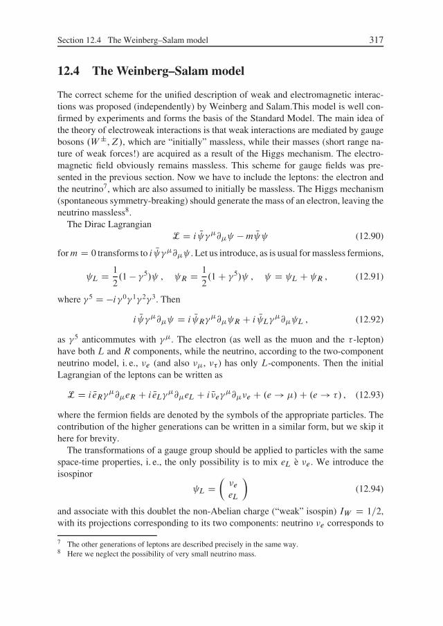
Section 12.4 The Weinberg–Salam model 317
12.4 The Weinberg–Salam model
The correct scheme for the unified description of weak and electromagnetic interac-tions was proposed (independently) by Weinberg and Salam.This model is well con-firmed by experiments and forms the basis of the Standard Model. The main idea ofthe theory of electroweak interactions is that weak interactions are mediated by gaugebosons .W ˙,Z/, which are “initially” massless, while their masses (short range na-ture of weak forces!) are acquired as a result of the Higgs mechanism. The electro-magnetic field obviously remains massless. This scheme for gauge fields was pre-sented in the previous section. Now we have to include the leptons: the electron andthe neutrino7, which are also assumed to initially be massless. The Higgs mechanism(spontaneous symmetry-breaking) should generate the mass of an electron, leaving theneutrino massless8.
The Dirac LagrangianL D i N ��@� �m N (12.90)
form D 0 transforms to i N ��@� . Let us introduce, as is usual for massless fermions,
L D 1
2.1 � �5/ , R D 1
2.1 C �5/ , D L C R , (12.91)
where �5 D �i�0�1�2�3. Then
i N ��@� D i N R��@� R C i N L��@� L , (12.92)
as �5 anticommutes with ��. The electron (as well as the muon and the � -lepton)have both L and R components, while the neutrino, according to the two-componentneutrino model, i. e., �e (and also ��, �� ) has only L-components. Then the initialLagrangian of the leptons can be written as
L D i NeR��@�eR C i NeL��@�eL C i N�e��@��e C .e ! �/C .e ! �/ , (12.93)
where the fermion fields are denoted by the symbols of the appropriate particles. Thecontribution of the higher generations can be written in a similar form, but we skip ithere for brevity.
The transformations of a gauge group should be applied to particles with the samespace-time properties, i. e., the only possibility is to mix eL è �e. We introduce theisospinor
L D��eeL
�(12.94)
and associate with this doublet the non-Abelian charge (“weak” isospin) IW D 1=2,with its projections corresponding to its two components: neutrino �e corresponds to
7 The other generations of leptons are described precisely in the same way.8 Here we neglect the possibility of very small neutrino mass.

318 Chapter 12 The Weinberg–Salam model
I 3W D C1=2, while “electron” eL to I 3
W D �1=2. The remaining
R D eR , (12.95)
is considered to be an isosinglet: IW D 0. Then we can write the Lagrangian as
L D i N R��@� R C i N L��@� L , (12.96)
which is invariant with respect to the SU.2/ group of isospin transformations:
L ! e� i2 E� E L , R ! R (12.97)
or, in more detail, 0
@�eeLeR
1
A ! e�i E�
2 E 00 1
!0
@�eeLeR
1
A . (12.98)
The electric chargeQ and the third component of the weak isospin I 3W for the left and
right fields are connected by the obvious relations
L : Q D I 3W � 1
2; R : Q D I 3
W � 1 . (12.99)
If we make this symmetry a local gauge symmetry, i. e., put E D E.x/, this will lead tothe appearance of three massless Yang–Mills fields. However, the photon will not bethere, as the right electron eR, being an isosinglet, will not interact with these fields,while it is obviously interacting with the usual photons. To solve this problem we canuse the fact that SU.2/ is not the maximal possible symmetry of our Lagrangian. Wecan additionally transform eR by simple U.1/:
eR ! eiˇeR . (12.100)
But this can be only the common transformation for all the fields of our model. Then�e and eL should also acquire the common phase factor, but its phase is not necessarilythe same as for R. Thus, we can write
0
@�eeLeR
1
A !0
@einˇ 0 0
0 einˇ 00 0 eiˇ
1
A
0
@�eeLeR
1
A . (12.101)
where n is some number to be determined later. This U.1/-symmetry leads to theexistence of some conserving charge, with eR having one value of this charge, whileboth �e and eL have another value. This is obviously not the electric charge Q, as �eand eL in reality have different values ofQ. The gauge field corresponding to thisU.1/symmetry is not the usual electromagnetic field. Weinberg proposed to consider this

Section 12.4 The Weinberg–Salam model 319
symmetry as the conservation of the “weak hypercharge” YW , defined by the relation9
Q D I 3W C YW
2. (12.102)
Comparing this expression with (12.99), we see that for the left and right leptons it isnecessary to introduce
L : YW D �1 ; R : YW D �2 . (12.103)
Thus, in equation (12.101) we have to put n D 1=2, so that the coupling constantfor interaction of the hypercharge gauge field for left fields is twice as small as thecorresponding constant for right fields. As a result, the U.1/ group transformation isfinally written as
0
@�eeLeR
1
A !0
@eiˇ=2 0 0
0 eiˇ=2 00 0 eiˇ
1
A
0
@�eeLeR
1
A . (12.104)
Thus, the Lagrangian (12.93), (12.96) is invariant to the direct product of groupsSU.2/ ˝ U.1/. The Yang–Mills theory with such a symmetry was already exam-ined in the previous section. We have introduced four gauge fields: isotriplet EA� andisosinglet B�, for all of them YW D 0.
Lepton fields L and R interact with fields EA�,B�, and the Higgs field �. First ofall, let us consider this last interaction. The corresponding term in Lagrangian is writtenin a form similar to equation (12.12), which was already discussed in connection withthe mass generation mechanism for fermions:
LM D �p2a. N L R� C N R L��/ , (12.105)
where a is the dimensionless coupling constant of this (renormalizable!) interaction.We write the Higgs field as an isospinor:
� D�'C'0
�, �� D .'�,'0�/ , (12.106)
with components corresponding to projections of weak isospin I 3W D ˙1=2. From
(12.102) we find the corresponding quantum numbers
IW D 1=2 , YW D 1 . (12.107)
Both fields 'C and '0 are complex, so that we can write
� D�'C'0
�D
1p2.'3 C i'4/
1p2.'1 C i'2/
!
, (12.108)
where '1, : : : ,'4 are real fields.
9 This expression is written in analogy with the Gell-Mann–Nishijima formula for the hypercharge ofhadrons [40]

320 Chapter 12 The Weinberg–Salam model
The covariant derivative describing the interaction of the Higgs field with the gaugefields has the form
D�� D .@� � i
2gE� � EA� � i
2fB�/� . (12.109)
Finally, the part of the Lagrangian containing field � is equal to
L� D .D��/�.D��/��2�����.���/4 �p2a. N L R�C N R L��/ . (12.110)
The part of the Lagrangian corresponding to Higgs field interaction with the leptonsis written in more detail as
�p2a. N�eeR'C C NeLeR'0 C NeR�e'� C NeReL'0/ . (12.111)
Further, we have
��� D .'C/�'C C .'0/�'0 D 1
2.'2
1 C '22 C '2
3 C '24/ . (12.112)
For �2 < 0 the Higgs field Bose condenses and the minimum energy corresponds to
h0j.'�'/j0i D �2 D ��2
�. (12.113)
Let us choose a vacuum to satisfy
h0j'1j0i D � , h0j'2j0i D h0j'3j0i D h0j'4j0i D 0 , (12.114)
i. e.,
h0j�j0i D 1p2
�0�
�. (12.115)
Then, the lowest-order (over excitations) interaction is written as
LM D p2a. N L R C N R L/� D a. NeLeR C NeReL/� D a� N , (12.116)
so that the Higgs condensate � interacts only with electrons. Thus, we achieved whatwas desired: the electron acquired the mass
me D a� , (12.117)
while the neutrino remained massless!Consider now lepton interactions with gauge fields, which is described by the co-
variant derivatives
D� D�@� � ig ET � EA� � if Y
2B�
� , (12.118)
where Y is the weak hypercharge of field , and g and f are the corresponding cou-pling constants. For L we have ET D 1
2 E� , Y D �1, while for R we have ET D 0 and

Section 12.4 The Weinberg–Salam model 321
Y D �2. Then the part of the Lagrangian corresponding to the interaction betweenthe leptons and the gauge fields has the form
L D i N L���@� � ig E�
2� EA� C i
f
2B�
� L C i N R��.@� C ifB�/ R . (12.119)
The gauge fields entering these expressions, as we seen in (12.81), (12.82), (12.83),can be divided into three types: a field of charged heavy nosons W�, a field of neutralheavy bosons Z�, and an electromagnetic field A�. Let us separately write the partsof Lagrangian LW , LZ , LA, corresponding to the interaction with these fields. Firstwe write
LW D g
2N L��.�1A1� C �2A2�/ L D gp
2��. N�eW�eL C NeLW �
� �e/ . (12.120)
This is the Lagrangian of the weak interaction of the leptons due to the exchange byW ˙-bosons (the so-called charged currents). There are also interactions with fieldsA�3 and B�, from (12.119); these are written as
1
2N L��.g�3A�3 � fB�/ L � f N R��B� R (12.121)
or, using (12.82), (12.83),
Qg2��Œ N�e.cos˛A�3 � sin˛B�/�e � NeL.cos˛A�3 C sin˛B�/eL � 2 sin˛ NeRB�eR� ,
(12.122)so that, expressing A�3 and B� via Z� and A� according to (12.82), we get
LZ D Qg2��. N�eZ��e � cos 2˛ NeLZ�eL C 2 sin2 ˛ NeRZ�eR/, (12.123)
the weak interaction due to the exchange by neutral Z-bosons (the so-called neutralcurrents), and
LA D �g sin˛��. NeLA�eL C NeRA�eR/, (12.124)
the usual electromagnetic interaction. Note that (12.124) once more confirms the rela-tion for the electric charge (12.89). Thus, the model under discussion gives a unifieddescription of weak and electromagnetic interactions, where the fields correspondingto W ˙- and Z-bosons as well as to the electromagnetic field appear from the funda-mental requirement of invariance with respect to the local gauge transformations ofSU.2/˝ U.1/.
During the first years since the construction of Weinberg–Salam model, weak in-teraction processes due to neutral currents (12.123) were not known, which was con-sidered to be a shortcoming of the model. The experimental discovery of such pro-cesses in 1973 in CERN was actually the first serious confirmation of the theory ofelectroweak interactions. One of the simplest processes due to weak interactions ismuon � decay, described by the diagram shown in Figure 12.3. If the mass of the

322 Chapter 12 The Weinberg–Salam model
Figure 12.3
W -boson is a significantly larger muon mass, its propagator is simply proportional to1m2
W
, and the appropriate transition amplitude is equivalent to the amplitude derivedfrom the phenomenological (nonrenormalizable) 4-fermion interaction introduced byFermi (10.96), (10.270):
g2
2m2W
. NeL�˛�e/. N���˛�/ . (12.125)
Comparing with (10.270), we obtain the following expression for Fermi coupling:
Gp2
D g2
8m2W
. (12.126)
The value of G is well known experimentally (10.273). We see, that its smallness(“weakness” of the weak interactions) is actually due to the large mass of the interme-diate boson in the denominator of (12.125), while the fundamental coupling constantis actually g � e ! Using (12.89)) and the experimental values of e and G, we can,with the help of (12.85) and (12.126), find the following estimates for the masses ofintermediate gauge bosons:
mW D e
25=4G1=2 sin˛D 37 GeV
sin˛, mZ D mW
cos˛D 74 GeV
sin 2˛, (12.127)
so that mW > 37 GeV and mZ > 74 GeV. Using (12.85) and (12.127) we can write
� D mW
gD 37 GeV
eD 122 GeV . (12.128)
Then from (12.117) we have
a D me
�� 5 � 10�6 , (12.129)
so that the coupling constant of leptons with the Higgs field is very small.

Section 12.4 The Weinberg–Salam model 323
Experimental studies of the weak interactions due to neutral currents has alreadyled in the early 1980s to the following estimate of “angle” ˛:
sin˛ � 0.47 . (12.130)
Then from (12.127) we have
mW � 78.6 GeV , mZ � 89.3 GeV . (12.131)
The triumph of the theory was the experimental discovery in 1983 of W ˙- and Z-bosons in CERN with masses mW � 80 GeV, mZ � 92 GeV. Since then the theoryhas been confirmed in numerous experiments, and at present it is the commonly ac-cepted scheme for describing electroweak interactions. The constants of the theory areknown with high accuracy. The present-day experimental situation is well describedin [67].
For many years the main unsolved problem was the absence of any direct experi-mental observation of Higgs bosons. One of the difficulties was due to the inability tomake definite predictions for Higgs boson mass within the Weinberg–Salam model;only a rather wide interval of possible values were theoretically predicted. However, aswe already mentioned in Chapter 1, in July 2012 it was announced that a particle withthe properties expected for the Higgs boson was discovered in a number of LHC ex-periments, with mass around 125–126 GeV. If finally confirmed by further studies, thiswill definitely be the final triumph of the theory. The brief discussion of the present-day situation with the experimental discovery of the Higgs oson can be found in [55].
The Standard Model
The “Standard Model” of elementary particles is the combination of the electroweaktheory due to Weinberg and Salam with quantum chromodynamics (QCD), which wediscussed above babove. The full gauge symmetry is given by the direct product ofcolor symmetry and the symmetries of weak isospin and weak hypercharge: SU.3/˝SU.2/˝U.1/. If we limit ourselves to the most important first generation of fermions,the fermion sector of the model is defined by
L D��ee
�
L
, eR, QL D�u˛d˛
�
L
, uR˛ , dR˛ , (12.132)
where u and d denote the corresponding quarks (˛ is the color index). The covariantderivative which determine the fermion interactions with Yang–Mills fields has theform
D� D @� � ig1Y
2B� � ig2
� i
2W i� � ig3
�a
2Ga� , (12.133)
where �a are the generators of the color group SU.3/ (cf. Chapter 2) and Ga� are thevector fields of gluons. The Higgs sector of the theory was described above. Gluons

324 Chapter 12 The Weinberg–Salam model
remain massless, but they are not observed as free particles, due to the phenomenon of“confinement”, which we shall discuss later. This theory is sufficient, in principle, todescribe the entire world (or universe) surrounding us. At present all the predictions ofthis theory are rather satisfactorily confirmed by existing experiments10. The attemptsof the real unification of all known interactions within some single gauge group, whichincludes symmetries SU.3/ ˝ SU.2/ ˝ U.1/ of the Standard Model as a subgroup,are usually called “great unification theories” (GUT). We shall briefly discuss suchattempts in the next chapter.
Phase transitions in quantum field theory at finite temperatures
Finally, let us briefly discuss one very interesting direction of research in modern quan-tum field theory. We have seen that the basis of the unified theory of electroweak inter-actions is the phenomenon of spontaneous symmetry-breaking and the Higgs mecha-nism. We already noted that this is a typical phase transition, like that taking place e. g.,in superconductors. From the theory of condensed matter we know that any symmetry-breaking disappears at high enough temperature T > Tc , when the system goes to asymmetric phase. The same phenomenon takes place in the models of quantum fieldtheory introduced above. This was clearly demonstrated for the first time by Kirzhnitzand Linde [41]. An appropriate theoretical analysis can be performed using the stan-dard (Matsubara) formulation of quantum field theory at finite temperatures, which iswidely used in statistical physics [1]. We have no room for a detailed discussion ofthese interesting problems here and therefore limit ourselves only to formulating someof the main conclusions.
The vacuum average of the Higgs field, which plays the role of the order parameter,becomes zero for T > Tc , where
Tc �r
3j�2j�
� �.0/ � 102 � 103 GeV . (12.134)
For T < Tc the order parameter behaves in the more or less usual way:
�2.T / D j�2j�
�ˆ.T / , (12.135)
where ˆ.T / is some increasing function of temperature. As a result, we obtain theorder parameter dependence shown in Figure 12.4(a). But we have seen above thatmasses appearing due to spontaneous symmetry-breaking are proportional to the vac-uum average � at T D 0. Correspondingly, as temperature increases the masses ofthe gauge bosons, leptons, and other particles diminish, and at T D Tc become zero,as shown in Figure 12.4(b). Already at this elementary level of discussion it becomes
10 A rief review of experimental situation with the Standard Model can be found in the review paper [22],while the importance of this theory for “common day” life is well-described in [12].

Section 12.4 The Weinberg–Salam model 325
(a) (b)
Figure 12.4
clear that the disappearance of the masses of the elementary particles creates stronglong range forces which may play a decisive role in cosmology, because in the firstmoments after the “Big Bang” the temperature of the universe was extremely high.These conclusions were followed by explosive developments of new approaches incosmology [16, 41]. Similar effects may be important for experiments with very highenergy collisions of heavy nuclei when very high temperatures can also be generated.
At present, the analysis the effects of temperature in quantum field theory is an im-portant part of elementary particles theory, which again stresses the unity of quantumfield theory and modern statistical physics.

Chapter 13
Renormalization
13.1 Divergences in '4
The concept of renormalizability plays an absolutely fundamental role in modern quan-tum field theory. Only renormalizable theories are considered to be physical. In Chap-ter 8 we briefly discussed the renormalizability of QED. Now we will return to a moredetailed discussion of the general situation for different field theory models.
Below we shall mainly consider the simplest scalar field g'4 theory, which was al-ready discussed above in Chapter 10. There we already met with typical divergenceslike in equation (10.125). Now we shall present a more serious analysis of divergences.Using the rules of diagram technique we can once again write the first order (� g) cor-rection to self-energy, corresponding to the diagram in Figure 13.1. The correspondinganalytic expression is
1
i† D �ig1
2
Zd 4q
.2�/41
q2 �m2, (13.1)
where we have taken into account the symmetry factor 1=2. Here in the integrand wehave the fourth power of q, while in the denominator we have q squared, so that ourintegral diverges quadratically at large q (i. e., at the upper limit, “ultraviolet diver-gence”).
Another typical divergence arises in the order � g2 from the diagram shown inFigure 13.2, where p1 C p2 D q and p1 C p2 C p3 C p4 D 0. The correspondinganalytic expression is
�g2Z
d 4p
.2�/41
p2 �m2
1
.p � q/2 �m2. (13.2)
Figure 13.1 Figure 13.2

Section 13.1 Divergences in '4 327
Here we have the fourth power of p both in the numerator and denominator of theintegrand, which leads to logarithmic divergence1.
Let us show how we can determine the divergence power of an arbitrary diagram.A similar analysis was already performed for QED in Chapter 8. But here we shallpresent more of the details. It is obvious that in an arbitrary diagram each propagatorcontributes � p2 (for large p we can neglectm!) in the denominator of the integrand,while each vertex contributes � p4 in the numerator, as well as the ı-function, ex-pressing momentum conservation in this vertex. The number of independent integra-tion momenta is equal to the number of closed loops in the diagram. For the diagrams,shown above, this number is 1 (one-loop diagrams). Consider a diagram of the orderof � gn, i. e., with n vertices. Suppose it has E external lines, I internal lines, andL loops. For generality we consider space-time with dimensionality d ; in this casethe vertices contribute pd to the numerator. Let us define the conditional degree ofdivergence D of the given diagram as
D D dL � 2I . (13.3)
For the diagrams shown above we have D D 2 and D D 0. Now we can expressD via E and n, excluding I and L. In fact, we have in total I internal momenta. Ineach of the n vertices we have momentum conservation, and we also have the totalmomentum conservation law for the scattering process described by our diagram (ex-ternal momenta are fixed). As a result, there are in total n � 1 relations between theintegration momenta. Thus, there are only I�nC1 independent integration momenta.But this number is equal to L:
L D I � nC 1 . (13.4)
In '4-theory each vertex is entered by four lines, so that we have in total 4n lines inthe diagram, but part of the lines are internal and another part external. During thesecalculations the internal lines are counted twice, as each of them connects two vertices.Then we have
4n D E C 2I . (13.5)
From (13.3), (13.4), (13.5) we immediately get
D D d ��d
2� 1
�E C n.d � 4/ . (13.6)
In particular, for d D 4 we have
D D 4 �E , (13.7)
1 In fact, we have already considered such diagrams during our discussion of the theory of critical phe-nomena in four-dimensional space, where the problem of divergence was solved by the introductionof a natural cutoff ƒ, of the order of the inverse lattice constant.
328 Chapter 13 Renormalization
which, by the way, gives the correct answers for the simplest diagrams discussedabove. From (13.7) we can see that the degree of divergence diminishes with thegrowth of the number of external lines (and depends only on this number!)2.
Let us return to the discussion of the general formula (13.6) and consider the lastterm in this expression. If the coefficient before n is positive, the situation is hopeless:the degree of divergenceD grows with the growth of n, so that the full theory (summedover all n) will contain an infinite number of terms containing divergences (in eachorder of perturbation theory) with a higher degree of divergence (than in the previousorder). This is equivalent to the nonrenormalizability of the theory. In '4-theory at d D4, the degree of divergence depends only on E and does not depend on the order ofperturbation theory, so that we have the finite number of the types of divergences, so wecan hope that the corresponding infinite contributions can be hidden in a finite numberof (infinite) renormalizations of the appropriate physical characteristics (renormalizedtheory). A finite number of the types of divergences is the necessary condition forrenormalizability.
It is useful to analyze similar formulas for the theory with the general interaction'r . Equations (13.3) and (13.4) do not change, while equation (13.5) transforms into
rn D E C 2I , (13.8)
so that equation (13.6) is rewritten as
D D d ��d
2� 1
�E C n
hr2.d � 2/ � d
i. (13.9)
Now for d D 4 we haveD D 4 �E C n.r � 4/ . (13.10)
For '6-theory we have D D 4 � E C 2n, and it is nonrenormalizable. On the otherhand, for '3-theory we haveD D 4 �E�n, and the degree of divergence diminisheswith the increase of n, so that for fixed E there is only the finite number of divergentdiagrams, and we are dealing with the so-called super-renormalizable theory3. Notethat for d D 2 we have D D 2 � 2n and independent of r .
Let us return to equation (13.7) and discuss the convergence or divergence of dia-grams with E > 4. In '4-theory the number E is always even. Consider the examplesof diagrams shown in Figure 13.3. Here E D 6, so that according to criterion (13.7)all of these diagrams seem to be convergent. This is correct for the diagram in Fig-ure 13.3(a), but obviously wrong for diagrams (b) and (c), which contain “hidden”divergences from loops (considered above). It is because of such cases that we calledD the conditional degree of divergence. It is important, however, that the inverse state-
2 It may seem that all diagrams with the number of external lines greater than 4 are convergent. Forexample, for E D 6 we have D D �2. However, this is a wrong conclusion, as we shall see below.
3 However, this theory is actually bad: there is a stable ground state!

Section 13.1 Divergences in '4 329
(a) (b) (c)
Figure 13.3
ment is always correct: the Feynman diagram converges if its degree of divergenceDand the degrees of divergence of all its subdiagrams are negative (Weinberg theorem).
Two divergent diagrams shown above in Figures 13.1 and 13.2, are called primi-tively divergent. These are the only primitively divergent diagrams of '4-theory (typesof divergences).
Dimensional analysis
Let us perform dimensional analysis in d -dimensional space. The action S D RddxL
is dimensionless. Then we easily find
ŒL� D L�d , ŒL� D ƒd , (13.11)
where L is some length, and ƒ is the corresponding momentum. From the term� @�'@
�' in L, taking into account Œ@�� D L�1, we have
Œ'� D L1� d2 D ƒ
d2 �1 . (13.12)
Consider the interaction g'r . If we define the dimensionality of the coupling constant
as Œg� D L�ı D ƒı , we obviously get �ı C r
1 � d2
�D �d , so that
ı D d C r � rd
2. (13.13)
Thus, the dimensionality of the coupling constants in different theories is
g'4 : ı D 4 � d , Œg� D ƒ4�d , ı � 0 for d � 4 ,
g'3 : ı D 3 � d2 , Œg� D ƒ3� d
2 , ı � 0 for d � 6 ,
g'6 : ı D 6 � 2d , Œg� D ƒ6�2d , ı � 0 for d � 3 .
(13.14)
Excluding the r-form equations (13.9) and (13.13), we obtain
D D d ��d
2� 1
�E � nı . (13.15)

330 Chapter 13 Renormalization
In particular, for d D 4 we have D D 4 � E � nı. Now it is clear that the necessarycondition for the renormalizability of the theory is ı � 0. Previously, for simplicity wehave spoken of the dimensionless coupling constants .ı D 0/ as the necessary condi-tion for renormalizability. From (13.14) we can see when this condition is fulfilled forthe simplest models of interaction. These results show that the dependence on spatialdimensionality is also very important.
In conclusion, we present the table of “canonical” dimensions for different Green’sfunctions and vertices [56]:
Field function Dimensionality in units of ƒ Dimensionality at d D 4
' d2 � 1 1
G.n/.x1, : : : , xn/ nd2 � 1
�n
G.n/.p1, : : : ,pn/ �nd C nd2 � 1
�D �n
d2 C 1
��3n
NG.n/.p1, : : : ,pn�1/ d � nd2 C 1
�4 � 3n
�.2/.x � y/ 2 C d 6
�.n/.x1, : : : xn/ nd2 C 1
�3n
�.n/.p1, : : : ,pn/ �dnC nd2 C 1
�D n
1 � d
2
��n
N�.n/.p1, : : : ,pn�1/ d C n
1 � d2
�4 � n
In addition to the Green’s functions and vertices already known to us, we introducedhere NG.n/ and N�.n/, defined as
G.n/.p1, : : : ,pn/ D NG.n/.p1, : : : ,pn�1/ı.p1 C � � � C pn/ ,
�.n/.p1, : : : ,pn/ D N�.n/.p1, : : : ,pn�1/ı.p1 C � � � C pn/ , (13.16)
where the ı-function of the total momentum conservation is explicitly shown (in unitsof ƒ it has dimensionality �d ).
13.2 Dimensional regularization of '4-theory
To analyze divergences of Feynman diagrams, first of all we have to formulate welldefined rules to separate the divergent parts of integrals. This is achieved by one oranother method of regularization of Feynman integrals. Above (e. g., during our dis-cussion of divergences in QED in Chapter 8) we used the simplest regularization pro-cedure, introducing the upper integration limit cutoffƒ. This method explicitly breaksrelativistic invariance, as it is equivalent to the introduction of some “minimal length”.
Section 13.2 Dimensional regularization of '4-theory 331
Now we shall discuss a more modern and elegant method of the so-called dimensionalregularization (t’Hooft and Veltman). The main idea of this method is somehow sim-ilar to the analysis of critical phenomena in the space with d D 4 � " dimensions(Wilson) and considers divergent integrals in space-time with continuous d < 4, withfurther limiting procedure of d ! 4. We shall see that the singularities of single-loopdiagrams considered above are simple poles over the variable " D d � 4.
First we have to generalize the Lagrangian of 4-dimensional theory
L D 1
2@�'@
�' � m2
2'2 � g
4Š'4 (13.17)
to d dimensions. As field ' has dimensionality d2 � 1, while the dimensionality of the
Lagrangian L is d , the coupling constant g is dimensionless for d D 4; and to make itdimensionless in d dimensions we have to multiply it �4�d , where � is an arbitraryparameter of dimensionality of mass (or momentum)4 . Thus, in the following we shallconsider the theory with the Lagrangian
L D 1
2@�'@
�' � m2
2'2 � 1
4Šg�4�d'4 . (13.18)
Let us calculate the simplest self-energy correction shown by the diagram in Fig-ure 13.1. Similarly to (13.1) it is determined by the integral
1
2g�4�d
Zddp
.2�/d1
p2 �m2. (13.19)
This integral should be calculated at arbitrary d .
Integration in d-dimensions
We are working in d-dimensional “Minkowski space” with one time and d � 1 spatial dimen-sions .d � 4/. Consider an integral of the general form
Id .q/ DZddp
1
.p2 C 2pq �m2/˛, (13.20)
where p D .p0, r/. Let us introduce polar coordinates .p0, r ,', �1, �2, : : : , �d�3/, so that
ddp D dp0rd�2drd' sin �1d�1 sin2 �2d�2 � � � sind�3 �d�3d�d�3
D dp0rd�2drd'
d�3Y
kD1
sink �kd�k ,
.�1 < p0 < 1 , 0 < r < 1 , 0 < ' < 2� , 0 < �k < �/ . (13.21)
Then
Id .q/ D 2�Z 1
�1dp0
Z C1
0dr rd�2
Z
0
Qd�3kD1 sink �kd�k
.p20 � r2 C 2p0q0 � 2r jqj cos �
d�3 �m2/˛.
(13.22)
4 The arbitrariness of parameter� is obvious, because at the end we have to perform the limit of d ! 4

332 Chapter 13 Renormalization
Direct calculations [56] give
Id .q/ D i�d=2�˛ � d
2
�
�.˛/
1
Œ�q2 �m2�˛�d=2. (13.23)
Using (13.23) we obtain for (13.19)
� ig
32�2m2�
�4��2
m2
�2� d2
�
�1 � d
2
�. (13.24)
The �-function has poles at zero and at negative integers. We see that the divergenceof (13.24) is reflected in the simple pole for d ! 4. It can be shown that
�.�nC "/ D .�1/n
nŠ
�1
"C 1.nC 1/CO."/
�, (13.25)
where 1.z/ D d ln�.z/=dz D � 0.z/=�.z/ is the logarithmic derivative of the �-function, for which 1.nC 1/ D 1 C 1
2 C � � � C 1n
� � , where � D � 1.1/ D 0.577is the Euler constant. Taking " D 4 � d we obtain
�
�1 � d
2
�D �
�1 C "
2
�D �2
"� 1 C � CO."/ . (13.26)
As a result, using a" D 1 C " ln aC � � � we obtain the following expansion of (13.24)near d D 4:
� igm2
32�2
h�2
"� 1 C � CO."/
i �1 C "
2ln
��4��2
m2
��
D igm2
16�2"C igm2
32�2
�1 � � C ln
��4��2
m2
��CO."/
D igm2
16�2"C finite expression. (13.27)
The finite contribution here is of no special importance, but we note that it depends onthe arbitrary factor �. The important point is that we succeeded in a correct separationof the divergent part. For " > 0 this contribution is finite, and we can deal with it in anormal way.
Let us now calculate a 4-point function up to the terms of the order of � g2. Simi-larly to (13.2) we obtain the contribution of the diagram in Figure 13.2 as
�1
2g2.�2/4�d
Zddp
.2�/d1
p2 �m2
1
.p � q/2 �m2. (13.28)
Denominators in the integrand here can be joined with the help of Feynman’s formula
1
abDZ 1
0
dz
Œaz C b.1 � z/�2 . (13.29)

Section 13.2 Dimensional regularization of '4-theory 333
This formula is derived from
1
abD 1
b � a1
a� 1
b
�D 1
b � aZ b
a
dx
x2, (13.30)
taking x D az C b.1 � z/, with a and b complex, to exclude singularity at a D b.Now we have
1
p2 �m2
1
.p � q/2 �m2DZ 1
0
dz
Œp2 �m2 � 2pq.1 � z/C q2.1 � z/�2 . (13.31)
Changing variables to p0 D p�q.1�z/, we see that the denominator of the integrandis the square of p02 �m2 Cq2z.1�z/. We have ddp0 D ddp, so that after the changeof notations p0 ! p, (13.28) takes the form
�1
2g2.�2/4�d
Z 1
0dz
Zddp
.2�/d1
Œp2 �m2 C q2z.1 � z/�2 . (13.32)
Using (13.23) we now have
ig2
2.�2/4�d 1
4�
�d=2 �.2 � d=2/
�.2/
Z 1
0dzŒq2z.1 � z/ �m2�d=2�2 D
ig2
32�2.�2/2�d=2�
�2 � d
2
�Z 1
0dz
�q2z.1 � z/ �m2
4��2
�d2 �2
. (13.33)
In the limit of d ! 4, from (13.25) we get
�
�2 � d
2
�D 2
"� � CO."/ , (13.34)
so that after writing a" � 1 C " ln a (13.33) take the form
ig2�"
32�2
�2
"� � CO."/
�²1 � "
2
Z 1
0dz ln
�q2z.1 � z/ �m2
4��2
�³D
ig2�"
16�2"� ig2�"
32�2
²� C
Z 1
0ln
�q2z.1 � z/ �m2
4��2
�³. (13.35)
In this expression, the main (diverging) term depends on �, while the finite part de-pends on the square of .p1 C p2/
2 D q2 D s (Mandelstam variable). Let us define tafunction
F.s,m,�/ DZ 1
0dz ln
�sz.1 � z/ �m2
4��2
�. (13.36)
Then the final expression for the contribution of the diagram of Figure 13.2 is written as
� ig2�"
16�2"C ig2�"
32�2Œ� C F.s,m,�/� D � ig
2�"
16�2"C finite expression . (13.37)
Thus, we have explicitly written the lowest order corrections to 2-point and 4-pointfunctions in '4-theory. Let us now write the corresponding irreducible vertices�.2/.p/

334 Chapter 13 Renormalization
Figure 13.4
and �.4/.pi /. Equation (13.27) according to (13.1) reduces to 1i†, so that in the first
order over g we have
†.p/ D � gm2
16�2"C finite expression. (13.38)
Accordingly, from the definition �.2/.p/ D G�1.p/G.p/G�1.p/ D p2 �m2 �†.p/we have
�.2/.p/ D G�1.p/ D p2 �m2
1 � g
16�2"
�. (13.39)
Obviously, for " ! 4 this expression diverges.Further on, the 4-point vertex �.4/.p1, : : : ,p4/ in momentum representation is writ-
ten as
�.4/.p1,p2,p3,p4/ D G�1.p1/G�1.p2/G
.4/.p1,p2,p3,p4/G�1.p3/G
�1.p4/
(13.40)
and is expressed by the sum of the diagrams shown in Figure 13.4, taking into accountcontributions of all the cross-channels, which are obtained from (13.37) and anothertwo similar terms obtained from (13.37), changing the Mandelstam variable s to t andu (cf. Chapter 5):
s D .p1 C p2/2 , t D .p1 C p3/
2 , u D .p1 C p4/2 . (13.41)
The action of G�1.pi / in (13.40) reduces to the “amputation” of the external lines.Finally we obtain
�.4/.pi / D �ig�" � 3ig2�"
16�2"C ig2�"
32�2Œ3�CF.s,m,�/CF.t ,m,�/CF.u,m,�/�
D �ig�"
1 C 3g
16�2"
�C finite expression. (13.42)
The main contribution here is also infinite for " ! 0. To make vertices �.2/ and �.4/
physically sensible, we should make them finite! This is done by renormalization!
Loop expansion
Note that above we analyzed diagrams with the same number of loops equal to 1 (single-loopapproximation). Actually, we can present arguments showing that loop-expansion is, in somesense, even more interesting than the usual perturbation expansion in powers of g. Expansion

Section 13.3 Renormalization of '4-theory 335
in the number of loops L is equivalent to expansion in the powers of the Planck constant „. Infact, restoring „ in all expressions, we can write the generating functional as
ZŒJ.x/� DZ
D' exp
²i
„ZdxŒL.x/C „J.x/'.x/�
³. (13.43)
Introducing L D L0 C Lint , we can write
ZŒJ � D exp
²i
„Lint
�1
i
ı
ıJ
�³Z0ŒJ � , (13.44)
where
Z0ŒJ � D N exp
��1
2i„Zdx
ZdyJ.x/F .x � y/J.y/
�. (13.45)
From (13.44) it follows that every vertex introduces the factor of „�1 into an arbitrary diagramof the n-th order of the usual perturbation theory, while from (13.45) it follows that eachpropagator contributes the factor of „. Thus, the given diagram contains the factor of „I�n D„L�1 (where we have used the previously derived relation (13.4): L D I � n C 1, where Iis the number of internal lines of this diagram). Then we conclude that the expansion over thenumber of loops is actually an expansion in the powers of „, i. e., the expansion “around” theclassical theory.
13.3 Renormalization of '4-theory
Our aim now is to make all physical quantities finite! In a single-loop approximationwe can easily explicitly make renormalization. After the regularization, all the quanti-ties we are dealing with are finite, and we can act in a direct way. From the definitionof the physical mass of the particle it is clear that the inverse propagator must be ofthe form
G�1.p/ D �.2/.p/ D p2 �m21 or m2
1 D ��.2/.0/ D �G�1.0/ , (13.46)
where the physical mass m1 is finite. The initial (“bare”) mass m entering the La-grangian does not have any direct physical meaning and can even be infinite in thelimit of d ! 4. This is a mass which characterizes a particle in the absence of inter-actions, which is unobservable; only m1 is physically sensible, and it should be finite.From (13.39) and definition (13.46) we have
m21 D m2
1 � g
16�2"
�. (13.47)
In the second term in the right-hand side we may, with the same accuracy � g, replacem by m1, which gives
m21 D m2 � g
16�"m2
1 , (13.48)
so that we getm2 D m2
1
1 C g
16�2"
�. (13.49)

336 Chapter 13 Renormalization
This is the value of the “bare” mass guaranteeing the finite value m1 of the physicalmass in single-loop approximation. We see that for " ! 0 the value of m diverges,but m1 is finite!
We can similarly analyze the vertex part �.4/. We rewrite (13.42) as
i�.4/.pi / D g�" C g2�"
32�2
�6
"� 3� � F.s,m,�/ � F.t ,m,�/ � F.u,m,�/
�.
(13.50)
Let us define the renormalized (finite!) coupling constant g1 as
g1 D i�.4/.pi D 0/ , (13.51)
i. e., as the vertex part for particles with zero momenta. Then, from (13.50) we obtain
g1 D g�" C g2�"
32�2
�6
"� 3� � 3F.0,m,�/
�. (13.52)
Considering g1 to be fixed and finite, we immediately see that the “bare” couplingconstant g should be infinite (for " ! 0). In fact, rewriting equation (13.52) replacingg by g1�
�" and m by m1 everywhere (which always can be done with an accuracyup to terms �g2), we can obtain an expression for g, expressed via g1, similar toequation (13.49):
g D g1��" � 3g2
1��2"
32�2
�2
"� � � F.0,m1,�/
�. (13.53)
Then we can express �.4/ (13.50) via g1 as
i�.4/.pi / D g1 � g21�
�"32�2
ŒF .s,m1,�/CF.t ,m1,�/CF.u,m1,�/� 3F.0,m1,�/� .(13.54)
From here (13.51) follows directly, as for p1 D p2 D p3 D p4 D 0 we have s D t Du D 0. Thus, the physical (renormalized) coupling constant g1 coincides with i�.4/
with all external momenta equal to zero5. Now everything is finite! We completedrenormalization in a single-loop approximation.
Now, how does this look in two-loop approximation? In this case we have to con-sider the diagrams shown in Figure 13.5. Appropriate analysis shows that in this caseG�1.p/ D �.2/.p/ acquires an additional divergence due to the diagram of Fig-ure 13.5(b). This divergence is not cancelled by mass and coupling constant renor-malization. It is hidden into an additional multiplicative factor, which is introduced byredefining 2-point function as
G�1r D �.2/r D Z'.g1,m1,�/�.2/.p,m1/ . (13.55)
5 This is not the only way to define the renormalized coupling constant. Sometimes g1 is defined viai�.4/ at the so-called symmetric point p2
i D m2, pipj D �m2=3 .i ¤ j /, which corresponds tos D t D u D 4m2=3.

Section 13.3 Renormalization of '4-theory 337
(a) (b) (c) (d) (e)
Figure 13.5
Here �.2/r is finite, while the factor Z' is infinite. The factor of Z1=2' is called wave
function renormalization. For Z' it is possible to write an expansion in the number ofloops, which has the form
Z' D 1 C g1Z1 C g21Z2 C � � � D 1 C g2
1Z2 C � � � , (13.56)
because the single-loop contribution is absent. Wave function renormalization (renor-malization of the field amplitude) cannot be just arbitrary. To define it we need torequire that at some point, e. g., at p2 D 0, we have
@
@p2G�1r .p/
ˇˇp2D0
D @
@p2�.2/r
ˇˇp2D0
D 1 . (13.57)
The choice of p2 D 0 is more or less arbitrary.The divergence of Z' means that in a two-loop approximation the value of m1
defined above is actually infinite (in the limit of " ! 0). However, renormalizedG�1r .p/ D �
.2/r gives the finite value of renormalized mass mr :
m2r D Z'm
21 . (13.58)
In other words, divergences ofZ' andm21 cancel each other. The value of renormalized
coupling constant changes similarly. For �.4/r we have the relation similar to (13.55):
�.4/r D Z2'�
.4/.p,m1,�/ (13.59)
and the new renormalized coupling constant gr , defined by the relation similar to(13.46), has the form
i�.4/r .pi D 0/ D gr D Z2'g1 . (13.60)
The factor Z' is the function of g�", so that writing this dependence explicitly weobtain the renormalized n-particle vertex part as
�.n/r .pi ,gr ,mr ,�/ D Zn=2' .g�"/�.n/.pi ,g,m/ (13.61)
or�.n/.pi ,g,m/ D Z�n=2
' .g�"/�.n/r .pi ,gr ,mr ,�/ . (13.62)
Thus, in two-loop approximation we also can make our theory finite. Is it so in anyorder? This is the problem of the proof of renormalizability. This proof is tedious

338 Chapter 13 Renormalization
enough, but it can actually be done in all orders of perturbation theory (Dyson). Adetailed presentation of this proof for different models of quantum field theory can befound in [9]. Note, that the proof of renormalizability in '4-theory is actually moredifficult than the similar proof for QED, which is made more simple due to the gaugeinvariance.
Counter-terms
There is an alternative way to introduce renormalizability, which became popular afterthe publication of [9]. The point is that from the start we can consider parameters mand g in an initial Lagrangian as the physical mass and charge (coupling constant).The fact that this Lagrangian does not produce finite Green’s functions now leads tothe requirement that we introduce into the Lagrangian some additional terms whichcancel the divergences. These terms are called counter-terms. Renormalized theorycan be made finite by the introduction of the finite number of counter-terms. Let usbriefly describe how this is done.
Consider again mass renormalization in a single-loop approximation, which is de-fined by equations (13.46)–(13.49). This may be described as follows. A single-loopcorrection to a free propagator is shown in Figure 13.6 and diverges for " ! 0. Letus add to the initial Lagrangian L the term
ıL1 D � gm2
32�2"'2 �1
2ım2'2 . (13.63)
This may be considered as an additional interaction, which we shall denote by the“cross” on the diagrams:
� D � igm2
16�2"D �iım2 . (13.64)
Then, up to terms of the order of �g, the total inverse propagator is represented bydiagrams in Figure 13.7 and is equal to
�.2/.p/ D iG.p/�1
D i
�1
i.p2 �m2/ �
�igm2
16�2
1
"C finite part
�C igm2
16�2"
�
D p2 �m2 , (13.65)
where we have dropped the finite contribution (alternatively we can include it intom2).Here m2 is considered to be the finite physical mass, which in corresponding order of
Figure 13.6

Section 13.3 Renormalization of '4-theory 339
Figure 13.7
perturbation theory is equal to ��.2/.0/. The Lagrangian is now LC ıL1, where ıL1
is a diverging counter-term.
The meaning of the introduction of a mass term in the Lagrangian as an additional interactionis rather simple. Consider noninteracting theory:
L D 1
2.@�'/.@
�'/ � 1
2m2' (13.66)
and assume,that it describes massless field (first term in Lagrangian), with interaction deter-mined by the second terms. Corresponding Feynman rules are shown in Figure 13.8. The fullpropagator is determined now by the diagrams shown in Figure 13.9. Then, the perturbationseries reduces to the simple geometric progression
G.p/ D i
p2C i
p2.�im2/
i
p2C i
p2.�im2/
i
p2.�im2/
i
p2C � � � D i
p2 �m2, (13.67)
which gives the usual propagator of the massive field. This we actually used while consideringthe mass counter-term as perturbation.
In a similar way we can also deal with �.4/. From (13.42) it is seen, that �.4/,corresponding to diagrams � g2, shown in Figure 13.10, diverges for " ! 0. Thenwe can add to the Lagrangian the counter-term
ıL2 D 1
4Š
3g2�"
16�2"'4 D Bg�"
4Š'4 , (13.68)
corresponding to the additional interaction, shown in Figure 13.11. As a result �.4/, asshown in Figure 13.12, becomes finite. The divergence of �.2/ in a two-loop approxi-mation, qualitatively described above and leading to the necessity to multiply �.n/ by
Figure 13.8
Figure 13.9

340 Chapter 13 Renormalization
Figure 13.10
Figure 13.11
Figure 13.12
Zn=2' , is equivalent to the addition to the Lagrangian of the counter-term
ıL3 D A
2.@�'/
2 , (13.69)
where 1 C A D Z' .Thus, finite expressions for Green’s functions and vertices can be obtained by adding
to the Lagrangian
L D 1
2@�'@
�' � 1
2m2'2 � 1
4Šg�4�d'4 (13.70)
the counter-term LCT :
LCT D A
2@�'@
�' � 1
2ım2'2 � 1
4ŠBg�4�d'4 . (13.71)
The total Lagrangian, which is usually called the “bare” Lagrangian LB , is equal to
LB D L C LCT D 1 C A
2@�'@
�' � 1
2.m2 C ım2/'2 � 1
4Š.1 C B/g�4�d'4 .
(13.72)

Section 13.3 Renormalization of '4-theory 341
Thus, the addition of counter-terms is equivalent to the multiplication of ', m, andg by some renormalization factors Z (multiplicative renormalization). If we define“bare” quantities
'B D pZ''r , Z' D 1 C A ,
mB D Zmmr , Z2m D m2 C ım2
1 C A, (13.73)
gB D �"Zggr , Zg D 1 C B
.1 C A/2,
the “bare” Lagrangian (13.72) is written as
LB D 1
2@�'B@
�'B � 1
2m2B'
2B � 1
4ŠgB'
4B . (13.74)
Note that here there is no explicit dependence on �. The values of A, B , and ım2 areassumed to be chosen in such a way as to make Green’s functions finite (for " ! 0). Interms of the counter-terms approach, the theory is renormalizable if the counter-termsneeded to cancel the divergences in every order of perturbation theory have the sameform as the terms entering the initial Lagrangian. If this is so, the “bare” quantities canbe defined with (infinite!) renormalization factors, as was done above, and the “bare”Lagrangian has the same form as the initial Lagrangian.
Lagrangian LB leads to finite theory, in contrast to initial L. This means that, “hid-ing” all divergences into 'B , mB and gB , we can make theory finite: the divergencesare absorbed by renormalization. All “bare” quantities are divergent for " ! 0 6, whilerenormalized quantities are finite for " ! 0, but their values are more or less arbitraryand should be taken to be equal to the physical parameters of the theory.
Equation (13.62) is also obvious from the counter-terms approach. From equa-tions (13.73) and (13.74) it is clear that, taking (13.74) as the initial Lagrangian, wehave to replacem ! mB , g ! gB , ' ! 'B in all expressions for Green’s functions.But now we can (and need to!) express the “bare” parameters via physicalmr , gr , and'r according to expressions (13.73). Then we obtain
�.n/B .pi ,gB ,mB/ D Z�n=2
' �.n/r .pi ,gr ,mr ,�/ , (13.75)
which is equivalent to (13.62) (index B can now be dropped). The absence of explicitdependence of the left-hand side of this equation on � is obvious from the form of theLagrangian (13.74), where it is also absent.
6 For finite " there are no divergences at all!

342 Chapter 13 Renormalization
13.4 The renormalization group
In Chapter 8 we already discussed briefly the renormalization group in QED. Renor-malization groups plays the major role in quantum field theory [9,28,56] and statisticalphysics [3, 42], as well as in some other fields of theoretical physics. Below we shallpresent a more detailed discussion. There are several (more or less equivalent) for-mulations of this method. For example, in Chapter 8 the renormalization group wasrelated to transformations from one value of the cutoff parameter (for divergent in-tegrals) to another, in the theory of critical phenomena [42] Wilson’s formulation isquite popular, which is based on integrating out regions of momentum space, corre-sponding to large momenta, i. e., restricting the analysis of fluctuations to long enoughwavelengths etc. Here we shall use the most common (though probably more formal)approach used in quantum field theory literature, which is based on dimensional reg-ularization [56].
Within the framework of dimensional regularization we have introduced an arbi-trary parameter � with dimensionality of the mass. Dependence of renormalized irre-ducible vertices on� is determined, according to equation (13.61), by a corresponding�-dependence of renormalization factor Z' . In other words (cf. (13.62), (13.75)) thenonrenormalized (“bare”) function �.n/ does not depend on �:
�.n/.pi ,g,m/ D Z�n=2' .g�"/�.n/r .pi ,gr ,mr ,�/ (13.76)
and, in this sense, is invariant towards the group of transformations
� ! es� or � D es�0 i. e., s D ln�
�0. (13.77)
These transformations represent the renormalization group. Introducing the dimen-sionless differential operator � @
@�, we get
�@
@��.n/ D 0 (13.78)
or, taking into account (13.76),
�@
@�ŒZ�n=2' .g�"/�.n/r .pi ,gr ,mr ,�/� D 0 , (13.79)
where gr andmr depend on �. Making a differentiation and multiplying the result byZn=2' , we obtain��n� @
@�lnpZ' C �
@
@�C �
@gr
@�
@
@grC �
@mr
@�
@
@mr
��.n/r D 0 . (13.80)
In the following, for brevity we shall everywhere write g instead of gr and m insteadof mr , assuming that we are dealing only with renormalized quantities. In general,only renormalized quantities enter equation (13.80), which are finite for " ! 0.

Section 13.4 The renormalization group 343
Let us define the following functions:
m�m.g/ D �@m
@�,
�.g/ D �@
@�lnpZ' , (13.81)
ˇ.g/ D �@g
@�.
Then equation (13.80) takes the form��@
@�C ˇ.g/
@
@g� n�.g/Cm�m.g/
@
@m
��.n/ D 0 . (13.82)
This is the main differential equation of the renormalization group, usually called aCallan–Symanzik equation. It reflects invariance of the renormalized vertex �.n/ tochanges of the regularization parameter �7.
Let us write a similar equation, expressing the invariance of �.n/ to changes of themomentum scale (mass). Consider the replacement pi ! tpi ,m ! tm,� ! t�. Thevertex �.n/ has mass dimensionality D, determined according to the table presentedabove, by the following expression
D D d C n
�1 � d
2
�D 4 � nC "
n2
� 1�
, (13.83)
where d D 4 � ". Then we have
�.n/.tpi , tm, t�/ D tD�.n/.pi ,m,�/ , (13.84)
which, after the simple variable changes tm ! Qm, m ! Qm=t , Qm ! m, and t� !Q�, � ! Q�=t , Q� ! �, is rewritten as
�.n/.tpi ,m,�/ D tD�.n/.pi ,m=t ,�=t/ . (13.85)
Thus, �.n/ is actually the homogeneous function of its variables of the power D.
Homogeneous functions. The Euler theorem
Let us recall the basic facts about homogeneous functions. The function u D f .x1, x2, : : : , xm/is called a homogeneous function of power p, if for any t we have
u D f .tx1, : : : , txm/ D tpf .x1, : : : , xm/ . (13.86)
For homogeneous functions we have the Euler theorem
x1@u
@x1C � � � C xm
@u
@xmD pu . (13.87)
7 To avoid misunderstanding we note that here we are dealing with the vertex, defined in (13.16) anddenoted previously by N�.n/.

344 Chapter 13 Renormalization
To prove this, consider u D f .tx01 , : : : , tx0
m/, where .x01 , : : : , x0
m/ is an arbitrary point, fromthe region of the definition of our function. Then we have
du
dt
ˇˇˇtD1
D @u
@x1x0
1 C : : :C @u
@xmx0m . (13.88)
On the other hand,
du
dtD ptp�1f .x0
1 , : : : , x0m/ , so that
du
dt
ˇˇtD1
D pf .x01 , : : : , x0
m/ D pu . (13.89)
Comparison of (13.88) with (13.89) gives (13.87).
From (13.85), using the Euler theorem, we have�t@
@tCm
@
@mC �
@
@��D
��.n/.tpi ,g,m,�/ D 0 . (13.90)
Excluding �@�.n/
@�from (13.82) and (13.90), we obtain another form of the Callan–
Symanzik equation:��t @@t
C ˇ@
@g� n�.g/Cm.�m.g/ � 1/
@
@mCD
��.n/.tpi ,g,m,�/ D 0 ,
(13.91)
which directly expresses the result of the scale change of momenta in �.n/ by thefactor of t . Note that for ˇ.g/ D �.g/ D 0, �m.g/ D 1, this result reduces to thecanonical dimension D, which is determined by the “naïve” dimensional analysis.The necessity of renormalization and nontrivial values of ˇ.g/, �.g/, �m.g/ is directlyrelated to interactions which lead to anomalous dimensions.
Let us find the solution of equation (13.91). In fact, this equation reflects the factthat the change of t can be compensated by an appropriate change of m and g and ofthe common factor. Suppose the existence of functions g.t/,m.t/ and f .t/, such that
�.n/.tp,m,g,�/ D f .t/�.n/.p,m.t/,g.t/,�/ . (13.92)
Differentiating by t , we obtain
@
@t�.n/.tp,m,g,�/ D
df .t/
dt�.n/.p,m.t/,g.t/,�/C f .t/
@m
@t
@�.n/
@mC @g
@t
@�.n/
@g
!
, (13.93)

Section 13.4 The renormalization group 345
or, taking into account (13.92),
t@
@t�.n/.tp,m,g,�/
D�tdf .t/
dtC f .t/t
@m
@t
@
@mC f .t/t
@g
@t
@
@g
��.n/.p,m.t/,g.t/,�/
D�tdf .t/
dtC tf .t/
@m
@t
@
@mC tf .t/
@g
@t
@
@g
�1
f .t/�.n/.tp,m,g,�/ , (13.94)
which, after the regrouping, reduces to�
�t @@t
C t
f .t/
df .t/
dtC t
@m
@t
@
@mC t
@g
@t
@
@g
��.n/.tp,m,g,�/ D 0 . (13.95)
Compare now (13.91) with (13.95). Equating the coefficients at @=@g, we obtain theGell-Mann–Low equation
@tD ˇ.g/ . (13.96)
The function g.t/ is called the “running” coupling constant, and the ˇ.g/-function iscalled the Gell-Mann–Low function. This equation is of basic importance in the studyof asymptotic properties in quantum field theory. The knowledge of ˇ.g/ allows us tofind g.t/. Of major interest, as we shall see, is the asymptotics of g.t/ at t ! 1. Theinitial condition for equation (13.96) is g.1/ D g.
Comparison of the coefficients before @=@m in (13.91) and (13.95) gives
t@m
@tD mŒ�m.g/ � 1� , (13.97)
and comparison of the remaining terms gives
t
f .t/
df .t/
dtD D � n�.g/ . (13.98)
The last equation can be integrated to obtain
f .t/ D tD exp
��Z t
0dtn�.g.t//
t
�; (13.99)
substituting this into (13.92) and takingD D 4 �nC "�n2 � 1
, in the limit of " ! 0,
we get
�.n/.tp,m,g,�/ D t4�n exp
��n
Z t
0dt�.g.t//
t
��.n/.p,m.t/,g.t/,�/ . (13.100)
This is the solution of (13.91), expressed via the “running” coupling constant g.t/and the “running” mass m.t/. The exponential determines the anomalous dimension.Thus, the physics at high momenta is determined by functions g.t/ andm.t/. Relationslike (13.100) in some sense allow us to analyze the situation outside the region ofapplicability of perturbation theory.

346 Chapter 13 Renormalization
(a) (b)
Figure 13.13
In the limit of very large momenta we can neglect particle masses. Thus, we canusually limit our analysis to studies of the Gell-Mann–Low equation (13.96). Con-sider the possible qualitative behavior which may appear. We shall be interested inthe behavior of g.t/ for t ! 1. The Gell-Mann–Low equation is written as (13.96),and the possible variants of the qualitative behavior of the ˇ.g/-function are shownin Figure 13.13. We always have ˇ.g D 0/ D 0, which corresponds to free the-ory without interactions. Perturbation theory allows us to determine the behavior ofˇ.g/ close to g D 0; it is always (as we shall see below) quadratic in g. In principle,where zeroes of ˇ.g/ at finite g, may be, it is sufficient to consider only one, say atg D g0, to understand the consequences of its existence. Consider first ˇ.g/, shownin Figure 13.13(a). The zeroes of this function at g D 0 and g D g0 correspond to theso-called fixed points of the Gell-Mann–Low equation. It is easy to see that, for t ! 1and initial values of g close to g0, the value of g.t/, determined from (13.96), tends tog0. In fact, for initial g < g0 we have ˇ.g/ > 0, so that g grows with the growth of tand tends to g0 (where further growth is just stopped). Similarly, for initial g > g0 wehave ˇ.g/ < 0, and g diminishes with the growth of t , i. e., also tends to g0, moving ina negative direction. Thus g.1/ D g0, and we have an ultraviolet stable fixed point:the fixed value of the coupling constant (charge) at very large momenta. For smallinitial values of g in the limit of t ! 0 we always obtain g D 0, the infrared stablefixed point (“Moscow zero”). If the zeroes of the Gell-Mann–Low function at finiteg are absent, equation (13.96) leads to the continuous growth of g for t ! 1, and afixed value of charge does not appear. If for the large values of argument ˇ.g/ � g˛
and ˛ > 1, the theory becomes internally inconsistent: the inevitable divergence ofg appears at the finite value of t (the Landau “ghost pole”). For ˛ � 1 we obtain themonotonous growth of g for t ! 1; the theory is consistent, but for t ! 1 we havea crossover to “strong coupling”.
Consider now the ˇ.g/-function, shown in Figure 13.13(b). Again we have twofixed points, but the sign of ˇ.g/ is now opposite, so that g D g0 is not the infraredstable fixed point at .t ! 0/, while g D 0 is the ultraviolet stable fixed point at.t ! 1/. In the last case g ! 0 for t ! 1 and effective interaction diminishes with

Section 13.4 The renormalization group 347
the growth of energy (momentum) becoming zero in the limit. This is called asymptoticfreedom. With the absence of zero ofˇ.g/ at finite values of g now we have problems atsmall momenta; interaction grows and can produce unphysical divergence. In any case,here we obtain the transition to “strong coupling” at large distances (confinement?).
These possibilities in fact represent all the variants of asymptotic behavior in anyreasonable model of quantum field theory. As a concrete example we can consider theg'4 .g > 0/-theory. Let us take the result of the single-loop approximation (13.52)for the renormalized coupling constant. Dropping irrelevant finite corrections we canwrite
g1 D g�"
1 C 3g
16�2"
�. (13.101)
Then we have
�@g1
@�D "g�" C 3g2
16�2�" . (13.102)
For finite " everything is finite, and we can (with the same accuracy) rewrite (13.102)as
�@g1
@�D "g1 C 3g2
1
16�2��" , (13.103)
and then just drop the index 1, assuming that we are working with a renormalizedcoupling constant. Then from (13.103), for " ! 0, we obtain the Gell-Mann–Lowfunction as
ˇ.g/ D �@g
@�D 3g2
16�2. (13.104)
Introducing s D ln t D ln ��0
, so that � @@�
D @@s
D t @@t
, we can rewrite equa-tion (13.103) as
@g
@sD 3g2
16�2. (13.105)
Now, without any calculations we can see that “running” coupling constant of '4-theory grows with the growth of s, i. e., with the growth of momentum, so that thistheory is not asymptotically free. The Gell-Mann–Low function is �g2. The elemen-tary integration of equation (13.105) with initial condition g.s D 0/ D g0 gives
g D g0
1 � 3162g0s
D g0
1 � 3162g0 ln t
D g0
1 � 3162g0 ln �
�0
. (13.106)
With the growth of t (or �) the coupling constant grows, and finally we meet theunphysical singularity (“ghost pole”) at 1 D 3
162g0 ln. ��0/, which corresponds to� D
�0 exp.162
3g0/. The situation here is quite similar to that in QED, which we discussed
in Chapter 8. The same behavior was discussed in Chapter 10 in relation to criticalphenomena.
Of course, this behavior of the Gell-Mann–Low function is completely based ona single-loop approximation and is formally valid only for small enough values of

348 Chapter 13 Renormalization
the coupling constant g. The problem of the ˇ.g/ behavior for large values of g andthe related question of the consistency of g'4-theory remains open. Many researchersobtain forg ! 1 the asymptotic behavior ofˇ.g/, which is practically the same as theresult of a single-loop approximation, which is equivalent to the internal inconsistencyof the theory in accordance with the initial Landau claim, discussed above in Chapter 8.Alternative suggestions will be discussed in Chapter 14.
Note that g'4-theory is “easily” made asymptotically free if we assume g < 0. Then weobviously have to change the sign before the logarithm in the denominator of equation (13.106)and the effective coupling constant will drop with the growth of t and �. However, such atheory is unstable: there is no ground state (potential energy can be arbitrarily negative), andthis model is usually not considered in quantum field theory. However, the specific variantof such models, which is reduced to the generalized Landau functional (10.160), with thenumber of field components n D 0 (!), describes the motion of an electron in the randompotential field of impurities with point-like potential V , chaotically distributed in space withfixed average density �, if in (10.160) we put g D ��V 2 and � D �E, whereE is the electronenergy. This problem is basic for the theory of electrons in disordered systems and related tothe still unsolved problem of electron localization in such systems (Anderson localization – thebasic mechanism of metal-insulator transitions). These problems are deeply connected with thedescription of the infrared region of asymptotically free models in quantum field theory. Weshall not discuss these problems in more detail here, referring the readers to existing reviews[57, 64].
13.5 Asymptotic freedom of the Yang–Mills theory
Now let us consider the asymptotic properties of gauge theories. The situation in QEDwas discussed in Chapter 8, where it was shown that this theory is not asymptoticallyfree, which leads to a “zero-charge” problem and pathological behavior at large mo-menta (energy). Remarkably, in non-Abelian theories the situation is different, and inthese theories we can obtain asymptotic freedom. The discovery of this phenomenonby Gross and Wilczek has opened the way to construction of quantum chromody-namics and guaranteed the possibility of reliable calculations of QCD effects at highenergies using perturbation theory.
Here we limit ourselves to the main results for the case of SU.3/ gauge theory(QCD) and a qualitative interpretation of asymptotic freedom, referring the reader fordetails to existing textbooks [13, 53, 56]. The key to finding asymptotic behavior isthe Gell-Mann–Low ˇ.g/-function. In QED in Chapter 8 we used the simplest single-loop approximation for vacuum polarization. In single-loop approximation of QCDwe have additional contributions, related to the non-Abelian nature of the theory (self-interaction). We have to take into account the contribution to charge renormalizationfrom the simple loop graphs for gluon–gluon interaction, shown in Figure 13.14, fromgluon–ghost interaction, shown in Figure 13.15, and the QED-like contribution from

Section 13.5 Asymptotic freedom of the Yang–Mills theory 349
Figure 13.14 Figure 13.15 Figure 13.16
gluon–quark interaction, shown in Figure 13.16. After some tedious calculations [56]we obtain the renormalized QCD coupling constant in a single-loop approximation,similar to (13.101), in the form 8
g1 D g�"=2�
1 C g2
4�"
�11 C 2nf
3
��, (13.107)
where nf is the number of quark “flavors” (type of quarks). A similar single-loopcorrection for electrons in QED is e2
4
��43
. The sign of the fermion loop contribution
in QCD is the same as in QED. However, the combined contribution from the diagramsof Figures 13.14 and 13.15 has the opposite sign! Correspondingly, for nf < 16 thesign of the full polarization correction in (13.107) is opposite to that in QED (“anti-screening”). The physical reasons for such behavior will be explained below, whilenow, acting similarly to transformations leading from (13.101) to (13.104), in the limitof " ! 0, we obtain
ˇ.g/ D �@g
@�D g3
12�
��33 C 2nf
. (13.108)
For nf � 16 from (13.108) it follows that ˇ.g/ < 0 and the coupling constant gdiminishes with the growth of the momentum (mass) scale, in accordance with thequalitative picture discussed above. We see that in this case the theory is asymptoti-cally free. In nature we have nf D 6.
Let us obtain the expression for the “running” coupling constant. Introducing onceagain s D ln t D ln �
�0, � @
@�D @
@s, we obtain the Gell-Mann–Low equation
@g
@sD ��g3 , where � D 33 � 2nf
12�. (13.109)
Let us rewrite it asd
ds.g�2/ D 2� . (13.110)
8 Here we use the Gaussian system of units.

350 Chapter 13 Renormalization
It is easy to see that the solution of this equation has the form
1
g2D 1
g20
C 2�s (13.111)
or
g2 D g20
1 C 2g20�s
D g20
1 C 2g20� ln t
. (13.112)
Introducing t D Q=� and defining g0 atQ D �, we obtain the result, already quotedin Chapter 8,
g2.Q2/ D g2.�/
1 C g2.�2/12 .33 � 2nf / ln
Q2
�2
� . (13.113)
Only in the world with nf > 16 the sign in the denominator of (13.113) will be thesame as in QED. In real world the effective charge of QCD does not grow, but dropswith the growth of Q2 and becomes small at small distances. In contrast, for smallenough Q2 (at large distances between quarks) the effective coupling constant be-comes large, which is reflected in confinement of quarks (“infrared jail”). For the valueof Q2, corresponding to the “ghost pole” in (13.113), we can introduce the notationƒ2QCD:
ƒ2QCD D �2 exp
�� 12�
.33 � 2nf /g2.�2/
�. (13.114)
so that (13.113) is rewritten as
g2.Q2/ D 12�
.33 � 2nf / lnQ2
ƒ2
� . (13.115)
For Q2 � ƒ2QCD the effective coupling constant is small, and quark–gluon interac-
tion (at small distances or large momenta) can be described by perturbation theory,similarly to electron-photon interactions in QED (at big distances of small momenta).For Q2 � ƒ2
QCD such a description becomes impossible, and quarks and gluonsform strongly interacting clusters: hadrons. The experimental value ofƒQCD is some-where in the interval between 0.1 and 0.5 GeV. Then, for experiments being done atQ2 � .30 GeV/2 from (13.115) we obtain g2 � 0.1, so that perturbation theory isapplicable as in QED. In the limit of large Q2 we can neglect all quark masses, butthe theory still contains the mass scale �2, which appeared during the renormalizationprocedure.
Let us stress that the theoretical result (13.115) is well confirmed by experiments!In Figure 13.17 we show the experimental data for the effective coupling constantof QCD, as a function of the characteristic energy-momentum scale if with differentscattering processes, studied at different experimental installations9. We see a ratherconvincing agreement between the theory and experiments.
9 M. Schmelling. ArXiv: hep-ex/9701002.

Section 13.5 Asymptotic freedom of the Yang–Mills theory 351
Figure 13.17
Antiscreening – the paramagnetism of Yang–Mills vacuum
We have seen that asymptotic freedom appears due to charge antiscreening in a Yang–Millsvacuum. This phenomenon has a rather simple explanation, based upon analogies with con-densed matter theory10.
Charge antiscreening means that a vacuum acts like dielectric a medium with dielectricpermeability < 1. The vacuum of quantum field theory differs from the usual polarizablemedium in one important aspect: it is relativistically invariant. This means that its magneticpermeability � is related to dielectric and both satisfy
� D 1 . (13.116)
In fact, is the coefficient before the electric field term in action EE � ED / FoiFoi , while ��1
is the coefficient before the magnetic field term EB � EH / ��1FijFij . The sum of these terms
is relativistically invariant only if the condition D ��1 is satisfied. This relation allows usto connect electric properties of the medium with their magnetic properties, which may be oftwo types:
1. Landau diamagnetism (� < 1). Charged particles in the medium respond to the magneticfield creating the current, which itself induces the magnetic field with the direction oppositeto the external field.
2. Pauli paramagnetism (� > 1). If particles possess magnetic moments, these are orientedalong the field direction.
10 Below we shall follow mainly F. Wilczek. Asymptotic Freedom. ArXiv: hep-th/9609099.

352 Chapter 13 Renormalization
Then, the property of antiscreening of a Yang–Mills vacuum can be interpreted as � > 1, i. e.,paramagnetism11. The thing is that non-Abelian gauge fields are Bose fields and, in contrastto Abelian photons, possess a gauge charge. Let us stress that the terminology of electromag-netism is used here, based on the analogy with U.1/ gauge theory (QED), while in reality wemean charges, corresponding to gauge SU.3/ (color) symmetry and color charges; electric andmagnetic fields are understood as electric-like and magnetic-like components of a non-Abeliangauge field, corresponding to SU.3/ symmetry of QCD. When we are speaking about Yang–Mills fields in QCD (gluons) possessing charge and a magnetic moment, we mean that thesefields possess a color charge and a color magnetic moment. Gluons are, of course. electricallyneutral in the usual (electrodynamic) sense.
The well-known result of the theory of metals is that for an ideal gas of electrons Landaudiamagnetism is overtaken by Pauli paramagnetism, so that the total response is paramagnetic[36]. We shall see that for non-Abelian gauge theories the situation is similar.
The standard classical Lagrangian of non-Abelian gauge theory has the form
L D � 1
16�Ga˛ˇG
a˛ˇ C N .i��D� �m/ C ��.�D�D� � �2/� C other contributions,
(13.117)
where the field tensor is defined as Ga˛ˇ
@˛Aaˇ
� @ˇAa˛ � gf abcAb˛A
cˇ
, and f abc are thestructural constants of the gauge group, covariant derivativeD� D @�C igAa� �T a, and T a arethe generators of the group (e. g., Pauli matrices �2 for the fundamental representation ofSU.2/,
or Gell–Mann matrices �2 for fundamental representation of SU.3/). “Other contributions” areassumed to originate from Yukawa-type interactions and self-interactions of scalar fields. It isimportant that these contributions are independent of gauge fields. It is convenient to redefinegA ! A, so that the Yang–Mills constant g enters only the “free” part of the gauge fieldLagrangian:
L D � 1
16�g2Ga˛ˇG
a˛ˇ C N .i��D� �m/ C ��.�D�D� � �2/� C other contributions,
(13.118)
where now Ga˛ˇ
@˛Aaˇ
� @ˇAa˛ � f abcAb˛Acˇ , D� D @� C iAa� � T a and g now enters onlyas a coefficient in the first term.
To calculate the magnetic susceptibility of a vacuum we need to know the change of itsenergy density due to a change of the external magnetic field. It may seem that everything isdetermined only by the first term in (13.118): 1
8g2B2. But this is only the classical contribution
to energy; in quantum theory we need also to consider the charge of zero-point energy of allfields, entering (13.118), under the change of the external magnetic field. In fact, everythingis similar to the theory of metals, where the vacuum corresponds to the filled Fermi sphere.
Before starting explicit calculations we shall write the correct answer and analyze its mean-ing and consequences. As we shall show, with the additional contribution of the zero-point
11 The usual polarizable medium, in contrast, can simultaneously be screening ( > 1) and paramagnetic(� > 1). But still, there is some historical irony that the physical behavior leading to asymptoticfreedom was, in fact, known to Landau, who made some fundamental contributions to the quantumtheory of magnetism, but at the same time criticized the basics of quantum field theory, because ofthe pathological behavior of interactions at high momenta.

Section 13.5 Asymptotic freedom of the Yang–Mills theory 353
oscillationsE , the vacuum energy density in the external magnetic fieldB can be written as12
E CE D 1
8�g2.ƒ2/B2 � 1
8��B2 ln
�ƒ2
B
�C finite contributions , (13.119)
where � was defined above in (13.109):
� D 33 � 2nf12�
, (13.120)
and the neglected terms are finite in the limit of g ! 0 and ƒ ! 1. Here we introducedthe usual cutoff ƒ, i. e., dropped the contribution of all oscillations with wave vectors exceed-ing ƒ. The origin of the notation g2.ƒ2/ will soon become clear.
Consider the case when the cutoffƒ in (13.120) is changed to a smaller valueƒ0. Then it iseasy to see that all oscillation modes with wave vectors in the interval betweenƒ0 andƒ givethe following contribution to the change of vacuum energy:
ı.E CE/ D � 1
8��B2 ln
�ƒ2
ƒ02�
D�
1
�� 1
�1
8�g2B2 , (13.121)
where in the second equality we introduced the contribution to vacuum magnetic susceptibility(permeability) from these modes, thus giving, in fact, its definition.
Now, for small g, we get
� � 1 D �g2 ln
�ƒ2
ƒ02
�, (13.122)
where we explicitly wrote the contribution to susceptibility from modes with energies (mo-menta) in the interval between ƒ0 and ƒ. From equation (13.120) it is clear that here (as inthe theory of metals) we have two contributions: the first is connected with the tendency ofspins to orient along the field (paramagnetism), while the second is due to the orbital motionof charged particles (diamagnetism). For electron gas the paramagnetic response is three timesgreater, than the diamagnetic one [36]. The result (13.122) shows that in QCD the situationis similar and � > 1, which, as we have seen, corresponds to the antiscreening of the charge. < 1/. To determine the correct sign we have to take into account the fact that particleswith spin 1 (gluons) have only two polarizations, and also that the fermion (quark) contribu-tion to vacuum energy is negative (cf. Chapter 3), which leads to partial cancellation of theparamagnetic effect. In particular, in QED, where the Abelian electromagnetic field is not self-interacting, the entire effect is due to fermions, and we have the usual vacuum screening of thecharge.
What are the consequences of equation (13.119) for physical observables? First of all wehave to deal with the problem of arbitrary cutoffƒ. We define the effective coupling constantin such a way that the right-hand side of (13.119) becomes independent of ƒ. To achieve thiswe require
const 1
g2.ƒ2/� � ln
�ƒ2
B
�, (13.123)
which is equivalent to (13.111). It is better to write this condition in a differential form:
d
d.lnƒ2/
1
g2.ƒ2/D � , (13.124)
12 In our system of units ŒB� D ŒL�2� D Œƒ2�, and we are using here the Gaussian system of units ofelectrodynamics.

354 Chapter 13 Renormalization
which is the same as the Gell-Mann–Low equation (13.110). Now we see that the effectivecoupling constant drops with the growth of cutoffƒ, going to zero as the inverse logarithm ofƒ for ƒ ! 1, when there are not too many quarks i. e., until � > 0. This is what we calledasymptotic freedom.
Now let us proceed with the derivation of equation (13.119). A paramagnetic contributionto � from spin projections ˙s is easily calculated as follows. Let the electric charge be 1,and gyromagnetic ratio gm. As we are interested in the contribution of modes with very largemomenta, the cutoff parameter ƒ is much larger than the masses of all the particles, and wecan consider all of them as massless (ignoring infrared divergences, which we may regularize,introducing a low momentum cutoff �B). Switching on the magnetic field leads to the energyshift of the relativistic particle [6]:E2 D k2
1 Ck22 Ck2
3 ! E2˙gmBs. Thus, the correspondingchange of zero-point energy is
E DZ
d 3k
.2�/31
2.pk2 C gmsB C
pk2 � gmsB � 2
pk2/ . (13.125)
Expanding here up to terms quadratic in B and making angular integrations, we get
E D �B2.gms/2 1
32�2
Z ƒ2
0
dk2
k2D �B2.gms/
2 1
32�2lnƒ2
B. (13.126)
This gives the paramagnetic contribution to (13.119). The precise value of the numerical co-efficient in (13.119) is related to group constants of SU.3/ and we shall not derive it here.
Calculation of diamagnetic contribution to � is more difficultı. Let us take the vector poten-tial of a magnetic field in the Landau gauge: Ay D Bx. the Klein–Gordon equation for orbitalmotion of a relativistic particle in a magnetic field is
�E2 C @2
@x2C�@
@y� iBx
�2
C @2
@z2
�� D 0 , (13.127)
and its solutions are written as
� D ei.k2yCk3z/�n
�x � k2
B
�(13.128)
with corresponding eigenvalues E2n D k2
3 C B.2n C 1/. Here �n is the usual oscillatorwave function [35]. Energy levels are characterized by the integer n and momentum k3, butare degenerate over k2, as for the usual Landau levels in a magnetic field [35]. If we con-sider the states in the cube with side L, the coordinate of the center of the oscillator k2=B
should satisfy the inequality 0 � k2=B � L, which means that in the interval k3 we havek2k3=.2�/2 D B
42k3 states with fixed n (for unit volume L3 D 1). Then the corre-sponding contribution to the energy of zero-point modes is given by
E0 D B
.2�/2
ƒ22B � 1
2X
nD0
Z 1
�1dk3�
�ƒ2 �k2
3 �B.2nC1/�pk2
3 C B.2nC 1/ ƒ22B � 1
2X
nD0
fnC 1
2
�.
(13.129)This is a rather complicated expression because of the sum over n. For us it is sufficient to takeinto account the first nontrivial contribution using the Euler–Maclaurin summation formula:
pX
nD0
gnC 1
2
�DZ pC1
0dng.n/ � 1
24.g0.p C 1/ � g0.0//C : : : (13.130)

Section 13.6 “Running” coupling constants and the “grand unification” 355
as the next terms lead to contributions of higher orders inB=ƒ2. Applying (13.130) to (13.129),we see that the integral term is independent ofB , while the significant contribution comes fromthe derivative at zero:
1
24f 0.0/ D 1
24
B
4�22Z ƒ
pB
dk3Bpk2
3
D B2 1
96�2lnƒ2
B. (13.131)
This gives the diamagnetic part of (13.119), which is smaller than paramagnetic term (13.126)for any reasonable values of gm and s.
As we noted many times, the discovery of asymptotic freedom in non-Abelian gaugetheories played a revolutionary role in modern quantum field theory, transformingQCD into a “respectable” theory and the foundation of the Standard Model. Dur-ing the last thirty-five or so years this theory was tested in many experiments andwas always confirmed. We shall not discuss this. Many aspects of QCD are discussedin [13]. A raher detailed presentation of the mathematical apparatus of QCD can befound in [62]. Among the unsolved problems we have to mention the problem of con-finements, which is deeply related to the problem description of the strong coupling(nonperturbative) effects of QCD in the infrared region (large distances). We shallbriefly discuss these problems in the next chapter.
In recent years there has been an intensive development of the theory of quark-gluon matter under extreme conditions of high temperatures and densities, importantfor problems of astrophysics and cosmology as well as for the study of heavy nucleicollisions in accelerator experiments. Here we meet some remarkable analogies withthe physics of condensed matter. In particular, great attention is devoted to the study ofthe so-called color superconductivity, appearing in quark-gluon matter due to Cooperpairing of quarks, induced by the attraction due to gluon exchange. A detailed andclear presentation of these problems can be found in [54, 72]13.
13.6 “Running” coupling constants and the “grandunification”
In Chapter 12 we considered the SU.2/ ˝ U.1/ symmetric unified theory of elec-troweak interactions, which is in remarkable agreement with experiments, similarlyto the SU.3/ invariant QCD. But is it really a unified theory? In fact, SU.2/˝ U.1/represents the direct product of two disconnected groups of gauge transformations: theSU.2/ group of weak isospin with coupling constant g and the U.1/ group of weakhypercharge with coupling constant f . The ratio of these two coupling constants, in-troduced in equation (12.83) as
tg˛ D f
g(13.132)
13 An elementary presentation of the successes of modern QCD is given in a mini-review [74].

356 Chapter 13 Renormalization
is to be determined from experiments. However, if we consider groups SU.2/ andU.1/ as subgroups of some larger gauge group
G � SU.2/˝ U.1/ , (13.133)
the constants g and f can be related to each other by group relations, which willdetermine the Weinberg angle ˛. Some of the transformations of the wider group Gwill connect previously disconnected subsets of groups SU.2/ and U.1/. It is naturalto try to unify electroweak symmetries SU.2/ and U.1/ with the color gauge SU.3/symmetry of QCD:
G � SU.3/˝ SU.2/˝ U.1/ . (13.134)
Then the gauge transformations of the group G will connect electroweak constantsg and f with QCD coupling. As a result all known interactions will be describedby a single gauge group with the single coupling constant gG , while all observableconstants of known interactions will be unambiguously defined by the group structureof G. This type of model is usually called grand unified theories (GUT). There are anumber of such models under discussion for possible verification, and below we shallbriefly discuss some aspects of this approach.
The foundation for such a description can be guessed from the real behavior of “run-ning” coupling constants for known interactions. We shall denote these constants asg1.Q/, g2.Q/, and g3.Q/, corresponding to gauge groups U.1/, SU.2/, and SU.3/.Let us introduce the following standard notations relating gi .i D 1, 2, 3/ with thecoupling constants used above:
SU.3/ : g2.Q/ D 4�g23.Q/ ,
SU.2/ : g.Q/ D g2.Q/ ,U.1/ : f .Q/ D 1
Cg1.Q/ .
(13.135)
Here we also introduced (not very important for us in the future) the coefficient C ,which is usually defined by some group constants ofG. In particular, the angle ˛ from(13.132) becomes the function of Q:
tg˛.Q/ D 1
C
g1.Q/
g2.Q/. (13.136)
Figure 13.18 shows the behavior of “running” coupling constants of the Standard
Model ˛i D g2i
4 as functions of log10.�=GeV/, obtained from scattering experi-ments and (at very large momenta) from single-loop expressions, which were dis-cussed above in some details for QED and QCD. We see that the QCD constant g3
drops with the growth of momentum (asymptotic freedom), while the constants ofelectroweak theory g1 and g2 grow. However, we clearly observe the tendency foreffective constants to become more or less equal in the region of Q � 1015 GeV. Itcan be expected, that in the true theory of elementary particles at some large value ofQ � MX (at small distances!) all three constants become just one universal constant

Section 13.6 “Running” coupling constants and the “grand unification” 357
Figure 13.18
of “grand unification”14:
gi .Q/ D gG.Q/ for Q � MX , (13.137)
corresponding to gauge group G. ForQ < MX constants gi .Q/ separate and at largedistances tend to the phenomenological constants gi , describing the observable in-teractions, roughly corresponding to Q � � � 10 GeV. Such behavior of couplingconstants is also obtained in some supersymmetric generalizations of the StandardModel15. An example of the “running” couplings behavior obtained in such modelsis shown in Figure 13.19. Such behavior of effective coupling constants is considereda strong argument for theories with supersymmetry. However, it should be noted thatsupersymmetry is, in any case, strongly broken in real nature. Also, up to now thereis no experimental evidence for its existence. In particular, it is not known whether ornot any “superpartners” of the known elementary particles exist.
Assuming the existence of the GUT groupG and using the phenomenological valuesof coupling constants determined at Q � � � mW , we can make a more accurateestimate of MX . For the QCD constant, using (13.109)–(13.113), we can write
1
g23.�/
D 1
g23.Q/
C 2b3 lnQ
�, (13.138)
14 In this region the Weinberg angle, in accordance with (13.136), is determined by group coefficient C .15 We recall that supersymmetry transforms fermions into bosons and back.

358 Chapter 13 Renormalization
Figure 13.19
where we have introduced
b3 D 1
.4�/2
2
3nf � 11
�, (13.139)
which differs from � introduced above, by its sign and constant factor. For Q D MXwe have g3 D gG , so that from equation (13.138) we get
1
g2i .�/
D 1
g2G
C 2bi lnMX
�, where i D 3 . (13.140)
The same relation can be applied to coupling constants g1 and g2 of gauge groupsSU.2/ and U.1/, with
b1D 1
.4�/2
4
3ng
�,
b2D 1
.4�/2
�22
3
�C b1 , (13.141)
b3D 1
.4�/2.�11/C b1 , (13.142)
where ng is the number of fermion flavors for the given model. In the general case ofSU.N/ gauge group, we have
bN D 1
.4�/2
�11
4N C 4
3ng
�, (13.143)

Section 13.6 “Running” coupling constants and the “grand unification” 359
where the first term is connected with loop contribution of gauge bosons, while thesecond one with fermion loops.
Excluding ng and gG from three equations like (13.142) and using (13.143) we cancompose the following linear combination:
C 2
g21
C 1
g22
� 1 C C 2
g23
D 2ŒC 2b1 C b2 � .1 C C 2/b3� lnMX
�, (13.144)
where g2i D g2
i .�/. The left hand side here is chosen in such a way that it can beexpressed via e2 and g2
3. In fact, we have
C 2
g21
C 1
g22
D 1
f 2C 1
g2D 1
e2, (13.145)
where we have used (13.135) and electroweak theory relation e D g sin˛ D f cos˛.Substituting the coefficients bi from (13.142) into (13.144), we obtain
lnMX
�D 3.4�/2
22.1 C 3C 2/
�1
e2� 1 C C 2
g23
�. (13.146)
For � � 10 GeV we have e2 � 10�2 and g23 � 0.1. Assuming16 C 2 D 5=3 we have
MX � 5 � 1014 GeV. (13.147)
This estimate is not very sensitive to the choice of � and the precise value of C .Actually, the mass MX is very large, but we can still neglect the gravitation effects17.
A minimal group satisfying the condition of
G � SU.3/˝ SU.2/˝ U.1/ (13.148)
is SU.5/, leading to the simplest GUT model (Georgi–Glashow). What kinds of gaugebosons appear in this theory? In the general case of a SU.N/-symmetric gauge groupwe have N 2 � 1 gauge bosons. Then for SU.5/ we have
24 D .8, 1/Gluons C Œ.1, 3/C .1, 1/�W ,Z, C Œ.3, 2/C .N3, 2/�X ,Y . (13.149)
Thus, in this model superheavy bosons X and Y appeark. They have color and are
16 This follows from (13.136) and sin2 ˛ � 0.2. In the general case, from (13.136) we have sin2 ˛ Dg2
1 .Q/
g21 .Q/CC 2g2
2 .Q/. If we take C 2 D 5=3, then for Q D MX , i. e., for g1 D g2, we get sin2 ˛ D 3=8.
However, for Q � � the value of sin2 ˛ is different because of g1 ¤ g2..17 The account of gravitation becomes important for GM
2
r jrD „
MC
� Mc2, which gives the Planck mass
MP c2 � .„c5
G/1=2 � 1.2 � 1019 GeV.

360 Chapter 13 Renormalization
intermediate bosons for interactions, transforming quarks into leptons:
.u, d/L ! eCL C . NY , NX/ , (13.150)
which inevitably leads to proton decay18
Fermions in the SU.5/ model belong to fundamental representations N5 and 10. Ex-plicitly, for left-handed states we have
N5 D .1, 2/C .N3, 1/ D .�e , e�/L C NdL ,
10 D .1, 1/C .N3, 1/C .3, 2/ D eCL C uC
L C .u, d/L . (13.151)
Theoretical estimates for the lifetime of proton give
�p � M 4X
m5p
. (13.152)
It is seen that its numerical value is not very sensitive to the precise value of MXand is within the interval of 1030–1032 years! The present day experimental limit is�p > 1032 years. This contradicts the simplest SU.5/ GUT model. However, in morecomplicated GUT models, the proton lifetime can be made much larger. Unfortunately,at present there is no clear experimental way to search for proton decay with a lifetimeexceeding 1032 years. In this sense, and also because of the immense scale of theMX masses, all GUT models represent a kind of theoretical “game”. However, purelytheoretical considerations stimulate further work in this direction [73].
18 Proton decay is not so unexpected as it may seem. Conservation of electric charge is related to theexistence of a massless photon, but apparently there are no particles, responsible for conservation ofbaryon charge (cf. Chapter 2). ForQ � MX ,Y the strong color interaction is mixed with electroweakinteraction, and a clear distinction between color quarks and colorless leptons just vanishes.

Chapter 14
Nonperturbative approaches
14.1 The lattice field theory
Our previous presentation of the theory of interacting quantum fields was based onperturbation theory. In fact, it is the only universal method to deal with interactions.However, it is clear that there is are number of problems in quantum field theory whichcannot be solved without the use of methods outside perturbation theory. In particular,we are meeting such problems in studies of the asymptotic properties of quantum fieldtheory, where we have to use nonperturbative approaches in our attempts to find thecorrect behavior of the Gell-Mann–Low function. Among the physical problems ofinterest here we mention first of all the problem of quark confinement. It is obviousthat there is no universal way to move outside the framework of perturbation theory.At the same time, a number of specific approaches were developed in the literatureallowing us to analyze certain nonperturbative effects. This has led to some generalconcepts, which are currently important not only in quantum field theory, but also inother fields, such as condensed matter theory. In this chapter we shall discuss a numberof such problems, concentrating mainly on these conceptual aspects.
An important part of modern quantum field theory is lattice gauge theory. It wasproposed by Wilson, and so far is the only method allowing a more or less completesolution of the confinement problem. In this approach, instead of the usual space-timecontinuum, we introduce discrete space-time1. Now we do not have any problem withultraviolet divergences, as we have a natural cutof: wavelengths in a discrete latticecannot be smaller than the double lattice constant a, while the momentum projectioncan change from zero up to
a(i. e., within the first Brillouin zone of solid state theory).
In this formulation, quantum field theory becomes similar to the statistical mechanicsof lattice models, where we have well-developed methods which allow (sometimes)us to solve problems outside the limits of perturbation theory. In particular, in latticemodels we can effectively use numerical approaches, such as Monte-Carlo simula-tions. Below we follow mainly [13]; a more detailed presentation of the lattice modelsin quantum field theory can be found in [30, 31].
Here we shall deal only with the Euclidean formulation of lattice quantum fieldtheory, though there are methods allowing the explicit treatment of time dependence.We shall consider only simple the cubic lattice with the lattice constant a in four-
1 The introduction of the lattice obviously breaks the relativistic invariance of the theory, but it is notvery important for problems under discussion; our main interest will be QCD behavior at large dis-tances, where we can just forget about the discrete lattice.

362 Chapter 14 Nonperturbative approaches
dimensional space. The lattice sites will be parametrized by 4-vector n. Then, four-dimensional integration is replaced by summation:
Zd 4x � � � ! a4
X
n
� � � . (14.1)
Scalar fields
Consider the simplest case of scalar field �.x/. The action in continuous Euclideanspace has the form
S.�/ DZd 4x
h1
2.@��/
2 C V.�/i
, (14.2)
where
V.�/ D 1
2m2�2 C �
4�4 . (14.3)
To go to the lattice representation we note that scalar filed is now defined at everylattice site n:
�.x/ D �n . (14.4)
The erivative of the field on the lattice is defined as
@��.x/ ! 1
a.�nC O� � �n/ , (14.5)
where O� is the 4-vector with length a in direction �.Then for the lattice action we have
S.�/ DX
n
´a2
2
4X
�D1
.�nC O� � �n/2 C a4�m2
2�2n C �
4�4n
�μ
. (14.6)
It is useful to transform to momentum representation and define the excitation spec-trum of free theory .� D 0/. Let us use Fourier transformation:
�n DZ
d 4k
.2�/4eik�n�.k/ . (14.7)
Integration in (14.7) is performed over the Brillouin zone of the inverse lattice, i. e.,
��a
� k� � �
afor every � D 1, : : : , 4 . (14.8)
Here k� k � O�. After the substitution of (14.7) into (14.6) we can write terms,originating from “kinetic” energy, as
a4X
n
Zd 4k
.2�/4
Zd 4k0.2�/4
ei.kCk0/�n.eiak� � 1/.eiak0
� � 1/ DZ
d 4k
.2�/4.eiak� � 1/.e�iak� � 1/ D 4
Zd 4k
.2�/4sin2
�ak�
2
�, (14.9)

Section 14.1 The lattice field theory 363
(a) (b)
Figure 14.1
so that free action takes the form
S0.�/ D 1
2
Zd 4k
.2�/4
�X
�
4
a2sin2
�ak�
2
�Cm2
��.�k/�.k/ , (14.10)
Thus, each mode gives the following contribution to action:
S.k/ D 1
2
�X
�
4
a2sin2
�ak�
2
�Cm2
�(14.11)
instead of standard 12
�k2 Cm2
. However, both expressions have the same continuous
limit (the limit of small k), so that everything is consistent. The spectrum obtained isshown in Figure 14.1(a).
The theory with lattice action (14.6) can be quantized using functional integral for-malism, when the vacuum average is defined as2
h0j�n1�n2 � � ��nl j0i D 1
Z
Z Y
n
Œd�n�.�n1�n2 � � ��nl /e�SŒ�� , (14.12)
where
Z DZ Y
n
Œd�n�e�SŒ�� . (14.13)
This is a typical statistical mechanics of the field (order parameter) �n on a lattice!The value of SŒ�� corresponds to fluctuation-free energy. Equation (14.12) representsthe correlation function of this order parameter at different lattice sites. It is usefulto compare these expressions with equations (10.160), (10.162), and (10.164), usedabove in the theory of critical phenomena.
Let us change the variable (change the field scale):
�0n D
p��n . (14.14)
2 In Euclidean theory there is no sense in introducing T -ordering!

364 Chapter 14 Nonperturbative approaches
Then the lattice action takes the form
S.�/ D 1
�S 0.�0/ , (14.15)
where
S 0.�0/ DX
n
´a2
2
X
�
.�0nC� � �0
n/2 C a4
�m2
2�02n C 1
4�04n
�μ
, (14.16)
so that the coupling constant � becomes the common factor for the whole action. Then(14.12) and (14.13) are rewritten as
h0j�0n1�
0n2 � � ��0
nl j0i D 1
Z0Z Y
n
Œd�0n�.�
0n1�
0n2 � � ��0
nl / exp°� 1
�S 0Œ�0�
±, (14.17)
Z0 DZ Y
n
Œd�0n� exp
²�S
0Œ�0��
³. (14.18)
If we change here 1
�! ˇ D 1
T, (14.19)
where T is the temperature, the strong coupling expansion of quantum field theory,which is to be done over the inverse powers of coupling constant�, becomes equivalentto the high temperature expansion of statistical mechanics. This opens wide prospectsfor studying such expansions, as the high-temperature expansions are widely used inlattice models of statistical mechanics (e. g., to study critical phenomena) and are fairlywell developed [21, 63].
Fermion fields
Let us consider fermions. The same procedure as we used for scalar fields leads toEuclidean action of free fermions in the form
S0. / DX
n
²a3
2
4X
�D1
N n��. nC O� � n� O�/Cma4 N n n³
, (14.20)
where the � -matrices of Euclidean theory satisfy anticommutation relations:
¹��, ��º D 2ı�� . (14.21)
In momentum representation the action (14.20) is written as
S0. / DZ
d 4k
.2�/4N .�k/
²iX
�
��sin ak�a
Cm
³ .k/ . (14.22)
As compared with the continuous case we have the replacement ��k� ! ��1a
sin ak�.In the same way as in the usual (Euclidean) Dirac’s theory, the operator ��k� C m

Section 14.1 The lattice field theory 365
produces the spectrum k2 Cm2; here we obtain the excitation spectrum
S.k/ D sin2 ak�
a2Cm2 , (14.23)
shown in Figure 14.1(b). We see that now we have two equivalent minima of the spec-trum in the Brillouin zone. One is at k D 0 and leads to the correct continuous limit.The other mode, corresponding to the minimum at k� D ˙
a, corresponds (in the limit
of a ! 0) to infinite momentum, but can be excited in the case of finite a. Correspond-ingly, we have to modify the theory in such a way that we exclude the contribution ofthe second minimum without changing the continuous limit. To achieve this, Wilsonproposed adding to the lattice Lagrangian the term
L D 1
2aN n. nC O� C n� O� � 2 n/ , (14.24)
so that in Euclidean space the action of free fermions takes the form
S0. / DX
n
²a3
2
X
�
N nŒ.1 C ��/ nC O� C .1 � ��/ n� O� � 2 n�Cma4 N n n³
.
(14.25)In momentum representation we have
S0. / DZ
d 4k
.2�/4N .�k/
²iX
�
��sin ak�a
Cm�X
�
cos ak� � 1
a
³ .k/. (14.26)
This action leads to the shift of the second minimum to finite energies, while the be-havior at small k does not change. Then, in the continuous limit we remain only withthe contribution from the “correct” minimum at k D 0.
Local gauge invariance
Let us now construct the lattice gauge theory. For concreteness we shall deal withSU.3/-symmetric QCD. Local (depending on the site!) gauge transformation is writ-ten as
n ! ˆn n , N n ! N nˆCn , (14.27)
where
ˆn D exp
´
i�i
2� in
μ
. (14.28)
Here �i .i D 1, 2, : : : , 8/ are Gell-Mann matrices (generators of SU.3/), cf. equa-tions (2.186)).
Now we introduce the so-called link variable, defined on the lattice link, connectingthe nearest neighbors sites:
U.nC O�,n/ D exp
´
iga�i
2Ain�
μ
, (14.29)

366 Chapter 14 Nonperturbative approaches
Figure 14.2
where Ain� is the lattice field of the gluons, g is the Yang–Mills coupling constant.Gauge transformation for this matrix is defined as
U.nC O�,n/ ! ˆnC O�U.nC O�,n/ˆCn . (14.30)
From (14.27) and (14.30) it follows that the combination N nU.n,nC O�/ nC O� is thegauge invariant. Then in becomes clear how we should modify the action (14.25) toobtain the quark part of SU.3/-symmetric action of QCD:
SQCD D S.q/C S.A/ , (14.31)
S.q/ DX
n
´a3
2
X
�
� N n.1 C ��/U.n,nC O�/ nC O�
C N n.1 � ��/U.n,n � O�/ n� O� � 2 n�Cma4 N n n
μ
. (14.32)
In the continuous limit of a ! 0 the expansion of (14.32) in powers of a gives theusual expression for fermion action with the covariant derivatives of gauge theory.
How should we write the action for gauge (gluon) field itself? It is clear that it shouldbe built of link variables. The simplest gauge invariant combination is defined on theelementary square of plaquette of the lattice, shown in Figure 14.2. Let us composethe matrix product of link variables, taken along the links of the plaquette p:
Up D U.n,nC O�/U.nC O�,nC O�C O�/U.nC O�C O�,nC O�/U.nC O�,n/. (14.33)
This combination is obviously invariant with respect to transformations (14.30). Letus define the action of the gauge field as the following sum over all plaquettes on thelattice:
S.A/ D � 1
8�g2
X
p
SpUp . (14.34)
Here the trace of the product is taken over the SU.3/ matrix indices. If we expandthe exponents in (14.33), (14.34) in powers of a and neglect the terms of the order ofO.a3/, equation (14.34) can be rewritten as
S.A/ D � 1
8�g2
X
p
Sp¹exp.iga2Fn��/º , (14.35)

Section 14.1 The lattice field theory 367
whereFn�� D @�An� � @�An� � igŒAn� ,An�� , (14.36)
where we have introduced the notation
@�An� 1
a.AnC O�� � An�/ , (14.37)
where An� D Ai��i=2 is the gluon field at lattice site n. This expression immediately
gives the correct continuous limit:
S.A/ D � 1
8�g2
X
p
²1 � g2a4
2F i��F
i�� C � � �³
! const C 1
16�
Zd 4xF i��F
i�� ,
(14.38)where during the derivation we used Sp�i D 0 and Sp.�i�j / D 2ıij .
The criterion for confinement. The Wilson loop
To define the confinement criterion for quarks in QCD, we shall find the energy of thesystem consisting of a quark at point x D .t , 0/ and an antiquark at x D .t ,R/. In theabsence of confinement we obviously have
E.R/ ! 2m for R ! 1 , (14.39)
where m is the quark mass. Confinement corresponds to the infinitely growing (withinterquark distance) interaction potential:
E.R/ ! 1 for R ! 1 . (14.40)
We shall denote the fermion quark field as q.x/ and introduce the gauge invariantq Nq-operator:
�Œx, x0;C � D Nq.x0/U.x0, x;C/q.x/ , (14.41)
whereU.x0, x;C/ is the ordered product of link variables along some path (trajectory)C , connecting points x and x0 on the lattice3. Consider the gauge invariant correlator,describing the overlap of q Nq at the moment of (Euclidean!) time t D 0 and q Nq at thetime moment t D T :
�.T ,R/ D h0j�CŒ.0, 0/, .0,R/;C ��Œ.T , 0/, .T ,R/;C �j0i . (14.42)
Inserting between operators the unity representation (completeness condition!) via thesum over the complete system of the energy eigenstates of our system, we obtain (com-pare the similar treatment in Chapter 9)
�.T ,R/ DX
n
jh0j�CŒ.0, 0/, .0,R/;C �jnij2e�EnT . (14.43)
3 In a continuous limit: U.x0,x/ D P exp¹ig R x0
x dy� �i
2 Ai�.y/º, where P is the ordering operator
along path C .

368 Chapter 14 Nonperturbative approaches
Figure 14.3
We see that for large T the main contribution here comes from the state with thesmallestEn. This minimal eigenvalue of energy obviously corresponds to the potentialenergy of the static q Nq system, with a quark and antiquark placed at distance R fromeach other:
limT!1�.T ,R/ � e�E.R/T . (14.44)
In terms of quark fields we have
�.T ,R/ Dh0j Nq.0,R/U Œ.0,R/, .0, 0/;C �q.0, 0/ Nq.T , 0/U Œ.T , 0/, .T ,R/;C �q.T ,R/j0i .
(14.45)
Considering quarks as very heavy (classical c-number) external sources and pathC , represented by closed rectangle, shown in Figure 14.3, we may rewrite equa-tion (14.45) as
�.T ,R/ � e�2mTW.C/ � e�E.R/T , (14.46)
whereW.C/ D h0jSpU Œx, x0;C �j0i (14.47)
defines the so-called Wilson loop. The behavior of the correlator W.C/ determinesthe presence or absence of confinement. In fact, from (14.46) it is clear that
limT!1W.C/ � exp¹�T ŒE.R/ � 2m�º . (14.48)
As we shall see below, in the limit of the strong coupling .g ! 1/ of the lattice theorythe Wilson loop satisfies the so-called area law, so that for large enough contour Cwe have
W.C/ � exp¹�KA.C/º , (14.49)
where K is some constant and A.C/ is the area encircled on the lattice by contour C(i. e., the minimal area of the surface, with its border defined byC ). For the rectangularcontour shown in Figure 14.3 we have
A.C/ D TR . (14.50)
Then from (14.48), (14.49), and (14.50) we obtain
T ŒE.R/ � 2m� � KTR or E.R/ � 2m � KR , (14.51)

Section 14.1 The lattice field theory 369
i. e., linearly growing with R interaction potential in the q Nq system, which obviouslycorresponds to the confinement. CoefficientK is called the string tension (the force ofconfinement). This term is connected with the picture of gluon fields between quarksbeing in a tube – “string” – to produce linearly growing potential. This string connectsquarks, and its tension grows when quarks move from each other, thus preventing theirseparation at large distances.
Area law in strong coupling expansion
Let us present a schematic derivation of area law in the limit of strong coupling. Linkvariables, associated with gauge fields, can be used as the main dynamic degrees offreedom in lattice theories. This allows us to write (14.47) in the form of “functional”integral4
W.C/ D 1
Z
Z Y
m,�
dU.n,nC O�/SpU.x, x;C/ exp
²� 1
8�g2
X
p
SpUp
³, (14.52)
where
Z DZ Y
m,�
dU.n,nC O�/ exp
²� 1
8�g2
X
p
SpUp
³. (14.53)
Note that, here, there is no need of additional gauge fixing terms, as the link variableschange in the limited interval. Correspondingly, the volume of field configurationsspace generated by gauge transformations is actually finite.
Link variables, as was shown above, are the elements of the SU.3/ group. The uni-tary matrices of SU.3/ are parametrized by eight generalized Euler angles, so that thegroup integrals in (14.52), (14.53) can be explicitly written via these angles. We shallnot do so, limiting ourselves to the quotation of the following orthogonality condi-tions [13]:
ZdU.n,nC O�/ŒU.n,nC O�/�ij D 0 ,
ZdU.n,nC O�/ŒU.n,nC O�/�ij ŒUC.n,nC O�/�kl D 1
3ıilıjk , (14.54)
ZdU.n,nC O�/ŒU.n,nC O�/�ij ŒU.n,nC O�/�kl D 0 .
Equations (14.54) mean that during the computation of the integrals determining(14.52), the only nonzero contributions are from the lattice links, which are passedin opposite directions. Thus, if we consider two neighboring plaquettes of the sameorientation, then after integration over the variables defined on their common link,these plaquettes are “joined” in one rectangle, as shown in Figure 14.4.
4 On a lattice this is just the usual multiple integral!

370 Chapter 14 Nonperturbative approaches
Figure 14.4
In the strong coupling limit the value of 1g2 is considered to be a small parameter.
Thus, the exponent in (14.52) can be expanded as
W.C/ D 1
Z
Z Y
n,�
dU.n,nC O�/SpU.x, x;C/
�1 � 1
8�g2
X
p
SpUp
C 1
2Š
�1
8�g2
�2X
p
X
p0
SpUpSpUp0 C � � ��
. (14.55)
For simplicity we can consider a rectangular path C. According to equations (14.54),in this expansion a nonzero contribution comes only from those terms in the expansionin powers of 1
g2 , for which the plaquettes completely fill the surface, encircled by thepath C . Only in this case is each link in group integral passed twice in opposite direc-tions (or is not passed at all), so that the corresponding integrals over the link variablesgive finite contributions. Thus, the nonzero contribution to W.C/ in the lowest ordercomes from the term of the order of . 1
g2 /Np , where Np is the minimum number of
plaquettes necessary to fill the surface encircled by C :
W.C/ ��
1
g2
�Np
. (14.56)
This corresponds to area law, as the surface area of C is given by
A.C/ D a2Np . (14.57)
ThenW.C/ � .g2/�A.C/=a2 D exp¹�.TR ln g2/=a2º . (14.58)
Comparing this expression with (14.49) and (14.51), we obtain linearly the growingpotential
E.R/ D KR , where K D 1
a2ln g2 , (14.59)
which corresponds to g2.a/ � eKa2.
We can also consider the weak coupling expansion for a Wilson loop, transformingto the continuous limit and taking the action in a Gaussian approximation. In this casethe perimeter law is obtained, which corresponds to Coulomb potential E.R/ � 1
R.

Section 14.1 The lattice field theory 371
Does all this mean, that we have proved the confinement? No! All our argumen-tation can actually be repeated also for the Abelian SU.1/ theory; we never used anon-Abelian nature of SU.3/. Strong coupling and weak coupling regimes can beseparated by one or several phase transitions, taking place at different values of cou-pling constant g. There is no general proof of the absence of such transitions in QCD.This problem was thoroughly studied numerically, using Monte-Carlo simulations.These calculations has shown that in QCD there are no phase transitions at interme-diate values of g, and there is continuous crossover from g2.a/ � eKa
2dependence
of equation (14.59) in the strong coupling region, to weak the coupling region withasymptotically free behavior g2.a/ � 1
lna�1 , valid for a ! 0. The interaction poten-tial of quarks, following from these calculations, is well approximated by the superpo-sition of the Coulomb potential, dominating at small distances, and linearly growingpotential, determining confinement at large distances: V.R/ D C
RC KR. A typical
result of such calculations is shown in Figure 14.5 [61], where we show the potentialacting between two static quarks, calculated for the lattice with 324 sites, with the linka D 0.055 � 10�13 cm. the continuous line shows the fit with the superposition of the
Figure 14.5

372 Chapter 14 Nonperturbative approaches
0.4
0.6
0.8
1.0
1.2
1.4
1.6
1.8
m (
GeV
)
GF11 infinite volume K−inputCP−PACS K−inputCP−PACS φ−input
K
K*
φN
ΛΣ
Ξ
ΔΣ*
Ξ*
Ω
Figure 14.6
Coulomb and linear potentials. It is clearly seen that the linear growth of V.R/ takesplace at distances R > 0.25 � 10�13 cm. At smaller distances we have the usual per-turbation theory dynamics and asymptotic freedom. A typical value of string tension,following from these calculations, isK � 0.2 GeV2 � 1.0�1013 GeVcm�1 � 14 tons!Thes effectively proves the confinement.
The details of Monte-Carlo calculations for the lattice field theories are well de-scribed in [11, 43]. The current situation with analytical models of confinement is re-viewed in [61].
The study of lattice models has become one of the most important and actively de-veloping directions in quantum field theory. As an illustration we show in Figure 14.6[4] the early results of Monte-Carlo calculations of the masses of light hadrons, con-sidered as bound states of quarks and gluons, which demonstrates a rather satisfac-tory agreement with experiments. Current results on hadron masses are well describedin [11].
Confinement is not absolute, and at some very high temperature Tc (deconfinementtemperature), or at some very high density there is a phase transition from the phase ofhadron matter to quark–gluon plasma [72]. Physically this is rather clear. Ifƒ is somecharacteristic momentum scale characterizing the transition to asymptotically free be-havior, then at T � ƒ the transferred momentum in scattering processes will almostalways satisfy the inequality Q2 � ƒ2. Correspondingly we can apply the usual per-turbation theory. But in the perturbative approach to QCD, both quarks and gluons are

Section 14.2 Effective potential and loop expansion 373
physical states of the theory. This means that at T � ƒ we have nearly an ideal gasof quarks and gluons (quark–gluon plasma). This phase transition is quite importantin astrophysics for neutron stars and cosmology. Experimentally this transition can beobserved in collisions of heavy nuclei, and there are already some indications for it inCERN experiments. The value of Tc was calculated by Monte-Carlo in lattice QCD.Typical values obtained show that Tc is somewhere in the interval of 0.15–0.20 MeV.A detailed review of phase transitions in QCD can be found in [45].
14.2 Effective potential and loop expansion
To study the theories with spontaneous symmetry-breaking the convenient conceptthere is the so-called effective potential. It allows a universal analysis of these the-ories and calculation of quantum corrections to the classical picture of spontaneoussymmetry-breaking which was discussed above.
Let us once again discuss the simplest case of a scalar field:
L D 1
2.@�'/
2 � V.'/ , V.'/ D m2
2'2 C g
4Š'4 , SŒ'� D
Zd 4xL . (14.60)
This Lagrangian is invariant with respect to ' ! �', but in the case of spontaneoussymmetry-breaking this property is absent for the solutions of the equation
dV
d'
ˇˇ'D'0
D 0 , (14.61)
where '0 ¤ 0. This is already obvious from our previous analysis.Quantum corrections, as we have seen above, appear from loop expansion contain-
ing divergences which require renormalization. The conditions for renormalizationwere formulated in terms of irreducible vertices �.n/. The generating functional for�.n/.x1, : : : , xn/ is the effective action �.'/, defined in (10.150). The meaning of thisterm will be clarified below.
The generating functional for connected diagrams W ŒJ � is defined according to(10.131) as
eiW ŒJ � D h0j0iJ . (14.62)
Then the classical field 'c (in the presence of source J ) is determined from (10.151):
'c.x/ D ıW ŒJ �
ıJ.x/D h0j'.x/j0iJ
h0j0iJ . (14.63)
The vacuum average h'i is by definition
h'i D limJ!0
'c . (14.64)

374 Chapter 14 Nonperturbative approaches
According to (10.150) the effective action �Œ'c � is given by
�.'c/ D W ŒJ � �ZdxJ.x/'c.x/ (14.65)
and, in accordance with (10.151), it satisfies the equation
ı�Œ'c�
ı'c.x/D �J.x/ . (14.66)
For J.x/ ! 0 the value of 'c becomes constant, equal to h'i, so that the vacuumaverage of ' is the solution of the equation
d�Œ'c�
d'c
ˇˇ'cDh'i
D 0 . (14.67)
The usual expansion of the functional �Œ'c� in powers of 'c is written as
�Œ'c� D1X
nD0
1
nŠ
Zdx1 � � �dxn�.n/.x1, : : : , xn/'c.x1/ � � �'c.xn/ (14.68)
or, equivalently, in momentum representation,
�Œ'c� D1X
nD0
1
nŠ
Zdp1 � � �dpnı.p1 C � � � C pn/�
.n/.p1, : : : ,pn/'c.p1/ � � �'c.pn/ .
(14.69)Alternatively, we can expand �Œ'c� over field 'c and its derivatives:
�Œ'c� DZdx ¹�U.'c.x//º C 1
2.@�'c/
2Z.'c.x// . (14.70)
In this case, the function (not a functional!) U.'c/ is called an effective potential.Below we shall see that in classical limit it just coincides with the potential V.'/. Inthe case when 'c.x/ D h'i D ' D const , all terms of the last expansion except forthe first one are zero, so that
�Œ'� D ��U.'/ , (14.71)
where � is the total volume, filled by the field in space-time. Comparing (14.69) and(14.71), we have
U.'/ D �1X
nD0
'n�.n/.pi D 0/ . (14.72)
The normalization conditions for �.2/.pi D 0/ and �.4/.pi D 0/ can be reformulatedin terms of potential U :
d 2U.'c/
d 2'c
ˇˇˇ'cDh'i
D m2 , (14.73)

Section 14.2 Effective potential and loop expansion 375
d 4U.'c/
d 4'c
ˇˇˇ'cDh'i
D g . (14.74)
Besides, the condition (14.67) for the vacuum average takes the form
dU.'c/
d'c
ˇˇˇ'cDh'i
D 0 . (14.75)
To study the properties of the theory with spontaneous symmetry-breaking, it is con-venient to define the new field '0:
'0 D ' � h'i , (14.76)
for which the vacuum average is simply zero.Note that all divergences of the theory were hidden in counter-terms before we
apply normalization conditions (14.73), (14.74), so that in the theory with sponta-neous symmetry-breaking no new divergences appear (in addition to the theory with-out symmetry-breaking), so that the structure of the divergences in renormalized fieldtheory is not changed by spontaneous symmetry-breaking.
Let us calculate the effective potential. We shall use (14.65) and start with calcu-lations of the functional W ŒJ � by the stationary phase (or steepest descent method).Let us recall what steepest descent calculation is in the case of the usual integral of theform
I DZ 1
�1dx e�f .x/ . (14.77)
Assume that the function f .x/ has a minimum at some point x0. Then we have
f .x/ D f .x0/C 1
2.x � x0/
2f 00.x0/C � � � , (14.78)
so that we can write
I � e�f .x0/
Z 1
�1dx e� 1
2 .x�x0/2f 00.x0/, (14.79)
and the problem reduces to the calculation of the well-known Gaussian integral, whichis an easy task.
Restoring the Planck constant in the definition of the functional W ŒJ �, we have
ei„W ŒJ � D
ZD' e
i„SŒ',J � , (14.80)
where
SŒ', J � DZd 4xŒL.'/C „'.x/J.x/� . (14.81)
From (14.60) and (14.61) it follows that
ıSŒ', J �
ı'.x/
ˇˇˇ'0
D „J.x/ . (14.82)

376 Chapter 14 Nonperturbative approaches
For J ! 0 this reduces to the condition of extremal action. Let us expand the actionin the vicinity of '0:
SŒ', J � D SŒ'0, J �CZdxŒ'.x/ � '0�
ıS
ı'.x/
ˇˇ'0
CZdx
Zdy
1
2Œ'.x/ � '0�
ı2S
ı'.x/ı'.y/
ˇˇ'0
Œ'.y/ � '0�C � � �
D SŒ'0, J �C „ZdxŒ'.x/ � '0�J.x/
C 1
2
Zdx
ZdyŒ'.x/ � '0�
ı2S
ı'.x/ı'.y/
ˇˇˇ'
Œ'.y/ � '0�C � � � , (14.83)
where we have used (14.82). Performing functional differentiation we can understandthat
ı2S
ı'.x/ı'.y/
ˇˇ'0
D �Œ� C V 00.'0/�ı.x � y/. (14.84)
If we take '0 D ' � '0, the expansion (14.83) takes the form
SŒ', J � D SŒ'0, J �C „Zdx'0.x/J.x/ � 1
2
Zdx'0.x/Œ� C V 00.'0/�'
0.x/C � � � .
(14.85)Substitution of this expression into (14.80), to use the stationary phase approach,
gives (here we write ' instead of '0)
exp
�i
„W�
D exp
²i
„SŒ'0, J �
³ZD' exp
²� i„
1
2
Zdx'Œ� C V 00.'0/�'
³,
(14.86)
where we have dropped the contribution of the second term in (14.85), as in the follow-ing we shall make the transition to the limit of J ! 0. To obtain the loop expansion(equivalent, as we have seen, to the expansion in „), we replace ' ! „1=2', thusexcluding „ from the second exponent in (14.86). Let us transform the integral to Eu-clidean space so that i also vanishes. Now, calculating the functional integral we canuse the usual Gaussian expression and obtain
exp
�i
„W�
D exp
²i
„SŒ'0, J �
³.DetŒ� C V 00.'0/�/
�1=2 . (14.87)
Using the relation DetA D expSp lnA, we get
W ŒJ � D SŒ'0�C „Zdx'0.x/J.x/C i„
2Sp lnŒ� C V 00.'0/� . (14.88)
This expression gives W ŒJ � with a single-loop correction, while the terms O.„2/ aredropped. Now we can substitute (14.88) into (14.65). But first we express SŒ'c � via

Section 14.2 Effective potential and loop expansion 377
SŒ'0�. Taking '0 D 'c � '1, we have
SŒ'0� D SŒ'c � '1� (14.89)
D SŒ'c� �Zdx'1.x/
ıS
ı'.x/
ˇˇ'c
C � � �
D SŒ'c� � „Zdx'1.x/J.x/C � � � . (14.90)
Then the substitution of (14.88) and (14.90) into (14.65), in the limit of J ! 0, yields
�Œ'c � D SŒ'c�C i„2Sp lnŒ� C V 00.'0/� (14.91)
which is the effective action with a single-loop quantum correction. Take now 'c.x/ D' D const . Then �Œ'� is determined by (14.71), while from (14.60) it follows thatSŒ'� D ��V.'/. Correspondingly, from (14.91) we obtain the effective potential ofthe form
U.'/ D V.'/ � i„2��1Sp lnŒ� C V 00.'/� . (14.92)
Now we see that for „ ! 0 (in the classical limit) the effective potential just co-incides with the classical potential V.'/, while the effective action (14.91) reducesto the classical action (14.60). A trace of an operator gives the sum (integral) overall eigenvalues, and we can (after the transformation to Euclidean momentum space)rewrite (14.92) as
U.'/ D V.'/C „2
Zd 4kE
.2�/4lnŒk2
E C V 00.'/�
D V.'/C „2
Zd 4kE
.2�/4lnk2E Cm2 C 1
2g'2
�. (14.93)
This type of expression can be used to study spontaneous symmetry-breaking takinginto account the quantum corrections. In the classical limit we used above, form2 > 0the vacuum is nondegenerate, while for m2 < 0 there was spontaneous symmetry-breaking and the appearance of degeneracy of the vacuum (phase transition). Whatwill happen taking into account the quantum corrections, in particular at m2 D 0?From the single-loop expression for effective potential it follows that the nontrivialminimum ' ¤ 0 already appears at m2 D 0, so that we have spontaneous symmetry-breaking due to quantum corrections. Unfortunately, the single-loop approximation isinsufficient for a complete understanding of this problem [13, 56]. A more detaileddiscussion of effective potential formalism, its relation to the renormalization group,and the other aspects of the theory are presented in [27].
The loop expansion, considered above, is in fact the expansion in powers of „, not in powersof the coupling constant g. In this sense it is nonperturbative, but in fact this is not precisely

378 Chapter 14 Nonperturbative approaches
so! In classical theory, g is irrelevant by itself. It can be easily understood if we make thetransformation to '0 D g'. Then the Lagrangian of '4-theory can be rewritten as
L D 1
g2
1
2@�'
0@�'0 � 1
2m2'02 � '04� . (14.94)
and g just drops from the classical equations of motion, becoming irrelevant. This is obviouslynot the case in quantum theory, which is essentially due to the appearance of „. In quantumtheory we are always dealing with the ratio:
1
„L D 1
g2„1
2@�'
0@�'0 C � � ��
(14.95)
and the relevant parameter is g2„. Thus, the quasi-classical approximation (small „) is, in fact,intimately connected with the weak coupling approximation (small g).
14.3 Instantons in quantum mechanics
Nontrivial nonperturbative effects can arise in quantum field theory even for smallvalues of the coupling constant, and perturbation theory may become inadequate whennaïvely it should be applicable5. A simple example is quantum tunneling, which weshall consider below.
Let us start with quantum mechanics. Consider a particle with unit mass, moving inone-dimensional potential:
H D 1
2p2 � V.x/ . (14.96)
Below we shall derive the well-known results of quantum mechanics, but in a ratherunusual way, which will be further generalized for the case of quantum field theory.
Euclidean path integrals
Consider the Euclidean (imaginary time!) version of the Feynman path integral:
hxf je�HT=„jxi i D N
ZŒdx�e�S=„ . (14.97)
Here jxi i and jxf i are eigenstates of the coordinate operator of the particle, H is itsHamiltonian. Here the integration measure which we previously denoted as Dx, iswritten as Œdx�; T is considered to be positive.
Let us introduce as usual the complete set of eigenstates of the Hamiltonian:
H jni D Enjni (14.98)
and writehxf je�HT=„jxi i D
X
n
e�EnT=„hxf jnihnjxi i . (14.99)
Then in the limit of T ! 1 only the contribution of the ground state survives.
5 Below we follow mainly lectures by Coleman [15]; these problems are discussed in more detail in thenice book by Rajaraman [52]
Section 14.3 Instantons in quantum mechanics 379
In the right-hand side of (14.97) is the Euclidean action:
S DZ T=2
�T=2dt
�1
2
�dx
dt
�2
C V
�. (14.100)
Integration Œdx� is performed over all trajectories, with boundary conditionsx.�T=2/ D xi , x.T=2/ D xf . In more detail, if Nx.t/ is the given function and sat-isfies these conditions, the arbitrary function, satisfying the same conditions, can bewritten as
x.t/ D Nx.t/CX
n
cnxn.t/ , (14.101)
where xn.t/ is the complete set of orthonormalized functions, being zero at the bound-aries: Z T=2
�T=2dtxn.t/xm.t/ D ınm , xn.˙T=2/ D 0 . (14.102)
Then the integration measure Œdx� can be defined as
Œdx� DY
n
.2�„/�1=2dcn . (14.103)
It is obvious, that acting in this way we take into account all the paths, and this defini-tion differs from that of Feynman only by the normalization constant.
The right-hand side of equation (14.97) is easily calculated in quasi-classical ap-proximation (small „!). The main contribution to the action comes from the vicinityof the extremal trajectory, defined by
ıS
ı Nx D �d2 Nxdt2
C V 0. Nx/ D 0, (14.104)
Euclidean Newton equations. Let us choose xn as the eigenfunctions of the secondvariational derivative of action S at Nx:
�d2xn
dt2C V 00. Nx/xn D �nxn . (14.105)
Similarly to the analysis carried out at the beginning of Chapter 2, the first variation of theaction, due to variation of trajectory x ! Nx C a, in this case reduces to
ıS DZ T=2
�T=2dt a
��d
2x
dt2C V 0.x/
�D 0 for x D Nx , (14.106)
which leads to Newton law (14.104). If we vary once again x ! Nx C a, we get
ı2S DZ T=2
�T=2dt a
��d
2. Nx C a/
dt2C V 0. Nx C a/
�DZ T=2
�T=2dt aŒ� RNx � RaC V 0. Nx/C V 00. Nx/a�
DZ T=2
�T=2dt aŒ�RaC V 00. Nx/a� , (14.107)
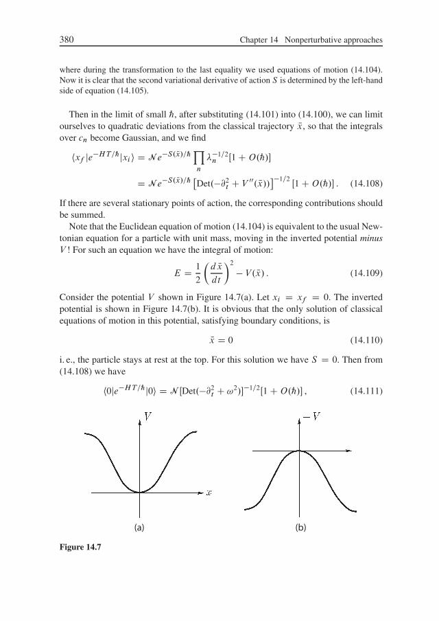
380 Chapter 14 Nonperturbative approaches
where during the transformation to the last equality we used equations of motion (14.104).Now it is clear that the second variational derivative of action S is determined by the left-handside of equation (14.105).
Then in the limit of small „, after substituting (14.101) into (14.100), we can limitourselves to quadratic deviations from the classical trajectory Nx, so that the integralsover cn become Gaussian, and we find
hxf je�HT=„jxi i D N e�S. Nx/=„Y
n
��1=2n Œ1 CO.„/�
D N e�S. Nx/=„ �Det.�@2t C V 00. Nx//��1=2
Œ1 CO.„/� . (14.108)
If there are several stationary points of action, the corresponding contributions shouldbe summed.
Note that the Euclidean equation of motion (14.104) is equivalent to the usual New-tonian equation for a particle with unit mass, moving in the inverted potential minusV ! For such an equation we have the integral of motion:
E D 1
2
�d Nxdt
�2
� V. Nx/ . (14.109)
Consider the potential V shown in Figure 14.7(a). Let xi D xf D 0. The invertedpotential is shown in Figure 14.7(b). It is obvious that the only solution of classicalequations of motion in this potential, satisfying boundary conditions, is
Nx D 0 (14.110)
i. e., the particle stays at rest at the top. For this solution we have S D 0. Then from(14.108) we have
h0je�HT=„j0i D N ŒDet.�@2t C !2/��1=2Œ1 CO.„/� , (14.111)
(a) (b)
Figure 14.7

Section 14.3 Instantons in quantum mechanics 381
where zeroes denote transition from the origin to the origin of our coordinate system,while !2 D V 00.0/ is the square of the frequency of the small oscillations around theminimum of potential V . It can be shown [15] that for large T
N ŒDet.@2t C !2/��1=2 D
!�„�1=2
e�!T=2 . (14.112)
Then from (14.111) and the discussion around (14.99) we immediately see that theground state energy in this problem is given by
E0 D 1
2„!Œ1 CO.„/� , (14.113)
i. e., the zero-point energy of the oscillator near the minimum of V . The probabilityfor a particle to be at the origin of the coordinate system when it is at its ground stateis given by
jhx D 0jn D 0ij2 D !�„�1=2
Œ1 CO.„/� . (14.114)
These are the well-known results of the quasi-classical approximation of quantummechanics. Actually, from this correspondence we immediately see the validity of(14.112). The physics is also quite clear: in the limit of small „ the particle is in theground state of oscillator near th#e origin of coordinate system.
Double-well potential and instantons
Let us consider now a more interesting example: the double-well potential, shown inFigure 14.8(a). Here we have V.x/ D V.�x/, and the potential minima are at pointsx D ˙a. We can also introduce !2 D V 00.˙a/: the square of the frequency of theclassical oscillations of a particle in the vicinity of the minima. Let us calculate thetransition amplitudes:
h�aje�HT=„j � ai D haje�HT=„jai , (14.115)
haje�HT=„j � ai D h�aje�HT=„jai , (14.116)
(a) (b)
Figure 14.8

382 Chapter 14 Nonperturbative approaches
making a quasi-classical approximation for the path integral, similar to the case ofa particle in single well. As a first step we shall again look for the solutions of theclassical Euclidean equations of motion (14.104), satisfying the appropriate bound-ary conditions. There are two obvious solutions: one corresponding to the case of theparticle remaining the entire time at the top of the left or right hill in Figure 14.8(b).However, there may be also another more interesting solution when the particle startsfrom one of the tops (e. g., the left one) at the moment �T=2 and rolls to the right top,reaching it at the moment CT=2 (T ! 1). Here we are dealing with solutions ofequations of motion, corresponding to energy E D 0 (because E D 0 in the initialstates x D ˙a). Correspondingly (cf. (14.109)),
d Nxdt
D p2V , (14.117)
and the solution of this equation has the form
t D t1 CZ x
0dx0 1p
2V, (14.118)
where t1 is the integration constant (time at which x D 0). This solution obviouslyhas the form shown in Figure 14.9. This solution is called an instanton6, centeredat point t1. A mirror reflection of this solution can be called an anti-instanton. It isimportant to stress that an instanton has a finite action:
S0 DZ T=2
�T=2dt
�1
2
�d Nxdt
�2
C V
�DZ T=2
�T=2dt
�d Nxdt
�2
DZ a
�adx
p2V , (14.119)
Figure 14.9
6 The origin of this term is related to the obvious analogy with soliton, but stresses the fact that we aredealing here with solutions of Euclidean equations of motion.

Section 14.3 Instantons in quantum mechanics 383
Figure 14.10
where we have used (14.117). For large t we have Nx ! a, so that (14.117) can beapproximated by
d Nxdt
Dp!2. Nx � a/2 D !.a � Nx/ (14.120)
so that at large t ,.a � Nx/ � e�!t (14.121)
and the instanton is “localized in time” (at times � 1!
), which clarifies its name.It is clear that for large T the instanton and anti-instanton are not the only solutions
of equations of motion; approximate solutions can be built as chains of well-separatedinstantons and anti-instantons. An example of such a configuration is shown in Fig-ure 14.10, with n objects (instantons and anti-instantons), centered at points t1, : : : , tn:
T
2> t1 > t2 > � � � > tn > �T
2. (14.122)
Correspondingly, in the path integral we have to sum the contributions from all suchconfigurations.
Now let us calculate! Obviously, n well-separated objects contribute additively tothe actions giving S D nS0, which in the path integral give the contribution of theorder � exp.�nS0/. To find the determinant we need the more complicated procedure.Consider the time evolution operator e�HT as the product of the operators of evolutionbetween the points where instantons and anti-instantons are placed. In the absence ofthese, on all time axes we have V 00 D !2, and we get the same result as above for thecase of single-well potential (14.112):
!�„�1=2
e�!T=2 . (14.123)

384 Chapter 14 Nonperturbative approaches
Intervals with instantons and anti-instantons lead to a correction, which we can write as !�„�1=2
e�!T=2Kn , (14.124)
whereK can be determined from the requirement of a correct answer for the case of asingle instanton. Later we shall give the appropriate explicit expression, while for themoment we note that in order to take into account all the possible contributions to thepath integral we have to integrate over the arbitrary positions of all centers:
Z T=2
�T=2dt1
Z t1
�T=2dt2 � � �
Z tn�1
�T=2dtn D T n
nŠ. (14.125)
We should also take into account the fact, that we are not completely free in placingthe instantons and anti-instantons. For example, if we start from �a, the first objectwe meet is to be an instanton, the next one an anti-instanton, etc. If we finally returnto �a, n should be even, while if we end at Ca, n should be odd. Thus we obtain
h�aje�HT=„j � ai D !�„�1=2
e�!T=2X
Even n
.Ke�S0=„T /nnŠ
Œ1 CO.„/� , (14.126)
while haje�HT=„j � ai is given by the same expression, but with summation overodd n. The sums are elementary, and we obtain
h˙aje�HT=„j � ai D !�„�1=2
e�!T=2 1
2
�exp.Ke�S0=„T /� exp.�Ke�S0=„T /
�.
(14.127)
Recalling (14.99),
hxf je�HT=„jxi i DX
n
e�EnT=„hxf jnihnjxi i , (14.128)
we understand that the two lowest energy levels correspond to energies
E˙ D 1
2„! ˙ „Ke�S0=„ . (14.129)
If we denote the corresponding states as jCi and j�i, we see that
jhCj ˙ aij2 D jh�j ˙ aij2 D haj�ih�j � ai D �hajCihCj � ai D 1
2
!�„� .1=2
(14.130)
These are the well-known results of quantum mechanics [35]: we just obtained thesplitting of the level in the double-well potential due to tunneling (degeneracy liftingof two levels in two potential wells). The size of this splitting is � e�S0=„. The loweststate j�i is even combination of wave functions, corresponding to a particle, localizedin each of the wells, while the first excited state jCi is described by antisymmetriccombination of these functions.

Section 14.3 Instantons in quantum mechanics 385
Now let us calculate the factor K. First, let us study the properties of the solutionsof equation (14.105):
�d2xn
dt2C V 00. Nx/xn D �nxn , (14.131)
where Nx denotes a single instanton solution. Due to invariance with respect to thetime-shift (the instanton center can be placed at an arbitrary point on the time axis),this equation has an eigenfunction with zero eigenvalue (the so-called zero translationmode). Explicitly this function is written as
x1 D S�1=20
d Nxdt
. (14.132)
The normalization factor here appears from (14.119):Zdt
�d Nxdt
�2
D S0 , (14.133)
The existence of zero-mode can be confirmed as follows. The instanton Nx.t/ satisfies the equa-tion (14.104):
�d2 Nxdt2
C V 0. Nx/ D 0 . (14.134)
But Nx.t C T /, with arbitrary T , is also the solution of this equation:
�d2 Nx.t C T /
dt2C V 0. Nx.t C T // D 0 . (14.135)
Differentiating this equation by T , we obtain
�d2x1
dt2C V 00. Nx/x1 D 0 , (14.136)
which proves our statement on (14.132).
The existence of zero-mode with �1 D 0 seems to lead to a problem. If we cal-culate the Gaussian integral around the extremal trajectory (instanton), as describedin connection with (14.101), (14.103), and (14.108), integration over c1 will lead todivergence! However, we have already done the appropriate integration, integratingover the centers of the instantons (anti-instantons) in (14.125). In fact, the change ofx.t/ under the small shift of the instanton center t1 is equal to
dx D�d Nxdt
�dt1 . (14.137)
At the same time, the corresponding change due to variation of the coefficient c1 in(14.101) is
dx D x1dc1 . (14.138)

386 Chapter 14 Nonperturbative approaches
Then, writing in (14.137)d Nxdt
�dt1 D p
S0x1dt1, and comparing this with (14.138),
we get dc1 D pS0dt1, or
.2�„/�1=2dc1 D�S0
2�„�1=2
dt1 , (14.139)
where „ is introduced to make normalization dimensionless. Thus, during the calcu-lation of the determinant in the Gaussian integral in expressions like (14.108) we donot need to include the zero eigenvalue, but instead we have to include inK the factor. S0
2„/1=2. Then the single-instanton contribution to the matrix element is given by
haje�HT=„j�ai1inst D N T
�S0
2�„�1=2
e�S0=„ŒDet0.�@2tCV 00. Nx//��1=2, (14.140)
where the prime over the determinant corresponds to dropping the zero eigenvalue.Comparing (14.140) with the single-instanton contribution to (14.126), we find
K D�S0
2�„�1=2 ˇ
ˇ Det.�@2t C !2/
Det0.�@2t C V 00. Nx//
ˇˇ1=2
. (14.141)
This completes our calculation!Let us make some comments:
1. It can be shown that the results obtained are equivalent to the standard results ofquantum mechanics [35].
2. We assumed that all �n > 0 (except �1 D 0). This is really so, as the lowest state x1
(as is easily seen from its explicit form) does not have zeroes, as it should be for thesolution of a one-dimensional Schroedinger equation. This is clear from the fact thatour instanton is monotonously growing (ant-instanton: decreasing) function of t , sothat its derivative x1 � d Nx
dthas no zeroes.
3. The coefficient K is proportional to „�1=2, which is related to the contribution ofthe zero-mode. In fact, this is a general rule: each zero-mode (there may be severalsuch modes!) produces the factor of „�1=2.
In a similar way we can analyze the problem of a particle moving in a periodic potential, asshown in Figure 14.11. The difference from the previous case is that now we have no restrictionof alternating the placement of the instantons and anti-instantons, which is connected with theexistence here of the multitude of equivalent potential minima. At the same time, the totalnumber of instantons minus the total number of anti-instantons should now be equal to thechange of Nx between the initial and final coordinates. Then, from (14.127) we obtain
hjCje�HT=„jj�i D !�„�1=2
e�!T=21X
nD0
1X
NnD0
1
nŠ NnŠ .Ke�S0=„T /nC Nnın� Nn�jCCj�
, (14.142)

Section 14.3 Instantons in quantum mechanics 387
(a)
(b)
Figure 14.11
where n is the number of instantons, while Nn is the number of anti-instantons. Using now
ıab DZ 2
0
d�
2�ei�.a�b/ , (14.143)
twe rewrite (14.142) as
hjCje�HT=„jj�i D !�„�1=2
e�!T=2Z 2
0
d�
2�expŒ2KT cos �e�S0=„� expŒ�i�.jC � j /� .
(14.144)In this case we have the continuum of energy eigenvalues (band!), parametrized by an “an-gle” � :
E.�/ D 1
2„! � 2„Ke�S0=„ cos � . (14.145)
Matrix elements
h� jj i D !�„�1=4
.2�/�1=2eij� (14.146)
represent, in fact, the appropriate Bloch wave.
Instantons and metastable states
Consider the potential shown in Figure 14.12(a). If we neglect tunneling, there will bea bound state at the origin. Reflected potential is shown in Figure 14.12(b). Classicalequations of motion have the obvious solution corresponding to a particle starting fromthe top of the hill at x D 0, which is then reflected from the classical point of return and returns back to the top, as shown in Figure 14.13. Let us calculate the matrixelement of transition from x D 0 to x D 0, summing over all the well-separatedinstantons of Figure 14.13. We can proceed as above (with obvious redefinition of S0,

388 Chapter 14 Nonperturbative approaches
(a) (b)
Figure 14.12
Figure 14.13
!2, etc.), but with no limitation on the number of instantons being even or odd. Thenthe summation produces the full exponent:
h0je�HT=„j0i D !�„�1=2
e�!T=2 expŒKTe�S0=„� (14.147)
and the ground state energy eigenvalue is
E0 D 1
2„! � „Ke�S0=„ (14.148)
But this is wrong! In fact, in this situation we have tunneling and the appearance ofan unstable state! From the form of the instanton in Figure 14.13 it is clear that theeigenfunction x1 � d Nx
dthas zero and cannot be the ground-state wave function. But
its energy is zero, and now we understand that there is another state with �0 < 0 andan eigenfunction without zeroes. Then the factor K, containing the square root of theproduct of the eigenvalues, is imaginary. Thus, in fact we obtain
ImE0 D �
2� „jKje�S0=„ (14.149)
which corresponds to the finite-level width, corresponding to the metastable state.

Section 14.4 Instantons and the unstable vacuum in field theory 389
14.4 Instantons and the unstable vacuum in field theory
Consider now Euclidean scalar field theory with the action
S DZd 4x
h1
2.@��/
2 C U.�/i
, (14.150)
where potential U.�/ is shown in Figure 14.14. Here we have two nonequivalent min-ima at �C and ��, and �� is an absolute minimum. Let us choose the origin of theenergy scale so that U.�C/ D 0. In quantum theory, the minimum at � D �C playsthe role of a “false” (metastable) vacuum. The description of the decay of such “false”vacuums is similar to the description of nucleation in statistical physics (e. g., duringthe boiling of a superheated liquid). In quantum field theory this problem is of impor-tance for cosmology [41]. Who knows whether our vacuum is stable or metastable!
We have to calculate the value of �V
, the probability of metastable vacuum decay inunits of time per unit volume. First we have to find the corresponding instanton N� asa solution of the Euclidean equations of motion:
@�@� N� D U 0. N�/ , (14.151)
satisfying the boundary conditions
limx4!˙1
N�.x, x4/ D �C . (14.152)
It is easily seen that to guarantee the finiteness of the action at instanton we have tosatisfy the condition
limjxj!1
N�.x, x4/ D �C . (14.153)
If an instanton is found, then in the leading approximation in „ we have
�
VD Ke�S0 , (14.154)
Figure 14.14
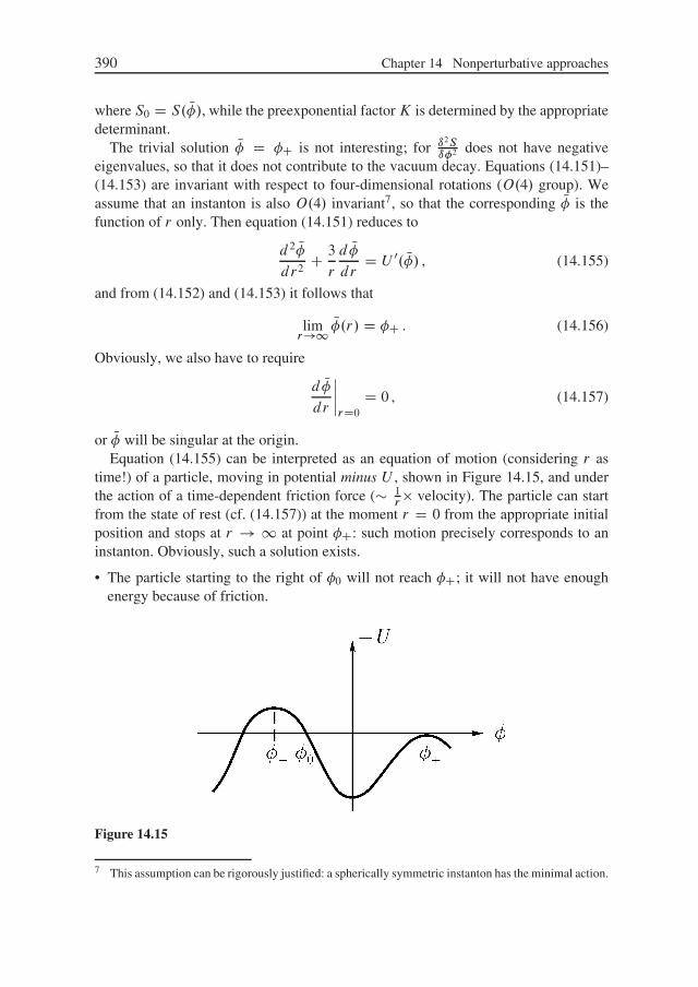
390 Chapter 14 Nonperturbative approaches
where S0 D S. N�/, while the preexponential factorK is determined by the appropriatedeterminant.
The trivial solution N� D �C is not interesting; for ı2Sı�2 does not have negative
eigenvalues, so that it does not contribute to the vacuum decay. Equations (14.151)–(14.153) are invariant with respect to four-dimensional rotations (O.4/ group). Weassume that an instanton is also O.4/ invariant7, so that the corresponding N� is thefunction of r only. Then equation (14.151) reduces to
d 2 N�dr2
C 3
r
d N�dr
D U 0. N�/ , (14.155)
and from (14.152) and (14.153) it follows that
limr!1
N�.r/ D �C . (14.156)
Obviously, we also have to require
d N�dr
ˇˇˇrD0
D 0 , (14.157)
or N� will be singular at the origin.Equation (14.155) can be interpreted as an equation of motion (considering r as
time!) of a particle, moving in potential minus U , shown in Figure 14.15, and underthe action of a time-dependent friction force (� 1
r� velocity). The particle can start
from the state of rest (cf. (14.157)) at the moment r D 0 from the appropriate initialposition and stops at r ! 1 at point �C: such motion precisely corresponds to aninstanton. Obviously, such a solution exists.
� The particle starting to the right of �0 will not reach �C; it will not have enoughenergy because of friction.
Figure 14.15
7 This assumption can be rigorously justified: a spherically symmetric instanton has the minimal action.

Section 14.4 Instantons and the unstable vacuum in field theory 391
� If we choose the initial point correctly to the left of �0 but to the right of ��, we canguarantee that for large r the particle will reach �C and stop there.
In fact, for � close to �� we can linearize the equation of motion and write it as�d 2
dr2C 3
r
d
dr� �2
�. N� � ��/ D 0 , (14.158)
where �2 D U 00.��/. This equation can be solved rather easily [15], and its solutionis expressed via the modified Bessel function. Then we see that choosing N�.0/ closeenough to ��, we can also guarantee that for large-enough r the particle will remain asclose as possible to ��. But for large-enough r we can neglect friction, as it is � 1=r .But in absence of friction the particle will overshoot the top at �C. This means that inour problem there is always an intermediate point (between �� and �0), starting fromwhich the particle will at r ! 1 stop at �C.
Let UC.�/ be some even function of �:
UC.�/ D UC.��/ (14.159)
with minima at points ˙a:U 0C.˙a/ D 0 . (14.160)
Let us define�2 D U 00C.˙a/ . (14.161)
Let us add to UC a small term, breaking the symmetry between the minima:
U D UC C ".� � a/=2a , " > 0 . (14.162)
In the first order in " we have�˙ D ˙a . (14.163)
The value of " defines the energy difference between the “true” and “false” vacuum.Let us choose the initial position of the particle N�.0/ very close to ��. Then the particleremains close to �� up to some large moment of time r D R; then afterwards it rapidlypasses through the valley and slowly approaches �C for r ! 1. Thus, our instantonlooks like a large four-dimensional spherically symmetric “bubble” of radius R witha thin wall separating the “false” vacuum �C (outside the bubble) from the “true”vacuum �� (inside the bubble). Correspondingly, our bubble (instanton) representsthe nuclei of a new (“true”) vacuum inside the metastable (“false”) vacuum.
For r � R we can neglect the friction as well as the "-dependent term in U . Thenthe equation of motion has the form
d 2 N�dr2
D U 0C. N�/ , (14.164)
which corresponds to the classical equation of motion of a particle in a double-well po-tential, which was analyzed in details above. This equation has as its solution the sim-

392 Chapter 14 Nonperturbative approaches
plest one-dimensional instanton of Figure 14.9, which we studied above (and whichdescribes the transition from �a to Ca at “moment” R with the growth of r). This isthe approximate description of an instanton in our field problem.
Up to now we have not yet defined R. The action of the instanton is given by
S D 2�2Z 1
0dr r3
�1
2
�d N�dr
�2
C U. N�/�
. (14.165)
Here we have three regions of integration: outside the bubble, close to its surface, andinside. Outside we can take N� D �C and U D 0, so that this contribution to theintegral is just zero (which actually guarantees the finiteness of the instanton action).Inside the bubble we have N� D ��, U D �", so that the corresponding contributionto the integral is
�1
2�2R4" . (14.166)
Close to the bubble surface, i. e., for r � R, we can neglect �" term in U, so that theintegral reduces to
2�2R3Zdr
�1
2
�d N�dr
�2
C UC�
D 2�2R3S1 , (14.167)
where
S1 DZ a
�ad�p
2UC (14.168)
is the action of the one-dimensional instanton (14.119). Finally we get
S D �1
2�2R4"C 2�2R3S1 . (14.169)
Let us now define R from the requirement of extremal action:dS
dRD �2�2R3"C 6�2R2S1 D 0 , (14.170)
which gives
R D 3S1
". (14.171)
Then we have8
S0 D 27�2S41
2"3. (14.172)
The bubble radius (14.171) can be found from the elementary considerations used in nucle-ation theory of statistical mechanics: the energy gain within the bubble should compensate theenergy loss, connected with the surface tension of the bubble:
4
3�R3" D 4�R2 , which gives R D 3
", (14.173)
where is the surface energy of the bubble well. In our case D S1.
8 Our analysis is valid in the limit of small " and in the limit when the bubble radius is much larger thanthe width of its wall: R � ��1, which reduces to 3S1� � ".

Section 14.4 Instantons and the unstable vacuum in field theory 393
Finally, we obtain the probability of “false” vacuum decay as
�
V� exp.�S0/ . (14.174)
Determinants and renormalization
The preexponential factor in (14.174) should be defined in the same way as in the quan-tum mechanical problem discussed above. But there are some important differencesand questions:
1. In quantum mechanics we had only one zero translational mode; here there are four.
2. It was very important that there was only one negative energy eigenvalue, leadingto an imaginary contribution. Is this also the case in the present problem?
3. In quantum field theory we have ultraviolet divergences, and it is necessary to per-form renormalization. What is the role of renormalization here?
Consider first the zero modes. Here we have four directions for instanton translation(the instanton can be place at an arbitrary point of four-dimensional Euclidean space);correspondingly we have four eigenfunctions of a differential operator, related to thesecond variational derivative of action, with zero eigenstates. These functions � @� N�.The normalization condition reduces toZ
d 4x@� N�@� N� D 1
4ı��
Zd 4x@� N�@� N� D ı��S0 . (14.175)
As a result, the preexponential in (14.174) contains four factors ofS02
�1=2instead of
one.
The proof of the last equality in (14.175) goes as follows. Consider ��.x/ D N�.x=�/. Thenthe action is
S.��/ D 1
2�2Zd 4x.@� N�/2 C �4
Zd 4xU. N�/ . (14.176)
As N� is the solution of equations of motion, we should satisfy the condition of stationarity ofthe action (14.176) at � D 1. This yields
Zd 4x.@� N�/2 D �4
Zd 4xU. N�/ (14.177)
or
S0 D 1
4
Zd 4x.@� N�/2 > 0 . (14.178)
Finally, we obtain the preexponential factor as
K D S20
4�2
ˇˇˇ
Det0Œ�@�@� C U 00. N�/�DetŒ�@�@� C U 00.�C/�
ˇˇˇ
�1=2
, (14.179)
assuming there are no problems with negative eigenvalues and renormalization.

394 Chapter 14 Nonperturbative approaches
As to negative eigenvalues, this is really so. It is clear that ı2Sı�2 (at the instanton)
has at least one negative eigenstate. It can be rigorously proved that there is only onenegative eigenstate in this problem [15]. Thus, equation (14.179) gives the correctprobability of vacuum decay.
We shall not discuss in detail the problem of the renormalization of (14.174). In principle,it is clear that in theories with renormalizable U.'/, all expressions, including (14.179), canbe rewritten via renormalized parameters, and everything should be finite. Some additionaldetails can be found in [15].
The bubble, expanding in real Minkowski space-time, can be obtained as the ana-lytical continuation of the instanton:
�.x0, x/ D N�.r Dq
jxj2 � x20/ . (14.180)
Thus, at small " we have a thin wall at r D R, separating the two vacuums, andexpansion of the bubble is determined by
jxj2 � x20 � R2 . (14.181)
The value of R is determined, as we have seen, by the microscopic parameters of thetheory and is itself microscopic. Then, equation (14.181) means that the expandingsurface of the bubble moves practically with the speed of light (v � 1)! The walltransports the energy (per unit surface) S1p
1�v2. At the moment, when the bubble radius
reaches jxj, the wall energy becomes
Ewall D 4�jxj2S1p1 � v2
. (14.182)
From (14.181) it is easy to find that
v D d jxjdt
Ds
1 � R2
jxj2 . (14.183)
Then the wall energy is
Ewall D 4�jxj3S1
RD 4�"jxj3
3, (14.184)
so that practically the whole energy released during the “false” vacuum decay goesto the wall acceleration. No particles are created; from both sides of the wall we havethe corresponding vacuum states. In this sense, the “observer” will never know thatthe wall passed through him; he will also just “decay” in the corresponding micro-scopic time.
Section 14.5 The Lipatov asymptotics of a perturbation series 395
Examples of applications of this formalism to problems of relativistic cosmologycan be found in [41].
The concept of instantons plays a major role in many problems of quantum fieldtheory and statistical mechanics. As an example, we can again mention the g'4 withg < 0 and the number of filed components n D 0, which describes the motion ofan electron in the random field of impurities in solid state theory. In this model withan unstable ground state there are t instanton solutions which determine the electrondensity of the states in the so-called “tail” region, appearing due to electron localizationby random field fluctuations [57, 64].
Especially important are nontrivial instanton solutions in non-Abelian gauge theo-ries, which are related to the topological properties of gauge transformations and thecomplicated structure of a Yang–Mills vacuum [15,51,52]. We shall not discuss theseaspects of the theory here, as well as their importance for particle physics (QCD). Adetailed presentation can be found in [52, 58].
14.5 The Lipatov asymptotics of a perturbation series
At the end of Chapter 8 we briefly discussed the asymptotic nature of a perturbationseries in quantum field theory. Here we shall consider it in more detail, describingthe elements of the elegant approach proposed by Lipatov. The idea of the Lipatovmethod is as follows. If we have some physical function F.g/ which is expanded in aperturbation series in powers of coupling constant g
F.g/ D1X
ND0
FNgN , (14.185)
the coefficients of this expansion FN can be determined as
FN DZ
C
dg
2�i
F.g/
gNC1, (14.186)
where integration contour C encircles the point g D 0 in the complex plane of thecoupling constant. Rewriting the denominator here as exp ¹�.N C 1/ ln gº, for largeN we can use the steepest-descent (stationary phase) approach to estimate (14.186).
We know that all problems solved by the diagram technique can be reformulated interms of functional integrals like
Z.g/ DZD' exp .�S0¹'º � gSint ¹'º/ , (14.187)
and we can write the coefficients of perturbation expansion as
ZN DZ
C
dg
2�ig
ZD' exp .�S0¹'º � gSint ¹'º �N ln g/ . (14.188)
396 Chapter 14 Nonperturbative approaches
The Lipatov idea is to search for the steepest descent in (14.188) not simply over g,but over g and ' simultaneously:
ıS.'/
ı'
ˇˇˇ'c
D 0 , (14.189)
S.'c/
gcD 0 . (14.190)
The solution of these equations exists for all interesting models and is realized on aspatially localized instanton 'c.x/. The steepest descent approach is applicable herefor large N , independent of its applicability to the initial functional integral (14.187).This fact is of prime importance; in the general case an exact calculation of the func-tional integrals is impossible, but they are easily calculated by steepest descent.
This allows us to determine the general form of large N asymptotics of the pertur-bation theory coefficients for any physical characteristics (such as Green’s functions,vertex parts, etc.) for different models of quantum field theory. The typical form ofLipatov asymptotics for the perturbation coefficients of an arbitrary function F.g/has the form
FN D c �.N C b/aN , (14.191)
where �.x/ is the �-function, and parameters a, b, c depend on the specific problemunder discussion. In a concrete model of field theory the constant a is universal, theparameter b depends on the physical function F.g/ under study, and c contains de-pendence on external momenta (or coordinates). The appearance of �.N C b/ � NŠ
in (14.191) simply reflects the factorial growth of the number of diagrams with theorder N of perturbation theory. Obviously, such asymptotic behavior of perturbationtheory coefficients corresponds to the divergent series!
The knowledge of Lipatov asymptotics in combination with the exact results fora few lowest orders of perturbation theory, obtained by direct diagrammatic calcu-lations, gives information on the perturbation series as a whole. Approximating thecomplete series by the sum of lowest order contributions with asymptotics of higherorders, and applying the mathematical methods of the summation of the divergent se-ries, we can obtain approximate solutions of an arbitrary physical problem.
The most common method to deal with a divergent (asymptotic) series of perturba-tion theory is to use so-called Borel transformation. We can divide and multiply eachterm of the series by NŠ and use the integral representation of the �-function, so thatafter the interchange of summation and integration, we can write
F.g/ D1X
ND0
FNgN D
1X
ND0
FN
NŠ
Z 1
0dx xN e�xgN D
Z 1
0dx e�x
1X
ND0
FN
NŠ.gx/N .
(14.192)The power series in the right-hand side is in most cases converging (it actually hasfactorially improved convergence!) and defines Borel transform B.z/ of the function

Section 14.6 The end of the “zero-charge” story? 397
F.g/, which can now be determined from the following integral transformation:
F.g/ DZ 1
0dx e�xB.gx/ , B.z/ D
1X
ND0
FN
NŠzN , (14.193)
Borel transformation gives the natural method of summation of a factorially divergentperturbation series of quantum field theory9.
14.6 The end of the “zero-charge” story?
In Chapter 13 we stressed the importance of the asymptotic behavior of the Gell-Mann–Low function ˇ.g/ at large values of the coupling constant g for the internalconsistency of quantum field theory. However, until recently, only perturbation the-ory estimates of ˇ.g/ were available, and no definite conclusions on its behavior atlarge g could be drawn. Below we shall present some nonperturbative arguments dueto Suslov, allowing us to find this asymptotic behavior in analytic form [66].
For simplicity we shall consider the O.N/ symmetric Euclidean '4 theory in d -dimensional space with the action10
S¹'º DZddx
²12
NX
˛D1
.r'˛/2 C 12m
20
NX
˛D1
' 2˛ C 1
8u
� NX
˛D1
' 2˛
�2³, (14.194)
where u D g0ƒ� and D 4 � d . Actually, this is the direct analogue of equa-
tion (10.160) used in the theory of critical phenomena. Here we are using lattice reg-ularization of ultraviolet divergences, introducing the cut-off ƒ � a�1, where a isthe lattice constant. Following the usual renormalization group formalism, we con-sider the “amputated” vertex �.n/ with n external lines of field '. The multiplicativerenormalizability of the theory means that we may write the direct analogue of equa-tion (13.76) as
�.n/.pi ;g0,m0,ƒ/ D Z�n=2�.n/R .pi ;g,m/ , (14.195)
so that divergence at ƒ ! 1 disappears after extraction of the proper Z-factors andtheir transfer to the renormalized charge and mass, which are denoted here as g andm. We shall accept the renormalization conditions at zero momentum:
�.2/R .p;g,m/
ˇˇp!0
D m2 C p2 CO.p4/ ,
�.4/R .pi ;g,m/
ˇˇpi D0
D gm� , (14.196)
9 A detailed discussion of methods to deal with divergent series of perturbation theory can be found inthe review paper [65]
10 Generalization to QED is more or less straightforward.

398 Chapter 14 Nonperturbative approaches
which are typical for applications in the phase transitions theory. From equa-tions (14.196) and (14.195) we can obtain expressions for renormalized g, m, Z interms of the “bare” quantities:
Z.g0,m0,ƒ/ D�@
@p2�.2/.p;g0,m0,ƒ/
ˇˇpD0
��1
,
m2 D Z.g0,m0,ƒ/ �.2/.p;g0,m0,ƒ/ˇˇpD0
,
g D m��Z2.g0,m0,ƒ/ �.4/.pi ;g0,m0,ƒ/ˇˇpi D0
. (14.197)
Applying the differential operator d=d lnm to (14.195) for fixed g0 and ƒ gives thedirect equivalent of the Callan–Symanzik equation (13.82), which for large momentajpi j=m � 1 has the form
�@
@ lnmC ˇ.g/
@
@g� n�.g/
��.n/R .pi ;g,m/ � 0 , (14.198)
where functions ˇ.g/ and �.g/ are defined as
ˇ.g/ D dg
d lnm
ˇˇg0,ƒD const
, �.g/ D d lnpZ
d lnm
ˇˇˇg0,ƒD const
, (14.199)
and according to the general theorems depend only on g.Now we shall show how the renormalization group functions are expressed via func-
tional integrals. The functional integrals of '4-theory are determined as
Z.M/˛1:::˛M
.x1, : : : , xM / DZD' '˛1.x1/'˛2.x2/ � � �'˛M
.xM / exp .�S¹'º/ .
(14.200)Fourier transform of equation (14.200) can be written as
Z.M/˛1:::˛M
.p1, : : : ,pM /N ıp1C���CpM
DX
x1,:::,xM
Z.M/˛1:::˛M
.x1, : : : , xM /eip1x1C:::CipMxM
D KM .pi /I˛1:::˛Mıp1C���CpM
(14.201)
where N is the number of sites on the lattice, which is implied in the definition of the(regularized) functional integral, and symmetry factors I˛1���˛M
are similar to thosediscussed in Chapter 10 in relation to critical phenomena. Now we have
Z.0/ D K0 , Z.2/˛ˇ.p, �p/ D K2.p/ı˛ˇ , Z
.4/˛ˇı
¹piº D K4¹piºI˛ˇı (14.202)
where I˛ˇı is given by an expression similar to that in equation (10.168). Now we canintroduce the vertex part �.4/ by the usual relation for two-particle (4-point) Green’s

Section 14.6 The end of the “zero-charge” story? 399
function:
G.4/˛ˇı
.p1, : : : ,p4/ D G.2/˛ˇ.p1/G
.2/ı.p3/N ıp1Cp2 CG.2/˛ .p1/G
.2/ˇı.p2/N ıp1Cp3
CG.2/˛ı.p1/G
.2/ˇ.p3/N ıp1Cp4
�G.2/˛˛0.p1/G.2/ˇˇ 0.p2/G
.2/ 0.p3/G
.2/ıı0.p4/�
.4/˛0ˇ 0 0ı0
.p1, : : : ,p4/
(14.203)
where G.2/˛ˇ.pi / are single-particle (2-point) Green’ functions. Extracting factors
I˛1:::˛Mwe have
G.2/˛ˇ.p/ D G2.p/ı˛ˇ , G
.4/˛ˇı
¹piº D G4¹piºI˛ˇı , �.4/˛ˇı
¹piº D �4¹piºI˛ˇı(14.204)
Now we can write
G4 D K4
K0, �4 D �G4
G42
D �K4K30
K42
, (14.205)
and
G2 D K2.p/
K0, �2.p/ D 1
G2.p/D K0
K2.p/� K0
K2C K0 QK2
K22p2 , (14.206)
where for small p we have written
K2.p/ D K2 � QK2p2 C � � � . (14.207)
Expressions for the Z-factors, renormalized mass, and charge follow from (14.197):
Z D�@
@p2�2.p/
��1
pD0D K2
2
K0 QK2, (14.208)
m2 D Z�2.0/ D K2
QK2, (14.209)
g D m��Z2�4 D ��K2
QK2
�d=2 K4K0
K22
, (14.210)
anddm2
dm20
D�K2
QK2
�0D K 0
2QK2 �K2 QK 0
2
QK22
, (14.211)
where the prime denotes the derivatives overm20. Parameters g0 andƒ are considered
to be fixed, while m2 is a function of m20 only and derivative dm2
0=dm2 is defined by
400 Chapter 14 Nonperturbative approaches
the expression inverse to (14.211). Using the definitions (14.199) we have
ˇ.g/ D�K2
QK2
�d=2´
�d K4K0
K22
C2.K 0
4K0 CK4K00/K2 � 2K4K0K
02
K22
QK2
K2 QK 02 �K 0
2QK2
μ
(14.212)
�.g/ D � K2 QK2
K2 QK 02 �K 0
2QK2
"
2K 0
2
K2� K 0
0
K0�
QK 02
QK2
#
(14.213)
These equations determine ˇ.g/ and �.g/ in parametric form: for fixed g0 and ƒ, theright-hand side of these equations are functions of m2
0 only, while dependence on thespecific choice of g0 and ƒ is absent due to general theorems.
Any infinities in the right-hand sides of equations (14.212) and (14.213) can beinduced only by the zeroes of functional integrals11. It is clear from equation (14.210)that the limit g ! 1 can be achieved by two ways: tending to zero either K2 or QK2.For QK2 ! 0 equations (14.210) and equations (14.212), (14.213) give
g D ��K2
QK2
�d=2 K4K0
K22
, ˇ.g/ D �d�K2
QK2
�d=2 K4K0
K22
, �.g/ ! 1 , (14.214)
and the parametric representation is resolved as
ˇ.g/ D dg , �.g/ D 1 , .g ! 1/ . (14.215)
For K2 ! 0, the limit of g ! 1 can be achieved only for d < 4:
ˇ.g/ D .d � 4/g , �.g/ ! 2 .g ! 1/ . (14.216)
The results (14.215) and (14.216) probably correspond to different branches of thefunction ˇ.g/. It is easy to understand that the physical branch is the first one. Indeed,it is commonly accepted in phase transitions theory that the properties of '4-theorychange smoothly as a function of space dimension, and the results for d D 2, 3 canbe obtained by analytic continuation from d D 4 � . All the available informationindicates the positivity of ˇ.g/ for d D 4, and consequently its asymptotics at g ! 1is also positive. The same property is expected for d < 4 by continuity. The result(14.215) does obey such a property, while the branch (14.216) does not exist for d D 4at all.
According to our discussion in Chapter 13, the behavior of the Gell-Mann–Lowfunction given by equation (14.215) corresponds to the continuous growth of the renor-malized charge as we go to the region of strong coupling at small distances, and sig-nifies the consistency of quantum field theory without “pathologies” like a Landau
11 This is the most nontrivial moment of our discussion. Actually, it can be shown that zeroes of thefunctional integrals can be obtained by a rather subtle compensation of the contributions of the trivialvacuum and some instanton configuration with finite action.

Section 14.6 The end of the “zero-charge” story? 401
“ghost pole” (or a “zero-charge” problem). However, it should be clearly understood,that during our discussion here we have skipped many subtle details, which are to belooked for in original papers, as well as the difficulties which are making this point-of-view less than commonly accepted.

Bibliography
[1] A. A. Abrikosov, L. P. Gor’kov, and I. E. Dzyaloshinskii, Quantum Field TheoreticalMethods in Statistical Physics, Pergamon Press, Oxford, 1965.
[2] A. I. Akhiezer and V. B. Berestetskii, Quantum Electrodynamics, Interscience Publish-ers, New York, 1965.
[3] D. Amit, Field Theory, the Renormalization Group and Critical Phenomena, McGraw-Hill, New York, 1978.
[4] S. Aoki et al., Quenched Light Hadron Spectrumm, Phys. Rev. Lett. 84 (2000), 238.
[5] V. B. Berestetskii, Problems of Physics of Elementary Particles, Nauka, Moscow, 1979(in Russian).
[6] V. B. Berestetskii, E. M. Lifshitz, and L. P. Pitaevskii, Quantum Electrodynamics, Perg-amon Press, Oxford, 1982.
[7] F. A. Berezin, The Method of Second Quantization, Academic Press, New York, 1966.
[8] J. Bjorken and S. Drell, Relativistic Quantum Mechanics. Relativistic Quantum Fieldsin two volumes, Mc Graw-Hill, New York, 1964, 1965.
[9] N. N. Bogolyubov and D. V. Shirkov, Introduction to the Theory of Quantized Fields,Interscience Publishers, New York, 1959.
[10] N. N. Bogolyubov and D. V. Shirkov, Quantum Fields, Addison-Wesley, New York,1982.
[11] V. G. Bornyakov, M. I. Polikarpov, T. Suzuki, M. N. Chernodub, and G. Schierholz,Usp. Fiz. Nauk 174 (2004), 19.
[12] R. N. Cahn, Rev. Mod. Phys. /1996) 68, 951.
[13] T.-P. Cheng and L.-F. Li, Gauge Theory of Elementary Particle Physics, ClarendonPress, Oxford, 1984.
[14] G. F. Chew, The Analytic S-Matrix: A Basis for Nuclear Democracy, W. A. Benjamin,New York, 1966.
[15] S. Coleman, The Uses of Instantons, in: A. Zichichi (ed.), The Whys of SubnuclearPhysics, Plenum Press, New York, 1979.
[16] A. D. Dolgov, Y .B. Zel’dovich, and M. V. Sazhin, Basics of Modern Cosmology, Edi-tions Frontieres, Gif sur Yvette Cedex, 1990.
[17] I. T. Dyatlov, V. V. Sudakov, and K. A. Ter-Martirosyan, Asymptotic theory of meson-meson scattering, Zh. Eksp. Teor. Fiz. (JETP) 32 (1957), 767.

Bibliography 403
[18] R. P. Feynman, Asymptotic theory of meson-meson scattering, Quantum Electrodynam-ics, W. A. Benjamin, New York, 1961.
[19] R. P. Feynman, Statistical Mechanics, W. A. Benjamin, New York, 1972.
[20] R. P. Feynman and A. R. Hibbs, Quantum Mechanics and Path Integrals, Mc Graw-Hill,New York, 1965.
[21] M. E. Fisher, The Nature of Critical Points, University of Colorado Press, Boulder, 1965.
[22] M. K. Gaillard, P. D. Grannis, and F. J. Sciulli, Rev. Mod. Phys. (1999) 71, 96.
[23] K. Gottfried and V. F. Weisskopf, Concepts of Particle Physics, Clarendon Press, Ox-ford, 1984.
[24] F. Halzen and A. D. Martin, Quarks and Leptons: An Introductory Course in ModernParticle Physics, John Wiley and Sons, New York, 1984.
[25] K. Huang, Quarks, Leptons and Gauge Fields, World Scientific, Singapore, 1982.
[26] K. Huang, Fundamental Forces of Nature. The Story of Gauge Fields, World Scientific,Singapore, 2007.
[27] J. Illiopoulos, C. Itzykson, and A. Martin, Functional methods and perturbation theory,Rev. Mod. Phys. 47 (1975), 165.
[28] C. Itzykson and J. Zuber, Quantum Field Theory, McGraw-Hill, New York, 1980.
[29] G. Kane, Modern Elementary Particle Physics, Addison-Wesley, New York, 1990.
[30] J. B. Kogut, An introduction to lattice gauge theory and spin systems, Rev. Mod. Phys.51 (1979), 659.
[31] M. Kreutz, Quarks, Gluons and Lattices, Cambridge University Press, Cambridge,1983.
[32] A. Lambrecht, The Casimir effect: a force from nothing, Physics World 15(9) (2002),29.
[33] L. D. Landau and E. M. Lifshitz, The Classical Theory of Fields, Pergamon, Oxford,1962.
[34] L. D. Landau and E. M. Lifshitz, Mechanics, Pergamon Press, Oxford, 1976.
[35] L. D. Landau and E. M. Lifshitz, Quantum Mechanics, Pergamon Press, Oxford, 1977.
[36] L. D. Landau and E. M. Lifshitz, Statistical Physics, Part I, Pergamon Press, Oxford,1980.
[37] L. D. Landau and E. M. Lifshitz, Statistical Physics, Part II, Pergamon Press, Oxford,1980.
[38] A. I. Larkin and D. E. Khmelnitskii, Phase Transition in Uniaxial Ferroelectrics Zh.Eksp. Teor. Phys. (JETP) 56 (1969), 2087.
[39] T. D. Lee and C. N. Yang, Conservation of Heavy Particles and Generalized GaugeTransformations, Phys. Rev. 98 (1955), 1501.

404 Bibliography
[40] E. M. Lifshitz and L. P. Pitaevskii, Relativistic Quantum Field Theory, Part 2, PergamonPress, Oxford, 1974.
[41] A. D. Linde, Particle Physics and Inflationary Cosmology, Harwood, Chur, 1990.
[42] S.-K. Ma, Modern Theory of Critical Phenomena, W. A. Benjamin, New York, 1976.
[43] Y. M. Makeenko, The Monte Carlo method in lattice gauge theories, Usp. Fiz. Nauk143 (1984), 161.
[44] M. B. Mensky, Measurability of quantum fields and energy-time uncertainty rela-tion,Usp. Fiz. Nauk 181 (2011), 543.
[45] H. Meyer-Ortmanns, Phase transitions in quantum chromodynamics, Rev. Mod. Phys.68 (1996), 473.
[46] L. B. Okun, Particle Physics. The Quest for the Substance of Substance, Harwood, Chur,1985.
[47] L. B. Okun, Current status of elementary particle physics, Usp. Fiz. Nauk 168 (1998),625.
[48] A. Z. Patashinskii and V. L. Pokrovskii, Fluctuation Theory of Phase Transitions, Perg-amon Press, Oxford, 1979.
[49] W. Pauli (ed.), Niels Bohr and the Development of Physics, Pergamon Press, London,1955.
[50] D. H. Perkins, Introduction to High Energy Physics, Addison-Wesley, New York, 1987.
[51] A. M. Polyakov, Gauge Fields and Strings, Harwood, Chur, 1987.
[52] P. Rajaraman, Solitons and Instantons, North Holland, Amsterdam, 1982.
[53] P. Ramond, Field Theory: A Modern Primer, Benjamin/Cummings, London, 1982.
[54] K. Rajagopal and F. Wilczek, The Condensed Matter Physics of QCD, ArXiv: hep-ph/0011333.
[55] V. A. Rubakov, On Large Hadron Collider’s discovery of a new particle with Higgsboson properties, Usp. Fiz. Nauk 182 (2012), 1017.
[56] L. Ryder, Quantum Field Theory, Cambridge University Press, Cambridge, 1985.
[57] M. V. Sadovskii, Electron localization in disordered systems: critical behavior andmacroscopic manifestations, Usp. Fiz. Nauk 133 (1981), 223.
[58] T. Schäfer and E. V. Shuryak, Instantons in QCD, Rev. Mod. Phys. 70 (1998), 323.
[59] S. Schweber, An Introduction to Relativistic Quantum Field Theory, Row, Peterson andCo., New York, 1961.
[60] S. Schweber, H. Bethe, and F. de Hoffmann, Mesons and Fields, vol. I, Row, Petersonand Co., New York, 1955.
[61] Y. A. Simonov, The confinement, Usp. Fiz. Nauk 166 (1996), 337.
[62] A. V. Smilga, Lectures on the Foundations of QCD, ArXiv: hep-ph/9901412.
Bibliography 405
[63] H. Stanley, Introduction to Phase Transitions and Critical Phenomena, Clarendon Press,Oxford, 1971.
[64] I. M. Suslov, Divergent perturbation series, Usp. Fiz. Nauk 168 (1998), 503.
[65] I. M. Suslov, Development of (4- /-dimensional theory for the density of states of adisordered system near the Anderson transition, Zh. Eksp. Teor. Fiz. (JETP) 127 (2005),1350.
[66] I. M. Suslov, Strong coupling asymptotics of the ˇ-function in '4 theory and QCD,Applied Numerical Mathematics 60 2010), 1418.
[67] S. V. Troitskii, Unsolved problems in particle physics, Usp. Fiz. Nauk 182 (2012), 77.
[68] R. Utiyama, Invariant Theoretical Interpretation of Interaction, Phys. Rev. 101 (1956),1597.
[69] A. N. Vasil’ev, The Field Theoretic Renormalization Group in Critical Behavior Theoryand Stochastic Dynamics, Chapman and Hall/CRC, London, 2004.
[70] V. S. Vladimirov, Equations of Mathematical Physics, Mir, Moscow, 1984.
[71] E. T. Whittaker and G. N. Watson. A Course of Modern Analysis. Cambridge UniversityPress, Cambridge, 1927.
[72] F. Wilczek, QCD in Extreme Conditions, ArXiv: hep-ph/0003183.
[73] F. Wilczek, The Future of Particle Physics as a Natural Science, ArXiv: hep-ph/9702371.
[74] F. Wilczek, QCD Made Simple, Phys. Today 53(8) (2000), 2.
[75] C. N. Yang and R. L. Mills, Conservation of Isotopic Spin and Isotopic Gauge Invari-ance, Phys. Rev. 96 (1954), 191.
[76] V. I. Zakharov, B. L. Ioffe, and L. B. Okun, New elementary particles, Usp. Fiz. Nauk117 (1975), 227.
[77] Y. B. Zel’dovich, Classification of elementary particles and quarks “presented for pedes-trians”, Usp. Fiz. Nauk 86 (1965), 303.

Index
actionfunctional, 12integral, 9
adiabatic hypothesis, 133, 134anomalous
dimensions, 344magnetic moment, 182
anticommutators, 83antiparticle, 53antiscreening, 206, 351area law, 368, 369asymptotic
behavior, 200expansions, 209freedom, 5, 190, 347, 348
baryons, 2Bethe–Salpeter equation, 114bilinear forms, 86bispinor, 75, 76Borel transformation, 396Bose statistics, 46
Callan–Symanzik equation, 343, 344cancellation of vacuum diagrams, 165Casimir
effect, 48force, 50
charge conjugation, 58, 85color symmetry, 38commutation relations, 43Compton effect, 140conditional degree of divergence, 327confinement, 371
of quarks, 350connected diagrams, 161, 257conservation laws, 6conserving current, 16Coulomb gauge, 40
counter-terms, 338covariant derivative, 23, 25, 33CPT -theorem, 59critical
exponents, 271, 276, 277phenomena, 264
cutoff, 178, 207
diagram rules, 256diagrammatic rules, 108, 154dimensional
analysis, 329regularization, 331
dimensionalities, 13, 77dimensionality of coupling constants, 247dimensionless coupling constants, 4Dirac
equations, 74, 75matrices, 75, 79
discrete symmetries, 57divergence, 178Dyson equation, 166, 167, 172, 261
"-expansion, 272, 277effective
action, 262, 373potential, 374
electronpropagator, 141, 142, 145self-energy part, 166
energy-momentum tensor, 15Euclidean path integrals, 378evolution operator, 129
Faddeev–PopovAnsatz, 292Faddeev–Popov determinant, 291“ghosts”, 293
“false” vacuum, 389, 391Feynman diagram, 98, 138

Index 407
Feynman’s rule, 101, 103, 145, 235fixed points of the Gell-Mann–Low equa-
tion, 3464-point function, 254functional
derivative, 226integral, 213, 216, 225integration, 237
fundamentalbosons, 3fermions, 2
gauge field, 24Gauss–Poisson integral, 217Gaussian
functional integral, 239integral over Grassmann variables, 281model, 236, 266
Gell-Mann–Lowequation, 207function, 207, 208, 345, 400
generating functional, 231, 232of interacting theory, 249of interacting Dirac fields, 284
“ghost pole”, 190Ginzburg–Landau theory, 310global gauge transformations, 19gluons, 4Goldstone theorem, 308Goldstones, 308gradient transformations, 22grand unified theories, 356Grassmann
algebra, 278variables, 278
Green’s function, 93, 95, 104, 211
hadrons, 2Heisenberg representation, 125helicity, 78, 88, 90Higgs
bosons, 310phenomenon, 310, 316
high temperature expansion, 364homogeneous functions, 343
infraredcatastrophe, 182stable fixed point, 346
instanton, 381–383, 391, 396instantons and metastable states, 387integral over Grassmann variables, 279integration in d-dimensions, 331interaction representation, 126internal parity, 57inversion
of spinors, 72of time, 58
irreducible self-energy part, 261isotopic space, 18, 24
Klein–Gordon equation, 14, 51
Lagrange function, 9Lagrangian, 12Lamb shift, 180, 181Landau
functional, 265gauge, 148“ghost pole”, 346, 401
lattice gauge theory, 361leading logarithm approximation, 269leptons, 2link variable, 365Lipatov asymptotics, 396local
gauge transformations, 20field, 5
loop expansion, 334Lorentz
condition, 41group, 55transformations, 55
Majorana neutrino, 90Mandelstam variables, 120mass
operator, 166surface, 50
masses and lifetimes of fundamentalfermions, 3
massive vector bosons, 4Maxwell equations, 40, 41

408 Index
measurability of fields, 47mechanism of mass generation, 305Meissner effect, 311Moscow zero, 190, 204, 206, 270multiplicative renormalization, 341
n-point function, 258, 260negative eigenstate, 394Noether theorem, 16non-Abelian gauge field, 27normal product, 149normalized generating functional, 250
optical theorem, 122orbit of the gauge group, 290order parameter, 265Ornstein–Zernike correlator, 266
parquet equations, 267path integral, 213perimeter law, 370phase transitions in quantum field theory,
324photon
propagator, 136, 146, 148self-energy part, 162
physicalcharge, 185mass, 262
Planckenergies, 7length, 8
plaquette, 366Poincaré transformations, 56polarization operator, 162primitively diverging diagrams, 198principle of least action, 12Proca equation, 61, 310propagator, 93, 95, 211
quantization, 42, 52of Yang-Mills fields, 287
quantumchromodynamics, 38electrodynamics, 175mechanics “imaginary time”, 220
quarks, 2
regularization, 330relativistic notations, 11renormalizability, 179, 185, 192, 200renormalization, 179, 335
factor, 194group, 188, 273, 342
renormalized charge, 179running coupling constant, 5, 189, 190,
345Rutherford scattering, 175
S -matrix, 115, 129scattering
amplitude, 115cross-section, 117matrix, 115, 129
Schroedinger representation, 124screening, 206second quantization, 43single-particle irreducible diagrams, 261spatial inversion, 86spin and statistics, 84spin-statistics theorem, 6, 54spinors, 64, 67, 68
and 4-vectors, 69of a higher rank, 65
spontaneous symmetry-breaking, 6, 305Standard Model, 323strong coupling expansion, 364subtraction scheme of renormalization,
199superstring theory, 8supersymmetry, 7symmetries, 6
T -exponent, 132T-ordering, 229T -product, 131tensor of Yang–Mills fields, 27, 28thermodynamic analogy, 264time inversion, 59, 85Tomonaga–Schwinger equation, 128two-particle Green’s function, 111, 1712-point function, 252
ultraviolet divergences, 182, 253ultraviolet stable fixed point, 346

Index 409
unitarity condition, 121, 122universality of critical behavior, 276upper critical dimension, 272
vacuumfluctuations, 45, 48polarization, 5
vertex part, 169virtual photon, 111
Ward identity, 174Weyl equation, 87Wick theorem, 149Wilson loop, 367
Yang–Mills field, 25, 27, 28, 35, 312
zero charge, 190, 204, 206, 270, 401zero mode, 385