Embed Size (px)
Citation preview
Quality Technology & Quantitative Management Vol. 3, No. 4, pp. 513-527, 2006
QQTTQQMM © ICAQM 2006
The Effect of Estimated Parameters on Poisson EWMA Control Charts
Murat Caner Testik1, B. D. McCullough2 and Connie M. Borror3
1Department of Industrial Engineering, Hacettepe University, Ankara, Turkey 2Department of Decision Sciences, Drexel University, Philadelphia, PA, USA
3Department of Mathematical Sciences, Arizona State University West, Glendale, AZ, USA (Received March 2005, accepted March 2006)
______________________________________________________________________
Abstract: Performance of control charts is generally evaluated with the assumption that the process parameters are known. In many control chart applications, however, the process parameters are rarely known and their estimates from an in-control reference sample are used instead. In such cases, the moments of the run length distribution depend on the values of the estimated parameters. The Poisson exponentially weighted moving average (EWMA) is an effective control chart in situations where the number of nonconformities per unit from a repetitive production process is monitored. The objective of this paper is to study the effect of estimating the mean on the performance of the Poisson EWMA control chart. We make use of the Markov Chain approach. Sample-size recommendations and some concluding comments are provided.
Keywords: Attributes control chart, exponentially weighted moving average, Markov chain, Poisson distribution, statistical process control.
______________________________________________________________________
1. Introduction
he exponentially weighted moving average (EWMA) control chart, which was first introduced by Roberts [1], is a widely accepted statistical process control tool for
quality monitoring applications. It is known to be effective in detecting small changes in the mean of a process. This is because the EWMA control statistic accumulates information from current and past observations for determining whether the process is in a state of statistical control or not.
T
Let the monitored quality characteristic of interest, X, be the number of nonconformities in a unit from a repetitive production process. The usual approach to model such a process is to employ the Poisson distribution. Consider that the observations X1, X2, X3… are independent and identically distributed (i.i.d.) Poisson random variables with mean µ. The process is said to be in control when µ = µ0 . Otherwise, i.e. for µ ≠ µ0 , the process is said to be out of control. Because a process mean greater than µ0 , say µ1 , implies an increase in the mean number of nonconformities and this would be attributable to the occurrence of an assignable cause, quick detection of the shift is desired for bringing the process back to its in-control state by necessary adjustments. On the other hand, a process mean less than µ0 indicates a decrease in the mean number of nonconformities and detection of the shift would allow quality improvement by determining the cause and making changes to the process.
The Shewhart c-chart is one alternative to monitor for shifts in the mean of a Poisson distribution. This control chart is operated by determining Xt, the number of
514 Testik, McCullough and Borror
nonconformities from a production unit at time t and then comparing it to an upper control limit, hU, for an upward mean shift detection and to a lower control limit, hL, for a downward mean shift detection. The process is said to be out of control if Xt < hL or Xt > hU, otherwise, it is deemed in control (for details of the c-chart, see Montgomery [2]). Although the Shewhart c-chart would be the simplest control chart to operate, its main drawback is slow detection of small shifts in the mean. Note that this chart makes use of the information only from the current observation.
Various control chart alternatives to the Shewhart c-chart exist in the literature. The cumulative sum (CUSUM) control chart for a Poisson model is suggested in Brook and Evans [3] and further analyzed in Lucas [4]. A computer program making use of the Markov Chain approach to evaluate the performance of the Poisson CUSUM chart was developed in White and Keats [5]. The performance of the Poisson CUSUM chart with the Shewhart c-chart is compared in White et al. [6]. An EWMA control chart for a Poisson model is introduced in Gan [7], which uses a procedure to round the EWMA statistic to an integer value. Borror et al. [8], throughout BCR, proposed another Poisson EWMA chart, which uses the exact EWMA statistic so that no information is lost. Both the CUSUM and EWMA procedures accumulate information from current and past observations and therefore are more sensitive to small changes in the mean compared to a Shewhart c-chart.
Count data occurs regularly in all types of business and industry including healthcare, manufacturing, internet security, transportation, and pharmaceutical. The use of valid and effective process monitoring techniques in these and other situations is a vital component of quality improvement initiatives. When a shift in the process from normal operating conditions occurs, it is important that the shift be detected quickly and accurately. Quick detection of a real shift and a low false alarm rate are two significant priorities of any business or industry. The Shewhart c-chart has been used extensively in these areas and can be quite effective. However, research has shown that the Shewhart c-charts perform poorly with respect to detecting small but significant shifts in the process. The Poisson EWMA control chart has been shown to detect small shifts more quickly than the c-chart since it incorporates past process information. It is also important to note that if the system consists of a low number of counts – that is, very few counts which occur sporadically or occasionally – then it may be more useful to monitor the time between the events (TBE). TBE control charts are not presented here, but have been developed and studied in the literature (see, e.g., Borror et al. [9], Gan [10], and Gan [11]).
Performance of a control chart is generally evaluated in terms of the chart’s run length (RL) distribution. The run length is defined as the number of control chart statistics plotted until the first time the control statistic exceeds a control limit. The expected value of run length, namely the average run length (ARL), is one of the most common metrics used for assessing the control chart performance. Although a control chart is designed to signal the occurrence of an assignable cause, there is always a possibility for a false alarm when the process is in control. The average run length due to a false alarm will be denoted by ARL0. Conversely, in the presence of an assignable cause the average run length will be denoted by ARL1. A control chart with a large ARL0 and a small ARL1 is desirable. Consequently, for a given ARL0, a control chart with the smaller ARL1 is often considered to be better than the one with the larger ARL1 considering the same shift magnitude.
The Markov chain approach is very effective in estimating run lengths and used in the present research. The Markov chain method is particularly attractive when no closed-form expression for the distributional properties exists and must be estimated. Several studies illustrating the usefulness of the Markov chain approach for estimating run lengths in
The Effect of Estimated Parameters on Poisson EWMA Control Charts 515
control charts include Brook and Evans [3], Gan [7], Gan [10], Champ and Rigdon [12], Chao [13], Crowder [14], Crowder [15], Fu et al. [16], Lucas and Saccucci [17], Reynold [18], Robinson and Ho [19], Saccucci and Lucas [20], Vardeman and Ray [21], Waldmann [22], and Woodall [23].
In the literature, control chart performance is often evaluated based on aspects of the derived or simulated run length distribution with the assumption that the parameters of the in-control process are known. A typical approach when the process parameters are unknown is to make use of estimates obtained from a reference sample representing the in-control process. In such a case, however, the run length distribution depends on the values of the estimated parameters. The objective of this paper is to study the effect of estimating the mean on the performance of the Poisson EWMA chart suggested in BCR. We make use of the Markov Chain approach. Sample-size recommendations and some concluding comments are provided.
2. Background Information on the Poisson EWMA Control Chart
Assume that the sequence of observations X1, X2, ,… from a repetitive production process is i.i.d. Poisson random variables with mean µ . To detect changes from the in-control mean µ = µ0 to an out-of-control mean µ = µ1 , the use of an EWMA control chart is proposed in BCR. The EWMA statistic is defined at time t as
Zt = (1−λ)Zt-1+ λXt, t = 1, 2, 3, … (1)
where Z0 = 0µ and λ is the smoothing constant such that 0 1λ< ≤ . For an in-control process, it can be shown that the expected value of the EWMA statistic is
E(Zt) = µ0
and its variance is
ttZ
λ λ µλ⎡ ⎤= − −⎣ ⎦−
20Var( ) 1 (1 )
2. (2)
For large values of t, the exact EWMA variance in (2) approaches its asymptotic value
Zλµ
λ∞ =−
0Var( )2
. (3)
Either exact or asymptotic variance of the EWMA statistic may be used in control limit calculations. For this article, we consider the control limits based on the asymptotic variance given in (3). Asymptotic control limits are constant over time. In contrast, control limits based on the exact EWMA variance are parabolic and these may lead to faster detection of a change at the process start-up. The Poisson EWMA control chart gives an out-of-control signal at the first time t such that Zt < hL or Zt > hU, where
00 2
λµµ
λ= −
−L Lh A (4)
and
00 .
2λµ
µλ
= +−U Uh A (5)
For a given smoothing constant λ, the values of AL and AU are chosen to give the desired in-control ARL. Often AL and AU are chosen to be equal (AL = AU = A), which yields a
516 Testik, McCullough and Borror
symmetric control chart. However, the value of the lower control limit hL should be set to zero when its computed value is less than or equal to zero. This is because the quality characteristic of interest Xt is a Poisson random variable and therefore the EWMA statistic Zt in (1) will be nonnegative. The choice of the smoothing constant λ typically depends on how fast a mean shift of given size should be detected. It is generally accepted that smaller values of λ are more effective in rapidly detecting smaller mean shifts and vice versa. For details of the Poisson EWMA control chart and determination of the A and λ pairs for a desired in-control ARL value, see Borror et al. [8].
Up to this point, we have assumed that the actual in-control process mean µ0 is known. However, it is also common industrial applications that the process mean is unknown. In such a case, the estimate of the in-control process mean, denoted by 0µ̂ , may be substituted for µ0 in equations (2)-(5) for constructing the control chart and in the assignment of the initial EWMA value Z0 = µ0. The maximum likelihood estimator for the parameter 0µ is,
01
1µ̂=
= ∑n
ii
Xn
.
Here, n is the size of the reference sample. The central limit theorem ensures that the sampling distribution of 0µ̂ is approximately normal with mean 0µ and variance 0µ n .
3. Markov Chain Approach Conditioned on the Estimated Parameter for Performance Evaluation
The Markov chain approach for studying the run length distribution of a Poisson CUSUM control chart, introduced in Brook and Evans [3], assumes that the process parameter is known. BCR made use of this approach to compute the ARLs of a Poisson EWMA control chart for various shift magnitudes in the process mean. In this section, we briefly explain the Markov chain approximation for assessing the performance of Poisson EWMA schemes with the estimated parameter.
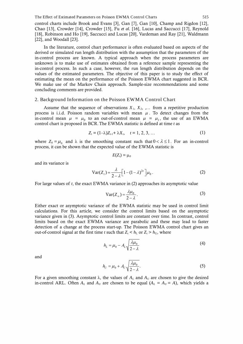
Figure 1. In-control region divided into N subintervals or states.
Let the interval [hL, hU] between the upper and lower control limits be divided into N subintervals called the states as shown in Figure 1. The boundaries Lj and Uj of the jth state are
( 1)( ) ( ), , − − −⎡ ⎤⎡ ⎤ = + +⎢ ⎥⎣ ⎦ ⎣ ⎦U L U L
j j L Uj h h j h hL U h h
N N,
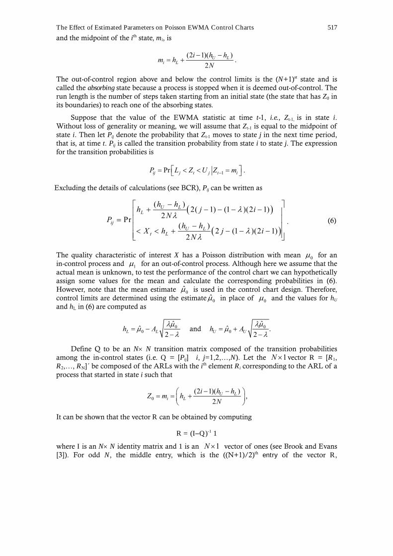
The Effect of Estimated Parameters on Poisson EWMA Control Charts 517
and the midpoint of the ith state, mi, is
(2 1)( )2
− −= + U L
i Li h hm h
N.
The out-of-control region above and below the control limits is the (N+1)st state and is called the absorbing state because a process is stopped when it is deemed out-of-control. The run length is the number of steps taken starting from an initial state (the state that has Z0 in its boundaries) to reach one of the absorbing states.
Suppose that the value of the EWMA statistic at time t-1, i.e., Zt-1, is in state i. Without loss of generality or meaning, we will assume that Zt-1 is equal to the midpoint of state i. Then let Pij denote the probability that Zt-1 moves to state j in the next time period, that is, at time t. Pij is called the transition probability from state i to state j. The expression for the transition probabilities is
1Pr −⎡ ⎤= < < =⎣ ⎦ij j t j t iP L Z U Z m .
Excluding the details of calculations (see BCR), Pij can be written as
( )
( )
( ) 2( 1) (1 )(2 1)2Pr
( ) 2 (1 )(2 1)2
λλ
λλ
−⎡ ⎤+ − − − −⎢ ⎥= ⎢ ⎥
−⎢ ⎥< < + − − −⎢ ⎥⎣ ⎦
U LL
ijU L
t L
h hh j iNP
h hX h j iN
. (6)
The quality characteristic of interest X has a Poisson distribution with mean 0µ for an in-control process and 1µ for an out-of-control process. Although here we assume that the actual mean is unknown, to test the performance of the control chart we can hypothetically assign some values for the mean and calculate the corresponding probabilities in (6). However, note that the mean estimate 0µ̂ is used in the control chart design. Therefore, control limits are determined using the estimate 0µ̂ in place of 0µ and the values for hU and hL in (6) are computed as
00
ˆˆ2λµ
µλ
= −−L Lh A and 0
0ˆˆ .
2λµ
µλ
= +−U Uh A
Define Q to be an N× N transition matrix composed of the transition probabilities among the in-control states (i.e. Q = [Pij] i, j=1,2,…,N). Let the vector R = [R1N × 1, R2,…, RN]΄ be composed of the ARLs with the ith element Ri corresponding to the ARL of a process that started in state i such that
0(2 1)( )
2− −⎛ ⎞= = +⎜ ⎟
⎝ ⎠U L
i Li h hZ m h
N,
It can be shown that the vector R can be obtained by computing
R = (I−Q)-1 1
where I is an N× N identity matrix and 1 is an 1N × vector of ones (see Brook and Evans [3]). For odd N, the middle entry, which is the ((N+1)/2)th entry of the vector R,
518 Testik, McCullough and Borror
corresponds to the ARL of a Poisson EWMA control chart with 0 0ˆZ µ= .
Often, more information than just the ARL is of interest and higher-order moments are useful in describing some other aspects of the run length distribution. This is because the run length distribution is fairly skewed so that the ARL will not be a typical run length. Therefore, to study the performance of a Poisson EWMA control chart with estimated mean, other metrics that we will use in addition to the ARL are the percentiles of the run length distribution and standard deviation of the run length (SDRL).
The percentiles of the run length distribution may be determined using the cumulative probability for run length. Let Fr denote the 1N × cumulative probability vector, where each of the N entries is for one starting value Z0 and the index r = 1, 2, … represents a value of the run length. Then
( )rr = −F I Q 1 .
The cumulative probability times 100 gives the percentile corresponding to the run length value r. For example, the 10th percentile for the case of Z µ=0 ˆ0 is the smallest value of r for the middle entry of Fr being greater than or equal to 0.1.
The magnitude of the SDRL is another important metric for performance comparisons. The SDRL vector, denoted by D is 1N ×
{ }0.51 22 ( )−⎡ ⎤= + − −⎣ ⎦D R I -Q I R R .
In this study, the middle entries in the vectors R, D and Fr corresponding to the cases with the starting value 0 ˆZ 0µ= are of interest. Because the performance measures defined are functions of the estimate of the in-control process mean and the actual mean, we will also adopt the notation ARL( 0µ̂ , µ ), SDRL( 0µ̂ , µ ) and PERC( 0µ̂ , µ ) for the ARL, SDRL, and percentiles, respectively.
4. The Conditional Performance (Performance Under Known Estimation Error)
Suppose that a reference sample of observations is collected, the mean of the in control process is estimated, and the Poisson EWMA control chart is constructed. The run length of the control chart will follow some conditional distribution, which will depend on the particular realization of the process mean estimate. Studying a control chart in several hypothetical cases of parameter estimation gives us insight into the effect of estimation on the performance (see for example Woodall [24] and Jones [25]). In particular, the increase in the false alarm rate may be substantial. In the last section, the Markov chain approximation was described for ARL, SDRL, and percentile calculations of the run length distribution when the Poisson EWMA was conditioned on specific values of the estimated mean. Consequently, in this section we evaluate the conditional run length performance of the Poisson EWMA control chart. The Markov chain calculations are programmed in Matlab® v6.0 (code available upon request from the lead author) and validated using simulations. (Conditional performances for several cases are simulated to validate the results of the Markov Chain code. In the simulations, several thousand replications are performed by generating Poisson observations with the true mean but the chart is designed using the estimated mean.)
To give an idea of how the Poisson EWMA will perform in some hypothetical cases of estimated mean, the conditional run length performances are given in Tables 1, 2, and 3 for the values 5, 10, and 20 of 0µ̂ , respectively. In the tables three situations are considered:
The Effect of Estimated Parameters on Poisson EWMA Control Charts 519
0µ̂ assumes a value in the 25th (underestimation), 50th (nominal), and 75th (overestimation) percentiles of the sampling distribution of 0µ̂ . This is equivalent to the actual in-control process mean being equal to the estimated in-control process mean (nominal), lower (overestimation), or upper (underestimation)
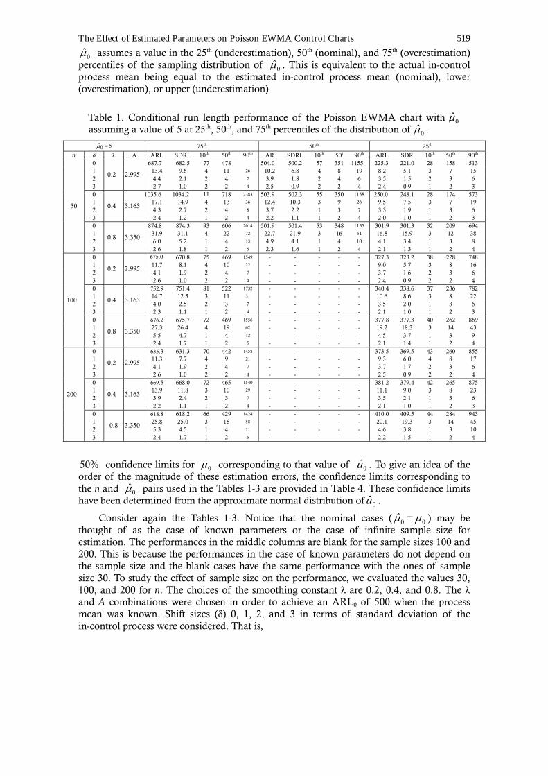
Table 1. Conditional run length performance of the Poisson EWMA chart with 0µ̂ assuming a value of 5 at 25th, 50th, and 75th percentiles of the distribution of 0µ̂ .
ˆ 50µ = 75th 50th 25th n δ λ A ARL SDRL 10th 50th 90th AR SDRL 10th 50t 90th ARL SDR 10th 50th 90th
0 687.7 682.5 77 478
504.0 500.2 57 351 1155 225.3 221.0 28 158 513 1 13.4 9.6 4 11 26 10.2 6.8 4 8 19 8.2 5.1 3 7 15 2 4.4 2.1 2 4 7 3.9 1.8 2 4 6 3.5 1.5 2 3 6 3
0.2 2.995
2.7 1.0 2 2 4 2.5 0.9 2 2 4 2.4 0.9 1 2 3 0 1035.6 1034.2 11 718 2383 503.9 502.3 55 350 1158 250.0 248.1 28 174 573 1 17.1 14.9 4 13 36 12.4 10.3 3 9 26 9.5 7.5 3 7 19 2 4.3 2.7 2 4 8 3.7 2.2 1 3 7 3.3 1.9 1 3 6 3
0.4 3.163
2.4 1.2 1 2 4 2.2 1.1 1 2 4 2.0 1.0 1 2 3 0 874.8 874.3 93 606 2014 501.9 501.4 53 348 1155 301.9 301.3 32 209 694 1 31.9 31.1 4 22 72 22.7 21.9 3 16 51 16.8 15.9 3 12 38 2 6.0 5.2 1 4 13 4.9 4.1 1 4 10 4.1 3.4 1 3 8
30
3
0.8 3.350
2.6 1.8 1 2 5 2.3 1.6 1 2 4 2.1 1.3 1 2 4 0 675.0 670.8 75 469 1549 - - - - - 327.3 323.2 38 228 748 1 11.7 8.1 4 10 22 - - - - - 9.0 5.7 3 8 16 2 4.1 1.9 2 4 7 - - - - - 3.7 1.6 2 3 6 3
0.2 2.995
2.6 1.0 2 2 4 - - - - - 2.4 0.9 2 2 4 0 752.9 751.4 81 522 1732 - - - - - 340.4 338.6 37 236 782 1 14.7 12.5 3 11 31 - - - - - 10.6 8.6 3 8 22 2 4.0 2.5 2 3 7 - - - - - 3.5 2.0 1 3 6 3
0.4 3.163
2.3 1.1 1 2 4 - - - - - 2.1 1.0 1 2 3 0 676.2 675.7 72 469 1556 - - - - - 377.8 377.3 40 262 869 1 27.3 26.4 4 19 62 - - - - - 19.2 18.3 3 14 43 2 5.5 4.7 1 4 12 - - - - - 4.5 3.7 1 3 9
100
3
0.8 3.350
2.4 1.7 1 2 5 - - - - - 2.1 1.4 1 2 4 0 635.3 631.3 70 442 1458 - - - - - 373.5 369.5 43 260 855 1 11.3 7.7 4 9 21 - - - - - 9.3 6.0 4 8 17 2 4.1 1.9 2 4 7 - - - - - 3.7 1.7 2 3 6 3
0.2 2.995
2.6 1.0 2 2 4 - - - - - 2.5 0.9 2 2 4 0 669.5 668.0 72 465 1540 - - - - - 381.2 379.4 42 265 875 1 13.9 11.8 3 10 29 - - - - - 11.1 9.0 3 8 23 2 3.9 2.4 2 3 7 - - - - - 3.5 2.1 1 3 6 3
0.4 3.163
2.2 1.1 1 2 4 - - - - - 2.1 1.0 1 2 3 0 618.8 618.2 66 429 1424 - - - - - 410.0 409.5 44 284 943 1 25.8 25.0 3 18 58 - - - - - 20.1 19.3 3 14 45 2 5.3 4.5 1 4 11 - - - - - 4.6 3.8 1 3 10
200
3
0.8 3.350
2.4 1.7 1 2 5 - - - - - 2.2 1.5 1 2 4
50% confidence limits for 0µ corresponding to that value of 0µ̂ . To give an idea of the order of the magnitude of these estimation errors, the confidence limits corresponding to the n and 0µ̂ pairs used in the Tables 1-3 are provided in Table 4. These confidence limits have been determined from the approximate normal distribution of 0µ̂ .
Consider again the Tables 1-3. Notice that the nominal cases ( 0µ̂ = 0µ ) may be thought of as the case of known parameters or the case of infinite sample size for estimation. The performances in the middle columns are blank for the sample sizes 100 and 200. This is because the performances in the case of known parameters do not depend on the sample size and the blank cases have the same performance with the ones of sample size 30. To study the effect of sample size on the performance, we evaluated the values 30, 100, and 200 for n. The choices of the smoothing constant λ are 0.2, 0.4, and 0.8. The λ and A combinations were chosen in order to achieve an ARL0 of 500 when the process mean was known. Shift sizes (δ) 0, 1, 2, and 3 in terms of standard deviation of the in-control process were considered. That is,
520 Testik, McCullough and Borror
0 0µ µ δ µ= +
The case of δ = 0 corresponds to the in-control performance. Here, we only evaluate the performance for the case of an increase in the mean. The assessment of ARL, SDRL and 10th, 50th (median), and 90th percentiles of the run length distribution are given for each of the cases considered in the tables.
Table 2. Conditional run length performance of the Poisson EWMA chart with 0µ̂ assuming a value of 10 at 25th, 50th, and 75th percentiles of the distribution of 0µ̂ .
ˆ 100µ = 75th 50th 25th n δ λ A ARL SDRL 10th 50th 90th ARL SDRL 10th 50th 90th ARL SDRL 10th 50th 90th
0 541.9 536.6 62 377 1241 507.7 503.6 57 353 1164 246.2 241.7 30 172 5611 13.3 9.4 4 11 26 10.3 6.7 4 9 19 8.3 5.0 3 7 15 2 4.3 2.0 2 4 7 3.8 1.7 2 4 6 3.5 1.5 2 3 5 3
0.2 2.976
2.6 1.0 2 2 4 2.4 0.9 2 2 4 2.3 0.8 1 2 3 0 794.7 792.6 86 551 1827 503.5 501.6 55 350 1157 266.8 264.7 30 186 6121 17.1 14.8 4 13 36 12.5 10.3 3 9 26 9.6 7.5 3 7 19 2 4.2 2.5 2 4 7 3.7 2.1 2 3 6 3.3 1.7 2 3 5 3
0.4 3.104
2.3 1.1 1 2 4 2.2 1.0 1 2 3 2.0 0.9 1 2 3 0 841.3 840.6 89 583 1936 500.7 500.0 53 347 1152 306.5 305.7 33 213 7051 31.5 30.6 4 22 71 22.7 21.8 3 16 51 16.9 15.9 3 12 38 2 5.7 4.8 1 4 12 4.7 3.8 1 4 10 4.0 3.1 1 3 8
30
3
0.8 3.223
2.4 1.6 1 2 4 2.2 1.4 1 2 4 2.0 1.2 1 2 3 0 597.3 592.8 67 415 1369 - - - - - 351.5 347.3 41 245 8041 11.8 8.0 4 10 22 - - - - - 9.1 5.7 4 8 16 2 4.1 1.8 2 4 6 - - - - - 3.6 1.6 2 3 6 3
0.2 2.976
2.5 0.9 2 2 4 - - - - - 2.4 0.8 1 2 3 0 676.5 674.6 73 469 1555 - - - - - 357.1 355.1 39 248 8201 14.8 12.4 4 11 31 - - - - - 10.8 8.6 3 8 22 2 3.9 2.3 2 3 7 - - - - - 3.4 1.9 2 3 6 3
0.4 3.104
2.2 1.0 1 2 3 - - - - - 2.1 0.9 1 2 3 0 663.5 662.9 71 460 1527 - - - - - 381.2 380.4 41 264 8771 27.1 26.1 4 19 61 - - - - - 19.2 18.3 3 14 43 2 5.2 4.3 1 4 11 - - - - - 4.3 3.4 1 3 9
100
3
0.8 3.223
2.3 1.5 1 2 4 - - - - - 2.0 1.3 1 2 4 0 587.0 582.7 66 408 1346 - - - - - 396.1 391.9 45 276 9071 11.3 7.6 4 9 21 - - - - - 9.4 6.0 4 8 17 2 4.0 1.8 2 4 6 - - - - - 3.7 1.6 2 3 6 3
0.2 2.976
2.5 0.9 2 2 4 - - - - - 2.4 0.8 2 2 3 0 625.7 623.8 68 434 1438 - - - - - 395.8 393.8 43 275 9091 14.0 11.7 3 11 29 - - - - - 11.2 9.0 3 9 23 2 3.8 2.2 2 3 7 - - - - - 3.5 1.9 2 3 6 3
0.4 3.104
2.2 1.0 1 2 3 - - - - - 2.1 0.9 1 2 3 0 610.5 609.9 65 423 1405 - - - - - 412.5 411.8 44 286 9491 25.7 24.8 4 18 58 - - - - - 20.2 19.2 3 14 45 2 5.0 4.2 1 4 10 - - - - - 4.4 3.5 1 3 9
200
3
0.8 3.223
2.2 1.5 1 2 4 - - - - - 2.1 1.3 1 2 4
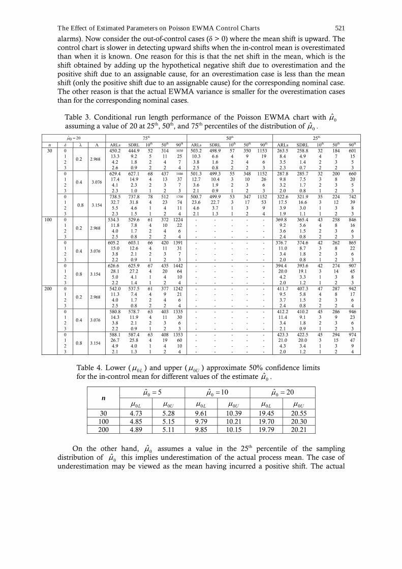
First consider the in-control cases (δ = 0) in Tables 1-3. The in-control nominal ARL values are approximately equal to the corresponding SDRL values. This is also true for the cases when the mean is under or over estimated. From a comparison of the overestimation and underestimation performance with the nominal, it can be seen that the run length distribution is noticeably affected by the value of the mean estimate. This is as it would be if the process mean were to shift from the nominal to the estimate. Note that the case of overestimation may be viewed as a case where the mean has incurred a hypothetical negative shift. To see this, consider 0ˆ 5µ = . With sample sizes 30, 100, and 200, 0ˆ 5µ = corresponds to the 75th percentile of the sampling distribution of 0µ̂ for 0µ = 4.73, 4.85, and 4.89, respectively. As a consequence of the overestimation of the mean, the actual EWMA variance would also be smaller than it is expected to be. Therefore, the false alarms are expected to be less frequent than the nominal values. Note that overestimation of the mean does not imply violations of the lower control limit (otherwise we would have false
The Effect of Estimated Parameters on Poisson EWMA Control Charts 521
alarms). Now consider the out-of-control cases (δ > 0) where the mean shift is upward. The control chart is slower in detecting upward shifts when the in-control mean is overestimated than when it is known. One reason for this is that the net shift in the mean, which is the shift obtained by adding up the hypothetical negative shift due to overestimation and the positive shift due to an assignable cause, for an overestimation case is less than the mean shift (only the positive shift due to an assignable cause) for the corresponding nominal case. The other reason is that the actual EWMA variance is smaller for the overestimation cases than for the corresponding nominal cases.
Table 3. Conditional run length performance of the Poisson EWMA chart with 0µ̂ assuming a value of 20 at 25th, 50th, and 75th percentiles of the distribution of 0µ̂ .
ˆ 200µ = 75th 50th 25th n δ λ A ARLs SDRL 10th 50th 90th ARLs SDRL 10th 50th 90th ARLs SDRL 10th 50th 90th
30 0 450.2 444.9 52 314 1030 503.2 498.9 57 350 1153 263.5 258.8 32 184 601 1 13.3 9.2 5 11 25 10.3 6.6 4 9 19 8.4 4.9 4 7 15 2 4.2 1.8 2 4 7 3.8 1.6 2 4 6 3.5 1.4 2 3 5 3
0.2 2.968
2.6 0.9 2 2 4 2.5 0.8 2 2 3 2.3 0.7 2 2 3 0 629.4 627.1 68 437 1446 501.3 499.3 55 348 1152 287.8 285.7 32 200 660 1 17.4 14.9 4 13 37 12.7 10.4 3 10 26 9.8 7.5 3 8 20 2 4.1 2.3 2 3 7 3.6 1.9 2 3 6 3.2 1.7 2 3 5 3
0.4 3.076
2.3 1.0 1 2 3 2.1 0.9 1 2 3 2.0 0.8 1 2 3 0 738.5 737.8 78 512 1700 500.7 499.9 53 347 1152 322.6 321.9 35 224 742 1 32.7 31.8 4 23 74 23.6 22.7 3 17 53 17.5 16.6 3 12 39 2 5.5 4.6 1 4 11 4.6 3.7 1 3 9 3.9 3.0 1 3 8
3
0.8 3.154
2.3 1.5 1 2 4 2.1 1.3 1 2 4 1.9 1.1 1 2 3 100 0 534.3 529.6 61 372 1224 - - - - - 369.8 365.4 43 258 846
1 11.8 7.8 4 10 22 - - - - - 9.2 5.6 4 8 16 2 4.0 1.7 2 4 6 - - - - - 3.6 1.5 2 3 6 3
0.2 2.968
2.5 0.8 2 2 4 - - - - - 2.4 0.8 2 2 3 0 605.2 603.1 66 420 1391 - - - - - 376.7 374.6 42 262 865 1 15.0 12.6 4 11 31 - - - - - 11.0 8.7 3 8 22 2 3.8 2.1 2 3 7 - - - - - 3.4 1.8 2 3 6 3
0.4 3.076
2.2 0.9 1 2 3 - - - - - 2.0 0.8 1 2 3 0 626.6 625.9 67 435 1442 - - - - - 394.4 393.6 42 274 907 1 28.1 27.2 4 20 64 - - - - - 20.0 19.1 3 14 45 2 5.0 4.1 1 4 10 - - - - - 4.2 3.3 1 3 8
3
0.8 3.154
2.2 1.4 1 2 4 - - - - - 2.0 1.2 1 2 3 200 0 542.0 537.5 61 377 1242 - - - - - 411.7 407.3 47 287 942
1 11.3 7.4 4 9 21 - - - - - 9.5 5.8 4 8 17 2 4.0 1.7 2 4 6 - - - - - 3.7 1.5 2 3 6 3
0.2 2.968
2.5 0.8 2 2 4 - - - - - 2.4 0.8 2 2 4 0 580.8 578.7 63 403 1335 - - - - - 412.2 410.2 45 286 946 1 14.3 11.9 4 11 30 - - - - - 11.4 9.1 3 9 23 2 3.8 2.1 2 3 6 - - - - - 3.4 1.8 2 3 6 3
0.4 3.076
2.2 0.9 1 2 3 - - - - - 2.1 0.9 1 2 3 0 588.1 587.4 63 408 1353 - - - - - 423.3 422.5 45 294 974 1 26.7 25.8 4 19 60 - - - - - 21.0 20.0 3 15 47 2 4.9 4.0 1 4 10 - - - - - 4.3 3.4 1 3 9
3
0.8 3.154
2.1 1.3 1 2 4 - - - - - 2.0 1.2 1 2 4
Table 4. Lower ( 0Lµ ) and upper ( 0Uµ ) approximate 50% confidence limits for the in-control mean for different values of the estimate 0µ̂ .
0ˆ 5µ = 0ˆ 10µ = 0ˆ 20µ = n
0Lµ 0Uµ 0Lµ 0Uµ 0Lµ 0Uµ
30 4.73 5.28 9.61 10.39 19.45 20.55 100 4.85 5.15 9.79 10.21 19.70 20.30 200 4.89 5.11 9.85 10.15 19.79 20.21
On the other hand, 0µ̂ assumes a value in the 25th percentile of the sampling distribution of 0µ̂ this implies underestimation of the actual process mean. The case of underestimation may be viewed as the mean having incurred a positive shift. The actual
522 Testik, McCullough and Borror
EWMA mean and variance would be larger than they would be expected. Therefore, the false alarms are expected to be more frequent than the nominal values. However, positive shifts in the mean due to an assignable cause are detected faster when the mean is underestimated than when the mean is known.
Increasing sample sizes yield better performance as expected. The typical effect of larger smoothing constant λ compared to a smaller smoothing constant is faster detection of larger shifts. Smaller smoothing constants are generally better than the larger ones in detecting small shifts of the mean.
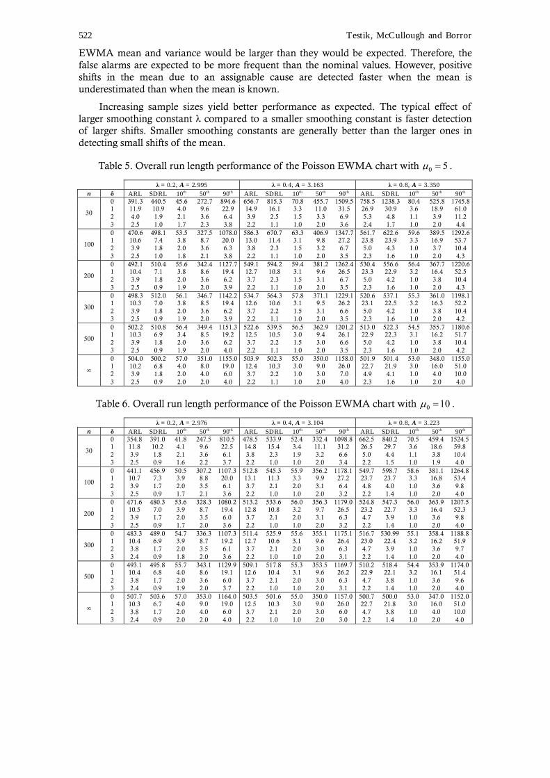
Table 5. Overall run length performance of the Poisson EWMA chart with 0 5µ = .
λ = 0.2, A = 2.995 λ = 0.4, A = 3.163 λ = 0.8, A = 3.350 n δ ARL SDRL 10th 50th 90th ARL SDRL 10th 50th 90th ARL SDRL 10th 50th 90th
0 391.3 440.5 45.6 272.7 894.6 656.7 815.3 70.8 455.7 1509.5 758.5 1238.3 80.4 525.8 1745.8 1 11.9 10.9 4.0 9.6 22.9 14.9 16.1 3.3 11.0 31.5 26.9 30.9 3.6 18.9 61.0 2 4.0 1.9 2.1 3.6 6.4 3.9 2.5 1.5 3.3 6.9 5.3 4.8 1.1 3.9 11.2
30
3 2.5 1.0 1.7 2.3 3.8 2.2 1.1 1.0 2.0 3.6 2.4 1.7 1.0 2.0 4.4 0 470.6 498.1 53.5 327.5 1078.0 586.3 670.7 63.3 406.9 1347.7 561.7 622.6 59.6 389.5 1292.6 1 10.6 7.4 3.8 8.7 20.0 13.0 11.4 3.1 9.8 27.2 23.8 23.9 3.3 16.9 53.7 2 3.9 1.8 2.0 3.6 6.3 3.8 2.3 1.5 3.2 6.7 5.0 4.3 1.0 3.7 10.4
100
3 2.5 1.0 1.8 2.1 3.8 2.2 1.1 1.0 2.0 3.5 2.3 1.6 1.0 2.0 4.3 0 492.1 510.4 55.6 342.4 1127.7 549.1 594.2 59.4 381.2 1262.4 530.4 556.6 56.4 367.7 1220.6 1 10.4 7.1 3.8 8.6 19.4 12.7 10.8 3.1 9.6 26.5 23.3 22.9 3.2 16.4 52.5 2 3.9 1.8 2.0 3.6 6.2 3.7 2.3 1.5 3.1 6.7 5.0 4.2 1.0 3.8 10.4
200
3 2.5 0.9 1.9 2.0 3.9 2.2 1.1 1.0 2.0 3.5 2.3 1.6 1.0 2.0 4.3 0 498.3 512.0 56.1 346.7 1142.2 534.7 564.3 57.8 371.1 1229.1 520.6 537.1 55.3 361.0 1198.1 1 10.3 7.0 3.8 8.5 19.4 12.6 10.6 3.1 9.5 26.2 23.1 22.5 3.2 16.3 52.2 2 3.9 1.8 2.0 3.6 6.2 3.7 2.2 1.5 3.1 6.6 5.0 4.2 1.0 3.8 10.4
300
3 2.5 0.9 1.9 2.0 3.9 2.2 1.1 1.0 2.0 3.5 2.3 1.6 1.0 2.0 4.2 0 502.2 510.8 56.4 349.4 1151.3 522.6 539.5 56.5 362.9 1201.2 513.0 522.3 54.5 355.7 1180.6 1 10.3 6.9 3.4 8.5 19.2 12.5 10.5 3.0 9.4 26.1 22.9 22.3 3.1 16.2 51.7 2 3.9 1.8 2.0 3.6 6.2 3.7 2.2 1.5 3.0 6.6 5.0 4.2 1.0 3.8 10.4
500
3 2.5 0.9 1.9 2.0 4.0 2.2 1.1 1.0 2.0 3.5 2.3 1.6 1.0 2.0 4.2 0 504.0 500.2 57.0 351.0 1155.0 503.9 502.3 55.0 350.0 1158.0 501.9 501.4 53.0 348.0 1155.0 1 10.2 6.8 4.0 8.0 19.0 12.4 10.3 3.0 9.0 26.0 22.7 21.9 3.0 16.0 51.0 2 3.9 1.8 2.0 4.0 6.0 3.7 2.2 1.0 3.0 7.0 4.9 4.1 1.0 4.0 10.0
∞
3 2.5 0.9 2.0 2.0 4.0 2.2 1.1 1.0 2.0 4.0 2.3 1.6 1.0 2.0 4.0
Table 6. Overall run length performance of the Poisson EWMA chart with 0 10µ = .
λ = 0.2, A = 2.976 λ = 0.4, A = 3.104 λ = 0.8, A = 3.223 n δ ARL SDRL 10th 50th 90th ARL SDRL 10th 50th 90th ARL SDRL 10th 50th 90th
0 354.8 391.0 41.8 247.5 810.5 478.5 533.9 52.4 332.4 1098.8 662.5 840.2 70.5 459.4 1524.5 1 11.8 10.2 4.1 9.6 22.5 14.8 15.4 3.4 11.1 31.2 26.5 29.7 3.6 18.6 59.8 2 3.9 1.8 2.1 3.6 6.1 3.8 2.3 1.9 3.2 6.6 5.0 4.4 1.1 3.8 10.4
30
3 2.5 0.9 1.6 2.2 3.7 2.2 1.0 1.0 2.0 3.4 2.2 1.5 1.0 1.9 4.0 0 441.1 456.9 50.5 307.2 1107.3 512.8 545.3 55.9 356.2 1178.1 549.7 598.7 58.6 381.1 1264.8 1 10.7 7.3 3.9 8.8 20.0 13.1 11.3 3.3 9.9 27.2 23.7 23.7 3.3 16.8 53.4 2 3.9 1.7 2.0 3.5 6.1 3.7 2.1 2.0 3.1 6.4 4.8 4.0 1.0 3.6 9.8
100
3 2.5 0.9 1.7 2.1 3.6 2.2 1.0 1.0 2.0 3.2 2.2 1.4 1.0 2.0 4.0 0 471.6 480.3 53.6 328.3 1080.2 513.2 533.6 56.0 356.3 1179.0 524.8 547.3 56.0 363.9 1207.5 1 10.5 7.0 3.9 8.7 19.4 12.8 10.8 3.2 9.7 26.5 23.2 22.7 3.3 16.4 52.3 2 3.9 1.7 2.0 3.5 6.0 3.7 2.1 2.0 3.1 6.3 4.7 3.9 1.0 3.6 9.8
200
3 2.5 0.9 1.7 2.0 3.6 2.2 1.0 1.0 2.0 3.2 2.2 1.4 1.0 2.0 4.0 0 483.3 489.0 54.7 336.3 1107.3 511.4 525.9 55.6 355.1 1175.1 516.7 530.99 55.1 358.4 1188.8 1 10.4 6.9 3.9 8.7 19.2 12.7 10.6 3.1 9.6 26.4 23.0 22.4 3.2 16.2 51.9 2 3.8 1.7 2.0 3.5 6.1 3.7 2.1 2.0 3.0 6.3 4.7 3.9 1.0 3.6 9.7
300
3 2.4 0.9 1.8 2.0 3.6 2.2 1.0 1.0 2.0 3.1 2.2 1.4 1.0 2.0 4.0 0 493.1 495.8 55.7 343.1 1129.9 509.1 517.8 55.3 353.5 1169.7 510.2 518.4 54.4 353.9 1174.0 1 10.4 6.8 4.0 8.6 19.1 12.6 10.4 3.1 9.6 26.2 22.9 22.1 3.2 16.1 51.4 2 3.8 1.7 2.0 3.6 6.0 3.7 2.1 2.0 3.0 6.3 4.7 3.8 1.0 3.6 9.6
500
3 2.4 0.9 1.9 2.0 3.7 2.2 1.0 1.0 2.0 3.1 2.2 1.4 1.0 2.0 4.0 0 507.7 503.6 57.0 353.0 1164.0 503.5 501.6 55.0 350.0 1157.0 500.7 500.0 53.0 347.0 1152.0 1 10.3 6.7 4.0 9.0 19.0 12.5 10.3 3.0 9.0 26.0 22.7 21.8 3.0 16.0 51.0 2 3.8 1.7 2.0 4.0 6.0 3.7 2.1 2.0 3.0 6.0 4.7 3.8 1.0 4.0 10.0
∞
3 2.4 0.9 2.0 2.0 4.0 2.2 1.0 1.0 2.0 3.0 2.2 1.4 1.0 2.0 4.0
The Effect of Estimated Parameters on Poisson EWMA Control Charts 523
5. The Overall Performance (Performance Under Estimation Uncertainty)
In reality one would not really know how the estimated parameter compares to the observed parameter. Therefore, it would also be useful to evaluate the unconditional performance of a Poisson EWMA with estimated mean. Since we have the expressions to evaluate the conditional performance, it is straightforward to evaluate the unconditional performance of the chart. Because the estimator is a random variable itself and has a probability distribution, the unconditional (also called marginal or overall) performance of the chart is the conditional performance averaged over all possible values for the parameter estimator. That is, the moments and the percentiles of the conditional run length distribution are viewed as random variables.
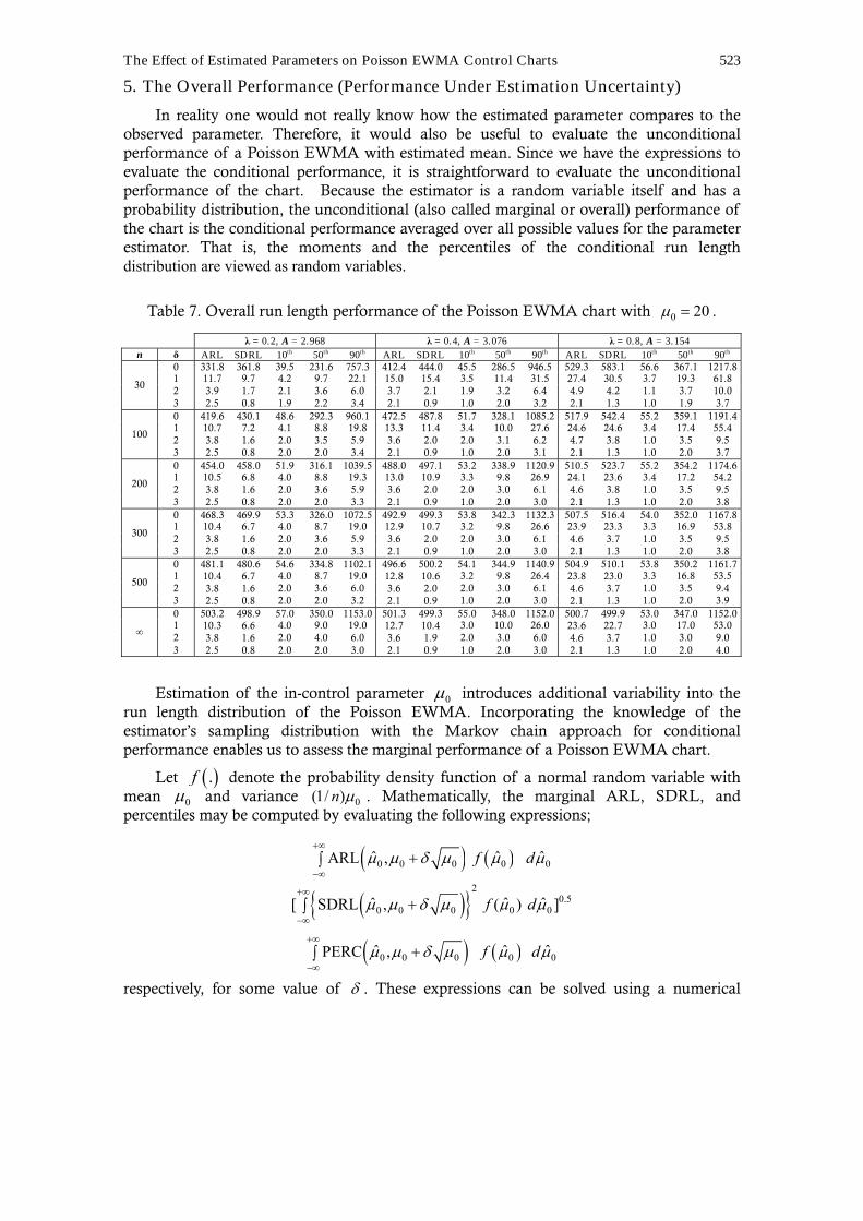
Table 7. Overall run length performance of the Poisson EWMA chart with 0 20µ = .
λ = 0.2, A = 2.968 λ = 0.4, A = 3.076 λ = 0.8, A = 3.154 n δ ARL SDRL 10th 50th 90th ARL SDRL 10th 50th 90th ARL SDRL 10th 50th 90th
0 331.8 361.8 39.5 231.6 757.3 412.4 444.0 45.5 286.5 946.5 529.3 583.1 56.6 367.1 1217.8 1 11.7 9.7 4.2 9.7 22.1 15.0 15.4 3.5 11.4 31.5 27.4 30.5 3.7 19.3 61.8 2 3.9 1.7 2.1 3.6 6.0 3.7 2.1 1.9 3.2 6.4 4.9 4.2 1.1 3.7 10.0
30
3 2.5 0.8 1.9 2.2 3.4 2.1 0.9 1.0 2.0 3.2 2.1 1.3 1.0 1.9 3.7 0 419.6 430.1 48.6 292.3 960.1 472.5 487.8 51.7 328.1 1085.2 517.9 542.4 55.2 359.1 1191.4 1 10.7 7.2 4.1 8.8 19.8 13.3 11.4 3.4 10.0 27.6 24.6 24.6 3.4 17.4 55.4 2 3.8 1.6 2.0 3.5 5.9 3.6 2.0 2.0 3.1 6.2 4.7 3.8 1.0 3.5 9.5
100
3 2.5 0.8 2.0 2.0 3.4 2.1 0.9 1.0 2.0 3.1 2.1 1.3 1.0 2.0 3.7 0 454.0 458.0 51.9 316.1 1039.5 488.0 497.1 53.2 338.9 1120.9 510.5 523.7 55.2 354.2 1174.6 1 10.5 6.8 4.0 8.8 19.3 13.0 10.9 3.3 9.8 26.9 24.1 23.6 3.4 17.2 54.2 2 3.8 1.6 2.0 3.6 5.9 3.6 2.0 2.0 3.0 6.1 4.6 3.8 1.0 3.5 9.5
200
3 2.5 0.8 2.0 2.0 3.3 2.1 0.9 1.0 2.0 3.0 2.1 1.3 1.0 2.0 3.8 0 468.3 469.9 53.3 326.0 1072.5 492.9 499.3 53.8 342.3 1132.3 507.5 516.4 54.0 352.0 1167.8 1 10.4 6.7 4.0 8.7 19.0 12.9 10.7 3.2 9.8 26.6 23.9 23.3 3.3 16.9 53.8 2 3.8 1.6 2.0 3.6 5.9 3.6 2.0 2.0 3.0 6.1 4.6 3.7 1.0 3.5 9.5
300
3 2.5 0.8 2.0 2.0 3.3 2.1 0.9 1.0 2.0 3.0 2.1 1.3 1.0 2.0 3.8 0 481.1 480.6 54.6 334.8 1102.1 496.6 500.2 54.1 344.9 1140.9 504.9 510.1 53.8 350.2 1161.7 1 10.4 6.7 4.0 8.7 19.0 12.8 10.6 3.2 9.8 26.4 23.8 23.0 3.3 16.8 53.5 2 3.8 1.6 2.0 3.6 6.0 3.6 2.0 2.0 3.0 6.1 4.6 3.7 1.0 3.5 9.4
500
3 2.5 0.8 2.0 2.0 3.2 2.1 0.9 1.0 2.0 3.0 2.1 1.3 1.0 2.0 3.9 0 503.2 498.9 57.0 350.0 1153.0 501.3 499.3 55.0 348.0 1152.0 500.7 499.9 53.0 347.0 1152.0 1 10.3 6.6 4.0 9.0 19.0 12.7 10.4 3.0 10.0 26.0 23.6 22.7 3.0 17.0 53.0 2 3.8 1.6 2.0 4.0 6.0 3.6 1.9 2.0 3.0 6.0 4.6 3.7 1.0 3.0 9.0
∞
3 2.5 0.8 2.0 2.0 3.0 2.1 0.9 1.0 2.0 3.0 2.1 1.3 1.0 2.0 4.0
Estimation of the in-control parameter 0µ introduces additional variability into the run length distribution of the Poisson EWMA. Incorporating the knowledge of the estimator’s sampling distribution with the Markov chain approach for conditional performance enables us to assess the marginal performance of a Poisson EWMA chart.
Let ( ).f denote the probability density function of a normal random variable with mean 0µ and variance 0(1/ )µn . Mathematically, the marginal ARL, SDRL, and percentiles may be computed by evaluating the following expressions;
( )0 0 0ˆARL ,µ µ δ µ+∞
−∞+∫ ( )0ˆ µf 0µ̂d
( ){ }2
0 0 0ˆ[ SDRL ,µ µ δ µ+∞
−∞+∫ 0ˆ( )µf 0.5
0ˆ ]µd
( )0 0 0ˆPERC , µ µ δ µ+∞
−∞+∫ ( )0µ̂f 0ˆ µd
respectively, for some value of δ . These expressions can be solved using a numerical
524 Testik, McCullough and Borror
integration procedure. For this paper, we made use of the recursive adaptive Simpson quadrature in Matlab® v6.0.
The marginal run length performances are summarized in Tables 5, 6, and 7 for the values 5, 10, and 20 of 0µ , respectively. In the tables, the performance metrics are weighted averages over all the values that the estimation may yield for the in-control mean 0µ . To study how large the sample size should be to perform essentially like the known parameter case, the values 30, 100, 200, 300, 500, and ∞ for n are evaluated. The infinite sample size (n = ∞) corresponds to the known parameter or the nominal case. Again, the λ and A combinations were chosen in order to achieve an ARL0 of 500 when the process mean was known. The ARL, SDRL and 10th, 50th (median), and 90th percentiles of the run length distribution are given for each of the cases considered in the tables.
In Tables 5-7 for the overall performance, the in-control SDRL values are generally larger than the ARL0 values since the sampling variation of the mean is incorporated into the marginal run length distribution. For all cases where λ = 0.2, the ARL0 of the Poisson EWMA with estimated mean is smaller than the corresponding case with known mean. This suggests that the chart signals false alarms more frequently on average when the mean is estimated than when the mean is known. Similarly, the percentiles of the run length distribution for an in control process indicate a shorter run length when the mean is estimated than when the mean is known. On the other hand, for the other cases where λ is 0.4 or 0.8, the ARL0 values of the chart with estimated mean are generally larger than the corresponding cases with known mean. Although this suggests that the expected false alarm rate of the chart when λ is 0.4 or 0.8 is less with estimated mean than with known mean, further assessment of the percentiles is necessary to get a better picture. For example consider Table 6, λ = 0.8, and n = 30. In this case, ARL0 = 662.5 and the 10th and 50th percentiles are smaller than in the known mean case, which indicates that shorter runs are more likely. Still, the 90th percentile is larger than in the known mean case, which indicates that the larger ARL0 is a result of skewness of the run length distribution. The ARL0 values and percentiles get close to the nominal values as n increases, which is expected since the estimated parameter converges to the true parameter.
The marginal out-of-control performance of Poisson EWMA chart is also affected by estimation. In all studied cases, the ARL1 values are larger when the mean is estimated than when it is known. The difference in the performance gets smaller as n increases.
The choice of λ would depend on how fast one wants to detect a shift of given size. From the tables, the sample size n greater than 300 for estimating the mean of a Poisson EWMA chart would generally result in marginal operational performance fairly close to the one with known mean.
6. Example
To illustrate the effect of sample size on the control chart design, we generated Poisson random numbers with 0 5µ = and estimated the in-control mean from a sample of size 30 and from a sample of size 200. The in-control mean estimates are 0ˆ 5.67µ = and
0ˆ 4.93µ = . The estimate using the 200 observations is much closer to the actual value. Suppose now that an ARL0 performance of 250 is desired and the smoothing constant λ is chosen to be 0.2. The values for the constant A would be 2.731 and 2.734 for 0ˆ 5.67µ = and 0ˆ 4.93µ = , respectively. Furthermore, corresponding control limits and initial EWMA statistic for these cases would be (hL = 3.502, hU = 7.838, Z0 = 5.67) and (hL = 2.907, hU = 6.954, Z0 = 4.93). Notice the differences between the widths of the control limits for the
The Effect of Estimated Parameters on Poisson EWMA Control Charts 525
two charts. Although, the case of n = 200 is expected to perform approximately as designed, this won’t be true for the n = 30 case.
7. Concluding Remarks
The Poisson EWMA control chart would be very useful in any situation that involves count data following a Poisson distribution such as in healthcare applications (monitoring billing errors or patient errors resulting in serious injury or death), intrusion detection (detecting anomalies or attacks on computer systems), and manufacturing (defects, nonconforming items). The Poisson EWMA could be used and should be used if small shifts from normal operating conditions are important to detect quickly.
Actual values of process parameters for designing a control chart are often unknown in practice. In such cases, a typical approach is to conduct a retrospective study, where a reference sample of observations is obtained and then used for estimating these unknown parameters. However, operational performance of a control chart may be significantly different from the expected performance if the parameters are not well estimated. In this study, we assess the performance of the Poisson EWMA control chart with estimated mean. The Markov chain approach is used to evaluate both conditional and marginal run length performance of the chart in terms of average run length, standard deviation of the run length, and percentiles of the run length distribution. Various shift magnitudes, estimated mean values, and sample sizes are used for investigation. Our results indicate that sample sizes greater than 300 for estimating process mean would generally yield fairly close performance to the chart with known process mean. The in-control average run length performance may be affected significantly when estimation is used. Furthermore, for smaller EWMA smoothing constants, say 0.2, the chart with an estimated mean triggers more false alarms than the chart with the known mean. A smoothing constant greater than 0.2 may be suggested, however, this choice depends on the required sensitivity of the chart with respect to detecting changes in the mean.
Acknowledgments
We would like to thank the Editors and two anonymous referees for their insightful comments.
References
1. Roberts, S. W. (1959). Control chart tests based on geometric moving averages. Technometrics, 1, 239-250.
2. Montgomery, D. C. (2006). Introduction to Statistical Quality Control, 6th ed. John Wiley and Sons, New York, NY.
3. Brook, D. and Evans, D. A. (1972). An approach to the probability distribution of CUSUM run length. Biometrika, 59, 539-549.
4. Lucas, J. M. (1985). Counted data CUSUM’s. Technometrics, 27, 129-144.
5. White, C. H. and Keats, J. B. (1996). ARLs and higher-order run-length moments for the poisson CUSUM. Journal of Quality Technology, 28, 363-369.
6. White, C. H., Keats, J. B. and Stanley, J. (1997). Poisson CUSUM vs. c-chart for defect rate . Quality Engineering, 9, 673-679.
7. Gan, F. F. (1989). Monitoring Poisson observations using modified exponentially weighted moving average control charts. Communications in Statistics and Simulation, 19, 103-124.
526 Testik, McCullough and Borror
8. Borror, C. M., Champ, C. W. and Rigdon, S. E. (1998). Poisson EWMA control charts. Journal of Quality Technology, 30, 352-361.
9. Borror, C. M., Keats, J. B. and Montgomery, D. C. (2000). Robustness of the time between events CUSUM. International Journal of Production Research 41, 3435-3444.
10. Gan, F. F. (1992). Exact run length distribution for One-Sided Exponential CUSUM Schemes. Statistica Sinica, 2, 297–312.
11. Gan, F. F. (1994). Design of Optimal Exponential CUSUM control charts. Journal of Quality Technology, 26, 109-124.
12. Champ, C. W. and Rigdon, S. E. (1991). A comparison of the Markov chain and the integral equation approaches for evaluating the run length distribution of quality control charts. Communication in Statistics – Simulation and Computation, 20, 191–204.
13. Chao, M. T. (2000). Applications of Markov chains in quality-related matters in Statistical Process Monitoring and Optimization, edited by S. H. Park, and G. G. Vining, Marcel-Dekker, New York, 175–188.
14. Crowder, S. V. (1987a). Computation of ARL for combined individual measurement and moving range charts. Journal of Quality Technology, 19, 98–102.
15. Crowder, S. V. (1987b). A program for the computation of ARL for combined individual measurement and moving range charts. Journal of Quality Technology, 19, 103–106.
16. Fu, J. C., Spiring, F.A. and Xie, H. (2002). On the average run lengths of quality control schemes using a Markov chain approach. Statistics & Probability Letters, 56, 369–380.
17. Lucas, J. M. and Saccucci, M. S. (1990). Exponentially weighted moving average control Schemes: properties and enhancements. Technometrics, 32, 1–12.
18. Reynold, M. R. (1975). Approximations to the average run length in cumulative sum control charts. Technometrics, 25, 295–301.
19. Robinson, P. B. and Ho, T. Y. (1978). Average run lengths of geometric moving average charts by numerical methods. Technometrics, 20, 85–93.
20. Saccucci, M. S. and Lucas, J. M. (1990). Average run lengths for exponentially moving average control schemes using the Markov chain approach. Journal of Quality Technology, 22, 154–158.
21. Vardeman, S. and Ray, D. (1985). Average run lengths for CUSUM when observations are exponentially distributed. Technometrics, 27, 145–150.
22. Waldmann, K. H. (1986). Bounds for the distribution of the run length of one-sided and two-sided CUSUM quality control schemes. Technometrics, 28, 61-67.
23. Woodall, W. H. (1983). The distribution of run length of one-sided CUSUM procedures for continuous random variables. Technometrics, 25, 295–301.
24. Woodall, W. H. (1984). On the Markov chain approach to the two-sided CUSUM procedure. Technometrics, 26, 41-46.
25. Jones, L. A. (2002). The statistical design of EWMA control charts with estimated parameters. Journal of Quality Technology, 34, 277-288.
26. Jones, L. A., Champ, C. W. and Rigdon, S. E. (2001). The performance of exponentially weighted moving average charts with estimated parameters. Technometrics, 43, 156-167.
The Effect of Estimated Parameters on Poisson EWMA Control Charts 527
Authors’ Biographies:
Murat Caner Testik is an Associate Professor and Chair of the Department of Industrial Engineering at Hacettepe University, Ankara, Turkey. His research interests include statistical quality control and data mining for quality improvement. He is the co-author of two book chapters and several publications in the engineering and statistical literature.
B. D. McCullough is a Professor of Decision Sciences at Drexel University. His research focuses on the accuracy of statistical software, the reproducibility of published research, and data mining. His publications have appeared in the economics and statistics literatures.
Connie Borror is an Associate Professor in the Department of Mathematical Sciences and Applied Computing. Her research areas include response surface methodology, statistical process control, and experimental design with applications in engineering and other sciences. She is the co-author of several journal articles, two books, and three book chapters.

![Quality Technology & QTQM - unimi.it · 118 Ferrari and Manzi RELationship) [12]. The second approach does not assume any model, but uses](https://img.pdfslide.us/doc/110x75/5b1b69b17f8b9a46258e803f/quality-technology-qtqm-unimiit-118-ferrari-and-manzi-relationship-12.jpg)