Quality of TEC Estimated with Mod_Ion Using GPS and GLONASS

Hindawi Publishing CorporationMathematical Problems in EngineeringVolume 2009, Article ID 794578, 16 pagesdoi:10.1155/2009/794578

Research ArticleQuality of TEC Estimated with Mod Ion Using GPSand GLONASS Data

Paulo de Oliveira Camargo

Department of Cartography, Faculty of Science and Technology, Sao Paulo State University (UNESP),Rua Roberto Simonsen 305, 19060-900 Presidente Prudente, SP, Brazil

Correspondence should be addressed to Paulo de Oliveira Camargo, [email protected]

Received 1 July 2009; Accepted 28 September 2009

Recommended by Silvia Maria Giuliatti Winter

One of the largest sources of error in positioning and navigation with GNSS is the ionosphere, andthe associated error is directly proportional to the TEC and inversely proportional to the square ofthe signal frequency that propagates through the ionosphere. The equatorial region, especially inBrazil, is where the highest spatial and temporal value variations of the TEC are seen, and wherethese various features of the ionosphere, such as the equatorial anomaly and scintillation, can befound. Thus, the development and assessments of ionospheric models are important. In this paper,the quality of the TEC was evaluated, as well as the systematic error in the L1 carrier and the inter-frequency biases of satellites and receivers estimated with the Mod Ion, observable from GPS andintegration with the GLONASS, collected with dual frequency receivers.

Copyright q 2009 Paulo de Oliveira Camargo. This is an open access article distributed underthe Creative Commons Attribution License, which permits unrestricted use, distribution, andreproduction in any medium, provided the original work is properly cited.

1. Introduction

The Global Navigation Satellite System (GNSS) is one of the most advanced technologiesand has revolutionized the activities related to navigation and positioning from spacetechnology. A main component of GNSS is the Global Positioning System (GPS), developedby the United States, and Global’naya Navigatsionnaya Sputnikowaya Sistema (GLONASS)of responsibility of the Republic of Russia. A relevant fact is that, in December 2005, thefirst GALILEO satellite was launched, which is being developed by the European Unionand must come into operation in 2013. The GNSS is composed by the so-called (SatelliteBased Augmentation System) SBAS, such as the Wide Area Augmentation System (WAAS)in USA, European Geostationary Navigation Overlay Service (EGNOS) in Europe, Multi-functional Satellite-Based Augmentation Service (MSAS) in Japan, and Satellite NavigationAugmentation System (SNAS) in China [1].

2 Mathematical Problems in Engineering

In general, most users simply use the GNSS system to get their coordinates, withoutbeing committed to details, but for the quality of information (precision) provided by it,except aviation. This quality information is very optimistic, demanding attention from users.However, certain applications require the knowledge of the various processes related tothe system. The mitigation of the effects of the atmosphere (troposphere and ionosphere)over GNSS observables requires knowledge of the signal analysis and its behavior inthe atmosphere, requiring interaction with other sciences such as Aeronomy, Meteorology,among others. Accordingly, this interaction allows studies related to the behavior of theionosphere and the troposphere to be made from GNSS observables. In Brazil, the ionosphereshows a very complex behavior, for being located near the geomagnetic equator, requiring thedevelopment of models and appropriate studies for the region [1–12].

With the Selective Availability (SA) deactivation, in the case of GPS, the error dueto the ionosphere has become a major source of systematic error in positioning, especiallyin periods of high solar activity for one frequency GNSS users, in the conventional pointpositioning as well as relative positioning. Another effect that affects considerably the GNSSsignals is ionosphere scintillation, a result of propagating the signal through a region in whichthere are irregularities in the density of electrons.

The error due to the ionosphere depends on the Total Electron Content (TEC) presentin the ionosphere and in signal frequency. Users of, at least, dual frequency receivers canmake corrections of this effect, using the ionospheric free linear combination. This observableeliminates first-order ionospheric effect. Users of single frequency receivers, however, needto correct the systematic effect observables due to the ionosphere. The quantification ofthis effect can be done by [3, 4, 12]: coefficients transmitted by navigation messages, usingthe Klobuchar model; observations collected with one or dual frequency GNSS receivers of(Ionosphere map Exchange format) IONEX archives obtained from Global Ionospheric Maps(GIM), which provide values of vertical TEC (VTEC) in a grid with spatial resolution of5◦ × 2.5◦ in longitude and latitude, respectively, and temporal resolution of 2 hours [13].

In the geodetic community, one of the models used and implemented in commercialsoftware, to minimize the effects of the ionosphere on GPS observables, is the Klobucharmodel. This model, also called Broadcast model, estimates the systematic error due tothe ionosphere to one frequency receivers [14] and its coefficients are transmitted by GPSsatellites in navigation messages. However, this model removes around 50% to 60% of thetotal effect [15, 16]. Being more appropriate for use in regions of middle latitudes, which isthe more predictable ionospheric region, where the ionosphere has a more regular behavior.However, this is not an appropriate model to be used in Brazil, where there is high variationin the density of electrons as well as in South America. So with the need to have a moreeffective correction strategy of the ionosphere effect, several models were developed byvarious research centers and universities, using observations collected with dual frequencyGPS receivers. In terms of South America, we can quote the (La Plata Ionospheric Model)LPIM model, developed at (Astronomical and Geophysical Sciences Faculty of UniversidadNacional de La Plata) FCAG/UNLP, Argentine [2] and the Regional Model of Ionosphere(Mod Ion) developed in FCT/UNESP, Brazil [3].

The accuracy of VTEC values in the final IONEX files grid (∼11 days of latency) is 2–8TEC units (TECUs) and for rapid files (<24 hours) of 2–9 TECU [17]. Ciraolo et al. [18], ina calibration process, determined the interfrequency bias (IFB) of a pair of receivers, whichranged from 1.4 to 8.8 TECU. This paper aims to assess the quality of TEC and the error in theL1 carrier estimated with the Mod Ion, from GPS observables and integration with the onesfrom GLONASS, collected with dual frequency receivers.

Mathematical Problems in Engineering 3

The paper is organized as follows. In Section 2 there is a brief description of impactof the ionosphere on the propagation of GNSS signals; Section 3 describes the equations,based on the geometry-free linear combination of observables collected with dual frequencyreceivers, used in the Mod Ion, as well as gets the TEC and the systematic error due tothe ionosphere in the L1 carrier, and some aspects of adjustment by the least squares; theresults and analysis of the experiments in order to verify the quality of the TEC provided bymodel, as well as the IFB of the satellites and receivers are presented in Section 4; based onthe experiments, conclusions and future works will be presented in Section 5.

2. Impact of the Ionosphere on the Propagation of GNSS Signals

The terrestrial atmosphere, for practical purposes, can be considered as a set of gas layers,spherical and concentric to the Earth. Its structure is related to various thermal, chemical, andelectromagnetic elements. These combined parameters vary depending on the time, latitude,longitude, time of year, and solar activity.

With respect to the propagation of electromagnetic waves, the Earth’s atmosphereis divided into ionosphere and troposphere. In this division, the troposphere is the layerbetween the Earth’s surface up to 50 km in height. It is composed of neutral particles, andthe highest concentration of gas is found on up to a height of 12 km, consisting of nitrogen,oxygen, carbon dioxide, argon, water vapor, among others. The propagation of the signal inthe troposphere depends mainly on the water vapor content, air pressures, and temperature.For frequencies below 30 GHz, the refraction does not depend on the frequency of the signaltransmitted [16].

The ionosphere is defined as the portion of the upper atmosphere, where there issufficient ionization to affect the propagation of radio waves [19]. Unlike the troposphere,it is a dispersive medium; that is, in this case, signal propagation depends on the frequency. Itis characterized mainly by the formation of ions and electrons, and it starts at around 50 km,extending to approximately 1000 km in height.

In the region covered by the ionosphere, the electron density is sufficient to alter thepropagation of electromagnetic waves. The ions and free electrons in the ionosphere aremainly created by the process of photo ionization. The ionospheric photo ionization is theabsorption of solar radiation, predominantly in the range of extreme ultraviolet and X-raysby neutral atmospheric elements [19–21]. The ionosphere as a dispersive means affects themodulation and phase of the carrier, causing, respectively, a delay and an advance [16]. Thedelay is also referred to as ionospheric delay and increases the apparent length of the pathtraveled by the signal.

The troposphere effects on GNSS signals are usually reduced by processing techniquesor determined directly by models. Since it is not possible to assess the atmospheric pressureand temperature along the route of the signal through the neutral layer, there are severalmodels available, which correct for 92% to 95% of this effect [22]. In contrast, the ionosphereeffect, which depends on frequency and, hence, on the refractive index proportional to theTEC, that is, to the number of electrons present along the path between the satellite and thereceiver. If the TEC values were constant, the effects caused by the ionosphere would be easyto determine. The problem is that the TEC varies in time and space, in relation daytime,season, solar cycle, geographical location of the receiver and Earth’s magnetic field, and soforth. Besides the refraction effect, these variations can cause the receiver to go out of tunewith the satellite, by weakening the signal strength, the specific case of the phenomenonknown as scintillation.


Table 1: Maximum vertical ionospheric range error (m).

Frequency 1st-order effect (1/f2) 2nd-order effect (1/f3) 3rd-order effect (1/f4)L1 32.5 0.036 0.002L2 53.5 0.076 0.007L0 0.0 0.026 0.006

The ionosphere effects are divided into effects of 1st, 2nd, and 3rd order. Table 1 showsthe maximum error in the vertical direction, which can be expected for the GPS L1, L2 carriersand for the ionospheric free linear combination (L0). For inclined directions, the influenceincreases [1].

The error or effect of 1st order, due to the ionosphere in phase (Isfr) and pseudorange

(Isgr) along the satellite direction (s) and receiver antenna (r), is given according to the TECand the frequency of the signal (f) [3, 16]:

Isfr = −40.3f2

TEC, (2.1)

Isgr =40.3f2

TEC. (2.2)

According to (2.1) and (2.2), we can see that the errors due to the ionospherefor the phase and pseudorange have the same magnitude but opposite signs. Both areproportional to the TEC and inversely proportional to the square of the frequency of thecarrier. The TEC unit (TECU) is given in electrons per square meter (el/m2) and theconstant 40.3 m Hz2(el/m2)−1. The effect of first order can be obtained from the free geometrylinear combination using observables collected with GPS receivers and/or dual frequencyGPS/GLONASS, and the remaining error represents a few centimeters [1].

The effect of second order of the ionosphere depends on, besides the TEC and thefrequency, geomagnetic induction at the point where the signal passes through the layer ofthe ionosphere and the angle of the signal in the geomagnetic induction vector. Unlike theeffect of first order which is the same and has opposite signals to the phase and pseudorange,the one of the second order of the phase is half of the second-order effect of the group [23].

But the effect of third order does not depend on the magnetic field, but is a functionof maximum density of electrons, at the phase the effect is equivalent to one third of thepseudorange effect [23].

2.1. Regular Variations of the TEC

The regular temporal changes of the TEC include daytime and seasonal variations and cyclesof long periods. The daytime variation is mainly due to Sunlight, that is, solar radiation.Throughout the day, the density of electrons depends on the local time, with its peakoccurring between 12 and 16 local times [24]. In the low latitude equatorial region, a secondpeak occurs in the hours preceding midnight, especially in periods close to the equinoxes andto the summer and during periods of high solar activity.


Seasons also influence variation in electron density, due to the change in the zenithalangle of the sun and the intensity of the ionization flow, characterizing seasonal variations.During the equinoxes, the effects of the ionosphere are bigger, whereas in the solstices, theyare smaller [5].

Changes in long-period cycles, with cycles of approximately 11 years, are associatedwith the occurrence of sunspots and the increase of ionization and thus the TEC isproportional to the number of spots.

The geographic location also influences the variation of the density of electrons in theionosphere, because the overall structure of the ionosphere is not homogeneous. It changeswith latitude, due to the variation of the zenithal angle of the Sun, which influences directly,the level of radiation, which changes, in turn, the density of electrons in the ionosphere.The equatorial regions are characterized by a high density of electrons and have a highspatial variation. The regions of middle latitudes, however, are considered relatively freefrom ionospheric abnormalities, presenting a more regular behavior, close to that describedby theoretical models. The ionosphere over the north and south poles, alternatively, knownas polar or high latitudes ionosphere, is extremely unstable [20]. More details on the changesof regular TEC can be obtained, for example, from [19, 20].

3. Regional Ionosphere Model (Mod Ion)

The Mod Ion was developed in FCT/UNESP to represent the ionosphere in an analyticalway [3]. The parameters of the model are estimated from data collected with dual frequencyGNSS receivers. With the introduction of several receivers it was possible to also estimate thesystematic error due to satellites and receivers, called Differential Code Bias (DCB) or IFB,caused by the signal route on the hardware of satellites, until it was spread out on space, andon antenna cables and hardware of receivers, until the signal decorrelation.

The adjustment by the Least Squares Method (LSM) with constraints is used in bathin the process of estimating the parameters of the model. The GNSS observable used in thecalculation of the TEC or the systematic error due to the ionosphere in the L1 carrier is thepseudorange filtered by the carrier phase [25]. The original observable can also be used aswell as the carrier phase.

3.1. Ionospheric Model

Models that use GNSS data are based on the geometry-free linear combination of observablescollected with dual frequency receivers. In the derivation of the model, errors due tononsynchronism of the satellite and receiver, ephemeredes and the tropospheric refractionare neglected, since their effects contaminate both frequencies the same way and do not affectthe validity of results.

The model is based on the difference between the pseudoranges of the carriers L2 andL1, with frequencies f2 and f1 of signals generated by the satellites that are part of the GNSS[3]:

Ps2r − Ps1r = I

s2r − I

s1r +

(Ssp2 − S

sp1

)+(Rp2 − Rp1

)+ εp21. (3.1)


From (2.2) we have

Is2r − Is1r = 40.3 TECs f

21 − f

22

f21f

22

= Is1rf2

1 − f22

f22

, (3.2)

thus

FTEC(Ps2r − Ps1r)= TECs

r + FTEC

[(Ssp2 − S

sp1

)+(Rp2 − Rp1

)]+ FTECεp21 (3.3)

or

FI1(Ps2r − P

s1r

)= Is1r + F

I1[(Ssp2 − S

sp1

)+(Rp2 − Rp1

)]+ FI1εp21. (3.4)

Equation (3.3) is the observation equation of Mod Ion used to calculate the TEC in thesatellite/receiver direction. The unknowns (Ssp2 −S

sp1) and (Rp2 −Rp1) represent, respectively,

the IFBs of satellites and receivers, and εP21 represents another differential remaining errors(multipath, receiver noise, etc.), where FTEC = f2

1f22/40.3(f2

1 − f22 ), in general representing a

constant for the GPS satellites and particularly for each of the GLONASS satellites.By (3.4), one can calculate the ionospheric delay, that is, ionospheric error (Is1r) in the

L1 carrier, in the satellite/receiver direction, with FI1 = f22/(f

21 − f

22 ).

The TEC or the ionospheric delay along the path of the satellite/receiver can beobtained according to the VTEC or the vertical ionospheric delay (Iv1 ), by the expression,assigned as standard geometric mapping function (1/cos z′), which provides the slant factor,like this

TECsr =

VTECcos z′sr

(3.5)

or

Is1r =Iv1

cos z′′sr(3.6)

for a receiver (r), z′s is the zenithal angle of the signal path from the satellite (s) to aionospheric point located in a ionospheric layer, for example, of 400 km of height. Then

FTEC(Ps2r − Ps1r)=

VTECcos z′sr

+ FTEC[(Ssp2 − S

sp1

)+(Rp2 − Rp1

)]+ FTECεp21 (3.7)

or

FI1(Ps2r − P

s1r

)=

Iv1cos z′sr

+ FI1[(Ssp2 − S

sp1

)+(Rp2 − Rp1

)]+ FI1εp21. (3.8)


Due to the periodic nature of the effect, to model the diurnal behavior of the VTEC orthe error in the L1 carrier [10] use the series

VTEC or IV1 = a1 + a2Bs +

n=4∑i=1

j=2i+1

{aj cos(iBs) + aj+1 sin(iBs)

}

+ an∗2+3h2 +

m=4∑i=1

j=2i+10

{aj cos(ihs) + aj+1 sin(ihs)

}.

(3.9)

The variable Bs represents geographic latitude of the subionospheric point (projectionof a point on ionospheric layer on the earth surface) and variable hs is given as

hs =2πT

(t − 14h

), (3.10)

where T represents the 24-hour period and t the local time of the subionospheric point.The total number of parameters of the model is given by 4∗4 + 3 + r + s, where the

4∗4+3 represent the coefficients of the series, r is the receivers IFB, a total equal to the numberof receivers used in the network, and s is the satellites IFB, which is equal to the number ofsatellites tracked to determine the parameters of the model.

In adjustment by least squares, matrix A shows rank deficiency, equal to two. Thisimplies that satellite or receivers IFBs have to be determined for two of them, one regardingGPS and the other regarding GLONASS. Thus, the constraints were imposed in one of theGPS/GLONASS receivers.

4. Experiments, Results, and Analysis

The experiments were performed at the Laboratory of Space Geodesy of the FCT/UNESP,where 4 dual frequency GPS/GLONASS receivers were connected to a TRM 55971.00 ZephyrGNSS Geodetic Model 2 Antenna, using a splitter with 4 outputs. Data were collected for 15days in the year 2007 (132 to 137, 153 to 157, and 173 to 177) using 2 Topcon TPS HYPERGGD (H826 and H819), TRIMBLE NTR5, and LEICA GRX1200 GGPRO receivers. Twoexperiments were conducted, the first using only GPS observables, and the second aimingthe integration of GPS and GLONASS systems. The experiments were conducted using datain RINEX format, with observables collected every 15 seconds, with 20 degrees elevation.The precise ephemerides and satellite clocks of the International GNNS Service (IGS) wereused. It is worth mentioning that all experiments passed the quality control of adjustmentand, according to the Dst geomagnetic index, the observables were collected in condition ofweak geomagnetic storm (−30 nT to −50 nT), and that on days in question they did not exceed−25 nT.

Receiver H826 was chosen as a reference for estimation of IFBs, and relativelyconstrained as zero and weight tending to infinity, since the value of the receivers IFB isunknown. Some GLONASS satellites did not participate in some days, for being under main-tenance in the quoted period (http://gge.unb.ca/Resources/GLONASSConstellationPlot.pdf).


0 1 2 3 4 5 6 7 8 9 10 11 12 13 14 15

Experiments

−30−25−20−15−10−5

05

10

TE

C(T

EC

U)

IFB-satellites

G1G2G3G4G5G6

G7G8G9G10G11G12

G13G14G16G17G18G19

G20G21G22G23G24G25

G26G27G28G29G30G31

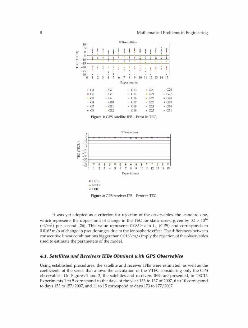
Figure 1: GPS satellite IFB—Error in TEC.

0 1 2 3 4 5 6 7 8 9 10 11 12 13 14 15

Experiments

−45−40−35−30−25−20−15−10−5

05

TE

C(T

EC

U)

IFB-receivers

H819NETRLEIC

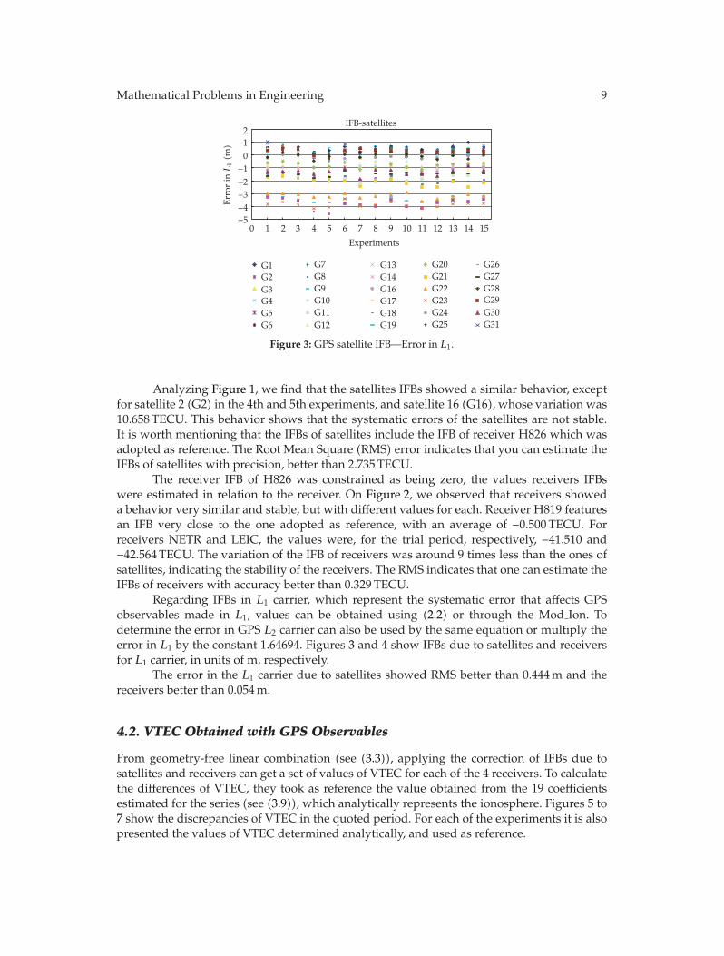
Figure 2: GPS receiver IFB—Error in TEC.

It was yet adopted as a criterion for rejection of the observables, the standard one,which represents the upper limit of change in the TEC for static users, given by 0.1 × 1016

(el/m2) per second [26]. This value represents 0.085 Hz in L1 (GPS) and corresponds to0.0163 m/s of change in pseudoranges due to the ionospheric effect. The differences betweenconsecutive linear combinations bigger than 0.0163 m/s imply the rejection of the observablesused to estimate the parameters of the model.

4.1. Satellites and Receivers IFBs Obtained with GPS Observables

Using established procedures, the satellite and receiver IFBs were estimated, as well as thecoefficients of the series that allows the calculation of the VTEC considering only the GPSobservables. On Figures 1 and 2, the satellites and receivers IFBs are presented, in TECU.Experiments 1 to 5 correspond to the days of the year 133 to 137 of 2007, 6 to 10 correspondto days 153 to 157/2007, and 11 to 15 correspond to days 173 to 177/2007.


0 1 2 3 4 5 6 7 8 9 10 11 12 13 14 15

Experiments

−5−4−3−2−1

012

Err

orinL

1(m

)

IFB-satellites

G1G2G3G4G5G6

G7G8G9G10G11G12

G13G14G16G17G18G19

G20G21G22G23G24G25

G26G27G28G29G30G31

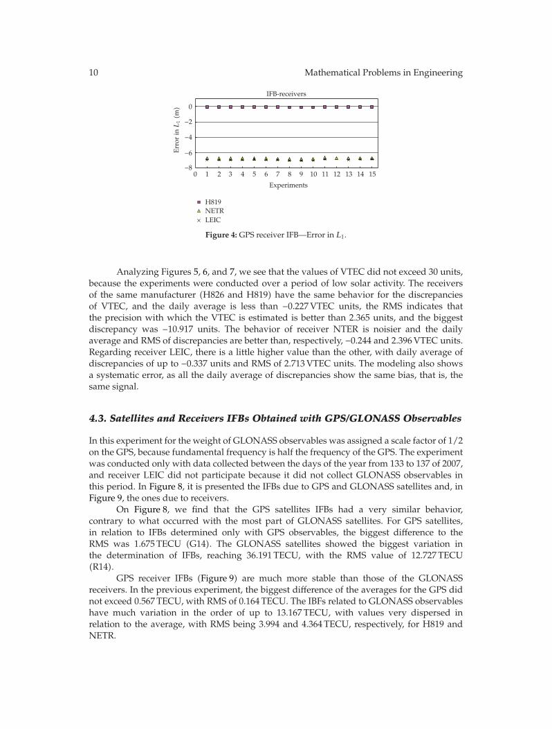
Figure 3: GPS satellite IFB—Error in L1.

Analyzing Figure 1, we find that the satellites IFBs showed a similar behavior, exceptfor satellite 2 (G2) in the 4th and 5th experiments, and satellite 16 (G16), whose variation was10.658 TECU. This behavior shows that the systematic errors of the satellites are not stable.It is worth mentioning that the IFBs of satellites include the IFB of receiver H826 which wasadopted as reference. The Root Mean Square (RMS) error indicates that you can estimate theIFBs of satellites with precision, better than 2.735 TECU.

The receiver IFB of H826 was constrained as being zero, the values receivers IFBswere estimated in relation to the receiver. On Figure 2, we observed that receivers showeda behavior very similar and stable, but with different values for each. Receiver H819 featuresan IFB very close to the one adopted as reference, with an average of −0.500 TECU. Forreceivers NETR and LEIC, the values were, for the trial period, respectively, −41.510 and−42.564 TECU. The variation of the IFB of receivers was around 9 times less than the ones ofsatellites, indicating the stability of the receivers. The RMS indicates that one can estimate theIFBs of receivers with accuracy better than 0.329 TECU.

Regarding IFBs in L1 carrier, which represent the systematic error that affects GPSobservables made in L1, values can be obtained using (2.2) or through the Mod Ion. Todetermine the error in GPS L2 carrier can also be used by the same equation or multiply theerror in L1 by the constant 1.64694. Figures 3 and 4 show IFBs due to satellites and receiversfor L1 carrier, in units of m, respectively.

The error in the L1 carrier due to satellites showed RMS better than 0.444 m and thereceivers better than 0.054 m.

4.2. VTEC Obtained with GPS Observables

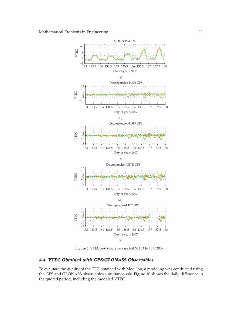
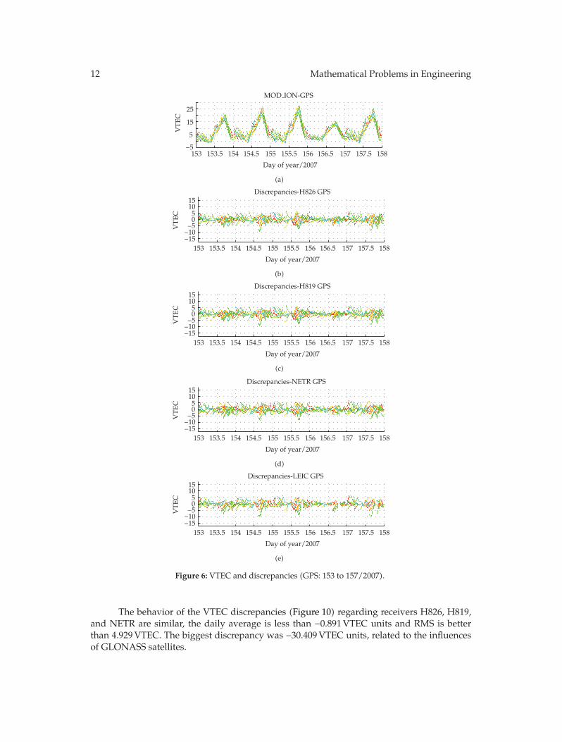
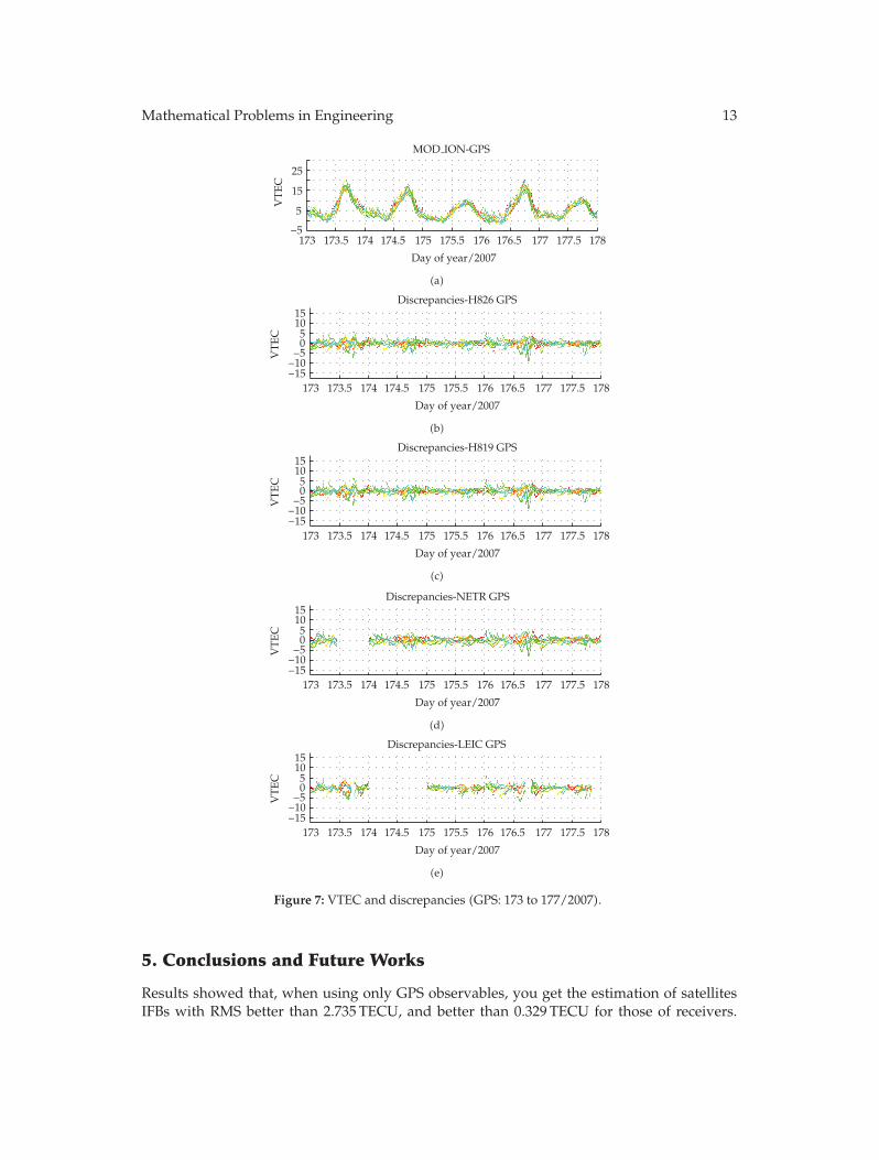
From geometry-free linear combination (see (3.3)), applying the correction of IFBs due tosatellites and receivers can get a set of values of VTEC for each of the 4 receivers. To calculatethe differences of VTEC, they took as reference the value obtained from the 19 coefficientsestimated for the series (see (3.9)), which analytically represents the ionosphere. Figures 5 to7 show the discrepancies of VTEC in the quoted period. For each of the experiments it is alsopresented the values of VTEC determined analytically, and used as reference.


0 1 2 3 4 5 6 7 8 9 10 11 12 13 14 15

Experiments

−8

−6

−4

−2

0

Err

orinL

1(m

)

IFB-receivers

H819NETRLEIC

Figure 4: GPS receiver IFB—Error in L1.

Analyzing Figures 5, 6, and 7, we see that the values of VTEC did not exceed 30 units,because the experiments were conducted over a period of low solar activity. The receiversof the same manufacturer (H826 and H819) have the same behavior for the discrepanciesof VTEC, and the daily average is less than −0.227 VTEC units, the RMS indicates thatthe precision with which the VTEC is estimated is better than 2.365 units, and the biggestdiscrepancy was −10.917 units. The behavior of receiver NTER is noisier and the dailyaverage and RMS of discrepancies are better than, respectively, −0.244 and 2.396 VTEC units.Regarding receiver LEIC, there is a little higher value than the other, with daily average ofdiscrepancies of up to −0.337 units and RMS of 2.713 VTEC units. The modeling also showsa systematic error, as all the daily average of discrepancies show the same bias, that is, thesame signal.

4.3. Satellites and Receivers IFBs Obtained with GPS/GLONASS Observables

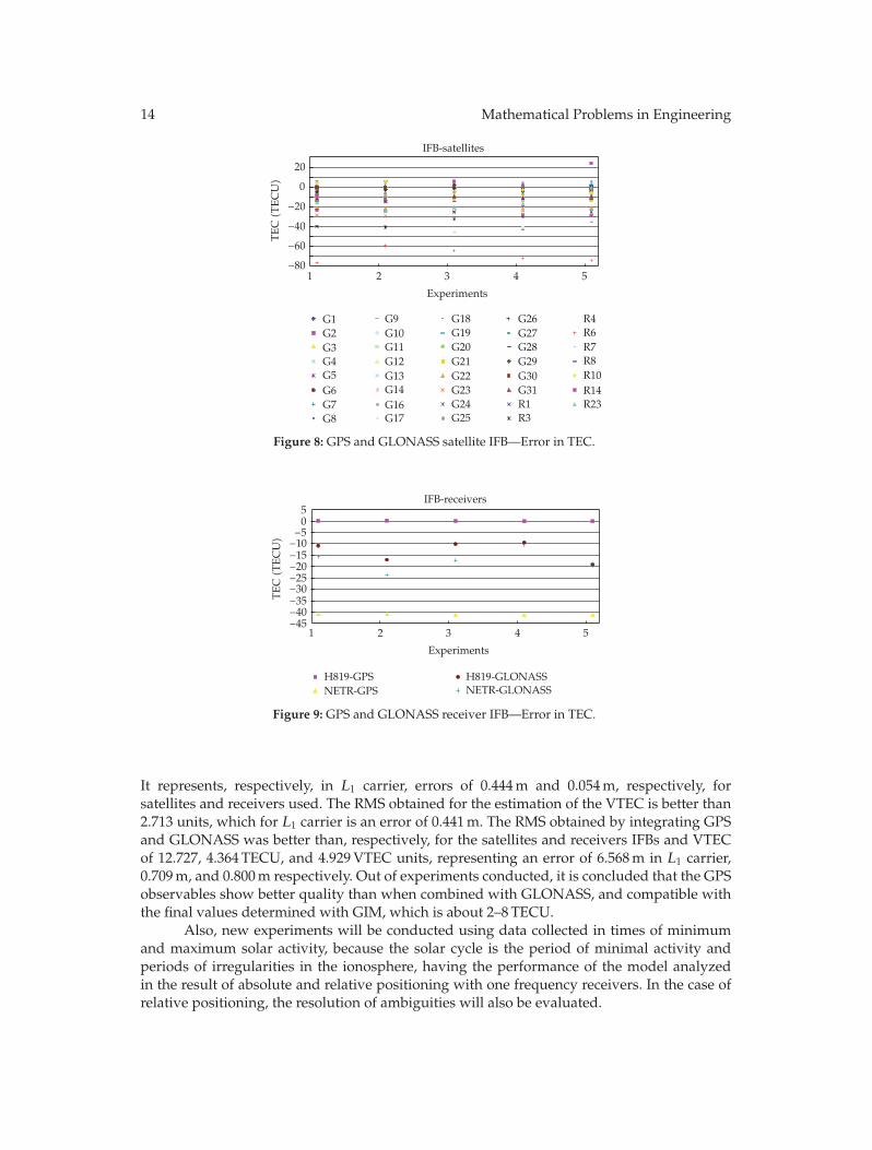
In this experiment for the weight of GLONASS observables was assigned a scale factor of 1/2on the GPS, because fundamental frequency is half the frequency of the GPS. The experimentwas conducted only with data collected between the days of the year from 133 to 137 of 2007,and receiver LEIC did not participate because it did not collect GLONASS observables inthis period. In Figure 8, it is presented the IFBs due to GPS and GLONASS satellites and, inFigure 9, the ones due to receivers.

On Figure 8, we find that the GPS satellites IFBs had a very similar behavior,contrary to what occurred with the most part of GLONASS satellites. For GPS satellites,in relation to IFBs determined only with GPS observables, the biggest difference to theRMS was 1.675 TECU (G14). The GLONASS satellites showed the biggest variation inthe determination of IFBs, reaching 36.191 TECU, with the RMS value of 12.727 TECU(R14).

GPS receiver IFBs (Figure 9) are much more stable than those of the GLONASSreceivers. In the previous experiment, the biggest difference of the averages for the GPS didnot exceed 0.567 TECU, with RMS of 0.164 TECU. The IBFs related to GLONASS observableshave much variation in the order of up to 13.167 TECU, with values very dispersed inrelation to the average, with RMS being 3.994 and 4.364 TECU, respectively, for H819 andNETR.


133 133.5 134 134.5 135 135.5 136 136.5 137 137.5 138

Day of year/2007

−5

5

15

25

VT

EC

MOD ION-GPS

(a)

133 133.5 134 134.5 135 135.5 136 136.5 137 137.5 138

Day of year/2007

−15−10−5

05

1015

VT

EC

Discrepancies-H826 GPS

(b)

133 133.5 134 134.5 135 135.5 136 136.5 137 137.5 138

Day of year/2007

−15−10−5

05

1015

VT

EC


(c)

133 133.5 134 134.5 135 135.5 136 136.5 137 137.5 138

Day of year/2007

−15−10−5

05

1015

VT

EC

Discrepancies-NETR GPS

(d)

133 133.5 134 134.5 135 135.5 136 136.5 137 137.5 138

Day of year/2007

−15−10−5

05

1015

VT

EC

Discrepancies-LEIC GPS

(e)

Figure 5: VTEC and discrepancies (GPS: 133 to 137/2007).

4.4. VTEC Obtained with GPS/GLONASS Observables

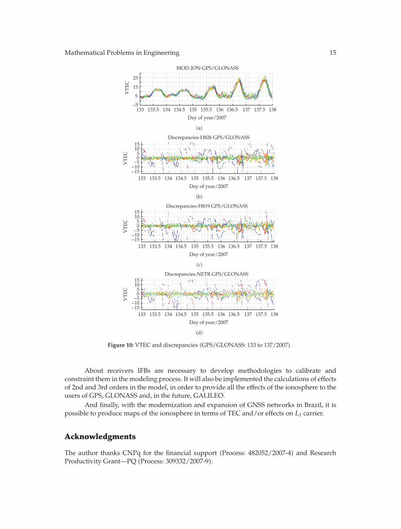
To evaluate the quality of the TEC obtained with Mod Ion, a modeling was conducted usingthe GPS and GLONASS observables simultaneously. Figure 10 shows the daily difference inthe quoted period, including the modeled VTEC.


153 153.5 154 154.5 155 155.5 156 156.5 157 157.5 158

Day of year/2007

−5

5

15

25

VT

EC

MOD ION-GPS

(a)

153 153.5 154 154.5 155 155.5 156 156.5 157 157.5 158

Day of year/2007

−15−10−5

05

1015

VT

EC


(b)

153 153.5 154 154.5 155 155.5 156 156.5 157 157.5 158

Day of year/2007

−15−10−5

05

1015

VT

EC


(c)

153 153.5 154 154.5 155 155.5 156 156.5 157 157.5 158

Day of year/2007

−15−10−5

05

1015

VT

EC


(d)

153 153.5 154 154.5 155 155.5 156 156.5 157 157.5 158

Day of year/2007

−15−10−5

05

1015

VT

EC


(e)


The behavior of the VTEC discrepancies (Figure 10) regarding receivers H826, H819,and NETR are similar, the daily average is less than −0.891 VTEC units and RMS is betterthan 4.929 VTEC. The biggest discrepancy was −30.409 VTEC units, related to the influencesof GLONASS satellites.


173 173.5 174 174.5 175 175.5 176 176.5 177 177.5 178

Day of year/2007

−5

5

15

25

VT

EC

MOD ION-GPS

(a)

173 173.5 174 174.5 175 175.5 176 176.5 177 177.5 178

Day of year/2007

−15−10−5

05

1015

VT

EC


(b)

173 173.5 174 174.5 175 175.5 176 176.5 177 177.5 178

Day of year/2007

−15−10−5

05

1015

VT

EC


(c)

173 173.5 174 174.5 175 175.5 176 176.5 177 177.5 178

Day of year/2007

−15−10−5

05

1015

VT

EC


(d)

173 173.5 174 174.5 175 175.5 176 176.5 177 177.5 178

Day of year/2007

−15−10−5

05

1015

VT

EC


(e)


5. Conclusions and Future Works

Results showed that, when using only GPS observables, you get the estimation of satellitesIFBs with RMS better than 2.735 TECU, and better than 0.329 TECU for those of receivers.


1 2 3 4 5

Experiments

−80

−60

−40

−20

0

20

TE

C(T

EC

U)

IFB-satellites

G1G2G3G4G5G6G7G8

G9G10G11G12G13G14G16G17

G18G19G20G21G22G23G24G25

G26G27G28G29G30G31R1R3

R4R6R7R8R10R14R23

Figure 8: GPS and GLONASS satellite IFB—Error in TEC.

1 2 3 4 5

Experiments

−45−40−35−30−25−20−15−10−5

05

TE

C(T

EC

U)

IFB-receivers

H819-GPSNETR-GPS

H819-GLONASSNETR-GLONASS

Figure 9: GPS and GLONASS receiver IFB—Error in TEC.

It represents, respectively, in L1 carrier, errors of 0.444 m and 0.054 m, respectively, forsatellites and receivers used. The RMS obtained for the estimation of the VTEC is better than2.713 units, which for L1 carrier is an error of 0.441 m. The RMS obtained by integrating GPSand GLONASS was better than, respectively, for the satellites and receivers IFBs and VTECof 12.727, 4.364 TECU, and 4.929 VTEC units, representing an error of 6.568 m in L1 carrier,0.709 m, and 0.800 m respectively. Out of experiments conducted, it is concluded that the GPSobservables show better quality than when combined with GLONASS, and compatible withthe final values determined with GIM, which is about 2–8 TECU.

Also, new experiments will be conducted using data collected in times of minimumand maximum solar activity, because the solar cycle is the period of minimal activity andperiods of irregularities in the ionosphere, having the performance of the model analyzedin the result of absolute and relative positioning with one frequency receivers. In the case ofrelative positioning, the resolution of ambiguities will also be evaluated.


133 133.5 134 134.5 135 135.5 136 136.5 137 137.5 138

Day of year/2007

−5

5

15

25

VT

EC

MOD ION-GPS/GLONASS

(a)

133 133.5 134 134.5 135 135.5 136 136.5 137 137.5 138

Day of year/2007

−15−10−5

05

1015

VT

EC

Discrepancies-H826 GPS/GLONASS

(b)

133 133.5 134 134.5 135 135.5 136 136.5 137 137.5 138

Day of year/2007

−15−10−5

05

1015

VT

EC

Discrepancies-H819 GPS/GLONASS

(c)

133 133.5 134 134.5 135 135.5 136 136.5 137 137.5 138

Day of year/2007

−15−10−5

05

1015

VT

EC

Discrepancies-NETR GPS/GLONASS

(d)

Figure 10: VTEC and discrepancies (GPS/GLONASS: 133 to 137/2007).

About receivers IFBs are necessary to develop methodologies to calibrate andconstraint them in the modeling process. It will also be implemented the calculations of effectsof 2nd and 3rd orders in the model, in order to provide all the effects of the ionosphere to theusers of GPS, GLONASS and, in the future, GALILEO.

And finally, with the modernization and expansion of GNSS networks in Brazil, it ispossible to produce maps of the ionosphere in terms of TEC and/or effects on L1 carrier.

Acknowledgments

The author thanks CNPq for the financial support (Process: 482052/2007-4) and ResearchProductivity Grant—PQ (Process: 309332/2007-9).


References

[1] G. Seeber, Satellite Geodesy, Walter de Gruyter, Berlin, Germany, 2003.[2] C. A. Brunini, Global ionospheric model from GPS measurement, Ph.D. thesis, Facultad de Ciencias

Astronomicas y Geofısicas, Universidad Nacional de La Plata, La Plata, Argentina, 1998.[3] P. de Oliveira Camargo, Modelo regional da ionosfera para uso em posicionamento com receptores de uma

frequencia, Ph.D. thesis, Universidade Federal do Parana, Curitiba, Brazil, 1999.[4] P. de Oliveira Camargo, J. F. G. Monico, and L. D. D. Ferreira, “Application of ionospheric corrections

in the equatorial region for L1 GPS users,” Earth, Planets and Space, vol. 52, no. 11, pp. 1083–1089, 2000.[5] E. S. Fonseca Jr., O sistema GPS como ferramenta para avaliacao da refracao ionosferica no Brasil, Ph.D.

thesis, Escola Politecnica da Universidade de Sao Paulo, Sao Paulo, Brazil, 2002.[6] M. Fedrizzi, Estudo do efeito das tempestades magneticas sobre a ionosfera utilizando dados do GPS, Ph.D.

thesis, Instituto Nacional de Pesquisas Espaciais, Sao Jose dos Campos, Brazil, 2003.[7] M. T. Matsuoka and P. de Oliveira Camargo, “Evaluation of functions for modelling of the effect of the

ionospheric refraction in the propagation of the GPS signals,” in Proceedings of the 16th InternationalTechnical Meeting of the Satellite Division of the Institute of Navigation (ION GPS/GNSS ’03), pp. 1736–1741, Portland, Ore, USA, 2003.

[8] M. T. Matsuoka, P. de Oliveira Camargo, and W. R. Dal Poz, “Declınio do numero de manchas solaresdo ciclo 23: reducao da atividade ionosferica e melhora da performance do posicionamento comGPS,” Boletim de Ciencias Geodesicas, vol. 10, no. 2, pp. 141–157, 2004.

[9] W. R. Dal Poz and P. de Oliveira Camargo, “Consequencias de uma tempestade geomagnetica noposicionamento relativo com receptores GPS de simples frequencia,” Boletim de Ciencias Geodesicas,vol. 12, no. 2, pp. 275–294, 2006.

[10] C. R. de Aguiar and P. de Oliveira Camargo, “Modelagem em tempo real do erro sistematico dasobservaveis GPS devido a ionosfera,” Boletim de Ciencias Geodesicas, vol. 12, no. 1, pp. 101–120, 2006.

[11] I. S. Batista, M. A. Abdu, J. R. Souza, et al., “Unusual early morning development of the equatorialanomaly in the Brazilian sector during the Halloween magnetic storm,” Journal of Geophysical ResearchA, vol. 111, no. 5, Article ID A05307, 2006.

[12] M. T. Matsuoka, Influencia de diferentes condicoes da ionosfera no posicionamento com GPS: avaliacao naregiao brasileira, Ph.D. thesis, Faculdade de Ciencias e Tecnologia, Universidade Estadual Paulista,Presidente Prudente, Brazil, 2007.

[13] S. Schaer, Mapping and predicting the earth’s ionosphere using the Global Positioning System, Ph.D.dissertation, University of Bern, Bern, Switzerland, 1999.

[14] J. A. Klobuchar, “Ionospheric time-delay algorithm for single-frequency GPS users,” IEEE Transactionson Aerospace and Electronic Systems, vol. 23, no. 3, pp. 325–331, 1987.

[15] S. P. Newby and R. B. Langley, “Three alternative empirical ionospheric models—are they better thanGPS broadcast model?” in Proceeding of the 6th International Geodetic Symposium on Satellite Positioning,vol. 1, pp. 240–244, Columbus, Ohio, USA, 1992.

[16] A. Leick, GPS Satellite Surveying, John Wiley & Sons, New York, NY, USA, 1995.[17] IGS, International GNSS Service, 2009, http://igscb.jpl.nasa.gov/components/prods.html.[18] L. Ciraolo, F. Azpilicueta, C. Brunini, A. Meza, and S. M. Radicella, “Calibration errors on

experimental slant total electron content (TEC) determined with GPS,” Journal of Geodesy, vol. 81,no. 2, pp. 111–120, 2007.

[19] K. Davies, Ionospheric Radio, Peter Peregrinus, London, UK, 1990.[20] L. F. McNamara, The Ionosphere: Communications, Surveillance, and Direction Finding, Krieger, Malabar,

Fla, USA, 1991.[21] V. W. J. H. Kirchhoff, Introducao a Geofısica Espacial, EDUSP, Sao Paulo, Brazil, 1991.[22] D. Wells, N. Beck, D. Delikaraoglou, et al., Guide to GPS Positionin, Canadian GPS Associates,

Frederiction, Canada, 1986.[23] D. Odijk, Fast Precise GPS Positioning in the Presence of Ionospheric Delays, Netherlands Geodetic

Commission, Delft, The Netherlands, 2002.[24] I. Webster, A regional model for prediction of ionospheric delay for single frequency users of the global

positioning system, M.S. thesis, University of New Brunswick, New Brunswick, Canada, 1993.[25] X. X. Jin, Theory of carrier adjusted DGPS positioning approach and some experimental results, Ph.D. thesis,

Delft University of Technology, Delft, The Netherlands, 1996.[26] J. A. Klobuchar, “Ionospheric effects on GPS,” in Global Positioning System: Theory and Applications,

vol. 1, chapter 12, pp. 485–515, American Institute of Aeronautics and Astronautics, Washington, DC,USA, 1996.

Submit your manuscripts athttp://www.hindawi.com

Hindawi Publishing Corporationhttp://www.hindawi.com Volume 2014

MathematicsJournal of


Mathematical Problems in Engineering

Hindawi Publishing Corporationhttp://www.hindawi.com

Differential EquationsInternational Journal of

Volume 2014

Applied MathematicsJournal of


Probability and StatisticsHindawi Publishing Corporationhttp://www.hindawi.com Volume 2014

Journal of


Mathematical PhysicsAdvances in

Complex AnalysisJournal of


OptimizationJournal of


CombinatoricsHindawi Publishing Corporationhttp://www.hindawi.com Volume 2014

International Journal of


Operations ResearchAdvances in

Journal of


Function Spaces

Abstract and Applied AnalysisHindawi Publishing Corporationhttp://www.hindawi.com Volume 2014

International Journal of Mathematics and Mathematical Sciences


The Scientific World JournalHindawi Publishing Corporation http://www.hindawi.com Volume 2014


Algebra

Discrete Dynamics in Nature and Society



Decision SciencesAdvances in

Discrete MathematicsJournal of

Hindawi Publishing Corporationhttp://www.hindawi.com

Volume 2014 Hindawi Publishing Corporationhttp://www.hindawi.com Volume 2014

Stochastic AnalysisInternational Journal of

Documents

Quality of TEC Estimated with Mod_Ion Using GPS and GLONASS