Embed Size (px)
Citation preview

Too Slow for the Urban March: Litigations and Real Estate Market in Mumbai, India | 1
QUALITY, INDEPENDENCE, IMPACT
Working Paper-06
March, 2019
Prachi Singh
Sagnik Dey
Sourangsu Chowdhury
Kunal Bali
© Brookings Institu�on India Center, 2019
Early Life Exposureto Outdoor Air Pollution:
Effect on Child Health in India


Early Life Exposure to Outdoor Air Pollution:
Effect on Child Health in India
Prachi Singh∗ Sagnik Dey† Sourangsu Chowdhury† Kunal Bali†
March, 2019
∗Indian Statistical Institute, Delhi & Brookings India†Indian Institute of Technology, Delhi
1

Early Life Exposure to Outdoor Air Pollution:
Effect on Child Health in India
Abstract
This paper examines effect of outdoor air pollution on child health in India by
combining satellite PM2.5 data with geo-coded Demographic and Health Survey of In-
dia(2016). We use an instrumental variable strategy for identification as local pollution
levels may be endogenous due to local household behavioural choices like participation
in local fuel wood market, burning crop residue etc which are not observed in sur-
vey data. Our identification strategy relies on use of upwind biomass burning events
in neighbouring areas to identify the effect of air pollution on child health. Our re-
sults indicate that one standard deviation increase in exposure to pollution during first
trimester lowers Height-for-age (by 6.7 percent) and Weight-for-age (by 7.8 percent);
the effect is prominent for poor people and Northern states of India which have higher
incidence of such events.
JEL Classification: 012 I15 Q53 Q56
Corresponding author:
Prachi Singh
Associate Fellow, Brookings India
&
PhD Candidate
Economics and Planning Unit
Indian Statistical Institute
New Delhi
Email: [email protected], [email protected]
2

Effect of Early Life Exposure to Outdoor Air Pollution
on Child Health in India 1
[PRELIMINARY DRAFT]
1 Introduction
Pollution in any form, whether it be air or water, poses an environmental risk to the health
of the exposed population. Literature from both developing and developed nations indicates
the adverse health effects that air (Soo and Pattnayak, 2019 & Chay and Greenstone, 2003)
and water pollution (Brainerd and Menon, 2014) have on children. In spite of enormous
evidence about ill effects of pollution, there is little effective management or regulation to
curtail activities which contribute to high levels of pollution in developing nations.
According to WHO global air pollution database, out of the 15 most polluted cities in
the world, 14 belong to India. Another recently published report by Health Effects Institute
on air pollution in India (2018) reports that air pollution was responsible for 1.1 million
deaths in India in 2015. The major contributors to air pollution in India are household
burning emissions, coal combustion, agricultural burning and transport. In the absence of
effective pollution regulatory policies, air pollution levels have reached alarming levels in
various parts of India (Greenpeace, 2017). This warrants a closer look at the air pollution
problem from the standpoint of welfare of the younger generation currently being exposed
to harmful pollutants with possible long-lasting effect on their health.
This paper examines the effect of outdoor air pollution on child health in India. Par-
ticularly we study the effect of early life exposure to air pollution (as measured by PM
2.5) on children’s weight and height measures. We use gridded satellite data on PM2.5 and
1 We are thankful to Dr.Abhiroop Mukhopadhyay & Dr.E.Somanathan for their valuable comments. We
are also thankful to conference participants at CECFEE, ADEW, EfD Annual Meet, AWEHE (inaugral
meet), ACEGD & Brookings India. We are especially grateful for valuable feedback which we got from
Dr.Randall Ellis, Dr.Shiko Maruyama, Dr.Sabyasachi Das and Dhritiman Gupta. We thank Athisii Kayina
for his immense help with ArcGIS software.
3

GPS locations of sampled clusters in Demographic Health Survey (DHS, 2015-16 round for
India) to produce rich geo-spatial information about local pollution levels in the place of
conception(residence) of a child. In an empirical exercise which causally links child health to
local pollution levels, household income and behavioural choices are omitted variables which
make local pollution levels endogenous. We use neighbouring (or non-local) fire-events as an
instrument for local pollution levels as they are not related to household behavioural choices
or local economic activity, but they affect local pollution levels as smoke and pollutants from
these neighbouring fire events can travel long distances.
Our analysis shows that air pollution negatively affects children’s health. Exposure to
air pollution during the first trimester decreases both Height-for-age (stunting measure)
and Weight-for-age (underweight measure) for children aged below five years. The effect is
prominent for poorer households, with Northern states being more vulnerable due to high
pollution levels in the area.
Evaluating this link between poor air quality and child health is important as many
regions in India have very high pollution levels which breach the safe standards often. If
stunting is affected by early life exposure to pollution then it can have long-lasting effect
on life earnings of a child due to poor cognition and also increase the vulnerability towards
hypertension and diabetes. Thus, failure to curb air pollution problem in India adversely
affects the human capital of the country in the long run.
The literature linking air pollution to child health has mostly focused on child mortality.
We add analysis towards child’s growth indicators conditional on child’s survival. Most of the
studies for developing nations lack rich geo-spatial data for analysis and rely on pollution
measures which are estimated for a large area (and hence are riddled with measurement
error). To the best of our knowledge, this is the first study for India which addresses the
endogeneity issues present while studying the link between child health with local pollution
levels.
The paper follows the following structure. The next section provides a literature overview
of the effect of pollution on child health. Section 3 describes the various datasets that we
use in our analysis. The next section presents the empirical methodology that we follow and
4

it is followed by results in Section 5. Lastly, Section 6 concludes with an estimate of the
extent of the problem and discusses current state of policies regarding air pollution in India.
2 Previous Literature
Our work is motivated by the “fetal origins” hypothesis (Douglas and Currie, 2011), which
states that the in-utero period of a child critically determines mortality outcomes, disease
prevalence and future health outcomes, abilities and earnings. Fetal growth, if restricted, can
negatively affect future outcomes. The biological link between fetal growth and air pollution
has not been documented in the literature, but it is mediated by placental growth which
determines supply of oxygen and nutrients to the fetus. Exposure to pollution would affect
placental function which can be impacted by inflammation caused by maternal infection.
Additionally pollution is known to cause epigenetic changes (interaction between our genes
and environment which can cause DNA methylation, which regulates gene expression) which
could affect fetal growth as well. A recent paper by Chakrabarti et. al (2019) has shown how
exposure to biomass burning (which causes pollution) affects respiratory health in adults as
well as children. This link shows how mothers can possibly be affected during the pregnancy
time due to exposure to pollution.
The intrauterine period has been the focus of many studies in economics literature which
has linked occurrence of early life shocks to multiple outcomes. Early life shocks studied in
economics literature include incidence of a) disastrous events (like famines, war, drought);
b) nutritional shocks (like introduction of iodised salt, pregnancy during Ramadan) and
c) pollution (air or water). Currie and Vogl (2013) provide a review of these early life
shocks (a and b) on various outcomes; broadly summarised these shocks negatively affect
adult cognition, years of schooling, literacy status, adult height and stunting measures; and
increase the likelihood of presence of birth defects, prevalence of heart disease and obesity.
The focus of our study is in-utero exposure to air pollution and Currie et. al (2014)
reviews landmark studies which have been done in this area. Most of these studies are
from developed nations with few exceptions. Similar to previous studies, a major part of
5
the literature focuses on learning outcomes (test-scores) and earnings which are negatively
affected due to in-utero exposure to pollution (Bharadwaj et al., 2013; Isen et al., 2013 &
Sanders, 2012).
The strand of literature which is most relevant for our study has mainly looked at the
effect of in-utero or early life exposure to air-pollution on infant mortality and birth weight.
Few papers in this area have used natural experiments to causally identify the effect of
air pollution on infant survival, for example, Chay and Greenstone (2003a and 2003b) use
introduction of environmental regulations under Clean Air Act, 1970 and recession in 1981-82
in United States to show that reduction in pollution levels led to reduction in infant mortality.
Currie and Walker (2011) show that introduction of congestion-reducing automated toll
payment systems in United States (which reduced number of idle vehicles emitting harmful
pollutants) reduced pre-mature and low birth-weight births. Currie and Neidell (2005) use
spatial and temporal variation in CO levels to analyse the effect of CO levels on infant
mortality.
The paper by Greenstone and Hanna (2014) is one of the landmark studies which analyses
the effect of water and air pollution regulation policies on infant mortality in a developing
nation context (India). Another study from a developing nation includes Foster et al. (2009)
which uses Mexico’s clean industry certification program to study its effect on pollution (we
use a similar measure of pollution i.e. satellite data on Aerosol Optical Depth to infer PM2.5
levels) and resulting respiratory related infant deaths. Wildfires and their negative health
effects (like increase in infant mortality, reported asthma cases, pre-term births etc) have also
been studied in context of Indonesian wildfire of 1997 (Jayachandran, 2009; Rukumnuaykit,
2003; Kunii et al., 2002; Frankenberg et al., 2005 & Barber and James, 2000), California
wildfires (Holstius et al.,2012) and Australian wildfires (O’Donnell and Behie, 2015). Two
recent papers assess the effect of in-utero exposure to biomass burning events and pollution
Vogl & Rangel (2016) and Soo & Pattnayak (2019) on birth weight and long-term health
outcomes like adult height respectively. These two papers come closest to our paper as we
also explore the link between in-utero exposure to pollution and child health but our sample
is much bigger than the Indonesian study and we focus on solving the endogeneity problem
6

in our paper rather than focusing on reduced form effect of biomass burning events on child
health.
Additionally two studies on India analyse the effect of water pollution on child health.
Brainerd and Menon (2014) have focused on use of fertilisers in India during crop sowing
season which increases concentration of harmful chemicals in water. They find that exposure
to these pollutants during the month of conception increases infant mortality and reduces
Height-for-age and Weight-for-age for children. Do et al. (2018) have shown that regulation
targeting industrial pollution in the Ganga River led to reduction in water pollution levels
and infant death. In case of India, literature has shown how air pollution can affect infant
mortality but no study has focused on post-natal growth outcomes for surviving children.
Also due to lack of local air pollution monitoring systems which cover the entire nation,
there has been no study which calculates local pollution levels and assesses its effect on
health outcomes.
3 Data
3.1 Demographic Data
The demographic data we use comes from the Demographic and Health Survey (Round-4
for 2015-16) for India. DHS-IV contains detailed information about birth history of each
woman who was interviewed. The latest round of this survey sampled 601,509 households
and interviewed 0.7 million eligible 2 women in the age group 15-49. Further anthropometric
measures of health were collected for 0.22 million children of age five years and below.
The DHS sample is a stratified two-stage sample and the primary sampling units (PSUs
or clusters) correspond to villages in rural areas and blocks in urban areas. The DHS-IV
comprises of around 28526 clusters with GIS information on almost all clusters3. To hide
the identity of the village (block in urban areas) all clusters were displaced by five kilometres
(two kilometres for urban clusters), with one percent of the clusters being displaced by as
2 Eligible women - married or unmarried women of reproductive age.3 131 clusters have no GIS information.
7

much as 10 kilometres. We account for this displacement when we discuss our identification
strategy in the next section.
Our focus is on in-utero exposure to pollution for which we need the location and time
of conception. To measure in-utero exposure to pollution we use the birth history of every
child ever born to a woman. We use the location of the cluster, birth date and pregnancy
duration of a child to impute exposure to pollution during the first trimester 4. We make an
important assumption that the place of stay of mother when the child was in-utero is same
as the same of current residence of a child 5.
We measure long-term impact by using anthropometric measures like Height-for-age and
Weight-for-age (WHO standard z-scores) for children. While estimating the effect of in-utero
exposure to pollution on measures of child health we also control for child characteristics
like birth order, age and gender. As informed by previous literature, mother’s characteristics
can also affect child’s health and hence we control for the age at which she had the child and
her education level. DHS data also contains information about source of water, method of
cooking and toilet facility of the dwelling, all of these characteristics have important bearing
on health of a child and we include them in our analysis as well. Additional controls for
gender and age of head of household are also used in our analysis.
We provide summary statistics of our analysis sample in Table 1. 52 percent of children
in our estimation sample 6 are males with mean age around 29 months (2.5 years old) and
the mean birth order of children is 2.2. The birth order is slightly lower for children in South
India. The average age at which mothers have children is 24.5 years. Mothers had on an
average 6.2 years of education (with mothers in South India having more years of education
(7.8) than North Indian mothers (5.8)) and 97 percent of fathers are literate. Three-fourth
of our sample consists of rural households and a similar proportion of households report their
4 We also construct separate measures of exposures to pollution for other trimesters and first three months
after birth.5 This assumption is a standard assumption which is employed by many papers which used DHS data for
analysis. In our sample the mean number of years for which the interviewed family has stayed at the place
of residence is around 15 years. See Brainerd & Menon, 2014 for reference.6 Details about estimation sample discussed in pollution section later.
8

religion to be Hindu. The mean household size for our estimation sample is is 6.5. 88 percent
of the households are headed by a male member and the average age of household head is
44.5 years. 85 percent of the households have an electricity connection, but only 23 percent
of the households use piped water as their source of drinking water, 28 percent of our sample
uses clean source of cooking fuel like LPG or bio-gas and the mean open defecation rate in
a cluster is 43 percent.
The mean Height-for-age (HFA) and Weight-for-age (WFA) z-score for our sample is
-1.46 and -1.52 respectively (mean weight-for-height is -0.97 for our sample). Children from
South India have much better HFA and WFA as compared to North Indian children. Height-
for-age is a measure of stunting and it represents the effect of early life shocks that a child
receives. Stunting generally occurs before age two and its effects are largely irreversible. It
is associated with an underdeveloped brain, with long-lasting harmful consequences, includ-
ing diminished mental ability and learning capacity, poor school performance in childhood,
reduced earnings and increased risks of nutrition-related chronic diseases such as diabetes,
hypertension, and obesity in future. Weight-for-age (underweight measure) reflects body
mass relative to chronological age. It is influenced by both the height of the child (height-
for-age) and his or her weight (weight-for-height). Deaton and Dreze (2009) advocate the use
of Weight-for-age as the health status indicator for children as its a comprehensive measure
which captures both stunting and wasting.
3.2 Pollution Data
In India, ground-based pollution measurement started post 2009 under the National Ambi-
ent Air Quality monitoring program maintained by Central Pollution Control Board. The
network has slowly expanded to around 90 sites across 35 cities over the years, which leaves
majority of India unmonitored 7. Amongst these cities, only Delhi has greater than 20 mon-
itoring sites while most other cities have a single monitoring site. Furthermore, most of the
sites do not have continuous temporal data. We use PM2.5 as our measure of pollution
7 India has around 600 ground based monitors to cover the entire country with only 148 monitors which
capture PM2.5 for the entire country.
9
which is a correlate of other pollutants (like NO2, SO2, CO) which are not captured in our
analysis. To address the paucity in ground-based pollution data in India, we estimate PM2.5
exposure using satellite data (van Donkelaar et al., 2010). We convert Aerosol Optical Data
(AOD) retrieved at 0.5 x 0.5 degree resolution from Multiangle Imaging SpectroRadiometer
(MISR) to PM2.5 data (Liu et al, 2004; Kahn and Gaitley 2015; Dey et al 2010) using a
spatially and temporally heterogeneous conversion factor (Dey et al., 2012). The data was
statistically downscaled at 0.1 x 0.1 degree resolution (using spline interpolation) PM2.5.
The PM2.5 data after processing is available at monthly frequency with a 0.1 * 0.1 degree
resolution (10km*10km grid).
We explore the spatial variation in PM2.5 by plotting a heat map in Figure 1. We plot
mean annual PM2.5 (average over monthly data for years 2010 to 2016) for each district
of India. As the figure shows, the Northern region of the country is severely impacted
by high and dangerous levels of pollution, especially the states which lie in Indo-Gangetic
plains (Punjab, Haryana, Uttar Pradesh, Bihar) have the highest levels of pollution. On the
other hand the Southern part of the country has much lower levels of pollution as shown
by the lighter shades in heat map. The WHO guideline for maintaining safe standards
of pollution recommends a threshold of mean annual pollution levels of 10ug/m3. Other
standards include WHO-IT1 which is 35ug/m3, WHO-IT2 is 25ug/m3 and WHO-IT3 is
15ug/m3. The Indian National Ambient Air Quality Standards (NAAQS) is 40ug/m3. For
our estimation sample we observe in Table 1 that the mean level of PM2.5 for is between
55ug/m3 & 60ug/m3 during all critical windows of development for children from North
India while the corresponding level of pollution exposure is much lower for children from
South India, that is around 35ug/m3 for all windows.
We use cluster location from DHS data and calculate mean PM2.5 in the 75km radius
for each month since the time of conception. We use these monthly pollution measures to
construct trimester level pollution exposure by calculating mean PM2.5 for three month
periods. Our estimation sample is constrained by the availability of PM2.5 data as we only
keep those children in our estimation sample for whom the pollution measure for each month
in the first trimester is present. The missing PM2.5 are due to missing satellite retrievals
10

due to cloud covers. In the appendix (Table A1) we show that our outcome variables along
with our control variables are very similar between the estimation sample and out-sample
(with missing PM2.5 information).
We now link exposure to pollution during the first trimester with anthropometric measure
(Height-for-age z-score) for children in Figure 2. The descriptive graph is a bin-scatter plot
which shows a negative relationship between Height-for-age and exposure to pollution during
first trimester, we explore this relationship empirically in greater detail in Section 4.
4 Empirical Model
We seek to investigate whether early life exposure to outdoor pollution during first trimester
has an impact on future child health. We measure child health by Height-for-age (z-scores)
and Weight-for age (z-scores). For ease of exposition we focus on Height-for-age and exposure
in first trimester as early life exposure to pollution. The logic of our argument is same for
all other outcomes and exposure windows. Formally, we estimate the following empirical
model:
Hicdmt = θ1PMcdmt + βXicdmt + γc + δt + λm + ρ1dt + ρ2mt + εicdmt (1)
Our main outcomes of interest (Hicdmt) are z-score for Height-for-age (stunting measure)
and Weight-for-age (underweight measure) for child i who was conceived in month m, year
t in cluster c belonging to district d. We also control for other confounding factors in the
vector Xicdmt which includes gender, birth order and age of child, mother’s and father’s
educational status, mother’s age at birth, age and gender of household head, dummy for
whether household has piped water, has clean cooking source, whether household practices
open defecation and the fraction of households who practice open defecation in the cluster
(excluding self). Since all children in our sample are aged five or below, we use the assumption
that these controls have not changed a lot over time (i.e. from the time of conception to the
time when they were surveyed).
The main variable of interest is PMcdmt which captures the mean PM2.5 in the 75km
11

radius during first trimester for a child. Different clusters (villages or blocks) can have
different levels of development (health infrastructure) which can affect health of a child
hence we include cluster fixed effects in our specification. We also include month and year
fixed effects to account for systematic effects related to season and year. We also remove
any omitted variables that are related to a district in any particular year as well as any
seasonality effect specific to a month of a particular year by including district into year,
ρ1dt and month into year, ρ2mt fixed effects. The inclusion of these fixed effects means that
the variation that remains is the spatial variation pollution across clusters and temporal
variation within a year for a district.
While our estimation exercise removes systematic variation using various fixed effects but
endogeneity concerns still remain. These endogeneity concerns arise as the local residential
area for a household corresponds to the region of economic activity that a household depends
on and also affects based on its behavioural decisions. The economic activity of a household
determines key inputs (like income) which feed into the production function of health of a
child. An example of this can be dependence of a household on nearby forest resources for
fuel-wood consumption or for livelihood (if it sells these resources in a market). In this case
the choice of use of fuel-wood by household affects the local pollution level in the region.
Additionally the forest cover is affected by the demand for forest resources (like fuel-wood)
in the market, which in turn affects the pollution level in the area where they are finally
consumed. A similar logic holds true for crop residue burning as well, it is a conscious
decision taken by a household which impacts local pollution levels and at the same time
affects a farmer’s income which is a determinant of child health. This essentially points
towards the fact that local pollution level is endogenous in the region of economic activity
of the household.
4.1 Identification
The household behavioural choice of collecting fuel-wood or crop-burning and household
income are omitted variables in our specification hence the local pollution variable is en-
12

dogenous. To solve this endogeneity problem, we rely on an instrumental variable which
in our case is the probability weighted number of upwind fire-events which take place in
non-local areas. These fire-events refer to biomass burning events that include crop residue
burning and forest fires. We use wind direction as well to tag each fire-event as an upwind
or downwind event with respect to each cluster. An upwind fire-event refers to a fire-event
from which wind is blowing towards the cluster and down-wind fire-events refer to events
with wind blowing away from the cluster.
We use upwind fire-events which happen in non-local areas (between 75 and 100 km) as
an IV as they impact local mean PM2.5 levels but are not affected by household behavioural
choices. The IV that we use has been explained diagrammatically in Figure 3, where the light
grey center denotes the cluster location, the white circle forms the 75 km radius around the
cluster and the grey ring represents the area between 75 and 100 km radii around the cluster.
Our endogenous variable is the mean PM2.5 variable which is calculated for the white circle
(within 75 km) and the probability weighted number of upwind fire-events in the grey ring
form the IV (between 75 and 100 km). We choose the fire-events in non-local far away
areas to ensure that they belong to a region which is not a part of economic activity area
of a household. This essentially removes the effect of dependence on crop-burning or nearby
forest resources (or farmlands) for livelihood or fuel-consumption. By capturing fire-events
in this ring, we ensure that we only capture the part which contributes to the local pollution
levels but is not correlated with household behavioural choices. Exogenous changes in wind
direction is unlikely to be correlated with local behavioural choices or economic activity
in the area and thus non-local upwind fire-events serves as an ideal instrumental variable.
Zheng et. al (2019) use a similar IV in their paper where they study the impact of air
pollution on happiness levels using pollution level of neighbouring areas as an IV for local
pollution levels.
One of the main limitations of our study is that we are only able to capture big fire-
events as satellite recordings for fire-events fail to capture smaller fires which happen in
smaller farms. The satellite can only capture fires which burn brightly enough (big enough
to be quite intensive which guarantees that they get captured) to be recorded below the tree
13

canopy or cloud cover. The estimates we thus get can be considered as the lower-bound
effect of outdoor pollution due to non-local fire-events on child health.
4.2 Fire-events Data
Our source of biomass burning events (called fire incidents) is NASA’s Fire Information for
Resource Management System (FIRMS) data which captures real-time active fire locations
across the globe. The FIRMS data that we use is called MODIS (shortform for MODerate
Resolution Imaging Spectro radiometer) data and it records fire incidents at pixel level where
each pixel is identified by a latitude and longitude reading. Each latitude (and longitude)
is the center of a one kilometre fire pixel (1 km X 1 km in size). This data records not
just the location of a fire but also the brightness (temperature) of fire (in Kelvin units) and
date and time when the incident was picked by the Terra satellite. An observation for a
fire incident in MODIS data for a latitude and longitude does not necessarily mean that the
size of the fire is one square kilometre, but it means that atleast one fire is located within
this fire pixel (under good conditions the satellite can detect fires as small as 100m2). The
MODIS data is available on a daily basis since November 2000 and NASA reports that the
fires captured by this dataset are mostly vegetation fires. NASA data on fire incidents also
provides a variable “confidence”, which depicts the quality of the observations and it ranges
from 0-100. Following Vogl, 2016 we use this variable to construct a probability weighted
count of fire-events around a cluster (between 75 and 100 km). NASA’s FIRMs data can
also have some missing values attributable to satellite sensor outage however major incidents
reported for sensor outage happened in years 2001-2003 which precedes our analysis period.
We use the cluster GIS information from DHS data and calculate the total number of all
fire events which took place between 75 and 100 km radii (non-local exposure) during the
first (in-utero) trimester of a child. To ensure respondent confidentiality, all clusters in the
DHS data are displaced from their true location. The displacement is done by displacing an
urban cluster by two kilometre and a rural cluster by five kilometre with one percent of the
rural clusters being displaced by as much as 10 kilometres. The displacement can take place
14

in any direction but the cluster remains within the country boundary, within the same state
and district. We take the radius for our analysis to be 75 kilometre which is large enough
so that the true location of the cluster and sphere of economic activity of a household is
contained within the 75 kilometre radius circle. Additionally capturing fire-events which
take place between 75 to 100 kilometres radii ensures far away fire-incidents get captured
(as smoke from fire-incidents which do not happen in the immediate neighbourhood can also
travel long distances and affect local pollution levels).
Meteorological variables such as wind speed and wind direction are expected to play
an important role in modulating the outflow of fire burning residues emitted from a fire
event. To account for this, we tag each fire event with the respective wind speed and wind
direction. We use ERA-Interim data of u (zonal wind) and v (meridional wind) at 10m
from the European Centre for Medium-Range Weather Forecasts (ECMWF) ERA-Interim
dataset at 0.125*0.125 degree resolution.
The wind speed and wind direction was estimated as in equation (2) and (3) respectively.
ws = sqrt[(u)2 + (v)2] (2)
winddirection = [atan(u/v) ∗ (180/pi] + 180 (3)
Figure 4 provides a linear fit plot between local PM2.5 levels and non-local fire-events
(all fire-events - left panel and just upwind fire-events - right panel). A strong positive
relationship between the two is evident from this graph and forms the basis for using non-
local fire-events as an IV for local pollution levels.
4.3 Fire-events in India
India has a substantial amount of land under cultivation( 60%) and under forest cover( 25%),
with majority biomass burning events taking place in these areas. Over the past few decades,
Indian agriculture has been marked with expansion of irrigation facilities, adoption of high
yield variety seeds and increased mechanisation (like use of combine harvester). A combi-
15

nation of these factors led to adoption of multi-cropping system by farmers which leaves
little time in between the harvest of one crop and sowing of another. In this scenario, crop
residue burning thus emerged as the quickest and cheapest way to get the farm ready for
the next crop. Cereals are the prime contributor to crop burning activity in India, with rice
and wheat crop residue burning forming the major chunk of residue burning process (Jain
et al, 2014). Two major residue burning seasons are thus related to crop harvest seasons:
kharif crop harvest (rice stubble burning) which takes place in the months of October and
November; and rabi crop harvest (wheat straw burning) which happens in the months of
March to May.
Biomass burning in India is not limited to just crop residue burning, it covers forest fires
as well. Forest fires or wildfires are caused by various factors acting in conjunction with
each other. These factors include availability of biomass (dry vegetation) and appropriate
climatic conditions(high temperature, low pressure, windy conditions). Forest Survey of
India lists vulnerable months for each state when forest fires are most likely to happen,
which mainly span the high temperature months from March to June. Wildfires happen
due to both intentional and unintentional human activity. In North Eastern states and in
states along the Eastern Ghats, slash and burn activity is rampant wherein vegetation in
forests is cut (slashed) and then burned to clear the piece of land for human use. In a lot of
cases unintentional human activities like leaving active cigarette butts behind in open forests
lead to forest fires. Other natural factors which cause forest fires include lightening which
produces a spark to start a fire in dry vegetation.
In Figure 5, we plot the temporal variation in PM2.5 and fire-events. The figure plots
mean levels across all sampled clusters in the latest DHS round for India. We look at mean
PM2.5, mean count of total fire-events which take place in non-local areas (75 to 100 km)
and mean count of total upwind fire-events which take place in non-local areas (75 to 100
km). As shown in the graph (solid blue line) the winter months (from October to January)
have highest pollution levels in comparison to summer months (March to June), with lowest
pollution levels recorded in monsoon period (August-September). Corresponding to two
harvest seasons we see two peaks in fire-events plots (both all fire-events and upwind fire-
16

events).
In western countries forest fires are mainly responsible for the carbon content release due
to biomass burning; however, in case of India (and other South Asian countries) crop residue
burning contributes the most to total carbon release. In South Asia, India stands out both
in terms of total area burned (4.5 million hectares burned in 2015) and in terms of total
carbon content (1.5 million metric tonnes) released due to biomass burning. A raw count
of biomass burning events in India shows that roughly both crop residue burning and forest
fires contribute equally. However, if we weigh these events based on the population density
8 of the area in which these events occur then crop burning events contribute more to the
total biomass burning events (65 percent). This mainly happens because residue burning
activities happen in more populated areas as against forest fires which happen in low density
areas. Appendix Figure 1 provides the population weighted split between forest fires and
crop residue burning in few selected states in India. As can be seen in this graph, with
an exception of Punjab, almost all other states are affected by both forest fires and residue
burning.
Biomass burning is a major source of pollution as it releases harmful pollutants like Car-
bon Dioxide(CO2), Carbon Monoxide (CO), Sulphur Oxides and particulate matter (PM) in
the atmosphere. The release of harmful pollutants in the atmosphere is captured by aerosol
loading 9 in the region. Studies have found that aerosol loading increases in the downwind
regions and in the vertical direction as well. Kaskaoutis et. al (2014) find that crop burning
in Punjab has an effect on aerosol properties of the Indo-Gangetic Plains, also particulate
matter (PM2.5) concentrations increase near ground surface and the concentration of pollu-
tants fall as we move from west to east India. To summarise, fine particulate matter released
during biomass burning incidents have long range travel properties and affect not just the
local areas but far away regions as well.
8 Geo-coded fire events have been projected onto land mask cover for India to categorise each fire event
as an event which happens in a forest area vs cropped area. This data is then projected onto density map
of India, to get the density of the population in which these events take place.9 Aerosol loading is the suspensions of solids and/or liquid particles in the air that we breathe. Dust,
smoke, haze are also part of aerosol loading.
17

5 Results
5.1 Pollution and Child Health
For our entire analysis, the main independent variable PMcdmt and IV variable - probability
weighted count of upwind fire-events in 75 to 100 kms have been converted into z-scores for
the estimation sample. Table 2 presents the estimates for the first stage of 2SLS methodology
outlined in the previous section. Columns 1 and 2 present the results for the first stage of our
2SLS methodology using two different Instrumental Variables, that is probability weighted
total number of fire-events which lie between 75 to 100 km radius (IV1) and probability
weighted total number of upwind fire-events which lie between 75 to 100 km radius (IV2).
We introduce month, year and cluster fixed effects, month into year fixed effects and district
into year fixed effects to account for any omitted variables at these levels. As expected
the relationship between the endogenous variable - local PM2.5 in 75km radius and our
IVs is positive and highly significant. A z-score increase in total fire-events leads to 0.16
standard deviation unit increase in PM2.5 (column 1). Similarly a one standard unit change
in number of upwind fire-events leads to a 0.10 standard deviation unit increase in local
pollution levels (column 2). This is in line with our hypothesis that particulate matter from
fire-events far away affect local pollution levels. The first stage F-stat is also greater than 10
(rule of thumb) and rk-LM statistic is highly significant. These results represent that local
PM2.5 variation is affected by the seasonality present in biomass burning events happening
in non-local adjacent areas.
Table 3 presents the OLS and IV results of effect of mean outdoor pollution in the first
trimester on child health outcomes. As explained in the previous section the OLS regression
of outdoor pollution on child health (equation (1)) is riddled with endogeneity problem, hence
the estimates that we see in columns 1 and 2 are biased. We next move to the second stage
results obtained using 2SLS strategy. We find that both weight-for-age (WFA-Z) and height-
for-age(HFA-Z) are negatively affected by outdoor pollution experienced in-utero during the
first trimester. Columns 3 and 4 present our 2SLS results using all fire events as an IV. A
standard deviation unit change in mean PM2.5 during first trimester leads to a decrease in
18
WFA-Z(HFA-Z) by -0.068(-0.085) standard deviation units. Finally columns 5 and 6 provide
2SLS results using upwind fire-events in 75 to 100 kms as an IV. Using upwind fire-events
increases the precision of our results and we find that a standard deviation unit change in
mean PM2.5 during first trimester leads to a decrease in WFA-Z(HFA-Z) by -0.102(-0.115)
standard deviation units which translates into a 6.7 percent decrease in WFA-Z and 7.8
percent decrease in HFA-Z. These results are similar in magnitude to the results which were
found by Brainerd and Menon(2014) owing to exposure to water pollutants in the month of
conception.
Literature suggests that variation in concentration of pollutants is highly correlated as
they often emanate from same sources. So although the focus of this study has been on
outdoor pollution as captured by PM2.5 but the results that we see might represent the
effect of other pollutants as well (like CO, CO2 and Sulphur Oxides etc). And although we
observe a negative relation between birth weight and exposure to pollution, the result is not
significant unlike the Brazilian study by Vogl(2016) 10. In Appendix Table A2 we show the
reduced form specification results (that is direct effect of non-local upwind fire events on
child health indicators) for our estimation sample.
5.2 Robustness Checks
In this section we provide multiple robustness checks for our results. Local weather condition
like rainfall can play an important role as rainfall makes the ash and other pollutant particles
settle on the ground thereby reducing pollution levels. Temperature also plays an important
role in pollution dynamics. We control for both local temperature and rainfall in Table
4 (columns 1 and 2). The number of observations is slightly smaller than before due to
few random missing rainfall and temperature information. Our original results still hold
and the magnitude of the effect is slightly larger after accounting for weather controls.
The gestational age or pregnancy duration is also an important determinant of intrauterine
growth of a foetus which affects future child health. We control for gestational age in column
10 Results available on request.
19

3 and 4 and find that our estimates remain unchanged.
The analysis uptil now used upwind fire-events happening in 75 to 100 km radius as the
IV for local mean PM2.5 in the 75 km radius around the cluster location. We now provide
results for alternate radii specifications to test the sensitivity of our model. In Table 5,
columns 1 and 2, the IV being used is the probability weighted total number of upwind fire-
events in 50 to 100 km radius (compressing the white inner circle in Figure 5). In columns
3 and 4, the IV being used is the probability weighted total number of upwind fire-events
in 50 to 75 km radius for local mean PM2.5 in the 50 km radius (compressing the donut in
Figure 5). Reducing the local pollution radius to 50 kms leads to a significant drop in total
number of observations as PM2.5 information is missing for a lot of observations. However
we still find that our results are of similar magnitude (they are slightly smaller for HFA-Z
analysis) and still remain significant. The HFA-Z result in Table 5 column 2 is significant
at 10 percent level while in column 4 it is marginally significant at 10 percent level (p-value
= 0.109). Lastly in columns 5 and 6, we drop the observations corresponding to the state
of Punjab. This has been done to ensure that our results are not driven in any way by the
state of Punjab which is affected by high levels of pollution corresponding to highest level
of recorded fire-events in India11. Our results become larger in magnitude and are more
significant after dropping the state of Punjab.
We next provide some falsification tests for our analysis. In Table 6 (column 1 and 2)
instead of using upwind fires as an IV we use downwind fires (which lie in opposite octant
from that of upwind fires with wind blowing away from cluster location). We find that using
downwind fire-events as an IV makes our results insignificant and in case of HFA-Z the sign
also counter-intuitively turns positive. In columns 3 and 4, we provide results on the effect
of pollution on child health where the location of a child has been randomly shuffled. This
random assignment of location leads to counter-intuitive positive (and insignificant) effect
of early life exposure to pollution during first trimester on child health which strengthens
our hypothesis that location does matter when it comes to pollution exposure (and in turn
affects child health).
11 Almost 25% of total fire-events in India take place in Punjab.
20

We check whether our instrument meets exclusion restriction in Table 7. We regress
various characteristics of a household (and its members) on our main IV - upwind fire-events,
essentially an insignificant result shows that there is no systematic relationship between our
IV and household (and its member’s) characteristics. The level of education of mother and
literacy status of father is not systematically related to our IV. The asset ownership of a
household and rich-poor status of a household is also unrelated to our IV. The household
size and vaccination behaviour is also not significantly related to fire-intensity in non-local
areas.
Do mothers plan conception?
An important threat in our analysis can be avoidance behaviour by mothers, that is if mothers
purposely avoid particular months for conception due to their concern about future child
health related to seasonal biomass burning activities. We test this by looking at birth history
of mothers for last five years, we calculate the number of conceptions in each month for each
mother living in cluster c. For example, if a mother conceived two kids in two different years
in the month of February then the count will be 2 for this variable corresponding to the
month of February. We regress log of this variable (number of conceptions per month) on
our IV i.e. non-local fire-events between 75 and 100 kms to see if there is any systematic
relationship between the two. We also control for mother’s education, father’s literacy level,
characteristics of household head and wealth index of the household. Month and cluster fixed
effects are also introduced to account for any time related and region related heterogeneity.
We present these results in Table 8. In column 1, we present results where we try and see
whether there is correlation between three month exposure to upwind fire-events and log
number of conceptions and in column 2, we assess whether exposure to fire-events in the
month of conception has any effect on conception behaviour. We find that in both the cases
non-local fire-events have no impact on mother’s conception behaviour.
21

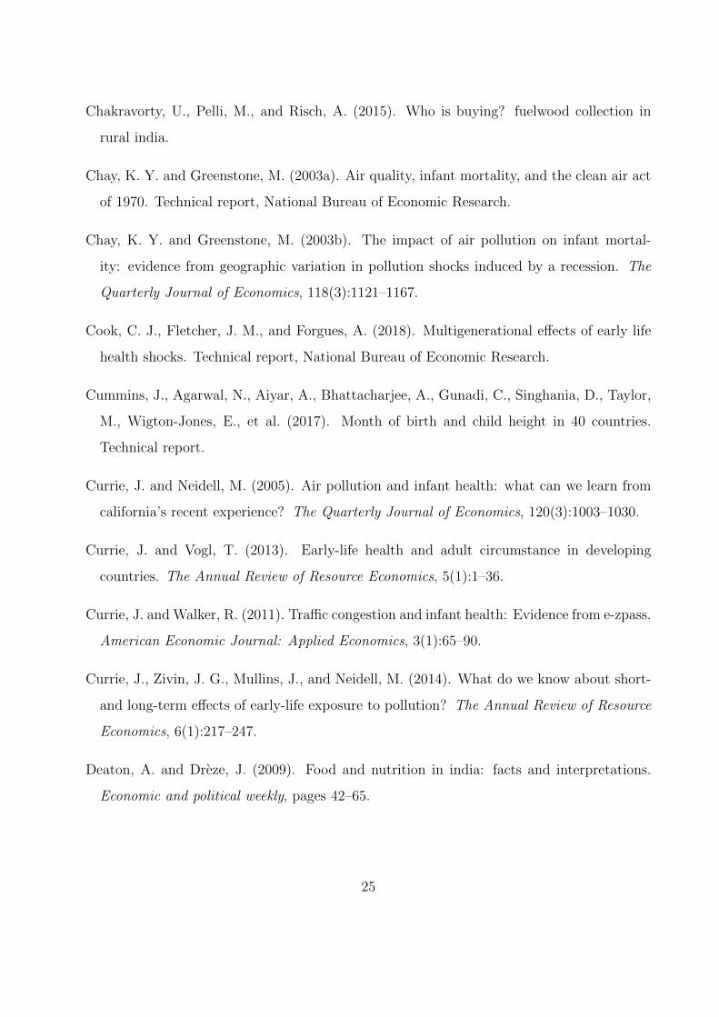
5.3 Heterogeneity
We provide disaggregated regressions for Height-for-age for the following sub-samples: Poor-
Rich and North-South. By splitting our sample into Poor (wealth index lower than 2) and
Rich sample (wealth index greater than equal to 3). In Table 9, we find that the effect is
present only for poor households. This can possibly be due to the fact that children in poor
households have less access to health care to abate negative effect of pollution on health.
We also provide results by splitting our sample into Northern-Southern states and find that
most of the effects that we see are limited to North India.
We now focus on other time windows of critical development, that is second, third
trimester and the post-natal period of first three months after birth. Table 10 summarises
our results, we find that in-utero exposure to outdoor pollution which is experienced by the
mother (and her foetus) for second, third trimester and post-natal period has no impact
on Height-for-age, but some negative effect is present for Weight-for-age corresponding to
exposure in second trimester.
6 Conclusion
Outdoor pollution in India breaches safe standards in many areas. We link outdoor pollution
to biomass burning which is a significant source of carbonaceous aerosols, it plays a vital
role in atmospheric chemistry, air quality, ecosystems, and human health. Our analysis
shows that outdoor pollution is affected by neighbouring biomass burning events; thi is used
to causally infer the effect of outdoor pollution (as measured by PM2.5) on child growth
indicators. We find that a z-score increase in PM2.5 levels during first trimester leads
to a reduction in Height-for-age (HFA-Z, stunting measure) and Weight-for-age (WFA-Z,
underweight measure) by 0.115 and 0.102 standard deviation units respectively. Figure 6
summarises our results graphically, exposure to outdoor pollution during different critical
windows of growth of a child is associated with worse child health outcomes. Almost all the
estimates are negative with significant effect present for exposure to pollution during first
trimester and second trimester (only WFA-Z measure).
22

The above results establish that exposure to pollution is linked to stunting measure
(HFA) in childhood. We now provide an estimate of this problem on GDP of India using a
back-of-an-envelope calculation based on the Galasso et al. (2016) study. This study does a
literature review of the effect of stunting on GDP. Stunting affects GDP of a nation via three
channels: lower returns to lower education, lower returns to lower height and lower returns to
lower cognition. For India, where 66 percent of the workforce was stunted in childhood, this
study estimates that a complete elimination of stunting would have increased GDP by 10
percent 12. We use a point estimate of probability of being stunted due to outdoor pollution,
and find that one standard deviation increase in outdoor pollution leads to a 0.18 percent
reduction in GDP.
India needs effective policies regarding regulation and management of outdoor pollution,
since the current policies are ineffective. Cross-border policies are needed to tackle the
problem of pollution. To curb air pollution, effective management of forest fires is needed;
however, the budget allocation for this purpose is really small and remains unused in every
financial year. Similarly the government has committed itself to subsidising the use of happy-
seeder technology (this is an alternative to combine harvester, it leaves rice residue in form
of a mulch on farm which doesn’t hamper wheat crop sowing and hence doesn’t require
burning), however the uptake of this policy remains quite low due to high initial investment
in the machine (Gupta and Somnathan, 2016). The National Clean Air Program (2018) is
a welcome step in this domain as it plans to extend air quality monitoring network, conduct
intensive awareness and monitoring campaigns, create city-specific action plans, among many
other initiatives.
12 This is an average figure for South Asia.
23

References
State of Global Air 2018. Technical report, Health Effects Institute.
Vulnerability of forest fire 2017. Technical report, Forest Survey of India.
(2017). Assessment of air pollution in indian cities. Technical report, Greenpeace.
Acharya, P., Sreekesh, S., and Kulshrestha, U. (2016). Ghg and aerosol emission from
fire pixel during crop residue burning under rice and wheat cropping systems in north-
west india. The International Archives of Photogrammetry, Remote Sensing and Spatial
Information Sciences, 41:753.
Almond, D. and Currie, J. (2011). Killing me softly: The fetal origins hypothesis. Journal
of Economic Perspectives, 25(3):153–72.
Barber, C. and Schweithelm, J. (2000). Trial by fire: Forest fires and forestry policy in
indonesia’s era of crisis and reform. Technical report, World Resources Institute, Wash-
ington, DC (EUA). Forest Frontiers Initiative.
Bharadwaj, P., Gibson, M., Zivin, J. G., and Neilson, C. (2017). Gray matters: fetal pollution
exposure and human capital formation. Journal of the Association of Environmental and
Resource Economists, 4(2):505–542.
Brainerd, E. and Menon, N. (2014). Seasonal effects of water quality: The hidden costs of the
green revolution to infant and child health in India. Journal of Development Economics,
107:49–64.
Chakrabarti, S., Khan, M. T., Kishore, A., Roy, D., and Scott, S. P. (2019). Risk of acute
respiratory infection from crop burning in india: estimating disease burden and economic
welfare from satellite and national health survey data for 250 000 persons. International
journal of epidemiology.
Chakravorty, U., Pelli, M., and Risch, A. (2014). Far away from the forest? fuelwood
collection and time allocation in rural india.
24
Chakravorty, U., Pelli, M., and Risch, A. (2015). Who is buying? fuelwood collection in
rural india.
Chay, K. Y. and Greenstone, M. (2003a). Air quality, infant mortality, and the clean air act
of 1970. Technical report, National Bureau of Economic Research.
Chay, K. Y. and Greenstone, M. (2003b). The impact of air pollution on infant mortal-
ity: evidence from geographic variation in pollution shocks induced by a recession. The
Quarterly Journal of Economics, 118(3):1121–1167.
Cook, C. J., Fletcher, J. M., and Forgues, A. (2018). Multigenerational effects of early life
health shocks. Technical report, National Bureau of Economic Research.
Cummins, J., Agarwal, N., Aiyar, A., Bhattacharjee, A., Gunadi, C., Singhania, D., Taylor,
M., Wigton-Jones, E., et al. (2017). Month of birth and child height in 40 countries.
Technical report.
Currie, J. and Neidell, M. (2005). Air pollution and infant health: what can we learn from
california’s recent experience? The Quarterly Journal of Economics, 120(3):1003–1030.
Currie, J. and Vogl, T. (2013). Early-life health and adult circumstance in developing
countries. The Annual Review of Resource Economics, 5(1):1–36.
Currie, J. and Walker, R. (2011). Traffic congestion and infant health: Evidence from e-zpass.
American Economic Journal: Applied Economics, 3(1):65–90.
Currie, J., Zivin, J. G., Mullins, J., and Neidell, M. (2014). What do we know about short-
and long-term effects of early-life exposure to pollution? The Annual Review of Resource
Economics, 6(1):217–247.
Deaton, A. and Dreze, J. (2009). Food and nutrition in india: facts and interpretations.
Economic and political weekly, pages 42–65.
25

Dey, S. and Di Girolamo, L. (2010). A climatology of aerosol optical and microphysical
properties over the indian subcontinent from 9 years (2000–2008) of multiangle imaging
spectroradiometer (misr) data. Journal of Geophysical Research: Atmospheres, 115(D15).
Dey, S., Girolamo, L., Van Donkelaar, A., Tripathi, S., Gupta, T., and Mohan, M. (2012).
Decadal exposure to fine particulate matters (pm 2.5) in the indian subcontinent using
remote sensing data. Remote Sens Environ, 127:153–161.
Do, Q.-T., Joshi, S., and Stolper, S. (2018). Can environmental policy reduce infant mor-
tality? evidence from the ganga pollution cases. Journal of Development Economics,
133:306–325.
Douglass, R. L. (2008). Quantification of the health impacts associated with fine particulate
matter due to wildfires.
Fletcher, J. M., Green, J. C., and Neidell, M. J. (2010). Long term effects of childhood
asthma on adult health. Journal of Health Economics, 29(3):377–387.
Foster, A., Gutierrez, E., and Kumar, N. (2009). Voluntary compliance, pollution levels,
and infant mortality in mexico. American Economic Review, 99(2):191–97.
Foster, A. D. and Rosenzweig, M. R. (2003). Economic growth and the rise of forests. The
Quarterly Journal of Economics, 118(2):601–637.
Frankenberg, E., McKee, D., and Thomas, D. (2005). Health consequences of forest fires in
indonesia. Demography, 42(1):109–129.
Galasso, E., Wagstaff, A., Naudeau, S., and Shekar, M. (2016). The economic costs of
stunting and how to reduce them. Policy Research Note World Bank, Washington, DC.
Greenstone, M. and Hanna, R. (2014). Environmental regulations, air and water pollution,
and infant mortality in india. American Economic Review, 104(10):3038–72.
26

Gupta, P. K., Sahai, S., Singh, N., Dixit, C., Singh, D., Sharma, C., Tiwari, M., Gupta,
R. K., and Garg, S. (2004). Residue burning in rice–wheat cropping system: Causes and
implications. Current science, pages 1713–1717.
Gupta, R. (2014). Low-hanging fruit in black carbon mitigation: Crop residue burning in
south asia. Climate Change Economics, 5(04):1450012.
Gupta, S., Agarwal, R., and Mittal, S. K. (2016). Respiratory health concerns in children
at some strategic locations from high pm levels during crop residue burning episodes.
Atmospheric environment, 137:127–134.
Holstius, D. M., Reid, C. E., Jesdale, B. M., and Morello-Frosch, R. (2012). Birth weight
following pregnancy during the 2003 southern california wildfires. Environmental health
perspectives, 120(9):1340.
Isen, A., Rossin-Slater, M., and Walker, W. R. (2017). Every breath you take—every dollar
you’ll make: The long-term consequences of the clean air act of 1970. Journal of Political
Economy, 125(3):848–902.
Jain, N., Bhatia, A., and Pathak, H. (2014). Emission of air pollutants from crop residue
burning in india. Aerosol and Air Quality Research, 14(1):422–430.
Jayachandran, S. (2009). Air quality and early-life mortality evidence from indonesia’s
wildfires. Journal of Human resources, 44(4):916–954.
Kahn, R. A. and Gaitley, B. J. (2015). An analysis of global aerosol type as retrieved by
misr. Journal of Geophysical Research: Atmospheres, 120(9):4248–4281.
Kaskaoutis, D., Kumar, S., Sharma, D., Singh, R. P., Kharol, S., Sharma, M., Singh, A.,
Singh, S., Singh, A., and Singh, D. (2014). Effects of crop residue burning on aerosol
properties, plume characteristics, and long-range transport over northern india. Journal
of Geophysical Research: Atmospheres, 119(9):5424–5444.
27

Kunii, O., Kanagawa, S., Yajima, I., Hisamatsu, Y., Yamamura, S., Amagai, T., and Ismail,
I. T. S. (2002). The 1997 haze disaster in indonesia: its air quality and health effects.
Archives of Environmental Health: An International Journal, 57(1):16–22.
Neidell, M. J. (2004). Air pollution, health, and socio-economic status: the effect of outdoor
air quality on childhood asthma. Journal of health economics, 23(6):1209–1236.
O’Donnell, M. and Behie, A. (2015). Effects of wildfire disaster exposure on male birth weight
in an australian population. Evolution, medicine, and public health, 2015(1):344–354.
Prinz, D., Chernew, M., Cutler, D., and Frakt, A. (2018). Health and economic activity over
the lifecycle: Literature review. Technical report, National Bureau of Economic Research.
Rangel, M. A. and Vogl, T. (2016). Agricultural fires and infant health. Technical report,
National Bureau of Economic Research.
Rukumnuaykit, P. (2003). Crises and child health outcomes: the impacts of economic and
drought/smoke crises on infant mortality and birth weight in indonesia. Economics De-
partment.
Sahu, S. K., Zhang, H., Guo, H., Hu, J., Ying, Q., and Kota, S. H. (2019). Health risk
associated with potential source regions of pm 2.5 in indian cities. Air Quality, Atmosphere
& Health, pages 1–14.
Sanders, N. J. (2012). What doesn’t kill you makes you weaker prenatal pollution exposure
and educational outcomes. Journal of Human Resources, 47(3):826–850.
Sharma, A. R., Kharol, S. K., Badarinath, K., and Singh, D. (2010). Impact of agriculture
crop residue burning on atmospheric aerosol loading–a study over punjab state, india.
Annales Geophysicae (09927689), 28(2).
Simeonova, E., Currie, J., Nilsson, P., and Walker, R. (2018). Congestion pricing, air pollu-
tion and children’s health. Technical report, National Bureau of Economic Research.
28

Singh, C. P. and Panigrahy, S. (2011). Characterisation of residue burning from agricultural
system in india using space based observations. Journal of the Indian Society of Remote
Sensing, 39(3):423.
Soo, J.-S. T. and Pattanayak, S. K. (2019). Seeking natural capital projects: Forest fires,
haze and early-life exposure in indonesia. Proceedings of the National Academy of Sciences.
Srivastava, P. and Garg, A. (2013). Forest fires in india: Regional and temporal analyses.
Journal of Tropical Forest Science, pages 228–239.
Vadrevu, K. P., Lasko, K., Giglio, L., and Justice, C. (2015). Vegetation fires, absorb-
ing aerosols and smoke plume characteristics in diverse biomass burning regions of asia.
Environmental Research Letters, 10(10):105003.
van Donkelaar, A., Martin, R., Verduzco, C., Brauer, M., Kahn, R., Levy, R., and Villeneuve,
P. (2010). A hybrid approach for predicting pm2. 5 exposure: van donkelaar et al. respond.
Environmental Health Perspectives, 118(10):A426–A426.
Van Donkelaar, A., Martin, R. V., Brauer, M., Kahn, R., Levy, R., Verduzco, C., and
Villeneuve, P. J. (2010). Global estimates of ambient fine particulate matter concentrations
from satellite-based aerosol optical depth: development and application. Environmental
health perspectives, 118(6):847.
Vijayakumar, K., Safai, P., Devara, P., Rao, S. V. B., and Jayasankar, C. (2016). Effects
of agriculture crop residue burning on aerosol properties and long-range transport over
northern india: A study using satellite data and model simulations. Atmospheric Research,
178:155–163.
Zheng, S., Wang, J., Sun, C., Zhang, X., and Kahn, M. E. (2019). Air pollution lowers chinese
urbanites’ expressed happiness on social media. Nature Human Behaviour, page 1.
29

Tables and Figures
Figure 1: Spatial variation in Pollution: Mean PM2.5 in districts of India (2010 to 2016)
30

Figure 2: Binscatter plot for relationship between Height-for-age Z scores and Mean PM2.5
in first trimester.
31

CMea
n PM2.5
75 Km radius
100 Km radius
uF
F
F
uF F
Figure 3: Identification Strategy: Center (smallest grey circle) represents the cluster location,
White circle corresponds to 75km radius circle around the cluster location, grey ring area
(donut shape) corresponds to area between two circles (75 and 100 Km radii circles) with
cluster location as the center. Mean pollution level is calculated for the white circle, we call
this local pollution level for cluster C.
Local pollution level is instrumented using i) non-local biomass burning events which take
place in the grey ring area (F + uF). ii) Upwind non-local biomass burning events which
take place in the grey ring area (only uF). Probability weighted counts used everywhere.
32

Figure 4: Linear fit plot between Mean PM2.5 (in 75 km radius), Total number of fire-events
between 75 and 100 km radius(Non-local fire-events) & Total number of upwind fire-events
between 75 and 100 km radius (Non-local upwind fire-events). Unit of observation is a child,
shaded area is 95% confidence interval.
Figure 5: Mean PM2.5, Mean count of all fire-events (in 75-100 km radius) & Mean count
of upwind fire-events (in 75-100 km radius) for each month in every year from 2010 to 2016.
Figure represents mean over all sampled clusters belonging to all states of India.
33

Figure 6: Coefficient of 2SLS regression of outcomes(HFA-Z and WFA-Z) on outdoor air
pollution for different critical windows of development of a child. Vertical lines represent 95
percent confidence intervals.
34

Table 1: Summary Statistics
All India NorthIndia SouthIndia
Variable Mean Std Dev Mean Std Dev Mean Std Dev
Outcomes
Height-for-age z score -1.46 1.68 -1.52 1.68 -1.27 1.66
Weight-for-age z score -1.52 1.22 -1.54 1.22 -1.44 1.22
Weight-for-height z score -0.97 1.38 -0.96 1.38 -1.01 1.41
Child characteristics
Dummy for male child 0.52 0.50 0.52 0.50 0.51 0.50
Birth-order 2.26 1.46 2.38 1.54 1.88 1.05
Childage in months 29.00 16.55 29.02 16.58 28.94 16.46
Pregnancy duration 9.02 0.48 9.00 0.46 9.10 0.52
Parents characteristics
Mother’s age at birth 24.50 4.91 24.67 5.00 23.91 4.56
Mother’s number of education years 6.26 5.16 5.81 5.18 7.81 4.77
Dummy for literate father 0.97 0.17 0.97 0.18 0.98 0.15
Household characteristics
Rural 0.76 0.43 0.77 0.42 0.70 0.46
Dummy for head of household being a male 0.88 0.33 0.88 0.33 0.89 0.32
Age of head of household 44.59 15.18 44.51 15.21 44.88 15.09
Dummy for source of water: Pipedwater 0.23 0.42 0.23 0.42 0.24 0.43
Dummy for using clean cooking fuel 0.28 0.45 0.26 0.44 0.37 0.48
Dummy for household practicing open
defecation (OD)0.42 0.49 0.41 0.49 0.44 0.50
Fraction of HHs practicing OD in a
village0.43 0.35 0.43 0.35 0.45 0.33
Has electricity connection 0.85 0.36 0.82 0.38 0.94 0.23
Religion = Hindu 0.73 0.44 0.70 0.46 0.83 0.38
Household size 6.57 2.87 6.75 2.93 5.99 2.57
Mean pollution in 75 km radius
1st Trimester 54.06 31.87 59.33 32.90 35.96 19.07
2nd Trimester 52.23 29.84 56.98 30.90 35.90 18.02
3rd Trimester 53.30 32.40 58.52 33.68 35.32 18.47
Post-natal (3 months after birth) 53.32 35.38 58.46 36.89 35.44 21.46
Observations 1,81,361 1,40,476 40,885
35

Table 2: First-stage regression
Mean PM2.5 in
75 km radius(Z)
(1) (2)
IV1: Number of fire events between 75 and 100 km radius (Z) 0.165***
(0.003)
IV2: Number of upwind fire events between 75 and 100 km radius (Z) 0.105***
(0.003)
First Stage F-stat 2099 863
rk LM statistic 1997 1005
Anderson Rubin wald statistic (p-value) 0.0018 0.0016
Observations 179816 179816
Includes other controls from 2nd stage Yes Yes
Includes FEs for Month, Year & Cluster Yes Yes
Includes FEs for Month*Year & District*Year Yes Yes
Note: Each coefficient corresponds to an individual FIRST stage 2SLS regression of HFA-Z or WFA-Z on
variables mentioned in the first column. Standard errors in parentheses are clustered by DHS cluster. Notation
for p-values *** is p < 0.01, ** is p < 0.05 & * is p < 0.1. Regressions include other controls - gender, birth
order and age of child, mother’s years of education, mother’s age at birth and its square, age and gender of
household head, dummy for whether household has pipedwater, has clean cooking source, whether household
practices open defecation and fraction of the village who practice open defecation(excluding self). PM2.5,
Fire-events variables (IV1, IV2) have all been converted into z-scores.
36

Table 3: Instrumental variable regression of outcomes on weighted PM2.5 (z-score)
All Fire events between 75
and 100 Km radius
Upwind Fire events
between 75 and 100 Km radius
OLS IV1 IV2
(1) (2) (3) (4) (5) (6)
WFA-Z HFA-Z WFA-Z HFA-Z WFA-Z HFA-Z
Trimester-1: Mean PM2.5 in 75km radius (Z) -0.0121** -0.0116 -0.0683*** -0.0854*** -0.102*** -0.115***
(0.00512) (0.00709) (0.0219) (0.0298) (0.0323) (0.0447)
Mean of Dependent Variable -1.52 -1.46 -1.52 -1.46 -1.52 -1.46
Includes Child, Mother & HH characteristics Yes Yes Yes Yes Yes Yes
Includes FEs for Month, Year & Cluster Yes Yes Yes Yes Yes Yes
Includes FEs for Month*Year & District*Year Yes Yes Yes Yes Yes Yes
Observations 179816 179816 179816 179816 179816 179816
Note: Standard errors in parentheses are clustered by DHS cluster. Notation for p-values *** is p < 0.01, ** is p < 0.05 & * is p < 0.1. Each
coefficient corresponds to an individual OLS or 2SLS regression of HFA-Z or WFA-Z on weighted mean PM2.5 in first trimester (z-score). Regressions
include controls which are same as those mentioned in Table 2 notes.
37

Table 4: Robustness Checks: Extended control for weather & gestational age
IV: Upwind fire-events
b/w 75 and 100 km radius
(1) (2) (3) (4)
WFA-Z HFA-Z WFA-Z HFA-Z
Trimester-1: Mean PM2.5 in 75km radius (Z) -0.111*** -0.125*** -0.103*** -0.116***
(0.0328) (0.0453) (0.0323) (0.0448)
Mean rainfall in 75 km radius -0.046** -0.049
(0.021) (0.030)
Mean temperature in 75 km radius 0.003** 0.003
(0.001) (0.002)
Gestational period 0.137*** 0.165***
(0.025) (0.034)
Observations 179459 179459 179816 179816
Includes Child, Mother & HH characteristics Yes Yes Yes Yes
Includes FEs for Month, Year & Cluster Yes Yes Yes Yes
Includes FEs for Month*Year & District*Year Yes Yes Yes Yes
Note: Standard errors in parentheses are clustered by DHS cluster. Notation for p-values *** is p <
0.01, ** is p < 0.05 & * is p < 0.1. Each coefficient corresponds to an individual 2SLS regression of
HFA-Z or WFA-Z on weighted mean PM2.5 in first trimester (z-score). Regressions include controls
which are same as those mentioned in Table 2 notes.
38

Tab
le5:
Sen
siti
vit
yA
nal
ysi
s
IV:
Upw
ind
Fir
eev
ents
b/w
50an
d10
0K
mra
diu
s
IV:
Upw
ind
Fir
eev
ents
b/w
50an
d75
Km
radiu
s
IV:
Upw
ind
Fir
eev
ents
b/w
75an
d10
0K
mra
diu
s
Dro
ppin
gP
unja
b
(1)
(2)
(3)
(4)
(5)
(6)
WFA
-ZH
FA
-ZW
FA
-ZH
FA
-ZW
FA
-ZH
FA
-Z
Tri
mest
er-
1:
Mean
PM
2.5
in50km
rad
ius
(Z)
-0.1
01**
*-0
.086
7*-0
.111
***
-0.0
770
(0.0
331)
(0.0
461)
(0.0
349)
(0.0
481)
Tri
mest
er-
1:
Mean
PM
2.5
in75km
rad
ius
(Z)
-0.0
910*
**-0
.121
***
(0.0
285)
(0.0
413)
Obse
rvat
ions
1644
6216
4462
1644
6216
4462
1751
4117
5141
Incl
udes
Child,
Mot
her
&H
Hch
arac
teri
stic
sY
esY
esY
esY
esY
esY
es
Incl
udes
FE
sfo
rM
onth
,Y
ear
&C
lust
erY
esY
esY
esY
esY
esY
es
Incl
udes
FE
sfo
rM
onth
*Yea
r&
Dis
tric
t*Y
ear
Yes
Yes
Yes
Yes
Yes
Yes
Note
:Sta
ndar
der
rors
inpar
enth
eses
are
clust
ered
by
DH
Scl
ust
er.
Not
atio
nfo
rp-v
alues
***
isp<
0.01
,**
isp<
0.0
5&
*is
p<
0.1.
Each
coeffi
cien
t
corr
esp
onds
toan
indiv
idual
2SL
Sre
gres
sion
ofH
FA
-Zor
WFA
-Zon
wei
ghte
dm
ean
PM
2.5
infirs
ttr
imes
ter
(z-s
core
).R
egre
ssio
ns
incl
ude
contr
ols
whic
h
are
sam
eas
thos
em
enti
oned
inT
able
2not
es.
39

Table 6: Falsification Tests
IV: Downwind Fire-events
in 75 to 100km radius
IV: Upwind Fire-events
in 75 to 100 km radius
(shuffled location)
(1) (2) (3) (4)
WFA-Z HFA-Z WFA-Z HFA-Z
Trimester-1: Mean PM2.5 in 75km radius (Z) -0.008 0.003 0.033 0.054
(0.03) (0.04) (0.033) (0.048)
Observations 179816 179816 179539 179539
Includes Child, Mother & HH characteristics Yes Yes Yes Yes
Includes FEs for Month, Year & Cluster Yes Yes Yes Yes
Includes FEs for Month*Year & District*Year Yes Yes Yes Yes
Note: Standard errors in parentheses are clustered by DHS cluster. Notation for p-values *** is p < 0.01,
** is p < 0.05 & * is p < 0.1. Each coefficient corresponds to an individual 2SLS regression of HFA-Z or
WFA-Z on weighted mean PM2.5 in first trimester (z-score). Regressions include controls which are same
as those mentioned in Table 2 notes.
40

Tab
le7:
IVV
alid
ity
Mot
her
’sF
ath
erA
sset
Poor
Vac
cin
atio
nH
Hsi
ze
Ed
uca
tion
Lit
erat
eO
wn
ersh
ip
(1)
(2)
(3)
(4)
(5)
(6)
Upw
ind
fire
even
tsb
etw
een
0.01
6-0
.000
2-0
.001
0.00
10.
0007
0.01
75an
d10
0km
rad
ius
in1s
tT
rim
este
r(Z
)(0
.01)
(0.0
003)
(0.0
02)
(0.0
008)
(0.0
01)
(0.0
06)
Ob
serv
atio
ns
1798
1617
9816
1798
1617
9816
1798
1617
9816
Incl
ud
esC
hil
d,
Mot
her
&H
Hch
arac
teri
stic
sY
esY
esY
esY
esY
esY
es
Incl
ud
esF
Es
for
Mon
th,
Yea
r&
Clu
ster
Yes
Yes
Yes
Yes
Yes
Yes
Incl
ud
esF
Es
for
Mon
th*Y
ear
&D
istr
ict*
Yea
rY
esY
esY
esY
esY
esY
es
Sta
nd
ard
erro
rsin
par
enth
eses
are
clust
ered
by
DH
Scl
ust
er.
Not
atio
nfo
rp-v
alu
es**
*is
p<
0.0
1,**
isp<
0.05
&*
isp
<0.
1.F
ire-
even
tshav
eb
een
conver
ted
toz-
score
s.
41

Table 8: Mother’s conception behaviour
(1) (2)
log conceptions log conceptions
3 month exposure to Upwind fire-events 0.00732
in 75-100kms (0.0119)
Exposure to Upwind fire-events in 75-100kms 0.0119
in the month of conception (0.0219)
Observations 197753 197753
Cluster FE Yes Yes
Month FE Yes Yes
Note: Standard errors in parentheses are clustered by DHS cluster. Notation for p-
values *** is p < 0.01, ** is p < 0.05 & * is p < 0.1. Each coefficient corresponds to
an individual OLS regression of log number of conceptions on controls mentioned in
the table. Regressions include other controls for mother’s education, father’s literacy
level, characteristics of household head and wealth index of the household.
42
Table 9: Heterogeneity
IV regression: Height-for-age Z score
Poor Rich North South
(1) (2) (3) (4)
Trimester-1: Mean PM2.5 in 75km radius(Z) -0.139** -0.0824 -0.120*** -0.0226
(0.0592) (0.0633) (0.0433) (1.813)
Observations 84458 88932 139656 40159
Includes Child, Mother & HH characteristics Yes Yes Yes Yes
Includes FEs for Month, Year & Cluster Yes Yes Yes Yes
Includes FEs for Month*Year & District*Year Yes Yes Yes Yes
Note: Standard errors in parentheses are clustered by DHS cluster. Notation for p-values ***
is p < 0.01, ** is p < 0.05 & * is p < 0.1. Each coefficient corresponds to an individual 2SLS
regression of HFA-Z on weighted mean PM2.5 in first trimester (z-score). Regressions include
controls which are same as those mentioned in Table 2 notes.
North Indian states: Arunachal Pradesh, Assam, Bihar, Chandigarh, Gujarat, Haryana, Hi-
machal Pradesh, Jammu and Kashmir, Jharkhand, Madhya Pradesh, Manipur, Meghalaya,
Mizoram Nagaland, Delhi, Punjab, Rajasthan, Sikkim, Tripura, Uttar Pradesh and Uttarak-
hand.
South Indian states: Andhra Pradesh, Karnataka, Kerala, Maharashtra, Chhattisgarh, Odisha,
Telangana, West Bengal, Lakshwadeep Islands, Andaman and Nicobar Islands, Dadar and Na-
gar Haveli, Daman and Diu, Puducherry and Goa.
43

Table 10: Instrumental variable effects:
Impact of weighted PM2.5 in 2nd Trimester to Post-natal period
(1) (2)
WFA-Z HFA-Z
Trimester-2: Mean PM2.5 in 75km radius (Z) -0.05* -0.03
(0.03) (0.04)
Observations 184183 184183
Trimester-3: Mean PM2.5 in 75km radius (Z) -0.05 -0.05
(0.04) (0.05)
Observations 172917 172917
Post-natal: Mean PM2.5 in 75km radius (Z) -0.01 0.05
(0.03) (0.04)
Observations 190717 190717
Includes Child, Mother & HH characteristics Yes Yes
Includes FEs for Month, Year & Cluster Yes Yes
Includes FEs for Month*Year & District*Year Yes Yes
Note: Standard errors in parentheses are clustered by DHS cluster. No-
tation for p-values *** is p < 0.01, ** is p < 0.05 & * is p < 0.1. Each
coefficient corresponds to an individual 2SLS regression of HFA-Z or
WFA-Z on weighted mean PM2.5 in first trimester (z-score). Regres-
sions include controls which are same as those mentioned in Table 2
notes.
44
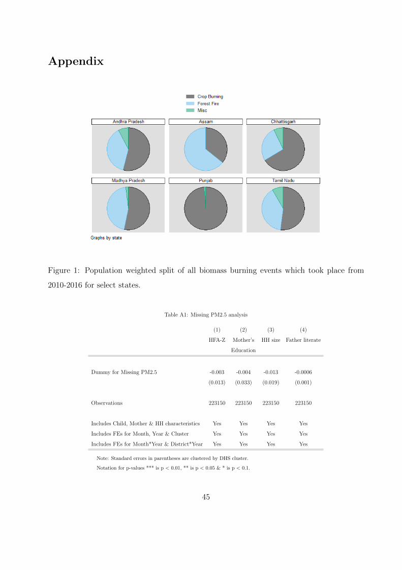
Appendix
Figure 1: Population weighted split of all biomass burning events which took place from
2010-2016 for select states.
Table A1: Missing PM2.5 analysis
(1) (2) (3) (4)
HFA-Z Mother’s HH size Father literate
Education
Dummy for Missing PM2.5 -0.003 -0.004 -0.013 -0.0006
(0.013) (0.033) (0.019) (0.001)
Observations 223150 223150 223150 223150
Includes Child, Mother & HH characteristics Yes Yes Yes Yes
Includes FEs for Month, Year & Cluster Yes Yes Yes Yes
Includes FEs for Month*Year & District*Year Yes Yes Yes Yes
Note: Standard errors in parentheses are clustered by DHS cluster.
Notation for p-values *** is p < 0.01, ** is p < 0.05 & * is p < 0.1.
45

Table A2: Reduced form Effect
(1) (2)
WFA-Z HFA-Z
Trimester-1: Upwind Fire events (75 to 100 kms radius) -0.00845** -0.0156***
(0.00414) (0.00560)
Trimester-2: Upwind Fire events (75 to 100 kms radius) 0.00439 -0.00453
(0.00418) (0.00550)
Trimester-3: Upwind Fire events (75 to 100 kms radius) 0.00303 -0.00568
(0.00410) (0.00526)
Includes Chils, Mother & HH Characteristics Yes Yes
Includes FE for Month, Year, Cluster Yes Yes
Includes FE for Month*Year & District*Year Yes Yes
Observations 179449 179449
Note: Standard errors in parentheses are clustered by DHS cluster. Notation for p-
values *** is p < 0.01, ** is p < 0.05 & * is p < 0.1. Each coefficient corresponds to
an individual OLS regression of HFA-Z or WFA-Z on fire-events (z-score). Regressions
include controls which are same as those mentioned in Table 2 notes.
46


28 | Too Slow for the Urban March: Litigations and Real Estate Market in Mumbai, India
QUALITY
INDEPENDENCE
IMPACT