Quality Control Tutorial for DTI

UNC Neuro Image and Research Analysis Laboratories Cheryl Dietrich, Joseph Blocher, Martin Styner

2

There are three main steps to Quality Control protocol for DTI 1.) DICOM conversion – Download and conversion of files to .nhdr files for use in programs 2.) DTIPrep Automatic QC – Execution of a protocol script to automatically QC scans 3.) Visual DWI & DTI QC – Visual recheck of DITPrep QC results, preliminary fiber tracking, and visual check of signal loss and anomalies

I. DICOM conversion A. Conversion of Dicom to NHDR

Step Description Action

1 Go to subject folder example cd /projects4/CHDI_TrackHD/HDNI/<subjectID>

2a. Run Dicom conversion DicomToNrrdConverter - - inputDicomDirectory <path to

directory with dcms> - -outputVolume <subjectID_dwi.nhdr>

- -outputDirectory <path to output directory>

2b. Optional: add option to

the command to write a

report for debugging

DicomToNrrdConverter - - inputDicomDirectory <path to

directory with dcms> - -outputVolume <subjectID_dwi.nhdr>

- -outputDirectory <path to output directory>

- -writeProtocolGradientsFile >! <DicomConvReport.txt>

3 Verify correct conversion

with DTIPrep

DTIPrep – In DTIPrep GUI, click on “File” and then “Open

DWI” to open the .nhdr file

4 Record conversion date in notes

II. DTIPrep Automatic QC

A. Initial Visual QC i. In DTIPrep, review baseline images in axial, sagittal, and coronal views. Note any issues

of coverage, i.e. inferior axial slices missing such as the cerebellum and temporal lobe, and/or superior slices missing. Second, for future reference, notice any artifacts or motion in these scans, i.e. “venetian blind” effect, checkers, etc. DTIPrep will automatically detect and extract most of these artifacts. For more details on these artifacts see section III - “Visual DWI & DTI QC”

Figure 1.1 Some basic functions in DTIPrep GUI – See Table 1 in Appendix for more information

3

Note: In the TrackHD study, coverage issues automatically received a rating of “Borderline” with rankings of minor, intermediate, and severe appearing in the notes. Depending on the type of analysis, full coverage may be required to produce a suitable atlas.

Figure 1.2 “Bad coverage (severe)” a scan missing nearly all of the cerebellum and a large portion of the temporal lobe Figure 1.3 Good coverage

B. Run Protocol

i. Click on the “Protocol” tab on the left side of the screen. Select “Load” and choose the appropriate protocol file. Click on RunByProtocol button on the bottom of the DTIPrep box.

ii. The RunProtocol progress bar at the bottom of the screen will stop when the protocol is finished.

iii. The QC results for each gradient are visible in the QCResults tab. Also, the results for each gradient check read Pass or Fail in the command line, depending on the parameters and threshold set in the protocol.

Figure 1.4 Loading and running QC protocol files in DTIPrep GUI

4

Figure 1.5 Command line showing results overlaying DTIPrep GUI with protocol results under the QCResults tab

Figure 1.6 Exclusions from automatic QC (results from protocol) are shown in the QCResults tab for each gradient. Scrolling through the dwi images, the gradient number box is red for exclusions and green for inclusions

III. Visual DWI & DTI QC A. Visual DWI QC

i. After the protocol runs, if DTIPrep1.1.1 has been closed, open the original ~_dwi.nhdr file (not the QCed file). On the QCResults tab, load the ~QCResults.xml file created by DTIPrep

ii. Selecting a representative slice, examine axial, sagittal and coronal views across all DWI gradients; adjust contrast and scroll through other slices as necessary.

iii. Document any perceived image quality issues; i.e. “venetian blind” effect/horizontal stripes (Fig. 2.2), “checkers” effects - particularly in axial views (Fig. 2.3), motion artifacts, geometric artifacts, “bar” artifacts, distortion, “Z-stripe” artifacts, gradients with intensity differences between slices (Fig. 2.6), “cartoon/blur” artifacts (Figs. 2.12-13) and any other anomalies.

5

iv. For each direction deemed appropriate for manual exclusion based on image quality, go to the QCResults tab, follow the drop-down menus: DWI Check>gradient_#>Visual Check then double-click on “VC_status” and select “Exclude” in the pop-up box. a) General, mild, distortions often seen in the pre-frontal lobe are not usually excluded b) Certain artifacts may occur across most or all gradients. In these cases, perform

further analysis and documentation of the artifact. If the artifact is associated with a particular scan, that scan may receive a “Fail” rating.

c) If the artifact is present in multiple scans from the same protocol a determination of a “Borderline” rating might be made in the interest of preserving data. [In this study, Zoltan-protocol-related distortion was associated with gradient-consistent artifacts (see Figures 2.7-2.10)] Following this conclusion, carefully record the nature and location of the artifact and include this information.

v. Record the amount and gradient numbers of manually excluded directions in notes. Select the “Save Dwi and QCResult” button under “Manual Checking” to save the changes in the ~QCResult.xml file and create a new ~.nhdr and ~.raw

Figure 2.1 Visual Checking/Manual Exclusion of “bad” gradients.

Examples of visual artifacts found in dwi images are on the following pages: 6-10

6

Figure 2.2 “Venetian Blind” Effect A clear example of the “venetian blind” artifact as seen in DTIPrep

Figure 2.3 (left) “Checkers” artifact shown in an axial slice in a DWI gradient This artifact occurs most commonly in scans that also have a three-stripe blurring effect. In this study, some of the Siemen’s protocol dataset contained these three-stripe blur artifacts as shown below in Fig. 1.6

Figure 2.4 (right) “Three-stripe blur” artifact in sagittal view of DWI gradients

Figure 2.5 (left) Frontal Distortions Distortion clearly visible in a baseline image from a Zoltan-protocol dataset

7

Figure 2.6 DWI with a high-intensity axial slice as displayed in DTIPrep Although in the sagittal view this slice appears only halfway bright, both the axial and coronal views show a consistent difference in intensity compared to the surrounding slices; this gradient was excluded

Figure 2.7 Distortion-related artifact “Z stripe” running in the anterior/posterior direction and visible in axial slices and occasionally in sagittal view. Prominent in Zoltan protocol.

Figure 2.8 One type of geometric artifact, triangular in shape, possibly caused by eddy current motion

8

Figure 2.9 Another type of triangle-shaped geometric artifact, outlined on the right

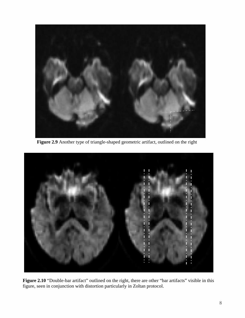
Figure 2.10 “Double-bar artifact” outlined on the right, there are other “bar artifacts” visible in this figure, seen in conjunction with distortion particularly in Zoltan protocol.

9

Figure2.11 Lateral sulcus anomaly present in all protocols, but more consistently in Zoltan dataset

Figure 2.12 Cartoon/blur artifact in cerebellum This artifact was noted, but not excluded due to its specific location in the cerebellum and areas with high CSF (such as along ventricle borders)

Figure 2.13 Extreme cartoon/blur This artifact was automatically excluded by the protocol in QC.

10

Note: Beware of “false artifacts” The issue below is due only to the positioning of the head and not a scanner or acquisition-related artifact

Figure 2.14 Falsely perceived anomaly or artifact - A superior indentation appears to “travel” in the anterior-posterior direction as the sagittal slices progress, shown with arrows. This can occur in cases where the axial direction is “yawed” or rotated in relation to the sagittal plane. (shown in next figure, 2.15).

Figure 2.15 Rotated axial slices – As the sagittal plane crosses the medial plane of the brain at angle, the cross-point appears as an “indentation” in the sagittal view, seen above and in Figure 2.13.

Cross point of sagittal slice

and medial plane of the brain

11

vi. After making and saving manual exclusions, select 3D view tab and click on the sphere icon as well as the F and I icons to view distribution of directionality. The F represents the directions before QC. These directions are represented in blue. The I represents the directions left after QC, labeled in green. Note any major unevenness in spatial distribution caused by “clustering” of excluded gradients [For the purposes of the TrackHD study, “major unevenness in spatial distribution” was defined generously. For example, no documentation/failures of subjects due to spatial gaps occurred unless a visual estimation equals approximately 40% or more of the sphere.]

Figure 2.16 3D View displaying distribution of direction of gradients before and after automatic QC by DTIPrep

B. Preliminary DTI Tracking QC (glyphs and fiducial seeding) i. Convert ~dwi_VC.nhdr (or ~QCed.nhdr if there are no manual extractions) files into

~.nrrd files using CreateDTIImages.script Open ~float.nrrd file in Slicer under File>Add Volumes>Apply

ii. Glyph check a) Under the “Volumes” module, select the “Display” drop down menu and change the

Scalar Mode to “Color Orientation” b) Select all three boxes in the “Glyphs Visibility Display” area c) Adjust spacing setting as necessary to clearly see the individual glyphs d) Look at the directionality of the glyphs in the Axial window, examine the Corpus

Callosum, genu and splenium, to ensure that the glyphs are following the tract e) Do the same with the coronal section of the CC, which can be seen in the Coronal

slices. After QC check, deselect the three glyph visibility boxes

12

Figure 3.1 Selecting “Color Orientation” in the Scalar Mode

Figure 3.2 Viewing Glyph Directions in Slicer – Selecting “glyph visibility” and changing the spacing

iii. Tracking using Fiducial Seeding a) Select the “Fiducials” Module and click on the arrow icon in the top icon toolbar,

selecting “Use mouse to create-and-place persistently” to place seeds for five tracts: Corpus Callosum (genu, splenium, coronal); Cingulum, Uncinate, Arcuate, and Internal Capsule

b) Directionalities are demonstrated in the color map along the following orientations: red is left/right, green is anterior/posterior, and blue is inferior/superior

13

Figure 3.3 Incorrect Glyph Directions in Slicer – It is imperative to regulate this problem before continuing with QC, otherwise the resulting tracts are incorrect

c) Seedmap labeling of tracts CC – Starting in the Sagittal plane, identify the CC, which typically appears red

in DTI Color Orientation maps. It is bounded superiorly by the cingulum and inferiorly by the lateral ventricles. Place a fiducial in the most anterior part to mark the genu. Place another label in the posterior section of the CC, to mark the splenium. In the coronal view, mark the CC at its vertex to track the coronal fiber bundles of the CC.

Cingulum – In the Coronal view, superior to the CC, is the cingulum appearing normally as two green “teardrop” shaped bodies. Mark the left side cingulum.

Uncinate – In the axial view, move inferiorly through the slices. Lateral to the brainstem, the anterior tip of the inferior longitudinal fasciculus appears blue/purple. Place a fiducial on the right side to mark the uncinate.

Arcuate (2 fiducials) – In the axial view, locate the arcuate. Lateral to the inferior fronto-occipital fasciculus/inferior longitudinal fasciculus, and at the temporo-parietal junction towards the posterior direction of the brain, lies a blue/purple portion of the arcuate. Place a fiducial here. “The fronto-parietal portion of the arcuate fasciculus encompasses a group of fibers with antero-posterior direction (green)” that can be found lateral to the corticospinal tract a few axial slices superior from the last fiducial, place a second marker here. (Catani et. al., 2008, “A diffusion tensor imaging tractography atlas for virtual in vivo dissections”)

14

Figure 3.4 Placing Fiducial Label Seeds to track the Uncinate, Cingulum and Corpus Callosum (genu, splenium, and coronal section)

Place one fiducial in posterior portion (normally blue/purple) of the arcuate. (see left) Place another several slices up in the superior direction next to corticospinal tract; the arcuate is usually green here. (see right)

Internal Capsule – In the coronal view, medial to the arcuate and inferior longitudinal fasciculus and lateral to the CC is the internal capsule. Usually, it is mostly blue/purple. Place 2-3 fiducials in the internal capsule, particularly, in the most inferior part of the IC that is blue/purple

15

Figure 3.5 Placing Fiducial Label Seeds to track the Internal Capsule (IC) in Slicer

d) Diffusion Tractography for preliminary QC Under “Modules”, go to Diffusion > Tractography> Fiducial Seeding; Choose

“L” from the “Select FiducialList or Model” drop down menu, then “Create New Fiber Bundle” from the “Output Fiber Bundle Node” drop down menu.

Set the Stopping Value to 0.10, the Fiducial Seeding Region (mm) to 6.0 mm, and the Fiducial Seeding Step Size (mm) to 1.0 mm.

Figure 3.6 Diffusion Tractography of Fiducial Labels

16

[Optional] To increase speed and performance, it is possible to change the display of tubes to lines. Go to Diffusion > Tractography > Fiber Bundles. Click on the “Lines” tab and select the “Visibility” box. Click on the “Tubes” tab and deselect the “Visibility” box.

Figure 3.7 Cingulum fiber bundle tractography viewed with Line display

Return to the Fiducials module; deselect any labels that are undesired to appear in the 3D Viewing pane. Look to ensure that all tracts are present. If they are incomplete, add more fiducial seeds in areas that are lacking. Or, move the existing labels using the “Use mouse to Pick-and-Manipulate persistently” option under the hand icon.

Figure 3.8 Uncinate label only selected, shown with Sagittal slice in 3D window

17

e) Record any unusual tracts; if correlated with unusual coloration of the ColorFA, see Color Artifact PowerPoint If the above steps are not successful, note any incomplete or missing tracts. Figure 3.9 (right) displays an unusual-looking genu and splenium. In this example, the pathology of the subject (observe enlarged lateral ventricles), rather than tractography, is the suspected cause of the difference and was appropriately documented in the visual QC notes.

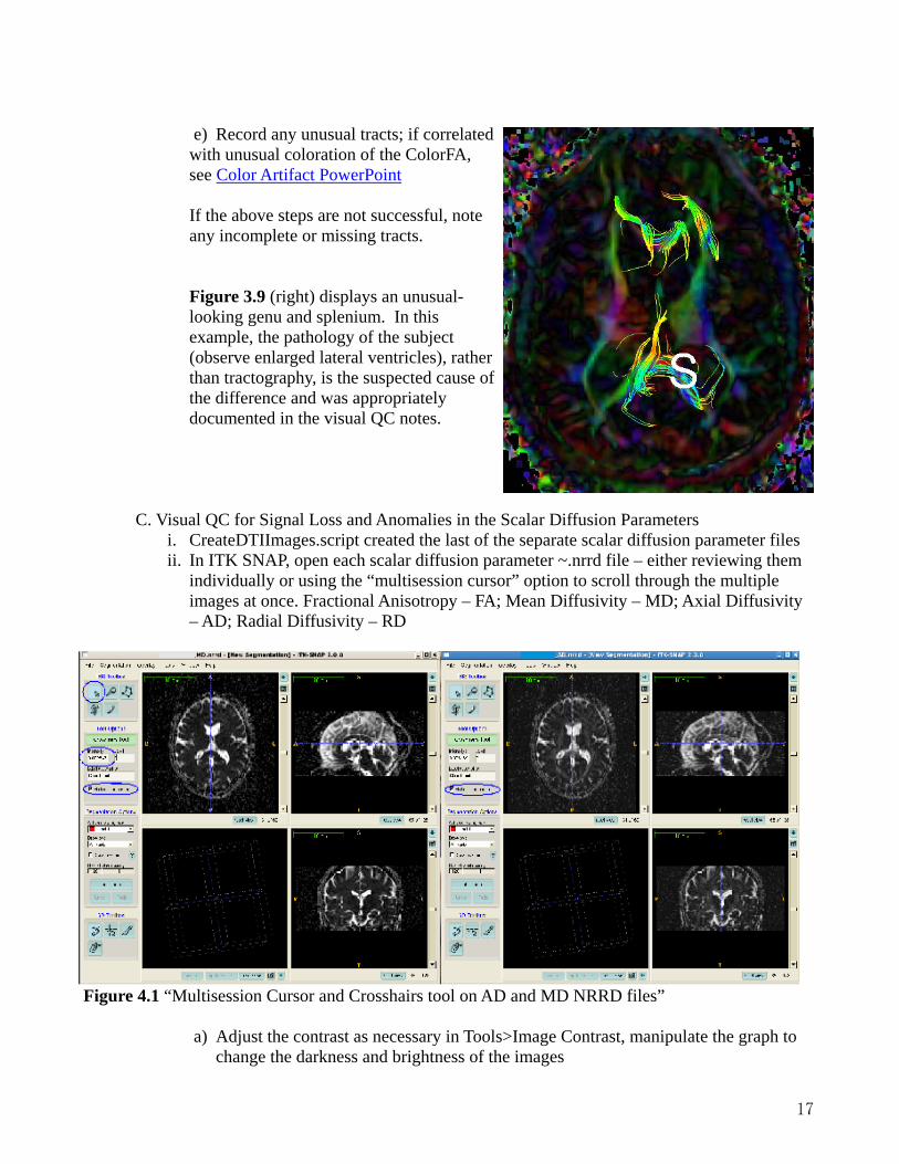
C. Visual QC for Signal Loss and Anomalies in the Scalar Diffusion Parameters

i. CreateDTIImages.script created the last of the separate scalar diffusion parameter files ii. In ITK SNAP, open each scalar diffusion parameter ~.nrrd file – either reviewing them

individually or using the “multisession cursor” option to scroll through the multiple images at once. Fractional Anisotropy – FA; Mean Diffusivity – MD; Axial Diffusivity – AD; Radial Diffusivity – RD

Figure 4.1 “Multisession Cursor and Crosshairs tool on AD and MD NRRD files”

a) Adjust the contrast as necessary in Tools>Image Contrast, manipulate the graph to change the darkness and brightness of the images

18

b) Visually check all slices for signal loss/noise represented by pixilated bright spots in

the FA file and dark spots in the MD, AD, and RD files.

Look for clusters of this

perceived signal loss. If present, click the Crosshairs tool in the area and review the intensity information. In the FA, anatomy should not equal more than 1.0.

Figure 4.2 Adjusting Image Contrast in ITK SNAP In the MD, RD, and AD files, it should not be less than zero. If these intensities are more than 1.0 and less than 0, note the area for signal loss.

Figure 4.3 Signal Loss demonstrated in FA image in Right Pre-Frontal Lobe

Observe that some signal loss in the orbital regions is typical

19

Figure 4.4 Diagonal NRRD artifact displayed in ITK SNAP, FA and MD images respectively This case was subsequently failed as a result of this issue with image-acquisition

c) During the visual check, also note any anomalous regions that may be due to

anatomical lesions or problems in image acquisition. In this study, five types of artifacts were identified in the scalar diffusion files: diagonal NRRD artifact, possible motion artifacts, wrapping artifacts, a pre-frontal anomaly traced to the Philips protocol, and distortion-related signal loss artifacts. Diagonal NRRD artifact, Figure 4.4 demonstrates this diagonal striping artifact.

The MD image reveals the large extent of the brain area affected by this issue.

Figure 4.5 (left) Possible motion artifacts in the NRRD files Figure 4.6 (right) Wrapping artifacts in the NRRD files

20

Possible motion artifacts such as the one displayed in Figure 4.5 are often

apparent in inferior axial slices up through the eye area. Like all visually detected artifacts, these are noted in visual QC notes.

Wrapping artifacts contain one or several “shadow” images that may or may not be inverted. In Figure 4.6, the eyes clearly mark this artifact.

Figure 4.7 Pre-frontal anomaly in RD ~.nrrd file, axial and sagittal views

Figure 4.7 demonstrates a pre-frontal anomaly in ~50% of a dataset from a

Philips protocol. It is mostly visible in axial views, but is occasionally visible in the sagittal view as well.

If available, the color FA can be loaded on top of the FA ~.nrrd file in ITK SNAP for closer examination of such anomalies. Go to File>Open RGB Image. Click “Browse” to find the appropriate color FA ~.nrrd file

Figure 4.8 Pre-frontal anomaly in FA_color ~.nrrd file, Axial view in ITK SNAP This is the same case and anomaly as in Figure 4.7, but viewed in the FA color file. The red arc showing in the pre-frontal area is not a result of anatomy and may be examined in Slicer for further evidence in determining whether the anomaly is anatomical or acquisition-based.

21

Figure 4.9 displays evidence of both wrapping artifacts and pre-frontal distortion-related signal loss. A similar type of artifact is shown in the posterior part of the occipital lobe in Figure 4.10

Figure 4.9 Wrapping artifacts, anterior pre-frontal signal loss, and frontal distortion shown in AD

Figure 4.10 Posterior occipital signal loss

D. Reporting i. The automatic QC report is ~QCReport.txt created by the DTIPrep QC protocol. ii. After selecting the appropriate Quality Control Result (pass, fail, or borderline), record

all QC notes including coverage issues, percentage of gradients automatically excluded by DTIPrep, gradient numbers of manual exclusions, and Visual QC notes in the QC note field for each subject (example in the Appendix, Table 2)

22

APPENDIX

Table 1

Table 2

Sample Notes Page

Subject

ID

Status Downloaded Conversion

to NHDR

DTIPrep pass Visual QC

pass

Upload of

dataset

###### Borderline,

coverage

(intermediate)

02/24/15 02/25/15 03/03/2015, Bad

coverage, cerebellum

major cut; 6 (18%)

directions excluded,

1 direction (# 4)

manually extracted

03/03/2015,

pre-frontal

artifact in

NRRD files

04/01/15

###### Pass 09/15/15 09/16/15 09/20/15; no auto

excl; 1 grad # 15

manually excluded

(slight low intensity

in ax @ 42, 54);

intense areas -

border temporal

lobe, inf. PF lobe;

09/21/11;

some noise

showing in

Slicer FA

genu; -

Color FA

very noisy; all

tracts are

normal

04/01/16

Color Artifact PowerPoint

Basic commands and functions of DTIPrep GUI

3D Window Zoom Place cursor outside of visible planes in 3D window – hold right-click on

the mouse OR scroll ball, up = zoom in (+); down= zoom out (-);

Contrast In 3D window or 2D windows - left click on image. This function is omni-

directional, but general guidelines are:

down - brighter, up – darker, left – more contrast, right – less contrast

Scrolling through

gradients

Use top scroll bar labeled “DWI” on any of the 2D windows

(Image2dViewers)

Scrolling through

slices

Use the second scroll bar labeled by the name of the desired plane (i.e.

axial, sagittal, coronal) in the appropriate 2D window

Plane visibility in

3D window

Click on the “Vis” button in the appropriate 2D window to selectively

view certain planes (axial, sagittal, coronal) in the 3D viewing area

Window level

contrast 2D Images

Click on the “W/L” button to the left of the “Vis” button to synchronize

contrast in the 2D windows with contrast controls in the 3D window