Alma Mater Studiorum - Università di Bologna

DOTTORATODIRICERCAINSCIENZEDELLATERRA

CicloXXVIISettoreConcorsualediafferenza:04/A2SettoreScientificodisciplinare:GEO/02

Quality assessment of a landslide inventory map and itsapplication to land‐use planning. A case study in theNorthernApennines(Emilia‐Romagnaregion,Italy)Presentatada: CristinaBaroniCoordinatoreDottorato: Relatore:Prof.JoH.A.DeWaele Prof.EnzoFarabegoli

Co‐relatore: Dott.GiuseppeOnorevoli

Esamefinaleanno2015

Tomyson,Matteo

“Civilizationexistsbygeologicalconsent,subjecttochangewithoutnotice.”

W.Durant

“Oneobstacletoasimpledefinitionof"landslide"istheerroneousassumptionthatalandslideis,simply,

aslideofland.Asimilarlinguisticanalysiswouldsuggestthatacowboyisamalecalf.”

D.M.Cruden

i

ABSTRACT

Eachyear landslidescausecasualtiesandmillionsofEurosworthofdamage.Despite the

UnitedNationsefforts toreducetheir impacts, landslidehazardandriskaregrowingasa

consequenceofclimatechangeanddemographicpressure.Land‐useplanningrepresentsa

valuable andpowerful tool tomanage this socio‐economicproblemandbuild sustainable

andlandslideresilientcommunities.Landslideinventorymapsareacornerstoneofland‐use

planningand,asaconsequence,theirqualityassessmentrepresentsaburningissue.

Thisworkaimedtodefinethequalityparametersofalandslideinventoryandtoassessits

spatialandtemporalaccuracywithregardtoitspossibleapplicationstoland‐useplanning.

In order to achieve this goal, I proceeded according to a two‐steps approach. An overall

assessment of the accuracy of data geographic positioning and of the geological,

geomorphological, and land‐usesettingwasperformedon fourcasestudysites located in

the Italian Northern Apennines. The quantification of the overall spatial and temporal

accuracy, instead, focused on the Dorgola Valley, a landslide‐prone catchment in the

Province of Reggio Emilia. The assessment of the overall spatial accuracy involved a

comparisonbetweenremotelysensedandfieldsurveydata,aswellasaninnovativefuzzy‐

like analysis of amulti‐temporal landslide inventorymap. Long‐ and short‐term landslide

temporalpersistence,ontheotherhand,wasappraisedoveraperiodof60yearswiththe

aid of 18 remotely sensed image sets. These resultswere eventually comparedwith the

current Territorial Plan for Provincial Coordination (PTCP) of the Province of Reggio

Emilia.

The outcome of this work suggested that geomorphologically detected and mapped

landslides,representedaswelldefinedpolygons,areasignificantapproximationofamore

complexreality.Inordertoconveytotheend‐usersthisintrinsicuncertainty,anewformof

cartographicrepresentation isneeded. In thissense,a fuzzyraster landslidemap, like the

onepreparedforthiswork,maybeanoption.Withregardtoland‐useplanning, landslide

inventorymaps,ifappropriatelyupdated,confirmedtobeessentialdecision‐supporttools.

Thisresearch,however,provedthattheirspatialandtemporaluncertaintydiscouragesany

direct use as zoning maps, especially when zoning itself is associated to statutory or

advisoryregulations.

ii

ACKNOWLEDGMENTS

First and foremost, I wish to express my sincere gratitude to my advisor, Prof. Enzo

Farabegoli. This wonderful journey would not have been possible without his

encouragement and guidance. Prof. Farabegoli has been an extraordinary mentor; our

endlessconversationswerealwayspricelesssourcesofinspirationformyresearchaswell

asformylife.Hewassupportive,buthealsogavemethefreedomtopursuemyideasand

projectsallowingmetogrowasascienceresearcher.

Iwouldalsoliketothankmyco‐advisor,GiuseppeOnorevoli,forhisvaluablesupportand

forhispatienceinhandlingmystubbornnessduringourmanybrainstormingsessions.He

wasaperfectteammatefortheemotionalrollercoasterthatwasmyPhDresearch.

IamdeeplygratefultomyKiwihostsatGNSScienceandattheUniversityofCanterbury,in

particulartoSallyDellowandProf.TimDavies,fortheirco‐operationandthestimulating

learningexperience.

SpecialthankstoProf.RiccardoRigon,DepartmentofCivil,EnvironmentalandMechanical

Engineering, University of Trento, whose comments helped improve and clarify this

manuscript.

Thisdoctoraldissertationwaspossiblewiththehelpofseveralpeople.Inparticular,Iwould

liketoacknowledgethestaffofalltheauthorities,agencies,institutions,andcompaniesthat

collaborated to this research by proving data and technical support. Special thanks to

Marina Albertelli, Luigi Doria, Stefania Errico, Alessandro Flamini, Luca Grulla, Emanuele

Mandanici,MatteoNardo,andSimonePoggiali.

Aheartfelt thanks tomypartner,Gianni, forhisunconditional love.Withouthim, Iwould

nothavebeenabletobalancemydoctoralresearchwiththerestofmylife.Thankyoufor

joiningmeinthisamazingadventure.Icouldnothaveaccomplishedthisfeatwithoutyou

bymyside.IamalsoincrediblygratefultomybelovedMatteoandMarcofortheirsupport

and the innumerable sacrifices. Thanks also tomy parents who have always sharedmy

decisions,eventhehardestones.

Finally, Iwould like to thankallmy friendswhohavealways stoodbymealong theway.

Thanks to Martina, who with her lively enthusiasm has always brought light into the

darkness.

iii

Tableofcontents

CHAPTER1:Introduction1.1. Backgroundandsignificanceoftheresearchstudy 21.2. Researchaims 41.3. Structureofthedissertation 6

CHAPTER2:Methodology2.1. Introduction 82.2. Dataquality 9

2.2.1.Geospatialdataquality 92.2.2.Geospatialdataqualitycomponents 102.2.3.Definitionofthequalityparametersofalandslideinventorymap 14

2.3. Datacollection 192.3.1.Selectionofthecasestudysites 20

2.3.1.1. CastelnovonéMonti 212.3.1.2. Guiglia 292.3.1.3. Zattaglia 302.3.1.4. CastrocaroTerme 30

2.3.2.Fieldinvestigationsandinterviews 312.3.3.AcquisitionofGeoEYEsatelliteimages 342.3.4.Historicaldata 34

2.4. Dataprocessing 342.4.1. Imageprocessing 352.4.2.Landslidedetectionandprocessing 37

2.5. Conclusions 44

CHAPTER3:Accuracyofdatageographicpositioning3.1. Introduction 473.2. Datumandmapprojections 48

3.2.1.CoordinateReferenceSystemsadoptedinItaly 493.2.2.Emilia‐RomagnaRegionCoordinateReferenceSystem 52

3.3. Datumtransformation 543.3.1.Transformationalgorithms 553.3.2.Transformationsoftware 56

3.4. Methodology 583.5. Analysisanddiscussion 61

3.5.1.Transformationreversibility 613.5.2.ComparisonbetweenthetransformedfilesandtheoriginalWGS84file 623.5.3.Comparisonamongfilestransformedwithdifferentsoftware 67

3.6. Conclusions 69

iv

CHAPTER4:Spatialaccuracyoflandslidedetectionandmapping4.1. Introduction 724.2. Landslidedetectionandmappingtechniques:acomparisonbetween 73

remotelysensedandfieldsurveydata 4.2.1.Analysisandresults 76

4.2.1.1. Descriptivestatistics 774.2.1.2. Landslideabundance 804.2.1.3. Correspondenceoflandslideareas 834.2.1.4. Timeandcostevaluation 86

4.2.2.Discussion 874.2.2.1. Limitingfactorsofthedetectionandmappingtechniques 874.2.2.2. Datainterpretation 90

4.3. Spatialaccuracyofamulti‐temporallandslideinventorymap 914.3.1.Analysisandresults 924.3.2.Discussion 100

4.4. Conclusions 102

CHAPTER5:Landslidetemporalpersistence5.1. Introduction 1055.2. Multi‐temporallandslideinventorymapoftheDorgolacatchment 106

5.2.1.Analysis and results 106 5.2.1.1.Descriptivestatistics 1065.2.1.2.Correspondenceoflandslideareas 111

5.2.2.Discussion 1125.3. Characterizationofnewandundetectedlandslides 115

5.3.1.Analysis and results 117 5.3.1.1.Descriptivestatistics 1175.3.1.2.Newdetectionsize 1195.3.1.3.Newdetectionlocation 122

5.3.2.Discussion 122 5.4. Temporalpersistenceoflandslidefootprints 1265.5. Conclusions 128

CHAPTER6:Landslideinventorymapsandland‐useplanning6.1. Introduction 1316.2. Land‐useplanninginlandslide‐proneareas 132

6.2.1.ThelandslideprobleminItalyandintheEmilia‐Romagnaregion 1326.2.2.Theplanningprocessandsetting 1346.2.3.Landslidesusceptibility,hazard,andriskzoning 1396.2.4.LandslidemanagementintheEmilia‐Romagnaregion 143

6.3. Limitsandapplicationsofalandslideinventorymaptoland‐useplanning. 145ThecasestudyoftheDorgolacatchment.6.3.1.Analysisandresults 146

6.3.1.1.Descriptivestatisticsandlandslideabundance 1466.3.1.2.Correspondenceoflandslideareas 1506.3.1.3.Spatialandtemporalaccuracyassessmentofthe 150

2010PTCPinventorymap

v

6.3.2.Discussion 1526.4. Conclusions 157

CHAPTER7:Conclusionsandrecommendations7.1. Generalconclusions 1607.2. Researchlimitsandrecommendations 164

REFERENCES 167

APPENDIXA 178APPENDIXB 185

vi

Listofacronyms

AGEA AgencyforfundsDistributioninAgriculture(AgenziaperleErogazioniinAgricoltura)

AGS AustralianGeomechanicsSociety

API AreaofPotentialInstability

CRS CoordinateReferenceSystem

CTR RegionalTechnicalMap(CartaTecnicaRegionale)

DEM DigitalElevationModel

DI DetectionIndex

ETRS89 EUREFTerrestrialReferenceSystem1989

IGM (Italian)GeographicMilitaryInstitute(IstitutoGeograficoMilitare)

IFFI InventoryoftheLandslidesEventsinItaly(InventariodeiFenomeniFranosiinItalia)

GBO WesternzoneoftheGauss‐Boagaprojection(Gauss‐BoagaOvest)

GIS GeographicInformationSystem

GPS GlobalPositioningSystem

GCP GroundControlPoint

GSUEG ResearchGrouponGeomorphologyoftheUniversitiesofEmilia(GruppodiStudiodelleUniversitàEmilianeperlaGeomorfologia)

INSPIRE Infrastructure for Spatial Information in Europe

IOGP InternationalassociationofOil&GasProducers(exEuropeanPetroleumSurveyGroup‐EPSG)

ISO InternationalOrganizationforStandardization

vii

JTC‐1 JointTechnicalCommitteeonLandslidesandEngineeredSlopes

LL Lazaruslandslide

LR RegionalLaw(LeggeRegionale)

PGA PeakGroundAcceleration

PTCP TerritorialPlanforProvincialCoordination(PianoTerritorialediCoordinamentoProvinciale)

RDN NationalDynamicsNetwork(ReteDinamicaNazionale)

RMS RootMeanSquare

RPC RationalPolynomialCoefficient

UIE ElementaryHydromorphologicalUnit(UnitàIdromorfologicheelementari)

UNISDR UnitedNationsOfficeforDisasterRiskReduction

UTM UniversalTransverseMercator

VHR VeryHighResolution

WGS84 WorldGeodeticSystem1984

WMS WebMapService

Note:ItalianacronymsweretranslatedinEnglishbytheauthor.ThistranslationdoesnotimplyanyofficialrecognitionbyItalianpublicauthoritiesoragencies.

Introduction

CHAPTER1

Introduction

1.1. Backgroundandsignificanceoftheresearchstudy1.2. Researchaims1.3. Structureofthedissertation

CHAPTER1

2

1.Introduction

1.1.Backgroundandsignificanceoftheresearchstudy

Landslidesareaworldwideproblemandrepresentamajorthreattohumanlife,properties,

and activities (Brabb, 1991). In most mountainous and hilly regions landslides cause

casualtiesandmillionsofEurosworthofdamage.Indeed,theyaffectcommunitiesdirectly,

intermsoflossoflivesandproperties(e.g.damagestobuildings,vehicles,transportroutes,

utilities, etc.), but also with important, and sometimes long‐term, side‐effects (e.g.

disruptionsoftransportroutesandofutilitysupplies,floodsduetoriverdamming,lossof

forest,etc.).AccordingtotheUnitedNationsOfficeforDisasterRiskReduction(UNISDR),

from1980to2008366landslidesaffected7,031,523peoplecausing20,008 fatalitiesand

about 6 billion US$ economic damages (UNISDR, 2014). Nevertheless, landslide socio‐

economicimpactisgenerallyunderestimatedasmassmovementsareoftenovershadowed

by their triggering events (e.g. earthquakes, volcanoes, storms, floods, and heavy rains).

Unfortunately,thismisperceptioncontributestoreducethegeneralawarenessandconcern

aboutlandslidesocial,economic,andpoliticalconsequences(Brabb,1991).

Despite the UnitedNations efforts to reduce their impacts, landslide hazard and risk are

growingand,indeed,morelandslidesareexpectedasaconsequenceofclimatechangeand

demographicpressure(Cascinietal.,2005;SchusterandHighland,2007;Felletal.,2008a).

Among European countries, Italy is the one that has suffered the greatest human and

economiclossesduetolandslides.Onlyinthe20thcentury7,799casualties(including5,831

deaths,108missingpeople,and1,860injuredpeople)wererecorded,whilethenumberof

affectedpeopleisuncertainbutprobablyexceeds100,000(Guzzetti,2000).

A sound policy with legal and institutional foundations is an essential element to build

sustainableand landslideresilientcommunities. Inthissense, land‐useplanningprovedto

beavaluableandpowerful tool forthemanagement, thereduction,andthemitigationof

landslide hazard and risk (Cascini et al., 2005; Greiving et al., 2006; Greiving and

Introduction

3

Fleischhauer,2006;SaundersandGlassey,2007;AGS,2007a;SchusterandHighland,2007;

Felletal.,2008a;Felletal.,2008b;LeventhalandKotze,2008;Glavovicetal.,2010;Guillard

andZezere,2012).Duetothepeculiarityofthebackgroundandscenarioofeachcountry,

severalplanningapproacheshavebeenappliedworldwide(Cascinietal.,2005).Oneofthe

most common is zoning, which effectively allows to represent homogeneous areas or

domainsaccordingtotheirdegreesofactualorpotentiallandslidesusceptibility,hazard,or

risk. Furthermore, in order to bemore effective, zoning is usually associated to specific

regulationswhichgovernacceptableandinacceptableusesandcanbasicallybeadvisoryor

statutory.Hence,theimportanceofland‐useplanningisduetobothitssuccessasaplanning

tool and the legal effects of its application. Indeed, an inadequate or erroneous land‐use

planningmay threaten community safetywith serious, if not tragic, social, andeconomic

consequences. Meanwhile, its legally binding regulation may lead to litigations between

private and public subjects. In fact, on one hand, regulatory restrictions on private

properties are often perceived as a form of expropriation. On the other hand, however,

landslide victims, finding themselves financially unable to rebuild their houses, seek to

recover their losses through lawsuit other potentially involved subjects (Schwab et al.,

2005).As a consequence, it is fundamental thatplanningdocuments can relyona sound

scientificbackground.Inparticular,ifstatutoryconstraintsaretobeimposedonthebasisof

landslide zoning, it is essential that the type, the scale, and the level of zoning itself is

comparabletotherequiredusage,aswellastothequantity,quality,andresolutionofthe

availableinputdata(AGS,2007a;Felletal.,2008a).

In Italy land‐useplansareactsofpublicauthoritiesandrepresent the“certezzapubblica”

(publiccertainty).Inthisregard,accordingtoGiannini(1960),“tralarealtàrappresentatae

larappresentazionefornitadall’attodicertezzasussiste,anzidevesussistere,corrispondenza;

tuttavia lo scopo dell’atto di certezza non è quello di fondare una verità, ma di fornire

un’utilità chepossaessereaccettata, inquantoèplausibile che sia rispondentealla realtà”

(between reality and its representation on the act of legal certainty there must be

correspondence. However, the goal of the legal act is not to define “truth”, but rather to

supply a tool that likely resembles reality). In this context, if reality proves the

inconsistencyofthelegalcertainty,themostpowerfultooltoreviewthelegalactisthelegal

process.

CHAPTER1

4

Inthiscontext,theroleoflandslideinventorymapsiscrucial.Indeed,bydescribinglandslide

location, abundance, characteristics, and pattern distribution, they provide a valuable

referencebackgroundforplanninganddecision‐making.Furthermore, landslideinventory

mapsarealsokeyinputparametersforsusceptibilityandhazardassessmentandvalidation

(Galli etal., 2008; vanWesten etal., 2008; Guzzetti etal., 2012). In this sense, it can be

statedthatlandslideinventorymapsarethecornerstoneofland‐useplanning.

The Emilia‐Romagna Region was among the first Italian local governments to invest

resources on geological and landslide mapping, so that today it can rely on a valuable

database.Atthesametime,sinceitsterritoryisremarkablypronetolandslides,theEmilia‐

RomagnaRegionalAuthorityhasalsogivenawideprominencetoland‐useplanning.Indeed,

most of its Provincial Administrations already have two generations of land‐use plans.

Despitetheseefforts,however,massmovementsarestillanimportantsocialandeconomic

issuedue to the intense interactionbetween landslidesandmanactivities andstructures.

Althoughhumancasualtiesarefortunatelyuncommon,accordingtoBertoliniandPizziolo

(2008),inafiveyearstimeframeabout390millionEuroswereinvestedbynationaland

regional governments in reconstructions, village relocations, consolidation works, and

monitoring activities. These costs, however, are not sustainable and call for a careful

analysisaboutthecurrentland‐useplanningsystemwhichis,indeed,essentiallybasedon

landslideinventorymaps.Forthisreason,theirqualityassessmentisafundamentalstep.

1.2.Researchaims

Understandingslopefailuredistributionandcharacteristicsisnecessaryforreducingfuture

landslide‐related losses. In this sense, landslide inventory maps are essential decision‐

support tools for land‐useplanning andmanagement (Galli et l., 2008; vanWestenetal.,

2008;Guzzettietal.,2012).Notwithstandingthis, to thisday, therearenostandards,best

practises, or operational protocols for their preparation, validation, and update.

Furthermore,noabsolutecriteriahavebeenproposedtoassesstheirqualityandreliability

(Guzzettietal.,2000;Gallietal.,2008;Trigilaetal.,2010;Guzzettietal.,2012).Inmodern

Earth Science, however, the lack of standards and shared protocols sets significant

Introduction

5

restrictions to data credibility and usefulness with negative effects also on the derivate

productsandanalysis(Guzzettietal.,2006).

Given the importance of landslide inventorymaps for the success and the legal effects of

land‐useplanning, thisresearch focusesontheirqualityassessmentwithrespect to their

possible applications within land‐use planning. In particular, I address the following

questions:

Whichparametersbetterdefinethequalityofalandslideinventorymaps?

Whatisthespatialandtemporalaccuracyofalandslideinventorymap?

Accordingto its limits,whatarethepossibleapplicationsofa landslide inventorymap

withintheland‐useplanningcontext?

Inordertoanswerthesequestions,Icarriedoutthefollowingtasks:

detailedliteraturesurveyaboutthemeaningoftheterm“quality”anditsapplicationto

landslideinventorymaps;

identificationandfieldinvestigationoffourcasestudysitesintheNorthernApennines

(Emilia‐RomagnaRegion,Italy)tobeusedastestandtrainingareas;

definition and quantitative analysis of the quality parameters of a landslide inventory

map;

appraisal of the landslide inventory map of the Reggio Emilia Territorial Plan for

Provincial Coordination (Piano Territoriale di Coordinamento Provinciale – PTCP)

appliedtothecasestudyareaoftheDorolacatchment.

CHAPTER1

6

1.3.Structureofthedissertation

InadditiontothisChapter,whichintroducesthebackground,significance,andaimsofthe

research,thisdissertationpresentssixchaptersorganisedinthefollowingway:

‐ CHAPTER 2. After introducing the concept of quality and its application to landslide

inventorymaps,Idescribethefourtestareas,datacollection,andthemethodologyused

fordataprocessing.

‐ CHAPTER3. The specific CoordinateReference System (CRS) adopted by theEmilia‐

RomagnaRegioncalls forattentionondatum transformationasacrucialconditioning

factor of data geographic positioning. In this chapter, I present the effects of datum

transformationsonthelandslideinventorymapsofthefourtestareas.

‐ CHAPTER4.Ianalyseanddiscussthespatialaccuracyofthelandslideinventorymapof

the Dorgola catchment by comparing two different landslide detection and mapping

techniques(ground‐andremote‐based)andbyquantifyingtheoverallspatialaccuracy

ofaremote‐basedmulti‐temporallandslideinventorymap.

‐ CHAPTER 5. In this chapter, I focus on landslide short‐ and long‐term temporal

persistencethroughtheanalysisofthemulti‐temporal landslideinventorymapofthe

Dorgola catchment. I also outline the main characteristics of new and undetected

landslides.

‐ CHAPTER 6. After a review of land‐use planning processes and settings in landslide‐

prone areas, I evaluate the efficiency of the landslide inventory map of the 2010

TerritorialPlanforProvincialCoordination(PTCP)oftheReggioEmiliaProvinceonthe

basisoftheresultsofthepreviouschapters.

‐ CHAPTER7.Idrawthegeneralconclusionsandtheresearchlimits,andIproposesome

recommendationsforland‐useplanningpracticesinlandslide‐proneareas.

Methodology

CHAPTER2

Methodology

2.1. Introduction2.2. Dataquality

2.2.1.Geospatialdataquality2.2.2.Geospatialdataqualitycomponents2.2.3.Definitionofthequalityparametersofalandslideinventorymap

2.3. Datacollection2.3.1.Selectionofcasestudysites

2.3.1.1. CastelnovonéMonti2.3.1.2. Guiglia2.3.1.3. Zattaglia2.3.1.4. CastrocaroTerme

2.3.2.Fieldinvestigationsandinterviews2.3.3.AcquisitionofGeoEYEsatelliteimages2.3.4.Historicaldata

2.4. Dataprocessing2.4.1.Imageprocessing2.4.2.Landslidedetectionandprocessing

2.5. Conclusions

CHAPTER2

8

2.Methodology

2.1.Introduction

The definition of “quality” and the identification of quality parameters represent an

essential step for this researchas theyascertain the reference frameworkagainstwhich

qualityitselfhastobeassessed.Definingtheterm“quality”,however,isnotaneasytask.In

particular,definingthequalityofadatasetisevenmorechallengingas,unlikemanufactured

goods,datadonothaveanyphysicalcharacteristicsandtheirqualityhastobeassessedasa

functionofintangiblepropertiessuchas“completeness”and“consistency”(Veregin,1999).

Thewidespreaduseof landslideinventorymapsdemandsforspecialattentiontotheuser

awarenessasfarastoolrestrictionsareconcerned.Anincompleteorunclearknowledgeof

datalimitationsmayactuallyleadtomisusesandultimatelytofaultydecision‐makingwith

significantsocial, legal,andeconomicconsequences(Devillersetal.,2002;Devillersetal.,

2005).Landslidedetectionandmappingaredifficult, tedious, time‐consuming,anderror‐

proneoperationswithanintrinsicuncertainty.Forthisreason,itisessentialthattheend

users(planners,decision‐makers,butalsolandslidespecialists)clearlyunderstandthat,even

if landslides are mapped with sharp boundaries, they are not well‐defined entities

discriminatingsafeandunsafelandsurface(Ardizzoneetal.,2002).

Inthischapter,Iintroducethemeaningoftheterm“quality”andItrytodefinethequality

parametersofalandslideinventorymap.Inaddition,Idescribethefourstudysites,aswell

asdatacollectionandprocessing.Thefinalgoalistopresentandexplainthemethodand

the techniques thatwereadopted for thequantificationof landslide spatial and temporal

accuracy.

Methodology

9

2.2.Dataquality

In1986theInternationalOrganizationforStandardization(ISO)describedqualityas"the

totality of features and characteristics of a product or service that bears on its ability to

meet a statedor impliedneed" (ISO8402, 1986), but themore recent ISO9000 (2005)

defined it as the “degree to which a set of inherent characteristics fulfils requirements”.

Quality,however,wasalsodefinedbyotherauthorsas“value”(Abbott,1955;Feigenbaum,

1951), “conformance to specifications” (Gilmore, 1974; Levitt, 1972), “conformance to

requirements” (Crosby, 1979), and “fitness for use” (Juran, 1974). By looking at the

differentdefinitionsoftheterm“quality”,itisworthnotingthatthereisacertainambiguity

aboutit.Dataproducersanddatausersmayindeedviewqualityfromdifferentperspectives

(ISO 19114, 2009); while producers refer to it as consistency with the product

specifications, users tend to assess quality on the basis of their expectations (Kahn and

Strong,1998).

2.2.1.Geospatialdataquality

The production, processing, and use of geospatial data have changed significantly in the

pastdecades.Historically, theywereproducedandusedbygeospatial expertswithin the

same organization, usually governmental agencies (Veregin, 1999; Devillers et al., 2002;

Devillers et al., 2005). In this context, knowledge about data production processes and

characteristics, including quality, was more implicit (i.e., organizational memory) than

explicit(i.e.,metadata)(Devillersetal.,2005).Theintroductionofinternetanddigitaldata,

as well as the easier access to Geographic Information System (GIS) applications,

encouragedthesharing,interchange,anduseofgeospatialdata.Intheirwork,Devillerset

al.(2002)statedthatgeospatialdataarebecominga“massproduct”.Indeed,theyarenow

usedinmanyfieldsoftenasadecision‐supporttool(Devillersetal.,2002).However,most

geospatialdatausersarenotfamiliarwiththebasicconceptsofgeographicalinformation

andmanyofthemarenotawareoftheuncertaintythatdigitaldatamaycontain(Guptill&

Morrison,1995;Fisher,1999).Tothisend,Goodchild(1995)assertedthat“GISisitsown

worst enemy: by inviting people to find new uses for data, it also invites them to be

CHAPTER2

10

irresponsibleintheiruse.”

Althoughthewidespreadavailabilityanduseofgeospatialdataincreasedtheconcernabout

their quality, the definition of data quality remains uncertain. In the literature, authors

generally refer to “internal”and “externalquality”.The formerrestrictsquality todataset

internalcharacteristics,i.e.theintrinsicpropertiesresultingfromdataproductionmethods.

“External quality”, instead, follows the definition of “fitness for use” according to which

quality isdefinedas the levelof fitnessbetweendatacharacteristicsanduserneeds.Asa

consequence, “externalquality” isa relativeconcept that requiresalso informationabout

“internal quality” (Devillersetal., 2005). Theneed of the consumer to assesswhether a

databasemeets the requirements of a particular application led to the “truth‐in‐labelling”

paradigm. “Truth‐in‐labelling” considers errors as inevitable and interprets data quality

issuesintermsofmisusecausedbyanincompleteknowledgeofdatalimitations(Goodchild,

1995;Veregin,1999).Althoughchallenging,documentingandcommunicatingdataquality

information is essential, not only for the reliability of data representation and

interpretation,butalsofortheireffectivenessandfortheevaluationofdecisionalternatives

(Buttenfield and Beard, 1991; Goodchild, 1995). To this end, data producers provide

metadata, i.e. “data about data”. Metadata, however, still present some disadvantages

(Devillersetal.,2002):

‐ theyareusuallystoredinfilesthatareindependentfromtheirrelateddata; ifdataare

modified,changesarenotautomaticallyrecordedintheirassociatedmetadata;

‐ due to their staticnature,metadata arenotparticularlyuseful fordynamicoperations

whenusingaGIS;

‐ metadata are usually related to the entire dataset, so that they do not represent data

qualityheterogeneityorgranularity(Devillersetal.,2005);

‐ theyusuallyprovidetechnicaldescriptionsthatarehermetictonon‐expertusers.

Tobemoreeffective,dataqualitycommunicationshouldovercomealltheselimitations.

2.2.2.Geospatialdataqualitycomponents

Like physical processes, geospatial data are multidimensional and relate essentially to

spatial,temporal,andthematiccomponents.Intuitively,spaceisthedominantparameterof

Methodology

11

geospatialdataanalysis.Withoutspacethereisnothinggeographicalaboutdata(Veregin,

1999). Time aswell, however, is a crucial variable in understanding andmeasuring data

quality. Indeed, perceived quality is time‐dependent, and a product that exceeds user

expectations at one point in timemay be judged as inadequate at another point in time

(ReevesandBednar,1994;Rivestetal.,2001).Inparticular,physicalprocesseshavetobe

understood not as entities that exist at some location but as events that appear and

disappear in space and time (Peuquet, 1999; Raper, 1999; Veregin, 1999). That being

stated,spaceandtimehavetobeintendedasaframeworkonwhichathemeismeasured.

Without attributes geospatial data would only be geometries; theme itself has to be

consideredanessentialcomponentofdatadimension.Asaconsequence,inordertoassess

geospatial data quality, quality parameters,wherepossible, have to be identified for each

dimension:spatial,temporal,andthematic(Veregin,1999).

Standards organizations and academic researchers suggested several parameters for

definingquality.Listedbelowarethemainones(Veregin,1999;Devillersetal.,2005;ISO

19114,2009):

accuracy;

precision;

consistency;

completeness;

lineage.

Accuracy

“Error”referstothediscrepancybetweenameasuredvalueandthetruevalue(Buttenfield

and Beard, 1991; Fisher, 1999; Veregin, 1999). “Accuracy”, instead, is defined as the

closeness of agreement between ameasured value and the true one, where the latter is

substituted by an accepted reference (ISO 5725, 1994, Mark and Csillag, 1989). This

definitionof“error” impliesthatthereisanobjectiverealitywithwhichmeasuredvalues

canbecomparedto(Fisher,1999).However,therequirementthat“truth”existsandthatit

canbeobservedraisessomeissues(Veregin,1999):

truthmaynotbeobservable,e.g.historicaldata;

truthobservationmaybeinfeasible,e.g.forcostsortechnicallimitations;

CHAPTER2

12

theremightbemultipletruthssinceseveralnaturalphenomenatendtobevariable.In

these cases, inexactness is a fundamental property of spatial data (Goodchild, 1995;

Veregin,1999).

Giventhecomplexityofphysicalprocesses,geospatialdatacanatbestapproximatereality

through a model that implies generalization and abstraction. This conceptual model (or

database “specification”) is itself a distorted and abstracted view of reality, interposed

betweentherealworldandthedatabase(Goodchild,1993;Goodchild,1995;Veregin,1999)

(Fig. 2.1). Goodchild (1993) defined as “source errors” those that exist in the source

document (conceptual model) with respect to ground truth and as “processing errors”

those between the source document and the database. The former are generally more

substantialthanprocessingerrorsduetothewayasourcedocumentrepresentsthereality.

Models,indeed,allowtoexpresscomplexphenomenaintheformofrelativelysimpleobjects

butatthecostofdecreasingaccuracy.Forexample,acontinuousvariationofaparameter

may be represented by a simple line or sharp discontinuity; in this case, however, the

attributeassignedtothecorrespondingpolygondonotinfactapplyhomogeneouslytoall

thepolygon(Goodchild,1993).

Asmentionedabove, in order to assess thequalityof geospatialdata, accuracyhas tobe

identified for each data dimension: spatial, temporal, and thematic. Regarding the spatial

components, various metrics were developed for points, whereas for lines and areas

acceptedmetricshavenotyetbeendeveloped(Veregin,1999).Temporalaccuracyisoften

underestimated,despitetheomissionoftemporalinformationhassignificantimplications

forfeatureswithahighfrequencyofchange(Veregin,1999).Metricsofthematicaccuracy

varywiththemeasurementscale,andtheyaredifferentforquantitativeattributesandfor

categoricaldata(Veregin,1999).

Precision

According to Veregin (1999) “precision refers to the amount of detail that can be

discerned” and affects the degree to which a database is suitable for a certain purpose.

Indeed, all data have limited resolution because no measurement system is infinitely

precise. Furthermore, conceptual models are generalized by definition since they imply

elimination and merging, reduction in detail, smoothing, thinning, and aggregation of

classes.

Methodology

13

Fig. 2.1: Correlation among real world, database specification (conceptual model), anddatabase(operationalmodel)(Veregin,1999).

With regard to remote sensed and raster images, spatial resolution refers to theground

dimensions of pixelswhich determine theminimum size of objects that can be detected

(Mark and Csillag, 1989). Temporal precision deals with the discernible duration of an

event,anditdependsfromthedurationoftherecordingintervalandtherateofchangeof

the event. Temporal precision, though, should not be confused with the sampling rate.

Whiletheformerreferstothetimecollectioninterval,samplingratereferstothefrequency

ofacquisition(Veregin,1999).

Consistency

Consistencyreferstotheabsenceofapparentcontradictions,anditmaybeconsideredasa

measureof internalvalidity.With regard to geospatialdata, consistencyusually refers to

topologicalpropertiesthatarenormallycheckedduringGISprocessingroutines.

Completeness

Completeness should be intended as an error of omission but also as an error of

CHAPTER2

14

commission(Veregin,1999).WithregardtoFig.2.1,itmayrefertoboththedatabaseand

theconceptualmodel.Thedatabasecompletenessisassessedbetweenthedatabaseandits

specification,while themodel (or specification) completeness refers to thediscrepancies

betweenthemodelitselfandtherealworld.Theformerisapplication‐independentwhereas

the latter is application‐dependent. For this reason, the model completeness has to be

consideredforthe“fitnessforuse”analysis(Veregin,1999).

Lineage

For data quality assessment it is essential to store, handle, and report data historical

informationsuchasacquisitionscaleandresolution,dateofcreation,previousprocessing,

etc..Tothisend,itisworthnotingthat,whilesourcedatamaybewelldocumented,derived

or second generation data are frequently lacking any information about their processing

history.

2.2.3.Definitionofthequalityparametersofalandslideinventorymap

The generation of a landslide inventory represents a challenging effort to minimise the

intrinsicuncertaintyoflandslidedetectionandmapping.Inparticular,alandslideinventory

is a conceptualmodel used to generate a simplified knowledge ofmassmovements (Fig.

2.1).Inthiscontext,thereferencesourceofthemodelisnotrealitysensustricto,butit is

thegroundtruth.Groundtruth,however,isitselfaffectedbyuncertaintyduetothespatial

and temporal complexity of landslide phenomena and to the subjective nature of reality

perception. At the same time, a landslide inventory is also the database (digital and/or

cartographic) where all the detected landslides and their related data are gathered and

mapped.Thatbeingso,whatstatedaboutthequalityassessmentandqualityparametersof

geospatialdatamaybeappliedalsotolandslideinventorymaps.

The quality of the conceptual model depends on the capability of understanding and

portraying the ground truth in themost reliable way. This intent, however, is inevitably

conditioned by landslide active nature and complexity (e.g. spatio‐temporal landslide

interaction, landslide age and freshness, coexistence and interaction of different type of

movements, persistence of landslide scars, etc.), as well as from the geological,

geomorphological,andland‐usesetting.Conversely,thequalityofthedatabasereliesonthe

Methodology

15

Fig.2.2:Comparisonbetween the fieldbased inventory (solid redhatch)and the remotelysensed inventorypreparedonthe2012GeoEYEsatellite image(black line).ThedashedredlinesaretheGPStracks.

ability of mapping the detected landslides. Realistically, it is impossible to distinguish

between theconceptualmodeland thedatabasequality.Therefore, in thiswork, I treated

thetwoconceptstogether.

Several factors affect quality (Carrara et al., 1993; Guzzetti et al., 2000; Malamud et al.,

2004;Gallietal.,2008;vanWestenetal.,2008;Trigilaetal.,2010;Guzzettietal.,2012):

investigatorskillsandexperience;

subjectiveperceptionofthegroundtruth;

detection techniques and supports (scale, date, and quality of aerial photographs or

characteristicsofsatelliteimages;type,scale,andqualityofthebasemap;instrument

typeandprecision);

CHAPTER2

16

completeness,type,andreliabilityoftheavailableinformation;

dataprocessingandmanipulation (digitizingandscanningprocesses, raster‐to‐vector

and vector‐to‐raster conversions, transformations of Coordinate Reference Systems,

planarprojection,etc.);

finalpurpose.

Intheliterature,qualityisgenerallyassociatedtoaccuracyandcompleteness(Trigilaetal.,

2010; Guzzetti et al., 2012), and most commonly, it is assessed in relative or statistical

terms,e.g.bycomparingdifferent landslideinventories(Carraraetal.,1993;Ardizzoneet

al.,2002;WillsandMcCrink,2002;Gallietal.,2008)or through frequency‐areastatistics

(Malamudetal.,2004;Gallietal.,2008;Trigilaetal.,2010).Withregardtocompleteness,it

isworthnotingthatitisaspaceandtimedependentvariable.Indeed,landslidesarecomplex

events that take place in space and time and whose scars persist on the territory for

variableperiods.Landslidesmaynotbedetectedforthreemaininterrelatedreasons:

failureofthedetectiontechnique;

landslideambiguousandundefinednature;

Fig. 2.3: Fuzzy spatial logic may be a good method for handling spatial data inherentuncertainties.Ontheleft,theresultsoflandslidemappingrelatedto14snapshotsfrom1981to2013;ontheright,therelatedfuzzy‐likeanalysis.Theoverallspatialaccuracyisexpressedby normalised pixel values ranging from 0 (low spatial persistence) to 1 (high spatialpersistence).

Methodology

17

inappropriatetemporalsamplingrate.

Landslideinventorymapsareultimatelycartographicproducts.Asaconsequence,giventhe

importance of spatial and temporal dimensions, I focused on their spatial and temporal

accuracy.Inordertodothis,Iidentifiedthreekeyfactors:

positionalaccuracyinrelationtoCoordinateReferenceSystem(CRS)transformations;

spatialaccuracysensustricto,namelythedefinitionoflandslideshapeandsize;

long‐termandshort‐term1temporalaccuracy,i.e.landslidetemporalpersistence.

In this context, in order to keep subjectivity as constant as possible, I conducted all the

investigations(fieldandremotesurveys)bymyself.Notwithstandingthis,thevariabilityof

interpretation remained an issue as my experience as a geomorphologist progressively

increasedwithtime.

Accuracyofdatageographicpositioning

Datageographicpositioningisaninherentcharacteristicofspatialaccuracy.Althoughthis

topicwaswidelydebatedinacountrywithalongandimportantcartographichistorylike

Italy,itstillrepresentsasourceofsignificanterrors.

As argued in Chapter 3, I did not take into consideration absolute positioning. The

widespread use of satellite survey techniques and Global Positioning Systems (GPS)

emphasisetheneedoftransformationbetweenlocalCRS’sandtheWorldGeodeticSystem

1984 (WGS84). For this reason, I focused on datum transformations and on different

transformationalgorithmsandsoftwaretools(Fig.3.3).

Spatialaccuracyoflandslidedetectionandmapping

Inthiswork,withtheterm“spatialaccuracy”Imeantthedefinitionoflandslideshapeand

size.SinceItriedtocontrolsubjectivity,spatialaccuracydependsbasicallyontwofactors:

detectiontechniquesandsupports;

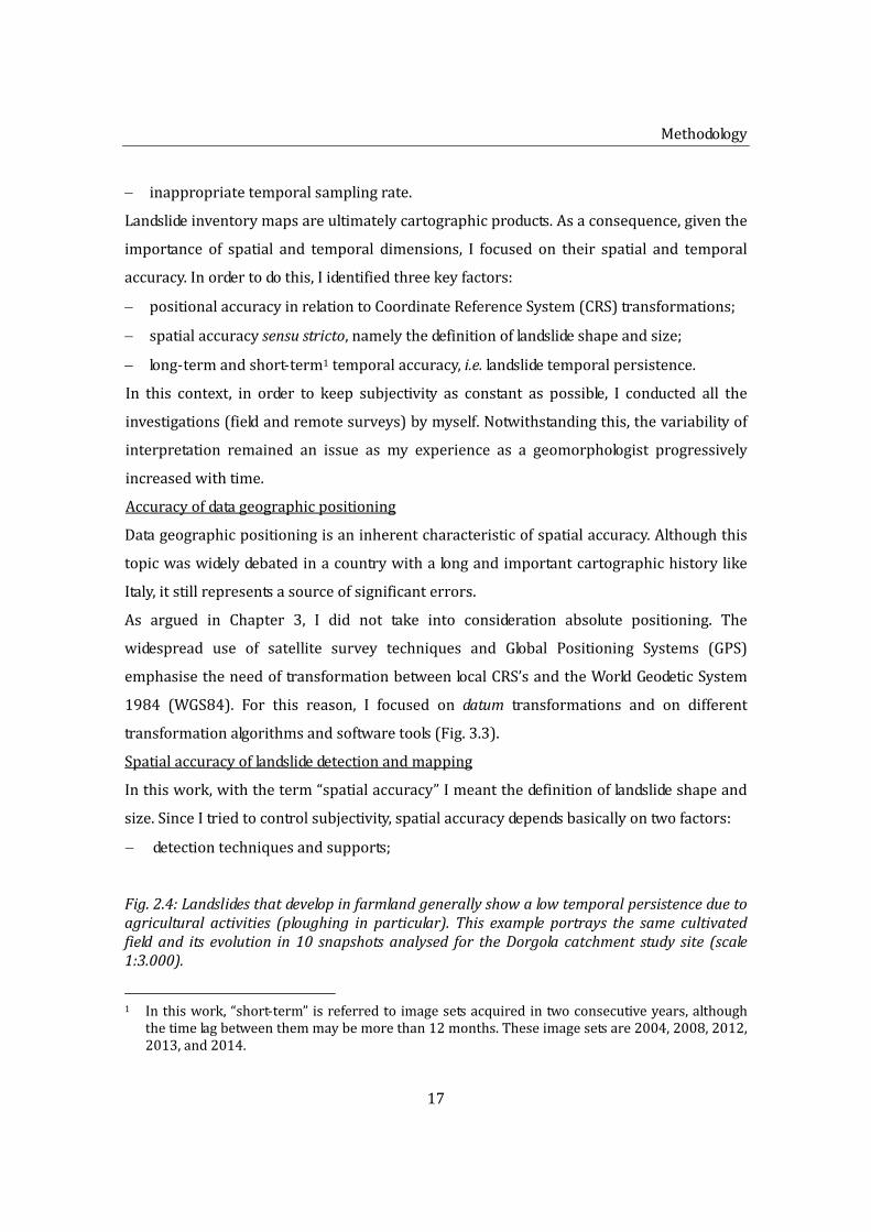
Fig.2.4:Landslidesthatdevelopinfarmlandgenerallyshowalowtemporalpersistenceduetoagriculturalactivities (ploughing inparticular).This exampleportrays the same cultivatedfieldand itsevolution in10 snapshotsanalysed for theDorgolacatchment study site (scale1:3.000).

1 Inthiswork,“short‐term”isreferredtoimagesetsacquiredintwoconsecutiveyears,although

thetimelagbetweenthemmaybemorethan12months.Theseimagesetsare2004,2008,2012,2013,and2014.

CHAPTER2

18

Methodology

19

dataprocessingandmanipulation.

Toevaluatethefirstpoint,Icomparedtwodifferentdetectiontechniques(seeChapter4):a

detailed field survey and the visual interpretation of a very high resolution (VHR)

orthorectifiedsatelliteimage(Fig.2.2).Thechoiceofthecompareddetectionmethodswas

madeaccordingtoland‐useplanninggoals,resources,andscale.

On the other hand, I assessed the overall spatial accuracy of landslide detection and

mapping, aswell as the consequencesof data and supportprocessing andmanipulation,

troughafuzzy‐likeanalysisofamulti‐temporallandslideinventory(Fig.2.3)(seeChapter

4).Fuzzyspatiallogicis,indeed,aneffectivemethodforhandlingtheuncertaintiesrelated

to spatial data, and it proved to be particularly efficient when dealing with boundary

imprecision.

Landslidetemporalpersistence

The temporaldimension is anessential element for thequality assessmentof a landslide

inventorymapduetothenaturalandanthropogenicevolutionoflandscape.Indeed,despite

thetechniquesusedforlandslidedetectionandmapping,oneofthemostchallengingissue

isthetemporalvalidityofthedetecteddata(Fig.2.4).Inthissense,oneoftheaimsofthis

researchwas to assess the temporal reliability of landslide inventorymaps. At the same

time,sincelandslidesaredetectedthroughaseriesofsnapshots,Ialsotriedtodeterminean

acceptabletimeintervalbetweentwoconsecutiveimages.Infact,ifthesamplingrateisnot

suitable for landslideactivity, someeventsor changesmay remainundetected (Dragicevic

andMarceau,2000).

2.3.Datacollection

FourcasestudysiteswerechosenintheItalianNorthernApennineswithinfourdifferent

Provincial Administrations of the Emilia‐Romagna Region (Reggio Emilia, Modena,

Ravenna, and Forlì‐Cesena) (Fig. 2.5). For each of them, I collected or acquired the

followingmaterial:

topographic,thematic,andhistoricalmaps;

allavailableaerialphotographsandhighresolutionsatelliteimages(GeoEYEand

CHAPTER2

20

Fig.2.5:LocationofthefourcasestudysiteswithrespecttotheEmilia‐RomagnaRegionandits Provincial Administrations (RE – Provincial Administration of Reggio Emilia, MO ‐Provincial Administration of Modena, RA ‐ Provincial Administration of Ravenna, FC ‐ProvincialAdministrationofForlì‐Cesena).

IKONOS);

specificallyacquiredVHRGeoEYEsatelliteimages(foronlytwoareas);

pastandcurrentland‐useplans;

detailedfieldsurveysspecificallyperformedwiththeaidofahighprecisionGPS;

publicarchivaldocumentsanddataaboutlandslidesandlandslideconsolidationworks.

2.3.1.Selectionofcasestudysites

Testareaswereessentiallyusedastrainingfieldsinordertoexerciseandimprovemyskills

todetectandcharacterise landslides invariousgeological, geomorphological, and land‐use

settings.Alloftheareaswereusedtoquantifytheaccuracyofdatageographicpositioning.

On the other hand, given the high precision and time‐consuming operations involved in

theirassessment,Ievaluatedthespatialandtemporalaccuracyonlyforonearea.

Thecasestudysiteswerechosenaccordingtothefollowingcriteria:

Methodology

21

Tab.2.1:ApprovalsoftheTerritorialPlansforProvincialCoordinationofthefourProvincesunderinvestigation.

ReggioEmilia Modena Ravenna Forlì‐Cesena

1°PTCPRCRn°769 RCRn°1864 RCRn°94 RCRn°159505/25/1999 10/26/1998 02/01/2000 07/31/2001

(RCRn°2489 12/21/1999) 1°PTCP ‐ PCRn°107 RCRn°2663 ‐(modification) 07/21/2006 12/03/2001

2°PTCP PCRn°124 PCRn°46 PCRn°9 PCRn°68886/14606/17/2010 03/18/2009 02/28/2006 09/14/2006

2°PTCP ‐ ‐ ‐ PCRn°70346/146(modification) 07/19/2010

RCR RegionalCommitteeResolutionPCR ProvincialCommitteeResolution

every area had to be in a different Provincial Administration and possibly within

differentMunicipalities, inordertomeetheterogeneousland‐useplanningrules.Allof

theProvincialAdministrationsunder investigationhave twogenerationsofTerritorial

PlanforProvincialCoordination(PTCP)(Tab.2.1);

differentgeological,geomorphological,andland‐usesettings;

higheravailabilityofarchivalaerialphotographsandsatelliteimages;

proximitytopluviometricgauges.

The final aims were to avoid a priori biases and to select representative areas of the

regionalnaturalandadministrativecontext.

2.3.1.1.CastelnovonéMonti

The Castelnovo né Monti study site is located in the homonymous municipality of the

Provincial Administration of Reggio Emilia in thewestern sector of the Emilia‐Romagna

region.Thisareaisthemaincasestudysitebecauseitwasusedfortheanalysisofspatial

accuracyandlandslidetemporalpersistence.

The test area corresponds to the catchment of the Dorgola Creek, a left tributary of the

SecchiaRiver,anditextendsoveranareaofapproximately16km2.Thefirsthumantraces

CHAPTER2

22

Fig. 2.6:With its sheer drops andmassive presence themesa‐like feature of the Pietra diBismantovaoverlookstheentireDorgolaValley.

in the area are dated back to the Upper Palaeolithic (Tirabassi, 2011). Ever since, man

presence has been basically constant and mostly concentrated around the Pietra di

Bismantova,areligiousbutalsohistoricalmilitarysite.Todaytheareaissparselypopulated

withnosignificantindustrialsites.CastelnovonéMonti,locatedonthenorthernpartofthe

area, is the only medium size village in the surroundings. Nevertheless, small (mostly

historical)settlementsarescatteredaroundthecatchment.

The landscape is characterised by forested terrain, cultivated fields, and permanent

meadows.ThesceneryisdominatedbytheTriassicGypsumsandbythemassivepresence

of thePietradiBismantova(Fig.2.6),acharacteristic landformwithasheerdropofover

100m.Forthebeautyanduniquenessofitsnaturalfeatures,in2010partoftheareawas

includedintheAppenninoTosco‐EmilianoNationalPark.

The Northern Apennines are a fold‐and‐thrust belt built up by a complex multiphase

convergencethatstartedintheUpperCretaceouswiththeclosingoftheTethyanSeaand

evolvedintheNeogenewiththeApennineOrogenysensustrictostillactiveatpresent.In

general terms, this convergence involved two continental blocks: theEuropeanPlate and

theAdriatic(micro)PlateoncepartoftheAfricanPlate.Thiscomplexplatetectonicsetting

formed a thrust nappe system generally divided into three distinct paleogeographic

domains(BettelliandDeNardo,2001):

Methodology

23

Fig. 2.7: Geological Domains (scale 1:100,000) (modified from Regione Emilia‐Romagna,2013).

Tuscan‐Umbria‐RomagnaUnits;

Sub‐LigurianUnits;

LigurianUnits.

CHAPTER2

24

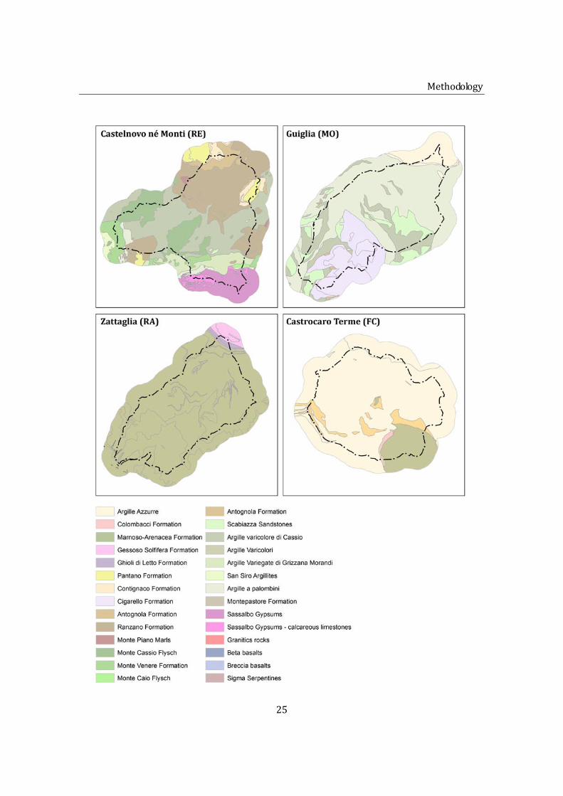
The Tuscan‐Umbria‐Romagna and the Ligurian Units with their Tertiary cover (Epi‐

Ligurian Sequence) are both present in the Dorgola catchment (Fig. 2.7). The Tuscan‐

Umbria‐RomagnaUnitsoutcropinthesouthpartofthestudyareaincorrespondenceofthe

SecchiaValley.There,theescarpmentsofMt.RossoandMt.Merlo,carvedinLateTriassic

evaporates,createdistinctgeomorphologicalfeatures.TheLigurianUnitswereoverthrust

on top of the Tuscan‐Umbria‐Romagna Units during the collision stage of the Apennine

orogenesis(BettelliandDeNardo,2001).IntheDorgolaValleytheycorrespondessentially

to the Upper Cretaceous deep‐water shaly and clayey units of the Argille Varicolore di

Cassio,ArgilleVariegatediGrizzanaMorandi,andArgilleaPalombiniandtothecalcareous

andarenaceousturbiditebasinsoftheMonteCassioFlyschandMonteVenereFormation.

TheEpi‐LigurianSequencewasdepositedduring theEarly‐MiddleEocene tectonicphase.

In the Dorgola Valley it is separated from the underlying Ligurian Units by tectonic

boundaries(BettelliandDeNardo,2001;BorgattiandTosatti,2010),anditisrepresented

by the arenaceous and marly Ranzano (Upper Eocene‐Lower Oligocene) and Antognola

Formations (UpperOligocene‐LowerMiocene) and by the biocalcarenites of the Pantano

Formation(Mid‐LowerMiocene),whichformstheBismantovarelief(BorgattiandTosatti,

2010)(Fig.2.8).

The Northern Apennines are an active convergent orogenic wedge (GSUEG, 1976).

According to the Hazard Maps of Albarello et al. (1999), the Peak Ground Acceleration

(PGA)valuesvarybetween0.15and0.3g,thelatterwitha10%probabilityofexceedance

in 50 years (475‐year return period). The strongest historically documented earthquake

(6.5M)isdated1920anditsepicentrewaslocatedjustsouthoftheregionalborderinthe

Lunigiana‐Garfagnanaarea(DipartimentodiProtezioneCivile,2014).

During the Würmian glacial period the area around the Pietra di Bismantova was

characterized by a periglacial morphoclimatic environment. According to the Gruppo di

StudiodelleUniversitàEmilianeperlaGeomorfologia(GSUEG)(GSUEG,1976),atthattimea

vastglacistopographicalsurfaceradiatedfromthePietradiBismantova.Thislandformwas

theresultofgelifluctionandfrostweatheringprocessesthattookplaceongentleslopes

Fig. 2.8: Geologicalmaps of the four study sites (scale 1:100,000) (modified from RegioneEmilia‐Romagna,2012and2013).

Methodology

25

CHAPTER2

26

withlittleornovegetation.Withtimetheglacishasbeenerodedbythedrainagesystem,so

thatitnowappearsasgentlyslopingterraceslikethosenearthesettlementsofGinepreto,

CaseMerlo,Piastre,andBellaria (GSUEG,1976).After the lastglacialperiod theareawas

covered by forests and the Secchia River started to deepen its bed. Eventually, the

geomorphic system evolved again during theHolocene basically due to climatic changes

(GSUEG,1976).

Nowadays,fromageomorphologicalpointofview,incorrespondencetotheLigurianUnits

the Dorgola Valley is essentially characterised by a gentle hilly landscape. Indeed, their

clayeyandshalydepositsdeepgently(usually10°‐20°)incontrastwiththeoverlyingEpi‐

LigurianSequencethatmaylocallyformsub‐verticalslopes(Fig.2.9)likeinthemesa‐like

feature of the Pietra di Bismantova,whose summit corresponds to a lithologic‐structural

surface.

Due to their clayey and structurally complex nature, Ligurian Units are more prone to

landslides than the Epi‐Ligurian Sequence (GSUEG, 1976; Bertolini and Pellegrini, 2001,

ServizioGeologicoSismicoedeiSuoli,2006).Nevertheless,withtheexceptionoftheareaof

CastelnovonéMonti, landslidesareprettycommonallovertheDorgolacatchment.Inthis

context,somelargelandslidesdominateonentireslopes(fromthewatershedtothevalley

bottom) creating what Crozier (2010) defined a “landslide morphology”. These large

landslides can be detected from geomorphological features (e.g. through hummocky

morphology, drainage pattern, damages and misalignments of natural and man‐made

features)buttheycannotbepreciselycharacterizedwithoutmoredetailedinvestigations.

Furthermore, some of these mass movements had a complex and composite evolution.

Indeed,afterthelastglaciations,theywereinitiallytriggeredasmulti‐phaseearthflowsand

thenevolvedintonewearthflowsduringtherainiestperiodoftheHolocene(Bertoliniet

al.,2005;BertoliniandPizziolo,2008).ThebiggestlandslideinthestudyareaistheBondolo

landslidethatextendsfromtheSEsectorofthePietradiBismantovatothebottomof the

Dorgola Valley, close to the Secchia River. In this massive landslide, which strongly

contributedtoshapethelocallandscape,largebouldersfromthePietradiBismantovafloat

orareburiedintotheclayeydebrisderivedfromtheLigurianUnits(GSUEG,1976).

Therockycliffsof thePietradiBismantova, instead,aresubject to lateralspread, topples,

andfalls,whichovertimeaccumulatedalargeamountofdebris(fromlargeboulderswith

Methodology

27

Fig.2.9:SlopemapsrealisedwithEsri®ArcMapTM10.1(scale1:100,000).

volumeupto103m3tosmallblocks)atthefootoftheslopes(BorgattiandTosatti,2010).In

some cases this material was then mobilised by earth slides and flows affecting the

underlyingformations(e.g.intheBondololandslide).BorgattiandTosatti(2010)estimated

thatthemaximumbounceheight is22m,whereasthemaximumrun‐out is110mfrom

theprofilestartingpoint,whichis45mfromthefootoftheslope.Accordingtothisstudy,

the areas most susceptible to landsliding are the SE, NE and NW faces of the Pietra di

CHAPTER2

28

Bismantova. Here rock parameters are poorer and the degradational processes are

particularlyintense.

Somebadlands, nowadaysonlypartially active, canbeobserved in theupperpart of the

Dorgola Valley in the marly sediments of the Ranzano Formation. These badlands are

basicallyconcentratedclosetothevalleybottomandtheirevolutionisrelatedtothecreek

erosion.

Thehigh instabilityof theDorgola catchment is the resultof various interrelated factors.

The geological characteristics of the area (weak and weathered materials, material

combination and permeability contrasts, join sets, etc.) are the main predisposing and

preparatory factors for landslides. Intenseandprolungatedrainfall, aswell as snow‐melt,

are, instead, the most important triggering factors (Garberi et al., 1999; Basenghi and

Bertolini,2001;Bertolinietal.,2005;Pizzioloetal.,2008;Rossietal.,2010;Montrasioetal.,

2012),althoughaccordingtosomeauthors(GSUEG,1976,BertoliniandPellegrini,2001;

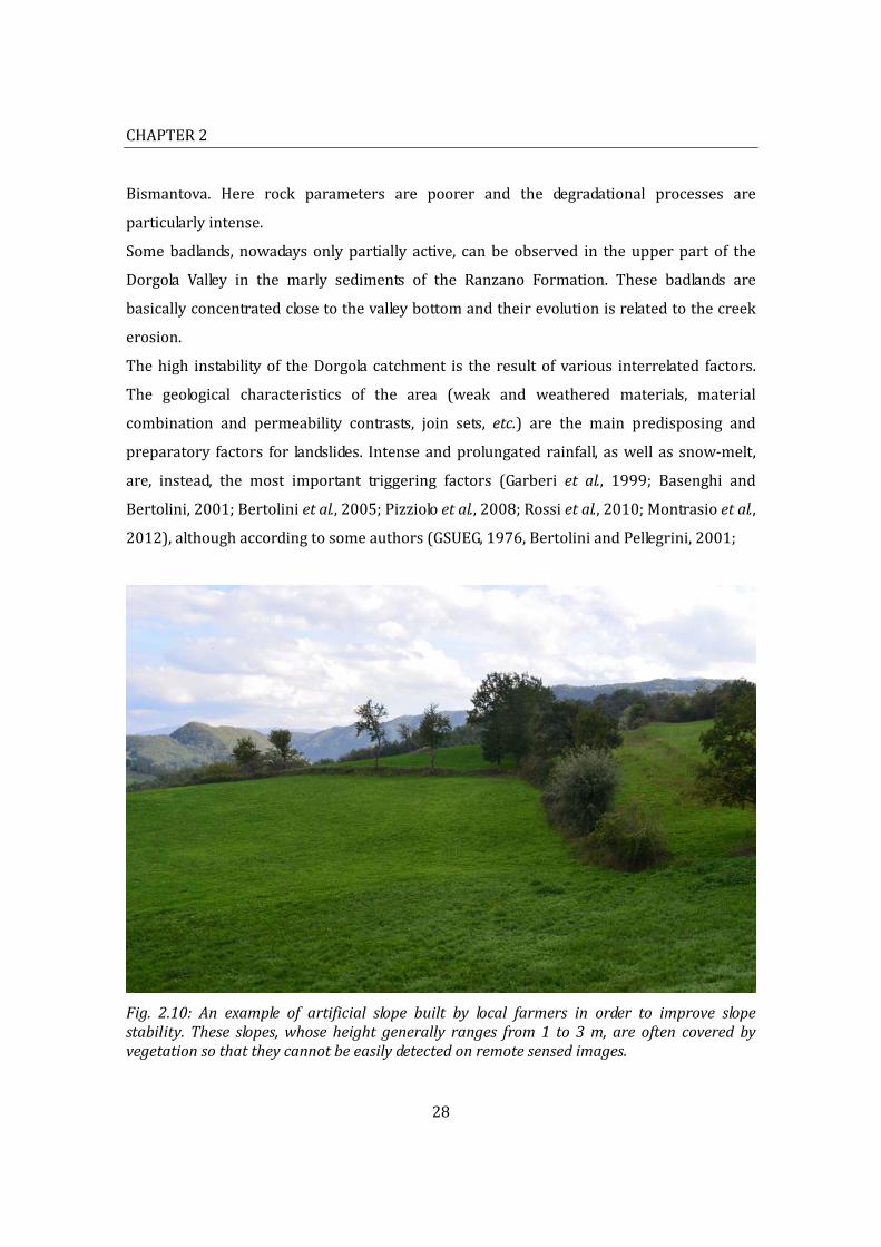
Fig. 2.10: An example of artificial slope built by local farmers in order to improve slopestability.These slopes,whoseheightgenerally ranges from1 to3m,areoften coveredbyvegetationsothattheycannotbeeasilydetectedonremotesensedimages.

Methodology

29

Tosatti et al., 2008) earthquakes should be considered as well. Furthermore, another

importantcomponentforslopeinstabilityishumanactivity.Inthestudyarea,indeed,men

have strongly contributed to alter and to accelerate the natural evolution of landscape

through(GSUEG,1976):

deforestation;

roadconstructions;

farming.

Inparticular, itwasacommonpractice for local farmers tobuildsmallartificial slopes to

decrease theslopeangle (Fig.2.10).Moreover, the intenseagriculturalactivity (especially

ploughing) contributed to soil creep and to accumulate rock stockpiles along the sides of

cultivated fields (GSUEG,1976).Humanactivitieshavebeenparticularly significant in the

area of Castelnovo né Monti where the original topography was extensively levelled to

allocate buildings. Nevertheless, slope stability was not affected by these important

processesbecauseofthegeologicalsettingofthatparticulararea(GSUEG,1976).

2.3.1.2.Guiglia

Thisstudysite takes itsnameafter themunicipalityofGuigliaalthough itextendsontwo

differentmunicipalities: Guiglia and Savignano sulPanaro, both located in theProvincial

AdministrationofModena.

The study site extends for about 16 km2 over the right bank of the Panaro River and

includesfewminortributarybasins.ThesmalltownofGuigliaistheonlysignificanturban

area of the study site, which is essentially characterised by small scattered settlements.

Apartfromfewforestedterrain,thelandscapeisbasicallyanthropogenic,anditconsistsof

cultivatedfieldsandbadlands.Maninfluenceissignificantlyevidentonriversandstreams

thataremostlyengineered. Inparticular, thePanaroRiverwasheavilydepletedbygravel

extraction.

Guiglia study site falls within the Ligurian Units and their Tertiary cover (Epi‐Ligurian

Sequence) (Fig. 2.7). The former corresponds essentially to the Cretaceous deep‐water

shalyandclayeyunitsoftheArgilleVaricolorediCassioandArgilleaPalombiniandtothe

arenaceous turbidite basin of the Arenarie di Scabiazza. The Epi‐Ligurian Sequence,

instead,iscomposedofMiocenesandstonesandmarls,respectivelyfromthePantanoand

CHAPTER2

30

CigarelloFormation(Fig.2.8).

2.3.1.3.Zattaglia

ZattagliastudysiteislocatedinthemunicipalitiesofBrisighellaandCasolaValseniointhe

ProvincialAdministrationofRavenna(easternsectoroftheEmilia‐RomagnaRegion).

The original test area is a small section (about 5 km long) of the Sintria Valley, and it

extendsforapproximately14km2.However,duetothewinterseason,only7km2onthe

rightriverbankwereactually fieldsurveyed(fromthesettlement“IlTre” to thevillageof

Zattaglia). In the study site there are no significant residential areas but only scattered

houses. The landscape is characterised by steep slopes often ending in deep canyon‐like

features.Olivetreecultivationismorefrequentthansowablefields,whereaswideareasare

coveredbyyoungforests.

ZattagliatestareaisentirelyincludedintheTuscan‐Umbria‐RomagnaUnits(Fig.2.7)andis

composedbydifferentmembersoftheMarnoso‐ArenaceaFormation:Miocenemarlyand

arenaceousturbites(Fig.2.8).

From a geomorphological point of view, the succession of clayey and arenaceous layers

plays a key role in shaping the landscape. Gentle slopes are generally present on the

backslopesofcrests(incorrespondenceofdipslopes),whereasonthefrontslopesofsuch

creststhereareusuallysheerdropsorcliffs.NearbythevillageofZattagliathemonotonous

stratificationcropoutinimpressivecanyon‐likefeaturesupto100mdeep.

2.3.1.4.CastrocaroTerme

ThisstudysitetakesitsnameafterthemunicipalityofCastrocaroTermeandTerradelSole,

located in the Provincial Administration of Forlì‐Cesena (eastern sector of the Emilia‐

RomagnaRegion).

CastrocaroTermestudysiteextendsoveranareaof approximately16km2 including two

different catchments (the Cozzi‐Converselle Creek and the Zanetta‐Pietra Brook) and a

smallsectionoftherightbankofthelargerSamoggiabasin.Apartfromthesmalltownof

CastrocaroTerme,whichliesinthealluvialplainoftheMontoneRiver,thestudysitehasno

significanturbanareasbutonlysomescatteredhouses.Humanpresence,though,maybe

datedbackatleastasfarastheLowerPalaeolithicand,nowadays,theentireareaisheavily

affected by human activities. Indeed, the landscape is dominated by cultivated fields

Methodology

31

(especiallycereals,olive treesandvineyards)andbadlands. It isworthnoting that in the

areathereusedtobetwopigbreedingfarmsbothwithfewthousandsanimals.Oneisstill

active,whereastheotherwasdismissedafteritwasseverelydamagedbyalandslideinthe

late1990’.

TheCastrocaroTermestudysiteisdominatedbytheNeogenic‐QuaternarySequence(Fig.

2.7)thatintheareaconsistsessentiallyintheArgilleAzzurreFormation(LowerPliocene‐

Lower Pleistocene) (Fig. 2.8). These pelagic clayey andmarly‐clayey deposits are rich in

foraminiferousandsubordinatelyinmacrofossilslikegasteropodsandbivalves.Amongthe

ArgilleAzzurrethereisapeculiarrockthatconsistofanorganogeniclimestonereferredto

asSpungone.Thesetwotypesofdepositscreateasharpcontrastinthelandscape.Agentle

hillymorphology,with frequent badlands basins, is indeed typical of the Argille Azzurre,

whereas the Spungone generates cliff‐dominated morphology characterised by NW‐SE

orientedcrests.Landslides,intheformofmudandearthflows,areessentiallyconcentrated

inbadlandcatchments.

2.3.2.Fieldinvestigationsandinterviews

I conducted a detailed geomorphological field investigation for all test areas. The survey

campaign started in July 2012 and, delayed by thewinter season, finished inApril 2013

(Tab. 2.2). I also carried out expeditious supplementary field reconnaissances in spring

2013(GuigliaandCastrocaroTerme)andspring2014(Guiglia).The2012surveysfocused

notonlyonevidentlandslides(depositsandsourceareas)butwerealsoaimedtorecognise

areas of potential instability. Hummocky topography, as well as topographic anomalies,

consolidation works, infrastructure and building damages, superficial drainage systems,

anomalous patterns, and ponds, badlands, particular land‐uses, and water‐demanding

vegetationwereallsurveyedandreportedonmaps.

During field investigations, I identified landslides visually and then I located andmapped

themontheRegionalTechnicalMap(CTR)at1:5,000scale,whichIemployedasreference

basesupport.To this regard, it isworthnoting that theoriginalsurveyused togenerate

this topographic map dates back to the 1970s (only buildings and infrastructures were

occasionallyupdated)and,therefore,quitefrequentlyitpre‐dateslandslides.Asremarked

CHAPTER2

32

Tab.2.2:Datesofthesurveycampaigns.

2012 2013 2014

CastelnovonéMonti 10/01to11/13 05/19 (23days) Guiglia 07/20to08/14 05/28 06/02 (13days) Zattaglia(notcompleted) 11/26to04/17 (18days) CastrocaroTerme 08/21to09/26 05/14 (18days)

bySantangeloetal.(2010)thiswasanissueespeciallywherethebasemapdidnotshow

clear,orsufficient,landmarksortopographicreferencepointstolocateandmaplandslides,

e.g.wherepre‐andpost‐failuretopographywerecompletelydifferentfromeachother.At

thesametime,fieldinvestigationswerealsoconductedwithahighprecisionGPS(Garmin

Montana 650T). In particular, the GPS receiver was carried along landslide perimeters

including, and if possible differentiating, source areas and deposits. This operation was

relatively simple when dealing with small to medium recent fresh landslides. On the

contrary,olddormantlandslidescouldnotbeidentifiedandmappedwiththesamecertainty

because they were significantly concealed by either intense farming activities or thick

forests. In this cases the definition of landslide perimeters was not straightforward and

univocal. In fact, itwasextremely subjective, and it impliedahighuncertaintywithboth

visual reconnaissance and GPS survey. Consequently, small to medium fresh landslides

wereessentiallydetectedonthebasisofGPStracks,whileolddormantlandslidesrequired

also the aid of the contour lines of the base map (drainage pattern anomalies and

deviations, concave/convex slope features, valley morphology, lobate landforms) (Soeters

andvanWesten,1996;Santangeloetal.,2010).

Icompletedfieldinvestigationswithinterviewstothelocalpopulationinordertoacquire

moreinformationabouthistoricalslopefailures,farmingcommonpractices,landuses,and

landscapeevolution.The interactionwith local communities representedalsoachance to

analysepeopleperceptionaboutlandslidesandman‐landslideinteraction.

Methodology

33

Theprincipalaimofthesurveycampaignwastoacquireacompleteandrobustknowledge

about local land instability and mass movements (e.g. warning signs, movement types,

degree of activity, causes and triggers, local lithological settings, man interaction and

commonconsolidationpractices,damagesandcosts,etc.).Moreover,groundsurveyswere

also used as training fields to exercise and improve my skills with regard to landslide

detection and characterization in various geological, geomorphological, and land‐use

settings. Finally, survey operations represented an important occasion for valuable

considerations about field survey difficulties, limitations, subjectivity, and cost‐benefit

analyses.

FortheCastelnovonéMontistudysite,Iscannedandgeoreferencedthefieldsurveymapin

order to prepare a detailed geomorphological landslide inventory map. To this end, for

landslide detection andmapping I basically used the field data and theCTR.No remotely

senseddatawereusedinthiscontextand,inthesameway,theregionallandslideinventory

map2wasintentionallyignored.LandslideswereclassifiedaccordingtoCrudenandVarnes

(1996)andtheircharacteristics(typeofmovement,age,estimateddegreeofactivityand

depth,potentialcausesand triggers)weredeterminedon the localgeomorphologicaland

geological context, general appearance, setting, and, where available, on historical and

archival information. Inparticular, I inferredtherelativeageof themassmovement from

the degree of morphological freshness and vegetation colonization. Where possible, I

generally mapped the crown area separately from the deposit together with other

significant features (e.g. tension cracks, damages to natural or man‐made features,

topographic anomalies, consolidationworks, drainage ponding,major escarpments, etc.).

Ultimately, in this inventory I also introduced an extra class to identify areas where no

landslides were clearly detected, but where morphological (e.g. hummocky or generally

irregularoranomalousmorphology,drainagepatternanomalies,semicircularfeaturesand

escarpments,etc.)andvegetationelementssuggestedprobableorimminentslopefailures.

Theseareas,thatInamedAPI(AreasofPotentialInstability),maybetheresultsoflandslide

natural or anthropogenic evolution and/or stabilisation. In order to be precisely

characterized,theseareasrequiremoredetailedinvestigations.

2 The regional landslide inventory map is the same one reported in the Territorial Plan for

ProvincialCoordination(PTCP),whichwillbeanalysedinChapter6.

CHAPTER2

34

2.3.3.AcquisitionofGeoEYEsatelliteimages

VHR panchromatic and multispectral GeoEYE images were acquired for the areas of

Castelnovo ne' Monti and Castrocaro Terme. Panchromatic (black and white) images

presenta0.5mresolution,whereasmultispectralimageshavea2mresolution.Allimages

wereprovidedresampledwith theCubicConvolutionmethod.On thewhole, threesetsof

images for each areawere captured from 2012 to 2014. In particular, the 2012 images

wereacquiredrespectivelyinAugustandJuly,theaimsfortheseacquisitionswere:

tohaveaVHRsupporttopreparearemotelysensedinventorytobecomparedwiththe

coevalgeomorphologicalfieldinventory;

to build up annual sequences of VHR images. In this sense, the three sets ofGeoEYE

images were added to the 2011 digital aerial photographs of the Agenzia per le

ErogazioniinAgricoltura(AGEA).Thisallowedtohaveremotesensedannualdatafrom

2011to2014.

2.3.4.Historicaldata

Historicaldataplayakeyroleinthereconstructionoflandslideandlandscapeevolution.For

this reason, the acquisition of all available historical data (e.g. consolidation works,

infrastructure and building damages, previous studies and/or inventories, historical

landslides,etc.)wasanimportantsteppingstoneoftheresearch.

Thesearchinvolveddifferentpublicadministrationsandagencies,anditaimedtocollecta

widedataset.Particularattentionwasgivento the land‐useplanningsetting(e.g.pastand

current land‐useplans)andtotheacquisitionofallavailableremotesensedimages(both

aerialandsatellite)inordertoacquirethemostcompleteseriesofhistoricaldata.

2.4.Dataprocessing

Sincetheyhadbeengeneratedandmanagedbyvariousproducersandagencies,datahad

different CRS’s. Therefore, in order to use them all together, theyhad to be transformed

into a unique CRS. Nevertheless, CRS transformations, and particularly datum

transformations, are not trivial tasks andmay lead to errors and positional inaccuracies.

Methodology

35

Indeed, geographic positioning is an important factor for data spatial accuracy, and it is

treatedindetailinChapter3.

2.4.1.Imageprocessing

TheaerialphotographsandsatelliteimagesusedforthisworkaresummarizedinTab.5.1.

Orthorectification is the process of removing the distortion within an image caused by

terrain relief and by the camera (Exelis VIS, 2013). Indeed, aerial photographs show

geometric errors in the representation of features due to the effects of tilts and relief

displacement. Objects are not represented in their correct planimetric position and, as a

consequence, images cannot be used for accurate measurements without being first

orthorectified (Campbell and Wynne, 2012). GeoEYE and IKONOS images were

orthorectifiedbye‐geos3butnoinformationareavailableaboutthemethodandsoftware

thatwereusedforthispurpose.E‐geosalsoperformedthepan‐sharpingprocess4,i.e.the

panchromatic imagery was combined with the multispectral bands to create a 0,5 m

resolutioncolourimage.Withregardtothepositionalaccuracy,theGeoEyeProductGuide

(2009)reportsaCE905equalto5mforthe0,5mresolutionimages.Conversely,according

totheirmetadata, theaerialphotographsaccessibleasWebMapService(WMS) fromthe

GeoportaleNazionale(seeTab.5.1)weregeoreferencedbyusingtheverticesofthegeodetic

network IGM95 and additional GPS points available in official databases. Then theywere

orthorectified and mosaicked with internationally recognized software. Except for the

1996 aerial photographs, for which there are no available data, the overall declared

positional accuracy for these images is 4 m. Also the 2008 and 2011 AGEA aerial

photographs(accessibleinWMSfromtheGeoportaleoftheEmilia‐RomagnaRegion)have

thesamepositionalaccuracy.However, theywereorthorectifiedbyusing the5mDigital

Elevation Model (DEM) and the photographic points derived from the CTR. The aerial

photographs supplied by the Emilia‐Romagna Region and by the Geographic Military

3 OneofthetwocertifiedresellersofDigitalGlobeinItaly.4 Pansharpening was performed with the commercial software ERDAS IMAGINE® (e‐geos,

personalcommunication,August21st,2013).5 Circularerrorat90%confidencewhichbasicallyindicatesthattheactuallocationofanobjectis

represented on the imagewithin the stated accuracy for 90% of the points (GeoEYE ProductGuide,2009).

CHAPTER2

36

Institute (IGM) (Tab. 5.1) were neither orthorectified nor georeferenced. Unfortunately,

with the technology available for thiswork, the 1973 and the 1978 images could not be

orthorectified.Indeed,duetothelowflyingaltitude,thestudyareawascoveredbyseveral

overlappingsnapshots.Inthiscase,orthorectificationandmosaickingshouldbeperformed

simultaneouslyforallsnapshotsandnotonesnapshotatatimeaswithENVIsoftware.For

thisreasonthe1973and1978aerialphotographswereonlygeoreferencedwiththeaidof

the CTR using Quantum GIS, Version 1.8.0‐Lisboa6. The same was done for the 1954

imageryforwhichtheIGMcouldnotprovidethecameracalibrationcertificate.

Thehighflyingaltitudeoftheremainingaerialphotographsallowedtoperformatwosteps

single‐image orthorectification with ENVI 4.8 software. The first step consisted in the

computationoftheRationalPolynomialCoefficients(RPCs),whereasthesecondstepwas

theRPCorthorectification. Inorder tobuild the sensorgeometryandcomputeRPCs, the

ENVIBuildRPCstoolrequires todeterminethe interiorandtheexteriororientation.The

formerestablishestherelationshipbetweenthecameraandtheaerialphotographimage,

anditneedsthecamerafocallengthandthetiepointsbetweentheaerialphotographsand

the camera fiducialmarks (Exelis VIS, 2013). To this end, I used the camera calibration

certificatesprovidedbytheIGMandbyCGRSpa,whoacquiredtheaerialphotographson

behalfof theEmilia‐RomagnaRegionalAuthority.Exteriororientation,ontheotherhand,

determinates theposition and angular orientationparameters associatedwith the image

(Exelis VIS, 2013). For its definition, it requiresGroundControl Points (GCPs)with their

relativeelevation. In this case, sincenoGCPswereavailable, Idetected themon the2013

orthorectifiedpansharpenedGeoEYE image andmanually entered them into ENVI. I did

thesamealsowiththeirelevation,whichIextractedfromtheCTR.Theseoperationswere

quitechallenging.Indeed,duetothedifferentageofthebasemap,thebaseimage,andthe

different aerial photographs, identifying reliable equivalent points was not a trivial task.

Moreover, in this way, the image orthorectification was affected by the positional and

geometricaccuracyof thebasesupports.Also thenumber,distribution,and typeofGCPs

canaffect theaccuracyof theorthorectification (Zanuttaetal.,2006;Aguilaretal.,2008;

Hughesetal.,2006).Tothisend,IscatteredGCPsaroundtheedgesofthe imagebutalso

6 Alsohistoricalmapsweregeoreferencedinthesameway.

Methodology

37

across the image itself (Hughes etal., 2006). This, however, in a scarcely populated and

forestedarea,liketheoneunderstudy,wasnotaneasytask.WithregardtoGCPstype,as

suggestedbyHughesetal.(2006),Iusedonlyhardpointswithsharpedgesorcorners,i.e.

buildingcornersandroadinteractions,bearinginmindthatevenbuildingsandroadsmay

hadalteredovertime.About40GCPswereusedforeachimagewithanaverageRMS(Root

Mean Square) residual7 <0,5 pixel. Finally, the RPC orthorectification was applied. To

performit,the5mDEMoftheEmilia‐RomagnaRegionwasusedandboth,theDEMand

theaerialphotographs,wereprocessedusingcubicconvolutionresampling.

2.4.2.Landslidedetectionandprocessing

In order to represent landslide evolution through space and time, I prepared a multi‐

temporal landslide inventorymap for the Castelnovo néMonti study site. Given the high

level of complexity involved, the realization of this kind of product is challenging and

particularlytime‐consuming.Indeed,itrequiresmultiplesetsofaerialphotographsforthe

sameareaandahighdegreeofexperienceinordertodetectsmallmorphologicalchanges

related to slopemovements.Moreover, landslidedetectionalwaysdemands tohavea clear

ideaofwhattoidentifyandmap.Inthisspecificcase,Iusedtheterm“landslide”todefine

the slope failure, i.e. the sliding action and not the deposit. To this end, I identified and

mapped the affected area (depletion and accumulation zones) of each single mass

movementincludingalllevelsofreactivationsofmajorlandslides.

Landslides can be detected and mapped using different techniques and tools (Guzzetti,

2006;vanWestenetal.,2008).Forseveralreasons(e.g.cost/benefitratio,workingscale,

reliability,etc.),oneofthemostusedmethodisthevisualinterpretationofremotelysensed

images(airborneandsatellite)(RibandLiang,1978;TurnerandShuster,1996;Guzzetti,

2006; vanWesten et al, 2008). In this regard, photo‐interpretation and digital mapping

from orthorectified images can be a good substitute of 3D vision or stereoscopic

techniques (Fernandez et al., 2006). The multi‐temporal landslide inventory map of the

Dorgola catchment was prepared using visual interpretation of orthorectified remotely

7 TheRootMeanSquare(RMS)residualrepresentsthedifferenceinlocationbetweentheGCPson

the transformed and on the original image (Hughes et al., 2006), and it is generally used toprovideameasureofthefitoftheentiresetofGCPstotherationalpolynomialmodel.

CHAPTER2

38

sensed images,and it tookmeabout4months tocomplete it. Since Ihadconducted the

fieldsurveyaswell,thisinventorywasinevitablyinfluencedbymyfieldexperience.Overall,

15 to18setsofaerialphotographsandsatellite imageswereused for landslidedetection

andmapping(Tab.5.1)8,andtheywereanalysedbothseparatelyandincombinationwith

each others. Landslide identification was based on the recognition of peculiar

morphological,vegetation,anddrainageterrainfeatureslikethosereportedinTab.2.3.In

thisway,landslidedetectabilitydependedessentiallyonthecontrastwiththesurroundings.

Inparticular,thedistinctionbetweenstableandunstableareaswasdeterminedbyspecific

image characteristics like e.g. tone, texture, pattern, and shape variations or differences.

AccordingtoSoetersandvanWesten(1996)thiscontrastisaffectedby:

the time lapse between the failure and the detection, since with time erosion and

vegetationcolonizationtendtoconceallandslidedistinctivefeatures;

theseveritywithwhichthelandslidingaffectedmorphology,vegetation,anddrainage.

After identification, I digitallymapped landslides as polygons using Esri®ArcMapTM 10.1.

Sinceeachlandslidewasoutlinedoneveryimageset,inordertoconnectthesamelandslide

throughtime,IlabelledeachonewithauniqueIDnumber9.Thisoperationwasparticularly

time‐consuminganderror‐pronesince ithadtobecarriedoutmanuallyaccording toan

heuristicmethod.Indeed,therecognitionofthesamelandslideindifferentimagesrequires

complex evaluations that could not be substituted by automated procedures based on

simple geometric and spatial relations. At the same time, I used a second digital code

(ID_landslide)todefinethegeometricandspatialcorrelationsamongdifferentreactivations.

This allowed todifferentiateup to6differenthierarchical levelsof geometric and spatial

associations(Fig.2.11).

Furthermore,Ialsoclassifiedlandslidesaccordingtothefollowingelements:

landslidetype,accordingtoCrudenandVarnes(1996);

location,i.e.thenameofthenearesttoponym;

8 Georeferenced images (1954, 1973 and 1978) were used for landslide detection but not for

mapping.Inthisway,thetemporalanalysiscouldrelyon18imagesetsspanningovera60‐yeartime frame (from 1954 to 2014), while for the fuzzy‐like analysis were used only the 15orthrectifiedimages(from1981to2014).

9 The same ID numberwas used to define both the original landslide and its reactivations. Thelatterwere,indeed,differentiatedbyusingthedetectionindex.

Methodology

39

Tab. 2.3: Morphological, vegetation, and drainage terrain features used for the remotedetectionoflandslides(modifiedfromSoetersandvanWesten,1996).

TERRAINFEATURES RELATIONTOSLOPEINSTABILITY

Morphology

Concave/convexslopefeatures Landslidenicheandassociateddeposit

Steplikemorphology Retrogressiveslinding

Semicircularbackscarpandsteps Headpartofslideoutcropoffailureplane

Back‐tiltingofslopefacets Rotationalmovementofslideblocks

Hummockyandirregularslopemorphology Microreliefassociatedwithshallowmovementsorsmallretrogressiveslideblocks

Infilledvalleyswithslightconvexbotton,whereV‐shapedvalleysarenormal

Massmovementdepositofflow‐typeform

Vegetation

Vegetationalclearancesonsteepscarps,coincidingwithmorphologicalsteps

Absenceofvegetationonheadscarporonstepsinslidebody

Irregularlinearclearancesalongslope Slipsutfaceoftranslationalslidesandtrackofflowsandavalanches

Disrupted,disordered,andpartlydeadvegetation

Slideblockanddifferentialmovementsinbody

Differentialvegetationassociatedwithchangingdrainageconditions

Stagnateddrainageonback‐tiltingblocks,seepageatfrontallobe,anddifferentialconditionsonbody

Drainage

Areaswithstagnateddrainage Landslideniche,back‐tiltinglandslideblocks,andhummockyinternalreliefonlandslidebody

Excessivelydrainedareas Outbulginglandslidebody(withdifferentialvegetationandsomesoilerosion)

Seepageandspringlevels Springsalongfrontallobeandatplaceswherefailureplaneoutcrops

Interruptionofdrainagelines Drainageanomalycausedbyheadscarp

Anomalousdrainagepattern Streamscurvingaroundfrontallobeorstreamsonbothsidesofbody

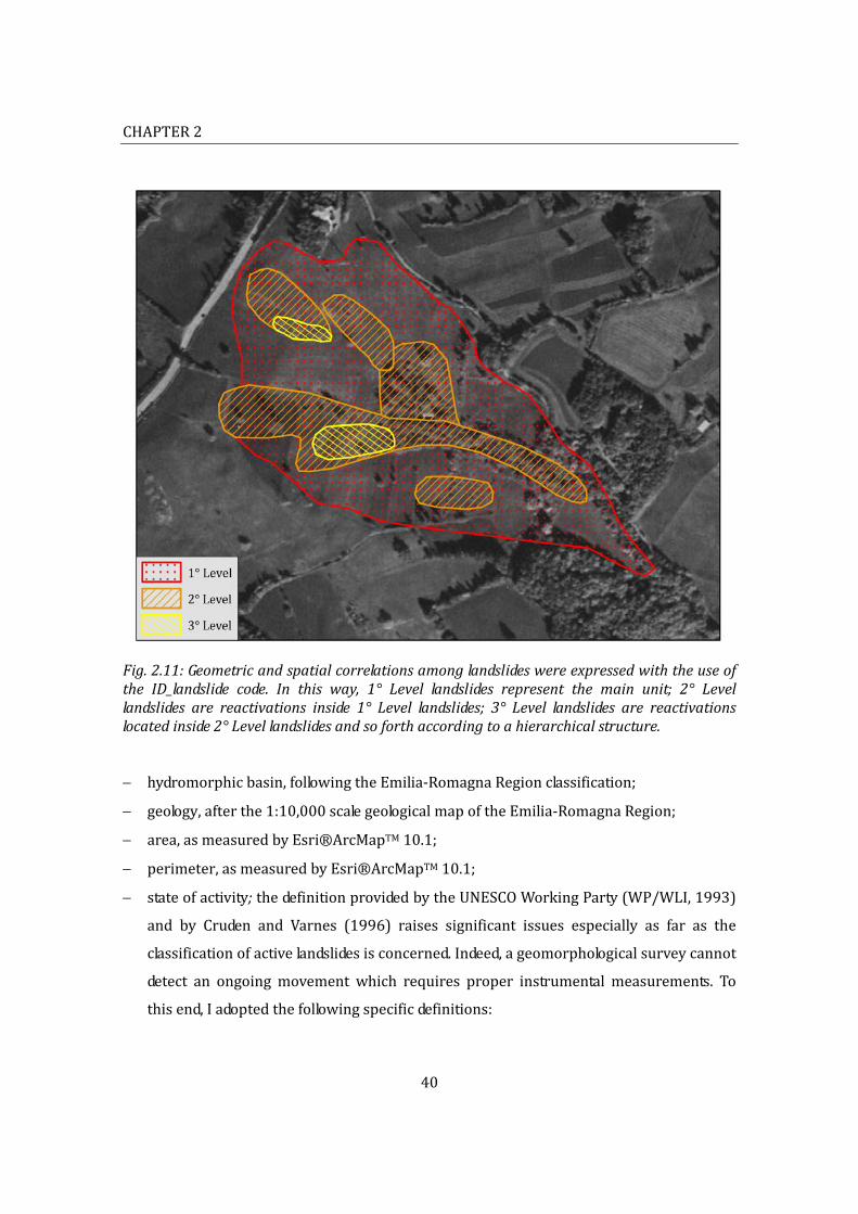
CHAPTER2

40

Fig.2.11:Geometricandspatialcorrelationsamonglandslideswereexpressedwiththeuseofthe ID_landslide code. In this way, 1° Level landslides represent the main unit; 2° Levellandslides are reactivations inside 1° Level landslides; 3° Level landslides are reactivationslocatedinside2°Levellandslidesandsoforthaccordingtoahierarchicalstructure.

hydromorphicbasin,followingtheEmilia‐RomagnaRegionclassification;

geology,afterthe1:10,000scalegeologicalmapoftheEmilia‐RomagnaRegion;

area,asmeasuredbyEsri®ArcMapTM10.1;

perimeter,asmeasuredbyEsri®ArcMapTM10.1;

stateofactivity;thedefinitionprovidedbytheUNESCOWorkingParty(WP/WLI,1993)

and by Cruden and Varnes (1996) raises significant issues especially as far as the

classificationofactivelandslidesisconcerned.Indeed,ageomorphologicalsurveycannot

detect an ongoing movement which requires proper instrumental measurements. To

thisend,Iadoptedthefollowingspecificdefinitions:

Methodology

41

1 “active”landslidesarethosethatmovedwithinthelastannualcycleofseasons.To

bestrictlycongruouswiththisdefinition,theselandslidesweredefinedonlywhere

images from two consecutive years were available (2004, 2008, 2012, 2013 and

2014)eventhoughtheoverallperiodwasmorethan12months;

2 “suspended”landslidesarethosethatmovedmorethanoneannualcycleofseasons

ago,but theystillshowa freshaspectwithclearsignsofrecentactivity(e.g.bare

groundorlittleornovegetation,irregularmorphology,wellpreservedcrownareas

andscarps,cracks,etc.);

3 “dormant”landslidesarethosethatshownoevidencesofrecentmovements.Inthis

sense, they appear intensively colonised by a developed or fully‐developed

vegetationandsometimesalsointensivelysettledbyhumanactivities.

Inthisworktheuseoftheterm“relict”wasdiscouraged.Indeed,althoughsomeancient

landslides developed under different morphoclimatic conditions, hundreds if not

thousandsofyearsago, theymaystill reactivateasreportedbyBertoliniandPizziolo

(2008)onthebasisofrecentandpastevents.

pre‐andpost‐land‐use;Ivisuallyidentifiedthefollowingcategories:

1 bareground(e.g.freshscars);

2 cultivatedfieldsandgrassland;

3 scrub;

4 wood;

5 mixed(e.g.inlargelandslides);

landslide age; in order to estimate landslide age, land‐usewasused as aproxy.On the

basis of the above listed categories, landslides were classified into: recent (land‐use

categories1and2), relativelyrecent (land‐usecategory3)andold(land‐usecategory

4).Ontheotherhand,land‐usecategory5indicateanundefinedagesince,accordingto

the different combinations of land‐uses and to the type of landslide, it can include

landslidesfromrecenttooldandveryold.

In order to assess landslide temporal persistence, I used all available snapshots including

1954, 1973 and 1978 image sets. For this analysis an additional index, that I named

DetectionIndex(ID),wasappliedtoeachlandslideforeveryavailableimageset.Thefinal

aimwastoquantifyboththenumberof“new”landslidesandthenumberofdisappearing

CHAPTER2

42

landslides foreachyearof investigation.Particular carewas taken indistinguishing those

landslidesthatweretrulynewmassmovements(namelytheresultsofanactualactivation

or reactivation) from those that were reappearances of temporarily concealed existing

landslides,e.g.duetothepresenceofclouds,shadowareas,orotherimpendingfactors.Asin

palaeontologyaLazarustaxonisataxonthatdisappearsfromthefossilrecordforacertain

periodtoappearagainlater(Fara,2001),InamedtheselandslidesLazarusLandslides(LL).

Thedetectionindexwasgiventhefollowingvalues:

NULL:wheneverthelandslidewasnotidentified;

0: when the landslide was detected and apparently unchanged (no significant and

evidentreactivationstookplace);

##:thedoubledigitstandsfora“new”massmovement.Inparticular,thefirstnumber

indicates the current “new”appearance,while the second shows the total numberof

activations/reactivations,e.g.11standsforthefirstandonlyoneactivation,34stands

for the third out of four “new” detections, etc.. LL’swere further differentiated to be

distinguishedfromtrulynewmassmovements;

‐##:thenegativedoubledigitstandsfordisappearinglandslidesaccordingtoacriteria

similartotheonefornewlandslides;

‐99:thisnumberstandsforalandslidethatwaserasedbytheactivationorreactivation

ofabiggermassmovement.

DIswereprocessedautomaticallywithanExcelworksheet.

Landslidedetectionandmappingareaffectedbyanintrinsicuncertaintyduetotheiractive,

and sometimes undefined, nature. Further imprecisions are also introduced by data and

base support (e.g. maps and images) processing and manipulation (e.g. digitizing and

scanning processes, CRS transformations, orthorectification or georeferencing, vector‐to‐

rasterandraster‐to‐vectortransformations,etc.).Inordertoavoidmisuses,itisofprimary

importancethatthisspatialuncertaintyiscorrectlycommunicatedtotheend‐usersaspart

ofdatalimitations.Tothisend,Itriedtoquantifytheoverallspatialaccuracyofalandslide

inventory through a fuzzy‐like analysis (Fig. 2.3), which I performed according to the

followingstep‐by‐stepprocedure:

1) in order to avoid spatial alterations related to new mass movements, unchanged

Methodology

43

landslides were selected using the DIs. In particular, LL’s were always considered

unchanged,whereas,wherea landslidehadmultiple reactivations, I chose tomaintain

thelongestperiodofpersistenceand,asasecondchance,themostrecentone.Inthis

case,landslideswereselectedmanually;

2) usingthe ID_landslide, theselected itemswere furthersubdividedaccordingly to their

geometricandspatialcorrelationsinordertoeliminateanyspatialoverlappingamong

different landslides. This expedient, however, could not remove partial overlapping

amonglandslidesofthesameleveldetectedfromdifferentimages.Moreover,duetothe

lownumberoflandslides,level5and6werenotconsideredstatisticallysignificant,and

therefore,theywerenotusedinthefollowingsteps;

3) eachgroupoflandslideswastransformedfromfeaturestoraster(cellsize0.5m)giving

thevalue1tounstableareasandthevalue0tostableareas;

4) the “Cell Statistics” command of Esri®ArcMapTM 10.1 was applied to sum up the

rastersofthe15snapshotsusedforthisanalysis.Theoutcomeswerefourrastermaps,

one for every level of geometric and spatial connection, with integer pixel values

ranging from 1 (for unstable areas that had been detected andmapped once on 15

snapshots)to15(forunstableareasthathadbeenalwaysdetectedandmapped);

5) thefouroutputrasterswerethennormalisedbydividingthemby15,sothatthefinal

outcomespresentedfloatingpixelvaluesrangingfrom0(lowspatialpersistence)to1

(high spatial persistence). However, since floating values do not allow to quantify

Counts, rasters were eventually reclassified into equal intervals in order to re‐

transformedpixelvaluesintointegers.Inthisway,tenclasseswitha0.1binwidthwere

created.

Theserasterspurposelyaimtoquantifytheoverallspatialaccuracyofalandslideinventory

map over a certain period of time. Consequently, fuzzy indexes were provided only for

thosepixelswherea landslidehadbeendetectedat leastonce.All theotherpixelsof the

rastermap,whichanyhowcouldnotbeconsideredfreeofmassmovements,wereclassified

as “nodata”.To thisregard, it isworthnoting that in thiswork the term“fuzzyanalysis”

was used to define this type of output, although it may differ from more rigorous

interpretations.

Thesameprocedurewasalsousedtoproduceadifferentmapthatcouldbeadoptedasa

CHAPTER2

44

proxy to quantify the temporal persistence ofmassmovements on the territory. To this

end,alllandslides(bothunchangedandreactivated)wereincludedintotheanalysisand,at

step4,alltherastersweresummeduptogether.Theoutcomewasonesinglemapwitha

potential maximum pixel value of 60 (15 snapshots multiplied by 4 different levels). In

relationtotheperiodoftimecoveredbytheavailableimages,anormalisedvaluecloseto0

stands for a low frequency of failure, whereas a value close to 1 is indicative of a high

frequency.

Since it is strictlyrelated to itsanalysis, themethodologyused for theassessmentofdata

geographic positioning, as well as the related data processing, are directly presented in

Chapter3.

2.5.Conclusions

Inthiswork“quality”wasintendedas“fitnessforuse”(Juran,1974),i.e.asthecapabilityof

data characteristics to fulfil user needs and purposes. In this sense, the lack of suitable

information about the quality of a landslide inventory map represents a significant

limitationto itsuseand,withrespectto land‐useplanning,raisesseriousquestionsabout

misuseswithpotentiallydramaticimplications.

Theidentificationofqualityparametersdefinedthecontextagainstwhichqualityitselfhas

to be quantified and evaluated. In this regard, landslide data were considered

multidimensionalandrelatedtospatial,temporal,andthematiccomponents.Thiswork,in

particular,focusedonthespatialandtemporalaccuracy,andtothisend,Iidentifiedthree

factors:

positionalaccuracyinrelationtoCRStransformations;

spatialaccuracysensustricto,namelythedefinitionoflandslideshapeandsize;

long‐termandshort‐termtemporalaccuracy,i.e.landslidetemporalpersistence.

Inthiscontext,inordertocontrolsubjectivity,whichstronglyconditionsuncertainty,Iwas

theonlygeomorphologisttoconductthefieldandremotesurveys.

Fourtestareas,locatedintheNorthernApennines,wereusedtoexerciseandimprovemy

skills to detect and characterise landslides in different geological, geomorphological, and

Methodology

45

land‐use settings. The same areas were also used to quantify the accuracy of data

geographic positioning, while, due to time constraints, the investigations on spatial and

temporal accuracy were conducted only on one area, i.e. the Dorgola catchment in the

MunicipalityofCastelnovonéMonti(ReggioEmiliaProvince).

Inordertoevaluatespatialaccuracy,twofactorswereconsideredessential:

detectiontechniquesandsupports;

dataprocessingandmanipulation.

Inrelationtothefirstpoint,Icomparedadetailedgeomorphologicalinventory,basedona

fieldsurvey,toavisualremotelysensedinventoryrealisedonacoevalVHRsatelliteimage.

Thechoiceof thedetection techniques tobeusedas comparisonwasmadeaccording to

land‐use planning goals and resources. Conversely, in order to assess the overall spatial

accuracy of landslide detection and mapping, I realised a fuzzy‐like analysis on a multi‐

temporal inventory. Fuzzy spatial logic is, indeed, a valuablemethod for handling spatial

data inherent uncertainties. Finally, I used all available snapshots to quantify landslide

temporalpersistenceoveranintervalof60years.Inparticular,toinvestigatechangesona

shortertimescale,threesetsofGeoEYEsatelliteimageswerepurposelyacquiredandthen

addedtotheAGEA2011digitalaerialphotographsinordertohaveremotesensedannual

datafrom2011to2014.

Accuracyofdatageographicpositioning

CHAPTER3

Accuracyofdatageographicpositioning

3.1. Introduction3.2. Datumsandmapprojections

3.2.1.CoordinateReferenceSystemsadoptedinItaly3.2.2.Emilia‐RomagnaRegionCoordinateReferenceSystem

3.3. Datumtransformation3.3.1.Transformationalgorithms3.3.2.Transformationsoftware

3.4. Methodology3.5. Analysisanddiscussion

3.5.1.Transformationreversibility3.5.2.ComparisonbetweenthetransformedfilesandtheoriginalWGS84file3.5.3.Comparisonamongfilestransformedwithdifferentsoftwareproducts

3.6. Conclusions

CHAPTER3

47

3.Accuracyofdatageographicpositioning

3.1.Introduction

Geographicpositioningisaninherentaspectofdataspatialaccuracy,andconsequently, it

represents an essential component of data quality. In particular, in landslide studies it is

essential to rely on a constant geographicpositioning in order to evaluate,withperiodic

measurements,potentialdisplacements.

ThewideravailabilityofGlobalPositioningSystems(GPS)andofremotesensingdataona

globalscaledemandsmorefrequenttransformationsbetweenlocalgeodeticsystemsandthe

World Geodetic System 1984 (WGS84) (Featherstone, 1997; Surace, 1998; Iliffe, 2000;

Travaglini, 2004; Chen e Hill, 2005; Kwon et al.., 2005; You e Hwang, 2006).

Notwithstandingthis,duetotheintrinsicdistortionsoflocalgeodeticnetworks,thereisnot

a comprehensive transformation algorithm that can be applied worldwide (Chen e Hill,

2005). Furthermore, every datum transformation implies approximations (Maseroli e

Nicolodi, 2002). The development of Geographic Information Systems (GIS) and the

increasing exchange of data on a global scale also highlights the need to relate datawith

different CRS’s, and at the same time, it emphasises the necessity to raise the general

awarenessofthisissue,especiallywiththoseGISoperatorswhodonothaveanadequate

geodeticbackground(Surace,1998;Travaglini,2004;CheneHill,2005).Ultimately,onthe

one hand, since in a computerised environment there are no physical limits for

measurements,theadventofdigitaldatasolvedtheproblemoferrorsduetographicsigns.

On the other hand, however, despite the introduction of metadata, it represented a

deteriorationofthehistoricalrecordofprocessingandmanipulationofthedata.

The history of Italian cartography started before 18611. Today, though, this outstanding

heritage, with all its approximations and limitations, must deal with modern satellite

techniques.Inthiscontext,thetransformationbetweenlocalandglobalgeodeticsystemsis 1 UnificationofItalianstates.

Accuracyofdatageographicpositioning

48

notaneasytask.Indeed,itimpliesacompromisebetweenthehistoricalnationalstandards2

still inuseand theaccuracyandprecisionof satellite systems. In thecaseof theEmilia‐

Romagnaregionthere isalsoanadditional issuesince theRegionalAuthorityadopted,as

standardforallregionalcartography,anexclusivereferencesystem.

Inthischapter,Ianalysetheaccuracyofgeographicpositioningwithregardtoalandslide

inventory map. In particular, I focus on datum transformations rather than on absolute

positing. Indeed, as already remarked, potential displacements are usually detected by

meansof repeatedmeasurementsand, therefore,acontinuouspositioning isanessential

prerequisite. Nevertheless, data are frequently providedwith different CRS’s so that it is

crucialtoassesstheprecisionofthealgorithmsandsoftwareproductsusedforthedatum

conversions.

3.2.Datumsandmapprojections

In order to locate an object on the earth surface, a geodetic system is required, i.e. a

coordinate system (usually Geographic or Cartesian) associated with a reference

framework.Thelatteriscalledageodeticdatum,orsimplyadatum,anditbasicallyconsists

of a spatial reference againstwhichmeasurements aremade (Soler eHothem,1988).By

definitionadatum isaconventionalentitydefinedby8parameters:twoofshapeandsize

andsixofpositionandorientation.Inordertobeused,adatummustbefirst“realised”,i.e.

itrequiresareferencenetworkrepresentedbyacertainnumberofphysicalmonumentsof

known coordinates that are used as references for any mapping or survey operations

(Surace, 1998; Iliffe, 2000). Most datums, however, are realised by national reference

networks that, although rigorouslydefined,areoftenaffectednotonlyby important local

deformations but also by themeasurement errors and computational approximations of

theoriginalsurvey(Surace,1998;Donatellietal..,2002;MaseroliandNicolodi,2002;You

andHwang,2006). InItaly, forexample,mostgeodeticcontrolpointswererealisedat the

beginning of the XX century if not even before (Donatelli et al.., 2002; Maseroli and

Nicolodi, 2002). According to the dimensions involved, a datum can be planimetric

2 Historicalstandardswerewidelyused,amongothers,forlegalpurposes.

CHAPTER3

49

(horizontaldatum),altimetric(verticaldatum),ortridimensional(SolerandHothem,1988;

Surace, 1998). In consideration of the goals of this research, I do not consider vertical

datum.

Inclassicalgeodesy(uptothe1960s),thecomputationsregardingpositioningarereferred

toamathematicalsurfacethatapproximatestheshapeofthegeoidandisactuallynamed

“reference ellipsoid”. This reference surface is generally defined by its semi‐major axis,

semi‐minor axis, and flattening. These parameters alone, however, are not sufficient to

define a datum. Indeed, the ellipsoid needs to be oriented by fixing its origin. This

orientation can either be local (local datum) or regional (regional datum). The former is

generallyusedatanationalscale,whilethelatterisappliedtowiderareaslike,forexample,

continents.

The advent of satellite geodesy required a tridimensional datum related to a geocentric

ellipsoidwith a global orientation (globaldatum) and an earth‐centred earth‐fixed set of

cartesiancoordinates(SolerandHothem,1988).

Ultimately,thereisanadditionalfactortobetakenintoconsideration:time.Indeed,dueto

astronomical precession and plate tectonics, reference monuments, as well as the

coordinatesofagivenpoint,changewithtime.Asaconsequence,geodeticdatummustbe

relatedtoaspecificyear(Surace,1998;Iliffe,2000).

Positioning,however,isonlypartoftheproblem.Indeed,inordertofacilitatecomputations

and to produce simple cartographic representations, data need to be displayed on a flat

surface. To this end, map projections are effective tools to represent the surface of an

ellipsoidonaplane.Nevertheless,allmapprojectionsproducedistortionsthat,according

tothefinalpurpose,canbeacceptableornot. Inthissense,differentprojectionsproduce

distinctdeformationsandpreservedifferentproperties(e.g.area,shape,distance,etc.).

3.2.1.CoordinateReferenceSystemsadoptedinItaly

Three different datums (ROMA40, ED50, andWGS84/ETRF89/ETRF2000) and twomap

projections (Gauss‐Boaga and theUniversal TransverseMercator) are suitable for use in

Italy(Surace,1998;Baiocchietal..,2002;Donatellietal..,2002;Travaglini,2004;Cimaet

al.., 2013;) although, historically, an additional geodetic datum was applied to cadastral

Accuracyofdatageographicpositioning

50

maps. The latter is the GE02 datum associated to the Bessel 1841 ellipsoid and to the

Cassini‐Soldner projection (Surace, 1998; Condorelli, 2010),while for geospatial data the

followingCRS’s(Tab.3.1)areused:

ROMA40GeodeticReferenceSystem

This system isassociatedwithan Internationalellipsoid1924(orHayfordellipsoid),

anditisorientedinRomaMonteMario(Surace,1998;Travaglini,2004).TheROMA40

system,whichusesaGauss‐Boagaprojection,isalsonamedtheNationalSystemasitis

theofficial system in use in Italyforgeodeticandtopographicpurposes.Indeed,most

of the Italian cartography, as well as the 1° order IGM triangulation network, are

referredtothissystem(Donatellietal..,2002;Cimaetal..,2013).

ED50(EuropeanDatum1950)ReferenceSystem

The ED50 reference system, created in order to connect European national geodetic

networks, uses an International ellipsoid 1924 centred in Potsdam (Germany) and a

UniversalTransverseMercator(UTM)projection.Latitudeand longitudearecalculated

respectivelyfromtheequatorandfromtheGreenwichmeridian.Thesystem,however,

presentsalowaccuracyand,forthisreason,inItalyitisappliedonlyforcartographic

purposes(Surace,1998;Donatellietal..,2002;Cimaetal..,2013).

WGS84(WorldGeodeticSystem1984)ReferenceSystem

The WGS84 is a globally consistent system that adopts a datum surface (WGS84

ellipsoid) centred at the Earth’s centre of mass (geocentric system) and a UTM

projection.Asastandardgeodeticsystemforthewholeworld, theWGS84 iscurrently

thereferencesystembeingusedbyGPS’sandsatellitedata.InEuropethissystemwas

substitutedbytheETRS89(EUREFTerrestrialReferenceSystem1989)andnowbythe

ERTF2000(Donatellietal..,2002;Cimaetal..,2013).TheWGS84wasrealisedinItaly

byahighprecisiontridimensionalgeodeticnetworknamedIGM95.Inaddition,thenew

ReteDinamicaNazionale (RDN)was recently introduced; this realization includes100

GPSpermanentstationshomogenouslyscatteredontheItalianterritory.

CHAPTER3

51

Tab.3.1:MaincharacteristicsoftheCoordinateReferenceSystemsusedinItaly(modifiedbySurace,1998).

GE02 ROMA40

Ellipsoid Bessel1841 International1924orHayfordOrientation Genoa,IIM(1902) Rome,M.Mario(1940) f=44°25'08.235'' f=44°25'08.235'' L=0° l=0°(12°27'08.4''EofGreenwich) azimuthonM.delTelegrafo

a=117°31'08.91''azimuthonM.Sorattea=6°35'00.88''

Realization FundamentalIGMgeodeticnetworkimplementedbythecadastraltriangulationnetwork.

FundamentalIGMtriangulationnetwork(1908‐1919)implementedbythehighdensitygeodeticnetwork.

Mapprojection Cassini‐Soldner Gauss‐Boaga TheItalianterritoryisdividedinto

twozones(WestandEast)6°wide. Scalefactor:0,9996 Falseeasting: 1.500km (Westzone) 2.520km (Eastzone)

ED50 WGS84

Ellipsoid International1924orHayford WGS84Orientation MediumEuropeanorientation

(EuropeanDatum1950),Potsdam(Germany)

GeodeticsystemcentredattheEarth’scentreofmassandwiththeZ‐axisparalleltotheEarth'srotationaxis.

GreenwichistheprimemeridianRealization Sinceitwasintroducedfor

cartographicpurposes,ithasnophysicalrealization.

InItalyitwasrealisedbytheIGM95geodeticnetworkandbytheReteDinamicaNazionale

Mapprojection UniversalTransverseMercator UniversalTransverseMercator TheItalianterritoryisdividedinto

threezones(32,33,and34)about6°wide.

TheItalianterritoryisdividedintothreezones(32,33,and34)about6°wide.

Scalefactor:0,9996 Scalefactor:0,9996 Falseeasting:500km Falseeasting:500km

Accuracyofdatageographicpositioning

52

3.2.2.Emilia‐RomagnaRegionCoordinateReferenceSystem

According to the INSPIRE (Infrastructure for Spatial Information in Europe) project, the

Emilia‐Romagna Regional Authority is now starting to apply the ETRF2000

(ETRS89/UTM32N,EPSG:25832)as itsofficial systemforcartographyanddataexchange

(Cimaetal..,2013).Untiltoday,however,alocalreferencesystemhasbeenadoptedforthe

entireregionalterritory(Del.delConsiglioRegionalen°484,2003;Cimaetal..,2013).This

system,specificallycreatedfortheEmilia‐RomagnaRegion,isknownasUTMAorUTM*or

UTM asteriscato3, and historically, it has been used as the official CRS for the regional

cartographic database (e.g. CTR, thematic maps, spatial, land‐use, and urban plans, etc.).

Recently,theUTMAwasimplementedasanewregionalsystemnamedUTMRER.

This exclusive reference system was introduced in order to solve the following issues

(ConvER3"GPS7",2013;Cimaetal.,2013):

bypassofzonesubdivision;

possibilitytoperformsimple,althoughapproximated,datumtransformations;

useof coordinateswith fewerdigits inorder tobemanagedbyold calculatorswitha

reducedprecisionandmemory.

To this end, however, it isworth noting that Surace (1998) states that the discontinuity

introducedbyzonescannotbeeliminatedbysimplyextendingazoneover thenextone.

Indeed,thisartificeviolatestwofundamentalprinciplesindicatedbyGauss:thesymmetryof

therepresentationandtheminimizationofthelongitudinalextension.Inaddition,itleadsto

increasingdeformationsalongthelongitudinaldirectionandanonhomogeneousprecision

betweenthosepartsoftheterritorythatareincludedintheextendedzoneandthosethat

arenot(Surace,1998).

ThelocalreferencesystemsusedbytheEmilia‐RomagnaRegionweredevelopedfromthe

Gauss‐BoagaOvest (GBO)4asshowninFig.3.1. Inparticular, theUTMAwasderivedfrom

the GBO by means of two sets of translations. The first one, however, replaced a datum

transformationand,consequently,theresultwasanapproximatedED50datumwhich

3 Star.4 WesternzoneoftheGauss‐Boagaprojection,alsoknownasMonteMario/Italyzone1orRome

1940/Italyzone1.

CHAPTER3

53

Fig. 3.1: Origin of the UTMA and UTMRER systems from the GBO. The UTMA has anUTM32/ED50*datumderivedfromtheGBObymeansoftwosetsoftranslationsratherthanaproperdatumconversion.TheUTMRER, instead,hasaROMA40 (MonteMario)datumand,therefore,impliednodatumtransformationbutjustasimpletranslation(modifiedfromCimaetal..,2013).

wasdenominatedUTM32/ED50*orUTM32CTR;thesecondset,ontheotherhand,basically

aimedtoreducethelatitudecoordinatedigits.Moreover,zone32wasextendedonthatpart

of the regional territory included in zone 33 (ConvER3 "GPS7"; Cima et al.., 2013). The

UTRER,instead,wasintroducedonlyrecently,and,asshowninFig.3.1,itsharesthesame

originoftheUTMA.Inthiswayagivenpointisidentifiedbythesamecoordinatesinboth

reference systems which basically differ from each other because the UTMRER uses a

ROMA40(MonteMario)datum,whereas theUTMAusesanapproximatedED50*datum5.

This factor is irrelevant for the transformation between UTMA and UTMRER6, but it

becomes particularly important for datum conversions like, for example, for the

transformation toWGS84. In this case, it is actually recommended to use the UTMRER,

althoughuntilrecentlytheUTMAwastheonlyreferencesystemavailable7.

5 IusethistermtoindicatetheapproximatedED50datumcreatedbytheEmilia‐RomagnaRegion

anddenominatedUTM32/ED50*orUTM32CTR.6 For the transformation betweenUTMA andUTMRER shapefiles, the Emilia‐RomagnaRegional

AuthoritysuggeststosimplysubstitutetherelatedPRJfileswithoutusinganysoftware(Cimaetal.,2013).

7 Ifdirectlyusedfordatumtransformations,duetoitsorigin,theUTMAwouldinevitablyintroduceanapproximation.

Accuracyofdatageographicpositioning

54

3.3.Datumtransformation

Historically,many countries developed their own national datum. The advent of satellite

geodesy,however,introducedmoreprecisepositioningtechniquesthat,duetheiraccuracy,

continuity, and efficiency, represent a standard method for establishing networks and

constructing a basis for spatial data (Surace, 1998;Kwonetal.., 2005). Furthermore, the

increasinguseofGPS’sandGIS’sdemandsmoreattentiontothetransformationsbetween

localandglobalgeodeticsystems(Featherstone,1997;Iliffe,2000;Travaglini,2004;Chene

Hill,2005;Kwonetal..,2005;YoueHwang,2006).ChoosingtheCRSforaGISproject is,

indeed, a fundamental step for its preparation since the available data may have been

acquired using different methods and techniques and, therefore, may present different

datums, projections, and coordinate systems (Chen e Hill, 2005). In this sense, only the

definitionofasingleCRSmayguaranteeaproperdataoverlayandacorrectapplicationof

all GIS tools and commands (Condorelli, 2010). The required transformations may be

simpleoperationswithin the samedatum ormay involvemore complex computations to

convertonedatumintoanother.Accordingtotheresearchaims,Ifocusedonlyonthelatter

and,inparticular,onthemutualconversionsbetween:ROMA40,ED50*,andWGS84.

Due to the inherent distortions of the classical geodetic networks, there is no optimal

transformation algorithm that can be adapted to all cases (Chen e Hill, 2005). In fact,

effectivecorrelations, i.e. thecomparisonofpointswhosecoordinatesareknown inboth

systems, can be carried out only locally and must be limited to areas with similar

distortions (Vanicek e Steeves, 1996; Donatelli et al.., 2002; Maseroli e Nicolodi, 2002).

Furthermore,Maseroli andNicolodi (2002) stated that the conversionofGPSdata to the

ItalianlocalreferencesystemnecessaryimpliesacorruptionoftheGPSaccuracy.Indeed,in

ordertoadapttotheofficialstandards,satellitegeometrymustaligntoareferencesystem

that is inevitably affected by errors8. For this reason, Maseroli and Nicolodi (2002)

recommended to avoid datum transformations whenever they are not necessary and

specifically in those studies that appraise relative movements on the basis of repeated

8 InItalythedifferencebetweentheprecisionofthehistoricalnetwork(20‐30cm)andthatofthe

IGM95(about2.5cm)isoneorderofmagnitude(MaseroliandNicolodi,2002).

CHAPTER3

55

measurementslike,forexample,intheanalysisofslopefailures.Notwithstandingthis,with

regardto landslidehazardandrisk, it isquiteunlikelytobypassdatumconversionssince

theavailabledataoftenpresentdifferentdatum. In this specificwork, for example, itwas

necessarytocorrelatedatawithaWGS84datum (GPS’srecordsandsatellite images)and

datathatusetheregionalreferencesystemsUTMAandUTMRER(e.g.CTR,land‐useplans,

raingaugelocation,etc.).

3.3.1.Transformationalgorithms

According to Collier and Steed (2001), the essential conditions to perform a datum

transformation are simplicity, efficiency, uniqueness, and rigor. In this sense, the 7‐

parameter transformations (e.g. theBursa‐Wolf and theMolodensky‐Badekas) are among

the most widely used conversion methods (Maseroli and Nicolodi, 2002; Chen and Hill,

2005; Kwon et al., 2005). Essentially, they handle the datum conversion as a three‐

dimensional Cartesian coordinate transformation with three translations (origin offset),

threerotations(axisorientation),andonescalefactor.The7‐paramters(dx,dy,dz,rx,ry,rz

andonescalefactor)areappraisedbyapplyingthemethodoftheleastsquarestoagiven

numberofpointswhosecoordinateareknowinbothsystems.Ideally,ifcontrolnetworks

had no distortions, the residuals would be null. This, however, is not the case and, as a

consequence, the transformations are not precise. The Bursa‐Wolf and the Molodensky‐

Badekas transformations basicallydiffer for their applicationpoint. Indeed, the former is

specificallysuitedtosatellitedatumonaglobalscale,whilethelatterismoresuitabletothe

transformation between terrestrial and satellite datums (Featherstone, 1997; Deakin,

2006).

The Molodensky‐Badekas, in particular, had been adopted by the IGM for the ROMA40–

WGS84transformation.Tothisend,the7‐prametersweresetforthesurrounding(10‐15

km)of each IGM95controlpoint.Despite fewadvantages, the consequent subdivisionof

the national territory presented, however, evident problems of continuity and ambiguity

(Donatellietal..,2002).ForthisreasontheIGMintroducedanewempiricaltransformation

methodbasedonamatrix(grigliati9)madeupbythedifferencesbetweenthecoordinates

9 Grids.

Accuracyofdatageographicpositioning

56

ofhomologouspoints.Thismatrixwaseventually integrated into a specific software tool

(IGMsoftwareVerto)thatprovidesinterpolatedbutcontinuousandunivocalresults10.With

regardtotheED50–WGS84datums,theIGMperformedthetransformationinanindirect,

although analogous, way through the conversions ROMA40‐ED50 and ROMA40‐WGS84

(Donatellietal..,2002).

3.3.2.Transformationsoftware

Three independent studieswere realisedbyBaiocchietal.. (2002),DelMoro andLancia

(2007), and Travaglini (2004) to test the performance of different software tools with

regard to datum transformation. Some of the tested products, which include dedicated

software and GIS’s, are available only in Italy (CartLab, TN‐ShArc e Transpunto) while

othersarecommercial internationalsoftware(ArcGISeMapInfoProfessional).According

tothesestudies,Transpunto11andCartLabshowthemostpreciseresults.Inparticular,for

theROMA40–WGS84conversion,theyprovidevaluesthataregenerallylessthan1mand

that,especiallyforCartLab,presentaquitehomogeneousdistribution(DelMoroeLancia,

2007).Conversely,theprecisionoftheothersoftwareisrathervariableandrangesfrom1

m to a few tensofmetres. ForDelMoroandLancia (2007), thisdiscrepancy isdue to a

datumconversionbasedonasimplemathematical transformationwithouttheuseofany

physicalcontrolpoint

DespitetheUTMRERwasofficiallyenteredintheIOGP’sEPSGGeodeticParameterDataset

(EPSG:5659),ithasnotyetbeenintroducedinthemostcommonsoftwaretoolsandGIS’s12.

Asaconsequence,althoughthereareplentyofproductsfordatumtransformation,forthis

work the choice was limited by the specific CRS’s and the type of files (shapefiles of

polygons). Ultimately, three software tools were used as comparison: the freeware

ConvER3‐GPS713,purposelyproducedbytheEmilia‐RomagnaRegion,andtheBlueMarble

10 SeeDonatellietal.(2002)formoredetailsaboutthegrigliatimethod..11 AfreewareproducedbytheItalianMinistryofEnvironment.12 SomeGIS’s,likeforexampleEsri®ArcMapTM,allowtomanageunconventionalreferencesystems.

This,however,requirescomplexgeodeticsettingsthatgobeyondthepurposesofthiswork.13 Thiswork did not test the 2013 version of the software, because itwas not possible to solve

somedoubtsandissuesaboutit.

CHAPTER3

57

programsGlobalMapper13ENandGlobalMapper14ITA14whichbothallowtotransform

unconventionalCRS’sthroughasimplePRJfile.ThedifferencebetweentheEnglishandthe

ItalianversionofGlobalMapperisthattheformerisconceivedtobeusedworldwide,while

the latter is specifically dedicated to the Italian territory. The default transformations

applied byGlobalMapper 13EN are the 3‐parameterMolodensky‐Badekas for the ED50

and the 7‐parameter Bursa‐Wolf for the ROMA40 (see Tab. 3.2) (Blue Marble, personal

communication,April1st,2014).Ontheotherhand,accordingtotheItaliancompanythat

managesthesoftwareonbehalfofBlueMarble,GlobalMapper14ITAadoptsaconversion

methodsimilartothatusedbyIGM,i.e.thegrigliatimethod(GlobalMapperItalia,personal

communication, April, 2013). With regard to ConvER3‐GPS7, it adopts a transformation

algorithmverysimilartothatoftheIGMsoftwareVertodescribedbyDonatellietal.(2002).

Tab.3.2:ParametersusedbyGlobalMapper13ENforthe3‐parameterMolodensky‐Badekasandthe7‐parameterBursa‐Wolftransformations.

DatumName ED50(ITALY)ROME40(M.MARIO)

(GREENWICH)ROME40(M.MARIO)

(ROME)

EPSGCode 6230 6265 6806

EllipsoidNameInternational1909 International1909 International1909

(Hayford/Intl1924) (Hayford/Intl1924) (Hayford/Intl1924)

dX(m) ‐87.00 ‐104.10 ‐104.10

dY(m) ‐98.00 ‐49.10 ‐49.10

dZ(m) ‐121.00 ‐9.90 ‐9.90

rX(as) N/A 0.9710 0.9710

rY(as) N/A ‐2.9170 ‐2.9170

rZ(as) N/A 0.7140 0.7140

Scale(x10^‐6) N/A ‐11.68000 ‐11.68000

14 During the research, Blue Marble released new versions of both software. In order to test

compatibility, Iperformedanexpeditious comparisonbetween theusedversionsand thenewones (GlobalMapper15ENandGlobalMapper15 IT).Resultsproved that the transformationalgorithmshadnotbeenrevisedandthat,therefore,theoutcomesofthisworkmaybeextendedalsotothenewestversionsofGlobalMapper.

Accuracyofdatageographicpositioning

58

In this sense, it canrunboth the IGMgrigliati15 and therelatedversionpreparedby the

Emilia‐RomagnaRegiononthebasisoftheGPS7kmregionalnetwork(ConvER3"GPS7",

2013).TheoutcomesofdatumconversioninsidetheregionalbordersdifferfromtheIGM

valuesoffewcminplanimetryandoffewdminheight(ConvER3"GPS7",2013).

3.4.Methodology

The data collected for this work refer to three different datums. Consequentely, datum

transformationsareanessentialstepforaproperanalysis. Inparticular, I focusedonthe

conversions between the unconventional regional reference systems (UTMA/ED50* and

UTMRER/ROMA40) and theWGS84,whereas the transformation betweenUTMA/ED50*

and UTMRER/ROMA40 was not tested (see par. 3.2.2. for details). With regard to the

softwaretools,instead,thisworkwasboundtothreeprograms(seepar.3.3.2.fordetails).

The conventional method used to appraise the geodetic performance of a software tool

requires a network of control points equally distributed on the territory and whose

coordinates are known in different reference systems (Baiocchi et al.., 2002; Travaglini,

2004;DelMoroeLancia,2007).Nevertheless,inordertotestdirectlytheeffectsofdatum

transformations on a landslide inventory map, in this work I used landslide polygons as

references16.Itwas,therefore,necessarytohavea landslideinventorymapavailableinall

three reference systems.To this end, Idownloaded the shapefiles “Coperturequaternarie”

(Quaternarydeposits) fromtheregionalwebsiteCatalogodeiDatiGeografici (catalogueof

geographicdata)(RegioneEmilia‐Romagna,2013)withthefollowingCRS’s:

‐ EPSG:202032 UTMA/ED50*

‐ EPSG:202003/5659 UTMRER/ROMA40

‐ EPSG:32632 WGS84/UTMZona32N

According to their metadata, however, these files were all acquired with an ED50

UTM32N*RER (false North = ‐4.000.000 m)17 CRS; therefore, only the EPSG:202032

UTMA/ED50*filehasatruly“original”datum.Notwithstandingthis,sincethesedatawere

15 TheIGMgrigliati,however,arenotincludedinthesoftwaretool.16 Iusedpolygonshapefilesinsteadofpointsinordertoappraisepotentialarealdistortions.17 InApril2014thesamemetadatawerechangedintoUTMRER(MONTEMARIO/UTMRER).

CHAPTER3

59

providedby anofficial and reliable source, I assumed that theywereadequatelyverified

andthatthedeclaredCRSwas,indeed,correct.

Inconsiderationoftheresearchaims,andinordertoreducetheprocessingtimes,Ifocused

onlyonthelandslidepolygonsincludedinthefourstudysitessothatIcouldselectcomplete

featuresidentifiedbyauniqueGISID18.ThethreeshapefileswiththedifferentCRS’swere

thentransformedoneintotheotherbyusingtheabovementionedsoftwaretools(seepar.

3.3.2.). To this end, it is worth noting that while ConvER3‐GPS7 could distinguish the

regional reference systems both BlueMarble products could not perform the conversion

directly,but, instead, theyhad touse the“UTMA.prj”and“UTMRER.prj” filesprovidedby

theEmilia‐RomagnaRegion(Tab.3.3).

Tab.3.3:DetailsofthePRJfilesoftheUTMAandUTMRERsystems.

UTMA.prj UTMRER.prj

PROJCS["ED_1950_UTM_Zone_32A"] PROJCS["UTMRER"]

GEOGCS["GCS_European_1950"] GEOGCS["GCS_Monte_Mario"]

DATUM["D_European_1950"] DATUM["D_Monte_Mario"]

SPHEROID["International_1924"",6378388.0,297.0]

SPHEROID["International_1924",6378388.0,297.0]

PRIMEM["Greenwich",0.0] PRIMEM["Greenwich",0.0]

UNIT["Degree",0.0174532925199433] UNIT["Degree",0.0174532925199433]

PROJECTION["Transverse_Mercator"] PROJECTION["Transverse_Mercator"]

PARAMETER["False_Easting",500000.0] PARAMETER["False_Easting",500053.0]

PARAMETER["False_Northing",‐4000000.0] PARAMETER["False_Northing",‐3999820.0]

PARAMETER["Central_Meridian",9.0] PARAMETER["Central_Meridian",9.0]

PARAMETER["Scale_Factor",0.9996] PARAMETER["Scale_Factor",0.9996]

PARAMETER["Latitude_Of_Origin",0.0] PARAMETER["Latitude_Of_Origin",0.0]

UNIT["Meter",1.0] UNIT["Meter",1.0]

18 Since the study areas were identified on watersheds, the landslide polygons within them are

essentiallycompletefeatures.

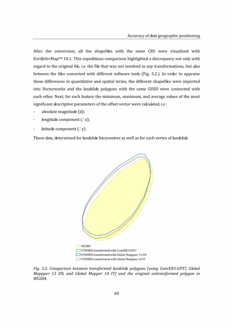
Accuracyofdatageographicpositioning

60

After the conversion, all the shapefiles with the same CRS were visualised with

Esri®ArcMapTM10.1.Thisexpeditiouscomparisonhighlightedadiscrepancynotonlywith

regardtotheoriginalfile,i.e.thefilethatwasnotinvolvedinanytransformations,butalso

between the files convertedwith different software tools (Fig. 3.2.). In order to appraise

thesedifferencesinquantitativeandspatialterms,thedifferentshapefileswereimported

into Vectorworks and the landslide polygons with the same GISID were connected with

eachother.Next,foreachfeaturetheminimum,maximum,andaveragevaluesofthemost

significantdescriptiveparametersoftheoffsetvectorwerecalculated,i.e.:

‐ absolutemagnitude(d);

‐ longitudecomponent(Dx);

‐ latitudecomponent(Dy).

Thesedata,determinedforlandslidebarycentresaswellasforeachvertexoflandslide

Fig.3.2:Comparisonbetween transformed landslidepolygons (usingConvER3‐GPS7,GlobalMappper 13 EN, and Global Mapper 14 IT) and the original untransformed polygon inWGS84.

CHAPTER3

61

Tab.3.4:Outlineof thecomparisonsrealised in thiswork.Theorangehatches indicate thecomparisonswiththeoriginalWGS84,whilethegreenhatchesrefertothecomparisonsoftheresultsobtainedwithdifferentsoftwaretools.

polygons,wereeventuallyimportedintoanExcelworksheet.

Ultimately,inordertoquantifyboththeabsoluteandtherelativeaccuracyofeachprogram,

Icomparedthetransformedfileswiththeoriginaloneandwitheachother(Tab.3.4). In

particular, to analyse the offset spatial distribution and to evaluate if it shows a peculiar

trend,thedataofeverysinglevertexwereelaboratedandinterpolated19withSurfer11.The

Surfer grid was then used by Esri®ArcMapTM 10.1 to elaborate offset isolines with an

intervalof1cm.TherelatedcontourmapsareshowninAppendixAandB,whileTab.3.5

andTab.3.7showthenumericalvaluesrelatedtolandslidebarycentres.

3.5.Analysisanddiscussion

3.5.1.Transformationreversibility

AccordingtotheOGP,theEPSG:5659hasareversibleconversion.However,sincethisisa

local reference systemwith implicit approximations, Idecided toappraise theveracityof

thisstatement.Tothisend,Iperformedaforwardtransformationandthenareverseone,

i.e.fromUTMA/UTMRERtoWGS84andbackwards.TheresultsshowthatfortheUTMRER

thedifferenceis<1mmwhenusingConvER‐GPS7andGlobalMapper14IT,whereasisone

order ofmagnitude higher for GlobalMapper 13 EN.With regard to the UTMA, instead,

ConvER3‐GPS7 and Global Mapper 13 EN present an unchanged precision, while Global

19 FortheinterpolationwasusedtheKrigingmethod.

Accuracyofdatageographicpositioning

62

Mapper14ITincreasesitsdifferenceofoneorderofmagnitude.

At the same time, I compared the outcomes of single opposite transformations (e.g.

UTMA→WGS84andWGS84→UTMA)which,ifcompletelyreversible,shouldreturnvectors

with an equal magnitude. In this sense, Tab. 3.5 shows that ConvER3‐GPS7 has an

imprecision<1mm,whilefortheBlueMarbleproductsitisintheorderofthemillimetre.

These differences almost certainly arise from rounding in the finite precision

representationofthetransformparametersandthecoordinates.Nevertheless,accordingto

theaimsofthisworkandinconsiderationoftheorderofmagnitudeof thesedifferences,

this approximation can be considered acceptable. As a consequence, in the following

paragraphs I present only the results of the transformations from UTMRER/UTMA to

WGS84consideringtheinverseconversionsashomologous.

3.5.2.ComparisonbetweenthetransformedfilesandtheoriginalWGS84file

Themaps contained in Appendix A show the spatial representation of the effects of the

transformations from UTMRER/UTMA to WGS84. Their analysis reveals that the offset

progressively increases eastward (average gradient <1 m) with the exception of the

conversions performed with ConvER3‐GPS7 which present a minimum offset in

correspondence of the Guiglia study site. This latter trend cannot be explained, at least

apparently,bythespatialdistributionof thevertexesof theGPS7kmnetwork(Fig.3.3),

though, it may be interpreted as a consequence of the different transformationmethod

usedby the software.Given theaimsof thiswork,however, the in‐depthanalysisof this

issue should be addressed by further researches. Conversely, the fact that the offset

increases eastward is compatible with the approximations introduced by both local

referencesystemswhichincludealltheEmilia‐Romagnaterritoryinzone32(Gauss‐Boaga

westernzone).Anapproximation thatvoluntarily introducesanerror in thoseareas that

wouldbeinzone33(Gauss‐Boagaeasternzone).

TheanalysisofthemapsinAppendixAalsoshowsthat,withineachsinglestudysite,the

offsetisintheorderofthecentimetrewithanapproximateSW‐NEtrend.Localfluctuations,

especiallyintheareaofGuiglia,maybeaffectedbythedifferenttransformation

CHAPTER3

63

Tab. 3.5: Descriptive parameters of the offset vector between the transformedUTMRER/UTMA filesand theoriginalWGS84 file.Thesevalues (inmetres)werecalculatedwith respect to the barycentre of landslide polygons. Dmin/max/average – absolutemagnitude of the offset vector; Dxmin/max/average ‐ longitude component;Dymin/max/average‐latitudecomponent.

UTMRERConvER3‐GPS7 GlobalMapper13EN GlobalMapper14IT

A B A B A B

Dmin 1.0892 1.0890 1.7627 1.7611 1.1618 1.1624Dmax 1.9739 1.9738 3.2162 3.2147 2.0203 2.0216Dmean 1.5387 1.5385 2.4401 2.4385 1.5203 1.5207

Dxmin 0.1654 0.1654 0.2486 0.2490 0.1409 0.1417Dxmax 1.4803 1.4804 1.3236 1.3236 1.5330 1.5341Dxmean 0.9380 0.9380 0.8143 0.8143 0.9322 0.9325

Dymin 1.0258 1.0255 1.7369 1.7353 0.9233 0.9228Dymax 1.3263 1.3261 2.9406 2.9390 1.3286 1.3292Dymean 1.1631 1.1629 2.2831 2.2815 1.1323 1.1325

UTMAConvER3‐GPS7 GlobalMapper13EN GlobalMapper14IT

A B A B A B

Dmin 1.0892 1.0890 2.1464 2.1472 2.1464 2.1472Dmax 1.9739 1.9738 2.6313 2.6324 2.6313 2.6324Dmean 1.5387 1.5385 2.4033 2.4040 2.4033 2.4040

Dxmin 0.1654 0.1654 1.3848 1.3829 1.3848 1.3829Dxmax 1.4803 1.4804 1.8094 1.8077 1.8094 1.8077Dxmean 0.9380 0.9380 1.6305 1.6287 1.6305 1.6287

Dymin 1.0258 1.0255 1.6024 1.6051 1.6024 1.6051Dymax 1.3263 1.3261 2.0142 2.0169 2.0142 2.0169Dymean 1.1631 1.1629 1.7628 1.7655 1.7628 1.7655

A‐UTMRER/UTMA→WGS84B‐WGS84→UTMRER/UTMA

Accuracyofdatageographicpositioning

64

Fig.3.3:Spatialdistributionofthevertexes(reddots)oftheGPS7kmnetworkrealisedbytheEmilia‐RomagnaRegion.

algorithms20 aswell asby the spatial relationship among the four study sites andby the

quantity and the spatial distribution of the data used for this study. Indeed, while the

algorithm and the grid used for the contouring are the same for all the four areas, the

spatial distribution of landslide polygons and the concentration of the related vertexes

(digit/m)arenothomogeneous(Fig.3.4andTab.3.6).

Thiswork revealed that the total offset, due to the conversion from UTMRER/UTMA to

WGS84,isintheorderofametre.Inparticular,ashighlightedbythemapsinAppendixA,

ConvER3‐GPS7providestheminimumvalues(1,10m‐1,97m)whereasGlobalMapper13

ENpresentsthehighestones(UTMRER:1,77m‐3,21m;UTMA:2,15m‐2,63m).Global

Mapper14IT,ontheotherhand,showscontrastingvalues.Indeed,fortheUTMRERsystem

itprovidesresultssimilartothoseofConvER3‐GPS7(1,17m‐2,02m),whilefortheUTMA

system it is more in agreement with Global Mapper 13 EN (2,15 m ‐ 2,63 m). Similar

outcomesemergealsofromTab.3.5thatshowstheabsolutemagnitudeandthelongitude

and latitude components of the offset vector calculatedwith respect to the barycentre of

landslidepolygons.

Inthisspecificcase,thedifferencesbetweenthetransformedUTMRER/UTMAfilesandthe

20 Thetrendchangesfromsoftwaretosoftware.

CHAPTER3

65

originalWGS84fileemphasisetheimportanceofanadditionalfactor:datalineage,i.e.data

historical information (see par. 2.2.2.). Indeed, as already remarked (see par. 3.4.), the

metadataprovidedbytheCatalogodeiDatiGeograficireportthatthedatausedforthiswork

wereinitiallyacquiredasED50UTM32N*RER(falseNorth=‐4.000.000m)21,therefore,

Fig.3.4–Spatialdistributionoflandslidepolygonsandoftherelatedvertexeswithinthefourstudysites.

21 InApril2014thesamemetadatawerechanged.Thenewmetadatareportthatdatawereinitially

acquiredasUTMRER(MONTEMARIO/UTMRER).

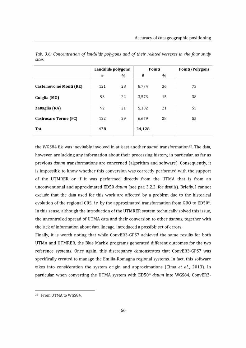
Accuracyofdatageographicpositioning

66

Tab.3.6:Concentrationof landslidepolygonsandof their relatedvertexes in the four studysites.

Landslidepolygons Points Points/Polygons

# % # %

CastelnovonéMonti(RE) 121 28 8,774 36 73

Guiglia(MO) 93 22 3,573 15 38Zattaglia(RA) 92 21 5,102 21 55

CastrocaroTerme(FC) 122 29 6,679 28 55

Tot. 428 24,128

theWGS84filewasinevitablyinvolvedinatleastanotherdatumtransformation22.Thedata,

however,arelackinganyinformationabouttheirprocessinghistory,inparticular,asfaras

previousdatum transformationsareconcerned(algorithmandsoftware).Consequently, it

isimpossibletoknowwhetherthisconversionwascorrectlyperformedwiththesupport

of the UTMRER or if it was performed directly from the UTMA that is from an

unconventionalandapproximatedED50datum(seepar.3.2.2.fordetails).Briefly,Icannot

exclude that the data used for this work are affected by a problem due to the historical

evolutionoftheregionalCRS,i.e.bytheapproximatedtransformationfromGBOtoED50*.

Inthissense,althoughtheintroductionoftheUTMRERsystemtechnicallysolvedthisissue,

theuncontrolledspreadofUTMAdataandtheirconversiontootherdatums,togetherwith

thelackofinformationaboutdatalineage,introducedapossiblesetoferrors.

Finally, it is worth noting that while ConvER3‐GPS7 achieved the same results for both

UTMAandUTMRER,theBlueMarbleprogramsgenerateddifferentoutcomesforthetwo

reference systems. Once again, this discrepancy demonstrates that ConvER3‐GPS7 was

specificallycreatedtomanagetheEmilia‐Romagnaregionalsystems.Infact,thissoftware

takes into consideration the system origin and approximations (Cima et al.., 2013). In

particular,when converting theUTMA systemwith ED50*datum intoWGS84, ConvER3‐

22 FromUTMAtoWGS84.

CHAPTER3

67

GPS7operatesbotha translationandanappropriatedatum transformation23.Conversely,

since they do not recognise the distinctiveness of the ED50* datum, the Blue Marble

software tools treat it as if it were a conventional ED50 datum introducing important

approximationsintothecomputationalprocess.

3.5.3.Comparisonamongfilestransformedwithdifferentsoftwareproducts

Theoffsetvaluesbetweenthebarycentreoflandslidepolygonstransformedwithdifferent

softwaretoolsareshowninTab.3.7,whereasAppendixBcontainsthecontourmapswith

the spatial representation of the offset values referred to each single vertex of landslide

polygons.

Despite the different transformation method, for the UTMA Global Mapper 13 EN and

GlobalMapper14ITAprovidedthesameresultssincebothofthemcouldnotrecognisethe

peculiarity of this system (Tab. 3.7). On the other hand, in absolute terms, the offset

betweentheoutcomesoftheBlueMarblesoftwareandConvER3‐GPS7rangefrom0.72m

intheCastrocaroTermeareato2.25mintheCastelnovonéMontisite(AppendixB).

With regard to the UTRER, instead, Global Mapper 14 ITA performed quite similarly to

ConvER3‐GPS7.Infact,althoughspatiallyirregular,theoffsetbetweenthesetwoprograms

barelyexceeded20cmwith thehighestvaluesconcentrated in theareaofCastelnovoné

Monti. Conversely, with respect to ConvER3‐GPS7, Global Mapper 13 EN shows offset

valuesthatrangefrom0.76mintheCastrocaroTermeareato1.66mintheCastelnovoné

Montisite.

Itisworthnotingthat,inbothcases,theoffsetwithinthesameareaneverexceeds10cm.

The analysis of the contour maps of Appendix B reveals also that the offset generally

increaseswestwardwith the exception of the comparisons between ConvER3‐GPS7 and

Global Mapper 13 EN, and Global Mapper 14 ITA and Global Mapper 13 EN for the

UTMRER. The explanation of these trends, however, exceeds the aims of this work and

shouldbeinvestigatedbymoredetailedgeodeticanalyses.

Ingeneral,Isuggestthatthediscrepancieshighlightedbythisstudymaybeessentially

23 ConvER3‐GPS7recognisestheED50*forwhat it is, i.e.anunconventionalapproximateddatum

developed from the GBO by means of a simple translation (see par. 3.2.2.). Consequently, itoperatesthecorrecttransformation.

Accuracyofdatageographicpositioning

Tab.3.7:Descriptiveparametersoftheoffsetvectorbetweenfilestransformedwithdifferentsoftwaretools.A)referstoUTMRER,whileB)referstoUTMA.Values (inmetres)werecalculatedwithrespect to thebarycentreof landslidepolygons.Dmin/max/average–absolutemagnitudeof theoffsetvector;Dxmin/max/average‐longitudecomponent;Dymin/max/average‐latitudecomponent.

A)

B)

CHAPTER3

69

attributedtothefollowingcauses:

‐ differentdatum transformationmethod (e.g.grigliatimethod vs 3‐ or 7‐parameters

roto‐translation);

‐ useoflocalparametersacquiredfromphysicalgeodeticcontrolpoints;

‐ originoftheED50*datum(seepar.3.2.2.);

‐ inherentimprecisionoftheUTMAandUTMRERsystems(especiallyzoneextension).

Thefirsttwocausescanbeconsideredintrinsicfactorsofsoftwaretools,whiletheothers

are related to the peculiarity of the Emilia‐Romagna reference systems with respect to

which ConvER3‐GPS7 and the Blue Marble software products behave differently. Indeed,

ConvER3‐GPS7 was intentionally created to be used only within the Emilia‐Romagna

regionandwiththespecificpurposeofmanagingtheunconventionalregionalsystem.On

theotherhand,GlobalMapper13ENisaninternationalcommercialsoftwaresystemand,

for this reason, it must adopt a more generic transformation algorithm which does not

implytheuseoflocalparameters(seepar.3.3.1.and3.3.2.formoredetails).Tothisend,it

isworthnotingthat,accordingtoDonatellietal.(2002),inmostoftheItalianterritory,the

differences between the results of the grigliati method and those of the 7‐parameters

transformation,performedonthebasisoftheIGM95controlpoints,aregenerally<10cm.

Inthissense, it is likelythatthediscrepancybetweenConvER3‐GPS7andGlobalMapper

13ENisduetotheuseoflocalparametersbasedonphysicalgeodeticcontrolpointsrather

thantothetransformationmethoditself.Theimportanceofthe“geodeticcontextualization”

oftheconversionalgorithmisunderlinedbytheresultsprovidedbyGlobalMapper14ITA,

which,asreportedinpar.3.3.2.,wasadaptedtotheItalianterritory.

3.6.Conclusions

Given the importance of geographic positioning for landslide studies, thiswork aimed to

assess,inquantitativeandspatialterms,theeffectsofdatumtransformationsinrelationto

thesoftwaretools,andthealgorithms,usedfortheconversion.Thefinalgoal,however,was

nottoappraisetheiroverallgeodeticefficiencybutrathertoquantifythefalloutsofthese

transformationsonalandslideinventorymap.Tothisend,Itestedthreedifferentsoftware

toolswithrespecttotheWGS84andtheunconventionalreferencesystemsadoptedbythe

Accuracyofdatageographicpositioning

70

Emilia‐RomagnaRegionalAuthority(UTMRERandUTMA).

Ingeneral,thisworkprovedthat,withregardtothelandslideinventorymapsofthestudy

sites, theoffsetassociated todatum conversionmaybeof theorderofmetric length, i.e.

oneorderofmagnitudehigherthantheresolutionofaVHRsatelliteimage(0.50m).Italso

confirmed that there is no comprehensive transformation algorithm that can be applied

worldwide as, instead, would require international software products. Indeed, datum

conversions are affected by the intrinsic distortions of local geodetic networks and, as a

consequence, it isadvisabletousesoftwaretoolsbasedon localparameterscalculatedon

physicalcontrolpoints.

Onthisbasis,wheneverpossible,inordertopreservethebenefitsofthehighprecisionof

satellitedata, it isrecommendedtoavoiddatum transformationsbyacquiringdatawith

the same CRS. Otherwise, datum conversions should be performed by using only one

softwareproductsoastokeeptheoffsetasconstantaspossible;anessentialconditionfor

multi‐temporalstudies.Inaddition,themagnitudeofthisuncertaintyshouldbecorrectly

quantified and taken into consideration for the assessment of potential data uses. In

particular,asfaraslandslideinventorymapsareconcerned,animprecisionoftheorderof

metriclengthshoulddiscourageanyrigid applicationoflandslidepolygons.

Finally, this work underlined the unsuitability as well as the difficult and complex

managementrequiredbyunconventionalreferencesystems.Tothisregard, itparticularly

emphasised the importance of data lineage as an essential parameter to define quality

especiallyforderivedorsecondhanddata.

Spatialaccuracyoflandslidedetectionandmapping

CHAPTER4

Spatial accuracy of landslide detection andmapping

4.1. Introduction4.2. Landslidedetectionandmappingtechniques:acomparisonbetweenremotelysensed

andfieldsurveydata4.2.1.Analysisandresults

4.2.1.1.Descriptivestatistics4.2.1.2.Landslideabundance4.2.1.3.Correspondenceoflandslideareas4.2.1.4.Timeandcostevaluation

4.2.2.Discussion4.2.2.1.Limitingfactorsofthedetectionandmappingtechniques4.2.2.2.Datainterpretation

4.3. Spatialaccuracyofamulti‐temporallandslideinventorymap4.3.1.Analysisandresults4.3.2.Discussion

4.4. Conclusions

CHAPTER4

72

4.Spatialaccuracyoflandslidedetectionandmapping

4.1.Introduction

InthisChapter,Iaddressspatialaccuracy,i.e.thedefinitionoflandslidesizeandshape,from

twodifferent points of view: landslide detection andmapping techniques and the overall

spatialaccuracyofalandslideinventorymap.

Landslidedatacanatbestapproximatethecomplexityofphysicalreality(seepar.2.2.3.).In

thissense, landslidedetectionmethod is thebasic tool throughwhichreality isperceived

and, therefore, it decisively affects the conceptual model that is ultimately realised in a

landslideinventorymap.Inordertoappraisethisaspect,Icarryoutacomparisonbetween

two different detection techniques: remote sensing and field investigation. To this end, I

preparedtwoinventories(bothrealisedonthe2012status)thatIcomparedonthebasisof

theirdescriptivestatistics,landslideabundance,correspondenceoflandslideareas,time,and

cost/benefitratio.

Conversely,toquantifyandeffectivelycommunicatetheoverallspatialaccuracyoflandslide

detection andmapping, I performa fuzzy‐like analysis on amulti‐temporal inventory. In

this sense, spatial persistence and boundary reliability are used as proxies for spatial

accuracy.

This study is conductedon the catchmentof theDorgolaCreek, i.e. on theCastelnovoné

Monti site (seepar. 2.3.1.1.).Despite itsnatural aspect, thisareahadbeen, and it still is,

severely modified by human activities so that anthropogenic processes must always be

consideredwhendealingwithslopestability.

Withregardtolandslides,inthisworktheuseoftheterms“cancel”,“erase”,orsimilarare

discouraged. Indeed, geomorphological surveys are limited to superficial analysis and do

not provide any subsurface information. As a consequence, they do not supply any real

evidencesthatagivenmassmovementwasactuallyremovedorstabilisedandnotmerely

concealedorjustpartiallysloweddown.

Spatialaccuracyoflandslidedetectionandmapping

73

4.2. Landslidedetection andmapping techniques: a comparisonbetweenremotelysensedandfieldsurveydata

Thequalityofalandslideinventoryreliesonseveralfactors(seepar.2.2.3.).Amongothers,

for example, detection techniques and supports strongly influence the inventory

completeness and the overall accuracy of landslide identification andmapping. Landslide

inventorymapscanbepreparedusingdifferentmethodsandtools,however,mostofthese

techniquescouldnotbeeffectivelyused in thiscontextdue theircost, timecommitment,

and tested reliability. In the lastdecades, visual interpretationof remotely sensed images

becamea substantial support to field investigationsandoneof themost frequentlyused

method for landslide detection andmapping (Rib and Liang, 1978; Turner and Schuster,

1996;Guzzetti,2006).Remotesensingtechniquespresent,indeed,importantadvantages:

coverageoflargeareas;

possibilitytoinvestigatethetemporaldimension;

sufficienttoexcellentresolution;

goodcost/benefitratio.

In particular, until recently, aerial photographswere themost common type of remotely

senseddata(Mantovanietal.,1996).Nowadays,thus,thecost,availability,resolution,and

knowledgeofsatellite imagesandtechniquesconsiderablyimprovedsothattheybecame

an effective alternative to aerial photographs. The GeoEye‐1 satellite is a commercial

remotesensingsystemlaunchedon6thSeptember2008.Itprovidesimagesatnadirwith

0.5mpanchromatic (black&white)and2mmultispectral resolution.TheGeoEYE‐1 isa

polar‐orbitingsun‐synchronoussatellitethatorbitstheEarth15timesperdayatanaltitude

of681kmandwitha10:30a.m.equatorcrossing(E‐geos.it,2014).

According to the research aims, I tried to assess the efficiency of two of themost used

landslide detection andmapping techniques. To this end, I compared a remotely sensed

inventory(Fig.4.1),preparedonaVHRorthorectifiedpanchromaticGeoEYEimage,witha

detailed geomorphological field‐based inventory (Fig. 4.2). For this comparison the time

issuewasdisregarded (seeChapter 5), since the two inventorieswerepreparedonnew

coevaldata:theGeoEYEimageacquiredonAugust2012andthefieldsurveyconductedin

October‐November2012.Furthermore,inordertocontroltheeffectsofsubjectivity,I

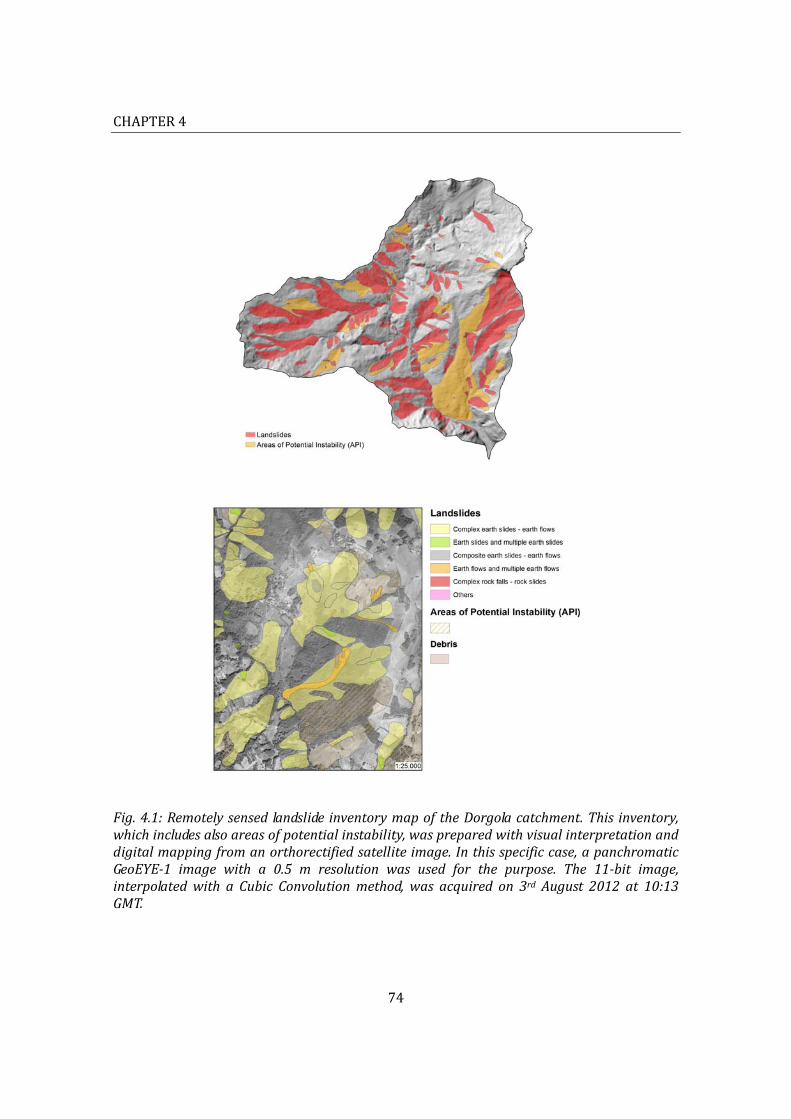
CHAPTER4

74

Fig.4.1:Remotelysensed landslide inventorymapoftheDorgolacatchment.This inventory,whichincludesalsoareasofpotentialinstability,waspreparedwithvisualinterpretationanddigitalmappingfromanorthorectifiedsatelliteimage.Inthisspecificcase,apanchromaticGeoEYE‐1 image with a 0.5 m resolution was used for the purpose. The 11‐bit image,interpolatedwith a Cubic Convolutionmethod,was acquired on 3rdAugust 2012 at 10:13GMT.

Spatialaccuracyoflandslidedetectionandmapping

75

Fig.4.2:Ground‐basedgeomorphological landslide inventorymapoftheDorgolacatchment.Thesurveycampaignwasconductedoveranon‐continuousperiodfromthe1stOctobertothe13thNovember2012foratotalamountof23workingdays.Fieldinvestigationsfocusednotonlyonevidentlandslides(depositsandsourceareas),buttheyalsodetectedareasofpotentialinstability and hummocky topography, as well as topographic anomalies, consolidationworks, infrastructure and building damages, superficial drainage systems, ponds, andanomalous patterns, badlands, anthropogenic features, particular land‐uses, and water‐demandingvegetation.

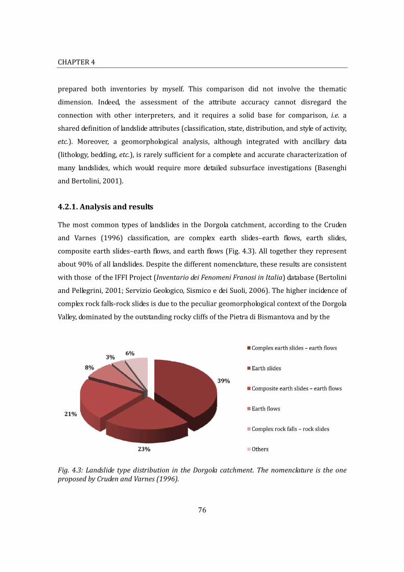
CHAPTER4

76

prepared both inventories by myself. This comparison did not involve the thematic

dimension. Indeed, the assessment of the attribute accuracy cannot disregard the

connection with other interpreters, and it requires a solid base for comparison, i.e. a

shareddefinitionoflandslideattributes(classification,state,distribution,andstyleofactivity,

etc.). Moreover, a geomorphological analysis, although integrated with ancillary data

(lithology,bedding,etc.),israrelysufficientforacompleteandaccuratecharacterizationof

many landslides, which would require more detailed subsurface investigations (Basenghi

andBertolini,2001).

4.2.1.Analysisandresults

Themost common typesof landslides in theDorgola catchment, according to theCruden

and Varnes (1996) classification, are complex earth slides–earth flows, earth slides,

compositeearthslides–earthflows,andearthflows(Fig.4.3).All togethertheyrepresent

about90%ofalllandslides.Despitethedifferentnomenclature,theseresultsareconsistent

withthoseoftheIFFIProject(InventariodeiFenomeniFranosiinItalia)database(Bertolini

andPellegrini,2001;ServizioGeologico,SismicoedeiSuoli,2006).Thehigherincidenceof

complexrockfalls‐rockslidesisduetothepeculiargeomorphologicalcontextoftheDorgola

Valley,dominatedbytheoutstandingrockycliffsofthePietradiBismantovaandbythe

Fig.4.3:Landslide typedistribution in theDorgolacatchment.Thenomenclature is theoneproposedbyCrudenandVarnes(1996).

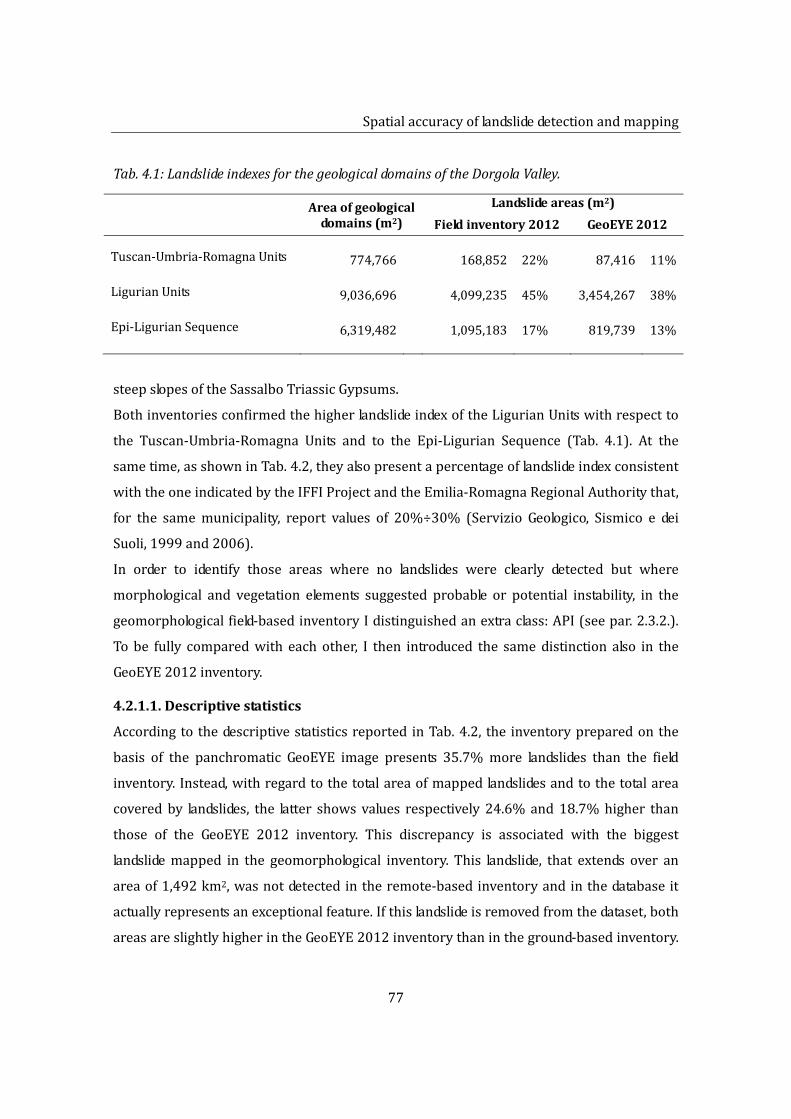
Spatialaccuracyoflandslidedetectionandmapping

77

Tab.4.1:LandslideindexesforthegeologicaldomainsoftheDorgolaValley.

Areaofgeologicaldomains(m2)

Landslideareas(m2)

Fieldinventory2012 GeoEYE2012 Tuscan‐Umbria‐RomagnaUnits 774,766 168,852 22% 87,416 11% LigurianUnits 9,036,696 4,099,235 45% 3,454,267 38% Epi‐LigurianSequence 6,319,482 1,095,183 17% 819,739 13%

steepslopesoftheSassalboTriassicGypsums.

BothinventoriesconfirmedthehigherlandslideindexoftheLigurianUnitswithrespectto

the Tuscan‐Umbria‐Romagna Units and to the Epi‐Ligurian Sequence (Tab. 4.1). At the

sametime,asshowninTab.4.2,theyalsopresentapercentageoflandslideindexconsistent

withtheoneindicatedbytheIFFIProjectandtheEmilia‐RomagnaRegionalAuthoritythat,

for the samemunicipality, report values of 20%÷30% (Servizio Geologico, Sismico e dei

Suoli,1999and2006).

In order to identify those areas where no landslides were clearly detected but where

morphological and vegetation elements suggested probable or potential instability, in the

geomorphologicalfield‐basedinventoryIdistinguishedanextraclass:API(seepar.2.3.2.).

To be fully comparedwith each other, I then introduced the samedistinction also in the

GeoEYE2012inventory.

4.2.1.1.Descriptivestatistics

Accordingtothedescriptivestatisticsreported inTab.4.2, the inventorypreparedonthe

basis of the panchromatic GeoEYE image presents 35.7%more landslides than the field

inventory.Instead,withregardtothetotalareaofmappedlandslidesandtothetotalarea

coveredby landslides, the latter showsvalues respectively 24.6%and18.7%higher than

those of the GeoEYE 2012 inventory. This discrepancy is associated with the biggest

landslidemapped in the geomorphological inventory. This landslide, that extends over an

areaof1,492km2,wasnotdetectedintheremote‐basedinventoryandinthedatabaseit

actuallyrepresentsanexceptionalfeature.Ifthislandslideisremovedfromthedataset,both

areasareslightlyhigherintheGeoEYE2012inventorythanintheground‐basedinventory.

CHAPTER4

78

Thesameconsiderationisvalidalsoforthesmallestlandslideofthefieldinventory(28m2)

which represents an isolated value. Moreover, despite their different meanings, mean,

median,andmodeareasareallhigherintheground‐basedinventorythanintheGeoEYE

2012inventory.Thisindicatesthatthetwomapsdivergefromeachothernotonlyforthe

total amount of landslides but also as far as the mapped landslide size is concerned. In

particular,smalllandslidesaremoreabundantintheremotelysensedinventory.Thisisalso

confirmed by the area frequency distribution shown in Fig. 4.4 A. This histogram was

preparedbyusinganareaclassbinwidthprogressivelyincreasedaccordingtoalog5scale

in order to display in a proper way all the area range. The histogram shows that, with

respecttothefieldsurvey2012,themostfrequentclassoftheGeoEYE2012corresponds

tosmallerareas.Indeed,itisevidentthatthediscrepancyinthetotalnumberoflandslides

Tab.4.2:Descriptivestatisticsoftheground‐basedandremote‐basedinventories.ThevaluesinparenthesesdonotconsidertheBondololandslide.

Fieldinventory2012 GeoEYE2012

Numberoflandslides # 224* 304

Totalareaofmappedlandslides Km2 6.245(4.752)

5.039

Totalareacoveredbylandslides Km2 5.37(4.193)

4.365

%oflandslidearea % 33.12 26.92 (25.86)

Landslidedensity #/Km2 13.81 18.75

Areaofsmallestlandslide m2 28 79

Areaofbiggestlandslide m2 1,492,740 392,681 (434,995)

Landslideaveragearea m2 27,880 16,577

Landslidemedianarea m2 4,622 2,522

Mostabundantlandslidearea m2 ~300 ~200

* Thetotalnumberoflandslideswasgenerallyconsideredtobe223sincetwoofthemwererecognizedintheGeoEYEinventoryasasingleobject.

Spatialaccuracyoflandslidedetectionandmapping

79

Fig. 4.4: Landslide area frequency distribution for the ground‐based and the remote‐baseinventories. Inorder todisplayall thearea range,area classbinwidthwereprogressivelyincreased according to a log5 scale. A) The histogram represents the absolute number oflandslidesineachareaclassrepresentedbythebincentralvalue.B)Thediagramshowsboththecumulativeandthenon‐cumulativecurvesrelatedtolandslidepercentage.

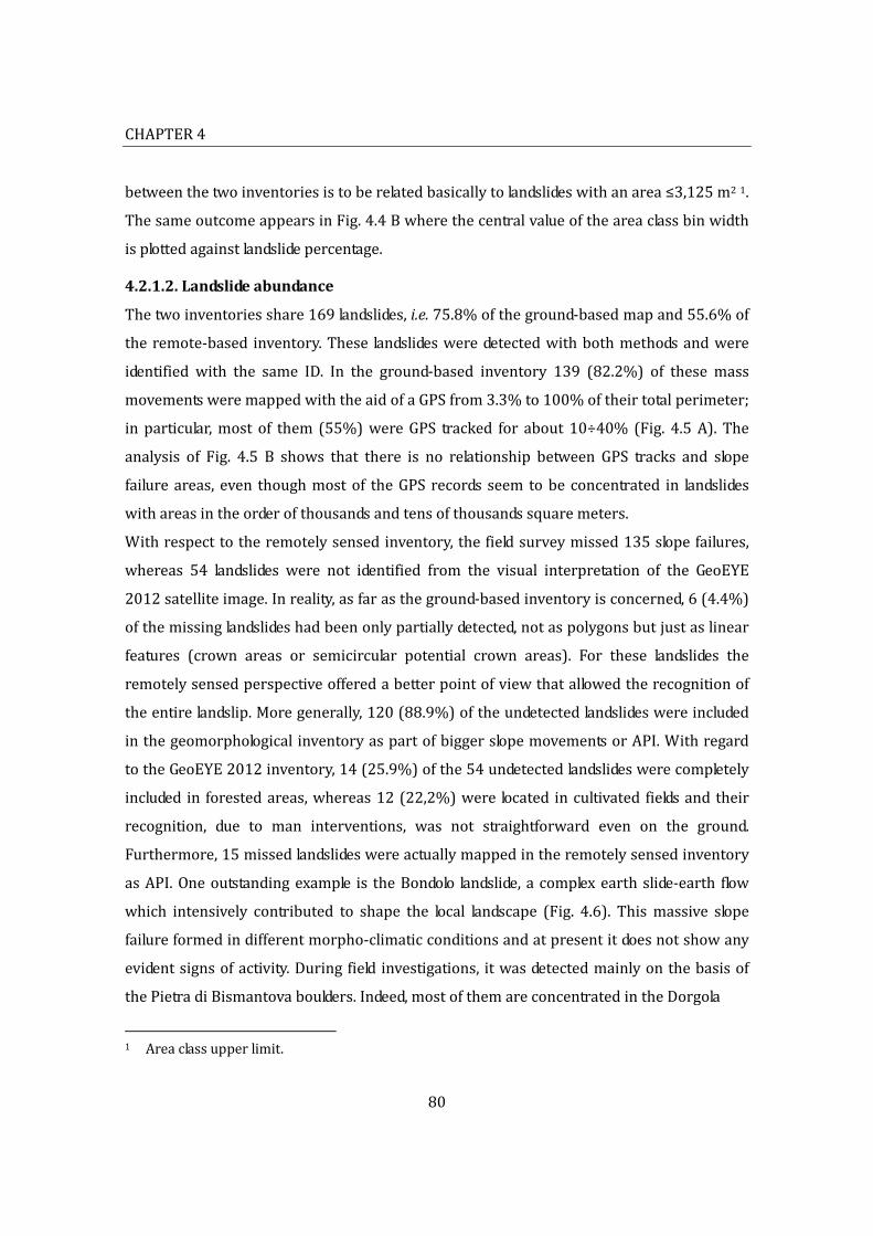
CHAPTER4

80

betweenthetwoinventoriesistoberelatedbasicallytolandslideswithanarea≤3,125m21.

ThesameoutcomeappearsinFig.4.4Bwherethecentralvalueoftheareaclassbinwidth

isplottedagainstlandslidepercentage.

4.2.1.2.Landslideabundance

Thetwoinventoriesshare169landslides,i.e.75.8%oftheground‐basedmapand55.6%of

theremote‐based inventory.These landslidesweredetectedwithbothmethodsandwere

identified with the same ID. In the ground‐based inventory 139 (82.2%) of these mass

movementsweremappedwiththeaidofaGPSfrom3.3%to100%oftheirtotalperimeter;

inparticular,most of them (55%)wereGPS tracked for about10÷40% (Fig. 4.5A). The

analysis of Fig. 4.5 B shows that there is no relationship between GPS tracks and slope

failure areas, even thoughmostof theGPS records seem tobe concentrated in landslides

withareasintheorderofthousandsandtensofthousandssquaremeters.

Withrespecttotheremotelysensedinventory,thefieldsurveymissed135slopefailures,

whereas 54 landslides were not identified from the visual interpretation of the GeoEYE

2012satelliteimage.Inreality,asfarastheground‐basedinventoryisconcerned,6(4.4%)

ofthemissinglandslideshadbeenonlypartiallydetected,notaspolygonsbutjustaslinear

features (crown areas or semicircular potential crown areas). For these landslides the

remotelysensedperspectiveofferedabetterpointofviewthatallowedtherecognitionof

theentirelandslip.Moregenerally,120(88.9%)oftheundetectedlandslideswereincluded

inthegeomorphologicalinventoryaspartofbiggerslopemovementsorAPI.Withregard

totheGeoEYE2012inventory,14(25.9%)ofthe54undetectedlandslideswerecompletely

included in forestedareas,whereas12(22,2%)were located incultivated fieldsandtheir

recognition, due to man interventions, was not straightforward even on the ground.

Furthermore,15missedlandslideswereactuallymappedintheremotelysensedinventory

asAPI.Oneoutstandingexample is theBondolo landslide,acomplexearthslide‐earth flow

which intensively contributed to shape the local landscape (Fig. 4.6). Thismassive slope

failureformedindifferentmorpho‐climaticconditionsandatpresentitdoesnotshowany

evidentsignsofactivity.Duringfieldinvestigations, itwasdetectedmainlyonthebasisof

thePietradiBismantovaboulders.Indeed,mostofthemareconcentratedintheDorgola

1 Areaclassupperlimit.

Spatialaccuracyoflandslidedetectionandmapping

81

Fig. 4.5: These 2D and 3D histograms display the relationship between GPS records andlandslidespercentage(A)andamongGPSrecords,landslidespercentage,andarea(B)whichisindicatedbytheclassbinuppervalue.

CHAPTER4

82

riverbedalongthemarginofthelandslidetoe(about3kmfromthePietradiBismantova),

butmanyothersarescatteredallovertheentirelandslidedeposit.Furthermore,theconvex

lobateshapeoftherun‐outareawasclearlydetectableontheCTRandontheshadedrelief

rastercreatedbyEsri®ArcMapTM10.1fromtheCTR5mDEM.Ontheotherhand,withjust

few isolated exceptions, boulders,mostly hidden by vegetation, could not be seen on the

satellite image (Fig. 4.7)making the landslide identificationmore challenging. Indeed, the

Bondololandslideisremotelydetectableonlyonthebasisofitslandform.This,however,was

notrecognisedbothforitsmassivedimensions2andbecausewithtimethesourceareawas

partiallyconcealedanderodedbysuccessive,andatleastpartiallystillactive,mass

Fig.4.6:TheBondololandslideextendsoveranareaofapproximately1,5km2,fromthePietradi Bismantova to the Dorgola riverbed. A) The landslide as itwas identified andmappedduring the2012 field survey.Reddots represent someof thePietradiBismantovabouldersthat had been GPSmapped over the landslide deposit. B) The Bondolo landslide as itwasmappedbytheGSUEG(1976).

2 In away, the Bondolo landslide is not part of the landscape, but it is itself themain landscape

feature.

Spatialaccuracyoflandslidedetectionandmapping

83

movements. To this end, a 3D/stereoscopic vision would have probably helped the

recognition.Eventually,ontheGeoEYE2012imagetheBondololandslidewasnotmapped

as a mass movement, but it was identified as an API basically due to the characteristic

shapeofitstoe.

The area frequency distribution of the missing landslides in the two inventories is

representedinFig.4.8.Undetectedlandslidesizesconfirmthattheground‐basedinventory

missedmoresmalllandslidesthantheremotelysensedone,whichinsteadseemtopartially

failonmediumtolargelandslides.

4.2.1.3.Correspondenceoflandslideareas

Inordertoquantifythedegreeofcartographicmatchingbetweenthetwomaps,theoverall

mappingerrorwascalculatedaccordingtothemethodproposedbyCarraraetal.(Carrara

etal.,1993)asmodifiedbyGallietal.(2008):

E=((A1⋃A2)–(A1⋂A2))/(A1⋃A2) 0⪕E⪕1 (1)

whereA1andA2arethetotallandslideareainthetwoinventories,whereas⋃and⋂are

respectively the cartographic union and intersection of the two maps automatically

computedbyEsri®ArcMapTM10.1.FromEq(1)Gallietal.(2008)obtainedthematching

index:

M=1‐E, 0⪕M⪕1 (2)

Ideallyiftwomapsmatchperfectlytheerrorindexwouldbe0and,consequently,thedegree

ofmatchingwouldbe1.Onthecontrary, iftwomapsdonotoverlapatall theerrorindex

wouldbe1andthematchingindex0.Eq.(1)showstheoverallmismatchasitencompasses

landslideidentification,positioning,andmapping.

Thecomparisonbetweentheground‐andtheremote‐basedlandslidemapsoftheDorgola

catchmentshowsanerrorindexvalueof0,54(54%), i.e.amatchingindexof0,46(46%).

However, if the comparison is extended also to the APImapped in both inventories, the

error index decreases to 0,36 (36%)which corresponds to a rather satisfyingmatching

index of 0,64 (64%). The cartographic matching was computed also for every single

landslidethathadbeenmappedinbothinventories(169landslides).Inthiscase,theerror

indexrangesfromamaximumof0.90(M=0.10)toaminimumof0.16(M=0.84),witha

CHAPTER4

84

Fig.4.7:BouldersfromthePietradiBismantovaincludedintheBondololandslide.Inspiteoftheir large dimensions (up to 103m3), these boulders cannot be easily remotely detectedgenerallyduetovegetationcanopy.A)aboulderisincludedintoanhistoricalruralbuilding.B)ahugeboulder,althoughpartiallyhiddenbyvegetation, isremotelydetectable.However,theuseofacoloredorB/Wimageconsiderablyinfluenceitsrecognition.

Spatialaccuracyoflandslidedetectionandmapping

85

Fig.4.8:Area frequencydistributionofmissing landslides inthetwo inventories.Inordertodisplayallthearearange,areaclassbinwidthwereprogressively increasedaccordingtoalog5scale.A)Thehistogramrepresentstheabsolutenumberof landslides ineachareaclassrepresentedbythebincentralvalue.B)Thediagramshowsboththecumulativeandthenon‐cumulativecurvesrelatedtolandslidepercentage.

median value of 0.4 (M=0.6). The analysis of Fig. 4.9 shows that apparently there is no

relationshipbetweentheerrorindexandthelandslideareas.Indeed,thelackofhighvalues

oferrorindexincorrespondencetolargerlandslidesmaybeaconsequenceoftheirreduced

frequency.

CHAPTER4

86

4.2.1.4.Timeandcostevaluation

The survey campaign (see Chapter 2 for details) was realized during a non‐continuous

periodfromthe1stOctobertothe13thNovember2012foratotalamountof23working

days (Tab. 2.2). Data processing for the realization of the geomorphological landslide

inventory required10extraworkingdays for a total of 33days (Tab.4.3). Therewasno

needtobuysupportmaterialoranyspecificinstrumentation(theCTRandtheGPSwere

both already available to the geomorphologist) so that costs (about 687,98 euro) are

ascribableonlytotransportstoandfromthesurveyarea3.Conversely, theGeoEYEimage

was tasked on the 26th June 2012 and acquired on the 3rd August 2012. The time lapse

between the image tasking and acquisition depends on weather conditions and satellite

availability.AccordingtotheproducerDeliveryTerms(GeoEYE,2009)forareas<500km2

GeoEYE‐1 images aredeliveredwithin 60days.The realization of the landslide inventory

required5extraworkingdays(Tab.4.3).TheminimumordersizeforGeoimageis100km2

andthecostforitwithanAcademyLicence(‐30%)is1.522,50euro+VAT.

Fig.4.9:Inthisdiagramtheerrorindexvalues,calculatedforeachsinglelandslidedetectedinbothinventories,areplottedagainstthetwosetsoflandslideareas.

3 Fortimeandresourceoptimisation,duringweekdaysIdecidedtostayatthestudyareainsteadof

dailycommuting.Accommodationcosts,however,arenotincludedinthetotalexpense.

Spatialaccuracyoflandslidedetectionandmapping

87

Tab.4.3:TimeandcostofthetwoinventoriespreparedfortheDorgolacatchment.

Fieldinventory2012 GeoEYE2012

Surveyperiod days 23 (38)*

Processingtime days 10 5

Costs euro 687,98 1,522.50+VAT**

* Timelapsebetweenimagetaskingandacquisition.** Thiscost isreferredto100km2anditdoesnot includeorthorectificatio;theproportionalexpense for16

km2isabout348euroincludingorthorectifiation.

Orthorectificationoperationswerelaterperformedbye‐geosatthecostof6,50euro/km24

(Tab.4.3).

4.2.2.Discussion

4.2.2.1.Limitingfactorsofthedetectionandmappingtechniques

Somethemajor limiting factorsofbothdetectiontechniquesunderstudyarecommonto

bothofthem(weather/cloudcover,cost/benefitratio,surveyorexperience),whileothers

are more specifically connected to one method or the other (Tab. 4.4). Generally, the

importanceofeach factor isbasicallyrelated to the landscapeand themorphologyof the

area,sothatitisimpropertolistthemaccordingtoanabsoluterelevance.

Asfarasfieldsurveyisconcerned,areainaccessibilitycanbeduetodifferentcauses:steep

orimperviousslopes,riskyareas,impenetrablevegetation,andprohibitedareas(fenced‐in

private properties, hunting areas, military zones, etc.). Most of these issues were

encountered during the survey of the Dorgola catchment. Another relevant factor is the

surface detail of the survey, i.e. the surveyor trekking intensity with respect to local

morphology,landslidesizeandland‐use.Indeed,inordertobedetected,asmalllandslideina

forestedareawithanirregularmorphologyrequiresamoreintensewanderthanasimilar

landslidelocatedinanopenfieldwithlittleornovegetationandamoreregularmorphology.

Tothisend,itisevidentthatthisfactorisstrictlyrelatedtotheavailabletimeaswellasto

4 Inthiscase,theminimumordersizeof100Km2canbesubdividedamongdifferentareas.

CHAPTER4

88

Tab.4.4:Limitingfactorsofthedataqualityforfieldsurveyandforthevisualinterpretationoforthorectifiedsatelliteimages.

FieldsurveyVisualinterpretationof

orthorectifiedsatelliteimages

areainaccessibility forestandsnowcanopy

surfacedetailofthesurveywithrespecttolocalmorphology,landslidesizeandland‐use

shadowareas

weather cloudcover

availabletime imageillumination

lackofperspective lackof3D/stereoscopicvision

cost/benefitratio cost/benefitratio

surveyorexperience surveyorexperience

land‐use imagebands(colourvsB/W)andresolution

Landslidedraftinganddigitizing positionalandorthorectificationaccuracy

theactualfeasibilitytowalkandseeeverywhere.Inthissense,thelackofperspectivefrom

differentpointsofview,e.g. fromtheoppositeslopeorfromahigherposition,represents

anothersignificantrestrictiontothedataqualityoffieldsurvey.Land‐usecanbeafurther

limitingfactor.Indeed,differentland‐usesimplydifferentchallenges.Nevertheless,alsothe

same land‐use in a different season or a different time of the day can either facilitate or

prevent landslide detection. This, for example, is the case of cultivated fields where old

dormantmediumtolargelandslidescanbemoreeasilydetectedwhenthecropjuststarted

togrowratherthanbeforeharvestorjustafterploughing.Youngplantstendactuallytobe

healthieronthelandslidemoistdepositthaninthesoildepletedsourcearea.Inthissense,it

isevidentthattheseasonisanimportant,althoughnotnecessarylimiting5,aspectoffield

5 Everyseason,indeed,presentssomeadvantagesandsomedisadvantages.

Spatialaccuracyoflandslidedetectionandmapping

89

surveynotonlyforthetotalamountofdaylight6butalsoforthegrowthofbothnaturaland

cultivatedvegetation.Finally,thequalityofthefieldsurveydataisalsoaffectedbylandslide

draftinganddigitizing. Inparticular, landslidedraftingcanbequitechallenginganderror‐

proneifthetopographicsupportpre‐datesthemassmovement.

Withregardtoremotesensing,mostofthelimitingfactorsaffectingdataqualityarequite

straightforward,andtheydonotrequireaparticularexplanation(forestandsnowcanopy,

cloud cover, shadow areas, etc.). According to the geographic position and altitude of the

studyarea,ausefulexpedienttoreducesomeoftheseissuesistoacquiresatelliteimages

inaparticularseason.InthecaseoftheDorgolaValley,springtimeandlateautumnproved

tobe thebestmomentsof theyearsince forestandsnowcanopiesaregenerallyabsent.

Unfortunately, in theNorthernApennines these are also the rainiest periods of the year

and,besides,snow‐melt itself isconsideredasoneof themost important landslidecauses.

Indeed, 48% of mass movements take place between March and May, whereas 29% of

landslides occur between October and December (Bertolini & Pellegrini, 2001). This

suggests that an image captured in spring may miss some mass movements, while in

autumn some landslides may have been concealed by summer farming activities. A

compromise between these two factors is, therefore, necessary. The quality of remote

sensed data also depends on image bands and resolution. Along with the interpreter

personal sensibility towards coloured and B/W images, there are also more objective

situationswhenonetypeofimageismoreeffectivethantheotherlike,forexample,inthe

caseofthePietradiBismantovaboulderrepresentedinFig.4.7B.Imageresolution,onthe

other hand, determines the minimum dimensions of the smallest detectable object.

However,whenmoreimagesetsarecomparedorrelatedtoeachother,likee.g.inamulti‐

temporalinventorymap,highprecisionmaybecorruptedbyapoororthorectificationor

positionalaccuracy(seeChapter3).Infact,bothoftheseterms,aswellasimageresolution

itself, should be as constant as possible throughout the different image sets in order to

provideanhomogeneousbasisforcomparisonsandoverlays.Imageilluminationmayalso

bealimitingfactorforthedetectionofparticularlandslides.Indeed,withoutthesupportofa

3D/stereoscopicvision,averticalintenseilluminationcanflattentheimagemakingitmore

6 Duringshortwinterdaysthetotalnumberofhourswithanoptimumilluminationislowerthan

insummer.

CHAPTER4

90

difficulttorecognisedhummockymorphologyandtopographicconcavitiesandconvexities.

The cost/benefit ratio, instead, may be generally considered an advantage of remote

sensing,althoughiftheareaofinterestisverysmallitmaybeworthreconsideringother

surveyoptions.

4.2.2.2.Datainterpretation

The ground‐ and the remote‐based inventories share a significant amount of landslides,

respectively 75.8% and 55.6%. Furthermore, according to the literature (Carrara et al.,

1993;Ardizzoneetal.,2002;Gallietal.,2008;Santangeloetal.,2010),theypresentalsoa

satisfactory cartographicmatching indexof0,64 (64%).Hence,overall, the twodetection

techniques provide quite analogous outcomes. Notwithstanding this, there is still a

reasonabledisagreementaboutthetotalnumber,aswellasaboutthesize,ofthedetected

and mapped landslides. Furthermore, since both techniques present advantages and

disadvantages,itisworthconsideringwhichonedidbetterappraise“truth”.Fieldsurveyis

generally considered themost reliable termof comparison, although several factorsmay

influence its accuracyandsoundness (seepar.4.2.2.1.). Inparticular, the coexistenceand

interaction of these elements generate more degrees of outcome quality, thus offering

different“groundtruths”.Nevertheless,despitesomegreatadvantages,alsoremotesensing

canproducedifferentresultsonthebasisofdifferentpreconditions.

ThefieldsurveyrealisedintheDorgolacatchmentwasconductedindetailswithanaverage

surveyedareaofabout0,7km2perdayandatotalamountofGPSrecordsofabout185km.

Dataquality,however,waspartiallyreducedbybothareainaccessibilityandsurfacedetail

ofthesurvey.Conversely,inmanycasestheairborneperspectiveofferedabetterpointof

view andwasmore efficient in detecting the contrast between stable andunstable areas,

especiallywithrespecttoreactivationsofmajorlandslideswithlittleornovegetation.

At the same time, however, this comparison revealed that, although not completely

essential, the visual interpretation of remotely sensed images should be associatedwith

3D/stereoscopic vision in order to improve the identification of large dormant landslides

that,incertainconditions,maybemissed(e.g.Bondololandslide).Indeed,althoughthiskind

ofmassive slope failures had contributed to shape the local landscape, the recognition of

theirdistinctive features(e.g.concaveandconvexslopemorphology)basicallyreliesona

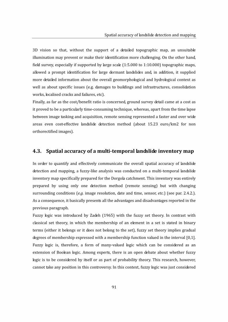
Spatialaccuracyoflandslidedetectionandmapping

91

3D vision so that, without the support of a detailed topographic map, an unsuitable

illuminationmaypreventormaketheiridentificationmorechallenging.Ontheotherhand,

fieldsurvey,especiallyifsupportedbylargescale(1:5.000to1:10.000)topographicmaps,

allowed a prompt identification for large dormant landslides and, in addition, it supplied

moredetailedinformationabouttheoverallgeomorphologicalandhydrologicalcontextas

well as about specific issues (e.g. damages tobuildings and infrastructures, consolidation

works,localisedcracksandfailures,etc).

Finally,asfarasthecost/benefitratioisconcerned,groundsurveydetailcameatacostas

itprovedtobeaparticularlytime‐consumingtechnique,whereas,apartfromthetimelapse

betweenimagetaskingandacquisition,remotesensingrepresentedafasterandoverwide

areas even cost‐effective landslide detection method (about 15.23 euro/km2 for non

orthorectifiedimages).

4.3. Spatialaccuracyofamulti‐temporallandslideinventorymap

In order toquantify andeffectively communicate theoverall spatial accuracyof landslide

detectionandmapping,a fuzzy‐likeanalysiswasconductedonamulti‐temporal landslide

inventorymapspecificallypreparedfortheDorgolacatchment.Thisinventorywasentirely

prepared by using only one detection method (remote sensing) but with changing

surroundingconditions(e.g. imageresolution,dateandtime,sensor,etc.)(seepar.2.4.2.).

Asaconsequence,itbasicallypresentsalltheadvantagesanddisadvantagesreportedinthe

previousparagraph.

Fuzzy logic was introduced by Zadeh (1965) with the fuzzy set theory. In contrast with

classical set theory, inwhich themembership of an element in a set is stated in binary

terms(eitheritbelongsor itdoesnotbelongtotheset), fuzzysettheory impliesgradual

degreesofmembershipexpressedwithamembershipfunctionvaluedintheinterval[0,1].

Fuzzy logic is, therefore, a form of many‐valued logic which can be considered as an

extension ofBoolean logic. Among experts, there is an opendebate aboutwhether fuzzy

logic is tobeconsideredby itselforaspartofprobability theory.Thisresearch,however,

cannottakeanypositioninthiscontroversy.Inthiscontext,fuzzylogicwasjustconsidered

CHAPTER4

92

moresuitabletoexpresstheuncertaintyoflandslidedetectionandmappingthanprobability

theorywhich,inturn,isusuallyassociatedtoslopesusceptibilitytosliding.

In the fuzzy raster landslide map specifically conceived for this work pixel values

correspond to thedegreeofmembershipofa singlepixel toa landslidepolygon(seepar.

2.4.2.).Inthissense,membershipmaybe1,0,oranygradualvalueinbetween.Hence,this

typeofrepresentationdoesnotshowaclearseparationbetweenwhatisinandwhatisout

of the landslide polygon as it does instead a sharp linear boundary. On the contrary, it

displays towhatextendacertainpixelbelongsordoesnotbelong toa landslidepixelset.

More specifically, spatial persistence was here meant as the repeatedmembership of a

pixel to a landslide polygon. In this way, if a landslidewas detected in every image pixel

valuesisequalto1,whereasifitcouldbeidentifiedandmappedonlyinafewimagespixel

membershipiscloseto0. It isworthnoting,however,that ifa landslidewasdetectedand

mapped even only once, there are no doubts that it existed at some point in time. As a

consequence,alowdegreeofmembershipdoesnotindicatethattherearefewchancesthat

thereisalandslide.Onthecontrary,itmeansthatthatparticularmassmovementmayhad

beenpoorlyidentifiedfromaspatialpointofviewsinceitsrecognitionandmappingwere

based only on one or just a few images. Indeed,where a landslidewas detected inmore

snapshots,itwasnevermappedinthesamewaysothatinthefuzzyrasterlandslidemapits

boundary isnotsharpandwelldefined,but instead it is“fuzzy”.Fundamentally,whilethe

pixelsofthecentralpartofthemappedlandslidepresenthighvaluesofmembership,those

in the external part are characterised by decreasingmembership values from the inside

toward the outside (Fig. 2.3). On this basis, it is clear that spatial persistence is strictly

related to time.However, in thiscontext, the twovariablescannotbebasicallyseparated.

Indeed, a “short ‐lasting” landslide has less chances to be captured in several images and,

therefore,theopportunitiestocheckitssizeandshapearefewer.

4.3.1.Analysisandresults

In this study, I used spatial persistence and boundary reliability as proxies for spatial

accuracy, i.e. the definition of landslide shape and size. To this end, I prepared a multi‐

temporallandslideinventorymapwhereeachlandslidewasoutlinedoneveryavailable

Spatialaccuracyoflandslidedetectionandmapping

93

Fig.4.10:Outputofthefuzzy‐likeanalysisperformedfortheDorgolacatchment.Resultsareexpressedinrelationtothetotalnumberofimagesetsusedfortheanalysis.

orthorectified image. Overall, I used 15 image sets spanning over an approximately 30

year7 time intervalwithanaverage temporal sampling rateof about2years. Inorder to

avoidspatialalterationsrelatedtonewslidingmovements,forthefuzzy‐likeanalysisIused

only unchanged landslides, i.e. only those that did not undergo any substantial and

detectablereactivation(seepar.2.4.2.).ThefinalresultsaredisplayedinFig.4.10andFig.

4.11.Theformershowsanabsolutevaluewithrespecttothe15snapshotsusedforthe

7 Forthefuzzy‐likeanalysiswereusedonlytheimagesetsfrom1981to2014.

CHAPTER4

94

Fig.4.11:Finaloutputofthefuzzy‐likeanalysisperformedfortheDorgolacatchment.Resultsareexpressedthroughafuzzyindexvaluedintheinterval[0,1].

analysis,whereas the latter represents the same results according to a normalised fuzzy

index.

Before proceedingwith the fuzzy‐like analysis, in order to avoid any spatial overlapping

among differentmassmovements, I subdivided landslides into 6 six different levels. This

classificationisbasedsimplyongeometricalandspatialbonds,sothata1° level landslide

maycontaina2°levellandslide,whichinturnmaycontaina3°levelandsoonaccordingto

a hierarchical structure (Fig. 2.11). This expedient was essential to avoid merging of

differentoverlappingmassmovements(e.g.smallerreactivationsoflargerlandslides)

Spatialaccuracyoflandslidedetectionandmapping

95

Fig. 4.12: Landslide area frequency distribution for the four levels used for the fuzzy‐likeanalysis.Thissubdivision,basedessentiallyongeometricalandspatialbonds,wasadoptedinorder to avoid merging of overlapping mass movements during the vector‐to‐rastertransformation.

duringthevector‐to‐rastertransformation.Duetothelownumberoflandslides,5°and6°

levels were not considered statistically significant and, therefore, were not used for the

fuzzy‐likeanalysis.TheareafrequencydistributionofthefirstfourlevelsisshowninFig.

4.12. In general, thishistogramsuggests that the1° and2° levels containmore landslides

andthat thesemassmovementsaremoreheterogeneousand larger than thoseof the3°

and4°levels(seealsoTab.4.5).

Overall, themulti‐temporal landslide inventory of the Dorgola catchment contains 1.1058

landslides. About 14.5% (160) of these slope failureswere identified as LL’s, i.e. asmass

movements that temporarilydisappeared fromtherecordtoreappearagainwithoutany

apparentreactivation(seepar.2.4.2.fordetails).Thistemporaryconcealmentwasbasically

causedbydifferentimpendingfactors,mainly:clouds,vegetation,shadowareas,andmore

generallyimagescaleandillumination.Asaconsequence,thislapseoftimewasconceived

asa“black‐outperiod”duetothedetectionmethodandnottothelandslidetrueevolution.

8 Thisnumberdoesnotincludereactivationswhich,asalreadyremarked,wereclassifiedwiththe

sameIDnumberoftheoriginallandslide.

CHAPTER4

96

Tab.4.5:Descriptivestatisticsforthelandslidelevelsusedforthefuzzy‐likeanalysis.Forthispurposewereusedonlythoselandslidesthatdidnotundergoanysubstantialanddetectablereactivations.

Level1 Level2 Level3 Level4

Numberoflandslides* 1.881 1.989 981 234

%oftotalnumberoflandslides 37,0 39,1 19,3 4,6

Totalareacoveredbylandslides 7.082.375 4.970.672 509.890 91.663

Areaofsmallestlandslide 54,19 65,70 54,66 73,03

Areaofbiggestlandslide 474.010 403.442 27.906 5268

Median 7.585 3.238 1.293 1.190

* Asremarked in the text, in themulti‐temporal inventoryeach landslidewasoutlinedonevery imageset.Thisvalueincludestheoverallnumberofdetectedmassmovements,whichmeansalsothesamelandslidemappedindifferentimages.

InthespecificcaseoftheDorgolaValley,the160LL’sweresodivided:

121 (75.6%) were temporary concealed due to image illumination, tone and bands

(colorvsB/Wimages);

25(15.6%)wereincludedinwoodyareas;

14(8.8%)werecoveredbyshadows.

Since theoretically theydonot implyanyreal reactivationsand, therefore,anynewmass

movements,inthefuzzy‐likeanalysisIconsideredLL’sasawhole,includingtheir“black‐out

periods”.Ontheotherhand,withregardtoreactivatedlandslides,Ichosetomaintainonly

thelongestperiodofpersistenceor,asasecondchance,themostrecentone.

The histogram in Fig. 4.13 shows the pixel (counts) frequency distribution in the four

output rasters representing the fuzzy index classes. In particular, the class bins were

obtainedbydividingtheinterval[0,1]by0.1,whereasthepixelnumberofeachlevelwas

plotted as a percentage of the counts of the total area covered by landslides. Despite the

Spatialaccuracyoflandslidedetectionandmapping

97

unequalmagnitude,thehistogramshowsthat1°and2°levelspresentpixelswithbothlow

andhighmembershipdegree,i.e.areaswithlowandhighspatialpersistence,whereasin3°

and4°levelslowfuzzyindexesaremorecommon.ThesetrendsarebetterdisplayedinFig.

4.14whereeverysinglelevelisplottedalone.

Thehistogramof the1° level isquite irregularprobablydue to theheterogeneityof this

group,whichisbasicallymadeupoftwodifferentcategoriesofmassmovements:

olddormantlandslides;

smalltomediumisolatedlandslides.

Olddormantlandslideshavebeenintensivelycolonisedbothbynaturalandanthropogenic

processes.Theyusuallyinvolvetheentireslope,andtheycouldbeidentifiedonlyatsmaller

scale. However, their imprinting on the local landscape is so intense that, if remotely

detectable,theycouldalwaysbeidentifiedregardlessofimagecapturingconditions.Inthis

case,alltheuncertaintiesabouttheirmappingwereconcentratedalongtheboundaries.As

a consequence, these large landslides, concentrated mainly in the Ligurian Units, are

responsibleforthehighfuzzyindexvalues(0.8÷1.0),buttosomeextenttheyarealso

Fig.4.13:Pixelfrequencyinfuzzyindexclassesforthefourlandslidelevels.

CHAPTER4

98

Fig.4.14:Pixelfrequencyinfuzzyindexclassesforeachofthefourlandslidelevels.

Spatialaccuracyoflandslidedetectionandmapping

99

relatedto lowervaluesas faras theirmarginalpartsareconcerned.Thesecondcategory

containsstand‐alonelandslides.MostofthemareincludedintheEpi‐LigurianSequence,and

theygenerallydifferfromthepreviousonesforage,depth,andspatialpersistence.Inthis

case, the low fuzzy index values (0÷0.3) can be related to a truly short “lifetime”, to

challengingoptimaldetectionconditions,ortoalowinactivity,whichindeedincreasesthe

detectioncomplexity.ItisnotachancethatthiscategoryincludesmanyLazaruslandslides.

The2° levelhistogram isquite irregularaswell,but its landslidesareabitdifferent from

thoseofthe1°level.Indeed,inthiscasemassmovementscanbeattributedtothefollowing

categories:

activeandsuspendedportionsofbiggerlandslides;

smalltomediumreactivationsofbiggerlandslides.

Duetotheirfreshandpersistentaspect,massmovementsfromthefirstcategorycouldbe

detectedbasicallyineveryimagesetand,therefore,areresponsibleforthehighfuzzyindex

values(0.8÷1.0).Inthiscase,likeforbiggerlandslides,onlyboundaryareasareaffectedby

asignificantuncertainty.Lowtomediumfuzzyindexvalues(0÷0.5)areduetotheseareas

and to small to medium reactivations of bigger landslides. Although generally unrelated

fromageneticpointofview,small landslidestakeplacewithinbiggeronesanddisappear

quite quickly due to man activities (especially farming) and further overlapping slope

failures. Medium size landslides, instead, are inactive parts of bigger landslides. Indeed,

inactivity and the consequent colonization byplants increase the detection complexity by

concealinglandslideoriginalshape.

Withrespecttothe1°and2°,the3°and4°levelscontainmorehomogeneousandsmaller

landslidesincludedinbiggerones.Probablyduetolandslidehomogeneity,bothhistograms

showa distinct trend that highlights a clear abundance of low fuzzy index values (0÷0.3)

(Fig. 4.14). This complies with the fact that small landslides can be easily concealed by

naturaland/oranthropogenicprocessesorcompletelymaskedbynewreactivations.

CHAPTER4

100

4.3.2.Discussion

In this work, a fuzzy raster landslide map was used to quantify and display the spatial

accuracy of a landslide inventory map. Although in a rigorous fuzzy analysis the

membership function is valued in the interval [0,1], in this context I referredalso to the

absolutevaluerelatedtothetotalnumberofimagesets.Indeed,thisisanimportantpieceof

information for the end‐users since the spatial accuracy of a landslide inventory map

stronglyreliesonthenumberandcharacteristicsoftheimagesusedtoprepareit.Inthis

sense,a landslide inventorymappreparedon thebasisof15differentsnapshotswithan

average temporal sampling rate of about 2 years basically presents a higher overall

accuracythanalandslideinventorymapthatcouldrelyonfewerimagesetsseparatedbya

longertimeinterval.

Apparently,relatinglandslidespatialpersistenceand,hence,spatialaccuracytothenumber

ofimagesetsusedtopreparetheinventorymaynotseemappropriate.Indeed,onesingle

snapshot,ifacquiredintherightmomentandintherightconditions,maybesufficientto

define landslide spatial attributes in themost accurateway.To thisend, addingmoredata

maygenerallyworsentheoveralllandslidemappingaccuracysincewithtimethelandslide

boundary tends to be concealed or altered by natural and/or anthropogenic processes.

Notwithstanding this, chances to catch a landslide just after it had happened are little

especiallywithahightemporalsamplingrate. In thisway, inmostcases, the first timea

landslideisdetectedandmappedit isdifficulttoprovethatitactuallydisplaysitsoriginal

sizeandshape.Furthermore,anewmassmovementmayconcealanolderone.Inthiscase,

ifdetectionconditionsarenotadvantageous,relictpartsofthepreviousslopefailurecanbe

confused with the more recent landslides altering its original size and shape. As a

consequence, for most landslides, spatial persistence proves to be a good proxy for the

definitionoftheirspatialaccuracy.Forthispurpose,moredataareavailablethebetteritis.

Inthissense,afuzzyrasterlandslidemap,liketheonepreparedforthiswork,isatoolthat

needstobecontinuouslyimplemented.

InthespecificcaseoftheDorgolacatchment,oldlargedormantlandslidescouldbedetected

constantly innearlyall imagesets regardlessof thequalityof the imageusedassupport

Spatialaccuracyoflandslidedetectionandmapping

101

andofthegeneralcapturingconditions.Indeed,theselandslideshadsucharelevantrolein

thedefinitionoflandscapeandlocalmorphologythatunlikelytheirdistinctivefeatures(e.g.

concave and convex slopemorphology, lobate run‐out areas, drainage pattern deviations,

irregularmorphology, etc.) could be concealed by natural or anthropogenic processes. In

this case, the fuzzy‐like analysis confirmed that these landslides present a high spatial

persistenceand,therefore,arecharacterisedbyhighfuzzyindexvalueswiththeexception

oftheouterparts.Indeed,externalboundariesareaffectedbyasignificantuncertaintyand

theiraccurateidentificationstrictlydependsonseveralfactors.Smallerlandslides(<10.000

m2), on the other hand, generally present a poor spatial persistence and are actually

defined by low fuzzy index values. This means that their mapping is affected by a high

uncertainty. The main issue about these landslides is that they usually have a short

“lifetime”, i.e. theypresenta lowtemporalpersistence(seeChapter5).Asaconsequence,

they have few chances to be captured in several image sets, and, hence, their mapping

accuracy relies entirely on the quality, capturing conditions, and landslide appearance of

thosefewsnapshots.

Ultimately, another landslide category that proved to be particularly challenging for

mappingareLL’s.Adisadvantageoussetofimages,forexample,maycausetheselandslides

to be completely undetected. For this reason, although certain capturing conditionsmay

appearbetterthanothers,theircontinuousapplicationmustbecarefullyevaluated.Indeed,

iftheyleadtosomesortofbias(e.g.repeatedshadowsorforestcoveroverthesameareas)

theymay constantly prevent the detection of somemassmovements. If this is the case,

optionsshouldbeanalysed.

On the basis of this work, landslide spatial accuracy depends on extrinsic and intrinsic

factors.Basicallyextrinsicfactorscanberelatedto:

orthorectificationaccuracy;

geographicpositioningaccuracy(seeChapter3);

scaleandresolutionofimagesets;

imagecapturingconditions(date,time,azimuth,weather,etc.).Withtheexceptionofimagecapturingconditions,whichcouldhaveahighermagnitude,the

effects of these aspects on spatial accuracy are of the order of metric length. As a

CHAPTER4

102

consequence, their influence isproportionallymoresignificant forsmaller landslidesthan

for largerones. Inthisparticularcase,geographicpositioningaccuracycouldbeassessed

separately,whereastheremainingvariableswereappraisedalltogether.Effortsshouldbe

made to quantify and improve every single aspect, e.g. by creating a protocol for

orthorectificationmethod,limitations,andsoftware.

Landslidespatialaccuracyiscontrolledalsobyseveralintrinsicvariableslikeforexample:

landslidenaturalstabilization,revegetation,andprogressiveconcealment;

inherentuncertaintyrelatedtolandslidegeomorphologicalsurvey9;

landslideactivenature, so that a landslide canbe strongly affectedor even completely

concealedbyotherslidingmovementsorbysignificantreactivations;

anthropogenicprocessesthatcanbothstabilise(consolidationworks)orconceal(e.g.

farmingactivities)theoriginalmassmovements10.

Ingeneral,thesefactorsaffectspatialaccuracyintheorderoftensofmeters.Moreover,also

in this case, the separation of every single contribute is quite challenging, because it is

specificallyrelatedtoeachindividuallandslide.

4.4. Conclusions

ThisChapterfocusedonthespatialaccuracyofalandslideinventorymap.Inparticular,this

subjectwasaddressed fromtwodifferentpointsofview: landslidedetectionandmapping

techniques,andtheoverallspatialaccuracy.

I carried out a comparison between a remotely sensed inventory, prepared on a VHR

orthorectifiedGeoEYE image, and a detailed geomorphological field‐based inventory. This

workultimatelyproved thatneitherof these twodetectionmethodsprovideda complete

inventory map, consequently, they should be considered complementary. Indeed, field

surveyisanessentialandefficientmethodtodevelopadetailedreferenceframework,while

the visual interpretation of orthorectified satellite images represents a precise, cost‐

effective,andquickmethodnotonly tocomplete,butalso tomonitorand implement the 9 Geomorphologicalsurveyisgenerallylimitedtothesuperficialanalysisoflandforms.10 Man‐inducedmodifications should probably be considered as extrinsic factors, but since they

modifydirectlythelandslideappearance,Idecidedtolistthemamongintrinsicvariables.

Spatialaccuracyoflandslidedetectionandmapping

103

initialframeworkandkeepitconstantlyupdated.

In order to quantify the overall spatial accuracy of landslide detection and mapping, I

performed a fuzzy‐like analysis on a multi‐temporal landslide inventory specifically

prepared for the Dorgola catchment. In this context, spatial persistence and boundary

reliabilitywereusedasproxiestoassesstheuncertaintyrelatedtoslopefailuremapping.

Thisanalysisdemonstratedthatoldlargedormantlandslidesgenerallypresentaverygood

spatialpersistence,whilesmallerlandslides(<10.000m2)aregenerallyaffectedbyahigh

mappinguncertaintyexpressedbylowfuzzyindexes. Inthissense,thisworkprovedthat

mappingaccuracystronglyreliesonthe“lifetime”ofalandslidefootprintaswellasonthe

image quality and capturing conditions. The former, in particular, emphasises the

importanceofthetimevariable.Imagequalityandcapturingconditions,instead,shouldbe

carefully evaluated as they may prevent the detection of certain slope failures like, for

example,whenthey leadtosomesortofbias(e.g. repeatedshadowsor forestcoverover

thesamearea).Ultimately,thefuzzy‐likeanalysisdemonstratedthatrepresentinglandslides

with sharp boundaries is a significant simplification of a more complex and uncertain

situation.According to the “truth‐in‐labelling”paradigm, the fuzzyraster landslidemap is

aneffectivetoolnotonlytoquantifybutalsotodisplayandconveyinformationaboutthe

inherentuncertaintyandspatialaccuracyoflandslidedetectionandmapping.Forwideand

heterogeneousareas,itwouldbeactuallyawkwardtoresumespatialaccuracyinaunique

number.Inthissense,amapisamuchmoreefficientmetadatatoconveypunctualaswell

asspatialinformation.

Inconclusion,thisresearchappraisedthatlandslideidentificationandmappingareaffected

by a significant uncertainty. This confirmed that the conceptualmodel that is ultimately

realisedina landslideinventoryisamerelyapproximationandageneralizationofreality.

This consideration, however, must not reduce the importance of landslide inventories as

decision‐supporttools.Indeed,aswidelyargued,itisnotthetoolbutrathertheusethatcan

bepotentiallyerroneous.Inthissense,inordertoavoidanypossiblemisuses,itisessential

to convey to the end‐users all the limitations of a landslide inventory map in the most

accuratewaypossible.

Landslidetemporalpersistence

CHAPTER5

Landslidetemporalpersistence

5.1. Introduction5.2. Multi‐temporallandslideinventorymapoftheDorgolacatchment

5.2.1.Analysisandresults5.2.1.1.Descriptivestatistics5.2.1.2.Correspondenceoflandslideareas

5.2.2.Discussion5.3. Characterizationofnewandundetectedlandslides

5.3.1.Analysisandresults5.3.1.1.Descriptivestatistics5.3.1.2.Newdetectionsize5.3.1.3.Newdetectionlocation

5.3.2.Discussion5.4. Temporalpersistenceoflandslidefootprints5.5. Conclusions

CHAPTER5

105

5.Landslidetemporalpersistence

5.1.Introduction

Inordertobeareliableandeffectivereferencetoolforlandinstability,alandslideinventory

maphastorecordeverysinglemassmovement.Intheliterature,completenessisactually

consideredasafundamentalelementforqualityassessment(Trigilaetal..,2010;Guzzettiet

al., 2012). Completeness, however, is a space‐time dependent variable as landslides are

complexeventsthattakeplaceinspaceandtime.

In general, for a landslide inventory map used within the land‐use planning context, a

landslide is forever. Inparticular,although itsdepositmaybestabilised,concealed,oreven

completelyremoved(e.g.landslidedepositsalongroadcuts)oreroded(e.g.landslidedeposits

alongriverbeds), the fact thata slope failurehadhappened inacertainplace inacertain

momentisanimportantpieceofinformationthatalandslideinventorymap,preparedfor

planning purposes, cannot ignore ormiss. Indeed, this event is indicative of a potential,

albeit not necessarily current, sliding susceptibility and is essential for a complete and

detailed framework of landslide activity. In this sense, it is fundamental to map a mass

movement when it is still well recognizable and, in order to determine a proper data

acquisitionfrequency,toassessforhowlongalandslidecanbeidentified.

Inthischapter,Idealwithlandslideactivityandwiththetemporalpersistenceoflandslide

footprints. Inparticular, Icarefullyanalyse themulti‐temporal inventoryprepared for the

Dorgolacatchmentinordertoevaluatepotentialtemporaltrendsandtocharacterisenew

detectedandundetectedlandslides,i.e.thoselandslidesthatdisappearfromtherecords.The

ultimatepurposeistoinvestigatethetemporalreliabilityofalandslideinventorymap.

Landslidetemporalpersistence

106

5.2. Multi‐temporal landslide inventory map of the Dorgolacatchment

ThetemporalevolutionoftheactivelandscapeoftheDorgolacatchmentwasportrayedbya

multi‐temporal landslide inventoryspecificallyprepared for thispurpose(seepar.2.4.2.).

ForthetemporalanalysisIusedallavailableimagesets(18spanningfrom1954to2014)

includingthosethatwerejustgeoreferencedbutnotorthrectified.

5.2.1.Analysisandresults

Most of the image sets used for this work are aerial photographs, while the remaings

consistofVHRsatellite images(GeoEYEandIKONOS)(Tab.5.1).Withregardtothetime

frame,most imageswereacquiredbetween JuneandSeptemberas theywere tasked for

agriculturalpurposes. In thispartof theApennineRange,however,48%ofslope failures

take place betweenMarch andMay, and 29%betweenOctober andDecember (Bertolini

andPellegrini,2001).Unfortunately,just5imagesetswerecapturedinthefirstperiodand

only1inthesecond.Ontheotherhand,asfarassamplingrate isconcerned,thefirst30

years are not particularly well represented as they rely only on 4 image sets with a

significant 19‐years time lag between the first (1954) and the second (1973) snapshot.

From1986onward, instead,theacquisitionfrequencybecamesmallerwithanaverageof

about2years(min:1year,max:6years).

5.2.1.1.Descriptivestatistics

Onthewhole,themulti‐temporallandslideinventorycontains1,1051landslides.Theaverage

number of mass movements without LL’s for each snapshot is about 3342. However, in

ordertogetamorerealisticdistribution,thehistogramofFig.5.1displaysthetotalnumber

ofmassmovements including hidden LL’s, whichwere added to those image setswhere,

althoughundetected, theywere likelypresent. Inparticular,data fromTab.5.2 show that

1996,1998,2000,2003,2007,and2008arethemostaffectedimagesets.Majorlandslide

peakswererecordedin1981,1996,2003,2011,and2013,whileconverselythe1954,

1 Seefootnote#8inChapter4.2 IfconsideringLL’stheaverageis356.

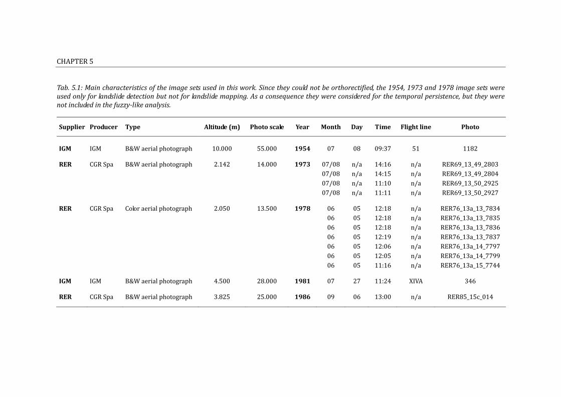
CHAPTER5

Tab.5.1:Maincharacteristicsoftheimagesetsusedinthiswork.Sincetheycouldnotbeorthorectified,the1954,1973and1978imagesetswereusedonlyforlandslidedetectionbutnotforlandslidemapping.Asaconsequencetheywereconsideredforthetemporalpersistence,buttheywerenotincludedinthefuzzy‐likeanalysis.

Supplier Producer Type Altitude(m) Photoscale Year Month Day Time Flightline Photo

IGM IGM B&Waerialphotograph 10.000 55.000 1954 07 08 09:37 51 1182

RER CGRSpa B&Waerialphotograph 2.142 14.000 1973 07/08 n/a 14:16 n/a RER69_13_49_2803 07/08 n/a 14:15 n/a RER69_13_49_2804 07/08 n/a 11:10 n/a RER69_13_50_2925 07/08 n/a 11:11 n/a RER69_13_50_2927

RER CGRSpa Coloraerialphotograph 2.050 13.500 1978 06 05 12:18 n/a RER76_13a_13_7834 06 05 12:18 n/a RER76_13a_13_7835 06 05 12:18 n/a RER76_13a_13_7836 06 05 12:19 n/a RER76_13a_13_7837 06 05 12:06 n/a RER76_13a_14_7797 06 05 12:05 n/a RER76_13a_14_7799 06 05 11:16 n/a RER76_13a_15_7744

IGM IGM B&Waerialphotograph 4.500 28.000 1981 07 27 11:24 XIVA 346

RER CGRSpa B&Waerialphotograph 3.825 25.000 1986 09 06 13:00 n/a RER85_15c_014

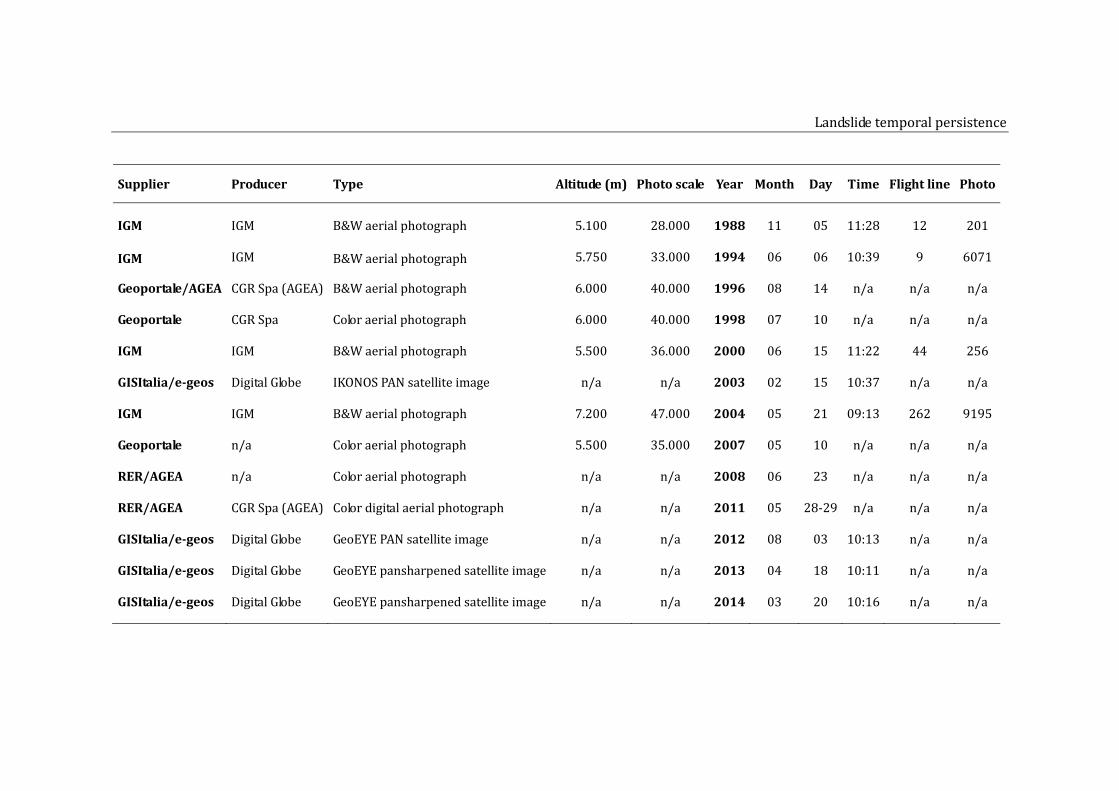
Landslidetemporalpersistence

Supplier Producer Type Altitude(m) Photoscale Year Month Day Time Flightline Photo

IGM IGM B&Waerialphotograph 5.100 28.000 1988 11 05 11:28 12 201

IGM IGM B&Waerialphotograph 5.750 33.000 1994 06 06 10:39 9 6071

Geoportale/AGEA CGRSpa(AGEA) B&Waerialphotograph 6.000 40.000 1996 08 14 n/a n/a n/a

Geoportale CGRSpa Coloraerialphotograph 6.000 40.000 1998 07 10 n/a n/a n/a

IGM IGM B&Waerialphotograph 5.500 36.000 2000 06 15 11:22 44 256

GISItalia/e‐geos DigitalGlobe IKONOSPANsatelliteimage n/a n/a 2003 02 15 10:37 n/a n/a

IGM IGM B&Waerialphotograph 7.200 47.000 2004 05 21 09:13 262 9195

Geoportale n/a Coloraerialphotograph 5.500 35.000 2007 05 10 n/a n/a n/a

RER/AGEA n/a Coloraerialphotograph n/a n/a 2008 06 23 n/a n/a n/a

RER/AGEA CGRSpa(AGEA) Colordigitalaerialphotograph n/a n/a 2011 05 28‐29 n/a n/a n/a

GISItalia/e‐geos DigitalGlobe GeoEYEPANsatelliteimage n/a n/a 2012 08 03 10:13 n/a n/a

GISItalia/e‐geos DigitalGlobe GeoEYEpansharpenedsatelliteimage n/a n/a 2013 04 18 10:11 n/a n/a

GISItalia/e‐geos DigitalGlobe GeoEYEpansharpenedsatelliteimage n/a n/a 2014 03 20 10:16 n/a n/a

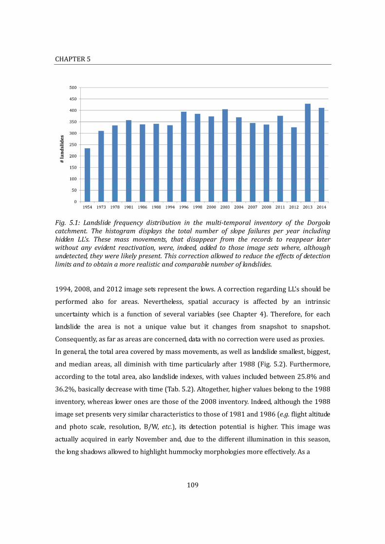
CHAPTER5

109

Fig. 5.1: Landslide frequency distribution in themulti‐temporal inventory of the Dorgolacatchment. The histogram displays the total number of slope failures per year includinghidden LL’s. These mass movements, that disappear from the records to reappear laterwithout any evident reactivation,were, indeed, added to those image setswhere, althoughundetected,theywerelikelypresent.Thiscorrectionallowedtoreducetheeffectsofdetectionlimitsandtoobtainamorerealisticandcomparablenumberoflandslides.

1994,2008,and2012imagesetsrepresentthelows.AcorrectionregardingLL’sshouldbe

performed also for areas. Nevertheless, spatial accuracy is affected by an intrinsic

uncertaintywhich is a function of several variables (see Chapter 4). Therefore, for each

landslide the area is not a unique value but it changes from snapshot to snapshot.

Consequently,asfarasareasareconcerned,datawithnocorrectionwereusedasproxies.

Ingeneral,thetotalareacoveredbymassmovements,aswellaslandslidesmallest,biggest,

andmedian areas, all diminishwith timeparticularly after1988 (Fig. 5.2). Furthermore,

accordingtothetotalarea,alsolandslideindexes,withvaluesincludedbetween25.8%and

36.2%,basicallydecreasewithtime(Tab.5.2).Altogether,highervaluesbelongtothe1988

inventory,whereasloweronesarethoseofthe2008inventory.Indeed,althoughthe1988

imagesetpresentsverysimilarcharacteristicstothoseof1981and1986(e.g.flightaltitude

and photo scale, resolution, B/W, etc.), its detection potential is higher. This image was

actuallyacquired inearlyNovemberand,due to thedifferent illumination in this season,

thelongshadowsallowedtohighlighthummockymorphologiesmoreeffectively.Asa

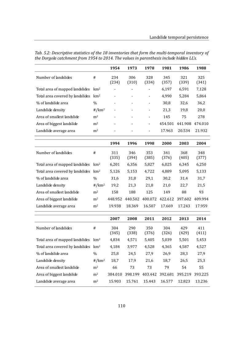
Landslidetemporalpersistence

110

Tab.5.2:Descriptivestatisticsofthe18inventoriesthatformthemulti‐temporalinventoryoftheDorgolacatchmentfrom1954to2014.ThevaluesinparenthesisincludehiddenLL’s.

1954 1973 1978 1981 1986 1988

Numberoflandslides # 234 306 328 345 321 325 (234) (310) (334) (357) (339) (341)

Totalareaofmappedlandslides km2 ‐ ‐ ‐ 6,197 6,591 7,128

Totalareacoveredbylandslides km2 ‐ ‐ ‐ 4,990 5,284 5,864

%oflandslidearea % ‐ ‐ ‐ 30,8 32,6 36,2

Landslidedensity #/km2 ‐ ‐ ‐ 21,3 19,8 20,0

Areaofsmallestlandslide m2 ‐ ‐ ‐ 145 75 278

Areaofbiggestlandslide m2 ‐ ‐ ‐ 454.501 441.908 474.010

Landslideaveragearea m2 ‐ ‐ ‐ 17.963 20.534 21.932

1994 1996 1998 2000 2003 2004

Numberoflandslides # 311 346 353 341 368 348 (335) (394) (385) (376) (405) (377)

Totalareaofmappedlandslides km2 6,201 6,356 5,827 6,025 6,345 6,250

Totalareacoveredbylandslides km2 5,126 5,153 4,722 4,889 5,095 5,133

%oflandslidearea % 31,6 31,8 29,1 30,2 31,4 31,7

Landslidedensity #/km2 19,2 21,3 21,8 21,0 22,7 21,5

Areaofsmallestlandslide m2 158 188 125 149 88 93

Areaofbiggestlandslide m2 448.952 440.502 400.072 422.612 397.602 409.994

Landslideaveragearea m2 19.938 18.369 16.507 17.669 17.243 17.959

2007 2008 2011 2012 2013 2014

Numberoflandslides # 304 290 350 304 429 411 (345) (338) (376) (326) (429) (411)

Totalareaofmappedlandslides km2 4,834 4,571 5,405 5,039 5,501 5,453

Totalareacoveredbylandslides km2 4,184 3,977 4,528 4,365 4,587 4,527

%oflandslidearea % 25,8 24,5 27,9 26,9 28,3 27,9

Landslidedensity #/km2 18,7 17,9 21,6 18,7 26,5 25,3

Areaofsmallestlandslide m2 66 73 73 79 54 55

Areaofbiggestlandslide m2 384.010 398.199 403.442 392.681 395.219 393.225

Landslideaveragearea m2 15.903 15.761 15.443 16.577 12.823 13.236

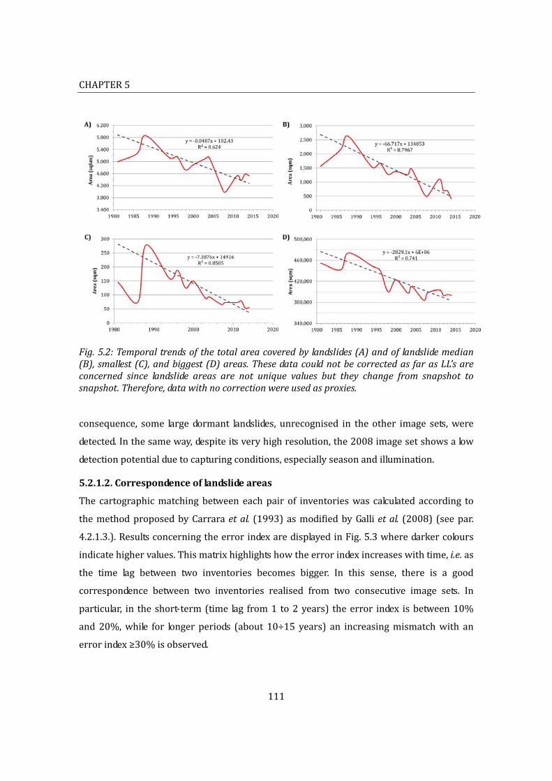
CHAPTER5

111

Fig.5.2:Temporaltrendsofthetotalareacoveredby landslides(A)andof landslidemedian(B),smallest(C),andbiggest(D)areas.Thesedatacouldnotbecorrectedas farasLL’sareconcerned since landslide areas are not unique values but they change from snapshot tosnapshot.Therefore,datawithnocorrectionwereusedasproxies.

consequence, some large dormant landslides, unrecognised in the other image sets,were

detected.Inthesameway,despiteitsveryhighresolution,the2008imagesetshowsalow

detectionpotentialduetocapturingconditions,especiallyseasonandillumination.

5.2.1.2.Correspondenceoflandslideareas

The cartographicmatching between eachpair of inventorieswas calculated according to

themethodproposedbyCarraraetal. (1993)asmodifiedbyGallietal. (2008) (seepar.

4.2.1.3.).ResultsconcerningtheerrorindexaredisplayedinFig.5.3wheredarkercolours

indicatehighervalues.Thismatrixhighlightshowtheerrorindexincreaseswithtime,i.e.as

the time lag between two inventories becomes bigger. In this sense, there is a good

correspondence between two inventories realised from two consecutive image sets. In

particular, in theshort‐term(time lag from1 to2years) theerror index isbetween10%

and 20%,while for longer periods (about 10÷15 years) an increasingmismatchwith an

errorindex≥30%isobserved.

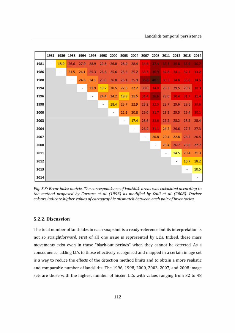
Landslidetemporalpersistence

112

Fig.5.3:Errorindexmatrix.Thecorrespondenceoflandslideareaswascalculatedaccordingtothemethod proposed by Carrara et al. (1993) asmodified by Galli et al. (2008). Darkercoloursindicatehighervaluesofcartographicmismatchbetweeneachpairofinventories.

5.2.2.Discussion

Thetotalnumberoflandslidesineachsnapshotisaready‐referencebutitsinterpretationis

not so straightforward. First of all, one issue is represented by LL’s. Indeed, these mass

movements exist even in those “black‐out periods” when they cannot be detected. As a

consequence,addingLL’stothoseeffectivelyrecognisedandmappedinacertainimageset

isawaytoreducetheeffectsofthedetectionmethodlimitsandtoobtainamorerealistic

andcomparablenumberoflandslides.The1996,1998,2000,2003,2007,and2008image

setsare thosewith thehighestnumberofhiddenLL’swithvalues ranging from32 to48

CHAPTER5

113

items (Tab. 5.2).On the basis of these image sets, possible causes for LL’s include image

illumination,vegetation,andshadowedareas(seepar.4.3.1.).Indeed,withtheexceptionof

the2003image,alltheotherwereacquiredfromMaytoAugust,i.e.whenthevegetation

canopyispresentandfarmingisparticularlyactive.Thecapturingtime,ontheotherhand,

is not always available but it is strictly related to illumination which affects landslide

detection.Inthissense,highilluminationanglesincreaseshadowswhich,ononehand,may

obscuresomelandslidesbutontheotherhandmayemphasisehummockymorphologies.

DespiteLL’s correction, the totalnumberof landslidesmust stillbe interpretedwithcare

since it is the result of two further time‐dependent and partially contrasting forces: the

intrinsic activity and evolution of landslides, and anthropogenic processes. The variable

trendofslope failuredistributionshown inFig.5.1 is theresultof these two factors.The

intrinsic activity and evolution of mass movements act toward an increase (new

activations/reactivations)andadecrease(naturalconcealmentoperatedbyvegetation)of

the total number of landslides. Conversely, anthropogenic processes basically lead to a

decreaseofthisnumber3astheycontributetotheconcealmentoflandslidesbothwith(e.g.

consolidation works) or without (e.g. ploughing) any real improvement in the slope

stability. Peaks in Fig. 5.1 correspond to landslide climaxes4, whereas lows are probably

correlatedtoperiodsofminoractivitywhentheanthropogeniccomponenttakesoverslope

failuresreducingtheiroverallnumber.Theoverallvaluealone,however,doesnotgiveany

precise information about the respective contribution of the two variables. To this end,

moredetailedanalysisonthenumberofnewdetections(newactivationsandreactivations)

andundetectedlandslidesareessential.

Theprogressivedecreasewithtimeofthetotalareacoveredbylandslides,aswellasthatof

landslide smallest, biggest, and median areas, became particularly evident after 1988.

Indeed, from1988onwarda lineardecrease canbeobserved forall the four terms.This

meansthatmappedlandslidesbecamegenerallysmaller.Giventhatminorfluctuationsmay

3 As potential causes of mass movements, anthropogenic processes are included in landslide

activityandevolution.4 For the Emilia‐Romagna region, the correlation between landslides and rainfalls is not

straightforward.Indeed,asremarkedbyBasenghiandBertolini(2001),therelationshipbetweencausesandeffectsisanythingbutsimpleand,forthisreason,itsanalysiswasnotincludedinthiswork.

Landslidetemporalpersistence

114

Fig. 5.4: Comparison between the 1954 and the 2012 image sets (scale 1:20,000). Theincrease of forestedand scrubbyareas is evident and it proves the general revegetationalprocessesthattookplaceintheDorgolaValleyinthistimelag.

beascribedtolandslideandanthropogenicactivities,thegeneraltrendcanbeexplainedby

twomainfactors:

improvement of image set resolution. In fact, a better resolution, besides allowing to

recognisesmallerlandslides,improvesmappingdefinition;

naturalandanthropogenicrevegetation.Asshown inFig.5.4, since1954 theDorgola

Valleyhasbeensignificantlyreforestedandnaturallyrevegetated.Thisprocesswas,at

leastpartially,directlyinducedbymanthroughtreeplanting,butitwasalsoduetothe

relinquishment of some areas thatwere progressively recolonised by the vegetation.

Although it potentially improved local slope stability, the presence of wider forested

areasandscrublandsworsenedlandslidedetectionconditionsbypreventingorreducing

therecognitionofsomelandslides.

In thisdataset, however, image resolutiondoesnot improve linearly.On the contrary, the

transition is rather sharp with the introduction in 2008 of VHR (0.5 m) digital aerial

photographs and satellite images. This may suggest that revegetation had a more

significantrolethanimageresolution.

Thecorrespondenceoflandslideareasrevealsthattheerrorindexincreaseswiththetime

lagbetween two image sets.Although this valuemaybeaffectedbydetection issues (e.g.

CHAPTER5

115

2008 image set), it suggests that data temporal quality undergoes a progressive

deteriorationbothintheshort‐(10%≤errorindex≤20%)andlong‐term(errorindex≥30%).

Asaconsequence,periodicupdatesareessentialinordertoguaranteeareliablereference

frame.Indeed,landslideactivityandevolutiondependonseveraltime‐dependentvariables:

triggeringfactors(intensiverainfall,snow‐melt,earthquakes,etc.);

hydrologicandhydrogeologicsetting;

anthropogenicprocesses;

vegetationandvegetationevolution;

localcharacteristicsthatchangeaftereachslopefailure(e.g.soilthickness).

Theanalysisofthemulti‐temporallandslideinventoryoftheDorgolacatchmentconfirmed

that time is an important dimension of landslide data and, therefore, is a fundamental

componentofitsqualityassessment.However,inordertounderstandhowmuchalandslide

inventory map is affected by time and what are the characteristics of the involved

landslides,itisessentialtodistinguishnewdetectionsaswellasthoselandslidesthateach

yeardisappearfromtherecords(e.g.shallowlandslides).

5.3.Characterizationofnewandundetectedlandslides

Inthepreviousparagraphthemulti‐temporallandslideinventoryoftheDorgolacatchment

wasconsideredasawhole.Herebelow,Ianalysenewdetectionsandundetectedlandslides

separatelyinordertoassesstheirmaincharacteristicslikelocationandsize.Inparticular,I

subdividednewdetectionsintothreegroups:newactivations,reactivations,andLL’s.New

activationsarethoselandslidesthataredetectedforthefirsttimewithinthetimeframeof

themulti‐temporallandslideinventory,whereasreactivationsrepresentafurtheractivityof

alreadydetectedlandslides.Ingeneral,thisdistinctionisquitequestionablesincethereisno

waytoascertainwhether inthepastacertainareawas involved inamassmovementor

not.Undetectedlandslides,ontheotherhand,arethoseslopefailuresthatdisappearfrom

the records because they were concealed either by natural (e.g. consolidation of the

vegetation)oranthropogenic(e.g.farming)processes.

Landslidetemporalpersistence

116

Fig. 5.5: Frequency distribution of new detected and undetected landslides in the multi‐temporalinventoryoftheDorgolacatchment.

CHAPTER5

117

5.3.1.Analysisandresults

5.3.1.1.Descriptivestatistics

NewdetectionsandundetectedlandslidesforeachimagesetarelistedinTab.5.3,whereas

Fig. 5.5 shows their frequency distribution. In general, these data confirm that the total

numberoflandslidesinaninventoryhastobetreatedwithcareasitistheresultofthree

main factors: detection issues, slope failure activity and evolution, and anthropogenic

processes.

Since1954,thetotalnumberofnewdetections(newactivations,reactivations,andLL’s)is

1,583 with yearly values ranging from 42 (2008) to 199 (2013). In order to get a

representative average, I divided thenumberof newdetectionsof each image set by the

number of years of the time lag with the previous snapshot. In this way, for the entire

periodfrom1978to20145,Icalculatedanaverageofabout48,6newmassmovementsper

yearwithvaluesrangingfromaminimumof9.8#/y(1986)toamaximumof199.0#/y

(2013)(Tab.5.4).Ontheotherhand,fortheshort‐termtheaverageis75.6#/ywithvalues

ranging from 16.0 #/y (2012) to 199.0 #/y (2013) (Tab. 5.4). Due to the reduced data

sample, thisaverage isparticularlyhighbecause isstronglyaffectedbythe2013extreme

event.Ingeneral,theanalysisofthefrequencyhistogramofFig.5.5showsthatthereare

severalhighsand lows.Theyearswith thehighestnumbersofnewdetectionsare1973,

1996,2003,2011,and2013forwhichmorethana100newlandslidesweredetected.The

1973 peak, however, is probably a fake as, most likely, it is the result of a resolution

contrastwiththepreviousimageset(1954).Conversely,the1996,2003,2011,and2013

peaks likely indicate sliding climaxes. For 1996, for example, data from the literature

confirm that in 1995 landslide events had been particularly intense in the Reggio Emilia

Province (Basenghi and Bertolini, 2001). The high number of reappearing LL’s in 1998,

2003, 2004, 2011, and 2013 (all exceeding 20 events) is due, instead, to the favourable

detectionconditionsoftheseimagesets6(season,colour,time,illumination,etc.).

5 The1954wasnotconsideredbothforitslowqualityandforthelongtimelagwiththesuccessive

snapshot.6 As previously stated, 1998 and 2003 image sets are characterised by some detection limiting

factorswhichaccount for thehighnumberofhiddenLL’s.The former, inparticular,presentsa

Landslidetemporalpersistence

118

Tab. 5.3: List of new detections and undetected landslides. All values are calculated withrespect to the previous image set. New detections are subdivided into new activations,reactivations,andLL’s.Newactivationsare those slope failures that supposedlyappear forthe first time,whereas reactivations represent a further activity of already detectedmassmovements.Undetectedlandslides,ontheotherhand,arethoseslopefailuresthatapparentlydisappearfromtherecordsduetovegetationconsolidationortomanactivities.

1954 1973 1978 1981 1986 1988

Newdetections: # ‐ 116 82 89 49 83newactivations ‐ 116 58 69 29 35

reactivations ‐ 0 21 18 15 36

Lazarus ‐ 0 3 2 5 12

Undectedlandslides # ‐ 48 39 55 63 49

1994 1996 1998 2000 2003 2004

Newdetections: # 78 156 109 60 138 90newactivations 53 85 50 29 56 37

reactivations 14 60 23 18 55 26

Lazarus 11 11 36 13 27 27

Undectedlandslides # 80 80 91 59 82 94

2007 2008 2011 2012 2013 2014

Newdetections: # 78 42 167 16 199 31newactivations 46 28 66 8 89 17

reactivations 21 9 70 1 89 14

Lazarus 11 5 31 7 21 0

Undectedlandslides # 110 50 64 61 20 34

With regard to undetected landslides, their overall number is 1,079 with yearly values

rangingfrom20#/y(2013)to110#/y(2007)(Tab.5.3).Thelong‐termaverage7turned

outtobe33.4#/ywithvaluesrangingfrom11.0#/y(1981)to94.0#/y(2004),whereas

fortheshort‐termis51.8#/ywithvaluesrangingfrom20.0#/y(2013)to94.0#/y(2004)

disadvantageous scale and season of acquisition, whereas the latter has an unfavourableillumination. Both image sets, however, aremore effective for the recognition of certainmassmovementsduerespectivelytocolourandtotheseasonofacquisition.

7 Long‐termandshort‐termaverageswerecalculatedasfornewdetections.

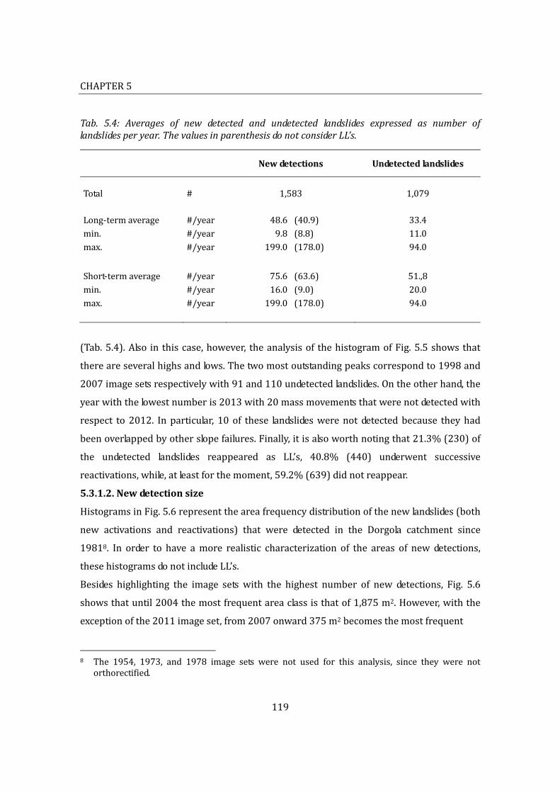
CHAPTER5

119

Tab. 5.4: Averages of new detected and undetected landslides expressed as number oflandslidesperyear.ThevaluesinparenthesisdonotconsiderLL’s.

Newdetections Undetectedlandslides

Total # 1,583 1,079

Long‐termaverage #/year 48.6 (40.9) 33.4min. #/year 9.8 (8.8) 11.0max. #/year 199.0 (178.0) 94.0

Short‐termaverage #/year 75.6 (63.6) 51.,8min. #/year 16.0 (9.0) 20.0max. #/year 199.0 (178.0) 94.0

(Tab.5.4).Also inthiscase,however, theanalysisof thehistogramofFig.5.5showsthat

thereareseveralhighsandlows.Thetwomostoutstandingpeakscorrespondto1998and

2007imagesetsrespectivelywith91and110undetectedlandslides.Ontheotherhand,the

yearwiththelowestnumberis2013with20massmovementsthatwerenotdetectedwith

respect to 2012. Inparticular, 10of these landslideswerenot detectedbecause theyhad

beenoverlappedbyotherslopefailures.Finally,itisalsoworthnotingthat21.3%(230)of

the undetected landslides reappeared as LL’s, 40.8% (440) underwent successive

reactivations,while,atleastforthemoment,59.2%(639)didnotreappear.

5.3.1.2.Newdetectionsize

HistogramsinFig.5.6representtheareafrequencydistributionofthenewlandslides(both

new activations and reactivations) that were detected in the Dorgola catchment since

19818. In order to have amore realistic characterization of the areas of new detections,

thesehistogramsdonotincludeLL’s.

Besides highlighting the image sets with the highest number of new detections, Fig. 5.6

showsthatuntil2004themostfrequentareaclassisthatof1,875m2.However,withthe

exceptionofthe2011imageset,from2007onward375m2becomesthemostfrequent

8 The 1954, 1973, and 1978 image sets were not used for this analysis, since they were not

orthorectified.

Landslidetemporalpersistence

120

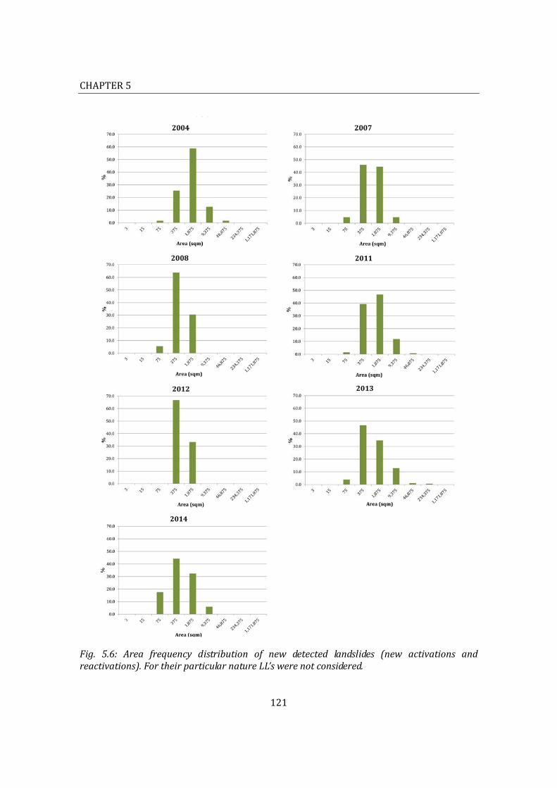
CHAPTER5

121

Fig. 5.6: Area frequency distribution of new detected landslides (new activations andreactivations).FortheirparticularnatureLL’swerenotconsidered.

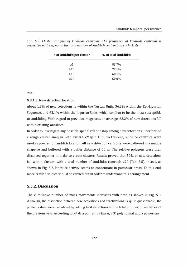
Landslidetemporalpersistence

122

Tab. 5.5: Cluster analysis of landslide centroids. The frequency of landslide centroids iscalculatedwithrespecttothetotalnumberoflandslidecentroidsineachcluster.

#oflandslidespercluster %oftotallandslides

≥5 83,7%

≥10 72,1%

≥15 60,1%

≥20 50,0%

one.

5.3.1.3.Newdetectionlocation

About1.8%ofnewdetections iswithin theTuscanUnits,36.2%within theEpi‐Ligurian

Sequence,and62.1%withintheLigurianUnits,whichconfirmtobethemostsusceptible

tolandsliding.Withregardtopreviousimagesets,onaverage,63.2%ofnewdetectionsfall

withinexistinglandslides.

Inordertoinvestigateanypossiblespatialrelationshipamongnewdetections,Iperformed

a rough cluster analysis with Esri®ArcMapTM 10.1. To this end, landslide centroids were

usedasproxiesforlandslidelocation.Allnewdetectioncentroidsweregatheredinaunique

shapefile and buffered with a buffer distance of 50 m. The relative polygons were then

dissolved together inorder tocreateclusters.Resultsproved that50%ofnewdetections

fall within clusterswith a total number of landslides centroids ≥20 (Tab. 5.5). Indeed, as

shown in Fig. 5.7, landslide activity seems to concentrate in particular areas. To this end,

moredetailedstudiesshouldbecarriedoutinordertounderstandthisarrangement.

5.3.2.Discussion

The cumulative number of mass movements increases with time as shown in Fig. 5.8.

Although, the distinction between new activations and reactivations is quite questionable, the

plotted values were calculated by adding firstdetectionstothetotalnumberoflandslidesof

thepreviousyear.AccordingtoR2,datapointsfitalinear,a3°polynomial,andapower‐law

CHAPTER5

123

Fig.5.7:Newlandslidecentroiddistribution.Colouredareasarethoseclustersthatcontainanumberof landslidecentroid ≥10.Clusterswereobtainedbybufferingeachcentroidwithabufferdistanceof50m.Greendotsrepresentlong‐term,whilereddotsrefertoshort‐termnewdetections.Inthiswork,“short‐term”isreferredtoimagesets(2004,2008,2012,2013,and2014)acquiredintwoconsecutiveyears,althoughthetime lagbetweenthemmaybemorethan12months.

curve.Thelatter,however,representsanunlikelymodelasitwouldprobablyoverestimate

the increasing number of landslides. Conversely, data dispersion around the linear

regressionsuggestsamorecomplextrend.Indeed,from1996to2012landslidetotalnumber

increasesatahigherratethanfrom1973to1994,andapparentlyitincreasesevenfurther

from2013.Thistrend,togetherwiththegoodfitforthe3°polynomialcurve,indicatesthat

most likely the increase is linear but with different gradients. This kind of evolution is

consistentwiththefactthatlandslideactivity,triggeredbyoccasionalevents,develops

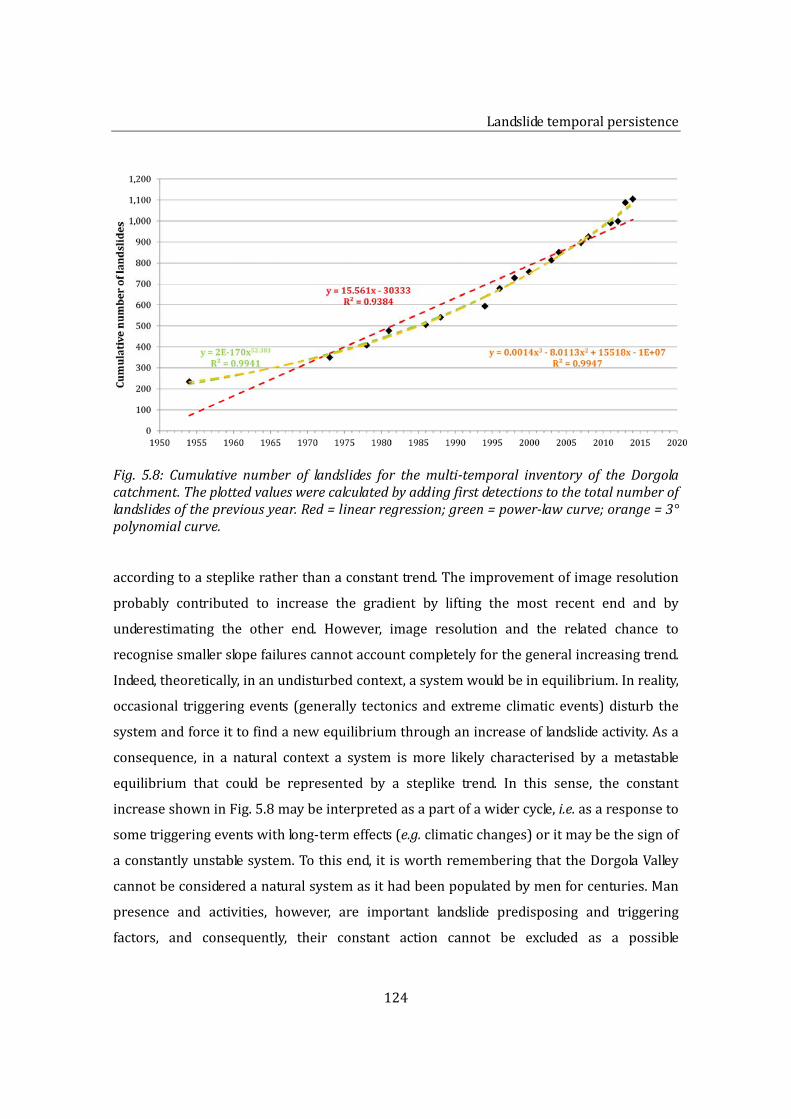
Landslidetemporalpersistence

124

Fig. 5.8: Cumulative number of landslides for themulti‐temporal inventory of theDorgolacatchment.Theplottedvalueswerecalculatedbyaddingfirstdetectionstothetotalnumberoflandslidesofthepreviousyear.Red=linearregression;green=power‐lawcurve;orange=3°polynomialcurve.

accordingtoasteplikeratherthanaconstanttrend.Theimprovementofimageresolution

probably contributed to increase the gradient by lifting the most recent end and by

underestimating the other end. However, image resolution and the related chance to

recognisesmallerslopefailurescannotaccountcompletelyforthegeneralincreasingtrend.

Indeed,theoretically,inanundisturbedcontext,asystemwouldbeinequilibrium.Inreality,

occasional triggeringevents (generally tectonicsandextremeclimaticevents)disturb the

systemandforceittofindanewequilibriumthroughanincreaseoflandslideactivity.Asa

consequence, in a natural context a system ismore likely characterised by ametastable

equilibrium that could be represented by a steplike trend. In this sense, the constant

increaseshowninFig.5.8maybeinterpretedasapartofawidercycle,i.e.asaresponseto

sometriggeringeventswithlong‐termeffects(e.g.climaticchanges)oritmaybethesignof

aconstantlyunstablesystem.Tothisend,itisworthrememberingthattheDorgolaValley

cannotbeconsideredanaturalsystemasithadbeenpopulatedbymenforcenturies.Man

presence and activities, however, are important landslide predisposing and triggering

factors, and consequently, their constant action cannot be excluded as a possible

CHAPTER5

125

explanationforthelandslidetrendofFig.5.8.Indeed,furtherresearchesshouldbedonein

orderto investigate if inthefuturethis increasingtrend,undercontinuousanthropogenic

solicitations, will remain constant or if, being part of some sort of natural cycle, it will

eventually lead to equilibrium. Furthermore, it would also be interesting to compare

differentareastoevaluateiftheincreasinggradientmaybeconsideredasaquantification

forthisdisequilibrium.

On the basis of Fig. 5.8, the total number of landslides in a multi‐temporal inventory is

expected to progressively increase with time. This, however, in the case of the Dorgola

catchment does not happen as landslide distribution presents a quite variable trend (Fig.

5.2). In fact, although the Dorgola Valley is not intensively populated, man activities are

particularly intense, and they effectively influence landslide footprints. In this sense, as

alreadyremarked,landslidedistributionistheresultoftwoantagonisticforces.Inparticular,

accordingtoFig.5.5,maneffortstoovercomelandslidesapparentlybecomemorerelevant

and intense after slope instability climaxes like, for example, in 1986, 1998, 2004, 2007,

2008,2012,and2014.Asaconsequence,landscapeisalwayschanginginonesenseorthe

other.

Dataaboutnewandundetectedlandslidesrevealedthat,generally,newdetectionsaremore

abundant than those landslides that each year apparently disappeared from the records.

Indeed,accordingtotheintensityoftriggeringfactors,thenumberofnewdetectionsmay

be in the order of tens or hundreds ofmassmovements per year,whereas, on the other

hand,slopefailuresseemtodisappearatalowerrate,intheorderoftensoflandslidesper

year(Tab.5.3).

Withregardtothelocationofnewdetections,thisstudyprovedthatintheDorgolaValley

theyarenotscatteredrandomlybutrathertheytendtobeclusteredinspecificareasand

within existing landslides. In the same way, new detections also present characteristic

dimensions. Indeed,newlandslidesshowquitesmallareas(from125to3,125m2)which

becomeevensmallerwithtimeprobablyduetotheimprovementofimageresolution.

Landslidetemporalpersistence

126

5.4.Temporalpersistenceoflandslidefootprints

The definition of the persistence of a landslide scar is an essential information for the

assessment of the temporal reliability of a landslide inventory map and a fundamental

elementforthedeterminationofaproperdataacquisitionfrequency.

Toquantifythepersistenceontheterritoryoflandslidefootprints,Ianalysedtheimagesets

from 1973 to 2014. I excluded the 1954 image set in order to reduce the time range

between two successive snapshots since in this interval landslide presence had to be

interpolated.Inthissense,ifaslopefailureappearedintheoldestimagesetIconsideredit

present,atleast,untilthesuccessivesnapshot.Landslidepersistencewascalculatedasthe

ratiobetweenthenumberofyearsinwhichalandslidehadbeenrecognisedorinterpolated

dividedbytheoveralltimeframe(42years),assimplifiedinFig.5.9.Inordertoavoidfloat

results, thesevalueswere then reclassifiedaccording to integernumbers, i.e.persistence

classes that are equal to the total number of years in which a certainmassmovements

supposedlyexisted.ThehistograminFig.5.10displaysthelandslidefrequencydistribution

withrespecttothesepersistenceclasses.Inparticular,thishistogramshowsthat,although

Fig.5.9–Asimplifieddescriptionof theprocedureused to interpolate landslidesanddefinelandslide persistence and persistence classes.Thismethod could be used since the time lagbetween twosuccessive imagesets isquiteshortandgenerallyconstant. It isworthnotingthatthepersistenceclass isbasicallyequaltothenumberofyears inwhicha landslidewasdetectedorinterpolated.

CHAPTER5

127

Fig.5.10:Landslidefrequencydistributionwithrespecttopersistenceclasses(seeFig.5.9forasimpleexplanationofpersistenceclasses).

about18%ofmassmovementsscarsresistontheterritoryfortimeperiods≥30years,the

frequencyoflandslidefootprintsgenerallydecreaseswithincreasingpersistenceclasses.In

particular,about23%oflandslidescars(247)showsatemporalpersistence≤2years,while

61%ofthem(647)seemtopersistforperiods≤10years.

Itisworthnoting,however,thattheseresultsareaffectedbytheintrinsiccharacteristicsof

the study area like, for example, the geo‐morphological setting, the sampling rate of the

dataset, and the frequency and intensity of the triggering factors and of man activities

during theconsidered time frame.Furthermore, inFig.5.10 “old” landslides, i.e. landslides

that had time to evolve and eventually disappear, were plotted together with “young”

landslides, i.e. recentlyappeared landslides.This isclearlyanapproximationwhichalmost

certainlyleadtoanoverestimationofthelowestpersistenceclasses.Notwithstandingthis,

theseresultsprovedthatintheDorgolacatchmentlandslidefootprintsdisappearwithtime

and,atleastapparently,theydisappearquiteswiftly.Indeed,apartfromareducedgroupof

massmovements whose scars have a relative high temporal persistence9, most of them

(61%)cannotbedetectedafter10yearsfromtheirappearance.Asaconsequence,inorder

torecordallofthemproperlyandproduceacompletereferenceframeoflandslideactivity,

9 As already remarked in Chapter 4, these landslides fundamentally include old large dormant

landslides.

Landslidetemporalpersistence

128

it is essential to adopt a high data acquisition frequency. Although these resultsmay be

overestimated, a reasonable sampling rate is once a year or maximum every 2 years.

Finally,itisworthrememberingthattheseoutcomesrequiretobetestedalsoindifferent

geo‐morphologicalcontextsand,ifpossible,forlongertimeperiods.

5.5.Conclusions

The time variable is an essential aspect of landslide inventory maps and a fundamental

component of their quality assessment. The realization of a multi‐temporal inventory

allowedtopartiallyreconstructtheevolutionoftheDorgolacatchmentinthelast60years.

An overall analysis of this multi‐temporal inventory revealed that data temporal quality

underwentaprogressivedeteriorationbothintheshort‐andlong‐term.Inparticular, this

work highlighted thatwith timemapped landslides became generally smaller. A possible

explanationforthismaybetheevolutionofthelandscape, i.e.theprogressivenaturaland

anthropogenic revegetationof theDorgola catchment. Indeed, the spreadof forestedand

scrubby areas worsened landslide detection conditions by preventing or reducing the

recognition of some landslides that, anyhow, are still present. According to land‐use

planning goals, for which unstable areas are probably more significant than the overall

number of landslides, this is a valuable piece of information. To this regard, however, a

careful correlation analysis between land‐uses (forested and scrubby areas in particular)

andtheevolutionoflandslideareasshouldbeaddressedbyfurtherresearches.

Thisworkprovedthatthecumulativenumberoflandslidesincreasedwithtimeaccording

to multiple linear gradients. To this end, further researches and monitoring programs

should investigate future developments to assess whether this trend could be the

consequence of some sort of existing triggering factors with long‐term effects or the

response to the constant anthropogenic action.Moreover, given that the total numberof

landslides ineach inventorydidnot raise, this studyremarked that landslide frequency is

the result of two antagonistic forces: landslide activity sensu stricto and anthropogenic

processes. Inthissense, thetotalnumberofmassmovements inan inventory isaready‐

reference,butithastobeinterpretedwithcareastheterritoryisanever‐changingreality

CHAPTER5

129

thatreactstodifferentandopposingsolicitations.

This work also revealed that new landslides are basically quite small and tend to be

concentratedinspecificareasandwithinexistinglandslides.Thisconfirmsthat,atleastfor

sometypesofmassmovements,modellingandsusceptibilitymapsmaybevaluabletoolsfor

landslidepredictionandforecasting.

Ultimately, with regard to the persistence of landslide footprints, an approximated

evaluationrevealed thatonly18%ofallmassmovements insiston the territory for time

periods≥30years,whereasabout61%ofthem,althoughmost likelypresent,cannotbe

detectedafter10yearsfromtheirappearance.Thisoutcomecallsforgreaterattentionto

the timevariable and to thepotentialuses and applicationsof a landslide inventorymap

especially as far as land‐use planning is concerned. With regard to landslide inventory

completeness,thisworksuggestedthat,inordertorecordallmassmovementsproperly,it

is essential to adopt a high data acquisition frequency. Although these data may be

overestimated, a reasonable sampling rate is once a year or maximum every two years.

However,giventhattheseresultsarerestrictedtoaparticulargeomorphological,climatic,

andanthropogeniccontext, aswellas toadefined time frame, further researchesshould

extendthestudytodifferentandwiderdatasets.

Theland‐useplanningprocessandthepossibleapplicationsofalandslideinventorymap

CHAPTER6

The land‐use planning process and thepossible applications of a landslide inventorymap

6.1. Introduction6.2. Land‐useplanninginlandslide‐proneareas

6.2.1.ThelandslideprobleminItalyandintheEmilia‐Romagnaregion6.2.2.Theplanningprocessandsetting6.2.3.Landslidesusceptibility,hazard,andriskzoning6.2.4.LandslidemanagementintheEmilia‐Romagnaregion

6.3. Limits and applications of a landslide inventorymap to land‐use planning. The casestudyoftheDorgolacatchment.6.3.1.Analysisandresults

6.3.1.1.Descriptivestatisticsandlandslideabundance6.3.1.2.Correspondenceoflandslideareas6.3.1.3.Spatialandtemporalaccuracyassessmentofthe2010PTCPinventorymap

6.3.2.Discussion6.4. Conclusions

CHAPTER6

131

6. The land‐use planning process and the possibleapplicationsofalandslideinventorymap

6.1.Introduction

Worldwide landslides cause fatalities, environmental degradation, and millions of Euros

worth of damage to buildings, transport routes, utility supplies, and more generally, to

human activities. In order to build sustainable and landslide resilient communities, it is

essential to invest into a solidpolicywith a legal, institutional, and scientific foundation.

Land‐useplanningisapowerfultooltoreduceterritorymismanagementandtosustainan

effectiveriskreductionandmitigation.However,aninadequateorerroneousland‐useplan,

thatdisregardsitsgoalandthesocietalrequests,mayleadtoseriousconsequencesinterms

ofcommunitysafetyandoflegalconflicts.Tothisend,arealisticunderstandingofthetype,

accuracy,andlimitationsofzoningboundariesisakeyissue.

Landslideinventorymapsareessentialtoolsforland‐useplanningandfordecision‐making

regardingterritorymanagement.Nevertheless,aswidelyarguedinthepreviouschapters,

they are affectedby spatial and temporal uncertainties. Furthermore, landslide inventory

mapsarenotcontinues inspaceas theydonotprovideany informationwhere landslides

were not detected. Indeed, these areas remain unclassified as they cannot be considered

free of mass movements, but rather they represent “blind” areas with no available data

(GuzzettiandCardinali,1989;Cardinalietal.,1990;Antoninietal.,1993;Cardinalietal.,

2001;Guzzetti,2006).This,however,makesasignificantdifference for land‐useplanning

purposes.

Planners can rely on awide range of tools andmechanisms, like for example, regulatory

planningdocuments(SchusterandHighland,2007;Glavovicetal.,2010).Inalltheland‐use

plansinvestigatedinthisstudy, landslideinventorymapswereusedasreferenceframeto

describe landslide distribution and characteristics. At the same time, however, theywere

also adopted as zoningmaps, i.e. landslide polygonswere used as spatial constraints for

Theland‐useplanningprocessandthepossibleapplicationsofalandslideinventorymap

132

regulatingcompatibleandincompatibleland‐uses.

Firstofall,inthischapterIproposeageneraloverviewofland‐useplanningpracticesand

issuesinlandslide‐proneareas.Then,onthebasisoftheresultsofthisresearch,Ianalyse

thelimitsandapplicationsofalandslideinventorymaptoland‐useplanningfortheDorgola

studysite.

6.2.Land‐useplanninginlandslide‐proneareas

6.2.1.ThelandslideprobleminItalyandintheEmilia‐Romagnaregion

Muchof the Italian territoryconsistsofhillyandmountainousareas.Consequently,mass

movementsareacommonnaturalhazardandlandslideriskrepresentsasignificantsocial

andeconomicissue(Guzzetti,2000;Cardinalietl.,2002;Salvatietal.,2010).

Alandslidedatabasespanningfrom1279to1999wascompiledbyGuzzetti(2000)froma

varietyofdifferentsources.Accordingtothesedata,Italyyearlyaverageofdeadormissing

peopleisthehighestinEuropeandamongthehighestworldwide.Morethan10,000people

died in a total of 840 landslides events. In particular, probably due to the better

completeness of the catalogue, in the 20th century 7,799 casualties (comprising 5,831

deaths,108missingpeople,and1,860injuredpeople)wererecordedforanaverageof59.4

victims per year. On the other hand, the number of homeless or evacuated people is

uncertain,butitprobablyexceeds100,000.Fast‐movinglandslides(e.g.rockfalls,rockslides,

soilslips,debrisflows,androckavalanches)wereresponsibleformorethan80%ofdeaths

and injuries,whileslow‐moving landslides(e.g.deepseatedandearth flows)resulted ina

large number of homeless and evacuated people but not in fatalities (Guzzetti, 2000).

Ultimately, it isworthnotingthattwoofthelargest landslidedisastersofthe20thcentury

(VajontandStava)weredirectlyinfluencedbyhumanactivity(ChandlerandTosatti,1995;

Semenza and Ghirotti, 2000; Genevois and Ghirotti, 2005; Fondazione Stava 1985 onlus,

2014).

The Emilia‐Romagna region is particularly prone to landslides. Some of itsmunicipalities

arecoveredbylandslidesforabout40%and,insomecases,upto50%oftheirterritory

CHAPTER6

133

Table 6.1: Damages and costs of the two landslide events that took place in the Emilia‐Romagnaregion inMarch‐April2013and fromNovember2013toMarch2014(Pizzioloetal.,2014a;Pizzioloetal.,2014b).

Mar‐Apr2013 Nov2013‐Mar2014

Destroyed residential buildings andresidential buildings with irreparabledamages

33 30*

Destroyedorhighlydamagedproductionactivities

36 n/a

Evacuatedpeople 130 50

Roaddisruptions 38 n/a

Damagedroads >800 >370

Estimatedeconomiclosses(Euros)** >200million n/a

* Totalnumberofevacuatedbuildings,ofwhich20wereseriouslydamaged** Damages, estimated after the Ordinance n° 130 22/11/2013, include those to private properties and to

publicinfrastructures,aswellashydraulicdamages

(Servizio Geologico, Sismico e dei Suoli, 1999). A main issue is represented by ancient

dormant landslides. Indeed, due to their long periods of inactivity and to their gentle

morphology, thesemassmovementswere “colonised” bymen andman activities as they

wereconsideredsuitableforhumansettlements(BertoliniandPizziolo,2008;Bertoliniand

Pizziolo, 2012). In general, 1,608 settlements lie on dormant landslides,whereas 281 are

located on or are affected by active slope failures. Furthermore, 16% of the total road

networkpasses throughexistingmassmovements, so that it is threatenandperiodically

affectedbytheiractivity.Althoughhumancasualtiesarefortunatelyuncommon,economic

lossesareextremelyhigh.Inafiveyearstimeframeabout390millionEuroswereactually

invested by national and regional governments in reconstructions, village relocations,

consolidationworks,andmonitoringactivities(BertoliniandPizziolo,2008).

Even during this research the Emilia‐Romagna region was involved in two important

landslideevents.ThefirstonetookplaceintheperiodbetweenMarchandApril2013,and

it is well documented by this study. The other one took place from November 2013 to

Theland‐useplanningprocessandthepossibleapplicationsofalandslideinventorymap

134

March 2014. The respective damages and costs are reported in Tab. 6.1 (Pizziolo et al.,

2014a;Pizzioloetal.,2014b).Theseresultsundoubtedlyhighlight the intense interaction

between landslides andmen, and the socio‐economic impact of massmovements in the

region.Mostofall,however,theycallforacarefulconsiderationaboutthecurrentland‐use

planningsystem.

6.2.2.Theplanningprocessandsetting

According to Greiving et al. (2006), until the mid‐1990s natural hazards were mainly

addressed by emergency management and sectorial planning. In this sense, land‐use

planning has represented a significant improvement. Indeed, on the basis of long‐term

economic, social, and environmental goals, land‐use planning identifies, evaluates, and

decidesonthedifferentoptionsconcerningtheuseoftheland.Althoughitisundertakenby

publicauthorities,itusuallyinvolvescommunitiesandinterestgroups.Land‐useplanning

goalsareachievedwiththepromulgationofplansthatstatethepermittedandacceptable

uses.

In general, mass movements represent a potential issue where one or more of these

elementsarepresent(AGS,2007a;Felletal.,2008a;Felletal.,2008b):

existinglandslidesincludinginactiveones;

topographic,geological,andgeomorphologicalpredisposingfactors;

forestryworksandagriculturallandclearing;

anthropogenic featuresandstructureswithcutor filledslopes(e.g.dams,minewaste

dumps,retainingwalls,loosesilty‐sandyfills,etc.).

Indeed,land‐useplanningconcentratesnotonlyonexistingorknownlandslidesbutalsoon

potential slope failures which can be reasonably predicted on the basis of geology,

geometry,andslope formingprocesses(Felletal.,2008a).Furthermore,humanactivities

maycontributetodestabiliseslopesthatotherwisecouldhaveenduredmuchlongerif left

undisturbed(Schwabetal.,2005;SchusterandHighland,2007).Thesealterationsinclude

(Olshansky,1996;SchusterandHighland,2007):

slopeundercuttingandmodificationbyconstructionofroads,railways,buildings,etc;

slopeoverload;

CHAPTER6

135

redirectionofstormrunoffonunpreparedslopes;

increaseofporewaterpressure(e.g.leakingpipes);

vegetationremoval.

Inthissense,land‐useplanningmustconsideralltheterritory,i.e.unstableandapparently

stableareas.Inparticular,forthelatterthepossibleeffectsoffuturedevelopmentsshouldbe

evaluated(e.g.futurebuildingareas).

Duetothevariousscenariosandbackgroundsrelatedtoeverycountry,nosingleland‐use

planningapproachcanbeapplied(Cascinietal.,2005).Nevertheless,zoningprovedtobe

an effective tool in order tomanage and reduce landslide hazard and risk (Cascini etal.,

2005;Greivingetal.,2006;AGS,2007a;SchusterandHighland,2007;Felletal.,2008a;Fell

etal.,2008b).Withregardtolandslides,accordingtotheAustralianGeomechanicsSociety

(AGS)(2007a),thistermistobeintendedas“thedivisionoflandintohomogeneousareas

or domains and their ranking according to degrees of actual or potential landslide

susceptibility, hazard or risk”. Three different types of landslides zoning are identified:

susceptibility, hazard, and risk zoning (Cascini et al., 2005; Guzzetti, 2006; AGS, 2007a;

Schuster and Highland, 2007; Fell et al., 2008a; Fell et al., 2008b), although landslide

inventorymapsaresometimesconsideredasafurthertype(AGS,2007a;Felletal.,2008a;

Fell et al., 2008b). Zoning can be carried out at various scales (AGS, 2007a; Fell et al.,

2008a):

regional(1:250,000to1:25,000),

local(1:25,000to1:5,000),

andsite‐specific(<1:5,000),

andwiththreedifferentlevelsofcharacterization:preliminary,intermediate,andadvanced.

The type, the scale, and the level of landslide zoning strictly depends on the intended

purposesand the landmanagementpolicy (Tab.6.2)aswell asonother factors like, for

example:

thestageofdevelopmentoftheland‐useplan.Susceptibilityzoning,forexample,should

beusedinpreliminarystages,whereasriskzoningismoresuitablefordetailedstages.

In particular, whereby landslide zoning introduces a more detailed assessment at site

scale,susceptibilityandpreliminaryhazardmappingaresufficienttodefinethoseareas

wheremoredetailedlandslidehazardandriskassessmentareneeded(AGS,2007a;Fell

Theland‐useplanningprocessandthepossibleapplicationsofalandslideinventorymap

136

Table 6.2: Recommended types and scales of zoning maps related to zoning purposes(modifiedfromFelletal.,2008).

Purpose Typeofzoning Applicablezoningmapscales Inventory Susceptibility Hazard Risk

Regionalzoning 1:25,000÷1:250,000

Information X X

Advisory X X (X)

Statutory n.r.

Localzoning 1:5,000÷1:25,000

Information X X X (X)

Advisory (X) X X X

Statutory (X) X (X)

Site‐specificzoning 1:5,000÷1:1,000

Information n.r.

Advisory n.c.u.

Statutory (X) X X

Design (X) (X) X

Notes:X=applicable;(X)=maybeapplicable;n.r.=notrecommended;n.c.u.=notcommonlyused

etal.,2008a).Tothisend,itisworthnotingthatriskmapsgenerallyreflectthecurrent

situationofpotentialdamageand,inthissense,non‐urbanisedareasareoftendisplayed

ashavingalowrisklevelregardlessthelevelofexistinghazard(Cascinietal.,2005);

the classification, activity, volume, or intensity of landsliding. Risk zoning is usually

requiredwhere there is a threat to life (e.g. debris flows, rock avalanches, rock falls,

etc.), so that it canbe determinedusing life loss risk criteria (AGS, 2007a; Fell et al.,

2008a);

fundscanbeapracticalconstrainttozoning(AGS,2007a;Felletal.,2008a);

theamountandqualityofavailableinformation,i.e.inputdatamustbeappropriateand

musthaveasuitableresolutionandquality.Furthermore,inordertoprepareanhazard

quantitative zoning map, a reliable landslide frequency must be available. This also

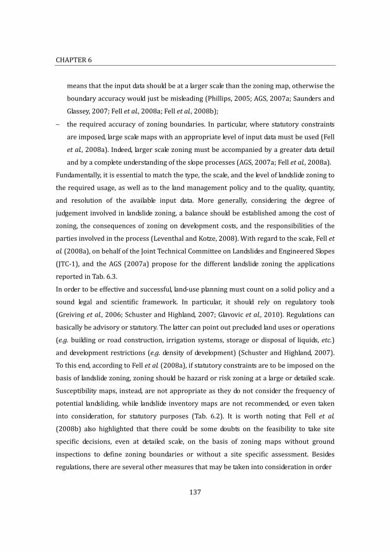
CHAPTER6

137

meansthattheinputdatashouldbeatalargerscalethanthezoningmap,otherwisethe

boundaryaccuracywouldjustbemisleading(Phillips,2005;AGS,2007a;Saundersand

Glassey,2007;Felletal.,2008a;Felletal.,2008b);

the requiredaccuracyof zoningboundaries. Inparticular,where statutory constraints

areimposed,largescalemapswithanappropriatelevelofinputdatamustbeused(Fell

etal.,2008a).Indeed,largerscalezoningmustbeaccompaniedbyagreaterdatadetail

andbyacompleteunderstandingoftheslopeprocesses(AGS,2007a;Felletal.,2008a).

Fundamentally,itisessentialtomatchthetype,thescale,andtheleveloflandslidezoningto

therequiredusage,aswellastothe landmanagementpolicyandtothequality,quantity,

and resolution of the available input data. More generally, considering the degree of

judgementinvolvedinlandslidezoning,abalanceshouldbeestablishedamongthecostof

zoning, the consequencesof zoningondevelopment costs, and the responsibilitiesof the

partiesinvolvedintheprocess(LeventhalandKotze,2008).Withregardtothescale,Fellet

al.(2008a),onbehalfoftheJointTechnicalCommitteeonLandslidesandEngineeredSlopes

(JTC‐1), and the AGS (2007a) propose for the different landslide zoning the applications

reportedinTab.6.3.

Inordertobeeffectiveandsuccessful,land‐useplanningmustcountonasolidpolicyanda

sound legal and scientific framework. In particular, it should rely on regulatory tools

(Greivingetal.,2006;SchusterandHighland,2007;Glavovicetal.,2010).Regulationscan

basicallybeadvisoryorstatutory.Thelattercanpointoutprecludedlandusesoroperations

(e.g. buildingor road construction, irrigation systems, storageordisposal of liquids,etc.)

anddevelopmentrestrictions(e.g.densityofdevelopment)(SchusterandHighland,2007).

Tothisend,accordingtoFelletal.(2008a),ifstatutoryconstraintsaretobeimposedonthe

basisoflandslidezoning,zoningshouldbehazardorriskzoningatalargeordetailedscale.

Susceptibilitymaps, instead,arenotappropriateastheydonotconsiderthefrequencyof

potential landsliding,while landslide inventorymapsarenot recommended,oreven taken

into consideration, for statutory purposes (Tab. 6.2). It is worth noting that Fell et al.

(2008b) also highlighted that there could be some doubts on the feasibility to take site

specific decisions, even at detailed scale, on the basis of zoning maps without ground

inspections to define zoning boundaries or without a site specific assessment. Besides

regulations,thereareseveralothermeasuresthatmaybetakenintoconsiderationinorder

Theland‐useplanningprocessandthepossibleapplicationsofalandslideinventorymap

138

Table6.3:Landslidezoningmappingscalesandtheirapplication(Felletal.,2008).

Scaledescription

Indicativerangeofscales

Examplesofzoningapplication

Typicalareaofzoning

Small <1:100,000 Landslideinventoryandsusceptibilityto

informpolicymakersandthegeneralpublic.

>10,000km2

Medium 1:100,000÷1:25,000 Landslideinventoryandsusceptibility

zoningforregionaldevelopmentorverylargescaleengineeringprojects.

1,000÷10,000km2

Preliminarylevelhazardmappingforlocalareas.

Large 1:25,000÷1:5,000 Landslideinventory,susceptibilityand

hazardzoningforlocalareas.10÷1,000km2

Intermediatetoadvancedlevelhazardzoningforregionaldevelopment.

Preliminarytointermediatelevelriskzoningforlocalareasandtheadvancedstagesofplanningforlargeengineeringstructures,roads,andrailways.

Detailed >5,000 Intermediateandadvancedlevelhazard

andriskzoningforlocalandsite‐specificareasandforthedesignphaseoflargeengineeringstructures,roads,andrailways.

Severalhectarestotensofsquarekilometres

to discourage new developments in landslide‐prone areas. The following proved to be

successfulintheUSA(SchusterandHighland,2007):

governmentacquisitionofproperties;

disclosure to potential property buyers of public records on urban land ownership

includinginformationonslopefailurehazards;

limiting public investments on infrastructures such as, for example,water and sewer

lines;

publiceducationinordertohavethesupportoftheaffectedpopulation;

publicawarenessoflegalliabilities;

CHAPTER6

139

postedwarningsigns;

taxcreditsandspecialassessments;

denyingloansfordevelopmentorconstruction;

prohibitiveinsurancecosts.

AccordingtoFelletal.(2008a),asaformofqualitycontrolandvalidation,zoningstudies

applied to land‐useplanningshouldbesubmitted toapeerreview inorder toprovidean

independent judgmentof the susceptibility, hazard, and risk assessment. InNewZealand,

for example, councils may request an independent peer review of any

geological/geotechnicalassessmentsoflandsliderisk(SaundersandGlassey,2007).

6.2.3.Landslidesusceptibility,hazard,andriskzoning

Landslide inventory maps as well as susceptibility, hazard, and also risk zoning maps

provide the technical and scientific support to Local Government politicians, decision‐

makers, and planners to regulate land management at large scale, but often also to the

cadastralscale.Forthisreasonitisessentialthatthesemapsareaccurateandreliable.The

frameworkof landslideriskassessment isshowninFig.6.1.Thisstructure iswidelyused

internationally and it is recommended for all kinds of zoning whether a quantitative or

qualitativeapproachisbeingtaken(AGS,2007a;Felletal.,2008a).

Thepreparationofalandslideinventoryisanessentialpartofthezoningprocess(Cascini

et al., 2005; Guzzetti, 2006; AGS, 2007a; Saunders and Glassey, 2007). It is, indeed, a

preliminary step for susceptibility zoning and, consequently, for hazard and risk zoning.

However, as partially quantified by this work, this exceptional tool presents some

uncertainties and limitations that must be clearly conveyed to the end‐users (Guzzetti,

2006; Fell et al., 2008a; Fell et al., 2008b). Moreover, landslide inventory maps do not

provide information on all the territory but just wheremassmovementswere detected.

This isan importantapproximationbecause,as itwasprovedalsobythisstudy, landslide

inventorymapsare far frombeing complete. In this sense, landslidedensitymaps,which

quantifythespatialdistributionofslopefailures,representanimprovementwithrespect

to landslide inventory maps as they are fillers of space. Furthermore, they show an

improvedreadabilityandareducedcartographicerror.Notwithstandingthis,alsodensity

Theland‐useplanningprocessandthepossibleapplicationsofalandslideinventorymap

140

Figure6.1:Frameworkforlandslideriskmanagement(Felletal.,2005).

CHAPTER6

141

mapshavesomelimitations.Indeed,theydonotshowlandslidelocationandtheiraccuracy

essentiallyrelyonthelandslideinventorymapquality(Guzzetti,2006).

The realization of a landslide susceptibilitymap basically relies on two assumptions that

provedtobegenerallyreasonable:

thepastisthekeytothefuture,i.e.areasthatinthepastwereinvolvedinlandsliding

arelikelytobeinvolvedagaininthefuture(Varnesetal.,1984;Hutchson,1995;Aleotti

andChowdhury,1999;AGS,2007a);

areasthatpresentsimilartopographic,geological,andgeomorphologicalcharacteristics

asthosethatexperiencedlandslidingarelikelytobeinvolvedinamassmovementas

well(AGS,2007a).

Regardlessofexistinglandslides,susceptibilityzoningassessesthepropensityoftheslopes

tobeinvolvedinamassmovementincludingrun‐outareasandthosezonesthatmaybe

caught up in the regression of the landslide crown area (Fell et al., 2008a). Also

susceptibilitymapsarefillerinspace,andingeneral,theyrepresentanimprovementwith

respecttoinventoryanddensitymaps.Inparticular,errorsinthelandslideinventorymaps

areherecompensatedforbyareliablesusceptibilitymodel(Guzzetti,2006).However,also

susceptibility maps show some limitations. In particular, they do not provide any

information about landslide temporal frequency or expected magnitude (Guzzetti, 2006;

Felletal., 2008a;Felletal., 2008b). Furthermore, theybasically rely ondeterministicor

statisticalmodelswhosebehaviourmustbe fullyunderstoodbefore it canbe applied for

practicaluses.Inthissense,likeanyotherscientificprediction,susceptibilitymapsshould

be accompanied by a quantitative estimate of the associated prediction error (Guzzetti,

2006).

Landslide hazard zoning estimates the frequency of the potential mass movements

highlightedby the susceptibilitymap.This, however, is not a trivial task, and it basically

depends on the type of landslide. For small slope failures and for rock falls, hazard is

described in terms of the number of sliding events per square kilometre of source

area/annum, whereas for large landslides hazard is generally expressed as the annual

probabilityofsliding(Felletal.,2008a).Furthermore,alsohazardzoningmustincludeboth

landslide source and deposition areas (Cascini et al., 2005; Guillard and Zezere, 2012).

Ultimately, it is essential to consider the possible changes produced by buildings and

Theland‐useplanningprocessandthepossibleapplicationsofalandslideinventorymap

142

infrastructureslocatedclosedtolandslidecrownortoe,andtounderstandthatdevelopment

boundaries,establishedforsafetybeyondtheunstablearea,maybecomeobsoleteinashort

timeframe(Feckner,2002;Cascinietal.,2005).Landslidehazardmaps,whicharefillerof

space,relyonamodelthatincorporatesasusceptibilitycomponent.Forthisreason,they

basicallypresentthesameadvantagesanddisadvantagesofsusceptibilitymodelsandmaps

(Guzzetti,2006).

AccordingtoFelletal.(2008a)andtotheAGS(2007a),riskis“ameasureoftheprobability

and severity of an adverse effect to health, propertyor the environment”. Indeed, on the

basisofhazardmapping,riskzoningassessesthepotentialdamagetoelementsatriskby

taking into account their vulnerability and the temporal and spatial probability of the

landslide event. Elements at risk are primarily the people and the properties potentially

affected by the slope failure because of their location (on, below, and up‐slope of the

potentiallandslide).However,theymayalsoincludeindirectimpactssuchasenvironmental

damagesandreducedeconomicactivitiesdue, forexample, to thedisruptionsofservices,

utilities, and roads. Given this wide variety of elements, risk is usually simplified in two

categories:riskforlifeloss(individualandsocietal)andriskforpropertyloss(Cascinietal.,

2005; AGS, 2007a; Fell et al., 2008a; Fell et al., 2008b). In particular, according to the

InternationalUnionofGeologicalSciences(IUGS)(1997), the formershouldbecalculated

onthebasisoftheprobabilityofnaturaldeath.Inthissense,tolerableandacceptedvalues

are generally between 10‐3 and 10‐6 per annum (Cascini et al., 2005; Bell et al., 2006;

Masseyetal.,2012).Forpropertyloss,ontheotherhand,riskisusuallyexpressedasthe

yearly loss value and the annual probability of loss (Fell et al., 2008a). It is, therefore,

essential that risk maps are at the right scale of detail and accuracy (essentially site

specific), and they alsomust be easily updatablewith regard to bothhazard assessment

andelementsatrisk(Cascinietal.,2005).

Hazard zonation requires a deep understanding of landslide processes and, of course, it

impliestheabilitytoidentifylandslidehazard.Forthisreasonhazardzonationisunderthe

responsibility of earth scientists. On the other hand, defining vulnerability and assessing

acceptablerisksrequireknowledgeoftheimpactoflandslidesonpeople,buildingareas,and

economic activities. As a consequence, the more suitable experts are planners, social

scientists, engineers, and ultimately decision‐makers (Soeters and van Westen, 1996;

CHAPTER6

143

SchusterandHighland,2007).

Severalfactorscontributetozoningpotentialinefficiency(AGS,2007a;Felletal.,2008a):

limitationsofthelandslideinventorymaps;

limitationsinthestabilityoftemporalseries;

limitationsintheavailablelevelofdatadetail;

modeluncertainty, i.e. limitationsof themethodused to assess landslide susceptibility

andhazard;

limitationsintheskilloftheoperatorthatrealisesthezoning.

Consequently,landslidezoningisnotaprecisescienceanditsresultsareonlyaprediction

ofperformanceoftheslopesbasedontheavailabledata.

6.2.4.LandslidemanagementintheEmilia‐Romagnaregion

In Italy the legal framework for planningwas established in 1942.However, in the early

1970sspatialandurbanplanningweretakeninchargebyregionalauthoritiesthat,within

thenationalregulations,promulgatedtheirownlaws.Today,intheEmilia‐Romagnaregion

spatialandurbanplanningareregulatedbytheregionallawLR20/2000(LeggeRegionale)

which,accordingtothethreelevelsofgoverning,identifiesthreedifferentlevelsofplanning:

regional,

provincial,

andmunicipal.

Inthiscontext,eachplanmustcomplywiththeupper‐tierplanningandpolicystatements.

As far as landslides are concerned, the regional plan PAI (Piano stralcio per l’Assetto

Idrogeologico)ispreparedbytheRiverBasinAuthority,anditrepresentsthestartingpoint

for the Territorial Plan for Provincial Coordination (Piano Territoriale di Coordinamento

Provinciale‐PTCP).Thisplan,realisedbytheProvincialAdministrationsatalocalscaleand

fortheentireprovincialterritory,isthestatutoryandadvisoryframeworkformunicipality

andsitespecificplans,whichshouldenhanceitandcompleteitwithfurtherinvestigations.

This work focused on the PTCP as it basically establishes the planning standards and

techniquesforallthesubordinatemunicipalplans.

According to the Attachment of LR 20/2000 (Art. A‐2), the PTCP, in line with PAI

Theland‐useplanningprocessandthepossibleapplicationsofalandslideinventorymap

144

previsions,mustlocatelandslidesandpotentiallyunstableareas,andwithrespecttothem,

itestablishesthemaincompatibleandincompatibleuses.Theregionallawalsoratifiesthat

thereferenceframe,whichdescribesandevaluatestheterritoryanditsevolution,ispartof

theplanningtoolandisessentialforthedefinitionoftheplangoalsandsustainability.

ThePTCP’softhefourtestareasaimtoprevent,reduce,andmitigatelandslideriskinorder

tobuildsustainableandresilientcommunities.ThePTCPplanningsystemreliesonzoning

andregulations. Inparticular, theseplanssupply threedifferent typesof regulationswith

respecttoland‐useinlandslide‐proneareas:

statutory, which directly influence the legal regime of properties by regulating the

compatibleandincompatibleuses;

directive,whichdefinethearrangementsthatmustbeabidebythesubordinateplans;

advisory,whichdefinethearrangementsthatshouldbeabidebythesubordinateplans

butwithacertaindegreeofdiscretion.

All the investigatedPTCP’suse landslide inventorymaps as zoningmaps1, i.e. they apply

regulationsonthebasisoflandslideboundaries.Amongotherrestrictions,forexample,on

dormantlandslidesitisprohibitedtobuildnewconstructions,whereasonactivelandslides

itisalsoforbiddentoextendexistingbuildingsandchangetheirurbanuseclassificationin

order to avoid an increase of landslide risk. The terms “active” and “dormant”, however,

implyacertainvagueness.Indeed, inthecaseoftheReggioEmiliaandModenaProvinces

dormantlandslidesarethosemassmovementsthatwerenotevidentlyactiveinthelast30

years although theymay reactivate anytime; active landslides, instead, are ongoing slope

failures or mass movements that showed some kind of activity in the last 30 years.

Conversely, no precise definitions for these terms are provided by the Forlì‐Cesena and

RavennaProvinces.Inthefourstudysites,landslideinventorymapsarealsousedaszoning

maps in themunicipalplansat localandsite‐specificscale,althoughall thePTCP’sunder

investigation require municipal plans to define safety zones around active landslides.

Ultimately, only two out of four plans (Reggio Emilia and Modena) provide a directive

regulationthatcallsforperiodicrevisionsoftheselandslideinventories.

TheReggio Emilia PTCPwas approved by the Provincial Administration in 2010 and its 1TheRavennaProvinceadoptsalsoariskmapbasedonhydromorphologicalelementaryunits(UnitàIdromorfologicheElementari‐UIE).

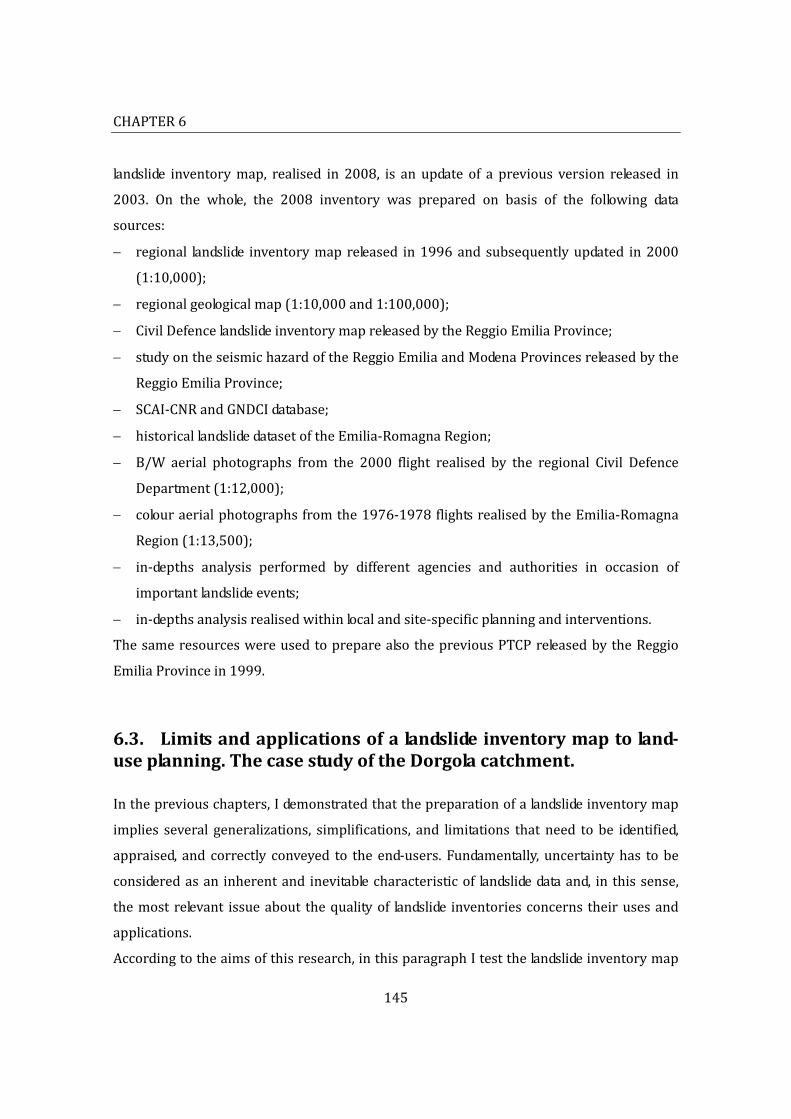
CHAPTER6

145

landslide inventorymap, realised in 2008, is an update of a previous version released in

2003. On the whole, the 2008 inventory was prepared on basis of the following data

sources:

regional landslide inventorymapreleased in1996andsubsequentlyupdated in2000

(1:10,000);

regionalgeologicalmap(1:10,000and1:100,000);

CivilDefencelandslideinventorymapreleasedbytheReggioEmiliaProvince;

studyontheseismichazardoftheReggioEmiliaandModenaProvincesreleasedbythe

ReggioEmiliaProvince;

SCAI‐CNRandGNDCIdatabase;

historicallandslidedatasetoftheEmilia‐RomagnaRegion;

B/W aerial photographs from the 2000 flight realised by the regional Civil Defence

Department(1:12,000);

colouraerialphotographsfromthe1976‐1978flightsrealisedbytheEmilia‐Romagna

Region(1:13,500);

in‐depths analysis performed by different agencies and authorities in occasion of

importantlandslideevents;

in‐depthsanalysisrealisedwithinlocalandsite‐specificplanningandinterventions.

ThesameresourceswereusedtopreparealsothepreviousPTCPreleasedbytheReggio

EmiliaProvincein1999.

6.3. Limitsandapplicationsofalandslideinventorymaptoland‐useplanning.ThecasestudyoftheDorgolacatchment.

Inthepreviouschapters,Idemonstratedthatthepreparationofalandslideinventorymap

implies several generalizations, simplifications, and limitations thatneed tobe identified,

appraised, and correctly conveyed to theend‐users. Fundamentally, uncertaintyhas tobe

consideredasan inherentand inevitablecharacteristicof landslidedataand, in thissense,

themostrelevant issueabout thequalityof landslide inventoriesconcerns theirusesand

applications.

Accordingtotheaimsofthisresearch,inthisparagraphItestthelandslideinventorymap

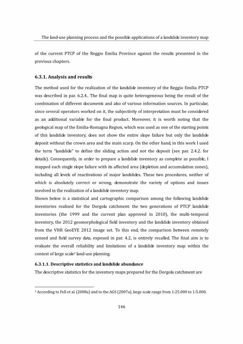
Theland‐useplanningprocessandthepossibleapplicationsofalandslideinventorymap

146

of the current PTCP of the Reggio Emilia Province against the results presented in the

previouschapters.

6.3.1.Analysisandresults

Themethodused for therealizationof the landslide inventoryof theReggioEmiliaPTCP

wasdescribed inpar.6.2.4..The finalmap isquiteheterogeneousbeing theresultof the

combinationofdifferentdocumentsandalsoofvariousinformationsources. Inparticular,

sinceseveraloperatorsworkedonit,thesubjectivityofinterpretationmustbeconsidered

as an additional variable for the final product. Moreover, it is worth noting that the

geologicalmapoftheEmilia‐RomagnaRegion,whichwasusedasoneofthestartingpoints

of this landslide inventory, does not show the entire slope failure but only the landslide

depositwithoutthecrownareaandthemainscarp.Ontheotherhand,inthisworkIused

the term “landslide” to define the sliding action and not the deposit (see par. 2.4.2. for

details). Consequently, in order toprepare a landslide inventoryas complete aspossible, I

mappedeachsingleslopefailurewithitsaffectedarea(depletionandaccumulationzones),

including all levels of reactivations ofmajor landslides. These two procedures, neither of

which is absolutely correct or wrong, demonstrate the variety of options and issues

involvedintherealizationofalandslideinventorymap.

Shown below is a statistical and cartographic comparison among the following landslide

inventories realised for the Dorgola catchment: the two generations of PTCP landslide

inventories (the 1999 and the current plan approved in 2010), the multi‐temporal

inventory,the2012geomorphologicalfieldinventoryandthelandslideinventoryobtained

from the VHR GeoEYE 2012 image set. To this end, the comparison between remotely

sensed and field survey data, exposed in par. 4.2, is entirely recalled. The final aim is to

evaluate the overall reliability and limitations of a landslide inventory map within the

contextoflargescale2land‐useplanning.

6.3.1.1.Descriptivestatisticsandlandslideabundance

ThedescriptivestatisticsfortheinventorymapspreparedfortheDorgolacatchmentare

2AccordingtoFelletal.(2008a)andtotheAGS(2007a),largescalerangefrom1:25.000to1:5.000.

CHAPTER6

Table6.4:DescriptivestatisticsforallthelandslideinventoriesavailablefortheDorgolacatchment.ThevaluesinparenthesesfortheFieldsurveyandtheGeoEYE2012inventoriesincludeAPI.

1999PTCP 2010PTCP Fieldinventory2012 GeoEYE2012 Multi‐temporalinventory

Numberoflandslides # 49 142 224 304 1.105 (249) (321)

Totalareaofmappedlandslides Km2 4,814 6,593 6.245 5,039 87,724 (9.669) (8.045)

Totalareacoveredbylandslides Km2 4,814 6,593 5,370 4,365 7,247 (7.266) (6.514)

%oflandslidearea % 29,69 40,66 33,12 26,92 44,69 (44.81) (40.17)

Landslidedensity #/Km2 3,02 8,76 13,81 18,75 68,15 (15.36) (19.80)

Areaofsmallestlandslide m2 11.331 625 28 79 54 (28) (79)

Areaofbiggestlandslide m2 990.457 974.900 1,492,740 392.681 474.010 (1,530,351) (1,675,594)

Landslideaveragearea m2 98.235 46.433 27,880 16.577 17.044 (38,833) (25,063)

Landslidemedianarea m2 59.975 16.768 4,622 2.522 2.870 (5,983) (2,820)Mostabundantlandslidearea m2 132.600 7.100 ~300 ~200 ~300

* Areacomplessiva=16,21Km2

Theland‐useplanningprocessandthepossibleapplicationsofalandslideinventorymap

148

summarisedinTab.6.4,wherefortheground‐basedandtheremote‐basedinventoriesare

reportedbothvalues:withandwithoutAPIareas(seeChapter4fordetails).Theanalysisof

Tab.6.4revealsthatthetotalnumberof landslidesincreases fromthe1999andthe2010

PTCPinventoriestothemulti‐temporal inventory. Inparticular, the1999PTCPinventory

shares4.4%ofthetotalnumberoflandslidesofthemulti‐temporalinventoryand16.1%of

that of the remote‐based inventory realised on the GeoEYE 2012 image set. These

percentagesreducerespectivelyto12.9%and46.7%forthe2010PTCPinventory,which

presents 189.8% more landslides than the previous plan. The higher number of mass

movements of the multi‐temporal inventory is reflected in the total area of mapped

landslide, while, despite the lower number of slope failures, the total area covered by

landslides in the 2010 PTCP inventory is similar to those of the ground‐based and the

remote‐based inventories. To this end, it is also worth noting that for both PTCP

inventories the total area of mapped landslides is equal to the total area covered by

landslides. This factor, togetherwith the low number ofmassmovements, indicates that

these inventories focused only on large landslides without mapping their inner

reactivations.According to the geometrical distinction introduced in Chapter 4, it can be

statedthatthe1999andthe2010PTCPinventoriesshowonly1°Levellandslides.

Thedisparityinlandslidenumbersandareas,reflectedalsointhedifferentlandslideindexes

anddensities,indicatethatdifferencesexistintheaveragesizeoftheslopefailuresmapped

in the inventoriesunder investigation. Indeed, themedian areaof the1999PTCPmap is

approximately10timeslargerthanthatofthefieldinventoryandabout20timesthoseof

theremotelysensedinventories.Proportionsareabitsmallerforthe2010PTCPmapbut,

anyhow, they tooreveal a consistentareadiscrepancy. Inparticular, themaindifferences

are related to smaller slope failures sincebiggeronespresent similarvalues, especially if

notconsideringtheBondololandslide.

The frequencydistribution shown inFig. 6.2 confirms thedivergenceas far asareas are

concerned.Infact,ithighlightsthatnotonlythe1999PTCPmaphaslesslandslidesbutthat,

withthehighestrecurrenceat46,875m2,theyarealsogenerallybiggerthanthoseofthe

other inventories.Conversely,despitethedifferenttotalamountof landslides, theground‐

based and the 2010 PTCP inventories show a similar area distributionwith the highest

peakat9,375m2.Ultimately,asalreadyremarked,theremotelysensedGeoEYEinventory

CHAPTER6

149

Figure 6.2: Landslide area frequency distribution for the 1999 PTCP, the 2010 PTCP, theground‐basedand the remote‐base inventories. Inorder todisplayall thearea range,areaclass binwidthwere progressively increased according to a log5 scale. A) The histogramrepresentstheabsolutenumberoflandslidesineachareaclassrepresentedbythebincentralvalue.B)Thediagramshowsboththepercentagecumulativeandthenon‐cumulativecurves.

Theland‐useplanningprocessandthepossibleapplicationsofalandslideinventorymap

150

presentssmaller(1,875m2)andmoreabundantlandslides.

6.3.1.2.Correspondenceoflandslideareas

The cartographic matching was again calculated according to the method proposed by

Carraraetal.(1993)asmodifiedbyGallietal.(2008).Overall,mappingerrorsrangefrom

30%to62%(Tab.6.5).Inparticular,thetwoPTCPmapsshowarathersatisfyingmatching

index (70%) being one the updated version of the other. Conversely, with regard to the

other inventories, the 2010PTCPmap shows amapping error ranging from39%, (field

survey 2012) to 50%, (multi‐temporal),whereas the 1999 PTCPmap basically presents

highererror indexeswithvaluesranging from49%,(fieldsurvey2012) to60%(GeoEYE

2012).Furthermore,itisworthnotingthatthemappingerrorsoftheGeoEYE2012andof

themulti‐temporalinventorymapsarequitesimilarprovingtheirequaldetectionmethod.

6.3.1.3.Spatialandtemporalaccuracyassessmentofthe2010PTCPinventorymap

This research showed that landslide detection and mapping pose several issues (see

Chapter 4 and 5). In order to quantify spatial uncertainty, I introduced a fuzzy raster

landslide map (see Chapter 4 for details), which, here below, I use to assess the overall

accuracyofthecurrentPTCPbyclippingthe1°Levelofthefuzzyinventoryonthe2010

PTCPmap.ResultsarereportedinTab.6.6whichrevealsthatinthe2010PTCPabout50%

Table6.5:Mappingerrorquantifying thecartographicmismatchof the landslide inventorymapsoftheDorgolacatchment.ThevaluesinparenthesesrefertodataincludingAPI.

Fieldsurvey2012 PTCP1999 PTP2010

Multi‐temporal 54% 60% 50% (41%)

GeoEYE2012 54% 62% 60% (35%) (50%) (45%)

Fieldsurvey2012 ‐ 55% 49% (49%) (39%)

PTCP1999 ‐ ‐ 30%

CHAPTER6

151

Table6.6:Percentagefrequencyofpixelcountsrelatedtofuzzyindexclasses.Datawereobtainbyclippingthe1°Levelofthefuzzyinventoryonthe2010PTCPmap.Itisworthnotingthat31.5%of thepixels couldnotbe classified since theywerenotmappedas landslides in themulti‐temporalinventory.

Fuzzyindexclasses %Counts

0–0,1 5.3

0,1–0,2 2.9

0,2–0,3 3.5

0,3–0,4 1.4

0,4–0,5 3.6

0,5–0,6 1.5

0,6–0,7 6.8

0,7–0,8 1.8

0,8–0,9 6.8

0,9–1,0 35.0

Notclassified 31.5

ofthepixelsofthetotalareacoveredbylandslidespresentsafuzzyindex≥0,6.Nevertheless,

31.5% of them could not be evaluated since theywere not mapped as landslides in the

multi‐temporalinventory,whichconverselywasnotincludedintheplanningdocumentfor

about 37.3% of its extension. These data proved that, despite a significant mapping

mismatch, landslide areas present a rather satisfying fuzzy index. This, however, is the

resultofwhatwasprobablyanaprioridecision, i.e. the2010PTCPinventoryapparently

focusedonlyonlargerlandslideswithouttakingintoconsiderationsmallmassmovements

and,inparticular,theinnerreactivationsinsidebiggerlandslides.

Withregardtothetemporalreliabilityoflandslidefootprints,thisstudysuggestedthatnew

activationsandreactivationsgenerallypresentanarearanging from125m2 to3,125m2

according to the image set resolution. These area classes, however, are not well

represented,orarenotrepresentedatall, in the2010PTCP inventory.Consequently, the

temporalreliabilityofthismapisonlyapparentanditcomesatacostofanoverallpoor

Theland‐useplanningprocessandthepossibleapplicationsofalandslideinventorymap

152

mapping accuracywhich, indeed, excludes small slope failures and inner reactivations of

largerlandslides.

6.3.2.Discussion

The1999andthe2010PTCPinventorymapsoftheReggioEmiliaProvincehavebeenboth

used as planning reference frame as well as zoning maps. The study realised for the

Dorgolacatchmentprovedthat,withrespecttothemulti‐temporal,theground‐based,and

the remote‐based inventories, both PTCP inventories present a cartographic matching

consistentwiththosereportedintheliterature(Carraraetal.,1993;Ardizzoneetal.,2002;

Gallietal.,2008). In thissense, inaddition to thosereportedandanalysed inChapters4

and 5, there are several other aspects that contributed to the poor mapping

correspondence:

interpreter’s subjectivity. Both PTCP inventories were, indeed, realised in multiple

phasesandbydifferentorganizationsandoperators;

specific a priori decisions. The geological map of the Emilia‐Romagna Region, for

example, shows only landslide deposits and not the whole landslide affected area

(depletionandaccumulationzones).Atthesametime,althoughnotdirectlystated,itis

likelythatsomesortofdimensionalfilterwasappliedtothemappedlandslides3;

heterogeneous information sources. The PTCP inventorymapswere realised on the

basis of different pre‐existing documents realised with various purposes and at

differentscale.

The1999andthe2010PTCPmapsunderestimatesmallslopefailuresandignoreevery

Figure 6.3: Visual comparison between the fuzzy raster landslide map (above) and thelandslide inventoryof the2010PTCPwithregard to theDorgolacatchment (below). In thefirst map a high fuzzy index (red tones) indicates a substantial spatial and temporalpersistenceof landslideactivity.Inthissense,thetwomapsconveydifferent information.Inparticular,thefuzzy‐likeanalysisisabletoemphasisethoseareaswherethelandslidingwasmoreintenseduringthetimeframeunderinvestigation.

3 Accordingtotheexplanatorynotesoftheregionallandslideinventorymap,thecartographiclimit

adoptedfor itsrealizationwas1:25.000. In thisway, landslideswithanarea<100m2werenotmapped(RegioneEmilia‐Romagna,1994).

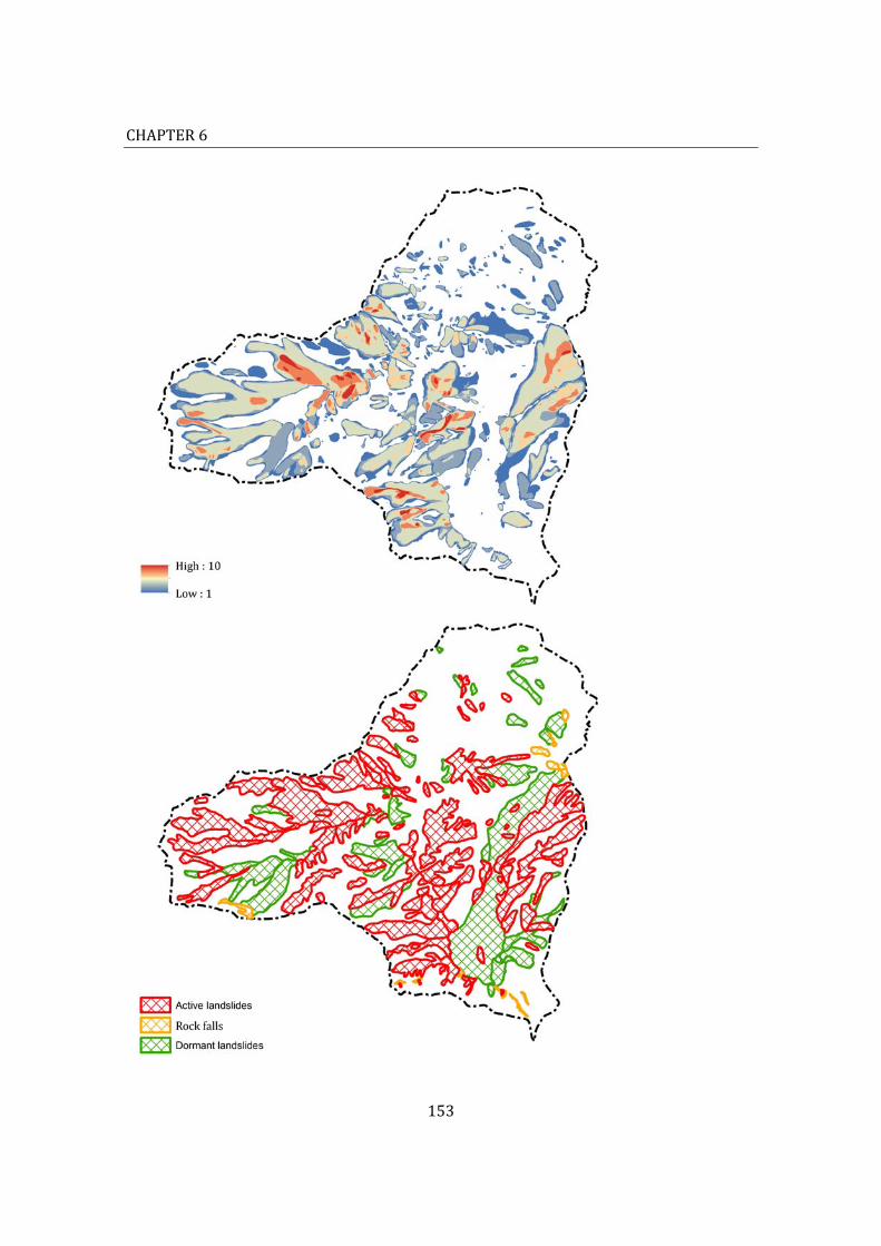
CHAPTER6

153

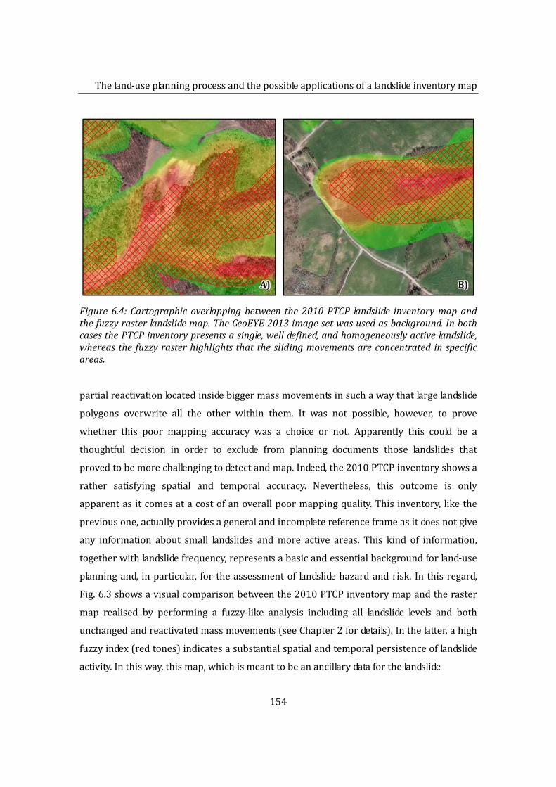
Theland‐useplanningprocessandthepossibleapplicationsofalandslideinventorymap

154

Figure6.4:Cartographicoverlappingbetween the2010PTCP landslide inventorymapandthefuzzyrasterlandslidemap.TheGeoEYE2013imagesetwasusedasbackground.InbothcasesthePTCPinventorypresentsasingle,welldefined,andhomogeneouslyactivelandslide,whereasthe fuzzyrasterhighlightsthattheslidingmovementsareconcentrated inspecificareas.

partialreactivationlocatedinsidebiggermassmovementsinsuchawaythatlargelandslide

polygons overwrite all the other within them. It was not possible, however, to prove

whether this poor mapping accuracy was a choice or not. Apparently this could be a

thoughtful decision in order to exclude from planning documents those landslides that

provedtobemorechallengingtodetectandmap.Indeed,the2010PTCPinventoryshowsa

rather satisfying spatial and temporal accuracy. Nevertheless, this outcome is only

apparentasitcomesatacostofanoverallpoormappingquality.Thisinventory, likethe

previousone,actuallyprovidesageneralandincompletereferenceframeasitdoesnotgive

any information about small landslides andmore active areas. This kind of information,

togetherwithlandslidefrequency,representsabasicandessentialbackgroundforland‐use

planningand, inparticular, for theassessmentof landslidehazardandrisk. In thisregard,

Fig.6.3showsavisualcomparisonbetweenthe2010PTCPinventorymapandtheraster

map realised by performing a fuzzy‐like analysis including all landslide levels and both

unchangedandreactivatedmassmovements(seeChapter2fordetails).Inthelatter,ahigh

fuzzyindex(redtones)indicatesasubstantialspatialandtemporalpersistenceoflandslide

activity.Inthisway,thismap,whichismeanttobeanancillarydataforthelandslide

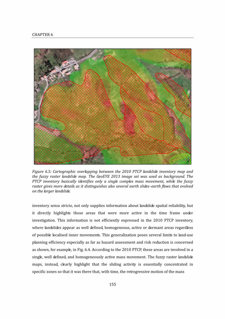
CHAPTER6

155

Figure6.5:Cartographicoverlappingbetween the2010PTCP landslide inventorymapandthe fuzzy raster landslidemap.TheGeoEYE 2013 image setwas used as background.ThePTCP inventory basically identifies only a single complexmassmovement,while the fuzzyrastergivesmoredetailsasitdistinguishesalsoseveralearthslides–earthflowsthatevolvedonthelargerlandslide.

inventorysensustricto,notonlysuppliesinformationaboutlandslidespatialreliability,but

it directly highlights those areas that were more active in the time frame under

investigation. This information is not efficiently expressed in the 2010 PTCP inventory,

wherelandslidesappearaswelldefined,homogeneous,activeordormantareasregardless

ofpossiblelocalisedinnermovements.Thisgeneralizationposesseveral limitstoland‐use

planningefficiencyespeciallyasfarashazardassessmentandriskreductionisconcerned

asshown,forexample,inFig.6.4.Accordingtothe2010PTCP,theseareasareinvolvedina

single,welldefined,andhomogeneouslyactivemassmovement.Thefuzzyrasterlandslide

maps, instead, clearly highlight that the sliding activity is essentially concentrated in

specificzonessothatitwastherethat,withtime,theretrogressivemotionofthemass

Theland‐useplanningprocessandthepossibleapplicationsofalandslideinventorymap

156

Figure6.6:Theoverlappingofthe2010PTCPlandslideinventorymapwiththeGeoEYE2013image set shows that,alreadyafter few years from its realization, the planningdocumentneedstobeupdatedasseveralnewlandslidesevolvedoutsidethedetectedboundaries.

movementsendedupinvolvingareasthatwereonceconsideredstable.Inordertooptimise

resources, this information would be essential for planning monitoring and emergency

activities,aswellasfordefiningprioritiesformitigationstrategies.

Furthermore,theoverallgeneralizationproposedbythePTCPmapdoesnotallowalsoto

separateoverlappedslidingmovements.This,forexample,isthecasereportedinFig.6.5,

whichshowsanareawhereseveralearthslides–earthflowsevolvedonalargeranddeeper

complexlandslide.Thesearedistincttypesofmassmovementswithdifferentfrequenciesof

CHAPTER6

157

occurrenceandgeomechanicalcharacteristics.Indeed,theyposeadifferentlevelofthreat

to lifeandpropertiesand, therefore, according to land‐useplanninggoals, theyshouldbe

differentiatedfromeachotherandmanagedseparately.

With regard to the temporal accuracy, the 2010 PTCP inventory is characterised by an

apparent reliability since new activations and reactivations are not included in the size

rangeofthisinventory.Thisisasignificantmappingsimplificationwithimportantfallouts

on the efficiency of the inventory for planningpurposes.Moreover, it does not solve the

issueoftemporalreliability.Indeed,asshowninFig.6.6,justafterfewyearsfromtheland‐

useplanrelease,thelegallandslidereferenceisoutdatedposingaseriesofquestionsabout

thepossibleapplicationsofalandslideinventorymapwithintheland‐useplanningcontext.

6.4. Conclusions

Inthefourstudysiteschosenforthiswork,landslideinventorymapsareusedasreference

framesandaszoningmaps,i.e.toimposestatutoryconstraintsandadvisoryregulationsto

propertiesandtothesubordinatemunicipalplans.

Ingeneral, theuseof a landslide inventorymapasa reference frame, toportray landslide

distribution and characteristics, is advantageous and basically recommended. Thiswork,

however,showedthegreatvarietyofoptionsandissuesinvolvedintherealizationofthis

typeofmap.Indeed,besidesthosefactorsanalysedinChapters4and5,thereareseveral

otheraspectsthataffectlandslidedetectionandmapping:

interpreter’ssubjectivity;

specificaprioridecisionsrelatedtothemappingpurposesandtotheavailabledata;

heterogeneousinformationsourcesintermsofscale,detail,quantity,andpurpose.

Thisworkdemonstrated that theapparentspatialand temporalaccuracyof the landslide

inventorymapofthe2010PTCPoftheReggioEmiliaProvinceistheresultofasignificant

mappingsimplificationwithimportantfalloutsonitsapplicationandefficiencyforplanning

purposes.Forthisreason,inordertoavoidmisunderstandings,andultimately,misusesand

faultyjudgments,thisstudyrecommendsthatallthelimitationsofalandslideinventoryare

clearly identified, quantified, and correctly conveyed to the end‐user. To this regard, a

questionisraisedonwhoistheultimateend‐userofalandslideinventorymap.Inthecase

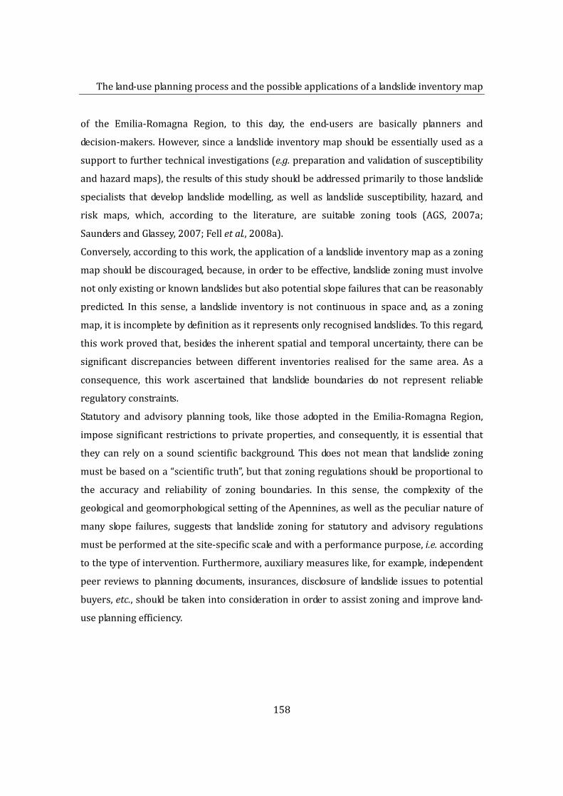
Theland‐useplanningprocessandthepossibleapplicationsofalandslideinventorymap

158

of the Emilia‐Romagna Region, to this day, the end‐users are basically planners and

decision‐makers.However,sincealandslideinventorymapshouldbeessentiallyusedasa

supporttofurthertechnicalinvestigations(e.g.preparationandvalidationofsusceptibility

andhazardmaps),theresultsofthisstudyshouldbeaddressedprimarilytothoselandslide

specialists that develop landslidemodelling, aswell as landslide susceptibility, hazard, and

risk maps, which, according to the literature, are suitable zoning tools (AGS, 2007a;

SaundersandGlassey,2007;Felletal.,2008a).

Conversely,accordingtothiswork,theapplicationofalandslideinventorymapasazoning

mapshouldbediscouraged,because,inordertobeeffective,landslidezoningmustinvolve

notonlyexistingorknownlandslidesbutalsopotentialslopefailuresthatcanbereasonably

predicted. In this sense, a landslide inventory isnot continuous in spaceand, asa zoning

map,itisincompletebydefinitionasitrepresentsonlyrecognisedlandslides.Tothisregard,

thisworkprovedthat,besidestheinherentspatialandtemporaluncertainty,therecanbe

significant discrepancies between different inventories realised for the same area. As a

consequence, this work ascertained that landslide boundaries do not represent reliable

regulatoryconstraints.

Statutory and advisory planning tools, like those adopted in the Emilia‐RomagnaRegion,

imposesignificantrestrictions toprivateproperties,andconsequently, it isessential that

theycan relyona soundscientificbackground.Thisdoesnotmean that landslidezoning

mustbebasedona“scientifictruth”,butthatzoningregulationsshouldbeproportionalto

the accuracy and reliability of zoning boundaries. In this sense, the complexity of the

geologicalandgeomorphologicalsettingoftheApennines,aswellasthepeculiarnatureof

many slope failures, suggests that landslide zoning for statutory and advisory regulations

mustbeperformedatthesite‐specificscaleandwithaperformancepurpose,i.e.according

tothetypeofintervention.Furthermore,auxiliarymeasureslike,forexample,independent

peerreviewstoplanningdocuments, insurances,disclosureof landslideissuestopotential

buyers,etc.,shouldbetakenintoconsiderationinordertoassistzoningandimproveland‐

useplanningefficiency.

Conclusionsandrecommendations

CHAPTER7

Conclusionsandrecommendations

7.1. Generalconclusions7.2. Researchlimitsandrecommendations

CHAPTER7

160

7.Conclusionsandrecommendations

7.1.Generalconclusions

Landslide inventory maps are essential decision‐support tools for land‐use planning, a

valuable and powerful attempt to build sustainable and landslide resilient communities.

Consequently, their quality assessment is a burning issue. In order to investigate it, I

addressedthreeissues.

Definitionofthequalityparametersofalandslideinventorymap

Theresultsofadetailedliteraturesurveyaboutqualityanditsdescriptivecomponents

were presented in Chapter 2. In this work, I used the term “quality” to define the

“fitnessforuse”(Juran,1974),i.e.thesuitabilityofdatacharacteristicstouser’sneeds,

andIalsoadoptedthe“truth‐in‐labelling”paradigm(Goodchild,1995;Veregin,1999).

Inthissense,Iinvestigatedthelimitsandthereliabilityoftheconceptualmodelandof

thedatabaseultimatelyrepresentedinalandslideinventory.

Likeallphysicalevents, landslidedataaremultidimensional, andconsequently,quality

parameters have to be identified for each dimension. In particular, I focused on the

spatial and temporal accuracyof a landslide inventorymap, and in order todo this, I

identifiedandinvestigatedthreekeyfactors:

‐ positionalaccuracy;

‐ overall spatial accuracy of landslide detection andmapping with respect to both

detectiontechniquesanddataprocessingandmanipulation;

‐ landslidetemporalaccuracy.

Quantificationofthespatialandtemporalaccuracyofalandslideinventorymap

The accuracy of data geographic positioningwas analysed for all four test areas and

was investigated in Chapter 3. Conversely, given the research time constraints, the

overall spatial accuracy and the temporal accuracy were elaborated only for the

Conclusionsandrecommendations

161

Dorgola catchment test area (Castelnovo né Monti – Reggio Emilia) and were the

subjectsrespectivelyofChapter4andChapter5.

Shown below are the general conclusions that can be used for the definition of

standards,bestpractices,andprotocolsforthepreparationofalandslideinventorymap.

Positionalaccuracyisanimportantparameterofquality.Itsimportancedoesnotlie

asmuchintheabsolutegeographicpositing,butratherintherelativeone.Indeed,

in order tomake proper comparison between different landslide inventorymaps

(e.g. toappraisepotentialrelativemovementsortoquantifyspatialdifferences),a

constant geographic positioning is essential. To this end, the end‐user must be

awareof theerrors that canbe introducedbydatum transformation, inparticular

whenusingdifferentsoftwaretools,i.e.differentalgorithms.Ingeneral,Isuggestto

avoid datum transformation, however, if this is not possible, the following tips

shouldbetakenintoconsideration:

‐ beawareofthemagnitudeoftheprobleminthestudyarea;

‐ if possible, always use the same software to keep the error as constant as

possible;

‐ be aware of data lineage, i.e. data history as far as datum transformations are

concern;

‐ the experience of the Emilia‐Romagna Region suggests that the adoption of

unconventionalregionalCRS’sshouldbediscouragedasitmaybeinappropriate

andleadtogrosserrors.

The spatial accuracy of a landslide inventory map is greatly influenced by the

detection and mapping technique. This work proved that neither a

geomorphological ground survey nor a visual interpretation of remotely sensed

imagesprovideacompletelandslideinventorymap.Asaconsequence,Irecommend

a combined use of these techniques. Field investigations are, indeed, essential to

developadetailedreferenceframework,whileremotesensingrepresentsaprecise,

cost‐effective, and quickmethod to complete,monitor, and update this setting. In

the case of theDorgola catchment, remote sensingwas evenmore efficient than

ground survey in recognizing and mapping small landslides, i.e. the dimensional

categorytowhichmostnewlandslides/reactivationsbelongto.

CHAPTER7

162

Theoverallspatialaccuracyisakeyelementofthequalityofalandslideinventory

map. Indeed,althoughrepresentedwithsharpboundaries, landslidesprovedtobe

uncertain and not well defined entities distinguishing safe and unsafe areas. In

particular, thisworkdemonstrated that their recognitionandmappingdependon

bothextrinsicandintrinsicvariableswhoseeffectsmayrangefrommetriclengthto

tensofmetersandevendetermineifacertainlandslidecanorcannotbedetected.

Tothisend,inordertoreduceorlimitthesefactors,Isuggesttoadoptthefollowing

measures:

‐ defineaprotocolfororthorectification(e.g. limitations,softwaretools,protocols

forthedefinitionofgroundcontrolpoints,etc.);

‐ datascaleandresolution (inparticularofbasesupportdata) shouldbekeptas

constantaspossible;

‐ avoidcapturingconditionsbias,e.g. repeatedshadowsor forestcoveroverthe

sameareasastheymightconstantlypreventthedetectionofsomelandslides;

‐ controlofpositionalaccuracy(seeabove);

‐ in order to reduce map heterogeneities and subjectivity, it would be

advantageous for landslide inventorymaps tobeelaboratedandmanagedbya

singleagency.

These efforts may help to improve spatial accuracy but they cannot completely

solve the issue. In this sense, according to the “truth‐in‐labelling” paradigm, the

type of fuzzy raster landslidemaps prepared for thiswork proved to be valuable

tools to convey to the end‐user the spatial approximations and limitations of

landslideinventorymaps.

The time variable is an essential aspect of landslide inventory maps. This work

proved that, due to the progressive deterioration of data temporal quality, these

maps need periodic updates especially as far as small landslides are concern.

According to the results obtained for the Dorgola catchment, a desirable data

acquisition frequency is once a year or maximum every two years. To this end,

remotesensingprovedtobeasuitableandcost‐effectivetoolinordertoguarantee

high acquisition frequency. In this regard, it is alsoworth remembering that data

acquisitionisaformoflong‐terminvestmentasitbasicallyrepresentsthebasefor

Conclusionsandrecommendations

163

futureresearches.

Possibleapplicationsandlimitsofalandslideinventorymaptoland‐useplanning

According to the definition given in this work, quality must be judged against a

particularapplication.Inthissense, inChapter6Ievaluatedthespatialandtemporal

accuracyof thePTCPlandslide inventorymapof theDorgolacatchment. It turnedout

thattheuseof landslideinventorymapsasreferenceframeisgenerallyadvantageous

andvaluable.However,itisessentialthattheirinherentsimplifications,generalizations,

andultimatelytheirlimitationsarecorrectlyconveyedtotheend‐userinordertoavoid

misusesandfaultydecision‐making.Tothisend,Iconsiderthesetasksessential:

‐ preparationofafuzzyrasterlandslidemaptoconveythespatialmappingreliability;

‐ definitionofthelandslidearearangewithrespecttothescaleandresolutionofthe

detectionmethod, i.e. the imprinting of detection andmapping operations on the

landslidearearange;

‐ frequentupdatesthat inthelong‐termwillallowtodefinethearearangeaffected

bynewlandslidesorreactivations;

‐ realization of a detailed report with, at least, these information: purpose and

limitationsoftheinventory,essentialdatainformation(e.g.resources,scale,lineage,

limits,etc.),andanaccuratedescriptionofthedetectionandmappingtechnique.

Conversely,theuseoflandslideinventorymapsaszoningmaps,especiallywhenrelated

to regulatory constraints, must be discouraged. Indeed, landslide zoningmust involve

also potential slope failures that can be reasonably predicted, and besides, zoning

regulationsmustbeproportional to theaccuracyof zoningboundaries. In this sense,

landslideinventorymapsnotonlyarenotcontinuousinspacebuttheyalsorepresent

unreliableboundariesduetotheirinherentspatialandtemporaluncertainty.

CHAPTER7

164

7.2.Researchlimitsandrecommendations

As landslide data, the quality assessment of a landslide inventory map must be

multidimensional.Thisworkperformedaquantitative evaluationof spatial and temporal

accuracy,but itdidnot investigate landslideattribute thatshouldbeaddressedby further

research.Anadditionallimitationconcernstheextensionoftheinvestigatedsite.Asfaras

theland‐useisconcerned,furtherinvestigationsshouldalsoconcentrateonthecorrelation

between the development of forests and scrubs, and the evolution of landslide areas.

Furthermore,moreresearchisalsoneededinordertoquantifytheinterpretersubjectivity.

To this end, to properly address this issue, all the other variables (e.g. detectionmethod,

time,basesupportmaterial,etc.)shouldberestrainedasmuchaspossible.Consideringthe

importanceof thedetectionmethodandof the interpretersubjectivity, Ialsorecommend

thatfutureresearchesassesstheresultsofthisworkbyapplyingonthesamestudysite

Figure7.1:Suggestediterativeflowchartforland‐useplanning.

Conclusionsandrecommendations

165

other landslide detection techniques, and in particular, automated and semi‐automated

detection methods (e.g. LIDAR, SAR interferometry, object‐based image analysis, NDVI

thresholding,etc.).

The use of landslide inventorymaps as support to further technical investigations raises

someseriousquestionsaboutthewholerangeoftheirpossibleend‐users.Indeed,itwould

be interesting to test theresultsof thiswork, inparticularas faras fuzzyraster landslide

maps are concerned, on landsidemodelling, andmore generally, on the preparation and

validationofsusceptibilityandhazardmaps.

Ultimately,Isuggesttoconsideradifferentland‐useplanningapproachforlandslide‐prone

areasintheEmilia‐RomagnaRegion.Indeed,giventhecomplexandchallenginggeological

andgeomorphological settingof this territory, theplanningapproachshouldbeassessed

also on the basis of the landslide type. Shallow landslides and old dormant landslides, for

example,poseadifferenthazardtomanlifeandproperties,andconsequently,theyshould

bemanaged in adifferentway. Shallow landslides can likely bepredictedon thebasis of

modelling,whereas, inorder toevaluate the frequencyand thebehaviourofolddormant

landslides, historical data andmore detailed subsurface investigations are required.More

generally,thestatutoryzoningoftheEmilia‐RomagnaRegionshouldbeappliedwithcare

atthelargescale.Indeed,theconstraintsimposebytheplanningregulationmustmatchthe

quality,quantity,andresolutionoftheavailabledata, i.e. thezoningboundaryreliability. In

this sense, at the site‐specific scale, statutory zoning must be integrated with detailed

groundinspectionsandgeotechnicaldata.Furthermore,asalreadyappliedtotheseismic

hazard, restrictions should be proportional to the type of intervention. Fundamentally, I

recommendtoadoptarisk‐basedapproachaccordingtowhichtherealizationofabarn,an

apartmentbuilding,oranhospitalimpliesdifferentplanningeffortsandrestrictions.

Landslideinventorymapsareacornerstoneof land‐useplanning,buttheyrepresentonly

thestartingpointoftheplanningworkflow,which,indeed,shouldcomprehendothertools

and should be iterative with constant data updates and revisions (Fig. 7.1). In general, I

suggest that large scale land‐use plans (e.g. PTCP) provide zoningmaps that are filler in

spaceandthatincludeunstableandpotentiallyunstableareasbytakingintoconsideration

alsotheeffectsoffuturedevelopments.Inthissense, landslidemodellingandsusceptibility

mapsareessentialtolikelypredictlandslidesandlandslidebehaviour,whereashazardand

CHAPTER7

166

riskmapsarecrucialtoassesstheeffects,theconsequences,andultimatelytheeconomic

andthesocialsustainabilityoflandslides.Asaconsequence,Istronglyrecommendtoadopt

thesetoolsinland‐useplanningdocuments.

References

167

References

Abbott,L.(1955),Qualityandcompetition,NewYork:ColumbiaUniversityPress.Aguilar,M.;Agüera,F.;Aguilar,F.&Carvajal,F. (2008), 'Geometricaccuracyassessmentofthe orthorectification process from very high resolution satellite imagery for CommonAgriculturalPolicypurposes',Internationaljournalofremotesensing,29(24),7181‐7197.Albarello,D.;Bosi,V.;Bramerini,F.;Lucantoni,A.;Naso,G.;Peruzza,L.;Rebez,A.;Sabetta,F.&SlejkoD.(1999),‘Hazardmaps1999.PGA(g)valueswitha10%probabilitàofexceedancein50years(475‐yearreturnperiod)’,Nat.Sism.Service,Rome,Italy.Aleotti,P. andChowdhury,R. (1999), ‘Landslidehazardassessment: summaryreviewandnewperspectives’,BulletinofEngineeringGeologyandtheEnvironment,58,21‐44.Antonini, G., Cardinali, M., Guzzetti, F., Reichenbach, P. & Sorrentino, A. (1993), ‘CartaInventario dei Fenomeni Franosi della Regione Marche ed aree limitrofe’, CNR GruppoNazionaleperlaDifesadalleCatastrofiIdrogeologiche,580,2sheets,scale1:100,000.Ardizzone, F.; Cardinali,M.; Carrara, A.; Guzzetti, F. & Reichenbach, P. (2002), 'Impact ofmapping errors on the reliability of landslide hazard maps', Natural Hazards and EarthSystemScience,2(1/2),3‐14.AGS (Australian Geomechanics Society) (2007a), ‘Guidelines for landslide susceptibility,hazardandriskzoningforlanduseplanning’,[on‐line].Availableat:http://lrm.australiangeomechanics.org/other‐resources/guidelines/ags‐2007/[Accessed13Oct.2014].Baiocchi,V.;Crespi,M.&DeLorenzo,C.(2002),‘Ilproblemadellatrasformazionedidatumedi coordinate per applicazioni cartografiche: soluzioni informatiche e loro prestazioni’,Documentidelterritorio,49,11‐18.Basenghi, R. & Bertolini, G. (2001), 'Ricorrenza e caratteristiche delle frane riattivateduranteilXXsecolonellaprovinciadiReggioEmiliaAppenninosettentrionale',Quad.Geol.Appl.,8(1),153–162.Bell,R.;Glade,T.&Danscheid,M. (2006), ‘Challenges indefiningacceptablerisk levels’. In:RISK21‐CopingwithRisks due toNaturalHazards in the 21stCentury:Proceedings of theRisk21Workshop,MonteVerita,Ascona,Switzerland,28,77‐87.Bertolini,G.&Pellegrini,M.(2001),'ThelandslidesoftheEmiliaApennines(northernItaly)withreferencetothosewhichresumedactivityinthe1994‐1999periodandrequiredCivilProtectioninterventions',Quad.Geol.Appl.,8(1),27‐74.Bertolini,G.;Guida,M.&Pizziolo,M.(2005), 'Landslides inEmilia‐Romagnaregion(Italy):

References

168

strategiesforhazardassessmentandriskmanagement',Landslides,2(4),302‐312.Bertolini,G.&Pizziolo,M.(2008),'RiskassessmentstrategiesforthereactivationofearthflowsintheNorthernApennines(Italy)',EngineeringGeology,102,178‐192.Bertolini, G. & Pizziolo, M. (2012), ‘The reactivation of ancient landslides in the Emilia‐RomagnaRegion(Italy):risk‐reductionstrategies’,[on‐line].Available at: http://ambiente.regione.emilia‐romagna.it/geologia/archivio_pdf/dissesto‐idrogeologico/reactivation_landslides_Bertolini_Pizziolo.pdf/view[AccessedJanuary2015].Bettelli,G.&DeNardo,M.(2001), 'Geologicaloutlinesof theEmiliaApennines(Italy)andintroductiontotherockunitscroppingoutintheareasofthelandslidesreactivatedinthe1994‐1999period',Quad.Geol.Appl.,8(1),1‐26.Borgatti, L. & Tosatti, G. (2010), 'Slope Instability Processes Affecting the Pietra DiBismantovaGeosite(NorthernApennines,Italy)',Geoheritage,2(3‐4),155‐168.Brabb,E.E.(1991),‘TheWorldLandslideProblem’,Episodes,14(1),52‐61.Buttenfield, B. P. & Beard, M. K. (1991), 'Visualizing the Quality of Spatial Information',National Center for Geographic Information and Analysis ‐ Research Initiative# 7,supportedbyflagrantfromtheNationalScienceFoundation(SES‐88‐10917).Campbell, J. & Wynne, R. (2012), Introduction to Remote Sensing, Fifth Edition, GuilfordPublications.Cardinali,M.,Guzzetti,F.&Brabb,E.E.(1990),‘Preliminarymapshowinglandslidedepositsand related features in NewMexico’, U.S. Geological Survey Open File Report 90/293, 4sheets,scale1:500,000.Cardinali, M., Antonini, G., Reichenbach, P. and Guzzetti, F. (2001), ‘Photo‐geological andlandslide inventory map for the Upper Tiber River basin’, CNR Gruppo Nazionale per laDifesadalleCatastrofiIdrogeologiche,2154,scale1:100,000.Cardinali,M.;Reichenbach,P.;Guzzetti,F.;Ardizzone,F.;Antonini,G.;Galli,M.;Cacciano,M.;Castellani,M.;Salvati,P.&others(2002),'Ageomorphologicalapproachtotheestimationoflandslide hazards and risks in Umbria, Central Italy', Natural hazards and earth systemscience,2(1/2),57‐72.Carrara,A.; Cardinali,M.&Guzzetti, F. (1993), 'Uncertainty in evaluating landslidehazardandrisk',ITCJour.,2,101‐109.Cascini, L.; Bonnard, C.; Corominas, J.; Jibson, R. & Montero‐Olarte, J. (2005), ‘Landslidehazardandriskzoning forurbanplanninganddevelopment’,LandslideRiskManagement,TaylorandFrancis,London,199‐235.

References

169

Chandler, R. J. & Tosatti, G. (1995), ‘The Stava tailings dams failure, Italy, July 1985’,Proceedingsoftheinstitutionofcivilengineers,GeotechnicalEngineering,113,67‐79.Chen,W.&Hill,C.(2005), ‘Evaluationprocedureforcoordinatetransformation’,Journalofsurveyingengineering,131(2),43‐49.Cima,V.;Olivucci,S.&Zennaro,L.(2013),‘SistemidicoordinategeograficheecartograficheinRegioneEmilia‐Romagnaelorotrasformazioni’,[on‐line].Availableat:http://geoportale.regione.emilia‐romagna.it/it/services/servizi%20tecnici/servizio‐di‐conversione/conver‐2013‐software‐per‐la‐conversione‐fra‐sistemi‐di‐coordinate‐in‐emilia‐romagna[AccessedAugust2013].Collier,P.&Steed,J.(2001),‘Australia’sNationalGDA94TransformationGrids’,Proceedingsofthe42ndAustralianSurveyorsCongress,Brisbane,Australia.Condorelli, A. (2010), ‘Impiego di cartografia catastale in Sistemi Informativi Geografici:problematiche fondamentali e possibili approcci applicativi’,Proceedingsof theASITAXIVNationalConference,Brescia,Italy,631‐636.ConvER3"GPS7"(2013),Softwareperlatrasformazionedicoordinate,[on‐line].Availableat:http://geoportale.regione.emilia‐romagna.it[AccessedMarch2013].Crosby, P. (1979), Quality is free: The art of making quality certain, New York: NewAmericanLibrary.Crozier,M.(2010),'Landslidegeomorphology:Anargumentforrecognition,withexamplesfromNewZealand',Geomorphology,120(1),3‐15.Cruden, D. M. & Varnes, D. J. (1996), 'Landslide types and processes', Landslides:investigationandmitigation,247,36‐75.Deakin, R. (2006), ‘A Note on the Bursa‐Wolf andMolodensky‐Badekas Transformations’,SchoolofMathematicalandGeospatialSciences,RMITUniversity,1‐21.Del Moro, M. A. & Lancia, F. (2007), ‘Disomogeneità territoriale dell'errore nelletrasformazionifradatum),ProceedingsoftheASITAXINationalConference,Torino,Italy,1‐6.Devillers, R.; Gervais, M.; Bédard, Y. & Jeansoulin, R. (2002), 'Spatial data quality: frommetadata to quality indicators and contextual end‐user manual', In OEEPE/ISPRS JointWorkshoponSpatialDataQualityManagement,21‐22.Devillers, R.; Bédard, Y. & Jeansoulin, R. (2005), 'Multidimensional management ofgeospatial data quality information for its dynamic use within GIS', PhotogrammetricEngineering&RemoteSensing,71(2),205‐215.

References

170

DipartimentodiProtezioneCivile(2014),[on‐line].Availableat:http://www.protezionecivile.gov.it/[Accessed22July2014].Donatelli, D.; Maseroli, R. & Pierozzi, M. (2002), ‘Le trasformazioni fra i sistemi diriferimentoutilizzatiinItalia’,BollettinodiGeodesiaeScienzeAffini,4.Dragicevic, S. & Marceau, D. J. (2000), 'An application of fuzzy logic reasoning for GIStemporalmodelingofdynamicprocesses',FuzzysetsandSystems,113(1),69‐80.E‐geos.it(2014),e‐GEOSGeoEye‐1/IKONOS,[on‐line].Availableat:http://www.e‐geos.it/products/geoeye.html[Accessed24Aug.2014].Exelis VIS (Visual Information Solutions) (2013), 'ENVI tutorial: orthorectifying aerialphotographs'.Fara,E.(2001),'WhatareLazarustaxa?',GeologicalJournal,36(3‐4),291‐303.Featherstone,W. E. (1997), ‘A comparison of existing co‐ordinate transformationmodelsandparametersinAustralia’,Australiansurveyor,42(2),25‐34.Feckner, S. (2002), ‘Development setbacks from river valley/ravine crests in newlydeveloping areas’. In: R. McInnes and J. Jakeways (eds.). Instability Planning andManagement,ThomasTelford,135‐142.Feigenbaum,A.(1951),Qualitycontrol:Principles,practice,andadministration,NewYork:McGraw‐Hill.Fell,R.;Ho,K.K.S.;Lacasse,S.&Leroi,E.(2005),‘StateoftheArtPaper1‐Aframeworkforlandslideriskassessmentandmanagement’.In:ProceedingsoftheInternationalConferenceonLandslideRiskManagement,Vancouver,Canada(31).Fell,R.;Corominas,J.;Bonnard,C.;Cascini,L.;Leroi,E.&Savage,W.Z.(2008a),'Guidelinesfor landslide susceptibility, hazard and risk zoning for land use planning', EngineeringGeology,102,85‐98.Fell, R.; Corominas, J.; Bonnard, C.; Cascini, L.; Leroi, E. & Savage, W. Z. (2008b),'Commentary ‐ Guidelines for landslide susceptibility, hazard and risk zoning for land‐useplanning',EngineeringGeology,102,99‐111.Fernandez, T.; Delgado, J.; Cardenal, J.; Irigaray, C.; El Hamdouni, R. & Chacon, J. (2006),'Improvement of positional accuracy of landslide database using digital photogrammetrytechneques', Proceedings of the 7th International Symposium on Spatial AccuracyAssessmentinNaturalResourcesandEnvironmentalSciences,[on‐line].Availableat:http://www.spatial‐accuracy.org[Accessed22July2014].Fisher,P.F.(1999),'Modelsofuncertaintyinspatialdata',Geographicalinformationsystems,

References

171

1,191‐205.FondazioneStava1985onlus(2014),[on‐line].Availableat:http://www.stava1985.it/[AccessedDecember2014].Galli, M.; Ardizzone, F.; Cardinali, M.; Guzzetti, F. & Reichenbach, P. (2008), 'Comparinglandslideinventorymaps',Geomorphology,94(3),268‐289.Garberi,M.;Palumbo,A.&Pizziolo,M.(1999),Inumerisullefrane,GraficheDamiani.Genevois, R. & Ghirotti, M. (2005), ‘The 1963 Vajont landslide’, Giornale di GeologiaApplicata,1,41‐52.GeoEYE(2009),'GeoEyeProductGuidev1.0.1',[on‐line].GeoportaleNazionale,[on‐line].Available at: http://www.pcn.minambiente.it/GN/ [Accessed from November 2013 toSeptember2014]GeoportaledellaRegioneEmilia‐Romagna,[on‐line].Availableat:http://geoportale.regione.emilia‐romagna.it/it[Accessed22July2014].Giannini,M.S. (1960), ‘Certezza pubblica’, In: Giufré (ed),Enciclopediadeldiritto.Annali,Milano,769‐792.Gilmore,H.(1974),'Productconformancecost',InQualityprogress,16‐19.Glavovic,B.;Saunders,W.&Becker,J.(2010),'Land‐useplanningfornaturalhazardsinNewZealand:thesetting,barriers,’burningissues’andpriorityactions',NaturalHazards,54(3),679‐706.Goodchild, M. F. (1993), 'Data models and data quality: problems and prospects',EnvironmentalmodelingwithGIS,94‐103.Goodchild,M.F.(1995),Sharingimperfectdata.Greiving, S. & Fleischhauer, M. (2006), 'Spatial planning response towards natural andtechnological hazards', Natural and technological hazards and risks affecting the spatialdevelopmentofEuropeanregions,GeologicalSurveyofFinland,SpecialPaper42,109‐123.Greiving, S.; Fleischhauer,M. &Wanczura, S. (2006), 'Management of natural hazards inEurope:theroleofspatialplanninginselectedEUmemberstates',Journalofenvironmentalplanningandmanagement,49(5),739‐757.GSUEG (Gruppo di Studio delle Università Emiliane per la Geomorfologia) (1976),‘Geomorfologia dell'area circostante la Pietra di Bismantova (Appennino reggiano)’, Boll.

References

172

Serv.Geol.It.,97.Guillard, C. & Zezere, J. (2012), 'Landslide susceptibility assessment and validation in theframework of municipal planning in Portugal: the case of Loures municipality',Environmentalmanagement,50(4),721‐735.Guptill, S. C. & Morrison, J. L. (1995), Elements of spatial data quality, Elsevier ScienceOxford,202.Guzzetti, F. & Cardinali, M. (1989), ‘Carta Inventario dei Fenomeni Franosi della Regionedell'Umbria ed aree limitrofe’, CNR Gruppo Nazionale per la Difesa dalle CatastrofiIdrogeologiche,204,2sheets,scale1:100,000.Guzzetti, F. (2000), 'Landslide fatalities and the evaluation of landslide risk in Italy',EngineeringGeology,58(2),89‐107.Guzzetti,F.;Cardinali,M.;Reichenbach,P.&Carrara,A.(2000),'Comparinglandslidemaps:A case study in the upper Tiber River Basin, central Italy', Environmentalmanagement,25(3),247‐263.Guzzetti, F. (2006), ‘Landslide hazard and risk assessment’, PhD thesis, Mathematisch‐Naturwissenschaftlichen Fakultät der Rheinischen Friedrich‐Wilhelms‐UniversitätUniversityofBonn,389.Guzzetti,F.;Reichenbach,P.;Ardizzone,F.;Cardinali,M.&Galli,M.(2006), 'Estimatingthequalityoflandslidesusceptibilitymodels',Geomorphology,81(1),166‐184.Guzzetti,F.;Mondini,A.C.;Cardinali,M.;Fiorucci,F.;Santangelo,M.&Chang,K.‐T.(2012),'Landslide inventorymaps:New tools for an old problem',Earth‐ScienceReviews, 112(1),42‐66.Hughes,M.L.;McDowell,P.F.&Marcus,W.A.(2006),'Accuracyassessmentofgeorectifiedaerial photographs: Implications for measuring lateral channel movement in a GIS',Geomorphology,74(1),1‐16.Hutchinson, J.N. (1995), ‘Landslide hazard assessment’, In: Bell (ed.) Landslides, A.A.Balkema,Rotterdam,1805‐1841.Iliffe,J.(2000),DatumsandMapProjectionsforremotesensing,GIS,andsurveying,WhittlesPublishingServices,Scotland,UK.ISO/TC176/SC1(1986),ISO8402Qualityvocabulary,InternationalStandardOrganization,Geneva.ISO/TC 69/SC6 (1994), ISO 5725‐1:1994 Measurement methods and results ‐ Accuracy(trueness and precision) of measurement methods and results, International Standard

References

173

Organization,Geneva.ISO/TC 176/SC (2005), ISO9000:2005Qualitymanagement systems–Fundamentalsandvocabulary,InternationalStandardOrganization,Geneva.ISO/TC 211 (2009), ISO 19114:2003 Geographic information – Quality evaluationprocedures,InternationalStandardOrganization,Geneva.IUGS(InternationalUnionofGeologicalSciences)(1997),‘Quantitativeriskassessmentforslopesandland‐slides–theStateoftheArt’,IUGSWorkingGrouponLandsldies,CommitteeonRiskAssessment.In:Landslideriskassessment,CrudenandFell(eds),Balkema,Rotter‐dam,3‐12.Juran, J.;Gryna,F. J.&Bingham,R.(1974),Qualitycontrolhandbook,NewYork:McGraw‐Hill.Kahn, B. & Strong, D. (1998), 'Product and Service Performance Model for InformationQuality: AnUpdate',Proceedingsof theConferenceon InformationQuality,MassachusettsInstituteofTechnology,Cambridge,MA.Kwon, J. H.; Bae, T.‐S.; Choi, Y.‐S.; Lee, D.‐C. & Lee, Y.‐W. (2005), ‘Geodetic datumtransformation to the global geocentric datum for seas and islands around Korea’,GeosciencesJournal,9(4),353‐361.Leventhal, A. R. & Kotze, G. P. (2008), 'Landslide susceptibility and hazard mapping inAustralia for land‐use planning with reference to challenges in metropolitan suburbia',EngineeringGeology,102(3),238‐250.Levitt,T.(1972),Production‐lineapproachtoservice,HarvardBusinessReview.Malamud,B.D.;Turcotte,D.L.;Guzzetti,F.&Reichenbach,P.(2004),'Landslideinventoriesandtheirstatisticalproperties',EarthSurfaceProcessesandLandforms,29(6),687‐711.Mantovani,F.;Soeters,R.&VanWesten,C.(1996),'RemotesensingtechniquesforlandslidestudiesandhazardzonationinEurope',Geomorphology,15(3),213‐225.Mark, D. M., & Csillag, F. (1989), 'The nature of boundaries on ‘area‐class’ maps',Cartographica:The International Journal forGeographic InformationandGeovisualization,26(1),65‐78.Maseroli, R. & Nicolodi, S. (2002), ‘Alcuni metodi per il passaggio dal sistemaWGS84 aisistemigeodeticilocali’,BollettinoASIT,32.Massey, C.; Taig, T. &Webb T. (2012), ‘Principles and criteria for the assessment of riskfrom slope stability in the Port Hills, Christchurch’,GNS Science ConsultancyReport, [on‐line].

References

174

Availableat:http://www.ccc.govt.nz/homeliving/civildefence/chchearthquake/porthillsgeotech/porthillsgnsreports.aspx[Accessed13Oct.2014].Montrasio, L.; Valentino, R. & Losi, G. L. (2012), 'Shallow landslides triggered by rainfalls:modeling of some case histories in the Reggiano Apennine (Emilia Romagna Region,NorthernItaly)',Naturalhazards,60(3),1231‐1254.Olshansky, R.B. (1996), Planning for hillside development, American Planning AssociationPlanningAdvisoryServiceReportno.466.Peuquet, D. (1999), 'Time in GIS and geographical databases', Geographical informationsystems,1,91‐103.Phillips,J.(2005),‘Weatheringinstabilityandlandscapeevolution’,Geomorphology,67,255‐272.Pizziolo, M.; Del Maschio, L.; Gozza, G. & Pignone, S. (2008), 'Determinazione di sogliepluviometricheperl'innescodifraneinEmilia‐Romagna',Geol.Emilia‐Romagna,29,21‐27.Pizziolo,M.;Bernardi,M.;Daniele,G.;Generali,M.&Piacentini,D.(2014a), ‘Rapportosuglieventi di frana avvenuti nei mesi di Marzo e Aprile 2013 in Emilia‐Romagna’, ServizioGeologicoSismicoedeiSuoli‐RegioneEmilia‐Romagna,[on‐line].Availableat:http://ambiente.regione.emilia‐romagna.it/geologia/temi/dissesto‐idrogeologico/rapporto‐frane‐marzo‐aprile‐2013‐1Pizziolo, M.; Daniele, G. & Generali, M. (2014b), ‘Rapporto sulle frane attivate in Emilia‐RomagnanelperiodoNovembre2013–Marzo2014’,ServizioGeologicoSismicoedeiSuoli‐RegioneEmilia‐Romagna,[on‐line].Availableat:http://ambiente.regione.emilia‐romagna.it/geologia/temi/dissesto‐idrogeologico/rapporto‐frane‐novembre‐2013‐marzo‐2014Porporato, C. (2012), ‘Transformation from the CadastralDATUM to theRoma1940 andETRF2000DATUM’,TerritorioItalia,1,107‐119.ProvinciadiForlì‐Cesena(2001),PianoTerritorialediCoordinamentoProvinciale.ProvinciadiForlì‐Cesena(2006),PianoTerritorialediCoordinamentoProvinciale.Provincia di Forlì‐Cesena (2010), Variante Integrativa al Piano Territoriale diCoordinamentoProvinciale.ProvinciadiModena(1999),PianoTerritorialediCoordinamentoProvinciale.Provincia di Modena (2006), Variante al PTCP di adeguamento in materia di dissestoidrogeologicoaiPianidiBacinodeifiumiPoeReno.

References

175

ProvinciadiModena(2009),PianoTerritorialediCoordinamentoProvinciale.ProvinciadiRavenna(2000),PianoTerritorialediCoordinamentoProvinciale.ProvinciadiRavenna(1999),VarianteintegrativaalPTCP.ProvinciadiReggioEmilia(1999),PianoTerritorialediCoordinamentoProvinciale.ProvinciadiRavenna(2010),PianoTerritorialediCoordinamentoProvinciale.Raper, J. F. (1999), 'Spatial representation: the scientist's perspective', Geographicalinformationsystems,1,61‐70.Reeves, C. A. & Bednar, D. A. (1994), 'Defining quality: alternatives and implications',AcademyofmanagementReview,19(3),419‐445.RegioneEmilia‐Romagna(1994),Note illustrativedellacartadeldissestogeologicoattuale,Firenze.Regione Emilia‐Romagna (2003), ‘DELIBERAZIONE DEL CONSIGLIO REGIONALE 28maggio 2003, n. 484. Approvazione dell'atto di indirizzo e coordinamento tecnico perl'attuazionedellaL.R.24marzo2000,n.20,art.27,recante"Strumenticartograficidigitaliemodalita' di coordinamento ed integrazione delle informazioni a supporto dellapianificazione”.RegioneEmilia‐Romagna(2012),CartageologicadellaRegioneEmilia‐Romagna,[on‐line].Available at: http://ambiente.regione.emilia‐romagna.it/geologia/cartografia/webgis‐banchedati/webgis[AccessedJune2012].RegioneEmilia‐Romagna(2013),IlCatalogodeiDatiGeografici,ServizioGeologicoSismicoedeiSuoli,[on‐line].Availableat:http://geo.regione.emilia‐romagna.it/geocatalogo/[AccessedMarch2013andApril2014].Rib,H.T.&Liang,T.(1978),'Recognitionandidentification',LandslideAnalysisandControl,NationalAcademyofSciences,TransportationResearchBoardSpecialReport,176,34‐80.Rivest, S.; Bédard, Y. & Marchand, P. (2001), 'Toward better support for spatial decisionmaking: defining the characteristics of spatial on‐line analytical processing (SOLAP)',GEOMATICA‐OTTAWA,55(4),539‐555.Rossi,M.;Witt,A.;Guzzetti,F.;Malamud,B.D.&Peruccacci,S.(2010),'AnalysisofhistoricallandslidetimeseriesintheEmilia‐Romagnaregion,northernItaly',EarthSurfaceProcessesandLandforms,35(10),1123‐1137.Salvati, P.; Bianchi, C.; Rossi,M.& Guzzetti, F. (2010), 'Societal landslide and flood risk in

References

176

Italy',NaturalHazardsandEarthSystemScience,10(3),465‐483.Santangelo,M.;Cardinali,M.;Rossi,M.;Mondini,A.&Guzzetti,F.(2010),'Remotelandslidemappingusinga laser rangefinderbinocular andGPS',NaturalHazardsandEarthSystemScience,10(12),2539‐2546.Saunders,W.,&. Glassey, P. (2007), 'Guidelines for assessingplanning policy and consentrequirementsforlandslideproneland',GNSScienceMiscellaneousSeries7.SchwabJ.C.;Gori,P.L.&JeerS.(2005),Landslidehazardsandplanning,AmericanPlanningAssociationPlanningAdvisoryServiceReportno.533/534,208.Schuster,R. L.&Highland,L.M. (2007), 'TheThirdHansCloosLecture.Urban landslides:socioeconomic impacts and overview of mitigative strategies', Bulletin of EngineeringGeologyandtheEnvironment,66(1),1‐27.Semenza, E. & Ghirotti, M. (2000), ‘History of the 1963 Vajont slide: the importance ofgeologicalfactors’,BulletinofEngineeringGeologyandtheEnvironment,59(2),87‐97.Servizio Geologico Sismico e dei Suoli ‐ Regione Emilia‐Romagna (1999), I numeri sullefrane,RegioneEmilia‐Romagna,94.Servizio Geologico Sismico e dei Suoli ‐ Regione Emilia‐Romagna (2006),Progetto IFFI ‐RelazioneTecnicaRegioneEmilia‐Romagna, Regione Emilia‐Romagna, APAT and ServizioGeologicod'Italia,26.Soeters,R.&VanWesten,C.J.(1996),'Slopeinstabilityrecognition,analysisandzonation'.In: TurnerAK, SchusterRL (eds),Landslides, investigationandmitigation, TransportationResearchBoard,NationalResearchCouncil, SpecialReport 247,NationalAcademyPress,Washington,USA,129–177.Soler,T.&Hothem,L.D.(1988),‘Coordinatesystemsusedingeodesy:basicdefinitionsandconcepts’,JournalofSurveyingEngineering,114(2),84‐97.Surace,L.(1998),‘LageoreferenziazionedelleinformazioniterritorialiinItalia’,BollettinodiGeodesiaeScienzeAffini,57(2),181‐234.Tirabassi, I. (2011), 'Preistoria e protostoria nella Valle del Tassobbio', In La Valle delTassobbio.LavitaneisecoliprimadeiCanossa,ProlocoCortogno,35‐74.Tosatti, G.; Castaldini, D.; Barbieri,M.; D'AmatoAvanzi, G.; Giannecchini, R.;Mandrone, G.;Pellegrini,M.;Perego,S.;Puccinelli,A.;Romeo,R.W.&others(2008),'Additionalcausesofseismically‐relatedlandslidesintheNorthernApennines,Italy',Revistadegeomorfologie,10,5‐21.Travaglini,D.(2004),‘Trasformazionitrasistemidicoordinate:softwaredisponibili,limitiepotenzialità’,Forest@,1(2),128‐134.

References

177

Trigila,A.;Iadanza,C.&Spizzichino,D.(2010),'QualityassessmentoftheItalianLandslideInventoryusingGISprocessing',Landslides,7(4),455‐470.Turner,A.&Schuster,R.(1996),Landslides,Washington:NationalAcademyPress,673.UNISDR(UnitedNationsOfficeforDisasterRiskReduction)(2014),[on‐line].Availableat:http://www.preventionweb.net/english/hazards/statistics/?hid=65[Accessed7Oct.2014].Vanicek,P.&Steeves,R.R.(1996),‘Transformationofcoordinatesbetweentwohorizontalgeodeticdatums’,JournalofGeodesy,70(11),740‐745.van Westen, C. J.; Castellanos, E. & Kuriakose, S. L. (2008), 'Spatial data for landslidesusceptibility, hazard, and vulnerability assessment: an overview', Engineering geology,102(3),112‐131.Varnes, D.J. and IAEG Commission on Landslides and other Mass‐Movements (1984),Landslidehazardzonation:areviewofprinciplesandpractice,TheUNESCOPress,Paris,63.Veregin,H.(1999),'Dataqualityparameters',Geographicalinformationsystems,1,177‐189.Wills, C.&McCrink,T. (2002), 'Comparing landslide inventories: themapdependson themethod',Environmental&EngineeringGeoscience,8(4),279‐293.WP/WLI–InternationalGeotechnicalSocieties'UNESCOWorkingPartyonWorldLandslideInventory (1993), 'A suggestedmethod for describing the activity of a landslide', Int.Ass.Eng.Geol.Bull.,47,53‐57.You,R.‐J.&Hwang,H.‐W.(2006),‘CoordinatetransformationbetweentwogeodeticdatumsofTaiwanbyleast‐squarescollocation’,Journalofsurveyingengineering,132(2),64‐70.Zadeh,L.A.(1965),'Fuzzysets',Informationandcontrol,8(3),338‐353.Zandbergen, P. A. (2008), ‘Positional Accuracy of SpatialData:Non‐NormalDistributionsandaCritiqueof theNationalStandard forSpatialDataAccuracy’,Transactions inGIS,12(1),103‐130.Zanutta,A.;Baldi,P.;Bitelli,G.;Cardinali,M.&others (2006), 'Qualitativeandquantitativephotogrammetric techniques for multi‐temporal landslide analysis', Annals of Geophysics,49(4/5),1067‐1080.

APPENDIXA

178

APPENDIXA

This Appendix contains the spatial representation of the offsets of the datumtransformations from UTMRER/UTMA to WGS84 performed with the three differentsoftware:ConvER3‐GPS7,GlobalMapper13ENandGlobalMapper14IT.

a) UTMRERtoWGS84withConvER3‐GPS7

b) UTMRERtoWGS84withGlobalMapper13EN

c) UTMRERtoWGS84withGlobalMapper14IT

d) UTMAtoWGS84withConvER3‐GPS7

e) UTMAtoWGS84withGlobalMapper13EN

f) UTMAtoWGS84withGlobalMapper14IT

APPENDIXA

179

a)

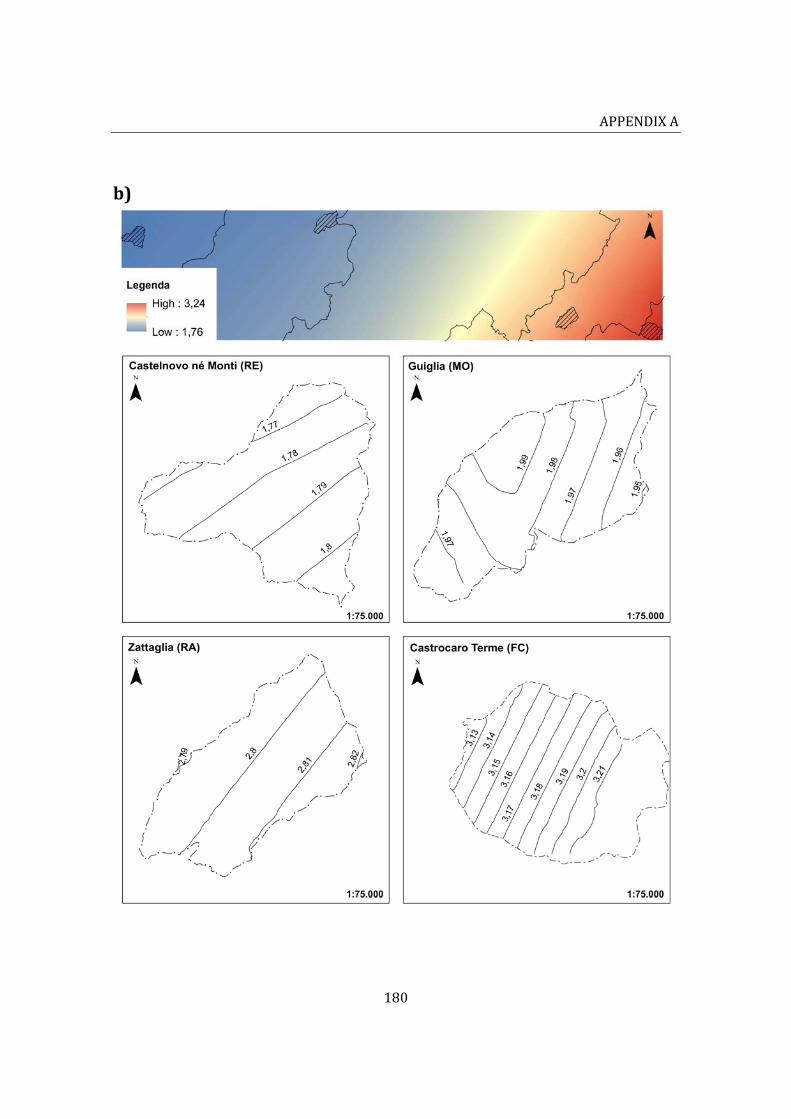
APPENDIXA

180

b)

APPENDIXA

181

c)

APPENDIXA

182

d)

APPENDIXA

183

e)

APPENDIXA

184

f)

APPENDIXB

185

APPENDIXB

ThisAppendixcontains thespatial representationof theoffsetsbetween thesamedatumtransformationperformedwithtwodifferentsoftware.

a) UTMRERtoWGS84transformation:ConvER3‐GPS7vsGlobalMapper13EN

b) UTMRERtoWGS84transformation:ConvER3‐GPS7vsGlobalMapper14IT

c) UTMRERtoWGS84transformation:GlobalMapper13ENvsGlobalMapper14IT

d) UTMAtoWGS84transformation:ConvER3‐GPS7vsGlobalMapper13EN

e) UTMAtoWGS84transformation:ConvER3‐GPS7vsGlobalMapper14IT

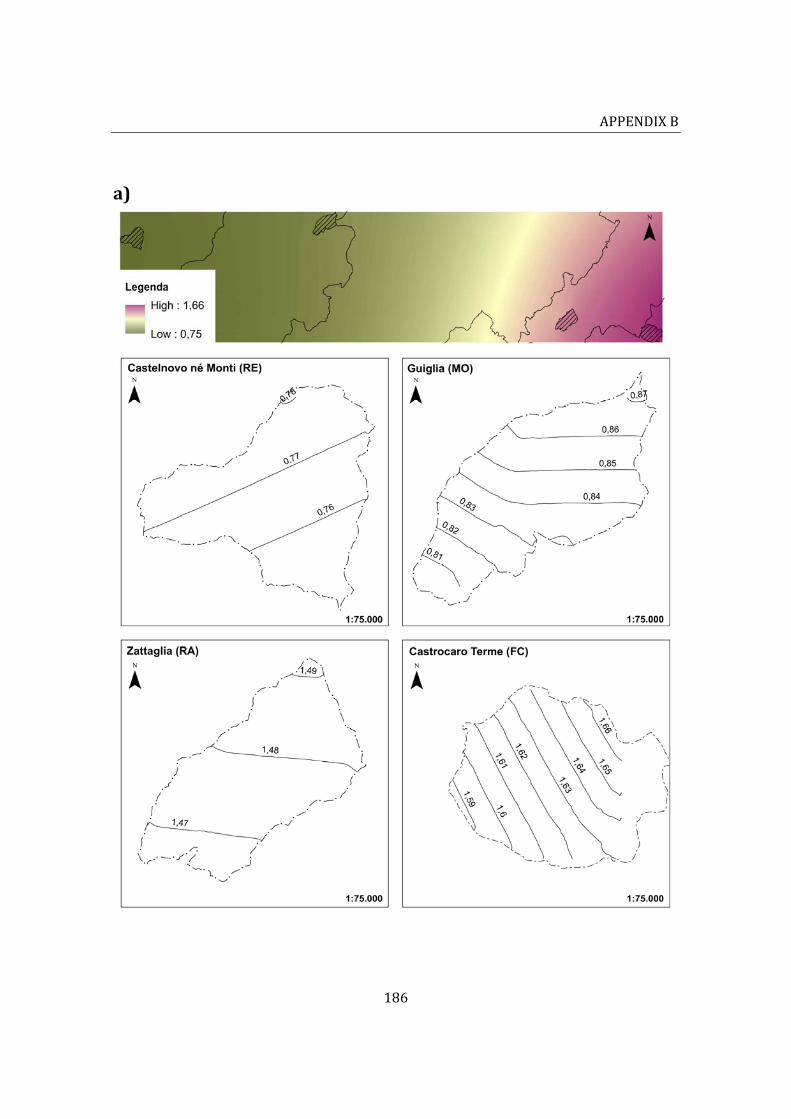
APPENDIXB

186

a)

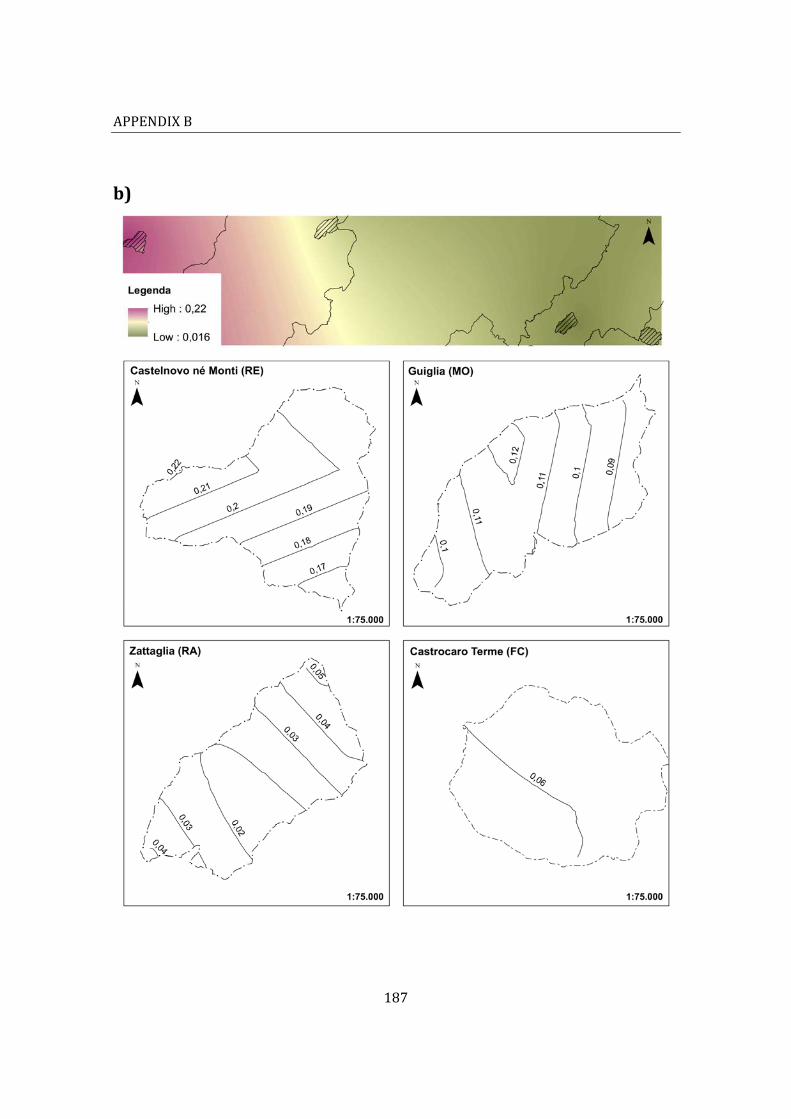
APPENDIXB

187

b)

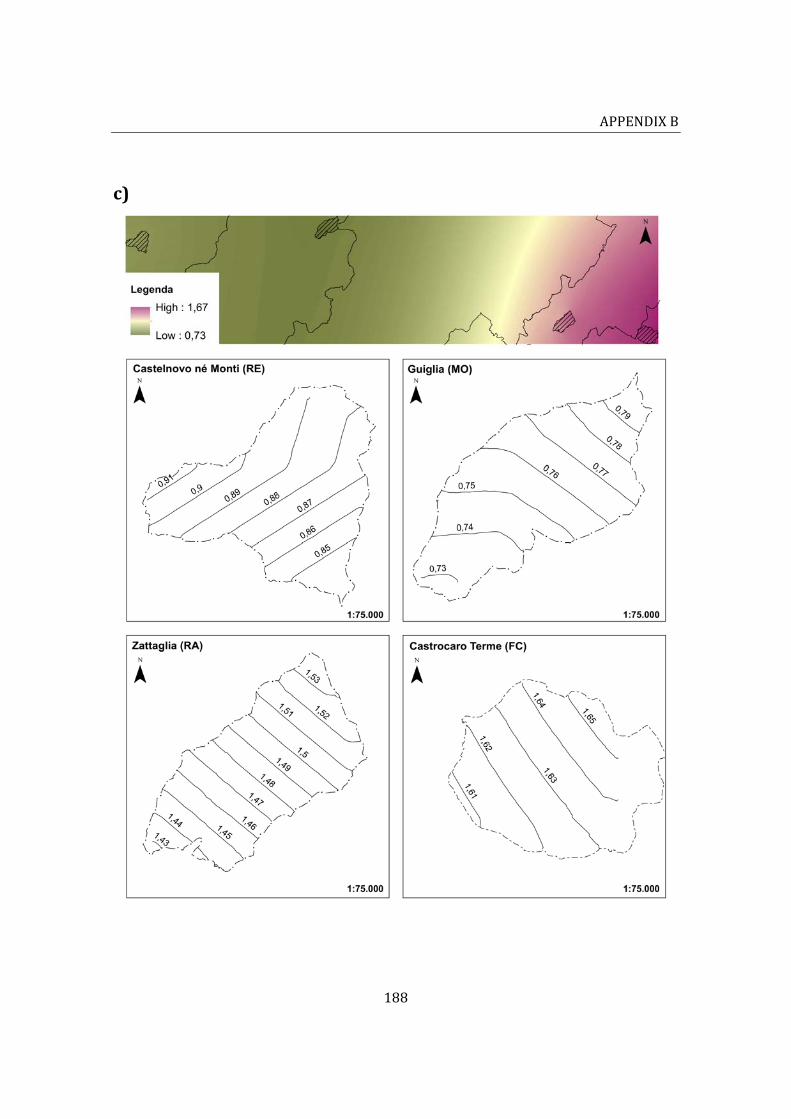
APPENDIXB

188

c)

APPENDIXB

189

d)

APPENDIXB

190

e)