QUALITY-ADAPTIVE MEDIA STREAMING

A Thesis Submitted tothe Graduate School of Engineering and Sciences of

Izmir Institute of Technologyin Partial Fulfillment of the Requirements for the Degree of

MASTER OF SCIENCE

in Computer Engineering

byUras TOS

June 2012IZMIR

We approve the thesis of Uras TOS

Examining Committee Members:

Assist. Prof. Dr. Tolga AYAVDepartment of Computer EngineeringIzmir Institute of Technology

Assist. Prof. Dr. Pars MUTAFInternational Computer InstituteEge University

Assist. Prof. Dr. Tugkan TUGLULARDepartment of Computer EngineeringIzmir Institute of Technology

25 June 2012

Assist. Prof. Dr. Tolga AYAVSupervisor, Department of Computer EngineeringIzmir Institute of Technology

Prof. Dr. I. Sıtkı AYTAC Prof. Dr. R. Tugrul SENGERHead of the Department of Dean of the Graduate School ofComputer Engineering Engineering and Sciences

ACKNOWLEDGMENTS

I would like express my sincerest gratitude to my advisor Assist. Prof. Dr. Tolga

AYAV. His motivation and inspiration during my studies made this research valuable.

I would also like to thank my colleagues at Izmir Institute of Technology Depart-

ment of Computer Engineering for providing me a friendly and productive workplace that

is very helpful for doing scientific research.

Last but not least, I would like to thank my father Turan, my mother Nursen, and

especially my sister Eda for their endless love and care for not only during my research

but also for my whole life. Their everlasting support made this work possible.

ABSTRACT

QUALITY-ADAPTIVE MEDIA STREAMING

In this study, an adaptive method for maximizing network bandwidth utilization

for real-time media streaming applications is presented. The proposed method imple-

ments a rate control approach over the transport protocol RTP. RTP is coupled with an

existing multimedia codec, H.264.

A controller that keeps the RTP packet loss fraction at a predefined reference point

is implemented. During the course of the stream transmission, the information about the

network state is generated by the RTP/RTCP and sent to the server by the clients. Packet

loss fraction parameter is fed into the controller. Controlling the multimedia codec bitrate

directly affects the packet transmission rate, therefore RTP packet transmission rate is

also controlled.

Two control approaches are proposed. Firstly, a PID controller is introduced. This

PID controller is designed without any self adaptation and manually tuned to maximize

all of the available bandwidth. Secondly, a model reference adaptive controller (MRAC)

is proposed. This MRAC controller constantly adjusts its parameters according to a refer-

ence model. The output of the TCP Friendly Rate Control Algorithm (TFRC) is used as

the model to keep the MRAC controller friendly towards other flows flows at a level that

the application requires.

Simulations are provided to demonstrate the operation of the proposed methods.

In the simulations, a content streaming scenario is run against background traffic for the

available bandwidth in a bottleneck network configuration.

iv

OZET

NITELIK OZUYARLI ORTAM AKISI

Bu calısmada, ortam akısı uygulamaları icin bant genisligi kullanımını en ust se-

viyeye cıkaran ozuyarlı bir yontem sunulmaktadır. Onerilen yontem, tasıma protokolu

olarak secilen RTP uzerinde aktarım hızı kontrolu yaklasımı uygulamaktadır. RTP, mev-

cut bir coklu ortam kodlayıcı olan H.264 ile eslenmistir.

Bir denetleyici, RTP paket kaybı oranını daha onceden belirlenmis bir dayanak

noktasında tutmak uzere tasarlanmıstır. Ortam akısı iletimi boyunca ag durumu ile ilgili

bilgiler, RTP/RTCP tarafından uretilir ve istemci tarafından sunucuya gonderilir. Paket

kaybı oranı parametresi denetleyiciye beslenir. Ortam akısı bit hızının kontrol edilmesi,

paket iletim hızını dogrudan etkiler, dolayısıyla RTP paket iletim hızının da denetlenmesi

saglanır.

Iki tur denetleme yaklasımı sunulmaktadır. Birinci olarak, bir PID kontrolcu uygu-

lanmaktadır. Bu PID kontrolcu, mevcut olan bant genisligini en ust seviyede kullanmak

uzere ayarlanmıstır. Ikinci olarak, bir model referansı ozuyarlı kontrolcu ortaya koyul-

maktadır. Bu kontrolcu, bir modele baglı kalacak bicimde, surekli olarak kendi parame-

trelerini ayarlamaktadır. TCP uyumlu hız kontrol algoritmasının cıktısı, kontrolcuyu, TCP

akısları ile uygulama gereksinimleri dogrultusunda uyumlu kılmaktadır.

Onerilen yontemlerin calısmasını gostermek icin, benzetimler sunulmaktadır. Ben-

zetimlerde, ortam akısı icerigi iletimi senaryosu, bir arka plan iletimine karsı, darbogaz

ag yapılandırmasında yurutulmektedir.

v

TABLE OF CONTENTS

LIST OF FIGURES . . . . . . . . . . . . . . . . . . . . . . . . . . . . . . . . . . . . . . . . . . . . . . . . . . . . . . . . . . . . . . . . . . . . . . viii

LIST OF TABLES . . . . . . . . . . . . . . . . . . . . . . . . . . . . . . . . . . . . . . . . . . . . . . . . . . . . . . . . . . . . . . . . . . . . . . . ix

LIST OF SYMBOLS . . . . . . . . . . . . . . . . . . . . . . . . . . . . . . . . . . . . . . . . . . . . . . . . . . . . . . . . . . . . . . . . . . . . x

LIST OF ABBREVIATIONS . . . . . . . . . . . . . . . . . . . . . . . . . . . . . . . . . . . . . . . . . . . . . . . . . . . . . . . . . . . . xi

CHAPTER 1. INTRODUCTION . . . . . . . . . . . . . . . . . . . . . . . . . . . . . . . . . . . . . . . . . . . . . . . . . . . . . . 1

1.1. Goal and Objectives . . . . . . . . . . . . . . . . . . . . . . . . . . . . . . . . . . . . . . . . . . . . . . . . . . . 2

1.2. Organization of Thesis . . . . . . . . . . . . . . . . . . . . . . . . . . . . . . . . . . . . . . . . . . . . . . . . 3

CHAPTER 2. RELATED WORK . . . . . . . . . . . . . . . . . . . . . . . . . . . . . . . . . . . . . . . . . . . . . . . . . . . . . . 5

2.1. Network . . . . . . . . . . . . . . . . . . . . . . . . . . . . . . . . . . . . . . . . . . . . . . . . . . . . . . . . . . . . . . . . 6

2.1.1. Real-time Transport Protocol . . . . . . . . . . . . . . . . . . . . . . . . . . . . . . . . . . . . . 6

2.1.2. TCP-Friendly Rate Control . . . . . . . . . . . . . . . . . . . . . . . . . . . . . . . . . . . . . . . 7

2.2. H.264 Multimedia Codec . . . . . . . . . . . . . . . . . . . . . . . . . . . . . . . . . . . . . . . . . . . . . 8

CHAPTER 3. ADAPTIVE CONTROL OF MULTIMEDIA STREAMS . . . . . . . . . . . . 10

3.1. Feedback Control Systems . . . . . . . . . . . . . . . . . . . . . . . . . . . . . . . . . . . . . . . . . . . . 10

3.2. PID Control of Transmission Rate . . . . . . . . . . . . . . . . . . . . . . . . . . . . . . . . . . . 11

3.3. Model Reference Adaptive Control of Media Transmission Rate . . 14

3.4. Stability Analysis . . . . . . . . . . . . . . . . . . . . . . . . . . . . . . . . . . . . . . . . . . . . . . . . . . . . . . 19

CHAPTER 4. SIMULATION . . . . . . . . . . . . . . . . . . . . . . . . . . . . . . . . . . . . . . . . . . . . . . . . . . . . . . . . . . 23

4.1. Simulation Software . . . . . . . . . . . . . . . . . . . . . . . . . . . . . . . . . . . . . . . . . . . . . . . . . . . 23

4.2. Simulation Environment . . . . . . . . . . . . . . . . . . . . . . . . . . . . . . . . . . . . . . . . . . . . . . 23

4.3. Simulations of PID Controlled Method . . . . . . . . . . . . . . . . . . . . . . . . . . . . . . 24

4.3.1. Simulation Setup . . . . . . . . . . . . . . . . . . . . . . . . . . . . . . . . . . . . . . . . . . . . . . . . . . 25

4.3.2. Simulation Results . . . . . . . . . . . . . . . . . . . . . . . . . . . . . . . . . . . . . . . . . . . . . . . . 26

4.4. Simulations of MRAC Controlled Method . . . . . . . . . . . . . . . . . . . . . . . . . . . 28

vi

4.4.1. Simulation Environment . . . . . . . . . . . . . . . . . . . . . . . . . . . . . . . . . . . . . . . . . . 30

4.4.2. Simulation Results . . . . . . . . . . . . . . . . . . . . . . . . . . . . . . . . . . . . . . . . . . . . . . . . 30

CHAPTER 5. CONCLUSION . . . . . . . . . . . . . . . . . . . . . . . . . . . . . . . . . . . . . . . . . . . . . . . . . . . . . . . . . 35

REFERENCES . . . . . . . . . . . . . . . . . . . . . . . . . . . . . . . . . . . . . . . . . . . . . . . . . . . . . . . . . . . . . . . . . . . . . . . . . . . 37

vii

LIST OF FIGURES

Figure Page

Figure 1.1. A typical use case. . . . . . . . . . . . . . . . . . . . . . . . . . . . . . . . . . . . . . . . . . . . . . . . . . . . . . . . . . . 2

Figure 3.1. Feedback control system for RTP communication . . . . . . . . . . . . . . . . . . . . . . . . 11

Figure 3.2. PID controller used in the proposed method. . . . . . . . . . . . . . . . . . . . . . . . . . . . . . . 12

Figure 3.3. Overview of the proposed model reference adaptive control system. . . . . 15

Figure 3.4. Operation zone of the controller and controller approximation. . . . . . . . . . . 20

Figure 4.1. Network topology used in the simulations. . . . . . . . . . . . . . . . . . . . . . . . . . . . . . . . . 24

Figure 4.2. Background traffic transmission rate. . . . . . . . . . . . . . . . . . . . . . . . . . . . . . . . . . . . . . . 25

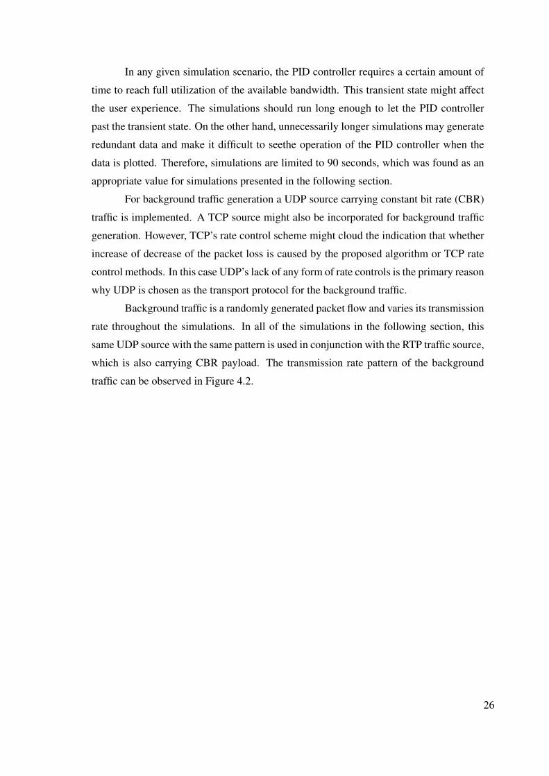
Figure 4.3. Packet loss fraction of 4Mb/s constant rate RTP traffic. RTP traffic is

run alongside the background traffic. . . . . . . . . . . . . . . . . . . . . . . . . . . . . . . . . . . . . . . . 27

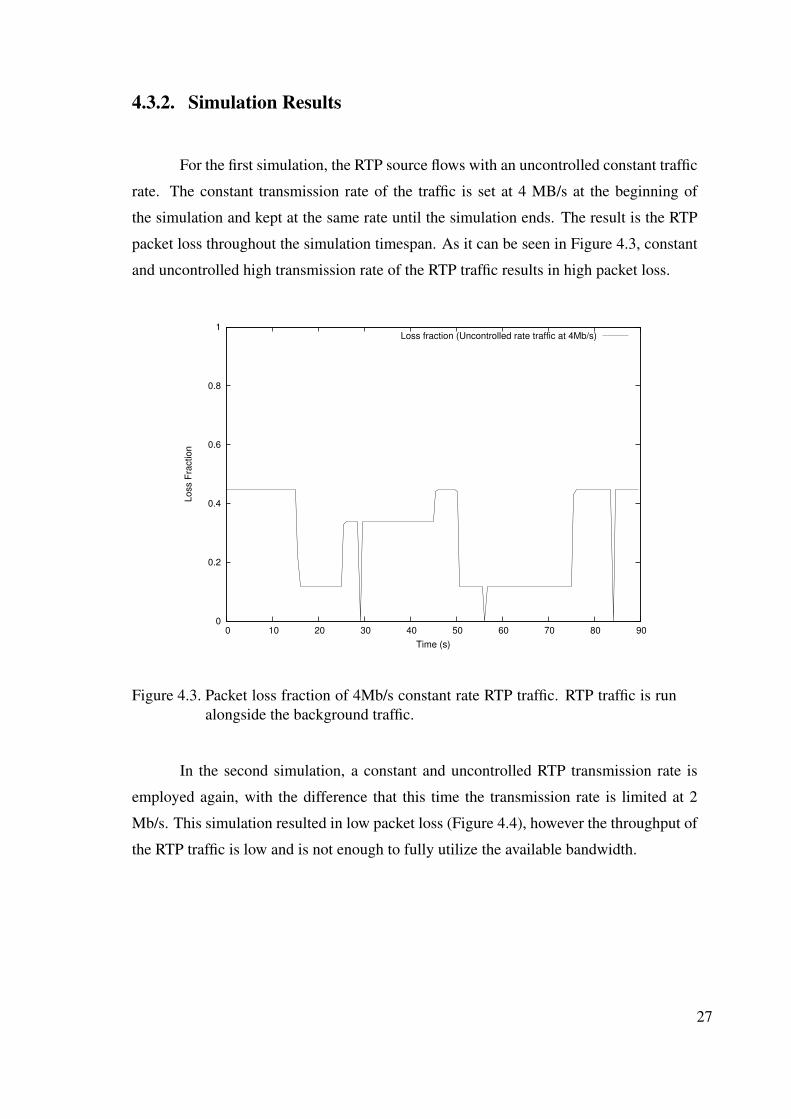
Figure 4.4. Packet loss fraction of 2Mb/s constant rate RTP traffic. RTP traffic is

run alongside the background traffic. . . . . . . . . . . . . . . . . . . . . . . . . . . . . . . . . . . . . . . . 28

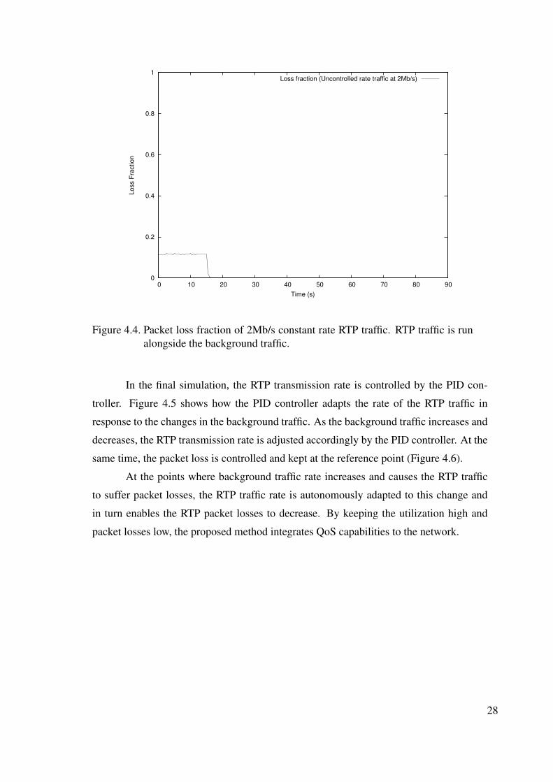
Figure 4.5. Transmission rate of PID controlled RTP traffic. RTP traffic is run

alongside the background traffic. . . . . . . . . . . . . . . . . . . . . . . . . . . . . . . . . . . . . . . . . . . . 29

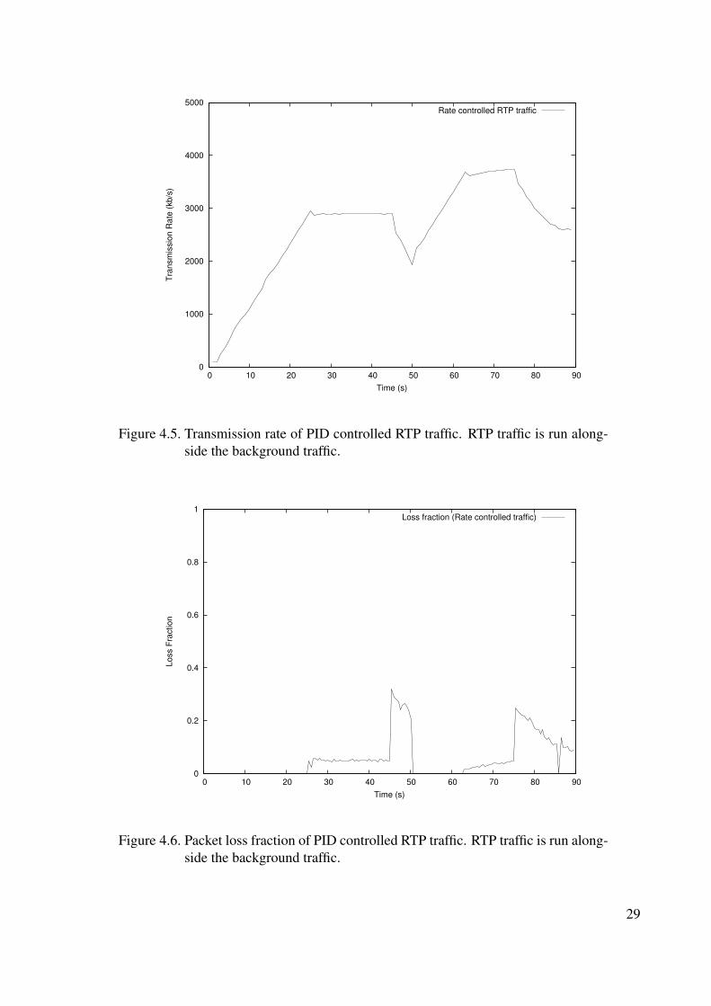
Figure 4.6. Packet loss fraction of PID controlled RTP traffic. RTP traffic is run

alongside the background traffic. . . . . . . . . . . . . . . . . . . . . . . . . . . . . . . . . . . . . . . . . . . . 29

Figure 4.7. Background traffic. . . . . . . . . . . . . . . . . . . . . . . . . . . . . . . . . . . . . . . . . . . . . . . . . . . . . . . . . . . 30

Figure 4.8. Available bandwidth estimation by PID controller. . . . . . . . . . . . . . . . . . . . . . . . 31

Figure 4.9. Available bandwidth according to TFRC algorithm. . . . . . . . . . . . . . . . . . . . . . . 32

Figure 4.10. Available bandwidth according to adaptive PID controller. . . . . . . . . . . . . . . . 33

Figure 4.11. Bandwidth used by H.264 multimedia stream. . . . . . . . . . . . . . . . . . . . . . . . . . . . . 34

Figure 4.12. Packet loss rate during the H.264 multimedia stream. . . . . . . . . . . . . . . . . . . . . 34

viii

LIST OF TABLES

Table Page

Table 3.1. System parameters and their respective values for the PID controlled

method . . . . . . . . . . . . . . . . . . . . . . . . . . . . . . . . . . . . . . . . . . . . . . . . . . . . . . . . . . . . . . . . . . . . . . . . 13

Table 3.2. System parameters and their respective values for the MRAC con-

trolled method . . . . . . . . . . . . . . . . . . . . . . . . . . . . . . . . . . . . . . . . . . . . . . . . . . . . . . . . . . . . . . . . 18

Table 3.3. Example points that shows the stability of the controller . . . . . . . . . . . . . . . . . 22

ix

LIST OF SYMBOLS

t . . . . . . . . . . . . . . . . . . . . . . . . . . . . . . . . . . . . . . . . . . . . . . . . . . . . . . . . . . . . . . Discrete time index

t . . . . . . . . . . . . . . . . . . . . . . . . . . . . . . . . . . . . . . . . . . . . . . . . . . . . . . . . . . . . . . . . . . . . . Actual time

r(t) . . . . . . . . . . . . . . . . . . . . . . . . . . . . . . . . . . . . . . . . . . . . . . . . . . . . . . . . . . . . Reference variable

s(t) . . . . . . . . . . . . . . . . . . . . . . . . . . . . . . . . . . . . . . . . . . . . . . . . . . . . . . . . . . . Controlled variable

e(t) . . . . . . . . . . . . . . . . . . . . . . . . . . . . . . . . . . . . . . . . . . . . . . . . . . . . . . . . . . . . . . . . . . . . . . . . Error

e′(t) . . . . . . . . . . . . . . . . . . . . . . . . . . . . . . . . . . . . . . . . . . . . . . . . . . . . . . . . . . . . .Normalized error

Kp . . . . . . . . . . . . . . . . . . . . . . . . . . . . . . . . . . . . . . . . . . . . . . . . . . . . . . . . . . . . . . Proportional gain

Ki . . . . . . . . . . . . . . . . . . . . . . . . . . . . . . . . . . . . . . . . . . . . . . . . . . . . . . . . . . . . . . . . . . Integral gain

Kd . . . . . . . . . . . . . . . . . . . . . . . . . . . . . . . . . . . . . . . . . . . . . . . . . . . . . . . . . . . . . . . . Derivative gain

P (t) . . . . . . . . . . . . . . . . . . . . . . . . . . . . . . . . . . . . . . . . . . . . . . . . . . . . . . Proportional component

I(t) . . . . . . . . . . . . . . . . . . . . . . . . . . . . . . . . . . . . . . . . . . . . . . . . . . . . . . . . . . . Integral component

D(t) . . . . . . . . . . . . . . . . . . . . . . . . . . . . . . . . . . . . . . . . . . . . . . . . . . . . . . . . Derivative component

Ec . . . . . . . . . . . . . . . . . . . . . . . . . . . . . . . . . . . . . . . . . . . . . . . . . . . . . . . . . . . . . . . . . Error constant

N . . . . . . . . . . . . . . . . . . . . . . . . . . . . . . . . . . . . . . . . . . . . . . . . . . . . . . . . . Normalization function

L . . . . . . . . . . . . . . . . . . . . . . . . . . . . . . . . . . . . . . . . . . . . . . . . . . . . . . . . . . . . . . . Limiting function

SP . . . . . . . . . . . . . . . . . . . . . . . . . . . . . . . . . . . . . . . . . . . . . . . . . . . . . . . . . . . . . . Sampling period

b(t) . . . . . . . . . . . . . . . . . . . . . . . . . . . . . . . . . . . . . . . . . . . . . . . . . . . . . . . . . . . . . Transmission rate

Bmin . . . . . . . . . . . . . . . . . . . . . . . . . . . . . . . . . . . . . . . . . . . . . . . . . . Minimum transmission rate

Bmax . . . . . . . . . . . . . . . . . . . . . . . . . . . . . . . . . . . . . . . . . . . . . . . . . . Maximum transmission rate

y(t) . . . . . . . . . . . . . . . . . . . . . . . . . . . . . . . . . . . . . . . . . . . . . . . . . . . . . . . . . . . . . . . . . . .Packet loss

l . . . . . . . . . . . . . . . . . . . . . . . . . . . . . . . . . . . . . . . . . . . . . . . . . . . . . . . . . . . . . . . . . . . . . .Packet size

Rt . . . . . . . . . . . . . . . . . . . . . . . . . . . . . . . . . . . . . . . . . . . . . . . . . . . . . . . . . . . . . . . Round-trip time

pt . . . . . . . . . . . . . . . . . . . . . . . . . . . . . . . . . . . . . . . . . . . . . . . . . . . . Packet loss fraction in TFRC

u(t) . . . . . . . . . . . . . . . . . . . . . . . . . . . . . . . . . . . . . . . . . . . . . . . . . . . . . . . . . PID controller output

em(t) . . . . . . . . . . . . . . . . . . . . . . . . . . . . . . . . . Error value used in the adjustment mechanism

C(t) . . . . . . . . . . . . . . . . . . . . . . . . . . . . . . . . . . . . . . . . . . . . . . . . . . . . . . . . Codec bitrate function

K ′p . . . . . . . . . . . . . . . . . . . . . . . . . . . . . . . . . . Proportional gain of the adjustment mechanism

K ′i . . . . . . . . . . . . . . . . . . . . . . . . . . . . . . . . . . . . . . . Integral gain of the adjustment mechanism

um(t) . . . . . . . . . . . . . . . . . . . . . . . . . . . . . . . . . . . . . . . . . . . . . . . . . . .Output of TFRC algorithm

Ka . . . . . . . . . . . . . . . . . . . . . . . . . . . . . . . . . . . . . . . . . . . . . . . . . . . . . . . . . . . . . . Adjustment gain

x

LIST OF ABBREVIATIONS

RTP . . . . . . . . . . . . . . . . . . . . . . . . . . . . . . . . . . . . . . . . . . . . . . . . . . Real-time Transport Protocol

RTCP . . . . . . . . . . . . . . . . . . . . . . . . . . . . . . . . . . . . . . . . . . . . . . . . . . . . . . . RTP Control Protocol

TCP . . . . . . . . . . . . . . . . . . . . . . . . . . . . . . . . . . . . . . . . . . . . . . . . Transmission Control Protocol

PID . . . . . . . . . . . . . . . . . . . . . . . . . . . . . . . . . . . . . . . . . . . . . . . . Proportional Integral Derivative

MRAC . . . . . . . . . . . . . . . . . . . . . . . . . . . . . . . . . . . . . . . . . . Model Reference Adaptive Control

TFRC . . . . . . . . . . . . . . . . . . . . . . . . . . . . . . . . . . . . . . . . . . . . . . . . . . TCP Friendly Rate Control

IETF . . . . . . . . . . . . . . . . . . . . . . . . . . . . . . . . . . . . . . . . . . . . . . Internet Engineering Task Force

AIMD . . . . . . . . . . . . . . . . . . . . . . . . . . . . . . . . . . . . . Additive increase multiplicative decrease

CPU . . . . . . . . . . . . . . . . . . . . . . . . . . . . . . . . . . . . . . . . . . . . . . . . . . . . . . Central Processing Unit

MPEG . . . . . . . . . . . . . . . . . . . . . . . . . . . . . . . . . . . . . . . . . . . . . . Moving Picture Experts Group

AVC . . . . . . . . . . . . . . . . . . . . . . . . . . . . . . . . . . . . . . . . . . . . . . . . . . . . . Advanced Video Coding

SP . . . . . . . . . . . . . . . . . . . . . . . . . . . . . . . . . . . . . . . . . . . . . . . . . . . . . . . . . . . . . . . Sampling period

NS2 . . . . . . . . . . . . . . . . . . . . . . . . . . . . . . . . . . . . . . . . . . . . . . The Network Simulator version 2

UDP . . . . . . . . . . . . . . . . . . . . . . . . . . . . . . . . . . . . . . . . . . . . . . . . . . . . . . User Datagram Protocol

CBR . . . . . . . . . . . . . . . . . . . . . . . . . . . . . . . . . . . . . . . . . . . . . . . . . . . . . . . . . . . . . Constant bit rate

QoS . . . . . . . . . . . . . . . . . . . . . . . . . . . . . . . . . . . . . . . . . . . . . . . . . . . . . . . . . . . . Quality of service

RTT. . . . . . . . . . . . . . . . . . . . . . . . . . . . . . . . . . . . . . . . . . . . . . . . . . . . . . . . . . . . . .Round-trip time

xi

CHAPTER 1

INTRODUCTION

In the recent years, multimedia content delivery over networks has greatly in-

creased. Rising popularity of smartphones, movie streaming services and video telephony

services over the Internet greatly contributes to this increase. As the quality demand of

these services increase in terms of audio and video definition, bandwidth requirements

of these services also pushes the boundaries of the present network infrastructures. The

bandwidth intensive nature of multimedia streaming can strain any network. At this point,

without any form of bandwidth sharing and transmission rate control, this bandwidth

strain would undoubtedly cause network congestions.

TCP and UDP are the popular transmission protocols used on the Internet today.

If those two most popular network protocols and their properties are evaluated, how they

would or would not be suitable for multimedia streaming can be better understood.

On one hand there is TCP and its very rich feature set. This feature set includes

transmission rate control, retransmission, sequencing, etc.. Even the rate control capabil-

ities of TCP alone is enough for a TCP traffic to adapt the packet flow to the changing

network conditions. However, the rich feature set brings its own overhead to TCP. As

a result, this makes TCP a heavyweight protocol. In addition, the bursty sending nature

of TCP also make it a less than ideal protocol choice for multimedia streaming. A recent

study shows that an acceptable multimedia streaming scenario would require almost twice

the bandwidth of the multimedia bitrate as stated by Wang et al. (2008).

On the other hand there is UDP, which is the lightweight counterpart of the two

popular network protocols. Due to its connectionless nature, lack of flow control, re-

transmission, and sequencing; UDP has much smaller overhead compared to TCP. The

lightweight architecture of UDP makes it more suitable to real-time applications e.g. mul-

timedia content delivery. However, because of those same features that make the UDP

lightweight, UDP is not very suitable for the purposes of media streaming. Lack of trans-

mission rate control causes UDP to be not friendly towards other streams on the shared

bandwidth resource. In addition, if the application required a to implement a transmis-

sion rate control method on UDP, it would most certainly require introducing additional

1

header fields simply because UDP does not have built-in sequencing. There are cases

where UDP can be considered suitable, however, for the purposes of this study it is not an

ideal candidate.

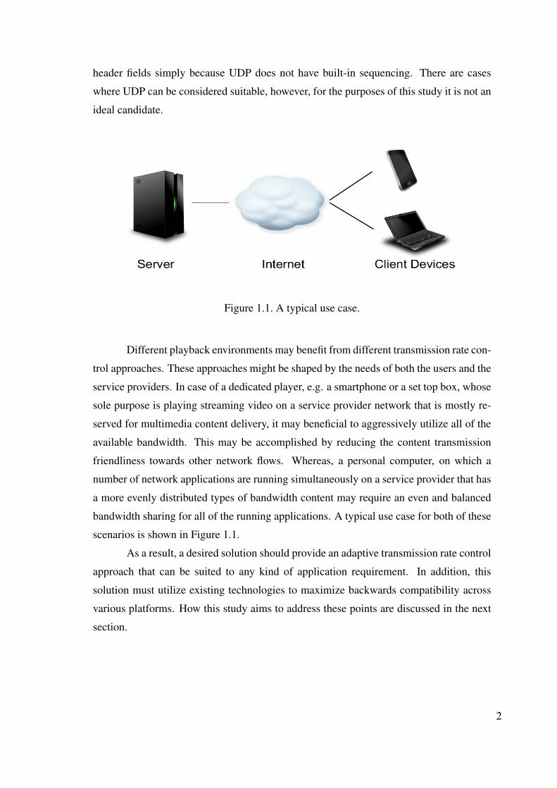
Figure 1.1. A typical use case.

Different playback environments may benefit from different transmission rate con-

trol approaches. These approaches might be shaped by the needs of both the users and the

service providers. In case of a dedicated player, e.g. a smartphone or a set top box, whose

sole purpose is playing streaming video on a service provider network that is mostly re-

served for multimedia content delivery, it may beneficial to aggressively utilize all of the

available bandwidth. This may be accomplished by reducing the content transmission

friendliness towards other network flows. Whereas, a personal computer, on which a

number of network applications are running simultaneously on a service provider that has

a more evenly distributed types of bandwidth content may require an even and balanced

bandwidth sharing for all of the running applications. A typical use case for both of these

scenarios is shown in Figure 1.1.

As a result, a desired solution should provide an adaptive transmission rate control

approach that can be suited to any kind of application requirement. In addition, this

solution must utilize existing technologies to maximize backwards compatibility across

various platforms. How this study aims to address these points are discussed in the next

section.

2

1.1. Goal and Objectives

The motivation of this thesis is to implement a multimedia streaming solution that

can adjust the content transmission bitrate according to the network conditions. Addi-

tionally, the proposed solution should not only adapt the stream bitrate, it should also

autonomously adapt itself to the needs of the application as well. These needs might

range from maximum bandwidth utilization to total fairness towards other packet streams

that exist on the shared bandwidth.

It should be noted that, any proposed method should aim to accomplish its goals

without altering the structure of the transport protocol or making changes to the video

coding algorithm. Therefore, this study specifically targets to employ readily available

components to maximize compatibility with existing systems.

The rate control methods proposed in this study are based on sender adaptation.

Sender adaptation is a transmission rate adjustment scheme in which the traffic source

adjusts the packet transmission rate to respond changing conditions of the network.

In this method, sender adaptation is applied to the packet traffic and adaptation

is accomplished by altering the transmission rate of the network packets by a controller

that keeps the packet loss rate of the packet traffic at a predefined value. Packet loss rate

parameter must be readily available or it should be obtained with existing features of the

network protocol chosen for the application.

In order to achieve the goals described, adaptive control mechanisms for RTP/RTCP

are proposed. Without altering the protocol, the proposed methods vary the multimedia

codec bitrate by controlling the network packet loss rate reported by the RTCP reports

that generated by the clients.

1.2. Organization of Thesis

This thesis is organized as follows:

Chapter 2 provides general information about adaptive multimedia streaming and

more specifically RTP transmission rate control. Additionally, background information

on the methods and technologies used to implement the proposed methods is provided.

Chapter 3 describes the proposed methods that provide the basis of this study.

Mapping of the parameters and fields of RTP communication to feedback control systems

3

is explained. The two proposed methods for controlling the transmission rate are given in

detail in their two respective sections. Finally, control theoretical analysis is presented in

the section of the chapter.

Chapter 4 describes the simulations. A brief summary of the chosen simulation

software is provided. Also, the details of the network topology on which the tests are

performed is described. Finally, simulation results for both of the provided methods are

presented.

Chapter 5 gives the conclusion of the thesis. The contribution of this work is

summarized and possible future work is discussed in this chapter.

4

CHAPTER 2

RELATED WORK

Eckart et al. (2008) proposes PA-UDP, a method to maximize data transfer over

high throughput network links. PA-UDP uses UDP for data transmission and TCP for

control packets that carry network statistics. PA-UDP also extends its adaptation features

over the CPU and disk performance of the endpoints. Barberis et al. (2001) implements a

rate control method for RTP traffic with additive increase multiplicative decrease (AIMD)

approach. AIMD algorithm increments and decrements the transmission rate at a constant

pace throughout the course of network transmission. Ling and ShaoWen (2009) provides

means to control RTP flow by employing low pass filters and a constant increase/decrease

method that depends on the last known state of the network. Sisalem and Wolisz (1999)

and Sisalem (1997) propose adaptive methods for sender rate adaptation which is es-

sentially a modified AIMD algorithm. This method perform calculates increment and

decrement amounts as a function of the current and previous network state. Wanxiang

and Zhenming (2001) also uses a similar approach for adjusting RTP transmission rate.

This method proposes an improved determination of increment and decrement amounts

for the RTP transmission rate.

Schierl et al. (2005) and Burza et al. (2007) propose MPEG compliant adaptive

video streaming solutions that focus only on wireless networks using RTP as the transport

protocol. Grieco and Mascolo (2004) and Bernaschi et al. (2005) follow a generic ap-

proach to the problem by focusing on the network side without integrating a video codec

to the system. The latter also focuses on TCP friendliness. Kuschnig et al. (2010) eval-

uates a TCP based approach to the problem and uses H.264 as the video codec. Tos and

Ayav (2011) proposes a sender adaptation method to control RTP traffic flow but does not

offer a solution to multimedia streaming problem. Bouras and Gkamas (2003) proposes

a multimedia streaming solution using RTP, but the proposed method does not provide

means to adjust the level of the adaptation.

Proposed AIMD algorithms that control RTP traffic rate relies on additively in-

creasing and multiplicatively decreasing the RTP traffic rate according to the network

state described in the RTCP reports. An intelligent algorithm should not only rely on the

5

present state and the last state before the present state. Doing so means that the algo-

rithm loses track of the history of the network status. In a typical scenario that the RTCP

receiver reports are generated every 500 milliseconds, it takes at least two subsequent

receiver reports to gather information about the trend in the changing condition of the

network. Using the network status information gathered only in the last 1 second might

not be enough to correctly understand the trend of the traffic flow going on at that specific

point in time.

2.1. Network

In this section, a brief background information is provided about the network re-

lated technologies that are employed in this study.

2.1.1. Real-time Transport Protocol

The Real-time Transport Protocol (RTP) is a protocol standard designed for de-

livering multimedia content over IP networks. RTP was developed by Internet Engineer-

ing Task Force (IETF) and first introduced in RFC 1889 (Group et al. (1996)). Later, it

reached its current state in 2003 as published in RFC 3550 (Schulzrinne et al. (2003)).

RTP is a networking protocol specifically designed for real-time application needs.

RTP works in conjunction with RTCP, the RTP Control Protocol (RTCP). While the RTP

carries the multimedia payload, RTCP is responsible for monitoring the transmission

quality and providing statistics of the RTP stream. These statistics include a variety of

information ranging from the packet loss fraction to transmission jitter.

Especially in multimedia audio and video streaming applications, in which the

need of end-to-end QoS for efficient transmission is critical, transmission rate control is

necessary as described by Bouras and Gkamas (2003); Wagner et al. (2009); Papadim-

itriou and Tsaoussidis (2007). Even though RTP does not have rate control functionality

implemented in the specification, it has the means to gather information about the network

state by the RTCP status packets.

RTP header includes a field that contains the sequence number. This field con-

tains a number that sequentially increases and marks each packet for identification. Upon

6

receipt of the packets, the clients evaluate the sequence numbers to detect whether any

packets are missing in the sequence of packets.

RTCP protocol generates four type of report packets:

• Sender reports (SR)

• Receiver reports (RR)

• Source description (SDES) items

• Bye message

From these four types of reports, RTCP receiver reports are the one relevant to the

goals of this thesis. The collected statistic of packet loss fraction, that is explained earlier,

is sent in the receiver report packets. The period of this report packets are application

specific. Therefore, a server has the ability to determine the fraction of the packets lost

in a given timespan. This report period is usually set in such a way that RTCP does not

consume more than 5 percent of the stream bandwidth.

The packet loss fraction is calculated by dividing the number of packets lost by

number of packet expected. Since the number of packets lost is the difference between

number of packets received and number of packets expected, the fraction of packets lost

can be represented as follows:

fraction = 1− received

expected(2.1)

However, the interpretation of the information contained in these feedback reports

is left to the application that employs RTP as the transport protocol. The scope of this

thesis is interpreting these feedback reports to create and an adaptive rate control scheme

for the multimedia stream, and in return, the RTP traffic source.

2.1.2. TCP-Friendly Rate Control

TCP-Friendly Rate Control (TFRC) is a transmission rate control mechanism de-

signed for protocols that are operating in the same environment and competing with TCP

traffic (Floyd et al. (2008)).

7

TFRC does not provide a complete protocol description. Instead, it specifies a rate

control algorithm that can be integrated into other transport protocols such as, RTP. This

algorithm is basically a function that is derived from TCP throughput equation (Floyd

et al. (2000)).

TFRC is designed in such a way that, when the protocol implementing TFRC for

rate control competes with TCP flows for bandwidth, the flows become reasonably fair

towards each other. However, the specification states that, TFRC has a lower through-

put variation over time compared to TCP which makes it suitable for streaming media

applications where smoothness of packet transmission is of key importance.

When in operation, TFRC rate control mechanism works as follows:

• Receiver calculates the fraction of packet loss and transmits this information to the

sender.

• Sender calculates the round-trip time.

• Packet loss fraction and round-trip time are fed into TFRC throughput equation.

• Sender adjusts the transmission rate according to the TFRC algorithm’s output.

Instead of directly using TFRC algorithm as the rate control mechanism, the work

presented in this thesis accepts it as a model to be employed in the model reference adap-

tive controller.

2.2. H.264 Multimedia Codec

In this thesis, transmission rate control is achieved by varying the multimedia

stream bitrate. Therefore any video codec with stream switching or scalable encoding can

be used by the application. Because of its widespread use in the time of publication of

this thesis, H.264 is chosen as the multimedia codec in the simulations.

H.264 is a relatively new video codec standard that aims achieve high quality video

in relatively low bitrates. Also known as AVC (Advanced Video Coding, MPEG-4 Part

10), H.264 is actually defined in an identical pair of standards maintained by different

organizations, together known as the Joint Video Team (JVT). While MPEG-4 Part 10

is an ISO/IEC standard, it was developed in cooperation with the ITU, an organization

heavily involved in broadcast television standards (Marpe et al. (2006)).

8

The idea behind the development of the H.264/AVC codec was to create a standard

capable of providing good video quality at significantly lower bit rates than previous

standards without increasing the complexity of the design. Increasing the complexity was

avoided because it would be impractical or expensive to implement. In addition, flexibility

to allow the standard to be applicable to a wide selection of networks and platforms was

also aimed.

The H.264 standard can be considered as a family of standards (Schwarz et al.

(2007)). In this family, there are various profiles and specifications for different appli-

cations of H.264 codec. In this thesis, baseline profile of H.264/AVC is employed in

the simulations. Packetization of H.264 data over RTP is out of scope of this thesis and

implemented as described by Wang et al. (2011).

9

CHAPTER 3

ADAPTIVE CONTROL OF MULTIMEDIA STREAMS

In this chapter, the details of the proposed methods are presented. First section

describes how feedback control approach is applied to network communication. This

provides basis for the latter two sections, in which the actual work done is discussed in

detail.

Second section gives the details of using a PID control approach for controlling

RTP transmission rate. This part of the work is performed at earlier stages of the thesis

with the aim of whether a control theoretical approach is suitable for transmission rate

control.

Third section is where the multimedia transmission and model reference adaptive

control is introduced. After the progress of the second section, the controller idea is

taken one step further and coupled with a multimedia codec to develop a more complete

solution.

Final section explains the control theoretical aspect of the proposed methods. Sta-

bility properties of the control system is evaluated and the stability conditions of the sys-

tem is presented.

3.1. Feedback Control Systems

In order introduce an autonomic behavior, we first map the classical feedback

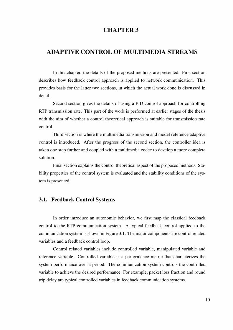
control to the RTP communication system. A typical feedback control applied to the

communication system is shown in Figure 3.1. The major components are control related

variables and a feedback control loop.

Control related variables include controlled variable, manipulated variable and

reference variable. Controlled variable is a performance metric that characterizes the

system performance over a period. The communication system controls the controlled

variable to achieve the desired performance. For example, packet loss fraction and round

trip delay are typical controlled variables in feedback communication systems.

10

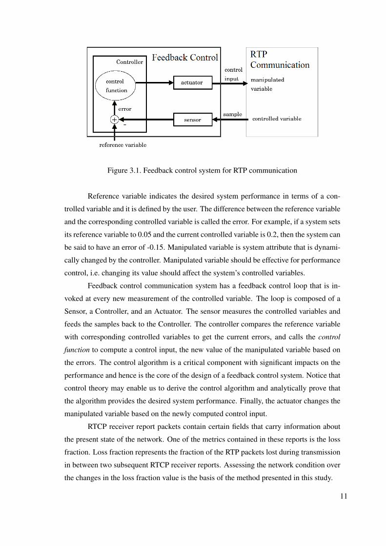
Figure 3.1. Feedback control system for RTP communication

Reference variable indicates the desired system performance in terms of a con-

trolled variable and it is defined by the user. The difference between the reference variable

and the corresponding controlled variable is called the error. For example, if a system sets

its reference variable to 0.05 and the current controlled variable is 0.2, then the system can

be said to have an error of -0.15. Manipulated variable is system attribute that is dynami-

cally changed by the controller. Manipulated variable should be effective for performance

control, i.e. changing its value should affect the system’s controlled variables.

Feedback control communication system has a feedback control loop that is in-

voked at every new measurement of the controlled variable. The loop is composed of a

Sensor, a Controller, and an Actuator. The sensor measures the controlled variables and

feeds the samples back to the Controller. The controller compares the reference variable

with corresponding controlled variables to get the current errors, and calls the control

function to compute a control input, the new value of the manipulated variable based on

the errors. The control algorithm is a critical component with significant impacts on the

performance and hence is the core of the design of a feedback control system. Notice that

control theory may enable us to derive the control algorithm and analytically prove that

the algorithm provides the desired system performance. Finally, the actuator changes the

manipulated variable based on the newly computed control input.

RTCP receiver report packets contain certain fields that carry information about

the present state of the network. One of the metrics contained in these reports is the loss

fraction. Loss fraction represents the fraction of the RTP packets lost during transmission

in between two subsequent RTCP receiver reports. Assessing the network condition over

the changes in the loss fraction value is the basis of the method presented in this study.

11

3.2. PID Control of Transmission Rate

With the aim of autonomously adapting RTP transmission rate, a PID controller

is implemented as shown in Figure 3.2. In the PID controller, RTP packet loss fraction,

denoted with s(t), is gathered from the RTCP receiver reports and used as the controlled

variable.

RTCP

N I

s(t)

r(t)

u(t)Plant��

+

- +

b(t)e(t) e'(t)

D

P

+

+

Ly(t)

Figure 3.2. PID controller used in the proposed method.

The error value (e(t)), is calculated by subtracting the controlled variable (s(t))

from the reference variable (r(t)). Since the value of s(t) is gathered from the RTCP

receiver reports, it is assumed that there is no measurement error.

e(t) = r(t)− s(t) (3.1)

Calculated error value is normalized by the error normalization function (N (e(t)))

and fed into the PID controller as the normalized error, denoted by e′(t).

e′(t) = N (e(t)) =

{Ece(t) if e(t) > 0

e(t) if e(t) < 0(3.2)

At any given time the packet loss fraction indicated by the RTCP receiver reports

ranges from 0 to 1. In this application, 0.05 is chosen as the reference variable to keep the

RTP packet loss at a relatively minimum, while allowing enough packet loss to enable the

PID controller to manipulate the transmission rate. However, there is a significant differ-

ence in the absolute values of the maximum values of positive and negative error values.

If the error is fed into the controller without any form of normalization, this would cause

12

an unwanted biasing effect. This effect results in the controller to run in the b(t) incre-

ment direction slower than it runs in the b(t) decrement direction. In order to eliminate

this unfair behavior, PID controller is designed to have an asymmetrical structure (Baskys

and Zlosnikas (2006)). The asymmetrical operation is ensured by the error normalization

function (N (e(t))). Error normalization function multiplies the error value by an error

constant (Ec) if the error value is greater than zero.

The controller starts the RTP traffic with the minimum transmission rate (Bmin)

and measures the value of the RTP packet loss fraction gathered by the RTCP receiver

reports at each sampling period (SP ). After the measurement, the controller compares

the measurement against the reference value. P, I and D components of the controller

performs the necessary calculations according to the error. Finally the controller gener-

ates a new RTP transmission rate to be used by the RTP sender. The parameters of the

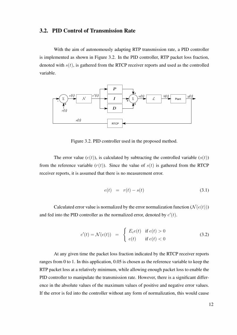
controller is manually tuned (Ang et al. (2005)) to maximize bandwidth utilization. This

manually tuned gain values and other system parameters of the PID controller can be seen

in Table 3.1.

Table 3.1. System parameters and their respective values for the PID controlled method

Parameter Value

Proportional gain (Kp) 1200000Integral gain (Ki) 410000Derivative gain (Kd) 150000Error constant (Ec) 0.15Reference variable (r(t)) 0.05Sampling period (SP ) 500 msMinimum transmission rate (Bmin) 100 kb/sMaximum transmission rate (Bmax) 5 Mbit/s

The PID controller consists of three components as described by Johnson et al.

(2005). First component of the PID controller is P (t), namely the proportional compo-

nent. The output of the proportional component is the multiplication of proportional gain,

denoted by Kp, and the normalized error value. Second component is I(t), the integral

component. Integral component is the product of integral gain, denoted by Ki and the

sum of normalized error values from time index 0 to time index t. Final component is

D(t), the derivative component. Derivative component is the product of the derivative

gain, Kd, and the difference between current and previous value of the normalized error.

13

P (t) = Kpe′(t) (3.3)

I(t) = Ki

t∑i=0

e′(i) (3.4)

D(t) = Kd(e′(t)− e′(t− 1)) (3.5)

u(t) = P (t) + I(t) +D(t) (3.6)

After each component of the PID controller is calculated, the sum of outputs is

fed into the limiting function, L(u(t)). In the cases where the packet loss fraction cannot

be decreased within the acceptable limits even though RTP transmission rate is slowed

down to the point of nearly stopping, the PID controller might continue to decrease RTP

transmission rate and eventually stop it. This is an unwanted situation. The PID controller

gets the feedback from RTCP receiver reports. In order to have a continuous flow of

RTCP receiver reports to be generated, there needs to be an RTP traffic in transit. If the

PID controller is let to decrease RTP transmission rate to the point of stopping, the whole

operation of the system is crippled. Therefore, a limiting function, denoted by L(u(t)),is implemented on RTP traffic reduction. If the adjusted RTP transmission rate reaches

to the point of the minimum allowed transmission rate (Bmin), RTP transmission rate is

limited to Bmin and is not allowed to decrease further more. Similarly, RTP transmission

rate cannot exceed the bandwidth of the link, namely Bmax. In this manner, the output of

the limiting function is used as the new transmission rate (b(t+ 1)) for RTP traffic.

L(u(t)) =

Bmax if u(t) > Bmax

Bmin if u(t) < Bmin

u(t) if Bmin ≤ u(t) ≤ Bmax

(3.7)

b(t+ 1) = L(u(t)) (3.8)

Once b(t+1) is calculated, RTP packet transmission rate is immediately set at this

value and RTP traffic continues to flow. The PID controller waits for the sampling period

(SP ) amount of time until a new RTCP receiver report packet is received. Upon the arrival

of the new RTCP receiver report packet, the PID controller calculates the new traffic rate

according to the new packet loss fraction. This autonomous operation continues to run as

long as there is RTP traffic flow from the sender. It should be noted that, let t ∈ N denote

the discrete time index, i.e. the actual time t can be computed as t = SP t.

14

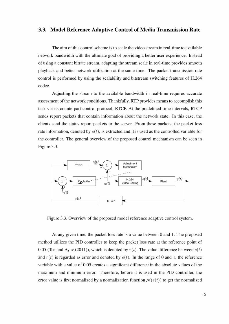
3.3. Model Reference Adaptive Control of Media Transmission Rate

The aim of this control scheme is to scale the video stream in real-time to available

network bandwidth with the ultimate goal of providing a better user experience. Instead

of using a constant bitrate stream, adapting the stream scale in real-time provides smooth

playback and better network utilization at the same time. The packet transmission rate

control is performed by using the scalability and bitstream switching features of H.264

codec.

Adjusting the stream to the available bandwidth in real-time requires accurate

assessment of the network conditions. Thankfully, RTP provides means to accomplish this

task via its counterpart control protocol, RTCP. At the predefined time intervals, RTCP

sends report packets that contain information about the network state. In this case, the

clients send the status report packets to the server. From these packets, the packet loss

rate information, denoted by s(t), is extracted and it is used as the controlled variable for

the controller. The general overview of the proposed control mechanism can be seen in

Figure 3.3.

RTCP

TFRC

Controller

Adjustment

Mechanism

H.264

Video Coding

s(t)

r(t)

u(t)

b(t)

u (t)m

Plant

�

�

+

-

+

-

y(t)

Figure 3.3. Overview of the proposed model reference adaptive control system.

At any given time, the packet loss rate is a value between 0 and 1. The proposed

method utilizes the PID controller to keep the packet loss rate at the reference point of

0.05 (Tos and Ayav (2011)), which is denoted by r(t). The value difference between s(t)

and r(t) is regarded as error and denoted by e(t). In the range of 0 and 1, the reference

variable with a value of 0.05 creates a significant difference in the absolute values of the

maximum and minimum error. Therefore, before it is used in the PID controller, the

error value is first normalized by a normalization function N (e(t)) to get the normalized

15

error, e′(t). Normalization function works toward balancing the controller to work in

both b(t) increment and decrement directions more fairly through an asymmetrical control

approach (Baskys and Zlosnikas (2006)).

e(t) = r(t)− s(t) (3.9)

e′(t) = N (e(t)) =

{Ece(t) if e(t) > 0

e(t) if e(t) < 0(3.10)

Calculated e′(t) value is fed into the PID controller. The controller consists of

three parallel functions (Johnson et al. (2005)). First function is the proportional com-

ponent, denoted by P (t). The output of the P (t) is the multiplication of e′(t) and the

proportional gain Kp. Secondly, the integral component I(t) is calculated by multiplying

accumulated e′(t) value with the integral gain, Ki. Finally the derivative gain, D(t), is

calculated by multiplying the derivative gain, Kd, with the difference of the last and cur-

rent values of e′(t). The output u(t) of the PID controller is the sum of the outputs of all

the components.

P (t) = Kpe′(t) (3.11)

I(t) = Ki

t∑i=0

e′(i) (3.12)

D(t) = Kd(e′(t)− e′(t− 1)) (3.13)

u(t) = P (t) + I(t) +D(t) (3.14)

The controller is initially tuned by using Ziegler-Nichols method (Ziegler and

Nichols (1942)) to ensure stability. In addition, manual fine tuning is performed. As a

result, the PID controller is tuned to aggressively utilize all of the available bandwidth, as

long as the PID controller is used standalone without any further adaptive control.

However, as mentioned in the earlier sections, the aim of this work is to design

an adaptive controller that changes its behavior according to the application expectations.

This adaptive behavior is crucial for obtaining a predefined degree of TCP friendliness.

For this reason, instead of a simple PID controller; a more complex model reference

adaptive controller (MRAC) is implemented.

16

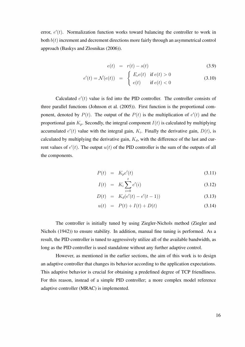
In the proposed method, TCP Friendly Rate Control (TFRC) algorithm (Floyd

et al. (2008)) is employed as the reference model for the MRAC. TFRC is designed in such

a way that any network stream that employs it as the transmission rate control algorithm,

that stream is considered to be friendly towards TCP flows. The output of TFRC algorithm

that serves as the model is denoted with um(t). The output equation derived from TCP

throughput equation is given as:

um(t) =l

Rt(√

2s(t)3

+ 12s(t)√

3s(t)8

(1 + 32(s(t))2))(3.15)

where l denotes the packet size, Rt denotes the round-trip time in seconds and s(t) is the

packet loss fraction.

At any given time, there is a difference between the output of the PID controller

u(t) and TFRC algorithm’s output um(t). This output difference is considered as the error

value for the adjustment mechanism and it is denoted by em(t).

em(t) = um(t)− u(t) (3.16)

The adjustment mechanism component of the MRAC is basically a PI controller

that operates to minimize em(t) value. Instead of a PID controller, a PI control scheme

is adopted in order to ease the initial tuning process. In this PI controller, the propor-

tional gain is denoted by K ′p and the integral gain is denoted by K ′

i. In the adjustment

mechanism, the of TFRC algorithm, um(t), becomes the reference variable and the PID

controller’s output, u(t), becomes the controlled variable. The output of the adjustment

mechanism, the adjustment gain is denoted by Ka. This adjustment gain is used to ma-

nipulate the Kp, Ki and Kd constants of the PID controller.

Ka = K ′pem(t) +K ′

i

t∑i=0

em(i) (3.17)

How the value of Ka affects the PID controller’s gain constants can be observed

in Table 3.2 alongside other values for the proposed system.

In normal operation, the controller starts the multimedia stream with the minimum

transmission rate (Bmin) by selecting the minimum bitrate for the multimedia stream. The

17

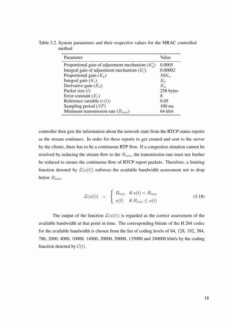
Table 3.2. System parameters and their respective values for the MRAC controlledmethod

Parameter Value

Proportional gain of adjustment mechanism (K ′p) 0.0005

Integral gain of adjustment mechanism (K ′i) 0.00002

Proportional gain (Kp) 10Ka

Integral gain (Ki) Ka

Derivative gain (Kd) Ka

Packet size (l) 258 bytesError constant (Ec) 8Reference variable (r(t)) 0.05Sampling period (SP ) 100 msMinimum transmission rate (Bmin) 64 kb/s

controller then gets the information about the network state from the RTCP status reports

as the stream continues. In order for these reports to get created and sent to the server

by the clients, there has to be a continuous RTP flow. If a congestion situation cannot be

resolved by reducing the stream flow to the Bmin, the transmission rate must not further

be reduced to ensure the continuous flow of RTCP report packets. Therefore, a limiting

function denoted by L(u(t)) enforces the available bandwidth assessment not to drop

below Bmin.

L(u(t)) =

{Bmin if u(t) < Bmin

u(t) if Bmin ≤ u(t)(3.18)

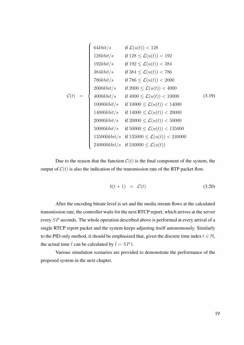
The output of the function L(u(t)) is regarded as the correct assessment of the

available bandwidth at that point in time. The corresponding bitrate of the H.264 codec

for the available bandwidth is chosen from the list of coding levels of 64, 128, 192, 384,

786, 2000, 4000, 10000, 14000, 20000, 50000, 135000 and 240000 kbit/s by the coding

function denoted by C(t).

18

C(t) =

64kbit/s if L(u(t)) < 128

128kbit/s if 128 ≤ L(u(t)) < 192

192kbit/s if 192 ≤ L(u(t)) < 384

384kbit/s if 384 ≤ L(u(t)) < 786

786kbit/s if 786 ≤ L(u(t)) < 2000

2000kbit/s if 2000 ≤ L(u(t)) < 4000

4000kbit/s if 4000 ≤ L(u(t)) < 10000

10000kbit/s if 10000 ≤ L(u(t)) < 14000

14000kbit/s if 14000 ≤ L(u(t)) < 20000

20000kbit/s if 20000 ≤ L(u(t)) < 50000

50000kbit/s if 50000 ≤ L(u(t)) < 135000

135000kbit/s if 135000 ≤ L(u(t)) < 240000

240000kbit/s if 240000 ≤ L(u(t))

(3.19)

Due to the reason that the function C(t) is the final component of the system, the

output of C(t) is also the indication of the transmission rate of the RTP packet flow.

b(t+ 1) = C(t) (3.20)

After the encoding bitrate level is set and the media stream flows at the calculated

transmission rate, the controller waits for the next RTCP report, which arrives at the server

every SP seconds. The whole operation described above is performed at every arrival of a

single RTCP report packet and the system keeps adjusting itself autonomously. Similarly

to the PID only method, it should be emphasized that, given the discrete time index t ∈ N,

the actual time t can be calculated by t = SP t.

Various simulation scenarios are provided to demonstrate the performance of the

proposed system in the next chapter.

19

3.4. Stability Analysis

Under normal conditions, i.e. past the transient state, the controller must be stable.

When the packet transmission rate exceeds the available bandwidth, packet losses occur

and the transmission rate is reduced. Similarly, when the existing amount of packet loss

is under the reference variable, the packet transmission rate is increased. Therefore, it is

safe to say that the controller must have a tendency to stay at an equilibrium point.

0

1

0 B

Packe

t lo

ss fra

ctio

n (

s(t

))

Bandwidth (u(t))

max

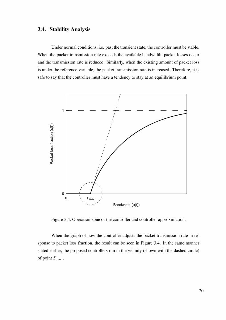
Figure 3.4. Operation zone of the controller and controller approximation.

When the graph of how the controller adjusts the packet transmission rate in re-

sponse to packet loss fraction, the result can be seen in Figure 3.4. In the same manner

stated earlier, the proposed controllers run in the vicinity (shown with the dashed circle)

of point Bmax.

20

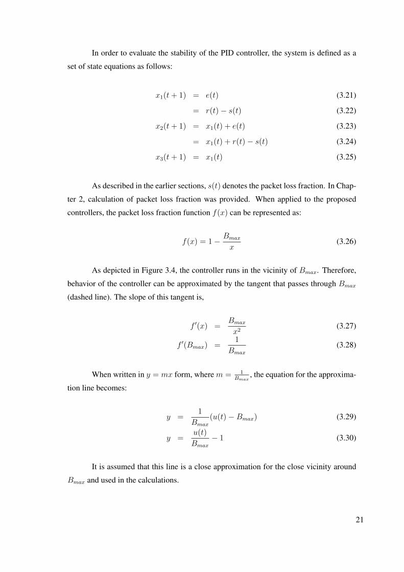
In order to evaluate the stability of the PID controller, the system is defined as a

set of state equations as follows:

x1(t+ 1) = e(t) (3.21)

= r(t)− s(t) (3.22)

x2(t+ 1) = x1(t) + e(t) (3.23)

= x1(t) + r(t)− s(t) (3.24)

x3(t+ 1) = x1(t) (3.25)

As described in the earlier sections, s(t) denotes the packet loss fraction. In Chap-

ter 2, calculation of packet loss fraction was provided. When applied to the proposed

controllers, the packet loss fraction function f(x) can be represented as:

f(x) = 1− Bmax

x(3.26)

As depicted in Figure 3.4, the controller runs in the vicinity of Bmax. Therefore,

behavior of the controller can be approximated by the tangent that passes through Bmax

(dashed line). The slope of this tangent is,

f ′(x) =Bmax

x2(3.27)

f ′(Bmax) =1

Bmax

(3.28)

When written in y = mx form, where m = 1Bmax

, the equation for the approxima-

tion line becomes:

y =1

Bmax

(u(t)−Bmax) (3.29)

y =u(t)

Bmax

− 1 (3.30)

It is assumed that this line is a close approximation for the close vicinity around

Bmax and used in the calculations.

21

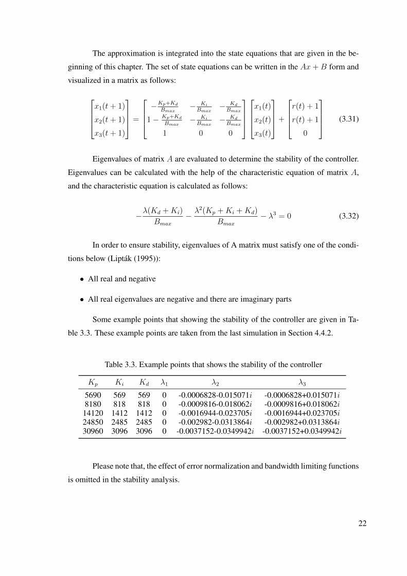
The approximation is integrated into the state equations that are given in the be-

ginning of this chapter. The set of state equations can be written in the Ax+B form and

visualized in a matrix as follows:

x1(t+ 1)

x2(t+ 1)

x3(t+ 1)

=

−Kp+Kd

Bmax− Ki

Bmax− Kd

Bmax

1− Kp+Kd

Bmax− Ki

Bmax− Kd

Bmax

1 0 0

x1(t)

x2(t)

x3(t)

+

r(t) + 1

r(t) + 1

0

(3.31)

Eigenvalues of matrix A are evaluated to determine the stability of the controller.

Eigenvalues can be calculated with the help of the characteristic equation of matrix A,

and the characteristic equation is calculated as follows:

−λ(Kd +Ki)

Bmax

− λ2(Kp +Ki +Kd)

Bmax

− λ3 = 0 (3.32)

In order to ensure stability, eigenvalues of A matrix must satisfy one of the condi-

tions below (Liptak (1995)):

• All real and negative

• All real eigenvalues are negative and there are imaginary parts

Some example points that showing the stability of the controller are given in Ta-

ble 3.3. These example points are taken from the last simulation in Section 4.4.2.

Table 3.3. Example points that shows the stability of the controller

Kp Ki Kd λ1 λ2 λ3

5690 569 569 0 -0.0006828-0.015071i -0.0006828+0.015071i8180 818 818 0 -0.0009816-0.018062i -0.0009816+0.018062i

14120 1412 1412 0 -0.0016944-0.023705i -0.0016944+0.023705i24850 2485 2485 0 -0.002982-0.0313864i -0.002982+0.0313864i30960 3096 3096 0 -0.0037152-0.0349942i -0.0037152+0.0349942i

Please note that, the effect of error normalization and bandwidth limiting functions

is omitted in the stability analysis.

22

CHAPTER 4

SIMULATION

4.1. Simulation Software

As a widely used application for network simulation, all of the simulation work

presented in this study is performed using NS2, the discrete event network simulator

(Breslau et al. (2000)).

NS2 is an open source network simulator that is available on many platforms. In

this study, a Linux computer is used for both development and simulations. Open source

licensing of NS2 allows developers to easily modify and extend NS2 for their simulation

needs. In this study, RTP protocol implementation of NS2 is extended to be able to

simulate the proposed methods. After each modification, NS2 source is compiled and the

resulting executable is run with the simulation scenario as the program parameter.

Everything that is related to a simulation scenario is coded in Tcl language and

saved for later use as the program parameter for the NS2 binary. This scenario file includes

the topology, occurrence time and type of network events, logging options, etc.

When NS2 binary is executed with a scenario parameter, a log file is generated.

This log file, described by the simulation scenario file, includes details about every sin-

gle packet transmission. This log file is parsed and inspected to extract the necessary

information to plot the result graphs in the following sections.

4.2. Simulation Environment

As the simulation topology, a bottleneck network configuration is designed. Two

servers, Server 1 and Server 2, represent the RTP transmission source and the background

traffic source, respectively. Router 1 and Router 2 are the topology routers that connect

the servers to the clients. Finally, Client 1 represents the RTP transmission client and

Client 2 denotes the background traffic client, in that order. How the topology elements

are connected to each other is depicted in Figure 4.1.

23

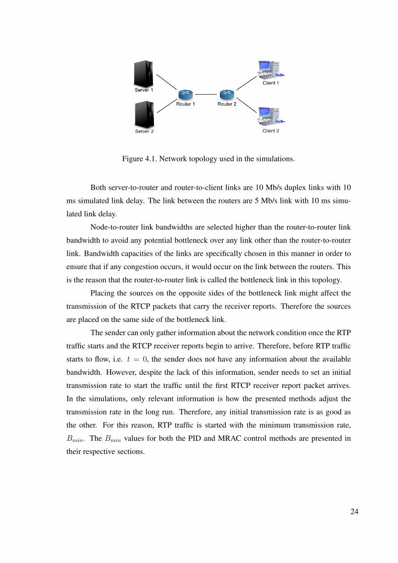
Figure 4.1. Network topology used in the simulations.

Both server-to-router and router-to-client links are 10 Mb/s duplex links with 10

ms simulated link delay. The link between the routers are 5 Mb/s link with 10 ms simu-

lated link delay.

Node-to-router link bandwidths are selected higher than the router-to-router link

bandwidth to avoid any potential bottleneck over any link other than the router-to-router

link. Bandwidth capacities of the links are specifically chosen in this manner in order to

ensure that if any congestion occurs, it would occur on the link between the routers. This

is the reason that the router-to-router link is called the bottleneck link in this topology.

Placing the sources on the opposite sides of the bottleneck link might affect the

transmission of the RTCP packets that carry the receiver reports. Therefore the sources

are placed on the same side of the bottleneck link.

The sender can only gather information about the network condition once the RTP

traffic starts and the RTCP receiver reports begin to arrive. Therefore, before RTP traffic

starts to flow, i.e. t = 0, the sender does not have any information about the available

bandwidth. However, despite the lack of this information, sender needs to set an initial

transmission rate to start the traffic until the first RTCP receiver report packet arrives.

In the simulations, only relevant information is how the presented methods adjust the

transmission rate in the long run. Therefore, any initial transmission rate is as good as

the other. For this reason, RTP traffic is started with the minimum transmission rate,

Bmin. The Bmin values for both the PID and MRAC control methods are presented in

their respective sections.

24

4.3. Simulations of PID Controlled Method

In this section, simulation environment and the simulation results for the PID

controlled rate control method is presented. As this method is implemented to evalu-

ate whether a PID controller can effectively control an RTP transmission, instead of a

multimedia content payload, a constant bitrate (CBR) payload is generated as the payload

for the RTP transmission and the transmission rate is controlled by varying the rate of

CBR payload.

4.3.1. Simulation Setup

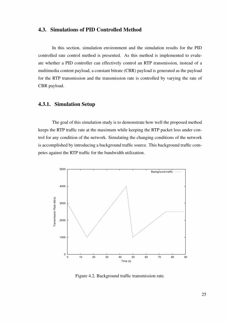
The goal of this simulation study is to demonstrate how well the proposed method

keeps the RTP traffic rate at the maximum while keeping the RTP packet loss under con-

trol for any condition of the network. Simulating the changing conditions of the network

is accomplished by introducing a background traffic source. This background traffic com-

petes against the RTP traffic for the bandwidth utilization.

0

1000

2000

3000

4000

5000

0 10 20 30 40 50 60 70 80 90

Tra

nsm

issio

n R

ate

(kb

/s)

Time (s)

Background traffic

Figure 4.2. Background traffic transmission rate.

25

In any given simulation scenario, the PID controller requires a certain amount of

time to reach full utilization of the available bandwidth. This transient state might affect

the user experience. The simulations should run long enough to let the PID controller

past the transient state. On the other hand, unnecessarily longer simulations may generate

redundant data and make it difficult to seethe operation of the PID controller when the

data is plotted. Therefore, simulations are limited to 90 seconds, which was found as an

appropriate value for simulations presented in the following section.

For background traffic generation a UDP source carrying constant bit rate (CBR)

traffic is implemented. A TCP source might also be incorporated for background traffic

generation. However, TCP’s rate control scheme might cloud the indication that whether

increase of decrease of the packet loss is caused by the proposed algorithm or TCP rate

control methods. In this case UDP’s lack of any form of rate controls is the primary reason

why UDP is chosen as the transport protocol for the background traffic.

Background traffic is a randomly generated packet flow and varies its transmission

rate throughout the simulations. In all of the simulations in the following section, this

same UDP source with the same pattern is used in conjunction with the RTP traffic source,

which is also carrying CBR payload. The transmission rate pattern of the background

traffic can be observed in Figure 4.2.

26

4.3.2. Simulation Results

For the first simulation, the RTP source flows with an uncontrolled constant traffic

rate. The constant transmission rate of the traffic is set at 4 MB/s at the beginning of

the simulation and kept at the same rate until the simulation ends. The result is the RTP

packet loss throughout the simulation timespan. As it can be seen in Figure 4.3, constant

and uncontrolled high transmission rate of the RTP traffic results in high packet loss.

0

0.2

0.4

0.6

0.8

1

0 10 20 30 40 50 60 70 80 90

Lo

ss F

ractio

n

Time (s)

Loss fraction (Uncontrolled rate traffic at 4Mb/s)

Figure 4.3. Packet loss fraction of 4Mb/s constant rate RTP traffic. RTP traffic is runalongside the background traffic.

In the second simulation, a constant and uncontrolled RTP transmission rate is

employed again, with the difference that this time the transmission rate is limited at 2

Mb/s. This simulation resulted in low packet loss (Figure 4.4), however the throughput of

the RTP traffic is low and is not enough to fully utilize the available bandwidth.

27

0

0.2

0.4

0.6

0.8

1

0 10 20 30 40 50 60 70 80 90

Lo

ss F

ractio

n

Time (s)

Loss fraction (Uncontrolled rate traffic at 2Mb/s)

Figure 4.4. Packet loss fraction of 2Mb/s constant rate RTP traffic. RTP traffic is runalongside the background traffic.

In the final simulation, the RTP transmission rate is controlled by the PID con-

troller. Figure 4.5 shows how the PID controller adapts the rate of the RTP traffic in

response to the changes in the background traffic. As the background traffic increases and

decreases, the RTP transmission rate is adjusted accordingly by the PID controller. At the

same time, the packet loss is controlled and kept at the reference point (Figure 4.6).

At the points where background traffic rate increases and causes the RTP traffic

to suffer packet losses, the RTP traffic rate is autonomously adapted to this change and

in turn enables the RTP packet losses to decrease. By keeping the utilization high and

packet losses low, the proposed method integrates QoS capabilities to the network.

28

0

1000

2000

3000

4000

5000

0 10 20 30 40 50 60 70 80 90

Tra

nsm

issio

n R

ate

(kb

/s)

Time (s)

Rate controlled RTP traffic

Figure 4.5. Transmission rate of PID controlled RTP traffic. RTP traffic is run along-side the background traffic.

0

0.2

0.4

0.6

0.8

1

0 10 20 30 40 50 60 70 80 90

Lo

ss F

ractio

n

Time (s)

Loss fraction (Rate controlled traffic)

Figure 4.6. Packet loss fraction of PID controlled RTP traffic. RTP traffic is run along-side the background traffic.

29

4.4. Simulations of MRAC Controlled Method

In this section, simulation environment and the simulation results for the MRAC

controlled rate control method is presented. Simulations implemented in this section em-

ploys a simulated multimedia content as the payload for the RTP transmission.

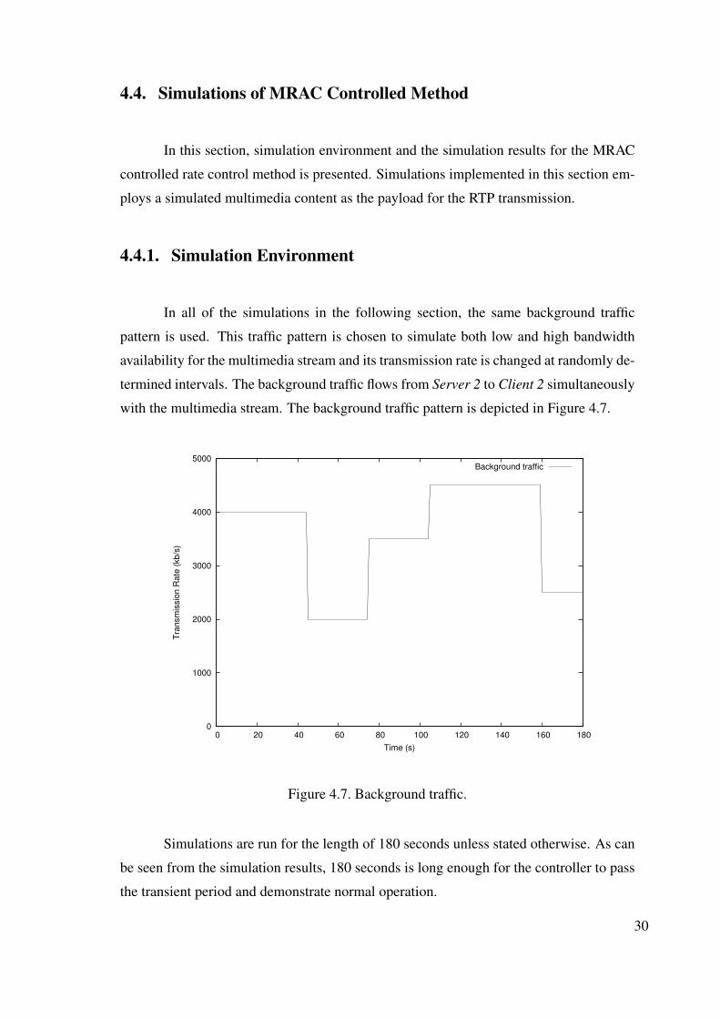
4.4.1. Simulation Environment

In all of the simulations in the following section, the same background traffic

pattern is used. This traffic pattern is chosen to simulate both low and high bandwidth

availability for the multimedia stream and its transmission rate is changed at randomly de-

termined intervals. The background traffic flows from Server 2 to Client 2 simultaneously

with the multimedia stream. The background traffic pattern is depicted in Figure 4.7.

0

1000

2000

3000

4000

5000

0 20 40 60 80 100 120 140 160 180

Tra

nsm

issio

n R

ate

(kb

/s)

Time (s)

Background traffic

Figure 4.7. Background traffic.

Simulations are run for the length of 180 seconds unless stated otherwise. As can

be seen from the simulation results, 180 seconds is long enough for the controller to pass

the transient period and demonstrate normal operation.

30

4.4.2. Simulation Results

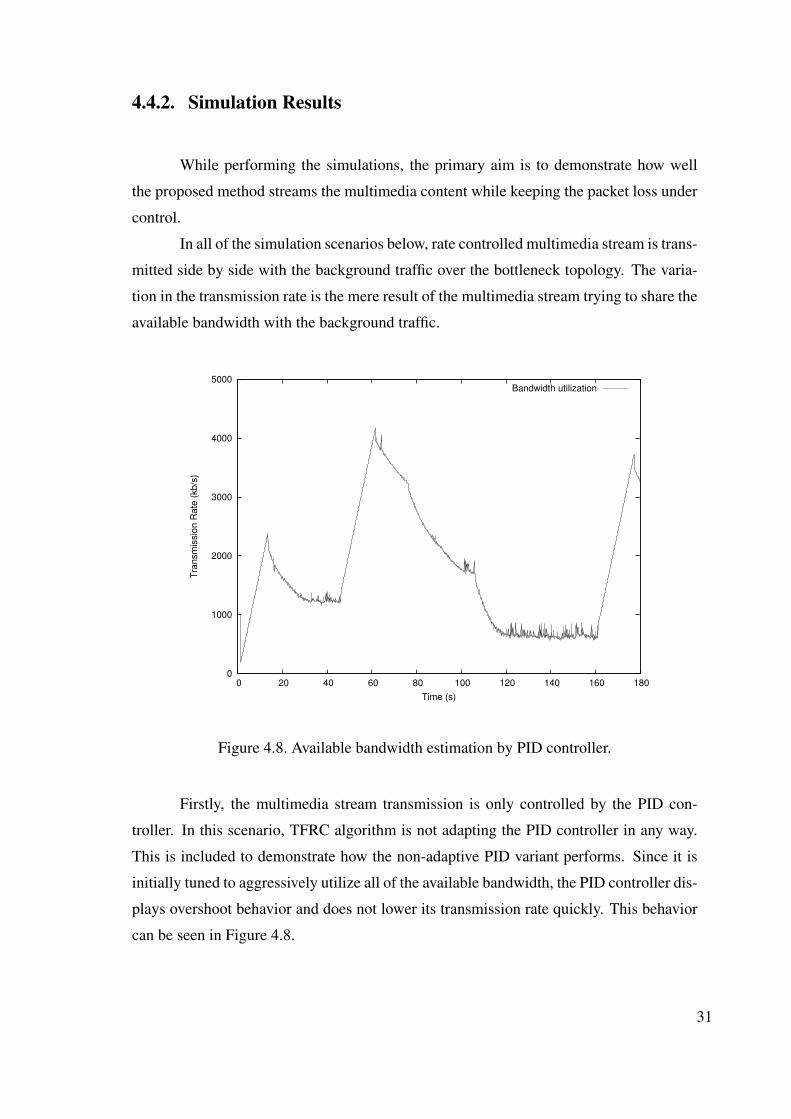
While performing the simulations, the primary aim is to demonstrate how well

the proposed method streams the multimedia content while keeping the packet loss under

control.

In all of the simulation scenarios below, rate controlled multimedia stream is trans-

mitted side by side with the background traffic over the bottleneck topology. The varia-

tion in the transmission rate is the mere result of the multimedia stream trying to share the

available bandwidth with the background traffic.

0

1000

2000

3000

4000

5000

0 20 40 60 80 100 120 140 160 180

Tra

nsm

issio

n R

ate

(kb

/s)

Time (s)

Bandwidth utilization

Figure 4.8. Available bandwidth estimation by PID controller.

Firstly, the multimedia stream transmission is only controlled by the PID con-

troller. In this scenario, TFRC algorithm is not adapting the PID controller in any way.

This is included to demonstrate how the non-adaptive PID variant performs. Since it is

initially tuned to aggressively utilize all of the available bandwidth, the PID controller dis-

plays overshoot behavior and does not lower its transmission rate quickly. This behavior

can be seen in Figure 4.8.

31

0

1000

2000

3000

4000

5000

0 20 40 60 80 100 120 140 160 180

Tra

nsm

issio

n R

ate

(kb

/s)

Time (s)

Bandwidth utilization

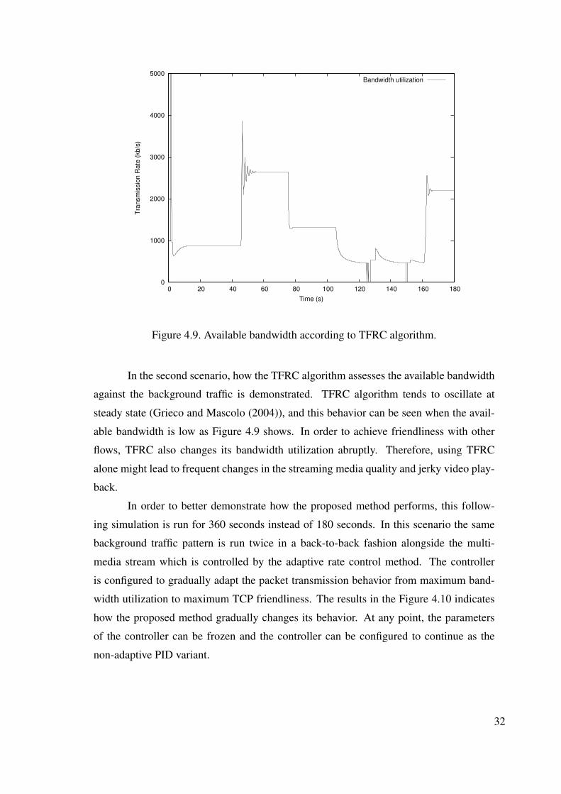
Figure 4.9. Available bandwidth according to TFRC algorithm.

In the second scenario, how the TFRC algorithm assesses the available bandwidth

against the background traffic is demonstrated. TFRC algorithm tends to oscillate at

steady state (Grieco and Mascolo (2004)), and this behavior can be seen when the avail-

able bandwidth is low as Figure 4.9 shows. In order to achieve friendliness with other

flows, TFRC also changes its bandwidth utilization abruptly. Therefore, using TFRC

alone might lead to frequent changes in the streaming media quality and jerky video play-

back.

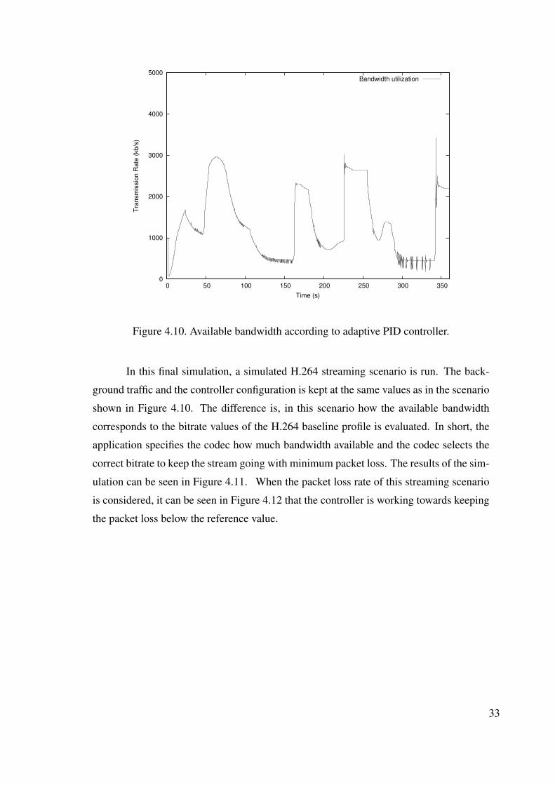
In order to better demonstrate how the proposed method performs, this follow-

ing simulation is run for 360 seconds instead of 180 seconds. In this scenario the same

background traffic pattern is run twice in a back-to-back fashion alongside the multi-

media stream which is controlled by the adaptive rate control method. The controller

is configured to gradually adapt the packet transmission behavior from maximum band-

width utilization to maximum TCP friendliness. The results in the Figure 4.10 indicates

how the proposed method gradually changes its behavior. At any point, the parameters

of the controller can be frozen and the controller can be configured to continue as the

non-adaptive PID variant.

32

0

1000

2000

3000

4000

5000

0 50 100 150 200 250 300 350

Tra

nsm

issio

n R

ate

(kb

/s)

Time (s)

Bandwidth utilization

Figure 4.10. Available bandwidth according to adaptive PID controller.

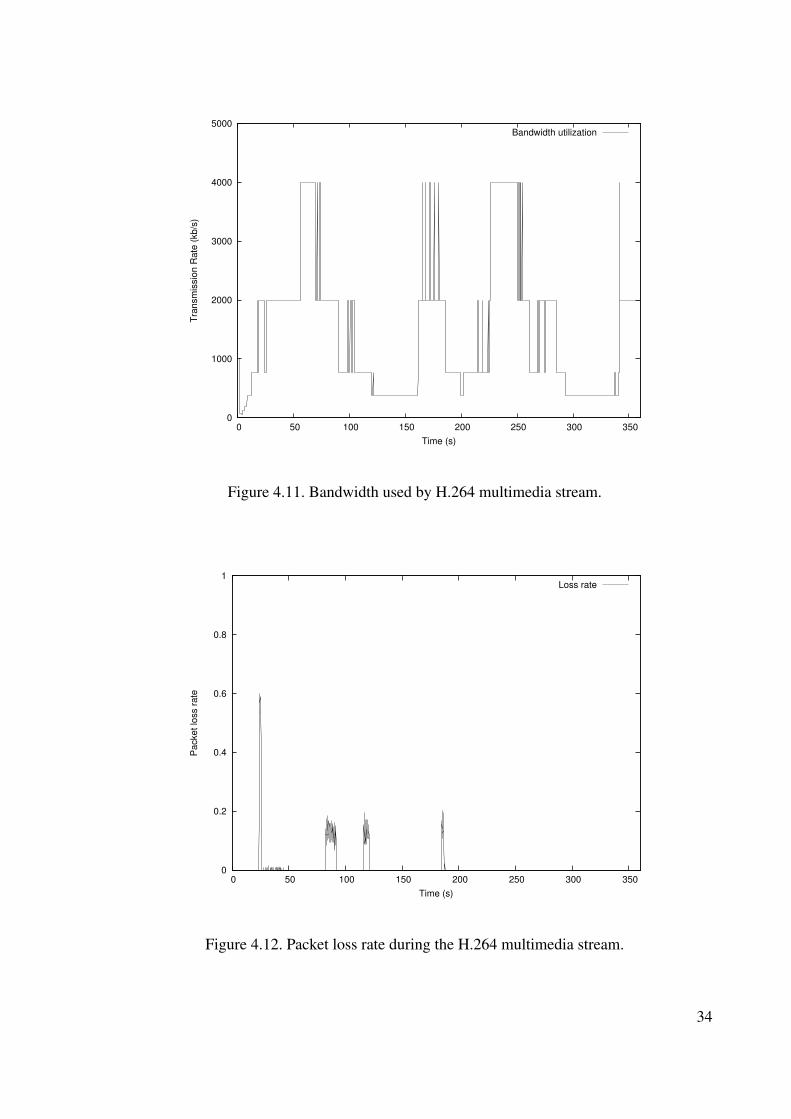
In this final simulation, a simulated H.264 streaming scenario is run. The back-

ground traffic and the controller configuration is kept at the same values as in the scenario

shown in Figure 4.10. The difference is, in this scenario how the available bandwidth

corresponds to the bitrate values of the H.264 baseline profile is evaluated. In short, the

application specifies the codec how much bandwidth available and the codec selects the

correct bitrate to keep the stream going with minimum packet loss. The results of the sim-

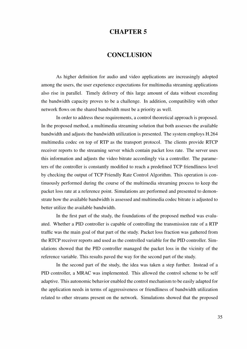
ulation can be seen in Figure 4.11. When the packet loss rate of this streaming scenario

is considered, it can be seen in Figure 4.12 that the controller is working towards keeping

the packet loss below the reference value.

33

0

1000

2000

3000

4000

5000

0 50 100 150 200 250 300 350

Tra

nsm

issio

n R

ate

(kb

/s)

Time (s)

Bandwidth utilization

Figure 4.11. Bandwidth used by H.264 multimedia stream.

0

0.2

0.4

0.6

0.8

1

0 50 100 150 200 250 300 350

Pa

cke

t lo

ss r

ate

Time (s)

Loss rate

Figure 4.12. Packet loss rate during the H.264 multimedia stream.

34

CHAPTER 5

CONCLUSION

As higher definition for audio and video applications are increasingly adopted

among the users, the user experience expectations for multimedia streaming applications

also rise in parallel. Timely delivery of this large amount of data without exceeding

the bandwidth capacity proves to be a challenge. In addition, compatibility with other

network flows on the shared bandwidth must be a priority as well.

In order to address these requirements, a control theoretical approach is proposed.

In the proposed method, a multimedia streaming solution that both assesses the available

bandwidth and adjusts the bandwidth utilization is presented. The system employs H.264

multimedia codec on top of RTP as the transport protocol. The clients provide RTCP

receiver reports to the streaming server which contain packet loss rate. The server uses

this information and adjusts the video bitrate accordingly via a controller. The parame-

ters of the controller is constantly modified to reach a predefined TCP friendliness level

by checking the output of TCP Friendly Rate Control Algorithm. This operation is con-

tinuously performed during the course of the multimedia streaming process to keep the

packet loss rate at a reference point. Simulations are performed and presented to demon-

strate how the available bandwidth is assessed and multimedia codec bitrate is adjusted to

better utilize the available bandwidth.

In the first part of the study, the foundations of the proposed method was evalu-

ated. Whether a PID controller is capable of controlling the transmission rate of a RTP

traffic was the main goal of that part of the study. Packet loss fraction was gathered from

the RTCP receiver reports and used as the controlled variable for the PID controller. Sim-

ulations showed that the PID controller managed the packet loss in the vicinity of the

reference variable. This results paved the way for the second part of the study.

In the second part of the study, the idea was taken a step further. Instead of a

PID controller, a MRAC was implemented. This allowed the control scheme to be self

adaptive. This autonomic behavior enabled the control mechanism to be easily adapted for

the application needs in terms of aggressiveness or friendliness of bandwidth utilization

related to other streams present on the network. Simulations showed that the proposed

35

method demonstrated a smoother bandwidth utilization adjustment compared to TFRC

algorithm. While the TFRC responds quickly to the bandwidth changes, smoothness is

the key for any multimedia streaming application for an acceptable user experience.

In conclusion, the primary strengths of the proposed methods are; the integration

of the existing network protocols and multimedia codec algorithms to maximize back-

wards compatibility, autonomous self adaptive bandwidth estimation and transmission

rate control to allow for a higher compatibility and coexistence with other network flows

on the bandwidth and ease of implementation.

Future work might focus on applying the proposed methods to a real streaming

environment in place of the synthetic background traffic used in the simulations. Because

the controller is tuned according to the environment it is run in, a real life scenario might

enable the users to tune the controller for a better initial starting point.

Proposed method only accepts the loss fraction as the controlled variable for the

control scheme. This results in the system to adjust the sending rate once the packet losses

start to occur. As described by Jiang and Schulzrinne (2000), packet loss is usually pre-

ceded by increasing transmission delays. Future work may focus on incorporating another

controlled variable, namely the transmission delay. Since feedback control paradigms

that employ more than one controlled variable are not uncommon (Lu et al. (2002)), us-

ing transmission delay as a controlled variable might provide the controller the ability

to adjust the rate of the stream transmission even before the actual packet losses occur.

Comparison with present transmission rate control methods may also be considered.

36

REFERENCES

Ang, K., G. Chong, and Y. Li (2005, July). Pid control system analysis, design, and

technology. IEEE Transactions on Control Systems Technology 13(4), 559–576.

Barberis, A., C. Casetti, J. C. D. Martin, and M. Meo (2001). A simulation study of

adaptive voice communications on ip networks. Computer Communications 24(9),

757 – 767.

Baskys, A. and V. Zlosnikas (2006, nov.). Asymmetric pid controller. In IEEE Industrial

Electronics, IECON 2006 - 32nd Annual Conference on, pp. 219 –223.

Bernaschi, M., F. Cacace, R. Clementelli, and L. Vollero (2005). Adaptive streaming

on heterogeneous networks. In Proceedings of the 1st ACM workshop on Wireless

multimedia networking and performance modeling, WMuNeP ’05, New York, NY,

USA, pp. 16–23. ACM.

Bouras, C. and A. Gkamas (2003). Multimedia transmission with adaptive qos based

on real-time protocols. International Journal of Communication Systems 16(3), 225–

248.

Breslau, L., D. Estrin, K. Fall, S. Floyd, J. Heidemann, A. Helmy, P. Huang, S. Mc-

canne, K. Varadhan, Y. Xu, and H. Yu (2000). Advances in network simulation. Com-

puter 33(5), 59–67.

Burza, M., J. Kang, and P. van der Stok (2007). Adaptive streaming of mpeg-based au-

dio/video content over wireless networks. Journal of Multimedia, 17–27.

Eckart, B., X. He, and Q. Wu (2008). Performance adaptive udp for high-speed bulk data

transfer over dedicated links. In Parallel and Distributed Processing, 2008. IPDPS

2008. IEEE International Symposium on, pp. 1 –10.

Floyd, S., M. Handley, J. Padhye, and J. Widmer (2000). Equation-based congestion con-

trol for unicast applications. In Proceedings of the conference on Applications, Tech-

37

nologies, Architectures, and Protocols for Computer Communication, SIGCOMM

’00, New York, NY, USA, pp. 43–56. ACM.

Floyd, S., M. Handley, J. Padhye, and J. Widmer (2008, September). TCP friendly rate

control (TFRC): Protocol specification. RFC 5348, RFC Editor, Fremont, CA, USA.

Grieco, L. and S. Mascolo (2004). Adaptive rate control for streaming flows over the

internet. Multimedia Systems 9, 517–532. 10.1007/s00530-003-0124-1.

Group, A.-V. T. W., H. Schulzrinne, S. Casner, R. Frederick, and V. Jacobson (1996, Jan-

uary). RTP: A Transport Protocol for Real-Time Applications. RFC 1889 (Proposed

Standard). Obsoleted by RFC 3550.

Jiang, W. and H. Schulzrinne (2000). Modeling of packet loss and delay and their effect

on real-time multimedia service quality. In PROCEEDINGS OF NOSSDAV ’2000.

Johnson, M., M. Moradi, and E. Corporation (2005). PID control: new identification and

design methods. Springer.

Kuschnig, R., I. Kofler, and H. Hellwagner (2010). An evaluation of tcp-based rate-

control algorithms for adaptive internet streaming of h.264/svc. In Proceedings of

the first annual ACM SIGMM conference on Multimedia systems, MMSys ’10, New

York, NY, USA, pp. 157–168. ACM.

Ling, P. and L. ShaoWen (2009). An improved algorithm of rtp adaptive transmission

control. In Genetic and Evolutionary Computing, 2009. WGEC ’09. 3rd International

Conference on, pp. 595 –599.

Liptak, B. G. (1995). Instrument Engineers’ Handbook: Process Control. Instrument

Engineers’ Handbook. Chilton Book Company.

Lu, C., J. A. Stankovic, S. H. Son, and G. Tao (2002, July). Feedback control real-time

scheduling: Framework, modeling, and algorithms. Real-Time Syst. 23, 85–126.

Marpe, D., T. Wiegand, and G. J. Sullivan (2006, August). The H.264/MPEG4 Advanced

38

Video Coding Standard and its Applications. IEEE Communications 44(8), 134–143.

Papadimitriou, P. and V. Tsaoussidis (2007). A rate control scheme for adaptive video

streaming over the internet. In Communications, 2007. ICC ’07. IEEE International

Conference on, pp. 616 –621.

Schierl, T., T. Wiegand, and M. Kampmann (2005, sept.). 3gpp compliant adaptive wire-

less video streaming using h.264/avc. In Image Processing, 2005. ICIP 2005. IEEE

International Conference on, Volume 3, pp. III – 696–9.

Schulzrinne, H., S. Casner, R. Frederick, and V. Jacobson (2003, July). RTP: A Transport

Protocol for Real-Time Applications. RFC 3550 (Standard). Updated by RFCs 5506,

5761, 6051, 6222.

Schwarz, H., D. Marpe, and T. Wieg (2007). Overview of the scalable video coding

extension of the h.264/avc standard. In IEEE Transactions on Circuits and Systems

for Video Technology In Circuits and Systems for Video Technology, pp. 1103–1120.

Sisalem, D. (1997). End-to-end quality of service control using adaptive applications. In

In IFIP Fifth International Workshop on Quality of Service (IWQOS ’97.

Sisalem, D. and A. Wolisz (1999). Towards tcp-friendly adaptive multimedia applications

based on rtp. In Computers and Communications, 1999. Proceedings. IEEE Interna-

tional Symposium on.

Tos, U. and T. Ayav (2011, july). Adaptive rtp rate control method. In Computer Software

and Applications Conference Workshops (COMPSACW), 2011 IEEE 35th Annual, pp.

7 –12.

Wagner, M., I. Kopilovic, S. Dohla, N. Farber, and H. Fuchs (2009). Towards an rtp

profile for iptv. Broadcasting, IEEE Transactions on 55(2), 343 –352.

Wang, B., J. Kurose, P. Shenoy, and D. Towsley (2008, May). Multimedia streaming

via tcp: An analytic performance study. ACM Trans. Multimedia Comput. Commun.

Appl. 4(2), 16:1–16:22.

39

Wang, Y.-K., R. Even, T. Kristensen, and R. Jesup (2011, May). RTP Payload Format for

H.264 Video. RFC 6184 (Proposed Standard).

Wanxiang, C. and L. Zhenming (2001). An modified rtp adaptive algorithm. In Info-tech

and Info-net, 2001. Proceedings. ICII 2001 - Beijing. 2001 International Conferences

on.

Ziegler, J. G. and N. B. Nichols (1942). Optimum Settings for Automatic Controllers.

Transactions of ASME 64, 759–768.

40