1

Qualitative Problem Solving Strategies of

First Order Differential Equations: The Case of Amy

Chris L. Rasmussen

University of Maryland

2

Abstract

This study explores one student’s understanding of qualitative methods of analysis for first

order differential equations. The student demonstrated a strong graphical understanding of

the derivative and used her prior knowledge of population modeling to make sense of

various graphical representations. Despite this strong background knowledge, several

potential difficulties related to qualitative methods of analysis are uncovered and

propositions regarding the sources of these difficulties are offered. A misconception

involving the interpretation of direction fields is suggested by the data, which in turn raises

questions about the usefulness of phase lines in some recent reform-oriented curriculums.

3

Introduction and Problem Statement

The typical engineering or physical science student begins his or her university

studies with a year of calculus, generally followed by differential equations in the

sophomore year. In the past decade there has been a nationwide effort at revitalizing the

calculus curriculum (Douglas, 1986; Fraga, 1993; Tucker, 1990), but less well publicized

and less well researched are the changes occurring in the content, pedagogy, and learning of

differential equations. These changes are evident in several recent curriculum reform efforts

(Blanchard, Devaney, & Hall, 1996; Borrelli & Coleman, 1996; Coombes, Hunt, Lipsman,

Osborn, & Stuck, 1995; Kostelich & Armbruster, 1995; Lomen & Lovelock, 1996; West,

Strogatz, McDill, & Cantwell, in press) which now include, with the aide of technology, a

stronger emphasis on qualitative and numerical methods. Prior to these reform efforts, the

sophomore level course in differential equations typically used little technology and

emphasized mainly analytic techniques.

Spurred on by the calculus reform effort and advances in technology, the

introductory level differential equations course is changing, and this change requires

students to interpret and connect graphical representations such as direction fields, solution

graphs, and phase portraits. Concepts once treated only symbolically are now explored

graphically, numerically, and descriptively. The goal of these changes is to provide students

with a deeper understanding of the subject, to provide insight about the behavior of

solutions, and to give students an idea of how the subject is relevant to other disciplines. In

order to realize these goals, curriculum and pedagogy will necessarily need to be informed

by research that explores students’ understanding. To date, there is little research in this

area, with the exception of the work by Artigue (1992), who reports on the capabilities and

4

cognitive difficulties of first-year French university students when using geometric settings

to construct qualitative analyses.

The purpose of this exploratory, interpretive study is to investigate one student’s

understanding of qualitative methods of analysis of first order differential equations. The

questions of interest in this study are:

1) What does it mean to this student to qualitatively analyze a first order differentialequation?

2) What strategies does this student use in a direction field-differential equationmatching activity?

3) What characterizes this student’s understanding of stability of first order differentialequations?

The results from this study will provide educators with one image of what their

students are understanding from this new approach, strategies they use, and the possible

difficulties they may be encountering. Knowledge of students’ understanding, strategies,

and difficulties, when linked and synthesized with further studies in other contexts, can lead

to increased communication between teacher and student, new insight into instructional

practices, and revised and improved curriculum.

Theoretical Perspective

A brief but complete description of the researcher’s theoretical perspective on the

nature of learning and understanding mathematics will assist the reader in understanding the

choices made regarding the research questions and the research methodology.

Constructivism provides the overall perspective on how students learn and Hiebert and

Lefevre’s distinction between conceptual and procedural knowledge provides a useful

perspective on understanding mathematics.

5

Understanding is assumed to be an ongoing activity, not a final accomplishment or

attainment. In other words, “mathematical knowledge is not a thing that you have, but an

activity that you (might) engage in” (Dubinsky, 1994, p. 224). This perspective is

consistent with the writings of Piaget, who stressed knowing to be an adaptive activity, and

with von Glasersfeld’s theory of knowing, often referred to as constructivsim.

Constructivism, as used here, is the belief that knowledge is constructed by the individual

and that this construction is adaptive and influenced profoundly by our experiences and our

own cognitive lenses (Confrey, 1990; von Glasersfeld, 1995). Regarding the importance of

social interactions in the construction of knowledge, the analysis reported here considers it a

matter of “figure versus ground,” where the individual is the figure and the relationships

among individuals is the ground (Thompson, 1995, p. 127-128). Thus, the emphasis is on

the individual student and not on the social aspects or interactions.

Constructivism deals essentially with the construction of conceptual knowledge.

However, this does not imply that memorization and rote learning as useless, but rather as

potential means for learning other matters (von Glasersfeld, 1995). Von Glasersfeld does

not expand upon what these other matters might be, but Hiebert and Lefevre’s distinction

between conceptual and procedural knowledge helps to clarify the discussion. Hiebert and

Lefevre (1986) characterize conceptual knowledge as “knowledge that is rich in

relationships. It can be thought of as a connected web of knowledge, a network in which

the linking relationships are as prominent as the discrete pieces of information” (p. 3-4).

Procedural knowledge is “made up of two distinct parts. One part is composed of the

formal language, or symbol representation system, of mathematics. The other part consists

of the algorithms, or rules, for completing mathematical tasks” (p. 6). In regard to this

6

study, there are conceptual and procedural aspects to qualitative methods and

understanding has been defined broadly enough to include both the conceptual and

procedural aspects. However, constructivism provides the most useful perspective when

dealing with the conceptual aspects of understanding.

From a constructivist’s perspective, the researcher’s interest will be focused on what

can be inferred to be going on inside the student’s head rather than on overt responses. The

primary techniques for exploring students’ understanding are careful observations and in-

depth interviews with students.

Method

In order to provide in-depth information on this student’s understanding of

qualitative methods of analysis, two semi-structured interviews were conducted. Each

interview, which was audio-taped and transcribed by the researcher, consisted of two parts.

The first part consisted of several questions aimed at uncovering what it means to Amy to

qualitatively analyze a differential equation, strategies she might use, and the sources that

influenced this understanding. This provided an opportunity for the researcher to gain some

insight into Amy’s understanding prior to her solving the problems and it assisted the

researcher in interpreting her solutions. The second part consisted of one to two problems

drawn from other reform oriented texts dealing with qualitative methods of analysis. Amy

was asked to “think aloud” during her solution of these problems and was asked about her

thinking and reasoning as needed.

Triangulation of the interview data was accomplished through document analysis of

her first exam and her Mathematica problem set dealing with the qualitative analysis of first

7

order differential equations. The use of interviews in conjunction with document analysis is

one way for the researcher to “develop insights on how subjects interpret some piece of the

world” (Bogdan & Biklen, 1992, p.96). The “piece of the world” of interest in this study is

the student’s understanding of qualitative methods of analysis of first order differential

equations. In addition, the researcher observed most of the class sessions dealing with first

order differential equations in order to have a better sense of the environment in which

learning took place.

The Setting

The study reported here was carried out in Fall, 1995 semester in one section of an

introductory differential equations course at the University of Maryland, College Park. The

class used the fifth edition of the textbook Elementary Differential Equations by Boyce &

DiPrima and the supplemental text Differential Equations with Mathematica by Coombes,

Hunt, Lipsman, Osborn, and Stuck. The philosophy of the supplemental text is as follows:

• To guide students into a more interpretive mode of thinking.• To use a mathematical software system to enhance students’ ability to compute

symbolic and numerical solutions, and perform qualitative and graphical analysisof differential equations.

• To develop course material that reflects the current state of differentialequations and emphasizes the mathematical modeling of physical problems.

• To minimize the time required to learn to use the computer platform (Coombes,Hunt, Lipsman, Osborn, & Stuck, 1995, p. 5).

Assignments from the supplemental text, which were the major source for learning about

qualitative and graphical analysis, counted 20% towards the course grade.

The class met for two 75 minute periods per week in a room with no computer

resources and lecture was the predominant mode of instruction. One student from a class of

approximately 25 was asked to participate in this study. The participant was a 26 year old

8

graduate student named Amy (not her real name). Amy holds a bachelor degree in

comparative religion and a master’s degree in interdisciplinary science studies, with a

concentration in environmental science. At the time of this study, Amy was a first year

graduate student in fishery science. Her college mathematics background consisted of two

semesters of calculus at the University of Maryland during the 1994-95 school year. Prior

to this course, she had never used a computer algebra system, but she had used word

processing, spreadsheet, and statistics programs. I asked Amy to participate in this

exploratory study since, as I had been her teaching assistant for both semesters of calculus, I

knew her to have a sound understanding of the subject, to be thoughtful and able to

articulate her thinking of complex subjects.

Results and Discussion

The results of the two interviews with Amy and the analysis of her Mathematica

problem set and exam are discussed in the following three sections: graphs and fish,

invented strategies, and notions of stability. The first section, graphs and fish, provides

some insight into what it means to Amy to qualitatively analyze a differential equation,

strategies she might use to qualitatively analyze a differential equation, and sources that

influenced this understanding. The second section, invented strategies, describes and

interprets Amy’s solution strategies on a direction field-differential equation matching

activity. The final section, notions of stability, characterizes Amy’s understanding of the

concept of stability as it relates to first order differential equations.

Graphs and Fish

9

A central premise of the researcher’s theoretical orientation is that people

reassemble information taken from the outside world in ways that allow them to make

personal sense of it. One way to explore how people make sense of something is to

investigate the meanings these things hold for them and the sources they cite as particularly

influential in the development of this understanding. Thus, before presenting Amy with the

matching activity, it is useful to obtain some sense of what it means to her to qualitatively

analyze a differential equation, strategies she might use, and the sources that influenced this

understanding.

R: What does it mean to study a differential equation qualitatively?A: It means to be able to tell general properties. To be able to figure out general

properties of the differential equation by looking at the graphs of solution curves orthe actual differential equation, the slopes and things like that. So it means to me tobe able to look at slopes and equilibrium and be able to tell equilibrium, whetherthings are decreasing or increasing.

Determining the “general properties” of solutions is a component of any qualitative

analysis and for Amy, these properties include an understanding of the nature of equilibrium

solutions, looking at slopes, and determining whether a solution is increasing or decreasing.

During the second interview, Amy states that to understand a differential equation means to

“understand the process the equation is describing, how something changes over time. For

me to understand that is to come up with a graphical image of how something changes.”

Here we see that Amy’s concept of a qualitative analysis also includes an

understanding that a differential equation models a dynamic process, one that changes over

time. The above suggests that graphical representations and an understanding of the

“process the equation is describing” are two key themes in Amy’s understanding of a

qualitative analysis.

10

As Amy alludes to above, graphical images are an important component in her

qualitative understanding of differential equations and she appears comfortable with and

confident in her ability to use graphical representations. Moreover, she appears to rely on

graphs to understand certain concepts. For example, when talking about the Euler method,

Amy said, “I need a graph because that’s the only way I understood it.” When asked about

the influences on her ability to qualitatively analyze a differential equation, Amy cites her

previous calculus courses where she “got a good basis in understanding what derivatives

and integrals meant graphically” and was “able to interchange the graph of a curve, its

solution, and its integral and seeing how to go from one to the other, to make the

transition.” She related this to the differential equations course, where she felt the

supplemental text had “a good little section on putting these ideas together with the

direction field.” Amy also emphasized her study of fish populations as a major influence.

A: The biggest thing that has helped me is just my study of fish populations orunderstanding of populations and then with differential equations describe the rateof population growth. So when I look at a curve, I can sometimes think about itmore easily in terms of the rate of change of a population.....I already have agraphical understanding of the rate of change and now I’m learning the mathematicsthat’s behind it.

When asked about other sources of influences, such as fellow students or the

professor, Amy said that she “hadn’t really talked to any of my classmates” and that “the

professor is helpful answering questions after class, but I’ve never gone to his extra help

sessions [office hours].” In regards to the lectures, Amy said, “the lectures are helpful, but

there it’s much more procedural than graphical.” The implication is that qualitative

analyses, which rely heavily upon graphical interpretation, are something other than

procedural and require a level of thinking beyond mimicking “how you do it.” However,

11

other research I am currently working on documents how even “good” students like Amy

find ways to proceduralize certain qualitative analyses in a way that renders them

conceptually meaningless.

Graphical representations also play an important role in Amy’s description of the

strategies she would use to qualitatively analyze a differential equation. Amy mentions

three different graphical representations from which she would be able to qualitatively

analyze a differential equation--graphs of the solution curves, graphs of the differential

equation, and direction fields. Regarding graphs of the differential equation, Amy states

that this method works only for autonomous differential equations, whereas one can use

Mathematica to plot the direction field for any differential equation, “even if Mathematica

can’t solve it.” It appears that Amy has a good understanding of when it is appropriate to

use particular graphical representations and is beginning to understand the power and

flexibility of Mathematica. By looking at the direction field, she says you get “a more

precise idea of what solution curves look like depending on the initial values.”

R: If you were given a differential equation and asked to discuss the system itdescribes, what would you do?

A: The first thing I’d do, if I had Mathematica, I’d do a direction field because you canreally see what’s happening and then I’d say well, that’s like a fish population goingup and down or whatever, but they’re really not. Most differential equations don’treally look like that. They don’t really lend themselves to being interpreted aspopulation growth, but I’m kind of making a transition between only being able tobeing able to see bunches of fish getting larger and smaller to just seeing how afunction which can describe a physical, biological, or something or other, just be afunction in and of itself. Just that shows its behavior at the time.

One explanation regarding Amy’s attempt to make this “transition” draws from

Hiebert and Lefevre’s discussion on how relationships between pieces of mathematical

knowledge can be established. At the reflective level,

12

relationships are constructed at a higher, more abstract level than the pieces ofinformation they connect. Relationships at this level are less tied to specificcontexts. They often are created by recognizing similar core features in pieces ofinformation that are superficially different (Hiebert & Lefevre, 1986, p. 5).

From this perspective, it appears that Amy’s “transition” is an attempt to move from the

specific context of modeling fish populations to a more abstract level.

Invented Strategies

The second portion of the first interview was a direction field-differential equation

matching activity taken from an article describing the reform-oriented course at Boston

University (see Blanchard, 1994). This type of activity does not appear anywhere in the

text or in the supplemental text and requires no new knowledge or understanding and

therefore provides an opportunity to illuminate Amy’s problem solving strategies and her

understanding of the relationship between direction fields and differential equations.

13

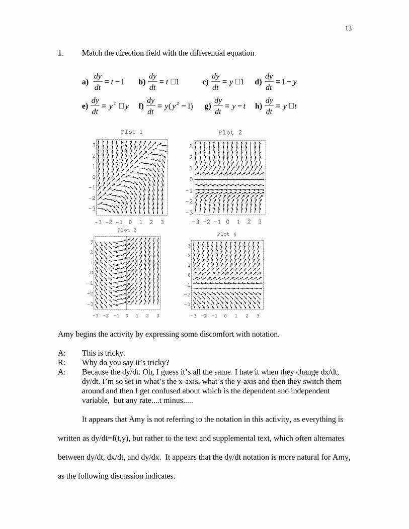
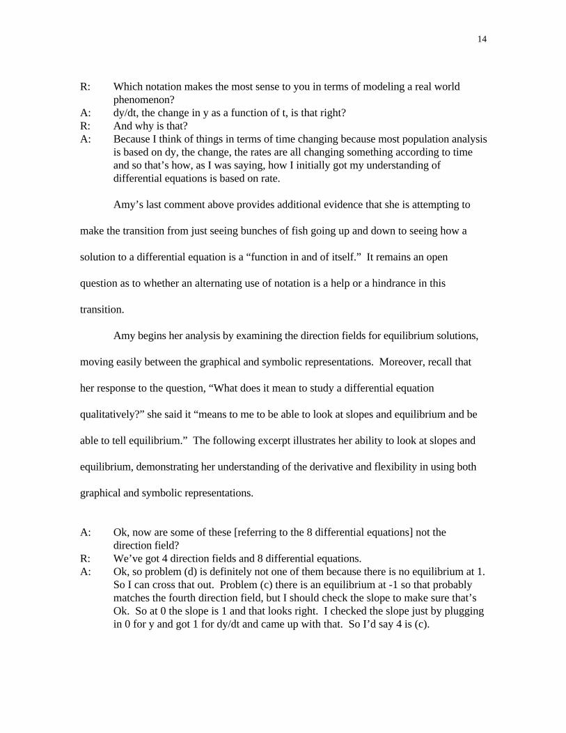
1. Match the direction field with the differential equation.

a) dy

dtt= −1 b)

dy

dtt= +1 c)

dy

dty= +1 d)

dy

dty= −1

e) dy

dty y= +2 f)

dy

dty y= −( )2 1 g)

dy

dty t= − h)

dy

dty t= +

-3 -2 -1 0 1 2 3

-3

-2

-1

0

1

2

3

Plot 1

-3 -2 -1 0 1 2 3

-3

-2

-1

0

1

2

3

Plot 2

-3 -2 -1 0 1 2 3

-3

-2

-1

0

1

2

3

Plot 3

-3 -2 -1 0 1 2 3

-3

-2

-1

0

1

2

3

Plot 4

Amy begins the activity by expressing some discomfort with notation.

A: This is tricky.R: Why do you say it’s tricky?A: Because the dy/dt. Oh, I guess it’s all the same. I hate it when they change dx/dt,

dy/dt. I’m so set in what’s the x-axis, what’s the y-axis and then they switch themaround and then I get confused about which is the dependent and independentvariable, but any rate....t minus.....

It appears that Amy is not referring to the notation in this activity, as everything is

written as dy/dt=f(t,y), but rather to the text and supplemental text, which often alternates

between dy/dt, dx/dt, and dy/dx. It appears that the dy/dt notation is more natural for Amy,

as the following discussion indicates.

14

R: Which notation makes the most sense to you in terms of modeling a real worldphenomenon?

A: dy/dt, the change in y as a function of t, is that right?R: And why is that?A: Because I think of things in terms of time changing because most population analysis

is based on dy, the change, the rates are all changing something according to timeand so that’s how, as I was saying, how I initially got my understanding ofdifferential equations is based on rate.

Amy’s last comment above provides additional evidence that she is attempting to

make the transition from just seeing bunches of fish going up and down to seeing how a

solution to a differential equation is a “function in and of itself.” It remains an open

question as to whether an alternating use of notation is a help or a hindrance in this

transition.

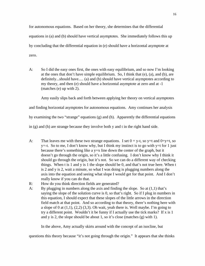
Amy begins her analysis by examining the direction fields for equilibrium solutions,

moving easily between the graphical and symbolic representations. Moreover, recall that

her response to the question, “What does it mean to study a differential equation

qualitatively?” she said it “means to me to be able to look at slopes and equilibrium and be

able to tell equilibrium.” The following excerpt illustrates her ability to look at slopes and

equilibrium, demonstrating her understanding of the derivative and flexibility in using both

graphical and symbolic representations.

A: Ok, now are some of these [referring to the 8 differential equations] not thedirection field?

R: We’ve got 4 direction fields and 8 differential equations.A: Ok, so problem (d) is definitely not one of them because there is no equilibrium at 1.

So I can cross that out. Problem (c) there is an equilibrium at -1 so that probablymatches the fourth direction field, but I should check the slope to make sure that’sOk. So at 0 the slope is 1 and that looks right. I checked the slope just by pluggingin 0 for y and got 1 for dy/dt and came up with that. So I’d say 4 is (c).

15

Next, she turns her attention to the differential equation in (b), inventing a theory for

finding vertical asymptotes.

A: Well, now wait a second here, I hate these things. t = ...yes that’s right, now if.. I’mlooking at (b) with dy/dt = t + 1. If t =..., if I find it’s equal to 0 then I’m thinkingthis means there’s a vertical asymptote, is that right?

R: Which problem is this?A: For (b),R: For (b).A: If you set it equal to 0, then.... wait a second (mumbling). That’s right, because I

don’t see a vertical asymptote at -1, I’m going to discount that. Actually I don’t seea vertical asymptote anywhere that’s explicit. I still question my theory aboutvertical asymptotes, I’m not sure.

R: What’s your theory about vertical asymptotes?A: That if you set dy/dt =0, so 0 = t +1, and you get t=-1 that means there should be a

vertical asymptote at -1. I mean I believe that for finding horizontal asymptotes, butI’ve never, I haven’t come across a problem that says there are vertical asymptotesand you can find them this way, so I don’t know if it’s true.

R: Ok, so that’s a theory you’ve just developed?A: Yeah.

Amy appears to be searching for a strategy to deal with differential equations, such

as the one in (b), that depend only on time. One interpretation of her “theory” is she is

overgeneralizing a strategy to find constant solutions for autonomous differential equations,

which do not depend on time. The differential equations in (c), (d), (e), and (f) are all

autonomous and will therefore have equilibrium solutions whenever dy/dt=0. This follows

directly from the interpretation of the derivative as slope. Although she has demonstrated a

solid understanding of the derivative as slope, she appears to see no conflict or

contradiction between this and her theory, which would call for a function to have near zero

slope as it approached a vertical asymptote.

Amy continues to work with the differential equations and attempts to apply her

theory of vertical asymptotes as well as the strategy for determining equilibrium solutions

16

for autonomous equations. Based on her theory, she determines that the differential

equations in (a) and (b) should have vertical asymptotes. She immediately follows this up

by concluding that the differential equation in (e) should have a horizontal asymptote at

zero.

A: So I did the easy ones first, the ones with easy equilibrium, and so now I’m lookingat the ones that don’t have simple equilibrium. So, I think that (e), (a), and (b), aredefinitely...should have..... (a) and (b) should have vertical asymptotes according tomy theory, and then (e) should have a horizontal asymptote at zero and at -1(matches (e) up with 2).

Amy easily slips back and forth between applying her theory on vertical asymptotes

and finding horizontal asymptotes for autonomous equations. Amy continues her analysis

by examining the two “strange” equations (g) and (h). Apparently the differential equations

in (g) and (h) are strange because they involve both y and t in the right hand side.

A: That leaves me with these two strange equations. I set 0 = y-t, so y=t and 0=y+t, soy=-t. So to me, I don’t know why, but I think my instinct is to go with y=t for 1 justbecause there’s something like a y=x line down the center of the graph, but itdoesn’t go through the origin, so it’s a little confusing. I don’t know why I think itshould go through the origin, but it’s not. So we can do a different way of checkingthings. When t is 1 and y is 1 the slope should be 0, and that’s not true here. When tis 2 and y is 2, wait a minute, so what I was doing is plugging numbers along theaxis into the equation and seeing what slope I would get for that point. And I don’treally know if you can do that.

R: How do you think direction fields are generated?A: By plugging in numbers along the axis and finding the slope. So at (1,1) that’s

saying the slope of the solution curve is 0, so that’s right. So if I plug in numbers inthis equation, I should expect that these slopes of the little arrows in the directionfield match at that point. And so according to that theory, there’s nothing here witha slope of 0 at (1,1), (2,2) (3,3). Oh wait, yeah there is. Well maybe. I’m going totry a different point. Wouldn’t it be funny if I actually use the tick marks? If x is 1and y is 2, the slope should be about 1, so it’s close (matches (g) with 1).

In the above, Amy actually skirts around with the concept of an isocline, but

questions this theory because “it’s not going through the origin.” It appears that she thinks

17

the “arrow” should be centered at the point in question, rather than having its foot at the

point. The method of isoclines was not covered in class or in the textbook, so this suggests

that the strategy she begins to pursue is self-generated. Amy next decides to “test (h) on 3

because it’s the only one I haven’t ruled out yet.” In order to recap her decisions thus far, I

asked her to explain why she ruled out the various choices, which seemed to provide her

with an opportunity to reflect on what it means for a differential equation to be

autonomous.

R: Can you explain why you ruled out the other ones? I mean obviously the ones youruled out because you matched them up correctly, but the other ones you’ve ruledout, can you explain why you ruled those out?

A: Ok, there’s another reason why I can rule out the other ones that I just thought ofand that’s because these, (a), (b), and (e), only have one variable on the one side ofthe equation--they’re autonomous, is that correct?

R: What does autonomous mean to you?A: Autonomous means to me it’s only, that the equations only vary by one variable.R: Ok, not quite. Autonomous means there is only one variable on the right hand side,

but it also means that that variable is the dependent variable--not time.A: Oh!R: So an autonomous equation does not depend on....A: Time. So (e) is autonomous, (f) is autonomous, (c) is autonomous, and (d) is

autonomous.R: Some people say that if a differential equation is autonomous, the direction field is

easy to graph, why do you think they say that?A: Because since it doesn’t vary with time if you find one slope along a y = c line then

the slope is the same all the way across. So 2 and 4 are direction fields ofautonomous equations because the slopes of the lines do not change as t changes,but 1 and 3 are not autonomous, so 3 has to be (a), (b), or (h). so, I’ll check (a) and(b), though I’m hesitant because I really don’t want to blow my vertical asymptotetheory.

R: Is this vertical asymptote theory something you developed by yourself?A: Yeah, definitely, just right now.

Although the original intent of the interview was to try and capture what she could

do on her own, without my intervention, my questions and interaction most likely influenced

18

her solution strategy. After this brief clarification of what the term autonomous means,

both symbolically and graphically, Amy rethinks some of her choices.

A: Using the same thinking about the autonomous equations and if it only depends onthe change, and t is the independent variable. Ok, so if dy/dt=t-1, 3 could be it. Thedifferential equation only varies with t and so you would get equal slopes along linest=c , c = a number. And if you had a differential equation that depended on both yand t then you would not get equal slopes on any lines of y=c or t=c.

R: Is that consistent with your choices so far?A: So far it is, so it could be. So the vertical asymptote theory is blown, in place of

another. So when t=0, y' , the slope, equals -1. We can discount (a) for 3.R: Why can we discount (a)?A: Because when t=0 the slope should be -1 and this is obviously from a graph that’s

increasing, so it can’t be a negative value.

Amy then checks the value of dy/dt in (b) for several values of t and decides that (b)

matches the direction field labeled 3. Throughout the above activity, Amy demonstrated

flexible and versatile thinking. She essentially discovered a special case of the isocline

method for sketching direction fields and she immediately transferred the idea behind

graphing direction fields for autonomous differential equations to differential equations that

vary only with time and to those that involve both time and the dependent variable. This

analysis then led to the rejection of her vertical asymptote theory. In other words, Amy

decided her theory on vertical asymptotes was no longer “viable.” From a constructivist

perspective, “the conception of truth as the correct representation of states or events of an

external world is replaced by the notion of viability. To the constructivist, concepts,

models, theories, and so on are viable if they prove adequate in the contexts in which they

were created” (von Glasersfeld, 1995, p. 7-8). Thus, Amy’s vertical asymptote theory was

no longer adequate and was replaced by “another,” which may also prove to be inadequate.

In terms of the distinction between conceptual and procedural knowledge as described by

19

Hiebert and Lefevre (1986), Amy’s conceptual knowledge assumed an “executive control

function” (p. 13). That is, her conceptual knowledge acted as “validating critic,” judging

the reasonableness of the outcome to the vertical asymptote theory and ultimately rejecting

it.

Notions of Stability

Amy’s understanding of stability was examined from two related, but slightly

different perspectives. The first aspect of stability examined deals with the stability of a

differential equation itself and the second aspect deals with the asymptotic stability of

equilibrium solutions. Triangulation of the data sources in this study provided convergent

evidence of Amy’s understanding of stability, but it also yielded some inconsistency in the

data. As Mathison (1988) points out, triangulation of data sources in qualitative research

often leads to inconsistency among the data and it is the goal of the researcher to provide

meaningful propositions regarding the data. The following discussion describes the data

collected and an explanation regarding the inconsistent data is offered.

The first source of data regarding Amy’s understanding of stability comes from an

activity in the Mathematica problem set. This activity read as follows:

Solve the initial value problem y y x' cos− = , y c( )0 = . Use Mathematica to graphsolutions for c = -0.9,-0.8,...,-0.1,0. Display all the solutions on the same intervalbetween x = 0 and an appropriately chosen right endpoint. Explain what happens tothe solution curves for large values of x. (Hint: You should identify three distincttypes of behavior.) Now, based on this problem, and the material in Chapters 5 and6, discuss what effect small changes in initial data can have on the global behavior ofsolution curves.

Amy’s response, which follows below (minus the two graphs she generated), provides a

clear and accurate answer to these questions.

20

The behavior of the solution curves for y’-y=cos(x) at large values of x dependsupon the value of the initial value c. When -0.9<c<-0.5, the solution curvesapproach −∞. When -0.5<c<0, the solution curves approach +∞. When c=-0.5, the

solution curve oscillates around x=0 according to the equation − +cos sinx x

2.

As seen in this example, small changes in initial conditions can have verylarge effects on the behavior of the solution curves. As x grows larger, solutioncurves with different values of c diverge drastically, some going to +∞, some to-∞, and one oscillating around x=0. Because the solution of y’-y=cos(x) is verysensitive to initial conditions, the differential equation is unstable. Not alldifferential equations behave like this one. For example, some stable differentialequations have solutions whose curves converge as x grows larger, regardless of theinitial value c.

In her response to this problem, Amy coordinates the symbolic expression for the

solution when c = -0.5 with the plot of the solution curve that oscillates around x=0 and

demonstrates a solid understanding of what it means for a differential equation to be stable.

This aspect of stability is inextricably linked to an understanding of what it means for a

solution to be sensitive to initial conditions. The excerpt below from the second interview

was intended to uncover Amy’s understanding of this principle.

R: Describe what the phrase sensitivity to initial conditions means.A: That means the solution to your differential equation depends on the initial

condition, so if it’s extremely sensitive and you have different initial conditions thenthe solutions will diverge a lot and if its insensitive, then regardless of the initialcondition, all the solutions of the differential equation will end up looking the sameway after a long time.

The above excerpt strongly suggests that Amy has a thorough and solid understanding of

this concept. The next segment of the interview provides some additional insight into her

thinking and the continual way in which she draws on her knowledge of fishery science.

R: Why is this concept of sensitivity of initial conditions important?A: It’s important when you try to estimate error. It’s definitely important for the

application of differential equations and any situation where you are trying to fit an

21

equation to your observed data, whether it’s in physics or biology. If you have anequation that is sensitive, then your initial conditions you establish have to beextremely accurate, especially in biology where its really hard and often times inpopulation growth you can only estimate or assume the initial conditions so you cannever really know (the exact initial conditions). So if it’s a sensitive differentialequation that you’re using, with quite possibility incorrect initial conditions, yourjust going to get an outrageous answer anyway.

R: Where do you feel you’ve gotten most of your understanding of sensitivity to initialconditions?

A: The homework assignments from Mathematica and my understanding of fisheryscience. When I was doing the Mathematica problem about sensitively, it made a lotof sense to me and it helped me to think about it in terms of population and fishstock.

The above statement is accurate and well said. What is of particular relevance to

understanding Amy’s concept of stability is the perspective from which she considers the

issue of sensitivity to initial conditions. When Amy speaks of trying to fit an equation (a

differential equation) to some observed data, she is viewing the subject of differential

equations as a means for modeling observed phenomena. From a modeling perspective, it is

perhaps more useful to think of the differential equation itself as being stable or unstable,

as opposed to thinking of a particular solution to an initial value problem as stable or

unstable and Amy provides a valid argument for why this perspective is useful.

In addition to demonstrating a solid understanding of the notion of stability as it

applies to a differential equation, Amy also demonstrates a well-connected understanding of

stability as it applies to the equilibrium solutions to an autonomous differential equation.

Two of the activities from the Mathematica problem set involve autonomous differential

equations and require the student to determine the equilibrium solutions and whether these

particular solutions are stable or unstable. In the first activity, Amy uses Mathematica to

plot the direction field for the differential equation y y y' sin= + −3 2, uses the equation

solver to determine the equilibrium, and correctly interprets the direction field to determine

22

the stability of each equilibrium solution. In the second activity, Amy uses Mathematica to

plot the direction field for x x x x' ( ln )( )= − −1 3 , which appears to show a continuum of

equilibrium solutions for 3<x<2.5 Thus, the direction field alone is insufficient to reach a

firm conclusion regarding the number and nature of equilibrium solutions. In response to

the ambiguity, Amy uses the graph of the differential equation itself to figure out “what’s

going on” for 3<x<2.5. In so doing, she demonstrates a solid, conceptual understanding of

the derivative and its relationship to the direction field.

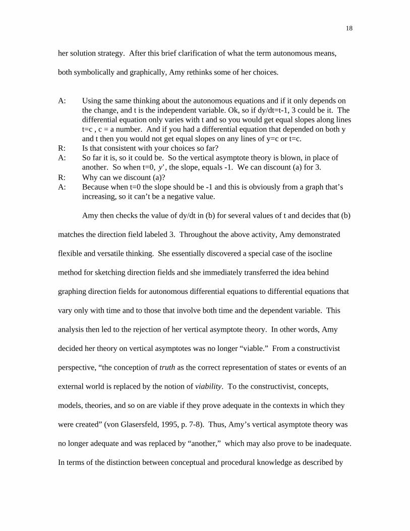
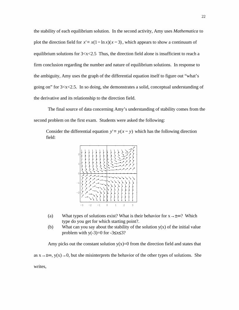
The final source of data concerning Amy’s understanding of stability comes from the

second problem on the first exam. Students were asked the following:

Consider the differential equation y y x y' ( )= − which has the following directionfield:

-3 -2 -1 0 1 2 3

-2

-1

0

1

2

(a) What types of solutions exist? What is their behavior for x→±∞? Whichtype do you get for which starting point?.

(b) What can you say about the stability of the solution y(x) of the initial valueproblem with y(-3)=0 for -3≤x≤3?

Amy picks out the constant solution y(x)=0 from the direction field and states that

as x→±∞, y(x)→0, but she misinterprets the behavior of the other types of solutions. She

writes,

23

Solutions starting to the left of x ≅ -2.5 in the lower left quadrant, and solutionsstarting to the left of x ≅ -.5 in the upper quadrant appear to be stable. Theyconverge to y = 0, and their limit as x→∞ is 0.Solutions starting to the right of x ≅ -2.5 in the lower left quadrant, and solution(s)starting to the right of x ≅ -.5 in the upper quadrant appear to be unstable. Theydiverge from the equilibrium value, and as x→∞, their limit →∞ .

Why, despite Amy’s self-acknowledged preference for graphical representations, did

she incorrectly interpret this direction field? Solution curves such as Amy describes above

would necessarily cross and hence violate the uniqueness theorem. However, examination

of students’ understanding of the uniqueness theorem remains for further investigation.

Was Amy’s incorrect response caused by simply “misreading” the direction field? If so,

what aspects of the direction field did she find difficult to interpret? I spoke with her

shortly after the exam and she explained how she was unsure what was happening near the

positive x-axis. This is understandable as this region is somewhat sparsely populated with

arrows. Amy mentioned she actually plugged in a few points into the differential equation

(much like she did in the matching activity), but found no contradiction between the slopes

and her description. Not having any evidence to contradict her initial impression, she

decided she was correct. That is, her interpretation remained viable. However, another,

perhaps more serious problem, is that she believes once solutions appear to become stable,

or approach an equilibrium solution in an asymptotic manner, they will remain close to the

equilibrium solution. Evidence to support this hypothesis has been found in other research

that I am currently working on. Moreover, the use of phase lines, which are the one-

dimensional analog to the phase plane and used in part to help students qualitatively analyze

first order autonomous differential equations, may in fact foster this misconception.

Although not part of the curriculum in this course, phase lines are used in some recent

24

reform-oriented texts (see Blanchard, Devaney, & Hall, 1996; Lomen & Lovelock, 1996)

and the results here suggest the need for further investigation regarding the use of phase

lines.

For part (b), Amy gave the following response, which is also flawed.

At y(-3), the solution is y(x)=0. This is an equilibrium solution which is very stablesince it never changes. As x→∞, y(x) →0.

In the two previous problems from the Mathematica problem set, Amy was able to identify

the stability and/or instability of the equilibrium solutions to autonomous differential

equations. However, she was unable to transfer this ability to this problem, where the

differential equation is not autonomous. Recall the matching activity discussed in the

beginning of this paper where she called the two differential equations in which both the

dependent and independent variable appeared in the right hand side “strange.” Perhaps the

“strangeness” of this situation led her to fall back on her understanding of stability as a

concept that applies to a set of solutions and thus conclude that this one solution is “very

stable since it never changes.” In support of this hypothesis, her strong and thorough

description of why sensitivity to initial conditions is important suggests that the aspect of

stability which refers to a differential equation is dominant in her mind.

Conclusions

Amy demonstrated a solid understanding of and ability to qualitatively analyze first

order differential equations and a strong and coherent concept of stability. There were

three main sources which she cited as major influences: her strong conceptual and graphical

understanding of the derivative as slope or rate of change, her prior knowledge of

25

population modeling, and the Mathematica supplement. She continually made reference to

her preference for graphical representations as the best means for her to understand a

concept and her knowledge of fishery science appeared to provide a “hook” on which she

could hang her emerging understanding of differential equations. Moreover, Amy appeared

to recognize the need to move beyond just seeing “bunches of fish getting larger and

smaller” to just seeing how a solution to a differential equation can be a “function in and of

itself.” Despite her solid conceptual understanding of the derivative and her understanding

of modeling population growth with differential equations, several potential difficulties were

uncovered. These difficulties included:

• an overgeneralization of the term autonomous to include first order differentialequations that only involve the independent variable.

• an overgeneralization of a strategy used to sketch and/or interpret direction fields for

autonomous differential equations. This led to her “vertical asymptote theory.” • an incorrect interpretation of the behavior of solutions based on the direction field.

Despite attempts to disprove this interpretation, her initial image remained viable. Onepossible explanation for this incorrect interpretation is the misconception that oncesolutions appear to become stable, or approach an equilibrium solution in an asymptoticmanner, they will remain close to that equilibrium solution.

• a strong notion of stability of a differential equation that possibly prevented her from

correctly interpreting the stability of an equilibrium solution for a non-autonomousdifferential equation.

Besides uncovering some possible difficulties, this study also raised further

questions:

• To what extent are these difficulties resilient to instruction and/or other curriculums?• How widespread is the misconception that a solution which approaches an equilibrium

solution in an asymptotic manner must remain asymptotic to that equilibrium solution?Does the use of phase lines foster that misconception?

26

• What role should class time play in the development of students’ ability to interpret anduse the various graphical representations which are now so readily available withtechnology?

• What characterizes the understanding and difficulties of students who do not initiallyhave a strong conceptual and graphical understanding of the derivative?

• What characterizes the understanding and difficulties of students who do not initiallyhave an awareness of the power of differential equations to model real worldphenomena?

The growing number of innovative curriculums, new learning theories, and the

increasingly availability of technology provides an extraordinary opportunity to deepen

students’ understanding of differential equations, to provide insight about the behavior of

solutions, and to give students an idea of how the subject is relevant to other disciplines.

Continued research efforts in all aspects of the teaching and learning of mathematics in

general and differential equations in particular is needed to realize these goals.

27

References

Artigue, M. (1992). Cognitive difficulties and teaching practices. In G. Harel, & E.

Dubinsky (Eds.), The concept of function: Aspects of epistemology and pedagogy. (pp.

109-132). (MAA Notes Number 25). Washington, DC: Mathematical Association of

America.

Blanchard, P. (1994). Teaching differential equations with a dynamical systems

viewpoint. The College Mathematics Journal, 25, 385-393.

Blanchard, P., Devaney, R., & Hall, R. (1996). Differential equations (preliminary

ed.). Boston: PWS.

Bogdan, R. C., & Biklen, S. K. (1992). Qualitative research for education. Boston:

Allyn and Bacon.

Borrelli, R., & Coleman, C. (1996). Differential equations: A modeling perspective.

New York: Wiley.

Coombes, K. R., Hunt, B. R., Lipsman, R. L., Osborn, J. E., & Stuck, G. J. (1995).

Differential Equations with Mathematica. New York: Wiley.

Confrey, J. (1990). What constructivism implies for teaching. In R. B. Davis, C. A.

Maher, &N. Noddings, (Eds.), Constructivist Views on the Teaching and Learning of

Mathematics. Journal for Research in Mathematics Education Monograph No. 4 (pp. 107,

122).

Douglas, R. G. (Ed.). (1986). Toward a lean and lively calculus. (MAA Notes

Number 6). Washington, DC: Mathematical Association of America.

28

Dubinsky, E. (1994). A theory and practice of learning college mathematics. In A.

H. Schoenfeld (Ed.), Mathematical Thinking and Problem Solving (pp. 221-243). Hillsdale,

NJ: Erlbaum.

Fraga, R. (Ed.). (1993). Calculus problems for a new century. (MAA Notes Number

28). Washington, DC: Mathematical Association of America.

Hiebert, J., & Lefevre, P. (1986). Conceptual and procedural knowledge in

mathematics: An introductory analysis. In J. Hiebert (Ed.), Conceptual and procedural

knowledge: The case of mathematics. (pp. 1-27). Hillsdale, NJ: Erlbaum.

Kostelich, E., & Armbruster, D. (1995). Introductory differential equations: From

linearity to chaos (preliminary ed.). Reading, MA: Addison-Wesley.

Lomen, D., & Lovelock, D. (1996). Exploring differential equations via graphics

and data. (preliminary ed.). New York: Wiley.

Mathison, S. (1988). Why triangulate? Educational Researcher 17 (2), 13-17.

Thompson, P. W. (1995). Constructivism, cybernetics, and information processing:

Implications for technologies of research on learning. In L. P. Steffe, & J. Gale (Eds.),

Constructivism in Education (pp. 123- 270). Hillsdale, NJ: Erlbaum.

Tucker, T. W. (Ed.). (1990). Priming the calculus pump: Innovations and resources.

(MAA Notes Number 17). Washington, DC: Mathematical Association of America.

von Glasersfeld. E. (1995). A constructivist approach to teaching. In L. P. Steffe, &

J. Gale (Eds.), Constructivism in Education (pp. 3-15). Hillsdale, NJ: Erlbaum.

West, B., Strogatz, S., McDill, J. M., & Cantwell, J. (in press). Interactive

differential equations. Reading, MA: Addison-Wesley.