Quadratic Parametric Programming for

Portfolio Selection with Random

Problem Generation and Computational

Experience

Markus Hirschberger∗

Department of MathematicsUniversity of Eichstatt-Ingolstadt

Eichstatt, Germanyand

Yue Qi and Ralph E. SteuerTerry College of Business

University of GeorgiaAthens, Georgia 30602-6253 USA

March 22, 2004

Abstract

For researchers intending to investigate mid- to large-scale portfolio se-lection, good, inexpensive and understandable quadratic parametric pro-gramming software, capable of computing the efficient frontiers of prob-lems with up to two thousand securities without simplifications to thecovariance matrix, is hardly known to be available anywhere. As an alter-native to Markowitz’s critical line method, a full explication of a simplex-based quadratic parametric programming procedure, utilizing well-knowncomponents, is coded in Java for public domain use on modern desktopsand laptops. The advantage of the different design is to provide an al-gorithm that can ultimately be extended (not a part of this paper) toportfolio problems with objectives beyond mean and variance. Using thecode, aspects of portfolio selection problems are investigated and compu-tational experience is reported.

Keywords: Portfolio selection, quadratic parametric programming, Kuhn-Tucker Conditions, efficient frontier, nondominated frontier, turning points,random problem generator, computational experience

∗Research conducted while a visiting scholar at the Department of Banking and Finance,Terry College of Business, University of Georgia, October 2003–March 2004.

1

1 Introduction

Due to Markowitz [?], the model of portfolio selection is as follows. Assume

(a) n securities(b) an initial sum of money to be invested(c) the beginning of a holding period(d) the end of the holding period

Let x1, . . . , xn be investment proportion weights. The xi are the proportions ofthe initial sum invested in the n securities to form a portfolio at the beginningof the holding period. Unless restricted to the contrary, an xi can take on anyvalue. Nevertheless, all xi must sum to one. An xi < 0 means that securityi is sold short with the cash generated then providing additional money to beinvested in the other securities. An xi > 1 is possible. Assume a two-stockportfolio and an initial sum of $100. If security 1 is sold short to the extent of$40, then because all weights must sum to one, the $40 plus the initial sum areinvested in security 2 in which case x1 = −0.4 and x2 = 1.4.

Let ri be the random variable for the percent return realized on security ibetween the beginning of the holding period and the end of the holding period.Let rp be the random variable for the percent return realized on a portfoliobetween the beginning of the holding period and the end of the holding period,where

rp =n∑

i=1

rixi (1)

In this way, rp is a function of both the ri and the xi. Since the ri are not knownuntil the end of the holding period, but the xi must be chosen at the beginningof the period, attempting to maximize rp via (1) is a stochastic optimizationproblem. With solutions of a stochastic optimization problems not well defined,a decision is required on how to proceed.

Since an investor can never know at the beginning of the holding periodthe value of rp to be realized at the end of the holding period, the investoris in a quandary. Ideally, an investor would like to position his initial sumto maximize his chances of reaping a high value of rp while at the same timeminimizing his exposure to disconcertingly low values of rp. Assuming that allri are from distributions whose means µi , variances σii and covariances σij areknown, Markowitz’s mean-variance solution procedure, which has come to formthe foundation of what we know of today as “modern portfolio analysis,” is to

2

proceed with the bi-criterion program

min {n∑

i=1

n∑

j=1

xiσijxj = σ2p} (2.1)

max {n∑

i=1

µjxj = µp} (2.2)

s.t.

n∑

i=1

xi = 1 (2.3)

`i ≤ xi ≤ ωi (2.4)

where σ2p is the variance of rp and µp is expected value, in accordance with the

following two-step approach.Before describing the approach, let us note that (a) each (x1, . . . , xn) ∈ Rn

via (2.1–2.2) generates an image vector (σ2p, µp), and (b) an image vector is

said the be feasible in (2.1–2.4) if and only if its inverse image (x1, . . . , xn) isfeasible with respect to (2.3–2.4). In this way, the goal of Step 1 is to obtain allnondominated image vectors (σ2

p, µp) by computing among some collection of(x1, . . . , xn) solutions feasible with respect to (2.3–2.4) that generate them.

Definition 1. Image vector (σ2p, µp) generated by (x1, . . . , xn) feasible w.r.t.

(2.3–2.4) is nondominated if and only if there does not exist another (σ2p, µp)

generated by a (x1, . . . , xn) feasible w.r.t. (2.3–2.4) such that

(i) σ2p ≤ σ2

p

(ii) µp ≥ µp, and(iii) (σ2

p, µp) 6= (σ2p, µp)

Otherwise, (σ2p, µp) is dominated.

When interfacing with an investor, it is customary to convert the first componentof each (σ2

p, µp) to standard deviation and then plot the (σp, µp), which are nowcalled attribute vectors, on a graph, with standard deviation of portfolio returnσp on the horizontal and expected portfolio return µp on the vertical. Notaffecting the dominance/nondominace status of the vector, the conversion isdone for two reasons. One is that variance is not workable with investors, andthe other is that now both axes are in the same units (% per time period) tobetter facilitate the comparisons among (σp, µp) attribute vectors that needs tobe done in Step 2.

The set of all nondominated (σp, µp) plot as a concave curve in 2-spacethat we will call the nondominated frontier. We are aware that this curveis widely known as the “efficient frontier,” but we wish to reserve the terms“nondominated” and “dominated” for use with points in attribute space, whilereserving the terms “efficient” and “inefficient” for use with points (x1, . . . , xn)in investment proportion space.

3

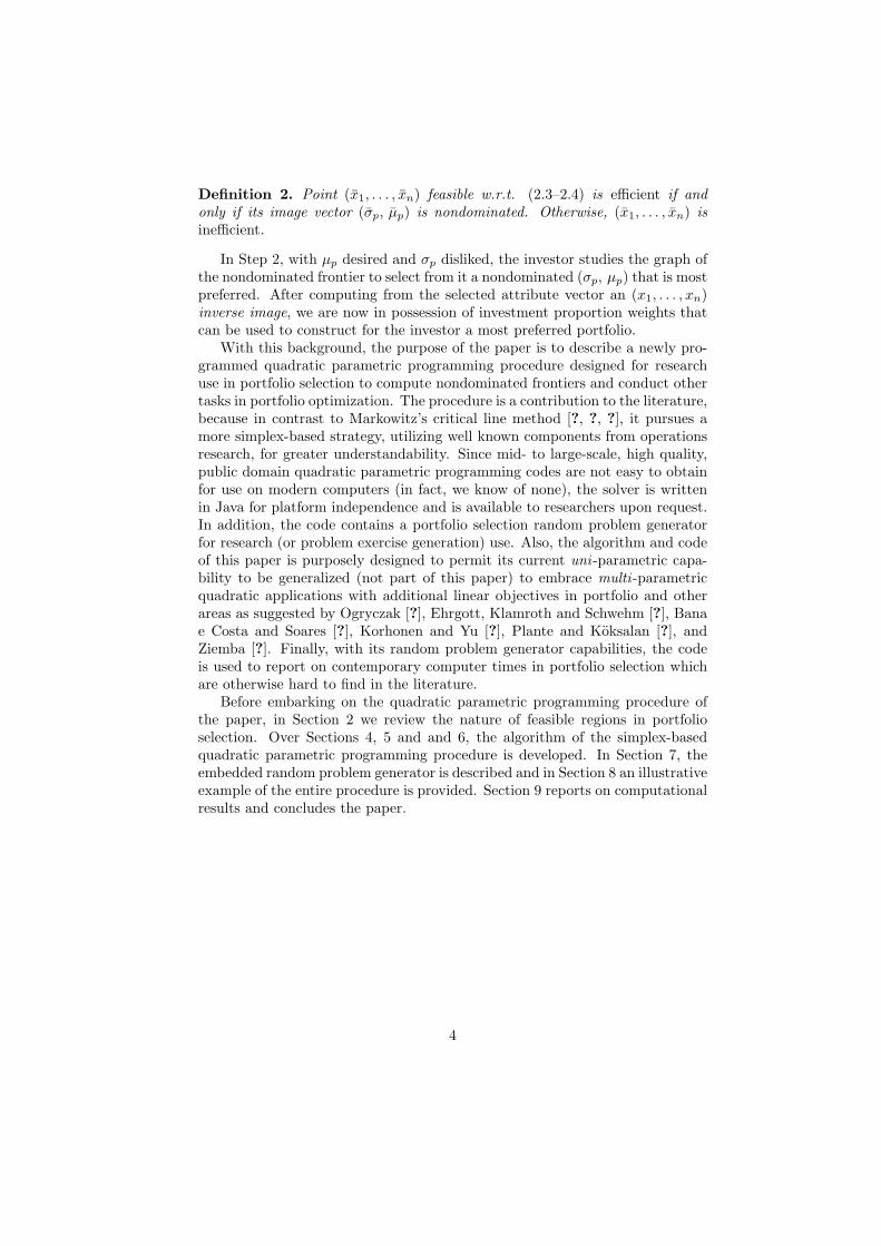
Definition 2. Point (x1, . . . , xn) feasible w.r.t. (2.3–2.4) is efficient if andonly if its image vector (σp, µp) is nondominated. Otherwise, (x1, . . . , xn) isinefficient.

In Step 2, with µp desired and σp disliked, the investor studies the graph ofthe nondominated frontier to select from it a nondominated (σp, µp) that is mostpreferred. After computing from the selected attribute vector an (x1, . . . , xn)inverse image, we are now in possession of investment proportion weights thatcan be used to construct for the investor a most preferred portfolio.

With this background, the purpose of the paper is to describe a newly pro-grammed quadratic parametric programming procedure designed for researchuse in portfolio selection to compute nondominated frontiers and conduct othertasks in portfolio optimization. The procedure is a contribution to the literature,because in contrast to Markowitz’s critical line method [?, ?, ?], it pursues amore simplex-based strategy, utilizing well known components from operationsresearch, for greater understandability. Since mid- to large-scale, high quality,public domain quadratic parametric programming codes are not easy to obtainfor use on modern computers (in fact, we know of none), the solver is writtenin Java for platform independence and is available to researchers upon request.In addition, the code contains a portfolio selection random problem generatorfor research (or problem exercise generation) use. Also, the algorithm and codeof this paper is purposely designed to permit its current uni -parametric capa-bility to be generalized (not part of this paper) to embrace multi -parametricquadratic applications with additional linear objectives in portfolio and otherareas as suggested by Ogryczak [?], Ehrgott, Klamroth and Schwehm [?], Banae Costa and Soares [?], Korhonen and Yu [?], Plante and Koksalan [?], andZiemba [?]. Finally, with its random problem generator capabilities, the codeis used to report on contemporary computer times in portfolio selection whichare otherwise hard to find in the literature.

Before embarking on the quadratic parametric programming procedure ofthe paper, in Section 2 we review the nature of feasible regions in portfolioselection. Over Sections 4, 5 and and 6, the algorithm of the simplex-basedquadratic parametric programming procedure is developed. In Section 7, theembedded random problem generator is described and in Section 8 an illustrativeexample of the entire procedure is provided. Section 9 reports on computationalresults and concludes the paper.

4

2 Feasible Regions in Portfolio Selection

It is convenient to slightly generalize and re-write (2.1–2.4) in matrix notation

min {xT Σx = σ2p} (3.1)

max {µT x = µp} (3.2)

s.t. Hx = d (3.3)

Gx ≤ b (3.4)x ≤ ω (3.5)x ≥ ` (3.6)

where Σ ∈ Rn×n is the covariance matrix of the σij , Hx = d allows for thereto be equality constraints in addition to (2.3), Gx ≤ b allows for inequalityconstraints (should there be any), and ω and ` are vectors of upper and lowerbounds on the xi. Note: We know the “check” notation in the three cases aboveis probably annoying, but it will disappear shortly.

Formulation (3.1–3.6) has two feasible regions. One is S ⊂ Rn in investmentproportion space, where

S = {x ∈ Rn | x is feasible w.r.t. (3.3–3.6)}

The other is Z ⊂ R2 in attribute (standard-deviation, expected-return) space,where

Z = {z ∈ R2 | z1 =√

xT Σx, z2 = µT x, for all x ∈ S}Feasible region S is always some subset of the hyperplane x1 + . . . + xn = 1,while Z, the set of images of the x ∈ S, typically takes on a bullet-shapedappearance as in Figure 2. As for the nondominated frontier, it is the concavecurve that constitutes the upper portion of the minimum standard deviationboundary of Z. More specifically, it is the set of attribute vectors from which itis not possible to feasibly increase expected return without decreasing standarddeviation, or feasibly decrease standard deviation without increasing expectedreturn.

To elaborate on some aspects of the nondominated frontier particularly rel-evant to this paper, consider Examples 1 and 2. Example 1 shows that the(σp, µp) attribute vectors of linear combinations of two securities whose weightssum to one lie along a hyperbola in (standard-deviation, expected-return) space.Example 2 shows that nondominated frontiers are typically piecewise hyperbolicand that all portfolios on a given hyperbolic segment involve the same securities,just in different proportions.

Example 1. Consider two securities whose individual standard deviations ofreturn σi, individual expected returns µi, correlation matrix Γ, and covariancematrix Σ = diag(σ1, σ2)Γ diag(σ1, σ2), are in Table 1.

5

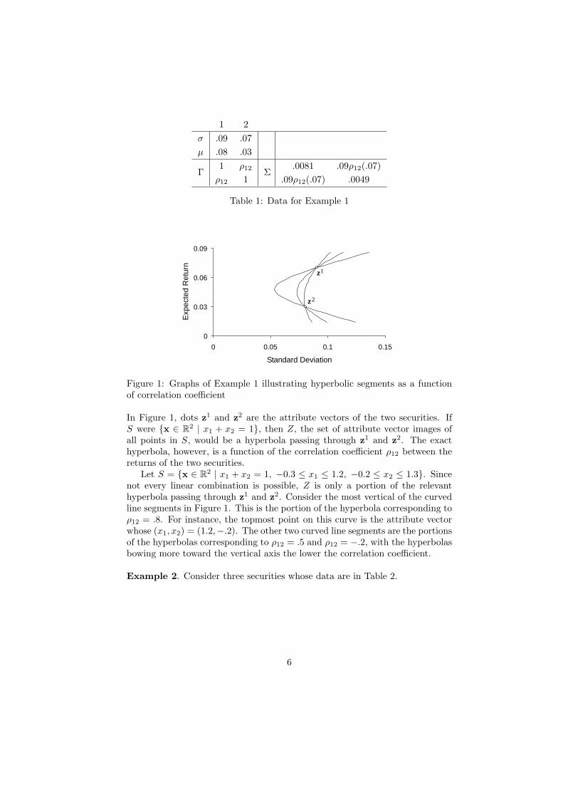
1 2σ .09 .07µ .08 .03

Γ1 ρ12 Σ

.0081 .09ρ12(.07)ρ12 1 .09ρ12(.07) .0049

Table 1: Data for Example 1

0

0.03

0.06

0.09

0 0.05 0.1 0.15

Standard Deviation

Exp

ecte

d R

etur

n

z2

z1

dd

Figure 1: Graphs of Example 1 illustrating hyperbolic segments as a functionof correlation coefficient

In Figure 1, dots z1 and z2 are the attribute vectors of the two securities. IfS were {x ∈ R2 | x1 + x2 = 1}, then Z, the set of attribute vector images ofall points in S, would be a hyperbola passing through z1 and z2. The exacthyperbola, however, is a function of the correlation coefficient ρ12 between thereturns of the two securities.

Let S = {x ∈ R2 | x1 + x2 = 1, −0.3 ≤ x1 ≤ 1.2, −0.2 ≤ x2 ≤ 1.3}. Sincenot every linear combination is possible, Z is only a portion of the relevanthyperbola passing through z1 and z2. Consider the most vertical of the curvedline segments in Figure 1. This is the portion of the hyperbola corresponding toρ12 = .8. For instance, the topmost point on this curve is the attribute vectorwhose (x1, x2) = (1.2,−.2). The other two curved line segments are the portionsof the hyperbolas corresponding to ρ12 = .5 and ρ12 = −.2, with the hyperbolasbowing more toward the vertical axis the lower the correlation coefficient.

Example 2. Consider three securities whose data are in Table 2.

6

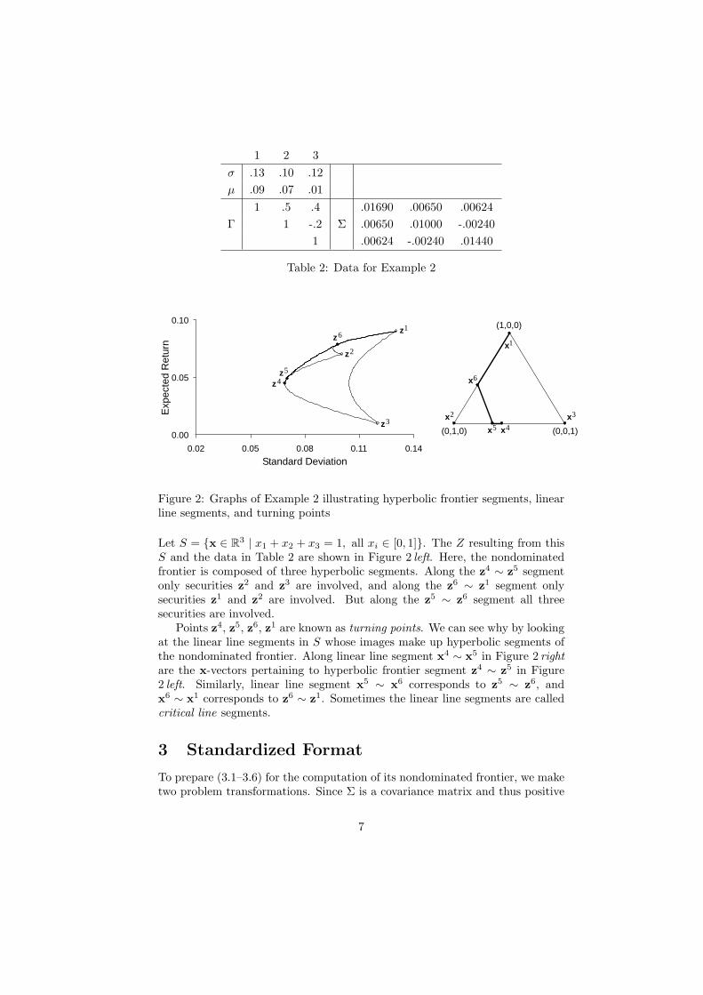
1 2 3σ .13 .10 .12µ .09 .07 .01

1 .5 .4 .01690 .00650 .00624Γ 1 -.2 Σ .00650 .01000 -.00240

1 .00624 -.00240 .01440

Table 2: Data for Example 2

z1

z2

z3

z4z5

z6

0.00

0.05

0.10

0.02 0.05 0.08 0.14

Standard Deviation

Exp

ecte

d R

etur

n

0.11

x1

x2 x3

x4x5

x6

(0,1,0)

(1,0,0)

(0,0,1)

Figure 2: Graphs of Example 2 illustrating hyperbolic frontier segments, linearline segments, and turning points

Let S = {x ∈ R3 | x1 + x2 + x3 = 1, all xi ∈ [0, 1]}. The Z resulting from thisS and the data in Table 2 are shown in Figure 2 left. Here, the nondominatedfrontier is composed of three hyperbolic segments. Along the z4 ∼ z5 segmentonly securities z2 and z3 are involved, and along the z6 ∼ z1 segment onlysecurities z1 and z2 are involved. But along the z5 ∼ z6 segment all threesecurities are involved.

Points z4, z5, z6, z1 are known as turning points. We can see why by lookingat the linear line segments in S whose images make up hyperbolic segments ofthe nondominated frontier. Along linear line segment x4 ∼ x5 in Figure 2 rightare the x-vectors pertaining to hyperbolic frontier segment z4 ∼ z5 in Figure2 left. Similarly, linear line segment x5 ∼ x6 corresponds to z5 ∼ z6, andx6 ∼ x1 corresponds to z6 ∼ z1. Sometimes the linear line segments are calledcritical line segments.

3 Standardized Format

To prepare (3.1–3.6) for the computation of its nondominated frontier, we maketwo problem transformations. Since Σ is a covariance matrix and thus positive

7

semidefinite,1 −xT Σx is then concave. Since most Σs are empirically derived,they usually are not of full rank. When not of full rank, we recommend adding anumber such as 10−6 to each diagonal element of Σ. This goal is for the numberto be small enough not to affect the problem, but large enough to make Σinvertible, in which case −xT Σx becomes strictly concave. With −xT Σx+µT xstrictly concave, one transformation is to note that by solving

max {−xT Σx + λ µT x} λ ≥ 0 (Pλ)

s.t. Hx = d

Gx ≤ b

x ≤ ω

x ≥ `

for all λ ≥ 0, we will obtain the set of x-vectors whose collection of (σp, µp)images is the nondominated frontier. Note that because of the boundedness ofS, for each λ ∈ [0,∞) there is an x-vector in the set.

To avoid unnecessarily burdening the procedure for computing such sets ofx-vectors, we make one more problem transformation. In this transformation,we translate the axis system to the point ` ∈ Rn for the purpose of saving thesimplex-based procedure a row for each xi lower bound that is nonzero. Toaccomplish the translation, we replace x with x + ` in (Pλ). In terms of thenew x-vector, we have

max {−xT Σx− 2 `T Σx− `T Σ` + λ µTx + λ µT`} λ ≥ 0

s.t. Hx = d− H`

Gx ≤ b−G`

x ≤ ω − `

x ≥ `− `

After dropping the `T Σ` and λ µT` terms from the objective function as they donot affect the solution, we have in standardized format the quadratic parametricprogramming problem

max {−xT Σx + λ µTx− 2 `T Σx} λ ≥ 0 (Pλ)s.t. Hx = d

Gx ≤ b

x ≤ β

x ≥ 0

for computing a set of x-vectors whose image vectors (σp, µp) create the non-dominated frontier, where d ≥ 0, and H, b and β are clear.

1Let Σ ∈ Rn×n. Then Σ is positive semidefinite if and only if Σ is symmetric and for allx ∈ Rn we have xTΣx ≥ 0.

8

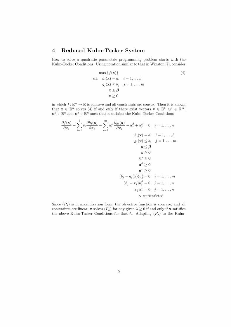
4 Reduced Kuhn-Tucker System

How to solve a quadratic parametric programming problem starts with theKuhn-Tucker Conditions. Using notation similar to that in Winston [?], consider

max {f(x)} (4)s.t. hi(x) = di i = 1, . . . , l

gj(x) ≤ bj j = 1, . . . , m

x ≤ β

x ≥ 0

in which f : Rn → R is concave and all constraints are convex. Then it is knownthat x ∈ Rn solves (4) if and only if there exist vectors v ∈ Rl, us ∈ Rm,uβ ∈ Rn and ux ∈ Rn such that x satisfies the Kuhn-Tucker Conditions

∂f(x)∂xj

−l∑

i=1

vi∂hi(x)∂xj

−m∑

i=1

usi

∂gi(x)∂xj

− uβj + ux

j = 0 j = 1, . . . , n

hi(x) = di i = 1, . . . , l

gj(x) ≤ bj j = 1, . . . , m

x ≤ β

x ≥ 0

us ≥ 0

uβ ≥ 0

ux ≥ 0

(bj − gj(x))usj = 0 j = 1, . . . , m

(βj − xj)uβj = 0 j = 1, . . . , n

xj uxj = 0 j = 1, . . . , n

v unrestricted

Since (Pλ) is in maximization form, the objective function is concave, and allconstraints are linear, x solves (Pλ) for any given λ ≥ 0 if and only if x satisfiesthe above Kuhn-Tucker Conditions for that λ. Adapting (Pλ) to the Kuhn-

9

Tucker Conditions, we have in matrix format the following system

2Σx− λµ + 2Σ` + HT v + GT us + Inuβ − Inux = 0 (7.1)Hx = d (7.2)Gx ≤ b (7.3)Inx ≤ β (7.4)

x ≥ 0 , us ≥ 0 , uβ ≥ 0 , ux ≥ 0 (7.5)

(bj − gj(x))usj = 0, j = 1, . . . ,m (βj − xj)u

βj = 0, j = 1, . . . , n (7.6)

xiuxi = 0, i = 1, . . . , n (7.7)v unrestricted (7.8)

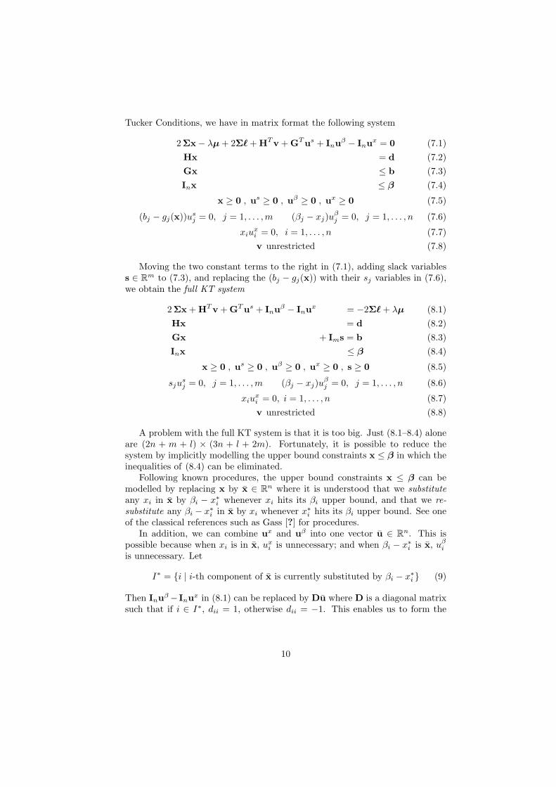
Moving the two constant terms to the right in (7.1), adding slack variabless ∈ Rm to (7.3), and replacing the (bj − gj(x)) with their sj variables in (7.6),we obtain the full KT system

2Σx + HT v + GT us + Inuβ − Inux = −2Σ` + λµ (8.1)Hx = d (8.2)Gx + Ims = b (8.3)Inx ≤ β (8.4)

x ≥ 0 , us ≥ 0 , uβ ≥ 0 , ux ≥ 0 , s ≥ 0 (8.5)

sjusj = 0, j = 1, . . . , m (βj − xj)u

βj = 0, j = 1, . . . , n (8.6)

xiuxi = 0, i = 1, . . . , n (8.7)v unrestricted (8.8)

A problem with the full KT system is that it is too big. Just (8.1–8.4) aloneare (2n + m + l) × (3n + l + 2m). Fortunately, it is possible to reduce thesystem by implicitly modelling the upper bound constraints x ≤ β in which theinequalities of (8.4) can be eliminated.

Following known procedures, the upper bound constraints x ≤ β can bemodelled by replacing x by x ∈ Rn where it is understood that we substituteany xi in x by βi − x∗i whenever xi hits its βi upper bound, and that we re-substitute any βi − x∗i in x by xi whenever x∗i hits its βi upper bound. See oneof the classical references such as Gass [?] for procedures.

In addition, we can combine ux and uβ into one vector u ∈ Rn. This ispossible because when xi is in x, ux

i is unnecessary; and when βi − x∗i is x, uβi

is unnecessary. Let

I∗ = {i | i-th component of x is currently substituted by βi − x∗i } (9)

Then Inuβ− Inux in (8.1) can be replaced by Du where D is a diagonal matrixsuch that if i ∈ I∗, dii = 1, otherwise dii = −1. This enables us to form the

10

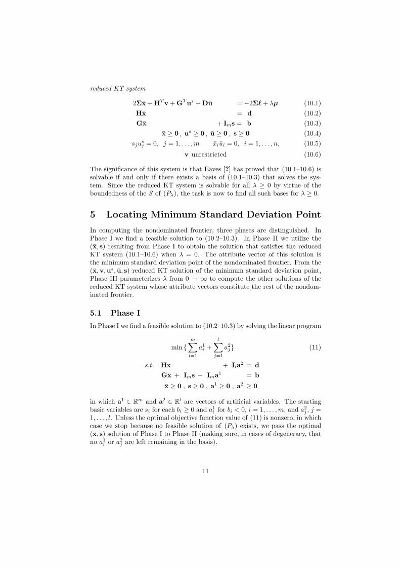
reduced KT system

2Σx + HT v + GT us + Du = −2Σ` + λµ (10.1)Hx = d (10.2)Gx + Ims = b (10.3)

x ≥ 0 , us ≥ 0 , u ≥ 0 , s ≥ 0 (10.4)sju

sj = 0, j = 1, . . . , m xiui = 0, i = 1, . . . , n, (10.5)

v unrestricted (10.6)

The significance of this system is that Eaves [?] has proved that (10.1–10.6) issolvable if and only if there exists a basis of (10.1–10.3) that solves the sys-tem. Since the reduced KT system is solvable for all λ ≥ 0 by virtue of theboundedness of the S of (Pλ), the task is now to find all such bases for λ ≥ 0.

5 Locating Minimum Standard Deviation Point

In computing the nondominated frontier, three phases are distinguished. InPhase I we find a feasible solution to (10.2–10.3). In Phase II we utilize the(x, s) resulting from Phase I to obtain the solution that satisfies the reducedKT system (10.1–10.6) when λ = 0. The attribute vector of this solution isthe minimum standard deviation point of the nondominated frontier. From the(x,v,us, u, s) reduced KT solution of the minimum standard deviation point,Phase III parameterizes λ from 0 → ∞ to compute the other solutions of thereduced KT system whose attribute vectors constitute the rest of the nondom-inated frontier.

5.1 Phase I

In Phase I we find a feasible solution to (10.2–10.3) by solving the linear program

min {m∑

i=1

a1i +

l∑

j=1

a2j} (11)

s.t. Hx + Ila2 = d

Gx + Ims − Ima1 = b

x ≥ 0 , s ≥ 0 , a1 ≥ 0 , a2 ≥ 0

in which a1 ∈ Rm and a2 ∈ Rl are vectors of artificial variables. The startingbasic variables are si for each bi ≥ 0 and a1

i for bi < 0, i = 1, . . . , m; and a2j , j =

1, . . . , l. Unless the optimal objective function value of (11) is nonzero, in whichcase we stop because no feasible solution of (Pλ) exists, we pass the optimal(x, s) solution of Phase I to Phase II (making sure, in cases of degeneracy, thatno a1

i or a2j are left remaining in the basis).

11

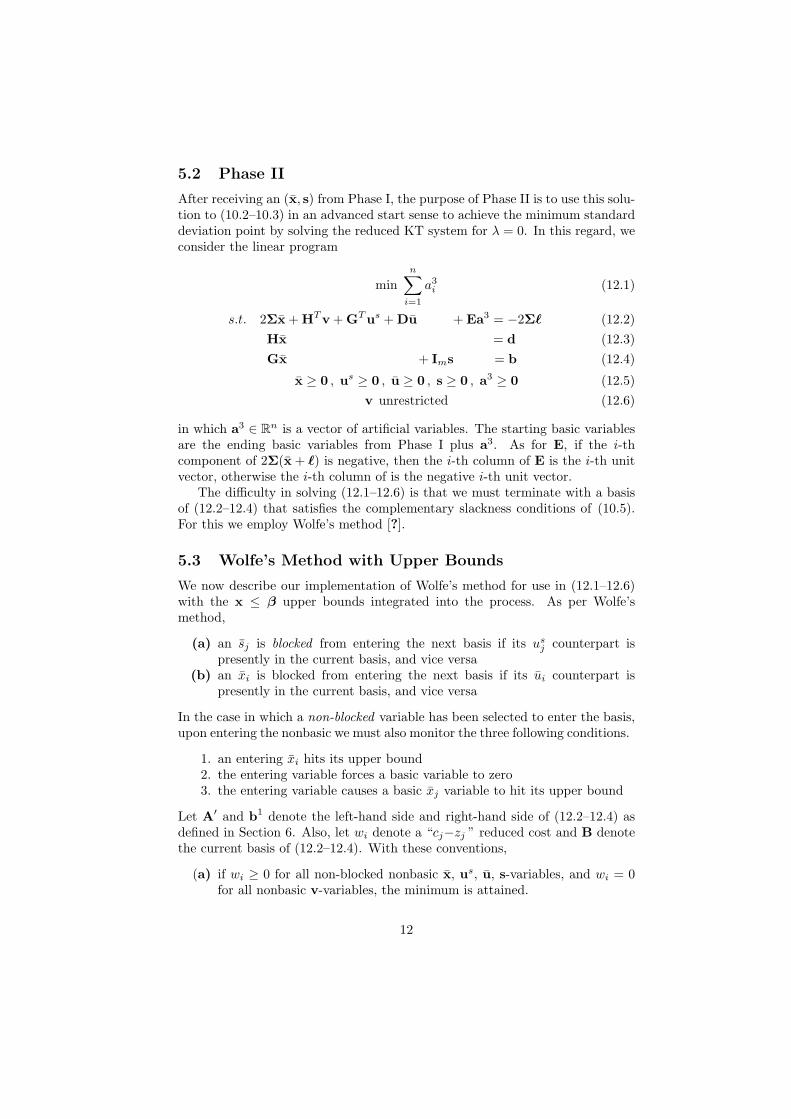
5.2 Phase II

After receiving an (x, s) from Phase I, the purpose of Phase II is to use this solu-tion to (10.2–10.3) in an advanced start sense to achieve the minimum standarddeviation point by solving the reduced KT system for λ = 0. In this regard, weconsider the linear program

minn∑

i=1

a3i (12.1)

s.t. 2Σx + HT v + GT us + Du + Ea3 = −2Σ` (12.2)Hx = d (12.3)Gx + Ims = b (12.4)

x ≥ 0 , us ≥ 0 , u ≥ 0 , s ≥ 0 , a3 ≥ 0 (12.5)v unrestricted (12.6)

in which a3 ∈ Rn is a vector of artificial variables. The starting basic variablesare the ending basic variables from Phase I plus a3. As for E, if the i-thcomponent of 2Σ(x + `) is negative, then the i-th column of E is the i-th unitvector, otherwise the i-th column of is the negative i-th unit vector.

The difficulty in solving (12.1–12.6) is that we must terminate with a basisof (12.2–12.4) that satisfies the complementary slackness conditions of (10.5).For this we employ Wolfe’s method [?].

5.3 Wolfe’s Method with Upper Bounds

We now describe our implementation of Wolfe’s method for use in (12.1–12.6)with the x ≤ β upper bounds integrated into the process. As per Wolfe’smethod,

(a) an sj is blocked from entering the next basis if its usj counterpart is

presently in the current basis, and vice versa(b) an xi is blocked from entering the next basis if its ui counterpart is

presently in the current basis, and vice versa

In the case in which a non-blocked variable has been selected to enter the basis,upon entering the nonbasic we must also monitor the three following conditions.

1. an entering xi hits its upper bound2. the entering variable forces a basic variable to zero3. the entering variable causes a basic xj variable to hit its upper bound

Let A′ and b1 denote the left-hand side and right-hand side of (12.2–12.4) asdefined in Section 6. Also, let wi denote a “cj−zj ” reduced cost and B denotethe current basis of (12.2–12.4). With these conventions,

(a) if wi ≥ 0 for all non-blocked nonbasic x, us, u, s-variables, and wi = 0for all nonbasic v-variables, the minimum is attained.

12

(b) otherwise, select a p such that wp < 0 for an x, us, u, s-variable, orwp 6= 0 for a v-variable and compute yp = B−1ap (where ap is the p-thcolumn of A′). If a v-variable with wp > 0 has been selected, multiplywp by −1 and then compute yp = −B−1ap.

Let r1 be the vector that results after deleting the components of B−1b1 thatpertain to v-variables. Then for the p selected, compute

δ1 = βp if p ∈ {1, . . . , n}, otherwise δ1 = ∞δ2 = min

j

{r1

j

ypj| yp

j > 0}

δ3 = minj

{βij

−r1j

−ypj| yp

j < 0, ij ∈ {1, . . . , n}}

where ij is the index of r1j in x. Noting that r1 has been purged of all references

to v-variables, this means that once a v-variable enters the basis, it is never acandidate for removal, which is good for Phase III. Depending upon which δi isthe minimum, we have

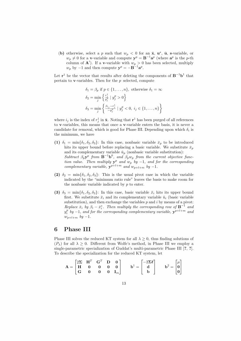
(1) δ1 = min{δ1, δ2, δ3}: In this case, nonbasic variable xp to be introducedhits its upper bound before replacing a basic variable. We substitute xp

and its complementary variable up (nonbasic variable substitution):Subtract βpyp from B−1b0, and βpwp from the current objective func-tion value. Then multiply yp and wp by −1, and for the correspondingcomplementary variable, yp+l+m and wp+l+m by −1.

(2) δ2 = min{δ1, δ2, δ3}: This is the usual pivot case in which the variableindicated by the “minimum ratio rule” leaves the basis to make room forthe nonbasic variable indicated by p to enter.

(3) δ3 = min{δ1, δ2, δ3}: In this case, basic variable xi hits its upper boundfirst. We substitute xi and its complementary variable ui (basic variablesubstitution), and then exchange the variables p and i by means of a pivot:Replace xi by βi − x∗i . Then multiply the corresponding row of B−1 andyp

i by −1, and for the corresponding complementary variable, yp+l+m andwp+l+m by −1.

6 Phase III

Phase III solves the reduced KT system for all λ ≥ 0, thus finding solutions of(Pλ) for all λ ≥ 0. Different from Wolfe’s method, in Phase III we employ asingle-parametric specialization of Guddat’s multi-parametric Phase III [?, ?].To describe the specialization for the reduced KT system, let

A =

2Σ HT GT D 0H 0 0 0 0G 0 0 0 Im

b1 =

−2Σ`

db

b2 =

µ00

13

and x = (x,v,us, u, s). Again, denoting by B the columns of A that comprisea basis, the (10.1–10.3) portion of the reduced KT system can be rewritten as

BxB = b1 + λb2

where xB = (xB ,v,usB , uB , sB). Since a basis of the (n+ l+m)× (2n+ l+2m)

reduced KT system contains (n+ l +m) variables, we observe two things aboutPhase III bases. By virtue of the complementary slackness conditions of (10.5),one is that all v-variables are always in a basis. The other is that all nonbasicvariables always have their complementary variables in the basis. This meansthat whenever we pivot in Phase III, whatever variable leaves, in comes itscomplementary slackness counterpart.

6.1 General Idea

Let B1 be the basis of the reduced KT system inherited from Phase II, and letJB1 be its basic index set. Since B1 is invertible,

xB1 = B−11 b1 + λB−1

1 b2

Now, delete the components corresponding to the v-variables in the right-handvectors B−1

1 b1 and B−11 b2, and denote the resulting right-hand vectors r1 ∈

Rn+m and r2 ∈ Rn+m, respectively. After recalling index set I∗ from (9), usethe r-vectors to define vectors x1 ∈ Rn and ∆1 ∈ Rn where

ξ1i =

`i i 6∈ JB1 and i 6∈ I∗

ωi i 6∈ JB1 and i ∈ I∗

`i + r1ji

i ∈ JB1 and i 6∈ I∗

ωi − r1ji

i ∈ JB1 and i ∈ I∗

∆1i =

0 i 6∈ JB1 and i 6∈ I∗

0 i 6∈ JB1 and i ∈ I∗

r2ji

i ∈ JB1 and i 6∈ I∗

−r2ji

i ∈ JB1 and i ∈ I∗

where ji is the index of xi in r1j , i ∈ JB1 . Then

x = ξ1 + λ∆1

solves (Pλ) for all λ ≥ 0 as long as all components of xB1 stay within theirupper bounds and

(xB1 ,usB1

, uB1 , sB1) = r1 + λr2 ≥ 0

Starting at λ1 = 0, λ may be increased up to

λ2 = minj=1,...,n+m

r1j

−r2j

r2j < 0

βij−r1

j

r2j

r2j > 0 and ij ∈ {1, . . . , n}

at which point, if λ2 < ∞, λ hits a binding constraint. This means that either

(a) a basic variable xi, usi , ui or si is driven to 0, in which case we remove

the variable and enter its counterpart ui, si, xi or usi to obtain B2, or

14

(b) a basic variable xj hits its upper bound, in which case, after substitutingfor xj and uj as described in Section 5.3, we exchange the variables toobtain B2.

Repeating in this way, we compute a sequence of linear line segments, or inMarkowitz terminology, critical line segments

ξh + λ∆h λ ∈ [λh, λh+1]

with λi ≤ λi+1 until λ becomes unbounded. While these are the line segmentsthat “zig-zag” through S, their images are the hyperbolic segments comprisingthe nondominated frontier in Z.

6.2 Iterative Procedure

Let the turning points in feasible region S be denoted xh and the turning pointsin feasible region Z be given by (σh, µh). Then the procedure to be followed inPhase III can now be spelled out step-by-step as follows.

Step 1. Let B1 be from Phase II, λ1 = 0, and h = 1.

Step 2. From the r1 and r2 associated with B−1h b1 and B−1

h b2, construct

ξh and ∆h

Step 3. If h > 1, go to Step 4. Otherwise, do

x1 = ξ1

µ1 = µT x1

write to a file x1

Step 4. Compute λh+1. If λh+1 = ∞, stop because we are done.

Step 5. Do

xh+1 = ξh + λh+1∆h

µh+1 = µT xh+1

if µT ∆h > 0, compute ah0 , ah

1 , ah2

count number of securities nh in xh ∼ xh+1

write to a file h, µh, µh+1, λh, λh+1, nh, ah0 , ah

1 , ah2 , xh+1

pivot to Bh+1

Step 6. h = h + 1. Go to Step 2.

We now explain the ah0 , ah

1 , ah2 . They are used to compute the attribute

vectors (σ, µ, ) that define the h-th hyperbolic frontier segment correspondingto the h-th critical line segment xh ∼ xh+1. Thus for λ ∈ [λh, λh+1],

µ = µT ξh + λµT ∆h (13)

σ =√

(ξh)T Σξh + λ2(ξh)T Σ∆h + λ2(∆h)T Σ∆h (14)

15

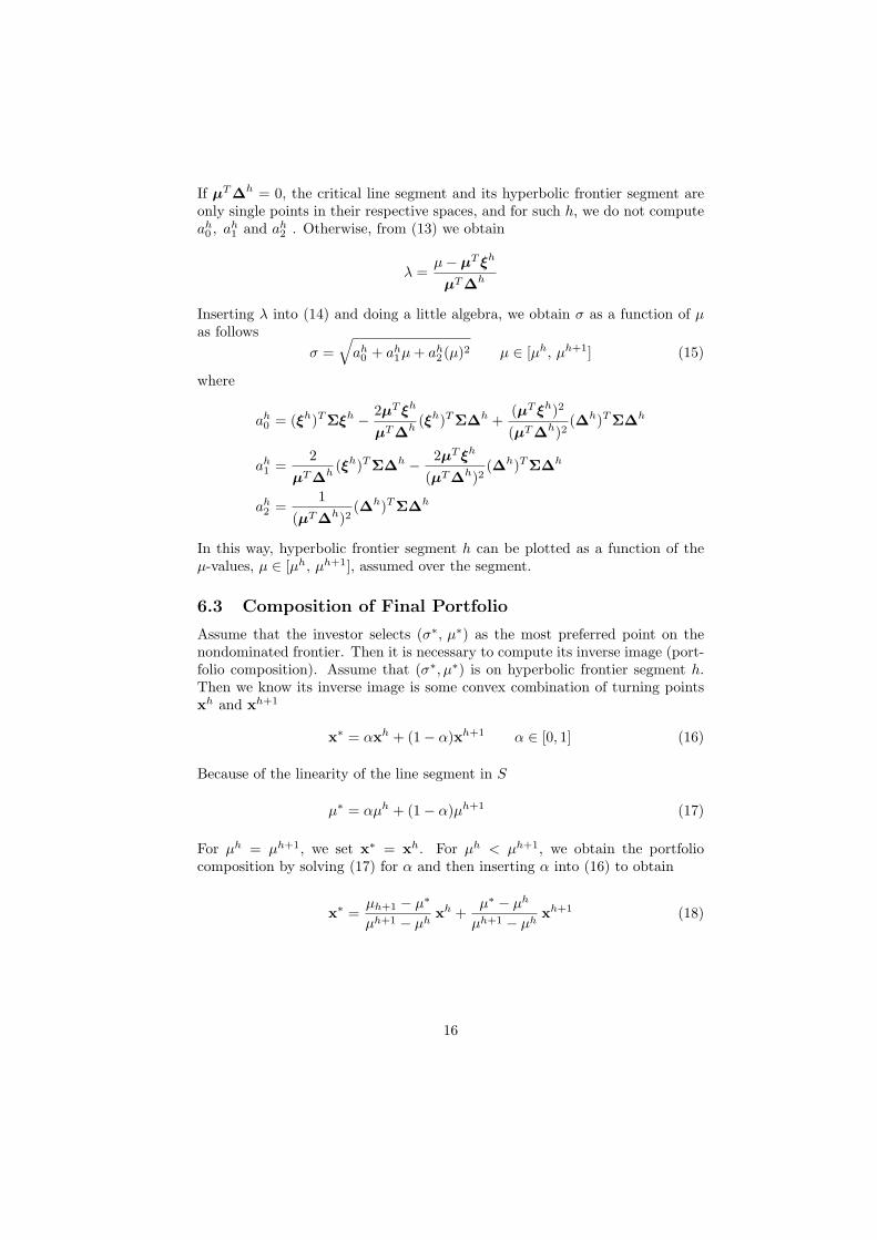
If µT ∆h = 0, the critical line segment and its hyperbolic frontier segment areonly single points in their respective spaces, and for such h, we do not computeah0 , ah

1 and ah2 . Otherwise, from (13) we obtain

λ =µ− µT ξh

µT ∆h

Inserting λ into (14) and doing a little algebra, we obtain σ as a function of µas follows

σ =√

ah0 + ah

1µ + ah2 (µ)2 µ ∈ [µh, µh+1] (15)

where

ah0 = (ξh)T Σξh − 2µT ξh

µT ∆h(ξh)T Σ∆h +

(µT ξh)2

(µT ∆h)2(∆h)T Σ∆h

ah1 =

2µT ∆h

(ξh)T Σ∆h − 2µT ξh

(µT ∆h)2(∆h)T Σ∆h

ah2 =

1(µT ∆h)2

(∆h)T Σ∆h

In this way, hyperbolic frontier segment h can be plotted as a function of theµ-values, µ ∈ [µh, µh+1], assumed over the segment.

6.3 Composition of Final Portfolio

Assume that the investor selects (σ∗, µ∗) as the most preferred point on thenondominated frontier. Then it is necessary to compute its inverse image (port-folio composition). Assume that (σ∗, µ∗) is on hyperbolic frontier segment h.Then we know its inverse image is some convex combination of turning pointsxh and xh+1

x∗ = αxh + (1− α)xh+1 α ∈ [0, 1] (16)

Because of the linearity of the line segment in S

µ∗ = αµh + (1− α)µh+1 (17)

For µh = µh+1, we set x∗ = xh. For µh < µh+1, we obtain the portfoliocomposition by solving (17) for α and then inserting α into (16) to obtain

x∗ =µh+1 − µ∗

µh+1 − µhxh +

µ∗ − µh

µh+1 − µhxh+1 (18)

16

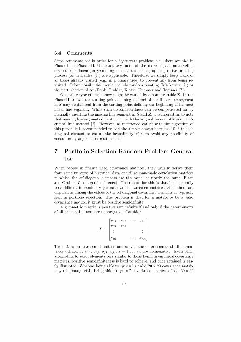
6.4 Comments

Some comments are in order for a degenerate problem, i.e., there are ties inPhase II or Phase III. Unfortunately, none of the more elegant anti-cyclingdevices from linear programming such as the lexicographic positive orderingprocess (as in Hadley [?]) are applicable. Therefore, we simply keep track ofall bases already visited (e.g., in a binary tree) to prevent any from being re-visited. Other possibilities would include random pivoting (Markowitz [?]) orthe perturbation of b1 (Bank, Guddat, Klatte, Kummer and Tammer [?]).

One other type of degeneracy might be caused by a non-invertible Σ. In thePhase III above, the turning point defining the end of one linear line segmentin S may be different from the turning point defining the beginning of the nextlinear line segment. While such disconnectedness can be compensated for bymanually inserting the missing line segment in S and Z, it is interesting to notethat missing line segments do not occur with the original version of Markowitz’scritical line method [?]. However, as mentioned earlier with the algorithm ofthis paper, it is recommended to add the almost always harmless 10−6 to eachdiagonal element to ensure the invertibility of Σ to avoid any possibility ofencountering any such rare situations.

7 Portfolio Selection Random Problem Genera-tor

When people in finance need covariance matrices, they usually derive themfrom some universe of historical data or utilize man-made correlation matricesin which the off-diagonal elements are the same, or nearly the same (Eltonand Gruber [?] is a good reference). The reason for this is that it is generallyvery difficult to randomly generate valid covariance matrices when there aredispersions among the values of the off-diagonal covariance elements as typicallyseen in portfolio selection. The problem is that for a matrix to be a validcovariance matrix, it must be positive semidefinite.

A symmetric matrix is positive semidefinite if and only if the determinantsof all principal minors are nonnegative. Consider

Σ =

σ11 σ12 · · · σ1n

σ21 σ22

......

σn1 · · · σnn

Then, Σ is positive semidefinite if and only if the determinants of all subma-trices defined by σ11, σ1j , σj1, σjj , j = 1, . . . , n, are nonnegative. Even whenattempting to select elements very similar to those found in empirical covariancematrices, positive semidefiniteness is hard to achieve, and once attained is eas-ily disrupted. Whereas being able to “guess” a valid 20× 20 covariance matrixmay take many trials, being able to “guess” covariance matrices of size 50× 50

17

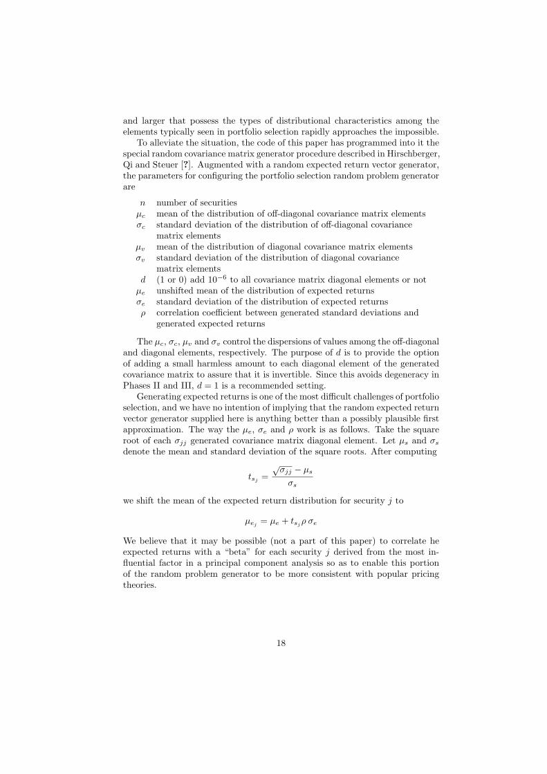
and larger that possess the types of distributional characteristics among theelements typically seen in portfolio selection rapidly approaches the impossible.

To alleviate the situation, the code of this paper has programmed into it thespecial random covariance matrix generator procedure described in Hirschberger,Qi and Steuer [?]. Augmented with a random expected return vector generator,the parameters for configuring the portfolio selection random problem generatorare

n number of securitiesµc mean of the distribution of off-diagonal covariance matrix elementsσc standard deviation of the distribution of off-diagonal covariance

matrix elementsµv mean of the distribution of diagonal covariance matrix elementsσv standard deviation of the distribution of diagonal covariance

matrix elementsd (1 or 0) add 10−6 to all covariance matrix diagonal elements or not

µe unshifted mean of the distribution of expected returnsσe standard deviation of the distribution of expected returnsρ correlation coefficient between generated standard deviations and

generated expected returns

The µc, σc, µv and σv control the dispersions of values among the off-diagonaland diagonal elements, respectively. The purpose of d is to provide the optionof adding a small harmless amount to each diagonal element of the generatedcovariance matrix to assure that it is invertible. Since this avoids degeneracy inPhases II and III, d = 1 is a recommended setting.

Generating expected returns is one of the most difficult challenges of portfolioselection, and we have no intention of implying that the random expected returnvector generator supplied here is anything better than a possibly plausible firstapproximation. The way the µe, σe and ρ work is as follows. Take the squareroot of each σjj generated covariance matrix diagonal element. Let µs and σs

denote the mean and standard deviation of the square roots. After computing

tsj =√

σjj − µs

σs

we shift the mean of the expected return distribution for security j to

µej = µe + tsj ρ σe

We believe that it may be possible (not a part of this paper) to correlate heexpected returns with a “beta” for each security j derived from the most in-fluential factor in a principal component analysis so as to enable this portionof the random problem generator to be more consistent with popular pricingtheories.

18

8 Illustrative Example

We tie this paper together with a standard (no extra constraints and all variablelower bounds zero) 6-security illustrative example. Let the parameters of therandom problem generator be

n = 6 d = 1µc = .0020 µe = .0100σc = .0015 σe = .0050µv = .0150 ρ = .25σv = .0120

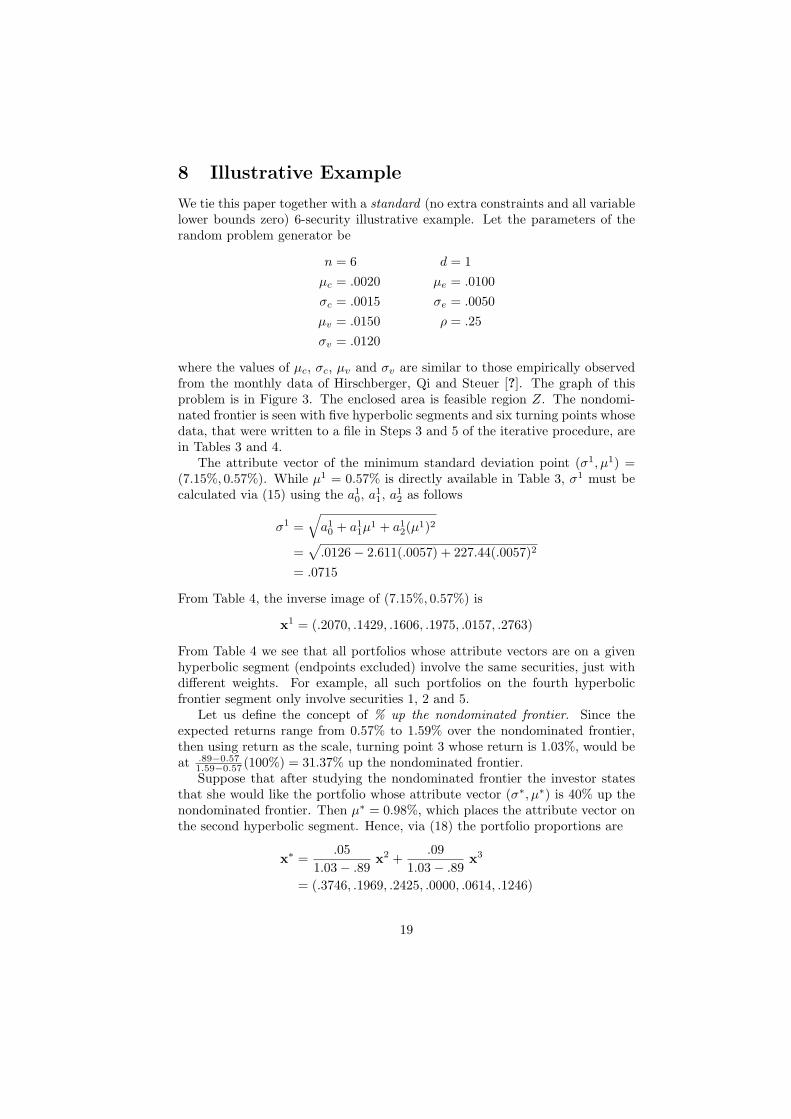
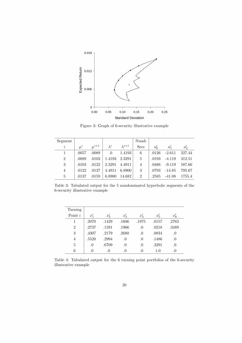
where the values of µc, σc, µv and σv are similar to those empirically observedfrom the monthly data of Hirschberger, Qi and Steuer [?]. The graph of thisproblem is in Figure 3. The enclosed area is feasible region Z. The nondomi-nated frontier is seen with five hyperbolic segments and six turning points whosedata, that were written to a file in Steps 3 and 5 of the iterative procedure, arein Tables 3 and 4.

The attribute vector of the minimum standard deviation point (σ1, µ1) =(7.15%, 0.57%). While µ1 = 0.57% is directly available in Table 3, σ1 must becalculated via (15) using the a1

0, a11, a1

2 as follows

σ1 =√

a10 + a1

1µ1 + a1

2(µ1)2

=√

.0126− 2.611(.0057) + 227.44(.0057)2

= .0715

From Table 4, the inverse image of (7.15%, 0.57%) is

x1 = (.2070, .1429, .1606, .1975, .0157, .2763)

From Table 4 we see that all portfolios whose attribute vectors are on a givenhyperbolic segment (endpoints excluded) involve the same securities, just withdifferent weights. For example, all such portfolios on the fourth hyperbolicfrontier segment only involve securities 1, 2 and 5.

Let us define the concept of % up the nondominated frontier. Since theexpected returns range from 0.57% to 1.59% over the nondominated frontier,then using return as the scale, turning point 3 whose return is 1.03%, would beat .89−0.57

1.59−0.57 (100%) = 31.37% up the nondominated frontier.Suppose that after studying the nondominated frontier the investor states

that she would like the portfolio whose attribute vector (σ∗, µ∗) is 40% up thenondominated frontier. Then µ∗ = 0.98%, which places the attribute vector onthe second hyperbolic segment. Hence, via (18) the portfolio proportions are

x∗ =.05

1.03− .89x2 +

.091.03− .89

x3

= (.3746, .1969, .2425, .0000, .0614, .1246)

19

0

0.006

0.012

0.018

0.00 0.05 0.10 0.15 0.20 0.25

Standard Deviation

Exp

ecte

d R

etur

n

Figure 3: Graph of 6-security illustrative example

Segment Numbi µi µi+1 λi λi+1 Secs ai

0 ai1 ai

2

1 .0057 .0089 .0 1.4193 6 .0126 -2.611 227.442 .0089 .0103 1.4193 2.3291 5 .0193 -4.119 312.513 .0103 .0122 2.3291 4.4911 4 .0486 -9.119 587.664 .0122 .0137 4.4911 6.8900 3 .0793 -14.85 795.675 .0137 .0159 6.8900 14.682 2 .2585 -41.08 1755.4

Table 3: Tabulated output for the 5 nondominated hyperbolic segments of the6-security illustrative example

TurningPoint i xi

1 xi2 xi

3 xi4 xi

5 xi6

1 .2070 .1429 .1606 .1975 .0157 .27632 .2737 .1591 .1966 .0 .0218 .34893 .4307 .2179 .2680 .0 .0834 .04 .5520 .2994 .0 .0 .1486 .05 .0 .6709 .0 .0 .3291 .06 .0 .0 .0 .0 1.0 .0

Table 4: Tabulated output for the 6 turning point portfolios of the 6-securityillustrative example

20

9 Computational Experience

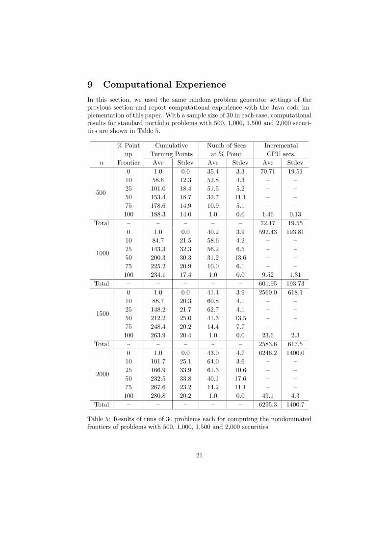
In this section, we used the same random problem generator settings of theprevious section and report computational experience with the Java code im-plementation of this paper. With a sample size of 30 in each case, computationalresults for standard portfolio problems with 500, 1,000, 1,500 and 2,000 securi-ties are shown in Table 5.

% Point Cumulative Numb of Secs Incrementalup Turning Points at % Point CPU secs.

n Frontier Ave Stdev Ave Stdev Ave Stdev

500

0 1.0 0.0 35.4 3.3 70.71 19.5110 58.6 12.3 52.8 4.3 – –25 101.0 18.4 51.5 5.2 – –50 153.4 18.7 32.7 11.1 – –75 178.6 14.9 10.9 5.1 – –100 188.3 14.0 1.0 0.0 1.46 0.13

Total – – – – – 72.17 19.55

1000

0 1.0 0.0 40.2 3.9 592.43 193.8110 84.7 21.5 58.6 4.2 – –25 143.3 32.3 56.2 6.5 – –50 200.3 30.3 31.2 13.6 – –75 225.2 20.9 10.0 6.1 – –100 234.1 17.4 1.0 0.0 9.52 1.31

Total – – – – – 601.95 193.73

1500

0 1.0 0.0 41.4 3.9 2560.0 618.110 88.7 20.3 60.8 4.1 – –25 148.2 21.7 62.7 4.1 – –50 212.2 25.0 41.3 13.5 – –75 248.4 20.2 14.4 7.7 – –100 263.9 20.4 1.0 0.0 23.6 2.3

Total – – – – – 2583.6 617.5

2000

0 1.0 0.0 43.0 4.7 6246.2 1400.010 101.7 25.1 64.0 3.6 – –25 166.9 33.9 61.3 10.6 – –50 232.5 33.8 40.1 17.6 – –75 267.6 23.2 14.2 11.1 – –100 280.8 20.2 1.0 0.0 49.1 4.3

Total – – – – – 6295.3 1400.7

Table 5: Results of runs of 30 problems each for computing the nondominatedfrontiers of problems with 500, 1,000, 1,500 and 2,000 securities

21

In the Cumulative Turning Point columns we see how the nondominatedfrontier consists of many hyperbolic segments (where the number of hyperbolicsegments is one less than the number of turning points) and how the bulk of thehyperbolic segment activity takes place, at least in the larger problems, in thefirst 25% up the nondominated frontier. In the Number of Securities columns,we see how the number of securities in portfolios along the nondominated fron-tier at first increases, hitting its peak at about the 10% mark, and then fromthere commences its long decline. We also note how the number of securitiesonly grows modestly with n. In the Incremental CPU Seconds columns, whatis remarkable is how quickly the nondominated frontier can be calculated oncethe minimum standard deviation point has been obtained, and how the distinc-tion becomes more pronounced with problem size. For instance, in 200-securityproblems (not shown), the split is roughly 96% vs. 4%, but in the 2,000-securityproblems, the split widens to more than 99% vs. less than 1%. Whereas largescale was roughly 500 securities in 1984 at the time of Perold’s paper [?], withthe algorithm and code of this paper, problems (to which no covariance ma-trix simplification techniques have been applied) with several times this manysecurities are now within reach of anyone even on a laptop.

As for validation, we ran test problems up to the 256-column limit on thecritical line method code written in VBA (Visual Basic for Applications) kindlysupplied by G. P. Todd from the appendix of Markowitz and Todd [?] andobtained identical results. All CPU times in this paper are from a Dell 3.06GHzdesktop at the University of Georgia.

References

[1] B. Bank, J. Guddat, D. Klatte, B. Kummer, and K. Tammer. NonlinearParametric Optimization. Birkhauser Verlag, Basel, 1983.

[2] C. A. Bana e Costa and J. O. Soares. A multicriteria model for portfoliomanagement. European Journal of Finance, 10(3), 2004. Forthcoming.

[3] B. C. Eaves. On quadratic programming. Management Science, 17(11):698–711, 1971.

[4] M. Ehrgott, K. Klamroth, and C. Schwehm. An MCDM approach to port-folio optimization. European Journal of Operational Research, 155(3):752–770, 2004.

[5] E. J. Elton, M. J. Gruber, S. J. Brown, and W. Goetzmann. ModernPortfolio Theory and Investment Analysis. John Wiley, New York, 6thedition, 2002.

[6] S. I. Gass. Linear Programming: Methods and Applications. Boyd & Fraser,Danvers, Massachusetts, 5th edition, 1985.

22

[7] J. Guddat. “Stability Investigations in Quadratic Parametric Program-ming,” Doctoral dissertation (in German), Humboldt University, Berlin,1974.

[8] J. Guddat. Stability in convex quadratic programming. Operations-forschung und Statistik, 7:223–245, 1976.

[9] G. Hadley. Linear Programming. Addison-Wesley, Reading, Massachusetts,1962.

[10] M. Hirschberger, Y. Qi, and R. E. Steuer. “Randomly Generating Portfolio-Selection Covariance Matrices with Specified Distributional Characteris-tics,” Department of Banking and Finance, University of Georgia, Athens,February, 2004.

[11] M. Koksalan and R. D. Plante. Interactive multicriteria optimization formultiple-response product and process design. Manufacturing & ServiceOperations Management, 5(4):334–347, 2003.

[12] P. Korhonen and G.-Y. Yu. A reference direction approach to multipleobjective quadratic-linear programming. European Journal of OperationalResearch, 102:601–610, 1996.

[13] H. M. Markowitz. Portfolio selection. Journal of Finance, 7(1):77–91, 1952.

[14] H. M. Markowitz. The optimization of a quadratic function subject tolinear constraints. Naval Research Logistics Quarterly, 3:111–133, 1956.

[15] H. M. Markowitz. Portfolio Selection: Efficient Diversification in Invest-ments. John Wiley, New York, 1959.

[16] H. M. Markowitz and G. P. Todd. Mean-Variance Analysis in Portfo-lio Choice and Capital Markets. Frank J. Fabozzi Associates, New Hope,Pennsylvania, 2000.

[17] W. Ogryczak. Multiple criteria linear programming model for portfolioselection. Annals of Operations Research, 97:143–162, 2000.

[18] A. Perold. Large-scale porfolio optimization. Management Science,30(10):1143–1160, 1984.

[19] W. L. Winston. Operations Research: Applications and Algorithms.Duxbury Press, Belmont, California, 5th edition, 2003.

[20] P. Wolfe. The simplex method for quadratic programming. Econometrica,27(3):382–398, 1959.

[21] W. T. Ziemba. The Stochastic Programming Approach to Asset, Liabil-ity, and Wealth Management. Research Foundation of the AIMR, Char-lottesville, Virginia, 2003.

23