Embed Size (px)
Citation preview
Quadratic Optimization ProblemsArising in Computer Vision
Jean GallierSpecial Thanks to Jianbo Shi and Ryan Kennedy
CIS DepartmentUniversity of Pennsylvania
March 23, 2011

Perverse Cohomology of Potatoes and the Stability of theUniverse
The stability of our universe is clearly a fundamental problem.Unfortunately, I proved
Theorem 1
Our universe, U, is unstable.
Proof.
It can be shown that the perverse cohomology group
H237pot (U) = 101010
potatoes.
This is too big, therefore, the universe is unstable.
It is obvious that Theorem 1 implies that P 6= NP.
Jean Gallier (Upenn) Quadratic Optimization Problems March 23, 2011 2 / 61
1. Quadratic Optimization Problems; What Are They?
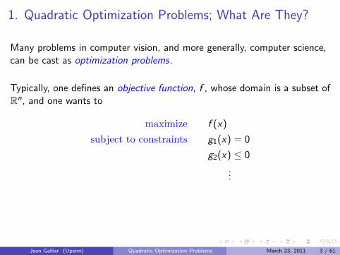
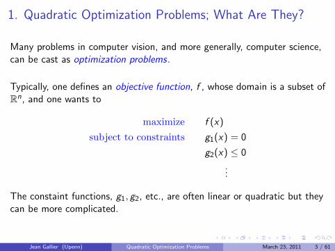
Many problems in computer vision, and more generally, computer science,can be cast as optimization problems.
Typically, one defines an objective function, f , whose domain is a subset ofRn, and one wants to
maximize f (x)
subject to constraints g1(x) = 0
g2(x) ≤ 0
...
The constaint functions, g1, g2, etc., are often linear or quadratic but theycan be more complicated.
Jean Gallier (Upenn) Quadratic Optimization Problems March 23, 2011 3 / 61
1. Quadratic Optimization Problems; What Are They?
Many problems in computer vision, and more generally, computer science,can be cast as optimization problems.
Typically, one defines an objective function, f , whose domain is a subset ofRn, and one wants to
maximize f (x)
subject to constraints g1(x) = 0
g2(x) ≤ 0
...
The constaint functions, g1, g2, etc., are often linear or quadratic but theycan be more complicated.
Jean Gallier (Upenn) Quadratic Optimization Problems March 23, 2011 3 / 61
We usually want to find the maximum value of f (subject to theconstaints) and find some/all values of x for which f (x) is maximal (an“argmax” problem).
Sometimes, one wants to minimize f (x), but this is equivalent tomaximizing −f (x).
Sometimes the domain of f is a discrete subset of Rn, for example, {0, 1}n.
The complexity of optimization problems over discrete domains is oftenworse that than it is over continuous domains (NP-hard).
When we don’t know how to solve efficiently a discrete optimizationproblem, we can try solving a relaxation of the problem.
Jean Gallier (Upenn) Quadratic Optimization Problems March 23, 2011 4 / 61
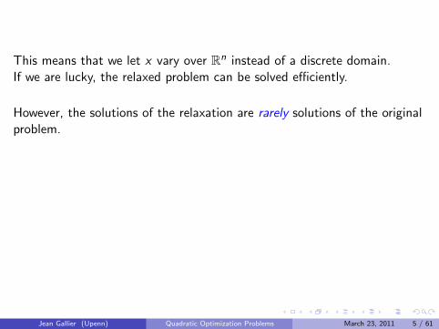
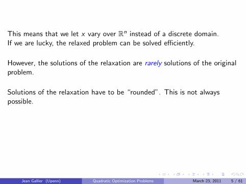
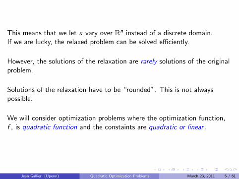
This means that we let x vary over Rn instead of a discrete domain.If we are lucky, the relaxed problem can be solved efficiently.
However, the solutions of the relaxation are rarely solutions of the originalproblem.
Solutions of the relaxation have to be “rounded”. This is not alwayspossible.
We will consider optimization problems where the optimization function,f , is quadratic function and the constaints are quadratic or linear .
Jean Gallier (Upenn) Quadratic Optimization Problems March 23, 2011 5 / 61
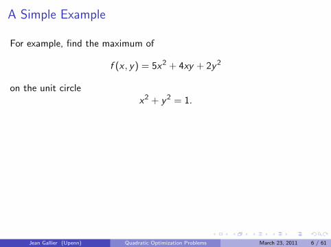
A Simple Example
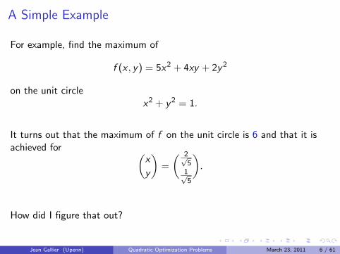
For example, find the maximum of
f (x , y) = 5x2 + 4xy + 2y 2
on the unit circlex2 + y 2 = 1.
It turns out that the maximum of f on the unit circle is 6 and that it isachieved for (
x
y
)=
( 2√5
1√5
).
How did I figure that out?
Jean Gallier (Upenn) Quadratic Optimization Problems March 23, 2011 6 / 61

A Simple Example
For example, find the maximum of
f (x , y) = 5x2 + 4xy + 2y 2
on the unit circlex2 + y 2 = 1.
It turns out that the maximum of f on the unit circle is 6 and that it isachieved for (
x
y
)=
( 2√5
1√5
).
How did I figure that out?
Jean Gallier (Upenn) Quadratic Optimization Problems March 23, 2011 6 / 61
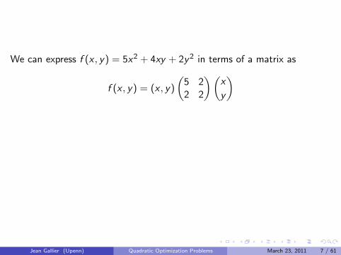
We can express f (x , y) = 5x2 + 4xy + 2y 2 in terms of a matrix as
f (x , y) = (x , y)
(5 22 2
)(x
y
)
The matrix
A =
(5 22 2
)is symmetric (A = A>), so it can be diagonalized .
Jean Gallier (Upenn) Quadratic Optimization Problems March 23, 2011 7 / 61
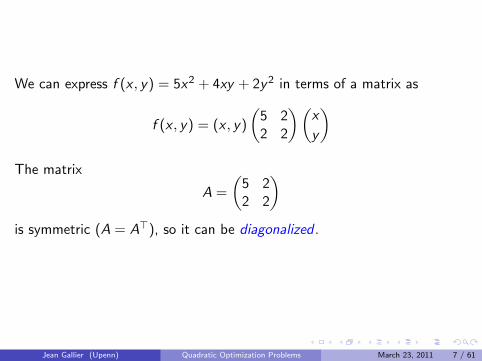
We can express f (x , y) = 5x2 + 4xy + 2y 2 in terms of a matrix as
f (x , y) = (x , y)
(5 22 2
)(x
y
)The matrix
A =
(5 22 2
)is symmetric (A = A>), so it can be diagonalized .
Jean Gallier (Upenn) Quadratic Optimization Problems March 23, 2011 7 / 61
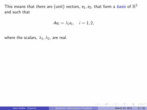
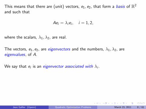
This means that there are (unit) vectors, e1, e2, that form a basis of R2
and such that
Aei = λiei , i = 1, 2,
where the scalars, λ1, λ2, are real.
The vectors, e1, e2, are eigenvectors and the numbers, λ1, λ2, areeigenvalues, of A.
We say that ei is an eigenvector associated with λi .
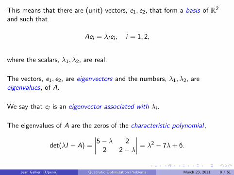
The eigenvalues of A are the zeros of the characteristic polynomial ,
det(λI − A) =
∣∣∣∣5− λ 22 2− λ
∣∣∣∣ = λ2 − 7λ+ 6.
Jean Gallier (Upenn) Quadratic Optimization Problems March 23, 2011 8 / 61
This means that there are (unit) vectors, e1, e2, that form a basis of R2
and such that
Aei = λiei , i = 1, 2,
where the scalars, λ1, λ2, are real.
The vectors, e1, e2, are eigenvectors and the numbers, λ1, λ2, areeigenvalues, of A.
We say that ei is an eigenvector associated with λi .
The eigenvalues of A are the zeros of the characteristic polynomial ,
det(λI − A) =
∣∣∣∣5− λ 22 2− λ
∣∣∣∣ = λ2 − 7λ+ 6.
Jean Gallier (Upenn) Quadratic Optimization Problems March 23, 2011 8 / 61
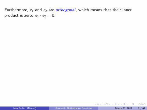
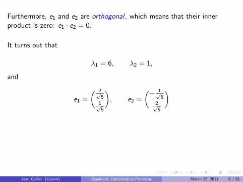
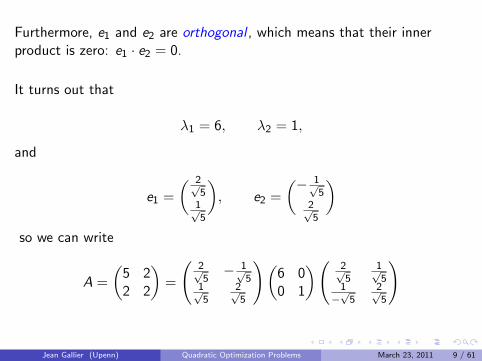
Furthermore, e1 and e2 are orthogonal , which means that their innerproduct is zero: e1 · e2 = 0.
It turns out that
λ1 = 6, λ2 = 1,
and
e1 =
( 2√5
1√5
), e2 =
(− 1√5
2√5
)so we can write
A =
(5 22 2
)=
(2√5− 1√
51√5
2√5
)(6 00 1
)( 2√5
1√5
1−√
52√5
)
Jean Gallier (Upenn) Quadratic Optimization Problems March 23, 2011 9 / 61
Furthermore, e1 and e2 are orthogonal , which means that their innerproduct is zero: e1 · e2 = 0.
It turns out that
λ1 = 6, λ2 = 1,
and
e1 =
( 2√5
1√5
), e2 =
(− 1√5
2√5
)
so we can write
A =
(5 22 2
)=
(2√5− 1√
51√5
2√5
)(6 00 1
)( 2√5
1√5
1−√
52√5
)
Jean Gallier (Upenn) Quadratic Optimization Problems March 23, 2011 9 / 61
Furthermore, e1 and e2 are orthogonal , which means that their innerproduct is zero: e1 · e2 = 0.
It turns out that
λ1 = 6, λ2 = 1,
and
e1 =
( 2√5
1√5
), e2 =
(− 1√5
2√5
)so we can write
A =
(5 22 2
)=
(2√5− 1√
51√5
2√5
)(6 00 1
)( 2√5
1√5
1−√
52√5
)
Jean Gallier (Upenn) Quadratic Optimization Problems March 23, 2011 9 / 61

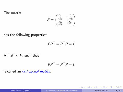
The matrix
P =
(2√5− 1√
51√5
2√5
)
has the following properties:
PP> = P>P = I .
A matrix, P, such that
PP> = P>P = I .
is called an orthogonal matrix .
Jean Gallier (Upenn) Quadratic Optimization Problems March 23, 2011 10 / 61
The matrix
P =
(2√5− 1√
51√5
2√5
)
has the following properties:
PP> = P>P = I .
A matrix, P, such that
PP> = P>P = I .
is called an orthogonal matrix .
Jean Gallier (Upenn) Quadratic Optimization Problems March 23, 2011 10 / 61

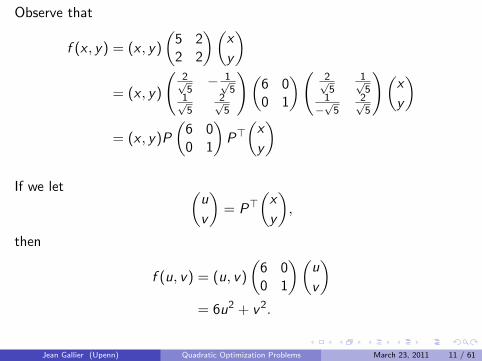
Observe that
f (x , y) = (x , y)
(5 22 2
)(x
y
)= (x , y)
(2√5− 1√
51√5
2√5
)(6 00 1
)( 2√5
1√5
1−√
52√5
)(x
y
)= (x , y)P
(6 00 1
)P>(
x
y
)
If we let (u
v
)= P>
(x
y
),
then
f (u, v) = (u, v)
(6 00 1
)(u
v
)= 6u2 + v 2.
Jean Gallier (Upenn) Quadratic Optimization Problems March 23, 2011 11 / 61
Observe that
f (x , y) = (x , y)
(5 22 2
)(x
y
)= (x , y)
(2√5− 1√
51√5
2√5
)(6 00 1
)( 2√5
1√5
1−√
52√5
)(x
y
)= (x , y)P
(6 00 1
)P>(
x
y
)
If we let (u
v
)= P>
(x
y
),
then
f (u, v) = (u, v)
(6 00 1
)(u
v
)= 6u2 + v 2.
Jean Gallier (Upenn) Quadratic Optimization Problems March 23, 2011 11 / 61
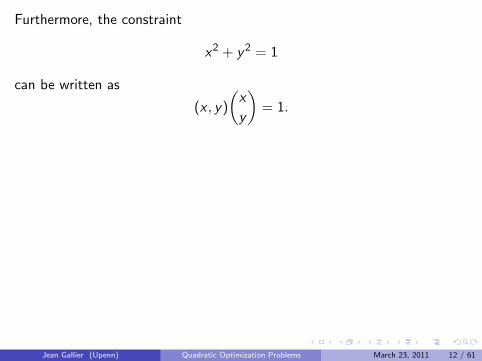
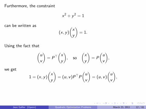
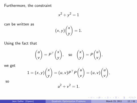
Furthermore, the constraint
x2 + y 2 = 1
can be written as
(x , y)
(x
y
)= 1.
Using the fact that(u
v
)= P>
(x
y
), so
(x
y
)= P
(u
v
),
we get
1 = (x , y)
(x
y
)= (u, v)P>P
(u
v
)= (u, v)
(u
v
),
sou2 + v 2 = 1.
Jean Gallier (Upenn) Quadratic Optimization Problems March 23, 2011 12 / 61
Furthermore, the constraint
x2 + y 2 = 1
can be written as
(x , y)
(x
y
)= 1.
Using the fact that(u
v
)= P>
(x
y
), so
(x
y
)= P
(u
v
),
we get
1 = (x , y)
(x
y
)= (u, v)P>P
(u
v
)= (u, v)
(u
v
),
sou2 + v 2 = 1.
Jean Gallier (Upenn) Quadratic Optimization Problems March 23, 2011 12 / 61
Furthermore, the constraint
x2 + y 2 = 1
can be written as
(x , y)
(x
y
)= 1.
Using the fact that(u
v
)= P>
(x
y
), so
(x
y
)= P
(u
v
),
we get
1 = (x , y)
(x
y
)= (u, v)P>P
(u
v
)= (u, v)
(u
v
),
sou2 + v 2 = 1.
Jean Gallier (Upenn) Quadratic Optimization Problems March 23, 2011 12 / 61
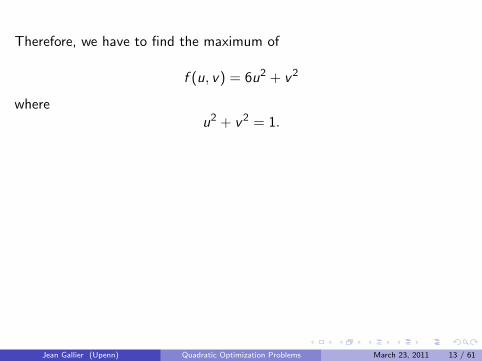
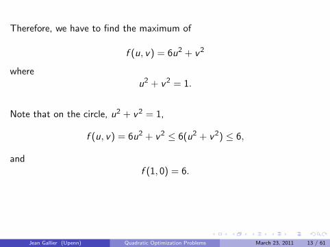
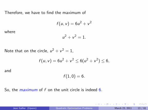
Therefore, we have to find the maximum of
f (u, v) = 6u2 + v 2
whereu2 + v 2 = 1.
Note that on the circle, u2 + v 2 = 1,
f (u, v) = 6u2 + v 2 ≤ 6(u2 + v 2) ≤ 6,
andf (1, 0) = 6.
So, the maximum of f on the unit circle is indeed 6.
Jean Gallier (Upenn) Quadratic Optimization Problems March 23, 2011 13 / 61
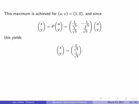
This maximum is achieved for (u, v) = (1, 0), and since(x
y
)= P
(u
v
)=
(2√5− 1√
51√5
2√5
)(u
v
)this yields (
x
y
)=
( 2√5
1√5
).
In general, a quadratric function is of the form
f (x) = x>Ax ,
where x ∈ Rn and A is an n × n matrix.
Jean Gallier (Upenn) Quadratic Optimization Problems March 23, 2011 14 / 61
I'lr- ONL"( Hl::, c.oULQ II-\IN~ IN
ABs-H2.A'-'\ -"{"f::.RlV\s.'" Reproduced by special permission 01 Playboy Ma\
Copyright © January 1970 by Playboy.
Figure: The power of abstraction
Jean Gallier (Upenn) Quadratic Optimization Problems March 23, 2011 15 / 61
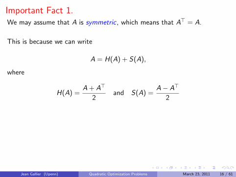
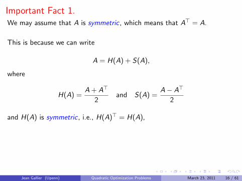
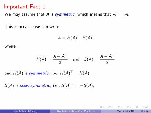
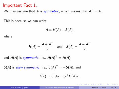
Important Fact 1.We may assume that A is symmetric , which means that A> = A.
This is because we can write
A = H(A) + S(A),
where
H(A) =A + A>
2and S(A) =
A− A>
2
and H(A) is symmetric , i.e., H(A)> = H(A),
S(A) is skew symmetric, i.e., S(A)> = −S(A), and
f (x) = x>Ax = x>H(A)x .
Jean Gallier (Upenn) Quadratic Optimization Problems March 23, 2011 16 / 61
Important Fact 1.We may assume that A is symmetric , which means that A> = A.
This is because we can write
A = H(A) + S(A),
where
H(A) =A + A>
2and S(A) =
A− A>
2
and H(A) is symmetric , i.e., H(A)> = H(A),
S(A) is skew symmetric, i.e., S(A)> = −S(A),
and
f (x) = x>Ax = x>H(A)x .
Jean Gallier (Upenn) Quadratic Optimization Problems March 23, 2011 16 / 61
Important Fact 1.We may assume that A is symmetric , which means that A> = A.
This is because we can write
A = H(A) + S(A),
where
H(A) =A + A>
2and S(A) =
A− A>
2
and H(A) is symmetric , i.e., H(A)> = H(A),
S(A) is skew symmetric, i.e., S(A)> = −S(A), and
f (x) = x>Ax = x>H(A)x .
Jean Gallier (Upenn) Quadratic Optimization Problems March 23, 2011 16 / 61
Indeed, is S is skew symmetric, as f (x) = x>Sx is a scalar, so
f (x) = f (x)>
= (x>Sx)>
= x>S>x
= −x>Sx
= −f (x)
and we get 2f (x) = 0, that is, f (x) = 0.
If A is a complex matrix, then we consider
A∗ = (A)>
(the transjugate, conjugate transpose or adjoint of A)
Jean Gallier (Upenn) Quadratic Optimization Problems March 23, 2011 17 / 61
We also have (replacing A> by A∗)
A = H(A) + S(A)
where H(A) is Hermitian, i.e., H(A)∗ = H(A),
and S(A) is skew Hermitian, i.e., S(A)∗ = −S(A).
Then, a quadratic function over Cn is of the form
f (x) = x∗Ax ,
with x ∈ Cn.
Jean Gallier (Upenn) Quadratic Optimization Problems March 23, 2011 18 / 61

We also have (replacing A> by A∗)
A = H(A) + S(A)
where H(A) is Hermitian, i.e., H(A)∗ = H(A),
and S(A) is skew Hermitian, i.e., S(A)∗ = −S(A).
Then, a quadratic function over Cn is of the form
f (x) = x∗Ax ,
with x ∈ Cn.
Jean Gallier (Upenn) Quadratic Optimization Problems March 23, 2011 18 / 61
We also have (replacing A> by A∗)
A = H(A) + S(A)
where H(A) is Hermitian, i.e., H(A)∗ = H(A),
and S(A) is skew Hermitian, i.e., S(A)∗ = −S(A).
Then, a quadratic function over Cn is of the form
f (x) = x∗Ax ,
with x ∈ Cn.
Jean Gallier (Upenn) Quadratic Optimization Problems March 23, 2011 18 / 61
We also have (replacing A> by A∗)
A = H(A) + S(A)
where H(A) is Hermitian, i.e., H(A)∗ = H(A),
and S(A) is skew Hermitian, i.e., S(A)∗ = −S(A).
Then, a quadratic function over Cn is of the form
f (x) = x∗Ax ,
with x ∈ Cn.
Jean Gallier (Upenn) Quadratic Optimization Problems March 23, 2011 18 / 61
If S is skew Hermitian, we have
(x∗Sx)∗ = −x∗Sx ,
but this only implies that the real part of f (x) is zero that is, f (x) is pureimaginary or zero.
However, if A is Hermitian, then f (x) = x∗Ax , is real .
Jean Gallier (Upenn) Quadratic Optimization Problems March 23, 2011 19 / 61
If S is skew Hermitian, we have
(x∗Sx)∗ = −x∗Sx ,
but this only implies that the real part of f (x) is zero that is, f (x) is pureimaginary or zero.
However, if A is Hermitian, then f (x) = x∗Ax , is real .
Jean Gallier (Upenn) Quadratic Optimization Problems March 23, 2011 19 / 61
If S is skew Hermitian, we have
(x∗Sx)∗ = −x∗Sx ,
but this only implies that the real part of f (x) is zero that is, f (x) is pureimaginary or zero.
However, if A is Hermitian, then f (x) = x∗Ax , is real .
Jean Gallier (Upenn) Quadratic Optimization Problems March 23, 2011 19 / 61
Important Fact 2.
Every n × n real symmetric matrix, A, has real eigenvalues, say
λ1 ≥ λ2 ≥ · · · ≥ λn,
and can be diagonalized with respect to an orthonormal basis ofeigenvectors.
This means that there is a basis of orthonormal vectors, (e1, . . . , en),where ei is an eigenvector for λi , that is,
Aei = λiei , 1 ≤ i ≤ n.
The same result holds for (complex) Hermitian matrices (w.r.t. theHermitian inner product).
Jean Gallier (Upenn) Quadratic Optimization Problems March 23, 2011 20 / 61

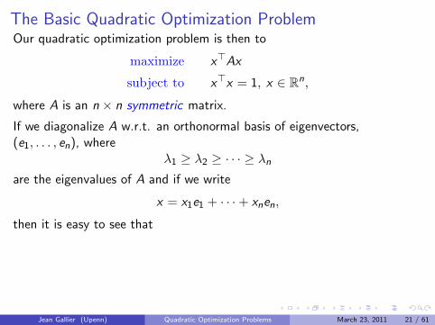
The Basic Quadratic Optimization ProblemOur quadratic optimization problem is then to
maximize x>Ax
subject to x>x = 1, x ∈ Rn,
where A is an n × n symmetric matrix.
If we diagonalize A w.r.t. an orthonormal basis of eigenvectors,(e1, . . . , en), where
λ1 ≥ λ2 ≥ · · · ≥ λnare the eigenvalues of A and if we write
x = x1e1 + · · ·+ xnen,
then it is easy to see that
f (x) = x>Ax = λ1x21 + · · ·+ λnx2
n ,
subject tox1
1 + · · ·+ x2n = 1.
Jean Gallier (Upenn) Quadratic Optimization Problems March 23, 2011 21 / 61
Courant Fischer
Consequently, generalizing the proof given for n = 2, we have:
maxx>x=1
x>Ax = λ1,
the largest eigenvalue of A, and this maximum is achieved for any uniteigenvector associated with λ1.
This fact is part of the Courant-Fischer Theorem.
Jean Gallier (Upenn) Quadratic Optimization Problems March 23, 2011 22 / 61

Figure: Richard Courant, 1888-1972
This result also holds for Hermitian matrices.
Jean Gallier (Upenn) Quadratic Optimization Problems March 23, 2011 23 / 61
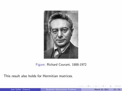
Figure: Richard Courant, 1888-1972
This result also holds for Hermitian matrices.
Jean Gallier (Upenn) Quadratic Optimization Problems March 23, 2011 23 / 61
A Quadratic Optimization Problem Arising in ContourGrouping
Jianbo Shi and his students Qihui Zhu and Gang Song have investigatedthe problem of contour grouping in 2D images.
The problem is to find 1D (closed) curve-like structures in images.
The goal is to find cycles linking small edges called edgels.
The method uses a directed graph where the nodes are edgels and theedges connect pairs of edgels within some distance.
Every edge has a weight, Wij , measuring the (directed) collinearity of twoedgels using the elastic energy between these edgels.
Jean Gallier (Upenn) Quadratic Optimization Problems March 23, 2011 24 / 61
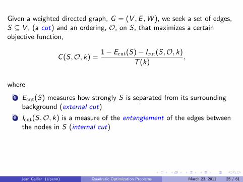
Given a weighted directed graph, G = (V ,E ,W ), we seek a set of edges,S ⊆ V , (a cut) and an ordering, O, on S , that maximizes a certainobjective function,
C (S ,O, k) =1− Ecut(S)− Icut(S ,O, k)
T (k),
where
1 Ecut(S) measures how strongly S is separated from its surroundingbackground (external cut)
2 Icut(S ,O, k) is a measure of the entanglement of the edges betweenthe nodes in S (internal cut)
3 T (k) is the tube size of the cut; it depends on the thickness factor , k(in fact, T (k) = k/|S |).
Jean Gallier (Upenn) Quadratic Optimization Problems March 23, 2011 25 / 61

Very recently, Shi and Kennedy found a better formulation of the objectivefunction involving a new normalization of the matrix arising from thegraph G .
We will only present the “old” formulation.
Maximizing C (S ,O, k) is a hard combinatorial problem so, Shi, Zhu andSong had the idea of converting the orginal problem to a simpler problemusing acircular embedding .
Jean Gallier (Upenn) Quadratic Optimization Problems March 23, 2011 26 / 61

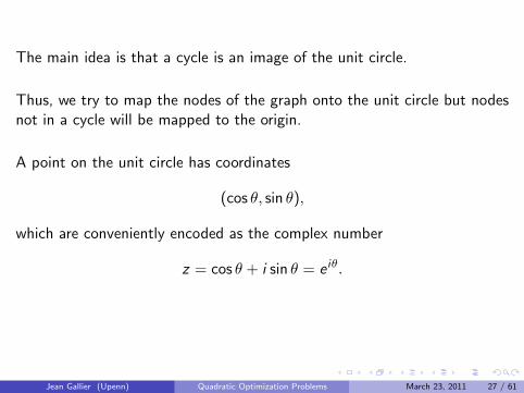
The main idea is that a cycle is an image of the unit circle.
Thus, we try to map the nodes of the graph onto the unit circle but nodesnot in a cycle will be mapped to the origin.
A point on the unit circle has coordinates
(cos θ, sin θ),
which are conveniently encoded as the complex number
z = cos θ + i sin θ = e iθ.
Jean Gallier (Upenn) Quadratic Optimization Problems March 23, 2011 27 / 61
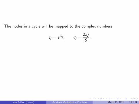
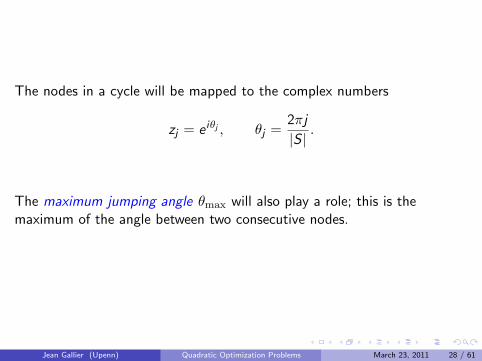
The nodes in a cycle will be mapped to the complex numbers
zj = e iθj , θj =2πj
|S |.
The maximum jumping angle θmax will also play a role; this is themaximum of the angle between two consecutive nodes.
Jean Gallier (Upenn) Quadratic Optimization Problems March 23, 2011 28 / 61
The nodes in a cycle will be mapped to the complex numbers
zj = e iθj , θj =2πj
|S |.
The maximum jumping angle θmax will also play a role; this is themaximum of the angle between two consecutive nodes.
Jean Gallier (Upenn) Quadratic Optimization Problems March 23, 2011 28 / 61
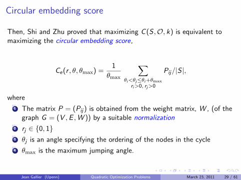
Circular embedding score
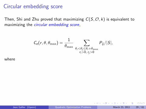
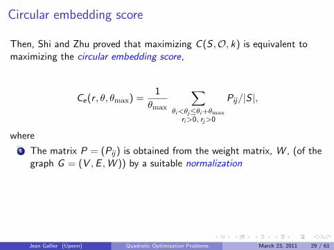
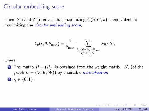
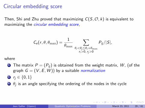
Then, Shi and Zhu proved that maximizing C (S ,O, k) is equivalent tomaximizing the circular embedding score,
Ce(r , θ, θmax) =1
θmax
∑θi<θj≤θi+θmax
ri>0, rj>0
Pij/|S |,
where
1 The matrix P = (Pij) is obtained from the weight matrix, W , (of thegraph G = (V ,E ,W )) by a suitable normalization
2 rj ∈ {0, 1}3 θj is an angle specifying the ordering of the nodes in the cycle
4 θmax is the maximum jumping angle.
Jean Gallier (Upenn) Quadratic Optimization Problems March 23, 2011 29 / 61
Circular embedding score
Then, Shi and Zhu proved that maximizing C (S ,O, k) is equivalent tomaximizing the circular embedding score,
Ce(r , θ, θmax) =1
θmax
∑θi<θj≤θi+θmax
ri>0, rj>0
Pij/|S |,
where
1 The matrix P = (Pij) is obtained from the weight matrix, W , (of thegraph G = (V ,E ,W )) by a suitable normalization
2 rj ∈ {0, 1}
3 θj is an angle specifying the ordering of the nodes in the cycle
4 θmax is the maximum jumping angle.
Jean Gallier (Upenn) Quadratic Optimization Problems March 23, 2011 29 / 61
Circular embedding score
Then, Shi and Zhu proved that maximizing C (S ,O, k) is equivalent tomaximizing the circular embedding score,
Ce(r , θ, θmax) =1
θmax
∑θi<θj≤θi+θmax
ri>0, rj>0
Pij/|S |,
where
1 The matrix P = (Pij) is obtained from the weight matrix, W , (of thegraph G = (V ,E ,W )) by a suitable normalization
2 rj ∈ {0, 1}3 θj is an angle specifying the ordering of the nodes in the cycle
4 θmax is the maximum jumping angle.
Jean Gallier (Upenn) Quadratic Optimization Problems March 23, 2011 29 / 61
Circular embedding score
Then, Shi and Zhu proved that maximizing C (S ,O, k) is equivalent tomaximizing the circular embedding score,
Ce(r , θ, θmax) =1
θmax
∑θi<θj≤θi+θmax
ri>0, rj>0
Pij/|S |,
where
1 The matrix P = (Pij) is obtained from the weight matrix, W , (of thegraph G = (V ,E ,W )) by a suitable normalization
2 rj ∈ {0, 1}3 θj is an angle specifying the ordering of the nodes in the cycle
4 θmax is the maximum jumping angle.
Jean Gallier (Upenn) Quadratic Optimization Problems March 23, 2011 29 / 61

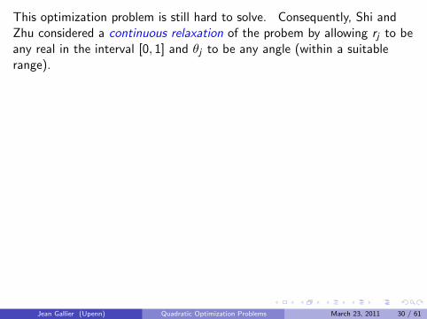
This optimization problem is still hard to solve.
Consequently, Shi andZhu considered a continuous relaxation of the probem by allowing rj to beany real in the interval [0, 1] and θj to be any angle (within a suitablerange).
In the circular embedding, a node in then represented by the complexnumber
xj = rjeiθj .
We also introduce the average jumping angle
∆θ = θk − θj .
Then, it is not hard to see that the numerator of Ce(r , θ, θmax) is wellapproximated by the expression∑
j ,k
Pjk cos(θk − θj −∆θ) =∑j ,k
Re(x∗j xk · e−i∆θ).
Jean Gallier (Upenn) Quadratic Optimization Problems March 23, 2011 30 / 61
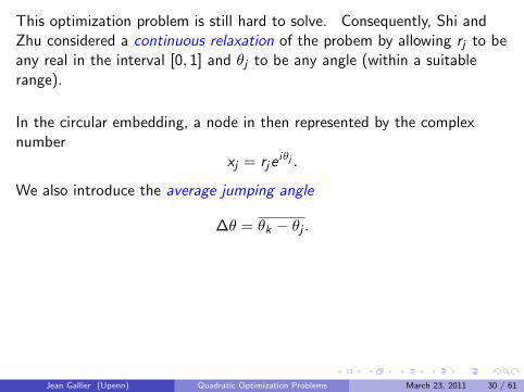
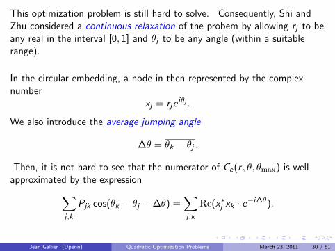
This optimization problem is still hard to solve. Consequently, Shi andZhu considered a continuous relaxation of the probem by allowing rj to beany real in the interval [0, 1] and θj to be any angle (within a suitablerange).
In the circular embedding, a node in then represented by the complexnumber
xj = rjeiθj .
We also introduce the average jumping angle
∆θ = θk − θj .
Then, it is not hard to see that the numerator of Ce(r , θ, θmax) is wellapproximated by the expression∑
j ,k
Pjk cos(θk − θj −∆θ) =∑j ,k
Re(x∗j xk · e−i∆θ).
Jean Gallier (Upenn) Quadratic Optimization Problems March 23, 2011 30 / 61
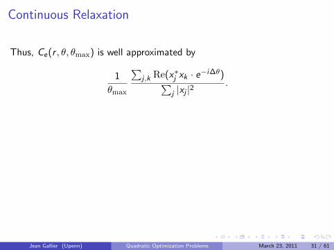
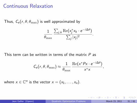
Continuous Relaxation
Thus, Ce(r , θ, θmax) is well approximated by
1
θmax
∑j ,k Re(x∗j xk · e−i∆θ)∑
j |xj |2.
This term can be written in terms of the matrix P as
Ce(r , θ, θmax) ≈ 1
θmax
Re(x∗Px · e−i∆θ)
x∗x,
where x ∈ Cn is the vector x = (x1, . . . , xn).
Jean Gallier (Upenn) Quadratic Optimization Problems March 23, 2011 31 / 61
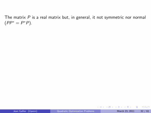
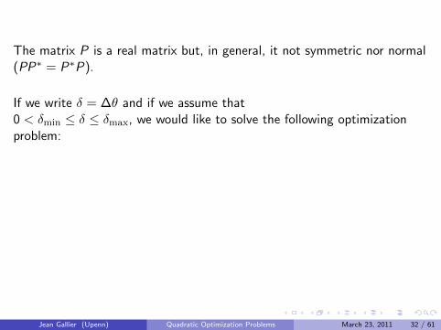
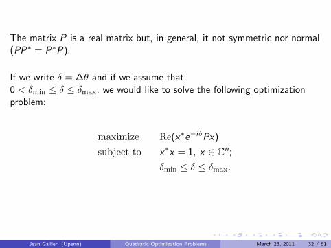
The matrix P is a real matrix but, in general, it not symmetric nor normal(PP∗ = P∗P).
If we write δ = ∆θ and if we assume that0 < δmin ≤ δ ≤ δmax, we would like to solve the following optimizationproblem:
maximize Re(x∗e−iδPx)
subject to x∗x = 1, x ∈ Cn;
δmin ≤ δ ≤ δmax.
Jean Gallier (Upenn) Quadratic Optimization Problems March 23, 2011 32 / 61
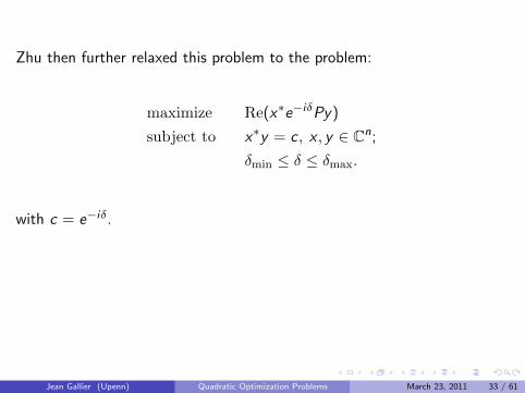
Zhu then further relaxed this problem to the problem:
maximize Re(x∗e−iδPy)
subject to x∗y = c, x , y ∈ Cn;
δmin ≤ δ ≤ δmax.
with c = e−iδ.
However, it turns out that this problem is too relaxed , because theconstraint x∗y = c is weak; it allows x to be very large and y to be verysmall , and conversely.
Jean Gallier (Upenn) Quadratic Optimization Problems March 23, 2011 33 / 61

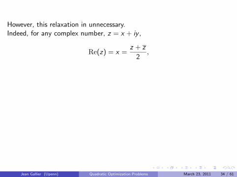
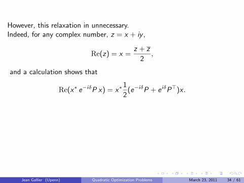
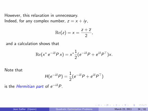
However, this relaxation in unnecessary.
Indeed, for any complex number, z = x + iy ,
Re(z) = x =z + z
2,
and a calculation shows that
Re(x∗ e−iδP x) = x∗1
2(e−iδP + e iδP>)x .
Note that
H(e−iδP) =1
2(e−iδP + e iδP>)
is the Hermitian part of e−iδP.
Jean Gallier (Upenn) Quadratic Optimization Problems March 23, 2011 34 / 61
However, this relaxation in unnecessary.Indeed, for any complex number, z = x + iy ,
Re(z) = x =z + z
2,
and a calculation shows that
Re(x∗ e−iδP x) = x∗1
2(e−iδP + e iδP>)x .
Note that
H(e−iδP) =1
2(e−iδP + e iδP>)
is the Hermitian part of e−iδP.
Jean Gallier (Upenn) Quadratic Optimization Problems March 23, 2011 34 / 61
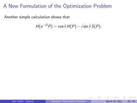
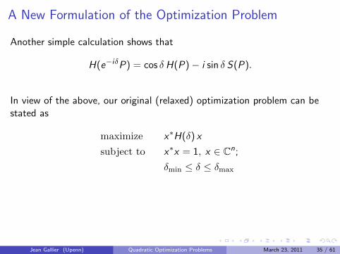
A New Formulation of the Optimization Problem
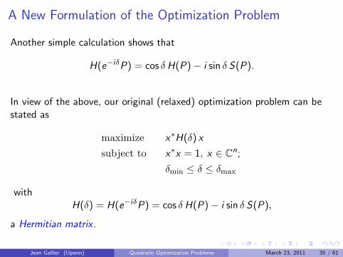
Another simple calculation shows that
H(e−iδP) = cos δH(P)− i sin δ S(P).
In view of the above, our original (relaxed) optimization problem can bestated as
maximize x∗H(δ) x
subject to x∗x = 1, x ∈ Cn;
δmin ≤ δ ≤ δmax
withH(δ) = H(e−iδP) = cos δH(P)− i sin δ S(P),
a Hermitian matrix .
Jean Gallier (Upenn) Quadratic Optimization Problems March 23, 2011 35 / 61
A New Formulation of the Optimization Problem
Another simple calculation shows that
H(e−iδP) = cos δH(P)− i sin δ S(P).
In view of the above, our original (relaxed) optimization problem can bestated as
maximize x∗H(δ) x
subject to x∗x = 1, x ∈ Cn;
δmin ≤ δ ≤ δmax
withH(δ) = H(e−iδP) = cos δH(P)− i sin δ S(P),
a Hermitian matrix .
Jean Gallier (Upenn) Quadratic Optimization Problems March 23, 2011 35 / 61
The optimal value is the largest eigenvalue, λ1, of H(δ), over all δ suchthat δmin ≤ δ ≤ δmax and it is attained for any associated complex uniteigenvector, x = xr + ixi .
Ryan Kennedy has implemented this method and has obtained goodresults.
Jean Gallier (Upenn) Quadratic Optimization Problems March 23, 2011 36 / 61
The Case Where P is a Normal Matrix
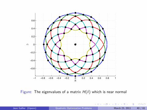
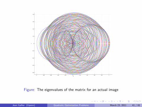
When P is a normal matrix (PP> = P>P) it is possible to express theeigenvalues of H(δ) and the corresponding eigenvectors in terms of the(complex) eigenvalues of P and its eigenvectors.
If u + iv is an eigenvector of P for the (complex) eigenvalue λ+ iµ, thenu + iv is also an eigenvector of H(δ) for the (real) eigenvaluecos δ λ− sin δ µ.
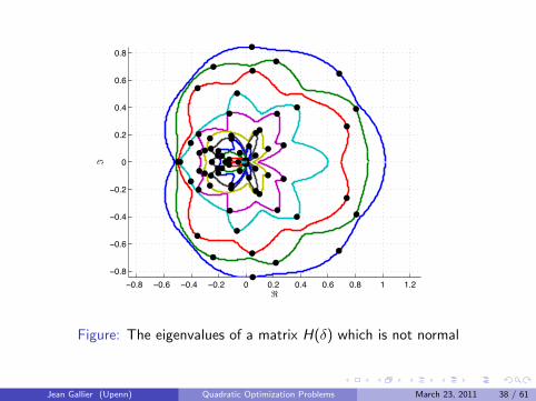
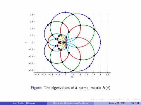
Geometrically, this means that the eigenvalues of H(δ) vary on circles,plotted as a function of δ.
The next four Figures were produced by Ryan Kennedy.
Jean Gallier (Upenn) Quadratic Optimization Problems March 23, 2011 37 / 61
The Case Where P is a Normal Matrix
When P is a normal matrix (PP> = P>P) it is possible to express theeigenvalues of H(δ) and the corresponding eigenvectors in terms of the(complex) eigenvalues of P and its eigenvectors.
If u + iv is an eigenvector of P for the (complex) eigenvalue λ+ iµ, thenu + iv is also an eigenvector of H(δ) for the (real) eigenvaluecos δ λ− sin δ µ.
Geometrically, this means that the eigenvalues of H(δ) vary on circles,plotted as a function of δ.
The next four Figures were produced by Ryan Kennedy.
Jean Gallier (Upenn) Quadratic Optimization Problems March 23, 2011 37 / 61
0.8 0.6 0.4 0.2 0 0.2 0.4 0.6 0.8 1 1.20.8
0.6
0.4
0.2
0
0.2
0.4
0.6
0.8
Figure: The eigenvalues of a matrix H(δ) which is not normal
Jean Gallier (Upenn) Quadratic Optimization Problems March 23, 2011 38 / 61
0.8 0.6 0.4 0.2 0 0.2 0.4 0.6 0.8 1 1.2
0.8
0.6
0.4
0.2
0
0.2
0.4
0.6
0.8
Figure: The eigenvalues of a normal matrix H(δ)
Jean Gallier (Upenn) Quadratic Optimization Problems March 23, 2011 39 / 61
1 0.8 0.6 0.4 0.2 0 0.2 0.4 0.6 0.8 1
0.6
0.4
0.2
0
0.2
0.4
0.6
Figure: The eigenvalues of a matrix H(δ) which is near normal
Jean Gallier (Upenn) Quadratic Optimization Problems March 23, 2011 40 / 61
1 0.8 0.6 0.4 0.2 0 0.2 0.4 0.6 0.8 1
0.8
0.6
0.4
0.2
0
0.2
0.4
0.6
0.8
Figure: The eigenvalues of the matrix for an actual image
Jean Gallier (Upenn) Quadratic Optimization Problems March 23, 2011 41 / 61
Derivatives of Eigenvectors and Eigenvalues
To solve our maximization problem, we need to study the variation of thelargest eigenvalue, λ1(δ), of H(δ).
This problem has been studied before and it is possible to find explicitformulae for the derivative of a simple eigenvalue of H(δ) and for thederivative of a unit eigenvector of H(δ).
Shi and Cour obtained similar formulae in a different context.
It turns out that it is not easy to find clean and complete derivations ofthese formulae.
The best source is Peter Lax’s linear algebra book (Chapter 9). A niceaccount is also found in a blog by Terence Tao.
Jean Gallier (Upenn) Quadratic Optimization Problems March 23, 2011 42 / 61
Let X (δ) be a matrix function depending on the parameter δ.
It is proved in Lax (Chapter 9, Theorem 7 and Theorem 8) that if λ is asimple eigenvalue of X (δ), for δ = δ0 and if u is a unit eigenvectorassociated with λ, then, in a small open interval around δ0, the matrixX (δ) has a simple eigenvalue, λ(δ), that is differentiable (with λ(δ0) = λ)and that there is a choice of an eigenvector, u(t), associated with λ(t), sothat u(t) is also differentiable (with u(δ0) = u).
In the case of an eigenvalue, the proof uses the implicit function theoremapplied to the characteristic polynomial, det(λI − X (δ)).
The proof of differentiability for an eigenvector is more involved and usesthe non-vanishing of some principal minor of det(λI − X (δ)).
Jean Gallier (Upenn) Quadratic Optimization Problems March 23, 2011 43 / 61

The formula for the derivative of an eigenvector is simpler if we assumeX (δ) to be normal. In this case, we get
Theorem 2
Let X (δ) be a normal matrix that depends differentiably on δ. If λ is anysimple eigenvalue of X at δ0 (it has algebraic multiplicity 1) and if u is thecorresponding unit eigenvector, then the derivatives at δ = δ0 of λ(δ) andu(δ) are given by
λ′ = u∗X ′u
u′ = (λI − X )†X ′u,
where (λI − X )† is the pseudo-inverse of λI − X , X ′ is the derivative of Xat δ = δ0 and u′ is orthogonal to u.
Jean Gallier (Upenn) Quadratic Optimization Problems March 23, 2011 44 / 61
Proof.
If X is a normal matrix, it is well known that Xu = λu iff X ∗u = λu andso, if Xu = λu then
u∗X = λu∗.
Taking the derivative of Xu = λu and using the chain rule, we get
X ′u + Xu′ = λ′u + λu′.
By taking the inner product with u∗, we get
u∗X ′u + u∗Xu′ = λ′u∗u + λu∗u′.
However, u∗X = λu∗, so u∗Xu′ = λu∗u′, and as u is a unit vector,u∗u = 1, so
u∗X ′u + λu∗u′ = λ′ + λu∗u′,
that is, λ′ = u∗X ′u.
Deriving the formula for the derivative of u is more involved.
Jean Gallier (Upenn) Quadratic Optimization Problems March 23, 2011 45 / 61

Proof.
If X is a normal matrix, it is well known that Xu = λu iff X ∗u = λu andso, if Xu = λu then
u∗X = λu∗.
Taking the derivative of Xu = λu and using the chain rule, we get
X ′u + Xu′ = λ′u + λu′.
By taking the inner product with u∗, we get
u∗X ′u + u∗Xu′ = λ′u∗u + λu∗u′.
However, u∗X = λu∗, so u∗Xu′ = λu∗u′, and as u is a unit vector,u∗u = 1,
sou∗X ′u + λu∗u′ = λ′ + λu∗u′,
that is, λ′ = u∗X ′u.
Deriving the formula for the derivative of u is more involved.
Jean Gallier (Upenn) Quadratic Optimization Problems March 23, 2011 45 / 61
Proof.
If X is a normal matrix, it is well known that Xu = λu iff X ∗u = λu andso, if Xu = λu then
u∗X = λu∗.
Taking the derivative of Xu = λu and using the chain rule, we get
X ′u + Xu′ = λ′u + λu′.
By taking the inner product with u∗, we get
u∗X ′u + u∗Xu′ = λ′u∗u + λu∗u′.
However, u∗X = λu∗, so u∗Xu′ = λu∗u′, and as u is a unit vector,u∗u = 1, so
u∗X ′u + λu∗u′ = λ′ + λu∗u′,
that is, λ′ = u∗X ′u.
Deriving the formula for the derivative of u is more involved.
Jean Gallier (Upenn) Quadratic Optimization Problems March 23, 2011 45 / 61
(
~
t .
Figure: Just checking!
Jean Gallier (Upenn) Quadratic Optimization Problems March 23, 2011 46 / 61
The Field of Values of P
It turns out that
x∗H(δ)x ≤ |x∗Px |
for all x and all δ, and this has some important implications regarding thelocal maxima of these two functions.
In fact, if we write x∗Px in polar form as
x∗Px = |x∗Px |(cosϕ+ i sinϕ),
I proved that
x∗H(δ)x = |x∗Px | cos(δ − ϕ).
Jean Gallier (Upenn) Quadratic Optimization Problems March 23, 2011 47 / 61
This implies that
x∗H(δ)x ≤ |x∗Px |
for all x ∈ Cn and all δ, (0 ≤ δ ≤ 2π), with equality iff
δ = ϕ,
the argument (phase angle) of x∗Px .
In particular, for x fixed, f (x , δ) = x∗Hx has a local optimum when δ = ϕand, in this case, x∗Hx = |x∗Px |.
Jean Gallier (Upenn) Quadratic Optimization Problems March 23, 2011 48 / 61
The inequality x∗Hx ≤ |x∗Px | also implies that if |x∗Px | achieves a localmaximum for some vector, x, then f (x , δ) = x∗Hx achieves a localmaximum equal to |x∗Px | for δ = ϕ and for the same x (where ϕ is theargument of x∗Px).
Furthermore, x must be an eigenvector of H(ϕ).
Generally, if f (x , δ) = x∗Hx is a local maximum of f at (x , δ), then |x∗Px |is not necessarily a local maximum at x .
However, we can show that if f (x , δ) = x∗Hx is a local maximum of f at(x , δ), then δ = ϕ, the phase angle of |x∗Px | and so, x∗Hx = |x∗Px |.
Jean Gallier (Upenn) Quadratic Optimization Problems March 23, 2011 49 / 61

Unfortunately, this doesn’t not seem to help much in finding for which δthe function f (x , δ) has local maxima.
Still, since the maxima of |x∗Px | dominate the maxima of x∗H(δ)x , andare a subset of those maxima, it is useful to understand better how to findthe local maxima of |x∗Px |.
The determination of the local extrema of |x∗Px | (with x∗x = 1) is closelyrelated to the structure of the set of complex numbers
F (P) = {x∗Px ∈ C | x ∈ Cn, x∗x = 1},
known as the field of values of P or the numerical range of P (thenotation W (P) is also commonly used, corresponding to the Germanterminology “Wertvorrat” or “Wertevorrat”).
Jean Gallier (Upenn) Quadratic Optimization Problems March 23, 2011 50 / 61
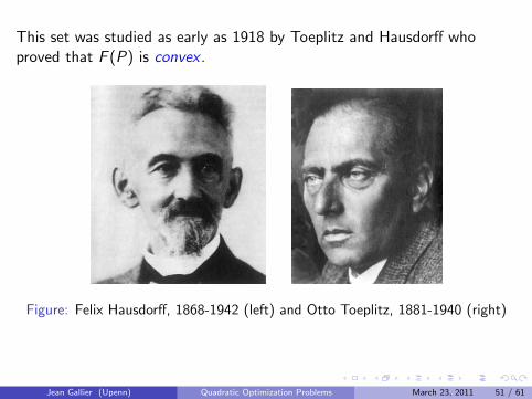
This set was studied as early as 1918 by Toeplitz and Hausdorff whoproved that F (P) is convex .
Figure: Felix Hausdorff, 1868-1942 (left) and Otto Toeplitz, 1881-1940 (right)
Jean Gallier (Upenn) Quadratic Optimization Problems March 23, 2011 51 / 61
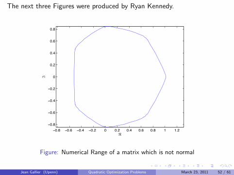
The next three Figures were produced by Ryan Kennedy.
0.8 0.6 0.4 0.2 0 0.2 0.4 0.6 0.8 1 1.20.8
0.6
0.4
0.2
0
0.2
0.4
0.6
0.8
Figure: Numerical Range of a matrix which is not normal
Jean Gallier (Upenn) Quadratic Optimization Problems March 23, 2011 52 / 61
0.8 0.6 0.4 0.2 0 0.2 0.4 0.6 0.8 1 1.2
0.8
0.6
0.4
0.2
0
0.2
0.4
0.6
0.8
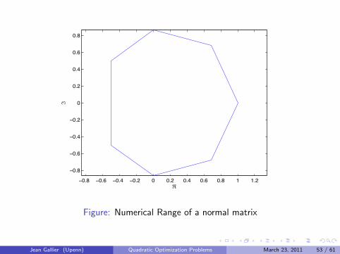
Figure: Numerical Range of a normal matrix
Jean Gallier (Upenn) Quadratic Optimization Problems March 23, 2011 53 / 61
1 0.8 0.6 0.4 0.2 0 0.2 0.4 0.6 0.8 1
0.6
0.4
0.2
0
0.2
0.4
0.6
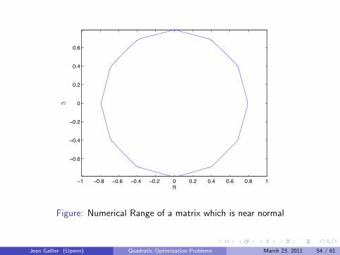
Figure: Numerical Range of a matrix which is near normal
Jean Gallier (Upenn) Quadratic Optimization Problems March 23, 2011 54 / 61
\\T~ ~\Jri OF IH1S.1 S IHkf rf '5 OAJL'f OF T~"CAL IMPoRTArJc.E:., AND 1FfE:RE. IS NO WAy rf cAN SS or MY pgAC:lltAL use. W\-Wr$Ob.\f~. \\
Figure: Beauty
Jean Gallier (Upenn) Quadratic Optimization Problems March 23, 2011 55 / 61
The quantityr(P) = max{|z | | z ∈ F (P)}
is called the numerical radius of P.
It is obviously of interest to us since it corresponds to the maximum of|x∗Px |, over all unit vectors, x .
It is easy to show that
F (e−iδP) = e−iδF (P)
and so,F (P) = e iδF (e−iδP).
Geometrically, this means that F (P) is obtained from F (e−iδP) byrotating it by δ.
Jean Gallier (Upenn) Quadratic Optimization Problems March 23, 2011 56 / 61
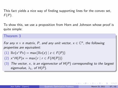
This fact yields a nice way of finding supporting lines for the convex set,F (P).
To show this, we use a proposition from Horn and Johnson whose proof isquite simple:
Theorem 3
For any n × n matrix, P, and any unit vector, x ∈ Cn, the followingproperties are equivalent:
(1) Re(x∗Px) = max{Re(z) | z ∈ F (P)}(2) x∗H(P)x = max{r | r ∈ F (H(P))}(3) The vector, x, is an eigenvector of H(P) corresponding to the largest
eigenvalue, λ1, of H(P).
Jean Gallier (Upenn) Quadratic Optimization Problems March 23, 2011 57 / 61
In fact, Theorem 3 immediately implies that
max{Re(z) | z ∈ F (P)} = max{r | r ∈ F (H(P))} = λ1.
As a consequence, for every angle, δ ∈ [0, 2π), if we let λδ be the largesteigenvalue of the matrix H(e−iδP) and if xδ is a corresponding uniteigenvector, then zδ = x∗δPxδ is on the boundary, ∂F (P), of F (P) and theline, Lδ, given by
Lδ = {e iδ(λδ + ti) | t ∈ R}= {(x , y) ∈ R2 | cos δ x + sin δ y − λδ = 0},
is a supporting line of F (P) at zδ.
Jean Gallier (Upenn) Quadratic Optimization Problems March 23, 2011 58 / 61
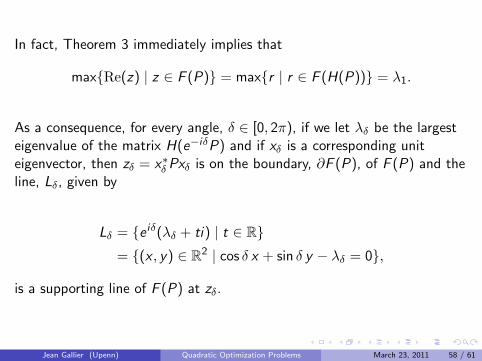
These properties can be exploited to find the local maxima of the objectivefunction of our contour identification problem. Ryan Kennedy has donesome work on this problem.
Much more work needs to be done, in particular
Cope with the dimension of the matrix, P
Understand the role of various normalizations of P (stochastic,bi-stochastic).
Shi and Kennedy have made recent progress on the issue ofnormalization.
Jean Gallier (Upenn) Quadratic Optimization Problems March 23, 2011 59 / 61
Other Quadratic Optimization Problems
Some variations of the basic quadratic optimization problem have occurredin the contex of computer vision:
Adding linear constraints of the form
C>x = 0.
It is relatively easy to eliminate these constraints using aQR-decomposition or a pseudo-inverse. This was shown by Golub(1973).
Adding linear constraints of the form
C>x = t,
where t 6= 0. This is a lot harder to deal with!
Jean Gallier (Upenn) Quadratic Optimization Problems March 23, 2011 60 / 61
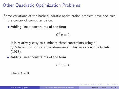
Other Quadratic Optimization Problems
Some variations of the basic quadratic optimization problem have occurredin the contex of computer vision:
Adding linear constraints of the form
C>x = 0.
It is relatively easy to eliminate these constraints using aQR-decomposition or a pseudo-inverse. This was shown by Golub(1973).
Adding linear constraints of the form
C>x = t,
where t 6= 0.
This is a lot harder to deal with!
Jean Gallier (Upenn) Quadratic Optimization Problems March 23, 2011 60 / 61
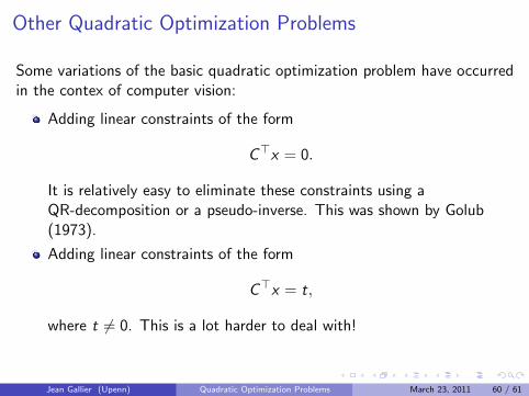
Other Quadratic Optimization Problems
Some variations of the basic quadratic optimization problem have occurredin the contex of computer vision:
Adding linear constraints of the form
C>x = 0.
It is relatively easy to eliminate these constraints using aQR-decomposition or a pseudo-inverse. This was shown by Golub(1973).
Adding linear constraints of the form
C>x = t,
where t 6= 0. This is a lot harder to deal with!
Jean Gallier (Upenn) Quadratic Optimization Problems March 23, 2011 60 / 61
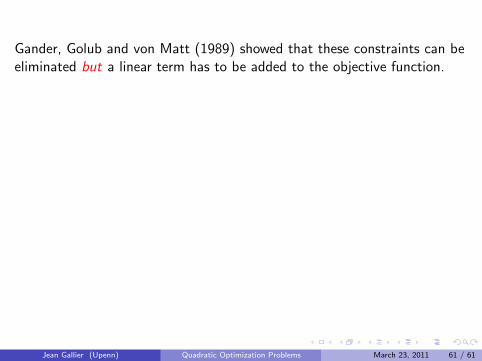
Gander, Golub and von Matt (1989) showed that these constraints can beeliminated but a linear term has to be added to the objective function.
One needs to consider objective functions of the form
f (x) = x>Ax + 2x>b,
with b 6= 0.
This problem was studied by Gander, Golub and von Matt (1989).
I also have a solution to this problem involving an algebraic curvegeneralizing the hyperbola to Rn, but this will have to wait for anothertalk!
Jean Gallier (Upenn) Quadratic Optimization Problems March 23, 2011 61 / 61
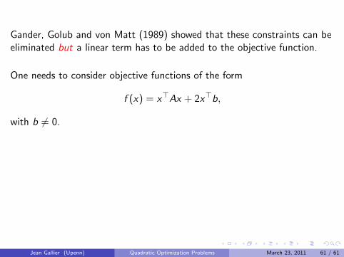