Embed Size (px)
Citation preview

QUaD: A High-Resolution CosmicMicrowave Background Polarimeter
The Harvard community has made thisarticle openly available. Please share howthis access benefits you. Your story matters
Citation Hinderks, James R., Peter Ade, James Bock, Melanie Bowden,Michael L. Brown, Gary Cahill, John E. Carlstrom, and et al. 2009.QUaD: A high-resolution cosmic microwave background polarimeter.The Astrophysical Journal 692, no. 2: 1221-1246.
Published Version doi:10.1088/0004-637X/692/2/1221
Citable link http://nrs.harvard.edu/urn-3:HUL.InstRepos:11129145
Terms of Use This article was downloaded from Harvard University’s DASHrepository, and is made available under the terms and conditionsapplicable to Other Posted Material, as set forth at http://nrs.harvard.edu/urn-3:HUL.InstRepos:dash.current.terms-of-use#LAA

The Astrophysical Journal, 692:1221–1246, 2009 February 20 doi:10.1088/0004-637X/692/2/1221c© 2009. The American Astronomical Society. All rights reserved. Printed in the U.S.A.
QUaD: A HIGH-RESOLUTION COSMIC MICROWAVE BACKGROUND POLARIMETER
J. R. Hinderks1,10
, P. Ade2, J. Bock
3,4, M. Bowden
1, M. L. Brown
5,11, G. Cahill
6, J. E. Carlstrom
7, P. G. Castro
5,12,
S. Church1, T. Culverhouse
7, R. Friedman
7, K. Ganga
8, W. K. Gear
2, S. Gupta
2, J. Harris
2, V. Haynes
2,13, B.
G. Keating9, J. Kovac
3,4, E. Kirby
1, A. E. Lange
4, E. Leitch
3,4, O. E. Mallie
2, S. Melhuish
2,13, Y. Memari
5, A. Murphy
7,
A. Orlando2,4
, R. Schwarz7, C. O’ Sullivan
6, L. Piccirillo
2,13, C. Pryke
7, N. Rajguru
14, B. Rusholme
1,3, A. N. Taylor
5,
K. L. Thompson1, C. Tucker
2, A. H. Turner
2, E. Y. S. Wu
1, and M. Zemcov
3,41 Kavli Institute for Particle Astrophysics and Cosmology and Department of Physics, Stanford University, 382 Via Pueblo Mall, Stanford, CA 94305, USA
2 School of Physics and Astronomy, Cardiff University, Queen’s Buildings, The Parade, Cardiff CF24 3AA, UK3 Jet Propulsion Laboratory, 4800 Oak Grove Dr., Pasadena, CA 91109, USA
4 California Institute of Technology, Pasadena, CA 91125, USA5 Institute for Astronomy, University of Edinburgh, Royal Observatory, Blackford Hill, Edinburgh EH9 3HJ, UK
6 Experimental Physics, National University of Ireland, Maynooth, Ireland7 Kavli Institute for Cosmological Physics, Department of Astronomy & Astrophysics, University of Chicago, 5640 South Ellis Avenue, Chicago, IL 60637, USA
8 Laboratoire APC/CNRS; Batiment Condorcet; 10, rue Alice Domon et Leonie Duquet, 75205 Paris Cedex 13, France9 Center for Astrophysics and Space Sciences, University of California, San Diego, 9500 Gilman Drive, La Jolla, CA 92093, USA
Received 2008 May 14; accepted 2008 October 2; published 2009 February 24
ABSTRACT
We describe the QUaD experiment, a millimeter-wavelength polarimeter designed to observe the cosmicmicrowave background (CMB) from a site at the South Pole. The experiment comprises a 2.64 m Cassegraintelescope equipped with a cryogenically cooled receiver containing an array of 62 polarization-sensitivebolometers. The focal plane contains pixels at two different frequency bands, 100 GHz and 150 GHz, withangular resolutions of 5′ and 3.′5, respectively. The high angular resolution allows observation of CMBtemperature and polarization anisotropies over a wide range of scales. The instrument commenced operationin early 2005 and collected science data during three successive Austral winter seasons of observation.
Key words: cosmic microwave background – instrumentation: polarimeters
Online-only material: color figures
1. INTRODUCTION
The cosmic microwave background (CMB) remains a keytool for understanding the origin and evolution of the universe.Thompson scattering from quadrupole anisotropies at the sur-face of last scattering polarizes the CMB at the level of 10%.The resulting polarization pattern on the sky can be mathemat-ically decomposed into even-parity E modes and odd-parityB modes (Zaldarriaga & Seljak 1997). The E-mode signal,which has been detected by a number of experiments (Readheadet al. 2004; Leitch et al. 2005; Montroy et al. 2006; Page et al.2007; Wu et al. 2007; CAPMAP Collaboration: C. Bischoffet al. 2008), is dominated by scalar perturbations (density fluc-tuations) in the early universe. A B-mode signal has yet to bedetected but could be generated by gravitational waves in theearly universe or lensing of E modes by intervening structure.
This paper describes QUaD,15 a polarimeter designed toobserve the CMB. QUaD comprises a bolometric receiverlocated on a 2.64 m telescope near the geographic South
10 Current address: NASA Goddard Space Flight Center, 8800 GreenbeltRoad, Greenbelt, Maryland 20771, USA.11 Current address: Cavendish Laboratory, University of Cambridge, J.J.Thomson Avenue, Cambridge CB3 OHE, UK.12 Current address: CENTRA, Departamento de Fısica, Edifıcio Ciencia,Instituto Superior Tecnico, Universidade Tecnica de Lisboa, Av. Rovisco Pais1, 1049-001 Lisboa, Portugal.13 Current address: School of Physics and Astronomy, University ofManchester, Manchester M13 9PL, UK.14 Current address: Department of Physics and Astronomy, University CollegeLondon, Gower Street, London WC1E 6BT, UK.15 QUaD stands for QUEST (QU Extragalactic Survey Telescope) at DASI(Degree Angular Scale Interferometer).
Pole. The QUaD receiver contains a focal plane array of 31pixels, each composed of a corrugated feed horn and a pairof orthogonal polarization-sensitive bolometers (PSBs). Eachpixel simultaneously measures both temperature and one linearpolarization Stokes parameter. The pixels are divided betweentwo observing frequencies with 12 at 100 GHz and 19 at150 GHz. The angular resolution is 5.′0 at 100 GHz and 3.′5at 150 GHz, and the instantaneous field of view is 1.◦5. Table 1gives the optical properties of the telescope and receiver. Firstlight was in 2005 February, and three seasons of Australwinter observations were completed before the instrument wasdecommissioned in late 2007. Results from the first season’sdata are presented in Ade et al. (2008). Results from the secondand third seasons’ data are presented in Pryke et al. (2008), acompanion paper that will be referred to in this work as the DataPaper.
This paper is organized as follows: Sections 2 and 3 reviewthe observing site, telescope mount, and optics. Sections 4–6describe the focal plane, cryogenics, and readout electronics.Section 7 presents the performance of the instrument as mea-sured in the laboratory and the field. Section 8 describes themeasures taken to mitigate interfering signals. Section 9 de-scribes the calibration procedures for the instrument. Section 10discusses the instrument sensitivity.
2. OBSERVING SITE AND TELESCOPE MOUNT
QUaD is sited at the Martin A. Pomerantz Observatory(MAPO), part of the Amundsen–Scott Station, 0.7 km from thegeographic South Pole. The Observatory is atop the AntarcticPlateau at a physical elevation of 2800 m and at an equivalent
1221

1222 HINDERKS ET AL. Vol. 692
Figure 1. QUaD telescope within the reflective ground shield.
(A color version of this figure is available in the online journal.)
Table 1Optical Properties of the QUaD Telescope and Receiver
TelescopePrimary mirror diameter (m) 2.64Secondary mirror diameter (m) 0.45Total field of view (deg) 1.5Pointing accuracy (arcmin) 0.5Nominal frequency bands (GHz) 100 150Beam FWHM (arcmin) 5.0 3.5
ReceiverBand center (GHz) 94.6 149.5Bandwidth (GHz) 26 41Number of detectors 24 38Number of pixels 12 19Operating pixels (06,07) 9 18Optical efficiency (%) 27 34Time constant (ms) 30 30Cross-polar leakage (%) 8 8
Note. Parameters listed here are average values for the band. The details areprovided in Section 7.
pressure elevation in excess of 3200 m. This is recognized asa premier site for ground-based millimeter-wave observations(Lane 1998; Lay & Halverson 2000; Peterson et al. 2003;Bussmann et al. 2005). The low temperature freezes out muchof the remaining precipitable water vapor above the telescope,reducing emission and absorption at millimeter wavelengths.The temperature and atmosphere are stable over long periodsof time with minimal diurnal variation during the six-monthdarkness of the Austral winter. The site also affords unchangingaccess to the Southern Celestial Hemisphere, allowing deep andcontinuous integration on the target region with rigorous controlof ground-spill systematics.
Figure 1 shows the observatory and Figure 2 shows aschematic of the experiment. The telescope is located on themount previously used by the DASI experiment (Leitch et al.2002a, 2002b). The mount is an altitude–azimuth design, withan additional axis of rotation that allows the entire telescope andreceiver to be rotated about the optical axis of the instrument.Known as “deck” rotation, which allows each detector to
Figure 2. Schematic of the telescope and receiver.
(A color version of this figure is available in the online journal.)
view the sky at multiple polarization angles, despite the fixedparallactic angle of sources viewed from the Polar location.Observations are made by scanning the telescope in azimuth,stepping in elevation between scans.
The telescope mount is isolated from wind loading andother sources of vibration by being situated on the inner oftwo concentric, mechanically isolated towers. The outer towersupports the reflective ground shield and is connected to theobservatory building. The receiver, readout electronics, andcryogen lines for filling are accessed from a heated room belowthe mount. This arrangement minimizes outdoor activity, whichis difficult in winter due to darkness and extreme cold (as lowas −80◦ C ambient).

No. 2, 2009 QUaD: A HIGH-RESOLUTION CMB POLARIMETER 1223
Figure 3. Receiver optics and filter chain. The window is made from AR-coatedUHMW PE. The lenses are AR-coated HDPE.
3. OPTICS
The QUaD telescope is an axisymmetric Cassegrain design.The warm fore optics comprise a parabolic primary mirror andhyperbolic secondary. The upward-looking cryogenic receivercontains two cooled reimaging lenses, a cold stop at the imageof the primary, and a curved focal plane. Figure 3 details thereceiver optics chain. The design requirements were for highimage quality (Strehl ratios > 0.98) over a large (1.◦5) fieldof view, and a cold stop for sidelobe control. Minimizing thesecondary blockage required curving the focal plane and movingthe field lens above the primary.
The optical design was primarily performed with theZEMAX ray-tracing software. Gaussian beam mode analysisand the GRASP8 physical optics package were used for finaloptimization, and to investigate the effects of diffraction. Theoptical design process is described in greater detail in Cahillet al. (2004) and O’Sullivan et al. (2008).
3.1. Telescope Optics
The telescope design, including the use of a foam cone tosupport the secondary mirror, is closely based on the COMPASSexperiment (Farese et al. 2004). The 2.64 m, F/0.5 primarymirror16 is molded from a single plate of aluminum with supportribs welded on the rear surface and is identical to the oneused in COMPASS. To minimize movement of the foam conewhen the telescope elevation is changed, the secondary mirrorassembly was made as light as possible. For this reason, the0.45 m secondary mirror was manufactured from a thin sheet ofaluminum supported by a carbon fiber backing.17
Spillover and sidelobes are a concern for any on-axis tele-scope design. Several steps, outlined here, were taken to mitigatetheir effects. The receiver optics (see Section 4.2) illuminate theprimary with a Gaussian pattern and a −20 dB edge taper. Athin aluminum guard ring was used to extend the primary radiusby 0.3 m to reflect spillover onto cold sky. The secondary mirrorhas a 48 mm hole in its center to prevent reillumination of thereceiver window by the central portion of the beams from the
16 Costruzioni Ottico-Meccaniche MARCON, Italy17 Forestal SRL, 248 Via Di Salone, Rome, Italy
receiver. The hole is also used to periodically inject a calibra-tion signal into the data stream from a source located behindthe secondary mirror. Additionally, an annular aluminum re-flecting collar surrounds the window of the cryostat, filling thegeometric shadow of the secondary. Finally, the telescope is lo-cated within a reflective ground shield that blocks line-of-sightcontact between the primary mirror and the ground. To preventexcess loading from snow accumulation, the ground shield andfoam cone were inspected and swept daily, and detailed logs ofsnow buildup were kept. Section 8.5 describes measurements ofthe sidelobes and their effects.
3.2. The Foam Cone
The primary reason for using a foam cone to support thesecondary mirror was to preserve the axial symmetry of theinstrument which would have been broken by discrete support-ing legs. However, the cone conferred an extra advantage bytrapping warm air venting up from the heated room below inthe space between the cone and the mirror. This warm air keptthe components inside the cone (the receiver snout, secondaryassembly, and calibration source) at ∼ 15 ◦C, even during theextreme cold of the polar winter. This protected both the pri-mary and secondary mirrors, and the cryostat window, fromicing and contraction issues and removed concerns about thecryostat O-rings freezing.
After testing for millimeter-wave transmission, mechanicalstiffness, and weather resistance, Zotefoam PPA30 (a closed cellpropazote foam expanded with dry nitrogen gas) was selected asthe most suitable material for the cone. The cone was constructedfrom two layers of ∼ 1.′′1 Zotefoam bonded with Scotch 924film transfer adhesive. Each layer is composed of nine sectionsthat were cut from flat sheets and molded into the appropriateshape by pressing them between machined aluminum formswhile baking them in a custom oven. The cone assembly wasperformed on a full-size wooden mandrel. The two layersof foam are rotated so that the sector seams are antialigned.After assembly, the cone and mandrel were placed in a largeplastic bag which was then evacuated to apply uniform pressuresimultaneously over the full cone surface, producing excellentadhesion. A fiberglass mounting collar clamps the cone alongthe bottom edge and provides an attachment point where itis bolted to the primary mirror guard ring. A similar clampingcollar along the top edge forms a mount for the secondary mirrorassembly.
As manufactured, Zotefoam sheets have a ∼ 0.′′1 thickoverdense skin on both surfaces. For improved transmission,the QUaD cone was assembled from sheets that had the skinremoved. Reflection off a sample section of the cone (includingtwo Zotefoam layers and adhesive) was measured to be 2% at150 GHz. This reflection coefficient, though small, creates anarrow annular sidelobe at 100◦ from the telescope boresight(Section 8.5).
3.3. Cryogenic Optics
The cryogenic optics couple the Cassegrain focus of thetelescope onto the detectors and form an image of the primarymirror at the cold stop. Figure 4 shows the optics mounted inthe receiver. The two lenses are 18 cm in diameter and aremade from high-density polyethylene (HDPE18). The relativelylow refractive index of HDPE is desirable to limit lossesdue to surface reflection. The room temperature index of a
18 Professional Plastics, www.professionalplastics.com

1224 HINDERKS ET AL. Vol. 692
Figure 4. Schematic of the cryogenic receiver. Rays are shown for the centraland two outer pixels.
(A color version of this figure is available in the online journal.)
sample of the HDPE used for the QUaD lenses was measuredusing a Fourier Transform Spectrometer (FTS) to be n =1.5413 ± 0.0007 at 150 GHz. Using published data on thetemperature dependence of the refractive index of HDPE (Birch& Ping 1984) this was scaled to 1.583 at 4 K. A consequence ofthe low refractive index of HDPE is that the lenses are highlycurved.
The lenses are antireflection (AR)-coated with a thin filmof porous PTFE, resulting in negligible loss, and are cooledto minimize loading on the detectors. The location of the fieldlens complicates cooling, requiring a snout on the cryostat thatprotrudes through the hole in the primary mirror. The lenses aremounted coaxially in an OFHC copper tube that is thermallyanchored to the top of the Helium tank. The temperature of thetop lens is 6.2 K after a cryogen fill and increases by less than1 K over the course of an 18 hr observing run as the liquidhelium level decreases.
Corrugated feeds couple the optical signal from the lensesonto the polarization-sensitive bolometric detectors. Thesefocal-plane optical components are described in detail in thenext section. A 4 K knife-edged cold stop, located at a pupilbetween the camera lens and the focal plane, truncates the feedhorn beams at approximately −20 dB to prevent the sidelobesfrom viewing warm elements further down the optical chain. Theunderside of the cold stop is coated in a thin layer of carbon-loaded Stycast for increased absorption (Bock 1994).
4. THE FOCAL PLANE
The QUaD focal plane (Figure 5) is a dual-frequency arrayof 31 pixels, each composed of a corrugated feed horn and apair of orthogonally oriented, PSBs. The focal plane assemblyis cooled to ∼ 250 mK with a three-stage sorption fridge and
Focal plane(250 mK)
Baseplate(4 K)
Intermediatestage
(430 mK)
FETbox
Figure 5. QUaD receiver core including the focal plane, JFET boxes, hexapod,and cold wiring. The feed horns and cylindrical light-tight bolometer enclosureare at 250 mK. Six Vespel legs separate this stage from the intermediatetemperature (430 mK) stage below. A Vespel hexapod isolates the intermediatestage from the 4 K baseplate. Low thermal conductivity ribbon cable, wrappedaround the Vespel legs, connects the focal plane to the JFET boxes and readsout thermometers located on both sub-Kelvin temperature stages. The cutoutin the 4 K baseplate is for access to attach the focal plane to the fridge duringinstallation. Note, in this photograph, optical filters had yet to be installed onthe feed horns, which are shown blanked off with Eccosorb-backed aluminumdisks for dark testing.
(A color version of this figure is available in the online journal.)
is supported from the 4 K baseplate by a two-tiered structuremade from low thermal conductivity plastic (Section 5).
The feed horns are arranged in a hexagonal configuration(Figure 6) and are positioned so that their phase centers liealong the spherical focal surface created by the optics. Nineteenof the feeds operate at 150 GHz and the remaining 12 operateat 100 GHz. The focal plane bowl (radius of 175 mm), whichsupports the feeds, was milled from a single piece of aluminum6061 and gold plated to improve thermal conductivity.
Each feed terminates in a pair of orthogonal PSBs that detectthe incident radiation. Summing the two PSB voltages froma pair results in a signal proportional to the total intensity.Subtracting the two voltages produces a measurement that isa linear combination of Stokes Q and U, where the relativeproportion depends on the orientation angle of the PSB withrespect to the sky (Equation (5)). In order to determine thevalues of both Q and U for a given spot on the sky, it mustbe observed at two different orientation angles. For QUaD, thevoltage from each PSB is independently recorded. Summing anddifferencing is performed in software during post-processing.
Maps of the sky are made by scanning the telescope in azimuthwith the detector rows aligned along the scan direction. Thepixel orientations were chosen so that a given location on thesky is observed at two different angles by the detectors in a

No. 2, 2009 QUaD: A HIGH-RESOLUTION CMB POLARIMETER 1225
0.5 0.0 -0.5RA Offset (deg. on sky)
-0.5
0.0
0.5
Dec O
ffset (d
eg.)
150-01
150-02150-03
150-04
150-05 150-06
150-07
150-08150-09
150-10
150-11
150-12
150-13
150-14 150-15
150-16
150-17
150-18
150-19100-01100-02100-03
100-04
100-05
100-06
100-07 100-08 100-09
100-10
100-11
100-12
Figure 6. Layout of the QUaD PSBs, showing the relative direction ofpolarization to which each pixel is sensitive. The 150 GHz pixels are in blue,the 100 GHz in red.
(A color version of this figure is available in the online journal.)
given row during each scan. Additionally, two different valuesof the telescope “deck” rotation angle (0◦ and 60◦) were usedwhile mapping to better constrain the polarization angles of thesource and as a check for systematic effects.
A cylindrical light shield, also made from aluminum, sur-rounds the underside of the focal plane bowl and encloses thedetectors, load resistor boards (Section 6.1), and miscellaneousthermometry. Two thermistors and three heater resistors aremounted on the focal plane bowl and are used with an ex-ternal control system to stabilize the focal plane temperatureduring operation (Section 5.4). Four “dark” PSB modules aremounted to the back of the focal plane and are used to moni-tor for nonoptically induced contamination due to, for example,temperature drifts or electrical pickup. Several fixed resistors arealso included and are used to monitor the noise in the readoutelectronics.
4.1. Spectral Bands and Filtering
The two QUaD bands of 78–106 and 126–170 GHz werechosen to span atmospheric windows of high transparency(Figure 7). They are near the maximum of the 2.7 K CMBblackbody spectrum and the minimum of polarized foregroundcontamination from galactic dust and synchrotron emission(Kogut et al. 2007). Observing at two frequencies allows thelevel of foreground contamination in the final maps to beinvestigated.
The band edges are set entirely using optical methods. Thewaveguide cutoff in the narrow throat section of each feed hornsets the lower band edge (Section 4.2) while metal-mesh low-pass filters on the horn apertures set the upper band edge. Thelow-pass filters were manufactured at Cardiff University usingphotolithography to pattern capacitative structures on thin layersof vacuum-deposited metal over a polypropylene substrate (Adeet al. 2006). Multiple layers with staggered cutoff frequenciesare required to block leaks that occur at the harmonics and give
0 50 100 150 200 250Freq. (GHz)
0.0
0.2
0.4
0.6
0.8
1.0
Atm
ospheri
c T
ransm
issio
n
0.0
0.1
0.2
0.3
0.4
0.5
QU
aD
Receiv
er
Effic
iency
Figure 7. QUaD average spectral bands (red, blue), the South Pole atmospherictransmission (solid black), and the CMB spectrum (dashed black). The QUaDbands are normalized in terms of absolute transmission per polarization referringto the scale on the right.
(A color version of this figure is available in the online journal.)
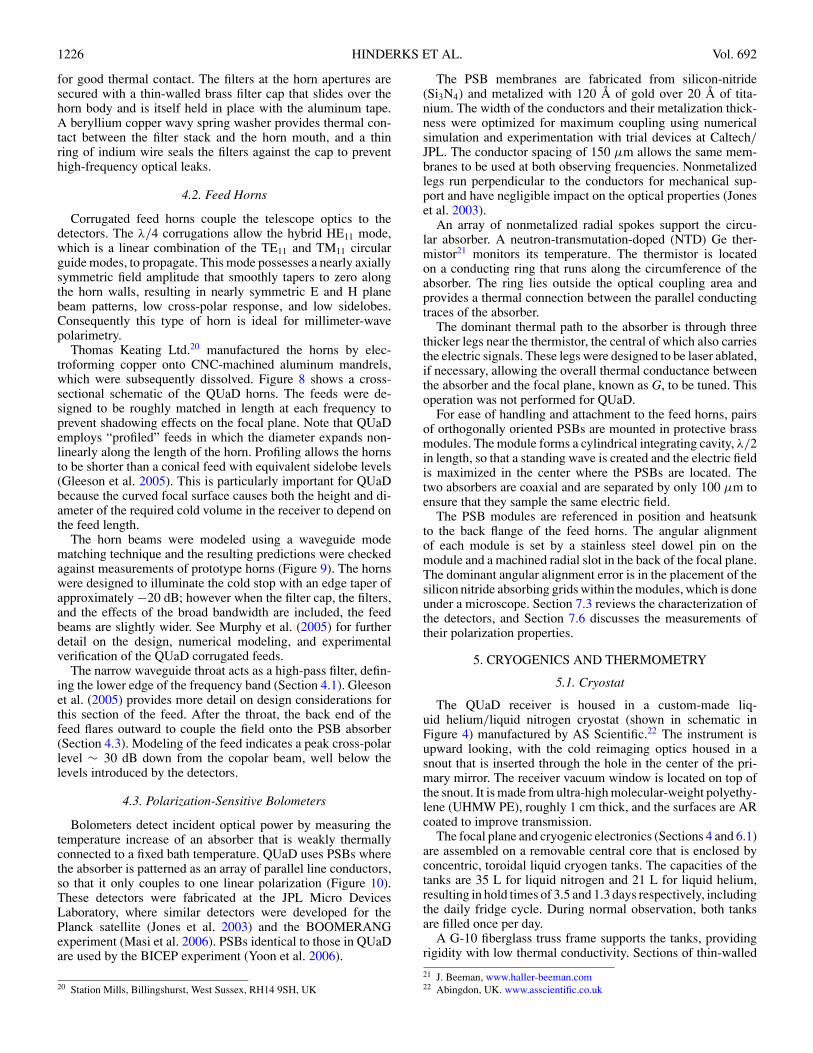
Figure 8. Schematic of the QUaD corrugated feeds, band-defining filters, andfilter caps. The length of the 100 GHz (150 GHz) feed is 100 mm (102 mm),not including the filters and filter cap.
(A color version of this figure is available in the online journal.)
the required rejection of out-of-band power. The filters are ARcoated to improve in-band transmission.
The particular filter combinations at each frequency(Figure 8) were chosen after extensive testing of different filtersin a single-pixel optical test bed. An FTS was used to measurethe band shape and thick grill filters were used to check forout-of-band leaks.19 FTS measurements of all feeds were madeprior to shipping the receiver to the Pole and again before thereceiver was installed on the telescope. By adding or removingfilters from the chain during laboratory testing we were able toverify that the filters contribute negligible cross-polar leakage(Section 7.6).
Blocking filters that reflect high-frequency out-of-band ra-diation are located on each thermal stage within the cryostat,reducing the radiative load on the colder stages. They are heldin place with aluminum clamping rings that are screwed down
19 Thick-grill filters are metal plates with drilled holes that act as high-passfilters via their waveguide cutoff. Filters with holes sized to cut on just abovethe band of interest allows the above-band power to be measured.
1226 HINDERKS ET AL. Vol. 692
for good thermal contact. The filters at the horn apertures aresecured with a thin-walled brass filter cap that slides over thehorn body and is itself held in place with the aluminum tape.A beryllium copper wavy spring washer provides thermal con-tact between the filter stack and the horn mouth, and a thinring of indium wire seals the filters against the cap to preventhigh-frequency optical leaks.
4.2. Feed Horns
Corrugated feed horns couple the telescope optics to thedetectors. The λ/4 corrugations allow the hybrid HE11 mode,which is a linear combination of the TE11 and TM11 circularguide modes, to propagate. This mode possesses a nearly axiallysymmetric field amplitude that smoothly tapers to zero alongthe horn walls, resulting in nearly symmetric E and H planebeam patterns, low cross-polar response, and low sidelobes.Consequently this type of horn is ideal for millimeter-wavepolarimetry.
Thomas Keating Ltd.20 manufactured the horns by elec-troforming copper onto CNC-machined aluminum mandrels,which were subsequently dissolved. Figure 8 shows a cross-sectional schematic of the QUaD horns. The feeds were de-signed to be roughly matched in length at each frequency toprevent shadowing effects on the focal plane. Note that QUaDemploys “profiled” feeds in which the diameter expands non-linearly along the length of the horn. Profiling allows the hornsto be shorter than a conical feed with equivalent sidelobe levels(Gleeson et al. 2005). This is particularly important for QUaDbecause the curved focal surface causes both the height and di-ameter of the required cold volume in the receiver to depend onthe feed length.
The horn beams were modeled using a waveguide modematching technique and the resulting predictions were checkedagainst measurements of prototype horns (Figure 9). The hornswere designed to illuminate the cold stop with an edge taper ofapproximately −20 dB; however when the filter cap, the filters,and the effects of the broad bandwidth are included, the feedbeams are slightly wider. See Murphy et al. (2005) for furtherdetail on the design, numerical modeling, and experimentalverification of the QUaD corrugated feeds.
The narrow waveguide throat acts as a high-pass filter, defin-ing the lower edge of the frequency band (Section 4.1). Gleesonet al. (2005) provides more detail on design considerations forthis section of the feed. After the throat, the back end of thefeed flares outward to couple the field onto the PSB absorber(Section 4.3). Modeling of the feed indicates a peak cross-polarlevel ∼ 30 dB down from the copolar beam, well below thelevels introduced by the detectors.
4.3. Polarization-Sensitive Bolometers
Bolometers detect incident optical power by measuring thetemperature increase of an absorber that is weakly thermallyconnected to a fixed bath temperature. QUaD uses PSBs wherethe absorber is patterned as an array of parallel line conductors,so that it only couples to one linear polarization (Figure 10).These detectors were fabricated at the JPL Micro DevicesLaboratory, where similar detectors were developed for thePlanck satellite (Jones et al. 2003) and the BOOMERANGexperiment (Masi et al. 2006). PSBs identical to those in QUaDare used by the BICEP experiment (Yoon et al. 2006).
20 Station Mills, Billingshurst, West Sussex, RH14 9SH, UK
The PSB membranes are fabricated from silicon-nitride(Si3N4) and metalized with 120 Å of gold over 20 Å of tita-nium. The width of the conductors and their metalization thick-ness were optimized for maximum coupling using numericalsimulation and experimentation with trial devices at Caltech/JPL. The conductor spacing of 150 μm allows the same mem-branes to be used at both observing frequencies. Nonmetalizedlegs run perpendicular to the conductors for mechanical sup-port and have negligible impact on the optical properties (Joneset al. 2003).
An array of nonmetalized radial spokes support the circu-lar absorber. A neutron-transmutation-doped (NTD) Ge ther-mistor21 monitors its temperature. The thermistor is locatedon a conducting ring that runs along the circumference of theabsorber. The ring lies outside the optical coupling area andprovides a thermal connection between the parallel conductingtraces of the absorber.
The dominant thermal path to the absorber is through threethicker legs near the thermistor, the central of which also carriesthe electric signals. These legs were designed to be laser ablated,if necessary, allowing the overall thermal conductance betweenthe absorber and the focal plane, known as G, to be tuned. Thisoperation was not performed for QUaD.
For ease of handling and attachment to the feed horns, pairsof orthogonally oriented PSBs are mounted in protective brassmodules. The module forms a cylindrical integrating cavity, λ/2in length, so that a standing wave is created and the electric fieldis maximized in the center where the PSBs are located. Thetwo absorbers are coaxial and are separated by only 100 μm toensure that they sample the same electric field.
The PSB modules are referenced in position and heatsunkto the back flange of the feed horns. The angular alignmentof each module is set by a stainless steel dowel pin on themodule and a machined radial slot in the back of the focal plane.The dominant angular alignment error is in the placement of thesilicon nitride absorbing grids within the modules, which is doneunder a microscope. Section 7.3 reviews the characterization ofthe detectors, and Section 7.6 discusses the measurements oftheir polarization properties.
5. CRYOGENICS AND THERMOMETRY
5.1. Cryostat
The QUaD receiver is housed in a custom-made liq-uid helium/liquid nitrogen cryostat (shown in schematic inFigure 4) manufactured by AS Scientific.22 The instrument isupward looking, with the cold reimaging optics housed in asnout that is inserted through the hole in the center of the pri-mary mirror. The receiver vacuum window is located on top ofthe snout. It is made from ultra-high molecular-weight polyethy-lene (UHMW PE), roughly 1 cm thick, and the surfaces are ARcoated to improve transmission.
The focal plane and cryogenic electronics (Sections 4 and 6.1)are assembled on a removable central core that is enclosed byconcentric, toroidal liquid cryogen tanks. The capacities of thetanks are 35 L for liquid nitrogen and 21 L for liquid helium,resulting in hold times of 3.5 and 1.3 days respectively, includingthe daily fridge cycle. During normal observation, both tanksare filled once per day.
A G-10 fiberglass truss frame supports the tanks, providingrigidity with low thermal conductivity. Sections of thin-walled
21 J. Beeman, www.haller-beeman.com22 Abingdon, UK. www.asscientific.co.uk

No. 2, 2009 QUaD: A HIGH-RESOLUTION CMB POLARIMETER 1227
Figure 9. Measured and predicted beam pattern from a QUaD 100 GHz corrugated feed horn.
(A color version of this figure is available in the online journal.)
Figure 10. Scanning electron micrograph of a single PSB membrane. The 4.5 mm diameter absorber is suspended with an array of radial supports. Metalized traces(running from the upper left to the lower right) selectively absorb one linear polarization of incident optical radiation. Perpendicular, nonmetalized traces providemechanical support. The 150 μm spacing of the conductors allows the same membranes to be used for the 100 and 150 GHz bands. A thermistor, located on the edgeof the absorber (upper left), measures the temperature. Three thicker legs (upper left) set the thermal conductance to the housing (known as G). The center leg alsocaries the electrical leads from the thermistor to a pair of wirebond pads. The outer two legs could be trimmed, allowing G to be tuned to one of the four possiblevalues.
stainless steel bellows limit the conductivity through the filltubes and allow for differential contraction of the differentthermal stages. The cryostat has four fill tubes (fill and vent pertank), two of which house gauges to monitor cryogen levels.Because the fill tubes are inaccessible when the cryostat isinstalled on the telescope, refills are performed via flexibletransfer lines, about 3.5 m long, made out of two sectionsconnected through standard bayonet fittings. The shorter sectionis inserted in the cryostat fill tube and remains in place
throughout the observing season. The longer section is onlyconnected during refills.
Within the cryostat, both liquid cryogen tanks, as well asthe aluminum radiation shields thermally connected to them,are wrapped in multilayer aluminized mylar insulation. Filteredapertures on the top of each shield allow the optical signal toreach the focal plane, while blocking out-of-band IR radiation(see Figure 3). The focal plane is surrounded by an additionalradiation shield that is thermally connected to the intermediate

1228 HINDERKS ET AL. Vol. 692
stage of the sub-Kelvin refrigerator, maintaining a temperatureof 430 mK. The large focal plane mass (∼ 10 kg) combinedwith the thermally isolating support structure results in a longcool down period. Starting from room temperature, both tanksare initially filled with liquid nitrogen. Approximately five dayslater, the focal plane reaches 100 K at which point the inner tankis filled with liquid helium. Two more days of precooling arethen required before the fridge can be cycled.
In order to speed up the cool down, two active He-3 gas-gap heat switches are used.23 The first connects the fridge 4 Kbaseplate to the intermediate stage. The second connects thefridge intermediate stage to the ultracold stage. These switchesare turned off once the focal plane temperature approaches 4 K.The heat switch connected to the fridge ultracold stage has anestimated off-conductance < 0.1 μW.
5.2. Fridge
The focal plane is cooled to an operating temperature of∼250 mK using a three-stage He-4/He-3/He-3 sorption refrig-erator, manufactured by Chase Research Cryogenics (Bhatiaet al. 2000). Similar fridges have been used successfully inbolometer-based receivers such as ACBAR and BOLOCAM(Runyan et al. 2003; Glenn et al. 1998). The first and secondfridge stages, known together as the Intercooler (IC), contain,respectively, He-4 and He-3. The third stage contains He-3 andis referred to as the Ultracooler (UC). The fridge is cycled byfirst condensing He-4 and using the enthalpy of that liquid tocool the IC and UC condensation points below the He-3 criticaltemperature. During normal operations at the South Pole, thefridge IC and UC stages achieve temperatures of 430 mK and253 mK. The heat loads on the fridge stages are measured to be∼ 40 μW on the IC and < 0.5 μW on the UC.
To achieve better condensation efficiency during the cycle,the fridge is mounted directly on the LHe tank, in a position thatkeeps the fridge baseplate in contact with liquid helium whenthe telescope is at the typical observing elevation of ∼ 50◦. Topreserve this contact, rotation of the system about the optical axis(“deck” rotation) is limited to ∼ ±60◦ during normal observing.
The large focal plane mass (∼ 10 kg) presented a particularchallenge to achieving an optimized fridge cycle. A maximumpossible hold time and minimum loss of observing due to thecycling time were desired. The procedure that was developed(shown in Figure 11) allowed the QUaD fridge to be cycled inapproximately four hours and results in hold times for the UCand IC stages of 24 and 31 hr, respectively (duty cicle ∼ 83%).Once the optimized cycle was determined, the procedure wasautomated (Section 5.4) so that the operator can perform a fridgecycle by issuing a single command on the control system.
5.3. Receiver Core
The receiver core comprises the focal plane and the associatedmechanical and electrical support hardware (Figure 5). It iscomposed of three stages that are each held at a differenttemperature during operation: a 4 K baseplate, a 430 mKintermediate stage, and the 250 mK focal plane assembly.
The 4 K baseplate is made of gold-plated 6061 aluminum. Itsupports the rest of the focal plane structure and provides themounting point for the two JFET amplifier boxes (Section 6).When installed in the cryostat, the baseplate is mechanically at-tached to the liquid helium tank through a cylindrical aluminum
23 Chase Research Cryogenics, 140 Manchester Rd, Sheffield S10 5DL (UK)
0 1 2 3 4 5 6Time (Hours)
0.1
1.0
10.0
100.0
Tem
pera
ture
(K
)
Cal srcAir
LN2 snoutInter pumpUltra pumpHe-4 pumpLHe snoutBaseplateInter headUltra head
Cal srcAir
LN2 snoutInter pumpUltra pumpHe-4 pumpLHe snoutBaseplateInter headUltra head
Figure 11. Temperatures of QUaD components through a fridge cycle at thestart of an observing day. “Cal src” is the temperature of the calibration sourcelocated above the secondary mirror, inside the foam cone (Section 9). “Air” isthe external air temperature. “LN2 snout” and “LHe snout” are the temperaturesat the top of the liquid nitrogen and liquid helium cryostat snouts. The remainingitems are the temperatures of the fridge pumps, cold heads, and baseplate(Section 5.2).
(A color version of this figure is available in the online journal.)
radiation shield. The dominant thermal path is through two par-allel OFHC copper straps that connect to the helium tank. Thisensures that the baseplate stays near 4 K despite the 26 mWdissipation from the JFETs.
The intermediate stage is a gold-plated aluminum ring that isthermally connected to the fridge IC. It is mechanically attachedto the 4 K baseplate by a six-legged hexapod structure of 6′′ SP-1Vespel tubes (0.′′438 outside diameter and 0.′′031 wall thickness).The focal plane assembly is mounted to the intermediate stagewith six shorter legs made from SP-22 Vespel24 tubing machinedto the same diameter and wall thickness. The focal plane isthermally connected to the fridge UC.
The estimated heat load on the fridge from the Vespel supportsis 0.13 μK on the UC and 24 μK on the IC. SP-22 is used for thefocal plane supports because it has lower thermal conductivitythan SP-1 in the sub-Kelvin temperature range (Runyan 2002).Both the focal plane and the intermediate stage are attached totheir respective fridge cold heads via flexible, copper heat strapsmade from braided OFHC copper electrical shielding. Multiplebraids are twisted together to increase the cross-sectional areaand the straps are annealed for increased conductivity.
Because of the high electrical impedance of the bolometers,microphonic pickup from vibrations of the wiring is a concern(Section 8). For this reason, all of the wiring between theJFET amplifiers and the bolometers must be rigidly supported.The Vespel legs that support the focal plane provide naturalattachment points for the wiring that runs between the stages(Figure 5). All of the nonisothermal wires in the cryostat aremanganin (0.′′003) ribbon cables woven into a robust ribbon
24 http://www2.dupont.com/Vespel/en_US/

No. 2, 2009 QUaD: A HIGH-RESOLUTION CMB POLARIMETER 1229
cable with nylon thread for strain relief.25 The wiring is tightlywrapped around the Vespel legs along a helical path and fixeddown at regular intervals using a combination of teflon tapeand lacing tape. Two additional Vespel tubes between theintermediate stage and the JFET modules act as a bridge tosupport the wiring along this critical signal path. The heatload on the fridge UC stage is reduced by heat sinking thefocal plane wiring to the intermediate temperature stage. Theheat load from the wiring is estimated to be ∼ 8 μW on thefridge IC and < 0.1 μW on the UC. On the isothermal stages,including the back of the focal plane bowl, stiffer (28 AWG)copper wiring is used and is held down by the aluminum tape.Specially designed aluminum brackets support the wiring at allconnector interfaces, including the PSB modules.
5.4. Thermometry and Temperature Control
The temperatures of all the major cryogenic components aremonitored, including the focal plane, the fridge pumps, coldheads, and baseplate, the snout that holds the two lenses, andthe liquid cryogen tanks. Silicon diode sensors26 monitor thetemperatures of components that operate at or above 4 K.Germanium resistance thermometers27 (GRTs) monitor thetemperatures of sub-Kelvin components. The diodes that aremounted on the focal plane allow the monitoring of the cooldown from room temperature; however, their large powerdissipation (∼ 15 μW) requires that they be switched off duringsub-Kelvin operation.
Figure 11 shows temperature readouts during and shortlyafter a routine fridge cycle. In order to monitor the temperaturesof all the different cryogenic components and to operate theheaters of fridge pumps and gas-gap heat switches, requiredto cycle the sorption fridge, we use custom-made thermometerreadout and control electronics. With a very compact design(only one main unit and one separate power supply unit), it canreadout up to six GRTs and 21 diodes, and operate five heaters.An embedded computer, the TINI28(Tiny INternet Interface),reads the digitized voltage outputs, sets the heaters drives, andcommunicates with the control system. With this system it ispossible to cycle the fridge with no external intervention, byrunning a script on the TINI. The same electronics drives twoadditional heaters (with constant drive and manual control) forthe gas-gap heat switches we use to precool fridge and focalplane at liquid helium temperature.
The focal plane temperature is stabilized with a separate sys-tem. Temperature is read out with a custom AC bridge connectedto an NTD Ge thermistor (Haller-Beeman) located on the focalplane. The bridge operates at the bolometer bias frequency. AStanford Research Systems SIM960 PID controller, served offthe thermistor readout, drives three heater resistors in parallel,located symmetrically around the joint between the fridge heatstrap and the focal plane. An additional thermistor, read out withthe same system, is used as a temperature monitor. During rou-tine observing, the PID set point is 258 mK, ∼ 5 mK above thenatural operating temperature of the fridge, requiring ∼ 0.3 μWof electrical heater power. This maintains a stable temperaturedespite the telescope motion associated with raster scanning andthe slight warming of the fridge UC that occurs over the courseof an 18 hr observation.
25 www.tekdata.co.uk26 Lake Shore DT-470 series, Lake Shore Cryotronics, Inc.,www.lakeshore.com27 Lake Shore GR-200 series28 MAXIM, www.maxim-ic.com
Table 2Electronics Parameters
Number of channels 96DC mode gain 200AC mode gain 105
Capacitancea (pF) 85Load resistance (MΩ) 40Bias generator noise (nV Hz−1/2) 3JFET noise (nV Hz−1/2) 7Warm amplifier noise (nV Hz−1/2) 5Total electronics noise (nV Hz−1/2) 91/f knee (mHz) 10AC bias frequencyb (Hz) 110AC bias currentc (nA) 1.25Readout bandwidth (Hz) 20Sampling frequency (Hz) 100Powerd (W) 60
Notes.a The capacitance between the two signal leads of a channel arising from theconnectors and wiring between the PSBs and the JFETs.b The bias frequency is adjustable from 40 to 250 Hz. The frequency is chosento minimize interference (Section 8).c The bias current is adjustable from 0 to 30 nA. The current is a tradeoffbetween stability and sensitivity (Section 7).d Power for the amplifier boxes, not including the commercial ADC system.
6. ELECTRONICS
The QUaD electronics employ an AC-biased, fully differ-ential readout to amplify the bolometer signals. The basicscheme has a long history in bolometric CMB instruments (seeHolzapfel et al. 1997; Glenn et al. 1998; Crill et al. 2003, forinstance). An overview of the electronics chain is shown inFigure 12. The bias generator excites the bolometers with a sinu-soidal current through a pair of equal-valued load resistors. Thebalanced nature of the bolometer/load resistor bridge minimizescrosstalk and pickup along the high-impedance wiring leadingto the cryogenic JFET buffer amplifiers. The warm electron-ics amplify, demodulate, and filter the output from the JFETs.Finally, the data acquisition system digitizes and archives theprocessed signals. The QUaD electronics are interfaced to thecontrol software to allow the bias frequency and amplitude, am-plifier gain, DC offset removal, and phase adjustment to be setremotely. Table 2 gives the parameters of the readout electronicschain. The electronics development and testing are described inmore detail in Hinderks (2005).
6.1. Cold Electronics
The load resistors are Nichrome metal film on a siliconsubstrate in a surface-mount package.29 There are two 20 MΩload resistors in each circuit. This value was chosen to be muchlarger than the bolometer resistance to provide a bias current thatremains approximately constant for small loading changes. Theload resistor boards (Figure 13) are located on the 250 mKstage to reduce Johnson noise. The boards were fabricatedfrom standard 1/16′′ FR-4 substrate. Input and output fromthe board is via surface-mount 51-way micro-D connectors.30
These connectors have leads that were specifically designed totake up differential contraction between the fiberglass boardand the aluminum mounting structure that is used to provide
29 Mini Systems, Inc., www.mini-systems.biz30 Cristek Interconnects Inc., www.cristek.com

1230 HINDERKS ET AL. Vol. 692
ACBiasGen.
JFETBuffers
RL
RL
RBolo
V+
V-
++
--
SquareWaveDemod.
BP Filterx5
LP Filter20HzPreamp
x100 x100
DACPhaseDelay
Figure 12. Block diagram of the QUaD readout electronics. The components within the dashed lines are located in the cryostat. The load resistors and detectors areon the focal plane assembly and operate at approximately 250 mK. The JFET amplifiers modules are mounted on the 4 K baseplate; however, within the modules theJFETs themselves operate at roughly 120 K (Section 6).
Figure 13. Photograph of a QUaD load resistor board. Each board contains 56 resistors (including eight spares) in four surface-mount packages and services up to 24channels. The boards themselves are with double-sided 1 oz copper and 8 mil traces. Input and output from the board is via surface-mount 51-way micro-D connectors(Cristek Interconnects Inc., www.cristek.com). These connectors have long surface-mount leads that take up differential contraction between the fiberglass board andthe aluminum mounting structure that provides mechanical support.
(A color version of this figure is available in the online journal.)
mechanical support. In three years of sub-Kelvin operation andnumerous thermal cycles, we did not experience a single failure.
The JFET amplifiers are located in two boxes mounted onthe 4 K baseplate, directly below the focal plane assembly.The transistors themselves operate at an elevated temperatureof ∼ 120 K for optimum noise performance and consequentlyneed to be thermally isolated from their 4 K enclosure. Eachbox contains two silicon nitride membranes, each holding 24dual JFET dies31 allowing readout of 48 channels per box.The membranes provide thermal isolation of the amplifiersfrom the 4 K stage and are mechanically supported by themicro-D input/output connectors. The JFETs are configuredas source followers with their drains connected to a commonpositive supply and the sources connected via 125 kΩ resistorsto the common negative supply. The power supply voltages foreach membrane is adjusted for lowest noise performance. Eachmembrane dissipates ∼ 6.5 mW during normal operation withheater resistors used to assist at startup. The low thermal massallows the membranes to reach a stable operating temperaturein approximately one minute.
31 Siliconix U401
6.2. Warm Electronics
The bias generator is used to provide a stable sine-waveexcitation that can be adjusted over a frequency range of40–250 Hz with 10 bit resolution. The sine wave is generatedby filtering a square wave with a Q=10 bandpass filter. Alow-noise DC voltage reference and an analog modulatorswitched by a crystal oscillator generate the square wave.The bandpass filter is made electronically tunable by usingmultiplying DACs in place of fixed resistors. The bias frequencyis common to all bolometers but the 100 GHz and 150 GHz biasamplitudes can be independently adjusted. A DC bias mode isprovided for testing and is used for taking bolometer I-V curves(Section 7.3). The bias amplitudes are archived along with thebolometer data. The bias frequency, amplitude and bandpasstuning are computer controlled via a serial interface.
The bolometer signals are amplified with low-noise AD624amplifiers and then filtered with a broad bandpass filter(Q ∼ 0.5) that is designed to have a close to flat response overthe available range of bias frequencies. The signals are thenmultiplied by a square-wave reference from the bias board todemodulate the component at the bias frequency. An adjustabledelay circuit for each channel compensates the demodulator

No. 2, 2009 QUaD: A HIGH-RESOLUTION CMB POLARIMETER 1231
reference signal for phase shifts within the cryostat. A steeplow-pass filter (20 Hz, 6-pole) follows the demodulator.
To ease the dynamic range requirement on the ADC system,a 12-bit DAC is adjusted periodically to null out the large DCcomponent of the demodulated signal. This is followed by anadditional gain stage of 100. During observation, the DC-offsetremoval DAC settings are adjusted approximately every 30minutes to prevent any channels saturating due to 1/f -noiseor elevation changes.
The electronics can be switched to a “low-gain” mode inwhich the DC-offset removal and additional gain stage arebypassed. This mode is useful for testing, and is used routinelyby the control system to automatically determine the appropriatesetting for each channel’s DC-offset removal DAC. Finally,buffer circuitry creates a balanced differential output for drivingthe cabling to the ADC. All of the settings including referencephase delay, DC offset removal, and gain mode are controlledvia a serial interface.
The bias and readout electronics are located in radio fre-quency (RF) boxes attached via an RF-tight interface box di-rectly to the bottom surface of the cryostat. All wiring enteringthe cryostat passes through these interface boxes and is RF fil-tered using filtered D-sub connectors.32
6.3. Data Acquisition and Control System
Real-time operations including telescope control, and digiti-zation of the bolometer data, are handled by a VME controllerrunning VXWorks in a crate mounted adjacent to the cryostat.Two 64-channel, 16-bit ADC cards digitize the bolometer data.A 32-channel DIO card provides the control interface to the biasand readout boards. A Linux-based PC system provides the userinterface and data archiving for the real-time controller.
Once per second, the software archives a complete snap-shot of the system, known as a register frame. Each registerframe contains the most recent values from all of the attachedhardware, including thermometry, bias settings, and DC offsetremoval values. The bolometer data along with the telescopeaxis encoders are sampled at 100 Hz, with 100 samples perchannel stored in each register frame. Software commands areprovided for controlling all the components of the system. Thesecommands are combined to form complete observing scripts. Aclient program allows users to run scripts and monitor the datain real time.
7. INSTRUMENT CHARACTERIZATION
7.1. Telescope Pointing
QUaD used a nine-parameter pointing model with thetelescope control computer handling full conversion from rightascension/declination/paralactic angle request values to az-imuth/elevation/deck encoder command values. The model pa-rameters were established from a combination of optical datafrom a small telescope attached to the elevation structure ofthe mount and from several special day-long radio pointingruns. These radio pointing runs consisted of scanning the centralpixel across five bright, compact millimeter sources (MAT6A,NGC3576, IRAS1022, RCW38, and IRAS08576) in both az-imuth and elevation, in a pattern known as a “pointing cross.”This determines the pointing offset between the optical and ra-dio systems, the flexure with elevation of the radio pointing, and
32 Spectrum Control Series 700 with 1000 pF PI filters.
-0.5
0.0
0.5
De
c O
ffse
t (d
eg
.)
0.5 0.0 -0.5RA Offset (deg. on sky)
-0.5
0.0
0.5D
ec O
ffse
t (d
eg
.)
Figure 14. Top: raster map over the galactic source RCW38. The map has beensmoothed with a 1.′2 Gaussian. Bottom: radio pointing locations for each channelderived from 12 full raster maps spread over the second and third seasons. Theblack crosses indicate the mean offset for each channel.
(A color version of this figure is available in the online journal.)
the magnitude and angle of the offset between the radio point-ing direction and the rotation axis of the mount’s third axis. Theazimuth axis tilts and encoder zero points were measured a fewtimes per season from the optical data. Later radio pointing runsestablished the accuracy of the absolute pointing at ∼ 0.′5.
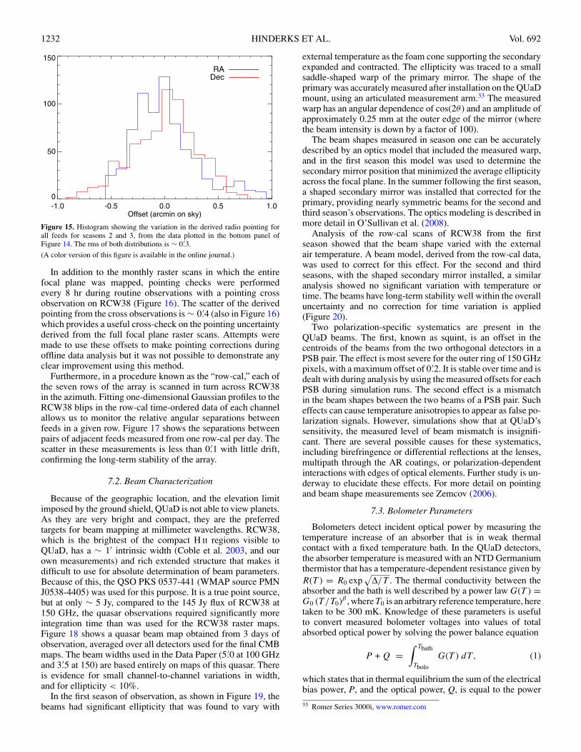
Approximately one day per month was devoted to mak-ing full raster maps using a bright source, usually RCW38(Figure 14, top). Gaussian profiles were fitted to the raster dataand were then used to determine the pointing offset of each feed.The feed offsets obtained from 12 full beam maps are shownin Figure 14 (bottom). The offset angles used in the data anal-ysis were determined by averaging over the 12 mapping runs,to reduce the effects of the random pointing wander that occursduring each 16 hr run. The rms scatter in the feed offset anglesversus the mean is ∼ 0.′3 (Figure 15). There is no evidence fora systematic change in the feed offset angles over time.
1232 HINDERKS ET AL. Vol. 692
-1.0 -0.5 0.0 0.5 1.0Offset (arcmin on sky)
0
50
100
150
RADec
Figure 15. Histogram showing the variation in the derived radio pointing forall feeds for seasons 2 and 3, from the data plotted in the bottom panel ofFigure 14. The rms of both distributions is ∼ 0.′3.
(A color version of this figure is available in the online journal.)
In addition to the monthly raster scans in which the entirefocal plane was mapped, pointing checks were performedevery 8 hr during routine observations with a pointing crossobservation on RCW38 (Figure 16). The scatter of the derivedpointing from the cross observations is ∼ 0.′4 (also in Figure 16)which provides a useful cross-check on the pointing uncertaintyderived from the full focal plane raster scans. Attempts weremade to use these offsets to make pointing corrections duringoffline data analysis but it was not possible to demonstrate anyclear improvement using this method.
Furthermore, in a procedure known as the “row-cal,” each ofthe seven rows of the array is scanned in turn across RCW38in the azimuth. Fitting one-dimensional Gaussian profiles to theRCW38 blips in the row-cal time-ordered data of each channelallows us to monitor the relative angular separations betweenfeeds in a given row. Figure 17 shows the separations betweenpairs of adjacent feeds measured from one row-cal per day. Thescatter in these measurements is less than 0.′1 with little drift,confirming the long-term stability of the array.
7.2. Beam Characterization
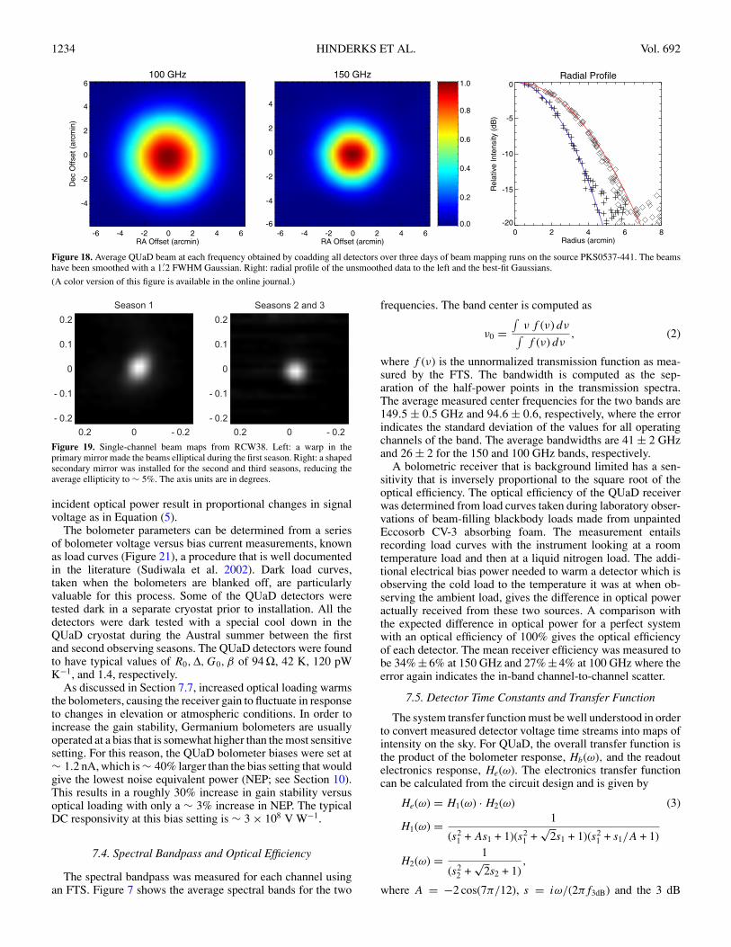
Because of the geographic location, and the elevation limitimposed by the ground shield, QUaD is not able to view planets.As they are very bright and compact, they are the preferredtargets for beam mapping at millimeter wavelengths. RCW38,which is the brightest of the compact H ii regions visible toQUaD, has a ∼ 1′ intrinsic width (Coble et al. 2003, and ourown measurements) and rich extended structure that makes itdifficult to use for absolute determination of beam parameters.Because of this, the QSO PKS 0537-441 (WMAP source PMNJ0538-4405) was used for this purpose. It is a true point source,but at only ∼ 5 Jy, compared to the 145 Jy flux of RCW38 at150 GHz, the quasar observations required significantly moreintegration time than was used for the RCW38 raster maps.Figure 18 shows a quasar beam map obtained from 3 days ofobservation, averaged over all detectors used for the final CMBmaps. The beam widths used in the Data Paper (5.′0 at 100 GHzand 3.′5 at 150) are based entirely on maps of this quasar. Thereis evidence for small channel-to-channel variations in width,and for ellipticity < 10%.
In the first season of observation, as shown in Figure 19, thebeams had significant ellipticity that was found to vary with
external temperature as the foam cone supporting the secondaryexpanded and contracted. The ellipticity was traced to a smallsaddle-shaped warp of the primary mirror. The shape of theprimary was accurately measured after installation on the QUaDmount, using an articulated measurement arm.33 The measuredwarp has an angular dependence of cos(2θ ) and an amplitude ofapproximately 0.25 mm at the outer edge of the mirror (wherethe beam intensity is down by a factor of 100).
The beam shapes measured in season one can be accuratelydescribed by an optics model that included the measured warp,and in the first season this model was used to determine thesecondary mirror position that minimized the average ellipticityacross the focal plane. In the summer following the first season,a shaped secondary mirror was installed that corrected for theprimary, providing nearly symmetric beams for the second andthird season’s observations. The optics modeling is described inmore detail in O’Sullivan et al. (2008).
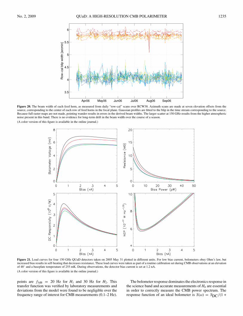
Analysis of the row-cal scans of RCW38 from the firstseason showed that the beam shape varied with the externalair temperature. A beam model, derived from the row-cal data,was used to correct for this effect. For the second and thirdseasons, with the shaped secondary mirror installed, a similaranalysis showed no significant variation with temperature ortime. The beams have long-term stability well within the overalluncertainty and no correction for time variation is applied(Figure 20).
Two polarization-specific systematics are present in theQUaD beams. The first, known as squint, is an offset in thecentroids of the beams from the two orthogonal detectors in aPSB pair. The effect is most severe for the outer ring of 150 GHzpixels, with a maximum offset of 0.′2. It is stable over time and isdealt with during analysis by using the measured offsets for eachPSB during simulation runs. The second effect is a mismatchin the beam shapes between the two beams of a PSB pair. Sucheffects can cause temperature anisotropies to appear as false po-larization signals. However, simulations show that at QUaD’ssensitivity, the measured level of beam mismatch is insignifi-cant. There are several possible causes for these systematics,including birefringence or differential reflections at the lenses,multipath through the AR coatings, or polarization-dependentinteractions with edges of optical elements. Further study is un-derway to elucidate these effects. For more detail on pointingand beam shape measurements see Zemcov (2006).
7.3. Bolometer Parameters
Bolometers detect incident optical power by measuring thetemperature increase of an absorber that is in weak thermalcontact with a fixed temperature bath. In the QUaD detectors,the absorber temperature is measured with an NTD Germaniumthermistor that has a temperature-dependent resistance given byR(T ) = R0 exp
√Δ/T . The thermal conductivity between the
absorber and the bath is well described by a power law G(T ) =G0 (T/T0)β , where T0 is an arbitrary reference temperature, heretaken to be 300 mK. Knowledge of these parameters is usefulto convert measured bolometer voltages into values of totalabsorbed optical power by solving the power balance equation
P + Q =∫ Tbath
Tbolo
G(T ) dT , (1)
which states that in thermal equilibrium the sum of the electricalbias power, P, and the optical power, Q, is equal to the power
33 Romer Series 3000i, www.romer.com

No. 2, 2009 QUaD: A HIGH-RESOLUTION CMB POLARIMETER 1233
-0.50.0
0.5
R.A
. (d
eg
)0 10 20 30 40 50
-500
50100150200
Sig
na
l (m
K)
-0.80.0
0.8
De
cl.
(de
g)
90 100 110 120 130 140seconds
-200-100
0
100
200
Sig
na
l (m
K)
R.A.
-2 -1 0 1 2arcmin
0
20
40
60
80
100
120Decl.
-2 -1 0 1 2arcmin
0
20
40
60
80
100
Figure 16. Two upper panels show a “pointing cross” observation in which the central pixel is scanned across a bright source, first in right ascension (R.A.), then indeclination (decl.). The lower panels show the variation of the derived pointing offset over the course of a season. The rms of both distributions is ∼ 0.′4.
(A color version of this figure is available in the online journal.)
Apr06 May06 Jun06 Jul06 Aug06 Sep06
0
0.1
0.2
Resi
dual H
orn
Spaci
ng [arc
min
]
Figure 17. Residual separation between pairs of adjacent feeds as measured by daily azimuth “row-cal” scans of all channels across RCW38. The nominal feedseparation is 18′. These daily scans are also performed with the telescope rotated by 60◦ about the optical axis with similar results.
(A color version of this figure is available in the online journal.)
flowing from the absorber (at Tbolo) to the bath across the weakthermal link, G. It should be emphasized that this analysis is not
needed to interpret the astronomical data, because during normalobservation the bolometers are biased so that small changes in
1234 HINDERKS ET AL. Vol. 692
100 GHz
-6 -4 -2 0 2 4 6RA Offset (arcmin)
-4
-2
0
2
4
6
De
c O
ffse
t (a
rcm
in)
150 GHz
-6 -4 -2 0 2 4 6RA Offset (arcmin)
-6
-4
-2
0
2
4
0.0
0.2
0.4
0.6
0.8
1.0Radial Profile
0 2 4 6 8Radius (arcmin)
-20
-15
-10
-5
0
Re
lative
In
ten
sity (
dB
)
Figure 18. Average QUaD beam at each frequency obtained by coadding all detectors over three days of beam mapping runs on the source PKS0537-441. The beamshave been smoothed with a 1.′2 FWHM Gaussian. Right: radial profile of the unsmoothed data to the left and the best-fit Gaussians.
(A color version of this figure is available in the online journal.)
Figure 19. Single-channel beam maps from RCW38. Left: a warp in theprimary mirror made the beams elliptical during the first season. Right: a shapedsecondary mirror was installed for the second and third seasons, reducing theaverage ellipticity to ∼ 5%. The axis units are in degrees.
incident optical power result in proportional changes in signalvoltage as in Equation (5).
The bolometer parameters can be determined from a seriesof bolometer voltage versus bias current measurements, knownas load curves (Figure 21), a procedure that is well documentedin the literature (Sudiwala et al. 2002). Dark load curves,taken when the bolometers are blanked off, are particularlyvaluable for this process. Some of the QUaD detectors weretested dark in a separate cryostat prior to installation. All thedetectors were dark tested with a special cool down in theQUaD cryostat during the Austral summer between the firstand second observing seasons. The QUaD detectors were foundto have typical values of R0, Δ,G0, β of 94 Ω, 42 K, 120 pWK−1, and 1.4, respectively.
As discussed in Section 7.7, increased optical loading warmsthe bolometers, causing the receiver gain to fluctuate in responseto changes in elevation or atmospheric conditions. In order toincrease the gain stability, Germanium bolometers are usuallyoperated at a bias that is somewhat higher than the most sensitivesetting. For this reason, the QUaD bolometer biases were set at∼ 1.2 nA, which is ∼ 40% larger than the bias setting that wouldgive the lowest noise equivalent power (NEP; see Section 10).This results in a roughly 30% increase in gain stability versusoptical loading with only a ∼ 3% increase in NEP. The typicalDC responsivity at this bias setting is ∼ 3 × 10⁸ V W−1.
7.4. Spectral Bandpass and Optical Efficiency
The spectral bandpass was measured for each channel usingan FTS. Figure 7 shows the average spectral bands for the two
frequencies. The band center is computed as
ν0 =∫
ν f (ν) dν∫f (ν) dν
, (2)
where f (ν) is the unnormalized transmission function as mea-sured by the FTS. The bandwidth is computed as the sep-aration of the half-power points in the transmission spectra.The average measured center frequencies for the two bands are149.5 ± 0.5 GHz and 94.6 ± 0.6, respectively, where the errorindicates the standard deviation of the values for all operatingchannels of the band. The average bandwidths are 41 ± 2 GHzand 26 ± 2 for the 150 and 100 GHz bands, respectively.
A bolometric receiver that is background limited has a sen-sitivity that is inversely proportional to the square root of theoptical efficiency. The optical efficiency of the QUaD receiverwas determined from load curves taken during laboratory obser-vations of beam-filling blackbody loads made from unpaintedEccosorb CV-3 absorbing foam. The measurement entailsrecording load curves with the instrument looking at a roomtemperature load and then at a liquid nitrogen load. The addi-tional electrical bias power needed to warm a detector which isobserving the cold load to the temperature it was at when ob-serving the ambient load, gives the difference in optical poweractually received from these two sources. A comparison withthe expected difference in optical power for a perfect systemwith an optical efficiency of 100% gives the optical efficiencyof each detector. The mean receiver efficiency was measured tobe 34% ± 6% at 150 GHz and 27% ± 4% at 100 GHz where theerror again indicates the in-band channel-to-channel scatter.
7.5. Detector Time Constants and Transfer Function
The system transfer function must be well understood in orderto convert measured detector voltage time streams into maps ofintensity on the sky. For QUaD, the overall transfer function isthe product of the bolometer response, Hb(ω), and the readoutelectronics response, He(ω). The electronics transfer functioncan be calculated from the circuit design and is given by
He(ω) = H1(ω) · H2(ω) (3)
H1(ω) = 1
(s21 + As1 + 1)(s2
1 +√
2s1 + 1)(s21 + s1/A + 1)
H2(ω) = 1
(s22 +
√2s2 + 1)
,
where A = −2 cos(7π/12), s = iω/(2πf3dB) and the 3 dB
No. 2, 2009 QUaD: A HIGH-RESOLUTION CMB POLARIMETER 1235
Apr06 May06 Jun06 Jul06 Aug06 Sep06
3.5
4
4.5
5
5.5
6
Figure 20. The beam width of each feed horn, as measured from daily “row-cal” scans over RCW38. Azimuth scans are made at seven elevation offsets from thesource, corresponding to the center of each row of feed horns in the focal plane. Gaussian profiles are fitted to the blip in the time stream corresponding to the source.Because full raster maps are not made, pointing wander results in errors in the derived beam widths. The larger scatter at 150 GHz results from the higher atmosphericnoise present in this band. There is no evidence for long-term drift in the beam width over the course of a season.
(A color version of this figure is available in the online journal.)
Figure 21. Load curves for four 150 GHz QUaD detectors taken on 2005 May 31 plotted in different units. For low bias current, bolometers obey Ohm’s law, butincreased bias results in self-heating that decreases resistance. These load curves were taken as part of a routine calibration set during CMB observations at an elevationof 48◦ and a baseplate temperature of 255 mK. During observations, the detector bias current is set at 1.2 nA.
(A color version of this figure is available in the online journal.)
points are f3dB = 20 Hz for H1 and 30 Hz for H2. Thistransfer function was verified by laboratory measurements anddeviations from the model were found to be negligible over thefrequency range of interest for CMB measurements (0.1–2 Hz).
The bolometer response dominates the electronics response inthe science band and accurate measurements of Hb are essentialin order to correctly measure the CMB power spectrum. Theresponse function of an ideal bolometer is S(ω) = SDC/(1 +

1236 HINDERKS ET AL. Vol. 692
Detector 1
0.01 0.1 1 10Time (sec)
0.0
0.2
0.4
0.6
0.8
1.0
1.2
No
rma
lize
d s
ign
al
Detector 2
0.01 0.1 1 10Time (sec)
0.0
0.2
0.4
0.6
0.8
1.0
1.2
No
rma
lize
d s
ign
al
Electronics (calculated)
0.01 0.1 1 10Time (sec)
0.0
0.2
0.4
0.6
0.8
1.0
1.2
No
rma
lize
d s
ign
al
0.00 0.02 0.04 0.06 0.08 0.10Primary Time Constant (sec)
0
5
10
15
20
25
0.01 0.1 1 10Freq (Hz)
0.0
0.2
0.4
0.6
0.8
1.0
Tra
nsfe
r fu
nctio
n m
ag
nitu
de
0.01 0.1 1 10Freq (Hz)
0.0
0.2
0.4
0.6
0.8
1.0
Tra
nsfe
r fu
nctio
n m
ag
nitu
de
0.01 0.1 1 10Freq (Hz)
0.0
0.2
0.4
0.6
0.8
1.0
Tra
nsfe
r fu
nctio
n m
ag
nitu
de
0 1 2 3 4 5Secondary Time Constant (sec)
0
10
20
30
40
Figure 22. A Gunn diode source was used to supply a square wave signal with fast edge transitions to the focal plane in order to measure the detector time constants.Left: the Gunn diode reference signal (black dashed) and the measured step response of two detectors (blue and green). The initial ∼ 150 ms is dominated by theelectronics transfer function which introduces the overshoot and ringing (red). The transfer function for the two detectors, derived from Fourier transforming thetime-domain data, is shown below the time ordered data. Fits to a single time constant model (dotted) and a dual time constant model (solid) are shown. The tworight-hand panels show the distribution of both the fast (upper right) and slow (lower right) time constants for all of the QUaD detectors.
(A color version of this figure is available in the online journal.)
iωτ ) where S is the detector responsivity (Volts/Watt), andthe time constant τ = C/G where C is the heat capacity ofthe absorber and G is the thermal conductivity between thesensor and the bath. Values for τ of order 30 ms are typical ofQUaD detectors although there is substantial device-to-devicevariation. Both C and G are temperature dependent, so it isessential to measure time constants with similar optical loadingand electrical bias power as during observation.
Two methods were used to determine the time constantsfor the QUaD detectors. The first method involved scanningthe telescope back and forth in the azimuth over RCW38 andrecording the shift in the apparent position of the source forthe forward and backward scan directions. The second methodinvolved a special test run during the Austral summer. Thetelescope was illuminated with a Gunn diode RF source thatwas chopped with a slow (100 s) square wave. This measuresthe system step response from which the transfer function canbe derived (Figure 22). Care was taken to ensure that theGunn setup did not substantially increase the optical loadingon the detectors. The results of the two methods are in excellentagreement with each other; however, the Gunn measurementsoffered a much larger signal-to-noise ratio, and these are thevalues used in the Data Paper.
It was found that for about half the detectors the single timeconstant model is a poor fit to the true response. The addition ofa second time constant term, so that the overall detector transferfunction is modeled as
Hb(ω) = 1 − α
1 + iωτ1+
α
1 + iωτ2(4)
where α � 0.5, was found to accurately model the detectorresponse in all but two cases—these detectors were not used. Insome cases, the second time constant is found to be extremelylong (τ2 > 1 s), but is still very well fitted by the double timeconstant model. These detectors are used in the science analysis.The physical origin of the second time constant is believed tobe debris on the PSB which is in weak thermal contact withthe absorbing grid. Figure 22 shows the transfer functions fortwo detectors, and the distribution of time constants for all thedetectors used in the season 2/3 analysis.
7.6. Polarization Angles and Cross-Polar Leakage
The voltage response of a single PSB to arbitrarily polarizedincident radiation is given by
v = s
[I +
1 − ε
1 + ε(Q cos 2θ + U sin 2θ )
], (5)
where θ gives the orientation angle of the PSB, ε givesthe cross-polar leakage, and s is a calibration constant thatdepends on detector responsivity, optical throughput (AΩ),optical efficiency, bandwidth, and readout electronics gain(Jones et al. 2003). From Equation (5), leakage can be seento result in a loss of optical efficiency to polarized radiation.This has the effect of reducing sensitivity (Section 10) but notof mixing Stokes parameters. The measurement of ε and θ isdescribed in this section. The determination of the calibrationconstant, s, is described in Section 9.
Because there are no bright, well calibrated polarized astro-nomical sources visible at these wavelengths, we characterized
No. 2, 2009 QUaD: A HIGH-RESOLUTION CMB POLARIMETER 1237
90 Degree Rotation
-20 -15 -10Azimuth (deg)
32
34
36
38
40
42
44
Ele
vation (
deg)
0 Degree Rotation
-20 -15 -10Azimuth (deg)
dB
-30
-25
-20
-15
-10
-5
0
-100 -50 0 50 100Rotation (deg)
0.0
0.2
0.4
0.6
0.8
1.0
Rela
tive
Inte
nsity
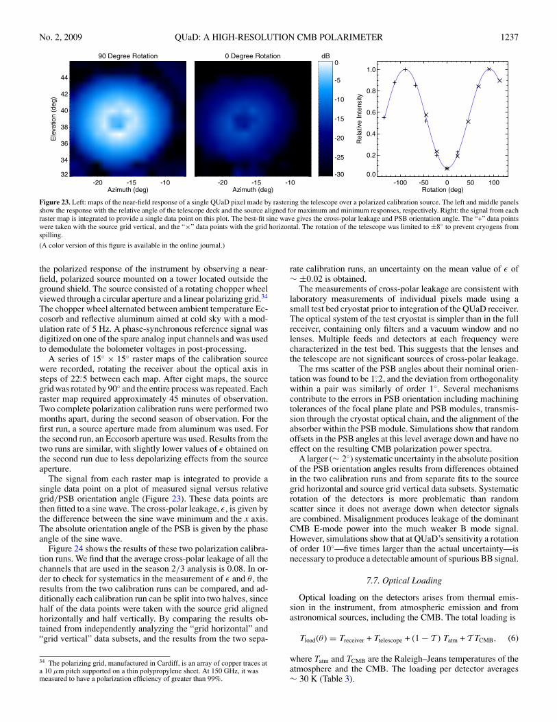
Figure 23. Left: maps of the near-field response of a single QUaD pixel made by rastering the telescope over a polarized calibration source. The left and middle panelsshow the response with the relative angle of the telescope deck and the source aligned for maximum and minimum responses, respectively. Right: the signal from eachraster map is integrated to provide a single data point on this plot. The best-fit sine wave gives the cross-polar leakage and PSB orientation angle. The “+” data pointswere taken with the source grid vertical, and the “×” data points with the grid horizontal. The rotation of the telescope was limited to ±8◦ to prevent cryogens fromspilling.
(A color version of this figure is available in the online journal.)
the polarized response of the instrument by observing a near-field, polarized source mounted on a tower located outside theground shield. The source consisted of a rotating chopper wheelviewed through a circular aperture and a linear polarizing grid.34
The chopper wheel alternated between ambient temperature Ec-cosorb and reflective aluminum aimed at cold sky with a mod-ulation rate of 5 Hz. A phase-synchronous reference signal wasdigitized on one of the spare analog input channels and was usedto demodulate the bolometer voltages in post-processing.
A series of 15◦ × 15◦ raster maps of the calibration sourcewere recorded, rotating the receiver about the optical axis insteps of 22.◦5 between each map. After eight maps, the sourcegrid was rotated by 90◦ and the entire process was repeated. Eachraster map required approximately 45 minutes of observation.Two complete polarization calibration runs were performed twomonths apart, during the second season of observation. For thefirst run, a source aperture made from aluminum was used. Forthe second run, an Eccosorb aperture was used. Results from thetwo runs are similar, with slightly lower values of ε obtained onthe second run due to less depolarizing effects from the sourceaperture.
The signal from each raster map is integrated to provide asingle data point on a plot of measured signal versus relativegrid/PSB orientation angle (Figure 23). These data points arethen fitted to a sine wave. The cross-polar leakage, ε, is given bythe difference between the sine wave minimum and the x axis.The absolute orientation angle of the PSB is given by the phaseangle of the sine wave.
Figure 24 shows the results of these two polarization calibra-tion runs. We find that the average cross-polar leakage of all thechannels that are used in the season 2/3 analysis is 0.08. In or-der to check for systematics in the measurement of ε and θ , theresults from the two calibration runs can be compared, and ad-ditionally each calibration run can be split into two halves, sincehalf of the data points were taken with the source grid alignedhorizontally and half vertically. By comparing the results ob-tained from independently analyzing the “grid horizontal” and“grid vertical” data subsets, and the results from the two sepa-
34 The polarizing grid, manufactured in Cardiff, is an array of copper traces ata 10 μm pitch supported on a thin polypropylene sheet. At 150 GHz, it wasmeasured to have a polarization efficiency of greater than 99%.
rate calibration runs, an uncertainty on the mean value of ε of∼ ±0.02 is obtained.
The measurements of cross-polar leakage are consistent withlaboratory measurements of individual pixels made using asmall test bed cryostat prior to integration of the QUaD receiver.The optical system of the test cryostat is simpler than in the fullreceiver, containing only filters and a vacuum window and nolenses. Multiple feeds and detectors at each frequency werecharacterized in the test bed. This suggests that the lenses andthe telescope are not significant sources of cross-polar leakage.
The rms scatter of the PSB angles about their nominal orien-tation was found to be 1.◦2, and the deviation from orthogonalitywithin a pair was similarly of order 1◦. Several mechanismscontribute to the errors in PSB orientation including machiningtolerances of the focal plane plate and PSB modules, transmis-sion through the cryostat optical chain, and the alignment of theabsorber within the PSB module. Simulations show that randomoffsets in the PSB angles at this level average down and have noeffect on the resulting CMB polarization power spectra.
A larger (∼ 2◦) systematic uncertainty in the absolute positionof the PSB orientation angles results from differences obtainedin the two calibration runs and from separate fits to the sourcegrid horizontal and source grid vertical data subsets. Systematicrotation of the detectors is more problematic than randomscatter since it does not average down when detector signalsare combined. Misalignment produces leakage of the dominantCMB E-mode power into the much weaker B mode signal.However, simulations show that at QUaD’s sensitivity a rotationof order 10◦—five times larger than the actual uncertainty—isnecessary to produce a detectable amount of spurious BB signal.
7.7. Optical Loading
Optical loading on the detectors arises from thermal emis-sion in the instrument, from atmospheric emission and fromastronomical sources, including the CMB. The total loading is
Tload(θ ) = Treceiver + Ttelescope + (1 − T ) Tatm + T TCMB, (6)
where Tatm and TCMB are the Raleigh–Jeans temperatures of theatmosphere and the CMB. The loading per detector averages∼ 30 K (Table 3).

1238 HINDERKS ET AL. Vol. 692
Epsilon
5 10 15 20 25Percent
0
5
10
15Angle
-3 -2 -1 0 1 2 3Degrees
0
5
10
15
Epsilon Comparison
5 10 15 20 25Grid H
5
10
15
20
25
Gri
d V
Angle Comparison
-2 -1 0 1 2 3 4 5Grid H
-5
-4
-3
-2
-1
0
1
2
Gri
d V
Epsilon Comparison
5 10 15 20 25Run 2
5
10
15
20
25
Run 1
Angle Comparison
-3 -2 -1 0 1 2 3Run 2
-3
-2
-1
0
1
2
3
Run 1
Figure 24. Upper panels: the distribution of the cross-polar leakage ε, and the deviation of the PSB angle θ from the nominal angle, for each pixel. The two middlepanels compare the derived ε and θ values for the source polarization direction oriented vertically and horizontally, to show that source effects are small. The twolower panels compare the ε and θ values derived from two different calibration runs two months apart, showing that the polarization properties of the instrument arestable with time.
Excess loading reduces sensitivity by increasing the photonnoise contribution and by warming the detectors, which reducesresponsivity (Section 10). The QUaD receiver was designedto minimize internal loading. All transmissive componentsincluding the window, lenses, and filters are AR coated withthin layers of intermediate index material. Also a blackenedcold stop located on the 4 K stage intercepts the sidelobes fromthe feed horns.
For QUaD, the atmospheric transmission is measured dailywith a procedure known as a skydip, during which the detectorvoltages are recorded as the telescope is tipped in elevationfrom zenith to 45◦. The atmospheric transmission depends onthe zenith angle as T = e−τ/ cos θ where the optical depth, τ ,depends on the frequency band of observation. The combinationof the excellent atmospheric conditions at the South Pole, withτ at 150 GHz less than ∼ 0.04, and the limited elevation rangeaccessible to QUaD means that T ≈ 1 − τ/ cos θ and the totalloading temperature is given by
Tload(θ ) ≈ T0 +τ Tatm
cos θ. (7)
Consequently it is not possible to separately fit for τ and Tatmfrom QUaD skydip data alone. The degeneracy was broken byusing data from the AST/RO 350 μm tipper which is located onan adjacent building and which measures Tatm (and τ at 350 μm)several times per hour. By using the tipper measurement ofTatm, the value of τ at the QUaD observing frequencies canbe derived.35 During routine observing, QUaD performs oneskydip per day.
Figure 25 shows the measured τ values for the 2006 season.It can be seen that the derived optical depth is larger at 100 GHzthan at 150 GHz, as expected from the atmospheric transmissionmodel in Figure 7. The optical depth is, however, more variableat 150 GHz than at 100 GHz because the former is more sensitiveto the water vapor content. A comparison of the 350 μm tipperdata and the 150 GHz optical depth derived from QUaD skydipsgives a best-fit linear relationship of
τ150 = 0.020 + 0.0127 × τ350μm (8)
and shows that the two are strongly correlated.
35 The atmospheric temperature, Tatm, is a weighted, line-of-sight-averagedtemperature and is not, in general, the same as the surface air temperature.

No. 2, 2009 QUaD: A HIGH-RESOLUTION CMB POLARIMETER 1239
0
10
20
30
40
50L
oa
din
g (
K)
total sky dif
Apr May Jun Jul Aug Sep Oct Nov
0.02
0.04
0.06
0.08
Ta
u
100 GHz150 GHz
0.02 0.03 0.04 0.05 0.06 0.07Tau
0
10
20
30
Figure 25. Top: average Raleigh–Jeans optical loading temperature for the 150 GHz channels, measured during the 2006 observing season. The total loading (black)is derived from daily load curves and the atmospheric loading (light blue) is derived from daily skydip measurements. The difference (dotted green) remains flat overthe season, indicating that the loading is not increasing due to, for example, snow accumulation on the foam cone. Bottom: atmospheric optical depth (τ ), as measuredby daily QUaD skydips for both observing bands. Data from the AST/RO 350 μm tipper (located in a neighboring building) is shown in gray. The gray line showsan extrapolation of the 350 μm optical depth from the tipper data to 150 GHz using the relation in the text. There is excellent agreement between the two. Right:histogram of the 100 (red) and 150 GHz (blue) tau measurements.
(A color version of this figure is available in the online journal.)
Table 3Loading, Noise Budget, and Sensitivity
Frequency Band (GHz) 100 150
Loading (Temperatures are Raleigh–Jeans)Total loading per detector (pW) 2.8 5.1Total loading per detector (K) 27 26Atmospheric loading (K) 11 9Telescope loading (K) 8 8CMB loading (K) 1.1 0.6
Bolometer parametersR0 (106 Ω) 94.1 94.8Δ (K) 42.0 42.1TBolo (K) 0.356 0.357G (pW K−1) 147 156Responsivity (108 V W−1) 3.6 3.1
Noise Equivalent Power (10−17 W/Hz1/2)NEP amplifier 2.5 3.0NEP Johnson 1.4 1.7NEP Phonon 2.5 2.7NEP photon shot 1.9 3.2NEP photon Bose 1.7 2.5Total NEP without Bose 4.3 5.4Total NEP with Bose 5.6 5.9NEP achieved 4.7 5.8
SensitivityCalibration (K V−1) 0.55 0.47NET per feed (μK s−1/2) 440 390NEQ per feed (μK s−1/2) 510 450
Note. Values are for a good observing day at the field elevation of ∼ 50◦. SeeSection 10.
8. REJECTION OF SPURIOUS SIGNALS
All bolometric detector systems are susceptible to contami-nation from a variety of effects including stray light, crosstalk,radio frequency interference (RFI), and microphonic pickup.Although the differential nature of polarization measurements
provides an extra level of rejection compared to total-powermeasurements, careful design is still required. To monitor anyresidual effect, the focal plane includes several dark bolometersand fixed resistors.
8.1. Stray Light
The QUaD bolometer modules are not light tight, so a 250 mKshield is mounted beneath the focal plane bowl to prevent straylight from entering through the modules themselves. All jointsin the shield are stepped to provide a convoluted path for light,and the inside is blackened with carbon-loaded Stycast 2850FT.The volume enclosed by the focal plane bowl and the shieldis vented through small-diameter, teflon tubes embedded in theabsorber. The long tubes are bent and glued to the inside ofthe shield to remove any light path while still providing an exitfor gas. Load curves of the dark bolometers show negligiblestray light inside the focal plane enclosure. Correlations of theoutput signals from the dark bolometers with the signal fromlight channels made while the receiver observes a modulatedoptical load show that cross-talk (both optical and electrical) isless than 1%.
8.2. Electrical Pickup and Radio Frequency Interference
QUaD is well protected from pickup in the warm readoutelectronics and cabling. The electronics boxes mount onto RF-tight interface boxes which themselves attach directly to thecryostat bottom flange and are sealed with the RF braid. Allsignals entering or exiting the interface boxes pass throughfiltered D-Sub connectors (Section 6). The signals are againfiltered at the 4 K bulkhead, this time with filtered micro-Dconnectors. The signal paths for the two halves of each PSBmodule are kept as similar as possible, so that any electricalpickup will affect each in a similar manner and will be attenuatedby differencing.
RFI in the low-GHz range is particularly insidious as it easilyenters the cryostat through the window, where it is picked upby the signal wiring and then coupled to the detectors. Any RF

1240 HINDERKS ET AL. Vol. 692
0.00 0.05 0.10 0.15 0.20 0.25time (sec)
-1.0
-0.8
-0.6
-0.4
-0.2
0.0
0.2
No
rma
lize
bo
lom
ete
r vo
lta
ge
Figure 26. The response of a channel to a cosmic ray hit. The crosses show themeasured data points. A good fit is given by the transfer function described inSection 7.5 with the detector time constant left as a free parameter (solid bluecurve). In this case, the best-fit detector time constant is 6 ms, much shorterthan the optically measured value of 19 ms (dashed green). The electronics-onlyimpulse response is given by the dotted red curve.
(A color version of this figure is available in the online journal.)
power picked up in this way will heat the thermistors, causinga decrease in voltage that can be confused with true signal.Fortunately, the RF environment at the remote South Pole siteis both exceptionally clean and tightly controlled, especiallyduring the Austral winter. All communication and weather-monitoring transmissions are in the low-MHz region of thespectrum and are thus blocked by the size of QUaD’s opticalsnout. During three years of observations, no contaminatingtransmissions were detected by the instrument during the winterobserving season.
8.3. Microphonic Pickup
Mechanical vibrations in the high-impedance signal wiringbetween the detectors and the JFET buffers can cause spurioussignals—an effect known as microphonic pickup. To mitigatethis effect, the JFET buffer amplifiers are placed as close aspossible to the detectors, reducing the length of the susceptiblewiring, and all the high-impedance wiring is carefully tieddown along its entire path to limit vibration. Additionally, theQUaD mount has extremely smooth tracking; accelerometermeasurements showed the vibration level to be under 0.5 ×10⁻⁴ g Hz− 1
2 within the range of 40–200 Hz during typicalazimuth scans. Finally, the phase compensation in the lockinamplifiers is frequently adjusted which minimizes sensitivity tomicrophonically induced phase shifts.
Although these measures significantly reduce the amountof microphonic pickup, there remain some broad resonantfeatures in the output signals. However, the adjustable biasfrequency allows operation in a clean region so that the signalfrequencies remain uncontaminated. With the bias frequencyproperly adjusted, the receiver shows no increase in white noiselevel or the 1/f -knee frequencies, even during telescope motion.
8.4. Cosmic Rays
Cosmic ray hits cause a short glitch in the data stream ofthe affected channel (Woodcraft et al. 2003). See Figure 27for a typical cosmic ray event. The PSBs used in QUaD havea small cross section to cosmic rays, so these events occurinfrequently. During observation at the South Pole, QUaD
experienced approximately 0.5 cosmic ray events per channelper hour. These events are tagged in the low-level data reduction,and contaminated regions are excluded from further analysis.This results in a loss of data of much less than 1%.
Cosmic ray impacts closely approximate delta function powerinputs, providing a measure of the system impulse responsefunction. These events are typically well fitted using the transferfunction described in Section 7.5, with the detector time constantleft as a free parameter. The best-fit detector time constantsare shorter than those obtained from optical measurements (onaverage, by a factor of 3). They vary for different events onthe same device and show little correlation with the opticallymeasured time constants. These effects are due to poor thermalconductance across the PSB absorber combined with the randomimpact location of each event. Cosmic ray glitches are thus notuseful for measuring the detector time constants, but they doprovide a monitor of the electronics impulse response.
8.5. Sidelobe Pickup
Figure 27 shows the location of the telescope sidelobes. Theinner circular sidelobe arises from reflection off the cryostatcollar baffle (Section 3). The radial sidelobe, caused by thetruncation of the beam inside the cryostat, is present in the outerring of 150 GHz channels. Finally, all channels exhibit an outercircular sidelobe at approximately 100◦ from the optical axiscaused by reflection off the foam cone. These sidelobes havebeen extensively studied with a series of special mapping runs,as described in this section.
An optics model was used to estimate the amplitude of thesesidelobes. Of the power leaving a feed horn, approximately 5%passes through the hole in the secondary mirror. Another 10% isreflected from the cryostat baffle to the inner circular sidelobe.Combined, these two terms represent the loss of efficiency thatresults from blockage by the on-axis secondary mirror. A further∼ 2% of the power is lost due to reflection off the foam cone.Half of this power forms the narrow, 100◦ sidelobe, while therest scatters off the primary resulting in a wide, diffuse sidelobeat ∼ 30◦ off the boresight.
The inner circular sidelobe and the radial lobe were studiedwith a series of special mapping runs using a chopped Gunndiode mounted on the top of the ground shield as a source.The results of these runs are shown in Figure 28. After thesetests, it was decided to replace the original first season parabolicbaffle with a flat, reflecting baffle. This moved the sidelobe from∼ 25◦ off the optical axis to ∼ 10◦ for seasons 2 and 3, whereit would be less likely to intercept a contaminating source. Thetotal power in this sidelobe remains the same.
As a further test during the summer of 2006, the annular cryo-stat baffle was coated in absorbing material, and a cylindricalabsorbing baffle was placed above the cryostat snout. Tests withthe Gunn source indicated that these baffles eliminated the innercircular sidelobe and the radial lobe. However, the increase inthe average detector loading from these baffles resulted in anunacceptable loss of sensitivity and they were removed beforebeginning CMB observations. With just the absorbing collar baf-fle, an average of 10 K increased loading was seen at 150 GHzversus a 20 K increase with both baffles. There were channel-to-channel variations of order a factor of 2. This indicates thatthe inner circular sidelobe and radial sidelobe are of similarstrength. These loading increases are slightly less than expectedfrom the optics model.
The sidelobes can introduce spurious signals into the datavia pickup from the ground as the telescope scans or if they
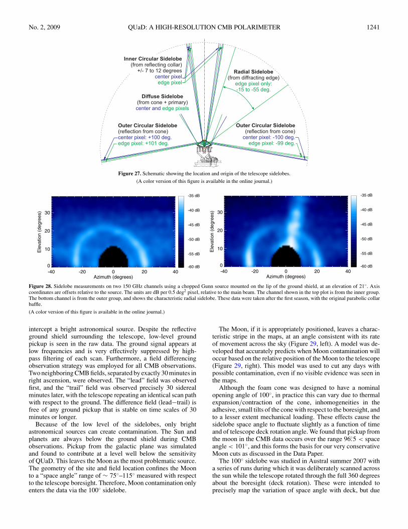
No. 2, 2009 QUaD: A HIGH-RESOLUTION CMB POLARIMETER 1241
Figure 27. Schematic showing the location and origin of the telescope sidelobes.
(A color version of this figure is available in the online journal.)
-40 -20 0 20 40Azimuth (degrees)
0
10
20
30
Ele
vatio
n (
de
gre
es)
-60 dB
-55 dB
-50 dB
-45 dB
-40 dB
-35 dB
-40 -20 0 20 40Azimuth (degrees)
0
10
20
30E
leva
tio
n (
de
gre
es)
-60 dB
-55 dB
-50 dB
-45 dB
-40 dB
-35 dB
Figure 28. Sidelobe measurements on two 150 GHz channels using a chopped Gunn source mounted on the lip of the ground shield, at an elevation of 21◦. Axiscoordinates are offsets relative to the source. The units are dB per 0.5 deg2 pixel, relative to the main beam. The channel shown in the top plot is from the inner group.The bottom channel is from the outer group, and shows the characteristic radial sidelobe. These data were taken after the first season, with the original parabolic collarbaffle.
(A color version of this figure is available in the online journal.)
intercept a bright astronomical source. Despite the reflectiveground shield surrounding the telescope, low-level groundpickup is seen in the raw data. The ground signal appears atlow frequencies and is very effectively suppressed by high-pass filtering of each scan. Furthermore, a field differencingobservation strategy was employed for all CMB observations.Two neighboring CMB fields, separated by exactly 30 minutes inright ascension, were observed. The “lead” field was observedfirst, and the “trail” field was observed precisely 30 siderealminutes later, with the telescope repeating an identical scan pathwith respect to the ground. The difference field (lead−trail) isfree of any ground pickup that is stable on time scales of 30minutes or longer.
Because of the low level of the sidelobes, only brightastronomical sources can create contamination. The Sun andplanets are always below the ground shield during CMBobservations. Pickup from the galactic plane was simulatedand found to contribute at a level well below the sensitivityof QUaD. This leaves the Moon as the most problematic source.The geometry of the site and field location confines the Moonto a “space angle” range of ∼ 75◦–115◦ measured with respectto the telescope boresight. Therefore, Moon contamination onlyenters the data via the 100◦ sidelobe.
The Moon, if it is appropriately positioned, leaves a charac-teristic stripe in the maps, at an angle consistent with its rateof movement across the sky (Figure 29, left). A model was de-veloped that accurately predicts when Moon contamination willoccur based on the relative position of the Moon to the telescope(Figure 29, right). This model was used to cut any days withpossible contamination, even if no visible evidence was seen inthe maps.
Although the foam cone was designed to have a nominalopening angle of 100◦, in practice this can vary due to thermalexpansion/contraction of the cone, inhomogeneities in theadhesive, small tilts of the cone with respect to the boresight, andto a lesser extent mechanical loading. These effects cause thesidelobe space angle to fluctuate slightly as a function of timeand of telescope deck rotation angle. We found that pickup fromthe moon in the CMB data occurs over the range 96.◦5 < spaceangle < 101◦, and this forms the basis for our very conservativeMoon cuts as discussed in the Data Paper.
The 100◦ sidelobe was studied in Austral summer 2007 witha series of runs during which it was deliberately scanned acrossthe sun while the telescope rotated through the full 360 degreesabout the boresight (deck rotation). These were intended toprecisely map the variation of space angle with deck, but due

1242 HINDERKS ET AL. Vol. 692
Az offset (deg)
El offset (d
eg)
Sun (data)
02
4.2
4.3
4.4
4.5
4.6
4.7
4.8
Az offset (deg)
El offset (d
eg)
Sun (sim)
02
4.2
4.3
4.4
4.5
4.6
4.7
4.8
Az offset (deg)
El offset (d
eg)
Moon (data)
020.5
0.6
0.7
0.8
0.9
1
1.1
Az offset (deg)
El offset (d
eg)
Moon (sim)
020.5
0.6
0.7
0.8
0.9
1
1.1
Figure 29. Left: single PSB pair maps of data contaminated by the Sun and Moon. Note these sources move across the sky at different rates, resulting in different stripeangles in the maps. Right: simulated maps that incorporate a best-fit cone angle, the sidelobe width, and polarization information based on the Sun/Moon coordinatesduring the same day as the real data. The cone opening angle (allowed to vary from 96◦ to 101◦) is the only free parameter of this model.
to differing weather conditions in summer and winter, we couldnot use these results to provide tighter cuts on the CMB data.These runs did, however, confirm that the sidelobe is extremelynarrow (FWHM ∼ 0.◦22).
Since it is the result of reflection off a dielectric surface,the sidelobe is highly polarized. Laboratory tests using a foamcone structure identical to that on the telescope measured thefractional polarization to be 50% at 150 GHz, with a reflec-tion coefficient of approximately 2%. The amplitude of theelectric field of a reflected ray in the radial direction to thecone axis of symmetry is suppressed relative to that in the tan-gential direction. A PSB with its sensitivity axis aligned withthe cone tangent will therefore measure a larger signal thana perpendicular PSB, resulting in a false polarized signal inthe differenced data. We can predict the sign of the polarizedsignal if we know the PSB pair orientations, and the angle atwhich a bright source appears in the frame of the focal plane(Figure 30). The amplitude of the Moon contamination sig-nal (∼ 3 mK) is consistent with these laboratory foam conetransmission measurements, assuming a Moon brightness tem-perature of order 300 K.
9. CALIBRATION
The QUaD calibration process comprises frequent relativecalibrations, and an absolute calibration of the final maps basedon comparison with CMB temperature measurements fromother experiments. The primary method of channel-to-channel
relative gain calibration is to nod the telescope in elevation by1◦ (known as an “el-nod”). The resulting change in air massgenerates an approximately linear signal of order a Volt in theamplified time stream of each detector. The measured signal isused to normalize the gain of each detector to the mean gain of alldetectors in a band, and includes a correction for the elevationoffset of the feeds in the focal plane at the current telescoperotation angle. Figure 31 shows an example of an el-nod and themeasured distribution of relative detector gains. During routineCMB observations, el-nods are performed during a “cal set” thatprecedes each scan set, approximately every 30 minutes.
Each cal set also includes a run of the calibration source,which is located above the secondary mirror, inside the foamcone (Figure 32). When in use, a flip mirror reflects the portionof the beam passing through the secondary hole onto a rotat-ing polarizing grid in front of an ambient-temperature black-body target, introducing a sinusoidally modulated signal intothe detector time streams. To avoid running wires along thefoam cone which could introduce spurious polarized signals,the calibration source is battery powered and controlled via aninfrared link. The calibration source does not uniformly illumi-nate the focal plane, and hence cannot be used to correct forrelative channel-to-channel gain variation—this is done withthe el-nods. Instead, the calibration source is used to correct fordrifts in the mean receiver gain over time, an effect the el-nodsalone cannot correct since gain drifts and changes in atmo-spheric loading both affect the el-nod volts/airmass in the sameway.
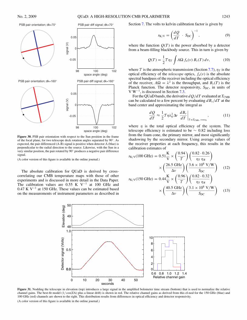
No. 2, 2009 QUaD: A HIGH-RESOLUTION CMB POLARIMETER 1243
PSB pair orientation; dk=70°
98 100 102
-0.05
0
0.05
space angle (deg)
)V( l
an
gis
PSB pair diff signal; dk=70°
PSB pair orientation; dk=160°
98 100 102
-0.05
0
0.05
space angle (deg)
signal (
V)
PSB pair diff signal; dk=160°
Figure 30. PSB pair orientation with respect to the Sun position in the frameof the focal plane, for two telescope deck rotation angles separated by 90◦. Asexpected, the pair differenced (A-B) signal is positive when detector A (blue) isperpendicular to the radial direction to the source. Likewise, with the Sun in avery similar position, the pair rotated by 90◦ produces a negative pair differencesignal.
(A color version of this figure is available in the online journal.)
The absolute calibration for QUaD is derived by cross-correlating our CMB temperature maps with those of otherexperiments and is discussed in more detail in the Data Paper.The calibration values are 0.55 K V−1 at 100 GHz and0.47 K V−1 at 150 GHz. These values can be estimated basedon the measurements of instrument parameters as described in
Section 7. The volts to kelvin calibration factor is given by
sK/V =(
dQ
dT· SDC
)−1
, (9)
where the function Q(T ) is the power absorbed by a detectorfrom a beam-filling blackbody source. This in turn is given by
Q(T ) = 1
2T ηT
∫AΩ fn(ν) Bν(T ) dν, (10)
where T is the atmospheric transmission (Section 7.7), ηT is theoptical efficiency of the telescope optics, fn(ν) is the absolutespectral bandpass of the receiver including the optical efficiencyof the receiver, AΩ = λ2 is the throughput, and Bν(T ) is thePlanck function. The detector responsivity, SDC, in units ofV W−1, is discussed in Section 7.3.
For the QUaD bands, the derivative dQ/dT evaluated at TCMBcan be calculated to a few percent by evaluating dBν/dT at theband center and approximating the integral as
dQ
dT≈ 1
2T ηλ2
0 ΔνdBν
dT
∣∣∣∣T =TCMB, ν=ν0
, (11)
where η is the total optical efficiency of the system. Thetelescope efficiency is estimated to be ∼ 0.82 including lossfrom the foam cone, the primary mirror, and most significantlyshadowing by the secondary mirror. Using average values ofthe receiver properties at each frequency, this results in thecalibration estimates of
sK/V(100 GHz) = 0.51K
V×
(0.94
T
) (0.82 · 0.26
ηT ηR
)
×(
26.5 GHz
Δν
) (3.6 × 10⁸ V/W
SDC
)(12)
sK/V(150 GHz) = 0.44K
V×
(0.96
T
) (0.82 · 0.32
ηT ηR
)
×(
40.5 GHz
Δν
) (3.1 × 10⁸ V/W
SDC
)(13)
48
49
50
Ele
vation (
deg)
0 10 20 30 40 50seconds
0.0
0.5
1.0
0.0Dete
cto
r sig
nal (V
olts)
0.6 0.8 1.0 1.2 1.4Relative channel gain
0
2
4
6
8
10
Figure 31. Nodding the telescope in elevation (top) introduces a large signal in the amplified bolometer time stream (bottom) that is used to normalize the relativechannel gains. The best-fit model (1/ cos(ZA) plus a linear drift) is shown in red. The relative channel gains as derived from this el-nod for the 150 GHz (blue) and100 GHz (red) channels are shown to the right. This distribution results from differences in optical efficiency and detector responsivity.
(A color version of this figure is available in the online journal.)

1244 HINDERKS ET AL. Vol. 692
Blackbodysource
link
Secondary
Cryostatsnout
0 5 10 15 20 25 30Seconds
4.00
4.05
4.10
4.15
4.20
0 2 4 6 8Seconds
-1
0
1
2
Figure 32. Left: the calibration source is located inside the foam cone, above the secondary mirror. When activated via the infrared link, a flip mirror reflects thesignal from a rotating polarizing grid into the telescope beam through the small hole in the secondary. To prevent the calibration signal from saturating the detectors,the flip mirror is actually a small aluminum disk suspended by Kevlar thread within an aluminum frame. Middle: an early test run of the calibration source showsthe procedure. Right: a cal source run showing the same channel, taken with the receiver electronics in the usual “high-gain” mode used during observation. The flipmirror area was doubled since the test run to increase the calibration signal.
(A color version of this figure is available in the online journal.)
Total
JohnsonPhononAmplifierPhoton
100
10
10 1 2 3 4 5
Bias (nA)
PE
N10
)-1
/2-1
7x
Figure 33. Contributions to the NEP as a function of electrical bias current fora typical 150 GHz detector.
(A color version of this figure is available in the online journal.)
which are in good agreement with the measured calibrationvalues given above.
10. SENSITIVITY
The sensitivity of bolometric detectors is limited by Johnsonnoise from the thermistor and load resistors, phonon noise due tothe quantization of the heat conducted between the absorber andthe bath, and amplifier noise generated in the readout electronics(Mather 1982, 1984). Additionally there are two sources ofnoise associated with the quantum nature of the incident opticalradiation: shot noise from the discrete photon arrival times and“clumping” noise due to the Boson properties of photons. See,for example, Appendix B of Runyan et al. (2003) for a thoroughdiscussion of this second term.
For millimeter-wave systems, the detector sensitivity is usu-ally quoted as an NEP in W Hz−1/2, computed by dividing thepower spectrum in Volts by the detector responsivity (volts/
0.01 0.10 1.00 10.00Freq (Hz)
10
100
PS
D (
nV
Hz-1
/2)
Light boloDark bolo
ResistorShort
Warm electronics
Figure 34. PSD of the noise from various sources. “Warm electronics” accountsfor both the readout and the bias generator and was made by connecting awarm 1 kΩ resistor in place of the cold bolometers and amplifiers. “Short”is a measurement of the noise across a short located on the focal plane andincludes contributions from the cold JFETS and the warm amplifiers (but notthe bias generator). “Resistor” is a properly biased 10 MΩ resistor on the focalplane. “Dark bolo” is the readout from a dark bolometer. “Light bolo” is thereadout from a 150 GHz bolometer made during normal operation and includescontributions from atmospheric 1/f.
(A color version of this figure is available in the online journal.)
watt). Figure 33 shows the expected contributions to the NEPfor a typical QUaD detector based on the measured propertiesof the bolometers and readout electronics. Figure 34 shows themeasured noise contributions from the readout electronics.
The sensitivity to CMB temperature fluctuations is quantifiedas a noise equivalent temperature (NET), which is computed bymultiplying the detector voltage noise by the absolute calibrationfactor in units of kelvin volt−1 (Section 9). The NET of a detectoris related to the measured NEP as
NET = NEP√2 (dQ/dT )|TCMB
, (14)
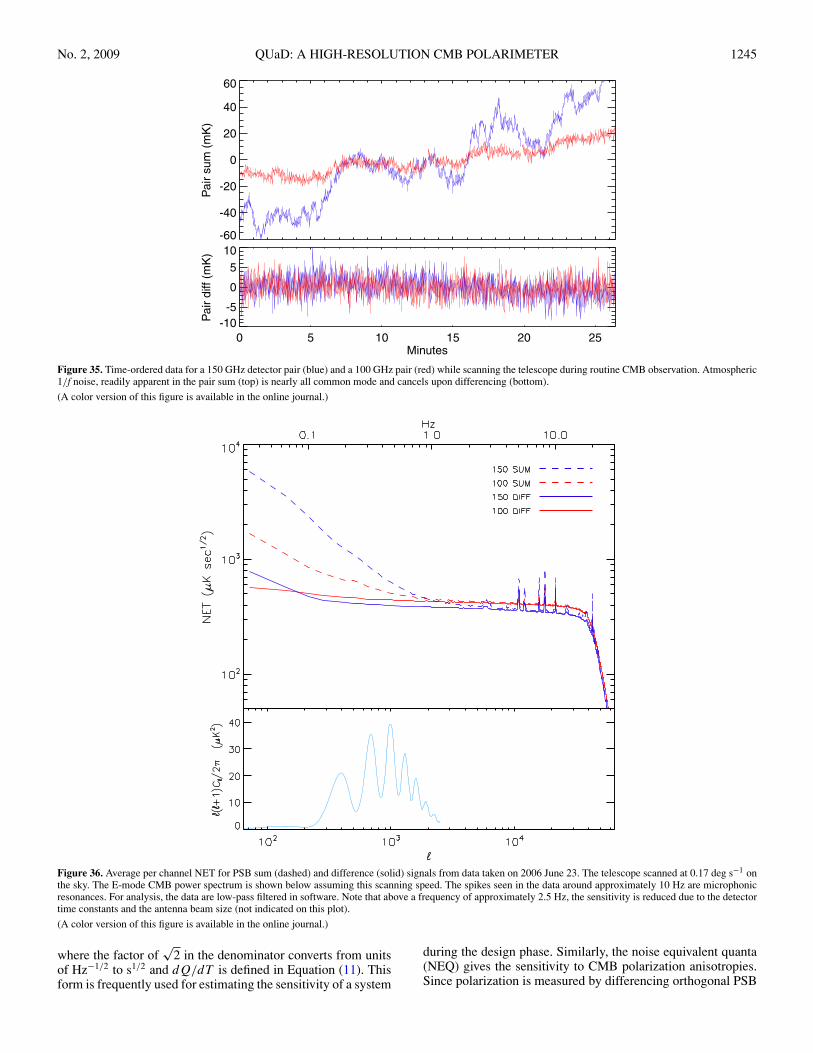
No. 2, 2009 QUaD: A HIGH-RESOLUTION CMB POLARIMETER 1245
-60
-40
-20
0
20
40
60
Pair s
um
(m
K)
0 5 10 15 20 25Minutes
-10
-5
0
5
10
Pa
ir d
iff
(mK
)
Figure 35. Time-ordered data for a 150 GHz detector pair (blue) and a 100 GHz pair (red) while scanning the telescope during routine CMB observation. Atmospheric1/f noise, readily apparent in the pair sum (top) is nearly all common mode and cancels upon differencing (bottom).
(A color version of this figure is available in the online journal.)
Figure 36. Average per channel NET for PSB sum (dashed) and difference (solid) signals from data taken on 2006 June 23. The telescope scanned at 0.17 deg s−1 onthe sky. The E-mode CMB power spectrum is shown below assuming this scanning speed. The spikes seen in the data around approximately 10 Hz are microphonicresonances. For analysis, the data are low-pass filtered in software. Note that above a frequency of approximately 2.5 Hz, the sensitivity is reduced due to the detectortime constants and the antenna beam size (not indicated on this plot).
(A color version of this figure is available in the online journal.)
where the factor of√
2 in the denominator converts from unitsof Hz−1/2 to s1/2 and dQ/dT is defined in Equation (11). Thisform is frequently used for estimating the sensitivity of a system
during the design phase. Similarly, the noise equivalent quanta(NEQ) gives the sensitivity to CMB polarization anisotropies.Since polarization is measured by differencing orthogonal PSB

1246 HINDERKS ET AL. Vol. 692
pairs, common mode atmospheric noise is greatly reduced(Figure 35). However, the NEQ is degraded relative to the NETby a factor of (1+ε)/(1−ε) (see Equation (5)) which for QUaDis ∼ 1.16 due to cross-polar leakage.
Figure 36 shows the sensitivity achieved during a typicalCMB observing day. The power spectral density (PSD) isestimated by averaging the Fourier transform of each of theapproximately 1000 azimuth scans performed during that day.Each scan is approximately 7◦ on the sky and takes 40 s. TwoPSDs are computed for each PSB pair, one by summing thedata, and the other by subtracting. The pair sum and differencePSDs are averaged over all the operational channels in eachfrequency band. Only minimal filtering is applied to the rawdata—a best-fit line is removed from each half scan.
The average NET for a feed horn (PSB pair), not includingthe effects of atmospheric 1/f noise, is computed from the pairdifference data as 440 and 390 μK
√s at 100 and 150 GHz,
respectively over the science band (0.1–1.0 Hz). The NET forthe two bands, including the effects of atmospheric 1/f , iscomputed from the pair sum PSD to be 490 and 580 μK
√s.
Since the atmosphere adds a large amount of 1/f -noise, theNET achieved over the course of a season depends on theangular scale of interest, on the filtering used during analysis,and on the weighting used to combine data taken during differingweather conditions. The NEQ for QUaD can be estimated bymultiplying the NET computed from the PSB pair differencedata by the polarization efficiency factor and is found to be 510and 450 μK
√s. Table 3 gives the noise budget and sensitivity
for QUaD.
11. CONCLUSION
We have presented the design and performance of the QUaDexperiment. Stability of key instrumental parameters such as thepointing, beams, and polarization efficiencies have been shownto be at a level that does not interfere with the data collection.Sources of data contamination, including atmospheric noise andsidelobe pickup, are sufficiently well understood to be dealtwith effectively—a combination of filtering, field differencing,and data cuts suppresses them to below the level of theinstrument sensitivity. QUaD began data collection in early2005 and completed three seasons of observation before beingdecommissioned in late 2007. Analysis of these surveys ispresented in Ade et al. (2008) and Pryke et al. (2008).
We acknowledge the staff of the Amundsen-Scott South PoleStation and all involved in the United States Antarctic Programfor their superb support during the construction and operationof this experiment. Special thanks go to our brave winter-overscientist Robert Schwarz who has spent three consecutive winterseasons with the QUaD. We also acknowledge the tremendousefforts of the Stanford University Physics Department machineshop in the construction of the focal plane assembly. J.R.H.thanks David Chuss for useful comments on this draft andSimon Radford for providing the 350 μm tipper data. QUaD isfunded by the National Science Foundation in the USA, throughgrants AST-0096778,ANT-0338138,ANT-0338335, and ANT-0338238, by the UK Science and technology Facilities Council(STFC) and its predecessor the Particle Physics and Astronomy
Research Council (PPARC), and by the Science FoundationIreland.
J.R.H. acknowledges the support of an NSF Graduate Re-search Fellowship, a Stanford Graduate Fellowship, and aNASA Postdoctoral Fellowship. M.L.B. and A.O. acknowl-edge the award of PPARC fellowships. P.G.C. is funded bythe Fundacao para a Ciencia e a Tecnologia. S.E.C. acknowl-edges support from a Stanford Terman Fellowship. J.M.K.acknowledges support from a John B. and Nelly L. KilroyFoundation Fellowship. C.P. and J.E.C. acknowledge partialsupport from the Kavli Institute for Cosmological Physicsthrough the grant NSF PHY-0114422. E.Y.W. acknowledgesreceipt of an NDSEG fellowship. M.Z. acknowledges the sup-port of a NASA Postdoctoral Fellowship. This research wassupported in part by appointments to the NASA PostdoctoralProgram at the Goddard Space Flight Center (J.R.H.) and theJet Propulsion Laboratory (M.Z.), administered by Oak RidgeAssociated Universities through a contract with NASA.
REFERENCES
Ade, P. A. R., Pisano, G., Tucker, C., & Weaver, S. 2006, Proc. SPIE, 6275,(Bellingham, WA: SPIE), 62750U
Ade, P., et al. 2008, ApJ, 674, 22Bhatia, R. S., et al. 2000, Cryogenics, 40, 685Birch, J. R., & Ping, K. F. 1984, Infrared Phys., 24, 309Bock, J. J. 1994, PhD thesis, AA, California Univ.Bischoff, C., et al. (CAPMAP Collaboration) 2008, ApJ, 684, 771Bussmann, R. S., Holzapfel, W. L., & Kuo, C. L. 2005, ApJ, 622, 1343Cahill, G., et al. 2004, Proc. SPIE, 5498, 396Coble, K., et al. 2003, arXiv:astro-ph/0301599Crill, B. P., et al. 2003, ApJS, 148, 527Farese, P. C., et al. 2004, ApJ, 610, 625Gleeson, E., et al. 2005, Infrared Phys. Technol., 46, 493Glenn, J., et al. 1998, Proc. SPIE, 3357, 326Hinderks, J. R. 2005, PhD thesis, Stanford UniversityHolzapfel, W. L., Wilbanks, T. M., Ade, P. A. R., Church, S. E., Fischer, M. L.,
Mauskopf, P. D., Osgood, D. E., & Lange, A. E. 1997, ApJ, 479, 17Jones, W. C., Bhatia, R., Bock, J. J., & Lange, A. E. 2003, Proc. SPIE, 4855,
227Kogut, A., et al. 2007, ApJ, 665, 355Lane, A. P. 1998, BAAS, 30, 883Lay, O. P., & Halverson, N. W. 2000, ApJ, 543, 787Leitch, E. M., Kovac, J. M., Halverson, N. W., Carlstrom, J. E., Pryke, C., &
Smith, M. W. E. 2005, ApJ, 624, 10Leitch, E. M., et al. 2002a, Nature, 420, 763Leitch, E. M., et al. 2002b, ApJ, 568, 28Masi, S., et al. 2006, A&A, 458, 687Mather, J. C. 1982, Appl. Opt., 21, 1125Mather, J. C. 1984, Appl. Opt., 23, 584Montroy, T. E., et al. 2006, ApJ, 647, 813Murphy, J. A., et al. 2005, Int. J. Infrared Mm Waves, 26, 505O’Sullivan, C., et al. 2008, Infrared Phys. Technol., 51, 277Page, L., et al. 2007, ApJS, 170, 335Peterson, J. B., Radford, S. J. E., Ade, P. A. R., Chamberlin, R. A., O’Kelly, M.
J., Peterson, K. M., & Schartman, E. 2003, PASP, 115, 383Pryke, C., et al. 2009, ApJ, 692, 1247Readhead, A. C. S., et al. 2004, Science, 306, 836Runyan, M. C. 2002, PhD thesis, California Institute of TechnologyRunyan, M. C., et al. 2003, ApJS, 149, 265Sudiwala, R. V., Griffin, M. J., & Woodcraft, A. L. 2002, Int. J. Infrared Mm
Waves, 23, 545Woodcraft, A. L., et al. 2003, Appl. Opt., 42, 5009Wu, J. H. P., et al. 2007, ApJ, 665, 55Yoon, K. W., et al. 2006, Proc. SPIE, 6275, 62751KZaldarriaga, M., & Seljak, U. 1997, Phys. Rev. D, 55, 1830Zemcov, M. 2006, PhD thesis, Cardiff University
![28. Cosmic Microwave Backgroundpdg.lbl.gov/.../rpp2019-rev-cosmic-microwave-background.pdf · 2019. 12. 6. · cosmic microwave background (CMB), discovered in 1965 [1]. The spectrum](https://img.pdfslide.us/doc/110x75/6143c67b6b2ee0265c02424a/28-cosmic-microwave-2019-12-6-cosmic-microwave-background-cmb-discovered.jpg)