QTL Mapping in RGhost QTLComposite Interval MappingMouse HypertensionPlant Data Ghost QTL 0 20 40 60 80 100 0 5 10 15 Simulated Backcross Map position (cM) lod March 16, 2010 QTL Mapping

QTL Mapping in R

March 16, 2010

Ghost QTL Composite Interval Mapping Mouse Hypertension Plant Data

R qtl

library(qtl)

R Library: qtl

sim.map: constructs a genetic map

sim.cross: simulates marker, QTL, and phenotype data

calc.genoprob: calculates conditional probabilities

scanone: produces a QTL map OR performs permutation tests

summary.scanone: identify QTLs and calculatie permutation thresholds

add.threshold: adds a permutation threshold to QTL plot

cim: performs composite interval mapping

find.marker: finds a marker near a specified position

pull.geno: extracts genotype data from a given marker

The residual phenotypic variation is normally distributed with variance 1.QTL effect: difference between the homozygote and the heterozygote

March 16, 2010 QTL Mapping in R 2 / 19


Ghost QTL

set.seed(1)

n<-200

map<-sim.map(len=100,n.mar=21,include.x=FALSE,eq.spacing=TRUE)

cross<-sim.cross(map,model = rbind(c(1,22,1),c(1,73,1)), type="bc",n.ind=n)

crossB<-calc.genoprob(cross,step=1)

est<-scanone(crossB)

plot(est,lwd=4,main="Simulated Backcross")

perm1<-scanone(crossB,chr=1,n.perm=500)

thresh<-summary(perm1,alpha=.05)[1]

thresh

add.threshold(est,perm=perm1,col="orange",lwd=4)

abline(v=22,col="magenta",lwd=4)


[1] 1.822760



Ghost QTL

0 20 40 60 80 100

0

5

10

15

Simulated Backcross

Map position (cM)

lod



Ghost QTL

est.cim.10 <- cim(crossB, n.marcovar=4, window=10)

est.cim.20 <- cim(crossB, n.marcovar=4, window=20)

plot(est,est.cim.10,est.cim.20,col=c("black","red","blue"),lwd=3,lty=1:3)

add.threshold(est,perm=perm1,col="orange",lwd=4)



axis(1,at=22,line=-1)

axis(1,at=73,line=-1)


0 20 40 60 80 100

0

5

10

15

Composite Interval Mapping

Map position (cM)

lod

22 73


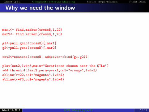
Why we need the window

mar1<- find.marker(crossB,1,22)

mar2<- find.marker(crossB,1,73)

g1<-pull.geno(crossB)[,mar1]

g2<-pull.geno(crossB)[,mar2]

est2<-scanone(crossB, addcovar=cbind(g1,g2))

plot(est2,lwd=3,main="Covariates chosen near the QTLs")

add.threshold(est2,perm=perm1,col="orange",lwd=3)




0 20 40 60 80 100

0.0

0.5

1.0

1.5

2.0Covariates chosen near the QTLs

Map position (cM)

lod


The Dataset hyper

data(hyper)

nind(hyper); nphe(hyper); nchr(hyper); totmar(hyper); nmar(hyper);

[1] 250

[1] 2

[1] 20

[1] 174

1 2 3 4 5 6 7 8 9 10 11 12 13 14 15 16 17 18 19 X

22 8 6 20 14 11 7 6 5 5 14 5 5 5 11 6 12 4 4 4

summary(hyper)

Backcross

No. individuals: 250

No. phenotypes: 2

Percent phenotyped: 100 100

No. chromosomes: 20

Autosomes: 1 2 3 4 5 6 7 8 9 10 11 12 13 14 15 16 17 18 19

X chr: X

Total markers: 174

No. markers: 22 8 6 20 14 11 7 6 5 5 14 5 5 5 11 6 12 4 4 4

Percent genotyped: 47.7

Genotypes (%): BB:50.2 BA:49.8March 16, 2010 QTL Mapping in R 9 / 19


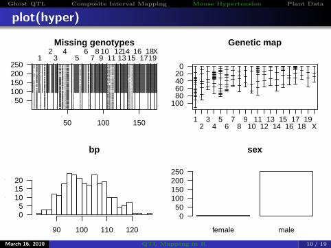
plot(hyper)

50 100 150

50100150200250

Markers

Indi

vidu

als

1 3 5 7 9 11 13 15 17192 4 6 8 10 1214 16 18X

Missing genotypes

10080604020

0

Chromosome

Loca

tion

(cM

)

1 3 5 7 9 11 13 15 17 192 4 6 8 10 12 14 16 18 X

Genetic map

bp

Fre

quen

cy

90 100 110 120

05

101520

female male

sex

050

100150200250



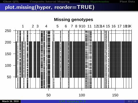
plot.missing(hyper, reorder=TRUE)

50 100 150

50

100

150

200

250

Indi

vidu

als

1 2 3 4 5 6 7 8 910 11 121314 15 16 17 1819X

Missing genotypes



More Commands

plot(hyper)

plot.missing(hyper)

plot.map(hyper)

plot.pheno(hyper, pheno.col=1)

plot.map(hyper, chr=c(1, 4, 6, 7, 15), show.marker.names=TRUE)

plot.missing(hyper, reorder=TRUE)

hyper <- drop.nullmarkers(hyper)

totmar(hyper)

hyper <- est.rf(hyper)

newmap <- est.map(hyper, error.prob=0.01)



plot.rf(hyper)

50 100 150

50

100

150

Mar

kers

1

1

2

2

3

3

4

4

5

5

6

6

7

7

8

8

9

9

10

10

11

11

12

12

13

13

14

14

15

15

16

16

17

17

18

18

1919

XX

Pairwise recombination fractions and LOD scores



plot.map(hyper, newmap)

120

100

80

60

40

20

0

Chromosome

Loca

tion

(cM

)

1 2 3 4 5 6 7 8 9 10 11 12 13 14 15 16 17 18 19 X

Comparison of genetic maps



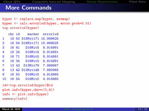
More Commands

hyper <- replace.map(hyper, newmap)

hyper <- calc.errorlod(hyper, error.prob=0.01)

top.errorlod(hyper)

chr id marker errorlod

1 16 50 D16Mit171 15.999625

2 16 54 D16Mit171 15.999625

3 16 81 D16Mit5 8.914991

4 16 24 D16Mit5 8.914991

5 16 71 D16Mit5 8.914991

6 16 34 D16Mit5 8.914991

7 13 42 D13Mit78 7.999967

8 13 42 D13Mit148 7.880965

9 16 50 D16Mit5 4.914965

10 16 54 D16Mit5 4.914965

id<-top.errorlod(hyper)$id

plot.info(hyper,chr=c(1,4))

info <- plot.info(hyper)

summary(info)



plot.geno(hyper, chr=16, ind=id)

0 10 20 30 40 50 60

Chromosome 16

Location (cM)

Indi

vidu

al

42

34

71

24

81

54

50 ●

●

●

●

●

●

●

●

●

●

●

●

●

●

●

●

●

●

●

●

●

●

●

●

●

●

●

●

●

●

●

●

●

●

●

●

●

●

●

●

●

●

●

●

●

●

●

●

●

●

●

●

●

●

●

●

●

●

●

●

●

●

●

●

●

●

●

●

●



plot.info(hyper)

0.0

0.2

0.4

0.6

0.8

1.0

Missing information

Chromosome

mis

info

.ent

ropy

1 2 3 4 5 6 7 8 9 10 11 12 13 1415 1617 18 19 X



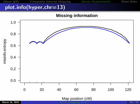
plot.info(hyper,chr=13)

0 20 40 60 80 100 120

0.0

0.2

0.4

0.6

0.8

1.0

Missing information

Map position (cM)

mis

info

.ent

ropy



Importing Data

mydata <- read.cross("csv",

"/Users/berg/Documents/courses/phs 516/slides/lecture 6",

"plantdata.csv",genotypes=c("A","H"))

summary(mydata)

Backcross

No. individuals: 200

No. phenotypes: 28

Percent phenotyped: 100 100 100 100 100 100 100 100 100 100 100 100 100 100

100 100 100 100 100 100 100 100 100 100 100 100 100 100

No. chromosomes: 11

Autosomes: 1 2 3 4 5 6 7 8 9 10 11

Total markers: 231

No. markers: 21 21 21 21 21 21 21 21 21 21 21

Percent genotyped: 100

Genotypes (%): AA:49.7 AB:50.3
