QTL Association Mapping

1 / 38

Introduction to Quantitative Trait Mapping

We previously focused on obtaining variance components of aquantitative trait to determine the proportion of the variance of thetrait that can be attributed to both genetic (additive and dominance)and environment (shared and unique) factors

We demonstrated that resemblance of trait values among relatives wecan be used to obtain estimates of the variance components of aquantitative trait without using genotype data.

Quantitative trait loci (QTL) mapping involves identifying genetic locithat influence the variation of a quantitative trait.

2 / 38

Introduction to Quantitative Trait Mapping

There generally is no simple Mendelian basis for variation ofquantitative traits

Some quantitative traits can be largely influenced by a single gene aswell as by environmental factors

Influences on a quantitative trait can be due to a a large number ofgenes with similar (or differing) effects

Many quantitative traits of interest are complex where phenotypicvariation is due to a combination of both multiple genes andenvironmental factors

Examples: Blood pressure, cholesterol levels, IQ, height, weight, etc.

3 / 38

Partition of Phenotypic Values

Today we will focus onI QTL association mappingI Contribution of a QTL to the variance of a quantitative traitI Statistical power for detecting QTL in GWAS

Consider once again the classical quantitative genetics model ofY = G +E where Y is the phenotype value, G is the genotypic value,and E is the environmental deviation that is assumed to have a meanof 0 such that E (Y ) = E (G )

4 / 38

Representation of Genotypic Values

For a single locus with alleles A1 and A2, the genotypic values for thethree genotypes can be represented as follows

Genotype Value =

−a if genotype is A2A2

d if genotype is A1A2

a if genotype is A1A1

If p and q are the allele frequencies of the A1 and A2 alleles,respectively in the population, we previously showed that

µG = a(p−q) +d(2pq)

and that the genotypic value at a locus can be decomposed intoadditive effects and dominance deviations:

Gij = GAij + δij = µG + αi + αj + δij

5 / 38

Decomposition of Genotypic Values

The model can be given in terms of a linear regression of genotypicvalues on the number of copies of the A1 allele such that:

Gij = β0 + β1Xij1 + δij

where X ij1 is the number of copies of the type A1 allele in genotype

Gij , and with β0 = µG + 2α2 and β1 = α1−α2 = α, the average effectof allele substitution.

Recall that α = a+d(q−p) and that α1 = qα and α2 =−pα

6 / 38

Linear Regression Figure for Genetic Values

Falconer model for single biallelic QTL

Var (X) = Regression Variance + Residual Variance = Additive Variance + Dominance Variance

bb Bb BB

m

-a

a d

15

7 / 38

QTL Mapping

For traits that are heritable, i.e., traits with a non-negligible geneticcomponent that contributes to phenotypic variability, identifying (ormapping) QLT that influence the trait is often of interest.

Genome-wide association studies (GWAS) are commonly used for theidentification of QTL

Single SNP association testing with linear regression models are oftenused in GWAS

Linear regression models will often include a single genetic marker(e.g., a SNP) as predictor in the model, in addition to other relevantcovariates (such as age, sex, etc.), with the quantitative phenotype asthe response

8 / 38

Linear regression with SNPs

Many analyses fit the ‘additive model’

y = β0 + β ×#minor alleles

●

●

●

●

●

●

●

●

●●

●

●

●

● ●●

●

● ●●

●

●

●●

●

●

●

●

●

●

●

●

●

●

●

●●

●

●●

●

●

●

●

● ●

●

●

●

●

● ●

●

●

●

● ●

●

●

●

●

●

●

●

●

●●

●

●

●

●

●

●

●

●

●

●

●●

●

●

●

●

●

●

●

●

●

●

●

●

●

●

● ●

●

●

●

●

●

●

●

●

●●

●

●

●

●

●

●

●●

●

●

●

●●

●

●

●

●

●

●

●●

●

●

●

●

●

●

●

●

●

●

●

●

●

●●

●

●

●

●

●

●

●

●

●●

●

●●

●

●

●●

●

●

●●

●

●

●

●

●

●

●●

●

●●

●

●

●

●

●

●

●●

●

●

●

●

●

● ●●

●

●

●

●

●

●

●

●

●

●

●●

●

●

●

●

●

●

●

●

●

●●●

●

●

●

●

●

●

●

●

●

●

●

●

●

●

●

●

●

●

●

●

●

●

●

●

●●

●

●

●

●

●

●

●

●●

●●●

●

●

●

●

●

●

●●

●

●

●

●

●

●

●

●

●

●

●

●

●

●●

●

●

●

●

●

●

●●

●

●

●

●

●

●●

●●

●

●

●

●

●

●

●

●

●

AA Aa aa

chol

este

rol

β

β

0 1 2

9 / 38

Linear regression, with SNPs

An alternative is the ‘dominant model’;

y = β0 + β × (G 6= AA)

●

●

●

●

●

●

●

●

●●

●

●

●

● ●●

●

● ●●

●

●

●●

●

●

●

●

●

●

●

●

●

●

●

●●

●

●●

●

●

●

●

● ●

●

●

●

●

● ●

●

●

●

● ●

●

●

●

●

●

●

●

●

●●

●

●

●

●

●

●

●

●

●

●

●●

●

●

●

●

●

●

●

●

●

●

●

●

●

●

● ●

●

●

●

●

●

●

●

●

●●

●

●

●

●

●

●

●●

●

●

●

●●

●

●

●

●

●

●

●●

●

●

●

●

●

●

●

●

●

●

●

●

●

●●

●

●

●

●

●

●

●

●

●●

●

●●

●

●

●●

●

●

●●

●

●

●

●

●

●

●●

●

●●

●

●

●

●

●

●

●●

●

●

●

●

●

● ●●

●

●

●

●

●

●

●

●

●

●

●●

●

●

●

●

●

●

●

●

●

●●●

●

●

●

●

●

●

●

●

●

●

●

●

●

●

●

●

●

●

●

●

●

●

●

●

●●

●

●

●

●

●

●

●

●●

●●●

●

●

●

●

●

●

●●

●

●

●

●

●

●

●

●

●

●

●

●

●

●●

●

●

●

●

●

●

●●

●

●

●

●

●

●●

●●

●

●

●

●

●

●

●

●

●

AA Aa aa

chol

este

rol

β

0 1 1

10 / 38

Linear regression, with SNPs

or the ‘recessive model’;

y = β0 + β × (G == aa)

●

●

●

●

●

●

●

●

●●

●

●

●

● ●●

●

● ●●

●

●

●●

●

●

●

●

●

●

●

●

●

●

●

●●

●

●●

●

●

●

●

● ●

●

●

●

●

● ●

●

●

●

● ●

●

●

●

●

●

●

●

●

●●

●

●

●

●

●

●

●

●

●

●

●●

●

●

●

●

●

●

●

●

●

●

●

●

●

●

● ●

●

●

●

●

●

●

●

●

●●

●

●

●

●

●

●

●●

●

●

●

●●

●

●

●

●

●

●

●●

●

●

●

●

●

●

●

●

●

●

●

●

●

●●

●

●

●

●

●

●

●

●

●●

●

●●

●

●

●●

●

●

●●

●

●

●

●

●

●

●●

●

●●

●

●

●

●

●

●

●●

●

●

●

●

●

● ●●

●

●

●

●

●

●

●

●

●

●

●●

●

●

●

●

●

●

●

●

●

●●●

●

●

●

●

●

●

●

●

●

●

●

●

●

●

●

●

●

●

●

●

●

●

●

●

●●

●

●

●

●

●

●

●

●●

●●●

●

●

●

●

●

●

●●

●

●

●

●

●

●

●

●

●

●

●

●

●

●●

●

●

●

●

●

●

●●

●

●

●

●

●

●●

●●

●

●

●

●

●

●

●

●

●

AA Aa aa

chol

este

rol

β

0 0 1

11 / 38

Linear regression, with SNPs

Finally, the ‘two degrees of freedom model’;

y = β0 + βAa× (G == Aa) + βaa× (G == aa)

●

●

●

●

●

●

●

●

●●

●

●

●

● ●●

●

● ●●

●

●

●●

●

●

●

●

●

●

●

●

●

●

●

●●

●

●●

●

●

●

●

● ●

●

●

●

●

● ●

●

●

●

● ●

●

●

●

●

●

●

●

●

●●

●

●

●

●

●

●

●

●

●

●

●●

●

●

●

●

●

●

●

●

●

●

●

●

●

●

● ●

●

●

●

●

●

●

●

●

●●

●

●

●

●

●

●

●●

●

●

●

●●

●

●

●

●

●

●

●●

●

●

●

●

●

●

●

●

●

●

●

●

●

●●

●

●

●

●

●

●

●

●

●●

●

●●

●

●

●●

●

●

●●

●

●

●

●

●

●

●●

●

●●

●

●

●

●

●

●

●●

●

●

●

●

●

● ●●

●

●

●

●

●

●

●

●

●

●

●●

●

●

●

●

●

●

●

●

●

●●●

●

●

●

●

●

●

●

●

●

●

●

●

●

●

●

●

●

●

●

●

●

●

●

●

●●

●

●

●

●

●

●

●

●●

●●●

●

●

●

●

●

●

●●

●

●

●

●

●

●

●

●

●

●

●

●

●

●●

●

●

●

●

●

●

●●

●

●

●

●

●

●●

●●

●

●

●

●

●

●

●

●

●

AA Aa aa

chol

este

rol

0 1 00 0 1

βAaβaa

12 / 38

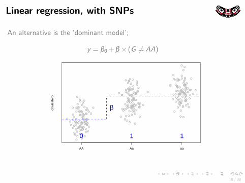
Association Testing with Dependent Samples

The observations in genetic association studies can have severalsources of dependence, including:

I population structure, i.e., ancestry differences among sample individualsI relatedness among the sampled individuals, some of which might be

known and some unknown.

Failure to appropriately account for this structure can invalidateassociation results that are based on an assumption of independenceand population homogeneity.

13 / 38

Confounding due to AncestryEthnic groups (and subgroups) often share distinct dietary habits andother lifestyle characteristics that leads to many traits of interestbeing correlated with ancestry and/or ethnicity.

14 / 38

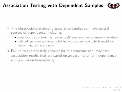
Spurious Association

Quantitative trait association testI Test for association between genotype and trait value

Consider sampling from 2 populations:

Histogram of Trait Values

Population 1Population 2

I Blue population has higher trait values.I Different allele frequency in each population

=⇒ spurious association between trait and genetic marker for samplescontaining individuals from both populations

15 / 38

Incomplete GenealogyCryptic and/or misspecified relatedness among the sample individualscan also lead to spurious association in genetic association studies

16 / 38

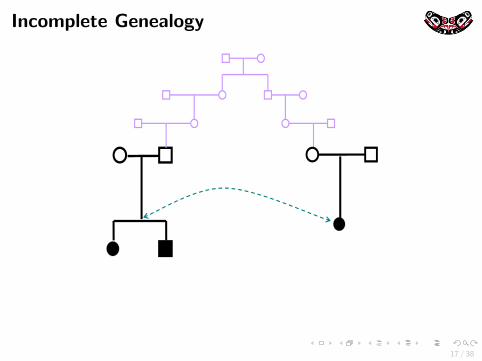
Incomplete Genealogy

17 / 38

Genotype and Phenotype Data

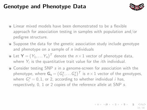
Linear mixed models have been demonstrated to be a flexibleapproach for association testing in samples with population and/orpedigree structure.

Suppose the data for the genetic association study include genotypeand phenotype on a sample of n individuals

Let Y = (Y1, . . .Yn)T denote the n×1 vector of phenotype data,where Yi is the quantitative trait value for the ith individual.

Consider testing SNP s in a genome-screen for association with thephenotype, where Gs = (G s

1 , . . .Gsn )T is n×1 vector of the genotypes,

where G si = 0,1, or 2, according to whether individual i has,

respectively, 0, 1 or 2 copies of the reference allele at SNP s.

18 / 38

Association Testing with Cryptic StructureConsider the following model:

Y = Wβ + Gsγ + g + ε

W is an n× (w + 1) matrix of relevant covariates that includes anintercept

β is the (w + 1)×1 vector of covariate effects, including intercept

γ is the (scalar) association parameter of interest, measuring theeffect of genotype on phenotype

g is a length n random vector of polygenic effects with g∼N(0,σ2gΨ)

σ2g represents additive genetic variance and Ψ is a matrix of pairwise

measures of genetic relatedness

ε is a random vector of length n with ε ∼ N(0,σ2e I)

σ2e represents non-genetic variance due to non-genetic effects

assumed to be acting independently on individuals

19 / 38

Mixed Linear ModelsFor Cryptic Structure

The matrix Ψ will be generally be unknown when there is populationstructure (ancestry differences ) and/or cryptic relatedness in thesample.Kang et al. [Nat Genet, 2010] proposed the EMMAX linear mixedmodel association method that is based on an empirical geneticrelatedness matrix (GRM) Ψ̂ calculated using SNPs from across thegenome. The (i , j)th entry of the matrix is estimated by

Ψ̂ij =1

S

S

∑s=1

(G si −2p̂s)(G s

j −2p̂s)

2p̂s(1− p̂s)

where p̂s is the sample average allele frequency. S will generally needto be quite large, e.g., larger than 100,000, to capture fine-scalestructure.

Kang, Hyun Min, et al. (2010) ”Variance component model to account for sample

structure in genome-wide association studies.” Nature genetics 4220 / 38

EMMAX Mixed Linear ModelFor Cryptic Structure

For genetic association testing, the EMMAX mixed-model approachfirst considers the following model without including any of the SNPsas fixed effects:

Y = Wβ + g + ε (1)

The variance components, σ2g and σ2

e , are then estimated using eithera maximum likelihood or restricted maximum likelihood (REML),with Cov(Y) set to σ2

g Ψ̂ + σ2e I in the likelihood with fixed Ψ̂

21 / 38

EMMAX Mixed Linear ModelFor Cryptic Structure

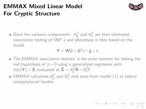
Once the variance components , σ2g and σ2

e are then estimated,association testing of SNP s and phenotype is then based on themodel

Y = Wβ + Gsγ + g + ε

The EMMAX association statistic is the score statistic for testing thenull hypothesis of γ = 0 using a generalized regression withVar(Y) = Σ evaluated at Σ̂ = σ̂2

g Ψ̂ + σ̂2e I

EMMAX calculates σ̂2g and σ̂2

e only once from model (1) to reducecomputational burden.

22 / 38

GEMMA Linear Mixed ModelFor Cryptic Structure

Zhou and Stephens [2012, Nat Genet] developed a computationallyefficient mixed-model approach named GEMMA

GEMMA is very similar to EMMAX and is essentially based on thesame linear mixed-model as EMMAX

Y = Wβ + Gsγ + g + ε

However, the GEMMA method is an ”exact” method that obtainsmaximum likelihood estimates of variance components σ̂2

g and σ̂2e for

each SNP s being tested for association.

Zhou and Stephens (2012) ”Genome-wide efficient mixed-model analysis for association

studies” Nature Genetics 44

23 / 38

Linear Mixed ModelsFor Cryptic Structure

A number of similar linear mixed-effects methods have recently beenproposed when there is cryptic structure: Zhang at al. [2010, NatGenet], Lippert et al. [2011, Nat Methods], Zhou & Stephens [2012,Nat Genet], and Svishcheva [2012, Nat, Genet], and others.

24 / 38

Additive Genetic Model

Most GWAS are performed via single SNP association testing underan additive model.

25 / 38

Additive Genetic Model

The additive linear regression model also has a nice interpretation, aswe saw from Fisher’s classical quantitative trait model!

The coefficient of determination (r2) of an additive linear regressionmodel gives an estimate of the proportion of phenotypic variation thatis explained by the SNP (or SNPs) in the model, e.g., the ”SNPheritability”

26 / 38

Additive Genetic Model

Consider the following additive model for association testing with aquantitative trait and a SNP with alleles A and a:

Y = β0 + β1X + ε

where X is the number of copies of the reference allele A.

What would your interpretation of ε be for this particular model?

27 / 38

Association Testing with Additive Model

Y = β0 + β1X + ε

Two test statistics for H0 : β1 = 0 versus Ha : β1 6= 0

T =β̂1√

var(β̂1)∼ tN−2 ≈ N(0,1) for large N

T 2 =β̂ 21

var(β̂1)∼ F1,N−2 ≈ χ

21 for large N

where

var(β̂1) =σ2

ε

SXX

and SXX is the corrected sum of squares for the Xi ’s

28 / 38

Statistical Power for Detecting QTL

Y = β0 + β1X + ε

We can also calculate the power for detecting a QTL for a giveneffect size β1 for a SNP.

For simplicity, assume that Y has been a standardized so that withσ2Y = 1.

Let p be the frequency of the A allele in the population

σ2Y = β

21 σ

2X + σ

2ε = 2p(1−p)β

21 + σ

2ε

Let h2s = 2p(1−p)β 21 , so we have σ2

Y = h2s + σ2ε

Interpret h2s (note that we assume that trait is standardized such thatσ2Y = 1)

29 / 38

Statistical Power for Detecting QTL

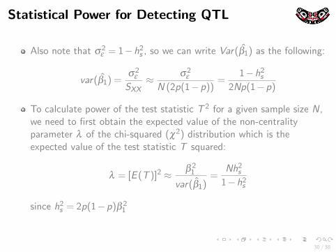
Also note that σ2ε = 1−h2s , so we can write Var(β̂1) as the following:

var(β̂1) =σ2

ε

SXX≈ σ2

ε

N (2p(1−p))=

1−h2s2Np(1−p)

To calculate power of the test statistic T 2 for a given sample size N,we need to first obtain the expected value of the non-centralityparameter λ of the chi-squared (χ2) distribution which is theexpected value of the test statistic T squared:

λ = [E (T )]2 ≈ β 21

var(β̂1)=

Nh2s1−h2s

since h2s = 2p(1−p)β 21

30 / 38

Required Sample Size for Power

Can also obtain the required sample size given type-I error α andpower 1−β , where the type–II error is β :

N =1−h2sh2s

(z(1−α/2) + z(1−β )

)2where z(1−α/2) and z(1−β) are the (1−α/2)th and (1−β )th quantiles,respectively, for the standard normal distribution.

31 / 38

Statistical Power for Detecting QTL

32 / 38

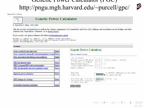
Genetic Power Calculator (PGC) http://pngu.mgh.harvard.edu/~purcell/gpc/

23

33 / 38

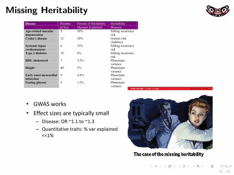
Missing Heritability

• !"#$%='(A1

• D&&06-%1.T01%+(0%-F8.6+??F%1:+??– >.10+10C%<a%mI4I%-'%mI4d

– h*+,-.-+-./0%-(+.-1C%n%/+(%0E8?+.,0;%ooIn

Disease Number of loci

Percent of Heritability Measure Explained

Heritability Measure

Age-related macular degeneration

5 50% Sibling recurrence risk

Crohn’s disease 32 20% Genetic risk (liability)

Systemic lupus erythematosus

6 15% Sibling recurrence risk

Type 2 diabetes 18 6% Sibling recurrence risk

HDL cholesterol 7 5.2% Phenotypic variance

Height 40 5% Phenotypic variance

Early onset myocardial infarction

9 2.8% Phenotypic variance

Fasting glucose 4 1.5% Phenotypic variance

34 / 38

!0,0-.6%2'=0(%O+?6*?+-'(%H$7+*,%2*(60??M7--8CVV8,B*4:B747+(/+(;40;*Vm8*(60??VB86V

35 / 38

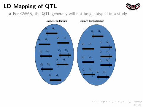
LD Mapping of QTLFor GWAS, the QTL generally will not be genotyped in a study

#$%&'()*)+,$-$./$,0**********************#$%&'()*1$2)+,$-$./$,0

Q1 M1

Q2 M2

Q1 M2

Q2 M1

Q1 M1

Q2 M2

Q1 M2

Q2 M1

Q1 M1

Q1 M1

Q2 M2

Q2 M2

Q1 M1

Q2 M2

Q1 M1

Q2 M2

36 / 38

LD Mapping of QTL

Linkage disequilibrium around an ancestral mutation

[Ardlie et al. 2002] 5

37 / 38

LD Mapping of QTL

r2 = LD correlation between QTL and genotyped SNP

Proportion of variance of the trait explained at a SNP ≈ r2h2s

Required sample size for detection is

N ≈ 1− r2h2sr2h2s

(z(1−α/2) + z(1−β)

)2Power of LD mapping depends on the experimental sample size,variance explained by the causal variant and LD with a genotypedSNP

38 / 38