QMT425.429-T7 Simulation 7

Noor Asiah RamliQMT425 – Quantitative Business Analysis

Topic 7: Simulation

Introduction

Simulation is one of the most widely used quantitative analysis tools.

It is a method for learning about a real system by experimenting with a model that represents the system.

To simulate means that to try to duplicate the features, appearance and characteristics of a real system.

In this chapter we will discuss how to simulate a business or management system by building a mathematical model that comes as close as possible to representing the original system.

Our mathematical model is then will be used to experiment and to estimate the effects of various action.

The idea behind simulation is to imitate a real-world situation mathematically, then to study its properties and operating characteristics and finally to draw conclusions and make action decisions based on the results of simulation.

In this way, the real life system is not touched until the advantages and disadvantages of a decision change are first measured on the system’s model.

The simulation model has mathematical relationship on how to determine the output values for certain known inputs.

A simulation model contains two types of input:

1. Controllable input – can be controlled by the decision maker

2. Uncontrollable input (probabilistic input) – not known and have to be generated (normally generated using random process)

139 | S i m u l a t i o n


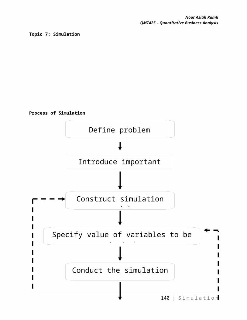
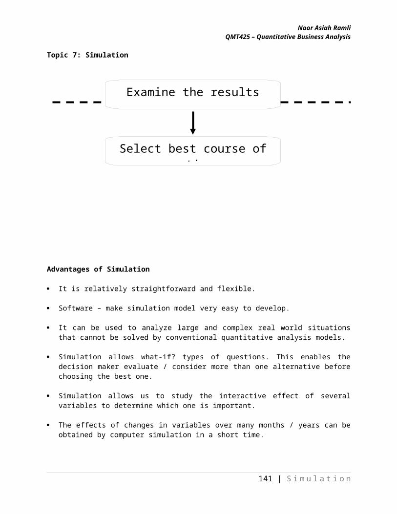
Topic 7: SimulationProcess of Simulation


Construct simulation model

Specify value of variables to be tested

Conduct the simulation

Examine the results

Select best course of action

Define problem

Introduce important variable


Topic 7: SimulationAdvantages of Simulation

It is relatively straightforward and flexible.

Software – make simulation model very easy to develop.

It can be used to analyze large and complex real world situations that cannot be solved by conventional quantitative analysis models.

Simulation allows what-if? types of questions. This enables the decision maker evaluate / consider more than one alternative before choosing the best one.

Simulation allows us to study the interactive effect of several variables to determine which one is important.

The effects of changes in variables over many months / years can be obtained by computer simulation in a short time.

Disadvantages of Simulation

Developing a good simulation model is often a long and complicated process especially for large problems.

Simulation does not give us the optimal solution. It is a trial and error approach that produces different solutions in repeated runs.

The user must generate all of the conditions and constraints for solutions that they want to examine.

The simulation must be done for many trials (100s or 1000s) to get reliable / usable results.

Monte Carlo Technique



Topic 7: Simulation When a system contains elements that exhibit chance (probability) in their behavior, the

Monte Carlo method of simulation can be applied.

The basic idea of Monte Carlo simulation is to generate values for the variables making up the model being studied.

There are a lot of variables in real world systems that are probabilistic in nature such as:

Inventory demand on daily or weekly basis Time between machine breakdown Time between arrivals Service time Time to complete project activities

The basis of Monte Carlo simulation is experimentation on the chance elements through random sampling.

Five steps in Monte Carlo Simulation

STEP 1: Setting up a probability distribution for important variables.

STEP 2: Building a cumulative probability distribution for each variable in STEP 1.

STEP 3: Establish interval of random numbers for each variable.

STEP 4: Generating random numbers.

STEP 5: Simulating a series of trials.

Example 7.1



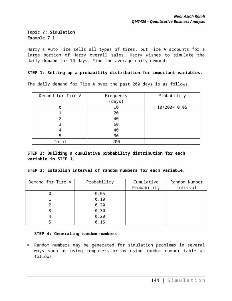
Topic 7: SimulationHarry’s Auto Tire sells all types of tires, but Tire A accounts for a large portion of Harry overall sales. Harry wishes to simulate the daily demand for 10 days. Find the average daily demand. STEP 1: Setting up a probability distribution for important variables.

The daily demand for Tire A over the past 200 days is as follows:

Demand for Tire A Frequency(days)

Probability

012345

102040604030

10/200= 0.05

Total 200

STEP 2: Building a cumulative probability distribution for each variable in STEP 1.

STEP 3: Establish interval of random numbers for each variable.

Demand for Tire A Probability Cumulative Probability

Random Number Interval

012345

0.050.100.200.300.200.15

STEP 4: Generating random numbers.

Random numbers may be generated for simulation problems in several ways such as using computers or by using random number table as follows.

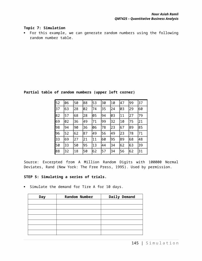
For this example, we can generate random numbers using the following random number table.

Partial table of random numbers (upper left corner)



Topic 7: Simulation52 06 50 88 53 30 10 47 99 37

37 63 28 02 74 35 24 03 29 60

82 57 68 28 05 94 03 11 27 79

69 02 36 49 71 99 32 10 75 21

98 94 90 36 06 78 23 67 89 85

96 52 62 87 49 56 49 23 78 71

33 69 27 21 11 60 95 89 68 48

50 33 50 95 13 44 34 62 63 39

88 32 18 50 62 57 34 56 62 31

Source: Excerpted from A Million Random Digits with 100000 Normal Deviates, Rand (New York: The Free Press, 1995). Used by permission.

STEP 5: Simulating a series of trials.

Simulate the demand for Tire A for 10 days.

Day Random Number Daily Demand

Average daily demand =



Topic 7: Simulation

Example 7.2: Inventory Problem

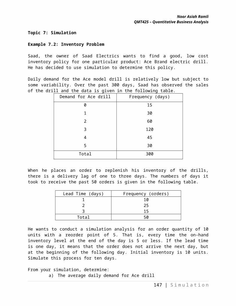
Saad, the owner of Saad Electrics wants to find a good, low cost inventory policy for one particular product: Ace Brand electric drill. He has decided to use simulation to determine this policy.

Daily demand for the Ace model drill is relatively low but subject to some variability. Over the past 300 days, Saad has observed the sales of the drill and the data is given in the following table.

Demand for Ace drill Frequency (days)

0

1

2

3

4

5

15

30

60

120

45

30

Total 300

When he places an order to replenish his inventory of the drills, there is a delivery lag of one to three days. The numbers of days it took to receive the past 50 orders is given in the following table.

Lead Time (days) Frequency (orders)123

102515

Total 50

He wants to conduct a simulation analysis for an order quantity of 10 units with a reorder point of 5. That is, every time the on-hand inventory level at the end of the day is 5 or less. If the lead time is one day, it means that the order does not arrive the next day, but at the beginning of the following day. Initial inventory is 10 units. Simulate this process for ten days.

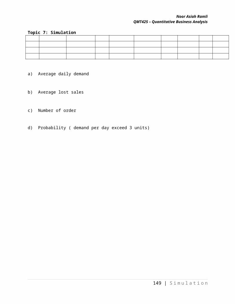
From your simulation, determine:a) The average daily demand for Ace drillb) The average lost salesc) The number of orders placedd) The probability that demand per day exceed 3 units

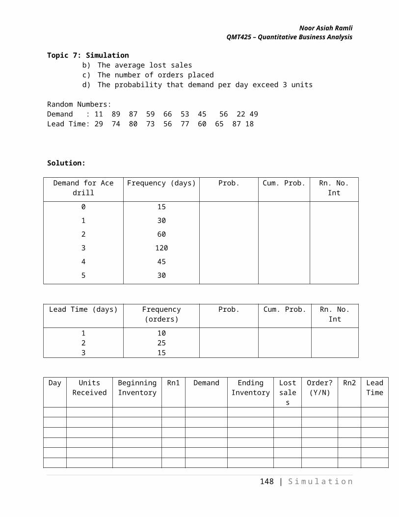
Random Numbers:Demand : 11 89 87 59 66 53 45 56 22 49Lead Time: 29 74 80 73 56 77 60 65 87 18



Topic 7: SimulationSolution:

Demand for Ace drill Frequency (days) Prob. Cum. Prob. Rn. No. Int

0

1

2

3

4

5

15

30

60

120

45

30

Lead Time (days) Frequency (orders) Prob. Cum. Prob. Rn. No. Int

123

102515

Day Units Received

Beginning Inventory

Rn1 Demand Ending Inventory

Lost sales

Order?(Y/N)

Rn2 Lead Time

a) Average daily demand

b) Average lost sales

c) Number of order

d) Probability ( demand per day exceed 3 units)



Topic 7: Simulation

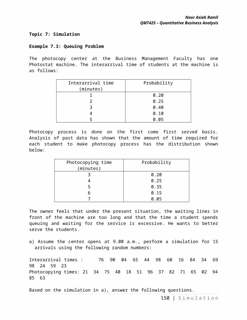
Example 7.3: Queuing Problem

The photocopy center at the Business Management Faculty has one Photostat machine. The interarrival time of students at the machine is as follows:

Interarrival time(minutes)

Probability

12345

0.200.250.400.100.05

Photocopy process is done on the first come first served basis. Analysis of past data has shown that the amount of time required for each student to make photocopy process has the distribution shown below:

Photocopying time(minutes)

Probability

34567

0.200.250.350.150.05

The owner feels that under the present situation, the waiting lines in front of the machine are too long and that the time a student spends queuing and waiting for the service is excessive. He wants to better serve the students.

a) Assume the center opens at 9.00 a.m., perform a simulation for 15 arrivals using the following random numbers:

Interarrival times : 76 90 04 65 44 98 60 16 84 34 69 98 24 59 23Photocopying times: 21 34 75 40 18 51 96 37 82 71 65 02 94 85 63

Based on the simulation in a), answer the following questions.

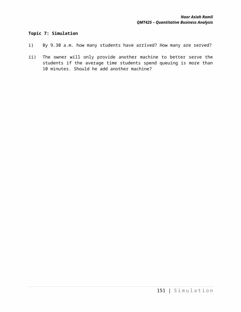
i) By 9.30 a.m. how many students have arrived? How many are served?

ii) The owner will only provide another machine to better serve the students if the average time students spend queuing is more than 10 minutes. Should he add another machine?



Topic 7: Simulation

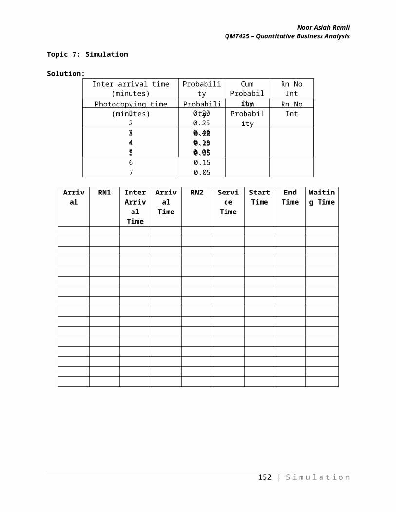
Solution:

Photocopying time (minutes)

Probability Cum Probability

Rn No Int

34567

0.200.250.350.150.05

Arrival RN1 Inter Arrival Time

Arrival Time

RN2 Service Time

Start Time

End Time

Waiting Time


Inter arrival time (minutes) Probability Cum Probability

Rn No Int

12345

0.200.250.400.100.05


Topic 7: Simulation

Problems:

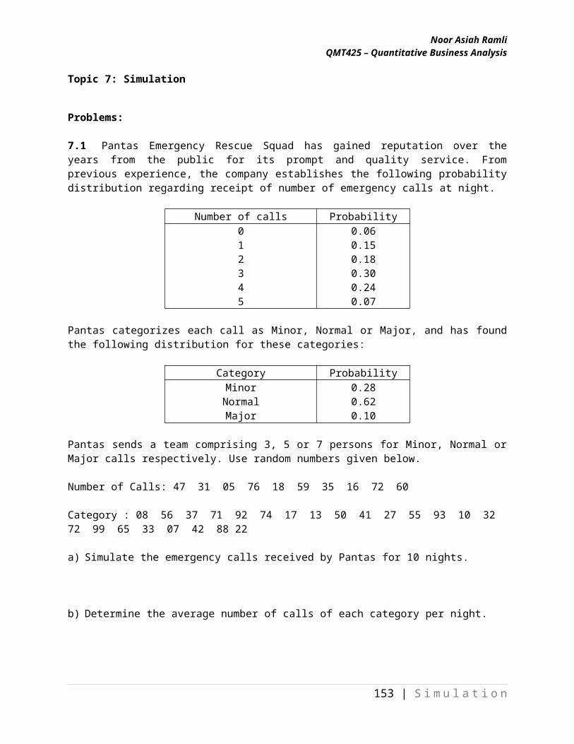
7.1 Pantas Emergency Rescue Squad has gained reputation over the years from the public for its prompt and quality service. From previous experience, the company establishes the following probability distribution regarding receipt of number of emergency calls at night.

Number of calls Probability012345

0.060.150.180.300.240.07

Pantas categorizes each call as Minor, Normal or Major, and has found the following distribution for these categories:

Category ProbabilityMinor

Normal Major

0.280.620.10

Pantas sends a team comprising 3, 5 or 7 persons for Minor, Normal or Major calls respectively. Use random numbers given below.

Number of Calls: 47 31 05 76 18 59 35 16 72 60

Category : 08 56 37 71 92 74 17 13 50 41 27 55 93 10 32 72 99 65 33 07 42 88 22

a) Simulate the emergency calls received by Pantas for 10 nights.

b) Determine the average number of calls of each category per night.

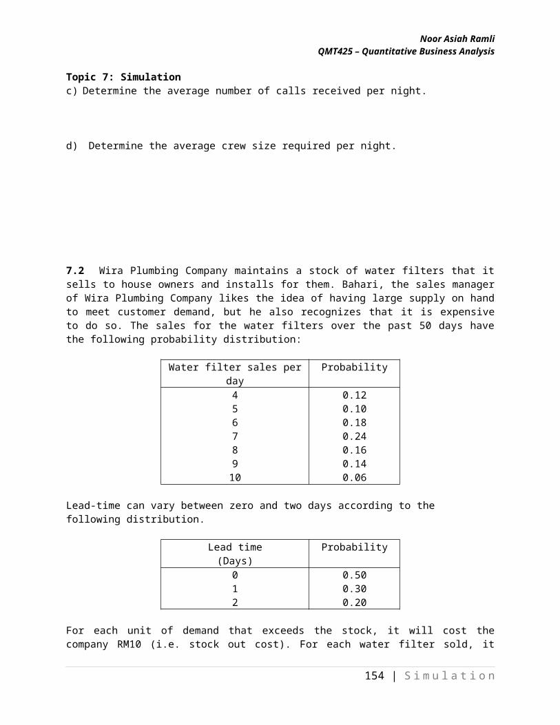
c) Determine the average number of calls received per night.

d) Determine the average crew size required per night.



Topic 7: Simulation

7.2 Wira Plumbing Company maintains a stock of water filters that it sells to house owners and installs for them. Bahari, the sales manager of Wira Plumbing Company likes the idea of having large supply on hand to meet customer demand, but he also recognizes that it is expensive to do so. The sales for the water filters over the past 50 days have the following probability distribution:

Water filter sales per day Probability456789

10

0.120.100.180.240.160.140.06

Lead-time can vary between zero and two days according to the following distribution.

Lead time(Days)

Probability

012

0.500.300.20

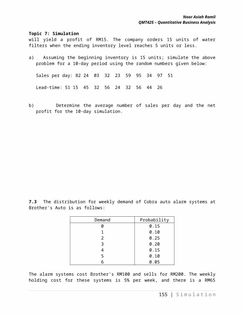
For each unit of demand that exceeds the stock, it will cost the company RM10 (i.e. stock out cost). For each water filter sold, it will yield a profit of RM15. The company orders 15 units of water filters when the ending inventory level reaches 5 units or less.

a) Assuming the beginning inventory is 15 units; simulate the above problem for a 10-day period using the random numbers given below:

Sales per day: 82 24 03 32 23 59 95 34 97 51

Lead-time: 51 15 45 32 56 24 32 56 44 26

b) Determine the average number of sales per day and the net profit for the 10-day simulation.



Topic 7: Simulation

7.3 The distribution for weekly demand of Cobra auto alarm systems at Brother's Auto is as follows:

Demand Probability0123456

0.150.100.250.200.150.100.05

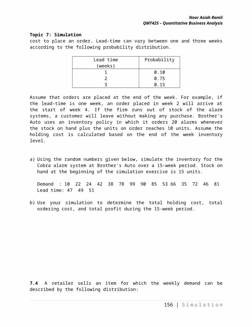
The alarm systems cost Brother's RM100 and sells for RM200. The weekly holding cost for these systems is 5% per week, and there is a RM65 cost to place an order. Lead-time can vary between one and three weeks according to the following probability distribution.

Lead time(weeks)

Probability

123

0.100.750.15

Assume that orders are placed at the end of the week. For example, if the lead-time is one week, an order placed in week 2 will arrive at the start of week 4. If the firm runs out of stock of the alarm systems, a customer will leave without making any purchase. Brother's Auto uses an inventory policy in which it orders 20 alarms whenever the stock on hand plus the units on order reaches 10 units. Assume the holding cost is calculated based on the end of the week inventory level.

a) Using the random numbers given below, simulate the inventory for the Cobra alarm system at Brother's Auto over a 15-week period. Stock on hand at the beginning of the simulation exercise is 15 units.

Demand : 10 22 24 42 38 78 99 90 85 53 66 35 72 46 81Lead time: 47 49 51

b) Use your simulation to determine the total holding cost, total ordering cost, and total profit during the 15-week period.



Topic 7: Simulation

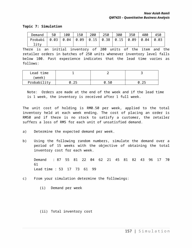
7.4 A retailer sells an item for which the weekly demand can be described by the following distribution:

There is an initial inventory of 200 units of the item and the retailer orders in batches of 250 units whenever inventory level falls below 100. Past experience indicates that the lead time varies as follows:

Lead time (week) 1 2 3Probability 0.25 0.50 0.25

Note: Orders are made at the end of the week and if the lead time is 1 week, the inventory is received after 1 full week.

The unit cost of holding is RM0.50 per week, applied to the total inventory held at each week ending. The cost of placing an order is RM50 and if there is no stock to satisfy a customer, the retailer suffers a loss of RM5 for each unit of unsatisfied demand.

a) Determine the expected demand per week.

b) Using the following random numbers, simulate the demand over a period of 15 weeks with the objective of obtaining the total inventory cost for each week.

Demand : 87 55 81 22 04 62 21 45 81 82 43 96 17 70 61Lead time : 53 17 73 61 99

c) From your simulation determine the followings:

(i) Demand per week

(ii) Total inventory cost


Demand 50 100 150 200 250 300 350 400 450Probability 0.03 0.04 0.09 0.15 0.38 0.15 0.09 0.04 0.03


Topic 7: Simulation7.5 HiTec Computers is considering using e-commerce to sell its computers directly over the internet. It is planning to monitor the website 24 hours a day with a supervisor and a trainee. If an order arrives when both of them are free, the order will be processed by the supervisor. However, if both of them are busy, the order will be put in a queue until one of them is available. Operations data are estimated to be as follows:

Time Between Orders

(minutes)

ProbabilitySupervisor’s Service

Time (minutes)

ProbabilityTrainee’s Service

Time (minutes)

Probability

2345

0.350.300.200.15

4567

0.300.250.250.20

6789

0.100.100.600.20

a) Develop a simulation model for this problem. Run the simulation for 10 orders. The simulation should include the arrival of order time, start and end service times, and waiting time in the queue. Start your simulation at 8.00 am.

b) The management of the company is interested in the average amount of time incoming orders will spend in the queue.

Use the following random numbers for time between orders and service time.

Time between orders: 06 61 70 88 11 52 82 12 35 99Service time : 38 74 31 39 51 83 60 81 36 96



Topic 7: Simulation7.6 Penang International Airport primarily serves domestic air traffic. However, chartered planes from abroad may occasionally arrive with passengers bound for Langkawi Island and other tourist destinations around Penang. There is one immigration officer and one custom officer available –at any time. Whenever an international plane arrives at the airport, the immigration and customs officers on duty will set up operations to process the passengers. Incoming passengers must first have their passports and visas checked by the immigration officer. The time required to check a passenger's passport and visa can be described by the following probability distribution:

Time required to check a passenger’s Passport & Visa

(seconds)

Probability

20406080

0.200.400.300.10

After having their passports and visas checked, the passengers proceed to the customs officer who will inspect their baggage. Passengers form a single waiting line and baggage are inspected on a first come, first serve basis. The time required for baggage inspection has the following probability distribution:

Time required for baggage inspection

(minutes)

Probability

0123

0.250.600.100.05

a) Suppose a chartered plane from abroad with 100 passengers lands at Penang Airport. Simulate the immigration and customs clearance process for the first 10 passengers and determine how long it will take them to clear the process. Use the following random numbers:

passport & visa check: 93 63 26 16 21 26 70 55 72 89

baggage inspection: 13 08 60 13 68 40 40 27 23 64

b) What is the average length of time a customer has to wait before having his baggage inspected after clearing passport control?



Topic 7: Simulation7.7 Com War Sdn. Bhd. produces monitors and printers for computers. Currently, all the monitors and printers are channeled to an inspection station, one at a time as they are completed. The interarrival time (in minutes) for the monitors has the following probability distribution:

Interarrival Time (minutes)

Probability

101214161820

0.050.100.200.300.250.10

The interarrival time for the printers, on the other hand, is constant at 15 minutes. The inspection station has two inspectors. One inspector works on the monitors only and the other one inspects the printers only. In either case, the inspection time (in minutes) has the following probability distribution:

Inspection Time (minutes)

Probability

5101520

0.150.250.400.20

The management wants to evaluate the waiting time for monitors at the inspection station.

a) Perform a simulation on the arrivals of the first 10 monitors at the inspection station. From the simulation, compute the average waiting time before beginning of inspection. Use the following random numbers:

Interarrival Time: 55 27 78 09 86 44 37 95 15 62

Inspection Time: 63 12 98 35 48 87 05 71 24 56

The management is considering training the two inspectors to work on either product. This is to prepare them for a new inspection procedure. Under the new procedure, a finished product will be channeled to either inspector for inspection.

b) Consider the arrivals of the first 10 products (printers and monitors) at the inspection station. Perform a simulation to determine the average waiting time (before inspection) for the monitors and printers. Use the random numbers from part (a).



Topic 7: Simulation7.8

a) Tech Rep Manufacturing Company is monitoring the breakdowns and repairs for one of its machines. The elapsed time between breakdowns of this particular machine has the following distribution.

Time Between Breakdowns(Days)

Probability

1020304050

0.050.250.400.200.10

When the machine breaks down, it must be repaired; and it takes either one, two, or three days for the repair to be completed. The probability distribution for machine repair time is as shown below.

Machine Repair Time (Days)

Probability

123

0.100.700.20

Every time the machine breaks down, the cost to the company is estimated at RM2000 per day in lost production until the machine is repaired. Simulate the existing maintenance system for the machine to determine the cost due to repair time for one year (365 days). Use as many of the following random numbers needed to conduct the simulation.

Breakdowns: 45 90 84 17 74 94 07 90 04 32 29 95 73 28 64 27 00 53 90 14

Repair Time : 19 65 54 10 61 87 74 15 33 11 26 29 18 57 85 00 12 89 43 72

You may use the template shown below to conduct the simulation.

Breakdown Random Number

Time Between

Breakdowns (Days)

Random Number

Repair Time

(Days)

Cumulative Time

(Days)

What is the annual repair cost for the machine?



Topic 7: Simulation

b) Tech Rep would like to know if it should implement a maintenance program at the cost of RM15000 per year that would reduce the frequency of breakdowns and thus the time for repair. The maintenance program would result in the following distribution for time between breakdowns.

Time Between Breakdowns(Days)

Probability

102030405060

0.050.100.150.300.250.15

The repair time resulting from the maintenance program has the following distribution.

Machine Repair Time (Days)

Probability

123

0.400.500.10

Simulate the breakdown and repair system with the maintenance program using the random numbers in part (a). Determine the annual repair cost and make a recommendation to Tech Rep on whether the maintenance program should be implemented.


Documents

QMT425.429-T7 Simulation 7