QM Reminder

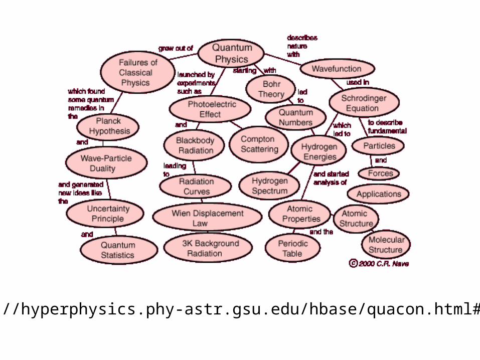
C Nave @ gsu.edu

http://hyperphysics.phy-astr.gsu.edu/hbase/quacon.html#quacon

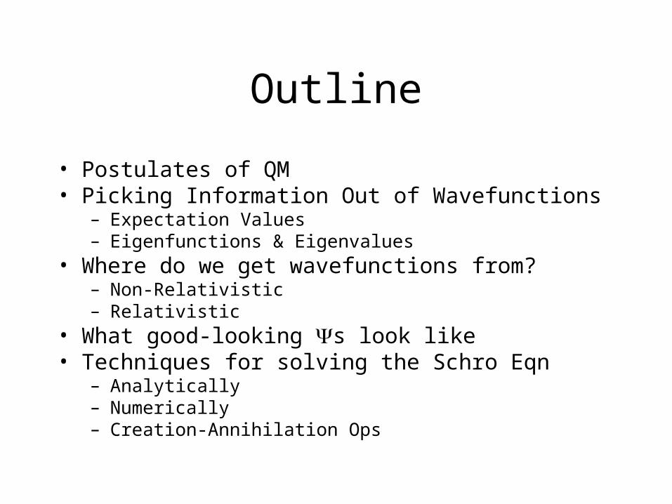
Outline

• Postulates of QM• Picking Information Out of Wavefunctions

– Expectation Values– Eigenfunctions & Eigenvalues

• Where do we get wavefunctions from?– Non-Relativistic– Relativistic

• What good-looking s look like• Techniques for solving the Schro Eqn

– Analytically– Numerically– Creation-Annihilation Ops

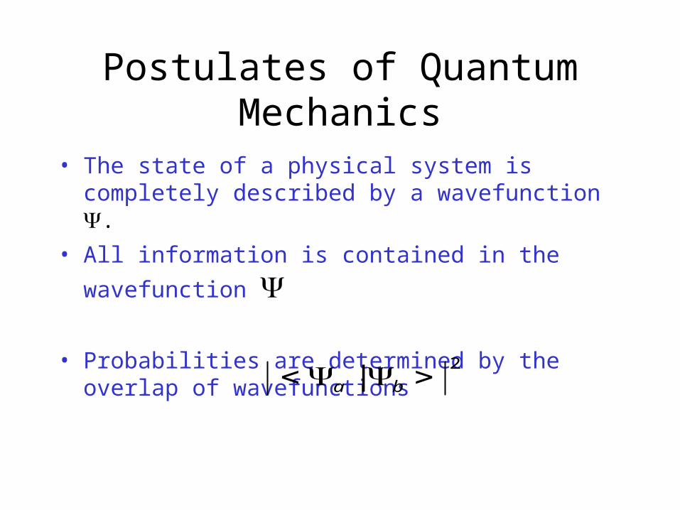
Postulates of Quantum Mechanics

• The state of a physical system is completely described by a wavefunction .

• All information is contained in the wavefunction

• Probabilities are determined by the overlap of wavefunctions

2| ba

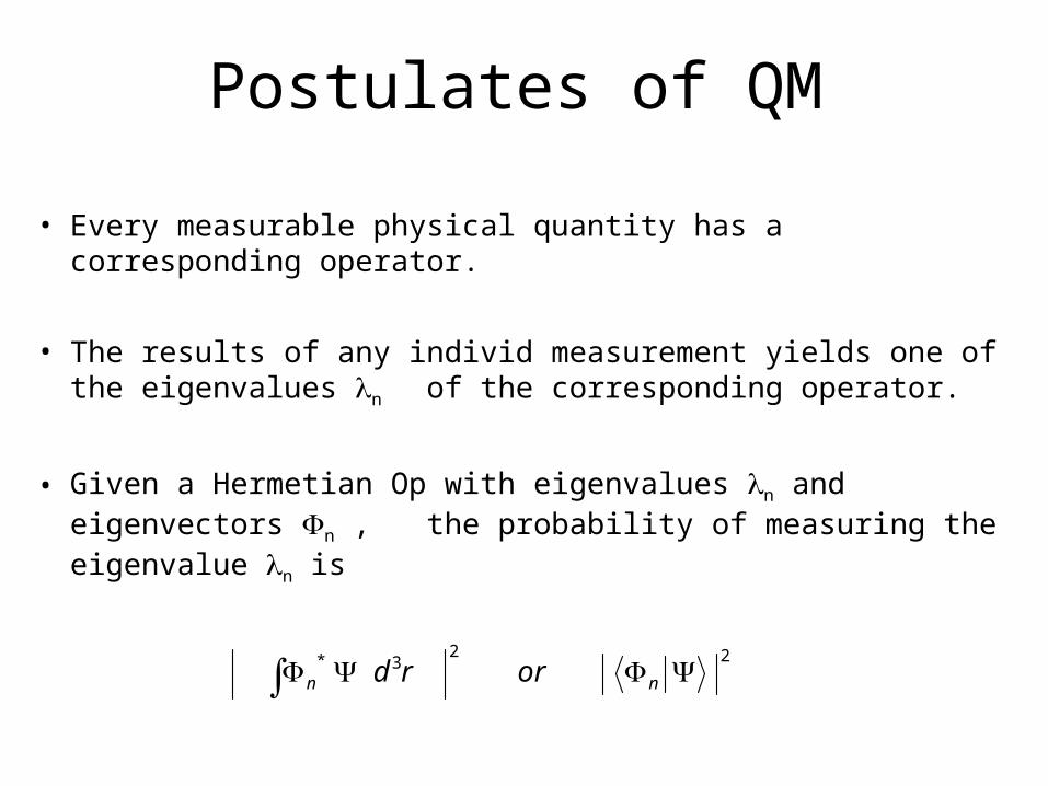
Postulates of QM

• Every measurable physical quantity has a corresponding operator.

• The results of any individ measurement yields one of the eigenvalues n of the corresponding operator.

• Given a Hermetian Op with eigenvalues n and eigenvectors n ,the probability of measuring the eigenvalue n is

223* nn orrd

Postulates of QM

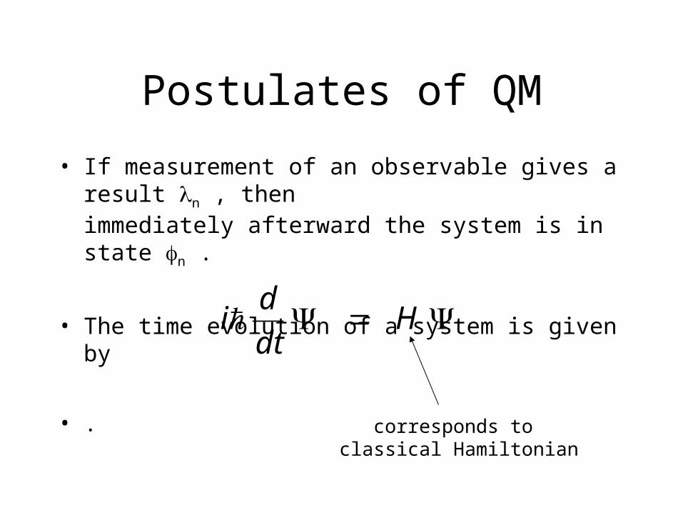
• If measurement of an observable gives a result n , then immediately afterward the system is in

state n .

• The time evolution of a system is given by

• .

Hdt

di

corresponds to classical Hamiltonian

Picking Information out of Wavefunctions

Expectation ValuesEigenvalue Problems

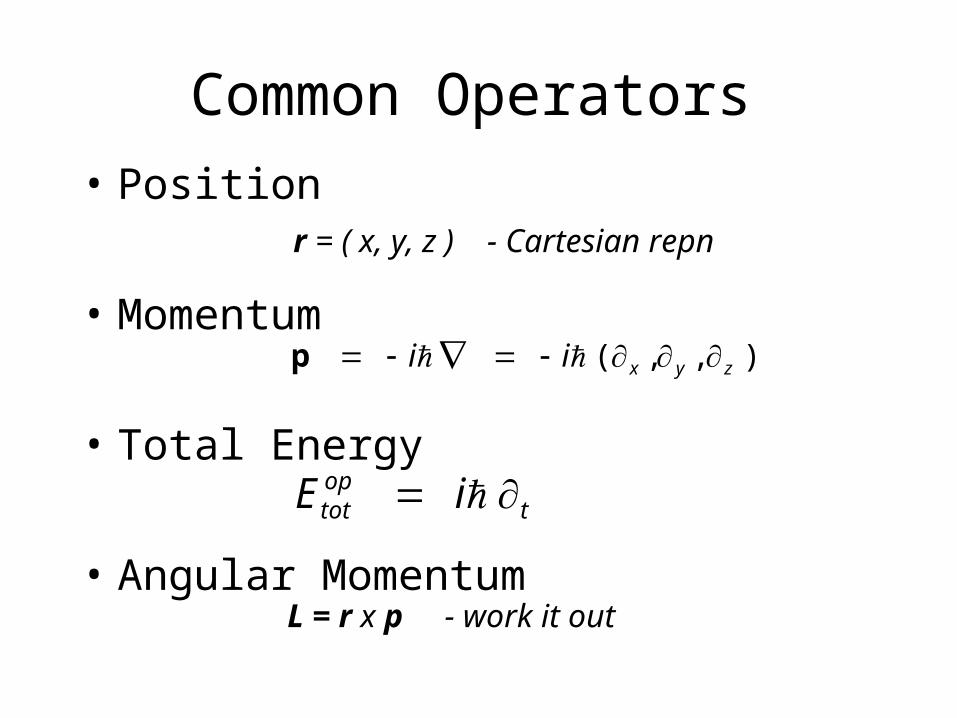
Common Operators

• Position

• Momentum

• Total Energy

• Angular Momentum

r = ( x, y, z ) - Cartesian repn

),,( zyxii p

toptot iE

L = r x p - work it out

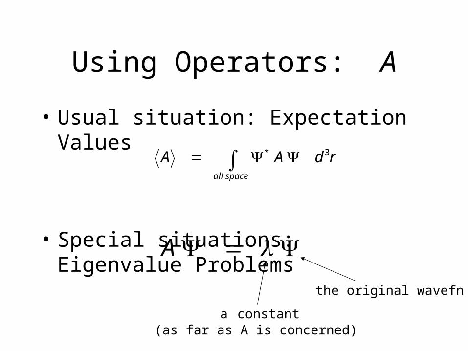
Using Operators: A

• Usual situation: Expectation Values

• Special situations: Eigenvalue Problems

rdAAspaceall

3*

A

the original wavefn

a constant(as far as A is concerned)

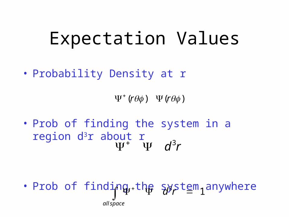
Expectation Values

• Probability Density at r

• Prob of finding the system in a region d3r about r

• Prob of finding the system anywhere

)()( rr

rd 3

13 rdspaceall

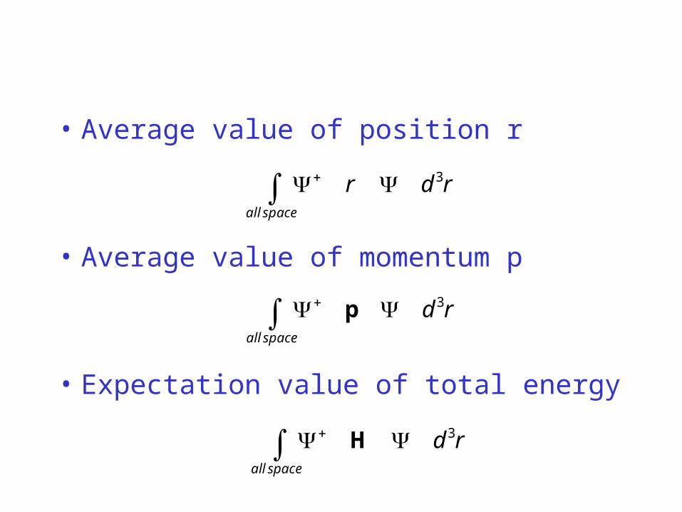
• Average value of position r

• Average value of momentum p

• Expectation value of total energy

rdrspaceall

3

rdspaceall

3 p

rdspaceall

3 H

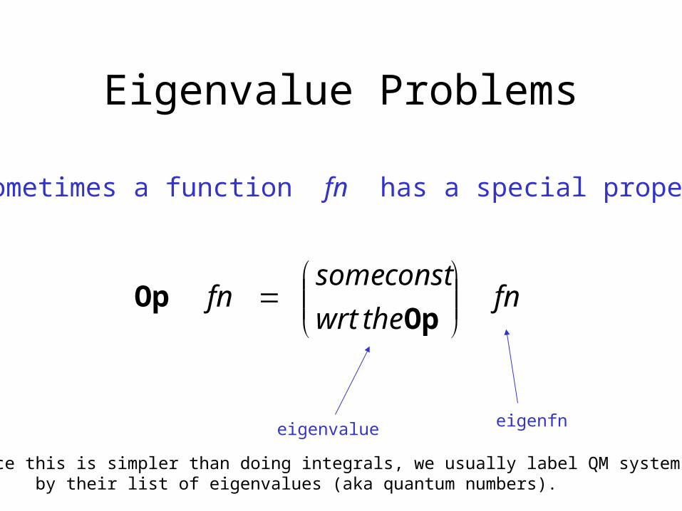
Eigenvalue Problems

Sometimes a function fn has a special property

fnthewrt

constsomefn

OpOp

eigenvalue eigenfn

Since this is simpler than doing integrals, we usually label QM systems by their list of eigenvalues (aka quantum numbers).

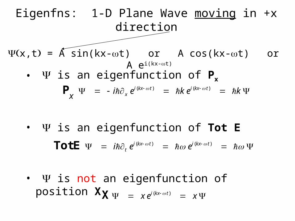
Eigenfns: 1-D Plane Wave moving in +x direction

x,t = A sin(kx-t) or A cos(kx-t) or A ei(kx-t)

• is an eigenfunction of Px

• is an eigenfunction of Tot E

• is not an eigenfunction of position X

kekeix

tkxitkxix )()( P

)()( tkxitkxit eeiETot

xex tkxi )( X

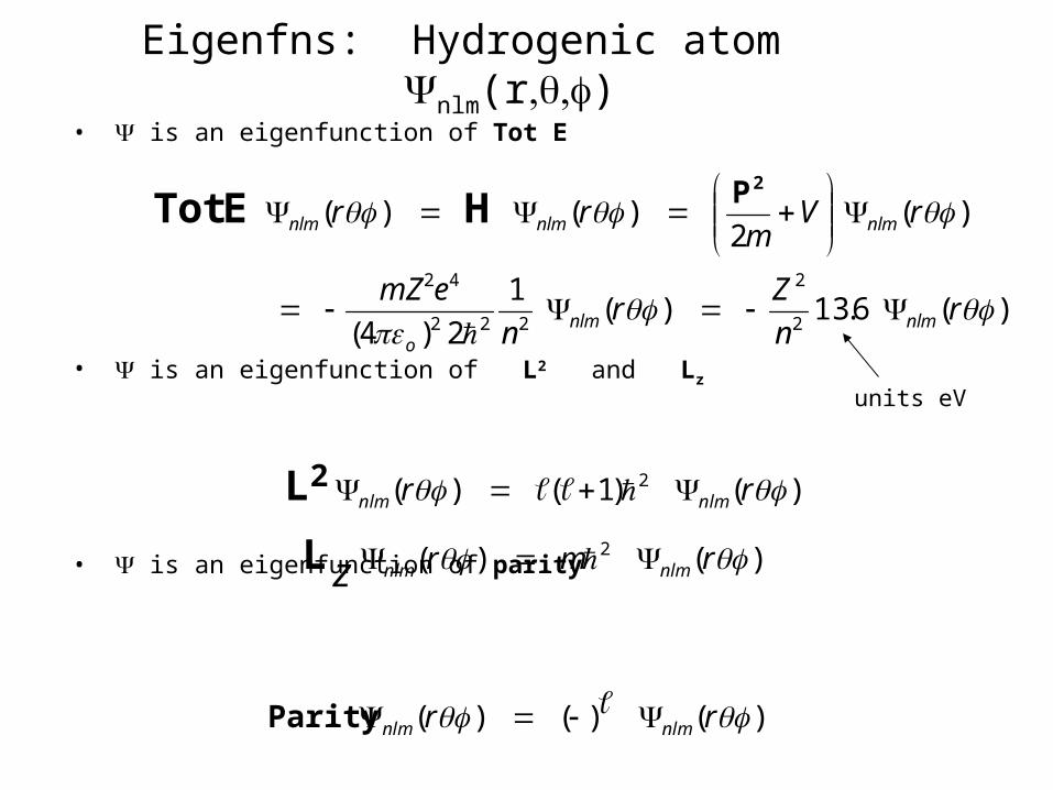
Eigenfns: Hydrogenic atom nlm(r)

• is an eigenfunction of Tot E

• is an eigenfunction of L2 and Lz

• is an eigenfunction of parity

)(6.13)(1

2)4(

)(2

)()(

2

2

222

42

rn

Zr

n

emZ

rVm

rr

nlmnlmo

nlmnlmnlm

2PHETot

)()1()( 2 rr nlmnlm 2L

units eV

)()( 2 rmr nlmnlmz L

)()()( rr nlmnlm Parity

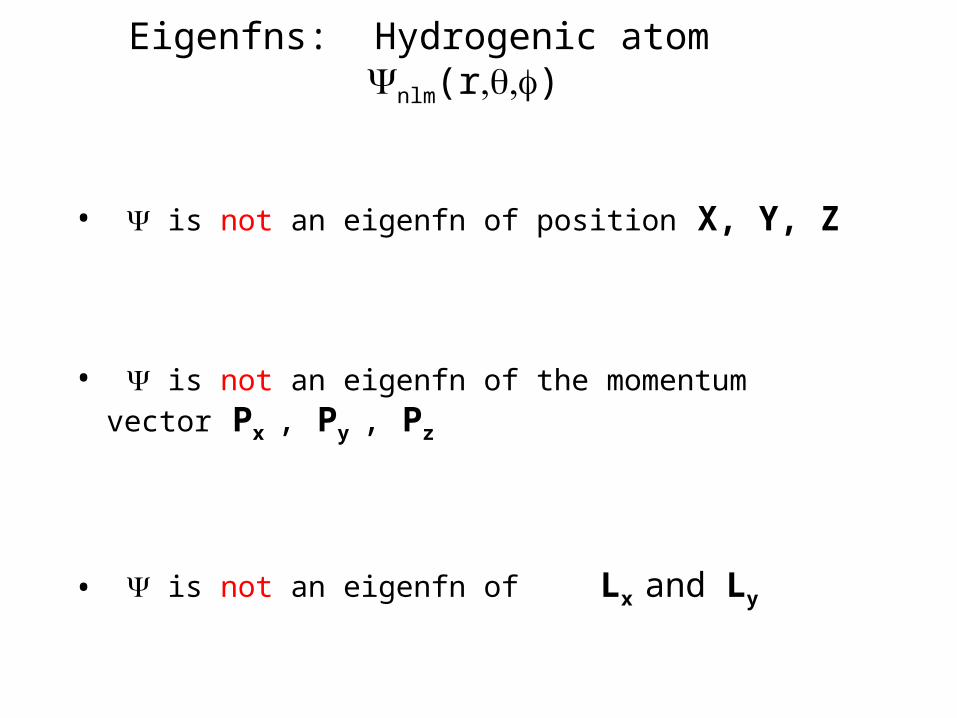
Eigenfns: Hydrogenic atom nlm(r)

• is not an eigenfn of position X, Y, Z

• is not an eigenfn of the momentum vector Px , Py , Pz

• is not an eigenfn of Lx and Ly

Where Wavefunctions come from

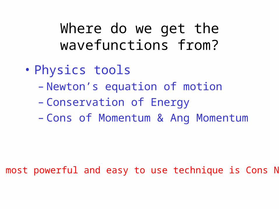
Where do we get the wavefunctions from?

• Physics tools– Newton’s equation of motion– Conservation of Energy– Cons of Momentum & Ang Momentum

The most powerful and easy to use technique is Cons NRG.

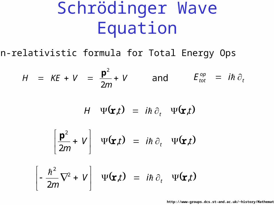
Schrödinger Wave Equation

Vm

VKEH 2

2p

Use non-relativistic formula for Total Energy Ops

toptot iE and

titH t ,, rr

titVm t ,,

2

2

rrp

titVm t ,,

22

2

rr

http://www-groups.dcs.st-and.ac.uk/~history/Mathematicians

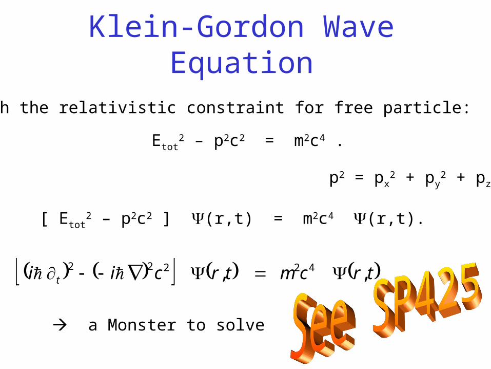
Klein-Gordon Wave Equation

Start with the relativistic constraint for free particle:

Etot2 – p2c2 = m2c4 .

[ Etot2 – p2c2 ] (r,t) = m2c4 (r,t).

trcmtrcii t ,, 42222

p2 = px2 + py

2 + pz2

a Monster to solve

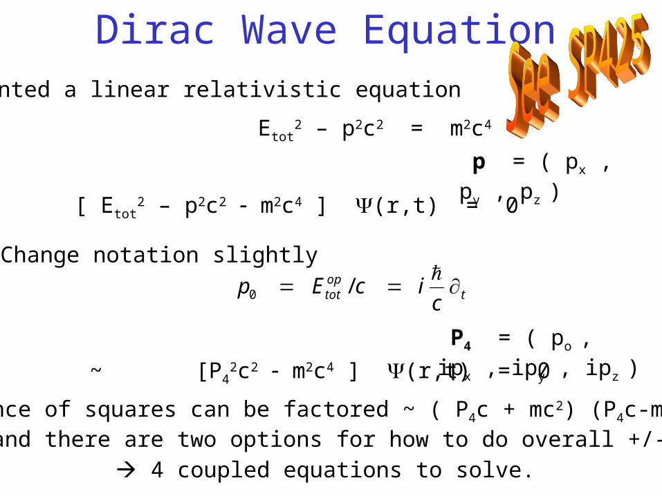
Dirac Wave EquationWanted a linear relativistic equation

[ Etot2 – p2c2 m2c4 ] (r,t) = 0

Etot2 – p2c2 = m2c4

Change notation slightly

toptot c

icEp

/0

p = ( px , py , pz )

~ [P42c2 m2c4 ] (r,t) = 0

P4 = ( po , ipx , ipy , ipz )

difference of squares can be factored ~ ( P4c + mc2) (P4c-mc2) and there are two options for how to do overall +/- signs

4 coupled equations to solve.

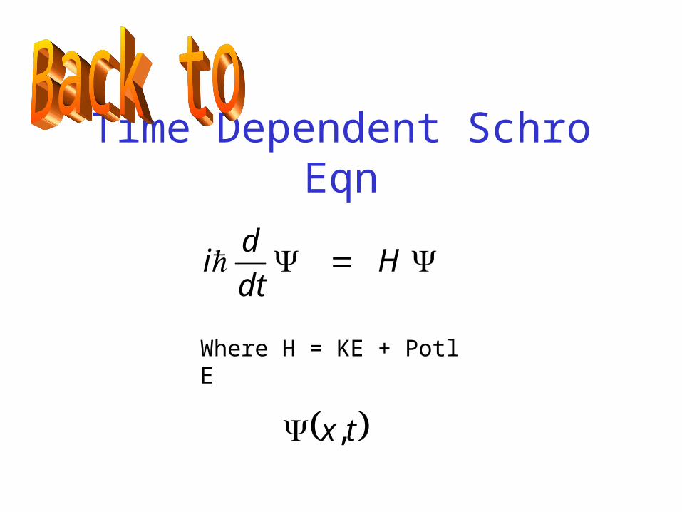
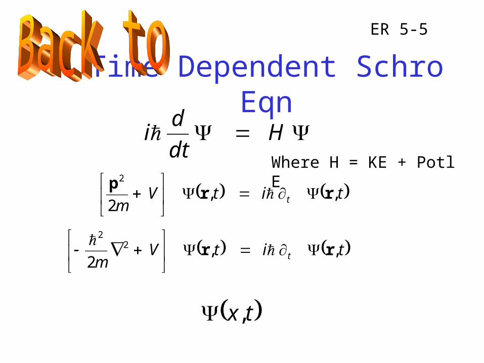
Time Dependent Schro Eqn

Hdt

di

Where H = KE + Potl E

tx,

Time Dependent Schro Eqn

Hdt

di

Where H = KE + Potl E

tx,

titVm t ,,

2

2

rrp

titVm t ,,

22

2

rr

ER 5-5

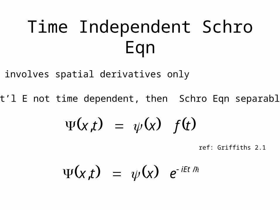
Time Independent Schro Eqn

KE involves spatial derivatives only

If Pot’l E not time dependent, then Schro Eqn separable

tfxtx ,

/, iEtextx

ref: Griffiths 2.1

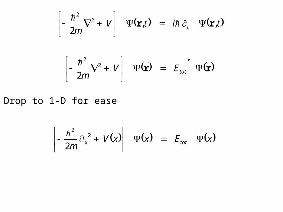
titVm t ,,

22

2

rr

rr

totEV

m2

2

2

xExxVm totx

2

2

2

Drop to 1-D for ease

What Good Wavefunctions Look Like

ER 5-6

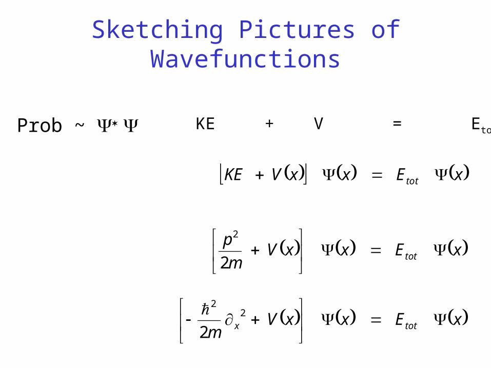
Sketching Pictures of Wavefunctions

xExxVm totx

2

2

2

xExxVm

ptot

2

2

xExxVKE tot

KE + V = EtotProb ~

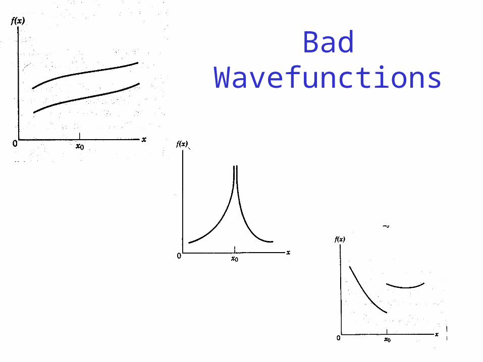
Bad Wavefunctions

xExxVm totx

2

2

2

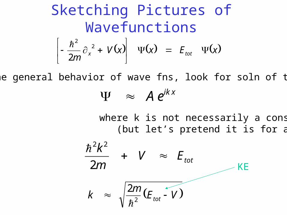
To examine general behavior of wave fns, look for soln of the form

xikeA where k is not necessarily a constant (but let’s pretend it is for a sec)

totEVm

k

2

22

VEm

k tot 2

2

Sketching Pictures of Wavefunctions

KE

VEm

k tot 2

2

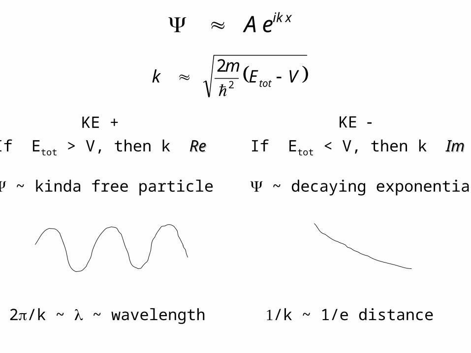
xikeA

If Etot > V, then k ReRe

~ kinda free particle

If Etot < V, then k ImIm

~ decaying exponential

2/k ~ ~ wavelength /k ~ 1/e distance

KE + KE

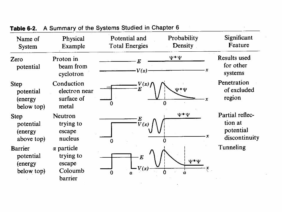
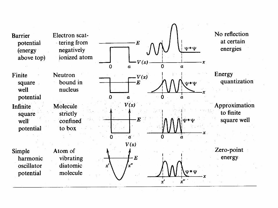
Sample (x) Sketches

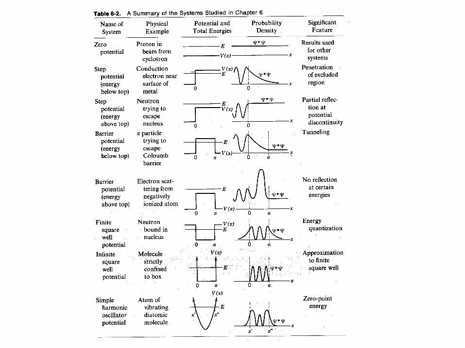
• Free Particles

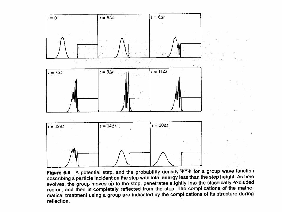
• Step Potentials

• Barriers

• Wells

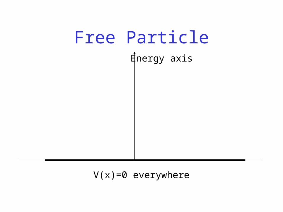
Free ParticleEnergy axis

V(x)=0 everywhere

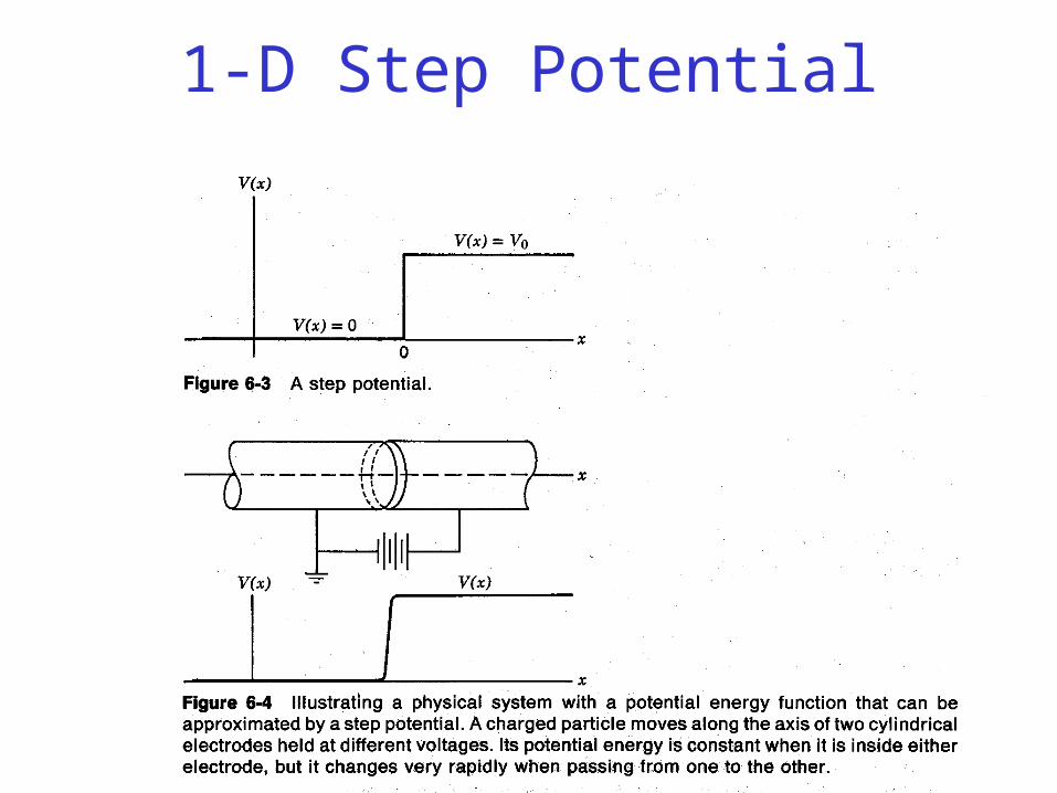
1-D Step Potential

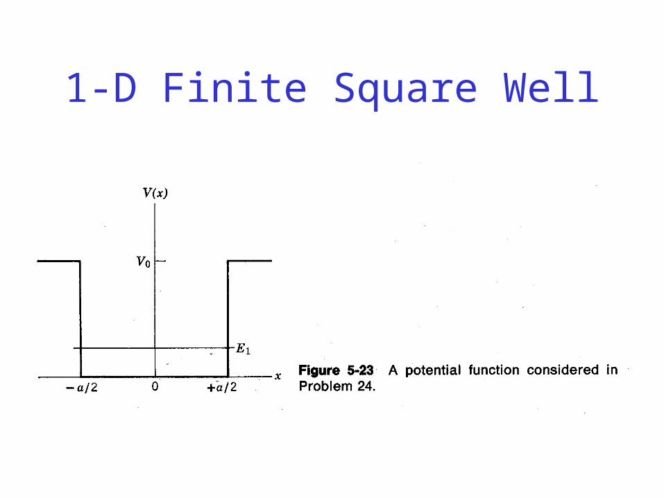
1-D Finite Square Well

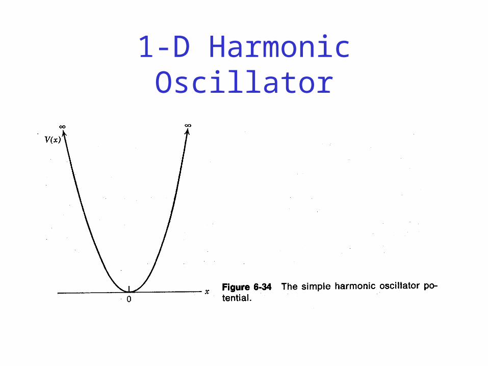
1-D Harmonic Oscillator

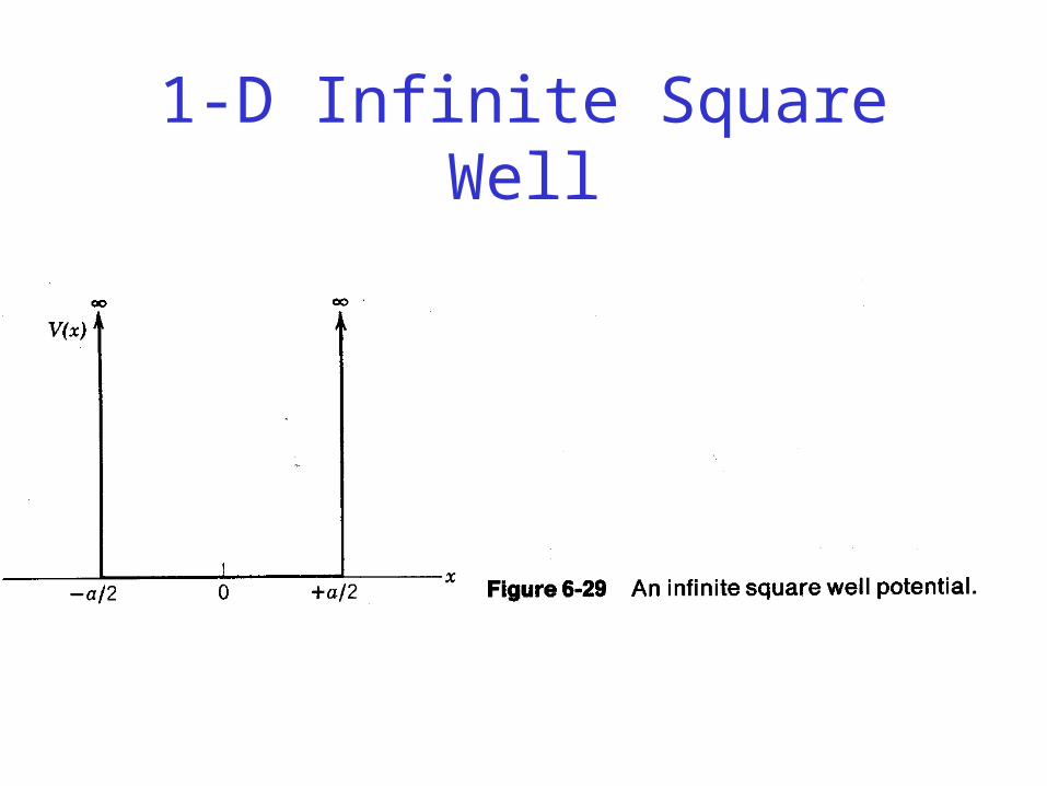
1-D Infinite Square Well

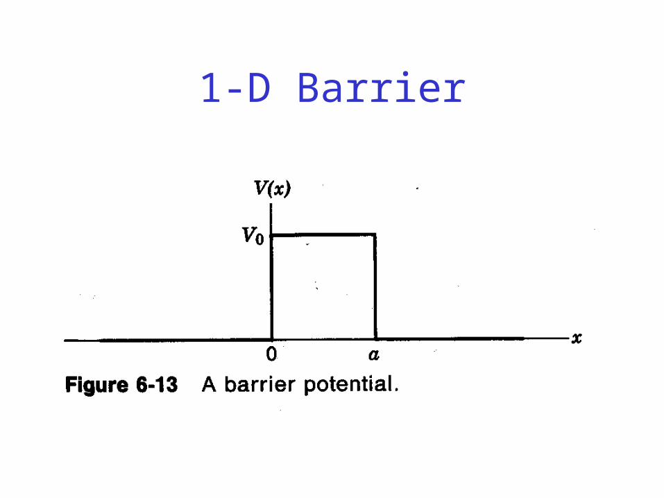
1-D Barrier

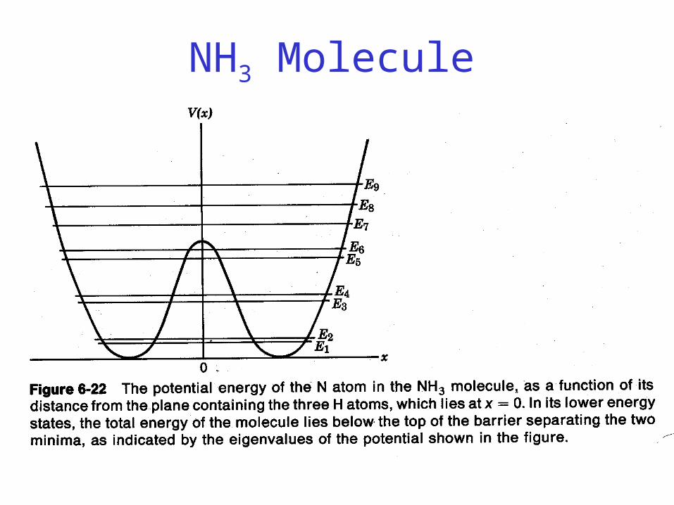
NH3 Molecule

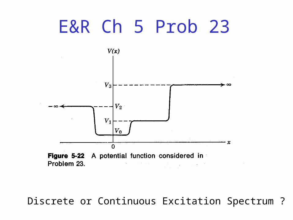
E&R Ch 5 Prob 23

Discrete or Continuous Excitation Spectrum ?

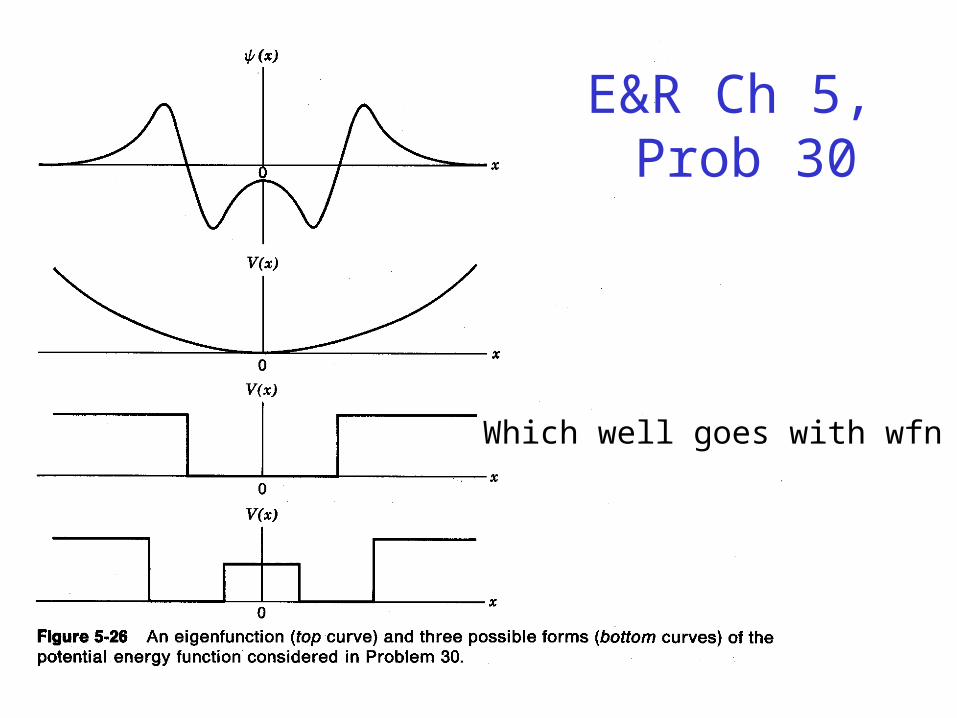
E&R Ch 5, Prob 30

Which well goes with wfn ?

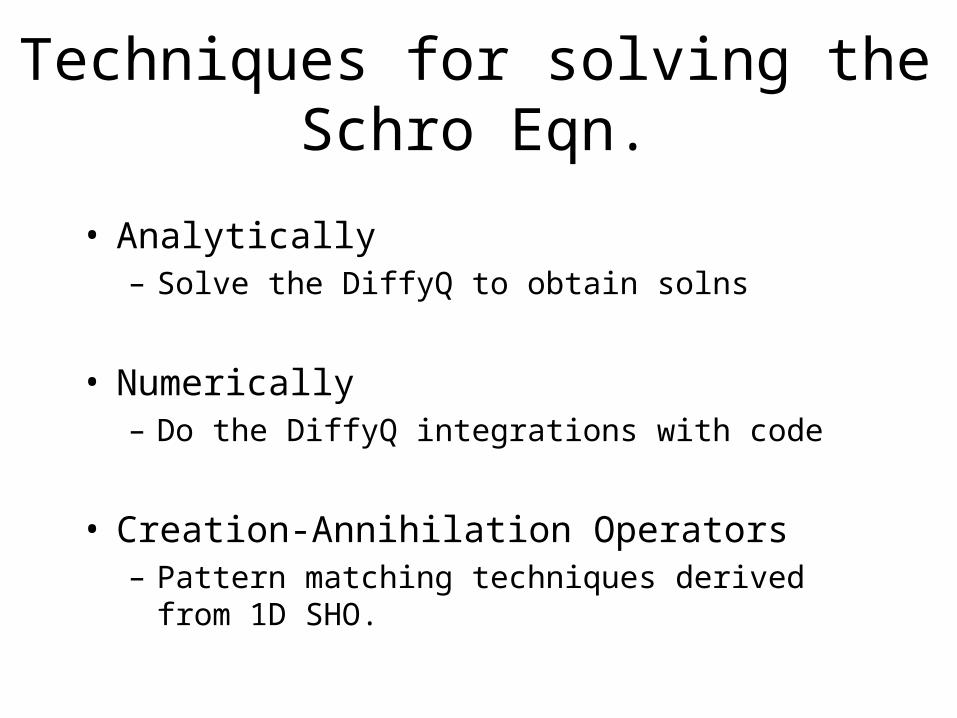
Techniques for solving the Schro Eqn.

• Analytically– Solve the DiffyQ to obtain solns

• Numerically– Do the DiffyQ integrations with code

• Creation-Annihilation Operators– Pattern matching techniques derived from 1D SHO.

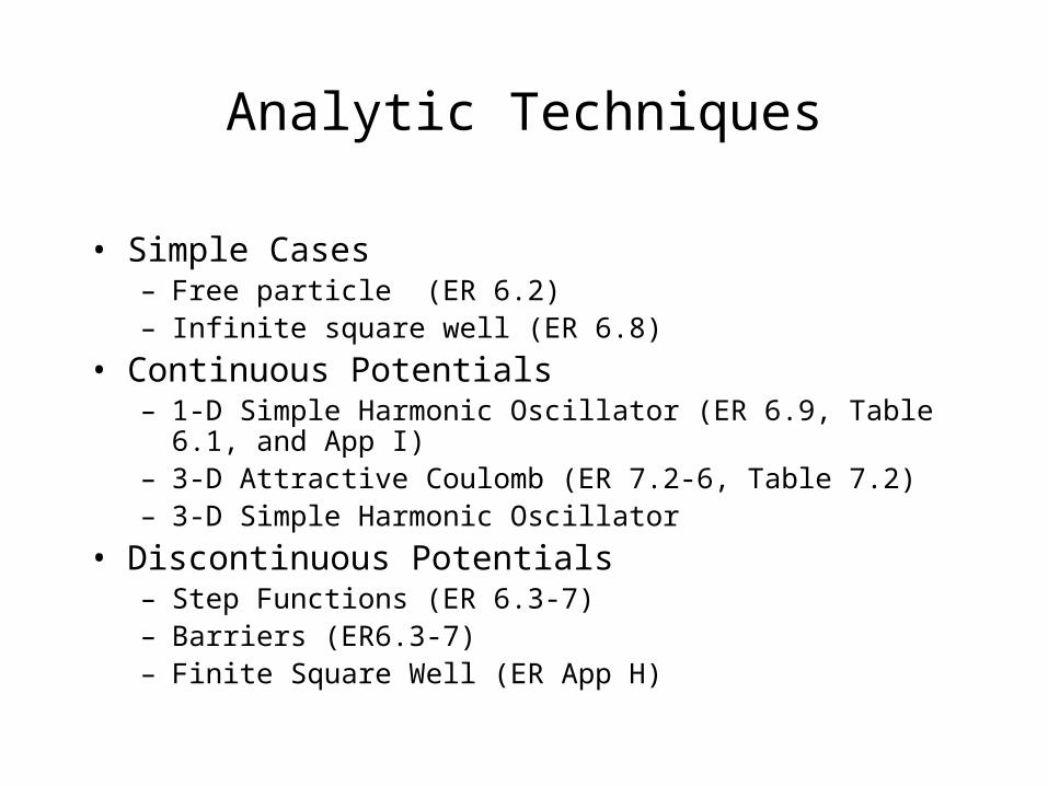
Analytic Techniques

• Simple Cases– Free particle (ER 6.2)– Infinite square well (ER 6.8)

• Continuous Potentials– 1-D Simple Harmonic Oscillator (ER 6.9, Table 6.1, and App I)– 3-D Attractive Coulomb (ER 7.2-6, Table 7.2)– 3-D Simple Harmonic Oscillator

• Discontinuous Potentials– Step Functions (ER 6.3-7)– Barriers (ER6.3-7)– Finite Square Well (ER App H)

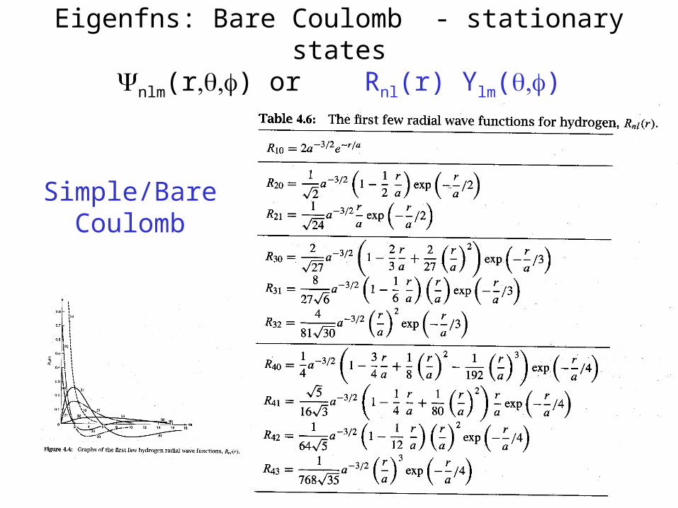
Simple/Bare Coulomb

Eigenfns: Bare Coulomb - stationary statesnlm(r) or Rnl(r) Ylm()

Numerical Techniques

• Using expectations of what the wavefn should look like…– Numerical integration of 2nd order DiffyQ

– Relaxation methods

– ..

– ..

– Joe Blow’s idea

– Willy Don’s idea

– Cletus’ lame idea

– ..

– ..

ER 5.7, App G

SHO Creation-Annihilation Op Techniques

xmpim

a ˆˆ2

1ˆ

xmpi

ma ˆˆ

2

1ˆ

22

2

1

2

1

2

ˆ)( xk

m

paa H

Define:

ipx ˆ, 1ˆ,ˆ aa

If you know the gnd state wavefn o, then the nth excited state is:

ona ˆ

Inadequacy of Techniques

• Modern measurements require greater accuracy in model predictions.– Analytic– Numerical– Creation-Annihilation (SHO, Coul)

• More Refined Potential Energy Fn: V()– Time-Independent Perturbation Theory

• Changes in the System with Time– Time-Dependent Perturbation Theory