Embed Size (px)
Citation preview
QGIS
Launch QGIS
• Launch QGIS from
Start All Programs Quantum GIS
OROR
QGIS Icon on the desk top
• Open window Quantum GIS (Figure 1.1 below)
2
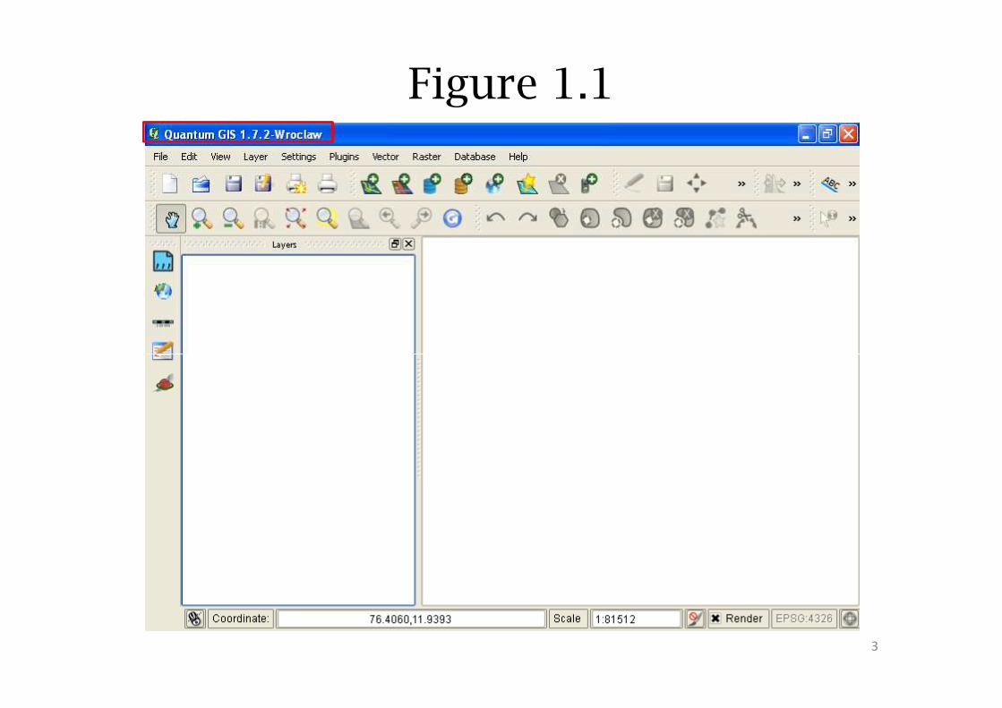
Figure 1.1
3
Opening Raster
• For this exercise we demonstrate three types of GIS data� point
� line
� polygon.
• These require geo-referenced base data. Such base datacould be in the form of� Topo sheetsTopo sheets
� Cadastral maps (village maps)
� Remote sensed imageseg., Google earth images, IRS data, LANDSAT data.
• The accompanying CD provides a registered image namednugu.tif.
• Open this file by selecting Add Raster Layer icon (Figure1.2)
4
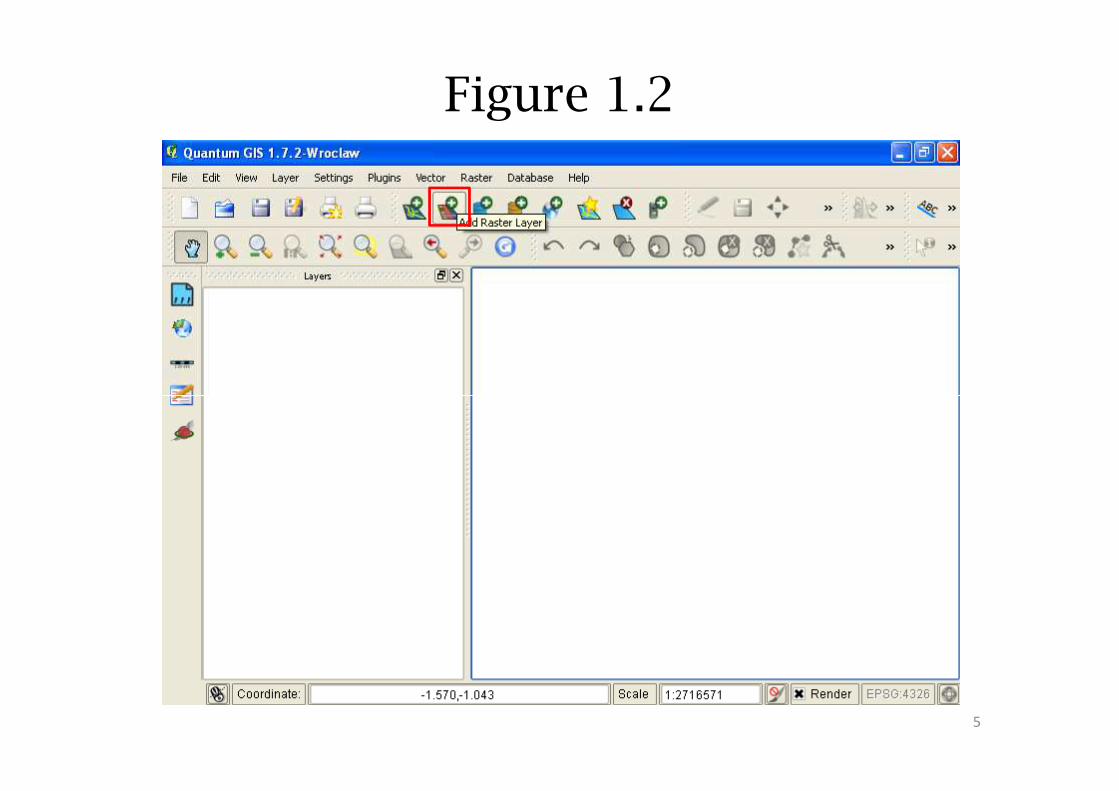
Figure 1.2
5
Opening Raster
• Open a GDAL Supported Raster Data Source
window opens (Figure 1.3)
• Select nugu.tif and select Open (Figure 1.3)• Select nugu.tif and select Open (Figure 1.3)
• Observe the nugu.tif opened in the window
(Figure 1.4 )
6
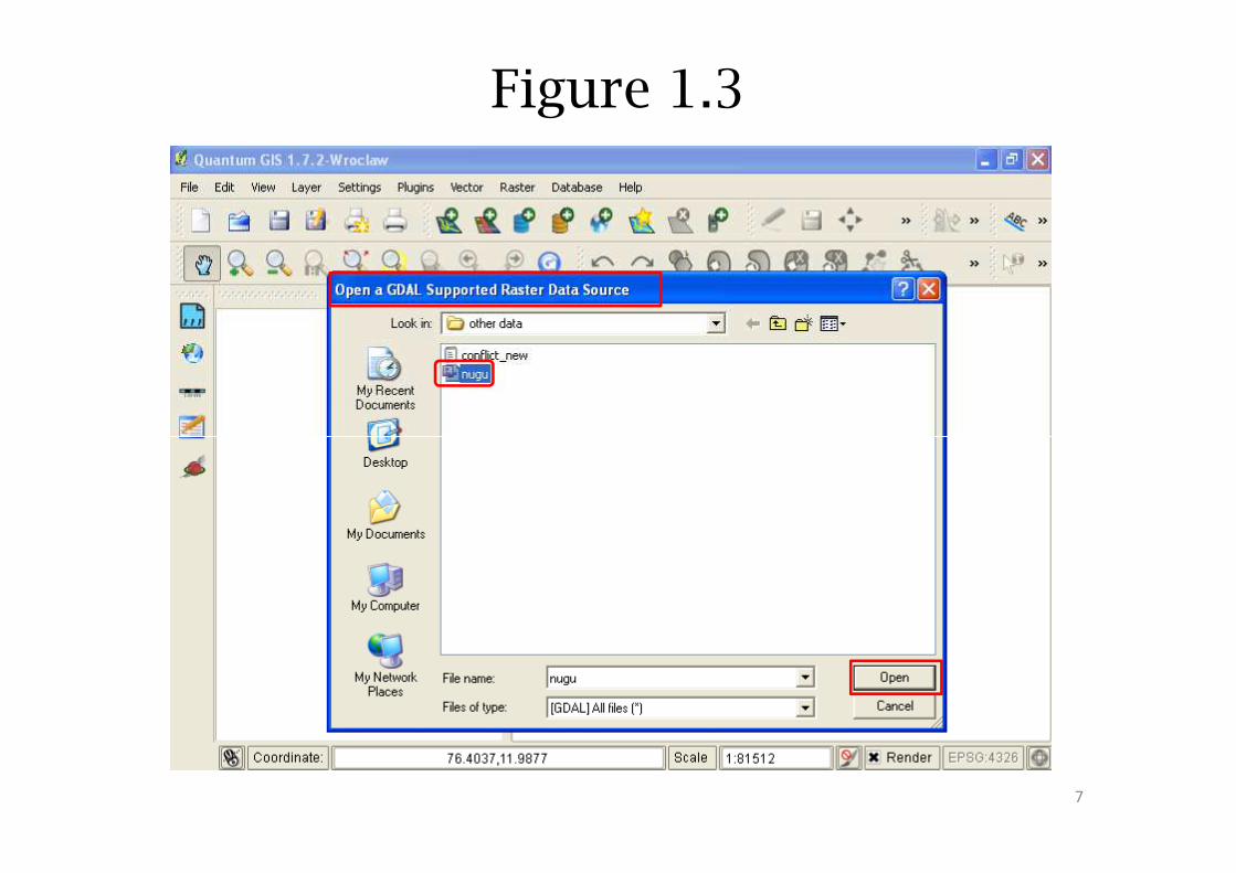
Figure 1.3
7
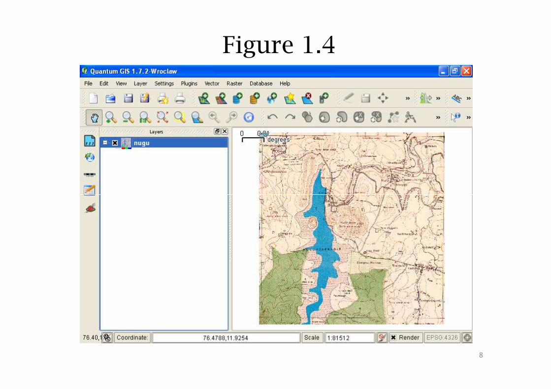
Figure 1.4
8
Verifying geo-referencing
• The opened raster file is geo-referenced
• To confirm the geo-referencing move the
cursor on the opened map; coordinates
change in the coordinate window at thechange in the coordinate window at the
bottom of the screen (Figure 1.5)
9
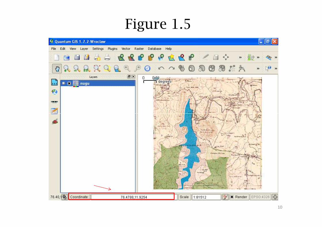
Figure 1.5
10
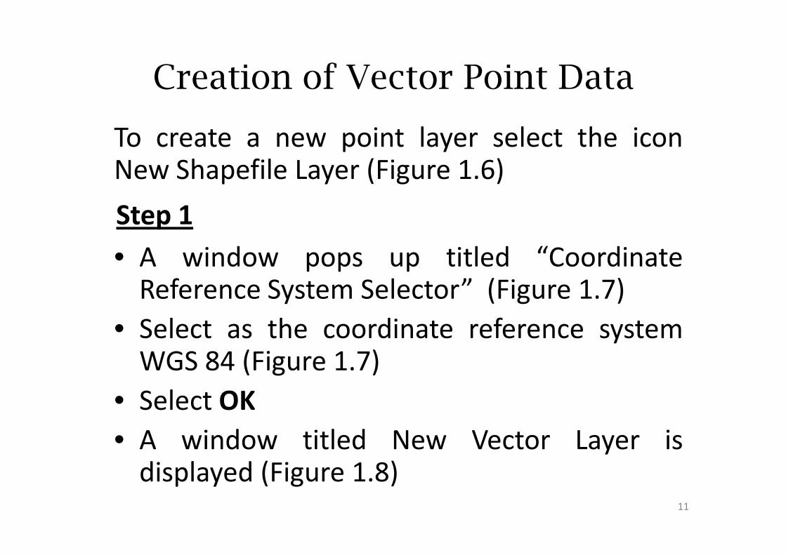
Creation of Vector Point Data
To create a new point layer select the iconNew Shapefile Layer (Figure 1.6)
• A window pops up titled “CoordinateReference System Selector” (Figure 1.7)
Step 1
Reference System Selector” (Figure 1.7)
• Select as the coordinate reference systemWGS 84 (Figure 1.7)
• Select OK
• A window titled New Vector Layer isdisplayed (Figure 1.8)
11
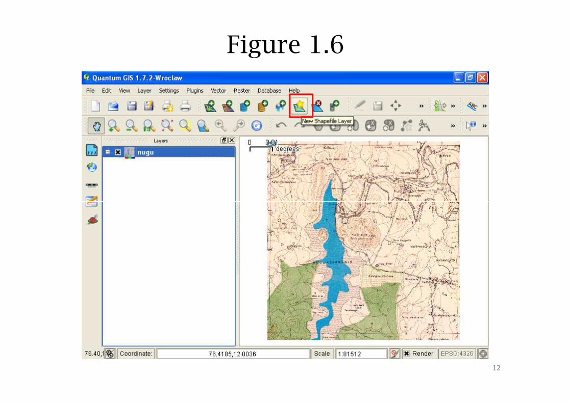
Figure 1.6
12
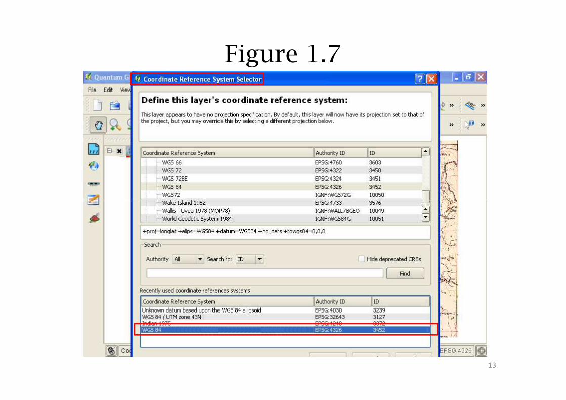
Figure 1.7
13
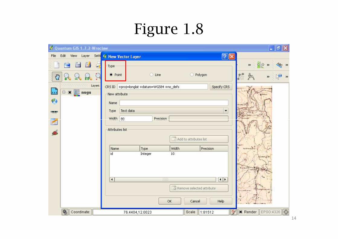
Figure 1.8
14
Creation of Vector Point Data
• In Figure 1.8 select option Type and thenarro Point
• We need to add ‘attributes’ next. This steprequires planning in detail
� For eg., an anti- poaching camp can have theattributes:attributes:
1. Number of staff
2. Number of GPS etc
� Next create layer of villages with attributessuch as:
1. Name
2. Taluk
3. District
4. Population 15
Creation of Vector Point Data
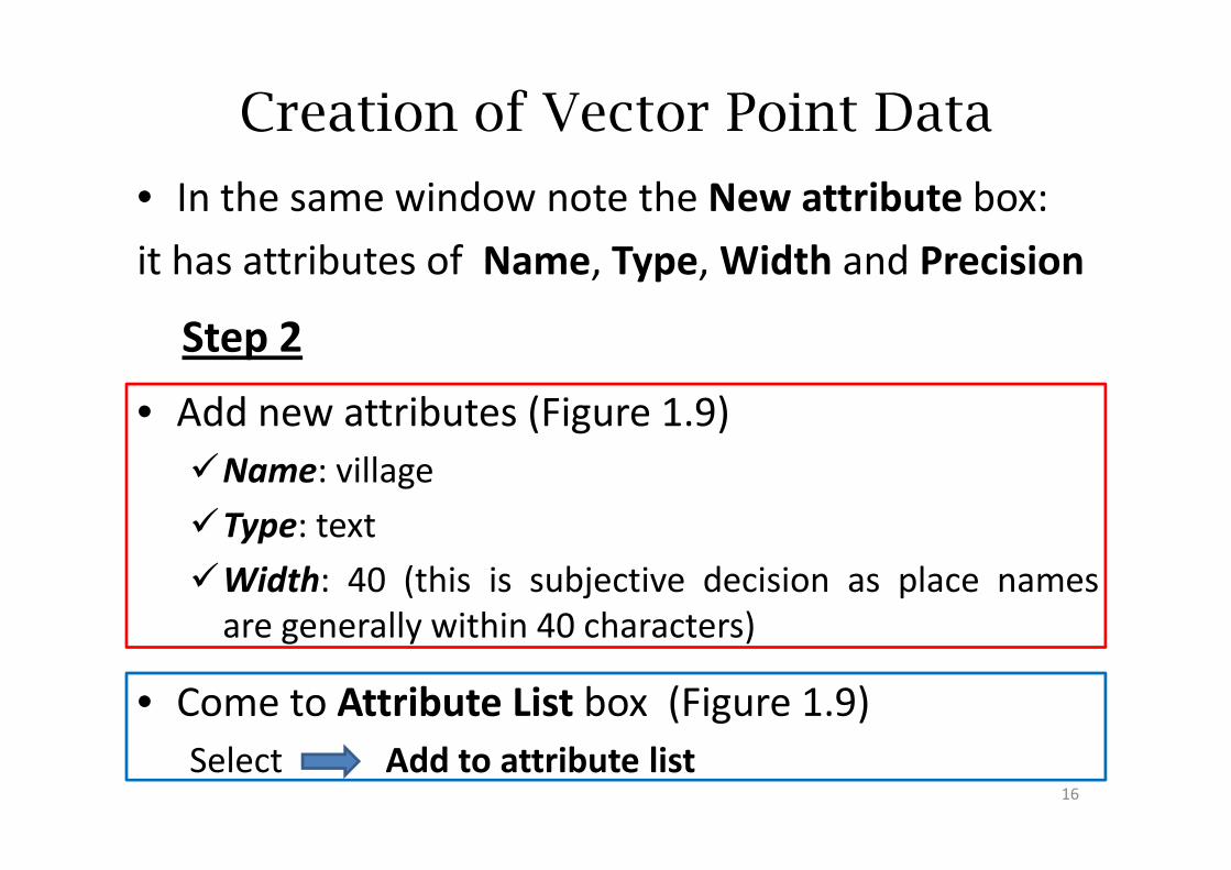
• In the same window note the New attribute box:
it has attributes of Name, Type, Width and Precision
• Add new attributes (Figure 1.9)
Step 2
• Add new attributes (Figure 1.9)
�Name: village
�Type: text
�Width: 40 (this is subjective decision as place names
are generally within 40 characters)
• Come to Attribute List box (Figure 1.9)
Select Add to attribute list16
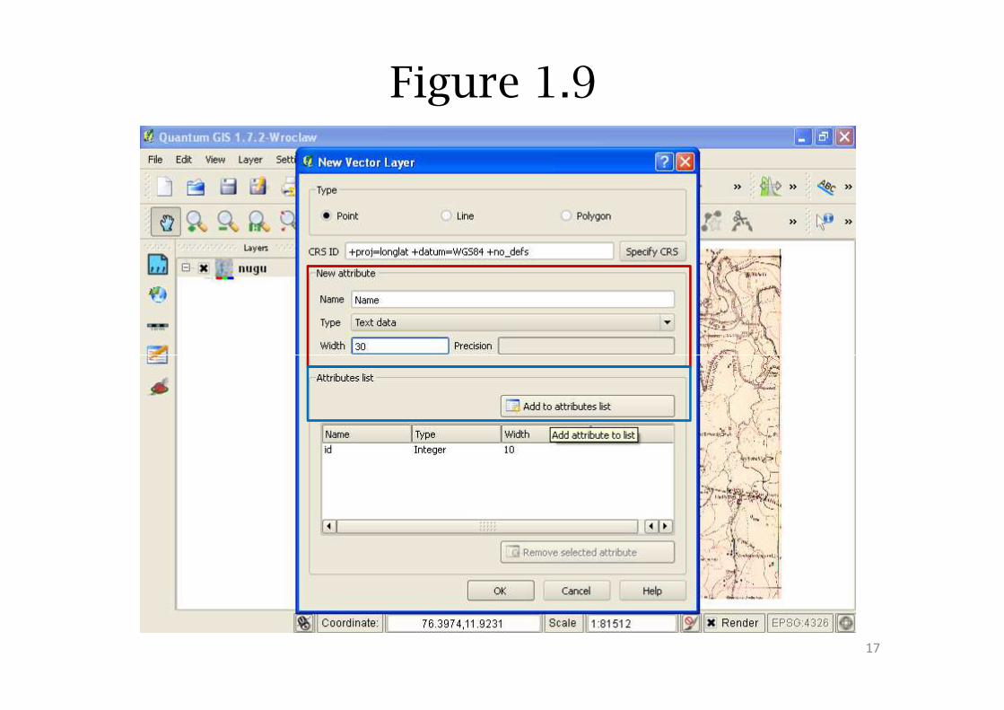
Figure 1.9
17
Creation of Vector Point Data
• Add taluk and district data in village attributes
� by repeating Step 2
• Add population data: to do this, we need to setType of data in whole number (Figure 1.10)
� repeat Step 2 (Figure 1.11)
• After this select OK (Figure 1.11)
• You will be guided to the Save As window.
� Select the directory in which you would like tosave the data. For this example name it as‘Village’ (Figure 1.12)
� Select Save.18
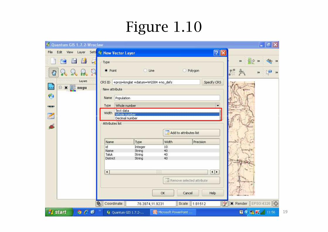
Figure 1.10
19
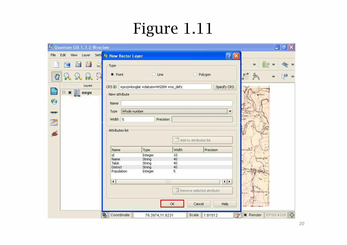
Figure 1.11
20
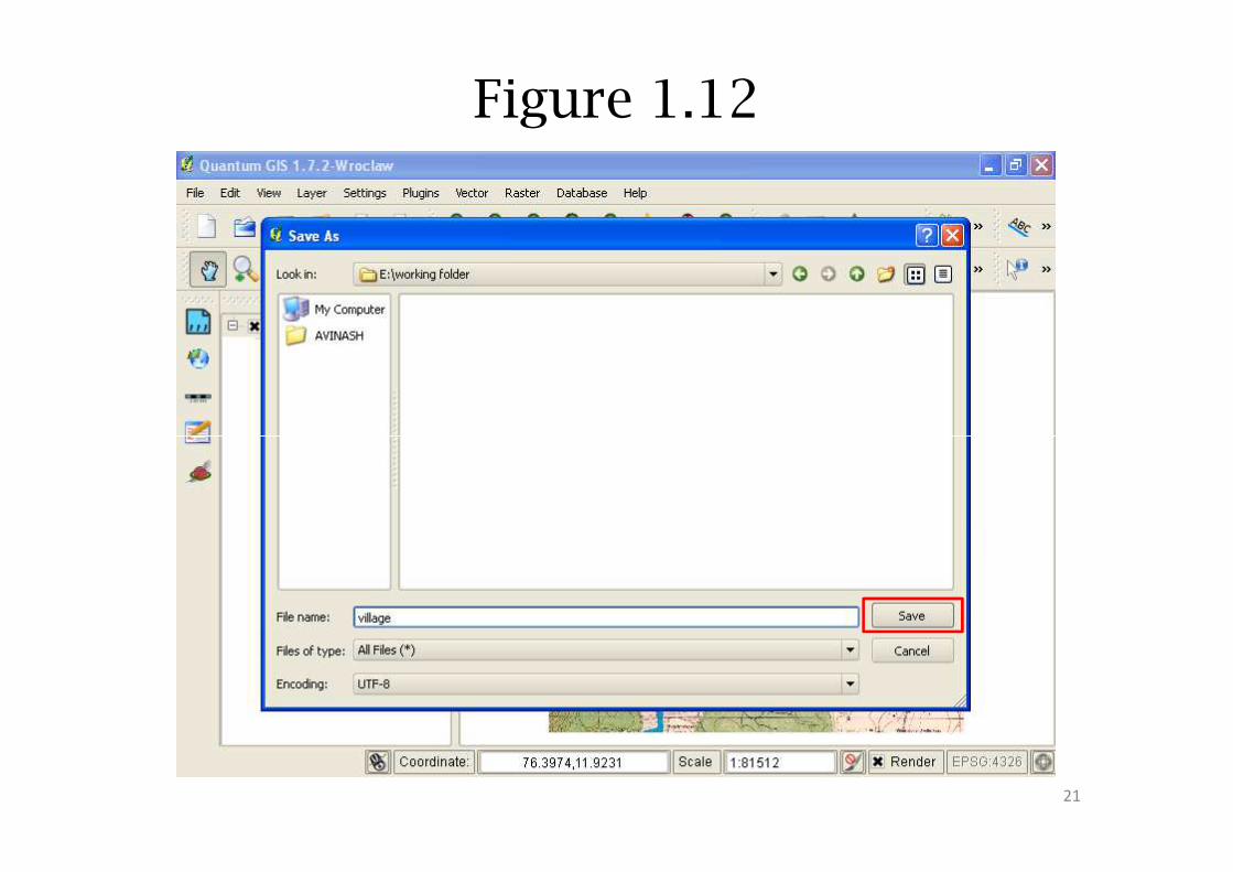
Figure 1.12
21
Creation of Vector Point Data
• On saving, layer is stored in specified folder
• This layer is automatically added to the QGIS
window. (Figure 1.13)window. (Figure 1.13)
22
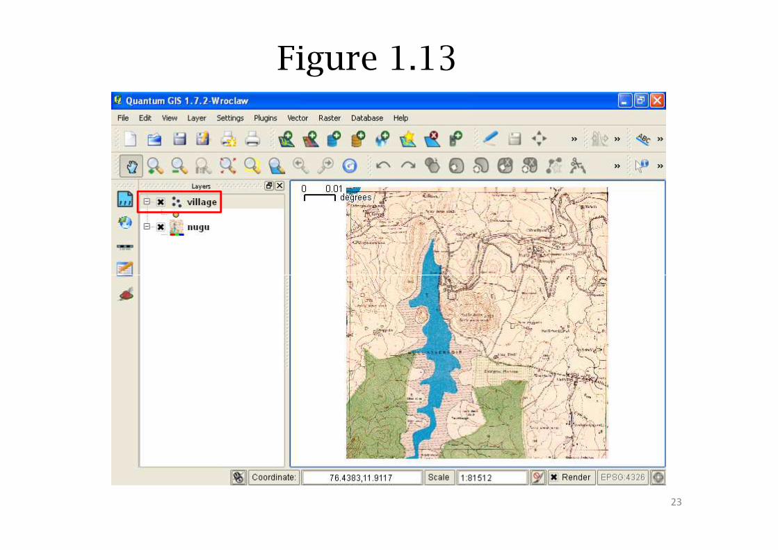
Figure 1.13
23
Creation of Vector Point Data
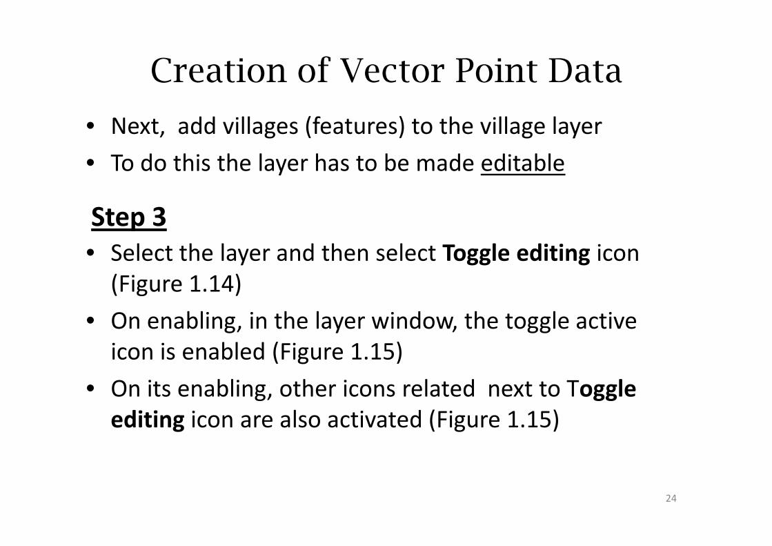
• Next, add villages (features) to the village layer
• To do this the layer has to be made editable
• Select the layer and then select Toggle editing icon
(Figure 1.14)
Step 3
(Figure 1.14)
• On enabling, in the layer window, the toggle active
icon is enabled (Figure 1.15)
• On its enabling, other icons related next to Toggle
editing icon are also activated (Figure 1.15)
24
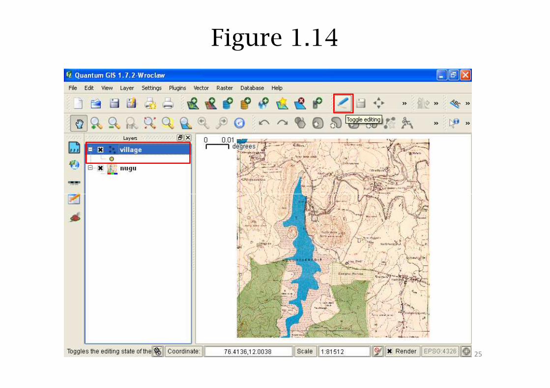
Figure 1.14
25
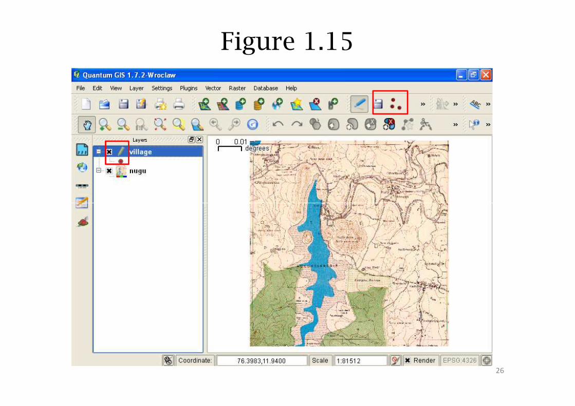
Figure 1.15
26
Creation of vector point data
27
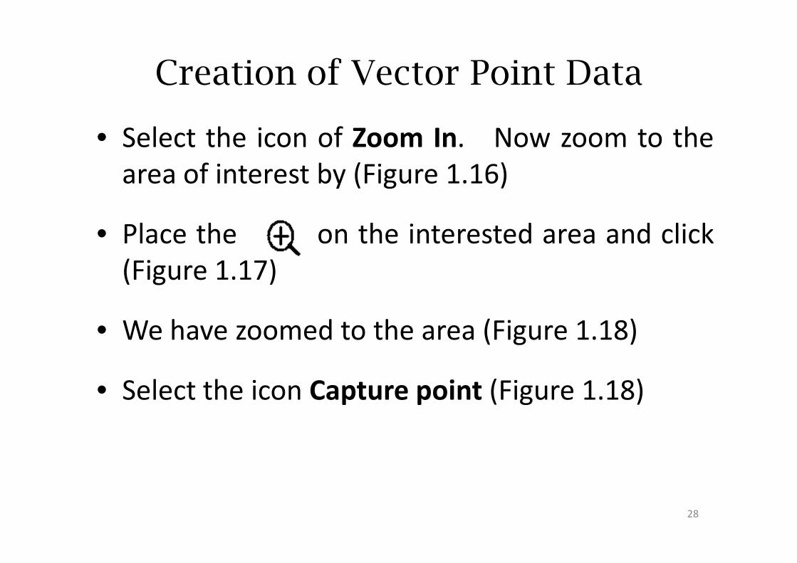
Creation of Vector Point Data
• Select the icon of Zoom In. Now zoom to the
area of interest by (Figure 1.16)
• Place the on the interested area and click
(Figure 1.17)(Figure 1.17)
• We have zoomed to the area (Figure 1.18)
• Select the icon Capture point (Figure 1.18)
28
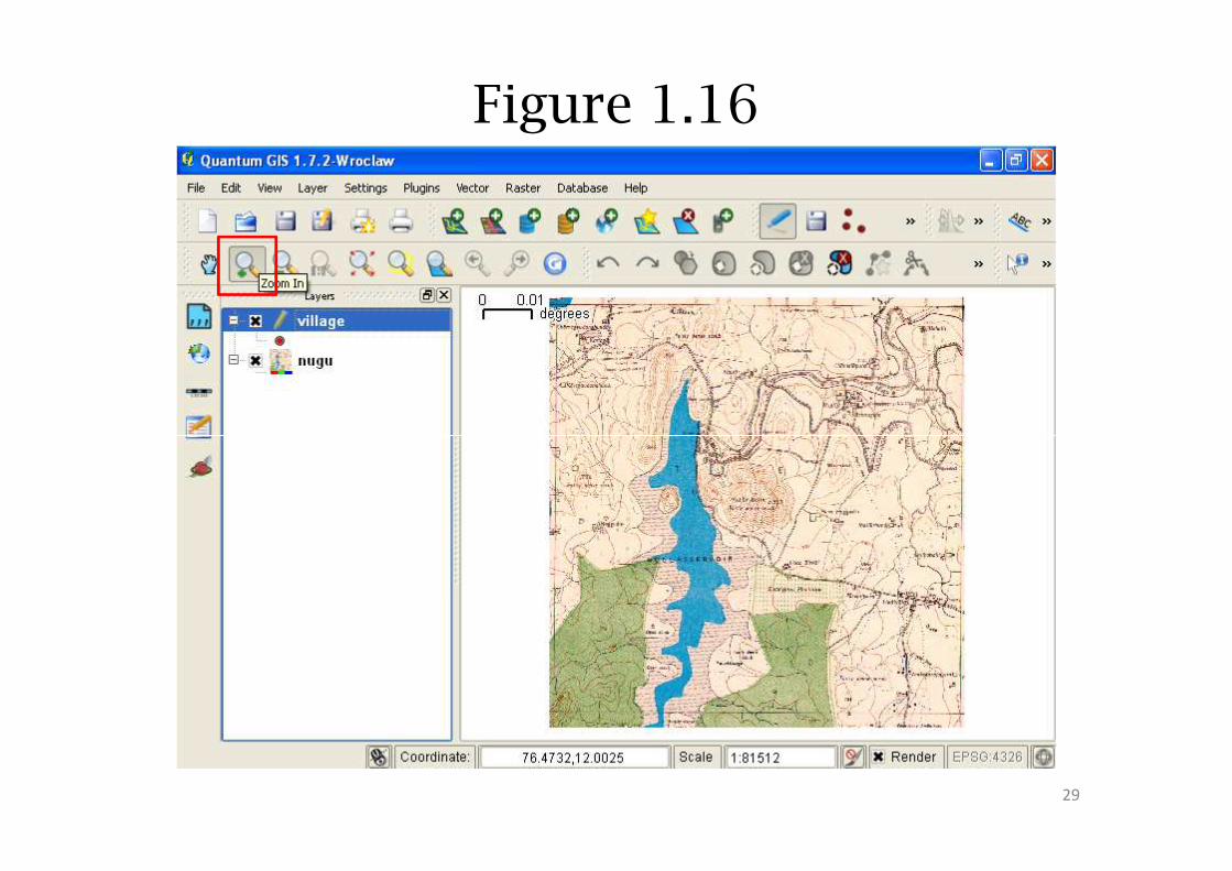
Figure 1.16
29
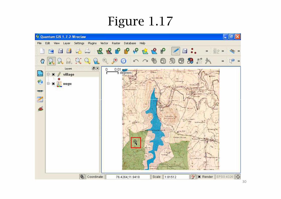
Figure 1.17
30
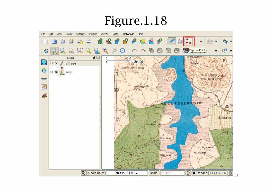
Figure.1.18
31

Figure 1.19
32
Creation of Vector Point Data
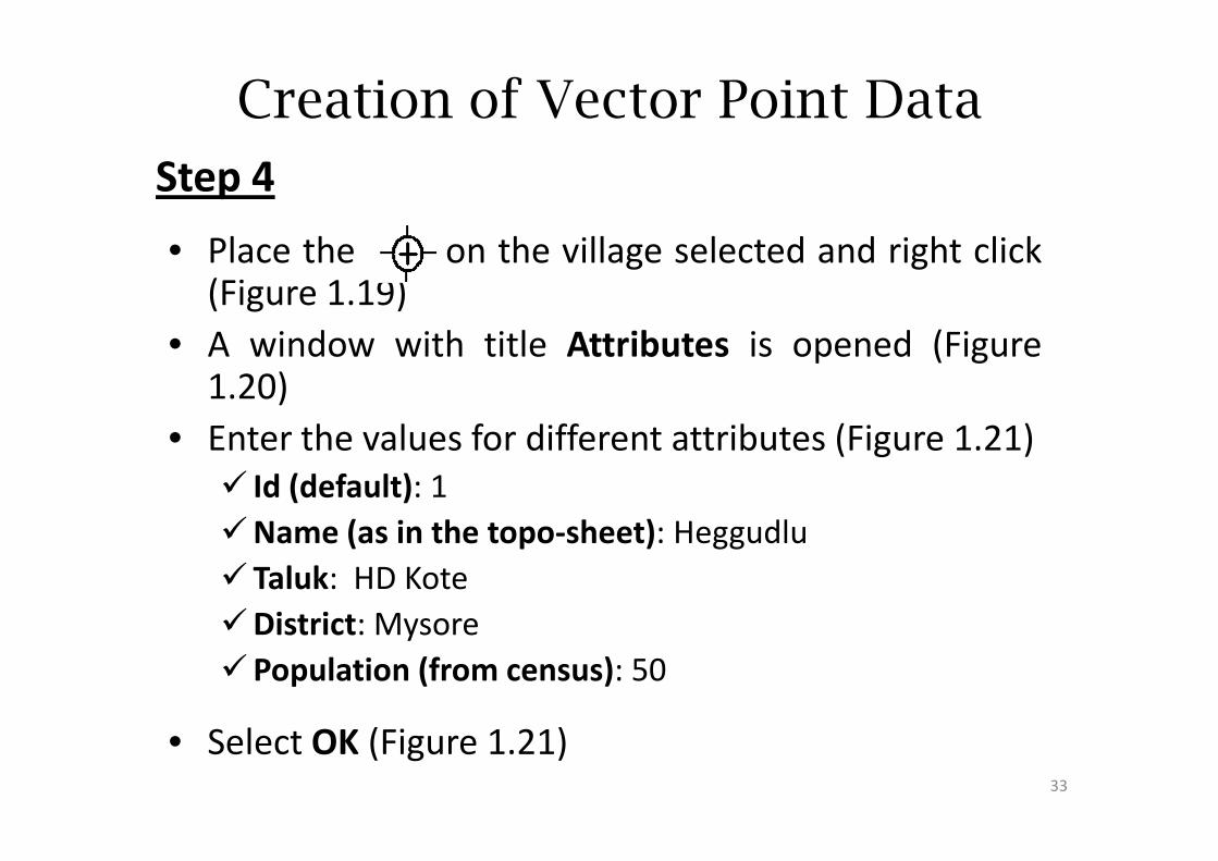
• Place the on the village selected and right click(Figure 1.19)
• A window with title Attributes is opened (Figure1.20)
• Enter the values for different attributes (Figure 1.21)
Step 4
• Enter the values for different attributes (Figure 1.21)
� Id (default): 1
�Name (as in the topo-sheet): Heggudlu
� Taluk: HD Kote
�District: Mysore
�Population (from census): 50
• Select OK (Figure 1.21)33
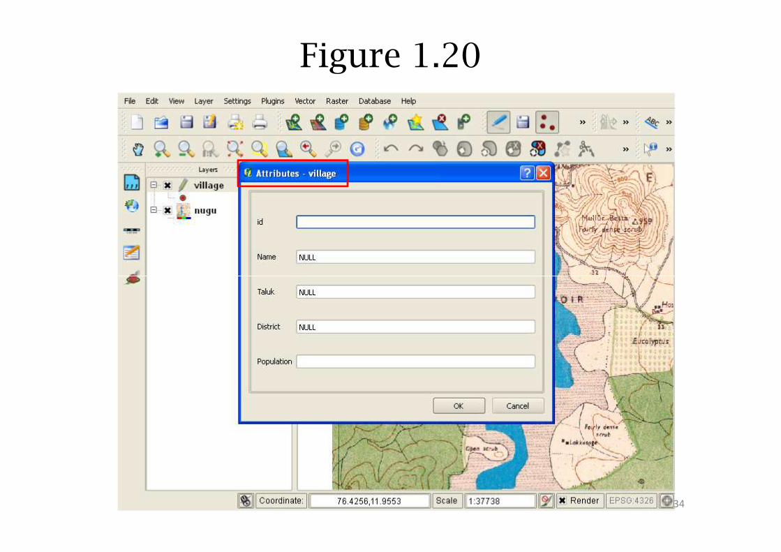
Figure 1.20
34
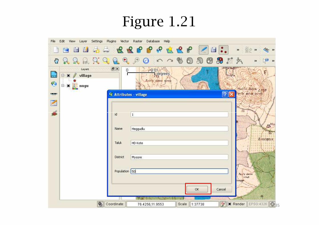
Figure 1.21
35
Creation of Vector Point Data
• Notice marked village can be seen on the map
(Figure 1.22)
• Repeat Step 4 (see page 34)• Repeat Step 4 (see page 34)
• Finally a map with villages in the Nugu is
displayed (Figure 1.23)
36
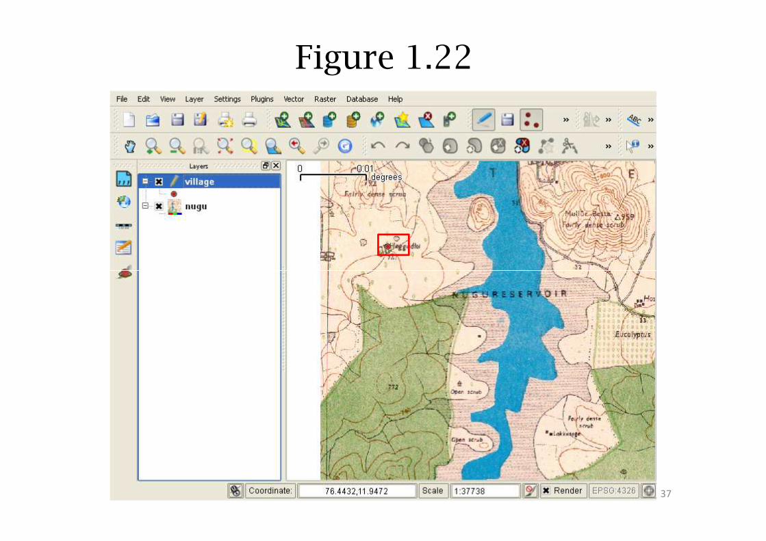
Figure 1.22
37
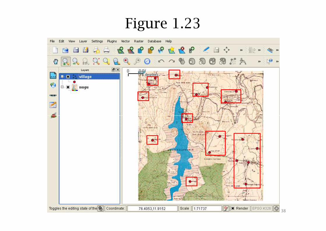
Figure 1.23
38
Creation of vector line data
39
Creation of vector line data - road
• To create new line layer select the icon Newshape layer (Figure 1.6, page 11)
• Complete Step 1 (page 10)
• As in Figure 1.8 where under Type, ‘point’ wasselected, select ‘Line’ (Figure 1.24)selected, select ‘Line’ (Figure 1.24)
• Next we need to add attributes (Figure 1.24)
� Attributes associated
� Type of the road
• After this step, select OK (Figure 1.24)
40
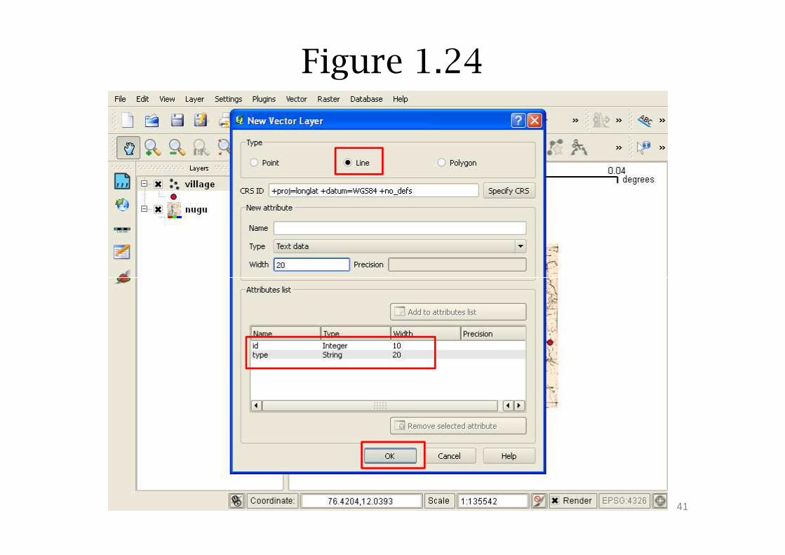
Figure 1.24
41
Creation of vector line data
• You will be guided to Save as window aspreviously done in Figure 1.12 (page 20)
– Select the directory in which you would like tosave the data. In this example name it as ‘road’(Figure 1.25)(Figure 1.25)
• Select Save; on saving, layer is stored inspecified folder (Figure 1.25 )
• This layer is automatically added to the QGISwindow (Figure 1.26)
42
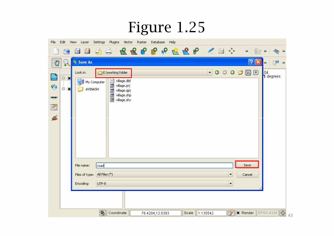
Figure 1.25
43
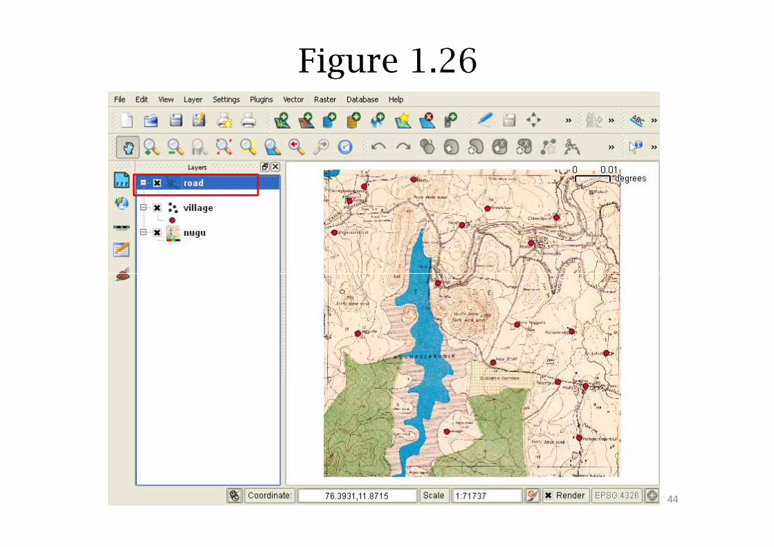
Figure 1.26
44
Creation of vector line data
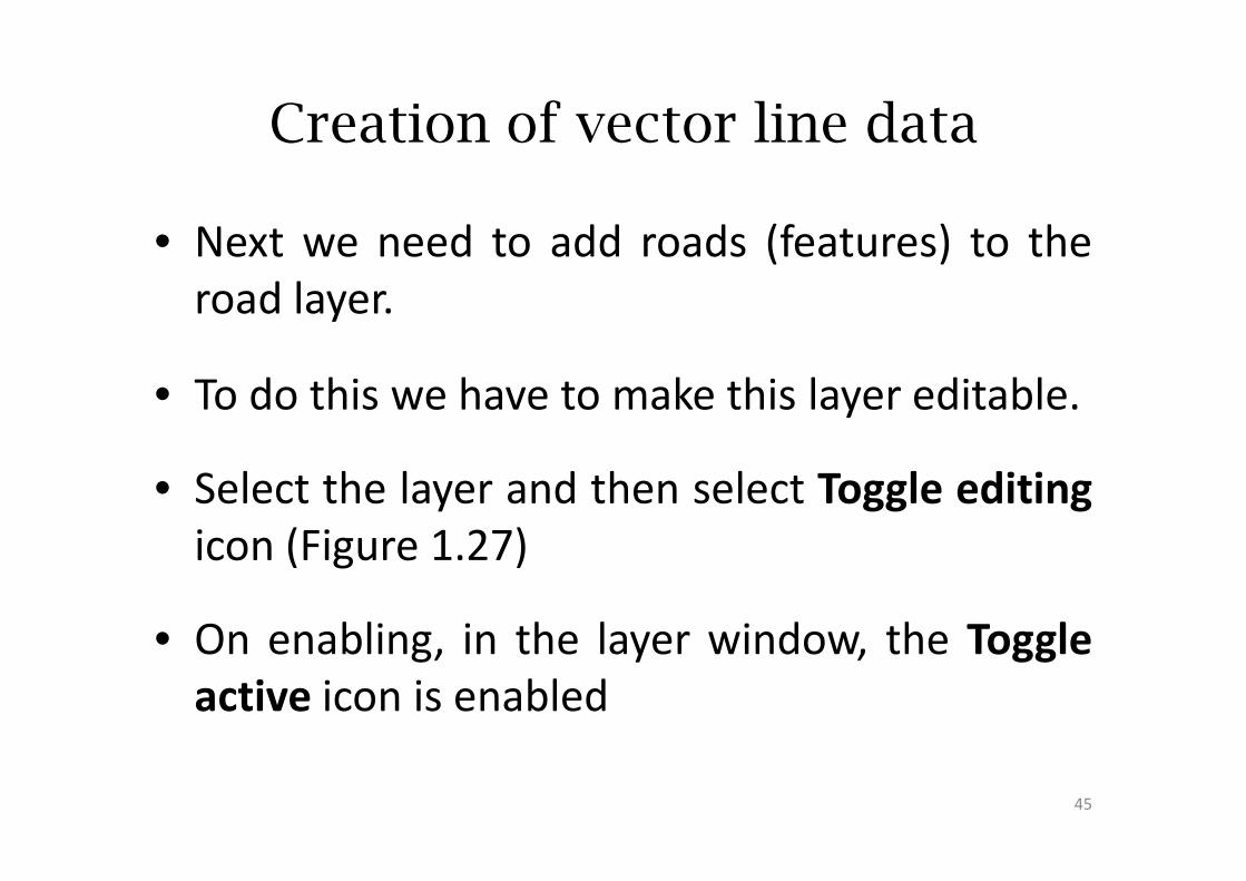
• Next we need to add roads (features) to the
road layer.
• To do this we have to make this layer editable.
• Select the layer and then select Toggle editing
icon (Figure 1.27)
• On enabling, in the layer window, the Toggle
active icon is enabled
45
Figure 1.27
46
Creation of vector line data
• Zoom to the area of interest by selecting the
icon of Zoom In (as in Figure 1.16, page 27)
• Then place the on the interested area and
click (as in Figure 1.17, page 28)
• We have zoomed to the area (Figure 1.28)
• Select the icon Capture Line (Figure 1.28)
• Place marker on road that we have to
digitize and left click (Figure 1.29)47
Step 5
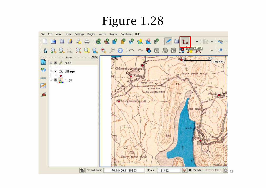
Figure 1.28
48
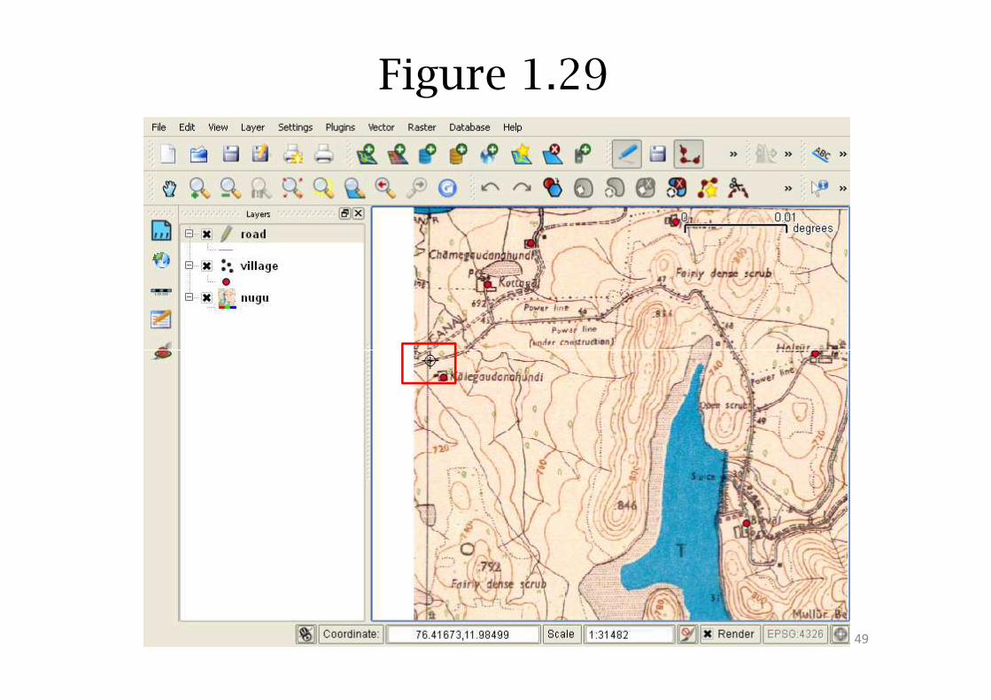
Figure 1.29
49
Creation of vector line data
• Place the marker to next position and left click(Figure 1.30)
• Repeat the same process till the next junction (for e.g.,change in direction is required)
• Similarly, continue till where you would like to end theprocess, right click.process, right click.
• A window with title Attributes is opened (Figure 1.31)
• Enter the information for different attributes (Figure1.31)
� Id (default): 1
� Type : Mud road
• Select OK (Figure 1.31)50
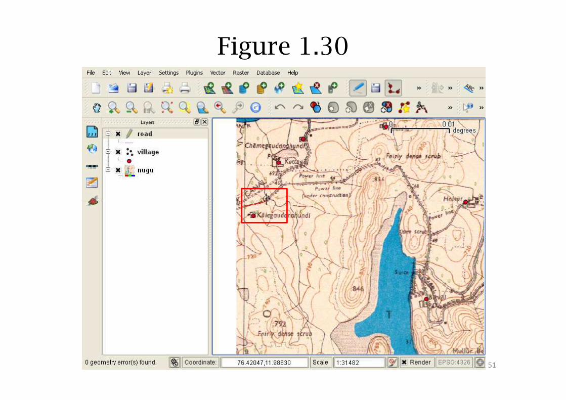
Figure 1.30
51
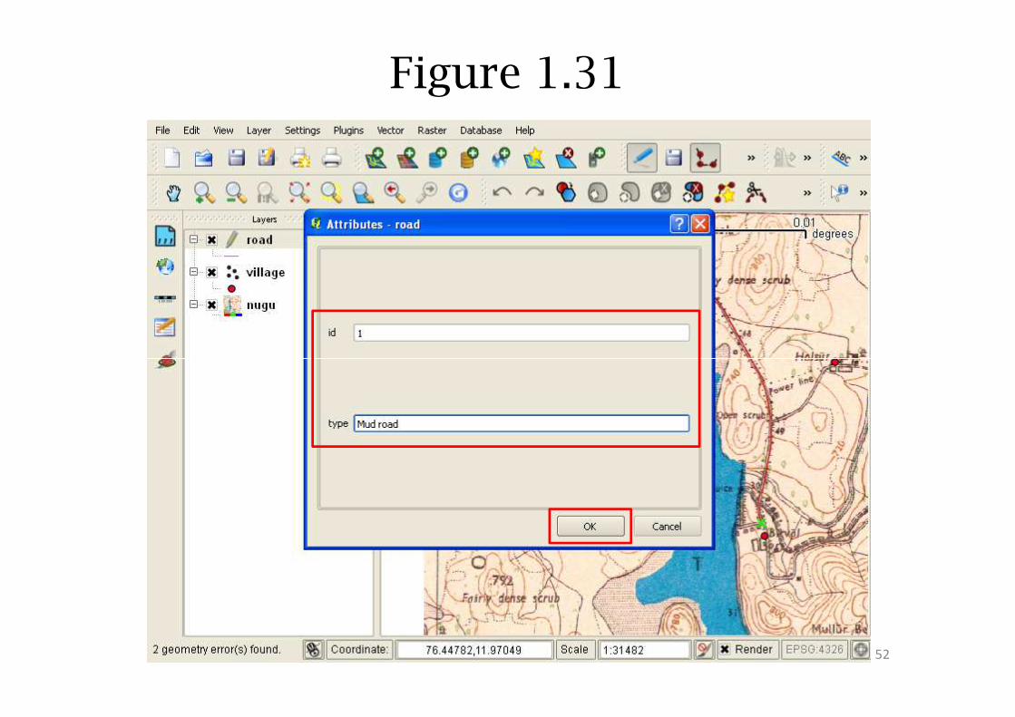
Figure 1.31
52
Creation of vector line data
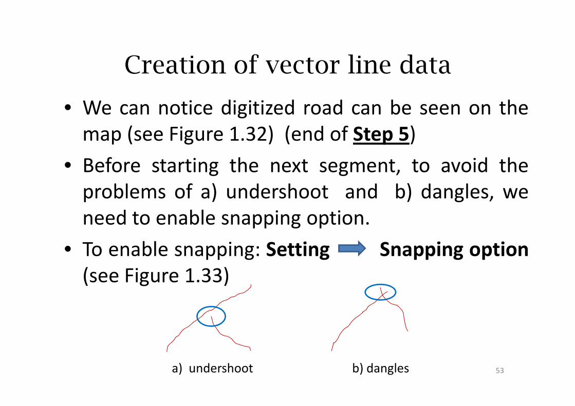
• We can notice digitized road can be seen on the
map (see Figure 1.32) (end of Step 5)
• Before starting the next segment, to avoid the
problems of a) undershoot and b) dangles, weproblems of a) undershoot and b) dangles, we
need to enable snapping option.
• To enable snapping: Setting Snapping option
(see Figure 1.33)
a) undershoot b) dangles 53
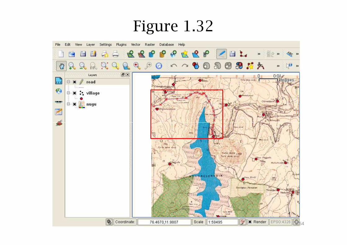
Figure 1.32
54
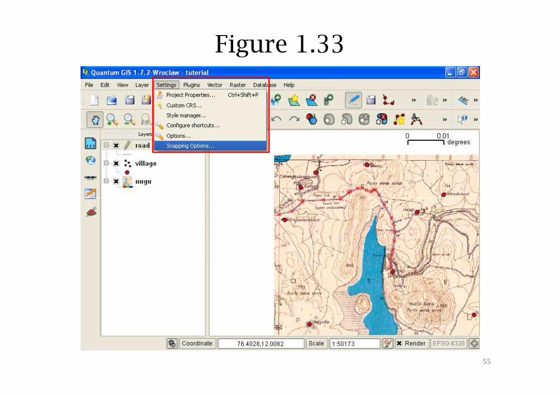
Figure 1.33
55
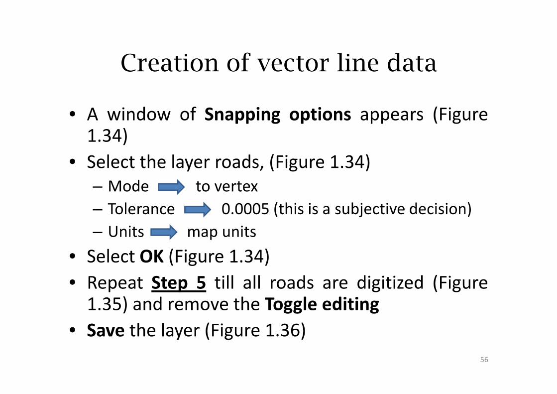
Creation of vector line data
• A window of Snapping options appears (Figure1.34)
• Select the layer roads, (Figure 1.34)
– Mode to vertex
– Tolerance 0.0005 (this is a subjective decision)
– Units map units
• Select OK (Figure 1.34)
• Repeat Step 5 till all roads are digitized (Figure1.35) and remove the Toggle editing
• Save the layer (Figure 1.36)
56
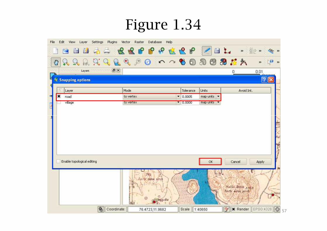
Figure 1.34
57
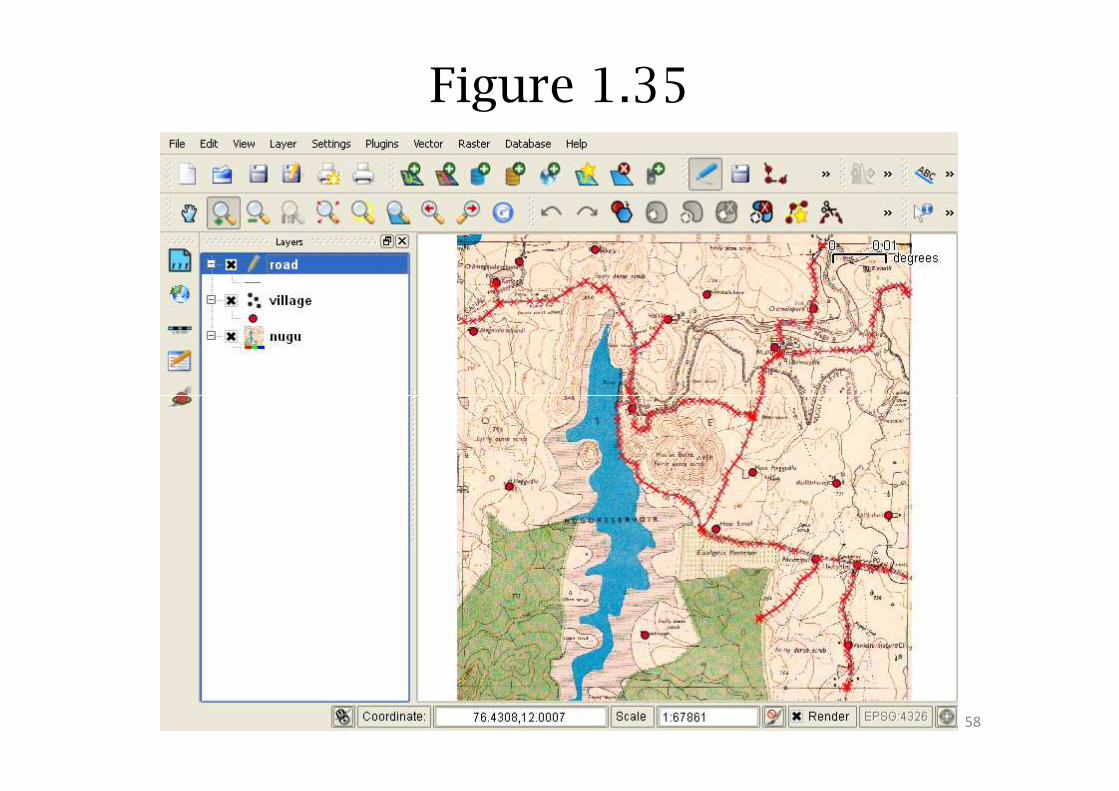
Figure 1.35
58
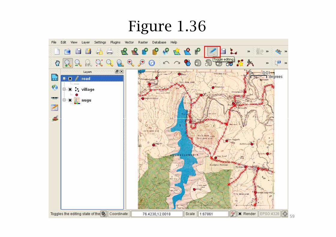
Figure 1.36
59
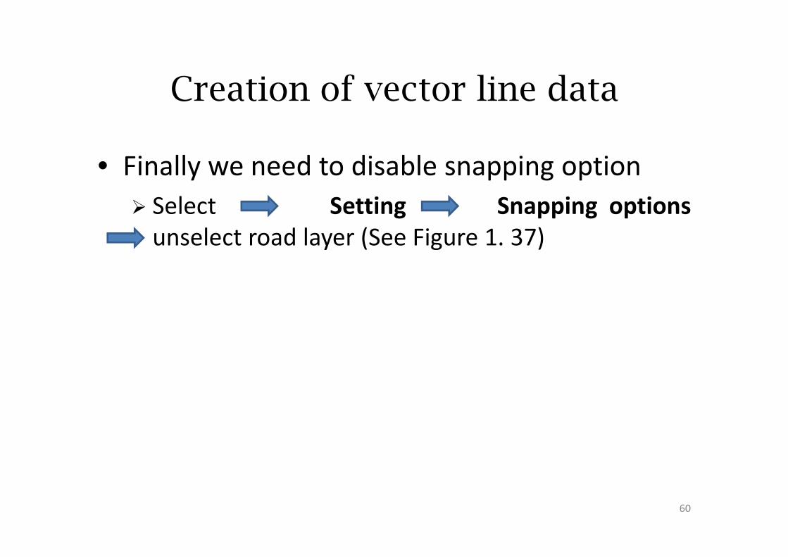
Creation of vector line data
• Finally we need to disable snapping option
� Select Setting Snapping options
unselect road layer (See Figure 1. 37)
60
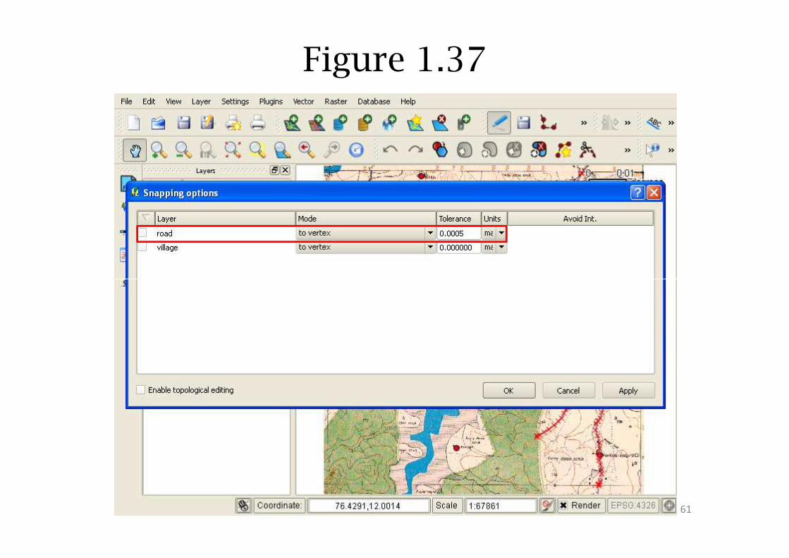
Figure 1.37
61
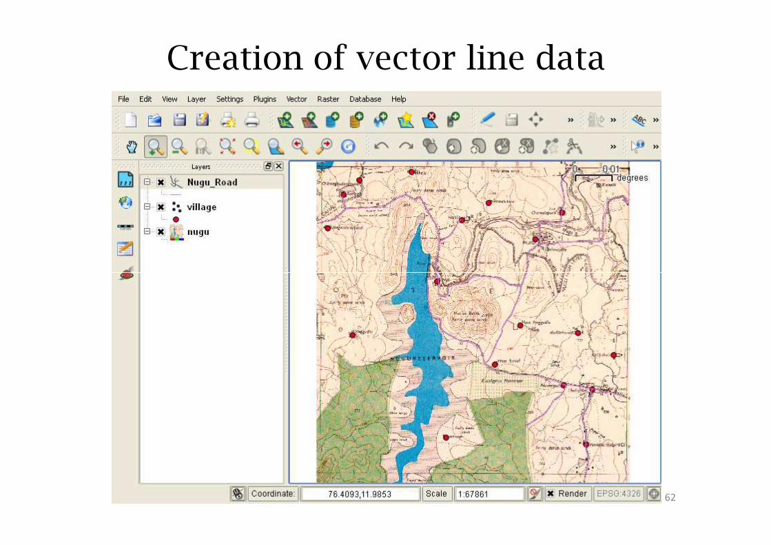
Creation of vector line data
62
Creation of vector polygon data
63
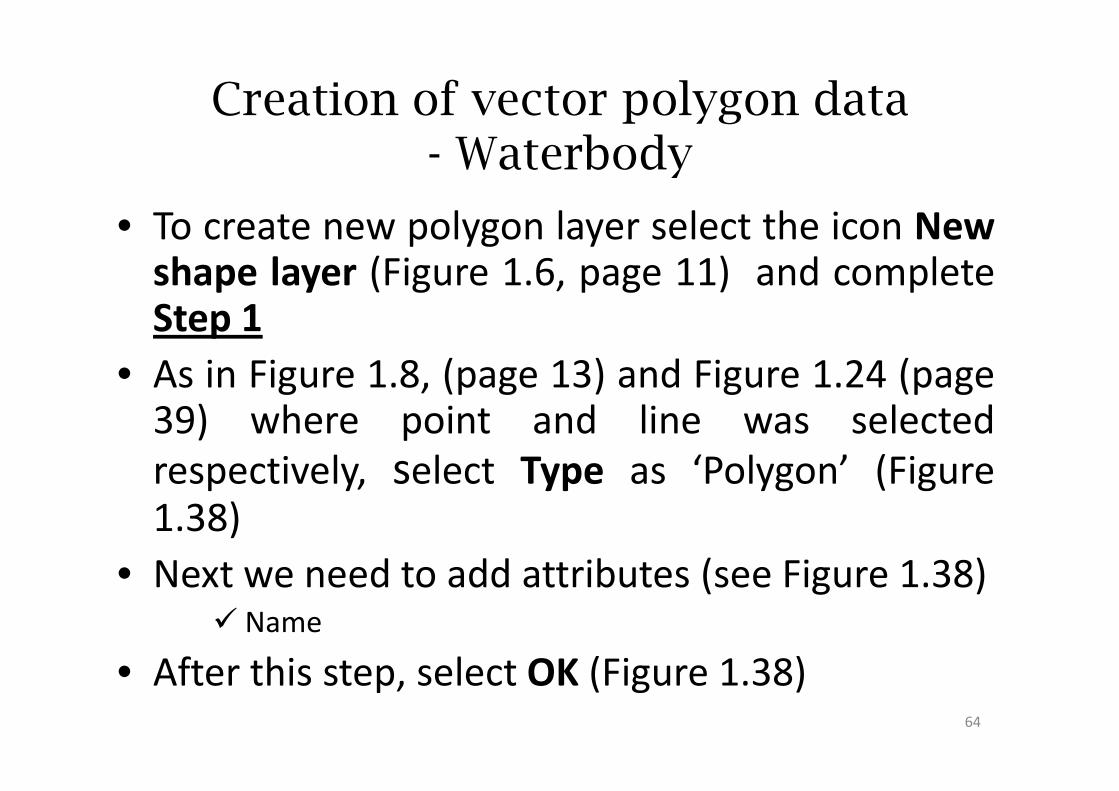
Creation of vector polygon data - Waterbody
• To create new polygon layer select the icon Newshape layer (Figure 1.6, page 11) and completeStep 1
• As in Figure 1.8, (page 13) and Figure 1.24 (page39) where point and line was selected
• As in Figure 1.8, (page 13) and Figure 1.24 (page39) where point and line was selected
respectively, select Type as ‘Polygon’ (Figure1.38)
• Next we need to add attributes (see Figure 1.38)� Name
• After this step, select OK (Figure 1.38)64
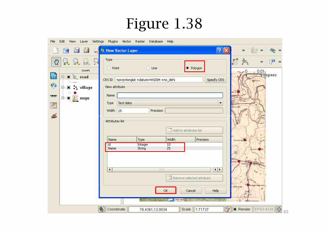
Figure 1.38
65
Creation of vector polygon data
• You will be guided to Save as window aspreviously done in Figure 1.12 (page 20)
– Select the directory in which you would like to savethe data. In this example name it as waterbody(Figure 1.39)
• Select Save ( Figure 1.39 )
• On saving, layer is stored in specified folder
• This layer is automatically added to the QGISwindow ( Figure 1.40)
66
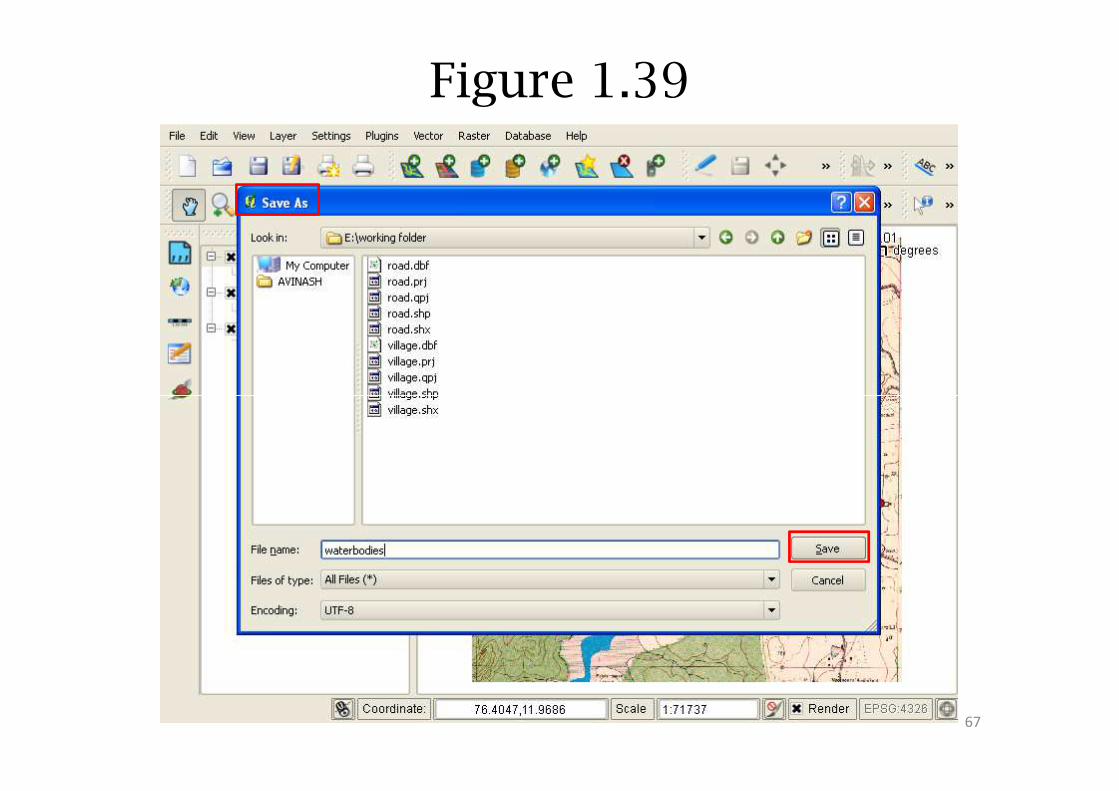
Figure 1.39
67
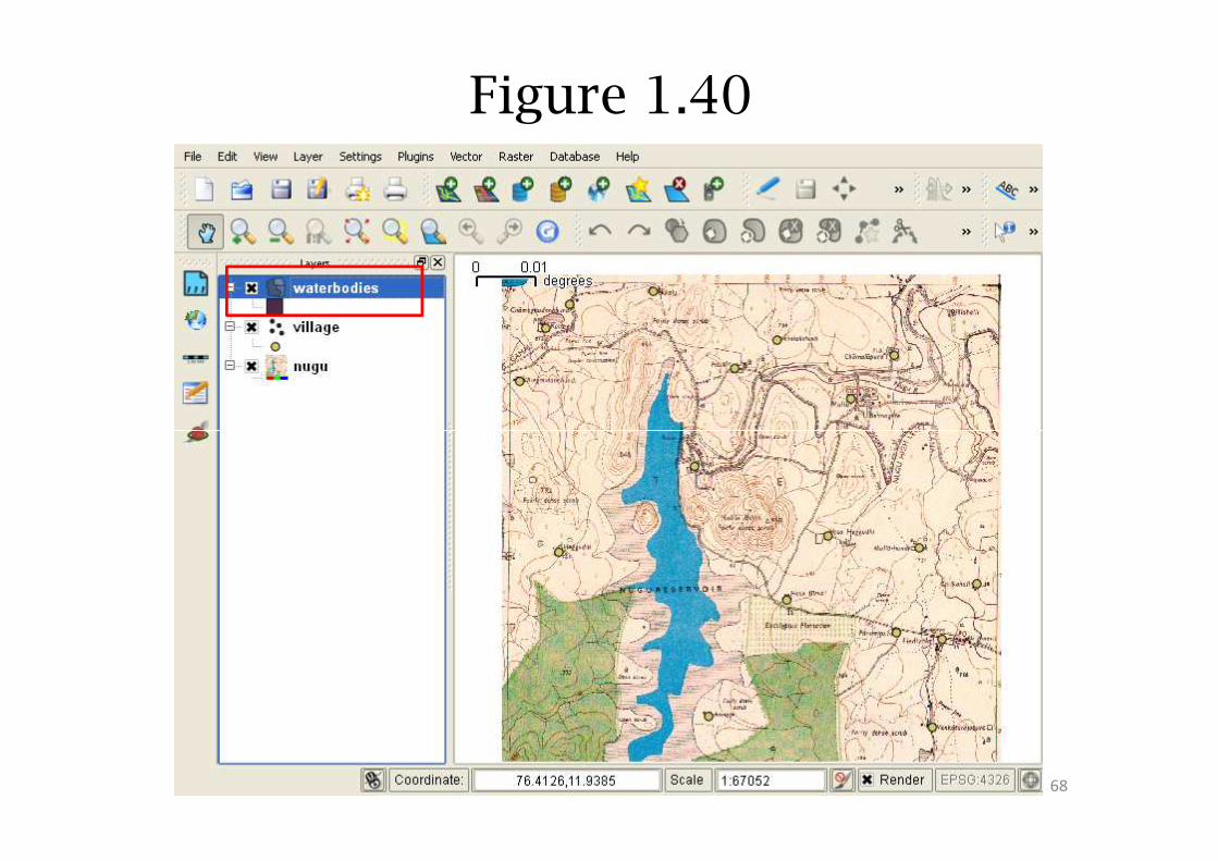
Figure 1.40
68
Creation of vector polygon data
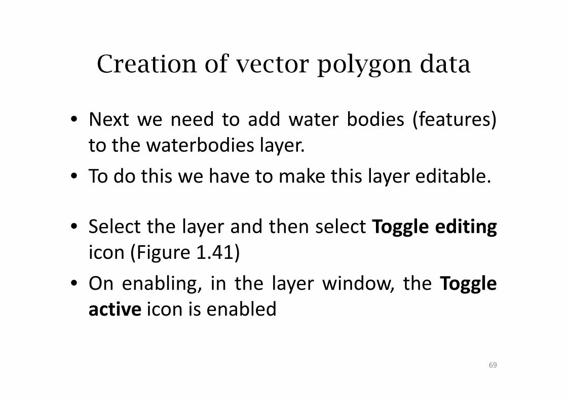
• Next we need to add water bodies (features)
to the waterbodies layer.
• To do this we have to make this layer editable.
• Select the layer and then select Toggle editing
icon (Figure 1.41)
• On enabling, in the layer window, the Toggle
active icon is enabled
69
Figure 1.41
70
Creation of vector polygon data
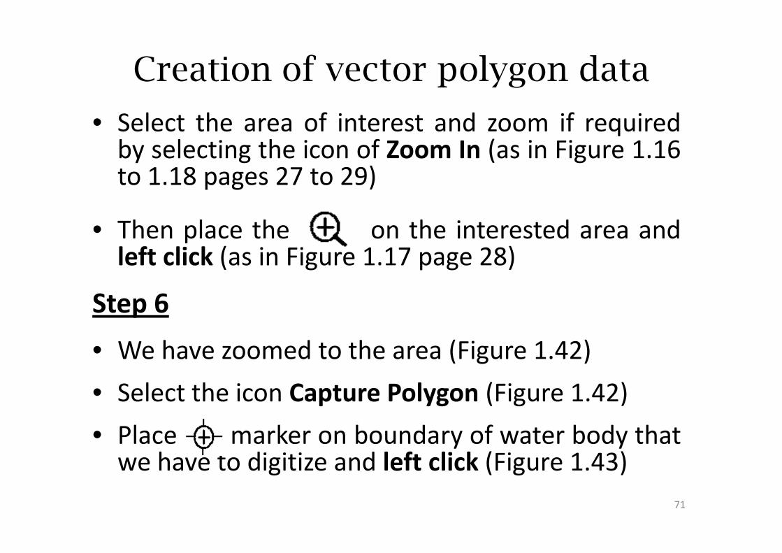
• Select the area of interest and zoom if requiredby selecting the icon of Zoom In (as in Figure 1.16to 1.18 pages 27 to 29)
• Then place the on the interested area andleft click (as in Figure 1.17 page 28)
• We have zoomed to the area (Figure 1.42)
• Select the icon Capture Polygon (Figure 1.42)
• Place marker on boundary of water body thatwe have to digitize and left click (Figure 1.43)
71
Step 6
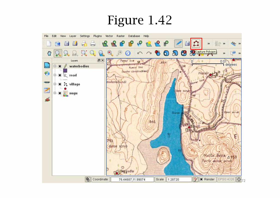
Figure 1.42
72
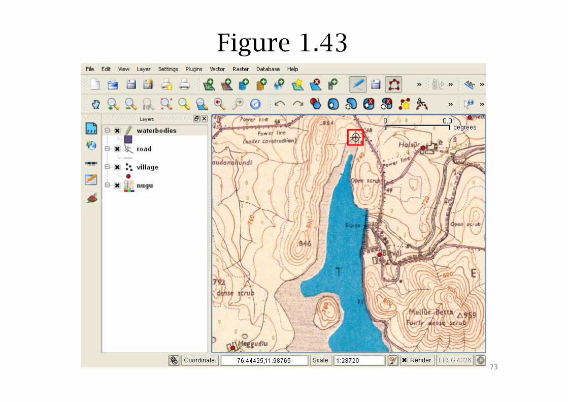
Figure 1.43
73
• Place the marker to next position and left
click (Figure 1.44)
• Repeat the same process till we complete the
polygon and right click
Creation of vector polygon data
polygon and right click
Note: if the viewing window covers only some portion of
the area, then use up arrow key for scrolling up or
down-arrow key or side way arrow keys ( / ) for
required scrolling
74
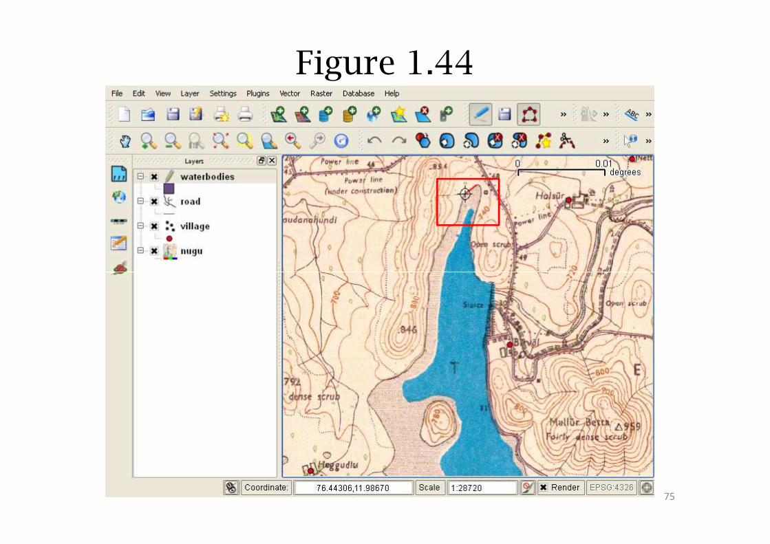
Figure 1.44
75
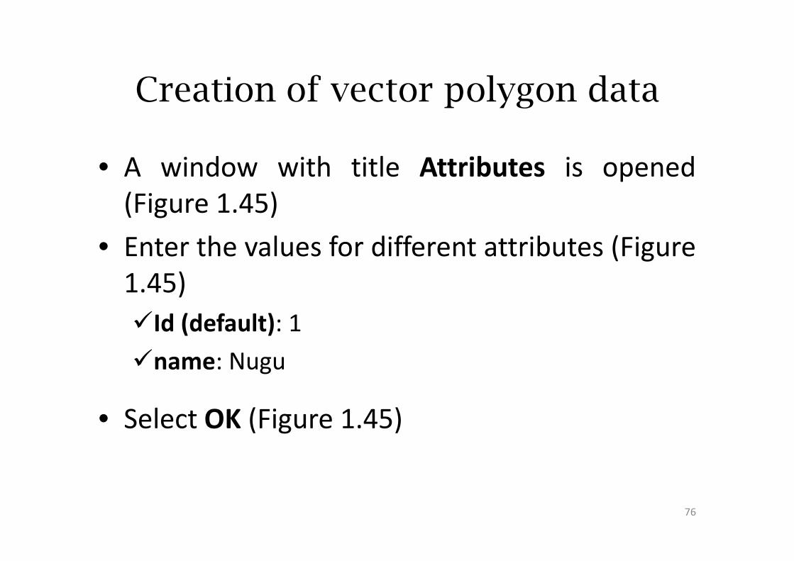
Creation of vector polygon data
• A window with title Attributes is opened
(Figure 1.45)
• Enter the values for different attributes (Figure
1.45)1.45)
�Id (default): 1
�name: Nugu
• Select OK (Figure 1.45)
76
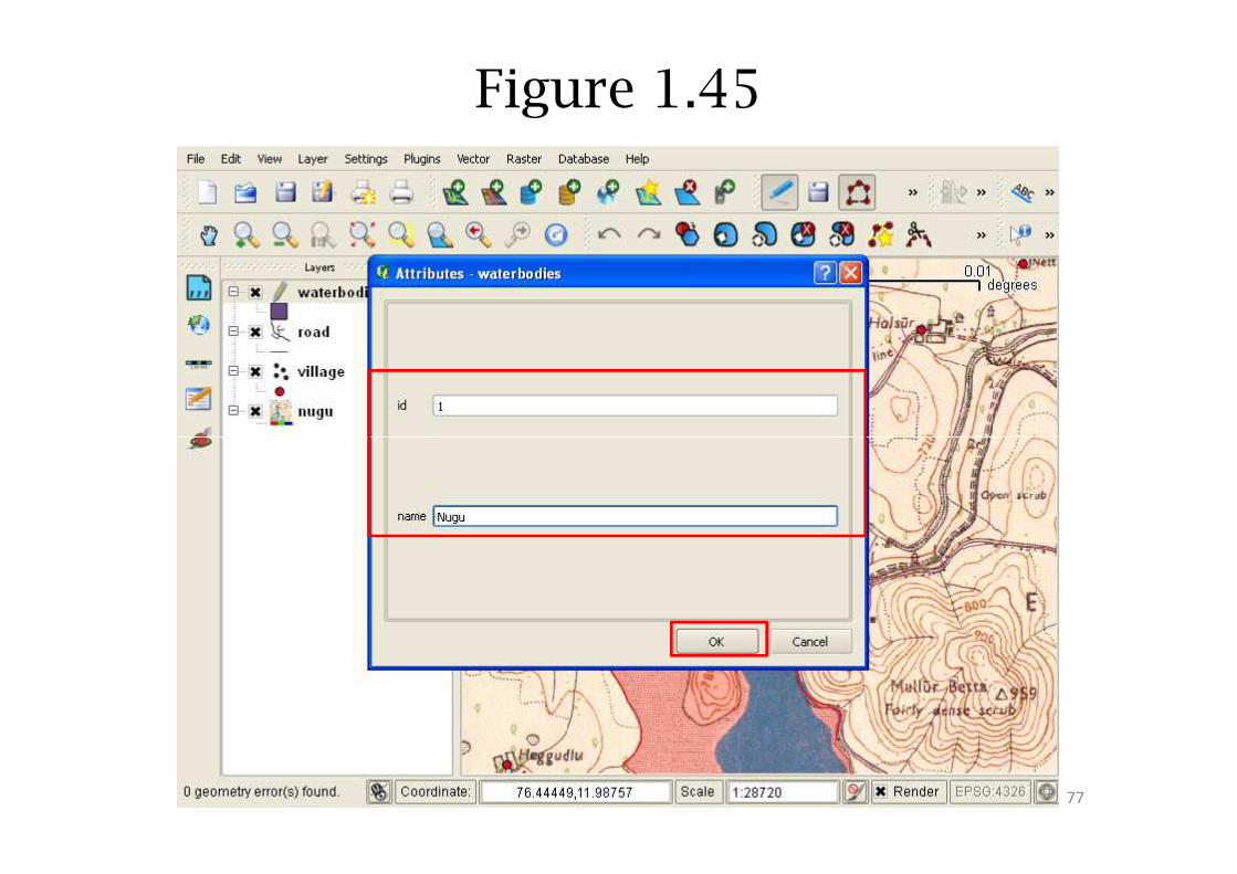
Figure 1.45
77
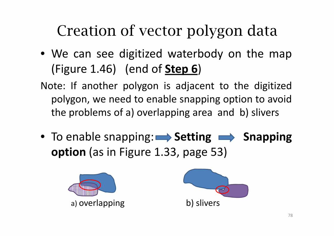
Creation of vector polygon data
• We can see digitized waterbody on the map
(Figure 1.46) (end of Step 6)
Note: If another polygon is adjacent to the digitized
polygon, we need to enable snapping option to avoid
the problems of a) overlapping area and b) sliversthe problems of a) overlapping area and b) slivers
• To enable snapping: Setting Snapping
option (as in Figure 1.33, page 53)
a) overlapping b) slivers
78
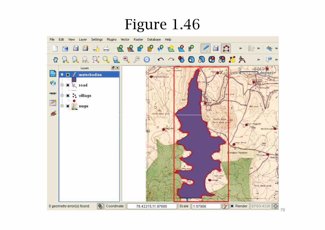
Figure 1.46
79
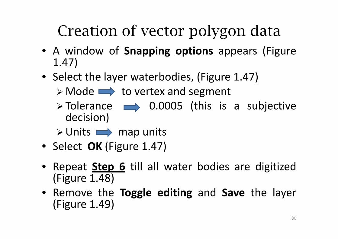
Creation of vector polygon data
• A window of Snapping options appears (Figure1.47)
• Select the layer waterbodies, (Figure 1.47)
� Mode to vertex and segment
� Tolerance 0.0005 (this is a subjectivedecision)decision)
� Units map units
• Select OK (Figure 1.47)
• Repeat Step 6 till all water bodies are digitized(Figure 1.48)
• Remove the Toggle editing and Save the layer(Figure 1.49)
80
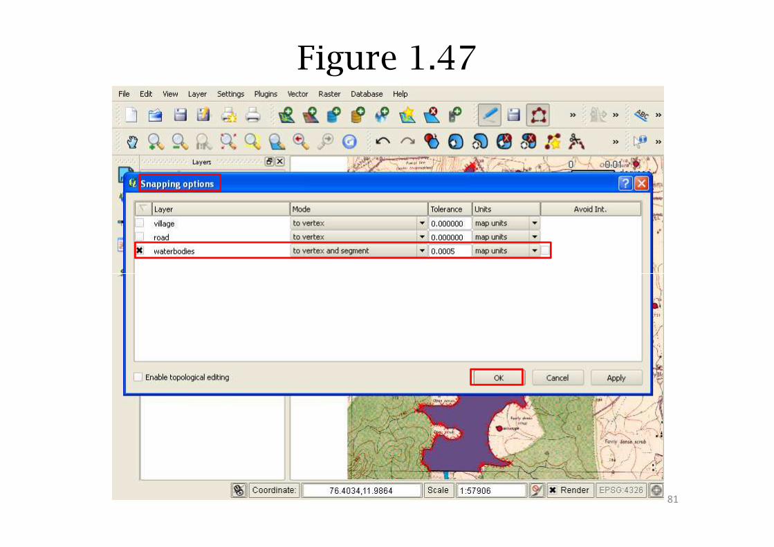
Figure 1.47
81
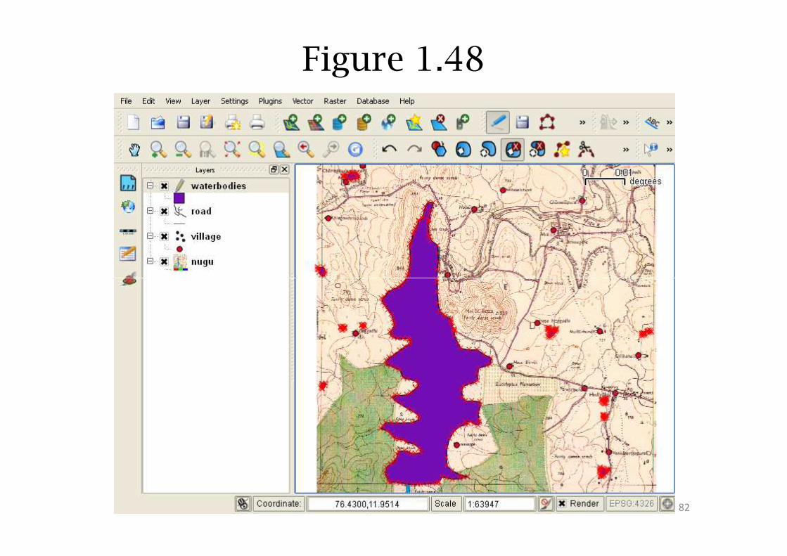
Figure 1.48
82

Figure 1.49
83
Creation of vector polygon data
• Finally we need to disable snapping option
� Select: Setting Snapping options
whitunselect waterbodies (Figure 1.50)
• The final output is ready (Figure 1.51)
84
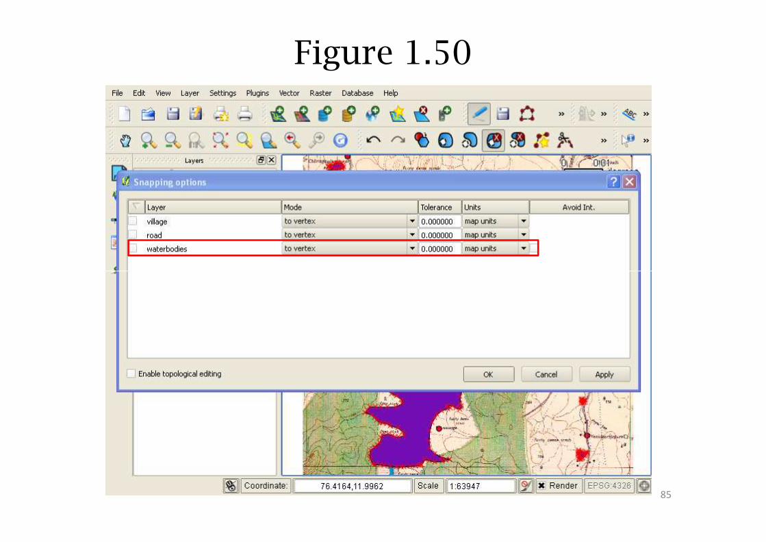
Figure 1.50
85
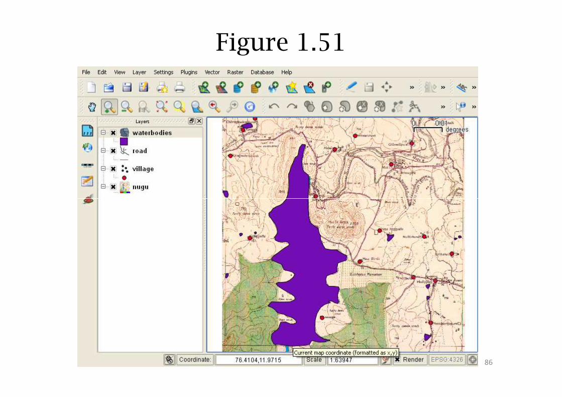
Figure 1.51
86
Coloring Coloring themesthemesColoring Coloring themesthemes
87
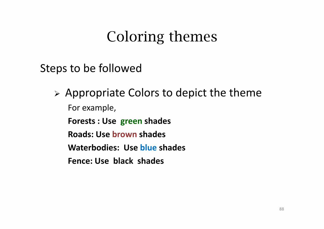
Coloring themes
Steps to be followed
� Appropriate Colors to depict the theme
For example,
Forests : Use green shades
Roads: Use brown shades
Waterbodies: Use blue shades
Fence: Use black shades
88
Organizing layers in hierarchy
Before Coloring layers
� organize the layers in the order of point, line
and polygon features (Figure 1.52)
� Select concerned layer and drag it up or down
89
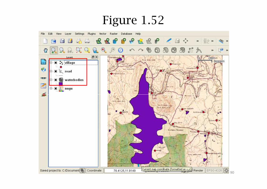
Figure 1.52
90
Point Style
• To change the color of point data, double click on
the point data (village layer). Layer properties
window opens (Figure 1.53)
Step 7
window opens (Figure 1.53)
End Step 7
• Layer properties has various tabs: Style, Labels,
Fields, General, Metadata, Actions, Joins and
Diagram (Figure 1.53)
91
Point Style
• Select Style (Figure 1.53)
• In style we can change Color , Size, Unit, etc.
• Let us change the color
Step 8
• Let us change the color
� Select Change (Figure 1.54)
� Select Color window opens (Figure 1.55)
� Select Color by placing + on the selected Color,
the select OK (Figure 1.56 )
End Step 8
92
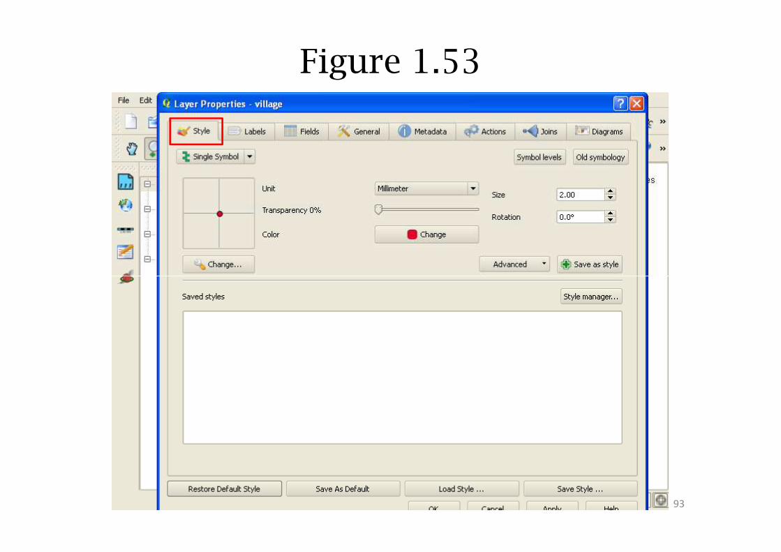
Figure 1.53
93
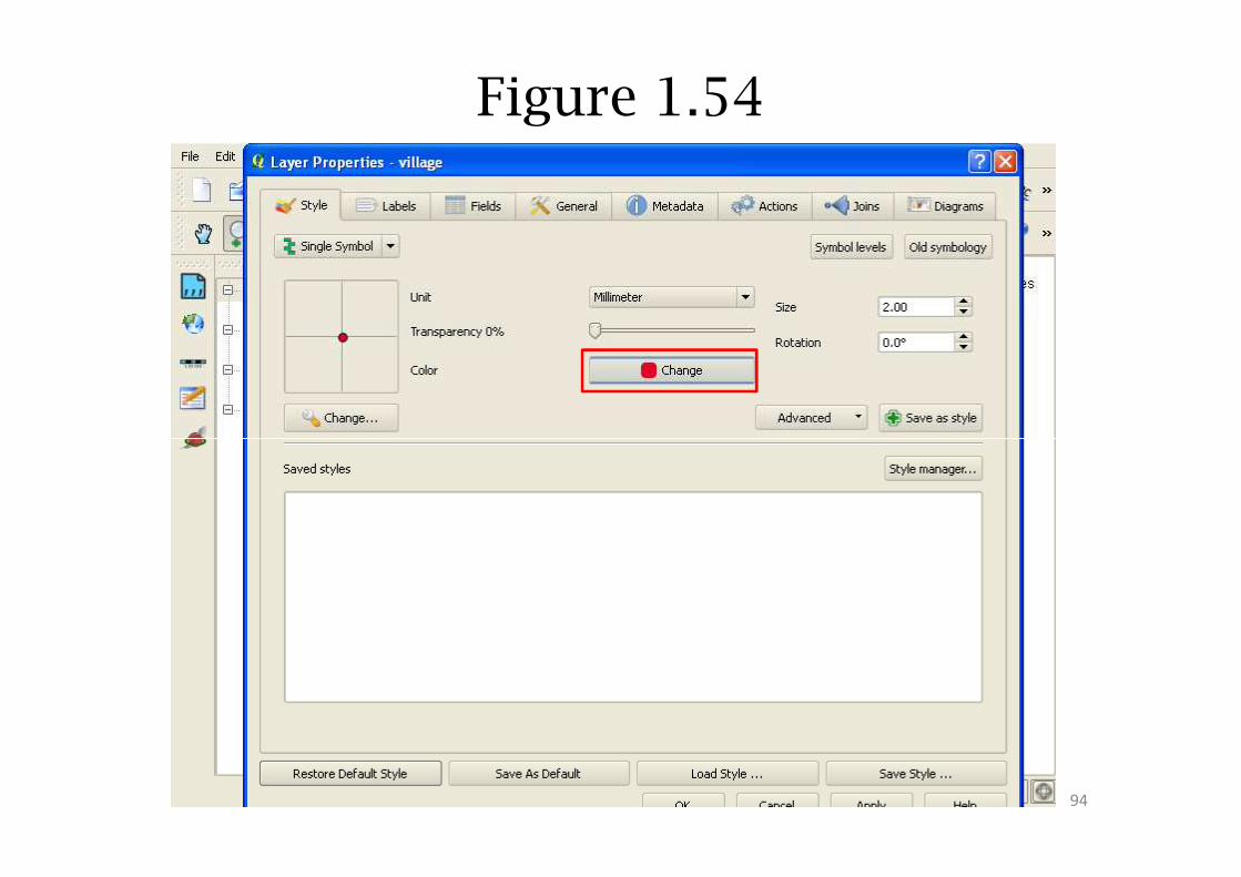
Figure 1.54
94
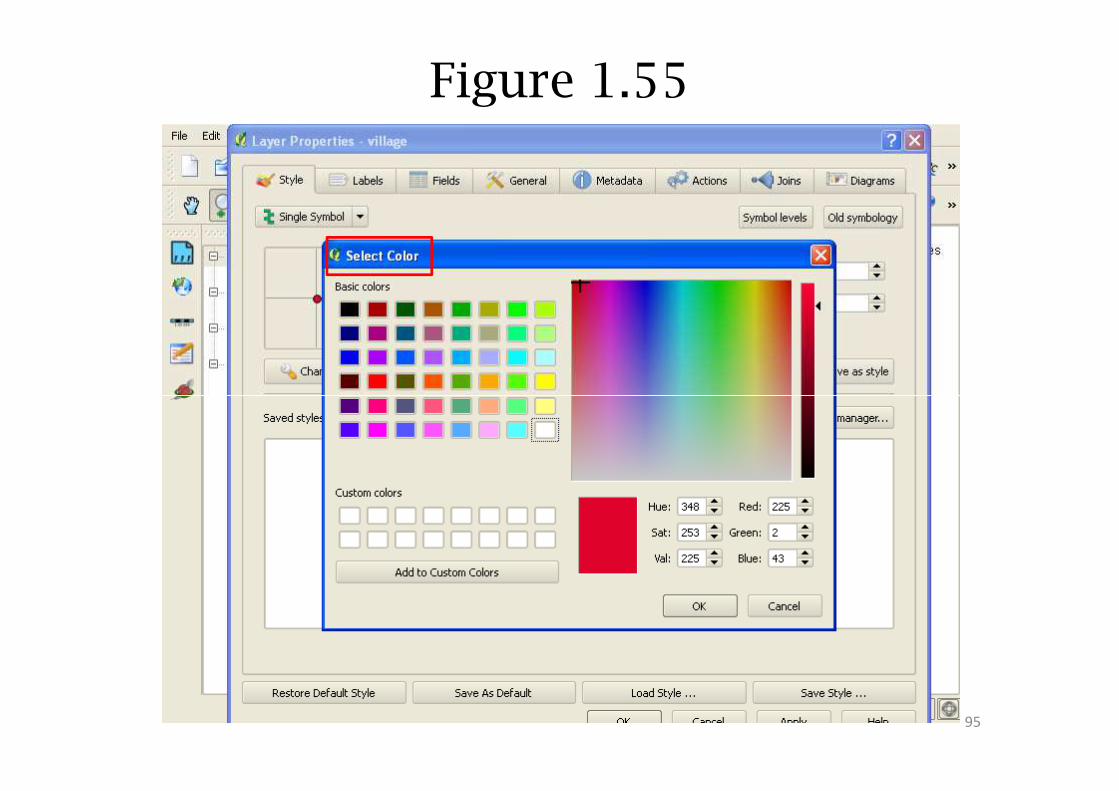
Figure 1.55
95
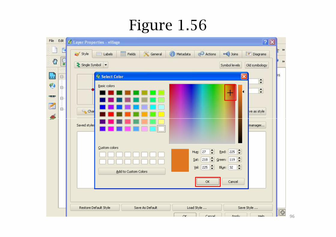
Figure 1.56
96
Point Style
• In the layer properties we can notice color has
changed (Figure 1.57)
• Select OK (Figure 1.57)• Select OK (Figure 1.57)
• Color change can be noticed in the village
layer (Figure 1.58)
97
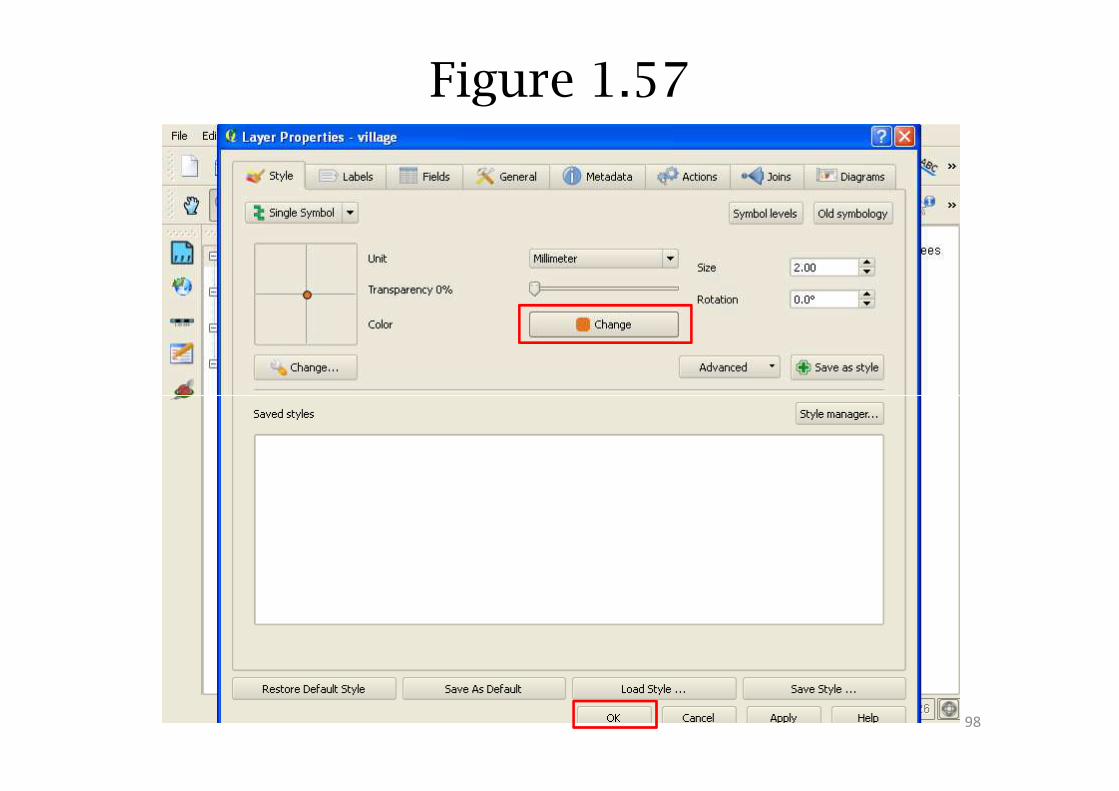
Figure 1.57
98
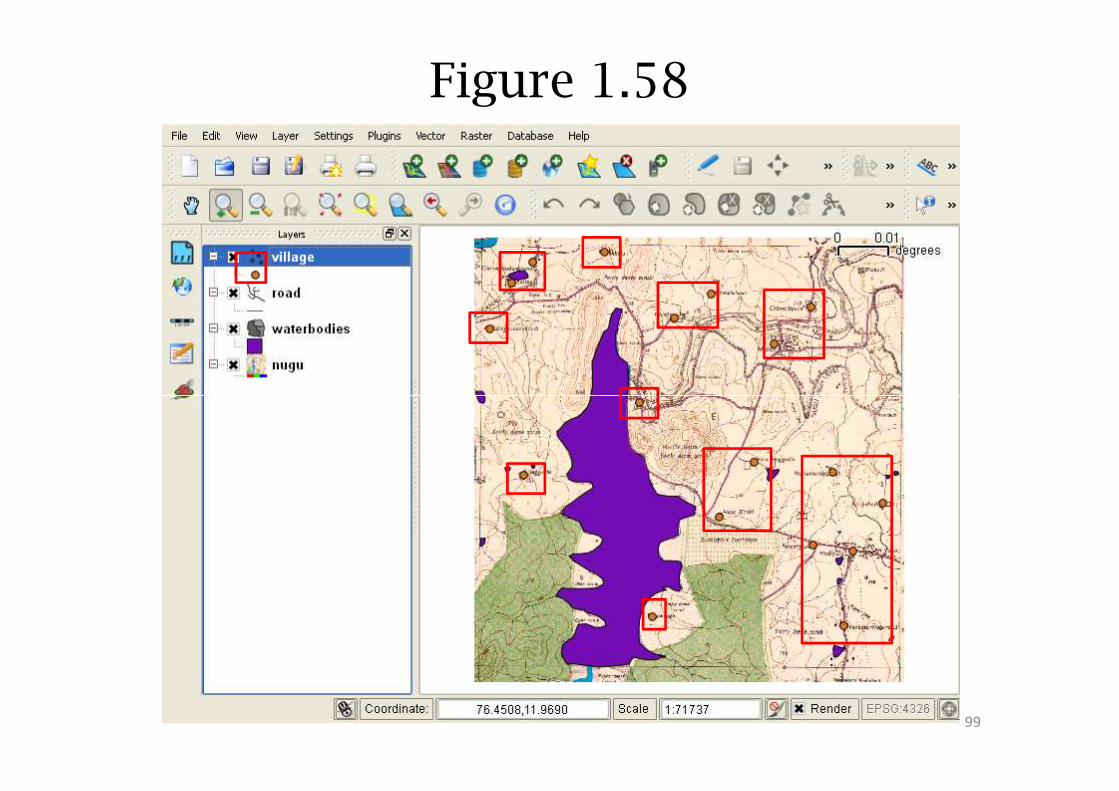
Figure 1.58
99
Line Style
• To change the color of road follow Step 7
(page 89)
• Layer Properties window opens (Figure 1.59)
� Select from saved styles an symbol appropriated � Select from saved styles an symbol appropriated
for roads, and even set width appropriately
(Figure 1.60)
� Select OK (Figure 1.60)
100
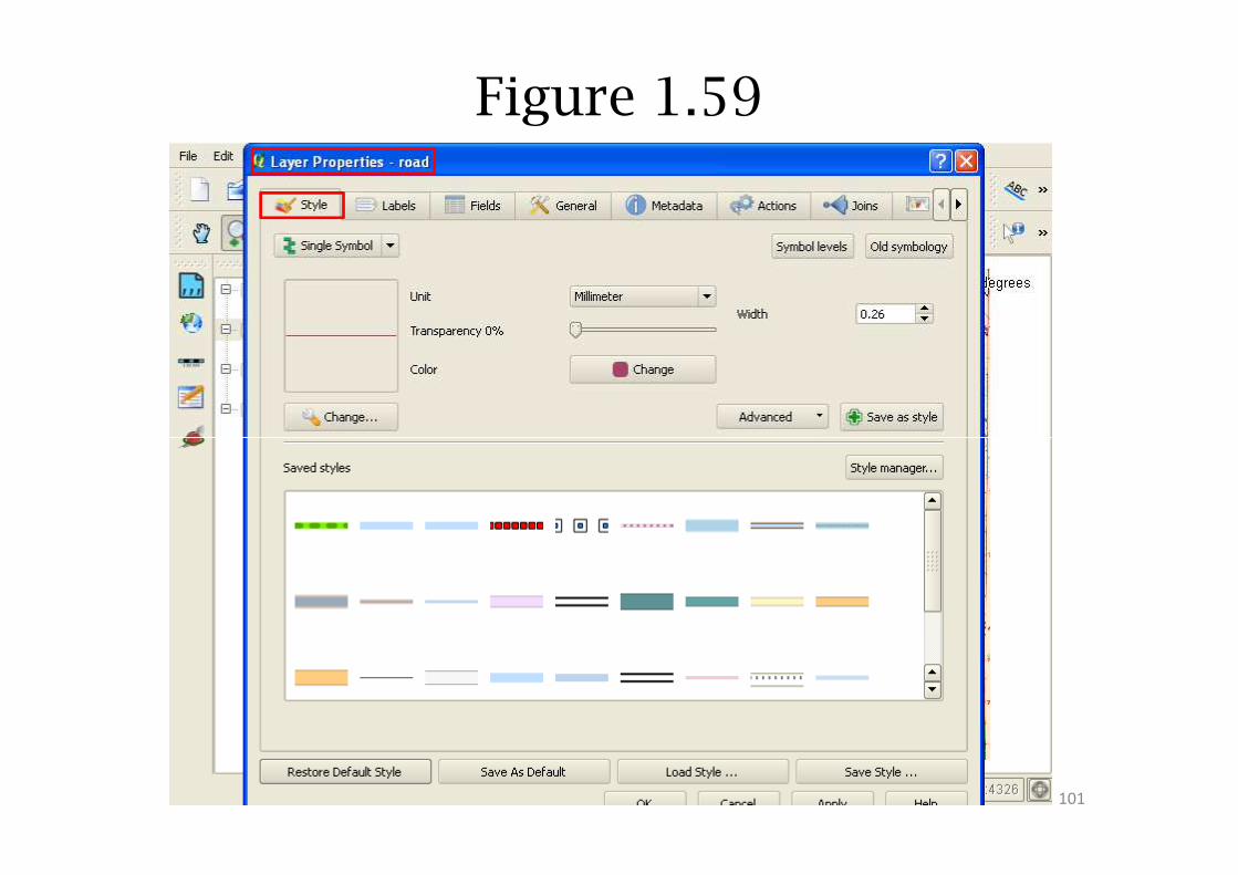
Figure 1.59
101
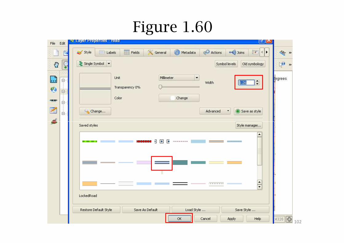
Figure 1.60
102
Polygon Style
• To change the color of polygon follow Step 7
(page 89)
• Follow Step 8, (page 90) and we get an output • Follow Step 8, (page 90) and we get an output
as in Figure 1.61
103
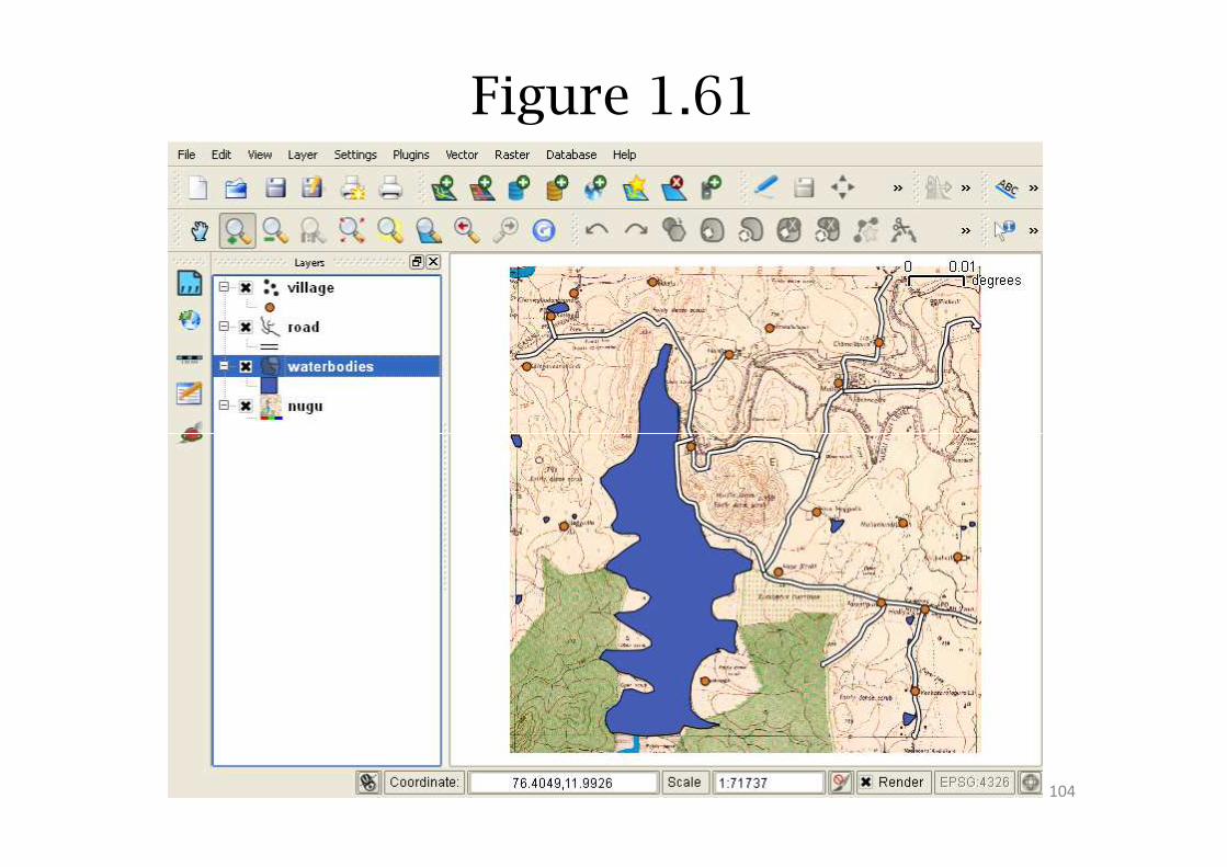
Figure 1.61
104
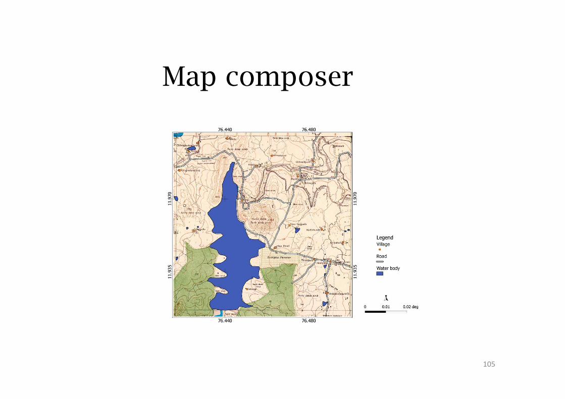
Map composer
105
Composition of Map
A output map should have
� Scale
� Legend
� North Arrow
� Grid (with coordinates)� Grid (with coordinates)
• To create map select New Print Composer (Figure2.1)
• The Composer opens (Figure 2.2)
• Composer has the buttons, General, Item andCommand history (Figure 2.2)
106
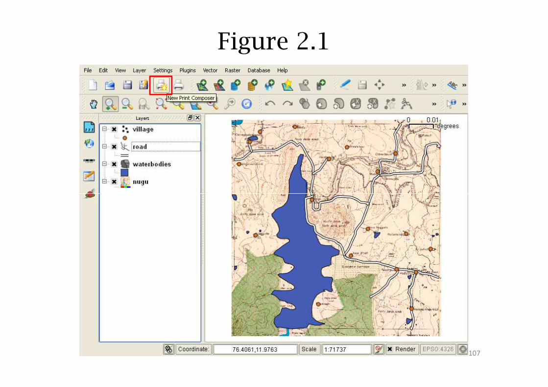
Figure 2.1
107
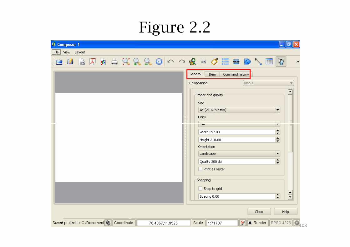
Figure 2.2
108
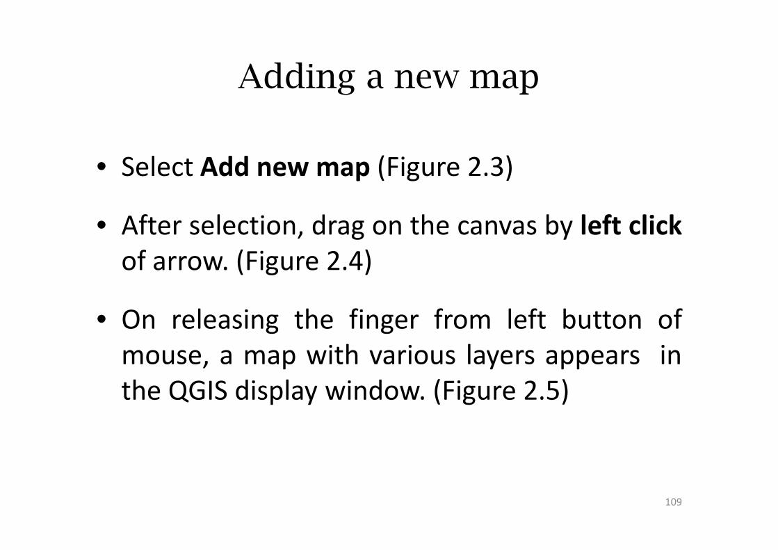
Adding a new map
• Select Add new map (Figure 2.3)
• After selection, drag on the canvas by left click
of arrow. (Figure 2.4)of arrow. (Figure 2.4)
• On releasing the finger from left button of
mouse, a map with various layers appears in
the QGIS display window. (Figure 2.5)
109
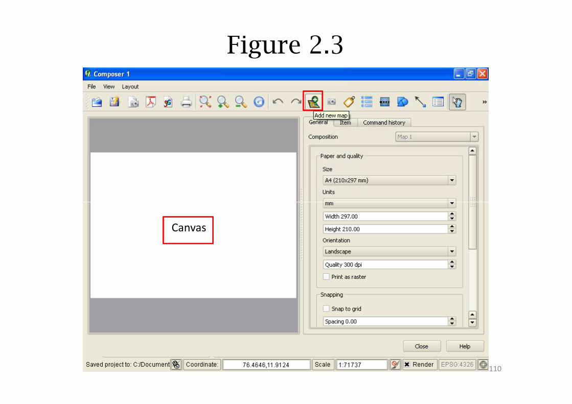
Figure 2.3
Canvas
110
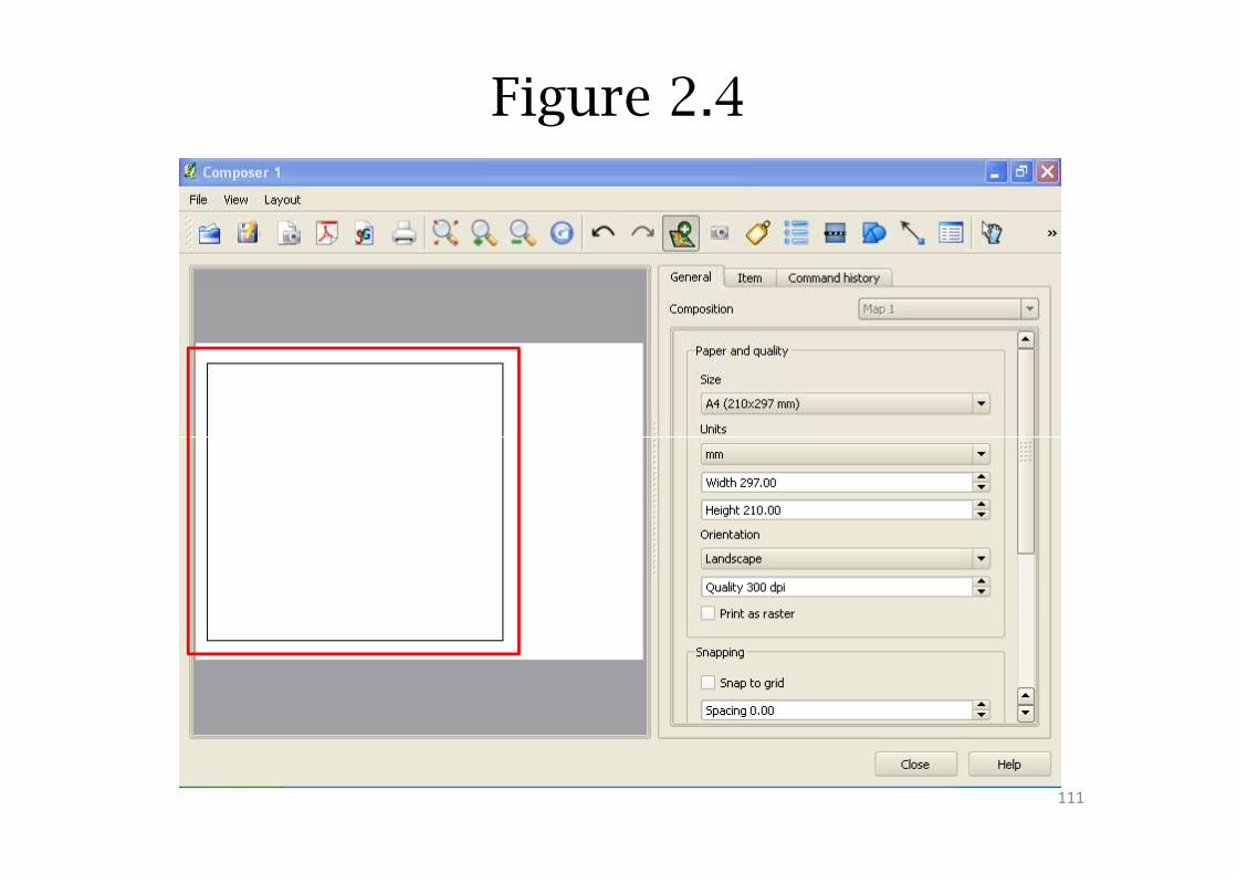
Figure 2.4
111
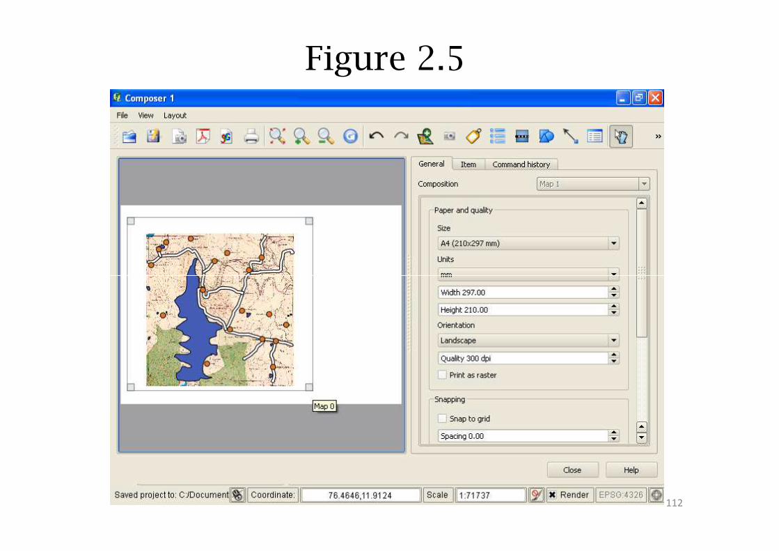
Figure 2.5
112

Adjusting the map
• In Figure 2.5 the complete display area is not
used by the map; to change this select Item
(Figure 2.6)
• By selecting either Width, Height or Scale the• By selecting either Width, Height or Scale the
map can use the complete display area
• For now, let us select Scale (Figure 2.6)
• Change Scale value to appropriate values
(Figure 2.7)
• Then select Grid(Figure 2.7)
113
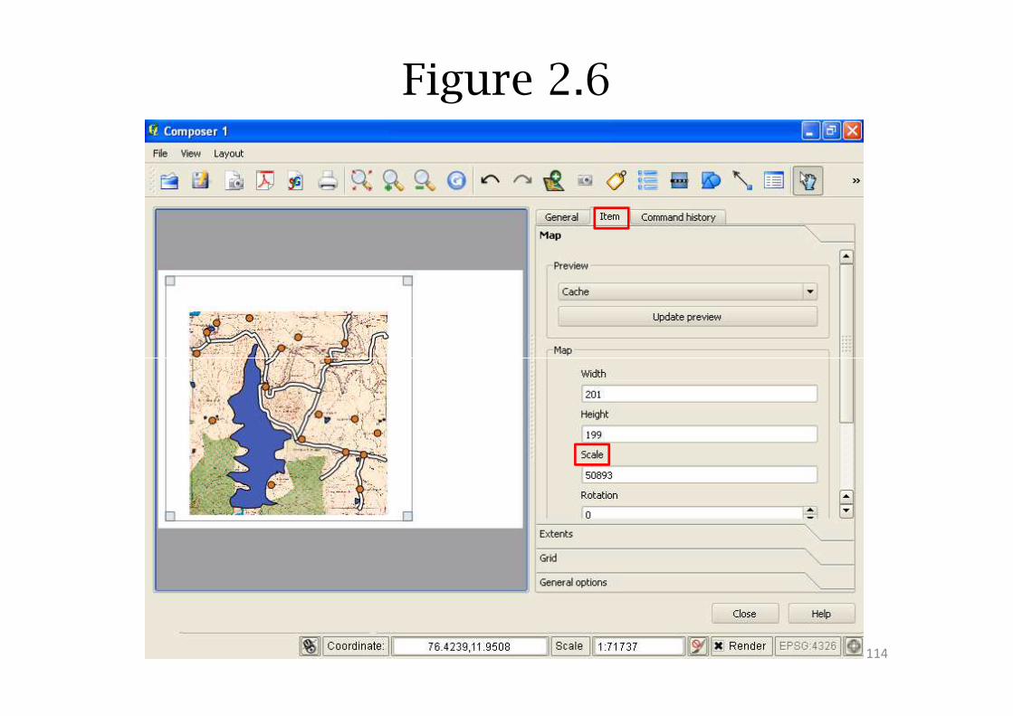
Figure 2.6
114
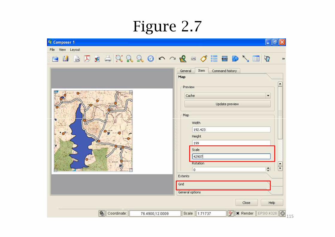
Figure 2.7
115
Grid creation
• Select Show Grid (Figure 2.8)
• Enter appropriate values (Figure 2.8)
�Interval X : 0.04
�Interval Y : 0.035�Interval Y : 0.035
• Scroll down (Figure 2.9)
� Select Draw annotation (Figure 2.9)
� Change Annotation Position and Annotation
direction appropriately (Figure 2.9) *
* These are subjective decisions and dependent on the projection system used. 116
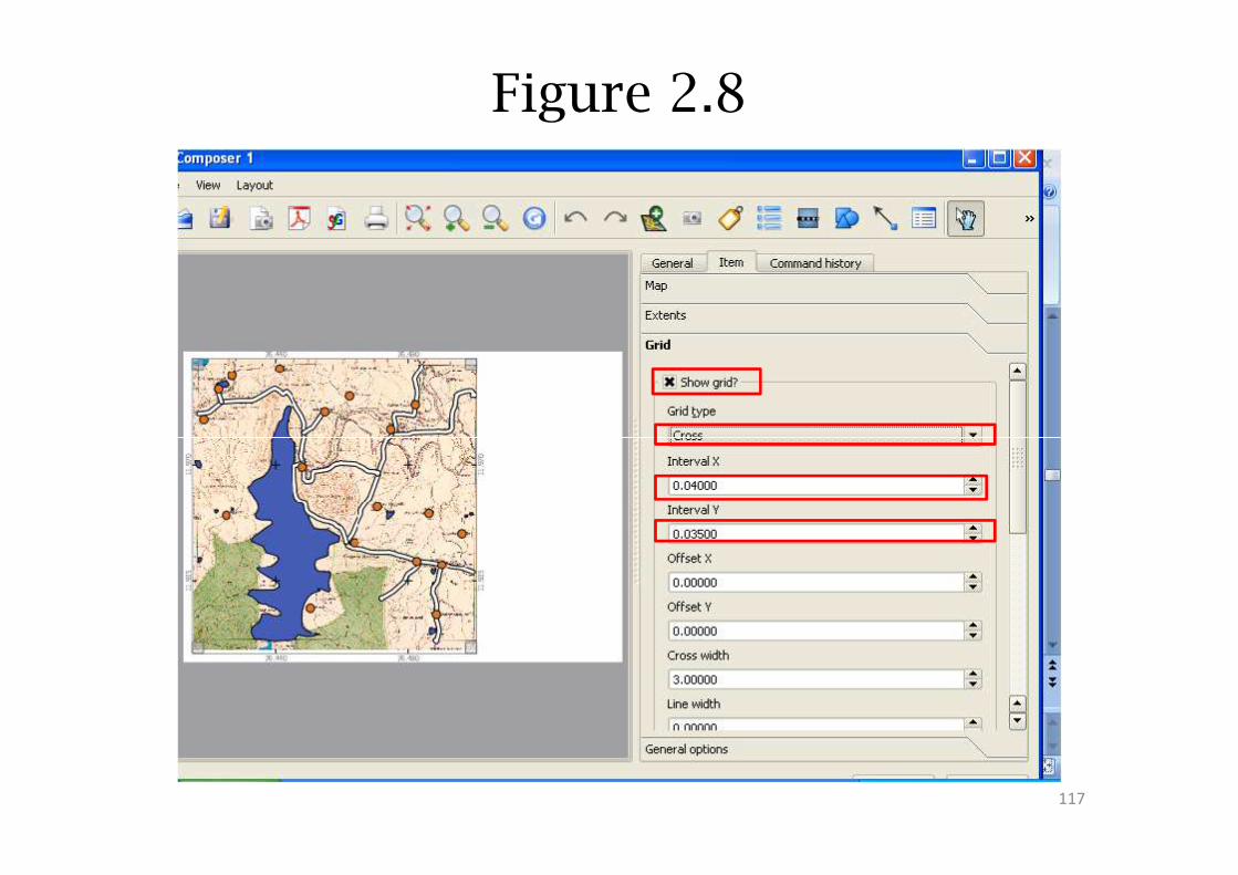
Figure 2.8
117
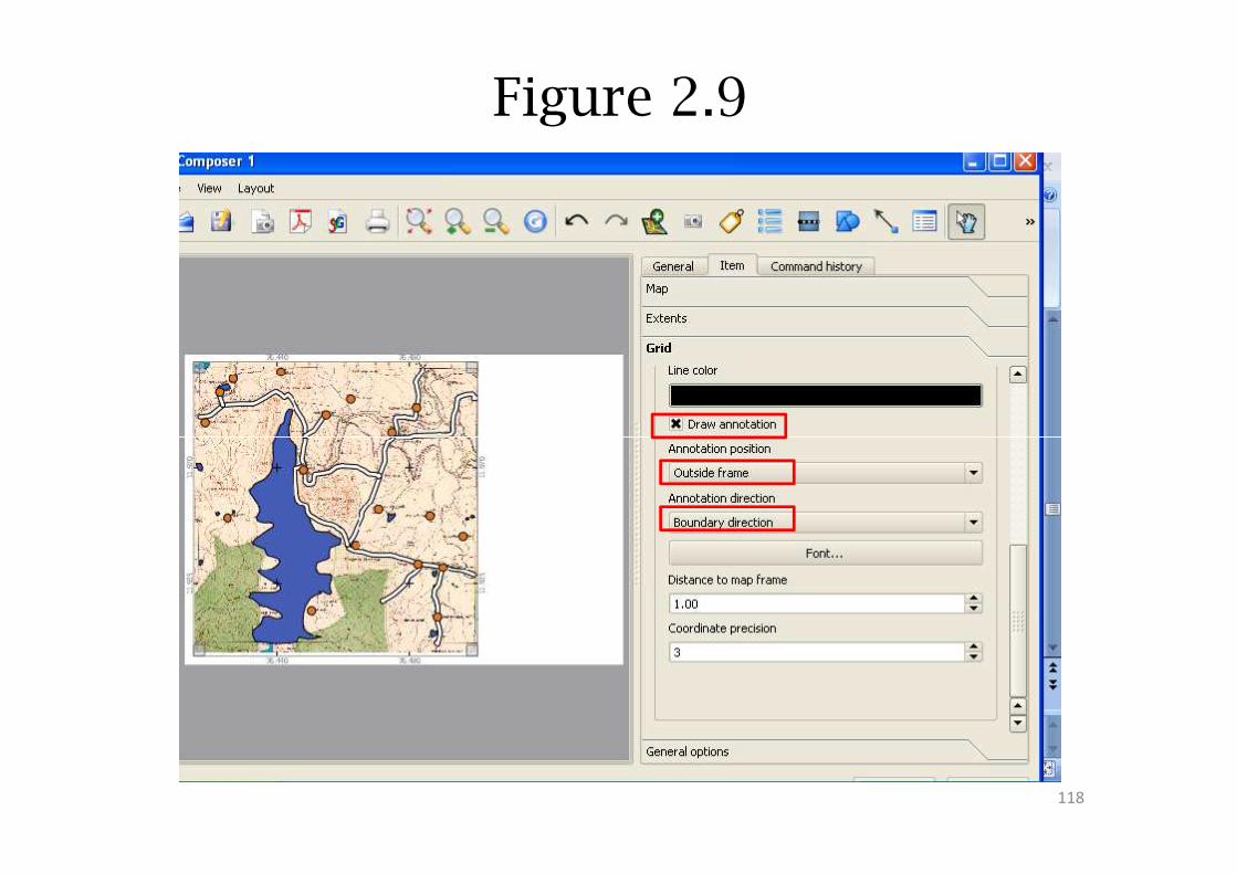
Figure 2.9
118
Adding North Arrow
• Next add a north arrow. Select Add Image
(Figure 2.10)
• Left click on the canvas, a window appears,
and in the Item window various images areand in the Item window various images are
displayed (Figure 2.11)
• Scroll down till we get the appropriate North
arrow image (Figure 2.12)
• In the Item General options de-select
Show frames (Figure 2.12 and Figure 2.13)
119
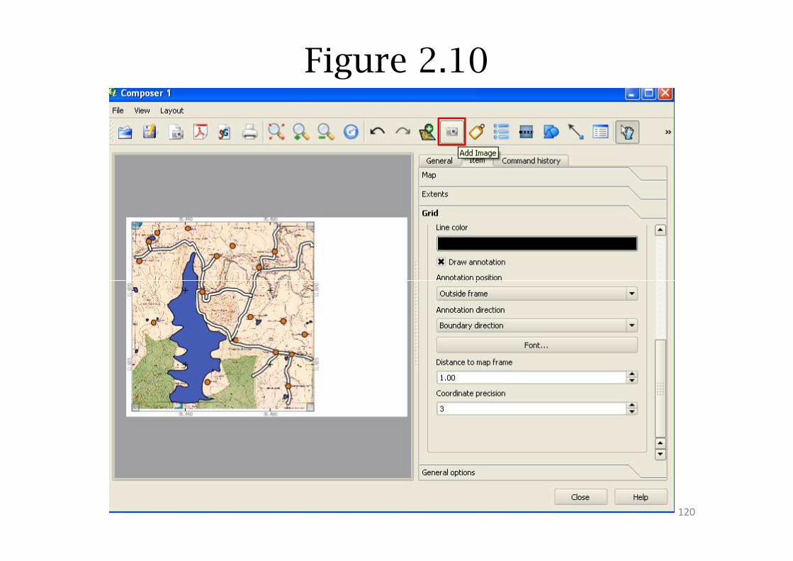
Figure 2.10
120
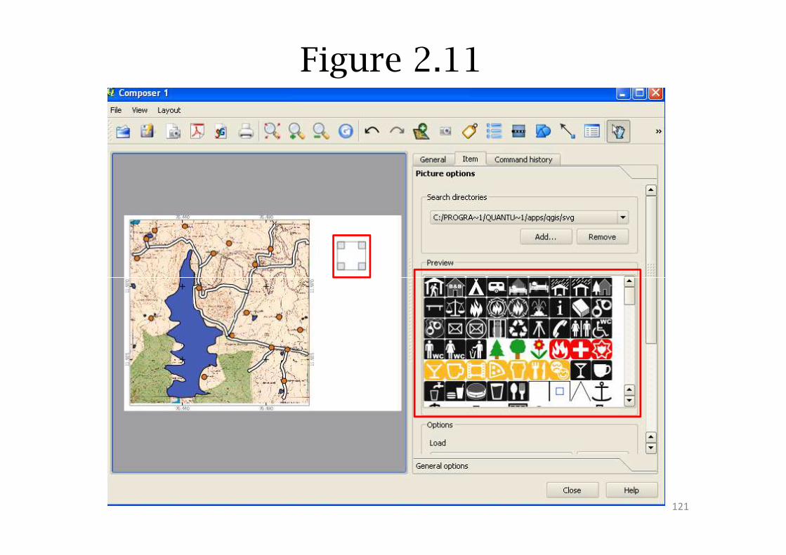
Figure 2.11
121

Figure 2.12
122
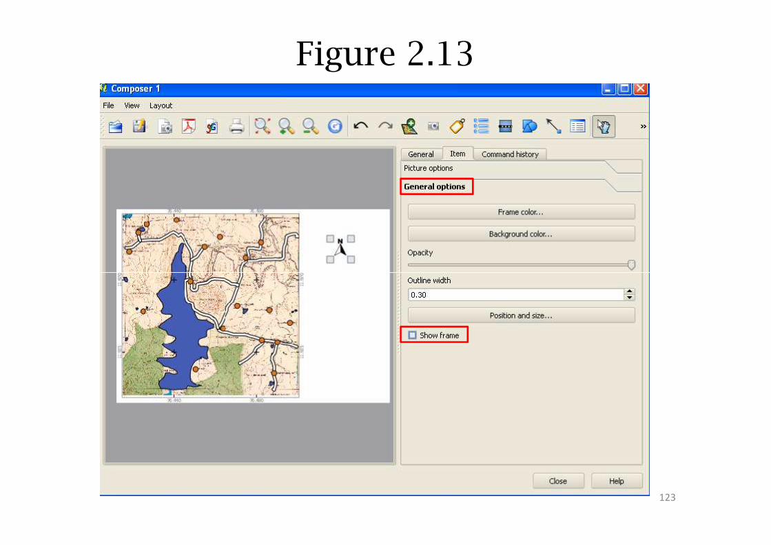
Figure 2.13
123
Adding Scale bar
• Next add scale to the map Add new scale bar
(Figure 2.14)
• Left click on canvas, a window appears. In the Item
window Scale bar tab is displayed (Figure 2.15)
• Enter appropriate values* (Figure 2.16)• Enter appropriate values* (Figure 2.16)
�Segment size: 0.01
�Map units per bar: 1
�Unit label: deg
• In the Item General options de-select Show
frames (as in Figure 2.12 and Figure 2.13)
* These are subjective decisions and dependent on the projection system used. 124
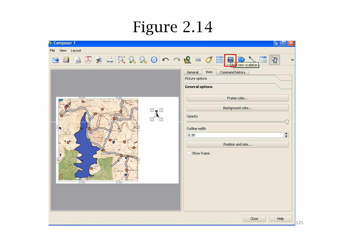
Figure 2.14
125
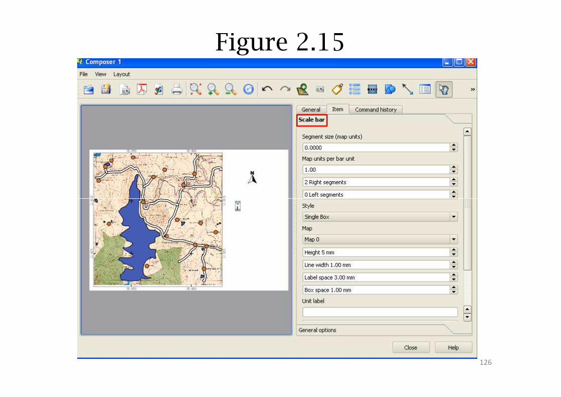
Figure 2.15
126
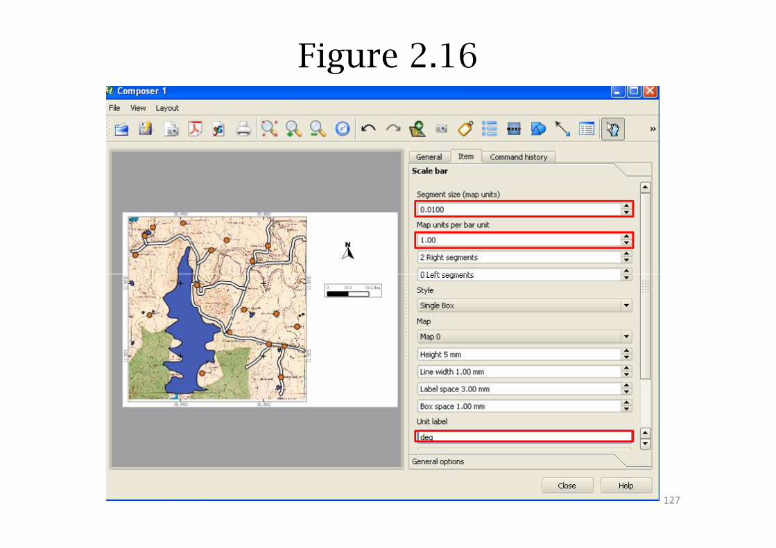
Figure 2.16
127
Adding Legend
• The final step is to add a legend, select Add
new vect legend
• Left click on the canvas, a window appears, and
in the Item window General tab is displayedin the Item window General tab is displayed
(Figure 2.18)
• Select Legend items (Figure 2.18) Legend
items tab opens (Figure 2.19)
128
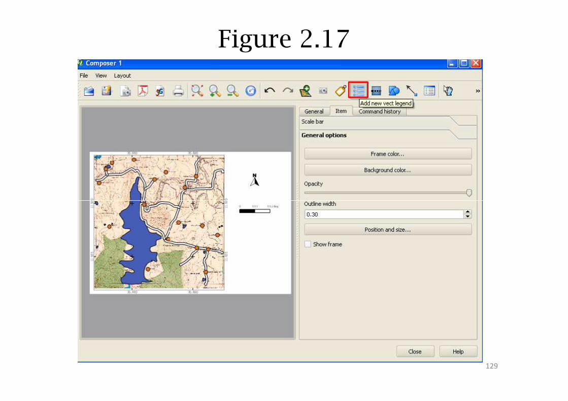
Figure 2.17
129
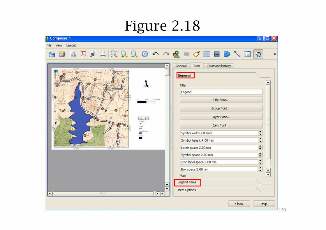
Figure 2.18
130
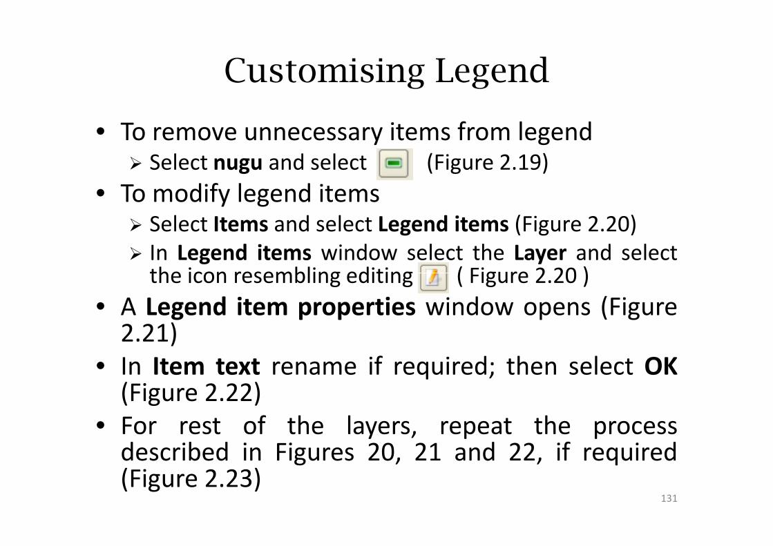
Customising Legend
• To remove unnecessary items from legend� Select nugu and select (Figure 2.19)
• To modify legend items� Select Items and select Legend items (Figure 2.20)
� In Legend items window select the Layer and selectthe icon resembling editing ( Figure 2.20 )the icon resembling editing ( Figure 2.20 )
• A Legend item properties window opens (Figure2.21)
• In Item text rename if required; then select OK(Figure 2.22)
• For rest of the layers, repeat the processdescribed in Figures 20, 21 and 22, if required(Figure 2.23)
131
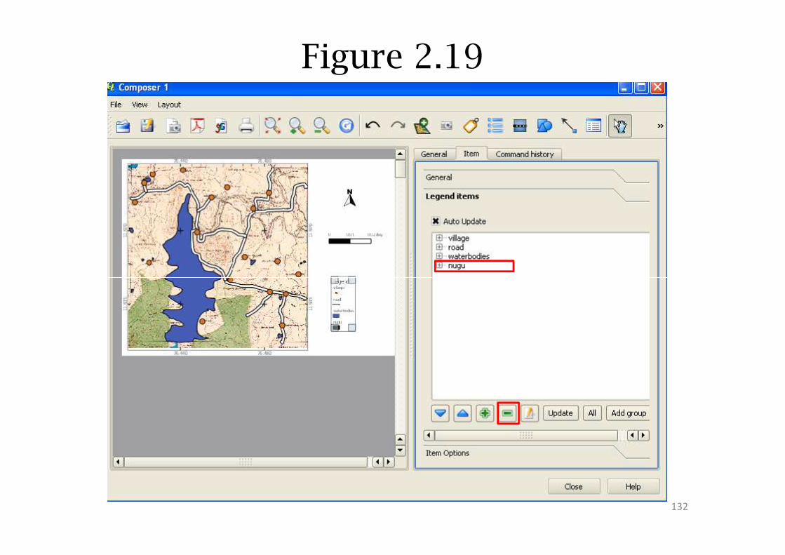
Figure 2.19
132
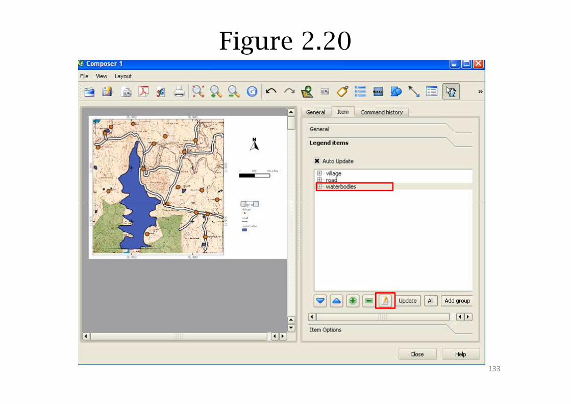
Figure 2.20
133
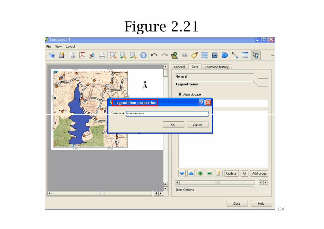
Figure 2.21
134
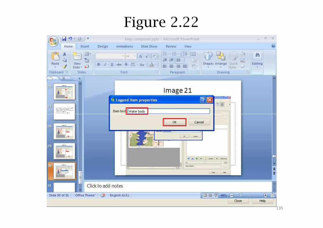
Figure 2.22
135
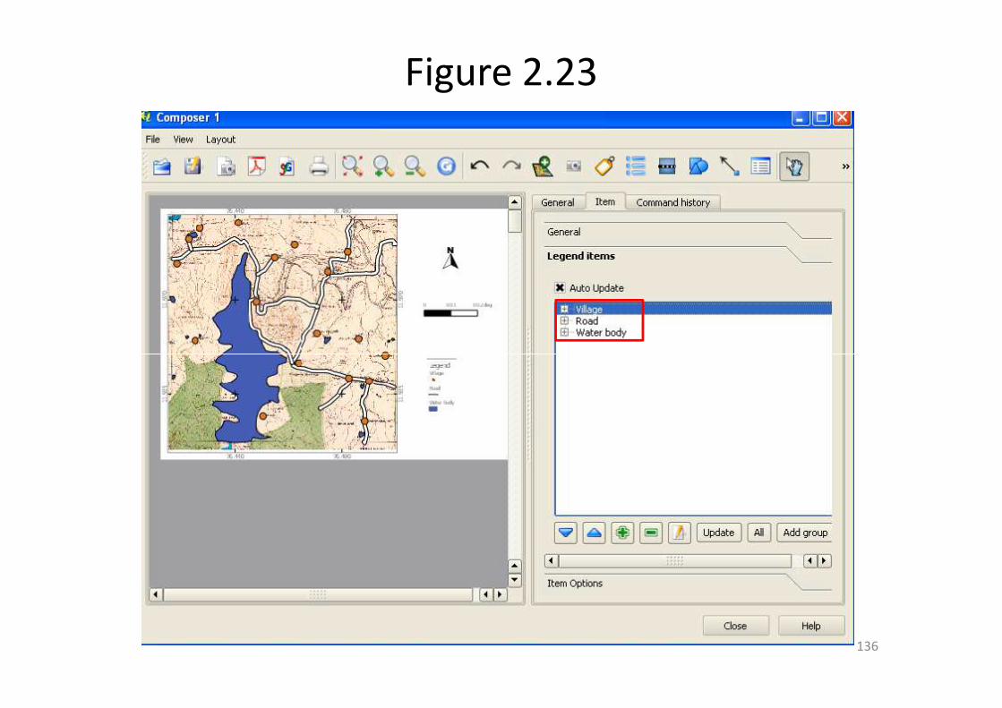
Figure 2.23
136
Customising Map window
• In the Item Item options de-selectShow frames as in Figure 2.12, page 17 (Figure2.24)
• Finally, all the required elements are placedon the canvas; rearrange the same to conveyon the canvas; rearrange the same to conveythe message in a elegant way (Figure 2.25)
• Save the composer window by selecting Saveas template (Figure 2.26)
• The Save template window opens, enter thefile name Nugu and select Save ( Figure 2.27 )
137
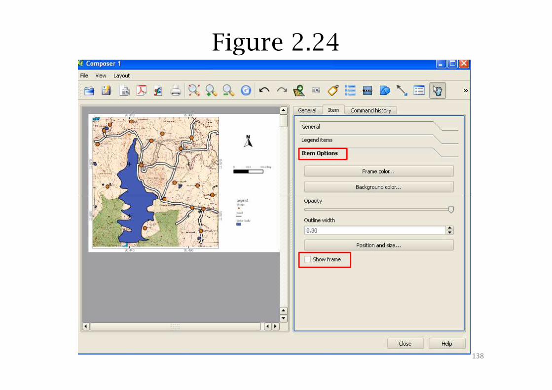
Figure 2.24
138
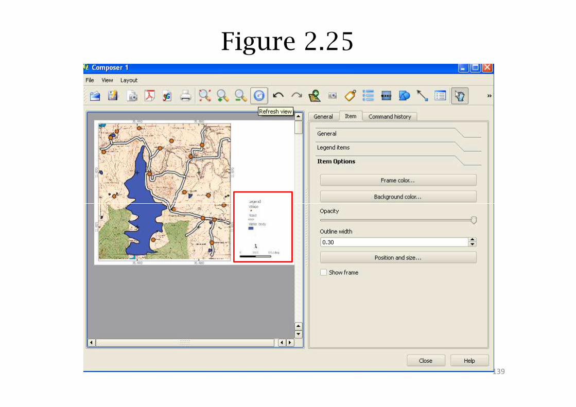
Figure 2.25
139
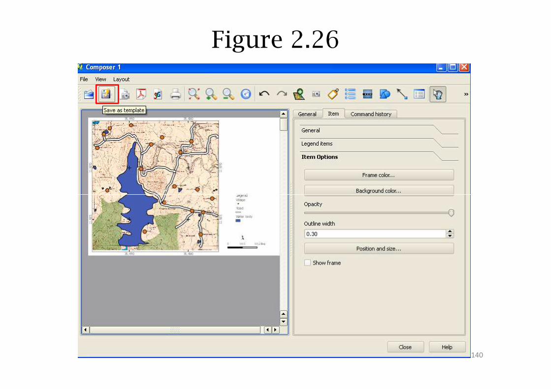
Figure 2.26
140
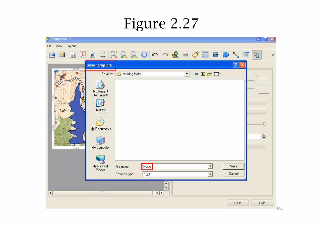
Figure 2.27
141
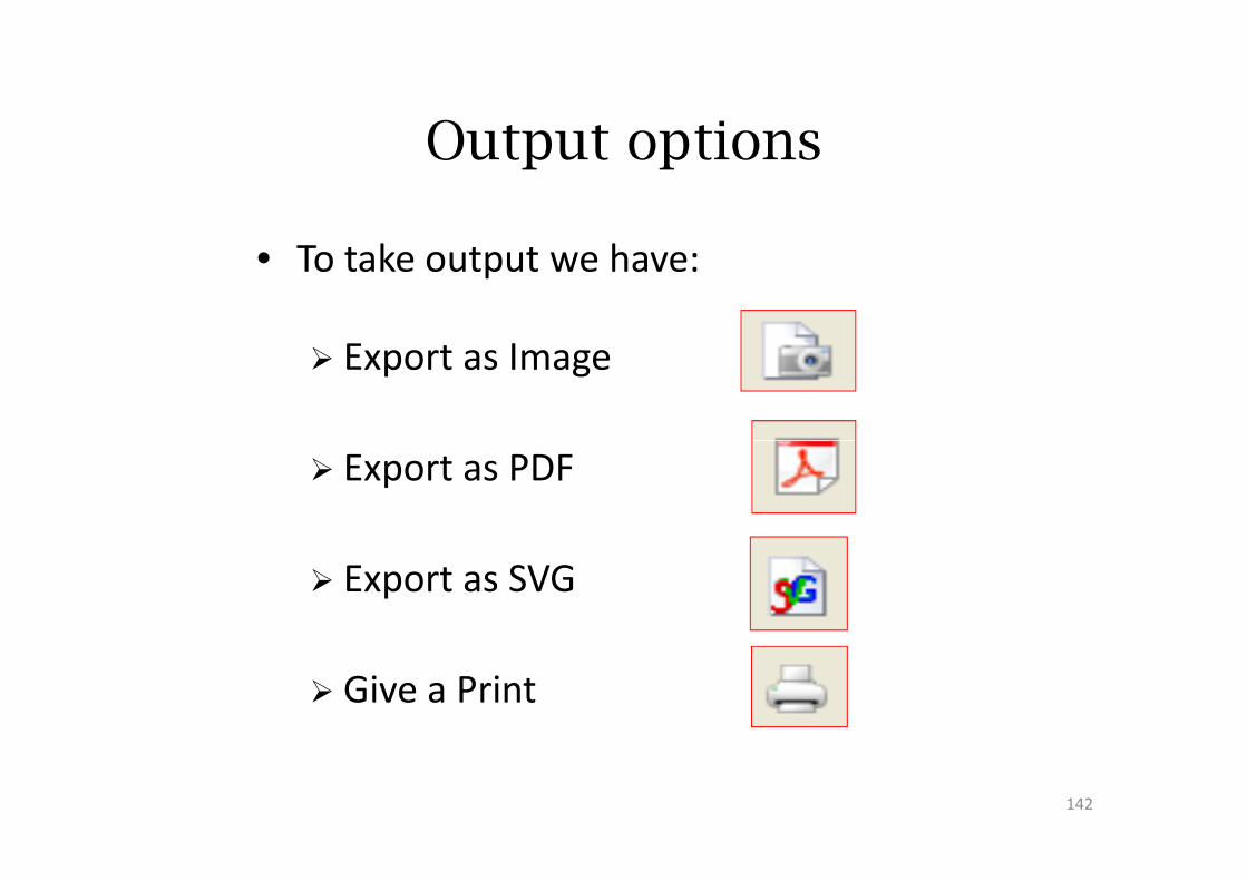
Output options
• To take output we have:
� Export as Image
� Export as PDF
� Export as SVG
� Give a Print
142
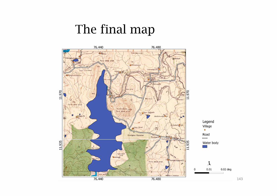
The final map
143
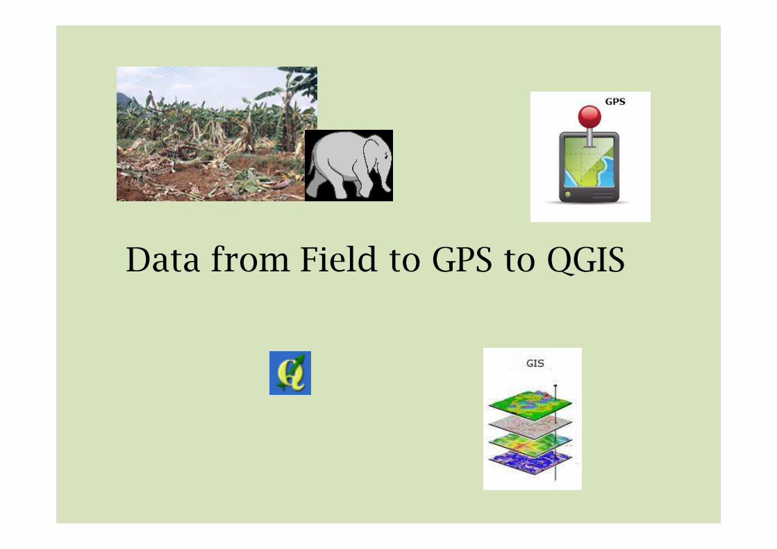
Data from Field to GPS to QGISData from Field to GPS to QGIS
Importing GPS data to GPS
TrackMarker
To import the data from GPS to QGIS, the
following steps are involved:
� Running GPS TrackMarker
� Connecting the GPS to the system
� Importing the data to GPS TrackMarker
� Saving it as GPX format.
145
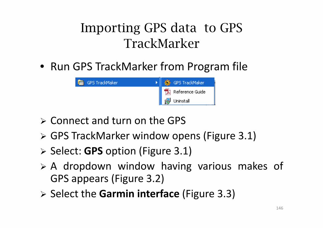
• Run GPS TrackMarker from Program file
Connect and turn on the GPS
Importing GPS data to GPS
TrackMarker
� Connect and turn on the GPS
� GPS TrackMarker window opens (Figure 3.1)
� Select: GPS option (Figure 3.1)
� A dropdown window having various makes ofGPS appears (Figure 3.2)
� Select the Garmin interface (Figure 3.3)146
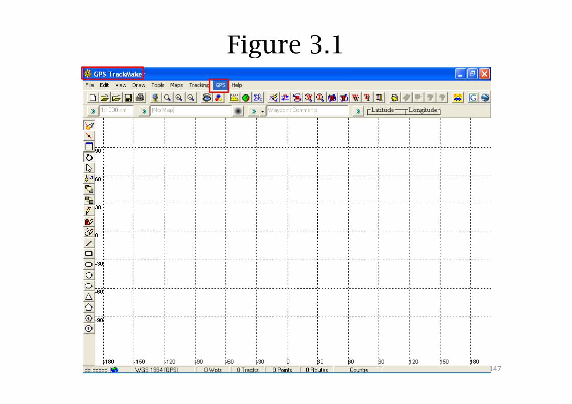
Figure 3.1
147
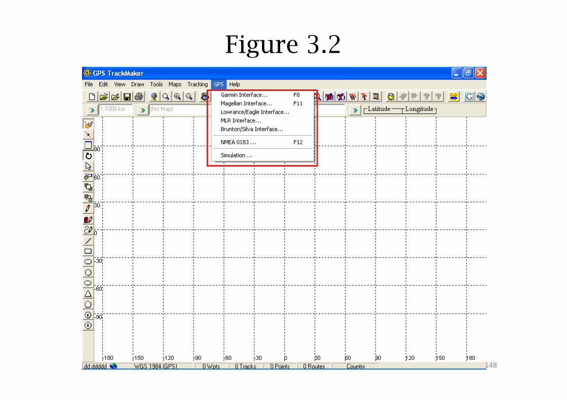
Figure 3.2
148
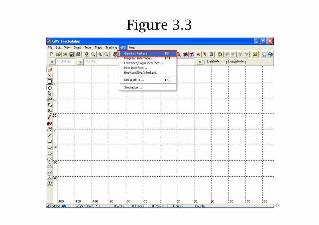
Figure 3.3
149
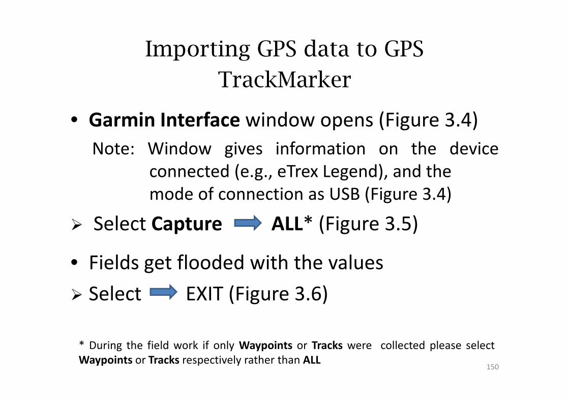
• Garmin Interface window opens (Figure 3.4)
Note: Window gives information on the device
connected (e.g., eTrex Legend), and the
mode of connection as USB (Figure 3.4)
Importing GPS data to GPS
TrackMarker
mode of connection as USB (Figure 3.4)
� Select Capture ALL* (Figure 3.5)
• Fields get flooded with the values
� Select EXIT (Figure 3.6)
* During the field work if only Waypoints or Tracks were collected please select
Waypoints or Tracks respectively rather than ALL150
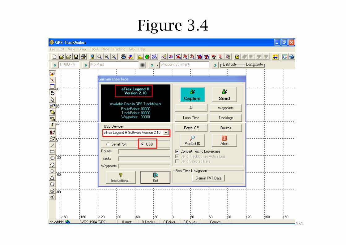
Figure 3.4
151
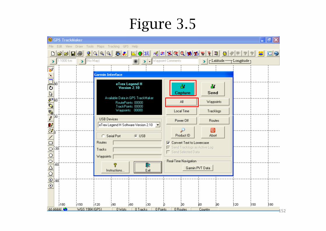
Figure 3.5
152
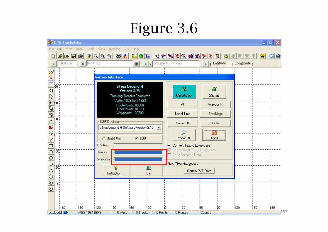
Figure 3.6
153
• The output is displayed in the window (Figure
3.7)
• Next save the data.
Importing GPS data to GPS
TrackMarker
• Next save the data.
� Select File Save File as (Figure 3.8)
� Select Save as type: GPS exchange file
(.gpx) format (Figure 3.9)
� Name appropriately and save (Figure 3.10)
154
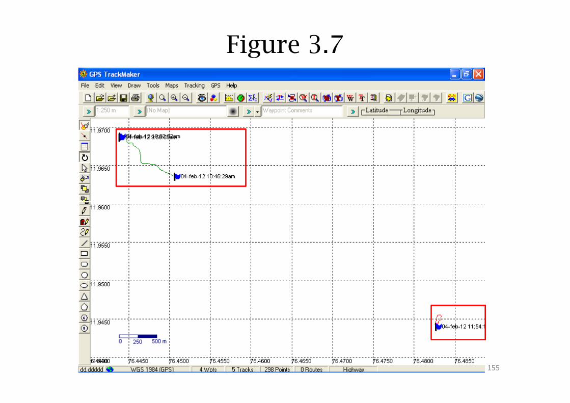
Figure 3.7
155
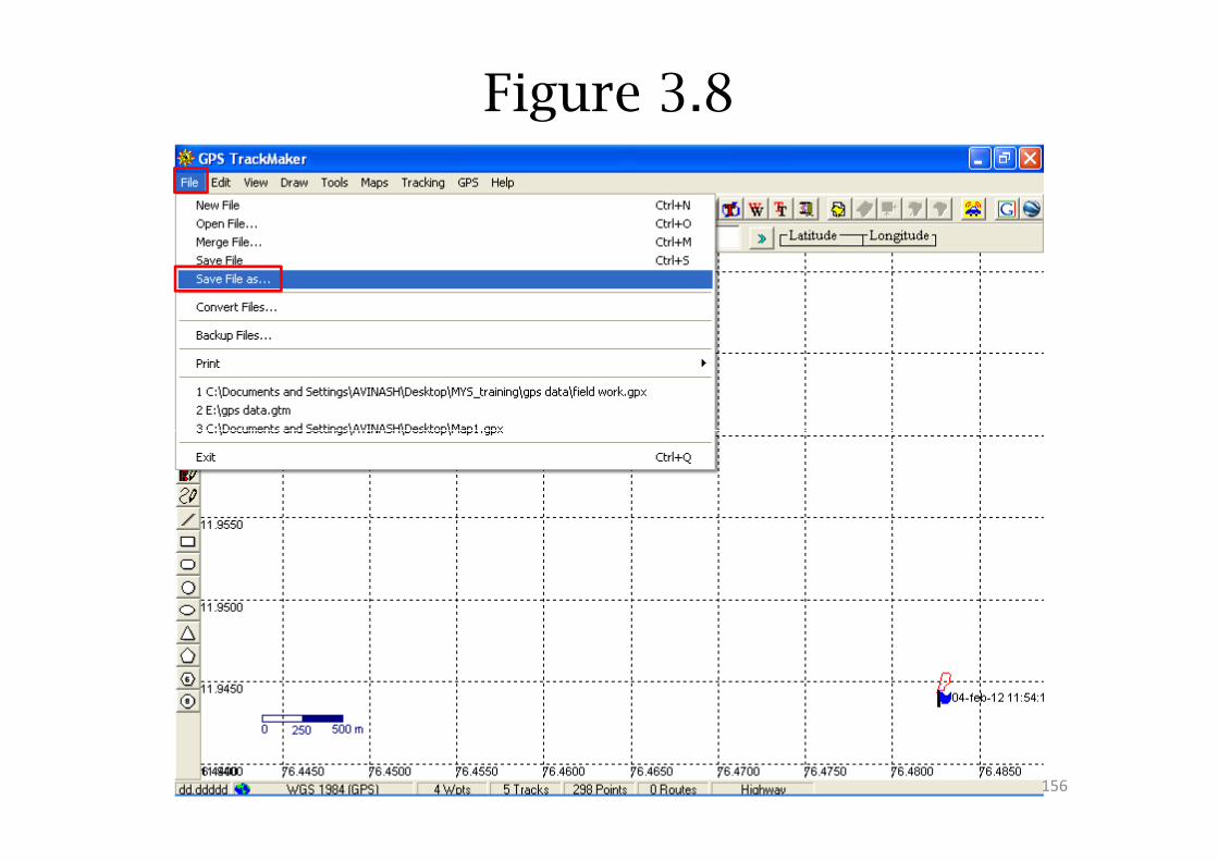
Figure 3.8
156
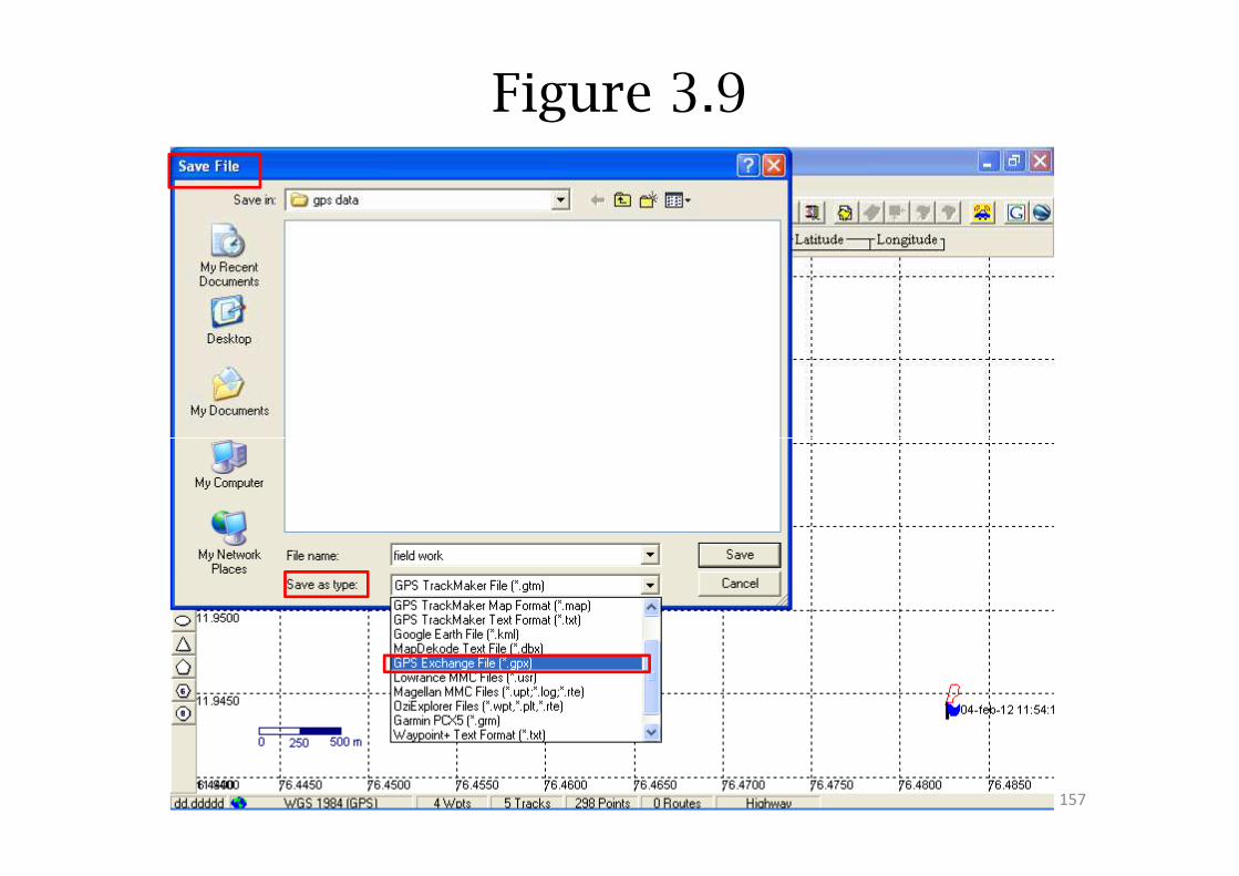
Figure 3.9
157
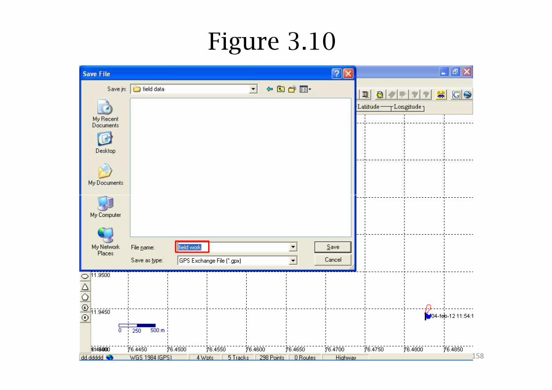
Figure 3.10
158
Importing the data to QGIS
• Close the GPS TrackMarker application
• Open QGIS
• To view this data in QGIS
Select Gps tools icon (Figure 3.11)� Select Gps tools icon (Figure 3.11)
� Gps Tools window appears Load GPX file
arro Browse (Figure 3.12)
� Directs to the saved file. Select the gpx file
created (Figure 3.13)
159
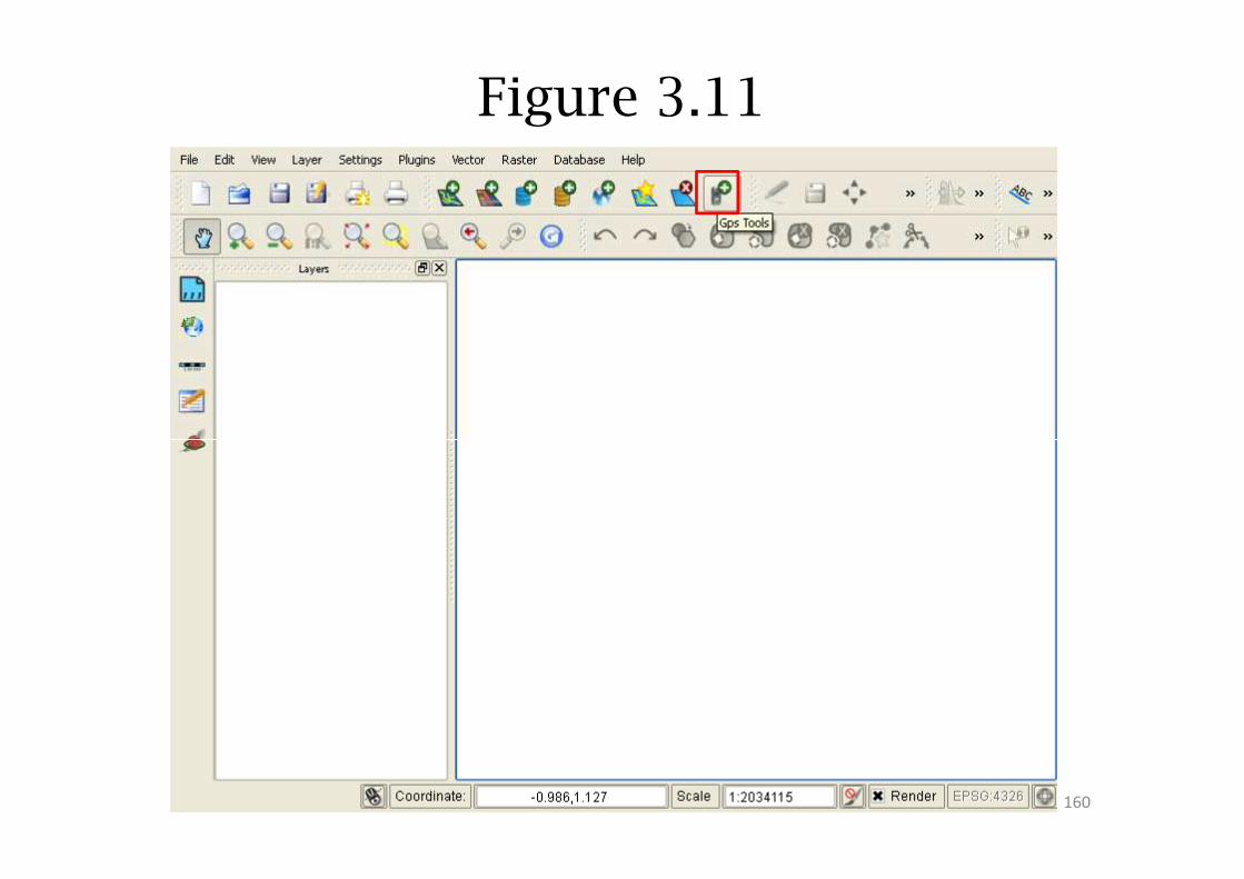
Figure 3.11
160
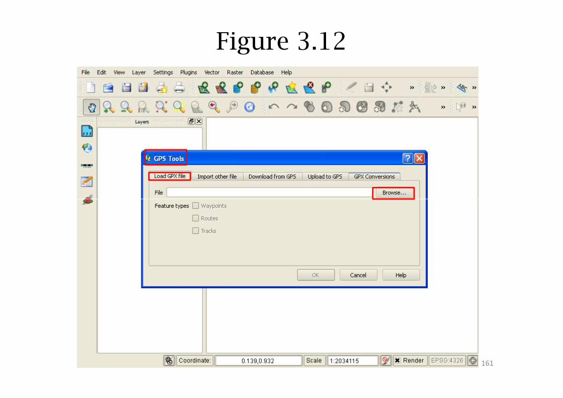
Figure 3.12
161
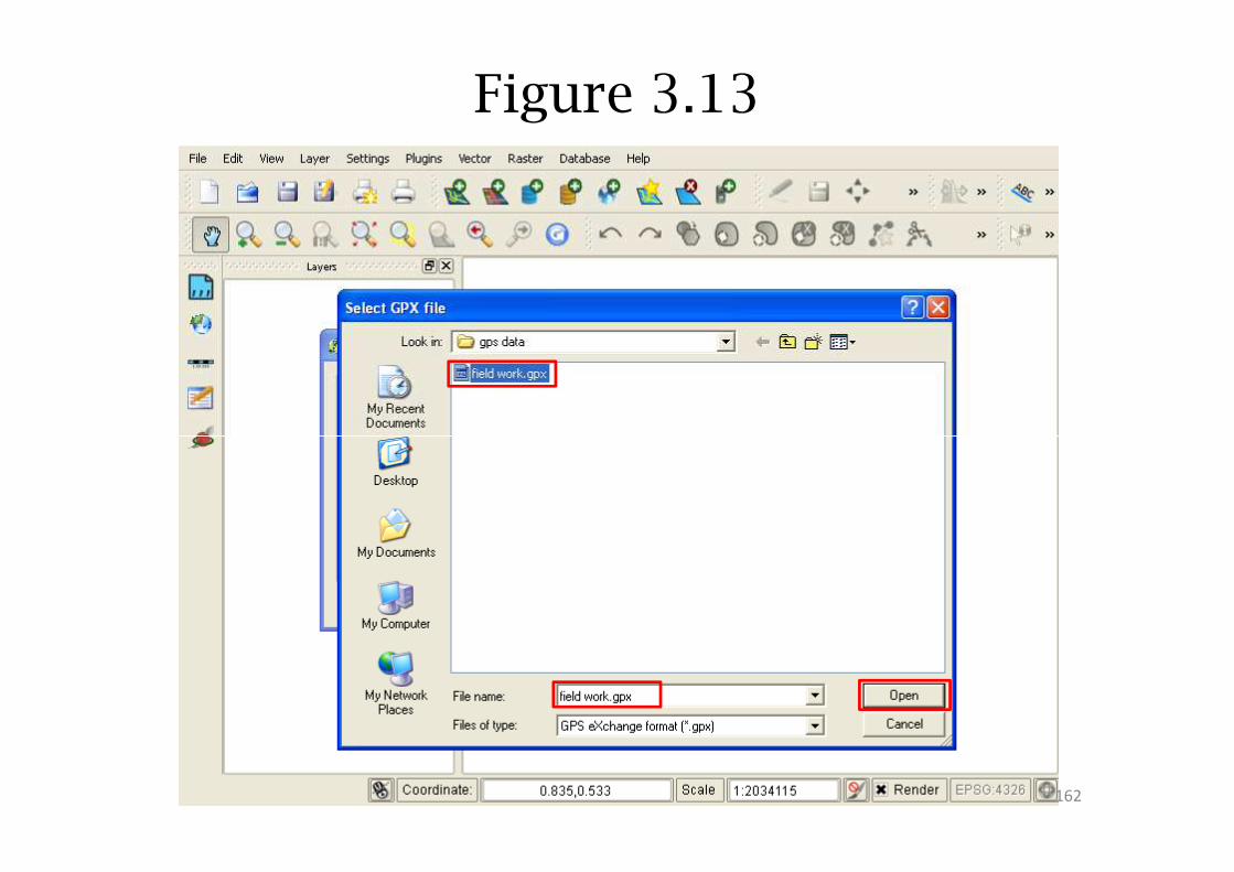
Figure 3.13
162
Importing the data to QGIS
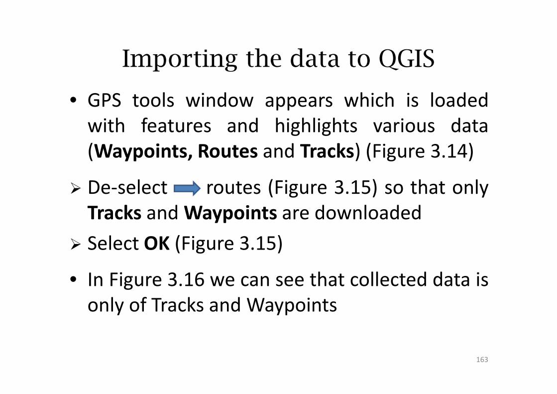
• GPS tools window appears which is loaded
with features and highlights various data
(Waypoints, Routes and Tracks) (Figure 3.14)
� De-select routes (Figure 3.15) so that only� De-select routes (Figure 3.15) so that only
Tracks and Waypoints are downloaded
� Select OK (Figure 3.15)
• In Figure 3.16 we can see that collected data is
only of Tracks and Waypoints
163
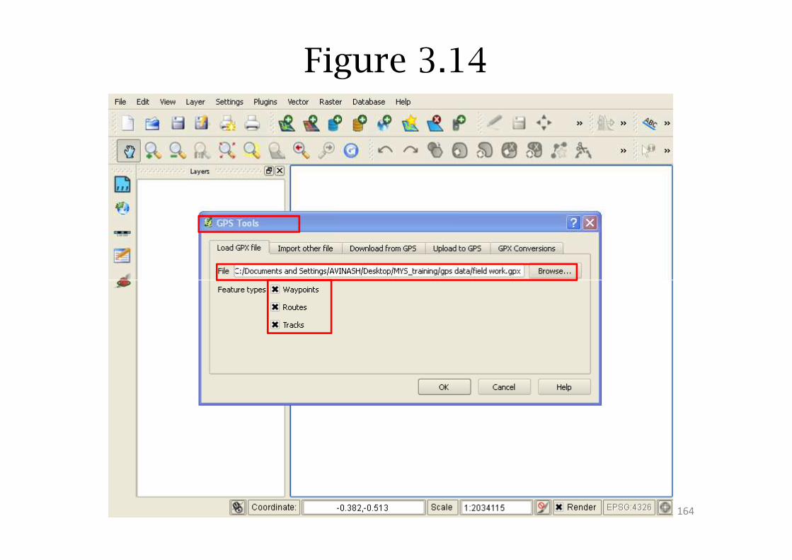
Figure 3.14
164
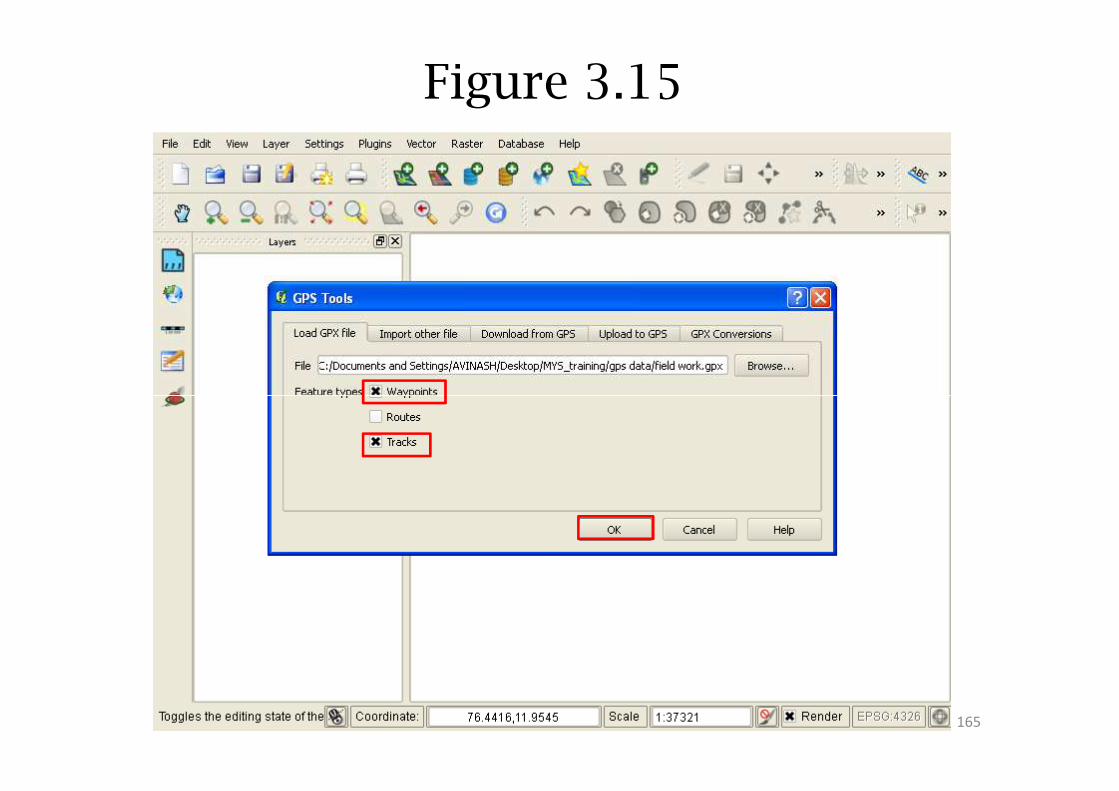
Figure 3.15
165
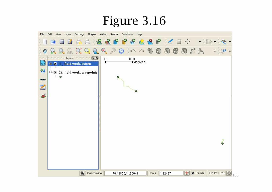
Figure 3.16
166
Saving the Imported Data
• Save the files one after the other by right
clicking Save as (Figure 3.17)
• Save vector layer as (Figure 3.18)
� Format: ESRI shapefiles� Format: ESRI shapefiles
� Save as: save in desired folder
� CRS : WGS 84
• Select OK (Figure 3.18)
167
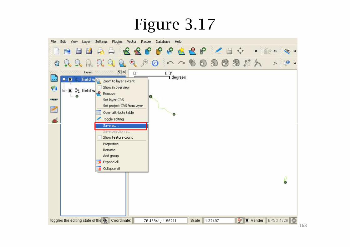
Figure 3.17
168
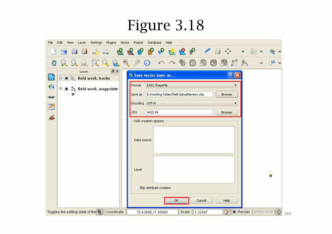
Figure 3.18
169
Representation on Map
• Remove both the layers.
• Load all the digitised layers from Nugu area, andalso the Nugu map (as described in QGIS tutorial)
• Now add the filed data saved from GPS (onlyshape files)
• Now add the filed data saved from GPS (onlyshape files)
� Select Add vector layer Browse
� select layers Open
� Once again, select Open (Figure 3.19)
• The output (Figure 3.20) would have both thefeatures (follow Map composer tutorial)
170
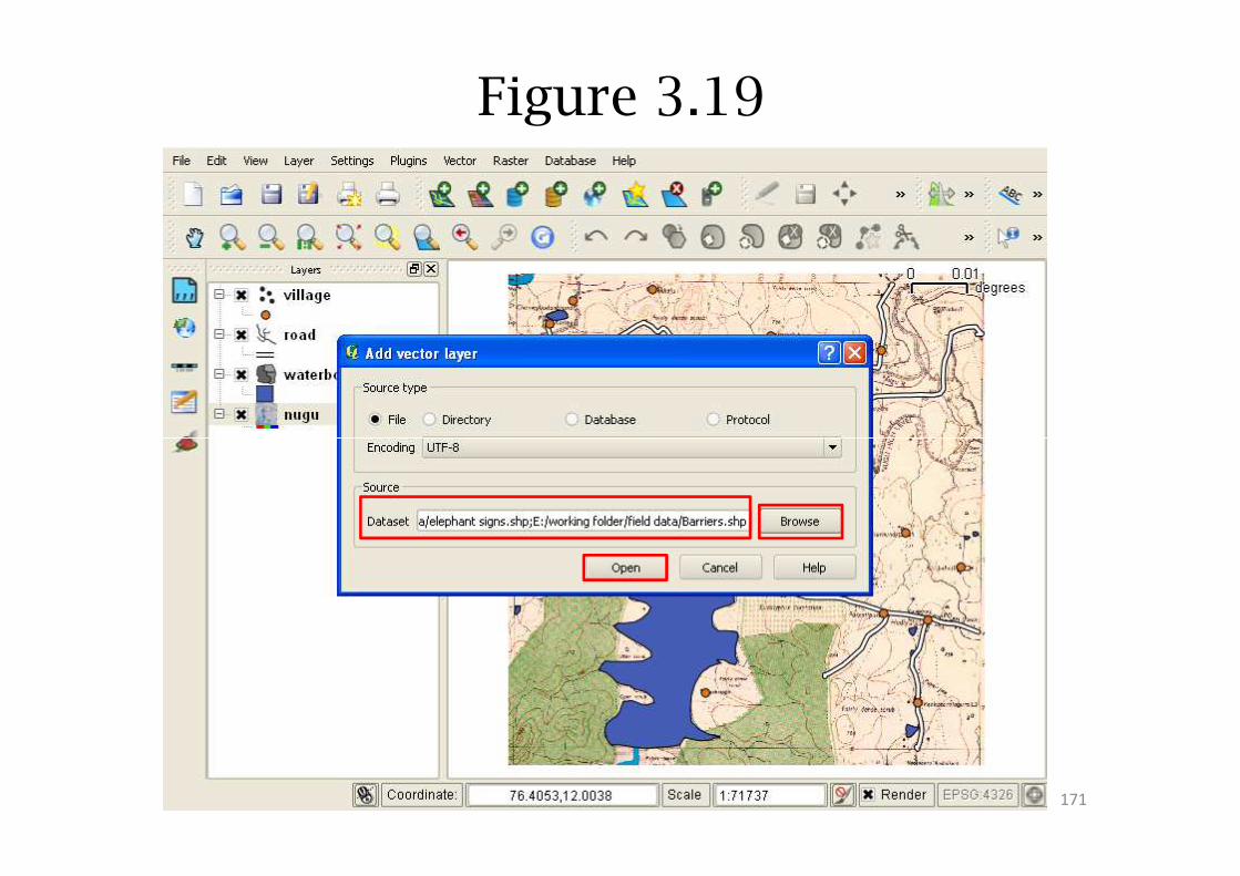
Figure 3.19
171
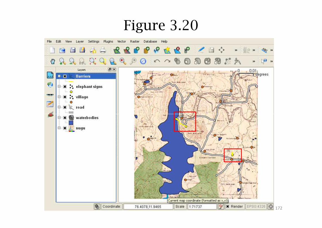
Figure 3.20
172
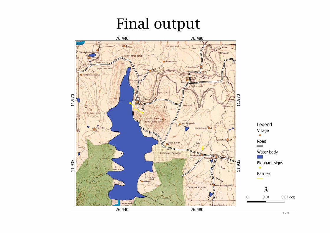
Final output
173
End of QGIS Workshop Tutorial for
Forest Managers