Embed Size (px)
Citation preview
QFT II Lecture Notes
Nabil Iqbal
November 11, 2020
Contents
1 Orientation 3
1.1 Motivation . . . . . . . . . . . . . . . . . . . . . . . . . . . . . . . . . . . . . . . . . . . . . . 3
1.2 Conventions . . . . . . . . . . . . . . . . . . . . . . . . . . . . . . . . . . . . . . . . . . . . . . 4
1.3 Quantum mechanics review . . . . . . . . . . . . . . . . . . . . . . . . . . . . . . . . . . . . . 4
2 Path Integrals in Free Quantum Field Theory 5
2.1 The generating functional . . . . . . . . . . . . . . . . . . . . . . . . . . . . . . . . . . . . . . 6
2.2 Calculating the Feynman propagator: poles, analytic continuation and iε . . . . . . . . . . . . 7
2.3 Higher-point functions in the free theory . . . . . . . . . . . . . . . . . . . . . . . . . . . . . . 8
3 Interacting theories 10
3.1 LSZ Reduction Formula . . . . . . . . . . . . . . . . . . . . . . . . . . . . . . . . . . . . . . . 11
3.2 Perturbation theory and Feynman diagrams . . . . . . . . . . . . . . . . . . . . . . . . . . . . 13
3.2.1 Combinatorics and symmetry factors . . . . . . . . . . . . . . . . . . . . . . . . . . . . 16
3.3 Connected diagrams . . . . . . . . . . . . . . . . . . . . . . . . . . . . . . . . . . . . . . . . . 16
3.4 Scattering amplitudes . . . . . . . . . . . . . . . . . . . . . . . . . . . . . . . . . . . . . . . . 18
4 Loops and Renormalization 21
4.1 Loops in λφ4 theory . . . . . . . . . . . . . . . . . . . . . . . . . . . . . . . . . . . . . . . . . 21
4.2 Coming to terms with divergences . . . . . . . . . . . . . . . . . . . . . . . . . . . . . . . . . 23
4.3 Renormalized perturbation theory . . . . . . . . . . . . . . . . . . . . . . . . . . . . . . . . . 25
4.3.1 Counterterms and renormalization conditions . . . . . . . . . . . . . . . . . . . . . . . 25
4.3.2 Determining the counterterms . . . . . . . . . . . . . . . . . . . . . . . . . . . . . . . . 26
4.4 What theories are renormalizable and what does this mean? . . . . . . . . . . . . . . . . . . . 29
1
4.5 A few non-renormalizable theories . . . . . . . . . . . . . . . . . . . . . . . . . . . . . . . . . 31
4.5.1 Pions . . . . . . . . . . . . . . . . . . . . . . . . . . . . . . . . . . . . . . . . . . . . . 32
4.5.2 Gravity . . . . . . . . . . . . . . . . . . . . . . . . . . . . . . . . . . . . . . . . . . . . 32
5 Global symmetries in the functional formalism 34
5.1 Classical Noether’s theorem . . . . . . . . . . . . . . . . . . . . . . . . . . . . . . . . . . . . . 34
5.2 Quantum Ward identities . . . . . . . . . . . . . . . . . . . . . . . . . . . . . . . . . . . . . . 35
6 Fermions 37
6.1 Fermions in canonical quantization . . . . . . . . . . . . . . . . . . . . . . . . . . . . . . . . . 37
6.2 Grassman variables . . . . . . . . . . . . . . . . . . . . . . . . . . . . . . . . . . . . . . . . . . 38
6.2.1 Anticommuting numbers . . . . . . . . . . . . . . . . . . . . . . . . . . . . . . . . . . . 38
6.2.2 Integrating many anticommuting numbers . . . . . . . . . . . . . . . . . . . . . . . . . 40
6.3 Fermions in the path integral . . . . . . . . . . . . . . . . . . . . . . . . . . . . . . . . . . . . 41
6.4 Feynman rules for fermions: an example . . . . . . . . . . . . . . . . . . . . . . . . . . . . . . 42
7 Abelian Gauge Theories 45
7.1 Gauge invariance . . . . . . . . . . . . . . . . . . . . . . . . . . . . . . . . . . . . . . . . . . . 45
7.2 Some classical aspects of Abelian gauge theory . . . . . . . . . . . . . . . . . . . . . . . . . . 47
7.3 Quantizing QED . . . . . . . . . . . . . . . . . . . . . . . . . . . . . . . . . . . . . . . . . . . 49
7.4 Things that I did not do: canonical quantization and LSZ . . . . . . . . . . . . . . . . . . . . 52
8 Non-Abelian gauge theories 54
8.1 Non-Abelian gauge invariance . . . . . . . . . . . . . . . . . . . . . . . . . . . . . . . . . . . . 54
8.2 The Yang-Mills field-strength and action . . . . . . . . . . . . . . . . . . . . . . . . . . . . . . 56
8.3 Quantizing non-Abelian gauge theories . . . . . . . . . . . . . . . . . . . . . . . . . . . . . . . 59
8.4 Qualitative discussion: Non-Abelian gauge theory at long distances . . . . . . . . . . . . . . . 63
8.4.1 What are the gauge fields doing in a confined phase? . . . . . . . . . . . . . . . . . . . 65
2
1 Orientation
These lecture notes were written for QFT II in the Particles, Strings and Cosmology MSc course at DurhamUniversity. They are a basic introduction to the path integral approach to quantum field theory. Most of thematerial follows the exposition in the well-known textbooks [2–4]. Please send all typos to [email protected].
It’s assumed the reader has some exposure to quantum field theory in canonical quantization, and also knowshow to apply path integrals to quantum mechanics.
1.1 Motivation
I want to begin with some philosophical words about quantum field theory. Why do we study quantum fieldtheory? What is it that makes us struggle through this confusing, technically difficult, at times seemingly1
ill-defined sea of ideas?
Presumably this question has many answers, but perhaps I’ll start making an extremely incomplete list of afew things that QFT is good for:
1. Particle physics and the Standard Model: this is the main focus of this course (both the QFTcourse and the larger MSc course of which it is a part). The Standard Model is a wildly successfulphysical theory, it is perhaps the most precise microscopic description of nature ever, and quantumfield theory is really at its very core.
Most textbooks lean heavily on this point of view, but it gives you the idea that QFT is only important ifyou care about high-energy physics, and that you need to build a giant particle accelerator to appreciateit. This is not true.
2. Metals and superconductors: this is maybe not obvious, but both metals and superconductors –real-life low-energy objects that you can find in your home (or, well, nearby physics lab) – are describedby quantum field theories; they are just not relativistic. The low energy fluctuations of electronsin metals are described by something called Fermi liquid theory, and superconductors are actuallydescribed by an analogue of the Higgs mechanism that you will study in the SM part of this course.
3. Boiling water: the phase diagram of water looks like picture on board. The critical point at 374 C isactually described by a three-dimensional quantum field theory called the 3d Ising model. I don’t havetime to explain why this is, but in general continuous phase transitions (...of any sort) are describedby quantum field theories.
4. Quantum gravity: if you don’t care about boiling water, perhaps you like quantum gravity. The so-called AdS/CFT correspondence tells us that quantum gravity in D dimensions is precisely equivalentto a quantum field theory in D−1 dimensions (in its most well-studied incarnation it is dual to SU(N)gauge theory). By the end of this course you will know what SU(N) gauge theory is.
One may ask what all of these phenomena have in common that makes them describable by quantum fieldtheory. In essence, if you ever have a situation where there are both fluctuations – thermal, quantum, etc.and locality – in space, in time, etc. – in some sense, it is likely that some sort of quantum field theorydescribes your system.
Having said all of that, in this course we will describe only relativistic quantum field theory; as always, extrasymmetries (such as those associated with relativistic invariance) simplify our lives.
1But only seemingly.
3
1.2 Conventions
In agreement with most (but not all) books on quantum field theory, I will use the “mostly-minus” metric:
ηµν = ηµν = diag(1,−1,−1,−1) (1.1)
Sadly this is the opposite convention to the one that I’m familiar with; thus everyone will need to be vigilantfor sign errors. We will mostly work in four spacetime dimensions (the “physical” value), but it is nice tokeep the spacetime dimension d arbitrary where possible.
Note that Greek indices µ, ν will run over time and space both, whereas i, j will run only over the threespatial coordinates, and thus
xµ = (x0, xi) (1.2)
I will sometimes use x0 to denote the time component and sometimes xt, depending on what I feel looksbetter in that particular formula.
I will always set ~ = c = 1.2 They can be restored if required from dimensional analysis.
1.3 Quantum mechanics review
In QFT I so far, you have understood in great detail how to compute things in quantum mechanics using thepath-integral; in other words you studied quantum mechanical systems with a classical real-time Lagrangian
L(q, q) =1
2q2 − V (q) S =
∫dtL(q, q) (1.3)
You then inserted this into a path-integral to define the generating functional, which was
Z[J ] ≡ N∫
[Dq] exp
(iS[q] + i
∫dtJ(t)q(t)
)(1.4)
where∫
[Dq] denotes the philosophically soothing but mathematically somewhat distressing “integral over allfunctions”. In the previous QFT1 course, you learned that to compute the time-ordered Green’s function,you simply had to bring down factors of q(t) when doing the average, i.e.
〈0|q(tN )q(tN−1) · · · q(t1)|0〉 = N∫
[Dq]q(tN )q(tN−1) · · · q(t1) exp (iS[q]) tN > tN−1 > · · · t1 (1.5)
Note it is absolutely crucial here that on the left-hand side tN > tN−1 > · · · t1. On the right-hand sideit doesn’t seem to matter; on the left-hand side it does, because these are quantum operators that do notcommute. It was explained in QFT I that path integrals only give you correlation functions that are time-ordered; to emphasize this, I will often put a T around the correlation function, i.e. I may write the left-handside as
〈0|T (q(tN )q(tN−1) · · · q(t1))|0〉 (1.6)
In fact, this quantity was typically somewhat ill-defined, even by physicist standards. However you couldmake it better by Wick-rotating, i.e. you wrote
t = −iτ (1.7)
where τ is real. This is sometimes called “Euclidean time”; note that the metric becomes
ds2 = dt2 − d~x2 = −(dτ2 + d~x2). (1.8)
2kB makes an appearance in a homework problem (or rather it would, if I hadn’t set it to 1).
4
The overall minus sign here is of no importance; we are working in a spacetime with Euclidean signature.Note that the action also becomes
iS = −∫dτ
(1
2
(dq
dτ
)2
+ V (q)
)≡ −SE (1.9)
where SE is positive-definite (if the potential is positive-definite). This Wick-rotated path integral is
Z[J ] ≡ N∫
[Dq] exp
(−SE +
∫dτJ(τ)q(τ)
)(1.10)
Note that the object in the exponential is now real rather than imaginary, and this makes the integralconvergent3. In general, many confusions about path integrals can be made to go away by imagining aWick-rotation to Euclidean signature. As explained in the first part, this prescription also guarantees thatyou are in the vacuum of the theory by suppressing the contribution of all states with energy E by a factorof exp(−Eτ).
2 Path Integrals in Free Quantum Field Theory
With this under our belt, we will now move on to quantum field theory. You have studied the basic ideas inIFT; let me just remind you. We will begin with a study of the free real scalar field φ. This has action
S[φ] =1
2
∫d4x
((∂φ(x))2 −m2φ(x)2
)=
1
2
∫d4x φ(x)(−∂2 −m2)φ(x) (2.1)
The classical equations of motion arising from the variation of this action are
(∂2 +m2)φ(x) = 0 (2.2)
This is philosophically the same as the quantum mechanics problem studied earlier. To make the transitionimagine going from the single quantum-mechanical variable q to a large vector qa where a runs (say) from 1to N . Now imagine formally that a runs over all the sites of a lattice that is a discretization of space, andnow qa(t) is basically the same thing as φ(xi; t) which is exactly the system we are studying above.
Now we would like to study the quantum theory. First, I point out that we can define a path integral inprecisely the same way as before, i.e. we can consider the following path-integral:
Z ≡∫
[Dφ] exp (iS[φ]) (2.3)
Where S[φ] is the action written down above, and [Dφ] now represents the functional integral over all fieldsand not just particle trajectories.
There are two main things that are nice about doing quantum field theory from path integrals the waydiscussed above. One of them is honest, the other is a bit “secret”.
1. The honest one: all of the symmetries of the problem are manifest. The action S is Lorentz-invariant,and it is fairly easy to see how these symmetries manifest themselves in a particular computation.Compare this to the Hamiltonian methods used in IFT, where you have to pick a time-slice and italways seems like a miracle when final answers are Lorentz-invariant.
2. The secret one: the path integral allows one to be quite cavalier about subtle issues like “what is thestructure of the Hilbert space exactly”. This is very convenient when we get to gauge fields, wherethere are subtle constraints in the Hilbert space (google “Dirac bracket”) that you can more or less notworry about when using the path integral (i.e. one can go quite far in life without knowing exactlywhat a “Dirac bracket” is).
3Well, more convergent than before, at least.
5
2.1 The generating functional
Now that the philosophy is out of the way, let us do a computation. We will begin by computing the followingtwo-point function:
〈0|T (φ(x)φ(y))|0〉 (2.4)
This object is called the Feynman propagator. It is quite important for many reasons; I will discuss themlater, for now let’s just calculate it. By arguments identical to those leading to (1.5), we see that we want
〈0|T (φ(x)φ(y))|0〉 = Z−10
∫[Dφ]φ(x)φ(y) exp (iS[φ]) (2.5)
To calculate this, it is convenient to define the same generating functional as we used for quantum mechanics
Z[J ] ≡∫
[Dφ] exp
(iS[φ] + i
∫d4xJ(x)φ(x)
)(2.6)
And we then see from functional differentiation that the two-point function is
〈0|T (φ(x)φ(y))|0〉 =1
Z0
(−i δ
δJ(x)
)(−i δ
δJ(y)
)Z[J ]
∣∣∣∣J=0
(2.7)
Each functional derivative brings down a φ(x). Now we will evaluate this function. We first note the identityderived in QFT I for doing Gaussian integrals in Section 7.1 of [1], which I have embellished with a few i’shere and there:∫
dx1dx2 · · · dxN exp
(−1
2xaAabx
b + iJaxa
)=
√(2π)
N
detAexp
(−1
2Ja(A−1)abJb
)(2.8)
We note from the form of the action (2.1) that the path integral Z[J ] we want to do is of precisely this form,where we do our usual “many integrals” limit and where a labels points in space and the operator A is
A = i(∂2 +m2
)(2.9)
We conclude that the answer for Z[J ] is
Z[J ] = det
(∂2 +m2
−2πi
)− 12
exp
(−1
2
∫d4xd4yJ(x)DF (x, y)J(y)
)(2.10)
where I have given the object playing the role of A−1 a prescient name DF . It is the inverse of the differentialoperator defined in (2.9) and thus satisfies
i(∂2 +m2
)DF (x, y) = δ(4)(x− y) (2.11)
This is an important result. Let us first note that the path integral is asking us to compute the functionaldeterminant of a differential operator. This is a product over infinitely many eigenvalues; it is quite a beautifulthing but we will not really need it here, so we will return to it later.
The next thing to note is that the dependence on J is quite simple; the exponential of a quadratic. Indeed,inserting this into (2.7) we get
〈0|T (φ(x)φ(y))|0〉 = DF (x, y) (2.12)
Thus, we have derived that the time-ordered correlation function of φ(x) is given by the inverse of i(∂2 +m2).You have already encountered this phenomenon in IFT.
6
2.2 Calculating the Feynman propagator: poles, analytic continuation and iε
Let us now actually calculate this object. I note that you have performed a similar computation in IFT, butI will repeat some elements of it to explain what the path integral is doing for us. We first go to Fourierspace:
DF (x, y) =
∫d4p
(2π)4e−ip·(x−y)DF (p) (2.13)
Inserting this into (2.11) we find∫d4p
(2π)4
(−p2 +m2
)e−ip·(x−y)DF (p) = −iδ(4)(x− y) (2.14)
We now see that we want the object in momentum space DF (p) to be proportional to p2 −m2 so that wecan use the identity
∫d4peip·x = (2π)4δ(4)(x). Getting the factors right, we find the following expression for
the propagator in Fourier space:
DF (p) =i
p2 −m2(2.15)
This looks nice, but actually, this expression is not yet complete, in that specifying this Fourier transformdoes not yet completely specify a function DF (x, y) in position space. To understand this, let us actuallyattempt to Fourier transform this thing back. We break the integral into time p0 and spatial ~p and do thetime integral first. Let me define ω~p ≡ +
√~p2 +m2:
DF (x, y) =
∫dp0
2π
∫d3p
(2π)3
i
p20 − p2 −m2
e−ip0(x0−y0)+i~p·(~x−~y) (2.16)
= i
∫dp0
2π
∫d3p
(2π)3
1
p0 + ω~p
1
p0 − ω~pe−ip0(x0−y0)+i~p·(~x−~y) (2.17)
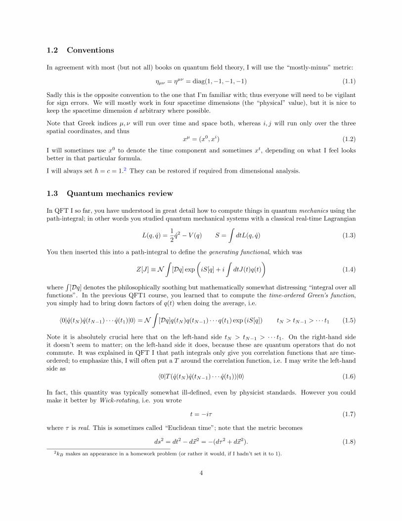
Now if we look at the integral, we see that there are poles when p0 = ±ω~p. The correct way to think aboutthis is to imagine it as an integral in the complex p0 plane, and we then have a pole. To actually perform theintegral, we need to specify how we go around the poles; different ways of going around the poles will give usdifferent answers.
There are two steps; first let’s say that x0 − y0 > 0; in the case we must complete the contour below forthe integral to converge. We are not done yet; to get the second bit of information, we should recall thatpath integrals only make since if we formulate them in Euclidean signature. This helps; let’s imagine that weformulated the whole thing in Euclidean time all along. Recall from (1.7) that the Wick rotation to Euclideantime and frequency is
t = −iτ p0 = ipE0 (2.18)
This means that if we were working in Euclidean time all along, we would have done the p0 integral up anddown the imaginary axis. This tells us which way to complete the integral, as only one pole prescription (oneup, one down) is compatible with this.
Now we can do the integral. We pick up the contribution from the +ω~p when x0 − y0 > 0, and the answer is
DF (x, y) =(−2πi)i
2π
∫d3p
(2π)3
1
2ω~pe−iω~p(x0−y0)+i~p·(~x−~y) x0 > y0 (2.19)
Similarly, if x0 < y0 we close the integral the other way and find
DF (x, y) =(2πi)i
2π
∫d3p
(2π)3
1
−2ω~pe+iω~p(x0−y0)+i~p·(~x−~y) x0 < y0 (2.20)
7
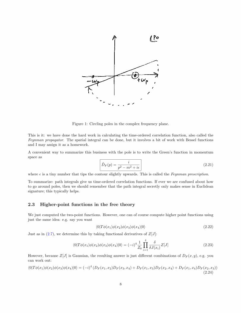
Figure 1: Circling poles in the complex frequency plane.
This is it: we have done the hard work in calculating the time-ordered correlation function, also called theFeynman propagator. The spatial integral can be done, but it involves a bit of work with Bessel functionsand I may assign it as a homework.
A convenient way to summarize this business with the pole is to write the Green’s function in momentumspace as
DF (p) =i
p2 −m2 + iε(2.21)
where ε is a tiny number that tips the contour slightly upwards. This is called the Feynman prescription.
To summarize: path integrals give us time-ordered correlation functions. If ever we are confused about howto go around poles, then we should remember that the path integral secretly only makes sense in Euclideansignature; this typically helps.
2.3 Higher-point functions in the free theory
We just computed the two-point functions. However, one can of course compute higher point functions usingjust the same idea: e.g. say you want
〈0|Tφ(x1)φ(x2)φ(x3)φ(x4)|0〉 (2.22)
Just as in (2.7), we determine this by taking functional derivatives of Z[J ]:
〈0|Tφ(x1)φ(x2)φ(x3)φ(x4)|0〉 = (−i)4 1
Z0
4∏i=1
δ
δJ(xi)Z[J ] (2.23)
However, because Z[J ] is Gaussian, the resulting answer is just different combinations of DF (x, y), e.g. youcan work out:
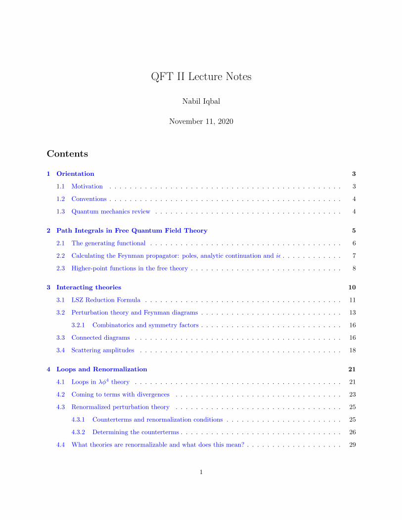
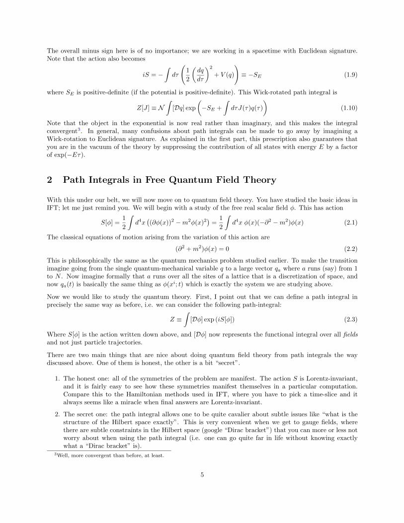
〈0|Tφ(x1)φ(x2)φ(x3)φ(x4)|0〉 = (−i)4 (DF (x1, x2)DF (x3, x4) +DF (x1, x3)DF (x2, x4) +DF (x1, x4)DF (x2, x3))(2.24)
8
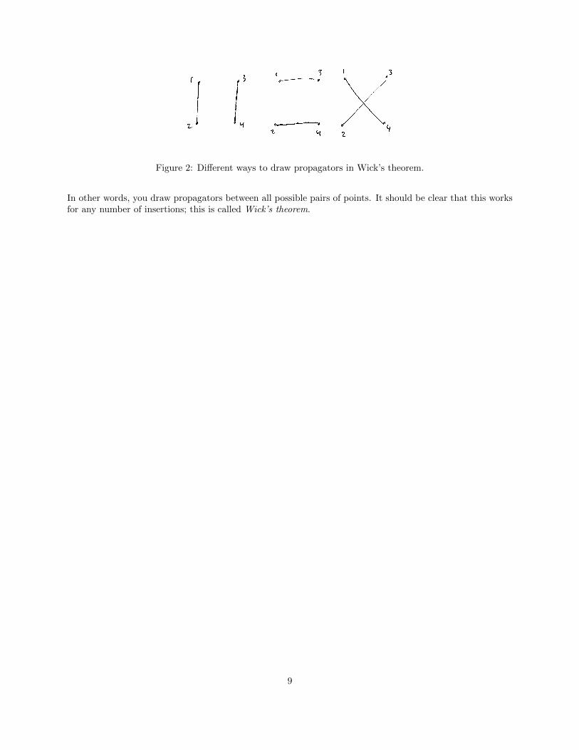
Figure 2: Different ways to draw propagators in Wick’s theorem.
In other words, you draw propagators between all possible pairs of points. It should be clear that this worksfor any number of insertions; this is called Wick’s theorem.
9
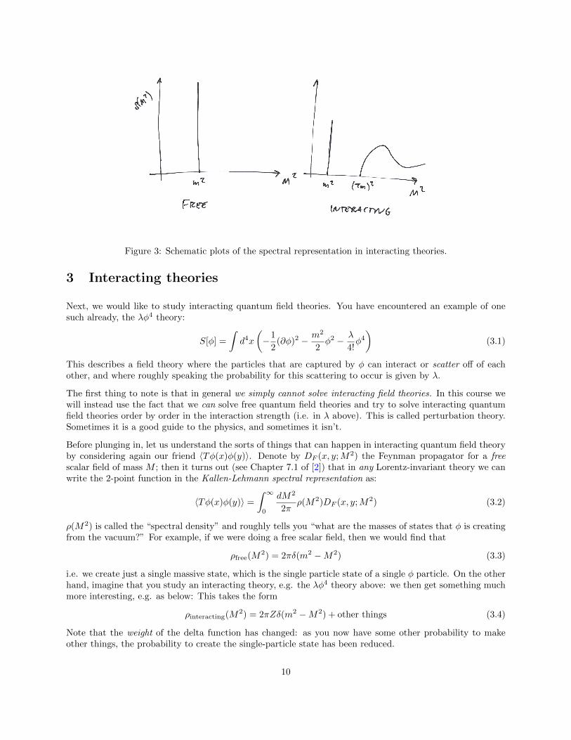
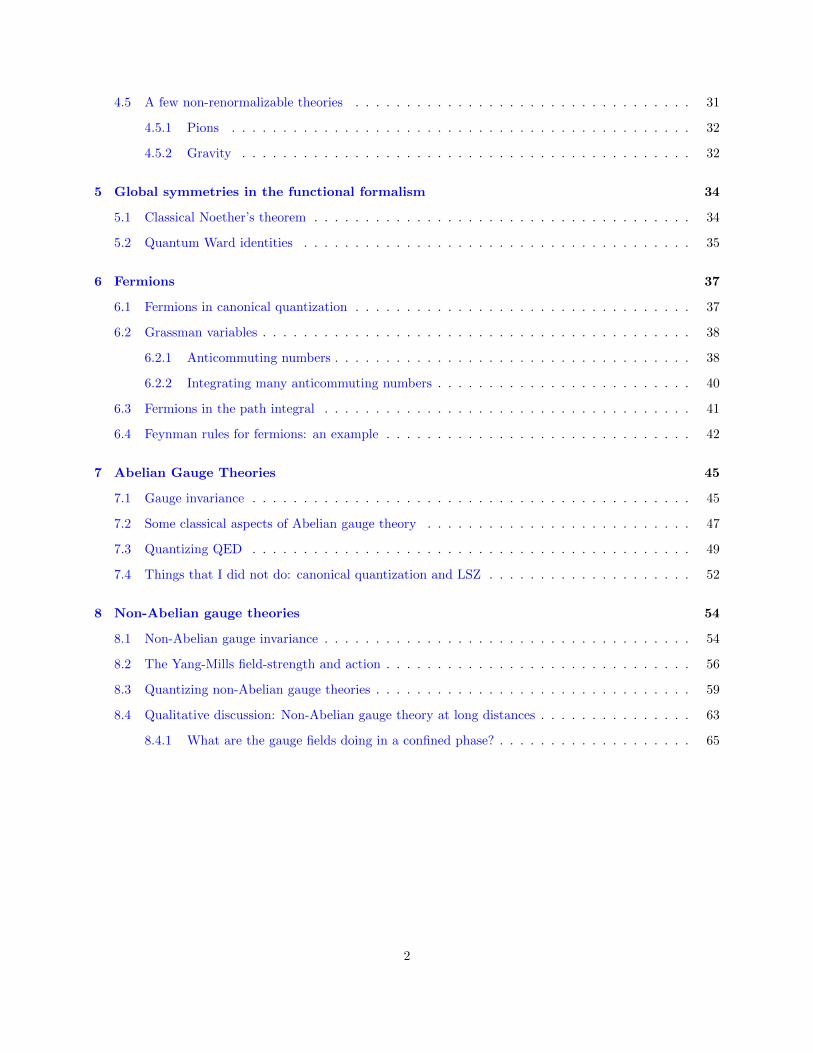
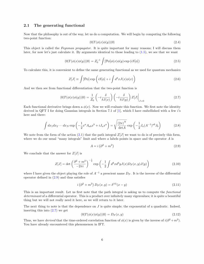
Figure 3: Schematic plots of the spectral representation in interacting theories.
3 Interacting theories
Next, we would like to study interacting quantum field theories. You have encountered an example of onesuch already, the λφ4 theory:
S[φ] =
∫d4x
(−1
2(∂φ)2 − m2
2φ2 − λ
4!φ4
)(3.1)
This describes a field theory where the particles that are captured by φ can interact or scatter off of eachother, and where roughly speaking the probability for this scattering to occur is given by λ.
The first thing to note is that in general we simply cannot solve interacting field theories. In this course wewill instead use the fact that we can solve free quantum field theories and try to solve interacting quantumfield theories order by order in the interaction strength (i.e. in λ above). This is called perturbation theory.Sometimes it is a good guide to the physics, and sometimes it isn’t.
Before plunging in, let us understand the sorts of things that can happen in interacting quantum field theoryby considering again our friend 〈Tφ(x)φ(y)〉. Denote by DF (x, y;M2) the Feynman propagator for a freescalar field of mass M ; then it turns out (see Chapter 7.1 of [2]) that in any Lorentz-invariant theory we canwrite the 2-point function in the Kallen-Lehmann spectral representation as:
〈Tφ(x)φ(y)〉 =
∫ ∞0
dM2
2πρ(M2)DF (x, y;M2) (3.2)
ρ(M2) is called the “spectral density” and roughly tells you “what are the masses of states that φ is creatingfrom the vacuum?” For example, if we were doing a free scalar field, then we would find that
ρfree(M2) = 2πδ(m2 −M2) (3.3)
i.e. we create just a single massive state, which is the single particle state of a single φ particle. On the otherhand, imagine that you study an interacting theory, e.g. the λφ4 theory above: we then get something muchmore interesting, e.g. as below: This takes the form
ρinteracting(M2) = 2πZδ(m2 −M2) + other things (3.4)
Note that the weight of the delta function has changed: as you now have some other probability to makeother things, the probability to create the single-particle state has been reduced.
10
Note that whenever Z is finite, it is at least true that we still create a particle. What if Z drops to zero?Then there is no probability that the φ field will create a physical particle. This is what happens in QCDdue to confinement, as you will see in due course.
3.1 LSZ Reduction Formula
From now on we assume that the Z appearing in the formula above is finite. We would now like to understandhow to compute scattering amplitudes: e.g. we would like to understand the question: if you smash togethertwo protons very hard, then what is the probability that a Higgs boson comes out? To do this we need tomake a connection between matrix elements of “single-particle states” (e.g. 2 protons, 1 Higgs, etc.) andthings that we know how to compute (i.e. time-ordered correlation functions). This connection happensthrough the LSZ Reduction Formula. My treatment follows that in Chapter 5 of [3].
I will work everything out in an example from the theory above, and we will consider doing 2− 2 scattering.So we need to prepare an initial and a final state. As we are discussing states, let me now return to thecanonical formalism, where we have in the Heisenberg picture:
φ(~x, t) =
∫d3p
(2π)3
1
2ω~p
(a~pe−ip·x + a†~pe
+ip·x)
pµ = (ω~p, ~p) (3.5)
It is easy enough to solve this for a~p to get:
a~p =
∫d3xeip·x (i∂tφ(x) + ω~pφ(x)) (3.6)
= i
∫d3xeip·x
←→∂t φ(x) (3.7)
where this two-headed arrow represents f←→∂ g = f∂g − (∂f)g. Note that in an interacting theory this a
depends on time.
For technical reasons, we will want to have wave-packets, i.e. we imagine some momentum envelope
f1(~k) ∼ exp
(− (~k − ~k1)2
4σ2
)(3.8)
and we then construct an operator that is a momentum-smeared version of the usual creation operator:
a†1 ≡∫d3kf1(~k)a†~k
(3.9)
Now in the free theory, we know that we create an initial state by acting with the creation operators. We willsimply assume that in the interacting theory we create an initial state by acting with the creation operatorin the distant past, and that this does what we want up to a renormalization factor Z: i.e. to make an initialstate of one particle in a wave-packet around ~k1, we write
|initial packet;~k1〉 =1√Z
limt→−∞
a†1|0〉 (3.10)
It may not be clear, but this factor Z is the same as the one that I introduced earlier. We will be interestedin an initial state of say two particles:
|i〉 = limt→−∞
1
Za†1a†2|0〉 (3.11)
Similarly, the final state is made out of operators that are defined at t = +∞:
|f〉 = limt→+∞
1
Za†1′a
†2′ |0〉 (3.12)
11
The amplitude that we are looking for is 〈f |i〉, i.e.
〈f |i〉 =
(1√Z
)4
〈0|Ta1′(+∞)a2′(+∞)a†1(−∞)a†2(−∞)|0〉 (3.13)
Note that everything is time-ordered anyway; thus we can stick a “T” for time-ordering in there with noissues.
I now want to express this amplitude in terms of the field φ(x). To do this, let us first derive an equationrelating a1(t = +∞) to a1(t = −∞). We write
a†1(+∞)− a†1(−∞) =
∫ +∞
−∞dt∂ta
†1(t) (3.14)
=
∫d3kf1(~k)
∫d4x∂t
(e−ik·x
(−i∂tφ(x) + ω~kφ(x)
))(3.15)
= −i∫d3kf1(~k)
∫d4xe−ik·x
(∂2t + ω2
~k
)φ(x) (3.16)
= −i∫d3kf1(~k)
∫d4xe−ik·x
(∂2t + ~k2 +m2
)φ(x) (3.17)
= −i∫d3kf1(~k)
∫d4xe−ik·x
(∂2t −←−∇2 +m2
)φ(x) (3.18)
= −i∫d3kf1(~k)
∫d4xe−ik·x
(∂2 +m2
)φ(x) (3.19)
Here we use the definition of the creation operator from the field; then we use the Fourier transform to tradethe momentum for a spatial gradient, and then use the fact that the wave-packets are localized to integrateby parts with impunity. We end with the wave operator acting on the field. Note that for a free field this iszero by the equations of motion; for an interacting field it is not. We conclude with the following formula
a†1(−∞) = a†1(+∞) + i
∫d3kf1(~k)
∫d4xe−ik·x(∂2 +m2)φ(x) (3.20)
There is a corresponding expression for the annihilation operator:
a1(+∞) = a1(−∞) + i
∫d3kf1(~k)
∫d4xe+ik·x(∂2 +m2)φ(x) (3.21)
Now insert these expressions into (3.13): here we see the magic of time-ordering: every a(−∞) is sent tothe right and annihilated against the vacuum ket. Similarly every a†(+∞) is sent to the left and annihilatedagainst the vacuum bra. The wave packets have done their magic; we now set them all equal to delta functionsf1(~k) = δ(3)(~k− ~k1). Thus the full answer for the amplitude (where I generalize now to n in-particles and n′
out-particles) becomes
〈f |i〉 = in+n′∫d4x1Z
− 12 e−ik1·x1(∂2
1 +m2) · · · d4x1′e+ik1′ ·x1′Z−
12 (∂2
1′ +m2) · · · 〈0|T (φ(x1)φ(x2) · · ·φ(x′1)φ(x′2) · · · |0〉
(3.22)This is the LSZ reduction formula, relating matrix elements to time-ordered n-point functions. Let’s expressit in momentum space, where it is:
n∏i=1
i√Z
k2i −m2
n′∏i=1
i√Z
k2i′ −m2
〈f |i〉 = 〈0|φ(k1)φ(k2) · · ·φ(k′n)|0〉 (3.23)
where the right-hand side is understood to be the Fourier transform of the time-ordered correlation function.In words: to calculate the transition amplitude (which is the physical thing), you should Fourier transform
12
the correlation function, and then put all the momentum close to their “on-shell values” (i.e k2i ∼ m2). In
that kinematic regime the correlation function should develop a pole so that it looks like the left-hand side;the coefficient of that pole is the transition amplitude you are looking for.
Whew. We now move on to actually calculating the multi-point function.
3.2 Perturbation theory and Feynman diagrams
We now understand that to calculate transition amplitudes, we should compute correlation functions ininteracting field theories, e.g. this one:
S[φ] =
∫d4x
(−1
2(∂φ)2 − m2
2φ2 − λ
4!φ4
)(3.24)
From the previous section, we understand that if we can compute the generating functional Z[J ]
Z[J ] ≡∫
[Dφ] exp
(iS[φ] + i
∫d4xJ(x)φ(x)
)(3.25)
and take functional derivatives then we will obtain the required correlation functions. There is no hope ofdoing this exactly for all λ; instead we will expand order by order in λ. The first thing to do is to expandthe action as
S[φ] = S0[φ] +
∫d4xL1(φ(x)) (3.26)
with S0 the free action and L1 the interacting part: in our case L1(φ) = λ4!φ
4. Now we will do a trick; noticethat every time you have a φ, you can replace it with a functional derivative with respect to J . Thus we canwrite
Z[J ] =
∫[Dφ] exp
(iS0[φ] + i
∫d4x (L1(φ(x)) + J(x)φ(x))
)(3.27)
=
∫[Dφ] exp
(i
∫d4xL1
(−i δ
δJ(x)
))exp (iS0[φ] + iJ(x)φ(x)) (3.28)
= exp
(i
∫d4xL1
(−i δ
δJ(x)
))Z0[J ] (3.29)
where Z0[J ] is the generating functional for the free quantum field theory. We calculated this before. Wefind then
Z[J ] = Z0[0] exp
(i
∫d4xL1
(−i δ
δJ(x)
))exp
(−1
2
∫d4xd4yJ(x)DF (x, y)J(y)
)(3.30)
Here I have absorbed the functional determinant into the object Z0[0].
In particular, if we specialize to the λφ4 theory, then we can write L1 explicitly as
Z[J ] ∝ exp
(i
∫d4x
λ
4!
(−i δ
δJ(x)
)4)
exp
(−1
2
∫d4xd4yJ(x)DF (x, y)J(y)
)(3.31)
We can now work out Z[J ] by taking many many functional derivatives. This turns out to organize itselfinto the delightful structure of Feynman diagrams. To understand this, we basically just expand everything:
13

Figure 4: Picture of how functional derivatives act and representation in terms of Feynman diagram.
expand L1 in powers of the coupling λ and expand the free partition function in powers of the source J :
exp
(−i∫d4x
λ
4!
(−iδδJ(x)
)4)
= 1− i∫d4x
λ
4!
(−iδδJ(x)
)4
+1
2
(i
∫d4x
λ
4!
(−iδδJ(x)
)4)2
+ · · · (3.32)
exp
(−1
2J ·D · J
)= 1− 1
2J ·D · J +
1
2
(−1
2J ·D · J
)2
+ · · · (3.33)
where for a shorthand I am denoting
J ·D · J ≡∫d4xd4yJ(x)DF (x, y)J(y) (3.34)
Now we work out the product. I first work out an example to demonstrate the structure, and I then describethe systematic rules for doing this. Examine the first non-trivial term:
− i∫d4x
λ
4!
(−iδδJ(x)
)41
2
(−1
2J ·D · J
)(−1
2J ·D · J
)(3.35)
Now each of the functional derivatives acts on one of the J ’s, and the DF ’s tie together the two J ’s that itis attached to. We end up with something that looks like
− N
4!iλ
∫d4xDF (x, x)DF (x, x) (3.36)
Where it is convenient to capture this with a picture, called a Feynman diagram, where a line indicates apropagator from x to y and a vertex indicates an insertion of the interaction λ. In a second we will discussthe numerical prefactor N . First let’s try to understand how this works for the next term,
i
∫d4xd4y
λ
4!
(−iδδJ(x)
)4λ
4!
(−iδδJ(y)
)41
4!
(−1
2J ·D · J
)4
(3.37)
The rules should be clear: assemble four propagators and two vertices however you can. There are threetopologically distinct terms that appear, and they look like this:
14
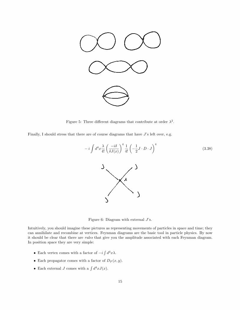
Figure 5: Three different diagrams that contribute at order λ2.
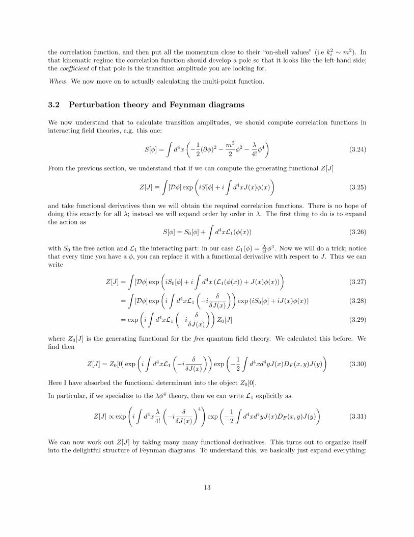
Finally, I should stress that there are of course diagrams that have J ’s left over, e.g.
− i∫d4x
λ
4!
(−iδδJ(x)
)41
4!
(−1
2J ·D · J
)4
(3.38)
Figure 6: Diagram with external J ’s.
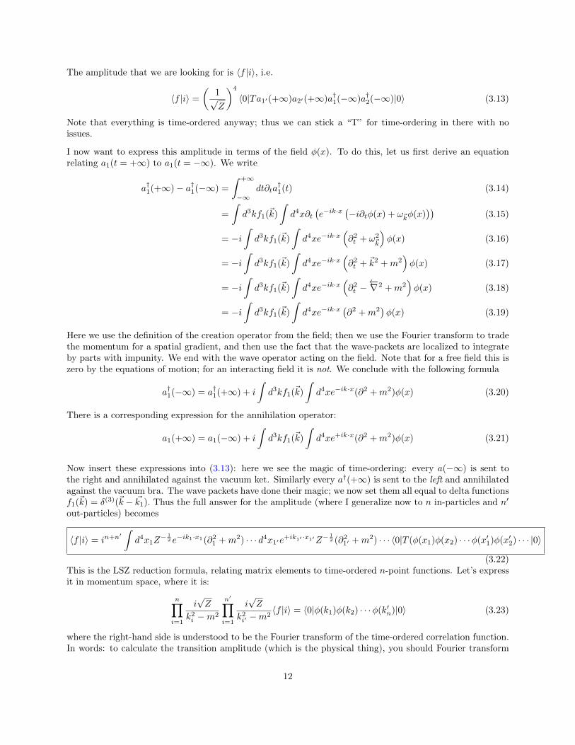
Intuitively, you should imagine these pictures as representing movements of particles in space and time; theycan annihilate and recombine at vertices. Feynman diagrams are the basic tool in particle physics. By nowit should be clear that there are rules that give you the amplitude associated with each Feynman diagram.In position space they are very simple:
• Each vertex comes with a factor of −i∫d4xλ.
• Each propagator comes with a factor of DF (x, y).
• Each external J comes with a∫d4xJ(x).
15
We will shortly rewrite them in momentum space, as they are slightly nicer in that form.
3.2.1 Combinatorics and symmetry factors
Now let’s examine the combinatorics more carefully. From the double expansion in (3.31), we see that aparticular term takes the form
∞∑V,P=0
1
V !
[(∫d4x−iλ4!
(−i δ
δJ(x)
)4)]V
1
P !
[−1
2J ·D · J
]P(3.39)
where V is the number of vertices and P the number of propagators. Now when you draw a picture, e.g. twokissing bubbles, this represents several different ways of contracting functional derivatives against sources:in other words, the same term appears a number of different times. How many? Well, there are 4! differentways to rearrange the derivatives coming out of a vertex, there are P ! ways to rearrange the P propagatorsamongst themselves, there are 2 ways to pick the two sides of a propagator, and there V ! ways to rearrangethe vertices. These factors precisely cancel all the factors in the denominator – and thus one might naivelythink that there is thus no combinatorics to do at all. (Note this is why the funny 4! is in the definition ofthe interaction vertex as λ
4! )
However this is not true, because we have actually overcounted. In doing that counting, we assumed thatevery rearrangement of propagators and vertices would give a distinct contribution: in reality this is not true,as they can “cancel” each other. For example, in two-kissing bubbles, note that if we switch the two sidesof the propagator and also switch the two corresponding functional derivatives at the vertex, then we get thesame contribution again. Similarly for the other side, and also for the two propagators themselves. Thus wehave overcounted by a factor of 2 · 2 · 2 = 8, and we must divide by this: thus the full diagram in this case is
iλ
8
∫d4xDF (x, x)DF (x, x) (3.40)
This factor of 8 is called the symmetry factor S of the diagram, as it always has to do with some operationthat leaves the diagram invariant.
It is a fun exercise in pure thought to figure out the symmetry factor; I recommend doing it for several otherdiagrams to get the hang of it. You will do this in a homework problem. But, to summarize: to determinethe right prefactor, figure out the correct symmetry factor and divide by it.
3.3 Connected diagrams
We now study a way to re-organize this sum over diagrams. Note that the generic contribution to Z[J ] is asum over several disconnected diagrams (where “disconnected” is the intuitively obvious “I can draw a linethrough it and separate it into two pieces”). If I label each connected diagram by I, call the value of thediagram CI , then the generic disconnected diagram gives a contribution
D =1
SD
∏I
(CI)nI (3.41)
where nI is the number of times each connected diagram appears and SD now being a new symmetryfactor associated with rearranging the connected diagrams themselves. As we have already dealt with therearrangements inside each connected diagram, SD discusses rearrangements of each connected diagram asa whole, and so is always
SD =∏I
nI ! (3.42)
16
Thus we have
Z[J ] =∑{nI}
∏I
1
nI !(CI)
nI
=∏I
∞∑nI=0
1
nI !(CI)
nI
=∏I
exp(CI)
= exp
(∑I
CI
)(3.43)
This is very nice – it says that the total Z[J ] is the exponential of the sum over only connected diagrams.It’s convenient to define the logarithm of the generating functional W [J ] as this sum.
iW [J ] =∑I
CI Z[J ] = exp (iW [J ]) (3.44)
17
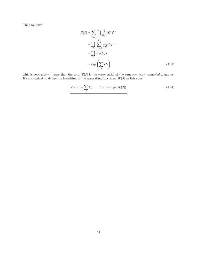
Figure 7: Wick’s theorem figure, repeated here to illustrate λ0 contribution to 2-2 scattering: replace 3 with1′ and 4 with 2′.
3.4 Scattering amplitudes
Now that we have all of this technology, let’s finally use it. Imagine in this λφ4 theory we want to calculatethe 2− 2 scattering of two particles. In other words, we want to compute the amplitude:
〈f |i〉 = 〈k′1, k′2; out|k1, k2; in〉 (3.45)
From the LSZ formula we see that this is equal to:
〈i|f〉 =
(i√Z
)n+n′ ∫d4x1e
−ik1·x1 · · · d4x1′e+ik1′ ·x1′ · · · 〈0|Tφ(x1)φ(x2)φ(x′1)φ(x′2)|0〉(k2
1 −m2) · · · (k′21 −m2)
(3.46)So now we need to calculate the four point function, which I will abbreviate as G(4)({xi}). If I also furtherabbreviate
δi ≡ −iδ
δJ(xi)(3.47)
Then the four-point function is given by
G(4)({xi}) =1
Z[J ]δ1δ2δ1′δ2′Z[J ]
∣∣J=0
(3.48)
As there are four functional derivatives acting on Z[J ], we should write down the terms in the diagrammaticexpansion of Z[J ] that contain four external J ’s, and then taking the functional derivative simply associateseach external J with an external insertion. We do this order by order: at order λ0 we find the terms inFigure 7.
Let’s examine the Fourier transform of one of these terms, e.g. the first one is∫d4x1e
−ik1·x1 · · · d4x1′e+ik1′ ·x1′DF (x1, x
′1)DF (x2, x
′2) (3.49)
But by translational invariance, the propagator only cares about the difference between the two points, sothis can be rewritten as ∫
d4x1e−ik1·x1 · · · d4x1′e
+ik1′ ·x1′DF (x1 − x′1)DF (x2 − x′2) (3.50)
Now notice that the sum x1 + x′1 does not enter in the expression with the propagators. I can rearrange thething in the exponent of the Fourier transform to read
k1′x1′ − k1x1 =1
2(k1 − k1′)(x1 + x′1) +
1
2(k1 + k1′)(x1 − x′1) (3.51)
18
Now the integral over the combination x1 + x′1 is easy to do, as it does not enter into the integrand. Thisintegral makes the whole thing proportional to a delta function
δ(4)(k1 − k′1) (3.52)
But this means that the incoming momentum is equal to the outgoing momentum: so there is no scattering!This should make intuitive sense from the picture: the particle 1 is becoming the 1′ without doing anything.Similar considerations apply to the other disconnected diagrams.
In general, scattering will only occur from connected diagrams; from the discussion above, this means that inthe LSZ formula we should actually use only derivatives of iW [J ], i.e.
G(4)({xi})C = δ1δ2δ1′δ2′iW [J ]∣∣J=0
(3.53)
W [J ] is trivial to lowest order in λ: so we see that there is no scattering at order λ0, which makes sense.
We now go to the next order in λ. Here we find one contribution that goes like picture of cross diagram.This will contribute non-trivially to scattering: in position space, this turns out to be
G(4)({xi})C = −iλ∫d4yDF (x1 − y)DF (x2 − y)DF (x′1 − y)DF (x′2 − y) (3.54)
It is very useful to go to momentum space. We Fourier tranform everything using the Fourier representationof the propagator:
DF (x− y) =
∫d4p
(2π)4e±ip·(x−y) i
p2 −m2(3.55)
In this expression it is up to us how to pick the momentum in the exponent: to line up with the inverseFourier transform in the LSZ formula it is convenient to pick the positive exponent for the in states andnegative one for the out states. Thus I find
G(4)({xi})C = −iλ∫d4y
4∏i=1
d4pi(2π)4
expip1(x1−y)+ip2(x2−y)−ip′1(x′1−y)−p′2(x′2−y) i
p21 −m2
· · · i
p′22 −m2(3.56)
There is momentum pi flowing in each leg. The integral over d4y in the vertex creates a delta function thatlooks like (2π)4δ(4)(p′1 + p′2 − p1 − p2). We also see that each propagator gives us a factor of i
p2−m2 .
Now when we insert this into the LSZ formula, the integral over the x’s give more delta functions that tie themomentum in each leg to the external momentum. Furthermore the LSZ formula provides a compensatingfactor of p2 −m2 that cancels the propagator: we find at the end for the amplitude:
〈k′1, k′2; out|k1, k2; in〉 = −(2π)4δ(4)(k′1 + k′2 − k1 − k2)iλ (3.57)
I have set the factor Z in the LSZ formula to 1: it turns out there is the possibility of correcting it at O(λ2)but we will get there in the next section. Whew. That’s it. We’ve done it. At the end of the day, the matrixelement simply goes like λ. It’s really kind of a miracle: if you built a particle accelerator and smashedtogether these particles, this is actually the probability that the particles would scatter.
This was semi-excruciating, and from now on I will be far more schematic, but I wanted you to understandhow the structure works. For future reference, let me define the invariant matrix element iM as follows:
〈ki′ ; out|ki; in〉 = (2π)4δ(4)
(∑i
ki −∑i′
k′i
)iM(k) (3.58)
The point of this is just to strip off all the boring kinematic factors and extract the bit where the physics is.In the above example we would have
iM = −iλ (3.59)
From here, hopefully it is clear how the momentum space Feynman rules work:
19
• For each amplitude you want, draw some external legs. Put an arrow on each one to indicate whichway the momentum goes: have it go inwards for in states and outwards for out states.
• Draw all possible vertices that connect together four lines. Each vertex comes with a factor −iλ.
• Put a momentum on each line. If the line is external, this is the momentum of the ingoing particle.
• For each internal line, associate a factor ip2−m2 . For each external line, associate a factor i√
Z. This is
given the graphic name “amputating the propagator”.
• Make sure momentum is conserved at each vertex. This will fix many of the momenta, but not neces-sarily all of them – it will leave some momenta unfixed if you have loops. Integrate over any unfixedmomenta. (We will see an example shortly).
This is it. You can now just draw pictures and multiply together factors, and not go through all of thisexcruciating work again.
20
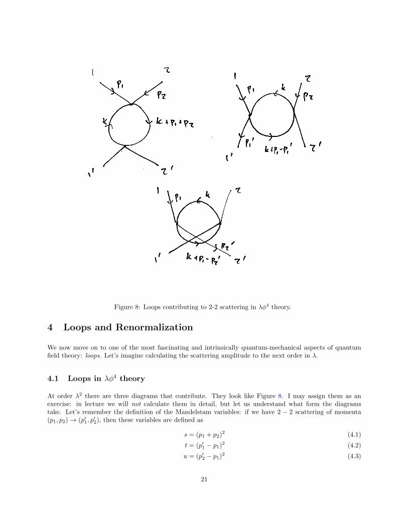
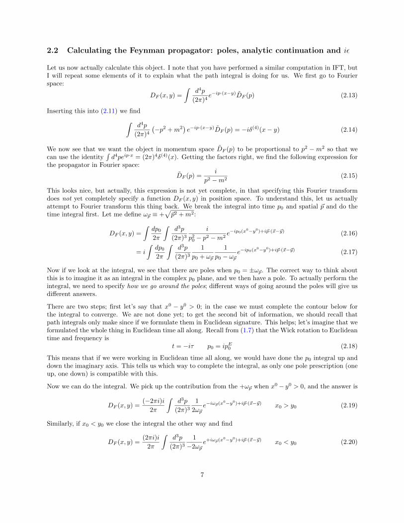
Figure 8: Loops contributing to 2-2 scattering in λφ4 theory.
4 Loops and Renormalization
We now move on to one of the most fascinating and intrinsically quantum-mechanical aspects of quantumfield theory: loops. Let’s imagine calculating the scattering amplitude to the next order in λ.
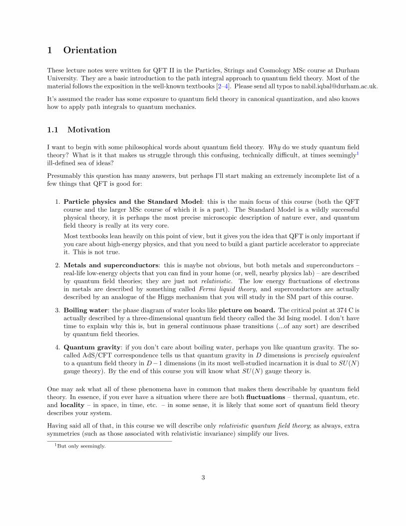
4.1 Loops in λφ4 theory
At order λ2 there are three diagrams that contribute. They look like Figure 8. I may assign them as anexercise: in lecture we will not calculate them in detail, but let us understand what form the diagramstake. Let’s remember the definition of the Mandelstam variables: if we have 2 − 2 scattering of momenta(p1, p2)→ (p′1, p
′2), then these variables are defined as
s = (p1 + p2)2 (4.1)
t = (p′1 − p1)2 (4.2)
u = (p′2 − p1)2 (4.3)
21
Now the first loop diagram is
D1 =(−iλ)
2
2
∫d4k
(2π)4
i
k2 −m2
i
(k + p1 + p2)2 −m2(4.4)
Now: we are integrating over all k. Thus the integrand is a Lorentz-invariant function of the only other thingthat appears in the diagram, i.e. the of the momentum (p1 + p2)2 = s, and we may then write it as
D1 = (−iλ)2iV (s) (4.5)
What can we conclude about V (s)? Let us first revisit an awkward fact: the integral over k is over allmomenta – does the integral even converge? At large k it is determined by the following integral:
I ≡∫
d4k
(2π)4
1
k4(4.6)
If I denote the upper range of the momentum integral by Λ (where I will define precisely what I mean bythis in a second), we conclude that actually this diagram does not converge – it instead goes like
D1 ∼ λ2 log(Λ) (4.7)
Wow. This seems bad. Actually, it is not “bad”: like many confusing things, this divergence is secretly atthe heart of all that is fun in quantum field theory. For the next few lectures, we will try to come to termswith this fact. Many discussions of this fact are a bit clouded by the fact that the expressions are actuallyquite complicated: thus I will make a series of simplifying assumptions to capture the relevant physics, andthen you will relax these assumptions in your homework problem. First I will assume that we are scatteringthese particles so hard that the Mandelstam variables s, t, u� m, are far larger than m, and we may simplydisregard the existence of m in these formulas.
Now let us carefully calculate the divergent part of V . This comes from calculating I. To do all such loopintegrals, we always follow the following procedures:
1. Wick-rotate. Note the integral is over Lorentzian four-momenta. It is simpler to rotate the timecoordinate of the momentum as:
k0 = ikE0 (4.8)
in which case a Lorentzian k2 becomes
(k2)Lorentzian = −((kE)2)Euclidean (4.9)
and the integration measure transforms as∫d4k = i
∫d4kE (4.10)
The integral is now
I = i
∫d4kE(2π)4
1
(kE)4(4.11)
But now it is a spherically symmetric integral with respect to SO(4) rotations in four-dimensionalEuclidean space! Thus I can use the 4d Euclidean analog of polar coordinates. The key point here isthat for a spherically symmetric integrand, the integration measure becomes:∫
d4kE = Vol(S3)
∫ ∞0
d|kE ||kE |3 (4.12)
where by |kE | I denote the magnitude of the Euclidean 4-vector kE , and where Vol(S3) is the 3d surfacearea of a unit 3-sphere, which turns out to be 2π2. (See p193 of [2]) for more discussion of this.) Thusthe integral simply becomes
I =i
8π2
∫ ∞0
d|kE |1
|kE |(4.13)
22
2. Regulate. This integral is divergent. We must thus cut it off at some high momenta. We will discussthe physical significance of this procedure in a moment.
There are many ways to cut off the integral; in lectures we will simply use what is called a “hard cut-off”and say the maximum Euclidean momenta that I will allow is that with |kE | = Λ. The divergent partof the integral is then
Idiv =i
8π2
∫ Λ
d|kE |1
|kE |=
i
8π2log Λ (4.14)
and where this expression does not capture any other information. Thus, as claimed, the integral islog divergent, and now we know the precise pre-factor of this divergence. This sort of cutoff is notgauge-invariant, so you get into trouble if using it in gauge theories. Let’s keep that in mind for later.
Now let’s return: we have computed the divergent part of V (s) as defined in (4.5). But now we note thatV (s) is a dimensionless function, and in the limit where we can neglect the mass m, the only dimensionful
things entering into it are Λ and s: thus I see that V (s) = f(Λ2
s ). But we know the dependence on Λ! Thuswe see that V (s) is
V (s) = − 1
32π2log
(Λ2
s
)+ const (4.15)
where the extra constant must be independent of s: for illustrative purposes, I will simply ignore it from nowon, as we are working in the large s limit and this is the sort of thing we are neglecting. Now the other twodiagrams are precisely the same with s replaced by the other Mandelstam variables t and u. We concludethat the full set of the 1-loop diagrams is this limit is:
Done−loop = iλ2
32π2
[log
(Λ2
s
)+ log
(Λ2
t
)+ log
(Λ2
u
)](4.16)
Ok, now that we have calculated this, let us remember the physical interpretation. To get the full matrixelement for 2− 2 scattering, we should add this to the previous “tree-level” bit. Thus we conclude that
iM(s, t, u) = −iλ+ iλ2
32π2
[log
(Λ2
s
)+ log
(Λ2
t
)+ log
(Λ2
u
)](4.17)
Now we need to interpret this.
4.2 Coming to terms with divergences
At first glance, this is an epic disaster! We have just calculated that the scattering amplitude depends ona parameter Λ! This is a “cut-off”, which means that we should take it to infinity, which means that theprobability for scattering together two φ particles is ∞! This is problematic. In this section I will follow thetreatment of [4].
Once we finish panicking, let us discuss a few features of this computation:
1. Something interesting has happened: while trying to solve a physics problem, the problem insisted thatyou do an integral over arbitrarily high momenta. But things might happen at small scales to invalidatethe calculation: note the hubris of quantum field theory: it seems to be suggesting that you need toknow physics all the way down to arbitrarily small scales just to scatter together two φ particles? Oneshould not need string theory to scatter two particles – surely something is wrong.
2. Relatedly, normally physics relates one observable quantity to another observable quantity. E.g. theideal gas law:
PV = NkT (4.18)
23
You know the temperature of a gas, and you measure how much the pressure changes when you heatit up: two observables. However, in this case, the formula above relates an observable (the scatteringamplitude) to λ. Is λ an observable?
It is not. λ is a parameter in a Lagrangian, not something you can measure. I will thus call it the “barecoupling” for a little while. The infinity above appeared when relating an unobservable parameter in aLagrangian to an observable: thus the infinity itself is not observable, and at the moment we are safe. Let’stry to rearrange this calculation to relate one observable quantity to another, and see what we can do.
So: what is observable? Really we are trying to give λ some kind of physical meaning. Presumably in reallife if you wanted to measure λ, you would go out and scatter some particles and get some number. Let’s usethis idea to define a new physical λ, which I will call λP . In other words, go to your lab and smash togethersome particles at a given energy (s0, t0, u0). Measure M at that value, and use that to define λP :
iM(s0, t0, u0) ≡ −iλP (4.19)
This is a definition! It is called a renormalization condition. Now from the theoretical calculation of theobservable M, this relates λP to our bare coupling λ:
− iλP = −iλ+ iλ2
32π2
[log
(Λ2
s0
)+ log
(Λ2
t0
)+ log
(Λ2
u0
)](4.20)
Now we can solve this for λ in terms of λP . This is totally trivial: note that as a perturbation theory, weassume that λP and λ are at the same order in perturbation theory, and we only work only to quadraticorder in λ and thus λP , which means it makes no difference which one we use in the second term.
λ = λP +λ2P
32π2
[log
(Λ2
s0
)+ log
(Λ2
t0
)+ log
(Λ2
u0
)]+O(λ3
P ) (4.21)
This is totally okay to lowest order, though you may want to go home and check this for yourself. Now weuse this expression to get rid of the non-physical λ in the scattering amplitude (4.17), to find:
iM(s, t, u) = −iλP + iλ2P
32π2
[log(s0
s
)+ log
(t0t
)+ log
(u0
u
)](4.22)
Look! The amplitude is now finite.
This process – what we just did – is called renormalization. It should really be called the far less impressivesounding “writing things in terms of observable quantities”.
Let’s discuss what happened:
1. We expressed our scattering amplitude in terms of only observable quantities; in the process of doingthis, the divergence vanished all by itself. Note that we did not “add anything to make it go away”: itis simply not there in the actual observable answer. This makes sense.
2. The relationship between the unobservable λ and the physical λP involves a divergence. There is thusa sense in which the divergence is there in a parameter in the Lagrangian, but not in any observablequantity.
3. This did come at a small cost: we had to pick a point (s0, t0, u0) and use that point to define ourphysical coupling λP . This is, in a sense, a loss of information: now we can only discuss physics relativeto that point. Reflecting on this, we will need to do this for (more or less) every divergence that appearsin our calculation.
4. Finally, this is a small cost, because once you specify this one bit of information, you can measure themomentum dependence of the scattering amplitude, which is a non-trivial function of the momenta:thus, there is plenty of predictive power in the theory.
24
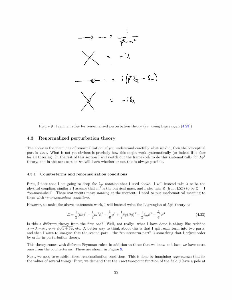
Figure 9: Feynman rules for renormalized perturbation theory (i.e. using Lagrangian (4.23))
4.3 Renormalized perturbation theory
The above is the main idea of renormalization: if you understand carefully what we did, then the conceptualpart is done. What is not yet obvious is precisely how this might work systematically (or indeed if it doesfor all theories). In the rest of this section I will sketch out the framework to do this systematically for λφ4
theory, and in the next section we will learn whether or not this is always possible.
4.3.1 Counterterms and renormalization conditions
First, I note that I am going to drop the λP notation that I used above. I will instead take λ to be thephysical coupling; similarly I assume that m2 is the physical mass, and I also take Z (from LSZ) to be Z = 1“on-mass-shell”. These statements mean nothing at the moment: I need to put mathematical meaning tothem with renormalization conditions.
However, to make the above statements work, I will instead write the Lagrangian of λφ4 theory as
L =1
2(∂φ)2 − 1
2m2φ2 − λ
4!φ4 +
1
2δZ(∂φ)2 − 1
2δmφ
2 − δλ4!φ4 (4.23)
Is this a different theory from the first one? Well, not really: what I have done is things like redefineλ → λ + δλ, φ → φ
√1 + δZ , etc. A better way to think about this is that I split each term into two parts,
and then I want to imagine that the second part – the “counterterm part” is something that I adjust orderby order in perturbation theory.
This theory comes with different Feynman rules: in addition to those that we know and love, we have extraones from the counterterms. These are shown in Figure 9.
Next, we need to establish these renormalization conditions. This is done by imagining experiments that fixthe values of several things. First, we demand that the exact two-point function of the field φ have a pole at
25
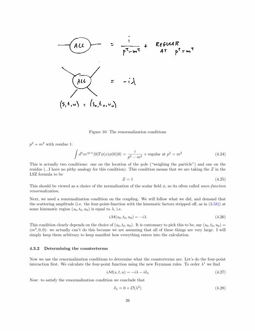
Figure 10: The renormalization conditions
p2 = m2 with residue 1: ∫d4xeip·x〈0|Tφ(x)φ(0)|0〉 =
i
p2 −m2+ regular at p2 = m2 (4.24)
This is actually two conditions: one on the location of the pole (“weighing the particle”) and one on theresidue (...I have no pithy analogy for this condition). This condition means that we are taking the Z in theLSZ formula to be
Z = 1 (4.25)
This should be viewed as a choice of the normalization of the scalar field φ, so its often called wave-functionrenormalization.
Next, we need a renormalization condition on the coupling. We will follow what we did, and demand thatthe scattering amplitude (i.e. the four-point-function with the kinematic factors stripped off, as in (3.58)) atsome kinematic region (s0, t0, u0) is equal to λ, i.e.
iM(s0, t0, u0) = −iλ (4.26)
This condition clearly depends on the choice of (s0, t0, u0). It is customary to pick this to be, say (s0, t0, u0) =(m2, 0, 0): we actually can’t do this because we are assuming that all of these things are very large. I willsimply keep them arbitrary to keep manifest how everything enters into the calculation.
4.3.2 Determining the counterterms
Now we use the renormalization conditions to determine what the counterterms are. Let’s do the four-pointinteraction first. We calculate the four-point function using the new Feynman rules. To order λ1 we find
iM(s, t, u) = −iλ− iδλ (4.27)
Now: to satisfy the renormalization condition we conclude that
δλ = 0 +O(λ2) (4.28)
26
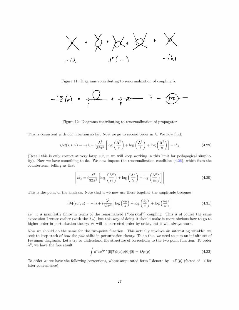
Figure 11: Diagrams contributing to renormalization of coupling λ:
Figure 12: Diagrams contributing to renormalization of propagator
This is consistent with our intuition so far. Now we go to second order in λ: We now find:
iM(s, t, u) = −iλ+ iλ2
32π2
[log
(Λ2
s
)+ log
(Λ2
t
)+ log
(Λ2
u
)]− iδλ (4.29)
(Recall this is only correct at very large s, t, u: we will keep working in this limit for pedagogical simplic-ity). Now we have something to do. We now impose the renormalization condition (4.26), which fixes thecounterterm, telling us that
iδλ = iλ2
32π2
[log
(Λ2
s0
)+ log
(Λ2
t0
)+ log
(Λ2
u0
)](4.30)
This is the point of the analysis. Note that if we now use these together the amplitude becomes:
iM(s, t, u) = −iλ+ iλ2
32π2
[log(s0
s
)+ log
(t0t
)+ log
(u0
u
)](4.31)
i.e. it is manifestly finite in terms of the renormalized (“physical”) coupling. This is of course the sameexpression I wrote earlier (with the λP ), but this way of doing it should make it more obvious how to go tohigher order in perturbation theory: δλ will be corrected order by order, but it will always work.
Now we should do the same for the two-point function. This actually involves an interesting wrinkle: weseek to keep track of how the pole shifts in perturbation theory. To do this, we need to sum an infinite set ofFeynman diagrams. Let’s try to understand the structure of corrections to the two point function. To orderλ0, we have the free result: ∫
d4xeip·x〈0|Tφ(x)φ(0)|0〉 = DF (p) (4.32)
To order λ1 we have the following corrections, whose amputated form I denote by −iΣ(p) (factor of −i forlater convenience)
27
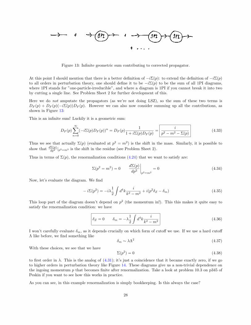
Figure 13: Infinite geometric sum contributing to corrected propagator.
At this point I should mention that there is a better definition of −iΣ(p): to extend the definition of −iΣ(p)to all orders in perturbation theory, one should define it to be −iΣ(p) to be the sum of all 1PI diagrams,where 1PI stands for ”one-particle-irreducible”, and where a diagram is 1PI if you cannot break it into twoby cutting a single line. See Problem Sheet 2 for further development of this.
Here we do not amputate the propagators (as we’re not doing LSZ), so the sum of these two terms isDF (p) + DF (p)(−iΣ(p))DF (p). However we can also now consider summing up all the contributions, asshown in Figure 13:
This is an infinite sum! Luckily it is a geometric sum:
DF (p)
∞∑n=0
(−iΣ(p)DF (p))n = DF (p)1
1 + iΣ(p)DF (p)=
i
p2 −m2 − Σ(p)(4.33)
Thus we see that actually Σ(p) (evaluated at p2 = m2) is the shift in the mass. Similarly, it is possible to
show that dΣ(p)dp2 |p2=m2 is the shift in the residue (see Problem Sheet 2).
Thus in terms of Σ(p), the renormalization conditions (4.24) that we want to satisfy are:
Σ(p2 = m2) = 0dΣ(p)
dp2
∣∣∣∣p2=m2
= 0 (4.34)
Now, let’s evaluate the diagram. We find
− iΣ(p2) = −iλ1
2
∫d4k
i
k2 −m2+ i(p2δZ − δm) (4.35)
This loop part of the diagram doesn’t depend on p2 (the momentum in!). This this makes it quite easy tosatisfy the renormalization condition: we have
δZ = 0 δm = −λ1
2
∫d4k
i
k2 −m2(4.36)
I won’t carefully evaluate δm, as it depends crucially on which form of cutoff we use. If we use a hard cutoffΛ like before, we find something like
δm ∼ λΛ2 (4.37)
With these choices, we see that we haveΣ(p2) = 0 (4.38)
to first order in λ. This is the analog of (4.31); it’s just a coincidence that it became exactly zero, if we goto higher orders in perturbation theory like Figure 14. These diagrams give us a non-trivial dependence onthe ingoing momentum p that becomes finite after renormalization. Take a look at problem 10.3 on p345 ofPeskin if you want to see how this works in practice.
As you can see, in this example renormalization is simply bookkeeping. Is this always the case?
28
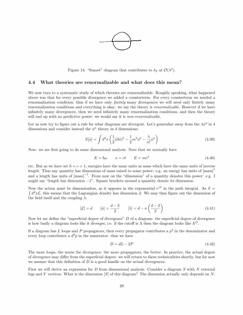
Figure 14: “Sunset” diagram that contributes to δZ at O(λ2).
4.4 What theories are renormalizable and what does this mean?
We now turn to a systematic study of which theories are renormalizable. Roughly speaking, what happenedabove was that for every possible divergence we added a counterterm. For every counterterm we needed arenormalization condition; thus if we have only finitely many divergences we will need only finitely manyrenormalization conditions and everything is okay: we say the theory is renormalizable. However if we haveinfinitely many divergences, then we need infinitely many renormalization conditions, and then the theorywill end up with no predictive power: we would say it is non-renormalizable.
Let us now try to figure out a rule for what diagrams are divergent. Let’s generalize away from the λφ4 in 4dimensions and consider instead the φn theory in d dimensions:
S[φ] =
∫ddx
(1
2(∂φ)2 − 1
2m2φ2 − λ
n!φn)
(4.39)
Now: we are first going to do some dimensional analysis. Note that we normally have
E = ~ω x = ct E = mc2 (4.40)
etc. But as we have set ~ = c = 1, energies have the same units as mass which have the same units of inverselength. Thus any quantity has dimensions of mass raised to some power: e.g. an energy has units of [mass]
1
and a length has units of [mass]−1
. From now on the “dimension” of a quantity denotes this power: e.g. Imight say “length has dimension −1”. Square brackets around a quantity denote its dimension.
Now the action must be dimensionless, as it appears in the exponential eiS in the path integral. As S =∫ddxL, this means that the Lagrangian density has dimension d. We may thus figure out the dimension of
the field itself and the coupling λ:
[L] = d [φ] =d− 2
2[λ] = d− n
(d− 2
2
)(4.41)
Now let me define the “superficial degree of divergence” D of a diagram: the superficial degree of divergenceis how badly a diagram looks like it diverges, i.e. if the cutoff is Λ then the diagram looks like ΛD.
If a diagram has L loops and P propagators, then every propagator contributes a p2 in the denominator andevery loop contributes a ddp in the numerator: thus we have
D = dL− 2P (4.42)
The more loops, the worse the divergence: the more propagators, the better. In practice, the actual degreeof divergence may differ from the superficial degree: we will return to these technicalities shortly, but for nowwe assume that this definition of D is a good handle on the actual divergences.
First we will derive an expression for D from dimensional analysis. Consider a diagram S with N externallegs and V vertices. What is the dimension [S] of this diagram? The dimension actually only depends on N :
29
one way to understand this is to imagine that we are considering a field theory with an interaction term ηφN
in it. (Note we are not adding this term to our theory: it is just a fictitious device for dimension-counting).The diagram might then receive a contribution that goes like η (with no extra dimensionful factors), andthus we must have [S] = [η]. But from the dimension counting in (4.41), we conclude that
[η] = d−N(d− 2
2
)(4.43)
However, another way to construct the diagram is by sewing together many propagators and vertices etc. inthe actual theory. If there are V vertices, then the most divergent part of the diagram must go (by definition)as λV ΛD; note that any other dimensionful scales (e.g. external momenta, etc.) will only decrease the degreeof divergence. By equating the two ways of computing the dimension, we conclude that
d−N(d− 2
2
)= [λV ΛD] = V [λ] +D = V
(d− n
(d− 2
2
))+D (4.44)
We solve this for D to find
D = d+ V
(n
(d− 2
2
)− d)−N
(d− 2
2
)(4.45)
The last term is always negative or 0 for all reasonable dimensions 4. Now we can understand that thephysics depends crucially on the sign of the thing multiplying V , which we note is simply the (inverse) massdimension of λ. There are three possibilities:
1. [λ] > 0, or Super-renormalizable: in this case, increasing V makes every diagram less divergent:thus there are only finitely many divergent diagrams, period. These theories can then definitely berenormalized for with a finite number of counterterms, and new divergences will stop happening atsufficiently high order in perturbation theory (i.e. in V ). This tends to happen in low dimension: e.gφ4 theory in d = 3 falls into this class.
2. [λ] = 0, or Renormalizable: in this case, the bit proportional to V vanishes. Now there are still onlyfinitely many divergent amplitudes, as for sufficiently large N , D is still 0. Nevertheless, we will findmore and more divergences as we go to higher orders in perturbation theory. We thus need to continueadjusting the counterterms to arbitrarily high order.
3. [λ] < 0, or Non-renormalizable: in this case, we cannot renormalize: as we increase V , we have alarger and larger window of N where we can have a D > 0. Thus there are infinitely many divergences,and we cannot absorb them into finitely many counterterms.
This closes the classification of field theories; what we just did is called “power-counting renormalization”.The key thing here is that everything is controlled by the mass dimension of the coupling: if ever it hasnegative mass dimension, then the theory will be non-renormalizable. For example, if we just add a ηφ6
term to our beloved φ4 theory in four dimensions, it will not be renormalizable any more. I will discuss thephysical significance of this in the next section.
There is a last worry: does the superficial degree of divergence adequately describe the degree of divergenceof the diagram? It actually does not, for two distinct reasons:
4What, you ask, of the case d = 1, i.e. quantum mechanics? This actually confuses me: it appears that by increasing thenumber of insertions N the superficial degree of divergence grows rapidly in quantum mechanics. This is against my naiveunderstanding, which is that quantum mechanics is actually always simple in the UV (and complicated in the IR; that’s whythe spectrum is different for every sort of potential). Thus, we have a extra credit homework assignment: explain why theterm proportional to N has a different sign for d = 1.
30
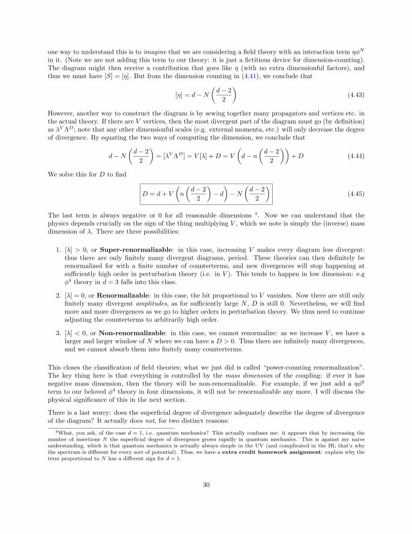
Figure 15: This contains a quadratically divergent subdiagram though its superficial degree of divergence Dis 0.
1. It might overstate the divergence: this could happen if some more sophisticated effect (e.g. a symmetry)sets the diagram to zero or reduces the divergence level. This happens in QED, for example.
2. It might understate the divergence: this happens if there is a badly divergent subdiagram, e.g. as inFigure 15, which from the formula has D = 0 but actually has a clearly quadratically divergent bit.This turns out to not upset the reasoning above, because it is not a “new” divergence: the countertermdoes its magic in the subdiagram.
Despite these subtleties, for most purposes the conclusions of “power-counting renormalization” give a goodphysical picture as to what is happening in the actual theory, though proving it can be difficult.
4.5 A few non-renormalizable theories
Here we will try to understand what it really means to be non-renormalizable. First, let’s try to understandwhat the dimension of the coupling means. More discussion of this in language very similar to that which Iuse here can be found in Chapter III.2 of [4]. Let’s consider adding a non-renormalizable term like φ6 to ourusual 4d action. In 4d, [φ] = 1 and so we have:
L6 =
∫d4x
c
M2φ6 (4.46)
where M has dimensions of mass and c is dimensionless. The claim is that adding this term makes the theorynon-renormalizable, which means that we can no longer take the cutoff to infinity and retain predictive power.Why is this? A clue is given by the following question: let’s imagine computing some sort of an observable –say a scattering amplitude at energy E – and asking how it depends on on E to first order in in c. Scatteringamplitudes are (at the end of the day), probabilities, and are thus dimensionless. Thus we see that thecontribution from the φ6 term must, from dimensional analysis, take the form
iM6 ∼c
M2E2 (4.47)
The E2 must appear in the numerator to soak up the factor of M2 from the denominator. Thus, no matterwhat, this contribution is unimportant at low-energies: but we also see that no matter what, eventually whenE ∼M perturbation theory in c will break down. Thus this theory seems to become strongly coupled in theUV: crudely speaking, this is what non-renormalizability hints at, it says that we do not know about what ishappening in the UV: this is why we cannot extend the cutoff to infinity.
So what should one do, then, if one is handed a non-renormalizable theory? Since you cannot take the cutoffΛ to infinity, you should take the idea of the cutoff seriously: have it hanging around your calculation, andjust try to ask questions at energies E � Λ: hopefully then the cutoff will not affect your life too much.
31
This is the idea behind effective field theory, and will be more correctly developed in V. Niarchos’s course onrenormalization next term, which I encourage everyone to take.
In the meantime, however, I will introduce two of my favorite non-renormalizable theories to explain howthese ideas affect low-energy physics:
4.5.1 Pions
Pions are real-life particles that you have probably heard of: they have a mass of roughly 135 MeV, andthere are three kinds of them. We can represent them by a triplet of real scalar fields ~π(x). In a particularlimit (massless quarks), we can choose to ignore their mass and their action looks like
S =
∫d4x
(1
2(∂µ~π · ∂µ~π) +
1
2F 2π
∂µ~π · π∂µ~π · ~π + · · ·)
(4.48)
From here we see that Fπ has dimensions of mass: it is called the pion decay constant, and in real life it is93 MeV. Note that this coupling thus has negative mass dimension, and so the theory is non-renormalizable.You can, however, use this theory at low energies: e.g. if you try to scatter together pions at energy E thenfrom here their scattering amplitude will go like
iM∼ E2
F 2π
(4.49)
This is okay at low energies, but perturbation theory seems to break down at E ∼ Fπ, and thus from thepion Lagrangian alone we do not know what to do.
I note, however, that in real life, we do actually know what happens: pions are actually made of quarks thatare held together by the strong interactions. At high energies, they come loose: this “coming loose” is whatmade the pion theory break down, and then we need to use the full theory of the strong interactions, whichis called QCD and is renormalizable.
4.5.2 Gravity
Everyone knows about gravity. From A. Donos’s course you even know the gravitational action. It is
S =1
16πGN
∫d4x√−gR (4.50)
Let’s do something bold and reckless: let’s treat gravity as a quantum field theory. We will do this byexpanding around flat space, i.e. write
gµν = ηµν + hµν (4.51)
and then treating hµν as a quantum field. If we plug this ansatz into the action above, we find schematicallythat R ∼ (∂h)2, and so we get (very schematically) something like:
S =1
16πGN
∫d4x(∂h)2
(1 + h2 + h4 + · · ·
)(4.52)
where there are actually arbitrarily many terms in h (coming, e.g., from inverting the metric, the square-rootof the determinant, etc.) and I am suppressing all indices as they are really quite bad.
Note from (4.51) that h is dimensionless, and thus GN must have mass dimension of −2: the resultingdimensionful scale is called the Planck scale, and is 1019 GeV.
1
16πGN≡ m2
Pl (4.53)
32
To make this look more like a normal quantum field theory, let’s rescale:
h = mPlh (4.54)
and we now find
S =
∫d4x(∂h)2
(1 +
1
m2Pl
h2 +1
m4Pl
h4 + · · ·)
(4.55)
There is a coupling constant with negative mass dimension in the Lagrangian. Thus, gravity – viewed as aquantum field theory – is non-renormalizable. You have probably heard that there are some difficulties withquantizing gravity: this is what people mean. Having said that, everything is fine at low energies: it is onlyat high energies (i.e. around the Planck scale) that things get difficult. Unlike in the pion case, here we donot know what to do, due to a pesky lack of experiments, but string theory is a candidate for a quantumtheory of gravity works perfectly fine at high energies. A nice review of the effective field theory of gravityis [5].
33
5 Global symmetries in the functional formalism
Here we will briefly discuss how global symmetries work in the path integral. Recall that an example of atheory with a global symmetry is the complex scalar field, whose action is
S[φ, φ†] =
∫d4x
((∂φ)†(∂φ)−m2φ†φ
)(5.1)
which is clearly invariant under phase rotations of the scalar field
φ→ eiαφ δφ = iαφ (5.2)
where the second equality is the infinitesimal action of the symmetry operation.
In this lecture, we will be instead more general, though maybe it is helpful to keep the complex scalar fieldin mind: consider a field theory with a bunch of fields φa with an action that is invariant under a generalglobal symmetry, i.e. under
φa(x)→ φa(x) + εδφa(x) (5.3)
that leaves the action invariant:S[φa + εδφa] = S[φa] (5.4)
5.1 Classical Noether’s theorem
As you are well aware, such global symmetries lead to conserved currents via Noether’s theorem. Let’s reviewthe classical version of this theorem (possibly in a slightly different form than you are used to). First, weperform a trick: let us consider the variation (5.3) with a symmetry parameter that depends on x:
φa(x)→ φa(x) + ε(x)δφa(x) (5.5)
(Note: no matter what it looks like, this has nothing to do with gauge symmetry, as we have not yet discussedgauge symmetry. This is just a trick). Now the action is not invariant under this transformation; however it isinvariant if the parameter ε is constant, which means that its variation must be proportional to a derivative.By locality of the action5, this means:
δεS[φa] =
∫d4xjµ(x)∂µε(x) = −
∫d4x∂µj
µ(x)ε(x) (5.6)
where I have defined jµ to be the “thing that multiplies ∂µε”, and in the second equality I have integratedby parts. This is, in general, not zero (why would it be?).
However, let us now imagine that the field φa obeys the equations of motion, i.e. that we are “on-shell”. Inthat case the variation of the action under all variations of the field φ is zero:
δφS[φa] = 0 (5.7)
and in particular under the specific variation (5.4). This means that the right hand-side of (5.6) is zero, andthus that
∂µjµ(x) = 0 on− shell (5.8)
In other words, we have shown that we have a current jµ, and that the current is conserved classically, whenthe fields obey the classical equations of motion. We used both the invariance of the action and the fact thatwe were on-shell. This also gives you a way to compute jµ, and it is instructive to verify that it gives youwhat you expect in the usual case.
5i.e. using the fact that the action is an integral of a local Lagrangian density.
34
5.2 Quantum Ward identities
Now let us study this phenomenon in the quantum theory, i.e. we study the path integral
Z =
∫[Dφa] exp (iS[φa]) (5.9)
and perform a similar operation. We consider the symmetry transformation given by (5.4) as defining achange of variables in the path integral:
φa(x)→ φ′a(x) = φa(x) + ε(x)δφa(x) (5.10)
The first thing to note is that this is a change of variables, and thus does not alter the numerical value ofthe functional integral: ∫
[Dφa] exp (iS[φa]) =
∫[Dφ′a] exp (iS[φ′a]) (5.11)
This is always true for any change of variables, whether a symmetry operation or not. Now, because this isa symmetry operation, you can convince yourself by discretizing the measure that the measure of the pathintegral (usually) does not change6, and we have
[Dφa] = [Dφ′a] (5.12)
The action however does change a little bit: we see that we have (to first order in ε(x))
S[φ′a] = S[φa]−∫d4x∂µj
µ(x)ε(x) (5.13)
Putting all these things on the right-hand side, we see that we have:∫[Dφa] exp (iS[φa]) =
∫[Dφa]
(1− i
∫d4x∂µj
µ(x)ε(x) +O(ε2)
)exp (iS[φa]) (5.14)
The 1 bit cancels: but the bit involving ∂µjµ is precisely what we use to calculate the expectation value of
∂µjµ from the path integral! As this must hold for any ε(x), we conclude that we must have:
〈0|∂µjµ(x)|0〉 = 0 (5.15)
In other words, the expectation value of the current in the vacuum is zero! This is part of the quantumversion of Noether’s theorem. From this, and from our classical intuition might be tempted to conclude that∂µj
µ = 0 as an operator, i.e. it will vanish in all states. This is actually not quite true. To understand this,let’s apply this not to the generating functional itself, but instead to the expectation value of
〈0|Tφb(x1)φc(x2)|0〉 =1
Z[0]
∫[Dφa]φb(x1)φc(x2) exp (iS[φa]) (5.16)
But by the arguments above, this quantity is also numerically equal to
1
Z[0]
∫[Dφ′a]φ′b(x1)φ′c(x2) exp (iS[φ′a]) (5.17)
Where we have followed the time-honored practice of “putting primes everywhere”. Now we connect every-thing to the unprimed variables using the symmetry transformation. We find
1
Z[0]
∫[Dφa](φb(x1) + ε(x1)δφb(x1))(φc(x2) + ε(x2)δφb(x2))
(1− i
∫d4x∂µj
µ(x)ε(x) +O(ε2)
)exp (iS[φa])
(5.18)
6A somewhat surprisingly beautiful exception to this fact arises in the case of anomalies, which happen precisely when thisstatement is wrong and the measure does transform under the symmetry. It turns out that the possible ways it can transformare very restricted. Look at Chapter 19 of Peskin.
35
Setting this equal to its unprimed version, we see that everything multiplying an ε must vanish. Those termsare
ε(x1)δφb(x1)φx(x2) + ε(x2)φb(x1)δφc(x2)− iφb(x1)φc(x2)
∫d4xε(x)∂µj
µ(x) (5.19)
where it is all multiplied by∫
[Dφa] exp(iS[φa]), and thus we are computing the vev of these quantities. Inother words, we have just shown that
i〈φb(x1)φc(x2)∂µjµ(x)〉 = 〈δφb(x1)φc(x2)〉δ(4)(x− x1) + 〈φb(x1)δφc(x2)〉δ(4)(x− x2) (5.20)
(where all expectation values are time-ordered). Compare this to the case when ∂µjµ was by itself, in (5.15):
we see that it is no longer quite conserved. In other words, if we look at correlation functions of ∂µjµ with
other operators that are charged under the symmetry associated with jµ, then it vanishes up to delta functionterms where those operators are inserted. It should be easy to understand how this works if you insert moreoperators.
This is called the Ward identity associated with the symmetry: it is the quantum manifestation of the classicalNoether’s theorem. I believe you have encountered similar things in QED, associated with the conservationof electric charge.
Our discussion has been very abstract, so I leave to you to work out the details of how this works for aspecific symmetry (e.g. the U(1) phase rotations of the complex scalar in (5.1)).
36
6 Fermions
We will now finally move beyond scalar fields. In this section we will discuss fermions from the point ofview of the path integral – to be more precise, we will only discuss Dirac fermions. Let us first review a fewaspects of Dirac fermions from the canonical point of view.
6.1 Fermions in canonical quantization
Recall from IFT that there is such a thing as a Dirac field ψ(x), whose canonical commutation results infermions. More precisely, one can write down the Dirac Lagrangian:
S[ψ, ψ] =
∫d4xψ
(i/∂ −m
)ψ, (6.1)
the variation of which gives you the celebrated Dirac equation:(i/∂ −m
)ψ = 0 /∂ ≡ γµ∂µ (6.2)
In IFT ψ was then promoted to an operator that acted on the Hilbert space.
There are two things that are different about the Dirac field relative to the scalar field that we have studied:
1. ψ is actually a four-component object called a spinor, which means that under a Lorentz transformationΛ ∈ SO(3, 1), we have an expression that looks like this:
U(Λ)†ψa(x)U(Λ) = M(Λ)abψb(x) (6.3)
where a, b run over 4 spinor indices, U(Λ) is the operator that represents the Lorentz transformationon the QFT Hilbert space, and M(Λ) is the matrix that acts on spinor indices that is in the spin- 1
2representation of the Lorentz group (which one can construct out of gamma matrices, see e.g. Chapter3 of [2] if this is not familiar). Thus the Dirac field has spin 1
2 .
2. The Dirac field obeys anti-commutation relations rather than commutation relations. In other words,the analog of the canonical commutator for the scalar field φ is the following canonical anticommutator:
{ψa(~x), ψ†b(~y)} = δ(3)(~x− ~y)δab {ψa(~x), ψb(~y)} = {ψ†a(~x), ψ†b(~y)} = 0 (6.4)
This is an important fact: it means that fermions obey Fermi-Dirac statistics. In usual quantummechanics this means that the wavefunction is antisymmetric as a function of fermion coordinates. InQFT this information is encoded in the following way: if we write the Dirac field in terms of creationand annihilation operators:
ψ(x) =
∫d3p
(2π)3
1
2Ep
∑s
(as~pu
s(~p)e−ip·x + bs†~p vs(~p)e+ip·x
)(6.5)
Then we find that the a and b’s obey these relations:
{ar~p, as~q} = {br~p, bs~q} = (2π)3(2E~p)δ(3)(~p− ~q)δrs (6.6)
with all other anticommutators 0. In particular, we have
{ar†~p , ar†~p } = 2(ar†~p )2 = 0 (6.7)
which means that we can never put two fermions with the same momentum ~p and spin r in the samestate! (This is important, as it is the only reason that all the electrons in all the atoms in the periodictable do not all simply collapse into the lowest 1S orbital. This would probably make chemistry easierbut I feel it would be bad for the existence of complex structures).
37
It turns out that these two facts that are a priori unrelated – the fact that the Dirac field has spin 12
and the fact that it obeys anticommmutation statistics – are actually related by the spin-statistics theorem,which tells you that to have a Lorentz-invariant and unitary theory you must quantize spin 1
2 fields withanticommutation relations. It is instructive to go through quantizing it the wrong way to see what happens,as I imagine you did in IFT.
One final thing that I discuss from the canonical formalism is the form of the Hamiltonian, which turns outto be
H =∑s
∫d3p
(2π)32E~pE~p
(as†~p a
s~p + bs†~p b
s~p − 2
(1
2
))(6.8)
The thing of interest here is the vacuum energy bit, i.e. the last term: note that it appears with a minussign.
6.2 Grassman variables
Now that we have reviewed everything that we know about fermions, we now turn to what we did for scalarsin the first half of this course: we seek to get the fermion physics from the path integral. How can we dothis? It should be clear that we will need some new ingredients, as we previously did:
Integral over ordinary numbers = Commuting fields in quantum theory (6.9)
Now we needIntegral over something = Anti-commuting fields in quantum theory (6.10)
The question is: what is the something? It turns out that we will need to develop a new sort of numbercalled a Grassman variable. My treatment follows Section 9.5 of [2] and Chapter 44 of [3]; in particular, Irefer you to the latter for a more detailed discussion.
6.2.1 Anticommuting numbers
As in the quantum theory the resulting operators should anticommute, it seems reasonable to demand thatwe want a sort of ordinary number that also anticommutes. So let us just start defining things and see howfar we can go. I define a Grassman number as an objects η, θ that anticommute, so:
θη = −ηθ (6.11)
This means that the square of any Grassman number vanishes:
θθ = −θθ = 0 (6.12)
This fact makes algebra refeshingly easy. We can multiply any Grassman numbers by normal numbers a, b inthe usual way, with all the normal rules. Note that the product of two Grassman numbers θη anti-commuteswith any other Grassman numbers: thus, for purposes of manipulation we can imagine θη to be a normalnumber.
Let’s now consider a function of a single Grassman numbers f(θ). We can always Taylor expand in powersof θ: the most general function is
f(θ) = A+Bθ (6.13)
where all the other possible terms in the Taylor expansion are zero due to Grassman-ness. This is nice andsimple. A brief aside: we are typically going to be interested in commuting functions of anticommutingnumbers: if this is the case for f , then we see that A is commuting and B is anticommuting.
38
Let’s now do calculus: how do we take a derivative with respect to a Grassman number? There is a little bitof ambiguity in whether we take the derivative from the left or the right. From the right we define
f(θ)←−∂θ = B (6.14)
and thus from the left we thus have∂θf(θ) = −B, (6.15)
where we anticommuted B and θ before taking the derivative. Great, derivatives were easy. Now let’s dointegrals! Our ultimate goal is to do path integrals, so we will need to perform the analogue of
∫ +∞−∞ dx for
an ordinary integral. So what is ∫dθf(θ) =
∫dθ(A+Bθ) (6.16)
The integral should be linear in f , so it should be a linear function of A and B. Its value can be fixed byappealing to another property: in our derivation of Ward identities, Gaussian integrals, etc. we made heavyuse of shifting the integration variable, so it would be nice if we could define Grassman integration to beinvariant under this property. In other words, we want∫
dθf(θ) ≡∫dθf(θ + η) =
∫dθ(A+Bη +Bθ) (6.17)
As a function of θ, the shift changes the constant term, but leaves the linear term in θ unchanged. Thusthe only possible integral that is shift-invariant is a constant times the coefficient of the linear term. Forconvenience we take this constant to be 1, and so we define∫
dθ(A+Bθ) ≡ B (6.18)
Above I quietly assumed that B was commuting as I didn’t worry about the ordering of B, θ. If we insteadintegrate multiple Grassman variables there is a sign ambiguity, and we will thus use the convention∫
dθ
∫dη(ηθ) = +1 (6.19)
(i.e. we do the innermost integral first).
As the Dirac field is complex, we will also need complex Grassman numbers: as we already have access to i,we can define complex numbers in terms of their real and imaginary parts like we do for ordinary numbers:
θ =1√2
(θ1 + iθ2) θ∗ ≡ 1√2
(θ1 − iθ2) (6.20)
It’s also convenient to define complex conjugation to reverse the order of products, as for Hermitian conju-gation of operators
(θη)∗ ≡ η∗θ∗ = −θ∗η∗ (6.21)
We may now verify that∫dθdθ∗(θ∗θ) =
1
2
∫(dθ1 + idθ2)(dθ1 − idθ2)
(θ1 − iθ2)(θ1 + iθ2)
2=
∫dθ1dθ2(θ2θ1) = 1, (6.22)
where in the last equality we used (6.19). In other words, we treat θ and θ∗ as independent variables, just aswe do for normal complex numbers.
39
Let’s now do our first Gaussian Grassman integral (where b is commuting):∫dθ∗dθe−θ
∗bθ =
∫dθ∗dθ (1− θ∗bθ) (6.23)
=
∫dθ∗dθ (1 + θθ∗b) (6.24)
= b (6.25)
Now, if θ had been an ordinary complex number, this integral would have instead come out to be(∫dθ∗dθe−θ
∗bθ
)commuting
=2π
b(6.26)
The 2π doesn’t mean much – the crucial difference here is that the factor of b is in the denominator in thenormal case, rather than in the numerator as for Grassman variables. This will turn out to be of physicalsignificance.
6.2.2 Integrating many anticommuting numbers
We now move to having multiple Grassman variables θi, where i ∈ 1 · · ·n. We now want to understand howchanges of variables work in integration. Consider having θi and a unitary matrix Uij such that θ′i = Uijθj .Then consider the product: ∏
i
θ′i =1
n!εi1i2···inθ′i1θ
′i2 · · · θ
′in (6.27)
=1
n!εi1i2···inUi1j1θj1Ui2j2θj2 · · ·Uinjnθjn (6.28)
=1
n!εi1i2···inUi1j1Ui2j2 · · ·Uinjnεj1j2···jn
∏j
θj (6.29)
= (detU)∏i
θi (6.30)
In other words, the product of many θ’s transforms as a power of the determinant. Let us now understandwhat this means for integration: consider a general integral∫
dnθ′f(θi) (6.31)
The only term that can possibly survive this integral is one which has a product of all possible θi, i.e. theterm in the expansion of f(θi) ⊃
∏i θi. We can now write this as a product over the primed θi’s using the
expression above. We can then simply evaluate the integral; however the factor of detU−1 that we obtainremains, leaving us with the expression:∫
dnθ′f(θi) = (detU)−1
∫dnθf(θi) (6.32)
One way to interpret this is that the measure for Grassman integration transforms in the opposite way thanwe are used to for normal commuting integration (note the factor of detU would have been in the numeratorthen).
Note in particular that thisimplies that if U is unitary, then an integral of the form∫dnθdnθ∗f(θ, θ∗) = (detU)(detU)∗
∫dnθ′dnθ′∗f(θ, θ∗) =
∫dnθ′dnθ′∗f(θ, θ∗) (6.33)
40
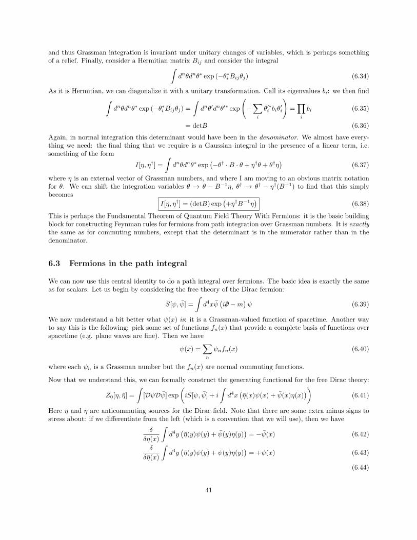
and thus Grassman integration is invariant under unitary changes of variables, which is perhaps somethingof a relief. Finally, consider a Hermitian matrix Bij and consider the integral∫
dnθdnθ∗ exp (−θ∗iBijθj) (6.34)
As it is Hermitian, we can diagonalize it with a unitary transformation. Call its eigenvalues bi: we then find∫dnθdnθ∗ exp (−θ∗iBijθj) =
∫dnθ′dnθ′∗ exp
(−∑i
θ′∗i biθ′i
)=∏i
bi (6.35)
= detB (6.36)
Again, in normal integration this determinant would have been in the denominator. We almost have every-thing we need: the final thing that we require is a Gaussian integral in the presence of a linear term, i.e.something of the form
I[η, η†] =
∫dnθdnθ∗ exp
(−θ† ·B · θ + η†θ + θ†η
)(6.37)
where η is an external vector of Grassman numbers, and where I am moving to an obvious matrix notationfor θ. We can shift the integration variables θ → θ − B−1η, θ† → θ† − η†(B−1) to find that this simplybecomes
I[η, η†] = (detB) exp(+η†B−1η
)(6.38)
This is perhaps the Fundamental Theorem of Quantum Field Theory With Fermions: it is the basic buildingblock for constructing Feynman rules for fermions from path integration over Grassman numbers. It is exactlythe same as for commuting numbers, except that the determinant is in the numerator rather than in thedenominator.
6.3 Fermions in the path integral
We can now use this central identity to do a path integral over fermions. The basic idea is exactly the sameas for scalars. Let us begin by considering the free theory of the Dirac fermion:
S[ψ, ψ] =
∫d4xψ
(i/∂ −m
)ψ (6.39)
We now understand a bit better what ψ(x) is: it is a Grassman-valued function of spacetime. Another wayto say this is the following: pick some set of functions fn(x) that provide a complete basis of functions overspacetime (e.g. plane waves are fine). Then we have
ψ(x) =∑n
ψnfn(x) (6.40)
where each ψn is a Grassman number but the fn(x) are normal commuting functions.
Now that we understand this, we can formally construct the generating functional for the free Dirac theory:
Z0[η, η] =
∫[DψDψ] exp
(iS[ψ, ψ] + i
∫d4x
(η(x)ψ(x) + ψ(x)η(x)
))(6.41)
Here η and η are anticommuting sources for the Dirac field. Note that there are some extra minus signs tostress about: if we differentiate from the left (which is a convention that we will use), then we have
δ
δη(x)
∫d4y
(η(y)ψ(y) + ψ(y)η(y)
)= −ψ(x) (6.42)
δ
δη(x)
∫d4y
(η(y)ψ(y) + ψ(y)η(y)
)= +ψ(x) (6.43)
(6.44)
41
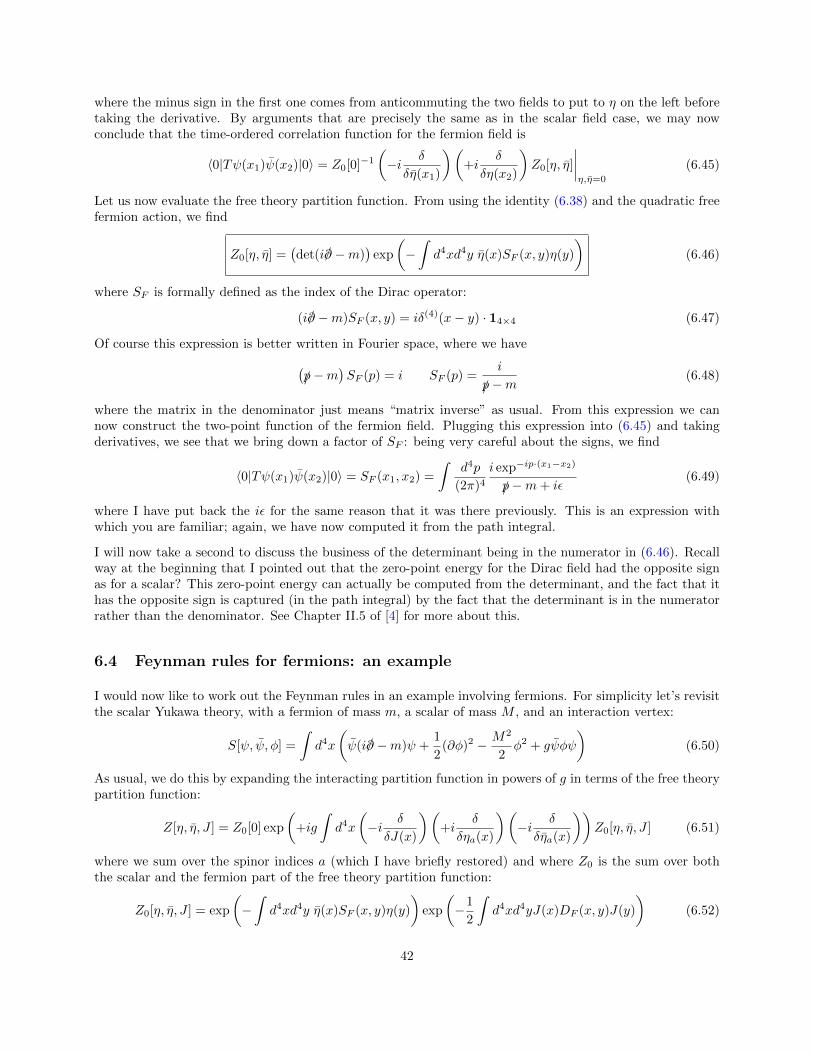
where the minus sign in the first one comes from anticommuting the two fields to put to η on the left beforetaking the derivative. By arguments that are precisely the same as in the scalar field case, we may nowconclude that the time-ordered correlation function for the fermion field is
〈0|Tψ(x1)ψ(x2)|0〉 = Z0[0]−1
(−i δ
δη(x1)
)(+i
δ
δη(x2)
)Z0[η, η]
∣∣∣∣η,η=0
(6.45)
Let us now evaluate the free theory partition function. From using the identity (6.38) and the quadratic freefermion action, we find
Z0[η, η] =(det(i/∂ −m)
)exp
(−∫d4xd4y η(x)SF (x, y)η(y)
)(6.46)
where SF is formally defined as the index of the Dirac operator:
(i/∂ −m)SF (x, y) = iδ(4)(x− y) · 14×4 (6.47)
Of course this expression is better written in Fourier space, where we have(/p−m
)SF (p) = i SF (p) =
i
/p−m(6.48)
where the matrix in the denominator just means “matrix inverse” as usual. From this expression we cannow construct the two-point function of the fermion field. Plugging this expression into (6.45) and takingderivatives, we see that we bring down a factor of SF : being very careful about the signs, we find
〈0|Tψ(x1)ψ(x2)|0〉 = SF (x1, x2) =
∫d4p
(2π)4
i exp−ip·(x1−x2)
/p−m+ iε(6.49)
where I have put back the iε for the same reason that it was there previously. This is an expression withwhich you are familiar; again, we have now computed it from the path integral.
I will now take a second to discuss the business of the determinant being in the numerator in (6.46). Recallway at the beginning that I pointed out that the zero-point energy for the Dirac field had the opposite signas for a scalar? This zero-point energy can actually be computed from the determinant, and the fact that ithas the opposite sign is captured (in the path integral) by the fact that the determinant is in the numeratorrather than the denominator. See Chapter II.5 of [4] for more about this.
6.4 Feynman rules for fermions: an example
I would now like to work out the Feynman rules in an example involving fermions. For simplicity let’s revisitthe scalar Yukawa theory, with a fermion of mass m, a scalar of mass M , and an interaction vertex:
S[ψ, ψ, φ] =
∫d4x
(ψ(i/∂ −m)ψ +
1
2(∂φ)2 − M2
2φ2 + gψφψ
)(6.50)
As usual, we do this by expanding the interacting partition function in powers of g in terms of the free theorypartition function:
Z[η, η, J ] = Z0[0] exp
(+ig
∫d4x
(−i δ
δJ(x)
)(+i
δ
δηa(x)
)(−i δ
δηa(x)
))Z0[η, η, J ] (6.51)
where we sum over the spinor indices a (which I have briefly restored) and where Z0 is the sum over boththe scalar and the fermion part of the free theory partition function:
Z0[η, η, J ] = exp
(−∫d4xd4y η(x)SF (x, y)η(y)
)exp
(−1
2
∫d4xd4yJ(x)DF (x, y)J(y)
)(6.52)
42
Figure 16: Sample diagram involving fermions
Figure 17: Sample diagram to illustrate minus signs in closed loops of fermions
It should be fairly clear that this works pretty much as you would expect: you just expand everything andcan associate a picture with term in the perturbation expansion. For example, one term arising from theperturbation expansion is
D1 = (ig)
∫d4xd4yd4zd4w (η(x)SF (x, y)SF (y, z)η(z))DF (y, w)J(w) (6.53)
which corresponds to Figure 16, where we draw a solid line to indicate a fermion and a dotted line to indicatea scalar.
I am not going to go into much detail here, as I believe the mechanics have been worked out in your QEDcourse. Everything about LSZ, etc. goes through as before, where you just have to worry about all the spinorindices and be careful with signs, but all else is as you expect. There are only two real wrinkles here.
1. Fermion lines are oriented: they have arrows on them. This is not because they are fermions, butbecause they are complex fields, and so the particles are different from anti-particles: thus we mustestablish a convention for them. The convention I use is that the arrow points towards the source η,which you recall is the source for the field ψ. It is also important that the interaction vertex has onearrow pointing towards the interaction and one pointing away.
2. Closed fermion loops come with a minus sign. There are various ways to see this: one way is torealize that the determinant basically captures the physics of closed fermion loops, and its logarithmcontributes with the opposite sign as in the commuting case. A more pedestrian way is through directbrutal evaluation of the signs involved. Consider the diagram in Figure 17:
This has a fermion loop: let’s evaluate the sign structure of (6.51), doing the abbreviation
δi ≡δ
δη(xi)δi ≡
δ
δη(xi)(6.54)
43
we have a term of the form ∫dx1dx2δ1δ1δ2δ2 (η · S · η) (η · S · η) (6.55)
Now let us look at the pattern of contractions of derivatives: if we insist that the pattern be such thatthe propagators form a closed loop, we always need to move an odd number of Grassman derivativesthrough each other. This gives us a minus sign (and is the same physics behind the determinant).
Let me then summarize with the new physics for the Feynman rules in momentum space for fermions. I havenot dotted all the i’s7 and crossed all the t’s in deriving them, but I leave that to you as an exercise.
• Every fermion propagator comes with a factor of i/p−m . Each propagator has an arrow on it that denotes
the flow of charge.
• For the Yukawa theory, every vertex comes with a factor of ig (for more general theories, it is easy tofigure out what the right vertex factor should be by staring at the interaction term).
• Every closed fermion loop comes with a minus sign.
I close the section on fermions with a final remark: the difficulty of doing quantum field theory really comesfrom the loops. However the fact that boson and fermion loops contribute with the opposite sign suggestsa tantalizing possibility: could we make them perhaps cancel each other out? If we could argue that theyalways canceled, then maybe we wouldn’t need to calculate them at all, and we could have stopped thiscourse after the first week. This would be a ridiculous coincidence, unless you could argue that there was asymmetry that enforces it. This symmetry would seem to require the bosons and fermions to have all thesame masses and charges and basically the same couplings. Indeed, this is the idea behind supersymmetry,which is a beautiful and important idea that Nature does not seem to be exploiting as much as it could be.S. Cremonesi will teach a course on this next term.
7Ha ha.
44
7 Abelian Gauge Theories
Now that we have understood fermions, we will move on to gauge theories. We warm up with Abelian gaugetheories before moving on to the full glory and beauty of non-Abelian gauge theories for the final part of thecourse.
7.1 Gauge invariance
We will now first understand what a gauge symmetry is, starting from the simplest example. First considera theory with a global U(1) symmetry: it is nice to consider the Dirac theory to start,
S[ψ, ψ] =
∫d4x ψ(x)(i/∂ −m)ψ(x) (7.1)
This theory is clearly invariant under a global U(1) phase rotation, which is
ψ(x)→ ψ′(x) = eiΛψ(x) ψ(x)→ e−iΛψ(x) (7.2)
I emphasize that the symmetry parameter Λ here is a constant in spacetime, which is why we call it a globalsymmetry. I also want to emphasize that two field configurations that are related by the symmetry are bothphysical field configurations. If ψ represents something that we integrate over in the path integral, then sodoes ψ′.
Now here is an idea, which I simply state without a huge amount of motivation: let’s do something different.Let us instead demand that we have a theory that is invariant under a symmetry where the symmetryparameter varies in spacetime:
ψ(x)→ ψ′(x) = eiΛ(x)ψ(x) (7.3)
This is called a local symmetry, or a gauge symmetry. As I will explain later, it should probably really becalled a gauge redundancy, but I will not use that language in this course and continue to call it a gaugesymmetry. Things that are invariant under this symmetry are called gauge-invariant.
Now, let’s understand what is and is not gauge-invariant. For example: ψ(x) itself is not gauge invariant,but it transforms under gauge transformations in a simple way (by an overall rotation).
The mass termmψ′(x)ψ′(x) = mψ(x)e−iΛ(x)e+iΛ(x)ψ(x)→ mψ(x)ψ(x) (7.4)
clearly is gauge invariant. Note that it would not have been if the field and its conjugate were evaluated atdifferent points, as then the gauge parameter would not have canceled.
Now how about the derivative term in the action? Now we run into an issue that has to do with the localcharacter of the gauge transformation: note that if we try to take a derivative we find
∂µψ′(x) = ∂µ
(eiΛ(x)ψ(x)
)= eiΛ(x) (i∂µΛ + ∂µ)ψ(x) (7.5)
Something very bad has happened because Λ(x) depends on space, we have picked up an extra term ∂µΛ.There is no obvious way to get rid of this, and thus we conclude that the Dirac action as written (7.12) isnot gauge invariant.
How do we fix this? A useful analogy for GR-educated students such as yourselves is to remember that wehad a similar problem when we tried to take a derivative of a tensor and found that the resulting objectwasn’t a tensor any more, in that it had a lousy transformation under coordinate changes. To fix that, wehad to invent a new kind of derivative, the covariant derivative.
45
This is a similar problem: the derivative of ψ no longer has nice gauge transformation properties. To fix it,wewill do the same thing that we did previously: we define a new object, called the gauge covariant derivative:
Dµψ ≡ (∂µ + ieAµ)ψ (7.6)
where I have introduced a new field Aµ, called the gauge field or the gauge connection. (GR students may betempted to compare it to the Christoffel connection: this analogy will get even closer when we do non-Abeliangauge theories soon). I have also chosen to take out a factor e for later convenience.
We will demand that the gauge-covariant derivative of ψ has a nice gauge transformation property, i.e. forinvariance purposes let us demand:
Dµψ → D′µψ′ = eiΛ(x)Dµψ, (7.7)
without any awkward inhomogenous piece. Let’s see what we require A′µ to do to make this happen. Ex-panding out we have
D′µψ′ =
(∂µ + ieA′µ
)eiΛ(x)ψ(x) = eiΛ(x)
(i∂µΛ + ieA′µ + ∂µ
)ψ(x) (7.8)
= eiΛ(x) (∂µ + ieAµ)ψ(x) (7.9)
where the last equality is our demand. We see that this will work out if and only if:
A′µ = Aµ −1
e∂µΛ(x) ψ′(x) = eiΛ(x)ψ(x) , (7.10)
where I have also written down the transformation property of ψ, as the two are related. This is the gauge-transformation of Aµ: if it transforms in this way, then our gauge-covariant derivative does indeed do whatwe want it to do. Note that now the following term:
ψ(x)γµDµψ(x)→ ψ′(x)γµD′µψ′(x) = ψ(x)e−iΛ(x)γµe+iΛ(x)Dµψ(x) = ψ(x)γµDµψ(x) (7.11)
is gauge-invariant, and thus we have succeeded in taking a derivative in a gauge-invariant way. With this,we see that we can write a fully gauge-invariantized-Dirac-action:
S[ψ, ψ, A]Dirac =
∫d4x ψ(x)(i /D −m)ψ(x) (7.12)
where we just promote the partial to a gauge-covariant derivative. To do this, we had to invent another fieldcalled Aµ. This is the price of gauge-invariance.
But now that we have this field Aµ, we may ask what more we can do with it. To see this, let’s first note thatDµψ has a nice gauge-transformation property, and thus so will DµDνψ. It thus makes sense to consider thecommutator of the two derivatives:
[Dµ, Dν ]ψ = [∂µ, ∂ν ]ψ + ie([∂µ, Aν ]− [∂ν , Aµ])ψ (7.13)
= ie (pµAν − ∂νAµ)ψ (7.14)
Notice that this commutator of derivatives is (when acting on ψ) actually not a derivative at all: it is just anumber multiplying ψ. Let’s call this number ieFµν , i.e.
Fµν ≡ ∂µAν − ∂νAµ (7.15)
Fµν is called the field-strength of the gauge field. Now, purely abstractly, we know that Fµν must be gauge-invariant. That’s because we have
[Dµ, Dν ] = ieFµν (7.16)
46
Now consider acting this equation on ψ and then doing a gauge-transformation on both sides: we know howboth sides transform
eiΛ(x)[Dµ, Dν ]ψ = ieFµνeiΛ(x)ψ (7.17)
and we can now cancel the eiΛ(x), which immediately implies that Fµν is gauge invariant. Of course wecould also simply directly use the gauge transformation property of Aµ (7.10) directly, but this more abstractviewpoint will be useful when we get to non-Abelian gauge theories.
It is not hard to convince yourself that random derivatives of Aµ, i.e ∂µAν by itself, are actually not gauge-invariant. So let us now try to write down the most general renormalizable gauge-invariant action involvingour new friend Aµ and ψ(x). It turns out the most general such action is
S[ψ, ψ] =
∫d4x
(−1
4FµνFµν + ψ(x)(i /D −m)ψ(x) + θεαβµνFαβFµν
)(7.18)
The first term is gauge-invariant since Fµν is gauge invariant. We have discussed the second term extensively.The third term looks weird, perhaps – it is weird for two distinct reasons: 1. It has an ε symbol, which meansthat it breaks parity and time reversal, and 2. It is a total derivative, and so does not seem to obviouslycontribute to the equations of motion – but see The Uses of Instantons in S. Coleman’s Aspects of Symmetry.We can, however, set θ to 0 if we demand that our theory be parity-invariant8 and from now on we will notworry about it.
How about a mass term for the gauge field, e.g.
M2AµAµ (7.19)
It is easy to see that this is not gauge-invariant, and thus one says that gauge-invariance forbids bare massterms for gauge fields. Thus we conclude that the most general gauge-invariant and P -invariant action witha gauge field and a single fermion is just
S[ψ, ψ, A]QED =
∫d4x
(−1
4FµνFµν + ψ(x)(i /D −m)ψ(x)
)(7.20)
This is the action of QED. Note that we have been led to it purely from symmetry principles: there is nothingelse that we could have written down.
7.2 Some classical aspects of Abelian gauge theory
For a little while, let us focus on the theory given by just the first part of the action above. This turns outto be ordinary Maxwell electrodynamics:
S[A]Maxwell =
∫d4x
(−1
4FµνFµν
)(7.21)
Let’s figure out the classical equations of motion: varying this action with respect to Aµ we find that theseequations of motion are just
∂µFµν = 0 (7.22)
If we pick a time direction and write this down in Lorentz-non-invariant notation F 0i = Ei, Bi = 12εijkFjk
then these are simply Maxwell’s equations, and thus this is the Lagrangian for free EM with no matter.
8Ok, this is not strictly true: more formally, P flips θ → −θ; however it turns out that when θ is correctly normalized it is aperiodic variable with periodicity 2π, which means that there is are two P -invariant points, one with θ = 0 and one with withθ = π, as −π + 2π = π. This seems like a ridiculous technicality that nobody should ever worry about, except that actually alot of beautiful physics associated with something called a “topological insulator” arises from the θ = π point.
47
Now, we should note an interesting fact: recall the Klein-Gordon equation of motion for a free scalar field
∂2φ = 0 (7.23)
This defines what is called a well-defined Cauchy problem, which means that if you pick a time t = 0 andspecify initial data φ(t = 0, ~x) as well as ∂tφ(t = 0, ~x), then you can use the equations of motion to propagateφ forwards in time unambiguiously. This is nice.
The fundamental degree of freedom for the Maxwell equation is Aµ(x), so this is the analog of φ(x). Theabove nice time evolution properties of the Klein-Gordon equation are not satisfied by the Maxwell equation.This can be understood from staring at the components of the equation, but there is an indirect route: notethat if Aµ is a solution to the equations of motion, then so is Aµ− 1
e∂µΛ(x), where Λ is any arbitrary functionof spacetime. If we pick Λ(t, ~x) to be a function that vanishes near t = 0 but is different at late t, it is clearthat the same initial data at t = 0 can lead to two completely different Aµ’s at late time, where they differby a gauge transformation.
What do we do with this? It looks like our theory has no predictive power, in that knowing what happens att = 0 does not fix what happens at late t. We can save our classical theory by making the following assertion:
Things that are not gauge-invariant are not physical.
So it is okay that we cannot unambiguously solve for their time evolution. It is only things that are gauge-invariant – in this case, the components of Fµν – that are physical, and you know from your elementary EMcourse that there is absolutely no issue solving for their time evolution.
Let’s be a bit more explicit. Writing Fµν = ∂µAν − ∂νAµ, we find
∂µ (∂µAν − ∂νAµ) = 0 (7.24)
As mentioned earlier, this is not a well-defined problem for time evolution of Aµ. We need to fix a gauge:one choice is Lorenz gauge:
∂µAµ = 0 (7.25)
(You can show that any Aµ can be placed in this form by a gauge transformation). If we do this, then wefind the equation
∂µ∂µAν = 0, (7.26)
which is now a perfectly nice wave equation that propagates all components of Aµ in time. It is also a waveequation with no mass term: in Fourier space, we get an equation that looks like:
(ω2 − k2)Aν = 0 (7.27)
and thus the on-shell energy of a single photon is ωk = k: the photon is massless.
However, it is still not true that all components are physical, as there is a residual gauge invariance in Lorenzgauge. I will not review here how this works, but you recall from elementary EM that for a plane wave withmomentum kµ it is the transverse components of Aµ to the momentum that are physical, and thus there aretwo physical polarizations. (One way to check this is to note that only those contribute to the field strengthtensor; more formally you can find a way to fix the residual gauge invariance in Lorenz gauge).
With this classical understanding under control, we now turn to the quantum theory, where all these subtletiesturn out to play a crucial role.
48
7.3 Quantizing QED
We turn now to the quantum theory. The new thing to do is to quantize the Maxwell action, i.e. we want toperform the following path integral:
Z =
∫[DA] exp
(i
∫d4x
(−1
4FµνF
µν
))(7.28)
We will ultimately be interested in quantizing the theory with the fermions also included, but first we willfocus on this. As we understand in detail by now, the propagator is always equal to the inverse of the operatorappearing in the quadratic part of the Lagrangian: let us thus write this in a useful way:
S[A] =
∫d4x
(−1
4(∂µAν − ∂νAµ)(∂µAν − ∂νAµ)
)(7.29)
=
∫d4x
1
2(Aν∂µ∂
µAν −Aν∂ν∂µAµ) (7.30)
=
∫d4x
1
2
(Aµ(∂2ηµν − ∂µ∂ν
)Aν)
(7.31)
Now whenever we do a functional integral, we want to invert the differential operator that appears in thequadratic part of the action. Thus we seek to find a photon Feynman propagator DF
µν that satisfies:(∂2ηµν − ∂µ∂ν
)DFνρ(x, y) = iδµρ δ
(4)(x− y) (7.32)
There is just one problem with this: no such DFνρ exists, because the differential operator has no inverse.
This is perhaps clear if we go to momentum space, when this equation becomes
(p2ηµν − pµpν)DFµν(p) = −iδµν (7.33)
But the matrix on the left-hand side has many zero eigenvalues: in fact, consider acting with it on any testfunction of the form pµα(p):
(p2ηµν − pµpν)pµα(p) =(p2pν − p2pν
)α(p) = 0 (7.34)
Thus the operator has a non-trivial kernel and cannot be inverted.
Physically, it should be clear that the issue is arising from the gauge transformations. The point is that anyfield configuration that is pure gauge
Aµ =1
e∂µΛ (7.35)
has field strength Fµν = 0, and thus has vanishing action. Thus when performing the path integral overfunctions in this “pure gauge” direction, the action does not oscillate and nothing suppresses their contributionto the path integral, which thus ends up diverges badly. This divergence is manifesting itself in the non-invertibility of the differential operator.
Clearly we are doing something wrong. Recall that things that are not gauge-invariant are not physical: thussomehow we are integrating over a bunch of non-physical stuff. Somehow we need to rearrange the integralso that we integrate over only the physical stuff.
We do this with a trick called the Fadeev-Popov procedure, which is basically the correct quantum analogof the gauge-fixing we did in the classical theory. Let G(A) be a function that we want to set to zero as agauge-fixing: e.g. if we were doing Lorenz gauge we would have
G(A) = ∂µAµ Lorenz gauge (7.36)
49
Let us now introduce the concept of a functional delta function: this is just what it sounds like, it is a mapfrom functions to numbers that satisfies the properties:
δ[φ] = 0, , φ(x) 6= 0 (7.37)∫[Dφ]δ[φ] = 1 (7.38)
You can think of a functional delta function as being an infinite product of delta functions, one at each pointin space. We want to somehow stick a functional delta function, a factor of δ(G(A)), inside the functionalintegral. We do this by first defining the gauge transformed field AΛ:
AΛµ(x) ≡ Aµ(x)− 1
e∂µΛ (7.39)
and then considering the following very fancy way to write the number 1:
1 =
∫[DΛ]δ
(G(AΛ)
)det
(δG(AΛ)
δΛ
)(7.40)
Note the factor of the functional determinant: this is just the Jacobian factor that you find when changingvariables in normal integrals, i.e. recall in one dimension we have the identity:
1 =
∫dyδ(y) =
∫dxδ(y(x))
dy
dx(7.41)
This is the same idea.
In any case, we now insert 1 in this fancy form into the functional integral, to obtain:
Z =
∫[DA][DΛ]δ
(G(AΛ)
)det
(δG(AΛ)
δΛ
)eiS[A] (7.42)
We now need to pick a convenient gauge-fixing function: we will pick the following:
Gω(A) = ∂µAµ − ω(x) (7.43)
where ω is some function. It does not matter what function it is: this picking of a gauge should not affectanything at all. However something nice about this choice is that we see that
δG(AΛ)
δΛ=
δ
δΛ
(∂µ
(Aµ +
1
e∂µΛ
)− ω
)=
1
e∂2 (7.44)
And thus this determinant is independent of everything! Thus we can take it outside the functional integral(and basically forget about it, at least in the Abelian case). We now find
Zω = det
(1
e∂2
)∫[DΛ]
∫[DA]δ
(Gω(AΛ)
)eiS[A] (7.45)
where I have put some ω’s in places to remind us that various things depend on ω. Now note that the actionis invariant, so we can write S[A] = S[AΛ]. Similarly, the integration measure is invariant (as it is just ashift), and we can thus write [DA] = [DAΛ]. But now A by itself doesn’t appear anywhere in the integral!So let us just rename AΛ → A, which we are clearly free to do, as its just a name. We then find
Zω = det
(1
e∂2
)∫[DΛ]
∫[DA]δ (Gω(A)) eiS[A] (7.46)
50
Now all of the integrals over Λ have completely factored out – they just contribute an overall prefactor thatwe will just call N . So we thus have
Zω = N∫
[DA]δ (∂µAµ − ω(x)) eiS[A] (7.47)
Now we will do one last thing – note that my notation makes it seem that Zω depends on ω, but actuallyit does not, as this is just a gauge-fixing condition. It it thus completely fine to average over all ω with aGaussian weight with width ξ. (Why not?). We then arrive at the following form of the partition function:
Z = N ′∫
[Dω][DA] exp
(−i∫d4x
1
2ξω2
)δ (∂µA
µ − ω(x)) eiS[A] (7.48)
The point of doing this possibly rather Baroque step is to make it possible to solve the delta functionconstraint in a simple way. Now that we integrate over all ω, we can interchange the order of integration andsee that actually the delta function sets ω = ∂µA
µ. Thus we find the following gauge-fixed form for the pathintegral:
Z = N ′∫
[DA] exp
(iS[A]−
∫d4x
1
2ξ(∂µA
µ)2
)(7.49)
The point of all of this was to modify the effective form of the Maxwell action to the following:
SFP[A] =
∫d4x
(−1
4FµνF
µν − 1
2ξ(∂µA
µ)2
)(7.50)
In other words, we have simply added a gauge-fixing term to the action. Note that the slick way in whichwe did it guarantees that everything is okay in the quantum theory. If we integrate by parts as before thisaction becomes:
SFP[A] =
∫d4x
1
2
(Aµ
(∂2ηµν −
(1− 1
ξ
)∂µ∂ν
)Aν
)(7.51)
Thus the kinetic term has been modified, and of course now we can now invert the propagator. We go toFourier space, and the equation to solve is then:(
−p2ηµν +
(1− 1
ξ
)pµpν
)DνρF (p) = iδρµ (7.52)
This sort of computation comes up again and again in field theory, so in this case I will work it out: considerthe most general form of DF . It is a tensor, and the only two tensor structures are ηµν and pµpν , so we theanswer must be of the form
DνρF (p) = A(p)ηνρ +B(p)
pνpρ
p2(7.53)
where I have taken out some factors of p to make the final thing look nicer. Now we plug this ansatz intothe equation and expand. We find
− p2A(p)δρµ + pµpρ
(A(p)
(1− 1
ξ
)− B(p)
ξ
)= iδρµ (7.54)
(Note taking away the gauge-fixing term corresponds to ξ → ∞, in which case there is clearly no solution).We find that A = − i
p2 , B = − ip2 (ξ − 1), and thus:
DνρF (p) = − i
p2
(ηµν − (1− ξ)p
µpν
p2
)(7.55)
This is the Feynman propagator for photons, carefully derived.
51
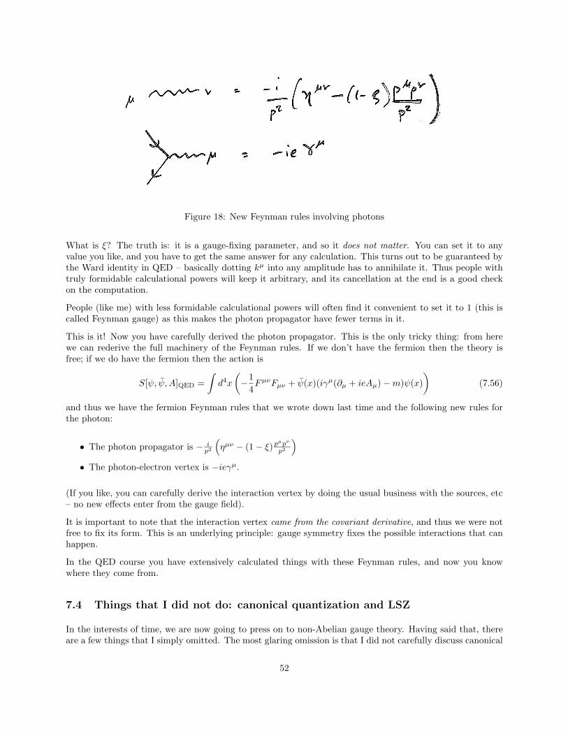
Figure 18: New Feynman rules involving photons
What is ξ? The truth is: it is a gauge-fixing parameter, and so it does not matter. You can set it to anyvalue you like, and you have to get the same answer for any calculation. This turns out to be guaranteed bythe Ward identity in QED – basically dotting kµ into any amplitude has to annihilate it. Thus people withtruly formidable calculational powers will keep it arbitrary, and its cancellation at the end is a good checkon the computation.
People (like me) with less formidable calculational powers will often find it convenient to set it to 1 (this iscalled Feynman gauge) as this makes the photon propagator have fewer terms in it.
This is it! Now you have carefully derived the photon propagator. This is the only tricky thing: from herewe can rederive the full machinery of the Feynman rules. If we don’t have the fermion then the theory isfree; if we do have the fermion then the action is
S[ψ, ψ, A]QED =
∫d4x
(−1
4FµνFµν + ψ(x)(iγµ(∂µ + ieAµ)−m)ψ(x)
)(7.56)
and thus we have the fermion Feynman rules that we wrote down last time and the following new rules forthe photon:
• The photon propagator is − ip2
(ηµν − (1− ξ)p
µpν
p2
)• The photon-electron vertex is −ieγµ.
(If you like, you can carefully derive the interaction vertex by doing the usual business with the sources, etc– no new effects enter from the gauge field).
It is important to note that the interaction vertex came from the covariant derivative, and thus we were notfree to fix its form. This is an underlying principle: gauge symmetry fixes the possible interactions that canhappen.
In the QED course you have extensively calculated things with these Feynman rules, and now you knowwhere they come from.
7.4 Things that I did not do: canonical quantization and LSZ
In the interests of time, we are now going to press on to non-Abelian gauge theory. Having said that, thereare a few things that I simply omitted. The most glaring omission is that I did not carefully discuss canonical
52
quantization for the photon fields. Let me say a few brief words, and you can find more details in Srednickichapters 54-57, and in Chapter 6 of D. Tong’s lecture notes.
You might be tempted to canonically quantize the photon field as follows:
Aµ(x) =∑λ
∫d3k
(2π)32ωk
(ελµ(~k)aλ,~ke
−ik·x + ε∗λµ (~k)a†λ,~ke+ik·x
)(7.57)
where the λ runs over photon polarizations, the ελµ are polarization vectors, and the a and a† are creationand annihilation operators, one for each photon polarization. The only issue is that not all of the states hereare physical, and we have to deal with this – all ways of doing it cut out two polariiations, leaving us with 2physical photon polarization. I will not go into this here and refer you to Srednicki, who explains the problemin Coulumb gauge:
∂iAi = 0 (7.58)
which is different from Lorenz gauge in that it is not Lorentz-invariant. The end effect is that the sum overλ only includes two spatial polarizations that are always perpendicular to ~k. I will say that the Hamiltonianformulation of this theory can get a bit tricky, and that we really sidestepped a lot of these complications bygoing through the path integral.
Once you accept this, it is not hard to go through LSZ for photons – everything goes through as before as in(3.23), except that there are some factors of εµ floating around:
n∏i=1
i
k2i
n′∏i=1
i
k2i′〈f |i〉 = εµ1 ε
µ2 · · · ε
∗µn′ 〈0|Aµ(k1)Aµ(k2) · · ·Aµ(k′n)|0〉 (7.59)
which tells us the rule for external photon lines: which is that you simply amputate the propagator, andin-states come with a factor of εµ(k) while out-states come with a factor of ε∗µ(k).
53
8 Non-Abelian gauge theories
Now that we understand Abelian gauge theories, we are going to move on to the next and final part of thiscourse: non-Abelian gauge theories. They are a powerful and nontrivial generalization of the same basic idea,and play a very important role in the Standard Model.
8.1 Non-Abelian gauge invariance
An abstract way of formulating the discussion above was the following: a gauge transformation in the Abeliancase was a map from spacetime to the group U(1), i.e. something like eiΛ(x). To be completely concrete, forany field ψ we should specify its charge q, and then the gauge transformation acts on the field like
ψ(x)→ eiqΛ(x)ψ(x) (8.1)
(We actually only discussed things with charge q = 1, but it should be clear that you could imagine othervalues for the charge of a field).
Now we will generalize the whole thing to non-Abelian gauge theory. Consider a (compact, simple) non-Abelian group G: the construction will work for any G, but for concreteness let’s take G to be SU(N).(In the back of my mind, I will always be imagining G = SU(2), but if your favorite group is SU(19) orsomething like that don’t let me stop you). We will now try to formulate a theory that is invariant undernon-Abelian gauge transformations, which are maps U(x) from spacetime to the group G.
Let’s review a little bit of group theory: I denote an abstract set of generators of the group by T a, where theindex a runs over the Lie algebra of the group. Let me denote the dimension of the algebra by d(G) (e.g.d(SU(N)) = N2 − 1). The T a satisfy the following equation:
[T a, T b] = ifabcT c (8.2)
where the fabc are the structure constants. Note that there is the Bianchi identity that all operations obey:
[T a, [T b, T c]] + [T b, [T c, T a]] + [T c, [T a, T b]] = 0 (8.3)
This identity together with the definition of the structure constants implies that they obey:
fadef bcd + f bdef cad + f cdefabd = 0 (8.4)
This is called the Jacobi identity.
Now there are many different representations for the group, i.e. the abstract T a can be represented byconcrete matrices. Let me denote the actual matrices in the fundamental representation of the group by littleta. It is of course also true that
[ta, tb] = ifabctc (8.5)
e.g. for the group SU(2) we have three generators and the ti = 12σ
i where the σi are the Pauli matrices.
Now let us imagine having a fermion ψ that transforms in the fundamental of our SU(N) gauge group: i.e.if U(x) ∈ SU(N), we want to have the symmetry property:
ψ(x)→ ψ′(x) = U(x)ψ(x), (8.6)
where ψ is now an N -component complex vector, as well as a spinor (so technically it has 4N components;we are suppressing all of that information here).
54
Again, we can imagine writing down the Dirac Lagrangian:
S[ψ, ψ] =
∫d4xψ
(i/∂ −m
)ψ (8.7)
It is clear that this is invariant under ψ(x) → Uψ(x), ψ(x) → ψ(x)U† if U is constant; however, if U(x)depends on space, then clearly the derivatives will not work out. The solution is clear: we now need toconstruct a non-Abelian gauge-covariant derivative.
We will do this as follows: the property that we want for the non-Abelian covariant derivative is
Dµψ(x)→ D′µψ′(x) = U(x)Dµψ(x) (8.8)
in other words, we want the whole thing to transform homogenously. From the U(1) case, it should be clearthat we will need a new object to do this: our new object is going to be the non-Abelian gauge field:
Aaµ(x) (8.9)
where a runs over the Lie algebra of the group. The covariant derivative acting on ψ is taken to be
Dµψ(x) ≡(∂µ − igAaµta
)ψ(x) (8.10)
where g is a number called the gauge-coupling, and is analogous to the e that we defined in the U(1) case.The ta are the group representation matrices in the fundamental: they are in the fundamental because I havetaken ψ to be in the fundamental. Now let us see what property we require Aaµ to have for (8.8) to work out:
D′µψ′(x) =
(∂µ − igA
′aµ t
a)U(x)ψ(x) (8.11)
= (∂µU)ψ + U(x)∂µψ − igA′aµ t
aU(x)ψ(x) (8.12)
≡ U(x)(∂µ − igAaµta
)ψ(x), (8.13)
where the last equality is what we want to be true. There is an interesting wrinkle here, because on the lastline U(x) is all the way on the left, whereas on the previous line it is always on the right, and because of thenon-Abelian-ness we cannot commute it through. Nevertheless, we can still solve for A
′aµ to find
∂µU − igA′aµ t
aU = U(−igAaµta) → A′aµ (x)ta = U(x)
(Aaµ(x)ta +
i
g∂µ
)U†(x) (8.14)
This is the transformation of the non-Abelian gauge field under a finite gauge transformation parametrizedby U(x). Before discussing what it means, it is instructive to also work out the infinitesimal version of thegauge transformation. To do this we parametrize U(x) as
U(x) = exp(iαa(x)ta) (8.15)
and then work to first order in αa. The fermion transformation law (8.6) is simply
ψ′(x) = (1 + iαa(x)ta)ψ(x) (8.16)
whereas the gauge field one is slightly more intricate:
A′aµ (x)ta = exp
(iαb(x)tb
)(Aaµ(x)ta +
i
g∂µ
)exp (−iαc(x)tc) (8.17)
= Aaµ(x)ta + i[αb(x)tb, Aaµta] +
1
g∂µα
ctc (8.18)
= Aaµ(x)ta − αbf bactcAaµ +1
g∂µα
ctc (8.19)
55

Relabeling some indices and equating terms we find that the individual components of the gauge field trans-form as transform as
A′aµ (x) = fabcAbµα
c +1
g∂µα
a (8.20)
So, what is going on? Here are a few important points:
1. The last term looks like the transformation of an Abelian gauge field.
2. The first term is different: what it means is that the non-Abelian gauge field points in a direction ingroup space (i.e. it has an a index), and the non-Abelian transformation rotates the direction that itpoints in. Let us be a bit more precise about this: Aaµ is trying to be in the adjoint. Recall that theadjoint is a special representation. In a sense it tells us how elements of the Lie algebra themselvestransform – i.e. they are a special representation where the dimension is the same as that of the Liealgebra itself, so if Φ is in the adjoint it has N2 − 1 components and I can write Φa. The way in whichsomething in the adjoint transforms is:
Φata → Φ′ata = UΦataU† (8.21)
This can be understood as a linear transformation on the components Φa.
Note from (8.14) now that the gauge field almost transforms like this, but not quite because of theinhomogenous bit.
3. Finally, this form should make clear that the transformation of the gauge field has nothing to do withthe representation of the field it is acting on. (e.g. our ψ was in the fundamental, but that was justfor my notational convenience – it is not important). In general you will have many different fieldsin different representations of a given group, but you only have one non-Abelian gauge field for all ofthem.
To emphasize this, let’s compute the covariant derivative of a field Φa that is in the adjoint. Inparticular, if we denote the representation matrices in the adjoint as T aG, then from (8.21) we candeduce that the components of these matrices are themselves the structure constants
(T aG)bc = if bac (8.22)
Let me explain the notation: a tells me which element of the algebra I am talking about, whereas band c denote the row and column of the matrix itself. Using this expression, the covariant derivativeof a field in the adjoint is then
DµΦa = ∂µΦa − igAbµ(T bG)acΦc (8.23)
= ∂µΦa + gfabcAbµΦc (8.24)
where in the last equality we used the definition of the representation matrix in the adjoint. In thesame way you can construct the covariant derivative of a field in any representation of the gauge groupG. (It is interesting to note that actually the action depends only on the Lie algebra, not on the globalproperties of the group).
4. As a brief aside: I will sometimes write Aµ with no superscript to mean Aµ ≡ Aaµta, i.e. it is a
matrix-valued (more properly, a Lie-algebra valued) vector field (more properly, a one-form) .
8.2 The Yang-Mills field-strength and action
So we have understood how to take non-Abelian covariant derivatives, and we have seen that this requiresus to introduce a non-Abelian gauge field Aaµ. We would now like to build an action out of these gauge
56
fields. We will do this in pretty much the same way as in the Abelian case: in particular, let’s consider thecommutator of two covariant derivatives acting on ψ. From the above discussion, we know that under agauge transformation:
[Dµ, Dν ]ψ(x)→ U(x)[Dµ, Dν ]ψ(x) ≡ U(x)(−igF aµνta
)ψ(x) (8.25)
i.e. there are no pesky derivative terms. Thus this object has nice transformation properties and is a naturalthing to think about. We will call it the field-strength tensor, and as the notation suggests, it is only amultiplicative operator acting on ψ(x), not a differential one. Let’s work it out:
[∂µ − igAaµta, ∂ν − igAbνtb]ψ =(−ig
(∂µA
aν − ∂νAaµ
)ta − g2AaµA
bν [ta, tb]
)ψ (8.26)
=(−ig
(∂µA
aν − ∂νAaµ
)ta − ig2AbµA
cνf
bcata)ψ (8.27)
Comparing this to the definition, we see that in components the field-strength is
F aµν =(∂µA
aν − ∂νAaµ
)+ gAbµA
cνf
abc (8.28)
Importantly, from our previous study we know that under a gauge transformation we have
Fµν = F′aµνt
a = U(x)F aµνtaU†(x) . (8.29)
Thus Fµν transforms in the adjoint. As explained above, the infinitesimal version of this transformation is
F′aµν = F aµν − fabcαbF cµν +O(α2) (8.30)
It is possible to check these properties explicitly by directly transforming the quantities in (8.28); there is anon-trivial cancellation between the terms that makes this possible, and thus the precise factors of g etc. areimportant. (The GR-savvy student will recall that the construction here is pretty much how we constructthe Riemann tensor in GR).
However, now that we have this object, we can construct a non-Abelian-gauge-invariant action for the gaugefield. This is essentially completely unique – just consider taking the trace of the matrix-valued field strengthsquared.
SYM[A] =
∫d4x
(−1
2tr (FµνF
µν)
)(8.31)
This is the celebrated Yang-Mills action. Let’s check its properties: due to (8.29), under a gauge transfor-mation we have
tr(F ′µνF′µν) = tr
(U(x)FµνU
†(x)U(x)FµνU†(x))
= tr(FµνFµν) (8.32)
and so it is clearly invariant. It’s also convenient to work it out in components: we have
− 1
2tr(F aµνt
aF bµνtb)
= −1
2F aµνF
bµνtr(tatb
)(8.33)
From your group theory course, it is always possible to pick the generators of SU(N) so that we have
tr(tatb
)=
1
2δab (8.34)
which is a convention we will use – we then have that the action is
SYM[A] =
∫d4x
(−1
4F aµνF
aµν
)(8.35)
where we sum over all the indices of the gauge field. This is it. Note that since F aµν is non-linear in the fieldAµ, this is a non-trivial interacting theory already. In the next section we will study the quantum theory –but first, let’s study a few classical aspects.
57
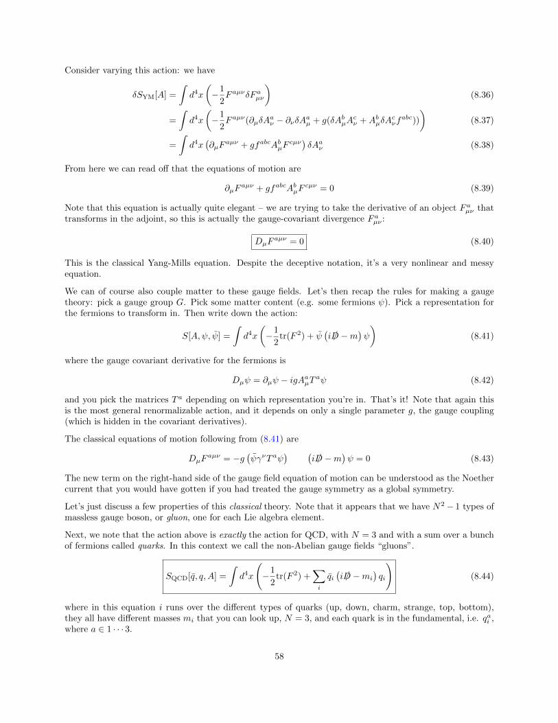
Consider varying this action: we have
δSYM[A] =
∫d4x
(−1
2F aµνδF aµν
)(8.36)
=
∫d4x
(−1
2F aµν(∂µδA
aν − ∂νδAaµ + g(δAbµA
cν +AbµδA
cνf
abc))
)(8.37)
=
∫d4x
(∂µF
aµν + gfabcAbµFcµν)δAaν (8.38)
From here we can read off that the equations of motion are
∂µFaµν + gfabcAbµF
cµν = 0 (8.39)
Note that this equation is actually quite elegant – we are trying to take the derivative of an object F aµν thattransforms in the adjoint, so this is actually the gauge-covariant divergence F aµν :
DµFaµν = 0 (8.40)
This is the classical Yang-Mills equation. Despite the deceptive notation, it’s a very nonlinear and messyequation.
We can of course also couple matter to these gauge fields. Let’s then recap the rules for making a gaugetheory: pick a gauge group G. Pick some matter content (e.g. some fermions ψ). Pick a representation forthe fermions to transform in. Then write down the action:
S[A,ψ, ψ] =
∫d4x
(−1
2tr(F 2) + ψ
(i /D −m
)ψ
)(8.41)
where the gauge covariant derivative for the fermions is
Dµψ = ∂µψ − igAaµT aψ (8.42)
and you pick the matrices T a depending on which representation you’re in. That’s it! Note that again thisis the most general renormalizable action, and it depends on only a single parameter g, the gauge coupling(which is hidden in the covariant derivatives).
The classical equations of motion following from (8.41) are
DµFaµν = −g
(ψγνT aψ
) (i /D −m
)ψ = 0 (8.43)
The new term on the right-hand side of the gauge field equation of motion can be understood as the Noethercurrent that you would have gotten if you had treated the gauge symmetry as a global symmetry.
Let’s just discuss a few properties of this classical theory. Note that it appears that we have N2 − 1 types ofmassless gauge boson, or gluon, one for each Lie algebra element.
Next, we note that the action above is exactly the action for QCD, with N = 3 and with a sum over a bunchof fermions called quarks. In this context we call the non-Abelian gauge fields “gluons”.
SQCD[q, q, A] =
∫d4x
(−1
2tr(F 2) +
∑i
qi(i /D −mi
)qi
)(8.44)
where in this equation i runs over the different types of quarks (up, down, charm, strange, top, bottom),they all have different masses mi that you can look up, N = 3, and each quark is in the fundamental, i.e. qai ,where a ∈ 1 · · · 3.
58

Finally, let us study some simple solutions to the Yang-Mills equation. As the quarks are in the fundamentalthey come in 3 types called color: pick a direction in this SU(3) space and call it red. Now imagine (classically)getting one of the quarks to sit still at a point x. In that case the time-component of the current on theright-hand side of (8.43) is a delta function, and to lowest order in g, we find something that looks like
DµFaµt = g(ta)11δ
(3)(~x) (8.45)
The right-hand side is proportional to a particular component of the representation matrix. There are allkinds on non-linear terms on the LHS proportional to gfabcA2, but you can show that they do not contributeand you end up with just getting a Maxwell-type equation, which should have an inverse-square solution:
∂µFaµt = g(ta)11δ
(3)(~x) F art ∼ 1
r2(8.46)
This suggests that a quark should make a color electric field that falls off as 1/r2.
Physically, however, this is completely incorrect. In real life the gluons are not massless, and it is impossibleto even find an isolated quark, let alone observe that it creates a color electric field that goes like 1/r2. Notethe difference with EM: there we get more or less the right answer in the full quantum theory from justlooking at the classical equations of motion. For QCD we get completely the wrong answer: apparently theclassical theory is a terrible approximation to the quantum theory.
8.3 Quantizing non-Abelian gauge theories
Thus motivated, we turn now to the quantum theory. We will temporarily throw out the quarks and workout the Feynman rules for pure Yang-Mills theory, i.e.
S[A] =
∫d4x
(−1
4F aµνF
aµν
)(8.47)
We turn back to a general gauge group G.
We first recall that since we have
F aµν =(∂µA
aν − ∂νAaµ
)+ gAbµA
cνf
abc (8.48)
this theory is no longer quadratic, and thus even before we add any matter it is already interacting. Again,the interaction structure is completely fixed by gauge-invariance. Expanding out the action we see that wehave
S[A] =
∫d4x
(−1
4
(∂µA
aν − ∂νAaµ + gAbµA
cνf
abc) (∂µA
aν − ∂νAaµ + gAdµA
eνf
ade))
(8.49)
Thus there will be an interaction vertex that couples three A’s and one that couples four of them.
We can work out the vertices through the usual techniques, which I will not go through in detail on the boardas it is just bookkeeping. Note that this the first example we have seen of an interaction term that involves aderivative of the field, and this means that the Feynman rule will explicitly involve the momentum in the lineconnected to the vertex. I encourage you to work through the details at home (see, in particular, Exercise 2from Week 4 for a simpler example with the same idea).
This structure is highly constrained – if you just wrote out the most general interaction there would be manyother possible terms. In particular, note that it all depends on a single parameter g.
Now that we have all the vertices worked out, we should perform manipulations similar to those that we didfor the Abelian case to derive the propagator for the gauge field. We will do precisely the same thing as wedid there: we will define a gauge-fixing function
Gaω(A) ≡ ∂µAaµ − ωa(x) (8.50)
59

Figure 19: Interaction vertices for non-Abelian gauge fields
60
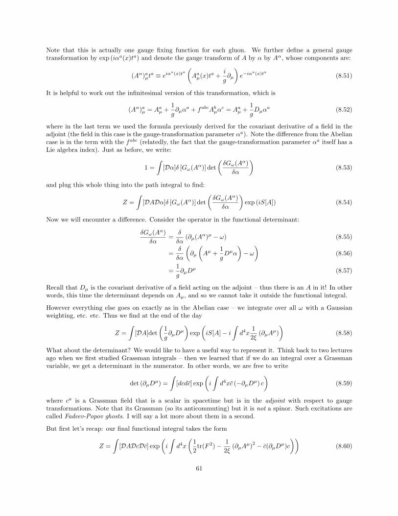
Note that this is actually one gauge fixing function for each gluon. We further define a general gaugetransformation by exp (iαa(x)ta) and denote the gauge transform of A by α by Aα, whose components are:
(Aα)aµta ≡ eiα
a(x)ta(Aaµ(x)ta +
i
g∂µ
)e−iα
a(x)ta (8.51)
It is helpful to work out the infinitesimal version of this transformation, which is
(Aα)aµ = Aaµ +1
g∂µα
a + fabcAbµαc = Aaµ +
1
gDµα
a (8.52)
where in the last term we used the formula previously derived for the covariant derivative of a field in theadjoint (the field in this case is the gauge-transformation parameter αa). Note the difference from the Abeliancase is in the term with the fabc (relatedly, the fact that the gauge-transformation parameter αa itself has aLie algebra index). Just as before, we write:
1 =
∫[Dα]δ [Gω(Aα)] det
(δGω(Aα)
δα
)(8.53)
and plug this whole thing into the path integral to find:
Z =
∫[DADα]δ [Gω(Aα)] det
(δGω(Aα)
δα
)exp (iS[A]) (8.54)
Now we will encounter a difference. Consider the operator in the functional determinant:
δGω(Aα)
δα=
δ
δα(∂µ(Aα)µ − ω) (8.55)
=δ
δα
(∂µ
(Aµ +
1
gDµα
)− ω
)(8.56)
=1
g∂µD
µ (8.57)
Recall that Dµ is the covariant derivative of a field acting on the adjoint – thus there is an A in it! In otherwords, this time the determinant depends on Aµ, and so we cannot take it outside the functional integral.
However everything else goes on exactly as in the Abelian case – we integrate over all ω with a Gaussianweighting, etc. etc. Thus we find at the end of the day
Z =
∫[DA]det
(1
g∂µD
µ
)exp
(iS[A]− i
∫d4x
1
2ξ(∂µA
µ)
)(8.58)
What about the determinant? We would like to have a useful way to represent it. Think back to two lecturesago when we first studied Grassman integrals – then we learned that if we do an integral over a Grassmanvariable, we get a determinant in the numerator. In other words, we are free to write
det (∂µDµ) =
∫[dcdc] exp
(i
∫d4xc (−∂µDµ) c
)(8.59)
where ca is a Grassman field that is a scalar in spacetime but is in the adjoint with respect to gaugetransformations. Note that its Grassman (so its anticommuting) but it is not a spinor. Such excitations arecalled Fadeev-Popov ghosts. I will say a lot more about them in a second.
But first let’s recap: our final functional integral takes the form
Z =
∫[DADcDc] exp
(i
∫d4x
(1
2tr(F 2)− 1
2ξ(∂µA
µ)2 − c(∂µDµ)c
))(8.60)
61
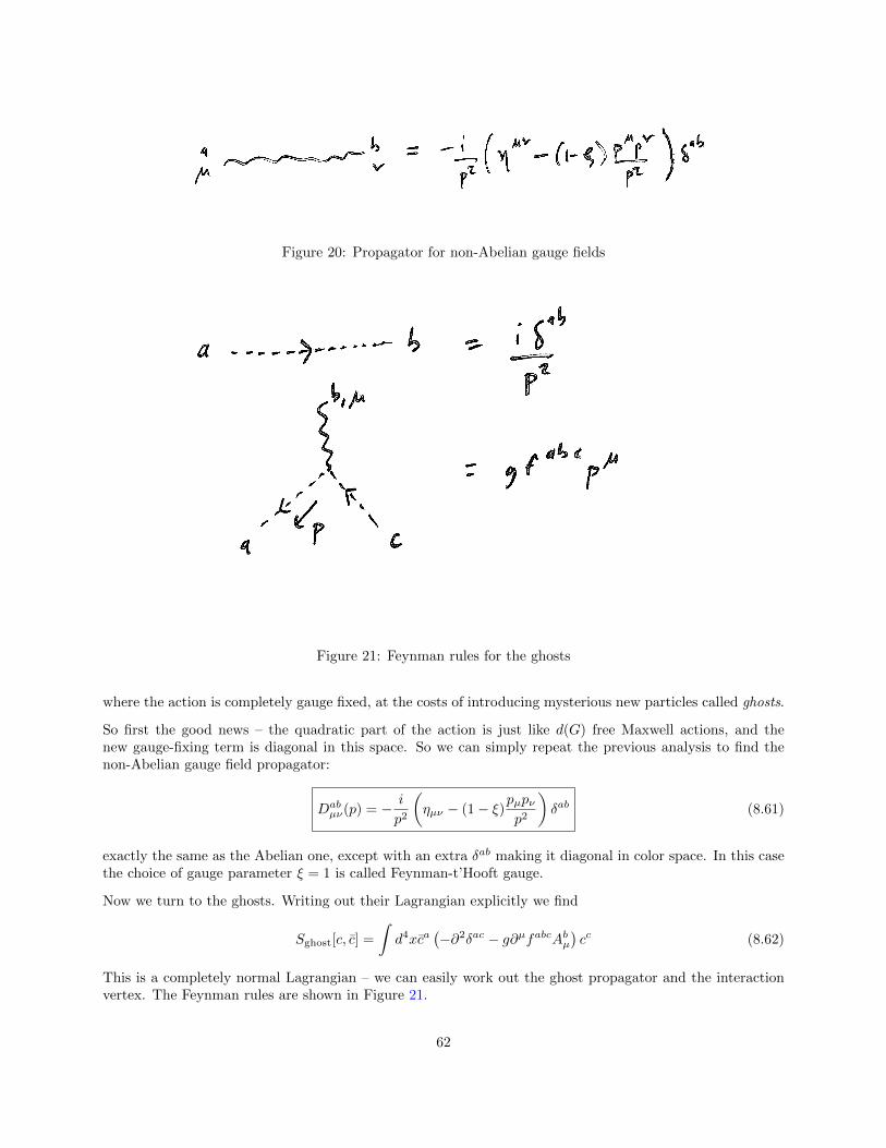
Figure 20: Propagator for non-Abelian gauge fields
Figure 21: Feynman rules for the ghosts
where the action is completely gauge fixed, at the costs of introducing mysterious new particles called ghosts.
So first the good news – the quadratic part of the action is just like d(G) free Maxwell actions, and thenew gauge-fixing term is diagonal in this space. So we can simply repeat the previous analysis to find thenon-Abelian gauge field propagator:
Dabµν(p) = − i
p2
(ηµν − (1− ξ)pµpν
p2
)δab (8.61)
exactly the same as the Abelian one, except with an extra δab making it diagonal in color space. In this casethe choice of gauge parameter ξ = 1 is called Feynman-t’Hooft gauge.
Now we turn to the ghosts. Writing out their Lagrangian explicitly we find
Sghost[c, c] =
∫d4xca
(−∂2δac − g∂µfabcAbµ
)cc (8.62)
This is a completely normal Lagrangian – we can easily work out the ghost propagator and the interactionvertex. The Feynman rules are shown in Figure 21.
62
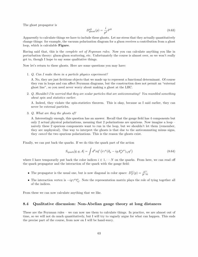
The ghost propagator is
Dabghost(p) =
i
p2δab (8.63)
Apparently to calculate things we have to include these ghosts. Let me stress that they actually quantitativelychange things: for example, the vacuum polarization diagram for a gluon receives a contribution from a ghostloop, which is calculable Figure.
Having said that, this is the complete set of Feynman rules. Now you can calculate anything you like inperturbation theory: gluon-gluon scattering, etc. Unfortunately the course is almost over, so we won’t reallyget to, though I hope to say some qualitative things.
Now let’s return to these ghosts. Here are some questions you may have:
1. Q. Can I make them in a particle physics experiment?
A. No, they are just fictitious objects that we made up to represent a functional determinant. Of coursethey run in loops and can affect Feynman diagrams, but the construction does not permit an “externalghost line”, so you need never worry about making a ghost at the LHC.
2. Q. Shouldn’t I be worried that they are scalar particles that are anticommuting? You mumbled somethingabout spin and statistics earlier.
A. Indeed, they violate the spin-statistics theorem. This is okay, because as I said earlier, they cannever be external particles.
3. Q. What are they the ghosts of?
A. Interestingly enough, this question has an answer. Recall that the gauge field has 4 components butonly 2 actual physical polarizations, meaning that 2 polarizations are spurious. Now imagine a loop –naively these 2 spurious components want to run in the loop, but we shouldn’t let them (remember,they are unphysical). One way to interpret the ghosts is that due to the anticommuting minus signs,they cancel the two spurious polarizations. This is the reason the ghosts exist.
Finally, we can put back the quarks. If we do this the quark part of the action
Squark[q, q, A] =
∫d4xqi
(iγµ(∂µ − igAaµta)ijq
j)
(8.64)
where I have temporarily put back the color indices i ∈ 1, · · ·N on the quarks. From here, we can read offthe quark propagator and the interaction of the quark with the gauge field:
• The propagator is the usual one, but is now diagonal in color space: DijF (p) = iδij
/p−m
• The interaction vertex is −igγµtaij . Note the representation matrix plays the role of tying together allof the indices.
From these we can now calculate anything that we like.
8.4 Qualitative discussion: Non-Abelian gauge theory at long distances
These are the Feynman rules – we can now use them to calculate things. In practice, we are almost out oftime, so we will not do much quantitatively, but I will try to vaguely argue for what can happen. This endsthe precise part of the course, from now on I will be hand-wavy.
63

Figure 22: Propagator for fermion transforming in fundamental
Let’s remember when we first calculated the one-loop correction to the amplitude for 2-2 scattering in λφ4
theory. We calculated the diagrams in Section 4 and found that at high energies the amplitude as a functionof s (and t,u). At large s� m it went like
iM = −iλ− i λ2
32π2
(log
(s
s0
)+ · · ·
)(8.65)
where s0 was a renormalization point and I’ve not written down the dependence on t and u (but it is similar).Now from staring at this, you can conclude that the interaction λ gets stronger at high energies, as increasings acts in the same direction as increasing λ. Also note this depends crucially on the sign of the prefactor ofthe one-loop term: if it had the other sign, then increasing s would have decreased the interaction strength.You can do a similar calculation in QED and arrive at a similar answer, QED also gets strongly interactingin the UV.
Now let’s imagine doing a similar calculation in non-Abelian gauge theory: the goal is to understand whetherit gets stronger or weaker as we go to high energies. We need to pick some interaction process: there are manydifferent processes that we could pick, they should all give the same result because they are all controlledby the same number g. So we pick the quark-quark-gluon coupling and calculate. We look at the diagrams.There is only one at tree level, but there are several at one loop.
So now we calculate them all (see Chapter 16.5 of Peskin), then we get a result that looks like (very veryschematically)
iM = −ig + ig3
(4π)2
(11
3N − 2
3nq
)(log
(E
E0
)+ · · ·
)(8.66)
where nq is the number of quark fields, and where E is the energy flowing into the vertex. I say this isschematic because I am being deliberately vague about what I mean by “energy flowing into the vertex”: it isclear that there are several different energies you could pick. So actually the correct way to parametrize thisenergy is to not do what I described, but to instead compute the beta function of the coupling g (again, tobe done in the course on renormalization). However this is gives you a reasonable idea of what is happening.
The crucial thing to note here is the sign! For a small enough number of quark fields nq, it looks like thisthing has the opposite sign as the φ4 theory, and so this means that the theory becomes weakly coupled – infact, a free theory – in the UV. This property is called asymptotic freedom: in the context of QCD, it wasfirst discovered by Gross, Politzer and Wilczek, for which they won the Nobel Prize in 2006. To appreciateits importance, we should think not in the UV, but in the IR – if the interaction is weak in the UV, then itseems to be getting stronger and stronger at low energies. So what happens?
There are a few possibilities – one thing that could happen is that the theory ends up getting Higgsed. Thishappens for the SU(2) × U(1) part of the Standard Model; you have studied this in that course, so I willdiscuss it no further here. I stress that you can often still understand that within perturbation theory – youjust expand around the new vacuum.
But let us assume this does not happen, and the interaction just gets stronger and stronger. Now you haveto take my work on what happens – from a renormalization group analysis it turns out that the strength of
64
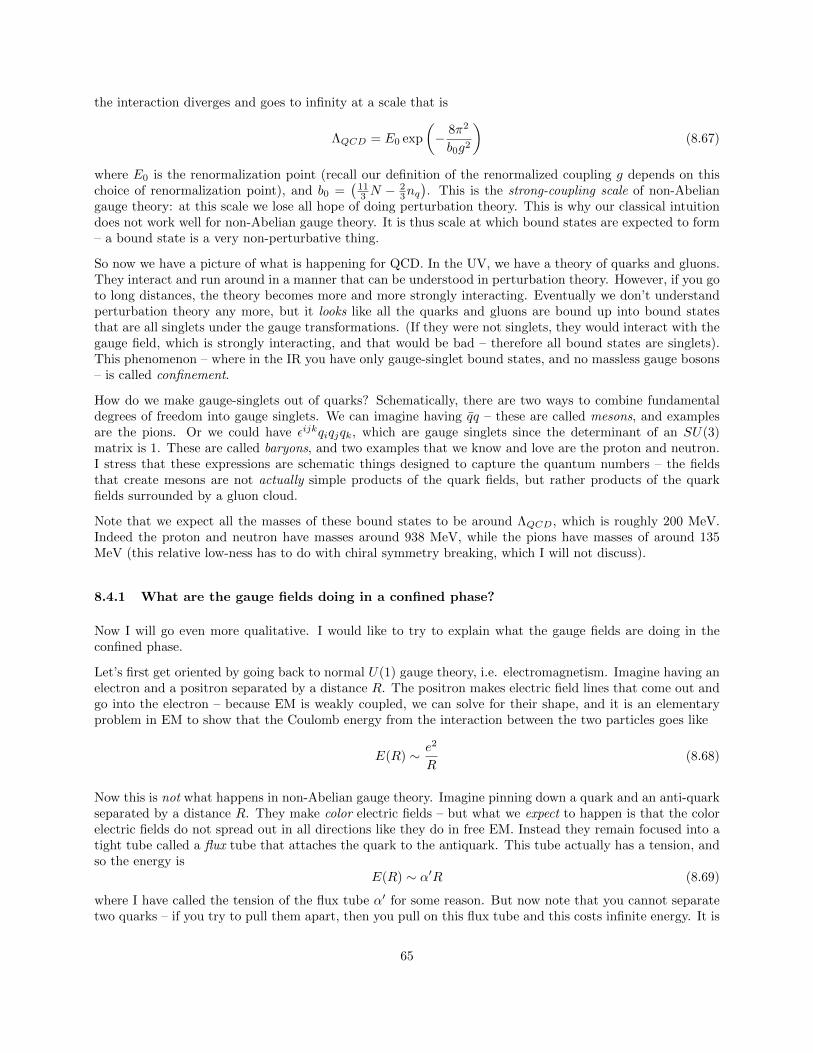
the interaction diverges and goes to infinity at a scale that is
ΛQCD = E0 exp
(− 8π2
b0g2
)(8.67)
where E0 is the renormalization point (recall our definition of the renormalized coupling g depends on thischoice of renormalization point), and b0 =
(113 N −
23nq). This is the strong-coupling scale of non-Abelian
gauge theory: at this scale we lose all hope of doing perturbation theory. This is why our classical intuitiondoes not work well for non-Abelian gauge theory. It is thus scale at which bound states are expected to form– a bound state is a very non-perturbative thing.
So now we have a picture of what is happening for QCD. In the UV, we have a theory of quarks and gluons.They interact and run around in a manner that can be understood in perturbation theory. However, if you goto long distances, the theory becomes more and more strongly interacting. Eventually we don’t understandperturbation theory any more, but it looks like all the quarks and gluons are bound up into bound statesthat are all singlets under the gauge transformations. (If they were not singlets, they would interact with thegauge field, which is strongly interacting, and that would be bad – therefore all bound states are singlets).This phenomenon – where in the IR you have only gauge-singlet bound states, and no massless gauge bosons– is called confinement.
How do we make gauge-singlets out of quarks? Schematically, there are two ways to combine fundamentaldegrees of freedom into gauge singlets. We can imagine having qq – these are called mesons, and examplesare the pions. Or we could have εijkqiqjqk, which are gauge singlets since the determinant of an SU(3)matrix is 1. These are called baryons, and two examples that we know and love are the proton and neutron.I stress that these expressions are schematic things designed to capture the quantum numbers – the fieldsthat create mesons are not actually simple products of the quark fields, but rather products of the quarkfields surrounded by a gluon cloud.
Note that we expect all the masses of these bound states to be around ΛQCD, which is roughly 200 MeV.Indeed the proton and neutron have masses around 938 MeV, while the pions have masses of around 135MeV (this relative low-ness has to do with chiral symmetry breaking, which I will not discuss).
8.4.1 What are the gauge fields doing in a confined phase?
Now I will go even more qualitative. I would like to try to explain what the gauge fields are doing in theconfined phase.
Let’s first get oriented by going back to normal U(1) gauge theory, i.e. electromagnetism. Imagine having anelectron and a positron separated by a distance R. The positron makes electric field lines that come out andgo into the electron – because EM is weakly coupled, we can solve for their shape, and it is an elementaryproblem in EM to show that the Coulomb energy from the interaction between the two particles goes like
E(R) ∼ e2
R(8.68)
Now this is not what happens in non-Abelian gauge theory. Imagine pinning down a quark and an anti-quarkseparated by a distance R. They make color electric fields – but what we expect to happen is that the colorelectric fields do not spread out in all directions like they do in free EM. Instead they remain focused into atight tube called a flux tube that attaches the quark to the antiquark. This tube actually has a tension, andso the energy is
E(R) ∼ α′R (8.69)
where I have called the tension of the flux tube α′ for some reason. But now note that you cannot separatetwo quarks – if you try to pull them apart, then you pull on this flux tube and this costs infinite energy. It is
65
like the two quarks are attached by a string. This is the idea of confinement. In this picture you can imaginethat a meson is a quark and an antiquark attached by a bit of string – the different vibrational modes of thebound state are the different mesons that exist in real life.
This is pretty much as far we we will go. There are a few things you could try to do now: one promising ideawas to try to take the flux tube as the starting point: in other words, try to build a theory out of quantizingthe dynamics of flux tubes. The problem with this approach is that it always resulted in a spin-2 masslessparticle, which is really annoying because if you look at the QCD spectrum there is no such particle.
Of course eventually it was realized that this theory of strings was really solving an entirely different problem,and this is how string theory as a theory of quantum gravity was discovered. This spin-2 particle is thegraviton.
References
[1] P. Mansfield, “QFT I Lecture Notes,”.
[2] M. E. Peskin and D. V. Schroeder, An Introduction to quantum field theory. Addison-Wesley, Reading,USA, 1995. http://www.slac.stanford.edu/~mpeskin/QFT.html.
[3] M. Srednicki, Quantum field theory. Cambridge University Press, 2007.
[4] A. Zee, Quantum field theory in a nutshell. 2003.
[5] J. F. Donoghue, “Introduction to the effective field theory description of gravity,” in Advanced Schoolon Effective Theories Almunecar, Spain, June 25-July 1, 1995. 1995. arXiv:gr-qc/9512024 [gr-qc].
66