Embed Size (px)
Citation preview
QFI QF Spring 2021 Solutions Page 1
QFI QF Model Solutions Spring 2021
1. Learning Objectives:
1. The candidate will understand the foundations of quantitative finance. Learning Outcomes: (1a) Understand and apply concepts of probability and statistics important in
mathematical finance. (1c) Understand Ito integral and stochastic differential equations. (1d) Understand and apply Ito’s Lemma. (1h) Define and apply the concepts of martingale, market price of risk and measures in
single and multiple state variable contexts. (1i) Demonstrate understanding of the differences and implications of real-world
versus risk-neutral probability measures, and when the use of each is appropriate. (1j) Understand and apply Girsanov’s theorem in changing measures. Sources: Problems and Solutions in Mathematical Finance: Stochastic Calculus, Chin, Eric, Nel, Dian and Olafsson, Sverrir, 2014 (pages 194-196, 203, 205, 218, 219, 221-224, 234) An Introduction to the Mathematics of Financial Derivatives, Hirsa, Ali and Neftci, Salih N., 3rd Edition 2nd Printing, 2014 (Ch. 10, 14) QFIQ-113-17 Frequently Asked Questions in Quantitative Finance, Wilmott, Paul, 2nd Edition, 2009, Ch. 2 Commentary on Question: The focus of this question is understanding the differences and implications of real-world versus risk-neutral probability measures by applying Ito’s lemma, Girsanov’s theorem, and the Radon-Nikodym (“R-N”) derivative. Candidates struggled to show this understanding, especially for parts (c) and (d). Detailed commentaries are listed underneath each part.

QFI QF Spring 2021 Solutions Page 2
1. Continued
Solution: (a) Determine the market price of risk for all
Commentary on Question: There is a typo in the question, where the “S” is missing in the process of dSt when 0 ≤ t ≤ 0.5. The correct process should be dSt = 0.05Stdt + 0.2StdWt. But most candidates identified the typo. Overall, most candidates were able to calculate the correct market price of risk. Credits were also given to the answers using the wrong process as stated in the question.
The market price of risk is defined as
𝜆𝜆𝑡𝑡 =𝜇𝜇𝑡𝑡 − 𝑟𝑟𝑡𝑡𝜎𝜎𝑡𝑡
where 𝜇𝜇𝑡𝑡 is the stock price drift rate, 𝑟𝑟𝑡𝑡 is the risk-free rate, and 𝜎𝜎𝑡𝑡 is the stock price volatility. By plugging in the numbers, we get
𝜆𝜆𝑡𝑡 =
0.05 − 0.010.2
= 0.2 𝑖𝑖𝑖𝑖 0 ≤ 𝑡𝑡 ≤ 0.5
−0.05 − 0.010.3
= −0.2 𝑖𝑖𝑖𝑖 0.5 < 𝑡𝑡 ≤ 1
(b) Calculate .
Commentary on Question:
For 0.5 < 𝑡𝑡 ≤ 1, we apply Ito’s lemma and get
𝑑𝑑𝑑𝑑𝑑𝑑𝑆𝑆𝑡𝑡 = 𝜇𝜇𝑡𝑡 − 𝜎𝜎𝑡𝑡2
2𝑑𝑑𝑡𝑡 + 𝜎𝜎𝑡𝑡𝑑𝑑𝑊𝑊𝑡𝑡 = −0.095 𝑑𝑑𝑡𝑡 + 0.3𝑑𝑑𝑊𝑊𝑡𝑡
which gives ln𝑆𝑆𝑡𝑡 − ln𝑆𝑆0.5 = −0.095(𝑡𝑡 − 0.5) + 0.3(𝑊𝑊𝑡𝑡 −𝑊𝑊0.5)
or 𝑆𝑆𝑡𝑡 = 𝑆𝑆0.5𝑒𝑒−0.095(𝑡𝑡−0.5)+0.3(𝑊𝑊𝑡𝑡−𝑊𝑊0.5)
Hence 𝐸𝐸𝑃𝑃[𝑆𝑆𝑡𝑡|𝑆𝑆0.5] = 𝑆𝑆0.5𝐸𝐸𝑃𝑃[𝑒𝑒−0.095(𝑡𝑡−0.5)+0.3(𝑊𝑊𝑡𝑡−𝑊𝑊0.5)] = 𝑆𝑆0.5𝑒𝑒−0.095(𝑡𝑡−0.5)+0.045(𝑡𝑡−0.5)
which leads to 𝐸𝐸𝑃𝑃[𝑆𝑆1|𝑆𝑆0.5] = 𝑆𝑆0.5𝑒𝑒−0.025.
1.t ≤
1 0.5E S S

QFI QF Spring 2021 Solutions Page 3
1. Continued (c) Derive the Radon-Nikodym derivative of the risk-neutral measure ℚ with respect
to the real-world measure ℙ.
Commentary on Question: Candidates performed poorly on this question. One source for this question (Chin et al) has many typos related to the Radon-Nikodym derivative. (page 222-223, 225, 239, 240). Whereas the other source - page 194-196, 203, 205, 218, 219 and 234 of (Chin el al) have the correct Radon-Nikodym derivatives. Credit was given to answers using the wrong R-N derivative as stated in the incorrect source. For candidates that provided a general form of the R-N derivative, a common mistake made was to use λt with the incorrect sign on the first integral component. Most candidates were not able to derive the correct derivative when 0.5 < 𝑡𝑡 ≤ 1.
Solution 1 – Based on the correct R-N derivative form from the source page 218. The Radon-Nikodym derivative is calculated as
𝑍𝑍𝑠𝑠 = 𝑒𝑒−∫ 𝜆𝜆𝑡𝑡𝑑𝑑𝑊𝑊𝑡𝑡−12∫ 𝜆𝜆𝑡𝑡2𝑑𝑑𝑡𝑡
𝑠𝑠0
𝑠𝑠0
where 𝜆𝜆𝑡𝑡 is the market price of risk as 𝜆𝜆𝑡𝑡 = 𝜇𝜇𝑡𝑡−𝑟𝑟𝑡𝑡
𝜎𝜎𝑡𝑡, we get
𝜆𝜆𝑡𝑡 = 0.2 , 0 ≤ 𝑡𝑡 ≤ 0.5−0.2, 0.5 < 𝑡𝑡 ≤ 1
Plugging in the numbers, we get
𝜆𝜆𝑡𝑡𝑑𝑑𝑊𝑊𝑡𝑡
𝑠𝑠
0=
0.2𝑊𝑊𝑠𝑠 𝑖𝑖𝑖𝑖 0 ≤ 𝑠𝑠 ≤ 0.5−0.2(𝑊𝑊𝑠𝑠 − 2𝑊𝑊0.5) 𝑖𝑖𝑖𝑖 0.5 < 𝑠𝑠 ≤ 1
and
𝜆𝜆𝑡𝑡2𝑑𝑑𝑡𝑡𝑠𝑠
0= 0.04𝑠𝑠
Hence
𝑍𝑍𝑠𝑠 = 𝑒𝑒−0.2𝑊𝑊𝑠𝑠−0.02𝑠𝑠 𝑖𝑖𝑖𝑖 0 ≤ 𝑠𝑠 ≤ 0.5
𝑒𝑒0.2(𝑊𝑊𝑠𝑠−2𝑊𝑊0.5)−0.02𝑠𝑠 𝑖𝑖𝑖𝑖 0.5 < 𝑠𝑠 ≤ 1.
Or The Radon-Nikodym derivative is calculated as (using notation in Neftci)
𝑍𝑍𝑠𝑠 = 𝑒𝑒∫ 𝑋𝑋𝑡𝑡𝑑𝑑𝑊𝑊𝑡𝑡−12∫ 𝑋𝑋𝑡𝑡2𝑑𝑑𝑡𝑡
𝑠𝑠0
𝑠𝑠0
where 𝑋𝑋𝑡𝑡 = −𝜆𝜆𝑡𝑡 = 𝑟𝑟𝑡𝑡−𝜇𝜇𝑡𝑡
𝜎𝜎𝑡𝑡, we get
𝑋𝑋𝑡𝑡 = −0.2, 0 ≤ 𝑡𝑡 ≤ 0.50.2, 0.5 < 𝑡𝑡 ≤ 1

QFI QF Spring 2021 Solutions Page 4
1. Continued Plugging in the numbers, we get
𝑋𝑋𝑡𝑡𝑑𝑑𝑊𝑊𝑡𝑡
𝑠𝑠
0=
−0.2𝑊𝑊𝑠𝑠 𝑖𝑖𝑖𝑖 0 ≤ 𝑠𝑠 ≤ 0.50.2(𝑊𝑊𝑠𝑠 − 2𝑊𝑊0.5) 𝑖𝑖𝑖𝑖 0.5 < 𝑠𝑠 ≤ 1
and
𝑋𝑋𝑡𝑡2𝑑𝑑𝑊𝑊𝑡𝑡
𝑠𝑠
0= 0.04𝑠𝑠
Hence
𝑍𝑍𝑠𝑠 = 𝑒𝑒−0.2𝑊𝑊𝑠𝑠−0.02𝑠𝑠 𝑖𝑖𝑖𝑖 0 ≤ 𝑠𝑠 ≤ 0.5
𝑒𝑒0.2(𝑊𝑊𝑠𝑠−2𝑊𝑊0.5)−0.02𝑠𝑠 𝑖𝑖𝑖𝑖 0.5 < 𝑠𝑠 ≤ 1
Solution that will not get credit for future sittings – Based on the wrong R-N
derivative from page 223 of Chin et al, where 𝑑𝑑𝑊𝑊𝑡𝑡 and 𝑑𝑑𝑡𝑡 were swapped. The errors will be published in the ERRATA list before the next sitting.
The Radon-Nikodym derivative is calculated as
𝑍𝑍𝑠𝑠 = 𝑒𝑒−∫ 𝜆𝜆𝑡𝑡𝑑𝑑𝑡𝑡−12∫ 𝜆𝜆𝑡𝑡2𝑑𝑑𝑊𝑊𝑡𝑡
𝑠𝑠0
𝑠𝑠0
where 𝜆𝜆𝑡𝑡 is the market price of risk. Plugging in the numbers, we get
𝜆𝜆𝑡𝑡𝑑𝑑𝑡𝑡𝑠𝑠
0=
0.2𝑠𝑠 𝑖𝑖𝑖𝑖 0 ≤ 𝑠𝑠 ≤ 0.50.2(1 − 𝑠𝑠) 𝑖𝑖𝑖𝑖 0.5 < 𝑠𝑠 ≤ 1
and
𝜆𝜆𝑡𝑡2𝑑𝑑𝑊𝑊𝑡𝑡
𝑠𝑠
0= 0.04𝑊𝑊𝑠𝑠
Hence
𝑍𝑍𝑠𝑠 = 𝑒𝑒−0.2𝑠𝑠−0.02𝑊𝑊𝑠𝑠 𝑖𝑖𝑖𝑖 0 ≤ 𝑠𝑠 ≤ 0.5
𝑒𝑒−0.2(1−𝑠𝑠)−0.02𝑊𝑊𝑠𝑠 𝑖𝑖𝑖𝑖 0.5 < 𝑠𝑠 ≤ 1
(d) Show that is a ℚ-martingale.
Commentary on Question: Candidates had the most difficulty with this part. Many were able to prove the no drift condition, but failed to mention Girsanov’s theorem or the R-N derivative as justification for the substitution of a different standard Wiener process under an equivalent measure. A complete response should demonstrate and justify the relationship between the two Wiener processes.
For ease of presentation, we use 𝑟𝑟𝑡𝑡, 𝜇𝜇𝑡𝑡, and 𝜎𝜎𝑡𝑡 to denote the risk-free rate, the drift rate of the stock price, and the volatility of the stock price. Let 𝑌𝑌𝑡𝑡 = 𝑆𝑆𝑡𝑡𝑒𝑒−∫ 𝑟𝑟𝑢𝑢𝑑𝑑𝑑𝑑
𝑡𝑡0 .
0.01 : 0 1ttS e t− ≤ ≤
QFI QF Spring 2021 Solutions Page 5
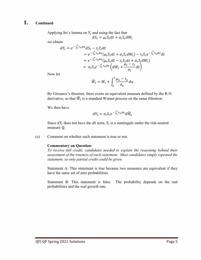
1. Continued Applying Ito’s lemma on 𝑌𝑌𝑡𝑡 and using the fact that
𝑑𝑑𝑆𝑆𝑡𝑡 = 𝜇𝜇𝑡𝑡𝑆𝑆𝑡𝑡𝑑𝑑𝑡𝑡 + 𝜎𝜎𝑡𝑡𝑆𝑆𝑡𝑡𝑑𝑑𝑊𝑊𝑡𝑡 we obtain
𝑑𝑑𝑌𝑌𝑡𝑡 = 𝑒𝑒−∫ 𝑟𝑟𝑢𝑢𝑑𝑑𝑑𝑑𝑡𝑡0 𝑑𝑑𝑆𝑆𝑡𝑡 − 𝑟𝑟𝑡𝑡𝑌𝑌𝑡𝑡𝑑𝑑𝑡𝑡
= 𝑒𝑒−∫ 𝑟𝑟𝑢𝑢𝑑𝑑𝑑𝑑𝑡𝑡0 (𝜇𝜇𝑡𝑡𝑆𝑆𝑡𝑡𝑑𝑑𝑡𝑡 + 𝜎𝜎𝑡𝑡𝑆𝑆𝑡𝑡𝑑𝑑𝑊𝑊𝑡𝑡) − 𝑟𝑟𝑡𝑡𝑆𝑆𝑡𝑡𝑒𝑒−∫ 𝑟𝑟𝑢𝑢𝑑𝑑𝑑𝑑
𝑡𝑡0 𝑑𝑑𝑡𝑡
= 𝑒𝑒−∫ 𝑟𝑟𝑢𝑢𝑑𝑑𝑑𝑑𝑡𝑡0 (𝜇𝜇𝑡𝑡𝑆𝑆𝑡𝑡𝑑𝑑𝑡𝑡 − 𝑟𝑟𝑡𝑡𝑆𝑆𝑡𝑡𝑑𝑑𝑡𝑡 + 𝜎𝜎𝑡𝑡𝑆𝑆𝑡𝑡𝑑𝑑𝑊𝑊𝑡𝑡)
= 𝜎𝜎𝑡𝑡𝑆𝑆𝑡𝑡𝑒𝑒−∫ 𝑟𝑟𝑢𝑢𝑑𝑑𝑑𝑑𝑡𝑡0 𝑑𝑑𝑊𝑊𝑡𝑡 +
𝜇𝜇𝑡𝑡 − 𝑟𝑟𝑡𝑡𝜎𝜎𝑡𝑡
𝑑𝑑𝑡𝑡
Now let
𝑊𝑊𝑡𝑡 = 𝑊𝑊𝑡𝑡 + 𝜇𝜇𝑑𝑑 − 𝑟𝑟𝑑𝑑𝜎𝜎𝑑𝑑
𝑡𝑡
0𝑑𝑑𝑑𝑑
By Girsanov’s theorem, there exists an equivalent measure defined by the R-N derivative, so that 𝑊𝑊𝑡𝑡 is a standard Wiener process on the same filtration. We then have
𝑑𝑑𝑌𝑌𝑡𝑡 = 𝜎𝜎𝑡𝑡𝑆𝑆𝑡𝑡𝑒𝑒−∫ 𝑟𝑟𝑢𝑢𝑑𝑑𝑑𝑑𝑡𝑡0 𝑑𝑑𝑊𝑊𝑑𝑑
Since 𝑑𝑑𝑌𝑌𝑡𝑡 does not have the 𝑑𝑑𝑡𝑡 term, 𝑌𝑌𝑡𝑡 is a martingale under the risk-neutral measure ℚ.
(e) Comment on whether each statement is true or not.
Commentary on Question: To receive full credit, candidates needed to explain the reasoning behind their assessment of the trueness of each statement. Most candidates simply repeated the statement, so only partial credit could be given.
Statement A: This statement is true because two measures are equivalent if they have the same set of zero probabilities. Statement B: This statement is false. The probability depends on the real probabilities and the real growth rate.

QFI QF Spring 2021 Solutions Page 6
2. Learning Objectives: 1. The candidate will understand the foundations of quantitative finance. Learning Outcomes: (1a) Understand and apply concepts of probability and statistics important in
mathematical finance. (1f) Understand and apply Jensen’s Inequality. (1h) Define and apply the concepts of martingale, market price of risk and measures in
single and multiple state variable contexts. Sources: Problems and Solutions in Mathematical Finance, Chin An introduction to Mathematics of Financial Derivatives, Nefci QFIQ-113-17 Commentary on Question: Only a few candidates get full marks on this question. For part (b), some candidates failed to work out the integral. For part (c), only a few candidates correctly stated the triangle-inequality. Most of candidates were able to get part (d) Solution: (a) List the criteria for the stochastic process tV to be a sub-martingale with respect to
( ), ,Ω .
Commentary on Question: Quite a few candidates misstated the 1st criteria with the incorrect filtration. The three criteria for 0 ≤ 𝑠𝑠 ≤ 𝑡𝑡 ≤ 𝑇𝑇 are: 𝐸𝐸ℙ(𝑉𝑉𝑡𝑡|ℱ𝑠𝑠) ≥ 𝑉𝑉𝑠𝑠; The inequality holds almost surely. 𝐸𝐸ℙ[|𝑉𝑉𝑡𝑡|] < ∞; And the 3rd criterion is that 𝑉𝑉𝑡𝑡 is ℱ𝑡𝑡-measurable
(b) Evaluate tVar W .
Commentary on Question: Most candidates failed to work out the integrals.
𝐸𝐸ℙ[|𝑊𝑊𝑡𝑡|] = ∫ |𝑤𝑤| 1√2𝜋𝜋𝑡𝑡
𝑒𝑒−𝑤𝑤2
2𝑡𝑡 𝑑𝑑𝑤𝑤∞−∞
𝐸𝐸ℙ[|𝑊𝑊𝑡𝑡|]= 2∫ |𝑤𝑤| 1√2𝜋𝜋𝑡𝑡
𝑒𝑒−𝑤𝑤2
2𝑡𝑡 𝑑𝑑𝑤𝑤∞0

QFI QF Spring 2021 Solutions Page 7
2. Continued
𝐸𝐸ℙ[|𝑊𝑊𝑡𝑡|] = −2𝑑𝑑𝑑𝑑𝑤𝑤
√𝑡𝑡√2𝜋𝜋
𝑒𝑒−𝑤𝑤2
2𝑡𝑡 𝑑𝑑𝑤𝑤 = 2√𝑡𝑡√2𝜋𝜋
=∞
0
2𝑡𝑡𝜋𝜋
𝑉𝑉𝑉𝑉𝑟𝑟ℙ[|𝑊𝑊𝑡𝑡|] = 𝐸𝐸ℙ[|𝑊𝑊𝑡𝑡|2] − 𝐸𝐸ℙ[|𝑊𝑊𝑡𝑡|]2 (definition of variance) 𝑉𝑉𝑉𝑉𝑟𝑟ℙ[|𝑊𝑊𝑡𝑡|] = 𝐸𝐸ℙ[𝑊𝑊𝑡𝑡
2] − 𝐸𝐸ℙ[|𝑊𝑊𝑡𝑡|]2 (𝑉𝑉𝑠𝑠 𝐸𝐸ℙ[|𝑊𝑊𝑡𝑡|2] = 𝐸𝐸ℙ[𝑊𝑊𝑡𝑡2])
𝑉𝑉𝑉𝑉𝑟𝑟ℙ[|𝑊𝑊𝑡𝑡|] = t – 2t/ 𝜋𝜋 (c) Prove that tW is a non-negative sub-martingale.
Commentary on Question: Not many candidates are able show the convexity using the triangle-inequality. Using part (a), we will demonstrate each of the 3 criteria: |𝑊𝑊𝑡𝑡| is clearly ℱ𝑡𝑡-measurable
From part (b), we have 𝐸𝐸ℙ|𝑊𝑊𝑡𝑡| = 𝐸𝐸ℙ[|𝑊𝑊𝑡𝑡|] = 2𝑡𝑡𝜋𝜋
< ∞
In order to use conditional jensen’s inequality, we need to establish that 𝜓𝜓() = abs() is a convex function on ℝ. Let 𝜃𝜃 ∈ [0,1] 𝑉𝑉𝑑𝑑𝑑𝑑 𝑥𝑥,𝑦𝑦 ∈ ℝ Using the triangle-inequality, |𝜃𝜃𝑥𝑥 + (1 − 𝜃𝜃)𝑦𝑦| ≤ |𝜃𝜃𝑥𝑥| + |(1 − 𝜃𝜃)𝑦𝑦| = 𝜃𝜃|𝑥𝑥| + (1 − 𝜃𝜃)|𝑦𝑦| Hence, we have shown abs() is convex Applying the conditional Jensen inequality, 𝐸𝐸ℙ(|𝑊𝑊𝑡𝑡||ℱ𝑠𝑠) ≥ 𝐸𝐸ℙ(𝑊𝑊𝑡𝑡|ℱ𝑠𝑠) = |𝑊𝑊𝑠𝑠|, since 𝑊𝑊𝑡𝑡 is a martingale Hence |𝑊𝑊𝑡𝑡| is a sub-martingale. It is non-negative as |𝑊𝑊𝑡𝑡| ⊆ ℝ+
(d) Determine integer k that makes k
tW a martingale.
Commentary on Question: Most of the candidates got this part right. Some did not provide the k = 0 solution.
By Ito’s Lemma, 𝑑𝑑𝑊𝑊𝑡𝑡
𝑘𝑘 = 𝑘𝑘𝑊𝑊𝑡𝑡𝑘𝑘−1𝑑𝑑𝑊𝑊𝑡𝑡 + 1
2𝑘𝑘(𝑘𝑘 − 1)𝑊𝑊𝑡𝑡
𝑘𝑘−2(𝑑𝑑𝑊𝑊𝑡𝑡)2
= 𝑘𝑘𝑊𝑊𝑡𝑡𝑘𝑘−1𝑑𝑑𝑊𝑊𝑡𝑡 +
12𝑘𝑘(𝑘𝑘 − 1)𝑊𝑊𝑡𝑡
𝑘𝑘−2𝑑𝑑𝑡𝑡 We need drift term to be zero to make the process a martingale. When k=0 or 1, the drift term=0. So if k=0, 1, then the process is a martingale.

QFI QF Spring 2021 Solutions Page 8
3. Learning Objectives: 1. The candidate will understand the foundations of quantitative finance. Learning Outcomes: (1c) Understand Ito integral and stochastic differential equations. (1d) Understand and apply Ito’s Lemma. (1h) Define and apply the concepts of martingale, market price of risk and measures in
single and multiple state variable contexts. Sources: An Introduction to the Mathematics of Financial Derivatives, Hirsa, Ali and Neftci, Salih N., 3rd Edition 2nd Printing, 2014, Chapters 6, 8, 9 Commentary on Question: This question tests candidates’ knowledge of Ito’s lemma, Ito’s isometry, martingales, and basic properties of Brownian Motion. Most candidates did well on this question. Some candidates did not state what rules and formulas they were applying to from step to step. Solution: (a) Derive 3
s tE W W for .t s>
Commentary on Question: Most candidates did well on this part. The few candidates who did badly tried to decompose the wrong term and failed to state the independence of 𝑊𝑊𝑠𝑠
3and 𝑊𝑊𝑡𝑡 −𝑊𝑊𝑠𝑠.
By the properties of Brownian motion, we have 𝐸𝐸[𝑊𝑊𝑠𝑠
3𝑊𝑊𝑡𝑡] = 𝐸𝐸[𝑊𝑊𝑠𝑠
3(𝑊𝑊𝑠𝑠 + 𝑊𝑊𝑡𝑡 −𝑊𝑊𝑠𝑠)] = 𝐸𝐸[𝑊𝑊𝑠𝑠
4] + 𝐸𝐸[𝑊𝑊𝑠𝑠3(𝑊𝑊𝑡𝑡 −𝑊𝑊𝑠𝑠)]
= 𝐸𝐸[𝑊𝑊𝑠𝑠4] + 𝐸𝐸[𝑊𝑊𝑠𝑠
3]𝐸𝐸[(𝑊𝑊𝑡𝑡 −𝑊𝑊𝑠𝑠)] = 𝐸𝐸[𝑊𝑊𝑠𝑠
4] Let 𝑍𝑍 = 𝑊𝑊𝑠𝑠
√𝑠𝑠, which is a standard normal distribution. Then 𝐸𝐸[𝑍𝑍4] = 3.
This gives 𝐸𝐸[𝑊𝑊𝑠𝑠
4] = 𝑠𝑠2𝐸𝐸[𝑍𝑍4] = 3𝑠𝑠2
(b) Determine the value of c such that 3t tW ctW− is a martingale.
Commentary on Question: Most candidates did well on this part. Some candidates pursued the alternate solution of using Ito’s lemma and setting the drift term to 0.

QFI QF Spring 2021 Solutions Page 9
3. Continued
Let 𝑀𝑀𝑡𝑡 = 𝑊𝑊𝑡𝑡3 − 𝑐𝑐𝑡𝑡𝑊𝑊𝑡𝑡. Then we have
𝐸𝐸[𝑀𝑀𝑡𝑡|𝐹𝐹𝑠𝑠] = 𝐸𝐸[(𝑊𝑊𝑠𝑠 +𝑊𝑊𝑡𝑡 −𝑊𝑊𝑠𝑠)3|𝐹𝐹𝑠𝑠] − 𝑐𝑐𝑡𝑡𝐸𝐸[𝑊𝑊𝑡𝑡|𝐹𝐹𝑠𝑠] = 𝐸𝐸[𝑊𝑊𝑠𝑠
3|𝐹𝐹𝑠𝑠] + 3𝐸𝐸[𝑊𝑊𝑠𝑠2(𝑊𝑊𝑡𝑡 −𝑊𝑊𝑠𝑠)|𝐹𝐹𝑠𝑠] + 3𝐸𝐸[𝑊𝑊𝑠𝑠(𝑊𝑊𝑡𝑡 −𝑊𝑊𝑠𝑠)2|𝐹𝐹𝑠𝑠] + 𝐸𝐸[(𝑊𝑊𝑡𝑡 −𝑊𝑊𝑠𝑠)3|𝐹𝐹𝑠𝑠] −
𝑐𝑐𝑡𝑡𝐸𝐸[𝑊𝑊𝑠𝑠|𝐹𝐹𝑠𝑠] − 𝑐𝑐𝑡𝑡𝐸𝐸[𝑊𝑊𝑡𝑡 −𝑊𝑊𝑠𝑠|𝐹𝐹𝑠𝑠] = 𝑊𝑊𝑠𝑠
3 + 0 + 3𝑊𝑊𝑠𝑠(𝑡𝑡 − 𝑠𝑠) + 0 − 𝑐𝑐𝑡𝑡𝑊𝑊𝑠𝑠 + 0 = 𝑀𝑀𝑠𝑠 if c = 3 (c) Show that
0
t
t uX W du= ∫ is not a martingale.
Commentary on Question: Most candidates did well on this part. However, some candidates mistook the integral ∫ 𝑊𝑊𝑑𝑑𝑑𝑑𝑑𝑑
𝑡𝑡0 for ∫ 𝑊𝑊𝑑𝑑 𝑑𝑑𝑊𝑊𝑑𝑑
𝑡𝑡0 and said it is a martingale. Some candidates
failed to apply stochastic integrals clearly and effectively to show that 𝑋𝑋𝑡𝑡 is not a martingale.
By Product Rule, we have
𝑋𝑋𝑡𝑡 = 𝑡𝑡𝑊𝑊𝑡𝑡 − 𝑑𝑑 𝑑𝑑𝑊𝑊𝑑𝑑
𝑡𝑡
0
Let 𝑠𝑠 ≤ 𝑡𝑡. Since the Ito integral is a martingale, we have
𝐸𝐸[𝑋𝑋𝑡𝑡|𝐹𝐹𝑠𝑠] = 𝐸𝐸[𝑡𝑡𝑊𝑊𝑡𝑡|𝐹𝐹𝑠𝑠] − 𝐸𝐸 𝑑𝑑𝑑𝑑𝑡𝑡
0𝑊𝑊𝑑𝑑|𝐹𝐹𝑠𝑠 = 𝑡𝑡𝑊𝑊𝑠𝑠 − 𝑑𝑑𝑑𝑑
𝑠𝑠
0𝑊𝑊𝑑𝑑 = 𝑋𝑋𝑠𝑠 + (𝑡𝑡 − 𝑠𝑠)𝑊𝑊𝑠𝑠 ≠ 𝑋𝑋𝑠𝑠
for t>s. Hence 𝑋𝑋𝑡𝑡 is not a martingale. (d) Calculate
(i) 2[ ]E V (ii) [ ]E VY
Commentary on Question: Most candidates did well on this part. Some candidates lost points for not mentioning Ito’s Isometry in part (i) or not stating the independence of V and G in part (ii).
By Ito’s isometry (i) 𝐸𝐸[𝑉𝑉2] = ∫ 𝑒𝑒−2𝑠𝑠𝑑𝑑𝑠𝑠 = 1
2(1 − 𝑒𝑒−2)1
0

QFI QF Spring 2021 Solutions Page 10
3. Continued (ii) Let G = ∫ 𝑒𝑒−𝑠𝑠𝑑𝑑𝑊𝑊𝑠𝑠
21
Y = V +G 𝐸𝐸[𝑉𝑉𝑌𝑌] = 𝐸𝐸[𝑉𝑉(𝑉𝑉 + 𝐺𝐺)] Since V and G are independent, = 𝐸𝐸[𝑉𝑉2] + 𝐸𝐸[𝑉𝑉𝐺𝐺] = 𝐸𝐸[𝑉𝑉2] + 𝐸𝐸[𝑉𝑉]𝐸𝐸[𝐺𝐺] = 𝐸𝐸[𝑉𝑉2] = 1
2(1 − 𝑒𝑒−2)

QFI QF Spring 2021 Solutions Page 11
4. Learning Objectives: 1. The candidate will understand the foundations of quantitative finance. Learning Outcomes: (1a) Understand and apply concepts of probability and statistics important in
mathematical finance. (1d) Understand and apply Ito’s Lemma. (1i) Demonstrate understanding of the differences and implications of real-world
versus risk-neutral probability measures, and when the use of each is appropriate. Sources: An Introduction to the Mathematics of Financial Derivatives, Hirsa, Ali and Neftci, Salih N., 3rd Edition 2nd Printing, 2014, Ch. 9, 10, 11, 15 Commentary on Question: The objective in this question was to test Ito’s Lemma as applied to the valuation of derivatives on a security that is driven by a Weiner Process. Most candidates performed above average and partial credit was given for answers with calculation errors or missing steps. Solution: (a) Show, using Ito’s lemma, that 𝜎𝜎 = 0.3.
Commentary on Question: Candidates performed well on this question. An alternative solution was also accepted.
Let 𝑉𝑉 = 𝑆𝑆𝑐𝑐. Find the partial derivatives: • 𝜕𝜕𝜕𝜕
𝜕𝜕𝜕𝜕= (𝑆𝑆)𝑐𝑐−1𝑐𝑐 = 𝑉𝑉𝑆𝑆−1𝑐𝑐
• 𝜕𝜕2𝜕𝜕𝜕𝜕𝜕𝜕2
= (𝑆𝑆)𝑐𝑐−2𝑐𝑐(𝑐𝑐 − 1) = 𝑉𝑉𝑆𝑆−2𝑐𝑐(𝑐𝑐 − 1)
• 𝜕𝜕𝜕𝜕𝜕𝜕𝑡𝑡
= 0

QFI QF Spring 2021 Solutions Page 12
4. Continued Apply Ito’s Lemma:
𝑑𝑑𝑉𝑉 =𝜕𝜕𝑉𝑉𝜕𝜕𝑆𝑆
(𝑑𝑑𝑆𝑆) +12𝜕𝜕2𝑉𝑉𝜕𝜕𝑆𝑆2
(𝑑𝑑𝑆𝑆)2 +𝜕𝜕𝑉𝑉𝜕𝜕𝑡𝑡
(𝑑𝑑𝑡𝑡)
= (𝑉𝑉𝑆𝑆−1𝑐𝑐)(0.045 𝑆𝑆 𝑑𝑑𝑡𝑡 + 𝜎𝜎𝑆𝑆𝑑𝑑𝑊𝑊𝑡𝑡) +12𝑉𝑉𝑆𝑆−2𝑐𝑐(𝑐𝑐 − 1)(𝜎𝜎𝑆𝑆 𝑑𝑑𝑊𝑊𝑡𝑡)2 + 0
= (𝑉𝑉𝑐𝑐)(0.045 𝑑𝑑𝑡𝑡 + 𝜎𝜎 𝑑𝑑𝑊𝑊𝑡𝑡) +12𝑉𝑉𝑐𝑐(𝑐𝑐 − 1)(𝜎𝜎2 𝑑𝑑𝑡𝑡)
= 𝑉𝑉 0.045𝑐𝑐 +12𝑐𝑐(𝑐𝑐 − 1)𝜎𝜎2 𝑑𝑑𝑡𝑡 + 𝑉𝑉𝑐𝑐𝜎𝜎𝑑𝑑𝑊𝑊𝑡𝑡
𝑑𝑑𝑉𝑉𝑉𝑉
= 0.045 𝑐𝑐 +12𝑐𝑐(𝑐𝑐 − 1)𝜎𝜎2 𝑑𝑑𝑡𝑡 + 𝑐𝑐𝜎𝜎 𝑑𝑑𝑊𝑊𝑡𝑡
𝑑𝑑𝑆𝑆𝑐𝑐
𝑆𝑆𝑐𝑐= 0.045 𝑐𝑐 +
12𝑐𝑐(𝑐𝑐 − 1)𝜎𝜎2 𝑑𝑑𝑡𝑡 + 𝑐𝑐𝜎𝜎 𝑑𝑑𝑊𝑊𝑡𝑡
Compare the coefficient of 𝑑𝑑𝑡𝑡 and 𝑑𝑑𝑊𝑊𝑡𝑡:
• 0.045 𝑐𝑐 + 12𝑐𝑐(𝑐𝑐 − 1)𝜎𝜎2 = 0.18
• 𝑐𝑐𝜎𝜎 = 0.6 ⇒ 𝑐𝑐 = 0.6𝜎𝜎
Substitute the second equation into the first:
0.045 0.6𝜎𝜎 +
12
0.6𝜎𝜎
0.6𝜎𝜎− 1 𝜎𝜎2 = 0.18
This can be written as
0.027𝜎𝜎
+ 0.3 0.6𝜎𝜎− 1 𝜎𝜎 = 0.18
or 𝜎𝜎2 = 0.09 which implies 𝜎𝜎 = 0.3 since it is positive. Alternative Solution: Using the solution formula to the Geometric Brownian Motion:
(𝑆𝑆𝑡𝑡)𝑐𝑐 = (𝑆𝑆0)𝑐𝑐𝑒𝑒𝑐𝑐𝑟𝑟−12𝜎𝜎
2𝑡𝑡+𝑐𝑐𝜎𝜎𝑊𝑊𝑡𝑡 = (𝑆𝑆0)𝑐𝑐𝑒𝑒𝑐𝑐.045−12𝜎𝜎
2𝑡𝑡+𝑐𝑐𝜎𝜎𝑊𝑊𝑡𝑡
(𝑆𝑆𝑡𝑡)𝑐𝑐 = (𝑆𝑆0)𝑐𝑐𝑒𝑒0.18−120.62𝑡𝑡+0.6𝑊𝑊𝑡𝑡 = (𝑆𝑆0)𝑐𝑐𝑒𝑒0.6𝑊𝑊𝑡𝑡 Compare the coefficient of 𝑑𝑑𝑡𝑡 and 𝑑𝑑𝑊𝑊𝑡𝑡:
• 0.045 𝑐𝑐 − 12𝑐𝑐𝜎𝜎2 = 0
• 𝑐𝑐𝜎𝜎 = 0.6

QFI QF Spring 2021 Solutions Page 13
4. Continued
Solve the system of equations: 𝜎𝜎2 = 2 ∗ 0.045 𝜎𝜎2 = 0.09 which implies 𝜎𝜎 = 0.3 since it is positive
𝑐𝑐 =0.6𝜎𝜎
=0.60.3
= 2 (b) Calculate the time-0 no-arbitrage price of this derivative security.
Commentary on Question: Candidates performed ok on this part of the question. Common mistakes were to forget the discount term when computing the time-0 no-arbitrage price and failing to convert to a standard normal random variable before applying the formula given in the question.
Use the following equivalency: 𝑑𝑑𝑆𝑆𝑡𝑡𝑆𝑆𝑡𝑡
= 𝑟𝑟 𝑑𝑑𝑡𝑡 + 𝜎𝜎 𝑑𝑑𝑊𝑊𝑡𝑡 ⟺ 𝑆𝑆𝑡𝑡 = 𝑆𝑆0𝑒𝑒𝑟𝑟−12𝜎𝜎
2𝑡𝑡+𝜎𝜎𝑊𝑊𝑡𝑡
𝑑𝑑𝑆𝑆𝑡𝑡𝑆𝑆𝑡𝑡
= 0.045 𝑑𝑑𝑡𝑡 + 0.3 𝑑𝑑𝑊𝑊𝑡𝑡 ⟺ 𝑆𝑆𝑡𝑡 = 1𝑒𝑒0.045−12(0.3)2𝑡𝑡+0.3𝑊𝑊𝑡𝑡 = 𝑒𝑒0.3𝑊𝑊𝑡𝑡
Thus, we have 𝑆𝑆3 = 𝑒𝑒0.3𝑊𝑊3, where 𝑊𝑊3~𝑁𝑁(0,3). The expected value of the derivative security under the risk-neutral probability measure is:
𝐸𝐸[𝑆𝑆3(ln 𝑆𝑆3)2] = 𝐸𝐸[𝑒𝑒0.3𝑊𝑊3(ln 𝑒𝑒0.3𝑊𝑊3)2] = 𝐸𝐸[𝑒𝑒0.3𝑊𝑊3(0.3𝑊𝑊3)2] = 0.09𝐸𝐸[𝑒𝑒0.3𝑊𝑊3𝑊𝑊3
2] Since 𝑍𝑍~𝑁𝑁(0,1), it follows that 𝑊𝑊3 = 𝑍𝑍√3, and thus:
𝐸𝐸[𝑆𝑆3(ln 𝑆𝑆3)2] = 0.09𝐸𝐸 𝑒𝑒0.3𝑍𝑍√3𝑍𝑍√32
= 0.09(3)𝐸𝐸𝑒𝑒0.3√3⋅𝑍𝑍𝑍𝑍2
= 0.09(3) ⋅ 1 + 0.3√32 𝑒𝑒0.50.3√3
2
= 0.39246 The time-0 no-arbitrage price is:
𝐸𝐸[𝑆𝑆3(ln 𝑆𝑆3)2] ⋅ 𝑒𝑒−3𝑟𝑟 = 0.39246 ⋅ 𝑒𝑒−3(0.045) = 0.3429

QFI QF Spring 2021 Solutions Page 14
5. Learning Objectives: 2. The candidate will understand the fundamentals of fixed income markets and
traded securities. Learning Outcomes: (2d) Understand the characteristics and uses of interest rate forwards, swaps, futures,
and options. Sources: Fixed Income securities (Chapter5,6), Veronesi Commentary on Question: The comparison of interest rate futures and forwards went very well, and the computation of their prices and values in part b) was relatively good also. The purchase price was missing in part c) and it was taken into consideration in the grading (see comment in part c)). The Put/Call Parity concept of part d) was well understood but there were some minor errors it the formula itself or in the computation of some of its components. The candidates did not perform well at all on part e). Maybe they have not understood well the question or have not analyzed or studied such a more elaborate strategy which was a new subject. Solution: (a) Compare interest rate futures and forwards, and discuss the
advantages/disadvantages of futures compared to forwards. Commentary on Question: The only item missing in general in answering the question was the definition of both contracts in terms of selling/buying the prescribed security, and how they can be settled. Futures: A futures contract is similar to a forward contract, in which the counterparty short the contract agrees to sell a prespecified security on a prespecified date and at a prespecified price to the counterparty long the contract. The latter agrees to buy the security and to pay the prespecified price. Some futures contracts are cash settled, meaning that no exchange of security actually takes place. Characteristics of futures contracts are that they are: • Traded in regulated exchanges. • Standardized: The maturity of the contracts as well as the delivery securities are decided by the exchange. • Marked-to-market: Profits and losses accrue to the counterparties on a daily basis.
QFI QF Spring 2021 Solutions Page 15
5. Contined Disadvantages: Basis risk. The available maturity of the bond, or the particular instrument may not be the exact instrument to hedge all of the risk. Using a forward rate agreement, a firm could perfectly hedge the risk. Using futures, the firm would retain some residual risk, as the available instruments (the Eurodollar futures, based on the 3-month LIBOR) is not perfectly correlated with the interest rate to hedge. Tailing of the Hedge. The cash flows arising from the futures position accrue over time, which implies the need of the firm to take into account the time value of money between the time at which the cash flow is realized and the maturity of the hedge position (maturity T in the example). Advantages: Liquidity. Because of their standardization, futures are more liquid than forward contracts, meaning that it is easy to get in and out of the position. Credit Risk. The existence of a clearinghouse guarantees performance on futures contracts, while the same may not be true for forward contracts. The clearing house hedges itself through the mark-to-market provision.
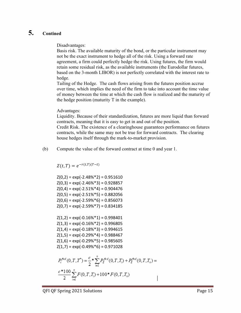
(b) Compute the value of the forward contract at time 0 and year 1.
𝑍𝑍(𝑡𝑡,𝑇𝑇) = 𝑒𝑒−𝑟𝑟(𝑡𝑡,𝑇𝑇)(𝑇𝑇−𝑡𝑡) Z(0,2) = exp(-2.48%*2) = 0.951610 Z(0,3) = exp(-2.46%*3) = 0.928857 Z(0,4) = exp(-2.51%*4) = 0.904476 Z(0,5) = exp(-2.51%*5) = 0.882056 Z(0,6) = exp(-2.59%*6) = 0.856073 Z(0,7) = exp(-2.59%*7) = 0.834185 Z(1,2) = exp(-0.16%*1) = 0.998401 Z(1,3) = exp(-0.16%*2) = 0.996805 Z(1,4) = exp(-0.18%*3) = 0.994615 Z(1,5) = exp(-0.29%*4) = 0.988467 Z(1,6) = exp(-0.29%*5) = 0.985605 Z(1,7) = exp(-0.49%*6) = 0.971028

QFI QF Spring 2021 Solutions Page 16
5. Contined [** Note that the formula is for a semi-annual coupon bond, however the question here is for an annual coupon bond so before applying the formula, we need to remove 2 from the formula. ]
where
21 2
1
( , )( , , )( , )
Z t TF t T TZ t T
=
Forward price at time 0 = 4%*(100*(0.928857+0.904476+0.882056+0.856073+0.834185)+100*0.834185)/0.951610 = 106.18 Forward price at time 1 = 4%*(100*(0.996805+0.994615+0.988467+0.985605+0.971028)+100*0.971028)/0.998401 = 117.04 Value of the forward contract at initiation is 0. Value of the forward contract at year 1 is (117.04 – 106.18)*0.998401= 10.84
(c) Yesterday you bought a 5-year Treasury note future expiring in 2 years and today
the future price drops to $100. The future contract size is $1,000,000. Your broker requires initial Margin: $1,485 (per contract); Maintenance Margin: $1,110 (per contract). Calculate the cash flow today.
& * * ( , ) ( , )fut futP L k contract P t T P t dt T = − − [The purchase price is missing in the stem. So candidates who tried to answer the question and gave a reasonable answer received full credit.]
(d) You are given the following data at time 0:
• The 6-month zero coupon bond is priced at $98.24 • The 9-month zero coupon bond is priced at $97.21 • Call option (European) on the 3-month Treasury bill with maturity in 6
months and strike price of $99.12 is priced at $0.2934 • Put option (European) on the 3-month Treasury bill with maturity in 6 months
and strike price of $99.12 is priced at $0.2044

QFI QF Spring 2021 Solutions Page 17
5. Contined Explain why the above securities are priced incorrectly.
0.2934 > 0.2044+0.9824*(97.21/98.24*100-99.12) = 0.038912 No, the security is not priced correctly.
(e) Describe a strategy to take advantage of the arbitrage opportunity:
(i) if the 3-month Treasury bill price is higher than the strike price.
(ii) if the 3-month Treasury bill price is lower than the strike price.
Commentary on Question: This is a new subject that may be was not enough studied, understood, or practiced.
Buy the put option on the 3 moth treasury bill with maturity in 6-months and strike price of $99.12 at $0.2044 Buy 9-month zero coupon bond with notional of $100 at $97.21 Sell 6-month zero coupon bond with notional of $99.12 at $97.38 (99.12*0.9824) Sell the call option on the 3 moth treasury bill with maturity in 6-months and strike price of $99.12 at $0.2934 At time 0 The net cash flow is -0.2044-97.21+97.38+0.2934 = $0.1323 Scenario 1: If the 3 month treasury bill price is higher than $99.12 at month 6. At month 6 The call option is exercised to receive 99.12 for selling the 3 month treasury bill Put option expires worthless. Pay 99.12 for the 6-month zero coupon bond No cash flow from the 9-month zero coupon bond. Net cash flow at month 6 is 0. At month 9 Receive $100 from the 9-month zero coupon bond maturity. Pay $100 from the 3-month zero coupon bond sold at month 6. Net cash flow is 0. Scenario 2: If 3 month treasury bill price is lower than $99.12 at month 6 At month 6 Exercise the put option to sell the 3 month treasury bill, receiving 99.12 The call option expires out of the money

QFI QF Spring 2021 Solutions Page 18
5. Contined Pay 99.12 for the 6-month zero coupon bond No cash flow from the 9-month zero coupon bond. At month 9 Receive $100 from the 9-month zero coupon bond maturity. Pay $100 from the 3-month zero coupon bond sold at month 6. Net cash flow is 0.

QFI QF Spring 2021 Solutions Page 19
6. Learning Objectives: 2. The candidate will understand the fundamentals of fixed income markets and
traded securities. Learning Outcomes: (2c) Understand measures of interest rate risk including duration, convexity, slope, and
curvature. (2d) Understand the characteristics and uses of interest rate forwards, swaps, futures,
and options. Sources: Fixed Income Securities: Valuation, Risk, and Risk Management, Veronesi, Pietro, 2010, Ch 4 QFIQ-121-20: A Guide to Duration, DV01, and Yield Curve Risk Transformations, pp. 1-28 Commentary on Question: Commentary listed underneath question component. Solution: (a) Calculate the value of k based on Analyst A’s proposal.
Commentary on Question: This part of the question was trying to test a candidate's comprehension of factor duration and ability to use it. Most candidates did well. Some candidates did not get the concept of dollar duration. Partial credits were given for work shown on intermediate calculations. Total portfolio value V = P + k x Pz In order to implement duration hedging, we need dV = 0 Dp x P + k x Dz x Pz (0,T) = 0 First calculate duration of the 5-year semi-annual coupon bond. Dp = ∑ 𝑤𝑤𝑖𝑖 × 𝑇𝑇𝑖𝑖10
𝑖𝑖=1 = 4.4304 Duration of a 5-year zero coupon bond (Dz) is 5 P = ∑ 𝑍𝑍(0,𝑇𝑇𝑖𝑖)𝑖𝑖 × 𝐶𝐶𝐹𝐹𝑖𝑖10
𝑖𝑖=1 = 111.23 million Pz = 100 x 0.8395 = 83.95 million Substitute into the original formula, k = - Dp x P / (Dz x Pz (0,T) )
= - (4.4304 x 111.23) / (5 x 83.95) = - 1.1741 (b) Calculate the DV01 of the portfolio consisting of the original bonds plus hedging
strategy calculated in part (a).

QFI QF Spring 2021 Solutions Page 20
6. Continued
Commentary on Question: Some candidates were not familiar with the formula of DV01. Partial credits were given if the candidates correctly calculate the price of the portfolio at the current yield plus or minus 0.1%. DV01 = 𝑃𝑃 (𝑐𝑐𝑑𝑑𝑟𝑟𝑟𝑟𝑐𝑐𝑐𝑐𝑡𝑡 𝑦𝑦𝑖𝑖𝑐𝑐𝑦𝑦𝑑𝑑 + 0.1%)− 𝑃𝑃 (𝑐𝑐𝑑𝑑𝑟𝑟𝑟𝑟𝑐𝑐𝑐𝑐𝑡𝑡 𝑦𝑦𝑖𝑖𝑐𝑐𝑦𝑦𝑑𝑑 – 0.1%)
0.2
(i.e. substituting k for correct portfolio value) Pick the correct values from the table showing Z(0,5) at different yields, i.e. 3.60% and 3.40% P(at 3.60%) = 110.74 - 1.1741 x 83.53 P(at 3.40%) = 111.72 - 1.1741 x 84.37 DV01 portfolio =
(110.74 - 1.1741 x 83.53 - 111.72 + 1.1741 x 84.37) / 0.2 = $0.031 (c) Construct a hedging portfolio based on Analyst B’s proposal.
Commentary on Question: This part of the question intends to test a candidate's ability to apply the concept of a duration and convexity hedged portfolio. Some candidates did not factor in price of the instruments when solving for the hedging units. Partial credits were given for calculating the components correctly.
Total value of the porposed portfolio is V = P + k1 x P1 + k2 x P2, where P1 and P2 represent prices of the 2-year zero coupon bond and 5-year zero coupon bond each with 100 million of par value. Then we need, k1 × D1 × P1 + k2 × D2 × P2 = −D × P (Delta Hedging) k1 × C1 × P1 + k2 × C2 × P2 = −C × P (Convexity Hedging) D1 = 2; C1 = 22 = 4 P1 = 100 x 0.9324 = 93.24 million From part a) (i) D2 = 5; P2 = 83.95 million; D = 4.4304; P = 111.23 million C2 = 52 = 25 Convexity of the coupon bond: C = ∑ 𝑤𝑤𝑖𝑖 × 𝑇𝑇𝑖𝑖210
𝑖𝑖=1 = 21.1320 The solution of this system of two equations in two unknowns is, k1 = - 𝑃𝑃
𝑃𝑃1 × ( 𝐷𝐷 ×𝐶𝐶2− 𝐶𝐶 ×𝐷𝐷2
𝐷𝐷1 ×𝐶𝐶2− 𝐶𝐶1 ×𝐷𝐷2 )
k2 = - 𝑃𝑃𝑃𝑃2
× ( 𝐷𝐷 ×𝐶𝐶1− 𝐶𝐶 ×𝐷𝐷1 𝐷𝐷2 ×𝐶𝐶1− 𝐶𝐶2 ×𝐷𝐷1
) Substitute the values into the above formulae and solve for k1 and k2 k1 = -0.2028 k2 = -1.0839
(d) Identify two other hedging instruments (in addition to zero-coupon bonds) that
your company can use to mitigate the risk of an upward shift in interest rates.

QFI QF Spring 2021 Solutions Page 21
6. Continued
Commentary on Question: Most candidates were able to list the hedging instruments; however, full credits are given only when candidate lists the instrument along with identifying whether a long or short position can mitigate interest rate risk
Examples of acceptable answers include: (i) short position in a forward rate agreement (ii) long position of fixed-for-floating interest rate swap contract (pay fixed, receive floating) (iii) long position of a cap on spot rate (interest rate option)
(e) Describe the procedure to construct a factor neutral hedge.
Commentary on Question: Most candidates struggled to provide a complete solution to this question. Partial credit was given for identifying pieces of the solution.
Consider now a portfolio P with factor durations D1 and D2 with respect to level and slope factors φ1 and φ2 , respectively To implement factor neutrality, we need to select two other securities, one for each factor we want to neutralize, in appropriate proportions. For instance, we could use short- and a long-dated zero coupon bonds, denoted by PSz and PLz . For each of these two bonds we can compute the factor durations. In order to immunize the portfolio against changes in level and slope, we must choose an amount of short-term and long-term zero coupon bonds, kS and kL , such that the variation of the portfolio plus the two bonds is approximately zero.
(f) Calculate factor duration of bond S and bond L by level, slope, and curvature.
Commentary on Question: Most candidates answered this question correctly. Some did not multiply the bonds by the appropriate time and were awarded partial credit if they got the beta only correct.
Recall that for zero coupon bonds, factor duration of zero coupon bound i with respect to factor j: Dj,z = (Ti − t) × βij
For bond S, D1 = 2x 1.0344 = 2.0688 D2 = 2 x -0.3507 =-0.7014 D3 = 2 x 0.3228 = 0.6456
For bond L, D1 = 7 x 1.0111 = 7.0777 D2 = 7 x 0.5208 = 3.6435 D3 = 7 x -0.1058 = -0.7406

QFI QF Spring 2021 Solutions Page 22
7. Learning Objectives: 3. The candidate will understand:
• The Quantitative tools and techniques for modeling the term structure of interest rates.
• The standard yield curve models. • The tools and techniques for managing interest rate risk.
Learning Outcomes: (3c) Calibrate a model to observed prices of traded securities. (3d) Describe the practical issues related to calibration, including yield curve fitting. Sources: Fixed Income Securities: Valuation, Risk, and Risk Management, Veronesi, Piertro, 2010, Chapter 14~15 Commentary on Question: The purpose of this question is to test candidates’ understanding of the Vasicek model and calibration used in practice. Most of candidates understood the Vasicek model well but almost all candidates did not perform well in the calibration problem. Solution: (a)
(i) Solve the stochastic differential equation.
(ii) Identify the distribution of tr by providing its mean and variance.
Consider 𝐹𝐹(𝑡𝑡, 𝑟𝑟𝑡𝑡) = 𝑒𝑒𝑎𝑎𝑡𝑡𝑟𝑟𝑡𝑡. Since 𝜕𝜕𝜕𝜕
𝜕𝜕𝑡𝑡= 𝑉𝑉𝑒𝑒𝑎𝑎𝑡𝑡𝑟𝑟𝑡𝑡,
𝜕𝜕𝜕𝜕𝜕𝜕𝑟𝑟
= 𝑒𝑒𝑎𝑎𝑡𝑡 , 𝜕𝜕2𝜕𝜕𝜕𝜕𝑟𝑟2
= 0, Ito’s lemma gives us 𝑑𝑑𝐹𝐹 = 𝑉𝑉𝑒𝑒𝑡𝑡𝑎𝑎𝑡𝑡𝑟𝑟𝑡𝑡𝑑𝑑𝑡𝑡 + 𝑒𝑒𝑎𝑎𝑡𝑡𝑑𝑑𝑟𝑟𝑡𝑡 = [𝑉𝑉𝑒𝑒𝑎𝑎𝑡𝑡𝑟𝑟𝑡𝑡 + 𝑒𝑒𝑎𝑎𝑡𝑡(𝜈𝜈 − 𝑉𝑉𝑟𝑟𝑡𝑡)]𝑑𝑑𝑡𝑡 + 𝑒𝑒𝑎𝑎𝑡𝑡𝜎𝜎𝑑𝑑𝑋𝑋𝑡𝑡
= 𝑒𝑒𝑎𝑎𝑡𝑡𝜈𝜈𝑑𝑑𝑡𝑡 + 𝑒𝑒𝑎𝑎𝑡𝑡𝜎𝜎𝑑𝑑𝑋𝑋𝑡𝑡
𝐹𝐹(𝑡𝑡, 𝑟𝑟𝑡𝑡) = 𝐹𝐹(0, 𝑟𝑟0) + 𝜈𝜈 𝑒𝑒𝑎𝑎𝑠𝑠𝑑𝑑𝑠𝑠 + 𝑒𝑒𝑎𝑎𝑠𝑠𝜎𝜎𝑑𝑑𝑋𝑋𝑠𝑠𝑡𝑡
0
𝑡𝑡
0
where 𝐹𝐹(0, 𝑟𝑟0) = 𝑟𝑟0
∴ 𝑟𝑟𝑡𝑡 = 𝑒𝑒−𝑎𝑎𝑡𝑡𝑟𝑟0 + 𝜈𝜈 𝑒𝑒𝑎𝑎(𝑠𝑠−𝑡𝑡)𝑑𝑑𝑠𝑠 + 𝜎𝜎𝑒𝑒−𝑎𝑎𝑡𝑡 𝑒𝑒𝑎𝑎𝑠𝑠𝑑𝑑𝑋𝑋𝑠𝑠𝑡𝑡
0
𝑡𝑡
0= 𝜇𝜇𝑡𝑡 + 𝜎𝜎𝑒𝑒−𝑎𝑎𝑡𝑡 𝑒𝑒𝑎𝑎𝑠𝑠𝑑𝑑𝑋𝑋𝑠𝑠
𝑡𝑡
0
where 𝜇𝜇𝑡𝑡 = 𝑒𝑒−𝑎𝑎𝑡𝑡𝑟𝑟0 + 𝜈𝜈 𝑒𝑒𝑎𝑎(𝑠𝑠−𝑡𝑡)𝑑𝑑𝑠𝑠𝑡𝑡
0
The mean of 𝑟𝑟𝑡𝑡 is 𝜇𝜇𝑡𝑡. The variance is: 𝜎𝜎2𝑒𝑒−2𝑎𝑎𝑡𝑡 ∫ 𝑒𝑒2𝑎𝑎𝑠𝑠𝑑𝑑𝑡𝑡𝑡𝑡
0 (by Ito Isometry) = 𝜎𝜎2𝑐𝑐−2𝑎𝑎𝑡𝑡
2𝑎𝑎(𝑒𝑒2𝑎𝑎𝑡𝑡 − 1) = 𝜎𝜎21−𝑐𝑐−2𝑎𝑎𝑡𝑡
2𝑎𝑎
Also, it shows Gaussian distribution.

QFI QF Spring 2021 Solutions Page 23
7. Continued
(b) Show that the limiting distribution of tr as t approaches infinity is 2
,2
vNa aσ
lim𝑡𝑡→∞
𝐸𝐸[𝑟𝑟𝑡𝑡] = lim𝑡𝑡→∞
𝑒𝑒−𝑎𝑎𝑡𝑡𝑟𝑟0 + 𝜈𝜈 𝑒𝑒𝑎𝑎(𝑠𝑠−𝑡𝑡)𝑑𝑑𝑠𝑠𝑡𝑡
0 = lim
𝑡𝑡→∞𝑒𝑒−𝑎𝑎𝑡𝑡𝑟𝑟0 +
(1 − 𝑒𝑒−𝑎𝑎𝑡𝑡)𝜈𝜈𝑉𝑉
=𝜈𝜈𝑉𝑉
lim𝑡𝑡→∞
𝑉𝑉𝑉𝑉𝑟𝑟[𝑟𝑟𝑡𝑡] = lim𝑡𝑡→∞
𝜎𝜎2(1 − 𝑒𝑒−2𝑎𝑎𝑡𝑡)2𝑉𝑉
=𝜎𝜎2
2𝑉𝑉
(c) Demonstrate that the interest rate, ,t mr + follows the same distribution. Hint: Use
time frame ( ),m t m+ from solution of part (a).
Commentary on Question: Quite a few candidates expressed 𝑟𝑟𝑡𝑡+m with an initial value of 𝑟𝑟0 instead of 𝑟𝑟𝑚𝑚.. Then, they took a limit value as in part (b) to get the desired answer.
Assume 𝑟𝑟𝑚𝑚 is stochastic, independent of the Brownian motion 𝑋𝑋𝑡𝑡. If we have that 𝑟𝑟𝑚𝑚~𝑁𝑁 𝜈𝜈
𝑎𝑎, 𝜎𝜎
2
2𝑎𝑎, independent of 𝑋𝑋𝑡𝑡, then we have:
𝐹𝐹(𝑡𝑡 + 𝑚𝑚, 𝑟𝑟𝑡𝑡+𝑚𝑚) = 𝐹𝐹(𝑚𝑚, 𝑟𝑟𝑚𝑚) + 𝜈𝜈 𝑒𝑒𝑎𝑎𝑠𝑠𝑑𝑑𝑠𝑠 + 𝑒𝑒𝑎𝑎𝑠𝑠𝜎𝜎𝑑𝑑𝑋𝑋𝑠𝑠𝑡𝑡+𝑚𝑚
𝑚𝑚
𝑡𝑡+𝑚𝑚
𝑚𝑚
where 𝐹𝐹(𝑚𝑚, 𝑟𝑟𝑚𝑚) = 𝑟𝑟𝑚𝑚𝑒𝑒𝑎𝑎𝑚𝑚
∴ 𝑟𝑟𝑡𝑡+𝑚𝑚 = 𝑒𝑒−𝑎𝑎(𝑡𝑡)𝑟𝑟𝑚𝑚 + 𝜈𝜈𝑒𝑒−𝑎𝑎(𝑡𝑡+𝑚𝑚) 𝑒𝑒𝑎𝑎𝑠𝑠𝑑𝑑𝑠𝑠 + 𝜎𝜎𝑒𝑒−𝑎𝑎(𝑡𝑡+𝑚𝑚) 𝑒𝑒𝑎𝑎𝑠𝑠𝑑𝑑𝑋𝑋𝑠𝑠𝑡𝑡+𝑚𝑚
𝑚𝑚
𝑡𝑡+𝑚𝑚
𝑚𝑚
𝐸𝐸[𝑟𝑟𝑡𝑡+𝑚𝑚] = 𝑒𝑒−𝑎𝑎(𝑡𝑡)𝐸𝐸[𝑟𝑟𝑚𝑚] +1 − 𝑒𝑒−𝑎𝑎(𝑡𝑡)𝜈𝜈
𝑉𝑉=𝜈𝜈𝑉𝑉
𝑉𝑉𝑉𝑉𝑟𝑟[𝑟𝑟𝑡𝑡+𝑚𝑚] = 𝑒𝑒−2𝑎𝑎(𝑡𝑡)𝑉𝑉𝑉𝑉𝑟𝑟[𝑟𝑟𝑚𝑚] +𝜎𝜎21 − 𝑒𝑒−2𝑎𝑎(𝑡𝑡)
2𝑉𝑉=𝜎𝜎2
2𝑉𝑉
(d)
(i) Estimate the parameters for interest rate process above.
(ii) Describe for the estimation of arbitrage free parameters using the table below observed in the market.
From
𝑑𝑑𝑟𝑟𝑡𝑡 = [𝜈𝜈 − 𝑉𝑉𝑟𝑟𝑡𝑡]𝑑𝑑𝑡𝑡 + 𝜎𝜎𝑑𝑑𝑋𝑋𝑡𝑡 It can be written in discrete manner
𝑟𝑟𝑡𝑡+𝛿𝛿 − 𝑟𝑟𝑡𝑡 = −𝑉𝑉𝑟𝑟𝑡𝑡𝛿𝛿 + 𝜈𝜈𝛿𝛿 + 𝜎𝜎𝜀𝜀𝑡𝑡√𝛿𝛿, 𝜀𝜀𝑡𝑡~𝑁𝑁(0,1) 𝑟𝑟𝑡𝑡+𝛿𝛿 = (1 − 𝑉𝑉𝛿𝛿)𝑟𝑟𝑡𝑡 + 𝜈𝜈𝛿𝛿 + 𝜎𝜎𝜀𝜀𝑡𝑡√𝛿𝛿, 𝜀𝜀𝑡𝑡~𝑁𝑁(0,1)
QFI QF Spring 2021 Solutions Page 24
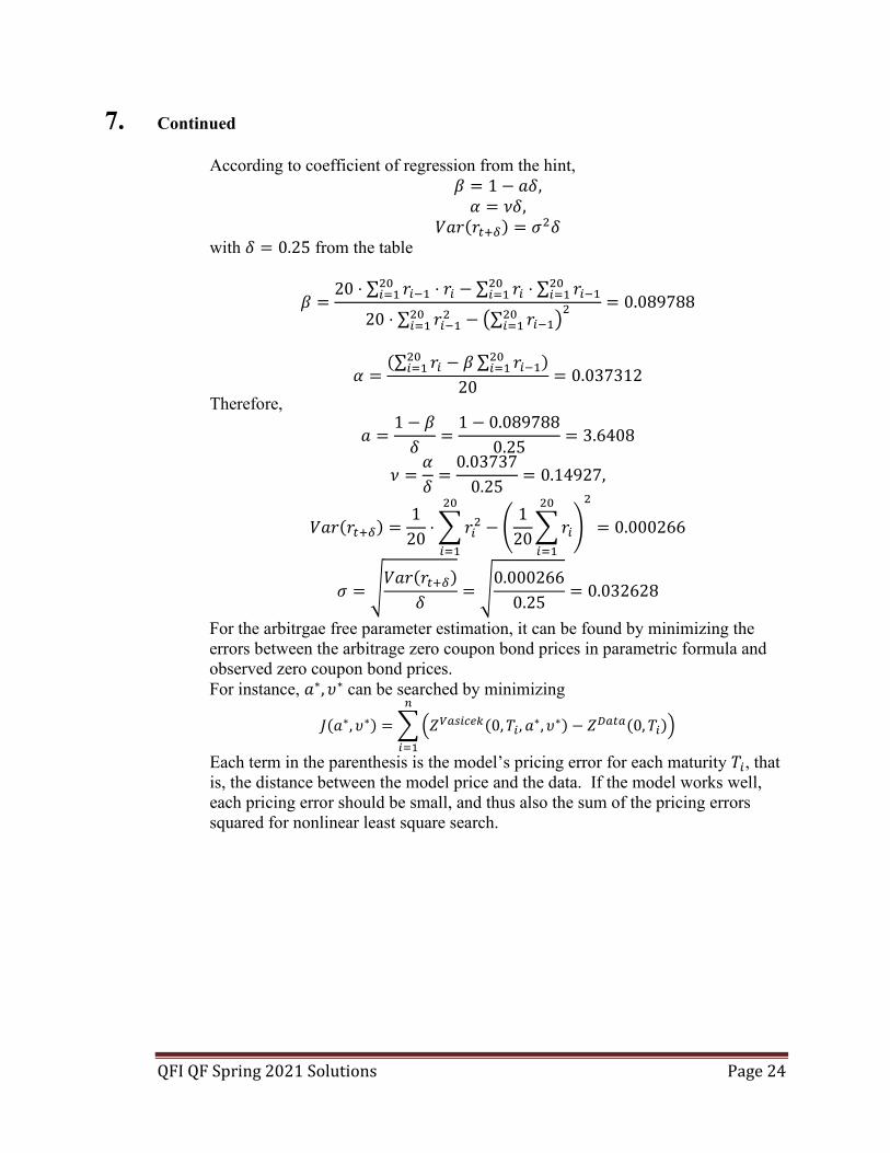
7. Continued According to coefficient of regression from the hint,
𝛽𝛽 = 1 − 𝑉𝑉𝛿𝛿, 𝛼𝛼 = 𝜈𝜈𝛿𝛿,
𝑉𝑉𝑉𝑉𝑟𝑟(𝑟𝑟𝑡𝑡+𝛿𝛿) = 𝜎𝜎2𝛿𝛿 with 𝛿𝛿 = 0.25 from the table
𝛽𝛽 =20 ⋅ ∑ 𝑟𝑟𝑖𝑖−120
𝑖𝑖=1 ⋅ 𝑟𝑟𝑖𝑖 − ∑ 𝑟𝑟𝑖𝑖20𝑖𝑖=1 ⋅ ∑ 𝑟𝑟𝑖𝑖−120
𝑖𝑖=1
20 ⋅ ∑ 𝑟𝑟𝑖𝑖−1220𝑖𝑖=1 − ∑ 𝑟𝑟𝑖𝑖−120
𝑖𝑖=1 2 = 0.089788
𝛼𝛼 =(∑ 𝑟𝑟𝑖𝑖20
𝑖𝑖=1 − 𝛽𝛽∑ 𝑟𝑟𝑖𝑖−120𝑖𝑖=1 )
20= 0.037312
Therefore,
𝑉𝑉 =1 − 𝛽𝛽𝛿𝛿
=1 − 0.089788
0.25= 3.6408
𝜈𝜈 =𝛼𝛼𝛿𝛿
=0.03737
0.25= 0.14927,
𝑉𝑉𝑉𝑉𝑟𝑟(𝑟𝑟𝑡𝑡+𝛿𝛿) =1
20⋅𝑟𝑟𝑖𝑖220
𝑖𝑖=1
− 1
20𝑟𝑟𝑖𝑖
20
𝑖𝑖=1
2
= 0.000266
𝜎𝜎 = 𝑉𝑉𝑉𝑉𝑟𝑟(𝑟𝑟𝑡𝑡+𝛿𝛿)𝛿𝛿
= 0.0002660.25
= 0.032628
For the arbitrgae free parameter estimation, it can be found by minimizing the errors between the arbitrage zero coupon bond prices in parametric formula and observed zero coupon bond prices. For instance, 𝑉𝑉∗, 𝜐𝜐∗ can be searched by minimizing
𝐽𝐽(𝑉𝑉∗, 𝜐𝜐∗) = 𝑍𝑍𝜕𝜕𝑎𝑎𝑠𝑠𝑖𝑖𝑐𝑐𝑐𝑐𝑘𝑘(0,𝑇𝑇𝑖𝑖,𝑉𝑉∗, 𝜐𝜐∗) − 𝑍𝑍𝐷𝐷𝑎𝑎𝑡𝑡𝑎𝑎(0,𝑇𝑇𝑖𝑖)𝑐𝑐
𝑖𝑖=1
Each term in the parenthesis is the model’s pricing error for each maturity 𝑇𝑇𝑖𝑖, that is, the distance between the model price and the data. If the model works well, each pricing error should be small, and thus also the sum of the pricing errors squared for nonlinear least square search.

QFI QF Spring 2021 Solutions Page 25
8. Learning Objectives: 3. The candidate will understand:
• The Quantitative tools and techniques for modeling the term structure of interest rates.
• The standard yield curve models. • The tools and techniques for managing interest rate risk.
Learning Outcomes: (3a) Understand and apply the concepts of risk-neutral measure, forward measure,
normalization, and the market price of risk, in the pricing of interest rate derivatives.
(3f) Apply the models to price common interest sensitive instruments including:
callable bonds, bond options, caps, floors, and swaptions. (3l) Demonstrate an understanding of the issues and approaches to building models
that admit negative interest rates. Sources: Fixed Income Securities: Valuation, Risk, and Risk Management, Veronesi, Pietro, 2010 p. 710, 716~717 Negative Interest Rates and Their Technical Consequences, AAE, 12/2016 p. 8, 9 QFIQ-116-17 Low Yield Curves and Absolute/Normal Volatilities p. 4~5, p. 7, p. 8, p. 9 Commentary on Question: This question was testing the candidates understanding of martingales, derivative pricing, and real-world application of different methodologies for calculating the derivative price. Most candidates did not do well with understanding martingales but improves with the pricing and real-world applications Most candidates did not do well in the beginning but much better in later parts. Solution: (a)
(i) Show that the forward price can also be computed as ( ) ( )*,A f T tF t T E A= under the T-forward risk-neutral measure ℚ𝑇𝑇.
(ii) Prove, using part (a)(i), that ( ) , , 0AF t T t ≥ is a martingale under the T-
forward measure ℚ𝑇𝑇.
Commentary on Question: The question was trying to test the concepts of alternative risk-neutral measure and martingale. Only a handful of candidates received full credits by demonstrating full understanding of the concepts by writing complete formulas.
QFI QF Spring 2021 Solutions Page 26
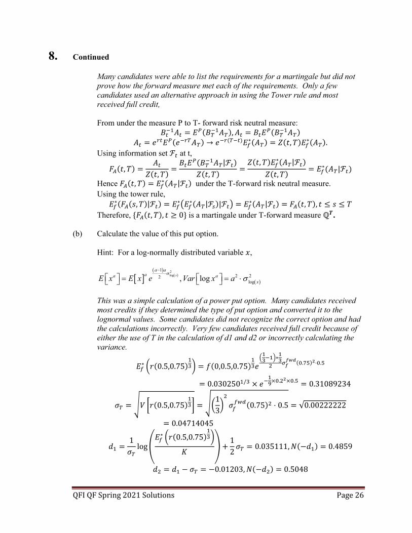
8. Continued Many candidates were able to list the requirements for a martingale but did not prove how the forward measure met each of the requirements. Only a few candidates used an alternative approach in using the Tower rule and most received full credit, From under the measure P to T- forward risk neutral measure:
𝐵𝐵𝑡𝑡−1𝐴𝐴𝑡𝑡 = 𝐸𝐸𝑃𝑃(𝐵𝐵𝑇𝑇−1𝐴𝐴𝑇𝑇),𝐴𝐴𝑡𝑡 = 𝐵𝐵𝑡𝑡𝐸𝐸𝑃𝑃(𝐵𝐵𝑇𝑇−1𝐴𝐴𝑇𝑇) 𝐴𝐴𝑡𝑡 = 𝑒𝑒𝑟𝑟𝑡𝑡𝐸𝐸𝑃𝑃(𝑒𝑒−𝑟𝑟𝑇𝑇𝐴𝐴𝑇𝑇) → 𝑒𝑒−𝑟𝑟(𝑇𝑇−𝑡𝑡)𝛦𝛦𝑓𝑓∗(𝐴𝐴𝑇𝑇) = 𝑍𝑍(𝑡𝑡,𝑇𝑇)𝛦𝛦𝑓𝑓∗(𝐴𝐴𝑇𝑇).
Using information set ℱ𝑡𝑡 at t,
𝐹𝐹𝐴𝐴(𝑡𝑡,𝑇𝑇) =𝐴𝐴𝑡𝑡
𝑍𝑍(𝑡𝑡,𝑇𝑇) =𝐵𝐵𝑡𝑡𝛦𝛦𝑃𝑃(𝐵𝐵𝑇𝑇−1𝐴𝐴𝑇𝑇|ℱ𝑡𝑡)
𝑍𝑍(𝑡𝑡,𝑇𝑇) =𝑍𝑍(𝑡𝑡,𝑇𝑇)𝛦𝛦𝑓𝑓∗(𝐴𝐴𝑇𝑇|ℱ𝑡𝑡)
𝑍𝑍(𝑡𝑡,𝑇𝑇) = 𝛦𝛦𝑓𝑓∗(𝐴𝐴𝑇𝑇|ℱ𝑡𝑡)
Hence 𝐹𝐹𝐴𝐴(𝑡𝑡,𝑇𝑇) = 𝛦𝛦𝑓𝑓∗(𝐴𝐴𝑇𝑇|ℱ𝑡𝑡) under the T-forward risk neutral measure. Using the tower rule,
𝛦𝛦𝑓𝑓∗(𝐹𝐹𝐴𝐴(𝑠𝑠,𝑇𝑇)|ℱ𝑡𝑡) = 𝛦𝛦𝑓𝑓∗𝛦𝛦𝑓𝑓∗(𝐴𝐴𝑇𝑇|ℱ𝑠𝑠)|ℱ𝑡𝑡 = 𝛦𝛦𝑓𝑓∗(𝐴𝐴𝑇𝑇|ℱ𝑡𝑡) = 𝐹𝐹𝐴𝐴(𝑡𝑡,𝑇𝑇), 𝑡𝑡 ≤ 𝑠𝑠 ≤ 𝑇𝑇 Therefore, 𝐹𝐹𝐴𝐴(𝑡𝑡,𝑇𝑇), 𝑡𝑡 ≥ 0 is a martingale under T-forward measure ℚ𝑻𝑻.
(b) Calculate the value of this put option.
Hint: For a log-normally distributed variable 𝑥𝑥,
[ ]( )
( )
( )
2log
12 22
log, logxa a
aa axE x E x e Var x a
σσ
−
= = ⋅ This was a simple calculation of a power put option. Many candidates received most credits if they determined the type of put option and converted it to the lognormal values. Some candidates did not recognize the correct option and had the calculations incorrectly. Very few candidates received full credit because of either the use of T in the calculation of d1 and d2 or incorrectly calculating the variance.
𝐸𝐸𝑓𝑓∗ 𝑟𝑟(0.5,0.75)13 = 𝑖𝑖(0,0.5,0.75)
13𝑒𝑒
13−1∗13
2 𝜎𝜎𝑓𝑓𝑓𝑓𝑤𝑤𝑓𝑓(0.75)2⋅0.5
= 0.0302501/3 × 𝑒𝑒−19×0.22×0.5 = 0.31089234
𝜎𝜎𝑇𝑇 = 𝑉𝑉 𝑟𝑟(0.5,0.75)13 =
132
𝜎𝜎𝑓𝑓𝑓𝑓𝑤𝑤𝑑𝑑(0.75)2 ⋅ 0.5 = √0.00222222
= 0.04714045
𝑑𝑑1 =1𝜎𝜎𝑇𝑇
log𝐸𝐸𝑓𝑓∗ 𝑟𝑟(0.5,0.75)
13
𝐾𝐾 +
12𝜎𝜎𝑇𝑇 = 0.035111,𝑁𝑁(−𝑑𝑑1) = 0.4859
𝑑𝑑2 = 𝑑𝑑1 − 𝜎𝜎𝑇𝑇 = −0.01203,𝑁𝑁(−𝑑𝑑2) = 0.5048
QFI QF Spring 2021 Solutions Page 27
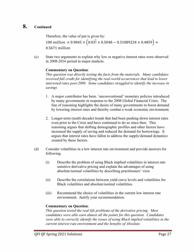
8. Continued Therefore, the value of put is given by: 100 𝑚𝑚𝑖𝑖𝑑𝑑𝑑𝑑𝑖𝑖𝑚𝑚𝑑𝑑 × 0.9845 × 0.03
13 × 0.5048 − 0.31089234 × 0.4859 =
0.5671 𝑚𝑚𝑖𝑖𝑑𝑑𝑑𝑑𝑖𝑖𝑚𝑚𝑑𝑑 (c) State two arguments to explain why low or negative interest rates were observed
in 2008-2016 period in major markets.
Commentary on Question: This question was directly testing the facts from the materials. Many candidates received full credit for identifying the real-world occurrences that lead to lower interested rates post-2008. Some candidates struggled to identify the increase in savings
1. A major contributor has been. ‘unconventional’ monetary policies introduced
by many governments in response to the 2008 Global Financial Crisis. The line of reasoning highlights the desire of many governments to boost demand by lowering interest rates and thereby combat a weak economic environment.
2. Longer-term (multi-decade) trends that had been pushing down interest rates even prior to the Crisis and have continued to do so since then. This reasoning argues that shifting demographic profiles and other factors have increased the supply of saving and reduced the demand for borrowings. It argues that interest rates have fallen to address the supply/demand dynamics created by these factors.
(d) Consider volatilities in a low interest rate environment and provide answers for
following. (i) Describe the problem of using Black implied volatilities in interest rate
sensitive derivative pricing and explain the advantages of using absolute/normal volatilities by describing practitioners’ view.
(ii) Describe the correlations between yield curve levels and volatilities for
Black volatilities and absolute/normal volatilities. (iii) Recommend the choice of volatilities in the current low interest rate
environment. Justify your recommendation.
Commentary on Question: This question tested the real-life problems of the derivative pricing. Most candidates were able earn almost all the points for this question. Candidates were able to correctly identify the issues of using Black implied volatilities in the current interest rate environment and the benefits of Absolute.

QFI QF Spring 2021 Solutions Page 28
8. Continued Many candidates struggled in identify the impact and magnitude of the correlations for Black and Absolute volatilities. Most candidates recommended the appropriate volatility and gave a valid justification for its use.
(i) The long-standing convention of quoting derivative prices for interest rate
options like caps, floors, and swaptions is to use Black’s formula for option pricing which assumes a lognormal distribution for interest rates.
As rates fell in response to the financial crisis in 2008, Black volatilities changed. Since 2009 there appears to have been three distinctive volatility regimes. In each circumstance, the reason for the increase in volatility regime was a drop in the underlying level of rates. Similar sensitivities of Black implied volatilities to rates are seen in different markets and for different tenor/maturity combinations. Ideally, an implied volatility measure used for pricing interest rate derivatives would hold approximately constant and vary in an intuitive way under a range of market conditions or across different ranges of instruments including: As strike and forward rates change. When maturities and tenors vary. For different types of instruments (for example puts and calls, payers
and receivers) linked via put-call parity. Before 2008 when rates were higher, Black implied volatilities performed reasonably well against these criteria. However, since 2009 participants in the swaption markets have increasingly chosen to use absolute/normal implied volatilities. The absolute/normal implied volatilities have been considerably more stable, and only a slight positive correlation between absolute volatilities and rate levels is observed. The more stable behavior of absolute/normal rates has led to a view among many traders of interest rate derivatives that interest rate distributions are closer to normal than lognormal.
(ii)
Correlations between yield curve levels and Black volatilities are typically strongly negative.
Correlations between yield curve levels and absolute/normal volatilities are weakly positive.

QFI QF Spring 2021 Solutions Page 29
8. Continued (iii) It is suggested the use of absolute/normal implied volatilities in the current
low interest rate environment. This conclusion is based on the research which implies normal/absolute volatiles are more robust across a range of interest rate regimes with respect to: Changes in strike and forward rates; Different maturities and tenors; and Different types of instrument.
(e) Describe two approaches to adapt the lognormal forward diffusion LMM to
accommodate negative forward rates.
Commentary on Question: This question tested the additional methodologies in derivative pricing. Most candidates were able to identify using a displacement adjustment to accommodate the negative forward rates but only some were able to also identify using a Stochastic variance process.
1. Displaced Diffusion LMM The forward rates are shifted so that the quantities forward rates +δ are positive. And the rates (forward and zero-coupon rates) are floored at -δ. The shift parameter is therefore easily interpretable and stands for the opposite of the lowest absolute level of the interest rates. 2. LMM+ This model is adapted from the LMM by simultaneously shifting the forward rate diffusion and adding a stochastic variance process. The diffusion process is the same as the Displaced Diffusion LMM, but instead of considering a time-dependent volatility function s(t), a stochastic mean-reversion type Cox-Ingersoll-Ross (CIR) process is used.

QFI QF Spring 2021 Solutions Page 30
9. Learning Objectives: 3. The candidate will understand:
• The Quantitative tools and techniques for modeling the term structure of interest rates.
• The standard yield curve models. • The tools and techniques for managing interest rate risk.
Learning Outcomes: (3k) Understand and apply multifactor interest rate models. (3l) Demonstrate an understanding of the issues and approaches to building models
that admit negative interest rates. Sources: QFIQ-130-21: Interest Rate Models – Theory and Practice, Second Edition, Brigo, Damiano and Mercurio, Fabio, 2006, Page 143 – 147 QFIQ-129-21: Negative Interest Rates and Their Technical Consequences, AAE, 12/2016, Page 2 Commentary on Question: Most of the candidates attempted part (a), (b) and (e). Only a few of candidates score full marks on this question. Solution: (a) Derive an expression for ( )r t .
Commentary on Question: One third of the candidates did not get this question right. Some candidates solved this question using partial differentiation approach, which was incorrect. When writing the equation for y(t), some candidates used 𝜎𝜎 instead of 𝜂𝜂. Partial points was given in this case Full points were also given to candidates who did the integration from s to t, instead of 0 to t. Full points was given to candidates who showed most all the steps. From Ito’s lemma:
𝑑𝑑(𝑥𝑥𝑒𝑒𝑎𝑎𝑡𝑡) = 𝑉𝑉𝑥𝑥𝑒𝑒𝑎𝑎𝑡𝑡𝑑𝑑𝑡𝑡 + 𝑒𝑒𝑎𝑎𝑡𝑡𝑑𝑑𝑥𝑥 Multiply both sides by 𝑒𝑒𝑎𝑎𝑡𝑡 𝑒𝑒𝑎𝑎𝑡𝑡𝑑𝑑𝑥𝑥(𝑡𝑡) = −𝑉𝑉𝑒𝑒𝑎𝑎𝑡𝑡𝑥𝑥(𝑡𝑡)𝑑𝑑𝑡𝑡 + 𝜎𝜎𝑒𝑒𝑎𝑎𝑡𝑡𝑑𝑑𝑊𝑊1(𝑡𝑡) 𝑒𝑒𝑎𝑎𝑡𝑡𝑑𝑑𝑥𝑥(𝑡𝑡) + 𝑉𝑉𝑒𝑒𝑎𝑎𝑡𝑡𝑥𝑥(𝑡𝑡)𝑑𝑑𝑡𝑡 = 𝜎𝜎𝑒𝑒𝑎𝑎𝑡𝑡𝑑𝑑𝑊𝑊1(𝑡𝑡)
𝑑𝑑(𝑥𝑥𝑒𝑒𝑎𝑎𝑡𝑡) = 𝜎𝜎𝑒𝑒𝑎𝑎𝑡𝑡𝑑𝑑𝑊𝑊1(𝑡𝑡)

QFI QF Spring 2021 Solutions Page 31
9. Continued Integrate both sides:
𝑥𝑥𝑒𝑒𝑎𝑎𝑑𝑑|0𝑡𝑡 = 𝜎𝜎𝑒𝑒𝑎𝑎u𝑑𝑑𝑊𝑊1(𝑑𝑑)𝑡𝑡
0
𝑥𝑥(𝑡𝑡)𝑒𝑒𝑎𝑎𝑡𝑡 − 𝑥𝑥(0)𝑒𝑒𝑎𝑎0 = 𝜎𝜎 𝑒𝑒𝑎𝑎𝑑𝑑𝑑𝑑𝑊𝑊1(𝑑𝑑)𝑡𝑡
0
𝑥𝑥(𝑡𝑡)𝑒𝑒𝑎𝑎𝑡𝑡 = 𝜎𝜎 𝑒𝑒𝑎𝑎𝑑𝑑𝑑𝑑𝑊𝑊1(𝑑𝑑)𝑡𝑡
0
We have:
𝑥𝑥(𝑡𝑡) = 𝜎𝜎 𝑒𝑒−𝑎𝑎(𝑡𝑡−𝑑𝑑)𝑑𝑑𝑊𝑊1(𝑡𝑡)𝑑𝑑𝑑𝑑𝑡𝑡
0
Similarly for y(t),
𝑦𝑦(𝑡𝑡) = 𝜂𝜂 𝑒𝑒−𝑏𝑏(𝑡𝑡−𝑑𝑑)𝑑𝑑𝑊𝑊2(𝑑𝑑)𝑡𝑡
0
Therefore,
𝑟𝑟(𝑡𝑡) = 𝜎𝜎 𝑒𝑒−𝑎𝑎(𝑡𝑡−𝑑𝑑)𝑑𝑑𝑊𝑊1(𝑑𝑑)𝑡𝑡
0+ 𝜂𝜂 𝑒𝑒−𝑏𝑏(𝑡𝑡−𝑑𝑑)𝑑𝑑𝑊𝑊2(𝑑𝑑)
𝑡𝑡
0+ 𝜑𝜑(𝑡𝑡)
(b) Derive expressions for ( ) E r t and ( ) Var r t .
Commentary on Question: Common mistakes for candidates who used approach Var (x + y) = Var (x) + Var (y) + 2Cov (x,y)
• The “2Cov(x,y)” term was missing completely • For some candidates who calculated “Cov(x,y)”, coefficient 2 was
missing Some candidates made mistake at the integration step (e.g. 2 was missing at the denominator).
Since 𝐸𝐸 ∫ 𝑒𝑒−𝑎𝑎(𝑡𝑡−𝑑𝑑)𝑑𝑑𝑊𝑊1(𝑑𝑑)𝑡𝑡
0 = 0, hence 𝐸𝐸[𝑟𝑟(𝑡𝑡)] = 𝜑𝜑(𝑡𝑡)
Var[r(t)] = E[r2(t)]− E[r(t)]2

QFI QF Spring 2021 Solutions Page 32
9. Continued
r2(t) = σ2 e−a(t−u)dW1(u)t
02
+ η2 e−b(t−u)dW2(u)t
02
+ φ2(t)
+ 2 φ(t)σ e−a(t−u)dW1(u)t
0+ η e−b(t−u)dW2(u)
t
0
+ 2σ e−a(t−u)dW1(u)t
0 η e−b(t−u)dW2(u)
t
0
E[r2(t)] = σ2 e−2a(t−u)dut
0+ η2 e−2b(t−u)du
t
0+ φ2(t)
+ 2ησ e−(a+b)(t−u)ρdut
0
E[r2(t)] =σ2
2a(1 − e−2at) +
η2
2b1 − e−2bt +
2ησρa + b
1 − e−(a+b)t + φ2(t) Hence,
Var[r(t)] =σ2
2a(1 − e−2at) +
η2
2b1 − e−2bt +
2ησρa + b
1 − e−(a+b)t (c) Explain the steps involved in the calibration process for the G2++ model in
practice.
Commentary on Question: Half of the candidates did not answer this question. Full marks will be given to candidate explained the calibration process and the practical constraints.
Start with the term structure of zero-coupon bond prices at maturities available in the market
PM(0, T) Compute the implied instantaneous forward rates as
fM(0, T) = −∂ ln PM(0, T)
∂T
Use the equation provided to optimize the parameters a, b, σ, η, ρ This would imply fitting the full market instantaneous forward curve
(d) Derive an expression for the risk-neutral probability that the instantaneous rate
𝑟𝑟(𝑡𝑡) is negative.

QFI QF Spring 2021 Solutions Page 33
9. Continued
Commentary on Question: Full marks will be given to candidate if the final equation of Q(r(t)) is shown. Some candidates did not recognize that short rate is Gaussian. Partial marks will be given to candidates who mentioned/showed that short rate is Gaussian, but did not get the correct Q(r(t)).
The short rate is Gaussian with mean μr(t) and variance σr2(t), where: μr(t) = Er(t) = φ(t)
= fM(0, t) +σ2
2a2(1 − e−at)2 +
η2
2b21 − e−bt
2+ ρ
σηab
(1 − e−at)1− e−bt
σr2(t) = Varr(t) =σ2
2a(1 − e−2at) +
η2
2b1 − e−2bt +
2ησρa + b
1 − e−(a+b)t
Qr(t) < 0 = Φ0 − μr(t)
σr(t) = Φ
−μr(t)σr(t)
(e) Comment on the pros and cons of using the G2++ model
Commentary on Question: Candidate will receive full marks if a pro and a con is provided.
Pros:
• G2++ model assumes normal distribution for the instantaneous rate and hence can support negative rates
• G2++ model can reproduce ATM volatilities well Cons:
• G2++ model is not fully satisfactory when attempting to replicate out-of-the-money volatility
• Estimation of parameters is time consuming (f) Comment on how appropriate this model would be for modeling guarantees that
are significantly out of the money.
Commentary on Question: Partial marks will be given if candidate mentioned that this model is inappropriate.
While G2++ model can reproduce ATM volatilities well but does not appear to be fully satisfactory when attempting to replicate out-of-the-money volatilities. Thus, the model may not be appropriate for deep out of the money products.

QFI QF Spring 2021 Solutions Page 34
10. Learning Objectives: 3. The candidate will understand:
• The Quantitative tools and techniques for modeling the term structure of interest rates.
• The standard yield curve models. • The tools and techniques for managing interest rate risk.
Learning Outcomes: (3a) Understand and apply the concepts of risk-neutral measure, forward measure,
normalization, and the market price of risk, in the pricing of interest rate derivatives.
(3b) Understand and apply various one-factor interest rate models. Sources: Fixed Income Securities: Valuation, Risk, and Risk Management, Veronesi, Pietro Commentary on Question: Overall, candidates performed as expected on this question. There was a mistake in the given equation for A(t;T). However, credit was given when it was due; candidates were not penalized for using the correct or incorrect version equation. The model solution showed the work assuming candidates used the equation for A(t;T) given in the question. Solution: (a) Compare ( ),m r t with an arbitrage-free parameter ( )* ,m r t and explain the
meaning of the parameters when ( ) ( )* * *,m r t r rγ= − .
Commentary on Question: Partial credit was awarded for candidates who demonstrated some understandings with regard to risk-neutral vs. real world as well as mean reversion. The drift 𝑚𝑚∗(𝑟𝑟, 𝑡𝑡) provides arbitrage-free bond return, while 𝑚𝑚(𝑟𝑟, 𝑡𝑡) does not. Vasicek model assumes that 𝑚𝑚∗(𝑟𝑟, 𝑡𝑡) has the same form as the drift rate of the original interest rate process:
𝑚𝑚∗(𝑟𝑟, 𝑡𝑡) = 𝛾𝛾∗(𝑟∗ − 𝑟𝑟) where 𝛾𝛾∗, 𝑟∗ are two constants, which 𝛾𝛾∗ controls the sensitivity of the long-term bond prices to variation in the short-term rates.

QFI QF Spring 2021 Solutions Page 35
10. Continued
(b) Show that ( ) ( )2
**
/ 12t
dZ dt BE E rZ
σ γγ
= + − using Ito’s lemma.
Commentary on Question: Partial credit was awarded for candidates who showed the appropriate partial derivatives and applying them using Ito’s Lemma.
∂Z∂t
= (A′ − B′r)Z,∂Z∂r
= −BZ,∂2Z∂r2
= B2Z where ∂B∂t
= B′ = −e−r∗(T−t) ∂A∂t
= A′ = (1 + B′)r∗ −σ2
2γ∗ −
σ2B(t; T)′B(t; T)2γ∗
By Ito’ lemma:
dZ = ∂Z∂t
+∂Z∂rγ∗(r∗ − rt) +
σ2
2∂2Z∂r2
dt +∂Z∂rσdXt
Note that γ∗B = 1 + B′, thus: A′ = γ∗Br∗ − σ2
2B − σ2(γ∗B−1)B(t;T)
2γ∗= γ∗Br∗ − σ2
2γB − σ2
2B2 + σ2B(t;T)
2γ∗
So: ∂Z∂t
= Bγ∗r∗ − σ2
2B2 − B′r Z
Therefore: dZZ
= γ∗Br∗ −σ2
2B −
σ2
2B2 +
σ2B2γ∗
− B′rt − Bγ∗(r∗ − rt) +σ2
2B2dt
+1Z∂Z∂rσdXt
E dZdtZ = −B′E(rt) + Bγ∗E(rt) −
σ2
2B +
σ2B2γ∗
= (−B′ + Bγ∗)E(rt) +σ2B2γ∗
(1 − γ∗) = E(rt) +σ2B2γ∗
(1 − γ∗)

QFI QF Spring 2021 Solutions Page 36
10. Continued
(c) Compute /dZ dtE
Z
on zero-coupon bond with 10 years to maturity.
Commentary on Question: The zero-coupon bond prices given were not correct for the given risk-neutral parameters. However, credit was given where it was due.
𝐵𝐵(0,10) =1
0.4653(1 − 𝑒𝑒−0.4653∗10) = 2.129
E[r0] = r0 = 2% Using the result from part (b), we have:
𝐸𝐸 𝑑𝑑𝑍𝑍/𝑑𝑑𝑡𝑡𝑍𝑍
= 2% +2.21%2 × 2.129
2 × 0.4653(1 − 0.4653) = 2.0597 %
(d) Calculate the value of a call option with 1 year to maturity ( )0 1T = , strike price
0.9K = , written on a zero-coupon bond with 5 years to maturity.
Under the Vasicek model, a European call open with strike price K and maturity 𝑇𝑇0 on a zero coupon maturiing on 𝑇𝑇𝐵𝐵 > 𝑇𝑇0is given by:
𝑉𝑉(𝑟𝑟0, 0) = 𝑍𝑍(𝑟𝑟0, 0;𝑇𝑇𝐵𝐵)𝑁𝑁(𝑑𝑑1) − 𝐾𝐾𝑍𝑍(𝑟𝑟0, 0;𝑇𝑇0)𝑁𝑁(𝑑𝑑2)
𝑑𝑑1 =1𝑆𝑆𝑑𝑑𝑚𝑚𝑙𝑙
𝑍𝑍(𝑟𝑟0, 0;𝑇𝑇𝐵𝐵)𝐾𝐾𝑍𝑍(𝑟𝑟0, 0;𝑇𝑇0) +
𝑆𝑆2
𝑑𝑑2 = 𝑑𝑑1 − 𝑆𝑆
𝑆𝑆 = 𝐵𝐵(𝑇𝑇0;𝑇𝑇𝐵𝐵) ∗ 𝜎𝜎2
2𝛾𝛾∗(1 − 𝑒𝑒−2𝛾𝛾∗𝑇𝑇0)
Thus, we have:
𝐵𝐵(1; 5) =1𝛾𝛾∗1 − 𝑒𝑒−𝛾𝛾∗(5−1) = 1.815
𝑆𝑆(1,5) = 1.815 ∗ 2.21%2
2 ∗ 0.4653(1 − 𝑒𝑒−2∗0.4653) = 0.03236
𝑑𝑑1 =1
0.03236𝑑𝑑𝑚𝑚𝑙𝑙
0.8980.9 ∗ 0.975
+0.03236
2= 0.7298
𝑑𝑑2 = 0.7298 − 0.03236 = 0.6975 The value of the call option is:
𝑉𝑉 = 0.898 ∗ 𝑁𝑁(𝑑𝑑1) − 0.9 ∗ 0.975 ∗ 𝑁𝑁(0.6975) = 0.02425
QFI QF Spring 2021 Solutions Page 37
11. Learning Objectives: 1. The candidate will understand the foundations of quantitative finance. 4. The candidate will understand:
• How to apply the standard models for pricing financial derivatives. • The implications for option pricing when markets do not satisfy the common
assumptions used in option pricing theory. • How to evaluate risk exposures and the issues in hedging them.
Learning Outcomes: (1d) Understand and apply Ito’s Lemma. (4a) Demonstrate an understanding of option pricing techniques and theory for equity
derivatives. (4i) Define and explain the concept of volatility smile and some arguments for its
existence. (4k) Describe and contrast several approaches for modeling smiles, including:
stochastic volatility, local-volatility, jump-diffusions, variance-gamma, and mixture models.
(4l) Explain various issues and approaches for fitting a volatility surface. Sources: The Volatility Smile, Derman, Emanuel and Miller, Michael B., 2016, Chapter 19 An Introduction to the Mathematics of Financial Derivatives, Hirsa, Ali and Neftci, Salih N., 3rd Edition 2nd Printing, 2014, Chapter 10, Chapter 12 QFIQ-120-19: Chapters 6 and 7 of Pricing and Hedging Financial Derivatives, Marroni, Leonardo and Perdomo, Irene, 2014 Commentary on Question: Commentary listed underneath each question component. Solution: (a)
(i) Derive td Π in terms of , ,tdt dS and tdv .
(ii) Construct a riskless portfolio tΠ to show that
QFI QF Spring 2021 Solutions Page 38
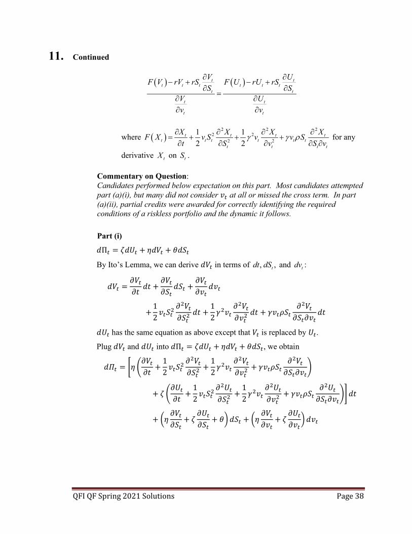
11. Continued
( ) ( )t tt t t t t t
t t
t t
t t
V UF V rV rS F U rU rSS S
V Uv v
∂ ∂− + − +
∂ ∂=
∂ ∂∂ ∂
where ( )2 2 2
2 22 2
1 12 2
t t t tt t t t t t
t t t t
X X X XF X v S v v St S v S v
γ γ ρ∂ ∂ ∂ ∂= + + +
∂ ∂ ∂ ∂ ∂ for any
derivative tX on tS .
Commentary on Question: Candidates performed below expectation on this part. Most candidates attempted part (a)(i), but many did not consider 𝑣𝑣𝑡𝑡 at all or missed the cross term. In part (a)(ii), partial credits were awarded for correctly identifying the required conditions of a riskless portfolio and the dynamic it follows.
Part (i)
𝑑𝑑Π𝑡𝑡 = 𝜁𝜁𝑑𝑑𝑑𝑑𝑡𝑡 + 𝜂𝜂𝑑𝑑𝑉𝑉𝑡𝑡 + 𝜃𝜃𝑑𝑑𝑆𝑆𝑡𝑡
By Ito’s Lemma, we can derive 𝑑𝑑𝑉𝑉𝑡𝑡 in terms of , ,tdt dS and tdv :
𝑑𝑑𝑉𝑉𝑡𝑡 =𝜕𝜕𝑉𝑉𝑡𝑡𝜕𝜕𝑡𝑡
𝑑𝑑𝑡𝑡 +𝜕𝜕𝑉𝑉𝑡𝑡𝜕𝜕𝑆𝑆𝑡𝑡
𝑑𝑑𝑆𝑆𝑡𝑡 +𝜕𝜕𝑉𝑉𝑡𝑡𝜕𝜕𝑣𝑣𝑡𝑡
𝑑𝑑𝑣𝑣𝑡𝑡
+12𝑣𝑣𝑡𝑡𝑆𝑆𝑡𝑡2
𝜕𝜕2𝑉𝑉𝑡𝑡𝜕𝜕𝑆𝑆𝑡𝑡2
𝑑𝑑𝑡𝑡 +12𝛾𝛾2𝑣𝑣𝑡𝑡
𝜕𝜕2𝑉𝑉𝑡𝑡𝜕𝜕𝑣𝑣𝑡𝑡2
𝑑𝑑𝑡𝑡 + 𝛾𝛾𝑣𝑣𝑡𝑡𝜌𝜌𝑆𝑆𝑡𝑡𝜕𝜕2𝑉𝑉𝑡𝑡𝜕𝜕𝑆𝑆𝑡𝑡𝜕𝜕𝑣𝑣𝑡𝑡
𝑑𝑑𝑡𝑡
𝑑𝑑𝑑𝑑𝑡𝑡 has the same equation as above except that 𝑉𝑉𝑡𝑡 is replaced by 𝑑𝑑𝑡𝑡.
Plug 𝑑𝑑𝑉𝑉𝑡𝑡 and 𝑑𝑑𝑑𝑑𝑡𝑡 into 𝑑𝑑Π𝑡𝑡 = 𝜁𝜁𝑑𝑑𝑑𝑑𝑡𝑡 + 𝜂𝜂𝑑𝑑𝑉𝑉𝑡𝑡 + 𝜃𝜃𝑑𝑑𝑆𝑆𝑡𝑡, we obtain
𝑑𝑑𝛱𝛱𝑡𝑡 = 𝜂𝜂 𝜕𝜕𝑉𝑉𝑡𝑡𝜕𝜕𝑡𝑡
+12𝑣𝑣𝑡𝑡𝑆𝑆𝑡𝑡2
𝜕𝜕2𝑉𝑉𝑡𝑡𝜕𝜕𝑆𝑆𝑡𝑡2
+12𝛾𝛾2𝑣𝑣𝑡𝑡
𝜕𝜕2𝑉𝑉𝑡𝑡𝜕𝜕𝑣𝑣𝑡𝑡2
+ 𝛾𝛾𝑣𝑣𝑡𝑡𝜌𝜌𝑆𝑆𝑡𝑡𝜕𝜕2𝑉𝑉𝑡𝑡𝜕𝜕𝑆𝑆𝑡𝑡𝜕𝜕𝑣𝑣𝑡𝑡
+ 𝜁𝜁 𝜕𝜕𝑑𝑑𝑡𝑡𝜕𝜕𝑡𝑡
+12𝑣𝑣𝑡𝑡𝑆𝑆𝑡𝑡2
𝜕𝜕2𝑑𝑑𝑡𝑡𝜕𝜕𝑆𝑆𝑡𝑡2
+12𝛾𝛾2𝑣𝑣𝑡𝑡
𝜕𝜕2𝑑𝑑𝑡𝑡𝜕𝜕𝑣𝑣𝑡𝑡2
+ 𝛾𝛾𝑣𝑣𝑡𝑡𝜌𝜌𝑆𝑆𝑡𝑡𝜕𝜕2𝑑𝑑𝑡𝑡𝜕𝜕𝑆𝑆𝑡𝑡𝜕𝜕𝑣𝑣𝑡𝑡
𝑑𝑑𝑡𝑡
+ 𝜂𝜂𝜕𝜕𝑉𝑉𝑡𝑡𝜕𝜕𝑆𝑆𝑡𝑡
+ 𝜁𝜁𝜕𝜕𝑑𝑑𝑡𝑡𝜕𝜕𝑆𝑆𝑡𝑡
+ 𝜃𝜃𝑑𝑑𝑆𝑆𝑡𝑡 + 𝜂𝜂𝜕𝜕𝑉𝑉𝑡𝑡𝜕𝜕𝑣𝑣𝑡𝑡
+ 𝜁𝜁𝜕𝜕𝑑𝑑𝑡𝑡𝜕𝜕𝑣𝑣𝑡𝑡
𝑑𝑑𝑣𝑣𝑡𝑡

QFI QF Spring 2021 Solutions Page 39
11. Continued
Part (ii)
Rewrite 𝑑𝑑Π𝑡𝑡 as
𝑑𝑑Π𝑡𝑡 = [𝜂𝜂𝐹𝐹(𝑉𝑉𝑡𝑡) + 𝜁𝜁𝐹𝐹(𝑑𝑑𝑡𝑡)]𝑑𝑑𝑡𝑡 + 𝜂𝜂𝜕𝜕𝑉𝑉𝑡𝑡𝜕𝜕𝑆𝑆𝑡𝑡
+ 𝜁𝜁𝜕𝜕𝑑𝑑𝑡𝑡𝜕𝜕𝑆𝑆𝑡𝑡
+ 𝜃𝜃𝑑𝑑𝑆𝑆𝑡𝑡 + 𝜂𝜂𝜕𝜕𝑉𝑉𝑡𝑡𝜕𝜕𝑣𝑣𝑡𝑡
+ 𝜁𝜁𝜕𝜕𝑑𝑑𝑡𝑡𝜕𝜕𝑣𝑣𝑡𝑡
𝑑𝑑𝑣𝑣𝑡𝑡
For a riskless portfolio, the coefficient of 𝑑𝑑𝑆𝑆𝑡𝑡 and 𝑑𝑑𝑣𝑣𝑡𝑡 must be 0, i.e.
⎩⎨
⎧𝜂𝜂𝜕𝜕𝑉𝑉𝑡𝑡𝜕𝜕𝑆𝑆𝑡𝑡
+ 𝜁𝜁𝜕𝜕𝑑𝑑𝑡𝑡𝜕𝜕𝑆𝑆𝑡𝑡
+ 𝜃𝜃 = 0
𝜂𝜂𝜕𝜕𝑉𝑉𝑡𝑡𝜕𝜕𝑣𝑣𝑡𝑡
+ 𝜁𝜁𝜕𝜕𝑑𝑑𝑡𝑡𝜕𝜕𝑣𝑣𝑡𝑡
= 0 ⇒
⎩⎪⎨
⎪⎧𝜁𝜁 = −𝜂𝜂
𝜕𝜕𝑉𝑉𝑡𝑡 𝜕𝜕𝑣𝑣𝑡𝑡⁄𝜕𝜕𝑑𝑑𝑡𝑡 𝜕𝜕𝑣𝑣𝑡𝑡⁄
𝜃𝜃 = −𝜂𝜂𝜕𝜕𝑉𝑉𝑡𝑡𝜕𝜕𝑆𝑆𝑡𝑡
− 𝜁𝜁𝜕𝜕𝑑𝑑𝑡𝑡𝜕𝜕𝑆𝑆𝑡𝑡
The riskless portfolio Π𝑡𝑡 follows the dynamic 𝑑𝑑Π𝑡𝑡 = 𝑟𝑟Π𝑑𝑑𝑡𝑡. Therefore,
𝑑𝑑Π𝑡𝑡 = [𝜂𝜂𝐹𝐹(𝑉𝑉𝑡𝑡) + 𝜁𝜁𝐹𝐹(𝑑𝑑𝑡𝑡)]𝑑𝑑𝑡𝑡 = 𝑟𝑟Π𝑑𝑑𝑡𝑡 = 𝑟𝑟(𝜁𝜁𝑑𝑑𝑡𝑡 + 𝜂𝜂𝑉𝑉𝑡𝑡 + 𝜃𝜃𝑆𝑆𝑡𝑡)𝑑𝑑𝑡𝑡
By comparing the coefficients of 𝑑𝑑𝑡𝑡, it follows that
𝜂𝜂𝐹𝐹(𝑉𝑉𝑡𝑡) + 𝜁𝜁𝐹𝐹(𝑑𝑑𝑡𝑡) = 𝑟𝑟(𝜁𝜁𝑑𝑑𝑡𝑡 + 𝜂𝜂𝑉𝑉𝑡𝑡 + 𝜃𝜃𝑆𝑆𝑡𝑡)
Substitute in 𝜃𝜃 and rearrange the terms
𝜂𝜂𝐹𝐹(𝑉𝑉𝑡𝑡) + 𝜁𝜁𝐹𝐹(𝑑𝑑𝑡𝑡) = 𝑟𝑟 𝜁𝜁𝑑𝑑𝑡𝑡 + 𝜂𝜂𝑉𝑉𝑡𝑡 − 𝜂𝜂𝑆𝑆𝑡𝑡𝜕𝜕𝑉𝑉𝑡𝑡𝜕𝜕𝑆𝑆𝑡𝑡
− 𝜁𝜁𝑆𝑆𝑡𝑡𝜕𝜕𝑑𝑑𝑡𝑡𝜕𝜕𝑆𝑆𝑡𝑡
𝜂𝜂 𝐹𝐹(𝑉𝑉𝑡𝑡) − 𝑟𝑟𝑉𝑉𝑡𝑡 + 𝑟𝑟𝑆𝑆𝑡𝑡𝜕𝜕𝑉𝑉𝑡𝑡𝜕𝜕𝑆𝑆𝑡𝑡
= −𝜁𝜁 𝐹𝐹(𝑑𝑑𝑡𝑡) − 𝑟𝑟𝑑𝑑𝑡𝑡 + 𝑟𝑟𝑆𝑆𝑡𝑡𝜕𝜕𝑑𝑑𝑡𝑡𝜕𝜕𝑆𝑆𝑡𝑡
Substitute in 𝜁𝜁 = −𝜂𝜂 𝜕𝜕𝜕𝜕𝑡𝑡 𝜕𝜕𝑣𝑣𝑡𝑡⁄𝜕𝜕𝑈𝑈𝑡𝑡 𝜕𝜕𝑣𝑣𝑡𝑡⁄ and rearrange the terms
𝐹𝐹(𝑉𝑉𝑡𝑡) − 𝑟𝑟𝑉𝑉𝑡𝑡 + 𝑟𝑟𝑆𝑆𝑡𝑡𝜕𝜕𝑉𝑉𝑡𝑡𝜕𝜕𝑆𝑆𝑡𝑡
𝜕𝜕𝑉𝑉𝑡𝑡𝜕𝜕𝑣𝑣𝑡𝑡
=𝐹𝐹(𝑑𝑑𝑡𝑡) − 𝑟𝑟𝑑𝑑𝑡𝑡 + 𝑟𝑟𝑆𝑆𝑡𝑡
𝜕𝜕𝑑𝑑𝑡𝑡𝜕𝜕𝑆𝑆𝑡𝑡
𝜕𝜕𝑑𝑑𝑡𝑡𝜕𝜕𝑣𝑣𝑡𝑡
(b) Derive the generic partial differential equation that any derivative tV on tS must
follow.
Commentary on Question: Candidates performed as expected on this part. No credits were awarded for writing down the Black-Scholes equation with a constant volatility.
QFI QF Spring 2021 Solutions Page 40
11. Continued The generic partial differential equation is
𝐹𝐹(𝑉𝑉𝑡𝑡) − 𝑟𝑟𝑉𝑉𝑡𝑡 + 𝑟𝑟𝑆𝑆𝑡𝑡𝜕𝜕𝑉𝑉𝑡𝑡𝜕𝜕𝑆𝑆𝑡𝑡
− 𝑖𝑖(𝑆𝑆𝑡𝑡,𝑣𝑣𝑡𝑡 , 𝑡𝑡)𝜕𝜕𝑉𝑉𝑡𝑡𝜕𝜕𝑣𝑣𝑡𝑡
= 0
Where 𝐹𝐹(𝑉𝑉𝑡𝑡) = 𝜕𝜕𝜕𝜕𝑡𝑡𝜕𝜕𝑡𝑡
+ 12𝑣𝑣𝑡𝑡𝑆𝑆𝑡𝑡2
𝜕𝜕2𝜕𝜕𝑡𝑡𝜕𝜕𝜕𝜕𝑡𝑡2
+ 12𝛾𝛾2𝑣𝑣𝑡𝑡
𝜕𝜕2𝜕𝜕𝑡𝑡𝜕𝜕𝑣𝑣𝑡𝑡2
+ 𝛾𝛾𝑣𝑣𝑡𝑡𝜌𝜌𝑆𝑆𝑡𝑡𝜕𝜕2𝜕𝜕𝑡𝑡𝜕𝜕𝜕𝜕𝑡𝑡𝜕𝜕𝑣𝑣𝑡𝑡
.
Additional explanation: In part (a)(ii), we have derived an equation where all
terms concerning 𝑉𝑉𝑡𝑡 are on the left side of the equation, and all terms concerning
𝑑𝑑𝑡𝑡 are on the right side of the equation. It follows that the value of
𝐹𝐹(𝑉𝑉𝑡𝑡) − 𝑟𝑟𝑉𝑉𝑡𝑡 + 𝑟𝑟𝑆𝑆𝑡𝑡𝜕𝜕𝜕𝜕𝑡𝑡𝜕𝜕𝜕𝜕𝑡𝑡 𝜕𝜕𝜕𝜕𝑡𝑡
𝜕𝜕𝑣𝑣𝑡𝑡 must not depend on the derivative 𝑉𝑉𝑡𝑡 and is the same
for all derivatives on 𝑆𝑆𝑡𝑡.
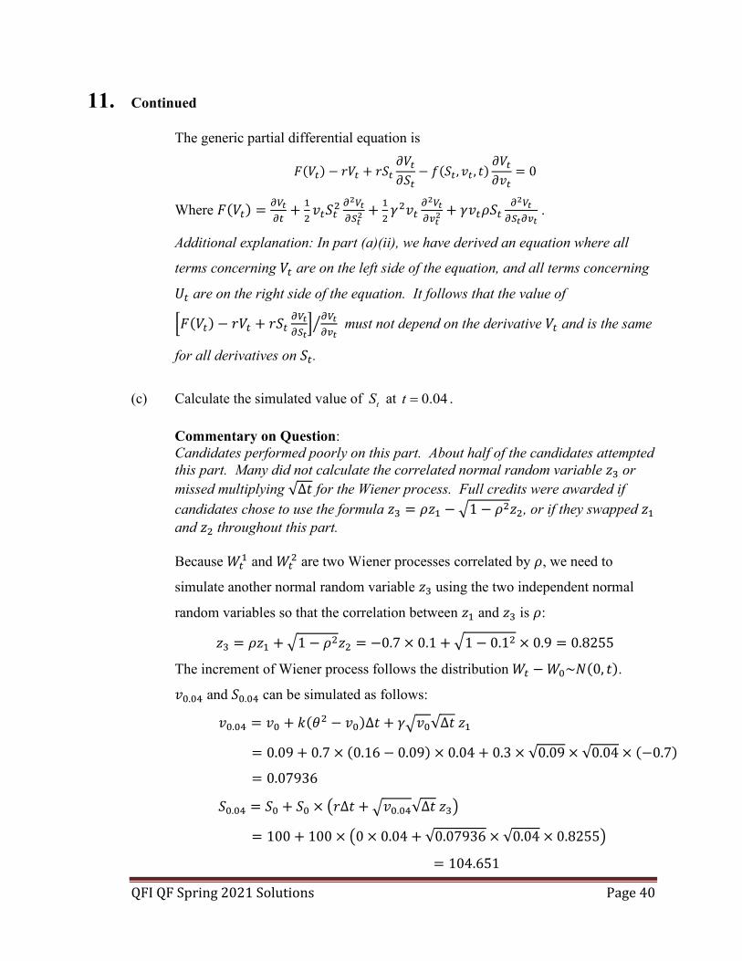
(c) Calculate the simulated value of tS at 0.04t = .
Commentary on Question: Candidates performed poorly on this part. About half of the candidates attempted this part. Many did not calculate the correlated normal random variable 𝑧𝑧3 or missed multiplying √Δ𝑡𝑡 for the Wiener process. Full credits were awarded if candidates chose to use the formula 𝑧𝑧3 = 𝜌𝜌𝑧𝑧1 − 1 − 𝜌𝜌2𝑧𝑧2, or if they swapped 𝑧𝑧1 and 𝑧𝑧2 throughout this part.
Because 𝑊𝑊𝑡𝑡
1 and 𝑊𝑊𝑡𝑡2 are two Wiener processes correlated by 𝜌𝜌, we need to
simulate another normal random variable 𝑧𝑧3 using the two independent normal
random variables so that the correlation between 𝑧𝑧1 and 𝑧𝑧3 is 𝜌𝜌:
𝑧𝑧3 = 𝜌𝜌𝑧𝑧1 + 1 − 𝜌𝜌2𝑧𝑧2 = −0.7 × 0.1 + 1 − 0.12 × 0.9 = 0.8255
The increment of Wiener process follows the distribution 𝑊𝑊𝑡𝑡 −𝑊𝑊0~𝑁𝑁(0, 𝑡𝑡).
𝑣𝑣0.04 and 𝑆𝑆0.04 can be simulated as follows:
𝑣𝑣0.04 = 𝑣𝑣0 + 𝑘𝑘(𝜃𝜃2 − 𝑣𝑣0)Δ𝑡𝑡 + 𝛾𝛾𝑣𝑣0√Δ𝑡𝑡 𝑧𝑧1
= 0.09 + 0.7 × (0.16 − 0.09) × 0.04 + 0.3 × √0.09 × √0.04 × (−0.7)
= 0.07936
𝑆𝑆0.04 = 𝑆𝑆0 + 𝑆𝑆0 × 𝑟𝑟Δ𝑡𝑡 + 𝑣𝑣0.04√Δ𝑡𝑡 𝑧𝑧3
= 100 + 100 × 0 × 0.04 + √0.07936 × √0.04 × 0.8255
= 104.651

QFI QF Spring 2021 Solutions Page 41
11. Continued (d) Describe how to produce the volatility smile implied by this Heston model.
Commentary on Question: Many candidates did not attempt this part. Instead of describing how one can produce the volatility smile, some explained why the Heston model can produce a volatility smile and received no credits.
1. Simulate 𝑁𝑁 paths of 𝑆𝑆𝑡𝑡 from time 0 to 𝑇𝑇 using the calculation in part (b). 2. Calculate call and put prices at various strikes using the simulated stock price. 3. Plug these calculated prices into the Black-Scholes formula and back-solve for
the implied volatility. 4. Plot the implied volatility against the respective strikes to generate the
volatility smile at the maturity 𝑇𝑇. (e)
(i) Explain why the Heston model would produce a volatility smile.
(ii) Describe one way to calibrate the Heston model.
(iii) Describe two potential disadvantages of such calibration.
Commentary on Question: Many candidates obtained credits on part (i) and part (ii) if they have attempted it. No credits were awarded if the disadvantages described in part (iii) were not specific to the calibration method described in part (ii).
Part (i) Because the volatility produced by the Heston model is stochastic, paths of asset prices ending far from the ATM level will have experienced, on average, a higher volatility than paths ending near ATM. The correlation between the asset price and the volatility naturally generates a volatility smile. Part (ii) The Heston model can be calibrated by minimizing the difference between the volatility generated by the model and the implied volatility in the market. Part (iii) Calibrating a stochastic volatility model to fit the market data potentially have the following disadvantages: • The calibration can be unstable, resulting in jumps in mark-to-market profit. • European vanilla option prices cannot be reproduced exactly, so a stochastic
volatility model may not be appropriate for vanilla instruments. • If the model is calibrated to vanilla options, it may not be able to produce the
market prices for exotic options, and vice versa.

QFI QF Spring 2021 Solutions Page 42
12. Learning Objectives: 4. The candidate will understand:
• How to apply the standard models for pricing financial derivatives. • The implications for option pricing when markets do not satisfy the common
assumptions used in option pricing theory. • How to evaluate risk exposures and the issues in hedging them.
Learning Outcomes: (4a) Demonstrate an understanding of option pricing techniques and theory for equity
derivatives. (4e) Analyze the Greeks of common option strategies. Sources: Pricing and Hedging of Financial Derivatives, Ch 6, by Marroni and Perdomo The Volatility Smile, Derman, Miller, and Park, 2016, Ch. 7 Commentary on Question: This question tests candidates’ understanding of option Greeks. Solution: (a) Determine which Greek (Delta, Gamma, Vega, Rho, or Theta) Exhibit I
represents. Justify your answer. (Here Theta is defined as the derivative of the option value with respect to the passage of time.)
Commentary on Question: Candidates performed as expected. Exhibit I shows Rho because: i. Delta is bounded by 1; ii. Gamma and Vega exhibit bell-shape around at-the-money stock price of $100; iii. Theta is negative; Since none of the above pattern fits Exhibit I, it is Rho.
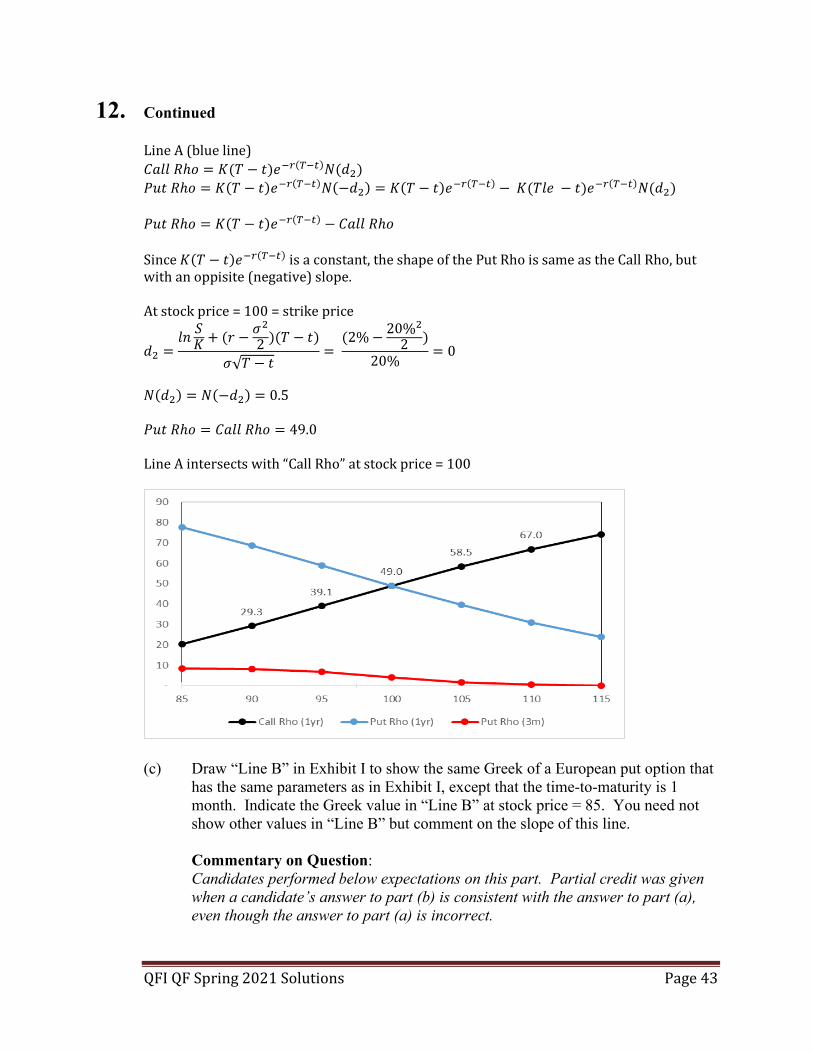
(b) Draw “Line A” in Exhibit I to show the same Greek of a European put option that
has the same parameters as the one in Exhibit I. Indicate the Greek value in “Line A” at stock price = 100. You need not show other values in “Line A” but comment on the slope of this line.
Commentary on Question: Candidates performed below expectations on this part. Partial credit was given when a candidate’s answer to part (b) is consistent with the answer to part (a), even though the answer to part (a) is incorrect.
QFI QF Spring 2021 Solutions Page 43
12. Continued
Line A (blue line) 𝐶𝐶𝑉𝑉𝑑𝑑𝑑𝑑 𝑅𝑅ℎ𝑚𝑚 = 𝐾𝐾(𝑇𝑇 − 𝑡𝑡)𝑒𝑒−𝑟𝑟(𝑇𝑇−𝑡𝑡)𝑁𝑁(𝑑𝑑2) 𝑃𝑃𝑑𝑑𝑡𝑡 𝑅𝑅ℎ𝑚𝑚 = 𝐾𝐾(𝑇𝑇 − 𝑡𝑡)𝑒𝑒−𝑟𝑟(𝑇𝑇−𝑡𝑡)𝑁𝑁(−𝑑𝑑2) = 𝐾𝐾(𝑇𝑇 − 𝑡𝑡)𝑒𝑒−𝑟𝑟(𝑇𝑇−𝑡𝑡) − 𝐾𝐾(𝑇𝑇𝑑𝑑𝑒𝑒 − 𝑡𝑡)𝑒𝑒−𝑟𝑟(𝑇𝑇−𝑡𝑡)𝑁𝑁(𝑑𝑑2) 𝑃𝑃𝑑𝑑𝑡𝑡 𝑅𝑅ℎ𝑚𝑚 = 𝐾𝐾(𝑇𝑇 − 𝑡𝑡)𝑒𝑒−𝑟𝑟(𝑇𝑇−𝑡𝑡) − 𝐶𝐶𝑉𝑉𝑑𝑑𝑑𝑑 𝑅𝑅ℎ𝑚𝑚 Since 𝐾𝐾(𝑇𝑇 − 𝑡𝑡)𝑒𝑒−𝑟𝑟(𝑇𝑇−𝑡𝑡) is a constant, the shape of the Put Rho is same as the Call Rho, but with an oppisite (negative) slope. At stock price = 100 = strike price
𝑑𝑑2 =𝑑𝑑𝑑𝑑 𝑆𝑆𝐾𝐾 + (𝑟𝑟 − 𝜎𝜎2
2 )(𝑇𝑇 − 𝑡𝑡)
𝜎𝜎√𝑇𝑇 − 𝑡𝑡=
(2%− 20%2
2 )20%
= 0
𝑁𝑁(𝑑𝑑2) = 𝑁𝑁(−𝑑𝑑2) = 0.5 𝑃𝑃𝑑𝑑𝑡𝑡 𝑅𝑅ℎ𝑚𝑚 = 𝐶𝐶𝑉𝑉𝑑𝑑𝑑𝑑 𝑅𝑅ℎ𝑚𝑚 = 49.0 Line A intersects with “Call Rho” at stock price = 100
(c) Draw “Line B” in Exhibit I to show the same Greek of a European put option that
has the same parameters as in Exhibit I, except that the time-to-maturity is 1 month. Indicate the Greek value in “Line B” at stock price = 85. You need not show other values in “Line B” but comment on the slope of this line.
Commentary on Question: Candidates performed below expectations on this part. Partial credit was given when a candidate’s answer to part (b) is consistent with the answer to part (a), even though the answer to part (a) is incorrect.

QFI QF Spring 2021 Solutions Page 44
12. Continued Line B (red line) For 1 month maturity, at stock price =85:
𝑑𝑑2 =𝑑𝑑𝑑𝑑 85
100 + 2%− 20%2
2 (1/12)
20%1/12= −0.8126
𝑁𝑁(−𝑑𝑑2) = 0.7918 1 month Put Rho = 100 ∗ 1
12 ∗ 𝑒𝑒−2%
112 ∗ 0.7918 = 8.30
“Line B” starts at below the “Call Rho” line with a negative slope. For ease of reference, “Line B” is shown in part (b). (d) Exhibit II below shows Vega and Gamma for a European option on a non-
dividend-paying stock. These Greek values are derived from the BSM model with the same strike price, volatility, interest rate, and time-to-maturity as in Exhibit I.
Exhibit II: Vega and Gamma with respect to the underlying stock price Stock price 60 X Vega (shown as the change in the option value to 1 percentage point change of the volatility, e.g., from 25% to 26%)
0.2401 0.2548
Gamma 0.0267 0.0159
Determine the stock price X in Exhibit II.
Commentary on Question: Candidates performed below expectations on this part. Note: The Vega and Gamma values in Exhibit II are derived in the same manner as the Rho in Exhibit I, but they are not based on the option parameters in Exhibit I. Nevertheless, credit was given if X was solved correctly by using the option parameters in Exhibit I.
𝑉𝑉𝑒𝑒𝑙𝑙𝑉𝑉 = 0.01 ∗ 𝑆𝑆√𝑇𝑇 − 𝑡𝑡𝑁𝑁′(𝑑𝑑1)
𝐺𝐺𝑉𝑉𝑚𝑚𝑚𝑚𝑉𝑉 = 𝑁𝑁′(𝑑𝑑1)𝑆𝑆𝜎𝜎√𝑇𝑇 − 𝑡𝑡
𝑉𝑉𝑒𝑒𝑙𝑙𝑉𝑉𝐺𝐺𝑉𝑉𝑚𝑚𝑚𝑚𝑉𝑉 = 0.01 ∗ 𝑆𝑆2𝜎𝜎(𝑇𝑇 − 𝑡𝑡) (1)

QFI QF Spring 2021 Solutions Page 45
12. Continued 0.24010.0267 = 0.01 ∗ 602𝜎𝜎(𝑇𝑇 − 𝑡𝑡) (2) 0.25480.0159 = 0.01 ∗ 𝑋𝑋2𝜎𝜎(𝑇𝑇 − 𝑡𝑡) (3)
𝑑𝑑𝑠𝑠𝑒𝑒 𝑒𝑒𝑒𝑒𝑑𝑑𝑉𝑉𝑡𝑡𝑖𝑖𝑚𝑚𝑑𝑑𝑠𝑠 (2) 𝑉𝑉𝑑𝑑𝑑𝑑 (3) 𝑡𝑡𝑚𝑚 𝑙𝑙𝑒𝑒𝑡𝑡 𝑋𝑋 = 60 ∗ 0.25480.0159
∗0.02670.2401
= 80
(e) Determine an upper bound of the option’s implied volatility.
Commentary on Question: Few candidates attempted to answer this part.
Based on equation (1) from part (d):
𝜎𝜎 =100 ∗ 𝑉𝑉𝑒𝑒𝑙𝑙𝑉𝑉
𝐺𝐺𝑉𝑉𝑚𝑚𝑚𝑚𝑉𝑉 ∗ 𝑆𝑆2(𝑇𝑇 − 𝑡𝑡)≤
100 ∗ 𝑉𝑉𝑒𝑒𝑙𝑙𝑉𝑉𝐺𝐺𝑉𝑉𝑚𝑚𝑚𝑚𝑉𝑉 ∗ 𝑆𝑆2
𝑏𝑏𝑒𝑒𝑐𝑐𝑉𝑉𝑑𝑑𝑠𝑠𝑒𝑒 (𝑇𝑇 − 𝑡𝑡) > 1
𝜎𝜎 ≤100 ∗ 024010.0267 ∗ 602
= 25%

QFI QF Spring 2021 Solutions Page 46
13. Learning Objectives: 4. The candidate will understand:
• How to apply the standard models for pricing financial derivatives. • The implications for option pricing when markets do not satisfy the common
assumptions used in option pricing theory. • How to evaluate risk exposures and the issues in hedging them.
Learning Outcomes: (4a) Demonstrate an understanding of option pricing techniques and theory for equity
derivatives. (4b) Identify limitations of the Black-Scholes-Merton pricing formula (4c) Demonstrate an understating of the different approaches to hedging – static and
dynamic. (4f) Appreciate how hedge strategies may go awry. Sources: The Volatility Smile, Derman, Emanuel and Miller, Michael B., 2016 Commentary on Question: Commentary listed underneath each question component. Solution: (a) Derive the replicating portfolio using options for the interest credited above the
guaranteed rate, i.e. .tInterest Credited g− Specify each option, including position, option type, term, and strike ratio 1/ tK S − . Commentary on Question: Points are awarded for both deriving the formula and correct description of the replication portfolio. Detailed description of the portfolio is required, including, strike ratio, option term, option type.
𝐼𝐼𝑑𝑑𝑡𝑡𝑒𝑒𝑟𝑟𝑒𝑒𝑠𝑠𝑡𝑡 𝐶𝐶𝑟𝑟𝑒𝑒𝑑𝑑𝑖𝑖𝑡𝑡𝑒𝑒𝑑𝑑𝑡𝑡 − 𝐺𝐺𝑑𝑑𝑉𝑉𝑟𝑟
= 𝑚𝑚𝑉𝑉𝑥𝑥 𝑚𝑚𝑖𝑖𝑑𝑑 𝜕𝜕𝑡𝑡𝜕𝜕𝑡𝑡−1
− 1 ∗ 𝑃𝑃𝑉𝑉𝑟𝑟,𝐶𝐶𝑉𝑉𝐶𝐶 ,𝐺𝐺𝑑𝑑𝑉𝑉𝑟𝑟 − 𝐺𝐺𝑑𝑑𝑉𝑉𝑟𝑟,
= 𝐶𝐶𝑉𝑉𝑟𝑟 ∗ 𝑚𝑚𝑉𝑉𝑥𝑥 𝑚𝑚𝑖𝑖𝑑𝑑 𝜕𝜕𝑡𝑡𝜕𝜕𝑡𝑡−1
− 1 − 𝐺𝐺𝑑𝑑𝑎𝑎𝑟𝑟𝑝𝑝𝑎𝑎𝑟𝑟
, 𝐶𝐶𝑎𝑎𝑝𝑝𝑝𝑝𝑎𝑎𝑟𝑟
− 𝐺𝐺𝑑𝑑𝑎𝑎𝑟𝑟𝑝𝑝𝑎𝑎𝑟𝑟
, 0,

QFI QF Spring 2021 Solutions Page 47
13. Continued
= 𝐶𝐶𝑉𝑉𝑟𝑟 ∗ 𝑚𝑚𝑉𝑉𝑥𝑥
⎩⎪⎨
⎪⎧
𝑚𝑚𝑖𝑖𝑑𝑑
⎣⎢⎢⎢⎡ 𝜕𝜕𝑡𝑡
𝜕𝜕𝑡𝑡−1− 1 − 𝐺𝐺𝑑𝑑𝑎𝑎𝑟𝑟
𝑝𝑝𝑎𝑎𝑟𝑟 ,
𝜕𝜕𝑡𝑡𝜕𝜕𝑡𝑡−1
− 1 − 𝐺𝐺𝑑𝑑𝑎𝑎𝑟𝑟𝑝𝑝𝑎𝑎𝑟𝑟
− 𝜕𝜕𝑡𝑡𝜕𝜕𝑡𝑡−1
− 1 − 𝐶𝐶𝑎𝑎𝑝𝑝𝑝𝑝𝑎𝑎𝑟𝑟
⎦⎥⎥⎥⎤
, 0
⎭⎪⎬
⎪⎫
Denote 𝐺𝐺 = 𝜕𝜕𝑡𝑡𝜕𝜕𝑡𝑡−1
− 1 − 𝐺𝐺𝑑𝑑𝑎𝑎𝑟𝑟𝑝𝑝𝑎𝑎𝑟𝑟
, 𝐶𝐶 = 𝜕𝜕𝑡𝑡𝜕𝜕𝑡𝑡−1
− 1 − 𝐶𝐶𝑎𝑎𝑝𝑝𝑝𝑝𝑎𝑎𝑟𝑟
,
as 𝐶𝐶𝑉𝑉𝐶𝐶 > 𝐺𝐺𝑑𝑑𝑉𝑉𝑟𝑟, 𝐺𝐺 > 𝐶𝐶. Thus, 𝐼𝐼𝑑𝑑𝑡𝑡𝑒𝑒𝑟𝑟𝑒𝑒𝑠𝑠𝑡𝑡 𝐶𝐶𝑟𝑟𝑒𝑒𝑑𝑑𝑖𝑖𝑡𝑡𝑒𝑒𝑑𝑑𝑡𝑡 − 𝐺𝐺𝑑𝑑𝑉𝑉𝑟𝑟 = 𝐶𝐶𝑉𝑉𝑟𝑟 ∗ 𝑚𝑚𝑉𝑉𝑥𝑥[𝑚𝑚𝑖𝑖𝑑𝑑(𝐺𝐺,𝐺𝐺 − 𝐶𝐶), 0] = 𝐶𝐶𝑉𝑉𝑟𝑟 ∗ 𝑚𝑚𝑉𝑉𝑥𝑥[0,−𝑚𝑚𝑖𝑖𝑑𝑑(𝐺𝐺,𝐺𝐺 − 𝐶𝐶)] + 𝑚𝑚𝑖𝑖𝑑𝑑(𝐺𝐺,𝐺𝐺 − 𝐶𝐶) = 𝐶𝐶𝑉𝑉𝑟𝑟 ∗ 𝑚𝑚𝑉𝑉𝑥𝑥[0,𝑚𝑚𝑉𝑉𝑥𝑥(−𝐺𝐺,𝐶𝐶 − 𝐺𝐺)] −𝑚𝑚𝑉𝑉𝑥𝑥(−𝐺𝐺,𝐶𝐶 − 𝐺𝐺) = 𝐶𝐶𝑉𝑉𝑟𝑟 ∗ 𝑚𝑚𝑉𝑉𝑥𝑥[𝐺𝐺,𝑚𝑚𝑉𝑉𝑥𝑥(0,𝐶𝐶)] −𝑚𝑚𝑉𝑉𝑥𝑥(0,𝐶𝐶) = 𝐶𝐶𝑉𝑉𝑟𝑟 ∗ 𝑚𝑚𝑉𝑉𝑥𝑥[0,𝑚𝑚𝑉𝑉𝑥𝑥(𝐺𝐺,𝐶𝐶)] −𝑚𝑚𝑉𝑉𝑥𝑥(0,𝐶𝐶) = 𝐶𝐶𝑉𝑉𝑟𝑟 ∗ 𝑚𝑚𝑉𝑉𝑥𝑥(0,𝐺𝐺) −𝑚𝑚𝑉𝑉𝑥𝑥(0,𝐶𝐶), as 𝐺𝐺 > 𝐶𝐶 = 𝐶𝐶𝑉𝑉𝑟𝑟 ∗ 𝑚𝑚𝑉𝑉𝑥𝑥 𝜕𝜕𝑡𝑡
𝜕𝜕𝑡𝑡−1− 1 + 𝐺𝐺𝑑𝑑𝑎𝑎𝑟𝑟
𝑝𝑝𝑎𝑎𝑟𝑟 , 0 − 𝑚𝑚𝑉𝑉𝑥𝑥 𝜕𝜕𝑡𝑡
𝜕𝜕𝑡𝑡−1− 1 + 𝐶𝐶𝑎𝑎𝑝𝑝
𝑝𝑝𝑎𝑎𝑟𝑟 , 0.
Therefore, the interest credited above the guaranteed rate can be replicated by 𝐶𝐶 units of call spread, with the following options:
• Long position of a 1-year term European call option, with strike ratio 𝐾𝐾𝐿𝐿𝜕𝜕𝑡𝑡−1
= 1 + 𝐺𝐺𝑑𝑑𝑎𝑎𝑟𝑟𝑝𝑝𝑎𝑎𝑟𝑟
=
1 + 0.010.9
= 1.0111
• Short position of a 1-year term European call option, with strike ratio 𝐾𝐾𝑆𝑆𝜕𝜕𝑡𝑡−1
= 1 + 𝐶𝐶𝑎𝑎𝑝𝑝𝑝𝑝𝑎𝑎𝑟𝑟
=
1 + 0.050.9
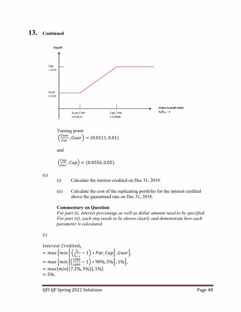
= 1.0556 (b) Sketch the payoff of the replicating portfolio against the index growth rate
1
1t
t
SS −
−
.
Commentary on Question: Correct shape of the curve as well as identification of both the turning points are required for full credit.
QFI QF Spring 2021 Solutions Page 48
13. Continued
Turning point: 𝐺𝐺𝑑𝑑𝑎𝑎𝑟𝑟
𝑃𝑃𝑎𝑎𝑟𝑟,𝐺𝐺𝑑𝑑𝑉𝑉𝑟𝑟 = (0.0111, 0.01)
and 𝐶𝐶𝑎𝑎𝑝𝑝𝑃𝑃𝑎𝑎𝑟𝑟
,𝐶𝐶𝑉𝑉𝐶𝐶 = (0.0556, 0.05). (c)
(i) Calculate the interest credited on Dec 31, 2019.
(ii) Calculate the cost of the replicating portfolio for the interest credited above the guaranteed rate on Dec 31, 2018.
Commentary on Question: For part (i), interest percentage as well as dollar amount need to be specified.
For part (ii), each step needs to be shown clearly and demonstrate how each parameter is calculated.
(i) 𝐼𝐼𝑑𝑑𝑡𝑡𝑒𝑒𝑟𝑟𝑒𝑒𝑠𝑠𝑡𝑡 𝐶𝐶𝑟𝑟𝑒𝑒𝑑𝑑𝑖𝑖𝑡𝑡𝑒𝑒𝑑𝑑𝑡𝑡 = 𝑚𝑚𝑉𝑉𝑥𝑥 𝑚𝑚𝑖𝑖𝑑𝑑 𝜕𝜕𝑡𝑡
𝜕𝜕𝑡𝑡−1− 1 ∗ 𝑃𝑃𝑉𝑉𝑟𝑟,𝐶𝐶𝑉𝑉𝐶𝐶 ,𝐺𝐺𝑑𝑑𝑉𝑉𝑟𝑟,
= 𝑚𝑚𝑉𝑉𝑥𝑥 𝑚𝑚𝑖𝑖𝑑𝑑 10801000
− 1 ∗ 90%, 5% , 1%, = 𝑚𝑚𝑉𝑉𝑥𝑥𝑚𝑚𝑖𝑖𝑑𝑑[(7.2%, 5%)], 1% = 5%.

QFI QF Spring 2021 Solutions Page 49
13. Continued Therefore, interest credited per $1000 of investment = 5% ∗ 1000 = $50. (ii) From (a), the interest crediting strategy can be replicated by the following call spread: 𝐶𝐶𝑉𝑉𝑟𝑟 ∗ 𝑚𝑚𝑉𝑉𝑥𝑥 𝜕𝜕𝑡𝑡
𝜕𝜕𝑡𝑡−1− 1 + 𝐺𝐺𝑑𝑑𝑎𝑎𝑟𝑟
𝑝𝑝𝑎𝑎𝑟𝑟 , 0 − 𝑚𝑚𝑉𝑉𝑥𝑥 𝜕𝜕𝑡𝑡
𝜕𝜕𝑡𝑡−1− 1 + 𝐶𝐶𝑎𝑎𝑝𝑝
𝑝𝑝𝑎𝑎𝑟𝑟 , 0.
The cost of the replicating portfolio is the option value of this call spread at 𝑡𝑡 − 1. Using Black-Scholes model to calculate the option value, 𝐶𝐶(𝑆𝑆𝑡𝑡, 𝑡𝑡) = 𝑆𝑆𝑡𝑡𝑁𝑁(𝑑𝑑1) − 𝐾𝐾𝑒𝑒−𝑟𝑟(𝑇𝑇−𝑡𝑡)𝑁𝑁(𝑑𝑑2), where 𝑑𝑑1 = 1
𝜎𝜎√𝑇𝑇−𝑡𝑡ln 𝜕𝜕𝑡𝑡
𝐾𝐾 + 𝑟𝑟 + 𝜎𝜎2
2 (𝑇𝑇 − 𝑡𝑡),
𝑑𝑑2 = 𝑑𝑑1 − 𝜎𝜎√𝑇𝑇 − 𝑡𝑡. Option value of the long position of a 1-year term European call option with strike ratio 𝐾𝐾𝐿𝐿 𝑆𝑆𝑡𝑡−1⁄ = 1.0111 is: 𝐶𝐶𝐿𝐿(𝑆𝑆𝑡𝑡−1, 𝑡𝑡 − 1) = 𝑆𝑆𝑡𝑡−1𝑁𝑁(𝑑𝑑1) − 𝐾𝐾𝐿𝐿𝑒𝑒−𝑟𝑟𝑁𝑁(𝑑𝑑2), where
𝐾𝐾𝐿𝐿 = 𝑆𝑆𝑡𝑡−1 1 +𝐺𝐺𝑑𝑑𝑉𝑉𝑟𝑟𝐶𝐶𝑉𝑉𝑟𝑟
= 1000 ∗ 1.0111 = 1011.11
𝑑𝑑1 = 1𝜎𝜎ln 1
1+𝐺𝐺𝑢𝑢𝑎𝑎𝐺𝐺𝑝𝑝𝑎𝑎𝐺𝐺
+ 𝑟𝑟 + 𝜎𝜎2
2 = 1
0.2ln 1
1+0.010.9 + 0.05 + 0.22
2 = 0.2948
𝑁𝑁(𝑑𝑑1) = 0.6141. 𝑑𝑑2 = 𝑑𝑑1 − 𝜎𝜎 = 0.2948 − 0.2 = 0.0948, 𝑁𝑁(𝑑𝑑2) = 0.5359. 𝐶𝐶𝐿𝐿(𝑆𝑆𝑡𝑡−1, 𝑡𝑡 − 1) = 1000 ∗ 0.6141 − 1011.11 ∗ 𝑒𝑒−0.05 ∗ 0.5359 = $98.7. Option value of the short position of a 1-year term European call option with strike ratio 𝐾𝐾𝜕𝜕 𝑆𝑆𝑡𝑡−1⁄ = 1.0556 is: 𝐶𝐶𝜕𝜕(𝑆𝑆𝑡𝑡−1, 𝑡𝑡 − 1) = 𝑆𝑆𝑡𝑡−1𝑁𝑁(𝑑𝑑1) − 𝐾𝐾𝜕𝜕𝑒𝑒−𝑟𝑟𝑁𝑁(𝑑𝑑2), where 𝐾𝐾𝜕𝜕 = 𝑆𝑆𝑡𝑡−1 1 + 𝐶𝐶𝑎𝑎𝑝𝑝
𝑝𝑝𝑎𝑎𝑟𝑟 = 1000 ∗ 1.0556 = 1055.56.
𝑑𝑑1 = 1𝜎𝜎ln 1
1+𝐶𝐶𝑎𝑎𝑝𝑝𝑝𝑝𝑎𝑎𝐺𝐺
+ 𝑟𝑟 + 𝜎𝜎2
2 = 1
0.2ln 1
1+0.050.9 + 0.05 + 0.22
2 = 0.0797,
𝑁𝑁(𝑑𝑑1) = 0.5319. 𝑑𝑑2 = 𝑑𝑑1 − 𝜎𝜎 = 0.0797 − 0.2 = −0.1203,

QFI QF Spring 2021 Solutions Page 50
13. Continued 𝑁𝑁(𝑑𝑑2) = 1 − 𝑁𝑁(−𝑑𝑑2) = 1 − 0.5478 = 0.4522. 𝐶𝐶𝜕𝜕(𝑆𝑆𝑡𝑡−1, 𝑡𝑡 − 1) = 1000 ∗ 0.5319 − 1055.56 ∗ 𝑒𝑒−0.05 ∗ 0.4522 = $77.8. Therefore, the total cost = 𝐶𝐶𝑉𝑉𝑟𝑟 ∗ [𝐶𝐶𝐿𝐿(𝑆𝑆𝑡𝑡−1, 𝑡𝑡 − 1) − 𝐶𝐶𝜕𝜕(𝑆𝑆𝑡𝑡−1, 𝑡𝑡 − 1)] = 0.9 ∗ ($98.7 −$77.8) = $18.8. (d)
(i) Calculate the effective volatility 𝜎𝜎 that covers the transaction costs for long and short option positions, respectively. Assume 52 weeks per year and 3.14π = .
(ii) Justify the calculation of effective volatility regarding to each option
position.
Commentary on Question:
For part (i), solutions using the variance formula 𝜎𝜎2 ± 2𝜎𝜎𝑘𝑘 2𝜋𝜋𝑑𝑑𝑡𝑡
are awarded full
credit as well.
(i)
The effective volatility 𝜎𝜎 for long call position = 𝜎𝜎 − 𝑘𝑘 2𝜋𝜋𝑑𝑑𝑡𝑡
= 20% −
0.52% × 23.14
× 521
= 17.00%.
The effective volatility 𝜎𝜎 for short call position = 𝜎𝜎 + 𝑘𝑘 2𝜋𝜋𝑑𝑑𝑡𝑡
= 20% +
0.52% × 23.14
× 521
= 23.00%.
(ii) When you long an option, you should pay less than the fair BSM value, since the hedging cost will diminish your P&L. Fora long position, the effective volatility is reduced. When you short an option, you must ask for more money to cover your hedging costs, and therefore you should have sold it for a greater price than the BSM value. For a short position, the effective volatility should be enhanced.
(e)
(i) Describe the relationship between hedging frequency and the profit.
(ii) Describe strategies that can be used for rebalancing.

QFI QF Spring 2021 Solutions Page 51
13. Continued
Commentary on Question: For part (i), the candidate needs to mention smaller hedging error leads to more certainty regarding the profit. “Frequent rebalancing reduces hedging error” does not answer the question. For part (ii), reasonable description of benchmarks that trigger rebalancing are accepted.
(i) The more you rebalance: • the smaller the hedging error, the more certain about the profit,
• but the greater the cost and the smaller the expected profit as the more of profit is
given away in transaction costs. (ii) Rebalancing strategies: • Rebalancing at regular intervals: set a time interval and rebalance at the end of every time
step, no matter how little or how much additional options must be traded.
• Rebalancing Triggered by changes in the hedge ratio: set a trigger rate and rebalance only after a substantial change in the hedge ratio has occurred, where the trigger rate is hit.

QFI QF Spring 2021 Solutions Page 52
14. Learning Objectives: 5. The candidate will learn how to apply the techniques of quantitative finance to
applied business contexts. Learning Outcomes: (5a) Identify and evaluate embedded options in liabilities, specifically indexed annuity
and variable annuity guarantee riders (GMAB, GMDB, GMWB and GMIB). (5b) Demonstrate an understanding of embedded guarantee risk including: market,
insurance, policyholder behavior, and basis risk. (5c) Demonstrate an understanding of dynamic and static hedging for embedded
guarantees, including: (i) Risks that can be hedged, including equity, interest rate, volatility and cross
Greeks. (ii) Risks that can only be partially hedged or cannot be hedged including
policyholder behavior, mortality and lapse, basis risk, counterparty exposure, foreign bonds and equities, correlation and operation failures
Sources: QFIQ-122-20: Equity Indexed Annuities: Downside Protection, But at What Cost? QFIQ-132-21: Investment Instruments with Volatility Target Mechanism, Albeverio, Steblovskaya, and Wallbaum, 2013 Commentary on Question: Commentary listed underneath question component. Solution: (a) (i)
The potential product has the following features: • Minimum Guarantee or floor value on the contract, as the cumulative return
has a lower bound. The client is guaranteed a minimum value. • Index Participation rate: The client shares in the growth of the reference
portfolio (or index). The client’s returns are a percentage of the reference portfolio (i.e., 70%). The slope is less steep than that of the S&P 500.
• Growth Rate Cap: A cap on the maximum crediting rate for the applicable period. The cumulative return has an upper bound.
• Surrender Charge period (a)(ii)
The buyer of the potential product has discretionary long-term wealth and exhibits a great sensitivity to down-side risk. The floor value is attractive to someone who is sensitive to changes in wealth as it approaches the critical floor.

QFI QF Spring 2021 Solutions Page 53
14. Continued The surrender charges mean that the product is not liquid, so it cannot be used as precautionary savings for economic downturns (discretionary long-term wealth).
(b) Describe a condition when the market-value adjustment works in an investor’s
favor. Commentary on Question: Candidate did well on this question, but quite a few did not specify that MVA would work in an investor’s favor when the current market rate drops below the declared rate. The market-value adjustment works in an investor’s favor when the contract is surrendered in a low-interest rate environment, where the current market rate drops below the declared interest rate.
(c) Calculate the risk budget of the EIA contract.
Commentary on Question: Most candidates understood the calculation of risk budget, but missed correctly factoring the minimum guarantee of 3%.
At time 0, the insurer received $100,000 initial investment from the policyholder. In order to guarantee minimum 3% interest rate credit on the 100% of the initial investment at maturity of 1-year, the amount 100,000*1.03*𝑒𝑒−0.03×1 needs to be invested at time 0 in a zero-coupon bond (where the 3% is the continuously compounded yield of the 1-year zero-coupon bond). Thus, the remaining part of the initial investment constitutes the risk budget of the guarantee structure, which is calculated as
RB = 100,000 – 103,000*𝑒𝑒−0.03×1 RB = 44
(d) Assess if the risk budget in part (c) is sufficient to fund the option purchase that
would replicate the EIA payoff in excess of the minimum return. Commentary on Question: Many candidates struggled to calculate the call option price.
The strike of the call option is 1.03, where 0.03 is the minimum guaranteed interest rate credit. Thus, the call option price factor is .07986. Total cost of the option purchase is 100,000 x .07986 = 7,986, which is higher than the risk budget. Therefore, the risk budget is not sufficient to fund the option purchase that would replicate the EIA payoff in excess of minimum returns.

QFI QF Spring 2021 Solutions Page 54
14. Continued (e) Calculate the index participation rate to break-even using the risk budget
calculated in part (c). Commentary on Question: Most candidates understood the concept of the participate rate.
Break-even Participation rate = RB/Option price = 44/7,986 = 0.55%
(f) State and explain whether each of the above statements is true or false.
Commentary on Question: Most candidates received partial credits on this question.
• Statemant A: False. An EIA provides an insurance company with limited
opportunity for either actuarial or investment gains.
• Statement B: True. The participation rate is applied to the index’s price appreciation, and not applied to the dividend yield.
• Statement C: False. An EIA is not liquid and has surrender charges, which
prevent it from consideration as a precautionary savings vehicle.

QFI QF Spring 2021 Solutions Page 55
15. Learning Objectives: 5. The candidate will learn how to apply the techniques of quantitative finance to
applied business contexts. Learning Outcomes: (5a) Identify and evaluate embedded options in liabilities, specifically indexed annuity
and variable annuity guarantee riders (GMAB, GMDB, GMWB and GMIB). (5c) Demonstrate an understanding of dynamic and static hedging for embedded
guarantees, including: (i) Risks that can be hedged, including equity, interest rate, volatility and cross
Greeks. (ii) Risks that can only be partially hedged or cannot be hedged including
policyholder behavior, mortality and lapse, basis risk, counterparty exposure, foreign bonds and equities, correlation and operation failures
Sources: Hedging Variable Annuities: How Often Should the Hedging Portfolio be Rebalanced?, Risks and Rewards, Feb 2018 QFIQ-128-20: Mitigating Interest Rate Risk in Variable Annuities: An Analysis of Hedging Effectiveness under Model Risk Commentary on Question: The question is to test the candidates’ ability to identify and evaluate embedded options in liabilities specifically GMWB, to demonstrate the understanding of the effectiveness of different hedging strategies, and to explain and evaluate the effectiveness of different hedging strategies through the statistical information provided. The candidates are required to not just provide the results but also give the explanation, especially the connection between the theory and statistical information. Solution: (a) Compare using a daily vs. less frequent rebalancing strategy for hedging VA
guarantees.
Commentary on Question: Most candidates only explain the differences in the transaction cost and model efficiency between more frequent and less frequent rebalancing. Some candidates do provide very deeper understanding of the differences outlined below. Hedging portfolios can be rebalanced daily or less frequently. • More frequent rebalancing leads to a more effective hedge under a Black-
Scholes setting. • Empirical Evidence favors less frequent rebalancing of hedging portfolios, as
hedging strategies are exposed to model risk.
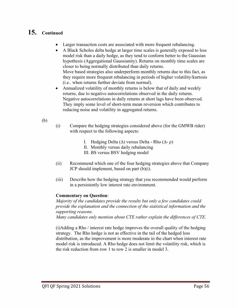
QFI QF Spring 2021 Solutions Page 56
15. Continued
• Larger transaction costs are associated with more frequent rebalancing. • A Black Scholes delta hedge at larger time scales is generally exposed to less
model risk than a daily hedge, as they tend to conform better to the Gaussian hypothesis (Aggregational Gaussianity). Returns on monthly time scales are closer to being normally distributed than daily returns. Move based strategies also underperform monthly returns due to this fact, as they require more frequent rebalancing in periods of higher volatility/kurtosis (i.e.. when returns further deviate from normal).
• Annualized volatility of monthly returns is below that of daily and weekly returns, due to negative autocorrelations observed in the daily returns. Negative autocorrelations in daily returns at short lags have been observed. They imply some level of short-term mean reversion which contributes to reducing noise and volatility in aggregated returns.
(b) (i) Compare the hedging strategies considered above (for the GMWB rider)
with respect to the following aspects:
I. Hedging Delta (∆) versus Delta - Rho (∆- ρ) II. Monthly versus daily rebalancing III. BS versus BSV hedging model
(ii) Recommend which one of the four hedging strategies above that Company
JCP should implement, based on part (b)(i).
(iii) Describe how the hedging strategy that you recommended would perform in a persistently low interest rate environment.
Commentary on Question: Majority of the candidates provide the results but only a few candidates could provide the explanation and the connection of the statistical information and the supporting reasons. Many candidates only mention about CTE rather explain the differences of CTE. (i)Adding a Rho / interest rate hedge improves the overall quality of the hedging strategy. The Rho hedge is not as effective in the tail of the hedged loss distribution, as the improvement is more moderate in the chart when interest rate model risk is introduced. A Rho hedge does not limit the volatility risk, which is the risk reduction from row 1 to row 2 is smaller in model 3.
QFI QF Spring 2021 Solutions Page 57
15. Continued More frequent rebalancing reduces hedging risk.v However, model risk reduces the benefit of hedging more frequently (Improvement in Model 3 is less than Model 1). vComputing hedging positions more frequently with the wrong model could lead to a larger accumulation of hedging errors. More frequent rebalancing also comes with higher monitoring and trading costs. Modeling interest rates stochastically does not have a definitive impact on hedging risk, as the impact is small and the direction is not consistent between financial market models. The table of hedged loss’ results indicates that there is a small impact of hedging using BSV model compared to using BS model. The inclusion of a rho hedge seems to be more important for a hedging program compared with the choice of a model for interest rates. (ii) I would recommend using a hedging strategy with a ∆- ρ hedge, rebalanced daily with an BS model. The rho hedge and daily rebalancing improved the hedging risk, which the BSV model did not have a definite improvement and added complexity to the model. (iii)Interest rates are currently very low, so they may either remain low or rise. Guarantee values will decrease if interest rates rise, which will result in a gain for the insurer if interest rate risk is not hedged. Hedging interest rate risk will benefit insurers if interest rates remain low, as they can be exposed to large hedging losses. Delta-Rho hedging strategies are not significantly impacted by the interest rate environment. Delta only hedging strategies may result in a gain for the insurer if interest rates rise, but it may result in a loss for the insurer if interest rates remain low.
(c) Define the two schools of thought regarding the calibration of the equity stochastic volatility parameter and their application to VA hedging programs.
Commentary on Question: Not many candidates could list the two schools of the thought regarding the calibration of the equity stochastic volatility parameter and their application to VA hedging programs. Partial marks are given to those who mention calibration, extract from data or similar arguments.
QFI QF Spring 2021 Solutions Page 58
15. Continued
Backward looking: Calibration based on Historical Data • Stable estimate over time and preferred approach for most companies
Forward Looking: Extracted from market data, such as implied volatility surface from vanilla options • Difficult to get the implied volatility as options over 2-3 years to maturity are
sold on the over-the-counter market (VA contracts are long) • Implied volatilities may not produce appropriate volatility inputs for hedging
VAs with non-vanilla features (i.e., GMWB) (d) Calculate the 1-year VIXt under the following stochastic differential equation:
• ( )3 2 v
t t v t tdv v dt v dWσ= − + • 1vλ = −
• , 0vtW t ≥ is a standard Brownian motion under the real-world measure
Commentary on Question: Very few candidates try the question. No candidate demonstrates the understanding that the risk neutral dynamics are needed to generate the values of the VIX.
The risk neutral dynamics are needed to generate the values of the VIX. Let λv(t, vt) represent the market price of risk process and assume Wt
v , t ≥ 0 is a risk neutral Brownian motion, where Wt
v = Wtv + ∫ λv(t, vt)
t0 ds. In the Heston model
λv(t, vt) = λvvtσv
, where λvis the volatility risk premium parameter. The risk neutral
dynamics are given by d𝑣𝑣𝑡𝑡 = κθ − 𝑣𝑣𝑡𝑡𝑑𝑑𝑡𝑡 + 𝜎𝜎𝑣𝑣𝑣𝑣𝑡𝑡𝑑𝑑𝑊𝑊𝑡𝑡𝑣𝑣 .
κ = κ + λ𝑣𝑣 = 3 − 1 = 2
θ =κθ
κ + λ𝑣𝑣=
3 ∗ 23 − 1
= 3
𝐴𝐴 = θ 1 −1 − 𝑒𝑒−κ
κ = 3 ∗ 1 −
1 − 𝑒𝑒−2
2 = 1.703003
𝐵𝐵 = 1 − 𝑒𝑒−κ
κ =
1 − 𝑒𝑒−2
2 = 0.4323324
1 − year VIXt = A + Bvt = 1.7 + 0.432vt