qDSA: Small and Secure Digital Signatureswith Curve-based Diffie–Hellman Key Pairs

Joost Renes1? and Benjamin Smith2

1 Digital Security Group, Radboud University, The Netherlandsj.renes@cs.ru.nl

2 INRIA and Laboratoire d’Informatique de l’École polytechnique (LIX),Université Paris–Saclay, Francesmith@lix.polytechnique.fr

Abstract. qDSA is a high-speed, high-security signature scheme that facilitates implementa-tions with a very small memory footprint, a crucial requirement for embedded systems andIoT devices, and that uses the same public keys as modern Diffie–Hellman schemes based onMontgomery curves (such as Curve25519) or Kummer surfaces. qDSA resembles an adaptationof EdDSA to the world of Kummer varieties, which are quotients of algebraic groups by ±1.Interestingly, qDSA does not require any full group operations or point recovery: all computa-tions, including signature verification, occur on the quotient where there is no group law. Weinclude details on four implementations of qDSA, using Montgomery and fast Kummer surfacearithmetic on the 8-bit AVR ATmega and 32-bit ARM Cortex M0 platforms. We find that qDSAsignificantly outperforms state-of-the-art signature implementations in terms of stack usage andcode size. We also include an efficient compression algorithm for points on fast Kummer surfaces,reducing them to the same size as compressed elliptic curve points for the same security level.Keywords. Signatures, Kummer, Curve25519, Diffie–Hellman, elliptic curve, hyperelliptic curve.

1 Introduction

Modern asymmetric cryptography based on elliptic and hyperelliptic curves [31, 33] achievestwo important goals. The first is efficient key exchange using the Diffie–Hellman protocol [18],using the fact that the (Jacobian of the) curve carries the structure of an abelian group. Butin fact, as Miller observed [33], we do not need the full group structure for Diffie–Hellman:the associated Kummer variety (the quotient by ±1) suffices, which permits more efficiently-computable arithmetic [23,34]. Perhaps the most well-known example is Curve25519 [6], whichoffers fast scalar multiplications based on x-only arithmetic.

The second objective is efficient digital signatures, which are critical for authentication.There are several group-based signature schemes, the most important of which are ECDSA [1],Schnorr [43], and now EdDSA [9] signatures. In contrast to the Diffie–Hellman protocol, all ofthese signature schemes explicitly require the group structure of the (Jacobian of the) curve.An unfortunate side-effect of this is that users essentially need two public keys to support bothcurve-based protocols. Further, basic cryptographic libraries need to provide implementationsfor arithmetic on both the Jacobian and the Kummer variety, thus complicating and increasingthe size of the trusted code base. For example, the NaCl library [10] uses Ed25519 [9] for sig-natures, and Curve25519 [6] for key exchange. This problem is worse for genus-2 hyperellipticcurves, where the Jacobian is significantly harder to use safely than its Kummer surface.

There have been several partial solutions to this problem. By observing that elements of theKummer variety are elements of the Jacobian up to sign, one can build scalar multiplication? This work has been supported by the Technology Foundation STW (project 13499 - TYPHOON & ASPA-SIA), from the Dutch government.

on the Jacobian based on the fast Kummer arithmetic [15, 37]. This avoids the need for aseparate scalar multiplication on the Jacobian, but does not avoid the need for its group law;it also introduces the need for projecting to and recovering from the Kummer. In any case, itdoes not solve the problem of having different public key types.

Another proposal is XEdDSA [38], which uses the public key on the Kummer variety toconstruct EdDSA signatures. In essence, it creates a key pair on the Jacobian by appendinga sign bit to the public key on the Kummer variety, which can then be used for signatures.In [25] Hamburg shows that one can actually verify signatures using only the x-coordinatesof points on an elliptic curve, which is applied in the recent STROBE framework [26]. Wegeneralize this approach to allow Kummer varieties of curves of higher genera, and naturallyadapt the scheme by only allowing challenges up to sign. This allows us to provide a proof ofsecurity, which has thus far not been attempted (in [25] Hamburg remarks that verifying upto sign does “probably not impact security at all”). Similar techniques have been applied forbatch verification of ECDSA signatures [30], using the theory of summation polynomials [44].

In this paper we show that there is no intrinsic reason why Kummer varieties cannot beused for signatures. We present qDSA, a signature scheme relying only on Kummer arithmetic,and prove it secure in the random oracle model. It should not be surprising that the reductionin our proof is slightly weaker than the standard proof of security of Schnorr signatures [39],but not by more than we should expect. There is no difference between public keys for qDSA andDiffie–Hellman. After an abstract presentation in §2, we give a detailed description of elliptic-curve qDSA instances in §3. We then move on to genus-2 instances based on fast Kummersurfaces, which give better performance. The necessary arithmetic appears in §4, before §5describes the new verification algorithm.

We also provide an efficient compression method for points on fast Kummer surfaces in §6,solving a long-standing open problem [7]. Our technique means that qDSA public keys for g = 2can be efficiently compressed to 32 bytes, and that qDSA signatures fit into 64 bytes; it alsofinally reduces the size of Kummer-based Diffie–Hellman public keys from 48 to 32 bytes.

Finally, we provide constant-time software implementations of genus-1 and genus-2 qDSAinstances for the AVR ATmega and ARM Cortex M0 platforms. The performance of all fourqDSA implementations, reported in §7, comfortably beats earlier implementations in terms ofstack usage and code size.

Source code. We place all of the software described here into the public domain, to maximizethe reusability of our results. The software is available at http://www.cs.ru.nl/~jrenes/.

2 The qDSA signature scheme

In this section we define qDSA, the quotient Digital Signature Algorithm. We start by recallingthe basics of Kummer varieties in §2.1 and defining key operations in §2.2. The rest of thesection is dedicated to the definition of the qDSA signature scheme, which is presented infull in Algorithm 1, and its proof of security, which follows Pointcheval and Stern [39, 40].qDSA closely resembles the Schnorr signature scheme [43], as it results from applying theFiat–Shamir heuristic [21] to an altered Schnorr identification protocol, together with a fewstandard changes as in EdDSA [9]. We comment on some special properties of qDSA in §2.5.

Remark 1. We note that although this section gives a theoretical proof of security, this does(of course) not imply security in a real-world implementation (eg. on an embedded system).

2

There are many attacks which the security model we assume does not include, for exampleattacks based on timing analysis, power analysis or (differential) faults. This is a very activeresearch area in the context of elliptic curves and many results immediately carry over toKummer varieties. However, in many circumstances the attacks and respective countermea-sures depend heavily on the instantiation of the signature scheme (eg. deploying constant-timefield arithmetic), as opposed to the scheme itself. We briefly comment on those in the sectiondedicated to our reference implementations, see Remark 3. Exceptions to this are the recentattacks on deterministic signatures, in particular on EdDSA [3,42], which also directly applyto qDSA. In contexts where these attacks apply, it may be necessary to include extra random-ness into the nonce generation (Line 8 of Algorithm 1) as proposed in [3, §4.2]. We emphasizethat the intent of this work is not to provide a signature scheme secure in all possible con-texts, but rather provide a basic signature scheme based on Kummer varieties analogous tothe group-based Schnorr and EdDSA signatures on which real-world protocols can be based.

Throughout, we work over finite fields Fp with p > 3. Our low-level algorithms include costsin terms of basic Fp-operations: M, S, C, a, s, I, and E denote the unit costs of computinga single multiplication, squaring, multiplication by a small constant, addition, subtraction,inverse, and square root, respectively.

2.1 The Kummer variety setting

Let C be a (hyper)elliptic curve and J its Jacobian3. The Jacobian is a commutative algebraicgroup with group operation +, inverse −, and identity 0. We assume J has a subgroup of largeprime order N . The associated Kummer variety K is the quotient K = J /±. By definition,working with K corresponds to working on J up to sign. If P is an element of J , we denoteits image in K by ±P . In this paper we take log2N ≈ 256, and consider two important cases.

Genus 1. Here J = C/Fp is an elliptic curve with log2 p ≈ 256, while K = P1 is the x-line.We choose C to be Curve25519 [6], which is the topic of §3.

Genus 2. Here J is the Jacobian of a genus-2 curve C/Fp, where log2 p ≈ 128, and K isa Kummer surface. We use the Gaudry–Schost parameters [24] for our implementations.Kummer arithmetic, including some new constructions we need for signature verificationand compression, is described in §4-6.

A point ±P in K(Fp) is the image of a pair of points {P,−P} on J . It is important tonote that P and −P are not necessarily in J (Fp); if not, then they are conjugate points inJ (Fp2), and correspond to points in J ′(Fp), where J ′ is the quadratic twist of J . Both Jand J ′ always have the same Kummer variety; we return to this fact, and its implications forour scheme, in §2.5 below.

2.2 Basic operations

While a Kummer variety K has no group law, the operation

{±P,±Q} 7→ {±(P +Q),±(P −Q)} (1)

3 In what follows, we could replace J by an arbitrary abelian group and all the proofs would be completelyanalogous. For simplicity we restrict to the cryptographically most interesting case of a Jacobian.

3

is well-defined. We can therefore define a pseudo-addition operation by

xADD : (±P,±Q,±(P −Q)) 7→ ±(P +Q).

The special case where ±(P − Q) = ±0 is the pseudo-doubling xDBL : ±P 7→ ±[2]P . In ourapplications we can often improve efficiency by combining two of these operations in a singlefunction

xDBLADD : (±P,±Q,±(P −Q)) 7−→ (±[2]P,±(P +Q)) .

For any integer m, the scalar multiplication [m] on J induces the key cryptographic operationof pseudomultiplication on K, defined by

Ladder : (m,±P ) 7−→ ±[m]P .

As its name suggests, we compute Ladder using Montgomery’s famous ladder algorithm [34],which is a uniform sequence of xDBLADDs and constant-time conditional swaps.4 This constant-time nature will be important for signing.

Our signature verification requires a function Check on K3 defined by

Check : (±P,±Q,±R) 7−→

{True if ±R ∈ {±(P +Q),±(P −Q)}False otherwise

Since we are working with projective points, we need a way to uniquely represent them.Moreover, we want this representation to be as small as possible, to minimize communicationoverhead. For this purpose we define the functions

Compress : K(Fp) −→ {0, 1}256 ,

writing ±P := Compress(±P ), and

Decompress : {0, 1}256 −→ K(Fp) ∪ {⊥}

such that Decompress(±P ) = ±P for ±P in K(Fp) and Decompress(X) = ⊥ for X ∈{0, 1}256 \ Im(Compress).

For the remainder of this section we assume that Ladder, Check, Compress, and Decompressare defined. Their implementation depends on whether we are in the genus 1 or 2 setting; wereturn to this in later sections.

2.3 The qID identification protocol

Let P be a generator of a prime order subgroup of J , of order N , and let ±P be its image inK. Let Z+

N denote the subset of ZN with zero least significant bit (where we identify elementsof ZN with their representatives in [0, N−1]). Note that since N is odd, LSB(−x) = 1−LSB(x)for all x ∈ Z∗N . The private key is an element d ∈ ZN . Let Q = [d]P and let the public key be±Q. Now consider the following Schnorr-style identification protocol, which we call qID:

(1) The prover sets r ←R Z∗N , ±R← ±[r]P and sends ±R to the verifier;(2) The verifier sets c←R Z+

N and sends c to the prover;4 In contemporary implementations such as NaCl, the Ladder function is sometimes namedcrypto_scalarmult.

4

(3) The prover sets s← (r − cd) mod N and sends s to the verifier;(4) The verifier accepts if and only if ±R ∈ {±([s]P + [c]Q),±([s]P − [c]Q)}.

There are some important differences between qID and the basic Schnorr identification protocolin [43].

Scalar multiplications on K. It is well-known that one can use K to perform the scalarmultiplication [15, 37] within a Schnorr identification or signature scheme, but with thisapproach one must always lift back to an element of a group. In contrast, in our schemethis recovery step is not necessary.

Verification on K. The original verification [43] requires checking that R = [s]P + [c]Q forsome R, [s]P, [c]Q ∈ J . Working on K, we only have these values up to sign (i. e. ±R,±[s]P and ±[c]Q), which is not enough to check that R = [s]P + [c]Q. Instead, we onlyverify that ±R = ± ([s]P ± [c]Q).

Challenge from Z+N . A Schnorr protocol using the weaker verification above would not sat-

isfy the special soundness property: the transcripts (±R, c, s) and (±R,−c, s) are bothvalid, and do not allow us to extract a witness. Choosing c from Z+

N instead of Z eliminatesthis possibility, and allows a security proof (this is the main difference with Hamburg’sSTROBE [26]).

Proposition 1. The qID identification protocol is a sigma protocol.

Proof. We prove the required properties (see [27, §6]).Completeness: If the protocol is followed, then r = s+cd, and therefore [r]P = [s]P+[c]Q

on J . Mapping to K, it follows that ±R = ±([s]P + [c]Q).Special soundness: Let (±R, c0, s0) and (±R, c1, s1) be two valid transcripts such that

c0 6= c1. By verification, each si ≡ ±r±cid (mod N), so s0±s1 ≡ (c0 ± c1) d (mod N), wherethe signs are chosen to cancel r. Now c0± c1 6≡ 0 (mod N) because c0 and c1 are both in Z+

N ,so we can extract a witness d ≡ (s0 ± s1) (c0 ± c1)−1 (mod N).

Honest-verifier zero-knowledge: A simulator S generates c←R Z+N and sets s←R ZN

and R← [s]P + [c]Q.5 If R = O, it restarts. It outputs (±R, c, s). As in [40, Lemma 5], we let

δ ={(±R, c, s) : c ∈R Z+

N , r ∈R Z∗N ,±R = ±[r]P , s = r − cd},

δ′ ={(±R, c, s) : c ∈R Z+

N , s ∈R ZN , R = [s]P + [c]Q ,R 6= O}

be the distributions of honest and simulated signatures, respectively. The elements of δ and δ′

are the same. First, consider δ. There are exactly N − 1 choices for r, and exactly (N + 1)/2for c; all of them lead to distinct tuples. There are thus (N2−1)/2 possible tuples, all of whichhave probability 2/(N2− 1) of occurring. Now consider δ′. Again, there are (N +1)/2 choicesfor c. We have N choices for s, exactly one of which leads to R = O. Thus, given c, there areN − 1 choices for s. We conclude that δ′ also contains (N2 − 1)/2 possible tuples, which allhave probability 2/(N2 − 1) of occurring. ut

2.4 Applying Fiat–Shamir

Applying the Fiat–Shamir transform [21] to qID yields a signature scheme qSIG. We will need ahash function H : {0, 1}∗ → Z+

N , which we define by taking a hash function H : {0, 1}∗ → ZN5 As we only know Q up to sign, we may need two attempts to construct S.

5

and then setting H by

H(M) 7−→

{H(M) if LSB(H(M)) = 0

−H(M) if LSB(H(M)) = 1.

The qSIG signature scheme is defined as follows:

(1) To sign a message M ∈ {0, 1}∗ with private key d ∈ ZN and public key ±Q ∈ K, theprover sets r ←R Z∗N , ±R ← ±[r]R, h ← H(±R || M), and s ← (r − hd) mod N , andsends (±R || s) to the verifier.

(2) To verify a signature (±R || s) ∈ K × ZN on a message M ∈ {0, 1}∗ with public key±Q ∈ K, the verifier sets h ← H(±R || M), ±T0 ← ±[s]P , and ±T1 ← ±[h]Q, andaccepts if and only if ±R ∈ {±(T0 + T1),±(T0 − T1)}.

Proposition 2 asserts that the security properties of qID carry over to qSIG.

Proposition 2. In the random oracle model, if an existential forgery of the qSIG signaturescheme under an adaptive chosen message attack has non-negligible probability of success, thenthe DLP in J can be solved in polynomial time.

Proof. This is the standard proof of applying the Fiat–Shamir transform to a sigma protocol:see [39, Theorem 13] or [40, §3.2]. ut

2.5 The qDSA signature scheme

Moving towards the real world, we slightly alter the qSIG protocol with some pragmaticchoices, following Bernstein et al. [9]:

(1) We replace the randomness r by the output of a pseudo-random function, which makesthe signatures deterministic.

(2) We include the public key ±Q in the generation of the challenge, to prevent attackers fromattacking multiple public keys at the same time.

(3) We compress and decompress points on K where necessary.

The resulting signature scheme, qDSA, is summarized in Algorithm 1.

Unified keys. Signatures are entirely computed and verified on K, which is also the nat-ural setting for Diffie–Hellman key exchange. We can therefore use identical key pairs forDiffie–Hellman and for qDSA signatures. This significantly simplifies the implementation ofcryptographic libraries, as we no longer need arithmetic for the two distinct objects J and K.Technically, there is no reason not to use a single key pair for both key exchange and signing;but one should be very careful in doing so, as using one key across multiple protocols couldpotentially lead to attacks. The primary interest of this aspect of qDSA is not necessarily inreducing the number of keys, but in unifying key formats and reducing the size of the trustedcode base.

Security level. The security reduction to the discrete logarithm problem is almost identical tothe case of Schnorr signatures [39]. Notably, the challenge space has about half the size (Z+

N

versus ZN ) while the proof of soundness computes either s0 + s1 or s0 − s1. This results in aslightly weaker reduction, as should be expected by moving from J to K and by weakeningverification. By choosing log2N ≈ 256 we obtain a scheme with about the same security levelas state-of-the-art schemes (eg. EdDSA combined with Ed25519). This could be made moreprecise (cf. [40]), but we do not provide this analysis here.

6

Algorithm 1: The qDSA signature scheme

1 function keypairInput: ()Output: (±Q || (d′ || d′′)): a compressed public key ±Q ∈ {0, 1}256 where ±Q ∈ K,

and a private key (d′ || d′′) ∈({0, 1}256

)22 d← Random({0, 1}256)3 (d′ || d′′)← H(d)

4 ±Q← Ladder(d′,±P ) // ±Q = ±[d′]P5 ±Q← Compress(±Q)

6 return (±Q || (d′ || d′′))

7 function signInput: d′, d′′ ∈ {0, 1}256, ±Q ∈ {0, 1}256, M ∈ {0, 1}∗

Output: (±R || s) ∈({0, 1}256

)28 r ← H(d′′ ||M)

9 ±R← Ladder(r,±P ) // ±R = ±[r]P10 ±R← Compress(±R)11 h← H(±R || ±Q ||M)

12 s← (r − hd′) mod N

13 return (±R || s)

14 function verifyInput: M ∈ {0, 1}∗, the compressed public key ±Q ∈ {0, 1}256, and a putative

signature (±R || s) ∈({0, 1}256

)2Output: True if (±R || s) is a valid signature on M under ±Q, False otherwise

15 ±Q← Decompress(±Q)

16 if ±Q = ⊥ then17 return False

18 h← H(±R || ±Q ||M)

19 ±T0 ← Ladder(s,±P ) // ±T0 = ±[s]P20 ±T1 ← Ladder(h,±Q) // ±T1 = ±[h]Q21 ±R← Decompress(±R)22 if ±R = ⊥ then23 return False

24 v ← Check(±T0,±T1,±R) // is ±R = ± (T0 ± T1)?25 return v

Key and signature sizes. Public keys fit into 32 bytes in both the genus 1 and genus 2 settings.This is standard for Montgomery curves; for Kummer surfaces it requires a new compressiontechnique, which we present in §6. In both cases log2N < 256, which means that signatures(±R || s) fit in 64 bytes.

Twist security. Rational points on K correspond to pairs of points on either J or its quadratictwist. As opposed to Diffie–Hellman, in qDSA scalar multiplications with secret scalars areonly performed on the public parameter ±P , which is chosen as the image of large primeorder element of J . Therefore J is not technically required to have a secure twist, unlikein the modern Diffie–Hellman setting. But if K is also used for key exchange (which is thewhole point!), then twist security is crucial. We therefore strongly recommend twist-secureparameters for qDSA implementations.

Hash function. The function H can be any hash function with at least a log2√N -bit security

level and at least 2 log2N -bit output. Throughout this paper we take H to be the extendableoutput function SHAKE128 [20] with fixed 512-bit output. This enables us to implicitly use Has a function mapping into either ZN ×{0, 1}256 (eg. Line 3 of Algorithm 1), ZN (eg. Line 8 ofAlgorithm 1), or Z+

N (eg. Line 11 of Algorithm 1, by combining it with a conditional negation)by appropriately reducing (part of) the output modulo N .

Signature compression. Schnorr mentions in [43] that signatures (R || s) may be compressedto (H(R || Q ||M) || s), taking only the first 128 bits of the hash, thus reducing signature sizefrom 64 to 48 bytes. This is possible because we can recompute R from P , Q, s, and H(R ||Q || M). However, on K we cannot recover ±R from ±P , ±Q, s, and H(±R || ±Q || M), soSchnorr’s compression technique is not an option for us.

Batching. Proposals for batch signature verification typically rely on the group structure,verifying random linear combinations of points [9, 35]. Since K has no group structure, thesebatching algorithms are not possible.

Scalar multiplication for verification. Instead of computing the full point [s]P + [c]Q with atwo-dimensional multiscalar multiplication operation, we have to compute ±[s]P and ±[c]Qseparately. As a result we are unable to use standard tricks for speeding up two-dimensionalscalar multiplications (eg. [22]), resulting in increased run-time. On the other hand, it hasthe benefit of relying on the already implemented Ladder function, mitigating the need fora separate algorithm, and is more memory-friendly. Our implementations show a significantdecrease in stack usage, at the cost of a small loss of speed (see §7).

3 Implementing qDSA with elliptic curves

Our first concrete instantiation of qDSA uses the Kummer variety of an elliptic curve, whichis just the x-line P1.

3.1 Montgomery curves

Consider the elliptic curve in Montgomery form

EAB/Fp : By2 = x(x2 +Ax+ 1) ,

8

where A2 6= 4 and B 6= 0. The map EAB → K = P1 defined by

P = (X : Y : Z) 7−→ ±P =

{(X : Z) if Z 6= 0

(1 : 0) if Z = 0

gives rise to efficient x-only arithmetic on P1 (see [34]). We use the Ladder specified in [19, Alg.1]. Compression uses Bernstein’s map

Compress : (X : Z) ∈ P1(Fp) 7−→ XZp−2 ∈ Fp ,

while decompression is the near-trivial

Decompress : x ∈ Fp 7−→ (x : 1) ∈ P1(Fp) .

Note that Decompress never returns ⊥, and that Decompress(Compress((X : Z))) = (X : Z)whenever Z 6= 0 (however, the points (0 : 1) and (1 : 0) should never appear as public keys orsignatures).

3.2 Signature verification

It remains to define the Check operation for Montgomery curves. In the final step of verificationwe are given±R,±P , and±Q in P1, and we need to check whether±R ∈ {±(P +Q),±(P −Q)}.Proposition 3 reduces this to checking a quadratic relation in the coordinates of ±R, ±P , and±Q.

Proposition 3. Writing (XP : ZP ) = ±P for P in EAB, etc.: If P , Q, and R are points onEAB, then ±R ∈

{±(P +Q),±(P −Q)

}if and only if

BZZ(XR)2 − 2BXZX

RZR +BXX(ZR)2 = 0 (2)

where

BXX =(XPXQ − ZPZQ

)2, (3)

BXZ =(XPXQ + ZPZQ

)(XPZQ + ZPXQ

)+ 2AXPZPXQZQ , (4)

BZZ =(XPZQ − ZPXQ

)2. (5)

Proof. Let S = (XS : ZS) = ±(P +Q) and D = (XD : ZD) = ±(P −Q). If we temporarilyassume ±0 6= ±P 6= ±Q 6= ±0 and put xP = XP /ZP , etc., then the group law on EAB givesus xSxD = (xPxQ − 1)2/(xP − xQ)2 and xS + xD = 2((xPxQ + 1)(xP + xQ) + 2AxPxQ).Homogenizing, we obtain(

XSXD : XSZD + ZSXD : ZSZD)= (λBXX : λ2BXZ : λBZZ) . (6)

One readily verifies that Equation (6) still holds even when the temporary assumption doesnot (that is, when ±P = ±Q or ±P = ±0 or ±Q = ±0). Having degree 2, the homogeneouspolynomial BZZX2 −BXZXZ +BXXZ

2 cuts out two points in P1 (which may coincide); byEquation (6), they are ±(P +Q) and ±(P −Q), so if (XR : ZR) satisfies Equation (2) thenit must be one of them. ut

9

Algorithm 2: Checking the verification relation for P1

1 function CheckInput: ±P , ±Q, ±R = (x : 1) in P1 images of points of EAB(Fp)Output: True if ±R ∈ {±(P +Q),±(P −Q)}, False otherwiseCost: 8M+ 3S+ 1C+ 8a+ 4s

2 (BXX , BXZ , BZZ)← BValues(±P,±Q)

3 if BXXx2 −BXZx+BZZ = 0 then return True4 else return False

5 function BValuesInput: ±P = (XP : ZP ), ±Q = (XQ : ZQ) in K(Fp)Output: (BXX(±P,±Q), BXZ(±P,±Q), BZZ(±P,±Q)) in F3

p

Cost: 6M+ 2S+ 1C+ 7a+ 3s

// See Algorithm 8 and Proposition 3

3.3 Using cryptographic parameters

We use the elliptic curve E/Fp : y2 = x3 + 486662x2 + x where p = 2255 − 19, which iscommonly referred to as Curve25519 [6]. Let P ∈ E(Fp) be such that ±P = (9 : 1). Then Phas order 8N , where

N = 2252 + 27742317777372353535851937790883648493

is prime. The xDBLADD operation requires us to store (A+ 2)/4 = 121666, and we implementoptimized multiplication by this constant. In [6, §3] Bernstein sets and clears some bits of theprivate key, also referred to as “clamping”. This is not necessary in qDSA, but we do it anywayin keypair for compatibility.

4 Implementing qDSA with Kummer surfaces

A number of cryptographic protocols that have been successfully implemented with Mont-gomery curves have seen substantial practical improvements when the curves are replacedwith Kummer surfaces. From a general point of view, a Kummer surface is the quotient ofsome genus-2 Jacobian J by ±1; geometrically it is a surface in P3 with sixteen point singu-larities, called nodes, which are the images in K of the 2-torsion points of J (since these areprecisely the points fixed by −1). From a cryptographic point of view, a Kummer surface isjust a 2-dimensional analogue of the x-coordinate used in Montgomery curve arithmetic.

The algorithmic and software aspects of efficient Kummer surface arithmetic have alreadybeen covered in great detail elsewhere (see eg. [23], [8], and [41]). Indeed, the Kummer scalarmultiplication algorithms and software that we use in our signature implementation are iden-tical to those described in [41], and use the cryptographic parameters proposed by Gaudryand Schost [24].

This work includes two entirely new Kummer algorithms that are essential for our signaturescheme: verification relation testing (Check, Algorithm 3) and compression/decompression(Compress and Decompress, Algorithms 4 and 5). Both of these new techniques require a fair

10

amount of technical development, which we begin in this section by recalling the basic Kummerequation and constants, and deconstructing the pseudo-doubling operation into a sequence ofsurfaces and maps that will play important roles later. Once the scene has been set, we willdescribe our signature verification algorithm in §5 and our point compression scheme in §6.The reader primarily interested in the resulting performance improvements may wish to skipdirectly to §7 on first reading.

The Check, Compress, and Decompress algorithms defined below require the followingsubroutines:

– Mul4 implements a 4-way parallel multiplication. It takes a pair of vectors (x1, x2, x3, x4)and (y1, y2, y3, y4) in F4

p, and returns (x1y1, x2y2, x3y3, x4y4).– Sqr4 implements a 4-way parallel squaring. Given a vector (x1, x2, x3, x4) in F4

p, it returns(x21, x

22, x

23, x

24).

– Had implements a Hadamard transform. Given a vector (x1, x2, x3, x4) in F4p, it returns

(x1 + x2 + x3 + x4, x1 + x2 − x3 − x4, x1 − x2 + x3 − x4, x1 − x2 − x3 + x4).– Dot computes the sum of a 4-way multiplication. Given a pair of vectors (x1, x2, x3, x4)

and (y1, y2, y3, y4) in F4p, it returns x1y1 + x2y2 + x3y3 + x4y4.

4.1 Constants

Our Kummer surfaces are defined by four fundamental constants α1, α2, α3, α4 and four dualconstants α1, α2, α3, and α4, which are related by

2α21 = α2

1 + α22 + α2

3 + α24 ,

2α22 = α2

1 + α22 − α2

3 − α24 ,

2α23 = α2

1 − α22 + α2

3 − α24 ,

2α24 = α2

1 − α22 − α2

3 + α24 .

We require all of the αi and αi to be nonzero. The fundamental constants determine the dualconstants up to sign, and vice versa. These relations remain true when we exchange the αiwith the αi; we call this “swapping x with x” operation “dualizing”. To make the symmetry inwhat follows clear, we define

µ1 := α21 , ε1 := µ2µ3µ4 , κ1 := ε1 + ε2 + ε3 + ε4 ,

µ2 := α22 , ε2 := µ1µ3µ4 , κ2 := ε1 + ε2 − ε3 − ε4 ,

µ3 := α23 , ε3 := µ1µ2µ4 , κ3 := ε1 − ε2 + ε3 − ε4 ,

µ4 := α24 , ε4 := µ1µ2µ3 , κ4 := ε1 − ε2 − ε3 + ε4 ,

along with their respective duals µi, εi, and κi. Note that

(ε1 : ε2 : ε3 : ε4) = (1/µ1 : 1/µ2 : 1/µ3 : 1/µ4)

and µiµj −µkµl = µiµj − µkµl for {i, j, k, l} = {1, 2, 3, 4}. There are many clashing notationalconventions for theta constants in the cryptographic Kummer literature; Table 1 provides adictionary for converting between them.

Our applications use only the squared constants µi and µi, so only they need be in Fp. Inpractice we want them to be as “small” as possible, both to reduce the cost of multiplying by

11

them and to reduce the cost of storing them. In fact, it follows from their definition that itis much easier to find simultaneously small µi and µi than it is to find simultaneously smallαi and αi (or a mixture of the two); this is ultimately why we prefer the squared surface forscalar multiplication. We note that if the µi are very small, then the εi and κi are also small,and the same goes for their duals. While we will never actually compute with the unsquaredconstants, we need them to explain what is happening in the background below.

Finally, the Kummer surface equations involve some derived constants

E :=16α1α2α3α4µ1µ2µ3µ4

(µ1µ4 − µ2µ3)(µ1µ3 − µ2µ4)(µ1µ2 − µ3µ4),

F := 2µ1µ4 + µ2µ3µ1µ4 − µ2µ3

, G := 2µ1µ3 + µ2µ4µ1µ3 − µ2µ4

, H := 2µ1µ2 + µ3µ4µ1µ2 − µ3µ4

,

and their duals E, F , G, H. We observe that E2 = F 2 + G2 + H2 + FGH − 4 and E2 =F 2 + G2 + H2 + F GH − 4.

Source Fundamental constants Dual constants[23] and [8] (a :b :c :d) = (α1 :α2 :α3 :α4) (A :B :C :D) = (α1 : α2 : α3 : α4)

[12] (a :b :c :d) = (α1 :α2 :α3 :α4) (A :B :C :D) = (µ1 : µ2 : µ3 : µ4)

[41] (a :b :c :d) = (µ1 :µ2 :µ3 :µ4) (A :B :C :D) = (µ1 : µ2 : µ3 : µ4)

[17] (α :β :γ :δ) = (µ1 :µ2 :µ3 :µ4) (A :B :C :D) = (µ1 : µ2 : µ3 : µ4)Table 1. Relations between our theta constants and others in selected related work

4.2 Fast Kummer surfaces

We compute all of the pseudoscalar multiplications in qDSA on the so-called squared Kum-mer surface

KSqr : 4E2 ·X1X2X3X4 =

(X2

1 +X22 +X2

3 +X24 − F (X1X4 +X2X3)

−G(X1X3 +X2X4)−H(X1X2 +X3X4)

)2

,

which was proposed for factorization algorithms by the Chudnovskys [14], then later for Diffie–Hellman by Bernstein [7]. Since E only appears as a square, KSqr is defined over Fp. The zeropoint on KSqr is ±0 = (µ1 : µ2 : µ3 : µ4). In our implementations we used the xDBLADD andMontgomery ladder exactly as they were presented in [41, Algorithms 6-7] (see also Algo-rithm 9). The pseudo-doubling xDBL on KSqr is

±P =(XP

1 : XP2 : XP

3 : XP4

)7−→

(X

[2]P1 : X

[2]P2 : X

[2]P3 : X

[2]P4

)= ±[2]P

where

X[2]P1 = ε1(U1 + U2 + U3 + U4)

2 , U1 = ε1(XP1 +XP

2 +XP3 +XP

4 )2 , (7)

X[2]P2 = ε2(U1 + U2 − U3 − U4)

2 , U2 = ε2(XP1 +XP

2 −XP3 −XP

4 )2 , (8)

X[2]P3 = ε3(U1 − U2 + U3 − U4)

2 , U3 = ε3(XP1 −XP

2 +XP3 −XP

4 )2 , (9)

X[2]P4 = ε4(U1 − U2 − U3 + U4)

2 , U4 = ε4(XP1 −XP

2 −XP3 +XP

4 )2 (10)

for ±P with all XPi 6= 0; more complicated formulæ exist for other ±P (cf. §5.1).

12

4.3 Deconstructing pseudo-doubling

Figure 1 deconstructs the pseudo-doubling on KSqr from §4.2 into a cycle of atomic mapsbetween different Kummer surfaces, which form a sort of hexagon. Starting at any one of

KCan S(2,2)

// KSqr

H∼= ##

KInt

C∼=

;;

KInt

C

∼=||

KSqrH

∼=bb

KCan

S

(2,2)oo

Fig. 1. Decomposition of pseudo-doubling on fast Kummer surfaces into a cycle of morphisms. Here, KSqr

is the “squared” surface we mostly compute with; KCan is the related “canonical” surface; and KInt is a new“intermediate” surface which we use in signature verification. (The surfaces KSqr, KCan, and KInt are theirduals.)

the Kummers and doing a complete cycle of these maps carries out pseudo-doubling on thatKummer. Doing a half-cycle from a given Kummer around to its dual computes a (2, 2)-isogenysplitting pseudo-doubling.

Six different Kummer surfaces may seem like a lot to keep track of—even if there are reallyonly three, together with their duals. However, the new surfaces are important, because theyare crucial in deriving our Check routine (of course, once the algorithm has been written down,the reader is free to forget about the existence of these other surfaces).

The cycle actually begins one step before KSqr, with the canonical surface

KCan : 2E · T1T2T3T4 =T 41 + T 4

2 + T 43 + T 4

4 − F (T 21 T

24 + T 2

2 T23 )

−G(T 21 T

23 + T 2

2 T24 )−H(T 2

1 T22 + T 2

3 T24 ) .

This was the model proposed for cryptographic applications by Gaudry in [23]; we call it“canonical” because it is the model arising from a canonical basis of theta functions of level(2, 2).

Now we can begin our tour around the hexagon, moving from KCan to KSqr via the squar-ing map

S :(T1 : T2 : T3 : T4

)7−→

(X1 : X2 : X3 : X4

)=(T 21 : T 2

2 : T 23 : T 3

4

),

which corresponds to a (2, 2)-isogeny of Jacobians. Moving on from KSqr, the Hadamardtransform isomorphism

H : (X1 : X2 : X3 : X4) 7−→ (Y1 : Y2 : Y3 : Y4) =

X1 +X2 +X3 +X4

: X1 +X2 −X3 −X4

: X1 −X2 +X3 −X4

: X1 −X2 −X3 +X4

13

takes us into a third kind of Kummer, which we call the intermediate surface:

KInt :2E

α1α2α3α4· Y1Y2Y3Y4 =

Y 41

µ21+

Y 42

µ22+

Y 43

µ23+

Y 44

µ24− F

(Y 21µ1

Y 24µ4

+Y 22µ2

Y 23µ3

)− G

(Y 21µ1

Y 23µ3

+Y 22µ2

Y 24µ4

)− H

(Y 21µ1

Y 22µ2

+Y 23µ3

Y 24µ4

).

We will use KInt for signature verification. Now the dual scaling isomorphism

C :(Y1 : Y2 : Y3 : Y4

)7−→

(T1 : T2 : T3 : T4

)=(Y1/α1 : Y2/α2 : Y3/α3 : Y4/α4

)takes us into the dual canonical surface

KCan : 2E · T1T2T3T4 =T 41 + T 4

2 + T 43 + T 4

4 − F (T 21 T

24 + T 2

2 T23 )

− G(T 21 T

23 + T 2

2 T24 )− H(T 2

1 T22 + T 2

3 T24 ) .

We are now halfway around the hexagon; the return journey is simply the dual of the outboundtrip. The dual squaring map

S :(T1 : T2 : T3 : T4

)7−→

(X1 : X2 : X3 : X4

)=(T 21 : T 2

2 : T 23 : T 3

4

),

another (2, 2)-isogeny, carries us into the dual squared surface

KSqr : 4E2 · X1X2X3X4 =

(X2

1 + X22 + X2

3 + X24 − F (X1X4 + X2X3)

− G(X1X3 + X2X4)− H(X1X2 + X3X4)

)2

,

before the dual Hadamard transform

H :(X1 : X2 : X3 : X4

)7−→

(Y1 : Y2 : Y3 : Y4

)=

X1 + X2 + X3 + X4

: X1 + X2 − X3 − X4

: X1 − X2 + X3 − X4

: X1 − X2 − X3 + X4

takes us into the dual intermediate surface

KInt :2E

α1α2α3α4· Y1Y2Y3Y4 =

Y 41

µ21+

Y 42

µ22+

Y 43

µ23+

Y 44

µ24− F

(Y 21µ1

Y 24µ4− Y 2

2µ2

Y 23µ3

)− G

(Y 21µ1

Y 23µ3− Y 2

2µ2

Y 24µ4

)− H

(Y 21µ1

Y 22µ2− Y 2

3µ3

Y 24µ4

).

A final scaling isomorphism

C :(Y1 : Y2 : Y3 : Y4

)7−→

(T1 : T2 : T3 : T4

)=(Y1/α1 : Y2/α2 : Y3/α3 : Y4/α4

)takes us from KInt back to KCan, where we started.

The canonical surfacesKCan resp. KCan are only defined over Fp(α1α2α3α4) resp. Fp(α1α2α3α4),while the scaling isomorphisms C resp. C are defined over Fp(α1, α2, α3, α4) resp. Fp(α1, α2, α3, α4).Everything else is defined over Fp.

We confirm that one cycle around the hexagon, starting and ending on KSqr, computes thepseudo-doubling of Equations (7), (8), (9), and (10). Similarly, one cycle around the hexagonstarting and ending on KCan computes Gaudry’s pseudo-doubling from [23, §3.2].

14

5 Signature verification on Kummer surfaces

To verify signatures in the Kummer surface implementation, we need to supply a Checkalgorithm which, given ±P , ±Q, and ±R on KSqr, decides whether ±R ∈ {±(P +Q),±(P −Q)}. For the elliptic version of qDSA described in §3, we saw that this came down to checkingthat ±R satisfied one quadratic relation whose three coefficients were biquadratic forms in±P and ±Q. The same principle extends to Kummer surfaces, where the pseudo-group law issimilarly defined by biquadratic forms; but since Kummer surfaces are defined in terms of fourcoordinates (as opposed to the two coordinates of the x-line), this time there are six simplequadratic relations to verify, with a total of ten coefficient forms.

5.1 Biquadratic forms and pseudo-addition

Let K be a Kummer surface. If ±P is a point on K, then we write (ZP1 : ZP2 : ZP3 : ZP4 )for its projective coordinates. The classical theory of abelian varieties tells us that there existbiquadratic forms Bij for 1 ≤ i, j ≤ 4 such that for all ±P and ±Q, if ±S = ±(P + Q) and±D = ±(P −Q) then

(ZSi Z

Dj + ZSj Z

Di

)4i,j=1

= λ(Bij(Z

P1 , Z

P2 , Z

P3 , Z

P4 , Z

Q1 , Z

Q2 , Z

Q3 , Z

Q4 ))4i,j=1

(11)

where λ ∈ k× is some common projective factor depending only on the affine representativeschosen for ±P , ±Q, ±(P +Q) and ±(P −Q). These biquadratic forms are the foundation ofpseudo-addition and doubling laws on K: if the “difference” ±D is known, then we can use theBij to compute ±S.

Proposition 4. Let {Bij : 1 ≤ i, j ≤ 4} be a set of biquadratic forms on K × K satisfyingEquation (11) for all ±P , ±Q, ±(P +Q), and ±(P −Q). Then

±R = (ZR1 : ZR2 : ZR3 : ZR4 ) ∈ {±(P +Q),±(P −Q)}

if and only if (writing Bij for Bij(ZP1 , . . . , ZQ4 )) we have

Bjj · (ZRi )2 − 2Bij · ZRi ZRj +Bii · (ZRj )2 = 0 for all 1 ≤ i < j ≤ 4 . (12)

Proof. Looking at Equation (11), we see that the system of six quadratics from Equation (12)cuts out a zero-dimensional degree-2 subscheme of K: that is, the pair of points {±(P +Q),±(P −Q)} (which may coincide). Hence, if (ZR1 : ZR2 : ZR3 : ZR4 ) = ±R satisfies all of theequations, then it must be one of them. ut

5.2 Deriving efficiently computable forms

Proposition 4 is the exact analogue of Proposition 3 for Kummer surfaces. All that we need toturn it into a Check algorithm for qDSA is an explicit and efficiently computable representationof the Bij . These forms depend on the projective model of the Kummer surface; so we writeBCanij , BSqr

ij , and BIntij for the forms on the canonical, squared, and intermediate surfaces.

15

On the canonical surface, the forms BCanij are classical (see e.g. [4, §2.2]). The on-diagonal

forms BCanii are

BCan11 =

1

4

(V1µ1

+V2µ2

+V3µ3

+V4µ4

), BCan

22 =1

4

(V1µ1

+V2µ2− V3µ3− V4µ4

), (13)

BCan33 =

1

4

(V1µ1− V2µ2

+V3µ3− V4µ4

), BCan

44 =1

4

(V1µ1− V2µ2− V3µ3

+V4µ4

), (14)

where

V1 =((TP1 )2 + (TP2 )2 + (TP3 )2 + (TP4 )2

)((TQ1 )2 + (TQ2 )2 + (TQ3 )2 + (TQ4 )2

),

V2 =((TP1 )2 + (TP2 )2 − (TP3 )2 − (TP4 )2

)((TQ1 )2 + (TQ2 )2 − (TQ3 )2 − (TQ4 )2

),

V3 =((TP1 )2 − (TP2 )2 + (TP3 )2 − (TP4 )2

)((TQ1 )2 − (TQ2 )2 + (TQ3 )2 − (TQ4 )2

),

V4 =((TP1 )2 − (TP2 )2 − (TP3 )2 + (TP4 )2

)((TQ1 )2 − (TQ2 )2 − (TQ3 )2 + (TQ4 )2

),

while the off-diagonal forms Bij with i 6= j are

BCanij =

2

µiµj − µkµl

(αiαj

(TPi T

Pj T

Qi T

Qj + TPk T

Pl T

Qk T

Ql

)− αkαl

(TPi T

Pj T

Qk T

Ql + TPk T

Pl T

Qi T

Qj

)) (15)

where {i, j, k, l} = {1, 2, 3, 4}.All of these forms can be efficiently evaluated. The off-diagonal BCan

ij have a particularlycompact shape, while the symmetry of the on-diagonal BCan

ii makes them particularly easy tocompute simultaneously: indeed, that is exactly what we do in Gaudry’s fast pseudo-additionalgorithm for KCan [23, §3.2].

Ideally, we would like to evaluate the BSqrij on KSqr, since that is where our inputs ±P ,

±Q, and ±R live. We can compute the BSqrij by dualizing the BCan

ij , then pulling the BCanij on

KCan back to KSqr via C ◦H. But while the resulting on-diagonal BSqrii maintain the symmetry

and efficiency of the BCanii ,6 the off-diagonal BSqr

ij turn out to be much less pleasant, withless apparent exploitable symmetry. For our applications, this means that evaluating BSqr

ij fori 6= j implies taking a significant hit in terms of stack and code size, not to mention time.

We could avoid this difficulty by mapping the inputs of Check from KSqr into KCan, andthen evaluating the BCan

ij . But this would involve using—and, therefore, storing—the fourlarge unsquared αi, which is an important drawback.

Why do the nice BCanij become so ugly when pulled back to KSqr? The map C : KInt → KCan

has no impact on the shape or number of monomials, so most of the ugliness is due to theHadamard transform H : KSqr → KInt. In particular, if we only pull back the BCan

ij as far asKInt, then the resulting BInt

ij retain the nice form of the BCanij but do not involve the αi. This

fact prompts our solution: we map ±P , ±Q, and ±R through H onto KInt, and verify usingthe forms BInt

ij .

6 As they should, since they are the basis of the efficient pseudo-addition on KSqr!

16

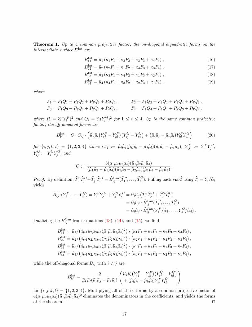
Theorem 1. Up to a common projective factor, the on-diagonal biquadratic forms on theintermediate surface KInt are

BInt11 = µ1 (κ1F1 + κ2F2 + κ3F3 + κ4F4) , (16)

BInt22 = µ2 (κ2F1 + κ1F2 + κ4F3 + κ3F4) , (17)

BInt33 = µ3 (κ3F1 + κ4F2 + κ1F3 + κ2F4) , (18)

BInt44 = µ4 (κ4F1 + κ3F2 + κ2F3 + κ1F4) , (19)

where

F1 = P1Q1 + P2Q2 + P3Q3 + P4Q4 , F2 = P1Q2 + P2Q1 + P3Q4 + P4Q3 ,

F3 = P1Q3 + P3Q1 + P2Q4 + P4Q2 , F4 = P1Q4 + P4Q1 + P2Q3 + P3Q2 ,

where Pi = εi(YPi )2 and Qi = εi(Y

Qi )2 for 1 ≤ i ≤ 4. Up to the same common projective

factor, the off-diagonal forms are

BIntij = C · Cij ·

(µkµl

(Y Pij − Y P

kl

)(Y Qij − Y

Qkl

)+(µiµj − µkµl

)Y Pkl Y

Qkl

)(20)

for {i, j, k, l} = {1, 2, 3, 4} where Cij := µiµj(µiµk − µjµl)(µiµl − µjµk), Y Pij := Y P

i YPj ,

Y Qij := Y Q

i YQj , and

C :=8(µ1µ2µ3µ4)(µ1µ2µ3µ4)

(µ1µ2 − µ3µ4)(µ1µ3 − µ2µ4)(µ1µ4 − µ2µ3).

Proof. By definition, TSi TDj +TSj T

Di = BCan

ij (TP1 , . . . , TQ4 ). Pulling back via C using Ti = Yi/αi

yields

BIntij (Y P

1 , . . . , YQ4 ) = Y S

i YDj + Y S

j YDi = αiαj

(TSi T

Dj + TSj T

Di

)= αiαj · BCan

ij (TP1 , . . . , TQ4 )

= αiαj · BCanij (Y P

1 /α1, . . . , YQ4 /α4) .

Dualizing the BCanij from Equations (13), (14), and (15), we find

BInt11 = µ1/

(4µ1µ2µ3µ4(µ1µ2µ3µ4)

2)·(κ1F1 + κ2F2 + κ3F3 + κ4F4

),

BInt22 = µ2/

(4µ1µ2µ3µ4(µ1µ2µ3µ4)

2)·(κ2F1 + κ1F2 + κ4F3 + κ3F4

),

BInt33 = µ3/

(4µ1µ2µ3µ4(µ1µ2µ3µ4)

2)·(κ3F1 + κ4F2 + κ1F3 + κ2F4

),

BInt44 = µ4/

(4µ1µ2µ3µ4(µ1µ2µ3µ4)

2)·(κ4F1 + κ3F2 + κ2F3 + κ1F4

),

while the off-diagonal forms Bij with i 6= j are

BIntij =

2

µkµl(µiµj − µkµl)

(µkµl

(Y Pij − Y P

kl

)(Y Qij − Y

Qkl

)+ (µiµj − µkµl)Y P

kl YQkl

)

for {i, j, k, l} = {1, 2, 3, 4}. Multiplying all of these forms by a common projective factor of4(µ1µ2µ3µ4)(µ1µ2µ3µ4)

2 eliminates the denominators in the coefficients, and yields the formsof the theorem. ut

17

5.3 Signature verification

We are now finally ready to implement the Check algorithm for KSqr. Algorithm 3 does thisby applying H to its inputs, then using the biquadratic forms of Theorem 1. Its correctness isimplied by Proposition 4.

Algorithm 3: Checking the verification relation for points on KSqr

1 function CheckInput: ±P , ±Q, ±R in KSqr(Fp)Output: True if ±R ∈ {±(P +Q),±(P −Q)}, False otherwiseCost: 76M+ 8S+ 88C+ 42a+ 42s

2 (YP ,YQ)← (Had(±P ), Had(±Q))

3 (B11,B22,B33,B44)← BiiValues(YP ,YQ)4 YR ← Had(±R)5 for (i, j) in {(1, 2), (1, 3), (1, 4), (2, 3), (2, 4), (3, 4)} do6 LHS← Bii · (YRj )2 + Bjj · (YRi )2

7 Bij ← BijValue(YP ,YQ, (i, j))8 RHS← 2Bij · YRi · YRj9 if LHS 6= RHS then

10 return False

11 return True

12 function BiiValuesInput: ±P , ±Q in KInt(Fp)Output: (BInt

ii (±P,±Q))4i=1 in F4p

Cost: 16M+ 8S+ 28C+ 24a

// See Algorithm 13 and Theorem 1

13 function BijValueInput: ±P , ±Q in KInt(Fp) and (i, j) with 1 ≤ i, j ≤ 4 and i 6= j

Output: BIntij (±P,±Q) in Fp

Cost: 10M+ 10C+ 1a+ 5s

// See Algorithm 12 and Theorem 1

5.4 Using cryptographic parameters

Gaudry and Schost take p = 2127 − 1 and (µ1 : µ2 : µ3 : µ4) = (−11 : 22 : 19 : 3) in [24]. Wealso need the constants (µ1 : µ2 : µ3 : µ4) = (−33 : 11 : 17 : 49), (κ1 : κ2 : κ3 : κ4) = (−4697 :5951 : 5753 : −1991), and (ε1 : ε2 : ε3 : ε4) = (−833 : 2499 : 1617 : 561).7 In practice, wherethese constants are “negative”, we reverse their sign and amend the formulæ above accordingly.7 Following the definitions of §4.1, the µi are scaled by −2, the εi by 1/11, and C by 2/112. These changesinfluence the BInt

ij , but only up to the same projective factor.

18

All of these constants are small, and fit into one or two bytes each (and the εi are alreadystored for use in Ladder). We store one large constant

C = 0x40F50EEFA320A2DD46F7E3D8CDDDA843,

and recompute the Cij on the fly.

6 Kummer point compression

Our public keys are points on KSqr, and each signature includes one point on KSqr. Minimizingthe space required by Kummer points is therefore essential.

A projective Kummer point is composed of four field elements; normalizing by dividingthrough by a nonzero coordinate reduces us to three field elements (this can also be achievedusing Bernstein’s “wrapping” technique [7], as in [8] and [41]). But we are talking about Kum-mer surfaces—two-dimensional objects—so we might hope to compress to two field elements,plus a few bits to enable us to correctly recover the whole Kummer point. This is analogousto elliptic curve point compression, where we compress projective points (X : Y : Z) by nor-malizing to (x, y) = (X/Z, Y/Z), then storing (x, σ), where σ is a bit indicating the “sign” ofy. Decompressing the datum (x, σ) to (X : Y : Z) = (x : y : 1) then requires solving a simplequadratic to recover the correct y-coordinate.

For some reason, no such Kummer point compression method has explicitly appeared inthe literature. Bernstein remarked in 2006 that if we compress a Kummer point to two co-ordinates, then decompression appears to require solving a complicated quartic equation [7].This would be much more expensive than computing the single square root required for ellip-tic decompression; this has perhaps discouraged implementers from attempting to compressKummer points.

But while it may not always be obvious from their defining equations, the classical theorytells us that every Kummer is in fact a double cover of P2, just as elliptic curves are doublecovers of P1. We use this principle below to show that we can always compress any Kummerpoint to two field elements plus two auxiliary bits, and then decompress by solving a quadratic.In our applications, this gives us a convenient packaging of Kummer points in exactly 256 bits.

6.1 The general principle

First, we sketch a general method for Kummer point compression that works for any Kummerpresented as a singular quartic surface in P3.

Recall that if N is any point in P3, then projection away from N defines a map πN : P3 →P2 sending points in P3 on the same line through N to the same point in P2. (The map πNis only a rational map, and not a morphism; the image of N itself is not well-defined.) Now,let N be a node of a Kummer surface K: that is, N is one of the 16 singular points of K. Therestriction of πN to K forms a double cover of P2. By definition, πN maps the points on Kthat lie on the same line through N to the same point of P2. Now K has degree 4, so eachline in P3 intersects K in four points; but since N is a double point of K, every line throughN intersects K at N twice, and then in two other points. These two remaining points maybe “compressed” to their common image in P2 under πN , plus a single bit to distinguish theappropriate preimage.

19

To make this more concrete, let L1, L2, and L3 be linearly independent linear forms onP3 vanishing on N ; then N is the intersection of the three planes in P3 cut out by the Li. Wecan now realise the projection πN : K → P2 as

πN : (P1 : · · · : P4) 7−→(L1(P1, . . . , P4) : L2(P1, . . . , P4) : L3(P1, . . . , P4)

).

Replacing (L1, L2, L3) with another basis of 〈L1, L2, L3〉 yields another projection, which cor-responds to composing πN with a linear automorphism of P2.

If L1, L2, and L3 are chosen as above to vanish on N , and L4 is any linear form not in〈L1, L2, L3〉, then the fact that πN is a double cover of the (L1, L2, L3)-plane implies that thedefining equation of K can be rewritten in the form

K : K2(L1, L2, L3)L24 − 2K3(L1, L2, L3)L4 +K4(L1, L2, L3) = 0

where eachKi is a homogeneous polynomial of degree i in L1, L2, and L3. This form, quadraticin L4, allows us to replace the L4-coordinate with a single bit indicating the “sign” in thecorresponding root of this quadratic; the remaining three coordinates can be normalized to anaffine plane point. The net result is a compression to two field elements, plus one bit indicatingthe normalization, plus another bit to indicate the correct value of L4.

Remark 2. Stahlke gives a compression algorithm in [45] for points on genus-2 Jacobians inthe usual Mumford representation. The first step can be seen as a projection to the mostgeneral model of the Kummer (as in [13, Chapter 3]), and then the second is an implicitimplementation of the principle above.

6.2 From squared Kummers to tetragonal Kummers

We want to define an efficient point compression scheme for KSqr. The general principle abovemakes this possible, but it leaves open the choice of node N and the choice of forms Li. Thesechoices determine the complexity of the resulting Ki, and hence the cost of evaluating them;this in turn has a non-negligible impact on the time and space required to compress anddecompress points, as well as the number of new auxiliary constants that must be stored.

In this section we define a choice of Li reflecting the special symmetry of KSqr. A similarprocedure for KCan appears in more classical language8 in [28, §54]. The trick is to distinguishnot one node of KSqr, but rather the four nodes forming the kernel of the (2, 2)-isogenyS ◦ C ◦ H : KSqr → KSqr, namely

±0 = N0 = (µ1 : µ2 : µ3 : µ4) , N1 = (µ2 : µ1 : µ4 : µ3) ,

N2 = (µ3 : µ4 : µ1 : µ2) , N3 = (µ4 : µ3 : µ2 : µ1) .

We are going to define a coordinate system where these four nodes become the vertices of acoordinate tetrahedron; then, projection onto any three of the four coordinates will represent aprojection away from one of these four nodes. The result will be an isomorphic Kummer KTet

whose defining equation is quadratic in all four of its variables. This might seem like overkill8 The analogous model of KCan in [28, §54] is called “the equation referred to a Rosenhain tetrad”, whose defin-ing equation “...may be deduced from the fact that Kummer’s surface is the focal surface of the congruenceof rays common to a tetrahedral complex and a linear complex.” Modern cryptographers will understandwhy we have chosen to give a little more algebraic detail here.

20

for point compression—quadratic in just one variable would suffice—but it has the agreeableeffect of dramatically reducing the overall complexity of the defining equation, saving timeand memory in our compression and decompression algorithms.

The key is the matrix identityκ4 κ3 κ2 κ1

κ3 κ4 κ1 κ2

κ2 κ1 κ4 κ3

κ1 κ2 κ3 κ4

µ1 µ2 µ3 µ4

µ2 µ1 µ4 µ3

µ3 µ4 µ1 µ2

µ4 µ3 µ2 µ1

= 8µ1µ2µ3µ4

0 0 0 1

0 0 1 0

0 1 0 0

1 0 0 0

, (21)

which tells us that the projective isomorphism T : P3 → P3 defined by

T :

X1

: X2

: X3

: X4

7→

L1

: L2

: L3

: L4

=

κ4X1 + κ3X2 + κ2X3 + κ1X4

: κ3X1 + κ4X2 + κ1X3 + κ2X4

: κ2X1 + κ1X2 + κ4X3 + κ3X4

: κ1X1 + κ2X2 + κ3X3 + κ4X4

maps the four “kernel” nodes to the corners of a coordinate tetrahedron:

T (N0) = (0 : 0 : 0 : 1) , T (N2) = (0 : 1 : 0 : 0) ,

T (N1) = (0 : 0 : 1 : 0) , T (N3) = (1 : 0 : 0 : 0) .

The image of KSqr under T is the tetragonal surface

KTet : 4tL1L2L3L4 =

r21(L1L2 + L3L4)2 + r22(L1L3 + L2L4)

2 + r23(L1L4 + L2L3)2

− 2r1s1((L21 + L2

2)L3L4 + L1L2(L23 + L2

4))

− 2r2s2((L21 + L2

3)L2L4 + L1L3(L22 + L2

4))

− 2r3s3((L21 + L2

4)L2L3 + L1L4(L22 + L2

3))

where t = 16µ1µ2µ3µ4µ1µ2µ3µ4 and

r1 = (µ1µ3 − µ2µ4)(µ1µ4 − µ2µ3) , s1 = (µ1µ2 − µ3µ4)(µ1µ2 + µ3µ4) ,

r2 = (µ1µ2 − µ3µ4)(µ1µ4 − µ2µ3) , s2 = (µ1µ3 − µ2µ4)(µ1µ3 + µ2µ4) ,

r3 = (µ1µ2 − µ3µ4)(µ1µ3 − µ2µ4) , s3 = (µ1µ4 − µ2µ3)(µ1µ4 + µ2µ3) .

As promised, the defining equation of KTet is quadratic in all four of its variables.For compression we project away from T (±0) = (0 : 0 : 0 : 1) onto the (L1 : L2 : L3)-plane.

Rewriting the defining equation as a quadratic in L4 gives

KTet : K4(L1, L2, L3)− 2K3(L1, L2, L3)L4 +K2(L1, L2, L3)L24 = 0

where

K2 := r23L21 + r22L

22 + r21L

23 − 2 (r3s3L2L3 + r2s2L1L3 + r1s1L1L2) ,

K3 := r1s1(L21 + L2

2)L3 + r2s2(L21 + L2

3)L2 + r3s3(L22 + L2

3)L1

+ (2t− (r21 + r22 + r23))L1L2L3 ,

K4 := r23L22L

23 + r22L

21L

23 + r21L

21L

22 − 2 (r3s3L1 + r2s2L2 + r1s1L3)L1L2L3 .

21

Lemma 1. If (l1 : l2 : l3 : l4) is a point on KTet, then

K2(l1, l2, l3) = K3(l1, l2, l3) = K4(l1, l2, l3) = 0 ⇐⇒ l1 = l2 = l3 = 0 .

Proof. Write ki for Ki(l1, l2, l3). If (l1, l2, l3) = 0 then (k2, k3, k4) = 0, because each Ki isnonconstant and homogeneous. Conversely, if (k2, k3, k4) = 0 and (l1, l2, l3) 6= 0 then we couldembed a line in KTet via λ 7→ (l1 : l2 : l3 : λ); but this is a contradiction, because KTet containsno lines. ut

6.3 Compression and decompression for KSqr

In practice, we compress points on KSqr to tuples (l1, l2, τ, σ), where l1 and l2 are field elementsand τ and σ are bits. The recipe is

(1) Map (X1 : X2 : X3 : X4) through T to a point (L1 : L2 : L3 : L4) on KTet.(2) Compute the unique (l1, l2, l3, l4) in one of the forms (∗, ∗, 1, ∗), (∗, 1, 0, ∗), (1, 0, 0, ∗), or

(0, 0, 0, 1) such that (l1 : l2 : l3 : l4) = (L1 : L2 : L3 : L4).(3) Compute k2 = K2(l1, l2, l3), k3 = K3(l1, l2, l3), and k4 = K4(l1, l2, l3).(4) Define the bit σ = Sign(k2l4 − k3); then (l1, l2, l3, σ) determines l4. Indeed, q(l4) = 0,

where q(X) = k2X2 − 2k3X + k4; and Lemma 1 tells us that q(X) is either quadratic,

linear, or identically zero.– If q is a nonsingular quadratic, then l4 is determined by (l1, l2, l3) and σ, becauseσ = Sign(R) where R is the correct square root in the quadratic formula l4 = (k3 ±√k23 − k2k4)/k2.

– If q is singular or linear, then (l1, l2, l3) determines l4, and σ is redundant.– If q = 0 then (l1, l2, l3) = (0, 0, 0), so l4 = 1; again, σ is redundant.Setting σ = Sign(k2l4 − k3) in every case, regardless of whether or not we need it todetermine l4, avoids ambiguity and simplifies code.

(5) The normalization in Step 2 forces l3 ∈ {0, 1}; so encode l3 as a single bit τ .

The datum (l1, l2, τ, σ) completely determines (l1, l2, l3, l4), and thus determines (X1 : X2 :X3 : X4) = T −1((l1 : l2 : l2 : l4)). Conversely, the normalization in Step 2 ensures that(l1, l2, τ, σ) is uniquely determined by (X1 : X2 : X3 : X4), and is independent of the repre-sentative values of the Xi.

Algorithm 4 carries out the compression process above; the most expensive step is thecomputation of an inverse in Fp. Algorithm 5 is the corresponding decompression algorithm;its cost is dominated by computing a square root in Fp.

Proposition 5. Algorithms 4 and 5 (Compress and Decompress) satisfy the following prop-erties: given (l1, l2, τ, σ) in F2

p × {0, 1}2, Decompress always returns either a valid point inKSqr(Fp) or ⊥; and for every ±P in KSqr(Fp), we have

Decompress(Compress(±P )) = ±P .

Proof. In Algorithm 5 we are given (l1, l2, τ, σ). We can immediately set l3 = τ , viewed as anelement of Fp. We want to compute an l4 in Fp, if it exists, such that k2l24−2k3l4+k4 = 0 andSign(k2l4− l3) = σ where ki = Ki(l1, l2, l3). If such an l4 exists, then we will have a preimage(l1 : l2 : l3 : l4) in KTet(Fp), and we can return the decompressed T −1((l1 : l2 : l3 : l4)) in KSqr.

22

Algorithm 4: Kummer point compression for KSqr

1 function CompressInput: ±P in KSqr(Fp)Output: (l1, l2, τ, σ) with l1, l2 ∈ Fp and σ, τ ∈ {0, 1}Cost: 8M+ 5S+ 12C+ 8a+ 5s+ 1I

2(L1, L2,

L3, L4

)←(Dot(±P, (κ4, κ3, κ2, κ1)), Dot(±P, (κ3, κ4, κ1, κ2)),Dot(±P, (κ2, κ1, κ4, κ3)), Dot(±P, (κ1, κ2, κ3, κ4))

)3 if L3 6= 0 then4 (τ, λ)← (1, L−13 ) // Normalize to (∗ : ∗ : 1 : ∗)5 else if L2 6= 0 then6 (τ, λ)← (0, L−12 ) // Normalize to (∗ : 1 : 0 : ∗)7 else if L1 6= 0 then8 (τ, λ)← (0, L−11 ) // Normalize to (1 : 0 : 0 : ∗)9 else

10 (τ, λ)← (0, L−14 ) // Normalize to (0 : 0 : 0 : 1)

11 (l1, l2, l4)← (L1 · λ, L2 · λ, L4 · λ) // (l1 : l2 : τ : l4) = (L1 : L2 : L3 : L4)12 (k2, k3)← (K2(l1, l2, τ),K3(l1, l2, τ)) // See Algorithm 14,1513 R← k2 · l4 − k314 σ ← Sign(R)15 return (l1, l2, τ, σ)

If (k2, k3) = (0, 0) then k4 = 2k3l4 − k2l24 = 0, so l1 = l2 = τ = 0 by Lemma 1. The onlylegitimate datum in this form is is (l1 : l2 : τ : σ) = (0 : 0 : 0 : Sign(0)). If this was the input,then the preimage is (0 : 0 : 0 : 1); otherwise we return ⊥.

If k2 = 0 but k3 6= 0, then k4 = 2k3l4, so (l1 : l2 : τ : l4) = (2k3l1 : 2k3l2 : 2k3τ : k4). Thedatum is a valid compression unless σ 6= Sign(−k3), in which case we return ⊥; otherwise,the preimage is (2k3l1 : 2k3l2 : 2k3τ : k4).

If k2 6= 0, then the quadratic formula tells us that any preimage satisfies k2l4 = k3 ±√k23 − k2k4, with the sign determined by Sign(k2l4 − k3). If k23 − k2k4 is not a square in Fp

then there is no such l4 in Fp; the input is illegitimate, so we return ⊥. Otherwise, we have apreimage (k2l1 : k2l2 : k2l3 : l3 ±

√k23 − k2k4).

Line 17 maps the preimage (l1 : l2 : l3 : l4) in KTet(Fp) back to KSqr(Fp) via T −1, yieldingthe decompressed point (X1 : X2 : X3 : X4). ut

6.4 Using cryptographic parameters

Our compression scheme works out particularly nicely for the Gaudry–Schost Kummer overF2127−1. First, since every field element fits into 127 bits, every compressed point fits intoexactly 256 bits. Second, the auxiliary constants are small: we have (κ1 : κ2 : κ3 : κ4) =(−961 : 128 : 569 : 1097), each of which fits into well under 16 bits. Computing the polynomialsK2, K3, K4 and dividing them all through by 112 (which does not change the roots of the

23

Algorithm 5: Kummer point decompression to KSqr

1 function DecompressInput: (l1, l2, τ, σ) with l1, l2 ∈ Fp and τ, σ ∈ {0, 1}Output: The point ±P in KSqr(Fp) such that Compress(±P ) = (l1, l2, τ, σ), or ⊥ if

no such ±P existsCost: 10M+ 9S+ 18C+ 13a+ 8s+ 1E

2 (k2, k3, k4)← (K2(l1, l2, τ),K3(l1, l2, τ),K4(l1, l2, τ)) // Alg. 14,15,163 if k2 = 0 and k3 = 0 then4 if (l1, l2, τ, σ) 6= (0, 0, 0, Sign(0)) then5 return ⊥ // Invalid compression

6 L← (0, 0, 0, 1)

7 else if k2 = 0 and k3 6= 0 then8 if σ 6= Sign(−k3) then9 return ⊥ // Invalid compression

10 L← (2 · l1 · k3, 2 · l2 · k3, 2 · τ · k3, k4) // k4 = 2k3l411 else12 ∆← k23 − k2k413 R← HasSquareRoot(∆,σ) // R = ⊥ or R2 = ∆, Sign(R) = σ

14 if R = ⊥ then15 return ⊥ // No preimage in KTet(Fp)

16 L← (k2 · l1, k2 · l2, k2 · τ, k3 + R) // k3 + R = k2l4

17(X1, X2,

X3, X4

)←(Dot(L, (µ4, µ3, µ2, µ1)), Dot(L, (µ3, µ4, µ1, µ2)),Dot(L, (µ2, µ1, µ4, µ3)), Dot(L, (µ1, µ2, µ3, µ4))

)18 return (X1 : X2 : X3 : X4)

quadratic) gives

K2(l1, l2, τ) = (q5l1)2 + (q3l2)

2 + (q4τ)2 − 2q3

(q2l1l2 + τ(q0l1 − q1l2)

), (22)

K3(l1, l2, τ) = q3(q0(l

21 + τ)l2 − q1l1(l22 + τ) + q2(l

21 + l22)τ

)− q6q7l1l2τ , (23)

K4(l1, l2, τ) = ((q3l1)2 + (q5l2)

2 − 2q3l1l2(q0l2 − q1l1 + q2

))τ + (q4l1l2)

2 , (24)

where (q0, . . . , q7) = (3575, 9625, 4625, 12259, 11275, 7475, 6009, 43991); each of the qi fits into16 bits. In total, the twelve new constants we need for Compress and Decompress together fitinto less than two field elements’ worth of space.

7 Implementation

In this section we present the results of the implementation of the scheme on the AVR ATmegaand ARM Cortex M0 platforms. We have a total of four implementations: on both platformswe implemented both the Curve25519-based scheme and the scheme based on a fast Kummersurface in genus 2. The benchmarks for the AVR software are obtained from the Arduino

24

MEGA development board containing an ATmega2560 MCU, compiled with GCC v4.8.1.For the Cortex M0, they are measured on the STM32F051R8 MCU on the STMF0Discoveryboard, compiled with Clang v3.5.0. We refer to the (publicly available) code for more detailedcompiler settings. For both Diffie–Hellman and signatures we follow the eBACS [5] API.

Remark 3. The presented implementations are constant-time whenever the code uses secretdata. However, as noted in Remark 1, they are not claimed to be secure against all side-channeland fault attacks. Extra coutermeasures that could be considered are those first proposed byCoron [16, §5], which easily generalize to Kummer surfaces. Also, one could do point validation.Although in the case of Curve25519 any x-coordinate corresponds to some point on the curveor its twist, it could still help to verify correctness of the base point9. A similar check canbe done on the Kummer surface of the Gaudry–Schost curve to prevent an analogous attack,at almost no cost. Finally, additional generic countermeasures on the software and hardwarelevel should be added. Again, the intent of this section is to give an idea of the cost of qSIGand qDSA signature schemes compared to the standard schemes based on elliptic curves.

7.1 Core functionality

The arithmetic of the underlying finite fields is well-studied and optimized, and we do notreinvent the wheel. For field arithmetic in F2255−19 we use the highly optimized functionspresented by Hutter and Schwabe [29] for the AVR ATmega, and the code from Düll et al. [19]for the Cortex M0. For arithmetic in F2127−1 we use the functions from Renes et al. [41], whichin turn rely on [29] for the AVR ATmega, and on [19] for the Cortex M0.

The SHAKE128 functions for the ATmega are taken from [11], while on the Cortex M0 weuse a modified version from [2]. Cycle counts for the main functions defined in the rest ofthis paper are presented in Table 2. Notably, the Ladder routine is by far the most expensivefunction. In genus 1 the Compress function is relatively costly (it is essentially an inversion),while in genus 2 Check, Compress and Decompress have only minor impact on the total run-time. More interestingly, as seen in Table 3 and Table 4, the simplicity of operating only onthe Kummer variety allows smaller code and less stack usage.

Genus Function Ref. AVR ATmega ARM Cortex M0

1

Ladder Alg. 6 12 539 098 3 338 554

Check Alg. 2 46 546 17 044

Compress §3.1 1 067 004 270 867

Decompress §3.1 694 102

2

Ladder Alg. 9 9 624 637 2 683 371

Check10 Alg. 3 84 424 24 249

Compress Alg. 4 212 374 62 165

Decompress Alg. 5 211 428 62 471

Table 2. Cycle counts for the four key functions of qDSA at the 128-bit security level.

9 This would prevent an attack presented by Mehdi Tibouchi at ECC 2017 [46].

25

7.2 Comparison to previous work

There are not many implementations of complete signature and key exchange schemes onmicrocontrollers. On the other hand, there are implementations of scalar multiplication onelliptic curves. The current fastest on our platforms are presented by Düll et al. [19], and sincewe are relying on exactly the same arithmetic, we have essentially the same results. Similarly,the current records for scalar multiplication on Kummer surfaces are presented by Renes etal. [41]. Since we use the same underlying functions, we have similar results.

More interestingly, we compare the speed and memory usage of signing and verificationto best known results of implementations of complete signature schemes. To the best of ourknowledge, the only other works are the Ed25519-based scheme by Nascimento et al [36],the FourQ-based scheme (obtaining fast scalar multiplication by relying on easily computableendomorphisms) by Liu et al [32], and the genus-2 implementation from [41].

AVR ATmega. As we see in Table 3, our implementation of the scheme based on Curve25519outperforms the Ed25519-based scheme from [36] in every way. It reduces the number of clockcycles needed for sign resp. verify by more than 26% resp. 17%, while reducing stack usageby more than 65% resp. 47%. Code size is not reported in [36]. Comparing against the FourQimplementation of [32], we see a clear trade-off between speed and size: FourQ has a clearspeed advantage, but qDSA on Curve25519 requires only a fraction of the stack space.

The implementation based on the Kummer surface of the genus-2 Gaudry–Schost Jacobiandoes better than the Curve25519-based implementation across the board. Compared to [41],the stack usage of sign resp. verify decreases by more than 54% resp. 38%, while decreasingcode size by about 11%. On the other hand, verification is about 26% slower. This is explainedby the fact that in [41] the signature is compressed to 48 bytes (following Schnorr’s suggestion),which means that one of the scalar multiplications in verification is only half length. Comparingto the FourQ implementation of [32], again we see a clear trade-off between speed and size, butthis time the loss of speed is less pronounced than in the comparison with Curve25519-basedqDSA.

ARM Cortex M0. In this case there is no elliptic-curve-based signature scheme to compareto, so we present the first. As we see in Table 4, it is significantly slower than its genus-2counterpart in this paper (as should be expected), while using a similar amount of stack andcode. The genus-2 signature scheme has similar trade-offs on this platform when compared tothe implementation by Renes et al. [41]. The stack usage for sign resp. verify is reduced byabout 57% resp. 43%, while code size is reduced by about 8%. For the same reasons as above,verification is about 28% slower.

Acknowledgements. We thank Peter Schwabe for his valuable contributions to discussionsduring the creation of this paper, and the anonymous Asiacrypt reviewers for their helpfulcomments.10 The implementation decompresses ±R within Check, while Algorithm 3 assumes ±R to be decompressed.

We have subtracted the cost of the Decompress function once.11 All reported code sizes except those from [32, Table 6] include support for both signatures and key exchange.12 In this work 8 448 bytes come from the SHAKE128 implementation, while [41] uses 6 938 bytes. One could

probably reduce this significantly by optimizing the implementation, or by using a more memory-friendlyhash function.

26

Ref. Object Function Clock cycles Stack Code size11

[36] Ed25519sign 19 047 706 1 473 bytes

–verify 30 776 942 1 226 bytes

[32] FourQ sign 5 174 800 1 572 bytes 25 354 bytesverify 11 003 800 4 957 bytes 33 372 bytes

This work Curve25519sign 14 067 995 512 bytes

21 347 bytesverify 25 355 140 644 bytes

[41]Gaudry– sign 10 404 033 926 bytes

20 242 bytesSchost J verify 16 240 510 992 bytes

This workGaudry– sign 10 477 347 417 bytes

17 880 bytesSchost K verify 20 423 937 609 bytes

Table 3. Performance comparison of the qDSA signature scheme against the current best implementations, onthe AVR ATmega platform.

Ref. Object Function Clock cycles Stack Code size12

This work Curve25519sign 3 889 116 660 bytes

18 443 bytesverify 6 793 695 788 bytes

[41]Gaudry– sign 2 865 351 1 360 bytes

19 606 bytesSchost J verify 4 453 978 1 432 bytes

This workGaudry– sign 2 908 215 580 bytes

18 064 bytesSchost K verify 5 694 414 808 bytes

Table 4. Performance comparison of the qDSA signature scheme against the current best implementations, onthe ARM Cortex M0 platform.

References

1. Accredited Standards Committee X9. American National Standard X9.62-1999, Public key cryptographyfor the financial services industry: the elliptic curve digital signature algorithm (ECDSA). Technical report,ANSI, 1999. Preliminary draft at http://grouper.ieee.org/groups/1363/Research/Other.html. 1

2. E. Alkim, P. Jakubeit, and P. Schwabe. NewHope on ARM Cortex-M. In Security, Privacy, and AppliedCryptography Engineering - 6th International Conference, SPACE 2016, Hyderabad, India, December 14-18, 2016, Proceedings, pages 332–349, 2016. 25

3. C. Ambrose, J. W. Bos, B. Fay, M. Joye, M. Lochter, and B. Murray. Differential attacks on deterministicsignatures. Cryptology ePrint Archive, Report 2017/975, 2017. https://eprint.iacr.org/2017/975. 3

4. W. L. Baily, Jr. On the theory of θ-functions, the moduli of abelian varieties, and the moduli of curves.Ann. of Math. (2), 75:342–381, 1962. 16

5. D. Bernstein and T. Lange. eBACS: ECRYPT Benchmarking of Cryptographic Systems. https://bench.cr.yp.to/index.html. Accessed: 2017-05-18. 25

6. D. J. Bernstein. Curve25519: new Diffie-Hellman speed records. In M. Yung, Y. Dodis, A. Kiayias,and T. Malkin, editors, Public Key Cryptography – PKC 2006, volume 3958 of Lecture Notes in Com-puter Science, pages 207–228. Springer-Verlag Berlin Heidelberg, 2006. http://cr.yp.to/papers.html#curve25519. 1, 3, 10

7. D. J. Bernstein. Elliptic vs. hyperelliptic, part 1, 2006. http://cr.yp.to/talks/2006.09.20/slides.pdf.2, 12, 19

8. D. J. Bernstein, C. Chuengsatiansup, T. Lange, and P. Schwabe. Kummer strikes back: New DH speedrecords. In P. Sarkar and T. Iwata, editors, Advances in Cryptology – ASIACRYPT 2014, volume 8873 ofLNCS, pages 317–337. Springer, 2014. https://cryptojedi.org/papers/#kummer. 10, 12, 19

27

9. D. J. Bernstein, N. Duif, T. Lange, P. Schwabe, and B.-Y. Yang. High-speed high-security signatures. J.Cryptographic Engineering, 2(2):77–89, 2012. https://cryptojedi.org/papers/#ed25519. 1, 2, 6, 8

10. D. J. Bernstein, T. Lange, and P. Schwabe. The security impact of a new cryptographic library. InProgress in Cryptology - LATINCRYPT 2012 - 2nd International Conference on Cryptology and Informa-tion Security in Latin America, Santiago, Chile, October 7-10, 2012. Proceedings, pages 159–176, 2012.1

11. G. Bertoni, J. Daemen, M. Peeters, and G. V. Assche. The Keccak sponge function family, 2016.http://keccak.noekeon.org/. 25

12. J. W. Bos, C. Costello, H. Hisil, and K. E. Lauter. Fast cryptography in genus 2. In T. Johansson and P. Q.Nguyen, editors, Advances in Cryptology – EUROCRYPT 2013, volume 7881 of LNCS, pages 194–210.Springer, 2013. https://eprint.iacr.org/2012/670.pdf. 12

13. J. W. S. Cassels and E. V. Flynn. Prolegomena to a middlebrow arithmetic of curves of genus 2, volume230. Cambridge University Press, 1996. 20

14. D. V. Chudnovsky and G. V. Chudnovsky. Sequences of numbers generated by addition in formal groupsand new primality and factorization tests. Adv. in Appl. Math., 7:385–434, 1986. 12

15. P.-N. Chung, C. Costello, and B. Smith. Fast, uniform, and compact scalar multiplication for ellipticcurves and genus 2 jacobians with applications to signature schemes. Cryptology ePrint Archive, Report2015/983, 2015. https://eprint.iacr.org/2015/983. 2, 5

16. J. Coron. Resistance against differential power analysis for elliptic curve cryptosystems. In CryptographicHardware and Embedded Systems, First International Workshop, CHES’99, Worcester, MA, USA, August12-13, 1999, Proceedings, pages 292–302, 1999. 25

17. R. Cosset. Applications des fonctions theta à la cryptographie sur les courbes hyperelliptiques. PhD thesis,Université Henri Poincaré - Nancy I, 2011. https://tel.archives-ouvertes.fr/tel-00642951/file/main.pdf. 12

18. W. Diffie and M. E. Hellman. New directions in cryptography. Information Theory, IEEE Transactionson, 22(6):644–654, 1976. 1

19. M. Düll, B. Haase, G. Hinterwälder, M. Hutter, C. Paar, A. H. Sánchez, and P. Schwabe. High-speedCurve25519 on 8-bit, 16-bit and 32-bit microcontrollers. Design, Codes and Cryptography, 77(2), 2015.http://cryptojedi.org/papers/#mu25519. 9, 25, 26

20. M. J. Dworkin. SHA-3 standard: Permutation-based hash and extendable-output functions. Tech-nical report, National Institute of Standards and Technology (NIST), 2015. http://www.nist.gov/manuscript-publication-search.cfm?pub_id=919061. 8

21. A. Fiat and A. Shamir. How to prove yourself: Practical solutions to identification and signature problems.In Advances in Cryptology - CRYPTO ’86, Santa Barbara, California, USA, 1986, Proceedings, pages 186–194, 1986. 2, 5

22. T. E. Gamal. A Public Key Cryptosystem and a Signature Scheme Based on Discrete Logarithms. InAdvances in Cryptology, Proceedings of CRYPTO ’84, Santa Barbara, California, USA, August 19-22,1984, Proceedings, pages 10–18, 1984. 8

23. P. Gaudry. Fast genus 2 arithmetic based on Theta functions. J. Mathematical Cryptology, 1(3):243–265,2007. https://eprint.iacr.org/2005/314/. 1, 10, 12, 13, 14, 16

24. P. Gaudry and E. Schost. Genus 2 point counting over prime fields. J. Symb. Comput., 47(4):368–400,2012. 3, 10, 18

25. M. Hamburg. Fast and compact elliptic-curve cryptography. Cryptology ePrint Archive, Report 2012/309,2012. http://eprint.iacr.org/2012/309. 2

26. M. Hamburg. The STROBE protocol framework. Cryptology ePrint Archive, Report 2017/003, 2017.http://eprint.iacr.org/2017/003. 2, 5

27. C. Hazay and Y. Lindell. Efficient Secure Two-Party Protocols. Springer-Verlag Berlin Heidelberg, 2010.5

28. R. W. H. T. Hudson. Kummer’s quartic surface. Cambridge University Press, 1905. 2029. M. Hutter and P. Schwabe. NaCl on 8-bit AVR microcontrollers. In A. Youssef and A. Nitaj, editors,

Progress in Cryptology – AFRICACRYPT 2013, volume 7918 of LNCS, pages 156–172. Springer, 2013.http://cryptojedi.org/papers/#avrnacl. 25

30. S. Karati and A. Das. Faster batch verification of standard ECDSA signatures using summation polynomi-als. In I. Boureanu, P. Owesarski, and S. Vaudenay, editors, Applied Cryptography and Network Security:12th International Conference, ACNS 2014, Lausanne, Switzerland, June 10-13, 2014. Proceedings, pages438–456, Cham, 2014. Springer International Publishing. 2

31. N. Koblitz. Elliptic curve cryptosystems. Mathematics of Computation, 48:203–209, 1987. 1

28

32. Z. Liu, P. Longa, G. Pereira, O. Reparaz, and H. Seo. FourQ on embedded devices with strong coun-termeasures against side-channel attacks. Cryptology ePrint Archive, Report 2017/434, 2017. http://eprint.iacr.org/2017/434. 26, 27

33. V. Miller. Use of Elliptic Curves in Cryptography. In Advances in Cryptology - CRYPTO 85 Proceedings,volume 218 of Lecture Notes in Computer Science, pages 417–426. Springer Berlin / Heidelberg, Berlin,Germany, 1986. 1

34. P. L. Montgomery. Speeding the Pollard and elliptic curve methods of factorization. Mathematics ofComputation, 1987. 1, 4, 9

35. D. Naccache, D. M’Raïhi, S. Vaudenay, and D. Raphaeli. Can D.S.A. be improved? complexity trade-offswith the digital signature standard. In Advances in Cryptology - EUROCRYPT ’94, Workshop on theTheory and Application of Cryptographic Techniques, Perugia, Italy, May 9-12, 1994, Proceedings, pages77–85, 1994. 8

36. E. Nascimento, J. López, and R. Dahab. Efficient and secure elliptic curve cryptography for 8-bit avrmicrocontrollers. In R. S. Chakraborty, P. Schwabe, and J. Solworth, editors, Security, Privacy, andApplied Cryptography Engineering, volume 9354 of LNCS, pages 289–309. Springer, 2015. 26, 27

37. K. Okeya and K. Sakurai. Efficient elliptic curve cryptosystems from a scalar multiplication algorithmwith recovery of the y-coordinate on a Montgomery-form elliptic curve. In Ç. K. Koç, D. Naccache, andC. Paar, editors, Cryptographic Hardware and Embedded Systems – CHES 2001, volume 2162 of LNCS,pages 126–141. Springer, 2001. 2, 5

38. T. Perrin. The XEdDSA and VXEdDSA Signature Schemes. https://whispersystems.org/docs/specifications/xeddsa/. Accessed: 2017-05-18. 2

39. D. Pointcheval and J. Stern. Security proofs for signature schemes. In Advances in Cryptology - EU-ROCRYPT ’96, International Conference on the Theory and Application of Cryptographic Techniques,Saragossa, Spain, May 12-16, 1996, Proceeding, pages 387–398, 1996. 2, 6

40. D. Pointcheval and J. Stern. Security arguments for digital signatures and blind signatures. J. Cryptology,13(3):361–396, 2000. 2, 5, 6

41. J. Renes, P. Schwabe, B. Smith, and L. Batina. µKummer: Efficient hyperelliptic signatures and keyexchange on microcontrollers. In Cryptographic Hardware and Embedded Systems - CHES 2016 - 18thInternational Conference, Santa Barbara, CA, USA, August 17-19, 2016, Proceedings, pages 301–320,2016. 10, 12, 19, 25, 26, 27, 30

42. N. Samwel, L. Batina, G. Bertoni, J. Daemen, and R. Susella. Breaking ed25519 in wolfssl. CryptologyePrint Archive, Report 2017/985, 2017. https://eprint.iacr.org/2017/985. 3

43. C.-P. Schnorr. Efficient identification and signatures for smart cards. In G. Brassard, editor, Advances inCryptology - CRYPTO ’89, volume 435 of LNCS, pages 239–252. Springer, 1989. 1, 2, 5, 8

44. I. A. Semaev. Summation polynomials and the discrete logarithm problem on elliptic curves. IACRCryptology ePrint Archive, 2004:31, 2004. 2

45. C. Stahlke. Point compression on jacobians of hyperelliptic curves over Fq. Cryptology ePrint Archive,Report 2004/030, 2004. https://eprint.iacr.org/2004/030. 20

46. M. Tibouchi. Attacks on schnorr signatures with biased nonces, 2017. https://ecc2017.cs.ru.nl/slides/ecc2017-tibouchi.pdf. 25

A Elliptic implementation details

The algorithms in this section complete the description of elliptic qDSA in §3.

A.1 Pseudoscalar multiplication

The keypair, sign, and verify functions all require Ladder, which we define below. Al-gorithm 6 describes the scalar pseudomultiplication that we implemented for Montgomerycurves, closely following our C reference implementation. To make our Ladder constant-time,we use a conditional swap procedure CSWAP. This takes a single bit and a pair of items asarguments, and swaps those items if and only if the bit is 1.

Algorithm 7 implements xDBLADD for Montgomery curves in the usual way. Note that theassumption that ±(P − Q) 6∈ {(1 : 0), (0 : 1)} implies that xDBLADD will always return thecorrect result.

29

Algorithm 6: Ladder: the Montgomery ladder for elliptic pseudo-multiplication on P1,using a combined differential double-and-add (Algorithm 7).

1 function LadderInput: m =

∑255i=0mi2

i ∈ Z and ±P = (x : 1) ∈ P1(Fp) , x 6= 0

Output: ±[m]P

Cost: 1280M+ 1024S+ 256C+ 1024a+ 1024s

2 prevbit← 0

3 (V0,V1)←((1 : 0),±P

)4 for i = 255 down to 0 do5 (bit, prevbit, swap)← (mi, bit, bit⊕ prevbit)6 CSWAP(swap, (V0,V1))

7 xDBLADD(V0,V1, x)

8 CSWAP(bit, (V0,V1))

9 return V0

A.2 The BValues subroutine for signature verification

The elliptic version of the crucial Check subroutine of verify (Algorithm 2) used a functionBValues to calculate the values of the biquadratic forms BXX , BXZ , and BZZ . This functioncan be implemented in a number of ways, with different optimizations for speed or stack usage.Algorithm 8 illustrates the approach we used for BValues, motivated by simplicity and stackminimisation.

B Kummer surface implementation details

The algorithms in this section complete the description of Kummer qDSA in §§4-6. They followour C reference implementation very closely. Recall that we have the following subroutines:

– Mul4 implements a 4-way parallel multiplication. It takes a pair of vectors (x1, x2, x3, x4)and (y1, y2, y3, y4) in F4

p, and returns (x1y1, x2y2, x3y3, x4y4).– Sqr4 implements a 4-way parallel squaring. Given a vector (x1, x2, x3, x4) in F4

p, it returns(x21, x

22, x

23, x

24).

– Had implements a Hadamard transform. Given a vector (x1, x2, x3, x4) in F4p, it returns

(x1 + x2 + x3 + x4, x1 + x2 − x3 − x4, x1 − x2 + x3 − x4, x1 − x2 − x3 + x4).– Dot computes the sum of a 4-way multiplication. Given a pair of vectors (x1, x2, x3, x4)

and (y1, y2, y3, y4) in F4p, it returns x1y1 + x2y2 + x3y3 + x4y4.

B.1 Scalar pseudomultiplication

The Montgomery Ladder for scalar pseudomultiplication on KSqr is implemented in Algo-rithm 9, replicating the approach in [41]. It relies on the WRAP and xDBLADD functions, im-plemented in Algorithm 10 respectively 11. The function WRAP takes a Kummer point ±P inKSqr(Fp) and returns w2, w3, and w4 in Fp such that (1 : w2 : w3 : w4) = (1/XP

1 : 1/XP2 :

1/XP3 : 1/XP

4 ). The resulting values are required in every xDBLADD within Ladder; the idea

30

Algorithm 7: xDBLADD: combined pseudo-addition and doubling on P1.

1 function xDBLADDInput: ±P = (XP : ZP ) and ±Q = (XQ : ZQ) in P1(Fq), and x ∈ F∗q such that

(x : 1) = ±(P −Q)

Output: (±[2]P,±(P +Q))

Cost: 5M+ 4S+ 1C+ 4a+ 4s

2 (U0,U1,V0,V1)← (XP , ZP , XQ, ZQ)

3 (W0,W1)← (U0 + U1,U0 − U1)

4 (U0,U1)← (V0 + V1,V0 − V1)

5 (V0,U1)← (W0 · U1,W1 · U0)

6 (U0,V1)← (V0 + U1,V0 − U1)

7 (U0,V0,V1)← (U20,V

20, x · U0)

8 (W0,U0)← (W21,W

20)

9 U1 ← U0 −W0

10 U0 ←W0 · U0

11 W1 ← A+24 · U1

12 W1 ←W0 ·W1

13 U1 ←W1 · U1

14 return((U0,U1), (V0,V1)

)

Algorithm 8: BValues: evaluates BXX , BXZ , and BZZ on P1.

1 function BValues

Input: ±P = (XP : ZP ), ±Q = (XQ : ZQ) in K(Fp)Output: (BXX(±P,±Q), BXZ(±P,±Q), BZZ(±P,±Q)) in F3

p

Cost: 6M+ 2S+ 1C+ 7a+ 3s

2 (T0,T1)← (XP ·XQ, ZP · ZQ)3 U← (T0 − T1)

2

4 T0 ← T0 + T1

5 (T1,T2)← (XP · ZQ, XQ · ZP )6 W← (T1 − T2)

2

7 V← T0 · (T1 + T2)

8 T0 ← 4 · T1 · T2

9 T1 ← 2 · T0

10 T1 ← A+24 · T1

11 V← V + T1 − T0

12 return (U,V,W)

is to compute them once with a single inversion at the start of the procedure, thus avoidingfurther expensive inversions. We note that this “wrapped” form of the point ±P was previouslyused as a compressed form for Kummer point transmission, but since it requires three full fieldvalues it is far from an optimal compression.

B.2 Subroutines for signature verification

The crucial Check function for KSqr (Algorithm 3) calls subroutines BiiValues and BijValueto compute the values of the biquadratic forms on KInt. Algorithms 12 and 13 are our simpleimplementations of these functions. We choose to only store the four constants µ1, µ2, µ3and µ4, but clearly one can gain some efficiency by pre-computing more constants (eg. µ1µ2,µ1µ4 − µ2µ3, etc.). As the speed of this operation is not critical, it allows us to reduce thenumber of necessary constants. The four values of B11, B22, B33, and B44 are computed simul-taneously, since many of the intermediate operands are shared (as is clear from Equations (16)through (19)).

31

Algorithm 9: Ladder: the Montgomery ladder for pseudomultiplication on KSqr, basedon a combined differential double-and-add (Algorithm 11).1 function Ladder

Input: m =∑255

i=0mi2i ∈ Z and ±P ∈ KSqr(Fp)

Output: ±[m]PCost: 1799M+ 3072S+ 3072C+ 4096a+ 4096s+ 1I

2 prevbit← 03 W← WRAP(±P )4 (V0,V1)←

((µ1 : µ2 : µ3 : µ4),±P

)5 for i = 255 down to 0 do6 (bit, prevbit, swap)← (mi, bit, bit⊕ prevbit)7 CSWAP(swap, (V0,V1))8 xDBLADD(V0,V1,W)

9 CSWAP(bit, (V0,V1))10 return V0

Algorithm 10: WRAP: (pre)computes inverted Kummer point coordinates.

1 function WRAPInput: ±P ∈ KSqr(Fp)Output: (w2, w3, w4) ∈ F3

p such that(1 : w2 : w3 : w4) = (1/XP

1 : 1/XP2 : 1/XP

3 : 1/XP4 )

Cost: 7M+ 1I

2 V1 ← XP2 ·XP

3 // 1M3 V2 ← XP

1 /(V1 ·XP4 ) // 2M+1I

4 V3 ← V2 ·XP4 // 1M

5 return (V3 ·X3,V3 ·X2,V1 · V2) // 3M

Algorithm 11: xDBLADD: combined pseudo-addition and doubling on KSqr.

1 function xDBLADDInput: ±P,±Q in KSqr(Fp), and (w2, w3, w4) = WRAP(±(P −Q)) in F3

p

Output: (±[2]P,±(P +Q)) ∈ KSqr(Fp)2

Cost: 7M+ 12S+ 12C+ 16a+ 16s

2 (V1,V2)← (Had(V1), Had(V2))

3 (V1,V2)← (Sqr4(V1), Mul4(V1,V2))

4 (V1,V2)← (Mul4(V1, (ε1, ε2, ε3, ε4)), Mul4(V2, (ε1, ε2, ε3, ε4)))

5 (V1,V2)← (Had(V1), Had(V2))

6 (V1,V2)← (Sqr4(V1), Sqr4(V2))

7 (V1,V2)← (Mul4(V1, (ε1, ε2, ε3, ε4))), Mul4(V2, (1, w2, w3, w4))))

8 return (V1,V2)

32

Algorithm 12: BijValue: evaluates one of the off-diagonal Bij on KInt.

1 function BijValueInput: ±P , ±Q in KInt(Fp) and (i, j) such that {i, j, k, l} = {1, 2, 3, 4}Output: BInt

ij (±P,±Q) in FpCost: 10M+ 10C+ 1a+ 5s

2 (V0,V1,V2,V3)← (Y Pi · Y P

j , YPk · Y P

l , YQi · Y

Qj , Y

Qk · Y

Ql )

3 (V0,V2)← (V0 − V1,V2 − V3)

4 (V0,V1)← (V0 · V2,V1 · V3)

5 (V0,V1)← (V0 · µkµl,V1 · (µiµj − µkµl))6 V0 ← V0 + V1

7 V0 ← V0 · µiµj(µiµk − µjµl)(µiµl − µjµk)8 V0 ← V0 · C9 return V0

B.3 Subroutines for compression and decompression

The compression and decompression functions in Algorithms 4 and 5 require the evaluationof the polynomials K2, K3, and K4. We used the simple strategy in Algorithms 14, 15, and 16(get_K2, get_K3, and get_K4, respectively), which prioritises low stack usage over speed(which is again not critical here).

33

Algorithm 13: BiiValues: evaluates B11, B22, B33, and B44 on KInt.

1 function BiiValuesInput: ±P , ±Q in KInt(Fp)Output: (BInt

ii (±P,±Q))4i=1 in F4p

Cost: 16M+ 8S+ 28C+ 24a

2 (V,W)← (±P,±Q)

3 (V,W)← (Sqr4(V), Sqr4(W))

4 (V,W)← (Mul4(V, (ε1, ε2, ε3, ε4)), Mul4(W, (ε1, ε2, ε3, ε4)))

5 U←

(Dot(V, (W1,W2,W3,W4)) , Dot(V, (W2,W1,W4,W3)) ,

Dot(V, (W3,W4,W1,W2)) , Dot(V, (W4,W3,W2,W1))

)

6 V←

(Dot(U, (κ1, κ2, κ3, κ4)) , Dot(U, (κ2, κ1, κ4, κ3)) ,

Dot(U, (κ3, κ4, κ1, κ2)) , Dot(U, (κ4, κ3, κ2, κ1))

)7 V← Mul4(V, (µ1, µ2, µ3, µ4))8 return V

Algorithm 14: get_K2: evaluates the polynomial K2 at (l1, l2, τ).

1 function get_K2Input: (l1, l2, τ) with l1, l2 ∈ Fp and τ ∈ {0, 1}Output: K2(l1, l2, τ) in Fp as in Equation (22)Cost: 1M+ 3S+ 6C+ 4a+ 2s

2 V← l1 · q23 V← l2 · V4 if τ = 1 then5 W← l1 · q06 V← V + W7 W← l2 · q18 V← V −W

9 V← V · q310 V← V + V11 W← l1 + q5

12 W←W2

13 V←W − V14 W← l2 · q315 W←W2

16 V←W + V17 if τ = 1 then18 W← q2419 V←W + V

20 return V

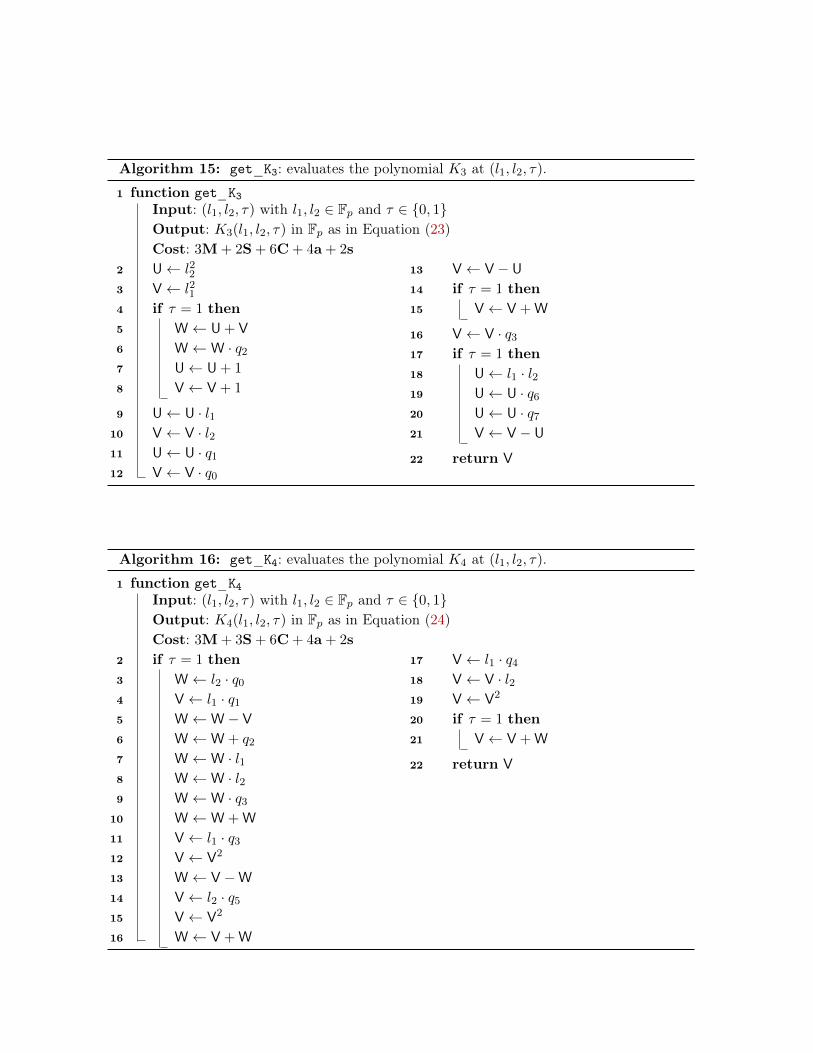
Algorithm 15: get_K3: evaluates the polynomial K3 at (l1, l2, τ).

1 function get_K3Input: (l1, l2, τ) with l1, l2 ∈ Fp and τ ∈ {0, 1}Output: K3(l1, l2, τ) in Fp as in Equation (23)Cost: 3M+ 2S+ 6C+ 4a+ 2s

2 U← l223 V← l214 if τ = 1 then5 W← U + V6 W←W · q27 U← U + 1

8 V← V + 1

9 U← U · l110 V← V · l211 U← U · q112 V← V · q0

13 V← V − U14 if τ = 1 then15 V← V + W

16 V← V · q317 if τ = 1 then18 U← l1 · l219 U← U · q620 U← U · q721 V← V − U

22 return V

Algorithm 16: get_K4: evaluates the polynomial K4 at (l1, l2, τ).

1 function get_K4Input: (l1, l2, τ) with l1, l2 ∈ Fp and τ ∈ {0, 1}Output: K4(l1, l2, τ) in Fp as in Equation (24)Cost: 3M+ 3S+ 6C+ 4a+ 2s

2 if τ = 1 then3 W← l2 · q04 V← l1 · q15 W←W − V6 W←W + q27 W←W · l18 W←W · l29 W←W · q3

10 W←W + W11 V← l1 · q312 V← V2

13 W← V −W14 V← l2 · q515 V← V2

16 W← V + W

17 V← l1 · q418 V← V · l219 V← V2

20 if τ = 1 then21 V← V + W

22 return V