Video Coding

Python Video ProcessingThe OpenCV library also gives us the ability to stream data directly from a webcam, suchas the Raspberry Pi to the computer!For this purpose, the command is:

cap=cv2.VideoCapture(0)

This accesses the default camera 0, which, for example, is the inserted USB webcam. "Cap" contains a pointer to the address of this camera.We can read a frame of this stream as:[retval, frame]=cap.read()

where "retval" is a return value (says if everything is fine), and "frame" contains the frame thus exctracted.Withcv2.imshow('frame',frame)

we can display this frame in a window.With cv2.waitKey(..)

the window is opened by cv2.imshow (it does not open without waitKey) and is kept open for as long prompted by waitKey. The function cv2.waitkey is only active when the associated window is active (if clicked on it). Only when this window is active, cv2.waitKey responds to the keystrokes!

When we do this in an infinite loop, we get the live video from the camera in the window. A sample program is shown as here:import cv2

#Program to capture a video from the default camera (0) and display it live on the screen

cap = cv2.VideoCapture(0)

while(True):

# Capture frame-by-frame

[retval, frame] = cap.read()

# Display the resulting frame

cv2.imshow('frame',frame)

if cv2.waitKey(1) & 0xFF == ord('q'):

break

# When everything done, release the capture

cap.release()

cv2.destroyAllWindows()

This is stored as "videorecdisp.py" and then called from console window with:

python videorecdisp.py

and we obtain the live video. We can end thedisplay with typing “q”.

A practical application is e.g. a "pipe camera" with goose-neck for the inspection of pipes.

The following example shows the contents ofthe upper left pixel of the video at the start of the program:

import cv2 #Program to capture an image from a cameraand display the pixel value on the screen cap = cv2.VideoCapture(0) # Capture one frame [ret, frame] = cap.read() print("image format: ", frame.shape) print("pixel 0,0: ",frame[0,0,:])

Save it under "pyimageshowpixel.py" and start it with:python pyimageshowpixel.pyWith Output:'image format: ', (480, 640, 3)) ('pixel 0,0: ', array([ 35, 167, 146], dtype=uint8))

Note that we only had addressed the pixels, so only 2 indices: frame [0,0,:].The colon ":" means that all the indices of these dimensions are addressed.In this way, we can also address an index range, via, Start:End, e.g, 0:3 addresses the indices 0,1,2 and onwards (Note: Not the lastvalue, 3).In our case, the above notation is identical to:

frame[0,0,0:3]

At the output, we, therefore, do not get a single value but a special array with the values of the 3 primary colors, in the order BGR. Here "Red" has the value 146, green 167, and blue 35.We can also observe the numeric representation in "uint8",i.e. unsigned integer with 8 bits, hence a number between0 and 255 (= 28

−1 ).

With the program “videorecdispRGB.py” we can see the separate R, G, and B components of our video stream, with the command linepython videorecdispRGB.py

Observe: if you hold e.g. e red paper in front of the camera, only the red component will show it bright, as expected.

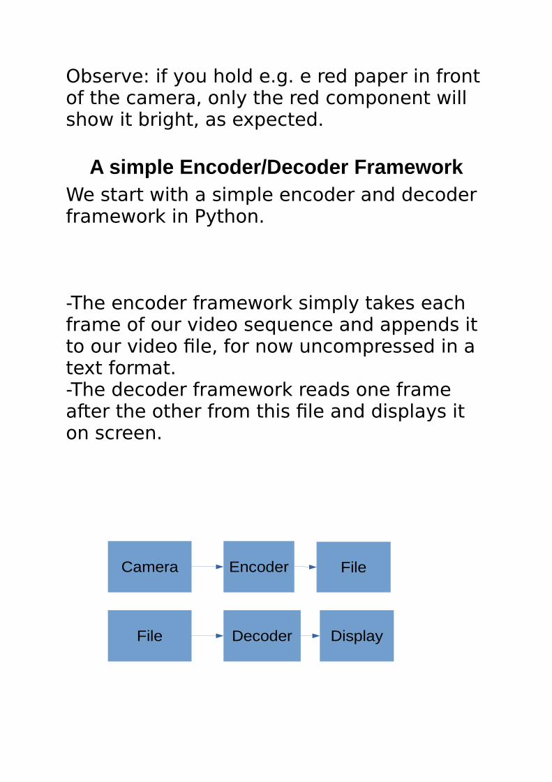
A simple Encoder/Decoder FrameworkWe start with a simple encoder and decoder framework in Python.

-The encoder framework simply takes each frame of our video sequence and appends it to our video file, for now uncompressed in a text format. -The decoder framework reads one frame after the other from this file and displays it on screen.

Camera Encoder File

File Decoder Display

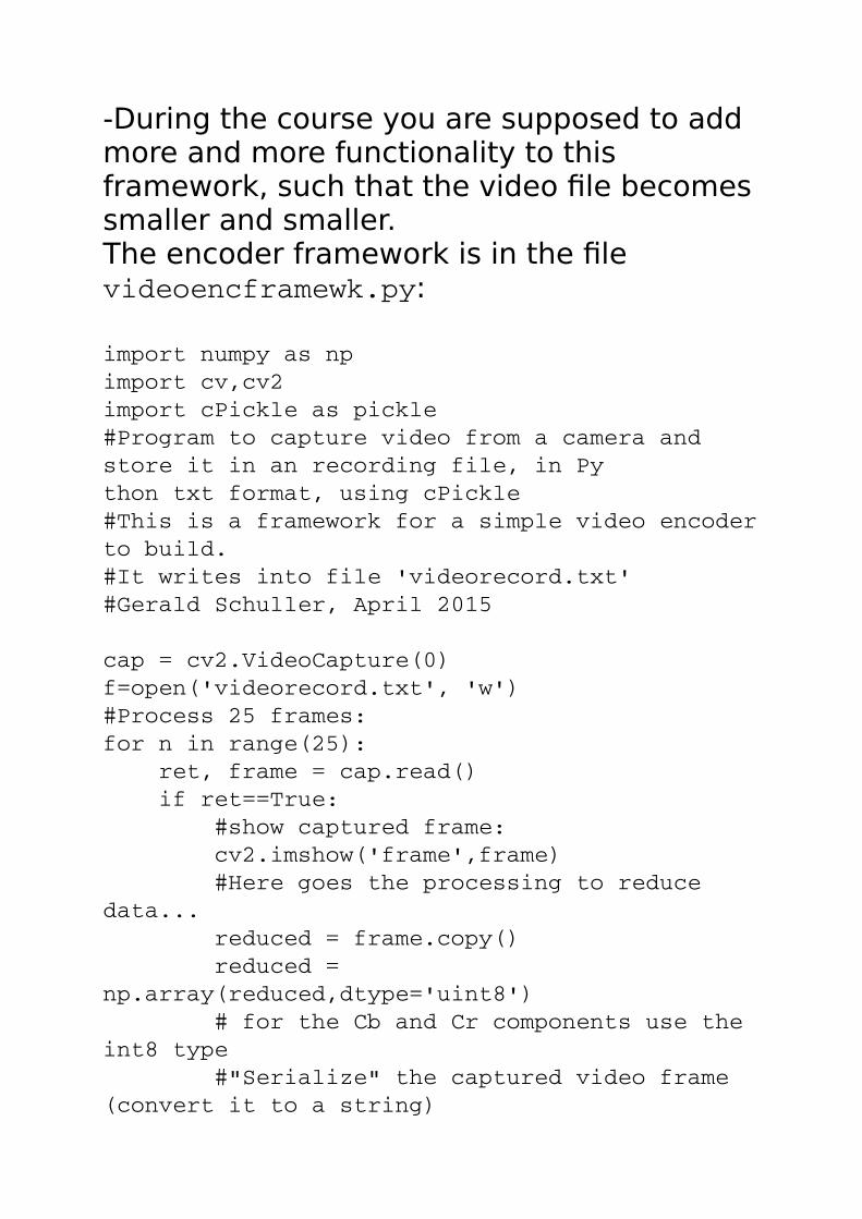
-During the course you are supposed to add more and more functionality to this framework, such that the video file becomessmaller and smaller. The encoder framework is in the file videoencframewk.py:

import numpy as np import cv,cv2 import cPickle as pickle #Program to capture video from a camera and store it in an recording file, in Py thon txt format, using cPickle #This is a framework for a simple video encoderto build. #It writes into file 'videorecord.txt' #Gerald Schuller, April 2015 

cap = cv2.VideoCapture(0) f=open('videorecord.txt', 'w') #Process 25 frames: for n in range(25):     ret, frame = cap.read()     if ret==True:         #show captured frame:         cv2.imshow('frame',frame)         #Here goes the processing to reduce data...         reduced = frame.copy()         reduced = np.array(reduced,dtype='uint8')        # for the Cb and Cr components use the int8 type        #"Serialize" the captured video frame (convert it to a string) 

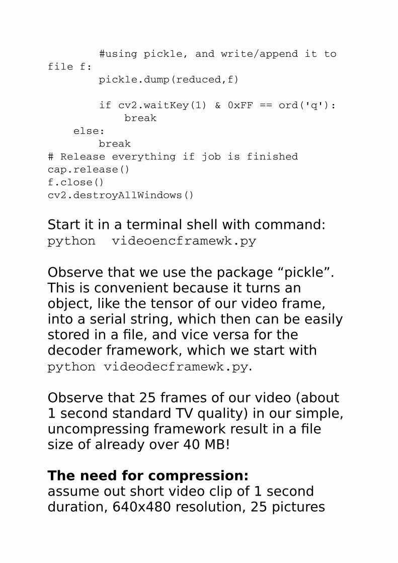
        #using pickle, and write/append it to file f:         pickle.dump(reduced,f)                 if cv2.waitKey(1) & 0xFF == ord('q'):             break     else:         break # Release everything if job is finished cap.release() f.close() cv2.destroyAllWindows() 

Start it in a terminal shell with command:python  videoencframewk.py

Observe that we use the package “pickle”. This is convenient because it turns an object, like the tensor of our video frame, into a serial string, which then can be easily stored in a file, and vice versa for the decoder framework, which we start withpython videodecframewk.py.

Observe that 25 frames of our video (about 1 second standard TV quality) in our simple, uncompressing framework result in a file size of already over 40 MB!

The need for compression: assume out short video clip of 1 second duration, 640x480 resolution, 25 pictures

per second, and 8 bits per pixel and primary color.Hence we have 8*3 * 640 * 480 bits per frame, times 25 frames per second..This results to 184 Mbit/s or ca. 23 Mbyte/s!(Our framework has about twice as much because it uses a text format). Observe: HD Video would be about 2 MegaPixel (1920x1080 pixel).This is particularly a problem if we want to stream a video, to transmit it: DSL usually has max. 16 Mb/s. But it is already possible to stream HD video over DSL! This shows the power of compression. Example: with good compression, HD video can be transmitted with about 4 Mb/s (from about 480 Mb/s uncompressed).

How does this compression work? There are 2 basic principles:

1)Irrelevance reduction2)Redundancy reduction

Both are necessary to obtain the most compression.

Irrelevance reduction: This principle looksat the receiver of our data, in this case the human eye. We only need to transmit information that the eye can observe or detect. But observe that for this we need

assumptions about the context in which the eye sees our signal (video); for instance the viewing distance, the size of the monitor, the brightness of the monitor and of the surroundings. For this reason we have specifically determined viewing environments for perceptual measurements.

What are the usual properties of the eye used for compression?

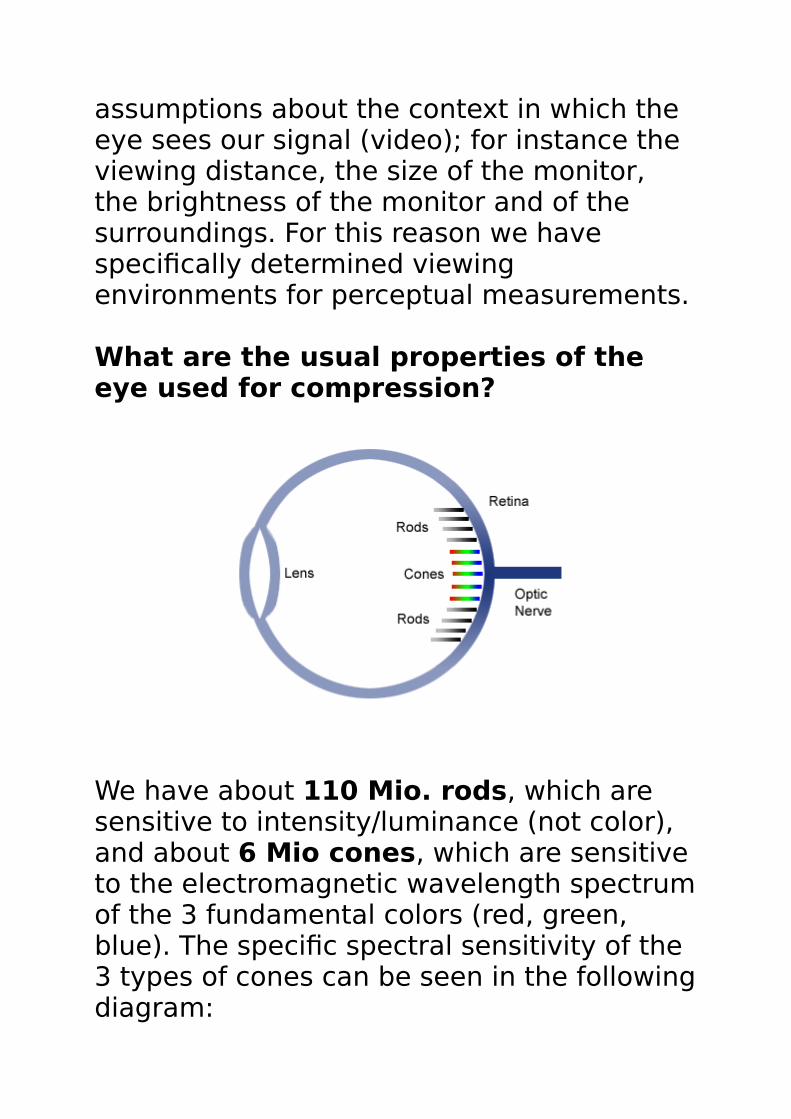
We have about 110 Mio. rods, which are sensitive to intensity/luminance (not color), and about 6 Mio cones, which are sensitive to the electromagnetic wavelength spectrumof the 3 fundamental colors (red, green, blue). The specific spectral sensitivity of the 3 types of cones can be seen in the followingdiagram:

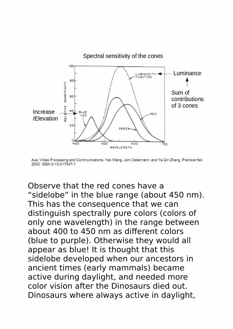
Observe that the red cones have a “sidelobe” in the blue range (about 450 nm).This has the consequence that we can distinguish spectrally pure colors (colors of only one wavelength) in the range between about 400 to 450 nm as different colors (blue to purple). Otherwise they would all appear as blue! It is thought that this sidelobe developed when our ancestors in ancient times (early mammals) became active during daylight, and needed more color vision after the Dinosaurs died out. Dinosaurs where always active in daylight,

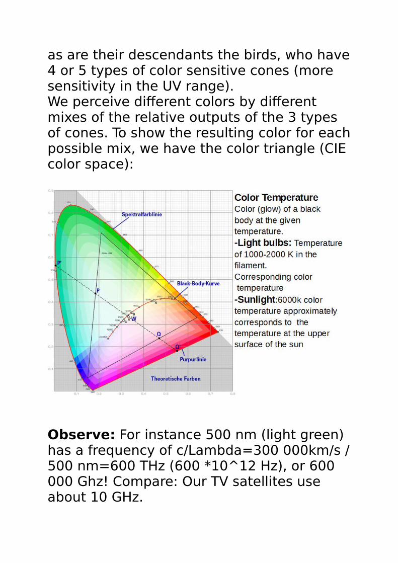
as are their descendants the birds, who have4 or 5 types of color sensitive cones (more sensitivity in the UV range).We perceive different colors by different mixes of the relative outputs of the 3 types of cones. To show the resulting color for eachpossible mix, we have the color triangle (CIE color space):

Observe: For instance 500 nm (light green) has a frequency of c/Lambda=300 000km/s /500 nm=600 THz (600 *10^12 Hz), or 600 000 Ghz! Compare: Our TV satellites use about 10 GHz.

This shows the possibilities of fiber optics to transmit data.

Those about 6 Mio. cones are unequally distributed on our retina. They are highly concentrated in the center of vision, the Fovea, and become more sparse towards theperiphery of vision. This is unlike typical digital cameras, which have equally distributed sensors.

Also observe the big difference in the number of only intensity or luminance sensitive rods: There are 110 Mio rods., but only 6 Mio cones. This means that the eye is much more sensitive for spatial changes in intensity or luminance than for spatial changes in color! This is also an important principle in video coding, where color is usually encoded and transmitted with less spatial resolution. For instance, the color information is subsampled by a factor of 2 vertically and horizontally.They are also unequally distributed, with less density towards the periphery of vision, but with the exception of the Fovea, where there are only cones at high density, with nospace for rods left.Rods are also much more light sensitive thancones, hence they are the main contributor

for our night vision. Unlike the cones, which are tuned to our sun light, our rods spectral sensitivity is tuned to the spectrum of our moon light.

We see that the eye has a much higher spatial resolution, corresponding to about 110 Mega-Pixel, for luminance (the intensity or black-and white picture) than forchrominance or color, corresponding to only about 6 Mega-Pixel. How can this be used in video coding?

First of all, luminance (intensity) and chrominance (color) can be coded differently. For that, we first have to separate the two, because usual cameras only have color sensitive sensors (similar to our cones), but they don’t have intensity sensors, like our rods. Hence we need to create an “artificial rod output”.For this we have a color transformation, if we take the red (R), green (G), and blue (B) channel:

Intensity Y= 0.299R + 0.587 G + 0.114 B,color component Cb=0.564(B-Y) =-0.16864R - 0.33107G + 0.49970B

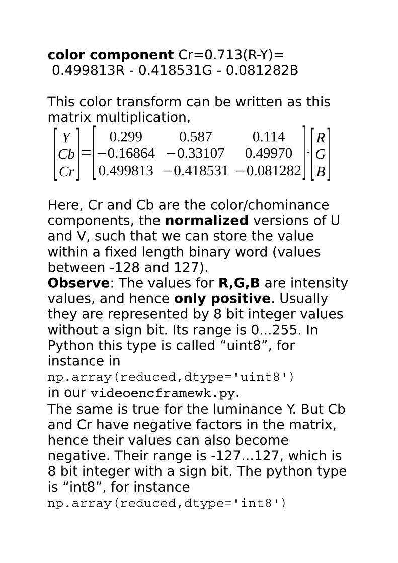
color component Cr=0.713(R-Y)= 0.499813R - 0.418531G - 0.081282B

This color transform can be written as this matrix multiplication,

[YCbCr ]=[

0.299 0.587 0.114−0.16864 −0.33107 0.499700.499813 −0.418531 −0.081282]⋅[

RGB ]

Here, Cr and Cb are the color/chominance components, the normalized versions of U and V, such that we can store the value within a fixed length binary word (values between -128 and 127).Observe: The values for R,G,B are intensityvalues, and hence only positive. Usually they are represented by 8 bit integer values without a sign bit. Its range is 0...255. In Python this type is called “uint8”, for instance innp.array(reduced,dtype='uint8')in our videoencframewk.py.The same is true for the luminance Y. But Cb and Cr have negative factors in the matrix, hence their values can also become negative. Their range is -127...127, which is 8 bit integer with a sign bit. The python typeis “int8”, for instancenp.array(reduced,dtype='int8')

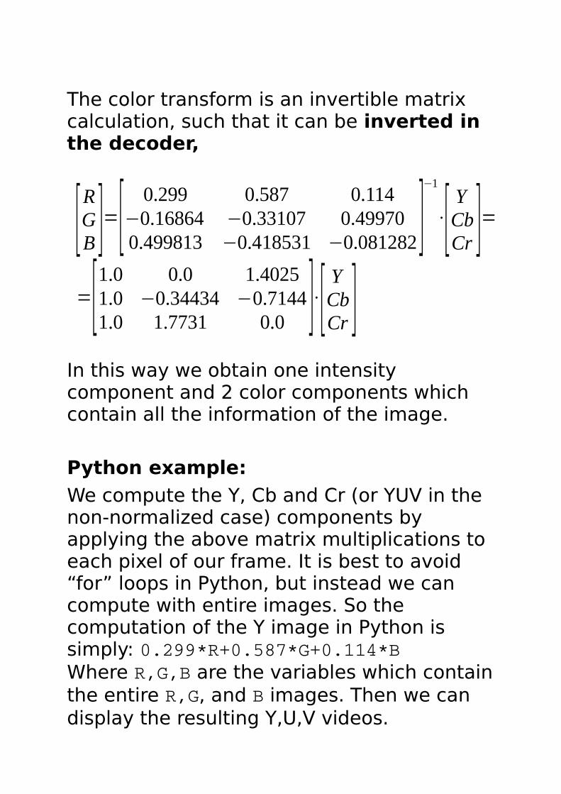
The color transform is an invertible matrix calculation, such that it can be inverted in the decoder,

[RGB ]=[

0.299 0.587 0.114−0.16864 −0.33107 0.499700.499813 −0.418531 −0.081282]

−1

⋅[YCbCr ]=

=[1.0 0.0 1.40251.0 −0.34434 −0.71441.0 1.7731 0.0 ]⋅[

YCbCr ]

In this way we obtain one intensity component and 2 color components which contain all the information of the image.

Python example:

We compute the Y, Cb and Cr (or YUV in the non-normalized case) components by applying the above matrix multiplications to each pixel of our frame. It is best to avoid “for” loops in Python, but instead we can compute with entire images. So the computation of the Y image in Python is simply: 0.299*R+0.587*G+0.114*BWhere R,G,B are the variables which containthe entire R,G, and B images. Then we can display the resulting Y,U,V videos.

Start the program in a terminal shell with the commandpython videorecprocyuv.py

Observe: The Y video is a monochrome version as expected. The U and V videos only contain content if there is color, for monochrome light they show black. Also observe how different colors appear at different channels (U or V).

Python example for switching on and off the YUV components:python videorecencdecyuvkey.py

Observe: Turning off the Luminance components Y make the image appear indeed less sharp, because our eyes have areduced spacial resolution for color.Turning on and off the color components U and V shows the color space associated with each of them.

Compare this with the original color components, using our Python app:python videorecdispRGBkey.py

Here we can turn the R,G,B components individually on and off.

Observe: Here, each individual color component looks still sharp (despite having just one color), because it still contains the intensity, the Luminance information. This shows why we use a color transform.

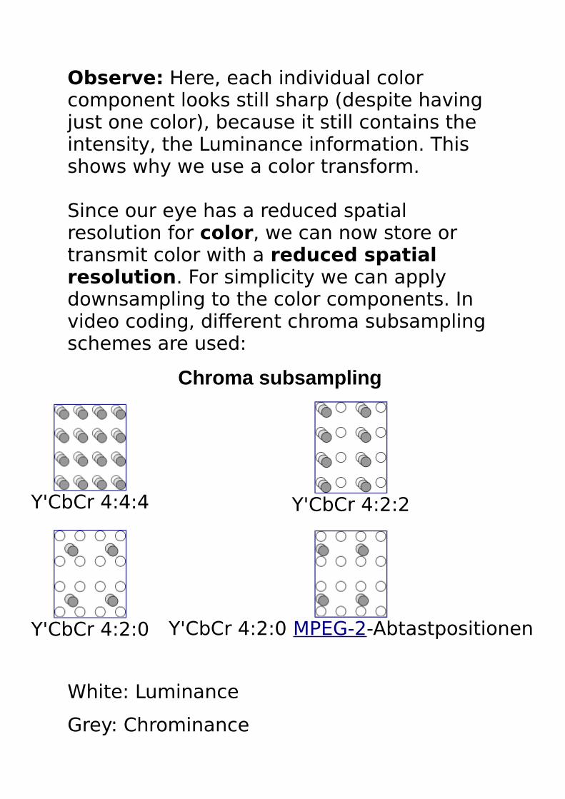
Since our eye has a reduced spatial resolution for color, we can now store or transmit color with a reduced spatial resolution. For simplicity we can apply downsampling to the color components. In video coding, different chroma subsampling schemes are used:

Chroma subsampling

Y'CbCr 4:4:4 Y'CbCr 4:2:2

Y'CbCr 4:2:0 Y'CbCr 4:2:0 MPEG-2-Abtastpositionen

White: Luminance

Grey: Chrominance

(from: http://de.wikipedia.org/wiki/Farbunterabtastung)

You can imagine the naming as the number of samples for each component along a line. The last name doesn’t really follow this naming convention, because it also has a downsampling along the rows, hence the name 4:2:0 was assigned. This is also the most used scheme for digital video. 4:2:2 is used for higher quality, and 4:4:4 is used for highest quality video (e.g. raw or lossless formats).With the 4:2:0 scheme we can now reduce the required data rate for the two color components by a factor of 4! (2 in each dimension), at least theoretically without visible artefacts!

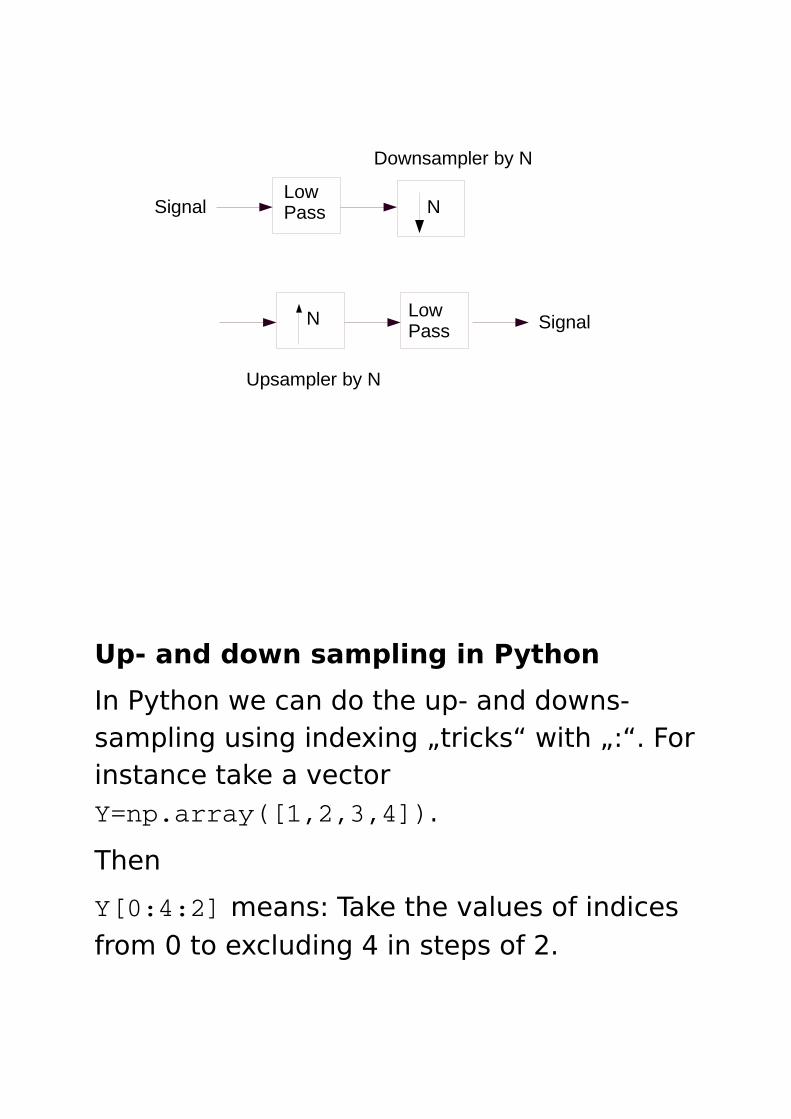
Downsampling, Upsampling, FilteringHow do we do the downsampling in the encoder and then the upsampling in the decoder, such that we don't see artifacts and such that it is not too complex?

If in the encoder we simply downsample our image directly, by keeping only every 2nd

sample (or N'th sample in general), we might get aliasing artifacts if we have finepatterns in the image.

If in the decoder we simply upsample our image by inserting N-1 zeros after each sample in each dimension, we obtain a „pointy“ image, which results again from aliasing or spectral copies of our image.

To avoid both, we need to suitably lowpass our image before downsampling, and alsolowpass filter it after upsampling as a sort of interpolation.

This is what the Nyquist Theorem tells us. We know it from 1-dimensional signal processing:

Now we just have to think about how to extend it to 2-dimensional signals like images.

Up- and down sampling in Python

In Python we can do the up- and downs-sampling using indexing „tricks“ with „:“. Forinstance take a vector Y=np.array([1,2,3,4]).

Then

Y[0:4:2] means: Take the values of indices from 0 to excluding 4 in steps of 2.

SignalLow Pass

Low Pass Signal

N

N

Downsampler by N

Upsampler by N

Y[0::2] means: Take the values of indices from 0 to the end in steps of 2.

Then down-sampling with a factor of 2 is simply:

Yds=Y[0::2]

Yds contains the down-sampled signal.

For a 2D signal and downsampling in each dimension, Y it would be simply:

Yds=Y[0::2,0::2]

For up-sampling you first generate a vectorof zeros:

Yus=np.zeros(4)

and then we can assign every 2nd value to the output:

Yus[0::2]=Yds

For a 2D signal and upsampling in each dimension it would be:

Yus=np.zeros((4,4))

Yus[0::2,0::2]=Yds

Python example:

This is shown in the following python example. We take each frame and

downsample it by N=8 in each dimension, then upsample it, and display the result.

Start it with:

python videofiltresampkey.py

It uses scipy.signal.convolve2d as convolution or filter function, where we 2D-convolve our frame with a 2D „filter kernel“ or 2D impulse response. This is the 2-D version of a lowpass filter.

The Python program uses two types of low pass filter:

-filter 1 consists of a 8x8 coefficient square matrix with entries of 1/8:

filt1=np.ones((8,8))/8;

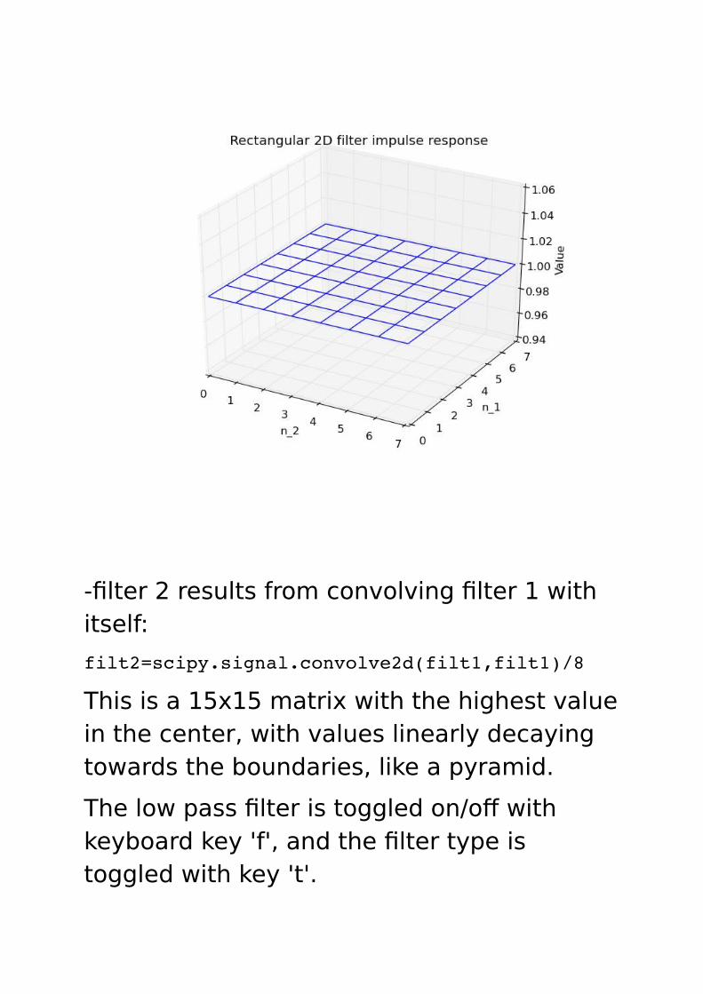
-filter 2 results from convolving filter 1 with itself:

filt2=scipy.signal.convolve2d(filt1,filt1)/8

This is a 15x15 matrix with the highest valuein the center, with values linearly decaying towards the boundaries, like a pyramid.

The low pass filter is toggled on/off with keyboard key 'f', and the filter type is toggled with key 't'.

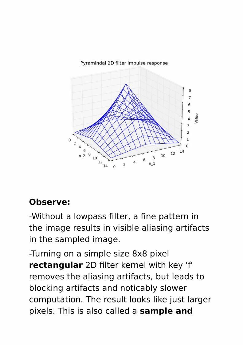
Observe:

-Without a lowpass filter, a fine pattern in the image results in visible aliasing artifacts in the sampled image.

-Turning on a simple size 8x8 pixel rectangular 2D filter kernel with key 'f' removes the aliasing artifacts, but leads to blocking artifacts and noticably slower computation. The result looks like just larger pixels. This is also called a sample and

hold (hold the value of the sample until the value of the next sample arrives).

Observe: Convolution of our impulse response with the pulses of our sampled image results in placing the impulse response at the place of the pulses.

-Turning on a pyramid shaped size 15x15 2D filter with key 't' removes the blocking artefacts, but leads to even slower computation. The reconstructed image lookslike from a linear interpolation between neigbouring sampled pixels.

Observe: Now the pyramid impulse response appears at the place of the samplepulses. Adding them up results in the linear interpolation.

So how do we design „good“ 2D filters, such that we get good results and still reasonably fast computation?

For that it is helpful to look at the 2D frequency domain.

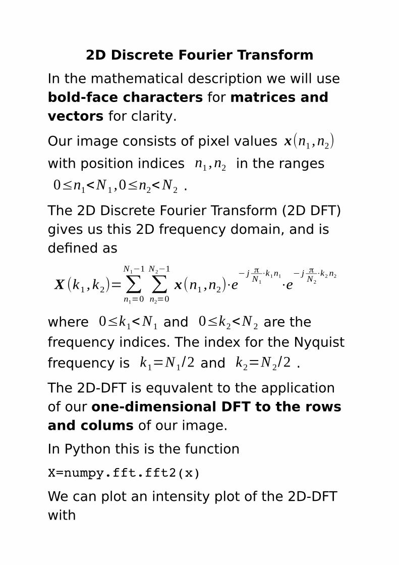
2D Discrete Fourier Transform

In the mathematical description we will use bold-face characters for matrices and vectors for clarity.

Our image consists of pixel values x(n1 , n2)

with position indices n1 , n2 in the ranges

0≤n1<N 1 ,0≤n2<N2 .

The 2D Discrete Fourier Transform (2D DFT) gives us this 2D frequency domain, and is defined as

X (k1 , k2)=∑n1=0

N1−1

∑n2=0

N2−1

x(n1 ,n2)⋅e− j π

N1

⋅k1n1

⋅e− j π

N2

⋅k2 n2

where 0≤k1<N1 and 0≤k2<N 2 are the

frequency indices. The index for the Nyquist

frequency is k1=N1/2 and k2=N 2/2 .

The 2D-DFT is equvalent to the application of our one-dimensional DFT to the rows and colums of our image.

In Python this is the function

X=numpy.fft.fft2(x)

We can plot an intensity plot of the 2D-DFT with

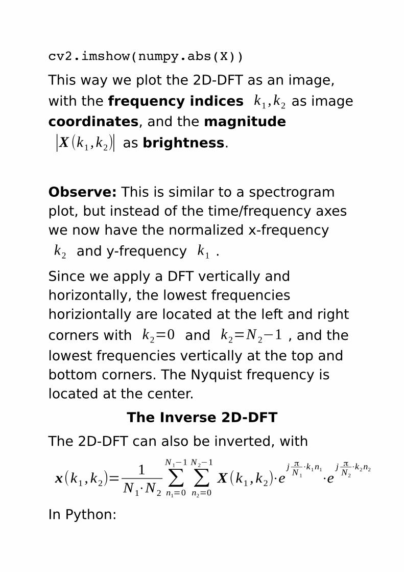
cv2.imshow(numpy.abs(X))

This way we plot the 2D-DFT as an image,

with the frequency indices k1 , k2 as image

coordinates, and the magnitude

|X (k1 , k2)| as brightness.

Observe: This is similar to a spectrogram plot, but instead of the time/frequency axes we now have the normalized x-frequency

k2 and y-frequency k1 .

Since we apply a DFT vertically and horizontally, the lowest frequencies horiziontally are located at the left and right

corners with k2=0 and k2=N 2−1 , and the

lowest frequencies vertically at the top and bottom corners. The Nyquist frequency is located at the center.

The Inverse 2D-DFT

The 2D-DFT can also be inverted, with

x(k1 , k2)=1

N1⋅N2∑n1=0

N 1−1

∑n2=0

N 2−1

X (k1 , k2)⋅ej πN 1

⋅k1n1

⋅ej πN2

⋅k2n2

In Python:

x=numpy.fft.ifft2(X)

Python Example:

This example takes the webcam input, computes the Y Luminance component, and displays it. Then it takes the 2D-DFT and displays its magnitude in a separate window.Then it takes the inverse 2D-DFT and displays it in the final third window.

Keyboard key 'f': A low pass can be switched on, which is implemented in the 2D-DFT domain, by setting the DFT coefficients of higher frequencies to 0 and then apply the inverse 2D-DFT. This is done before the downsampling and after the upsampling.

Keyboard key 's': Sampling with a factor of 8 in horizontal and vertical direction is turned on/off. First downsampling (for the encoder) and then upsampling (for the decoder).

Start the Python demo with:

python videofft0ifftresampleykey.py

Observe:

-Most coefficients of the 2D-DFT with high magnitudes appear in the corners, where thelow frequencies are located.

-Holding fine patterns in front of the camera results also in high magnitudes at higher frequencies, like brighter rays.

-By pushing key “f” we can set most of the high frequency coefficients to 0 and still get a “good” picture, just a little blurry

-By pushing key “s” we can turn sampling on/off. Without the lowpass filter the reconstructed image only has a “lattice” of active pixels. The 2D-DFT image shows spectral copies, aliasing, appearing periodically in the spectrum.

-By then switching the low pass filter on we remove or suppress the spectral copies. As the result, the reconstructed images looks like before with only the low pass turned on, and much better than without the low pass filter!

-If we leave the low pass on, we don't see a difference in the reconstructed image when we toggle sampling on and off!