JSS Journal of Statistical SoftwareMMMMMM YYYY, Volume VV, Issue II. http://www.jstatsoft.org/

pyParticleEst: A Python Framework for Particle

Based Estimation Methods

Jerker NordhLund University

Abstract

Particle methods such as the Particle Filter and Particle Smoothers have proven veryuseful for solving challenging nonlinear estimation problems in a wide variety of fieldsduring the last decade. However, there is still very few existing tools to support andassist researchers and engineers in applying the vast number of methods in this field totheir own problems. This paper identifies the common operations between the methodsand describes a software framework utilizing this information to provide a flexible andextensible foundation which can be used to solve a large variety of problems in this domain,thereby allowing code reuse to reduce the implementation burden and lowering the barrierof entry for applying this exciting field of methods. The software implementation presentedin this paper is freely available and permissively licensed under the GNU Lesser GeneralPublic License, and runs on a large number of hardware and software platforms, makingit usable for a large variety of scenarios.

Keywords: particle-filter, particle-smoother, expectation-maximization, system identification,rao-blackwellized, Python.

1. Introduction

During the last few years, particle based estimation methods such as particle filtering (Doucet,Godsill, and Andrieu 2000) and particle smoothing (Briers, Doucet, and Maskell 2010) havebecome increasingly popular and provide a powerful alternative for nonlinear/non-Gaussianand multi-modal estimation problems. Noteworthy applications of particle methods includemulti-target tracking (Okuma, Taleghani, De Freitas, Little, and Lowe 2004), SimultanousLocalization and Mapping (SLAM) (Montemerlo, Thrun, Koller, Wegbreit et al. 2002) andRadio Channel Estimation (Mannesson 2013). Popular alternatives to the particle filter arethe Extended Kalman Filter (Julier and Uhlmann 2004) and Unscented Kalman Filter (Julierand Uhlmann 2004), but they can not always provide the performance needed, and neither

2 pyParticleEst: A Python Framework for Particle Based Estimation Methods

handles multimodal distributions well. The principles of the Particle Filter and Smootherare fairly straight forward, but there are still a few caveats when implementing them. Thereis a large part of the implementation effort that is not problem specific and thus could bereused, thereby reducing both the overall implementation effort and the risk of introducingerrors. Currently there is very little existing software support for using these methods, andfor most applications the code is simply written from scratch each time. This makes it harderfor people new to the field to apply methods such as particle smoothing. It also increasesthe time needed for testing new methods and models for a given problem. This paper breaksa number of common algorithms down to a set of operations that need to be performed onthe model for a specific problem and presents a software implementation using this structure.The implementation aims too exploit the code reuse opportunities by providing a flexibleand extensible foundation to build upon where all the basic parts are already present. Themodel description is clearly separated from the algorithm implementations. This allows theend user to focus on the parts unique for their particular problem and to easily compare theperformance of different algorithms. The goal of this article is not to be a manual for thisframework, but to highlight the common parts of a number of commonly used algorithmsfrom a software perspective. The software presented serves both as a proof of concept and asan invitation to those interested to study further, use and to improve upon.

The presented implementation currently supports a number of filtering and smoothing algo-rithms and has support code for the most common classes of models, including the special caseof Mixed Linear/Nonlinear Gaussian State Space (MLNLG) models using Rao-Blackwellizedalgorithms described in Section 3, leaving only a minimum of implementation work for theend user to define the specific problem to be solved.

In addition to the filtering and smoothing algorithms the framework also contains a modulethat uses them for parameter estimation (grey-box identification) of nonlinear models. Thisis accomplished using an Expectation Maximization (EM)(Dempster, Laird, and Rubin 1977)algorithm combined with a Rao-Blackwellized Particle Smoother (RBPS) (Lindsten and Schon2010).

The framework is implemented in Python and following the naming conventions typicallyused within the Python community it has been named pyParticleEst. For an introduction toPython and scientific computation see (Oliphant 2007). All the computations are handled bythe Numpy/Scipy (Jones, Oliphant, Peterson et al. 2001–) libraries. The choice of Python ismotivated by that it can run on a wide variety of hardware and software platforms, moreoversince pyParticleEst is licensed under the LGPL (FSF 1999) it is freely usable for anyonewithout any licensing fees for either the software itself or any of its dependencies. The LGPLlicense allows it to be integrated into proprietary code only requiring any modifications tothe actual library itself to be published as open source. All the code including the examplespresented in this article can be downloaded from (Nordh 2013).

The remaining of this paper is organized as follows. Section 2 gives a short overview of otherexisting software within this field. Section 3 gives an introduction to the types of modelsused and a quick summary of notation, Section 4 presents the different estimation algorithmsand isolates which operations each method requires from the model. Section 5 provides anoverview of how the software implementation is structured and details of how the algorithmsare implemented. Section 6 shows how to implement a number of different types of models inthe framework. Section 7 presents some results that are compared with previously publisheddata to show that the implementation is correct. Section 8 concludes the paper with a short

Journal of Statistical Software 3

discussion of the benefits and drawbacks with the approach presented.

2. Related software

The only other software package within this domain to the authors knowledge is LibBi (MurrayIn review). LibBi takes a different approach and provides a domain-specific language fordefining the model for the problem. It then generates high performance code for a ParticleFilter for that specific model. In contrast, pyParticleEst is more focused on providing aneasily extensible foundation where it is easy to introduce new algorithms and model types, agenerality which comes at some expense of run-time performance making the two softwaressuitable for different use cases. It also has more focus on different smoothing algorithms andfilter variants.

There is also a lot of example code that can be found on the Internet, but nothing in the formof a complete library with a clear separation between model details and algorithm implemen-tation. This separation is what gives the software presented in this article its usability asa general tool, not only as a simple template for writing a problem specific implementation.This also allows for easy comparison of different algorithms for the same problem.

3. Modelling

While the software framework supports more general models, this paper focuses on discretetime stace-space models of the form

xt+1 = f(xt, vt) (1a)

yt = h(xt, et) (1b)

where xt are the state variables, vt is the process noise and yt is a measurement of the stateaffected by the measurement noise et. The subscript t is the time index. Both v and e arerandom variables according to some known distributions, f and h are both arbitrary functions.

If f, h are affine and v, e are Gaussian random variables the system is what is commonlyreferred to as a Linear Gaussian State Space system (LGSS) and the Kalman filter is boththe best linear unbiased estimator (Arulampalam, Maskell, Gordon, and Clapp 2002) and theMaximum Likelihood estimator.

Due to the scaling properties of the Particle Filter and Smoother, which are discussed in moredetail in Section 4.1, it is highly desirable to identify any parts of the models that conditionedon the other states would be linear Gaussian. The state-space can then be partitioned asxT =

(ξT zT

), where z are the conditionally linear Gaussian states and ξ are the rest.

4 pyParticleEst: A Python Framework for Particle Based Estimation Methods

Extending the model above to explicitly indicate this gives

ξt+1 =

(fnξ (ξt, v

nξ )

f lξ(ξt)

)+

(0

Aξ(ξt)

)zt +

(0vlξ

)(2a)

zt+1 = fz(ξt) +Az(ξt)zt + vz (2b)

yt =

(hξ(ξt, e

n)hz(ξt)

)+

(0

C(ξt)

)zt +

(0el

)(2c)

vlξ ∼ N(0, Qξ(ξt)), vz ∼ N(0, Qz(ξt)), el ∼ N(0, R(ξt)) (2d)

As can be seen all relations in (2) involving z are linear with additive Gaussian noise whenconditioned on ξ. Here the process noise for the non-linear states vξ is split in two parts: vlξappears linearly and must be Gaussian whereas vnξ can be from any distribution, similarly

holds true for el and en. This is referred to as a Rao-Blackwellized model.

If we remove the coupling from z to ξ we get what is referred to as a hierarchical model

ξt+1 = fξ(ξt, vξ) (3a)

zt+1 = fz(ξt) +A(ξt)zt + vz (3b)

yt =

(hξ(ξt, e

n)hz(ξt)

)+

(0

C(ξt)

)zt +

(0el

)(3c)

vz ∼ N(0, Qz(ξt)), el ∼ N(0, R(ξt)) (3d)

Another interesting class are Mixed Linear/Nonlinear Gaussian (MLNLG) models

ξt+1 = fξ(ξt) +Aξ(ξt)zk + vξ (4a)

zt+1 = fz(ξt) +Az(ξt)zt + vz (4b)

yt = h(ξt) + C(ξt)zt + e (4c)

e ∼ N(0, R(ξt)) (4d)[vξvz

]∼ N

([00

],

[Qξ(ξt) Qξz(ξt)Qξz(ξt)

T Qz(ξt)

])(4e)

(4f)

The MLNLG model class (4) allows for non-linear dynamics but with the restrictions that allnoise must enter additively and be Gaussian.

Journal of Statistical Software 5

4. Algorithms

This section gives an overview of some common particle based algorithms, they are subdividedinto those used for filtering, smoothing and static parameter estimation. For each algorithmit is identified which operations need to be performed on the model.

4.1. Filtering

This subsection gives a quick summary of the principles of the Particle Filter, for a thoroughintroduction see for example Doucet et al. (2000).

The basic concept of a Particle Filter is to approximate the probability density function (pdf)for the states of the system by a number of point estimates

p(xt|y1:t) ≈N∑i=1

w(i)δ(xt − x(i)t ) (5)

Each of the N particles in (5) consists of a state, x(i)t , and a corresponding weight, w

(i)t ,

representing the likelihood of that particular particle. Each estimate is propagated forwardin time using (1a) by sampling vt from the corresponding noise distribution, providing anapproximation of p(xt+1|yt, ..., y1). The measurement yt+1 is incorporated by updating theweights of each particle with respect to how well it predicted the new measurement, giving anapproximation of p(xt+1|yt+1, yt, ..., y1). This procedure is iterated forward in time providinga filtered estimate of the state x.

A drawback with this approach is that typically all but one of the weights, w(i)t , eventually

go to zero resulting in a poor approximation of the true pdf. This is referred to as particledegeneracy and is commonly solved by a process called resampling (Arulampalam et al. 2002).The idea behind resampling is that at each time-step, or when some criteria is fulfilled,a new collection of particles with all weights equal (w(i) = 1

N ,∀i) is created by randomlydrawing particles, with replacement, according to their weights. This focuses the particleapproximation to the most likely regions of the pdf, not wasting samples in regions with lowprobability. This method is summarized in Algorithm 1.

Another issue with the standard Particle Filter is that the number of particles needed inthe filter typically grows exponentially with the dimension of the state-space as discussed inBeskos, Crisan, and Jasra (2011) and Rebeschini and van Handel (2013), where they alsopresent methods to avoid this issue. Another popular approach is to use Rao-Blackwellizedmethods when there exists a conditionally linear Gaussian substructure. Using the partition-ing from model (2) this provides a better approximation of the underlying pdf for a givennumber of particles by storing the sufficient statistics for the z-states instead of samplingfrom the Gaussian distributions. For an introduction to the Rao-Blackwellized Particle Filter(RBPF) see Schon, Gustafsson, and Nordlund (2005).

A variant of the Particle Filter is the so called Auxiliary Particle Filter (APF), it attemptsto focus the particles to regions of high interest by looking one step ahead by evaluatingp(yt+1|xt) and using this to resample the particles before the propagation stage. Since thereis typically no analytic expression for this density it is often approximated by assuming thatthe next state will be the predicted mean; p(yt+1|xt+1 = xt+1|t).

Table 1 summaries the methods needed for the two different filters.

6 pyParticleEst: A Python Framework for Particle Based Estimation Methods

Algorithm 1: Standard Particle Filter algorithm, this is typically improved by not performingthe resampling step at every iteration, but only when some prespecified criteria on the weightsis fulfilled

Draw x(i)0 from p(x0), i ∈ 1..N

Set w(i)0 = 1

N , i ∈ 1..Nfor t← 0 to T − 1 do

for i← 1 to N do

Sample x(i)t+1 from p(xt+1|x(i)

t )

Set w(i)t+1 = w

(i)t p(yt+1|x(i)

t+1);

Normalize weights, w(i) = w(i)t+1/

∑j w

(j)t+1

for i← 1 to N do

Sample x(i)t+1 ∼ p(xt+1|yt+1) by drawing new particles from the categorical

distribution defined by (x(k)t+1, w

(k)), k ∈ 1..N

Set w(i)t+1 = 1

N , i ∈ 1..N

Operations Methods

Sample from p(x1) PF, APF

Sample from p(xt+1|xt) PF, APF

Evaluate p(yt|xt) PF, APF

Evaluate* p(yt+1|xt) APF

Table 1: Operations that need to be performed on the model for the different filter algorithms.(*typically only approximately).

4.2. Smoothing

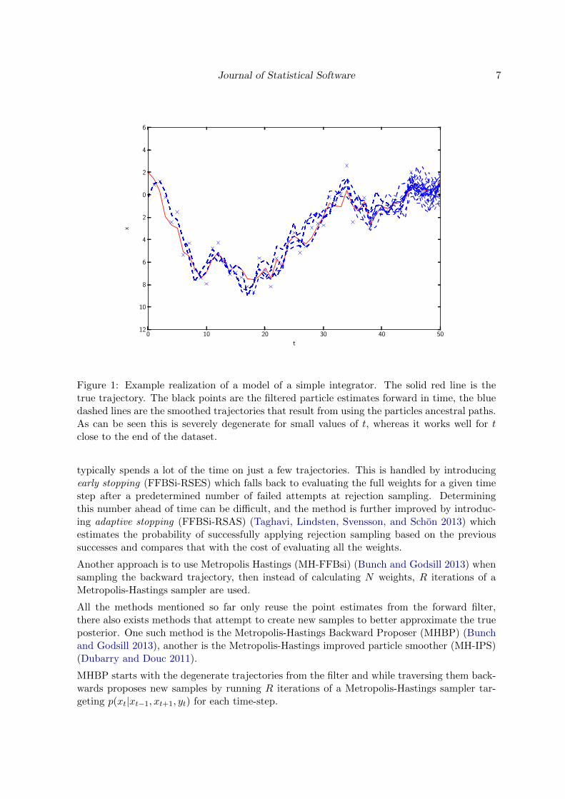
Conceptually the Particle Filter provides a smoothed estimate if the trajectory for each par-ticle is saved and not just the estimate for the current time-step. The full trajectory weightsare then given by the corresponding particle weights for the last time-step. In practice thisdoesn’t work due to the resampling step which typically results in that all particles eventuallyshare a common ancestor, thus providing a very poor approximation of the smoothed pdf fort� T . An example of this is shown in Fig. 1

Forward Filter Backward Simulators (FFBSi) are a class of methods that reuse the pointestimates for xt|t generated by the particle filter and attempt to improve the particle diver-sity by drawing backward trajectories that are not restricted to follow the same paths asthose generated by the filter. This is accomplished by selecting the ancestor of each particlewith probability ωt|T ∼ ωt|tp(xt+1|xt). Evaluating all the weights ωt|T gives a time complex-ity O(MN) where N is the number of forward particles and M the number of backwardtrajectories to be generated.

A number of improved algorithms have been proposed that improve this by removing the needto evaluate all the weights. One approach is to use rejection sampling (FFBSi-RS) (Lindstenand Schon 2013), this however does not guarantee a finite end-time for the algorithm, and

Journal of Statistical Software 7

0 10 20 30 40 50

t

12

10

8

6

4

2

0

2

4

6x

Figure 1: Example realization of a model of a simple integrator. The solid red line is thetrue trajectory. The black points are the filtered particle estimates forward in time, the bluedashed lines are the smoothed trajectories that result from using the particles ancestral paths.As can be seen this is severely degenerate for small values of t, whereas it works well for tclose to the end of the dataset.

typically spends a lot of the time on just a few trajectories. This is handled by introducingearly stopping (FFBSi-RSES) which falls back to evaluating the full weights for a given timestep after a predetermined number of failed attempts at rejection sampling. Determiningthis number ahead of time can be difficult, and the method is further improved by introduc-ing adaptive stopping (FFBSi-RSAS) (Taghavi, Lindsten, Svensson, and Schon 2013) whichestimates the probability of successfully applying rejection sampling based on the previoussuccesses and compares that with the cost of evaluating all the weights.

Another approach is to use Metropolis Hastings (MH-FFBsi) (Bunch and Godsill 2013) whensampling the backward trajectory, then instead of calculating N weights, R iterations of aMetropolis-Hastings sampler are used.

All the methods mentioned so far only reuse the point estimates from the forward filter,there also exists methods that attempt to create new samples to better approximate the trueposterior. One such method is the Metropolis-Hastings Backward Proposer (MHBP) (Bunchand Godsill 2013), another is the Metropolis-Hastings improved particle smoother (MH-IPS)(Dubarry and Douc 2011).

MHBP starts with the degenerate trajectories from the filter and while traversing them back-wards proposes new samples by running R iterations of a Metropolis-Hastings sampler tar-geting p(xt|xt−1, xt+1, yt) for each time-step.

8 pyParticleEst: A Python Framework for Particle Based Estimation Methods

MH-IPS can be combined with the output from any of the other smoothers to give an improvedestimate. It performs R iterations where each iteration traverses the full backward trajectoryand for each time-step runs a single iteration of a Metropolis-Hastings sampler targetingp(xt|xt−1, xt+1, yt).

Table 2 lists the operations needed for the different smoothing methods. For a more detailedintroduction to Particle Smoothing see for example Briers et al. (2010), Lindsten and Schon(2013), and for an extension to the Rao-Blackwellized case see Lindsten and Schon (2011)

Operations Methods

Evaluate p(xt+1|xt) FFBSi, FFBSi-RS, FFBSi-RSES,FFBSi-RSAS, MH-FFBSi, MH-IPS,MHBP

Evaluate argmaxxt+1 p(xt+1|xt) FFBSi-RS, FFBSi-RSES, FFBSi-RSAS

Sample from q(xt|xt−1, xt+1, yt) MH-IPS, MHBP

Evaluate q(xt|xt−1, xt+1, yt) MH-IPS, MHBP

Table 2: Operations that need to be performed on the model for the different smoothingalgorithms. They all to some extent rely on first running a forward filter, and thus in additionrequire the operations needed for the filter. Here q is a proposal density, a simple option isto choose q = p(xt+1|xt), as this does not require any further operations. The ideal choicewould be q = p(xt|xt+1, xt−1, yt), but it is typically not possible to directly sample from thisdensity.

4.3. Parameter estimation

Using a standard Particle Filter or Smoother it is not possible to estimate stationary parame-ters, θ, due to particle degeneracy. A common work-around for this is to include θ in the statevector and model the parameters as a random walk process with a small noise covariance. Adrawback with this approach is that the parameter is no longer modeled as being constant,in addition it increases the dimension of the state-space, worsening the problems mentionedin Section 4.1.

PS+EM

Another way to do parameters estimation is to use an Expectation Maximization (EM) al-gorithm where the expectation part is calculated using a RBPS. For a detailed introductionto the EM-algorithm see Dempster et al. (1977) and for how to combine it with a RBPS forparameter estimates in model (4) see Lindsten and Schon (2010).

The EM-algorithm finds the maximum likelihood solution by alternating between estimatingthe Q-function for a given θk and finding the θ that maximizes the log-likelihood for a givenestimate of x1:T , where

Q(θ, θk) = EX|θk [Lθ(X,Y |Y )] (6a)

θk+1 = argmaxθ

Q(θ, θk) (6b)

Here X is the complete state trajectory (x1, ..., xN ), Y is the collection of all measurements(y1, ..., yN ) and Lθ is the log-likelihood as a function of the parameters θ. In Lindsten and

Journal of Statistical Software 9

Schon (2010) it is shown that the Q-function can be split into three parts as follows

Q(θ, θk) = I1(θ, θk) + I2(θ, θk) + I3(θ, θk) (7a)

I1(θ, θk) = Eθk [log pθ(x1)|Y ] (7b)

I2(θ, θk) =

N−1∑t=1

Eθk [log pθ(xt+1|xt)|Y ] (7c)

I3(θ, θk) =

N∑t=1

Eθk [log pθ(yt|xt)|Y ] (7d)

The expectations in (7b)-(7d) are approximated using a (Rao-Blackwellized) Particle Smoother,where the state estimates are calculated using the old parameter estimate θk. This procedureis iterated until the parameter estimates converge. The methods needed for PS+EM are listedin Table 3

Operations Methods

Maximize Eθk [log pθ(x1)|Y ] PS+EM

Maximize Eθk [log pθ(xt+1|xt)|Y ] PS+EM

Maximize Eθk [log pθ(yt|xt)|Y ] PS+EM

Evaluate q(θ′|θ) PMMH

Sample from q(θ′|θ) PMMH

Evaluate π(θ) PMMH

Table 3: Operations that need to be performed on the model for the presented parameterestimation methods. PS-EM relies on running a smoother, and thus in addition requiresthe operations needed for the smoother. The maximization is with respect to θ. Typicallythe maximization can not be performed analytically, and then depending on which type ofnumerical solver is used, gradients and Hessians might be needed as well. PMMH does notrequire a smoothed estimate, it only uses a filter, and thus puts fewer requirements on thetypes of models that can be used. Here q is the proposal density for the static parameters, π isthe prior probability density function. PMMH does not need a smoothed trajectory estimate,it is sufficient with the filtered estimate.

PMMH

Another method which instead takes a Bayesian approach is Particle Marginal Metropolis-Hastings (PMMH)(Andrieu, Doucet, and Holenstein 2010) which is one method within thebroader class known as Particle Markov Chain Monte Carlo (PMCMC) methods. It uses aparticle filter as part of a Metropolis-Hastings sampler targeting the joint density of the statetrajectory and the unknown parameters. This method is not discussed further in this paper.The methods needed for PMMH are listed in Table 3.

10 pyParticleEst: A Python Framework for Particle Based Estimation Methods

5. Implementation

5.1. Language

The framework is implemented in Python, for an introduction to the use of Python in scientificcomputing see Oliphant (2007). The numerical computations rely on Numpy/Scipy (Joneset al. 2001–) for a fast and efficient implementation. This choice was made as it provides afree environment, both in the sense that there is no need to pay any licensing fees to use it,but also that the code is open source and available for a large number of operating systemsand hardware platforms. The pyParticleEst framework is licensed under the LGPL (FSF1999), which means that it can be freely used and integrated into other products, but anymodifications to the actual pyParticleEst code must be made available. The intent behindchoosing this license is to make the code easily usable and integrable into other softwarepackages, but still encourage sharing of any improvements made to the library itself. Thesoftware and examples used in this article can be found in Nordh (2013).

5.2. Overview

The fundamental idea in pyParticleEst is to provide algorithms operating on the methodsidentified in Section 4, thus effectively separating the algorithm implementation from theproblem description. Additionally, the framework provides an implementation of these meth-ods for a set of common model classes which can be used for solving a large set of problems.They can also be extended or specialized by the user by using the inheritance mechanism inPython. This allows new types of problems to be solved outside the scope of what is cur-rently implemented, but it also allows creation of classes building on the foundations presentbut overriding specific methods for increased performance, without rewriting the whole algo-rithm from scratch. The author believes this provides a good trade-off between generality,extensibility and ease of use.

For each new type of problem to be solved the user defines a class extending the most suitableof the existing base classes, for example the one for MLNLG systems. In this case the useronly has to specify how the matrices and functions in (4) depend on the current estimate ofthe nonlinear state. For a more esoteric problem class the end user might have to do moreimplementation work and instead derive from a class higher up in the hierarchy, for examplethe base class for models that can be partioned into a conditionally linear part, which isuseful when performing Rao-Blackwellized filtering or smoothing. This structure is explainedin more detail in sections 5.3.1-5.3.3.

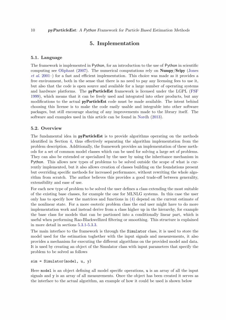
The main interface to the framework is through the Simulator class, it is used to store themodel used for the estimation toghether with the input signals and measurements, it alsoprovides a mechanism for executing the different algorithms on the provided model and data.It is used by creating an object of the Simulator class with input parameters that specify theproblem to be solved as follows

sim = Simulator(model, u, y)

Here model is an object defining all model specific operations, u is an array of all the inputsignals and y is an array of all measurements. Once the object has been created it serves asthe interface to the actual algorithm, an example of how it could be used is shown below

Journal of Statistical Software 11

sim.simulate(num, nums, res=0.67, filter='PF', smoother='mcmc')

Here num is the number of particles used in the forward filter, nums are the number of smoothedtrajectories generated by the smoother, res is the resampling threshhold (expressed as theratio of effective particles compared to total number of particles), filter is the filteringmethod to be used and finally smoother is the smoothing algorithm to be used.

After calling the method above the results can be access by using some of the followingmethods

(est_filt, w_filt) = sim.get_filtered_estimates()

mean_filt = sim.get_filtered_mean()

est_smooth = sim.get_smoothed_estimates()

smean = sim.get_smoothed_mean()

where (est_filt, w_filt) will contain the forward particles for each time step with thecorresponding weights, mean_filt is the weighted mean of all the forward particles for eachtime step. est_smooth is an array of all the smoothed trajectories and smean the mean valuefor each time step of the smoothed trajectories.

5.3. Software design

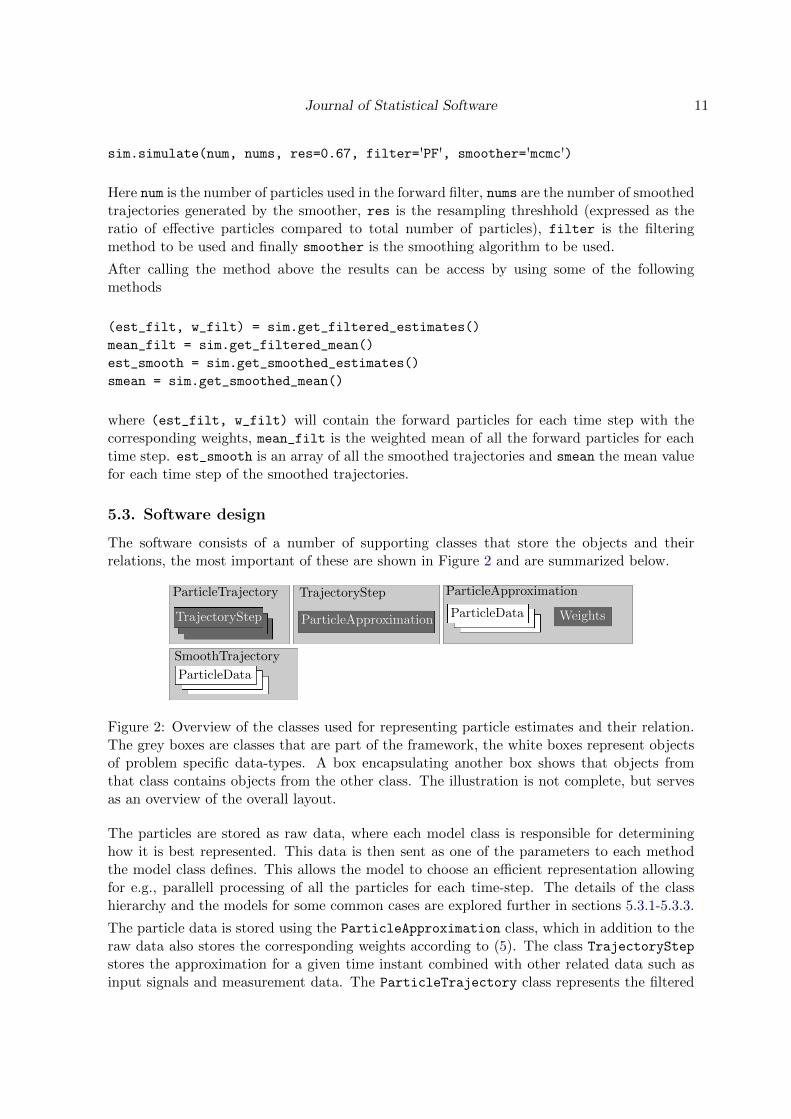
The software consists of a number of supporting classes that store the objects and theirrelations, the most important of these are shown in Figure 2 and are summarized below.

ParticleApproximation

TrajectoryStepParticleTrajectory

SmoothTrajectory

ParticleApproximation

TrajectoryStep WeightsParticleData

ParticleData

Figure 2: Overview of the classes used for representing particle estimates and their relation.The grey boxes are classes that are part of the framework, the white boxes represent objectsof problem specific data-types. A box encapsulating another box shows that objects fromthat class contains objects from the other class. The illustration is not complete, but servesas an overview of the overall layout.

The particles are stored as raw data, where each model class is responsible for determininghow it is best represented. This data is then sent as one of the parameters to each methodthe model class defines. This allows the model to choose an efficient representation allowingfor e.g., parallell processing of all the particles for each time-step. The details of the classhierarchy and the models for some common cases are explored further in sections 5.3.1-5.3.3.

The particle data is stored using the ParticleApproximation class, which in addition to theraw data also stores the corresponding weights according to (5). The class TrajectoryStep

stores the approximation for a given time instant combined with other related data such asinput signals and measurement data. The ParticleTrajectory class represents the filtered

12 pyParticleEst: A Python Framework for Particle Based Estimation Methods

estimates of the entire trajectory by storing a collection of TrajectorySteps, it also providesthe methods for interfacing with the chosen filtering algorithm.

The SmoothTrajectory class takes a ParticleTrajectory as input and using a ParticleSmoother creates a collection of point estimates representing the smoothed trajectory esti-mate. In the same manner as for the ParticleApproximation class the point estimates hereare of the problem specific data type defined by the model class, but not necessarily of thesame structure as the estimates created by the forward filter. This allows for example meth-ods where the forward filter is Rao-Blackwellized but the backward smoother samples the fullstate vector.

Model class hierarchy

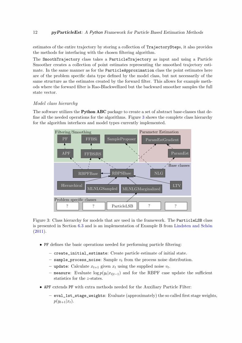
The software utilizes the Python ABC package to create a set of abstract base-classes that de-fine all the needed operations for the algorithms. Figure 3 shows the complete class hierarchyfor the algorithm interfaces and model types currently implemented.

PF

RBPSBase

HierarchicalMLNLGSampled

LTV

ParticleLSB ?

Problem specific classes

Filtering/Smoothing

FFBSi

ParamEst

Base classes

?

RBPFBase

? ?

NLG

FFBSiRSAPF

ParamEstGradientSampleProposer

Parameter Estimation

MLNLGMarginalized

Figure 3: Class hierarchy for models that are used in the framework. The ParticleLSB classis presented in Section 6.3 and is an implementation of Example B from Lindsten and Schon(2011).

• PF defines the basic operations needed for performing particle filtering:

– create_initial_estimate: Create particle estimate of initial state.

– sample_process_noise: Sample vt from the process noise distribution.

– update: Calculate xt+1 given xt using the supplied noise vt.

– measure: Evaluate log p(yt|xt|t−1) and for the RBPF case update the sufficientstatistics for the z-states.

• APF extends PF with extra methods needed for the Auxiliary Particle Filter:

– eval_1st_stage_weights: Evaluate (approximately) the so called first stage weights,p(yt+1|xt).

Journal of Statistical Software 13

• FFBSi defines the basic operations needed for performing particle smoothing:

– logp_xnext_full: Evaluate log p(xt+1:T |x1:t, y1:T ). This method normally justcalls logp_xnext, but the distinction is needed for non-Markovian models.

– logp_xnext: Evaluate log p(xt+1|xt).– sample_smooth: For normal models the default implementation can be used which

just copies the estimate from the filter, but for e.g., Rao-Blackwellized modelsadditional computations are made in this method.

• FFBSiRS extends FFBSi:

– next_pdf_max: Calculate maximum of log p(xt+1|xt).

• SampleProposer defines the basic operations needed for proposing new samples, usedin the MHBP and MH-IPS algorithms:

– propose_smooth: Propose new sample from q(xt|xt+1, xt−1, yt).

– logp_proposal: Evaluate logq(xt|xt+1, xt−1, yt).

• ParamEstInterface defines the basic operations needed for performing parameter esti-mation using the EM-algorithm presented in Section 4.3:

– set_params: Set θk estimate.

– eval_logp_x0: Evaluate log p(x1).

– eval_logp_xnext: Evaluate log p(xt+1|xt).– eval_logp_y: Evaluate log p(yt|xt) .

• ParamEstInterface_GradientSearch extends the operations from the ParamEstInter-face to include those needed when using analytic derivatives in the maximization step:

– eval_logp_x0_val_grad: Evaluate log p(x1) and its gradient.

– eval_logp_xnext_val_grad: Evaluate log p(xt+1|xt) and its gradient.

– eval_logp_y_val_grad: Evaluate log p(yt|xt) and its gradient.

Base classes

To complement the abstract base classes from Section 5.3.1 the software includes a numberof base classes to help implement the required functions.

• RBPFBase Provides an implementation handling the Rao-Blackwellized case automat-ically by defining a new set of simpler functions that are required from the derivedclass.

• RBPSBase Extends RBPFBase to provide smoothing for Rao-Blackwellized models.

Model classes

These classes further specialize those from sections 5.3.1-5.3.2.

14 pyParticleEst: A Python Framework for Particle Based Estimation Methods

• LTV Handles Linear Time-Varying systems, the derived class only needs to providecallbacks for how the system matrices depend on time.

• NLG Nonlinear dynamics with additive Gaussian noise.

• MixedNLGaussianSampled Provides support for models of type (4) using an algorithmwhich samples the linear states in the backward simulation step. The sufficient statisticsfor the linear states are later recovered in a post processing step. See Lindsten and Schon(2011) for details. The derived class needs to specify how the linear and non-lineardynamics depend on time and the current estimate of ξ.

• MixedNLGaussianMarginalized Provides an implementation for models of type (4) thatfully marginalizes the linear Gaussian states, resulting in a non-Markovian smoothingproblem. See Lindsten, Bunch, Godsill, and Schon (2013) for details. The derived classneeds to specify how the linear and non-linear dynamics depend on time and the currentestimate of ξ. This implementation requires that Qξz = 0.

• Hierarchial Provides a structure useful for implementing models of type (3) usingsampling of the linear states in the backward simulation step. The sufficient statisticsfor the linear states are later recovered in a post processing step.

For the LTV and MLNLG classes the parameters estimation interfaces, ParamEstInterfaceand ParamEstInterface_GradientSearch, are implemented so that the end-user can specifythe element-wise derivative for the matrices instead of directly calculating gradients of (7b)-(7d). Typically there is some additional structure to the problem, and it is then beneficialto override this generic implementation with a specialized one to reduce the computationaleffort by utilizing that structure.

5.4. Algorithms

RBPF

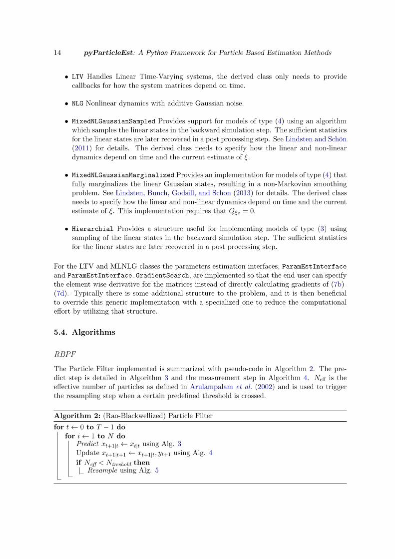
The Particle Filter implemented is summarized with pseudo-code in Algorithm 2. The pre-dict step is detailed in Algorithm 3 and the measurement step in Algorithm 4. Neff is theeffective number of particles as defined in Arulampalam et al. (2002) and is used to triggerthe resampling step when a certain predefined threshold is crossed.

Algorithm 2: (Rao-Blackwellized) Particle Filter

for t← 0 to T − 1 dofor i← 1 to N do

Predict xt+1|t ← xt|t using Alg. 3Update xt+1|t+1 ← xt+1|t, yt+1 using Alg. 4

if Neff < Ntreshold thenResample using Alg. 5

Journal of Statistical Software 15

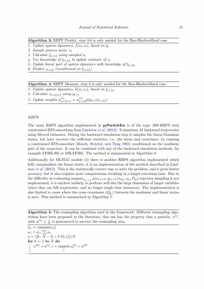
Algorithm 3: RBPF Predict, step 4-6 is only needed for the Rao-Blackwellized case

1. Update system dynamics, f(xt, vt), based on ξt2. Sample process noise, vt3. Calculate ξt+1|t using sampled vt4. Use knowledge of ξt+1|t to update estimate of zt5. Update linear part of system dynamics with knowledge of ξt+1|t6. Predict zt+1|t (conditioned on ξt+1|t)

Algorithm 4: RBPF Measure, step 2 is only needed for the Rao-Blackwellized case

1. Update system dynamics, h(xt, et), based on ξt+1|t2. Calculate zt+1|t+1 using yt+1

3. Update weights w(i)t+1|t+1 = w

(i)t+1|tp(yt+1|xt+1|t)

RBPS

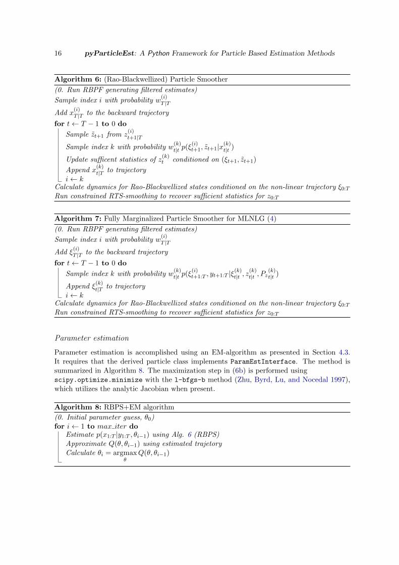
The main RBPS algorithm implemented in pyParticleEst is of the type JBS-RBPS withconstrained RTS-smoothing from Lindsten et al. (2013). It simulates M backward trajectoriesusing filtered estimates. During the backward simulation step it samples the linear/Gaussianstates, but later recovers the sufficient statistics, i.e., the mean and covariance, by runninga constrained RTS-smoother (Rauch, Striebel, and Tung 1965) conditioned on the nonlinearpart of the trajectory. It can be combined with any of the backward simulation methods, forexample FFBSi-RS or MH-FFBSi. The method is summarized in Algorithm 6.

Additionally for MLNLG models (4) there is another RBPS algorithm implemented whichfully marginalizes the linear states, it is an implementation of the method described in Lind-sten et al. (2013). This is the statistically correct way to solve the problem, and it gives betteraccuracy, but it also requires more computations resulting in a longer execution time. Due tothe difficulty in evaluating argmaxxt+1:T

p(xt+1:T , yt+1:T |xt|t, zt|t, Pt|t) rejection sampling is notimplemented, it is anyhow unlikely to perform well due the large dimension of target variables(since they are full trajectories, and no longer single time instances). The implementation isalso limited to cases where the cross covariance (Qξz) between the nonlinear and linear statesis zero. This method is summarized in Algorithm 7.

Algorithm 5: The resampling algorithm used in the framework. Different resampling algo-rithms have been proposed in the literature, this one has the property that a particle, x(i),with w(i) ≥ 1

N is guaranteed to survive the resampling step.

ωc = cumsum(ω)ωc = ωc/

∑ωc

u = ([0 : N − 1] + U(0, 1))/Nfor k ← 1 to N do

x(k) = x(i), i = argminj

ω(j)c > u(k)

16 pyParticleEst: A Python Framework for Particle Based Estimation Methods

Algorithm 6: (Rao-Blackwellized) Particle Smoother

(0. Run RBPF generating filtered estimates)

Sample index i with probability w(i)T |T

Add x(i)T |T to the backward trajectory

for t← T − 1 to 0 do

Sample zt+1 from z(i)t+1|T

Sample index k with probability w(k)t|t p(ξ

(i)t+1, zt+1|x(k)

t|t )

Update sufficent statistics of z(k)t conditioned on (ξt+1, zt+1)

Append x(k)t|T to trajectory

i← kCalculate dynamics for Rao-Blackwellized states conditioned on the non-linear trajectory ξ0:T

Run constrained RTS-smoothing to recover sufficient statistics for z0:T

Algorithm 7: Fully Marginalized Particle Smoother for MLNLG (4)

(0. Run RBPF generating filtered estimates)

Sample index i with probability w(i)T |T

Add ξ(i)T |T to the backward trajectory

for t← T − 1 to 0 do

Sample index k with probability w(k)t|t p(ξ

(i)t+1:T , yt+1:T |ξ(k)

t|t , z(k)t|t , Pz

(k)t|t )

Append ξ(k)t|T to trajectory

i← kCalculate dynamics for Rao-Blackwellized states conditioned on the non-linear trajectory ξ0:T

Run constrained RTS-smoothing to recover sufficient statistics for z0:T

Parameter estimation

Parameter estimation is accomplished using an EM-algorithm as presented in Section 4.3.It requires that the derived particle class implements ParamEstInterface. The method issummarized in Algorithm 8. The maximization step in (6b) is performed usingscipy.optimize.minimize with the l-bfgs-b method (Zhu, Byrd, Lu, and Nocedal 1997),which utilizes the analytic Jacobian when present.

Algorithm 8: RBPS+EM algorithm

(0. Initial parameter guess, θ0)for i← 1 to max iter do

Estimate p(x1:T |y1:T , θi−1) using Alg. 6 (RBPS)Approximate Q(θ, θi−1) using estimated trajetoryCalculate θi = argmax

θQ(θ, θi−1)

Journal of Statistical Software 17

6. Example models

6.1. Integrator

A trivial example consisting of a linear Gaussian system

xt+1 = xt + wt (8a)

yt = xt + et, x1 ∼ N(0, 1) (8b)

wt ∼ N(0, 1), et ∼ N(0, 1) (8c)

This model could be implemented using either the LTV or NLG model classes, but for thisexample it was decided to directly implement the required top level interfaces to illustratehow they work. In this example only the methods needed for filtering are implemented. Touse smoothing the logp_xnext method would be needed as well. An example realizationusing this model was shown in Fig. 1

1 class I n t e g r a t o r ( i n t e r f a c e s . P a r t i c l e F i l t e r i n g ) :def i n i t ( s e l f , P0 , Q, R) :

s e l f . P0 = numpy . copy (P0)s e l f .Q = numpy . copy (Q)s e l f .R = numpy . copy (R)

6

def c r e a t e i n i t i a l e s t i m a t e ( s e l f , N) :return numpy . random . normal ( 0 . 0 , s e l f . P0 , (N, )

) . reshape ((−1 , 1 ) )

11 def s amp l e p ro c e s s no i s e ( s e l f , p a r t i c l e s , u , t ) :N = len ( p a r t i c l e s )return numpy . random . normal ( 0 . 0 , s e l f .Q, (N, )

) . reshape ((−1 , 1 ) )

16 def update ( s e l f , p a r t i c l e s , u , t , no i s e ) :p a r t i c l e s += no i s e

def measure ( s e l f , p a r t i c l e s , y , t ) :logyprob = numpy . empty ( len ( p a r t i c l e s ) )

21 for k in range ( len ( p a r t i c l e s ) ) :logyprob [ k ] = kalman . lognormpdf ( p a r t i c l e s [ k , 0 ] − y ,

s e l f .R)return logyprob

Line 08 Samples the initial particles from a zero-mean Gaussian distribution with variance P0.

Line 13 This samples the process noise at time t.

Line 16 Propagates the estimates forward in time using the noise previously sampled.

Line 19 Calculates the log-probability for the measurement yt for particles x(i)t .

18 pyParticleEst: A Python Framework for Particle Based Estimation Methods

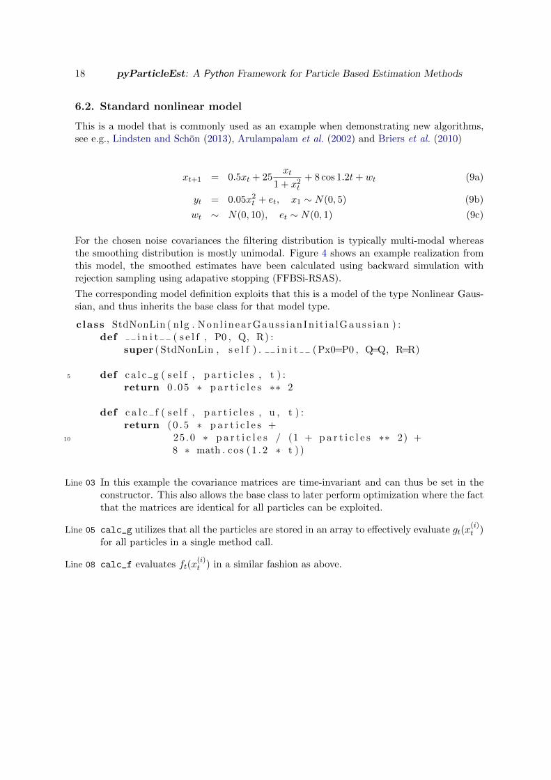
6.2. Standard nonlinear model

This is a model that is commonly used as an example when demonstrating new algorithms,see e.g., Lindsten and Schon (2013), Arulampalam et al. (2002) and Briers et al. (2010)

xt+1 = 0.5xt + 25xt

1 + x2t

+ 8 cos 1.2t+ wt (9a)

yt = 0.05x2t + et, x1 ∼ N(0, 5) (9b)

wt ∼ N(0, 10), et ∼ N(0, 1) (9c)

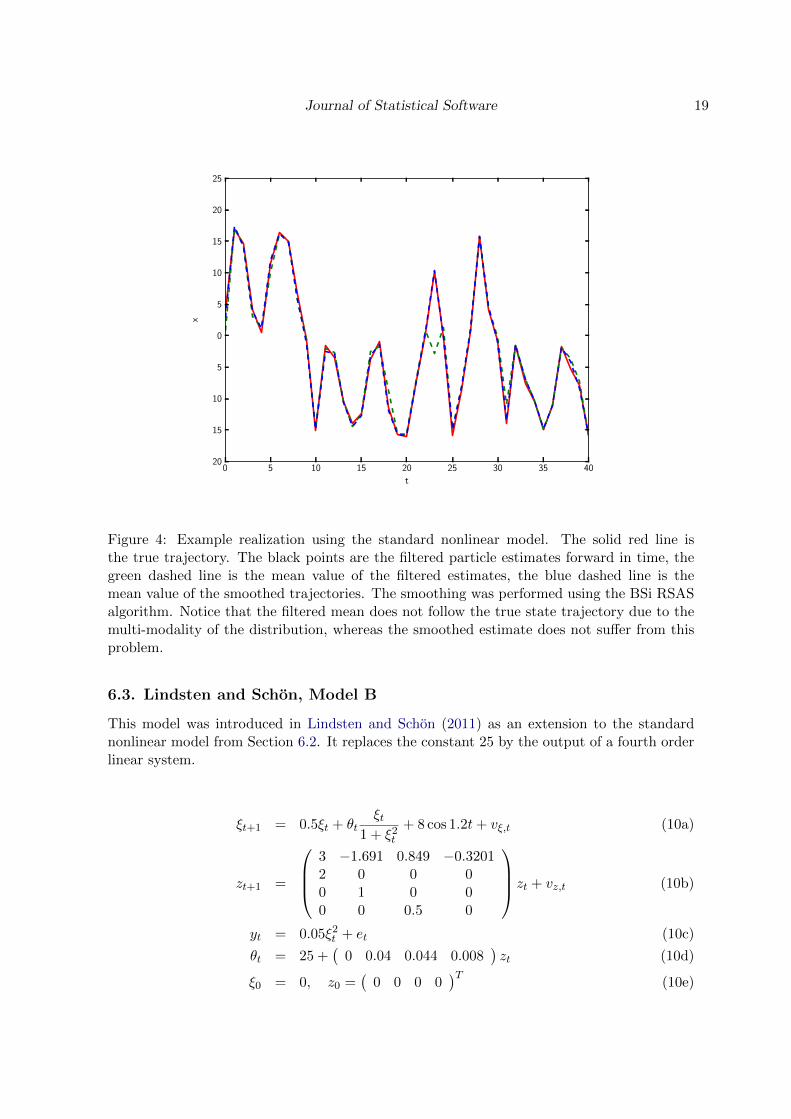
For the chosen noise covariances the filtering distribution is typically multi-modal whereasthe smoothing distribution is mostly unimodal. Figure 4 shows an example realization fromthis model, the smoothed estimates have been calculated using backward simulation withrejection sampling using adapative stopping (FFBSi-RSAS).

The corresponding model definition exploits that this is a model of the type Nonlinear Gaus-sian, and thus inherits the base class for that model type.

class StdNonLin ( nlg . Non l inea rGaus s i an In i t i a lGaus s i an ) :def i n i t ( s e l f , P0 , Q, R) :

super ( StdNonLin , s e l f ) . i n i t (Px0=P0 , Q=Q, R=R)

5 def c a l c g ( s e l f , p a r t i c l e s , t ) :return 0 .05 ∗ p a r t i c l e s ∗∗ 2

def c a l c f ( s e l f , p a r t i c l e s , u , t ) :return ( 0 . 5 ∗ p a r t i c l e s +

10 25 .0 ∗ p a r t i c l e s / (1 + p a r t i c l e s ∗∗ 2) +8 ∗ math . cos ( 1 . 2 ∗ t ) )

Line 03 In this example the covariance matrices are time-invariant and can thus be set in theconstructor. This also allows the base class to later perform optimization where the factthat the matrices are identical for all particles can be exploited.

Line 05 calc_g utilizes that all the particles are stored in an array to effectively evaluate gt(x(i)t )

for all particles in a single method call.

Line 08 calc_f evaluates ft(x(i)t ) in a similar fashion as above.

Journal of Statistical Software 19

0 5 10 15 20 25 30 35 40

t

20

15

10

5

0

5

10

15

20

25

x

Figure 4: Example realization using the standard nonlinear model. The solid red line isthe true trajectory. The black points are the filtered particle estimates forward in time, thegreen dashed line is the mean value of the filtered estimates, the blue dashed line is themean value of the smoothed trajectories. The smoothing was performed using the BSi RSASalgorithm. Notice that the filtered mean does not follow the true state trajectory due to themulti-modality of the distribution, whereas the smoothed estimate does not suffer from thisproblem.

6.3. Lindsten and Schon, Model B

This model was introduced in Lindsten and Schon (2011) as an extension to the standardnonlinear model from Section 6.2. It replaces the constant 25 by the output of a fourth orderlinear system.

ξt+1 = 0.5ξt + θtξt

1 + ξ2t

+ 8 cos 1.2t+ vξ,t (10a)

zt+1 =

3 −1.691 0.849 −0.32012 0 0 00 1 0 00 0 0.5 0

zt + vz,t (10b)

yt = 0.05ξ2t + et (10c)

θt = 25 +(

0 0.04 0.044 0.008)zt (10d)

ξ0 = 0, z0 =(

0 0 0 0)T

(10e)

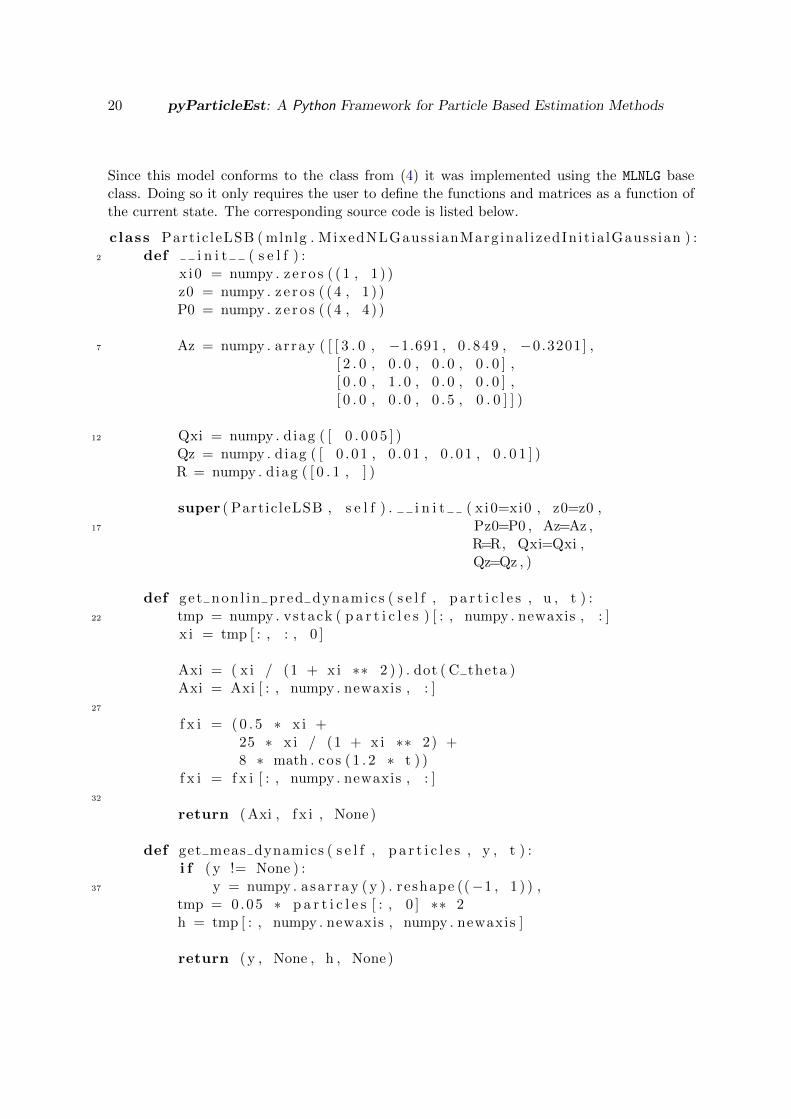
20 pyParticleEst: A Python Framework for Particle Based Estimation Methods

Since this model conforms to the class from (4) it was implemented using the MLNLG baseclass. Doing so it only requires the user to define the functions and matrices as a function ofthe current state. The corresponding source code is listed below.

class Part ic leLSB ( mlnlg . MixedNLGauss ianMargina l izedInit ia lGauss ian ) :2 def i n i t ( s e l f ) :

x i0 = numpy . z e ro s ( ( 1 , 1 ) )z0 = numpy . z e ro s ( ( 4 , 1 ) )P0 = numpy . z e ro s ( ( 4 , 4 ) )

7 Az = numpy . array ( [ [ 3 . 0 , −1.691 , 0 . 849 , −0.3201] ,[ 2 . 0 , 0 . 0 , 0 . 0 , 0 . 0 ] ,[ 0 . 0 , 1 . 0 , 0 . 0 , 0 . 0 ] ,[ 0 . 0 , 0 . 0 , 0 . 5 , 0 . 0 ] ] )

12 Qxi = numpy . diag ( [ 0 . 0 0 5 ] )Qz = numpy . diag ( [ 0 . 01 , 0 . 01 , 0 . 01 , 0 . 0 1 ] )R = numpy . diag ( [ 0 . 1 , ] )

super ( ParticleLSB , s e l f ) . i n i t ( x i0=xi0 , z0=z0 ,17 Pz0=P0 , Az=Az ,

R=R, Qxi=Qxi ,Qz=Qz , )

def get non l in pred dynamics ( s e l f , p a r t i c l e s , u , t ) :22 tmp = numpy . vstack ( p a r t i c l e s ) [ : , numpy . newaxis , : ]

x i = tmp [ : , : , 0 ]

Axi = ( x i / (1 + x i ∗∗ 2 ) ) . dot ( C theta )Axi = Axi [ : , numpy . newaxis , : ]

27

f x i = ( 0 . 5 ∗ x i +25 ∗ x i / (1 + x i ∗∗ 2) +8 ∗ math . cos ( 1 . 2 ∗ t ) )

f x i = f x i [ : , numpy . newaxis , : ]32

return ( Axi , f x i , None )

def get meas dynamics ( s e l f , p a r t i c l e s , y , t ) :i f ( y != None ) :

37 y = numpy . asar ray ( y ) . reshape ((−1 , 1 ) ) ,tmp = 0.05 ∗ p a r t i c l e s [ : , 0 ] ∗∗ 2h = tmp [ : , numpy . newaxis , numpy . newaxis ]

return (y , None , h , None )

Journal of Statistical Software 21

Line 02 In the constructor all the time-invariant parts of the model are set

Line 21 This function calculates Aξ(ξ(i)t ), fξ(ξ

(i)t ) and Qξ(ξ

(i)t )

Line 26 The array is resized to match the expected format (The first dimension indices theparticles, each entry being a two-dimensional matrix)

Line 33 Return a tuple containing Aξ, fξ and Qξ arrays. Returning None for any element in thetuple indicates that the time-invariant values set in the constructor should be used

Line 36 This function works in the same way as above, but instead calculates h(ξt), C(ξt) andR(ξt). The first value in the returned tuple should be the (potentially preprocessed)measurement.

22 pyParticleEst: A Python Framework for Particle Based Estimation Methods

7. Results

The aim of this section is to demonstrate that the implementation in pyParticleEst is correctby reproducing results previously published elsewhere.

7.1. Rao-Blackwellized particle filtering / smoothing

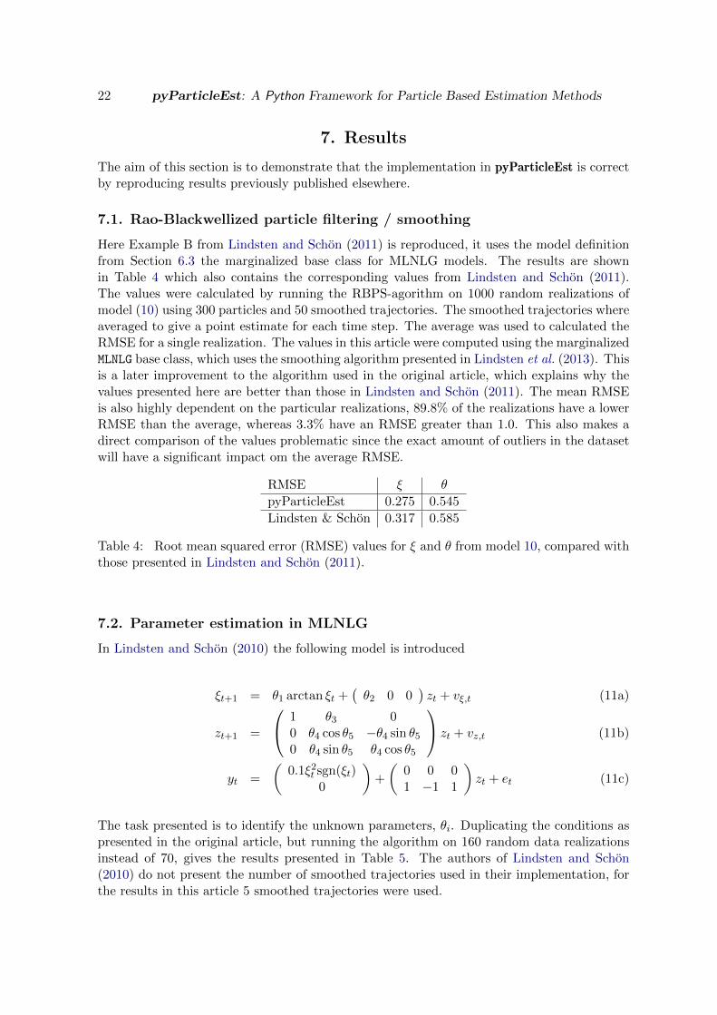
Here Example B from Lindsten and Schon (2011) is reproduced, it uses the model definitionfrom Section 6.3 the marginalized base class for MLNLG models. The results are shownin Table 4 which also contains the corresponding values from Lindsten and Schon (2011).The values were calculated by running the RBPS-agorithm on 1000 random realizations ofmodel (10) using 300 particles and 50 smoothed trajectories. The smoothed trajectories whereaveraged to give a point estimate for each time step. The average was used to calculated theRMSE for a single realization. The values in this article were computed using the marginalizedMLNLG base class, which uses the smoothing algorithm presented in Lindsten et al. (2013). Thisis a later improvement to the algorithm used in the original article, which explains why thevalues presented here are better than those in Lindsten and Schon (2011). The mean RMSEis also highly dependent on the particular realizations, 89.8% of the realizations have a lowerRMSE than the average, whereas 3.3% have an RMSE greater than 1.0. This also makes adirect comparison of the values problematic since the exact amount of outliers in the datasetwill have a significant impact om the average RMSE.

RMSE ξ θ

pyParticleEst 0.275 0.545

Lindsten & Schon 0.317 0.585

Table 4: Root mean squared error (RMSE) values for ξ and θ from model 10, compared withthose presented in Lindsten and Schon (2011).

7.2. Parameter estimation in MLNLG

In Lindsten and Schon (2010) the following model is introduced

ξt+1 = θ1 arctan ξt +(θ2 0 0

)zt + vξ,t (11a)

zt+1 =

1 θ3 00 θ4 cos θ5 −θ4 sin θ5

0 θ4 sin θ5 θ4 cos θ5

zt + vz,t (11b)

yt =

(0.1ξ2

t sgn(ξt)0

)+

(0 0 01 −1 1

)zt + et (11c)

The task presented is to identify the unknown parameters, θi. Duplicating the conditions aspresented in the original article, but running the algorithm on 160 random data realizationsinstead of 70, gives the results presented in Table 5. The authors of Lindsten and Schon(2010) do not present the number of smoothed trajectories used in their implementation, forthe results in this article 5 smoothed trajectories were used.

Journal of Statistical Software 23

True value Lindsten & Schon pyParticleEst pyParticleEst*

θ1 1 0.966± 0.163 0.981± 0.254 1.006± 0.091

θ2 1 1.053± 0.163 0.947± 0.158 0.984± 0.079

θ3 0.3 0.295± 0.094 0.338± 0.308 0.271± 0.112

θ4 0.968 0.967± 0.015 0.969± 0.032 0.962± 0.017

θ5 0.315 0.309± 0.057 0.263± 0.134 0.312± 0.019

Table 5: Results presented by Lindsten and Schon in Lindsten and Schon (2010) comparedto results calculated using pyParticleEst. The column marked with * are the statistics whenexcluding those realizations where the EM-algorithm was stuck in local maxima for θ5.

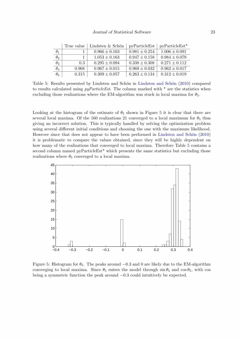
Looking at the histogram of the estimate of θ5 shown in Figure 5 it is clear that there areseveral local maxima. Of the 160 realizations 21 converged to a local maximum for θ5 thusgiving an incorrect solution. This is typically handled by solving the optimization problemusing several different initial conditions and choosing the one with the maximum likelihood.However since that does not appear to have been performed in Lindsten and Schon (2010)it is problematic to compare the values obtained, since they will be highly dependent onhow many of the realizations that converged to local maxima. Therefore Table 5 contains asecond column named pyParticleEst* which presents the same statistics but excluding thoserealizations where θ5 converged to a local maxima.

−0.4 −0.3 −0.2 −0.1 0 0.1 0.2 0.3 0.40

5

10

15

20

25

30

35

40

45

Figure 5: Histogram for θ5. The peaks around −0.3 and 0 are likely due to the EM-algorithmconverging to local maxima. Since θ5 enters the model through sin θ5 and cos θ5, with cosbeing a symmetric function the peak around −0.3 could intuitively be expected.

24 pyParticleEst: A Python Framework for Particle Based Estimation Methods

8. Conclusion

pyParticleEst lowers the barrier of entry to the field of particle methods, allowing many prob-lems to be solved with significantly less implementation effort compared to starting fromscratch. This was exemplified by the models presented in Section 6, demonstrating the sig-nificant reduction in the amount of code needed to be produced by the end-user. Its use forgrey-box identification was demonstrated in Section 7.2. The software and examples used inthis article can be found at Nordh (2013).

There is an overhead due to the generic design which by necessity gives lower performancecompared to a specialized implementation in a low-level language. For example a hand opti-mized C-implementation that fully exploits the structure of a specific problem will always befaster, but also requires significantly more time and knowledge from the developer. Thereforethe main use-case for this software when it comes to performance critical applications is likelyto be prototyping different models and algorithms that will later be re-implemented in a low-level language. That implementation can then be validated against the results provided bythe generic algorithms. In many circumstances the execution time might be of little concernand the performance provided using pyParticleEst will be sufficient. There are projects suchas Numba (Continuum Analytics 2014), Cython (Behnel, Bradshaw, and Seljebotn 2009) andPyPy (Rigo 2004) that aim to increase the efficiency of Python-code. Cython is already usedfor some of the heaviest parts in the framework. By selectively moving more of the compu-tationally heavy parts of the model base classes to Cython it should be possible to use theframework directly for many real-time applications.

For the future the plan is to extend the framework to contain more algorithms, for examplethe interesting field of PMCMC methods (Del Moral, Doucet, and Jasra 2006). Anotherinteresting direction is smoothing of non-Markovian models as examplified by the marginalizedsmoother for MLNLG models. This type of smoother could also be combined with Gaussianprocesses as shown by Lindsten and Schon (2013). The direction taken by e.g., Murray (Inreview) with a high level language is interesting, and something that might be worthwhile toimplement for automatically generating the Python code describing the model, providing afurther level of abstraction for the end user.

Acknowledgments

The author is a member of the LCCC Linnaeus Center and the eLLIIT Excellence Center atLund University. The author would like to thank professor Bo Bernhardsson, Lund University,and professor Thomas Schon, Uppsala University, for the feedback provided on this work.

Journal of Statistical Software 25

References

Andrieu C, Doucet A, Holenstein R (2010). “Particle Markov Chain Monte Carlo Methods.”Journal of the Royal Statistical Society B (Statistical Methodology), 72(3), 269–342.

Arulampalam M, Maskell S, Gordon N, Clapp T (2002). “A Tutorial on Particle Filters forOnline Nonlinear/Non-Gaussian Bayesian Tracking.” IEEE Trans. Signal Process., 50(2),174–188. ISSN 1053-587X.

Behnel S, Bradshaw RW, Seljebotn DS (2009). “Cython Tutorial.” In G Varoquaux, S van derWalt, J Millman (eds.), Proceedings of the 8th Python in Science Conference, pp. 4 – 14.Pasadena, CA USA.

Beskos A, Crisan D, Jasra A (2011). “On the Stability of Sequential Monte Carlo Methodsin Hgh Fimensions.” arXiv preprint arXiv:1103.3965.

Briers M, Doucet A, Maskell S (2010). “Smoothing Algorithms for State-Space Models.”Annals of the Institute of Statistical Mathematics, 62(1), 61–89. ISSN 0020-3157. doi:

10.1007/s10463-009-0236-2. URL http://dx.doi.org/10.1007/s10463-009-0236-2.

Bunch P, Godsill S (2013). “Improved Particle Approximations to the Joint Smoothing Dis-tribution using Markov Chain Monte Carlo.” Signal Processing, IEEE Transactions on,61(4), 956–963.

Continuum Analytics (2014). Numba, Version 0.14. URL http://numba.pydata.org/

numba-doc/0.14/index.html.

Del Moral P, Doucet A, Jasra A (2006). “Sequential Monte Carlo Samplers.” Journal of theRoyal Statistical Society B (Statistical Methodology), 68(3), 411–436.

Dempster AP, Laird NM, Rubin DB (1977). “Maximum Likelihood from Incomplete Data viathe EM Algorithm.” Journal of the Royal Statistical Society B, 39(1), 1–38.

Doucet A, Godsill S, Andrieu C (2000). “On Sequential Monte Carlo Sampling Methods forBayesian Filtering.” Statistics and Computing, 10(3), 197–208. ISSN 0960-3174. doi:

10.1023/A:1008935410038. URL http://dx.doi.org/10.1023/A%3A1008935410038.

Dubarry C, Douc R (2011). “Particle Approximation Improvement of the Joint SmoothingDistribution with On-the-Fly Variance Estimation.” arXiv preprint arXiv:1107.5524.

FSF (1999). “The GNU Lesser General Public License.” See http://www.gnu.org/copyleft/lesser.html.

Jones E, Oliphant T, Peterson P, et al. (2001–). “SciPy: Open Source Scientific Tools forPython.” URL http://www.scipy.org/.

Julier S, Uhlmann J (2004). “Unscented Filtering and Nonlinear Estimation.” Proceedings ofthe IEEE, 92(3), 401–422. ISSN 0018-9219. doi:10.1109/JPROC.2003.823141.

Lindsten F, Bunch P, Godsill SJ, Schon TB (2013). “Rao-Blackwellized Particle Smoothers forMixed Linear/Nonlinear State-Space Models.” In Acoustics, Speech and Signal Processing(ICASSP), 2013 IEEE International Conference on, pp. 6288–6292. IEEE.

26 pyParticleEst: A Python Framework for Particle Based Estimation Methods

Lindsten F, Schon T (2010). “Identification of Mixed Linear/Nonlinear State-Space Models.”In Decision and Control (CDC), 2010 49th IEEE Conference on, pp. 6377–6382. ISSN0743-1546. doi:10.1109/CDC.2010.5717191.

Lindsten F, Schon T (2011). “Rao-Blackwellized Particle Smoothers for Mixed Linear/Non-linear State-Space Models.” Technical report. URL http://user.it.uu.se/~thosc112/

pubpdf/lindstens2011.pdf.

Lindsten F, Schon TB (2013). “Backward Simulation Methods for Monte Carlo StatisticalInference.” Foundations and Trends®in Machine Learning, 6(1), 1–143. ISSN 1935-8237.doi:10.1561/2200000045. URL http://dx.doi.org/10.1561/2200000045.

Mannesson A (2013). “Joint Pose and Radio Channel Estimation.” Licentiate thesis, Dept.of Automatic Control, Lund University, Sweden.

Montemerlo M, Thrun S, Koller D, Wegbreit B, et al. (2002). “FastSLAM: A Factored Solutionto the Simultaneous Localization and Mapping Problem.” In AAAI/IAAI, pp. 593–598.

Murray LM (In review). “Bayesian State-Space Modelling on High-Performance HardwareUsing LibBi.” URL http://arxiv.org/abs/1306.3277.

Nordh J (2013). “pyParticleEst.” URL http://www.control.lth.se/Staff/JerkerNordh/

pyparticleest.html.

Okuma K, Taleghani A, De Freitas N, Little JJ, Lowe DG (2004). “A Boosted ParticleFilter: Multitarget Detection and Tracking.” In Computer Vision-ECCV 2004, pp. 28–39.Springer-Verlag.

Oliphant TE (2007). “Python for Scientific Computing.” Computing in Science Engineering,9(3), 10–20. ISSN 1521-9615. doi:10.1109/MCSE.2007.58.

Rauch HE, Striebel CT, Tung F (1965). “Maximum Likelihood Estimates of Linear DynamicSystems.” Journal of the American Institute of Aeronautics and Astronautics, 3(8), 1445–1450.

Rebeschini P, van Handel R (2013). “Can Local Particle Filters Beat the Curse of Dimen-sionality?” arXiv preprint arXiv:1301.6585.

Rigo A (2004). “Representation-Based Just-in-Time Specialization and the Psyco Prototypefor Python.” In Proceedings of the 2004 ACM SIGPLAN Symposium on Partial Evaluationand Semantics-Based Program Manipulation, pp. 15–26. ACM, Verona, Italy. ISBN 1-58113-835-0. doi:10.1145/1014007.1014010. URL http://portal.acm.org/citation.

cfm?id=1014010.

Schon T, Gustafsson F, Nordlund PJ (2005). “Marginalized Particle Filters for Mixed Lin-ear/Nonlinear State-Space Models.” Signal Processing, IEEE Transactions on, 53(7), 2279–2289. ISSN 1053-587X. doi:10.1109/TSP.2005.849151.

Taghavi E, Lindsten F, Svensson L, Schon T (2013). “Adaptive Stopping for Fast ParticleSmoothing.” In Acoustics, Speech and Signal Processing (ICASSP), 2013 IEEE Inter-national Conference on, pp. 6293–6297. ISSN 1520-6149. doi:10.1109/ICASSP.2013.

6638876.

Journal of Statistical Software 27

Zhu C, Byrd RH, Lu P, Nocedal J (1997). “Algorithm 778: L-BFGS-B: Fortran Subroutinesfor Large-Scale Bound-Constrained Optimization.” ACM Transactions on MathematicalSoftware (TOMS), 23(4), 550–560.

Affiliation:

Jerker NordhDepartment of Automatic ControlLund UniversityBox 118, SE-221 00 Lund, SwedenE-mail: jerker.nordh@control.lth.seURL: http://www.control.lth.se/Staff/JerkerNordh/

Journal of Statistical Software http://www.jstatsoft.org/

published by the American Statistical Association http://www.amstat.org/

Volume VV, Issue II Submitted: yyyy-mm-ddMMMMMM YYYY Accepted: yyyy-mm-dd