Embed Size (px)
Citation preview


3G, HSPA and FDD versus TDD Networking

3G, HSPA and FDDversus TDD Networking
Smart Antennas and Adaptive Modulation
Second Edition
L. Hanzo, University of Southampton, UK
J. S. Blogh, Anritsu, UK
S. Ni, Panasonic Mobile Communication, UK
IEEE Communications Society, Sponsor
John Wiley & Sons, Ltd

Copyright c© 2008 John Wiley & Sons Ltd, The Atrium, Southern Gate, Chichester,West Sussex PO19 8SQ, England
Telephone (+44) 1243 779777
Email (for orders and customer service enquiries): [email protected] our Home Page on www.wiley.com
All Rights Reserved. No part of this publication may be reproduced, stored in a retrieval system or transmitted in any formor by any means, electronic, mechanical, photocopying, recording, scanning or otherwise, except under the terms of theCopyright, Designs and Patents Act 1988 or under the terms of a licence issued by the Copyright Licensing Agency Ltd, 90Tottenham Court Road, London W1T 4LP, UK, without the permission in writing of the Publisher. Requests to thePublisher should be addressed to the Permissions Department, John Wiley & Sons Ltd, The Atrium, Southern Gate,Chichester, West Sussex PO19 8SQ, England, or emailed to [email protected], or faxed to (+44) 1243 770620.
Designations used by companies to distinguish their products are often claimed as trademarks. All brand names andproduct names used in this book are trade names, service marks, trademarks or registered trademarks of their respectiveowners. The Publisher is not associated with any product or vendor mentioned in this book. All trademarks referred to inthe text of this publication are the property of their respective owners.
This publication is designed to provide accurate and authoritative information in regard to the subject matter covered. It issold on the understanding that the Publisher is not engaged in rendering professional services. If professional advice orother expert assistance is required, the services of a competent professional should be sought.
Other Wiley Editorial Offices
John Wiley & Sons Inc., 111 River Street, Hoboken, NJ 07030, USA
Jossey-Bass, 989 Market Street, San Francisco, CA 94103-1741, USA
Wiley-VCH Verlag GmbH, Boschstr. 12, D-69469 Weinheim, Germany
John Wiley & Sons Australia Ltd, 42 McDougall Street, Milton, Queensland 4064, Australia
John Wiley & Sons (Asia) Pte Ltd, 2 Clementi Loop #02-01, Jin Xing Distripark, Singapore 129809
John Wiley & Sons Canada Ltd, 6045 Freemont Blvd, Mississauga, ONT, L5R 4J3, Canada
Wiley also publishes its books in a variety of electronic formats. Some content that appears in print may not be available inelectronic books.
IEEE Communications Society, SponsorCOMMS-S Liaison to IEEE Press, Mostafa Hashem Sherif
Library of Congress Cataloging-in-Publication Data
Hanzo, Lajos, 1952-3G, HSPA and FDD versus TDD Networking / by L. Hanzo, J. S. Blogh and S. Ni – 2nd ed.
p. cm.Includes bibliographical references and index.ISBN 978-0-470-75420-7 (cloth)
1. Wireless communication systems. 2. Cellular telephone systems.I. Blogh, J. S. (Jonathan S.) II. Title.
TK5103.2.H35 2008621.382’1–dc22
2007046621British Library Cataloguing in Publication Data
A catalogue record for this book is available from the British Library
ISBN 978-0-470-75420-7 (HB)
Typeset by the authors using LATEX software.Printed and bound in Great Britain by Antony Rowe Ltd, Chippenham, England.This book is printed on acid-free paper responsibly manufactured from sustainable forestry in which at least two trees areplanted for each one used for paper production.

Contents
About the Authors xv
Other Wiley and IEEE Press Books on Related Topics xvii
Preface xix
Acknowledgments xxxi
1 Third-generation CDMA Systems 11.1 Introduction . . . . . . . . . . . . . . . . . . . . . . . . . . . . . . . . . . . 11.2 Basic CDMA System . . . . . . . . . . . . . . . . . . . . . . . . . . . . . . 2
1.2.1 Spread Spectrum Fundamentals . . . . . . . . . . . . . . . . . . . . 21.2.1.1 Frequency Hopping . . . . . . . . . . . . . . . . . . . . . 31.2.1.2 Direct Sequence . . . . . . . . . . . . . . . . . . . . . . . 3
1.2.2 The Effect of Multipath Channels . . . . . . . . . . . . . . . . . . . 61.2.3 Rake Receiver . . . . . . . . . . . . . . . . . . . . . . . . . . . . . 91.2.4 Multiple Access . . . . . . . . . . . . . . . . . . . . . . . . . . . . 13
1.2.4.1 DL Interference . . . . . . . . . . . . . . . . . . . . . . . 141.2.4.2 Uplink Interference . . . . . . . . . . . . . . . . . . . . . 151.2.4.3 Gaussian Approximation . . . . . . . . . . . . . . . . . . 18
1.2.5 Spreading Codes . . . . . . . . . . . . . . . . . . . . . . . . . . . . 191.2.5.1 m-sequences . . . . . . . . . . . . . . . . . . . . . . . . . 201.2.5.2 Gold Sequences . . . . . . . . . . . . . . . . . . . . . . . 211.2.5.3 Extended m-sequences . . . . . . . . . . . . . . . . . . . . 21
1.2.6 Channel Estimation . . . . . . . . . . . . . . . . . . . . . . . . . . . 221.2.6.1 DL Pilot-assisted Channel Estimation . . . . . . . . . . . . 221.2.6.2 UL Pilot-symbol Assisted Channel Estimation . . . . . . . 231.2.6.3 Pilot-symbol Assisted Decision-directed Channel
Estimation . . . . . . . . . . . . . . . . . . . . . . . . . . 241.2.7 Summary . . . . . . . . . . . . . . . . . . . . . . . . . . . . . . . . 26

vi CONTENTS
1.3 Third-generation Systems . . . . . . . . . . . . . . . . . . . . . . . . . . . . 261.3.1 Introduction . . . . . . . . . . . . . . . . . . . . . . . . . . . . . . . 261.3.2 UMTS Terrestrial Radio Access (UTRA) . . . . . . . . . . . . . . . 29
1.3.2.1 Characteristics of UTRA . . . . . . . . . . . . . . . . . . 291.3.2.2 Transport Channels . . . . . . . . . . . . . . . . . . . . . 331.3.2.3 Physical Channels . . . . . . . . . . . . . . . . . . . . . . 34
1.3.2.3.1 Dedicated Physical Channels. . . . . . . . . . . . 351.3.2.3.2 Common Physical Channels . . . . . . . . . . . 37
1.3.2.3.2.1 Common Physical Channels of the FDDMode. . . . . . . . . . . . . . . . . . . . 37
1.3.2.3.2.2 Common Physical Channels of the TDDMode. . . . . . . . . . . . . . . . . . . . 40
1.3.2.4 Service Multiplexing and Channel Coding in UTRA . . . . 431.3.2.4.1 CRC Attachment. . . . . . . . . . . . . . . . . . 431.3.2.4.2 Transport Block Concatenation. . . . . . . . . . 431.3.2.4.3 Channel-coding. . . . . . . . . . . . . . . . . . . 431.3.2.4.4 Radio Frame Padding. . . . . . . . . . . . . . . . 461.3.2.4.5 First Interleaving. . . . . . . . . . . . . . . . . . 461.3.2.4.6 Radio Frame Segmentation. . . . . . . . . . . . . 461.3.2.4.7 Rate Matching. . . . . . . . . . . . . . . . . . . 461.3.2.4.8 Discontinuous Transmission Indication. . . . . . 471.3.2.4.9 Transport Channel Multiplexing. . . . . . . . . . 471.3.2.4.10 Physical Channel Segmentation. . . . . . . . . . 471.3.2.4.11 Second Interleaving. . . . . . . . . . . . . . . . 471.3.2.4.12 Physical Channel Mapping. . . . . . . . . . . . . 471.3.2.4.13 Mapping Several Multirate Services to the UL
Physical Channels in FDD Mode . . . . . . . . . 481.3.2.4.14 Mapping of a 4.1 Kbps Data Service to the DL
DPDCH in FDD Mode. . . . . . . . . . . . . . . 491.3.2.4.15 Mapping Several Multirate Services to the UL
Physical Channels in TDD Mode . . . . . . . . . 501.3.2.5 Variable-rate and Multicode Transmission in UTRA . . . . 521.3.2.6 Spreading and Modulation . . . . . . . . . . . . . . . . . 52
1.3.2.6.1 Orthogonal Variable Spreading Factor Codes. . . 551.3.2.6.2 Uplink Scrambling Codes. . . . . . . . . . . . . 571.3.2.6.3 Downlink Scrambling Codes. . . . . . . . . . . . 571.3.2.6.4 Uplink Spreading and Modulation. . . . . . . . . 581.3.2.6.5 Downlink Spreading and Modulation. . . . . . . 58
1.3.2.7 Random Access . . . . . . . . . . . . . . . . . . . . . . . 601.3.2.7.1 Mobile-initiated Physical Random Access
Procedures . . . . . . . . . . . . . . . . . . . . . 601.3.2.7.2 Common Packet Channel Access Procedures. . . 61
1.3.2.8 Power Control . . . . . . . . . . . . . . . . . . . . . . . . 611.3.2.8.1 Closed-loop Power Control in UTRA. . . . . . . 621.3.2.8.2 Open-loop Power Control in TDD Mode. . . . . 62

CONTENTS vii
1.3.2.9 Cell Identification . . . . . . . . . . . . . . . . . . . . . . 631.3.2.9.1 Cell Identification in the FDD Mode. . . . . . . . 631.3.2.9.2 Cell Identification in the TDD Mode. . . . . . . . 65
1.3.2.10 Handover . . . . . . . . . . . . . . . . . . . . . . . . . . 661.3.2.10.1 Intra-frequency Handover or Soft Handover. . . . 661.3.2.10.2 Inter-frequency Handover or Hard Handover. . . 67
1.3.2.11 Intercell Time Synchronization in the UTRA TDD Mode . 681.3.3 The cdma2000 Terrestrial Radio Access . . . . . . . . . . . . . . . . 68
1.3.3.1 Characteristics of cdma2000 . . . . . . . . . . . . . . . . 701.3.3.2 Physical Channels in cdma2000 . . . . . . . . . . . . . . . 711.3.3.3 Service Multiplexing and Channel Coding . . . . . . . . . 741.3.3.4 Spreading and Modulation . . . . . . . . . . . . . . . . . 74
1.3.3.4.1 Downlink Spreading and Modulation. . . . . . . 751.3.3.4.2 Uplink Spreading and Modulation. . . . . . . . . 77
1.3.3.5 Random Access . . . . . . . . . . . . . . . . . . . . . . . 791.3.3.6 Handover . . . . . . . . . . . . . . . . . . . . . . . . . . 81
1.3.4 Performance-enhancement Features . . . . . . . . . . . . . . . . . . 821.3.4.1 Downlink Transmit Diversity Techniques . . . . . . . . . . 82
1.3.4.1.1 Space Time Block Coding-based TransmitDiversity . . . . . . . . . . . . . . . . . . . . . . 82
1.3.4.1.2 Time-switched Transmit Diversity. . . . . . . . . 821.3.4.1.3 Closed-loop Transmit Diversity. . . . . . . . . . 82
1.3.4.2 Adaptive Antennas . . . . . . . . . . . . . . . . . . . . . 841.3.4.3 Multi-user Detection/Interference Cancellation . . . . . . . 84
1.3.5 Summary of 3G Systems . . . . . . . . . . . . . . . . . . . . . . . . 841.4 Summary and Conclusions . . . . . . . . . . . . . . . . . . . . . . . . . . . 85
2 High Speed Downlink and Uplink Packet Access 872.1 Introduction . . . . . . . . . . . . . . . . . . . . . . . . . . . . . . . . . . . 872.2 High Speed Downlink Packet Access . . . . . . . . . . . . . . . . . . . . . . 88
2.2.1 Physical Layer . . . . . . . . . . . . . . . . . . . . . . . . . . . . . 922.2.1.1 High Speed Physical Downlink Shared Channel
(HS-PDSCH) . . . . . . . . . . . . . . . . . . . . . . . . 942.2.1.2 High Speed Shared Control Channel (HS-SCCH) . . . . . 962.2.1.3 High Speed Dedicated Physical Control Channel
(HS-DPCCH) . . . . . . . . . . . . . . . . . . . . . . . . 982.2.2 Medium Access Control (MAC) Layer . . . . . . . . . . . . . . . . 98
2.3 High Speed Uplink Packet Access . . . . . . . . . . . . . . . . . . . . . . . 992.3.1 Physical Layer . . . . . . . . . . . . . . . . . . . . . . . . . . . . . 102
2.3.1.1 E-DCH Dedicated Physical Data Channel (E-DPDCH) . . 1042.3.1.2 E-DCH Dedicated Physical Control Channel (E-DPCCH) . 1062.3.1.3 EDCH HARQ Indicator Channel (E-HICH) . . . . . . . . 1062.3.1.4 E-DCH Absolute Grant Channel (E-AGCH) . . . . . . . . 1072.3.1.5 E-DCH Relative Grant Channel (E-RGCH) . . . . . . . . . 107
2.3.2 MAC Layer . . . . . . . . . . . . . . . . . . . . . . . . . . . . . . . 1082.4 Implementation Issues . . . . . . . . . . . . . . . . . . . . . . . . . . . . . 112

viii CONTENTS
2.4.1 HS-SCCH Detection Algorithm . . . . . . . . . . . . . . . . . . . . 1122.4.1.1 Viterbi’s Path Metric Difference Algorithm . . . . . . . . . 1122.4.1.2 Yamamoto–Itoh Algorithm . . . . . . . . . . . . . . . . . 1132.4.1.3 Minimum Path Metric Difference Algorithm . . . . . . . . 1132.4.1.4 Average Path Metric Difference Algorithm . . . . . . . . . 1142.4.1.5 Frequency of Path Metric Difference Algorithm . . . . . . 1142.4.1.6 Last Path Metric Difference Algorithm . . . . . . . . . . . 1142.4.1.7 Detection Algorithm Performances . . . . . . . . . . . . . 114
2.4.2 16QAM . . . . . . . . . . . . . . . . . . . . . . . . . . . . . . . . . 1152.4.2.1 Amplitude and Phase Estimation . . . . . . . . . . . . . . 1152.4.2.2 Equalizer . . . . . . . . . . . . . . . . . . . . . . . . . . . 116
2.4.3 HARQ Result Processing Time . . . . . . . . . . . . . . . . . . . . 1162.4.4 Crest Factor . . . . . . . . . . . . . . . . . . . . . . . . . . . . . . . 117
3 HSDPA-style Burst-by-Burst Adaptive Wireless Transceivers 1193.1 Motivation . . . . . . . . . . . . . . . . . . . . . . . . . . . . . . . . . . . . 1193.2 Narrowband Burst-by-Burst Adaptive Modulation . . . . . . . . . . . . . . . 1203.3 Wideband Burst-by-Burst Adaptive Modulation . . . . . . . . . . . . . . . . 123
3.3.1 Channel Quality Metrics . . . . . . . . . . . . . . . . . . . . . . . . 1233.4 Wideband BbB-AQAM Video Transceivers . . . . . . . . . . . . . . . . . . 1263.5 BbB-AQAM Performance . . . . . . . . . . . . . . . . . . . . . . . . . . . 1293.6 Wideband BbB-AQAM Video Performance . . . . . . . . . . . . . . . . . . 131
3.6.1 AQAM Switching Thresholds . . . . . . . . . . . . . . . . . . . . . 1333.6.2 Turbo-coded AQAM Videophone Performance . . . . . . . . . . . . 135
3.7 Burst-by-Burst Adaptive Joint-Detection CDMA Video Transceiver . . . . . 1363.7.1 Multi-user Detection for CDMA . . . . . . . . . . . . . . . . . . . . 1363.7.2 JD-ACDMA Modem Mode Adaptation and Signalling . . . . . . . . 1383.7.3 The JD-ACDMA Video Transceiver . . . . . . . . . . . . . . . . . . 1393.7.4 JD-ACDMA Video Transceiver Performance . . . . . . . . . . . . . 141
3.8 Subband-adaptive OFDM Video Transceivers . . . . . . . . . . . . . . . . . 1453.9 Summary and Conclusions . . . . . . . . . . . . . . . . . . . . . . . . . . . 150
4 Intelligent Antenna Arrays and Beamforming 1514.1 Introduction . . . . . . . . . . . . . . . . . . . . . . . . . . . . . . . . . . . 1514.2 Beamforming . . . . . . . . . . . . . . . . . . . . . . . . . . . . . . . . . . 152
4.2.1 Antenna Array Parameters . . . . . . . . . . . . . . . . . . . . . . . 1524.2.2 Potential Benefits of Antenna Arrays in Mobile Communications . . 153
4.2.2.1 Multiple Beams . . . . . . . . . . . . . . . . . . . . . . . 1534.2.2.2 Adaptive Beams . . . . . . . . . . . . . . . . . . . . . . . 1554.2.2.3 Null Steering . . . . . . . . . . . . . . . . . . . . . . . . . 1554.2.2.4 Diversity Schemes . . . . . . . . . . . . . . . . . . . . . . 1554.2.2.5 Reduction in Delay Spread and Multipath Fading . . . . . 1584.2.2.6 Reduction in Co-channel Interference . . . . . . . . . . . . 1604.2.2.7 Capacity Improvement and Spectral Efficiency . . . . . . . 1614.2.2.8 Increase in Transmission Efficiency . . . . . . . . . . . . . 1614.2.2.9 Reduction in Handovers . . . . . . . . . . . . . . . . . . . 161

CONTENTS ix
4.2.3 Signal Model . . . . . . . . . . . . . . . . . . . . . . . . . . . . . . 1624.2.4 A Beamforming Example . . . . . . . . . . . . . . . . . . . . . . . 1654.2.5 Analog Beamforming . . . . . . . . . . . . . . . . . . . . . . . . . . 1664.2.6 Digital Beamforming . . . . . . . . . . . . . . . . . . . . . . . . . . 1674.2.7 Element-space Beamforming . . . . . . . . . . . . . . . . . . . . . . 1674.2.8 Beam-space Beamforming . . . . . . . . . . . . . . . . . . . . . . . 168
4.3 Adaptive Beamforming . . . . . . . . . . . . . . . . . . . . . . . . . . . . . 1694.3.1 Fixed Beams . . . . . . . . . . . . . . . . . . . . . . . . . . . . . . 1704.3.2 Temporal Reference Techniques . . . . . . . . . . . . . . . . . . . . 171
4.3.2.1 Least Mean Squares . . . . . . . . . . . . . . . . . . . . . 1744.3.2.2 Normalized Least Mean Squares Algorithm . . . . . . . . 1764.3.2.3 Sample Matrix Inversion . . . . . . . . . . . . . . . . . . 1764.3.2.4 Recursive Least Squares . . . . . . . . . . . . . . . . . . . 183
4.3.3 Spatial Reference Techniques . . . . . . . . . . . . . . . . . . . . . 1844.3.3.1 Antenna Calibration . . . . . . . . . . . . . . . . . . . . . 185
4.3.4 Blind Adaptation . . . . . . . . . . . . . . . . . . . . . . . . . . . . 1874.3.4.1 Constant Modulus Algorithm . . . . . . . . . . . . . . . . 188
4.3.5 Adaptive Arrays in the Downlink . . . . . . . . . . . . . . . . . . . 1894.3.6 Adaptive Beamforming Performance Results . . . . . . . . . . . . . 191
4.3.6.1 Two Element Adaptive Antenna Using Sample MatrixInversion . . . . . . . . . . . . . . . . . . . . . . . . . . . 191
4.3.6.2 Two Element Adaptive Antenna Using UnconstrainedLeast Mean Squares . . . . . . . . . . . . . . . . . . . . . 195
4.3.6.3 Two Element Adaptive Antenna Using Normalized LeastMean Squares . . . . . . . . . . . . . . . . . . . . . . . . 197
4.3.6.4 Performance of a Three Element Adaptive Antenna Array . 1994.3.6.5 Complexity Analysis . . . . . . . . . . . . . . . . . . . . 212
4.4 Summary and Conclusions . . . . . . . . . . . . . . . . . . . . . . . . . . . 213
5 Adaptive Arrays in an FDMA/TDMA Cellular Network 2155.1 Introduction . . . . . . . . . . . . . . . . . . . . . . . . . . . . . . . . . . . 2155.2 Modelling Adaptive Antenna Arrays . . . . . . . . . . . . . . . . . . . . . . 216
5.2.1 Algebraic Manipulation with Optimal Beamforming . . . . . . . . . 2165.2.2 Using Probability Density Functions . . . . . . . . . . . . . . . . . . 2185.2.3 Sample Matrix Inversion Beamforming . . . . . . . . . . . . . . . . 219
5.3 Channel Allocation Techniques . . . . . . . . . . . . . . . . . . . . . . . . . 2205.3.1 Overview of Channel Allocation . . . . . . . . . . . . . . . . . . . . 221
5.3.1.1 Fixed Channel Allocation . . . . . . . . . . . . . . . . . . 2225.3.1.1.1 Channel Borrowing. . . . . . . . . . . . . . . . . 2245.3.1.1.2 Flexible Channel Allocation. . . . . . . . . . . . 226
5.3.1.2 Dynamic Channel Allocation . . . . . . . . . . . . . . . . 2265.3.1.2.1 Centrally Controlled DCA Algorithms. . . . . . . 2285.3.1.2.2 Distributed DCA Algorithms. . . . . . . . . . . . 2285.3.1.2.3 Locally Distributed DCA Algorithms. . . . . . . 229
5.3.1.3 Hybrid Channel Allocation . . . . . . . . . . . . . . . . . 2305.3.1.4 The Effect of Handovers . . . . . . . . . . . . . . . . . . . 231

x CONTENTS
5.3.1.5 The Effect of Transmission Power Control . . . . . . . . . 2325.3.2 Simulation of the Channel Allocation Algorithms . . . . . . . . . . . 232
5.3.2.1 The Mobile Radio Network Simulator, “Netsim” . . . . . . 2325.3.2.1.1 Physical Layer Model. . . . . . . . . . . . . . . 2355.3.2.1.2 Shadow Fading Model. . . . . . . . . . . . . . . 235
5.3.3 Overview of Channel Allocation Algorithms . . . . . . . . . . . . . 2365.3.3.1 Fixed Channel Allocation Algorithm . . . . . . . . . . . . 2375.3.3.2 Distributed Dynamic Channel Allocation Algorithms . . . 2375.3.3.3 Locally Distributed Dynamic Channel Allocation
Algorithms . . . . . . . . . . . . . . . . . . . . . . . . . . 2385.3.3.4 Performance Metrics . . . . . . . . . . . . . . . . . . . . 2395.3.3.5 Nonuniform Traffic Model . . . . . . . . . . . . . . . . . 240
5.3.4 DCA Performance without Adaptive Arrays . . . . . . . . . . . . . . 2415.4 Employing Adaptive Antenna Arrays . . . . . . . . . . . . . . . . . . . . . . 2425.5 Multipath Propagation Environments . . . . . . . . . . . . . . . . . . . . . . 2455.6 Network Performance Results . . . . . . . . . . . . . . . . . . . . . . . . . 251
5.6.1 System Simulation Parameters . . . . . . . . . . . . . . . . . . . . . 2525.6.2 Non-wraparound Network Performance Results . . . . . . . . . . . . 261
5.6.2.1 Performance Results over a LOS Channel . . . . . . . . . 2625.6.2.2 Performance Results over a Multipath Channel . . . . . . . 2685.6.2.3 Performance over a Multipath Channel using Power
Control . . . . . . . . . . . . . . . . . . . . . . . . . . . . 2725.6.2.4 Transmission over a Multipath Channel using Power
Control and Adaptive Modulation . . . . . . . . . . . . . . 2785.6.2.5 Power Control and Adaptive Modulation Algorithm . . . . 2815.6.2.6 Performance of PC-assisted, AQAM-aided Dynamic
Channel Allocation . . . . . . . . . . . . . . . . . . . . . 2845.6.2.7 Summary of Non-wraparound Network Performance . . . 291
5.6.3 Wrap-around Network Performance Results . . . . . . . . . . . . . . 2925.6.3.1 Performance Results over a LOS Channel . . . . . . . . . 2935.6.3.2 Performance Results over a Multipath Channel . . . . . . . 2975.6.3.3 Performance over a Multipath Channel using Power
Control . . . . . . . . . . . . . . . . . . . . . . . . . . . . 3005.6.3.4 Performance of an AQAM based Network using Power
Control . . . . . . . . . . . . . . . . . . . . . . . . . . . . 3075.7 Summary and Conclusions . . . . . . . . . . . . . . . . . . . . . . . . . . . 315
6 HSDPA-style FDD Networking, Adaptive Arrays and Adaptive Modulation 3176.1 Introduction . . . . . . . . . . . . . . . . . . . . . . . . . . . . . . . . . . . 3176.2 Direct Sequence Code Division Multiple Access . . . . . . . . . . . . . . . . 3186.3 UMTS Terrestrial Radio Access . . . . . . . . . . . . . . . . . . . . . . . . 320
6.3.1 Spreading and Modulation . . . . . . . . . . . . . . . . . . . . . . . 3216.3.2 Common Pilot Channel . . . . . . . . . . . . . . . . . . . . . . . . . 3256.3.3 Power Control . . . . . . . . . . . . . . . . . . . . . . . . . . . . . 326
6.3.3.1 Uplink Power Control . . . . . . . . . . . . . . . . . . . . 3276.3.3.2 Downlink Power Control . . . . . . . . . . . . . . . . . . 328

CONTENTS xi
6.3.4 Soft Handover . . . . . . . . . . . . . . . . . . . . . . . . . . . . . 3286.3.5 Signal-to-interference plus Noise Ratio Calculations . . . . . . . . . 329
6.3.5.1 Downlink . . . . . . . . . . . . . . . . . . . . . . . . . . 3296.3.5.2 Uplink . . . . . . . . . . . . . . . . . . . . . . . . . . . . 330
6.3.6 Multi-user Detection . . . . . . . . . . . . . . . . . . . . . . . . . . 3316.4 Simulation Results . . . . . . . . . . . . . . . . . . . . . . . . . . . . . . . 332
6.4.1 Simulation Parameters . . . . . . . . . . . . . . . . . . . . . . . . . 3326.4.2 The Effect of Pilot Power on Soft Handover Results . . . . . . . . . 336
6.4.2.1 Fixed Received Pilot Power Thresholds without Shadowing 3366.4.2.2 Fixed Received Pilot Power Thresholds with 0.5 Hz
Shadowing . . . . . . . . . . . . . . . . . . . . . . . . . . 3396.4.2.3 Fixed Received Pilot Power Thresholds with 1.0 Hz
Shadowing . . . . . . . . . . . . . . . . . . . . . . . . . . 3426.4.2.4 Summary . . . . . . . . . . . . . . . . . . . . . . . . . . . 3426.4.2.5 Relative Received Pilot Power Thresholds without
Shadowing . . . . . . . . . . . . . . . . . . . . . . . . . . 3446.4.2.6 Relative Received Pilot Power Thresholds with 0.5 Hz
Shadowing . . . . . . . . . . . . . . . . . . . . . . . . . . 3466.4.2.7 Relative Received Pilot Power Thresholds with 1.0 Hz
Shadowing . . . . . . . . . . . . . . . . . . . . . . . . . . 3486.4.2.8 Summary . . . . . . . . . . . . . . . . . . . . . . . . . . . 351
6.4.3 Ec/Io Power Based Soft Handover Results . . . . . . . . . . . . . . 3516.4.3.1 Fixed Ec/Io Thresholds without Shadowing . . . . . . . . 3516.4.3.2 Fixed Ec/Io Thresholds with 0.5 Hz Shadowing . . . . . . 3546.4.3.3 Fixed Ec/Io Thresholds with 1.0 Hz Shadowing . . . . . . 3556.4.3.4 Summary . . . . . . . . . . . . . . . . . . . . . . . . . . . 3576.4.3.5 Relative Ec/Io Thresholds without Shadowing . . . . . . . 3586.4.3.6 Relative Ec/Io Thresholds with 0.5 Hz Shadowing . . . . 3596.4.3.7 Relative Ec/Io Thresholds with 1.0 Hz Shadowing . . . . 3616.4.3.8 Summary . . . . . . . . . . . . . . . . . . . . . . . . . . . 363
6.4.4 Overview of Results . . . . . . . . . . . . . . . . . . . . . . . . . . 3636.4.5 Performance of Adaptive Antenna Arrays in a High Data Rate
Pedestrian Environment . . . . . . . . . . . . . . . . . . . . . . . . 3656.4.6 Performance of Adaptive Antenna Arrays and Adaptive
Modulation in a High Data Rate Pedestrian Environment . . . . . . . 3736.5 Summary and Conclusions . . . . . . . . . . . . . . . . . . . . . . . . . . . 380
7 HSDPA-style FDD/CDMA Performance Using Loosely SynchronizedSpreading Codes 3837.1 Effects of Loosely Synchronized Spreading Codes on the Performance
of CDMA Systems . . . . . . . . . . . . . . . . . . . . . . . . . . . . . . . 3837.1.1 Introduction . . . . . . . . . . . . . . . . . . . . . . . . . . . . . . . 3837.1.2 Loosely Synchronized Codes . . . . . . . . . . . . . . . . . . . . . . 3847.1.3 System Parameters . . . . . . . . . . . . . . . . . . . . . . . . . . . 3867.1.4 Simulation Results . . . . . . . . . . . . . . . . . . . . . . . . . . . 3887.1.5 Summary . . . . . . . . . . . . . . . . . . . . . . . . . . . . . . . . 391

xii CONTENTS
7.2 Effects of Cell Size on the UTRA Performance . . . . . . . . . . . . . . . . 3927.2.1 Introduction . . . . . . . . . . . . . . . . . . . . . . . . . . . . . . . 3927.2.2 System Model and System Parameters . . . . . . . . . . . . . . . . . 3937.2.3 Simulation Results and Comparisons . . . . . . . . . . . . . . . . . 395
7.2.3.1 Network Performance using Adaptive Antenna Arrays . . . 3957.2.3.2 Network Performance using Adaptive Antenna Arrays and
Adaptive Modulation . . . . . . . . . . . . . . . . . . . . 3987.2.4 Summary and Conclusion . . . . . . . . . . . . . . . . . . . . . . . 400
7.3 Effects of SINR Threshold on the Performance of CDMA Systems . . . . . . 4017.3.1 Introduction . . . . . . . . . . . . . . . . . . . . . . . . . . . . . . . 4017.3.2 Simulation Results . . . . . . . . . . . . . . . . . . . . . . . . . . . 4027.3.3 Summary and Conclusion . . . . . . . . . . . . . . . . . . . . . . . 406
7.4 Network-layer Performance of Multi-carrier CDMA . . . . . . . . . . . . . . 4077.4.1 Introduction . . . . . . . . . . . . . . . . . . . . . . . . . . . . . . . 4077.4.2 Simulation Results . . . . . . . . . . . . . . . . . . . . . . . . . . . 4137.4.3 Summary and Conclusions . . . . . . . . . . . . . . . . . . . . . . . 419
8 HSDPA-style TDD/CDMA Network Performance 4218.1 Introduction . . . . . . . . . . . . . . . . . . . . . . . . . . . . . . . . . . . 4218.2 UMTS FDD versus TDD Terrestrial Radio Access . . . . . . . . . . . . . . . 422
8.2.1 FDD versus TDD Spectrum Allocation of UTRA . . . . . . . . . . . 4228.2.2 Physical Channels . . . . . . . . . . . . . . . . . . . . . . . . . . . 423
8.3 UTRA TDD/CDMA System . . . . . . . . . . . . . . . . . . . . . . . . . . 4248.3.1 The TDD Physical Layer . . . . . . . . . . . . . . . . . . . . . . . . 4258.3.2 Common Physical Channels of the TDD Mode . . . . . . . . . . . . 4258.3.3 Power Control . . . . . . . . . . . . . . . . . . . . . . . . . . . . . 4268.3.4 Time Advance . . . . . . . . . . . . . . . . . . . . . . . . . . . . . 428
8.4 Interference Scenario in TDD CDMA . . . . . . . . . . . . . . . . . . . . . 4288.4.1 Mobile-to-Mobile Interference . . . . . . . . . . . . . . . . . . . . . 4298.4.2 Base Station-to-Base Station Interference . . . . . . . . . . . . . . . 429
8.5 Simulation Results . . . . . . . . . . . . . . . . . . . . . . . . . . . . . . . 4308.5.1 Simulation Parameters . . . . . . . . . . . . . . . . . . . . . . . . . 4318.5.2 Performance of Adaptive Antenna Array Aided TDD CDMA
Systems . . . . . . . . . . . . . . . . . . . . . . . . . . . . . . . . . 4338.5.3 Performance of Adaptive Antenna Array and Adaptive Modulation
Aided TDD HSDPA-style Systems . . . . . . . . . . . . . . . . . . . 4388.6 Loosely Synchronized Spreading Code Aided Network Performance
of UTRA-like TDD/CDMA Systems . . . . . . . . . . . . . . . . . . . . . . 4428.6.1 Introduction . . . . . . . . . . . . . . . . . . . . . . . . . . . . . . . 4428.6.2 LS Codes in UTRA TDD/CDMA . . . . . . . . . . . . . . . . . . . 4448.6.3 System Parameters . . . . . . . . . . . . . . . . . . . . . . . . . . . 4458.6.4 Simulation Results . . . . . . . . . . . . . . . . . . . . . . . . . . . 4468.6.5 Summary and Conclusions . . . . . . . . . . . . . . . . . . . . . . . 449

CONTENTS xiii
9 The Effects of Power Control and Hard Handovers on the UTRATDD/CDMA System 4519.1 A Historical Perspective on Handovers . . . . . . . . . . . . . . . . . . . . . 4519.2 Hard HO in UTRA-like TDD/CDMA Systems . . . . . . . . . . . . . . . . . 452
9.2.1 Relative Pilot Power-based Hard HO . . . . . . . . . . . . . . . . . . 4539.2.2 Simulation Results . . . . . . . . . . . . . . . . . . . . . . . . . . . 454
9.2.2.1 Near-symmetric UL/DL Traffic Loads . . . . . . . . . . . 4559.2.2.2 Asymmetric Traffic loads . . . . . . . . . . . . . . . . . . 458
9.3 Power Control in UTRA-like TDD/CDMA Systems . . . . . . . . . . . . . . 4649.3.1 UTRA TDD Downlink Closed-loop Power Control . . . . . . . . . . 4649.3.2 UTRA TDD Uplink Closed-loop Power Control . . . . . . . . . . . 4669.3.3 Closed-loop Power Control Simulation Results . . . . . . . . . . . . 466
9.3.3.1 UL/DL Symmetric Traffic Loads . . . . . . . . . . . . . . 4679.3.3.2 UL Dominated Asymmetric Traffic Loads . . . . . . . . . 4709.3.3.3 DL Dominated Asymmetric Traffic Loads . . . . . . . . . 473
9.3.4 UTRA TDD UL Open-loop Power Control . . . . . . . . . . . . . . 4759.3.5 Frame-delay-based Power Adjustment Model . . . . . . . . . . . . . 476
9.3.5.1 UL/DL Symmetric Traffic Loads . . . . . . . . . . . . . . 4809.3.5.2 Asymmetric Traffic Loads . . . . . . . . . . . . . . . . . . 483
9.4 Summary and Conclusion . . . . . . . . . . . . . . . . . . . . . . . . . . . . 486
10 Genetically Enhanced UTRA/TDD Network Performance 48910.1 Introduction . . . . . . . . . . . . . . . . . . . . . . . . . . . . . . . . . . . 48910.2 The Genetically Enhanced UTRA-like TDD/CDMA System . . . . . . . . . 49010.3 Simulation Results . . . . . . . . . . . . . . . . . . . . . . . . . . . . . . . 49410.4 Summary and Conclusion . . . . . . . . . . . . . . . . . . . . . . . . . . . . 499
11 Conclusions and Further Research 50111.1 Summary of FDD Networking . . . . . . . . . . . . . . . . . . . . . . . . . 50111.2 Summary of FDD versus TDD Networking . . . . . . . . . . . . . . . . . . 50611.3 Further Research . . . . . . . . . . . . . . . . . . . . . . . . . . . . . . . . 511
11.3.1 Advanced Objective Functions . . . . . . . . . . . . . . . . . . . . . 51311.3.2 Other Types of GAs . . . . . . . . . . . . . . . . . . . . . . . . . . 513
Glossary 515
Bibliography 521
Subject Index 547
Author Index 553


About the Authors
Lajos Hanzo (http://www-mobile.ecs.soton.ac.uk) FREng, FIEEE,FIET, DSc received his degree in electronics in 1976 and his doctoratein 1983. During his 31-year career in telecommunications he has heldvarious research and academic posts in Hungary, Germany and the UK.Since 1986 he has been with the School of Electronics and ComputerScience, University of Southampton, UK, where he holds the chairin telecommunications. He has co-authored 15 books on mobile radiocommunications totalling in excess of 10 000, published in excess of700 research papers, acted as TPC Chair of IEEE conferences, presented
keynote lectures and been awarded a number of distinctions. Currently he is directing anacademic research team, working on a range of research projects in the field of wirelessmultimedia communications sponsored by industry, the Engineering and Physical SciencesResearch Council (EPSRC) UK, the European IST Programme and the Mobile Virtual Centreof Excellence (VCE), UK. He is an enthusiastic supporter of industrial and academic liaisonand he offers a range of industrial courses. He is also an IEEE Distinguished Lecturer of boththe Communications Society (ComSoc) and the Vehicular Technology Society (VTS) as wellas a Governor of both ComSoc and the VTS. For further information on research in progressand associated publications please refer to http://www-mobile.ecs.soton.ac.uk
Jonathan Blogh was awarded an MEng. degree with Distinction inInformation Engineering from the University of Southampton, UK in1997. In the same year he was also awarded the IEE Lord Lloydof Kilgerran Memorial Prize for his interest in and commitment tomobile radio and RF engineering. Between 1997 and 2000 he conductedpostgraduate research and in 2001 he earned a PhD in mobile com-
munications at the University of Southampton, UK. His current areas of research includethe networking aspects of FDD and TDD mode third generation mobile cellular networks.Following a spell with Radioscape, London, UK, working as a software engineer, currentlyhe is a senior researcher with Anritsu, UK.

xvi ABOUT THE AUTHORS
Song Ni received his BEng degree in Information detection and instru-mentation from Shanghai Jiaotong University in 1999. Subsequently, hewas employed by Winbond Electronics (Shanghai) Ltd. as a SoftwareEngineer. His primary responsibility was telecom products R & D.In 2001 he started a PhD on Intelligent Wireless Networking at theUniversity of Southampton, which was sponsored by IST SCOUTproject. During four years research, he developed a simulation platformfor the UTRA TDD network layer in the UMTS WCDMA system and
studied various technologies to enhance achievable performance of UTRA systems. Dr SongNi is currently a system engineer with Panasonic Mobile Communication, UK.

Other Wiley and IEEE PressBooks on Related Topics1
• R. Steele, L. Hanzo (Ed): Mobile Radio Communications: Second and Third Genera-tion Cellular and WATM Systems, John Wiley and IEEE Press, 2nd edition, 1999, ISBN07 273-1406-8, 1064 pages.
• L. Hanzo, T.H. Liew, B.L. Yeap: Turbo Coding, Turbo Equalisation and Space-TimeCoding, John Wiley and IEEE Press, 2002, 751 pages.
• L. Hanzo, C.H. Wong, M.S. Yee: Adaptive Wireless Transceivers: Turbo-Coded,Turbo-Equalised and Space-Time Coded TDMA, CDMA and OFDM Systems, JohnWiley and IEEE Press, 2002, 737 pages.
• L. Hanzo, L-L. Yang, E-L. Kuan, K. Yen: Single- and Multi-Carrier CDMA: Multi-User Detection, Space-Time Spreading, Synchronization, Networking and Standards,John Wiley and IEEE Press, June 2003, 1060 pages.
• L. Hanzo, M. Munster, T. Keller, B-J. Choi, OFDM and MC-CDMA for BroadbandMulti-User Communications, WLANs and Broadcasting, John-Wiley and IEEE Press,2003, 978 pages.
• L. Hanzo, S-X. Ng, T. Keller and W.T. Webb, Quadrature Amplitude Modulation: FromBasics to Adaptive Trellis-Coded, Turbo-Equalised and Space-Time Coded OFDM,CDMA and MC-CDMA Systems, John Wiley and IEEE Press, 2004, 1105 pages.
• L. Hanzo, T. Keller: An OFDM and MC-CDMA Primer, John Wiley and IEEE Press,2006, 430 pages.
• L. Hanzo, F.C.A. Somerville, J.P. Woodard: Voice and Audio Compression for WirelessCommunications, John Wiley and IEEE Press, 2nd edition, 2007, 858 pages.
1For detailed contents and sample chapters please refer to http://www-mobile.ecs.soton.ac.uk

xviii OTHER WILEY AND IEEE PRESS BOOKS ON RELATED TOPICS
• L. Hanzo, P.J. Cherriman, J. Streit: Video Compression and Communications:H.261, H.263, H.264, MPEG4 and HSDPA-Style Adaptive Turbo-Transceivers JohnWiley and IEEE Press, 2nd edition, 2007, 680 pages.

Preface
Background and Overview
Wireless communications is experiencing an explosive growth rate. This high demand forwireless communications services requires increased system capacities. The simplest solutionwould be to allocate more bandwidth to these services, but the electromagnetic spectrum is alimited resource, which is becoming increasingly congested [1]. Furthermore, the frequencybands to be used for the Third-Generation (3G) wireless services have been auctioned invarious European countries, such as Germany and the UK, at an extremely high price.Therefore, the efficient use of the available frequencies is paramount [1, 2].
The digital transmission techniques of the Second-Generation (2G) mobile radio net-works have already improved upon the capacity and voice quality attained by the analogmobile radio systems of the first generation. However, more efficient techniques allowingmultiple users to share the available frequencies are necessary. Classic techniques ofsupporting a multiplicity of users are frequency, time, polarization, code or spatial divisionmultiple access [3]. In Frequency Division Multiple (FDMA) Access [4, 5] the availablefrequency spectrum is divided into frequency bands, each of which is used by a differentuser. Time Division Multiple Access (TDMA) [4,5] allocates each user a given period of time,referred to as a timeslot, over which their transmission may take place. The transmitter mustbe able to store the data to be transmitted and then transmit it at a proportionately increasedrate during its timeslot constituting a fraction of the TDMA frame duration. Alternatively,Code Division Multiple Access (CDMA) [4, 5] allocates each user a unique code. This codeis then used to spread the data over a wide bandwidth shared with all users. For detecting thetransmitted data the same unique code, often referred to as the user signature, must be used.
The increasing demand for spectrally efficient mobile communications systems motivatesour quest for more powerful techniques. With the aid of spatial processing at a cell site,optimum receive and transmit beams can be used for improving the system’s performance interms of the achievable capacity and the Quality of Service (QoS) measures. This approachis usually referred to as Spatial Division Multiple Access (SDMA) [3, 6], which enablesmultiple users in the same cell to be accommodated on the same frequency and timeslotby exploiting the spatial selectivity properties offered by adaptive antennas [7]. In contrast,if the desired signal and interferers occupy the same frequency band and timeslot, then

xx PREFACE
“temporal filtering” cannot be used to separate the signal from the interference. However,the desired and interfering signals usually originate from different spatial locations andthis spatial separation may be exploited in order to separate the desired signal from theinterference using a “spatially selective filter” at the receiver [8–10]. As a result, given asufficiently large distance between two users communicating in the same frequency band,there will be negligible interference between them. The higher the number of cells in a region,owing to using small cells, the more frequently the same frequency is re-used and, hence, thehigher the teletraffic density per unit area that can be carried.
However, the distance between co-channel cells must be sufficiently high so that theintra-cell interference becomes lower than its maximum acceptable limit [3]. Therefore, thenumber of cells in a geographic area is limited by the base stations’ transmission power level.A method of increasing the system’s capacity is to use 120◦ sectorial beams at differentcarrier frequencies [11]. Each of the sectorial beams may serve the same number of usersas supported in ordinary omni-directional cells, while the Signal-to-Interference Ratio (SIR)can be increased owing to the antenna’s directionality. The ultimate solution, however, is touse independently steered high-gain beams for tracking the individual users [3] roaming inthe network.
High Speed Downlink Packet Access (HSDPA)-style Adaptive Quadrature AmplitudeModulation (AQAM) [12,13] is another technique that is capable of increasing the achievablespectral efficiency. The philosophy behind adaptive modulation is to select a specificmodulation mode, from a set of modes, according to the instantaneous radio channelquality [12,13]. Thus, if the channel quality exhibits a high instantaneous Signal-to-Interfaceplus Noise Ratio (SINR), then a high-order modulation mode may be employed, enabling theexploitation of the temporarily high channel capacity. In contrast, if the channel has a lowinstantaneous SINR, using a high-order modulation mode would result in an unacceptablyhigh Frame Error Ratio (FER) and, hence, a more robust, but lower throughput modulationmode would be invoked. Therefore, adaptive modulation not only combats the effects of apoor quality channel, but also attempts to maximize the throughput, whilst maintaining agiven target FER. Thus, there is a trade-off between the mean FER and the data throughput,which is governed by the modem mode switching thresholds. These switching thresholdsdefine the SINRs, at which the instantaneous channel quality requires the current modulationmode to be changed, i.e. where an alternative AQAM mode must be invoked.
A more explicit representation of the wideband HSDPA-style AQAM mode switchingregime is shown in Figure 1, which displays the variation of the modulation mode with respectto the near-instantaneous SINR at average channel SNRs of 10 and 20 dB. In this figure, it canbe seen explicitly that the lower-order modulation modes were chosen when the pseudo-SNRwas low. In contrast, when the pseudo-SNR was high, the higher-order modulation modeswere selected in order to increase the transmission throughput. This figure can also be usedto exemplify the application of wideband AQAM in an indoor and outdoor environment. Inthis respect, Figure 1(a) can be used to characterize a hostile low-SINR outdoor environment,where the average channel quality was low. This resulted in the utilization of predominantlymore robust modulation modes, such as Binary Phase Shift Keying (BPSK) and 4 QuadratureAmplitude Modulation (4QAM). Conversely, a less hostile high-SINR indoor environmentis exemplified by Figure 1(b), where the channel quality was consistently higher. As aresult, the wideband AQAM regime can adapt by suitably invoking higher-order modula-tion modes, as evidenced by Figure 1(b). Again, this simple example demonstrated that

PREFACE xxi
0 100 200 300 400 500Frame index
-20
-15
-10
-5
0
5
10
15
20
Pseu
doSN
R(d
B)
0 100 200 300 400 500Frame index
1
2
4
6
BPS
BPSPseudo SNR (dB)
(a)
0 100 200 300 400 500Frame index
-10
-5
0
5
10
15
20
25
30
Pseu
doSN
R(d
B)
0 100 200 300 400 500Frame index
12
4
6
BPS
BPSPseudo SNR (dB)
(b)
Figure 1: Modulation mode variation with respect to the pseudo-SNR evaluated at the output of thechannel equalizer of a wideband AQAM modem for transmission over the TU Rayleighfading channel. The Bits per symbol (BPS) throughputs of 1, 2, 4 and 6 represent BPSK,4QAM, 16QAM and 64QAM, respectively. Channel SNR of (a) 10 dB and (b) 20 dB.
HSDPA-style wideband AQAM can be utilized in order to provide a seamless, near-instantaneous reconfiguration for example between indoor and outdoor environments. Themost convincing argument in favor of HSDPA-style AQAM is that a fixed-mode systemwould increase the required uplink (UL) or downlink (DL) transmit power for the sake ofmaintaining a given user’s target Bit Error Ratio (BER), hence the system is expected toinflict a higher Multi-User Interface (MUI) upon all other system users. Therefore, all of theother users would in turn also increase their power requirement, which may result in a systeminstability. In contrast, an AQAM system would simply adjust the AQAM mode used, in orderto use the system’s resources as judiciously as possible.
In this book we study the network capacity gains that may be achieved with theadvent of adaptive antenna arrays and HSDPA-style adaptive modulation techniques in bothFDMA/TDMA and CDMA-based mobile cellular networks employing Frequency DivisionDuplexing (FDD) as well as Time Division Duplexing (TDD). The advantages of employingadaptive antennas are multifold, as outlined in the following.
Reduction of Co-channel Interference
Antenna arrays employed by the base station allow the implementation of spatial filtering, asshown in Figure 2, which may be exploited in both transmitting as well as receiving modesin order to reduce co-channel interferences [1, 2, 14, 15] experienced in the UL and DL ofwireless systems. When transmitting with an increased antenna gain in a certain directionof the DL, the base station’s antenna is used to focus the radiated energy in order to form ahigh-gain directive beam in the area where the mobile receiver is likely to be. This, in turn,implies that there is a reduced amount of radiated energy and, hence, reduced interferenceinflicted upon the mobile receivers roaming in other directions where the directive beamhas a lower gain. The co-channel interference generated by the base station in its transmit

xxii PREFACE
Base StationMobile Stations
Figure 2: A cell layout showing how an antenna array can support many users on the same carrierfrequency and timeslot with the advent of spatial filtering or SDMA.
mode may be further reduced by forming beams exhibiting nulls in the directions of otherreceivers [6, 16]. This scheme deliberately reduces the transmitted energy in the direction ofco-channel receivers and, hence, requires prior knowledge of their positions.
The employment of antenna arrays at the base station for reducing the co-channelinterference in its receive mode has been also reported widely [1,2,6,16–18]. This techniquedoes not require explicit knowledge of the co-channel interference signal itself, however, ithas to possess information concerning the desired signal, such as the direction of its source,a reference signal, such as a channel sounding sequence, or a signal that is highly correlatedwith the desired signal.
Capacity Improvement and Spectral Efficiency
The spectral efficiency of a wireless network refers to the amount of traffic a given systemhaving a certain spectral allocation could handle. An increase in the number of users ofthe mobile communications system without a loss of performance increases the spectralefficiency. Channel capacity refers to the maximum data rate a channel of a given bandwidthcan sustain. An improved channel capacity leads to an ability to support more users of aspecified data rate, implying a better spectral efficiency. The increased QoS that results fromthe reduced co-channel interference and reduced multipath fading [18, 19] upon using smartantennas may be exchanged for an increased number of users [2, 20].
Increase of Transmission Efficiency
An antenna array is directive in its nature, having a high gain in the direction where thebeam is pointing. This property may be exploited in order to extend the range of the basestation, resulting in a larger cell size or may be used to reduce the transmitted power of themobiles. The employment of a directive antenna allows the base station to receive weakersignals than an omni-directional antenna. This implies that the mobile can transmit at a lowerpower and its battery recharge period becomes longer, or it would be able to use a smallerbattery, resulting in a smaller size and weight, which is important for hand-held mobiles.

PREFACE xxiii
A corresponding reduction in the power transmitted from the base station allows the use ofelectronic components having lower power ratings and, therefore, lower cost.
Reduction of the Number of Handovers
When the amount of traffic in a cell exceeds the cell’s capacity, cell splitting is often used inorder to create new cells [2], each with its own base station and frequency assignment. Thereduction in cell size leads to an increase in the number of handovers performed. By usingantenna arrays for increasing the user capacity of a cell [1] the number of handovers requiredmay actually be reduced. More explicitly, since each antenna beam tracks a mobile [2], nohandover is necessary, unless different beams using the same frequency cross each other.
Avoiding Transmission Errors
When the instantaneous channel quality is low, conventional fixed-mode transceivers typi-cally inflict a burst of transmission errors. In contrast, adaptive transceivers avoid this problemby reducing the number of transmitted bits per symbol, or even by disabling transmissionstemporarily. The associated throughput loss can be compensated for by transmitting a highernumber of bits per symbol during the periods of relatively high channel qualities. Thisadvantageous property manifests itself also in terms of an improved service quality, whichis quantified in this book in terms of the achievable video quality.
However, realistic propagation scenarios are significantly more complex than thatdepicted in Figure 2. Specifically, both the desired signal and the interference sourcesexperience multipath propagation, resulting in a high number of received uplink signalsimpinging upon the base station’s receiver antenna array. A result of the increased number ofreceived uplink signals is that the limited degrees of freedom of the base station’s adaptiveantenna array are exhausted, resulting in reduced nulling of the interference sources. Asolution to this limitation is to increase the number of antenna elements in the base station’sadaptive array, although this has the side effect of raising the cost and complexity of the array.In a macro-cellular system it may be possible to neglect multipath rays arriving at the basestation from interfering sources, since the majority of the scatterers are located close to themobile station [21]. In contrast, in a micro-cellular system the scatterers are located in boththe region of the reduced-elevation base station and that of the mobile, and hence multipathpropagation must be considered. Figure 3 shows a realistic propagation environment for boththe UL and the DL, with the multipath components of the desired signal and interferencesignals clearly illustrated, where the UL and DL multipath components were assumed tobe identical for the sake of simplicity. Naturally, this is not always the case and, hence, weinvestigate the potential performance gains, when the UL and DL beamforms are determinedindependently.
To elaborate a little further, the design of wireless networks is based on a complexinterplay of the various performance metrics as well as on a range of other often contradictorytrade-offs, which are summarized in the stylized illustration seen in Figure 7.4. For example,Figure 7.4 suggests that it is always possible to reduce the call dropping probability byincreasing the call blocking probability, since this implies admitting less users to the system.In contrast, we may admit more users to the system for the sake of reducing the call blockingprobability, which however results in an increased call dropping probability. Furthermore,

xxiv PREFACE
Interference paths
Basestation
Mobile station
Mobile station
Multipath
LOS
Multipath
LOS
Multipath
Basestation
Beam pattern
(a)
Basestation
Mobile station
Mobile station
Multipath
LOS
Multipath
LOS
Multipath
Basestation
Beam pattern
Interference paths
(b)
Figure 3: The multipath environments of both (a) the UL and (b) the DL, showing the multipathcomponents of the desired signals, the line-of-sight interference and the associated basestation antenna array beam patterns.
Grade of Service System ComplexityForced TerminationProbability
Uplink/DownlinkTransmit Power Supported
Number of Users
Probability of LowQuality Access
Call Blocking
System Capacity/Performance
Figure 4: System capacity/performance illustration factors.

PREFACE xxv
the performance of the entire system may also be improved by increasing the system’scomplexity upon using more intelligent, but more complex signal processing algorithms, suchas the beamforming and HSDPA-style adaptive modulation aided transceiver techniques ad-vocated throughout the book, more specifically for example in Chapters 6 and 8. Similarly, theGenetic Algorithm (GA)-based intelligent scheduling techniques of Chapter 10 may be usedfor reducing the co-channel interference experienced by the system and, hence, for increasingthe number of users, and/or for improving the call blocking and call dropping performance.Still continuing our discourse in the spirit of Figure 4, the number of users supported mayalso be increased, provided that an increased probability of low-quality access value may betolerated. A whole raft of further similar comments may be made in the context of Figure 4,which will emanate from our detailed discourse throughout the forthcoming chapters. Hence,we postpone the discussion of these detailed findings to our forthcoming chapters.
The various contributions on the network performance of the UMTS Terrestrial RadioAccess (UTRA) FDD and TDD modes are summarized in Table 1.
The Outline of the Book
• Chapter 1. Following a brief introduction to the principles of CDMA the threemost important 3G wireless standards, namely UTRA, IMT 2000 and cdma 2000 arecharacterized. The range of various transport and physical channels, the multiplexingof various services for transmission, the aspects of channel coding are discussed. Thevarious options available for supporting variable rates and a range QoS are highlighted.The UL and DL modulation and spreading schemes are described and UTRA andIMT 2000 are compared in terms of the various solutions standardized. The chaptercloses with a similar portrayal of the pan-American cdma 2000 system.
• Chapter 2. Since the standardization of the 3G systems substantial technologicaladvances have been made in adaptive modulation and coding techniques, which maybe employed to compensate for the inevitably time-variant channel quality fluctuationsof wireless channels. These advances led to the definition of the HSDPA and HSUPAmodes, which are detailed in this chapter. The HSDPA mode is capable of supportinga bitrates up to about 14 MBit/s with the aid of adaptive modulation. In contrast, theUL dispenses with the employment of adaptive modulation in the interest of avoidingthe application of low-efficiency, power-hungry class-A amplification in the mobileterminal. It rather employs multiple spreading sequences to increase the achievable ULbitrate, which may reach about 4 MBit/s.
• Chapter 3. Following the portrayal of the HSDPA/High Speed Uplink Packet Access(HSUPA) standards, in this chapter the HSDPA-style adaptive modulation techniquesare further detailed, which are invoked in an effort to compensate for the inevitablytime-variant channel quality fluctuations of wireless channels. In this chapter wehave not restricted ourselves to standardized solutions, we have rather provided anevolutionary landscape, speculating on the types of more advanced solutions that mightfind their way into future standards, such as the extensions of the 3GPP Long-TermEvolution (LTE) project or the IEEE 802.11 Wireless Local Area Network (WLAN)standards. We commence our discourse by briefly reviewing the state-of-the-art in

xxvi PREFACE
Table 1: Contributions on the network performance of UTRA FDD and TDD cellular systems.
Year Author Contribution
1998 Ojanpera and Prasad [22] An overview of 3G wireless personal communicationssystems was presented.
Dahlman, Gudmundson,Nilsson and Skold [23]
Wideband Code Division Multiple Access (WCDMA)was presented as a mature technology to provide thebasis for the Universal Mobile TelecommunicationsSystem (UMTS)/IMT-2000 standards.
Brand and Aghvami [24] Multidimensional Packet Reservation Multiple Access(PRMA) was proposed as a Medium Access Control(MAC) strategy for the UL channel of the UTRATDD/CDMA mode.
Markoulidakis, Menolascino, An efficient network planning methodology applied toGalliano and Pizarroso [25] the UTRA specifications was proposed.
1999 Mestre, Najar, Anton A semi-blind beamforming technique was proposedand Fonollosa [26] for the UTRA FDD system.
Akhtar and Zeghlache [27] A network capacity study of the UTRA WCDMAsystem was presented.
Berens, Bing, Michel,Wormand Baier [28]
The performance of low-complexity turbo-codes em-ployed in the UTRA TDD mode was studied.
2000 Haardt and Mohr [29] An overview of UMTS as specified by the ThirdGeneration Partnership Project (3GPP) was presented.
Holma, Heikkinen, Lehtinenand Toskala [30]
An interference study of the UTRA TDD system basedon simulations was provided.
Aguado, O’Farrell andHarris [31]
An investigation into the impact of mixed traffic on theUTRA system’s performance was presented.
2001 Haas and McLaughlin [32] The “TS-opposing” DCA algorithm was proposed for aTD-CDMA/TDD air–interface.
Guenach and The DL performance of the conventional RakeVandendorpe [33] receiver was investigated in the context of the
UTRA-WCDMA system.
Poza, Heras, Lablanca An analytical DL interference estimationand Lopez [34] technique was proposed for the UMTS system.
2002 Perez-Romero, Sallent, Congestion control mechanisms were proposed andAgusti and Sanchez [35] analyzed designed for the UTRA FDD system.
Allen, Beach and Karlsson [36] The outage imposed by beamformer-based smartantennas was studied in a UTRA FDD macro-cellenvironment.
Ruiz-Garcia, Romero-Jerezand Diaz-Estrella [37]
The effect of the MAC on QoS guarantees wasinvestigated in order to handle multimedia traffic in theUTRA system.

PREFACE xxvii
Table 1: Continued
Year Author Contribution
2002 Ebner, Rohling, Halfmann andLott [38]
Solutions for the synchronization of ad hoc networksbased on the UTRA TDD system were proposed.
2003 Agnetis, Brogi, Ciaschetti Dettiand Giambene [39]
A frame-by-frame exact DL scheduling algorithmconsidering different traffic QoS levels was proposed.
Kao and Mar [40] An intelligent MAC protocol based on cascade fuzzy-logic-control (CFLC) and designed for the UTRATDD mode was presented.
Blogh and Hanzo [41] The adaptive antenna array and adaptive modulation-aided network performance of a UTRA FDD systemwas investigated.
Rummler, Chung andAghvami [42]
A new multicast protocol contrived for UMTS wasproposed.
2004 Yang and Yum [43] A flexible OVSF spreading code assignment designedfor multirate traffic in the UTRA system was proposed.
Sivarajah andAl-Raweshidy [44]
A comparative analysis of different Dynamic ChannelAssignment (DCA) schemes conceived for supportingongoing calls in a UTRA TDD system was presented.
Yang and Yum [45] A power-ramping scheme contrived for the UTRAFDD random access channel was proposed.
2005 Ni and Hanzo [46] A genetic algorithm-aided timeslot scheduling schemedesigned for UTRA TDD CDMA networks wasproposed.
Rouse, S. McLaughlin andBand [47]
A network topology was investigated that allows bothpeer-to-peer and non-local traffic in a TDD CDMAsystem.
Zhang, Tao, Wang and Li [48] Developments beyond 3G mobile proposed by theChinese communications TDD Special Work Groupwere disseminated.
near-instantaneously adaptive modulation and introduce the associated principles. Wethen apply the AQAM philosophy in the context of CDMA as well as OrthogonalFrequency Division Multiplexing (OFDM) and quantify the service-related benefitsof adaptive transceivers in terms of the achievable video quality. The associatedapplication examples demonstrate the potential of the proposed adaptive techniquesin terms of tangible service quality improvements.
• Chapter 4. The principles behind beamforming and the various techniques bywhich it may be implemented are presented. From this the concept of adaptivebeamforming is developed, and temporal as well as spatial reference techniques are ex-amined. Performance results are then presented for three different temporal-reference-based adaptive beamforming algorithms, namely the Sample Matrix Inversion (SMI),

xxviii PREFACE
Unconstrained Least Mean Squares (ULMS) and the Normalized Least Mean Squares(NLMS) algorithms.
• Chapter 5. A brief summary of possible methods used for modeling the performanceof an adaptive antenna array is provided. This is followed by an overview of fixedand dynamic channel allocation. Multipath propagation models are then consideredfor use in our network simulations. Metrics are then developed for characterizing theperformance of mobile cellular networks and our results are presented for simulationsconducted under Line-Of-Sight (LOS) propagation conditions, both with and withoutadaptive antennas. Further results are then given for identical networks under multipathpropagation conditions, which are then extended to power-controlled scenarios usingboth fixed and adaptive Quadrature Amplitude Modulation (QAM) techniques. Thesenetwork capacity results are obtained for both “island” type simulation areas and foran infinite plane, using wraparound techniques.
• Chapter 6. In this chapter we briefly review the 3G mobile cellular network, knownas the UTRA network, in order to enable readers to turn directly to the network-layerperformance characterization of the system, without having to consult the previouschapters. This chapter then continues to present network capacity results obtainedunder various propagation conditions, in conjunction with different soft handoverthreshold metrics. The performance benefits of adaptive antenna arrays are thenanalyzed, both in a non-shadowed environment and in log-normal shadow fadingconditions obeying frequencies of 0.5 and 1.0 Hz. This work is then extended byinvoking HSDPA-style adaptive modulation techniques combined with beamforming,which are studied when the channel quality fluctuation is further aggravated by shadowfading.
• Chapter 7. We characterize the achievable system performance of a UTRA-likeFDD CDMA system employing Loosely Synchronized (LS) spreading codes. Theachievable network performance is quantified by simulation and is compared withthat of a UTRA-like FDD/CDMA system using Orthogonal Variable SpreadingFactor (OVSF) spreading codes. The trade-offs between the achievable user capacityand the cell size as well as the SINR threshold are then explored. We also examinethe achievable user-load and the overall performance of a Multi-Carrier Code DivisionMultiple Access (MC-CDMA)-based cellular network benefiting from both adaptiveantenna arrays and adaptive modulation techniques.
• Chapter 8. In this chapter we present FDD versus TDD network capacity resultsobtained under various propagation conditions. The performance benefits of adaptivebeamforming and adaptive modulation techniques are analyzed. These results are thencompared with those acquired when employing LS spreading codes.
• Chapter 9. In this chapter, we study the effects of the hard handover margin and ofdifferent power control schemes on the UTRA TDD/CDMA system’s performance.Both closed-loop power control as well as open-loop power control schemes aredeveloped based on the 3GPP standard. A frame-delay based power adjustmentalgorithm is proposed to overcome the channel quality variations imposed by theerratically fluctuating timeslot allocations in the different interfering radio cells.

PREFACE xxix
• Chapter 10. In this chapter, we design a GA assisted UL/DL timeslot schedulingscheme for the sake of avoiding the severe inter-cell interference caused by using theUTRA TDD/CDMA air interface.
• Chapter 11. Here we give our conclusions and further work.
Contributions of the Book
• Providing an introduction to near-instantaneously adaptive modulation invoked in thecontext of both single- and multi-carrier modulation or OFDM, as well as CDMA.
• Quantifying the service-related benefits of HSDPA-style adaptive transceivers in thecontext of wireless video telephony.
• Providing an overview of the various CDMA-based 3G wireless standards.
• Study of the network performance gains using adaptive antenna arrays at the basestation in an FDMA/TDMA cellular mobile network [49, 50].
• Study of the network performance gains using adaptive antenna arrays in conjunctionwith power control at the base station in an FDMA/TDMA cellular mobile network [51,52].
• Design of a combined power control and adaptive modulation assisted channelallocation algorithm, and characterization of its performance in an FDMA/TDMAcellular mobile network [52, 53].
• Comparing the performance of various UTRA/HSDPA-style soft-handover techniques.
• Quantifying the UTRA network capacity under various channel conditions.
• Evaluating the network performance of UTRA with the aid of adaptive antenna arrays.
• Demonstrating the benefits of adaptive modulation in the context of both FDMA/TDMA and CDMA cellular mobile networks.
Our hope is that the book offers you a range of interesting topics in the era of theimminent introduction of 3G wireless networks. We have attempted to provide an informativetechnological roadmap, allowing the reader to quantify the achievable network capacitygains with the advent of introducing more powerful enabling technologies in the physicallayer. Analyzing the associated system design trade-offs in terms of network complexityand network capacity is the basic aim of this book. We aimed for underlining the rangeof contradictory system design trade-offs in an unbiased fashion, with the motivation ofproviding you with sufficient information for solving your own particular wireless networkingproblems. Most of all, however, we hope that you will find this book an enjoyable andrelatively effortless reading, providing you with intellectual stimulation.
Lajos Hanzo, Jonathan Blogh and Song Ni


Acknowledgements
We are indebted to our many colleagues who have enhanced our understanding of thesubject, in particular to Prof. Emeritus Raymond Steele. These colleagues and valuedfriends, too numerous to be mentioned, have influenced our views concerning variousaspects of wireless multimedia communications. We thank them for the enlightenment gainedfrom our collaborations on various projects, papers, and books. We are grateful to JanBrecht, Marco Breiling, Marco del Buono, Sheng Chen, Peter Cherriman, Stanley Chia,Byoung Jo Choi, Joseph Cheung, Peter Fortune, Sheyam Lal Dhomeja, Lim Dongmin,Dirk Didascalou, Stephan Ernst, Eddie Green, David Greenwood, Hee Thong How, ThomasKeller, Ee Lin Kuan, W. H. Lam, Matthias Munster, C. C. Lee, M. A. Nofal, Xiao Lin,Chee Siong Lee, Tong-Hooi Liew, Jeff Reeve, Vincent Roger-Marchart, Redwan Salami,David Stewart, Clare Sommerville, Jeff Torrance, Spyros Vlahoyiannatos, William Webb,Stefan Weiss, John Williams, Jason Woodard, Choong Hin Wong, Henry Wong, James Wong,Lie-Liang Yang, Bee-Leong Yeap, Mong-Suan Yee, Kai Yen, Andy Yuen, and many otherswith whom we enjoyed an association.
We also acknowledge our valuable associations with the Virtual Centre of Excellencein Mobile Communications, in particular with its chief executive, Dr. Walter Tuttlebee,and other members of its Executive Committee, namely Dr. Keith Baughan, Prof. HamidAghvami, Prof. Mark Beach, Prof. John Dunlop, Prof. Barry Evans, Prof. Steve MacLaughlin,Prof. Joseph McGeehan and many other valued colleagues. Our sincere thanks are also dueto John Hand and Nafeesa Simjee EPSRC, UK for supporting our research. We would alsolike to thank Dr. Joao Da Silva, Dr Jorge Pereira, Bartholome Arroyo, Bernard Barani,Demosthenes Ikonomou, and other valued colleagues from the Commission of the EuropeanCommunities, Brussels, Belgium, as well as Andy Aftelak, Mike Philips, Andy Wilton, LuisLopes, and Paul Crichton from Motorola ECID, Swindon, UK, for sponsoring some of ourrecent research. Further thanks are due to Tim Wilkinson at HP in Bristol for funding someof our research efforts.
Similarly, our sincere thanks are due to Katharine Unwin, Mark Hammond, Sarah Hintonand their colleagues at Wiley in Chichester, UK, as well as Denise Harvey, who assistedus during the production of the book. Finally, our sincere gratitude is due to the numerousauthors listed in the Author Index—as well as to those, whose work was not cited due to spacelimitations—for their contributions to the state of the art, without whom this book would nothave materialized.
Lajos Hanzo, Jonathan Blogh and Song Ni


Chapter 1Third-generation CDMA Systems
K. Yen and L. Hanzo
1.1 Introduction
Although the number of cellular subscribers continues to grow worldwide [54], the predom-inantly speech-, data- and e-mail-oriented services are expected to be enriched by a wholehost of new services in the near future. Thus the performance of the recently standardizedCode Division Multiple Access (CDMA) third-generation (3G) mobile systems is expectedto become comparable to, if not better than, that of their wired counterparts.
These ambitious objectives are beyond the capabilities of the present second-generation(2G) mobile systems such as the Global System for Mobile Communications knownas GSM [55], the Interim Standard-95 (IS-95) Pan-American system, or the PersonalDigital Cellular (PDC) system [56] in Japan. Thus, in recent years, a range of newsystem concepts and objectives were defined, and these will be incorporated in the 3Gmobile systems. Both the European Telecommunications Standards Institute (ETSI) and theInternational Telecommunication Union (ITU) are defining a framework for these systemsunder the auspices of the Universal Mobile Telecommunications System (UMTS) [54,56–60]and the International Mobile Telecommunications scheme in the year 2000 (IMT-2000)1
[57, 58, 61].Their objectives and the system concepts will be discussed in more detail in later
sections. CDMA is the predominant multiple access technique proposed for the 3G wirelesscommunications systems worldwide. CDMA was already employed in some 2G systems,such as the IS-95 system and it has proved to be a success. Partly motivated by this success,both the Pan-European UMTS and the IMT-2000 initiatives have opted for a CDMA-basedsystem, although the European system also incorporates an element of TDMA. In this chapter,we provide a rudimentary introduction to a range of CDMA concepts. Then the European,
1Formerly known as Future Public Land Mobile Telecommunication Systems.
3G, HSPA and FDD versus TDD Networking Second EditionL. Hanzo, J. S. Blogh and S. Ni c© 2008 John Wiley & Sons, Ltd

2 CHAPTER 1. THIRD-GENERATION CDMA SYSTEMS
American and Japanese CDMA-based 3G mobile system concepts are considered, followedby a research-oriented outlook on potential future systems.
The chapter is organized as follows. Section 1.2 offers a rudimentary introductionto CDMA in order to make this chapter self-contained, whereas Section 1.3 focuses onthe basic objectives and system concepts of the 3G mobile systems, highlighting theEuropean, American and Japanese CDMA-based third-generation system concepts. Finally,our conclusions are presented in Section 1.4.
1.2 Basic CDMA System
CDMA is a spread spectrum communications technique that supports simultaneous digitaltransmission of several users’ signals in a multiple access environment. Although thedevelopment of CDMA was motivated by user capacity considerations, the system capacityprovided by CDMA is similar to that of its more traditional counterparts, frequency divisionmultiple access (FDMA), and time division multiple access (TDMA) [62]. However, CDMAhas the unique property of supporting a multiplicity of users in the same radio channel witha graceful degradation in performance due to multi-user interference. Hence, any reductionin interference can lead to an increase in capacity [63]. Furthermore, the frequency reusefactor in a CDMA cellular environment can be as high as unity, and being a so-calledwideband system, it can coexist with other narrowband microwave systems, which maycorrupt the CDMA signal’s spectrum in a narrow frequency band without inflicting significantinterference [64]. This eases the problem of frequency management as well as allowinga smooth evolution from narrowband systems to wideband systems. But perhaps the mostglaring advantage of CDMA is its ability to combat or in fact to benefit from multipath fading,as it will become explicit during our further discourse.
In the forthcoming sections, we introduce our nomenclature, which will be usedthroughout the subsequent sections. Further in-depth information on CDMA can be foundin a range of excellent research papers [62, 64, 65] and textbooks [66–69].
1.2.1 Spread Spectrum Fundamentals
In spread spectrum transmission, the original information signal, which occupies a bandwidthof B Hz, is transmitted after spectral spreading to a bandwidth N times higher, where N isknown as the processing gain. In practical terms the processing gain is typically in the rangeof 10 − 30 dB [64]. This frequency-domain spreading concept is illustrated in Figure 1.1.The power of the transmitted spread spectrum signal is spread over N times the originalbandwidth, while its spectral density is correspondingly reduced by the same amount. Hence,the processing gain is given by:
N =Bs
B, (1.1)
where Bs is the bandwidth of the spread spectrum signal while B is the bandwidth ofthe original information signal. As we shall see during our further discourse, this uniquetechnique of spreading the information spectrum is the key to improving its detection in amobile radio environment, and it also allows narrowband signals exhibiting a significantlyhigher spectral density to share the same frequency band [64].

1.2. BASIC CDMA SYSTEM 3
Powerdensity
Frequency
P watts/Hz
B
Bs = B × N
PN
watts/Hz
Figure 1.1: Power spectral density of signal before and after spreading.
There are basically two main types of spread spectrum (SS) systems [62]:
• Direct Sequence (DS) SS systems and
• Frequency Hopping (FH) SS systems.
1.2.1.1 Frequency Hopping
In FH spreading, which was invoked in the 2G GSM system the narrowband signal is trans-mitted using different carrier frequencies at different times. Thus, the data signal is effectivelytransmitted over a wide spectrum. There are two classes of frequency hopping patterns. In fastfrequency hopping, the carrier frequency changes several times per transmitted symbol, whilein slow frequency hopping, the carrier frequency changes typically after a number of symbolsor a transmission burst. In the GSM system each transmission burst of 114 channel-codedspeech bits was transmitted on a different frequency and since the TDMA frame durationwas 4.615 ms, the associated hopping frequency was its reciprocal, that is, 217 hops/s. Theexact sequence of frequency hopping will be made known only to the intended receiver sothat the frequency hopped pattern may be dehopped in order to demodulate the signal [64].Direct sequence (DS) spreading is more commonly used in CDMA. Hence, our forthcomingdiscussions will be in the context of direct sequence spreading.
1.2.1.2 Direct Sequence
In DS spreading, the information signal is multiplied by a high-frequency signature sequence,also known as a spreading code or spreading sequence. This user signature sequencefacilitates the detection of different users’ signals in order to achieve a multiple accesscapability in CDMA. Although in CDMA this user “separation” is achieved using orthogonalspreading codes, in FDMA and TDMA orthogonal frequency slots or timeslots are provided,respectively.

4 CHAPTER 1. THIRD-GENERATION CDMA SYSTEMS
1
-1
1
-1
1
-1
Informationsignal
Signaturesequence
Spreadspectrumsignal
b(t)
a(t)
u(t)
Ts = Nc × Tc
Tc
Tc
Tc
2Tc
2Tc
2Tc
t
t
t
Figure 1.2: Time-domain waveforms involved in generating a direct sequence spread signal.
a(t)
√2Pb coswct
u(t)b(t)
s(t)
Figure 1.3: BPSK modulated DS-SS transmitter.
We can see from Figure 1.2 that each information symbol of duration Ts is broken into Nc
equi-spaced subintervals of duration Tc, each of which is multiplied with a different chip ofthe spreading sequence. Hence, Nc = Ts
Tc. The resulting output is a high-frequency sequence.
For binary signaling Ts = Tb, where Tb is the data bit duration. Hence, Nc is equal tothe processing gain N . However, for M -ary signaling, where M > 2, Ts �= Tb and henceNc �= N . An understanding of the distinction between Nc and N is important, since thevalues of Nc and N have a direct effect on the bandwidth efficiency and performance of theCDMA system.
The block diagram of a typical binary phase shift keying (BPSK) modulated DS-SStransmitter is shown in Figure 1.3. We will now express the associated signals mathematically.
The binary data signal may be written as:
b(t) =∞∑
j=−∞bjΓTb
(t − jTb), (1.2)
1.2. BASIC CDMA SYSTEM 5
1
-1
1
-1
1
-1
Input
Despreadingsequence
Data
b(t)
a∗(t)
u(t)
Ts = Nc × Tc
Tc
Tc
Tc
2Tc
2Tc
2Tc
t
t
t
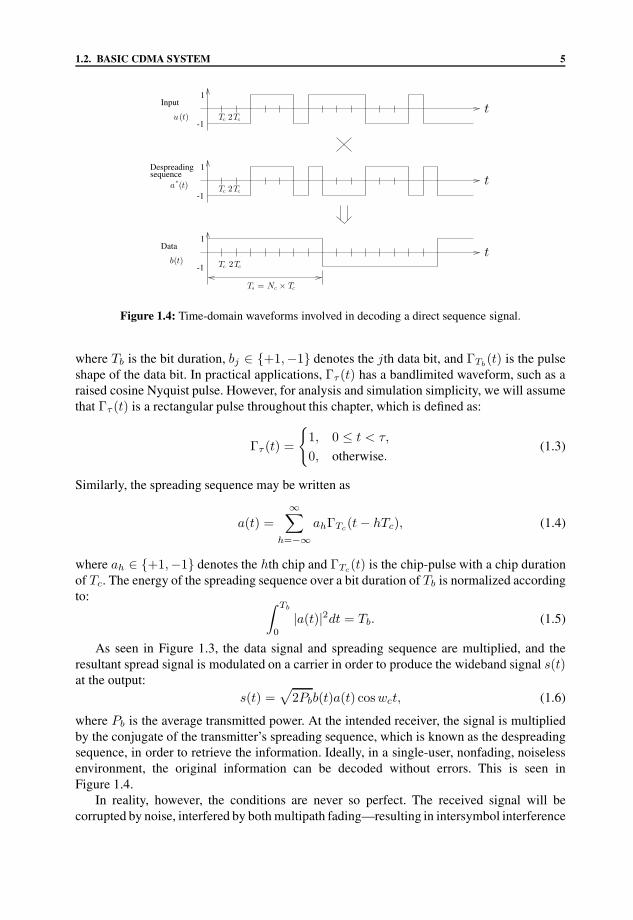
Figure 1.4: Time-domain waveforms involved in decoding a direct sequence signal.
where Tb is the bit duration, bj ∈ {+1,−1} denotes the jth data bit, and ΓTb(t) is the pulse
shape of the data bit. In practical applications, Γτ (t) has a bandlimited waveform, such as araised cosine Nyquist pulse. However, for analysis and simulation simplicity, we will assumethat Γτ (t) is a rectangular pulse throughout this chapter, which is defined as:
Γτ (t) =
{1, 0 ≤ t < τ,
0, otherwise.(1.3)
Similarly, the spreading sequence may be written as
a(t) =∞∑
h=−∞ahΓTc(t − hTc), (1.4)
where ah ∈ {+1,−1} denotes the hth chip and ΓTc(t) is the chip-pulse with a chip durationof Tc. The energy of the spreading sequence over a bit duration of Tb is normalized accordingto: ∫ Tb
0
|a(t)|2dt = Tb. (1.5)
As seen in Figure 1.3, the data signal and spreading sequence are multiplied, and theresultant spread signal is modulated on a carrier in order to produce the wideband signal s(t)at the output:
s(t) =√
2Pbb(t)a(t) coswct, (1.6)
where Pb is the average transmitted power. At the intended receiver, the signal is multipliedby the conjugate of the transmitter’s spreading sequence, which is known as the despreadingsequence, in order to retrieve the information. Ideally, in a single-user, nonfading, noiselessenvironment, the original information can be decoded without errors. This is seen inFigure 1.4.
In reality, however, the conditions are never so perfect. The received signal will becorrupted by noise, interfered by both multipath fading—resulting in intersymbol interference

6 CHAPTER 1. THIRD-GENERATION CDMA SYSTEMS
LPF
signalRecovered
Signaturesequence
Receivedsignal
Sample at
s(t) + n(t)
coswct a∗(t)
1√Tb
∫ (i+1)Tb
iTb
t = (i + 1)Tb
bi
Figure 1.5: BPSK DS-SS receiver for AWGN channel.
(ISI)—and by other users, generating multi-user interference. Furthermore, this signal isdelayed by the time-dispersive medium. It is possible to reduce the interference due tomultipath fading and other users by innovative signal processing methods, which will bediscussed in more detail in later sections.
Figure 1.5 shows the block diagram of the receiver for a noise-corrupted channel using acorrelator for detecting the transmitted signal, yielding:
bi = sgn
{1√Tb
∫ (i+1)Tb
iTb
a∗(t)[s(t) + n(t)] coswct dt
}
= sgn
{√ξb
2bi +
1√Tb
∫ (i+1)Tb
iTb
a∗(t)n(t) coswct dt
}, (1.7)
where ξb = Tb × Pb is the bit energy and sgn(x) is the signum function of x, which returnsa value of 1, if x > 0 and returns a value of −1, if x < 0. In a single-user Additive WhiteGaussian Noise (AWGN) channel, the receiver shown in Figure 1.5 is optimum. In fact, theperformance of the DS-SS system discussed so far is the same as that of a conventional BPSKmodem in an AWGN channel, whereby the probability of bit error Prb(ε) is given by:
Prb(ε) = Q
(√2ξb
N0
), (1.8)
where
Q(x) =1√2π
∫ ∞
x
e−y2/2dy (1.9)
is the Gaussian Q-function. The advantages of spread spectrum communications and CDMAwill only be appreciated in a multipath multiple access environment. The multipath aspectsand how the so-called Rake receiver [5, 70] can be used to overcome the multipath effectswill be highlighted in the next section.
1.2.2 The Effect of Multipath Channels
In this section, we present an overview of the effects of the multipath wireless channelsencountered in a digital mobile communication system, which was treated in depth forexample in [11]. Interested readers may also refer to the recent articles written by Sklarin [71, 72] for a brief overview on this subject.

1.2. BASIC CDMA SYSTEM 7
Since the mobile station is usually close to the ground, the transmitted signal isreflected, refracted, and scattered from objects in its vicinity, such as buildings, trees, andmountains [62]. Therefore, the received signal is comprised of a succession of possiblyoverlapping, delayed replicas of the transmitted signal. Each replica is unique in its arrivaltime, power, and phase [73]. As the receiver or the reflecting objects are not stationary, suchreflections will be imposed fading on the received signal, where the fading causes the signalstrength to vary in an unpredictable manner. This phenomenon is referred to as multipathpropagation [11].
There are typically two types of fading in the mobile radio channel [71]:
• long-term fading
• short-term fading.
As argued in [11] long-term fading is caused by the terrain configuration between the basestation and the mobile station, such as hills and clumps of buildings, which result in anaverage signal power attenuation as a function of distance. For our purposes the channelcan be described in terms of its average pathloss, typically obeying an inverse fourth powerlaw [62] and a log-normally distributed variation around the mean. Thus, long-term shadowfading was also referred to as log-normal fading in [11, 71] .
On the other hand, short-term fading refers to the dramatic changes in signal amplitudeand phase as a result of small changes in the spatial separation between the receiver andtransmitter, as we noted in [11, 71].
Furthermore, the motion between the transmitter and receiver results in propagationpath changes, such that the channel appears to be time-variant. The time-variant frequency-selective channel was modeled as a tapped delay line in [11], where the complex low-passimpulse response can be modeled as:
h(t) =L∑
l=1
|αl(t)|ejφl(t)δ(t − τl), (1.10)
where |αl(t)|, φl(t) and τl are the amplitude, phase, and delay of the lth path, respectively,and L is the total number of multipath components. It was argued in [11] that the rate of signallevel fluctuation is determined by the Doppler frequency, fD, which in turn is dependent onthe carrier frequency, fc, and the speed of the mobile station v according to (see also page 16of [74]):
fD = vfc
c, (1.11)
where c is the speed of light.Typically, the short-term fading phenomenon is modeled statistically by a Rayleigh,
Rician, or Nakagami-m distribution [75]. The Rayleigh and Rician distributions werecharacterized for example in [11]. There have been some contrasting views in the literature asto which of these distributions best describes the fast-fading channel statistically. Althoughempirical results have shown that the fading statistics are best described by a Nakagamidistribution [76], in most cases a Rayleigh-distributed fading is used for analysis and sim-ulation because of simplicity, and it serves as a useful illustrative example in demonstratingthe effects of fading on transmission. Moreover, the Rayleigh distribution is a special case

8 CHAPTER 1. THIRD-GENERATION CDMA SYSTEMS
0 1 2 3 4 5 6 7 8 9 10Time Delay [ s]
0.0
0.1
0.2
0.3
0.4
0.5
0.6
0.7
0.8
0.9
1.0
Am
plitu
de
Figure 1.6: COST 207 BU impulse response.
of the Nakagami distribution, when m, known as the fading parameter, is equal to unity(see page 48 in [5]). The Rician distribution is more applicable to satellite communication,due to the presence of a dominant signal component known as the specular component [71],than to large-cell terrestrial communication, where often there is no Line-of-Sight (LOS)path between the terrestrial base station and the mobile station. However, in small microcellsoften the opposite is true. In our investigations in this chapter, Rayleigh-distributed frequencyselective fading is assumed.
The delay is proportional to the length of the corresponding signal path between thetransmitter and receiver. The delay spread due to the path-length differences between themultipath components causes Intersymbol Interference (ISI) in data transmission, whichbecomes particularly dominant for high data rates.
A typical radio channel impulse response is shown in Figure 1.6. This channel impulseresponse is known as the COST 207 bad urban (BU) impulse response [77]. It can be clearlyseen that the response consists of two main groups of delayed propagation paths: a mainprofile and a smaller echo profile following the main profile at a delay of 5 µs. The mainprofile is caused by reflections of the signal from structures in the vicinity of the receiverwith shorter delay times. On the other hand, the echo profile could be caused by severalreflections from a larger but more distant object, such as a hill [78]. In either case, we cansee that both profiles approximately follow a negative exponentially decaying function withrespect to the time-delay.
Figure 1.7 shows the impairments of the spread spectrum signal travelling over amultipath channel with L independent paths, yielding the equivalent baseband received signalof:
r(t) =L∑
l=1
αl(t)s(t − τl) + n(t), (1.12)
where αl(t) is the time-variant complex channel gain, which is given by |αl(t)|ejφl(t) inEquation 1.10 with a Rayleigh-distributed amplitude, uniformly distributed phase over the

1.2. BASIC CDMA SYSTEM 9
s(t)
τ1
τ2
τL
α1(t)
α2(t)
αL(t)n(t)
r(t)
Figure 1.7: Multipath propagation model of the transmitted signal.
interval [−π . . . π] and s(t−τl) is the equivalent baseband transmitted spread spectrum signalfrom Equation 1.6 delayed by τl. The above equation shows that the lth path is attenuated bythe channel coefficient αl(t) and delayed by τl. Without intelligent diversity techniques [5],these paths are added together at the receiver and any phase or delay difference between thepaths may result in a severely multipath interfered signal, corrupted by dispersion-inducedintersymbol interference (ISI).
Figure 1.8 shows the effect of a nonfading channel and a fading channel on the biterror probability of BPSK-modulated CDMA. Without diversity, the bit error rate (BER)in a fading channel decreases approximately according to Prb(ε) ≈ 1
4γc, where γc is the
average Signal-to-Noise Ratio (SNR), and hence plotted on a logarithmic scale according tolog Prb(ε) = − log 4γc we have a near-linear curve [5]. This is different from a nonfading,or AWGN, channel, whereby the BER decreases exponentially with increasing the SNR.Thus, in a fading channel, a high transmitted power is required to obtain a low probability oferror. As we shall see in the next section, diversity techniques can be used to overcome thisimpediment.
1.2.3 Rake Receiver
As mentioned previously, spread spectrum techniques can take advantage of the multipathnature of the mobile channel in order to improve reception. This is possible due to thesignal’s wideband nature, which has a significantly higher bandwidth than the multipathchannel’s coherence bandwidth [79]. In this case, the channel was termed a frequencyselective fading channel, since different transmitted frequencies faded differently if theirseparation was higher than the previously mentioned coherence bandwidth. Suppose that thespread spectrum has a bandwidth of Bs and the channel’s coherence bandwidth is Bc, suchthat Bs � Bc. Thus, the number of resolvable independent paths—that is, the paths that fade

10 CHAPTER 1. THIRD-GENERATION CDMA SYSTEMS
AWGN
0 5 10 15 20 25 30Average SNR per bit
10-6
10-5
10-4
10-3
10-2
10-1
100
BE
R3 diversity paths2 diversity pathsNo diversity
Figure 1.8: Performance of BPSK modulated CDMA over various Rayleigh-fading channels. Thecurves were obtained using perfect channel estimation, and there was no self-interferencebetween diversity paths.
near-independently—LR is equal to
LR =⌊
Bs
Bc
⌋+ 1, (1.13)
where �x� is the largest integer that is less than or equal to x. The number of resolvablepaths LR varies according to the environment, and it is typically higher in urban than insuburban areas, since in urban areas the coherence bandwidth is typically lower due to thetypically higher delay-spread of the channel [62]. More explicitly, this is a consequenceof the more dispersive impulse response, since the coherence bandwidth is proportional tothe reciprocal of the impulses responses delay spread, as it was argued in [79]. Similarlyto frequency diversity or space diversity, these LR resolvable paths can be employed inmultipath diversity schemes, which exploit the fact that statistically speaking, the differentpaths cannot be in deep fades simultaneously; hence, there is always at least one propagationpath, which provides an unattenuated channel. These multipath components are diversitypaths.
Multipath diversity can only be exploited in conjunction with wideband signals. FromEquation 1.13, for a narrowband signal, where no deliberate signal spreading takes place,the signal bandwidth Bs is significantly lower than Bc. In this case, the channel was termedfrequency nonselective in [79]. Hence, no resolvable diversity paths can be observed, unlikein a wideband situation, and this renders TDMA and FDMA potentially less robust in anarrowband mobile radio channel than CDMA.
Multipath diversity is achieved, for example, by a receiver referred to as the Rakereceiver invented by Price and Green [70]. This is the optimum receiver for wideband fading

1.2. BASIC CDMA SYSTEM 11
multipath signals. It inherited its name from the analogy of a garden rake, whereby the fingersconstitute the resolvable paths. The point where the handle and fingers meet is where diversitycombining takes place. There are four basic methods of diversity combining, namely [80]:
• Selection Combining (SC).
• Maximal Ratio Combining (MRC).
• Equal Gain Combining (EGC).
• Combining of the n best signals (SCn).
The performance analysis of selection combining in CDMA can be found in [81, 82], whilea general comparison of the various diversity combining techniques can be found in [80]for Rayleigh-fading channels. Maximal ratio combining gives the best performance, whileselection combining is the simplest to implement. The number of resolvable paths thatare combined at the receiver, represents the order of diversity of the receiver, which isdenoted here as LP . We note, however, that in practical receivers not all resolvable multipathcomponents are combined due to complexity reasons, that is, LP ≤ LR.
There are two basic demodulation techniques, namely coherent and noncoherent demod-ulation [5]. We will highlight the basics of coherent demodulation in this section in thecontext of CDMA. However, before demodulation can take place, synchronization betweenthe transmitter and the intended receiver has to be achieved.
Synchronization in DS-CDMA is performed by a process known as code acquisitionand tracking. Acquisition is usually carried out by invoking correlation techniques betweenthe receiver’s own copy of the signature sequence and the received signature sequence andsearching for the displacement between them—associated with a specific chip epoch—thatresults in the high correlation [64, 83, 84]. Once acquisition has been accomplished, usuallya code tracking loop [85] is employed to achieve fine alignment of the two sequences and tomaintain their alignment. The details of code acquisition and tracking are beyond the scopeof this chapter. Interested readers may refer to [86–89] and the references therein for an in-depth treatise on this subject. Hence, in this chapter, we will assume that the transmitter andthe intended receiver are perfectly synchronized.
For optimum performance of the Rake receiver using coherent demodulation, the pathattenuation and phase must be accurately estimated. This estimation is performed by anotherprocess known as channel estimation, which will be elaborated on in Section 1.2.6. Intypical low-complexity applications, known pilot symbols can be inserted in the transmittedsequence in order to estimate the channel’s attenuation and phase rotation. However, for now,let us assume perfect channel estimation in order to assess the performance of the Rakediversity combiner.
Figure 1.9 shows the block diagram of the BPSK Rake receiver. The received signal isfirst multiplied by the estimated channel coefficients α1(t), . . . , αLP (t) in each Rake branchtuned to each resolvable path. For optimum performance of the Rake receiver using maximalratio combining, these channel coefficient estimates should be the conjugates of the actualcoefficients of the appropriate paths in order to invert the channel effects.2 Note that forequal gain combining only the phase is estimated, and the various path contributions are
2αlejφl × αle
−jφl = α2l .

12 CHAPTER 1. THIRD-GENERATION CDMA SYSTEMS
variableDecision
r(t)
α∗1(t)
α∗LP
(t)
a∗(t − τ1)
a∗(t − τLP )
∫ (i+1)Tb+τ1
iTb+τ1
∫ (i+1)Tb+τLP
iTb+τLP
bi
Figure 1.9: Rake receiver.
multiplied by a unity gain before summation. The resulting signals in each Rake branchare then multiplied by the conjugate signature sequences as we have seen in Figure 1.3,delayed accordingly by the code acquisition process. After despreading by the conjugatesignature sequences a∗(t − τ1), . . . , a∗(t − τLP ), the outputs of the correlators in Figure 1.9are combined in order to obtain the decoded symbol of:3
bi = sgn
{LP∑l=1
[1√Tb
∫ (i+1)Tb+τl
iTb+τl
α∗l (t)r(t)a
∗(t − τl) dt
]}
= sgn
{LP∑l=1
[√Pb
Tb
∫ (i+1)Tb+τl
iTb+τl
|αl(t)|2b(t − τl)a(t − τl)a∗(t − τl) dt
+1√Tb
∫ (i+1)Tb+τl
iTb+τl
α∗l (t)n(t)a∗(t − τl) dt
]}
= sgn
{LP∑l=1
[|αl(t)|2
√ξbbi
+1√Tb
∫ (i+1)Tb+τl
iTb+τl
α∗l (t)n(t)a∗(t − τl) dt
]}. (1.14)
Normally, the first term of Equation 1.14, which contains the useful information, ismuch larger than the despread, noise-related second term. This is because the first term isproportional to the sum of the absolute values of the channel coefficients, whereas the secondterm in Equation 1.14 is proportional to the vectorial sum of the complex-valued channelcoefficients. Hence, the real part of the first term is typically larger than that of the secondterm. Thus, the Rake receiver can enhance the detection of the data signal in a multipathenvironment.
Referring back to the BER curves of Figure 1.8, we can see that the performance ofthe system is improved when multipath diversity is used. Better performance is observed by
3Here we assumed that there is no multipath interference. This interference can be considered as part of multi-user interference, which will be discussed in the next section.

1.2. BASIC CDMA SYSTEM 13
Decision
Decision
Decision
Delay
Delay
Delay
b(1)(t)
b(2)(t)
b(K)(t)
P(1)b a(1)(t)
P(2)b a(2)(t)
P(K)b a(K)(t)
s(1)(t)
s(2)(t)
s(K)(t)
τ (1)
τ (2)
τ (K)
n(t)
r(t)
a(1)(t − τ (1))
a(2)(t − τ (2))
a(K)(t − τ (K))
∫
∫∫
b(1)(t)
b(2)(t)
b(K)(t)
Figure 1.10: CDMA system model.
increasing the number of diversity paths LP . However, this also increases the complexity ofthe receiver, since the number of correlators has to be increased, which is shown in Figure 1.9.
1.2.4 Multiple Access
So far, only single-user transmission was considered. The system is simple and straight-forward to implement. Let us now consider how multiple user transmission can affect theperformance of the system.
Multiple access is achieved in DS-CDMA by allowing different users to share a commonfrequency band. Each transmitter and its intended receiver are assigned a distinct usersignature sequence. Only the receivers having the explicit knowledge of this distinct sequenceare capable of detecting the transmitted signal. Consider a CDMA scenario with K numberof active users, transmitting simultaneously. The baseband equivalent system model is shownin Figure 1.10. For simplicity, it is assumed that there is no multipath propagation and perfectpower control is maintained.
The mathematical representation of the kth user’s data signal is similar to that shown inEquation 1.2, except for an additional superscript, denoting multi-user transmission. Hence,it is written as:
b(k)(t) =∞∑
j=−∞b(k)j ΓTb
(t − jTb), (1.15)
where b(k)j ∈ {+1,−1}. There is a distinct user signature sequence a(k)(t) associated with
the kth user, which is similar to that of Equation 1.4, with the exception of a superscript,differentiating between users:
a(k)(t) =∞∑
h=−∞a(k)h ΓTc(t − hTc). (1.16)

14 CHAPTER 1. THIRD-GENERATION CDMA SYSTEMS
The kth user’s data signal b(k)(t) and signature sequence a(k)(t) are multiplied in order toproduce an equivalent baseband wideband signal, namely,
s(k)(t) =√
P(k)b b(k)(t)a(k)(t), (1.17)
where P(k)b is the average transmit power of the kth user’s signal. The composite multi-user
baseband received signal is:
r(t) =K∑
k=1
√P
(k)b b(k)(t − τ (k))a(k)(t − τ (k)) + n(t), (1.18)
where τ (k) is the propagation delay plus the relative transmission delay of the kth user withrespect to other users, and n(t) is the AWGN with a double-sided power spectral density ofN02 W/Hz.
1.2.4.1 DL Interference
In the DL (base station to mobile), the base station is capable of synchronizing thetransmission of all the users’ signals, such that the symbol durations are aligned with eachother. Hence the composite signal is received at each mobile station with τ (k) = 0 fork = 1, 2, . . . , K . This scenario is also known as symbol-synchronous transmission. Usingthe conventional so-called single-user detector, each symbol of the jth user is retrieved fromthe received signal r(t) by correlating it with the jth user’s spreading code in order to give:
b(j)i = sgn
{1√Tb
∫ (i+1)Tb
iTb
r(t)a(j)∗ (t)dt
}. (1.19)
Substituting Equation 1.18 into Equation 1.19 yields:
b(j)i = sgn
{1√Tb
∫ (i+1)Tb
iTb
[K∑
k=1
√P
(k)b b(k)(t)a(k)(t) + n(t)
]a(j)∗(t) dt
}
= sgn
{1√Tb
∫ (i+1)Tb
iTb
√P
(j)b b(j)(t)a(j)(t)a(j)∗(t) dt
+1√Tb
∫ (i+1)Tb
iTb
K∑k=1k �=j
√P
(k)b b(k)(t)a(k)(t)a(j)∗(t) dt
+1√Tb
∫ (i+1)Tb
iTb
n(t)a(j)∗(t) dt
}
= sgn
√ξ(j)b b
(j)i︸ ︷︷ ︸
wanted signal
+K∑
k=1k �=j
√ξ(k)b b
(k)i Rjk
︸ ︷︷ ︸multiple access interference
+ n(j)︸︷︷︸white noise
, (1.20)

1.2. BASIC CDMA SYSTEM 15
where Rjk is the cross-correlation of the spreading codes of the kth and jth user for iTb ≤t ≤ (i + 1)Tb, which is given by:
Rjk =1Tb
∫ Tb
0
a(j)(t)a(k)(t) dt. (1.21)
There will be no interference from the other users if the spreading codes are perfectlyorthogonal to each other. That is, Rjk = 0 for all k �= j. However, designing orthogonalcodes for a large number of users is extremely complex. The so-called Walsh-Hadamardcodes [90] used in the IS-95 system excel in terms of achieving orthogonality.
1.2.4.2 Uplink Interference
In contrast to the previously considered DL scenario, in practical systems perfect orthogonal-ity cannot be achieved in the UL (mobile to base station), since there is no coordination in thetransmission of the users’ signals. In CDMA, all users transmit in the same frequency band inan uncoordinated fashion. Hence, τ (k) �= 0, and the corresponding scenario is referred to asan asynchronous transmission scenario. In this case, the time-delay τ (k), k = 1, . . . , K , hasto be included in the calculation. Without loss of generality, it can be assumed that τ (1) = 0and that 0 < τ (2) < τ (3) < · · · < τ (K) < Tb. In contrast to the synchronous DL scenario ofEquation 1.19, the demodulation of the ith symbol of the jth user is performed by correlatingthe received signal r(t) with a(j)∗(t) delayed by τ (j), yielding:
b(j)i = sgn
{1√Tb
∫ (i+1)Tb+τ (j)
iTb+τ (j)r(t)a(j)∗ (t − τ (j))dt
}, (1.22)
where τ (j) is the estimated time-delay at the receiver.Substituting Equation 1.18 into Equation 1.22 and assuming perfect code acquisition and
tracking yield:4
b(j)i = sgn
{1√Tb
∫ (i+1)Tb+τ (j)
iTb+τ(j)
[ K∑k=1
√P
(k)b b(k)(t − τ (k))a(k)(t − τ (k)) + n(t)
]
· a(j)∗(t − τ (j))dt
}
= sgn
{1√Tb
[∫ (i+1)Tb+τ(j)
iTb+τ (j)
√P
(j)b b(j)(t − τ (j))a(j)(t − τ (j))
× a(j)∗(t − τ (j))dt
+j−1∑k=1
∫ (i+1)Tb+τ (k)
(i+1)Tb+τ (j)
√P
(k)b b(k)(t − τ (k))a(k)(t − τ (k))
4For perfect code acquisition and tracking, τ (j) = τ(j).

16 CHAPTER 1. THIRD-GENERATION CDMA SYSTEMS
× a(j)∗(t − τ (j))dt
+j−1∑k=1
∫ (i+1)Tb+τ(j)
iTb+τ (k)
√P
(k)b b(k)(t + Tb − τ (k))a(k)(t + Tb − τ (k))
× a(j)∗(t − τ (j))dt
+K∑
k=j+1
∫ iTb+τ (k)
iTb+τ (j)
√P
(k)b b(k)(t − Tb − τ (k))a(k)(t − Tb − τ (k))
× a(j)∗(t − τ (j))dt
+K∑
k=j+1
∫ (i+1)Tb+τ (j)
iTb+τ (k)
√P
(k)b b(k)(t − τ (k))a(k)(t − τ (k))
× a(j)∗(t − τ (j))dt +∫ (i+1)Tb+τ (j)
iTb+τ (j)n(t)a(j)∗(t − τ (j))dt
]}(1.23)
b(j)i = sgn
√ξ(j)b b
(j)i︸ ︷︷ ︸
wanted signal
+j−1∑k=1
√ξ(k)b b
(k)i Rjk(0)
︸ ︷︷ ︸multiple access interference
+j−1∑k=1
√ξ(k)b b
(k)i+1Rjk(+1) +
K∑k=j+1
√ξ(k)b b
(k)i−1Rjk(−1)
︸ ︷︷ ︸multiple access interference
+K∑
k=j+1
√ξ(k)b b
(k)i Rjk(0)
︸ ︷︷ ︸multiple access interference
+ n(j)︸︷︷︸white noise
, (1.24)
where Rjk(i) and Rjk(i), i ∈ {+1, 0,−1} represent the cross-correlation of the spreadingcodes due to asynchronous transmissions, which are given by [91]:
Rjk(i) =1Tb
∫ τ (k)
τ (j)a(j)(t − τ (j))a(k)(t + iTb − τ (k))dt (1.25)
and
Rjk(i) =1Tb
∫ Tb+τ (j)
τ (k)a(j)(t − τ (j))a(k)(t + iTb − τ (k))dt (1.26)
and is limited to +1, 0,−1, since the maximum path delay is assumed to be limited to onesymbol duration, as mentioned in Section 1.2.2.

1.2. BASIC CDMA SYSTEM 17
Equations 1.24 and 1.20 represent the estimated demodulated data symbol of the jthuser at the base station and mobile station, respectively. Both contain the desired symbolof the jth user. However, this is corrupted by noise and interference from the other users.This interference is known as multiple access interference (MAI). It contains the undesiredinterfering signals from the other (K − 1) users. The MAI arises due to the nonzerocross-correlation of the spreading codes. Ideally, the spreading codes should satisfy theorthogonality property such that
Rjk(τ) =1Tb
∫ Tb
0
a(k)(t)a(j)(t − τ)dt ={
1 for k = j, τ = 00 for all k and all τ.
(1.27)
However, it is impossible to design codes that are orthogonal for all possible time offsetsimposed by the asynchronous UL transmissions. Thus there will always be MAI in the UL.These observations are augmented by comparing the terms of Equations 1.20 and 1.24.
On the other hand, multipath interference is always present in both the forward andreverse link. Multipath interference is due to the different arrival times of the same signalvia the different paths at the receiver. This is analogous to the signals transmitted from otherusers; hence, multipath interference is usually analyzed in the same way as MAI.
As the number of users increases, the MAI increases too. Thus, the capacity of CDMAis known to be interference limited. CDMA is capable of accommodating additional users atthe expense of a gradual degradation in performance in a fixed bandwidth, whereas TDMAor FDMA would require additional bandwidth to accommodate additional users. Intensiveresearch has been carried out to find ways of mitigating the effects of MAI. Some of themethods include voice activity control, spreading code design, power control schemes, andsectored/adaptive antennas [92]. These methods reduce the MAI to a certain extent.
The most promising UL method so far has been in the area of multi-user detection, whichwas first proposed by Verdu [93]. Multi-user detection [94–96], which will be discussedin more depth in the next chapter, invokes the knowledge of all users’ signature sequencesand all users’ channel impulse response estimates in order to improve the detection of eachindividual user. The employment of this algorithm is more feasible for the UL, because allmobiles transmit to the base station and the base station has to detect all the users’ signalsanyway. The topic of multi-user detection is however beyond the scope of this chapter, sinceit will be discussed in a little more detail in the next chapter, namely in Chapter 3. For a moreindepth treatment the interested readers are referred to Verdu’s excellent book [97], whichprovides a comprehensive discussion on the topic. A general review of the various multi-user detection schemes and further references can also be found, for example, in Moshavi’scontribution [92].
Another shortcoming of CDMA systems is their susceptibility to the near–far problem tobe highlighted below. If all users transmit at equal power, then signals from users near thebase station are received at a higher power than those from users at a higher distance due totheir different pathlosses. The effects of fading highlighted in Section 1.2.2 also contribute tothe power variation. Hence, according to Equation 1.24, if the jth user is transmitting fromthe cell border and all other users are transmitting near the base station, then the desired jthuser’s signal will be masked by the other users’ stronger signals, which results in a high biterror rate. In order to mitigate this so-called near–far problem, power control is used to ensurethat all signals from the users are received at near-equal power, regardless of their distancefrom the base station.

18 CHAPTER 1. THIRD-GENERATION CDMA SYSTEMS
There are typically two basic types of power control [65]:
• open-loop power control
• closed-loop power control.
Open-loop power control is usually used to overcome the variation in power caused bypathloss. On the other hand, closed-loop power control is used to overcome shadow fadingcaused by multipath. The details of the various power control techniques will not beelaborated on in this chapter. Readers may refer to [98] for more information.
1.2.4.3 Gaussian Approximation
In order to simplify any analysis involving multi-user transmission in CDMA, the MAI isusually assumed to be Gaussian distributed by virtue of the central limit theorem [99–101].This assumption is fairly accurate even for K < 10 users, when the BER is 10−3 orhigher. We will use the standard Gaussian approximation theory presented by Pursley [99] torepresent the MAI. When the desired user sequence is chip- and phase-synchronous withall the interfering sequences, where the phase-synchronous relationship is defined as inthe absence of noise, the worst-case probability of error Prb(ε) performance was given byPursley [99] as:
Prb(ε) = Q
[√Nc
(K − 1)
], (1.28)
where Q(·) is the Gaussian Q-function of Equation 1.9, since the synchronous transitions donot generate pure random Gaussian-like impairments. This formula would be characteristicof the synchronous DL scenario of Section 1.2.4.1. However, in practical UL situations asaugmented in Section 1.2.4.2, there is always some delay among the users, and each receivedsignal will be phase-shifted independently. In this case, according to Pursley, the probabilityof error in the absence of noise will be [99]:
Prb(ε) = Q
[√3Nc
(K − 1)
]. (1.29)
Equation 1.29 represents the best performance corresponding to Gaussian-like impair-ments. In between these two extremes are situations whereby, in the first case, the desiredsequence and the interfering sequence are chip synchronous but not phase synchronous. Theprobability of error in the absence of noise is given by [99]:
Prb(ε) = Q
[√2Nc
(K − 1)
]. (1.30)
In the second case, the desired sequence and interfering sequence are phase synchronousbut not chip synchronous. Hence, the probability of error in the absence of noise is givenby [99]:
Prb(ε) = Q
[√3Nc
2(K − 1)
]. (1.31)

1.2. BASIC CDMA SYSTEM 19
2 4 6 8 10 12 14 16 18 20 22Number of Users
10-4
2
5
10-3
2
5
10-2
2
5
10-1
2
5
100
BE
R
AsyncChip syncPhase syncChip & phase sync
Figure 1.11: Probability of error against number of users using Equations 1.28, 1.29, 1.30, and 1.31.Markers: Simulation; solid line: Numerical computation. The processing gain is 7.
Analyzing the above equations, it can be seen that by increasing the number of chipsNc per symbol, the performance of the system will be improved. However, there is alimitation to the rate of the spreading sequence based on Digital Signal Processing (DSP)technology. Figure 1.11 compares the simulated results with the numerical results given byEquations 1.28 to 1.31 for a binary system with a processing gain of 7. The figure shows thatthe assumption of Gaussian distributed MAI is valid, especially for a high number of users. Italso demonstrates that CDMA attains its best possible performance in an asynchronous multi-user transmission system. This is an advantage over TDMA and FDMA because TDMAand FDMA require some coordination among the transmitting users, which increases thecomplexity of the system.
1.2.5 Spreading Codes
As seen previously, the choice of spreading codes plays an important role in DS-CDMA. Themain criteria for selecting a particular set of user signature sequences in CDMA applicationsare that the number of possible different sequences in the set for any sequence length must behigh in order to accommodate a high number of users in a cell. The spreading sequences mustalso exhibit low cross-correlations for the sake of reducing the multi-user interference duringdemodulation. A high autocorrelation main-peak to secondary-peak ratio—as indicated byEquation 1.27—is also essential, in order to minimize the probability of so-called false alarmsduring code acquisition. This also reduces the self-interference among the diversity paths.Below we provide a brief overview of a few different spreading sequences.

20 CHAPTER 1. THIRD-GENERATION CDMA SYSTEMS
1 2 3 4 m
c1 c2 c3 c4 cm
+
Output
Figure 1.12: m-stage shift register with linear feedback.
Table 1.1: Properties of m- and Gold-sequences. c©McGraw-Hill, 1995 [5].
Number of Peak cross- Number of Peak cross-m m-sequences correlation Gold sequences correlation
3 2 5 2m + 1 = 9 54 2 9 2m + 1 = 17 95 6 11 2m + 1 = 33 96 6 23 2m + 1 = 65 177 18 41 2m + 1 = 129 178 16 95 2m + 1 = 257 33
1.2.5.1 m-sequences
Perhaps the most popular set of codes known are the m-sequences [5]. An m-sequence witha periodicity of n = 2m − 1 can be readily generated by an m-stage shift register with linearfeedback, as shown in Figure 1.12.
The tap coefficients c1, c2, . . . , cm can be either 1 (short circuit) or 0 (open circuit).Information on the shift register feedback polynomials, describing the connections betweenthe register stages and the modulo-2 adders can be found, for example, in [5]. Note that inspread spectrum applications, the output binary sequences of 0,1 are mapped into a bipolarsequence of −1, 1, respectively. Table 1.1 shows the total number of m-sequences and theassociated chip-synchronous peak cross-correlation for m = 3, 4, 5, 6, 7, and 8.
In this context, the peak cross-correlation quantifies the maximum number of identicalchips in a pair of different spreading codes. It is desirable to have as low a number of codepairs as possible, which exhibit this peak cross-correlation. Furthermore, the peak cross-correlation has to be substantially lower than the codes’ autocorrelation, which is given bythe length of the code. In general, the cross-correlations of m-sequences are too high to beuseful in CDMA. Another set of spreading codes, which exhibit fairly low chip-synchronouscross-correlations are the Gold sequences [5], which will be elaborated on in the next section.

1.2. BASIC CDMA SYSTEM 21
1.2.5.2 Gold Sequences
Gold sequences [5] with a period of n = 2m − 1 are derived from a pair of m-sequenceshaving the same period. Out of the total number of possible m-sequences having a periodicityor length of n, there exists a pair of m-sequences, whose chip-synchronous cross-correlationequals to either −1,−t(m) or [t(m) − 2], where
t(m) ={
2(m+1)/2 + 1 odd m
2(m+2)/2 + 1 even m.(1.32)
This unique pair of m-sequences is commonly known as the pair of preferred codes. A setof n = 2m − 1 sequences can be constructed by cyclically shifting a preferred code one chipat a time and then taking the modulo-2 summation with the other code for every chip shift.The resulting set of n = 2m − 1 sequences together with the two preferred codes constitutea set of Gold sequences. Table 1.1 compares the total number of Gold sequences for m = 3,4, 5, 6, 7, and 8, and their corresponding peak cross-correlation with the same parameters ofm-sequences.
Table 1.1, shows that the Gold sequences exhibit equal or lower peak cross-correlationbetween different sequences of the set, in comparison to m-sequences for all m. There arealso more Gold sequences than m-sequences for all values of m. Thus, Gold sequencesare always preferred to m-sequences in CDMA applications, despite having a poorerasynchronous autocorrelation peak, which is a disadvantage in terms of both code acquisitionand detection by correlators. Pseudo Noise (PN) sequences, such as m-sequences and Goldsequences, have periods of N = 2l − 1 where l is the sequence length, which is a ratherawkward number to match to the system clock requirements. Extended m-sequences havingperiods of 2l solved this problem, an issue augmented below.
1.2.5.3 Extended m-sequences [102]
Extended m-sequences are derived from an m-sequence, generated by a linear feedbackshift register, by adding an element into each period of the m-sequence. We will followthe notation, whereby the binary sequences of 0 and 1 are mapped to the correspondingbipolar sequences of −1 and +1, respectively. In order to arrive at zero-balanced extendedm-sequences, which have a zero DC-component, the element to be inserted must be chosenso that the number of −1 s and +1 s within a period is the same. There are 2m − 1positions in a period, where the additional element can be inserted. In [102], the elementis inserted into the longest run of −1 s in a period. In an m-sequence of period 2m − 1,the longest run of −1 s is n − 1 = 2m − 2. It was shown in [102] that the off-peakautocorrelation of extended sequences was similar to that of Gold sequences. However, thecross-correlation of different extended m-sequences at even-indexed chip-positions—that is,time-domain displacements—is similar to that of the m-sequences, which is much higher thanthat of the Gold sequences in Table 1.1. Thus, the extended m-sequences are not suitable ina multi-user environment, where the cross-correlation between the codes of different usersis required to be as low as possible. Since this has a high impact on the user-capacity ofcellular mobile systems, the additional hardware needed to synchronize the N = 2l − 1chip-duration m-sequences or Gold sequences with the system clock has to be tolerated andhence, extended m-sequences are not recommended in CDMA. Section 1.3.2.6 highlights the

22 CHAPTER 1. THIRD-GENERATION CDMA SYSTEMS
various spreading codes proposed for employment in the forthcoming 3G systems. In the nextsection we provide a rudimentary introduction to channel estimation for CDMA systems.
1.2.6 Channel Estimation
As mentioned earlier, accurate estimation of the channel parameters is vital in optimizingthe coherent demodulation. This channel parameter estimation process is an integral part ofcoherent demodulation, particularly in a multipath mobile radio environment. This is becausethe mobile radio channel changes randomly as a function of time, and thus the channelestimates have to be continuously estimated. This section describes various techniques used toestimate the channel path gains and phases, which will be referred to as channel coefficients.There are basically three practical channel coefficient estimation methods, each with theiradvantages and disadvantages, namely:
• Pilot-channel assisted, [103–105]
• Pilot-symbol assisted and [106]
• Pilot-symbol assisted decision-directed channel estimation [107],
which we briefly characterized in the following subsections.
1.2.6.1 DL Pilot-assisted Channel Estimation
Channel estimation using a pilot channel/tone was proposed, for example, in [103–105],where a channel is dedicated solely for the purpose of estimating the multipath channelattenuations and delays. In order to prevent the pilot channel from interfering with the datachannel, the pilot channel must either be allocated to a dedicated portion of the spectrumor share the spectrum with the data channel, but a spectral notch has to be created foraccommodating the pilot. The former technique is known as the pilot tone-above-band (TAB)regime, while the latter is referred to as the transparent tone-in-band (TTIB) technique [103],both of which have been used in conventional single-carrier modems [12].
However, CDMA is more amenable to employing the TAB or TTIB techniques and theirvarious derivatives, since the pilot signal can be transmitted in the same frequency band asthe data signal by invoking orthogonal or quasi-orthogonal spreading codes. Hence, the pilotsignal is treated as part of the MAI, and no notch filtering or additional pilot frequency bandis required. In some 2G mobile systems, such as the IS-95 system this method is used on theDL but not on the UL. This is because it would be inefficient to have every mobile stationtransmitting their own pilot channel.
In 3G mobile systems, however, it was proposed [108] that a separate dedicated usercontrol channel be transmitted simultaneously with the information channel, which couldalso be used as an alternative to the pilot channel – an issue to be elaborated on at a laterstage. Suffice to say here that the main advantage of pilot-channel based channel estimationis that since the pilot channel is always present, the channel coefficients can be continuouslyestimated for every data symbol’s demodulation. Hence, it is particularly useful for channelsthat are highly time-variant.
The block diagram of the channel estimator is shown in Figure 1.13, where r(t) is

1.2. BASIC CDMA SYSTEM 23
*
Known bit stream
Smoothing
filterr(t)
a∗(t)
∫ (k+1)Tb
kTb
α(k)α(k)
Figure 1.13: Structure of the channel estimator using known transmitted pilot symbols or bits.
the received signal and a(t) is the spreading code. Assume that the known bit-stream is acontinuous sequence of binary 1 s, then
α(k) =1Tb
∫ (k+1)Tb
kTb
r(t)a∗(t)dt
=1Tb
∫ (k+1)Tb
kTb
[α(t)a(t) + n(t)]a∗(t)dt
= α(k) +1Tb
∫ (k+1)Tb
kTb
n(t)a∗(t)dt, (1.33)
where α(k) is the complex channel coefficient in the bit interval kTb ≤ t < (k + 1)Tb.The variable α(k) is termed the noisy channel estimate derived from the received signalcontaminated by the noise element in the second term of Equation 1.33, while α(k) areestimates obtained from the output of the smoothing filter in Figure 1.13, which assists inaveraging out the random effects of channel noise. Assuming that n(t) is the AWGN havinga zero mean (any MAI can be fairly accurately modeled also as AWGN [109]), averaging alarge number of these noisy estimates will suppress the noise’s influence. Several proposalshave been published in the literature regarding the smoothing algorithm used in channelestimation, such as moving average [110, 111], least squares line fitting [112], low-passfiltering [106, 107, 112], and adaptive linear smoothing [113]. A more in-depth discourseon the TTIB technique was also given in Section 10.3.1 of [12] in the context of QAM. Acompromise in terms of complexity and accuracy has to be made in selecting a particularalgorithm. So far, only the DL channel estimation has been elaborated on. The associated ULissues are discussed next.
1.2.6.2 UL Pilot-symbol Assisted Channel Estimation
Pilot-symbol assisted channel estimation was first proposed by Moher and Lodge [106], andthe first detailed analysis of this technique was carried out by Cavers [113]. Since then, severalpapers have been published, which analyzed its effect on system performance [111,112,114].This technique is the time-domain equivalent of the frequency-domain pilot channel-assistedTTIB method mentioned in Section 1.2.6.1, which was detailed in Section 10.3.2 of [12].

24 CHAPTER 1. THIRD-GENERATION CDMA SYSTEMS
Data symbols Data symbols
Pilot symbols
Figure 1.14: Data stream with embedded pilot symbols.
The advantage of this technique is that it dispensed with the use of a notch filter in thecontext of QAM modems, and so it did not result in an expanded bandwidth. However, forthis technique, several parameters such as the number of pilot symbols or their periodicityhas to be carefully chosen in order to trade-off the accuracy of estimation against the requiredpilot overhead. More explicitly, the pilot-spacing has to be sufficiently low to satisfy theNyquist sampling theorem for the fading Doppler frequency encountered. This technique canbe used for efficient coherent demodulation on the UL, and Section 1.3.2.3 highlights howUL channel estimation is carried out in the context of 3G systems.
The pilot symbols are multiplexed with the data stream periodically, as shown inFigure 1.14. This multiplexed stream is then transmitted to the base station from everycommunicating mobile station. The base station will extract the channel estimates from theknown demodulated pilot symbols, and using, for example, ideal low-pass or simple linearinterpolation [112], it will generate a channel magnitude and phase estimate for each ULsymbol. These channel estimates will then be used to “de-fade”, “de-rotate”, and demodulatethe data symbols.
If the channel has a slow fading characteristic, such that it is more or less constantbetween consecutive pilot symbols, this method can be fairly accurate and of low complexity.However, the bandwidth efficiency is slightly compromised, since again, a sufficientlyhigh number of pilots has to be incorporated in order to satisfy the Nyquist samplingcriterion corresponding to the normalized Doppler frequency of the fading channel. For moreinformation on this subject we refer to Section 10.3.2 of [12]. The above pilot-symbol assisted(PSA) concept is further developed in the next section.
1.2.6.3 Pilot-symbol Assisted Decision-directed Channel Estimation
Pilot-symbol assisted decision-directed channel estimation was first proposed by Irvine andMcLane [107], and it was shown that it improves the accuracy of the estimation as comparedwith the original pilot symbol-assisted method of Section 1.2.6.2. It extends the concept ofthe pilot-symbol assisted channel estimation technique by using the detected data symbolsin order to obtain the subsequent channel parameters, since in the absence of channel errorsthese demodulated data symbols can be considered to be known pilot symbols.
A decision-directed pilot-symbol assisted (PSA) scheme is illustrated in Figure 1.15,where s(k) is the kth received symbol and b(k) is the kth detected symbol. The signal is stilltransmitted in a transmission burst or frame format, similarly to that shown in Figure 1.14. Atthe beginning of the frame, the pilot symbols will be used to estimate the channel parameters

1.2. BASIC CDMA SYSTEM 25
Pilot-Symbol
ChannelEstimator
Smoothing
Filter
b(k)∗
*
Despreadr(t)
Delay
dataoutput
Assisted
α(k)
s(k + 1)
s(k)
Figure 1.15: Receiver structure of PSA decision-directed channel estimation.
in order to demodulate the data symbol immediately following the pilot symbol. This isperformed by the pilot symbol-assisted channel estimator block of Figure 1.15. The detecteddata symbol b(k) is then fed back and multiplied with its original but delayed received versions(k), as seen in Figure 1.15. If this symbol is detected correctly, then it is analogous to aknown pilot symbol and the channel coefficient corresponding to this received symbol canbe estimated in the same way. This estimated channel coefficient is then passed through thesmoothing filter of Figure 1.15 in order to obtain a smoothed estimate α(k) to be used in itsconjugate form for de-fading and de-rotating the next symbol, as portrayed in Figure 1.15.
If the decision is wrong, obviously the estimated channel coefficient would be inaccurate.The effect of erroneous decisions is mitigated by the smoothing filter, which will suppressthe effects of an occasional glitch due to the incorrect channel estimates. In the event thatthe smoothing filter is unable to average out the channel coefficient errors and its output is acomplex channel coefficient, which is far from the actual value, then this error may propagatethrough the data stream, since the correct decoding of each data symbol is dependent onthe accuracy of the previous channel coefficient estimates. In order to prevent this fromhappening, the smoothing process is reset when the next block of pilot symbols arrives. Theaveraging process will recommence with the pilot symbol-assisted channel estimates.
The schematic diagram shown in Figure 1.15 is only one of the few possibilities ofimplementing a decision-directed PSA channel estimation arrangement. This structure isalso known as a decision-feedback PSA channel estimator because the estimated channelcoefficient is used for compensating the channel’s effects for the next symbol. In anotherversion of this algorithm, shown in Figure 1.16, a tentative decision, b(k), is carried outconcerning the current symbol, s(k), using the pilot symbol-assisted estimate, α∗(k). Usingthis tentative decision concerning the received symbol s(k), its corresponding channelcoefficient estimate, α(k), is derived from the product of b∗(k) and s(k) in Figure 1.15 andaveraged or smoothed with the aid of the previous estimates. The output of the smoothingfilter is then multiplied with the received signal s(k) again, in order to compensate the channelattenuation and phase rotation and hence to obtain the final decision, b(k). Such an estimatoris known as a feedforward estimator. This implementation is slightly more complicated buthas the advantage of using the current estimate on the current symbol rather than tolerating alatency in the channel estimation process.

26 CHAPTER 1. THIRD-GENERATION CDMA SYSTEMS
Despread
Filter
*
Data output
Smoothing
Delay
AssistedPilot Symbol
ChannelEstimator
r(t)s(k)
s(k)s(k)
α∗
b(k)∗ α(k) α(k)
b(k)
Figure 1.16: Receiver structure using decision-feedforward PSA channel estimation.
1.2.7 Summary
In this section we have briefly studied the fundamentals of a CDMA system. We have seenthat several processes are vital in optimizing the performance, such as spreading, channelestimation, code synchronization, and power control. In the subsequent sections, we willmake certain assumptions that will ease our analysis and simulation. These assumptions are:
• Perfect code acquisition and tracking. Hence, the transmitter and the intended receiverwill always be synchronized for every path.
• Perfect channel estimation. This assumption will be used unless our focus is on theeffects of imperfect estimation.
• Gaussian approximation of multi-user and multipath interference. This assumptionwill be used only in analysis and numerical computation, and will be validated bysimulations performed in actual multi-user and multipath transmission scenarios. Thisalso implies that random sequences will be considered instead of the deterministicsequences introduced in Section 1.2.5.
• On the UL, the number of paths encountered by each user’s signal is equal.
• Perfect power control is used. This implies that all users’ signals will be received at thebase station with equal power.
Following the above rudimentary considerations on PSA channel estimation, let us nowreview the third-generation (3G) mobile system proposals in the next section.
1.3 Third-generation Systems
1.3.1 Introduction
The evolution of third-generation (3G) wireless systems began in the late 1980s when theInternational Telecommunication Union’s Radiocommunication Sector (ITU-R) Task Group8/1 defined the requirements for the 3G mobile radio systems. This initiative was then known

1.3. THIRD-GENERATION SYSTEMS 27
as Future Public Land Mobile Telecommunication System (FPLMTS) [54,61]. The frequencyspectrum for FPLMTS was identified on a worldwide basis during the World AdministrativeRadio Conference (WARC) in 1992 [61], as the bands 1885–2025 MHz and 2110–2200 MHz.
The tongue-twisting acronym of FPLMTS was also aptly changed to IMT-2000, whichrefers to the International Mobile Telecommunications system in the year 2000. Besidespossessing the ability to support services from rates of a few kbps to as high as 2 Mbpsin a spectrally efficient way, IMT-2000 aimed to provide a seamless global radio coveragefor global roaming. This implied the ambitious goal of aiming to connect virtually any twomobile terminals worldwide. The IMT-2000 system was designed to be sufficiently flexiblein order to operate in any propagation environment, such as indoor, outdoor to indoor, andvehicular scenarios. It is also aiming to be sufficiently flexible to handle circuit as wellas packet mode services and to handle services of variable data rates. In addition, theserequirements must be fulfilled with a QoS comparable to that of the current wired network atan affordable cost.
Several regional standard organizations—led by the European TelecommunicationsStandards Institute (ETSI) in Europe, the Association of Radio Industries and Businesses(ARIB) in Japan, and the Telecommunications Industry Association (TIA) in the UnitedStates—have been dedicating their efforts to specifying the standards for IMT-2000. A totalof 15 Radio Transmission Technology (RTT) IMT-2000 proposals were submitted to ITU-Rin June 1998, five of which are satellite-based solutions, while the rest are terrestrial solutions.Table 1.2 shows a list of the terrestrial-based proposals submitted by the various organizationsand their chosen radio access technology.
As shown in Table 1.2 most standardization bodies have based their terrestrial orientedsolutions on Wideband-CDMA (W-CDMA), due to its advantageous properties, which satisfymost of the requirements specified for 3G mobile radio systems. W-CDMA is aiming toprovide improved coverage in most propagation environments in addition to an increaseduser capacity. Furthermore, it has the ability to combat—or to benefit from—multipath fadingthrough Rake multipath diversity combining [66–68]. W-CDMA also simplifies frequencyplanning due to its unity frequency reuse. A rudimentary discourse on the RTT proposalssubmitted by ETSI, ARIB, and TIA can be found in [11].
Recently, several of the regional standard organizations have agreed to cooperate andjointly prepare the Technical Specifications (TS) for the 3G mobile systems in order to assistas well as to accelerate the ITU process for standardization of IMT-2000. This led to the for-mation of two Partnership Projects (PPs), which are known as 3GPP1 [115] and 3GPP2 [116].3GPP1 was officially launched in December 1998 with the aim of establishing the TS forIMT-2000 based on the evolved Global System for Mobile Telecommunications (GSM) [55]core networks and the UMTS5 Terrestrial Radio Access (UTRA) RTT proposal. There aresix organizational partners in 3GPP1: ETSI, ARIB, the China Wireless TelecommunicationStandard (CWTS) group, the Standards Committee T1 Telecommunications (T1, USA),the Telecommunications Technology Association (TTA, Korea), and the TelecommunicationTechnology Committee (TTC, Japan). The first set of specifications for UTRA was released inDecember 1999, which contained detailed information on not just the physical layer aspectsfor UTRA, but also on the protocols and services provided by the higher layers. Here we will
5UMTS, an abbreviation for Universal Mobile Telecommunications System, is a term introduced by ETSI for the3G wireless mobile communication system in Europe.

28 CHAPTER 1. THIRD-GENERATION CDMA SYSTEMS
Table 1.2: Proposals for the radio transmission technology of terrestrial IMT-2000 (obtained fromITU’s web site: http://www.itu.int/imt).
Proposal Description Multiple access Source
DECT Digital EnhancedCordlessTelecommunications
Multicarrier TDMA(TDD)
ETSI Project (EP)DECT
UWC-136 Universal WirelessCommunications
TDMA (FDD andTDD)
USA TIA TR45.3
WIMS W-CDMA Wireless Multimediaand Messaging ServicesWideband CDMA
Wideband CDMA(FDD)
USA TIA TR46.1
TD-CDMA Time DivisionSynchronous CDMA
Hybrid withTDMA/CDMA/SDMA (TDD)
Chinese Academy ofTelecommunicationTechnology (CATT)
W-CDMA Wideband CDMA WidebandDS-CDMA (FDDand TDD)
Japan ARIB
CDMA II AsynchronousDS-CDMA
DS-CDMA (FDD) South Korean TTA
UTRA UMTS TerrestrialRadio Access
WidebandDS-CDMA (FDDand TDD)
ETSI SMG2
NA: W-CDMA North AmericaWideband CDMA
WidebandDS-CDMA (FDDand TDD)
USA T1P1-ATIS
cdma2000 Wideband CDMA(IS-95)
DS-CDMA (FDDand TDD)
USA TIA TR45.5
CDMA I Multiband synchronousDS-CDMA
MultibandDS-CDMA
South Korean TTA
concentrate on the UTRA physical layer specifications, and a basic familiarity with CDMAprinciples is assumed.
In contrast to 3GPP1, the objective of 3GPP2 is to produce the TS for IMT-2000 basedon the evolved ANSI-41 core networks, the cdma2000 RTT. 3GPP2 is spearheaded by TIA,and its members include ARIB, CWTS, TTA, and TTC. Despite evolving from completelydiversified core networks, members from the two PPs have agreed to cooperate closely inorder to produce a globally applicable TS for the 3G mobile systems.
This chapter serves as an overview of the UTRA specifications, which is based on theevolved GSM core network. However, information given here is by no means the finalspecifications for UTRA or indeed for IMT-2000. It is very likely that the parameters andtechnologies presented in this chapter will evolve further. Readers may also want to refer toa recent book by Ojanpera and Prasad [117], which addresses W-CDMA 3G mobile radiosystems in more depth.

1.3. THIRD-GENERATION SYSTEMS 29
1.3.2 UMTS Terrestrial Radio Access (UTRA) [59, 115, 117–124]
Research activities for UMTS [54, 56, 58, 60, 118, 119, 125] within ETSI have been spear-headed by the European Union’s (EU) sponsored programmes, such as the Research inAdvanced Communication Equipment (RACE) [108, 126] and the Advanced Communica-tions Technologies and Services (ACTS) [118, 125, 126] initiative. The RACE programme,which is comprised of two phases, commenced in 1988 and ended in 1995. The objectiveof this programme was to investigate and develop testbeds for the air interface technologycandidates. The ACTS programme succeeded the RACE programme in 1995. Within theACTS Future Radio Wideband Multiple Access System (FRAMES) project, two multipleaccess modes have been chosen for intensive study, as the candidates for UMTS terrestrialradio access (UTRA). They are based on Time Division Multiple Access (TDMA) with andwithout spreading, and on W-CDMA [57, 59, 127].
As early as January 1997, ARIB decided to adopt W-CDMA as the terrestrial radioaccess technology for its IMT-2000 proposal and proceeded to focus its activities on thedetailed specifications of this technology [58]. Driven by a strong support behind W-CDMAworldwide and this early decision from ARIB, ETSI reached a consensus agreement inJanuary 1998 to adopt W-CDMA as the terrestrial radio access technology for UMTS. Inthis section, we highlight the key features of the physical layer aspects of UTRA that havebeen developed since then. Most of the material in this section is based on an amalgamof [59, 115, 117–124].
1.3.2.1 Characteristics of UTRA
The proposed spectrum allocation for UTRA is shown in Figure 1.17. As can be seen, UTRAis unable to utilize the full frequency spectrum allocated for the 3G mobile radio systemsduring the WARC’92, since those frequency bands have also been partially allocated tothe Digital Enhanced Cordless Telecommunications (DECT) systems. Also, the allocatedfrequency spectrum was originally based on the assumption that speech and low data ratetransmission would be the dominant services offered by IMT-2000. However, this assumptionhas become invalid, as the trend has shifted toward services that require high-speed datatransmission, such as Internet access and multimedia services. A study conducted by theUMTS Forum [128] forecasted that the current frequency bands allocated for IMT-2000 areonly sufficient for the initial deployment until the year 2005. According to the current demandestimates, it was foreseen that an additional frequency spectrum of 187 MHz is requiredfor IMT-2000 in high-traffic demand areas by the year 2010. This extension band will beidentified during the World Radio Conference (WRC)-2000. Among the many candidateextension bands, the band 2520–2670 MHz has been deemed by many people to be themost likely to be chosen. Unlike other bands, which have already been allocated for use inother applications, this band was allocated to mobile services in all regions. Furthermore, the150 MHz bandwidth available is sufficiently wide to satisfy most of the forecasted spectrumrequirements.
The radio access supports both Frequency Division Duplex (FDD) and Time DivisionDuplex (TDD) operations. The operating principles of these two schemes are augmented herein the context of Figure 1.18.
Specifically, the UL and DL signals are transmitted using different carrier frequenciesf1 and f2, respectively, separated by a frequency guard band in FDD mode. On the other

30 CHAPTER 1. THIRD-GENERATION CDMA SYSTEMS
DECT : Digital Enhanced Cordless TelecommunicationsFDD : Frequency Division DuplexTDD : Time Division Duple
������������
������������DECT
1980
MS
2010
W-CDMA(TDD)
W-CDMAUplink(FDD)
1900 1920
W-CDMA(TDD)
2170
W-CDMADownlink(FDD)
21102025
Frequency (MHz)
MS : Mobile satellite application
MS
22001885
DECT frequency band : 1880 − 1900 MHz
Figure 1.17: The proposed spectrum allocation in UTRA.
hand, the UL and DL messages in the TDD mode are transmitted using the same carrierfrequency fc, but in different timeslots, separated by a guard period. As seen from thespectrum allocation in Figure 1.17, the paired bands of 1920–1980 MHz and 2110–2170 MHzare allocated for FDD operation in the UL and DL, respectively, whereas the TDD mode isoperated in the remaining unpaired bands [118]. The parameters designed for FDD and TDDoperations are mutually compatible so as to ease the implementation of a dual-mode terminalcapable of accessing the services offered by both FDD and TDD operators.
We note furthermore that recent research advocates the TDD mode quite strongly inthe context of burst-by-burst adaptive CDMA modems [96], in order to adjust the modemparameters, such as the spreading factor or the number of bits per symbol on a burst-by-burstbasis. This allows the system to more efficiently exploit the time-variant wireless channelcapacity, hence maintaining a higher bits/s/Hz bandwidth efficiency. Furthermore, there havebeen proposals in the literature for allowing TDD operation in certain segments of the FDDspectrum as well, since FDD is incapable of surrendering the UL or DL frequency band of theduplex link, when the traffic demand is basically simplex. In fact, segmenting the spectrumin FDD/TDD bands inevitably results in some inefficiency in bandwidth utilization terms,especially in case of asymmetric or simplex traffic, when only one of the FDD bands isrequired. Hence, the more flexible TDD link could potentially double the link’s capacityby allocating all timeslots in one direction. The idea of eliminating the dedicated TDDband was investigated [129], where TDD was invoked within the FDD band by simplyallowing TDD transmissions in either the UL or DL frequency band, depending on whichone was less interfered. This flexibility is unique to CDMA, since as long as the amount ofinterference is not excessive, FDD and TDD can share the same bandwidth. This would beparticularly feasible in the indoor scenario of [129], where the surrounding outdoor cell couldbe using FDD, while the indoor cell would reuse the same frequency band in TDD mode.The buildings’ walls and partitions could mitigate the interference between the FDD/TDDschemes.
Table 1.3 shows the basic parameters of the UTRA. Some of these parameters arediscussed during our further discourse, but significantly more information can be gleanedconcerning the UTRA system by carefully studying the table.

1.3. THIRD-GENERATION SYSTEMS 31
BaseStation (BS)
MobileStation (MS)
Up-link (UL)
Down-link (DL)
BS
DL UL DL DLUL UL
TDD Operation
FDD Operation
Time
MS
Frequency
Frequency
Time
f1
f2
fc
Figure 1.18: Principle of FDD and TDD operation.
The UTRA system is operated at a basic chip rate of 3.84 Mcps,6 giving a nominalbandwidth of 5 MHz, when using root-raised cosine Nyquist pulse-shaping filters with arolloff factor of 0.22. UTRA fulfilled the requirements of 3G mobile radio systems by offeringa range of user bit rates up to 2 Mbps. Various services having different bit rates and QoS canbe readily supported using Orthogonal Variable Spreading Factor (OVSF) codes [130], whichwill be highlighted in Section 1.3.2.6.1, and service multiplexing, which will be discussedin Section 1.3.2.4. A key feature of the UTRA system, which was absent in the second-generation (2G) IS-95 system [90] was the use of a dedicated pilot sequence embedded inthe users’ data stream. These can be invoked in order to support the operation of adaptive
6In the UTRA RTT proposal submitted by ETSI to ITU, the chip rate was actually set at 4.096 Mcps.

32 CHAPTER 1. THIRD-GENERATION CDMA SYSTEMS
Table 1.3: UTRA basic parameters.
Radio access technology FDD:DS-CDMATDD : TDMA/CDMA
Operating environments Indoor/Outdoor to indoor/VehicularChip rate (Mcps) 3.84Channel bandwidth (MHz) 5Nyquist rolloff factor 0.22Duplex modes FDD and TDDChannel bit rates (kbps) FDD (UL) : 15/30/60/120/240/480/960
FDD (DL) : 15/30/60/120/240/480/960/1920TDD (UL)† : variable, from 366 to 6624TDD (DL)† : 366/414/5856/6624
Frame length 10 msSpreading factor FDD (UL) : variable, 4 to 256
FDD (DL) : variable, 4 to 512TDD (UL) : variable, 1 to 16TDD (DL) : 1, 16
Detection scheme Coherent with time-multiplexed pilot symbolsCoherent with common pilot channel
Intercell operation FDD : AsynchronousTDD : Synchronous
Power control Inner-loopOpen loop (TDD UL)
Transmit power dynamic range 80 dB (UL), 30 dB (DL)Handover Soft handover
Inter-frequency handover† Channel bit rate per timeslot.
antennas at the base station (BS), which was not facilitated by the common pilot channelof the IS-95 system. However, a common pilot channel was still retained in UTRA in orderto provide the demodulator’s phase reference for certain common physical channels, whenembedding pilot symbols for each user is not feasible.
Regardless of whether a common pilot channel is used or dedicated pilots are embedded inthe data, they facilitate the employment of coherent detection. Coherent detection is knownto provide better performance than noncoherent detection [5]. Furthermore, the inclusionof short spreading codes enables the implementation of various performance enhancementtechniques, such as interference cancellers and joint-detection algorithms, which results inexcessive complexity in conjunction with long spreading codes. In order to support flexiblesystem deployment in indoor and outdoor environments, inter-cell-asynchronous operationis used in the FDD mode. This implies that no external timing source, such as a referencesignal or the Global Positioning System (GPS) is required. However, in the TDD mode inter-cell synchronization is required in order to be able to seamlessly access the timeslots offeredby adjacent BSs during handovers. This is achieved by maintaining synchronization betweenthe BSs.

1.3. THIRD-GENERATION SYSTEMS 33
Table 1.4: UTRA transport channels.
Dedicated Transport Channel Common Transport Channel
Dedicated CHannel (DCH) (UL/DL) Broadcast CHannel (BCH) (DL)Forward Access CHannel (FACH) (DL)Paging CHannel (PCH) (DL)Random Access CHannel (RACH) (UL)Common Packet CHannel (CPCH) (UL)DL Shared CHannel (DSCH) (DL)
1.3.2.2 Transport Channels
Transport channels are offered by the physical layer to the higher Open Systems Inter-connection (OSI) layers, and they can be classified into two main groups, as shown inTable 1.4 [59, 118]. The Dedicated transport CHannel (DCH) is related to a specific MobileStation (MS)-BS link, and it is used to carry user and control information between the networkand an MS. Hence, the DCHs are bidirectional channels. There are six transport channelswithin the common transport channel group, as shown in Table 1.4. The Broadcast CHannel(BCH) is used to carry system- and cell-specific information on the DL to all MSs in theentire cell. This channel conveys information, such as the initial UL transmit power of the MSduring a random access transmission and the cell-specific scrambling code, as we shall see inSection 1.3.2.7. The Forward Access CHannel (FACH) of Table 1.4 is a DL common channelused for carrying control information and short user data packets to MSs, if the system knowsthe serving BS of the MS. On the other hand, the Paging CHannel (PCH) of Table 1.4 is usedto carry control information to an MS if the serving BS of the MS is unknown, in order topage the MS, when there is a call for the MS. The Random Access CHannel (RACH) ofTable 1.4 is UL channel used by the MS to carry control information and short user datapackets to the BS, in order to support the MS’s access to the system, when it wishes to setup a call. The Common Packet CHannel (CPCH) is UL channel used for transmitting burstydata traffic in a contention-based random access manner. Lastly, as its name implies, the DLShared CHannel (DSCH) is a DL channel that is shared by several users.
The philosophy of these channels is fairly plausible, and it is informative as well asenlightening to explore the differences between the somewhat less flexible control regimeof the 2G GSM [55] system and the more advanced 3G proposals, which we leave forthe motivated reader due to lack of space. Unfortunately it is not feasible to design thecontrol regime of a sophisticated mobile radio system by “direct synthesis” and so someof the solutions reviewed throughout this section in the context of the 3G proposals mayappear somewhat heuristic and quite ingenious. These solutions constitute an amalgam of thewireless research community’s experience in the design of the existing 2G systems and ofthe lessons learned from their operation. Further contributing factors in the design of the 3Gsystems were based on solving the signaling problems specific to the favored physical layertraffic channel solutions, namely, CDMA. In order to mention only one of them, the TDMA-based GSM system [55] was quite robust against power control inaccuracies, while the Pan-American IS-95 CDMA system [90] required an accurate power control. As we will see in

34 CHAPTER 1. THIRD-GENERATION CDMA SYSTEMS
Radio frame (10 ms)
Time-slot (2/3 ms)
Radio frame #1 Radio frame #2
Time-slot #1 Time-slot #2 Time-slot #3 Time-slot #15
Figure 1.19: UTRA physical channel structure.
Section 1.3.2.8, the power control problem was solved quite elegantly in the 3G proposals.We will also see that statistical multiplexing schemes—such as ALOHA, the original root ofthe recently more familiar Packet Reservation Multiple Access (PRMA) procedure—foundtheir way into public mobile radio systems. A variety of further interesting solutions have alsofound applications in these 3G proposals, which are the results of the past decade of wirelesssystem research. Let us now review the range of physical channels in the next section.
1.3.2.3 Physical Channels
The transport channels are transmitted using the physical channels. The physical channelsare typically organized in terms of radio frames and timeslots, as shown in Figure 1.19.The philosophy of this hierarchical frame structure is also reminiscent to a certain degreeof the GSM TDMA frame hierarchy of [55]. However, while in GSM each TDMA user hadan exclusive slot allocation, in W-CDMA the number of simultaneous users supported isdependent on the users’ required bit rate and their associated spreading factors. The MSscan transmit continuously in all slots or discontinuously, for example, when invoking a voiceactivity detector (VAD). Some of these issues will be addressed in Section 1.3.2.4.
As seen in Figure 1.19, there are 15 timeslots within each radio frame. The duration ofeach timeslot is 2
3ms, which gives a duration of 10 ms for the radio frame. As we shall
see later in this section, the configuration of the information in the timeslots of the physicalchannels differs from one another in the UL and DL, as well as in the FDD and TDD modes.The 10 ms frame duration also conveniently coincides, for example, with the frame length ofthe ITU’s G729 speech codec for speech communications, while it is a “submultiple” of theGSM system’s various full- and half-rate speech codecs’ frame durations [55]. We also notethat a convenient mapping of the video stream of the H.263 videophone codec can be arrangedon the 10 ms-duration radio frames for supporting interactive video services, while on themove. Furthermore, the spreading factor (SF) can be varied on a 10 ms burst-by-burst (BbB)basis, in order to adapt the transmission mode in harmony with channel quality fluctuations,while maintaining a given target bit error rate. Although it is not part of the standard proposal,we found that it was more beneficial to adapt the number of bits per symbol on a BbB basisthan varying the SF [96].
In the FDD mode, a DL physical channel is defined by its spreading code and frequency.Furthermore, in the UL, the modem’s orthogonal in-phase (I) and quadrature-phase (Q)

1.3. THIRD-GENERATION SYSTEMS 35
Dedicated Physical Channels
Dedicated Physical Data CHannel (DPDCH) (UL/DL)
Dedicated Physical Control CHannel (DPCCH) (UL/DL)
Common Physical Channels
Physical Random Access CHannel (PRACH) (UL)
Physical Common Packet CHannel (PCPCH) (UL)
Common PIlot CHannel (CPICH) (DL)
Primary Common Control Physical CHannel (P-CCPCH) (DL)
Secondary Common Control Physical CHannel (S-CCPCH) (DL)
Synchronisation CHannel (SCH) (DL)
Physical Downlink Shared CHannel (PDSCH) (DL)
Acquisition Indication CHannel (AICH) (DL)
Page Indication CHannel (PICH) (DL)
Transport Channels
DCH
RACH
CPCH
BCH
FACH
PCH
DSCH
On the DL, the DPDCH and DPCCH are time-multiplexed in each time slot to forma single Dedicated Physical CHannel (DPCH).
Transport Channels
†
†
Table 1.5: Mapping the transport channels of Table 1.4 to the UTRA physical channels.
branches are used to deliver the data and control information simultaneously in parallel (aswill be augmented in Figure 1.37). Thus, knowledge of the relative carrier phase, namelywhether the I or Q branch is involved, constitutes part of the physical channel’s identifier.On the other hand, in the TDD mode, a physical channel is defined by its spreading code,frequency, and timeslot.
Similarly to the transport channels of Table 1.4, the physical channels in UTRA canalso be classified as dedicated and common channels. Table 1.5 shows the type of physicalchannels and the corresponding mapping of transport channels on the physical channels inUTRA.
1.3.2.3.1 Dedicated Physical Channels. The dedicated physical channels of UTRAshown in Table 1.5 consist of the Dedicated Physical Data CHannel (DPDCH) and DedicatedPhysical Control CHannel (DPCCH), both of which are bidirectional. The timeslot structuresof the UL and DL dedicated physical channels are shown in Figures 1.20 and 1.21,respectively. Notice that on the DL, as illustrated by Figure 1.21, the DPDCH and DPCCH areinterspersed by time-multiplexing to form a single Dedicated Physical CHannel (DPCH), aswill be augmented in the context of Figure 1.38. On the other hand, the DPDCH and DPCCHon the UL are transmitted in parallel on the I and Q branches of the modem, as will becomemore explicit in the context of Figure 1.37 [59]. The reason for the parallel transmission onthe UL is to avoid Electromagnetic Compatibility (EMC) problems due to DiscontinuousTransmission (DTX) of the DPDCH of Table 1.5 [58]. DTX occurs when temporarily thereare no data to transmit, but the link is still maintained by the DPCCH. If the UL DPCCH istime-multiplexed with the DPDCH, as in the DL of Figure 1.21, this can create short, sharp

36 CHAPTER 1. THIRD-GENERATION CDMA SYSTEMS
Data
Pilot TFCI FBI TPC
S field D field
ULDPDCH
ULDPCCH
DPCCH : Dedicated Physical Control CHannelDPDCH : Dedicated Physical Data CHannelTFCI : Transport-Format Combination IndicatorFBI : FeedBack InformationTPC : Transmit Power Control
2/3 ms, 10 × 2k bits (k = 0 . . . 6)
2/3 ms, 10 bits
Figure 1.20: UTRA UL FDD dedicated physical channels timeslot configuration, which is mapped tothe timeslots of Figure 1.19. The UL DPDCH and DPCCH messages are transmitted inparallel on the I and Q branches of the modem of Figure 1.37. By contrast, the DPDCHand DPCCH bursts are time-multiplexed on the DL as shown in Figure 1.21.
Data1 TPC TFCI PilotData2DPCHDL
DPDCH DPCCH DPDCH DPCCH
DPDCH : Dedicated Physical Data CHannelDPCCH : Dedicated Physical Control CHannelTFCI : Transport-Format Combination IndicatorTPC : Transmit Power Control
2/3 ms, 10 × 2k bits (k = 0 . . . 7)
Figure 1.21: UTRA DL FDD dedicated physical channels timeslot configuration, which is mapped tothe timeslots of Figure 1.19. The DPDCH and DPCCH messages are time-multiplexed onthe DL, as it will be augmented in Figure 1.38. By contrast, the UL DPDCH and DPCCHbursts are transmitted in parallel on the I and Q branches of the modem as shown inFigure 1.20.
energy spikes. Since the MS may be located near sensitive electrical equipment, these spikesmay affect this equipment.
The DPDCH is used to transmit the DCH information between the BS and MS, whilethe DPCCH is used to transmit the Layer 1 information, which includes the pilot bits,Transmit Power Control (TPC) commands, and an optional Transport-Format CombinationIndicator (TFCI), as seen in Figures 1.20 and 1.21. In addition, on the UL the FeedbackInformation (FBI) is also mapped to the DPDCH in Figure 1.20. The pilot bits areused to facilitate coherent detection on both the UL and DL as well as to enable the

1.3. THIRD-GENERATION SYSTEMS 37
implementation of performance enhancement techniques, such as adaptive antennas andinterference cancellation. Since the pilot sequences are known, they can also be used as framesynchronization words in order to maintain transmission frame synchronization between theBS and MS. The TPC commands support an agile and efficient power control scheme, whichis essential in DS-CDMA using the techniques to be highlighted in Section 1.3.2.8. TheTFCI carries information concerning the instantaneous parameters of each transport channelmultiplexed on the physical channel in the associated radio frame. The FBI is used to providethe capability to support certain transmit diversity techniques. The FBI field is further dividedinto two smaller fields as shown in Figure 1.20, which are referred to as the S field and D field.The S field is used to support the Site Selection DiversiTy (SSDT), which can reduce theamount of interference caused by multiple transmissions during a soft handover operation,while assisting in fast cell selection. On the other hand, the D field is used to provideattenuation and phase information in order to facilitate closed-loop transmit diversity, atechnique highlighted in Section 1.3.4.1.3. Given that the TPC and TFCI segments render thetransmission packets “self-descriptive”, the system becomes very flexible, supporting burst-by-burst adaptivity, which substantially improves the system’s performance [96], althoughthis side-information is vulnerable to transmission errors.
The parameter k in Figures 1.20 and 1.21 determines the number of bits in each timeslot,which in turn corresponds to the bit rate of the physical channel. Therefore, the channel bitrates available for the UL DPDCH are 15/30/60/120/240/480/960 kbps, due to the associated“payload” of 10× 2k bits per 2
3ms burst in Figure 1.20, where k = 0 . . . 6. Note that the UL
DPCCH has a constant channel bit rate of 15 kbps. Similarly, the channel bit rates availablefor the DL DPCH are 15/30/60/120/240/480/960 and 1920 kbps. However, since the userdata is time-multiplexed with the Layer 1 control information, the actual user data rates onthe DL will be slightly lower than those mentioned above. Even higher channel bit ratescan be achieved using a technique known as multicode transmission [131], which will behighlighted in more detail in the context of Figure 1.35 in Section 1.3.2.5. Let us now considerthe common physical channels summarized in Table 1.5.
1.3.2.3.2 Common Physical Channels
1.3.2.3.2.1 Common Physical Channels of the FDD Mode. The Physical RandomAccess CHannel (PRACH) of Table 1.5 is used to carry the RACH message on the UL. Arandom access transmission is activated whenever the MS has data to transmit and wishesto establish a connection with the local BS. Although the procedure of this transmission willbe elaborated on in Section 1.3.2.7, here we will briefly highlight the structure of a randomaccess transmission burst. Typically, a random access burst consists of one or several so-called preambles and a message. Each preamble contains a signature that is constructed of256 repetitions of a 16-chip Hadamard code, which yields a 256 × 16 = 4096-chip-longsignature. Similarly to the UL dedicated physical channels of Figure 1.20, the message partof the random access transmission consists of data information and control information thatare transmitted in parallel on the I/Q channels of the modulator, as shown in Figure 1.22. Thechannel bit rates available for the data part of the message are 15/30/60/120 kbps. By contrast,the control information, which contains an 8-bit pilot and a 2-bit TFCI, is transmitted at afixed rate of 15 kbps. Obviously in this case, no FBI and TPC commands are required, sincetransmission is initiated by the MS.

38 CHAPTER 1. THIRD-GENERATION CDMA SYSTEMS
DataData
Control TFCIPilot
TFCI : Transport-Format Combination Indicator
2/3 ms, 10 × 2k bits (k = 0 . . . 3)
2/3 ms, 10 bits
Figure 1.22: The timeslot configuration of the message part during a random access transmission inUTRA, which are mapped to the frame structure of Figure 1.19. The data and controlinformation are multiplexed on the I/Q channels of the modulator and the frame istransmitted at the beginning of an access slot, as it will be augmented in Section 1.3.2.7.1.
P-CCPCHDL
Data
256 chips
SCH
P-CCPCH: Primary Common Control Physical CHannelSCH: Synchronization CHannel
2/3 ms, 20 bits
Figure 1.23: UTRA DL FDD Primary Common Control Physical CHannel (P-CCPCH) timeslotconfiguration, which is mapped to the timeslots of Figure 1.19.
The Physical Common Packet CHannel (PCPCH) of Table 1.5 is used to carry the CPCHmessage on the UL, based on a Digital Sense Multiple Access-Collision Detection (DSMA-CD) random access technique. A CPCH random access burst consists of one or severalAccess Preambles (A-P), one Collision Detection Preamble (CD-P), a DPCCH Power ControlPreamble (PC-P), and a message. The length of both the A-P and CD-P spans a total of4096 chips, while the duration of the PC-P can be equivalent to either 0 or 8 timeslots. Eachtimeslot of the PC-P contains the pilot, the FBI, and the TPC bits. The message part of theCPCH burst consists of a data part and a control part, which is identical to the UL dedicatedphysical channel shown in Figure 1.20 in terms of its structure and available channel bit rates.A 15 kbps DL DPCH is always associated with an UL PCPCH. Hence, both the FBI and TPCinformation are included in the message of a CPCH burst in order to facilitate a DL transmitdiversity and power control, unlike a RACH burst. The procedure of a CPCH transmissionwill be further elaborated in Section 1.3.2.7.
The DL Primary Common Control Physical CHannel (P-CCPCH) of Table 1.5 is usedby the BS in order to broadcast the BCH information at a fixed rate of 30 kbps to all MSsin the cell. The P-CCPCH is transmitted only after the first 256 chips of each slot, as shownin Figure 1.23. During the first 256 chips of each slot, the Synchronization CHannel (SCH)message is transmitted instead, as will be discussed in Section 1.3.2.9. The P-CCPCH isused as a timing reference directly for all the DL physical channels and indirectly for allthe UL physical channels. Hence, as long as the MS is synchronized to the DL P-CCPCH
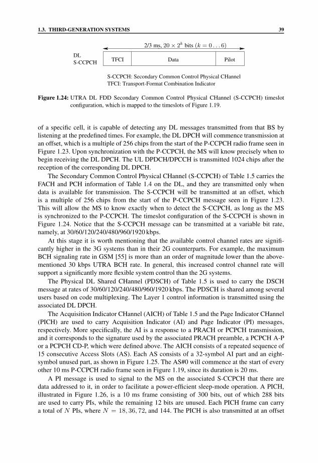
1.3. THIRD-GENERATION SYSTEMS 39
S-CCPCHDL
TFCI Data Pilot
S-CCPCH: Secondary Common Control Physical CHannelTFCI: Transport-Format Combination Indicator
2/3 ms, 20 × 2k bits (k = 0 . . . 6)
Figure 1.24: UTRA DL FDD Secondary Common Control Physical CHannel (S-CCPCH) timeslotconfiguration, which is mapped to the timeslots of Figure 1.19.
of a specific cell, it is capable of detecting any DL messages transmitted from that BS bylistening at the predefined times. For example, the DL DPCH will commence transmission atan offset, which is a multiple of 256 chips from the start of the P-CCPCH radio frame seen inFigure 1.23. Upon synchronization with the P-CCPCH, the MS will know precisely when tobegin receiving the DL DPCH. The UL DPDCH/DPCCH is transmitted 1024 chips after thereception of the corresponding DL DPCH.
The Secondary Common Control Physical CHannel (S-CCPCH) of Table 1.5 carries theFACH and PCH information of Table 1.4 on the DL, and they are transmitted only whendata is available for transmission. The S-CCPCH will be transmitted at an offset, whichis a multiple of 256 chips from the start of the P-CCPCH message seen in Figure 1.23.This will allow the MS to know exactly when to detect the S-CCPCH, as long as the MSis synchronized to the P-CCPCH. The timeslot configuration of the S-CCPCH is shown inFigure 1.24. Notice that the S-CCPCH message can be transmitted at a variable bit rate,namely, at 30/60/120/240/480/960/1920 kbps.
At this stage it is worth mentioning that the available control channel rates are signifi-cantly higher in the 3G systems than in their 2G counterparts. For example, the maximumBCH signaling rate in GSM [55] is more than an order of magnitude lower than the above-mentioned 30 kbps UTRA BCH rate. In general, this increased control channel rate willsupport a significantly more flexible system control than the 2G systems.
The Physical DL Shared CHannel (PDSCH) of Table 1.5 is used to carry the DSCHmessage at rates of 30/60/120/240/480/960/1920 kbps. The PDSCH is shared among severalusers based on code multiplexing. The Layer 1 control information is transmitted using theassociated DL DPCH.
The Acquisition Indicator CHannel (AICH) of Table 1.5 and the Page Indicator CHannel(PICH) are used to carry Acquisition Indicator (AI) and Page Indicator (PI) messages,respectively. More specifically, the AI is a response to a PRACH or PCPCH transmission,and it corresponds to the signature used by the associated PRACH preamble, a PCPCH A-Por a PCPCH CD-P, which were defined above. The AICH consists of a repeated sequence of15 consecutive Access Slots (AS). Each AS consists of a 32-symbol AI part and an eight-symbol unused part, as shown in Figure 1.25. The AS#0 will commence at the start of everyother 10 ms P-CCPCH radio frame seen in Figure 1.19, since its duration is 20 ms.
A PI message is used to signal to the MS on the associated S-CCPCH that there aredata addressed to it, in order to facilitate a power-efficient sleep-mode operation. A PICH,illustrated in Figure 1.26, is a 10 ms frame consisting of 300 bits, out of which 288 bitsare used to carry PIs, while the remaining 12 bits are unused. Each PICH frame can carrya total of N PIs, where N = 18, 36, 72, and 144. The PICH is also transmitted at an offset

40 CHAPTER 1. THIRD-GENERATION CDMA SYSTEMS
AI Unused
AS #0 AS #i AS # 14
32 bits 8 bits
20 ms
DLAICH
AICH: Acquisition Indicator CHannelAI: Acquisition IndicatorAS: Access Slot
Figure 1.25: UTRA DL Acquisition Indicator CHannel (AICH) Access Slot (AS) configuration, whichis mapped to the corresponding AS of the AICH. Due to its duration of 20 ms, it is mappedto every other 10 ms frame in Figure 1.19.
PIs Unused
288 bits 12 bits
10 ms
DLPICH
PICH: Page Indicator CHannelPI: Page Indicator
Figure 1.26: UTRA DL Page Indicator CHannel (PICH) configuration. Each PICH frame can carry atotal of N PIs, where N = 18, 36, 72, and 144.
with respect to the start of the P-CCPCH, which is a multiple of 256 chips. The associatedS-CCPCH will be transmitted 7680 chips later.
Finally, the Common PIlot CHannel (CPICH) of Table 1.5 is a 30 kbps DL physicalchannel that carries a predefined bit sequence. It provides a phase reference for the SCH,P-CCPCH, AICH, and PICH, since these channels do not carry pilot bits, as shown inFigures 1.23, 1.25, and 1.26, respectively. The PICH is transmitted synchronously with theP-CCPCH.
1.3.2.3.2.2 Common Physical Channels of the TDD Mode. In contrast to theprevious FDD structures of Figures 1.20–1.26, in TDD operation the burst structureof Figure 1.27 is used for all the physical channels, where each timeslot’s transmittedinformation can be arbitrarily allocated to the DL or UL, as shown in the three possibleTDD allocations in Figure 1.28. Hence, this flexible allocation of the UL and DL burst in theTDD mode enables the use of an adaptive modem [96,132] whereby the modem parameters,such as the spreading factor or the number of bits per symbol can be adjusted on a burst-by-burst basis to optimize the link quality. A symmetric UL/DL allocation refers to a scenario

1.3. THIRD-GENERATION SYSTEMS 41
Burst Type 1 : Data = 976 chips, Midamble = 512 chipsBurst Type 2 : Data = 1104 chips, Midamble = 256 chips
Data DataMidamble
GP : Guard Period = 96 chips
GP
2/3 ms
Figure 1.27: Burst configuration mapped on the TDD burst structure of Figure 1.28 in the UTRA TDDmode. Two different types of TDD bursts are defined in UTRA, namely, Burst Type 1 andBurst Type 2.
: Downlink : Uplink
(a) Symmmetric UL/DL allocation with multiple switching points
(c) Asymmetric UL/DL allocation with a single switching point
(b) Asymmetric UL/DL allocation with multiple switching points
10 ms
2/3 ms
Figure 1.28: UL/DL allocation examples for the 15 slots in UTRA TDD operation using the timeslotconfigurations of Figure 1.27.
in which an approximately equal number7 of DL and UL bursts are allocated within a TDDframe, while in asymmetric UL/DL allocation, there is an unequal number of UL and DLbursts, such as, for example, in “near-simplex” file download from the Internet or video-on-demand.
In UTRA, two different TDD burst structures, known as Burst Type 1 and Burst Type 2,are defined, as shown in Figure 1.27. The Type 1 burst has a longer midamble (512 chips) thanthe Type 2 burst (256 chips). However, both types of bursts have an identical Guard Period(GP) of 96 chips. The midamble sequences that are allocated to the different TDD bursts in
7Since there are 15 timeslots per frame, there will always be one more additional DL or UL burst per frame in asymmetric allocation.

42 CHAPTER 1. THIRD-GENERATION CDMA SYSTEMS
Burst structure with TFCI information only
Midamble GP
Burst structure with TFCI and TPC information
GP : Guard Period
TPC : Transmit Power ControlTFCI : Transport Format Combination Indicator
Midamble GPData Data
DataData
TFC
I
TFC
I
TFC
I
TPC
TFC
I
2/3 ms
2/3 ms
Figure 1.29: Burst configuration mapped on the TDD burst configuration of Figure 1.28 in the UTRATDD mode incorporating TFCI and/or TPC information.
each timeslot belong to a so-called midamble code set. The codes in each midamble codeset are derived from a unique Basic Midamble Code. Adjacent cells are allocated differentmidamble code sets, that is, different basic midamble code. This can be exploited to assist incell identification.
Unlike in the FDD mode, there is only one type of Dedicated Physical CHannel (DPCH)in the TDD mode. Hence, the Layer 1 control information—such as the TPC commandand the TFCI information—will be transmitted in the data field of Figure 1.27, if required.The TDD burst structures that incorporate the TFCI information as well as the TFCI+TPCinformation are shown in Figure 1.29. This should be contrasted with their correspondingFDD allocations in Figures 1.20 and 1.21. The TFCI field is divided into two parts, whichreside immediately before and after the midamble (or after the TPC command, if powercontrol is invoked) in the data field. The TPC command is always transmitted immediatelyafter the midamble, as portrayed in Figure 1.29. As a result of these control informationsegments, the amount of user data is reduced in each timeslot. Note that the TPC commandis only transmitted on the UL and only once per 10 ms frame for each MS.
In contrast to the FDD mode, the SCH in the TDD mode is not time-multiplexed onto theP-CCPCH of Table 1.5. Instead, the SCH messages are transmitted on one or two timeslotsper frame.8 The P-CCPCH will be code-multiplexed with the first SCH timeslot in eachframe.
Having highlighted the basic features of the various UTRA channels, let us now considerhow the various services are error protected, interleaved, and multiplexed on to the physicalchannels. This issue is discussed with reference to Figures 1.30 and 1.31 in the context ofUTRA.
8If two timeslots are allocated to the SCH per frame, they will be spaced seven slots apart.

1.3. THIRD-GENERATION SYSTEMS 43
1.3.2.4 Service Multiplexing and Channel Coding in UTRA
Service multiplexing is employed when multiple services of identical or different bit ratesrequiring different QoS belonging to the same user’s connection are transmitted. An examplewould be the simultaneous transmission of a voice and video service for a multimediaapplication. Each service is represented by its corresponding transport channels, as describedin Section 1.3.2.2. The coding and multiplexing of the transport channels are performed insets of transport blocks that arrived from the higher layers at fixed intervals of 10, 20, 40or 80 ms. These intervals are known as the Transmission Time Interval (TTI). Note thatthe number of bits on each transport channel can vary between different TTIs, as well asbetween different transport channels. A possible method of transmitting multiple services isby using code-multiplexing with the aid of orthogonal codes. Every service could have itsown DPDCH and DPCCH, each assigned to a different orthogonal code. This method is notvery efficient, however, since a number of orthogonal codes would be reserved by a singleuser, while on the UL it would also inflict self-interference when the multiple DPDCH andDPCCH codes’ orthogonality is impaired by the fading channel. Alternatively, these servicescan be time-multiplexed into one or several DPDCHs, as shown in Figures 1.30 and 1.31for the UL and DL, respectively. The function of the individual processing steps is detailedbelow.
1.3.2.4.1 CRC Attachment. A Cyclic Redundancy Checksum (CRC) is first calculatedfor each incoming transport block within a TTI. The CRC consists of either 24, 16, 12, 8, or 0parity bits, which is decided by the higher layers. The CRC is then attached to the end of thecorresponding transport block in order to facilitate reliable error detection at the receiver. Thisfacility is very important, for example, for generating the video packet acknowledgement flagin wireless video telephony using standard video codecs, such as H.263 [133].
1.3.2.4.2 Transport Block Concatenation. Following the CRC attachment, the incom-ing transport blocks within a TTI are serially concatenated in order to form a code block.If the number of bits exceeds the maximum code block length, denoted as Z , then the codeblock is segmented into shorter ones and filler bits (zeros) are added to the last code block, ifnecessary, in order to generate code blocks of the same length. The maximum code blocklength Z is dependent on the type of channel-coding invoked. For convolutional codingZ = 504, while for turbo coding Z = 5114, since turbo codes require a long coded blocklength [134]. If no channel-coding is invoked, then the code block can be of unlimited length.
1.3.2.4.3 Channel-coding. Each of the code blocks is then delivered to the channel-coding unit. Several Forward Error Correction (FEC) techniques are proposed for channel-coding. The FEC technique used is dependent on the QoS requirement of that specifictransport channel. Table 1.6 shows the various types of channel-coding techniques invokedfor different transport channels. Typically, convolutional coding is used for services with abit error rate requirement on the order of 10−3, for example, for voice services. For servicesrequiring a lower BER, namely, on the order of 10−6, turbo coding is applied. Turbo codingis known to guarantee a high performance [135] over AWGN channels at the cost of increasedinterleaving-induced latency or delay. The implementational complexity of the turbo codec(TC) does not necessarily have to be higher than that of the convolutional codes (CC), since

44 CHAPTER 1. THIRD-GENERATION CDMA SYSTEMS
SegmentationPhysical Channel
CRC Attachment
Transport Block Concatenation/Code Block Segmentation
Channel Coding
1st Interleaving
Rate Matching
CRC Attachment
Transport Block Concatenation/Code Block Segmentation
Channel Coding
1st Interleaving
Rate Matching
Physical Channel Mapping
2nd Interleaving
Transport Channel in Blocks Transport Channel in Blocks
Physical Channels
Radio Frame PaddingRadio Frame Padding
to create 10 ms framesRadio Frame Segmentation Radio Frame Segmentation
to create 10 ms frames
Transport Channel Multiplexingto create the CCTrCH
Figure 1.30: Transport channel-coding/multiplexing flowchart for the UL in UTRA.

1.3. THIRD-GENERATION SYSTEMS 45
SegmentationPhysical Channel
Physical Channel Mapping
2nd Interleaving
Physical Channels
CRC Attachment
Transport Block Concatenation/Code Block Segmentation
Channel Coding
1st Interleaving
CRC Attachment
Transport Block Concatenation/Code Block Segmentation
Channel Coding
1st Interleaving
2nd insertion of DTXIndication Bits
Transport Channel in Blocks
Rate Matching
1st insertion of DTXIndication Bits
Transport Channel in Blocks
Rate Matching
1st insertion of DTXIndication Bits
Radio Frame Segmentationto create 10 ms frames
Radio Frame Segmentationto create 10 ms frames
Transport Channel Multiplexingto create CCTrCH
Figure 1.31: Transport channel-coding/multiplexing flowchart for the DL in UTRA.

46 CHAPTER 1. THIRD-GENERATION CDMA SYSTEMS
Table 1.6: UTRA Channel-coding parameters for the channels of Table 1.4.
Transport channels Channel-coding schemes Coding rate
BCH, PCH, RACH Convolutional code 1/2CPCH,DCH,DSCH,FACH Convolutional code 1/3, 1/2
Turbo code 1/3No coding
a constraint-length K = 7 or K = 9 CC is often invoked, while the constraint-length of theturbo codes employed may be as low as K = 3. In somewhat simplistic but plausible terms,one could argue that a K = 3 TC using two decoding steps per iteration and employing fouriterations has a similar complexity to a K = 6 CC, since they are associated with the samenumber of trellis states. The encoded code blocks within a TTI are then serially concatenatedafter the channel-coding unit, as seen in Figures 1.30 and 1.31.
1.3.2.4.4 Radio Frame Padding. Radio frame padding is only performed on the ULwhereby the input bit sequence (the concatenated encoded code blocks from the channel-coding unit) is padded in order to ensure that the output can be segmented equally into(TTI/10 ms) number of 10 ms radio frames. Note that radio frame padding is not required onthe DL, since DTX is invoked, as seen in Figure 1.31. This process was termed Radio FrameEqualization in the standard. However, in order to avoid confusion with channel equalization,we used the terminology “padding”.
1.3.2.4.5 First Interleaving. The depth of this first interleaver seen in Figures 1.30 and1.31 may range from one radio frame (10 ms) to as high as 80 ms, depending on the TTI.
1.3.2.4.6 Radio Frame Segmentation. The input bit sequence after the first interleavingis then segmented into consecutive radio frames of 10 ms duration, as highlighted inSection 1.3.2.3. The number of radio frames required is equivalent to (TTI/10). Because ofthe Radio Frame Padding step performed prior to the segmentation on the UL in Figure 1.30and also because of the Rate Matching step on the DL in Figure 1.31, the input bit sequencecan be conveniently divided into the required number of radio frames.
1.3.2.4.7 Rate Matching. The rate matching process of Figures 1.30 and 1.31 implies thatbits on a transport channel are either repeated or punctured in order to ensure that the total bitrate after multiplexing all the associated transport channels will be identical to the channelbit rate of the corresponding physical channel, as highlighted in Section 1.3.2.3. Thus, ratematching must be coordinated among the different coded transport channels, so that the bitrate of each channel is adjusted to a level that fulfills its minimum QoS requirements [118].On the DL, the bit rate is also adjusted so that the total instantaneous transport channel bitrate approximately matches the defined bit rate of the physical channel, as listed in Table 1.3.

1.3. THIRD-GENERATION SYSTEMS 47
1.3.2.4.8 Discontinuous Transmission Indication. On the DL, the transmission is inter-rupted if the bit rate is less than the allocated channel bit rate. This is known as discontinuoustransmission (DTX). DTX indication bits are inserted into the bit sequence in order to indicatewhen the transmission should be turned off. The first insertion of the DTX indication bitsshown in Figure 1.31 is performed only if the position of the transport channel in the radioframe is fixed. In this case, a fixed number of bits is reserved for each transport channel inthe radio frame. For the second insertion step shown in Figure 1.31, the DTX indication bitsare inserted at the end of the radio frame.
1.3.2.4.9 Transport Channel Multiplexing. One radio frame from each transport chan-nel that can be mapped to the same type of physical channel is delivered to the transportchannel multiplexing unit of Figures 1.30 and 1.31, where they are serially multiplexed toform a Coded Composite Transport CHannel (CCTrCH). At this point, it should be noted thatthe bit rate of the multiplexed radio frames may be different for the various transport channels.In order to successfully de-multiplex each transport channel at the receiver, the TFCI—which contained information about the bit rate of each multiplexed transport channel—canbe transmitted together with the CCTrCH information (which will be mapped to a physicalchannel), as highlighted in Section 1.3.2.3. Alternatively, blind transport format detection canbe performed at the receiver without the explicit knowledge of the TFCI, where the receiveracquires the transport format combination through some other means, such as, for example,the received power ratio of the DPDCH to the DPCCH.
1.3.2.4.10 Physical Channel Segmentation. If more than one physical channel is re-quired in order to accommodate the bits of a CCTrCH, then the bit sequence is segmentedequally into different physical channels, as seen in Figures 1.30 and 1.31. A typical exampleof this scenario would be where the bit rate of the CCTrCH exceeds the maximum allocatedbit rate for the particular physical channel. Thus, multiple physical channels are required forits transmission. Furthermore, restrictions are imposed on the number of transport channelsthat can be multiplexed onto a CCTrCH. Hence, several physical channels are required tocarry any additional CCTrCHs.
1.3.2.4.11 Second Interleaving. The depth of the second interleaving stage shown inFigures 1.30 and 1.31 is equivalent to one radio frame. Hence, this process does not increasethe system’s delay.
1.3.2.4.12 Physical Channel Mapping. Finally, the bits are mapped to their respectivephysical channels summarized in Table 1.5, as portrayed in Figures 1.30 and 1.31.
Having highlighted the various channel-coding and multiplexing techniques as well asthe structures of the physical channels illustrated by Figures 1.20–1.27, let us now considerhow the services of different bit rates are mapped on the UL and DL dedicated physical datachannels (DPDCH) of Figures 1.20 and 1.21, respectively. In order to augment the process,we will present three examples. Specifically, we consider the mapping of two multirateservices on a UL DPDCH and an example of the mapping of a 4.1 kbps data service on aDL DPDCH in the FDD mode. We will then use the same parameters as employed in the first

48 CHAPTER 1. THIRD-GENERATION CDMA SYSTEMS
Table 1.7: Parameters for the multimedia communication example of Section 1.3.2.4.13.
Service 1, DCH#1 Service 2, DCH#2
Transport Block Size 640 bits 164 bitsTransport Block Set Size 4 * 640 bits 1 * 164 bitsTTI 40 ms 40 msBit Rate 64 kbps 4.1 kbpsCRC 16 bits 16 bitsCoding Turbo Convolutional
Rate: 1/3 Rate: 1/3
example and show how the multirate services can be mapped to the corresponding UL DPCHin TDD mode.
1.3.2.4.13 Mapping Several Multirate Services to the UL Physical Channels in FDDMode [115]. In this example, we assume that a 4.1 kbps speech service and a 64 kbpsvideo service are to be transmitted simultaneously on the UL. The parameters used for thisexample are shown in Table 1.7. As illustrated in Figure 1.32, a 16-bit CRC checksum is firstattached to each transport block of DCH#1, that is, #1a,. . . ,#1d, as well as the transport blockof DCH#2 for the purpose of error detection. As a result, the number of bits in the transportblock of Service 1 and Service 2 is increased to 640+16 = 656 bits and 164+16 = 180 bits,respectively. The four transport blocks of Service 1 are then concatenated, as illustrated inFigure 1.32. Notice that no code block segmentation is invoked, since the total number of bitsin the concatenated transport block is less than Z = 5114 for turbo coding, as highlightedin Section 1.3.2.4.2. Since the video service typically requires a low BER—unless specificmeasures are invoked for mitigating the video effects of transmission errors [132]—turbocoding is invoked, using a coding rate of 1
3 . Hence, after turbo coding and the attachment oftailing bits, the resulting 40 ms segment would contain (656 × 4) × 3 + 12 = 7884 bits,as shown in Figure 1.32. By contrast, the speech service can tolerate a higher BER. Hence,convolutional coding is invoked. First, a block of 4 + 4 = 8 tail bits is concatenated to thetransport block in order to flush the assumed constraint-length K = 5 shift registers of theconvolutional encoder. Thus, a total of 180 + 8 = 188 bits are conveyed to the convolutionalencoder of DCH#1, as shown in Figure 1.32. Again, no code block segmentation is invoked,since the total number of bits in the transport channel is less than Z = 504 for convolutionalcoding, as highlighted in Section 1.3.2.4.2. A coding rate of 1
3 is used for the convolutionalencoding of DCH#1, as exemplified in Table 1.7. The output of the convolutional encoder ofDCH#1 will have a total of 188 × 3 = 564 bits per 40 ms segment. Since the TTI of thesetransport channels is 40 ms, four radio frames are required to transmit the associated data.At this stage, notice that there are a total of 7884 bits and 564 bits for DCH#1 and DCH#2,respectively. Since these numbers are divisible by four, they can be divided equally into fourradio frames. Thus, no padding is required as illustrated in the Radio Frame Padding stepof Figure 1.32. Interleaving is then performed across the 40 ms segment for each transportchannel before being segmented into four 10 ms radio frames.
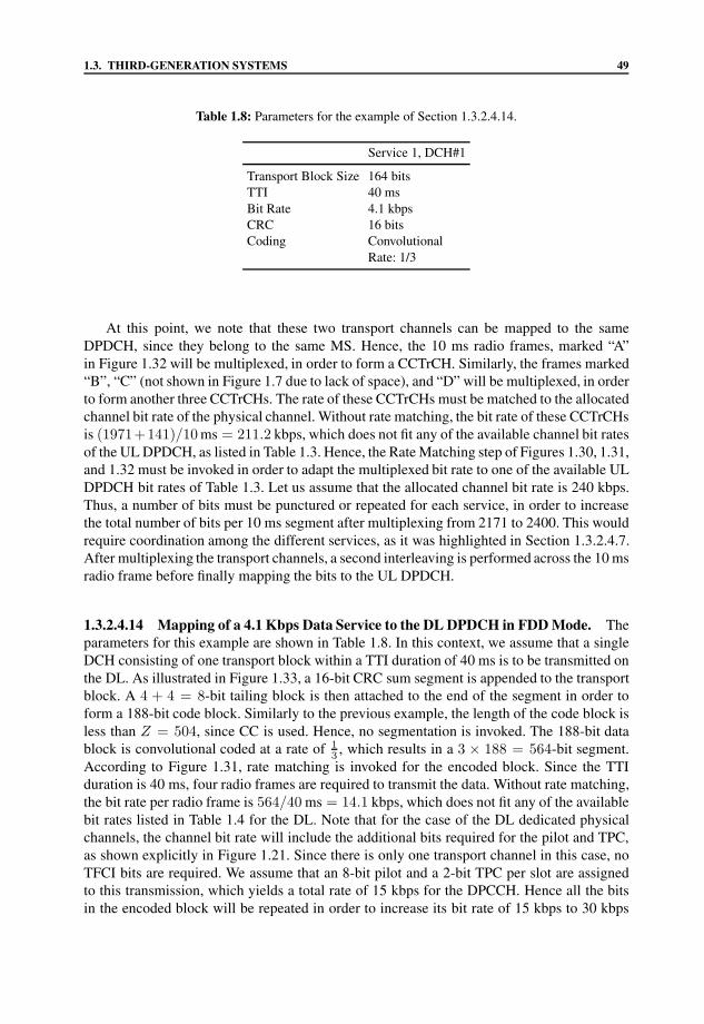
1.3. THIRD-GENERATION SYSTEMS 49
Table 1.8: Parameters for the example of Section 1.3.2.4.14.
Service 1, DCH#1
Transport Block Size 164 bitsTTI 40 msBit Rate 4.1 kbpsCRC 16 bitsCoding Convolutional
Rate: 1/3
At this point, we note that these two transport channels can be mapped to the sameDPDCH, since they belong to the same MS. Hence, the 10 ms radio frames, marked “A”in Figure 1.32 will be multiplexed, in order to form a CCTrCH. Similarly, the frames marked“B”, “C” (not shown in Figure 1.7 due to lack of space), and “D” will be multiplexed, in orderto form another three CCTrCHs. The rate of these CCTrCHs must be matched to the allocatedchannel bit rate of the physical channel. Without rate matching, the bit rate of these CCTrCHsis (1971+141)/10 ms = 211.2 kbps, which does not fit any of the available channel bit ratesof the UL DPDCH, as listed in Table 1.3. Hence, the Rate Matching step of Figures 1.30, 1.31,and 1.32 must be invoked in order to adapt the multiplexed bit rate to one of the available ULDPDCH bit rates of Table 1.3. Let us assume that the allocated channel bit rate is 240 kbps.Thus, a number of bits must be punctured or repeated for each service, in order to increasethe total number of bits per 10 ms segment after multiplexing from 2171 to 2400. This wouldrequire coordination among the different services, as it was highlighted in Section 1.3.2.4.7.After multiplexing the transport channels, a second interleaving is performed across the 10 msradio frame before finally mapping the bits to the UL DPDCH.
1.3.2.4.14 Mapping of a 4.1 Kbps Data Service to the DL DPDCH in FDD Mode. Theparameters for this example are shown in Table 1.8. In this context, we assume that a singleDCH consisting of one transport block within a TTI duration of 40 ms is to be transmitted onthe DL. As illustrated in Figure 1.33, a 16-bit CRC sum segment is appended to the transportblock. A 4 + 4 = 8-bit tailing block is then attached to the end of the segment in order toform a 188-bit code block. Similarly to the previous example, the length of the code block isless than Z = 504, since CC is used. Hence, no segmentation is invoked. The 188-bit datablock is convolutional coded at a rate of 1
3, which results in a 3 × 188 = 564-bit segment.
According to Figure 1.31, rate matching is invoked for the encoded block. Since the TTIduration is 40 ms, four radio frames are required to transmit the data. Without rate matching,the bit rate per radio frame is 564/40 ms = 14.1 kbps, which does not fit any of the availablebit rates listed in Table 1.4 for the DL. Note that for the case of the DL dedicated physicalchannels, the channel bit rate will include the additional bits required for the pilot and TPC,as shown explicitly in Figure 1.21. Since there is only one transport channel in this case, noTFCI bits are required. We assume that an 8-bit pilot and a 2-bit TPC per slot are assignedto this transmission, which yields a total rate of 15 kbps for the DPCCH. Hence all the bitsin the encoded block will be repeated in order to increase its bit rate of 15 kbps to 30 kbps

50 CHAPTER 1. THIRD-GENERATION CDMA SYSTEMS
#1a #1d
#1a CR
C
CR
C
#1d CR
C
Tail
Tail
Service #1 Service #2
CRC Attachment
Transport Block
Transport BlockConcatenation
Channel Coding/
Tail Bit Attachment
1st interleaving
Radio FrameSegmentation
Rate Matching
Transport ChannelMultiplexing
2nd Interleaving
Physical ChannelMapping
164
16164
8Convolutional coding, R=1/3
564
141 141
141+88=229 141+88=229
2400 2400
2400 2400
640 640
640 64016 16
Turbo coding, R=1/3
7872 12
7884
1971 1971
1971+200=2171 1971+200=2171
DPDCH, 240 kbps DPDCH, 240 kbps
#1D#1A #2A #2D
#1A #2A #2D#1D
#1A #1D#2A #2D
(640+16)*4=2624
164+16=1802624*3=7872
(180+8)*3=564
Figure 1.32: Mapping of several multimedia services to the UL dedicated physical data channel ofFigure 1.20 in FDD mode. The corresponding schematic diagram is seen in Figure 1.30.
for the DL DPCH. In this case the number of padding bits appended becomes N = 36.After the second interleaving stage of Figure 1.31, the segmented radio frames are mappedto the corresponding DPDCH, which are then multiplexed with the DPCCH, as shown inFigure 1.33.
1.3.2.4.15 Mapping Several Multirate Services to the UL Physical Channels in TDDMode [115]. In this example, we will demonstrate how the multirate multimedia ser-vices, considered previously in the example of Section 1.3.2.4.13 in an FDD context,are mapped to the corresponding dedicated physical channels (DPCH) in the TDD mode.

1.3. THIRD-GENERATION SYSTEMS 51
164
164
CRC
16
CRC Attachment
Transport Block
Tail Bit Attachment Tail
180 8
ConvolutionalCoding
564
Rate Matching
1st Interleaving
564 + N
564 + N
(564+N)/4 (564+N)/4 (564+N)/4(564+N)/4
#1 #2 #3 #4Radio FrameSegmentation
N = 36
150 150 150150
2nd Interleaving
Physical ChannelMapping
TPC Pilot
1 slot
30 kbps DPCH
Figure 1.33: Mapping of a 4.1 kbps data service to the DL dedicated physical channel of Figure 1.21in FDD mode. The corresponding schematic diagram is seen in Figure 1.31.
The channel-coding/multiplexing process is identical in the FDD and TDD mode, and so bothare based on Figures 1.30 and 1.31. The only difference is in the mapping of the transportchannels to the corresponding physical channels seen at the bottom of Figures 1.30 and 1.31,since the FDD and TDD modes have a different frame structure, as shown previously inFigures 1.20–1.26 and Figure 1.27, respectively. In this example, we are only interested in

52 CHAPTER 1. THIRD-GENERATION CDMA SYSTEMS
the process of service mapping to the physical channel, which follows the second interleavingstage of Figure 1.34. Here we assumed that for the TDD UL scenario of Table 1.7 the totalnumber of bits per segment after DCH multiplexing is 2186 as a result of rate matching. In theFDD example of Section 1.3.2.4.13, this was 2400. Each segment is divided into two bursts,which can be transmitted either by orthogonal code multiplexing onto a single timeslot, orusing two timeslots within a 10 ms radio frame. Note that only one burst in each segment isrequired to carry the TFCI and the TPC information.
Following these brief discussions on service multiplexing, channel coding, and interleav-ing, let us now concentrate on the aspects of variable-rate and multicode transmission inUTRA in the next section.
1.3.2.5 Variable-rate and Multicode Transmission in UTRA
Three different techniques have been proposed in the literature for supporting variable-ratetransmission, namely, multicode-, modulation-division multiplexing- (MDM), and multipleprocessing gain (MPG)-based techniques [136]. UTRA employs a number of differentprocessing gains, or variable spreading factors, in order to transmit at different channel bitrates, as highlighted previously in Section 1.3.2.3. The spreading factor (SF) has a directeffect on the performance and capacity of a DS-CDMA system. Since the chip rate is constant,the SF—which is defined as the ratio of the spread bandwidth to the original informationbandwidth—becomes lower, as the bit rate increases. Hence, there is a limit to the valueof the SF used, which is SF = 4 in FDD mode in the proposed UTRA standards. Multicodetransmission [131,136,137] is used if the total bit rate to be transmitted exceeds the maximumbit rate supported by a single DPDCH, which was stipulated as 960 kbps for the UL and1920 kbps for the DL. When this happens, the bit rate is split among a number of spreadingcodes and the information is transmitted using two or more codes. However, only one DPCCHis transmitted during this time. Thus, on the UL one DPCCH and several DPDCH are code-multiplexed and transmitted in parallel, as it will be augmented in the context of Figure 1.37.On the DL, the DPDCH and DPCCH are time-multiplexed on the first physical channelassociated with the first spreading code as seen in Figure 1.35. If more physical channelsare required, the DPCCH part in the slot will be left blank again, as shown in Figure 1.35.The transmit power of the DPDCH is also reduced.
1.3.2.6 Spreading and Modulation
It is well known that the performance of DS-CDMA is interference limited [99]. The majorityof the interference originates from the transmitted signals of other users within the samecell, as well as from neighboring cells. This interference is commonly known as MultipleAccess Interference (MAI). Another source of interference, albeit less dramatic, is a result ofthe wideband nature of CDMA, yielding several delayed replicas of the transmitted signal,which reach the receiver at different time instants, thereby inflicting what is known asinterpath interference. However, the advantages gained from wideband transmissions, such asmultipath diversity and the noise-like properties of the interference, outweigh the drawbacks.
The choice of the spreading codes [138,139] used in DS-CDMA will have serious impli-cations for the amount of interference generated. Suffice to say that the traditional measuresused in comparing different codes are their cross-correlations (CCL) and autocorrelation

1.3. THIRD-GENERATION SYSTEMS 53
#1a #1d
#1a CR
C
CR
C
#1d CR
C
Tail
Tail
Service #1 Service #2
CRC Attachment
Transport Block
Transport BlockConcatenation
Channel Coding/
Tail Bit Attachment
1st interleaving
Radio FrameSegmentation
Rate Matching
Transport ChannelMultiplexing
164
16164
8Convolutional coding, R=1/3
564
141 141
141+14=155 141+14=155
2186 2186
2186 2186
640 640
640 64016 16
Turbo coding, R=1/3
7872 12
7884
1971 1971
1971+60=2031 1971+60=2031
#1D#1A #2A #2D
#1A #2A #2D#1D
#1A #1D#2A #2D
(640+16)*4=2624
164+16=1802624*3=7872
(180+8)*3=564
Physical Channel
2nd Interleaving
Mapping
M
T M
M
MT
M : MidambleT : TFCI, 8 bits (4 on either side)
976 976 976 976
T TP P
P : TPC (2 bits)
118 116 118 116
Figure 1.34: Mapping of several multirate multimedia services to the UL dedicated physical datachannel of Figure 1.20 in TDD mode. The corresponding schematic diagram is seen inFigure 1.30.

54 CHAPTER 1. THIRD-GENERATION CDMA SYSTEMS
TPC
TFC
I
Pilo
t
DPCCHDPDCH DPDCH DPCCH
TransmissionPower
TransmissionPower
TransmissionPower
Physical Channel 1
Physical Channel 2
Physical Channel L
2/3 ms (one timeslot)
Figure 1.35: DL FDD slot format for multicode transmission in UTRA, based on Figure 1.21, butdispensing with transmitting DPCCH over all multicode physical channels.
(ACL). If the CCL of the spreading codes of different users is nonzero, this will increasetheir interference, as perceived by the receiver. Thus a low CCL reduces the MAI. The so-called out-of-phase ACL of the codes, on the other hand, plays an important role during theinitial synchronization between the BS and MS, which has to be sufficiently low to minimizethe probability of synchronizing to the wrong ACL peak.
In order to reduce the MAI and thereby improve the system’s performance and capacity,the UTRA physical channels are spread using two different codes, namely, the channelizationcode and a typically longer so-called scrambling code. In general, the channelization codesare used to maintain orthogonality between the different physical channels originating fromthe same source. On the other hand, the scrambling codes are used to distinguish betweendifferent cells, as well as between different MSs. All the scrambling codes in UTRA are incomplex format. Complex-valued scrambling balances the power on the I and Q branches.This can be shown by letting cI
s and cQs be the I and Q branch scrambling codes, respectively.
Let d(t) be the complex-valued data of the transmitter, which can be written as:
d(t) = dI + jdQ, (1.34)
where dI and dQ represent the data on the I and Q branches, respectively. Let us assume forthe sake of argument that the power level in the I and Q branches is unbalanced due to, forinstance, their different bit rates or different QoS requirements. If only real-valued scramblingis used, then the output becomes:
s(t) = cIs (dI + jdQ) , (1.35)

1.3. THIRD-GENERATION SYSTEMS 55
Table 1.9: UL/DL spreading and modulation parameters in UTRA.
Channelization Codes Scrambling Codes
Type of codes OVSF UL : Gold codes, S(2) codes (Section 1.3.2.6.2)(Section 1.3.2.6.1) DL : Gold codes (Section 1.3.2.6.3)
Code length Variable UL : 10 ms of (225 − 1)-chip Gold codeDL : 10 ms of (218 − 1)-chip Gold code
Type of spreading BPSK (UL/DL) QPSK (UL/DL)
which is also associated with an unbalanced power level on the I and Q branches. By contrast,if complex-valued scrambling is used, then the output would become:
s(t) = (dI + jdQ) · (cIs + jcQ
s
)(1.36)
= cIs · dI − cQ
s · dQ + j(cQs · dI + cI
s · dQ
). (1.37)
As can be seen, the power on the I and Q branches after complex scrambling is the same,regardless of the power level of the unscrambled data on the I and Q branches. Hence,complex scrambling potentially improves the power amplifier’s efficiency by reducing thepeak-to-average power fluctuation. This also relaxes the linearity requirements of the ULpower amplifier used.
Table 1.9 shows the parameters and techniques used for spreading and modulation inUTRA, which will be discussed in depth in the following sections.
1.3.2.6.1 Orthogonal Variable Spreading Factor Codes. The channelization codes usedin the UTRA systems are derived from a set of orthogonal codes known as OrthogonalVariable Spreading Factor (OVSF) codes [130]. OVSF codes are generated from a tree-structured set of orthogonal codes, such as the Walsh-Hadamard codes, using the procedureshown in Figure 1.36. Specifically, each channelization code is denoted by cN,n, wheren = 1, 2, . . . , N and N = 2x, x = 2, 3, . . . 8. Each code cN,n is derived from the previouscode c(N/2),n as follows [130]:
cN,1
cN,2
cN,3
...cN,N
=
c(N/2),1|c(N/2),1
c(N/2),1|c(N/2),1
c(N/2),2|c(N/2),2
...c(N/2),(N/2)|c(N/2),(N/2)
, (1.38)
where [|] at the right-hand side of Equation 1.38 denotes an augmented matrix and c(N/2),n isthe binary complement of c(N/2),n. For example, according to Equation 1.38 and Figure 1.36,cN,1 = c8,1 is created by simply concatenating c(N/2),1 and c(N/2),1, which doubles thenumber of chips per bit. By contrast, cN,2 = c8,2 is generated by attaching c(N/2),1 toc(N/2),1. From Equation 1.38, we see that, for example, cN,1 and cN,2 at the left-hand sideof Equation 1.38 are not orthogonal to c(N/2),1, since the first half of both was derived

56 CHAPTER 1. THIRD-GENERATION CDMA SYSTEMS
Lowest bit rateHighest bit rate
c4,1
c4,2
c4,3
c4,4
c8,1
c8,2
c16,1
c16,2
c32,1
c32,2
c64,1
c64,2
c128,1
c128,2
c256,1
c256,2
k = 0k = 1k = 2k = 3k = 4k = 5k = 6
Figure 1.36: Orthogonal variable-spreading factor code tree in UTRA according to Equation 1.38. Theparameter k in the figure is directly related to that found in Figures 1.20–1.24.
from c(N/2),1 in Figure 1.36, but they are orthogonal to c(N/2),n, n = 2, 3, . . . , (N/2).The code c(N/2),1 in Figure 1.36 is known as the mother code of the codes cN,1 and cN,2,since these two codes are derived from c(N/2),1. The codes on the “highest”-order branches(k = 6) of the tree at the left of Figure 1.36 have a spreading factor of 4, and they areused for transmission at the highest possible bit rate for a single channel, which is 960 kbps.

1.3. THIRD-GENERATION SYSTEMS 57
On the other hand, the codes on the “lowest”-order branches (k = 0) of the tree at theright of Figure 1.36 result in a spreading factor of 256, and these are used for transmissionat the lowest bit rate, which is 15 kbps. It is worth noting here that an intelligent BbBadaptive scheme may vary its SF on a 10 ms frame basis in an attempt to adjust the SF on anear-instantaneous channel-quality motivated basis [96,132]. Orthogonality between paralleltransmitted channels of the same bit rate is preserved by assigning each channel a differentorthogonal code accordingly. For channels with different bit rates transmitting in parallel,orthogonal codes are assigned, ensuring that no code is the mother-code of the other. Thus,OVSF channelization codes provide total isolation between different users’ physical channelson the DL that are transmitted synchronously and hence eliminate MAI among them. OVSFchannelization codes also provide orthogonality between the different physical channels seenin Figure 1.35 during multicode transmission.
Since there is only a limited set of OVSF codes, which is likely to be insufficientto support a large user-population, while also allowing identification of the BSs by theMSs on the DL, each cell will reuse the same set of OVSF codes. Statistical multiplexingschemes such as packet reservation multiple access (PRMA) can be used to allocate andde-allocate the OVSF codes on a near-instantaneous basis, for example, depending on theusers’ voice activity in the case of DTX-based communications [140]. However, orthogonalcodes, such as the orthogonal OVSF codes, in general exhibit poor out-of-phase ACL andCCL properties [141]. Therefore, the correlations of the OVSFs of adjacent asynchronousBSs will become unacceptably high, degrading the correlation receiver’s performance at theMS. On the other hand, certain long codes such as Gold codes exhibit low CCL, whichis advantageous in CDMA applications [66]. Hence in UTRA, cell-specific long codes areused in order to reduce the inter-cell interference on the DL. On the UL, MAI is reduced byassigning different scrambling codes to different users.
1.3.2.6.2 Uplink Scrambling Codes. The UL scrambling codes in UTRA can be classi-fied into long scrambling codes and short scrambling codes. A total of 224 UL scramblingcodes can be generated for both the long and short codes.
Long scrambling codes are constructed from two m-sequences using the polynomials of1+X3+X25 and 1+X+X2+X3+X25, following the procedure highlighted by Proakis [5]in order to produce a set of Gold codes for the I branch. The Q-branch Gold code is a shiftedversion of the I-branch Gold code, where a shift of 16,777,232 chips was recommended. Goldcodes are rendered different from each other by assigning a unique initial state to one of theshift registers of the m-sequence. The initial state of the other shift register is a sequence oflogical 1. Although the Gold codes generated have a length of 225 − 1 chips, only 38,400chips (10 ms at 3.84 Mcps) are required in order to scramble a radio frame.
Short scrambling codes are defined from a family of periodically extended S(2) codes.This 256-chip S(2) code was introduced to ease the implementation of multi-user detectionat the BS [58]. The multi-user detector has to invert the so-called system matrix [95], thedimension of which is proportional to the sum of the channel impulse response duration andthe spreading code duration. Thus, using a relatively short scrambling code is an importantpractical consideration in reducing the size of the system-matrix to be inverted.
1.3.2.6.3 Downlink Scrambling Codes. Unlike the case for the UL, only Gold codes areused on the DL. The DL Gold codes on the I branch are constructed from two m-sequences

58 CHAPTER 1. THIRD-GENERATION CDMA SYSTEMS
using the polynomials of 1 + X7 + X18 and 1 + X5 + X7 + X10 + X18. These Gold codesare shifted by 131,072 chips in order to produce a set of Gold codes for the Q branch.
Although a total of 218 − 1 = 262, 143 Gold codes can be generated, only 8192 of themwill be used as the DL scrambling code. These codes are divided into 512 groups, each ofwhich contains a primary scrambling code and 15 secondary scrambling codes. Altogetherthere are 512 primary scrambling codes and 8192−512 = 7680 secondary scrambling codes.Each cell is allocated one primary scrambling code, which is used on the CPICH and P-CCPCH channels of Table 1.5. This primary scrambling code will be used to identify the BSfor the MS. All the other physical channels belonging to this cell can use either the primaryscrambling code or any of the 15 secondary scrambling codes that belong to the same group,as the primary scrambling code. In order to facilitate fast cell or BS identification, the setof 512 primary scrambling codes is further divided into 64 subsets, each consisting of eightprimary scrambling codes, as will be shown in Section 1.3.2.9.
1.3.2.6.4 Uplink Spreading and Modulation. A model of the UL transmitter for a singleDPDCH is shown in Figure 1.37 [59]. We have seen in Figure 1.20 that the DPDCH andDPCCH are transmitted in parallel on the I and Q branches of the UL, respectively. Hence,to avoid I/Q channel interference in case of I/Q inbalance of the quadrature carriers, differentorthogonal spreading codes are assigned to the DPDCH and DPCCH on the I and Q branch,respectively. These two channelization codes for DPDCH and DPCCH, denoted by cD,1 andcC in Figure 1.37, respectively, are allocated in a predefined order. From Figure 1.20, weknow that the SF of the DPCCH is 256. Hence, cC = c256,1 in the context of Figure 1.36.This indicates that the high SF of the DPCCH protects the vulnerable control channel messageagainst channel impairments. On the other hand, we have cD,1 = cSF,2, depending on theSF of the DPDCH. In the event of multicode transmission portrayed by the dashed linesin Figure 1.37, different additional orthogonal channelization codes, namely, cD,2 and cD,3,are assigned to each DPDCH for the sake of maintaining orthogonality, and they can betransmitted on either the I or Q branch. In this case, the BS and MS have to agree on thenumber of channelization codes to be used. After spreading, the BPSK modulated I and Qbranch signals are summed in order to produce a complex Quadrature Phase Shift Keying(QPSK) signal. The signal is then scrambled by the complex scrambling code, cscramb. Thepulse-shaping filters, p(t), are root-raised cosine Nyquist filters using a roll-off factor of 0.22.
The transmitter of the UL PRACH and PCPCH message part is also identical tothat shown in Figure 1.37. As we have mentioned in Section 1.3.2.3.2 in the context ofFigure 1.22, the PRACH and the CPCH message consist of a data part and a control part.In this case, the data part will be transmitted on the I branch, and the control part on the Qbranch. The choice of the channelization codes for the data and control part depends on thesignature of the preambles transmitted beforehand. As highlighted in Section 1.3.2.3.2, thepreamble signature is a 256-chip sequence generated by the repetition of a 16-chip Hadamardcode. This 16-chip code actually corresponds to one of the OVSF codes, namely, to c16,n,where n = 1, . . . , 16. The codes in the subtree of Figure 1.36 below this specific 16-chipcode n will be used as the channelization codes for the data part and control part.
1.3.2.6.5 Downlink Spreading and Modulation. The schematic diagram of the DLtransmitter is shown in Figure 1.38. All the DL physical channel bursts (except for the SCH)are first QPSK modulated in order to form the I and Q branches, before spreading to the chip

1.3. THIRD-GENERATION SYSTEMS 59
ComplexMultiply
DPCCHQ
DPDCH2
I
DPDCHI
DPDCH3
Q
cD,1
cD,2
cD,3
cC
cscramb
p(t)
p(t)
coswct
− sinwct
Figure 1.37: UL transmitter in UTRA using the frame structure of Figure 1.20. Multicode transmissionsare indicated by the dashed lines.
rate. In contrast to the UL of Figure 1.37, the same OVSF channelization code cch is usedon the I and Q branches. Different physical channels are assigned different channelizationcodes in order to maintain their orthogonality. For instance, the channelization codes for theCPICH and P-CCPCH of Table 1.5 are fixed to the codes c256,1 and c256,2 of Figure 1.36,respectively. The channelization codes for all the other physical channels are assigned by thenetwork.
The resulting signal in Figure 1.38 is then scrambled by a cell-specific scrambling codecscramb. Similarly to the DL, the pulse-shaping filters are root-raised cosine Nyquist filtersusing a rolloff factor of 0.22.
In TDD mode, the transmitter structure for both the UL and DL are similar to that of aFDD DL transmitter of Figure 1.38. Since each timeslot can be used for transmitting severalTDD bursts from the same source or from different sources, the OVSF codes are invoked inorder to maintain orthogonality between the burst of different TDD/CDMA users/messages.An advantage of the TDD/CDMA mode is that the user population is separated in both thetime and the code domain. In other words, only a small number of CDMA users/services willbe supported within a TDD timeslot, which dramatically reduces the complexity of the multi-

60 CHAPTER 1. THIRD-GENERATION CDMA SYSTEMS
S PComplexMultiply
DL PhysicalChannel
cch
cscramb
p(t)
p(t)
coswct
− sinwct
Figure 1.38: DL transmitter in UTRA using the frame structure of Figure 1.21.
AS#1 AS#2 AS#15AS#14
5120chips
20 ms
AS : Access Slot
Figure 1.39: ALOHA-based physical UL random access slots in UTRA.
user detector that can be used in both the UL and DL for mitigating the MAI or multi-codeinterference.
1.3.2.7 Random Access
1.3.2.7.1 Mobile-initiated Physical Random Access Procedures. If data transmissionis initiated by an MS, it is required to send a random access request to the BS. Since suchrequests can occur at any time, collisions may result when two or more MSs attempt toaccess the network simultaneously. Hence, in order to reduce the probability of a collision,the random access procedure in UTRA is based on the slotted ALOHA technique [118].
Random access requests are transmitted to the BS via the PRACH of Table 1.5. Eachrandom access transmission request may consist of one or several preambles and a messagepart, whose timeslot configuration was shown in Figure 1.22. According to the regime ofFigure 1.39, the preambles and the message part can only be transmitted at the beginning ofone of those 15 so-called access slots, which span two radio frames (i.e., 20 ms). Thus, eachaccess slot has a length equivalent to 5120 chips or 4
3ms.
Before any random access request can be transmitted, the MS has to obtain certaininformation via the DL BCH transmitted on the P-CCPCH of Table 1.5 according to theformat of Figure 1.23. This DL BCH/PCCPCH information includes the identifier of the cell-specific scrambling code for the preamble and message part of Figure 1.22, the availablepreamble signatures, the available access slots of Figure 1.39, which can be contended forin ALOHA mode, the initial preamble transmit power, the preamble power ramping factor,

1.3. THIRD-GENERATION SYSTEMS 61
and the maximum number of preamble retransmissions necessitated by their decoding failuredue to collisions at the BS. All this information may become available once synchronizationis achieved, as will be discussed in Section 1.3.2.9. After acquiring all the necessaryinformation, the MS will randomly select a preamble signature from the available signaturesand transmit a preamble at the specific power level specified by the BS on a randomly selectedaccess slot chosen from the set of available access slots seen in Figure 1.39. Note that thepreamble is formed by multiplying the selected signature with the preamble scrambling code.
After the preamble is transmitted, the MS will listen for the acknowledgement ofreception transmitted from the BS on the AICH of Table 1.5. Note that the AICH is alsotransmitted at the beginning of an access slot and the phase reference for coherent detectionis obtained from the DL CPICH of Table 1.5. The acknowledgement is represented by an AIin the AICH of Table 1.5 that corresponds to the selected preamble signature. If a negativeacknowledgement is received, the random access transmission will recommence in a lateraccess slot. If a positive acknowledgement is received, the MS will proceed to transmit themessage part at the beginning of a predefined access slot. However, if the MS fails to receiveany acknowledgement after a predefined time-out, it will retransmit the preamble in anotherrandomly selected access slot of Figure 1.39 with a newly selected signature, provided thatthe maximum number of preamble retransmissions was not exceeded. The transmit power ofthe preamble is also increased, as specified by the above-mentioned preamble power rampingfactor. This procedure is repeated until either an acknowledgement is received from the BSor the maximum number of preamble retransmissions is reached.
1.3.2.7.2 Common Packet Channel Access Procedures. The transmission of the CPCHof Table 1.5 is somewhat similar to that of the RACH transmission regime highlightedin Figure 1.39. Before commencing any CPCH transmission, the MS must acquire vitalinformation from the BCH message transmitted on the P-CCPCH. This information includesthe scrambling codes, the available signatures and the access slots for both the A-P and CD-P messages introduced in Section 1.3.2.3.2.1, the scrambling code of the message part, theDL AICH and the associated DL DPCCH channelization code, the initial transmit power ofthe preambles, the preamble power ramping factor, and the maximum allowable number ofretransmissions.
The procedure of the A-P transmission is identical to that of the random accesstransmission highlighted in Section 1.3.2.7.1. We will accordingly omit the details here.
Once a positive acknowledgement is received from the BS on the DL AICH, the MSwill transmit the CD-P on a randomly selected access slot of Figure 1.39 using a randomlyselected signature. Upon receiving a positive acknowledgment from the BS on the AICH, theMS will begin transmitting the PC-P followed immediately by the message part shown inFigure 1.20 at a predefined access slot of Figure 1.39.
1.3.2.8 Power Control
Accurate power control is essential in CDMA in order to mitigate the so-called near–farproblem [142, 143]. Furthermore, power control has a dramatic effect on the coverage andcapacity of the system: we will therefore consider the UTRA power control issues in detail.

62 CHAPTER 1. THIRD-GENERATION CDMA SYSTEMS
1.3.2.8.1 Closed-loop Power Control in UTRA. Closed-loop power control is employedon both the UL and DL of the FDD mode through the TPC commands that are conveyed inthe UL and DL according to the format of Figures 1.20 and 1.21, respectively. Since thepower control procedure is the same on both links, we will only elaborate further on the ULprocedure.
UL closed-loop power control is invoked in order to adjust the MS’s transmit power suchthat the received Signal-to-Interference Ratio (SIR) at the BS is maintained at a given targetSIR. The value of the target SIR depends on the required quality of the connection. The BSmeasures the received power of the desired UL transmitted signal for both the DPDCH andthe DPCCH messages shown in Figure 1.20 after Rake combining, and it also estimatesthe total received interference power in order to obtain the estimated received SIR. ThisSIR estimation process is performed every 2
3 ms, or a timeslot duration, in which the SIRestimate is compared to the target SIR. According to the values of the estimated and requiredSIRs, the BS will generate a TPC command, which is conveyed to the MS using the burst ofFigure 1.21. If the estimated SIR is higher than the target SIR, the TPC command will instructthe MS to lower the transmit power of the DPDCH and DPCCH of Figure 1.20 by a stepsize of ∆TPC dB. Otherwise, the TPC command will instruct the MS to increase the transmitpower by the same step size. The step size ∆TPC is typically 1 dB or 2 dB. Transmitting atan unnecessarily high power reduces the battery life, while degrading other users’ receptionquality, who—as a consequence—may request a power increment, ultimately resulting in anunstable overall system operation.
In some cases, BS-diversity combining may take place, whereby two or more BSstransmit the same information to the MS in order to enhance its reception quality. TheseBSs are known as the active BS set of the MS. The received SIR at each BS will be differentand so the MS may receive different TPC commands from its active set of BSs. In this case,the MS will adjust its transmit power according to a simple algorithm, increasing the transmitpower only if the TPC commands from all the BSs indicate an “increase power” instruction.Similarly, the MS will decrease its transmit power if all the BSs issue a “decrease power”TPC command. Otherwise, the transmit power remains the same. In this way, the multi-userinterference will be kept to a minimum without significant deterioration of the performance,since at least one BS has a good reception. Again, the UL and DL procedures are identical,obeying the TPC transmission formats of Figures 1.20 and 1.21, respectively.
1.3.2.8.2 Open-loop Power Control in TDD Mode. As mentioned previously in Sec-tion 1.3.2.3, in contrast to the closed-loop power control regime of the FDD mode, no TPCcommands are transmitted on the DL in TDD mode. Instead, open-loop power control isused to adjust the transmit power of the MS. Prior to any data burst transmission, the MSwould have acquired information about the interference level measured at the BS and alsoabout the BS’s P-CCPCH transmitted signal level, which are conveyed to the MS via theBCH according to the format of Figure 1.27. At the same time, the MS would also measurethe power of the received P-CCPCH. Hence, with knowledge of the transmitted and receivedpower of the P-CCPCH, the DL pathloss can be found. Since the interference level and theestimated pathloss are now known, the required transmitted power of the TDD burst can bereadily calculated based on the required SIR level. Let us now consider how the MS identifiesthe different cells or BSs with which it is communicating.

1.3. THIRD-GENERATION SYSTEMS 63
1.3.2.9 Cell Identification
1.3.2.9.1 Cell Identification in the FDD Mode. System- and cell-specific information isconveyed via the BCH transmitted by the P-CCPCH of Table 1.5 in the context of Figure 1.23in UTRA. This information has to be obtained before the MS can access the network. TheP-CCPCH information broadcast from each cell is spread by the system-specific OVSFchannelization code c256,2 of Figure 1.36. However, each P-CCPCH message is scrambledby a cell-specific primary scrambling code as highlighted in Section 1.3.2.6.3 in order tominimize the inter-cell interference as well as to assist in identifying the correspondingcell. Hence, the first step for the MS is to recognize this primary scrambling code and tosynchronize with the corresponding BS.
As specified in Section 1.3.2.6.3, there are a total of 512 DL primary scrambling codesavailable in the network. Theoretically, it is possible to achieve scrambling code identificationby cross-correlating the P-CCPCH broadcast signal with all the possible 512 primaryscrambling codes. However, this would be an extremely tedious and slow process, undulydelaying the MS’s access to the network. In order to achieve a fast cell identification by theMS, UTRA adopted a three-step approach [144], which invoked the SCH broadcast from allthe BSs in the network. The SCH message is transmitted during the first 256 chips of the P-CCPCH, as illustrated in Figure 1.23. The concept behind this three-step approach is to dividethe set of 512 possible primary scrambling codes into 64 subsets, each containing a smallerset of primary scrambling codes, namely, eight codes. Once knowledge of which subset theprimary scrambling code of the selected BS belongs to is acquired, the MS can proceed tosearch for the correct primary scrambling code from a smaller subset of the possible codes.
The frame structure of the DL SCH message seen in Figure 1.23 is shown in moredetail in Figure 1.40. It consists of two subchannels, the Primary SCH and Secondary SCH,transmitted in parallel using code multiplexing. As seen in Figure 1.40, in the Primary SCH aso-called Primary Synchronization Code (PSC), based on a generalized hierarchical Golaysequence [145] of length 256 chips, is transmitted periodically at the beginning of eachslot, which is denoted by cp in Figure 1.40. The same PSC is used by all the BSs in thenetwork. This allows the MS to establish slot-synchronization and to proceed to the frame-synchronization phase with the aid of the secondary SCH. On the secondary SCH, a sequenceof 15 Secondary Synchronization Codes (SSCs), each of length 256 chips, is transmitted witha period of one 10 ms radio frame duration, that is, 10 ms, as seen in Figure 1.40. An exampleof this 15-SSC sequence would be:
c11 c2
1 c32 c4
8 c59 c6
10 c715 c8
8 c910 c10
16 c112 c12
7 c1315 c14
7 c1516, (1.39)
where each of these 15 SSCs is selected from a set of 16 legitimate SSCs. The specificsequence of 15 SSCs denoted by c1
i , . . . , c15i —where i = 1, . . . , 16 in Figure 1.40—is
used as a code in order to identify and signal to the MS which of the 64 subsets theprimary scrambling code used by the particular BS concerned belongs to. The parametera in Figure 1.40 is a binary flag used to indicate the presence (a = +1) or absence (a = −1)of a Space Time Block Coding Transmit Diversity (STTD) encoding scheme [146] in the P-CCPCH, as will be discussed in Section 1.3.4.1.1. Specifically, when each of the 16 legitimate256-chip SSCs can be picked for any of the 15 positions in Figure 1.40 and assuming no other

64 CHAPTER 1. THIRD-GENERATION CDMA SYSTEMS
256chips
BCH
One time-slot (2/3 ms)
P-CCPCH : Primary Common Control Physical CHannelBCH : Broadcast CHannelSCH : Synchronisation CHannel
BCH
One P-CCPCH radio frame (10 ms)
Primary SCH
Secondary SCH
acpacpacp
ac1i ac2
i ac15i
cp : Primary Synchronization Codecji , i = 1, . . . , 16; j = 1, . . . , 15 : Secondary Synchronization Code
Figure 1.40: Frame structure of the UTRA DL synchronization channel (SCH), which is mapped tothe first 256 chips of the P-CCPCH of Figure 1.23. The primary and secondary SCH aretransmitted in parallel using code multiplexing. The parameter a is a gain factor used toindicate the presence (a = +1) or absence (a = −1) of STTD encoding in the P-CCPCH.
further constraints, one could construct
crepeatedi,j =
(i + j − 1
j
)
=(i + j − 1)!j!(i − 1)!
=30!
15! · 15!= 155, 117, 520 (1.40)
different such sequences, where i = 16 and j = 15. However, the 15 different 256-chip SSCsof Figure 1.40 must be constructed so that their cyclic shifts are also unique, since thesesequences have to be uniquely recognized before synchronization. In other words, none ofthe cyclic shifts of the 64 required 15×256 = 3840-chip sequences can be identical to any ofthe other sequences’ cyclic shifts. Provided that these conditions are satisfied, the 15 specific256-chip secondary SCH sequences can be recognized within one 10 ms-radio frame-durationof 15 slots. Thus, both slot and frame synchronization can be established within the particular10 ms frame received. Using this technique, initial cell identification and synchronization canbe carried out in the following three basic steps.
Step 1: The MS uses the 256-chip PSC of Figure 1.40 to perform cross-correlation withall the received Primary SCHs of the BSs in its vicinity. The BS with the highest correlatoroutput is then chosen, which constitutes the best cell site associated with the lowest pathloss.Several periodic correlator output peaks have to be identified in order to achieve a high BSdetection reliability, despite the presence of high-level interference. Slot synchronization isalso achieved in this step by recognizing the 15 consecutive cp sequences, providing 15periodic correlation peaks.
Step 2: Once the best cell site is identified, the primary scrambling code subset of that cellsite is found by cross-correlating the Secondary SCH with the 16 possible SSCs in each of the15 timeslots of Figure 1.40. This can be easily implemented using 16 correlators, since the

1.3. THIRD-GENERATION SYSTEMS 65
timing of the SSCs is known from Step 1. Hence, there are a total of 15×16 = 240 correlatoroutputs. From these outputs, a total of 64 × 15 = 960 decision variables corresponding tothe 64 possible secondary SCH sequences and 15 cyclic shifts of each 15× 256 = 3840-chipsequence are obtained. The highest decision variable determines the primary scrambling codesubset. Consequently, frame synchronization is also achieved.
Step 3: With the primary scrambling code subset identified and frame synchronizationachieved, the primary scrambling code itself is acquired in UTRA by cross-correlatingthe received CPICH signal—which is transmitted synchronously with the P-CCPCH—ona symbol-by-symbol basis with the eight possible primary scrambling codes belonging tothe identified primary scrambling code subset. Note that the CPICH is used in this case,because it is scrambled by the same primary scrambling code as the P-CCPCH and also usesa predefined pilot sequence and so it can be detected more reliably. By contrast, the P-CCPCHcarries the unknown BCH information. Once the exact primary scrambling code is identified,the BCH information of Table 1.5, which is conveyed by the P-CCPCH of Figure 1.23, canbe detected.
1.3.2.9.2 Cell Identification in the TDD Mode. The procedure of cell identificationin the TDD mode is somewhat different from that in FDD mode. In the TDD mode, acombination of three 256-chip SSCs out of 16 unique SSCs are used to identify one of 32SSC code groups allocated to that cell. Each code group contains four different scramblingcodes and four corresponding long (for Type 1 burst) and short (for Type 2 burst) basicmidamble codes, which were introduced in the context of Figure 1.27. Each code groupis also associated with a specific time offset, toffset. The three SSCs, c1
i , c2i , and c3
i , aretransmitted in parallel with the PSC, cp, at a time offset toffset measured from the start ofa timeslot, as shown in Figure 1.41. Similarly to the FDD mode, the PSC is based on a so-called generalized hierarchical Golay sequence [145], which is common to all the cells in thesystem. Initial cell identification and synchronization in the TDD mode can also be carriedout in three basic steps.
Step 1: The MS uses the 256-chip PSC of Figure 1.41 to perform cross-correlation withall the received PSC of the BSs in its vicinity. The BS associated with the highest correlatoroutput is then chosen, which constitutes the best cell site exhibiting the lowest pathloss. Slotsynchronization is also achieved in this step. If only one timeslot per frame is used to transmitthe SCH as outlined in the context of Figure 1.27, then frame synchronization is also achieved.
Step 2: Once the PSC of the best cell site is identified, the three SSCs transmitted inparallel with the PSC in Figure 1.41 can be identified by cross-correlating the received signalwith the 16 possible prestored SSCs. The specific combination of the three SSCs will identifythe code group used by the corresponding cell. The specific frame timing of that cell alsobecomes known from the time offset toffset associated with that code group.
If two timeslots per frame are used to transmit the SCH as outlined in the context ofFigure 1.27, then the second PSC must be detected at an offset of seven or eight timeslotswith respect to the first one in order to achieve frame synchronization.
Step 3: As mentioned in Section 1.3.2.3, each basic midamble code defined in the contextof Figure 1.27 is associated with a midamble code set. The P-CCPCH of Table 1.5 is alwaysassociated with the first midamble of that set. Hence, with the code group identified andframe synchronization achieved, the cell-specific scrambling code and the associated basicmidamble code are acquired in the TDD mode of UTRA by cross-correlating the four possible

66 CHAPTER 1. THIRD-GENERATION CDMA SYSTEMS
2/3 ms (one time-slot)
256chips
PrimarySynchronisation
Code
SynchronisationSecondary
Codes
cp
c1i
c2i
c3i
toffset
Figure 1.41: Timeslot structure of the UTRA TDD DL synchronization channel (SCH), which obeysthe format of Figure 1.19. The primary and three secondary synchronization codes aretransmitted in parallel at a time offset toffset from the start of a timeslot.
midamble codes with the P-CCPCH. Once the exact basic midamble code is identified, theassociated scrambling code will be known, and the BCH information of Table 1.5, which isconveyed by the P-CCPCH of Figure 1.23, can be detected. Having highlighted the FDD andTDD UTRA cell-selection and synchronization solutions, let us now consider some of theassociated handover issues.
1.3.2.10 Handover
In this section, we consider the handover issues in the context of the FDD mode, sincethe associated procedures become simpler in the TDD mode, where the operations canbe carried out during the unused timeslots. Theoretically, DS-CDMA has a frequencyreuse factor of one [147]. This implies that neighboring cells can use the same carrierfrequency without interfering with each other, unlike in TDMA or FDMA. Hence, seamlessuninterrupted handover can be achieved when mobile users move between cells, since noswitching of carrier frequency and synthesizer retuning is required. However, in hierarchicalcell structures (HCS)9 catering, for example, for high-speed mobiles with the aid of amacrocell oversailing a number of microcells, using a different carrier frequency is necessaryin order to reduce the inter-cell interference. In this case, inter-frequency handover isrequired. Furthermore, because the various operational GSM systems used different carrierfrequencies, handover from UTRA systems to GSM systems will have to be supported duringthe transitory migration phase, while these systems will coexist. Thus, handovers in terrestrialUMTSs can be classified into inter-frequency and intra-frequency handovers.
1.3.2.10.1 Intra-frequency Handover or Soft Handover. Soft handover [148, 149]involves no frequency switching because the new and old cell use the same carrier frequency.
9Microcells overlaid by a macrocell.

1.3. THIRD-GENERATION SYSTEMS 67
Slot #1 Slot #M Slot #N Slot #15DPDCH
andDPCCH data
No
N M
One radio frame (10 ms)
Figure 1.42: UL frame structure in compressed mode operation during UTRA handovers.
TPC
Slot #M
Data1 TPC
TFC
I
Data2 Pilo
t
Data1 TPC
TFC
I
Data2 Pilo
t
Pilo
t
Nodata
Slot #N
N M
Slot #M
Data1 TPC
TFC
I
Data2 Pilo
t
Data1 TPC
TFC
I
Data2 Pilo
t
Pilo
t
Nodata Type A
Type B
Slot #N
Figure 1.43: DL frame structure in compressed mode operation during UTRA handovers using thetransmission formats of Figure 1.19.
The MS will continuously monitor the received signal levels from the neighboring cells andcompares them against a set of thresholds. This information is fed back to the network. Basedon this information, if a weak or strong cell is detected, the network will instruct the MS todrop or add the cell from/to its active BS set. In order to ensure a seamless handover, anew link will be established before relinquishing the old link, using the make before breakapproach.
1.3.2.10.2 Inter-frequency Handover or Hard Handover. In order to achieve handoversbetween different carrier frequencies without affecting the data flow, a technique knownas compressed mode can be used [150]. With this technique, the UL data, which normallyoccupies the entire 10 ms frame of Figure 1.19 is time-compressed, so that it only occupies aportion of the frame, that is, slot#1-slot#M and slot#N-slot#15, while no data is transmittedduring the remaining portion, that is, slot#(M+1)-slot#(N-1). The latter interval is known asthe idle period, as shown in Figure 1.42. There are two types of frame structures for the DLcompressed mode, as shown in Figure 1.43. In the Type A structure, shown at the top ofFigure 1.43, no data is transmitted after the pilot field of slot#M until the start of the pilotfield of slot#(N-1) in order to maximize the transmission gap length. By contrast, in the TypeB structure shown at the bottom of Figure 1.43, a TPC command is transmitted in slot#(M+1)during the idle period in order to optimize the power control.
The idle period has a variable duration, but the maximum period allowable within a 15-slot, 10 ms radio frame is seven slots. The idle period can occur either at the centre of a

68 CHAPTER 1. THIRD-GENERATION CDMA SYSTEMS
10 ms frame or at the end and the beginning of two consecutive 10 ms frames, such that theidle period spans over two frames. However, in order to maintain the seamless operation ofall MSs occupying the uncompressed 15-slot, 10 ms frame, the duration of all timeslots hasto be shortened by “compressing” their data. The compression of data can be achieved bychannel-code puncturing, a procedure that obliterates some of the coded parity bits, therebyslightly reducing the code’s error correcting power, or by adjusting the spreading factor. Inorder to maintain the quality of the link, the instantaneous power is also increased during thecompressed mode operation. After receiving the data, the MS can use this idle period in the10 ms frame, to switch to other carrier frequencies of other cells and to perform the necessarylink-quality measurements for handover.
Alternatively, a twin-receiver can be used in order to perform inter-frequency handovers.One receiver can be tuned to the desired carrier frequency for reception, while the otherreceiver can be used to perform handover link-quality measurements at other carrierfrequencies. This method, however, results in a higher hardware complexity at the MS.
The 10 ms frame length of UTRA was chosen so that it is compatible with the multiframelength of 120 ms in GSM. Hence, the MS is capable of receiving the Frequency CorrectionChannel (FCCH) and Synchronization Channel (SCH) messages in the GSM [55] frameusing compressed mode transmission and to perform the necessary handover link-qualitymeasurements [117].
1.3.2.11 Intercell Time Synchronization in the UTRA TDD Mode
Time synchronization between BSs is required when operating in the TDD mode in order tosupport seamless handovers. A simple method of maintaining inter-cell synchronization is byperiodically broadcasting a reference signal from a source to all the BSs. The propagationdelay can be easily calculated, and hence compensated, from the fixed distance between thesource and the receiving BSs. There are three possible ways of transmitting this referencesignal, namely, via the terrestrial radio link, via the physical wired network, or via the GlobalPositioning System (GPS).
Global time synchronization in 3G mobile radio systems is achieved by dividing thesynchronous coverage region into three areas, namely, the so-called subarea, main areaand coverage area, as shown in Figure 1.44. Intercell synchronization within a sub-area isprovided by a subarea reference BS. Since the subarea of Figure 1.44 is smaller than themain area, transmitting the reference signal via the terrestrial radio link or the physicalwired network is more feasible. All the subarea reference BSs in a main area are in turnsynchronized by a main-area reference BS. Similarly, the reference signal can be transmittedvia the terrestrial radio link or the physical wired network. Finally, all the main-area referenceBSs are synchronized using the GPS. The main advantage of dividing the coverage regionsinto smaller areas is that each lower hierarchical area can still operate on its own, even if thesynchronization link with the higher hierarchical areas is lost.
1.3.3 The cdma2000 Terrestrial Radio Access [151–153]
The current 2G mobile radio systems standardized by TIA in the United States are IS-95-A and IS-95-B [151]. The radio access technology of both systems is based on narrowbandDS-CDMA with a chip rate of 1.2288 Mcps, which gives a bandwidth of 1.25 MHz. IS-95-A

1.3. THIRD-GENERATION SYSTEMS 69
GPS
subarea
coverage areamain area
: base stations
: subarea beacon base station
: main area beacon base station
Figure 1.44: Intercell time synchronization in UTRA TDD mode.
was commercially launched in 1995, supporting circuit and packet mode transmissions at amaximum bit rate of only 14.4 kbps [151]. An enhancement to the IS-95-A standards, knownas IS-95-B, was developed and introduced in 1998 in order to provide higher data rates, onthe order of 115.2 kbps [58]. This was feasible without changing the physical layer of IS-95-A. However, this still falls short of the 3G mobile radio system requirements. Hence, thetechnical committee TR45.5 within TIA has proposed cdma2000, a 3G mobile radio systemthat is capable of meeting all the requirements laid down by ITU. One of the problems facedby TIA is that the frequency bands allocated for the 3G mobile radio system, identified duringWARC’92 to be 1885–2025 MHz and 2110–2200 MHz, have already been allocated forPersonal Communications Services (PCS) in the United States from 1.8 GHz to 2.2 GHz. Inparticular, the CDMA PCS based on the IS-95 standards has been allocated the frequencybands of 1850–1910 MHz and 1930–1990 GHz. Hence, the 3G mobile radio systems haveto fit into the allocated bandwidth without imposing significant interference on the existingapplications. Thus, the framework for cdma2000 was designed so that it can be overlaid onIS-95 and it is backwards compatible with IS-95. Most of this section is based on [151–153].

70 CHAPTER 1. THIRD-GENERATION CDMA SYSTEMS
Table 1.10: The cdma2000 basic parameters.
Radio Access Technology DS-CDMA, Multicarrier CDMA
Operating environments Indoor/Outdoor to Indoor/VehicularChip rate (Mcps) 1.2288/3.6864/7.3728/11.0592/14.7456Channel bandwidth (MHz) 1.25/3.75/7.5/11.25/15Duplex modes FDD and TDDFrame length 5 and 20 msSpreading factor Variable, 4 to 256Detection scheme Coherent with common pilot channelIntercell operation FDD : Synchronous
TDD : SynchronousPower control Open and closed loopHandover Soft-handover
Inter-frequency handover
1.3.3.1 Characteristics of cdma2000
The basic parameters of cdma2000 are shown in Table 1.10. The cdma2000 system hasa basic chip rate of 3.6864 Mcps, which is accommodated in a bandwidth of 3.75 MHz.This chip rate is in fact three times the chip rate used in the IS-95 standards, whichis 1.2288 Mcps. Accordingly, the bandwidth was also trebled. Hence, the existing IS-95networks can also be used to support the operation of cdma2000. Higher chip rates on theorder of N × 1.2288 Mcps, N = 6, 9, 12 are also supported. These are used to enablehigher bit rate transmission. The value of N is an important parameter in determining thechannel-coding rate and the channel bit rate. In order to transmit the high chip-rate signals(N > 1), two modulation techniques are employed. In the direct-spread modulation mode,the symbols are spread according to the chip rate and transmitted using a single carrier, givinga bandwidth of N × 1.25 MHz. This method is used on both the UL and DL. In multicarrier(MC) modulation, the symbols to be transmitted are de-multiplexed into separate signals,each of which is then spread at a chip rate of 1.2288 Mcps. N different carrier frequenciesare used to transmit these spread signals, each of which has a bandwidth of 1.25 MHz. Thismethod is used for the DL only, because in this case, transmit diversity can be achieved bytransmitting the different carrier frequencies over spatially separated antennas.
By using multiple carriers, cdma2000 is capable of overlaying its signals on the existingIS-95 1.25 MHz channels and its own channels, while maintaining orthogonality. An exampleof an overlay scenario is shown in Figure 1.45. Higher chip rates are transmitted at a lowerpower than lower chip rates, thereby keeping the interferences to a minimum.
Similarly to UTRA and IMT-2000, cdma2000 also supports TDD operation in unpairedfrequency bands. In order to ease the implementation of a dual-mode FDD/TDD terminal,most of the techniques used for FDD operation can also be applied in TDD operation. Thedifference between these two modes is in the frame structure, whereby an additional guardtime has to be included for TDD operation.

1.3. THIRD-GENERATION SYSTEMS 71
1.25 MHz
Multicarrier modulation (N = 3) Direct-spread modulation (N = 3)
Single-carrier modulation
Figure 1.45: Example of an overlay deployment in cdma2000. The multicarrier mode is only used inthe DL.
In contrast to UTRA and IMT-2000, where the pilot symbols of Figure 1.21 are time-multiplexed with the dedicated data channel on the DL, cdma2000 employs a common codemultiplexed continuous pilot channel on the DL, as in the IS-95 system. The advantage of acommon DL pilot channel is that no additional overhead is incurred for each user. However,if adaptive antennas are used, then additional pilot channels have to be transmitted from eachantenna.
Another difference with respect to UTRA and IMT-2000 is that the base stations areoperated in synchronous mode in cdma2000. As a result, the same PN code but with differentphase offsets can be used to distinguish the base stations. Using one common PN sequencecan expedite cell acquisition as compared to a set of PN sequences, as we have seen inSection 1.3.2.9 for IMT-2000/UTRA. Let us now consider the cdma2000 physical channels.
1.3.3.2 Physical Channels in cdma2000
The physical channels (PHCH) in cdma2000 can be classified into two groups, namely Ded-icated Physical Channels (DPHCH) and Common Physical Channels (CPHCH). DPHCHscarry information between the base station and a single mobile station, while CPHCHscarry information between the base station and several mobile stations. Table 1.11 shows thecollection of physical channels in each group. These channels will be elaborated on duringour further discourse. Typically, all physical channels are transmitted using a frame length of20 ms. However, the control information on the so-called Fundamental Channel (FCH) andDedicated Control Channel (DCCH) can also be transmitted in 5 ms frames.
Each base station transmits its own DL Pilot Channel (PICH), which is shared by allthe mobile stations within the coverage area of the base station. Mobile stations can usethis common DL PICH in order to perform channel estimation for coherent detection, softhandover, and fast acquisition of strong multipath rays for Rake combining. The PICH istransmitted orthogonally along with all the other DL physical channels from the base stationby using a unique orthogonal code (Walsh code 0) as in the IS-95 system The optionalCommon Auxiliary Pilot Channels (CAPICH) and Dedicated Auxiliary Pilot Channels(DAPICH) are used to support the implementation of antenna arrays. CAPICHs provide spot
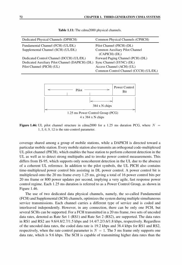
72 CHAPTER 1. THIRD-GENERATION CDMA SYSTEMS
Table 1.11: The cdma2000 physical channels.
Dedicated Physical Channels (DPHCH) Common Physical Channels (CPHCH)
Fundamental Channel (FCH) (UL/DL) Pilot Channel (PICH) (DL)Supplemental Channel (SCH) (UL/DL) Common Auxiliary Pilot Channel
(CAPICH) (DL)Dedicated Control Channel (DCCH) (UL/DL) Forward Paging Channel (PCH) (DL)Dedicated Auxiliary Pilot Channel (DAPICH) (DL) Sync Channel (SYNC) (DL)Pilot Channel (PICH) (UL) Access Channel (ACH) (UL)
Common Control Channel (CCCH) (UL/DL)
PilotPower Control
Bit
1.25 ms Power Control Group (PCG)
384 x N chips
4 x 384 x N chips
Figure 1.46: UL pilot channel structure in cdma2000 for a 1.25 ms duration PCG, where N =1, 3, 6, 9, 12 is the rate-control parameter.
coverage shared among a group of mobile stations, while a DAPICH is directed toward aparticular mobile station. Every mobile station also transmits an orthogonal code-multiplexedUL pilot channel (PICH), which enables the base station to perform coherent detection in theUL as well as to detect strong multipaths and to invoke power control measurements. Thisdiffers from IS-95, which supports only noncoherent detection in the UL due to the absenceof a coherent UL reference. In addition to the pilot symbols, the UL PICH also containstime-multiplexed power control bits assisting in DL power control. A power control bit ismultiplexed onto the 20 ms frame every 1.25 ms, giving a total of 16 power control bits per20 ms frame or 800 power updates per second, implying a very agile, fast response powercontrol regime. Each 1.25 ms duration is referred to as a Power Control Group, as shown inFigure 1.46.
The use of two dedicated data physical channels, namely, the so-called Fundamental(FCH) and Supplemental (SCH) channels, optimizes the system during multiple simultaneousservice transmissions. Each channel carries a different type of service and is coded andinterleaved independently. However, in any connection, there can be only one FCH, butseveral SCHs can be supported. For a FCH transmitted in a 20 ms frame, two sets of uncodeddata rates, denoted as Rate Set 1 (RS1) and Rate Set 2 (RS2), are supported. The data ratesin RS1 and RS2 are 9.6/4.8/2.7/1.5 kbps and 14.4/7.2/3.6/1.8 kbps, respectively. Regardlessof the uncoded data rates, the coded data rate is 19.2 kbps and 38.4 kbps for RS1 and RS2,respectively, when the rate-control parameter is N = 1. The 5 ms frame only supports onedata rate, which is 9.6 kbps. The SCH is capable of transmitting higher data rates than the

1.3. THIRD-GENERATION SYSTEMS 73
������������
������������
������
������
������
������
������
������
������������
������������
������
������
������������
������������
���������������
���������������
�������
�������
1.25 ms
20 ms
#1 #2 #16
1.25 ms
5 ms
#1 #2 #4
Guard time
Figure 1.47: The cdma2000 TDD frame structure.
FCH. The SCH supports variable data rates ranging from 1.5 kbps for N = 1 to as highas 2073.6 kbps, when N=12. Blind rate detection [154] is used for SCHs not exceeding14.4 kbps, while rate information is explicitly provided for higher data rates. The dedicatedcontrol physical channel has a fixed uncoded data rate of 9.6 kbps on both 5 ms and 20 msframes. This control channel rate is more than an order of magnitude higher than that of theIS-95 system hence it supports a substantially enhanced system control.
The Sync Channel (SYCH)—note the different acronym in comparison to the SCHabbreviation in UTRA/IMT-2000—is used to aid the initial synchronization of a mobilestation to the base station and to provide the mobile station with system-related information,including the Pseudo Noise (PN) sequence offset, which is used to identify the base stationsand the long code mask, which will be defined explicitly in Section 1.3.3.4. The SYCH hasan uncoded data rate of 1.2 kbps and a coded data rate of 4.8 kbps.
Paging functions and packet data transmission are handled by the DL Paging Channel(PCH) and the DL Common Control Channel (CCCH). The uncoded data rate of the PCHcan be either 4.8 kbps or 9.6 kbps. The CCCH is an improved version of the PCH, which cansupport additional higher data rates, such as 19.2 and 38.4 kbps. In this case, a 5 ms or 10 msframe length will be used. The PCH is included in cdma2000 in order to provide IS-95-Bfunctionality.
In TDD mode, the 20 ms and 5 ms frames are divided into 16 and 4 timeslots, respectively.This gives a duration of 1.25 ms per timeslot, as shown in Figure 1.47. A guard timeof 52.08 µs and 67.44 µs is used for the DL in multicarrier modulation and for direct-spread modulation, respectively. In the UL, the guard time is 52.08 µs. Having describedthe cdma2000 physical channels of Table 1.11, let us now consider the service multiplexingand channel-coding aspects.

74 CHAPTER 1. THIRD-GENERATION CDMA SYSTEMS
Table 1.12: The cdma2000 channel-coding parameters.
Convolutional Turbo
Rate 1/2 or 1/3 or 1/4 1/2 or 1/3 or 1/4Constraint length 9 4
1.3.3.3 Service Multiplexing and Channel Coding
Services of different data rates and different QoS requirements are carried by different physi-cal channels, namely, by the FCH and SCH of Table 1.11. This differs from UTRA and IMT-2000, whereby different services were time-multiplexed onto one or more physical channels,as highlighted in Section 1.3.2.4. These channels in cdma2000 are code-multiplexed usingWalsh codes. Two types of coding schemes are used in cdma2000, as shown in Table 1.12.Basically, all channels use convolutional codes for forward error correction. However, forSCHs at rates higher than 14.4 kbps, turbo coding [135] is preferable. The rate of the inputdata stream is matched to the given channel rate by either adjusting the coding rate orusing symbol repetition with and without symbol puncturing, or alternatively, by sequencerepetition. Tables 1.13 and 1.14 show the coding rate and the associated rate matchingprocedures for the various DL and UL physical channels, respectively, when N = 1.Following the above brief notes on the cdma2000 channel coding and service multiplexingissues, let us now turn to the spreading and modulation processes.
1.3.3.4 Spreading and Modulation
There are generally three layers of spreading in cdma2000, as shown in Table 1.15. Eachuser’s UL signal is identified by different offsets of a long code, a procedure that is similarto that of the IS-95 system portrayed in [155]. As seen in Table 1.15, this long code is an m-sequence with a period of 242 − 1 chips. The construction of m-sequences was highlightedby proakis [5]. Different user offsets are obtained using a long code mask. Orthogonalitybetween the different physical channels of the same user belonging to the same connection inthe UL is maintained by spreading using Walsh codes.
In contrast to the IS-95 DL of Figure 1.42 of [155], whereby Walsh code spreading isperformed prior to QPSK modulation, the data in cdma2000 is first QPSK modulated beforespreading the resultant I and Q branches with the same Walsh code. In this way, the numberof Walsh codes available is increased twofold due to the orthogonality of the I and Q carriers.The length of the UL/DL channelization Walsh codes of Table 1.15 varies according to thedata rates. All the base stations in the system are distinguished by different offsets of thesame complex DL m-sequence, as indicated by Table 1.15. This DL m-sequence code isthe same as that used in IS-95, which has a period of 215 = 32768, and it is derived fromm-sequences. The feedback polynomials of the shift registers for the I and Q sequences areX15 + X13 + X9 + X8 + X7 + X5 + 1 and X15 + X12 + X11 + X10 + X6 + X5 +X4 + X3 + 1, respectively. The offset of these codes must satisfy a minimum value, whichis equal to N × 64×Pilot Inc, where Pilot Inc is a code reuse parameter, which depends on

1.3. THIRD-GENERATION SYSTEMS 75
Table 1.13: The cdma2000 DL physical channel (see Table 1.11) coding parameters for N = 1, whererepetition × 2 implies transmitting a total of two copies.
rateData
Physicalchannel
Conv/TurboEncoder
Code rateRepetition Puncturing
Channelrate
Physical Data Rate Channel RateChannel (kbps) Code Rate Repetition Puncturing (ksps)
SYCH 1.2 1/2 ×2 0 4.8PCH 4.8 1/2 ×2 0 19.2
9.6 1/2 ×1 0 19.2CCCH 9.6 1/2 ×1 0 19.2
19.2 1/2 ×1 0 38.438.4 1/2 ×1 0 76.8
FCH 1.5 1/2 ×8 1 of 5 19.22.7 1/2 ×4 1 of 9 19.24.8 1/2 ×2 0 19.29.6 1/2 ×1 0 19.21.8 1/3 ×8 1 of 9 38.43.6 1/3 ×4 1 of 9 38.47.2 1/3 ×2 1 of 9 38.4
14.4 1/3 ×1 1 of 9 38.4SCH 9.6 1/2 ×1 0 19.2
19.2 1/2 ×1 0 38.438.4 1/2 ×1 0 76.876.8 1/2 ×1 0 153.6
153.6 1/2 ×1 0 307.2307.2 1/2 ×1 0 614.414.4 1/3 ×1 1 of 9 38.428.8 1/3 ×1 1 of 9 76.857.6 1/3 ×1 1 of 9 153.6
115.2 1/3 ×1 1 of 9 307.2230.4 1/3 ×1 1 of 9 614.4
DCCH 9.6 1/2 ×1 0 19.2
the topology of the system, analogously to the frequency reuse factor in FDMA. Let us nowfocus on DL spreading issues more closely.
1.3.3.4.1 Downlink Spreading and Modulation. Figure 1.48 shows the structure of aDL transmitter for a physical channel. In contrast to the IS-95 DL transmitter shown in [155],the data in the cdma2000 DL transmitter shown in Figure 1.48 are first QPSK modulatedbefore spreading using Walsh codes. As a result, the number of Walsh codes available isincreased twofold due to the orthogonality of the I and Q carriers, as mentioned previously.

76 CHAPTER 1. THIRD-GENERATION CDMA SYSTEMS
Table 1.14: The cdma2000 UL physical channel (see Table 1.11) coding parameters for N = 1, whererepetition × 2 implies transmitting a total of two copies.
Conv/TurboEncoder
Code rate
Datarate
Repetition 1 Puncturing Interleaver Repetition 2
Channelrate
Physical Data Rate Code Repetition Repetition Channel RateChannel (kbps) Rate 1 Puncturing 2 (ksps)
CCCH 19.2 1/4 ×1 0 ×4 307.238.4 1/4 ×1 0 ×2 307.2
FCH 1.5 1/4 ×8 1 of 5 ×8 307.22.7 1/4 ×4 1 of 9 ×8 307.24.8 1/4 ×2 0 ×8 307.29.6 1/4 ×1 0 ×8 307.21.8 1/4 ×16 1 of 3 ×4 307.23.6 1/4 ×8 1 of 3 ×4 307.27.2 1/4 ×4 1 of 3 ×4 307.2
14.4 1/4 ×2 1 of 3 ×4 307.2SCH 9.6 1/4 ×1 0 ×16 614.4
19.2 1/4 ×1 0 ×8 614.438.4 1/4 ×1 0 ×4 614.476.8 1/4 ×1 0 ×2 614.4
153.6 1/4 ×1 0 ×1 614.4307.2 1/2 ×1 0 ×1 614.4
ACH 4.8 1/4 ×1 0 ×8 307.29.6 1/4 ×1 0 ×4 307.2
DCCH 9.6 1/4 ×1 0 ×4 307.2
The user data is first scrambled by the long scrambling code by assigning a different offset todifferent users for the purpose of improving user privacy, which is then mapped to the I andQ channels. This long, scrambling code is identical to the UL user-specific scrambling codegiven in Table 1.15. The DL pilot channels of Table 1.11 (PICH, CAPICH, DAPICH) and theSYNC channel are not scrambled with a long code since there is no need for user-specificity.The UL power control symbols are inserted into the FCH at a rate of 80 Hz, as shown inFigure 1.48. The I and Q channels are then spread using a Walsh code and complex multipliedwith the cell-specific complex PN sequence of Table 1.15, as portrayed in Figure 1.48. Eachbase station’s DL channel is assigned a different Walsh code in order to eliminate any intra-cell interference since all Walsh codes transmitted by the serving base station are receivedsynchronously. The length of the DL channelization Walsh code of Table 1.15 is determinedby the type of physical channel and its data rate. Typically for N = 1, DL FCHs with datarates belonging to RS1, that is, those transmitting at 9.6/4.8/2.7/1.5 kbps, use a 128-chipWalsh code, and those in RS2, transmitting at 14.4/7.2/3.6/1.8 kbps, use a 64-chip Walshcode. Walsh codes for DL SCHs can range from 4-chip to 128-chip Walsh codes. The DL

1.3. THIRD-GENERATION SYSTEMS 77
Table 1.15: Spreading parameters in cdma2000.
Channelization User-specific Cell-specificCodes (UL/DL) Scrambling Codes (UL) Scrambling Codes (DL)
Type of codes Walsh codes Different offsets of Different offsets ofa real m-sequence a complex m-sequence
Code length Variable 242 − 1 chips 215 chips
Type of BPSK BPSK QPSKSpreading
Data DL : QPSKModulation UL : BPSK
scrambling code
Data S P
Power ControlSymbol
Power ControlSymbol
Complex
Multiply
Complex
Insertion
Insertion
ChannelisationWalsh code
cell-specificscrambling code
Long
I
Qp(t)
p(t)
cos wct
− sin wct
Figure 1.48: The cdma2000 DL transmitter. The long scrambling code is used for the purpose ofimproving user privacy. Hence, only the paging channels and the traffic channels arescrambled with the long code. The common pilot channel and the SYNC channel arenot scrambled by this long code (the terminology of Table 1.15 is used).
PICH is an unmodulated sequence (all 0 s) spread by Walsh code 0. Finally, the complexspread data in Figure 1.48 are baseband filtered using the Nyquist filter impulse responsesp(t) in Figure 1.48 and modulated on a carrier frequency.
For the case of multicarrier modulation, the data is split into N branches immediatelyafter the long code scrambling of Figure 1.48 which was omitted in the figure for the sakeof simplicity. Each of the N branches is then treated as a separate transmitter and modulatedusing different carrier frequencies.
1.3.3.4.2 Uplink Spreading and Modulation. The UL cdma2000 transmitter is shownin Figure 1.49. The UL PICH and DCCH of Table 1.11 are mapped to the I data channel,while the UL FCH and SCH of Table 1.11 are mapped to the Q channel in Figure 1.49.Each of these UL physical channels belonging to the same user is assigned different Walshchannelization codes in order to maintain orthogonality, with higher rate channels usingshorter Walsh codes. The I and Q data channels are then spread by complex multiplication

78 CHAPTER 1. THIRD-GENERATION CDMA SYSTEMS
Channel
Walsh Code
Walsh Code
Fundamental
SupplementalChannel
ChannelPilot
Walsh Code
ControlChannel
Dedicated
Walsh Code
ComplexMultiply
scrambling codeUser-specific
I
Q
scrambling codeComplex
p(t)
p(t)
cos wct
− sin wct
Figure 1.49: The cdma2000 UL transmitter. The complex scrambling code is identical to the DL cell-specific complex scrambling code of Table 1.15 used by all the base stations in the system(the terminology of Table 1.15 is used).
with the user-specifically offset real m-sequence based scrambling code of Table 1.15 and acomplex scrambling code, which is the same for all the mobile stations in the system, as seenat the top of Figure 1.49. However, this latter complex scrambling code is not explicitly shownin Table 1.15, since it is identical to the DL cell-specific scrambling code. This complexscrambling code is only used for the purpose of quadrature spreading. Thus, in order to reducethe complexity of the base station receiver, this complex scrambling code is identical to thecell-specific scrambling code of Table 1.15 used on the DL by all the base stations.

1.3. THIRD-GENERATION SYSTEMS 79
Subattempt(BS1)
Subattempt Subattempt(BS2) (BSn)
Access Attempt
Access Probe
Time
Power
Figure 1.50: An access attempt by a mobile station in cdma2000 using the access probe of Figure 1.51.
AccessPreamble
Access ChannelMessage Capsule
Pilot Channel (PICH)
Access Channel (ACH)
Power
Figure 1.51: A cdma2000 access probe transmitted using the regime of Figure 1.50.
1.3.3.5 Random Access
The mobile station initiates an access request to the network by repeatedly transmitting aso-called access probe until a request acknowledgement is received. This entire process ofsending a request is known as an access attempt. Within a single access attempt, the requestmay be sent to several base stations. An access attempt addressed to a specific base station isknown as a subattempt. Within a subattempt, several access probes with increasing power canbe sent. Figure 1.50 shows an example of an access attempt. The access probe transmissionfollows the slotted ALOHA algorithm, which is a relative of PRMA. An access probe canbe divided into two parts, as shown in Figure 1.51. The access preamble carries a nondata-bearing pilot channel at an increased power level. The so-called access channel messagecapsule carries the data-bearing Access Channel (ACH) or UL Common Control Channel(CCCH) messages of Table 1.11 and the associated nondata-bearing pilot channel. Thestructure of the pilot channel is similar to that of the UL pilot channel (PICH) of Figure 1.46except that in this case there are no time-multiplexed power control bits. The preamble length

80 CHAPTER 1. THIRD-GENERATION CDMA SYSTEMS
Complex
Multiply
ChannelPilot
(PICH)
ChannelAccess
(ACH)
Walsh code
Walsh code
Baseband
Baseband
scrambling codeACH-specific
scrambling code
Filter
Filter
Complex
p(t)
p(t)
coswct
sin wct
Figure 1.52: The cdma2000 access channel modulation and spreading. The complex scrambling codeis identical to the DL cell-specific complex scrambling code of Table 1.15 used by all thebase stations in the system (the terminology of Table 1.15 is used).
in Figure 1.51 is an integer multiple of the 1.25 ms slot intervals. The specific access preamblelength is indicated by the base station, which depends on how fast the base station can searchthe PN code space in order to recognize an access attempt. The ACH is transmitted at a fixedrate of either 9.6 or 4.8 kbps, as seen in Table 1.14. This rate is constant for the duration of theaccess probe of Figure 1.50. The ACH or CCCH and their associated pilot channel are spreadby the spreading codes of Table 1.15, as shown in Figure 1.52. Different ACHs or CCCHsand their associated pilot channels are spread by different long codes.
The access probes of Figures 1.50 and 1.51 are transmitted in predefined slots, wherethe slot length is indicated by the base station. Each slot is sufficiently long in orderto accommodate the preamble and the longest message of Figure 1.51. The transmissionmust begin at the start of each 1.25 ms slot. If an acknowledgement of the most recentlytransmitted probe is not received by the mobile station after a time-out period, another probeis transmitted in another randomly chosen slot, obeying the regime of Figure 1.50.
Within a subattempt of Figure 1.50, a sequence of access probes is transmitted untilan acknowledgement is received from the base station. Each successive access probe istransmitted at a higher power compared to the previous access probe, as shown in Figure 1.53.The initial power (IP) of the first probe is determined by the open-loop power control plus anominal offset power that corrects for the open-loop power control imbalance between ULand DL. Subsequent probes are transmitted at a power level higher than the previous probe.

1.3. THIRD-GENERATION SYSTEMS 81
PI
IP
PI
Time
IP : Initial power
PI : Power increment
Access probes
Figure 1.53: Access probes within a subattempt of Figure 1.50.
This increased level is indicated by the Power Increment (PI). Let us now highlight some ofthe cdma2000 handover issues.
1.3.3.6 Handover
Intra-frequency or soft-handover is initiated by the mobile station. While communicating, themobile station may receive the same signal from several base stations. These base stationsconstitute the Active Set of the mobile station. The mobile station will continuously monitorthe power level of the received pilot channels (PICH) transmitted from neighboring basestations, including those from the mobile station’s active set. The power levels of these basestations are then compared to a set of thresholds according to an algorithm, which will behighlighted later in this chapter. The set of thresholds consists of the static thresholds, whichare maintained at a fixed level, and the dynamic thresholds, which are dynamically adjustedbased on the total received power. Subsequently, the mobile station will inform the networkwhen any of the monitored power levels exceed the thresholds.
Whenever the mobile station detects a PICH, whose power level exceeds a given staticthreshold, denoted as T1, this PICH will be moved to a candidate set and will be searchedand compared more frequently against a dynamically adjusted threshold denoted as T2. Thisvalue of T2 is a function of the received power levels of the PICHs of the base stations in theactive set. This process will determine whether the candidate base station is worth adding tothe active set. If the overall power level in the active set is weak, then adding a base stationof higher power will improve the reception. By contrast, if the overall power level in theactive set is relatively high, then adding another high-powered base station may not only beunnecessary, but may actually utilize more network resources.
For the base stations that are already in the active set, the power level of theircorresponding PICH is compared to a dynamically adjusted threshold, denoted as T3, which isalso a function of the total power of the PICH in the active set, similar to T2. This is to ensurethat each base station in the active set is contributing sufficiently to the overall power level.If any of the PICH’s power level dropped below T3 after a specified period of time allowed

82 CHAPTER 1. THIRD-GENERATION CDMA SYSTEMS
ChannelPhysical
Data
Antenna 1
Antenna 2b0
b0
b0
b1
b1
b2
b2
b3
b3
b3
−b1−b2
Figure 1.54: Transmission of a physical channel using Space Time block coding Transmit Diversity(STTD).
in order to eliminate any uncertainties due to fading which may have caused fluctuations inthe power level, the base station will again be moved to the candidate set where it will becompared with a static threshold T4. At the same time, the mobile station will report to thenetwork the identity of the low-powered base station in order to allow the correspondingbase station to increase its transmit power. If the power level decreases further below a staticthreshold, denoted as T4, then the mobile station will again report this to the network and thebase station will subsequently be dropped from the candidate set.
Inter-frequency or hard-handovers can be supported between cells having different carrierfrequencies. Here we conclude our discussions on the cdma2000 features and provide somerudimentary notes on a number of advanced techniques, which can be invoked in order toimprove the performance of the 3G W-CDMA systems.
1.3.4 Performance-enhancement Features
The treatment of adaptive antennas, multi-user detection, interference cancellation, or theportrayal of transmit diversity techniques is beyond the scope of this chapter. Here we simplyprovide a few pointers to the associated literature.
1.3.4.1 Downlink Transmit Diversity Techniques
1.3.4.1.1 Space Time Block Coding-based Transmit Diversity. Further diversity gaincan be provided for the mobile stations by upgrading the base station with the aid of SpaceTime block coding assisted Transmit Diversity (STTD) [146], which can be applied to all theDL physical channels with the exception of the SCH. Typically the data of physical channelsare encoded and transmitted using two antennas, as shown in Figure 1.54.
1.3.4.1.2 Time-switched Transmit Diversity. Time-Switched Transmit Diversity(TSTD) [156] is only applicable to the SCH, and its operation becomes explicit in Figure 1.55.
1.3.4.1.3 Closed-loop Transmit Diversity. Closed-loop transmit diversity is only appli-cable to the DPCH and PDSCH messages of Table 1.5 on the DL, which is illustratedin Figure 1.56. The weights w1 and w2 are related to the DL channel’s estimated phaseand attenuation information, which are determined and transmitted by the MS to the BSusing the FBI D field, as portrayed in Figure 1.20. The weights for each antenna are

1.3. THIRD-GENERATION SYSTEMS 83
BCH
BCH
BCH
BCH
One time slot (2/3 ms)
Antenna 1
Antenna 2
Time slot #1 Time slot #2
One P-CCPCH radio frame (10 ms)
Time slot #15
BCH : Broadcast CHannelP-CCPCH : Primary Common Control Physical CHannel
BCH
BCHacp
acp
acp
ac1i
ac2i
ac15i
cp : Primary Synchronization Codecj
i , i = 1, . . . , 16; j = 1, . . . , 15 : Secondary Synchronization Code
Figure 1.55: Frame structure of the UTRA DL synchronization channel (SCH), transmitted by a TSTDscheme. The primary and secondary SCH are transmitted alternatively from Antennas 1and 2. The parameter a is a binary flag used to indicate the presence (a = +1) or absence(a = −1) of STTD encoding in the P-CCPCH.
from UL DPCCHDecode FBI
DPCH(from the outputof Figure 1.17)
CPICH1
CPICH2
Determineweights
Antenna 1
Antenna 2
DPCH : Dedicated Physical CHannel
CPICH : Common PIlot CHannelFBI : FeedBack Information
w1
w1
w2 w2
Figure 1.56: Transmission of the DL DPCH using a closed-loop transmit diversity technique.

84 CHAPTER 1. THIRD-GENERATION CDMA SYSTEMS
independently measured by the MS using the corresponding pilot channels CPICH1 andCPICH2.
1.3.4.2 Adaptive Antennas
The transmission of time-multiplexed user-specific pilot symbols on both the UL andDL as seen for UTRA in Figures 1.20–1.24 facilitates the employment of adaptive an-tennas. Adaptive antennas are known to enhance the capacity and coverage of thesystem [157, 158].
1.3.4.3 Multi-user Detection/Interference Cancellation
Following Verdu’s seminal paper [93], extensive research has shown that Multi-user Detec-tion (MUD) [92, 95, 159–164] and Interference Cancellation techniques [91, 165–175] cansubstantially improve the performance of the CDMA link in comparison to conventionalRake receivers. However, using long scrambling codes increases the complexity of theMUD [58]. As a result, UTRA introduced an optional short scrambling code, namely, theS(2) code of Table 1.9, as mentioned in Section 1.3.2.6.4, in order to reduce the complexity ofMUD [118]. Another powerful technique is invoking burst-by-burst adaptive CDMA [96,132]in conjunction with MUD.
However, interference cancellation and MUD schemes require accurate channel estima-tion, in order to reproduce and deduct or cancel the interference. Several stages of cancellationare required in order to achieve a good performance, which in turn increases the canceller’scomplexity. It was shown that recursive channel estimation in a multistage interferencecanceller improved the accuracy of the channel estimation and hence gave improved BERperformance [111].
Because of the complexity of the multi-user or interference canceller detectors, they wereoriginally proposed for the UL. However, recently reduced-complexity DL MUD techniqueshave also been proposed [176].
1.3.5 Summary of 3G Systems
We have presented an overview of the terrestrial radio transmission technology of 3Gmobile radio systems proposed by ETSI, ARIB, and TIA. All three proposed systems arebased on Wideband-CDMA. Despite the call for a common global standard, there are somedifferences in the proposed technologies, notably, the chip rates and inter-cell operation.These differences are partly due to the existing 2G infrastructure already in use all over theworld, and are specifically due to the heritage of the GSM and the IS-95 systems. Huge capitalhas been invested in these current 2G mobile radio systems. Therefore, the respective regionalstandard bodies have endeavored to ensure that the 3G systems are compatible with the 2Gsystems. Because of the diversified nature of these 2G mobile radio systems, it is not aneasy task to reach a common 3G standard that can maintain perfect backwards compatibility.Non-coherent M -ary orthogonal CDMA is described in the next chapter.

1.4. SUMMARY AND CONCLUSIONS 85
1.4 Summary and Conclusions
Following the rudimentary introduction of Sections 1.1–1.2.6, Section 1.3 reviewed the 3GWB-CDMA standard proposals. The 3G systems are more amenable to the transmission ofinteractive video signals than their more rigid 2G counterparts. This is due partly to the highersupported bit rate and partly to the higher variety of available transmission integrities and bitrates. During our further discourse we will rely on this chapter and quantify the networkperformance of various joint-detection-based CDMA systems.

Chapter 2High Speed Downlink and UplinkPacket Access
T-H. Liew and L. Hanzo
2.1 Introduction
The work on the standardization of third-generation (3G) mobile communication systemscommenced in the early 1990s. In 1997, the choice of Wideband Code Division MultipleAccess (WCDMA) was ratified by the different regions of the globe as the core technologyof 3G systems. However, numerous regional versions of WCDMA emerged and in order toavert the risk of arriving at incompatible solutions, a collaboration agreement was establishedin December 1998 in order to form the 3rd Generation Partnership Project (3GPP). The 3GPPbrings together the following regional telecommunications standardization bodies:
• Association of Radio Industries and Businesses (ARIB) from Japan;
• China Communications Standards Association (CCSA) from China;
• European Telecommunications Standard Institute (ETSI) from Europe;
• Alliances for Telecommunications Industry Solutions (ATIS) from the USA;
• Telecommunications Technology Association (TTA) from South Korea;
• Telecommunication Technology Committee (TTC) from Japan.
At the end of 1999, the 3GPP research activities reached a major milestone with thepublication of WCDMA Release 99. The maximum theoretical DL speed is 936 Kbps [177]for a single physical channel and 2.3 Mbps, if three physical channels are multiplexed.In contrast, the maximum UL speed is 480 Kbps [177] for a single physical channel and2.3 Mbps, provided that six physical channels are multiplexed.
3G, HSPA and FDD versus TDD Networking Second EditionL. Hanzo, J. S. Blogh and S. Ni c© 2008 John Wiley & Sons, Ltd

88 CHAPTER 2. HIGH SPEED DOWNLINK AND UPLINK PACKET ACCESS
Figure 2.1: HSDPA physical channels.
Unfortunately, the bitrate offered by the WCDMA Release 99 specifications does notsatisfy the requirements of seamless wireless Internet services and file download, forexample. Therefore, the quest for higher bitrates has initiated the formation of a new 3GPPworking group in 2000. A year later, this resulted in the standardization of the High SpeedDownlink Packet Access (HSDPA) mode of the 3G systems in Release 5 of the 3GPP. Thisevolution to the HSDPA mode has increased the maximum DL speed to 13.976 Mbps. AsHSDPA only improves the throughput of the DL, there is a demand for improving theUL throughput as well. Hence, another 3GPP working group was started in 2002. It tookabout one and half years to release the standardization of High Speed Uplink Packet Access(HSUPA) in Release 6 of 3GPP, which increased the maximum UL speed to 5.742 Mbps.
2.2 High Speed Downlink Packet Access
Three powerful techniques have been employed in HSDPA in order to increase the achievablethroughput, namely:
• adaptive modulation, multiple spreading codes and variable rate channel coding;
• Hybrid Automatic Repeat Request (HARQ) techniques;
• fast packet scheduling.
Let us highlight how these techniques may be used to improve the attainable DL throughput.When a HSDPA-enabled User Equipment (UE), i.e. the Mobile Station (MS) shown inFigures 2.1 and 2.2 is switched on, it registers itself with the network. When the UE

2.2. HIGH SPEED DOWNLINK PACKET ACCESS 89
Figure 2.2: HSDPA time diagram.
starts an application, such as file downloading for example, which requires a high DLbandwidth, the protocol initiates HSDPA transmission invoking the protocol handshake seenin Figure 2.2. Then the UE estimates the DL Signal-to-Interference Ratio (SIR) encounteredby the reference channel’s Common Pilot Channel (CPICH) transmitted from Node B.Node B is the term used in the 3G systems for the Base Station (BS). The resultant DL SIRmeasurements are mapped to the so-called Channel Quality Indicator (CQI) value, whichhas a range spanning from 0 to 30. The DL CQI value is then transmitted in the UL controlchannel referred to as the High Speed Dedicated Physical Control Channel (HS-DPCCH) toNode B, as shown in Figures 2.1 and 2.2, in order to inform the BS about the MS’s channelwhich determines the achievable bitrate of the BS’s transmission. More explicitly, basedon the CQI value received from the UE, Node B determines the transport block size to betransmitted to the UE in the DL data channel termed as the High Speed Physical DownlinkShared Channel (HS-PDSCH).1 Table 2.1 is reproduced from [178] and it shows the CQImapping table used by Node B for UE category 10. The UE category is further detailed at
1The terminology of “shared” is used, because in the DL the BS is capable of serving numerous UEs by sharinga single channel amongst them, which in the UL a dedicated channel has to be used in order to avoid the potentiallyexcessive complexity UL scheduling and synchronization of all of the UEs.

90 CHAPTER 2. HIGH SPEED DOWNLINK AND UPLINK PACKET ACCESS
Table 2.1: CQI mapping table for UE category 10 (see [178]).
CQI Transport Number of Modulation Coding Throughputvalue block size multicodes scheme rate (Mbps)
0 NA Out of range1 137 1 QPSK 0.14 0.0692 173 1 QPSK 0.18 0.087...
......
......
...7 650 2 QPSK 0.24 0.325...
......
......
...10 1262 3 QPSK 0.44 0.631...
......
......
...13 2279 4 QPSK 0.59 1.14014 2583 4 QPSK 0.67 1.29215 3319 5 QPSK 0.69 1.66016 3565 5 16QAM 0.37 1.783...
......
......
...22 7168 5 16QAM 0.75 3.58423 9719 7 16QAM 0.72 4.86024 11 418 8 16QAM 0.74 5.70925 14 411 10 16QAM 0.76 7.20626 17 237 12 16QAM 0.75 8.61927 21 754 15 16QAM 0.76 10.877...
......
......
...30 25 558 15 16QAM 0.89 12.779
a later stage in this section. It is shown in Table 2.1 that logically a larger transport blocksize is used when the CQI value is higher, i.e. a higher channel SIR is encountered. Onthe other hand, a smaller transport block size is employed when the CQI signals a low SIRin order to activate more robust modulation and coding modes and hence avoid inflictinga huge number of errors. In order to accommodate diverse transport block sizes spanningfrom 137 to 27 952 bits [179], according to the wide range of SIRs encountered, the numberof HS-PDSCH spreading codes transmitted in parallel varies from 1 to 15. Furthermore,Adaptive Modulation and Coding (AMC) is used, where both QPSK and 16QAM schemesare employed in conjunction with various channel coding rates.
Note that Table 2.1 shows the CQI mapping table for UE category 10. Depending on theUE’s specific capabilities, they are grouped in 12 different HSDPA-enabled UE categories.These categories are listed in the 3GPP standard [180] and are reproduced in Table 2.2. It isshown in Table 2.2 that the UE category 10 is potentially capable of supporting a transportblock size as high as 27 952 bits, when employing 15 parallel spreading codes and 16QAM,which is equivalent to the HSDPA mode’s maximum DL speed of 13.976 Mbps. Table 2.1shows that the UE is operating close to its limit when the CQI value is 30. The second to last

2.2. HIGH SPEED DOWNLINK PACKET ACCESS 91
Table 2.2: HSDPA enabled UE categories (see [180]).
Maximum Maximum Highest order Total numberUE transport number of modulation of soft Throughput
category block size multicodes scheme channel bits (Mbps)
1 7298 5 16QAM 19 200 3.6492 7298 5 16QAM 28 800 3.6493 7298 5 16QAM 28 800 3.6494 7298 5 16QAM 38 400 3.6495 7298 5 16QAM 57 600 3.6496 7298 5 16QAM 67 200 3.6497 14 411 10 16QAM 115 200 7.2068 14 411 10 16QAM 134 400 7.2069 20 251 15 16QAM 172 800 10.126
10 27 952 15 16QAM 172 800 13.97611 3630 5 QPSK 14 400 1.81512 3630 5 QPSK 28 800 1.815
column of Table 2.2 shows the total memory space in the UE and its purpose is explainedduring our further discourse in Section 2.2.1.1.
The error-free reception of the control information transport block conveying the specificmodulation scheme activated by the BS for its DL transmission, the number of spreadingcodes and other transmission-rate related parameters are essential for successfully decodingthe HS-PDSCH by the HSDPA-enabled UEs. The corresponding side-information is alsomasked with the identity of the destination UE, which is a unique UE identity used forexclusively informing the UE of the specific parameters to be used for decoding the transportblock. This side-information is then signaled to the UE with the aid of the High Speed SharedControl Channel (HS-SCCH), as shown in Figures 2.1 and 2.2. The HSDPA-enabled UE isconfigured to simultaneously monitor up to four HS-SCCHs, but only one of them shall carrythe required control information masked with its UE identity. Using the received DL controlinformation decoded from the HS-SCCH, the UE has to appropriately configure itself in orderto decode the HS-PDSCH’s message. As shown in Figure 2.2, Cyclic Redundancy Checking(CRC) is performed at the end of each decoding process in order to ascertain that the data inHS-PDSCH was received error free. Depending on the result of the CRC, the UE shall informNode B as to whether the packet has been received successfully or not. It does so by sendinga positive Acknowledgement (ACK) or a Negative Acknowledgement (NACK) UL messagealong with the associated CQI value in the HS-PDSCH shown in Figure 2.2.
Based on the UL Hybrid Automatic Repeat Request (HARQ) result received on the HS-PDSCH, the BS shall activate the HARQ procedure, as follows. It transmits a new DL packet,if the UL ACK message was received and it performs a DL packet retransmission whenthe UL NACK message is received. When a DL packet retransmission was requested, twodifferent HARQ techniques may be activated. The first entails the identical DL retransmissionof the corrupted message, where the same systematic and parity bits are retransmitted in theirentirety. At the UE, the received soft decision bits of the previous and current replicas of

92 CHAPTER 2. HIGH SPEED DOWNLINK AND UPLINK PACKET ACCESS
the message shall be added together. This technique is referred to as Chase [181] or soft-combining. Naturally, this technique improves the reliability of the soft decision based bitvalues input to the turbo decoder and hence increases the probability of successful decoding.
The second HARQ technique invokes a more intelligent, non-identical retransmissiontechnique, where incremental or additional redundancy is transmitted. This may take theform of initially transmitting only a low number of parity bits of a high-rate punctured code.Then, in the event of receiving corrupted bits and hence failing the CRC test, the previouslyunsent bits of a punctured mother code will be transmitted. Depending on the availabilityof unused DL payload transmission capability, the same original systematic information bitsmay be transmitted as well. At the UE, the original systematic information bits are soft-combined with those received during the previous transmission and the extra parity bits areused along with the parity bits of the previous transmission. Given the extra redundancy, theturbo decoder would have a better chance of successfully decoding the error-infested packet.This technique requires extra memory space at the UE to store the extra parity bits receivedduring the retransmissions. As shown in the last column of Table 2.2, different UE categorieshave different amounts of memory space for incremental redundancy decoding and Node Bmust take the UE’s memory into consideration when performing DL packet retransmissionsusing this technique.
In the DL Dedicated Physical Channel (DPCH) of release 99 of the 3GPP standard thechannel capacity resource allocation remains fixed, once it has been set up. The bandwidthassigned is occupied by a UE, even if it is not transmitting at the maximum allocated bitrate. Changing the maximum allocated bit rate involves tearing down the existing DPCH andsetting up a new DPCH with the new bit rate and this takes time. In contrast to the Release99 DL DPCH, the HSDPA system has the beneficial feature of dynamic resource allocation,which enables fast packet scheduling. In a typical scenario, Node B might be serving severalHSDPA enabled UEs. Since the UEs are independent of each other, their reported CQI valueprofiles are different and their maximum tolerable bit rates may also be different, dependingon the services they support. By exploiting this information, Node B might allocate the entireDL bandwidth required for transmitting 15 HS-PDSCH spreading codes to a particular UE,when its reported DL CQI value is high, provided that the corresponding DL transmit bufferis not empty, i.e. there are a lot of data packets to be delivered to the UE. When the DLCQI value reported by the UE to the BS is low or the DL data packet buffer has been“flushed”, Discontinuous Transmission (DTX) is activated for the UE. The benefit of thisDTX mode is that the carrier is disabled during the instances of having an empty DL buffer,which mitigates the interference imposed. When no data is found in the transmit buffer, theassociated bandwidth is reallocated to other UEs. The prompt scheduling of packets for DLtransmission is facilitated by having a short Transmission Time Interval (TTI) of only threeslot durations, corresponding to 2 ms which results in five subframes in Figure 2.3. The 3GPPradio frame of Figure 2.3 has 15 timeslots, which span over a frame duration of 10 ms.
2.2.1 Physical Layer
As discussed in the previous section and portrayed in Figure 2.1, the HSDPA uses the HS-PDSCH and HS-SCCH physical channels in the DL and HS-DPCCH in the UL. Again,Figure 2.3 shows the timing diagram of the HSDPA physical channels with respect to thePrimary Common Control Physical Channel (P-CCPCH), which is the DL broadcast channel

2.2. HIGH SPEED DOWNLINK PACKET ACCESS 93
Figure 2.3: Timing diagram of the HSDPA physical channels.
of Node B. It carries information such as the System Frame Number (SFN) for the UE tosynchronize with Node B. The propagation delay between Node B and the UE is assumedto be insignificant, which implies having small cell sizes since they may be expected to havesufficiently better propagation conditions for supporting a high bit rate. As an additionalmeasure, the classic timing advance control technique known from the Global System ofMobile communications known as GSM may be invoked, which allows the BS to measurethe turn-around delay of its transmitted signal, when it prompts the MS for a turn-arounddelay measurement response. The BS may then advance its transmissions by the estimated DLpropagation delay, so that its transmitted signal arrives at the MS within a significantly shorterwindow, thereby reducing the guard-time-related wastage of active information transmissiontime.
It can be seen from Figure 2.3 that the role of the five subframes is that of creating 2 msduration transmission frames for the sake of supporting low-delay delivery of delay-sensitiveinformation. The data from Layer 2 is split into blocks of various sizes, such as those shown inTable 2.1. Each block of data is then passed through the coding chain shown in Figure 2.4. Thecoded block is then mapped onto one of the HARQ processes, for example HARQ process0 of Figure 2.3. The classic Stop And Wait (SAW) method is employed, where no furthertransmission takes place during the HARQ process 0 until the corresponding ACK or NACKcontrol channel message is received from the intended UE. However, the Node B is stillallowed to transmit different block of coded data on other HARQ processes. The total numberof HARQ processes was chosen to be eight. This allows sufficient processing time in betweenthe consecutive HARQ action of the same process number for both the UE and Node B.
Figure 2.3 also shows that the required control information bearing HS-SCCH’s messageis transmitted two timeslots before the data-bearing HS-PDSCH. This gives sufficient timefor the UE to decode the necessary control information and to configure itself appropriatelyin preparation for decoding the HS-PDSCH message, namely the data. The success or failureof the HS-PDSCH decoding operation results in the UL transmission of the ACK or NACKmessage using the HS-DPCCH 5 ms after the UE has received the HS-PDSCH subframe, as

94 CHAPTER 2. HIGH SPEED DOWNLINK AND UPLINK PACKET ACCESS
seen in Figure 2.3. On the other hand, Node B has only 1.3 ms to determine, whether its nextDL transmission will have to be a new transmission packet or a retransmitted packet.
2.2.1.1 High Speed Physical Downlink Shared Channel (HS-PDSCH)
The HS-PDSCH has a subframe structure, where the transmit time interval used for fastpacket scheduling is constituted by three slots corresponding to 2 ms, as shown in Figure 2.3.In release 99 of the 3GPP standard the Dedicated Physical Data Channel (DPDCH) mayopt for using various Spreading Factors (SF), such as SF = 4, 8, 16, . . . , 256 and 512,depending on the slot format of the transmission. Naturally, increasing the SF improves thespreading gain, but proportionately reduces the maximum data rate. In contrast, the SF of HS-PDSCH is fixed to SF = 16 to avoid signaling and hence simplifying the receiver algorithm.Adaptive modulation and multicodes utilization in HS-PDSCH have already enabled varioustransmission rates. In adaptive modulation, there are two possible modulation schemes,namely QPSK and 16QAM [182]. For multicodes utilization, only the channelization codes1 to 15 are used because the channelization code 0 is reserved for the transmission ofother messages, such as the CPICH message used by the UE for SIR measurements andchannel estimation. The 15 other channelization codes can be allocated dynamically to anyUE, resulting in the transmission of different number of codes, as shown in Table 2.1 forsupporting different bit rates.
The transport channel referred to as the High Speed Downlink Shared Channel (HS-DSCH) carries the HSDPA data packets and it is mapped to the physical channel HS-PDSCHwith the aid of a single or multiple spreading codes. Its coding chain, which was extractedfrom [183] is shown in Figure 2.4. When the UE activates its continuous, i.e. non-DTX-style 2 ms TTI transmission mode mapped to the subframes of Figure 2.3, there is alwaysa HS-DSCH transport block having a variable size ranging from 137 to 27 952 bits [179],as shown in the second column of Table 2.1. During the first stage of the channel codingprocess, the CRC bits are attached to the transport block. The CRC-protected transport blockis then scrambled. Since a rate-1/3 turbo code is employed, the scrambled transport block issegmented into a number of transmission blocks of the same size, where the maximum sizeis 5114 bits. The turbo interleaver’s memory does not extend beyond this block size.
There are two rate-matching stages in the physical layer’s HARQ functionality. The taskof the first rate matching stage is to match the number of turbo encoded bits to be transmittedin the DL to the memory of the UE, which is determined by its capability or class, as definedin Table 2.2. If the UE’s available memory is higher than the number of turbo encoded bits,the first rate-matching stage should be transparent. The second rate-matching stage matchesthe number of output bits generated by the first stage to the available physical channelcapacity. The DL physical channel capacity depends on both the number of HS-PDSCHspreading codes and on the modulation scheme activated, which in turn depend on the bit raterequirement and the SIR experienced. In addition to rate matching, the second stage of theHARQ functionality seen in Figure 2.3 additionally allows the selection of both systematicand parity bits during both the first transmission attempt as well as during the subsequentretransmissions. The DL transmission of the systematic and parity bits is controlled with theaid of the so-called Redundancy Version (RV) parameters. This enables the UE to performChase combining or incremental redundancy decoding, as briefly described earlier.

2.2. HIGH SPEED DOWNLINK PACKET ACCESS 95
Figure 2.4: Coding chain for HS-DSCH [183].

96 CHAPTER 2. HIGH SPEED DOWNLINK AND UPLINK PACKET ACCESS
Following the action of the HARQ functionality, the rate-matched bits are segmented intothe required number of bit-sequences, which are then mapped to the HS-PDSCH spreadingcodes, as shown in Figure 2.4. The appropriately segmented bits are channel-interleaved over960× n bits for QPSK and 1920× n bits for 16QAM, where n is the number of multicodes.Then the channel interleaved bits are re-arranged for 16QAM modulation. There are fourpossible re-arrangements which involve bits swapping and logical values inversion. In thecase of QPSK, this functionality is transparent. Finally, as portrayed in Figure 2.4, they arethen mapped to the HS-PDSCH physical channel for transmission.
2.2.1.2 High Speed Shared Control Channel (HS-SCCH)
As seen in Figure 2.3, the control information associated with the HS-PDSCH messageis carried by the HS-SCCH. Similarly to the HS-PDSCH message, it is transmitted in asubframe, as shown in Figure 2.3. The spreading factor is fixed to SF = 128. Figure 2.5shows the coding chain for the HS-SCCH [183]. Observe from Figure 2.5 that the HS-SCCHconsists of two parts, which are encoded by two separate coding chains. This enables the UEto decode the first part without receiving the second part. Therefore the first part, which isconstituted by the first slot of the three-slot, 2 ms subframe of Figure 2.3, contains essentialinformation required for configuring the UE, which are as follows:
• first HS-PDSCH channelization code number and the number of parallel codes, xccs
(7 bits);
• modulation scheme, xms (1 bit).
The remaining two slots of the subframe constitute the second part, which contains thefollowing information:
• transport block size, xtbs (6 bits);
• HARQ process number, xhap (3 bits);
• redundancy version parameters and 16QAM constellation re-arrangement, xrv (3 bits);
• HARQ new data packet transmission indicator, xnd (1 bit).
Both of the aforementioned parts are encoded with the aid of two separate coding chains, asshown in Figure 2.5. The first part constituted by the 8-bit xccs and xms messages mappedto the first slot, is rate-1/3 convolutional encoded and rate-matched in order to fit into a slotof 40 bits. The rate-matched bits are then masked with the UE identity of the intended UE.This is because the UE can be configured to monitor up to four HS-SCCHs and masking withthe target UE’s identity xue assists the UE to detect the first part. In Section 2.4.1 a rangeof different UE identity detection algorithms will be explored. In order to assist the UE incorrectly identifying the HS-SCCH that is intended for itself, the CRC bits are attached tothe second part, before they are masked with the UE’s identity. Similarly to the first part,the CRC-protected and masked second part of Figure 2.5 is then also rate-1/3 convolutionalencoded. The resultant encoded bits are then rate-matched in order to fit them into two slotswith a total of 80 bits. Finally, both parts are mapped to the physical channel, ready fortransmission, as seen in Figure 2.5.
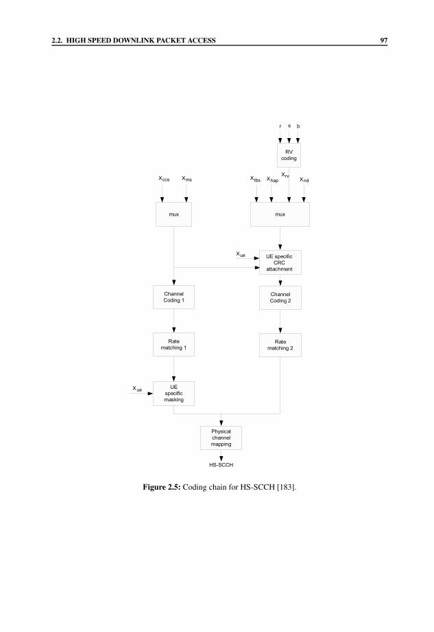
2.2. HIGH SPEED DOWNLINK PACKET ACCESS 97
msccs tbs haprv
ue
ue
nd
Figure 2.5: Coding chain for HS-SCCH [183].

98 CHAPTER 2. HIGH SPEED DOWNLINK AND UPLINK PACKET ACCESS
Figure 2.6: MAC-hs details at Node B [179].
2.2.1.3 High Speed Dedicated Physical Control Channel (HS-DPCCH)
The HARQ result of decoding success or failure indicated by the ACK or NACK messages,as well as the channel-quality related information CQI are transmitted with the aid of theHS-DPCCH in a three-slot subframe, as shown in Figure 2.3. The spreading factor is fixedto SF = 256. Similarly to the HS-SCCH, the HS-DPCCH message is also constituted bytwo parts. The single-bit HARQ result of ACK/NACK is repetitively encoded and mapped tothe first slot, which constitutes the first part of the three-slot HS-DPCCH message. The CQIvalue is protected with the aid of a short block code and the coded bits are mapped to the lasttwo slots of the HS-DPCCH subframe of Figure 2.3.
2.2.2 Medium Access Control (MAC) Layer
In order to support the HSDPA mode, the so-called high-speed functionality MAC-hs wasadded to the existing MAC layer specifications of both the UE and BS side. This functionalityis responsible for handling the data transmitted on the transport channel HS-DSCH, which isthen mapped to the physical channel HS-PDSCH. The MAC-hs functionality also managesthe physical resources allocated to HS-DSCH. Figure 2.6 was adopted from the 3GPPstandard [179] and it portrays some of the MAC-hs functionality details at Node B.
To elaborate a little further in the context of Figure 2.6, there are four MAC-hs functionalentities. The flow control is responsible for the data flow between the MAC-hs and otherentities within the MAC layer. Naturally, it is beneficial to limit the associated MAC layersignaling latency as well as to reduce the amount of discarded and retransmitted data, whichmay be imposed as a result of HS-DSCH congestion. The scheduling/priority handling seenin Figure 2.6 checks the HARQ decision of ACK/NACK received in the HS-DPCCH messageand determines whether a new transmission or a retransmission action should be authorized.

2.3. HIGH SPEED UPLINK PACKET ACCESS 99
Figure 2.7: HSUPA physical channels.
Furthermore, the scheduling/priority handling ensures that the new data packets are trans-mitted in accordance with their priority class. The role of the HARQ functionality seen inFigure 2.6 has already been made plausible and, finally, the Transport Format and ResourceCombination (TFRC) functionality selects the appropriate transport block size as well as thenumber of spreading codes used for conveying the data to be transmitted on the HS-DSCH.The corresponding inverse operations of the MAC-hs are carried out at the UE side.
2.3 High Speed Uplink Packet Access
When the standardization of the HSUPA mode commenced, the plausible choice of tech-niques to be used encompassed those, which became well-established during the HSDPAstandardization. However, not all HSDPA techniques described in Section 2.2 were adopted.The specific techniques used in HSUPA are as follows:
• multiple spreading codes and variable rate channel coding;
• HARQ;
• fast packet scheduling.

100 CHAPTER 2. HIGH SPEED DOWNLINK AND UPLINK PACKET ACCESS
Figure 2.8: HSUPA time diagram.
Adaptive modulation is not employed in the HSUPA mode, because the employment of high-order modulation schemes, such as 16QAM, increases the crest factor [184] of the UL signal,which would require a high-linearity class-A or linearized class-AB amplifier [182]. Thesehigh-linearity amplifiers typically have a low power efficiency and hence would adverselyaffect the power consumption of the UE. In addition, they typically impose an increased RFamplifier complexity, hence adding to the cost of the UE. Finally, high-order modulationschemes typically require an increased energy per bit and this drains the battery more rapidly.

2.3. HIGH SPEED UPLINK PACKET ACCESS 101
Table 2.3: HSUPA enabled UE categories (see [180]).
Maximum Minimum TTI Maximum transport blockUE number of spreading support size (Throughput in Mbps)
category multicodes factor (ms) 10 ms 2 ms
1 1 SF4 10 7110 (0.711) N/A2 2 SF4 2, 10 14484 (1.448) 2798 (1.399)3 2 SF4 10 14484 (1.448) N/A4 2 SF2 2, 10 20000 (2.000) 5772 (2.886)5 2 SF2 10 20000 (2.000) N/A6 4 SF2 2, 10 20000 (2.000) 11484 (5.742)
Let us now detail further how the standardized HSUPA techniques may be used toimprove the achievable UL throughput by considering a real-life scenario. When a HSUPAenabled UE is switched on, as shown in Figures 2.7 and 2.8, it registers itself with the network.When it is granted access to the network, it is informed of the maximum total power that itcan transmit in the UL. When the UE starts an application, such as file uploading, whichrequires a high UL bandwidth, the protocol initiates HSUPA transmission. As shown inFigure 2.8, when the UE is configured for HSUPA transmission, the UE is also granted acertain maximum transmit power budget by the serving BS for HSUPA transmission. Thisgranted power may be lower than or equal to the total transmit power limit of the UE. Giventhe amount of energy required to transmit a data bit, the employment of a larger transportblock size would inherently require a higher total transmit power. Therefore, at the beginningof each HSUPA transmission, the UE determines the maximum transport block size that it cantransmit in the UL E-DCH Dedicated Physical Data Channel (E-DPDCH) without exceedingits given “grant” and the maximum total transmit power, as shown in Figure 2.8.
The transport block size ranges from 18 bits to 20 000 bits [179]. In order to accommodatethis wide-ranging transport block size variation, the number of E-DPDCH spreading codesemployed varies from 1 to 4. In addition, various channel coding rates are employed. UnlikeHSDPA HS-PDSCH that employs adaptive modulation and fixed spreading factor of 16, E-DPDCH employs the fixed modulation scheme of BPSK, but the spreading factor varies fromSF = 2 to 256. Table 2.3 shows that there are six different HSUPA enabled UE categories, aslisted in [180]. Note that for HSUPA there are two possible TTIs having a duration of either 2or 10 ms, whereas HSDPA always employs 2 ms TTIs. Recall that the HSDPA transmissionframe structure was shown in Figure 2.3. Each TTI has its corresponding maximum transportblock size.
The error-free reception of the control information, such as the transport block size, isvital for the successful decoding of the E-DPDCH message by Node B. The related controlinformation is carried by the E-DCH Dedicated Physical Control Channel (E-DPCCH), asshown in Figures 2.7 and 2.8. Based on the CRC result of the decoded E-DPDCH, Node Bwill inform the UE whether the packet has been received successfully. The HARQ ACKor NACK message is then carried in the DL E-DCH Hybrid ARQ Indicator Channel (E-HICH). Similarly to HSDPA, the UE carries out the required HARQ procedures and activateseither the transmission of a new packet or the appropriately configured retransmission of

102 CHAPTER 2. HIGH SPEED DOWNLINK AND UPLINK PACKET ACCESS
the previous one based on the E-HICH results received from Node B. At Node B, Chasecombining or incremental redundancy decoding can then be performed in the interest ofreducing the associated BER. As seen in Figure 2.7, the neighboring or non-serving BSsmight be able to correctly decode the E-DPDCH message and hence may generate the ACKmessage in the E-HICH as well. The UE will then perform a new transmission, even thoughthe serving BS transmits NACK. This is due to the fact that an ACK message is received fromthe non-serving Node B.
Recall that in HSDPA, fast packet scheduling is achieved by having a shared HS-PDSCH, which conveys the data of all UEs. This may be readily achieved, because DL datatransmission takes place from a single Node B to many UEs. In contrast, when a single ULphysical channel is shared by many UEs, there is a lot of signaling involved in synchronizingthe data transmission of many UEs to a single Node B. Therefore, each UE has to have its owndedicated physical channel E-DPDCH. However, this poses a problem for Node B, if all UEsare transmitting their E-DPDCH at the peak rate, because the interference level experiencedat the receiver of Node B will be excessive for the data to be decoded correctly. The situationbecomes even worse when the power control algorithm starts to increase the transmit powerof a particular UE in the interest of maintaining its target BER. This transmit power-surgemay inflict increased interference upon the other UEs and hence the power control algorithmhas to increase the transmit power of the other UEs. This may result in an avalanche effect,where all UEs may eventually transmit at their full power and yet no data can be successfullydecoded at the BS.
As shown in Figure 2.8, in order to avoid the above-mentioned avalanche-like power-boosting problem at Node B and achieve prompt scheduling of packets for their transmission,Node B should limit the maximum transmit power of the UEs by issuing an “absolute grant”or power assignment to a single UE or a group of UEs. This absolute grant power level isthe same as that issued when the UE is switched on and it also limits the maximum transportblock size of E-DPDCH messages, which ultimately limits the transmit power of the UE.The absolute grant message is carried by the E-DCH Absolute Grant Channel (E-AGCH), asshown in Figures 2.7 and 2.8. Given the current grant, the UE shall generate a feedback toNode B reporting for example its buffer occupancy status and the estimated time required toclear the buffer, etc. Based on the feedback provided by the UE, Node B might issue anotherabsolute grant to the UE in order to increase or decrease its current grant. Alternatively,Node B might issue a “relative grant” command to the UE in order to increase or decreaseits current grant. The relative grant command is carried on E-DCH Relative Grant Channel(E-RGCH), as shown in Figures 2.7 and 2.8.
Occasionally, the UE’s transmit power assigned to the E-DPDCH message might imposeexcessive interference on the active links in the neighboring cell. Therefore, as shown inFigure 2.7 the neighboring or non-serving Node B might issue a power-down command inE-RGCH to the UE in order to decrease its grant. Note that the non-serving Node B is notallowed to increase the UE’s current grant.
2.3.1 Physical Layer
As described in the previous section and in Figure 2.7, the HSUPA system employs the E-AGCH, E-RGCH and E-HICH in the DL. In contrast, in the UL it employs the E-DPDPCHand E-DPCCH. Figure 2.9 shows the timing diagram of the 2 ms subframe-duration HSUPA

2.3. HIGH SPEED UPLINK PACKET ACCESS 103
Figure 2.9: Timing diagram of 2 ms TTI HSUPA physical channels.
physical channels with respect to the broadcast channel P-CCPCH of the serving Node B.The timing diagram of the P-CCPCH and HSUPA DL physical channels of the non-servingNode B is also shown in Figure 2.9. Note that the timing difference between the broadcastchannel P-CCPCH of the serving and non-serving BSs is chosen to be one slot-duration.This limits the maximum delay imposed on the non-serving Node B, within which it hasto provide the E-HICH result. For the UE, there is a minimum delay of 0.4 slots [185]between the serving BS’s P-CCPCH message and the commencement of the E-DPCCH andE-DPDCH transmission. The offset of the E-AGCH from the serving Node B is fixed to2 slots [185] with respect to P-CCPCH. In contrast, the delay of E-HICH and E-RGCH withrespect to P-CCPCH varies depending on the UE’s E-DPCCH delay. In this example, thedelay is calculated to be 5 slots [185], as shown in Figure 2.9. No DL E-AGCH message issent from the non-serving Node B, but there is an E-RGCH DL message, which has a fixeddelay of 2 slots with respect to the serving Node B’s P-CCPCH. Using the same calculationfor the E-HICH DL transmission from the serving Node B, the delay of E-HICH with respectto the serving Node B’s P-CCPCH is found to be 7 slots, as shown in Figure 2.9. Again, thepropagation delay from the serving and non-serving Node Bs to the UE is assumed to beinsignificant.

104 CHAPTER 2. HIGH SPEED DOWNLINK AND UPLINK PACKET ACCESS
Figure 2.9 indicates that the control information bearing E-DPCCH message is transmit-ted at the same time as the data packets of the E-DPDCH. This regime is different to thatof the HSDPA solution, where the HS-SCCH messages are transmitted two slots in advanceof the HS-PDSCH messages in order to allow sufficient time for the configuration of theadaptive modulation modes, for example. In contrast, no adaptive modulation is employed inthe HSUPA mode and, hence, the simultaneous reception of the E-DPCCH and E-DPDCHmessages does not result in any implementational problems. Moreover, there is no need forthe Node B to monitor more than one E-DPCCH. This philosophy is different from that ofHSDPA, where the UE has to monitor up to four HS-SCCHs. As shown in Figure 2.9, thereare a maximum of eight HARQ processes for the HSUPA E-DPDCH messages in conjunctionwith a 2 ms TTI, which is similar to the corresponding transmission regime of HSDPA.However, the number of HARQ processes is reduced to four for the 10 ms duration TTI. Thisis because it has a significantly longer TTI and, hence, there is sufficient processing time inbetween the same consecutive HARQ process number for both the UE and Node B. Again,the SAW method is employed in HSUPA, where the UE sends a packet on a specific HARQprocess and it waits for the ACK or NACK message, before there is any further transmissionon the same HARQ process.
Observe in Figure 2.9 that the HARQ process 0 is highlighted, in order to show the HARQSAW procedure. After the E-DPDCH message is received, the serving Node B has about7.2 ms before sending the ACK or NACK feedback in the E-HICH message. Since there isa single slot difference between the transmission of the P-CCPCH message of serving andnon-serving Node B, the non-serving Node B has a longer time, about 8.4 ms, before sendingits E-HICH message to the UE. The E-HICH message received from both the serving andnon-serving Node B must be decoded by the UE. The slightly higher 8.4 ms delay of theE-HICH message received from the non-serving Node B inherently reduces the UE’s HARQprocessing time before the UE transmits a new packet or retransmits the E-DPDCH messagein the UL. In the example shown in Figure 2.9, the UE has only about 3.6 ms before the nexttransmission takes place on the same HARQ process.
In addition to the DL E-HICH message received from the serving and non-servingNode Bs, there are E-AGCH and E-RGCH messages to be decoded by the UE. As shownin Figure 2.8, these messages affect the grant and, hence, the transmit power. As for theexample shown in Figure 2.9, the E-AGCH message of subframe 4 and the E-RGCH messageof subframe 3 will limit the transmit power of E-DPDCH transmission of the HARQ process0 in subframe 3 and all of its subsequent HARQ processes. Note that the power limitation isonly applicable when there is a new E-DPDCH transmission in the HARQ process. There isno E-AGCH transmission from the non-serving Node B, but there is E-RGCH transmission inthe 10 ms TTI. Owing to the timing of the non-serving Node B and the E-RGCH transmissionduring a TTI of 10 ms, the E-RGCH command is applied earlier to HARQ process 7 insubframe 2 and all of its subsequent HARQ processes.
2.3.1.1 E-DCH Dedicated Physical Data Channel (E-DPDCH)
The UL E-DPDCH is quite similar to the Release 99 UL DPDCH. They both use BPSKmodulation. They are dedicated to a specific UE in order to avoid that rather complexscheduling of messages which would be required by a shared UL channel owing to differentdistances of the UEs from the Node B. They avoid the employment of high-order modulation

2.3. HIGH SPEED UPLINK PACKET ACCESS 105
Figure 2.10: Coding chain for E-DCH [183].
schemes for the sake of employing high-efficiency class-C power amplifiers by the UE.They use multiple spreading codes and variable spreading factors for supporting high datarates. The spreading factors of the DPDCH messages are SF = 4, 8, . . . , 128 and 256indicating that the ratio of the maximum and minimum rate is as high as 64. The E-DPDCHhas the same set of spreading factors, with the addition of the extra spreading factor ofSF = 2. In order to support high data rates, the E-DPDCH messages use the spreading factorcombinations arranged in the order of increasing bit rates, such as the rates associated withSF = 256, 128, . . . , 2 × SF4, 2 × SF2 and 2 × SF4 + 2 × SF2.
The transport channel referred to as the Enhanced Dedicated Channel (E-DCH) carries theHSUPA data packets and it is mapped to the physical channel E-DPDCH using a single codeor multiple codes associated with different spreading factors. Its coding chain was extractedfrom [183] and it is shown in Figure 2.10. Compared with the HS-DSCH coding chain ofFigure 2.4, it can be seen that the E-DPDCH coding chain is a simplified version of theHS-DSCH regime. For each continuous mode, i.e. non-DTX 2 or 10 ms TTI regime, thereis always an E-DCH transport block having a packet size spanning from 18 to 20 000 bits

106 CHAPTER 2. HIGH SPEED DOWNLINK AND UPLINK PACKET ACCESS
[179]. Similarly to the HS-DSCH coding chain, CRC bits are used for detecting any potentialerrors in the transport block at the first stage of the coding process of Figure 2.10. The CRC-protected transport block is segmented into identical-length data blocks having a maximumsize of 5114 bits and the resultant blocks are then encoded using a rate-1/3 turbo code. Recallfrom Section 2.2.1.1 that the first stage of the HSDPA HS-DSCH’s HARQ functionality is tomatch the number of turbo encoded bits about to be transmitted to the available memory of theUE. In contrast, in HSUPA no restrictions are imposed on the BS receiver’s memory spaceand, hence, the first-stage rate-matching process of HSDPA portrayed in Figure 2.4 is notneeded in the HSUPA E-DCH’s HARQ functionality. Therefore, only a single rate-matchingstage is required in the E-DCH physical layer’s HARQ functionality of Figure 2.10, whichmatches the number of turbo encoded bits to the available physical channel capacity. Thephysical channel’s capacity depends on the number of E-DPDCH spreading codes used aswell as on the specific choice of the spreading factor.
In addition to rate matching, the Redundancy Version parameters RV previously intro-duced in the context of the HSDPA mode are also used in the HSUPA mode to control theselection of systematic and parity bits during both the first transmission of a packet as wellas in subsequent retransmission attempts. This enables the BS to perform Chase combiningor incremental redundancy decoding. Following the action of the HARQ functionality, therate-matched bits are segmented into the required number of sequences for further mappingto the corresponding number of E-DPDCH spreading codes as shown in Figure 2.10. Thesegmented bits of Figure 2.10 are interleaved and mapped to the E-DPDCH, ready for ULtransmission.
2.3.1.2 E-DCH Dedicated Physical Control Channel (E-DPCCH)
The control information associated with the E-DPDCH is carried in the UL E-DPCCH. Itsspreading factor is fixed to SF = 256 which ensures a high spreading gain and, hence, a highintegrity. The information contained in E-DPCCH is as follows:
• Retransmission Sequence Number (RSN), Xrsn (2 bits);
• E-DCH Transport Format Combination Indicator (E-TFCI), which represents thetransport block size used, Xtfci (7 bits);
• “Happy” bit which indicates whether the UE is satisfied with the current transmissionrate, Xh (1 bit).
As shown in Figure 2.11, the resultant 2+7+1 = 10 information bits are first multiplexedand then they are Reed–Muller channel encoded. After channel encoding, they are mappedto the physical channel E-DPCCH and then they are ready for transmission.
2.3.1.3 EDCH HARQ Indicator Channel (E-HICH)
The HARQ result ACK or NACK (1 bit) is carried in the DL E-HICH and its spreading factoris fixed to SF = 128. In order to reduce spreading code tree usage, 40-bit long orthogonalsignature sequence [185] is used to multiplex 40 different 1-bit HARQ result bits in 1 slot ona single spreading factor 128-code channel. Therefore, one single spreading factor 128-codechannel is capable of supporting up to 40 users’ E-HICH. Different signature sequences are

2.3. HIGH SPEED UPLINK PACKET ACCESS 107
Figure 2.11: Coding chain for E-DPCCH [183].
used for each of the 3 slots by following a hopping pattern [185], but the signature sequencepattern repeats itself after 3 slots.
2.3.1.4 E-DCH Absolute Grant Channel (E-AGCH)
The spreading factor of the DL E-AGCH is fixed to SF = 256 and it carries the followinginformation:
• absolute grant value index (5 bits);
• absolute grant scope, which indicates whether the absolute grant value is applied to asingle or to all HARQ processes (1 bit).
The absolute grant value index ranges from 1 to 31 and represents the 31 different E-DPDCH transmit power levels. The absolute grant value index of 0 is to activate or de-activate the HARQ process. Both the absolute grant value index and the corresponding scopeare multiplexed and are protected with the aid of CRC bits, which facilitate the detectionof transmission errors. The CRC-protected bits are then masked with the UE identity andrate-1/3 convolutional encoded. The encoded bits are then rate matched and mapped to thephysical channel E-AGCH, again, ready for transmission.
2.3.1.5 E-DCH Relative Grant Channel (E-RGCH)
The relative grant value (1 bit) is carried in the DL E-RGCH message and its spreading factoris fixed to SF = 128. Similarly to the E-HICH, the relative grant bit is then mapped to a40-bit signature sequence and it follows the same hopping patterns as well.

108 CHAPTER 2. HIGH SPEED DOWNLINK AND UPLINK PACKET ACCESS
Figure 2.12: MAC-es/e block diagram at the UE side. The E-TFCI and MAC-e PDUs are generatedaccording to Figure 2.13 and the output of the HARQ block becomes the input of thecoding chain seen in Figure 2.10.
2.3.2 MAC Layer
In order to support the HSUPA mode, the so-called MAC-es/e functionality was added tothe existing MAC layer of both the UE and the BS. The MAC-es/e functionality is morecomplicated than the MAC-hs functionality of HSPDA, because the packet scheduling controlfunctionality of the E-DPDCH messages is split between Node B and the UE. Moreover, thescheduling control has to coordinate the transmissions of numerous UEs to a single Node B.Figure 2.12 shows the block diagram of the MAC-es/e functionality at the UE. The left-hand side of the diagram portrays the control information provided by the physical layerfor the MAC-es/e functionality. The HARQ result ACK or NACK is passed to the HARQblock. If the NACK message is received, the HARQ block increments the RetransmissionSequence Number (RSN) and invokes a retransmission. In contrast, if ACK is received orthe maximum affordable number of retransmissions has been exhausted, the HARQ blockinitiates the transmission of a new packet.
As shown in Figure 2.12, the Update Serving Grant (SG) block updates the servinggrant based on the Absolute Grant (AG) and Relative Grant (SG) received from the physicallayer. The serving grant represents the maximum transport block size that is allocated fora scheduled packet’s transmission. The updated serving grant is then passed to the SelectE-DCH Transport Format Combination (E-TFC) block of Figure 2.12.
Before any HSUPA transmission commences, Node B provides the UE with a set ofreference E-TFC indices and their corresponding transmission power. These parameters serveas a reference for the Select E-TFC block of Figure 2.12 to calculate the required transmission

2.3. HIGH SPEED UPLINK PACKET ACCESS 109
power for each of the various transport block sizes, so that Node B becomes capable ofsuccessfully decoding them. The Select E-TFC block compares the updated serving grantto the pre-calculated required transmission power for all available transport block sizes. Themaximum transport block size is specifically chosen to ensure that its required transmissionpower does not exceed the serving grant. The selected transport block size is referred toas the scheduled transport block size. In addition to determining the scheduled transportblock size, the Select E-TFC block also selects the maximum transport block size, whichlimits the length of both scheduled and non-scheduled transmissions. The difference betweenscheduled and non-scheduled transmissions will be explained later. The maximum transportblock size is determined by the power headroom which is calculated within the physicallayer and forwarded to the MAC layer, as shown in Figure 2.12. The power headroom is thedifference between the UE’s maximum allowed transmit power and the sum of the powerallocated to all of its active physical channels, except for the E-DPDCH.
The Report Buffer Occupancy (BO) block of Figure 2.12 keeps track of the bufferoccupancy of the ISO Layer 3, in order to avoid encountering a MAC buffer overflow.Based on the information provided by the Report BO and the Select E-TFC blocks, theMultiplexer block seen in Figure 2.12 extracts the so-called MAC-d Protocol Data Units(PDUs)2 from Layer 3 and constructs the so-called MAC-e PDUs. The length of the MAC-ePDUs constructed is rounded up to the nearest transport block size, which is quantified andsignaled in terms of the corresponding Enhanced Transport Format Combination Index (E-TFCI) parameter forwarded to the physical layer, as seen in Figure 2.12. The resultant MAC-ePDUs and the E-TFCI are then loaded into the buffer of the HARQ block.
The buffer occupancy message of the Report BO block is also passed to the GenerateScheduling Information (SI) and Derive Happy Bit block of Figure 2.12. The associatedscheduling information contains a detailed report of the total MAC-es/e buffer occupancy,the power headroom available for the UE and the ID of the highest priority UL channelassociated with a non-zero buffer occupancy. In contrast to the Generate SI block, the DeriveHappy bit block of Figure 2.12 generates the Happy bit, indicating whether the UE is satisfiedwith the current UL transmission rate and whether the current total MAC-es/e buffer statuscan be reset to its default value within a certain time limit. Note in Figure 2.12 that the Happybit is not loaded into the HARQ message and it is regenerated for every transmission attempt,regardless of whether a new transmission or a retransmission has to be authorized. On theother hand, the SI can be retransmitted.
Let us now explore further the inner working of the Multiplex block of the MAC-es/efunctionality by using the example shown in Figure 2.13. In this example, there are fivelogical channels, which have the logical channel IDs 1, 2, 3, 4 and 5, respectively.3 As can beseen in Figure 2.13, these logical channels are grouped into two MAC-d flow types: scheduledand non-scheduled. The scheduled logical channels are used for delay-insensitive non-real-time applications, such as file uploading etc. The associated bandwidth is limited by theserving grant, which is controlled by the received absolute and relative grant at every TTI.
2There are many entities within the MAC layer. When an entity receives data from a higher layer or from anotherentity within the MAC layer, it adds its header information to the data block. The resultant packet is then referredto as a PDU. In this case, MAC-d receives data from Layer 3 and constructs the MAC-d PDUs. Then, these MAC-dPDUs are used to construct the MAC-e PDUs.
3These five logical channels have to be appropriately mapped to the physical channels and are provided for thesake of conveying different type of information in support of flexible lip-synchronized video and audio, for example,while also facilitating high-rate wireless Internet services, such as file upload, web browsing, etc.

110 CHAPTER 2. HIGH SPEED DOWNLINK AND UPLINK PACKET ACCESS
Figure 2.13: MAC-e PDU construction at the Multiplexer block of the MAC-es/e. The transport blockseen at the bottom of the figure is then loaded into the HARQ block of Figure 2.12.
On the other hand, the non-scheduled channels are invoked for delay-sensitive traffic, suchas the control signals of higher layers The associated data rate is determined by the non-scheduled grant, which is configured during the initialization of the HSUPA transmissionsession and remains constant for the entire duration of the HSUPA connection. In the exampleshown in Figure 2.13, logical channel ID 1 and 2 are non-scheduled logical channels. Theremaining logical channel ID 3, 4 and 5 are scheduled logical channels. Since logical channelID 1 and 2 carry delay-sensitive signals, they should have a higher priority than the scheduledlogical channels. Therefore, in the example shown in Figure 2.13 logical channel ID 1 has thehighest priority and logical channel ID 4 has the lowest priority. Since logical channel ID 1has the highest priority, its buffer content would have the highest priority to become cleared.Therefore, its buffer is empty most of the time. The example seen in Figure 2.13 shows thebuffer content of a particular TTI. The logical channel IDs 1, 2, 3, 4 and 5 happen to have thebuffer occupancies of 0, 100, 100, 200 and 300 bits, respectively, which have to be mappedto the current transmission packet.
As defined in [179], not all logical channels can be mapped to all HARQ processes.By mapping higher priority channels to a small set of HARQ processes, this prevents thehigher priority channels from reserving all of the available bandwidth by ensuring that thelower priority channels can transmit in pre-determined HARQ processes. These mappingrestrictions are only applicable to 2 ms TTIs. In 10 ms TTIs, all logical channels are mapped

2.3. HIGH SPEED UPLINK PACKET ACCESS 111
to all HARQ processes. In the example shown in Figure 2.13, 2 ms TTIs are employed and,hence, Node B is configured the UE to ensure that only the specific logical channels havingthe IDs 1, 3 and 4 are mapped to the HARQ process 0, while all logical channels can bemapped to the HARQ process 1. Let us assume that the current transmission is the HARQprocess 1 in Figure 2.13 and that all logical channels are allowed to transmit. Logical channelID 1 would have the highest priority, if it had some data for transmission, but in this exampleit has zero buffer occupancy, i.e. it is empty. Therefore, logical channel ID 2 is the highestpriority channel having a non-zero buffer occupancy. Lets us assume that the MAC-d flowmultiplexing rule of the highest priority channel ID 2 defines that only logical channels ID 3and 4 are allowed to be multiplexed with it.
This is because logical channel ID 2 has the highest priority and its unique MAC-d flowprofile should be used to maintain a certain QoS. Since logical ID 5 requires a higher QoS,it must not be multiplexed with logical channel ID 2. Therefore, logical channel ID 5 isnot allowed to transmit in this TTI. On the other hand, logical channels ID 3 and 4 require asimilar or lower QoS than logical channel ID 2, hence they are allowed to transmit in this TTI.In short, the mapping and multiplexing rules then limit the current transmission to convey themessages of logical channels ID 2, 3 and 4 only, as seen in Figure 2.13.
It is shown in Figure 2.13 that the “non-scheduled grant” only allows 90 non-scheduledbits to be transmitted. Since only logical channel ID 2 is non-scheduled, the entire 90-bitpayload is assigned to logical channel ID 2. In addition, the current “serving grant” seenin Figure 2.13 permits the transmission of 120 scheduled bits and these have to be sharedbetween logical channel ID 3 and 4. Since logical channel ID 3 has the higher priority ofthe two, the available bandwidth is used to clear all 100 bits in its buffer and the remaining20 bits are allocated for logical channel ID 4.
At this point, the sum of the non-scheduled 90 bits and the scheduled 120 bits is a totalof 210 bits. However, in the example of Figure 2.13 this has exceeded the power headroomavailable for E-DPDCH transmission. Therefore, another tentative bit mapping process hasto be performed for mapping the services to the available capacity as best as possible. Again,priority is given to logical channel ID 2 and this time the UE tentatively assigns 80 bits outof the 90 bits of non-scheduled grant. This is because the minimum number of bits requiredfor the MAC-es PDU and for header construction amounts to 80 bits in Figure 2.13. Insertinganother MAC-d PDU into the current MAC-es PDU would require more than 90 bits. Sincethe power headroom4 this time only allows 130 bits to be transmitted, logical channel ID 3is only allowed to transmit 50 bits, even though the serving grant permits it to transmit100 bits.
If SI is transmitted, SI is inserted at the end of the MAC-e PDU. The MAC-e PDU lengthis then quantized to that specific E-TFCI, which has a transport block size equal to or largerthan the combined length of the MAC-es PDUs and headers plus the SI. If there is extraspace, according to Figure 2.13 padding will be added at the end of the block. The transportblock is then loaded into the buffer of the HARQ block of Figure 2.12, which then becomesthe input block of the E-DCH coding chain in Figure 2.10.
4The power headroom can be changed by the action of the power control, since the channels’ powers are increasedor decreased and this will reduce or increase the power headroom accordingly.

112 CHAPTER 2. HIGH SPEED DOWNLINK AND UPLINK PACKET ACCESS
2.4 Implementation Issues
In this section we briefly discuss some of the implementation issues involved in designing aHSDPA or/and HSUPA enabled UE.
2.4.1 HS-SCCH Detection Algorithm
It was argued in Section 2.2 that Node B may employ up to 15 HS-PDSCH channelizationcodes in a particular TTI. These 15 HS-PDSCH channelization codes are shared by numerousUEs within the cell. Not all HS-PDSCH transmissions of a specific TTI are intended fora particular UE. Therefore, there will be no HS-SCCH transmissions and this lack oftransmission is used to inform the intended UE that there is a HS-PDSCH transmissiondestined for it. If every UE within the cell were to be allocated a separate HS-SCCH, thiswould result in an inefficient exploitation of the spreading code space. In order to be able toappropriately proportion the reserved spreading code space, only a handful of HS-SCCHs areprovided, which are shared by all UEs within the cell. Since the allocation of HS-SCCHs isnot fixed to a specific UE, the UEs have to monitor up to four HS-SCCHs during each TTI. Itwas highlighted in Figure 2.5 of Section 2.2.1.2 that a HS-SCCH is constituted by two parts.The first part is masked with the intended UE’s identity so that only the intended UE cansuccessfully detect it. However, all of the UEs including the intended UE have to attempt itsdetection, for example with the aid of the following detection algorithms [186]:
• Viterbi’s Path Metric Difference (VPMD) algorithm;
• Yamamoto–Itoh (YI) algorithm [187].
Naturally, the detection algorithms have a limited integrity or reliability and, hence, some-times more than one HS-SCCH is detected during a TTI. Therefore, a so-called tie-breakingalgorithm has to be applied in order to select the most likely HS-SCCH that was intended fora specific UE. In [186], a range of different tie-breaking algorithms have been proposed:
• Minimum Path Metric Difference (MPMD);
• Average Path Metric Difference (APMD);
• Frequency of Path Metric Difference (FPMD);
• Last Path Metric Difference (LPMD).
Both the above-mentioned detection and tie-breaking algorithms are briefly described in thefollowing subsections.
2.4.1.1 Viterbi’s Path Metric Difference Algorithm
Figure 2.14 shows a typical example of Viterbi decoding with the all-zero path as the survivorpath, shown as dashed lines. Along the winning path, there are three competing paths atthree consecutive trellis states, which are drawn as continuous lines. These competing pathsare discarded, because their path metrics are smaller than that of the all-zero survivor path.The path metric difference between the surviving path and the discarded path is ∆k , wherek = 1, 2, 3.

2.4. IMPLEMENTATION ISSUES 113
Figure 2.14: Viterbi decoding, where the all-zero path is the survivor path, shown as dashed lines.
In the VPMD algorithm, the path metric difference ∆3 observed at the last trellis stage iscompared with a threshold ∆V PMD . If it is higher than the threshold, the decoding is deemedto be successful, i.e. the decoded HS-SCCH is deemed to be intended for the UE. Otherwise,it is declared as a failure and the decoded HS-SCCH is classified as not intended for the UE.The same decoding process is then applied to all monitored HS-SCCHs. The rationale of thisregime is that when the difference of the metric associated with the merging paths is low, ourdecision is likely to be unreliable.
2.4.1.2 Yamamoto–Itoh Algorithm
The philosophy of the YI algorithm is similar to that of the VPMD algorithm outlined in theprevious section, although it is more sophisticated and hence it typically yields a more reliabledecoding result. Again, let us refer to Figure 2.14 for the explanation of the YI algorithm.In the VPMD algorithm, only the path metric difference recorded at the last trellis stageis compared with a threshold. In the YI algorithm, all path metric differences, ∆k, wherek = 1, 2, 3, are compared with a threshold ∆Y I . The number of path metric differences N ,where we have ∆k > ∆Y I are calculated and are compared to a given parameter NY I . Ifwe have N > NY I , the decoding is deemed to be successful, i.e. the decoded HS-SCCHmessage is deemed to be intended for the UE. In [187], the value of NY I + 1 is fixed and itis equal to the number of paths that merge with the survivor path. In the example shown inFigure 2.14, we have NY I + 1 = 3.
In certain situations there may be more than one decoded HS-SCCHs being declared assuccessful, regardless of whether the VPMD or the YI algorithm is employed. As mentionedabove, in such scenarios a tie-breaking algorithm is used to determine the most likely HS-SCCH, some of which are highlighted in the next section.
2.4.1.3 Minimum Path Metric Difference Algorithm
In the MPMD algorithm, the minimum path metric difference between the survivor pathand the competing paths is retained. Let us briefly refer to Figure 2.14 for highlighting therationale of this algorithm. The minimum path metric difference is as follows:
∆min = min(∆k), (2.1)

114 CHAPTER 2. HIGH SPEED DOWNLINK AND UPLINK PACKET ACCESS
where we have k = 1, 2, 3 in this example. When more than one HS-SCCHs is declaredto have been successfully detected, the minimum path metric differences ∆min of all of thedetected HS-SCCHs are compared. In general, the larger the minimum path metric difference,the more reliable the decoding process. Therefore, the detected HS-SCCH associated with thelargest ∆min value will be selected as the serving HS-SCCH, which carries the HS-PDSCHcontrol information for the UE concerned.
2.4.1.4 Average Path Metric Difference Algorithm
The APMD algorithm calculates the average path metric difference between the survivingpath and all of the merging paths. In the example shown in Figure 2.14, the average pathmetric difference is calculated as follows:
∆average =∑T=3
k=1 ∆k
T = 3(2.2)
where T = 3 is the number of competing paths in this example. When there is more than oneHS-SCCH, which are deemed to be successfully detected, the average path metric differences∆average of all of the detected HS-SCCHs are compared. The one associated with the largest∆average is selected as the winner.
2.4.1.5 Frequency of Path Metric Difference Algorithm
The FPMD algorithm is similar to the YI algorithm. Each path metric difference ∆k betweenthe surviving path and the competing path is compared with a threshold ∆FPMD . Thenumber of path metric differences, where we have ∆k > ∆FPMD , is calculated and thisvalue is referred to as the frequency of path metric difference NFPMD . When there is moreone HS-SCCH being declared to be successfully detected, the frequency NFPMD of all ofthe detected HS-SCCHs is compared. The one associated with the largest NFPMD valuewill be selected as the winner. Again, this algorithm is similar to the YI algorithm, since thethreshold ∆FPMD is the same as the threshold ∆Y I in the YI algorithm, while the frequencyNFPMD is the same as the parameter N in the YI algorithm.
2.4.1.6 Last Path Metric Difference Algorithm
The LPMD algorithm has a lower complexity compared with the previous three algorithms.In this algorithm, the last path metric difference ∆last between the surviving path and the lastcompeting path is stored. In our example shown in Figure 2.14, the last path metric differenceis ∆last = ∆3. When more than one HS-SCCH is declared as successfully decoded, thedetected HS-SCCH associated with the largest path metric difference recorded at the lasttrellis state will be selected as the winner.
2.4.1.7 Detection Algorithm Performances
In [186], the simulation results characterizing the VPMD and YI algorithms were presented.It was shown that the YI algorithm outperforms the VPMD algorithm by about 0.5 dB, whenthere is only one HS-SCCH to be monitored. The performance of the detection algorithmwas also investigated, when the power of the four monitored HS-SCCHs was different. It was

2.4. IMPLEMENTATION ISSUES 115
Figure 2.15: QPSK and 16QAM constellation points.
found that if the intended HS-SCCH’s power is lower than that of the others, the detectionperformance degrades. However, if the intended HS-SCCH power becomes equal to or higherthan that of the others, the detection performance may slightly improve.
As shown in Figure 2.5, UE-specific CRC attachments are used in the second part of theHS-SCCH message. Therefore, if the detection and tie-breaking algorithms result in a falselydetected HS-SCCH, the UE can still check the CRC bits in order to rule out falsely detectedHS-SCCHs.
2.4.2 16QAM
In HSDPA, adaptive modulation is employed, where the higher-order modulation schemeused is 16QAM. The achievable bit rate is doubled compared with those of the QPSK modes,when using the same channel codec. However, the price to pay for this increased throughputis a substantially increased complexity. Some of the issues associated with 16QAM arediscussed in the following subsections.
2.4.2.1 Amplitude and Phase Estimation
As described in Section 2.2.1.1, turbo coding is used in the HS-DSCH channel coding chainof Figure 2.4. At the UE, the turbo decoder requires log-likelihood ratio calculations atits input. Therefore, this involves demapping of the received symbols to bits. Figure 2.15shows the constellation points of both QPSK and 16QAM. Two bits per symbol aretransmitted in QPSK, one bit is mapped to the in-phase component of the constellation andthe corresponding log-likelihood ratio of the bit is estimated purely based on the in-phasecomponent. Similarly, the second bit of QPSK is mapped to the quadrature phase componentand the corresponding log-likelihood ratio is calculated.
On the other hand, four bits/symbol are transmitted in 16QAM. The calculation of thelog-likelihood ratio of the bits is no longer as straightforward as in QPSK, where the bits’ log-likelihood ratio only depends on either the in-phase or on the quadrature-phase componentof the constellation. More explicitly, the log-likelihood ratio of the bits in 16QAM dependson both the in-phase and quadrature-phase of the constellation, i.e. on both the amplitude andphase. Therefore, accurate amplitude and phase estimation is required for HSDPA-enabledUEs, in order to separate the constellation points and provide an accurate log-likelihood ratioestimate of the bits.

116 CHAPTER 2. HIGH SPEED DOWNLINK AND UPLINK PACKET ACCESS
2.4.2.2 Equalizer
It is specified in the standard [188] that the minimum requirement for Release 99 DPCH’sreception is that the DPCH received power level has to be −19 dB with respect to the totalreceived power level. On the other hand, the HSDPA HS-PDSCH using 16QAM requiresthat the received power level has to be −3 dB with respect to the total received power. Inother words, the received signal level requirement of HSDPA HS-PDSCH using 16QAMis 16 dB higher than that of the Release 99 DPCH. If a traditional Rake receiver differingwith a power-thirsty channel equalizer is used in a multipath environment, reliable receptionis only possible if the second received signal path is at least 20 dB [189] below the firstpropagation path imposing no significant dispersion and no other source of interference ispresent. However, it is very unlikely that we encounter such an almost entirely non-dispersivemultipath propagation channel in outdoor scenarios. Therefore, typically more advancedreceivers are required in order to mitigate the Inter-Symbol Interference (ISI) caused bythe multipath propagation channel. In [189, 190], Minimum Mean Square Error (MMSE)and Normalized Mean Squares (NLMS) equalizers were proposed for employment in theHSDPA enabled UE. The simulation results of [190] demonstrate that the MMSE equalizeroutperforms the Rake receiver by about 10 dB for the case of no transmit diversity and byabout 3 dB, when using closed loop transmit diversity.
There are three main components in the MMSE equalizer, namely channel estimation,equalizer-weight generation and adaptive filtering, mimicking the inverse of the channel’seffects. The equalizer weight generation component imposes a high implementationalcomplexity, because it involves the inversion of a sizeable matrix and it requires about 50 000[190] complex-valued multiplication using the Cholesky decomposition. These operationstypically occupy about three slots in an FPGA implementation, when using a clock rate of16 times the chip rate. Therefore, the equalizer weights used for adaptive filtering of thereceived signal have to be frequently updated. When the channel is imposing fast fading, thismay adversely affect the performance of the equalizer. Although it is acceptable to delay thenon-interactive data while carrying out channel equalization, this imposes additional delayon the already tight processing schedule of generating the HARQ result in the UL, as shownin Figure 2.3.
The LMS equalizer is more simple than the above-mentioned equalizers and, hence, it ismore popular in low-budget implementations. Although its weights can be evaluated usingmatrix inversion, this complex operation may be avoided by using an iterative approach [190].However, the convergence rate of the resultant equalizer is slow and it is therefore onlyeffective in slow-fading channels.
2.4.3 HARQ Result Processing Time
As seen in Figure 2.3, only 5 ms is available to decode the received HSDPA DL HS-PDSCHmessage, before generating a HARQ result in the UL. This imposes a very tight constraint ondesigning a HSDPA-enabled UE, since a lot of intensive processing has to be completedwithin this period. The received radio-frequency HS-PDSCH’s symbols are sampled anddown-converted to the baseband, where the initial processing is carried out at the chip rate,followed by bit-rate processing. The first stage of processing, which is implemented at thechip rate is that of buffering the data, while the channel’s impulse response is being estimated

2.4. IMPLEMENTATION ISSUES 117
and the corresponding equalizer weights are calculated. Then, the data is filtered with the aidof the adaptive equalizer using the regularly updated equalizer weights. The filtered data isdescrambled and despread using the appropriate scrambling and spreading codes. After this,the received non-binary symbols are demapped to bits and the log-likelihood ratio of the bitsis calculated. Then the remaining processing is carried out by processing the signal at thebit rate. The processing steps carried out at the bit rate involve the reverse operations of thecoding chain shown in Figure 2.4. At the end of the bit rate processing, the HARQ result isgenerated based on the associated CRC check. In the whole processing chain spanning fromcapturing the radio-frequency signal to generating the HARQ result, the turbo decoding andequalization operations are the most time-critical, since they are the most complex.
On the other hand, Figure 2.9 shows that on receiving the HSUPA HARQ result fromthe non-serving cell, there is only 3.6 ms before a new transmission or retransmission ofthe E-DPDCH message should ensue in the UL. Similarly to HSDPA-enabled UEs, theresponse timing is also a major issue in a HSUPA-enabled UE. After the E-HICH, E-AGCHand E-RGCH’s received symbols are captured, they are down-converted to the baseband forchip-rate and bit-rate processing at the physical layer. Since no channel equalizer is requiredand only convolutional decoding is used, the physical layer processing is less time-critical.The processed E-HICH, E-AGCH and E-RGCH results are then passed to the MAC-es/efunctionality, which resides in Layer 2. Typically, the physical layer is implemented inhardware specifically designed for signal processing. In contrast, the Layer 2 and higher-layer functions mostly involve the processing of digital control information, therefore theseoperations may be implemented using general-purpose CPUs. Since physical layer andLayer 2 and higher layers are implemented in separate hardware, there will be delay intransporting data like MAC-e PDUs. Both the physical layer and Layer 2 communicatewith the upper OSI layers through a specific transport layer, when conveying the E-HICH,E-AGCH and E-RGCH messages, for example. At the MAC-es/e functionality shown inFigure 2.13, the MAC-e PDU is constructed, which is then transported back to the physicallayer. At the physical layer, the MAC-e PDU block is channel coded according to the codingchain shown in Figure 2.10, before it is transmitted in the UL E-DPDCH message. In thewhole process, a lot of the available time budget will be consumed during the transport of theMAC-e PDU from Layer 2 to the physical layer, especially when the transport block size ishigh. Furthermore, both the turbo encoding and the HARQ functionality of Figure 2.10 areimplementationally complex as well.
2.4.4 Crest Factor
In HSDPA, the HS-DPCCH message transmitted in the UL increases the crest factor of theRelease 99 UL DPCH only slightly. In contrast, the crest factor is increased quite significantly,when the HSUPA E-DPCCH and E-EDPDCH messages are mapped to four spreading codesin the HSUPA UL. Given this increased crest factor, more expensive linear or linearizedclass-A or class-AB linear power amplifiers having an increased dynamic range have to beemployed and this further increases the cost of the UE.


Chapter 3HSDPA-style Burst-by-BurstAdaptive Wireless Transceivers
L. Hanzo, P.J. Cherriman, C.H. Wong, E.L. Kuan, T. Keller1
3.1 Motivation
In recent years the concept of intelligent multi-mode, multimedia transceivers (IMMT)has emerged in the context of wireless systems [94, 191–193] and the range of variousexisting solutions that have found favor in existing standard systems was summarized in theexcellent overview by Nanda et al. [194]. The aim of these adaptive transceivers is to providemobile users with the best possible compromise amongst a number of contradicting designfactors, such as the power consumption of the hand-held portable station (PS), robustnessagainst transmission errors, spectral efficiency, teletraffic capacity, audio/video quality andso forth [193]. In this introductory chapter we have to limit our discourse to a small subset ofthe associated wireless transceiver design issues, referring the reader for a deeper exposureto the literature cited [192]. A further advantage of the IMMTs of the near future is that dueto their flexibility they are likely to be able to reconfigure themselves in various operationalmodes in order to ensure backwards compatibility with existing, so-called second generationstandard wireless systems, such as the Japanese Digital Cellular [195], the Pan-American IS-54 [196] and IS-95 [197] systems, as well as the Global System of Mobile Communications(GSM) [11] standards.
The fundamental advantage of burst-by-burst adaptive IMMTs is that—regardless of thepropagation environment encountered—when the mobile roams across different environmentssubject to pathloss, shadow—and fast-fading, co-channel-, intersymbol- and multi-user
1This chapter is based on L. Hanzo, C.H. Wong, P.J. Cherriman: Channel-adaptive wideband wireless videotelephony, c©IEEE Signal Processing Magazine, July 2000; Vol. 17, No. 4, pp 10–30 and on L. Hanzo,P.J. Cherriman, Ee Lin Kuan: Interactive cellular and cordless video telephony: State-of-the-art, system designprinciples and expected performance, c©IEEE Proceedings of the IEEE, Sept. 2000, pp 1388–1413.
3G, HSPA and FDD versus TDD Networking Second EditionL. Hanzo, J. S. Blogh and S. Ni c© 2008 John Wiley & Sons, Ltd

120 CHAPTER 3. HSDPA-STYLE BURST-BY-BURST ADAPTIVE WIRELESS TRANSCEIVERS
interference, while experiencing power control errors, the system will always be able toconfigure itself in the highest possible throughput mode, whilst maintaining the requiredtransmission integrity. Furthermore, whilst powering up under degrading channel conditionsmay disadvantage other users in the system, invoking a more robust—although lowerthroughput—transmission mode will not. The employment of the above burst-by-burstadaptive modems in the context of Code Division Multiple Access (CDMA) is fairly naturaland it is motivated by the fact that all three third-generation mobile radio system proposalsemploy CDMA [11, 151, 198].
3.2 Narrowband Burst-by-Burst Adaptive Modulation
In Burst-by-Burst Adaptive Quadrature Amplitude Modulation (BbB-AQAM) a high-order,high-throughput modulation mode is invoked, when the instantaneous channel quality isfavorable [13]. By contrast, a more robust lower order BbB-AQAM mode is employed, whenthe channel exhibits inferior quality, for improving the average BER performance. In order tosupport the operation of the BbB-AQAM modem, a high-integrity, low-delay feedback pathhas to be invoked between the transmitter and receiver for signaling the estimated channelquality perceived by the receiver to the remote transmitter. This strongly protected messagecan be for example superimposed on the reverse-direction messages of a duplex interactivechannel. The transmitter then adjusts its AQAM mode according to the instructions of thereceiver in order to be able to meet its BER target.
A salient feature of the proposed BbB-AQAM technique is that regardless of the channelconditions, the transceiver achieves always the best possible multi-media source-signalrepresentation quality—such as video, speech or audio quality—by automatically adjustingthe achievable bit rate and the associated multimedia source-signal representation qualityin order to match the channel quality experienced. The AQAM modes are adjusted on anear-instantaneous basis under given propagation conditions in order to cater for the effectsof pathloss, fast-fading, slow-fading, dispersion, co-channel interference (CCI), multi-userinterference, etc. Furthermore, when the mobile is roaming in a hostile outdoor—or evenhilly terrain—propagation environment, typically low-order, low-rate modem modes areinvoked, while in benign indoor environments predominantly the high-rate, high source-signal representation quality modes are employed.
BbB-AQAM has been originally suggested by Webb and Steele [199], stimulatingfurther research in the wireless community for example by Sampei et al. [200], showingpromising advantages, when compared to fixed modulation in terms of spectral efficiency,BER performance and robustness against channel delay spread. Various systems employingAQAM were also characterized in [13]. The numerical upper bound performance of narrow-band BbB-AQAM over slow Rayleigh flat-fading channels was evaluated by Torranceand Hanzo [201], while over wide-band channels by Wong and Hanzo [202]. Followingthese developments, the optimization of the BbB-AQAM switching thresholds was carriedemploying Powell-optimization using a cost-function, which was based on the combination ofthe target BER and target Bit Per Symbol (BPS) performance [203]. Adaptive modulation wasalso studied in conjunction with channel coding and power control techniques by Matsuokaet al. [204] as well as Goldsmith and Chua [205].

3.2. NARROWBAND BURST-BY-BURST ADAPTIVE MODULATION 121
In the early phase of research more emphasis was dedicated to the system aspects ofadaptive modulation in a narrow-band environment. A reliable method of transmitting themodulation control parameters was proposed by Otsuki et al. [206], where the parameterswere embedded in the transmission frame’s mid-amble using Walsh codes. Subsequently, atthe receiver the Walsh sequences were decoded using maximum likelihood detection. Anothertechnique of estimating the required modulation mode used was proposed by Torranceand Hanzo [207], where the modulation control symbols were represented by unequalerror protection 5-PSK symbols. The adaptive modulation philosophy was then extendedto wideband multi-path environments by Kamio et al. [208] by utilizing a bi-directionalDecision Feedback Equalizer (DFE) in a micro- and macro-cellular environment. Thisequalization technique employed both forward and backward oriented channel estimationbased on the pre-amble and post-amble symbols in the transmitted frame. Equalizer tap gaininterpolation across the transmitted frame was also utilized, in order to reduce the complexityin conjunction with space diversity [208]. The authors concluded that the cell radius couldbe enlarged in a macro-cellular system and a higher area-spectral efficiency could be attainedfor micro-cellular environments by utilizing adaptive modulation. The latency effect, whichoccurred when the input data rate was higher than the instantaneous transmission throughputwas studied and solutions were formulated using frequency hopping [209] and statisticalmultiplexing, where the number of slots allocated to a user was adaptively controlled.
In [210] symbol rate adaptive modulation was applied, where the symbol rate or thenumber of modulation levels was adapted by using 1
8-rate 16QAM, 1
4-rate 16QAM, 1
2-rate
16QAM as well as full-rate 16QAM and the criterion used to adapt the modem modes wasbased on the instantaneous received signal-to-noise ratio and channel delay spread. Theslowly varying channel quality of the UL and DL was rendered similar by utilizing shortframe duration Time Division Duplex (TDD) and the maximum normalized delay spreadsimulated was 0.1. A variable channel coding rate was then introduced by Matsuoka et al.in conjunction with adaptive modulation in [204], where the transmitted burst incorporatedan outer Reed Solomon code and an inner convolutional code in order to achieve high-quality data transmission. The coding rate was varied according to the prevalent channelquality using the same method, as in adaptive modulation in order to achieve a certaintarget BER performance. A so-called channel margin was introduced in this contribution,which adjusted the switching thresholds in order to incorporate the effects of channel qualityestimation errors. As mentioned above, the performance of channel coding in conjunctionwith adaptive modulation in a narrow-band environment was also characterized by Goldsmithand Chua [205]. In this contribution, trellis and lattice codes were used without channelinterleaving, invoking a feedback path between the transmitter and receiver for modem modecontrol purposes. The effects of the delay in the feedback path on the adaptive modem’sperformance were studied and this scheme exhibited a higher spectral efficiency, whencompared to the non-adaptive trellis coded performance.
Subsequent contributions by Suzuki et al. [211] incorporated space-diversity and power-adaptation in conjunction with adaptive modulation, for example in order to combat theeffects of the multi-path channel environment at a 10 Mbits/s transmission rate. Themaximum tolerable delay-spread was deemed to be one symbol duration for a target meanBER performance of 0.1%. This was achieved in a Time Division Multiple Access (TDMA)scenario, where the channel estimates were predicted based on the extrapolation of previouschannel quality estimates. Variable transmitted power was then applied in combination

122 CHAPTER 3. HSDPA-STYLE BURST-BY-BURST ADAPTIVE WIRELESS TRANSCEIVERS
with adaptive modulation in [205], where the transmission rate and power adaptation wasoptimized in order to achieve an increased spectral efficiency. In this treatise, a slowly varyingchannel was assumed and the instantaneous received power required in order to achieve acertain upper bound performance was assumed to be known prior to transmission. Powercontrol in conjunction with a pre-distortion type non-linear power amplifier compensator wasstudied in the context of adaptive modulation in [212]. This method was used to mitigate thenon-linearity effects associated with the power amplifier, when QAM modulators were used.
Results were also recorded concerning the performance of adaptive modulation inconjunction with different multiple access schemes in a narrow-band channel environment.In a TDMA system, dynamic channel assignment was employed by Ikeda et al., where inaddition to assigning a different modulation mode to a different channel quality, prioritywas always given to those users in reserving timeslots, which benefitted from the bestchannel quality [213]. The performance was compared to fixed channel assignment systems,where substantial gains were achieved in terms of system capacity. Furthermore, a lowercall termination probability was recorded. However, the probability of intra-cell hand-offincreased as a result of the associated dynamic channel assignment (DCA) scheme, whichconstantly searched for a high-quality, high-throughput timeslot for the existing active users.The application of adaptive modulation in packet transmission was introduced by Ue, Sampeiand Morinaga [214], where the results showed improved data throughput. Recently, theperformance of adaptive modulation was characterized in conjunction with an automaticrepeat request (ARQ) system in [215], where the transmitted bits were encoded using acyclic redundant code (CRC) and a convolutional punctured code in order to increase thedata throughput.
A recent treatise was published by Sampei, Morinaga and Hamaguchi [216] on laboratorytest results concerning the utilization of adaptive modulation in a TDD scenario, wherethe modem mode switching criterion was based on the signal-to-noise ratio and on thenormalized delay-spread. In these experimental results, the channel quality estimation errorsdegraded the performance and consequently a channel estimation error margin was devised,in order to mitigate this degradation. Explicitly, the channel estimation error margin wasdefined as the measure of how much extra protection margin must be added to the switchingthreshold levels, in order to minimize the effects of the channel estimation errors. The delay-spread also degraded the performance due to the associated irreducible BER, which was notcompensated by the receiver. However, the performance of the adaptive scheme in a delay-spread impaired channel environment was better than that of a fixed modulation scheme.Lastly, the experiment also concluded that the AQAM scheme can be operated for a Dopplerfrequency of fd = 10 Hz with a normalized delay spread of 0.1 or for fd = 14 Hz with anormalized delay spread of 0.02, which produced a mean BER of 0.1% at a transmission rateof 1 Mbits/s.
Lastly, the latency and interference aspects of AQAM modems were investigated in [209,217]. Specifically, the latency associated with storing the information to be transmitted duringseverely degraded channel conditions was mitigated by frequency hopping or statisticalmultiplexing. As expected, the latency is increased, when either the mobile speed or thechannel SNR are reduced, since both of these result in prolonged low instantaneous SNRintervals. It was demonstrated that as a result of the proposed measures, typically morethan 4 dB SNR reduction was achieved by the proposed adaptive modems in comparisonto the conventional fixed-mode benchmark modems employed. However, the achievable

3.3. WIDEBAND BURST-BY-BURST ADAPTIVE MODULATION 123
gains depend strongly on the prevalent co-channel interference levels and hence interferencecancellation was invoked in [217] on the basis of adjusting the demodulation decisionboundaries after estimating the interfering channel’s magnitude and phase.
Having reviewed the developments in the field of narrowband AQAM, let us now considerwideband AQAM modems in the next section.
3.3 Wideband Burst-by-Burst Adaptive Modulation
In the above narrow-band channel environment, the quality of the channel was determinedby the short-term SNR of the received burst, which was then used as a criterion in orderto choose the appropriate modulation mode for the transmitter, based on a list of switchingthreshold levels, ln [199–201]. However, in a wideband environment, this criterion is notan accurate measure for judging the quality of the channel, where the existence of multi-path components produces not only power attenuation of the transmission burst, but alsointersymbol interference. Consequently, appropriate channel quality criteria have to bedefined, in order to estimate the wideband channel quality for invoking the most appropriatemodulation mode.
3.3.1 Channel Quality Metrics
The most reliable channel quality estimate is the BER, since it reflects the channel quality,irrespective of the source or the nature of the quality degradation. The BER can be estimatedwith a certain granularity or accuracy, provided that the system entails a channel decoder or—synonymously—Forward Error Correction (FEC) decoder employing algebraic decoding [11,218]. If the system contains a so-called soft-in-soft-out (SISO) channel decoder, such as aturbo decoder [134], the BER can be estimated with the aid of the Logarithmic LikelihoodRatio (LLR), evaluated either at the input or the output of the channel decoder. Hence aparticularly attractive way of invoking LLRs is employing powerful turbo codecs, whichprovide a reliable indication of the confidence associated with a particular bit decision. TheLLR is defined as the logarithm of the ratio of the probabilities associated with a specific bitbeing binary zero or one. Again, this measure can be evaluated at both the input and the outputof the turbo channel codecs and both of them can be used for channel quality estimation.
In the event that no channel encoder/decoder (codec) is used in the system, the channelquality expressed in terms of the BER can be estimated with the aid of the mean-squared error(MSE) at the output of the channel equalizer or the closely related metric, the Pseudo-Signal-to-Noise-Ratio (Pseudo-SNR) [202]. The MSE or pseudo-SNR at the output of the channelequalizer have the important advantage that they are capable of quantifying the severity ofthe Inter-Symbol-Interference (ISI) and/or CCI experienced, in other words quantifying theSignal-to-Interference-plus-Noise-Ratio (SINR).
In our proposed systems the wideband channel-induced degradation is combated notonly by the employment of adaptive modulation but also by equalization. In following thisline of thought, we can formulate a two-step methodology in mitigating the effects of thedispersive wideband channel. In the first step, the equalization process will eliminate most ofthe intersymbol interference based on a Channel Impulse Response (CIR) estimate derived

124 CHAPTER 3. HSDPA-STYLE BURST-BY-BURST ADAPTIVE WIRELESS TRANSCEIVERS
using the channel sounding midamble and consequently, the signal-to-noise and residualinterference ratio at the output of the equalizer is calculated.
We found that the residual channel-induced ISI at the output of the DFE is near-Gaussiandistributed and that if there are no decision feedback errors, the pseudo-SNR at the output ofthe DFE, γdfe can be calculated as [94, 202, 219]:
γdfe =Wanted Signal Power
Residual ISI Power + Effective Noise Power
=E[|Sk
∑Nf−1m=0 Cmhm|2
]∑−1
q=−(Nf−1) E[|fqSk−q |2
]+ No
∑Nf−1m=0 |Cm|2
,
(3.1)
where Cm and hm denotes the DFE’s feed-forward coefficients and the channel impulseresponse, respectively. The transmitted signal and the noise spectral density is representedby Sk and No. Lastly, the number of DFE feed-forward coefficients is denoted by Nf .By utilizing the pseudo-SNR at the output of the equalizer, we are ensuring that thesystem performance is optimized by employing equalization and AQAM [13] in a widebandenvironment according to the following switching regime:
Modulation Mode =
No TX if γDFE < f0
BPSK if f0 < γDFE < f1
4QAM if f1 < γDFE < f2
16QAM if f2 < γDFE < f3
64QAM if γDFE > f3,
(3.2)
where fn, n = 0 . . . 3 are the pseudo-SNR thresholds levels, which are set according tothe system’s integrity requirements and the modem modes may assume 0 . . . 6 bits/symboltransmissions corresponding to no transmissions (No TX), Binary Phase Shift Keying(BPSK), as well as 4- 16- and 64QAM [13]. We note, however that in the context ofthe interactive BbB-AQAM videophone schemes introduced during our later discourse forquantifying the service-related benefits of such adaptive transceivers we refrained fromemploying the No Tx mode. This allowed us to avoid the associated latency of the bufferingrequired for storing the information, until the channel quality improved sufficiently forallowing transmission of the buffered bits.
In [220, 221] a range of novel Radial Basis Function (RBF) assisted BbB-AQAMchannel equalizers have been proposed, which exhibit a close relationship with the so-called Bayesian schemes. Decision feedback was introduced in the design of the RBFequalizer in order to reduce its computational complexity. The RBF DFE was found to givesimilar performance to the conventional DFE over Gaussian channels using various BbB-AQAM schemes, while requiring a lower feedforward and feedback order. Over Rayleigh-fading channels similar findings were valid for binary modulation, while for higher ordermodems the RBF-based DFE required increased feedforward and feedback orders in order tooutperform the conventional MSE DFE scheme. Then turbo BCH codes were invoked [220]for improving the associated BER and BPS performance of the scheme, which was shown togive a significant improvement in terms of the mean BPS performance compared to that of the

3.3. WIDEBAND BURST-BY-BURST ADAPTIVE MODULATION 125
Feedback Information
n
n
VideoEncoder Assembly
Packet MapperEncoder
FECn-class Mapper
&TDMA MPX QAM
bits/symbol1,2,4,6
Channel
QAMDemodulator
TDMA DEM
Mapper&
DecoderFEC
n-classMapperDisassembly
PacketVideoDecoder
Figure 3.1: Reconfigurable transceiver schematic diagram.
uncoded RBF equalizer assisted adaptive modem. Finally, a novel turbo equalization schemewas presented in [221], which employed an RBF DFE instead of the conventional trellis-based equalizer, which was advocated in most turbo equalizer implementations. The so-calledJacobian logarithmic complexity reduction technique was proposed, which was shown toachieve an identical BER performance to the conventional trellis-based turbo equalizer, whileincurring a factor 4.4 lower “per-iteration” complexity in the context of 4QAM.
In summary, in contrast to the narrowband, statically reconfigured multimode systemsof [192], in this section wideband, near-instantaneously reconfigured or burst-by-burstadaptive modulation was invoked, in order to quantify the achievable service-related benefits,as perceived by users of such systems. More specifically, the achievable video performancebenefits of wireless BbB-AQAM video transceivers will be quantified in this section, whenusing the H.263 video encoder [192]. Similar BbB-AQAM speech and audio transceiverswere portrayed in [222].
It is an important element of the system that when the binary BCH [11, 218] orturbo codes [134, 218] protecting the video stream are overwhelmed by the plethora oftransmission errors, the systems refrains from decoding the video packet in order to preventerror propagation through the reconstructed frame buffer [192]. Instead, these corruptedpackets are dropped and the reconstructed frame buffer will not be updated, until the nextpacket replenishing the specific video frame area arrives. The associated video performancedegradation is fairly minor for packet dropping or frame error rates (FER) below about 5%.These packet dropping events are signaled to the remote decoder by superimposing a stronglyprotected one-bit packet acknowledgement flag on the reverse-direction packet, as outlinedin [192]. In the proposed scheme we also invoked the adaptive rate control and packetizationalgorithm of [192], supporting constant Baud-rate operation.
Having reviewed the basic features of adaptive modulation, in the forthcoming section wewill characterize the achievable service-related benefits of BbB-AQAM video transceivers, asperceived by the users of such systems.

126 CHAPTER 3. HSDPA-STYLE BURST-BY-BURST ADAPTIVE WIRELESS TRANSCEIVERS
Table 3.1: Modulation and channel parameters.
Parameter Value
Carrier Frequency 1.9 GHzVehicular Speed 30 mphDoppler frequency 85 HzNorm. Doppler fr. 3.27 × 10⁻⁵
Channel type COST 207 Typ. Urban (Figure 3.2)No. of channel paths 4Data modulation Adaptive QAM
(BPSK, 4-QAM, 16-QAM, 64-QAM)Decision Feedback Equalizer
Receiver type No. of Forward Filter Taps = 35No. of Backward Filter Taps = 7
3.4 Wideband BbB-AQAM Video Transceivers
Again, in this section we set out to demonstrate the service-quality related benefits ofa wideband BbB-AQAM in the context of a wireless videophone system employing theprogrammable H.263 video codec in conjunction with an adaptive packetizer. The system’sschematic diagram is shown in Figure 3.1, which will be referred to in more depth during ourfurther discourse.
In these investigations 176x144 pixel QCIF-resolution, 30 frames/s video sequences weretransmitted, which were encoded by the H.263 video codec [192, 223] at bit rates resultingin high perceptual video quality. Table 3.1 shows the modulation- and channel parametersemployed. The COST207 [77] four-path typical urban (TU) channel model was used, whichis characterized by its CIR in Figure 3.2. We used the Pan-European FRAMES proposal [224]as the basis for our wideband transmission system, invoking the frame structure shown inFigure 3.3. Employing the FRAMES Mode A1 (FMA1) so-called non-spread data burst moderequired a system bandwidth of 3.9 MHz, when assuming a modulation excess bandwidth of50% [13]. A range of other system parameters are shown in Table 3.2. Again, it is importantto note that the proposed AQAM transceiver of Figure 3.1 requires a duplex system, since theAQAM mode required by the receiver during the next received video packet has to be signaledto the transmitter. In this system we employed TDD and the feedback path is indicated by thedashed line in the schematic diagram of Figure 3.1.
Again, the proposed video transceiver of Figure 3.1 is based on the H.263 videocodec [223]. The video coded bitstream was protected by near-half-rate binary BCHcoding [11] or by half-rate turbo coding [134] in all of the burst-by-burst adaptive widebandAQAM modes [13]. The AQAM modem can be configured either under network control ona more static basis, or under transceiver control on a near-instantaneous basis, in order tooperate as a 1, 2, 4 and 6 bits/symbol scheme, while maintaining a constant signaling rate.This allowed us to support an increased throughput expressed in terms of the average numberof bits per symbol (BPS), when the instantaneous channel quality was high, leading ultimatelyto an increased video quality in a constant bandwidth.

3.4. WIDEBAND BBB-AQAM VIDEO TRANSCEIVERS 127
0 1 2 3Path delay ( s)
0.0
0.1
0.2
0.3
0.4
0.5
0.6
0.7
0.8
0.9
Nor
mal
ized
mag
nitu
de
Figure 3.2: Normalized channel impulse response for the COST 207 [77] four-path Typical Urban (TU)channel.
Trainingsequence
bitsTailing
bitsTailing
342 data symbols 49 symbols 342 data symbols
288 microseconds
Non-spread data burst
Data Data
3 3 11
Guard
Figure 3.3: Transmission burst structure of the FMA1 non-spread data burst mode of the FRAMESproposal [224].
The transmitted bit rate for all four modes of operation is shown in Table 3.3. Theunprotected bit rate before approximately half-rate BCH coding is also shown in the table.The actual useful bit rate available for video is slightly less than the unprotected bit rate dueto the required strongly protected packet acknowledgement information and packetizationinformation. The effective video bit rate is also shown in the table.
In order to be able to invoke the inherently error-sensitive variable-length coded H.263video codec in a high-BER wireless scenario, a flexible adaptive packetization algorithmwas necessary, which was highlighted in [192]. The technique proposed exhibits highflexibility, allowing us to drop corrupted video packets, rather than allowing erroneous bitsto contaminate the reconstructed frame buffer of the H.263 codec. This measure prevents thepropagation of errors to future video frames through the reconstructed frame buffer of theH.263 codec. More explicitly, corrupted video packets cannot be used by either the local or

128 CHAPTER 3. HSDPA-STYLE BURST-BY-BURST ADAPTIVE WIRELESS TRANSCEIVERS
Table 3.2: Generic system features of the reconfigurable multi-mode video transceiver, using the non-spread data burst mode of the FRAMES proposal [224] shown in Figure 3.3.
Features Value
Multiple access TDMADuplexing TDDNo. of Slots/Frame 16TDMA frame length 4.615 msTDMA slot length 288µsData Symbols/TDMA slot 684User Data Symbol Rate (KBd) 148.2System Data Symbol Rate (MBd) 2.37Symbols/TDMA slot 750User Symbol Rate (KBd) 162.5System Symbol Rate (MBd) 2.6System Bandwidth (MHz) 3.9Eff. User Bandwidth (kHz) 244
Table 3.3: Operational-mode specific transceiver parameters.
Features Multi-rate System
Mode BPSK 4QAM 16QAM 64QAMBits/Symbol 1 2 4 6FEC Near Half-rate BCHTransmission bit rate (kbit/s) 148.2 296.4 592.8 889.3Unprotected bit rate (kbit/s) 75.8 151.7 303.4 456.1Effective Video-rate (kbit/s) 67.0 141.7 292.1 446.4Video fr. rate (Hz) 30
the remote H.236 decoder, since that would result in unacceptable video degradation overa prolonged period of time due to the error propagation inflicted by the associated motionvectors and run-length coding. Upon dropping the erroneous video packets, both the local andremote H.263 reconstruction frame buffers are updated by a blank packet, which correspondsto assuming that the video block concerned was identical to the previous one.
A key feature of our proposed adaptive packetization regime is therefore the provisionof a strongly error protected binary transmission packet acknowledgement flag [192], whichinstructs the remote decoder not to update the local and remote video reconstruction buffersin the event of a corrupted packet. This flag can be for example conveniently repetition-coded,in order to invoke Majority Logic Decision (MLD) at the decoder. Explicitly, the binary flagis repeated an odd number of times and at the receiver the MLD scheme counts the number ofbinary ones and zeros and opts for the logical value, constituting the majority of the receivedbits. These packet acknowledgement flags are then superimposed on the forthcoming reverse-

3.5. BBB-AQAM PERFORMANCE 129
0 100 200 300 400 500Frame index
-20
-15
-10
-5
0
5
10
15
20
Pseu
doSN
R(d
B)
0 100 200 300 400 500Frame index
1
2
4
6
BPS
BPSPseudo SNR (dB)
(a)
0 100 200 300 400 500Frame index
-10
-5
0
5
10
15
20
25
30
Pseu
doSN
R(d
B)
0 100 200 300 400 500Frame index
12
4
6
BPS
BPSPseudo SNR (dB)
(b)
Figure 3.4: Modulation mode variation with respect to the pseudo-SNR at Channel SNRs of (a) 10 dBand (b) 20 dB; defined by Equation 3.1 over the TU Rayleigh fading channel. The BPSthroughputs of 1, 2, 4 and 6 represent BPSK, 4QAM, 16QAM and 64QAM, respectively.
direction packet in our advocated Time Division Duplex (TDD) regime [192] of Table 3.2, asseen in the schematic diagram of Figure 3.1.
The proposed BbB-AQAM modem maximizes the system capacity available by usingthe most appropriate modulation mode for the current instantaneous channel conditions.As stated before, we found that the pseudo-SNR at the output of the channel equalizerwas an adequate channel quality measure in our burst-by-burst adaptive wide-band modem.A more explicit representation of the wideband AQAM regime is shown in Figure 3.4,which displays the variation of the modulation mode with respect to the pseudo-SNR atchannel SNRs of 10 and 20 dB. In these figures, it can be seen explicitly that the lower-order modulation modes were chosen, when the pseudo-SNR was low. In contrast, when thepseudo-SNR was high, the higher-order modulation modes were selected in order to increasethe transmission throughput. These figures can also be used to exemplify the application ofwideband AQAM in an indoor and outdoor environment. In this respect, Figure 3.4(a) canbe used to characterize a hostile outdoor environment, where the perceived channel qualitywas low. This resulted in the utilization of predominantly more robust modulation modes,such as BPSK and 4QAM. Conversely, a less hostile indoor environment is exemplifiedby Figure 3.4(b), where the perceived channel quality was high. As a result, the widebandAQAM regime can adapt suitably by invoking higher-order modulation modes, as evidencedby Figure 3.4(b). Again, this simple example demonstrated that wideband AQAM can beutilized, in order to provide a seamless, near-instantaneous reconfiguration between forexample indoor and outdoor environments.
3.5 BbB-AQAM Performance
The mean BER and BPS performances were numerically calculated [202] for two differenttarget BER systems, namely for the High-BER and Low-BER schemes, respectively. Theresults are shown in Figure 3.5 over the COST207 TU Rayleigh fading channel of Figure 3.2.

130 CHAPTER 3. HSDPA-STYLE BURST-BY-BURST ADAPTIVE WIRELESS TRANSCEIVERS
0 5 10 15 20 25 30 35 40Channel SNR(dB)
5
10-6
2
5
10-5
2
5
10-4
2
5
10-3
2
5
10-2
BE
R
0 5 10 15 20 25 30 35 400
1
2
3
4
5
6
BPS
Low BER - NumericalHigh BER - NumericalBPS - NumericalBER - Numerical
Figure 3.5: Numerical mean BER and BPS performance of the wideband equalized AQAM scheme forthe High-BER and Low-BER regime over the COST207 TU Rayleigh fading channel.
The targeted mean BERs of the High-BER and Low-BER regime of 1% and 0.01% wasachieved for all average channel SNRs investigated, since this scheme also invoked a no-transmission mode, when the channel quality was extremely hostile. In this mode onlydummy data was transmitted, in order to facilitate monitoring the channel’s quality.
At average channel SNRs below 20 dB the lower-order modulation modes were dominant,producing a robust system in order to achieve the targeted BER. Similarly, at high averagechannel SNRs the higher-order modulation mode of 64QAM dominated the transmissionregime, yielding a lower mean BER than the target, since no higher-order modulation modecould be legitimately invoked. This is evidenced by the modulation mode probability resultsshown in Figure 3.6 for the COST207 TU Rayleigh fading channel of Figure 3.2. The targetedmean BPS values for the High-BER and Low-BER regime of 4.5 and 3 were achieved atapproximately 19 dB channel SNR for the COST207 TU Rayleigh fading channels. However,at average channel SNRs below 3 dB the above-mentioned no-transmission or transmissionblocking mode was dominant in the Low-BER system and thus the mean BER performancewas not recorded for that range of average channel SNRs.
The transmission throughput achieved for the High-BER and Low-BER transmissionregimes is shown in Figure 3.7. The transmission throughput for the High-BER transmissionregime was higher than that of the Low-BER transmission regime for the same transmittedsignal energy due to the more relaxed BER requirement of the High-BER transmissionregime, as evidenced by Figure 3.7. The achieved transmission throughput of the widebandAQAM scheme was higher than that of the BPSK, 4QAM and 16QAM schemes for thesame average channel SNR. However, at higher average channel SNRs the throughput

3.6. WIDEBAND BBB-AQAM VIDEO PERFORMANCE 131
0 10 20 30 40Channel SNR(dB)
0.0
0.2
0.4
0.6
0.8
1.0
Prob
abili
ty
64QAM16QAM4QAMBPSKNo TX
(a)
0 10 20 30 40Channel SNR(dB)
0.0
0.2
0.4
0.6
0.8
1.0
Prob
abili
ty
64QAM16QAM4QAMBPSKNo TX
(b)
Figure 3.6: Numerical probabilities of each modulation mode utilized for the wideband AQAM andDFE scheme over the TU Rayleigh Fading channel for the (a) High-BER Transmissionregime and (b) Low-BER Transmission regime.
performance of both schemes converged, since 64QAM became the dominant modulationmode for the wideband AQAM scheme. SNR gains of 1–3 dB and 7–9 dB were recordedfor the High-BER and Low-BER transmission schemes, respectively. These gains wereconsiderably lower than those associated with narrow-band AQAM, where 5–7 dB and10–18 dB of gains were reported for the High-BER and Low-BER transmission scheme,respectively [209, 217]. This was expected, since in the narrow-band environment thefluctuation of the instantaneous SNR was more severe, resulting in increased utilization of themodulation switching mechanism. Consequently, the instantaneous transmission throughputincreased, whenever the fluctuations yielded a high received instantaneous SNR. Conversely,in a wideband channel environment the channel quality fluctuations perceived by the DFEwere less severe due to the associated multi-path diversity, which was exploited by theequalizer.
Having characterized the wideband BbB-AQAM modem’s performance, let us nowconsider the entire video transceiver of Figure 3.1 and Tables 3.1–3.3 in the next section.
3.6 Wideband BbB-AQAM Video Performance
As a benchmarker, the statically reconfigured modems of [192] were invoked in Figure 3.8,in order to indicate how a system would perform, which cannot act on the basis of thenear-instantaneously varying channel quality. As it can be inferred from Figure 3.8, such astatically reconfigured transceiver switches its mode of operation from a lower-order modem

132 CHAPTER 3. HSDPA-STYLE BURST-BY-BURST ADAPTIVE WIRELESS TRANSCEIVERS
5 10 15 20 25 30 35 40Channel SNR(dB)
100
2
3
4
5
6
7
8
910
1
Thr
ough
put(
BPS
)
BPSK
4QAM
16QAM
64QAMFixed - Low-BER 0.01%Fixed - High-BER 1%AQAM - Low-BER 0.01%AQAM - High-BER 1%TU Channel
Figure 3.7: Transmission throughput of the wideband AQAM and DFE scheme and fixed modulationmodes over the TU Rayleigh Fading channel for both the High-BER and Low-BERtransmission regimes.
0 5 10 15 20 25 30 35 40Channel SNR (dB)
5
10-3
2
5
10-2
2
5
10-1
2
5
FE
R
AQAM BPSK,4,16,64QAM (1 TDMAframe delay)AQAM BPSK,4,16,64QAMBPSK,4,16,64QAM Fixed modulation with 5% FER switching
10% FER
5% FER
BPSK 4QAM 16QAM 64QAM
Fixed Modulation Modes
Figure 3.8: Transmission FER (or packet loss ratio) versus Channel SNR comparison of the fourfixed modulation modes (BPSK, 4QAM, 16QAM, 64QAM) with 5% FER switching andadaptive burst-by-burst modem (AQAM). AQAM is shown with a realistic one TDMAframe delay between channel estimation and mode switching, and a zero delay version isincluded as an upper bound. The channel parameters were defined in Table 3.1 and near-half-rate BCH coding was employed [225] Cherriman, Wong, Hanzo, 2000 c©IEEE.

3.6. WIDEBAND BBB-AQAM VIDEO PERFORMANCE 133
mode, such as for example BPSK to a higher-order mode, such as 4QAM, when the channelquality has improved sufficiently for the 4QAM mode’s FER to become lower than 5% afterreconfiguring the transceiver in this more long-term 4QAM mode.
In order to assess the effects of imperfect channel estimation on BbB-AQAM weconsidered two scenarios. In the first scheme the adaptive modem always chose theperfectly estimated AQAM modulation mode, in order to provide a maximum upper boundperformance. In the second scenario the modulation mode was based upon the perfectlyestimated AQAM modulation mode for the previous burst, which corresponded to a delayof one TDMA frame duration of 4.615 ms. This second scenario represents a practical burst-by-burst adaptive modem, where the one-frame channel quality estimation latency is dueto superimposing the receiver’s required AQAM mode on a reverse-direction packet, forinforming the transmitter concerning the best mode to be used for maintaining the targetperformance.
Figure 3.8 demonstrates on a logarithmic scale that the “one-frame channel estimationdelay” AQAM modem manages to maintain a similar FER performance to the fixed rateBPSK modem at low SNRs, although we will see during our further discourse that AQAMprovides increasingly higher bit rates, reaching six times higher values than BPSK for highchannel SNRs, where the employment of 64QAM is predominant. In this high-SNR regionthe FER curve asymptotically approaches the 64QAM FER curve for both the realistic andthe ideal AQAM scheme, although this is not visible in the figure for the ideal scheme, sincethis occurs at SNRs outside the range of Figure 3.8. Again, the reason for this performancediscrepancy is the occasionally misjudged channel quality estimates of the realistic AQAMscheme. Additionally, Figure 3.8 indicates that the realistic AQAM modem exhibits a near-constant 3% FER at medium SNRs. The issue of adjusting the switching thresholds in orderto achieve the target FER will be addressed in detail at a later stage in this section and thethresholds invoked will be detailed with reference to Table 3.4. Suffice to say at this stage thatthe average number of bits per symbol—and potentially also the associated video quality—can be increased upon using more “aggressive” switching thresholds. However, this results inan increased FER, which tends to decrease the video quality, as it will be discussed later in thissection. Having shown the effect of the BbB-AQAM modem on the transmission FER, let usnow demonstrate the effects of the AQAM switching thresholds on the system’s performancein terms of the associated FER performance.
3.6.1 AQAM Switching Thresholds
The set of switching thresholds used in all the previous graphs was the “standard” set shownin Table 3.4, which was determined on the basis of the required channel SINR for maintainingthe specific target video FER. In order to investigate the effect of different sets of switchingthresholds, we defined two new sets of thresholds, a more “conservative” set, and a more“aggressive” set, employing less robust, but more bandwidth-efficient modem modes at lowerSNRs. The more conservative switching thresholds reduced the transmission FER at theexpense of a lower effective video bit rate. By contrast, the more aggressive set of thresholdsincreased the effective video bit rate at the expense of a higher transmission FER. Thetransmission FER performance of the realistic burst-by-burst adaptive modem, which has aone TDMA frame delay between channel quality estimation and mode switching is shown inFigure 3.9 for the three sets of switching thresholds of Table 3.4. It can be seen that the more

134 CHAPTER 3. HSDPA-STYLE BURST-BY-BURST ADAPTIVE WIRELESS TRANSCEIVERS
0 5 10 15 20 25 30Channel SNR (dB)
5
10-3
2
5
10-2
2
5
10-1
2
5
FE
RConservativeNormalAggressiveSwitching Thresholds
Fixed BPSKAQAM (1 TDMAframe delay)
10% FER
5% FER
1% FER
Figure 3.9: Transmission FER (or packet loss ratio) versus Channel SNR comparison of the fixed BPSKmodulation mode and the adaptive burst-by-burst modem (AQAM) for the three sets ofswitching thresholds described in Table 3.4. AQAM is shown with a realistic one TDMAframe delay between channel estimation and mode switching. The channel parameters weredefined in Table 3.1 [225] Cherriman, Wong, Hanzo, 2000 c©IEEE.
5 10 15 20 25 30 35 40Channel SNR (dB)
50
100
150
200
250
300
350
400
450
Bitr
ate
(Kbi
t/s) B
its/Sym
bol
ConservativeNormalAggressiveSwitching Thresholds
1
2
4
6
Figure 3.10: Video bit rate versus channel SNR comparison for the adaptive burst-by-burst modem(AQAM) with a realistic one TDMA frame delay between channel estimation and modeswitching for the three sets of switching thresholds as described in Table 3.4. The channelparameters were defined in Table 3.1 [225] Cherriman, Wong, Hanzo, 2000 c©IEEE.

3.6. WIDEBAND BBB-AQAM VIDEO PERFORMANCE 135
Table 3.4: SINR estimate at output of the equalizer required for each modulation mode in burst-by-burstadaptive modem, i.e. switching thresholds.
BPSK 4QAM 16QAM 64QAM
Standard <10 dB ≥10 dB ≥18 dB ≥24 dBConservative <13 dB ≥13 dB ≥20 dB ≥26 dBAggressive <9 dB ≥9 dB ≥17 dB ≥23 dB
“conservative” switching thresholds reduce the transmission FER from about 3% to about 1%for medium channel SNRs, while the more “aggressive” thresholds increase the transmissionFER from about 3% to 4–5%. However, since FERs below 5% are not objectionable in videoquality terms, this FER increase is an acceptable compromise for attaining a higher effectivevideo bit rate.
The effective video bit rate for the realistic adaptive modem with the three sets ofswitching thresholds is shown in Figure 3.10. The more conservative set of switchingthresholds reduces the effective video bit rate but also reduces the transmission FER. Theaggressive switching thresholds increase the effective video bit rate, but also increase thetransmission FER. Therefore the optimal switching thresholds should be set such that thetransmission FER is deemed acceptable in the range of channel SNRs considered. Let us nowconsider the performance improvements achievable, when employing powerful turbo codecs.
3.6.2 Turbo-coded AQAM Videophone Performance
Let us now demonstrate the additional performance gains that are achievable when asomewhat more complex turbo codec [134] is used in comparison to similar-rate algebraicallydecoded binary BCH codecs [11]. The generic system parameters of the turbo-codedreconfigurable multi-mode video transceiver are the same as those used in the BCH-codedversion summarized in Table 3.2. Turbo-coding schemes are known to perform best inconjunction with square-shaped turbo interleaver arrays and their performance is improvedupon extending the associated interleaving depth, since then the two constituent encoders arefed with more independent data. This ensures that the turbo decoder can rely on two quasi-independent data streams in its efforts to make as reliable bit decisions as possible. A turbointerleaver size of 18 × 18 bits was chosen, requiring 324 bits for filling the interleaver.The required so-called recursive systematic convolutional (RSC) component codes had acoding rate of 1/2 and a constraint length of K = 3. After channel coding the transmissionburst length became 648 bits, which facilitated the decoding of all AQAM transmissionbursts independently. The operational-mode specific turbo transceiver parameter are shownin Table 3.5, which should be compared to the corresponding BCH-coded parameters ofTable 3.3. The turbo-coded parameters result in a 10% lower effective throughput bit ratecompared to the similar-rate BCH-codecs under error-free conditions. However, Figure 3.11demonstrates that the PSNR video quality versus channel SNR performance of the turbo-coded AQAM modem becomes better than that of the BCH-coded scenario, when the channelquality degrades. Having highlighted the operation of wideband single-carrier burst-by-burst AQAM modems, let us now consider briefly in the next two sections how the above

136 CHAPTER 3. HSDPA-STYLE BURST-BY-BURST ADAPTIVE WIRELESS TRANSCEIVERS
Table 3.5: Operational-mode specific turbo-coded transceiver parameters.
Features Multi-rate System
Mode BPSK 4QAM 16QAM 64QAMBits/Symbol 1 2 4 6FEC Half-Rate Turbo coding with CRCTransmission bit rate (kbit/s) 140.4 280.8 561.6 842.5Unprotected bit rate (kbit/s) 66.3 136.1 275.6 415.2Effective Video-rate (kbit/s) 60.9 130.4 270.0 409.3Video fr. rate (Hz) 30
0 5 10 15 20 25 30 35 40Channel SNR (dB)
24
26
28
30
32
34
36
38
40
Ave
rage
PS
NR
(dB
)
QCIF - CarphoneAQAM BPSK,4,16,64QAM (1 TDMAframe delay)
BCH codedTurbo coded
Figure 3.11: Decoded video quality (PSNR) versus transmission FER (or packet loss ratio) comparisonof the realistic adaptive burst-by-burst modems (AQAM) using either BCH or turbocoding. The channel parameters were defined in Table 3.1 [225] Cherriman, Wong,Hanzo, 2000 c©IEEE.
burst-by-burst adaptive principles can be extended to CDMA and Orthogonal FrequencyDivision Multiplex (OFDM) systems [13, 226].
3.7 Burst-by-Burst Adaptive Joint-Detection CDMA VideoTransceiver
3.7.1 Multi-user Detection for CDMA
In the previous chapter a simple conceptual introduction was provided to CDMA, assumingthe employment of simple single-user receivers. Then the most recent family of CDMA-basedthird-generation standards was reviewed. In this chapter we introduce a number of advanced

3.7. BURST-BY-BURST ADAPTIVE JOINT-DETECTION CDMA VIDEO TRANSCEIVER 137
d(1)^
d(2)^
d(K)^
d(1)
(2)d
d(K)
c (K)
= *b(K) (K)c h(K)
h(K)
h(2)
c (2)
= *b(2) (2)c h(2)
h(1)
= *b(1) (1)c h(1)
(1)cspreading code 1,
mobile radiochannel 1,
spreading code 2,
spreading code K,
jointdetectiondata
estimator
mobile radio
mobile radio
interferenceand noise
channel 2,
channel K,
n
y
Figure 3.12: System model of a synchronous CDMA system on the UL using joint detection.
near-instantaneously adaptive transceiver concepts, which may find their way into futurestandards, in order to enhance the performance of the existing systems. We also introducethe concept of multi-user detection in an effort to maintain a near-single-user performance,whilst supporting a multiplicity of users. These adaptive system concepts are discussed insignificantly more depth in [94, 192].
The effects of multi-user interference (MAI) are similar to those of the IntersymbolInterference (ISI) inflicted by the multipath propagation channel. More specifically, each userin a K-user system will suffer from MAI due to the other (K − 1) users. This MAI canalso be viewed as a single user’s signal contaminated by the ISI due to (K − 1) propagationpaths in a multipath channel. Therefore, conventional equalization techniques used to mitigatethe effects of ISI can be modified for employment in multi-user detection assisted CDMAsystems. The so-called joint detection (JD) receivers constitute a category of multi-userdetectors developed for synchronous burst-based CDMA transmissions and they utilize thesetechniques.
Figure 3.12 depicts the block diagram of a synchronous joint-detection assisted CDMAsystem model for UL transmissions. There are a total of K users in the system, where theinformation is transmitted in bursts. Each user transmits N data symbols per burst and thedata vector for user k is represented as d(k). Each data symbol is spread with a user-specificspreading sequence, c(k), which has a length of Q chips. In the UL, the signal of eachuser passes through a different mobile channel characterized by its time-varying complex

138 CHAPTER 3. HSDPA-STYLE BURST-BY-BURST ADAPTIVE WIRELESS TRANSCEIVERS
impulse response, h(k). By sampling at the chip rate of 1/Tc, the impulse response can berepresented by W complex samples. Following the approach of Klein and Baier [227], thereceived burst can be represented as y = Ad+n, where y is the received vector and consistsof the synchronous sum of the transmitted signals of all the K users, corrupted by a noisesequence, n. The matrix A is referred to as the system matrix and it defines the system’sresponse, representing the effects of MAI and the mobile channels. Each column in the matrixrepresents the combined impulse response obtained by convolving the spreading sequence ofa user with its channel impulse response, b(k) = c(k) ∗ h(k). This is the impulse responseexperienced by a transmitted data symbol. Upon neglecting the effects of the noise the jointdetection formulation is simply based on inverting the system matrix A, in order to recoverthe data vector constituted by the superimposed transmitted information of all the K CDMAusers.
3.7.2 JD-ACDMA Modem Mode Adaptation and Signalling
In mobile communications systems typically power control techniques are used to mitigatethe effects of pathloss and slow fading. However, in order to counteract the problem of fastfading and co-channel interference, agile and tight-specification power control algorithms arerequired [228]. Another technique that can be used to overcome the problems due to fadingis adaptive-rate transmission [199,229], where the information rate is varied according to thequality of the channel.
Different methods of multi-rate transmission have been proposed by Ottosson andSvensson [230]. According to the multi-code method, multiple codes are assigned to auser requiring a higher bit rate [230]. Multiple data rates can also be provided by amultiple processing-gain scheme, where the chip rate is kept constant but the data ratesare varied by changing the processing gain of the spreading codes assigned to the users.Performance comparisons for both of these schemes have been carried out by Ottosson andSvensson [230] and Ramakrishna and Holtzman [231], demonstrating that both schemesachieved similar performance. Saquib and Yates [232] and Johansson and Svensson [233]have also investigated the employment of the so-called decorrelating detector and thesuccessive interference cancellation receiver for multi-rate CDMA systems.
Adaptive rate transmission schemes, where the transmission rate is adapted according tothe channel quality have also been proposed. Abeta et al. [234] have conducted investigationsinto an adaptive CDMA scheme, where the transmission rate is modified by varying thechannel code rate and the processing gain of the CDMA user, employing the carrier tointerference and noise ratio (CINR) as the switching metric. In their investigations, theoverall packet rate was kept constant by transmitting in shorter bursts, when the transmissionbit rate was high and lengthening the burst when the bit rate was low. This resulted in adecrease in interference power, which translated to an increase in system capacity. Hashimotoet al. [235] extended this work to show that the proposed system was capable of achieving ahigher capacity with a smaller hand-off margin and lower average transmitter power. In theseschemes, the conventional Rake receiver was used for the detection of the data symbols.Kim [229] analysed the performance of two different methods of combatting the mobilechannel’s variations, which were the adaptation of the transmitter power to compensate forchannel variations or the switching of the information rate to suit the channel conditions.

3.7. BURST-BY-BURST ADAPTIVE JOINT-DETECTION CDMA VIDEO TRANSCEIVER 139
Using a Rake receiver, it was demonstrated that rate adaptation provided a higher averageinformation rate than power adaptation for a given average transmit power and a given BER.
In our design example here we also propose to vary the information rate in accordancewith the channel quality. However, in comparison to conventional power control techniques—which may disadvantage other users by increasing their transmitted powers in an effortto maintain the quality of their own links—the JD-AQAM scheme employed does notdisadvantage other users. This is achieved by “non-destructively” adjusting the modulationmode of the user supported according to the near-instantaneous channel quality experienced.Additionally, burst-by-burst adaptive transceivers are capable of increasing the networkcapacity, as we will demonstrate in the book. This is because conventional transceivers woulddrop a call, when the interference levels become excessive. By contrast, adaptive transceiversreconfigure themselves in a more robust coding/modulation mode.
In this section we will quantify the expected video performance of a range of intelligentmulti-mode CDMA transceivers, employing JD multi-user reception CDMA techniques atthe BS, which are optional in the 3G system proposals due to their high implementationalcomplexity and hence are likely to be employed only in future implementations of the3G standards. As a potential further future enhancement, we will also invoke the powerfulprinciple of burst-by-burst adaptive JD-CDMA (JD-ACDMA) transmissions, which wasdiscussed in some depth in Section 3.7. Burst-by-burst adaptive transmissions can be readilyaccommodated by JD-CDMA receivers, as it will be augmented in more detail below. Theduplex JD-ACDMA video transceiver used in our system design example operates on thebasis of the following philosophy.
• The channel quality estimation is based on evaluating the Mean Squared Error (MSE)at the output of the JD-CDMA multi-user equalizer at the receiver, as suggested forwideband single-carrier Kalman-filtered DFE-based modems by Liew et al. in [236].
• The decision concerning the modem mode to be used by the local transmitter forthe forthcoming CDMA transmission burst is based on the prediction of the expectedchannel quality.
• Specifically, if the channel quality can be considered predictable, then the channelquality estimate for the UL can be extracted from the received signal and the receiverinstructs the local transmitter as to what modem mode to use in its next transmissionburst. We refer to this regime as open–loop adaptation. In this case, the transmitter hasto explicitly signal the modem modes to the receiver.
• By contrast, if the channel cannot be considered reciprocal, then the channel qualityestimation is still performed at the receiver, but the receiver has to instruct the remotetransmitter as to what modem modes have to be used at the transmitter, in order to meetthe target integrity requirements of the receiver. We refer to this mode as closed–loopadaptation.
3.7.3 The JD-ACDMA Video Transceiver
In this JD-CDMA system performance study we transmitted 176 × 144 pixel QuarterCommon Intermediate Format (QCIF) and 128 × 96 pixel Sub-QCIF (SQCIF) videosequences at 10 frames/s using a reconfigurable Time Division Multiple Access/Code

140 CHAPTER 3. HSDPA-STYLE BURST-BY-BURST ADAPTIVE WIRELESS TRANSCEIVERS
Division Multiple Access (TDMA / CDMA) transceiver, which can be configured as a1, 2 or 4 bit/symbol scheme. The H.263 video codec [237] extensively employs variable-length compression techniques and hence achieves a high compression ratio. However, as allentropy- and variable-length coded bit streams, its bits are extremely sensitive to transmissionerrors.
This error sensitivity was counteracted in our system by invoking the adaptive videopacketization and video packet dropping regime of [133], when the channel codec protectingthe video stream became incapable of removing all channel errors. Specifically, we refrainedfrom decoding the corrupted video packets in order to prevent error propagation through thereconstructed video frame buffer [133, 237]. Hence—similarly to our AQAM/TDD-basedsystem design example—these corrupted video packets were dropped at both the transmitterand receiver and the reconstructed video frame buffer was not updated, until the next videopacket replenishing the specific video frame area was received. This required a low-delay,strongly protected video packet acknowledgement flag, which was superimposed on thetransmitted payload packets [133]. As in the system design example of the previous section,the associated video performance degradation was found perceptually unobjectionable fortransmission burst error rates below about 5%.
The associated JD-ACDMA video system parameters are summarized in Table 3.7, whichwill be addressed in more depth during our further discourse. Employing a low spreadingfactor of 16 allowed us to improve the system’s multi-user performance with the aid of joint-detection techniques [95], whilst imposing a realistic implementational complexity. This isbecause the JD operation is based on inverting the system matrix, which is constructed fromthe convolution of the channel’s impulse response (CIR) and the spreading codes. Hencemaintaining a low spreading factor (SF) is critical as to the implementational complexity. Wenote furthermore that the implementation of the joint detection receivers is independent ofthe number of bits per symbol associated with the modulation mode used, since the receiversimply inverts the associated system matrix and invokes a decision concerning the receivedsymbol, irrespective of how many bits per symbol were used. Therefore, joint detectionreceivers are amenable to amalgamation with the above 1, 2 and 4 bit/symbol CDMA modem,since they do not have to be reconfigured each time the modulation mode is switched.
In this performance study we used the Pan-European FRAMES proposal [224] asthe basis for our CDMA system. The associated transmission burst structure is shown inFigure 3.13, while a range of generic system parameters are summarized in Table 3.6. In our
TrainingSequence
Data Data
577 microseconds
34 symbols = 34 symbols =544 chips 544 chips107 chips
Guard
55CP
Spread Speech/Data Burst 2
Figure 3.13: Transmission burst structure of the FMA1 spread speech/data mode 2 of the FRAMESproposal [224].

3.7. BURST-BY-BURST ADAPTIVE JOINT-DETECTION CDMA VIDEO TRANSCEIVER 141
Table 3.6: Generic system parameters using the FRAMES spread speech/data mode 2 proposal [224].
Parameter
Multiple access TDMA/CDMAChannel type COST 207 Bad UrbanNumber of paths in channel 7Normalized Doppler frequency 3.7 × 10⁻⁵
CDMA spreading factor 16Spreading sequence RandomTx. Frame duration 4.615 msTx. Slot duration 577 µsJoint detection CDMA receiver Whitening matched filter (WMF) or Minimum
mean square error block decision feedbackequalizer (MMSE-BDFE)
No. of Slots/Frame 8TDMA slots/Video packet 3Chip Periods/TDMA slot 1250Data Symbols/TDMA slot 68User Data Symbol Rate (kBd) 14.7System Data Symbol Rate (kBd) 117.9
performance studies we used the COST207 [77] seven-path bad urban (BU) channel model,whose impulse response is portrayed in Figure 3.14.
Again, the remaining generic system parameters are defined in Table 3.6. In our JD-ACDMA design example we investigated the performance of a multi-mode convolutionallycoded video system employing joint detection, while supporting two users. The associatedconvolutional codec parameters are summarized in Table 3.7 along with the operational-modespecific transceiver parameters of the multi-mode JD-ACDMA system. As seen in Table 3.7,when the channel is benign, the unprotected video bit rate will be approximately 26.9 kbit/sin the 16QAM/JD-CDMA mode. However, as the channel quality degrades, the modem willswitch to the BPSK mode of operation, where the video bit rate drops to 5 kbit/s and formaintaining a reasonable video quality, the video resolution has to be reduced to SQCIF(128 × 96 pels).
3.7.4 JD-ACDMA Video Transceiver Performance
The burst-by-burst adaptive JD-ACDMA scheme of our design example maximizes thesystem’s throughput expressed in terms of the number of bits per transmitted non-binarysymbol by allocating the highest possible number of bits to a symbol based on the receiver’sperception concerning the instantaneous channel quality. When the instantaneous channelconditions degrade, the number of bits per symbol (BPS) is reduced in order to maintainthe required target transmission burst error rate. Figure 3.15 provides a snap-shot of theJD-ACDMA system’s mode switching dynamics, which is based on the fluctuating channelconditions determined by all factors influencing the channel’s quality, such as pathloss, fast-fading, slow-fading, dispersion, co-channel interference, etc. The adaptive modem uses the

142 CHAPTER 3. HSDPA-STYLE BURST-BY-BURST ADAPTIVE WIRELESS TRANSCEIVERS
0 1 2 3 4 5 6 7 8Path Delay ( s)
0.0
0.1
0.2
0.3
0.4
0.5
0.6
0.7
0.8
Nor
mal
ized
Mag
nitu
de
Figure 3.14: Normalized channel impulse response for the COST 207 [77] seven-path Bad Urbanchannel.
Table 3.7: Operational-mode specific JD-ACDMA video transceiver parameters used in our designexample.
Features Multi-rate System
Mode BPSK 4QAM 16QAMBits/Symbol 1 2 4FEC Convolutional CodingOctal Gen. Pol. 561; 753Coding-rate R = 1/2Constraint-length K = 9Transmitted bits/packet 204 408 816Total bit rate (kbit/s) 14.7 29.5 58.9FEC-coded bits/packet 102 204 408Assigned to FEC-coding (kbit/s) 7.4 14.7 29.5Error detection per packet 16 bit CRCFeedback bits/packet 9Video packet size 77 179 383Packet header bits 8 9 10Video bits/packet 69 170 373Unprotected video-rate (kbit/s) 5.0 12.3 26.9Video framerate (Hz) 10

3.7. BURST-BY-BURST ADAPTIVE JOINT-DETECTION CDMA VIDEO TRANSCEIVER 143
0.0 0.1 0.2 0.3 0.4 0.5 0.6Time
6
8
10
12
14
Join
t-D
etec
tor
SIN
RE
stim
ate
(dB
)
1
2
4
Bits
/Sym
bol
Modulation Mode (bits/symbol)Joint-Detector SINR estimate (dB)
BPSK
4QAM
16QAM
4.615ms
Figure 3.15: Example of modem mode switching in a dynamically reconfigured burst-by-burst modemin operation, where the modulation mode switching is based upon the SINR estimate atthe output of the joint-detector over the channel model of Figure 3.14.
2 4 6 8 10 12 14 16 18 20Channel SNR
0.0
0.1
0.2
0.3
0.4
0.5
0.6
0.7
0.8
0.9
1.0
PD
F
16QAM4QAMBPSK
BPSK
4QAM
16QAM
16QAM
Figure 3.16: PDF of the various adaptive modem modes versus channel SNR over the channel modelof Figure 3.14.
SINR estimate at the output of the joint-detector, in order to estimate the instantaneouschannel quality, and hence to set the modulation mode. The probability density function(PDF) of the JD-ACDMA scheme using each modulation mode for a particular averagechannel SNR is portrayed in Figure 3.16. It can be seen at high channel SNRs that themodem predominantly uses the 16QAM/JD-ACDMA modulation mode, while at low channelSNRs the BPSK mode is most prevalent. However, the PDF is widely spread, indicating thatoften the channel quality is misjudged by the receiver due to unpredictable channel qualityfluctuations caused by a high doppler frequency or co-channel interference, etc. Hence in

144 CHAPTER 3. HSDPA-STYLE BURST-BY-BURST ADAPTIVE WIRELESS TRANSCEIVERS
0 5 10 15 20 25 30Channel SNR (dB)
0
5
10
15
20
25
30
Thr
ough
putB
itR
ate
(Kbi
t/s)
All: SQCIF Miss-AmericaAQAM 5-26.9KbpsBPSK 5Kbps4QAM 12.3Kbps16QAM 26.9Kbps
Figure 3.17: Throughput bit rate versus channel SNR comparison of the three fixed modulationmodes (BPSK, 4QAM, 16QAM) and the adaptive burst-by-burst modem (AQAM), bothsupporting two users with the aid of joint detection over the channel model of Figure 3.14.
certain cases BPSK is used under high channel quality conditions or 16QAM is employedunder hostile channel conditions.
The advantage of the dynamically reconfigured burst-by-adaptive JD-ACDMA modemover a statically reconfigured system, which would be incapable of near-instantaneouschannel quality estimation and modem mode switching is that the video quality is smoothly—rather than abruptly—degraded, as the channel conditions deteriorate and vice versa. Bycontrast, a less “agile” statically switched or reconfigured multi-mode system results in morevisible reductions in video quality, when the modem switches to a more robust modulationmode, as it is demonstrated in Figure 3.17. Explicitly, Figure 3.17 shows the throughput bitrate of the dynamically reconfigured burst-by-burst adaptive modem, compared to the threemodes of a less agile, statically switched multi-mode system. The reduction of the fixedmodem modes’ effective throughput at low SNRs is due to the fact that under such channelconditions an increased fraction of the transmitted packets have to be dropped, reducing theeffective throughput, since dropped packets do not contribute towards the system’s effectivethroughput. The figure shows the smooth reduction of the throughput bit rate, as the channelquality deteriorates. The burst-by-burst modem matches the BPSK mode’s bit rate at lowchannel SNRs, and the 16QAM mode’s bit rate at high SNRs. In this example the dynamicallyreconfigured burst-by-burst adaptive modem characterized in the figure perfectly estimatesthe prevalent channel conditions although in practice the estimate of channel quality is notperfect and it is inherently delayed. Hence our results constitute the best-case performance.
The smoothly varying effective throughput bit rate of the burst-by-burst adaptive modemtranslates into a smoothly varying video quality, as the channel conditions change. Thevideo quality measured in terms of the average PSNR is shown versus the channel SNRin Figure 3.18 in contrast to that of the individual modem modes. The figure demonstratesthat the burst-by-burst adaptive modem provides equal or better video quality over a large

3.8. SUBBAND-ADAPTIVE OFDM VIDEO TRANSCEIVERS 145
0 5 10 15 20 25Channel SNR (dB)
30
32
34
36
38
40
42
Ave
rage
PS
NR
(dB
)
AQAM 5-26.9Kbps SQCIF Miss-AmericaBPSK 5Kbps SQCIF Miss-America4QAM 12.3Kbps SQCIF Miss-America16QAM 26.9Kbps SQCIF Miss-America
Figure 3.18: Average decoded video quality (PSNR) versus channel SNR comparison of the fixedmodulation modes of BPSK, 4QAM and 16QAM, and the burst-by-burst adaptive modem.Both supporting two-users with the aid of joint detection. These results were recorded forthe Miss-America video sequence at SQCIF resolution (128 × 96 pels) over the channelmodel of Figure 3.14.
proportion of the SNR range shown than the individual modes. However, even at channelSNRs, where the adaptive modem has a slightly reduced PSNR, the perceived video qualityof the adaptive modem is better, since the video packet loss rate is far lower than that of thefixed modem modes.
3.8 Subband-adaptive OFDM Video Transceivers
In order to demonstrate the benefits of the proposed near-instantaneously adaptive videotransceivers also in the context of OFDM schemes [13, 226], in this section we compare theperformance of a subband-adaptive OFDM video scheme [192] to that of a fixed modulationmode transceiver under identical propagation conditions, while having the same transmissionbit rate. The subband-adaptive modem is capable of achieving a lower BER, since it candisable transmissions over low quality sub-carriers and compensate for the lost throughputby invoking a higher-order modulation mode, than that of the fixed-mode transceiver over thehigh-quality sub-carriers.
Table 3.8 shows the system parameters for the fixed-mode BPSK and QPSK transceivers,as well as for the corresponding AOFDM transceivers. The system employs constraint lengththree, half-rate turbo coding, using octal generator polynomials of 5 and 7 as well as randomturbo interleavers, where the channel- and turbo-interleaver depth was adjusted for eachAOFDM transmission burst, in order to facilitate burst-by-burst or symbol-by-symbol basedOFDM demodulation and turbo decoding. Therefore the unprotected bit rate is approximatelyhalf the channel coded bit rate. The protected to unprotected video bit rate ratio is notexactly half, since two tailing bits are required to reset the convolutional encoders’ memory

146 CHAPTER 3. HSDPA-STYLE BURST-BY-BURST ADAPTIVE WIRELESS TRANSCEIVERS
Table 3.8: System parameters for the fixed QPSK and BPSK transceivers, as well as for thecorresponding subband-adaptive OFDM (AOFDM) transceivers for Wireless Local AreaNetworks (WLANs).
BPSK QPSKmode mode
Packet rate 4687.5 Packets/sFFT length 512OFDM symbols/packet 3OFDM symbol duration 2.6667 µsOFDM time frame 80 Timeslots = 213 µsNormalized Doppler frequency, f ′
d 1.235 × 10⁻⁴
OFDM symbol normalized Doppler frequency, FD 7.41 × 10⁻²
FEC coded bits/packet 1536 3072FEC-coded video bit rate 7.2 Mbps 14.4 MbpsUnprotected bits/packet 766 1534Unprotected bit rate 3.6 Mbps 7.2 MbpsError detection CRC (bits) 16 16Feedback error flag bits 9 9Packet header bits/packet 11 12Effective video bits/packet 730 1497Effective video bit rate 3.4 Mbps 7.0 Mbps
to their default state in each transmission burst. In both the BPSK and QPSK modes 16-bit Cyclic Redundancy Checking (CRC) is used for error detection and 9 bits are used toencode the reverse link feedback acknowledgement information by simple repetition coding.The packet acknowledgement flag decoding ensues using majority logic decisions. Thepacketization [192] requires a small amount of header information added to each transmittedpacket, which is 11 and 12 bits per packet for BPSK and QPSK, respectively. The effectiveor useful video bit rates for the fixed BPSK and QPSK modes are then 3.4 and 7.0 Mbps.
The fixed-mode BPSK and QPSK transceivers are limited to one and two bits per symbol,respectively. By contrast, the proposed AOFDM transceivers operate at the same bit rate astheir corresponding fixed modem mode counterparts, although they can vary their modulationmode on a subband by subband basis between 0, 1, 2 and 4 bits per symbol. Zero bits persymbol implies that transmissions are disabled for the subband concerned.
The “micro-adaptive” nature of the subband-adaptive modem is characterized by Fig-ure 3.19, portraying at the top a contour plot of the channel SNR for each subcarrier versustime. This channel SNR fluctuation was recorded here for the short indoor WLAN channelimpulse response of Figure 3.20 having a maximum dispersion of about 60 ns, which wasreferred to as the short Wireless Asynchronous Transfer Mode (WATM) channel in [13].
At the centre and bottom of the figure the modulation mode chosen for each 32-subcarriersubband is shown versus time for the 3.4 and 7.0 Mbps target-rate subband-adaptive modems,respectively. Again, this was recorded for the short WATM channel impulse response ofFigure 3.20. It can be seen that when the channel is of high quality—like for example at aboutframe 1080—the subband-adaptive modem used the same modulation mode as the equivalent

3.8. SUBBAND-ADAPTIVE OFDM VIDEO TRANSCEIVERS 147
0
4
8
12
16
Sub
band
inde
x
1050 1060 1070 1080 1090 1100
Transmission Frame (time)
No TXBPSKQPSK16QAM
0
4
8
12
16
Sub
band
inde
x
1050 1060 1070 1080 1090 1100
Transmission Frame (time)
No TXBPSKQPSK16QAM
Figure 3.19: The “micro-adaptive” nature of the subband-adaptive OFDM modem. The top graph isa contour plot of the channel SNR for all 512 subcarriers versus time. The bottom twographs show the modulation modes chosen for all 16 32-subcarrier subbands for thesame period of time. The middle graph shows the performance of the 3.4 Mbps subband-adaptive modem, which operates at the same bit rate as a fixed BPSK modem. The bottomgraph represents the 7.0 Mbps subband-adaptive modem, which operated at the same bitrate as a fixed QPSK modem. The average channel SNR was 16dB. c©IEEE, 2001, Hanzo,Cherriman, Streit [192].

148 CHAPTER 3. HSDPA-STYLE BURST-BY-BURST ADAPTIVE WIRELESS TRANSCEIVERS
0.0
0.1
0.2
0.3
0.4
0.5
0.6
0.7
0.8
0.9
1.0
Am
plitu
de
0 25 50 75 100 125 150 175 200 225 250 275 300Time Delay [ns]
0 10 20 30 40 50 60 70 80 90
Path-Length Difference [m]
Figure 3.20: Indoor three-path WATM channel impulse response. c©IEEE, 2001, Hanzo, Webb,Keller [13].
fixed rate modem in all subcarriers. When the channel is hostile—like around frame 1060—the subband-adaptive modem used a lower-order modulation mode in some subbands, thanthe equivalent fixed mode scheme, or in extreme cases disabled transmission for that subband.In order to compensate for the loss of throughput in this subband a higher-order modulationmode was used in the highest quality subbands.
One video packet is transmitted per OFDM symbol, therefore the video packet lossratio is the same as the OFDM symbol error ratio. The video packet loss ratio is plottedversus the channel SNR in Figure 3.21. It is shown in the graph that the subband-adaptivetransceivers—or synonymously termed as microscopic-adaptive (µAOFDM), in contrast toOFDM symbol-by-symbol adaptive transceivers—have a lower packet loss ratio (PLR) at thesame SNR compared to the fixed modulation mode transceiver. Note in Figure 3.21 that thesubband-adaptive transceivers can operate at lower channel SNRs than the fixed modem modetransceivers, while maintaining the same required video packet loss ratio. Again, the figurelabels the subband-adaptive OFDM transceivers as µAOFDM, implying that the adaptationis not noticeable from the upper layers of the system. A macro-adaption could be appliedin addition to the microscopic adaption by switching between different target bit rates on anOFDM symbol-by-symbol basis, as the longer-term channel quality improves and degrades.This issue was further investigated in [192].
The figure shows that when the channel quality is high, the throughput bit rate of the fixedand adaptive transceivers is identical. However, as the channel degrades, the loss of packetsdue to channel impairments results in a lower throughput bit rate. The lower packet loss ratioof the subband-adaptive transceiver results in a higher throughput bit rate than that of the fixedmodulation mode transceiver. Finally, these improved throughput bit rate results translate tothe enhanced decoded video quality performance results evaluated in terms of Peak Signal-to-Noise Ratio (PSNR) in Figure 3.22. Again, for high channel SNRs the performance of thefixed and adaptive OFDM transceivers is identical. However, as the channel quality degrades,the video quality of the subband-adaptive transceiver degrades less dramatically than that ofthe corresponding fixed modulation mode transceiver.

3.8. SUBBAND-ADAPTIVE OFDM VIDEO TRANSCEIVERS 149
0 5 10 15 20 25 30Channel SNR (dB)
10-4
2
5
10-3
2
5
10-2
2
5
10-1
2
5
100
FE
Ror
Pac
ketL
oss
Rat
io(P
LR)
AOFDM 3.4MbpsBPSK 3.4Mbps
AOFDM 7.0MbpsQPSK 7.0Mbps
10% PLR
5% PLR
Figure 3.21: Frame Error Rate (FER) or video packet loss ratio (PLR) versus channel SNR for theBPSK and QPSK fixed modulation mode OFDM transceivers and for the correspondingsubband-adaptive µAOFDM transceiver, operating at identical effective video bit rates,namely at 3.4 and 7.0 Mbps, over the channel model of Figure 3.20 at a normalizedDoppler frequency of FD = 7.41×10⁻². c©IEEE, 2001, Hanzo, Cherriman, Streit [192].
10 15 20 25 30 35Channel SNR (dB)
24
26
28
30
32
34
36
Ave
rage
PS
NR
(dB
)
BPSK 3.4MbpsAOFDM 3.4Mbps
QPSK 7.0MbpsAOFDM 7.0Mbps
American Football - CIF4
Figure 3.22: Average video quality expressed in PSNR versus channel SNR for the BPSK andQPSK fixed modulation mode OFDM transceivers and for the corresponding µAOFDMtransceiver operating at identical channel SNRs over the channel model of Figure 3.20 at anormalized Doppler frequency of FD = 7.41× 10⁻². c©IEEE, 2001, Hanzo, Cherriman,Streit [192].

150 CHAPTER 3. HSDPA-STYLE BURST-BY-BURST ADAPTIVE WIRELESS TRANSCEIVERS
3.9 Summary and Conclusions
In contrast to the statically reconfigured narrow-band multimode video transceivers [192], inthis chapter we have advocated BbB-AQAM based wireless transceivers [192]. We justifiedtheir service-related benefits in terms of the video quality improvements perceived by theusers of such systems. As an example, the channel quality perceived by the channel equalizeror the multi-user equalizer was used for controlling the AQAM modes. When an adaptivepacketizer is used in conjunction with the AQAM modem, it continually adjusts the videocodec’s target bit rate in order to match the instantaneous throughput provided by the adaptivemodem.
We have also shown that the delay between the instants of channel estimation and AQAMmode switching has an effect on the performance of the proposed AQAM video transceiver.This performance penalty can be mitigated by reducing the modem mode signaling delay. Itwas also demonstrated that the system can be tuned to the required FER performance usingappropriate AQAM switching thresholds. In harmony with our expectations, we found thatthe more complex turbo channel codecs were more robust against channel effects than thelower-complexity binary BCH codecs. Finally, the AQAM principles were extended to joint-detection assisted AQAM/CDMA and adaptive OFDM systems, where similar findings wereconfirmed to those found in the context of unspread AQAM.
It is a natural thought to combine these adaptive transceivers [94,191–193] with diversityaided Multiple Input, Multiple Output (MIMO) systems and space-time coding [218, 238–241] in a further effort towards mitigating the effects of fading and rendering the channelmore Gaussian-like. A vital question in this context is, whether adaptive transceivers retaintheir performance advantages in conjunction with MIMOs? As expected, no significant jointbenefits accrue, since both of these regimes aim at mitigating the effects of fading and oncethe fading is mitigated sufficiently for it to become near-Gaussian, no further fading counter-measures are necessary. It is worth noting, however that MIMOs have been predominantlystudied in the context of narrowband or non-dispersive fading channels or in conjunction withOFDM—a scheme that decomposes a high-rate bit stream into a high number of low-rate bitstreams—thereby rendering the dispersive channel non-dispersive for each of the low-ratecomposite streams.
A further problem, when invoking high-order receiver diversity in an effort to mitigate theeffects of fading and hence rendering the wireless channel Gaussian-like is that the receivercomplexity increases. It is a more attractive proposition to employ complex, transmit diversityassisted base stations, which allows us to aim for low-complexity terminals. In this contextin recent years space-time codecs have found favor and have also been proposed for theIMT2000 system and for multi-user HIPERLAN 2 type systems.

Chapter 4Intelligent Antenna Arrays andBeamforming
4.1 Introduction
Adaptive beamforming was initially developed in the 1960s for the military applications ofsonar and radar, in order to remove unwanted noise and jamming from the output. The relatedliterature of the past 40 years is extremely rich [242–278] and since this book is mainlyconcerned with the networking aspects of wireless systems, rather than with specific antennaarray designs, here we will restrict our discussions on the topic to a rudimentary overview.
The first fully adaptive array was conceived in 1965 by Applebaum [279], whichwas designed to maximize the Signal-to-Noise Ratio (SNR) at the array’s output. Analternative approach to cancelling unwanted interference is the Least Mean Squares (LMS)error algorithm of Widrow [280]. While a simple idea, satisfactory performance can beachieved under specific conditions. Further work on the LMS algorithm, by Frost [281] andGriffiths [282], introduced constraints to ensure that the desired signals were not filteredout along with the unwanted signals. The optimization process takes place as before, butthe antenna gain is maintained constant in the desired direction. For stationary signals, bothalgorithms converge to the optimum Wiener solution [3, 281, 283]. A different techniquewas proposed in 1969 by Capon [284] using a Minimum-Variance Distortionless Response(MVDR) or the Maximum Likelihood Method (MLM). In 1974, Reed et al. demonstratedthe power of the Sample-Matrix Inversion (SMI) technique, which determines the adaptiveantenna array weights directly [285]. Unlike the algorithms of Applebaum [279] andWidrow [280], which may suffer from slow convergence if the eigenvalue spread of thereceived sample correlation matrix is relatively large, the performance of the SMI techniqueis virtually independent of the eigenvalue spread.
In recent years the tight frequency reuse of cellular systems has stimulated renewedresearch interests in the field [3, 6, 283, 286]. In this book we will attempt to review therecent literature and highlight the most important research issues for UMTS, HiperLAN andWATM applications, while providing some performance results. We commence in Section 4.2
3G, HSPA and FDD versus TDD Networking Second EditionL. Hanzo, J. S. Blogh and S. Ni c© 2008 John Wiley & Sons, Ltd

152 CHAPTER 4. INTELLIGENT ANTENNA ARRAYS AND BEAMFORMING
by reviewing beamforming and its potential benefits, then we provide a generic signal modelin Section 4.2.3 and we describe the processes of element and beam space beamforming. InSection 4.3 we highlight a range of adaptive beamforming algorithms and consider the lesscommonly examined DL scenario in Section 4.3.5. Finally, in Section 4.3.6 we provide someperformance results and outline our future work.
4.2 Beamforming
The signals induced in different elements of an antenna array are combined to form a singleoutput of the array. This process of combining the signals from the different elements isknown as beamforming. This section describes the basic characteristics of an antenna, theadvantages of using beamforming techniques in a mobile radio environment [3, 6], anda generic signal model for use in beamforming calculations. For further details on theassociated issues the reader is referred to [3, 6, 8, 279–283, 285–291].
4.2.1 Antenna Array Parameters
Below we provide a few definitions used throughout this report in order to describe antennasystems:
Radiation Pattern. The radiation pattern of an antenna is the relative distribution of theradiated power as a function of direction in space. The radiation pattern of an antenna arrayis the product of the element pattern and the array factor, both of which are defined below. Iff(θ, φ) is the radiation pattern of each antenna element and F (θ, φ) is the array factor, thenthe array’s radiation pattern, G(θ, φ), which is also referred to as the beam pattern, is givenby
G(θ, φ) = f(θ, φ)F (θ, φ). (4.1)
Figure 4.1 gives an example of a stylized antenna element response, an array factor of an8 element linear array with an element spacing of λ/2 steered at 0◦ and the radiation pattern,which results from combining the two.
Array Factor. The array factor, F (θ, φ), is the far-field radiation pattern of an array ofisotropically radiating elements, where θ is the azimuth angle and φ is the elevation angle.
Main Lobe. The main lobe of an antenna radiation pattern is the lobe containing thedirection of maximum radiated power.
Sidelobes. Sidelobes are lobes of the antenna radiation pattern, which do not constitutethe mainlobe. They allow signals to be received in directions other than that of the main lobeand hence they are undesirable, but they are also unavoidable.
Beamwidth. The beamwidth of an antenna is the angular width of the main lobe. The 3 dBbeamwidth is the angular width between the points on the main lobe that are 3 dB below thepeak of the main lobe. A smaller beamwidth results from an array of a greater aperture size,which is the distance between the two farthest elements of the array.
Antenna Efficiency. Antenna efficiency is the ratio of the total power radiated by theantenna to the total power input to the antenna.
Grating Lobes. When the distance between the antenna array elements, d, exceeds λ/2,spatial under-sampling of the received radio frequency carrier wave takes place, causingsecondary maxima [2, 288], referred to as grating lobes, to appear in the radiation pattern,

4.2. BEAMFORMING 153
0 30 60 90 120 150 180 210 240 270 300 330 360Angle, (degrees)
-60
-50
-40
-30
-20
-10
0
Am
plitu
de(d
B)
Element pattern, f( , )Array factor, F( , )Radiation pattern, G( , )
Figure 4.1: The array factor of an eight element linear array with an element spacing of λ/2 steered at0◦, the response of each antenna element and the radiation pattern resulting from combiningthe two.
which can be clearly seen in Figure 4.2. The spatial under-sampling results in ambiguitiesin the directions of the arriving signals, which manifests itself as copies of the main lobe inunwanted directions. The grating lobe phenomenon in spatial sampling is analogous to thewell known aliasing effect in temporal sampling [288]. Therefore, the distance, d, betweenadjacent sensors in the array must be chosen to be less than or equal to λ/2, if grating lobesare to be avoided [288,292]. However, an inter-element spacing of greater than λ/2 improvesthe spatial resolution of the array [2], i.e. reduces the 3 dB beamwidth as shown in Figure 4.2,and reduces the correlation between the signals arriving at adjacent antenna elements.
4.2.2 Potential Benefits of Antenna Arrays in Mobile Communications
4.2.2.1 Multiple Beams [6]
The formation of multiple beams, or sectorization, uses multiple antennas at the base stationin order to form beams that cover the whole cell site [292]. For example, three beams, eachwith a beamwidth of 120◦ may cover the entire 360◦ as seen in Figure 4.3. The coverage areaof each beam may be regarded as a separate cell, with frequency assignment and handoversbetween beams performed in the usual manner [293]. No intelligence is required to locatea subscriber within a beam and to connect that beam to a radio channel unit. The use ofmultiple beams results in a reduction of the co-channel interference. In the UL scenario, thesignal received from the mobile station constitutes interference at only two base stations, andadditionally in only one sector. In the DL, the situation is similar, only now the sectors whichcan interfere with the user in the central cell are the images of the interfering sectors on theUL [19], again, as shown in Figure 4.3.

154 CHAPTER 4. INTELLIGENT ANTENNA ARRAYS AND BEAMFORMING
0 30 60 90 120 150 180 210 240 270 300 330 360
Angle (degrees)
-60
-50
-40
-30
-20
-10
0
Am
plitu
de(d
B)
Element spacing = 3 /2Element spacing = /2
Figure 4.2: The array factor of an eight element uniform linear array with element spacing of λ/2and 3λ/2. The grating lobes associated with the spatial under-sampling-induced secondarymaxima of the radiated carrier wave are clearly visible for the case when the elementspacing is 3λ/2.
StationMobile
Interfering sectors
Desired sector
Figure 4.3: An example of sectorization, using three sectors per base station, showing the reducedlevels of interference with respect to an omni-directional base station antenna scenario.

4.2. BEAMFORMING 155
Demod.
EnvelopeDetection
Figure 4.4: Switched-diversity combining.
4.2.2.2 Adaptive Beams [6]
The combined antenna array is used to find the location of each mobile, and then beams areformed, in order to cover different mobiles or groups of mobiles [20,294]. Each beam havingits own coverage area may be considered as a co-channel cell, and thus be able to use thesame carrier frequency [7, 292]. In conventional sectorization the location of the beams isfixed, while the adaptive system allows the beams to cover specific areas of the cell withinwhich users are located [17]. In intelligent near-future systems the beams may follow themobiles, which benefit from the concentrated transmission power, with inter-beam handoversoccurring as necessary.
4.2.2.3 Null Steering [6, 295]
In contrast to steering beams towards mobiles, null steering creates spatial radiation nullstowards co-channel mobiles [65]. The realization of true nulls or zero response is not possibledue to practical considerations, such as the isolation of the radio frequency components.The formation of spatial radiation nulls in the antenna response towards co-channel mobilesreduces the co-channel interference both on the UL and the DL [2, 294].
4.2.2.4 Diversity Schemes [6, 296]
The simplest and most commonly used diversity scheme is switched diversity. In this schemethe system switches between antennas, such that only one is in use at any one time [1, 297],as shown in Figure 4.4. The switching criterion is often the loss of received signal level atthe antenna being used. The switching may be performed at the Radio Frequency (RF) stage,avoiding the need for a down-converter for each antenna.
Selection diversity is a more sophisticated version of switched diversity, where the systemcan monitor the signal level on all of the antennas simultaneously, and select the specificbranch exhibiting the highest SNR at any given time, thus requiring an RF front-end for eachantenna in the system [1], as seen in Figure 4.5.
In a Rayleigh fading environment, the fading at each branch can be assumed to beindependent provided that the branches are sufficiently far apart. If each branch has aninstantaneous SNR of γl, the probability density function of γl is given by [3]
p(γl) =1Γ
e−γlΓ (4.2)

156 CHAPTER 4. INTELLIGENT ANTENNA ARRAYS AND BEAMFORMING
EnvelopeDetection
EnvelopeDetection
EnvelopeDetection
Demod.
Figure 4.5: Selective-diversity combining.
where Γ denotes the mean SNR at each branch. The probability that a single branch has aSNR less than some threshold γ is given by [3]
P [γl ≤ γ] =∫ ∞
0
p(γl)dγl = 1 − e−γΓ . (4.3)
Therefore, the probability that all the branches fail to achieve an SNR higher than γ is [3]:
PL(γ) = P [γ1, γ2, . . . , γL ≤ γ] =(1 − e−
γΓ)L
, (4.4)
from which the probability density function of the fading magnitude in conjunction withselection diversity can be obtained,
pL(γ) =d
dγPL(γ) =
L
Γ(1 − e−
γΓ)L−1
e−γΓ , (4.5)
leading to the average SNR, γ, of selection diversity assisted Rayleigh fading channels as [3]:
γ =∫ ∞
0
γpL(γ)dγ = ΓL∑
l=1
1l. (4.6)
In maximal ratio combining, which is also often referred to as optimal diversitycombining, the signal of each antenna is weighted by its instantaneous SNR. The weightedsignals are then combined for forming a single output, as shown in Figure 4.6. It hasbeen shown that the maximal ratio combining technique is optimal, if the diversity branchsignals are uncorrelated and follow a Rayleigh distribution [21], provided that the noise hasa Gaussian distribution and a zero mean. If each branch has a gain, gl, the output of thecombiner is [3]
sL =L∑
l=1
glsl, (4.7)
and if each branch has the noise power, σ2n, the total noise power at the output of the combiner
is [3]:
σ2N = σ2
n
L∑l=1
g2l . (4.8)

4.2. BEAMFORMING 157
Cophasing
EnvelopeDetection
Cophasing
EnvelopeDetection
Cophasing
EnvelopeDetection
Demod.∑
Figure 4.6: Optimal combining.
Therefore, the SNR at the output of the combiner is given by
γL =s2
l
2σ2N
. (4.9)
It can be easily shown that γL is maximized, when gl = s2l /σ2
n, which is the SNR in eachbranch. The expansion of Equation 4.9 is thus
γL =12
(∑Ll=1
s2l
σ2nsl
)2
σ2n
∑Ll=1
( s2l
σ2n
)2=
12
L∑l=1
s2l
σ2n
=L∑
l=1
γl. (4.10)
As γL has a chi-squared distribution [3], the probability density function of γL is [3]:
p(γL) =γL−1
L e−γLΓ
ΓL(L − 1)!. (4.11)
The probability that γL is less than the threshold, γ, is [3]
P [γL ≤ γ] =∫ γ
0
p(γL)dγL = 1 − e−γΓ
L∑l=1
( γΓ )l−1
(l − 1)!. (4.12)
The expectation of Equation 4.12, γL, is the average SNR at the output of the combiner:
γL =L∑
l=1
Γ = LΓ, (4.13)
where Γ is the mean SNR at each branch.Optimal combining processes the signals received from an antenna array such that
the contribution from unwanted co-channel sources is reduced, whilst enhancing that ofthe desired signal. The explicit knowledge of the directions of the interferences is not

158 CHAPTER 4. INTELLIGENT ANTENNA ARRAYS AND BEAMFORMING
Base StationMobile Stations
Figure 4.7: A cell layout showing how an antenna array can support many users on the same carrierfrequency and timeslot with the advent of spatial filtering or Space Division MultipleAccess (SDMA).
necessary, but some characteristics of the desired signal are required in order to protect itfrom cancellation as if it were an unwanted co-channel source [6]. A popular technique isto use a reference signal, such as a channel sounding sequence, which must be correlatedwith the desired signal. The scheme then phase-coherently combines all the signals that arecorrelated with the reference signal, whilst simultaneously cancelling the waveforms that arenot correlated with this signal, resulting in the removal of co-channel interferences.
A base station using an optimal combining antenna array may adjust the array weightsduring the receive cycle, in order to enhance the signal arriving from a desired mobile.A system using the same frequency for receiving and transmitting the signals in differenttimeslots, such as in the Time Division Duplex (TDD) Digital European Cordless Telephone(DECT) [298, 299] system may be able to use the complex conjugate of these weightsduring the transmit cycle in order to pre-process the transmit signal and to enhance thesignal received at the desired mobile, whilst suppressing this signal at the other mobiles.This process relies on the fact that the weights were adjusted during the receive cycle toreduce co-channel interference, thus placing nulls in the directions of co-channel mobiles [6].Therefore, by employing the complex conjugate of these weights during the transmit cycle,the same antenna pattern may be produced, resulting in no energy transmitted towards theco-channel mobiles [6].
4.2.2.5 Reduction in Delay Spread and Multipath Fading
Delay spread is caused by multipath propagation, where a desired signal arriving fromdifferent directions is delayed due to the different distances travelled [17]. In transmit mode anintelligent antenna is able to focus the energy in the required direction, assisting in reducingthe multipath reflections and thus delay spread. In receive mode the antenna array is ableto perform optimal combining after delay compensation of the multipath signals incidentupon it [1]. Those signals whose delays cannot be compensated for may be cancelled by theformation of nulls in their directions [18].

4.2. BEAMFORMING 159
Line Of Sight (LOS) component
Base station
of the mobile
station
Direction of motion
Mobileφv
Figure 4.8: Illustration of the Line Of Sight (LOS) component arriving at the mobile from the basestation showing the direction of motion of the mobile, φv.
The directive nature of an antenna array also results in a smaller spread of Dopplerfrequencies encountered at the mobile [300]. For an omni-directional antenna at both thebase station, and at the mobile the Direction-Of-Arrival (DOA) at the mobile is uniformlydistributed. Hence the Doppler spectrum is given by Clarke’s model [21] as:
Sr(f) =A2
o
πfm
√1 − (f/fm)2
, |f | < fm (4.14)
where Ao is the mean power transmitted and fm = v/λ is the maximum Doppler shift, wherev is the velocity of the mobile and λ is the carrier wavelength. However, if a directionalantenna is used at the base station then the Doppler power spectral density is given by [300]:
Sr(f) =A2
o
fm
√1 − (f/fm)2
(4.15)
× [fθ(φv + | cos−1(f/fm)|) + fθ(φv − | cos−1(f/fm)|)], |f | < fm,
where φv , as shown in Figure 4.8, is the direction of motion of the mobile with respect to thedirection of the base station from the mobile and fθ() is the PDF of the DOA of the multipathcomponents at the mobile, as given by [300]:
fθ(θ) =
R2
I, −θ1 < θ ≤ θ1
(D tan(α))2
I(sin(θ) + cos(θ) tan(α))2, θ1 < |θ| ≤ θ2
R2
I, θ2 < θ ≤ −θ2
(4.16)
where
I = 2R2(π + θ1 − θ2) + 4D sin(α)√
R2 − D2 sin2(α). (4.17)
Furthermore, 2α is the beamwidth of the so-called idealized “flat-top” directional antenna,which has zero gain except over the angular spread of 2α, where the gain is 1, R is the radius

160 CHAPTER 4. INTELLIGENT ANTENNA ARRAYS AND BEAMFORMING
-100 -80 -60 -40 -20 0 20 40 60 80 100Doppler frequency (Hz)
-40
-35
-30
-25
-20
-15
-10
-5
0
Pow
erSp
ectr
alD
ensi
ty(d
B)
Clarke modelBW = 20 degreesBW = 10 degreesBW = 2 degrees
v=0
(a)
-100 -80 -60 -40 -20 0 20 40 60 80 100Doppler frequency (Hz)
-40
-35
-30
-25
-20
-15
-10
-5
0
Pow
erSp
ectr
alD
ensi
ty(d
B)
Clarke modelBW = 20 degreesBW = 10 degreesBW = 2 degrees
v=45
(b)
-100 -80 -60 -40 -20 0 20 40 60 80 100Doppler frequency (Hz)
-35
-30
-25
-20
-15
-10
-5
0
Pow
erSp
ectr
alD
ensi
ty(d
B)
Clarke modelBW = 20 degreesBW = 10 degreesBW = 2 degrees
v=90
(c)
Figure 4.9: Doppler spectra at the mobile for: (a) φv = 0◦; (b) φv = 45◦; (c) φv = 90◦, when usinga directional antenna at the base station, and an omnidirectional antenna at the mobile, iscompared with Clarke’s model. R = 1 km, D = 3 km, fm = 100 Hz.
of the circular area containing all the scatters and D is the separation distance between thebase station and the mobile. Finally, θ1 and θ2 are constants calculated using
θ = cos−1
[D
Rsin2(α) ± cos(α)
R
√R2 − D2 sin2(α)
].
Figure 4.9 shows examples of the Doppler spectra for beamwidths of 2, 10 and 20 degrees fora mobile moving at angles of 0, 45 and 90 degrees with respect to the main LOS component,with a base station to mobile distance of 3 km, where the scatterers are all located within acircle of 1 km radius of the mobile.
4.2.2.6 Reduction in Co-channel Interference
An antenna array allows the implementation of spatial filtering, as shown in Figure 4.7,which may be exploited in both transmitting as well as receiving modes in order to reduce

4.2. BEAMFORMING 161
co-channel interferences [1, 2, 14, 15]. When transmitting, the antenna is used to focus theradiated energy in order to form a directive beam in the area, where the receiver is likely tobe. This in turn means that there is less interference in the other directions, where the beam isnot pointing. The co-channel interference generated in transmit mode may be further reducedby forming beams exhibiting nulls in the directions of other receivers [6, 16]. This schemedeliberately reduces the transmitted energy in the direction of co-channel receivers and hencerequires prior knowledge of their positions.
The employment of antenna arrays for reducing co-channel interference in the receivemode has been reported widely [1, 2, 6, 16–18]. It does not require knowledge of the co-channel interference, but must have some information concerning the desired signal, such asthe direction of its source, a reference signal, such as a channel sounding sequence, or a signalthat is correlated with the desired signal.
4.2.2.7 Capacity Improvement and Spectral Efficiency
The spectral efficiency of a network refers to the amount of traffic a given system with acertain spectral allocation could handle. An increase in the number of users of the mobilecommunications system without a loss of performance increases the spectral efficiency.Channel capacity refers to the maximum data rate a channel of a given bandwidth can sustain.An improved channel capacity leads to an ability to support more users of a specified datarate, implying a better spectral efficiency. The increased QoS that results from the reducedco-channel interference and reduced multipath fading [18,19] upon using smart antennas maybe exchanged for an increased number of users [2, 20].
4.2.2.8 Increase in Transmission Efficiency
An antenna array is directive in nature, having a high gain in the direction where thebeam is pointing. This property may be exploited in order to extend the range of the basestation, resulting in a larger cell size or may be used to reduce the transmitted powerof the mobiles. The employment of a directive antenna allows the base station to receiveweaker signals than an omni-directional antenna. This implies that the mobile can transmitat a lower power and its battery life becomes longer, or it would be able to use a smallerbattery, resulting in a smaller size and weight, which is important for hand-held mobiles.A corresponding reduction in the power transmitted from the base station allows the use ofelectronic components having lower power ratings and therefore, lower cost.
4.2.2.9 Reduction in Handovers
When the amount of traffic in a cell exceeds the cell’s capacity, cell splitting is often used inorder to create new cells [2], each with its own base station and frequency assignment. Thereduction in cell size leads to an increase in the number of handovers performed. By usingantenna arrays to increase the capacity of a cell [1] the number of handovers required mayactually be reduced. Since each beam tracks a mobile [2], no handover is necessary, unlessdifferent beams using the same frequency cross each other.

162 CHAPTER 4. INTELLIGENT ANTENNA ARRAYS AND BEAMFORMING
1 2 3
Array normal
d d
L
d sin φ
φ
Figure 4.10: Reception by a uniformly spaced linear antenna array.
4.2.3 Signal Model
Consider an array of L omni-directional antenna elements situated in the far field of asinusoidal point source, as shown in Figure 4.10. Given that the array element separationis d and the plane wavefront is impinging upon the array at an angle of θ with respect to thearray normal, the wavefront arrives at the l + 1th element before arriving at the lth element.Again, as seen in Figure 4.10, the extra distance that the wavefront must travel to reach thelth element relative to the l + 1th element is d sin θ. However, for an arbitrary array of Lelements the relative delays, assuming that the point of zero delay is the origin, are given by
tl(θ) =xl sin θ + yl cos θ
c, l = 1, . . . , L (4.18)
where c is the speed of wave propagation, i.e. the speed of light, while xl and yl are the x andy-coordinates of the lth element with respect to the origin located at (0,0). The extra cosineterm is due to the potential y-offset from the x-axis of the array elements which is zero, andthus omitted, from the example shown in Figure 4.10. The signal, xl,i(t), induced in the lth
element due to the ith source can be expressed as
xl,i(t) = mi(t)ejωtl(θ), (4.19)
with mi(t) denoting the complex modulating function. This expression is based upon thenarrow-band assumption for array signal processing, which assumes that the bandwidth ofthe signal is sufficiently small, so that the weighting co-efficients maintain a constant phasevariation across all of the antenna array elements.
Assuming M directional sources and isotropic background noise, the total signal at thelth element is
xl =M∑i=1
mi(t)ejωtl(θ) + nl(t), (4.20)

4.2. BEAMFORMING 163
x1w1
x2w2
xLwL
∑
...
y
Figure 4.11: A beamformer sums the weighted antenna element signals, yielding the received signal
y(t) =∑L
l=1 w∗l xl(t).
where nl(t) is a random noise component on the lth antenna array element, which includesbackground noise and electronic noise. It is assumed to be white noise with a mean of zeroand a variance of σ2
n.The array factor, F (θ) which was introduced in Section 4.2.1 may be calculated thus as:
F (θ) =L∑
l=1
wle−jωtl(θ), (4.21)
where wl is the complex weighting applied to the lth element to steer the antenna beam in thedirection of θ0. The maximum value of F (θ) will occur when θ = θ0, as shown previouslyin Figure 4.1.
Consider the narrow-band receiving beamformer, shown in Figure 4.11, where signalsfrom each element are multiplied by a complex weight, wl, l = 1, . . . , L and summed, inorder to form the array output. The array output, y(t) in Figure 4.11, at time t is given by
y(t) =L∑
l=1
w∗l xl(t), (4.22)
where * denotes the complex conjugate, xl(t) is the signal arriving from the lth element ofthe array, and wl is the weight applied to the lth element. Representing the weights of thebeamformer of Figure 4.11 as:
w = [w1, w2, . . . , wL]T , (4.23)
and the signals induced in all elements as
x = [x1(t), x2(t), . . . , xL(t)]T , (4.24)
the output of the beamformer receiver in Figure 4.11 becomes
y(t) = wT x(t), (4.25)

164 CHAPTER 4. INTELLIGENT ANTENNA ARRAYS AND BEAMFORMING
where the superscripts T and H , respectively, denote the transpose and complex conjugatetranspose of a vector or matrix.
Let R define the L-by-L correlation matrix of the signal received by the L elements:
R = E[x(t)xH(t)] = E
x1(t)x2(t)
...xL(t)
[
x∗1(t) x∗
2(t) . . . x∗L(t)
] , (4.26)
where the superscript H denotes Hermitian transposition (i.e., transposition combined withcomplex conjugation).
The correlation matrix R may be expressed in the expanded form:
R =
r(0) r(1) . . . r(L − 1)r(−1) r(0) . . . r(L − 2)
......
. . ....
r(−L + 1) r(−L + 2) · · · r(0)
. (4.27)
The element r(0) on the main diagonal is always real-valued. For complex-valued data, theremaining elements of R assume complex values. The correlation matrix of a stationarydiscrete-time stochastic process is Hermitian [288], i.e. RH = R. Alternatively, this maybe written as r(−k) = r∗(k), where r(k) is the autocorrelation function of the stochasticprocess for a lag of k. Therefore, Equation 4.27 may be rewritten as
R =
r(0) r(1) . . . r(L − 1)r∗(1) r(0) . . . r(L − 2)
......
. . ....
r∗(L − 1) r∗(L − 2) · · · r(0)
. (4.28)
The elements of the matrix, R, denote the correlation between the output signals of the variousantenna elements of Figure 4.11. For example, Rij denotes the correlation between the ith
and the jth elements of the array. Given that the steering vector associated with the directionθi, or the ith source, can be described by an L-dimensional complex vector si as [283],
si = [exp(jωt1(θi)), . . . , exp(jωtL(θi))]T , (4.29)
where L is the number of elements in the antenna array, and ti is the time delay taken bya plane wave arriving from the ith source, located in the direction θi, and measured fromthe element at the origin, then the correlation matrix, R, of the array elements’ outputs inFigure 4.11 may be expressed as [283]:
R =M∑i=1
pisisHi + σ2
nI, (4.30)
where pi is the power of the ith source, σ2n is the noise power and I is the identity matrix.
Using matrix notation, the correlation matrix, R, may be expressed in the followingform [283, 301]:
R = ASAH + σ2nI = UΛUH , (4.31)

4.2. BEAMFORMING 165
w2w1
x1 x2
∑
y
π6
i(t) = Nej2πfts(t) = Aej2πft
Figure 4.12: Example of a beamforming receiver problem with a wanted signal at 0◦ and interferingsignal at 30◦ using an array element spacing of λ/2.
where S = E[sisHi ] is the covariance matrix of the array elements’ outputs in Figure 4.11,
A = [s1, s2, . . . , sM ] and is the L×M matrix of steering vectors. Furthermore, the diagonalmatrix Λ =diag[λ1, λ2, . . . , λL] is constituted by the real eigenvalues of R, while U containsthe corresponding unit-norm eigenvectors of R.
4.2.4 A Beamforming Example
Consider the antenna array shown in Figure 4.12, which consists of two omni-directionalantenna elements having a spacing of λ
2. The desired unmodulated carrier signal, s(t) =
Aej2πft, arrives from the angle of θs=0 radians. The interfering signal, i(t) = Nej2πft,arrives from the direction of θi=π
6 radians or 30◦. Both signals have the same frequency,f . The signal arriving from each antenna array element is multiplied by a variable complexweight, and the weighted signals are then summed in order to form the array output. Thearray output due to the desired signal is
ys(t) = Aej2πft(w1 + w2). (4.32)
For the array output, y(t) in Figure 4.12, to be the desired signal s(t), the following equationmust be satisfied:
Aej2πft(w1 + w2) = Aej2πft, (4.33)
which leads to[w1] + [w2] = 1�[w1] + �[w2] = 0.
(4.34)

166 CHAPTER 4. INTELLIGENT ANTENNA ARRAYS AND BEAMFORMING
0 30 60 90 120 150 180 210 240 270 300 330 360
Angle (degrees)
-60
-50
-40
-30
-20
-10
0
Am
plitu
de(d
B)
Figure 4.13: The beam pattern produced using Equation 4.21 for a two element array with an elementspacing of λ/2 and element weights of 0.5 ± j0.5. The desired signal is at 0◦ , theinterference is at 30◦, while SNR = 9.0 dB and INR = 9.0 dB.
The interfering signal arrives at the second array element with a phase lead of π2 relative
to the first element, since their spacing is λ/2 and the angle of incidence is 30◦. Therefore,the array output due to the interfering signal is
yi(t) = w1Nej2πft + w2Nej(2πft+π/2). (4.35)
For this to become zero we require that:
[w1] −[w2] = 0�[w1] + �[w2] = 0.
(4.36)
Solving the simultaneous Equations 4.34 and 4.36 yields
w1 = 0.5 − j0.5, w2 = 0.5 + j0.5. (4.37)
The beam pattern obtained using these weights is shown in Figure 4.13. The desiredsignal at 0◦ is attenuated by about 3 dB, but the unwanted interference at an angle of 30◦
is subjected to an attenuation of more than 30 dB. This example shows how beamformingand the cancellation of unwanted interferences may be accomplished. However, a practicalbeamformer does not require the information regarding the location, number and nature ofthe signal sources.
4.2.5 Analog Beamforming
An antenna array consists of a number of antenna elements, the outputs of which arecombined via an amplitude and phase control network, in order to form a desired antennabeam [20]. It is possible to perform analog beamforming at the RF stage [20], using phaseshifters and amplifiers, however, the high specification required of these devices renders themcostly. An alternative solution is to down-convert the RF signal to an Intermediate Frequency(IF) and to perform the beamforming at the IF stage [3]. The disadvantage of this technique

4.2. BEAMFORMING 167
ADC
ADC
w11
w1L
∑y1
L
wK1
wKL
∑yK
x1
xL
1
Figure 4.14: An element-space beamformer receiver with L antenna elements capable of forming Kbeams.
is that each antenna must have its own RF-to-IF receiver. Multiple beamformers must beused to form multiple beams, resulting in the distribution of the signal energy across all theformed beams. The output SNR is thus reduced, when the lower signal energy of the beamsis combined with the increased noise injected by the increased number of RF and IF stages.
4.2.6 Digital Beamforming
The philosophy of digital beamforming is similar to that of analog beamforming in that theyboth adjust the amplitude and phase of the signal arriving from each antenna element, but theyuse different techniques to reach the same objective. The digitization of the signal received ateach antenna element ensures a higher information processing accuracy [295]. The RF signalreceived at each element is either digitized at RF or down-converted to IF and then digitizedusing an Analog-to-Digital Convertor (ADC). The digital baseband signals then represent theamplitudes and phases of the signals received at each element of the array [295]. The processof beamforming weights these digital signals, thereby adjusting their amplitudes and phases,such that when added together they form the desired beam [20]. The receivers used in a digitalbeamforming system need not be as closely matched in phase and amplitude, as in an analognetwork, since a calibration process can be performed by the controlling software, and anydiscrepancies can be removed by adjusting the weights appropriately [295].
4.2.7 Element-space Beamforming
The beamforming process described in Sections 4.2.3-4.2.6 is referred to as element-spacebeamforming, where the digitized data signals, xl, l = 1, . . . , L, received from the arrayelements are directly multiplied by a set of weights, wl, l = 1, . . . , L, in order to form a beamat the desired angle, θk. By multiplying the received data signals, x1, . . . , xL, by different setsof weights, wk
l , where l = 1, . . . , L, and k = 1, . . . , K , it is possible to form beams steeredin any direction, θk , where, again k = 1, . . . , K . More explicitly, by multiplying the signalreceived at each antenna element by a given complex-valued weight, which may be differentfor each antenna element, the desired signal may be recovered. Each of the beamformerscreates an independent beam, at an angle, θk, for receiving an arbitrary mobile’s signal, by

168 CHAPTER 4. INTELLIGENT ANTENNA ARRAYS AND BEAMFORMING
Bea
mse
lect
Bea
mse
lectADC
ADC
Lpo
intF
FT
wK1
wKL
∑yK
w11
w1L
∑y1
L
1
xL
x1 v1
vL
Figure 4.15: A beam-space beamformer receiver with L antenna elements capable of forming Kbeams [3].
applying independent weights, wkl , l = 1, . . . , L, k = 1, . . . , K , to the array signals, yielding:
y(θk) =L∑
l=1
wk∗l xl, k = 1, . . . , K (4.38)
where y(θk) is the output of the beamformer in the direction of source k, k = 1, . . . , K ,which is located at the angle θk, xl(t) is a sample from the lth array element and wk
l , l =1, . . . , L represents the weights for forming a beam at angle θk . This equation is very similarto Equation 4.22, except for the addition of the superscript k, k = 1, . . . , K denoting the kth
beam.Figure 4.14 shows an element-space beamformer with L antenna elements, capable of
forming K independent beams for receiving K mobiles’ signals. Each of the K beams mayindependently reject sources of interference, whilst receiving the desired signal.
4.2.8 Beam-space Beamforming
In contrast to the method of element-space beamforming, where the signals arriving fromeach of the L elements are weighted and summed to produce the desired output, the beam-space technique forms multiple fixed beams, using a fixed beamforming network, which maybe spatially orthogonal. The output of each beam is then weighted and the resultant signals arecombined to produce the desired output [3,283,287,288]. The signals from the beams, whichare not used to supply the desired response may be used to cancel unknown interference [288].
Assuming that the outputs from each antenna element are equally weighted and have auniform phase delay, the response of the array, the array factor F (Φ, α) in Equation 4.21,produced by an incident plane wave arriving at the antenna array from direction θ, measuredwith respect to the normal of the antenna array, is given by [288]
F (Φ, α) =N∑
n=−N
ejnΦe−jnα, (4.39)
where L = (2N + 1) is the total number of elements in the array, Φ = 2πdλ sin θ is the
electrical angle, where d is the inter-elemental distance and α is a constant known as the

4.3. ADAPTIVE BEAMFORMING 169
uniform phase factor. Substituting Φ into Equation 4.39 leads to
F (Φ, α) =N∑
n=−N
ejωtn(θ)e−jnα, (4.40)
where tn(θ) = d sin θc and c is the propagation velocity of the received signal. This equation
corresponds to Equation 4.21.For d = λ/2, we have Φ = π sin θ [288]. Summing the geometric series in Equation 4.39,
leads to [288]
F (Φ, α) =sin[ 1
2(2N + 1)(Φ − α)]sin[ 1
2(Φ − α)]
. (4.41)
By assigning different values to α, the main beam of the antenna may be swept across therange, −π ≤ Φ ≤ π. In order to generate an orthogonal set of 2N = L − 1 beams, theuniform phase factor, α, may be assigned the following values [288]:
α =π
2N + 1k, k = ±1,±3, . . . ,±2N − 1. (4.42)
Figure 4.16 illustrates the variations in the magnitude of the array factor, F (Φ, α), with −π ≤Φ ≤ π for the case of 2N + 1 = 5 elements and α = ±π/5,±3π/5. The orthogonalbeams generated by the beamforming network represent 2N independent directions, one perbeam. Depending on the target direction of interest, a particular beam of the set is identifiedas the main beam and the remainder are viewed as auxiliary beams. From Figure 4.16 itcan be seen that each of the auxiliary beams has a null in the direction of the main beam.Because of the fixed nature of these unweighted beams formed by the fixed beamformersof Figure 4.15, individual beam control requires interpolation between beams in order tofine-steer the resultant beam and linear combination of auxiliary beams to create nulls inthe direction of interfering sources. Alternatively, beam-space beamforming requires a setof beam-space combiners to generate weighted outputs as shown in Figure 4.15. The FastFourier Transform (FFT) block in the diagram generates the orthogonal beams, the processby which this is done is analogous to the performance of an FFT in the time-domain, whereit may be viewed as a bank of non-overlapping narrow-band filters whose passbands span thefrequency of interest [288]. Hence, the L point FFT generates L spatially orthogonal beams.
4.3 Adaptive Beamforming
An antenna array uses an array of simple antennas, such as omni-directional antennas,and combines the signal induced in these antennas to form the array output. Each antennaforming part of the array is known as an element of the array. The direction where themaximum gain would appear is controlled by adjusting the phase between the differentantenna elements. The phase and gain of the signals induced in each array element is adjustedsuch that the signals due to a source in the direction in which maximum gain is requiredare added in-phase. An adaptive antenna adjusts these phases and gains, known as weights,so that when the outputs from the antenna elements are combined, the desired output isachieved [6, 289]. The properties of the antenna array may be varied over time in orderto optimize the system’s performance with respect to different optimization criteria. This

170 CHAPTER 4. INTELLIGENT ANTENNA ARRAYS AND BEAMFORMING
-3 -2 -1 0 1 2 30
1
2
3
4
5|F
(,
)|
=3 /5= /5=- /5=-3 /5
Figure 4.16: The array factor, F (Φ, α), of a five element antenna array using beam-space beamformingshowing the four spatially orthogonal beams that may be generated.
criteria can include maximum power, maximum SNR, minimum interference and maximumSignal to Interference plus Noise Ratio (SINR) [287]. Depending upon the operationalenvironment that the antenna is currently in, it can change its performance metric and controlalgorithm, in order to provide the best service for the users of the network [302]. For example,conventional beamforming/diversity may be used to give maximum received signal power,while a null steering algorithm results in minimum interference. Finally, maximizing theSINR corresponds to optimum diversity combining. Given these examples and the genericoptimization criteria to maximize reliable information flow to users with minimum requiredresources such as power and bandwidth, it is plausible that using a range of different schemesmay be necessary. The term intelligent antenna encompasses the technologies of diversitycombining [1, 3, 6, 296, 297, 303], adaptive beamforming [3, 6, 8], optimum combining [3, 6],adaptive matching of the antenna’s impedance to the receiver [304, 305], and space divisionmultiple access [6, 8, 306, 307].
An adaptive antenna’s parameters are automatically adjusted, in order to obtain an optimalor near-optimal array output. The optimization cost-function and the method used to achievethis state are dependent upon the optimization algorithm chosen. The need for an adaptivesolution is obvious, once one considers that interference is seldom constant in either terms ofeither time or space and a fixed antenna response would be of little, if any, use.
4.3.1 Fixed Beams
The simplest technique of improving the system’s performance is to use fixed multiple beamsfor both reception and transmission at the base station [292]. The strongest beam in the ULwill also be used for the DL, since this is deemed to be the beam targeted at the desired

4.3. ADAPTIVE BEAMFORMING 171
user. On the UL, the base station determines the direction of the path on which the strongestcomponent of the desired signal arrives at the base station. On the DL, the base station pointsa beam in the corresponding direction. Although this simple technique is not optimal, theSINR achievable at the mobile can be improved.
Leth-Espensen et al. [20] describe a system of array processing, where an algorithmsearches through the 22 fixed beams that may be generated by the antenna array, in order tofind the strongest receiver beam of the desired signal. More explicitly, an exhaustive search isperformed over nine delay taps and the 22 directions until the tap and direction, which resultin the maximum received power are obtained. The estimated Direction of Arrival (DoA) wascompared to the actual DoA found using a Global Positioning System (GPS) receiver. Whenaveraging the received signals over 21 GSM transmission bursts (21× 8× 576µs ≈ 100 ms)the direction estimates occasionally indicated a direction quite different from that of themobile. This was attributed to the received signal’s lack of power due to undergoing adeep fade at that time. Increasing the number of bursts, over which the received signal wasaveraged, to 104 (≈ 480 ms) gave significantly improved results. The performance of eightelement arrays processing either 22 beams or eight beams as well as that of four elementarrays processing eight or four beams were compared. The average performance gain of theeight element array using 22 beams over that of a single element was 9.8 dB. For the eightelement, eight beam antenna the corresponding improvement was 8.8 dB and for the fourelement, eight beam array the gain was 8.7 dB. Finally, the gain offered by the four beam,four element array was 5.4 dB.
In a switched beam system [293] a mobile station is located within a specific antennabeam and the antenna is then switched in the required operational mode in order tocommunicate with the specific user supported by the selected beam. If one considers a cellsplit into three sectors, each of 120◦ coverage, the available channels are divided equallyamongst the sectors. No intelligence is required to locate a mobile station within a sector andto initiate a call. In the event of the mobile station changing sector a handover is performed.An intelligent antenna system is able to switch from a given beam to a new beam withoutnecessitating a handover, i.e. any of the beams can be assigned to one or more of thetransceivers. Therefore, should all the users be located in one sector, then as many usersas there are transceivers can be served. In contrast, using a conventionally sectorized basestation the transceivers in the empty sectors would not be used, while calls in the high-trafficsectors would be blocked [293].
4.3.2 Temporal Reference Techniques
Temporal reference techniques refer to the design of array processors which optimize thereceive antenna array weights, in order to be able to identify a known sequence at the outputof the antenna array. This known desired sequence is termed the reference signal, which mustbe specifically designed so as to be easily identifiable, for example with the aid of a high auto-correlation peak, while being readily distinguishable from or uncorrelated with unwantedinterferences and noise sources [3, 280, 290]. For example, in GSM [11] there are eightdifferent channel sounding sequences used for identifying the eight co-channel base stations,therefore, inevitably, co-channel interferers will use identical sounding sequences to thoseused by the desired mobile user, hence the system may become unable to distinguish betweenthe wanted signal and a co-channel interferer [1]. The spreading codes used in CDMA are

172 CHAPTER 4. INTELLIGENT ANTENNA ARRAYS AND BEAMFORMING
Weightestimation +
-
+Errorsignal
Output, y(t)
Reference signal
w2
x2
x1
w1
xL
wL
ε(t)
∑
r(t)
Figure 4.17: The structure of a temporal reference based beamformer with L antenna elements.
inherently unique and they are therefore suitable for use as the user specific sequence. Asignificant advantage of the temporal reference technique is that, unlike the spatial referenceapproach, it does not need careful characterization of the antenna array. Effects such as mutualcoupling between the antenna array elements are readily handled by the adaptation routine,since the array weights are adjusted automatically, in order to cancel them [1].
Figure 4.17 shows the structure of a temporal reference based beamformer, where thearray output is subtracted from the reference signal, r(t) which assists in identifying thedesired user, in order to generate the error signal ε(t) = r(t) − wHx(t), which is then usedto control the weights. The weights are adjusted such that the Mean Squared Error (MSE)between the array output and the reference signal is minimized, where the error is expressedas:
ε2(t) = [r(t) − wHx(t)]2. (4.43)
Taking the expected values of both sides of Equation 4.43 we get
E[ε2(t)] = E[r2(t)] − 2wHz + wHRw, (4.44)
where z = E[x(t)r∗(t)] is the cross-correlation between the reference signal and the arraysignal vector x(t) and R = E[x(t)xH(t)], as defined in Equations 4.26 and 4.27, is thecorrelation matrix of the array output signals.
The MSE surface is a quadratic function of the complex array weight vector w and it isminimized by setting its gradient with respect to w equal to zero:
∇w(E[ε2(t)]) = −2z + 2Rw = 0, (4.45)
yielding the well-known Wiener–Hopf equation for the optimal weight vector [3, 280, 283,287, 288, 290] in the form of:
wopt = R−1z. (4.46)

4.3. ADAPTIVE BEAMFORMING 173
The Minimum Mean Square Error (MMSE) at the output of the array processor, also knownas the Wiener filter, using these weights is given by [283]:
MMSE = E[|r(t)|2] − zHR−1z. (4.47)
In [308] a 16-bit reference signal was used in order to uniquely identify the mobiles.This contribution proposes an adaptive antenna algorithm suitable for GSM and the urbanenvironment, since this is where the highest capacity is generally needed. More specifically,the 16-bit reference signal used in this system is the GSM equalizer’s training sequence,which is one of the eight legitimate 16-bit codes exhibiting the highest main-peak to side-peak ratio in its auto-correlation function, which were found by exhaustive computer searchof all 216 possible sequences. These 16-bit sequences were then extended to 26 bits by quasi-periodically repeating five bits at both ends of the sequence. Neighboring base stations, andhence their mobiles, use a different one from the set of eight codes, as detailed in [11]. Thealgorithm described in this paper [308] calculates the initial weight vector using just theknown training sequence. This weight vector is then applied to all the data in the burst andthe result is passed to the GSM channel equalizer in order to detect the unknown bits. Thedetected bits are then input to the GSM modulator, in order to construct a modulated referencewaveform for the entire burst and a new weight vector is calculated. This weight vector isapplied to the whole data burst and the result is again passed to the GSM equalizer. Therefore,the SINR is improved for the whole burst, rather than just for the training sequence. In thesimulations carried out in [308] the process was repeated for a maximum of 20 iterationsor until the same data bits were returned twice. It was found that the typical number ofiterations required was three or four. The effect of varying the number of antenna elementswas investigated. If the multipath components of the wanted signal are sufficiently delayed,so that they are uncorrelated with the reference signal, they are cancelled. These delayedpaths can be exploited, if tapped delay-line filters are used in conjunction with amplitudeand phase weighting of the antenna elements. The paper presents results for an eight elementlinear array with up to three taps.
Barrett and Arnott [1] describe a similar system, in which the modulated trainingsequence is compared to the signal at the array’s output. After the training sequence has beenreceived and the data detection begins, the system switches into decision directed mode, inwhich the demodulator decisions are remodulated in order to form the reference signal on thebasis of the total received burst. Provided that the error rate is adequate (better than 10−2),a reference signal generated by this method would allow the system to track interferencechanges in the propagation environment. Field trials were conducted for a system using aneight element adaptive antenna. The data received at each antenna was digitized and stored, inorder to allow offline processing, enabling the comparison of different processing functionsoperating on the basis of the same recorded data. The results show a substantial improvementin terms of the demodulated SNR, when compared to that of a single element antenna. Theoptimum combining was implemented by updating the array weights every transmission burst(every 10 ms), and each update used 100 data snapshots taken from within the burst. Thereference signal was obtained using decision directed operation (no training sequence wasused) and the weights were updated using the Normalized Least Mean Squares (NLMS)algorithm. The amplitude resolution of the data and weights was eight bits. The results usingoptimum combining were found to be superior to those obtained using selection diversity.

174 CHAPTER 4. INTELLIGENT ANTENNA ARRAYS AND BEAMFORMING
Initial weights
Optimum weights
MSE
(w1, w2)
(wopt1 , wopt
2 )
w1
w2
Figure 4.18: An example of the quadratic error surface and the weights of a two element systemfollowing the negative direction of the gradient in order to minimize the MSE.
4.3.2.1 Least Mean Squares
The Least Mean Squares (LMS) algorithm is the most common technique used for continuousadaptation [3, 280, 283, 288, 290]. It is based on the steepest-descent method, a well-known optimization technique that recursively computes and updates the weight vector. Thealgorithm updates the weights at each iteration by estimating the gradient of the quadraticerror surface and then changing the weights in the direction opposite to the gradient by a smallamount in an attempt to minimize the MSE, as seen in Figure 4.18. The desired response,generated for example by inputting the reference sequence to the modulator is supplied tothe algorithm, allowing the estimation error and thus the error surface, to be calculated. Theconstant that determines the amount by which the weights are adjusted during each iterationis referred to as the step size. When the step size is sufficiently small, the process leads theseestimated weights to the near-optimal weights in Figure 4.18, whilst large step sizes allowfaster convergence, but exhibit a larger residual MSE due to the non-optimal weights [288].
The updated value of the weight vector at time n + 1 is computed using [3, 8, 283, 287–289, 309]:
w(n + 1) = w(n) − 12µ∇(J(n)), (4.48)
where w(n+1) denotes the new weights computed at the (n+1)th iteration; µ is the positivestep size that controls the rate of convergence and hence determines how close the estimatedweights approach the optimal weights and ∇(J(n)) is an estimate of the gradient of the MSE,J(n), where J(n) is given by [283]:
J(n) = E[|r(n + 1)|2] + wH(n)Rw(n) − 2wH(n)z, (4.49)

4.3. ADAPTIVE BEAMFORMING 175
where r(n + 1) is the reference signal at time n + 1 and z = E[x(t)r∗(t)] is the cross-correlation vector between the input vector x(n) and the desired response r(n), while thecorrelation matrix, R, was defined in Equations 4.26 and 4.27.
Differentiating Equation 4.49 with respect to w(n) gives:
∇(J(n)) = 2Rw(n) − 2z. (4.50)
Therefore, the instantaneous estimate of the gradient vector becomes:
∇(J(n)) = 2x(n)xH(n)w(n) − 2x(n)r∗(n) (4.51)
= 2x(n)ε∗(n),
where ε∗(w(n)) is the error between the array output and the reference signal, which isformulated as:
ε∗(n) = xH(n)w(n) − r∗(n). (4.52)
The array output in Figure 4.17 is given by:
y(n) = wH(n)x(n). (4.53)
Upon substituting Equation 4.52 in Equation 4.48 the weight adaptation equation becomes:
w(n + 1) = w(n) − µx(n)ε∗(n). (4.54)
Therefore, as Equation 4.52 shows, the estimated gradient, ∇(J(n)), is a function of theerror, ε(n), between the array output, y(n), and the reference signal, r(n), and the receivedarray signals, x(n), after the nth iteration. Convergence is guaranteed only, if [283, 289],
0 < µ <1
λmax, (4.55)
where λmax is the maximum eigenvalue of R, the correlation matrix of Equations 4.26and 4.27. Therefore, the eigenvalue spread or ratio of the matrix R controls the rate ofconvergence [288] according to:
χ(R) =λmax
λmin, (4.56)
where χ(R) ≥ 1.Under these conditions the algorithm is stable and the mean value of the estimated array
weights converges to the values of the optimal weights. Within these bounds, the speed ofadaptation and also the noise contaminating the weight vector are both determined by thesize of µ. Since the trace of R is given by the sum of the diagonal elements of R [288], λmax
therefore cannot be greater than the trace of R, that is,
λmax ≤ tr[R] =L∑
i=1
λi (4.57)
where L is the number of antenna elements, and λi is the ith eigenvalue of R. Hence we have:
0 < µ <1
tr[R]. (4.58)

176 CHAPTER 4. INTELLIGENT ANTENNA ARRAYS AND BEAMFORMING
This is a more restrictive bound on µ than Equation 4.55, but it is much easier to apply,because the elements of R and the signal power can generally be more readily estimatedthan the eigenvalues of R. The efficiency of the LMS algorithm has been shown to approacha theoretical limit for adaptive algorithms, when the eigenvalues of R are equal or nearlyequal [310]. When the eigenvalues of the correlation matrix R are widely spread, i.e.χ(R) = λmax
λmin� 1, then, according to Haykin [288], the excess mean-squared error
produced by the LMS algorithm with respect to the minimum is determined primarily bythe largest eigenvalues [288], and the time taken for the average weight vector to convergeis limited by the smallest eigenvalues. However, as the spread of the eigenvalues increases,the highest acceptable value of the stepsize µ required for maintaining stability decreasesinevitably, resulting in slower convergence to the optimal weights. Selecting too small a valuefor µ results in a slow rate of convergence, and in a non-stationary environment may causethe estimated weights to lag behind the evolution of the optimal weights [295], a phenomenaknown as the weight vector lag. Alternatively, using too high a value for µ allows the vicinityof the solution point to be reached more rapidly, but the weights then wander around a largerregion and cause a weight mis-adjustment error, as was demonstrated in Figure 4.18 [311].This is due to µ being equivalent to the reciprocal of the memory of the system, where a largevalue of µ uses fewer samples to estimate R, and hence a degraded estimation is performed,resulting in an increase in the average excess mean-squared error after adaptation.
4.3.2.2 Normalized Least Mean Squares Algorithm
In the LMS algorithm, the correction µx(n)ε∗(n) applied to the weight vector at time n+1 inEquation 4.54 is directly proportional to the input vector x(n). Therefore, when x(n) is large,the LMS algorithm experiences a gradient noise amplification problem [288]. Thereforean algorithm which normalizes the weight vector correction with respect to the squaredEuclidean norm of the input vector x(n) at time n can be invoked. At the nth iteration thestep size is then given by [283, 288]:
µ(n) =µ0
xH(n)x(n)=
µ0
‖x(n)‖2, (4.59)
where µ0 is a constant. The normalized LMS algorithm is convergent in the mean-squaresense, if 0 < µ0 < 2 [288]. However, if the input vector x(n) is small, then numericalproblems may arise due to the associated division by a small number. Therefore Equation 4.59may be modified to:
µ(n) =µ0
a + ‖x(n)‖2 , (4.60)
where a > 0. Hence, the weight update formula of Equation 4.54 is modified to:
w(n + 1) = w(n) +µ0
a + ‖x(n)‖2 x(n)ε∗(n). (4.61)
4.3.2.3 Sample Matrix Inversion
The Sample Matrix Inversion (SMI) algorithm is a method of directly calculating the antennaarray weights based on an estimate of the correlation matrix, R = E[x(t)xH(t)] of the

4.3. ADAPTIVE BEAMFORMING 177
adaptive array output samples. The Wiener–Hopf solution for the optimal weights is repeatedhere from Equation 4.46, for convenience:
wopt = R−1z, (4.62)
where z = E[x(t)r(t)] is the cross-correlation between the reference signal, r(t) and thearray output signal, x(t). If the signal, noise and interference characteristics are stationary,then the correlation matrix can be evaluated and the optimal solution for the adaptive weightscan be computed directly using the above equation, with the aid of matrix inversion. Inpractice however, due to the non-stationary mobile environments encountered, the adaptiveprocessor must continually update the weight vector, in order to meet the new conditionsimposed by the time-varying mobile environment. This need to regularly update the weightvector leads to the requirement of obtaining estimates of R and z in a finite observationinterval, and thus to obtain a weight vector estimate. This approach is termed block-adaptive,where the statistics are estimated from a temporal block of data and are used in a periodicoptimum weight calculation process. In the GSM system [11] it may be possible to use thesynchronization/channel sounding sequence in each burst to recompute the antenna arrayweights for each 4.615 ms burst.
If the cross-correlation vector z = E[x(t)xH(t)] is assumed to be known, then theoptimal weight vector estimate, w of Equation 4.62, for the situation when x(t) containsthe reference-signal related desired signal, where Rxx is the block based estimate of the truecorrelation of the array’s output samples, namely that of Rxx, may be determined using
w1 = R−1xx z. (4.63)
However, in the scenario when the received signal x(t) contains either noise of the interferingusers’ signals rather than the desired signal, the estimate of the correlation matrix Rxx isdenoted by Rnn, and the optimal antenna weights may be calculated thus according to:
w2 = R−1nnz. (4.64)
Therefore, the SNR at the output of the combiner seen in Figure 4.17 may be written as [290]:(s
n
)i
=wH
i ssH wi
wHi Rnnwi
, (4.65)
where i assumes values of 1 or 2, according to the first of second scenarios above, ands denotes the reference-signal related desired signal component of the array output signalvector x. The SNR (s/n)2 is only defined during those time intervals, when a reference-signal related desired signal is actually present; the weight adjustment is assumed to takeplace when the desired signal is absent.
The estimate of the sample correlation matrix can be evaluated according to:
Rxx =1N
N∑n=1
x(n)xH(n), (4.66)
where N is the size of the observation interval expressed in terms of the number of arrayoutput samples considered. Again, this approach is termed block-adaptive, where the statistics

178 CHAPTER 4. INTELLIGENT ANTENNA ARRAYS AND BEAMFORMING
1L 2L 3L 4L 5L 6L 7L 8L
Number of samples, in terms of antenna array elements
0.0
0.1
0.2
0.3
0.4
0.5
0.6
0.7
0.8
0.9
1.0
Nor
mal
ized
SNR
,E[
2]
ExpectedSimulated2 elements4 elements8 elementsw2=Rnn
-1z
Figure 4.19: The expected normalized SNR, E[ρ2] evaluated from Equation 4.69, for various numbersof array output samples, in terms of the number of antenna array elements, used toconstruct the noise- or interference-only correlation matrix. Simulated results for identicalscenarios are also presented for comparison. The SNR at each antenna array element was12.0 dB.
are estimated from a temporal block of data and used during the optimum weight calculationprocess. Given that each element of the matrix, Rxx, is a random variable, the output SNRis also a random variable [285, 290]. The maximum achievable SNR at the output of thecombiner seen in Figure 4.17 that may be obtained is:
SNRopt = sHR−1nns. (4.67)
The actual SNRs obtained using w1 and w2 may be normalized as follows [285, 290]:
ρi =(s/n)i
SNRopt. (4.68)
Reed [285] examined the number of samples, N , required in order to achieve a high-quality estimate of the noise- or interference-related co-variance matrix, Rnn, and derivedthe expected value of the normalized SNR at the output of the combiner seen in Figure 4.17,which was found to be:
E[ρ2] =N + 2 − L
N + 1, (4.69)
where L is the number of elements in the antenna array.The expectation of the normalized SNR in Equation 4.69 employing the antenna weights
calculated on the basis of the noise- or interference-only related co-variance matrix, is plottedin Figure 4.19 for two, four and eight element antenna arrays. Explicitly, Figure 4.19 suggeststhat as long as, N , the number of samples used to estimate the noise- or interference-related

4.3. ADAPTIVE BEAMFORMING 179
1L 2L 3L 4L 5L 6L 7L 8LNumber of samples, in terms of antenna array elements
0
5
10
15
20
Act
ualS
NR
(dB
)
Optimal SNRSimulated SNR2 elements4 elements8 elementsw2=Rnn
-1z
Figure 4.20: The SNR at the output of the array combiner determined by simulation and the optimalSNR according to Equation 4.67 for a varying number of array output samples, in termsof the number of antenna array elements, used to construct the noise- or interference-onlycorrelation matrix. The SNR at each antenna array element was 12.0 dB.
correlation matrix, Rnn, is greater than twice the number of antenna elements, the loss inE[ρ2] due to non-optimal weights is less than 3 dB. The expected values of E[ρ2] evaluatedfrom Equation 4.69 are compared to values determined using simulations. The simulationbased and theoretical SNRs were in good agreement. It is interesting to note that althoughboth the normalized simulated and theoretical SNRs approach unity, implying approachingthe optimum SNR in Equation 4.67, however the rate of convergence for both the theoreticaland simulated values slows down, as the number of antenna elements used to form the antennaarray increases. This is expected, since as the number of antenna array elements increases,so does the optimum SNR that may be obtained according to Equation 4.67, as also seen inFigure 4.20.
Thus far we have assumed the knowledge of the cross-correlation vector z, which isunrealistic in a practical system. Therefore, the optimal weight vector may be determinedwith the aid of the estimated cross-correlation vector z according to:
w2 = R−1xx z, (4.70)
where z is the sample cross-correlation vector given by
z =1N
N∑n=1
x(n)r∗(n), (4.71)
and r(n) is the reference signal.

180 CHAPTER 4. INTELLIGENT ANTENNA ARRAYS AND BEAMFORMING
1L 2L 3L 4L 5L 6L 7L 8L
Number of samples, in terms of antenna array elements
0.0
0.1
0.2
0.3
0.4
0.5
0.6
0.7
0.8
0.9
1.0
Nor
mal
ized
SNR
,i
SNR3
SNR2
SNR1
TheoryActual
Figure 4.21: The normalized SNR, ρi, for various numbers of array output samples, in terms of the
number of antenna array elements. Results are shown for w1 = R−1xx z, w2 = R−1
nnz, andw3 = R−1
xx z for both theory, according to Equations 4.63, 4.64 and 4.70, and simulation.The antenna array consisted of two antenna elements, separated by λ/2, and the SNR ateach of which was 12.0 dB.
The normalized SNR for a two element antenna array was determined by simulation usingEquation 4.70, for estimating the optimum antenna array weights, is presented in Figure 4.21.This figure shows that the SNR of the received signal, using the antenna weights determinedwhen the desired signal was present, is significantly lower than when using the weightsobtained when the desired user’s signal was absent. The simulated SNR, for the case oftwo antenna elements, when the desired signal was received is significantly higher than thatpredicted theoretically by Equation 4.68, although this phenomenon does not appear for thefour and eight element antenna arrays characterized in Figure 4.22.
The SNR obtained using Equation 4.70 is shown to be comparable to the SNR obtainedwith the noise- or interference-only correlation matrix, Rnn, which is because the estimatesz and Rxx are highly correlated under strong desired signal conditions, and the errors in eachestimate tend to compensate each other, thus yielding an improved weight estimate and fasterconvergence. Improvement of the transient response through careful selection of the initialweight vector is possible by invoking the following relationship [290]:
w1 =
[1N
(N∑
n=1
x(n)xH(n) + αI
)]−1
z (4.72)
where α is a scalar constant and I is the N × N identity matrix.

4.3. ADAPTIVE BEAMFORMING 181
1L 2L 3L 4L 5L 6L 7L 8L
Number of samples, in terms of antenna array elements
0.0
0.1
0.2
0.3
0.4
0.5
0.6
0.7
0.8
0.9
1.0
Nor
mal
ized
SNR
,i
SNR3
SNR2
SNR1
TheoryActual
(a)
1L 2L 3L 4L 5L 6L 7L 8L
Number of samples, in terms of antenna array elements
0.0
0.1
0.2
0.3
0.4
0.5
0.6
0.7
0.8
0.9
1.0
Nor
mal
ized
SNR
,i
SNR3
SNR2
SNR1
TheoryActual
(b)
Figure 4.22: The normalized SNR, ρi, for various numbers of samples, in terms of the (a) four and
(b) eight antenna array elements. Results are shown for w1 = R−1xx z, w2 = R−1
nnz, andw3 = R−1
xx z for both theory, according to Equations 4.63, 4.64 and 4.70, and simulation.The antenna elements were separated by λ/2. The SNR at each antenna element was12.0 dB.
The estimate of R may be updated, when new samples arrive from the antenna, accordingto [283]:
R(n + 1) =nR(n) + x(n + 1)xH(n + 1)
n + 1, (4.73)
and a new estimate of the weights w(n + 1) at time instant n + 1 may be made. Theexpression of the optimal weights in Equation 4.46 requires the inverse of R, and this processof estimating R and then its inverse may be combined to update the inverse of R from thearray signal samples, x(n), using the Matrix Inversion Lemma [283, 287] which is given inits general form as:
(A + XXH)−1 = A−1 − A−1XXHA−1
1 + XHA−1X, (4.74)

182 CHAPTER 4. INTELLIGENT ANTENNA ARRAYS AND BEAMFORMING
thus leading to:
R−1(n) = (n + 1)R−1(n − 1) − (1 + 1n )R−1(n − 1)x(n)xH(n)R−1(n − 1)
n + xH(n)R−1(n − 1)x(n), (4.75)
with
R−1(0) =1ε0
I, ε0 > 0, (4.76)
where I is the N × N identity matrix. This method of estimating the array weights using theinverse update technique is known as the Recursive Least Squares (RLS) algorithm.
Unlike for the LMS algorithms, the performance of the SMI algorithm is almostindependent of the eigenvalue spread of R and it is similar to that of the steepest descentalgorithm using a correlation matrix, R, of equal eigenvalues [287]. The matrix estimationin Equation 4.66 is only suitable for use in a stationary environment [287]. In a time varyingenvironment a de-weighted matrix estimate may be more applicable [309], yielding:
R(n) = αR(n − 1) + (1 − α)x(n)xH(n), 0 < α < 1 (4.77)
where α is the so-called “forgetting factor”.Hence, Equation 4.75 becomes
R−1(n) = α−1R−1(n − 1) − (1 − α)α−2R−1(n − 1)x(n)xH(n)R−1(n − 1)1 + (1 − α)α−1x(n)R−1(n − 1)xH(n)
. (4.78)
The vector, z = E[x(n)r∗(n)], containing the correlation between the reference signal,r(n), and the array output signals, x(n), must also be updated for each block of N receivedsamples according to:
z =1N
N∑n=1
x(n)r∗(n). (4.79)
If an error term, e = z − z, between the estimate of the correlation vector z and its actualvalue is used to represent the errors due to the estimation process, we may write
e = Rwopt − z. (4.80)
Therefore, the weight vector derived using the SMI method is a least squares solution. It canbe shown theoretically that the array weights derived by the SMI approach converge morerapidly towards their final values than those generated by the LMS algorithm. However, thereare practical difficulties associated with the employment of the SMI algorithm. Specifically,the inversion of the potentially large correlation matrix, R, requires a high complexity.Specifically, the complexity of the matrix inversion is proportional to L3, where L is thematrix dimensionality, and it is thus very computationally expensive. However, the matrixinversion may be avoided by using the recursive techniques of Equation 4.75.
In [15] Strandell et al. investigated the performance of an adaptive antenna system usingthe SMI adaptation algorithm. The system was integrated into an existing DCS-1800 basestation and used the 26-bit equalizer training sequence in each traffic burst as the referencesignal. The performance of the adaptive antenna was evaluated in the laboratory initially, so

4.3. ADAPTIVE BEAMFORMING 183
as to avoid multipath propagation. It was shown that the algorithm was capable of suppressingan interferer, when the power of the interferer was within the dynamic range of the Analog-to-Digital Converter (ADC) used to digitize the signals arriving at the antenna array elements.The ADC had an eight-bit resolution giving approximately a 48 dB dynamic range spanningfrom −32 dBm to −80 dBm. Consequently, below −80 dBm the interferer is buried in thenoise and no suppression is possible. Therefore, stronger interferers are suppressed moreeffectively than weak ones. The adaptive antenna was found to improve the SIR by morethan 30 dB in conjunction with an interferer power at −40 dBm and a desired input signalpower between −70 dBm and −40 dBm. When either of the signal levels exceeded thedynamic range of the ADC, the SIR improvement was very low, even less than 0 dB in somecircumstances.
The performance of the antenna was then evaluated in an open terrain environment, withno obstacles within 500 m of the antenna. It was found that even though there was somearray pattern distortion, or angular pointing error in the direction of the main beam, theinterfering signal located at an angle of 90◦ with respect to the desired signal was suppressedby about 25 dB relative to the main beam. The pointing error of the main beam was due tothe relatively short, 26-bit training sequence used, leading to a poorly estimated array outputcorrelation matrix, when the desired signal was present in the matrix [312]. A solution to thisproblem is the positive diagonal loading technique [312], where adding a small value to thediagonal elements of the matrix results in faster weight convergence. In conjunction with aperfectly estimated array output correlation matrix all the noise eigenvalues are identical andequal to the noise variance [15]. In contrast, a poor estimate of the array output correlationmatrix gives non-identical eigenvalues, resulting in a distorted array pattern. If the loadingvalue is larger than the noise eigenvalues, but smaller than the eigenvalues of the desiredand interfering signal, then the overall noise level is increased, resulting in almost identicalnoise eigenvalues [313]. The loading value l was chosen so that l/σ2 ≈ 102 [312]. Thediagonal loading decreases the SIR, but increases the SNR due to the lower sidelobe levels,leaving the SINR unchanged [312]. The SIR improvement achieved by the adaptive antennawas measured for Direction-Of-Arrival (DOA) separations ranging from 2.5◦ to 180◦ at aconstant input SIR of 20 dB. The interference suppression capability varied from 31 dB fora 180◦ angular separation to 26 dB for a 2.5◦ separation. However, as a consequence ofthe limited array beamwidth, the SNR gain decreased upon decreasing the DOA separation,reaching a minimum of −10 dB at 5◦ separation.
4.3.2.4 Recursive Least Squares
The RLS algorithm exploits the matrix inversion lemma defined in Equation 4.74 for updatingthe antenna array element weights. As the RLS algorithm utilizes information contained inthe array’s combiner output data as shown by Equations 4.74 and 4.75, extending back tothe time when the algorithm was initiated, the rate of convergence is typically an order ofmagnitude higher than that of the LMS algorithm. This performance improvement, however,is achieved at the expense of a substantial increase in computational complexity.
The correlation matrix, R of the array output, at time n, may be updated thus accordingto [3, 283, 288]:
R(n) = δ0R(n − 1) + x(n)xH(n), (4.81)

184 CHAPTER 4. INTELLIGENT ANTENNA ARRAYS AND BEAMFORMING
where, similarly to Equation 4.77, the “forgetting factor”, δ0, is used to de-emphasize oldarray output samples. The value 1/(1− δ0) is known as the memory of the algorithm, and forexample when δ0 = .99, the memory of the algorithm is approximately 100 samples, whileR(n − 1) is the previous value of the correlation matrix, R, at time n − 1.
Similarly, the cross-correlation vector between the array output signal and the desiredsignal may be calculated as:
z(n) = δ0z(n − 1) + x(n)r(n). (4.82)
Equation 4.46 states how the optimal receive antenna weights may be obtained, which isrepeated here for convenience:
wopt = R−1z, (4.83)
leading to,
w(n) = R−1(n)z (4.84)
= δ0R−1(n)z(n − 1) + R−1(n)x(n)r∗(n),
where
R−1(n) =1δ0
[R−1(n − 1) − R−1(n − 1)x(n)xH(n)R−1(n − 1)
δ0 + xH(n)R−1(n − 1)x(n)
](4.85)
with
R−1(0) =1ε0
I, ε0 > 0, (4.86)
as in Equation 4.76, when using the SMI algorithm. Therefore, with the aid of:
R−1(n) =1δ0
[R−1(n − 1) − q(n)xH(n)R−1(n − 1)
], (4.87)
where
q(n) =R−1(n − 1)x(n)
δ0 + xH(n)R−1(n − 1)x(n)(4.88)
we arrive at [3, 288],
w(n) = w(n − 1) + q(n)[r∗(n) − wH(n − 1)x(n)], (4.89)
where the square-bracketed term represents the error, e(n) = r∗(n) − y(n) between thedesired signal and the array output signal after processing. As can be seen from Equation 4.85,the inversion of the correlation matrix, R(n) required by Equation 4.83, has been replacedby the simple update formula of Equation 4.87, requiring scalar division, thus significantlyreducing the complexity imposed.
4.3.3 Spatial Reference Techniques
Spatial reference adaptation [1, 3, 8, 279–283, 301] relies on information regarding thedirection of arrival of the desired signal and its multipath components. There are numerousdifferent methods for obtaining estimates of the DOA information with the aid of the received
4.3. ADAPTIVE BEAMFORMING 185
antenna array signals [3, 283, 301]. Wave-number estimation techniques [3, 283, 284, 301]are based on the decomposition of the array output correlation matrix, R = E[x(t)xH(t)],whose terms consist of estimates of the correlation between the signals at the elements ofthe antenna array in Figure 4.10. The so-called MUltiple SIgnal Classification (MUSIC)algorithm [3, 283, 301] and the Estimation of Signal Parameters by Rotational InvarianceTechniques (ESPRIT) both use this approach [283, 301]. However, these algorithms are noteffective for detecting coherent signals [283,301]. The parametric estimation techniques [283,301] are mainly maximum likelihood estimation (MLE) based algorithms, where the MLestimates of desired parameters, such as the angles of arrival, are the ones for which thelikelihood function is maximized. These techniques impose a high computational complexityand also require the antenna array to be accurately calibrated. Again, further informationconcerning these algorithms may be found in [7, 9, 283, 314].
4.3.3.1 Antenna Calibration
Antenna calibrating procedures [7, 294, 315] can be readily incorporated in a digitalbeamforming array, facilitating the realization of highly selective antenna patterns exhibitingultra-low sidelobes. The feature of self-calibration is an advantage, but may indeed also be anessential requirement for a system employing an array of elemental receivers constituted bymultiple, cascaded active components [7, 295]. Several techniques are available, such as theinjection of precise radio frequency test signals at the receiver front-ends [15, 294], focusingon a source at a known position in the near or far-field, or employment of a known, welldefined scatterer of the transmitted signal.
In order to improve the SIR of the signal received by an adaptive antenna array, nullscan be created in the antenna array’s radiation pattern in the direction of strong co-channelinterferers. However, the depth and angular position of these nulls are very sensitive tophase and amplitude errors within the antenna array [7]. The performance of RF componentsgenerally varies over temperature, time and frequency. A study conducted by Tsoulos andBeach [7] found that a temperature variation of 14◦C to 27◦C resulted in a maximumamplitude variation of ±1.5 dB and a ±180◦ maximum phase error across the antenna array.Performing a calibration of phase and amplitude mis-matches between the antenna arrayelements at the time of manufacture would not take into account temperature variations andageing effects [294]. Reference [7] noted that even under the same room temperature theamplitude and phase mismatches varied from day to day. Therefore, an online calibrationprocedure is required that can take place, whilst the base station continues to functionnormally. Only the active components have to be calibrated, the passive components areassumed to be less susceptible to temperature and time. After calibration the amplitudemismatch was limited to ±0.04 dB and the phase mismatch to ±0.4◦.
The calibration process of an 8×8 element receiver antenna array developed for thepan-European TSUNAMI (II) SDMA Field Trial was described by Passman and Wixforthin [315]. The aim of the calibration procedure was to reduce the phase error to less than 3◦ andthe amplitude error to less than 0.5 dB. The receive antenna array, as shown in Figure 4.23,consists of ten linearly spaced active subarrays, each of which consists of eight verticallyseparated single antenna elements. The 1st and 10th subarrays act as dummy elements inan attempt to maintain a consistent mutual coupling between subarrays across the entirearray. The provision of circuitry to allow the reception of both vertically and horizontally

186 CHAPTER 4. INTELLIGENT ANTENNA ARRAYS AND BEAMFORMING
Polarization controlAmplifiersFilters
Polarization controlAmplifiersFilters
8 Elements
8 Subarrays
16:1 Wilkinson Divider
20dB Directional Couplers
Dummy ElementDummy Element
Calibration SystemAdaptive Beamformer Adaptive Beamformer
V V HH
Figure 4.23: Block diagram of the 8× 8 element antenna array receiver and in-built calibration systemof Passman and Wixforth showing the horizontal and vertical polarization ports [315].
polarized signals at each of the eight subarrays implies that the reception of 16 differentpolarizations is possible. The calibration of the antenna can be separated into two stages,namely the offline calibration after manufacture and the online calibration performed duringoperation. The offline calibration measures the characteristics of the passive components inthe signal path and assumes that the 16:1 Wilkinson divider and the 20 dB directional couplersare stable over both time and temperature. More specifically, the online calibration procedureuses the Wilkinson divider and the directional couplers to inject a calibration signal into eachof the eight signal paths dedicated to horizontal polarization and the eight paths for verticalpolarization. The magnitude and phase response of these 16 signal paths is then measured inthe baseband in order to characterize the entire antenna system. However, fully characterizingthis antenna array receiver at all of the frequencies of interest would generate vast amountsof data, and require an impractical length of time.
Fortunately, it is possible to use a reduced set of measurements [315]. Measurementsof the antenna array’s forward transfer function, S21, between the central calibration portand the 16 receiver ports for both the vertically and horizontally polarized signals were

4.3. ADAPTIVE BEAMFORMING 187
found to be essential for characterizing the calibration network itself. Phase differences ofup to 20◦ and amplitude variations of 2 dB were measured between two seemingly identicalcalibration signal paths, despite the symmetrical layout of the Wilkinson divider [315].Further measurements of S21 between each subarray port and all other subarray ports, in orderto account for mutual coupling of the subarrays showed coupling levels of below −30 dBbetween all ports. Thus far, the characterization of the calibration network has required 16phase and magnitude values, while the mutual coupling between the subarrays necessitateda further (2 × 8)2 = 256 readings. Additionally, any imbalances between subarrays in themagnitude radiation patterns over all specified azimuth and elevation angles must also bemeasured, leading to a still significant amount of information that must be processed.
Simmonds and Beach [294] described how an 8 element adaptive antenna array can becalibrated, with no interruption to the network, for both transmission and reception. The aimof the scheme was to achieve a post-calibration accuracy of 3◦ phase and 0.5 dB magnitudeerror across the array. The design of the process allows the receive calibration to be performedduring the unallocated timeslots within the DCS1800 frame structure. A Continuous Wave(CW) signal is injected simultaneously into each of the receiver antenna array elementsvia directional couplers and a power divider/combiner. Digital attenuators allow the injectedsignal strength to be varied over a range of 60 dB in 2 to 3 dB steps. The errors associated withthe received signal phase and amplitude are measured in the baseband and the beamformerweights are adjusted appropriately, in order to produce the desired beam pattern. Moreover,the same technique cannot be used for transmitter calibration, since this would result inspurious RF transmission. In the proposed scheme the transmitter would be calibrated inthe even timeslots, except for timeslot zero, which is used for the Broadcast Control CHannel(BCCH) in DCS1800 and GSM [294]. Each branch of the antenna array is sampled usingthe directional couplers and the resulting signals are down-converted to baseband. These 8-bit quantized I and Q samples are compared to the baseband digital beamformer outputs, inorder to obtain the correction factor required for each array path.
4.3.4 Blind Adaptation
Blind adaptation [3, 283, 301] of the array weights has several advantages over both thespatial [6, 7, 9, 283, 301, 314] and temporal reference [1, 3, 6, 280, 290, 308] based systems ofSections 4.3.3 and 4.3.2. Temporal reference assisted systems must achieve synchronizationand perform demodulation, before weight adaptation can commence, whereas spatial refer-ence aided systems require very strictly calibrated hardware and rely on DoA information.However, the typically large angular spread of the incoming signals in small picocells makesthis difficult to attain. In contrast, a blind adaptation scheme [3, 283, 301, 307] does notrequire training sequences or any information concerning the antenna array’s geometry.Dispensing with the reference or training sequence results in potentially increased datarates. For example, a capacity increase of 17% can be achieved in the UL for GSM [307]upon invoking blind joint space-time equalization. However, using for example the so-calledconstant modulus adaptive algorithm [316] can lead to the capture of interfering signalsinstead of the wanted signal, an issue argued more explicitly in [317, 318].

188 CHAPTER 4. INTELLIGENT ANTENNA ARRAYS AND BEAMFORMING
4.3.4.1 Constant Modulus Algorithm
The Constant Modulus (CM) algorithm [316] operates on the principle that the amplitudeof the receive antenna array output should remain constant, unless the interference causesfluctuations. If the transmitted signal, s(n), has a constant envelope, then the combiner output,y(n) in Figure 4.17, should also have a constant envelope. However, if multipath fadingoccurs, then the combiner output, y(n), will have a fluctuating envelope. The objective ofCM beamforming [3,283,301] is to restore the array output to a constant envelope signal, onaverage. This can be accomplished by adjusting the array weight vector, w, in such a way, soas to minimize a certain cost function.
In the classic paper by Godard [316], who used the CM property in order to carry outblind channel equalization, the criterion was to minimize the functions D(p), referred to asthe dispersion of order p (p > 0 integer), defined by
D(p)(n) = E[(|y(n)|p − Rp(n))2
], (4.90)
with Rp being real positive constants given by:
Rp(n) =E[|a(n)|2p]E[|a(n)|p] , (4.91)
where a(n) is the transmitted data symbol. The standard cost function of [3, 283, 316]
G(p)(n) = E[(|y(n)|p − |a(n)|p)2
], (4.92)
which is not used in blind array weight adaptation, is independent of the carrier phasebut depends on the magnitude of the antenna array’s output signal, |y(n)|, and that ofthe transmitted signal, |a(n)|. In contrast, the function D(p), used in the CM algorithm isindependent of both the carrier phase and the data symbol’s magnitude [316].
The most often used practical case is that of p = 2, where
D(2)(n) = E[(|y(n)|2 − R2(n))2], (4.93)
with
R2 =E[|a(n)|4]E[|a(n)|2] , (4.94)
and the cost function, D2(n), is effectively the mean squared error between the magnitudeof the antenna array’s output signal squared and the constant R2(n). Hence, again, the maindifference between the conventional cost function of Equation 4.92 and that of the constantmodulus algorithm in Equation 4.90 is that the constant modulus algorithm does not assumethe knowledge of the data sequence’s magnitude, |a(n)|, it rather attempts to minimize thedifference with respect to the constant quantity R2(n), which is related to the momentsof |a(n)| by Equation 4.94. In other words, the CM beamforming algorithm directs thecombiner’s output to a constant envelope.
In [283] a cost function is given in the form of:
J(n) =12E[(|y(n)|2 − y2
0)2], (4.95)

4.3. ADAPTIVE BEAMFORMING 189
where y0 is the desired amplitude in the absence of interference.The objective is to find a set of values for the array weight vector, w, that will minimize
the given cost function. This may be accomplished using the following equation [283]:
w(n + 1) = w(n) − 2µ(|y(n)|2 − y20)y(n)x(n + 1), (4.96)
or employing the update formula of [3]:
w(n + 1) = w(n) + µ[Rp(n) − |y(n)|2]y(n)x(n), (4.97)
which are used in a steepest descent fashion to update the array weights and are essentiallyidentical, apart from Equation 4.96 using the current sample, x(n + 1), of the array’s output,while Equation 4.97 using the previous sample, x(n). These equations are identical to theupdate regime of Equation 4.54 used in the LMS algorithm, with the only difference beingthe error term.
There are two conditions, which may lead to a zero-gradient situation, where thealgorithm stops adapting. The first is the condition of |y(n)| = 1, which represents thedesired convergence optimum. The second is y(n) = 0, which also forces the gradient tobecome zero. However, fortunately this is not a practical problem, since the point y(n) = 0is not a stable equilibrium and the system noise moves the weight vector from this zero-gradient point. A further problem in a hostile fading environment is that the beamformermay incorrectly select the interference as the signal to process, so as to maintain a constantmodulus, rather than the desired signal.
In [307] a blind array weight adaptation technique was described by Laurila andBonek, which performs joint space-time equalization, separation and detection of multipleunsynchronized co-channel digital signals. The scheme exploits the facts that the signalsare of fixed symbol rate, have a CM and a Finite Alphabet (FA) of symbols. Simulationswere conducted for an eight-element Uniform Linear Array (ULA) with an element spacingof λ/2 [307]. The equalizer order was five. Although the simulation parameters were notoptimized, the system gave results demonstrating that comparable BER can be achieved,when compared to reference-assisted adaptation methods.
4.3.5 Adaptive Arrays in the Downlink
Adaptive arrays have been more often studied for receiving UL data at the base station.However, they are equally suitable for transmitting data by the base station in the DL. Itis possible to steer a transmitting array in the same way as one used for reception, so asto minimize the DL interference inflicted upon co-channel mobiles. The wide frequencyseparation between the UL and DL frequency bands used in the Frequency DivisionDuplexing (FDD) GSM system, for example, results in uncorrelated fading between the up-and the down-link. Therefore, the weights calculated for reception are typically unsuitablefor employment in transmit mode. In contrast, in a Time Division Duplexing (TDD) system,such as UTRA [11] it may be possible to re-use the receive mode weights, provided that thelocation of the mobile has not changed significantly between timeslots, i.e. if the duration ofthe timeslots is sufficiently short.
In the UL scenario, the receive array can adapt to changes in the propagation mediumby observing its own outputs and modifying its own processing, since there is an in-built

190 CHAPTER 4. INTELLIGENT ANTENNA ARRAYS AND BEAMFORMING
feedback mechanism, as was shown in Figure 4.17. When used in the transmit mode, anadaptive antenna array at the base station needs an additional feedback signal from the mobilereceivers, in order to give the base station a means of measuring its own beam patterns. Thearray, by directing a mainlobe towards a mobile, could nonetheless produce a spurious fadein the desired signal or inflict interference upon other mobiles.
The scheme proposed by Gerlach and Paulraj [319] uses feedback of the signals receivedat the mobiles, in order to calculate the transmitter antenna weights to employ. The paperdescribes a system where data transmission is temporarily halted in for the transmission ofprobing signals. Each probing signal is sent on an orthogonal channel in the time, frequencyor code domain so that the receivers may measure the response of each probing signal. Theresponses to each of the probing signals at each of the receivers are fed back to the transmitter,allowing the channel responses to be estimated. Simulations were performed, by Gerlachand Paulraj [319], which showed that at a low mobile speed of 2.5 miles per hour (mph)adequate signal separation required a data feedback rate in the order of a few kbit/s, makingthe approach only viable for static or slow-moving receivers. It is worth noting here that the3G UTRA system has a total control channel rate of about 10 kbit/s.
Further to this scheme, Gerlach and Paulraj [320] presented a method which reduces thefeedback rate by exploiting that as the array’s weight vector fluctuates due to the mobilereceiver’s motion, the weight vector’s fluctuations will be confined to a certain subspace ofits total vector space. In contrast to the channel weight vector itself, the channel vector’ssubspace is much more stable during the mobile’s motion, and this fact can reduce therequired feedback rates. The method is best suited to environments having either a lownumber of propagation paths, or for several paths approaching the base station from similarangles. This implies that there must be only a few scattering bodies near to the base station.As the mobile receiver moves, its array weight vector varies at the fast fading rate, but thefluctuations are confined to the subspace Ψk, where the subscript k denotes the kth mobile,which varies slowly. A beamformer based on this more stable subspace structure, rather thanthe array weight vector, will need a lower feedback rate. Hence, the subspace structure tendsto be more useful when the subspace dimension, dim[Ψk], is small. The subspace dimension,dim[Ψk], will only be small however, if the number of propagation paths is low or if all ofthe paths have approximately the same angle of departure from the array. The paper derives asubspace beamformer and presents results obtained using simulations. The required feedbackrate for a mobile moving at 35 mph was estimated to be 250 bits/s. While this is a best-caseestimate, it is significantly reduced in comparison to the rate in [319] and it is also less thanthe feedback rate used for power control in Qualcomm’s IS-95 cellular system [320]. Hence,such a regime could realistically be used in a UTRA-type system.
Martin and Gaspard [292] presented a system based on the Discrete Fourier Transform(DFT) Beamspace technique. Each user’s signal was transmitted on the particular DFT beam,which offered the largest mean power level during the UL reception. With a four-elementlinear array the system provided a 175% radio capacity gain over a conventional base station.An eight-element array resulted in a gain of 200% in radio capacity. However, the DL capacityusing this method was not matched to the UL capacity. Similarly enhanced DL capacity wasachieved using exact DOA information, where the DL’s transmission beam was steered in thedirection of the strongest multipath component received at the UL. This provided an estimated350% increase in radio capacity.

4.3. ADAPTIVE BEAMFORMING 191
Table 4.1: Eigenvalue spread, χ(R) = λmaxλmin
, of Equation 4.56 evaluated for the array output cross-correlation matrix, R, for different values of SNR and INR.
SNR (dB) INR (dB) χ(R)
3.0 3.0 4.43.0 9.0 8.33.0 27.0 402.29.0 3.0 8.39.0 9.0 5.49.0 27.0 120.6
27.0 3.0 403.327.0 9.0 120.627.0 27.0 5.8
Monot et al. [16] also used a DOA based system. Their prototype implemented theCapon [284] and the MUSIC [3, 283, 301] algorithms using a five element antenna array,and it was reported to have successfully estimated the DOA of the different paths, in anenvironment consisting of one main path and a set of spatially dispersed other paths.
4.3.6 Adaptive Beamforming Performance Results
The performance of the SMI algorithm of Section 4.3.2.3 using the direct matrix inversionformula of Equation 4.70 and the iterative matrix inversion lemma in Equation 4.75 as wellas that of the ULMS and NLMS algorithms of Sections 4.3.2.1 and 4.3.2.2 was comparedfor identical scenarios. The effects of varying the reference signal lengths and the SNR aswell as INR on the level of interference rejection were measured. For the situations exposedto different SNRs and INRs, the eigenvalue spread χ(R) of Equation 4.56 is summarized inTable 4.1.
The effects of varying the reference signal length, the signal-to-noise, and theinterference-to-noise ratios on the interference rejection achieved were evaluated and acomplexity analysis was performed. The ability of the various beamforming algorithmsto combine multipath signals, whilst rejecting interference was also investigated. Themodulation scheme used in the simulations was BPSK. Our associated results are summarizedin the forthcoming sections.
4.3.6.1 Two Element Adaptive Antenna Using Sample Matrix Inversion
Recall that the SMI algorithm of Section 4.3.2.3 directly inverts the sample correlation matrix,Rxx = E[x(t)xH(t)], in order to find the optimal antenna element weights according toEquation 4.70. Specifically, we have w3 = R−1
xx z, where z is the sample cross-correlationvector between the array output vector, x, and the reference signal, r. The iterative version ofthis technique, as described in Section 4.3.2.3, forms the inverse of the sample correlationmatrix, R−1
xx , based on the received signal samples using Equation 4.75, and iteratively

192 CHAPTER 4. INTELLIGENT ANTENNA ARRAYS AND BEAMFORMING
0 32 64 96 128 160 192 224 256Reference Signal Length (bits)
0
10
20
30
40
50
60
70
80
Sign
al-t
o-In
terf
eren
ceR
atio
(dB
)
INR=6.0dB, SNR=6.0dB
INR=12.0dB, SNR=12.0dB
INR=18.0dB, SNR=18.0dB
(a)
0 32 64 96 128 160 192 224 256Reference Signal Length (bits)
0
10
20
30
40
50
60
70
80
Sign
al-t
o-In
terf
eren
ceR
atio
(dB
)
INR=6.0dB, SNR=6.0, 12.0 & 18.0dB
INR=12.0dB, SNR=6.0, 12.0 & 18.0dB
INR=18.0dB, SNR=6.0, 12.0 & 18.0dB
(b)
Figure 4.24: The interference rejection achieved using SMI beamforming upon varying the referencesignal lengths for a two element antenna array using an element spacing of λ/2 at (a) equalSNR and INR and (b) unequal SNR and INR. The source was at 0◦ and the interferer at30◦, whilst ε0 = 0.01 evaluating 10 000 averaged runs over a Gaussian channel.
updates it according to:
R−1(n) = R−1(n − 1) − R−1(n − 1)x(n)xH(n)R−1(n − 1)1 + xH(n)R−1(n − 1)x(n)
, (4.98)
with R−1(0) = 1ε0
I where ε0 is a scalar value greater than zero.The interference rejection achieved using the SMI algorithm as a function of the reference
signal length is shown in Figure 4.24(a) for equal values of SNR and INR, i.e. for equalsignal and interferer powers. The graph also shows how the interference rejection increases,as the SNR and INR are increased. The performance of the direct inversion method of

4.3. ADAPTIVE BEAMFORMING 193
0 5 10 15 20 25 30 35Signal & Interference-to-Noise Ratio (dB)
0
10
20
30
40
50
60
70
80
Sign
al-t
o-In
terf
eren
ceR
atio
(dB
)
1024 bits512 bits256 bits128 bits64 bits32 bits16 bits
Figure 4.25: The interference rejection achieved versus SNR and INR using SMI beamforming uponvarying the reference signal lengths for a two element antenna array using an elementspacing of λ/2, at equal SNR and INR. The source was at 0◦ and the interferer at 30◦,whilst ε0 = 0.01 evaluating 10 000 averaged runs over a Gaussian channel.
0 32 64 96 128 160 192 224 256Reference Signal Length (bits)
0
10
20
30
40
50
60
70
80
Sign
al-t
o-In
terf
eren
ceR
atio
(dB
)
SNR=33.0dBSNR=18.0dBSNR=12.0dBSNR=6.0dB
Figure 4.26: The interference rejection achieved using ULMS beamforming upon varying the referencesignal lengths, a two element antenna array, using an element spacing of λ/2, at equalSNR and INR. The source was at 0◦ and the interferer at 30◦, whilst µ = 0.00005evaluating 10 000 averaged runs over a Gaussian channel.
Equation 4.70 and the iterative method of Equation 4.75 was found to be identical using avalue of ε0 = 0.01 in Equation 4.76 to initialize the estimate of R−1. For a setting of ε0 = 0.3the difference between the rejection levels was of the order of 0.01 dB, while a 0.1 dBinterference rejection reduction resulted from ε0 = 0.9. As stated earlier in Section 4.3.2.3,an adequate performance can be achieved after processing only 2M data samples, where M

194 CHAPTER 4. INTELLIGENT ANTENNA ARRAYS AND BEAMFORMING
0 128 256 384 512 640 768 896 1024Reference Signal Length (bits)
0
10
20
30
40
50
60
70
80
Sign
al-t
o-In
terf
eren
ceR
atio
(dB
)
SNR=33.0dBSNR=18.0dBSNR=12.0dBSNR=6.0dB
(a)
0 32 64 96 128 160 192 224 256Reference Signal Length (bits)
0
10
20
30
40
50
60
70
80
Sign
al-t
o-In
terf
eren
ceR
atio
(dB
)
SNR=33.0dBSNR=18.0dBSNR=12.0dBSNR=6.0dB
(b)
Figure 4.27: The interference rejection achieved using ULMS beamforming upon varying the referencesignal lengths for a two element antenna array using an element spacing of λ/2, at equalSNR and INR. The source was at 0◦ and the interferer at 30◦, whilst (a) µ = 0.000 0005and (b) µ = 0.0005 evaluating 10 000 averaged runs over a Gaussian channel.
is the number of sources present, which was two in this case. Figure 4.24(b) shows that theinterference rejection is only affected by the INR and appears to be independent of the SNR.
The rate at which the interference rejection increases, as the SNR and INR improve isshown in Figure 4.25. The increased SNR and INR values allow for more accurate estimatesof the array output cross-correlation matrix, R, thus resulting in improved interferencerejection. The rate of increase of the interference rejection slows down as the SNR andINR increase, since the limit of the estimation accuracy is approached. As expected, thelonger reference lengths allow for a better estimate of R and hence exhibit higher interferencerejection levels for sufficiently high SNR and INR values. In contrast, for low SNR and INR

4.3. ADAPTIVE BEAMFORMING 195
0 5 10 15 20 25 30 35Signal & Interference-to-Noise Ratio (dB)
0
10
20
30
40
50
60
70
80
Sign
al-t
o-In
terf
eren
ceR
atio
(dB
)1024 bits512 bits256 bits128 bits64 bits32 bits16 bits
Figure 4.28: The interference rejection achieved using ULMS beamforming upon varying the referencesignal lengths, SNR and INR. A two element antenna array was used with an elementspacing of λ/2, at equal SNR and INR. The source was at 0◦ and the interferer at 30◦
while µ = 0.000 05 evaluating 10 000 averaged runs over a Gaussian channel.
the estimation quality of R is poor, resulting in marginal performance improvements due toextending the reference sequence length.
4.3.6.2 Two Element Adaptive Antenna Using Unconstrained Least Mean Squares
The Unconstrained Least Mean Squares (ULMS) technique [3,280–283] of beamforming wasdescribed in more detail in Section 4.3.2.1 but is based around the weight update formulaof Equation 4.54, i.e. w(n + 1) = w(n) − µx(n)ε∗(n), where µ is a constant controllingthe rate of convergence and ε(n) is the error between the combiner output, y(n), and thereference signal, r(n). For each array output sample, x(n), the new antenna element weightsare calculated, in order to minimize the mean square error between the measured array outputand the desired array output.
The performance of the ULMS algorithm of Section 4.3.2.1 was studied using µ =0.000 000 5, µ = 0.000 05, µ = 0.0005 in Equation 4.54 and varying the prevalent SNRand INR. It was found that convergence was extremely slow using µ = 0.000 000 5, and areasonable level of interference rejection required an SNR and INR of 33.0 dB in conjunctionwith a reference length of 1024 bits. This shows the dependence of the ULMS algorithmupon the received signal strength, which is evidenced by Figures 4.26, 4.27(a) and 4.27(b).Additionally, Figure 4.29(a) shows that step size is insufficient to allow convergence to anacceptable level of interference rejection regardless of the reference length or the number ofiterations. In contrast, using a value of µ = 0.000 05 in Figure 4.26 results in significantlyfaster convergence for all SNRs and INRs, where best performance was achieved by thestronger signals. However, the step size is excessive for SNRs and INRs in excess of about20 dB and the phenomenon of weight jitter can be seen becoming apparent. Figure 4.28illustrates this further since it can be seen that the interference rejection achieved actuallydecreases for high SNRs and INRs upon increasing the number of iterations. Again, this

196 CHAPTER 4. INTELLIGENT ANTENNA ARRAYS AND BEAMFORMING
0 5 10 15 20 25 30 35Signal & Interference-to-Noise Ratio (dB)
0
10
20
30
40
50
60
70
80
Sign
al-t
o-In
terf
eren
ceR
atio
(dB
)1024 bits512 bits256 bits128 bits64 bits32 bits16 bits
(a)
0 5 10 15 20 25 30 35Signal & Interference-to-Noise Ratio (dB)
0
10
20
30
40
50
60
70
80
Sign
al-t
o-In
terf
eren
ceR
atio
(dB
)
1024 bits512 bits256 bits128 bits64 bits32 bits16 bits
(b)
Figure 4.29: The interference rejection achieved using ULMS beamforming upon varying the referencesignal lengths, SNR and INR. A two element antenna array was used with an elementspacing of λ/2, at equal SNR and INR. The source was at 0◦ and the interferer at 30◦,whilst (a) µ = 0.000 000 5 and (b) µ = 0.0005 evaluating 10 000 averaged runs over aGaussian channel.
phenomenon is due to weight jitter around the optimal solution for high values of SNR aswell as INR and it becomes more prevalent for a large step size of 0.0005, which may beseen in Figure 4.29(b). Increasing the step size to 0.0005 results in a levelling off or even areduction in the interference rejection achieved, as shown in Figure 4.27(b). Therefore, if thestep size, µ, is chosen to be small, weak signals associated with low SNRs and INRs limit theconvergence speed and may not be of much practical use, while strong signals allow for rapidconvergence, as displayed in Figure 4.26. However, if µ is large then the convergence is rapid

4.3. ADAPTIVE BEAMFORMING 197
0 32 64 96 128 160 192 224 256Reference Signal Length (bits)
0
10
20
30
40
50
60
70
80
Sign
al-t
o-In
terf
eren
ceR
atio
(dB
)
SNR=33.0dBSNR=18.0dBSNR=12.0dBSNR=6.0dB
Figure 4.30: The interference rejection achieved using NLMS beamforming upon varying the referencesignal lengths for a two element antenna array with an element spacing of λ/2, at equalSNR and INR. The source was at 0◦ and the interferer at 30◦ whilst µ0 = 0.2 evaluating10 000 averaged runs over a Gaussian channel.
0 32 64 96 128 160 192 224 256Reference Signal Length (bits)
0
10
20
30
40
50
60
70
80
Sign
al-t
o-In
terf
eren
ceR
atio
(dB
)
SNR=33.0dBSNR=18.0dBSNR=12.0dBSNR=6.0dB
Figure 4.31: The interference rejection achieved using NLMS beamforming upon varying the referencesignal lengths for a two element antenna array with an element spacing of λ/2, at equalSNR and INR. The source was at 0◦ and the interferer at 30◦ whilst µ0 = 0.5 evaluating10 000 averaged runs over a Gaussian channel.
even for weak signals, but the algorithm exhibits weight jitter, resulting in poor performanceand potential instability.
4.3.6.3 Two Element Adaptive Antenna Using Normalized Least Mean Squares
The Normalized Least Mean Squares (NLMS) algorithm [283, 288] of Section 4.3.2.2 uses adata dependent step size calculated using Equation 4.59, namely µ(n) = µ0
‖x(n)‖2 , in order toeliminate the deficiencies of the ULMS method of Section 4.3.2.1. Figure 4.30 characterizesthe algorithm’s convergence, when µ0 = 0.2 in Equation 4.59.

198 CHAPTER 4. INTELLIGENT ANTENNA ARRAYS AND BEAMFORMING
0 32 64 96 128 160 192 224 256Reference Signal Length (bits)
0
10
20
30
40
50
60
70
80
Sign
al-t
o-In
terf
eren
ceR
atio
(dB
)
SNR=33.0dBSNR=18.0dBSNR=12.0dBSNR=6.0dB
Figure 4.32: The interference rejection achieved using NLMS beamforming upon varying the referencesignal lengths for a two element antenna array with an element spacing of λ/2, at equalSNR and INR. The source was at 0◦ and the interferer at 30◦ whilst µ0 = 1.0 evaluating10 000 averaged runs over a Gaussian channel.
When compared to the performance of the algorithm using the larger step sizes of µ0 =0.5 and µ0 = 1.0 in Figures 4.31 and 4.32, it can be seen that for a small reference signallength the level of interference rejection is increased in conjunction with the larger step sizes,due to their faster rates of convergence. However, after the final interference rejection levelhas been reached, the algorithm performs better for smaller step sizes, attaining a higher levelof interference rejection at the end of the convergence phase, and significantly lower weightjitter. For example, using µ0 = 1.0 when the SNR and INR was 6.0 dB, the interferencerejection became approximately 15 dB exhibiting a jitter of ±2.5 dB. In the case of µ0 = 0.2,the interference rejection was 20 dB exhibiting virtually no jitter effects. The performancedifference became even more marked for higher SNR and INR levels.
Figure 4.33 demonstrates how the interference rejection increases, as the SNR and INRimprove. When µ0 = 0.2, the rate of convergence is too slow for the optimal solution tobe reached for reference signal lengths of 16 and 32 bits. For a reference signal length of64 bits, a near optimal solution is obtained at low values of SNR and INR but as the SNRand INR increase, the performance of the algorithm does not improve beyond a certain point.This performance limitation experience for short reference signal lengths is due to the limitedestimation quality of the mean of the received signal. Using a larger step size, hence allowingfor faster convergence, resulted in shorter reference signal lengths converging to the optimalweights, although the final value of interference rejection reached did not match that of thesmaller step sizes.
The performance of the NLMS beamforming algorithm for unequal values of the SNRand the INR is portrayed in Figure 4.34. From the associated subfigures it can be seen that asthe INR improves, i.e. as the interference power increases, so does the interference rejection,regardless of the SNR. However, for a given level of interference, better interference rejectionis achieved for a higher SNR, although the rate of convergence may be slower, as seen for thecase when we have SNR=18.0 dB and the INR=6.0 dB. Faster convergence was observed forhigher values of the INR, for a given SNR. However, for a high INR associated with a lowSNR, i.e. for example for SNR=6.0 dB and INR=18.0 dB, significant weight jitter occurred,

4.3. ADAPTIVE BEAMFORMING 199
0 5 10 15 20 25 30 35Signal & Interference-to-Noise Ratio (dB)
0
10
20
30
40
50
60
70
80Si
gnal
-to-
Inte
rfer
ence
Rat
io(d
B)
1024 bits512 bits256 bits128 bits64 bits32 bits16 bits
(a)
0 5 10 15 20 25 30 35Signal & Interference-to-Noise Ratio (dB)
0
10
20
30
40
50
60
70
80
Sign
al-t
o-In
terf
eren
ceR
atio
(dB
)
1024 bits512 bits256 bits128 bits64 bits32 bits16 bits
(b)
0 5 10 15 20 25 30 35Signal & Interference-to-Noise Ratio (dB)
0
10
20
30
40
50
60
70
80
Sign
al-t
o-In
terf
eren
ceR
atio
(dB
)
1024 bits512 bits256 bits128 bits64 bits32 bits16 bits
(c)
Figure 4.33: The interference rejection achieved using NLMS beamforming upon varying the referencesignal lengths, and SNR and INR, for a two element antenna array with an element spacingλ/2, at equal SNR and INR. The source was at 0◦ and the interferer at 30◦, whilst (a) µ0 =0.2; (b) µ0 = 0.5; and (c) µ0 = 1.0, evaluating 10 000 averaged runs over a Gaussianchannel.
whilst fast convergence was maintained. Therefore, when the power spread of the receivedsignals is substantial, the NLMS adaptive beamforming algorithm does not perform as wellas the SMI algorithm. In contrast, when the range of input powers is smaller, the algorithmperforms well and for more than six antenna elements, this is achieved at a lower complexitythan that of the SMI algorithm, as will be shown in Section 4.3.6.5.
4.3.6.4 Performance of a Three Element Adaptive Antenna Array
The interference rejection capabilities of a three element uniformly spaced linear adaptivearray were investigated upon increasing the number of interference sources. The purposeof these experiments was to determine how the array behaved, when the total number ofsources and interferers exceeded the degrees of freedom of the array, which was defined as

200 CHAPTER 4. INTELLIGENT ANTENNA ARRAYS AND BEAMFORMING
0 32 64 96 128 160 192 224 256Reference Signal Length (bits)
0
10
20
30
40
50
60
70
80
Sign
al-t
o-In
terf
eren
ceR
atio
(dB
)
SNR=6.0dB INR=18.0dBSNR=6.0dB INR=12.0dBSNR=6.0dB INR=6.0dB
(a)
0 32 64 96 128 160 192 224 256Reference Signal Length (bits)
0
10
20
30
40
50
60
70
80
Sign
al-t
o-In
terf
eren
ceR
atio
(dB
)
SNR=12.0dB INR=18.0dBSNR=12.0dB INR=12.0dBSNR=12.0dB INR=6.0dB
(b)
0 32 64 96 128 160 192 224 256Reference Signal Length (bits)
0
10
20
30
40
50
60
70
80
Sign
al-t
o-In
terf
eren
ceR
atio
(dB
)
SNR=18.0dB INR=18.0dBSNR=18.0dB INR=12.0dBSNR=18.0dB INR=6.0dB
(c)
Figure 4.34: The interference rejection achieved using NLMS beamforming upon varying the referencesignal lengths, and SNR and INR, for a two element antenna array with an element spacingλ/2, at unequal SNR and INR: (a) SNR = 6.0 dB, (b) SNR = 12.0 dB, (c) SNR =18.0 dB. The source was at 0◦ and the interferer at 30◦ whilst µ0 = 0.5 evaluating 10 000averaged runs over a Gaussian channel.
the number of sources and/or interferences that may simultaneously be steered towards ornulled. The source was located at 15◦, interferer 1 was at −30◦, interferer 2 at 60◦, interferer3 was located at 80◦ and lastly, interference source 4 at −70◦. It was assumed that the sourceswere point sources located in the far-field of the antenna array, benefiting from pure line ofsight propagation without multipaths. Figure 4.35 shows the locations of the desired sourceand the interfering sources graphically. The simulations were carried out in conjunction witha 256-bit reference signal using the SMI and NLMS algorithms.
From the antenna array beam patterns portrayed in Figure 4.36 it can be observedthat successful nulling of the interference source was accomplished for all the scenariosconsidered. A minimum interference rejection of 40 dB was attained for an INR of 9 dB,and when the INR was increased to 21 dB, an even higher rejection was achieved.

4.3. ADAPTIVE BEAMFORMING 201
Source
Interferer 2
Interferer 1
Interferer 4
Interferer 3
λ/2 λ/2
70◦
15◦
30◦
80◦
60◦
Figure 4.35: Locations of the desired source and the interferers with respect to the three element lineararray with λ/2 element spacing.
0 30 60 90 120 150 180 210 240 270 300 330 360Direction (degrees)
-60
-50
-40
-30
-20
-10
0
Res
pons
e(d
B)
SNR=9.0dB INR=9.0dBSNR=9.0dB INR=21.0dBSNR=21.0dB INR=9.0dBSNR=21.0dB INR=21.0dB
(a)
0 30 60 90 120 150 180 210 240 270 300 330 360
Direction (degrees)
-60
-50
-40
-30
-20
-10
0R
espo
nse
(dB
)
SNR=9.0dB INR=9.0dBSNR=9.0dB INR=21.0dBSNR=21.0dB INR=9.0dBSNR=21.0dB INR=21.0dB
(b)
0 30 60 90 120 150 180 210 240 270 300 330 360Direction (degrees)
-60
-50
-40
-30
-20
-10
0
Res
pons
e(d
B)
SNR=9.0dB INR=9.0dBSNR=9.0dB INR=21.0dBSNR=21.0dB INR=9.0dBSNR=21.0dB INR=21.0dB
(c)
0 30 60 90 120 150 180 210 240 270 300 330 360
Direction (degrees)
-60
-50
-40
-30
-20
-10
0
Res
pons
e(d
B)
SNR=9.0dB INR=9.0dBSNR=9.0dB INR=21.0dBSNR=21.0dB INR=9.0dBSNR=21.0dB INR=21.0dB
(d)
Figure 4.36: Beam patterns of a three element uniformly spaced linear array with an inter-elementspacing of λ/2 with one desired source and one source of interference: (a) source locatedat 15◦ , interference at −30◦; (b) source located at 15◦, interference at 60◦; (c) sourcelocated at 15◦ , interference at 80◦; (d) source located at 15◦, interference at −70◦. TheSMI beamforming algorithm was used with a reference length of 256 bits.

202 CHAPTER 4. INTELLIGENT ANTENNA ARRAYS AND BEAMFORMING
0 30 60 90 120 150 180 210 240 270 300 330 360
Direction (degrees)
-60
-50
-40
-30
-20
-10
0R
espo
nse
(dB
)
Interference at -30o & -70oInterference at -30
o& 80
oInterference at -30o & 60o
(a)
0 30 60 90 120 150 180 210 240 270 300 330 360Direction (degrees)
-60
-50
-40
-30
-20
-10
0
Res
pons
e(d
B)
Interference at 80o
& -70o
Interference at 60o
& -70o
Interference at 60o
& 80o
(b)
Figure 4.37: Beam patterns of a three element uniformly spaced linear array having an inter-elementspacing of λ/2 in conjunction with one desired source and two sources of interference:(a) source located at 15◦, interferers located at −30◦ and, 80◦ or −30◦ and −70◦;(b) source located at 15◦, interferers located at 60◦ and 80◦, or 60◦ and −70◦, or 80◦
and −70◦. The SMI beamforming algorithm was used with a reference length of 256 bits.

4.3. ADAPTIVE BEAMFORMING 203
0 30 60 90 120 150 180 210 240 270 300 330 360
Direction (degrees)
-60
-50
-40
-30
-20
-10
0
Res
pons
e(d
B)
SNR 9dB, INR1 9dB and INR2 21dBSNR 21dB, INR1 9dB and INR2 9dBSNR 21dB, INR1 21dB and INR2 9dB
Figure 4.38: Beam patterns of a three element uniformly spaced linear array having an inter-elementspacing of λ/2 in conjunction with one desired source and two sources of interferencewith unequal powers. The SMI beamforming algorithm was used with a reference lengthof 256 bits. The desired source was at 15◦, interference source 1 was located at −30◦ andinterferer 2 at 60◦.
Figure 4.37 shows the array response for the situation where two interferers are incidentupon the antenna array, having equal signal strengths to that of the desired signal. For thecases illustrated in Figure 4.37(a), where one of the sources of interference is at a −30◦ anglewith respect to the array, good rejection of both sources of interference is achieved, whilstmaintaining a perfect response in the direction of the desired source. Even for the situation,where the interference sources are located fairly close to each other, i.e. at −30◦ and −70◦,strong nulling is maintained. Placing the interferers closer together, at angles of 60◦ and 80◦,resulted in an interference rejection of over 45 dB, albeit exhibiting some beam and nullmis-alignment. Spreading the interferers further apart, with each one tending to “end-fire”at opposite ends of the array leads to some beam mis-steering, but nevertheless, maintaininggood rejection of the sources of interference. Separating the interferers further so that theywere located at −70◦ and 80◦ yielded significantly poorer results with an average interferencerejection of about 25 dB. However, this is still perfectly acceptable and levels significantlyhigher than this would be unrealizable due to hardware limitations.
From Figure 4.38 it can be seen that, if two sources of interference are present, and one ofthem is weaker than the other, then the stronger one will be nulled more effectively than theweaker one. The SNR of the desired signal does not appear to affect the interference rejection.
When three sources of interference and one desired signal source are incident upon a threeelement antenna array, the performance of the array is reduced compared to the situation,when fewer sources impinge upon the array concurrently. In Figure 4.39(a) it can be seenthat an interference rejection ratio of at least 15 dB is achieved for all of the interference

204 CHAPTER 4. INTELLIGENT ANTENNA ARRAYS AND BEAMFORMING
0 30 60 90 120 150 180 210 240 270 300 330 360Direction (degrees)
-60
-50
-40
-30
-20
-10
0R
espo
nse
(dB
)
Interference at -30o, 60
o& -70
oInterference at -30
o, 60
o& 80
o
(a)
0 30 60 90 120 150 180 210 240 270 300 330 360Direction (degrees)
-60
-50
-40
-30
-20
-10
0
Res
pons
e(d
B)
Interference at 60o & 80o & -70oInterference at -30o, 80o & -70o
(b)
Figure 4.39: Beam patterns of a three element uniformly spaced linear array having an inter-elementspacing of λ/2 in conjunction with one desired source and three sources of interference:(a) source located at 15◦, interferers located at −30◦, 60◦ and 80◦ or −30◦, 60◦ and−70◦; (b) source located at 15◦ , interferers located at −30◦, 80◦ and −70◦, or 60◦, 80◦
and −70◦. The SMI beamforming algorithm was used with a reference length of 256 bits.The SNR and INRs were 21.0 dB.

4.3. ADAPTIVE BEAMFORMING 205
0 30 60 90 120 150 180 210 240 270 300 330 360Direction (degrees)
-60
-50
-40
-30
-20
-10
0
Res
pons
e(d
B)
Interference at -30o, 60o & -70oInterference at -30o, 60o & 80o
(a)
0 30 60 90 120 150 180 210 240 270 300 330 360Direction (degrees)
-60
-50
-40
-30
-20
-10
0
Res
pons
e(d
B)
Interference at 60o
& 80o
& -70o
Interference at -30o, 80
o& -70
o
(b)
Figure 4.40: Beam patterns of a three element uniformly spaced linear array having an inter-elementspacing of λ/2 in conjunction with one desired source and three sources of interference:(a) source located at 15◦, interferers located at −30◦, 60◦ and 80◦ or −30◦, 60◦ and−70◦; (b) source located at 15◦, interferers located at −30◦, 80◦ and −70◦, or 60◦ , 80◦
and −70◦. The SMI beamforming algorithm was used with a reference length of 256 bits.The SNR was 21.0 dB whilst the INRs were 9.0 dB.

206 CHAPTER 4. INTELLIGENT ANTENNA ARRAYS AND BEAMFORMING
0 30 60 90 120 150 180 210 240 270 300 330 360Direction (degrees)
-60
-50
-40
-30
-20
-10
0
Res
pons
e(d
B)
SNR and INRs 9.0dBSNR and INRs 21.0dB
(a)
0 30 60 90 120 150 180 210 240 270 300 330 360Direction (degrees)
-60
-50
-40
-30
-20
-10
0
Res
pons
e(d
B)
SNR and INRs 21dBSNR and INRs 21dB, INR@80o 9dB
(b)
Figure 4.41: Beam patterns of a three element uniformly spaced linear array having an inter-elementspacing of λ/2 in conjunction with one desired source located at 15◦ , and four sourcesof interference located at −30◦, 60◦ , 80◦ and −70◦: (a) equal SNR and INR of 21.0 dB;(b) comparison between all SNRs and INRs of 21.0 dB, and all at 21.0 dB except theinterferer at 80◦ which has an INR of 9.0 dB. The SMI beamforming algorithm was usedwith a reference length of 256 bits.
sources simultaneously, where greater than 20 dB rejection ratios are also frequently obtained.The results presented in Figure 4.39(b) are better than those in Figure 4.39(a), exhibiting aminimum interference rejection of 25 dB. Therefore, the interference rejection obtainablewhen the number of sources equals the number of antenna elements appears to be dependentupon the location of the sources, but on average a good interference rejection performanceis observed. Reducing the SNR from 21 dB to 9.0 dB, whilst keeping the INR at 21 dBproduced the results depicted in Figure 4.40. The beam patterns in this figure are similar

4.3. ADAPTIVE BEAMFORMING 207
0 30 60 90 120 150 180 210 240 270 300 330 360
Direction (degrees)
-60
-50
-40
-30
-20
-10
0R
espo
nse
(dB
)
SNR=9.0dB INR=9.0dBSNR=9.0dB INR=21.0dBSNR=21.0dB INR=9.0dBSNR=21.0dB INR=21.0dB
(a)
0 30 60 90 120 150 180 210 240 270 300 330 360Direction (degrees)
-60
-50
-40
-30
-20
-10
0
Res
pons
e(d
B)
SNR=9.0dB INR=9.0dBSNR=9.0dB INR=21.0dBSNR=21.0dB INR=9.0dBSNR=21.0dB INR=21.0dB
(b)
0 30 60 90 120 150 180 210 240 270 300 330 360Direction (degrees)
-60
-50
-40
-30
-20
-10
0
Res
pons
e(d
B)
SNR=9.0dB INR=9.0dBSNR=9.0dB INR=21.0dBSNR=21.0dB INR=9.0dBSNR=21.0dB INR=21.0dB
(c)
0 30 60 90 120 150 180 210 240 270 300 330 360Direction (degrees)
-60
-50
-40
-30
-20
-10
0
Res
pons
e(d
B)
SNR=9.0dB INR=9.0dBSNR=9.0dB INR=21.0dBSNR=21.0dB INR=9.0dBSNR=21.0dB INR=21.0dB
(d)
Figure 4.42: Beam patterns of a three element uniformly spaced linear array with an inter-elementspacing of λ/2 with one desired source and one source of interference: (a) source locatedat 15◦ , interference at −30◦; (b) source located at 15◦, interference at 60◦; (c) sourcelocated at 15◦ , interference at 80◦; (d) source located at 15◦, interference at −70◦. TheNLMS beamforming algorithm was used with a reference length of 256 bits.
in form to those of Figure 4.39, where the Interference-to-Noise Ratios was 21 dB, but thedepths of the nulls are shallower. Although the nulls are less deep, the INRs are not as high,so the resultant SIR should not be any higher. Furthermore, the nulls are generally still morethan 15 to 20 dB deep, which should be sufficient for effective interference rejection.
The performance of the three element antenna array when the desired source and thefour interfering sources, all exhibiting equal signal power, are incident upon it, is shown inFigure 4.41(a). The antenna array response is virtually identical for the scenario when all thesources have SNRs of 21 dB, to that when the SNRs are equal to 9 dB. The array succeeds insuppressing all of the interference sources by at least 15 dB, where one of the interferers isnulled by more than 40 dB. In the situation when one of the interference sources has an INRof 9 dB, as in Figure 4.41(b), it is nulled less strongly than in the case of an INR of 21 dB.Although the associated null-depth was reduced from 43 dB to 29 dB, due to the associated

208 CHAPTER 4. INTELLIGENT ANTENNA ARRAYS AND BEAMFORMING
0 30 60 90 120 150 180 210 240 270 300 330 360Direction (degrees)
-60
-50
-40
-30
-20
-10
0R
espo
nse
(dB
)
Interference at -30o
& -70o
Interference at -30o
& 80o
Interference at -30o
& 60o
(a)
0 30 60 90 120 150 180 210 240 270 300 330 360Direction (degrees)
-60
-50
-40
-30
-20
-10
0
Res
pons
e(d
B)
Interference at 80o
& -70o
Interference at 60o
& -70o
Interference at 60o
& 80o
(b)
Figure 4.43: Beam patterns of a three element uniformly spaced linear array with an inter-elementspacing of λ/2 with one desired source and two sources of interference: (a) source locatedat 15◦, interferers located at −30◦ and, 80◦ or −30◦ and −70◦; (b) source located at15◦, interferers located at 60◦ and 80◦ , or 60◦ and −70◦, or 80◦ and −70◦. The NLMSbeamforming algorithm was used with a reference length of 256 bits.

4.3. ADAPTIVE BEAMFORMING 209
0 30 60 90 120 150 180 210 240 270 300 330 360Direction (degrees)
-60
-50
-40
-30
-20
-10
0
Res
pons
e(d
B)
Interference at -30o, 60
o& -70
oInterference at -30o, 60o & 80o
(a)
0 30 60 90 120 150 180 210 240 270 300 330 360
Direction (degrees)
-60
-50
-40
-30
-20
-10
0
Res
pons
e(d
B)
Interference at 60o
& 80o
& -70o
Interference at -30o, 80
o& -70
o
(b)
Figure 4.44: Beam patterns of a three element uniformly spaced linear array with an inter-elementspacing of λ/2 with one desired source and three sources of interference: (a) sourcelocated at 15◦, interferers located at −30◦, 60◦ and 80◦ or −30◦, 60◦ and −70◦;(b) source located at 15◦, interferers located at −30◦, 80◦ and −70◦, or 60◦ , 80◦ and−70◦. The NLMS beamforming algorithm was used with a reference length of 256 bits.The SNR and INRs were 21.0 dB.

210 CHAPTER 4. INTELLIGENT ANTENNA ARRAYS AND BEAMFORMING
0 30 60 90 120 150 180 210 240 270 300 330 360Direction (degrees)
-60
-50
-40
-30
-20
-10
0R
espo
nse
(dB
)
Interference at -30o, 60
o& -70
oInterference at -30o, 60o & 80o
(a)
0 30 60 90 120 150 180 210 240 270 300 330 360Direction (degrees)
-60
-50
-40
-30
-20
-10
0
Res
pons
e(d
B)
Interference at 60o
& 80o
& -70o
Interference at -30o, 80o & -70o
(b)
Figure 4.45: Beam patterns of a three element uniformly spaced linear array with an inter-elementspacing of λ/2 with one desired source and three sources of interference: (a) sourcelocated at 15◦, interferers located at −30◦, 60◦ and 80◦ or −30◦, 60◦ and −70◦;(b) source located at 15◦, interferers located at −30◦, 80◦ and −70◦, or 60◦, 80◦ and−70◦. The NLMS beamforming algorithm was used with a reference length of 256 bits.The SNR was 21.0 dB whilst the INRs was 9.0 dB.

4.3. ADAPTIVE BEAMFORMING 211
0 30 60 90 120 150 180 210 240 270 300 330 360Direction (degrees)
-60
-50
-40
-30
-20
-10
0
Res
pons
e(d
B)
SNR and INRs 9.0dBSNR and INRs 21.0dB
(a)
0 30 60 90 120 150 180 210 240 270 300 330 360
Direction (degrees)
-60
-50
-40
-30
-20
-10
0
Res
pons
e(d
B)
SNR and INRs 21dBSNR and INRs 21dB, INR@80
o9dB
(b)
Figure 4.46: Beam patterns of a three element uniformly spaced linear array with an inter-elementspacing of λ/2 with one desired source located at 15◦, and four sources of interferencelocated at −30◦, 60◦ , 80◦ and −70◦: (a) equal SNR and INR of 21.0 dB; (b) comparisonbetween all SNRs and INRs of 21.0 dB, and all at 21.0 dB except the interferer at80◦ which has an INR of 9.0 dB. The NLMS beamforming algorithm was used with areference length of 256 bits.
21 − 9 = 12 dB decrease in the power of the interferer, the SIR only fell by 2 dB to 20 dB.However, the rejection of the other interference sources increased slightly.
The beam patterns obtained for exactly the same scenarios, except using the NLMSbeamforming algorithm along with µ0 = 0.5, are presented in Figures 4.42 to 4.46. Fromthe graphs in Figure 4.42 it can be observed that the nulls formed by the NLMS adaptivebeamforming algorithm are not as deep as those of the SMI algorithm. As for the SMIalgorithm, the null depths are also shallower when the INRs are lower.

212 CHAPTER 4. INTELLIGENT ANTENNA ARRAYS AND BEAMFORMING
2 4 6 8 10 12 14 16
Number of antenna elements, L
0
1000
2000
3000
4000
5000
6000
7000
Com
plex
mat
hem
atic
alop
erat
ions SMI
ULMSNLMS
Figure 4.47: The relative complexities of the DMI, ULMS and NLMS beamforming algorithms for areference signal length of 16 symbols.
In the case of two sources of interference, as shown in Figure 4.43, the algorithm has againsuccessfully nulled the sources, albeit with a lower attenuation than that achieved by the SMIalgorithm as may be seen in Figure 4.37. This is, however of purely academic interest, sincenull depths of 50 dB would be unrealizable. For three interferers, all having the same power asthe desired source, this phenomenon persists, as it does when the interference sources are oflower power. The corresponding results for three interferers are portrayed in Figure 4.44 foran SNR and INR value of 21.0 dB. Observe, however, in Figure 4.45(b) that the interferencerejection for the source at an angle of 60◦ is significantly lower at 20 dB than that obtainedusing the SMI algorithm, which was 27 dB. For deep nulls this difference would have littleimpact, but at these levels of interference rejection, it may be problematic.
Figure 4.46 shows the beam patterns encountered, when four sources of interference andone desired source are present simultaneously. In conjunction, with the NLMS beamformingalgorithm the levels of interference rejection for each interference source are lower than thoseobtained using the SMI algorithm. Specifically, the associated reductions vary from only 2 dBto 17 dB, having a mean difference of about 8 dB.
4.3.6.5 Complexity Analysis
The relative complexities of the DMI, ULMS and NLMS beamforming algorithms for areference signal length of 16 symbols are portrayed in Figure 4.47. The direct matrix inversionalgorithm requires the average of the cross-correlation matrix, R, which is a square-shapedmatrix of size L, where L is the number of antenna elements. In order to calculate eachelement of the matrix, R, N complex multiplications and N − 1 complex additions mustbe performed, where N is the sample size, in bits, used to generate the cross-correlationmatrix, R. Due to the Hermitian nature of the matrix, R, it is only necessary to execute theseinstructions L(L + 1)/2 times, rather than L2 times, as would be expected.
Therefore, NL(L + 1)/2 complex multiplications and L(L + 1)(N − 1)/2 complexadditions are required for forming the matrix, leading to a total of L(L + 1)(2N − 1)/2

4.4. SUMMARY AND CONCLUSIONS 213
complex operations. However, upon assuming that a Multiply-and-ACcumulate (MAC)instruction exists in the implementation, this complexity figure reduces to NL(L + 1).The Hermitian cross-correlation matrix, R, must then be inverted requiring L3/2 + L2
complex operations [285], rather than the usual L3 operations required for a non-Hermitianmatrix. In order to calculate the correlation between the reference signal and the arrayoutput vector requires a further L complex multiplications and L − 1 complex additions,reducing to L complex operations assuming a MAC instruction. Then, from the invertedmatrix, R−1, and the correlation vector, z, the weight vector, w, may be obtained after L2
complex operations. Therefore, the total complexity of the SMI beamforming algorithm isL(L + 1)(2N − 1)/2 + L3/2 + 2L2 + 2L − 1 complex operations.
The ULMS adaptive beamformer requires only 2L + 1 complex multiplications and2L complex additions per iteration, rendering it the least complex algorithm. However,the NLMS technique is more practical, since its performance is less dependent upon theinput power. The additional complexity associated with this algorithm is the L + 1 complexmultiplications required for calculating the current value of µ. Therefore, the final complexityof the NLMS algorithm is equivalent to 3L + 2 complex multiplications and 3L complexadditions per bit received. Hence the total number of complex operations required by theNLMS beamforming algorithm is N(3L + 2 + 3L)=N(6L + 2).
4.4 Summary and Conclusions
In this chapter we commenced in Section 4.2.2 by considering the possible applications ofantenna arrays and their related benefits. A signal model was then described in Section 4.2.3and a rudimentary example of how beamforming operates was presented. Section 4.3highlighted the process of adaptive beamforming in conjunction with several differenttemporal reference techniques detailed, along with the approaches of spatial referencetechniques and the associated process of antenna array calibration. The challenges thatmust be overcome before beamforming for the DL becomes feasible were also discussedin Section 4.3.5.
In Section 4.3.6 results were presented showing how the SMI, ULMS and NLMSbeamforming algorithms of Sections 4.3.2.3, 4.3.2.1 and 4.3.2.2 behaved for a two elementadaptive antenna having varying eigenvalue spread and reference signal length. The SMIalgorithm was shown to converge very rapidly, irrespective of the eigenvalue spread, andthe level of interference rejection was found to be purely dependent upon the interferencepower, regardless of the desired signal power. However, in Section 4.3.6.2 the convergencecharacteristics of the ULMS adaptive beamforming algorithm were shown to be heavilydependent upon both the desired signal power and the interfering signal powers. The NLMSalgorithm, in contrast, was found to be far superior in this respect, and considering itssignificantly lower complexity than that of the SMI technique, offered good performance.
The performance of the SMI and NLMS algorithms was then compared in Section 4.3.6.4for a three element antenna array with one desired source and between one and four sources ofinterference. The results obtained in Section 4.3.6.4 further evidenced the better performanceof the SMI algorithm, but as was shown in Section 4.3.6.5, this was achieved at a significantlyhigher complexity, when the number of array elements was higher than four. For a lownumber of elements, the SMI algorithm was found to have a lower complexity than both

214 CHAPTER 4. INTELLIGENT ANTENNA ARRAYS AND BEAMFORMING
the ULMS and the NLMS techniques. However, as the number of antenna elements usedin the array increased, the complexity of the SMI technique exponentially increased, whilethat of the LMS routines increased only linearly. Therefore, for about ten array elements thecomplexity of the SMI algorithm was about twice that of the NLMS technique.
In the next chapter we consider the performance benefits that may be obtained with theadvent of adaptive antenna arrays in a cellular radio network.
Chapter 5Adaptive Arrays in anFDMA/TDMA Cellular Network
5.1 Introduction
Cellular networks are typically interference limited, with co-channel interference arisingfrom cellular frequency reuse, ultimately limiting the quality and capacity of wirelessnetworks [321, 322]. However, Adaptive Antenna Arrays (AAAs) are capable of exploitingthe spatial dimension in order to mitigate this co-channel interference and thus to increasethe achievable network capacity [3, 6, 65, 283, 291, 323]. Since an AAA may receive signalswith a high gain from one direction, whilst nulling signals arriving from other directions,it is inherently suited to a CCI-limited cellular network. Thus a beam may be formed tocommunicate with the desired mobile, whilst nulling interfering mobiles [6]. Assuming thateach mobile station is uniquely identifiable, it is a relatively simple task to calculate theantenna array’s receiver weights, so as to maximize the received SINR. The use of adaptiveantenna arrays in a cellular network is an area of intensive research and adaptive antennaarray’s have been studied widely in the context of both interference rejection and in single-cell situations [1, 15, 18, 302, 308, 309]. More recently, work has been expanded to coverthe analysis and performance benefits of using base stations equipped with adaptive antennaarrays across the whole of a cellular network [2, 306, 324].
A further approach to improving the network performance is the employment of DynamicChannel Allocation (DCA) techniques [325–333], which offer substantially improved call-blocking, packet dropping, and grade-of-service performance in comparison to Fixed ChannelAllocation (FCA). A range of so-called distributed DCA algorithms were investigated byCheng and Chuang [331] where a given physical channel could be invoked anywhere in thenetwork, provided that the associated channel quality was sufficiently high. As compromiseschemes, locally optimized distributed DCA algorithms were proposed, for example, by DelliPriscoli et al. [334, 335], where the system imposed an exclusion zone for reusing a givenphysical channel around the locality, where it was already assigned.
3G, HSPA and FDD versus TDD Networking Second EditionL. Hanzo, J. S. Blogh and S. Ni c© 2008 John Wiley & Sons, Ltd

216 CHAPTER 5. ADAPTIVE ARRAYS IN AN FDMA/TDMA CELLULAR NETWORK
In Sections 5.2.1–5.2.3 we briefly consider how an adaptive antenna array may bemodeled for employment in a network level simulator, followed by a short overview ofa variety of channel allocation schemes in Section 5.3. This section also provides a briefperformance summary of the various channel allocation schemes based on our previouswork [50, 336], which suggested for the scenarios considered [50, 336] that the LocallyOptimized Least Interference Algorithm (LOLIA) provided the best overall compromise innetwork performance terms. Section 5.4 presents a theoretical analysis of the performanceof an adaptive antenna in a cellular network. A summary of several multipath propagationmodels is given in Section 5.5, with particular emphasis on the Geometrically Based Single-Bounce Statistical Channel Model [337, 338]. The potential methods of cellular networkperformance evaluation are described in Section 5.3.3.4, as are the parameters of the networksimulated in later sections. Simulation results for Fixed Channel Allocation (FCA) and twoDynamic Channel Allocation (DCA) schemes using single element antennas, as well as two-and four-element adaptive antenna arrays for Line-Of-Sight (LOS) scenarios are presentedand analyzed in Section 5.6.2.1. Furthermore, simulation-specific details of the multipathmodel are given in Section 5.6.1, with the associated results obtained for the FCA and theLOLIA in the context of two, four and eight element adaptive antenna arrays presented inSection 5.6.2.2. Performance results for a network using power control over a multipathchannel in conjunction with two and four element adaptive antenna arrays are providedin Section 5.6.2.3, followed by the description of a network using Adaptive QuadratureAmplitude Modulation (AQAM) in Section 5.6.2.4.
Performance results were also obtained for AQAM and the FCA algorithm as well asthe LOLIA, with both two- and four-element adaptive antenna arrays. Results using the“wraparound” technique, described in Section 5.6.1, which removes the cellular edge effectsobserved at the simulation area perimeter of a “desert-island” scenario, are then presentedin Sections 5.6.3.1–5.6.3.4. Finally, a performance summary of the investigated networks isgiven in Section 5.7.
5.2 Modelling Adaptive Antenna Arrays
The interference rejection capability of an antenna array is determined by both the direction ofarrival of the interference and the angle of arrival of the desired signal and therefore ultimatelyby the angular separation between the two. The direction of arrival and angle of arrival maybe used interchangeably throughout our discussions. The number of interferers and theirsignal strengths also affects the achievable attenuation of each of the interferers. This sectionattempts to derive a simple relationship between these factors for low-complexity modelingof an adaptive antenna array.
5.2.1 Algebraic Manipulation with Optimal Beamforming
Given that the steering vector associated with the direction θi of the ith source can bedescribed by an L-dimensional complex vector si as [283],
si = [exp(jωt1(θi)), . . . , exp(jωtL(θi))]T , (5.1)
where L is the number of elements in the antenna array, and ti is the time delay experiencedby a plane wave arriving from the ith source direction, θi, and measured from the antenna

5.2. MODELLING ADAPTIVE ANTENNA ARRAYS 217
element at the origin. Then the correlation matrix, R, of the steering vector si, may beexpressed as [283]:
R =M∑i=1
pisisHi + σ2
nI, (5.2)
where pi is the power of the ith source, σ2n is the noise power and I is the identity matrix.
Assuming optimal beamforming under the constraint of a unit response in the wanteduser’s direction, then the weight vector of the AAA is [283]:
w =R−1s0
sH0 R−1s0
. (5.3)
The array factor, F (θ), in the direction θ may be formulated as [65]:
F (θ) =L∑
l=1
wle−jωtl(θ). (5.4)
Therefore, given that the desired signal arrives from the direction θ0, and an interferingsignal arrives from the angle θ1, the corresponding array responses are F (θ0) and F (θ1),respectively. Hence, the level of interference rejection, F (θ0) − F (θ1), when one desiredsignal and one interfering signal are received at a two-element antenna array, may becalculated using Equation 5.4 to be:
F (θ0) − F (θ1) =(2p1 + σ2
n)ejωλ sin θ0
2c − (p1 + σ2n)e
jωλ(2 sin θ0−sin θ1)2c − p1e
jωλ sin θ12c
(2p1 + 2σ2n)e
jωλ sin θ02c − p1e
jωλ sin θ12c − p1e
jωλ(2 sin θ0−sin θ1)2c
,
(5.5)where the terms interference rejection is defined as the difference between the array responsein the direction of the desired signal source and that in the directions of the interfering source.
As can be seen from this equation, there is a non-linear relationship between the twoangles of arrival and the achievable interference rejection. Furthermore, the achievableinterference rejection is independent of the desired signal’s received power, p0, and it issolely dependent upon the power of the interfering signal, p1. Expanding this technique toeither an antenna array having more elements or to catering for more interfering sources,or to multiple incident beams, led to overly complicated expressions which would be toocomplex to evaluate in real-time. In order to avoid the associated complexity, the quantitiesrequired for interference rejection in a given scenario could be stored in lookup tables.However, the size of the table required to store all of the information would be impractical.For example, for the desired source, one dimension would be required for the angle of arrivaland then another one for every interference source. Two further table dimensions would berequired to store the angle of arrival and interference power. Therefore, the simple situationinvolving just one interferer, with a received power dynamic range of 40 dB, would requirean array of 180 × 180 × 40 = 1, 296, 000 elements, at an angular resolution of 1◦, andan interferer power resolution of 1 dB. For two interference sources this figure increases to180 × 180 × 40 × 180 × 40 = 0.3312× 10⁹ elements, which is clearly excessive.

218 CHAPTER 5. ADAPTIVE ARRAYS IN AN FDMA/TDMA CELLULAR NETWORK
10
10
10
10
10
10
20
20
20
20
20
20
-90
-60
-30
0
30
60
90
Inte
rfer
er a
ngle
(de
gree
s)
-90 -60 -30 0 30 60 90
Source angle (degrees)
(a)
10
10
20
20
20
20
20
20
30
30
30
30
30
30
-90
-60
-30
0
30
60
90
Inte
rfer
er a
ngle
(de
gree
s)-90 -60 -30 0 30 60 90
Source angle (degrees)
(b)
Figure 5.1: Contour plots of interference rejection achieved using a four element antenna array withan inter-element spacing of λ/2 using SMI beamforming with a reference signal length of16 bits: (a) desired signal SNR = 3.0 dB, interference SNR = 3.0 dB; (b) desired signalSNR = 3.0 dB, interference SNR = 12.0 dB. The angles of arrival of the signals from thedesired source and the interfering source were swept over the range, −90 degrees to +90degrees.
5.2.2 Using Probability Density Functions
Due to the inherent complexities of performing large-scale network simulations, whilstinvoking the required beamforming operations, we conducted an investigation into theprobability distribution of the interference rejection ratio achieved by an adaptive antennaarray. For our initial studies a two element antenna array with the elements located λ/2apart was considered, with one desired source and one interfering source. Therefore, theaverage interference rejection achieved in decibels, for a given source-direction and poweras well as interferer-direction and power could be determined. Unfortunately, as it can beseen from Figure 5.1(a), the achievable interference rejection was not based upon a linearrelationship between the two angles of arrival. Furthermore, Figure 5.1(b) illustrates that theinterference rejection achieved was also related to the power, or the Signal-to-Noise Ratio(SNR), of the undesired interference source, which was 3 dB or 12 dB. As it was found inSection 5.2.1, attempting to construct a model or probability density function to cater for theseparameters was not easily achievable. Rather than attempting to find the Probability DensityFunction (PDF) relating the two angles of arrival and interference power to the interferencerejection achieved, a brief study was initiated for determining the PDF of the interferencerejection achieved with respect to the angular separation between the desired signal andinterfering signal. Figure 5.2 shows the probability density function of interference rejectionachieved for one interference source and one desired source versus their angular separation.As this figure shows, the distribution of the interference rejection varies significantly, as the

5.2. MODELLING ADAPTIVE ANTENNA ARRAYS 219
0 10 20 30 40 50 60Interference rejection, dB
0.0
0.002
0.004
0.006
0.008
0.01
0.012
0.014
0.016
Prob
abili
tyde
nsity
func
tion
40o
20o
10o
5o
Separation
Figure 5.2: The PDF of the interference rejection (dB) achieved for various angular separations of thedesired signal and the interfering signal. The angles of arrival of both signals were variedover the range of −90 to +90 degrees and were of equal power. The antenna array consistedof two elements separated by λ/2.
separation between the sources changes. As a consequence of the PDF’s dependence on theangular separation encountered, modeling the achievable interference rejection expressed indecibels is an arduous task. Due to the complex nature of the PDF illustrated in Figure 5.2,an analysis of a smaller range of angles of arrival was conducted, in order to construct apiecewise valid model. The results are displayed in Figures 5.3(a) and 5.3(b) for angle ofarrival spreads of ±30◦ and ±10◦, respectively. While these PDFs appear to be considerablysimpler than that in Figure 5.2, it was not possible to match the PDFs to any commonlyknown distributions. Additionally, no information was available with regard to the correlationbetween successive interference rejection values. For these reasons, and due to the difficultiesassociated with adding multipath, it was decided to cease work on constructing a suitableinterference rejection model and instead to implement an actual SMI beamformer within thesimulation program as described in the following section.
5.2.3 Sample Matrix Inversion Beamforming
The process of defining a suitable model of an adaptive antenna array was becomingincreasingly complex, resulting in the decision to implement an SMI beamformer in thesimulation software. The SMI beamforming algorithm of Section 4.3.2.3 was chosen due toits independence from the received signal strengths, as well as due to its fast convergence withthe aid of few data samples and for the sake of its good overall performance in terms of itsinterference rejection capability. The reference signal was chosen to be eight bits in length asa compromise between the quality of the sample correlation matrix, R, and the computationalcomplexity required. Since a cellular network is an interference limited system, the addition

220 CHAPTER 5. ADAPTIVE ARRAYS IN AN FDMA/TDMA CELLULAR NETWORK
0 10 20 30 40 50 60Interference rejection, dB
0.0
0.002
0.004
0.006
0.008
0.01
0.012
0.014
0.016
Prob
abili
tyde
nsity
func
tion
40o
20o
10o5oSeparation
(a)
0 10 20 30 40 50 60Interference rejection, dB
0.0
0.002
0.004
0.006
0.008
0.01
0.012
0.014
0.016
Prob
abili
tyde
nsity
func
tion
19o10o5
o2
o1oSeparation
(b)
Figure 5.3: The PDF of the interference rejection achieved for the desired signal and the interferingsignal angular separations of 5, 10 and 20 degrees: (a) angular spread = ±30◦; (b) angularspread = ±10◦. The desired signal and the interfering signal were of equal power. Theantenna array consisted of two elements separated by λ/2.
of noise to the received signal vector was neglected. A result of this was that occasionallythe correlation matrix, R, was non-invertible, which was remedied by diagonally augmentingthe matrix with a positive constant as it was suggested in [15, 312, 313]. The addition ofmultipaths simply required the direction of arrival, and the strength of the multipath rays atthe antenna array to be determined before adding these received signal vectors to the totalreceived signal vector of the antenna array. In both the LOS and the multipath scenarios,the transmit/receive channel was assumed to be frequency invariant, thus allowing the sameantenna pattern to be used in both the UL and the DL.
5.3 Channel Allocation Techniques
P.J. Cherriman, L. Hanzo1
Channel assignment is the process of allocating a finite number of channels to the variousbase stations and mobile phones in the cellular network. In a system using fixed channelassignment, the channels are assigned to different cells during the network planning stage,and the assignment is rarely altered to reflect changes in traffic levels. A channel is assignedto a mobile at the commencement of the call and the mobile communicates with its basestation on this channel until either the call terminates or the mobile leaves the current cell.Dynamic channel allocation, however, assigns a channel that best meets the channel selectioncriteria, which may be the channel experiencing the minimum interference level, dependingupon the cost function used.
With the growth in the number of subscribers to mobile telecommunications systemsworldwide and the expected introduction of multimedia services in handheld wireless
1This section is based on [192].

5.3. CHANNEL ALLOCATION TECHNIQUES 221
terminals, a tremendous demand for bandwidth has arisen. Since bandwidth is scarce andbecoming increasingly expensive, it must be utilized in an efficient manner.
The main limiting factor in radio spectrum reuse is co-channel interference. In reducedcell-size micro/picocellular architectures, the frequency reuse distance is reduced, therebyincreasing the capacity and area spectral efficiency of the system. However, as the channelreuse distance is reduced, the co-channel interference increases. Co-channel interferencecaused by frequency reuse is the most severe limiting factor of the overall system capacity ofmobile radio systems. The most important technique for reducing co-channel interferenceis power control, an issue, which will be discussed in detail in the context of adaptivemodulation during our further discourse. Interference cancellation techniques [339] oradaptive antennas [340–342] can also be used to reduce co-channel interference. However,a simpler and more effective technique used in current systems is employing sectorizedantennas [343].
Although handovers are necessary in mobile radio systems, they often cause severalproblems, and they constitute the major cause of calls being forcibly terminated. As thecell size is decreased, the average sojourn time or cell-crossing time for a user is reduced.This results in an increased number of handovers, requiring more rapid handover completion.In practice a seamless handover is not always possible except when soft-handovers [344]are used in CDMA-based systems. Rapid and numerous handovers require a fast backbonenetwork between the base stations and the mobile switching centers, or they necessitatean increased number of mobile switching centers. Clearly, the handover process is crucialwith regard to the perceived Grade of Service (GOS), and a wide range of differentcomplexity techniques have been proposed, for example, by Tekinay and Jabbari [345] andPollini [346] for the forthcoming future systems. The related issue of timeslot reassignmentwas investigated by Bernhardt [347].
5.3.1 Overview of Channel Allocation
The purpose of channel allocation algorithms is to exploit the variability of the radio channelpropagation characteristics in order to allow increased efficiency radio spectrum utilization,while maintaining required signal quality. The most commonly used signal quality measureis the signal-to-interference ratio (SIR), also known as the carrier-to-interference ratio (CIR).The signal quality measure that we have used previously was the signal-to-interference+noiseratio (SINR). The SINR is approximately equal to the signal-to-noise ratio (SNR) in anoise-limited environment and approximately equal to the SIR in an interference-limitedenvironment.
The radio spectrum is divided into sets of noninterfering physical radio channels, whichcan be achieved using orthogonal time or frequency slots, orthogonal user signature codes,and so on. The channel allocation algorithm attempts to assign these physical channels tomobiles requesting a channel, such that the required signal quality constraints are met. Thereare three main techniques for dividing the radio spectrum into radio channels. The first isfrequency division (FD), in which the radio spectrum is divided into several nonoverlappingfrequency bands. However, in practice the spectral spillage from one frequency band toanother causes adjacent channel interference, which can be reduced by introducing frequencyguard bands. However, these guard bands waste radio spectrum, and hence there is acompromise between adjacent channel interference and frequency band-packing efficiency.

222 CHAPTER 5. ADAPTIVE ARRAYS IN AN FDMA/TDMA CELLULAR NETWORK
Tighter filtering can help reduce adjacent channel interference, allowing the guard bands tobe reduced.
The second technique is time division (TD), in which the radio spectrum is divided intodisjunct timeperiods, which are usually termed timeslots. However, using straight-forwardrectangular windowing of the time-domain signal corresponds to convolving the signalspectrum with a frequency-domain sinc-function, resulting in Gibbs-oscillation. Hence, inpractical systems a smooth time-domain ramp-up and ramp-down function associated witha time-domain guard period is employed. Therefore, there is a trade-off between complexsynchronization, time-domain guard periods, and adjacent channel interference.
The third technique for dividing the radio spectrum into channels is code division (CD).Code division multiple access (CDMA) [66–68, 348] has been used in military applications,in the IS-95 mobile radio system [349], and in the recently standardized Universal MobileTelecommunications System (UMTS) [348, 350]. In code division, the physical channels arecreated by encoding different users with different user signature sequences.
In most systems a combination of these techniques is used. For example, the Pan-European GSM system [55] uses frequency division duplexing for up- and down-linktransmissions, while accommodating eight TDMA users per carrier. In this chapter, the term“channel” typically implies a physical channel, constituted by a timeslot of a given carrierfrequency.
A wide variety of channel allocation algorithms have been suggested for mobile radiosystems. The majority of these techniques can be classified into one of three main classes:fixed channel allocation (FCA), dynamic channel allocation (DCA), and hybrid channelallocation (HCA). Hybrid channel allocation is constituted by a combination of fixed anddynamic channel allocation, which is designed to amalgamate the best features of both,in order to achieve better performance or efficiency than DCA or FCA can provide.Several channel allocation schemes and the associated trade-offs in terms of performanceand complexity are discussed in detail in the excellent overview papers of Katzela andNaghshineh [351] and those by Jabbari and Tekinay et al. [352, 353]. Figure 5.4 portraysthe family tree for the main types of channel allocation algorithms, where the acronymsare introduced during our further discourse. Zander [354] investigated the requirementsand limitations of radio resource management in general for future wireless networks.Everitt [355] compared various fixed and dynamic channel assignment techniques andinvestigated the effect of handovers in the context of CDMA-based systems.
5.3.1.1 Fixed Channel Allocation
In fixed channel allocation (FCA), the available radio spectrum is divided into sets of fre-quencies. One or more of these sets is then assigned to each base station on a semipermanentbasis. The minimum distance between two base stations, they have been assigned the sameset of frequencies is referred to as the frequency reuse distance. This distance is chosen suchthat the co-channel interference is within acceptable limits, when interferers are at least thereuse distance away from each other. The assignment of frequency sets to base stations isbased on a predefined reuse pattern. The group of cells that contain one of each of thefrequency sets is referred to as the frequency reuse cluster. The grade of frequency reuseis usually characterized in terms of the number of cells in the frequency reuse cluster. Thelower the number of cells in a reuse cluster, the more bandwidth-efficient the frequency reuse

5.3. CHANNEL ALLOCATION TECHNIQUES 223
SimpleFCA Fixed and Dynamic
channel sets MTA. LFAe.g., LIA, LTA,
Channelborrowing
Channel Assignment Strategies
Static borrowing Simple borrowing
DynamicFixed
Flexible
Dynamic channelslent to overloaded
Hybrid
channel sets.
Dynamic channels
duration of callused only for
Distributed Centrally controlled
RING, NN, NN+1
Locally Distributed
LOMIA
cells
Hybrid borrowing
Fixed and dynamic
e.g., LP-DDCA, LOLIA,
e.g., FA, LODA, MSQ,
Simple FCA Page 222 Static borrowing Page 225Simple borrowing Page 225 Hybrid borrowing Page 225Flexible Page 226 Hybrid Page 230Centrally controlled DCA Page 228 Distributed DCA Page 228Locally distributed DCA Page 229
Figure 5.4: Family tree of channel allocation algorithms.
pattern and the higher the so-called area spectral efficiency, since this implies partitioning theavailable total bandwidth in a lower number of frequency subsets used in the different cells,thereby supporting more users across a given cell area. However, small reuse clusters exhibitincreased co-channel interference, which has to be tolerated by the transceiver.
In FCA, the assignment of frequencies to cells is considered semipermanent. However, theassignment can be modified in order to accommodate teletraffic demand changes. AlthoughFCA schemes are very simple, modifying them to adapt to changing traffic conditions oruser distributions can be problematic. Hence, FCA schemes have to be designed carefully,in order to remain adaptable and scalable, as the number of mobile subscribers increases. Inthis context, adaptability implies the ability to rearrange the network to provide increasedcapacity in a particular area on a long- or short-term basis, where scalability refers to theability of easily increasing capacity across the whole network via tighter frequency reuse. Forexample, Dahlin et al. [356] suggested a reuse pattern structure for the GSM system that canbe scaled to meet increased capacity requirements, as the number of subscribers increases.This is discussed in more detail in the overview paper by Madfors et al. [357]. Each measureinvoked, in order to further increase the network capacity, increases the system’s complexityand hence becomes expensive. Furthermore, such systems cannot be easily modified toprovide increased capacity in the specific area of a traffic hot-spot on a short-term basis.
A commonly invoked reuse cluster/pattern is the seven-cell reuse cluster, providingcoverage over regular hexagonal shaped cells, which is shown in Figure 5.5. Each cellin the seven-cell reuse cluster has six first-tier co-channel interfering cells at a distanceD, the reuse distance. By exploiting the simple hexagonal geometry seen in Figure 5.5 itcan be shown that for the seven-cell cluster the reuse distance, D, is 4.58 times the cell

224 CHAPTER 5. ADAPTIVE ARRAYS IN AN FDMA/TDMA CELLULAR NETWORK
Cell
Base station withomnidirectional antenna
Co channel cell
Frequency reuse cluster
Figure 5.5: A commonly employed frequency reuse pattern for fixed channel assignment (FCA)algorithms. The frequency spectrum divided in seven frequency sets, one set assigned toeach cell, yielding a seven-cell reuse cluster. Omnidirectional antennas were used, and theshaded cells represent cells assigned the same frequency set.
radius r [192]. This reuse pattern supports the same number of channels at each cell site, andhence the same system capacity. Therefore, the teletraffic capacity is distributed uniformlyacross all the cells. Since traffic distributions usually are not uniform in practice, such asystem can lead to inefficiencies. For example, under nonuniform traffic loading, some cellsmay have no spare capacity; hence, new calls in these cells are blocked. However, nearbycells may have spare capacity.
Several studies have suggested techniques to find the optimal reuse pattern for particulartraffic and users distributions, as exemplified by the work of Safak [358], on optimal fre-quency reuse with interference. While such contributions are useful, a practical system wouldneed to modify the whole network configuration every time the traffic or user distributionschanged significantly. Therefore, suboptimal but adaptable and scalable solutions are moredesirable for practical implementations. When the traffic distribution changes, an alternativetechnique to modifying the reuse pattern is referred to as channel borrowing, which is thesubject of the next section.
5.3.1.1.1 Channel Borrowing. In channel-borrowing schemes, a cell that has a call setuprequest but no available channels (which is termed an acceptor cell), can borrow free channelsfrom neighboring cells referred to as donor cells in order to accommodate new calls, whichwould otherwise have been blocked. A channel can be borrowed only if its use will notinterfere with existing ongoing calls. When a channel is borrowed, several cells are thenprohibited from using the borrowed channel because it would cause interference. The process
5.3. CHANNEL ALLOCATION TECHNIQUES 225
of prohibiting the use of borrowed channels is referred to as channel locking [359]. Thevarious channel-borrowing algorithms differ in the way the free channel is chosen from adonor cell to be borrowed by an acceptor cell.
There are three main types of channel-borrowing algorithms: static, simple, and hybridborrowing; a good overview of these algorithms can be found in [351–353]. Static borrowingcould be described as a fixed channel re-allocation strategy rather than channel borrowing.In static borrowing, channels are reassigned from lightly loaded cells to heavily loaded cells,which are at distances in excess of the reuse distance. This reassignment is semipermanentand can be done based on measured or predicted changes in traffic. The other two types ofchannel borrowing (simple and hybrid) are different from static borrowing in that borrowedchannels are returned when the call using the channels ends or is handed off to anotherbase station. Therefore, the simple and hybrid channel borrowing schemes use short-termborrowing in order to cope with traffic excesses.
Simple channel-borrowing schemes allow any of the channels in a donor cell to be lentto an acceptor cell. Hybrid channel borrowing schemes split the channels assigned to eachcell into two subsets. One subset of channels cannot be lent to other cells; hence, these arereferred to as standard or local channels. The other subset can be lent to other cells, and sothey are termed nonstandard or borrowable channels.
Simple borrowing [328,352,360] can reduce new call blocking, but it can cause increasedinterference in other cells; it can also prevent handovers of future calls in these cells.Experiments have shown that simple channel-borrowing algorithms perform better than staticfixed channel allocation under light- and moderate traffic loads. However, at high traffic loadsthe borrowing of channels leads to channel locking, which reduces the channel utilization andtherefore results in an increase in new call blocking and in failed handovers. The varioussimple channel-borrowing algorithms differ in terms of flexibility, complexity and theirreduction of channel locking. Some algorithms [328, 360] pick the channel to borrow, whiletaking into account the associated “cost” in terms of channel locking for each candidatechannel. Other algorithms [360] invoke channel reassignment in order to reduce channellocking. The innovative technique used by Jiang and Rappaport [359] to reduce channellocking is to limit the transmission power of borrowed channels.
Hybrid channel borrowing [351, 352] is a hybrid of simple channel borrowing and staticfixed channel allocation. By dividing the channels at each base station into two subsets, andonly allowing channels of one of the subsets to be borrowed, the chance of channel locking orfailed handovers can be mitigated under high traffic loads. A range of algorithms is discussedin the literature, each having different objectives in terms of improving performance in aparticular area of operation. Some algorithms [361] have the ratio of channels in each subsetassigned a priori, while others dynamically adapt the size of the subsets based on trafficmeasurements or predictions [362]. The algorithm may also check whether the candidateborrowed channel is free in the co-channel cells [363]. A common technique [360, 364]is to reassign calls using a borrowed channel to another borrowed channel in order toreduce channel locking. A better policy is to reassign a call currently using a borrowedchannel to a local channel, thereby returning the borrowed channel to the donor cell. Anotherprocedure [361, 363] to reduce channel locking is to estimate the direction of movementof the mobile in an attempt to reduce future channel locking and interference. A simpletechnique [365] is to subdivide cells into sectors and only allow borrowed channels to beused in particular sectors of the acceptor cell, thereby reducing channel locking.

226 CHAPTER 5. ADAPTIVE ARRAYS IN AN FDMA/TDMA CELLULAR NETWORK
5.3.1.1.2 Flexible Channel Allocation. Flexible channel allocation schemes [351, 352,366] are similar to hybrid channel allocation schemes (which are described in Section 5.3.1.3)in that they divide the available channels into fixed and dynamic allocation subsets. However,flexible channel allocation is similar to a fixed channel allocation strategy, such as that usedin static channel borrowing. In flexible channel allocation, the fixed channel set is assignedto cells in the same way as in fixed and hybrid channel allocation. The dynamic or flexiblechannels can be assigned to cells depending on traffic measurements or predictions. Thedifference between so-called hybrid and flexible channel allocation schemes is that in hybridchannel allocation the dynamic channels are assigned to cells only for the duration of the call.In flexible channel allocation the dynamic channels are assigned to cells, when the blockingprobability in these cells becomes intolerable. Flexible channel allocation requires much morecentralized control than hybrid channel allocation.
5.3.1.2 Dynamic Channel Allocation
Although fixed channel allocation schemes are common in most existing cellular radiosystems, the cost of increasing their teletraffic capacity can become high. In theory, the useof dynamic channel allocation allows the employment of all carrier frequencies in everycell, thereby ensuring much higher capacity, provided the transceiver-specific interferenceconstraints can be met. Therefore, it is feasible to design a mobile radio system, whichconfigures itself to meet the required capacity demands as and when they arise. However, inpractice there are many complications, which make this simplistic view hard to implement inpractice. Dynamic channel allocation is used, for example, in the Digital European CordlessTelephone (DECT) standard [298, 299, 367–369]. Law and Lopes [370] used the DECTsystem to compare the performance of two distributed DCA algorithms. However, DECTis a low-capacity system, where the timeslot utilization is expected to be comparatively low.For low slot utilization DCA is ideally suited. Dynamic channel allocation becomes moredifficult to use in large-cell systems, which have higher channel utilization. Salgado-Galiciaet al. [371] discussed the practical problems that may be encountered in designing a DCA-based mobile radio system.
Even though much research has been carried out into channel allocation algorithms,particularly dynamic channel allocation, many unknowns remain. For example, the trade-offs and range of achievable capacity gains are not clearly understood. Furthermore, it isnot known how to combine even two simple algorithms in order to produce a hybrid thathas the best features of both. One reason that the issues of dynamic channel allocationare not well understood is the computational complexity encountered in investigating suchalgorithms. In addition, the algorithms have to be compared to others in a variety of scenarios.Furthermore, changing one algorithmic parameter in order to improve the performance inone respect usually has some effect on another aspect of the algorithm’s performance, due tothe parameters highly interrelated nature. This is particularly true, since experience showedthat some handover algorithms are better suited for employment in certain dynamic channelallocation algorithms [345]. Therefore the various channel allocation algorithms have to becompared in conjunction with a variety of handover algorithms in order to ensure that theperformance is not degraded significantly by a partially incompatible handover algorithm.The large number of parameters and the associated high computational complexity of

5.3. CHANNEL ALLOCATION TECHNIQUES 227
implementing channel allocation algorithms complicate study of the trade-offs of the variousalgorithms.
Again, in dynamic channel allocation, typically all channels can be used at any basestation as long as they satisfy the associated quality requirements. Channels are then allocatedfrom this pool as and when they are required. This solution provides maximum flexibility andadaptability at the cost of higher system complexity. The various dynamic channel allocationalgorithms have to balance allocating new channels to users against the potential co-channelinterference they could inflict upon users already in the system. Dynamic channel allocation isbetter suited to microcellular systems [372] because it can handle the more nonuniform trafficdistributions, the increased handover requests, and the more variable co-channel interferencebetter than fixed channel allocation due to its higher flexibility. The physical implementationof DCA is more complex than that of FCA. However, with DCA the complex and labor-intensive task of frequency planning is no longer required.
The majority of DCA algorithms choose the channel to be used based on received signalquality measurements. This information is then used to decide which channel to allocate orwhether to allocate a channel at all. It is sometimes better not to allocate a channel if it is likelyto inflict severe interference on another user, forcibly terminating existing calls or preventingthe setup of other new calls. Ideally, the channel quality measurements should be made at boththe mobile and base station. If measurements are made only at the mobile or only at the basestation, the channel allocation is partially blind [329]. Channel allocation decisions that arebased on blind channel measurements can in some circumstances cause severe interference,leading to the possible termination of the new call as well as curtailing another user’s call,who is using the same channel. If measurements are made at both the mobile and the basestation, then the measurements need to be compared, requiring additional signaling, whichincreases the call setup time. The call setup time is longer in DCA algorithms than in FCAdue to the time required to make measurements and to compare them. This can be a problem,when, for example, a handover is urgently required.
Probably the simplest dynamic channel allocation algorithm is to allocate the leastinterfered channel available to users requesting a channel. By measuring the receivedpower within unused channels, effectively the noise plus interference on that channel canbe measured. By allocating the least interfered channel, the new channel is not likelyto encounter interference, and, due to semireciprocity, it is not likely to cause too muchinterference to channels already allocated. This works well for lightly loaded systems.However, this algorithm’s performance is seriously impaired in high-load scenarios, whereFCA would work better. However, the above is a very simple dynamic channel allocationalgorithm. In Sections 5.3.4 and 5.4 we will demonstrate that it is possible to achieve abetter performance and efficiency than that of FCA even at high traffic loads, when usingcertain channel allocation algorithms. For these reasons, some channel allocation algorithmsuse a combination of FCA and DCA to achieve better performance than simple DCA, andbetter reuse efficiency than FCA. These algorithms are classified as hybrid channel allocation(HCA) algorithms.
The difference between the various dynamic channel allocation algorithms is, essentially,how the allocated channel is chosen. All the algorithms assign a so-called cost to allocatingeach of the possible candidate channels, and the one with the lowest cost is allocated. Thedifference between the algorithms is how the “cost” is calculated using the cost function. Thecost function can be calculated on the basis of one or more of the following aspects: future

228 CHAPTER 5. ADAPTIVE ARRAYS IN AN FDMA/TDMA CELLULAR NETWORK
call blocking probability; usage frequency of the channel; distance to where the channel isalready being used, that is, the actual reuse distance; channel occupancy distribution; radiosignal quality measurements; and so on. Some algorithms may give better performance thanothers, but only in certain conditions. Most DCA algorithms’ objectives can be classified intotwo types, where most of them attempt to reduce interference, while others try to maximizechannel utilization in order to achieve spectral compactness.
There are three main types of DCA algorithms, namely:
• centrally controlled algorithms;
• distributed algorithms;
• locally distributed algorithms (hybrid).
5.3.1.2.1 Centrally Controlled DCA Algorithms. Centrally controlled DCA algorithmsare also often referred to as centrally located or centralized DCA algorithms. Thesealgorithms use interference measurements that are made by the mobiles and base stationsthat are then passed to a central controller, which in most cases would be a mobileswitching center. The algorithm that determines the channel allocation is located at thecentral controller, and it decides on the allocation of channels based on the interferencemeasurements provided by all the base stations and mobiles under its control. Thesealgorithms provide very good performance even at high traffic loads. However, they arecomplex to implement and require a fast backbone network between the base stations andthe central controller. The central controller can become a “bottleneck” and increase the callsetup time, which may be critical for “emergency” handovers.
Centralized algorithms [361,363,373–375] have been researched actively for over twentyyears. One of the simplest is referred to as the First Available (FA) [373, 376] algorithm,which allocates the first channel found that is not reused within a given preset reusedistance. The Locally Optimized Dynamic Assignment (LODA) [361, 363] algorithm basesits allocation decisions on the future blocking probability in the vicinity of the cell. Somealgorithms exploit the amount of channel usage to make allocation decisions. The RINGalgorithm [351, 375], for example, allocates the most often used channel within the cells,which are approximately at the reuse distance, and the terminology RING is justified by thefact that these cells effectively form a ring. There are also several algorithms, which attempt tooptimize the reuse distance constraint. The Mean Square (MSQ) algorithm [376] attempts tominimize the mean square distance between cells using the same channel while maintainingthe required signal quality. The Nearest Neighbour (NN) and Nearest Neighbour plus One(NN+1) algorithms [373, 376] pick a channel used by the nearest cell, which is at least at aprotection distance amounting to the reuse distance (or reuse distance plus one cell radiusfor NN+1). Other algorithms [375] use channel reassignments to maintain the reuse distanceconstraint. Recall again that these algorithms were summarized in Figure 5.4.
5.3.1.2.2 Distributed DCA Algorithms. In contrast to centrally controlled algorithms,distributed algorithms are the least complex DCA techniques, in which the same algorithmis used by each mobile or base station in order to determine the best channel for setting up acall. Each mobile and/or base station makes channel allocation decisions independently usingthe same algorithm—hence the name distributed algorithms. The algorithmic decisions are

5.3. CHANNEL ALLOCATION TECHNIQUES 229
usually based on the interference measurements made by the mobile or the base station. Thesealgorithms are easy to implement, and they perform well for low-slot occupancy systems.However, in high-load systems their performance is degraded. Distributed algorithms requireless signaling than centralized algorithms. However, the allocation is generally suboptimalowing to their locally based decisions. One real advantage of distributed algorithms is thatbase stations can easily be added, moved, or removed because the system automaticallyreorganizes and reconfigures itself. However, the cost of this flexibility is that the localdecision making generally leads to a suboptimal channel allocation solution and to a higherprobability of interference in neighboring cells. Furthermore, generally distributed algorithmsare based on signal strength measurements and estimates of interference. However, theseinterference estimates can sometimes be poor, which can lead to bad channel allocationdecisions. When a new allocation is made, the co-channel interference it inflicts may leadto an ongoing call to experience low-service quality, often termed a service interruption. If aservice interruption leads to the ongoing call being terminated prematurely, this is referred todeadlock [351]. Successive service interruptions are termed as instability. A further problemwith distributed algorithms is that the same channel can be allocated at the same time totwo or more different users in adjacent cells. However, when the mobiles attempt to use thechannel, they may find the quality unacceptably low. Therefore, distributed algorithms haveto be able to check the quality of an allocation, before it is made permanent, which increasesthe call setup time further.
Chuang et al. [331] investigated the performance of several distributed DCA algorithms,arguing that under certain conditions these techniques can converge to a local minimum ofthe total interference averaged over the network. Grandhi et al. [377] and Chuang et al. [330]also evaluated the performance of combining dynamic channel allocation with transmissionpower control.
Examples of distributed algorithms are the Sequential Channel Search (SCS) and theleast interference algorithm (LIA). The SCS algorithm [378] searches the available channelsin a predetermined order, picking the first channel found, which meets the interferenceconstraints. The LIA algorithm, alluded to earlier, picks the channel with the lowestmeasured interference that is available. One of the most complex distributed algorithms isthe Channel segregation technique [379], which is a fully distributed, autonomous, self-organizing assignment scheme. Each cell maintains a measure of the relative frequency ofchannel usage for each channel. This probability-based measure is modified every time anattempt to access a specific channel is made. The channel assigned to the new call is the onewith the highest probability of being or having been idle. The algorithm has been shown toreduce blocking and adapt to traffic changes. Although the channel allocation may rapidlyconverge to a near-optimal solution, it may take a long time to reach a globally optimalsolution. As before, for the family tree of these techniques, please refer to Figure 5.4.
5.3.1.2.3 Locally Distributed DCA Algorithms. The third and final class of DCAalgorithms are the locally distributed algorithms, which constitute a hybrid of distributed andcentralized algorithms. These algorithms provide the greatest number of performance benefitsof the centralized algorithms at a much lower complexity. Examples of locally distributedDCA algorithms are those proposed by Delli Priscoli et al. [334, 335] as an evolution ofthe Pan-European GSM system [55]. Locally distributed DCA algorithms use informationfrom nearby base stations to augment their local channel quality information in order to

230 CHAPTER 5. ADAPTIVE ARRAYS IN AN FDMA/TDMA CELLULAR NETWORK
Table 5.1: FCA and DCA features.
Fixed Channel Allocation (FCA) Dynamic Channel Allocation (DCA)
• Better under heavy traffic loads • Better under light/moderate traffic loads• Low call setup delay • Moderate to high call setup delay• Suited to large-cell environment • Suited to microcellular environment• Low flexibility in channel assignment • Highly flexible channel assignment• Sensitive to time and spatial changes intraffic load
• Insensitive to time and spatial changes intraffic load
• Low computational complexity • High computational complexity• Labor-intensive and complex frequencyplanning
• No frequency planning required
• Radio equipment only covers channelsassigned to cell
• Radio equipment may have to cover allpossible channels available
• Low signaling load • High signaling load• Centralized control • Control dependent on the specific scheme
from centralized to fully distributed• Low implementational complexity • Medium to high implementational complex-
ity• Increasing system capacity is expensive andtime-consuming
• Simple and quick to increase systemcapacity
make a more informed channel allocation decision. Most of the locally distributed algorithmsmaintain an Augmented Channel Occupancy (ACO) matrix [332]. This matrix contains thechannel occupancy for the local and surrounding base stations from which information isreceived. After every channel allocation, the information to update the ACO matrices is sentto the nearby base stations. This signaling requires a fast backbone network, but it is far lesscomplex than the signaling required for the centralized algorithms.
The Local Packing Dynamic Distributed Channel Assignment (LP-DDCA) algorithm,proposed in [332], maintains an ACO matrix for every base station for all surrounding cellswithin the co-channel interference distance or reuse distance from the base station. The LP-DDCA algorithm assigns the first channel available that is not used by the surrounding basestations, whose information is contained in the ACO matrix. There are several algorithmssimilar to this one, including those by Del Re et al. [380], and the Locally OptimizedLeast/Most Interference Algorithms (LOLIA/LOMIA) that we will use in Section 5.3.3.3in the context of our performance comparisons.
An overview of the main differences between fixed and dynamic channel allocation isshown in Table 5.1; exploration of its detailed contents is left to the reader. However, this tabledoes not show the increase in spectral efficiency and channel utilization that becomes possiblewith dynamic schemes, as will be demonstrated during our performance comparisons.
5.3.1.3 Hybrid Channel Allocation
Hybrid channel allocation schemes constitute a compromise between fixed and dynamicchannel allocation schemes. They have been suggested in order to combine the benefits of

5.3. CHANNEL ALLOCATION TECHNIQUES 231
DCA at low and medium traffic loads with the more stable performance of FCA at hightraffic loads. Furthermore, hybrid schemes have been proposed as possible extensions to thefixed channel allocation used in second-generation mobile radio systems. In hybrid channelallocation schemes, the channels are divided into fixed and dynamic subsets. The fixedchannels are assigned to the cells, as would be done for fixed channel allocation, and theyare the preferred choice for channel allocation. When a cell exhausts all its fixed channels, itattempts to allocate a dynamically assigned channel from the central pool of channels. Thealgorithm used to pick the dynamically allocated channel depends on the hybrid scheme,but it can be any arbitrary DCA algorithm. The ratio of fixed and dynamic channels couldbe fixed [381] or varied dynamically, depending on the traffic load. At high loads, bestperformance is achieved, when the hybrid scheme behaves like FCA, by having none or alimited number of dynamically allocated channels [381,382]. Some hybrid channel allocationalgorithms reallocate fixed channels, which become free to calls using dynamic channels inorder to free up the dynamic channels. This technique is known as channel reordering [375].
5.3.1.4 The Effect of Handovers
A handover or handoff event occurs when the quality of the channel being used degrades,and hence the call is switched to a newly allocated channel. If the new channel belongs to thesame base station, then this is called an intra-cell handover. If the new channel belongs to adifferent base station, it is referred to as an inter-cell handover. Generally intra-cell handoversoccur when the channel quality degrades due to interference or when the channel allocationalgorithm decides that a channel reallocation will help increase the system’s performance andcapacity. Inter-cell handovers occur mainly because the mobile moves outside the cell area;hence, the signal strength degrades, requiring a handover to a nearer base station.
Handovers have a substantial effect on the performance of channel allocation algorithms.At high traffic loads, the majority of forced call terminations are due to the lack of channelsavailable for handover rather than to interference. This can be a particular problem inmicrocellular systems, where the rate of handovers is significantly higher than that in normalcellular systems.
There are several known solutions to reduce the performance penalty caused by han-dovers. One of the simplest solutions is to reserve some channels exclusively for handovers,commonly referred to as cutoff priority [345, 383, 384] or guard channel [385] schemes.However, this solution reduces the maximum amount of carried traffic or system capacityand hence yields increased new call blocking. The guard or handover channels do not needto be permanently assigned to cells; they are invoked from an “emergency pool.”
Algorithms that give higher priority to requests for handovers than to new calls arecalled Handover prioritization schemes. Guard channel schemes are therefore a type ofhandover prioritization arrangement. Another type of handover prioritization is constitutedby handover queuing schemes [351, 352, 383, 384]. Normally, when an allocation request forhandoff is rejected, the call is forcibly terminated. By allowing handover allocation requeststo be queued temporarily, the forced termination probability can be reduced. The simplesthandover queuing schemes use a First-In First-Out (FIFO) queuing regime [384]. Tekinayet al. [345] have suggested a nonpreemptive priority handover queuing scheme in whichhandover requests in the queue that are the most urgent ones are served first.

232 CHAPTER 5. ADAPTIVE ARRAYS IN AN FDMA/TDMA CELLULAR NETWORK
A further alternative to help reduce the probability of handover failure is to allowallocation requests for new calls to be queued [385]. New call allocation requests can bequeued more readily than handovers because they are less sensitive to delay. Handoverqueuing reduces the forced termination probability owing to handover failures but increasesthe new call blocking probability. New call queuing reduces the new call blocking probabilityand also increases the carried teletraffic. This is because the new calls are not immediatelyblocked but queued, and in most cases they receive an allocation later.
5.3.1.5 The Effect of Transmission Power Control
Transmission power control is an effective way of reducing co-channel interference whilealso reducing the power consumption of the mobile handset. Jointly optimizing transmissionpower control with the channel allocation decisions is promising in terms of increasingspectral efficiency. However, little research has been done into this area, apart from acontribution by Chuang and Sollenberger [330] showing the potential benefits. Transmissionpower control, like channel allocation, can be implemented in a centralized [386, 387] ordistributed [388] manner.
An alternative fixed channel allocation strategy, referred to as Reuse partitioning [351],relies on transmission power control. In reuse partitioning, a cell is divided into two or moreconcentric subcells or zones. If a channel is used in the inner zone with transmission powercontrol, the interference is reduced due to the reduced transmission power. Therefore, theinterference from channels used in the inner zones is less than that by those channels, used inthe outer zones. Channels used in the inner zones can thus be reused at much shorter distancesthan those utilized in the outer zones.
By combining transmission power control with dynamic channel allocation, the additionalperformance gains of reuse partitioning can be achieved. Using reuse partitioning with DCAis far simpler to implement than using FCA, since the system is self-configuring and does notrequire network reuse pattern planning.
5.3.2 Simulation of the Channel Allocation Algorithms
In this section, we highlight how we simulated the various channel allocation algorithms weinvestigated. Section 5.3.2.1 describes the simulation program, “Netsim”, which was devel-oped to simulate the performance of the channel allocation algorithms. The channel allocationalgorithms that we simulated are described in detail in Section 5.3.3. In Section 5.3.3.4, wedescribe the performance metrics we have used to compare the performance of the channelallocation algorithms. Finally, in Section 5.3.3.5, we describe the model used to generate thenonuniform traffic distributions we used in our simulations.
5.3.2.1 The Mobile Radio Network Simulator, “Netsim”
In order to characterize the performance of the various channel allocation algorithms, wesimulated a mobile radio network. The simulator program we developed is referred to asNetsim. The simulated base stations can be placed in a regular pattern or at arbitrary positionswithin the simulation area. Mobiles are distributed randomly across the simulation area. Eachmobile can have different characteristics, such as a particular mobility model or velocity.

5.3. CHANNEL ALLOCATION TECHNIQUES 233
Active Mobile
Radius of cell areaStatistics
Nonactive MobileBase station
Figure 5.6: Screenshot of the Netsim program, showing 100 users in a 49-cell simulation. Each basestation is located at the center of each cell, and the large circles represent the radius of thecell area. The connection between an active mobile and a base station is represented by aline.
A screenshot from the simulator is shown in Figure 5.6. The figure shows a 49-basestation simulation, where the cell areas are represented by circles. The mobiles are shownas small squares, and when they become active, they change color on the video screen. Theconnection between an active mobile and a base station is represented by a line linking thebase station and the mobile. The simulator has the following features:
New Call Queuing Channel allocation requests for new calls are queued if they cannotimmediately be served [385]. The new call request is blocked if its request cannotbe served within a preset timeout period, referred to as the Maximum new-call queuetime.
Handover Prioritization Channel allocation requests for handovers are given priority overnew calls, supporting Handover Prioritization [351].

234 CHAPTER 5. ADAPTIVE ARRAYS IN AN FDMA/TDMA CELLULAR NETWORK
Handover Urgency Prioritization Channel allocation requests for handovers are processedby each base station, so that the more urgent handovers are served first [345].
Handover Hysteresis A call will not be handed over to another base station or channelunless the new channel has a signal quality better than the current channel by at least thepreset handover hysteresis level. The only exception is when the current channel qualityis below the signal quality level required to maintain the call and the new channel isabove this quality level, but the difference between the quality of the new and currentchannel is less than the hysteresis threshold.
Channel Models The simulator models each propagation channel using one of severalpathloss models and a shadow fading model. The shadow fading model can be turnedoff if necessary.
Call Generation Model Each mobile’s activity is described by how much of the time themobile is active (i.e., making a call). The activity of each mobile is controlled by twoparameters, average call duration and average intercall time. The average call durationis the long-term mean of the length of all the calls made by the mobile. The duration ofall the calls made by the mobile is Poisson-distributed [330,389]. The average intercalltime is the long-term mean duration of time between calls being made. Similarly to thecall durations, the time between calls is also Poisson distributed [330, 389].
Edge effects The cells at the edge of the simulation area behave differently from cells nearthe center of the simulation area. This is because the cells near the edge have fewerneighboring cells and hence less interference. Therefore, in order to reduce the effectof these edge cells, the statistical results can be gathered only from the cells near thecenter of the grid (i.e., from the active cells). Furthermore, when a mobile reachesthe edge of the simulation area, it is randomly repositioned somewhere else in thesimulation area. In order that this does not cause handover problems, active mobilesreaching the edge of the simulation area finish their calls before they are repositioned.
Extensive Statistical data gathering The Netsim simulator stores a large range of statisticsfrom each simulation. For example, the probability density function of the number ofsimultaneous calls at each base station is stored. Furthermore, the simulation area canbe divided into a fine grid, the resolution of which depends on the required accuracy ofthe statistical evaluation aimed for. Statistics can be gathered separately for each gridsquare, allowing coverage maps of the simulation area to be generated.
Warmup period When the simulation is first begun, the number of active calls is far belowthe normal level. There is a latency, before the number of active calls is built upto the correct level, owing to the nature of the Poisson distributed call generationmodels [330,389]. Therefore, in order not to bias the results, simulations are conductedfor a sufficiently long period of time before the simulation statistics can be gathered.This period of time is referred to as a warmup period.
The Netsim simulator is a network layer-based framework employing a simple physicallayer model in order to reduce the complexity of the simulations, which is described in thenext section.

5.3. CHANNEL ALLOCATION TECHNIQUES 235
5.3.2.1.1 Physical Layer Model. The physical layer, that is, the modulator and de-modulator,are modeled using two parameters, Outage SINR and Reallocation SINR. TheReallocation SINR threshold is always set above the Outage SINR threshold. When thesignal quality measured in terms of the signal-to-interference+noise ratio (SINR) (definedin Equation 5.14 drops below the reallocation SINR level, the mobile requests a new channelto hand over to. This handover request can be asking for another channel from the samebase station to which the mobile is currently connected and is called an intra-cell handover.Alternatively, the handover can be initiated to a channel from a different base station and iscalled an inter-cell handover.
If, while waiting for a reallocation handover, the signal quality drops further, below theso-called Outage SINR threshold, the signal is deemed to be lost for that time period. Thisis referred to as an outage. If a channel is in outage for several consecutive time periods,then the call is forcibly terminated. The parameter termed the Maximum Consecutive Outagereflects the number of consecutive outages that need to occur to cause a call to be forciblyterminated.
The Reallocation SINR threshold should be set at the average SINR required to maintainmarginal signal quality. The Outage SINR threshold should be set as the SINR, below whichthe demodulated signal cannot be decoded error free. This twin-threshold physical layermodel is similar to those described by Tekinay et al. [352] and by Katzela et al. [351]. Thedifference is that our model is based on SINR thresholds instead of received power thresholdsused in these references. Since the computational complexity would be too high to simulatefast Rayleigh fading in a network-layer simulation, the SINR threshold of the physical layermodel should include a margin to emulate the effects of fast fading, thereby increasing therequired outage level.
The simulator calculates the probability of outage as the proportion of time in whicha channel was below the Outage SINR threshold (i.e., in outage). The simulator can alsocalculate the low signal quality probability, as the proportion of time a channel is below theReallocation SINR threshold.
The next section describes the model used to simulate shadow fading of the radiochannels.
5.3.2.1.2 Shadow Fading Model. The channel model used by the Netsim simulator isfairly simple in order to reduce the computational complexity of the simulations. The channelcan be modeled using a variety of pathloss models and an optional shadow fading model. Thissection is concerned with the shadow fading model. Network simulations are particularlycomplex, since all the possible interfering channels may need to be modeled, that is, fromeach transmitter to every receiver tuned to the same carrier frequency at the same time.
Shadow fading can be modeled using a correlated signal, which is log-normally dis-tributed [79]. In our previous chapters, shadow fading was modeled by using precalculatedshadow fading signal envelopes. However, because of the high number of interferingchannels, where the channels should be uncorrelated, a large number of precalculated shadowfading envelopes would be needed. This is impractical because of the associated high storagerequirements, and the increased simulation time resulting from storage access delays.
We decided to invoke a method originally used to generate Rayleigh fading ratherthan shadow fading in order to produce the correlated log-normally distributed shadowfading envelope required. Jakes’ method [74] was originally proposed to produce Rayleigh-

236 CHAPTER 5. ADAPTIVE ARRAYS IN AN FDMA/TDMA CELLULAR NETWORK
distributed correlated signal envelope and phase. Jakes’ technique is also often called thesum of sinusoids method, which uses the summation of several low-frequency sinusoids withregularly spaced phase differences in order to produce the desired signal. A signal, r(t),exhibiting Rayleigh-distributed envelope or magnitude fluctuations can be produced from thecomplex summation of two independent Gaussian random variables, which is formulated as:
r(t) = X1 + jX2. (5.6)
Jakes’ method produces the required pair of correlated independent Gaussian distributedrandom variables, X1, X2, which are approximated by x1(t) and x2(t), given by:
x1(t) = 2
[No∑
n=1
cos (βn) cos (ωnt)
]+
√2 cos(a) cos (ωmt) (5.7)
x2(t) = 2
[No∑
n=1
sin (βn) cos (ωnt)
]+
√2 sin(a) cos (ωmt) (5.8)
βn =nπ
(No + 1)(5.9)
N = 2 (2No + 1) (5.10)
ωn = ωm cos(
2πn
N
)(5.11)
ωm = 2πfd, (5.12)
where the functions x1(t) and x2(t) produce the in-phase and quadrature components of theRayleigh-fading signal, r(t). Both the in-phase and quadrature components are the sum of(No + 1) oscillators, yielding the sum of sinusoids. The maximum Doppler frequency (fd)sets the highest oscillator’s frequency (ωm), the phase of which is set by a. The remainingNo oscillators have frequencies of less than ωm set by ωn, the phase of which is set by βn.Therefore, x1(t) and x2(t) are functions of t, with parameters fd and No.
Either one of the variables x1(t) or x2(t) can be used to produce the log-normallydistributed shadow fading envelope s(t), given by:
s(t) = 10[x1(t)/10] or s(t) = 10[x2(t)/10]. (5.13)
In the next sections, we describe the investigated algorithms in detail.
5.3.3 Overview of Channel Allocation Algorithms
In this section, we describe the channel allocation algorithms that we have investigatedin order to identify the most attractive performance trade-offs. Our simulations haveconcentrated on dynamic channel allocation (DCA) algorithms (Section 5.3.1.2). However,we have also performed experiments using a basic fixed channel allocation (FCA) algorithm(Section 5.3.1.1) as a benchmarker.
We investigated two classes of dynamic channel allocation (DCA) algorithms, namely,distributed and locally distributed algorithms, described previously in Sections 5.3.1.2.2and 5.3.1.2.3. We studied four distributed DCA algorithms, which are characterized in

5.3. CHANNEL ALLOCATION TECHNIQUES 237
Section 5.3.3.2, while Section 5.3.3.3 portrays the two locally distributed DCA algorithmsthat we investigated. In the next section, we introduce the fixed channel allocation algorithmemployed.
5.3.3.1 Fixed Channel Allocation Algorithm
In order to benchmark our dynamic channel assignment (DCA) algorithms, a fixed channelallocation (FCA) scheme was required. We decided to employ a basic fixed channelassignment algorithm, which uses omnidirectional antennas and a reuse cluster size of sevencells. This structure is commonly used to provide coverage over a grid of regular hexagonallyshaped cells. The frequency spectrum was divided into seven frequency sets, and one set wasassigned to each cell.
Figure 5.5 shows such a reuse structure, where the shaded cells represent cells assignedthe same set of carrier frequencies. The figure shows the center cell and its six first-tierinterfering cells. This fixed channel allocation reuse structure provides uniform capacityacross all cells, since each cell site has the same number of carrier frequencies. In the nextsection we describe the distributed DCA algorithms investigated.
5.3.3.2 Distributed Dynamic Channel Allocation Algorithms
In this section we highlight four well-known distributed DCA algorithms that we havestudied comparatively. The most plausible technique is the Least Interference Algorithm(LIA) [331], which allocates the channel suffering from the least received instantaneousinterference power; hence, it attempts to minimize the total interference within the system.More specifically, this algorithm minimizes the interference at low traffic loads but increasesit at high loads. This is because at high loads the LIA algorithm will still attempt to allocatea channel to a new call, even when all the slots have a high level of interference. Again, thisincreases the total interference load of the system.
The second distributed DCA algorithm we studied is a refinement of the LIA algorithm,which is referred to as the Least interference below Threshold Algorithm (LTA) [331]. Thisalgorithm attempts to reduce the interference caused by the LIA algorithm at high loadsby blocking calls from using those channels, where the interference measured is deemedexcessive for the transceiver to sustain adequate communications quality. The algorithmallocates the least interfered channel, whose interference is below a preset maximum tolerableinterference threshold. Therefore, the LTA algorithm attempts to minimize the overallinterference in the system, while maintaining the quality of each call above the minimumacceptable level.
The third algorithm we investigated attempts to utilize the frequency spectrum moreefficiently while maintaining acceptable call quality. This algorithm works in a similar wayto the LTA algorithm, and it is termed the Highest (or Most) interference below ThresholdAlgorithm (HTA or MTA) [331]. Since its goal is not to reduce the interference, but tomaximize the spectral efficiency, it allocates the most interfered channel, whose interferenceis below the maximum tolerable interference threshold. The interference threshold isdetermined by the transceiver’s interference resilience.
The final distributed DCA algorithm can be characterized as the Lowest Frequency belowThreshold Algorithm (LFA) [331]. This algorithm is a derivative of the LTA algorithm, the

238 CHAPTER 5. ADAPTIVE ARRAYS IN AN FDMA/TDMA CELLULAR NETWORK
(a) (b) (c)
Figure 5.7: The nearest neighbor constraint for (a) n = 7 and (b) n = 19 for the locally optimizedalgorithms, LOLIA and LOMIA, compared to a (c) seven-cell reuse cluster for FCA.
difference being that the LFA algorithm attempts to reduce the number of carrier frequenciesbeing used concurrently. This has the advantage that, statistically speaking, fewer transceiversmay then be required at each base station. The algorithm allocates the least interfered channelbelow the maximum tolerable interference threshold, while also attempting to reduce thenumber of carrier frequencies used. Therefore, no new carrier frequency is invoked from theset of carriers, unless all the available timeslots on the currently used carrier frequencies areconsidered too interfered. In the next section, we describe the two locally distributed DCAalgorithms, whose performance we have compared to the above algorithms using simulations.
5.3.3.3 Locally Distributed Dynamic Channel Allocation Algorithms
We have investigated the performance of two locally distributed dynamic channel allocationalgorithms, both of which are quite similar. The Locally Optimized Least InterferenceAlgorithm (LOLIA) attempts to reduce the overall interference in a system, like the LIAand LTA algorithms, while the Locally Optimized Most Interference Algorithm (LOMIA)attempts to increase the spectral efficiency in a similar way to the HTA algorithm.
Specifically, the locally distributed DCA algorithms constitute a hybrid of distributedand centralized channel allocation decisions. They exploit the information provided byneighboring base stations in order to improve the channel allocation decisions, whichconstitute the centrally controlled part of the distributed/centralized hybrid solution. Theircomplexity is therefore somewhere between that required for centralized and distributedalgorithms.
The LOLIA algorithm carries out its channel allocation decisions in the same way asthe distributed LIA algorithm. However, it will not allocate a channel, if it is used in thenearest “n”, neighboring cells by another subscriber. Therefore, the nearby base stationsexchange information concerning the channels that are currently being used. This requires afast backbone network but does not rely on central control. The overall level of interference inthe system can be reduced by increasing the number of cells, which are classed as neighboringcells. However, the larger “n”. the more calls are blocked, since there will be fewer availablechannels, which are not being used in the nearest “n” base stations. Figure 5.7 shows thearrangement of neighboring cells for n = 7 and n = 19. The “n” parameter of the algorithmeffectively imposes a minimum reuse distance constraint on the algorithm.

5.3. CHANNEL ALLOCATION TECHNIQUES 239
The second locally distributed DCA algorithm we consider is similar to LOLIA, but it isbased on the HTA and not the LIA distributed algorithm. The LOMIA algorithm picks themost interfered channel, provided that this channel is not used in the nearest “n” neighboringcells. The LOLIA and LOMIA algorithms are similar to those proposed by De Re et al. [380]and ChihLin et al. [332].
Having described the algorithms that we have simulated in order to identify theperformance trade-offs of the various channel allocation algorithms, in the next section wedescribe the metrics used to compare the performance of the various algorithms.
5.3.3.4 Performance Metrics
Several performance metrics can be used to quantify the performance or QoS provided bya particular channel allocation algorithm. The five performance metrics defined below havebeen widely used in the literature [331], and we also opted for their employment:
• new call blocking probability, PB ;
• call dropping or forced termination probability, PD or PFT ;
• probability of low-quality connection, Plow;
• probability of outage, Pout;
• grade of Service, GOS.
The new call blocking probability, PB , is defined as the probability that a new call isdenied access to the network. This may be the case because there are no available channelsor the channel allocation algorithm decided that to allow the new call to access any of theavailable channels would cause increased interference, which might lead to loss of the newcall or calls in progress. Ideally, a low call blocking probability is desired. However, it is evenmore undesirable when calls in progress are lost, and this is where the second performancemetric, namely, PFT is useful.
The call dropping probability, PD , also widely known as the forced termination probabil-ity, PFT , is the probability that a call is forced to terminate prematurely. This can be causedby excessive interference. However, generally when a channel becomes excessively interferedwith, the mobile or base station will request a new channel. If no channels are available andthe quality of the call degrades significantly because of interference or low signal strength,then the call may be forcibly terminated. Calls can also be forcibly terminated when a mobilemoves across a cell boundary into a heavily loaded cell. If there are no available channelsin the new cell to hand over to, then the call may be lost prematurely. Since prematurecall termination is annoying to mobile subscribers, the channel allocation algorithm shouldattempt to keep the call dropping probability low.
The third performance metric we have used is the probability of a low-quality connectionor access, Plow. This is the probability that either the UL or DL signal quality is below thelevel required by the specific transceiver to maintain a good-quality connection. A low-qualityaccess could be due to low signal strength or high interference, which is defined as:
Plow = P{SINRUL < SINRreq or SINRDL < SINRreq}= P{min(SINRUL, SINRDL) < SINRreq}. (5.14)

240 CHAPTER 5. ADAPTIVE ARRAYS IN AN FDMA/TDMA CELLULAR NETWORK
This metric allows different channel allocation algorithms, which may have similar calldropping and blocking probability to be compared, in order to identify which is better,when calls are in progress. The quantity SINRreq is the required reallocation SINR thresholddescribed in Section 5.3.2.1.1. The probability of outage is similar to the probability of lowcommunications quality metric (Plow), which was defined in Equation 5.14, except in thiscase the quantity SINRreq is the required SINR value, below which the call is deemed to bein outage, as described in Section 5.3.2.1.1.
The final metric we have used to evaluate the performance of various channel allocationalgorithms is the grade of service (GOS). The definition we have used is that proposed byCheng and Chuang [331] which is stated as follows:
GOS = P{unsuccessful or low-quality call accesses}= P{call is blocked} + P{call is admitted}
× P{low signal quality and call is admitted}= PB + (1 − PB)Plow . (5.15)
The grade of service is the probability of unsuccessful network access (blocking, PB) orlow-quality access, when a call is admitted into the system (Plow). This performance metricis a hybrid of the new call blocking probability (PB) and the low-quality access probability(Plow), when calls are not blocked and it is therefore an important performance metric. Nowthat we have described the algorithms and the metrics used to compare their performance, thenext section describes the model used to generate nonuniform traffic distributions.
5.3.3.5 Nonuniform Traffic Model
Generally, investigations using fixed channel allocation assume a uniform traffic distributionand therefore a uniform carrier frequency allocation per base station. In practice some basestations have more channels, where demand is expected to be increased, for example, atairports and railway stations. However, fixed channel allocation cannot cope with unexpectedtraffic demand peaks [390], which are sometimes referred to as traffic “hot spots” [365].Dynamic channel allocation algorithms are better equipped to cope with these unexpectedtraffic demands, since a DCA system is effectively self-adapting. Furthermore, DCA schemestypically have more potential channels available at each base station. This is an area in whichDCA algorithms have a clear advantage over FCA.
Therefore we defined a model to generate a sudden unexpected traffic “hot spot” in orderto measure the performance benefits that DCA algorithms provide over FCA. The model wedeveloped is very simple and causes an increase in teletraffic in the cells affected. The modelsimply limits the maximum velocity of mobile terminals within a particular geographicalarea. Mobile users can still enter and leave a “hot spot” cell. However, since the users slowdown as they enter the cell, the average cell crossing time is increased. This leads to a highermobile terminal density in the cell, which in turn leads to increased generated teletraffic.
As an example, we refer to Figure 5.8, in which the speed of mobiles in the gray cellsis not limited by the model. For our simulations, however, the mobiles all travel at 30 mph.Upon roaming and entering the white cells, these mobiles reduced their speed to 20 mph. Thewhite cells could represent the outskirts of a city. Upon entering the black cell, which couldrepresent a city center, the speed of mobiles is again reduced to 9 mph.

5.3. CHANNEL ALLOCATION TECHNIQUES 241
Figure 5.8: Nonuniform traffic conditions exhibiting a traffic “hot spot” in the central cell (black), and a“warm spot” (white) surrounding it. Mobiles in the gray cells move at the standard speed of13.4 m/s (30 mph). Mobiles in the white (“warm-spot cells”) can move at a speed of 9 m/s(20 mph). Mobiles in the black “hot-spot cell” are limited to a speed of 4 m/s (9 mph).
In order to compare our network performance results attained by fixed and variousdynamic channel allocation algorithms, with and without adaptive antenna arrays at the basestation, it was necessary to consider more than one performance metric. For example, analgorithm may perform very well in one respect, yet have poor performance when measuredusing an alternative metric. Therefore, it was decided to invoke two different scenarios:
• A conservative scenario, where the maximum acceptable value for the call blockingprobability, PB , is 3%, for the call dropping probability, PFT , is 1%, for Plow is 1%,and for the GOS is 4%.
• A lenient scenario, where the maximum acceptable value for the call blockingprobability, PB , is 5%, for the call dropping probability, PFT , is 1%, for Plow is 2%,and for the GOS is 6%.
It must be noted that the maximum allowable GOS does not have to obey Equation 5.15for the given values of Pb and Plow, since they may be traded off against each other. Hence theGOS may be interpreted as a form of “user satisfaction”. As a consequence, for example inthe lenient scenario the GOS is 6%, rather than the expected 7%, since it may be unacceptablefor the user to simultaneously tolerate both a Pb of 5% and at the same time a low-qualitylink probability of Plow=2%. Therefore the required “user satisfaction” may be maintainedwith the proviso of satisfying any acceptable combination of Pb and Plow values, as long astheir sum remains below the required GOS level.
The next section presents a summary of the results obtained for the previously describedchannel allocation algorithms.
5.3.4 DCA Performance without Adaptive Arrays
In our previous work [50, 192, 336, 391] a comparative study of a range of DCA algorithmswas conducted and it was found that the algorithm which provided the best overallcompromise in terms of the desired performance measures was the Locally Optimized LeastInterference Algorithm (LOLIA). The results in Table 5.2 indicate the achievable networkcapacities, without AAAs and without shadow fading, for various DCA algorithms and for theFCA algorithm. Hence, our further investigations presented here we focus our attention on the

242 CHAPTER 5. ADAPTIVE ARRAYS IN AN FDMA/TDMA CELLULAR NETWORK
Table 5.2: Maximum number of mobile users that can be supported by the various DCAalgorithms [192, 336].
Number of users supported by network
Conservative LenientPF T = 1%, Plow = 1% PF T = 1%, Plow = 2%
Algorithm GOS=4%, PB = 3% GOS=6%, PB = 5%
FCA 820 1120HTA 1435 1520LFA 1555 1705LOMIA (n = 19) 1505 2040LTA 1815 1830LIA 1820 1820LOLIA (n = 7) 1860 2115LOLIA (n = 19) 1935 2005
LOLIA by combining it with adaptive beamforming and other network capacity enhancementtechniques.
5.4 Employing Adaptive Antenna Arrays
Here, a study into the usage of an adaptive antenna array in a cellular network is conducted.A theoretical analysis of such a system is performed and the results are presented for latercomparison with simulated results. To simplify this process the following assumptions weremade:
• There is a uniform distribution of users in each cell.
• There is a blocking probability of PB in all cells.
• The omni-directional base station antenna has an ideal beam pattern, giving a uniformcircular coverage.
• The adaptive base station antenna array can generate m ideal beams, each with a gainof 1.0 over a beamwidth of ∆θ = 2π/m radians, and a gain of 0.0 over the remainingangular sector, as shown in Figure 5.9
The blocking probability, PB , is the fraction of attempted calls that cannot be allocated achannel. If the traffic intensity offered is a Erlangs, then the actual traffic carried is a(1−PB)Erlangs. The Erlang is a measure of offered tele-traffic, which indicates the quantity of trafficon a channel or group of channels per unit time. This gives a channel usage efficiency of [2]:
η =a(1 − PB)
N, (5.16)
where N is the total number of channels allocated per cell.

5.4. EMPLOYING ADAPTIVE ANTENNA ARRAYS 243
Gain = 1.0
∆θ
Figure 5.9: Beam pattern of an ideal beamformer with beamwidth ∆θ.
It was also assumed that the main beam formed by the adaptive antenna was centredabout the angle of arrival of the desired mobile’s signal and that the mobile was tracked withno error. Additionally, all interfering sources outside the main beam were assumed to benulled successfully. The ideal beamformer model used has a single mainlobe with a unity-gain beamwidth of ∆θ and sidelobes of zero gain, as shown in Figure 5.9. When the desiredsignal’s power, S, does not exceed the co-channel interference power, I , by the requiredprotection ratio, γ. In this situation an “outage” will occur, i.e. we fail to achieve satisfactoryreception at the mobile in the presence of interference with the probability of [2, 392–394]:
P (outage) = P (S ≤ γI) = P (S/I ≤ γ) = P (SIR ≤ γ), (5.17)
where SIR is the signal-to-interference ratio. In other words, P (outage) is the probabilityof the power of the signal being insufficient to provide reliable communications due tothe interference in the channel. Considering only the propagation pathloss, but no fast- andshadow-fading, we have SIR = S/I = d2
i /d2w ≤ γ, hence for a given interference protection
ratio, a locus defined by di/dw =√
γ can be drawn, as in Figure 5.10. This defines aregion, where the signal-to-interference ratio necessary for reliable DL (DL) communicationsis maintained, and a region where interference occurs.
In a cellular network employing base station (BS) adaptive antenna arrays, the occurrenceof co-channel interference is a statistical phenomenon dependent upon the number of co-channel interferers and on the positions of these interferers in the co-channel cells. In generalthe UL (UL) and DL (DL) interference calculations are different and hence they have to beconsidered separately. The total probability of co-channel interference-induced outage can beevaluated by [2, 324, 394]:
P (outage) = P (SIR ≤ γ) =N∑
n=1
P (SIR ≤ γ|n)P (n), (5.18)
where N is the total number of co-channel interferers, usually restricted to the first tier ofinterferers, shown in white in Figure 5.7(a), i.e. to six, P (SIR ≤ γ|n) is the conditionalprobability of co-channel interference, P (SIR ≤ γ) given n interferers. Furthermore,

244 CHAPTER 5. ADAPTIVE ARRAYS IN AN FDMA/TDMA CELLULAR NETWORK
Region ofno interference
Wantedbase station
Region of interference
Worst-case position
Interferingbase station
didw
di
dw=
√γ
Figure 5.10: Contour defining interference regions in a DL scenario using omnidirectional antennas.
P (n) is the probability that there are n active interfering co-channel cells. Therefore, if theactivation of channels is assumed to be independent and identically distributed, P (n) has theform of a binomial PDF [2, 306, 394]:
P (n) =(
6n
)pn(1 − p)6−n, (5.19)
where p is the probability of finding one interfering co-channel active. The probability p thata single co-channel BS has an active DL co-channel interferer, given that the wanted mobilehas been assigned that DL channel already, is [2]:
p =number of active channelstotal number of channels
=a(1 − PB)
N= η. (5.20)
Therefore, the probability that n co-channel interfering BSs are using the same DL channelas the wanted mobile for its reception becomes:
P (n) =(
6n
)ηn(1 − η)6−n. (5.21)
Hence, from Equations (5.18) and (5.21) we have:
P (outage) = P (SIR ≤ γ) =N∑
n=1
P (SIR ≤ γ|n)(
6n
)ηn(1 − η)6−n. (5.22)
In conjunction with an omnidirectional BS antenna, the probability of an active DL co-channel interferer was given by η, the channel usage efficiency. For an adaptive BS antenna,forming m beams per cell, there will always be six DL beams targeted at the wanted mobilesfrom the six co-channel base stations. Therefore, for an adaptive base station antenna [2,306]

5.5. MULTIPATH PROPAGATION ENVIRONMENTS 245
we have:
p =(
probability that the beam pointing at the desiredmobile also contains an interfering mobile
)
=number of active channels in beam
total number of channels(5.23)
=a(1 − PB)/m
N=
η
m.
Hence, for an adaptive BS antenna array with m beams per BS we have:
P (n) =(
6n
)(η
m
)n(1 − η
m
)6−n
, (5.24)
leading to the overall outage probability for a BS adaptive antenna array in the form of:
P (outage) = P (SIR ≤ γ) =N∑
n=1
P (SIR ≤ γ|n)(
6n
)(η
m
)n(1 − η
m
)6−n
(5.25)
where P (SIR ≤ γ|n) is the conditional outage probability, which is dependent on the meanreceived signal power and the mean received interference power.
5.5 Multipath Propagation Environments
In Section 5.2 various situations were investigated where only a direct LOS link existedbetween the base station and the mobile handset. However, in a real environment, aphenomenon known as multipath scattering takes place, which results in the presence ofnumerous signal components, or multipath components, at the receiver. This is due toreflections, diffractions and signal scattering, caused by objects in the path between thetransmitter and the receiver. A simple figure showing an example of the multipath propagationchannel is shown in Figure 5.11. Each signal component experiences a different pathattenuation and phase rotation, which determines the received signal’s amplitude, carrierphase shift, time delay, angle of arrival and Doppler shift [21]. In general, each of thesecomponents will be time-varying. We note here that the various UL and DL scenarios will beconsidered in more depth in Figure 5.22 during our further discourse.
Figure 5.11 shows the multipath environment that may be found on the UL and DLin a macrocellular environment. It is usually assumed that the scatterers surrounding themobile station are at about the same height as or are higher than the mobile. This impliesthat the received signal at the mobile antenna arrives from all directions after bouncingfrom the surrounding scatterers, as illustrated in Figure 5.11. Under these conditions it isassumed that the DL Direction-Of-Arrival (DOA) at the mobile is uniformly distributedover [0, 2π] [21, 337]. However, the UL DOA of the received signal at the base stationis quite different. In a macrocellular environment, the base station is typically positionedhigher than the surrounding scatterers. Hence, the received signals at the base station resultpredominantly from the scattering process in the vicinity of the mobile station, as it maybe seen in Figure 5.11. The UL multipath components are restricted to a smaller angular

246 CHAPTER 5. ADAPTIVE ARRAYS IN AN FDMA/TDMA CELLULAR NETWORK
Base stationBase station
Mobile station
θBW
Figure 5.11: Macrocellular UL and DL multipath scattering scenarios.
region, θBW , and hence the distribution of the UL DOA is no longer uniform over [0, 2π].Many different models have been developed for use in different applications. Below a briefdescription of some of the models follows, but for a more detailed exposition the reader isreferred for example, to Ertel et al. [337]. The macrocellular models are all based around thesame principle of placing a number of scatterers near the mobile station in a given pattern,obeying a geographic probability distribution. In Lee’s model, the scatterers are evenly spacedon a circular ring about the mobile, as shown in Figure 5.12. Assuming that the N scatterersare uniformly spaced on the circle having a radius R and orientated such that a scatterer islocated along the LOS path, the discrete DOAs are [337]:
θi ≈ R
Dsin
(2π
Ni
), i = 0, 1, . . . , N − 1. (5.26)
However, the model was originally designed simply for providing information regarding thesignal correlations of the multipath components and when used to provide DOA and Time-Of-Arrival (TOA) information, the simulated results are not consistent with measurements [337].
A model similar to Lee’s, known as the discrete uniform distribution, evenly spaces Nscatterers within a narrow beamwidth centred about the LOS to the mobile, as shown inFigure 5.13. According to [337], the discrete possible DOAs, assuming that N is odd, aregiven by:
θi =1
N − 1θBW i, i = −N − 1
2, . . . ,
N − 12
. (5.27)

5.5. MULTIPATH PROPAGATION ENVIRONMENTS 247
y
x
Effective scatterers
D
R
Mobile
Base station
θBW
θ0
Figure 5.12: Lee’s model for multipath scattering using N scatterers in a circle of radius R around themobile station.
The Geometrically Based Single-Bounce (GBSB) Statistical Channel Models are definedby a spatial scatterer density function. This model involves randomly placing scatterers inthe scatterer region according to the spatial scatterer density function. From the locationof each of the scatterers, the DOA, TOA, and signal amplitude can be determined. TheGeometrically Based Single-Bounce Circular Model (GBSBCM) is shown in Figure 5.14,which was found to be suitable for macrocellular modeling, since it assumes that all thescatterers lie within the radius R about the mobile and R < D [337]. An alternative spatialdistribution of the scatterers, known as the Geometrically Based Single-Bounce EllipticalModel (GBSBEM) [337,338], assumes that the scatterers are uniformly distributed within anellipse, as shown in Figure 5.15, where the base station and the mobile station are the foci ofthe ellipse, and the parameters am and bm are the semi-major and semi-minor axis values,which may be calculated as [337, 338]:
am =cτm
2, bm =
12
√c2τ2
m − D2, (5.28)
where τm is the maximum time of arrival to be considered, D is the distance between thetransmitter and the receiver and c is the velocity of light in free space. This model wasproposed for microcellular environments [338], where the antenna heights are relatively low,and therefore, multipath scattering near the base station is equally likely, as scattering nearthe mobile station [338].

248 CHAPTER 5. ADAPTIVE ARRAYS IN AN FDMA/TDMA CELLULAR NETWORK
y
x
D
Base station
Effective scatterers
θBW
θ0
Figure 5.13: The Discrete Uniform Distribution model for multipath scattering using a line of Nscatterers centred about the line of sight to the mobile.
Base station
D
y
R
x
Scatterer region
Figure 5.14: The Geometrically Based Single-Bounce Circular Model (GBSBCM), which is suitablefor use as a macrocellular model, showing the region in which the scatterers are located.

5.5. MULTIPATH PROPAGATION ENVIRONMENTS 249
y
Base station
D
Scatterer region
x
Mobile
am
bm
Figure 5.15: The Geometrically Based Single-Bounce Elliptical Model (GBSBEM), which is suitablefor use as a microcellular model, showing the region in which the scatterers are located.
The GBSBEM may be used to generate the path time delay, τi, the angle of arrival, φi, thedirection of departure, Φi, the power of the multipath component, Pi, and the phase angle,αi. However, here we are only concerned with the angle of arrival information at the basestation. The Cumulative Density Function (CDF) of the angle of arrival, φi, conditioned onthe normalized multipath delay, ri = cτi/D = τi/τ0, is given as [338]:
Fφ|r(φi|ri) =
12π cos−1
(1−ri cos φi
ri−cos φi
)−
√r2
i −1 sin(−φi)(1−ri cos φi)
2π(2r2i −1)(ri−cos φi)2
−π ≤ φi ≤ 0
1 − 12π cos−1
(1−ri cos φi
ri−cos φi
)+
√r2
i −1 sin(φi)(1−ri cos φi)
2π(2r2i −1)(ri−cos φi)2
0 ≤ φi ≤ π.
(5.29)The conditional probability density function of φi, may be found by differentiating Equa-tion 5.29 with respect to Φ leading to:
fφ|r(φ|ri) =(r2
i − 1)3/2(r2i − 2ri cosφ + 1)
π(2r2i − 1)(ri − cosφ)3
− π ≤ φ ≤ π, (5.30)
which is plotted in Figure 5.16 for various values of the normalized multipath delay, ri. Fromthis figure it can be seen that as the normalized multipath delay increases, the distribution ofthe angles-of-arrival tends to the uniform distribution, since the longer the delays, the greaterthe distance travelled, which results in a wider range of angles-of-arrival. In contrast, a smallvalue of ri concentrates the multipath components around the angle-of-arrival of the directpath component.
In simulating multipath component parameters, it is necessary to generate samples ofrandom variables from specified distributions. The normalized path delay, ri, of the ith
multipath component, may be calculated thus as [338]:
ri =
√12
+12
√1 + 4β2x2
i , (5.31)

250 CHAPTER 5. ADAPTIVE ARRAYS IN AN FDMA/TDMA CELLULAR NETWORK
-180 -120 -60 0 60 120 180Direction-Of-Arrival (degrees)
0.0
0.2
0.4
0.6
0.8
1.0
1.2
Con
ditio
nalP
DF
ofD
irec
tion-
Of-
Arr
ival
,fr(
r i)ri=1.8ri=1.5ri=1.2ri=1.1ri=1.05
Figure 5.16: Probability density function of angle-of-arrival conditioned on the normalized multipathdelay, ri, for various values of ri, evaluated from Equation 5.30.
Table 5.3: Selection criteria for choosing rm, the maximum normalized path delay [337, 338].
Criteria Expression
Maximum path delay, τm rm = τm/τ0
Fixed threshold, T (in dB), with pathloss exponent n rm = 10(T−Lr)/10n
Fixed delay spread, στ rm = 3.24(στ /τ0) + 1Maximum excess delay, σe rm = (τ0 + τe)/τ0
where xi is a uniformly distributed random variable, denoted by U(0, 1), ranging from 0 to1 and β = rm
√r2m − 1 depends on the maximum value of the normalized path delay, rm.
The maximum normalized path delay, rm, may be determined by the four different selectioncriteria summarized in Table 5.3 [338].
Again, using large values of rm results in a near-uniform distribution of the angles ofarrival, whereas small values of rm gives low-delay multipath components clustered in angleof arrival about the direct LOS path component.
From normalized path delay ri and yi, a uniformly distributed random variable, againformulated as U(0, 1), over 0 to 1, it is now possible to determine the angle-of-arrival of theith multipath component by solving yi = Fφ|r(φi|ri) for φi, where Fφ|r(φi|ri) is defined inEquation 5.29.
The corresponding Cumulative Density Function (CDF) is a smooth and monotonicfunction of the angle-of-arrival, as illustrated in Figure 5.17. The figure shows that, if the

5.6. NETWORK PERFORMANCE RESULTS 251
-180 -120 -60 0 60 120 180Direction-Of-Arrival (degrees)
0.0
0.1
0.2
0.3
0.4
0.5
0.6
0.7
0.8
0.9
1.0
CD
Fof
Dir
ectio
n-of
-Arr
ival
ri=1.8ri=1.5ri=1.2ri=1.1ri=1.05ri=1.01ri=1.0
Figure 5.17: Cumulative density function of the angle-of-arrival conditioned on the normalizedmultipath delay, ri, for various values of ri.
normalized path delay, ri = 1, then the angle-of-arrival is 0◦, and that as ri increases, so doesthe spread of values of the angle-of-arrival.
Therefore, to summarize, the process of generating the angles-of-arrival obeying therequired distribution the following sequence of operations must be performed:
• Determine rm for the scenario under consideration.
• Calculate β = rm
√r2m − 1.
• Generate xi = U(0, 1).
• Calculate ri =√
12
+ 12
√1 + 4β2x2
i .
• Generate yi = U(0, 1).
• Solve Equation 5.29 for φi, given yi using numerical methods.
5.6 Network Performance Results
Section 5.6.1 describes the processes involved in the simulator used to obtain the networkperformance results, such as the adaptive beamforming techniques, new call generationand handover queues as well as the multipath propagation model. Section 5.6.2.1 presentsour simulation results obtained for the FCA and LOLIA DCA algorithms with a singleelement antenna, as well as two and four element adaptive antenna arrays, assuming aLOS propagation environment. Further results are presented in Section 5.6.2.2 which wereobtained using the multipath channel of Section 5.6.1, using two, four and eight elementadaptive antenna arrays. Section 5.6.2.3 characterizes the network performance of using twoand four element antenna arrays, in the multipath propagation environment, in conjunction

252 CHAPTER 5. ADAPTIVE ARRAYS IN AN FDMA/TDMA CELLULAR NETWORK
with power control. This is further expanded upon in Section 5.6.2.4, where power controlassisted Adaptive Quadrature Amplitude Modulation (AQAM) is employed.
Sections 5.6.3.1–5.6.3.4 present our results for similar scenarios generated using the“wrap-around” rather than the “desert-island” technique, which eliminates the edge effectsassociated with the reduced interference levels encountered at the boundary of the simulationarea. This process is described in Section 5.6.1. Finally, Section 5.6.2.7 provides a summaryof the results obtained in this section.
5.6.1 System Simulation Parameters
The performance of the various channel allocation algorithms was investigated in a GSM-like [55] microcellular system, the parameters of which are defined in Table 5.4. Thepropagation environment was modeled using the power pathloss model having a pathlossexponent of −3.5. The mobile and base station transmit powers were fixed at 10 dBm(10 mW) for the simulations using no power control. The mobile and base station transmitpowers were restricted to the range of −20 dBm to +10 dBm for the power controlassisted and adaptive modulation based simulations. The number of carrier frequencies inthe whole system was limited to seven, each supporting eight timeslots, in order to maintainan acceptable computational load. This implied that the DCA system employing seven carrierfrequencies in conjunction with eight timeslots, as in GSM for example, was potentiallycapable of handling a maximum of 7 × 8 = 56 (or 12 × 8 = 96) instantaneous calls atone base station, provided that their quality was adequate. If a channel allocation requestfor a new call could not be satisfied immediately, it was queued for a duration of up to5 s, after which time, if not satisfied, it was classed as blocked. It was assumed that thenetwork was synchronous from cell to cell, thus channels on different timeslots of the samefrequency were orthogonal in the time-domain and hence did not interfere with each other.The GSM-like system used a channel bandwidth of 200 kHz, but instead of the GaussianMinimum Shift Keying (GMSK) [11] based modulation scheme, 4-QAM was employed forthe sake of increasing the achievable bandwidth efficiency from 1.35 bps/Hz to 1.64 bps/Hz.Hence, the achievable bit rate was 200 kHz × 1.64 bps/Hz = 328 kbps. When dividingthis bit rate amongst the eight users supported by the eight timeslots, the channel rate of theusers—when for the sake of a simple argument neglecting transmission overheads, such as theequalizer training sequences, tailing sequences, guard periods and channel coding—became328/8 = 41 kbps. The call arrivals were Poisson distributed, and hence the call duration andinter-call periods were exponentially distributed [330, 389] with the mean values shown inTable 5.4.
The physical layer was modeled using two parameters, namely the “Outage SINR” and“Reallocation SINR”, defined as the average Signal-to-Interference+Noise Ratio (SINR)required by a transceiver in order to satisfy the FER requirements over a narrowband Rayleighfading channel. More specifically, Pilot Symbol Assisted (PSA) 4-QAM transmitting 2 bitsper symbol was assumed, which had an outage SINR of 17 dB and a reallocation SINR of21 dB [12, 13]. When the signal quality, expressed in terms of the SINR, drops below the“Reallocation SINR”, a low quality access is encountered, and the mobile requests a newphysical channel to handover to, thus initiating an intra- or inter-cell handover. If, whilewaiting for a reallocation handover, the signal quality drops further, below the so-called“Outage SINR”, defined as the SINR required to maintain a 10% FER, then an outage is

5.6. NETWORK PERFORMANCE RESULTS 253
Table 5.4: Network simulation parameters.
Parameter Value Parameter Value
Noisefloor −104 dBm Multiple Access F/TDMAFrame duration 0.4615 ms Cell radius 218 mBS transmit power 10 dBm MS transmit power 10 dBmBS power control No MS power control NoNumber of base stations 49 Handover hysteresis 2 dBOutage SINR threshold 17 dB Re-alloc. SINR threshold 21 dBModulation scheme 4-QAM Pathloss exponent −3.5Number of timeslots 8 Number of carriers 7Average inter-call-time 300 s Max new-call queue-time 5 sAverage call duration 60 s Ref. signal modulation BPSKBeamforming algorithm SMI Reference signal length 8 bitsMS speed 30 mph No. of antenna elements 2, 4 & 8Pathloss at 1 m ref. point 0 dB Shadow fading NoGeometry of antenna array Linear Array element spacing λ/2Channel/carrier bandwidth 200 kHz
encountered. A prolonged outage leads to the call being dropped or forcibly terminated.Since a user typically views a dropped call as less desirable than a blocked call, a HandoverQueueing System (HQS) was employed. By forming a queue of the handover requests, whichhave a higher priority during contention for network resources than new calls, it is possibleto reduce the number of dropped calls at the expense of a higher blocked call probability. Afurther advantage of the HQS is that a time window is formed, during which the handover maytake place, enabling the user to wait, if necessary, for a slot to become free, thus increasingits chances of a successful handover. This twin-threshold physical layer model is similar tothose described by Tekinay and Jabbari [352] and Katzela and Naghshineh [351]. However,the model described here is based on SINR thresholds, rather than on the received powerthresholds of Tekinay and Naghshineh [352] and Katzela and Naghshineh [351]. A furthermetric, namely the low signal quality probability, is calculated as the proportion of time thatthe SINR is below the “Reallocation SINR” threshold.
Again, the “Outage SINR” and “Reallocation SINR” threshold were determined, with theaid of independent bit-level simulations, for BPSK, QPSK/4-QAM and 16-QAM [12, 13],conducted in a Rayleigh fading environment using approximately half-rate Bose-Chaudhuri-Hocquenghem (BCH) codes, which employed bit interleaving over the different numberof bits per transmission frame conveyed by the different modem modes [395]. Thus, the“Reallocation SINR” threshold was determined to be the average SINR required by thespecific transceiver employed for maintaining a 5% transmission FER. This SINR valueis transceiver dependent and in general can be reduced at the cost of increased transceivercomplexity and power consumption. The loss of a maximum of 5% of the speech or videoframes can be considered a worst-case scenario for modern “wireless-oriented”, i.e. error-resilient source codecs. Therefore, by setting the reallocation threshold at this level, the

254 CHAPTER 5. ADAPTIVE ARRAYS IN AN FDMA/TDMA CELLULAR NETWORK
Table 5.5: The “Reallocation SINRs” and “Outage SINRs” used in the handover process, found bybit-level simulations for BPSK, QPSK/4-QAM, and 16-QAM modems. The “ReallocationSINR” is the SINR, below which a channel reallocation will be requested, while the “OutageSINR” is the SINR, below which a service outage is declared. Successive service outagesrender the call to be forcibly terminated.
Reallocation SINR Outage SINRModulation threshold (dB) threshold (dB)
scheme for 5% FER for 10% FER
BPSK 17 134-QAM 21 17
16-QAM 27 24
system requested handovers to new channels, before the speech or video quality degradationdue to excessive FERs became objectionable.
The “Outage SINR” threshold defines the SINR, below which the system declares that theradio channel has degraded to such a level as to cause a service outage. If the radio channelcontinues to be in outage, then the call is forcibly terminated. The “Outage SINR” thresholdwas determined by bit-level or physical layer simulations to be the average SINR requiredfor maintaining a 10% FER. Therefore, if the radio channel degrades such that at least 10%of the speech or video frames were lost for some period of time, then the call would beforcibly terminated. The corresponding SINR thresholds based on bit-level simulations ofBPSK, QPSK/4-QAM and 16-QAM modems are shown in Table 5.5.
The mobiles were capable of moving freely, at a speed of 30 mph, in a fixed randomdirection, selected at the start of the simulation from a uniform distribution, within thesimulation area of 49 traffic cells, each having a radius of 218 m. Two different typesof simulation area were invoked, the classical “desert island” type and the “wraparound”type. The “desert-island” or “urban, sub-urban, rural” environment neglects the interferenceemanating from the cells surrounding the outside of the simulation area. In other words, thetraffic cells at the centre of the simulation area are surrounded by interfering cells and thusare subjected to the highest levels of interference. However, the cells at the edges of thesimulation area are not surrounded by interfering cells and hence are subjected to a lowerlevel of interference. This can be likened to an “urban, sub-urban, rural” environment, wherethe centre cells represent the urban environment and the outer cells are considered to below traffic-density rural cells in nature. However, this can lead to optimistic results, andhence often a “wraparound” simulation area is used [396, 397]. In order to facilitate theemployment of an infinite plane of simulation area, a tessellating rhombic simulation areawas used. Hence, the simulation area was replicated around itself, or tiled to form a larger,or effectively infinite, simulation area. More explicitly, mobile stations and their signals were“wrapped around” from one side of the network to the other [396, 397]. Hence, for example,a mobile station in call, which leaves the network at its edge, re-enters the network at theopposite side, whilst inflicting Co-Channel Interference (CCI) to all users, which may bepositioned at any location in the network. Figure 5.18 depicts this scenario graphically.

5.6. NETWORK PERFORMANCE RESULTS 255
Imageof user 1
User 1
User 2
Imageof user 2
Figure 5.18: The 7 × 7 rhombic simulation area showing a user and its “wrapped” image.
The receiver antenna array weights were calculated using the Sample Matrix Inversion(SMI) algorithm [283, 285, 290], which determines the value of the AAA weights, such thatthey are optimized with respect to the received SINR [290]. In order to calculate the receiverantenna weights using the SMI algorithm, an eight-symbol long BPSK reference signal wasassigned to the desired mobile. The remaining seven orthogonal eight-symbol duration BPSKreference symbols were then assigned to the interfering mobiles. However, any of these sevencodes were allocated to more than one mobile, if the number of interferers was higher thanseven. Thus, the desired mobile was uniquely identifiable, with the aid of its reference signaland the receiver antenna weights were optimized for obtaining the maximum received SINR,as detailed in Section 4.3.2.3. The calculation of the receiver antenna array weights wasperformed on a transmission frame-by-frame basis, leading to updated UL and DL SINRsevery transmission frame.
The base station’s receiver antenna weights calculated for UL reception may not besuitable for the DL transmission due to the generally uncorrelated UL and DL channelsof Frequency Division Duplexed (FDD) systems. However, forming a feedback loop fromthe mobile to the base stations for conveying the mobile’s received reference signal andthus effectively conveying the quality of the mobile’s received reference signals for use inan iterative adaptive beamforming algorithm, would allow the base station to use the DLweights as proposed in [319, 320]. In a Time Division Duplexed (TDD) system having asufficiently short dwell time, the AAA weights calculated for UL reception can also be usedfor DL transmission, since the propagation channel does not vary significantly between the

256 CHAPTER 5. ADAPTIVE ARRAYS IN AN FDMA/TDMA CELLULAR NETWORK
Figure 5.19: Screenshot of the simulation software, “Netsim”, for a 7-cell, 5-user simulation, showingthe identical UL and DL, or receive and transmit, beam patterns generated by the adaptiveantenna arrays using 2 elements. The squares represent the mobiles, with the large blackcircles denoting the base stations. The black lines from the base stations, passing throughthe squares, show the array gain in the desired direction. While the half-tone grey linespoint in the direction of interfering sources, where the length of the lines indicates theantenna gain in that direction.
UL and DL timeslots [6]. However, the system considered here is an FDD based network,and hence the assumption of channel predictability should therefore give an upper limit to theperformance gains that may be achieved using an adaptive array. From now on we assumethat the base station’s receive and transmit, in other words the UL and DL beam patterns areidentical.
An example of the adaptive antenna array beam patterns generated by two elementadaptive antenna arrays is shown in Figure 5.19. In this figure the mobiles are denoted bythe use of small squares, while the base stations are represented by black filled circles. Thesolid black lines from the base stations to the users show the direction that the antenna arrayis steered in, and the gain in that direction. The half-tone grey lines pointing towards themobiles represent the interfering signals, where the length of these lines is proportional tothe gain of the antenna array in that direction. As it can be seen from the figure, the main

5.6. NETWORK PERFORMANCE RESULTS 257
Figure 5.20: Screenshot of the simulation software, “Netsim”, for a 7-cell, 5-user simulation, showingthe identical UL and DL, or receive and transmit, beam patterns generated by the adaptiveantenna arrays using 4 elements. The squares represent the mobiles, with the large blackcircles denoting the base stations. The black lines from the base stations, passing throughthe squares, show the array gain in the desired direction. While the half-tone grey linespoint in the direction of interfering sources, where the length of the lines indicates theantenna gain in that direction.
beamwidth is large and, although there is some beneficial interference nulling, its extent islimited. For the four element adaptive antenna array, as in Figure 5.20, the beams in thedirection of the desired users are significantly narrower, and hence the interference sourcesare nulled much more strongly, as indicated by the shortened half-tone lines. We can observein both Figures 5.23 and 5.24 that the antenna array beam patterns formed are symmetricalin the y-axis, as a direct consequence of the linear array geometry with the antenna arrayelements located on the y-axis. Using an alternative array geometry, such as a square orcircle shaped one, would prevent this beam pattern symmetry from occuring and thus couldpotentially improve the achievable performance.
Both a purely LOS propagation environment and a multipath propagation environmentwere considered. This multipath environment consisted of the LOS ray and two additionalrays, each having a third of the power of the LOS ray. The angles-of-arrival at the base

258 CHAPTER 5. ADAPTIVE ARRAYS IN AN FDMA/TDMA CELLULAR NETWORK
-180 -120 -60 0 60 120 180Angle-Of-Arrival (degrees)
0.0
0.01
0.02
0.03
0.04
0.05
Prob
abili
tyD
ensi
tyFu
nctio
n
Figure 5.21: Probability density function of the angle-of-arrival of the UL multipath rays, centred aboutthe angle-of-arrival of the line-of-sight path. Furthermore, rm = 1.36874 and 1 000 000trials were used.
station were determined using the Geometrically Based Single-Bounce Elliptical Model(GBSBEM) of Section 5.5 [337, 338], with its parameters chosen such that the multipathrays had one-third of the received power of the direct ray. The multipath received powercriteria of Table 5.3 was used to determine the value of rm to be used in the GBSBEM.Specifically, we opted for rm = 10(T−Lr)/10n, where T is the received power value in dB,Lr is the reflection loss and n is the pathloss exponent. Furthermore, T was set to 4.8 dBwith Lr equal to zero in conjunction with a pathloss exponent of 3.5, in order to achieve thedesired received signal power of one-third that of the LOS ray. Hence, using the formulae ofSection 5.5, rm = 10(4.8−0.0)/35 = 1.36874, leading to, β = rm
√r2m − 1 = 1.2792. Since
ri =√
12 + 1
2
√1 + 4β2x2
i where xi is a uniformly distributed random variable over [0, 1],ri varies from 1.0 to 1.36874. The PDF of the angle-of-arrival for rm=1.36874 is shown inFigure 5.21, which was generated using the GBSBEM algorithm of Section 5.5 for 100 000trials. It was assumed that all of these multipath rays arrived with zero time delay relative tothe LOS path, or that a space-time equalizer [18, 65] was employed, thus making full use ofthe additional received signal energy. However, the numerous extra desired and interferingsignals incident upon the antenna array rapidly consume the finite degrees of freedom of theantenna array, limiting its ability to fully cancel each source of interference.
The addition of multipath rays, for both the desired signal and the interference sources,results in many more received UL signals impinging upon the antenna array at the basestation. A result of the increased number of received UL signals is that the limited degreesof freedom of the base station’s adaptive antenna array are exhausted, resulting in reducednulling of the interference sources. A solution to this limitation is to increase the numberof antenna elements in the base station’s adaptive array, although this has the side effect ofraising the cost and complexity of the array. In a macro-cellular system it may be possible toneglect multipath rays arriving at the base station from interfering sources since the majorityof the scatterers are located close to the mobile station [21]. In contrast, in a micro-cellularsystem the scatterers are located in both the region of the reduced-elevation base station and

5.6. NETWORK PERFORMANCE RESULTS 259
Interference paths
Basestation
Mobile station
Mobile station
Multipath
LOS
Multipath
LOS
Multipath
Basestation
Beam pattern
(a)
Basestation
Mobile station
Mobile station
Multipath
LOS
Multipath
LOS
Multipath
Basestation
Beam pattern
Interference paths
(b)
Figure 5.22: The multipath environments of (a) the UL and (b) the DL, showing the multipathcomponents of the desired signals, the line-of-sight interference and the associated basestation antenna array beam patterns.
that of the mobile, and hence multipath propagation must be considered. Figure 5.22 showsthe simulated environment for both the UL and the DL, with the multipath componentsof the desired signal and interference signals clearly illustrated, where the UL and DL areassumed to be reciprocal. When the DCA algorithm is “listening”, in order to determine thebest channel to be selected, only the LOS signals are considered, while the multipath signalsare neglected. However, at all other times the multipath signals are used in the calculation ofthe received signal and interference levels.
Figures 5.23, 5.24 and 5.25 show examples of the beam patterns obtained for two, fourand eight element adaptive antenna arrays in the presence of multipath propagation. For thetwo element antenna array, as illustrated in Figure 5.23, the beamwidth of the antenna arrayis large, thus limiting its efficiency in nulling the sources of interference. Nonetheless, it canbe seen that the arrays are attempting to steer towards the desired signals, and away fromthe sources of interference. Here the desired signals are represented by the three black lines,where the black line passing through a square is the direct ray, while the remaining two

260 CHAPTER 5. ADAPTIVE ARRAYS IN AN FDMA/TDMA CELLULAR NETWORK
Figure 5.23: Screenshot of the simulation software, “Netsim”, for a 7-cell, 5-user scenario, showingthe beam patterns generated by the adaptive antenna arrays using 2 elements. The squaresrepresent the users, with the large black circles denoting the base stations. The blacklines from the base stations, passing through the squares, show the array gain in thedesired direction, the black lines not passing through the squares are the desired user’smultipath rays. The dark grey lines are the LOS interference paths, while the interferer’smultipath components are illustrated by the light grey lines, where the length of the linesis proportional to the corresponding antenna gains in their directions.
black lines indicate the multipath rays arriving from the desired user. Observe in the figuresthat most of these lines end on the unity-gain circles, implying that they are received with aunity gain by the base station. Furthermore, the dark grey lines indicate the LOS paths fromthe interference sources, while the corresponding two multipath rays of the interferers aredenoted by the light grey lines. The beam pattern of base station “1” is a good example ofhow the array is steering towards the desired signal paths, and away from the interference.For base station “5”, at the bottom of Figure 5.23, the small angular separation between thearriving signals, and the end-fire location of these sources, makes rejection of the interferenceharder to accomplish. The use of a four element antenna array, depicted in Figure 5.24,results in more successful nulling of the interference sources, but again, for base station “5”at the bottom, the similar angular location of the desired and interfering sources results inpoor interference cancellation performance. Figure 5.25 shows that an eight element adaptive

5.6. NETWORK PERFORMANCE RESULTS 261
Figure 5.24: Screenshot of the simulation software, “Netsim”, for a 7-cell, 5-user scenario, showingthe beam patterns generated by the adaptive antenna arrays using 4 elements. The squaresrepresent the users, with the large black circles denoting the base stations. The blacklines from the base stations, passing through the squares, show the array gain in thedesired direction, the black lines not passing through the squares are the desired user’smultipath rays. The dark grey lines are the LOS interference paths, while the interferer’smultipath components are illustrated by the light grey lines, where the length of the linesis proportional to the corresponding antenna gains in their directions.
antenna array performs well in most cases, nulling the sources of interference strongly, whilstefficiently steering towards the desired signals. Using an alternative layout of the antennaelements, rather than the uniform linear array, should minimize the possibility of a situation,similar to that of base station “5”, where all the sources are located at end-fire, which is thearea of poorest performance of the array.
Having described the simulation parameters, in the next section we present our simulationresults, quantifying the amount of traffic that can be carried by each of the simulatednetworks, whilst maintaining the required network quality.
5.6.2 Non-wraparound Network Performance Results
The results presented in this section were obtained for the “desert-island” or “urban, sub-urban, rural” scenario, i.e. with the highest levels of interference present at the centre of the

262 CHAPTER 5. ADAPTIVE ARRAYS IN AN FDMA/TDMA CELLULAR NETWORK
Figure 5.25: Screenshot of the simulation software, “Netsim”, for a 7-cell, 5-user scenario, showingthe beam patterns generated by the adaptive antenna arrays using 8 elements. The squaresrepresent the users, with the large black circles denoting the base stations. The blacklines from the base stations, passing through the squares, show the array gain in thedesired direction, the black lines not passing through the squares are the desired user’smultipath rays. The dark grey lines are the LOS interference paths, while the interferer’smultipath components are illustrated by the light grey lines, where the length of the linesis proportional to the corresponding antenna gains in their directions.
simulation area. Results were obtained for single, two and four element antenna arrays overan LOS channel for both the FCA algorithm and the LOLIA with exclusion zones of 7 and19 cells. This work was then extended to provide network capacity estimates for non-LOS ormultipath channels using adaptive antenna arrays comprising two, four and eight elements.Power control and adaptive modulation techniques were also employed for increasing thenetwork capacity further.
5.6.2.1 Performance Results over a LOS Channel
Figure 5.26 shows the new call blocking probability for a variety of uniform traffic loads,measured in terms of the mean normalized carried traffic, with units of Erlangs/km2/MHz.The figure shows that for a given traffic load, both FCA and the LOLIA, using an exclusion

5.6. NETWORK PERFORMANCE RESULTS 263
0 2 4 6 8 10 12 14 16 18 20
Mean Carried Teletraffic (Erlang/km2/MHz)
10-5
2
5
10-4
2
5
10-3
2
5
10-2
2
5
10-1
2
5
100
New
Cal
lBlo
ckin
gPr
obab
ility
,PB
3%
5%FCA
LOLIA(n=7)
LOLIA (n=19)
4 element BF2 element BFNo BFLOLIA (n=19)LOLIA (n=7)FCA
Figure 5.26: New call blocking probability performance versus mean carried traffic, for comparison ofthe LOLIA, with 7 and 19 “local” base stations, and of FCA using a 7-cell reuse cluster,under a uniform geographic traffic distribution, for a single antenna element as well asfor two and four element antenna arrays with beamforming in an LOS environment. SeeFigure 5.32 for the corresponding multipath results.
zone of n = 19 maintained a fairly similar probability of new call blocking, regardless ofthe number of elements in the antenna array. In the case of the FCA algorithm, this was dueto the limited number of frequency/timeslot combinations available as a direct result of thefixed nature of the network. However, for the LOLIA having an exclusion zone of 19 cells, thelack of frequency/timeslot combinations was due to the large exclusion zone. Thus, using thesmaller exclusion zone of 7 cells led to a significantly reduced new call blocking probability.The figure also shows that, since the new call blocking probability of the LOLIA using n = 7was reduced, thanks to the adaptive antenna arrays, the new call blocking performance wasinterference limited. This contrasts with the FCA algorithm and the LOLIA using n = 19,whose new call blocking performance was limited by the availability of frequency/timeslotcombinations. It is interesting to note that, in terms of its new call blocking probability, theFCA algorithm performed better using only one antenna element as a result of its significantlyincreased call dropping probability, which freed up network resources, thus enabling morenew calls to start.
The call dropping probability of the FCA algorithm, and that of the LOLIAs is depicted inFigure 5.27 for one, two and four element antenna arrays, when subjected to varying uniformtraffic loads. The FCA algorithm suffered from the highest call dropping probability of thethree channel allocation schemes. In conjunction with a four element adaptive antenna arrayit is similar to the LOLIA using n = 7 and a single antenna element for teletraffic loadshigher than 10 Erlang/km2/MHz. For teletraffic levels below this point, the FCA algorithmoffered superior performance due to the call dropping probability “floor” experienced by the

264 CHAPTER 5. ADAPTIVE ARRAYS IN AN FDMA/TDMA CELLULAR NETWORK
0 2 4 6 8 10 12 14 16 18 20
Mean Carried Teletraffic (Erlang/km2/MHz)
10-5
2
5
10-4
2
5
10-3
2
5
10-2
2
5
10-1
2
5
100
Forc
edTe
rmin
atio
nPr
obab
ility
,PFT
1%
FCA
LOLIA(n=7)
LOLIA(n=19)
4 element BF2 element BFNo BFLOLIA (n=19)LOLIA (n=7)FCA
Figure 5.27: Call dropping probability performance versus mean carried traffic, for comparison of theLOLIA, with 7 and 19 “local” base stations, and of FCA using a 7-cell reuse cluster,under a uniform geographic traffic distribution, for a single antenna element as well asfor two and four element antenna arrays with beamforming in an LOS environment. SeeFigure 5.33 for the corresponding multipath results.
LOLIA using n = 7. The large exclusion zone of the LOLIA using n = 19 resulted in a verylow probability of forced termination until the system approached its maximum capacity ofaround 12 Erlang/km2/MHz, where the dropping probability increased rapidly. However, theperformance of the LOLIA with n = 19 still exceeded that of both the FCA algorithm andthe LOLIA with n = 7 due to the low levels of co-channel interference resulting from thehigh frequency re-use distance associated with the large exclusion zone.
Figure 5.28 shows the probability of low quality access versus various uniform trafficloads. The figure shows our results for the FCA algorithm and the LOLIA for nearest basestation constraints of 7 and 19 cells. Again, the LOLIA with n = 19 offered the bestperformance at the lower traffic levels, but the low-quality access probability increased themost rapidly as the traffic load increased. For a given traffic load the LOLIA using n = 19provided the lowest probability of a low quality access. This resulted from the low level of co-channel interference of the network and the interference rejection capabilities of the adaptiveantenna arrays. The figure shows that all of the channel allocation schemes benefited fromthe use of the adaptive antenna arrays.
Figure 5.29 shows the Grade-Of-Service (GOS) for a range of uniform teletraffic loads.The figure shows results for the FCA algorithm and the LOLIAs with nearest base stationconstraints of 7 and 19 cells, for cases of a single antenna element as well as for two and fourelement adaptive antenna arrays. The grade of service is better, i.e. lower, for larger exclusionzone size when the traffic load is low, which is reversed for high traffic loads. This is mainlyattributable to the higher call blocking probability of the larger exclusion zone of 19 cells,

5.6. NETWORK PERFORMANCE RESULTS 265
0 2 4 6 8 10 12 14 16 18 20
Mean Carried Teletraffic (Erlang/km2/MHz)
10-5
2
5
10-4
2
5
10-3
2
5
10-2
2
5
10-1
2
5
100
Prob
abili
tyof
low
qual
ityac
cess
,Plo
w
1%
2%
FCA
LOLIA(n=7)
LOLIA(n=19) 4 element BF
2 element BFNo BFLOLIA (n=19)LOLIA (n=7)FCA
Figure 5.28: Probability of low quality access versus mean carried traffic, for comparison of theLOLIA, with 7 and 19 “local” base stations, and of FCA using a 7-cell reuse cluster,under a uniform geographic traffic distribution, for a single antenna element as well asfor two and four element antenna arrays with beamforming in an LOS environment. SeeFigure 5.34 for the corresponding multipath results.
particularly in the region of the highest traffic loads. The GOS for the FCA scheme followsthe probability of a blocked call and the dropping probability trends by increasing smoothlyand monotonically with the traffic load.
The effect of beamforming on the number of handovers performed can be seen inFigure 5.30. The performance of the LOLIAs was barely altered by the use of beamforming,with both performing the lowest number of handovers per call. At the highest teletraffic loadsit can be seen that the LOLIA using an exclusion zone of 7 base stations benefited slightlyfrom the use of the adaptive antenna arrays. In contrast, the number of handovers performedby the FCA algorithm was reduced significantly as a benefit of using adaptive antennas witha maximum reduction in the mean number of handovers performed per call of 69% for twoelements, and of 86% for four elements. This translates into a significantly reduced load forthe network, since it has to manage far less handovers, therefore reducing the complexity ofthe network infrastructure. As the network load exceeded about 12 Erlangs/km2/MHz, themean number of handovers performed per call dropped due to the excessive call droppingprobability, since calls were being dropped before they could handover, thus reducing thenumber of handovers.
Figure 5.31 portrays the mean carried teletraffic versus the number of mobiles in thesimulated system. The figure shows that at low traffic loads both FCA and the LOLIAcarry virtually identical amounts of traffic. However, as the mobile density, and hence thetraffic load, is increased, the LOLIA with the nearest base station limit of 19 reaches itsmaximum traffic load and cannot carry further traffic. In other words, the employment of

266 CHAPTER 5. ADAPTIVE ARRAYS IN AN FDMA/TDMA CELLULAR NETWORK
0 2 4 6 8 10 12 14 16 18 20
Mean Carried Teletraffic (Erlang/km2/MHz)
10-5
2
5
10-4
2
5
10-3
2
5
10-2
2
5
10-1
2
5
100
Gra
deof
Serv
ice
(GO
S)
4%
6%
FCA
LOLIA(n=7)
LOLIA(n=19) 4 element BF
2 element BFNo BFLOLIA (n=19)LOLIA (n=7)FCA
Figure 5.29: Grade-Of-Service (GOS) performance versus mean carried traffic, for comparison of theLOLIA, with 7 and 19 “local” base stations, and of FCA using a 7-cell reuse cluster,under a uniform geographic traffic distribution, for a single antenna element as well asfor two and four element antenna arrays with beamforming in an LOS environment. SeeFigure 5.35 for the corresponding multipath results.
adaptive antennas does not enable the network to carry more traffic, since the performance ofthe network is resource limited, not interference limited. The limiting factor is effectivelythe high frequency reuse distance of the LOLIA in conjunction with n = 19, since theassociated low level of interference cannot be substantially further reduced by the adaptivearrays. Hence in Figure 5.31 increasing the number of antenna elements in the adaptivearray does not support a substantially increased teletraffic capacity in terms of the numberof users supported, since the number of available frequency/timeslot combinations is limited,as indicated by the flattening performance curves.
By contrast, for FCA and the LOLIA in conjunction with n = 7, the advantage of usingadaptive antennas can be explicitly seen from the figure. Specifically, the FCA and the LOLIAin conjunction with n = 7, enable a higher level of traffic to be carried, at a higher qualitythan a system without adaptive antenna arrays. The performance gain attained by the LOLIA,over the FCA algorithm, is also shown in Figure 5.31, which illustrates the increase in carriedtraffic as a result of the dynamic configurability of DCA schemes.
It can be seen from Table 5.6 that for all of the channel allocation schemes, the useof adaptive antenna arrays at the receiver resulted in increased carried teletraffic, hencesupporting a higher number of simultaneous users. The FCA algorithm benefited most fromthe use of adaptive antennas with a 67% increase in the number of users supported when usingtwo antenna elements and a 144% rise in the carried traffic, when using an adaptive array withfour elements. The LOLIA associated with n = 7, supported a higher number of users thanFCA although the capacity increases obtained through the use of adaptive antenna arrays

5.6. NETWORK PERFORMANCE RESULTS 267
0 2 4 6 8 10 12 14 16 18 20
Mean Carried Teletraffic (Erlang/km2/MHz)
0
2
4
6
8
10
12
14
16
18
Mea
nnu
mbe
rof
hand
over
spe
rca
ll
FCA
LOLIA (n=7)LOLIA (n=19)
4 element BF2 element BFNo BFLOLIA (n=19)LOLIA (n=7)FCA
Figure 5.30: The mean number of handovers per call versus mean carried traffic, for comparison ofthe LOLIA, with 7 and 19 “local” base stations, and of FCA using a 7-cell reuse cluster,under a uniform geographic traffic distribution, for a single antenna element as well asfor two and four element antenna arrays with beamforming in an LOS environment. SeeFigure 5.36 for the corresponding multipath results.
Table 5.6: Maximum mean carried traffic, and the maximum number of mobile users that canbe supported by each configuration whilst meeting the preset quality constraintsof Section 5.3.3.4. The carried traffic is expressed in terms of normalized Erlangs(Erlang/km2/MHz), for the network described in Table 5.4 in an LOS environment.
Conservative Lenient
PF T = 1%, Plow = 1% PF T = 1%, Plow = 2%GOS = 4%, PB = 3% GOS = 6%, PB = 5%
Limiting LimitingAlgorithm Users Traffic factor Users Traffic factor
FCA, 1 element (el.) 815 5.10 Plow 1115 7.05 Plow
FCA, 2 elements 1360 8.45 Plow 1755 11.00 Plow
FCA, 4 elements 1985 12.40 Plow 2710 15.75 Plow
LOLIA (n = 7), 1 el. 1855 11.50 Plow 2110 13.00 Plow
LOLIA (n = 7), 2 el. 2260 14.15 Plow 2600 16.00 Plow
LOLIA (n = 7), 4 el. 2935 18.30 Plow >3200 >20.00 Plow
LOLIA (n = 19), 1 el. 1935 11.35 PB 2010 11.65 PB
LOLIA (n = 19), 2 el. 1940 11.35 PB 2045 11.70 PB
LOLIA (n = 19), 4 el. 1960 11.65 PB 2090 12.00 PB

268 CHAPTER 5. ADAPTIVE ARRAYS IN AN FDMA/TDMA CELLULAR NETWORK
0 500 1000 1500 2000 2500 3000Mobiles in the System
0
2
4
6
8
10
12
14
16
18
20
Mea
nC
arri
edTe
letr
affic
(Erl
ang/
km2 /M
Hz)
4 element BF2 element BFNo BFLOLIA (n=19)LOLIA (n=7)FCA
Figure 5.31: Mean traffic carried versus the number of mobiles in the system, for comparison of theLOLIA, with 7 and 19 “local” base stations, and of FCA using a 7-cell reuse cluster,under a uniform geographic traffic distribution, for a single antenna element as well asfor two and four element antenna arrays with beamforming in an LOS environment. SeeFigure 5.37 for the corresponding multipath results.
were more limited. Specifically, a two element array carried an extra 22% of users and withthe aid of four elements it supported 58% more users. Using a channel exclusion zone of 19base stations gave a slight performance advantage over the 7-cell variant for the conservativescenario of Section 5.3.3.4, but only without adaptive antennas. Employing adaptive antennashad little effect on the number of users supported by the network using the LOLIA withn = 19, increasing the traffic carried by only a small margin. The corresponding multipathresults are summarized in Table 5.7 with network configurations common between the twohighlighted in bold.
5.6.2.2 Performance Results over a Multipath Channel
Following our previous simulations, where a purely LOS environment existed between themobiles and their base stations, this section presents our performance results for the multipathenvironment described in Section 5.6.1, using two, four and eight element adaptive antennaarrays.
Comparing the blocking probabilities of the multipath environment, in Figure 5.32, withthose of the LOS environment, which were portrayed in Figure 5.26, reveals that the FCAalgorithm and both the LOLIAs behaved similarly in both propagation environments. Again,only the LOLIA with an exclusion zone of 7 base stations benefited from the use of theadaptive antenna arrays in terms of the new call blocking probability.

5.6. NETWORK PERFORMANCE RESULTS 269
0 2 4 6 8 10 12 14 16 18 20
Mean Carried Teletraffic (Erlang/km2/MHz)
10-5
2
5
10-4
2
5
10-3
2
5
10-2
2
5
10-1
2
5
100
New
Cal
lBlo
ckin
gPr
obab
ility
,PB
FCA
LOLIA(n=19)
LOLIA(n=7)
3%
5%
8 element BF4 element BF2 element BFLOLIA (n=19)LOLIA (n=7)FCA
Figure 5.32: New call blocking probability performance versus mean carried traffic, for comparisonof the LOLIA, with 7 and 19 “local” base stations, and of FCA using a 7-cell reusecluster, under a uniform geographic traffic distribution, for two, four and eight elementantenna arrays with beamforming in a multipath environment. See Figure 5.26 for thecorresponding LOS results.
In Figure 5.33 the probability of a dropped call in a multipath environment is presentedwhich, for the FCA algorithm, was similar under the multipath propagation conditions to thatof the LOS scenario in Figure 5.27. The LOLIA using an exclusion zone of 7 base stationsalso exhibited call dropping probabilities close to those observed in the LOS scenario, whenusing a two element adaptive antenna array. In conjunction with a four element antenna arraythe performance was slightly degraded in the multipath scenario, but using the eight elementantenna array resulted in superior performance to that of the four element array in the LOSenvironment. There was a slight call dropping performance improvement for the LOLIAusing n = 19.
The probability of low quality access is depicted in Figure 5.34. The FCA algorithm didnot perform as well, with respect to the probability of a low quality access, in the multipathpropagation environment, when compared to the LOS case of Figure 5.28. The same wastrue of the LOLIA using n = 7 at higher traffic levels, although, at lower levels of traffic theperformance in the multipath case was superior. At low levels of traffic the average level ofinterference was relatively low, and hence the extra signal power received in the multipathenvironment resulted in a reduced chance of a low quality access occurring. However, athigher levels of teletraffic, the background interference level was higher than in the LOSscenario of Figure 5.28, and hence the extra received power had a less beneficial impact, infact the multipath components created additional interference. The LOLIA using an exclusionzone of 19 base stations and an adaptive antenna array of two elements performed better in themultipath case. However, in conjunction with four elements it offered a superior performance

270 CHAPTER 5. ADAPTIVE ARRAYS IN AN FDMA/TDMA CELLULAR NETWORK
0 2 4 6 8 10 12 14 16 18 20
Mean Carried Teletraffic (Erlang/km2/MHz)
10-5
2
5
10-4
2
5
10-3
2
5
10-2
2
5
10-1
2
5
100
Forc
edTe
rmin
atio
nPr
obab
ility
,PFT
1%
FCA LOLIA(n=19)
LOLIA(n=7)
8 element BF4 element BF2 element BFLOLIA (n=19)LOLIA (n=7)FCA
Figure 5.33: Call dropping probability performance versus mean carried traffic, for comparison of theLOLIA, with 7 and 19 “local” base stations, and of FCA using a 7-cell reuse cluster, undera uniform geographic traffic distribution, for two, four and eight element antenna arrayswith beamforming in a multipath environment. See Figure 5.27 for the corresponding LOSresults.
in the LOS scenario of Figure 5.28. Overall, the improvement in the probability of low qualityaccess through increasing the number of adaptive antenna array elements, was reduced inthe multipath propagation environment, since the added interference power outweighed theincreased received signal power. This ultimately reduced the prevalent SINR even when usingadaptive antenna arrays.
As expected on the basis of Equation 5.15, the FCA algorithm and the LOLIA with n =19, offered a similar GOS performance for both the LOS scenario of Figure 5.29 and for themultipath environment. Figure 5.35 also shows that the GOS of the FCA algorithm using agiven number of antenna elements is inferior to the GOS of the LOS propagation environmentcharacterized in Figure 5.29, as for the probability of low quality access seen in Figures 5.28and 5.34. At network loads of less than about 13 Erlang/km2/MHz, the GOS of the LOLIAwith n = 7 was superior to that of the LOS environment in Figure 5.29, however, above thiscarried traffic value the performance was worse.
Figure 5.36 demonstrates the significant impact that adaptive antennas have on the meannumber of handovers per call for the FCA algorithm in a multipath environment. As inthe LOS propagation environment characterized in Figure 5.30, more handovers per callwere initiated when using FCA system employing two or four element antenna arrays, thanfor either of the LOLIAs using a single antenna element. Furthermore, a higher numberof handovers was required in the multipath environment than in the LOS scenario ofFigure 5.30, for a given antenna array configuration. The LOLIA schemes performed muchfewer handovers than FCA, irrespective of the propagation environment, and generally did
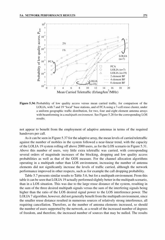
5.6. NETWORK PERFORMANCE RESULTS 271
0 2 4 6 8 10 12 14 16 18 20
Mean Carried Teletraffic (Erlang/km2/MHz)
10-5
2
5
10-4
2
5
10-3
2
5
10-2
2
5
10-1
2
5
100
Prob
abili
tyof
low
qual
ityac
cess
,Plo
w
1%
2%
FCA
LOLIA(n=7)
LOLIA(n=19) 8 element BF
4 element BF2 element BFLOLIA (n=19)LOLIA (n=7)FCA
Figure 5.34: Probability of low quality access versus mean carried traffic, for comparison of theLOLIA, with 7 and 19 “local” base stations, and of FCA using a 7-cell reuse cluster, undera uniform geographic traffic distribution, for two, four and eight element antenna arrayswith beamforming in a multipath environment. See Figure 5.28 for the corresponding LOSresults.
not appear to benefit from the employment of adaptive antennas in terms of the requiredhandovers per call.
As it can be seen in Figure 5.37 for the adaptive array, the mean levels of carried teletrafficagainst the number of mobiles in the system followed a near-linear trend, with the capacityof the LOLIA 19 system rolling off above 2000 users, as for the LOS scenario in Figure 5.31.Above this number of users, very little extra teletraffic was carried, with correspondingseveral orders of magnitude increases of the blocking, dropping and low quality accessprobabilities as well as that of the GOS measure. For the channel allocation algorithmsoperating in a multipath rather than LOS environment, increasing the number of antennaelements did not significantly increase the levels of traffic carried, although the networkperformance improved in other respects, such as for example the call dropping probability.
Table 5.7 presents similar results to Table 5.6, but for a multipath environment. From thistable it can be seen that LOLIA 19 actually performed slightly better in the multipath scenario,than in a LOS situation. This was due to the large reuse distance of the system, resulting inthe sum of the three desired multipath signals versus the sum of the interfering signals beinghigher than the ratio of the LOS desired signal power to the LOS interference power. TheLOLIA 7 algorithm, however, did not generally benefit from the multipath environment, sincethe smaller reuse distance resulted in numerous sources of relatively strong interference, allrequiring cancellation. Therefore, as the number of antenna elements increased, so shouldthe number of users supported by the network, as a result of the increased number of degreesof freedom, and therefore, the increased number of sources that may be nulled. The results

272 CHAPTER 5. ADAPTIVE ARRAYS IN AN FDMA/TDMA CELLULAR NETWORK
0 2 4 6 8 10 12 14 16 18 20
Mean Carried Teletraffic (Erlang/km2/MHz)
10-5
2
5
10-4
2
5
10-3
2
5
10-2
2
5
10-1
2
5
100
Gra
deof
Serv
ice
(GO
S)
4%
6%
FCA
LOLIA(n=7)
LOLIA(n=19) 8 element BF
4 element BF2 element BFLOLIA (n=19)LOLIA (n=7)FCA
Figure 5.35: Grade-Of-Service (GOS) performance versus mean carried traffic, for comparison of theLOLIA, with 7 and 19 “local” base stations, and of FCA using a 7-cell reuse cluster, undera uniform geographic traffic distribution, for two, four and eight element antenna arrayswith beamforming in a multipath environment. See Figure 5.29 for the corresponding LOSresults.
support this expectation with a 17% gain in the number of users, when upgrading the systemfrom two element to four element arrays, and a further 15% improvement in the numberof supported users with the aid of eight element antenna arrays instead of the four elementarrays. As for the LOS results, the FCA algorithm, again, benefited the most in terms of thenumber of users supported by the network from the employment of adaptive antenna arrays.The number of users increased by 35%, when doubling the number of antenna elementsfrom two to four, and on doubling from four to eight delivered a further 29% user capacityimprovement.
5.6.2.3 Performance over a Multipath Channel using Power Control
This section builds on the results obtained in the previous section for a multipath propagationenvironment. Simulations were conducted for a standard 7-cell FCA scheme and a LOLIA-assisted system using n = 7, both invoking power control. The power control algorithmimplemented attempted to independently adjust the mobile and base station transmit powers,such that the UL and DL SINRs were within a given target SINR window. The use of a targetwindow avoided constantly increasing and decreasing the transmission powers, which couldlead to potential power control instabilities within the network. Furthermore, using a rangeof possible transmission powers is analogous to accounting for an inherent power controlerror plus slow fading phenomenon. The “Target SINR” given in Table 5.8 is the SINR tobe maintained by the power control algorithm. The immediate effect of power control on

5.6. NETWORK PERFORMANCE RESULTS 273
0 2 4 6 8 10 12 14 16 18 20
Mean Carried Teletraffic (Erlang/km2/MHz)
0
2
4
6
8
10
12
14
16
18
Mea
nnu
mbe
rof
hand
over
spe
rca
ll
LOLIA(n=7)LOLIA (n=19)
FCA8 element BF4 element BF2 element BFLOLIA (n=19)LOLIA (n=7)FCA
Figure 5.36: Mean number of handovers per call versus mean carried traffic, for comparison of theLOLIA, with 7 and 19 “local” base stations, and of FCA using a 7-cell reuse cluster, undera uniform geographic traffic distribution, for two, four and eight element antenna arrayswith beamforming in a multipath environment. See Figure 5.30 for the corresponding LOSresults.
the SINR versus the mobile’s distance from the base station can be seen in Figure 5.38.This figure shows that power control attempts to maintain a constant SINR, sufficiently highfor reliable communications across the network, rather than allowing for unnecessarily highSINRs near the base station and providing insufficient levels of SINR far from the basestations, evident for a cordless telephone type network using no power control. It was foundthat in conjunction with 4-QAM using a target SINR of 27 dB was most suitable, when usingthe FCA algorithm. However, the LOLIA required a higher target SINR of 31 dB in orderto obtain satisfactory call dropping performance, as a result of its dynamic nature causingthe interference levels to vary more rapidly than for the FCA algorithm. In other words, theLOLIA required a higher SINR “headroom” above the re-allocation SINR threshold.
Figure 5.39 shows the new call blocking probability versus the mean normalizedcarried traffic, expressed in terms of Erlangs/km2/MHz. The figure shows that the blockingperformance of the FCA algorithm is limited by the availability of frequency/timeslotcombinations, and hence the addition of power control does not improve the new callblocking performance. However, the blocking performance of the LOLIA is not dominatedby the availability of frequency/timeslot combinations and hence it can be seen to benefitsignificantly from using power control.
From Figure 5.40 it can be seen that the Power Control (PC) algorithm substantiallyimproved the call dropping probability of the FCA algorithm in comparison to the scenariowithout PC in Figure 5.32. Specifically, at the highest traffic loads, the PC-assisted perfor-mance matched that without power control but using antenna arrays with twice the number

274 CHAPTER 5. ADAPTIVE ARRAYS IN AN FDMA/TDMA CELLULAR NETWORK
0 500 1000 1500 2000 2500 3000Mobiles in the System
0
2
4
6
8
10
12
14
16
18
20
Mea
nC
arri
edTe
letr
affic
(Erl
ang/
km2 /M
Hz)
8 element BF4 element BF2 element BFLOLIA (n=19)LOLIA (n=7)FCA
Figure 5.37: Mean traffic carried versus the number of mobiles in the system, for comparison of theLOLIA, with 7 and 19 “local” base stations, and of FCA using a 7-cell reuse cluster, undera uniform geographic traffic distribution, for two, four and eight element adaptive antennaarrays in a multipath environment. See Figure 5.31 for the corresponding LOS results.
Table 5.7: Maximum mean carried traffic, and maximum number of mobile users that can be supportedby each configuration, whilst meeting the preset quality constraints of Section 5.3.3.4.The carried traffic is expressed in terms of normalized Erlangs (Erlang/km2/MHz), forthe network described in Table 5.4 in a multipath environment. The corresponding LOSresults are summarized in Table 5.6 with network configurations common between the twohighlighted in bold.
Conservative Lenient
PF T = 1%, Plow = 1% PF T = 1%, Plow = 2%GOS = 4%, PB = 3% GOS = 6%, PB = 5%
Limiting LimitingAlgorithm Users Traffic factor Users Traffic factor
FCA, 2 elements (el.) 1315 8.10 Plow 1660 10.30 Plow
FCA, 4 elements 1790 11.10 Plow 2240 13.60 Plow
FCA, 8 elements 2400 14.20 PB 2780 15.70 GOSLOLIA (n = 7), 2 el. 2310 14.30 Plow 2610 16.10 Plow
LOLIA (n = 7), 4 el. 2735 16.90 Plow 3035 18.65 Plow
LOLIA (n = 7), 8 el. 3155 19.45 Plow >3200 >20.00 Plow
LOLIA (n = 19), 2 el. 1970 11.55 PB 2110 11.95 PB
LOLIA (n = 19), 4 el. 1990 11.65 PB 2155 12.05 PB
LOLIA (n = 19), 8 el. 2095 11.85 PB 2220 12.20 PB

5.6. NETWORK PERFORMANCE RESULTS 275
0 20 40 60 80 100 120 140 160 180Distance from basestation (m)
20
30
40
50
60
70
80
90
100
Ave
rage
SIN
R(d
B)
Network with power controlNetwork without power control
Figure 5.38: Signal-to-Interference plus Noise Ratio (SINR) versus mobile station distance measuredfrom the base station, for networks with and without power control. The unnecessarilyhigh SINR near the base station was a consequence of the base station’s inability to powerdown below the minimum transmit power of −20 dBm, when the mobile station waswithin a distance of about 60 m from the base station.
Table 5.8: Simulation parameters for the FCA, and DCA-assisted networks using power control.
Parameter Value Parameter Value
Noisefloor −104 dBm Multiple Access F/TDMAFrame duration 0.4615 ms Cell radius 218 mMax. BS transmit power 10 dBm Maximum MS transmit power 10 dBmMin. BS transmit power −20 dBm Minimum MS transmit power −20 dBmPower control stepsize 1 dB Power control hysteresis 3 dBNumber of base stations 49 Handover hysteresis 2 dBOutage SINR threshold 17 dB Power control FCA target SINR 27 dBRe-alloc. SINR threshold 21 dB Pow. cont. LOLIA7 target SINR 31 dBNumber of timeslots 8 Number of carriers 7Average inter-call-time 300 s Max new-call queue-time 5 sAverage call length 60 s Reference signal modulation BPSKBeamforming algorithm SMI Reference signal length 8 bitsMS speed 13.4 m/s Number of antenna elements 2 &4Pathloss at 1 m ref. point 0 dB Pathloss exponent −3.5Geometry of antenna array Linear Array element spacing λ/2Modulation scheme 4-QAM Channel/carrier bandwidth 200 kHz

276 CHAPTER 5. ADAPTIVE ARRAYS IN AN FDMA/TDMA CELLULAR NETWORK
0 2 4 6 8 10 12 14 16 18 20
Mean Carried Teletraffic (Erlang/km2/MHz)
10-5
2
5
10-4
2
5
10-3
2
5
10-2
2
5
10-1
2
5
100
New
Cal
lBlo
ckin
gPr
obab
ility
,PB
3%
5%
FCA
LOLIA(n=7)
8 element BF4 element BF2 element BFLOLIA (n=7) w/o PCFCA w/o PCLOLIA (n=7) with PCFCA with PC
Figure 5.39: New call blocking performance versus mean carried traffic, for comparison of the LOLIA,with 7 “local” base stations, and of FCA using a 7-cell reuse cluster, under a uniformgeographic traffic distribution, with and without power control, for two and four elementantenna arrays with beamforming in a multipath environment.
of antenna elements. At lower levels of traffic, the performance improvement obtained withthe aid of power control was even higher, with the two element array results approachingthose of the eight element array without power control. However, below approximately 10Erlang/km2/MHz a forced termination probability performance plateau was reached as aresult of the power control algorithm limiting the maximum SINR. In contrast, when nopower control is used and there are few users, the average SINR is very high and consequentlyfewer calls are dropped.
The performance gain of the LOLIA using power control is lower than that of the FCAalgorithm, but still significant, since its performance is about halfway between that of theLOLIA without power control and using the same number of antenna elements, and that withtwice the number of antenna elements.
The probability of low quality access of the PC-assisted scenario is shown in Figure 5.41.The corresponding curves for using no PC were plotted in Figure 5.33. The power controlledvariant of the FCA algorithm offered a significantly reduced probability of low quality accessfor a given number of antenna elements. In fact, the probability of low quality access, whenusing power control and a two element adaptive antenna array, was lower than that whenusing a four element array without power control. The LOLIA also benefited to the sameextent, with the probability of low quality access when using the power control algorithmequalling that obtained with the aid of twice the number of antenna elements and no powercontrol.
The GOS illustrated in Figure 5.42 is related to the probability of low quality access byEquation 5.15, hence the close resemblance to Figure 5.41. However, it can be seen that the
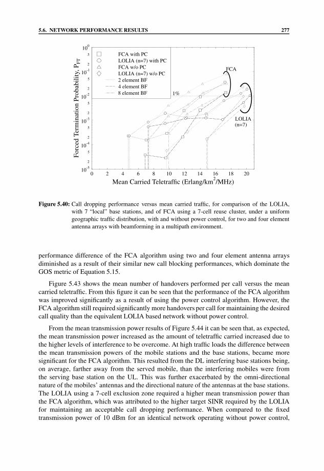
5.6. NETWORK PERFORMANCE RESULTS 277
0 2 4 6 8 10 12 14 16 18 20
Mean Carried Teletraffic (Erlang/km2/MHz)
10-5
2
5
10-4
2
5
10-3
2
5
10-2
2
5
10-1
2
5
100
Forc
edTe
rmin
atio
nPr
obab
ility
,PFT
1%
FCA
LOLIA(n=7)
8 element BF4 element BF2 element BFLOLIA (n=7) w/o PCFCA w/o PCLOLIA (n=7) with PCFCA with PC
Figure 5.40: Call dropping performance versus mean carried traffic, for comparison of the LOLIA,with 7 “local” base stations, and of FCA using a 7-cell reuse cluster, under a uniformgeographic traffic distribution, with and without power control, for two and four elementantenna arrays with beamforming in a multipath environment.
performance difference of the FCA algorithm using two and four element antenna arraysdiminished as a result of their similar new call blocking performances, which dominate theGOS metric of Equation 5.15.
Figure 5.43 shows the mean number of handovers performed per call versus the meancarried teletraffic. From this figure it can be seen that the performance of the FCA algorithmwas improved significantly as a result of using the power control algorithm. However, theFCA algorithm still required significantly more handovers per call for maintaining the desiredcall quality than the equivalent LOLIA based network without power control.
From the mean transmission power results of Figure 5.44 it can be seen that, as expected,the mean transmission power increased as the amount of teletraffic carried increased due tothe higher levels of interference to be overcome. At high traffic loads the difference betweenthe mean transmission powers of the mobile stations and the base stations, became moresignificant for the FCA algorithm. This resulted from the DL interfering base stations being,on average, farther away from the served mobile, than the interfering mobiles were fromthe serving base station on the UL. This was further exacerbated by the omni-directionalnature of the mobiles’ antennas and the directional nature of the antennas at the base stations.The LOLIA using a 7-cell exclusion zone required a higher mean transmission power thanthe FCA algorithm, which was attributed to the higher target SINR required by the LOLIAfor maintaining an acceptable call dropping performance. When compared to the fixedtransmission power of 10 dBm for an identical network operating without power control,

278 CHAPTER 5. ADAPTIVE ARRAYS IN AN FDMA/TDMA CELLULAR NETWORK
0 2 4 6 8 10 12 14 16 18 20
Mean Carried Teletraffic (Erlang/km2/MHz)
10-5
2
5
10-4
2
5
10-3
2
5
10-2
2
5
10-1
2
5
100
Prob
abili
tyof
low
qual
ityac
cess
,Plo
w
1%
2%
FCALOLIA(n=7)
8 element BF4 element BF2 element BFLOLIA (n=7) w/o PCFCA w/o PCLOLIA (n=7) with PCFCA with PC
Figure 5.41: Probability of low quality access per call versus mean carried traffic, for comparison ofthe LOLIA, with 7 “local” base stations, and of FCA using a 7-cell reuse cluster, undera uniform geographic traffic distribution, with and without power control, for 2 and 4element antenna arrays with beamforming in a multipath environment.
the reductions in transmitted power are significant, with a minimum average transmit powerreduction of 6 dB, which substantially extends the mobile stations’ battery lives.
Table 5.9 presents the summary of our results obtained for a network using power controlin a multipath environment. The table shows that the use of power control has increasedthe number of users that may be serviced according to the required network performancecriteria. The number of users supported by the network using the FCA algorithm increasedby 28% to 70%, with a mean of 54% over the conservative and lenient scenarios. The capacitygains obtained with the aid of power control in a network using the LOLIA 7, however, werelower, namely between 9% and 15%, with a mean of almost 13% for both the conservativeand lenient scenarios. Whilst the LOLIA 7 capacity gains are fairly modest, the overall callquality of the channel allocation techniques has improved for a given level of traffic, whencompared to an identical network without power control.
5.6.2.4 Transmission over a Multipath Channel using Power Control and AdaptiveModulation
The idea behind adaptive modulation is to select a modulation mode according to theinstantaneous radio channel quality [12, 13]. Thus, if the channel quality exhibits a highinstantaneous SINR, then a high order modulation mode may be employed, enabling theexploitation of the temporarily high channel capacity. In contrast, if the channel has a lowinstantaneous SINR, using a high-order modulation mode would result in an unacceptableFrame Error Ratio (FER), and hence a more robust, but lower throughput modulation mode

5.6. NETWORK PERFORMANCE RESULTS 279
0 2 4 6 8 10 12 14 16 18 20
Mean Carried Teletraffic (Erlang/km2/MHz)
10-5
2
5
10-4
2
5
10-3
2
5
10-2
2
5
10-1
2
5
100
Gra
deof
Serv
ice
(GO
S)4%
6%
FCALOLIA(n=7)
8 element BF4 element BF2 element BFLOLIA (n=7) w/o PCFCA w/o PCLOLIA (n=7) with PCFCA with PC
Figure 5.42: Grade-Of-Service (GOS) performance versus mean carried traffic, for comparison of theLOLIA, with 7 “local” base stations, and of FCA using a 7-cell reuse cluster, under auniform geographic traffic distribution, with and without power control, for two and fourelement antenna arrays with beamforming in a multipath environment.
would be invoked. Hence, adaptive modulation not only combats the effects of a poor qualitychannel, but also attempts to maximize the throughput, whilst maintaining a given target FER.Thus, there is a trade-off between the mean FER and the data throughput, which is governedby the modem mode switching thresholds. These switching thresholds define the SINRs, atwhich the channel is considered unsuitable for a given modulation mode, where an alternativeAQAM mode must be invoked.
The power control algorithm invoked attempted to independently adjust the mobile andbase station powers, such that the UL and DL SINRs were within a given target SINRwindow. The employment of a target window avoided constantly increasing and decreasingthe transmission powers, which could lead to potential power control instabilities withinthe network. Furthermore, the affect of a range of different possible transmission powersis analogous to an inherent power control error plus slow fading envelope.
The combination of power control with adaptive modulation leads to several performancetrade-offs, which must be considered when designing the power control and modulation modeswitching algorithm. For example, the transmitted power could be minimized, which wouldresult in either a high FER and a high throughput, or a low BER and a low throughput.Alternatively, the FER could be lowered even while maintaining a high throughput, whentolerating high transmission powers.
The power control and modulation mode switching algorithm invoked in our simulationsattempted to minimize the transmitted power, whilst maintaining a high throughput with a

280 CHAPTER 5. ADAPTIVE ARRAYS IN AN FDMA/TDMA CELLULAR NETWORK
0 2 4 6 8 10 12 14 16 18 20
Mean Carried Teletraffic (Erlang/km2/MHz)
0
2
4
6
8
10
12
14
16
18
Mea
nnu
mbe
rof
hand
over
spe
rca
ll
FCA
LOLIA (n=7)
8 element BF4 element BF2 element BFLOLIA (n=7) w/o PCFCA w/o PCLOLIA (n=7) with PCFCA with PC
Figure 5.43: Mean number of handovers per call versus mean carried traffic, for comparison of theLOLIA, with 7 “local” base stations, and of FCA using a 7-cell reuse cluster, under auniform geographic traffic distribution, with and without power control, for two and fourelement antenna arrays with beamforming in a multipath environment.
0 2 4 6 8 10 12 14 16 18 20
Mean Carried Teletraffic (Erlang/km2/MHz)
0
1
2
3
4
5
6
Mea
nT
rans
mis
sion
Pow
er(d
Bm
)
FCA
LOLIA (n=7)LOLIA (n=7) 4 elementsLOLIA (n=7) 2 elementsFCA 4 elementsFCA 2 elementsBasestation transmit powerMobile transmit power
Figure 5.44: Mean transmission power versus mean carried traffic, of the LOLIA, with 7 “local” basestations, under a uniform geographic traffic distribution, with power control, for two andfour element antenna arrays with beamforming in a multipath environment.

5.6. NETWORK PERFORMANCE RESULTS 281
Table 5.9: Maximum mean carried traffic, and maximum number of mobile users that can be supportedby each configuration whilst meeting the preset quality constraints of Section 5.3.3.4.The carried traffic is expressed in terms of normalized Erlangs (Erlang/km2/MHz) forthe network described in Table 5.8 both with and without power control in a multipathenvironment. The figures in bold indicate common network configurations to both the resultswithout power and those with.
Conservative Lenient
PF T = 1%, Plow = 1% PF T = 1%, Plow = 2%GOS = 4%, PB = 3% GOS = 6%, PB = 5%
Limiting LimitingAlgorithm Users Traffic factor Users Traffic factor
Without power cont.FCA, 2 elements (el.) 1315 8.10 Plow 1660 10.30 Plow
FCA, 4 elements 1790 11.10 Plow 2240 13.60 Plow
FCA, 8 elements 2400 14.20 PB 2780 15.70 GOSLOLIA (n = 7), 2 el. 2310 14.30 Plow 2610 16.10 Plow
LOLIA (n = 7), 4 el. 2735 16.90 Plow 3035 18.65 Plow
LOLIA (n = 7), 8 el. 3155 19.45 Plow >3200 >20.00 Plow
With power cont.FCA, 2 elements 2260 13.30 Plow 2455 14.25 PF T
FCA, 4 elements 2510 14.45 PB 2870 15.95 PB
LOLIA (n = 7), 2 el. 2665 16.30 Plow 2935 17.80 Plow
LOLIA (n = 7), 4 el. 3125 19.08 Plow 3295 20.42 PF T
less than 5% target FER. The pseudo-code of the proposed algorithm is described in the nextsection.
5.6.2.5 Power Control and Adaptive Modulation Algorithm
determine lowest SINR out of UL and DL SINRsif in 16-QAM mode
if lowest SINR < 16-QAM drop SINRdrop to 4-QAM mode
else if lowest SINR < 16-QAM reallocation SINRif at maximum transmit powerrevert to 4-QAM
elseincrease transmit power
else if lowest SINR < 16-QAM target SINRif not at maximum powerincrease transmit power
else if lowest SINR > 16-QAM target SINR+hysteresisdecrease transmit power

282 CHAPTER 5. ADAPTIVE ARRAYS IN AN FDMA/TDMA CELLULAR NETWORK
else if in 4-QAM modeif lowest SINR < 4-QAM drop SINRdrop to BPSK mode
else if lowest SINR < 4-QAM reallocation SINRif at maximum transmit power
revert to BPSKelse
increase transmit powerelse if lowest SINR < 4-QAM target SINRif not at maximum power
increase transmit powerelse if lowest SINR > 16-QAM target SINR+hysteresischange to 16-QAM mode
else if lowest SINR > 4-QAM target SINR+hysteresisif at maximum transmit power
reduce transmit powerelse
if lowest SINR > 16-QAM drop SINRchange to 16-QAM
elsedecrease transmit power
else if in BPSKif lowest SINR < BPSK drop SINRoutage occurs
else if lowest SINR < BPSK reallocation SINRif not at maximum transmit power
increase transmit powerelse if lowest SINR > 4-QAM target SINR+hysteresischange to 4-QAM
else if lowest SINR > BPSK target_hysteresisif at maximum transmit power
reduce transmit powerelse
change to 4-QAM
Figure 5.45 shows the flowchart of the AQAM and power control decision tree, when inthe 4-QAM mode. The first step in the process is to determine the lower of the UL and the DLSINRs. The next step is to determine whether the BPSK modulation mode should be selected.When in the BPSK mode, outages may occur due to an insufficiently high SINR level andafter a given number of BPSK outages the call is dropped. The conditions for this to occur arethat either the lower SINR is below the 4-QAM call dropping threshold or that it is below the4-QAM call reallocation threshold and currently the maximum possible transmission power isused. If the lower SINR is below the 4-QAM call reallocation threshold, or the SINR is belowthe 4-QAM target SINR, and the maximum transmission power has not been reached, then thetransmit power is increased. However, if the SINR is below the 4-QAM target SINR and themaximum possible transmit power is currently used, then the modem remains in the 4-QAM

5.6. NETWORK PERFORMANCE RESULTS 283
outages in BPSK modecalls are dropped
After ‘n’ consecutive
At maximum TX power?
Downlink SINR)min(Uplink SINR,
Lowest SINR < Y
N
4QAM drop SINR ?
Lowest SINR< 4QAM reallocation
SINR ?
N
Y
Y
Max. TX power?
Increase TX powerN
Max. TX power?4QAM target SINR ?
Lowest SINR < Y
N
> 16QAM target SINRLowest SINR
+ hysteresis ?
Y
N
Use 16QAM
4QAM STOP Decrease TX power
Decrease TX power
N
Y
N
> 16QAM drop SINRLowest SINR
Lowest SINR
+ hysteresis ?
Y
N
> 4QAM target SINR
Y
4QAM START
Y
Lowest SINR =
Remain in 4QAM
Y
N
Use BPSK
Figure 5.45: The AQAM and power control decision tree for the 4-QAM mode.

284 CHAPTER 5. ADAPTIVE ARRAYS IN AN FDMA/TDMA CELLULAR NETWORK
mode. The 16-QAM mode is chosen, if the SINR is higher than the 16-QAM target SINR,plus the associated hysteresis. Alternatively, the 16-QAM mode is invoked if the SINR ishigher than the 4-QAM target SINR plus the hysteresis, furthermore the transmission powerrequired to obtain this SINR is lower than the maximum transmit power, and the SINR ishigher than the 16-QAM call dropping SINR. However, if the SINR is below the 16-QAMcall dropping SINR or the maximum transmission power is in use, then the transmit poweris reduced in an effort to keep the SINR in the 4-QAM mode’s target SINR window. Theimproved SINR achieved using adaptive antenna arrays at the base station facilitates a highermean network data throughput.
The FER was evaluated for approximately half-rate Bose-Chaudhuri-Hocquenghem(BCH) codes, which employed interleaving over the different number of bits conveyed bythe different modem modes within a transmission frame [133]. The “Reallocation SINR” andthe “Outage SINR” are defined as the average SINRs necessary for satisfying the 5% and10% maximum FER constraints, respectively, using a given modulation mode such as BPSK,4-QAM, or 16-QAM. The “Target SINR” was chosen so as to maximize the network capacityand represents an FER of approximately 2%.
The calculation of the receive antenna arrays weights was performed on a transmissionframe-by-frame basis, leading to updated UL and DL SINRs every transmission frame. TheseSINR values were then used for selecting the modulation mode and transmission power tobe employed, and for determining whether any channel re-allocation was necessary. Hence,frame-by-frame adaptive modulation, power control and dynamic channel allocation wasjointly performed.
The system parameters for the network are defined in Table 5.10 and our performanceresults are provided in the next section.
5.6.2.6 Performance of PC-assisted, AQAM-aided Dynamic Channel Allocation
This section presents the simulation results obtained for a network using burst-by-burstadaptive modulation in order to improve the network’s performance. Simulations wereconducted for both a standard 7-cell FCA scheme and for the LOLIA using n = 7. Thebenchmark results obtained for a 4-QAM based network using power control were includedfor comparison purposes. Due to the enhanced network performance resulting from theemployment of AQAM, a further constraint of a minimum throughput of 2 bits/symbol wasinvoked. This ensured a fair comparison with the fixed 4-QAM based network.
Figure 5.46 shows the new call blocking probability versus the mean normalized carriedtraffic. From this figure it can be seen that in conjunction with the LOLIA there areno blocked calls, except for the highest levels of traffic. In contrast, the performance ofthe FCA algorithm was degraded by using AQAM. This was the result of the limitedavailability of frequency/timeslot combinations restricting the achievable performance gain,since the reduced call dropping probability encouraged the prolonged utilization of thelimited resources. This however, prevented new call setups.
The corresponding call dropping probability is depicted in Figure 5.47, which shows thatwhen invoking adaptive modulation, the FCA algorithm performs better than the LOLIAbelow a traffic load of about 14 Erlangs/km2/MHz. Both channel allocation algorithmsconsistently offered a lower call dropping probability, when employing AQAM compared towhen using the fixed-mode 4-QAM modulation scheme. This reduction in the call dropping

5.6. NETWORK PERFORMANCE RESULTS 285
Table 5.10: Simulation parameters for the AQAM based network using power control.
Parameter Value Parameter Value
Noisefloor −104 dBm Multiple Access TDMAFrame length 0.4615 ms Cell radius 218 mMin. BS transmit power −20 dBm Min. MS transmit power −20 dBmMax. BS transmit power 10 dBm Max. MS transmit power 10 dBmPower control stepsize 1 dB Power control hysteresis 3 dBBPSK outage SINR 13 dB BPSK reallocation SINR 17 dBBPSK target SINR 21 dB 4-QAM outage SINR 17 dB4-QAM reallocation SINR 21 dB 4-QAM target SINR 27 dB16-QAM outage SINR 24 dB 16-QAM reallocation SINR 27 dB16-QAM target SINR 32 dB Pathloss exponent −3.5Number of base stations 49 Handover hysteresis 2 dBNumber of timeslots/carrier 8 Number of carriers 7Average inter-call-time 300 s Max new-call queue-time 5 sAverage call length 60 s Ref. signal modulation BPSKBeamforming algorithm SMI Reference signal length 8 bitsMS speed 30 mph No. of antenna elements 2 & 4Pathloss at 1 m ref. point 0 dB Shadow fading NoGeometry of ant. array Linear Array element spacing λ/2Channel/carrier bandwidth 200 kHz
0 2 4 6 8 10 12 14 16 18 20 22 24 26 28 30
Mean Carried Teletraffic (Erlang/km2/MHz)
10-4
2
5
10-3
2
5
10-2
2
5
10-1
New
Cal
lBlo
ckin
gPr
obab
ility
,PB
3%
5%
FCA LOLIA 4-QAM PCLOLIAAQAM PC
4 element BF2 element BFLOLIA (n=7) AQAM PCLOLIA (n=7) 4-QAM PCFCA AQAM PCFCA 4-QAM PC
Figure 5.46: New call blocking probability versus mean carried traffic of the LOLIA, with 7 “local”base stations, and of FCA employing a 7-cell reuse cluster, for 2 and 4 element antennaarrays, with and without AQAM.

286 CHAPTER 5. ADAPTIVE ARRAYS IN AN FDMA/TDMA CELLULAR NETWORK
0 2 4 6 8 10 12 14 16 18 20 22 24 26 28 30
Mean Carried Teletraffic (Erlang/km2/MHz)
10-5
2
5
10-4
2
5
10-3
2
5
10-2
2
5
10-1
Cal
lTer
min
atio
nPr
obab
ility
,PFT
1%
FCA, 4-QAM PC
FCA,AQAM PC
LOLIA, 4-QAM PC
LOLIA, AQAM PC
4 element BF2 element BFLOLIA (n=7) AQAM PCLOLIA (n=7) 4-QAM PCFCA AQAM PCFCA 4-QAM PC
Figure 5.47: Call dropping or forced termination performance versus mean carried traffic of theLOLIA, with 7 “local” base stations, and of FCA employing a 7-cell reuse cluster, fortwo and four element antenna arrays, with and without AQAM.
rate using adaptive modulation was brought about by the inherent ability of the AQAMscheme to be reconfigured to a lower-order, and hence more interference resistant modulationmode, in order to prevent calls from being dropped.
Figure 5.48 shows that the probability of a low quality access was substantially reduced byAQAM for both the FCA scheme and the LOLIA. At lower traffic loads the probability of lowquality outage was higher than when using the fixed 4-QAM modulation mode for both of thechannel allocation schemes. This was due to the frequent use of the highest order modulationmode, 16-QAM, which was more susceptible to low quality outages. The more frequent usageof the 16-QAM mode by the four element adaptive antenna arrays also explains their greaterprobability of low quality outage at the lower traffic levels. However, as the traffic levelsincreased, the lower order modulation modes were invoked more frequently, and hence whencombined with the four element arrays, the system guaranteed a lower probability of lowquality outage than the two element arrays.
From Figure 5.49 it can be seen that the GOS of the FCA algorithm did not benefitfrom employing AQAM to the same extent as the LOLIA, except at the lower traffic levelswhen the new call blocking probability does not dominate the overall GOS performance.The LOLIA, however, benefited substantially, as we have also seen for the probability of lowquality outages, since its performance was not constrained by its new call blocking probabilityobserved in Figure 5.46 for both 4-QAM and AQAM.
The employment of AQAM, in Figure 5.50, reduced the mean number of handovers percall of the LOLIA at all traffic loads, and of the FCA for the highest traffic loads, althoughan increased number of handovers were performed by the FCA at lower traffic loads. Atthese lower traffic loads, more intra-cell handovers were performed by the FCA algorithm,

5.6. NETWORK PERFORMANCE RESULTS 287
0 2 4 6 8 10 12 14 16 18 20 22 24 26 28 30
Mean Carried Teletraffic (Erlang/km2/MHz)
10-4
2
5
10-3
2
5
10-2
2
5
10-1
Prob
abili
tyof
low
qual
ityac
cess
,Plo
w2%
1%
FCA AQAM PC
FCA 4-QAMPC
LOLIA AQAM PC
LOLIA 4-QAM PC
4 element BF2 element BFLOLIA (n=7) AQAM PCLOLIA (n=7) 4-QAM PCFCA AQAM PCFCA 4-QAM PC
Figure 5.48: Probability of low quality access versus mean carried traffic of the LOLIA, with 7 “local”base stations, and of FCA employing a 7-cell reuse cluster, for two and four elementantenna arrays, with and without AQAM.
0 2 4 6 8 10 12 14 16 18 20 22 24 26 28 30
Mean Carried Teletraffic (Erlang/km2/MHz)
10-5
2
5
10-4
2
5
10-3
2
5
10-2
2
5
10-1
Gra
deof
Serv
ice
(GO
S)
4%
6%
FCA AQAM PC
FCA 4-QAMPC
LOLIA AQAM PC
LOLIA 4-QAM PC 4 element BF2 element BFLOLIA (n=7) AQAM PCLOLIA (n=7) 4-QAM PCFCA AQAM PCFCA 4-QAM PC
Figure 5.49: GOS performance versus mean carried traffic of the LOLIA, with 7 “local” base stations,and of FCA employing a 7-cell reuse cluster, for two and four element antenna arrays,with and without AQAM.

288 CHAPTER 5. ADAPTIVE ARRAYS IN AN FDMA/TDMA CELLULAR NETWORK
0 2 4 6 8 10 12 14 16 18 20 22 24 26 28 30
Mean Carried Teletraffic (Erlang/km2/MHz)
0
1
2
3
4
5
6
7
Mea
nnu
mbe
rof
hand
over
spe
rca
ll
FCA, 4-QAM PC
FCA, AQAM PC
LOLIA, 4-QAM PC
LOLIA, AQAM PC
4 element BF2 element BFLOLIA (n=7) AQAM PCLOLIA (n=7) 4-QAM PCFCA AQAM PCFCA 4-QAM PC
Figure 5.50: Mean number of handovers per call versus mean carried traffic of the LOLIA, with 7“local” base stations, and of FCA employing a 7-cell reuse cluster, for two and fourelement antenna arrays, with and without AQAM.
due to the employment of the 16-QAM modulation mode, which required more frequentintra-cell handovers in order to maintain a sufficiently high SINR. However, as the trafficload increased, the lower-order modulation modes were used more frequently, and henceless intra-cell handovers were required, leading to a reduction in the number of handoversperformed.
The mean transmission power results of Figure 5.51 demonstrate how the employmentof AQAM can reduce the power transmitted both for the UL and the DL. At low trafficload levels the FCA algorithm performed slightly worse in transmitted power terms, than theLOLIA. However, as the traffic loads increased, the gap became negligible when using twoelement antenna arrays. By contrast, when using four element antenna arrays, the LOLIArequired a higher transmission power at these higher teletraffic loads. When compared to thefixed transmission power of 10 dBm for a network using no power control, the employmentof AQAM resulted in a significant reduction of the mean transmission power. Specifically,the minimum reduction of the transmitted power was more than 4 dB and a maximumreduction of more than 7 dB was attained in addition to achieving a superior call qualityand an increased mean modem throughput.
The average modem throughput expressed in bits per symbol versus the mean carriedteletraffic is shown in Figure 5.52. The figure shows how the mean number of bits per symboldecreased as the network traffic increased. The FCA algorithm offered the lowest throughputwith its performance degrading near-linearly upon increasing the network’s traffic load. TheLOLIA, especially for the lower levels of traffic, offered a greater modem throughput for agiven level of teletraffic carried, with the achievable performance gracefully decreasing, as
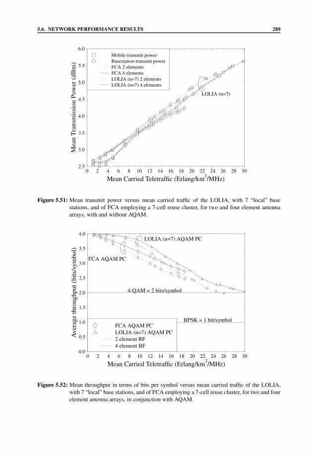
5.6. NETWORK PERFORMANCE RESULTS 289
0 2 4 6 8 10 12 14 16 18 20 22 24 26 28 30
Mean Carried Teletraffic (Erlang/km2/MHz)
2.5
3.0
3.5
4.0
4.5
5.0
5.5
6.0
Mea
nT
rans
mis
sion
Pow
er(d
Bm
)
LOLIA (n=7)
LOLIA (n=7) 4 elementsLOLIA (n=7) 2 elementsFCA 4 elementsFCA 2 elementsBasestation transmit powerMobile transmit power
Figure 5.51: Mean transmit power versus mean carried traffic of the LOLIA, with 7 “local” basestations, and of FCA employing a 7-cell reuse cluster, for two and four element antennaarrays, with and without AQAM.
0 2 4 6 8 10 12 14 16 18 20 22 24 26 28 30
Mean Carried Teletraffic (Erlang/km2/MHz)
0.0
0.5
1.0
1.5
2.0
2.5
3.0
3.5
4.0
Ave
rage
thro
ughp
ut(b
its/s
ymbo
l)
4-QAM = 2 bits/symbol
BPSK = 1 bit/symbol
LOLIA (n=7) AQAM PC
FCA AQAM PC
4 element BF2 element BFLOLIA (n=7) AQAM PCFCA AQAM PC
Figure 5.52: Mean throughput in terms of bits per symbol versus mean carried traffic of the LOLIA,with 7 “local” base stations, and of FCA employing a 7-cell reuse cluster, for two and fourelement antenna arrays, in conjunction with AQAM.

290 CHAPTER 5. ADAPTIVE ARRAYS IN AN FDMA/TDMA CELLULAR NETWORK
Table 5.11: Mean modem throughput, when supporting the maximum mean carried traffic, whilstmeeting the preset quality constraints of Section 5.3.3.4. The carried traffic is expressedin terms of normalized Erlangs (Erlang/km2/MHz) for the network described in Table 5.10in a multipath environment with AQAM.
Conservative Lenient
PF T = 1%, Plow = 1% PF T = 1%, Plow = 2%GOS = 4%, PB = 3% GOS = 6%, PB = 5%
Bits per Symbol Bits per Symbol
FCA, 2 elements 2.8 2.7FCA, 4 elements 3.1 2.9LOLIA (n = 7), 2 elements 2.1 ≈2.0LOLIA (n = 7), 4 elements 2.15 2.05
the carried teletraffic continued to increase. Table 5.11 shows the mean modem throughput inbits per symbol, for the maximum mean carried traffic levels, whilst meeting the predefinedquality constraints of Section 5.3.3.4.
From Table 5.12 it can be seen that it is the blocking performance of the network using theFCA algorithm which limits its associated network capacity, thus leading to a relatively highmean modem throughput at its user capacity limits. The increase in the modem throughput forthe FCA algorithm varied from 35% to 55%, with corresponding user capacity improvementsof 6% and −4%, when comparing the AQAM network to 4-QAM. The table also shows thatthe number of users supported by the FCA network using two element adaptive antennaarrays increased when using AQAM, which was restricted by the probability of low qualityaccess when using 4-QAM. In contrast, when using four element antenna arrays, the networkcapacity was limited by the network’s new call blocking performance. Hence, using AQAMtechniques did not increase the number of users supported. In fact, due to the superior calldropping performance of AQAM, the new call blocking probability increased as a result of thelack of available frequency/timeslot combinations, and hence the number of users supportedby the network decreased.
However, the dynamic nature of the LOLIA limited its fixed 4-QAM based networkcapacity due to its excessive low quality access probability, and thus in all cases, AQAMincreased the number of users supported, by 38% to 50%, whilst meeting the requiredcall quality criteria of Section 5.3.3.4. The AQAM-induced improvement in mean modemthroughput varied from 0% to 7.5% as a result of the particular AQAM implementation usedin the simulations. This can be further verified with the aid of Figure 5.51, which showsthat the mean transmission powers were not at their maxima and hence both the modemthroughput and the probability of low quality access were sub-optimal. In other words, hadthe AQAM algorithm been more aggressive in terms of its transmitted power usage, a reducedprobability of low quality access and an increased mean modem throughput would haveoccurred. However, a trade-off existed where both the number of users supported and themean modem throughput were increased, whilst achieving a significant reduction in the meantransmission powers.

5.6. NETWORK PERFORMANCE RESULTS 291
Table 5.12: Maximum mean carried traffic, and maximum number of mobile users that canbe supported by each configuration, whilst meeting the preset quality constraintsof Section 5.3.3.4. The carried traffic is expressed in terms of normalized Erlangs(Erlang/km2/MHz) for the network described in Table 5.10 in a multipath environment
Conservative Lenient
PF T = 1%, Plow = 1% PF T = 1%, Plow = 2%GOS = 4%, PB = 3% GOS = 6%, PB = 5%
Limiting LimitingAlgorithm Users Traffic factor Users Traffic factor
4-QAM with PCFCA, 2 elements (el.) 2260 13.30 Plow 2455 14.25 PF T
FCA, 4 elements 2510 14.45 PB 2870 15.95 PB
LOLIA (n = 7), 2 el. 2665 16.30 Plow 2935 17.80 Plow
LOLIA (n = 7), 4 el. 3125 19.08 Plow 3295 20.42 PF T
AQAM with PCFCA, 2 elements 2400 14.00 PB 2760 15.75 PB
FCA, 4 elements 2400 14.10 PB 2710 15.50 PB
LOLIA (n = 7), 2 el. 3675 23.10 Plow 4115 25.4 Plow
LOLIA (n = 7), 4 el. 4460 27.40 Plow 4940 29.6 Plow
5.6.2.7 Summary of Non-wraparound Network Performance
The performance results summarized in this section can be gleaned from Tables 5.6–5.12.Specifically, in this section simulation results were obtained for a LOS scenario, for boththe FCA algorithm and for the LOLIA, which showed that the FCA algorithm benefitedthe most from the employment of adaptive antenna arrays, with an increase of 144% in thenumber of users supported by four element antenna arrays. The corresponding figure was67% with the aid of two element arrays. The performance of the LOLIA with a 19 basestation constraint improved least using adaptive antenna arrays due to the inherently lowinterference levels present. However, for the LOLIA with a base station constraint of 7, usingtwo element adaptive antenna arrays, an extra 22% additional users were supported with thedesired performance metric limits of Section 5.3.3.4 observed. Using four element adaptiveantenna arrays at the base stations led to an increase of 58% in the number of users supported.
Identical simulations with the addition of two multipath rays were then performed.These simulations demonstrated that the LOLIA 19 actually performed better in a multipathscenario, than in a LOS situation. This was due to the large reuse distance of the system,resulting in the sum of the powers of the three desired multipath signals versus the sum ofthe interfering signal powers being higher than the ratio of the LOS desired signal powerto the interference power. The FCA algorithm, which offered the lowest network capacityin the LOS simulations, also suffered from the greatest capacity reduction in the multipathscenarios. The corresponding network capacities, expressed in terms of the number of userssupported, decreased by between 3% and 17%. The number of users supported by the

292 CHAPTER 5. ADAPTIVE ARRAYS IN AN FDMA/TDMA CELLULAR NETWORK
network using the LOLIA 7, was not significantly affected by the multipath propagationenvironment, with the highest reduction of almost 7% occurring using a four element antennaarray employed in the conservative network scenario of Section 5.3.3.4. The FCA algorithmbenefited the most from increasing the number of elements comprising the adaptive antennaarrays, with a minimum increase of 25% in the number of users supported upon doublingthe number of antenna elements. The LOLIA employing a reuse cluster size of seven alsoperformed well, with a user capacity increase of at least 15% for each doubling of the numberof antenna elements.
Simulations were then performed in the multipath environment, where the network usedthe power control algorithm to maintain a fairly constant received SINR across the cell area.It was found that the power control algorithm increased the number of users carried in allthe scenarios considered. The FCA algorithm exhibited the greatest gains in terms of thenumber of users supported by the network. When compared to an identical network withoutpower control, the user capacity increased by 28%–72%, with an average increase of 47%.The LOLIA 7 using power control carried more traffic than the equivalent power controlassisted FCA networks, and the LOLIA 7 system using no power control. When comparedto the LOLIA 7 network using no power control, 9% to 15% more users were carried witha satisfactory performance. With respect to an FCA based network using power control, theincrease in the number of supported users varied from 9% to almost 25%.
Further experiments were conducted in order to investigate the potential of AQAMtechniques to increase network capacity. The gains achievable by the FCA algorithm wererestricted by the number of available frequency/timeslot combinations, for both new callsand handovers, and hence the capacity increases were constrained by the new call blockingprobability to 6%. However, this limitation to the number of supported users resulted inan increased mean modem throughput of between 2.7 and 3.1 bits per symbol, a reducedmean transmission power, and an overall improvement in call quality. The LOLIA, however,was not constrained by its new call blocking probability and was able to fully exploit theadvantages of adaptive modulation. Thus, the LOLIA achieved a minimum network capacityincrease of 38% over an identical scenario not using adaptive modulation.
The next section presents similar results but obtained using the “wraparound” techniquein an effort to provide an effectively infinite simulation plane with, on average, constantinterference levels present over the entire simulation area.
5.6.3 Wrap-around Network Performance Results
This section presents a range of performance results similar to those obtained in the previoussection. However, in this section the “wrap-around” technique of Section 5.6.1 was used togenerate results not subjected to the edge effects present at the perimeter of the simulationarea. This process was described in Section 5.6.1. Results were obtained for the LOSpropagation environment in Section 5.6.3.1 and for the multipath propagation environmentof Section 5.6.3.2. Section 5.6.3.3 portrays the results obtained for the multipath propagationenvironment using power control, and Section 5.6.3.4 presents the network performanceusing adaptive modulation techniques.

5.6. NETWORK PERFORMANCE RESULTS 293
4 6 8 10 12 14 16 18
Mean Carried Teletraffic (Erlang/km2/MHz)
10-5
2
5
10-4
2
5
10-3
2
5
10-2
2
5
10-1
2
5
100
New
Cal
lBlo
ckin
gPr
obab
ility
,PB
3%
5%
FCA
LOLIA (n=19)
LOLIA (n=7)
LOLIA (n=19)LOLIA (n=7)FCA4 elements2 elementsNo BF
Figure 5.53: New call blocking probability performance versus mean carried traffic, for the LOLIAusing 7 and 19 “local” base stations, and for FCA employing a 7-cell reuse cluster, underuniform geographic traffic distribution, for a single antenna element, as well as for two andfour element antenna arrays with beamforming in a LOS environment using wrap-around.See Figure 5.26 for the corresponding “desert-island” scenario.
5.6.3.1 Performance Results over a LOS Channel
Firstly we compared the FCA and the LOLIA under uniform geographic traffic distributionconditions using both a single antenna element and adaptive antenna arrays consisting oftwo and four elements in a LOS propagation environment. The FCA scheme employed aseven-cell reuse cluster, corresponding to one carrier frequency per base station. The LOLIAwas used in conjunction with the constraints of seven and nineteen nearest base stations, i.e.,n = 7 or 19.
As seen in Figure 5.53 the LOLIA using n = 19 offered the worst call blockingperformance of the three channel allocation schemes, with the AAAs having little beneficialeffect. This demonstrated that the limiting factor was not inadequate signal quality for acall to be setup, but the lack of available frequency/timeslot combinations due to the largeexclusion zone. The FCA algorithm benefited only to a limited extent from the employmentof the AAAs, suggesting that the majority of the blocked calls were as a result of thelimited availability of frequency/timeslot combinations. Inadequate signal quality causedthe remainder of the blocked calls. The call blocking performance of the LOLIA usingn = 7 appeared mainly to be interference limited, hence the AAAs guaranteed a significantreduction of the number of blocked calls, particularly for mean carried traffic levels in excessof 9 Erlang/km2/MHz.
Figure 5.54 shows that—as expected—the FCA algorithm performed the least satisfac-torily of the three channel allocation schemes investigated with respect to its call dropping

294 CHAPTER 5. ADAPTIVE ARRAYS IN AN FDMA/TDMA CELLULAR NETWORK
4 6 8 10 12 14 16 18 20
Mean Carried Teletraffic (Erlang/km2/MHz)
10-5
2
5
10-4
2
5
10-3
2
5
10-2
2
5
10-1
2
5
100
Cal
lTer
min
atio
nPr
obab
ility
,PFT
1%
FCA
LOLIA (n=19)
LOLIA (n=7)
LOLIA (n=19)LOLIA (n=7)FCA4 element BF2 element BFNo BF
Figure 5.54: Dropping probability performance versus mean carried traffic, for the LOLIA using 7 and19 “local” base stations, and for FCA employing a 7-cell reuse cluster, under a uniformgeographic traffic distribution, for a single antenna element, as well as for two and fourelement antenna arrays with beamforming in a LOS environment using wrap-around. SeeFigure 5.27 for the corresponding “desert-island” scenario.
performance. Even in conjunction with a four-element adaptive antenna array, it exhibiteda higher call dropping rate than that of either of the LOLIAs (n = 19 and n = 7). Thelarge exclusion zone of the LOLIA using n = 19 led to a low dropping probability of lessthan 1 × 10⁻³ for teletraffic loads below approximately 12 Erlang/km2/MHz. However, therapid rise in the call dropping probability upon increasing the teletraffic became unacceptablefor teletraffic loads in excess of about 13 Erlang/km2/MHz. The large exclusion zone of thealgorithm prevented from handovers occurring, since there were no free channels availablein the vicinity, hence resulting in a high number of dropped calls. Thus, for n = 19 theemployment of adaptive antenna arrays at the base stations did not improve the performancesignificantly, unlike for the FCA and LOLIA using n = 7, which were predominantlyinterference limited. The call dropping performance of the LOLIA using n = 7 benefitedthe most from the assistance of adaptive antenna arrays, with the most dramatic gains in calldropping performance at the higher teletraffic levels.
Figures 5.55 and 5.56 show the probability of low quality access and the GOS, whichare similar in terms of their trends and are closely related to each other by Equation 5.15.The GOS of the FCA algorithm was dominated by the probability of low quality access,since it had a higher value than the blocking probability. However, the rapid rise of the newcall blocking probability of the LOLIA with n = 19 caused a steep increase in its GOS,especially when coupled with its rapidly degrading probability of low quality access. All ofthe algorithms benefited substantially from the employment of adaptive antenna arrays.

5.6. NETWORK PERFORMANCE RESULTS 295
0 2 4 6 8 10 12 14 16 18
Mean Carried Teletraffic (Erlang/km2/MHz)
10-5
2
5
10-4
2
5
10-3
2
5
10-2
2
5
10-1
2
5
100
Gra
deof
Serv
ice
(GO
S)4%
6%
FCA
LOLIA (n=19)
LOLIA (n=7)
4 element BF2 element BFNo BFLOLIA (n=19)LOLIA (n=7)FCA
Figure 5.55: GOS performance versus mean carried traffic, for the LOLIA using 7 and 19 “local” basestations, and for FCA employing a 7-cell reuse cluster, under a uniform geographic trafficdistribution, for a single antenna element, as well as for two and four element antennaarrays with beamforming in a LOS environment using wrap-around. See Figure 5.29 forthe corresponding “desert-island” scenario.
The effect of beamforming on the number of handovers performed can be seen inFigure 5.57. The LOLIAs required the least frequent handovers, with beamforming barelyaltering the results. In contrast, the number of handovers performed when using the FCAalgorithm was reduced significantly due to employing AAAs with a maximum reduction of72% for two elements, and of 89% for four elements. This translates into a significantlyreduced signaling load for the network, since it has to manage far less handovers, thereforereducing the complexity of the network infrastructure.
It can be seen from Table 5.13 that in a LOS environment all of the channel allocationschemes benefit from the use of base station AAAs in terms of an increased level of teletrafficcarried, hence supporting an increased number of users. The FCA algorithm benefited mostfrom the employment of AAAs, with a 160% increase in terms of the number of userssupported, when using a four-element antenna array. The performance improvements ofthe LOLIA in conjunction with n = 7 due to using AAAs were more modest than forthe FCA system. Specifically, 44% more users were supported by the four element AAA-assisted LOLIA using n = 7, when compared to the single antenna element based results.The network capacity of the LOLIA along with a 19-cell exclusion zone was higher than thatof the LOLIA using n = 7, until the limited number of channels available in conjunction withsuch a large exclusion zone became significant. Up to this point, the AAAs reduced the levelsof interference, thus improving the network capacity. However, when using a four-elementAAA, the new call blocking probability became the dominant network performance limitingfactor.
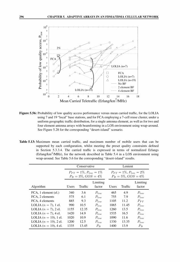
296 CHAPTER 5. ADAPTIVE ARRAYS IN AN FDMA/TDMA CELLULAR NETWORK
0 2 4 6 8 10 12 14 16 18
Mean Carried Teletraffic (Erlang/km2/MHz)
10-5
2
5
10-4
2
5
10-3
2
5
10-2
2
5
10-1
2
5
100
Prob
abili
tyof
low
qual
ityac
cess
,Plo
w
1%
2%
FCA
LOLIA (n=19)
LOLIA (n=7)
4 element BF2 element BFNo BFLOLIA (n=19)LOLIA (n=7)FCA
Figure 5.56: Probability of low quality access performance versus mean carried traffic, for the LOLIAusing 7 and 19 “local” base stations, and for FCA employing a 7-cell reuse cluster, under auniform geographic traffic distribution, for a single antenna element, as well as for two andfour element antenna arrays with beamforming in a LOS environment using wrap-around.See Figure 5.28 for the corresponding “desert-island” scenario.
Table 5.13: Maximum mean carried traffic, and maximum number of mobile users that can besupported by each configuration, whilst meeting the preset quality constraints definedin Section 5.3.3.4. The carried traffic is expressed in terms of normalized Erlangs(Erlang/km2/MHz), for the network described in Table 5.4 in a LOS environment usingwrap-around. See Table 5.6 for the corresponding “desert-island” results.
Conservative Lenient
PF T = 1%, Plow = 1% PF T = 1%, Plow = 2%PB = 3%, GOS = 4% PB = 5%, GOS = 6%
Limiting LimitingAlgorithm Users Traffic factor Users Traffic factor
FCA, 1 element (el.) 340 3.6 Plow 465 4.9 Plow
FCA, 2 elements 575 6.1 Plow 755 7.9 Plow
FCA, 4 elements 885 9.3 Plow 1105 11.2 PF T
LOLIA (n = 7), 1 el. 990 10.5 Plow 1065 11.45 Plow
LOLIA (n = 7), 2 el. 1155 12.35 Plow 1260 13.5 Plow
LOLIA (n = 7), 4 el. 1420 14.9 Plow 1535 16.5 Plow
LOLIA (n = 19), 1 el. 1020 10.9 Plow 1090 11.6 Plow
LOLIA (n = 19), 2 el. 1200 12.5 Plow 1330 13.35 Plow
LOLIA (n = 19), 4 el. 1335 13.45 PB 1400 13.9 PB

5.6. NETWORK PERFORMANCE RESULTS 297
2 4 6 8 10 12 14 16 18
Mean Carried Teletraffic (Erlang/km2/MHz)
0
10
20
30
40
50
60
Mea
nnu
mbe
rof
hand
over
spe
rca
ll4 element BF2 element BFNo BFLOLIA (n=19)LOLIA (n=7)FCA
Figure 5.57: Mean number of handovers per call versus mean carried traffic, for comparison of theLOLIA using 7 and 19 “local” base stations, and for FCA employing a 7-cell reuse cluster,under a uniform geographic traffic distribution, for a single antenna element, as well asfor two and four element antenna arrays with beamforming in a LOS environment usingwrap-around. See Figure 5.30 for the corresponding “desert-island” scenario.
5.6.3.2 Performance Results over a Multipath Channel
Following our previous experiments, where a purely LOS environment existed between themobiles and their base stations, this section presents results for a multipath environment usingtwo-, four- and eight-element AAAs.
Comparing the call blocking probabilities of the multipath environment, shown inFigure 5.58, with those of the LOS environment, shown in Figure 5.53, reveals that all ofthe channel allocation algorithms behave similarly for both radio environments. The FCAscheme actually behaved more unfavorably in terms of its new call blocking probability, asthe number of AAA elements was increased. However, this is a consequence of the additionalantenna elements improving the other performance measures, such as the call dropping rate.This enabled additional calls to be sustained at a given time, leading to a higher call blockingrate. In conjunction with an exclusion zone of 19 cells we found that the LOLIA’s blockingperformance was barely affected by the adaptive antenna arrays, whilst for n = 7 the blockedcall rate was improved by a factor of 10 at a traffic load of 14–17 Erlang/km2/MHz.
Figure 5.59 shows the probability of a dropped call in a multipath propagation environ-ment, which was slightly higher than for the LOS scenario of Figure 5.54, when consideredin the context of a given channel allocation algorithm and for a given antenna array size. Thecall dropping rate was improved with the aid of adaptive antenna arrays for all of the channelallocation algorithms, though the LOLIA using n = 19 did not benefit to the same extent asthe other algorithms.
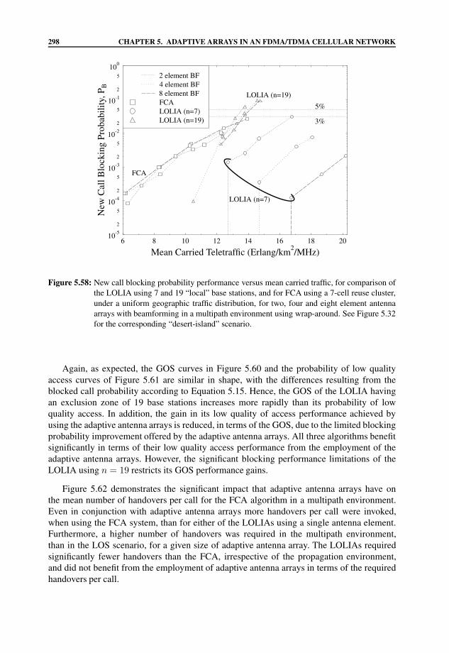
298 CHAPTER 5. ADAPTIVE ARRAYS IN AN FDMA/TDMA CELLULAR NETWORK
6 8 10 12 14 16 18 20
Mean Carried Teletraffic (Erlang/km2/MHz)
10-5
2
5
10-4
2
5
10-3
2
5
10-2
2
5
10-1
2
5
100
New
Cal
lBlo
ckin
gPr
obab
ility
,PB
3%
5%
FCA
LOLIA (n=19)
LOLIA (n=7)
LOLIA (n=19)LOLIA (n=7)FCA8 element BF4 element BF2 element BF
Figure 5.58: New call blocking probability performance versus mean carried traffic, for comparison ofthe LOLIA using 7 and 19 “local” base stations, and for FCA using a 7-cell reuse cluster,under a uniform geographic traffic distribution, for two, four and eight element antennaarrays with beamforming in a multipath environment using wrap-around. See Figure 5.32for the corresponding “desert-island” scenario.
Again, as expected, the GOS curves in Figure 5.60 and the probability of low qualityaccess curves of Figure 5.61 are similar in shape, with the differences resulting from theblocked call probability according to Equation 5.15. Hence, the GOS of the LOLIA havingan exclusion zone of 19 base stations increases more rapidly than its probability of lowquality access. In addition, the gain in its low quality of access performance achieved byusing the adaptive antenna arrays is reduced, in terms of the GOS, due to the limited blockingprobability improvement offered by the adaptive antenna arrays. All three algorithms benefitsignificantly in terms of their low quality access performance from the employment of theadaptive antenna arrays. However, the significant blocking performance limitations of theLOLIA using n = 19 restricts its GOS performance gains.
Figure 5.62 demonstrates the significant impact that adaptive antenna arrays have onthe mean number of handovers per call for the FCA algorithm in a multipath environment.Even in conjunction with adaptive antenna arrays more handovers per call were invoked,when using the FCA system, than for either of the LOLIAs using a single antenna element.Furthermore, a higher number of handovers was required in the multipath environment,than in the LOS scenario, for a given size of adaptive antenna array. The LOLIAs requiredsignificantly fewer handovers than the FCA, irrespective of the propagation environment,and did not benefit from the employment of adaptive antenna arrays in terms of the requiredhandovers per call.

5.6. NETWORK PERFORMANCE RESULTS 299
6 8 10 12 14 16 18 20
Mean Carried Teletraffic (Erlang/km2/MHz)
10-5
2
5
10-4
2
5
10-3
2
5
10-2
2
5
10-1
2
5
100
Cal
lTer
min
atio
nPr
obab
ility
,PFT
1%
FCA
LOLIA (n=19)
LOLIA (n=7)
LOLIA (n=19)LOLIA (n=7)FCA8 element BF4 element BF2 element BF
Figure 5.59: Call dropping probability performance versus mean carried traffic, for comparison of theLOLIA using 7 and 19 “local” base stations, and for FCA using a 7-cell reuse cluster,under a uniform geographic traffic distribution, for two, four and eight element antennaarrays with beamforming in a multipath environment using wrap-around. See Figure 5.33for the corresponding “desert-island” scenario.
Table 5.14: Maximum mean carried traffic, and maximum number of mobile users that can besupported by each configuration, whilst meeting the preset quality constraints definedin Section 5.3.3.4. The carried traffic is expressed in terms of normalized Erlangs(Erlang/km2/MHz), for the network described in Table 5.4 in a multipath environmentusing wrap-around. See Table 5.7 for the corresponding “desert-island” results.
Conservative Lenient
PF T = 1%, Plow = 1% PF T = 1%, Plow = 2%PB = 3%, GOS = 4% PB = 5%, GOS = 6%
Limiting LimitingAlgorithm Users Traffic factor Users Traffic factor
FCA, 2 element (el.) 600 6.0 Plow 740 7.65 Plow
FCA, 4 elements 790 8.3 Plow 995 10.3 Plow
FCA, 8 elements 1085 11.2 Plow 1250 12.8 PF T
LOLIA (n = 7), 2 el. 1195 12.65 Plow 1290 13.7 Plow
LOLIA (n = 7), 4 el. 1370 14.35 Plow 1475 15.6 Plow
LOLIA (n = 7), 8 el. 1555 16.15 Plow 1700 17.7 Plow
LOLIA (n = 19), 2 el. 1235 12.65 Plow 1325 13.3 Plow
LOLIA (n = 19), 4 el. 1360 13.55 PB 1410 13.8 PF T
LOLIA (n = 19), 8 el. 1385 13.7 PB 1475 14.15 PB

300 CHAPTER 5. ADAPTIVE ARRAYS IN AN FDMA/TDMA CELLULAR NETWORK
6 8 10 12 14 16 18 20
Mean Carried Teletraffic (Erlang/km2/MHz)
10-5
2
5
10-4
2
5
10-3
2
5
10-2
2
5
10-1
2
5
100
Gra
deof
Serv
ice
(GO
S)
4%
6%
FCA
LOLIA (n=7)
LOLIA (n=19)
8 element BF4 element BF2 element BFLOLIA (n=19)LOLIA (n=7)FCA
Figure 5.60: GOS performance versus mean carried traffic, for the comparison of the LOLIA with 7and 19 “local” base stations, and for FCA using a 7-cell reuse cluster, under a uniformgeographic traffic distribution, for two, four and eight element antenna arrays withbeamforming in a multipath environment using wrap-around. See Figure 5.35 for thecorresponding “desert-island” scenario.
Table 5.14 presents results similar to those in Table 5.13, but for a multipath environment,with the bold values highlighting the adaptive antenna array sizes common to both setsof investigations. From this table it can be seen that the LOLIA using n = 19 carriesapproximately the same amount of traffic in the multipath scenario, which translates intoa similar network capacity to that of the LOS scenario of Table 5.13. Again, the number ofusers supported by the network is limited by the probability of a low quality access and by thenew call blocking probability. The performance of the LOLIA using n = 7 was interferencelimited, where the smaller reuse distance or exclusion zone led to numerous sources ofrelatively strong interference, all requiring interference cancellation. Hence, as the numberof adaptive antenna array elements increased, so did the number of users supported, with anaverage improvement of about 15% for each doubling of the number of array elements.
5.6.3.3 Performance over a Multipath Channel using Power Control
This section presents results obtained using the same wrap-around scenario of Section 5.6.1over a multipath channel using power control. The power control algorithm was the sameas that described in Section 5.6.2.3. The power control algorithm implemented attempted toindependently adjust the mobile and base station transmit powers, such that the UL and DLSINRs were within a given target SINR window. The use of a target SINR window allowed usto avoid constantly increasing and decreasing the transmission powers, which could lead topotential power control instabilities within the network. Furthermore, the effect of employing

5.6. NETWORK PERFORMANCE RESULTS 301
6 8 10 12 14 16 18 20
Mean Carried Teletraffic (Erlang/km2/MHz)
10-5
2
5
10-4
2
5
10-3
2
5
10-2
2
5
10-1
2
5
100
Prob
abili
tyof
low
qual
ityac
cess
,Plo
w
1%
2%
FCA
LOLIA (n=7)
LOLIA (n=19)
8 element BF4 element BF2 element BFLOLIA (n=19)LOLIA (n=7)FCA
Figure 5.61: Probability of low quality access performance versus mean carried traffic, for thecomparison of the LOLIA using 7 and 19 “local” base stations, and for FCA using a 7-cell reuse cluster, under a uniform geographic traffic distribution, for two, four and eightelement antenna arrays with beamforming in a multipath environment using wrap-around.See Figure 5.34 for the corresponding “desert-island” scenario.
a range of possible transmission powers is analogous to an inherent power control error plusslow fading phenomenon.
Figure 5.63 portrays the new call blocking probability versus the mean normalized carriedtraffic, expressed in terms of Erlangs/km2/MHz. The figure shows that using power controlin conjunction with the FCA algorithm resulted in a slight increase in the new call blockingprobability as a direct consequence of the improved call dropping probability shown inFigure 5.64. In contrast, the blocking probability of the LOLIA improved significantly due tousing power control, achieving a reduction by a factor of 4 to 34.
The new call blocking performance of the LOLIA was superior to that of the FCAalgorithm both with and without power control, as seen in Figure 5.63, which is a resultof the dynamic nature of the LOLIA. This enabled the LOLIA to allocate any of the availablechannels not used within the 7-cell exclusion zone (maximum of 7×8=56 channels in thisscenario) to a new call request. However, the FCA algorithm only had one carrier frequencyper base station, and therefore was less likely to be able to satisfy a new call request. Theaddition of power control to the LOLIA in conjunction with n = 7 led to a reduced newcall blocking probability. Specifically, the new call blocking probability with power controlwas reduced to near that achieved using twice the number of antenna elements without powercontrol. The higher new call blocking probability of the network using no power control canbe attributed to the lower average SINR values, which prevent new call initiation, whereas the

302 CHAPTER 5. ADAPTIVE ARRAYS IN AN FDMA/TDMA CELLULAR NETWORK
6 8 10 12 14 16 18 20
Mean Carried Teletraffic (Erlang/km2/MHz)
0
10
20
30
40
50
60
Mea
nnu
mbe
rof
hand
over
spe
rca
ll
8 element BF4 element BF2 element BFLOLIA (n=19)LOLIA (n=7)FCA
Figure 5.62: Mean number of handovers per call versus mean carried traffic, for comparison of theLOLIA using 7 and 19 “local” base stations, and for FCA using a 7-cell reuse cluster,under a uniform geographic traffic distribution, for two, four and eight element antennaarrays with beamforming in a multipath environment using wrap-around. See Figure 5.36for the corresponding “desert-island” scenario.
higher average SINR level of the network observed in Figure 5.38 in conjunction with powercontrol enables additional calls to commence.
Figure 5.64 shows that the call dropping probability was significantly reduced for boththe FCA algorithm and the LOLIA using n = 7, in conjunction with power control. TheFCA algorithm in conjunction with power control offered a call dropping probability closeto that of a similar network without power control, and using twice the number of adaptiveantenna elements. However, at traffic loads of below approximately 7 Erlangs/km2/MHz thecall dropping probability began to level off for the FCA algorithm. This phenomenon wasalso noticeable in the context of the LOLIA and resulted from the power control algorithmlimiting the maximum SINR, leading to a flatter call dropping profile than that of the networkwithout power control. Thus, at lower traffic loads the network without power control had ahigher average SINR as was evidenced by Figure 5.38, leading to less dropped calls. However,at higher levels of teletraffic the power control algorithm offered a lower call dropping rate,as a consequence of the lower levels of interference present when using the power controlscheme.
The FCA algorithm exhibited the greatest improvement in the probability of a low qualityaccess due to the implementation of power control, as shown in Figure 5.65. Using a twoelement adaptive antenna array in conjunction with the power control algorithm resulted in aprobability of low quality access approximately equal to that obtained using an eight elementadaptive array without power control. The LOLIA also benefited from invoking the power

5.6. NETWORK PERFORMANCE RESULTS 303
2 4 6 8 10 12 14 16 18 20 22
Mean Carried Teletraffic (Erlang/km2/MHz)
10-4
2
5
10-3
2
5
10-2
2
5
10-1
New
Cal
lBlo
ckin
gPr
obab
ility
,PB
3%
5%
FCA
LOLIA
8 element BF4 element BF2 element BFLOLIA (n=7) w/o PCLOLIA (n=7) with PCFCA w/o PCFCA with PC
Figure 5.63: New call blocking probability versus mean carried traffic of the LOLIA using 7 “local”base stations, and for FCA employing a 7-cell reuse cluster, for two and four elementantenna arrays, with and without power control using wrap-around. See Figure 5.39 forthe corresponding “desert-island” scenario.
2 4 6 8 10 12 14 16 18 20 22
Mean Carried Teletraffic (Erlang/km2/MHz)
10-3
2
5
10-2
2
5
10-1
Forc
edTe
rmin
atio
nPr
obab
ility
,PFT
1%
FCA
LOLIA
8 element BF4 element BF2 element BFLOLIA (n=7) w/o PCLOLIA (n=7) with PCFCA w/o PCFCA with PC
Figure 5.64: Call dropping probability versus mean carried traffic of the LOLIA using 7 “local”base stations, and for FCA employing a 7-cell reuse cluster, for two and four elementantenna arrays, with and without power control using wrap-around. See Figure 5.40 forthe corresponding “desert-island” scenario.

304 CHAPTER 5. ADAPTIVE ARRAYS IN AN FDMA/TDMA CELLULAR NETWORK
2 4 6 8 10 12 14 16 18 20 22
Mean Carried Teletraffic (Erlang/km2/MHz)
10-4
2
5
10-3
2
5
10-2
2
5
10-1
Prob
abili
tyof
low
qual
ityac
cess
,Plo
w
1%
2%
FCA
LOLIA (n=7)
8 element BF4 element BF2 element BFLOLIA (n=7) w/o PCLOLIA (n=7) with PCFCA w/o PCFCA with PC
Figure 5.65: Probability of low quality outage versus mean carried traffic of the LOLIA using 7 “local”base stations, and for FCA employing a 7-cell reuse cluster, for two and four elementantenna arrays, with and without power control using wrap-around. See Figure 5.41 forthe corresponding “desert-island” scenario.
control algorithm, but to a lesser extent, offering a performance close to that of an array withtwice the number of elements without power control.
The GOS performance gains of the FCA algorithm using power control seen inFigure 5.66, were somewhat reduced compared to those of the probability of a low qualityaccess in Figure 5.65, due to the similar blocking performances of the power-controlled andnon-power-controlled scenarios seen in Figure 5.63. Nonetheless, the GOS gains remainedquite high in Figure 5.66. The GOS gains of the LOLIA due to power control were also quitesubstantial, as seen in Figure 5.66.
The effect of power control on the mean number of handovers performed per call becomesexplicit in Figure 5.67. From this figure it can be seen for the FCA algorithm that withrespect to the number of handovers per call, the performance of the network employing powercontrol significantly exceeded that of the network without power control using an adaptiveantenna array of twice the number of antenna elements. The employment of power control inconjunction with the FCA algorithm led to a mean reduction by a factor of 4.4 in the numberof handovers. The inherently good performance of the LOLIA was also slightly improved onaverage.
A further advantage of using power control in a cellular mobile network is portrayed inFigure 5.68, which shows that the mean transmit power was reduced from the fixed transmitpower of 10 dBm due to power control. The mean transmit power of the FCA algorithmwas reduced the most with reductions varying from 4.5 dB to almost 9 dB at the lowesttraffic levels. Doubling the number of antenna elements comprising the base stations’ adaptiveantenna arrays from two to four, resulted in additional mean transmission power gains of

5.6. NETWORK PERFORMANCE RESULTS 305
2 4 6 8 10 12 14 16 18 20 22
Mean Carried Teletraf“c (Erlang/km2/MHz)
10-4
2
5
10-3
2
5
10-2
2
5
10-1
Gra
deof
Serv
ice
(GO
S)4%
6%
FCA
8 element BF4 element BF2 element BFLOLIA (n=7) w/o PCLOLIA (n=7) with PCFCA w/o PCFCA with PC
LOLIA (n=7)
Figure 5.66: GOS performance versus mean carried traffic of the LOLIA using 7 “local” base stations,and for FCA employing a 7-cell reuse cluster, for two and four element antenna arrays,with and without power control using wrap-around. See Figure 5.42 for the corresponding“desert-island” scenario.
2 4 6 8 10 12 14 16 18 20 22
Mean Carried Teletraffic (Erlang/km2/MHz)
0
5
10
15
20
25
30
35
40
45
50
Mea
nnu
mbe
rof
hand
over
spe
rca
ll
8 element BF4 element BF2 element BFLOLIA (n=7) w/o PCLOLIA (n=7) with PCFCA w/o PCFCA with PC
Figure 5.67: Mean number of handovers per call versus mean carried traffic of the LOLIA using7 “local” base stations, and for FCA employing a 7-cell reuse cluster, for two andfour element antenna arrays, with and without power control using wrap-around. SeeFigure 5.43 for the corresponding “desert-island” scenario.

306 CHAPTER 5. ADAPTIVE ARRAYS IN AN FDMA/TDMA CELLULAR NETWORK
2 4 6 8 10 12 14 16 18 20 22
Mean Carried Teletraffic (Erlang/km2/MHz)
0
1
2
3
4
5
6
7
8
9
10
Mea
nT
rans
mis
sion
Pow
er(d
Bm
)
FCA
LOLIA
LOLIA (n=7) 4 elementsLOLIA (n=7) 2 elementsFCA 4 elementsFCA 2 elementsBasestation transmit powerMobile transmit power
Figure 5.68: Mean transmit power versus mean carried traffic of the LOLIA using 7 “local” basestations, and for FCA employing a 7-cell reuse cluster, for two and four element antennaarrays, with and without power control using wrap-around. See Figure 5.44 for thecorresponding “desert-island” scenario.
almost 1 dB at higher traffic loads, which is a consequence of the extra interference rejectioncapability of the four element array. The mean transmission powers of the LOLIAs weresignificantly higher due to the higher target SINRs required for maintaining an acceptablecall dropping rate. This was a consequence of the dynamic nature of the LOLIA, leading tomore rapidly changing interference levels, which required a relatively high target SINR of31 dB as seen in Table 5.8.
Table 5.15 presents similar results to Table 5.14, but using our power control algorithm,with the bold values highlighting the adaptive antenna array sizes common to both setsof investigations, for the sake of convenient comparison. The table shows the significantperformance improvement obtained for both the LOLIA and the FCA algorithm in termsof the number of users supported with the advent of power control, whilst maintaining thedesired network quality. In the conservative scenario, for example, the FCA algorithm usinga two element adaptive antenna array and power control supported the same number of usersas the network using an eight element adaptive antenna array without power control. TheLOLIA-based network, however, did not benefit from the employment of the power controlalgorithm to the same extent, although it still offered similar performance to that of a networkwithout power control and using adaptive antenna arrays having twice the number of antennaelements.

5.6. NETWORK PERFORMANCE RESULTS 307
Table 5.15: Maximum mean carried traffic, and maximum number of mobile users that can besupported by each configuration, whilst meeting the preset quality constraints definedin Section 5.3.3.4. The carried traffic is expressed in terms of normalized Erlangs(Erlang/km2/MHz), for the network described in Table 5.4 in a multipath environment withand without power control using wrap-around.
Conservative Lenient
PF T = 1%, Plow = 1% PF T = 1%, Plow = 2%PB = 3%, GOS = 4% PB = 5%, GOS = 6%
Limiting LimitingAlgorithm Users Traffic factor Users Traffic factor
4-QAM without PCFCA, 2 element (el.) 600 6.0 Plow 740 7.65 Plow
FCA, 4 elements 790 8.3 Plow 995 10.3 Plow
FCA, 8 elements 1085 11.2 Plow 1250 12.8 PF T
LOLIA (n = 7), 2 el. 1195 12.65 Plow 1290 13.7 Plow
LOLIA (n = 7), 4 el. 1370 14.35 Plow 1475 15.6 Plow
LOLIA (n = 7), 8 el. 1555 16.15 Plow 1700 17.7 Plow
4-QAM with PCFCA, 2 elements (el.) 1090 10.6 Plow 1120 10.85 PF T
FCA, 4 elements 1370 13.28 PF T 1370 13.28 PF T
LOLIA (n = 7), 2 el. 1350 14.05 Plow 1445 15.1 Plow
LOLIA (n = 7), 4 el. 1540 16.15 Plow 1640 17.35 Plow
5.6.3.4 Performance of an AQAM based Network using Power Control
This section presents our simulation results obtained for a network using burst-by-burst adap-tive modulation [13, 209, 398, 399] invoked in order to improve the network’s performance.Simulations were conducted for both a standard 7-cell FCA scheme and a 7-cell LOLIAassisted system. The results obtained for a 4-QAM based network using power control wereincluded for comparison purposes.
The new call blocking probability depicted in Figure 5.69 was essentially unchanged forthe FCA algorithm using power control in conjunction with 4-QAM or AQAM, suggestingthat the new call blocking performance of the FCA algorithm was limited by the lack ofavailable frequency/timeslot combinations, rather than by inadequate signal quality. Thishypothesis was confirmed by the improvement in the new call blocking performance of theLOLIA resulting from the superior signal quality of AQAM.
The corresponding call dropping probability is depicted in Figure 5.70. The AQAMLOLIA using n = 7 in conjunction with a two element adaptive antenna had, in general, ahigher call dropping probability compared to that of power control assisted 4-QAM. However,the power control algorithm, when used in conjunction with AQAM, maintained the calldropping probability below the given threshold for a significantly higher traffic load. Similarperformance trends were observed for both the two element and the four element adaptivearray, although the higher interference rejection capability offered by the four element arrayresulted in a substantially reduced call dropping probability. The dropped calls were caused

308 CHAPTER 5. ADAPTIVE ARRAYS IN AN FDMA/TDMA CELLULAR NETWORK
2 4 6 8 10 12 14 16 18 20 22 24 26
Mean Carried Teletraffic (Erlang/km2/MHz)
10-4
2
5
10-3
2
5
10-2
2
5
10-1
New
Cal
lBlo
ckin
gPr
obab
ility
,PB
3%
5%
FCA
LOLIA
4 element BF2 element BFLOLIA (n=7) AQAM PCLOLIA (n=7) 4-QAM PCFCA AQAM PCFCA 4-QAM PC
Figure 5.69: New call blocking probability versus mean carried traffic of the LOLIA using 7 “local”base stations, and for FCA employing a 7-cell reuse cluster, for two and four elementantenna arrays, with and without AQAM using wrap-around. See Figure 5.46 for thecorresponding “desert-island” scenario.
2 4 6 8 10 12 14 16 18 20 22 24 26
Mean Carried Teletraffic (Erlang/km2/MHz)
10-3
2
5
10-2
2
5
10-1
Cal
lTer
min
atio
nPr
obab
ility
,PFT
1%
FCA, 4-QAM PC
FCA,AQAM PC
LOLIA, 4-QAM PC
LOLIA, AQAM PC
4 element BF2 element BFLOLIA (n=7) AQAM PCLOLIA (n=7) 4-QAM PCFCA AQAM PCFCA 4-QAM PC
Figure 5.70: Call dropping, or forced termination, performance versus mean carried traffic of theLOLIA using 7 “local” base stations, and for FCA employing a 7-cell reuse cluster, fortwo and four element antenna arrays, with and without AQAM using wrap-around. SeeFigure 5.47 for the corresponding “desert-island” scenario.

5.6. NETWORK PERFORMANCE RESULTS 309
2 4 6 8 10 12 14 16 18 20 22 24 26
Mean Carried Teletraffic (Erlang/km2/MHz)
0
5
10
15
20
Mea
nnu
mbe
rof
hand
over
spe
rca
ll
FCA, 4-QAM PC
FCA, AQAM PC
LOLIA, 4-QAM PC
LOLIA, AQAM PC
4 element BF2 element BFLOLIA (n=7) AQAM PCLOLIA (n=7) 4-QAM PCFCA AQAM PCFCA 4-QAM PC
Figure 5.71: Mean number of handovers per call versus mean carried traffic of the LOLIA using 7“local” base stations, and for FCA employing a 7-cell reuse cluster, for two and fourelement antenna arrays, with and without AQAM using wrap-around. See Figure 5.50 forthe corresponding “desert-island” scenario.
almost exclusively by insufficient signal quality during the intra-cell handover process, thusincreasing the number of adaptive antenna elements from two to four improved the calldropping performance. The high call dropping probability observed for traffic loads between12 and 20 Erlangs/km2/MHz when using the two element adaptive antenna array was dueto the power control and AQAM attempting to trade-off modem throughput and transmitpower against each other, whilst attempting to minimize the number of dropped calls. Theextra interference suppression capability of the four-element adaptive antenna array led to areduced call dropping probability. Hence, altering the AQAM mode selection algorithm ofFigure 5.45, may improve its performance at these traffic loads, when used in conjunctionwith a two element antenna array.
The FCA algorithm dropped all of its calls during the inter-cell handover process dueto the lack of available slots to handover to. However, since inter-cell handovers couldbe performed, if necessary, in order to improve the signal quality, the number of droppedcalls was reduced when using the four element adaptive array, due to its better interferencerejection capability. All the calls were dropped during the inter-cell handover process, whichmeans that no calls were dropped due to insufficient SINR or through the intra-cell handoverprocess. This can be attributed to the AQAM scheme, which enabled users to drop to lowerorder modulation modes of the AQAM scheme, when the SINR became poor.
Figure 5.71 characterizes the mean number of handovers per call for 4-QAM and AQAM,both using power control. The LOLIA using n = 7 performed a lower total number ofhandovers per call, when using AQAM, due its inherent resilience to poor signal qualityconditions.

310 CHAPTER 5. ADAPTIVE ARRAYS IN AN FDMA/TDMA CELLULAR NETWORK
2 4 6 8 10 12 14 16 18 20 22 24 26
Mean Carried Teletraffic (Erlang/km2/MHz)
0
1
2
3
4
5
6
7
8
Mea
nnu
mbe
rof
hand
over
spe
rca
ll4 element BF2 element BFLOLIA (n=7) AQAM PC Intra-cell HOsLOLIA (n=7) AQAM PC Inter-cell HOsFCA AQAM PC Intra-cell HOsFCA AQAM PC Inter-cell HOs
Figure 5.72: Mean number of inter-cell and intra-cell handovers per call versus mean carried traffic ofthe LOLIA using 7 “local” base stations, and for FCA employing a 7-cell reuse cluster,for two and four element antenna arrays, in conjunction with AQAM using wrap-around.
The breakdown of the handovers into inter-cell and intra-cell handovers is given inFigure 5.72. Observe that the improved interference rejection capability, and the associatedsuperior SINR of the four-element array results in a lower number of intra-cell handoversfor the LOLIA. Since the intra-cell handover process is the primary cause of dropped callsand less intra-cell handovers are performed when using a four-element antenna, more inter-cell handovers are necessitated in the network using four-element adaptive antenna arrays,as the users roam from cell to cell. In other words, since the LOLIA using a four elementarray drops less calls than when using a two element array, more users are in call at a giventime, and hence these users cross more cell boundaries, thus necessitating more inter-cellhandovers.
In contrast, the number of intra-cell handovers performed in conjunction with the FCAalgorithm decreases, as the teletraffic rises, and as the number of antenna elements isincreased from two to four. This is a consequence of the particular implementation ofthe modulation mode selection/power control algorithm and its interaction with the FCAhandover process. The AQAM algorithm attempts to remain in the current modulation modeas long as possible, and hence as the SINR degrades, it will opt for performing an intra-cell handover in an attempt to maintain the SINR, rather than reconfiguring itself in order touse a lower-order modulation mode suitable for the reduced SINR level. Thus, when using afour-element adaptive antenna array, the average (and instantaneous) SINR is typically higherthan that of a two-element array, leading to a more frequent employment of the less resilienthigher-order modulation modes, which potentially requires additional intra-cell handovers.However, as the mean teletraffic increases, so does the level of interference in the networkand a greater proportion of transmission time is spent in the lower-order modulation modes,thus requiring less intra-cell handovers, as illustrated in Figure 5.72.

5.6. NETWORK PERFORMANCE RESULTS 311
2 4 6 8 10 12 14 16 18 20 22 24 26
Mean Carried Teletraffic (Erlang/km2/MHz)
10-4
2
5
10-3
2
5
10-2
2
5
10-1
Prob
abili
tyof
low
qual
ityac
cess
,Plo
w
2%
1%
FCA
LOLIA
4 element BF2 element BFLOLIA (n=7) AQAM PCLOLIA (n=7) 4-QAM PCFCA AQAM PCFCA 4-QAM PC
Figure 5.73: Probability of low quality access versus mean carried traffic of the LOLIA using 7 “local”base stations, and for FCA employing a 7-cell reuse cluster, for two and four elementantenna arrays, with and without AQAM using wrap-around. See Figure 5.48 for thecorresponding “desert-island” scenario.
The probability of a Low Quality (LQ) access is depicted in Figure 5.73, showing aninteresting interaction between the FCA algorithm and the AQAM scheme. The probabilityof an LQ access occurring is reduced, as the traffic level increases and the number of antennaelements is decreased. This can be attributed to the less frequent usage of the higher-ordermodulation modes at the higher traffic loads. Hence the lower-order modulation modes areused more frequently and thus the chance of an LQ access taking place is reduced. The four-element adaptive antenna array leads to a higher probability of a low quality access, since itshigher associated SINR levels activate a more frequent employment of the less robust, buthigher-throughput, higher-order modulation modes. For example, let us consider the FCAAQAM PC scenario supporting 400 users, which corresponded to a traffic load of about 4Erlang/km2/MHz. When using two antenna array elements, 85% of the LQ accesses occurredwhilst in the 16-QAM mode, however, on increasing the number of antenna array elementsto four this rose to 93%.
However, as the network loading rises, an increasing proportion of the LQ outages occurin the BPSK modulation mode. Coupled with the increase in the BPSK modulation mode’semployment due to the low SINR constraints, the probability of a low quality outage isexpected to increase at a certain traffic load. This can be seen in Figure 5.73, where the LQoutage probability is starting to rise for FCA in conjunction with both two and four elements,though the extra interference suppression capability of the four element array allows extratraffic to be carried, before this phenomenon commences. More specifically, although notexplicit in Figure 5.73, we found that for a network supporting 1200 users, correspondingto a traffic load of about 12 Erlang/km2/MHz, and employing two element adaptive antennaarrays, 43% of the LQ accesses occurred, whilst in the 16-QAM mode, versus 72% with four-

312 CHAPTER 5. ADAPTIVE ARRAYS IN AN FDMA/TDMA CELLULAR NETWORK
2 4 6 8 10 12 14 16 18 20 22 24 26
Mean Carried Teletraffic (Erlang/km2/MHz)
10-4
2
5
10-3
2
5
10-2
2
5
10-1
Gra
deof
Serv
ice
(GO
S)
4%
6%
FCA, AQAM
FCA,4-QAM PC
LOLIA,4-QAM PC
LOLIA, AQAM
4 element BF2 element BFLOLIA (n=7) AQAM PCLOLIA (n=7) 4-QAM PCFCA AQAM PCFCA 4-QAM PC
Figure 5.74: GOS performance versus mean carried traffic of the LOLIA using 7 “local” base stations,and for FCA employing a 7-cell reuse cluster, for two and four element antenna arrays,with and without AQAM using wrap-around. See Figure 5.49 for the corresponding“desert-island” scenario.
element antenna arrays. Again, not explicitly shown in the figure, but increasing the numberof users to 1400, or a traffic load of just less than 14 Erlang/km2/MHz, reduced the numberof 16-QAM LQ accesses, but increased the BPSK LQ outages to 69% and 31% for the two-and four-element arrays respectively, with reductions to 21% and 53% of the LQ outages inthe 16-QAM mode.
From Figure 5.74 it can be seen that the GOS, as defined in Section 5.3.3.4, of the FCAalgorithm did not benefit from invoking AQAM to the same extent as the LOLIA. Thisresulted from the fairly similar probability of low quality access performance of the twoand four element antenna array assisted systems in Figure 5.73, and the limiting blockingperformance observed in Figure 5.69. However, since the LOLIA did not suffer from theselimiting factors, its GOS improved due to the employment of both adaptive antenna arraysand AQAM techniques.
The average modem throughput expressed in bits per symbol versus the mean carriedteletraffic is shown in Figure 5.75, demonstrating that the mean number of bits per symbolthroughput of the users decreased, as the number of users supported increased. The FCAalgorithm offered the lowest throughput and its performance degraded near-linearly uponincreasing the number of users supported. At the user capacity limits of 1400 and 1565users, the mean modem throughput was 2.45 BPS and 2.35 BPS for the conservative andlenient scenarios, respectively, using two element adaptive antenna arrays. Using four elementadaptive antenna arrays the corresponding throughputs were 2.7 BPS and 2.6 BPS. TheLOLIA, especially for lower levels of traffic, offered a higher modem throughput for a givenlevel of teletraffic carried, with the BPS throughput performance gracefully decreasing, as the

5.6. NETWORK PERFORMANCE RESULTS 313
2 4 6 8 10 12 14 16 18 20 22 24 26
Mean Carried Teletraffic (Erlang/km2/MHz)
0.0
0.5
1.0
1.5
2.0
2.5
3.0
3.5
4.0
Ave
rage
thro
ughp
ut(b
its/s
ymbo
l)
4-QAM = 2 bits/symbol
BPSK = 1 bit/symbol
LOLIA (n=7) AQAM PC
FCA AQAM PC
4 element BF2 element BFLOLIA (n=7) AQAM PCFCA AQAM PC
Figure 5.75: Mean throughput of users in terms of bits per symbol versus mean carried traffic of theLOLIA using 7 “local” base stations, and for FCA employing a 7-cell reuse cluster, fortwo and four element antenna arrays, using AQAM using wrap-around. See Figure 5.52for the corresponding “desert-island” scenario.
2 4 6 8 10 12 14 16 18 20 22 24 26
Mean Carried Teletraffic (Erlang/km2/MHz)
3
4
5
6
7
8
9
10
Mea
nT
rans
mis
sion
Pow
er(d
Bm
)
LOLIA
FCA
LOLIA (n=7) 4 elementsLOLIA (n=7) 2 elementsFCA 4 elementsFCA 2 elementsBasestation transmit powerMobile transmit power
Figure 5.76: Mean transmit power versus mean carried traffic of the LOLIA using 7 “local” basestations, and for FCA employing a 7-cell reuse cluster, for two and four element antennaarrays, using AQAM using wrap-around. See Figure 5.48 for the corresponding “desert-island” scenario.

314 CHAPTER 5. ADAPTIVE ARRAYS IN AN FDMA/TDMA CELLULAR NETWORK
Table 5.16: Maximum mean carried traffic, and maximum number of mobile users that can besupported by each configuration, whilst meeting the preset quality constraints definedin Section 5.3.3.4. The carried traffic is expressed in terms of normalized Erlangs(Erlang/km2/MHz), for the network described in Table 5.4 in a multipath environment withand without power control and AQAM using wrap-around.
Conservative Lenient
PF T = 1%, Plow = 1% PF T = 1%, Plow = 2%GOS = 4%, PB = 3% GOS = 6%, PB = 5%
Limiting LimitingAlgorithm Users Traffic factor Users Traffic factor
4-QAM without PCFCA, 2 elements (el.) 600 6.0 Plow 740 7.65 Plow
FCA, 4 elements 790 8.3 Plow 995 10.3 Plow
LOLIA (n = 7), 2 el. 1195 12.65 Plow 1290 13.7 Plow
LOLIA (n = 7), 4 el. 1370 14.35 Plow 1475 15.6 Plow
4-QAM with PCFCA, 2 elements 1090 10.6 Plow 1120 10.85 PF T
FCA, 4 elements 1370 13.275 PF T 1370 13.275 PF T
LOLIA (n = 7), 2 el. 1350 14.05 Plow 1445 15.1 Plow
LOLIA (n = 7), 4 el. 1540 16.15 Plow 1640 17.35 Plow
AQAM with PCFCA, 2 elements 1400 13.8 PB 1565 15.20 PB
FCA, 4 elements 1415 13.7 PB 1575 15.15 PB
LOLIA (n = 7), 2 el. 1910 19.75 BPS 1910 19.75 BPSLOLIA (n = 7), 4 el. 2245 23.25 BPS 2245 23.25 BPS
carried teletraffic continued to increase. The capacity limiting factor of the LOLIA was thethroughput restriction of 2.0 BPS.
The mean transmission power results of Figure 5.76 demonstrate that the employmentof AQAM is capable of reducing the power transmitted, both for the UL and the DL. Atlow traffic levels the FCA algorithm performed noticeably worse in transmitted power terms,than the LOLIA. However, as the traffic load increased, the difference became negligible.The mean power reduction, when compared to a fixed transmission power of 10 dBm, variedfrom approximately 1 dB to more than 6 dB. A 1 dB reduction in transmission power is notparticularly significant for the mobile user, especially since at this network load a throughputof just 2 bits/symbol is possible. The difference between the network using AQAM and thatwithout, though, is the overall improved call quality that can be achieved in the context of ourperformance metrics, and the significantly increased number of users that can be supportedby the network Again, the constraint of a minimum throughput of 2 bits/symbol was invokedin order to ensure a fair comparison with the fixed 4-QAM based network.
Table 5.16 shows the performance of the various networks using AQAM with powercontrol, as well as 4-QAM with and without power control, in terms of the number of userssupported. A mean increase of 61% was achieved in terms of the number of users by the

5.7. SUMMARY AND CONCLUSIONS 315
addition of power control to the FCA algorithm based 4-QAM network. Invoking AQAMand power control led to a further average user capacity increase of almost 22%, with anyfurther gains limited by the lack of free frequency/timeslot combinations available for newcalls to start. Therefore, since the network capacity of the FCA algorithm when using adaptivemodulation was not limited by co-channel interference, it would be possible to reduce thefrequency re-use distance to increase the network capacity.
The performance of the LOLIA was not limited in this sense, however, and the additionof power control to the 4-QAM network provided an mean increase of 12% extra userssupported. In conjunction with AQAM techniques this user capacity was further extendedby an average of 39%, thus supporting an additional 56% more users, when compared to the4-QAM network using no power control.
5.7 Summary and Conclusions
In this chapter we have examined the network capacity and performance of the FCA algorithmand the LOLIA using an exclusion zone of seven or 19 base stations, in the context of LOSand multipath propagation environments. We have shown that the addition of power controlresults in a substantially increased number of supported users, additionally benefiting from asuperior call quality, and reduced transmission power for a given number of adaptive antennaarray elements located at the base stations. The advantages of using AQAM within a mobilecellular network have also been illustrated, resulting in performance improvements in termsof the mean modem throughout, call quality, mean transmission power and the number ofsupported users. The next chapter involves the investigation of network capacity in the contextof a CDMA-based UMTS-type FDD mode network.


Chapter 6HSDPA-style FDD Networking,Adaptive Arrays and AdaptiveModulation
6.1 Introduction
In January 1998, the European standardization body for third generation mobile radiosystems, the European Telecommunications Standards Institute—Special Mobile Group(ETSI SMG), agreed upon a radio access scheme for third generation mobile radio systems,referred to as the Universal Mobile Telecommunication System (UMTS) [11, 59]. Althoughthis chapter was detailed in Chapter 1, here we provide a rudimentary introduction to thesystem, in order to allow readers to consult this chapter directly, without having to readChapter 1 first. Specifically, the UMTS Terrestrial Radio Access (UTRA) supports two modesof duplexing, namely Frequency Division Duplexing (FDD) , where the UL and DL aretransmitted on different frequencies, and Time Division Duplexing (TDD) , where the UL andthe DL are transmitted on the same carrier frequency, but multiplexed in time. The agreementrecommends the employment of Wideband Code Division Multiple Access (W-CDMA) forUTRA FDD and Time Division—Code Division Multiple Access (TD-CDMA) for UTRATDD. TD-CDMA is based on a combination of Time Division Multiple Access (TDMA) andCDMA, whereas W-CDMA is a pure CDMA-based system. The UTRA scheme can be usedfor operation within a minimum spectrum of 2×5 MHz for UTRA FDD and 5 MHz for UTRATDD. Both duplex or paired and simplex or unpaired frequency bands have been identifiedin the region of 2 GHz to be used for the UTRA third generation mobile radio system. Bothmodes of UTRA have been harmonized with respect to the basic system parameters, suchas carrier spacing, chip rate and frame length. Thereby, FDD/TDD dual mode operation isfacilitated, which provides a basis for the development of low cost terminals. Furthermore,the interworking of UTRA with GSM [11] is ensured.
3G, HSPA and FDD versus TDD Networking Second EditionL. Hanzo, J. S. Blogh and S. Ni c© 2008 John Wiley & Sons, Ltd

318 CHAPTER 6. HSDPA-STYLE FDD NETWORKING, ADAPTIVE ARRAYS AND AQAM
In UTRA, the different service needs are supported in a spectrally efficient way by acombination of FDD and TDD. The FDD mode is intended for applications in both macro-and micro-cellular environments, supporting data rates of up to 384 kbps and high mobility.The TDD mode, on the other hand, is more suited to micro and pico-cellular environments,as well as for licensed and unlicensed cordless and wireless local loop applications. It makesefficient use of the unpaired spectrum—for example in wireless Internet applications, wheremuch of the teletraffic is in the DL—and supports data rates of up to 2 Mbps. Therefore, theTDD mode is particularly well suited for environments generating a high traffic density (e.g.in city centres, business areas, airports etc.) and for indoor coverage, where the applicationsrequire high data rates and tend to have highly asymmetric traffic again, as in Internet access.
In parallel to the European activities, extensive work has been carried out also in Japanand the USA on third generation mobile radio systems. The Japanese standardization bodyknown as the Association of Radio Industry and Business (ARIB) also opted for using W-CDMA, and the Japanese as well as European proposals for FDD bear strong similarities.Similar concepts have also been developed by the North-American T1 standardization bodyfor the pan-American third generation (3G) system known as cdma2000, which was alsodescribed in Chapter 1 [11].
In order to work towards a truly global third generation mobile radio standard, the ThirdGeneration Partnership Project (3GPP) was formed in December 1998. 3GPP consists ofmembers of the standardization bodies in Europe (ETSI), the US (T1), Japan (ARIB), Korea(TTA—Telecommunications Technologies Association), and China (CWTS—China Wire-less Telecommunications Standard). 3GPP merged the already well harmonized proposals bythe regional standardization bodies and now works towards a single common third generationmobile radio standard under the terminology UTRA, retaining its two modes, and aiming tooperate on the basis of the evolved GSM core network. The Third Generation PartnershipProject 2 (3GPP2), on the other hand, works towards a third generation mobile radiostandard, which is based on an evolved IS-95 type system which was originally referred to ascdma2000 [11]. In June 1999, major international operators in the Operator HarmonizationGroup (OHG) proposed a harmonized G3G (Global Third Generation) concept, which hasbeen accepted by 3GPP and 3GPP2. The harmonized G3G concept is a single standard withthe following three modes of operation:
• CDMA direct spread (CDMA-DS), based on UTRA FDD as specified by 3GPP.
• CDMA multi-carrier (CDMA-MC), based on cdma2000 using FDD as specified by3GPP2.
• TDD (CDMA TDD) based on UTRA TDD as specified by 3GPP.
6.2 Direct Sequence Code Division Multiple Access
A rudimentary introduction to CDMA was provided in Chapter 1 in the context of single-userreceivers, while in Chapter 3 the basic concepts of multi-user detection have been introduced.However, as noted earlier, our aim is to allow reader to consult this chapter directly, withouthaving to refer back to the previous chapters. Hence here a brief overview of the underlyingCDMA basics is provided.

6.2. DIRECT SEQUENCE CODE DIVISION MULTIPLE ACCESS 319
Code
Time
Freq
uenc
y
Freq
uenc
y
Freq
uenc
y
TimeTime
User 1
User 2 Use
r1
Use
r2
21
User 3
Figure 6.1: Multiple access schemes: FDMA (left), TDMA (middle) and CDMA (right).
Traditional ways of separating signals in time using TDMA and in frequency ensure thatthe signals are transmitted orthogonal in either time or frequency and hence they are non-interfering. In CDMA different users are separated employing a set of waveforms exhibitinggood correlation properties, which are known as spreading codes. Figure 6.1 illustrates theprinciples of FDMA, TDMA and CDMA. More explicitly, FDMA uses a fraction of thetotal FDMA frequency band for each communications link for the whole duration of aconversation, while TDMA uses the entire bandwidth of a TDMA channel for a fraction of theTDMA frame, namely for the duration of a timeslot. Finally, CDMA uses the entire availablefrequency band all the time and separates the users with the aid of unique, orthogonal usersignature sequences.
In a CDMA digital communications system, such as that shown in Figure 6.2, the datastream is multiplied by the spreading code, which replaces each data bit with a sequence ofcode chips. A chip is defined as the basic element of the spreading code, which typicallyassumes binary values. Hence, the spreading process consists of replacing each bit in theoriginal user’s data sequence with the complete spreading code. The chip rate is significantlyhigher than the data rate, hence causing the bandwidth of the user’s data to be spread, asshown in Figure 6.2.
At the receiver, the composite signal containing the spread data of multiple users ismultiplied by a synchronized version of the spreading code of the wanted user. The specificauto-correlation properties of the codes allow the receiver to identify and recover eachdelayed, attenuated and phase-rotated replica of the transmitted signal, provided that thesignals are separated by more than one chip period and the receiver has the capability oftracking each significant path. This is achieved using a Rake receiver [5] that can processmultiple delayed received signals. Coherent combination of these transmitted signal replicasallows the original signal to be recovered. The unwanted signals of the other simultaneoususers remain wideband, having a bandwidth equal to that of the noise, and appear asadditional noise with respect to the wanted signal. Since the bandwidth of the despreadwanted signal is reduced relative to this noise, the signal-to-noise ratio of the wanted signalis enhanced by the despreading process in proportion to the ratio of the spread and despreadbandwidths, since the noise power outside the useful despread signal’s bandwidth can be

320 CHAPTER 6. HSDPA-STYLE FDD NETWORKING, ADAPTIVE ARRAYS AND AQAM
A/SF
Signal
B
A
SF · BSpreading code
A/SF
Interferer
B
A
SF · BSpreading code
Despreading code
A/SF
A
Figure 6.2: CDMA Spreading and Despreading Processes
removed by a low-pass filter. This bandwidth ratio is equal to the ratio of the chip rate to thedata rate, which is known as the Processing Gain (PG). For this process to work efficiently,the signals of all of the users should be received at or near the same power at the receiver.This is achieved with the aid of power control, which is one of the critical elements of aCDMA system. The performance of the power control scheme directly affects the capacityof the CDMA network.
6.3 UMTS Terrestrial Radio Access
A bandwidth of 155 MHz has been allocated for UMTS services in Europe in the frequencyregion of 2.0 GHz. The paired bands of 1920-1980 MHz (UL) and 2110-2170 MHz (DL)have been set aside for FDD W-CDMA systems, and the unpaired frequency bands of 1900-1920 MHz and 2010-2025 MHz for TDD CDMA systems.
A UTRA Network (UTRAN) consists of one or several Radio Network Sub-systems(RNSs), which in turn consist of base stations (referred to as Node Bs) and Radio NetworkControllers (RNCs). A Node B may serve one or multiple cells. Mobile stations are known asUser Equipment (UE), which are expected to support multi-mode operation in order to enablehandovers between the FDD and TDD modes and, prior to complete UTRAN coverage, alsoto GSM. The key parameters of UTRA have been defined as in Table 6.1.

6.3. UMTS TERRESTRIAL RADIO ACCESS 321
Table 6.1: Key UTRA Parameters.
Duplex scheme FDD TDDMultiple access scheme W-CDMA TD-CDMAChip rate 3.84 Mchip/s 3.84 Mchip/sSpreading factor range 4–512 1–16Frequency bands 1920–1980 MHz (UL) 1900–1920 MHz
2110–2170 MHz (DL) 2010–2025 MHzModulation mode 4-QAM/QPSK 4-QAM/QPSKBandwidth 5 MHz 5 MHzNyquist pulse shaping 0.22 0.22Frame length 10 ms 10 msNumber of timeslots per frame 15 15
6.3.1 Spreading and Modulation
As usual, the UL is defined as the transmission path from the mobile station to the basestation, which receives the unsynchronized channel impaired signals from the network’smobiles. The base station has the task of extracting the wanted signal from the received signalcontaminated by both intra- and inter-cell interference. However, as described in Section 6.2,some degree of isolation between interfering users is achieved due to employing uniqueorthogonal spreading codes, although their orthogonality is destroyed by the hostile mobilechannel.
The spreading process consists of two operations. The first one is the channelizationoperation, which transforms every data symbol into a number of chips, thus increasing thebandwidth of the signal, as seen in Figure 6.2 of Section 6.2. The channelization codesin UTRA are Orthogonal Variable Spreading Factor (OVSF) codes [11] that preserve theorthogonality between a given user’s different physical channels, which are also capableof supporting multirate operation. These codes will be further discussed in the context ofFigure 6.4. The second operation related to the spreading, namely the “scrambling’ processthen multiplies the resultant signals separately on the I- and Q-branches by a complex-valuedscrambling code, as shown in Figure 6.3. The scrambling codes may be one of either 224
different “long” codes or 224 “short” UL scrambling codes.The Dedicated Physical Control CHannel (DPCCH) [11, 400] is spread to the chip rate
by the channelization code Cc, while the nth Dedicated Physical Data CHannel (DPDCH),namely DPDCHn, is spread to the chip rate by the channelization code Cd,n. One DPCCHand up to six parallel DPDCHs can be transmitted simultaneously, i.e. 1 ≤ n ≤ 6 (asseen in Figure 6.3). However, it is beneficial to transmit with the aid of a single DPDCH,if the required bit-rate can be provided by a single DPDCH for reasons of terminal amplifierefficiency. This is because multi-code transmissions increase the peak-to-average ratio ofthe transmission, which reduces the efficiency of the terminal’s power amplifier [59]. Themaximum user data rate achievable with the aid of a single code is derived from the maximumchannel bit rate, which is 960 kbps using a spreading factor of four without channel codingin the 1999 version of the UTRA standard. However, at the time of writing a spreading factorof one is being considered by the standardization body. With channel coding the maximum

322 CHAPTER 6. HSDPA-STYLE FDD NETWORKING, ADAPTIVE ARRAYS AND AQAM
Cd,1 βd
Cd,2 βd
Cd,4 βd
Cd,6 βd
Cc βd
Σ
Σ
I
Sdpch,n
S
DPDCH1
Cd,3 βd
Cd,5 βd
DPDCH3
DPDCH5
DPDCH2
DPDCH4
DPDCH6
DPCCH
Q
j
I+jQ
Figure 6.3: Spreading for UL DPCCH and DPDCHs.

6.3. UMTS TERRESTRIAL RADIO ACCESS 323
c
cch,1,1 = (1)
SF=4
cch,2,1 = (1, 1)
cch,2,2 = (1,−1)
cch,4,1 = (1, 1, 1, 1)
cch,4,2 = (1, 1,−1,−1)
cch,4,3 = (1,−1, 1,−1)
cch,4,4 = (1,−1,−1, 1)
(c, c)
(c,−c)
SF=2SF=1
Figure 6.4: Code tree for the generation of Orthogonal Variable Spreading Factor (OVSF) codes.
practical user data rate for single code transmission is of the order of 400–500 kbps. Forachieving higher data rates parallel multi-code channels are used. This allows up to sixparallel codes to be used, increasing the achievable channel bit rate up to 5740 kbps, whichcan accommodate a 2 Mbps user data rate or even higher data rates, when the channel codingrate is 1/2.
The OVSF codes [130] can be defined using the code tree of Figure 6.4. In Figure 6.4, thechannelization codes are uniquely described by Cch,SF,k, where SF is the spreading factorof the codes, and k is the code index where 0 ≤ k ≤ SF − 1. Each level in the code treedefines spreading codes of length SF, corresponding to a particular spreading factor of SF.The number of codes available for a particular spreading factor is equal to the spreadingfactor itself. All the codes of the same level in the code tree constitute a set and they areorthogonal to each other. Any two codes of different levels are also orthogonal to each other,as long as one of them is not the mother of the other code. For example, the codes c15(2),

324 CHAPTER 6. HSDPA-STYLE FDD NETWORKING, ADAPTIVE ARRAYS AND AQAM
c7(1) and c3(1) are all the mother codes of c31(3) and hence are not orthogonal to c31(3),where the number in the round bracket indicates the code index. Thus not all the codes withinthe code tree can be used simultaneously by a mobile station. Specifically, a code can be usedby an MS if and only if no other code on the path from the specific code to the root of thetree, or in the sub-tree below the specific node is used by the same MS.
For the DPCCH and DPDCHs the following applies:
• The PDCCH is always spread by code Cc = Cch,256,0.
• When only one DPDCH is to be transmitted, DPDCH1 is spread by the code Cd,1 =Cch,SF,k, where SF is the spreading factor of DPDCH1 and k = SF/4.
• When more than one DPDCHs have to be transmitted, all DPDCHs have spreadingfactors equal to four. Furthermore, DPDCHn is spread by the code Cd,n = Cch,4,k,where k = 1 if n ⊂ {1, 2}, k = 3 if n ⊂ {3, 4}, and k = 2 if n ⊂ {5, 6}.
A fundamental difference between the UL and the DL is that in the DL synchronizationis common to all users and channels of a given cell. This enables us to exploit the cross-correlation properties of the OVSF codes, which were originally proposed in [130]. Thesecodes offer perfect cross-correlation in an ideal channel, but there is only a limited numberof these codes available. The employment of OVSF codes allows the spreading factor to bechanged and orthogonality between the spreading codes of different lengths to be maintained.The codes are selected from the code tree, which is illustrated in Figure 6.4. As illustratedabove, there are certain restrictions as to which of the channelization codes can be used fortransmission from a single source. Another physical channel may invoke a certain code fromthe tree, if no other physical channel to be transmitted employing the same code tree is usinga code on an underlying branch, since this would be equivalent to using a higher spreadingfactor code generated from the spreading code to be used, which are not orthogonal to eachother on the same branch of the code tree. Neither can a smaller spreading factor code onthe path to the root of the tree be used. Hence, the number of available codes depends on therequired transmission rate and spreading factor of each physical channel.
In the UTRA DL a part of the multi-user interference can be orthogonal—apart fromthe channel effects. The users within the same cell share the same scrambling code, butuse different channelization/OVSF codes. In a non-dispersive DL channel, all intra-cellusers are synchronized and therefore they are perfectly orthogonal. Unfortunately, in mostcases the channel will be dispersive, implying that non-synchronized interference will besuppressed only by a factor corresponding to the processing gain, and thus they will interferewith the desired signal. The interference from other cells which is referred to as inter-cell interference, is non-orthogonal, due to employing different scrambling but possibly thesame channelization codes. Therefore inter-cell interference is also suppressed by a factorcorresponding to the processing gain.
The channelization code used for the Primary Common PIlot CHannel (CPICH) is fixed toCch,256,0, while the channelization code for the Primary Common Control Physical CHannel(CCPCH) is fixed to Cch,256,1 [400]. The channelization codes for all other physical channelsare assigned by the UTRAN [400].
A total of 218 − 1 = 262143 scrambling codes, numbered as 0 . . . 262142 can begenerated. However, not all of the scrambling codes are used. The scrambling codes are

6.3. UMTS TERRESTRIAL RADIO ACCESS 325
divided into 512 sets, each consisting of a primary scrambling code and 15 secondaryscrambling codes [400].
More specifically, the primary scrambling codes consist of scrambling codes n = 16 ∗ i,where i = 0 . . . 511. The ith set of secondary scrambling codes consists of scrambling codes16∗i+k where k = 1 . . . 15. There is a one-to-one mapping between each primary scramblingcode and the associated 15 secondary scrambling codes in a set, such that the ith primaryscrambling code uniquely identifies the ith set of secondary scrambling codes. Hence,according to the above statement, scrambling codes k = 0 . . . 8191 are used. Each of thesecodes is associated with a left alternative scrambling code and a right alternative scramblingcode, that may be used for the so-called compressed frames. Specifically, compressed framesare shortened duration frames transmitted right before a handover, in order to create aninactive period during which no useful data is transmitted. This allows the transceiversto carry out operations necessary for the handover to be successful. The left alternativescrambling code associated with scrambling code k is the scrambling code k+8192, while thecorresponding right alternative scrambling code is scrambling code k+16384. In compressedframes, the left alternative scrambling code is used, if n < SF/2 and the right alternativescrambling code is used, if n ≥ SF/2, where Cch,SF,n is the channelization code used fornon-compressed frames.
The set of 512 primary scrambling codes is further divided into 64 scrambling codegroups, each consisting of 8 primary scrambling codes. The jth scrambling code groupconsists of primary scrambling codes 16 ∗ 8 ∗ j + 16 ∗ k, where j = 0 . . . 63 and k = 0 . . . 7.
Each cell is allocated one and only one primary scrambling code. The primary CCPCHand primary CPICH are always transmitted using this primary scrambling code. The other DLphysical channels can be spread and transmitted with the aid of either the primary scramblingcode or a secondary scrambling code from the set associated with the primary scramblingcode of the cell.
6.3.2 Common Pilot Channel
The Common PIlot CHannel (CPICH) is an unmodulated DL code channel, which isscrambled with the aid of the cell-specific primary scrambling code. The function of the DLCPICH is to aid the Channel Impulse Response (CIR) estimation necessary for the detectionof the dedicated channel at the mobile station and to provide the CIR estimation referencefor the demodulation of the common channels, which are not associated with the dedicatedchannels.
UTRA has two types of common pilot channels, namely the primary and secondaryCPICHs. Their difference is that the primary CPICH is always spread by the primaryscrambling code defined in Section 6.3.1. More explicitly, the primary CPICH is associatedwith a fixed channelization code allocation and there is only one such channel andchannelization code for a cell or sector. The secondary CPICH may use any channelizationcode of length 256 and may use a secondary scrambling code as well. A typical applicationof secondary CPICHs usage would be in conjunction with narrow antenna beams intendedfor service provision at specific teletraffic “hot spots” or places exhibiting a high trafficdensity [59].
An important application of the primary common pilot channel is during the collection ofchannel quality measurements for assisting during the handover and cell selection process.

326 CHAPTER 6. HSDPA-STYLE FDD NETWORKING, ADAPTIVE ARRAYS AND AQAM
The measured CPICH reception level at the terminal can be used for handover decisions.Furthermore, by adjusting the CPICH power level the cell load can be balanced betweendifferent cells, since reducing the CPICH power level encourages some of the terminals tohandover to other cells, while increasing it invites more terminals to handover to the cell, aswell as to make their initial access to the network in that cell.
6.3.3 Power Control
Agile and accurate power control is perhaps the most important aspect in W-CDMA,in particular on the UL, since a single high-powered rogue mobile can cause seriousperformance degradation to other users in the cell. The problem is referred to as the “near–fareffect” and occurs when, for example, one mobile is near the cell edge, and another is nearthe cell centre. In this situation, the mobile at the cell edge is exposed to a significantly higherpathloss, say 70 dB higher, than that of the mobile near the cell centre. If there were no powercontrol mechanisms in place, the mobile near the base station could easily “overpower” themobile at the cell edge, and thus may block a large part of the cell. The optimum strategy inthe sense of maximizing the system’s capacity is to equalize the received power per bit of allmobile stations at all times.
A so-called open-loop power control mechanism [59] attempts to make a rough estimateof the expected pathloss by means of a DL beacon signal, but this method can be highlyinaccurate. The prime reason for this is that the fast fading is essentially uncorrelated betweenthe UL and DL, due to the large frequency separation of the UL and DL band of the W-CDMAFDD mode. Open-loop power control is however, used in W-CDMA, but only to provide acoarse initial power setting of the mobile station at the beginning of a connection.
A better solution is to employ fast closed-loop power control [59]. In closed-loop powercontrol in the UL, the base station performs frequent estimates of the received SIR andcompares it to the target SIR. If the measured SIR is higher than the target SIR, the basestation commands the mobile station to reduce the power, while if it is too low it will instructthe MS to increase its power. Since each 10 ms UTRA frame consists of 15 timeslots, eachcorresponding to one power control power adjustment period, this procedure takes place at arate of 1500 Hz. This is far faster than any significant change of pathloss, including streetcorner effects, and indeed faster than the speed of Rayleigh fading for low to moderatemobile speeds. The street corner effect occurs when a mobile turns the street corner andhence the received signal power drops markedly. Therefore the mobile responds by rapidlyincreasing its transmit power, which may inflict sever interference upon other closely locatedbase stations. In response, the mobiles using these base stations increase their transmit powersin an effort to maintain their communications quality. This is undesirable, since it results ina high level of co-channel interference, leading to excessive transmission powers and to areduction of the battery recharge period.
The same closed-loop power control technique is used on the DL, although the rationale isdifferent. More specifically, there is no near–far problem due to the one-to-many distributivescenario, i.e. all the signals originate from the single base station to all mobiles. It is, however,desirable to provide a marginal amount of additional power to mobile stations near the celledge, since they suffer from increased inter-cell interference. Hence, the closed loop powercontrol in CDMA systems ensures that each mobile transmits just sufficient power to satisfythe outer-loop power control scheme’s SIR target. The SIR target is controlled by an outer-

6.3. UMTS TERRESTRIAL RADIO ACCESS 327
loop power control process that adjusts the required SIR in order to meet the Bit Error Ratio(BER) requirements of a particular service. At higher mobile speeds typically a higher SIR isnecessary for attaining a given BER/FER.
6.3.3.1 Uplink Power Control
The UL’s inner-loop power control adjusts the mobile’s transmit power in order to maintainthe received UL SIR at the given SIR target, namely at SIRtarget. The base stations thatare communicating with the mobile generate Transit Power Control (TPC) commands andtransmit them, once per slot, to the mobile. The mobile then derives from the TPC commandsof the various base stations, a single TPC command, TPC cmd, for each slot, combiningmultiple received TPC commands if necessary. In [401] two algorithms were defined for theprocessing of TPC commands and hence for deriving TPC cmd.
Algorithm 1: [401]When not in soft-handover, i.e. when the mobile communicates with a single base station,
only one TPC command will be received in each slot. Hence, for each slot, if the TPCcommand is equal to 0 (SIR > SIRtarget) then TPC cmd = −1, otherwise, if the TPCcommand is 1 (SIR < SIRtarget) then TPC cmd = 1, which implies powering down orup, respectively.
When in soft handover, multiple TPC commands are received in each slot from thedifferent base stations in the active base station set. If all of the base station’s TPC commandsare identical, then they are combined to form a single TPC command, namely TPC cmd.However, if the TPC commands of the different base stations differ, then a soft decision Wi
is generated for each of the TPC commands, TPCi, where i = 1, 2, . . . , N , and N is thenumber of TPC commands. These N soft decisions are then used to form a combined TPCcommand TPC cmd according to:
TPC cmd = γ(W1, W2, . . . , WN ) (6.1)
where TPC cmd is either -1 or +1 and γ() is the decision function combining the soft values,W1, . . . , WN .
If the N TPC commands appear to be uncorrelated, and have a similar probability ofbeing 0 or 1, then function γ() should be defined such that the probability that the output ofthe function γ() is equal to 1, is greater than or equal to 1/2N , and the probability that theoutput of γ() is equal to −1, shall be greater than or equal to 0.5 [401]. Alternatively, thefunction γ() should be defined such that P (γ() = 1) ≥ 1/2N and P (γ() = −1) ≥ 0.5.
Algorithm 2: [401]When not in soft handover, only one TPC command will be received in each slot, and
the mobile will process the maximum 15 TPC commands in a five-slot cycle, where the setsof five slots are aligned with the frame boundaries and the sets do not overlap. Therefore,when not in soft handover, for the first four slots of a five-slot set TPC cmd = 0 is used forindicating that no power control adjustments are made. For the fifth slot of a set the mobileperforms hard decisions on all five of the received TPC commands. If all five hard decisionsresult in a binary 1, then we set TPC cmd = 1. In contrast, if all five hard decisions yield abinary 0, then TPC cmd = −1 is set, else TPC cmd = 0.
When the mobile is in soft handover, multiple TPC commands will be received in each slotfrom each of the base stations in the set of active base stations. When the TPC commands of

328 CHAPTER 6. HSDPA-STYLE FDD NETWORKING, ADAPTIVE ARRAYS AND AQAM
the active base stations are identical, then they can be combined into a single TPC command.However, when the received TPC commands are different, the mobile makes a hard decisionconcerning the value of each TPC command for three consecutive slots, resulting in N harddecisions for each of the three slots, where N is the number of base stations within the activeset. The sets of three slots are aligned to the frame boundaries and do not overlap. ThenTPC cmd = 0 is set for the first two slots of the three-slot set, and then TPC cmd isdetermined for the third slot as follows.
The temporary command TPC tempi is determined for each of the N sets of threeTPC commands of the consecutive slots by setting TPC tempi = 1 if all three TPChard decisions are binary 1. In contrast, if all three TPC hard decisions are binary 0,TPC tempi = −1 is set, otherwise we set TPC tempi = 0. These temporary TPCcommands are then used to determine the combined TPC command for the third slot invokingthe decision function γ(TPC temp1, TPC temp2, . . . , TPC tempN) defined as:
TPC cmd = 1 if1N
N∑i=1
TPC tempi > 0.5
TPC cmd = −1 if1N
N∑i=1
TPC tempi < −0.5 (6.2)
TPC cmd = 0 otherwise.
6.3.3.2 Downlink Power Control
The DL transmit power control procedure simultaneously controls the power of both theDPCCH and its corresponding DPDCHs, both of which are adjusted by the same amount,and hence the relative power difference between the DPCCH and DPDCHs remains constant.
The mobile generates TPC commands for controlling the base station’s transmit powerand sends them in the TPC field of the UL DPCCH. When the mobile is not in soft handover,the TPC command generated is transmitted in the first available TPC field using the ULDPCCH. In contrast, when the mobile is in soft handover, it checks the DL power controlmode (DPC MODE) before generating the TPC command. If DPC MODE = 0, themobile sends a unique TPC command in the first available TPC field in the UL DPCCH.If however, DPC MODE = 1, the mobile repeats the same TPC command over threeconsecutive slots of the same frame and the new TPC command is transmitted to the basestation in an effort the control its power at the beginning of the next frame. The minimumrequired transmit power step size is 1 dB, with a smaller step size of 0.5 dB being optional.The power control step size can be increased from 1 dB to 2 dB, thus allowing a 30 dBcorrection range during the 15 slots of a 10 ms frame. The maximum transmit powers are+21 dBm and +24 dBm, although it is likely that in the first phase of network deploymentmost terminals will belong to the 21 dBm power class [59].
6.3.4 Soft Handover
Theoretically, the ability of CDMA to despread the interfering signals, and thus adequatelyoperate at low signal-to-noise ratios, allows a CDMA network to have a frequency reusefactor of one [59]. Traditionally, non-CDMA based networks have required adjacent cells to

6.3. UMTS TERRESTRIAL RADIO ACCESS 329
have different carrier frequencies, in order to reduce the co-channel interference to acceptablelevels. Therefore, when a mobile hands over from one cell to another, it has to re-tuneits synthesizer to the new carrier frequency, i.e. it performs an inter-frequency handover.This process is a “break-before-make” procedure, known as a hard handover, and hencecall disruption or interruption is possible. However, in a CDMA based network, having afrequency reuse factor of one, so-called soft handovers may be performed, which is a “make-before-break” process, potentially allowing for a smoother handover between cells. Duringa soft handover a mobile is connected to two or more base stations simultaneously, thusutilizing more network resources and transmitting more signals, which interfere with otherusers. Therefore, it is in the network operator’s interests to minimize the number of users insoft handover, whilst maintaining a satisfactory QoS. In soft handover, each connected basestation receives and demodulates the user’s data, and selection diversity is performed betweenthe base stations, i.e. the best version of the UL frame is selected. In the DL, the mobile stationperforms maximal ratio combining [5] of the signal received from the multiple base stations.This diversity combining improves the coverage in regions of previously low-quality serviceprovision, but at the expense of increased backhaul connections.
The set of base stations engaged in soft handover is known as the active set. Themobile station continuously monitors the received power level of the PIlot CHannels (PICHs)transmitted by its neighboring base stations. The received pilot power levels of these basestations are then compared to two thresholds, the acceptance threshold, Tacc and the droppingthreshold Tdrop. Therefore, as a mobile moves away from base station 1, and towards basestation 2, the pilot signal strength received from base station 2 increases. When the pilotstrength exceeds the acceptance threshold, Tacc, the mobile station enters the soft handoverstate, as shown in Figure 6.5. As the mobile continues to move away from base station1, its pilot strength decreases, until it falls below the drop threshold. After a given timeinterval, Tdrop, during which the signal strength from base station 1 has not exceeded thedrop threshold, base station 1 is removed from the active set.
6.3.5 Signal-to-interference plus Noise Ratio Calculations
6.3.5.1 Downlink
The interference received at the mobile can be divided into interference due to the signalstransmitted to other mobiles from the same base station, which is known as intra-cellinterference, and that received due to the signals transmitted to other mobiles from other basestations, which is termed inter-cell interference. In an ideal case, the intra-cell interferencewould be zero, since all the signals from the base station are subjected to the same channelconditions, and orthogonal channelization codes are used for separating the users. However,after propagation through a dispersive multipath channel, this orthogonality is eroded. Theintra-cell and inter-cell interference values are always non-zero when in a single-user scenariodue to the inevitable interference inflicted by the common pilot channels.
The instantaneous SINR is obtained by dividing the received signal powers by the totalinterference plus thermal noise power, and then by multiplying this ratio by the spreadingfactor, SF, yielding
SINRDL =SF · S
(1 − α)IIntra + IInter + N0, (6.3)

330 CHAPTER 6. HSDPA-STYLE FDD NETWORKING, ADAPTIVE ARRAYS AND AQAM
Pilot 2
Time
Total Ec/Io
Ec/Io
Pilot 1
Active Set
Add thresholdDrop threshold
Add Pilot 2to Active Set
Tdrop
Remove Pilot 1from Active Set
Figure 6.5: The soft handover process showing the process of adding and dropping base stations fromthe active set.
where α = 1 corresponds to the ideal case of perfectly orthogonal intra-cell interference,and α = 0 is for completely asynchronous intra-cell interference. Furthermore, N0 is thethermal noise’s power spectral density, S is the received signal power, IIntra is the intra-cellinterference and IInter is the inter-cell interference. Again, the interference plus noise poweris scaled by the spreading factor, SF, since after the low-pass filtering the noise bandwidth isreduced by a factor of SF during the despreading process.
When in soft handover, the maximum ratio combining is performed on the N receivedsignals of the N active base stations. Therefore, provided that the active base stations’received signals are independent, the SINR in this situation is:
SINRDL = SINRDL1 + SINRDL2 + · · · + SINRDLN . (6.4)
6.3.5.2 Uplink
The UL differs from the DL in that the multiple access interference is asynchronous in the ULdue to the un-coordinated transmissions of the mobile stations, whereas it may remain quasi-synchronous in the DL. Therefore, the intra-cell UL interference is not orthogonal. A possiblesolution for mitigating this problem is employing Multi-User Detectors (MUDs) [93] at thebase stations.
Thus, we define β as the MUD’s efficiency, which effectively gives the percentage of theintra-cell interference that is removed by the MUD. Setting β = 0.0 implies 0% efficiency,when the intra-cell interference is not reduced by the MUD, whereas β = 1.0 results in theperfect suppression of all the intra-cell interference. Therefore, the expression for the ULSINR is:
SINRUL =SF · S
(1 − β)IIntra + IInter + N0. (6.5)

6.3. UMTS TERRESTRIAL RADIO ACCESS 331
When in soft handover, selection diversity is performed on the N received signals at eachof the active base stations. Therefore, the SINR in this situation becomes:
SINRUL = max(SINRUL1 , SINRUL2 , . . . , SINRULN ). (6.6)
6.3.6 Multi-user Detection
Multiple access communications using DS-CDMA is interference limited due to the MultipleAccess Interference (MAI) generated by the users transmitting simultaneously within thesame bandwidth. The signals received from the users are separated with the aid of thedespreader using spreading sequences that are unique to each user. Again, these spreadingsequences are usually non-orthogonal. Even if they are orthogonal, the asynchronous ULtransmissions of the users or the time-varying nature of the mobile radio channel may partiallydestroy this orthogonality. The non-orthogonal nature of the codes results in residual MAI,which degrades the performance of the system. The frequency selective mobile radio channelalso gives rise to Inter-Symbol Interference (ISI) due to dispersive multipath propagation.This is exacerbated by the fact that the mobile radio channel is time-varying.
Conventional CDMA detectors—such as the matched filter [5, 402] and the Rakecombiner [403]—are optimized for detecting the signal of a single desired user. Rakecombiners exploit the inherent multi-path diversity in CDMA, since they essentially consistof matched filters combining each resolvable path of the multipath channel. The outputsof these matched filters are then coherently combined according to a diversity combiningtechnique, such as maximal ratio combining [323], equal gain combining or selectivediversity combining. These conventional single-user detectors are inefficient, because theinterference is treated as noise, and our knowledge concerning the CIR of the mobile channel,or that of the spreading sequences of the interferers is not exploited. The efficiency ofthese detectors is dependent on the cross-correlation (CCL) between the spreading codesof all the users. The higher the cross-correlation, the higher the MAI. This CCL-inducedMAI is exacerbated by the effects of the dispersive multi-path channel and asynchronoustransmissions. The utilization of these conventional receivers results in an interference-limited system. Another weakness of the above-mentioned conventional CDMA detectorsis the phenomenon known as the “near–far effect” [404, 405]. For conventional detectorsto operate efficiently, the signals received from all the users have to arrive at the receiverwith approximately the same power. A signal that has a significantly weaker signal strengthcompared to the other signals will be “swamped” by the relatively higher powers of the othersignals and the quality of the weaker signal at the output of the conventional receiver willbe severely degraded. Therefore, stringent power control algorithms are needed to ensurethat the signals arrive at similar powers at the receiver, in order to achieve a similar QoSfor different users [405, 406]. Using conventional detectors to detect a signal corrupted byMAI, while encountering a hostile channel results in an irreducible BER, even if the Es/N0
ratio is increased. This is because at high Es/N0 values the probability of errors due tothermal noise is insignificant compared to the errors caused by the MAI and the channel.Therefore, detectors that can reduce or remove the effects of MAI and ISI are needed in orderto achieve user capacity gains. These detectors also have to be “near–far resistant”, in orderto avoid the need for stringent power control requirements. In order to mitigate the problemof MAI, Verdu [93] proposed the optimum multi-user detector for asynchronous Gaussian

332 CHAPTER 6. HSDPA-STYLE FDD NETWORKING, ADAPTIVE ARRAYS AND AQAM
multiple access channels. This optimum detector significantly outperforms the conventionaldetector and it is near–far resistant, but unfortunately its complexity increases exponentiallyaccording to the order of O(2NK), where N is the number of overlapping asynchronous bitsconsidered in the detector’s window, and K is the number of interfering users. In order toreduce the complexity of the receiver and yet to provide an acceptable BER performance,significant research efforts have been invested in the field of sub-optimal CDMA multiuserreceivers [93, 407].
In summary, multi-user detectors reduce the error floor due to MAI and this translates intouser capacity gains for the system. These multi-user detectors are also near–far resistant to acertain extent and this results in less stringent power control requirements. However, multi-user detectors are more complex than conventional detectors. Coherent detectors require theexplicit knowledge of the channel impulse response estimates, which implies that a channelestimator is needed in the receiver, and hence training sequences have to be included inthe transmission frames. Training sequences are specified in the TDD mode of the UTRAstandard and enable the channel impulse response of each simultaneously communicatinguser to be derived, which is necessary for the multi-user detectors to be able to separatethe signals received from each user. These multi-user detectors also exhibit an inherentlatency, which results in delayed reception. Multi-user detection is more suitable for the ULreceiver since the base station has to detect all users’ signals anyway and it can tolerate ahigher complexity. In contrast, a hand-held mobile receiver is required to be compact andlightweight, imposing restrictions on the available processing power. Recent research intoblind MUDs has shown that data detection is possible for the desired user without invokingthe knowledge of the spreading sequences and channel estimates of other users. Hence usingthese detectors for DL receivers is becoming feasible.
6.4 Simulation Results
This section presents simulation results obtained for an FDD mode UMTS type CDMAcellular network, investigating the applicability of various soft handover metrics whensubjected to different propagation conditions. This is followed by performance curvesobtained using adaptive antenna arrays, when subjected to both non-shadowed as wellas shadowed propagation conditions. The performance of adaptive modulation techniquesused in conjunction with adaptive antenna arrays in a shadow faded environment is thencharacterized.
6.4.1 Simulation Parameters
Simulations of an FDD mode UMTS type CDMA based cellular network were conducted forvarious scenarios and algorithms in order to study the interactions of the processes involvedin such a network. As in the standard, the frame length was set to 10 ms, containing 15power control timeslots. The power control target SINR was chosen to give a Bit Error Ratio(BER) of 1 × 10⁻³, with a low quality outage occurring at a BER of 5 × 10⁻³ and anoutage taking place at a BER of 1 × 10⁻². The received SINRs at both the mobile and thebase stations were required for each of the power control timeslots, and hence the outageand low quality outage statistics were gathered. If the received SINR was found to be below

6.4. SIMULATION RESULTS 333
the outage SINR for 75 consecutive power control timeslots, corresponding to 5 consecutivetransmission frames or 50 ms, the call was dropped. The post despreading SINRs necessaryfor obtaining the target BERs were determined with the aid of physical-layer simulationsusing a 4-QAM modulation scheme, in conjunction with 1/2 rate turbo coding and jointdetection over a COST 207 seven-path Bad Urban channel [408]. For a spreading factor of16, the post-despreading SINR required to give a BER of 1 × 10⁻³ was 8.0 dB, for a BERof 5 × 10⁻³ it was 7.0 dB, and for a BER of 1 × 10⁻² was about 6.6 dB. These values canbe seen along with the other system parameters in Table 6.2. The-pre despreading SINR isrelated to Eb/No and to the spreading factor by :
SINR = (Eb/No)/SF, (6.7)
where the spreading factor SF = W/R, with W being the chip rate and R the data rate.A receiver noise figure of 7 dB was assumed for both the mobile and the base stations [59].Thus, in conjunction with a thermal noise density of −174 dBm/Hz and a noise bandwidthof 3.84 MHz, this resulted in a receiver noise power of −100 dBm. The power controlalgorithm used was relatively simple, and unrelated to the previously introduced schemesof Section 6.3.3. Furthermore, since it allowed a full transmission power change of 15 dBwithin a 15-slot UTRA data frame, the power control scheme advocated is unlikely to limitthe network’s capacity.
Specifically, for each of the 15 timeslots per transmitted frame, both the mobile and basestation transmit powers were adjusted such that the received SINR was greater than the targetSINR, but less than the target SINR plus 1 dB of hysteresis. When in soft handover, a mobile’stransmission power was only increased if all of the base stations in the Active Base stationSet (ABS) requested a power increase, but was it decreased if any of the base stations inthe ABS had an excessive received SINR. In the DL, if the received SINR at the mobilewas insufficiently high then all of the active base stations were commanded to increase theirtransmission powers. Similarly, if the received SINR was unnecessarily high, then the activebase stations would reduce their transmit powers. The DL intra-cell interference orthogonalityfactor, α, as described in Section 6.3.5, was set to 0.5 [409–411]. Due to the frequency reusefactor of one, with its associated low frequency reuse distance, it was necessary for boththe mobiles and the base stations, when initiating a new call or entering soft handover, toincrease their transmitted power gradually. This was required to prevent sudden increases inthe level of interference, particularly on links using the same base station. Hence, by graduallyincreasing the transmit power to the desired level, the other users of the network were capableof compensating for the increased interference by increasing their transmit powers, withoutencountering undesirable outages. In an FDMA/TDMA network this effect is less noticeabledue to the significantly higher frequency reuse distance.
Since a dropped call is less desirable from a user’s viewpoint than a blocked call, tworesource allocation queues were invoked, one for new calls and the other—higher priority—queue, for handovers. By forming a queue of the handover requests, which have a higherpriority during contention for network resources than new calls, it is possible to reduce thenumber of dropped calls at the expense of an increased blocked call probability. A furtheradvantage of the Handover Queueing System (HQS) is that during the time a handover isin the queue, previously allocated resources may become available, hence increasing theprobability of a successful handover. However, in a CDMA based network the capacity isnot hard-limited by the number of frequency/timeslot combinations available, like in an
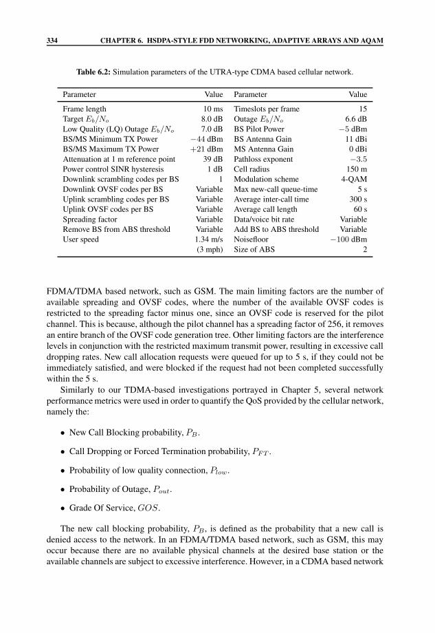
334 CHAPTER 6. HSDPA-STYLE FDD NETWORKING, ADAPTIVE ARRAYS AND AQAM
Table 6.2: Simulation parameters of the UTRA-type CDMA based cellular network.
Parameter Value Parameter Value
Frame length 10 ms Timeslots per frame 15Target Eb/No 8.0 dB Outage Eb/No 6.6 dBLow Quality (LQ) Outage Eb/No 7.0 dB BS Pilot Power −5 dBmBS/MS Minimum TX Power −44 dBm BS Antenna Gain 11 dBiBS/MS Maximum TX Power +21 dBm MS Antenna Gain 0 dBiAttenuation at 1 m reference point 39 dB Pathloss exponent −3.5Power control SINR hysteresis 1 dB Cell radius 150 mDownlink scrambling codes per BS 1 Modulation scheme 4-QAMDownlink OVSF codes per BS Variable Max new-call queue-time 5 sUplink scrambling codes per BS Variable Average inter-call time 300 sUplink OVSF codes per BS Variable Average call length 60 sSpreading factor Variable Data/voice bit rate VariableRemove BS from ABS threshold Variable Add BS to ABS threshold VariableUser speed 1.34 m/s Noisefloor −100 dBm
(3 mph) Size of ABS 2
FDMA/TDMA based network, such as GSM. The main limiting factors are the number ofavailable spreading and OVSF codes, where the number of the available OVSF codes isrestricted to the spreading factor minus one, since an OVSF code is reserved for the pilotchannel. This is because, although the pilot channel has a spreading factor of 256, it removesan entire branch of the OVSF code generation tree. Other limiting factors are the interferencelevels in conjunction with the restricted maximum transmit power, resulting in excessive calldropping rates. New call allocation requests were queued for up to 5 s, if they could not beimmediately satisfied, and were blocked if the request had not been completed successfullywithin the 5 s.
Similarly to our TDMA-based investigations portrayed in Chapter 5, several networkperformance metrics were used in order to quantify the QoS provided by the cellular network,namely the:
• New Call Blocking probability, PB .
• Call Dropping or Forced Termination probability, PFT .
• Probability of low quality connection, Plow .
• Probability of Outage, Pout.
• Grade Of Service, GOS.
The new call blocking probability, PB , is defined as the probability that a new call isdenied access to the network. In an FDMA/TDMA based network, such as GSM, this mayoccur because there are no available physical channels at the desired base station or theavailable channels are subject to excessive interference. However, in a CDMA based network

6.4. SIMULATION RESULTS 335
this does not occur, provided that no interference level based admission control is performedand hence the new call blocking probability is typically low.
The call dropping probability, PFT , is the probability that a call is forced to terminateprematurely. In a GSM type network, an insufficiently high SINR, which inevitably leadsto dropped calls, may be remedied by an intra- or inter-cell handover. However, in CDMAeither the transmit power must be increased, or a soft handover must be performed in orderto exploit the available diversity gain.
Again, the probability of a low quality connection is defined as:
Plow = P{SINRUL < SINRreq or SINRDL < SINRreq} (6.8)
= P{min(SINRUL, SINRDL) < SINRreq}.The GOS was defined in [331] as:
GOS = P{unsuccessful or low-quality call access} (6.9)
= P{call is blocked} + P{call is admitted}× P{low signal quality and call is admitted}
= PB + (1 − PB)Plow,
and is interpreted as the probability of unsuccessful network access (blocking), or low qualityaccess, when a call is admitted to the system.
In our forthcoming investigations, in order to compare the network capacities of differentnetworks, similarly to our TDMA-based investigations in Chapter 5, it was decided to usetwo scenarios defined as:
• A conservative scenario, where the maximum acceptable value for the new callblocking probability, PB , is 3%, the maximum call dropping probability, PFT , is 1%,and Plow is 1%.
• A lenient scenario, where the maximum acceptable value for the new call blockingprobability, PB , is 5%, the maximum call dropping probability, PFT , is 1%, and Plow
is 2%.
In the next section we consider the network’s performance considering both fixed andnormalized soft handover thresholds using both received pilot power and received pilot powerversus interference threshold metrics. A spreading factor of 16 was used, correspondingto a channel data rate of 3.84 Mbps/16 = 240 kbps with no channel coding, or 120 kbpswhen using 1/2 rate channel coding. It must be noted at this stage that the results presentedin the following sections are network capacities obtained using a spreading factor of 16.The network capacity results presented in the previous chapter, which were obtained for anFDMA/TDMA GSM-like system, were achieved for speech-rate users. Here we assumed thatthe channel coded speech-rate was 15 kbps, which is the lowest possible Dedicated PhysicalData CHannel (DPDCH) rate. Speech users having a channel coded rate of 15 kbps may besupported by invoking a spreading factor of 256. Hence, subjecting the channel data rate of15 kbps to 1/2 rate channel coding gives a speech-rate of 7.5 kbps, or if protected by a 2/3rate code the speech-rate becomes 10 kbps, which are sufficiently high for employing theso-called Advanced MultiRate (AMR) speech codec [412–414] capable of operating at rates

336 CHAPTER 6. HSDPA-STYLE FDD NETWORKING, ADAPTIVE ARRAYS AND AQAM
between 4.7 kbps and 12.2 kbps. Therefore, by multiplying the resultant network capacitiesaccording to a factor of 256/16 = 16, it is possible to estimate the number of speech userssupported by a speech-rate network. However, with the aid of our exploratory simulations,conducted using a spreading factor of 256, which are not presented here, we achievednetwork capacities higher than 30 times the network capacity supported in conjunction witha spreading factor of 16. Therefore, it would appear that the system is likely to support morethan 16 times the number of 240 kbps data users, when communicating at the approximately16 times lower speech-rate, employing a high spreading factor of 256. Hence, using theabove-mentioned scaling factor of 16 we arrive at the lower bound of network capacity. Amobile speed of 3 mph was used in conjunction with a cell size of 150 m radius, which wasnecessarily small in order to be able to support the previously assumed 240 kbps high targetdata rate. The performance advantages of using both adaptive beamforming and adaptivemodulation assisted networks are also investigated.
6.4.2 The Effect of Pilot Power on Soft Handover Results
In this section we consider the settings of the soft handover thresholds, for an IS-95type handover algorithm [58], where the handover decisions are based on DL pilot powermeasurements. Selecting inappropriate values for the soft handover thresholds, namely for theacceptance threshold and the drop threshold, may result in an excessive number of blockedand dropped calls in certain parts of the simulation area. For example, if the acceptancethreshold that has to be exceeded by the signal level for a base station to be added to theactive set is too high (Threshold B in Figure 6.6), then a user may be located within a cell,but it would be unable to add any base stations to its active base station set. Hence this user isunable to initiate a call. Figure 6.6 illustrates this phenomenon and shows that the acceptancethresholds must be set sufficiently low for ensuring that at least one base station covers everypart of the network.
Another consequence of setting the acceptance threshold to an excessively high value, isthat soft handovers may not be completed. This may occur when a user leaving the coveragearea of a cell, since the pilot signal from that cell drops below the drop threshold, before thesignal from the adjacent cell becomes sufficiently strong for it to be added to the active basestation set. However, if the acceptance threshold, in conjunction with the drop threshold, isset correctly, then new calls and soft handovers should take place as required, so long as theavailability of network resources allows it. Care must be taken however, not to set the softhandover threshold too low, otherwise the mobiles occupy additional network resources andcreate extra interference, due to initiating unnecessary soft-handovers.
6.4.2.1 Fixed Received Pilot Power Thresholds without Shadowing
Figure 6.7 shows the new call blocking probability of a network using a spreading factor of16, in conjunction with fixed received pilot signal strength based soft handover thresholdswithout imposing any shadowing effects. The figure illustrates that reducing both theacceptance and the dropping soft handover thresholds results in an improved new callblocking performance. Reducing the threshold at which further base stations may be added tothe Active Base station Set (ABS) increases the probability that base stations exist within theABS, when a new call request is made. Hence, as expected, the new call blocking probability

6.4. SIMULATION RESULTS 337
New call dead zone’
Threshold CThreshold B
Threshold A
Handover dead zone’
Figure 6.6: This figure indicates that using inappropriate soft handover thresholds may lead to blockedand dropped calls due to insufficient pilot coverage of the simulation area. Threshold A isthe drop threshold, which when combined with the acceptance threshold C can fail to coverthe simulation area sufficiently well, thus leading to soft handover failure. When combiningthreshold A with the acceptance threshold B, users located in the “new call dead zone” maybecome unable to initiate calls.
is reduced, when the acceptance threshold is reduced. Similarly, dropping the threshold atwhich base stations are removed from the ABS also results in an improved new call blockingprobability, since a base station is more likely to be retained in the ABS as a mobile movesaway from it. Therefore, should a mobile attempt to initiate a call in this situation, there is agreater chance that the ABS will contain a suitable base station.
The associated call dropping probability is depicted in Figure 6.8, indicating that reducingthe soft handover thresholds, and thus increasing the time spent in soft handover, improvedthe performance up to a certain point. However, above this point the additional interferenceinflicted by the soft handover process led to a degraded performance. For example, in thisfigure the performance associated with Tacc = −111 dBm improved, when Tdrop wasdecreased from −112 dBm to −113 dBm. However, at high traffic levels the performancedegraded when Tdrop was decreased further, to −114 dBm. The call dropping probabilityobtained using Tacc = −113 dBm and Tdrop = −115 dBm was markedly lower for thelesser levels of traffic carried due to the extra diversity gain provided by the soft handover

338 CHAPTER 6. HSDPA-STYLE FDD NETWORKING, ADAPTIVE ARRAYS AND AQAM
0.8 0.9 1.0 1.1 1.2 1.3 1.4 1.5 1.6 1.7 1.82
10-3
2
5
10-2
2
5
New
Cal
lBlo
ckin
gPr
obab
ility
,PB
3%
5%
-113, -115-112, -114-112, -113-111, -114-111, -113-111, -112Tacc (dBm), Tdrop (dBm)
Mean Carried Teletraffic (Erlangs/km /MHz)
Figure 6.7: New call blocking probability versus mean carried traffic of a CDMA based cellularnetwork using fixed received pilot power based soft handover thresholds without shadowingfor SF = 16.
process. However, since these soft handover thresholds resulted in a greater proportion oftime spent in soft handover, the levels of interference were increased, and thus at the highertraffic levels the performance degraded rapidly, as can be seen in Figure 6.8. Hence, the calldropping performance is based on a trade-off between the diversity gain provided by the softhandover process and the associated additional interference.
The probability of low quality access (not explicitly shown) was similar in terms of itscharacter to the call dropping probability, since reducing Tdrop improved the performance toa certain point, after which it degraded.
The mean number of base stations in the ABS is shown in Figure 6.9, illustrating thatreducing the soft handover thresholds leads, on average, to a higher number of base stationsin the ABS. Therefore, a greater proportion of call time is spent in soft handover. Theassociated diversity gain improves the link quality of the reference user but additional co-channel interference is generated by the diversity links, thus ultimately reducing the callquality, as shown in Figure 6.8. Additionally, this extra co-channel interference requiredmore transmission power for maintaining the target SINR as depicted in Figure 6.10. Thisfigure shows that when lower soft handover thresholds are used, and thus a greater proportionof time is spent in soft handover, greater levels of co-channel interference are present, andthus the required mean transmission powers became higher. It is interesting to note that forthe highest soft handover thresholds employed in Figure 6.10, the DL transmission powerrequired for maintaining the target SINR is lower than the UL transmission power, whereasfor the lower soft handover thresholds, the required mean UL transmission power is lowerthan the DL transmission power. The required DL transmission power was, in general, lowerthan the UL transmission power due to the mobile stations’ ability to perform maximal

6.4. SIMULATION RESULTS 339
0.8 0.9 1.0 1.1 1.2 1.3 1.4 1.5 1.6 1.7 1.82
10-3
2
5
10-2
2
FT1%
-113, -115-112, -114-112, -113-111, -114-111, -113-111, -112Tacc (dBm), Tdrop (dBm)
Cal
lDro
ppin
gPr
obab
ility
,P
Mean Carried Teletraffic (Erlangs/km /MHz)
Figure 6.8: Call dropping probability versus mean carried traffic of a CDMA based cellular networkusing fixed received pilot power based soft handover thresholds without shadowing forSF = 16.
ratio combining when in soft handover. This was observed despite the absence of the pilotinterference in the UL, and despite the base stations’ ability to perform selective diversitywhich offers less diversity gain when compared to maximal ratio combining. However,reducing the soft handover thresholds to the lowest levels shown in Figure 6.10, led toincreased co-channel interference on the DL, thus requiring higher base station transmissionpowers, as clearly seen in the figure.
In summary, as seen by comparing Figures 6.7–6.10 the maximum capacity of thenetwork using fixed received pilot power based soft handover thresholds was limited by thecall dropping probability. The new call blocking probability remained below the 3% limit,thanks to the appropriate choice of thresholds used, whilst the probability of low qualityaccess was constantly below the 1% mark. Therefore, the maximum normalized teletrafficload was 1.64 Erlangs/km2/MHz, corresponding to a total network capacity of 290 users,while satisfying both QoS constraints, was achieved with the aid of an acceptance thresholdof −112 dBm and a dropping threshold of −114 dBm. A mean ABS size of 1.7 base stationswas registered at this traffic level, and both the mobile and base stations exhibited a meantransmission power of 5.1 dBm.
6.4.2.2 Fixed Received Pilot Power Thresholds with 0.5 Hz Shadowing
In this section we examine the achievable performance, upon using fixed received pilotpower based soft handover thresholds when subjected to log-normal shadow fading having astandard deviation of 3 dB and a maximum frequency of 0.5 Hz.

340 CHAPTER 6. HSDPA-STYLE FDD NETWORKING, ADAPTIVE ARRAYS AND AQAM
0.8 0.9 1.0 1.1 1.2 1.3 1.4 1.5 1.6 1.7 1.82
1.0
1.1
1.2
1.3
1.4
1.5
1.6
1.7
1.8
1.9
2.0
Num
ber
ofB
Sin
the
AB
S
-113, -115-112, -114-112, -113-111, -114-111, -113-111, -112Tacc (dBm), Tdrop (dBm)
Mean Carried Teletraffic (Erlangs/km /MHz)
Figure 6.9: Mean number of base stations in the active base station set versus mean carried trafficof a CDMA based cellular network using fixed received pilot power based soft handoverthresholds without shadowing for SF = 16.
0.8 0.9 1.0 1.1 1.2 1.3 1.4 1.5 1.6 1.7 1.82
-1
0
1
2
3
4
5
6
7
8
9
Mea
nT
rans
mis
sion
Pow
er(d
Bm
)
Filled = BS, Blank = MS-113, -115-111, -114-111, -113-111, -112Tacc (dBm), Tdrop (dBm)
Mean Carried Teletraffic (Erlangs/km /MHz)
Figure 6.10: Mean transmission power versus mean carried traffic of a CDMA based cellular networkusing fixed received pilot power based soft handover thresholds without shadowing forSF = 16.

6.4. SIMULATION RESULTS 341
0.0 0.1 0.2 0.3 0.4 0.5 0.6 0.7 0.8 0.92
10-3
2
5
10-2
2
5
10-1
2
5
Cal
lDro
ppin
gPr
obab
ility
,PFT
1%
-113, -115-112, -114-111, -114-111, -113-111, -112Tacc (dBm), Tdrop (dBm)
Mean Carried Teletraffic (Erlangs/km /MHz)
Figure 6.11: Call dropping probability versus mean carried traffic of a CDMA based cellular networkusing fixed received pilot power based soft handover thresholds in conjunction with 0.5 Hzshadowing having a standard deviation of 3 dB for SF = 16.
0.0 0.1 0.2 0.3 0.4 0.5 0.6 0.7 0.8 0.92
10-3
2
5
10-2
2
Prob
abili
tyof
low
qual
ityac
cess
,Plo
w
1%
2%
-113, -115-112, -114-111, -114-111, -113-111, -112Tacc (dBm), Tdrop (dBm)
Mean Carried Teletraffic (Erlangs/km /MHz)
Figure 6.12: Probability of low quality access versus mean carried traffic of a CDMA based cellularnetwork using fixed received pilot power based soft handover thresholds in conjunctionwith 0.5 Hz shadowing having a standard deviation of 3 dB for SF = 16.

342 CHAPTER 6. HSDPA-STYLE FDD NETWORKING, ADAPTIVE ARRAYS AND AQAM
The call dropping results of Figure 6.11 suggested that the network’s performance waspoor when using fixed received pilot power soft handover thresholds in the above mentionedshadow fading environment. The root cause of the problem is that the fixed thresholds mustbe set such that the received pilot signals, even when subjected to shadow fading, are retainedin the active set. Therefore, setting the thresholds too high results in the base stations beingremoved from the active set, thus leading to an excessive number of dropped calls. However,if the thresholds are set too low, in order to counteract this phenomenon, then the base stationscan be in soft handover for too high a proportion of time, and thus an unacceptable level oflow quality accesses is generated due to the additional co-channel interference inflicted bythe high number of active base stations. Figure 6.11 shows that reducing the soft handoverthresholds improved the network’s call dropping probability, but Figure 6.12 illustrates thatreducing the soft handover thresholds engendered an increase in the probability of a lowquality access.
The network cannot satisfy the quality requirements of the conservative scenario, namelythat of maintaining a call dropping probability of 1% combined with a maximum probabilityof low quality access below 1%. However, the entire network supported 127 users, whilstmeeting the lenient scenario’s set of criteria, which consists of a maximum call droppingprobability of 1% and a probability of low quality access of below 2%, using the thresholdsof Tacc = −113 dBm and Tdrop = −115 dBm.
6.4.2.3 Fixed Received Pilot Power Thresholds with 1.0 Hz Shadowing
This section presents results obtained using fixed receiver pilot power based soft handoverthresholds in conjunction with log-normal shadow fading having a standard deviation of 3 dBand a maximum fading frequency of 1.0 Hz.
The corresponding call dropping probability is depicted in Figure 6.13, showing thatusing fixed thresholds in a propagation environment exposed to shadow fading resulted ina very poor performance. This was due to the shadow fading induced fluctuations of thereceived pilot signal power, which resulted in removing base stations from the ABS mid-call,which ultimately engendered dropped calls. Hence, lowering the fixed thresholds significantlyreduced the call dropping probability. However, this led to a deterioration of the low qualityaccess probability, as shown in Figure 6.14. The probability of low quality access was alsovery poor due to the rapidly fluctuating interference-limited environment. This was shownparticularly explicitly in conjunction with Tacc = −113 dBm and Tdrop = −115 dBm, wherereducing the number of users resulted in a degradation of the low quality access performancedue to the higher deviation of the reduced number of combined sources of interference.In contrast, adding more users led to a near-constant level of interference that varied lessdramatically.
It was found that the network was unable to support any users at the required servicequality, since using the thresholds that allowed the maximum 1% call dropping probabilityrestriction to be met, led to a greater than 2% probability of a low quality outage occurring.
6.4.2.4 Summary
In summary of our findings in the context of Figures 6.7–6.14, a disadvantage of using fixedsoft handover thresholds is that in some locations all pilot signals may be weak, whereas

6.4. SIMULATION RESULTS 343
0.0 0.1 0.2 0.3 0.4 0.5 0.6 0.7 0.8 0.92
10-3
2
5
10-2
2
5
10-1
2
5
FT
1%
-113, -115-112, -114-112, -113-111, -114-111, -113-111, -112Tacc (dBm), Tdrop (dBm)
Cal
lDro
ppin
gPr
obab
ility
,P
Mean Carried Teletraffic (Erlangs/km /MHz)
Figure 6.13: Call dropping probability versus mean carried traffic of a CDMA based cellular networkusing fixed received pilot power based soft handover thresholds in conjunction with 1 Hzshadowing having a standard deviation of 3 dB for SF = 16.
0.0 0.1 0.2 0.3 0.4 0.5 0.6 0.7 0.8 0.92
10-3
2
5
10-2
2
Prob
abili
tyof
low
qual
ityac
cess
,Plo
w
1%
2%
-113, -115-112, -114-112, -113-111, -114-111, -113-111, -112Tacc (dBm), Tdrop (dBm)
Mean Carried Teletraffic (Erlangs/km /MHz)
Figure 6.14: Probability of low quality access versus mean carried traffic of a CDMA based cellularnetwork using fixed received pilot power based soft handover thresholds in conjunctionwith 1 Hz shadowing having a standard deviation of 3 dB for SF = 16.

344 CHAPTER 6. HSDPA-STYLE FDD NETWORKING, ADAPTIVE ARRAYS AND AQAM
in other locations, all of the pilot signals may be strong due to the localized propagationenvironment or terrain. Hence, using relative or normalized soft handover thresholds isexpected to be advantageous in terms of overcoming this limitation. An additional benefit ofusing dynamic thresholds is confirmed within a fading environment, where the received pilotpower may drop momentarily below a fixed threshold, thus causing unnecessary removals andadditions to/from the ABS. However, these base stations may have been the only base stationsin the ABS, thus ultimately resulting in a dropped call. When using dynamically controlledthresholds this scenario would not have occurred. Hence, in the next section we consideredthe performance of using relative received pilot power based soft handover thresholds underboth non-shadowing and shadowing impaired propagation conditions.
To summarize, using fixed received pilot power thresholds in a non-shadowing envi-ronment resulted in a total network capacity of 290 users for both QoS scenarios, namelyfor both the conservative and lenient scenarios considered. However, this performance wasseverely degraded in a shadow fading impaired propagation environment, where a totalnetwork capacity of 127 users was supported in conjunction with a maximum shadow fadingfrequency of 0.5 Hz. Unfortunately, the network capacity could not be evaluated when usinga maximum shadow fading frequency of 1.0 Hz due to the contrasting characteristics of thedropped call and low quality access probability results.
6.4.2.5 Relative Received Pilot Power Thresholds without Shadowing
Employing relative received pilot power thresholds is important in realistic propagationenvironments exposed to shadow fading. More explicitly, in contrast to the previously usedthresholds, which were expressed in terms of dBm, i.e. with respect to 1 mW, in this sectionthe thresholds Tacc and Tdrop are expressed in terms of dB relative to the received pilotstrength of the base stations in the ABS. Their employment also caters for situations, wherethe absolute pilot power may be too low for use in conjunction with fixed thresholds, butnonetheless sufficiently high for reliable communications. Hence, in this section we examinethe performance of relative received pilot power based soft handover thresholds in a non-shadow faded environment.
The call dropping performance is depicted in Figure 6.15, which shows that reducing thesoft handover thresholds, and thus increasing the time spent in soft handover, improved thecall dropping performance. It was also found in the cases considered here, that simultaneouslythe probability of a low quality access decreased, as illustrated by Figure 6.16. However, itwas also evident in both figures, that reducing the soft handover thresholds past a certainpoint resulted in degraded performance due to the extra interference incurred during the softhandover process.
Since the probability of low quality access was under the 1% threshold, the networkcapacity for both the lenient and conservative scenarios were the same, namely 1.65Erlangs/km2/MHz or a total of 288 users over the entire simulation area of 2.86 km2. Themean ABS size was 1.7 base stations, with a mean mobile transmission power of 4.1 dBmand an average base station transmit power of 4.7 dBm.

6.4. SIMULATION RESULTS 345
0.8 0.9 1.0 1.1 1.2 1.3 1.4 1.5 1.6 1.7 1.82
10-3
2
5
10-2
2
Cal
lDro
ppin
gPr
obab
ility
,PFT
1%-14, -18-12, -18-10, -18-10, -12Tacc (dB), Tdrop (dB)
Mean Carried Teletraffic (Erlangs/km /MHz)
Figure 6.15: Call dropping probability versus mean carried traffic of a CDMA based cellular networkusing relative received pilot power based soft handover thresholds without shadowing forSF = 16.
1.1 1.2 1.3 1.4 1.5 1.6 1.7 1.82
10-3
2
5
10-2
2
Prob
abili
tyof
low
qual
ityac
cess
,Plo
w
1%
2%
-12, -18-12, -14-10, -18-10, -12Tacc (dB), Tdrop (dB)
Mean Carried Teletraffic (Erlangs/km /MHz)
Figure 6.16: Probability of low quality access versus mean carried traffic of a CDMA based cellularnetwork using relative received pilot power based soft handover thresholds withoutshadowing for SF = 16.

346 CHAPTER 6. HSDPA-STYLE FDD NETWORKING, ADAPTIVE ARRAYS AND AQAM
0.3 0.4 0.5 0.6 0.7 0.8 0.92
10-3
2
5
10-2
2
Cal
lDro
ppin
gPr
obab
ility
,PFT
1%-16, -18-15, -18-14, -18-12, -14-10, -12Tacc (dB), Tdrop (dB)
Mean Carried Teletraffic (Erlangs/km /MHz)
Figure 6.17: Call dropping probability versus mean carried traffic of a CDMA based cellular networkusing relative received pilot power based soft handover thresholds in conjunction with0.5 Hz shadowing and a standard deviation of 3 dB for SF = 16.
6.4.2.6 Relative Received Pilot Power Thresholds with 0.5 Hz Shadowing
In this section we present results obtained using relative received pilot power based softhandover thresholds in a shadowing-impaired propagation environment. The maximumshadow fading frequency was 0.5 Hz and the standard deviation of the log-normal shadowingwas 3 dB.
Figure 6.17 depicts the call dropping probability for several relative thresholds and showsthat by reducing both the thresholds, the call dropping performance is improved. This enablesthe mobile to add base stations to its ABS earlier on during the soft handover process, andto relinquish them at a much later stage than in the case of using higher handover thresholds.Therefore, using lower relative soft handover thresholds results in a longer period of timespent in soft handover, as can be seen in Figure 6.18, which shows the mean number of basestations in the ABS.
The probability of low quality access is shown in Figure 6.19, illustrating that, in general,as the relative soft handover thresholds were reduced, the probability of low quality accessincreased. This demonstrated that spending more time in soft handover generated more co-channel interference and thus degraded the network’s performance. However, the differencebetween the two thresholds must also be considered. For example, the probability of lowquality access is higher in conjunction with Tacc = −16 dB and Tdrop = −18 dB, thanusing Tacc = −16 dB and Tdrop = −20 dB, since the latter scenario has a higher meannumber of base stations in its ABS. Therefore, there is a point at which the soft handover gainexperienced by the desired user outweighs the detrimental effects of the extra interferencegenerated by base stations’ transmissions to users engaged in the soft handover process.

6.4. SIMULATION RESULTS 347
0.3 0.4 0.5 0.6 0.7 0.8 0.92
1.0
1.1
1.2
1.3
1.4
1.5
1.6
1.7
1.8
1.9
2.0
Num
ber
ofB
Sin
the
AB
S
-16, -18-15, -18-14, -18-12, -14-10, -12Tacc (dB), Tdrop (dB)
Mean Carried Teletraffic (Erlangs/km /MHz)
Figure 6.18: Mean number of base stations in the active base station set versus mean carried traffic ofa CDMA based cellular network using relative received pilot power based soft handoverthresholds in conjunction with 0.5 Hz shadowing and a standard deviation of 3 dB forSF = 16.
0.3 0.4 0.5 0.6 0.7 0.8 0.92
10-3
2
5
10-2
2
Prob
abili
tyof
low
qual
ityac
cess
,Plo
w
1%
2%
-16, -20-16, -18-15, -18-14, -18-12, -14-10, -12Tacc (dB), Tdrop (dB)
Mean Carried Teletraffic (Erlangs/km /MHz)
Figure 6.19: Probability of low quality access versus mean carried traffic of a CDMA based cellularnetwork using relative received pilot power based soft handover thresholds in conjunctionwith 0.5 Hz shadowing and a standard deviation of 3 dB for SF = 16.

348 CHAPTER 6. HSDPA-STYLE FDD NETWORKING, ADAPTIVE ARRAYS AND AQAM
0.3 0.4 0.5 0.6 0.7 0.8 0.92
-4
-3
-2
-1
0
1
2
3
Mea
nT
rans
mis
sion
Pow
er(d
Bm
)
-14, -18-14, -16-12, -14-10, -12Tacc (dB), Tdrop (dB)Filled = BS, Blank = MS
Mean Carried Teletraffic (Erlangs/km /MHz)
Figure 6.20: Mean transmission power versus mean carried traffic of a CDMA based cellular networkusing relative received pilot power based soft handover thresholds in conjunction with0.5 Hz shadowing and a standard deviation of 3 dB for SF = 16.
Figure 6.20 shows the mean transmission powers of both the mobiles and the basestations. The mobiles are required to transmit at a lower power than the base stations, becausethe base stations are not subjected to DL pilot power interference and to soft handoverinterference. Furthermore, the mobiles are not affected by the level of the soft handoverthresholds, because only selective diversity is performed in the UL, and hence the mobiletransmits as if not in soft handover. As the soft handover thresholds were reduced, thetime spent in soft handover increased and thus the mean base transmission power had tobe increased in order to overcome the additional DL interference.
The maximum network capacity of 0.835 Erlangs/km2/MHz, or 144 users over the entiresimulation area, was achieved using the soft handover thresholds of Tacc = −14 dB andTdrop = −18 dB for the conservative scenario. The mean ABS size was 1.77 base stations,while the mean mobile transmit power was −1.5 dBm and 0.6 dBm for the base stations. Inthe lenient scenario a maximum teletraffic load of 0.865 Erlangs/km2/MHz, correspondingto a total network capacity of 146 users was maintained using soft handover thresholds ofTacc = −16 dB and Tdrop = −18 dB. The mean number of base stations in the ABS was1.78, with an average transmit power of −1.5 dBm for the mobile handset, and 1.3 dBm forthe base station.
6.4.2.7 Relative Received Pilot Power Thresholds with 1.0 Hz Shadowing
In this section we present further performance results obtained using relative receivedpilot power based soft handover thresholds in a shadowing propagation environment. The

6.4. SIMULATION RESULTS 349
0.3 0.4 0.5 0.6 0.7 0.8 0.92
10-3
2
5
10-2
2
Cal
lDro
ppin
gPr
obab
ility
,PFT
1%
-18, -20-14, -18-14, -16-12, -14-2, -22-2, -20Tacc (dB), Tdrop (dB)
Mean Carried Teletraffic (Erlangs/km /MHz)
Figure 6.21: Call dropping probability versus mean carried traffic of a CDMA based cellular networkusing relative received pilot power based soft handover thresholds in conjunction with1 Hz shadowing and a standard deviation of 3 dB for SF = 16.
maximum shadow fading frequency was 1.0 Hz and the standard deviation of the log-normalshadowing was 3 dB.
On comparing the call dropping probability curves seen in Figure 6.21 with the calldropping probability obtained for a maximum shadow fading frequency of 0.5 Hz inFigure 6.17 it was found that the performance of the 1.0 Hz frequency shadowing scenariowas slightly worse. However, the greatest performance difference was observed in theprobability of low quality access, as can be seen in Figure 6.22.
Using the soft handover thresholds which gave a good performance for a maximumshadow fading frequency of 0.5 Hz resulted in significantly poorer low quality accessperformance for a maximum shadowing frequency of 1.0 Hz. In order to obtain a probabilityof low quality access of below 1% it was necessary to use markedly different soft handoverthresholds, which reduced the time spent in soft handover and hence also the size of the ABS,as illustrated in Figure 6.23.
For the conservative scenario, where the maximum probability of low quality access,Plow , was set to 1%, the maximum network capacity was found to be 0.69 Erlangs/km2/MHz,equivalent to a total network capacity of 127 users, obtained using Tdrop = −2 dB and Tacc =−16 dB. In contrast, in the lenient scenario, where the Plow limit was 2%, the maximumnumber of users supported was found to be 144, or 0.825 Erlangs/km2/MHz, in conjunctionwith Tacc = −14 dB and Tdrop = −18 dB.

350 CHAPTER 6. HSDPA-STYLE FDD NETWORKING, ADAPTIVE ARRAYS AND AQAM
0.3 0.4 0.5 0.6 0.7 0.8 0.92
10-3
2
5
10-2
2
Prob
abili
tyof
low
qual
ityac
cess
,Plo
w
1%
2%
-18, -20-14, -16-14, -16-12, -14-2, -22-2, -20Tacc (dB), Tdrop (dB)
Mean Carried Teletraffic (Erlangs/km /MHz)
Figure 6.22: Probability of low quality access versus mean carried traffic of a CDMA based cellularnetwork using relative received pilot power based soft handover thresholds in conjunctionwith 1 Hz shadowing and a standard deviation of 3 dB for SF = 16.
0.3 0.4 0.5 0.6 0.7 0.8 0.92
1.0
1.1
1.2
1.3
1.4
1.5
1.6
1.7
1.8
1.9
2.0
Num
ber
ofB
Sin
the
AB
S
-18, -20-14, -18-14, -16-12, -14-2, -22-2, -20Tacc (dB), Tdrop (dB)
Mean Carried Teletraffic (Erlangs/km /MHz)
Figure 6.23: Mean number of base stations in the active base station set versus mean carried traffic ofa CDMA based cellular network using relative received pilot power based soft handoverthresholds in conjunction with 1 Hz shadowing and a standard deviation of 3 dB for SF =16.

6.4. SIMULATION RESULTS 351
6.4.2.8 Summary
In summary, using relative received pilot power as a soft handover metric has resulted in asignificantly improved performance in comparison to that of the fixed received pilot powerbased results in a shadow fading environment. In the non-shadowed environment the networkcapacity was approximately the same as when using the fixed threshold algorithm, albeit witha slightly improved mean transmission power. Due to the time varying nature of the receivedsignals subjected to shadow fading, using relative thresholds has been found to be moreamenable to employment in a realistic propagation environment, than using fixed thresholds.In conclusion, without shadow fading the network supported a total of 288 users, whilst witha maximum shadow fading frequency of 0.5 Hz, approximately 145 users were supportedby the entire network, for both the conservative and lenient scenarios. However, differentsoft handover thresholds were required for each situation, for achieving these capacities.At a maximum shadowing frequency of 1.0 Hz, a total of 127 users were supported in theconservative scenario, and 144 in the lenient scenario. However, again, different soft handoverthresholds were required in each scenario in order to maximize the network capacity.
6.4.3 Ec/Io Power Based Soft Handover Results
An alternative soft handover metric used to determine “cell ownership” is the pilot to DLinterference ratio of a cell, which was proposed for employment in the 3rd generationsystems [59]. The pilot to DL interference ratio, or Ec/Io, may be calculated thus as [415]:
Ec
Io=
Ppilot
Ppilot + N0 +∑Ncells
k=1 PkTk
, (6.10)
where Pk is the total transmit power of cell k, Tk is the transmission gain, which includesthe antenna gain and pathloss as well as shadowing, N0 is the power spectral density of thethermal noise and Ncells is the number of cells in the network. The advantage of using such ascheme is that it is not an absolute measurement that is used, but the ratio of the pilot powerto the interference power. Thus, if fixed thresholds were used a form of admission controlmay be employed for new calls if the interference level became too high. A further advantageis that it takes into account the time-varying nature of the interference level in a shadowedenvironment.
6.4.3.1 Fixed Ec/Io Thresholds without Shadowing
The new call blocking probability obtained when using fixed Ec/Io soft handover thresholdswithout any form of shadow fading is shown in Figure 6.24, which suggests that in general,lowering the soft handover thresholds reduced the probability of a new call attempt beingblocked. However, it was found that in conjunction with Tdrop = −40 dB, dropping thethreshold Tacc from −20 dB to −24 dB actually increased the new call blocking probability.This was attributed to the fact that the lower threshold precipitated a higher level of co-channel interference, since there was a higher mean number of base stations in the ABS,as evidenced by Figure 6.25. Therefore, since the mean level of interference present in thenetwork is higher, when using a lower threshold, and the threshold determines the value ofthe pilot to DL interference ratio at which base stations may be added to the ABS, a more

352 CHAPTER 6. HSDPA-STYLE FDD NETWORKING, ADAPTIVE ARRAYS AND AQAM
0.8 0.9 1.0 1.1 1.2 1.3 1.4 1.5 1.6 1.7 1.82
10-3
2
5
10-2
2
5
10-1
New
Cal
lBlo
ckin
gPr
obab
ility
,PB
3%
5%
-34, -44-32, -44-28, -42-24, -40-20, -40Tacc (dB), Tdrop (dB)
Mean Carried Teletraffic (Erlangs/km /MHz)
Figure 6.24: New call blocking probability versus mean carried traffic of a CDMA based cellularnetwork using fixed Ec/Io based soft handover thresholds without shadowing forSF = 16.
frequent blocking of calls occurs. Alternatively, a lower threshold resulted in a higher level ofDL interference due to the additional interference inflicted by supporting the mobiles in softhandover, which prevented base stations from being included in the ABS due to insufficientpilot to interference “head-room”. This then ultimately led to blocked calls due to the lack ofbase stations in the ABS.
Again, the mean number of base stations in the ABS is given in Figure 6.25, whichillustrates that as expected, reducing the soft handover thresholds increased the proportion oftime spent in soft handover, and thus reduced the mean number of base stations in the ABS.The average size of the ABS was found to decrease, as the network’s traffic load increased.This was a consequence of the increased interference levels associated with the higher trafficloads, which therefore effectively reduced the pilot to interference ratio at a given point, andhence base stations were less likely to be in soft handover and in the ABS.
Figure 6.26 depicts the mean transmission powers for both the UL and the DL, for arange of different soft handover thresholds. These results show similar trends to the resultspresented in previous sections, with the required average DL transmission power increasing,since a greater proportion of call time is spent in soft handover. Again, the mean ULtransmission power varied only slightly, since the selection diversity technique of the basestations only marginally affected the received interference power at the base stations.
Figure 6.27 shows the call dropping performance, indicating that lowering the softhandover thresholds generally improved the call dropping performance. However, reducingthe soft handover thresholds too much resulted in a degradation of the call droppingprobability due to the increased levels of co-channel interference inherent when a higherproportion of the call time is spent in soft handover. This is explicitly illustrated by

6.4. SIMULATION RESULTS 353
0.8 0.9 1.0 1.1 1.2 1.3 1.4 1.5 1.6 1.7 1.82
1.0
1.1
1.2
1.3
1.4
1.5
1.6
1.7
1.8
1.9
2.0
Mea
nnu
mbe
rof
BS
inA
BS
-34, -44-32, -44-28, -42-24, -40-20, -40Tacc (dB), Tdrop (dB)
Mean Carried Teletraffic (Erlangs/km /MHz)
Figure 6.25: Mean number of base stations in the active base station set versus mean carried traffic of aCDMA based cellular network using fixed Ec/Io based soft handover thresholds withoutshadowing for SF = 16.
0.8 0.9 1.0 1.1 1.2 1.3 1.4 1.5 1.6 1.7 1.82
-2
0
2
4
6
8
10
12
14
16
Mea
nT
rans
mis
sion
Pow
er(d
Bm
)
-32, -44-28, -42-24, -40-20, -40Tacc (dB), Tdrop (dB)Filled = BS, Blank = MS
Mean Carried Teletraffic (Erlangs/km /MHz)
Figure 6.26: Mean transmission power versus mean carried traffic of a CDMA based cellular networkusing fixed received Ec/Io based soft handover thresholds without shadowing forSF = 16.

354 CHAPTER 6. HSDPA-STYLE FDD NETWORKING, ADAPTIVE ARRAYS AND AQAM
0.8 0.9 1.0 1.1 1.2 1.3 1.4 1.5 1.6 1.7 1.82
10-3
2
5
10-2
2
Forc
edTe
rmin
atio
nPr
obab
ility
,PFT
1%-34, -44-32, -44-28, -42-24, -40-20, -40Tacc (dB), Tdrop (dB)
Mean Carried Teletraffic (Erlangs/km /MHz)
Figure 6.27: Call dropping probability versus mean carried traffic of a CDMA based cellular networkusing fixed received Ec/Io based soft handover thresholds without shadowing forSF = 16.
Figure 6.28, which indicates that reducing the soft handover thresholds caused a significantdegradation in the probability of low quality access. This was a consequence of the additionalco-channel interference associated with the soft handover process. The figure also shows thatthere is a point where the diversity gain of the mobiles obtained with the advent of the softhandover procedure outweighs the extra interference that it generates.
On the whole, the capacity of the network when using fixed Ec/Io soft handoverthresholds was lower than when using fixed received pilot power based soft handoverthresholds. This can be attributed to the fact that the Ec/Io thresholds are related to theinterference level of the network, which changes with the network load and propagationconditions. Hence using a fixed threshold is sub-optimal. In the conservative scenario, thenetwork capacity was 1.275 Erlangs/km2/MHz, corresponding to a total network capacity of223 users. In the lenient scenario, this increased to 1.305 Erlangs/km2/MHz, or 231 users.In contrast, when using fixed received pilot power thresholds the entire network supported290 users.
6.4.3.2 Fixed Ec/Io Thresholds with 0.5 Hz Shadowing
In this section we consider fixed pilot to DL interference ratio based soft handover thresholdsin a propagation environment exhibiting shadow fading in conjunction with a maximumfading frequency of 0.5 Hz and a standard deviation of 3 dB.
Examining Figure 6.29, which shows the call dropping probability, we see, again, thatreducing the soft handover thresholds typically resulted in a lower probability of a droppedcall. However, since the handover thresholds are dependent upon the interference level,

6.4. SIMULATION RESULTS 355
0.8 0.9 1.0 1.1 1.2 1.3 1.4 1.5 1.6 1.7 1.82
10-3
2
5
10-2
2
Prob
abili
tyof
low
qual
ityac
cess
,Plo
w1%
2%
-34, -44-32, -44-28, -42-24, -40-20, -40Tacc (dB), Tdrop (dB)
Mean Carried Teletraffic (Erlangs/km /MHz)
Figure 6.28: Probability of low quality access versus mean carried traffic of a CDMA based cellularnetwork using fixed received Ec/Io based soft handover thresholds without shadowingfor SF = 16.
there was some interaction between the handover thresholds and the call dropping rate.For example, it can be seen in the figure that when Tdrop = −40 dB, the call droppingprobability fell as Tacc was reduced from −20 dB to −24 dB. However, on lowering Tacc
further, to −26 dB, the call dropping rate at low traffic loads became markedly higher. Asimilar phenomenon was observed in Figure 6.30, which shows the probability of low qualityoutage.
It is explicitly seen from Figures 6.29 and 6.30 that the performance of the fixed Ec/Io
soft handover threshold based scheme clearly exceeded that of the fixed received pilot powerthreshold based system in a shadow fading environment. The network supported a teletrafficload of 0.7 Erlangs/km2/MHz or a total of 129 users in the conservative scenario, which roseto 0.78 Erlangs/km2/MHz, or 140 users, in the lenient scenario. These network capacitieswere achieved with the aid of a mean number of active base stations in the ABS, which were1.88 and 1.91, respectively. In order to achieve the total network capacity of 129 users in theconservative scenario, a mean mobile transmit power of −2.4 dBm was required, while themean base station transmission power was 7 dBm. For the lenient scenario, these figures were−2.4 dBm and 8.7 dBm, respectively.
6.4.3.3 Fixed Ec/Io Thresholds with 1.0 Hz Shadowing
Increasing the maximum shadow fading frequency from 0.5 Hz to 1.0 Hz resulted in anincreased call dropping probability and a greater probability of low quality access, for a givenlevel of carried teletraffic. This is clearly seen by comparing Figures 6.31 and 6.32 withFigures 6.29 and 6.30. Explicitly, Figure 6.31 and 6.32 show that reducing the soft handover

356 CHAPTER 6. HSDPA-STYLE FDD NETWORKING, ADAPTIVE ARRAYS AND AQAM
0.3 0.4 0.5 0.6 0.7 0.8 0.92
10-3
2
5
10-2
2
Forc
edTe
rmin
atio
nPr
obab
ility
,PFT
1%
-30, -44-28, -42-28, -40-26, -40-24, -40-20, -40Tacc (dB), Tdrop (dB)
Mean Carried Teletraffic (Erlangs/km /MHz)
Figure 6.29: Call dropping probability versus mean carried traffic of a CDMA based cellular networkusing fixed received Ec/Io based soft handover thresholds in conjunction with 0.5 Hzshadowing and a standard deviation of 3 dB for SF = 16.
0.3 0.4 0.5 0.6 0.7 0.8 0.92
10-3
2
5
10-2
2
Prob
abili
tyof
low
qual
ityac
cess
,Plo
w
1%
2%
-30, -44-28, -42-28, -40-26, -40-24, -40-20, -40Tacc (dB), Tdrop (dB)
Mean Carried Teletraffic (Erlangs/km /MHz)
Figure 6.30: Probability of low quality access versus mean carried traffic of a CDMA based cellularnetwork using fixed received Ec/Io based soft handover thresholds in conjunction with0.5 Hz shadowing and a standard deviation of 3 dB for SF = 16.

6.4. SIMULATION RESULTS 357
0.3 0.4 0.5 0.6 0.7 0.8 0.92
10-3
2
5
10-2
2
Forc
edTe
rmin
atio
nPr
obab
ility
,PFT
1%-32, -44-30, -44-24, -40-22, -40-20, -40Tacc (dB), Tdrop (dB)
Mean Carried Teletraffic (Erlangs/km /MHz)
Figure 6.31: Call dropping probability versus mean carried traffic of a CDMA based cellular networkusing fixed received Ec/Io based soft handover thresholds in conjunction with 1.0 Hzshadowing and a standard deviation of 3 dB for SF = 16.
threshold, Tacc from−20 dB to −24 dB led to both an increased call dropping probability andan increased probability of low quality access. This can be attributed to the extra co-channelinterference generated by the greater proportion of call time being spent in soft handover. Thisis also confirmed by the increased probability of low quality access observed in Figure 6.32for lower soft handover thresholds Tacc and Tdrop.
The network capacity of the conservative scenario was 0.583 Erlangs/km2/MHz, givingan entire network capacity of 107 users. In the lenient scenario the network supported atotal of 128 users or a traffic load of 0.675 Erlangs/km2/MHz was carried. The 107 userswere serviced in conjunction with a mean ABS size of 1.86, a mean mobile transmit powerof −3 dBm and a mean base station transmit power of 4.5 dBm. The 128 users supportedin the lenient scenario necessitated an average mobile transmit power of −3 dBm and anaverage base station transmit power of 9.5 dBm. The mean number of base stations in theABS was 1.91.
6.4.3.4 Summary
In summary, a maximum network capacity of 290 users was obtained when employing thefixed Ec/Io soft handover thresholds. This capacity was equal to that when using fixedreceived pilot power thresholds in the lenient scenario without shadow fading. However, in theconservative scenario the network capacity was reduced from 290 to 231 users. Nevertheless,when a realistic shadowed propagation environment was considered, using the pilot powerto interference ratio based soft handover metric improved the network capacity significantly.This was particularly evident in conjunction with the maximum shadow fading frequency of

358 CHAPTER 6. HSDPA-STYLE FDD NETWORKING, ADAPTIVE ARRAYS AND AQAM
0.3 0.4 0.5 0.6 0.7 0.8 0.92
10-3
2
5
10-2
2
Prob
abili
tyof
low
qual
ityac
cess
,Plo
w
1%
2%
-32, -44-30, -44-24, -40-22, -40-20, -40Tacc (dB), Tdrop (dB)
Mean Carried Teletraffic (Erlangs/km /MHz)
Figure 6.32: Probability of low quality access versus mean carried traffic of a CDMA based cellularnetwork using fixed received Ec/Io based soft handover thresholds in conjunction with1.0 Hz shadowing and a standard deviation of 3 dB for SF = 16.
1.0 Hz, when using the fixed received pilot power thresholds no users could be supportedwhilst maintaining the desired call quality. In contrast, using the fixed Ec/Io soft handoverthresholds led to a total network capacity of between 107 and 128 users, for the conservativeand lenient scenarios, respectively. This capacity increase was the benefit of the more efficientsoft handover mechanism, which was capable of taking into account the interference levelexperienced, leading to a more intelligent selection of base stations supporting the call. At amaximum shadow fading frequency of 0.5 Hz the network had a maximum capacity of 129and 140 users, for the conservative and lenient scenario, respectively, when using the fixedEc/Io soft handover thresholds.
6.4.3.5 Relative Ec/Io Thresholds without Shadowing
In this section we combined the benefits of using the received Ec/Io ratio and relative softhandover thresholds, thus ensuring that variations in both the received pilot signal strengthand interference levels were monitored in the soft handover process.
The call dropping performance is shown in Figure 6.33, illustrating that reducing the softhandover thresholds improved the probability of dropped calls, in particular at higher trafficloads. This phenomenon is also evident in Figure 6.34, which shows the probability of alow quality outage. However, in some cases it was evident that excessive reduction of thethresholds led to increasing the co-channel interference, and hence to a greater probabilityof outage associated with low quality. Again, this was the consequence of supporting anexcessive number of users in soft handover, which provided a beneficial diversity gain for

6.4. SIMULATION RESULTS 359
0.8 0.9 1.0 1.1 1.2 1.3 1.4 1.5 1.6 1.7 1.82
10-3
2
5
10-2
2
Forc
edTe
rmin
atio
nPr
obab
ility
,PFT
1%-12, -16-12, -14-10, -20-10, -18-10, -16Tacc (dB), Tdrop (dB)
Mean Carried Teletraffic (Erlangs/km /MHz)
Figure 6.33: Call dropping probability versus mean carried traffic of a CDMA based cellular networkusing relative received Ec/Io based soft handover thresholds without shadowing forSF = 16.
the mobiles but also increased the amount of DL interference inflicted by the base stationssupporting the soft handovers.
The entire network supported a total of 256 users employing soft handover thresholds ofTacc = −12 dB and Tdrop = −16 dB. The mean number of base stations in the active set was1.68, and the mean mobile transmit power was 3.1 dBm. The average base station transmitpower was 2.7 dBm.
6.4.3.6 Relative Ec/Io Thresholds with 0.5 Hz Shadowing
Examining the call dropping probability graphs in Figure 6.35 shows that the probabilityof a dropped call was significantly lower than that of the other soft handover algorithmsconsidered for the same propagation environment. This was because the handover algorithmwas capable of taking the current interference levels into account when deciding whether toinitiate a handover, additionally, the employment of the relative thresholds minimized thechances of making an inappropriate soft handover decision concerning the most suitable basestation to use. The superiority of this soft handover algorithm was further emphasized by theassociated low probability of a low quality access, as illustrated in Figure 6.36, which was anorder of magnitude lower than that achieved using the alternative soft handover algorithms.
When Tacc was set to −10 dB the ultimate capacity of the network was only marginallyaffected by changing Tdrop, although some variation could be observed in the call droppingprobability. Furthermore, the probability of low quality access increased for the lowest valuesof Tdrop. This degradation of the probability of low quality access was due to the higherproportion of time spent in soft handover, as indicated by the correspondingly increased

360 CHAPTER 6. HSDPA-STYLE FDD NETWORKING, ADAPTIVE ARRAYS AND AQAM
0.4 0.6 0.8 1.0 1.2 1.4 1.6 1.8 2.02
10-4
2
5
10-3
2
5
10-2
2
Prob
abili
tyof
low
qual
ityac
cess
,Plo
w1%
2%
-12, -16-12, -14-10, -20-10, -18-10, -16Tacc (dB), Tdrop (dB)
Mean Carried Teletraffic (Erlangs/km /MHz)
Figure 6.34: Probability of low quality access versus mean carried traffic of a CDMA based cellularnetwork using relative received Ec/Io based soft handover thresholds without shadowingfor SF = 16.
0.3 0.4 0.5 0.6 0.7 0.8 0.92
10-3
2
5
10-2
2
Forc
edTe
rmin
atio
nPr
obab
ility
,PFT
1%+2, -20-10, -20-10, -18-10, -16Tacc (dB), Tdrop (dB)
Mean Carried Teletraffic (Erlangs/km /MHz)
Figure 6.35: Call dropping probability versus mean carried traffic of a CDMA based cellular networkusing relative received Ec/Io based soft handover thresholds in conjunction with 0.5 Hzshadowing and a standard deviation of 3 dB for SF = 16.

6.4. SIMULATION RESULTS 361
0.3 0.4 0.5 0.6 0.7 0.8 0.92
10-4
2
5
10-3
2
5
10-2
2
Prob
abili
tyof
low
qual
ityac
cess
,Plo
w
1%
2%
+2, -20-10, -20-10, -18-10, -16Tacc (dB), Tdrop (dB)
Mean Carried Teletraffic (Erlangs/km /MHz)
Figure 6.36: Probability of low quality access versus mean carried traffic of a CDMA based cellularnetwork using relative received Ec/Io based soft handover thresholds in conjunction with0.5 Hz shadowing and a standard deviation of 3 dB for SF = 16.
ABS size in Figure 6.37, which was a consequence of the associated increased co-channelinterference levels.
The mean transmit power curves of Figure 6.38 exhibited a different characteristic incomparison to that observed for the other soft handover algorithms. Specifically, at low trafficloads the mean mobile transmit power was less than that of the base stations, whereas at thehigher traffic loads, the mobile transmit power was greater than that of the base stations.Although, comparing this graph with Figure 6.20 revealed that the spread and the rate ofchange of the mobile transmit power versus the traffic load was similar in both scenarios, themean base station transmission power was lower in Figure 6.38. This reduced base stationtransmission power, again demonstrated the superiority of this soft handover algorithm, whichmanifested itself in its more efficient use of resources.
Since the probability of low quality access fell well below the 1% threshold, both theconservative and lenient scenarios exhibited the same total network capacity, which wasslightly above 150 users for the entire network. This was achieved on average with the aid of1.65 base stations, at a mean mobile transmit power of −1.2 dBm and at a mean base stationtransmit power of −1.7 dBm.
6.4.3.7 Relative Ec/Io Thresholds with 1.0 Hz Shadowing
The call dropping probability shown in Figure 6.39 is slightly worse than that obtained inFigure 6.35 for a maximum shadow fading frequency of 0.5 Hz, with a greater performancedifference achieved by altering Tdrop. A similar performance degradation was observed forthe probability of low quality access in Figure 6.40, with an associated relatively low impact

362 CHAPTER 6. HSDPA-STYLE FDD NETWORKING, ADAPTIVE ARRAYS AND AQAM
0.3 0.4 0.5 0.6 0.7 0.8 0.92
1.0
1.1
1.2
1.3
1.4
1.5
1.6
1.7
1.8
1.9
2.0
Mea
nnu
mbe
rof
BS
inth
eac
tive
set
+2, -20-10, -20-10, -18-10, -16Tacc (dB), Tdrop (dB)
Mean Carried Teletraffic (Erlangs/km /MHz)
Figure 6.37: Mean number of base stations in the active base station set versus mean carried trafficof a CDMA based cellular network using relative received Ec/Io based soft handoverthresholds in conjunction with 0.5 Hz shadowing and a standard deviation of 3 dB forSF = 16.
0.3 0.4 0.5 0.6 0.7 0.8 0.92
-4.0
-3.5
-3.0
-2.5
-2.0
-1.5
-1.0
Mea
nT
rans
mis
sion
Pow
er(d
Bm
)
+2, -20-12, -14-10, -18Tacc (dB), Tdrop (dB)Filled = BS, Blank = MS
Mean Carried Teletraffic (Erlangs/km /MHz)
Figure 6.38: Mean transmission power versus mean carried traffic of a CDMA based cellular networkusing relative received Ec/Io based soft handover thresholds in conjunction with 0.5 Hzshadowing and a standard deviation of 3 dB for SF = 16.

6.4. SIMULATION RESULTS 363
0.3 0.4 0.5 0.6 0.7 0.8 0.92
10-3
2
5
10-2
2
Forc
edTe
rmin
atio
nPr
obab
ility
,PFT
1%+2, -20-10, -20-10, -18-10, -16Tacc (dB), Tdrop (dB)
Mean Carried Teletraffic (Erlangs/km /MHz)
Figure 6.39: Call dropping probability versus mean carried traffic of a CDMA based cellular networkusing relative received Ec/Io based soft handover thresholds in conjunction with 1.0 Hzshadowing and a standard deviation of 3 dB for SF = 16.
due to varying the soft handover thresholds. Although not explicitly shown, we found thatthe mean transmission powers were similar to those required for a maximum shadow fadingfrequency of 0.5 Hz.
6.4.3.8 Summary
In summary, the employment of relative Ec/Io soft handover thresholds resulted in a superiornetwork performance and capacity under all the propagation conditions investigated. Thiswas achieved whilst invoking the lowest average number of base stations and the minimummean base station transmit power. A further advantage of this handover scheme is that thesame soft handover thresholds excelled in all of the propagation environments studied, unlikethe previously considered algorithms, which obtained their best results at different thresholdsfor different conditions. The entire network capacity was 256 users without shadow fading,with a mean ABS size of 1.68. At a maximum shadowing frequency of 0.5 Hz the networksupported just over a total of 150 users, whilst 144 users were served by the entire network,when a maximum shadow fading frequency of 1.0 Hz was encountered.
6.4.4 Overview of Results
Table 6.3 summarizes the results obtained for the various soft handover algorithms over thethree different propagation environments considered. The fixed receiver pilot power basedalgorithm performed the least impressively overall, as expected due to its inherent inability tocope with shadow fading. However, it did offer a high network capacity in a non-shadowed

364 CHAPTER 6. HSDPA-STYLE FDD NETWORKING, ADAPTIVE ARRAYS AND AQAM
0.3 0.4 0.5 0.6 0.7 0.8 0.92
10-4
2
5
10-3
2
5
10-2
2
Prob
abili
tyof
low
qual
ityac
cess
,Plo
w1%
2%
+2, -20-10, -20-10, -18-10, -16Tacc (dB), Tdrop (dB)
Mean Carried Teletraffic (Erlangs/km /MHz)
Figure 6.40: Probability of low quality access versus mean carried traffic of a CDMA based cellularnetwork using relative received Ec/Io based soft handover thresholds in conjunction with1.0 Hz shadowing and a standard deviation of 3 dB for SF = 16.
Table 6.3: Maximum number of mobile users that can be supported by the network, for different softhandover metrics/algorithms whilst meeting the preset quality constraints. The mean numberof base stations in the Active Base station Set (ABS) is also presented, along with the meanmobile and mean base station transmit powers.
Conservative scenario Lenient scenarioPF T = 1%, Plow = 1% PF T = 1%, Plow = 2%
Power (dBm) Power (dBm)Soft handoveralgorithm Shadowing Users ABS MS BS Users ABS MS BS
Fixed pilot pwr. No 290 1.7 5.1 5.1 290 1.7 5.1 5.1Fixed pilot pwr. 0.5 Hz, 3 dB — — — — 127 1.83 −2.0 6.5Fixed pilot pwr. 1.0 Hz, 3 dB — — — — — — — —
Delta pilot pwr. No 288 1.7 4.1 4.7 288 1.7 4.1 4.1Delta pilot pwr. 0.5 Hz, 3 dB 144 1.77 −1.5 0.6 146 1.78 −1.5 1.3Delta pilot pwr. 1.0 Hz, 3 dB 127 1.5 −2.4 −1.9 144 1.72 −1.5 0.8
Fixed Ec/Io No 223 1.83 2.0 10.0 231 1.86 2.0 10.3Fixed Ec/Io 0.5 Hz, 3 dB 129 1.88 −2.4 7.0 140 1.91 −2.4 8.7Fixed Ec/Io 1.0 Hz, 3 dB 107 1.86 −3.0 4.5 128 1.91 −3.0 9.5
Delta Ec/Io No 256 1.68 3.1 2.7 256 1.68 3.1 2.7Delta Ec/Io 0.5 Hz, 3 dB ≈150 1.65 −1.2 −1.7 ≈150 1.65 −1.2 −1.7Delta Ec/Io 1.0 Hz, 3 dB 144 1.65 −1.1 −1.6 144 1.65 −1.1 −1.6

6.4. SIMULATION RESULTS 365
environment. Using the relative received pilot power based soft handover algorithm improvedthe performance under shadow fading, but different fading rates required different thresholdsto meet the conservative and lenient quality criteria. The performance of the fixed Ec/Io
based soft handover algorithm also varied significantly, when using the same thresholdsfor the two different fading rates considered. However, the maximum network capacityachieved under the different shadow fading conditions was significantly higher, than thatof the fixed received pilot power based algorithm. This benefit resulted from the inclusionof the interference levels in the handover process, which thus took into account the fadingof both the signal and the co-channel interference. Combining the relative threshold basedscheme with using Ec/Io thresholds allowed us to support the highest number of users underthe shadow fading conditions investigated. Whilst its performance was not the highest inthe non-shadowed environment, this propagation environment is often unrealistic, and hencethe relative received Ec/Io based soft handover algorithm was chosen as the basis for ourfuture investigations, while using the soft handover thresholds of Tacc = −10 dB andTdrop = −18 dB. The advantages of this handover algorithm were its reduced fraction of timespent in soft handover, and its ability to perform well under both shadow fading conditionsevaluated, whilst utilizing the same soft handover thresholds. Since the constraining factor ofthese network capacity results was the probability of a dropped call, PFT , which was the samefor both scenarios, further network capacity results were only shown for the conservativescenario.
6.4.5 Performance of Adaptive Antenna Arrays in a High Data RatePedestrian Environment
In our previous investigations we endeavored to identify the soft handover algorithm, whichsupports the greatest number of users, at the best call quality, regardless of the propagationconditions. In this section we study the impact of adaptive antenna arrays on the network’sperformance. The investigations were conducted using the relative Ec/Io based soft handoveralgorithm in conjunction with Tacc = −10 dB and Tdrop = −18 dB, using a spreading factorof 16. Given that the chip rate of UTRA is 3.84 Mchips/sec, this spreading factor correspondsto a channel data rate of 3.84 × 10⁶/16 = 240 kbps. Applying 1/2 rate error correctioncoding would result in an effective data throughput of 120 kbps, whereas utilizing a 2/3rate error correction code would provide a useful throughput of 160 kps. As in the previoussimulations, a cell radius of 150 m was assumed and a pedestrian walking velocity of 3 mphwas used. In our previous results investigations employing adaptive antenna arrays at thebase station and using a FDMA/TDMA based network, as in Chapter 5, we observed quitesignificant performance gains as a direct result of the interference rejection capabilities ofthe adaptive antenna arrays invoked. Since the CDMA based network considered here has afrequency reuse of 1, the levels of co-channel interference are significantly higher, and hencethe adaptive antennas may be able to null the interference more effectively. However, thegreater number of interference sources may limit the achievable interference rejection.
Network performance results were obtained using two and four element adaptive antennaarrays, both in the absence of shadow fading, and in the presence of 0.5 Hz and 1.0 Hzfrequency shadow fading exhibiting a standard deviation of 3 dB. The adaptive beamformingalgorithm used was the Sample Matrix Inversion (SMI) algorithm, as described in Chapter4 and used in the FDMA/TDMA network simulations of Chapter 5. The specific adaptive
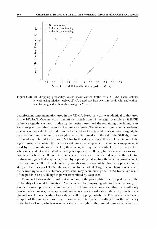
366 CHAPTER 6. HSDPA-STYLE FDD NETWORKING, ADAPTIVE ARRAYS AND AQAM
0.8 1.0 1.2 1.4 1.6 1.8 2.0 2.2 2.4 2.6 2.82
10-3
2
5
10-2
2
Forc
edTe
rmin
atio
nPr
obab
ility
,PFT
1%
4 element beamforming2 element beamformingNo beamforming
Mean Carried Teletraffic (Erlangs/km /MHz)
Figure 6.41: Call dropping probability versus mean carried traffic of a CDMA based cellularnetwork using relative received Ec/Io based soft handover thresholds with and withoutbeamforming and without shadowing for SF = 16.
beamforming implementation used in the CDMA based network was identical to that usedin the FDMA/TDMA network simulations. Briefly, one of the eight possible 8-bit BPSKreference signals was used to identify the desired user, and the remaining interfering userswere assigned the other seven 8-bit reference signals. The received signal’s autocorrelationmatrix was then calculated, and from the knowledge of the desired user’s reference signal, thereceiver’s optimal antenna array weights were determined with the aid of the SMI algorithm.The reader is referred to Section 5.6.1 for further details. Since this implementation of thealgorithm only calculated the receiver’s antenna array weights, i.e. the antenna arrays weightsused by the base station in the UL, these weights may not be suitable for use in the DL,when independent up/DL shadow fading is experienced. Hence, further investigations wereconducted, where the UL and DL channels were identical, in order to determine the potentialperformance gain that may be achieved by separately calculating the antenna array weightsto be used in the DL. The antenna array weights were re-calculated for every power controlstep, i.e. 15 times per UTRA data frame, due to the potential significant changes in terms ofthe desired signal and interference powers that may occur during one UTRA frame as a resultof the possible 15 dB change in power transmitted by each user.
Figure 6.41 shows the significant reduction in the probability of a dropped call, i.e. theprobability of forced termination PFT , achieved by employing adaptive antenna arrays ina non-shadowed propagation environment. The figure has demonstrated that, even with onlytwo antenna elements, the adaptive antenna arrays have considerably reduced the levels of co-channel interference, leading to a reduced call dropping probability. This has been achievedin spite of the numerous sources of co-channel interference resulting from the frequencyreuse factor of one, which was remarkable in the light of the limited number of degrees of

6.4. SIMULATION RESULTS 367
0.8 1.0 1.2 1.4 1.6 1.8 2.0 2.2 2.4 2.6 2.82
10-4
2
5
10-3
2
5
10-2
2
Prob
abili
tyof
low
qual
ityac
cess
,Plo
w
2%
1%4 element beamforming2 element beamformingNo beamforming
Mean Carried Teletraffic (Erlangs/km /MHz)
Figure 6.42: Probability of low quality access versus mean carried traffic of a CDMA based cellularnetwork using relative received Ec/Io based soft handover thresholds with and withoutbeamforming and without shadowing for SF = 16.
freedom of the two element array. Without employing antenna arrays at the base stationsthe network capacity was limited to 256 users, or to a teletraffic load of approximately1.4 Erlangs/km2/MHz. However, with the advent of two element adaptive antenna arraysat the base stations the number of users supported by the network rose by 27% to 325 users,or almost 1.9 Erlangs/km2/MHz. Replacing the two element adaptive antenna arrays withfour element arrays led to a further rise of 48%, or 88% with respect to the capacity of thenetwork using no antenna arrays. This is associated with a network capacity of 480 users,or 2.75 Erlangs/km2/MHz. A summary of the network capacities achieved under differentconditions is given in Table 6.4.
The probability of low quality outage, presented in Figure 6.42 also exhibited asubstantial improvement with the advent of two element adaptive antenna arrays. However,the performance gains obtained when invoking four element adaptive antenna arrays weremore involved. It can be seen from the figure that higher traffic loads were carried withat a sufficiently low probability of a low quality occurring, and at higher traffic loadsthe probability of a low quality access was lower than that achieved using a two elementarray. However, at lower traffic loads the performance was worse than that obtained whenusing two element arrays, and the gradient of the performance curve was significantlylower. Further in-depth analysis of the results suggested that the vast majority of the lowquality outages were occurring when new calls started. When a user decided to commencecommunications with the base station, the current interference level was measured, and thetarget transmission power was determined in order to reach the target SINR necessary forreliable communications. However, in order to avoid disrupting existing calls the transmissionpower was ramped up slowly, until the target SINR was reached. A network using no adaptive

368 CHAPTER 6. HSDPA-STYLE FDD NETWORKING, ADAPTIVE ARRAYS AND AQAM
111.0 111.5 112.0 112.5 113.0 113.5 114.0 114.5 115.0Frames
3
4
5
6
7
8
9
SIN
R(d
B)
DownlinkUplink
111.0 111.5 112.0 112.5 113.0 113.5 114.0 114.5 115.00.2
0.3
0.4
0.5
0.6
0.7
Ant
enna
gain
111.0 111.5 112.0 112.5 113.0 113.5 114.0 114.5 115.04
6
8
1012
14
16
18
Tra
nsm
itpo
wer
(dB
m)
DownlinkUplink
Figure 6.43: The changes in the antenna array gain, versus time, in the direction of the desired user, theUL and DL transmission powers, and the UL and DL received SINRs, when a new callstarts using four element adaptive antenna arrays without shadowing in conjunction withthe original power ramping algorithm and SF = 16.
antenna arrays, i.e. employing omnidirectional antennas, can be viewed as offering equal gainto all users of the network, which we assumed to be 1.0, or 0 dB. Thus, when a new call isinitiated, the level of interference rises gradually, and the power control algorithm ensures thatthe existing users compensate for the increased level of co-channel interference by increasingtheir transmission power. In a network using adaptive antenna arrays, the adaptive antennaarrays are used to null the sources of interference, and in doing so the array may reduce theantenna gain in the direction of the desired user, in order to maximize the SINR. Hence auser starting a new call, even if it has low transmission power, can alter the antenna array’sresponse, and thus the antenna gain experienced by the existing users. This phenomenon ismore marked when using four element arrays since their directivity, and thus sensitivity tointerfering signals, is greater.
Figure 6.43 illustrates this phenomenon, where another user starts a new call at frame 112suddenly reducing the antenna gain in the direction of the desired user from 0.4 to just above0.2, a drop of 3 dB. As can be seen from the figure, the DL SINR falls sharply below thelow quality outage threshold of 7.0 dB, resulting in several consecutive outages, until the DLtransmission power is increased sufficiently. The impact of reducing the initial transmissionpower, in order to ensure that the power ramping takes place more gently, is depicted inFigure 6.44. In this figure it can be seen that the antenna gain falls much more gently, overa prolonged period of time, thus reducing the number of low quality outages, as the DL

6.4. SIMULATION RESULTS 369
125.0 125.5 126.0 126.5 127.0 127.5 128.0 128.5 129.0Frames
3
4
5
6
7
8
9
SIN
R(d
B)
DownlinkUplink
125.0 125.5 126.0 126.5 127.0 127.5 128.0 128.5 129.00.2
0.3
0.4
0.5
0.6
0.7
Ant
enna
gain
125.0 125.5 126.0 126.5 127.0 127.5 128.0 128.5 129.04
6
8
1012
14
16
18
Tra
nsm
itpo
wer
(dB
m)
DownlinkUplink
Figure 6.44: The changes in the antenna array gain, versus time, in the direction of the desired user, theUL and DL transmission powers, and the UL and DL received SINRs, when a new callstarts using four element adaptive antenna arrays without shadowing in conjunction witha slower power ramping algorithm and SF = 16.
transmission power is increased in an effort to compensate for the lower antenna gain. It isof interest to note how the received SINR varies as the antenna gain and the power controlalgorithm interact, in order to maintain the target SINR.
Even though the employment of adaptive antenna arrays can result in the attenuation ofthe desired signal, this is performed in order to maximize the received SINR, and thus thelevels of interference are attenuated more strongly, ultimately leading to the reduction of themean transmission power, as emphasized by Figure 6.45. This figure clearly shows the lowerlevels of transmission power, required in order to maintain an acceptable performance, whilstusing adaptive antenna arrays at the base stations. A reduction of 3 dB in the mean mobiletransmission power was achieved by invoking two element antenna arrays, and a furtherreduction of 1.5 dB resulted from using four element arrays. These power budget savings wereobtained in conjunction with reduced levels of co-channel interference, leading to superiorcall quality, as illustrated in Figures 6.41 and 6.42. A greater performance advantage wasevident in the UL scenario, suggesting that the selective base station diversity techniquesemployed in the UL are amenable to amalgamation with adaptive antenna arrays. In contrast,the maximum ratio combining performed at the mobile inherently reduces the impact of co-channel interference, and hence benefits to a lesser extent from the employment of adaptiveantenna arrays.

370 CHAPTER 6. HSDPA-STYLE FDD NETWORKING, ADAPTIVE ARRAYS AND AQAM
0.8 1.0 1.2 1.4 1.6 1.8 2.0 2.2 2.4 2.6 2.82
-3
-2
-1
0
1
2
3
4
5
6
Mea
nT
rans
mis
sion
Pow
er(d
Bm
)4 element beamforming2 element beamformingNo beamformingFilled = Downlink, Blank = Uplink
Mean Carried Teletraffic (Erlangs/km /MHz)
Figure 6.45: Mean transmission power versus mean carried traffic of a CDMA based cellularnetwork using relative received Ec/Io based soft handover thresholds with and withoutbeamforming and without shadowing for SF = 16.
0.4 0.6 0.8 1.0 1.2 1.4 1.6 1.8 2.0 2.22
10-3
2
5
10-2
2
Forc
edTe
rmin
atio
nPr
obab
ility
,PFT
1%
4 element beamforming2 element beamformingNo beamforming
1.0Hz, 3dB shadowing0.5Hz, 3dB shadowing
downlink beamformingFilled = Independent up/
Mean Carried Teletraffic (Erlangs/km /MHz)
Figure 6.46: Call dropping probability versus mean carried traffic of a CDMA based cellularnetwork using relative received Ec/Io based soft handover thresholds with and withoutbeamforming and with shadowing having a standard deviation of 3 dB for SF = 16.

6.4. SIMULATION RESULTS 371
0.4 0.6 0.8 1.0 1.2 1.4 1.6 1.8 2.0 2.22
10-4
2
5
10-3
2
5
10-2
2
Prob
abili
tyof
low
qual
ityac
cess
,Plo
w
1%
2%
downlink beamformingFilled = independent up/1.0Hz, 3dB shadowing0.5Hz, 3dB shadowing4 element beamforming2 element beamformingNo beamforming
Mean Carried Teletraffic (Erlangs/km /MHz)
Figure 6.47: Probability of low quality access versus mean carried traffic of a CDMA based cellularnetwork using relative received Ec/Io based soft handover thresholds with and withoutbeamforming and with shadowing having a standard deviation of 3 dB for SF = 16.
The impact of adaptive antenna arrays in a propagation environment subjected toshadow fading was then investigated. The associated call dropping performance is shownin Figure 6.46. This figure illustrates the substantial network capacity gains achieved with theaid of both two and four element adaptive antenna arrays under shadow fading propagationconditions. Simulations were conducted in conjunction with log-normal shadow fadinghaving a standard deviation of 3 dB, and maximum shadowing frequencies of both 0.5 Hzand 1.0 Hz. As expected the network capacity was reduced at the faster fading frequency.The effect of performing independent UL and DL beamforming, as opposed to using thebase station’s receive antenna array weights in the DL was also studied, and a small, but notinsignificant call dropping probability reduction can be seen in the Figure 6.46. The networksupported just over 150 users, and 144 users, when subjected to 0.5 Hz and 1.0 Hz frequencyshadow fading, respectively. With the application of two element adaptive antenna arrays,re-using the base station’s UL receiver weights on the DL, these capacities increased by 35%and 40%, to 203 users and 201 users. Performing independent UL and DL beamformingresulted in a mean further increase of 13% in the network capacity. The implementation offour element adaptive antenna arrays led to a network capacity of 349 users at a 0.5 Hzshadowing frequency, and 333 users at a 1.0 Hz shadowing frequency. This corresponded torelative gains of 133% and 131% over the capacity provided without beamforming. Invokingindependent UL and DL beamforming gave another boost of 7% and 10% to network capacityfor 0.5 Hz and 1.0 Hz frequency shadowing environments, respectively, giving final networkcapacities of just over 375 users and 365 users.
Similar trends were observed regarding the probability of low quality outage to thosefound in the non-shadowing scenarios. However, the trend was much more prevalent under

372 CHAPTER 6. HSDPA-STYLE FDD NETWORKING, ADAPTIVE ARRAYS AND AQAM
0.4 0.6 0.8 1.0 1.2 1.4 1.6 1.8 2.0 2.22
-4
-3
-2
-1
0
1
2
3
Mea
nT
rans
mis
sion
Pow
er(d
Bm
)
Filled = Downlink, Blank = Uplink1.0Hz, 3dB shadowing0.5Hz, 3dB shadowing4 element beamforming2 element beamformingNo beamforming
Mean Carried Teletraffic (Erlangs/km /MHz)
Figure 6.48: Mean transmission power versus mean carried traffic of a CDMA based cellularnetwork using relative received Ec/Io based soft handover thresholds with and withoutbeamforming and shadowing having a standard deviation of 3 dB for SF = 16.
shadowing, due to greater variation of the received signal strengths, as a result of the shadowfading, as shown in Figure 6.47. The figure indicates that the trend is also evident, whenusing two element adaptive antenna arrays in conjunction with shadow fading. As expected,the performance deteriorated as the number of antenna elements increased, and when themaximum shadow fading frequency was increased from 0.5 Hz to 1.0 Hz. It should be noted,however that the probability of low quality access always remained below the 1% constraintof the conservative scenario, and the call dropping probability was considerably reduced bythe adaptive antenna arrays.
The mean transmission power performance is depicted in Figure 6.48, suggesting that asfor the non-shadowing scenario of Figure 6.45, the number of antenna elements had only alimited impact on the base stations’ transmission power, although there was some reductionin the mobile stations’ mean transmission power. The mean transmission powers requiredwhen using independent UL and DL beamforming are not explicitly shown, but were slightlyless than those presented here, with a mean reduction of about 0.4 dB.
A summary of the maximum network capacities of the networks considered in this sectionboth with and without shadowing, employing beamforming using two and four element arraysis given in Table 6.4, along with the teletraffic carried and the mean mobile and base stationtransmission powers required.
The lower bounds of the maximum network capacities obtained under identical scenariosin conjunction with a spreading factor of 256, are also presented in Table 6.5, leading toa bit rate of 15 kbps, which is suitable for use by speech-rate users. The network capacitycalculations were performed by scaling the number of users supported, as presented in

6.4. SIMULATION RESULTS 373
Table 6.4: Maximum mean carried traffic and maximum number of mobile users that can be supportedby the network, whilst meeting the conservative quality constraints. The carried traffic isexpressed in terms of normalized Erlangs (Erlang/km2/MHz) for the network described inTable 6.2 both with and without beamforming (as well as with and without independentUL/DL beamforming), and also with and without shadow fading having a standard deviationof 3 dB for SF = 16.
Conservative scenario, PF T =1%, Plow=1%
Power (dBm)Independent Traffic
Shadowing Beamforming: UL/DL Users (Erlangs/km2/MHz) MS BS
No No — 256 1.42 3.1 2.7No 2 elements — 325 1.87 3.75 0.55No 4 elements — 480 2.75 4.55 1.85
0.5 Hz, 3 dB No — ≈150 0.87 −1.2 −1.70.5 Hz, 3 dB 2 elements No 203 1.16 0.1 −1.10.5 Hz, 3 dB 4 elements No 349 2.0 2.0 0.650.5 Hz, 3 dB 2 elements Yes 233 1.35 0.2 −0.80.5 Hz, 3 dB 4 elements Yes ≈375 2.2 2.15 0.85
1.0 Hz, 3 dB No — 144 0.82 −1.1 −1.61.0 Hz, 3 dB 2 elements No 201 1.12 −0.3 −1.11.0 Hz, 3 dB 4 elements No 333 1.88 1.6 0.51.0 Hz, 3 dB 2 elements Yes 225 1.31 0.1 −0.91.0 Hz, 3 dB 4 elements Yes 365 2.05 1.65 0.6
Table 6.4, by the ratio of their spreading factors, i.e. 256/16 = 16. Further interesting usercapacity figures can be inferred for a variety of target bit rates by comparing Tables 6.4, 6.5,6.7 and 6.8 and applying the appropriate spreading factor related scaling mentioned in thecontext of estimating the number of 15 kbps speech users supported.
6.4.6 Performance of Adaptive Antenna Arrays and AdaptiveModulation in a High Data Rate Pedestrian Environment
In this section we build upon the results presented in the previous section by applyingAdaptive Quadrature Amplitude Modulation (AQAM) techniques. The various scenarios andchannel conditions investigated were identical to those of the previous section, except forthe application of AQAM. Since in the previous section an increased network capacity wasachieved due to using independent UL and DL beamforming, this procedure was invokedin these simulations. AQAM involves the selection of the appropriate modulation modein order to maximize the achievable data throughput over a channel, whilst minimizingthe Bit Error Ratio (BER). More explicitly, the philosophy behind adaptive modulation isthe most appropriate selection of a modulation mode according to the instantaneous radiochannel quality experienced [12, 13]. Therefore, if the SINR of the channel is high, thena high-order modulation mode may be employed, thus exploiting the temporal fluctuationof the radio channel’s quality. Similarly, if the channel is of low quality, exhibiting a low
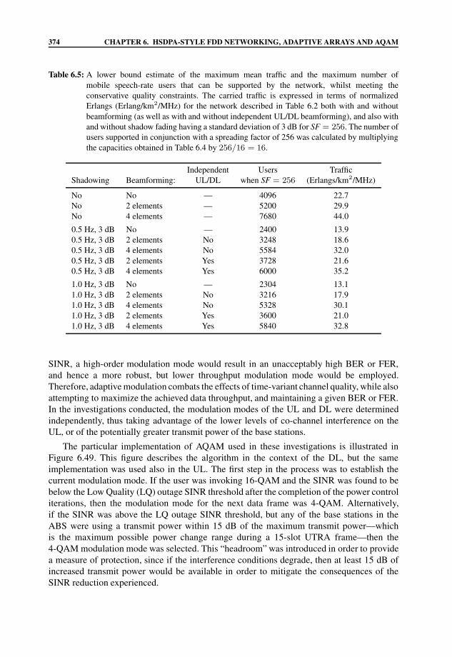
374 CHAPTER 6. HSDPA-STYLE FDD NETWORKING, ADAPTIVE ARRAYS AND AQAM
Table 6.5: A lower bound estimate of the maximum mean traffic and the maximum number ofmobile speech-rate users that can be supported by the network, whilst meeting theconservative quality constraints. The carried traffic is expressed in terms of normalizedErlangs (Erlang/km2/MHz) for the network described in Table 6.2 both with and withoutbeamforming (as well as with and without independent UL/DL beamforming), and also withand without shadow fading having a standard deviation of 3 dB for SF = 256. The number ofusers supported in conjunction with a spreading factor of 256 was calculated by multiplyingthe capacities obtained in Table 6.4 by 256/16 = 16.
Independent Users TrafficShadowing Beamforming: UL/DL when SF = 256 (Erlangs/km2/MHz)
No No — 4096 22.7No 2 elements — 5200 29.9No 4 elements — 7680 44.0
0.5 Hz, 3 dB No — 2400 13.90.5 Hz, 3 dB 2 elements No 3248 18.60.5 Hz, 3 dB 4 elements No 5584 32.00.5 Hz, 3 dB 2 elements Yes 3728 21.60.5 Hz, 3 dB 4 elements Yes 6000 35.2
1.0 Hz, 3 dB No — 2304 13.11.0 Hz, 3 dB 2 elements No 3216 17.91.0 Hz, 3 dB 4 elements No 5328 30.11.0 Hz, 3 dB 2 elements Yes 3600 21.01.0 Hz, 3 dB 4 elements Yes 5840 32.8
SINR, a high-order modulation mode would result in an unacceptably high BER or FER,and hence a more robust, but lower throughput modulation mode would be employed.Therefore, adaptive modulation combats the effects of time-variant channel quality, while alsoattempting to maximize the achieved data throughput, and maintaining a given BER or FER.In the investigations conducted, the modulation modes of the UL and DL were determinedindependently, thus taking advantage of the lower levels of co-channel interference on theUL, or of the potentially greater transmit power of the base stations.
The particular implementation of AQAM used in these investigations is illustrated inFigure 6.49. This figure describes the algorithm in the context of the DL, but the sameimplementation was used also in the UL. The first step in the process was to establish thecurrent modulation mode. If the user was invoking 16-QAM and the SINR was found to bebelow the Low Quality (LQ) outage SINR threshold after the completion of the power controliterations, then the modulation mode for the next data frame was 4-QAM. Alternatively,if the SINR was above the LQ outage SINR threshold, but any of the base stations in theABS were using a transmit power within 15 dB of the maximum transmit power—whichis the maximum possible power change range during a 15-slot UTRA frame—then the4-QAM modulation mode was selected. This “headroom” was introduced in order to providea measure of protection, since if the interference conditions degrade, then at least 15 dB ofincreased transmit power would be available in order to mitigate the consequences of theSINR reduction experienced.

6.4. SIMULATION RESULTS 375
Table 6.6: The target SINR, low quality outage SINR and outage SINR thresholds used for the BPSK,4-QAM and 16-QAM modulation modes of the adaptive modem.
SINR Threshold BPSK 4-QAM 16-QAM
Outage SINR 2.6 dB 6.6 dB 12.1 dBLow Quality Outage SINR 3.0 dB 7.0 dB 12.5 dBTarget SINR 4.0 dB 8.0 dB 13.5 dB
A similar procedure was invoked when switching to other legitimate AQAM modes fromthe 4-QAM mode. If the SINR was below the 4-QAM target SINR and any one of the basestations in the ABS was within 15 dB (the maximum possible power change during a 15-slot UTRA data frame) of the maximum transmit power, then the BPSK modulation modewas employed for the next data frame. However, if the SINR exceeded the 4-QAM targetSINR and there would be 15 dB of headroom in the transmit power budget in excess of theextra transmit power required for switching from 4-QAM to 16-QAM, then the 16-QAMmodulation mode was invoked.
And finally, when in the BPSK mode, the 4-QAM modulation mode was selected if theSINR exceeded the BPSK target SINR, and the transmit power of any of the base stationsin the ABS was less than the power required to transmit reliably using 4-QAM, while beingat least 15 dB below the maximum transmit power. The algorithm was activated at the endof each 15-slot UTRA data frame, after the power control algorithm had performed its 15iterations per data frame, and thus the AQAM mode selection was performed on a UTRAtransmission frame-by-frame basis. When changing from a lower-order modulation to ahigher-order modulation mode, the lower-order mode was retained for an extra frame in orderto ramp up the transmit power to the required level, as shown in Figure 6.50(a). Conversely,when changing from a higher-order modulation mode to a lower-order modulation mode,the lower-order modulation mode was employed whilst ramping the power down, in orderto avoid excessive outages in the higher-order modulation mode due to the reduction of thetransmit power, as illustrated in Figure 6.50(b).
Table 6.6 gives the BPSK, 4-QAM and 16-QAM SINR thresholds used in the simulations.The BPSK SINR thresholds were 4 dB lower than those necessary when using 4-QAM, whilethe 16-QAM SINR thresholds were 5.5 dB higher [408]. In other words, in moving from theBPSK modulation mode to the 4-QAM modulation mode, the target SINR, low quality outageSINR and outage SINR all increased by 4 dB. When switching to the 16-QAM mode fromthe 4-QAM mode, the SINR thresholds increased by 5.5 dB. However, setting the BPSK to4-QAM and the 4-QAM to 16-QAM mode switching thresholds to a value 7 dB higher thanthe SINR required for maintaining the target BER/FER was necessary in order to preventexcessive outages due to sudden dramatic channel-induced variations in the SINR levels.
Performance results were obtained both with and without beamforming in a log-normalshadow fading environment, at maximum fading frequencies of 0.5 Hz and 1.0 Hz, and astandard deviation of 3 dB. A pedestrian velocity of 3 mph, a cell radius of 150 m and aspreading factor of 16 were used, as in our previous investigations.

376 CHAPTER 6. HSDPA-STYLE FDD NETWORKING, ADAPTIVE ARRAYS AND AQAM
Y
N
16-QAM Mode?
Thus, in BPSK mode
4-QAM to 16-QAM thres.Any BS TX power <
Y
-15dB
Switch to 16-QAM
Downlink Start
Y
N
SINR < 4-QAM TargetSINR?
Switch to BPSK
Y
N
SINR < 16-QAM LQ Switch to 4-QAMOutage SINR?
max. BS TX power-15dBAny BS TX power >
Switch to 4-QAMY
Any BS TX power >max. BS TX power-15dB
Y
Y
N
4-QAM Mode?
SINR > BPSK TargetSINR?
YBPSK to 4-QAM thres.
Any BS TX power <
Y
-15dB
Switch to 4-QAM
Figure 6.49: The AQAM mode switching algorithm used in the DL of the CDMA based cellularnetwork.
16-QAM4-QAM4-QAM
Frame n Frame n+2Frame n+1
Tra
nsm
it po
wer
(a)
4-QAM4-QAM16-QAM
Frame n Frame n+2Frame n+1
Tra
nsm
it po
wer
(b)
Figure 6.50: Power ramping requirements whilst switching modulation modes: (a) ramping up thetransmit power whilst remaining in the lower order modulation mode; (b) ramping downthe transmit power whilst switching to the lower order modulation mode.

6.4. SIMULATION RESULTS 377
0.8 1.0 1.2 1.4 1.6 1.8 2.0 2.2 2.4 2.6 2.82
10-3
2
5
10-2
2
Forc
edTe
rmin
atio
nPr
obab
ility
,PFT
1%
4 element beamforming2 element beamformingNo beamforming
1Hz, 3dB shadowing0.5Hz, 3dB shadowing
Mean Carried Teletraffic (Erlangs/km /MHz)
Figure 6.51: Call dropping probability versus mean carried traffic of a CDMA based cellular networkusing relative received Ec/Io based soft handover thresholds both with and withoutbeamforming in conjunction with AQAM as well as with shadowing having a standarddeviation of 3 dB for SF = 16. See Figure 6.46 for corresponding results without adaptivemodulation.
Figure 6.51 shows the significant reduction in the probability of a dropped call, achievedby employing adaptive antenna arrays in conjunction with adaptive modulation in a log-normal shadow faded environment. The figure demonstrates that, even with the aid of atwo element adaptive antenna array and its limited degrees of freedom, a substantial calldropping probability reduction was achieved. The performance benefit of increasing thearray’s degrees of freedom, achieved by increasing the number of antenna elements, becomesexplicit from the figure, resulting in a further call dropping probability reduction. Simulationswere conducted in conjunction with log-normal shadow fading having a standard deviationof 3 dB, and maximum shadowing frequencies of 0.5 Hz and 1.0 Hz. As expected, the calldropping probability was generally higher at the faster fading frequency, as demonstrated byFigure 6.51. The network was found to support 223 users, corresponding to a traffic load of1.27 Erlang/km2/MHz, when subjected to 0.5 Hz frequency shadow fading. The capacityof the network was reduced to 218 users, or 1.24 Erlang/km2/MHz, upon increasing themaximum shadow fading frequency to 1.0 Hz. On employing two element adaptive antennaarrays, the network capacity increased by 64% to 366 users, or to an equivalent traffic loadof 2.11 Erlang/km2/MHz when subjected to 0.5 Hz frequency shadow fading. When themaximum shadow fading frequency was raised to 1.0 Hz, the number of users supportedby the network was 341 users, or 1.98 Erlang/km2/MHz, representing an increase of 56%in comparison to the network without adaptive antenna arrays. Increasing the number ofantenna elements to four, whilst imposing shadow fading with a maximum frequency of0.5 Hz, resulted in a network capacity of 2.68 Erlang/km2/MHz or 476 users, corresponding

378 CHAPTER 6. HSDPA-STYLE FDD NETWORKING, ADAPTIVE ARRAYS AND AQAM
0.8 1.0 1.2 1.4 1.6 1.8 2.0 2.2 2.4 2.6 2.82
10-4
2
5
10-3
2
5
10-2
2
Prob
abili
tyof
low
qual
ityac
cess
,Plo
w
1%
2%
1Hz, 3dB shadowing0.5Hz, 3dB shadowing4 element beamforming2 element beamformingNo beamforming
Mean Carried Teletraffic (Erlangs/km /MHz)
Figure 6.52: Probability of low quality access versus mean carried traffic of a CDMA based cellularnetwork using relative received Ec/Io based soft handover thresholds both with andwithout beamforming in conjunction with AQAM as well as with shadowing having astandard deviation of 3 dB for SF = 16. See Figure 6.47 for corresponding results withoutadaptive modulation.
to a gain of an extra 30% with respect to the network employing two element arrays, and of113% in comparison to the network employing no adaptive antenna arrays. In conjunctionwith a maximum shadow fading frequency of 1.0 Hz the network capacity was 460 users or2.59 Erlang/km2/MHz, which represented an increase of 35% with respect to the networkinvoking two element antenna arrays, or 111% relative to the identical network withoutadaptive antenna arrays.
The probability of low quality outage, presented in Figure 6.52, did not benefit fromthe application of adaptive antenna arrays, or from the employment of adaptive modulation.Figure 6.47 depicts the probability of low quality outage without adaptive modulation, andupon comparing these results to those obtained in conjunction with adaptive modulationshown in Figure 6.52, the performance degradation due to adaptive modulation can beexplicitly seen. However, the increase in the probability of low quality access can be attributedto the employment of less robust, but higher throughput, higher-order modulation modesinvoked by the adaptive modulation scheme. Hence, under given propagation conditionsand using the fixed 4-QAM modulation mode a low quality outage may not occur, yetwhen using adaptive modulation and a higher order modulation mode, the same propagationconditions may inflict a low quality outage. This phenomenon is further exacerbated by theadaptive antenna arrays, as described in Section 6.4.5, where the addition of a new source ofinterference, constituted by a user initiating a new call, results in an abrupt change in the gainof the antenna in the direction of the desired user. This in turn leads to low quality outages,which are more likely to occur for prolonged periods of time when using a higher order

6.4. SIMULATION RESULTS 379
0.8 1.0 1.2 1.4 1.6 1.8 2.0 2.2 2.4 2.6 2.82
0
1
2
3
4
5
6
Mea
nT
rans
mis
sion
Pow
er(d
Bm
)
1Hz, 3dB shadowing0.5Hz, 3dB shadowing4 element beamforming2 element beamformingNo beamformingFilled = Downlink, Blank = Uplink
Mean Carried Teletraffic (Erlangs/km /MHz)
Figure 6.53: Mean transmission power versus mean carried traffic of a CDMA based cellular networkusing relative received Ec/Io based soft handover thresholds both with and withoutbeamforming in conjunction with AQAM as well as with shadowing having a standarddeviation of 3 dB for SF = 16. See Figure 6.48 for corresponding results without adaptivemodulation.
modulation mode. Again, increasing the number of antenna elements from two to four resultsin an increased probability of a low quality outage due to the sharper antenna directivity. Thisresults in a higher sensitivity to changes in the interference incident upon it.
The mean transmission power versus teletraffic performance is depicted in Figure 6.53,suggesting that the mean UL transmission power was always significantly below the mean DLtransmission power, which can be attributed to the pilot power interference encountered bythe mobiles in the DL. This explanation can be confirmed by examining Figure 6.54, whichdemonstrates that the mean modem throughput in the DL, without adaptive antenna arrays,was lower than that in the UL even in conjunction with increased DL transmission power.Invoking adaptive antenna arrays at the base stations reduced the mean UL transmissionpower required in order to meet the service quality targets of the network. The attainableDL power reduction increased as the number of antenna array elements increased, as a resultof the superior interference rejection achieved with the aid of a higher number of arrayelements. A further advantage of employing a larger number of antenna array elements wasthe associated increase in the mean UL modem throughput, which became more significantat higher traffic loads. In the DL scenario, however, increasing the number of adaptiveantenna array elements led to an increased mean DL transmission power, albeit with asubstantially improved mean DL modem throughput. This suggests that there was someinteraction between the adaptive antenna arrays, the adaptive modulation mode switchingalgorithm and the maximal ratio combining performed at the mobiles. In contrast, simpleswitched diversity was performed by the base stations on the UL, thus avoiding such a

380 CHAPTER 6. HSDPA-STYLE FDD NETWORKING, ADAPTIVE ARRAYS AND AQAM
0.8 1.0 1.2 1.4 1.6 1.8 2.0 2.2 2.4 2.6 2.82
2.0
2.2
2.4
2.6
2.8
3.0
3.2
3.4
3.6
3.8
4.0
Mea
nM
odem
Thr
ough
put(
BPS
)
4 element beamforming2 element beamformingNo beamformingFilled = Uplink, Blank = Downlink
1Hz, 3dB shadowing0.5Hz, 3dB shadowing
Mean Carried Teletraffic (Erlangs/km /MHz)
Figure 6.54: Mean modem throughput versus mean carried traffic of a CDMA based cellular networkusing relative received Ec/Io based soft handover thresholds both with and withoutbeamforming in conjunction with AQAM as well as with shadowing having a standarddeviation of 3 dB for SF = 16.
situation. However, the increase in the mean DL transmission power resulted in a much moresubstantial increase in the mean DL modem throughput, especially with the advent of the fourelement antenna arrays, which exhibited an approximately 0.5 BPS throughput gain over thetwo element arrays for identical high traffic loads which can be seen in Figure 6.54.
A summary of the maximum user capacities of the networks considered in this sectionin conjunction with log-normal shadowing having a standard deviation of 3 dB, with andwithout employing beamforming using two and four element arrays is given in Table 6.7.The teletraffic carried the mean mobile and base station transmission powers required, and themean UL and DL modem data throughputs achieved are also shown in Table 6.7. Similarly,the lower bounds of the maximum network capacities obtained under identical scenariosin conjunction with a spreading factor of 256, leading to a bit rate of 15 kbps, suitablefor speech-rate users are presented in Table 6.8. The network capacity calculations wereperformed by scaling the number of users supported, as presented in Table 6.7, by the ratioof their spreading factors, i.e. by 256/16 = 16.
6.5 Summary and Conclusions
We commenced this chapter with a brief overview of the background behind the 3G UTRAstandard. This was followed in Sections 6.2 and 6.3 by an introduction to CDMA and thetechniques invoked in the UTRA standard.

6.5. SUMMARY AND CONCLUSIONS 381
Table 6.7: Maximum mean carried traffic and maximum number of mobile users that can besupported by the network, whilst meeting the conservative quality constraints. The carriedtraffic is expressed in terms of normalized Erlangs (Erlang/km2/MHz), for the networkdescribed in Table 6.2 both with and without beamforming (using independent up/down-link beamforming), in conjunction with shadow fading having a standard deviation of 3 dB,whilst employing adaptive modulation techniques for SF = 16.
Conservative scenario
Power (dBm) Throughput (BPS)Traffic (Erlangs
Shadowing Beamforming Users /km2/MHz) MS BS UL DL
0.5 Hz, 3 dB No 223 1.27 3.25 4.95 2.86 2.950.5 Hz, 3 dB 2 elements 366 2.11 3.55 4.7 2.56 2.660.5 Hz, 3 dB 4 elements 476 2.68 3.4 5.0 2.35 2.72
1.0 Hz, 3 dB No 218 1.24 3.3 4.95 2.87 2.961.0 Hz, 3 dB 2 elements 341 1.98 3.5 4.9 2.62 2.731.0 Hz, 3 dB 4 elements 460 2.59 3.5 4.95 2.4 2.8
Table 6.8: A lower bound estimate of the maximum mean carried traffic and maximum numberof mobile speech-rate users that can be supported by the network, whilst meeting theconservative quality constraints. The carried traffic is expressed in terms of normalizedErlangs (Erlang/km2/MHz), for the network described in Table 6.2 both with and withoutbeamforming (using independent up/down-link beamforming), in conjunction with shadowfading having a standard deviation of 3 dB, whilst employing adaptive modulationtechniques for SF = 256. The number of users supported in conjunction with a spreadingfactor of 256 was calculated by multiplying the capacities obtained in Table 6.7 by256/16 = 16.
Conservative scenario
TrafficShadowing Beamforming Users (Erlangs/km2/MHz)
0.5 Hz, 3 dB No 3568 20.30.5 Hz, 3 dB 2 elements 5856 33.80.5 Hz, 3 dB 4 elements 7616 42.9
1.0 Hz, 3 dB No 3488 19.81.0 Hz, 3 dB 2 elements 5456 31.71.0 Hz, 3 dB 4 elements 7360 41.4
Network capacity studies were then conducted in Section 6.4, which evaluated theperformance of four different soft handover algorithms in the context of both non-shadowedand log-normal shadow faded propagation environments. The algorithm using relativereceived pilot-to-interference ratio measurements at the mobile, in order to determine themost suitable base stations for soft handover, was found to offer the highest network capacitywhen subjected to shadow fading propagation conditions. Hence, this algorithm and its

382 CHAPTER 6. HSDPA-STYLE FDD NETWORKING, ADAPTIVE ARRAYS AND AQAM
associated parameters were selected for use in our further investigations. The impact ofadaptive antenna arrays upon the network capacity was then considered in Section 6.4.5 inboth non-shadowed and log-normal shadow faded propagation environments. Considerablenetwork capacity gains were achieved, employing both two and four element adaptiveantenna arrays. This work was then extended in Section 6.4.6 by the application of adaptivemodulation techniques in conjunction with the previously studied adaptive antenna arraysin a log-normal shadow faded propagation environment, which elicited further significantnetwork capacity gains.

Chapter 7HSDPA-style FDD/CDMAPerformance Using LooselySynchronized Spreading Codes
7.1 Effects of Loosely Synchronized Spreading Codes onthe Performance of CDMA Systems
7.1.1 Introduction
In this section we characterize the achievable system performance of a UTRA-like FDDCDMA system employing Loosely Synchronized (LS) spreading codes. Current CDMAsystems are interference limited, suffering from Inter-Symbol-Interference (ISI), since theorthogonality of the spreading sequences is destroyed by the channel. They also sufferfrom Multiple-Access-Interference (MAI) owing to the non-zero cross-correlations of thespreading codes. LS codes exhibit a so-called Interference Free Window (IFW), where boththe auto-correlation and cross-correlation values of the codes become zero. Therefore LScodes have the promise of mitigating the effects of both ISI and MAI in time dispersivechannels. Hence, LS codes have the potential of increasing the capacity of CDMA networks.This contribution studies the achievable network performance by simulation and comparesit to that of a UTRA-like FDD/CDMA system using Orthogonal Variable SpreadingFactor (OVSF) codes.
In our previous research [416–418], outlined in the preceding chapters the performanceof a UTRA-like FDD CDMA system was quantified, when supported by both adaptive beam-steering and adaptive modulation [419]. In [418], the system employed OVSF spreadingcodes [420], which offer the benefit of perfect orthogonality in an ideal channel. In a non-dispersive channel, all intra-cell users’ signals are perfectly orthogonal. However, uponpropagating through a dispersive multipath channel this orthogonality is eroded, hence
3G, HSPA and FDD versus TDD Networking Second EditionL. Hanzo, J. S. Blogh and S. Ni c© 2008 John Wiley & Sons, Ltd

384 CHAPTER 7. HSDPA-STYLE FDD/CDMA PERFORMANCE USING LS SPREADING CODES
Complementary Pair Complementary PairW0 0W
Figure 7.1: The LS code structure.
all other users will interfere with the desired signal. Therefore in practice the intra-cellinterference is always non-zero.
We will consider the employment of a specific family of spreading codes, which areknown as Loosely Synchronized codes [421]. These codes exhibit a so-called InterferenceFree Window, where the off-peak aperiodic autocorrelation values as well as the aperiodiccross-correlation values become zero, resulting in zero ISI and zero MAI, provided that thedelayed asynchronous transmissions arrive within the IFW. More specifically, interference-free CDMA communications become possible, when the total time offset expressed in termsof the number of chip intervals, which is the sum of the time-offset of the mobiles plus themaximum channel-induced delay spread is within the code’s IFW [422]. By employing thisspecific family of codes, we are capable of reducing both the ISI and the MAI, since usersroaming in the same cell do not interference with each other, as a benefit of the IFW of theLS codes used, provided that their multipath-induced ISI arrives within the IFW.
The spreading codes of the UTRA CDMA system are based on the Orthogonal VariableSpreading Factor (OVSF) technique, which was originally proposed in [420] and hence inthe previous chapters OVSF codes were employed. The UTRA DL employs synchronoustransmissions within each cell and hence it is capable of exploiting the orthogonality ofOVSF codes [59]. The OVSF codes used in the DL are hence capable of perfectly avoidingintra-cell multiuser interference, provided that no multipath-induced linear distortions areencountered. However, in the presence of wide-band multipath propagation channel-inducedlinear distortion is encountered and hence the orthogonality of the OVSF codes is destroyed,leading to multiuser interference in the DL [423–426]. More explicitly, the preservation ofthe OVSF codes’ orthogonality is primarily dependent upon the radio channel linking theuser population to the base station transmitter. Encountering a high number of multipathcomponents degrades the OVSF codes’ orthogonality, unless all the multipath componentsare resolved, and coherently combined at the receiver.
7.1.2 Loosely Synchronized Codes [427]
There exists a specific family of LS codes [421, 428–430], which exhibits an IFW. Specifi-cally, LS codes exploit the properties of the so-called orthogonal complementary sets [421,431]. To expound further, let us introduce the notation of LS(N, P, W0) for denoting thefamily of LS codes generated by applying a (P ×P )-dimensional Walsh-Hadamard matrix toan orthogonal complementary code set of length N , while inserting W0 number of zerosin the center and at the beginning of the LS code, as shown in Figure 7.1, using theprocedure described in [421]. Then, the total length of the LS(N, P, W0) code is given byL = 2NP + 2W0 and the number of codes available is given by 2P .
Since the construction method of binary LS codes was described in [421], we willfocus our attention on the employment of orthogonal complementary sets [432, 433]for the generation of LS codes. Firstly, we define a sequence set c1, . . . , cN , where

7.1. EFFECTS OF LS SPREADING CODES ON THE PERFORMANCE OF CDMA SYSTEMS 385
cn = [cn,0, . . . , cn,L−1] is a spreading sequence having a length of L. These spreading codesexhibit an IFW width of τIFW, if the cross-correlation of the spreading codes satisfies:
Rjk(τ) =L−1∑l=0
cj,lck,(l+τ) mod L =
L, for τ = 0, j = k
0, for τ = 0, j �= k
0, for 0 <| τ |≤ τIFW.
(7.1)
The aperiodic correlation Rj,k(τ) of two sequences gj and gk has to satisfy Equation 7.1for the sake of maintaining an IFW of τIFW chip intervals.
For a given complementary pair {c0, s0} of length N , one of the corresponding matepairs can be written as {c1, s1}, where we have:
c1 = s∗0, (7.2)
s1 = −c∗0, (7.3)
and where s0 denotes the reverse-ordered sequence, while −s0 is the negated version ofs0, respectively. Note that in (7.2) and (7.3) additional complex conjugation of the polyphasecomplementary sequences is required for deriving the corresponding mate pair in comparisonto binary complementary sequences [421]. Having obtained a complementary pair and itscorresponding mate pair, we may employ the construction method of [421] for generating afamily of LS codes. The LS codes generated exhibit an IFW, where we have Rjk(τ) = 0 for|τ | ≤ min{N −1, W0}. Hence, we may adopt a choice of W0 = N −1 in order to minimizethe total length of the LS codes generated, while providing as long an IFW as possible.
For example, the LS(4,2,3) codes can be generated based on the complementary pairof [432]:
c0 = + + +− (7.4)
s0 = + + −− . (7.5)
Upon substituting (7.2) and (7.3) into (7.4) and (7.5), the corresponding mate pair can beobtained as:
c1 = s∗0 = + − ++ (7.6)
s1 = −c∗0 = + −−− . (7.7)
The generation of this set of the four LS codes can be viewed in Figure 7.2. Upon invokingthe 2 × 2-dimensional Hadamard expansion of [421] in the context of the above orthogonalcomplementary pairs, we can generate a family of four LS(4,2,3) codes, which are denotedby gp, p = 0, . . . , 3.
All four different codes of the LS(4,2,3) code family exhibited the same autocorrelationmagnitudes, namely that seen in Figure 7.3(a). It can be observed in Figure 7.3(a) that the off-peak autocorrelation Rp[τ ] becomes zero for |τ | ≤ W0 = 3. The crosscorrelation magnitudes|Rj,k(τ)| depicted in Figure 7.3(b) are also zero for |τ | ≤ W0 = 3. Based on the observationsmade as regards to the aperiodic correlations we may conclude that the LS(4,2,3) codesexhibit an IFW of ±3 chip durations.

386 CHAPTER 7. HSDPA-STYLE FDD/CDMA PERFORMANCE USING LS SPREADING CODES
g
g
g
g
W0c0 s0 W0 c1 s1
c1
s1
c1s1
s1
c1
c0
s0
c0
s0
c0
0s
0
1
2
3
Figure 7.2: Generating four LS codes.
0
10
20
30-30 -20 -10 0 10 20 30
Aut
ocor
rela
tion
offsets[chip]
(a)
0
10
20
30-30 -20 -10 0 10 20 30
Cro
ssco
rrel
atio
n
offsets[chip]
(b)
Figure 7.3: Correlation magnitudes of the LS(4, 2, 3) codes. (a) All four codes exhibit the sameautocorrelation magnitude. (b) The crosscorrelation magnitudes of g0 and g2.
7.1.3 System Parameters
The cell-radius was 78 m, which was the maximum affordable cell radius for the IFWduration of ±1 chip intervals at a chip rate of 3.84 Mchip/s. The call duration and inter-call periods were Poisson distributed with the mean values shown in Table 7.1. For ourinitial investigations we have assumed that the basestations and mobiles form a synchronousnetwork.
Furthermore, the post-despreading SINRs required for obtaining the target BERs weredetermined with the aid of physical-layer simulations using a 4-QAM modulation scheme,in conjunction with 1/2-rate turbo coding for transmission over a COST 207 seven-path BadUrban channel [434]. Using this turbo-coded transceiver and LS codes having a spreadingfactor (SF) of 16, the post-despreading SINR required for maintaining the target BER of1 × 10−3 was 6.2 dB. The BER which was deemed to correspond to low-quality access, wasstipulated at 5×10⁻³. This BER was exceeded for SINRs falling below 5.2 dB. Furthermore,a low-quality outage was declared, when the BER of 1 × 10⁻² was exceeded, which wasencountered for SINRs below 4.8 dB. These values can be seen along with the other systemparameters in Table 7.1. The performance metrics used were defined in Section 5.3.3.4 and

7.1. EFFECTS OF LS SPREADING CODES ON THE PERFORMANCE OF CDMA SYSTEMS 387
Table 7.1: Simulation parameters.
Parameter Value Parameter Value
Noisefloor −100 dBm Pilot power −9 dBmFrame length 10 ms Cell radius 78 mMultiple access FDD/CDMA Number of basestations 49Modulation scheme 4QAM/QPSK Spreading factor 16Min BS transmit power −48 dBm Min MS transmit power −48 dBmMax BS transmit power 17 dBm Max MS transmit power 17 dBmPower control stepsize 1 dB Power control hysteresis 1 dBLow quality access SINR 5.2 dB Outage (1% BER) SINR 4.8 dBPathloss exponent −2.0 Size of Active BS Set (ABS) 2Average inter-call-time 300 s Max. new-call queue-time 5 sAverage call length 60 s Pedestrian speed 3 mphMax consecutive outages 5 Signal bandwidth 5 MHzTarget SINR 6.2 dB
Grade of Service System ComplexityForced TerminationProbability
Uplink/DownlinkTransmit Power Supported
Number of Users
Probability of LowQuality Access
Call Blocking
System Capacity/Performance
Figure 7.4: System capacity/performance illustration factors.
as before, our network performance studies were conducted with aim of maintaining: PB ≤3%, PFT ≤ 1%, Plow ≤ 1% and GOS ≤ 4%.
To elaborate a little further, the design of wireless networks is based on a complexinterplay of these four performance metrics as well as on a range of other often contradictorytrade-offs, which are summarized in the stylized illustration seen in Figure 7.4. For example,the figure suggests that it is always possible to reduce the call dropping probability byincreasing the call blocking probability, since this implies admitting less users to the system.By contrast, we may admit more users to the system for the sake of reducing the call blocking

388 CHAPTER 7. HSDPA-STYLE FDD/CDMA PERFORMANCE USING LS SPREADING CODES
probability, which however results in an increased call dropping probability. Furthermore, theperformance of the entire system may also be improved by increasing the system’s complexityupon using more intelligent, but more complex signal processing algorithms, such as thebeamforming and adaptive modulation aided transceiver techniques advocated in Chapter 8.Similarly, the genetic algorithm based scheduling techniques of Chapter 10 may be used forreducing the co-channel interference experienced by the system and hence for increasing thenumber of users, and/or for improving the call blocking and call dropping performance. Stillcontinuing our discourse in the spirit of Figure 7.4, the number of users supported may alsobe increased, provided an increased probability of low quality access value may be tolerated.A whole raft of further similar comments may be made in the context of Figure 7.4, whichwill emanate from our detailed discourse throughout the forthcoming chapters. Hence wepostpone the discussion of these detailed findings to our forthcoming chapters.
7.1.4 Simulation Results
In the investigations of [416], OVSF codes were used as spreading codes. However, the intra-cell interference is only eliminated by employing orthogonal OVSF codes, if the systemis perfectly synchronous and provided that the mobile channel does not destroy the OVSFcodes’ orthogonality. In an effort to prevent intra-cell interference, again, we employ LScodes, which exhibit ideal auto-correlation and cross-correlation functions within the IFW.Thereby, the “near–far effect” may be significantly reduced and hence the user capacity of thesystem can be substantially enhanced. Figure 7.5 compares the BER performance of OVSFcodes and LS codes, which were determined with the aid of physical-layer simulations using a4QAM modulation scheme, 1/2-rate turbo coding and a Minimum Mean Squared Error BlockDecision Feedback Equalizer (MMSE-BDFE) based Multi-User Detector (MUD) [93] jointdetection for transmission over a COST 207 seven-path Bad Urban channel [408]. The figureillustrates that the achievable BER performance of LS codes is better than that of OVSFcodes. For a spreading factor of 16, the post-despreading SINR required for maintaining aBER of 1 × 10⁻³ was 6.2 dB in case of LS codes, which is almost 2 dB lower than thatnecessitated by the OVSF codes.
Figure 7.6 shows the forced termination probability associated with a variety of trafficloads measured in terms of the mean normalized carried traffic expressed inErlangs/km2/MHz when subjected to 0.5 Hz frequency shadowing having a standarddeviation of 3 dB. The average call duration and inter-call duration are 60 s and 300 s,resulting in maximum 0.2 Erlang/user traffic during the busy hour. The UTRA system’sbandwidth is 5 MHz, the SF is 16 and given the cell-radius of 150 m as well as the49-cell simulation area, the Erlang capacity is computed by recording all the users’ calldurations and dividing it by the total of duration of the time-interval over which the statisticswere collected, while satisfying the network quality constraints of Section 5.3.3.4. Thefigure illustrates that the network’s performance was significantly improved by using LScodes. In conjunction with OVSF codes, the “No beamforming” scenario suffered fromthe highest forced termination probability of the six traffic scenarios characterized in thefigure at a given load. Specifically, the network capacity was limited to 152 users, or toa teletraffic load of approximately 2.65 Erlangs/km2/MHz. With the advent of employingfour-element adaptive antenna arrays at the base stations the number of users supportedby the network increased to 428 users, or almost to 7.23 Erlangs/km2/MHz. However, in

7.1. EFFECTS OF LS SPREADING CODES ON THE PERFORMANCE OF CDMA SYSTEMS 389
0 1 2 3 4 5 6 7 8 9Eb / N0 (dB)
10-3
2
5
10-2
2
5
10-1
2
Bit
Err
orR
ate
(BE
R)
OVSF CodesLS Codes
Figure 7.5: BER performance of a UTRA-like system using OVSF codes and LS codes generated withthe aid of physical-layer simulations using 4-QAM modulation, 1/2-rate turbo coding andMMSE-BDFE joint detection for transmissions over a COST 207 seven-path Bad Urbanchannel.
conjunction with LS codes, and even without employing antenna arrays at the base stations,the network capacity was dramatically increased to 581 users, or 10.10 Erlangs/km2/MHz.When four-element adaptive antenna arrays were employed in the LS-code based scenario,the system was capable of supporting 800 users, which corresponded to a teletraffic load of13.39 Erlang/km2/MHz. This is because the LS codes’ perfect auto-correlation and cross-correlation properties allowed the system to essentially eliminate the intra-cell interference,as it was discussed in Sections 7.1.1 and 7.1.2.
The probability of low quality access is depicted in Figure 7.7. As expected, a givenPlow value was associated with a higher traffic load, when the number of antenna elementswas increased. In the case of OVSF codes, it can be seen from the figure that withoutbeamforming the system suffered from encountering more multiuser interference as the trafficloads increased. Hence the probability of low quality access became higher. In conjunctionwith beamforming, both the intra- and inter-cell interference was reduced and hence theprobability of low quality access was reduced as well. However, increasing the number ofantenna elements from two to four resulted in an increased probability of a low quality outagewith the advent of the sharper antenna directivity. As a benefit of employing LS codes, theintra-cell interference was efficiently reduced and therefore the probability of low qualityaccess was found to be lower even without beamforming, than that of the system using OVSFcodes and employing 2- or 4-element beamforming. Again, owing to the sharper antennadirectivity, the probability of a low quality outage increased, when increasing the number

390 CHAPTER 7. HSDPA-STYLE FDD/CDMA PERFORMANCE USING LS SPREADING CODES
2 4 6 8 10 12 142
10-3
2
5
10-2
2
Forc
edTe
rmin
atio
nPr
obab
ility
,PFT
OVSF Codes
LS Codes
1%
4-element beamforming2-element beamformingNo beamforming
LS CodesOVSF Codes
Mean Carried Teletraffic (Erlangs/km /MHz)
Figure 7.6: Forced termination probability versus mean carried traffic of the UTRA-like FDD cellularnetwork using LS codes and OVSF codes both with as well as without beamforming inconjunction with shadowing having a frequency of 0.5 Hz and a standard deviation of 3 dBfor a spreading factor of SF = 16.
Table 7.2: Maximum mean carried traffic and maximum number of mobile users that can be supportedby the network, whilst meeting the network quality constraints, namely PB ≤ 3%, PF T ≤1%, Plow ≤ 1% and GOS ≤ 4%. The carried traffic is expressed in terms of normalizedErlangs (Erlang/km2/MHz) using OVSF codes and LS codes in conjunction with shadowfading having a standard deviation of 3 dB and a frequency of 0.5 Hz, for a spreading factorof SF = 16.
Power (dBm)Traffic (Erlangs
Spreading code Beamforming Users /km2/MHz) MS BS
OVSF codes No 152 2.65 −9.0 −9.0OVSF codes 2-elements 242 4.12 −8.28 −7.88OVSF codes 4-elements 428 7.23 −7.45 −5.40LS codes No 581 10.1 −8.19 −5.84LS codes 2-elements 622 10.6 −9.88 −5.53LS codes 4-elements 802 13.39 −10.57 −4.49
of antenna elements from two to four. It should be noted that the probability of low qualityaccess always remained below our 1% constraint in the scenarios studied.
Figure 7.8 shows the achievable Grade-Of Service (GOS) for a range of teletraffic loads.Similar trends were observed regarding the probability of low quality access to those shownin Figure 7.7. The grade of service is better (i.e. lower) when the traffic load is low, and viceversa for high traffic loads.

7.1. EFFECTS OF LS SPREADING CODES ON THE PERFORMANCE OF CDMA SYSTEMS 391
2 4 6 8 10 12 142
10-4
2
5
10-3
2
5
10-2
2
Prob
abili
tyof
low
qual
ityac
cess
,Plo
w
OVSF Codes
LS Codes
1%
4-element beamforming2-element beamformingNo beamforming
LS CodesOVSF Codes
Mean Carried Teletraffic (Erlangs/km /MHz)
Figure 7.7: Probability of low quality access versus number of users of the UTRA-like FDD cellularnetwork using LS codes and OVSF codes both with as well as without beamforming inconjunction with shadowing having a frequency of 0.5 and a standard deviation of 3 dB fora spreading factor of SF = 16.
The mean transmission power versus teletraffic performance is depicted in Figure 7.9.Again, as a benefit of employing LS codes, both the required mean UL and DL transmissionpower are lower than that necessitated by OVSF codes. It is worth pointing out that theemployment of adaptive antenna arrays may in fact result in the attenuation of the desiredsignal, but this is always performed for the sake of maximizing the received SINR, thusensuring that the effects of interference are mitigated. As a further benefit, invoking adaptiveantenna arrays at the basestation reduced the mean UL transmission power required formeeting the service quality targets of the network. In OVSF code based scenarios, thebasestation suffered from more multiuser interference, as the traffic loads increased. Thiswas particularly true for the intra-cell interference, which required an increased UL meantransmission power for the sake of reaching the target SINR. By contrast, the LS codes hadpotential of eliminating the intra-cell interference, ultimately leading to the reduction of themean transmission power required.
A summary of the maximum user capacities of the UTRA-like networks using OVSFcodes and LS codes in conjunction with log-normal shadowing having a standard deviationof 3 dB and a shadowing frequency of 0.5 Hz as well as both with and without beamformingis given in Table 7.2. The teletraffic carried and the mean mobile and base station transmissionpowers required are also shown in Table 7.2.
7.1.5 Summary
In this section it was demonstrated that the network performance of a UTRA-like CDMAsystem employing LS spreading codes was substantially better than that of the systemusing OVSF codes. Explicitly, a low forced termination probability, low mobile and base

392 CHAPTER 7. HSDPA-STYLE FDD/CDMA PERFORMANCE USING LS SPREADING CODES
2 4 6 8 10 12 142
10-4
2
5
10-3
2
5
10-2
2
Gra
deof
Serv
ice
(GO
S)
OVSF Codes
LS Codes
1%
4-element beamforming2-element beamformingNo beamforming
LS CodesOVSF Codes
Mean Carried Teletraffic (Erlangs/km /MHz)
Figure 7.8: Grade-Of-Service (GOS) versus number of users of the UTRA-like FDD cellular networkusing LS codes and OVSF codes both with as well as without beamforming in conjunctionwith shadowing having a frequency of 0.5 Hz and a standard deviation of 3 dB for aspreading factor of SF = 16.
station transmission power and high call quality has been maintained. In the context ofthe interference limited 3G CDMA system LS codes [422] might hold the promise of anincreased network capacity without dramatic changes of the 3G standards, while dispensingwith the employment of high-complexity, power-hungry multiuser detectors. It has to bementioned, however that the number of available LS codes is limited and hence the systemmay become code-limited, instead of being interference-limited. Therefore it is necessaryto invoke a range of supporting measures for the sake of increasing the number of systemusers that can be supported. This can be achieved for example by combining time-domain(TD) LS-code based direct-sequence spreading with frequency-domain (FD) OVSF-codebased spreading. The employment of FD spreading in the context of multicarrier CDMAhas the further advantage of potentially extending the length of the IFW proportionately tothe number of FD subcarriers, because the symbols to be transmitted are mapped to a numberof parallel subcarriers, where the subcarriers’ modulated symbols have an extended duration.Theses physical-layer issues were discussed in [435].
7.2 Effects of Cell Size on the UTRA Performance
7.2.1 Introduction
In this section we embark on exploring the trade-offs between the achievable user capacityand the cell size. In CDMA systems all signals share the entire bandwidth and the users aredifferentiated by their unique spreading codes. Naturally, the higher the number of users in a

7.2. EFFECTS OF CELL SIZE ON THE UTRA PERFORMANCE 393
2 4 6 8 10 12 142
-13
-12
-11
-10
-9
-8
-7
-6
-5
-4
Mea
nT
rans
mis
sion
Pow
er(d
Bm
)
OVSF Codes
LS Codes
4 element beamforming2 element beamformingNo beamformingFilled = Downlink, Blank = Uplink
LS CodesOVSF Codes
Mean Carried Teletraffic (Erlangs/km /MHz)
Figure 7.9: Mean transmission power versus number of users of the UTRA-like FDD cellular networkusing LS codes and OVSF codes both with as well as without beamforming in conjunctionwith shadowing having a frequency of 0.5 Hz and a standard deviation of 3 dB for aspreading factor of SF = 16.
cell, the higher the multiuser interference, which can be modeled by Gaussian noise accordingto the central limit theorem [436, 437].
Again, in this section we studied the effects of different cell sizes on the user capacity ofUTRA-like FDD/CDMA systems, employing cell-radii of 78 m, 150 m, 300 m, 500 m and800 m. The simulation results were compared for the sake of quantifying how the cell sizeeffects the achievable system performance.
7.2.2 System Model and System Parameters
As in our previous investigations, the mobiles were capable of moving freely, at a speedof 3 mph, in random directions, selected at the start of the simulation from a uniformdistribution, within the infinite simulation area of 49 wrapped-around traffic cells [396,397, 416]. In order to facilitate the employment of an infinite simulation area, a tessellatingrhombic simulation area was used [416]. More explicitly, mobile stations about to leave the49-cell simulation area were reflected back to it at a 180o-rotated angle, which we refer toas being “wrapped around” from one side of the network to the other [396, 397, 416]. Thebenefit of employing this technique is that a mobile station in call, which leaves the networkat its edge, re-enters the network at the opposite side, whilst continuing to inflict Co-ChannelInterference (CCI) to the surrounding users, which may be roaming in its vicinity in thenetwork [416]. Our earlier illustration seen in Figure 5.18 depicts this scenario graphically.By contrast, in the “desert-island”-like scenario of employing no wrap-around, the users nearthe fringes of the 49-cell simulation area would experience a reduced co-channel interference,resulting in optimistic users capacity estimates.

394 CHAPTER 7. HSDPA-STYLE FDD/CDMA PERFORMANCE USING LS SPREADING CODES
Table 7.3: Basic simulation parameters.
Parameter Value Parameter Value
Noisefloor −100 dBm Frame length 10 msMultiple access FDD/CDMA Number of basestations 49Modulation scheme 4QAM/QPSK Spreading factor 16Power control stepsize 1 dB Power control hysteresis 1 dBLow quality access SINR 7.0 dB Outage (1% BER) SINR 6.6 dBTarget SINR (at BER = 0.1%) 8.0 dB Size of Active Basestation Set 2Average inter-call-time 300 s Max. new-call queue-time 5 sAverage call length 60 s Pedestrian speed 3 mphMaximum consecutive outages 50 ms Signal bandwidth 5 MHz
Table 7.4: Signal power parameters.
Cell Maximum BS/MS Minimum BS/MS Pilot Pathlossradius transmit power transmit power power exponent
78 m 17.5 dBm −47.5 dBm −8.5 dBm −2.0150 m 21.0 dBm −44.0 dBm −5.0 dBm −3.5300 m 28.0 dBm −37.0 dBm 2.0 dBm −3.5500 m 32.67 dBm −32.33 dBm 6.67 dBm −3.5800 m 39.7 dBm −25.3 dBm 13.7 dBm −3.5
As in Section 7.1.3 the basestations are assumed to be equipped with the Minimum MeanSquared Error Block Decision Feedback Equalizer based Multi-User Detector (MUD) [93,434]. The post-despreading SINRs required by this MUD for obtaining the target BERs weredetermined with the aid of physical-layer simulations using a 4-QAM/QPSK modulationscheme, in conjunction with 1/2 rate turbo coding and MUD for transmission over a COST207 seven-path Bad Urban channel [408].
Using this turbo-coded MUD-assisted transceiver and a spreading factor of 16, the post-despreading SINR required for maintaining the target BER of 1 × 10⁻³ was 8.0 dB. TheBER which was deemed to correspond to low-quality access, was stipulated at 5 × 10⁻³.This BER was exceeded for SINRs falling below 7.0dB. Furthermore, a low-quality outagewas declared, when the BER of 1 × 10⁻² was exceeded, which was encountered for SINRsbelow 6.6 dB. These values can be seen along with the other system parameters in Table 7.3.
As the cell size changes, the minimum Base Station (BS) and Mobile Station (MS)transmit power as well as the pilot power also has to change for the sake of maintaining anadequate coverage. Table 7.4 summarizes the minimum required BS power associated withthe different cell radii. We consider the scenario having a cell radius of 78 m to be associatedwith Line of Sight (LOS) propagation having a pathloss exponent [436] of 20 dB/decade.

7.2. EFFECTS OF CELL SIZE ON THE UTRA PERFORMANCE 395
100 200 300 400 500 600 700 800Cell Radius (m)
0
1
2
3
4
5
6
7
8
2 4-element beamforming2-element beamformingNo beamforming
Mea
nC
arri
edTe
letr
affi
c(E
rlan
gs/k
m/M
Hz)
Figure 7.10: Cell radius versus mean carried traffic of the UTRA-like FDD cellular network both withand without beamforming in conjunction with shadowing having a frequency of 0.5 Hzand a standard deviation of 3 dB for a spreading factor of SF = 16.
7.2.3 Simulation Results and Comparisons
We investigated various scenarios having different cell radii and compared the QoS by usingthe performance metrics of Section 5.3.3.4 for estimating how the cell size affected thecapacity of the UTRA-like FDD/CDMA system, considered current FDD/CDMA systems areinterference limited, suffering from intra-cell interference imposed by the signals transmittedto other mobiles supported by the same basestation, and by the inter-cell interference inflictedby the surrounding base stations. When the cell radius was increased, the maximum/minimumBS/MS transmission powers and the pilot power had to be appropriately adjusted as seen inTable 7.4. Again, observed in Table 7.4 that the cell having a radius of 78 m encountered LOSpropagation, which may affect the system’s capacity.
7.2.3.1 Network Performance using Adaptive Antenna Arrays
Figure 7.10 shows achievable teletraffic capacity versus the cell radius associated with avariety of traffic loads measured in terms of the mean normalized carried traffic expressedin Erlangs/km2/MHz when subjected to 0.5 Hz frequency shadowing having a standarddeviation of 3 dB. The figure illustrates that the network’s user capacity was significantlydegraded, when the cell radius was increased, which was mitigated by employing adaptiveantenna arrays. The scenario having a cell radius of 78 m in Figure 7.11(a), reached a networkcapacity of 2.65 Erlang/km2/MHz even without employing antenna arrays, which is about94 times to that of the network having a cell radius of 800 m, which may characterizedin Figure 7.11(d) and had a capacity of 0.028 Erlang/km2/MHz. When using “2- or 4-element beamforming”, the adaptive antenna arrays have considerably reduced the levelsof interference, leading to a higher network capacity. It can be seen in Figure 7.11(a), that

396 CHAPTER 7. HSDPA-STYLE FDD/CDMA PERFORMANCE USING LS SPREADING CODES
scenario having a cell radius of 78 m, the exhibited a network capacity which was increasedby 59% to 4.12 Erlang/km2/MHz with the advent of employing 2-element adaptive antennaarrays at the basestations. Replacing the 2-element adaptive antenna arrays by 4-elementarrays led to a further capacity increase of 77%, which is associated with a network capacityof 7.26 Erlangs/km2/MHz. As it is widely recognized, the high capacity requirements ofdense urban environments require a high cell-site density.
2 3 4 5 6 7 8
Mean Carried Teletraffic (Erlangs/km2/MHz)
10-3
2
5
10-2
2
Forc
edTe
rmin
atio
nPr
obab
ility
,PFT
1%
4-element beamforming2-element beamformingNo beamforming
4QAM0.5 Hz ShadowingCell Radius 78 m
(a)
0.1 0.2 0.3 0.4 0.5 0.6
Mean Carried Teletraffic (Erlangs/km2/MHz)
10-3
2
5
10-2
2
Forc
edTe
rmin
atio
nPr
obab
ility
,PFT
1%
4-element beamforming2-element beamformingNo beamforming
4QAM0.5 Hz ShadowingCell Radius 300 m
(b)
0.04 0.06 0.08 0.1 0.12 0.14 0.16 0.18 0.2
Mean Carried Teletraffic (Erlangs/km2/MHz)
10-3
2
5
10-2
2
Forc
edTe
rmin
atio
nPr
obab
ility
,PFT
1%
4-element beamforming2-element beamformingNo beamforming
4QAM0.5 Hz ShadowingCell Radius 500 m
(c)
0.01 0.02 0.03 0.04 0.05 0.06 0.07 0.08
Mean Carried Teletraffic (Erlangs/km2/MHz)
10-3
2
5
10-2
2
Forc
edTe
rmin
atio
nPr
obab
ility
,PFT
1%
4-element beamforming2-element beamformingNo beamforming
4QAM0.5 Hz ShadowingCell Radius 800 m
(d)
Figure 7.11: Forced termination probability versus mean carried traffic of the UTRA-like FDD cellularnetwork both with and without beamforming in conjunction with shadowing having afrequency of 0.5 Hz and a standard deviation of 3 dB for a spreading factor of SF = 16:(a) cell radius is 78 m; (b) cell radius is 300 m; (c) cell radius is 500 m; (d) cell radius is800 m.
The probability of low quality access experienced in different cell radius scenarios isdepicted in Figure 7.12, which also exhibited a substantial improvement with the adventof two-element adaptive antenna arrays. Similar performance trends were observed in allfour sub-figures of Figure 7.11. At lower traffic loads the probability of low quality accessexperienced without employing adaptive antenna arrays is typically better than that ofthe antenna array-aided scenarios, because of the adaptive antenna arrays’ sensitivity tothe potentially damaging interfering signals, when a new call commences. This tendency

7.2. EFFECTS OF CELL SIZE ON THE UTRA PERFORMANCE 397
becomes more marked when using 4-element arrays. As the traffic load becomes heavier, thelevel of multiuser interference increases as well, as seen in Figure 7.12, resulting in a steeprise of the low quality access probability curves, when using no beamforming. By contrast,as expected, using adaptive antenna arrays in case of high traffic loads results in a reducedprobability of low quality access. The variation of the cell radius did not dramatically affectthe probability of the low quality outage.
2 3 4 5 6 7 8
Mean Carried Teletraffic (Erlangs/km2/MHz)
10-4
2
5
10-3
2
5
10-2
2
Prob
abili
tyof
low
qual
ityac
cess
,Plo
w
1%
4-element beamforming2-element beamformingNo beamforming
4QAM0.5 Hz ShadowingCell Radius 78 m
(a)
0.1 0.2 0.3 0.4 0.5 0.62
10-4
2
5
10-3
2
5
10-2
2
Prob
abili
tyof
low
qual
ityac
cess
,Plo
w
1%
4-element beamforming2-element beamformingNo beamforming
4QAM0.5 Hz Shadowing
Mean Carried Teletraffic (Erlangs/km /MHz)
Cell Radius 300 m
(b)
0.04 0.06 0.08 0.1 0.12 0.14 0.16 0.18 0.2
Mean Carried Teletraffic (Erlangs/km2/MHz)
10-4
2
5
10-3
2
5
10-2
2
Prob
abili
tyof
low
qual
ityac
cess
,Plo
w
1%
4-element beamforming2-element beamformingNo beamforming
4QAM0.5 Hz ShadowingCell Radius 500 m
(c)
0.01 0.02 0.03 0.04 0.05 0.06 0.07 0.08
Mean Carried Teletraffic (Erlangs/km2/MHz)
10-4
2
5
10-3
2
5
10-2
2
Prob
abili
tyof
low
qual
ityac
cess
,Plo
w
1%
4-element beamforming2-element beamformingNo beamforming
4QAM0.5 Hz ShadowingCell Radius 800 m
(d)
Figure 7.12: Probability of low quality access versus mean carried traffic of the UTRA-like FDDcellular network both with and without beamforming in conjunction with shadowinghaving a frequency of 0.5 Hz and a standard deviation of 3 dB for a spreading factorof SF = 16: (a) cell radius is 78 m; (b) cell radius is 300 m; (c) cell radius is 500 m;(d) cell radius is 800 m.
Figure 7.13 portrays the number of users supported versus the cell radius. In this contextthe “Number of Users” refers to the simulation area of 49 traffic cells as seen in Figure 5.18,although depending on the cell-radius this corresponds to widely different areas expressedin km2. Figure 7.13 suggests that varying the cell radius does not dramatically affect thenumber of users supported within the simulation area, since the number of users supported isapproximately proportional to the number of base stations. The more base stations there are ina fixed area, the more mobile users can be supported. As we have mentioned at the beginning

398 CHAPTER 7. HSDPA-STYLE FDD/CDMA PERFORMANCE USING LS SPREADING CODES
100 200 300 400 500 600 700 800Cell radius (m)
100
150
200
250
300
350
400
450
Num
ber
ofU
sers
4QAM4-element beamforming2-element beamformingNo beamforming
Figure 7.13: Cell radius versus number of users of the UTRA-like FDD cellular network both with andwithout beamforming in conjunction with shadowing having a frequency of 0.5 Hz and astandard deviation of 3 dB for a spreading factor of SF = 16.
of this section, CDMA systems are interference limited. Each additional user admitted to thesystem constitutes one more source of interference. Again, it can be seen from Figure 7.13that the scenarios carrying higher traffic loads benefitted from the employment of the 2- or4-element antenna arrays, which substantially enhanced the achievable network capacity.
The mean UL and DL transmission power versus cell radius is depicted in Figure 7.14,suggesting that a higher average signal power was required for maintaining an acceptablesignal to interference plus noise ratio, as the cell radius increased. When the cell radiusincreased from 78 m to 800 m, the mean transmission power had to be increased by more than30 dBm. A summary of the maximum achievable user capacities for the UTRA-like networkconsidered, which was subjected to log-normal shadowing having a standard deviation of3 dB and a frequency of 0.5 Hz, both with and without employing beamforming, is given inTable 7.5. The teletraffic carried and the mean mobile and base station transmission powersrequired are also shown in Table 7.5.
7.2.3.2 Network Performance using Adaptive Antenna Arrays and AdaptiveModulation
In this section we will quantify the impact of cell radius on the achievable networkcapacity, while using both adaptive antenna arrays and Adaptive Quadrature AmplitudeModulation (AQAM) [416, 419]. AQAM activates the most appropriate modulation mode

7.2. EFFECTS OF CELL SIZE ON THE UTRA PERFORMANCE 399
100 200 300 400 500 600 700 800Cell Radius (m)
-5
0
5
10
15
20
25
Mea
nT
rans
mis
sion
Pow
er(d
Bm
)
DownlinkUplink
AQAM4-element beamforming2-element beamformingNo beamforming
Figure 7.14: Mean UL and DL transmission power versus cell radius of the UTRA-like FDD cellularnetwork both with and without beamforming in conjunction with shadowing having afrequency of 0.5 Hz and a standard deviation of 3 dB for a spreading factor of SF = 16.
depending on the near-instantaneous channel quality in order to maximize the achievabledata throughput, while maintaining the target bit error ratio.
Figure 7.15 shows the cell radius associated with a variety of traffic loads in termsof the mean normalized carried traffic expressed in Erlang/km2/MHz. Similar trends wereobserved in Figure 7.10, namely that the system’s capacity degraded quite dramatically, whenthe cell size was increased. For the sake of comparison with the fixed-modulation basedQPSK scenario of Figure 7.10 we note that the highest AQAM-aided mean carried trafficimprovement was achieved by the 2-element AAA. Explicitly, in case of the 78 m cell-radiusthe 2.4 Erlang/km2/MHz carried traffic was increased to about 5.5 Erlang/km2/MHz. Uponcomparing Figure 7.11 to Figure 7.16, we observe that a further call dropping probabilityreduction is achieved, when using AQAM.
The probability of low quality outage was shown in Figure 7.17, which in fact indicatesa degradation imposed by the employment of adaptive modulation, when compared to thecorresponding 4QAM curves seen in Figure 7.12. The increase in the probability of lowquality access can be attributed to the employment of less robust, but higher-throughput,higher-order modulation modes invoked by the adaptive modulation scheme, which resultedin an increase of the achievable system capacity. For example, when we use fixed 4QAMmodulation mode, as characterized in Figure 7.12, a low quality outage may not occur. Bycontrast, an outage is more likely to happen for more prolonged periods of time, when ahigher-order AQAM mode is invoked, as suggested by Figure 7.17.

400 CHAPTER 7. HSDPA-STYLE FDD/CDMA PERFORMANCE USING LS SPREADING CODES
Table 7.5: Maximum mean carried traffic and maximum number of mobile users that can be supportedby the network, whilst meeting the network quality constraints, namely PB ≤ 3%, PF T ≤1%, Plow ≤ 1% and GOS ≤ 4%. The carried traffic is expressed in terms of normalizedErlangs (Erlang/km2/MHz) in conjunction with shadow fading having a standard deviationof 3 dB and a frequency of 0.5 Hz for a spreading factor of SF = 16. The averagetransmission power of the MSs and BSs are also summarized.
Power (dBm)Traffic
Cell radius (m) Beamforming Users (Erlangs/km2/MHz) MS BS
78 No 152 2.65 −8.30 −8.5778 2-elements 242 4.12 −8.28 −7.8878 4-elements 430 7.26 −7.41 −5.38
150 No 150 0.87 −1.05 −1.51150 2-elements 239 1.39 −0.43 −0.58150 4-elements 348 1.99 1.94 0.67300 No 139 0.19 8.76 7.69300 2-elements 229 0.32 9.49 8.85300 4-elements 385 0.54 10.12 10.91500 No 142 0.07 16.30 15.15500 2-elements 222 0.10 16.89 16.27500 4-elements 370 0.19 17.37 18.11800 No 138 0.02 23.53 22.39800 2-elements 217 0.04 23.84 23.42800 4-elements 371 0.07 24.53 25.56
Figure 7.18 shows the number of users supported versus the cell radius. From Figure 7.18we can see that the achievable user capacity of FDD/CDMA employing adaptive modulationwas improved in comparison to the system using fixed 4QAM. Figure 7.19 portrays the meantransmission power versus the cell radius. Naturally, the required signal power increased, asthe cell radius increased.
7.2.4 Summary and Conclusion
In Section 7.2 we quantified the impact of cell radius on the achievable network capacityof UTRA-like FDD/CDMA systems, while using both adaptive antenna arrays and adaptivemodulation. The simulation results demonstrate that the high capacity requirement of denseurban environments necessitates a high cell-site density. The variation of the cell size did notdramatically affect the probability of low call quality access. However, a higher average signalpower was required for maintaining an acceptable signal to interference plus noise ratio, as thecell radius increased. Considerable network capacity gains were achieved, employing both 2-and 4-element adaptive antenna arrays in conjunction with adaptive modulation techniques.

7.3. EFFECTS OF SINR THRESHOLD ON THE PERFORMANCE OF CDMA SYSTEMS 401
100 200 300 400 500 600 700 8000
1
2
3
4
5
6
7
8
2
AQAM4-element beamforming2-element beamformingNo beamforming
Cell Radius (m)
Mea
nC
arri
edTe
letr
affi
c(E
rlan
gs/k
m/M
Hz)
Figure 7.15: Cell radius versus mean carried traffic of the UTRA-like FDD cellular network both withand without beamforming in conjunction with AQAM as well as shadowing having afrequency of 0.5 Hz and a standard deviation of 3 dB for a spreading factor of SF = 16.
7.3 Effects of SINR Threshold on the Performance ofCDMA Systems
7.3.1 Introduction
The third generation wireless networks are capable of adjusting the transmission integrity forthe sake of providing multimedia services. The term multimedia encompasses a number ofdiverse media to be combined in novel ways for the sake of communicating using text, voice,video, graphics, images, audio etc [438]. In [439] Acampora and Naghshineh refer to threetypes of wireless communications services, namely: (a) real-time connections using voice andlow-rate video, (b) non-real-time delay-sensitive connection-oriented services with limiteddelay bounds, such as using remote login and the File Transfer Protocol (FTP), (c) message-oriented, delay-insensitive traffic such as paging, electronic mail, voice mail and fax. Thesedifferent types of services have diverse the target SINR requirements. As the target SINRrequirement are changing, so does the user capacity. In this section we study the effects ofthe SINR threshold on the user capacity of CDMA systems, since this allows us to directlyquantify the impact of more or less error-resilient transceivers on the network’s performance.

402 CHAPTER 7. HSDPA-STYLE FDD/CDMA PERFORMANCE USING LS SPREADING CODES
2 3 4 5 6 7 8
Mean Carried Teletraffic (Erlangs/km2/MHz)
10-3
2
5
10-2
2
Forc
edTe
rmin
atio
nPr
obab
ility
,PFT
1%
4-element beamforming2-element beamformingNo beamforming
AQAM0.5 Hz ShadowingCell Radius 78 m
(a)
0.1 0.2 0.3 0.4 0.5 0.6 0.7 0.8
Mean Carried Teletraffic (Erlangs/km2/MHz)
10-3
2
5
10-2
2
Forc
edTe
rmin
atio
nPr
obab
ility
,PFT
1%
4-element beamforming2-element beamformingNo beamforming
AQAM0.5 Hz ShadowingCell Radius 300 m
(b)
0.05 0.1 0.15 0.2 0.25
Mean Carried Teletraffic (Erlangs/km2/MHz)
10-3
2
5
10-2
2
Forc
edTe
rmin
atio
nPr
obab
ility
,PFT
1%
4-element beamforming2-element beamformingNo beamforming
AQAM0.5 Hz ShadowingCell Radius 500 m
(c)
0.02 0.03 0.04 0.05 0.06 0.07 0.08 0.09 0.1 0.11
Mean Carried Teletraffic (Erlangs/km2/MHz)
10-3
2
5
10-2
2
Forc
edTe
rmin
atio
nPr
obab
ility
,PFT
1%
4-element beamforming2-element beamformingNo beamforming
AQAM0.5 Hz ShadowingCell Radius 800 m
(d)
Figure 7.16: Forced termination probability versus mean carried traffic of the UTRA-like FDD cellularnetwork both with and without beamforming in conjunction with AQAM as well asshadowing having a frequency of 0.5 Hz and a standard deviation of 3 dB for a spreadingfactor of SF = 16: (a) cell radius is 78 m; (b) cell radius is 300 m; (c) cell radius is 500 m;(d) cell radius is 800 m.
7.3.2 Simulation Results
This simulation conditions were the same as in Section 7.2.2. Again, mobiles were capableof roaming freely, at a speed of 3 mph, in random directions, selected at the start of thesimulation from a uniform distribution, within the simulation area of 49 traffic cells. The cellradius was 150 m. The propagation environment was modeled using the a pathloss modelhaving a pathloss exponent of −3.5. The mobile and base station transmit powers wererestricted to the range of −44 dBm to +21 dBm for the power control assisted and adaptivemodulation based simulations. If a channel allocation request for a new call could not besatisfied immediately, this request was queued for a duration of up 5 s, after which time, ifnot satisfied, it was classed as blocked.
In Section 7.2 we observed significant performance gains with the advent of employingadaptive antenna arrays at the base station. The CDMA based network considered here has

7.3. EFFECTS OF SINR THRESHOLD ON THE PERFORMANCE OF CDMA SYSTEMS 403
2 3 4 5 6 7 8
Mean Carried Teletraffic (Erlangs/km2/MHz)
5
10-3
2
5
10-2
2
5Pr
obab
ility
oflo
wqu
ality
acce
ss,P
low
1%
4-element beamforming2-element beamformingNo beamforming
AQAM0.5 Hz ShadowingCell Radius 78 m
(a)
0.1 0.2 0.3 0.4 0.5 0.6 0.7 0.8
Mean Carried Teletraffic (Erlangs/km2/MHz)
10-4
2
5
10-3
2
5
10-2
2
Prob
abili
tyof
low
qual
ityac
cess
,Plo
w
1%4-element beamforming2-element beamformingNo beamforming
AQAM0.5 Hz ShadowingCell Radius 300 m
(b)
0.05 0.1 0.15 0.2 0.25
Mean Carried Teletraffic (Erlangs/km2/MHz)
10-4
2
5
10-3
2
5
10-2
2
Prob
abili
tyof
low
qual
ityac
cess
,Plo
w
1%
4-element beamforming2-element beamformingNo beamforming
AQAM0.5 Hz ShadowingCell Radius 500 m
(c)
0.0 0.02 0.04 0.06 0.08 0.1
Mean Carried Teletraffic (Erlangs/km2/MHz)
10-4
2
5
10-3
2
5
10-2
2
Prob
abili
tyof
low
qual
ityac
cess
,Plo
w1%
4-element beamforming2-element beamformingNo beamforming
AQAM0.5 Hz ShadowingCell Radius 800 m
(d)
Figure 7.17: Probability of low quality access versus mean carried traffic of the UTRA-like FDDcellular network both with and without beamforming in conjunction with AQAM aswell as shadowing having a frequency of 0.5 Hz and a standard deviation of 3 dB fora spreading factor of SF = 16. (a) Cell radius is 78 m; (b) cell radius is 300 m; (c) cellradius is 500 m; (d) cell radius is 800 m.
a frequency reuse factor of unity, therefore the level of co-channel interference is high, andhence the adaptive antennas are expected to provide substantial performance benefits. TheSINR threshold used by the network control algorithms is determined by the error resilienceof the wireless transceiver used, namely, by the SINR value required for maintaining the targetBER of the service concerned. For example, if a more error resilient transceiver is used, theSINR requirements may be reduced and hence more users can be supported. The same is true,when the service can tolerate a higher BER.
Figure 7.20 shows the target SINR threshold associated with a variety of traffic loadsmeasured in terms of the mean normalized carried traffic expressed in Erlangs/km2/MHzwhen subjected to 0.5 Hz frequency shadowing having a standard deviation of 3 dB as afunction of the target SINR threshold. As expected, the figure illustrates that the network’suser capacity degrades, when the target SINR requirement is increased. When the target SINRthreshold was 6 dB, it can be seen in Figure 7.21(a) that the network capacity reached 1.87

404 CHAPTER 7. HSDPA-STYLE FDD/CDMA PERFORMANCE USING LS SPREADING CODES
100 200 300 400 500 600 700 800Cell radius (m)
100
150
200
250
300
350
400
450
500
550
600
Num
ber
ofU
sers
4-element beamforming2-element beamformingNo beamforming
AQAM4QAM
Figure 7.18: Cell radius versus number of users of the UTRA-like FDD cellular network both withand without beamforming in conjunction with AQAM as well as shadowing having afrequency of 0.5 Hz and a standard deviation of 3 dB for a spreading factor of SF = 16.
Erlang/km2/MHz, which is about 27 times the capacity, when the SINR value was set to12 dB, as evidenced by Figure 7.21(d), where the corresponding carried traffic was 0.069Erlang/km2/MHz without employing antenna arrays at the base station.
When using 2- or 4-element beamforming, the adaptive antenna arrays have considerablyreduced the levels of interference, leading to a higher carried traffic. As it can be seen inFigure 7.21(a), when the SINR threshold was 6 dB, the carried traffic increased by 33%to 2.80 Erlang/km2/MHz with the advent of employing 2-element adaptive antenna arraysat the basestations. Replacing the 2-element adaptive antenna arrays with 4-element arraysled to a further capacity increase of 35%, which is associated with a network capacity of4.34 Erlangs/km2/MHz. When the target SINR threshold was increased to 12 dB, it canbe observed in Figure 7.21(d) that the carried traffic became extremely poor without theemployment of adaptive antenna arrays. This is because the target SINR is high, hence therequired transmitted power is increased, inevitably increasing the interference level imposed.Hence an error-sensitive transceiver, which requires a high SINR for maintaining the targetintegrity may lead to an unstable, low-capacity system. The benefits of using adaptive antennaarrays are clearly demonstrated in this scenario. With the advent of using 2- or 4-elementbeamforming the carried traffic becomes a factor four or eight higher than that of the “Nobeamforming” scenario, supporting 43 and 78 users, respectively.
Four different probability of low quality access scenarios associated with varioustarget SINR threshold were presented in Figure 7.22. Specifically, in Figure 7.22(a) and

7.3. EFFECTS OF SINR THRESHOLD ON THE PERFORMANCE OF CDMA SYSTEMS 405
100 200 300 400 500 600 700 800Cell Radius (m)
-5
0
5
10
15
20
25
Mea
nT
rans
mis
sion
Pow
er(d
Bm
)
DownlinkUplink
AQAM4-element beamforming2-element beamformingNo beamforming
Figure 7.19: Mean transmission power versus cell radius of the UTRA-like FDD cellular network bothwith and without beamforming in conjunction with AQAM as well as shadowing havinga frequency of 0.5 Hz and a standard deviation of 3 dB for a spreading factor of SF = 16.
Figure 7.22(b) similar trends were observed, namely that at lower traffic loads the achievablelow quality outage performance was worse than that of no beamforming when using adaptiveantenna arrays. This likely to be due to the addition of a new source of interference,constituted by a user initiating a new call, which results in an abrupt change in the gainof the antenna in the direction of the desired user, when invoking adaptive antenna arrays.Increasing the number of antenna elements from two to four results in an increased probabilityof low quality outage due to the sharper antenna directivity. In contrast to Figure 7.22(a)and Figure 7.22(b), Figure 7.22(c) and Figure 7.22(d) portray a better performance, whenemploying adaptive antenna arrays than that of no beamforming. However, the price to bepaid for this is that a network using no adaptive antenna arrays requires a higher transmissionpower for maintaining the target SINR level, as it will be discussed in more detail in thecontext of Figure 7.23 and Figure 7.24. This results in a higher overall interference level.In conclusion, in a network having a high target SINR threshold, employment of adaptivebeamforming holds the promise of a reduced probability of low quality outage.
The mean transmission power performance versus carried traffic is depicted in Figure 7.23and Figure 7.24. Figure 7.23 clearly shows the lower levels of transmission power requiredfor maintaining an acceptable SINR, while using adaptive antenna arrays at the base stations.These power budget savings were obtained in conjunction with reduced levels of co-channelinterference, leading to superior call quality, as illustrated in Figure 7.21 and Figure 7.22.This phenomenon can be seen more clearly in Figure 7.24, where we recorded the system’s

406 CHAPTER 7. HSDPA-STYLE FDD/CDMA PERFORMANCE USING LS SPREADING CODES
4 6 8 10 12 14Target Eb / N0 (SINR) dB
0.0
0.5
1.0
1.5
2.0
2.5
3.0
3.5
4.0
4.5
2
4QAM
2-element beamformingNo beamforming
4-element beamformingM
axC
arri
edTe
letr
affi
c(E
rlan
gs/k
m/M
Hz)
Figure 7.20: Mean carried traffic of the UTRA-like FDD cellular network versus the target SINRthreshold both with and without beamforming in conjunction with shadowing having afrequency of 0.5 Hz and a standard deviation of 3 dB for a spreading factor of SF = 16.
mean transmission power when the teletraffic load was 1 Erlang/km2/MHz. The meantransmission power was increasing rapidly, as the required target SINR was increased.An additional average transmission power of 5 dBm was required, when the target SINRthreshold was increased from 6 dB to 8 dB. A further transmission power increment of 5 dBmwas necessitated, when the required SINR threshold was increased from 8 dB to 10 dB.Figure 7.25 characterizes the mean transmission power versus SINR threshold performance,when the cellular network achieved the maximum user-capacity values shown in Figure 7.20.A summary of the maximum user capacities of the UTRA-like FDD networks in conjunctionwith log-normal shadowing having a standard deviation of 3 dB and a frequency of 0.5 Hz,both with and without employing beamforming is given in Table 7.6. The teletraffic carriedand the mean mobile as well as base station transmission powers required for attaining theseuser capacities are also shown in Table 7.6.
7.3.3 Summary and Conclusion
In this section we studied the effects of the SINR threshold on the achievable user capacityof the UTRA-like FDD/CDMA systems studied, in order to quantify the impact of theerror-resilience of the transceivers employed on the network’s performance. From thesimulation results we observed that increasing the required SINR for the sake of invokinghigher throughput, but less error resilient modems may in fact lead to an unstable, easilyoverloaded, low-capacity system, which is associated with a high power consumption.

7.4. NETWORK-LAYER PERFORMANCE OF MULTI-CARRIER CDMA 407
1.0 1.5 2.0 2.5 3.0 3.5 4.0
Mean Carried Teletraffic (Erlangs/km2/MHz)
10-3
2
5
10-2
2
Forc
edTe
rmin
atio
nPr
obab
ility
,PFT
1%
Target Eb / N0 = 6 dB 4QAM4-element beamforming2-element beamformingNo beamforming
(a)
0.5 1.0 1.5 2.0
Mean Carried Teletraffic (Erlangs/km2/MHz)
10-3
2
5
10-2
2
Forc
edTe
rmin
atio
nPr
obab
ility
,PFT
1%
Target Eb / N0 = 8 dB 4QAM4-element beamforming2-element beamformingNo beamforming
(b)
0.2 0.4 0.6 0.8 1.0
Mean Carried Teletraffic (Erlangs/km2/MHz)
10-3
2
5
10-2
2
Forc
edTe
rmin
atio
nPr
obab
ility
,PFT
1%
Target Eb / N0 = 10 dB 4QAM4-element beamforming2-element beamformingNo beamforming
(c)
0.2 0.4 0.6
Mean Carried Teletraffic (Erlangs/km2/MHz)
5
10-2
2
5
10-1
Forc
edTe
rmin
atio
nPr
obab
ility
,PFT
1%
4QAMTarget Eb / N0 = 12 dB4-element beamforming2-element beamformingNo beamforming
(d)
Figure 7.21: Forced termination probability versus mean carried traffic of the UTRA-like FDD cellularnetwork both with and without beamforming in conjunction with shadowing having afrequency of 0.5 Hz and a standard deviation of 3 dB for a spreading factor of SF = 16.This figure demonstrates the effects of the different target SINRs of 6, 8, 10 and 12 dBand may be compared to Figure 7.11, where the effects of different cell radii were studied.(a) Target SINR of 6 dB; (b) target SINR of 8 dB; (c) target SINR of 10 dB; (d) targetSINR of 12 dB.
However, the advantages of using adaptive antenna arrays within a mobile cellular networkresult in substantial performance improvements in terms of the achievable call quality, meantransmission power and the number of supported users.
7.4 Network-layer Performance of Multi-carrier CDMA
7.4.1 Introduction [440]
A range of novel techniques combining DS-CDMA and OFDM have been presented in theliterature [440–445].

408 CHAPTER 7. HSDPA-STYLE FDD/CDMA PERFORMANCE USING LS SPREADING CODES
0.5 1.0 1.5 2.0 2.5 3.0 3.5 4.0 4.5
Mean Carried Teletraffic (Erlangs/km2/MHz)
10-4
2
5
10-3
2
5
10-2
2
Prob
abili
tyof
low
qual
ityac
cess
,Plo
w
2%
1%
4QAMTarget Eb / N0 = 6 dB4-element beamforming2-element beamformingNo beamforming
(a)
0.4 0.6 0.8 1.0 1.2 1.4 1.6 1.8 2.0 2.2
Mean Carried Teletraffic (Erlangs/km2/MHz)
10-4
2
5
10-3
2
5
10-2
2
Prob
abili
tyof
low
qual
ityac
cess
,Plo
w
2%
1%
4QAMTarget Eb / N0 = 8 dB4-element beamforming2-element beamformingNo beamforming
(b)
0.2 0.4 0.6 0.8 1.0
Mean Carried Teletraffic (Erlangs/km2/MHz)
10-4
2
5
10-3
2
5
10-2
2
Prob
abili
tyof
low
qual
ityac
cess
,Plo
w
2%
1%
4QAMTarget Eb / N0 = 10 dB4-element beamforming2-element beamformingNo beamforming
(c)
0.2 0.4 0.6
Mean Carried Teletraffic (Erlangs/km2/MHz)
5
10-3
2
5
10-2
2
Prob
abili
tyof
low
qual
ityac
cess
,Plo
w
1%Target Eb / N0 = 12 dB 4QAM4-element beamforming2-element beamformingNo beamforming
(d)
Figure 7.22: Probability of low quality access versus mean carried traffic of the UTRA-like FDDcellular network both with and without beamforming in conjunction with shadowinghaving a frequency of 0.5 Hz and a standard deviation of 3 dB for a spreading factorof SF = 16. This figure demonstrates the effects of the different target SINRs of 6, 8, 10and 12 dB and may be compared to Figure 7.12, where the effects of different cell radiiwere studied. (a) Target SINR of 6 dB; (b) target SINR of 8 dB; (c) target SINR of 10 dB;(d) target SINR of 12 dB.
A DS-CDMA system applies spreading sequences in the time domain and uses Rakereceivers for optimally combining the time-dispersed energy in order to combat the effectsof multi-path fading. However, in indoor wireless environments the time dispersion islow, on the order of nano seconds, and hence a high chip rate, on the order of tens ofMHz, is required for resolving the multi-path components. This implies a high clock-rate,improving a high power consumption as well as a range of implementation difficulties.In order to overcome these difficulties, several techniques have been proposed, whichcombine DS-CDMA and multi-carrier modulation, such as MC-CDMA [441–443], MC-DS-CDMA [444] and Multi-Tone CDMA (MT-CDMA) [445]. This overview is mainly based onreferences [446, 447] by Prasad and Hara, as well as on [448] by Scott, Grant, McLaughlin,Povey and Cruickshank.

7.4. NETWORK-LAYER PERFORMANCE OF MULTI-CARRIER CDMA 409
0 1 2 3 4 5
Mean Carried Teletraffic (Erlangs/km2/MHz)
-6
-4
-2
0
2
4
6
Mea
nT
rans
mis
sion
Pow
er(d
Bm
)
4-element beamforming2-element beamformingNo beamformingTarget SINR = 6 dB 4QAM
(a)
0.0 0.5 1.0 1.5 2.0 2.5 3.0
Mean Carried Teletraffic (Erlangs/km2/MHz)
-4
-3
-2
-1
0
1
2
3
Mea
nT
rans
mis
sion
Pow
er(d
Bm
)
4-element beamforming2-element beamformingNo beamformingTarget SINR = 8 dB 4QAM
(b)
0.0 0.5 1.0 1.5 2.0
Mean Carried Teletraffic (Erlangs/km2/MHz)
-2
-1
0
1
2
3
4
5
6
Mea
nT
rans
mis
sion
Pow
er(d
Bm
)
4-element beamforming2-element beamformingNo beamformingTarget SINR = 10 dB 4QAM
(c)
0.0 0.5 1.0 1.5 2.0
Mean Carried Teletraffic (Erlangs/km2/MHz)
0
2
4
6
8
10
12
Mea
nT
rans
mis
sion
Pow
er(d
Bm
)4-element beamforming2-element beamformingNo beamformingTarget SINR = 12 dB 4QAM
(d)
Figure 7.23: Mean transmission power versus mean carried traffic of the UTRA-like FDD cellularnetwork both with and without beamforming in conjunction with shadowing having afrequency of 0.5 Hz and a standard deviation of 3 dB for a spreading factor of SF = 16.This figure demonstrates the effects of the different target SINRs of 6, 8, 10 and 12 dB.(a) Target SINR of 6 dB; (b) target SINR of 8 dB; (c) target SINR of 10 dB; (d) targetSINR of 12 dB.
In MC-CDMA, instead of applying spreading sequences in the time domain, we applythem in the frequency domain, mapping a different chip of a spreading sequence to anindividual OFDM subcarrier. Hence each OFDM subcarriers [440] has a data rate identicalto the original input data rate and the multicarrier system “absorbs” the increased chip-ratedue to spreading to a wider frequency band. The transmitted signal of the ith data symbol ofthe jth user sj
i (t) is written as [441, 449] :
sji (t) =
K−1∑k=0
bji cj
k cos{2π(f0 + kfd)t} p(t − iT ), (7.8)
where

410 CHAPTER 7. HSDPA-STYLE FDD/CDMA PERFORMANCE USING LS SPREADING CODES
4 6 8 10 12 14Target Eb / N0 (SINR) dB
-6
-4
-2
0
2
4
6
8
10
12
Mea
nT
rans
mis
sion
Pow
er(d
Bm
)
4QAM4-element beamforming2-element beamformingNo beamforming
Figure 7.24: Mean transmission power versus target SINR threshold of the UTRA-like FDD cellularnetwork while carried traffic is 1 Erlangs/km2/MHz, both with and without beamformingin conjunction with shadowing having a frequency of 0.5 Hz and a standard deviation of3 dB for a spreading factor of SF = 16.
• K is the number of subcarriers,
• bji is the ith message symbol of the jth user,
• cjk represents the kth chip, k = 0, . . . , K−1, of the spreading sequence of the jth user,
• f0 is the lowest subcarrier frequency,
• fd is the subcarrier separation and
• p(t) is a rectangular signaling pulse shifted in time given by:
p(t) �{
1 for 0 ≤ t ≤ T
0 otherwise.(7.9)
If 1/T is used for fd, the transmitted signal can be generated using the IFFT, as in thecase of an OFDM system [440]. The overall transmitter structure can be implementedby concatenating a DS-CDMA spreader [434] and an OFDM transmitter, as shown inFigure 7.26. At the spreader, the information bit, bj
i , is spread in the time domain by thejth user’s spreading sequence, cj
k, k = 0, . . . , K − 1. In this implementation, high-speedoperations are required at the output of the spreader in order to carry out the chip-related

7.4. NETWORK-LAYER PERFORMANCE OF MULTI-CARRIER CDMA 411
4 6 8 10 12 14Target Eb / N0 (SINR) dB
-2
-1
0
1
2
3
4
5
6
Mea
nT
rans
mis
sion
Pow
er(d
Bm
)4QAM4-element beamforming2-element beamformingNo beamforming
Figure 7.25: Mean transmission power versus target SINR threshold of the UTRA-like FDD cellularnetwork while the maximum user-capacity achieved, both with as well as withoutbeamforming in conjunction with shadowing having a frequency of 0.5 Hz and a standarddeviation of 3 dB for a spreading factor of SF = 16.
S/P IFFT P/S LPF
Spreader OFDM Modulator
1T sps
cjk cos(2πfct)
......
1T bps K
T cps
bji
Figure 7.26: Transmitter schematic of MC-CDMA.
operations. The spread chips are fed into the serial-to-parallel (S/P) block and IFFT isapplied to these K parallel chips. The output values of the IFFT in Figure 7.26 are timedomain samples in parallel form. After parallel to serial (P/S) conversion these time domainsamples are low-pass-filtered, in order to obtain the continuous time domain signal. Thesignal modulates the carrier and is transmitted to the receiver.

412 CHAPTER 7. HSDPA-STYLE FDD/CDMA PERFORMANCE USING LS SPREADING CODES
Table 7.6: Maximum mean carried traffic and maximum number of mobile users that can be supportedby the network, whilst meeting the network quality constraints, namely PB ≤ 3%, PF T ≤1%, Plow ≤ 1% and GOS ≤ 4%. The carried traffic is expressed in terms of normalizedErlangs (Erlang/km2/MHz) in conjunction with shadow fading having a standard deviationof 3 dB and a frequency of 0.5 Hz for a spreading factor of SF = 16.
Power (dBm)Traffic
Target SINR (dB) Beamforming Users (Erlangs/km2/MHz) MS BS
6 No 320 1.87 −1.55 −3.036 2-elements 489 2.81 −0.31 −1.586 4-elements 758 4.34 0.23 0.658 No 155 0.90 −1.19 −1.638 2-elements 203 1.16 −0.40 −0.568 4-elements 350 2.00 0.10 1.46
10 No 53 0.30 −0.91 −0.8110 2-elements 113 0.65 0.15 1.1510 4-elements 156 0.89 0.36 1.2612 No 9 0.07 1.64 1.4812 2-elements 43 0.25 2.01 2.5312 4-elements 78 0.44 5.61 2.79
cj0
cj1
......
cjK−1
bji
cos(2πfct)
Figure 7.27: Alternative transmitter schematic of MC-CDMA.
Figure 7.27 shows another implementation, which removes the time domain spreader. Inthis implementation, the spreading sequence is applied directly to the identical parallel inputbits. Hence, the high speed spreading operation is not required.
The unique, user-specific spreading sequences in MC-CDMA separate other users’signals from the desired signal, provided that their spreading sequences are orthogonal toeach other. Orthogonal codes have zero cross correlation and hence they are particularlysuitable for MC-CDMA.
At the MC-CDMA receiver shown in Figure 7.28 each carrier’s symbol, i.e. thecorresponding chip cj
k of user j, is recovered using FFT after sampling at a rate of K/Tsamples/sec and the recovered chip sequence is correlated with the desired user’s spreadingcode in order to recover the original information bit, bj
i . Let us define the ith received symbol

7.4. NETWORK-LAYER PERFORMANCE OF MULTI-CARRIER CDMA 413
c00 g0
c01 g1
......
c0K−1 gK−1
cos(2πfct)
d0i
Figure 7.28: Receiver schematic of MC-CDMA.
at the kth carrier in the DL as:
rk,i =J−1∑j=0
Hk bji cj
k + nk,i, (7.10)
where J is the number of users, Hk is the frequency response of the kth subcarrier and nk,i
is the corresponding noise sample. The MC-CDMA receiver of the 0-th user multiplies rk,i
of (7.10) by its spreading sequence chip, c0k , as well as by the gain, gk, which is given by the
reciprocal of the estimated channel transfer factor of subcarrier k, for each received subcarriersymbol for k = 0, . . . , K − 1. It sums all these products, in order to arrive at the decisionvariable, d0
i , which is given by:
d0i =
N−1∑k=0
c0k gk rk,i. (7.11)
Without the frequency domain equalization of the received subcarrier symbols discussedin great detail in [13,434], the orthogonality between the different users cannot be maintained.Several methods have been proposed for advantageously choosing the value of gk [441, 446,449]. The associated BER analysis was performed using various equalization methods overboth Rayleigh channels and Rician channels by Yee and Linnartz [441]. The comparativesummary of numerical results for various equalization strategies was given, for example, byPrasad and Hara [446, 447] and by Hanzo [440] et al.
7.4.2 Simulation Results
In this section simulations using an MC-CDMA [440] based cellular network were conductedin various scenarios employing adaptive antenna arrays [416] as well as adaptive modulationtechniques [419]. Network performance results were obtained using 2- and 4-elementadaptive antenna arrays in conjunction with adaptive modulation, in the presence of 0.5 Hzfrequency shadow fading exhibiting a standard deviation of 3 dB. As in the context of ourprevious investigations presented in Section 7.2, the expected carried traffic gains werequantified. For the sake of comparing to the achievable network performance to a UTRA-like wideband CDMA system, the similar parameters were adopted to those summarized in

414 CHAPTER 7. HSDPA-STYLE FDD/CDMA PERFORMANCE USING LS SPREADING CODES
0 1 2 3 4 5 6 7 8 9 10 11 12 13 14 15Eb/N0 (dB)
10-5
2
5
10-4
2
5
10-3
2
5
10-2
2
5
10-1
2
Bit
Err
orR
ate
(BE
R)
SF = 1616-QAMQPSKBPSK
Figure 7.29: BER performance of a MC-CDMA system generated with the aid of physical-layersimulations using BPSK, 4QAM, 16-QAM modulation, 1/2-rate turbo coding and MMSE-BDFE joint detection for transmissions over a COST207 Bad-Urban Reduced-mode A(BU-RA) channel.
Table 7.1. A cell radius of 150 m was assumed, 49 wrapped-around traffic cells constituted thesimulation area, as it was shown in Figure 5.18. Figure 7.29 portrays the BER performance ofthe MC-CDMA system using various modulation schemes for a spreading factor of 16, wherethe number of subcarriers was also 16. These results were determined with the aid of physical-layer simulations using BPSK, 4QAM and 16-QAM modulation schemes [13], 1/2-rateturbo coding [419] and a Minimum Mean Squared Error Block Decision Feedback Equalizer(MMSE-BDFE) based Multi-User Detector [93, 434] joint detection for transmission over aCOST207 Bad-Urban Reduced-mode A (BU-RA) channel [450]. The system was configuredto operate at a target BER of 0.1%, a low-quality outage was recorded for BERs in excess of0.5%, while an outage was declared for BER ≥ 1%. Table 7.7 summarizes the correspondingBPSK, 4QAM and 16-QAM SINR thresholds used in our simulations, when employingAQAM [419].
Figure 7.30 shows the forced termination probability associated with a variety oftraffic loads, measured in terms of the mean normalized carried traffic expressed inErlangs/km2/MHz. The figure shows that the carried traffic was significantly improved byusing adaptive antenna arrays [416] and adaptive modulation [419]. In Figure 7.30(a), thecurve labelled as “No beamforming” presents the achievable carried traffic of the MC-CDMA network without the aid of AAAs and AQAM techniques, which was limitedto 323 users, or to a teletraffic load of approximately 1.83 Erlangs/km2/MHz. However,with the advent of 2- and 4-element adaptive antenna arrays at the base stations, thenumber of users supported by the network increased by 44% to 466 users and by 127%

7.4. NETWORK-LAYER PERFORMANCE OF MULTI-CARRIER CDMA 415
Table 7.7: The target SINR, low quality outage SINR and outage SINR thresholds used for the BPSK,4-QAM and 16-QAM modulation modes of the adaptive modem in MC-CDMA basedcellular networks.
SINR Threshold BPSK 4-QAM 16-QAM
Outage SINR (1% BER) 0.87 dB 4.20 dB 10.3 dBLow Quality Outage SINR (0.5% BER) 1.60 dB 4.85 dB 11.0 dBTarget SINR (0.1% BER) 2.75 dB 6.15 dB 12.2 dB
0.5 1.0 1.5 2.0 2.5 3.0 3.5 4.0 4.5 5.0
Mean Carried Teletraffic (Erlangs/km2/MHz)
10-3
2
5
10-2
2
5
10-1
2
Forc
edTe
rmin
atio
nPr
obab
ility
,PFT
1%
4QAM MC-CDMA SF=164 element beamforming2 element beamformingNo beamforming
(a)
0.5 1.0 1.5 2.0 2.5 3.0 3.5 4.0 4.5 5.0 5.5
Mean Carried Teletraffic (Erlangs/km2/MHz)
10-3
2
5
10-2
2
5
10-1
2
Forc
edTe
rmin
atio
nPr
obab
ility
,PFT
1%
AQAM MC-CDMA SF=164 element beamforming2 element beamformingNo beamforming
(b)
Figure 7.30: Forced termination probability versus mean carried traffic of the MC-CDMA cellularnetwork both with and without beamforming in conjunction with 4QAM and AQAM fora spreading factor of SF = 16. (a) Using adaptive antenna arrays; (b) using AAAs andAQAM.
to 733 users, which corresponded to carried traffic values of 2.72 Erlangs/km2/MHz and 4.18Erlangs/km2/MHz, respectively. When the network employs AQAM techniques without theassistance of adaptive antenna arrays, the attainable performance is characterized by the curvelabelled as “No beamforming” in Figure 7.30(b). A carried traffic gain of 60% correspondingto supporting a total of 517 users was achieved compared to the “No beamforming” scenarioof Figure 7.30(a). This carried traffic was higher than the carried traffic supported upon 2-element beamforming in the 4QAM scenario of Figure 7.30(a). When both AAAs and AQAMtechniques were invoked in the MC-CDMA system, the maximum user capacity reached 869subscribers, which corresponded to a teletraffic load of 4.98 Erlangs/km2/MHz, which wasattained upon using 4-element beamforming in conjunction with AQAM.
The probability of low quality access versus the mean carried teletraffic load waspresented in Figure 7.31, where we observe that the system did not benefit from theapplication of adaptive antenna arrays, in fact on the contrary. This is likely to be aconsequence of the potentially more rapidly fluctuating SINR levels imposed the AAAs,which may experience abrupt SINR level variations as a detriment of their spatial selectivity,which subscribers move in and out of the high-gain beams. This low quality accessdegradation would be less pronounced in conjunction with omni-directional antennas.

416 CHAPTER 7. HSDPA-STYLE FDD/CDMA PERFORMANCE USING LS SPREADING CODES
0.5 1.0 1.5 2.0 2.5 3.0 3.5 4.0 4.5 5.0
Mean Carried Teletraffic (Erlangs/km2/MHz)
10-4
2
5
10-3
2
5
10-2
2
Prob
abili
tyof
low
qual
ityac
cess
,Plo
w
2%
1%4QAM MC-CDMA SF=164 element beamforming2 element beamformingNo beamforming
(a)
0.5 1.0 1.5 2.0 2.5 3.0 3.5 4.0 4.5 5.0
Mean Carried Teletraffic (Erlangs/km2/MHz)
10-5
2
5
10-4
2
5
10-3
2
5
10-2
2
Prob
abili
tyof
low
qual
ityac
cess
,Plo
w
1%
4QAM MC-CDMA SF=164 element beamforming2 element beamformingNo beamforming
Blank = Uplink, Filled = Downlink
(b)
0.5 1.0 1.5 2.0 2.5 3.0 3.5 4.0 4.5 5.0 5.5
Mean Carried Teletraffic (Erlangs/km2/MHz)
10-4
2
5
10-3
2
5
10-2
2
Prob
abili
tyof
low
qual
ityac
cess
,Plo
w
2%
1%AQAM MC-CDMA SF=164 element beamforming2 element beamformingNo beamforming
(c)
0.5 1.0 1.5 2.0 2.5 3.0 3.5 4.0 4.5 5.0 5.5
Mean Carried Teletraffic (Erlangs/km2/MHz)
10-5
2
5
10-4
2
5
10-3
2
5
10-2
2
Prob
abili
tyof
low
qual
ityac
cess
,Plo
w
1%
AQAM MC-CDMA SF=164 element beamforming2 element beamformingNo beamforming
Blank = Uplink, Filled = Downlink
(d)
Figure 7.31: Probability of low quality access versus mean carried traffic of the MC-CDMA cellularnetwork both with and without beamforming in conjunction with 4QAM and AQAMfor a spreading factor of SF = 16. (a) Averaged UL/DL Plow for 4QAM and AAAs;(b) separate UL and DL Plow for 4QAM and AAAs; (c) averaged UL/DL Plow for AQMAand AAAs; (d) separate UL and DL Plow AQAM and AAAs.
Furthermore, Figure 7.31(a) depicted the probability of low quality access without employingadaptive modulation, i.e. when using fixed 4QAM. Upon comparing these results to thoseobtained in conjunction with adaptive modulation in Figure 7.31(c), the probability of lowquality access degradation imposed by the employment of adaptive modulation can beexplicitly seen. This increased probability of low quality access can be attributed to theemployment of less robust, but higher-throughput, higher-order modulation modes invokedby the adaptive modulation scheme, which are more vulnerable to sudden SINR changes,than 4QAM. Hence, under given propagation and SINR conditions encountered in theinterference-resilient fixed 4QAM modulation mode characterized Figure 7.31(a), a lowquality outage event may be avoided. By contrast, when using adaptive modulation invoking aless resilient, but higher-throughput and higher-order modulation mode, the same propagationand SINR conditions may inflict a low quality outage. Upon comparing Figure 7.31(b)to Figure 7.31(d), it can be seen that this scenario was more often encountered in the

7.4. NETWORK-LAYER PERFORMANCE OF MULTI-CARRIER CDMA 417
0.5 1.0 1.5 2.0 2.5 3.0 3.5 4.0 4.5 5.0
Mean Carried Teletraffic (Erlangs/km2/MHz)
-8
-6
-4
-2
0
2
4
6
8
10M
ean
Tra
nsm
issi
onPo
wer
(dB
m)
4-element beamforming2-element beamformingNo beamformingMC-CDMA SF=16
Blank = UplinkFilled = Downlink4QAM
(a)
0.5 1.0 1.5 2.0 2.5 3.0 3.5 4.0 4.5 5.0
Mean Carried Teletraffic (Erlangs/km2/MHz)
-8
-6
-4
-2
0
2
4
6
8
10
Mea
nT
rans
mis
sion
Pow
er(d
Bm
)
4QAM Uplink4-element beamforming2-element beamformingNo beamformingMC-CDMA SF=16
(b)
0.5 1.0 1.5 2.0 2.5 3.0 3.5 4.0 4.5 5.0
Mean Carried Teletraffic (Erlangs/km2/MHz)
-6
-4
-2
0
2
4
Mea
nT
rans
mis
sion
Pow
er(d
Bm
)
4QAM Downlink4-element beamforming2-element beamformingNo beamformingMC-CDMA SF=16
(c)
0.5 1.0 1.5 2.0 2.5 3.0 3.5 4.0 4.5 5.0
Mean Carried Teletraffic (Erlangs/km2/MHz)
-15
-10
-5
0
5
10
15
Mea
nT
rans
mis
sion
Pow
er(d
Bm
)
4QAM Uplink + Downlink4-element beamforming2-element beamformingNo beamformingMC-CDMA SF=16
(d)
Figure 7.32: Mean transmission power versus mean carried traffic of the MC-CDMA cellular networkboth with as well as without beamforming for a spreading factor of SF = 16. (a) Mean ULand DL transmission power; (b) mean UL transmission power; (c) mean DL transmissionpower; (d) mean UL+DL transmission power.
UL transmission. This phenomenon will be discussed in more detail in the context ofFigure 7.34.
The mean transmission power versus teletraffic performance using both fixed andadaptive modulation in conjunction with AAAs is depicted in Figure 7.32 and Figure 7.33,respectively. The employment of AAAs may result in the attenuation of the desired signal,while maximizing the received SINR, hence the levels of interference are efficiently reduced,ultimately leading to the reduction of the mean transmission power, as seen in Figure 7.32(b)and Figure 7.32(c). Figure 7.33(a) suggests that the mean UL transmission power was belowthe mean DL transmission power when the traffic loads were low, which may be attributedto encountering interfered pilot signals by the mobiles in the DL. At higher traffic loadsthe mean required UL transmission power had to be increased for the sake of maintainingan acceptable SINR, as evidenced by Figure 7.33(b). However, it is seen in Figure 7.33(c)that the mean DL transmission power requirement was reduced, as the traffic load became

418 CHAPTER 7. HSDPA-STYLE FDD/CDMA PERFORMANCE USING LS SPREADING CODES
0.5 1.0 1.5 2.0 2.5 3.0 3.5 4.0 4.5 5.0 5.5
Mean Carried Teletraffic (Erlangs/km2/MHz)
1
2
3
4
5
6
7
8
9
10M
ean
Tra
nsm
issi
onPo
wer
(dB
m)
4-element beamforming2-element beamformingNo beamformingMC-CDMA SF=16
Blank = UplinkFilled = DownlinkAQAM
(a)
0.5 1.0 1.5 2.0 2.5 3.0 3.5 4.0 4.5 5.0 5.5
Mean Carried Teletraffic (Erlangs/km2/MHz)
1
2
3
4
5
6
7
8
9
10
Mea
nT
rans
mis
sion
Pow
er(d
Bm
)
AQAM Uplink4-element beamforming2-element beamformingNo beamformingMC-CDMA SF=16
(b)
0.5 1.0 1.5 2.0 2.5 3.0 3.5 4.0 4.5 5.0 5.5
Mean Carried Teletraffic (Erlangs/km2/MHz)
2.5
3.0
3.5
4.0
4.5
5.0
5.5
6.0
6.5
7.0
7.5
Mea
nT
rans
mis
sion
Pow
er(d
Bm
)
AQAM Downlink4-element beamforming2-element beamformingNo beamformingMC-CDMA SF=16
(c)
0.5 1.0 1.5 2.0 2.5 3.0 3.5 4.0 4.5 5.0 5.5
Mean Carried Teletraffic (Erlangs/km2/MHz)
4
6
8
10
12
14
Mea
nT
rans
mis
sion
Pow
er(d
Bm
)
AQAM Uplink + Downlink4-element beamforming2-element beamformingNo beamformingMC-CDMA SF=16
(d)
Figure 7.33: Mean transmission power versus mean carried traffic of the MC-CDMA cellular networkboth with and without beamforming in conjunction with AQAM for a spreading factor ofSF = 16. (a) Mean UL and DL transmission power; (b) mean UL transmission power;(c) mean DL transmission power; (d) mean UL+DL transmission power.
higher. That is because when the traffic load increased, the level of interference rose, resultingin a low SINR. In this scenario the AQAM control regime is expected to switch from16-QAM to 4-QAM or from 4-QAM to BPSK, hence requiring a reduced average powerlevel for the network. This hypothesis may be confirmed by examining Figure 7.34, whichportrays the mean SINR versus the mean carried teletraffic as well as the discrete histogrammodeling the probability density function (PDF) of the mean SINR. From Figure 7.34(a)we observe that the mean SINR of the network reduced as the traffic load became higher.The PDFs suggests that at lower traffic loads typically higher target SINRs were maintained,which facilitated the employment of higher-throughput but more vulnerable modulationmodes, such as 16-QAM. By contrast, at higher traffic loads typically low target SINRswere maintained, requiring lower-throughput but more robust modulation modes, such asBPSK.

7.4. NETWORK-LAYER PERFORMANCE OF MULTI-CARRIER CDMA 419
0.5 1.0 1.5 2.0 2.5 3.0 3.5 4.0 4.5 5.0 5.5
Mean Carried Teletraffic (Erlangs/km2/MHz)
6
8
10
12
14M
ean
Tra
nsim
issi
onSI
NR
(dB
)
4-element beamforming2-element beamformingNo beamformingMC-CDMA SF=16
Blank = UplinkFilled = DownlinkAQAM
(a)
0 2 4 6 8 10 12 14Mean SINR (dB)
0.0
0.1
0.2
0.3
0.4
0.5
Prob
abili
tyD
ensi
tyFu
nctio
n(P
DF)
16-QAM
4-QAMBPSK
800 users600 users400 users200 usersNo beamforming
Blank = UplinkFilled = DownlinkAQAM
(b)
0 2 4 6 8 10 12 14Mean SINR (dB)
0.0
0.1
0.2
0.3
0.4
0.5
Prob
abili
tyD
ensi
tyFu
nctio
n(P
DF)
16-QAM
4-QAMBPSK
800 users600 users400 users200 users2-element beamforming
Blank = UplinkFilled = DownlinkAQAM
(c)
0 2 4 6 8 10 12 14Mean SINR (dB)
0.0
0.1
0.2
0.3
0.4
0.5
Prob
abili
tyD
ensi
tyFu
nctio
n(P
DF)
16-QAM
4-QAMBPSK
800 users600 users400 users200 users4-element beamforming
Blank = UplinkFilled = DownlinkAQAM
(d)
Figure 7.34: Mean SINR versus mean carried traffic and the SINR histogram modeling the probabilitydensity function of the MC-CDMA cellular network’s SINR both with and withoutbeamforming in conjunction with AQAM for a spreading factor of SF = 16.
A summary of the maximum achievable user capacity of the MC-CDMA networksconsidered in this section under the detrimental effect of a log-normal shadowing havinga standard deviation of 3 dB, both with and without employing beamforming in conjunctionwith AQAM is given in Table 7.8. The teletraffic carried and the mean mobile as well asbase station transmission powers required for attaining these user capacities are also shownin Table 7.8.
7.4.3 Summary and Conclusions
In this section we have examined the achievable network capacity and the overall performanceof the MC-CDMA based cellular network benefiting from both adaptive antenna arrays andadaptive modulation techniques. We have shown that a substantially increased number ofusers may be supported, who benefit from a superior call quality, and reduced transmission

420 CHAPTER 7. HSDPA-STYLE FDD/CDMA PERFORMANCE USING LS SPREADING CODES
Table 7.8: Maximum carried traffic and maximum number of mobile users that can be supported by theMC-CDMA network, whilst meeting the target network quality constraints, namely PF T ≤1%, Plow ≤ 1% and GOS ≤ 4%. The carried traffic is expressed in terms of normalizedErlangs (Erlang/km2/MHz) in conjunction with shadow fading having a standard deviationof 3 dB and a frequency of 0.5 Hz, whilst employing adaptive modulation techniques [408]for a spreading factor of SF = 16. The average transmission power of the MSs and BSs arealso summarized.
Power (dBm)Traffic
Modulation mode Beamforming Users (Erlangs/km2/MHz) MS BS
4-QAM No 323 1.83 −1.15 −2.794-QAM 2-elements 466 2.72 −0.18 −1.224-QAM 4-elements 733 4.18 0.46 0.82AQAM No 517 2.95 5.20 4.48AQAM 2-elements 594 3.50 4.66 4.47AQAM 4-elements 869 4.98 4.65 4.39
power requirements for a given number of AAA array elements located at the basestations.

Chapter 8HSDPA-style TDD/CDMANetwork Performance
8.1 Introduction
In January 1998, the European standardization body created for the definition of the third-generation (3G) mobile radio system, namely the European Telecommunications Institute’sSpecial Mobile Group (ETSI SMG), ratified a radio access scheme referred to as the UniversalMobile Telecommunications System (UMTS) [416]. The UMTS Terrestrial Radio Access(UTRA) supports two duplexing modes, namely the Frequency Division Duplexing (FDD)mode, where the UL and DL are transmitted on different frequencies, and the Time DivisionDuplexing (TDD) mode, where the UL and the DL are transmitted on the same carrierfrequency, but multiplexed in time [416]. UMTS networks will introduce into wide area usinga completely new high bit rate radio technology: wideband CDMA (WCDMA).
In UTRA, the different services are expected to be supported in a spectrally efficientmanner, either by FDD or TDD. The FDD mode is intended for applications in bothmacro- and micro-cellular environments, supporting data rates of up to 384 Kbps both atrelatively high velocity. The TDD mode, on the other hand, is more suited to micro and pico-cellular environments, as well as for licensed and unlicensed cordless and wireless local loopapplications. It makes efficient use of the unpaired spectrum, for example in wireless Internetapplications, where much of the teletraffic is expected to be on the DL and supports datarates of up to 2 Mbps. Therefore, the TDD mode is particularly well suited for environmentsgenerating a high traffic density, e.g. in city centres, business areas, airports, etc., and forindoor coverage, where the applications require high data rates and tend to have highlyasymmetric traffic, again, as in wireless Internet access.
3G, HSPA and FDD versus TDD Networking Second EditionL. Hanzo, J. S. Blogh and S. Ni c© 2008 John Wiley & Sons, Ltd

422 CHAPTER 8. HSDPA-STYLE TDD/CDMA NETWORK PERFORMANCE
8.2 UMTS FDD versus TDD Terrestrial Radio Access
A bandwidth of 215 MHz in the region of 2.0 GHz has been allocated for UMTS servicesin Europe. The paired bands of 1920–1980 MHz (UL) and 2110–2170 MHz (DL) have beenset aside for FDD W-CDMA systems, and the unpaired frequency bands of 1900–1920 MHzand 2010–2025 MHz for TDD CDMA systems.
A UTRA Network (UTRAN) consists of one or several Radio Network Sub-systems(RNSs), which in turn consist of Base Stations (referred to as Node Bs) and Radio NetworkControllers (RNCs). A Node B may serve a single or multiple cells. Mobile stations (MSs)are known as User Equipment (UE), which are expected to support multi-mode operation inorder to enable handovers between the FDD and TDD modes and, prior to complete UTRANcoverage, also to GSM. The two modes differ in a number of ways in the physical layer,but for compatibility and implementation reasons they are harmonized as far as possible,especially in higher layers. More details on the differences and distinctions can be foundin [451]. The key parameters of UTRA have been defined in Table 6.1. The harmonizationenables the same services to be offered over both modes, while the differences lead to onemode being best utilized in certain system scenarios while the other mode may perform betterin other scenarios.
8.2.1 FDD versus TDD Spectrum Allocation of UTRA
The FDD versus TDD spectrum allocation of UTRA is shown in Figure 8.1. As can beseen, UTRA is unable to utilize the full frequency spectrum allocated for the 3G mobileradio systems during the WARC’92 conference [436], since those frequency bands havealso been partially allocated to the Digital Enhanced Cordless Telecommunications (DECT)system [452]. The frequency spectrum was originally allocated based on the assumption thatspeech and low data rate transmission would become the dominant services offered by IMT-2000 [416,453]. However, in recent years a paradigm has been experienced towards servicesthat require high-speed data transmission, such as wireless Internet access and multimediaservices. A study conducted by the UMTS Forum [454] forecast that the current frequencybands allocated for IMT-2000 are only sufficient for the initial deployment until the year 2005although this was not the case even at the time of writing. According to the current demandestimates, it was foreseen that an additional frequency spectrum of 187 MHz might berequired for IMT-2000 in high-traffic areas by the year 2010. Among of numerous candidateextension bands, the band 2520–2670 MHz has been deemed to be the most likely. Unlikeother bands, which have already been allocated for use in other applications, this band wasallocated to mobile services in all regions. Furthermore, the 150 MHz bandwidth available issufficiently wide for satisfying most of the forecast spectrum requirements.
Again, the UMTS radio access supports both FDD and TDD operations [416]. Theoperating principles of these two schemes are augmented here in the context of Figure 8.2.
Specifically, the UL and DL signals are transmitted using different carrier frequencies,namely fUL and fDL, respectively, separated by a frequency guard band in the FDD mode.On the other hand, the UL and DL messages in the TDD mode are transmitted using thesame carrier frequency fTDD, but in different timeslots, separated by a guard period. As seenfrom the spectrum allocation of Figure 8.1, the paired bands of 1920–1980 MHz and 2110–2170 MHz are allocated for FDD operation in the UL and DL, respectively, whereas the

8.2. UMTS FDD VERSUS TDD TERRESTRIAL RADIO ACCESS 423
1900 1920 1980 2010 2025 2110 2170 2200
MS TDD MS
18851710 1785 1805
GSM 1800UTRA
TDDDowlinkUplink
GSM 1800 DECT
RX/TX
UTRA
FDD
UTRA
RX/TXUplinkRX/TX DowlinkFDD
UTRA
Frequency (MHz)
Figure 8.1: The proposed spectrum allocation in UTRA.
f1
f2
fc
Up link (UL)
Down link (DL)
FrequencyTime
FDD Operation
TDD Operation
ULDL DL DLUL UL
Frequency
Time
Figure 8.2: Principle of FDD and TDD operation.
TDD mode is operated in the remaining unpaired bands. The parameters designed for FDDand TDD operations are mutually compatible so as to ease the implementation of a dual-modeterminal capable of accessing the services offered by both FDD and TDD operators.
8.2.2 Physical Channels
The transport channels are transmitted using the UTRA physical channels [416,455,456]. Thephysical channels are typically organized in terms of radio frames and timeslots, as shownin Figure 8.3. While in GSM [457] each TDMA user had an exclusive slot allocation, inWCDMA the number of simultaneous users supported is dependent on the users’ required bitrate and their associated spreading factors. The MSs can transmit continuously in all slots ordiscontinuously, for example, when invoking a Voice Activity Detector (VAD) [457].
As seen in Figure 8.3, there are 15 timeslots within each radio frame. The duration of eachtimeslot is 2/3 ms, which yields a total duration of 10 ms for the radio frame. As we show laterin this section, the configuration of the information in the timeslots of the physical channelsdiffers from one another in the UL and DL, as well as in the FDD and TDD modes. In the FDD

424 CHAPTER 8. HSDPA-STYLE TDD/CDMA NETWORK PERFORMANCE
Time slot2/3 ms
Radio frame Radio frame1 2
Radio frame (10 ms)
TS 1 TS 2 TS 3 TS 15 TS 1 TS 2 TS 15
Figure 8.3: UTRA physical channel structure.
mode, a DL physical channel is defined by its spreading code and frequency. Furthermore,in the UL, the modem’s orthogonal in-phase (I) and quadrature-phase (Q) branches are usedfor delivering the data and control information simultaneously in parallel [416]. On the otherhand, in the TDD mode, a physical channel is defined by its spreading code, frequency andtimeslot.
8.3 UTRA TDD/CDMA System
The UTRA TDD mode is partly a result of the original UMTS spectrum allocation, whichconsists of one paired and two unpaired bands. This led to an ETSI decision in 1998 thatnot just one but two of the proposed access technologies should be adopted for the UMTSstandard. Hence, the FDD mode should be used in the paired band and the TDD mode inthe unpaired band. The TDD UTRA scheme will be deployed in the unpaired IMT-2000frequency bands. The so-called band A is the 3G unpaired frequency allocation in Europe:1900–1920 MHz and 2010–2025 MHz. In the United States it is the so-called band B,namely the PCS spectrum allocation encompasses the range of 1850–1910 MHz and 1930–1990 MHz. Furthermore, the United States also allocated band C, an unlicensed band from1910 to 1930 MHz. The nominal channel spacing in UTRA is 5 MHz, with a channel rasterof 200 kHz, which means that the carrier frequency is a multiple of 200 kHz.
There are a few characteristics that are typical of TDD systems and different from thecharacteristics of FDD systems. These characteristics are listed below.
• Utilization of unpaired bands. The TDD system can be invoked in unpaired bands,while the FDD system always requires a pair of bands. It is more likely that in thefuture unpaired spectrum resources will be made available for UMTS.
• Possible interference between UL and DL. Since both the UL and DL share the samecarrier frequency in TDD, any timeslot can be used in any direction and, hence, thesignals of the two transmission directions may interfere with each other.
• Flexible capacity allocation between the UL and DL. In the TDD mode, the UL andDL are divided in the time domain. It is possible to control the switching point [458]between the UL and DL, as seen in Figure 8.2, and move capacity from the UL to DL,or vice versa, if the capacity requirement is asymmetric between the UL and DL.
• Discontinuous transmission. The mobile and the base station transmissions are dis-continuous in TDD. Discontinuous transmissions impose specific requirements on the

8.3. UTRA TDD/CDMA SYSTEM 425
implementation. Switching between the transmission directions requires a reflectingtime, since the effects of switching effects of transients must be avoided. Hence, inorder to avoid overlapping of the UL and DL transmissions, a guard period is used atthe end of each slot.
• UL/DL channel properties. In case of frequency selective fading the channel’s functiondepends on the frequency and, therefore, in the FDD mode the fast fading is typicallyuncorrelated between the UL and DL. Since the same frequency is used both for theUL and DL in the TDD mode, the fast fading properties are more similar in the UL andDL. The similarity of the fast fading between the UL and DL can be exploited in bothpower control and adaptive antenna arrays used in TDD.
It is unlikely that any of the service providers would operate standalone wide-area TDDnetworks, but rather they would invoke the FDD UTRA mode and possibly GSM to providecontinuous wide-area coverage, while using TDD to serve as a separate capacity-enhancinglayer in the network [459]. Furthermore, as a benefit of being able to arbitrarily adjust theUL/DL asymmetry, the TDD mode is also capable of supporting high bit rates, ranging from144 kbps to 2 Mbps in wireless Internet-type applications.
8.3.1 The TDD Physical Layer
The UTRA TDD mode has a similar frame structure to that of the UTRA FDD mode. Asseen in Figure 8.3, there are 15 slots in a frame, which has a period of 10 ms. Each slot has2560 chips and lasts for 0.667 ms. A superframe consists of 72 frames and lasts for 720 ms.A physical channel consists of bursts that are transmitted in the same slot of each frame. Forspecifying a physical channel explicitly, we also have to define its so-called repetition period,repetition length and superframe offset, which are exemplified below. The number of framesbetween slots belonging to the same physical channel is the repetition period of a givenphysical channel, which must be sub-multiple of 72, i.e. 1, 2, 3, 4, 6, 8, 9, 12, 18, 24, 36 and72. An example is given by the physical channel occupying slot 0 in every 12th frame. Thesuperframe offset defines the repetition period offset within a superframe, with respect to thebeginning of the frame. Returning to our example, if the superframe offset is 3, the physicalchannel will occupy slot 0 in frames 3, 15, 27, 39, . . . , since it was offset by 3 frames, wherethe corresponding slots are 12 frames apart. The repetition length defines the number of slotsassociated with each repetition, and may have values of 1, 2, 3, 4. For the example where thephysical channel occupies slot 0, the repetition period is 12, the superframe offset is 3, andsay, the repetition length is 4, the physical channel will occupy slot 0 in frames (3, 4, 5, 6),(15, 16, 17, 18), (27, 28, 29, 30), etc.
8.3.2 Common Physical Channels of the TDD Mode
The UTRA TDD mode employs TDD for creating bidirectional transmission links. Each slotin a frame can be used for carrying either UL or DL information. The switching point orpoints between UL and DL slots may be variable, as is the number of slots allocated to eachlink. At least one slot must be allocated in each direction.
In TDD operation, the burst structure of Figure 8.4 is used for all of the physical channels,where each timeslot’s transmitted information can be arbitrarily allocated to the UL or DL,

426 CHAPTER 8. HSDPA-STYLE TDD/CDMA NETWORK PERFORMANCE
GPDataMidambleData
2/3 ms
2560 chips
Guard PeriodMidamble
512
256 96
Burst type
Burst Type 1
Burst Type 2
Data
1104
976 96
Figure 8.4: Timeslot of the physical channels.
as shown in the four possible TDD allocations of Figure 8.5. A symmetric UL/DL allocationrefers to a scenario in which an approximately equal number of DL and UL bursts is allocatedwithin a TDD frame, while in case of asymmetric UL/DL allocation there is an unequalnumber of UL and DL bursts, such as services, etc., for example, in “near-simplex” filedownload from the wireless Internet or in the case of video-on-demand.
In UTRA, two different TDD burst structures, known as Burst Type 1 and Burst Type 2,are defined, which are shown in Figure 8.4. The Type 1 burst has a longer midamble of512 chips than the Type 2 burst of length 256 chips. However, both types of bursts havean identical Guard Period (GP) of 96 chips. The midamble sequences that are allocatedto the different TDD bursts in each timeslot belong to a so-called midamble code set. Thecodes in each midamble code set are derived from a unique Basic Midamble Code. Adjacentcells are allocated different midamble code sets. This can be exploited to assist in cellidentification.
8.3.3 Power Control
Power control of the UTRA TDD mode is performed on a per-frame basis, namely using apower control update per 10 ms frame, which is carried out differently for the UL and DL.
Specifically, the UL power control uses an open loop technique, which exploits thesimilarity of the UL and DL channel in a TDD system, in particular as regards to thepathloss. In each cell there is at least one beacon, i.e. a physical channel having a knowntransmit power. Furthermore, during unallocated UL timeslots the base station is capable ofestimating the UL interference by exploiting the knowledge of the required target SIR, theMS can set its transmission power in order to fulfill the transmission integrity requirementsat the BS. A first-order predictor corresponding to a weighting factor can be used fortaking into account the expected delay between the DL pathloss estimate and the actualUL pathloss. At the BS, an outer power control loop is used for estimating the SIR of thereceived signal, which is compared with the target SIR requirements. Then the necessary

8.3. UTRA TDD/CDMA SYSTEM 427
Up
Down
2/3 ms
10 ms
link :
link :
(a)
(b)
(c)
(d)
Figure 8.5: Multiple switching points per frame for different slot per frame allocations. (a) SymmetricUL/DL allocation with multiple switching points; (b) asymmetric UL/DL allocation withmultiple switching points; (c) symmetric UL/DL allocation with single switching point;(d) asymmetric UL/DL allocation with single switching point.
MS transmit power is calculated, which is signaled to the MS. This requirement allowsthe SIR-based outer loop to compensate for the long-term fluctuation of the associatedpathlosses.

428 CHAPTER 8. HSDPA-STYLE TDD/CDMA NETWORK PERFORMANCE
8.3.4 Time Advance
Timing advance is the mechanism used in UTRA for controlling the transmit time instant ofsignals from different MSs for mitigating leakage between timeslots. During the initial access,the base station estimates the instant of reception for the MSs and advances their instantof transmission by the estimated propagation delay, so that all signals arrive approximatelywithin the expected time window at the BS. The UTRA TDD system can be used in wide areacells, where the employment of this timing advance mechanism is necessary for preventingthe UL burst collisions at the BS receiver. The timing advance operates to a resolution offour chips or 1.04 µs, since the chip rate is 3.84 Mchip/s. The BS estimates the time offsetassociated with the PRACH transmissions [416] and calculates the required initial timingadvance. The timing advance parameter is transmitted as an 8-bit number, catering for amaximum timing advance of 256 × 1.04 µs corresponding to the UL transmissions from theMS. This maximum propagation delay of approximately 256 µs potentially allows for a cellsize of 80 km.
There are proposals to have an enhanced timing advance mechanism with a resolutionof one-eighth of a chip period. This potentially holds the promise of quasi-synchronous ULtransmission, which would dramatically decrease the multiple access interference, since allthe transmitted codes of the MSs would remain quasi-orthogonal.
When performing a handover to another TDD cell, which is generally synchronized to areference cell, the MS is capable of autonomously applying the right timing advance in thenew cell. In any case, the MS has to signal the timing advance it applies to the BS in the newcell.
8.4 Interference Scenario in TDD CDMA
One of the major attractions for the UTRA TDD mode system is that it allows the ULand DL capacities to be allocated asymmetrically. The UL and DL are transmitted on thesame carrier frequency, which creates additional interference scenarios compared with UTRAFDD, and as seen in Figure 8.6, the UL/DL transmission directions of adjacent co-channelBSs may severely interfere with each other. This kind of interference may become particularlydetrimental if the base stations are not synchronized or if a different ratio of UL and DLtimeslots is used in adjacent cells, even if the base stations are frame synchronized. Framesynchronization requires an accuracy of a few symbols, rather than an accuracy of a fewchips.
The interference between UL and DL can also occur between adjacent frequencies.Therefore, the interference between UL and DL can take place within one operator’s band,and also between two operators.
The interference between UL and DL can occur between two MSs and between two basestations. In FDD operation the duplex separation prevents the interference between UL andDL. In a TDD system there are four types of inter-cell/inter-operator interference. Theseare:
• MS → MS;
• BS → BS;

8.4. INTERFERENCE SCENARIO IN TDD CDMA 429
Cell 1
Cell 2
Uplink
DownlinkTimeslot 1 2 3 4 5 6 7 8 9 10 11 12 151413
BS2
Cell 2Cell 1
MS1
MS2
BS1
Figure 8.6: MS-to-MS BS-to-BS inter-cell interference.
• MS → BS;
• BS → MS.
The interference between a MS and a base station is the same both in TDD and in FDDoperation. The extent of the interference is dependent on many parameters such as the celllocations and user distributions; however, there are two parameters that can have a majoreffect on the system performance and can potentially be managed by the network. There aresynchronization between cells, and the asymmetry across the network.
8.4.1 Mobile-to-Mobile Interference
Mobile-to-mobile interference occurs in Figure 8.6, at the timeslot 7 the mobile MS2 istransmitting and the mobile MS1 is receiving in the same frequency in adjacent cells. Mobileto mobile interference is statistical because the locations of the mobiles cannot be controlled.Therefore, mobile to mobile interference cannot be avoided completely by the networkplanning.
8.4.2 Base Station-to-Base Station Interference
In Figure 8.6, base station-to-base station interference occurs, at the timeslot 7: the basestation BS1 is transmitting and the base station BS2 is receiving in the same frequency

430 CHAPTER 8. HSDPA-STYLE TDD/CDMA NETWORK PERFORMANCE
in adjacent cells. Base station to base station interference depends heavily on the pathlossbetween the two base stations and, therefore, the network planning has a major effect on thisinterference scenario [460].
8.5 Simulation Results
A number of studies have been conducted in order to characterize the network capacity ofWCDMA-assisted 3G networks [409–411]. The Timeslot (TS) opposing technique proposedby Haas, McLaughlin and Povey [32, 461] enables asynchronous cells to overlap withouta significant capacity degradation in comparison with the more idealistic scenario, whenthe base stations of all cells transmit and receive slot-synchronously in the UTRA-TDDsystem. Furthermore, the Dynamic Channel Allocation (DCA) [462] aided TS-opposingalgorithm [32] enables neighboring cells to adopt different grades of UL/DL asymmetrywithout inflicting a significant capacity loss. The co-existence of the UTRA-TDD andFDD modes was studied in [463–465], since they are expected to co-exist in the samegeographical area. Owing to the presence of increased levels of interference, capacitydegradations are expected. It is crucial to estimate this potential capacity degradation andto identify appropriate countermeasures. Power control is a standard technique of improvingthe performance of wireless systems. Different power control techniques and their applicationwithin the UMTS were presented in [466–469]. More specifically, in [466], received signallevel-based and interference level-based power control algorithms were introduced and theachievable system performance was compared by means of simulations. In [467], the UTRATDD mode was studied in conjunction with an open loop power control algorithm combinedwith outer loop power control functions, which resulted in an improved rate of successfulcall establishment in the network. An Optimum Power Control (OPC) method was proposedin [468], which achieved the same performance as Wu’s approach [470] at the cost of a lowercomplexity. Kurjenniemi et al. [469] studied UL power control in the context of the UTRATDD system by means of system-level simulations, demonstrating that the UTRA TDD ULpower control substantially benefited from exploiting accurate interference measurementsand, hence, achieved a high capacity, even in the presence of implementation errors. Apre-Rake smart antenna system designed for TDD CDMA was studied in [471]. The studydemonstrated that incorporating an antenna array at the base station significantly improvesthe achievable capacity by reducing the interference between the UL and DL of adjacentcells, which is a consequence of potentially using all timeslots in an arbitrary uncoordinatedfashion both in the UL and DL. Conventional single-user detectors, such as the Rake receiverare expected to result in a low network capacity owing to the excessive TDD-inducedMultiple Access Interference. In contrast, Multi-User Detectors (MUDs) have the potentialof increasing the network capacity at the cost of a higher complexity [93, 419, 472].
This section presents our simulation results obtained for a TDD mode UTRA-like CDMAcellular network, investigating the achievable user capacity of the TDD mode in bothnon-shadowed and shadowed propagation environments. This is described in Section 8.5.2followed by our performance investigations using adaptive antenna arrays, when subjected toboth non-shadowed as well as shadowed propagation conditions. Finally, the performance ofadaptive modulation techniques used in conjunction with adaptive antenna arrays in shadowfaded environments is then characterized in Section 8.5.3.

8.5. SIMULATION RESULTS 431
8.5.1 Simulation Parameters [416]
In this section simulations were conducted for various scenarios and algorithms in the contextof a TDD mode UTRA-like CDMA-based cellular network in order to study the interactionsof the processes involved in such a network. The simulation parameters are as follows [416].As in the UTRA standard, the frame length was set to 10 ms, containing 15 power controltimeslots. The power control target SINR was chosen to give a Bit Error Ratio (BER) of1 × 10−3, with a low-quality outage occurring at a BER of 5 × 10⁻³ and an outage takingplace at a BER of 1×10⁻². The received SINRs at both the mobile and the base stations wererequired for each of the power control timeslots, and hence the outage and low-quality outagestatistics were gathered. If the received SINR was found to be below the outage SINR for 75consecutive power control timeslots, corresponding to 5 consecutive transmission frames or50 ms, the call was dropped. The post-despreading SINRs necessary for obtaining the targetBERs were determined with the aid of physical-layer simulations using a 4QAM modulationscheme, in conjunction with 1/2 rate turbo coding and joint detection over a COST 207seven-path Bad Urban channel [408]. For a spreading factor of 16, the post-despreading SINRrequired for maintaining BER of 1 × 10⁻³ was 8.0 dB, while for a BER of 5 × 10⁻³ it was7.0 dB, and for a BER of 1×10⁻² was about 6.6 dB. These values can be seen along with theother system parameters specified earlier in Table 6.2. The pre-despreading SINR is relatedto Eb/No and to the spreading factor by
SINR = (Eb/No)/SF, (8.1)
where the spreading factor is given by SF = W/R, with W being the chip rate and R thedata rate. A receiver noise figure of 7 dB was assumed for both the mobile and the basestations [59]. Thus, in conjunction with a thermal noise density of −174 dBm/Hz and a noisebandwidth of 5 MHz, this resulted in a receiver noise power of −100 dBm. The power controlalgorithm used was relatively simple, and unrelated to the previously introduced schemesof Section 8.3.3. Furthermore, since it allowed a full transmission power change of 15 dBwithin a 15-slot UTRA data frame, the power control scheme advocated is unlikely to limitthe network’s capacity.
Specifically, for each of the 15 timeslots per transmitted frame, both the mobile and basestation transmit powers were adjusted such that the received SINR was higher than the targetSINR, but less than the target SINR plus a 1 dB hysteresis. When in handover, a mobile’stransmission power was only increased if all of the base stations in the Active Base stationSet (ABS) requested a power increase, but was it decreased if any of the base stations inthe ABS had an excessive received SINR. In the DL, if the received SINR at the mobilewas insufficiently high, then all of the active base stations were commanded to increase theirtransmission powers. Similarly, if the received SINR was unnecessarily high, then the activebase stations would reduce their transmit powers. The DL intra-cell interference orthogonalityfactor α, was set to 0.5 [409–411]. Owing to the use of a frequency reuse factor of one,with its associated low-frequency reuse distance, it was necessary for both the mobiles andthe base stations to increase their transmitted power gradually when initiating a new call orentering handover. This was required to prevent sudden increases in the level of interference,particularly on links using the same base station. Hence, by gradually increasing the transmitpower to the desired level, the other users of the network were capable of compensating for theincreased interference by increasing their transmit powers, without encountering undesirable

432 CHAPTER 8. HSDPA-STYLE TDD/CDMA NETWORK PERFORMANCE
outages. In an FDMA/TDMA network this effect is less noticeable owing to the significantlyhigher frequency reuse distance.
Since a dropped call is less desirable from a user’s viewpoint than a blocked call, tworesource allocation queues were invoked, one for new calls and the other (higher-priority)queue for handovers. By forming a queue of the handover requests, which have a higherpriority during contention for network resources than new calls, it is possible to reduce thenumber of dropped calls at the expense of an increased blocked call probability. A furtheradvantage of the Handover Queueing System (HQS) is that during the time a handover isin the queue, previously allocated resources may become available, hence increasing theprobability of a successful handover. However, in a CDMA-based network the capacityis not hard-limited by the number of frequency/timeslot combinations available, like in aFDMA/TDMA-based network such as GSM. The main limiting factors are the numberof available spreading or OVSF codes, or the interference levels in conjunction with therestricted maximum transmit power, resulting in excessive forced termination rates. New callallocation requests were queued for up to 5 s, if they could not be immediately satisfied, andwere blocked if the request had not been completed successfully within the 5 s.
There are several performance metrics that can be used for quantifying the QoS providedby a cellular network. The following performance metrics have been widely used in theliterature and were also advocated by Chuang and Sollenberger [397]:
• New call blocking probability, PB ,
• Call dropping or forced termination probability, PFT ,
• Probability of low-quality connection, Plow,
• Probability of outage, Pout,
• Grade of service, GOS.
The new call blocking probability, PB , is defined as the probability that a new call isdenied access to the network. In an FDMA/TDMA-based network, such as GSM, this mayoccur because there are no available physical channels at the desired base station or theavailable channels are subject to excessive interference. However, in a CDMA-based networkthis does not occur, and hence the new call blocking performance is typically very high.
The forced termination probability, PFT , is the probability that a call is forced toterminate prematurely. In a GSM-type network, an insufficiently high SINR, which inevitablyleads to dropped calls, may be remedied by an intra- or inter-cell handover. However, inCDMA either the transmit power must be increased, or a soft handover must be performed inorder to exploit the available diversity gain.
Again, the probability of a low quality connection is defined as
Plow = P{SINRUL < SINRreq or SINRDL < SINRreq} (8.2)
= P{min(SINRUL, SINRDL) < SINRreq}.

8.5. SIMULATION RESULTS 433
The GOS was defined in [397] as
GOS = P{unsuccessful or low-quality call access} (8.3)
= P{call is blocked} + P{call is admitted}× P{low signal quality and call is admitted}
= PB + (1 − PB)Plow,
and is interpreted as the probability of unsuccessful network access (blocking), or low-qualityaccess, when a call is admitted to the system. However, since the new call blocking probabilityof CDMA-based networks is negligible, this metric has been omitted.
In our forthcoming investigations, in order to compare the network capacities of differentnetworks, it was decided to use two scenarios defined as follows.
(i) A conservative scenario, where the maximum acceptable value for the new callblocking probability, PB , is 3%, the maximum forced termination probability, PFT ,is 1% and Plow is 1%.
(ii) A lenient scenario, where the maximum acceptable value for the new call blockingprobability, PB , is 5%, the maximum forced termination probability, PFT , is 1% andPlow is 2%.
In the next section we characterize the capacity of an adaptive modulation [13] assisted,beam-steering aided TDD/CDMA system. In TDD/CDMA the mobiles suffer from interfer-ence inflicted by the other MSs both in the reference cell the MS is roaming in (intra-cellinterference) as well as those in the neighboring cells (inter-cell interference). Furthermore,in contrast to FDD/CDMA, where the BSs transmit in an orthogonal frequency band, inTDD/CDMA there is additional interference imposed by other BSs of the adjacent cells,since all times-slots can be used in both the UL and DL. In return for this disadvantageTDD/CDMA guarantees the flexible utilization of all of the available bandwidth, which meetsthe demand for the support of asymmetric UL and DL services, such as high data rate filedownload in mobile Internet services, etc. In wireless systems the link quality fluctuatesowing to either fading- and dispersion-induced channel impairments or as a consequenceof the time-variant co-channel interference imposed by the teletraffic fluctuations owing tothe varying number of users supported. Owing to these impairments conventional wirelesssystems often drop the call. In contrast, a particular advantage of employing adaptivemodulation is that the transceiver is capable of automatically reconfiguring itself in a moreerror-resilient transmission mode, instead of dropping the call. Here we study the achievablenetwork performance by simulation and compare it to that of the FDD/UTRA system.
8.5.2 Performance of Adaptive Antenna Array Aided TDD CDMASystems
In this section we study the impact of adaptive antenna arrays on the network’s performance.The investigations were conducted using a spreading factor of 16. Given that the chip rate ofUTRA is 3.84 Mchips/s, this spreading factor corresponds to a channel data rate of 3.84 ×10⁶/16 = 240 kbps. Applying 1/2 rate error correction coding would result in an effectivedata throughput of 120 kbps, whereas utilizing a 2/3 rate error correction code would provide

434 CHAPTER 8. HSDPA-STYLE TDD/CDMA NETWORK PERFORMANCE
a useful throughput of 160 kbps. A cell radius of 150 m was assumed, and a pedestrianwalking velocity of 3 mph was used.
The advanced UTRA FDD system-level simulator [416] employing adaptive antennaarrays at the BS as well as adaptive modulation [13] was extended to the UTRA TDDmode for evaluating the system’s achievable performance. We observed quite significantperformance gains as a direct result of the interference rejection capabilities of the adaptiveantenna arrays and adaptive modulation invoked. Network performance results were obtainedusing two- and four-element adaptive antenna arrays, both in the absence of shadow fading,and in the presence of 0.5 Hz and 1.0 Hz frequency shadow fading exhibiting a standarddeviation of 3 dB. The adaptive beamforming algorithm used was the Sample MatrixInversion (SMI) algorithm [416]. The specific adaptive beamforming implementation usedin our TDD/CDMA-based network was identical to that used in the network simulationsof [416]. Briefly [416], one of the eight possible 8-bit BPSK reference signals was usedfor uniquely and unambiguously identifying the desired user, while the remaining interferingusers (up to seven of them) were assigned the other seven 8-bit reference signals. The receivedsignal’s autocorrelation matrix was then calculated, and from the knowledge of the desireduser’s reference signal the receiver’s optimal antenna array weights were determined with theaid of the SMI algorithm. This implementation of the algorithm only calculated the receiver’santenna array weights, namely the antenna array weights used by the BS for receiving themobiles’ UL transmissions. However, it was demonstrated in [416] that further performancegains are attainable, if the BS’s UL and DL array patterns, namely the transmit and receivebeamforms, are optimized individually. The antenna array weights were re-calculated forevery power control step, i.e. 15 times per UTRA data frame, owing to the potential significantchanges in terms of the desired signal and interference powers that may occur during oneUTRA frame as a result of the maximum possible 15 dB change in the power transmitted byeach user.
Figure 8.7 shows the forced termination probability associated with a variety of trafficloads without shadowing, measured in terms of the mean normalized carried traffic expressedin Erlangs/km2/MHz. The figure suggests that the TDD network’s performance was poorin comparison with the FDD mode both with and without employing antenna arrays atthe base stations. As expected, the “No beamforming” scenario suffered from the highestforced termination probability of the three beamforming scenarios at a given traffic load,which was valid for both the TDD and FDD modes. Our discussions are focused here onthe TDD mode, using FDD as the benchmark. When using “two-element beamforming”,the adaptive antenna arrays have considerably reduced the levels of interference, leading toa reduced forced termination probability. Without employing antenna arrays at the BSs thenetwork capacity was limited to 142 users, or to a teletraffic load of approximately 0.81Erlangs/km2/MHz. However, with the advent of employing two-element adaptive antennaarrays at the BSs the number of users supported by the network increased by 45% to 206users, or almost to 1.18 Erlangs/km2/MHz. Replacing the two-element adaptive antennaarrays with four-element arrays led to a further capacity increase of 56%, or 127% withrespect to the capacity of the network using no antenna arrays. This is associated with anetwork capacity of 322 users, or 1.85 Erlangs/km2/MHz. We can also see in Figure 8.7 thatthe capacity of the UTRA-like TDD/CDMA cellular system is significantly worse than thatof the UTRA-like FDD/CDMA system under the same propagation conditions. The “TDDfour-element beamforming” scenario has a similar performance to the “FDD two-element

8.5. SIMULATION RESULTS 435
0.4 0.8 1.2 1.6 2.0 2.4 2.82
10-3
2
5
10-2
2
Forc
edTe
rmin
atio
nPr
obab
ility
,PFT
1%
4-element beamforming2-element beamformingNo beamformingFilled = TDD, Blank = FDD
Mean Carried Teletraffic (Erlangs/km /MHz)
Figure 8.7: Forced termination probability versus mean carried traffic of the UTRA-like FDD andTDD/CDMA-based cellular network of Table 6.2 both with and without beamforming andwithout shadowing for SF = 16.
beamforming” scenario. This is because the TDD system suffers from the effects of the extrainter-cell interference, which we alluded to in Section 8.4.
Figure 8.8 portrays the probability of low-quality access versus various traffic loads. It canbe seen from the figure that higher traffic loads were carried with the aid of the four-elementarray at a sufficiently low probability of a low quality, than that achieved using a two-elementarray. Again, the user-capacity of the TDD mode is often a factor two lower than that of theFDD mode close to the 1% Plow limit and TDD system is more prone to rapid performancedegradation. However, at lower traffic loads the FDD mode performance with four elementswas worse than that using two elements. This is because in a network using adaptive antennaarrays, when new calls started, the adaptive antenna arrays are used to null the sources ofinterference, and the array may reduce the antenna gain in the direction of the desired user, inorder to maximize the SINR. This phenomenon was more marked when using four-elementarrays since the directivity, and thus sensitivity to interfering signals is greater.
Figure 8.9 shows the achievable GOS for a range of teletraffic loads. Similar trends wereobserved regarding the probability of call blocking to those shown in Figure 8.7. The GOSis better (i.e. lower) when the traffic load is low, and vice versa for high traffic loads. This ismainly attributable to the higher call blocking probability of the “No beamforming” scenario,particularly in the region of the highest traffic loads. As before, the TDD mode is more proneto rapid interference-level fluctuations as well as to avalanche-like teletraffic overload and itsteletraffic capacity is up to a factor two lower than that of the FDD mode. Our expectation isthat this performance trend may be partially mitigated with the aid of the adaptive modulation

436 CHAPTER 8. HSDPA-STYLE TDD/CDMA NETWORK PERFORMANCE
0.4 0.8 1.2 1.6 2.0 2.4 2.82
10-4
2
5
10-3
2
5
10-2
2
Prob
abili
tyof
low
qual
ity,P
low
1%
4-element beamforming2-element beamformingNo beamforming Filled = TDD, Blank = FDD
Mean Carried Teletraffic (Erlangs/km /MHz)
Figure 8.8: Probability of low-quality access versus mean carried traffic of the UTRA-like FDD andTDD/CDMA-based cellular network both with and without beamforming and withoutshadowing for SF = 16.
0.4 0.8 1.2 1.6 2.0 2.4 2.82
10-4
2
5
10-3
2
5
10-2
2
5
10-1
Gra
deof
Serv
ice
(GO
S)
1%
4-element beamforming2-element beamformingNo beamformingFilled = TDD, Blank = FDD
Mean Carried Teletraffic (Erlangs/km /MHz)
Figure 8.9: GOS versus mean carried traffic of the UTRA-like FDD and TDD/CDMA-based cellularnetwork both with and without beamforming and without shadowing for SF = 16.

8.5. SIMULATION RESULTS 437
0.0 0.5 1.0 1.5 2.02
10-3
2
5
10-2
2
Forc
edTe
rmin
atio
nPr
obab
ility
,PFT
1%
4-element beamforming2-element beamformingNo beamforming
1.0Hz, 3dB shadowing0.5Hz, 3dB shadowingBlank = FDDFilled = TDD
Mean Carried Teletraffic (Erlangs/km /MHz)
Figure 8.10: Forced termination probability versus mean carried traffic of the UTRA-like FDD andTDD/CDMA-based cellular network both with and without beamforming and withshadowing for SF = 16.
techniques of Section 8.5.3 [13], because when the instantaneous SINR is low, we activate arobust, but low-throughput modulation mode, and vice versa.
The impact of adaptive antenna arrays recorded in a propagation environment subjectedto shadow fading was then investigated. The associated forced termination performance isshown in Figure 8.10. This figure illustrates the substantial network capacity gains achievedwith the aid of both two- and four-element adaptive antenna arrays under shadow fadingpropagation conditions. Simulations were conducted in conjunction with log-normal shadowfading having a standard deviation of 3 dB, experiencing maximum shadowing frequenciesof both 0.5 Hz and 1.0 Hz. As expected, the network capacity was reduced at the highershadow fading frequency in both the FDD and TDD modes. Without employing adaptiveantenna arrays, the TDD network supported just over 71 users and 62 users, when subjectedto 0.5 Hz and 1.0 Hz frequency shadow fading, respectively. With the application of two-element adaptive antenna arrays, these capacities increased by 111% and 113%, to 151 usersand 131 users, respectively. The employment of four-element adaptive antenna arrays led toa TDD network capacity of 245 users at a 0.5 Hz shadowing frequency, and 234 users at a1.0 Hz shadowing frequency. This corresponded to relative gains of 62% and 78% over thecapacity provided in the TDD mode with the aid of two-element adaptive antenna arrays. Incomparison with the FDD benchmark we have again recorded a factor of up to two lowerteletraffic capacity.
The probability of low-quality access performance is depicted in Figure 8.11. Asexpected, a given Plow value was associated with a higher traffic load, as the number ofantenna elements increased. When the maximum shadow fading frequency was increasedfrom 0.5 to 1.0 Hz, Plow also increased. The probability of low-quality access seen inFigure 8.11 is similar in the scenarios employing adaptive antenna arrays in the UTRATDD and FDD CDMA systems. It should be noted, however, that the probability of low-

438 CHAPTER 8. HSDPA-STYLE TDD/CDMA NETWORK PERFORMANCE
0.0 0.5 1.0 1.5 2.02
10-4
2
5
10-3
2
5
10-2
2
Prob
abili
tyof
low
qual
ityac
cess
,Plo
w1%
4-element beamforming2-element beamformingNo beamforming
1.0Hz, 3dB shadowing0.5Hz, 3dB shadowingFilled = TDD, Blank = FDD
Mean Carried Teletraffic (Erlangs/km /MHz)
Figure 8.11: Probability of low-quality access versus mean carried traffic of the UTRA-like FDDand TDD/CDMA-based cellular network both with and without beamforming and withshadowing for SF = 16.
quality access always remained below the 1% constraint of the conservative scenario underthe scenarios studied, and the forced termination probability was considerably reduced by theadaptive antenna arrays, as is demonstrated in our discussion in the context of Figure 8.13below. When using beamforming, the inferiority of the TDD mode was less pronounced thanin the context of the previously studied performance metrics.
Figure 8.12 presents the GOS for a range of teletraffic loads with and without beamform-ing as well as in conjunction with shadowing. A summary of the maximum network capacitiesof the various scenarios considered in this section both with and without shadowing havinga standard deviation of 3dB, as well as with and without employing beamforming using twoand four element arrays is given in Table 8.1. Throughout this section we have observed thatthe capacity of the TDD mode was consistently lower than that of the FDD mode owing tothe fact that any timeslot may be used both in the UL and in the DL. In the next section weinvoke adaptive modulation as a further countermeasure for mitigating this deficiency.
8.5.3 Performance of Adaptive Antenna Array and AdaptiveModulation Aided TDD HSDPA-style Systems
In this section we build upon the results presented in the previous section by applyingAdaptive Quadrature Amplitude Modulation (AQAM) techniques [13]. The various scenariosand channel conditions to be investigated here are identical to those of the previous section,except for the application of AQAM. Since in the previous section an increased networkcapacity was achieved by using independent UL and DL beamforming, this procedure was

8.5. SIMULATION RESULTS 439
0.0 0.5 1.0 1.5 2.02
10-4
2
5
10-3
2
5
10-2
2
Gra
deof
Serv
ice
(GO
S) 1%
4-element beamforming2-element beamformingNo beamforming
1.0Hz, 3dB shadowing0.5Hz, 3dB shadowingBlank = FDDFilled = TDD
Mean Carried Teletraffic (Erlangs/km /MHz)
Figure 8.12: GOS versus mean carried traffic of the UTRA-like FDD and TDD/CDMA-based cellularnetwork both with and without beamforming and without shadowing for SF = 16.
Table 8.1: Maximum mean carried traffic and maximum number of mobile users that can be supportedby the FDD/TDD network, whilst meeting the conservative quality constraints. The carriedtraffic is expressed in terms of normalized Erlangs (Erlang/km2/MHz), for the networkdescribed in Table 6.2 both with and without beamforming, and also with and withoutshadow fading having a standard deviation of 3 dB for SF = 16. The FDD benchmarkresults were adopted from [416].
Conservative scenario
Number of users Traffic (Erlangs/km2/MHz)
Shadowing Beamforming FDD TDD FDD TDD
No No 256 142 1.42 0.81No Two elements 325 206 1.87 1.18No Four elements 480 322 2.75 1.85
0.5 Hz, 3 dB No 150 72 0.87 0.410.5 Hz, 3 dB Two elements 203 151 1.16 0.870.5 Hz, 3 dB Four elements 349 245 2.0 1.39
1.0 Hz, 3 dB No 144 62 0.82 0.351.0 Hz, 3 dB Two elements 201 131 1.12 0.751.0 Hz, 3 dB Four elements 333 234 1.88 1.33

440 CHAPTER 8. HSDPA-STYLE TDD/CDMA NETWORK PERFORMANCE
0.5 1.0 1.5 2.0 2.52
10-3
2
5
10-2
2
Forc
edTe
rmin
atio
nPr
obab
ility
,PFT
1%
2 element
4 element
4-element beamforming Filled2-element beamforming BlankNo beamforming
1.0Hz, 3dB shadowing0.5Hz, 3dB shadowingFilled = TDD, Blank = FDD
Mean Carried Teletraffic (Erlangs/km /MHz)
Figure 8.13: Forced termination probability versus mean carried traffic of the UTRA-like FDD andTDD/CDMA-based cellular network both with and without beamforming in conjunctionwith AQAM as well as with shadowing having a standard deviation of 3 dB for SF = 16.
invoked in these simulations. AQAM involves the selection of the appropriate modulationmode in order to maximize the achievable data throughput over a given channel, whilstmaintaining a given target the BER. More explicitly, the philosophy behind adaptivemodulation is the most appropriate selection of a modulation mode according to theinstantaneous radio channel quality experienced [13]. Therefore, if the SINR of the channelis high, then a high-throughput high-order modulation mode may be employed for exploitingthe high instantaneous quality of the radio channel. Similarly, if the channel is instantaneouslyof low quality, exhibiting a low SINR, a high-order modulation mode would result in anunacceptably high BER or FER, and hence a more robust, but lower throughput modulationmode would be employed. Therefore, adaptive modulation combats the effects of time-variant channel quality, while also attempting to maximize the achieved data throughput,and maintaining a given BER or FER. In the investigations conducted, the modulation modesof the UL and DL were determined independently, thus taking advantage of the lower levelsof co-channel interference on the UL, or of the potentially higher transmit power of the BSs.The particular implementation of AQAM used in these investigations is illustrated in [416].
A comparison of Figure 8.13 with Figure 8.10 shows the significant reduction in theprobability of a dropped TDD call, achieved by employing adaptive antenna arrays inconjunction with adaptive modulation [416,419] in a log-normal shadow faded environment.Figure 8.13 demonstrates that even with the aid of a two-element adaptive antenna array,a substantial forced termination probability reduction was achieved. The single-antennabased TDD network was found to support 153 users, corresponding to a traffic load of0.875 Erlang/km2/MHz, when subjected to 0.5 Hz frequency shadow fading. The capacity

8.5. SIMULATION RESULTS 441
0.5 1.0 1.5 2.0 2.52
10-4
2
5
10-3
2
5
10-2
2
Prob
abili
tyof
low
qual
ityac
cess
,Plo
w
1%
2 element
4 element
1.0Hz, 3dB shadowing0.5Hz, 3dB shadowing4-element beamforming Filled2-element beamforming BlankNo beamformingFilled = TDD, Blank = FDD
Mean Carried Teletraffic (Erlangs/km /MHz)
Figure 8.14: Probability of low-quality access versus mean carried traffic of the UTRA-like FDD andTDD/CDMA-based cellular network both with and without beamforming in conjunctionwith AQAM as well as with shadowing having a standard deviation of 3 dB for SF = 16.
of the single-antenna aided TDD network was slightly reduced to 152 users, correspondingto 0.874 Erlang/km2/MHz, when increasing the maximum shadow fading frequency to1.0 Hz. Upon employing two-element adaptive antenna arrays, the TDD network capacityincreased by 109% to 320 users, or to an equivalent traffic load of 1.834 Erlang/km2/MHz,when subjected to 0.5 Hz frequency shadow fading. When the maximum shadow fadingfrequency was increased to 1.0 Hz, the number of users supported by the TDD networkwas 307, or 1.82 Erlang/km2/MHz, representing an increase of 102% in comparison to thenetwork refraining from using adaptive antenna arrays. It is seen in Figure 8.13 that theforced termination probability of the UTRA-like TDD/CDMA scenarios is close to that ofthe FDD/CDMA scenarios, when employing adaptive antenna arrays in conjunction withadaptive modulation.
The probability of low-quality outage, presented in Figure 8.14, did not benefit from theapplication of adaptive antenna arrays, in fact the opposite occurred. Furthermore, recall thatFigure 8.11 depicted the probability of low-quality outage without adaptive modulation, i.e.using fixed modulation, and upon comparing these results to those obtained in conjunctionwith adaptive modulation shown in Figure 8.14, the performance degradation owing to theemployment of adaptive modulation can be seen explicitly. Similar trends may be observedalso in Figure 8.15 in the context of the GOS. This is because the increase in the probability oflow-quality access can be attributed to the employment of less robust, but higher throughput,higher-order modulation modes invoked by the adaptive modulation scheme. Hence, undergiven propagation conditions and using the interference-resilient fixed 4QAM modulationmode, as in Figure 8.11, a low-quality outage may not occur. In contrast, when using adaptive

442 CHAPTER 8. HSDPA-STYLE TDD/CDMA NETWORK PERFORMANCE
0.5 1.0 1.5 2.0 2.52
10-4
2
5
10-3
2
5
10-2
2
Gra
deof
Serv
ice
(GO
S)1%4-element beamforming
2-element beamformingNo beamforming
1.0Hz, 3dB shadowing0.5Hz, 3dB shadowingFilled = TDD, Blank = FDD
Mean Carried Teletraffic (Erlangs/km /MHz)
Figure 8.15: GOS versus mean carried traffic of the UTRA-like FDD and TDD/CDMA-based cellularnetwork both with and without beamforming in conjunction with AQAM as well as withshadowing having a standard deviation of 3 dB for SF = 16.
modulation invoking a less resilient, but higher-throughput and higher-order modulationmode, the same propagation conditions may inflict a low-quality outage.
A summary of the maximum user capacities of the FDD and TDD networks consideredin this section both with and without shadowing having a standard deviation of 3 dB aswell as with and without employing beamforming using two- and four-element arrays, whilstemploying adaptive modulation is given in Table 8.2.
8.6 Loosely Synchronized Spreading Code Aided NetworkPerformance of UTRA-like TDD/CDMA Systems
8.6.1 Introduction
In this section we investigate the achievable capacity of a UTRA-like TDD/CDMA systememploying Loosely Synchronized (LS) spreading codes. The family of operational CDMAsystems is interference limited, suffering from Inter-Symbol Interference (ISI), since theorthogonality of the spreading sequences is destroyed by the frequency selective channel.They also suffer from Multiple-Access Interference (MAI) owing to the non-zero cross-correlations of the spreading codes. In contrast, the family of LS codes exhibits a so-calledInterference-Free Window (IFW), where both the auto-correlation and cross-correlationvalues of the codes become zero. Therefore, LS codes have the promise of mitigating theeffects of both ISI and MAI in time dispersive channels. Hence, LS codes have the potential

8.6. LS CODE AIDED NETWORK PERFORMANCE OF UTRA-LIKE TDD/CDMA 443
Table 8.2: Maximum mean carried traffic and maximum number of mobile users that can be supportedby the FDD and TDD network, whilst meeting the conservative quality constraints. Thecarried traffic is expressed in terms of normalized Erlangs (Erlang/km2/MHz), for thenetwork described in Table 6.2 both with and without beamforming, in conjunction withshadow fading having a standard deviation of 3 dB, whilst employing adaptive modulationtechniques for SF = 16. The FDD benchmark results were adopted from [416].
Conservative scenario
Number of users Traffic (Erlangs/km2/MHz)
Shadowing Beamforming FDD TDD FDD TDD
0.5 Hz, 3 dB No 223 153 1.27 0.8750.5 Hz, 3 dB Two elements 366 320 2.11 1.8340.5 Hz, 3 dB Four elements 476 420 2.68 2.41
1.0 Hz, 3 dB No 218 152 1.24 0.8741.0 Hz, 3 dB Two elements 341 307 1.98 1.7581.0 Hz, 3 dB Four elements 460 393 2.59 2.234
of increasing the capacity of CDMA networks. This section studies the achievable networkperformance in comparison to that of a UTRA-like TDD/CDMA system using OrthogonalVariable Spreading Factor (OVSF) codes.
The air interface of UMTS supports both FDD and TDD mode [416], in order to facilitatean efficient exploitation of the paired and unpaired band of the allocated spectrum. The FDDmode is intended for applications in both macro- and micro-cellular environments, whensupporting both medium data rates and high mobility. In contrast to the FDD mode, the TDDmode was contrived for environments associated with a high traffic density and asymmetricUL as well as DL indoor coverage. Although the UTRA/TDD mode was contrived for thesake of improving the achievable network performance by assigning all of the timeslots ona demand basis to the UL and DL [436], this measure may result in an excessive BS → BSinterference and, hence, in a potentially reduced number of system users [473, 474]. Asseen in Figure 8.6, if BS1 is transmitting and BS2 is receiving at the same time in a giventimeslot, BS → BS interference takes place, provided that these BSs are in adjacent cells.In [473] we demonstrated that the employment of adaptive arrays in conjunction with AQAMlimited the detrimental effects of co-channel interference on the UTRA-like TDD/CDMAsystem and resulted in performance improvements both in terms of the achievable callquality and the number of users supported. However, in comparison with a UTRA-likeFDD/CDMA system, the capacity of the UTRA-like TDD/CDMA cellular system was shownto remain somewhat poorer than that of the UTRA-like FDD/CDMA system under the samepropagation conditions.
The network performance of the UTRA-like FDD/CDMA systems was quantified in ourprevious research [427], when supported by adaptive beam-steering [419] and LS [421]spreading codes. It was demonstrated that the network performance of a UTRA-likeFDD/CDMA system employing LS spreading codes was substantially better than that of thesystem using OVSF codes [420]. We consider the employment of this specific family of LS

444 CHAPTER 8. HSDPA-STYLE TDD/CDMA NETWORK PERFORMANCE
spreading codes in the UTRA-like TDD/CDMA system. The LS spreading codes exhibit a so-called IFW, where the off-peak aperiodic autocorrelation values as well as the aperiodic cross-correlation values become zero. With the advent of the IFW we may encounter both zero ISIand zero MAI, provided that all of the delayed asynchronous transmissions arrive within theIFW. More specifically, interference-free CDMA communications become possible, whenthe total time offset expressed in terms of the number of chip intervals, which is the sum ofthe time-offset of the mobiles plus the maximum channel-induced delay spread is within thecode’s IFW [422]. By employing this specific family of codes, we are capable of reducingthe ISI and MAI, since users in the same cell do not interference with each other, as a benefitof the IFW provided by the LS codes used.
8.6.2 LS Codes in UTRA TDD/CDMA
There exists a specific family of LS codes [421], which exhibit an IFW, where both theauto-correlation and cross-correlation values of the codes become zero. Specifically, LScodes exploit the properties of the so-called orthogonal complementary sets [421, 431]. Anexample of the design of LS spreading codes can be found in [427]. In the UTRA TDDmode, the UL and DL timeslots are transmitted on the same carrier frequency, which createsadditional undesirable and grave interference infested scenarios compared to UTRA FDD.More explicitly, as argued in the context of Figure 8.6, both transmission directions mayinterfere with each other, resulting in MS → MS and BS → BS interference, respectively. Theinterference experienced at the mobile may be divided into two categories. First, interferenceis imposed by the signals transmitted to other mobiles from the same base station, which isknown as intra-cell interference. Secondly, interference is encountered owing to the signalstransmitted to other mobiles from other basestations, as well as to other basestations fromother mobiles, which is termed inter-cell interference.
The instantaneous SINR is obtained upon dividing the received signal powers by the totalinterference plus thermal noise power, and then by multiplying this ratio by the spreadingfactor, SF, yielding [416]
SINRDL =SF · PBS
(1 − α)IIntra + IInter + N0, (8.4)
where α = 1 corresponds to the ideal case of perfectly orthogonal intra-cell interference andα = 0 to completely asynchronous intra-cell interference. Furthermore, PBS is the signalpower received by the mobile user from the base station, N0 is the thermal noise, IIntra
is the intra-cell interference and IInter is the inter-cell interference. Again, the interferenceplus noise power is scaled by the spreading factor, SF, since during the despreading processthe associated low-pass filtering reduces the noise bandwidth by a factor of SF. The inter-cell interference is not only due to the MSs, but also due to the BSs illuminating theadjacent cells by co-channel signals. Owing to invoking LS spreading codes in our UTRA-like TDD/CDMA system, the intra-cell interference may be completely eliminated, hencewe have α = 1. Our current research is building on our previous findings recorded inthe context of an UTRA-like TDD system [473], where we found that invoking adaptivemodulation as well as beam-steering proved to be a powerful means of enhancing the capacityof TDD/CDMA. In the investigations of [473], OVSF codes were used as spreading codes.However, the intra-cell interference is only eliminated by employing orthogonal OVSF codes,

8.6. LS CODE AIDED NETWORK PERFORMANCE OF UTRA-LIKE TDD/CDMA 445
Table 8.3: Simulation parameters [427].
Parameter Value Parameter Value
Noisefloor −100 dBm Pilot power −9 dBmFrame length 10 ms Cell radius 78 mMultiple access TDD/CDMA Number of basestations 49Modulation scheme 4QAM/QPSK Spreading factor 16Min BS transmit power −48 dBm Min MS transmit power −48 dBmMax BS transmit power 17 dBm Max MS transmit power 17 dBmLow quality access SINR 5.2 dB Outage (1% BER) SINR 4.8 dBPathloss exponent −2.0 Target SINR 6.2 dBAverage inter-call time 300 s Max. new-call queue-time 5 sAverage call length 60 s Pedestrian speed 3 mphMax consecutive outages 5 Signal bandwidth 5 MHz
if the system is perfectly synchronous and provided that the mobile channel does not destroythe OVSF codes’ orthogonality. In an effort to prevent intra-cell interference, again, in thissection we employ LS codes, which exhibit ideal auto-correlation and cross-correlationfunctions within the IFW. Thereby, the “near–far effect” may be significantly reduced andhence the user capacity of the system can be substantially enhanced. As a benefit of the LScodes’ interference resilience, it was shown in [427] that the achievable BER performance ofLS codes is better than that of OVSF codes. For a spreading factor of 16, the post-despreadingSINR required for maintaining a BER of 1 × 10⁻³ was 6.2 dB in case of LS codes, which isalmost 2 dB lower than that necessitated by the OVSF codes.
8.6.3 System Parameters
The cell radius was 78 m, which was the maximum affordable cell radius for the IFWduration of ±1 chip intervals at a chip rate of 3.84 Mchip/s. The mobiles were capableof moving freely, at a speed of 3 mph, in random directions, selected at the start of thesimulation from a uniform distribution, within the infinite simulation area of 49 wrapped-around traffic cells [416]. Furthermore, the post-despreading SINRs required for obtainingthe target BERs were determined with the aid of physical-layer simulations using a 4QAMmodulation scheme, in conjunction with 1/2-rate turbo coding for transmission over a COST207 seven-path Bad Urban channel [434]. Using this turbo-coded transceiver and LS codeshaving a SF of 16, the post-despreading SINR required for maintaining the target BER of1× 10−3 was 6.2 dB. The BER, which was deemed to correspond to low-quality access, wasstipulated at 5×10⁻³. This BER was exceeded for SINRs falling below 5.2 dB. Furthermore,a low-quality outage was declared when the BER of 1 × 10⁻² was exceeded, which wasencountered for SINRs below 4.8 dB. These values can be seen along with the other systemparameters in Table 8.3. All other experimental conditions were identical to those in [416].

446 CHAPTER 8. HSDPA-STYLE TDD/CDMA NETWORK PERFORMANCE
0.0 0.5 1.0 1.5 2.0 2.5 3.0 3.5 4.0 4.52
5
10-3
2
5
10-2
2
5
10-1
2
Forc
edTe
rmin
atio
nPr
obab
ility
,PFT
OVSF Codes
LS Codes1%
LS codes no BFOVSF codes 4-element BFOVSF codes 2-element BFOVSF codes no BF
Mean Carried Teletraffic (Erlangs/km /MHz)
Figure 8.16: Forced termination probability versus mean carried traffic of the UTRA-like TDD cellularnetwork using LS codes and OVSF codes both with and without beamforming inconjunction with shadowing having a frequency of 0.5 Hz and a standard deviation of3 dB for a spreading factor of SF = 16.
8.6.4 Simulation Results
Figure 8.16 shows the forced termination probability associated with a variety of traffic loadsquantified in terms of the mean normalized carried traffic expressed in Erlangs/km2/MHz,when subjected to 0.5 Hz frequency shadowing having a standard deviation of 3 dB. Asobserved in the figure, nearly an order of magnitude reduction of the forced terminationprobability has been achieved by employing LS spreading codes compared with those ofusing OVSF spreading codes. In conjunction with OVSF codes, the “No beamforming”scenario suffered from the highest forced termination probability of the four traffic scenarioscharacterized in the figure at a given load. Specifically, the network capacity was limited to50 users, or to a teletraffic density of approximately 0.55 Erlangs/km2/MHz. With the adventof employing four-element adaptive antenna arrays at the BSs the number of users supportedby the TDD system increased to 178 users, or a teletraffic density of 2.03 Erlangs/km2/MHz.However, in conjunction with LS codes, and even without employing antenna arrays at theBSs, the TDD system was capable of supporting 306 users, or an equivalent traffic density of3.45 Erlangs/km2/MHz.
Figure 8.17 portrays the probability of low-quality access versus various traffic loads. Inconjunction with OVSF codes, it can be seen from the figure that without beamforming thesystem suffered from encountering more multiuser interference, as the traffic loads increased.Hence, the probability of low-quality access became higher. When invoking beamforming,both the intra- and inter-cell interference was reduced and hence the probability of low-qualityaccess was reduced as well. As a benefit of employing LS codes, the intra-cell interference
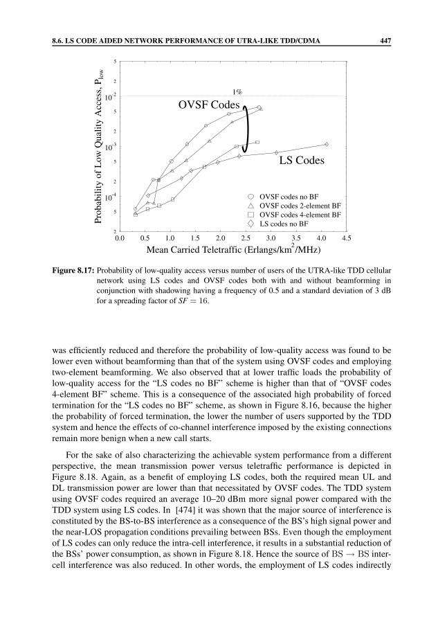
8.6. LS CODE AIDED NETWORK PERFORMANCE OF UTRA-LIKE TDD/CDMA 447
0.0 0.5 1.0 1.5 2.0 2.5 3.0 3.5 4.0 4.52
2
5
10-4
2
5
10-3
2
5
10-2
2
5
Prob
abili
tyof
Low
Qua
lity
Acc
ess,
P low
OVSF Codes
LS Codes
1%
LS codes no BFOVSF codes 4-element BFOVSF codes 2-element BFOVSF codes no BF
Mean Carried Teletraffic (Erlangs/km /MHz)
Figure 8.17: Probability of low-quality access versus number of users of the UTRA-like TDD cellularnetwork using LS codes and OVSF codes both with and without beamforming inconjunction with shadowing having a frequency of 0.5 and a standard deviation of 3 dBfor a spreading factor of SF = 16.
was efficiently reduced and therefore the probability of low-quality access was found to belower even without beamforming than that of the system using OVSF codes and employingtwo-element beamforming. We also observed that at lower traffic loads the probability oflow-quality access for the “LS codes no BF” scheme is higher than that of “OVSF codes4-element BF” scheme. This is a consequence of the associated high probability of forcedtermination for the “LS codes no BF” scheme, as shown in Figure 8.16, because the higherthe probability of forced termination, the lower the number of users supported by the TDDsystem and hence the effects of co-channel interference imposed by the existing connectionsremain more benign when a new call starts.
For the sake of also characterizing the achievable system performance from a differentperspective, the mean transmission power versus teletraffic performance is depicted inFigure 8.18. Again, as a benefit of employing LS codes, both the required mean UL andDL transmission power are lower than that necessitated by OVSF codes. The TDD systemusing OVSF codes required an average 10–20 dBm more signal power compared with theTDD system using LS codes. In [474] it was shown that the major source of interference isconstituted by the BS-to-BS interference as a consequence of the BS’s high signal power andthe near-LOS propagation conditions prevailing between BSs. Even though the employmentof LS codes can only reduce the intra-cell interference, it results in a substantial reduction ofthe BSs’ power consumption, as shown in Figure 8.18. Hence the source of BS → BS inter-cell interference was also reduced. In other words, the employment of LS codes indirectly

448 CHAPTER 8. HSDPA-STYLE TDD/CDMA NETWORK PERFORMANCE
0.0 0.5 1.0 1.5 2.0 2.5 3.0 3.5 4.0 4.52
-10
-5
0
5
10
15
Mea
nT
rans
mis
sion
Pow
er(d
Bm
)
OVSF Codes
LS Codes
LS codes no BFOVSF codes 4-element BFOVSF codes 2-element BFOVSF codes no BFFilled = Downlink, Blank = Uplink
Mean Carried Teletraffic (Erlangs/km /MHz)
Figure 8.18: Mean transmission power versus number of users of the UTRA-like TDD cellular networkusing LS codes and OVSF codes both with and without beamforming in conjunction withshadowing having a frequency of 0.5 Hz and a standard deviation of 3 dB for a spreadingfactor of SF = 16.
Table 8.4: Maximum mean carried traffic and maximum number of mobile users that can be supportedby the network, whilst meeting the network quality constraints of Section 8.6.3, namelyPB ≤ 3%, PF T ≤ 1%, Plow ≤ 1% and GOS ≤ 4%. The carried traffic is expressed in termsof normalized Erlangs (Erlang/km2/MHz) using OVSF codes and LS codes in conjunctionwith shadow fading having a standard deviation of 3 dB and a frequency of 0.5 Hz for aspreading factor of SF = 16.
Traffic Power (dBm)Spreading code Beamforming Users (Erlangs/km2/MHz) MS BS
OVSF codes No 50 0.55 0.54 −0.28OVSF codes Two-elements 113 1.18 1.33 0.90OVSF codes Four-elements 178 2.03 2.07 1.81LS codes No 306 3.45 −9.11 −9.21
reduced the severe BS → BS inter-cell interference by keeping the BSs’ transmission powerat a low level.
Figure 8.19 shows the achievable GOS for a range of teletraffic loads. We observesimilar trends regarding the probability of low-quality access, as shown in Figure 8.17.In Equation 5.15, the GOS performance is jointly determined by PB and Plow , which isinterpreted as the probability of unsuccessful network access (blocking), or the probabilityof encountering a low-quality access, provided that a call is admitted to the system.

8.6. LS CODE AIDED NETWORK PERFORMANCE OF UTRA-LIKE TDD/CDMA 449
0.0 0.5 1.0 1.5 2.0 2.5 3.0 3.5 4.0 4.52
2
5
10-4
2
5
10-3
2
5
10-2
2
5
Gra
deof
Serv
ide,
(GO
S) OVSF Codes
LS Codes
1%
LS codes no BFOVSF codes 4-element BFOVSF codes 2-element BFOVSF codes no BF
Mean Carried Teletraffic (Erlangs/km /MHz)
Figure 8.19: GOS versus number of users of the UTRA-like TDD cellular network using LS codes andOVSF codes both with and without beamforming in conjunction with shadowing havinga frequency of 0.5 Hz and a standard deviation of 3 dB for a spreading factor of SF = 16.
The employment of the LS codes may cause the shortage of spreading codes and, hence,may lead to the blocking of a new call, since there are only eight LS codes that can beused, when the IFW duration is ±1 chip length. The call duration and inter-call periods werePoisson distributed having the mean values shown in Table 8.3. When encountering this callarrival distribution, we observe that the new call blocking probability is negligible, as shownin Figures 8.17 and 8.19.
A summary of the maximum user capacities of the UTRA-like TDD/CDMA system usingOVSF codes and LS codes in conjunction with log-normal shadowing having a standarddeviation of 3 dB and a shadowing frequency of 0.5 Hz as well as both with and withoutbeamforming is given in Table 8.4. The teletraffic carried and the MS and BS transmissionpowers required are also shown in Table 8.4.
8.6.5 Summary and Conclusions
In this section we studied the network performance of a UTRA-like TDD/CDMA systememploying LS spreading codes. The computer simulation results provided showed thatthe TDD system invoking LS codes had a better performance compared with the systemusing OVSF codes. We designed a 49-cell “wrapped around” simulation area, constitutedby sufficiently small 78 m radius cells, which guaranteed that the delayed asynchronoustransmissions arrive within the IFW, where the auto-correlation and cross-correlation valuesof the LS codes became zero and hence eliminated the effects of intra-cell interference.The SINR required by the LS codes for the sake of maintaining a BER of 1 × 10⁻³ was

450 CHAPTER 8. HSDPA-STYLE TDD/CDMA NETWORK PERFORMANCE
almost 2 dB lower than that necessitated by the OVSF codes. Furthermore, a low MS and BStransmission power has been maintained. Hence, the average intra- and inter-cell interferencelevel has become low, the severe BS → BS interference has been reduced and this resulted inTDD system performance improvements both in terms of the achievable call quality andthe number of users supported. Our future research will focus on further improving theperformance of TDD systems using GA-based timeslot scheduling.

Chapter 9The Effects of Power Control andHard Handovers on the UTRATDD/CDMA System
9.1 A Historical Perspective on Handovers
The terminology of handover [475] is synonymous in mobile communications to theprocess of transferring a MS from one BS or channel to another. It is typically initiatedby experiencing a degraded signal quality in the current cell. Handovers (HOs) may bedivided into two broad categories, namely hard HOs and soft HOs, which are also oftencharacterized informally by the terms “break before make” and “make before break”,respectively. Therefore, in the context of hard HOs, the current transmission resources arereleased before the new resources are reserved, while in soft HOs, both the existing andnew resources are engaged in the HO process. Poorly designed HO schemes may generatevery heavy signaling traffic, hence potentially imposing a dramatic QoS degradation. Theincreasing interest and mass-market for mobile communications as well as the limitedavailable spectrum has motivated the employment of cellular architectures based on smallcells. As a result, the number of mobile users crossing the cell boundaries is increased and,hence, the resultant HO rate is also increased. Therefore, the efficiency of HO algorithms isexpected to play a crucial role in the overall system performance [476–479]. This suggeststhat efficient HO algorithms constitute a cost-effective way of enhancing both the capacityand the QoS in cellular systems.
The radio propagation environment and the related HO algorithms are different indifferent cellular systems [480, 481]. Hence, a particular HO algorithm endowed witha specific set of parameters cannot perform equally well in different communicationscenarios [482]. First- and second-generation cellular systems provide wide-area coverageeven in cities using macro-cells [483–489]. The brief history of HO algorithms designed forcellular systems is summarized in Table 9.1.
3G, HSPA and FDD versus TDD Networking Second EditionL. Hanzo, J. S. Blogh and S. Ni c© 2008 John Wiley & Sons, Ltd

452 CHAPTER 9. THE EFFECTS OF PC AND HOS ON THE UTRA TDD/CDMA SYSTEM
Table 9.1: Contributions on HO algorithms designed for cellular systems.
Year Author Contribution
1992 Tekinay and Jabbari [488] Studied the performance of non-preemptive priorityqueueing for HO calls.
1993 Vijayan and Holtzman [480] A HO algorithm based on signal strengthmeasurements made by the MSs in a lognormal fadingenvironment was proposed.
1994 Viterbi, Gilhousen and The effect of HO techniques on cell coverage andZehavi [484] UL capacity was investigated in a CDMA system.
1995 Nakano, Umeda and A BS-diversity aided HO algorithm was proposedOhno [485] for high-capacity DS-CDMA cellular systems.
1996 Kim, Lee and Chin [486] An adaptive HO algorithm taking into accountthe velocity of MSs was proposed.
1997 Calin and Zeghlache [489] An analytical model characterizing a non-preemptivepriority queueing system incorporating both voice anddata users was proposed.
1998 Wong and Cox [487] A handoff algorithm using pattern recognitionwas proposed.
1999 Benvenuto and A least squares pathloss estimation approach toSantucci [490] HO algorithms was proposed.
2000 Santucci, Pratesi, Ruggieri A range of statistical parameters used in the performanceand Graziosi [491] analysis of a relative signal strength based
HO algorithm.2001 Yang, Ghaheri-Niri and The performance of power-triggered and Ec/N0-triggered
Tafazolli [492] soft HO algorithms designed for UTRAwas investigated.
2002 Wang, Sridhar and An adaptive soft HO algorithm using the locationGreen [493] information of mobile stations was proposed.
2003 Wang, Liu and Cen [481] HO algorithms designed for a dynamic spreadingaided WCDMA multimedia system were proposed.
2004 Lugara, Tartiere and Inter-system HO algorithms supporting bothGirard [482] UMTS and GSM were proposed.
9.2 Hard HO in UTRA-like TDD/CDMA Systems
The UTRA network supports different types of HO, where the HO control procedure may bedivided in the following types [459]:
• Intra-system HO [494, 495] occurring within a UTRA system, which can be furthersubdivided into:
– Intra-frequency HO [496] between cells using to the same UTRA carriers;
– Inter-frequency HO [23] between cells employing different UTRA carriers.
• Inter-system HO [497,498] taking place between cells belonging to two different RadioAccess Technologies (RATs) or different Radio Access Modes (RAMs). The most

9.2. HARD HO IN UTRA-LIKE TDD/CDMA SYSTEMS 453
typical case of inter-system HO is expected to take place between UTRA [416] andGSM/EDGE systems [457]. A typical example of inter-RAM HO is likely to take placebetween the UTRA FDD [416] and UTRA TDD [416] modes.
Furthermore, the following HO procedures can be identified [459].
• Hard HOs [499, 500] represent a family of HO procedures, where the old radio linkof a MS is released before the new radio link is established. For real-time interactivevoice-type bearers this hard HO procedure implies encountering a brief disconnectionof the bearer. In contrast, for non-interactive data-type bearers hard HOs appear to beseamless. Invoking soft HOs is also a design option for the TDD mode, as suggestedin [501]. Soft HOs improve the QoS, since a diversity gain is provided by combiningthe signals received from both links [484]. However, being engaged in communicationswith two BSs introduces more interference [502], since in the TDD mode portrayedin Figure 8.6 a number of gravely detrimental interference scenarios may exist. Theinterference imposed is typically higher if the network is asynchronous [503] orif the neighboring cells carry different asymmetric traffic loads [32, 451, 460, 474].Furthermore, in the UTRA system the legitimate spreading factor range of the FDDmode is 4 to 256 in the UL and 4 to 512 in the DL, while in the TDD mode thecorresponding range is 1 to 16 in both the UL and DL [59, 504], as seen in Table 6.1.Hence, soft HOs carried out in the TDD mode would need two of the 16 spreadingcodes, because the communications between the MS and the serving as well as targetBSs would have to take place concurrently via two air interface channels to distinguishbetween the signals [59] arriving from the serving and target BSs. This may be expectedto severely limit the number of users supported. Hence hard HOs constitute a moreappropriate solution for a TDD CDMA system, despite having no diversity gain.
• Soft HOs [492, 505–507] and softer HOs [508, 509] constitute a category of HOprocedures in which a MS maintains at least one radio link all of the time, typicallyestablishing a new link to the target BS, before relinquishing the previous link. Moreexplicitly, during soft HO the MS is simultaneously controlled by two or more BSsof the same or different Radio Network Controllers (RNCs). Softer HOs constitute aspecial case of soft HOs, where the radio links that are added and removed belongto co-located BSs managed by the same BS controller. Soft and softer HOs are onlypossible, when using the same carrier frequency.
9.2.1 Relative Pilot Power-based Hard HO
The UTRA TDD/CDMA system supports both inter-system HOs and intra-system HOs. Allof these HOs are mobile-assisted hard HOs and hence their philosophy is clearly differentfrom that of the UTRA FDD mode, since in the latter protocol structure has been designedto support soft HOs. The generic HO procedure is typically described in four phases [510]:the related signal-quality measurements, HO initiation, HO decision and HO execution. Arange of signal-quality related parameters, such as the received power, BER and the MS’sdistance can be evaluated and processed as the related HO criteria. It is anticipated thatthe UTRA TDD system’s hard HO is likely to be predominantly MS assisted HO, wherethe MS performs signal-quality measurements that are signaled to the RNC that makes the

454 CHAPTER 9. THE EFFECTS OF PC AND HOS ON THE UTRA TDD/CDMA SYSTEM
actual HO decisions. The conception of efficient HOs is one of the main challenges in UTRATDD/CDMA networks, since it has a substantial impact on the system’s performance andcapacity. The philosophy of soft HO and macro diversity cannot be utilized in the TDD mode,since the active target BS set size is always equal to one during the HO procedure [511]. Thisis because HOs in the UTRA TDD mode are hard HOs, where the MS is connected to oneBS only [451].
In our simulations, we rely on a single RAT or a single RAM, hence we only considerintra-system hard HOs. Again, hard HOs cause a temporary disconnection of real-timeinteractive access bearers, but they appear to be seamless for non-interactive bearers. Thehard HO algorithm used is based on the relative1 pilot power of Ec/Io in the serving celland in the neighboring cells, where a minimum Ec/Io HO margin is used as a threshold forpreventing repetitive hard HOs between cells [59, 512]. A hard HO can be processed whenthe following condition is satisfied [459]:
Ec/Io(serving cell) + Ec/Io(margin) < Ec/Io(new cell), (9.1)
where Ec/Io(serving cell) represents the average relative pilot power of the serving cell, whileEc/Io(new cell) is the average pilot power of the best potential target cell. The parameterEc/Io(margin) is the margin by which the Ec/Io value of the best HO target cell has toexceed the Ec/Io value of the serving cell before the hard HO is activated. The so-calledHO acceptance threshold Tacc and call drop threshold Tdrop are the corresponding hard HOthresholds, where a HO is enabled and the call is dropped, respectively. Again, a relativerather than absolute received pilot power scheme is used in our investigations, which exhibitsperformance benefits in realistic propagation environments exposed to shadow fading [416].The relative hard HO thresholds Tacc and Tdrop are expressed in terms of dB, which arenormalized to the received pilot strength Ec/Io of the best potential neighboring HO targetcell. Again, when the Ec/Io value of the best neighboring HO target cell exceeds the Ec/Io
value of the serving cell, the hard HO may be enabled, provided that it is necessary due to theserving cell’s signal quality degradation. Hence the relative acceptance threshold Tacc is setto 0 dB, which implies that the best neighboring cell can be accepted as a candidate HO targetcell for hard HO, provided that it has at least as high a pilot power as the serving cell. The calldrop threshold Tdrop is the Ec/Io(margin) value shown in Equation 9.1. When the receivedsignal quality of the serving cell degrades and, hence, the relative pilot power Ec/Io of theserving cell becomes by at least Tdrop dB lower than the Ec/Io value of the HO candidatecell, the hard HO will be activated.
9.2.2 Simulation Results
In this section the effect of having a hysteresis in the TDD system’s hard HO candidate/activeBS set update procedure is evaluated. The appropriate choice of the HO hysteresis thresholdis critical for the sake of achieving an attractive tradeoff between the transmit power required
1The reason for using a relative rather than absolute pilot power-based hard HO procedure is because it was foundin [416] that in some cell areas all pilot signals may be weak, while in other locations they all may be strong, andthis phenomenon may generate either too many or too few potential target HO cells. This potential deficiency maybe overcome by normalizing the pilot powers of the potential HO target cells to that of the serving cell or to those ofthe other BSs in the active BS set, which allows the inclusion of at least one target HO BS.

9.2. HARD HO IN UTRA-LIKE TDD/CDMA SYSTEMS 455
0.1 0.2 0.3 0.4 0.5 0.6 0.7 0.8 0.9
Mean Carried Teletraffic (Erlangs/km2/MHz)
10-3
2
5
10-2
2
5
10-1
2
Forc
edTe
rmin
atio
nPr
obab
ility
,PFT
1%
0, -100, -50, -3Tacc (dB), Tdrop (dB)8UL 7DL
Figure 9.1: Forced termination probability versus mean carried traffic of the UTRA-like TDD/CDMA-based cellular network with shadowing and using relative received pilot power, Ec/Io,based hard-HO thresholds in conjunction with a near-symmetric traffic load of 8:7 (UL:DL)timeslots. The system parameters are summarized in Table 9.2.
for supporting the HO process and seamless call continuity [513]. Having a low HO hysteresisthreshold would enable a mobile user to capture and register a larger number of pilots,hence creating a high number of potential target BSs, but if they tend to provide a relativelylow signal quality, the undesirable “ping-pong” effect of switching back and forth betweencalls may not be avoided. On the other hand, an excessive HO hysteresis threshold wouldpractically eliminate the “ping-pong” effect, hence reducing the HO-related signaling, but thisis achieved at the risk of not finding any better-quality BSs. This would consequently generatean excessive call dropping rate. Three different traffic scenarios are studied, namely having anear-symmetric UL:DL traffic load of 8:7 timeslots, UL-dominated asymmetric traffic loadsand DL-dominated asymmetric traffic loads.
9.2.2.1 Near-symmetric UL/DL Traffic Loads
The forced termination performance at the near-symmetric traffic load ratio of 8:7 (UL:DL)timeslots is shown in Figure 9.1, illustrating that reducing the absolute value of the HOthreshold Tdrop to −3 dB and −5 dB improved the forced termination performance comparedwith Tdrop = −10 dB, in particular at low traffic loads. The reduced force terminationprobability is a benefit of handing over to potential target BSs earlier, without jeopardizingterminating the call. This phenomenon is also evident in Figure 9.2, which shows theprobability of a low-quality outage versus mean the carried teletraffic of a UTRA-likeTDD/CDMA-based cellular network carrying a near-symmetric traffic load of 8 : 7 (UL:DL).However, the reduction of the absolute value of Tdrop from −10 to −3 dB led to anincreased number of HO events, as shown in Figure 9.3. This is predictable, since having

456 CHAPTER 9. THE EFFECTS OF PC AND HOS ON THE UTRA TDD/CDMA SYSTEM
Table 9.2: Parameters used for the hard HO investigations.
Parameter Value Parameter Value
Cell radius 150 m Noisefloor −100 dBmChip rate 3.84 Mcps Spreading factor 16BS/MS minimum TX power −44 dBm BS/MS maximum TX power +21 dBmModulation scheme 4-QAM Pathloss exponent −3.5Target Eb/No 8.0 dB Low-quality outage Eb/No 7.0 dBOutage Eb/No 6.6 dB HO margin 3,5,10 dB
0.1 0.2 0.3 0.4 0.5 0.6 0.7 0.8 0.9
Mean Carried Teletraffic (Erlangs/km2/MHz)
2
5
10-3
2
5
10-2
2
5
10-1
2
Prob
abili
tyof
Low
Qua
lity
Acc
ess,
P low
1%
0, -100, -50, -3Tacc (dB), Tdrop (dB)8UL 7DL
Figure 9.2: Probability of low-quality access versus mean carried traffic of the UTRA-likeTDD/CDMA-based cellular network with shadowing and using relative received pilotpower, Ec/Io, based hard-HO thresholds in conjunction with a near-symmetric traffic loadof 8:7 (UL:DL) timeslots. The system parameters are summarized in Table 9.2.
higher hysteresis requires a higher received pilot power from the neighboring HO targetcells to be selected. Consequently, the rate of active BS set update becomes lower, leadingto an increased average BS and MS transmission power, as shown in Figure 9.4. Theincreased BS and MS transmission power results in an increased co-channel interferencelevel and, hence, in a higher probability of outage associated with a low call quality. It wasobserved in Figure 9.3 that the number of HO events started to reduce, when the traffic loadsexceeded 0.6 Erlang/km2/MHz in Figure 9.3. This is a consequence of the associated highforced termination probability, as seen in Figure 9.1. This phenomenon ultimately led to thereduction of the number of supported users, while most users also suffered from experiencinga high level of interference.

9.2. HARD HO IN UTRA-LIKE TDD/CDMA SYSTEMS 457
0.1 0.2 0.3 0.4 0.5 0.6 0.7 0.8 0.9
Mean Carried Teletraffic (Erlangs/km2/MHz)
5000
10000
15000
20000
25000
30000
35000
40000
Num
ber
ofH
ando
ver
Eve
nts
0, -100, -50, -3Tacc (dB), Tdrop (dB)8UL 7DL
Figure 9.3: Number of HO events per 49-cell simulation area versus mean carried traffic of the UTRA-like TDD/CDMA-based cellular network with shadowing and using relative received pilotpower, Ec/Io, based hard-HO thresholds in conjunction with a near-symmetric traffic loadof 8:7 (UL:DL) timeslots. The system parameters are summarized in Table 9.2.
0.1 0.2 0.3 0.4 0.5 0.6 0.7 0.8 0.9
Mean Carried Teletraffic (Erlangs/km2/MHz)
-3
-2
-1
0
1
2
3
4
5
Mea
nT
rans
mis
sion
Pow
er(d
Bm
)
0, -100, -50, -3Tacc (dB), Tdrop (dB)8UL 7DLFilled = Downlink, Blank = Uplink
Figure 9.4: Mean BS and MS transmission power versus mean carried traffic of the UTRA-likeTDD/CDMA-based cellular network with shadowing and using relative received pilotpower, Ec/Io, based hard-HO thresholds in conjunction with a near-symmetric traffic loadof 8:7 (UL:DL) timeslots. The system parameters are summarized in Table 9.2.

458 CHAPTER 9. THE EFFECTS OF PC AND HOS ON THE UTRA TDD/CDMA SYSTEM
0.1 0.2 0.3 0.4 0.5 0.6 0.7 0.8 0.9
Mean Carried Teletraffic (Erlangs/km2/MHz)
10-3
2
5
10-2
2
5
10-1
2
Forc
edTe
rmin
atio
nPr
obab
ility
,PFT
1%
0, -100, -50, -3Tacc (dB), Tdrop (dB)13UL 2DL
Figure 9.5: Forced termination probability versus mean carried traffic of the UTRA-like TDD/CDMA-based cellular network with shadowing and using relative received pilot power, Ec/Io,based hard-HO thresholds in conjunction with an asymmetric traffic load of 13:2 (UL:DL)timeslots. The system parameters are summarized in Table 9.2.
9.2.2.2 Asymmetric Traffic loads
In this section the effects of both UL-dominated as well as DL-dominated asymmetric trafficloads on the achievable teletraffic performance are examined, while using different hard HOhysteresis thresholds.
Figures 9.5 and 9.6 demonstrate that the system’s forced termination probability wasimproved, when Tdrop was adjusted from−10 to −3 dB. It is observed in Figure 9.6 that whencarrying predominantly DL traffic loads associated with a traffic load ratio of 1:14 (UL:DL)the system benefited more from reducing the absolute value of the hard HO hysteresis from−10 to −3 dB compared with the predominantly UL traffic load scenario of 13:2 (UL:DL)timeslots, as seen in Figure 9.5. A carried traffic improvement of 0.2 Erlangs/km2/MHz wasachieved in the 1:14 (UL:DL) timeslot scenario, which is twice as high as the performancegain observed in the 13:2 (UL:DL) scenario, when the HO hysteresis was reduced from−10 to −5 dB.
This is because the higher the HO hysteresis, the slower the HO process and hence aforced termination event may occur, before the hard HO can be completed owing to theinsufficiently high signal power received from the serving BS. More explicitly, during thehard HO process, the MS tends to recede from the serving BS and approaching the HOtarget BS. The received pilot signal level of the serving BS may gradually reduce, while thereceived pilot signal level of the HO target BS may be increased, as shown in Figure 9.7.The SINR of the mobile station was gradually reduced as it receded from the serving BS.When the received pilot power approaches Tdrop = −10 dB, the SINR is often alreadybelow the outage SINR, before the mobile can be handed over to the HO target BS, hence

9.2. HARD HO IN UTRA-LIKE TDD/CDMA SYSTEMS 459
0.1 0.2 0.3 0.4 0.5 0.6 0.7 0.8 0.9
Mean Carried Teletraffic (Erlangs/km2/MHz)
10-3
2
5
10-2
2
5
10-1
2
Forc
edTe
rmin
atio
nPr
obab
ility
,PFT
1%
0, -100, -50, -3Tacc (dB), Tdrop (dB)1UL 14DL
Figure 9.6: Forced termination probability versus mean carried traffic of the UTRA-like TDD/CDMA-based cellular network with shadowing and using relative received pilot power, Ec/Io,based hard-HO thresholds in conjunction with an asymmetric traffic load of 1:14 (UL:DL)timeslots. The system parameters are summarized in Table 9.2.
E c / Io
SINR outage
Tacc= 0 dB
= 5 dBTdrop Tdrop = 10 dB
Pilot candidate
SINR
Pilot
Successful handover
Call dropped
serving
Time orDistance
DistanceTime or
Figure 9.7: The hard-HO process in the UTRA/TDD CDMA system.

460 CHAPTER 9. THE EFFECTS OF PC AND HOS ON THE UTRA TDD/CDMA SYSTEM
0.1 0.2 0.3 0.4 0.5 0.6 0.7 0.8 0.9
Mean Carried Teletraffic (Erlangs/km2/MHz)
2
5
10-3
2
5
10-2
2
5
10-1
2
Prob
abili
tyof
Low
Qua
lity
Acc
ess,
P low
1%
0, -100, -50, -3Tacc (dB), Tdrop (dB)13UL 2DL
Figure 9.8: Probability of low-quality access versus mean carried traffic of the UTRA-likeTDD/CDMA-based cellular network with shadowing and using relative received pilotpower, Ec/Io, based hard-HO thresholds in conjunction with an asymmetric traffic loadof 13:2 (UL:DL) timeslots. The system parameters are summarized in Table 9.2.
the call is likely to be terminated, as shown in Figure 9.7. However, still considering thesame special case, if we have Tdrop = −5 dB, the mobile station may have been handedover to the HO target BS, before the SINR degraded further and the call was terminated. Fora predominantly DL traffic load of 1:14 (UL:DL) timeslot scenario, most of the terminatedcalls encountered during the hard HO process occurred owing to encountering a poor ULconnection quality, which is typically caused by the routinely incurred severe BS-to-BSinterference of the UTRA TDD mode. Only when the UL/DL TS allocation of the interferingcells is the as same as that of the serving cell can the BS-to-BS interference be avoided,since in this scenario the serving BS is not receiving during the interfering BS’s transmitTS. However, for the predominantly DL traffic load of 1:14 (UL:DL) a grave BS-to-BSinterference is encountered with a probability of 93.33% = 14/15, when a mobile userinvoking a hard HO is transmitting in a serving cell’s UL timeslot, since in the interferingcell 14 DL timeslots out of the total 15 timeslots may be inflicting interference. For thepredominantly UL traffic load of 13:2 (UL:DL), the probability of BS-to-BS interferenceoccurring is 13.33% = 2/15, when a mobile user invoking a hard HO is transmitting in aserving cell’s UL timeslot, and only two DL timeslots may be contaminated by the BS-to-BS interference. Hence, carrying a predominantly DL traffic load is more beneficial, since itallows us to reduce the HO hysteresis, which in turn reduces the call dropping probability, asseen in Figure 9.6.
Figures 9.8 and 9.9 portray the probability of low-quality access versus various trafficloads. It is observed that the specific choice of the HO hysteresis Tdrop does not significantlyaffect the probability of low-quality access. Similar trends were found for various traffic

9.2. HARD HO IN UTRA-LIKE TDD/CDMA SYSTEMS 461
0.1 0.2 0.3 0.4 0.5 0.6 0.7 0.8 0.9
Mean Carried Teletraffic (Erlangs/km2/MHz)
2
5
10-3
2
5
10-2
2
5
10-1
2
Prob
abili
tyof
Low
Qua
lity
Acc
ess,
P low
1%
0, -100, -50, -3Tacc (dB), Tdrop (dB)1UL 14DL
Figure 9.9: Probability of low-quality access versus mean carried traffic of the UTRA-likeTDD/CDMA-based cellular network with shadowing and using relative received pilotpower, Ec/Io, based hard-HO thresholds in conjunction with an asymmetric traffic loadof 1:14 (UL:DL) timeslots. The system parameters are summarized in Table 9.2.
loads. The low-quality access performance associated with predominantly UL traffic loadsis poorer than that recorded for predominantly DL traffic loads. This is because the specificUL and DL timeslot allocation is random in every cell and leads to a randomly fluctuatinginterference load for each timeslot. In the case of closed-loop power control [514], it isdifficult to accurately adjust the power level if the received interfering signal is uncorrelatedbetween timeslots. We provide more detailed justifications for this issue in the nextsection.
The number of HO events recorded across the entire 49-cell simulation area is shown inFigures 9.10 and 9.11, illustrating that reducing the absolute value of the hard-HO hysteresisthreshold Tdrop leads to a higher number of HO events, which is beneficial in terms ofreducing the call dropping probability. However, as a penalty, the associated HO signalingtraffic is increased and a higher proportion of the call duration is spent in the process of hardHO. From the perspective of the radio resource management, a high number of HO events willdecrease the overall available resources, since the control channels of both the serving BSsand the HO target BSs are more likely to be engaged by the mobile stations in HO [515,516].Having a high HO hysteresis also results in high BS and MS power consumption. The servingBS and the MS have to increase their transmission powers in an effort to maintain the SINRvalue required for sustaining the current connection quality during the process of hard HO, asdepicted in Figures 9.12 and 9.13. For example, it may be inferred from Figures 9.12 and 9.13that a 7 dB increase of the hysteresis threshold Tdrop results in an average transmission powerincrease of 1.5 dBm for both the BS and mobile station.

462 CHAPTER 9. THE EFFECTS OF PC AND HOS ON THE UTRA TDD/CDMA SYSTEM
0.1 0.2 0.3 0.4 0.5 0.6 0.7 0.8 0.9
Mean Carried Teletraffic (Erlangs/km2/MHz)
5000
10000
15000
20000
25000
30000
35000
Num
ber
ofH
ando
ver
Eve
nts
0, -100, -50, -3Tacc (dB), Tdrop (dB)13UL 2DL
Figure 9.10: Number of HO events per 49-cell simulation area versus mean carried traffic of the UTRA-like TDD/CDMA-based cellular network with shadowing and using relative received pilotpower, Ec/Io, based hard-HO thresholds in conjunction with an asymmetric traffic loadof 13:2 (UL:DL) timeslots. The system parameters are summarized in Table 9.2.
0.1 0.2 0.3 0.4 0.5 0.6 0.7 0.8 0.9
Mean Carried Teletraffic (Erlangs/km2/MHz)
5000
10000
15000
20000
25000
30000
35000
40000
Num
ber
ofH
ando
ver
Eve
nts
0, -100, -50, -3Tacc (dB), Tdrop (dB)1UL 14DL
Figure 9.11: Number of HO events per 49-cell simulation area versus mean carried traffic of the UTRA-like TDD/CDMA-based cellular network with shadowing and using relative received pilotpower, Ec/Io, based hard-HO thresholds in conjunction with an asymmetric traffic loadof 1:14 (UL:DL) timeslots. The system parameters are summarized in Table 9.2.

9.2. HARD HO IN UTRA-LIKE TDD/CDMA SYSTEMS 463
0.1 0.2 0.3 0.4 0.5 0.6 0.7 0.8 0.9
Mean Carried Teletraffic (Erlangs/km2/MHz)
-3
-2
-1
0
1
2
3
4
Mea
nT
rans
mis
sion
Pow
er(d
Bm
)0, -100, -50, -3Tacc (dB), Tdrop (dB)13UL 2DLFilled = Downlink, Blank = Uplink
Figure 9.12: Mean transmission power versus mean carried traffic of the UTRA-like TDD/CDMA-based cellular network with shadowing and using relative received pilot power, Ec/Io,based hard-HO thresholds in conjunction with an asymmetric traffic load of 13:2 (UL:DL)timeslots. The system parameters are summarized in Table 9.2.
0.1 0.2 0.3 0.4 0.5 0.6 0.7 0.8 0.9
Mean Carried Teletraffic (Erlangs/km2/MHz)
-2.5
-2.0
-1.5
-1.0
-0.5
0.0
0.5
1.0
1.5
2.0
2.5
Mea
nT
rans
mis
sion
Pow
er(d
Bm
)
0, -100, -50, -3Tacc (dB), Tdrop (dB)1UL 14DLFilled = Downlink, Blank = Uplink
Figure 9.13: Mean transmission power versus mean carried traffic of the UTRA-like TDD/CDMA-based cellular network with shadowing and using relative received pilot power, Ec/Io,based hard-HO thresholds in conjunction with an asymmetric traffic load of 1:14 (UL:DL)timeslots. The system parameters are summarized in Table 9.2.

464 CHAPTER 9. THE EFFECTS OF PC AND HOS ON THE UTRA TDD/CDMA SYSTEM
9.3 Power Control in UTRA-like TDD/CDMA Systems
Agile and accurate power control is one of the key factors predetermining the attainableperformance of the UTRA TDD/CDMA system, where all users share the same frequency.The power control regime has a vital influence on controlling the interference. Without powercontrol a MS roaming in the vicinity of the BS and transmitting at an excessive power mayoverwhelm mobiles that are at the cell edge, a phenomenon which is often referred to as thenear–far problem [517–520]. It is essential to keep the transmission power at the minimumlevel ensuring adequate signal quality at the receiver end. Power control may be classified asopen-loop power control, inner-loop power control sometimes also referred to as closed-looppower control and outer-loop power control, all of which may be used in both the UL andDL [59].
The preferred solution to power control in the UTRA FDD/CDMA system is based onthe philosophy of inner-loop power control or fast closed-loop power control in both the ULand DL. In the UL the BS generates frequent estimates of the received SINR and compares itwith the target SINR required for maintaining the quality of a specific service. If the measuredSINR is higher than the target SINR, the BS will instruct the MS to decrease its power. Thismeasure–instruct–react cycle is executed at a rate of 1500 times per second (1.5 kHz) for eachmobile station and thus operates faster than any significant change of pathloss could possiblyhappen. In fact, typically it is even faster than the typical Doppler frequency of fast Rayleighfading for low to moderate mobile speeds. Hence, closed-loop power control will prevent anypower inbalance among all of the UL signals received at the BS.
In the DL the same closed-loop power control is used as in the UL. However, there is nonear–far problem owing to the one-to-many broadcast-type transmission scenario in the DL.All of the signals received by the MS within a specific traffic cell originate from the same BStransmitting to all MSs. The motivation of using closed-loop power control in the DL is firstlyto provide the minimum amount of additional power to MSs roaming at the cell edge, sincethey suffer from increased inter-cell interference. Secondly, closed-loop DL power control iscapable of enhancing the signals attenuated by Rayleigh fading with the aid of transmittingan additional power with the aim of augmenting the action of error-correcting methods [59].
9.3.1 UTRA TDD Downlink Closed-loop Power Control
As argued in the previous section, the aim of the UTRA TDD DL power control scheme is tolimit the effects of interference. The transmitter typically uses a signal-quality-based powercontrol on the DL [514]. Closed-loop power control facilitates for the BS transmitter to adjustthe power in response to the MS’s specific request. Downlink closed-loop power controlis based on SIR measurements at the MS receiver and the corresponding Transmit PowerControl (TPC) commands are generated by the MS. The power control step size determinesthe change in the DL power in response to a TPC message received from the MS, where thelegitimate DL power steps are 1, 2 and 3 dB [514].
The inter-cell interference encountered is not only due to the MSs, but also due to the BSscontaminating the adjacent cells by co-channel signals. The DL closed-loop power controladjusts the MSs’ transmit power in order to maintain the DL SINR near the SINR target,namely near SINRtarget. As discussed in Section 9.2, the HOs in the UTRA TDD mode arebased on hard HOs [59]. The mobile communicates with a single BS, and only one TPC

9.3. POWER CONTROL IN UTRA-LIKE TDD/CDMA SYSTEMS 465
Table 9.3: TDD DL power control stepsize tolerance [514].
Range of average rate of change incode domain power per 10 steps
Stepsize Tolerance Minimum Maximum
1 dB ± 0.5 dB ± 8 dB ± 12 dB2 dB ± 0.75 dB ± 16 dB ± 24 dB3 dB ± 1 dB ± 24 dB ± 36 dB
Table 9.4: FDD DL power control tolerance for the 1 dB stepsize mode [521].
Range of average rate of change inTolerance code domain power per 10 steps
DL TPC commands Lower Upper Lower Upper
For powering up +0.5 dB +1.5 dB +8 dB +12 dBFor powering down −0.5 dB −1.5 dB −8 dB −12 dB
command will be received in each DL timeslot. When we have SINRDL > SINRtarget, theTPC command is set to 0, otherwise, if SINRDL < SINRtarget, then the TPC command isset to 1. When the MS receives a TPC command, the MS is instructed to power down orup according to the “stepsize” typically expressed in decibels. The tolerance of the transmitpower and the highest average rate of change in code domain power according to the powercontrol stepsize should be within the range shown in Table 9.3 [514].
For the sake of comparison, Table 9.4 shows the tolerance of the code domain power andthe highest average rate of change in the UTRA FDD mode in conjunction with a powerstepsize of 1 dB [521]. Upon comparing Tables 9.3 and 9.4, it can be seen that the toleranceand range of power control is the same in the FDD and TDD modes. However, the powercontrol agility of the TDD and FDD modes is different. In the FDD mode, there may be15 dB power change across a 15-timeslot, 10 ms FDD frame. In contrast, in the TDD modethe achievable power control agility in the DL depends on the ratio of the number of UL/DLtimeslots. To maintain the maximum possible flexibility, while facilitating closed-loop powercontrol whenever deemed useful, the Synchronization Channel (SCH) has two TSs per 15-timeslot, 10 ms TDD frame for DL transmission in cellular usage, which corresponds to themost extreme UL asymmetry of TS allocation having a ratio of 2:13 DL:UL allocation. On theother hand, at least one TS has to be allocated for the UL transmission of the Random AccessChannel (RACH), which corresponds to a maximum DL asymmetry of 14:1 (DL:UL). Theprocedure of carrying out one power-control step requires a pair of UL and DL TSs. Then aTPC command is transmitted in an UL TS, when the received signal power evaluated duringthe previous DL TS has to be adjusted. Hence, the TDD power-control rate in the DL rangesfrom 100 to 700 Hz, corresponding to having access to 1–7 DL TSs. The ability to supportasymmetric UL/DL capacity allocations is the most attractive feature of the TDD mode.

466 CHAPTER 9. THE EFFECTS OF PC AND HOS ON THE UTRA TDD/CDMA SYSTEM
However, the TDD mode imposes a problem in terms of the associated low power-controlrate. Hence the MS may require a relatively high BS transmitted power, when the mobilesuffers from experiencing a high level of interference or when it enters a building, whichsubstantially attenuates the signal power received from the BS. This phenomenon may alsolead to a high call dropping probability, when the BS is unable to satisfy the MS’s receivedpower requirement owing to the relatively low power-control agility of the TDD mode. Forexample, in the FDD mode a 15 dB power change can be achieved within a 15-timeslot10 ms frame, if the power control stepsize is 1 dB. In contrast, in the TDD mode a 15 timeslonger duration corresponding to 15 frames and 150 ms may be needed for the extreme DLasymmetry of 14:1 (DL:UL) TS allocation. A dropped call would be encountered, when thereare five consecutive 10 ms frames having an SINR value below the target SINR value. Forthe above-mentioned extreme asymmetric TDD traffic situation, after requesting a powerincrease in five consecutive frames only 5 dB power change has been achieved, potentiallyrequiring a further 10 dB = 15−5 dB powering up, which eventually leads to this connectionbeing terminated owing to having an insufficiently high received power level. One possibleoption of compensating for this relatively slow feedback loop is using a higher power-controlstepsize. In the 3GPP initiative [522], using 2 bits for the TPC command was proposed forthe DL, allowing for a more flexible power-control stepsize adjustment, ranging from 1 to3 dB. Hence, we could adjust the power-control stepsize commensurately with the differencebetween the measured and target SINR, namely according to ∆SINR:
∆SINR = |SINRtarget − SINRDL|. (9.2)
The relationship between the stepsize and ∆SINR is shown in Table 9.5 based on Table 9.3and the 3GPP initiative [523]. Using a flexible power-control stepsize adjustment is adesirable feature in the UTRA system’s TDD mode due to the associated reduced power-control feedback rate. However, a higher power-control stepsize may impose a possibleincrease of the interference level inflicted upon other MSs in both the same as well as in theadjacent cells. In Section 9.3.3 we provide a comparative study of using a 1 dB fixed powercontrol stepsize and a flexible power-control stepsize in order to investigate the achievablesystem performance, when invoking a higher PC stepsize.
9.3.2 UTRA TDD Uplink Closed-loop Power Control
Closed-loop power-control may also be used in the UTRA TDD mode’s 1.28 Mchip/soption [523]. The UL closed-loop power control is used to set the power of both the UL Ded-icated Physical Control Channel (DPCH) and Physical Common Packet Channel (PCPCH).Both the SINR measurement and power adjustment phase of the UTRA TDD UL closed-loopPC scheme is similar to that described in Section 9.3.1.
9.3.3 Closed-loop Power Control Simulation Results
In this section the effects of the closed-loop power-control stepsize on the UTRATDD/CDMA system’s performance was studied. As we have discussed in Section 9.3.1, theasymmetric teletraffic load of the UTRA TDD mode results in a potentially lower power-control rate compared to the FDD mode. The slow feedback loop of the power controlcommand may lead to calls being terminated owing to the insufficiently high transmitted

9.3. POWER CONTROL IN UTRA-LIKE TDD/CDMA SYSTEMS 467
Table 9.5: Closed-loop power control stepsizes.
Stepsize (dB) ∆SINR (dB) The number of TPC bits needed
+1 0 < ∆SINR ≤ 1.5 1+2 1.5 < ∆SINR ≤ 2.75 2+3 2.75 < ∆SINR ≤ 4 2+4 4 < ∆SINR ≤ 5.25 3+5 5.25 < ∆SINR ≤ 6.5 3+6 6.5 < ∆SINR ≤ 7.75 3
...−1 1 < ∆SINR ≤ 2.5 1−2 2.5 < ∆SINR ≤ 3.75 2−3 3.75 < ∆SINR ≤ 5 2−4 5 < ∆SINR ≤ 6.25 3−5 6.25 < ∆SINR ≤ 7.5 3−6 7.5 < ∆SINR ≤ 8.75 3
...
power [524]. The limited TPC command feedback rate can be compensated for by anappropriate stepsize selection, since it is possible to use three different power-controlstepsizes in the UTRA TDD mode [522], as we have seen in Table 9.3. In our simulationsboth the symmetric and asymmetric traffic loads of the UTRA-like TDD/CDMA system arestudied. Both the UL and DL use closed-loop power control. Three different power-controlstepsize algorithms are used in our simulations, namely:
• fixed power-control stepsize of 1 dB, one TPC bit is needed;
• flexible power-control stepsize of 1–3 dB, two TPC bits are needed;
• flexible power-control stepsize of 1–6 dB, three TPC bits are needed.
The stepsizes of the UL/DL commands and the required number of TPC bits are presented inTable 9.5 for each legitimate scenario.
9.3.3.1 UL/DL Symmetric Traffic Loads
For a near-symmetric traffic load, we used an 8:7 (UL:DL) TS allocation ratio in each 15-slotTDD frame, where the eight UL TSs and seven DL TSs are allocated randomly in each TDDframe. Hence, the achievable power control rate is 700 Hz, allowing a 7 dB power correctionrange during the 15 slots of a 10 ms frame. Figure 9.14 portrays the forced terminationprobability versus mean carried traffic of the UTRA-like TDD/CDMA-based cellular networkin conjunction with the above-mentioned symmetric traffic load of 8:7 (UL:DL). It may beobserved that the system’s achievable traffic load did not benefit from invoking an adaptivePC stepsize in the scenario considered, in fact, it performed slightly worse compared withusing a fixed 1 dB PC stepsize. The reason for this observation is outlined below. For the

468 CHAPTER 9. THE EFFECTS OF PC AND HOS ON THE UTRA TDD/CDMA SYSTEM
0.1 0.2 0.3 0.4 0.5 0.6 0.7 0.8 0.9
Mean Carried Teletraffic (Erlangs/km2/MHz)
10-3
2
5
10-2
2
5
10-1
2
Forc
edTe
rmin
atio
nPr
obab
ility
,PFT
1%
1 dB to 6 dBAdaptive PC Stepsize1 dB to 3 dBAdaptive PC StepsizePC Stepsize 1 dB8UL 7DL
Figure 9.14: Forced termination probability versus mean carried traffic of the UTRA-likeTDD/CDMA-based cellular network with shadowing and using various closed-loop PCschemes in conjunction with a near-symmetric traffic load of 8:7 (UL:DL) timeslots. Thesystem parameters are summarized in Table 9.6.
Table 9.6: Parameters used for the simulation of the power control.
Parameter Value Parameter Value
Cell radius 150 m Noisefloor −100 dBmChip rate 3.84 Mcps Spreading factor 16BS/MS minimum TX power −44 dBm BS/MS maximum TX power +21 dBmModulation scheme 4-QAM Pathloss exponent −3.5Target Eb/No 8.0 dB Low-quality (LQ) Outage Eb/No 7.0 dBOutage Eb/No 6.6 dB HO margin 5 dBPower control SINR hysteresis 1 to 6 dB
“PC Stepsize 1 dB” scenario of Figure 9.14, the TDD system was capable of supporting 78users at PFT = 1%, corresponding to a teletraffic density of 0.46 Erlang/km2/MHz. The“Adaptive PC Stepsize 1 dB to 3 dB” and “Adaptive PC Stepsize 1 dB to 6 dB” scenario ofthe TDD network was found to support 73 users and 70 users, corresponding to a normalizedtraffic load of 0.42 and 0.40 Erlang/km2/MHz, respectively. The percentage of forced callterminations entirely deemed to be due to encountering an insufficiently high signal power(rather than due to violating any of the other performance requirements) within the totalnumber of forced termination scenarios was found to be zero, although this is not explicitlydemonstrated here. This is because for the near-symmetric traffic scenario considered, theTDD system was capable of maintaining a relatively high power-control feedback rate of

9.3. POWER CONTROL IN UTRA-LIKE TDD/CDMA SYSTEMS 469
0.1 0.2 0.3 0.4 0.5 0.6 0.7 0.8 0.9
Mean Carried Teletraffic (Erlangs/km2/MHz)
-2
-1
0
1
2
3
4
5
Mea
nT
rans
mis
sion
Pow
er(d
Bm
)
1 dB to 6 dBAdaptive PC Stepsize1 dB to 3 dBAdaptive PC StepsizePC Stepsize 1 dB8UL 7DLFilled = Downlink, Blank = Uplink
Figure 9.15: Mean MS and BS transmission power versus mean carried traffic of the UTRA-likeTDD/CDMA-based cellular network with shadowing and using various closed-loop PCschemes in conjunction with a near-symmetric traffic load of 8:7 (UL:DL) timeslots. Thesystem parameters are summarized in Table 9.6.
700 Hz, which prevented the calls from being dropped due to experiencing an insufficientlyhigh signal power. This is why the adaptive power control stepsize adjustment algorithmfailed to improve the achievable system performance.
Figure 9.15 characterizes the mean transmission power versus mean carried traffic ofthe UTRA-like TDD/CDMA-based cellular network. It may be observed in the figure thatusing the adaptive PC stepsize-based algorithm required on average 0.1–0.5 dBm more signalpower as the traffic load became higher, which is the reason that invoking the adaptivePC stepsize-based algorithm slightly degraded the overall carried traffic load of a near-symmetrically loaded TDD system, as shown in Figure 9.14. The higher PC stepsize-basedalgorithm resulted in an increased average transmission power, which increased the system’sinterference level and led to the degradation of the TDD system’s carried traffic.
Figure 9.16 portrays the probability of low-quality access versus various traffic loads,where most of the connections appear to have a poor call quality. Even though the systemis capable of potentially achieving 0.46 Erlang/km2/MHz normalized traffic density whenjudged purely on the basis of the 1% forced termination probability shown in Figure 9.14,the overall system’s carried traffic is reduced to 0.27 Erlang/km2/MHz, when consideringthe probability of low-quality access, as shown in Figure 9.16. This is because the closed-loop power-control algorithm is unable to sufficiently accurately compensate for the SINRvariations imposed by the dynamically fluctuating timeslot allocations of the BSs. It wasobserved that the probability of low-quality access is the limiting factor of the overall systemthroughput, rather than the forced termination probability values shown in Figure 9.14.

470 CHAPTER 9. THE EFFECTS OF PC AND HOS ON THE UTRA TDD/CDMA SYSTEM
0.1 0.2 0.3 0.4 0.5 0.6 0.7 0.8 0.9
Mean Carried Teletraffic (Erlangs/km2/MHz)
2
5
10-3
2
5
10-2
2
5
10-1
2
Prob
abili
tyof
Low
Qua
lity
Acc
ess,
P low
1%
1 dB to 6 dBAdaptive PC Stepsize1 dB to 3 dBAdaptive PC StepsizePC Stepsize 1 dB8UL 7DL
Figure 9.16: Probability of low-quality access versus mean carried traffic of the UTRA-likeTDD/CDMA-based cellular network with shadowing and using various closed-loop PCschemes in conjunction with a near-symmetric traffic load of 8:7 (UL:DL) timeslots. Thesystem parameters are summarized in Table 9.6.
9.3.3.2 UL Dominated Asymmetric Traffic Loads
The adaptive PC stepsize scenario of “1 dB to 3 dB” and “1 dB to 6 dB” summarized inTable 9.5 is employed to compensate for the slowly acting power-control feedback loopassociated with the asymmetric TDD traffic loads, as highlighted in Section 9.3.1. In thissection we present the achievable carried traffic improvement of the TDD system, wheninvoking the adaptive PC stepsize algorithm of Table 9.5. The UL:DL TS allocation ratioof 13:2 (UL:DL) was studied in our simulations.
The associated forced termination probability versus mean carried traffic of the UTRA-like TDD CDMA system conveying an asymmetric traffic load of 13:2 (UL:DL) is portrayedin Figure 9.17. Observe in the figure that a significant forced termination probabilityimprovement was achieved by employing the adaptive PC stepsize algorithm of Table 9.5.When using the fixed 1 dB power control stepsize, the achievable performance of the TDDsystem was gravely degraded, because the MSs and BSs are unable to sufficiently increase thetransmission power at the 200 Hz power control rate facilitated by having only two DL TSs,hence only allowing a 2 dB power correction range during the 15-slot 10 ms frame. Morespecifically, although not explicitly shown here for reasons of space economy, we observedthat about 90% of the forced call terminations of the total number of dropped calls were due tothe slowly acting power-control feedback when the traffic load was low, which was reduced toabout 21%, when the traffic load was high. When using the fixed 1 dB power-control stepsize,the TDD system is capable of supporting only 50 users at PFT = 1%, corresponding to anormalized teletraffic density of 0.30 Erlang/km2/MHz. In conjunction with the “1 dB to 3 dBadaptive PC stepsize” algorithm, the number of users supported by the network increased by

9.3. POWER CONTROL IN UTRA-LIKE TDD/CDMA SYSTEMS 471
0.1 0.2 0.3 0.4 0.5 0.6 0.7 0.8 0.9
Mean Carried Teletraffic (Erlangs/km2/MHz)
10-3
2
5
10-2
2
5
10-1
2
Forc
edTe
rmin
atio
nPr
obab
ility
,PFT
1%
1 dB to 6 dBAdaptive PC Stepsize1 dB to 3 dBAdaptive PC StepsizePC Stepsize 1 dB13UL 2DL
Figure 9.17: Forced termination probability versus mean carried traffic of the UTRA-likeTDD/CDMA-based cellular network with shadowing and using various closed-loop PCschemes in conjunction with an asymmetric traffic load of 13:2 (UL:DL) timeslots. Thesystem parameters are summarized in Table 9.6.
46% to 73 users, corresponding to a traffic load of 0.44 Erlang/km2/MHz. When invoking the“1 dB to 6 dB adaptive PC stepsize” algorithm, the achievable forced termination probabilitybecomes similar to that of the “Adaptive PC Stepsize 1 dB to 3 dB” scenario. The numberof users supported by the network was 72, corresponding to a normalized traffic load of0.43 Erlang/km2/MHz. Using the “Adaptive PC Stepsize 1 dB to 3 dB” scheme, a maximumof 6 dB power correction range per TDD frame is possible, which is close to the powercorrection range of the near-symmetric traffic load of 8:7 (UL:DL) and statistically speakingavoids the forced termination events potentially inflicted by the provision of insufficienttransmit power. Hence no further performance improvement is achieved by employing thehigher power control stepsize of 6 dB, as seen in Figure 9.17.
Figure 9.18 portrays the mean transmission power versus mean carried traffic per-formance of the UTRA-like TDD network. Similar trends are observed to those seenin Figure 9.15. Using a high-power-control stepsize may promptly compensate for theassociated signal power variations based on the estimated channel quality, but the increasedtransmit power inflicts an increased interference upon the other mobile users at the sametime. Hence, the other users may also have to increase their transmit power owing to thissudden interference change. An additional 0.3 dBm signal power is required, when invokingthe adaptive PC stepsize algorithm. Figure 9.19 shows the associated low-quality accessperformance, both with and without adaptive stepsize control. Regardless of the presenceor absence of adaptive stepsize control, the various traffic loads result in a similar low-qualityaccess performance. Again, as we have discussed in Section 9.3.3.1, most of the low-qualityaccess events are imposed, because the closed-loop power control is incapable of accurately

472 CHAPTER 9. THE EFFECTS OF PC AND HOS ON THE UTRA TDD/CDMA SYSTEM
0.1 0.2 0.3 0.4 0.5 0.6 0.7 0.8 0.9
Mean Carried Teletraffic (Erlangs/km2/MHz)
-1.5
-1.0
-0.5
0.0
0.5
1.0
1.5
2.0
2.5
3.0
3.5
Mea
nT
rans
mis
sion
Pow
er(d
Bm
)
1 dB to 6 dBAdaptive PC Stepsize1 dB to 3 dBAdaptive PC StepsizePC Stepsize 1 dB13UL 2DLFilled = Downlink, Blank = Uplink
Figure 9.18: Mean MS and BS transmission power versus mean carried traffic of the UTRA-likeTDD/CDMA-based cellular network with shadowing and using various closed-loop PCschemes in conjunction with an asymmetric traffic load of 13:2 (UL:DL) timeslots. Thesystem parameters are summarized in Table 9.6.
0.1 0.2 0.3 0.4 0.5 0.6 0.7 0.8 0.9
Mean Carried Teletraffic (Erlangs/km2/MHz)
2
5
10-3
2
5
10-2
2
5
10-1
2
Prob
abili
tyof
Low
Qua
lity
Acc
ess,
P low
1%
1 dB to 6 dBAdaptive PC Stepsize1 dB to 3 dBAdaptive PC StepsizePC Stepsize 1 dB13UL 2DL
Figure 9.19: Probability of low-quality access versus mean carried traffic of the UTRA-likeTDD/CDMA-based cellular network with shadowing and using various closed-loop PCschemes in conjunction with an asymmetric traffic load of 13:2 (UL:DL) timeslots. Thesystem parameters are summarized in Table 9.6.

9.3. POWER CONTROL IN UTRA-LIKE TDD/CDMA SYSTEMS 473
compensating for the SINR variations imposed by the erratically varying timeslot allocationsof the different BSs. However, the SINR fluctuation imposed by an asymmetric traffic load of13:2 (UL:DL) for example is typically significantly smaller than that of the near-symmetrictraffic load of 8:7 (UL:DL). Hence, the overall probability of low-quality access seen inFigure 9.19 is better than the corresponding performance associated with a near-symmetrictraffic load, as seen in Figure 9.16.
9.3.3.3 DL Dominated Asymmetric Traffic Loads
For a TS allocation ratio of 1:14 (UL:DL), Figure 9.20 presents the forced terminationprobability versus the mean carried traffic performance of the UTRA-like TDD/CDMAsystem. In [474] it was shown that the major source of interference is constituted by theBS-to-BS interference as a consequence of the near-LOS propagation conditions prevailingbetween the high-elevation BSs. The co-channel interference is typically more severe in urbanareas, owing to the typically high number of interfering BSs and MSs. Hence, more frequentpower adjustments may be needed for maintaining the target SINR in the UL. In Figure 9.20we can see that there is a high probability of forced termination when using a low power-control stepsize of 1 dB. Although not shown graphically, a nearly 98% outage probabilitywas recorded owing to the insufficiently high signal power received from the MSs whenthe traffic load is as low as 0.25 Erlang/km2/MHz, and 70% when the traffic load is ashigh as 0.5 Erlang/km2/MHz. However, it is observed in Figure 9.20 that with the adventof the “1 dB to 3 dB” PC stepsize control regime, the TDD network can support a teletrafficdensity of 0.40 Erlang/km2/MHz, corresponding to 72 users. As also seen in Figure 9.20,the employment of the “1 dB to 6 dB” regime led to a TDD network that supported a trafficload of 0.52 Erlang/km2/MHz and handled 93 users. This corresponded to a relative gain of26% over the performance improvement provided in the TDD mode by the “1 dB to 3 dB”PC stepsize control regime. This suggests again that a 6 dB power-control correction rangeper TDD frame is needed for both symmetric and asymmetric TDD traffic loads for the sakeof avoiding a high forced termination probability imposed by an insufficiently responsivepower ramping. A TDD system using a TS allocation of 1:14 (UL:DL) has a rather limited100 Hz power-control rate imposed by the 1 dB transmit power adjustment per TDD frame.In conjunction with a power-control stepsize of 1 dB, this system can hardly handle anysudden power variations in excess of 5 dB, since a call is terminated within 50 ms or fiveTDD frames if the target SINR cannot be maintained. Hence, using a sufficiently high power-control stepsize is the key factor in maintaining an adequate system performance in the caseof carrying DL-dominated traffic loads.
The mean transmission power versus teletraffic performance achieved in conjunction withthe asymmetric traffic load of 1:14 (UL:DL) is depicted in Figure 9.21. Again, a higherthan necessary power may increase the interference imposed upon other MSs supported byboth the serving BS and by the BSs in the adjacent cells. Observe in Figure 9.21 that anadditional 0.3 dBm signal power is needed for both UL and DL transmission, when invokingthe adaptive PC stepsize scheme. Upon comparing Figure 9.22 with both Figure 9.19 andFigure 9.16 we observed that the probability of low-quality access in Figure 9.22 has beenreduced as a benefit of the reduced channel quality fluctuations imposed by the various TSallocations of the different cells, since only a single timeslot can be allocated to either the ULor the DL in conjunction with a TS-allocation ratio of 1:14 (UL:DL). This TS-allocation ratio

474 CHAPTER 9. THE EFFECTS OF PC AND HOS ON THE UTRA TDD/CDMA SYSTEM
0.1 0.2 0.3 0.4 0.5 0.6 0.7 0.8 0.9
Mean Carried Teletraffic (Erlangs/km2/MHz)
10-3
2
5
10-2
2
5
10-1
2
Forc
edTe
rmin
atio
nPr
obab
ility
,PFT
1%
1 dB to 6 dBAdaptive PC Stepsize1 dB to 3 dBAdaptive PC StepsizePC Stepsize 1 dB1UL 14DL
Figure 9.20: Forced termination probability versus mean carried traffic of the UTRA-likeTDD/CDMA-based cellular network with shadowing and using various closed-loop PCschemes in conjunction with an asymmetric traffic load of 1:14 (UL:DL) timeslots. Thesystem parameters are summarized in Table 9.6.
0.1 0.2 0.3 0.4 0.5 0.6 0.7 0.8 0.9
Mean Carried Teletraffic (Erlangs/km2/MHz)
-2.5
-2.0
-1.5
-1.0
-0.5
0.0
0.5
1.0
1.5
2.0
2.5
Mea
nT
rans
mis
sion
Pow
er(d
Bm
)
1 dB to 6 dBAdaptive PC Stepsize1 dB to 3 dBAdaptive PC StepsizePC Stepsize 1 dB1UL 14DLFilled = Downlink, Blank = Uplink
Figure 9.21: Mean transmission power versus mean carried traffic of the UTRA-like TDD/CDMA-based cellular network with shadowing and using various closed-loop PC schemes inconjunction with an asymmetric traffic load of 1:14 (UL:DL) timeslots. The systemparameters are summarized in Table 9.6.

9.3. POWER CONTROL IN UTRA-LIKE TDD/CDMA SYSTEMS 475
0.1 0.2 0.3 0.4 0.5 0.6 0.7 0.8 0.9
Mean Carried Teletraffic (Erlangs/km2/MHz)
2
5
10-3
2
5
10-2
2
5
10-1
2
Prob
abili
tyof
Low
Qua
lity
Acc
ess,
Plo
w
1%
1 dB to 6 dBAdaptive PC Stepsize1 dB to 3 dBAdaptive PC StepsizePC Stepsize 1 dB1UL 14DL
Figure 9.22: Probability of low-quality access versus mean carried traffic of the UTRA-likeTDD/CDMA-based cellular network with shadowing and using various closed-loop PCscheme in conjunction with an asymmetric traffic load of 1:14 (UL:DL) timeslots. Thesystem parameters are summarized in Table 9.6.
indirectly limits the rate of interference variation engendered by the TS-allocation variationsin the interfering cells.
9.3.4 UTRA TDD UL Open-loop Power Control
One of the inherent benefits of open-loop power control is that it makes a rough estimate ofthe pathloss encountered by means of a DL beacon signal. However, in the UTRA FDD modethis pathloss estimation technique is far too inaccurate, because the fast fading is essentiallyuncorrelated between the UL and DL, owing to the large frequency separation of the UL andDL bands of the UTRA FDD mode. Hence in the UTRA FDD mode, open-loop power controlis only used for providing a coarse initial power setting of the mobile station at the beginningof a call. In contrast, in the 3.84 Mcps UTRA TDD mode, the reciprocity of the UL/DLchannel may be exploited for assisting the operation of the open-loop power control in theUL. Based on the estimated interference level at the BS as well as on the pathloss estimate ofthe DL, the mobile weights the pathloss measurements by taking into account its interferenceestimate and sets the UL transmission power accordingly. The estimated interference leveland the BS transmitter power used are signaled to the MS for the sake of calculating therequired transmit power [514]. The transmitter power of the mobile is calculated accordingto [523]:
PUE = αLPCCPCH + (1 − α)L0 + IBS + SINRTARGET + C, (9.3)
where PUE is the transmitter power level expressed (in dBm), LPCCPCH is the measuredpathloss (in dB), L0 is the long-term average pathloss (in dB), IBS is the estimated

476 CHAPTER 9. THE EFFECTS OF PC AND HOS ON THE UTRA TDD/CDMA SYSTEM
interference power level at the BS’s receiver (quantified in terms of dBm), and, finally, αis a weighting parameter which represents the BS’s confidence in the pathloss measurements,which may be impaired by both interference and fading. Furthermore, SINRTARGET is thetarget SINR (expressed in dB), while C is a constant to be set by the higher Open SystemsInterconnection (OSI) layers. To elaborate a little further, the weighting factor α is a functionof the time delay between the UL TS of the MS, for which the power is being calculated andthe most recent DL PCCPCH TS. The specific value of the parameter α should also reflect thefading channel’s Doppler frequency, which depends on the speed of the MS. More explicitly,the weighting factor α is defined as a function of the time delay, d, which is expressed in termsof the number of the TSs between the UL TS and the most recent DL TS [469], obeying
α = 1 − (d − 1)6
. (9.4)
In our UTRA-like TDD system [473] a lognormally distributed slow fading obeyingan average frequency of 0.5 Hz using the sum-of-sinusoid-like shadowing model of [416],and a pedestrian walking velocity of 3 mph were used. The MSs’ positions and the fadingparameters are updated on a frame-by-frame basis. The measured pathloss LPCCPCH isassumed to be constant during the 15 timeslots of a 10 ms frame. Hence, we have LPCCPCH =L0, in Equation 9.3, yielding
PUE = LPCCPCH + IBS + SINRTARGET + C. (9.5)
9.3.5 Frame-delay-based Power Adjustment Model
In the FDD mode the UL and DL traffic is transmitted on different frequencies, whichprevents encountering interference between the UL and DL. Hence, only two differentinterference scenarios exist, namely the BS-to-MS interference encountered during DLtransmissions and the MS-to-BS interference engendered during UL transmissions. Theinterference received from other cells is near-constant during an FDD 10 ms frame.Figure 9.23 illustrates this phenomenon, where the DL SINR is below the target SINR of8 dB at TS0. Hence the closed-loop power control scheme starts to increase the DL transmitpower, seen in the middle trace of Figure 9.23, while the interference plotted at the top doesnot change between TS1 and TS2, as seen in the top trace of Figure 9.23. Therefore, the SINRreaches the target SINR value of 8 dB at TS2 and hence improves the call quality, as shownin the bottom trace of Figure 9.23.
In contrast, in TDD mode two additional interference scenarios exist, since the UL and DLTSs are transmitted on the same carrier frequency. The received interference is imposed eitherby a BS or a mobile station in the interfering cell. Hence the interference level may change, forexample, due to the movement of the dominant interfering source, as shown in Figure 9.24(a).The table seen at the bottom of Figure 9.24(d) presents the UL and DL timeslots’ allocationin both the interfered cell and the interfering cell. The BS and mobile station of the interferedcell are denoted as BSA and MSA, while BSB and MSB represent the interfering cell’s BSand mobile station, respectively. Figures 9.24(a), (b) and (c) portray the interference level,the received power and the instantaneous SINR value at the receiver of both BSA (solid line)and MSA (dotted line), respectively. At TS0 and TS2, the transmit direction is the UL in theinterfered cell. In contrast, in the interfering cell the transmit direction is the DL at TS0 and

9.3. POWER CONTROL IN UTRA-LIKE TDD/CDMA SYSTEMS 477
0 2 4 6 8 10 12 14TSi
4
6
8
10
12
SIN
R(d
B)
SINRtarget = 8 dB
DownlinkUplinkFDD
0 2 4 6 8 10 12 14-5
-4
-3
-2
-1
0In
terf
eren
ce(d
Bm
)
0 2 4 6 8 10 12 143
4
5
6
7
8
Rec
eive
dpo
wer
(dB
m)
Figure 9.23: A “snap-shot” of the interference, UL and DL received powers, extracted fromsimulations, also showing the UL and DL received SINRs, versus TS index in a FDDframe using closed-loop power control in conjunction with a near-symmetric traffic loadof 8:7 (UL:DL) timeslots.
the UL at TS2. Hence, the UL and DL interference scenarios are different from each other, asseen in Figure 9.24(a), which results in having an UL SINR that is below the target SINR of8 dB at TS2. Even though the closed-loop power control regime is capable of compensatingfor the interference degradation by increasing the transmit power at TS4, the same scenariois encountered again in Figure 9.24(c) at TS10, which results in an inadequate SINR value of5 dB. The closed-loop power control scheme is incapable of predicting the interference levelvariations imposed by the various TS allocations of the different cells, potentially leading toa poor call quality, as shown in Figure 9.16.
As seen in Figure 9.24(d), for example, in TS3, MSA roaming in the interfered cellreceives in the DL and its signal is contaminated by the dominant interfering BSB of theinterfering cell, which is also transmitting in TS3 in the DL. Owing to the dominant interfererBSB , MSA would request BSA to increase its power transmitted to MSA. However, asdepicted in Figure 9.24(d), during TS5 the interference scenario has changed, since now BSB
is no longer interfering with MSA, because it is also receiving. Therefore, the previously

478 CHAPTER 9. THE EFFECTS OF PC AND HOS ON THE UTRA TDD/CDMA SYSTEM
0 2 4 6 8 10 12 14 16 18 20 22 24 26 28TSi
-14
-12
-10
-8
-6
Inte
rfer
ence
(dB
m)
(a)
0 2 4 6 8 10 12 14 16 18 20 22 24 26 28TSi
-6
-4
-2
0
2
Rec
eive
dpo
wer
(dB
m)
(b)
0 2 4 6 8 10 12 14 16 18 20 22 24 26 28TSi
4
6
8
10
12
SIN
R(d
B)
SINRtarget = 8 dB
DownlinkUplinkTDD
(c)
Uplink Timeslot Downlink Timeslot
Interfering Cell
Interfered Cell
Timeslot 0 1 2 3 4 5 76 8 9 10 11 12 13 14
(d)
Figure 9.24: A “snap-shot” of the interference, the UL and the DL received powers, extracted from oursimulations, also showing the UL and DL received SINRs, versus the TS index in a TDDframe using closed-loop power control in conjunction with a near-symmetric traffic loadof 8:7 (UL:DL). The system parameters are summarized in Table 9.6.
requested BSA transmit power is likely to become excessive, since in reality now a BSA
transmit power reduction would be required. In order to circumvent this problem it may bebeneficial to postpone implementing the increased power request of MSA until the same TS(namely TS3 (TS18)) of the next TDD frame at which point the interference level may beexpected to be similar to that experienced at TS3 of MSA during the previous frame, as seen

9.3. POWER CONTROL IN UTRA-LIKE TDD/CDMA SYSTEMS 479
in Figure 9.24(a), unless MSA or MSB become inactive or, alternatively, another dominantinterferer initiates a call.
To elaborate on the related power control actions in a little more detail, let us now considerFigures 9.24(a)–(c), commencing from TS0, where MSA is transmitting in the UL and MSB
is receiving in the DL. During TS0 the target SINR of 8 dB is met at both the serving BS’s ULreceiver, namely at BSA and at the DL receiver of MSA. More explicitly, the UL interferencelevel at the receiver of BSA in Figure 9.24(a) is −10.3 dBm and the received power (PRX ) ofMSA is −2 dBm in Figure 9.24(b), yielding an SINR of 8.3 dB at the input of BSA, as seenin Figure 9.24(c). When the interference pattern changes during TS1 in Figure 9.24(d), in theexample considered in Figure 9.24(c) the target SINRA remained unchanged. To elaborate onthe associated scenario, MSA is receiving in TS1 of Figure 9.24(d), and the interference levelat its input is −14.5 dBm in Figure 9.24(a). The corresponding received power of MSA is−6 dBm in Figure 9.24(b), yielding an SINR of 8.5 dB at the input of MSA.
Let us now proceed to TS2, when MSA is transmitting in the UL and so is MSB . Observein Figure 9.24(a) that as shown by the continuous line, the interference at the input of BSA
increases from −10.3–−7.3 dBm, which is an indication that MSB is likely to be closer toBSA than to MSA, because in TS1, MSA was receiving and yet its received interference levelwas lower, namely −14.5 dBm as shown by the dotted line. Therefore the SINR at the inputof BSA is reduced to 5.3 dB, as shown using the continuous line in Figure 9.24(c), whichis below the target SINR of 8 dB, hence necessitating a transmit power increase by MSA
in time for its next UL transmission during TS4. Hence, the adaptive PC stepsize regimearranges for a 3 dB power increase in time for MSA’s transmission during TS4 as seen inFigure 9.24(b), which meets the 8 dB target SINR requirement depicted in Figure 9.24(c),because the interference level plotted in Figure 9.24(a) remained unchanged.
In contrast, the interference scenario encountered during TS3 and TS5 will highlight adeficiency of this PC regime. Explicitly, in TS3 both MSA and MSB are receiving in the DL,while in TS5 MSB switches to UL transmission. In TS3 the interference level experiencedby MSA is seen to increase in Figure 9.24(a) owing to the interference imposed by BSB
transmitting to the DL receiver of MSB . This degrades the SINR to 7.5 dB during TS3 atthe input of MSA, which hence requests a higher transmit power from BSA, as indicatedby the ramp up of the dotted curve of Figure 9.24(b) to 5 dBm, showing an increasedreceived power of −5 dBm during TS5. The resultant DL SINR of TS5 plotted using thedotted lines is increased to 9.5 dB. When MSB switches to UL transmit mode in TS5,BSB has to switch to its receiver mode, inevitably ceasing its transmission to MSB and,hence, the interference level plotted by the dotted line is seen to decease to −14.5 dBm inFigure 9.24(a). At the same time the received power of MSA printed using dotted lines inFigure 9.24(b) is seen to be increased to −5 dBm, which results in an unnecessarily highSINR of 9.5 dB, as plotted by the dotted line in Figure 9.24(c). This unnecessarily highSINR is a consequence of a change in the interference scenario between TS3 and TS5, whichresulted in MSA requesting an excessive transmit power from BSA. An even more undesirabledeficiency of this PC regime is encountered when the power requested by MSA becomesinsufficient owing to an unexpected rise in the interference level. This deficiency may bemitigated by a less agile power control regime, which does not react prematurely on the basisof the erratically fluctuating UL/DL interference pattern, it rather acts during the same TSof the next TDD frame, which is likely to have the same SINR as the specific TS, whenthe SINR estimate was generated. More explicitly, the benefit of this deferred power-control

480 CHAPTER 9. THE EFFECTS OF PC AND HOS ON THE UTRA TDD/CDMA SYSTEM
philosophy is that the UL/DL TS configuration as well as the received signal level are likely tobe similar to those experienced when the SINR estimate was generated. Whilst the advantagesof this frame-delay based PC regime might appear less tangible at this stage, the results ofSection 9.3.5 demonstrate its virtues in more quantitative terms. We demonstrate namely thatits benefits manifest themselves in terms of reducing the probability of low-quality access,which became excessive owing to the often deficient premature power adjustments imposedby the unpredictable UL/DL TS assignments.
As we have discussed above, the erratic interference-level fluctuation imposed by thetime-variant TS allocations governed by the different TDD cells results in a relatively highpower-control inaccuracy, as highlighted for example in Figure 9.24. However, the TSshaving the same index in consecutive TDD frames typically have the same UL/DL TSallocation pattern and their associated interference load may also be expected to be similar.Hence, if the power adjustment takes place in the TS having the same index in the nextframe, the accuracy of the power control may be improved, especially in the absence ofshadowing. It can be observed in Figure 9.25 that the interference-level fluctuation imposedby the interfering cells results in a low UL SINR between TS2 and TS5. When we invoke theabove-mentioned “frame-delay”-based power control scheme, the transmitted power seen inFigure 9.25(b) is not adjusted in the current frame, namely in frame N , it is rather postponeduntil frame (N + 1). More specifically, TS2 and TS17 are the third timeslots in frame N andframe (N + 1), respectively, and the associated TS allocation pattern as well as interferencepattern are identical, as seen in the context of TSFrameN
2 and TSFrameN+12 in Figure 9.25(d)
and in terms of the interference-level seen in Figure 9.25(a). Hence, a power adjustmentcarried out at TS17 based on the interference-related measurements conducted during TS2
has the potential of compensating for the interference load increase experienced, as shown inFigure 9.25(c).
In the frame-delay-based power-control simulations open-loop power control was used inthe UL, as discussed in Section 9.3.4. The estimated interference level and the BS transmitterpower used are signaled to the mobile station for the sake of calculating the required ULtransmit power. The required transmit power is calculated during each UL TS based on theinformation generated during the TS having the same index in the previous frame. The DLpower control also operates in a closed-loop fashion, but the power adjustment is frame-delayed. In other words, each TPC command is processed in the same TS of the next frame.In the next section we embark on studying the achievable performance of the frame-delaybased open-loop UL power control regime in case of different near-symmetric as well asasymmetric traffic loads and compare the associated results to the best system performanceobtained in Section 9.3.3, where closed-loop power control was used for both the UL and theDL without frame-delay power-based adjustment.
9.3.5.1 UL/DL Symmetric Traffic Loads
Recall from the simulation results of Section 9.3.3.1 that the system’s performance wasseriously limited by the poor probability of low-quality access in the case of supporting near-symmetric traffic loads, as evidenced by Figure 9.16. Again, the reason for this phenomenonwas that the power control was unable to compensate for the erratic interference-levelvariations imposed by the rapidly fluctuating TS allocations of the interfering cells. For atraffic load ratio of 8:7 (UL:DL), there are C7
15 = 6435 possible TS allocations in a TDD

9.3. POWER CONTROL IN UTRA-LIKE TDD/CDMA SYSTEMS 481
0 2 4 6 8 10 12 14 16 18 20 22 24 26 28TSi
-14
-12
-10
-8
-6
Inte
rfer
ence
(dB
m)
(a)
0 2 4 6 8 10 12 14 16 18 20 22 24 26 28TSi
-6
-4
-2
0
2
Rec
eive
dpo
wer
(dB
m)
(b)
0 2 4 6 8 10 12 14 16 18 20 22 24 26 28TSi
4
6
8
10
12
SIN
R(d
B)
SINRtarget = 8 dB
DownlinkUplinkTDD
(c)
Interfered Cell
Timeslot
Frame N+1Frame N
0 1 2 3 4 5 76 8 9 10 11 12 13 14
Interfering Cell
Uplink Timeslot Downlink Timeslot
0 1 2 3 4 5 76 8 9 10 11 12 13 14
(d)
Figure 9.25: A “snap-shot” of the interference, the UL and the DL received powers, extracted from oursimulations, also showing the UL and DL received SINRs, versus the TS index in a TDDframe using frame-delay-based power control in conjunction with a near-symmetric trafficload of 8:7 (UL:DL) timeslots. The system parameters are summarized in Table 9.6.
frame. In Figure 9.26 the forced termination probability of the system using closed-loopUL power control was found to be close to the one using open-loop UL power control. Incontrast, using open-loop power control instead of closed-loop power control in the UL didnot reduce the number of users supported. Explicitly, at PFT = 1%, a teletraffic density of0.46 Erlang/km2/MHz was achieved, corresponding to 78 users.
It is observed in Figure 9.27 that the probability of low-quality access reduced dramat-ically when invoking the frame-delay-based power-control scheme in comparison with thesystem without frame-delay-based power-control scheme. The system’s performance is nolonger dominated by the excessive number of low-quality outage events, which is a valuable

482 CHAPTER 9. THE EFFECTS OF PC AND HOS ON THE UTRA TDD/CDMA SYSTEM
0.1 0.2 0.3 0.4 0.5 0.6 0.7 0.8 0.92
10-3
2
5
10-2
2
5
Forc
edTe
rmin
atio
nPr
obab
ility
,PFT
1%
Open-loop PC with Frame-delayClosed-loop PC w/o Frame-delay8UL 7DL
Mean Carried Teletraffic (Erlangs/km /MHz)
Figure 9.26: Forced termination probability versus mean carried traffic of the UTRA-likeTDD/CDMA-based cellular network with shadowing as well as with and without frame-delay-based power control in conjunction with a near-symmetric traffic load of 8:7(UL:DL) timeslots. The system parameters are summarized in Table 9.6.
0.1 0.2 0.3 0.4 0.5 0.6 0.7 0.8 0.92
10-5
10-4
10-3
10-2
10-1
Prob
abili
tyof
Low
Qua
lity
Acc
ess,
Plo
w
1%
Open-loop PC with Frame-delayClosed-loop PC w/o Frame-delay8UL 7DL
Mean Carried Teletraffic (Erlangs/km /MHz)
Figure 9.27: Probability of low-quality access versus mean carried traffic of the UTRA-likeTDD/CDMA-based cellular network with shadowing as well as with and without usingframe-delay-based power control in conjunction with a near-symmetric traffic load of 8:7(UL:DL) timeslots. The system parameters are summarized in Table 9.6.

9.3. POWER CONTROL IN UTRA-LIKE TDD/CDMA SYSTEMS 483
6.5 7.0 7.5 8.0 8.5 9.0 9.5 10.0 10.5SINR (dB)
0.0
0.02
0.04
0.06
0.08
0.1
0.12
Prob
abilt
iyD
ensi
tyFu
nctio
n(P
DF) Closed-loop PC w/o Frame-delay
Open-loop PC with Frame-delay
Figure 9.28: The SINR histogram modeling the probability density function of the UTRA-likeTDD/CDMA cellular network’s SINR both with and without using frame-delay-basedpower control in conjunction with a near-symmetric traffic load of 8:7 (UL:DL) timeslots.
benefit of the frame-delay-based power adjustment. This phenomenon was confirmed byexamining Figure 9.28, which portrays the discrete histogram modeling the probabilitydensity function of the instantaneous SINR. The majority of the users reaches the targetSINR of 8 dB by employing the frame-delay-based power-control scheme. The enhancedcall quality associated with a 10−4 low-quality access probability has the benefit of a lowprobability of retransmission requests and enhances the system’s carried traffic.
9.3.5.2 Asymmetric Traffic Loads
Figure 9.29 characterizes the forced termination probability versus asymmetric traffic loadsof 13:2 and 1:14 (UL:DL) timeslots using different power control schemes. The UL versusDL traffic load ratio of 13:2 is characteristic of uploading data files from mobile users tothe BS, which typically requires a higher channel quality than the classic speech service, ifan excessive retransmission probability is to be avoided. In Figure 9.29 both the closed-looppower control refraining from frame-delay based power adjustment and the UL open-looppower control employing frame-delay-based power control have similar forced terminationperformances, which suggests that invoking the frame-delay-based power adjustment doesnot degrade the system’s overall performance, quite the opposite. There are three propagation-related phenomena, which may affect the accuracy of the power control in our system, namelythe shadow fading, pathloss and the interference variations. Since power update is carried outonly once per 10 ms frame duration, the effects of channel quality fluctuations due to bothshadowing and pathloss are similar [525] in a TDD frame. The interference variations maybe compensated by the frame-delay based power adjustment, hence both the closed-loop andopen-loop power control have a similar forced termination probability in Figure 9.29.

484 CHAPTER 9. THE EFFECTS OF PC AND HOS ON THE UTRA TDD/CDMA SYSTEM
0.1 0.2 0.3 0.4 0.5 0.6 0.7 0.8 0.92
2
5
10-2
2
5
10-1
Forc
edTe
rmin
atio
nPr
obab
ility
,PFT
1%
Open-loop PC with Frame-delayClosed-loop PC w/o Frame-delay
1UL 14DL13UL 2DL
Mean Carried Teletraffic (Erlangs/km /MHz)
Asymmetric Traffic
Figure 9.29: Forced termination probability versus mean carried traffic of the UTRA-likeTDD/CDMA-based cellular network with shadowing as well as with and without frame-delay-based power control in conjunction with an asymmetric traffic load of 13:2 and 1:14(UL:DL) timeslots. The system parameters are summarized in Table 9.6.
Similar trends are observed regarding the probability of forced termination call at anasymmetric traffic load ratio of 1:14 (UL:DL) in Figure 9.29 to those found for the trafficload of 13:2 (UL:DL) scenario. Again, the specific choice of employing the UL open-looppower control and the frame-delay-based power adjustment does not dramatically influencethe system’s performance. However, the mean DL dominated carried teletraffic correspondsto a better total throughput than the UL dominated traffic load. The TDD network carrying ULdominated traffic is found to support a traffic load of 0.43 Erlang/km2/MHz at PFT = 1%,corresponding to 72 users. In contrast, the TDD network conveying DL dominated trafficsupports an equivalent traffic load of 0.52 Erlang/km2/MHz, corresponding to 93 users. Thedifference is mainly caused by the co-channel interference imposed by the UL. In Figure 9.30the mean UL transmission power associated with a traffic load of 13:2 (UL:DL) requires onaverage 1.2 dBm higher power than the traffic loads of 1:14 (UL:DL). Since 86.7% of thetotal traffic load is generated for UL transmission, the interference engendered by the mobileusers degrades the achievable system performance.
The probability of low-quality access recorded for the asymmetric traffic loads of 13:2 and1:14 (UL:DL) versus the mean carried teletraffic load is portrayed in Figure 9.31. Observe thata substantial performance improvement has been achieved, when invoking the frame-delay-based power adjustment scheme, which is a benefit of the significantly higher call qualityshown in Figure 9.31. The low-quality outage probability was seen in Figure 9.31 to be below10−5–10−6 for a traffic load ratio of 1:14, when supporting 72 users or a traffic load of0.43 Erlang/km2/MHz. This phenomenon was observed because the mean UL transmissionpower is higher than that of the DL, as seen in Figure 9.31, and the more symmetric the

9.3. POWER CONTROL IN UTRA-LIKE TDD/CDMA SYSTEMS 485
0.1 0.2 0.3 0.4 0.5 0.6 0.7 0.8 0.92
-3
-2
-1
0
1
2
3
4
Mea
nT
rans
mis
sion
Pow
er(d
Bm
)Open-loop PC with Frame-delayClosed-loop PC w/o Frame-delayFilled = Downlink, Blank = Uplink
1UL 14DL13UL 2DL
Mean Carried Teletraffic (Erlangs/km /MHz)
Asymmetric Traffic
Figure 9.30: Mean transmission power versus mean carried traffic of the UTRA-like TDD/CDMA-based cellular network with shadowing as well as with and without frame-delay-basedpower control in conjunction with an asymmetric traffic load of 13:2 and 1:14 (UL:DL)timeslots. The system parameters are summarized in Table 9.6.
0.1 0.2 0.3 0.4 0.5 0.6 0.7 0.8 0.92
10-7
10-6
10-5
10-4
10-3
10-2
10-1
Prob
abili
tyof
Low
Qua
lity
Acc
ess,
P low
1%Open-loop PC with Frame-delayClosed-loop PC w/o Frame-delay
1UL 14DL13UL 2DL
Mean Carried Teletraffic (Erlangs/km /MHz)
Asymmetric Traffic
Figure 9.31: Probability of low-quality access versus mean carried traffic of the UTRA-likeTDD/CDMA-based cellular network with shadowing as well as with and without frame-delay-based power control in conjunction with an asymmetric traffic load of 13:2 and 1:14(UL:DL) timeslots. The system parameters are summarized in Table 9.6.

486 CHAPTER 9. THE EFFECTS OF PC AND HOS ON THE UTRA TDD/CDMA SYSTEM
Table 9.7: Maximum mean carried traffic and maximum number of mobile users that can be supportedby the network, whilst meeting the network quality constraints of Section 8.6.3, namelyPB ≤ 3%, PF T ≤ 1%, Plow ≤ 1% and GOS ≤ 4%. The carried traffic is expressed interms of Erlang/km2/MHz using both closed-loop and open-loop power control with as wellas without frame-delay power adjustment. Shadow fading with a standard deviation of 3 dBand a frequency of 0.5 Hz was encountered and a spreading factor of SF = 16 was used.
Traffic ratio Traffic Limiting Power (dBm)PC mode (UL:DL) Stepsize Users (Erlangs/km2/MHz) factor MS BS
Closed-loop 8:7 1 dB 45 0.27 Plow −0.09 −0.66Closed-loop 13:2 1–3 dB 73 0.44 PF T 1.19 0.01Closed-loop 1:14 1–6 dB 93 0.52 PF T 0.43 −0.98Open-loop 8:7 1–6 dB 78 0.46 PF T −1.05 −2.33Open-loop 13:2 1–6 dB 72 0.43 PF T −1.54 −2.60Open-loop 1:14 1–6 dB 93 0.52 PF T −0.43 −1.98
traffic load, the lower the overall co-channel interference level. Hence, a better link quality istypically achieved.
A summary of the maximum number of users supported by the UTRA-like TDD/CDMAsystem at various traffic load ratios using both closed-loop power control and UL open-looppower control in conjunction with log-normal shadowing having a standard deviation of 3 dBand a shadowing frequency of 0.5 Hz was summarized in Table 9.7 both with and withoutframe-delay-based power adjustment. The teletraffic carried and the mean mobile as well asbase station transmission powers required are also shown in Table 9.7.
9.4 Summary and Conclusion
In this chapter, we have studied the effects of both the hard HO margin and differentpower control schemes on the UTRA TDD/CDMA system’s performance. In Sections 9.3.1–9.3.4 both closed-loop power control as well as open-loop power control schemes weredeveloped. In Section 9.3.5 a frame-delay based power adjustment algorithm was proposedto overcome the channel quality variations imposed by the erratically fluctuating timeslotallocations in the different interfering radio cells. To elaborate a little further, we commencedour discourse in Sections 9.1 and 9.2 with a brief introduction to hard HOs in the contextof the UTRA TDD/CDMA system. In Section 9.2.1 a relative pilot power-based hardHO algorithm [59, 512] was employed. The related simulation results were provided inSection 9.2.2. A HO margin range of 3–10 dB was considered in three different near-symmetric and asymmetric traffic load scenarios. The best hard HO margin was found tobe 5 dB in conjunction with Tacc = 0 dB and Tdrop = −5 dB, whilst meeting the networkquality constraints of Section 8.6.3, as evidenced by Figures 9.1, 9.5 and 9.6 of Section 9.2.2.
We then continued our discourse with a power control study of the UTRA-like TDD/CDMA system in Section 9.3. We described a closed-loop power scheme designed for theDL and UL in Sections 9.3.1 and 9.3.2, respectively. Although it is a beneficial feature of the
9.4. SUMMARY AND CONCLUSION 487
UTRA TDD mode that it is capable of supporting both asymmetric traffic and a flexibletimeslot allocation, the associated low power-control rate often results in a high forcedtermination probability owing to the associated insufficiently high transmit power. However,this deficiency may be compensated by employing a flexible power-control stepsize, asevidenced by the simulation results of Section 9.3.3. Furthermore, an open-loop UL power-control scheme was also developed based on the 3GPP standard [526] in Section 9.3.4.Again, the main advantage of the TDD mode is its flexible timeslot allocation regimecapable of adopting to the prevalent traffic requirements. However, this may impose erraticchannel quality fluctuations and result in inaccurate power control. As a countermeasure,in Section 9.3.5, we proposed a frame-delay-based power adjustment algorithm, whichsubstantially improved the system’s performance, as evidenced by Figures 9.27 and 9.31 ofSection 9.3.5.


Chapter 10Genetically Enhanced UTRA/TDDNetwork Performance
10.1 Introduction
In Chapter 8 we demonstrated that although the UTRA/TDD mode was contrived for thesake of improving the achievable network performance by assigning all of the timeslots on ademand basis to the UL and DL, this measure may result in excessive BS-to-BS interferenceand, hence, in a potentially reduced number of system users. In Section 8.5 we thereforeinvoked both adaptive modulation and adaptive beamforming for the sake of mitigatingthis TDD-specific problem and demonstrated that with their advent the number of userssupported may become similar but still somewhat inferior in comparison to that of an FDDsystem. In this chapter our research evolves further and as a design alternative we apply aGenetic Algorithm (GA) to improve the achievable performance of the UTRA-TDD mode.More specifically, in Figure 8.13 we demonstrated that the employment of adaptive arraysin conjunction with AQAM limited the detrimental effects of co-channel interference on theUTRA-like TDD/CDMA system and resulted in performance improvements both in terms ofthe achievable call quality and the number of users supported. However, in comparison withan UTRA-like FDD/CDMA system, the capacity of the UTRA-like TDD/CDMA cellularsystem was shown to remain somewhat lower than that of the UTRA-like FDD/CDMAsystem under the same propagation conditions. It was shown, for example, in Figure 8.10of Chapter 8 that the TDD mode is more prone to avalanche-like teletraffic overload and itscarried teletraffic is up to a factor two lower than that of the FDD mode. Again, this is becausein the TDD mode MSs can interfere both with BSs as well as with each other. The same holdsfor BSs, which can interfere with both MSs and other BSs [474] owing to using all timeslotsin both the UL and DL. The resultant additional interference has a significant detrimentalimpact on the system’s capacity owing to the employment of the interference-limited CDMAtechnique. These conclusions were also corroborated by Wu [474], who also pointed out thatthe inter-cell BS-to-BS interference substantially decreases the system’s user capacity. Hence,we can increase the total system capacity by reducing the BS-to-BS interference. One way
3G, HSPA and FDD versus TDD Networking Second EditionL. Hanzo, J. S. Blogh and S. Ni c© 2008 John Wiley & Sons, Ltd

490 CHAPTER 10. GENETICALLY ENHANCED UTRA/TDD NETWORK PERFORMANCE
of achieving reduced BS-to-BS interference is by invoking beamforming, since the BS canfocus its transmitted signal energy on the MSs, while creating a radiation null in the directionof the adjacent BSs, as we have investigated in Chapter 8. However, this can only be achievedif there are no MSs roaming in the immediate vicinity of the line between the serving BS andthe neighboring BS. Hence, the achievable capacity of the beamforming-aided UTRA-likeTDD/CDMA system remains limited.
In order to mitigate these performance limitations, in this chapter we design a GA-assisted UTRA-like TDD/CDMA system. A DCA algorithm is developed, which minimizesthe amount of MUI experienced at the BSs by employing GAs [434, 527–533].
The structure of this chapter is as follows. We will first study the effect of timeslotallocation on the system performance. Then the GA-aided UTRA-like TDD/CDMA systemmodel used in this chapter is described in Section 10.2. The numerical results characterizingthe various interference scenarios and the number of users supported by the GA-assistedTDD/CDMA system is quantified and compared with that of the TDD/CDMA systemdispensing with GAs in Section 10.3. Let us now commence our discourse by brieflyhighlighting how GAs may be used for enhancing the UTRA/TDD system’s performance.
10.2 The Genetically Enhanced UTRA-like TDD/CDMASystem
Recently substantial advances have been made in the context of diverse wireless re-ceivers, such as in CDMA multiuser detectors [434], beamforming [534] and SDMA-aided OFDM [535]. GAs have been used as robust guided stochastic search algorithms forsolving various optimization problems, such as multiprocessor scheduling [536], topologydesign and bandwidth allocation in ATM networks [537], for improving the performance ofchannel allocation in cellular networks [538], for code design [539] and code set selectionin optical CDMA networks [540]. Despite establishing themselves as useful optimizationtools in numerous applications, the employment of GAs in the network layer of mobilecommunications has been extremely rare. In order to probe further in this promising field,in this chapter GAs have been utilized by a UTRA-like TDD/CDMA system, where theGA-assisted timeslot allocator assigns either UL or DL timeslots to MSs or BSs, whilemaintaining certain QoS guarantees.
The aim of this design is to maximize the achievable UTRA-like TDD/CDMA network’scapacity, measured in terms of the mean normalized carried traffic expressed in units ofErlang/km2/MHz. The performance metrics used to quantify the QoS have been described inSection 5.3.3.4. Recall that the call dropping probability, PFT , quantifies the probability thata call is forced to be prematurely terminated. This may be the consequence of an insufficientlyhigh SINR encountered during the call, which is not remedied by an intra-cell HO, either dueto the lack of available channels or due to an insufficient improvement of the SINR, whichleads to successive outages and eventually to a dropped call. Calls may also suffer fromforced termination, when a mobile enters a heavily loaded cell, which either suffers from apoor average SINR or has no available channels for the mobile to HO to. The main limitingfactors are the number of available spreading or OVSF codes, or high interference levels andlow maximum affordable transmit power, resulting in excessive call dropping rates. Since a

10.2. THE GENETICALLY ENHANCED UTRA-LIKE TDD/CDMA SYSTEM 491
f ij
1
2
3
n
2 3 4 5 m
. . .
. . .
. . .
. . .
. . .
. . .
...
1 . . .
. . .
1
1
1
1
1
1
1
1
1
1
1
10
0
0 0 0 0 0 0 0
1
10
0
0
0 0
0
0
0 0 0
0 0
0
0
0 0 0
0
0
0
0
0
0 0
0
0
0
0
0
0
0 0 0
000
0 0
0
0
0
00
Timeslot Index
Cell Index
Figure 10.1: Timeslot allocation matrix used by the GA.
dropped call constitutes an annoyance from a user’s viewpoint, the users’ SINR value has tobe maintained safely above the target SINR value.
The interference experienced at the mobile can be divided into interference due to thesignals transmitted to other mobiles from the same base station, which is known as intra-cellinterference, and that encountered due to the signals transmitted to other mobiles from otherBSs as well as to other BSs from other mobiles, which is termed inter-cell interference.
The instantaneous SINR is obtained by dividing the received signal powers by the totalinterference plus thermal noise power, and then by multiplying this ratio by the spreadingfactor, SF, yielding [416]
SINRDL =SF · PBS
(1 − α)IIntra + IInter + N0, (10.1)
where α = 1 corresponds to the ideal case of perfectly orthogonal intra-cell interference andα = 0 to completely asynchronous intra-cell interference. Furthermore, PBS is the signalpower received by the mobile user from the base station, N0 is the thermal noise, IIntra isthe intra-cell interference and IInter is the inter-cell interference. Again, the interference plusnoise power is scaled by the spreading factor, SF, since during the despreading process low-pass filtering reduces the noise bandwidth by a factor of SF. The inter-cell interference is notonly due to the MSs, but also due to the BSs illuminating the adjacent cells by co-channelsignals.
Following the above introductory considerations, let us represent the GA’s solution spaceF as n × m-dimensional binary matrix, where n is the number of radio cells and m is the totalnumber of timeslots. Explicitly, the total number of timeslots is the product of the number oftraffic cells, the number of RF carriers per cell and the number of timeslots per carrier. Eachelement fij in the matrix is either one or zero, as shown in Figure 10.1.
The UL differs from the DL in that the multiple access interference is asynchronous inthe UL due to the un-coordinated transmissions of the mobile stations, whereas it may remain

492 CHAPTER 10. GENETICALLY ENHANCED UTRA/TDD NETWORK PERFORMANCE
quasi-synchronous in the DL. To elaborate a little further, all of the synchronous DL signalsof the users sharing a given timeslot are assumed to arrive at the MS via the same propagationchannel. The pathloss and shadow fading are updated on a 10 ms frame-by-frame basis every15 timeslots. If this channel is dispersive, it does affect the orthogonality of each of the OVSFcodes, but the amount of interference inflicted remains lower than in case of the asynchronousUL, where all multipath components of the asynchronous users arrive at different times at theBS, as discussed in [541]. A possible solution for mitigating the problem of OVSF codeorthogonality degradation imposed by channel induced linear distortion is employing Multi-User Detectors (MUDs) [93, 434] at the base stations.
Thus, we define β as the MUD’s efficiency, which quantifies the percentage of the intra-cell interference that is removed by the MUD. Setting β = 0.0 implies 0% efficiency,implying that the intra-cell interference is not reduced by the MUD, whereas β = 1.0 resultsin perfect suppression of all of the intra-cell interference. Therefore, based on Equation 10.1UL SINR expression becomes
SINRUL =SF · PMS
(1 − β)IIntra + IInter + N0, (10.2)
in conjunction with a MUD, where PMS is the signal power received by BS from the mobileuser. Again, the inter-cell interference is imposed by the MSs and the BSs in the adjacentcells.
In our previous investigations [473] we quantified the achievable performance of theUTRA TDD/CDMA system, demonstrating that significant performance improvements canbe achieved as a direct result of the interference rejection capabilities of the adaptive antennaarrays and adaptive modulation invoked. Hence, the reduction of the interference improvedthe system’s performance. The amount of inter-cell interference imposed depends on theangle of arrival of the interference imposed by the adjacent radio cell. If the timeslot in theinterfering cell is used as an UL timeslot, then we have fij = 1 in Table 10.1, and vice versa.
A simple example of the possible timeslot allocation scenarios is given in Figure 10.2,portraying four possible timeslot allocation scenarios for two BSs and two MSs. Morespecifically in the scenario of Figures 10.2(a) and (c), BS1 experiences two types of inter-cell interference, namely MS2 → BS1 and BS2 → BS1, respectively. Similarly, in thescenario seen in Figures 10.2(b) and (d), MS1 also experiences two different types of inter-cell interferences imposed by the neighboring cell, which is experienced as MS2 → MS1
and BS2 → MS1, respectively. In [474] it was shown that the major source of interference isconstituted by the BS-to-BS interference as a consequence of the BS’s high signal powerand the near-LOS propagation conditions prevailing between BSs. Hence, we can avoidBS’s encountering a high BS → BS inter-cell interference by appropriately scheduling theallocation of timeslots. Interference is inherent in cellular systems, and it is challenging tocontrol it in practice owing to the presence of random propagation effects. Interference ismore severe in urban areas, owing to the typically large number of interfering BSs and MSs.If there are n BSs in an area, for each timeslot, there are 2n ways of allocating it to a specificBS either in the UL or DL. An optimal timeslot allocation algorithm would have to tentativelyinvoke all possible 2n TS allocations, in order to find the best, when a new TS has to beallocated to a user who is initiating a new call. However, since this new TS allocation affectsthe entire system’s interference patterns, the complexity of the optimum full-search algorithmwould become excessive. In order to reduce the complexity of the associated decision, we

10.2. THE GENETICALLY ENHANCED UTRA-LIKE TDD/CDMA SYSTEM 493
22
11 = 21=1
21=f11 =f21=f11 1=
0
0 0 0
( d )
( b )
BS
1
f =111 1=
MS
12MS
2
f
1MS
1
f f
2MS 2BSBS BS
1MS
1BS MS2BS
1MS
1BS MSBS2
f
( c )
Timeslot ID: 1
Number of MSs: 2Number of BSs: 2 Desired Signals
Inter cell interference
( a )
21
Figure 10.2: An example of UL/DL timeslot allocation options.
invoked a GA for determining the advantageous scheduling of UL and DL timeslots. The GAuses an objective function to determine how “fit” each UL/DL TS allocation is for survival inthe consecutive generations of the GA. For instance, the aim of the GA is to determine, in ourexample provided in Section 10.2, which UL/DL TS allocation of the total of four differentoptions has the best overall connection quality, lower UL/DL average power consumption andlower interference level. The GA’s objective function will be evaluated for a small fraction ofthe entire set of possible TS allocations, while aiming for a near-optimum solution.
In the following, several definitions are introduced for the sake of describing the GA’sobjective function. There are n radio cells and each radio cell is illuminated by a BS belongingto the set
BSdef= {BS1, BS2, . . . , BSn}. (10.3)
Several actively communicating mobile users belong to a radio cell and there are n setsof MSs, where each set is constituted by the MSs roaming in a specific cell and the entire setof MSs is defined as
Mdef= {M1, M2, . . . , Mn}. (10.4)
The GA-assisted timeslot allocation scheme decides on the UL/DL transmit direction ofeach timeslot of a carrier, as shown in each column of Figure 10.1. Then an individual of theGA, which is also often referred to as a genome, can be defined as:
fdef= {f1, f2, . . . , fn}, (10.5)
where fj (j = 1, 2, . . . , n) denotes the UL/DL transmit direction of each timeslot of a carrierin a radio cell. As mentioned earlier in Section 10.2, each gene fj of an individual is either

494 CHAPTER 10. GENETICALLY ENHANCED UTRA/TDD NETWORK PERFORMANCE
one or zero, where
fj =
{1 if cellj is dedicated to UL transmission,
0 if cellj is assigned to DL transmission.
Hence, in Equations 10.1 and 10.2, IInter can now be written as
IkInter =
n∑j=1:j �=k
(fj · IMj + (1 − fj) · IBSj ), (10.6)
where IMj and IBSj are the inter-cell interference received from the MSs and BS of cellj, respectively. When experiencing an instantaneous SINRk
UL or SINRkDL for the kth active
connection, the received signal power, the amount of intra-cell interference and thermalnoise power cannot be readily altered. However, the inter-cell interference can be minimizedby advantageously scheduling the UL/DL transmit direction in other radio cells, whichmaintains the value of SINRk above the target SINR. The performance of the network may becharacterized on the basis of the probability of having a sufficiently high SINR for a timeslot.This is defined as
PSatisfied =Nadequate
Noutage + Nlow-quality + Nadequate, (10.7)
where Noutage, Nlow-quality and Nadequate are the number of timeslots experiencing an outage,a low-quality and adequate SINRs. More explicitly, the probability of PSatisfied quantifies,how “fit” a specific GA-assisted timeslot allocation is. The values of Noutage, Nlow-quality andNadequate will be determined by comparing each slot’s SINR to the thresholds of 6.6, 7.0and 8.0 dBs. The flowchart of the GA invoked in this chapter is depicted in Figure 10.3.First, an initial population consisting P number of so-called individuals is created in the“Initialization” block, where P is known as the population size. Each individual is definedaccording to Equation 10.5, which represents a legitimate timeslot allocation. The size of eachindividual of the GA is n (0 < n � 49), which is the number of active BSs in the simulationarea containing binary flags corresponding the specific UL/DL TS allocation. There are49 cells in the simulation area, hence the size of the full search space is 249. However,since not all of the BSs are in active status, the GA-assisted TS allocation mechanismwill detect the number of active BSs and decide upon the specific size of the search spacegiven by 2n, which reduces the complexity, when we have n < 49. Each binary bit ofan individual represents the transmission direction in a cell, and it is a logical one for ULtransmission and vice versa. This initial population of individuals is generated randomly. Thefitness value is evaluated by substituting the candidate solution into the objective function,as indicated by the “Evaluation” block of Figure 10.3. The evaluation process is invokedaccording to Equation 10.7. The SINR value of each active connection is calculated accordingto Equations 10.1 and 10.2. Then the SINR value is classified by comparing it with the SINRthresholds of outage, low-quality access and adequate SINRs. The probability of PSatisfied inEquation 10.7 is the individual’s fitness value.
10.3 Simulation Results
In our initial investigations we do not impose any user requirements concerning the numberof UL and DL TSs requested, we simply aim for determining the best possible UL/DL

10.3. SIMULATION RESULTS 495
3f nfdef
, ,... }
Start
Evaluation
terminationcriterion
met?
Is
Decision Selection
Crossover
Mutation
Evaluation
taken
End
Yes
No
Initialization
According to Equation 5.7
Y = 1
f = { f 1 2, ,f
Y = 0
Y = Y + 1
Figure 10.3: A flowchart depicting the structure of a GA used for function optimization.
system configuration, which would allow us to estimate the capacity of the system. Theassociated UTRA/TDD system parameters are described in Table 6.2 of Section 8.5.1.These investigations were conducted using a spreading factor of 16. Given that the chiprate of UTRA is 3.84 Mchips/s, this spreading factor corresponds to a channel data rate of3.84 × 106/16 = 240 kbps. Applying 1/2-rate error correction coding would result in aneffective data throughput of 120 kbps. A cell radius of 150 m was assumed and a pedestrianwalking velocity of 3 mph was used. The simulation area was constituted by 49 traffic cellsusing the wrapped-around structure of Section 7.2.2.
It was shown for example in Chapter 9 of [434] that the GA’s performance is dependenton numerous factors, such as the population size P , the number of generations Y , the choiceof the parents’ selection method, as well as on a number of other genetic operations employed.In this section, we quantify the system’s achievable performance with the advent of GAs,

496 CHAPTER 10. GENETICALLY ENHANCED UTRA/TDD NETWORK PERFORMANCE
Table 10.1: Configuration of the GA used to obtain the results of Figure 10.4.
Set-up/parameter Method/value
Individual initialization method Uniform randomSelection method Fitness—proportionateCross-over operation Single pointMutation operation Uniform random bit flipPopulation size Variable P = 4, 10, 20Generation size Variable Y = 25, 10, 5Probability of mutation 0.1Probability of crossover 0.9Computational complexity 100
0.0 0.2 0.4 0.6 0.8 1.0 1.22
2
5
10-2
2
5
Forc
edTe
rmin
atio
nPr
obab
ility
,PFT
1%
No GAP=4 Y=25P=20 Y=5P=10 Y=10
Mean Carried Teletraffic (Erlangs/km /MHz)
Figure 10.4: Forced termination probability versus mean carried traffic of the UTRA-likeTDD/CDMA-based cellular network both with and without GA-assisted timeslotsallocation as well as with shadowing having a standard deviation of 3 dB for SF = 16.
and attempt to find an appropriate GA set-up and parameter configuration that are bestsuited for our optimization problem. The GA’s parameters are summarized in Table 10.1.Our performance metrics are, as before, the call dropping or forced termination probabilityPFT , the probability of low-quality access Plow and the mean transmission power, whichwere defined in Section 5.3.3.4. The complexity of the GA is governed by the number ofgenerations Y required in order to achieve a reliable decision. For the sake of simplicity, thecomputational complexity of the GA is quantified here in the context of the total number ofobjective function evaluations, given by P × Y .

10.3. SIMULATION RESULTS 497
Figure 10.4 shows the forced termination probability associated with a variety of trafficloads quantified in terms of the mean normalized carried traffic expressed inErlangs/km2/MHz, when subjected to 0.5 Hz frequency shadowing having a standard devia-tion of 3 dB. As observed in the figure nearly an order of magnitude reduction of the forcedtermination probability has been achieved by employing GA-assisted timeslots schedulingcompared with the “No GA” scheme refraining from using UL/DL TS optimization. Inthe context of the “No GA” scheme, the allocation of the UL and DL timeslots for eachBS was fixed to a ratio 7:8 (UL:DL). This fixed timeslot allocation may inflict a highBS→BS interference, when the serving cell is using UL timeslots and the interfering cellis using DL timeslots, as portrayed in Figures 10.2(b) and (c). The associated high inter-cell interference may result in a poor SINR, which fails to satisfy the system’s target SINRrequired for maintaining a high-quality connection and, hence, increases the probability offorced termination. In contrast, in the GA-assisted UTRA TDD/CDMA system each timeslotin a frame can be allocated to either the UL or DL, depending on the associated slot-SINR,potentially allowing us to allocate the timeslot by minimizing the inter-cell interferenceinflicted. As we mentioned in the previous section, for a UTRA/TDD system having n BSs,there are 2n possible UL/DL TS allocation schemes for each timeslot. In our simulatedscenario there are 49 wrapped-around traffic cells, as was shown in Figure 5.18, creatinga search space of size 249. As argued before, the size of this search space is excessive,preventing a full search. As a more attractive design option, a GA is utilized for finding asuboptimum, but highly beneficial UL or DL TS allocation. The computational complexityof GA-aided search was set to P · Y = 100, while using different P and Y values. The“No GA” based TDD network was found to support 58 users, at PFT = 1%, correspondingto a traffic load of 0.3 Erlang/km2/MHz. Upon employing GA-assisted UL/DL timeslotallocation, the number of users supported by the TDD network increased to 185 users, or to anequivalent traffic load of 1.05 Erlang/km2/MHz, when invoking a population size of 10 and 10generations. When the population size was reduced to 4 in conjunction with 25 generations,the TDD system was capable of supporting 174 users, corresponding to a teletraffic densityof 1.01 Erlang/km2/MHz.
Figure 10.5 portrays the probability of low-quality access versus various traffic loads. Itcan be seen from the figure that the probability of low-quality access for the “No GA” schemebecomes better than that of systems using GA-assisted UL/DL timeslot scheduling. This is aconsequence of the associated high probability of the forced termination “No GA” scheme,as shown in Figure 10.4, because the higher the probability of forced termination, the lowerthe number of users supported by the TDD system and, hence, the effects of co-channelinterference imposed by the existing connections remain more benign when a new call starts.Hence, a better connection quality is maintained compared with that of the “GA-assisted”scheme. From the figure we observe that the GA-aided TDD system’s teletraffic density waslimited to 0.87 Erlangs/km2/MHz, corresponding to 151 users, which was limited by theperformance metric Plow, as mentioned in Section 5.3.3.4.
For the sake of characterizing the achievable system performance also for a differentperspective, the mean transmission power versus teletraffic performance is depicted inFigure 10.6. We observe in the figure that both the “GA-assisted” and “No GA” scenariosobey a similar trend in terms of their DL power consumption. However, in terms of ULpower consumption, the “No GA” scheme requires an average of 2–5 dB more signal powerthan the “GA-assisted” scheme as the traffic load becomes higher. Again, this is because the

498 CHAPTER 10. GENETICALLY ENHANCED UTRA/TDD NETWORK PERFORMANCE
0.0 0.2 0.4 0.6 0.8 1.0 1.22
10-4
2
5
10-3
2
5
10-2
2
5
10-1
2
Prob
abili
tyof
Low
Qua
lity
Acc
ess,
P low
1%
No GAP=4 Y=25P=20 Y=5P=10 Y=10
Mean Carried Teletraffic (Erlangs/km /MHz)
Figure 10.5: Probability of low-quality access versus mean carried traffic of the UTRA-likeTDD/CDMA-based cellular network both with and without GA-assisted UL/DL TS-allocation as well as with shadowing having a standard deviation of 3 dB for SF = 16.
0.0 0.2 0.4 0.6 0.8 1.0 1.22
-1
0
1
2
3
4
5
6
7
8
Mea
nT
rans
mis
sion
Pow
er(d
Bm
)
No GAP=4 Y=25P=20 Y=5P=10 Y=10Blank = UplinkFilled = Downlink
Mean Carried Teletraffic (Erlangs/km /MHz)
Figure 10.6: Mean transmission power versus mean carried traffic of the UTRA-like TDD/CDMA-based cellular network both with and without GA-assisted UL/DL TS-allocation as wellas with shadowing having a standard deviation of 3 dB for a spreading factor of SF = 16.

10.4. SUMMARY AND CONCLUSION 499
0.0 0.2 0.4 0.6 0.8 1.0 1.22
0.8
0.85
0.9
0.95
1.0
Rat
ioof
UL
vers
usD
Lus
age
No GA 7:8P=4 Y=25P=20 Y=5P=10 Y=10
Mean Carried Teletraffic (Erlangs/km /MHz)
Figure 10.7: Ratio of UL timeslots to DL timeslots versus the mean carried traffic of the UTRA-like TDD/CDMA-based cellular network both with and without GA-assisted UL/DL TSallocation and with shadowing having a standard deviation of 3 dB for a spreading factorof SF = 16.
severe BS → BS inter-cell interference degrades the quality of the call. Hence, for the sakeof achieving the target SINR and maintain the existing connections, the MSs have to increasetheir transmission power, which results in an increased interference level imposed on otherconnections, hence inflicting a performance degradation upon the whole system. The “GA-assisted” system is capable of avoiding the presence of severe interference by advantageouslyscheduling the UL/DL timeslots, and keep the system’s average power as low as possible forthe sake of supporting more MSs.
Figure 10.7 shows the ratio of UL to DL timslots versus various traffic loads. In thecontext of the “No GA” scheme we fixed the UL to DL timeslot utilization ratio to 0.875,since there are seven UL timeslots and eight DL timeslots in each frame. In contrast, in the“GA-assisted” scheme we did not specify the UL to DL timeslots ratio. The GA-assistedtimeslot scheduling scheme determined whether a timeslot was used in the UL or DL of thesystem. From the resultant statistical results we observe that the UL/DL ratio of the “GA-assisted” schemes was between 0.9 and 1.0, which is close to the symmetric traffic loadallocation.
10.4 Summary and Conclusion
In this chapter, we introduced a GA-assisted UL/DL timeslot scheduling scheme for thesake of avoiding the severe inter-cell interference caused by using the UTRA TDD/CDMAair interface. The system model and simulation parameters used in this chapter werehighlighted in Section 10.2. The GA-aided UTRA TDD/CDMA system’s performance was

500 CHAPTER 10. GENETICALLY ENHANCED UTRA/TDD NETWORK PERFORMANCE
then examined using computer simulations in Section 10.3. Summaries of the variousparameters and the GA configuration that were used in our simulations are listed inTable 10.1. Significant system performance gains have been achieved by employing theGA-aided UL/DL TS scheduling scheme, as seen in Figure 10.4. The “No GA”-based TDDnetwork was found to support 58 users at PFT = 1%, corresponding to a traffic load of 0.6Erlang/km2/MHz. Upon employing GA-assisted UL/DL timeslot allocation in conjunctionwith the computational complexity of P · Y = 100 objective function evaluations, whileusing a population size of 10 and 10 generations, the number of users supported by theTDD network increased to 185, or to an equivalent traffic load of 2.11 Erlang/km2/MHz. InFigure 10.5 we observed that it was the probability of low-quality access, not the probabilityof forced termination, which imposed the more severe constraint on the system’s capacity.In Figure 10.6, we compared the power consumption between the “No GA” and the “GA-assisted” TDD systems. We observed a similar trend in terms of their DL power consumption.However, in terms of UL power consumption the “No GA” scheme requires on average 2–5 dB more signal power than the “GA-assisted” scheme as the traffic load is increased.

Chapter 11Conclusions and Further Research
11.1 Summary of FDD Networking
In this book we have discussed the performance implications of adaptive antenna arraysand adaptive modulation techniques in both FDMA/TDMA and CDMA cellular mobilecommunications networks.
Following Chapters 1 and 2 dedicated to the 3G and HSDPA/HSUPA standards,in Chapter 4 we investigated antenna arrays and adaptive beamforming algorithms. Wecommenced, in Section 4.2.2, by considering the possible applications of antenna arraysand their related benefits. The signal model used was then described in Section 4.2.3and a rudimentary example of how beamforming operates was presented. Section 4.3highlighted the process of adaptive beamforming using several different temporal referencetechniques, along with the approaches used in spatial reference techniques. The challengesthat must be overcome before beamforming for the DL becomes feasible were alsodiscussed in Section 4.3.5. Results were presented showing how the SMI, ULMS and NLMSbeamforming algorithms behaved for a two-element adaptive antenna in conjunction withvarying eigenvalue spread and reference signal length. The SMI algorithm was shown toconverge rapidly, irrespective of the eigenvalue spread. The performance of the ULMSbeamformer was shown to be highly dependent upon the input signal power presented to theantenna, rendering it impractical. However, the NLMS algorithm was found to be far superiorin this respect and it was later shown to approach the performance of the SMI beamformerfor a three-element adaptive array. A low SNR gives a poor estimate of the received signal’scross-correlation matrix, resulting in similar performance for all three algorithms. However,as the SNR improves, the SMI technique guarantees a stronger interference rejection. TheSMI algorithm is more complex for a large number of antenna elements, but for a realisticnumber of elements, such as four, its complexity is below that of the LMS routines.
In Chapter 5 the performance gains achieved using adaptive antenna arrays at the BSs ina cellular network were investigated for both LOS and multipath environments. An exposureto modeling an adaptive array was provided in Section 5.2, before an overview of fixed anddynamic channel allocation schemes was conducted in Section 5.3. Section 5.5 then reviewed
3G, HSPA and FDD versus TDD Networking Second EditionL. Hanzo, J. S. Blogh and S. Ni c© 2008 John Wiley & Sons, Ltd

502 CHAPTER 11. CONCLUSIONS AND FURTHER RESEARCH
some of the different models available for simulating multipath environments, followedby a more detailed portrayal of the Geometrically Based Single-Bounce Elliptical Model(GBSBEM). The metrics used for characterizing the performance of mobile cellular networkswere presented under both LOS and multipath propagation conditions, with and withoutadaptive antenna arrays. The network capacity was found to increase when using adaptiveantenna arrays, with further increases achieved owing to the adoption of power control. Anadaptive modulation mode switching algorithm with combined power control was developedand network capacity investigations were conducted. Employing adaptive modulation usingadaptive antenna arrays was found to increase the network’s capacity significantly, whilstproviding a superior call quality and a higher mean modem throughput.
Our investigations in Chapter 5 initially focused on the non-wraparound or “desert island”type networks, where the outer cells of the simulation area are subjected to lower levels of co-channel interference, a scenario that may be encountered in the suburbs of large conurbations.Simulations were carried out for the FCA algorithm, and the LOLIA using nearest BSconstraints of 7 and 19, when exposed to LOS propagation conditions. The FCA algorithmoffered the lowest network capacity, but benefited the most from employing adaptive antennaarrays. Specifically, the network capacity of FCA increased by 67%, when employing two-element antenna arrays at the BSs, and 144%, when using four element arrays. The LOLIAusing a nearest BS constraint of 7 cells supported a higher number of users, but the adaptiveantenna arrays did not result in such dramatic improvements in network capacity. Explicitly,a 22% increase was observed for the two-element case, and a 58% when using four elements.However, the network capacity supported by the LOLIA in conjunction with n = 7 alwaysexceeded that of the FCA algorithm. When using a 19 BS constraint, the LOLIA resultedin the highest network capacity without employing adaptive antenna arrays, although thelarge frequency reuse distance of this algorithm resulted in a modest increase of the networkcapacity.
We then conducted further simulations in Section 5.6.2.2 using a more realistic three-raymultipath propagation environment. Again, the FCA algorithm supported the lowest numberof users, and gained the most from invoking adaptive antenna arrays. Using a four-elementarray instead of a two-element array led to a network capacity increase of 35%, and replacingthe four-element array with one employing eight elements resulted in a 24–34% increase inthe number of users supported. The LOLIA employing n = 7 supported the greatest numberof users, but did not benefit from the same capacity increases as the FCA algorithm with theadvent of adaptive antenna arrays. The number of users supported increased by 18% uponupgrading the system from two- to four-element adaptive antenna arrays, and by between5% and 15% upon using eight-element arrays in place of the four-element arrays. Using afrequency reuse constraint of 19 in conjunction with the LOLIA resulted in a network whosecapacity was restricted by the high new call blocking probability associated with its largefrequency reuse distance. This large frequency reuse distance led to low levels of co-channelinterference, which could not be nulled effectively by the adaptive antenna arrays and, hence,the network capacity did not increase by more than 5% upon doubling the number of antennaelements comprising the array. Hence, our future studies only considered the FCA algorithmand the LOLIA in conjunction with n = 7.
The network capacity gains accruing from the implementation of power control overthe same three-ray multipath channel, as in the previous section, were then investigated forthe FCA algorithm and the LOLIA using n = 7. Significant network capacity increases

11.1. SUMMARY OF FDD NETWORKING 503
were observed for all of the scenarios considered. Specifically, the network capacity withoutpower control and using a given number of antenna elements, was frequently exceeded bythat of an identical scenario using power control and half the number of antenna elements.On comparing otherwise identical scenarios, an increase in the network capacity of between28% and 72% was attributed to the implementation of power control, whilst using the FCAalgorithm. When employing the LOLIA and power control, the number of users supportedincreased by between 8.5% and 15%. The network capacity gains resulting from increasingthe number of elements in the adaptive antenna arrays were reduced, however, to 11% and17% for the FCA algorithm. In contrast, the adaptive nature of the LOLIA enabled it tomaintain the network capacity increases of 12–17%, achieved due to increasing the numberof elements comprising the adaptive arrays.
The implementation of adaptive modulation techniques was then investigated in Sec-tion 5.6.2.4, since they allow the exploitation of good near-instantaneous channel conditions,whilst providing resilience when subjected to poor quality channels. The network capacity ofthe FCA algorithm was found to increase by 6–12%, when invoking adaptive modulationin conjunction with two-element adaptive antenna arrays. However, when using four-element adaptive antenna arrays the network capacity was reduced upon invoking adaptivemodulation. This was due to the improved call dropping probability accruing from employingadaptive modulation, leading in turn to a lower number of frequency/timeslot combinationsavailable for new calls. Since the new call blocking probability was the factor limiting thenetwork’s capacity, the capacity was reduced. This phenomenon was not observed whenemploying the LOLIA, which supported 43% more users on average upon invoking adaptivemodulation techniques. Doubling the number of antenna elements led to an extra 20%supported users.
In summary, the network using the FCA algorithm supported 2400 users, or14 Erlangs/km2/MHz, in the conservative scenario, and approximately 2735 users, or15.6 Erlangs/km2/MHz, in the lenient scenario. When using the LOLIA 7 channel allocationalgorithm and two-element adaptive antenna arrays, 3675 users (23.1 Erlangs/km2/MHz)were carried under the conservative conditions, and 4115 users (25.4 Erlangs/km2/MHz)under the lenient specifications. When invoking four-element adaptive antenna arrays, 4460users (27.4 Erlangs/km2/MHz) and 4940 users (29.6 Erlangs/km2/MHz) were supportedunder the conservative and lenient scenarios, respectively.
In Section 5.6.3 our investigations then led us to consider results obtained for an infinitenetwork using the so-called “wraparound” technique, which allows a cellular network to besimulated as if part of a much larger network, thus inflicting similar levels of co-channelinterference upon all cells within the network. The FCA algorithm again supported the lowestnumber of users, but benefited the most from the employment of adaptive antenna arrays,resulting in network capacity increases of between 46% and 70%, when employing adaptiveantenna arrays, or when using four rather than two elements. The LOLIA using a nearestbase station constraint of 7, supported an extra 17–23% of users due to the application ofadaptive antenna arrays at the base stations. As in the “desert island” scenarios, the LOLIAin conjunction with a frequency reuse constraint of 19 base stations, offered the greatestnetwork capacity without adaptive antenna arrays. However, when using two-element arrays,the network capacity grew by almost 20%, since the limiting factor was the co-channelinterference, not the new call blocking probability. The extra interference rejection potential

504 CHAPTER 11. CONCLUSIONS AND FURTHER RESEARCH
offered by the four-element arrays was also exploited, but was also somewhat limited, sincethe new call blocking probability became the capacity limiting constraint once again.
Under three-ray multipath propagation conditions the network capacities of both the FCAalgorithm and the LOLIAs were limited by the probability of low-quality access and, hence,invoking adaptive beamforming techniques increased the number of users supported. Foran adaptive antenna array consisting of a given number of elements, the FCA algorithmsupported the least number of users, and although exhibiting the greatest capacity gains dueto the adaptive antenna arrays, the LOLIA 7 employing two-element arrays exceeded thecapacity of the FCA algorithm using eight-element arrays. The LOLIA in conjunction with afrequency reuse of 19 base stations benefited from doubling the number of antenna elementsfrom two to four and from four to eight, but the network capacity was then limited by thenew call blocking probability and, hence, further increases in the number of antenna arrayelements would have had no impact on the network’s capacity.
The addition of power control in the “infinite” network was then considered under theabove three-ray multipath conditions. The capacity gains were significant for both the FCAalgorithm and the LOLIA 7, when compared with our identical investigations conductedwithout power control. Again, the network capacity when using the FCA algorithm benefitedthe most, with the number of users supported increasing by between 38% and 82%, exhibitinga mean increase of 61%. However, the LOLIA 7 based network still supported the greatestnumber of users, although the capacity gains of the power control were limited to around 12%.
The employment of adaptive modulation techniques led to the saturation of networkresources for the FCA algorithm, with the network capacity limited by the number offrequency/timeslot combinations available for new calls. Hence, increasing the number ofantenna elements from two to four resulted in an increase in the mean modem throughputfrom 2.4 BPS to 2.7 BPS, and a small reduction in the mean transmission power. The adaptivenature of the LOLIA allowed it to fully exploit the potential of adaptive modulation andsupported more than 32% extra users. The limiting factor of the LOLIA’s network capacitywas the requirement of a minimum mean modem throughput of 2.0 BPS.
Therefore, the FCA algorithm supported 1400 users and carried a teletraffic load of 13.8Erlangs/km2/MHz in the conservative scenario and 1570 users, or 15.2 Erlangs/km2/MHzof traffic under the lenient conditions. The LOLIA however supported an extra 35%of users, giving a network capacity of 1910 users, or 19.75 Erlangs/km2/MHz, whenusing two-element adaptive antenna arrays for both the conservative and lenient scenarios.Utilizing four-element antenna arrays at the base stations allowed 2245 users, or 23.25Erlangs/km2/MHz of network traffic to be supported at the required quality levels of theconservative and lenient scenarios.
Thus, the network capacity was found to substantially increase, when using adaptiveantenna arrays, with further increases achieved through the adoption of power control. Anadaptive modulation mode switching algorithm combined with power control was developedand network simulations were conducted. Employing adaptive modulation in conjunctionwith adaptive antenna arrays was found to increase the network capacity significantly, whilstproviding superior call quality and a greater mean modem throughput.
Chapter 6 examined the performance of a CDMA-based cellular mobile network, verysimilar in its nature to the FDD-mode of the proposed UTRA standard. A comparisonof various soft handover algorithms was conducted in both non-shadowed and shadowedpropagation environments. The algorithm that was found to offer the highest network

11.1. SUMMARY OF FDD NETWORKING 505
capacity, i.e. the highest number of users supported at a given QoS, used the relative receivedEc/Io for determining cell ownership. The impact of using adaptive antenna arrays at thebase stations was then investigated, in both non-shadowed and shadowed environments forhigh data rate users. This work was then extended by the application of adaptive modulationtechniques, in conjunction with adaptive antenna arrays.
The network capacity in terms of the number of users supported was 256 whenexperiencing no log-normal shadow fading and using no adaptive antenna arrays. However,with the application of two-element adaptive antenna arrays the network capacity increasedby 27% to 325 users, and when upgrading the system to four-element arrays, the capacity ofthe network increased by a further 47% to 480 users. When subjected to log-normal shadowfading having a standard deviation of 3 dB in conjunction with a maximum fading frequencyof 0.5 Hz, the network capacity without adaptive antennas was reduced to about 150 users.Again, invoking adaptive antenna arrays at the base stations increased the network capacityto 203 users and 349 users when employing two and four array elements, respectively.
We then applied independent UL and DL beamforming. This implied determiningseparately the optimum weights for both the UL and the DL, rather than re-using the antennaarray weights calculated for the UL scenario in the DL. This measure led to further networkcapacity gains. Specifically, employing independent UL and DL beamforming resulted in15% and 7% network capacity increases, for the two- and four-element arrays, respectively,giving total network capacities of 349 and 375 users. Increasing the maximum shadow fadingfrequency from 0.5 to 1.0 Hz slightly reduced the maximum number of users supported by thenetwork, resulting in a network capacity of 144 users without beamforming, and capacitiesof 201 and 333 users, when invoking two- and four-element arrays, respectively. Theseabsolute network capacity increases corresponded to relative network capacity gains of 40%and 131%, respectively. Again, performing independent UL and DL beamforming increasedthe network capacities, with 225 and 365 users supported by the two- and four-elementadaptive antenna arrays, respectively. Hence, these results show that applying both two andfour element adaptive antenna arrays have led to significant network capacity increases bothwith and without log-normal shadow fading. Furthermore, the capacity of the network wasfound to be reduced by approximately 40%, when subjected to log-normal shadow fadinghaving a standard deviation of 3 dB. However, increasing the maximum log-normal fadingfrequency from 0.5 to 1.0 Hz had little impact on the total network capacity.
These results were then extended by applying adaptive modulation techniques, bothwith and without adaptive antenna arrays, which were performing independent UL and DLbeamforming in conjunction with log-normal shadow fading having a standard deviation of3 dB as well as maximum fading frequencies of 0.5 and 1.0 Hz. Without adaptive antennaarrays the network supported 223 users, at a mean UL modem throughput of 2.86 BPS.The mean throughput of the DL was 2.95 BPS. Upon increasing the maximum shadowingfrequency from 0.5 to 1.0 Hz the network capacity fell slightly to 218 users, whilst themean modem throughputs remained essentially unchanged. However, invoking two-elementadaptive antenna arrays enhanced the network capacities by 64% upon encountering 0.5 Hzshadow fading, and by 56% when subjected to 1.0 Hz shadowing. In both cases the meanmodem throughput dropped by approximately 0.3 BPS. A further 0.2 BPS reduction ofthe mean modem throughput occurred when applying four-element adaptive antenna arrays.However, this allowed an extra 30% of users to be supported when subjected to shadow fadingfluctuating at a maximum frequency of 0.5 Hz and 35% in conjunction with 1.0 Hz frequency

506 CHAPTER 11. CONCLUSIONS AND FURTHER RESEARCH
shadowing. Therefore, these results have shown the significant network capacity increasesachieved by invoking adaptive modulation techniques. These network capacity improvementshave been achieved in conjunction with a higher mean modem throughput, albeit at a slightlyhigher mean transmission power.
The performance results obtained for the UTRA-type network of Chapter 6 were obtainedfor high data rate users communicating at a raw data rate of 240 kbps, using a spreading factorof 16. However, as described in Section 6.4, some exploratory investigations not presentedin this book demonstrated that the increase in the number of users supported by the network,was up to a factor of two higher than expected on the basis of simple spreading factorproportionate scaling. Specifically, the expected increase in switching from a spreading factorof 16 to 256 was a factor of 256/16 = 16, and hence Tables 6.5 and 6.8 were presentedshowing the potential worst-case network capacities achieved by multiplying the high datarate results by 16. Even when considering these user capacities, the teletraffic carried by thenetwork normalized with respect to both the occupied bandwidth and the network’s area, wasfound to be higher than that achieved by the FDMA/TDMA-based networks considered inChapter 5.
11.2 Summary of FDD versus TDD Networking
In the second half of this book we have investigated the performance of a CDMA-based cellular mobile network, similar in its nature to the FDD and TDD mode of theUTRA standard. We also characterized the performance benefits of HSDPA-style adaptivemodulation and beamforming.
Chapter 7 examined the performance of a FDD/CDMA-based cellular mobile network.In Section 7.1 we characterized the achievable capacity of a UTRA-like FDD CDMA systememploying LS spreading codes [416] in comparison to OVSF codes. We noted that theintra-cell interference may only be eliminated by employing orthogonal OVSF codes, if thesystem is perfectly synchronous and, hence, the mobile channel does not destroy the OVSFcodes’ orthogonality. The currently operational CDMA systems are interference limited,suffering from ISI, since the orthogonality of the spreading sequences is destroyed by thedispersive channel. They also suffer from MAI owing to the non-zero cross-correlations ofthe spreading codes. LS codes exhibit a so-called IFW, where both the auto-correlation andcross-correlation values of the codes become zero. Therefore, LS codes have the promise ofmitigating the effects of both ISI and MAI in time dispersive channels. Hence, LS codes havethe potential of increasing the attainable capacity of CDMA networks.
A quantitative comparison of the OVSF and LS codes was provided in Section 7.1.4.In conjunction with OVSF codes, the number of users supported by the “No beam-forming” scenario was limited to 152 users, or to a teletraffic load of approximately2.65 Erlangs/km2/MHz. With the advent of employing four-element adaptive antenna arraysat the base stations the number of users supported by the network increased to 428 users,or almost to 7.23 Erlangs/km2/MHz. However, in conjunction with LS codes, and evenwithout employing antenna arrays at the base stations, the network capacity was dramaticallyincreased to 581 users, or 10.10 Erlangs/km2/MHz, provided that the cell-size was sufficientlysmall for ensuring that all multipath components of the interfering users arrived withinthe IFW of the code. When four-element adaptive antenna arrays were employed in the

11.2. SUMMARY OF FDD VERSUS TDD NETWORKING 507
above-mentioned LS-code-based scenario, the system was capable of supporting 800 users,which is equivalent to a teletraffic load of 13.39 Erlang/km2/MHz. It was demonstratedthat the network performance of the UTRA-like system employing LS spreading codes wassubstantially better than that of the system using OVSF codes.
Explicitly, as evidenced by Figures 7.6, 7.7, 7.9, respectively, a low call droppingprobability, low MS and BS transmission power and high call quality has been maintained.In Section 7.2 we studied the network performance of different FDD/CDMA systems havingvarious cell sizes, i.e. a cell radius of 78, 150, 300, 500 and 800 m. The simulation resultswere compared for the sake of quantifying how the cell size affects the achievable systemperformance. From the results of Figure 7.11 we observed that, as expected, the network’sperformance became worse, when the cell radius increased and a further improvementof the system’s performance was achieved by using adaptive antenna arrays and adaptivemodulation, as evidenced by Figure 7.16. The teletraffic density of the scenario having a cellradius of 78 m and employing no antenna arrays at the BS reached 2.65 Erlang/km2/MHz,which is about 94 times higher than that of the system having a cell radius of 800 m,which supported a traffic density of 0.028 Erlang/km2/MHz. When using two- or four-element beamforming, the adaptive antenna arrays have considerably reduced the levelsof interference, leading to a higher network capacity, as seen in Figure 7.16. In practice,the coverage and capacity requirements within suburban and dense urban environmentslead directly to high BS site densities. Hence, microcells constitute attractive practicalsolutions in terms of their relative ease of site acquisition and increased air interfacecapacity. In Section 7.3 the performance of a UTRA-like FDD/CDMA cellular network wasinvestigated as a function of various target SINR thresholds. As expected, the comparisonsseen in Figure 7.21 illustrate that the network’s traffic-density performance became worse,when the target SINR was increased, resulting in supporting less links at a better quality.When the target SINR threshold was set to 6 dB, without employing antenna arrays theachievable traffic density reached 1.87 Erlang/km2/MHz, which is about 27 times higherthan that of the scenario, when the SINR value was set to 12 dB, which yielded 0.069Erlang/km2/MHz. When using two- or four-element beamforming, the adaptive antennaarrays have considerably reduced the levels of interference, leading to a higher networkcapacity, as evidenced by Figure 7.21. When the SINR threshold was set to 6 dB, with theadvent of employing two-element adaptive antenna arrays at the BSs the achievable trafficdensity increased by 33% to 2.80 Erlang/km2/MHz. Replacing the two-element adaptiveantenna arrays with four-element arrays led to a further traffic density increase of 35%, whichis associated with a density of 4.34 Erlangs/km2/MHz, as seen in Figure 7.21. When thetarget SINR threshold was increased to 12 dB, we observed in Figure 7.21 that the user-capacity became extremely poor without the employment of adaptive antenna arrays, andonly a total of nine users can be supported in the whole area of 49 base stations. This isbecause the target SINR was excessive and, hence, the required transmitted power increasedrapidly, which then increased the interference level imposed on other users, until the systembecame unstable. Hence, the receivers’ SINR cannot reach the target SINR and the vastmajority of the calls have to be dropped. The great advantage of using adaptive antennaarrays was clearly demonstrated in this scenario. In conjunction with two- or four-elementbeamforming the number of users supported by the system became a factor four or eighthigher than that of “no beamforming”, supporting 43 and 78 users, respectively. Hence,a low value of the target SINR results in a substantially increased number of supported

508 CHAPTER 11. CONCLUSIONS AND FURTHER RESEARCH
users, additionally benefiting from a superior call quality and from a reduced transmissionpower at a given number of adaptive antenna array elements installed at the base stations.When the target SINR is excessive, the overall required transmitted power rapidly increases,imposing an increased interference level and, hence, resulting in a degradation of the networkcapacity.
We continued our discourse in Section 6.3 by studying the characteristics of the UTRAFDD and TDD modes. Recall that the UTRA system supports two modes, the FDD mode,where the UL and DL signals are transmitted on different frequencies, and the TDD mode,where the UL and the DL signals are transmitted on the same carrier frequency, butmultiplexed in time [416]. The operating principles of these two schemes were describedin Figure 8.2. The UTRA TDD system was then further detailed in Section 8.3 and acomparison between the UTRA TDD system and FDD system was carried out. The UTRATDD physical layer and physical channels were highlighted in Sections 8.3.1 and 8.3.2, whilethe power control regime of the TDD system was discussed in Section 8.3.3. One of the majorattractions of the UTRA TDD mode is that it allows the UL and DL capacities to be adjustedasymmetrically. Recall from Figure 8.6 that the UL and DL are supported by the same carrierfrequency, which creates additional interference compared with the UTRA FDD mode of thesystem. Two additional interference scenarios were described in Section 8.4.
We then conducted simulations in Section 8.5.1 for the sake of investigating theachievable performance of the TDD mode in both non-shadowed and shadowed propagationenvironments, in conjunction with both adaptive antenna arrays and HSDPA-style adaptivemodulation techniques. As seen in Figure 8.7, the TDD network supported 256 users whenexperiencing no log-normal shadow fading and using no adaptive antenna arrays. However,with the advent of two-element adaptive antenna arrays the number of users supported wasincreased by 27% to 325 users, and when upgrading the system to four-element arrays, theTDD network supported a further 47% more users, increasing their number to 480 users. Asseen in Figure 8.10, when subjected to log-normal shadow fading having a standard deviationof 3 dB in conjunction with a maximum fading frequency of 0.5 Hz, the TDD mode supportedabout 150 users without adaptive antennas. Again, invoking adaptive antenna arrays at thebase stations increased the number of users supported to 203 and 349 when employing twoand four array elements, respectively. These results were then improved by applying adaptivemodulation techniques, both with and without adaptive antenna arrays. The beamforming-based investigations were performed in conjunction with log-normal shadow fading having astandard deviation of 3 dB as well as maximum fading frequencies of both 0.5 and 1.0 Hz.As seen in Figure 8.13, without adaptive antenna arrays the AQAM-aided TDD networksupported 223 users at a mean UL modem throughput of 2.86 BPS. The mean throughputof the DL was 2.95 BPS. Upon increasing the maximum shadowing frequency from 0.5to 1.0 Hz the number of users supported by the TDD network reduced slightly to 218 users,whilst the mean modem throughput remained essentially unchanged. However, invoking two-element adaptive antenna arrays enhanced the TDD network’s user population by 64% uponencountering 0.5 Hz shadow fading, and by 56% when subjected to 1.0 Hz shadowing, asevidenced by Figure 8.13. In both cases the mean TDD throughput dropped by approximately0.3 BPS. A further 0.2 BPS reduction of the mean TDD throughput occurred, when applyingfour-element adaptive antenna arrays. However, this allowed an extra 30% of TDD users to besupported, when subjected to shadow fading fluctuating at a maximum frequency of 0.5 Hzand 35% in conjunction with 1.0 Hz frequency shadowing, as supported by Figure 8.13.

11.2. SUMMARY OF FDD VERSUS TDD NETWORKING 509
Therefore, the results of Table 6.7 have shown the significant TDD user-population increasesachieved by invoking adaptive modulation techniques, which allowed us to achieve a FDD-like network performance. In Section 7.4 our discussions evolved further by examining theachievable network performance of a MC-CDMA-based cellular network benefiting fromboth adaptive antenna arrays and adaptive modulation techniques. A brief introduction ofMC-CDMA was given in Section 7.4.1. The adaptive beamforming and adaptive modulationassisted MC-CDMA network’s performance was quantified in Section 7.4.2.
In Chapter 9, we studied the effects of both the hard HO margin and of different powercontrol schemes on the UTRA TDD/CDMA system’s performance. In Sections 9.3.1–9.3.4both closed-loop power control as well as open-loop power control schemes were developed,respectively. In Section 9.3.5 a frame-delay-based power adjustment algorithm was proposedto overcome the channel quality variations imposed by the erratically fluctuating timeslotallocations in the different interfering radio cells. To elaborate a little further, we commencedour discourse in Sections 9.1 and 9.2 with a brief introduction to hard HOs in the contextof the UTRA TDD/CDMA system. In Section 9.2.1 a relative pilot power based hardHO algorithm [59, 512] was employed. The related simulation results were provided inSection 9.2.2. A handover margin range of 3–10 dB was considered in three different near-symmetric and asymmetric traffic load scenarios. The best hard handover margin was foundto be 5 dB in conjunction with Tacc = 0 dB and Tdrop = −5 dB, whilst meeting the networkquality constraints of Section 8.6.3, as evidenced by Figures 9.1, 9.5 and 9.6 of Section 9.2.2.
We then continued our discourse with a power control study of UTRA-like and HSDPA-style TDD/CDMA systems in Section 9.3. We described a closed-loop power schemedesigned for the DL and UL in Sections 9.3.1 and 9.3.2, respectively. Although it is abeneficial feature of the UTRA TDD mode that it is capable of supporting both asymmetrictraffic and a flexible timeslot allocation, the associated low power-control rate often resultsin a high forced termination probability owing to the associated insufficiently high transmitpower. However, this deficiency may be compensated by employing a flexible power-controlstepsize, as evidenced by the simulation results of Section 9.3.3. Furthermore, An open-loop UL power control scheme was also developed based on the 3GPP standard [526] inSection 9.3.4. Again, the main advantage of the TDD mode is its flexible timeslot allocationregime capable of adopting to the prevalent traffic requirements. However, this may imposeerratic channel quality fluctuations and result in inaccurate power control. As a countermea-sure, in Section 9.3.5, we proposed a frame-delay-based power adjustment algorithm, whichsubstantially improved the system’s performance, as evidenced by Figures 9.27 and 9.31 ofSection 9.3.5.
In Chapter 10, we introduced a GA-assisted UL/DL timeslot scheduling scheme for thesake of avoiding the severe inter-cell interference caused by using the UTRA TDD/CDMAair interface. The system model and simulation parameters used in this chapter werehighlighted in Section 10.2. The GA-aided UTRA TDD/CDMA system’s performance wasthen examined using computer simulations in Section 10.3. Summaries of the variousparameters and the GA configuration that were used in our simulations were listed inTable 10.1. Significant system performance gains have been achieved by employing theGA-aided UL/DL TS scheduling scheme, as seen in Figure 10.4. The “No GA”-based TDDnetwork was found to support 58 users at PFT = 1%, corresponding to a traffic load of 0.6Erlang/km2/MHz. Upon employing GA-assisted UL/DL timeslot allocation in conjunctionwith the computational complexity of P · Y = 100 objective function evaluations, while

510 CHAPTER 11. CONCLUSIONS AND FURTHER RESEARCH
Table 11.1: Summary of network performance results using the system parameters of Tables 7.1and 7.3.
Target Number ExtractedDuplex Spreading Cell SINR of AAA from Modulation Erlang Traffic/method codes radius (m) (dB) elements Figure mode Users km2/MHz
FDD OVSF 78 8 1 7.6 4QAM 152 2.65FDD OVSF 78 8 2 7.6 4QAM 242 4.12FDD OVSF 78 8 4 7.6 4QAM 428 7.23FDD LS 78 6 1 7.6 4QAM 581 10.1FDD LS 78 6 2 7.6 4QAM 622 10.6FDD LS 78 6 4 7.6 4QAM 802 13.39FDD OVSF 150 8 1 7.10 4QAM 150 0.87FDD OVSF 150 8 2 7.10 4QAM 239 1.39FDD OVSF 150 8 4 7.10 4QAM 348 1.99FDD OVSF 300 8 1 7.10 4QAM 139 0.19FDD OVSF 300 8 2 7.10 4QAM 229 0.32FDD OVSF 300 8 4 7.10 4QAM 385 0.54FDD OVSF 500 8 1 7.10 4QAM 142 0.07FDD OVSF 500 8 2 7.10 4QAM 222 0.10FDD OVSF 500 8 4 7.10 4QAM 370 0.19FDD OVSF 800 8 1 7.10 4QAM 138 0.02FDD OVSF 800 8 2 7.10 4QAM 217 0.04FDD OVSF 800 8 4 7.10 4QAM 371 0.07FDD OVSF 150 6 1 7.20 4QAM 320 1.87FDD OVSF 150 6 2 7.20 4QAM 489 2.81FDD OVSF 150 6 4 7.20 4QAM 758 4.34FDD OVSF 150 10 1 7.20 4QAM 53 0.30FDD OVSF 150 10 2 7.20 4QAM 113 0.65FDD OVSF 150 10 4 7.20 4QAM 156 0.89FDD OVSF 150 12 1 7.20 4QAM 9 0.07FDD OVSF 150 12 2 7.20 4QAM 43 0.25FDD OVSF 150 12 4 7.20 4QAM 78 0.44
using a population size of 10 and 10 generations, the number of users supported by theTDD network increased to 185, or to an equivalent traffic load of 2.11 Erlang/km2/MHz. InFigure 10.5 we observed that it was the probability of low-quality access, not the probabilityof forced termination, which imposed the more severe constraint on the system’s capacity.In Figure 10.6, we compared the power consumption between the “No GA” and the “GA-assisted” TDD system. We observed a similar trend in terms of their DL power consumption.However, in terms of UL power consumption the “No GA” scheme requires on average 2–5 dB more signal power than the “GA-assisted” scheme, as the traffic load is increased.
The number of users and the corresponding Erlang capacities of the various cellularsystems and various system environments considered are given in Tables 11.1 and 11.2.

11.3. FURTHER RESEARCH 511
Table 11.2: Summary of network performance results using the system parameters of Tables 7.7, 6.2and 8.3.
Cell Target Number ExtractedDuplex Spreading radius SINR of AAA from Modulation Erlang Traffic/method codes (m) (dB) elements Figure mode Users km2/MHz
TDD OVSF 150 8 1 8.10 4QAM 72 0.41TDD OVSF 150 8 2 8.10 4QAM 151 0.87TDD OVSF 150 8 4 8.10 4QAM 245 1.39GA-TDD OVSF 150 8 1 10.4 4QAM 185 1.05TDD OVSF 78 8 1 8.16 4QAM 50 0.55TDD OVSF 78 8 2 8.16 4QAM 113 1.18TDD OVSF 78 8 4 8.16 4QAM 178 2.03TDD LS 78 6 1 8.16 4QAM 306 3.45FDD OVSF 150 variable 1 7.15 AQAM 223 1.27FDD OVSF 150 variable 2 7.15 AQAM 366 2.11FDD OVSF 150 variable 4 7.15 AQAM 476 2.68TDD OVSF 150 variable 1 8.13 AQAM 153 0.88TDD OVSF 150 variable 2 8.13 AQAM 320 1.83TDD OVSF 150 variable 4 8.13 AQAM 420 2.41MC-CDMA OVSF 150 6 1 7.30(a) 4QAM 323 1.83MC-CDMA OVSF 150 6 2 7.30(a) 4QAM 466 2.72MC-CDMA OVSF 150 6 4 7.30(a) 4QAM 733 4.18MC-CDMA OVSF 150 variable 1 7.30(b) AQAM 517 2.95MC-CDMA OVSF 150 variable 2 7.30(b) AQAM 594 3.50MC-CDMA OVSF 150 variable 4 7.30(b) AQAM 869 4.98
11.3 Further Research
Future research that builds upon the investigations considered here includes applyingbeamforming techniques to the pilot signals, or developing a method by which the pilotsignals received at the mobile may be cancelled. In future systems the carrier frequency maybe sufficiently high so that two antenna elements may be incorporated into the mobile handset,thus enabling beamforming to be performed at both ends of the data link. Further researchis required for optimizing the AQAM mode switching criteria, which could amalgamatethe power control and beamforming algorithms. This could be further developed to a jointoptimization of the adaptive modulation mode switching, power control and beamforming,and potentially could also be incorporated into multi-user detection algorithms. In addition,the performance of multi-rate networks is worthy of investigation, especially when combinedwith adaptive modulation and adaptive beam-forming techniques, which are particularlysuitable for mitigating the significant levels of interference inflicted by the high data rateusers. Since the high-rate users impose the majority of interference on the numerous low-rate users, the employment of interference reduction techniques is of vital importance.This book has only considered the employment of uniform linear antenna arrays havingan antenna element spacing of λ/2. However, other antenna geometries, exhibiting no

512 CHAPTER 11. CONCLUSIONS AND FURTHER RESEARCH
symmetry and possibly relying on antenna elements, which are not omni-directional mayresult is higher network capacity gains. More sophisticated propagation models tailored fordifferent environments, such as macro- and pico-cells also have to be considered. The TDDmode of UTRA offers a further rich ground for system optimization in conjunction withvarious timeslot allocation techniques, whilst endeavoring to maintain the advantages of theasymmetric UL/DL data rate nature of the TDD mode.
As a further topic, the network performance of High Altitude Platform Stations (HAPS)[542] remains to be investigated, especially in the context of adaptive modulation and, finally,future networks may be ad-hoc [542] in nature, which currently is a promising unexploredregion of research.
Further research topics include increasing the achievable total system capacity byinvoking space-time coding aided sophisticated MC-CDMA networks [543–547]. In addition,the performance evaluation of AD-HOC networks [542, 548–553] is a promising unexploredarea of research.
In the context of the interference limited 3G CDMA system LS codes might hold thepromise of an increased network capacity without dramatic changes to the 3G standards.However, LS codes exhibit two impediments. First, the number of spreading codes exhibitinga certain IFW is limited and, hence, under high user-loads the system may become code-limited, rather than interference-limited. The number of LS codes may be increased usingthe procedure proposed in [428], but further research is required for increasing the numberof codes. A particularly attractive solution is to invoke both DS-CDMA TD and FDspreading [554] to multiple carriers in MC-CDMA. This can be achieved, for example, usingLS and OVSF codes in the TD and FD, respectively. Then no MUD is required in the TD andthe MUD employed in the FD has a low complexity owing to using an OVSF code having alow SF. The total number of users supported becomes the product of the number of LS andOVSF codes.
The second deficiency of LS codes is that they tend to exhibit a short IFW duration.However, this deficiency is also eliminated with the aid of the above-mentioned joint TDand FD spreading regime, because upon spreading to information to multiple carriers the TDchip-duration may be commensurately extended by a factor corresponding to the number ofcarriers.
We have concentrated our efforts on studying the performance of UTRA-like andHSDPA-style TDD/CDMA systems in both symmetric and asymmetric traffic scenarios byemploying various GA-assisted timeslot scheduling schemes. The most influential factor indetermining the achievable system performance is the specific choice of the GA’s objectivefunction invoked for capable of determining the near-optimum UL/DL TS allocation-baseduser scheduling. With the aid of a properly designed objective function it is possible to incor-porate additional information about the UTRA TDD/CDMA system in the context of differentsystem constraints, such as handover algorithms, user mobility, power-control algorithms,average power consumption, call connection quality, symmetric or asymmetric traffic loadrequirements, etc. Since the system’s performance depends on the dimensionality of the GA,it is a meritorious future research item to document the achievable network performance as afunction of the GA’s affordable complexity. It is also informative to determine the histogramof various network performance metrics for different GA configurations. The further GA-assisted UTRA TDD/CDMA system’s achievable performance under asymmetric traffic loadconstitutes the subject of our further interest.

11.3. FURTHER RESEARCH 513
11.3.1 Advanced Objective Functions
The employment of appropriate objective functions and fitness scaling aided GAs is oftenmore attractive in network optimization than using the family of classic gradient search-based methods, because they do not require the solution of differential equations or a smoothsearch surface. The GA requires only a single measure of how meritorious a single individualis compared with the other individuals [434, 527, 555]. The objective function provides agoodness measure, given a single solution to a problem. In Section 10.3 our objective functionevaluates how meritorious a genome is based on two aspects, the average power consumptionand the call’s connection quality. The mean UL and DL transmission power are calculated andcompared with that of the previous timeslot, respectively. A mean transmission power value,which requires the lowest power increment compared with that of the previous timeslot isdeemed to have a better fitness. To estimate the call’s connection quality, the SINR of eachUL/DL timeslot is compared with the target SINR and the number of low-quality outagesis monitored. The lower the number of low-quality outages, the better the fitness of anindividual. From Figures 10.4 and 10.6 we observed that significant system performancegains have been achieved and in terms of UL power consumption, since the “No GA” schemerequires an average of 2–5 dB more signal power than the “GA-assisted” scheme, as thetraffic load is increased by employing the GA-aided UL/DL TS scheduling scheme. Hence,we may conclude that our scheduling scheme is capable of maintaining a low average powerconsumption in the context of a UTRA-like TDD/CDMA system. Furthermore, we speculatethat a higher system capacity gain can be achieved by invoking more advanced objectivefunctions, since only two aspects of the TDD system, namely its average power consumptionand call connection quality were taken into account in optimizing the attainable TDD systemperformance. In our future research the effects of HOs, power control, the users’ movementand other factors on the TDD system’s achievable performance will be studied. The effectsof the GA’s population size, the probability of mutation, the choice of crossover operation,incest prevention and elitism will also be studied with the aid of computer simulations.
11.3.2 Other Types of GAs
In Section 10.3 we used a “simple” GA, employing so-called non-overlapping popula-tions [527]. Some other types of GA, namely Steady-State GAs and so-called DemeGAs [555] may be worth investigating.
To elaborate a little further, “Steady-State” GAs using overlapping populations are similarto the algorithms described by DeJong [556], where the amount of population overlap maybe controlled for the sake of adjusting the GA’s properties. The algorithm creates a newtemporary population of individuals and adds these to the previous population, then removesthe lowest-fitness individuals in order to reduce the population to its original size. Again,the amount of overlap between generations may be controlled. Newly generated offspringare added to the population, then the lowest-fitness individuals are removed, hence the newoffspring may or may not survive until the new generation, depending on whether they aremore meritorious than the least promising individuals in the current population.
The so-called “Deme” GA [555] has multiple independent populations. Each populationevolves using a steady-state GA, but in each generation some individuals migrate from onepopulation to another. More specifically, each population migrates a fixed number of its

514 CHAPTER 11. CONCLUSIONS AND FURTHER RESEARCH
best individuals to the neighboring population. The master population is updated in eachgeneration with the best individuals from each population. Our future work may investigatea range of migration methods or migration operators.
Our computer simulations will comparatively study the above-mentioned types of GAs atdifferent complexities of P · Y = C.

Glossary
16QAM 16 Quadrature Amplitude Modulation. A modulation scheme that conveys 4bits of data by modulating the signal amplitude and phase.
3G Third Generation. The third-generation standard of wireless communica-tions.
3GPP Third Generation Partnership Project. A collaboration between groups oftelecommunications associations, to make a globally applicable 3G mobilephone system specification.
ACK Acknowledgement. Indicates the received data has passed the CRC check
AG Absolute Grant. A grant access to the UE which determines the maximumtransmit power of the scheduled E-DCH transmission.
AMC Adaptive Modulation Coding. Adaptively select the modulation scheme andcoding rate to match the varying channel conditions.
APMD Average Path Metric Difference. A HS-SCCH tie-breaking algorithm thatworks by comparing the average path metric difference of the detected HS-SCCHs.
ARIB Association of Radio Industries and Businesses. A standardization organiza-tion in Japan.
ATIS Alliances for Telecommunications Industry Solutions. It is a standardizationorganization in USA.
AWGN Additive White Gaussian Noise
BO Buffer Occupancy. The number of bits in the buffer.
BPSK Binary Phase Shift Keying. A modulation scheme that conveys 1 bit of databy modulating the signal phase.
3G, HSPA and FDD versus TDD Networking Second EditionL. Hanzo, J. S. Blogh and S. Ni c© 2008 John Wiley & Sons, Ltd

516 GLOSSARY
BS A common abbreviation for Base Station
CCSA China Communications Standards Association. A standardization organiza-tion in China.
CDMA Code Division Multiple Access
CMA Constant Modulus Algorithm
CPICH Common Pilot Channel. Reference channel used by UE to measure the DLchannel quality.
CQI Channel Quality Indicator. A value range of 0 to 30 to indicate the channelquality.
CRC Cyclic Redundancy Check. A code which adds redundancy to the data fordetecting errors.
DCS1800 A digital mobile radio system standard, based on GSM, but operates at1.8GHz at a lower power.
DL Downlink. Transmission from Node B to UE.
DOA Direction Of Arrival
DPDCH Dedicated Physical Data Channel. R99 DL channel which carries the data.
DTX Discontinuous Transmission. No transmission of data.
E-AGCH E-DCH Absolute Grant Channel. HSUPA DL channel which carries absolutegrant value.
E-DCH Enhanced Dedicated Channel. HSUPA transport channel which carries thedata.
E-DPCCH E-DCH Dedicated Physical Control Channel. HSUPA UL channel whichcarries control signal for decoding E-DPDCH successfully.
E-DPDCH E-DCH Dedicated Physical Data Channel. HSUPA UL channel which carriesthe data.
E-HICH E-DCH Hybrid ARQ Indicator Channel. HSUPA DL channel which carriesHARQ result ACK or NACK.
E-RGCH E-DCH Relative Grant Channel. HSUPA DL channel which carries relativegrant command up, down or hold.
E-TFC E-DCH Transport Format Combination. HSUPA transport format combina-tion of transport block size, modulation scheme, number of physical codes.
E-TFCI E-DCH Transport Format Combination Indicator. An index to the HSUPAtransport block size table.

GLOSSARY 517
ETSI European Telecommunications Standard Institute. It is a standardizationorganization in Europe.
FDD Frequency Division Duplex
FPGA Field Programmable Gate Array. A type of logic chip that can be pro-grammed to perform specific signal processing operations.
FPMD Frequency Path Metric Difference. A HS-SCCH tie-breaking algorithmby comparing the number path metric difference which exceeds certainthreshold.
GSM Global System of Mobile communications.
HARQ Hybrid Automatic Repeat Request. Combination of error control codes andautomatic repeat request to improve performance.
HIPERLAN High Performance Radio Local Area Network
HSDPA High Speed Downlink Packet Access. 3G evolution to increase the DL speedto 13.976 Mbps.
HS-DPCCH High Speed Dedicated Physical Control Channel. HSDPA UL channel whichcarries control signals HARQ result and CQI value.
HS-DSCH High Speed Downlink Shared Channel. HSDPA transport channel whichcarries the data.
HS-PDSCH High Speed Physical Downlink Shared Channel HSDPA DL channel whichcarries the data and it is shared by all UEs.
HS-SCCH High Speed Shared Control Channel. HSDPA DL channel which carriescontrol signal for decoding HS-PDSCH successfully.
HSUPA High Speed Uplink Packet Access. 3G evolution to increase the UL speed to5.742 Mbps.
IF Intermediate Frequency
ISI Inter Symbol Interference. Additional interference caused by multipathenvironment.
LMS Least Mean Square, a stochastic gradient algorithm used in adapting coeffi-cients of a system
LPMD Last Path Metric Difference. An HS-SCCH tie-breaking algorithm by com-paring the last path metric difference of the detected HS-SCCHs.
MAC Medium Access Control. Layer 2 of the data communication protocol sub-layer in the seven-layer OSI model.

518 GLOSSARY
MAC-es/e Medium Access Control-es/e. A MAC entity which handles E-DCH transportchannel.
MAC-hs Medium Access Control-hs. A MAC entity which handles HS-DSCH trans-port channel.
MMSE Minimum Mean Square Error. An equalizer algorithm which gives minimummean square error.
MPMD Minimum Path Metric Difference. An HS-SCCH tie-breaking algorithm bycomparing the minimum path metric difference of the detected HS-SCCHs.
MS A common abbreviation for Mobile Station
MSE Mean Square Error, a criterion used to optimized the coefficients of a systemsuch that the noise contained in the received signal is minimized.
NACK Negative Acknowledgement. Indicates the received data has failed the CRCcheck.
NLMS Normalized Least Mean Square. An equalizer algorithm which gives leastmean square error.
P-CCPCH Primary Common Control Physical Channel. Reference channel used by UEto determine Node B’s system frame number.
PDF Probability Density Function
PDU Protocol Data Unit. A data block constructed within a MAC entity whichconsists of its header and payload from higher layer.
QPSK Quadrature Phase Shift Keying. A modulation scheme that conveys 2 bits ofdata by modulating the signal phase.
RF Radio Frequency
RLS Recursive Least Square
RSN Retransmission Sequence Number. A counter to count the number of HARQretransmission.
RV Redundancy Version. Parameters which control transmission modulationscheme and the way systematic and parity bits are punctured.
SAW Stop And Wait. A HARQ method where the sender transmits one frame at atime and it does not transmit until ACK or NACK is received.
SDMA Spatial Division Multiple Access
SFN System Frame Number. Frame number used by the UE to synchronize withNode B.

GLOSSARY 519
SG Serving Grant. An grant access value calculated using AG and RG, whichdetermines the maximum transmit power of the E-DCH scheduled data.
SI Scheduling Information. An UE’s report of its total buffer occupancy, highestpriority channel ID and its buffer occupancy and power headroom.
SINR Signal to Interference plus Noise Ratio, same as signal to noise ratio (SNR)when there is no interference.
SIR Signal to Interference Ratio
SNR Signal to Noise Ratio, noise energy compared to the signal energy
TDD Time Division Duplex
TDMA Time Division Multiple Access
TFRC Transport Format and Resource Combination. A functionality in MAC-hs toselect transport block size and allocate resources.
TTA Telecommunications Technology Association. A standardization organiza-tion in South Korea.
TTC Telecommunication Technology Committee. A standardization organizationin Japan.
TTI Transmission Time Interval. The length of transmission period for a packetof data from higher layer.
UE User Equipment. A term used in 3G for mobile phone.
UL Uplink. Transmission from UE to Node B.
UMTS Universal Mobile Telecommunication System
VPMD Viterbi’s Path Metric Difference. A HS-SCCH detection algorithm by com-paring the path metric difference of the last trellis stage to a threshold.
WCDMA Wideband Code Division Multiple Access. It is a wideband spread-spectrummobile air interface that utilizes the direct sequence Code Division MultipleAccess (CDMA).
YI Yamamoto–Itoh. A HS-SCCH detection algorithm by comparing the pathmetric difference of the every trellis stage to a threshold.


Bibliography
[1] M. Barrett and R. Arnott, “Adaptive antennas for mobile communications,” IEE Electronics &Communications Engineering Journal, pp. 203–214, August 1994.
[2] S. C. Swales, M. A. Beach, D. J. Edwards and J. P. McGeehan, “The Performance Enhancement of MultibeamAdaptive Base-Station Antennas for Cellular Land Mobile Radio Systems,” IEEE Transactions on VehicularTechnology, vol. 39, pp. 56–67, February 1990.
[3] J. Litva and T. Lo, Digital Beamforming in Wireless Communications. Artech House, London, 1996.
[4] A. B. Carlson, Communication Systems. McGraw-Hill, 1986.
[5] J. G. Proakis, Digital Communications. McGraw-Hill International Editions, 3rd ed., 1995.
[6] L. C. Godara, “Applications of Antenna Arrays to Mobile Communications, Part I: PerformanceImprovement, Feasibility, and System Considerations,” Proceedings of the IEEE, vol. 85, pp. 1029–1060,July 1997.
[7] G. V. Tsoulos and M. A. Beach, “Calibration and Linearity issues for an Adaptive Antenna System,” in IEEEProceedings of Vehicular Technology Conference, pp. 1597–1600, 1997.
[8] B. D. V. Veen and K. M. Buckley, “Beamforming: A Versatile Approach to Spatial Filtering,” IEEE ASSPMagazine, pp. 4–24, April 1988.
[9] A. J. Paulraj and B. C. Ng, “Space-Time Modems for Wireless Personal Communications,” IEEE PersonalCommunications, pp. 36–48, February 1998.
[10] A. J. Paulraj and E. Lindskog, “Taxonomy of space-time processing for wireless networks,” IEEE Proceedingson Radar, Sonar and Navigation, vol. 145, pp. 25–31, February 1998.
[11] R. Steele and L. Hanzo, Mobile Radio Communications. IEEE Press-John Wiley, 2nd ed., 1999.
[12] W. T. Webb and L. Hanzo, Modern Quadrature Amplitude Modulation: Principles and Applications forWireless Communications. IEEE Press-Pentech Press, 1994. ISBN 0-7273-1701-6.
[13] L. Hanzo, W. T. Webb and T. Keller, Single- and Multi-Carrier Quadrature Amplitude Modulation. JohnWiley, IEEE Press, 2000.
[14] N. Anderson and P. Howard, “Technology and Transceiver Architecture Considerations for Adaptive AntennaSystems,” in Proceedings of ACTS Summit, pp. 965–970, 1997.
[15] J. Strandell, M. Wennstrom, A. Rydberg, T. Oberg, O. Gladh, L. Rexberg, E. Sandberg, B. V. Andersson andM. Appelgren, “Experimental Evaluation of an Adaptive Antenna for a TDMA Mobile Telephony System,”in Proceedings of PIMRC, pp. 79–84, 1997.
[16] J. J. Monot, J. Thibault, P. Chevalier, F. Pipon, S. Mayrargue and A. Levy, “A fully programmable prototypefor the experimentation of the SDMA concept and use of smart antennas for UMTS and GSM/DCS1800networks,” in Proceedings of PIMRC, (Helsinki, Finland), pp. 534–538, September 1997.
[17] M. Mizuno and T. Ohgane, “Application of Adaptive Array Antennas to Radio Communications,” Electronicsand Communications in Japan, Part 1, vol. 77, no. 2, pp. 48–56, 1994.
3G, HSPA and FDD versus TDD Networking Second EditionL. Hanzo, J. S. Blogh and S. Ni c© 2008 John Wiley & Sons, Ltd

522 BIBLIOGRAPHY
[18] Y. Ogawa and T. Ohgane, “Adaptive Antennas for Future Mobile Radio,” IEICE Trans. Fundamentals,vol. E79-A, pp. 961–967, July 1996.
[19] G. V. Tsoulos, M. A. Beach and S. C. Swales, “On the Sensitivity of the Capacity Enhancement of a TDMAsystem with Adaptive Multibeam Antennas,” in IEEE VTC Proceedings, pp. 165–169, 1997.
[20] P. Leth-Espensen, P. E. Mogensen, F. Frederiksen, K. Olesen and S. L. Larsen, “Performance of DifferentCombining Algorithms for a GSM System applying Antenna Arrays,” in Proceedings of ACTS Summit, 1997.
[21] W. Jakes, ed., Microwave Mobile Communications. Wiley-Interscience, 1974.
[22] T. Ojanpera and R. Prasad, “An overview of third-generation wireless personal communications: a Europeanperspective,” IEEE Personal Communications, vol. 5, pp. 59–65, December 1998.
[23] E. Dahlman, B. Gudmundson, M. Nilsson and A. Skold, “UMTS/IMT-2000 based on wideband CDMA,”IEEE Communications Magazine, vol. 39, pp. 70–80, September 1998.
[24] B. Brand and A. Aghvami, “Multidimensional PRMA with prioritized Bayesian broadcast-a MAC strategyfor multiservice traffic over UMTS,” IEEE Transactions on Vehicular Technology, vol. 47, pp. 1148–1161,November 1998.
[25] J. Markoulidakis, R. Menolascino, F. Galliano and M. Pizarroso, “Network planning methodology appliedto the UTRA specifications,” in Proceedings of the IEEE International Symposium on Personal, Indoor andMobile Radio Communications, vol. 2, (Boston, USA), pp. 1009–1013, September 1998.
[26] X. Mestre, M. Najar, C. Anton and J. Fonollosa, “Adaptive beamforming for high bit rate services in theFDD mode of UTRA,” in Proceedings of the IEEE Vehicular Technology Conference 1999 Fall, vol. 4,(Amsterdam, Netherlands), pp. 1951–1955, 19–22 September 1999.
[27] S. Akhtar and D. Zeghlache, “Capacity evaluation of the UTRA WCDMA interface,” in Proceedings of theIEEE Vehicular Technology Conference 1999 Fall, vol. 2, (Amsterdam, Netherlands), pp. 914–918, 19–22September 1999.
[28] F. Berens, T. Bing, H. Michel, A. Worm and P. Baier, “Performance of low complexity turbo-codes inthe UTRA-TDD-mode,” in Proceedings of the IEEE Vehicular Technology Conference 1999 Fall, vol. 5,(Amsterdam, Netherlands), pp. 2621–2625, 19–22 September 1999.
[29] N. Haardt and W. Mohr, “The complete solution for third-generation wireless communications: two modeson air, one winning strategy,” IEEE Personal Communications, vol. 7, pp. 18–24, December 2000.
[30] H. Holma, S. Heikkinen, O.-A. Lehtinen and A. Toskala, “Interference considerations for the time divisionduplex mode of the UMTS Terrestrial Radio Access,” IEEE Journal on Selected Areas in Communications,vol. 18, pp. 1386–1393, August 2000.
[31] L. Aguado, T. O’Farrell and J. Harris, “Evaluation of impact of mixed traffic on UTRA performance,” IEEElectronics Letters, vol. 36, pp. 1876–1877, October 2000.
[32] H. Haas and S. McLaughlin, “A Dynamic Channel Assignment Algorithm for a Hybrid TDMA/CDMA-TDDInterface Using the TS-Opposing Technique,” IEEE Journal on Selected Areas in Communications, vol. 19,pp. 1831–1846, October 2001.
[33] M. Guenach and L. Vandendorpe, “Downlink performance analysis of a BPSK-based WCDMA usingconventional RAKE receivers with channel estimation,” IEEE Journal on Selected Areas in Communications,vol. 19, pp. 2165–2176, November 2001.
[34] M. Poza, A. Heras, J. Lablanca and E. Lopez, “Downlink interference estimation in UMTS,” IEE ElectronicsLetters, vol. 37, pp. 590–591, April 2001.
[35] J. Perez-Romero, O. Sallent, R. Agusti and J. Sanchez, “Managing radio network congestion in UTRA-FDD,”IEE Electronics Letters, vol. 38, pp. 1384–1386, October 2002.
[36] B. Allen, M. Beach and P. Karlsson, “Analysis of smart antenna outage in UTRA FDD networks,” IEEElectronics Letters, vol. 38, pp. 2–3, January 2002.
[37] M. Ruiz-Garcia, J. Romero-Jerez and A. Diaz-Estrella, “Quality of service support of MAC protocols formultimedia traffic in UTRA,” IEE Electronics Letters, vol. 38, pp. 139–141, January 2002.
[38] A. Ebner, H. Rohling, R. Halfmann and M. Lott, “Synchronization in ad hoc networks based on UTRA TDD,”in Proceedings of the IEEE International Symposium on Personal, Indoor and Mobile Radio Communications,vol. 4, (Lisbon, Portugal), pp. 1650–1654, 15–18 September 2002.

BIBLIOGRAPHY 523
[39] A. Agnetis, G. Brogi, G. Ciaschetti, P. Detti and G. Giambene, “Optimal packet scheduling in UTRA-TDD,”IEEE Communications Letters, vol. 7, pp. 112–114, March 2003.
[40] C. Kao and J. Mar, “Intelligent MBWIMA/UMTS protocol using cascade fuzzy logic control for UTRA TDDmode,” IEEE Transactions on Vehicular Technology, vol. 52, pp. 1663–1674, November 2003.
[41] J. Blogh and L. Hanzo, “Adaptive modulation and adaptive antenna array assisted network performanceof multi-user detection aided UTRA-like FDD/CDMA,” in Proceedings of the IEEE Vehicular TechnologyConference 2002 Fall, vol. 3, (Vancouver, Canada), pp. 1806–1810, 24–28 September 2002.
[42] R. Rummler, Y. W. Chung and H. Aghvami, “A new multicast protocol for UMTS,” in Proceedings of theIEEE Global Telecommunications Conference, vol. 2, (San Francisco, USA), pp. 687–691, 1–5 December2003.
[43] Y. Yang and T.-S. Yum, “Maximally flexible assignment of orthogonal variable spreading factor codes formultirate traffic,” IEEE Transactions on Wireless Communications, vol. 3, pp. 781–792, May 2004.
[44] K. Sivarajah and H. Al-Raweshidy, “Dynamic channel allocation for ongoing calls in UTRA TDD system,”IEE Electronics Letters, vol. 40, pp. 1197–1198, September 2004.
[45] Y. Yang and T.-S. P. Yum, “UTRA TDD handover performance,” in Proceedings of the IEEE GlobalTelecommunications Conference, vol. 5, (Dallas, TX, USA), pp. 3305–3309, 29 November–3 December 2004.
[46] S. Ni and L. Hanzo, “Genetic algorithm aided timeslot scheduling for UTRA TDD CDMA networks,” IEEElectronics Letters, vol. 41, pp. 422–424, March 2005.
[47] T. Rouse, S. McLaughlin and I. Band, “Congestion-based routing strategies in multihop TDD-CDMAnetworks,” IEEE Journal on Selected Areas in Communications, vol. 23, pp. 668–681, March 2005.
[48] P. Zhang, X. Tao, J. Zhang, Y. Wang, L. Li and Y. Wang, “A vision from the future: beyond 3g tdd,” IEEECommunications Magazine, vol. 43, pp. 38–44, January 2005.
[49] J. S. Blogh, P. J. Cherriman and L. Hanzo, “Adaptive Beamforming Assisted Dynamic Channel Allocation,”in Proceedings of VTC, (Houston, USA), pp. 199–203, May 1999.
[50] J. S. Blogh, P. J. Cherriman and L. Hanzo, “Comparative Study of Dynamic Channel Allocation Algorithms,”IEEE Transactions on Vehicular Technology, 2001.
[51] J. S. Blogh, P. J. Cherriman and L. Hanzo, “Dynamic Channel Allocation Using Adaptive Antennas andPower Control,” in Proceedings of ACTS Mobile Communications Summit, (Sorrento), pp. 943–948, June1999.
[52] J. S. Blogh, P. J. Cherriman and L. Hanzo, “Dynamic Channel Allocation Techniques using AdaptiveModulation and Adaptive Antennas,” Accepted for publication in IEEE Journal on Selected Areas inCommunications, 2001.
[53] J. S. Blogh, P. J. Cherriman and L. Hanzo, “Dynamic Channel Allocation Techniques using AdaptiveModulation and Adaptive Antennas,” in Proceedings of VTC Fall, (Amsterdam, The Netherlands), pp. 2348–2352, September 1999.
[54] J. Rapeli, “UMTS: Targets, system concept, and standardization in a global framework,” IEEE PersonalCommunications, vol. 2, pp. 20–28, February 1995.
[55] L. Hanzo and J. Stefanov, “The Pan-European Digital Cellular Mobile Radio System — known as GSM,” inSteele [155], ch. 8, pp. 677–765.
[56] P.-G. Andermo and L.-M. Ewerbring, “A CDMA-based radio access design for UMTS,” IEEE PersonalCommunications, vol. 2, pp. 48–53, February 1995.
[57] E. Nikula, A. Toskala, E. Dahlman, L. Girard and A. Klein, “FRAMES multiple access for UMTS and IMT-2000,” IEEE Personal Communications, vol. 5, pp. 16–24, April 1998.
[58] T. Ojanpera and R. Prasad, ed., Wideband CDMA for 3rd Generation Mobile Communications. Artech HousePublishers, 1998.
[59] H. Holma and A. Toskala, eds., WCDMA for UMTS: Radio Access for Third Generation MobileCommunications. John Wiley & Sons, Ltd., 2000.
[60] E. Berruto, M. Gudmundson, R. Menolascino, W. Mohr and M. Pizarroso, “Research activities on UMTSradio interface, network architectures, and planning,” IEEE Communications Magazine, vol. 36, pp. 82–95,February 1998.

524 BIBLIOGRAPHY
[61] M. Callendar, “Future public land mobile telecommunication systems,” IEEE Personal Communications,vol. 12, no. 4, pp. 18–22, 1994.
[62] W. Lee, “Overview of cellular CDMA,” IEEE Transactions on Vehicular Technology, vol. 40, pp. 291–302,May 1991.
[63] K. Gilhousen, I. Jacobs, R. Padovani, A. Viterbi, L. Weaver Jr. and C. Wheatley III, “On the capacity of acellular CDMA system,” IEEE Transactions on Vehicular Technology, vol. 40, pp. 303–312, May 1991.
[64] R. Pickholtz, L. Milstein and D. Schilling, “Spread spectrum for mobile communications,” IEEE Transactionson Vehicular Technology, vol. 40, pp. 312–322, May 1991.
[65] R. Kohno, Wireless Communications: TDMA versus CDMA, ch. 1. Spatial and Temporal CommunicationTheory using Software Antennas for Wireless Communications, pp. 293–321. Kluwer Academic Publishers,1997.
[66] A. Viterbi, CDMA: Principles of Spread Spectrum Communication. Addison-Wesley, June 1995. ISBN0201633744.
[67] S. Glisic and B. Vucetic, Spread Spectrum CDMA Systems for Wireless Communications. Artech House,April 1997. ISBN 0890068585.
[68] R. Prasad, CDMA for Wireless Personal Communications. Artech House, May 1996. ISBN 0890065713.
[69] V. Garg, K. Smolik, J. Wilkes and K. Smolik, Applications of CDMA in Wireless/Personal Communications.Englewood Cliffs NJ: Prentice-Hall, 1996.
[70] R. Price and E. Green Jr., “A communication technique for multipath channels,” Proceedings of the IRE,vol. 46, pp. 555–570, March 1958.
[71] B. Sklar, “Rayleigh fading channels in mobile digital communication systems part I : Characterization,” IEEECommunications Magazine, vol. 35, pp. 90–100, July 1997.
[72] B. Sklar, “Rayleigh fading channels in mobile digital communication systems part II: Mitigation,” IEEECommunications Magazine, vol. 35, pp. 148–155, July 1997.
[73] F. Amoroso, “Use of DS/SS signaling to mitigate Rayleigh fading in a dense scatterer environment,” IEEEPersonal Communications, vol. 3, pp. 52–61, April 1996.
[74] W. C. Jakes, ed., Microwave Mobile Communications. John Wiley and Sons, 1974. ISBN 0-471-43720-4.
[75] M. Nakagami, “The m-distribution-a general formula of intensity distribution of fading,” Statistical Methodsin Radio Wave Propagation, 1960. W. C. Hoffman, ed., New York: Pergamon.
[76] H. Suzuki, “A statistical model for urban multipath propagation,” IEEE Transactions on Communications,vol. COM-25, pp. 673–680, July 1977.
[77] “COST 207: Digital land mobile radio communications, final report.” Office for Official Publications of theEuropean Communities, 1989. Luxembourg.
[78] M. Whitmann, J. Marti and T. Kurner, “Impact of the power delay profile shape on the bit error rate in mobileradio systems,” IEEE Transactions on Vehicular Technology, vol. 46, pp. 329–339, May 1997.
[79] D. Greenwood and L. Hanzo, “Characterisation of mobile radio channels,” in Steele [155], ch. 2, pp. 92–185.
[80] T. Eng, N. Kong and L. Milstein, “Comparison of diversity combining techniques for Rayleigh-fadingchannels,” IEEE Transactions on Communications, vol. 44, pp. 1117–1129, September 1996.
[81] M. Kavehrad and P. McLane, “Performance of low-complexity channel coding and diversity for spreadspectrum in indoor, wireless communications,” AT&T Technical Journal, vol. 64, pp. 1927–1965, October1985.
[82] K.-T. Wu and S.-A. Tsaur, “Selection diversity for DS-SSMA communications on Nakagami fadingchannels,” IEEE Transactions on Vehicular Technology, vol. 43, pp. 428–438, August 1994.
[83] L.-L. Yang and L. Hanzo, “Serial acquisition techniques for DS-CDMA signals in frequency-selective multi-user mobile channels,” in Proceedings of VTC’98 (Spring) [557].
[84] L.-L. Yang and L. Hanzo, “Serial acquisition of DS-CDMA signals in multipath fading mobile channels.”submitted to IEEE Transactions on Vehicular Technology, 1998.
[85] R. Ziemer and R. Peterson, Digital Communications and Spread Spectrum System. New York: MacmillanPublishing Company, 1985.

BIBLIOGRAPHY 525
[86] R. Pickholtz, D. Schilling and L. Milstein, “Theory of spread-spectrum communications — a tutorial,” IEEETransactions on Communications, vol. COM-30, pp. 855–884, May 1982.
[87] S. Rappaport and D. Grieco, “Spread-spectrum signal acquisition: Methods and technology,” IEEECommunications Magazine, vol. 22, pp. 6–21, June 1984.
[88] E. Strom, S. Parkvall, S. Miller and B. Ottersten, “Propagation delay estimation in asynchronous direct-sequence code division multiple access systems,” IEEE Transactions on Communications, vol. 44, pp. 84–93,January 1996.
[89] R. Rick and L. Milstein, “Optimal decision strategies for acquisition of spread-spectrum signals in frequency-selective fading channels,” IEEE Transactions on Communications, vol. 46, pp. 686–694, May 1998.
[90] J. Lee, CDMA Systems Engineering Handbook. London: Artech House Publishers, 1998.
[91] M. Varanasi and B. Aazhang, “Multistage detection in asynchronous code-division multiple-accesscommunications,” IEEE Transactions on Communications, vol. 38, pp. 509–519, April 1990.
[92] S. Moshavi, “Multi-user detection for DS-CDMA communications,” IEEE Communications Magazine,vol. 34, pp. 124–136, October 1996.
[93] S. Verdu, Multiuser Detection. Cambridge University Press, 1998.
[94] L. Hanzo, C. H. Wong and M. S. Yee, Adaptive Wireless Transceivers. John Wiley, IEEE Press, 2002. (Fordetailed contents please refer to http://www-mobile.ecs.soton.ac.uk.)
[95] E. Kuan and L. Hanzo, “Joint detection CDMA techniques for third-generation transceivers,” in Proceedingsof ACTS Mobile Communication Summit ’98, (Rhodes, Greece), pp. 727–732, ACTS, 8–11 June 1998.
[96] E. Kuan, C. Wong and L. Hanzo, “Burst-by-burst adaptive joint detection CDMA,” in Proceedings of VTC’98(Spring) [557].
[97] S. Verdu, Multiuser Detection. Cambridge: Cambridge University Press, 1998.
[98] F. Simpson and J. Holtzman, “Direct sequence CDMA power control, interleaving, and coding,” IEEE Journalon Selected Areas in Communications, vol. 11, pp. 1085–1095, September 1993.
[99] M. Pursley, “Performance evaluation for phase-coded spread-spectrum multiple-access communication-partI: System analysis,” IEEE Transactions on Communications, vol. COM-25, pp. 795–799, August 1977.
[100] R. Morrow Jr., “Bit-to-bit error dependence in slotted DS/SSMA packet systems with random signaturesequences,” IEEE Transactions on Communications, vol. 37, pp. 1052–1061, October 1989.
[101] J. Holtzman, “A simple, accurate method to calculate spread-spectrum multiple-access error probabilities,”IEEE Transactions on Communications, vol. 40, pp. 461–464, March 1992.
[102] U.-C. Fiebig and M. Schnell, “Correlation properties of extended m-sequences,” Electronic Letters, vol. 29,pp. 1753–1755, September 1993.
[103] J. McGeehan and A. Bateman, “Phase-locked transparent tone in band (TTIB): A new spectrum configurationparticularly suited to the transmission of data over SSB mobile radio networks,” IEEE Transactions onCommunications, vol. COM-32, no. 1, pp. 81–87, 1984.
[104] A. Bateman, G. Lightfoot, A. Lymer and J. McGeehan, “Speech and data transmissions over a 942MHz TABand TTIB single sideband mobile radio system,” IEEE Transactions on Vehicular Technology, vol. VT-34,pp. 13–21, February 1985.
[105] F. Davarian, “Mobile digital communications via tone calibration,” IEEE Transactions on VehicularTechnology, vol. VT-36, pp. 55–62, May 1987.
[106] M. Moher and J. Lodge, “TCMP — a modulation and coding strategy for Rician fading channels,” IEEEJournal on Selected Areas in Communications, vol. 7, pp. 1347–1355, December 1989.
[107] G. Irvine and P. McLane, “Symbol-aided plus decision-directed reception for PSK/TCM modulation onshadowed mobile satellite fading channels,” IEEE Journal on Selected Areas in Communications, vol. 10,pp. 1289–1299, October 1992.
[108] A. Baier, U.-C. Fiebig, W. Granzow, W. Koch, P. Teder and J. Thielecke, “Design study for a CDMA-basedthird-generation mobile system,” IEEE Journal on Selected Areas in Communications, vol. 12, pp. 733–743,May 1994.

526 BIBLIOGRAPHY
[109] P. Rapajic and B. Vucetic, “Adaptive receiver structures for asynchronous CDMA systems,” IEEE Journal onSelected Areas in Communications, vol. 12, pp. 685–697, May 1994.
[110] M. Benthin and K.-D. Kammeyer, “Influence of channel estimation on the performance of a coherent DS-CDMA system,” IEEE Transactions on Vehicular Technology, vol. 46, pp. 262–268, May 1997.
[111] M. Sawahashi, Y. Miki, H. Andoh and K. Higuchi, “Pilot symbol-assisted coherent multistage interferencecanceller using recursive channel estimation for DS-CDMA mobile radio,” IEICE Transactions onCommunications, vol. E79-B, pp. 1262–1269, September 1996.
[112] J. Torrance and L. Hanzo, “Comparative study of pilot symbol assisted modem schemes,” in Proceedingsof IEE Conference on Radio Receivers and Associated Systems (RRAS’95), (Bath), pp. 36–41, IEE, 26–28September 1995.
[113] J. Cavers, “An analysis of pilot symbol assisted modulation for Rayleigh fading channels,” IEEE Transactionson Vehicular Technology, vol. 40, pp. 686–693, November 1991.
[114] S. Sampei and T. Sunaga, “Rayleigh fading compensation for QAM in land mobile radio communications,”IEEE Transactions on Vehicular Technology, vol. 42, pp. 137–147, May 1993.
[115] The 3GPP1 website. http://www.3gpp.org.
[116] The 3GPP2 website. http://www.3gpp2.org.
[117] T. Ojanpera and R. Prasad, Wideband CDMA for Third Generation Mobile Communications. London: ArtechHouse, 1998.
[118] E. Dahlman, B. Gudmundson, M. Nilsson and J. Skold, “UMTS/IMT-2000 based on wideband CDMA,”IEEE Communications Magazine, vol. 36, pp. 70–80, September 1998.
[119] T. Ojanpera, “Overview of research activities for third generation mobile communications,” in Glisic andLeppanen [348], ch. 2 (Part 4), pp. 415–446. ISBN 0792380053.
[120] European Telecommunications Standards Institute, The ETSI UMTS Terrestrial Radio Access (UTRA) ITU-RRTT Candidate Submission, June 1998. ETSI/SMG/SMG2.
[121] Association of Radio Industries and Businesses, Japan’s Proposal for Candidate Radio TransmissionTechnology on IMT-2000: W-CDMA, June 1998.
[122] F. Adachi, M. Sawahashi and H. Suda, “Wideband DS-CDMA for next-generation mobile communicationssystems,” IEEE Communications Magazine, vol. 36, pp. 56–69, September 1998.
[123] F. Adachi and M. Sawahashi, “Wideband wireless access based on DS-CDMA,” IEICE Transactions onCommunications, vol. E81-B, pp. 1305–1316, July 1998.
[124] A. Sasaki, “Current situation of IMT-2000 radio transmission technology study in Japan,” IEICE Transactionson Communications, vol. E81-B, pp. 1299–1304, July 1998.
[125] P. Baier, P. Jung and A. Klein, “Taking the challenge of multiple access for third-generation cellular mobileradio systems — a European view,” IEEE Communications Magazine, vol. 34, pp. 82–89, February 1996.
[126] J. Schwarz da Silva, B. Barani and B. Arroyo-Fernandez, “European mobile communications on the move,”IEEE Communications Magazine, vol. 34, pp. 60–69, February 1996.
[127] F. Ovesjo, E. Dahlman, T. Ojanpera, A. Toskala and A. Klein, “FRAMES multiple access mode 2 —wideband CDMA,” in Proceedings of IEEE International Symposium on Personal, Indoor and Mobile RadioCommunications, PIMRC’97 [558].
[128] The UMTS Forum website. http://www.umts-forum.org/.
[129] M. Sunay, Z.-C. Honkasalo, A. Hottinen, H. Honkasalo and L. Ma, “A dynamic channel allocation basedTDD DS CDMA residential indoor system,” in IEEE 6th International Conference on Universal PersonalCommunications, ICUPC’97, (San Diego, CA), pp. 228–234, October 1997.
[130] F. Adachi, M. Sawahashi and K. Okawa, “Tree-structured Generation of Orthogonal Spreading Codes withDifferent Lengths for Forward Link of DS-CDMA Mobile,” Electronics Letters, vol. 33, no. 1, pp. 27–28,1997.
[131] F. Adachi, K. Ohno, A. Higashi, T. Dohi and Y. Okumura, “Coherent multicode DS-CDMA mobile RadioAccess,” IEICE Transactions on Communications, vol. E79-B, pp. 1316–1324, September 1996.

BIBLIOGRAPHY 527
[132] L. Hanzo, C. Wong and P. Cherriman, “Channel-adaptive wideband video telephony,” IEEE Signal ProcessingMagazine, vol. 17, pp. 10–30, July 2000.
[133] P. Cherriman and L. Hanzo, “Programmable H.263-based wireless video transceivers for interference-limitedenvironments,” IEEE Trans. on Circuits and Systems for Video Technology, vol. 8, pp. 275–286, June 1998.
[134] C. Berrou and A. Glavieux, “Near optimum error correcting coding and decoding: turbo codes,” IEEETransactions on Communications, vol. 44, pp. 1261–1271, October 1996.
[135] A. Fujiwara, H. Suda and F. Adachi, “Turbo codes application to DS-CDMA mobile radio,” IEICETransactions on Communications, vol. E81A, pp. 2269–2273, November 1998.
[136] M. Juntti, “System concept comparison for multirate CDMA with multiuser detection,” in Proceedings ofIEEE Vehicular Technology Conference (VTC’98) [559], pp. 18–21.
[137] S. Ramakrishna and J. Holtzman, “A comparison between single code and multiple code transmissionschemes in a CDMA system,” in Proceedings of IEEE Vehicular Technology Conference (VTC’98) [559],pp. 791–795.
[138] M. K. Simon, J. K. Omura, R. A. Scholtz and B. K. Levitt, Spread Spectrum Communications Handbook.McGraw-Hill, 1994.
[139] T. Kasami, Combinational Mathematics and its Applications. University of North Carolina Press, 1969.
[140] A. Brand and A. Aghvami, “Multidimensional PRMA with prioritized Bayesian broadcast — a MAC strategyfor multiservice traffic over UMTS,” IEEE Transactions on Vehicular Technology, vol. 47, pp. 1148–1161,November 1998.
[141] R. Ormondroyd and J. Maxey, “Performance of low rate orthogonal convolutional codes in DS-CDMA,”IEEE Transactions on Vehicular Technology, vol. 46, pp. 320–328, May 1997.
[142] A. Chockalingam, P. Dietrich, L. Milstein and R. Rao, “Performance of closed-loop power control in DS-CDMA cellular systems,” IEEE Transactions on Vehicular Technology, vol. 47, pp. 774–789, August 1998.
[143] R. Gejji, “Forward-link-power control in CDMA cellular-systems,” IEEE Transactions on VehicularTechnology, vol. 41, pp. 532–536, November 1992.
[144] K. Higuchi, M. Sawahashi and F. Adachi, “Fast cell search algorithm in DS-CDMA mobile radio using longspreading codes,” in Proceedings of IEEE VTC ’97, vol. 3, (Phoenix, Arizona, USA), pp. 1430–1434, IEEE,4–7 May 1997.
[145] M. Golay, “Complementary series,” IRE Transactions on Information Theory, vol. IT-7, pp. 82–87, 1961.
[146] V. Tarokh, H. Jafarkhani and A. Calderbank, “Space-time block codes from orthogonal designs,” IEEETransactions on Information Theory, vol. 45, pp. 1456–1467, May 1999.
[147] W. Lee, Mobile Communications Engineering. New York: McGraw-Hill, 2nd ed., 1997.
[148] H. Wong and J. Chambers, “Two-stage interference immune blind equaliser which exploits cyclostationarystatistics,” Electronics Letters, vol. 32, pp. 1763–1764, September 1996.
[149] C. Lee and R. Steele, “Effects of Soft and Softer Handoffs on CDMA System Capacity,” IEEE Transactionson Vehicular Technology, vol. 47, pp. 830–841, August 1998.
[150] M. Gustafsson, K. Jamal and E. Dahlman, “Compressed mode techniques for inter-frequency measurementsin a wide-band DS-CDMA system,” in Proceedings of IEEE International Symposium on Personal, Indoorand Mobile Radio Communications, PIMRC’97 [558], pp. 231–235.
[151] D. Knisely, S. Kumar, S. Laha and S. Nanda, “Evolution of wireless data services : IS-95 to cdma2000,” IEEECommunications Magazine, vol. 36, pp. 140–149, October 1998.
[152] Telecommunications Industry Association (TIA), The cdma2000 ITU-R RTT Candidate Submission, 1998.
[153] D. Knisely, Q. Li and N. Rames, “cdma2000: A third generation radio transmission technology,” Bell LabsTechnical Journal, vol. 3, pp. 63–78, July–September 1998.
[154] Y. Okumura and F. Adachi, “Variable-rate data transmission with blind rate detection for coherent DS-CDMAmobile radio,” IEICE Transactions on Communications, vol. E81B, pp. 1365–1373, July 1998.
[155] R. Steele, ed., Mobile Radio Communications. IEEE Press-Pentech Press, 1992.
[156] M. Raitola, A. Hottinen and R. Wichman, “Transmission diversity in wideband CDMA,” in Proceedings ofVTC’98 (Spring) [557], pp. 1545–1549.
528 BIBLIOGRAPHY
[157] J. Liberti Jr. and T. Rappaport, “Analytical results for capacity improvements in CDMA,” IEEE Transactionson Vehicular Technology, vol. 43, pp. 680–690, August 1994.
[158] J. Winters, “Smart antennas for wireless systems,” IEEE Personal Communications, vol. 5, pp. 23–27,February 1998.
[159] T. Lim and L. Rasmussen, “Adaptive symbol and parameter estimation in asynchronous multiuser CDMAdetectors,” IEEE Transactions on Communications, vol. 45, pp. 213–220, February 1997.
[160] T. Lim and S. Roy, “Adaptive filters in multiuser (MU) CDMA detection,” Wireless Networks, vol. 4, pp. 307–318, June 1998.
[161] L. Wei, “Rotationally-invariant convolutional channel coding with expanded signal space, part I and II,” IEEETransactions on Selected Areas in Comms, vol. SAC-2, pp. 659–686, September 1984.
[162] T. Lim and M. Ho, “LMS-based simplifications to the kalman filter multiuser CDMA detector,”in Proceedings of IEEE Asia-Pacific Conference on Communications/International Conference onCommunication Systems, (Singapore), November 1998.
[163] D. You and T. Lim, “A modified blind adaptive multiuser CDMA detector,” in Proceedings of IEEEInternational Symposium on Spread Spectrum Techniques and Application (ISSSTA’98) [560], pp. 878–882.
[164] S. Sun, L. Rasmussen, T. Lim and H. Sugimoto, “Impact of estimation errors on multiuser detection inCDMA,” in Proceedings of IEEE Vehicular Technology Conference (VTC’98) [559], pp. 1844–1848.
[165] Y. Sanada and Q. Wang, “A co-channel interference cancellation technique using orthogonal convolutionalcodes on multipath rayleigh fading channel,” IEEE Transactions on Vehicular Technology, vol. 46, pp. 114–128, February 1997.
[166] P. Patel and J. Holtzman, “Analysis of a simple successive interference cancellation scheme in a DS/CDMAsystem,” IEEE Journal on Selected Areas in Communications, vol. 12, pp. 796–807, June 1994.
[167] P. Tan and L. Rasmussen, “Subtractive interference cancellation for DS-CDMA systems,” in Proceedingsof IEEE Asia-Pacific Conference on Communications/International Conference on Communication Systems,(Singapore), November 1998.
[168] K. Cheah, H. Sugimoto, T. Lim, L. Rasmussen and S. Sun, “Performance of hybrid interference canceller withzero-delay channel estimation for CDMA,” in Proceedings of Globecom’98, (Sydney, Australia), pp. 265–270, IEEE, 8–12 November 1998.
[169] S. Sun, L. Rasmussen and T. Lim, “A matrix-algebraic approach to hybrid interference cancellation inCDMA,” in Proceedings of IEEE International Conference on Universal Personal Communications ’98,(Florence, Italy), pp. 1319–1323, October 1998.
[170] A. Johansson and L. Rasmussen, “Linear group-wise successive interference cancellation in CDMA,” inProceedings of IEEE International Symposium on Spread Spectrum Techniques and Application (ISSSTA’98)[560], pp. 121–126.
[171] S. Sun, L. Rasmussen, H. Sugimoto and T. Lim, “A hybrid interference canceller in CDMA,” in Proceedingsof IEEE International Symposium on Spread Spectrum Techniques and Application (ISSSTA’98) [560],pp. 150–154.
[172] D. Guo, L. Rasmussen, S. Sun, T. Lim and C. Cheah, “MMSE-based linear parallel interference cancellationin CDMA,” in Proceedings of IEEE International Symposium on Spread Spectrum Techniques andApplication (ISSSTA’98) [560], pp. 917–921.
[173] L. Rasmussen, D. Guo, Y. Ma and T. Lim, “Aspects on linear parallel interference cancellation in CDMA,”in Proceedings of IEEE International Symposium on Information Theory, (Cambridge, MA), p. 37, August1998.
[174] L. Rasmussen, T. Lim, H. Sugimoto and T. Oyama, “Mapping functions for successive interferencecancellation in CDMA,” in Proceedings of IEEE Vehicular Technology Conference (VTC’98) [559], pp. 2301–2305.
[175] S. Sun, T. Lim, L. Rasmussen, T. Oyama, H. Sugimoto and Y. Matsumoto, “Performance comparison ofmulti-stage SIC and limited tree-search detection in CDMA,” in Proceedings of IEEE Vehicular TechnologyConference (VTC’98) [559], pp. 1854–1858.
[176] H. Sim and D. Cruickshank, “Chip based multiuser detector for the downlink of a DS-CDMA system using afolded state-transition trellis,” in Proceedings of VTC’98 (Spring) [557], pp. 846–850.

BIBLIOGRAPHY 529
[177] H. Holma and A. Toskala, WCDMA for UMTS. John Wiley and Sons, 2001.
[178] 3GPP, Physical Layer Procedures (FDD). TS 25.214.
[179] 3GPP, Medium Access Control (MAC) protocol specification. TS 25.321.
[180] 3GPP, UE Radio Access Capability. TS 25.306.
[181] D. Chase, “Code combining: a maximum-likelihood decoding approach for combining an arbitrary numberof noisy packets,” IEEE Transactions on Communications, vol. 33, pp. 593–607, 1985.
[182] L. Hanzo, S.-X. Ng, T. Keller and W. Webb, Quadrature Amplitude Modulation: From Basics to AdaptiveTrellis-Coded, Turbo-Equalised and Space-Time Coded OFDM, CDMA and MC-CDMA Systems. John Wileyand IEEE Press, 2004.
[183] 3GPP, Multiplexing and channel coding (FDD). TS 25.212.
[184] L. Hanzo, M. Munster, B.-J. Choi and T. Keller, OFDM versus MC-CDMA for Broadband Multi-UserCommunications, WLANs and Broadcasting. John Wiley and IEEE press, 2003.
[185] 3GPP, Physical channels and mapping of transport channels onto physical channels (FDD). TS 25.211.
[186] 3GPP TSG-RAN WG1 No. 25, Performance of HS-SCCH. R1-02-0649.
[187] H. Yamamoto and K. Itoh, “Viterbi decoding algorithm for convolutional codes with repeat request,” IEEETransaction on Information Theory, vol. IT-26, pp. 540–547, September 1980.
[188] 3GPP, User Equipment (UE) radio transmission and reception (FDD). TS 25.101.
[189] M. Harteneck, M. Boloorian, S. Georgoulis and R. Tanner, “Practical aspects of an HSDPA 14 Mbpsterminal,” Signals, Systems and Computers, vol. 1, pp. 799–803, 7–10 November 2004.
[190] M. Harteneck and C. Luschi, “Practical implementation aspects of MMSE equalisation in a 3GPP HSDPAterminal,” VTC Spring, vol. 1, pp. 445–449, 17–19 May 2004.
[191] J. Blogh and L. Hanzo, 3G Systems and Intelligent Networking. John Wiley and IEEE Press, 2002. (Fordetailed contents please refer to http://www-mobile.ecs.soton.ac.uk.)
[192] L. Hanzo, P. Cherriman and J. Streit, Video Compression and Communications over Wireless Channels: FromSecond to Third Generation Systems and Beyond. IEEE Press and John Wiley, 2001. (For detailed contentsplease refer to http://www-mobile.ecs.soton.ac.uk.)
[193] L. Hanzo, “Bandwidth-efficient wireless multimedia communications,” Proceedings of the IEEE, vol. 86,pp. 1342–1382, July 1998.
[194] S. Nanda, K. Balachandran and S. Kumar, “Adaptation techniques in wireless packet data services,” IEEECommunications Magazine, vol. 38, pp. 54–64, January 2000.
[195] Research and Development Centre for Radio Systems, Japan, Public Digital Cellular (PDC) Standard, RCRSTD-27.
[196] Telcomm. Industry Association (TIA), Washington, DC, USA, Dual-mode subscriber equipment — Networkequipment compatibility specification, Interim Standard IS-54, 1989.
[197] Telcomm. Industry Association (TIA), Washington, DC, USA, Mobile station — Base station compatibilitystandard for dual-mode wideband spread spectrum cellular system, EIA/TIA Interim Standard IS-95, 1993.
[198] T. Ojanpera and R. Prasad, Wideband CDMA for Third Generation Mobile Communications. Artech House,Inc., 1998.
[199] W. Webb and R. Steele, “Variable rate QAM for mobile radio,” IEEE Transactions on Communications,vol. 43, no. 7, pp. 2223–2230, 1995.
[200] S. Sampei, S. Komaki and N. Morinaga, “Adaptive Modulation/TDMA scheme for large capacity personalmultimedia communications systems,” IEICE Transactions on Communications, vol. E77-B, pp. 1096–1103,September 1994.
[201] J. M. Torrance and L. Hanzo, “Upper bound performance of adaptive modulation in a slow Rayleigh fadingchannel,” Electronics Letters, vol. 32, pp. 718–719, 11 April 1996.
[202] C. Wong and L. Hanzo, “Upper-bound performance of a wideband burst-by-burst adaptive modem,” IEEETransactions on Communications, vol. 48, pp. 367–369, March 2000.

530 BIBLIOGRAPHY
[203] J. M. Torrance and L. Hanzo, “Optimisation of switching levels for adaptive modulation in a slow Rayleighfading channel,” Electronics Letters, vol. 32, pp. 1167–1169, 20 June 1996.
[204] H. Matsuoka, S. Sampei, N. Morinaga and Y. Kamio, “Adaptive modulation system with variable coding rateconcatenated code for high quality multi-media communications systems,” in Proceedings of IEEE VTC’96[561], pp. 487–491.
[205] A. J. Goldsmith and S. G. Chua, “Variable Rate Variable Power MQAM for Fading Channels,” IEEETransactions on Communications, vol. 45, pp. 1218–1230, October 1997.
[206] S. Otsuki, S. Sampei and N. Morinaga, “Square-qam adaptive modulation/TDMA/TDD systems usingmodulation estimation level with walsh function,” IEE Electronics Letters, vol. 31, pp. 169–171, February1995.
[207] J. Torrance and L. Hanzo, “Demodulation level selection in adaptive modulation,” Electronics Letters, vol. 32,pp. 1751–1752, 12 September 1996.
[208] Y. Kamio, S. Sampei, H. Sasaoka and N. Morinaga, “Performance of modulation-level-control adaptive-modulation under limited transmission delay time for land mobile communications,” in Proceedings of IEEEVehicular Technology Conference (VTC’95), (Chicago, USA), pp. 221–225, IEEE, 15–28 July 1995.
[209] J. M. Torrance and L. Hanzo, “Latency and Networking Aspects of Adaptive Modems over Slow IndoorsRayleigh Fading Channels,” IEEE Transactions on Vehicular Technology, vol. 48, pp. 1237–1251, July 1999.
[210] T. Ue, S. Sampei and N. Morinaga, “Symbol rate controlled adaptive modulation/TDMA/TDD for wirelesspersonal communication systems,” IEICE Transactions on Communications, vol. E78-B, pp. 1117–1124,August 1995.
[211] T. Suzuki, S. Sampei and N. Morinaga, “Space and path diversity combining technique for 10 Mbits/s adaptivemodulation/TDMA in wireless communications systems,” in Proceedings of IEEE VTC ’96 [561], pp. 1003–1007.
[212] K. Arimochi, S. Sampei and N. Morinaga, “Adaptive modulation system with discrete power control andpredistortion-type non-linear compensation for high spectral efficient and high power efficient wirelesscommunication systems,” in Proceedings of IEEE International Symposium on Personal, Indoor and MobileRadio Communications, PIMRC’97 [558], pp. 472–477.
[213] T. Ikeda, S. Sampei and N. Morinaga, “TDMA-based adaptive modulation with dynamic channel assignment(AMDCA) for high capacity multi-media microcellular systems,” in Proceedings of IEEE VehicularTechnology Conference, (Phoenix, USA), pp. 1479–1483, May 1997.
[214] T. Ue, S. Sampei and N. Morinaga, “Adaptive modulation packet radio communication system using NP-CSMA/TDD scheme,” in Proceedings of IEEE VTC ’96 [561], pp. 416–421.
[215] M. Naijoh, S. Sampei, N. Morinaga and Y. Kamio, “ARQ schemes with adaptive modulation/TDMA/TDDsystems for wireless multimedia communication systems,” in Proceedings of IEEE International Symposiumon Personal, Indoor and Mobile Radio Communications, PIMRC’97 [558], pp. 709–713.
[216] S. Sampei, T. Ue, N. Morinaga and K. Hamguchi, “Laboratory experimental results of an adaptive modulationTDMA/TDD for wireless multimedia communication systems,” in Proceedings of IEEE InternationalSymposium on Personal, Indoor and Mobile Radio Communications, PIMRC’97 [558], pp. 467–471.
[217] J. Torrance and L. Hanzo, “Interference aspects of adaptive modems over slow Rayleigh fading channels,”IEEE Transactions on Vehicular Technology, vol. 48, pp. 1527–1545, September 1999.
[218] L. Hanzo, T. H. Liew and B. L. Yeap, Turbo Coding, Turbo Equalisation and Space-Time Coding. JohnWiley, IEEE Press, 2002. (For detailed contents please refer to http://www-mobile.ecs.soton.ac.uk.)
[219] J. Cheung and R. Steele, “Soft-decision feedback equalizer for continuous-phase modulated signals inwide-band mobile radio channels,” IEEE Transactions on Communications, vol. 42, pp. 1628–1638,February/March/April 1994.
[220] M. Yee, T. Liew and L. Hanzo, “Radial basis function decision feedback equalisation assisted block turboburst-by-burst adaptive modems,” in Proceedings of VTC ’99 Fall, (Amsterdam, Holland), pp. 1600–1604,19–22 September 1999.
[221] M. S. Yee, B. L. Yeap and L. Hanzo, “Radial basis function assisted turbo equalisation,” in Proceedings ofIEEE Vehicular Technology Conference, (Japan, Tokyo), pp. 640–644, IEEE, 15–18 May 2000.

BIBLIOGRAPHY 531
[222] L. Hanzo, F. Somerville and J. Woodard, Voice Compression and Communications: Principles andApplications for Fixed and Wireless Channels. IEEE Press and John Wiley, 2002. (For detailed contents,please refer to http://www-mobile.ecs.soton.ac.uk.)
[223] ITU-T, Recommendation H.263: Video coding for low bitrate communication, March 1996.
[224] A. Klein, R. Pirhonen, J. Skoeld and R. Suoranta, “FRAMES multiple access mode 1 — wideband TDMAwith and without spreading,” in Proceedings of IEEE International Symposium on Personal, Indoor andMobile Radio Communications, PIMRC’97 [558], pp. 37–41.
[225] P. Cherriman, C. Wong and L. Hanzo, “Turbo- and BCH-coded wide-band burst-by-burst adaptive H.263-assisted wireless video telephony,” IEEE Transactions on Circuits and Systems for Video Technology, vol. 10,pp. 1355–1363, December 2000.
[226] T. Keller and L. Hanzo, “Adaptive multicarrier modulation: A convenient framework for time-frequencyprocessing in wireless communications,” Proceedings of the IEEE, vol. 88, pp. 611–642, May 2000.
[227] A. Klein and P. Baier, “Linear unbiased data estimation in mobile radio systems applying CDMA,” IEEEJournal on Selected Areas in Communications, vol. 11, pp. 1058–1066, September 1993.
[228] K. Gilhousen, I. Jacobs, R. Padovani, A. Viterbi, L. Weaver Jr. and C. Wheatley III, “On the capacity of acellular CDMA system,” IEEE Transactions on Vehicular Technology, vol. 40, pp. 303–312, May 1991.
[229] S. Kim, “Adaptive rate and power DS/CDMA communications in fading channels,” IEEE CommunicationsLetters, vol. 3, pp. 85–87, April 1999.
[230] T. Ottosson and A. Svensson, “On schemes for multirate support in DS-CDMA systems,” Wireless PersonalCommunications (Kluwer), vol. 6, pp. 265–287, March 1998.
[231] S. Ramakrishna and J. Holtzman, “A comparison between single code and multiple code transmissionschemes in a CDMA system,” in Proceedings of IEEE Vehicular Technology Conference (VTC’98) [559],pp. 791–795.
[232] M. Saquib and R. Yates, “Decorrelating detectors for a dual rate synchronous DS/CDMAchannel,” WirelessPersonal Communications (Kluwer), vol. 9, pp. 197–216, May 1999.
[233] A.-L. Johansson and A. Svensson, “Successive interference cancellation schemes in multi-rate DS/CDMAsystems,” in Wireless Information Networks (Baltzer), pp. 265–279, 1996.
[234] S. Abeta, S. Sampei and N. Morinaga, “Channel activation with adaptive coding rate and processing gaincontrol for cellular DS/CDMA systems,” in Proceedings of IEEE VTC ’96 [561], pp. 1115–1119.
[235] M. Hashimoto, S. Sampei and N. Morinaga, “Forward and reverse link capacity enhancement of DS/CDMAcellular system using channel activation and soft power control techniques,” in Proceedings of IEEEInternational Symposium on Personal, Indoor and Mobile Radio Communications, PIMRC’97 [558],pp. 246–250.
[236] T. Liew, C. Wong and L. Hanzo, “Block turbo coded burst-by-burst adaptive modems,” in Proceedings ofMicrocoll’99, Budapest, Hungary, pp. 59–62, 21–24 March 1999.
[237] L. Hanzo, P. Cherriman and J. Streit, Wireless Video Communications: From Second to Third GenerationSystems, WLANs and Beyond. IEEE Press-John Wiley, 2001. IEEE Press, 2001. (For detailed contents pleaserefer to http://www-mobile.ecs.soton.ac.uk.)
[238] V. Tarokh, N. Seshadri and A. Calderbank, “Space-time codes for high data rate wireless communication:Performance criterion and code construction,” IEEE Transactions on Information Theory, vol. 44, pp. 744–765, March 1998.
[239] V. Tarokh, A. Naguib, N. Seshadri and A. Calderbank, “Space-time codes for high data rate wirelesscommunication: Performance criteria in the presence of channel estimation errors, mobility, and multiplepaths,” IEEE Transactions on Communications, vol. 47, pp. 199–207, February 1999.
[240] V. Tarokh, N. Seshadri and A. Calderbank, “Space-time codes for high data rate wireless communications:Performance criterion and code construction,” in Proc IEEE International Conference on Communica-tions’97, (Montreal, Canada), pp. 299–303, 1997.
[241] V. Tarokh, H. Jafarkhani and A. Calderbank, “Space-time block codes from orthogonal designs,” IEEETransactions on Information Theory, vol. 45, pp. 1456–1467, July 1999.
[242] T. Rappaport, ed., Smart Antennas: Adaptive Arrays, Algorithms and Wireless Position Location. IEEE, 1998.

532 BIBLIOGRAPHY
[243] B. Widrow, P. E. Mantey, L. J. Griffiths and B. B. Goode, “Adaptive Antenna Systems,” in Proceedings of theIEEE, vol. 55, pp. 2143–2159, December 1967.
[244] S. P. Applebaum, “Adaptive Arrays,” IEEE Transactions on Antennas and Propagation, vol. AP-24, pp. 585–598, September 1976.
[245] O. L. Frost III, “An Algorithm for Linearly Constrained Adaptive Array Processing,” in Proceedings of theIEEE, vol. 60, pp. 926–935, August 1972.
[246] I. S. Reed, J. D. Mallett and L. E. Brennan, “Rapid Convergence Rate in Adaptive Arrays,” IEEE Transactionson Aerospace Electronic System, vol. AES-10, pp. 853–863, November 1974.
[247] J. Fernandez, I. R. Corden and M. Barrett, “Adaptive Array Algorithms for Optimal Combining in DigitalMobile Communications Systems,” IEE 8th International Conference on Antennas and Propagation, pp. 983–986, 1993.
[248] L. C. Godara, “Applications of Antenna Arrays to Mobile Communications, Part I: PerformanceImprovement, Feasibility, and System Considerations,” in Proceedings of the IEEE, vol. 85, pp. 1031–1060,July 1997.
[249] L. C. Godara, “Application of Antenna Arrays to Mobile Communications, Part II: Beam-Forming andDirection-of-Arrival Considerations,” in Proceedings of the IEEE, vol. 85, pp. 1195–1245, August 1997.
[250] W. F. Gabriel, “Adaptive Processing Array Systems,” in Proceedings of the IEEE, vol. 80, pp. 152–162,January 1992.
[251] A. J. Paulraj and C. B. Papadias, “Space Time Processing for Wireless Communications,” IEEE PersonalCommunications, vol. 14, pp. 49–83, November 1997.
[252] J. H. Winters, “Smart Antennas for Wireless Systems,” IEEE Personal Communications, vol. 1, pp. 23–27,February 1998.
[253] R. Kohno, “Spatial and Temporal Communication Theory Using Adaptive Antenna Array,” IEEE PersonalCommunications, vol. 1, pp. 28–35, February 1998.
[254] H. Krim and M. Viberg, “Two Decades of Array Signal Processing Research,” IEEE Signal ProcessingMagazine, pp. 67–94, July 1996.
[255] G. V. Tsoulos, “Smart Antennas for Mobile Communication Systems: Benefits and Challenges,” IEEElectronics and Communication Engineering Journal, vol. 11, pp. 84–94, April 1999.
[256] Special Issue on Active and Adaptive Antennas, IEEE Transactions on Antennas and Propagation, vol. AP-12, March 1964.
[257] Special Issue on Adaptive Antennas, IEEE Transaction on Antennas and Propagation, vol. AP-24, September1976.
[258] Special Issue on Adaptive Antennas, IEEE Transaction on Antennas and Propagation, vol. AP-34, March1986.
[259] A. Paulraj, R. Roy and T. Kailath, “A Subspace Rotation Approach to Signal Parameter Estimation,” inProceedings of the IEEE, vol. 74, pp. 1044–1046, July 1986.
[260] J. H. Winters, “Signal Acquisition and Tracking with Adaptive Arrays in the Digital Mobile Radio SystemIS-54 with Flat Fading,” IEEE Transactions on Vehicular Technology, vol. 42, pp. 373–384, November 1993.
[261] L. C. Godara and D. B. Ward, “A General Framework for Blind Beamforming,” IEEE TENCON, pp. 1240–1243, June 1999.
[262] W. Pora, J. A. Chambers and A. G. Constantinides, “A Combined Kalman Filter and Constant ModulusAlgorithm Beamformer for Fast Fading Channels,” IEEE International Conference on Acoustics, Speech andSignal Processing, vol. 5, pp. 2925–2928, March 1999.
[263] J. H. Winters, J. Salz and R. D. Gitlin, “The Impact of Antenna Diversity on the Capacity of WirelessCommunications System,” IEEE Transactions on Communications, vol. 42, February/March/April 1994.
[264] G. V. Tsoulos, M. A. Beach and S. C. Swales, “Adaptive Antennas for Third Generation DS-CDMA CellularSystems,” IEEE Vehicular Technology Conference, vol. 45, pp. 45–49, 1995.
[265] L. E. Brennan and I. S. Reed, “Theory of Adaptive Radar,” IEEE Transactions on Aerospace and ElectronicSystems, vol. AES-9, pp. 237–252, March 1973.

BIBLIOGRAPHY 533
[266] L. E. Brennan, E. L. Pugh and I. S. Reed, “Control Loop Noise in Adaptive Array Antennas,” IEEETransactions on Aerospace and Electronic Systems, vol. AES-7, pp. 254–262, March 1971.
[267] L. E. Brennan and I. S. Reed, “Effect of Envelope Limiting in Adaptive Array Control Loops,” IEEETransactions on Aerospace and Electronic Systems, vol. AES-7, pp. 698–700, July 1971.
[268] L. E. Brennan, J. Mallet and I. S. Reed, “Adaptive Arrays in Airborne MTI Radar,” IEEE Transactions onAntennas and Propagation, vol. AP-24, pp. 607–615, September 1976.
[269] B. Widrow and J. M. McCool, “A Comparison of Adaptive Algorithms Based on the Method of SteepestDescent and Random Search,” IEEE Transactions on Antennas and Propagation, vol. AP-24, pp. 615–637,September 1976.
[270] R. O. Schmidt, “Multiple Emitter Location and Signal Parameter Estimation,” IEEE Transactions on AntennasPropagation, vol. AP-34, pp. 276–280, July 1986.
[271] R. Roy and T. Kailath, “ESPRIT-Estimation of Signal Parameters via Rotational Invariance Techniques,”IEEE Transactions on Acoustic, Speech and Signal Processing, vol. ASSP-37, pp. 984–995, July 1989.
[272] L. J. Griffiths, “A Simple Adaptive Algorithm for Real-time Processing in Antenna Arrays,” in Proceedingsof the IEEE, vol. 57, pp. 1696–1704, October 1969.
[273] B. D. Van Veen and K. M. Buckley, “Beamforming: A Versatile Approach to Spatial Filtering,” IEEEAcoustic, Speech and Signal Processing Magazine, pp. 4–24, April 1988.
[274] T. Chen, “Highlights of Statistical Signal and Array Processing,” IEEE Signal Processing Magazine, vol. 15,pp. 21–64, September 1998.
[275] C. Q. Xu, C. L. Law and S. Yoshida, “On Nonlinear Beamforming for Interference Cancellation,” in IEEEVehicular Technology Conference, May 2001.
[276] A. Margarita, S. J. Flores, L. Rubio, V. Almenar and J. L. Corral, “Application of MUSIC for SpatialReference Beamforming for SDMA in a Smart Antenna for GSM and DECT,” IEEE Vehicular TechnologyConference, May 2001.
[277] J. E. Hudson, Adaptive Array Principles. New York: Peter Peregrinus, Ltd., 1981.
[278] S. Haykin, Array Signal Processing. NJ: Prentice-Hall, Inc., 1985.
[279] S. P. Applebaum, “Adaptive Arrays,” tech. rep., Syracuse University Research Corporation, 1965. Reprintedin IEEE Transactions on Antennas and Propagation, September 1976.
[280] B. Widrow, P. E. Mantey, L. J. Griffiths and B. B. Goode, “Adaptive Antenna Systems,” Proceedings of theIEEE, vol. 55, pp. 2143–2159, December 1967.
[281] O. L. Frost III, “An Algorithm for Linearly Constrained Adaptive Array Processing,” Proceedings of theIEEE, vol. 60, pp. 926–935, August 1972.
[282] L. J. Griffiths, “A Simple Adaptive Algorithm for Real-Time Processing in Antenna Arrays,” Proceedings ofthe IEEE, vol. 57, pp. 1696–1704, October 1969.
[283] L. C. Godara, “Applications of Antenna Arrays to Mobile Communications, Part II: Beam-Forming andDirection-of-Arrival Considerations,” Proceedings of the IEEE, vol. 85, pp. 1193–1245, August 1997.
[284] J. Capon, “High-resolution frequency-wavenumber spectrum analysis,” Proceedings of the IEEE, vol. 57,pp. 1408–1418, August 1969.
[285] I. S. Reed, J. D. Mallett and L. E. Brennan, “Rapid Convergence Rate in Adaptive Arrays,” IEEE Transactionson Aerospace and Electronic Systems, vol. AES-10, pp. 853–863, November 1974.
[286] A. Paulraj and C. B. Papadias, “Space-Time Processing for Wireless Communications,” IEEE SignalProcessing Magazine, pp. 49–83, November 1997.
[287] J. E. Hudson, Adaptive Array Principles. Peregrinus, London, 1981.
[288] S. Haykin, Adaptive Filter Theory. Prentice-Hall International, 1991.
[289] B. Widrow and S. Steams, Adaptive Signal Processing. Prentice-Hall, 1985.
[290] R. A. Monzingo and T. W. Miller, Introduction to Adaptive Arrays. John Wiley & Sons, Inc., 1980.
[291] J. H. Winters, “Smart Antennas for Wireless Systems,” IEEE Personal Communications, vol. 5, pp. 23–27,February 1998.

534 BIBLIOGRAPHY
[292] U. Martin and I. Gaspard, “Capacity Enhancement of Narrowband CDMA by Intelligent Antennas,” inProceedings of PIMRC, pp. 90–94, 1997.
[293] A. R. Lopez, “Performance Predictions for Cellular Switched-Beam Intelligent Antenna Systems,” IEEECommunications Magazine, pp. 152–154, October 1996.
[294] C. M. Simmonds and M. A. Beach, “Active Calibration of Adaptive Antenna Arrays for Third GenerationSystems,” in Proceedings of ACTS Summit, 1997.
[295] H. Steyskal, “Digital Beamforming Antennas: An Introduction,” Microwave Journal, pp. 107–124, January1987.
[296] A. Mammela, Diversity receivers in a fast fading multipath channel. VTT Publications, 1995.
[297] W. Hollemans, “Performance Analysis of Cellular Digital Mobile Radio Systems including DiversityTechniques,” in Proceedings of PIMRC, pp. 266–270, 1997.
[298] W. Tuttlebee, ed., Cordless telecommunications in Europe: The Evolution of Personal Communications.London: Springer-Verlag, 1990. ISBN 3540196331.
[299] H. Ochsner, “The digital European cordless telecommunications specification, DECT,” in Tuttlebee [298],pp. 273–285. ISBN 3540196331.
[300] P. Petrus, J. H. Reed and T. S. Rappaport, “Effects of Directional Antennas at the Base Station on the DopplerSpectrum,” IEEE Communications Letters, vol. 1, pp. 40–42, March 1997.
[301] H. Krim and M. Viberg, “Two Decades of Array Signal Processing Research,” IEEE Signal ProcessingMagazine, pp. 67–94, July 1996.
[302] S. Ponnekanti, A. Pollard, C. Taylor and M. G. Kyeong, “Flexibility for the deployment of adaptive antennasin the IMT-2000 framework and enhanced interference cancellation,” in Proceedings of ACTS Summit, 1997.
[303] J. H. Winters, J. Salz and R. D. Gitlin, “The Impact of Antenna Diversity on the Capacity ofWireless Communication Systems,” IEEE Transactions on Communications, vol. 42, pp. 1740–1751,February/March/April 1994.
[304] M. Barnard and S. McLaughlin, “Reconfigurable terminals for mobile communication systems,” IEEElectronics and Communication Engineering Journal, vol. 12, pp. 281–292, December 2000.
[305] S. M. Leach, A. A. Agius and S. R. Saunders, “The intelligent quadrifilar helix antenna,” IEE Proceedings ofMicrowave Antennas Propagation, pp. 219–223, June 2000.
[306] P. Petrus, R. B. Ertel and J. H. Reed, “Capacity Enhancement Using Adaptive Arrays in an AMPS System,”IEEE Transactions on Vehicular Technology, vol. 47, pp. 717–727, August 1998.
[307] J. Laurila and E. Bonek, “SDMA Using Blind Adaption,” in Proceedings of ACTS Summit, 1997.
[308] M. C. Wells, “Increasing the capacity of GSM cellular radio using adaptive antennas,” IEE Proceedings onCommunications, vol. 143, pp. 304–310, October 1996.
[309] J. H. Winters, “Signal Acquisition and Tracking with Adaptive Arrays in the Digital Mobile Radio SystemIS-54 with Flat Fading,” IEEE Transactions on Vehicular Technology, vol. 42, November 1993.
[310] B. Widrow and E. Walach, “On the statistical efficiency of the LMS algorithm with nonstationary inputs,”IEEE Trans. Information Theory - Special Issue on Adaptive Filtering, vol. 30, pp. 211–221, March 1984.
[311] Z. Raida, “Steering an Adaptive Antenna Array by the Simplified Kalman Filter,” IEEE Trans. on Antennasand Propagation, vol. 43, pp. 627–629, June 1995.
[312] M. W. Ganz, R. L. Moses and S. L. Wilson, “Convergence of the SMI Algorithms with Weak Interference,”IEE Trans. Antenna Propagation, vol. 38, pp. 394–399, March 1990.
[313] H. Steyskal, “Array Error Effects in Adaptive Beamforming,” Microwave Journal, September 1991.
[314] M. C. Vanderveen, C. B. Papadias and A. Paulraj, “Joint Angle and Delay Estimation (JADE) for MultipathSignals Arriving at an Antenna Array,” IEEE Communications Letters, vol. 1, pp. 12–14, January 1997.
[315] C. Passman and T. Wixforth, “A Calibrated Phased Array Antenna with Polarization Flexibility for theTsunami (II) SDMA Field Trial,” in Proceedings of ACTS Summit, 1997.
[316] D. N. Godard, “Self-Recovering Equalization and Carrier Tracking in Two-Dimensional Data Communica-tion Systems,” IEEE Transactions on Communications, vol. COM-28, pp. 1876–1875, November 1980.

BIBLIOGRAPHY 535
[317] Z. Ding, R. A. Kennedy, B. D. O. Anderson and C. R. Johnson Jr, “Ill-Convergence of Godard BlindEqualizers in Data Communication Systems,” IEEE Transactions on Communications, vol. 39, pp. 1313–1327, September 1991.
[318] J. E. Mazo, “Analysis of decision-directed equalizer convergence,” Bell Systems Technical Journal, 1980.
[319] D. Gerlach and A. Paulraj, “Adaptive Transmitting Antenna Arrays with Feedback,” IEEE Signal ProcessingLetters, vol. 1, pp. 150–152, October 1994.
[320] D. Gerlach and A. Paulraj, “Base station transmitting antenna arrays for multipath environments,” SignalProcessing, pp. 59–73, 1996.
[321] T. Kanai, “Autonomous Reuse Partitioning in Cellular Systems,” in IEEE Proceedings of VehicularTechnology Conference, vol. 2, pp. 782–785, 1992.
[322] I. Katzela and M. Naghshineh, “Channel Assignment Schemes for Cellular Mobile TelecommunicationSystems: A Comprehensive Survey,” IEEE Personal Communications Magazine, vol. 3, pp. 10–31, June1996.
[323] M. Dell’Anna and A. H. Aghvami, “Performance of optimum and sub-optimum combining at the antennaarray of a W-CDMA system,” IEEE Journal on Selected Areas in Communications, pp. 2123–2137, December1999.
[324] I. Howitt and Y. M. Hawwar, “Evaluation of Outage Probability Due to Cochannel Interference in Fading fora TDMA System with a Beamformer,” in Proceedings of VTC, pp. 520–524, 1998.
[325] L. Ortigoza-Guerrero and A. H. Aghvami, “A self-adaptive prioritised hand-off DCA strategy for amicrocellular environment,” in Proceedings of PIMRC, (Helsinki, Finland), pp. 401–405, September 1997.
[326] L. Ortigoza-Guerrero and A. H. Aghvami, “A prioritised hand-off dynamic channel allocation strategy forPCS,” IEEE Transactions on Vehicular Technology, pp. 1203–1215, July 1999.
[327] T. H. Le and H. Aghvami, “Fast channel access and DCA scheme for connection and connectionless-orientedservices in UMTS,” Electronics Letters, pp. 1048–1049, June 1999.
[328] L. Anderson, “A simulation study of some dynamic channel assignment algorithms in a high capacity mobiletelecommunications system,” IEEE Trans. on Communication, vol. 21, pp. 1294–1301, November 1973.
[329] J. I. Chuang, “Performance issues and algorithms for dynamic channel assignment,” IEEE JSAC, vol. 11,pp. 955–963, August 1993.
[330] J. I. Chuang and N. Sollenberger, “Performance of autonomous dynamic channel assignment and powercontrol for TDMA/FDMA wireless access,” IEEE JSAC, vol. 12, pp. 1314–1323, October 1994.
[331] M. L. Cheng and J. I. Chuang, “Performance evaluation of distributed measurement-based dynamic channelassignment in local wireless communications,” IEEE JSAC, vol. 14, pp. 698–710, May 1996.
[332] Chihlin I and C. PiHui, “Local packing - distributed dynamic channel allocation at cellular base station,” inProceedings of IEEE Globecom ’93, vol. 1, (Houston, TX, USA), pp. 293–301, November 29–December 21993.
[333] G. L. Stuber, Principles of Mobile Communication. Kluwer Academic Publishers, 1996.
[334] A. Baiocchi, F. Delli-Priscoli, F. Grilli and F. Sestini, “The geometric dynamic channel allocation as a practicalstrategy in mobile networks with bursty user mobility,” IEEE Trans. on Vech. Tech., vol. 44, pp. 14–23,February 1995.
[335] F. D. Priscoli, N. P. Magnani, V. Palestini and F. Sestini, “Application of dynamic channel allocation strategiesto the GSM cellular network,” IEEE Journal on Selected Areas in Comms., vol. 15, pp. 1558–1567, October1997.
[336] P. J. Cherriman, F. Romiti and L. Hanzo, “Channel Allocation for Third-generation Mobile Radio Systems,”in ACTS ’98, Rhodes, Greece, pp. 255–260, June 1998.
[337] R. B. Ertel, P. Cardieri, K. W. Sowerby, T. S. Rappaport and J. H. Reed, “Overview of Spatial Channel Modelsfor Antenna Array Communications Systems,” IEEE Personal Communications, pp. 10–22, February 1998.
[338] J. C. Liberti and T. S. Rappaport, “A Geometrically Based Model for Line-Of-Sight Multipath RadioChannels,” in VTC Proceedings, pp. 844–848, 1996.
[339] S. W. Wales, “Technique for cochannel interference suppression in TDMA mobile radio systems,” IEE Proc.Communication, vol. 142, no. 2, pp. 106–114, 1995.

536 BIBLIOGRAPHY
[340] J. Litva and T. Lo, Digital Beamforming in Wireless Communications. Artech House, London, 1996.
[341] L. Godara, “Applications of antenna arrays to mobile communications, part I: Performance improvement,feasibility, and system considerations,” Proceedings of the IEEE, vol. 85, pp. 1029–1060, July 1997.
[342] L. Godara, “Applications of antenna arrays to mobile communications, part II: Beam-forming and direction-of-arrival considerations,” Proceedings of the IEEE, vol. 85, pp. 1193–1245, August 1997.
[343] E. Sourour, “Time slot assignment techniques for TDMA digital cellular systems,” IEEE Trans. Vech. Tech.,vol. 43, pp. 121–127, February 1994.
[344] D. Wong and T. Lim, “Soft handoffs in CDMA mobile systems,” IEEE Personal Comms., pp. 6–17, December1997.
[345] S. Tekinay and B. Jabbari, “A measurement-based prioritisation scheme for handovers in mobile cellularnetworks,” IEEE JSAC, vol. 10, no. 8, pp. 1343–1350, 1992.
[346] G. P. Pollini, “Trends in handover design,” IEEE Comms. Mag., vol. 34, pp. 82–90, March 1996.
[347] R. C. Bernhardt, “Timeslot re-assignment in a frequency reuse TDMA portable radio system,” IEEE Tr. onVech. Tech., vol. 41, pp. 296–304, August 1992.
[348] S. Glisic and P. Leppanen, eds., Wireless Communications : TDMA versus CDMA. Kluwer AcademicPublishers, June 1997. ISBN 0792380053.
[349] A. H. M. Ross and K. S. Gilhousen, “CDMA technology and the IS-95 north American standard,” in Gibson[562], ch. 27, pp. 430–448.
[350] ETSI, Universal Mobile Telecommunications Systems (UMTS); UMTS Terrestrial Radio Access (UTRA);Concept evaluation, December 1997. TR 101 146 V3.0.0.
[351] I. Katzela and M. Naghshineh, “Channel assignment schemes for cellular mobile telecommunication systems:A comprehensive survey,” IEEE Personal Comms., pp. 10–31, June 1996.
[352] S. Tekinay and B. Jabbari, “Handover and channel assignment in mobile cellular networks,” IEEE Comms.Mag., pp. 42–46, November 1991.
[353] B. Jabbari, “Fixed and dynamic channel assignment,” in Gibson [562], ch. 83, pp. 1175–1181.
[354] J. Zander, “Radio resource management in future wireless networks: Requirements and limitations,” IEEEComms. Magazine, pp. 30–36, August 1997.
[355] D. Everitt, “Traffic engineering of the radio interface for cellular mobile networks,” Proceedings of the IEEE,vol. 82, pp. 1371–1382, September 1994.
[356] J. Dahlin, “Ericsson’s multiple reuse pattern for DCS1800,” Mobile Communications International,November 1996.
[357] M. Madfors, K. Wallstedt, S. Magnusson, H. Olofsson, P. Backman and S. Engstrom, “High capacity withlimited spectrum in cellular systems,” IEEE Comms. Mag., vol. 35, pp. 38–45, August 1997.
[358] A. Safak, “Optimal channel reuse in cellular radio systems with multiple correlated log-normal interferers,”IEEE Tr. on Vech. Tech, vol. 43, pp. 304–312, May 1994.
[359] H. Jiang and S. S. Rappaport, “Prioritized channel borrowing without locking: a channel sharing strategy forcellular communications,” IEEE/ACM Transactions on Networking, vol. 43, pp. 163–171, April 1996.
[360] J. Engel and M. Peritsky, “Statistically optimum dynamic server assignment in systems with interferingservers,” IEEE Trans. on Vehicular Tech., vol. 22, pp. 203–209, November 1973.
[361] M. Zhang and T. Yum, “Comparisons of channel assignment strategies in cellular mobile telephone systems,”IEEE Trans. on Vehicular Tech., vol. 38, pp. 211–215, November 1989.
[362] S. M. Elnoubi, R. Singh and S. Gupta, “A new frequency channel assignment algorithm in high capacitymobile communications systems,” IEEE Trans. on Vehicular Tech., vol. 31, pp. 125–131, August 1982.
[363] M. Zhang and T. Yum, “The non-uniform compact pattern allocation algorithm for cellular mobile systems,”IEEE Trans. on Vehicular Tech., vol. 40, pp. 387–391, May 1991.
[364] S. S. Kuek and W. C. Wong, “Ordered dynamic channel assignment scheme with reassignment in highwaymicrocell,” IEEE Trans. on Vehicular Tech., vol. 41, pp. 271–277, August 1992.
[365] T. Yum and W. Wong, “Hot spot traffic relief in cellular systems,” IEEE Journal on selected areas in Comms.,vol. 11, pp. 934–940, August 1993.

BIBLIOGRAPHY 537
[366] J. Tajima and K. Imamura, “A strategy for flexible channel assignment in mobile communication systems,”IEEE Trans. on Vehicular Tech., vol. 37, pp. 92–103, May 1988.
[367] ETSI, Digital European Cordless Telecommunications (DECT), 1st ed., October 1992. ETS 300 175-1 – ETS300 175-9.
[368] R. Steele, “Digital European Cordless Telecommunications (DECT) systems,” in Steele [155], ch. 1.7.2,pp. 79–83.
[369] S. Asghar, “Digital European Cordless Telephone,” in Gibson [562], ch. 30, pp. 478–499.
[370] A. Law and L. B. Lopes, “Performance comparison of DCA call assignment algorithms within DECT,” inProceedings of IEEE VTC ’96 [561], pp. 726–730.
[371] H. Salgado-Galicia, M. Sirbu and J. M. Peha, “A narrowband approach to efficient PCS spectrum sharingthrough decentralized DCA access policies,” IEEE Personal Communications, pp. 24–34, February 1997.
[372] R. Steele, J. Whitehead and W. C. Wong, “System aspects of cellular radio,” IEEE Communications Magazine,vol. 33, pp. 80–86, January 1995.
[373] D. Cox and D. Reudink, “The behavior of dynamic channel-assignment mobile communications systems asa function of number of radio channels,” IEEE Trans. on Communications, vol. 20, pp. 471–479, June 1972.
[374] D. D. Dimitrijevic and J. Vuceric, “Design and performance analysis of the algorithms for channel allocationin cellular networks,” IEEE Trans. on Vehicular Tech., vol. 42, pp. 526–534, November 1993.
[375] D. C. Cox and D. O. Reudink, “Increasing channel occupancy in large scale mobile radio systems: Dynamicchannel reassignment,” IEEE Trans. on Vehicular Tech., vol. 22, pp. 218–222, November 1973.
[376] D. C. Cox and D. O. Reudink, “A comparison of some channel assignment strategies in large-scale mobilecommunications systems,” IEEE Trans. on Communications, vol. 20, pp. 190–195, April 1972.
[377] S. A. Grandhi, R. D. Yates and D. Goodman, “Resource allocation for cellular radio systems,” IEEE Trans.Vech. Tech., vol. 46, pp. 581–587, August 1997.
[378] M. Serizawa and D. Goodman, “Instability and deadlock of distributed dynamic channel allocation,” inProceedings of IEEE VTC ’93, (Secaucus, NJ, USA), pp. 528–531, May 18–20 1993.
[379] Y. Akaiwa and H. Andoh, “Channel segregation - a self-organized dynamic channel allocation method:Application to tdma/fdma microcellular system,” IEEE Journal on Selected Areas in Comms., vol. 11,pp. 949–954, August 1993.
[380] E. D. Re, R. Fantacci and G. Giambene, “Handover and dynamic channel allocation techniques in mobilecellular networks,” IEEE Trans. on Vech. Tech., vol. 44, pp. 229–237, May 1995.
[381] T. Kahwa and N. Georganas, “A hybrid channel assignment scheme in large-scale, cellular-structured mobilecommunication systems,” IEEE Trans. on Communications, vol. 26, pp. 432–438, April 1978.
[382] J. S. Sin and N. Georganas, “A simulation study of a hybrid channel assignment scheme for cellular land-mobile radio systems with erlang-c service,” IEEE Trans. on Communications, vol. 29, pp. 143–147, February1981.
[383] S.-H. Oh and D.-W. Tcha, “Prioritized channel assignment in a cellular radio network,” IEEE Trans. onCommunications, vol. 40, pp. 1259–1269, July 1992.
[384] D. Hong and S. Rappaport, “Traffic model and performance analysis for cellular mobile radio telephonesystems with prioritizes and nonprioritized handoff procedures,” IEEE Trans. on Vehicular Technology,vol. 35, pp. 77–92, August 1986.
[385] R. Guerin, “Queueing-blocking system with two arrival streams and guard channels,” IEEE Trans. onCommunications, vol. 36, pp. 153–163, February 1988.
[386] S. Grandhi, R. Vijayan, D. Goodman and J. Zander, “Centralized power control in cellular radio systems,”IEEE Trans. Vech. Tech., vol. 42, pp. 466–468, November 1993.
[387] J. Zander, “Performance of optimum transmitter power control in cellular radio systems,” IEEE Tr. onVehicular Technology, vol. 41, pp. 57–62, February 1992.
[388] J. Zander, “Distributed cochannel interference control in cellular radio systems,” IEEE Tr. on VehicularTechnology, vol. 41, pp. 305–311, August 1992.

538 BIBLIOGRAPHY
[389] A. Tanenbaum, “Introduction to queueing theory,” in Computer Networks, pp. 631–641, Prentice-Hall,2nd ed., 1989. ISBN 0131668366.
[390] D. C. Cox and D. O. Reudink, “Effects of some nonuniform spatial demand profiles on mobile radio systemperformance,” IEEE Trans. on Vehicular Tech., vol. 21, pp. 62–67, May 1972.
[391] P. J. Cherriman, Mobile Video Communications. PhD thesis, University of Southampton, 1998.
[392] R. C. French, “The Effect of Fading and Shadowing on Channel Reuse in Mobile Radio,” IEEE Transactionson Vehicular Technology, vol. 28, pp. 171–181, August 1979.
[393] W. Gosling, “A simple mathematical model of co-channel and adjacent channel interference in land mobileradio,” The Radio and Electronic Engineer, vol. 48, pp. 619–622, December 1978.
[394] R. Muammar and S. C. Gupta, “Cochannel Interference in High-Capacity Mobile Radio Systems,” IEEETransactions on Communications, vol. 30, pp. 1973–1978, August 1982.
[395] P. J. Cherriman and L. Hanzo, “Error-rate-based power-controlled multimode H.263-assisted videotelephony,” IEEE Transactions on Vehicular Technology, vol. 48, pp. 1726–1738, September 1999.
[396] G. Foschini and Z. Miljanic, “Distributed Autonomous Wireless Channel Assignment Algorithm with PowerControl,” IEEE Transactions on Vehicular Technology, vol. 44, pp. 420–429, August 1995.
[397] J.-I. Chuang and N. Sollenberger, “Spectrum Resource Allocation for Wireless Packet Access withApplication to Advanced Cellular Internet Service,” IEEE Journal On Selected Areas in Communications,vol. 16, pp. 820–829, August 1998.
[398] J. M. Torrance, L. Hanzo and T. Keller, “Interference Aspects of Adaptive Modems over Slow RayleighFading Channels,” IEEE Transactions on Vehicular Technology, vol. 48, pp. 1527–1545, September 1999.
[399] C. H. Wong and L. Hanzo, “Upper-bound performance of a wideband burst-by-burst adaptive mode,” IEEETransactions on Communications, March 2000.
[400] “3rd Generation Partnership Project; Technical Specification Group Radio Access Network; Spreading andmodulation (FDD).” 3G TS 25.213 V3.2.0 (2000-03).
[401] “3rd Generation Partnership Project; Technical Specification Group Radio Access Network; Physical layerprocedures (FDD).” 3G TS 25.214 V3.2.0 (2000-03).
[402] A. D. Whalen, Detection of Signals in Noise. Academic Press, 1971.
[403] W. T. Webb and L. Hanzo, Modern Quadrature Amplitude Modulation: Principles and Applications for Fixedand Wireless Channels. John Wiley and IEEE Press, 1994.
[404] R. L. Pickholtz, L. B. Milstein and D. L. Schilling, “Spread spectrum for mobile communications,” IEEETransactions on Vehicular Technology, vol. 40, pp. 313–322, May 1991.
[405] K. S. Gilhousen, I. M. Jacobs, R. Padovani, A. J. Viterbi, L. A. Weaver and C. E. Wheatley, “On the capacityof a cellular CDMA system design,” IEEE Transactions on Vehicular Technology, vol. 40, pp. 303–312, May1991.
[406] L. Wang and A. H. Aghvami, “Optimal power allocation based on QoS balance for a multi-rate packet CDMAsystem with multi-media traffic,” in Proceedings of Globecom, (Rio de Janeiro, Brazil), pp. 2778–2782,December 1999.
[407] D. Koulakiotis and A. H. Aghvami, “Data detection techniques for DS/CDMA mobile systems: A review,”IEEE Personal Communications, pp. 24–34, June 2000.
[408] P. J. Cherriman, E. L. Kuan and L. Hanzo, “Burst-by-burst adaptive joint-detection CDMA/H.263 based videotelephony,” in Proceedings of the ACTS Mobile Communications Summit, Sorrento, Italy, pp. 715–720, June1999.
[409] J. Laiho-Steffens, A. Wacker and P. Aikio, “The Impact of the Radio Network Planning and Site Configurationon the WCDMA Network Capacity and Quality of Service,” in IEEE Proceedings of Vehicular TechnologyConference, (Tokyo, Japan), pp. 1006–1010, 2000.
[410] R. D. Kimmo Hiltunen, “WCDMA Downlink Capacity Estimation,” in IEEE Proceedings of VehicularTechnology Conference, (Tokyo, Japan), pp. 992–996, 2000.
[411] K. Sipila, Z.-C. Honkasalo, J. Laiho-Steffens and A. Wacker, “Estimation of Capacity and RequiredTransmission Power of WCDMA Downlink Based on a Downlink Pole Equation,” in IEEE Proceedingsof Vehicular Technology Conference, (Tokyo, Japan), pp. 1002–1005, 2000.

BIBLIOGRAPHY 539
[412] “GSM 06.90: Digital cellular telecommunications system (Phase 2+).” Adaptive Multi-Rate (AMR) speechtranscoding, version 7.0.0, Release 1998.
[413] S. Bruhn, E. Ekudden and K. Hellwig, “Adaptive Multi-Rate: A new speech service for GSM and beyond,”in Proceedings of 3rd ITG Conference on Source and Channel Coding, (Technical Univ. Munich, Germany),pp. 319–324, 17–19 January 2000.
[414] S. Bruhn, P. Blocher, K. Hellwig and J. Sjoberg, “Concepts and Solutions for Link Adaptation and InbandSignalling for the GSM AMR Speech Coding Standard,” in Proceedings of VTC, (Houston, Texas, USA),16–20 May 1999.
[415] R. Owen, P. Jones, S. Dehgan and D. Lister, “Uplink WCDMA capacity and range as a function of inter-to-intra cell interference: theory and practice,” in IEEE Proceedings of Vehicular Technology Conference, vol. 1,(Tokyo, Japan), pp. 298–303, 2000.
[416] J. S. Blogh and L. Hanzo, Third-Generation Systems and Intelligent Wireless Networking - Smart Antennasand Adaptive Modulation. John Wiley and IEEE Press, 2002.
[417] J. S. Blogh and L. Hanzo, “Adaptive Antenna Assisted Network Performance of FDD-Mode UMTS,” inProceedings of the IEEE Vehicular Technology Conference 2001 Spring, (Rhodes, Greece), pp. 2455–2459,May, 2001.
[418] J. S. Blogh and L. Hanzo, “The Network Performance of Multi-Rate FDD-Mode UMTS,” in Proceedings ofthe IEEE Vehicular Technology Conference 2001 Fall, (Atlantic City, USA), pp. 1294–1298, October, 2001.
[419] L. Hanzo, C. Wong and M. Yee, Adaptive wireless transceivers: Turbo-Coded, Turbo-Equalised and Space-Time Coded TDMA, CDMA and OFDM systems. John Wiley and IEEE Press, 2002.
[420] F. Adachi, M. Sawahashi and K. Okawa, “Tree-structured Generation of Orthogonal Spreading Codes withDifferent Lengths for Forward Link of DS-CDMA Mobile,” IEE Electronics Letters, vol. 33, no. 1, pp. 27–28,1997.
[421] S. Stanczak, H. Boche and M. Haardt, “Are LAS-codes a miracle?,” in Proceedings of the IEEE GlobalTelecommunications Conference, GLOBECOM ’01, (San Antonio, Texas, USA), pp. 589–593, November,2001.
[422] D. Li, “A high spectrum efficient multiple access code,” Chinese Journal of Electronics, vol. 8, pp. 221–226,July 1999.
[423] N. B. Mehta, L. J. Greenstein, T. M. Willis and Z. Kostic, “Analysis and Results for the Orthogonality Factorin WCDMA Downlinks,” in Proceedings of the IEEE Vehicular Technology Conference 2002 Spring, vol. 1,(Birmingham, AL, USA), pp. 100–104, 6–9 May 2002.
[424] M. Hunukumbure, M. Beach and B. Allen, “Downlink Orthogonality Factor in UTRA FDD Systems,” IEEElectronics Letters, vol. 38, pp. 196–197, February 2002.
[425] R. Assarut, K. Kawanishi, R. Deshpande, U. Yamamoto and Y. Onozato, “Performance evaluation ofOrthogonal Variable-Spreading-Factor Code Assignment Schemes in W-CDMA,” in Proceeding of the IEEEInternational Conference on Communications ICC’2002, vol. 5, (New York, USA), pp. 3050–3054, 28 April–2 May 2002.
[426] K. I. Pedersen and P. E. Mogensen, “The Downlink Orthogonality Factors Influence on WCDMA SystemPerformance,” in Proceedings of the IEEE Vehicular Technology Conference 2002 Fall, vol. 4, (Vancouver,Canada), pp. 2061–2065, 24–28 September 2002.
[427] S. Ni, H. Wei, J. S. Blogh and L. Hanzo, “Network Performance of Asynchronous UTRA-like FDD/CDMASystems using Loosely Synchronised Spreading Codes,” in Proceedings of the IEEE Vehicular TechnologyConference 2003 Fall, vol. 2, (Orlando, USA), pp. 1359–1363, October, 2003.
[428] B. J. Choi and L. Hanzo, “On the Design of LAS Spreading Codes,” in Proceedings of the IEEE VehicularTechnology Conference 2002 Fall, vol. 4, (Vancouver, Canada), pp. 2172–2176, 24–28 September 2002.
[429] H. Wei, L. Yang and L. Hanzo, “Interference-free broadband single- and multicarrier ds-cdma,” IEEECommunications Magazine, vol. 43, pp. 68–73, February 2005.
[430] H. Wei and L. Hanzo, “On the Uplink Performance of LAS-CDMA,” in To appear in the IEEE VehicularTechnology Conference 2005 Spring, (Stockholm, Sweden), 30 May–1 June 2005.
[431] C.-C. Tseng and C. L. Liu, “Complementary Sets of Sequences,” IEEE Transactions on Information Theory,vol. 18, pp. 644–652, September 1972.

540 BIBLIOGRAPHY
[432] R. L. Frank, “Polyphase Complementary Codes,” IEEE Transactions on Information Theory, vol. 26, pp. 641–647, November 1980.
[433] R. Sivaswamy, “Multiphase Complementary Codes,” IEEE Transactions on Information Theory, vol. 24,pp. 546–552, September 1987.
[434] L. Hanzo, L. L. Yang, E. L. Kuan and K. Yen, Single- and Multi-carrier DS-CDMA. John Wiley and IEEEPress, 2003.
[435] H. Wei, L. Yang and L. Hanzo, “Interference-free broadband single- and multicarrier ds-cdma,” IEEECommunications Magazine, vol. 43, pp. 68–73, February 2005.
[436] L. Hanzo, P. J. Cherriman and J. Streit, Wireless Video Communications. John Wiley and IEEE Press, NewYork, 2001.
[437] B. Walke, Mobile Radio Networks - Networking, Protocols and Traffic Performance, 2nd Edition. John Wileyand Sons, IEEE Press, New York, 2002.
[438] M. Soleimanipour, W. Zhuang and G. H. Freeman, “Modelling and resource allocation in wireless multimediaCDMA system,” in Proceedings of the IEEE Vehicular Technology Conference 1998 Spring, vol. 2, (Ottawa,Canada), pp. 1279–1283, 18–21 May 1998.
[439] A. S. Acampora and M. Naghshinen, “Control and Quality-of-Service Provisioning in High-SpeedMicrocellular Networks,” IEEE Personal Communications, vol. 1, pp. 36–43, 2nd Quarter 1994.
[440] L. Hanzo, M. Muenster, B. Choi and T. Keller, OFDM and MC-CDMA for Broadband Multi-userCommunications, WLANs and Broadcasting. John Wiley and IEEE Press, 2003.
[441] N. Yee, J.-P. Linnartz and G. Fettweis, “Multicarrier CDMA in indoor wireless radio networks,” inProceedings of the IEEE Personal, Indoor and Mobile Radio Communications, PIMRC’93, vol. 1, pp. 109–113, 1993.
[442] K. Fazel and L. Papke, “On the performance of convolutionally-coded CDMA/OFDM for mobilecommunication system,” in Proceedings of the IEEE Personal, Indoor and Mobile Radio Communications,PIMRC’93, vol. 1, pp. 468–472, 1993.
[443] A. Chouly, A. Brajal and S. Jourdan, “Orthogonal multicarrier techniques applied to direct sequence spreadspectrum CDMA systems,” in Proceedings of the IEEE Global Telecommunications Conference 1993,(Houston, TX, USA), pp. 1723–1728, 29 November–2 December 1993.
[444] V. M. DaSilva and E. S. Sousa, “Performance of orthogonal CDMA codes for quasi-synchronouscommunication systems,” in Proceedings of the IEEE International Conference on Universal PersonalCommunications, ICUPC ’93, (Ottawa, Canada), pp. 995–999, October 1993.
[445] L. Vandendorpe, “Multitone direct sequence CDMA system in an indoor wireless environment,” inProceedings of the IEEE Symposium on Communications and Vehicular Technology, SCVT1993, (Delft, TheNetherlands), pp. 4.1.1–4.1.8, October 1993.
[446] R. Prasad and S. Hara, “Overview of multicarrier CDMA,” IEEE Communications Magazine, vol. 35,pp. 126–133, December 1997.
[447] R. Prasad and S. Hara, “Overview of multi-carrier CDMA,” in Proceedings of the IEEE InternationalSymposium on Spread Spectrum Techniques and Applications ISSSTA’1996, (Mainz, Germany), pp. 107–114,22–25 September 1996.
[448] D. I. Scott, P. M. Grant, S. McLaughlin, G. Povey and D. Cruickshank, “Research in reconfigurable terminaldesign for mobile and personal communications,” tech. rep., Department of Electrical Engineering, TheUniversity of Edinburgh, March 1997.
[449] N. Yee and J. P. Linnartz, “MICRO 93-101: Multi-carrier CDMA in an indoor wireless radio channel,” tech.rep., University of California at Berkeley, 1994.
[450] “COST 207 : Digital land mobile radio communications, final report,” tech. rep., Office for OfficialPublications of the European Communities, Luxembourg, 1989.
[451] M. Haardt, A. Klein, R. Koehn, S. Oestreich, M. Purat, V. Sommer and T. Ulrich, “The TD-CDMA BasedUTRA TDD Mode,” IEEE Journal on Selected Areas in Communications, vol. 18, pp. 1375–1385, August2000.
[452] J. Gibson, The Mobile Communications Handbook. CRC PRESS, 1996.

BIBLIOGRAPHY 541
[453] W. Lu, B. Walke and X. Shen, “4G mobile communications: toward open wireless architecture,” IEEEPersonal Communications, vol. 11, pp. 4–6, April 2004.
[454] The UMTS Forum website. http://www.umts-forum.org/.
[455] T. Le and H. Aghvami, “Fast channel access and DCA scheme for connection and connectionless-orientedservices in UMTS,” IEE Electronics Letters, vol. 35, pp. 1048–1049, June 1999.
[456] B. Walke, M. Althoff and P. Seidenberg, UMTS - A Comprehensive Introduction. John Wiley and Sons, IEEEPress, New York, 2002.
[457] R. Steele and L. Hanzo, Mobile Radio Communications. Piscataway, NJ: IEEE Press, 1999.
[458] T. Kriengchaiyapruk and I. Forkel, “Adaptive switching point allocation in TD/CDMA systems,” inProceedings of the IEEE Vehicular Technology Conference 2002 Fall, vol. 3, (Vancouver, Canada), pp. 1456–1460, 24–28 September 2002.
[459] J. Laiho, A. Wacker and T. Novosad, Radio Network Planning and Optimisation for UMTS. John Wiley &Sons, Ltd. and IEEE Press, 2002.
[460] H. Holma, G. J. R. Povey and A. Toskala, “Evaluation Interference Between Uplink and Downlink inUTRA/TDD,” in Proceedings of the IEEE Vehicular Technology Conference 1999 Fall, vol. 5, (Amsterdam,the Netherlands), pp. 2616–2620, 19–22 September 1999.
[461] H. Haas, S. McLaughlin and G. J. R. Povey, “A Novel Interference Resolving Algorithm for the TDD TD-CDMA Mode in UMTS,” in Proceedings of the IEEE International Symposium on Personal, Indoor andMobile Radio Communications, vol. 2, (London, UK), pp. 1231–1235, September 2000.
[462] T. Kriengchaiyapruk, Dynamic Channel Allocation in UTRA-TDD. PhD thesis, Lehrstuhl furKommunikationsnetze, July 2004.
[463] Q. Y. Miao, W. B. Wang and D. C. Yang, “The Coexistence of UTRA-TDD and FDD System In the AdjacentChannel,” in Proceedings of the IEEE Global Telecommunications Conference, Globecom 2001, vol. 6, (SanAntonio, USA), pp. 3714–3718, November 2001.
[464] T. L. Lee, C. Faure and D. Grandblaise, “Impact of FDD/TDD Co-Existence on Overall UMTS SystemPerformance,” in Proceedings of the IEEE Vehicular Technology Conference 2001 Spring, vol. 4, (Rhodes,Greece), pp. 2655–2659, May 2001.
[465] H. Haas, S. McLaughlin and G. Povey, “Capacity-coverage analysis of TDD and FDD Mode in UMTS at1920MHz,” IEE Electronics and Communication Engineering Journal, vol. 149, pp. 51–57, February 2002.
[466] I. Forkel, P. Seidenberg, R. Pabst and G. Heidelberger, “Performance Evaluation of Power Control Algorithmsin Cellular UTRA Systems,” 3G Mobile Communication Technologies (3G 2001), pp. 11–15, March 2001.
[467] J. Kurjenniemi, S. Hamalainen, T. Ristaniemi, O. Lehtinen and P. Patronen, “Convergence of UTRA TDDUplink Power Control,” in Proceedings of the IEEE Vehicular Technology Conference 2001 Spring, vol. 4,(Rhodes, Greece), pp. 2908–2912, May 2001.
[468] J. Wen, J. Sheu and J. Chen, “An Optimum Downlink Power Control Method for CDMA Cellular MobileSystems,” in Proceedings of the IEEE International Conference on Communication, ICC2001, vol. 6,(Helsinki, Finland), pp. 1738–1742, June 2001.
[469] J. Kurjenniemi, S. Hamalainen and T. Ristaniemi, “Uplink Power Control in UTRA TDD,” in Proceedings ofthe IEEE International Conference on Communication, ICC2001, vol. 5, (Helsinki, Finland), June 2001.
[470] Q. Wu, “Performance of optimum transmitter power control in CDMA cellular mobile systems,” IEEETransactions on Vehicular Technology, vol. 48, pp. 571–575, March 1999.
[471] R. Choi and R. Murch, “Evaluation of a Pre-Rake Smart Antenna System for TDD CDMA Systems,” inProceedings of the IEEE Vehicular Technology Conference 2002 Fall, vol. 1, (Vancouver, Canada), pp. 346–350, September 2002.
[472] R. Machauer, M. Iurascu and F. Jondral, “FFT Speed Multiuser Detection for High Rate Data Mode in UTRA-FDD,” in Proceedings of the IEEE Vehicular Technology Conference 2001 Fall, vol. 1, (Atlantic City, NJ,USA), pp. 502–505, October 2001.
[473] S. Ni, J. S. Blogh and L. Hanzo, “On the network performance of UTRA-like TDD and FDD CDMA systemsusing adaptive modulation and adaptive beamforming,” in Proceedings of the IEEE Vehicular TechnologyConference 2003 Spring, vol. 1, (Jeju, Korea), pp. 606–610, April, 2003.

542 BIBLIOGRAPHY
[474] X. Wu, L.-L. Yang and L. Hanzo, “Uplink capacity investigations of TDD/CDMA,” in Proceedings of theIEEE Vehicular Technology Conference, VTC Spring 2002, vol. 2, (Birmingham, Alabama, USA), pp. 997–1001, 6–9 May 2002.
[475] S. Tekinay and B. Jabbari, “Handover and channel assignment in mobile cellular networks,” IEEECommunications Magazine, vol. 29, pp. 42–46, November 1991.
[476] E. Berruto, M. Gudmundson, R. Menolascino, W. Mohr and M. Pizarroso, “Research activities on UMTSradio interface, network architectures, and planning,” IEEE Communications Magazine, vol. 36, pp. 82–95,February 1998.
[477] I. Katzela and M. Naghshineh, “Channel assignment schemes for cellular mobile telecommunication systems:a comprehensive survey,” IEEE Personal Communications, vol. 3, pp. 10–31, June 1996.
[478] B. Jabbari, “Teletraffic aspects of evolving and next-generation wireless communication networks,” IEEEPersonal Communications, vol. 3, pp. 4–9, December 1996.
[479] N. D. Tripathi, J. H. Reed and H. F. VanLandinoham, “Handoff in cellular systems,” IEEE PersonalCommunications, vol. 5, pp. 26–37, December 1998.
[480] R. Vijayan and J. Holtzman, “A model for analyzing handoff algorithms,” IEEE Transactions on VehicularTechnology, vol. 42, pp. 351–356, August 1993.
[481] J. Wang, J. Liu and Y. Cen, “Handoff algorithms in dynamic spreading WCDMA system supportingmultimedia traffic,” IEEE Journal on Selected Areas in Communications, vol. 21, pp. 1652–1662, December2003.
[482] D. Lugara, J. Tartiere and L. Girard, “Performance of UMTS to GSM handover algorithms,” in Proceedingsof the IEEE International Symposium on Personal, Indoor and Mobile Radio Communications, vol. 1,(Barcelona, Spain), pp. 444–448, 5–8 September 2004.
[483] O. Grimlund and B. Gudmundson, “Handoff strategies in microcellular,” in Proceedings of the IEEEVehicular Technology Conference, pp. 505–510, 19–22 May 1991.
[484] A. Viterbi, K. Gilhousen and E. Zehavi, “Soft handoff extends CDMA cell coverage and increases reverselink capacity,” IEEE Journal on Selected Areas in Communications, vol. 12, pp. 1281–1288, October 1994.
[485] E. Nakano, N. Umeda and K. Ohno, “Performance of diversity handover in DS-CDMA cellular systems,”in Proceedings of the IEEE 4th International Conference on Universal Personal Communications, (Tokyo,Japan), pp. 421–425, November 1995.
[486] Y.-I. Kim, K.-J. Lee and Y.-O. Chin, “Analysis of multi-level threshold handoff algorithm,” in Proceedings ofthe IEEE Global Telecommunications Conference, GLOBECOM ’96, vol. 2, (London, UK), pp. 1141–1145,November 1996.
[487] D. Wong and D. Cox, “A handoff algorithm using pattern recognition,” in Proceedings of the IEEEInternational Conference on Universal Personal Communications, vol. 1, (Florence, Italy), pp. 759–763,October 1998.
[488] S. Tekinay and B. Jabbari, “A measurement-based prioritization scheme for handovers in mobile cellularnetworks,” IEEE Journal on Selected Areas in Communications, vol. 10, pp. 1343–1350, October 1992.
[489] D. Calin and D. Zeghlache, “Performance and handoff analysis of an integrated voice-data cellularsystem,” in Proceedings of the IEEE 8th International Symposium on Personal, Indoor and Mobile RadioCommunications, vol. 2, (Helsinki, Finland), pp. 386–390, 1997.
[490] N. Benvenuto and F. Santucci, “A least squares path-loss estimation approach to handover algorithms,” IEEETransactions on Vehicular Technology, vol. 48, pp. 437–447, March 1999.
[491] F. Santucci, M. Pratesi, M. Ruggieri and F. Graziosi, “A general analysis of signal strength handoveralgorithms with cochannel interference,” IEEE Transactions on Communications, vol. 48, pp. 231–241,February 2000.
[492] X. Yang, S. Ghaheri-Niri and R. Tafazolli, “Performance of power-triggered and Ec/N0-triggered softhandover algorithms for UTRA,” in Second International Conference on 3G Mobile CommunicationTechnologies, no. 477, (London, UK), pp. 7–10, 2001.
[493] S. Wang, S. Sridhar and M. Green, “Adaptive soft handoff method using mobile location information,” inProceedings of the IEEE Vehicular Technology Conference 2002 Spring, vol. 4, (Birmingham, Alabama,USA), pp. 1936–1940, 6–9 May 2002.

BIBLIOGRAPHY 543
[494] H. Persson and J. Karlsson, “Maintaining QoS by utilizing hierarchical wireless systems,” in Proceedingsof The 9th Asia-Pacific Conference on Communications, vol. 1, (Penang, Malaysia), pp. 292–296, 21–24September 2003.
[495] A. Tolli, I. Barbancho, J. Gomez and P. Hakalin, “Intra-system load balancing between adjacent GSM cells,”in Proceedings of the IEEE Vehicular Technology Conference, vol. 1, (Jeju Island, Korea), pp. 393–397, 22–25April 2003.
[496] J. Kim, D. H. Kim, P. jung Song and S. Kim, “Design of optimum parameters for handover initiation inWCDMA,” in Proceedings of the IEEE Vehicular Technology Conference, vol. 4, (Atlantic City, NJ, USA),pp. 2768–2772, 7–11 October 2001.
[497] B. Singh, K. Aggarwal and S. Kumar, “An analytical model for intersystem handover,” in Proceedings of theIEEE Conference on Convergent Technologies for Asia-Pacific Region, vol. 4, (Bangalore, India), pp. 1311–1315, 15–17 October 2003.
[498] G. Durastante and A. Zanella, “An efficient monitoring strategy for intersystem handover from TD-SCDMAto GSM networks,” in Proceedings of the IEEE International Symposium on Personal, Indoor and MobileRadio Communications (PIMRC) 2002, vol. 4, (Lisbon, Portugal), pp. 1555–1560, 15–18 September 2002.
[499] M. Iwamura and A. Aghvami, “Impact of handover blocking on control load, capacity and coverage of W-CDMA downlink,” in Proceedings of the IEEE International Symposium on Personal, Indoor and MobileRadio Communications (PIMRC) 2004, vol. 1, (Barcelona, Spain), pp. 350–354, 5–8 September 2004.
[500] K. Hiramatsu, K. Miya, O.Kato and K. Homma, “Transmit diversity applied on the CDMA/TDD cellularsystems,” in Proceedings of the IEEE Vehicular Technology Conference, vol. 2, (Tokyo, Japan), pp. 1170–1174, 15–18 May 2000.
[501] P. Chaudhury, W. Mohr and S. Onoe, “The 3gpp proposal for imt-2000,” IEEE Communications Magazine,vol. 37, pp. 72–81, December 1999.
[502] J. Rodriguez, X. Yang, R. Tafazolli, D. Huy, V. Monteiro and A. Gameiro, “Dynamic System LevelPerformance for MC-CDMA Scheme,” in Proceedings of the European Wireless Conference 2004,(Barcelona, Spain), 24–27 February 2004.
[503] S. H. Hwang and L. Hanzo, “Effects of multipath propagation delay on uplink performance of synchronousDS-CDMA systems communicating in dispersive Rayleigh fading channels,” IEE Electronics Letters, vol. 40,pp. 1589–1591, December 2004.
[504] TS25.201, “Technical Specification Group Radio Access Network; Physical layer - General description,”3GPP TSG R6, v6.0.0, 2003-12.
[505] X. Yang, S. Ghaheri-Niri and R. Tafazolli, “Evaluation of soft handover algorithms for UMTS,” inProceedings of the IEEE International Symposium on Personal, Indoor and Mobile Radio Communications(PIMRC) 2000, vol. 2, (London, UK), pp. 772–776, 18–21 September 2000.
[506] N. Binucci, K. Hiltunen and M. Caselli, “Soft handover gain in WCDMA,” in Proceedings of the IEEEVehicular Technology Conference, vol. 3, (Boston, MA, USA), pp. 1467–1472, 24–28 September 2000.
[507] K. Sipila, M. Jasberg, J. Laiho-Steffens and A. Wacker, “Soft handover gains in a fast power controlledWCDMA uplink,” in Proceedings of the IEEE Vehicular Technology Conference 1999 Spring, vol. 2,(Houston, TX, USA), pp. 1594–1598, 16–20 May 1999.
[508] W. L. Lim, Y. C. Foo and R. Tafazolli, “Adaptive softer handover algorithm for high altitude platform stationUMTS with onboard power resource sharing,” in Proceedings of the IEEE International Symposium onWireless Personal Multimedia Communications, vol. 1, (Hawaii, USA), pp. 52–56, 27–30 October 2002.
[509] W.-U. Pistelli and R. Verdone, “Downlink capacity for WCDMA with soft and softer handover; advantagesof unbalanced received powers,” in Proceedings of the IEEE International Symposium on Wireless PersonalMultimedia Communications, vol. 1, (Hawaii, USA), pp. 77–81, 27–30 October 2002.
[510] R. Verdone and A. Zanella, “Performance of received power and traffic driven handover algorithms in urbancellular networks,” IEEE Transactions on Wireless Communications, vol. 9, pp. 60–70, February 2002.
[511] TS25.331, “Technical Specification Group Radio Access Network; Radio Resource Control (RRC),” 3GPPTSG R6, v6.0.1, 2004-01.
[512] R. Owen, P. Jones, S. Dehghan and D. Lister, “Uplink WCDMA capacity and range as a function of inter-to-intra cell interference: theory and practice,” in Proceedings of the IEEE Vehicular Technology Conference2000 Spring, vol. 1, (Tokyo, Japan), pp. 298–303, 2000.

544 BIBLIOGRAPHY
[513] D. Calin and M. Areny, “Impact of Radio Resource Allocation Policies on the TD-CDMA SystemPerformance: Evaluation of Major Critical Parameters,” IEEE Journal on Selected Areas in Communications,vol. 19, pp. 1847–1859, October 2001.
[514] TS25.105, “Technical Specification Group Radio Access Network; Base Station (BS) radio transmission andreception (TDD),” 3GPP TSG R6, v6.0.0, 2003-12.
[515] J. Kurjenniemi, S. Hamalainen and T. Ristanlemi, “UTRA TDD handover performance,” in Proceedings ofthe IEEE Global Telecommunications Conference, GLOBECOM ’01, vol. 1, (San Antonio, Texas, USA),pp. 533–537, 2001.
[516] TS25.123, “Technical Specification Group Radio Access Network; Requirements for support of radioresource management,” 3GPP TSG R6, v6.0.0, 2003-12.
[517] A. Chockalingam, P. Dietrich, L. Milstein and R. Rao, “Performance of closed-loop power control in DS-CDMA cellular systems,” IEEE Transactions on Vehicular Technology, vol. 47, pp. 774–789, August 1998.
[518] R. Gejji, “Forward-link-power control in CDMA cellular-systems,” IEEE Transactions on VehicularTechnology, vol. 41, pp. 532–536, November 1992.
[519] J. Dunlop, J. Irvine and B. Manzanedo, “Power control in a cellular adaptive air interface,” IEE ElectronicsLetters, vol. 32, pp. 1968–1969, October 1996.
[520] B. Manzanedo, P. Cosimini, J. Irvine and J. Dunlop, “Implementation and assessment of adaptive powercontrol in a 3rd generation cellular system,” in Proceedings of the IEEE Vehicular Technology Conference1996 Spring, vol. 2, (Atlanta, USA), pp. 1135–1139, 28 April–1 May 1996.
[521] TS25.104, “Technical Specification Group Radio Access Network; Base Station (BS) radio transmission andreception (FDD),” 3GPP TSG R6, v6.7.0, 2004-09.
[522] TS25.222, “Technical Specification Group Radio Access Network; Multiplexing and channel coding (TDD),”3GPP TSG R6, v6.0.0, 2003-12.
[523] TS25.224, “Technical Specification Group Radio Access Network; Physical layer procedures (TDD),” 3GPPTSG R6, v6.2.0, 2004-09.
[524] J. Kurjenniemi, O. Lehtinen and T. Ristaniemi, “Signaled step size for downlink power control of dedicatedchannels in UTRA TDD,” in 4th International Workshop On Mobile and Wireless Communications Network,2002, vol. 1, (Stockholm, Sweden), pp. 675–679, 2002.
[525] J. D. Gibson, The Communications Handbook. CRC Press and IEEE Press, Boca Raton, Florida, 1997.
[526] “3rd Generation Partnership Project; Technical Specification Group Radio Access Network; Physical layerprocedures (TDD).” 3G TS 25.224 V4.3.0 (2001-12).
[527] D. Goldberg, Genetic Algorithms in Search, Optimization, and Machine Learning. ISBN 0201157675, MAUSA: Addison-Wesley, August 2001.
[528] J. Holland, Adaptation in Natural and Artificial Systems. Ann Arbor, Michigan: University of Michigan Press,1975.
[529] M. Mitchell, An Introduction to Genetic Algorithms. Cambridge, Massachusetts: MIT Press, 1996.
[530] D. Whitley, “A Genetic Algorithm Tutorial,” Statistics and Computing, vol. 4, pp. 65–85, June 1994.
[531] S. Forrest, “Genetic algorithms: Principles of natural selection applied to computation,” Science, vol. 261,pp. 872–878, August 1993.
[532] H. Muhlenbein, Foundations of Genetic Algorithms, ch. Evolution in time and space – The Parallel GeneticAlgorithm, pp. 316–337. California, USA: G. Rawlins, ed., Morgan Kaufmann, 1991.
[533] J. J. Grefenstette and J. E. Baker, “How genetic algorithms work: A critical look at implicit parallelism,”in Proceedings of the IEEE Third International Conference on Genetic Algorithms (J. D. Schaffer, ed.),(California, USA), pp. 20–27, Morgan Kaufmann, 1989.
[534] A. Wolfgang, N. N. Ahmad, S. Chen and L. Hanzo, “Genetic algorithm assisted minimum bit error ratebeamforming,” in CDROM of the IEEE 59th Vehicular Technology Conference, vol. 1, (Milan Italy), pp. 142–146, 17–19 May, 2004.
[535] M. Alias, A. Samingan, S. Chen and L. Hanzo, “Multiple antenna aided OFDM employing minimum bit errorrate multiuser detection,” IEE Electronics Letters, vol. 39, pp. 1769–1770, November 2003.

BIBLIOGRAPHY 545
[536] E. Hou, N. Ansari and H. Ren, “A Genetic Algorithm for Multiprocessor Scheduling,” IEEE Transaction onParallel and Distributed Systems, vol. 5, pp. 113–120, February 1994.
[537] K.-S. Tang, K.-T. Ko, K. F. Man and S. Kwong, “Topology Design and Bandwidth Allocation of EmbeddedATM Networks Using Genetic Algorithms,” IEEE Communications Letters, vol. 2, pp. 171–173, June 1998.
[538] C. Y. Ngo and V. O. K. Li, “Fixed Channel Assignment in Cellular Radio Network Using a Modified GeneticAlgorithm,” IEEE Transactions on Vehicular Technology, vol. 47, pp. 163–172, February 1998.
[539] D. Sadot, U. Mahlab and V. Natan-Bar, “New method for developing optical CDMA address code sequencesusing the genetic algorithm,” in Proceedings of the IEEE International Conference on Communication,ICC1998, vol. 3, (Atlanta, GA, USA), pp. 7–11, June 1998.
[540] Y. H. Lee, S. T. Sheu and M. H. Chen, “Application of Genetic Algorithm for Optimal Simultaneous CodeSet Selection in Optical CDMA,” in Modelling and Simulation, MS99, vol. 3, (Philadelphia, USA), pp. 5–8,May 1999.
[541] S. H. Hwang and L. Hanzo, “Reverse-link performance of synchronous DS-CDMA systems in dispersiveRician multipath fading channels,” IEE Electronics Letters, vol. 39, pp. 1682–1684, November 2003.
[542] B. G. Evans and K. Baughan, “Visions of 4G,” IEE Electronics and Communication Engineering Journal,vol. 12, pp. 293–303, December 2000.
[543] S. Hara and R. Prasad, “Overview of Multicarrier CDMA,” IEEE Communications Magazine, vol. 35,pp. 126–133, December 1997.
[544] B. Abdool-Rassool, F. Heliot, L. Revelly, R. Nakhai and H. Aghvami, “4-PSK space-time trellis codes withfive and six transmit antennas for slow Rayleigh fading channels,” IEE Electronics Letters, vol. 39, pp. 297–299, February 2003.
[545] B. Rassool, B. Allen, R. Nakhai, R. Roberts and P. Sweeney, “Error statistics of optimal and sub-optimalspace-time trellis codes: concatenation requirements,” in Proceedings of the IEEE International Symposiumon Personal, Indoor and Mobile Radio Communications, vol. 2, (Beijing, China), pp. 1007–1011, 7–10September 2003.
[546] B. Rassool, F. Heliot, L. Revelly, M. Dohler, R. Nakhai and H. Aghvami, “Fast search techniques for obtainingspace-time trellis codes for Rayleigh fading channels and its performance in CDMA systems,” in Proceedingsof the IEEE Vehicular Technology Conference 2003 Spring, vol. 1, (Jeju, Korea), pp. 66–69, 22–25 April 2003.
[547] F. Heliot, M. Ghavami, R. Nakhai and A. Aghvami, “Performance of space-time block coding and space-timetrellis coding for impulse radio,” in Proceedings of the IEEE Global Telecommunications Conference, vol. 5,(Dallas, Texas USA), pp. 3225–3229, 29 November–3 December 2004.
[548] C. K. Toh, Wireless ATM and AD-HOC Networks Protocols and Architectures. Kluwer Academic Publishers,1997.
[549] A. Jardosh, E. Belding-Royer, K. Almeroth and S. Suri, “Real-world environment models for mobile networkevaluation,” IEEE Journal on Selected Areas in Communications, vol. 23, pp. 622–632, March 2005.
[550] X. Liu and L. Hanzo, “Effects of rate adaptation on the throughput of random ad hoc networks,” in To appearin the IEEE Vehicular Technology Conference 2005 Fall, (Dallas, Texas, USA), 25–28 September 2005.
[551] H. Luo and S. Lu, “A topology-independent wireless fair queueing model in ad hoc networks,” IEEE Journalon Selected Areas in Communications, vol. 23, pp. 585–597, March 2005.
[552] V. Srinivasan, P. Nuggehalli, C.-F. Chiasserini and R. Rao, “An Analytical Approach to the Study ofCooperation in Wireless Ad Hoc Networks,” IEEE Transaction on Wireless Communications, vol. 4, pp. 722–733, March 2005.
[553] M. Ghassemian, P. Hofmann, C. Prehofer, V. Friderikos and H. Aghvami, “Performance analysis of Internetgateway discovery protocols in ad hoc networks,” in Proceedings of the IEEE Wireless Communications andNetworking Conference, vol. 1, pp. 120–125, 21–25 March 2004.
[554] L. Yang, H. Wei and L. Hanzo, “A Multicarrier DS-CDMA System Using Both Time-Domain and Frequency-Domain Spreading,” in Proceedings of the IEEE Vehicular Technology Conference 2003 Fall, vol. 4, (Orlando,Florida, USA), pp. 2426–2430, 6–9 October 2003.
[555] M. Wall, GAlib Genetic Algorithm Package version 2.45. Massachusetts Institute of Technology:http://lancet.mit.edu/ga/, 1996.

546 BIBLIOGRAPHY
[556] W. Spears and K. DeJong, Foundations of Genetic Algorithms. California, USA: G. Rawlins ed., MorganKaufmann, 1991.
[557] IEEE, Proceedings of VTC’98 (Spring), (Houston, Texas, USA), 16–20 May 1999.
[558] IEEE, Proceedings of IEEE International Symposium on Personal, Indoor and Mobile Radio Communica-tions, PIMRC’97, (Marina Congress Centre, Helsinki, Finland), 1–4 September 1997.
[559] IEEE, Proceedings of IEEE Vehicular Technology Conference (VTC’98), (Ottawa, Canada), 18–21 May 1998.
[560] IEEE, Proceedings of IEEE International Symposium on Spread Spectrum Techniques and Application(ISSSTA’98), (Sun City, South Africa), September 1998.
[561] IEEE, Proceedings of IEEE VTC ’96, (Atlanta, GA, USA), 1996.
[562] J. D. Gibson, ed., The Mobile Communications Handbook. CRC Press and IEEE Press, 1996.

Subject Index
3GPP1, 27, 283GPP2, 27, 28
Active set, 328ACTS (Advanced Communications Technology and
Services), 29Adaptive antenna, 17, 32, 37, 84Adaptive beamforming, 170, 215, 262, 268, 272,
278, 293, 297, 300, 307Adaptive beams, 155Adaptive modulation, 278, 307Add threshold, 328Additive white Gaussian noise (AWGN), 5, 6, 9, 14Analog beamforming, 166Antenna array, 152, 162Antenna calibration, 185Antenna efficiency, 152ARIB (Association of Radio Industries and
Businesses), 27–29, 84ARQ, 122Array factor, 152, 163, 256Augmented channel occupancy matrix, 230Auto Correlation (ACL), 319
Bandwidth efficiency, 4Basic CDMA system, 2–26Beam space beamforming, 168Beamforming, 152Beamwidth, 152Binary phase shift keying (BPSK), 4, 6, 11
Probability of bit error, 6Blind adaptation, 187Blocking probability, 215, 242, 262, 268, 273, 284,
293, 297, 301, 307, 334, 432
Calibration, 185Call dropping probability, 239CDMA, 222, 318cdma2000, 28, 68–82
Channel coding, 74
Characteristics, 70–71Handover, 81–82Modulation, 74–78
Downlink, 75–77Uplink, 77–78
Physical channel, 71–73Random access, 79–81Service multiplexing, 74Spreading, 74–78
Downlink, 75–77Uplink, 77–78
Cell splitting, 161Central limit theorem, 18Channel allocation
Centrally controlled DCA algorithms, 228Channel borrowing, 224–225Comparison of FCA and DCA, 230Cutoff priority scheme, 231DCA, 226–230Deadlock definition, 229Distributed DCA algorithms, 228–229Dynamic channel allocation, 226–230Effect of handovers, 231–232Effect of transmission power control, 232Family tree, 223FCA, 222–226, 237FCA vs. DCA, 230Fixed channel allocation, 222–226, 237Flexible channel allocation, 226Guard channel schemes, 231Hybrid borrowing, 225Hybrid channel allocation, 230–231Instability, 229Interruption definition, 229Locally distributed DCA algorithms, 229–230Maximum consecutive outages parameter,
235Outage SINR threshold, 235Overview, 221
3G, HSPA and FDD versus TDD Networking Second EditionL. Hanzo, J. S. Blogh and S. Ni c© 2008 John Wiley & Sons, Ltd

548 SUBJECT INDEX
Performance metrics, 239–240Physical layer model, 235Reallocation SINR threshold, 235Service interruption definition, 229Simple borrowing, 225Static borrowing, 225
Channel allocation algorithms, 236–239Channel borrowing, 224–225Channel capacity, 161Channel estimation, 11, 22–26
Decision-directed, 24–25Decision feedback structure, 25Decision feedforward structure, 26
Pilot channel-assisted, 22–23Structure, 23Tone-above-band, 22Tone-in-band, 22
Pilot-symbol assisted, 23–24Data stream, 24
Channel segregation, 229Co-Channel Interference (CCI), 160, 243Code acquisition, 11, 15, 19Code Division Multiple Access (CDMA), 1, 2
System model, 13Coherence bandwidth, 9, 10Coherent demodulation, 11, 22Constant Modulus Algorithm (CMA), 188CPICH, 325Cross Correlation (CCL), 324, 331Cutoff priority scheme, 231CWTS (China Wireless Telecommunication
Standard), 27, 28
DCA, 222, 226–230Centralised algorithms, 228Centrally controlled algorithms, 228Centrally located algorithms, 228Comparison with FCA, 230Distributed algorithms, 228–229, 237–238First available algorithm, 228Highest interference below threshold
algorithm, 237HTA/MTA algorithm, 237Least interference algorithm, 237Least interference below threshold algorithm,
237LIA algorithm, 237Locally distributed algorithms, 229–230,
238–239Locally optimized least interference
algorithm, 238Locally optimized most interference
algorithm, 238LODA algorithm, 228LOLIA algorithm, 230, 238LOMIA algorithm, 230, 238LP-DDCA algorithm, 230LTA algorithm, 237
MSQ algorithm, 228Nearest neighbor algorithms, 228NN algorithm, 228NN+1 algorithm, 228Ring algorithm, 228
Deadlock, 229DECT (Digital Enhanced Cordless
Telecommunications), 29Delay spread, 158Digital beamforming, 167Digital European Cordless Telephone (DECT), 158Direct sequence, 3–6Direction-Of-Arrival (DOA), 159, 245, 246Discrete Fourier Transform (DFT), 190Discrete Uniform Distribution, 246Diversity, 9
Frequency, 10Multipath, 10Probability of bit error, 10Space, 10
Diversity combining, 11n best signals (SCn), 11Equal gain (EGC), 11Maximal ratio (MRC), 11Selection (SC), 11
Diversity Schemes, 156Doppler frequency, 7Downlink (see also Forward link), 23, 153, 158,
161, 189Downlink interference, 14–15Downlink pilot-assisted channel estimation, 22–23Downlink spreading and modulation, 75–77DPCCH, 328DPDCH, 328Drop threshold, 328Dropping probability, 215, 262, 268, 276, 286, 293,
297, 302, 307, 334, 432DTX (discontinuous transmission), 35, 47Dynamic Channel Allocation (DCA), 215, 226–230,
262, 268, 272, 278, 293, 297, 300, 307Centrally controlled algorithms, 228Distributed algorithms, 228–229Locally distributed algorithms, 229–230
Effect of multipath channels, 6–9Element pattern, 152Element separation, 162Element space beamforming, 167Equal Gain Combining (EGC), 331ETSI (European Telecommunications
Standards Institute), 27, 29, 84ETSI (European Telecommunications Standards
Institute), 27Extended m-sequences, 21–22
Far field, 162FCA, 222–226, 237

SUBJECT INDEX 549
FDMA (Frequency Division Multiple Access), 66,221, 318
Fixed beams, 170Fixed Channel Allocation (FCA), 215, 222–226,
237, 262, 268, 272, 278, 293, 297, 300,307
Flexible channel allocation, 226Forced termination probability, 239Forward link, 14, 17FPLMTS (Future Public Land Mobile
Telecommunication System), 27FRAMES (Future Radio Wideband Multiple Access
System), 29Frequency Division Duplexing (FDD), 189, 255,
317Frequency Division Multiple Access
(FDMA), 2, 3, 10, 17, 19Frequency hopping, 3Future Public Land Mobile Telecommunication
Systems(FPLMTS), 1
Gaussian approximation, 18–19Geometrically Based Single-Bounce Circular
Model (GBSBCM), 247Geometrically Based Single-Bounce Elliptical
Model (GBSBEM), 247, 257Geometrically Based Single-Bounce Statistical
Channel Model (GBSBSCM), 247Global System for Mobile communications (GSM),
1Gold sequences, 21GOS, 240GPS (Global Positioning System), 32Grade-Of-Service (GOS), 161, 215, 240, 264, 270,
277, 286, 294, 297, 304, 312, 334Grating lobes, 152GSM (Global System for Mobile
Telecommunications), 27, 28, 33, 34,39, 66, 68, 84, 189, 222, 223
Guard channel scheme, 231
Handover prioritization, 231Handovers, 81–82, 155, 161, 231–232, 252, 265,
270, 277, 288, 294, 298, 304, 309, 334Hard handover, 328HCA, 222HTA, 237Hybrid borrowing, 225Hybrid channel allocation, 230–231
IMT-2000 (International MobileTelecommunications - 2000), 1, 27–29,74
Instability, 229Inter-cell handover, 231, 235Inter-frequency handover, 328Interference cancellation, 32, 37, 84Interim Standard-95 (IS-95), 1
Interim Standard-95(IS-95), 1Interruption, 229Intersymbol interference, 8Intra-cell handover, 231, 235IS-95, 31–33, 68–75, 84, 222ITU (International Telecommunication Union), 26,
27, 69
Jakes, 246Jakes’ method, 235, 236Jakes’ model, 235, 236
Least Mean Squares (LMS), 151, 174Lee’s model, 246LFA, 237LIA, 229, 237Line-Of-Sight (LOS), 262Locally Optimized Least Interference Algorithm
(LOLIA), 230, 238, 262LOMIA, 230, 238LTA, 237
m-sequences, 20Main lobe, 152Maximal Ratio Combining (MRC), 155–157, 329,
331Maximum ratio combining, 328Minimum Mean Square Error (MMSE), 173MTA, 237Multipath, 158, 246, 268Multipath channels, 6–9
Frequency nonselective, 10Frequency selective, 9Impairments on signal, 9Impulse response, 7, 8
COST207, 8Resolvable paths, 9, 11
Multipath fading, 2, 5, 7–8Long term, 7
Lognormal, 7Short term, 7–8
Nakagami, 7Rayleigh, 7Rician, 7
Multipath propagation, 245Multiple access, 13–19
Gaussian approximation, 18–19, 26Probability of bit error, 19
Interference, 17Multiple beams, 153Multiuser detection, 17, 84
Near-far effect, 17, 326Nearest base stations, 238Neighborhood of cells, 238Neighboring base stations, 238Netsim mobile radio network simulator, 232Network capacity, 161

550 SUBJECT INDEX
New call blocking probability, 239Noncoherent demodulation, 11Nonuniform traffic, 240Nonuniform traffic model, 240Normalized Least Mean Squares (NLMS), 176, 197Null steering, 155, 158
Optimal beamforming, 216Optimal combining, 156OVSF (Orthogonal Variable Spreading Factor)
code, 31, 55–57, 321, 324
Path loss, 17, 18Performance metrics, 239–240Personal Digital Cellular (PDC), 1Physical channels in cdma2000, 71–73Pilot channel, 325Pilot signal, 328Pilot-symbol assisted decision-directed channel
estimation, 24–25Power control, 13, 17, 26, 272, 278, 300, 307,
326–328Closed loop, 18Open loop, 18
Probability of low quality access, 239, 264, 269,276, 286, 294, 297, 302, 310, 334, 432
Probability of outage, 334, 432Processing gain, 2, 4
Quality of service (QoS), 27, 31, 43, 451
RACE (Research in Advanced CommunicationEquipment), 29
Radiation pattern, 152, 153Rake receiver, 6, 9–13
Structure, 12Random access, 79–81Recursive Least Squares (RLS), 183Reference signal, 158Reuse partitioning, 232Reverse link, 15, 17
Sample Matrix Inversion (SMI), 151, 176, 191, 219SCS, 229Second generation, 31, 33, 39, 68, 84Sectorization, 153–155Selection diversity, 155, 156, 328, 331Service interruption, 229Service multiplexing and channel coding, 74Shadow fading model, 235–236Sidelobes, 152Signal model, 162Simple borrowing, 225Smoothing filter, 23Soft handover, 327, 328Space-time equalizer, 258Spatial Division Multiple Access (SDMA), 215Spatial filtering, 160
Spectral efficiency, 161Spread spectrum, 2–6
Direct sequence, 3–6Decoding waveforms, 5Encoding waveforms, 4Receiver, 6Transmitter, 4
Frequency hopping, 3Fast hopping, 3Slow hopping, 3
Power spectral density, 3Spread spectrum fundamentals, 2–6Spreading and modulation, 74–78Spreading codes, 19–22Spreading sequence, 3, 5, 12–14, 17, 19–22
m-sequence, 20Cross correlation, 20Shift register, 20
Autocorrelation, 19Cross correlation, 15Energy, 5Extended m-sequence, 21–22Gold sequence, 21
Cross correlation, 20Orthogonality property, 17
Static borrowing, 225Summary of 3G systems, 84Switched diversity, 155
Target SIR, 327TDMA (Time Division Multiple Access), 29, 66,
222, 318Third generation, 26–29, 31, 33, 34, 39, 68, 69, 82,
84Frequency allocation, 27
Third-generation CDMA systems, 1–87Third-generation systems, 26–84TIA (Telecommunications Industry Association),
27, 28, 68, 69, 84Time Division Duplexing (TDD), 158, 189, 255,
317Time Division Multiple Access (TDMA), 2, 3, 10,
17, 19Time-Of-Arrival (TOA), 246TPC MODE, 328Traffic, 161Transmission
Asynchronous, 15, 17Symbol-synchronous, 14
Transmission efficiency, 161Transmission power control, 232Transmit Power Command (TPC), 328Transmit Power Control (TPC), 327TSUNAMI (II), 185TTA (Telecommunications Technology
Association), 27, 28TTC (Telecommunication Technology Committee),
27, 28

SUBJECT INDEX 551
UL (see also Reverse link), 17UMTS (Universal Mobile Telecommunications
System), 1, 27, 29, 66Unconstrained Least Mean Squares (ULMS), 195Uniform Linear Array, 189Uplink (see also Reverse link), 23, 26, 153, 158Uplink interference, 15–18Uplink pilot-symbol assisted channel estimation,
23–24Uplink spreading and modulation, 77–78UTRA (UMTS Terrestrial Radio Access), 27–68
Cell identification, 37, 58, 63–66FDD mode, 63–65TDD mode, 65–66
Channel-coding, 43–46Characteristics, 29–32Downlink transmit diversity, 82–84Frequency spectrum, 29Handover, 32, 37, 66–68
Inter frequency, 67–68Soft, 66–67
Inter cell time synchronization, 32, 68Modulation, 52–60
Downlink, 58–60Uplink, 58
Multicode transmission, 37, 52, 57, 58Physical channels, 34–42Power control, 34, 37, 61–62
Inner loop, 61–62Open loop, 62
Random access, 33, 37, 60–61Service multiplexing, 31, 43–52Spreading, 52–60
Downlink, 58–60Uplink, 58
Transport channels, 33–35
VAD (Voice activity detection), 34Voice activity control, 17
W-CDMA (Wideband CDMA), 27–29, 34Walsh-Hadamard code, 15Wideband AQAM
modulation PDF, 131Wideband CDMA, 82


Author Index
AAazhang, B. [91] . . . . . . . . . . . . . . . . . . . . . . . . . . 16, 84Abdool-Rassool, B. [544] . . . . . . . . . . . . . . . . . . . . 512Abeta, S. [234] . . . . . . . . . . . . . . . . . . . . . . . . . . . . . . 138Achim Wacker, [459] . . . . . . . . . . . . . . . 425, 452–454Adachi, F. [131] . . . . . . . . . . . . . . . . . . . . . . . . . . .37, 52Adachi, F. [123] . . . . . . . . . . . . . . . . . . . . . . . . . . . . . . 29Adachi, F. [122] . . . . . . . . . . . . . . . . . . . . . . . . . . . . . . 29Adachi, F. [130] . . . . . . . . . . . . . . . . . 31, 55, 323, 324Adachi, F. [420] . . . . . . . . . . . . . . . . . . . . 383, 384, 443Adachi, F. [154] . . . . . . . . . . . . . . . . . . . . . . . . . . . . . . 73Adachi, F. [135] . . . . . . . . . . . . . . . . . . . . . . . . . . .43, 74Adachi, F. [144] . . . . . . . . . . . . . . . . . . . . . . . . . . . . . . 63Adaptive Antennas, [256] . . . . . . . . . . . . . . . . . . . . 151Aggarwal, K.K. [497] . . . . . . . . . . . . . . . . . . . . . . . . 452Aghvami, A.H. [323] . . . . . . . . . . . . . . . . . . . . 215, 331Aghvami, A.H. [24] . . . . . . . . . . . . . . . . . . . . . . . . . xxviAghvami, A.H. [407] . . . . . . . . . . . . . . . . . . . . . . . . 332Aghvami, A.H. [325] . . . . . . . . . . . . . . . . . . . . . . . . 215Aghvami, A.H. [326] . . . . . . . . . . . . . . . . . . . . . . . . 215Aghvami, A.H. [406] . . . . . . . . . . . . . . . . . . . . . . . . 331Aghvami, A.H. [140] . . . . . . . . . . . . . . . . . . . . . . . . . 57Aghvami, A.H. [547] . . . . . . . . . . . . . . . . . . . . . . . . 512Aghvami, A.H. [499] . . . . . . . . . . . . . . . . . . . . . . . . 453Aghvami, H. [455] . . . . . . . . . . . . . . . . . . . . . . . . . . 423Aghvami, H. [42] . . . . . . . . . . . . . . . . . . . . . . . . . . xxviiAghvami, H. [327] . . . . . . . . . . . . . . . . . . . . . . . . . . 215Aghvami, H. [553] . . . . . . . . . . . . . . . . . . . . . . . . . . 512Aghvami, H. [544] . . . . . . . . . . . . . . . . . . . . . . . . . . 512Aghvami, H. [546] . . . . . . . . . . . . . . . . . . . . . . . . . . 512Agius, A.A. [305] . . . . . . . . . . . . . . . . . . . . . . . . . . . 170Agnetis, A. [39] . . . . . . . . . . . . . . . . . . . . . . . . . . . . xxviiAguado, L.E. [31] . . . . . . . . . . . . . . . . . . . . . . . . . . xxviAgusti, R. [35] . . . . . . . . . . . . . . . . . . . . . . . . . . . . . xxviAhmad, N.N. [534] . . . . . . . . . . . . . . . . . . . . . . . . . . 490Aikio, P. [409] . . . . . . . . . . . . . . . . . . . . . 333, 430, 431Akaiwa, Y. [379] . . . . . . . . . . . . . . . . . . . . . . . . . . . . 229Akhtar, S. [27] . . . . . . . . . . . . . . . . . . . . . . . . . . . . . xxviAl-Raweshidy, H.S. [44] . . . . . . . . . . . . . . . . . . . . xxviiAlias, M.Y. [535] . . . . . . . . . . . . . . . . . . . . . . . . . . . . 490
Allen, B. [36] . . . . . . . . . . . . . . . . . . . . . . . . . . . . . . xxviAllen, B. [424] . . . . . . . . . . . . . . . . . . . . . . . . . . . . . . 384Allen, B. [545] . . . . . . . . . . . . . . . . . . . . . . . . . . . . . . 512Almenar, V. [276] . . . . . . . . . . . . . . . . . . . . . . . . . . . 151Almeroth, K.C. [549] . . . . . . . . . . . . . . . . . . . . . . . . 512Althoff, M.P. [456] . . . . . . . . . . . . . . . . . . . . . . . . . . 423Amoroso, F. [73] . . . . . . . . . . . . . . . . . . . . . . . . . . . . . . 7Andermo, P-G. [56] . . . . . . . . . . . . . . . . . . . . . . . . 1, 29Anderson, B.D.O. [317] . . . . . . . . . . . . . . . . . . . . . . 187Anderson, L.G. [328] . . . . . . . . . . . . . . . . . . . 215, 225Anderson, N. [14] . . . . . . . . . . . . . . . . . . . . . . . xxi, 161Andersson, B.V. [15] . . xxi, 161, 182, 183, 185, 215,
220Andoh, H. [379] . . . . . . . . . . . . . . . . . . . . . . . . . . . . . 229Andoh, H. [111] . . . . . . . . . . . . . . . . . . . . . . . . . . 23, 84Anja Klein, [451] . . . . . . . . . . . . . . . . . . 422, 453, 454Anthony S. Acampora, [439] . . . . . . . . . . . . . . . . . 401Anton, C. [26] . . . . . . . . . . . . . . . . . . . . . . . . . . . . . . xxviAntti Toskala, [460] . . . . . . . . . . . . . . . . . . . . . 430, 453Appelgren, M. [15]xxi, 161, 182, 183, 185, 215, 220Applebaum, S.P. [279] . . . . . . . . . . . . . . 151, 152, 184Applebaum, S.P. [244] . . . . . . . . . . . . . . . . . . . . . . . 151Arimochi, K. [212] . . . . . . . . . . . . . . . . . . . . . . . . . . 122Arnott, R. [1]xix, 155, 158, 161, 170–173, 184, 187,
215Arroyo-Fernandez, B. [126] . . . . . . . . . . . . . . . . . . . 29Asghar, S. [369] . . . . . . . . . . . . . . . . . . . . . . . . . . . . . 226Assarut, R. [425] . . . . . . . . . . . . . . . . . . . . . . . . . . . . 384
BBackman, P.O. [357] . . . . . . . . . . . . . . . . . . . . . . . . . 223Baier, A. [108] . . . . . . . . . . . . . . . . . . . . . . . . . . . . 22, 29Baier, P.W. [125] . . . . . . . . . . . . . . . . . . . . . . . . . . . . . 29Baier, P.W. [28] . . . . . . . . . . . . . . . . . . . . . . . . . . . . . xxviBaier, P.W. [227] . . . . . . . . . . . . . . . . . . . . . . . . . . . . 138Baiocchi, A. [334] . . . . . . . . . . . . . . . . . . . . . . 215, 229Baker, J.E. [533] . . . . . . . . . . . . . . . . . . . . . . . . . . . . 490Balachandran, K. [194] . . . . . . . . . . . . . . . . . . . . . . 119Band, I. [47] . . . . . . . . . . . . . . . . . . . . . . . . . . . . . . . xxviiBarani, B. [126] . . . . . . . . . . . . . . . . . . . . . . . . . . . . . . 29
3G, HSPA and FDD versus TDD Networking Second EditionL. Hanzo, J. S. Blogh and S. Ni c© 2008 John Wiley & Sons, Ltd

554 AUTHOR INDEX
Barbancho, I. [495] . . . . . . . . . . . . . . . . . . . . . . . . . . 452Barnard, M. [304] . . . . . . . . . . . . . . . . . . . . . . . . . . . 170Barrett, M. [1] . . . xix, 155, 158, 161, 170–173, 184,
187, 215Barrett, M. [247] . . . . . . . . . . . . . . . . . . . . . . . . . . . . 151Bateman, A. [104] . . . . . . . . . . . . . . . . . . . . . . . . . . . . 22Bateman, A. [103] . . . . . . . . . . . . . . . . . . . . . . . . . . . . 22Baughan, K. [542] . . . . . . . . . . . . . . . . . . . . . . . . . . . 512Beach, M. [36] . . . . . . . . . . . . . . . . . . . . . . . . . . . . . xxviBeach, M. [424] . . . . . . . . . . . . . . . . . . . . . . . . . . . . . 384Beach, M.A. [294] . . . . . . . . . . . . . . . . . 155, 185, 187Beach, M.A. [2] . . . . . . xix, 152, 153, 155, 161, 215,
242–244Beach, M.A. [19] . . . . . . . . . . . . . . . . . . xxii, 153, 161Beach, M.A. [7] . . . . . . . . . . . . . . . . xix, 155, 185, 187Beach, M.A. [264] . . . . . . . . . . . . . . . . . . . . . . . . . . .151Belding-Royer, E.M. [549] . . . . . . . . . . . . . . . . . . . 512Benthin, M. [110] . . . . . . . . . . . . . . . . . . . . . . . . . . . . 23Benvenuto, N. [490] . . . . . . . . . . . . . . . . . . . . . . . . . 452Berens, F. [28] . . . . . . . . . . . . . . . . . . . . . . . . . . . . . .xxviBernhardt, R.C. [347] . . . . . . . . . . . . . . . . . . . . . . . . 221Berrou, C. [134] . . . . . . . . . . . . 43, 123, 125, 126, 135Berruto, E. [476] . . . . . . . . . . . . . . . . . . . . . . . . . . . . 451Berruto, E. [60] . . . . . . . . . . . . . . . . . . . . . . . . . . . . 1, 29Bing, T. [28] . . . . . . . . . . . . . . . . . . . . . . . . . . . . . . . xxviBinucci, N. [506] . . . . . . . . . . . . . . . . . . . . . . . . . . . . 453Blocher, P. [414] . . . . . . . . . . . . . . . . . . . . . . . . . . . . 335Blogh, J. [191] . . . . . . . . . . . . . . . . . . . . . . . . . 119, 150Blogh, J.S. [50] . . . . . . . . . . . . . . . . . . . . xxix, 216, 241Blogh, J.S. [52] . . . . . . . . . . . . . . . . . . . . . . . . . . . . . xxixBlogh, J.S. [418] . . . . . . . . . . . . . . . . . . . . . . . . . . . . 383Blogh, J.S. [417] . . . . . . . . . . . . . . . . . . . . . . . . . . . . 383Blogh, J.S. [49] . . . . . . . . . . . . . . . . . . . . . . . . . . . . . xxixBlogh, J.S. [51] . . . . . . . . . . . . . . . . . . . . . . . . . . . . . xxixBlogh, J.S. [53] . . . . . . . . . . . . . . . . . . . . . . . . . . . . . xxixBlogh, J.S. [41] . . . . . . . . . . . . . . . . . . . . . . . . . . . . xxviiBoche, H. [421] . . . . . . . . . . . . . . . 384, 385, 443, 444Bonek, E. [307] . . . . . . . . . . . . . . . . . . . . 170, 187, 189Brajal, A. [443] . . . . . . . . . . . . . . . . . . . . . . . . . 407, 408Brand, A.E. [140] . . . . . . . . . . . . . . . . . . . . . . . . . . . . 57Brand, B.E. [24] . . . . . . . . . . . . . . . . . . . . . . . . . . . . xxviBrennan, L.E. [266] . . . . . . . . . . . . . . . . . . . . . . . . . 151Brennan, L.E. [267] . . . . . . . . . . . . . . . . . . . . . . . . . 151Brennan, L.E. [265] . . . . . . . . . . . . . . . . . . . . . . . . . 151Brennan, L.E. [268] . . . . . . . . . . . . . . . . . . . . . . . . . 151Brennan, L.E. [285] . . . . . . . 151, 152, 178, 213, 255Brennan, L.E. [246] . . . . . . . . . . . . . . . . . . . . . . . . . 151Brogi, G. [39]. . . . . . . . . . . . . . . . . . . . . . . . . . . . . . xxviiBruhn, S. [413]. . . . . . . . . . . . . . . . . . . . . . . . . . . . . .335Bruhn, S. [414]. . . . . . . . . . . . . . . . . . . . . . . . . . . . . .335Buckley, K.M. [8] . . . . . . . . . . xx, 152, 170, 174, 184Buckley, K.M. [273] . . . . . . . . . . . . . . . . . . . . . . . . . 151
CCalderbank, A. [238] . . . . . . . . . . . . . . . . . . . . . . . . 150Calderbank, A. [239] . . . . . . . . . . . . . . . . . . . . . . . . 150Calderbank, A. [240] . . . . . . . . . . . . . . . . . . . . . . . . 150Calderbank, A. [241] . . . . . . . . . . . . . . . . . . . . . . . . 150
Calderbank, A.R. [146] . . . . . . . . . . . . . . . . . . . . 63, 82Calin, D. [489] . . . . . . . . . . . . . . . . . . . . . . . . . 451, 452Callendar, M.H. [61] . . . . . . . . . . . . . . . . . . . . . . . 1, 27Capon, J. [284] . . . . . . . . . . . . . . . . . . . . .151, 185, 191Cardieri, P. [337] . . . . . . . . . . 216, 245–247, 250, 258Carlson, A.B. [4] . . . . . . . . . . . . . . . . . . . . . . . . . . . . xixCaselli, M. [506] . . . . . . . . . . . . . . . . . . . . . . . . . . . . 453Cavers, J.K. [113] . . . . . . . . . . . . . . . . . . . . . . . . . . . . 23Chambers, J.A. [262] . . . . . . . . . . . . . . . . . . . . . . . . 151Chambers, J.A. [148] . . . . . . . . . . . . . . . . . . . . . . . . . 66Chaudhury, P. [501]. . . . . . . . . . . . . . . . . . . . . . . . . .453Cheah, C. [172] . . . . . . . . . . . . . . . . . . . . . . . . . . . . . . 84Cheah, K.L. [168] . . . . . . . . . . . . . . . . . . . . . . . . . . . . 84Chen, J.L. [468] . . . . . . . . . . . . . . . . . . . . . . . . . . . . . 430Chen, M.H. [540] . . . . . . . . . . . . . . . . . . . . . . . . . . . 490Chen, S. [534] . . . . . . . . . . . . . . . . . . . . . . . . . . . . . . 490Chen, S. [535] . . . . . . . . . . . . . . . . . . . . . . . . . . . . . . 490Chen, T. [274] . . . . . . . . . . . . . . . . . . . . . . . . . . . . . . 151Cheng, M.M.L. [331] . 215, 229, 237, 239, 240, 335Cherriman, P. [133] . . . . . . . . . . . . . . . . . . 43, 140, 284Cherriman, P. [192] . . . . . . . 119, 125–129, 131, 137,
145–150, 220, 224, 241, 242Cherriman, P. [132] . . . . . . . . . . . . . . . . . 40, 48, 57, 84Cherriman, P. [237] . . . . . . . . . . . . . . . . . . . . . . . . . . 140Cherriman, P. [225] . . . . . . . . . . . . . . . . . 132, 134, 136Cherriman, P.J. [50] . . . . . . . . . . . . . . . . xxix, 216, 241Cherriman, P.J. [52] . . . . . . . . . . . . . . . . . . . . . . . . . xxixCherriman, P.J. [49] . . . . . . . . . . . . . . . . . . . . . . . . . xxixCherriman, P.J. [51] . . . . . . . . . . . . . . . . . . . . . . . . . xxixCherriman, P.J. [53] . . . . . . . . . . . . . . . . . . . . . . . . . xxixCherriman, P.J. [336] . . . . . . . . . . . . . . . 216, 241, 242Cherriman, P.J. [391] . . . . . . . . . . . . . . . . . . . . . . . . 241Cherriman, P.J. [408] . .333, 375, 388, 394, 420, 431Cherriman, P.J. [395] . . . . . . . . . . . . . . . . . . . . . . . . 253Cheung, J.C.S. [219] . . . . . . . . . . . . . . . . . . . . . . . . .124Chevalier, P. [16] . . . . . . . . . . . . . . . . . . . xxii, 161, 191Chiasserini, C.-F. [552] . . . . . . . . . . . . . . . . . . . . . . 512ChihLin, I. [332] . . . . . . . . . . . . . . . . . . . 215, 230, 239Chiu Y. Ngo, [538] . . . . . . . . . . . . . . . . . . . . . . . . . . 490Chockalingam, A. [142] . . . . . . . . . . . . . . . . . . . . . . . 61Chockalingam, A. [517] . . . . . . . . . . . . . . . . . . . . . .464Choi, B.J. [428]. . . . . . . . . . . . . . . . . . . . . . . . . 384, 512Choi, B.J. [440] . . . . . . . . . . . . . . . 407, 409, 410, 413Choi, R.L. [471] . . . . . . . . . . . . . . . . . . . . . . . . . . . . .430Chouly, A. [443] . . . . . . . . . . . . . . . . . . . . . . . . 407, 408Chua, S.G. [205] . . . . . . . . . . . . . . . . . . . . . . . . 120–122Chuang, J.C.-I. [397] . . . . . . . . . . . 254, 393, 432, 433Chuang, J.C.I. [329] . . . . . . . . . . . . . . . . . . . . .215, 227Chuang, J.C.I. [330] . . . . . . . 215, 229, 232, 234, 252Chuang, J.C.I. [331] . . 215, 229, 237, 239, 240, 335Ciaschetti, G. [39] . . . . . . . . . . . . . . . . . . . . . . . . . . xxviiConstantinides, A.G. [262] . . . . . . . . . . . . . . . . . . . 151Corden, I.R. [247] . . . . . . . . . . . . . . . . . . . . . . . . . . . 151Corral, J.L. [276] . . . . . . . . . . . . . . . . . . . . . . . . . . . . 151Cosimini, P. [520] . . . . . . . . . . . . . . . . . . . . . . . . . . . 464Cox, D. [487] . . . . . . . . . . . . . . . . . . . . . . . . . . 451, 452Cox, D.C. [376] . . . . . . . . . . . . . . . . . . . . . . . . . . . . . 228Cox, D.C. [373] . . . . . . . . . . . . . . . . . . . . . . . . . . . . . 228

AUTHOR INDEX 555
Cox, D.C. [375] . . . . . . . . . . . . . . . . . . . . . . . . 228, 231Cox, D.C. [390] . . . . . . . . . . . . . . . . . . . . . . . . . . . . . 240Cruickshank, D. [448] . . . . . . . . . . . . . . . . . . . . . . . 408Cruickshank, D. [176] . . . . . . . . . . . . . . . . . . . . . . . . 84
DDahlin, J. [356] . . . . . . . . . . . . . . . . . . . . . . . . . . . . . 223Dahlman, E. [23] . . . . . . . . . . . . . . . . . . . . . . . xxvi, 452Dahlman, E. [118] . . . . . . . . . . . 29, 30, 33, 46, 60, 84Dahlman, E. [150] . . . . . . . . . . . . . . . . . . . . . . . . . . . . 67Dahlman, E. [57] . . . . . . . . . . . . . . . . . . . . . . . . . . . 1, 29Dahlman, E. [127] . . . . . . . . . . . . . . . . . . . . . . . . . . . . 29Darrell Whitley, [530] . . . . . . . . . . . . . . . . . . . . . . . 490DaSilva, V.M. [444] . . . . . . . . . . . . . . . . . . . . . 407, 408Davarian, F. [105] . . . . . . . . . . . . . . . . . . . . . . . . . . . . 22De Bernadi, R. [410] . . . . . . . . . . . . . . . 333, 430, 431Dehgan adn D. Lister, S. [512] . . . . . . . 454, 486, 509Dehgan, S. [415] . . . . . . . . . . . . . . . . . . . . . . . . . . . . 351Del Re, E. [380] . . . . . . . . . . . . . . . . . . . . . . . . 230, 239Dell’Anna, M. [323] . . . . . . . . . . . . . . . . . . . . 215, 331Delli Priscoli, F. [335] . . . . . . . . . . . . . . . . . . . 215, 229Delli-Priscoli, F. [334] . . . . . . . . . . . . . . . . . . .215, 229Deshpande, R. [425] . . . . . . . . . . . . . . . . . . . . . . . . . 384Detti, P. [39] . . . . . . . . . . . . . . . . . . . . . . . . . . . . . . . xxviiDiaz-Estrella, A. [37] . . . . . . . . . . . . . . . . . . . . . . . xxviDietrich, P. [142] . . . . . . . . . . . . . . . . . . . . . . . . . . . . . 61Dietrich, P. [517] . . . . . . . . . . . . . . . . . . . . . . . . . . . . 464Dimitrijevic, D.D. [374] . . . . . . . . . . . . . . . . . . . . . .228Ding, Z. [317]. . . . . . . . . . . . . . . . . . . . . . . . . . . . . . .187Dohi, T. [131] . . . . . . . . . . . . . . . . . . . . . . . . . . . . 37, 52Dohler, M. [546] . . . . . . . . . . . . . . . . . . . . . . . . . . . . 512Dong Hoi Kim, [496] . . . . . . . . . . . . . . . . . . . . . . . . 452Doru Calin, [513] . . . . . . . . . . . . . . . . . . . . . . . . . . . 455Dunlop, J. [519] . . . . . . . . . . . . . . . . . . . . . . . . . . . . . 464Dunlop, J. [520] . . . . . . . . . . . . . . . . . . . . . . . . . . . . . 464Durastante, G. [498] . . . . . . . . . . . . . . . . . . . . . . . . . 452
EEbner, A. [38] . . . . . . . . . . . . . . . . . . . . . . . . . . . . . xxviiEdwards, D.J. [2] . . . . . xix, 152, 153, 155, 161, 215,
242–244Edwin Hou, [536] . . . . . . . . . . . . . . . . . . . . . . . . . . . 490Ekudden, E. [413] . . . . . . . . . . . . . . . . . . . . . . . . . . . 335Elnoubi, S.M. [362] . . . . . . . . . . . . . . . . . . . . . . . . . 225Eng, T. [80] . . . . . . . . . . . . . . . . . . . . . . . . . . . . . . . . . . 11Engel, J.S. [360] . . . . . . . . . . . . . . . . . . . . . . . . . . . . 225Engstrom, S. [357] . . . . . . . . . . . . . . . . . . . . . . . . . . 223Ertel, R.B. [337] . . . . . . . . . . 216, 245–247, 250, 258Ertel, R.B. [306] . . . . . . . . . . . . . . . . . . . 170, 215, 244Evans, B.G. [542] . . . . . . . . . . . . . . . . . . . . . . . . . . . 512Everitt, D.E. [355] . . . . . . . . . . . . . . . . . . . . . . . . . . . 222Ewerbring, L-M. [56] . . . . . . . . . . . . . . . . . . . . . . . 1, 29
FFantacci, R. [380] . . . . . . . . . . . . . . . . . . . . . . . 230, 239Faure, C. [464] . . . . . . . . . . . . . . . . . . . . . . . . . . . . . . 430Fazel, K. [442] . . . . . . . . . . . . . . . . . . . . . . . . . 407, 408Fernandez, J. [247] . . . . . . . . . . . . . . . . . . . . . . . . . . 151
Fettweis, G. [441] . . . . . . . . . . . . . . . . . . 407–409, 413Fiebig, U-C. [108] . . . . . . . . . . . . . . . . . . . . . . . . 22, 29Fiebig, U-C.G. [102] . . . . . . . . . . . . . . . . . . . . . . . . . . 21Flores, S.J. [276] . . . . . . . . . . . . . . . . . . . . . . . . . . . . 151Fonollosa, J. [26] . . . . . . . . . . . . . . . . . . . . . . . . . . . xxviForkel, I. [466] . . . . . . . . . . . . . . . . . . . . . . . . . . . . . . 430Forkel, I. [458] . . . . . . . . . . . . . . . . . . . . . . . . . . . . . . 424Forrest, S. [531] . . . . . . . . . . . . . . . . . . . . . . . . . . . . . 490Foschini, G.J. [396] . . . . . . . . . . . . . . . . . . . . . 254, 393Frank, R.L. [432] . . . . . . . . . . . . . . . . . . . . . . . 384, 385Frederiksen, F. [20] . . . xxii, 155, 161, 166, 167, 171French, R.C. [392] . . . . . . . . . . . . . . . . . . . . . . . . . . .243Friderikos, V. [553] . . . . . . . . . . . . . . . . . . . . . . . . . . 512Frost, O.L. III [281] . . . . . . . . . . . . 151, 152, 184, 195Frost, O.L. III [245] . . . . . . . . . . . . . . . . . . . . . . . . . 151Fujiwara, A. [135] . . . . . . . . . . . . . . . . . . . . . . . . 43, 74
GGabriel, W.F. [250] . . . . . . . . . . . . . . . . . . . . . . . . . . 151Galliano, F. [25] . . . . . . . . . . . . . . . . . . . . . . . . . . . . xxviGameiro, A. [502] . . . . . . . . . . . . . . . . . . . . . . . . . . . 453Ganz, M.W. [312] . . . . . . . . . . . . . . . . . . . . . . . 183, 220Garg, V.K. [69] . . . . . . . . . . . . . . . . . . . . . . . . . . . . . . . . 2Gaspard, I. [292] . . . . . . . . . . . . . . 153, 155, 170, 190Gejji, R. [518] . . . . . . . . . . . . . . . . . . . . . . . . . . . . . . 464Gejji, R.R. [143] . . . . . . . . . . . . . . . . . . . . . . . . . . . . . 61Georganas, N.D. [381] . . . . . . . . . . . . . . . . . . . . . . . 231Georganas, N.D. [382] . . . . . . . . . . . . . . . . . . . . . . . 231George H. Freeman, [438] . . . . . . . . . . . . . . . . . . . . 401Gerlach, D. [319] . . . . . . . . . . . . . . . . . . . . . . . 190, 255Gerlach, D. [320] . . . . . . . . . . . . . . . . . . . . . . . 190, 255Ghaheri-Niri, S. [492] . . . . . . . . . . . . . . . . . . . 452, 453Ghaheri-Niri, S. [505] . . . . . . . . . . . . . . . . . . . . . . . 453Ghassemian, M. [553] . . . . . . . . . . . . . . . . . . . . . . . 512Ghavami, M. [547] . . . . . . . . . . . . . . . . . . . . . . . . . . 512Giambene, G. [39] . . . . . . . . . . . . . . . . . . . . . . . . . xxviiGiambene, G. [380] . . . . . . . . . . . . . . . . . . . . . 230, 239Gilhousen, K.S. [484] . . . . . . . . . . . . . . . . . . . 451–453Gilhousen, K.S. [405] . . . . . . . . . . . . . . . . . . . . . . . . 331Gilhousen, K.S. [63] . . . . . . . . . . . . . . . . . . . . . . . . . . . 2Gilhousen, K.S. [349] . . . . . . . . . . . . . . . . . . . . . . . . 222Gilhousen, K.S. [228] . . . . . . . . . . . . . . . . . . . . . . . . 138Girard, L. [57] . . . . . . . . . . . . . . . . . . . . . . . . . . . . . 1, 29Girard, L. [482] . . . . . . . . . . . . . . . . . . . . . . . . . 451, 452Gitlin, R.D. [303] . . . . . . . . . . . . . . . . . . . . . . . . . . . 170Gitlin, R.D. [263] . . . . . . . . . . . . . . . . . . . . . . . . . . . 151Gladh, O. [15] . . . . xxi, 161, 182, 183, 185, 215, 220Glavieux, A. [134] . . . . . . . . . 43, 123, 125, 126, 135Glisic, S. [67] . . . . . . . . . . . . . . . . . . . . . . . . . 2, 27, 222Glisic, S. [348] . . . . . . . . . . . . . . . . . . . . . . . . . . . . . . 222Godara, L.C. [341] . . . . . . . . . . . . . . . . . . . . . . . . . . 221Godara, L.C. [342] . . . . . . . . . . . . . . . . . . . . . . . . . . 221Godara, L.C. [6] . xix, 151–153, 155, 158, 161, 169,
170, 187, 215, 256Godara, L.C. [283] . . . 151, 152, 164, 168, 172–176,
181, 183–185, 187–189, 191, 195, 197,215–217, 255
Godara, L.C. [248] . . . . . . . . . . . . . . . . . . . . . . . . . . 151

556 AUTHOR INDEX
Godara, L.C. [249] . . . . . . . . . . . . . . . . . . . . . . . . . . 151Godara, L.C. [261] . . . . . . . . . . . . . . . . . . . . . . . . . . 151Godard, D.N. [316] . . . . . . . . . . . . . . . . . . . . . 187, 188Golay, M.J.E. [145] . . . . . . . . . . . . . . . . . . . . . . . 63, 65Goldsmith, A.J. [205] . . . . . . . . . . . . . . . . . . . 120–122Gomez, J. [495] . . . . . . . . . . . . . . . . . . . . . . . . . . . . . 452Goode, B.B. [280]. . . .151, 152, 171, 172, 174, 184,
187, 195Goode, B.B. [243] . . . . . . . . . . . . . . . . . . . . . . . . . . . 151Goodman, D.J. [377] . . . . . . . . . . . . . . . . . . . . . . . . 229Goodman, D.J. [386] . . . . . . . . . . . . . . . . . . . . . . . . 232Goodman, D.J. [378] . . . . . . . . . . . . . . . . . . . . . . . . 229Gordon J R Povey, [460] . . . . . . . . . . . . . . . . .430, 453Gosling, W. [393] . . . . . . . . . . . . . . . . . . . . . . . . . . . 243Grandblaise, D. [464] . . . . . . . . . . . . . . . . . . . . . . . . 430Grandhi, S.A. [377] . . . . . . . . . . . . . . . . . . . . . . . . . .229Grandhi, S.A. [386] . . . . . . . . . . . . . . . . . . . . . . . . . .232Grant, P.M. [448] . . . . . . . . . . . . . . . . . . . . . . . . . . . . 408Granzow, W. [108] . . . . . . . . . . . . . . . . . . . . . . . . 22, 29Graziosi, F. [491] . . . . . . . . . . . . . . . . . . . . . . . . . . . . 452Green, E.P. Jr [70] . . . . . . . . . . . . . . . . . . . . . . . . . . 6, 10Green, M. [493] . . . . . . . . . . . . . . . . . . . . . . . . . . . . . 452Greenstein, L.J. [423] . . . . . . . . . . . . . . . . . . . . . . . . 384Greenwood, D. [79] . . . . . . . . . . . . . . . . . . . . 9, 10, 235Grefenstette, J.J. [533] . . . . . . . . . . . . . . . . . . . . . . . 490Gregory P. Pollini, [346] . . . . . . . . . . . . . . . . . . . . . 221Grieco, D.M. [87] . . . . . . . . . . . . . . . . . . . . . . . . . . . . 11Griffiths, L.J. [282] . . . . . . . . . . . . 151, 152, 184, 195Griffiths, L.J. [272] . . . . . . . . . . . . . . . . . . . . . . . . . . 151Griffiths, L.J. [280] . . . 151, 152, 171, 172, 174, 184,
187, 195Griffiths, L.J. [243] . . . . . . . . . . . . . . . . . . . . . . . . . . 151Grilli, F. [334] . . . . . . . . . . . . . . . . . . . . . . . . . . 215, 229Grimlund, O. [483] . . . . . . . . . . . . . . . . . . . . . . . . . . 451Gudmundson, B. [23] . . . . . . . . . . . . . . . . . . . xxvi, 452Gudmundson, B. [118] . . . . . . . 29, 30, 33, 46, 60, 84Gudmundson, B. [483] . . . . . . . . . . . . . . . . . . . . . . . 451Gudmundson, M. [476] . . . . . . . . . . . . . . . . . . . . . . 451Gudmundson, M. [60] . . . . . . . . . . . . . . . . . . . . . . 1, 29Guenach, M. [33] . . . . . . . . . . . . . . . . . . . . . . . . . . . xxviGuerin, R. [385] . . . . . . . . . . . . . . . . . . . . . . . . 231–233Guo, D. [172] . . . . . . . . . . . . . . . . . . . . . . . . . . . . . . . . 84Guo, D. [173] . . . . . . . . . . . . . . . . . . . . . . . . . . . . . . . . 84Gupta, S.C. [362] . . . . . . . . . . . . . . . . . . . . . . . . . . . .225Gupta, S.C. [394] . . . . . . . . . . . . . . . . . . . . . . . 243, 244Gustafsson, M. [150] . . . . . . . . . . . . . . . . . . . . . . . . . 67
HHaardt, M. [421] . . . . . . . . . . . . . . . 384, 385, 443, 444Haardt, N. [29] . . . . . . . . . . . . . . . . . . . . . . . . . . . . . xxviHaas, H. [465] . . . . . . . . . . . . . . . . . . . . . . . . . . . . . . 430Haas, H. [461] . . . . . . . . . . . . . . . . . . . . . . . . . . . . . . 430Haas, H. [32] . . . . . . . . . . . . . . . . . . . . . . xxvi, 430, 453Hakalin, P. [495] . . . . . . . . . . . . . . . . . . . . . . . . . . . . 452Halfmann, R. [38] . . . . . . . . . . . . . . . . . . . . . . . . . . xxviiHamalainen, S. [515] . . . . . . . . . . . . . . . . . . . . . . . . 461Hamalainen, S. [467] . . . . . . . . . . . . . . . . . . . . . . . . 430Hamguchi, K. [216] . . . . . . . . . . . . . . . . . . . . . . . . . 122
Hanzo, L. [95] . . . . . . . . . . . . . . . . . . . . 17, 57, 84, 140Hanzo, L. [133] . . . . . . . . . . . . . . . . . . . . . 43, 140, 284Hanzo, L. [419] . . 383, 398, 413, 414, 430, 440, 443Hanzo, L. [428] . . . . . . . . . . . . . . . . . . . . . . . . . 384, 512Hanzo, L. [50] . . . . . . . . . . . . . . . . . . . . .xxix, 216, 241Hanzo, L. [52] . . . . . . . . . . . . . . . . . . . . . . . . . . . . . . xxixHanzo, L. [418] . . . . . . . . . . . . . . . . . . . . . . . . . . . . . 383Hanzo, L. [417] . . . . . . . . . . . . . . . . . . . . . . . . . . . . . 383Hanzo, L. [49] . . . . . . . . . . . . . . . . . . . . . . . . . . . . . . xxixHanzo, L. [51] . . . . . . . . . . . . . . . . . . . . . . . . . . . . . . xxixHanzo, L. [53] . . . . . . . . . . . . . . . . . . . . . . . . . . . . . . xxixHanzo, L. [41] . . . . . . . . . . . . . . . . . . . . . . . . . . . . . xxviiHanzo, L. [191] . . . . . . . . . . . . . . . . . . . . . . . . . 119, 150Hanzo, L. [94] . . . . . . . . . . . . . 17, 119, 124, 137, 150Hanzo, L. [218] . . . . . . . . . . . . . . . . . . . . 123, 125, 150Hanzo, L. [12] . . . . . . xx, 22–24, 252, 253, 278, 373Hanzo, L. [192] . 119, 125–129, 131, 137, 145–150,
220, 224, 241, 242Hanzo, L. [222] . . . . . . . . . . . . . . . . . . . . . . . . . . . . . 125Hanzo, L. [202]. . . . . . . . . . . . . . . .120, 123, 124, 129Hanzo, L. [336] . . . . . . . . . . . . . . . . . . . . 216, 241, 242Hanzo, L. [408] . . . . . . 333, 375, 388, 394, 420, 431Hanzo, L. [84] . . . . . . . . . . . . . . . . . . . . . . . . . . . . . . . 11Hanzo, L. [96] . . . . . . . . . . . 17, 30, 34, 37, 40, 57, 84Hanzo, L. [541] . . . . . . . . . . . . . . . . . . . . . . . . . . . . . 492Hanzo, L. [503] . . . . . . . . . . . . . . . . . . . . . . . . . . . . . 453Hanzo, L. [79] . . . . . . . . . . . . . . . . . . . . . . . . .9, 10, 235Hanzo, L. [55] . . 1, 27, 33, 34, 39, 68, 222, 229, 252Hanzo, L. [209]. . . . . . . . . . . . . . . .121, 122, 131, 307Hanzo, L. [440]. . . . . . . . . . . . . . . .407, 409, 410, 413Hanzo, L. [434] . 386, 394, 410, 413, 414, 445, 490,
492, 495, 513Hanzo, L. [201] . . . . . . . . . . . . . . . . . . . . . . . . . 120, 123Hanzo, L. [203] . . . . . . . . . . . . . . . . . . . . . . . . . . . . . 120Hanzo, L. [554] . . . . . . . . . . . . . . . . . . . . . . . . . . . . . 512Hanzo, L. [236] . . . . . . . . . . . . . . . . . . . . . . . . . . . . . 139Hanzo, L. [226] . . . . . . . . . . . . . . . . . . . . . . . . . 136, 145Hanzo, L. [395] . . . . . . . . . . . . . . . . . . . . . . . . . . . . . 253Hanzo, L. [193] . . . . . . . . . . . . . . . . . . . . . . . . . 119, 150Hanzo, L. [13] . . . .xx, 120, 124, 126, 136, 145, 146,
148, 252, 253, 278, 307, 373, 413, 414,433, 434, 437, 438, 440
Hanzo, L. [403] . . . . . . . . . . . . . . . . . . . . . . . . . . . . . 331Hanzo, L. [427] . . . . . . . . . . . . . . . . . . . . 384, 443–445Hanzo, L. [473]. . . . . . . . . . . . . . . .443, 444, 476, 492Hanzo, L. [132] . . . . . . . . . . . . . . . . . . . . 40, 48, 57, 84Hanzo, L. [11] xx, 6, 7, 27, 119, 120, 123, 125, 126,
135, 171, 173, 177, 189, 252, 317, 318,321
Hanzo, L. [217] . . . . . . . . . . . . . . . . . . . . 122, 123, 131Hanzo, L. [112] . . . . . . . . . . . . . . . . . . . . . . . . . . . 23, 24Hanzo, L. [207] . . . . . . . . . . . . . . . . . . . . . . . . . . . . . 121Hanzo, L. [398] . . . . . . . . . . . . . . . . . . . . . . . . . . . . . 307Hanzo, L. [221] . . . . . . . . . . . . . . . . . . . . . . . . . 124, 125Hanzo, L. [237] . . . . . . . . . . . . . . . . . . . . . . . . . . . . . 140Hanzo, L. [429] . . . . . . . . . . . . . . . . . . . . . . . . . . . . . 384Hanzo, L. [430] . . . . . . . . . . . . . . . . . . . . . . . . . . . . . 384Hanzo, L. [435] . . . . . . . . . . . . . . . . . . . . . . . . . . . . . 392

AUTHOR INDEX 557
Hanzo, L. [399] . . . . . . . . . . . . . . . . . . . . . . . . . . . . . 307Hanzo, L. [225] . . . . . . . . . . . . . . . . . . . . 132, 134, 136Hanzo, L. [534] . . . . . . . . . . . . . . . . . . . . . . . . . . . . . 490Hanzo, L. [550] . . . . . . . . . . . . . . . . . . . . . . . . . . . . . 512Hanzo, L. [83] . . . . . . . . . . . . . . . . . . . . . . . . . . . . . . . 11Hanzo, L. [220] . . . . . . . . . . . . . . . . . . . . . . . . . . . . . 124Hanzo, L. [535] . . . . . . . . . . . . . . . . . . . . . . . . . . . . . 490Hara, S. [446] . . . . . . . . . . . . . . . . . . . . . . . . . . 408, 413Hara, S. [447] . . . . . . . . . . . . . . . . . . . . . . . . . . 408, 413Harri Holma, [460]. . . . . . . . . . . . . . . . . . . . . .430, 453Harris, J.W. [31] . . . . . . . . . . . . . . . . . . . . . . . . . . . . xxviHashimoto, M. [235] . . . . . . . . . . . . . . . . . . . . . . . . 138Hawwar, Y.M. [324] . . . . . . . . . . . . . . . . . . . . 215, 243Haykin, S. [288] . . . . . 152, 153, 164, 168, 169, 172,
174–176, 183, 184, 197Haykin, S. [278]. . . . . . . . . . . . . . . . . . . . . . . . . . . . .151Heidelberger, G. [466] . . . . . . . . . . . . . . . . . . . . . . . 430Heikkinen, S. [30] . . . . . . . . . . . . . . . . . . . . . . . . . . xxviHeliot, F. [544] . . . . . . . . . . . . . . . . . . . . . . . . . . . . . . 512Heliot, F. [547] . . . . . . . . . . . . . . . . . . . . . . . . . . . . . . 512Heliot, F. [546] . . . . . . . . . . . . . . . . . . . . . . . . . . . . . . 512Hellwig, K. [413]. . . . . . . . . . . . . . . . . . . . . . . . . . . .335Hellwig, K. [414]. . . . . . . . . . . . . . . . . . . . . . . . . . . .335Heras, A. [34] . . . . . . . . . . . . . . . . . . . . . . . . . . . . . . xxviHigashi, A. [131] . . . . . . . . . . . . . . . . . . . . . . . . . 37, 52Higuchi, K. [144] . . . . . . . . . . . . . . . . . . . . . . . . . . . . . 63Higuchi, K. [111] . . . . . . . . . . . . . . . . . . . . . . . . . 23, 84Hiltunen, K. [506] . . . . . . . . . . . . . . . . . . . . . . . . . . . 453Hiramatsu, K. [500] . . . . . . . . . . . . . . . . . . . . . . . . . 453Ho, M.H. [162] . . . . . . . . . . . . . . . . . . . . . . . . . . . . . . .84Hofmann, P. [553] . . . . . . . . . . . . . . . . . . . . . . . . . . . 512Hollemans, W. [297] . . . . . . . . . . . . . . . . . . . . 155, 170Holma, H. [30] . . . . . . . . . . . . . . . . . . . . . . . . . . . . . xxviHoltzman, J. [166] . . . . . . . . . . . . . . . . . . . . . . . . . . . . 84Holtzman, J.M. [480] . . . . . . . . . . . . . . . . . . . 451, 452Holtzman, J.M. [101] . . . . . . . . . . . . . . . . . . . . . . . . . 18Holtzman, J.M. [137] . . . . . . . . . . . . . . . . . . . . . . . . . 52Holtzman, J.M. [98] . . . . . . . . . . . . . . . . . . . . . . . . . . 18Holtzman, J.M. [231] . . . . . . . . . . . . . . . . . . . . . . . . 138Homma, K. [500]. . . . . . . . . . . . . . . . . . . . . . . . . . . .453Hong Ren, [536] . . . . . . . . . . . . . . . . . . . . . . . . . . . . 490Hong, D. [384] . . . . . . . . . . . . . . . . . . . . . . . . . . . . . . 231Honkasalo, H. [129] . . . . . . . . . . . . . . . . . . . . . . . . . . 30Honkasalo, Z-C. [411] . . . . . . . . . . . . . . 333, 430, 431Honkasalo, Z-C. [129] . . . . . . . . . . . . . . . . . . . . . . . . 30Hottinen, A. [156] . . . . . . . . . . . . . . . . . . . . . . . . . . . . 82Hottinen, A. [129] . . . . . . . . . . . . . . . . . . . . . . . . . . . . 30Howard, P. [14] . . . . . . . . . . . . . . . . . . . . . . . . . xxi, 161Howitt, I. [324] . . . . . . . . . . . . . . . . . . . . . . . . . 215, 243Hua Wei, [427] . . . . . . . . . . . . . . . . . . . . .384, 443–445Hudson, J.E. [287]152, 168, 170, 172, 174, 181, 182Hudson, J.E. [277] . . . . . . . . . . . . . . . . . . . . . . . . . . .151Hunukumbure, M. [424] . . . . . . . . . . . . . . . . . . . . . 384Huy, D. [502] . . . . . . . . . . . . . . . . . . . . . . . . . . . . . . . 453Hwang, S.H. [541] . . . . . . . . . . . . . . . . . . . . . . . . . . 492Hwang, S.H. [503] . . . . . . . . . . . . . . . . . . . . . . . . . . 453
IIkeda, T. [213] . . . . . . . . . . . . . . . . . . . . . . . . . . . . . . 122Imamura, K. [366] . . . . . . . . . . . . . . . . . . . . . . . . . . . 226Irvine, G.T. [107] . . . . . . . . . . . . . . . . . . . . . . . . . 22–24Irvine, J. [519] . . . . . . . . . . . . . . . . . . . . . . . . . . . . . . 464Irvine, J. [520] . . . . . . . . . . . . . . . . . . . . . . . . . . . . . . 464Iurascu, M. [472] . . . . . . . . . . . . . . . . . . . . . . . . . . . . 430Iwamura, M. [499] . . . . . . . . . . . . . . . . . . . . . . . . . . 453
JJaana Laiho, [459] . . . . . . . . . . . . . . . . . . 425, 452–454Jabbari, B. [478] . . . . . . . . . . . . . . . . . . . . . . . . . . . . 451Jabbari, B. [488] . . . . . . . . . . . . . . . . . . . . . . . . 451, 452Jabbari, B. [352] . . . . . . 222, 225, 226, 231, 235, 253Jabbari, B. [345] . . . . . . . . . . . . . . . 221, 226, 231, 234Jabbari, B. [475] . . . . . . . . . . . . . . . . . . . . . . . . . . . . 451Jabbari, B. [353] . . . . . . . . . . . . . . . . . . . . . . . . 222, 225Jacobs, I.M. [405] . . . . . . . . . . . . . . . . . . . . . . . . . . . 331Jacobs, I.M. [63] . . . . . . . . . . . . . . . . . . . . . . . . . . . . . . 2Jacobs, I.M. [228] . . . . . . . . . . . . . . . . . . . . . . . . . . . 138Jafarkhani, H. [146] . . . . . . . . . . . . . . . . . . . . . . . 63, 82Jafarkhani, H. [241] . . . . . . . . . . . . . . . . . . . . . . . . . 150Jakes, W.C. [74] . . . . . . . . . . . . . . . . . . . . . . . . . . 7, 235Jakes, W.C. [21] . . . . . . . . . . xxiii, 156, 159, 245, 258Jamal, K. [150] . . . . . . . . . . . . . . . . . . . . . . . . . . . . . . . 67Janne Kurjenniemi, [469] . . . . . . . . . . . . . . . . 430, 476Janne Kurjenniemi, [524] . . . . . . . . . . . . . . . . . . . . 467Jardosh, A.P. [549] . . . . . . . . . . . . . . . . . . . . . . . . . . 512Jasberg, M. [507] . . . . . . . . . . . . . . . . . . . . . . . . . . . . 453Jerry D. Gibson, [525] . . . . . . . . . . . . . . . . . . . . . . . 483Jerry Gibson, [452] . . . . . . . . . . . . . . . . . . . . . . . . . . 422Jiang, H. [359] . . . . . . . . . . . . . . . . . . . . . . . . . . . . . . 225Jianhua Zhang, [48] . . . . . . . . . . . . . . . . . . . . . . . . xxviiJohansson, A.-L. [233] . . . . . . . . . . . . . . . . . . . . . . . 138Johansson, A.L. [170] . . . . . . . . . . . . . . . . . . . . . . . . . 84Johnson, C.R. Jr [317] . . . . . . . . . . . . . . . . . . . . . . . 187Jonathan S. Blogh, [416] . . 383, 388, 393, 398, 413,
414, 421–424, 428, 431, 434, 439, 440,443–445, 453, 454, 476, 491, 506, 508
Jonathan S. Blogh, [427] . . . . . . . . . . . . 384, 443–445Jonathan S. Blogh, [473] . . . . . . . 443, 444, 476, 492Jondral, F. [472] . . . . . . . . . . . . . . . . . . . . . . . . . . . . . 430Jones, P. [415] . . . . . . . . . . . . . . . . . . . . . . . . . . . . . . 351Jones, P. [512] . . . . . . . . . . . . . . . . . . . . . 454, 486, 509Jongin Kim, [496] . . . . . . . . . . . . . . . . . . . . . . . . . . . 452Jourdan, S. [443] . . . . . . . . . . . . . . . . . . . . . . . 407, 408Ju Wang, [481] . . . . . . . . . . . . . . . . . . . . . . . . . 451, 452Jung, P. [125] . . . . . . . . . . . . . . . . . . . . . . . . . . . . . . . . 29Juntti, M.J. [136] . . . . . . . . . . . . . . . . . . . . . . . . . . . . . 52Jurgen Streit, [436] . . . . . . . . . . . . 393, 394, 422, 443
KKahwa, T.J. [381] . . . . . . . . . . . . . . . . . . . . . . . . . . . 231Kailath, T. [259] . . . . . . . . . . . . . . . . . . . . . . . . . . . . .151Kailath, T. [271] . . . . . . . . . . . . . . . . . . . . . . . . . . . . .151Kamio, Y. [208] . . . . . . . . . . . . . . . . . . . . . . . . . . . . . 121Kamio, Y. [204] . . . . . . . . . . . . . . . . . . . . . . . . 120, 121Kamio, Y. [215] . . . . . . . . . . . . . . . . . . . . . . . . . . . . . 122

558 AUTHOR INDEX
Kammeyer, K-D. [110] . . . . . . . . . . . . . . . . . . . . . . . . 23Kanai, T. [321] . . . . . . . . . . . . . . . . . . . . . . . . . . . . . . 215Kao, C.Y. [40] . . . . . . . . . . . . . . . . . . . . . . . . . . . . . xxviiKarlsson, J.M. [494] . . . . . . . . . . . . . . . . . . . . . . . . . 452Karlsson, P. [36] . . . . . . . . . . . . . . . . . . . . . . . . . . . . xxviKasami, T. [139] . . . . . . . . . . . . . . . . . . . . . . . . . . . . . 52Kato, O. [500] . . . . . . . . . . . . . . . . . . . . . . . . . . . . . . 453Katzela, I. [477] . . . . . . . . . . . . . . . . . . . . . . . . . . . . . 451Katzela, I. [351] . 222, 225, 226, 228, 229, 231–233,
235, 253Katzela, I. [322] . . . . . . . . . . . . . . . . . . . . . . . . . . . . . 215Kavehrad, M. [81] . . . . . . . . . . . . . . . . . . . . . . . . . . . . 11Kawanishi, K. [425] . . . . . . . . . . . . . . . . . . . . . . . . . 384Keller, T. [440] . . . . . . . . . . . . . . . . 407, 409, 410, 413Keller, T. [226] . . . . . . . . . . . . . . . . . . . . . . . . . 136, 145Keller, T. [13]xx, 120, 124, 126, 136, 145, 146, 148,
252, 253, 278, 307, 373, 413, 414, 433,434, 437, 438, 440
Keller, T. [398] . . . . . . . . . . . . . . . . . . . . . . . . . . . . . . 307Kennedy, R.A. [317] . . . . . . . . . . . . . . . . . . . . . . . . . 187Kim F. Man, [537] . . . . . . . . . . . . . . . . . . . . . . . . . . . 490Kim, S.W. [229] . . . . . . . . . . . . . . . . . . . . . . . . . . . . . 138Kimmo Hiltunen, [410] . . . . . . . . . . . . . 333, 430, 431King-Tim Ko, [537] . . . . . . . . . . . . . . . . . . . . . . . . . 490Kit-Sang Tang, [537] . . . . . . . . . . . . . . . . . . . . . . . . 490Klein, A. [125] . . . . . . . . . . . . . . . . . . . . . . . . . . . . . . . 29Klein, A. [227] . . . . . . . . . . . . . . . . . . . . . . . . . . . . . . 138Klein, A. [224] . . . . . . . . . . . . . . . . 126–128, 140, 141Klein, A. [57] . . . . . . . . . . . . . . . . . . . . . . . . . . . . . . 1, 29Klein, A. [127] . . . . . . . . . . . . . . . . . . . . . . . . . . . . . . . 29Knisely, D.N. [153] . . . . . . . . . . . . . . . . . . . . . . . 68, 69Knisely, D.N. [151] . . . . . . . . . . . . . . . . . . . 68, 69, 120Koch, W. [108] . . . . . . . . . . . . . . . . . . . . . . . . . . . 22, 29Kohno, R. [253] . . . . . . . . . . . . . . . . . . . . . . . . . . . . . 151Kohno, R. [65] . . . . . . . . . . . 2, 18, 155, 215, 217, 258Komaki, S. [200] . . . . . . . . . . . . . . . . . . . . . . . 120, 123Kong, N. [80] . . . . . . . . . . . . . . . . . . . . . . . . . . . . . . . . 11Kostic, Z. [423] . . . . . . . . . . . . . . . . . . . . . . . . . . . . . 384Koulakiotis, D. [407] . . . . . . . . . . . . . . . . . . . . . . . . 332Kriengchaiyapruk, T. [458] . . . . . . . . . . . . . . . . . . . 424Krim, H. [301] . . . . . . . 164, 184, 185, 187, 188, 191Krim, H. [254] . . . . . . . . . . . . . . . . . . . . . . . . . . . . . . 151Kuan, E.L. [95] . . . . . . . . . . . . . . . . . . . 17, 57, 84, 140Kuan, E.L. [408]. . . . . .333, 375, 388, 394, 420, 431Kuan, E.L. [96] . . . . . . . . . . 17, 30, 34, 37, 40, 57, 84Kuan, E.L. [434] 386, 394, 410, 413, 414, 445, 490,
492, 495, 513Kuek, S.S. [364] . . . . . . . . . . . . . . . . . . . . . . . . . . . . 225Kumar, S. [151] . . . . . . . . . . . . . . . . . . . . . . 68, 69, 120Kumar, S. [194] . . . . . . . . . . . . . . . . . . . . . . . . . . . . . 119Kumar, S. [497] . . . . . . . . . . . . . . . . . . . . . . . . . . . . . 452Kurjenniemi, J. [515] . . . . . . . . . . . . . . . . . . . . . . . . 461Kurjenniemi, J. [467] . . . . . . . . . . . . . . . . . . . . . . . . 430Kurner, T. [78] . . . . . . . . . . . . . . . . . . . . . . . . . . . . . . . . 8Kyeong, M.G. [302] . . . . . . . . . . . . . . . . . . . . . 170, 215Kyung-Jun Lee, [486] . . . . . . . . . . . . . . . . . . . 451, 452
LLablanca, J. [34] . . . . . . . . . . . . . . . . . . . . . . . . . . . . xxviLaha, S. [151] . . . . . . . . . . . . . . . . . . . . . . . . 68, 69, 120Laiho-Steffens, J. [411] . . . . . . . . . . . . . 333, 430, 431Laiho-Steffens, J. [409] . . . . . . . . . . . . . 333, 430, 431Laiho-Steffens, J. [507] . . . . . . . . . . . . . . . . . . . . . . 453Lajos Hanzo, [416] . . . 383, 388, 393, 398, 413, 414,
421–424, 428, 431, 434, 439, 440,443–445, 453, 454, 476, 491, 506, 508
Lajos Hanzo, [436] . . . . . . . . . . . . 393, 394, 422, 443Lajos Hanzo, [457]. . . . . . . . . . . . . . . . . . . . . .423, 453Lajos Hanzo, [46] . . . . . . . . . . . . . . . . . . . . . . . . . . xxviiLajos Hanzo, [474] . . . 443, 447, 453, 473, 489, 492Larsen, S.L. [20] . . . . . xxii, 155, 161, 166, 167, 171Laurila, J. [307] . . . . . . . . . . . . . . . . . . . . 170, 187, 189Law, A. [370] . . . . . . . . . . . . . . . . . . . . . . . . . . . . . . . 226Law, C.L. [275] . . . . . . . . . . . . . . . . . . . . . . . . . . . . . 151Le, T.H. [455] . . . . . . . . . . . . . . . . . . . . . . . . . . . . . . . 423Le, T.H. [327] . . . . . . . . . . . . . . . . . . . . . . . . . . . . . . . 215Leach, S.M. [305] . . . . . . . . . . . . . . . . . . . . . . . . . . . 170Lee, C.C. [149] . . . . . . . . . . . . . . . . . . . . . . . . . . . . . . . 66Lee, J.S. [90] . . . . . . . . . . . . . . . . . . . . . . . . . . 15, 31, 33Lee, T.L. [464] . . . . . . . . . . . . . . . . . . . . . . . . . . . . . . 430Lee, W.C.Y. [62] . . . . . . . . . . . . . . . . . . . . . . .2, 3, 7, 10Lee, W.C.Y. [147] . . . . . . . . . . . . . . . . . . . . . . . . . . . . 66Lee, Y.H. [540]. . . . . . . . . . . . . . . . . . . . . . . . . . . . . .490Lehtinen, O. [467] . . . . . . . . . . . . . . . . . . . . . . . . . . . 430Lehtinen, O.-A. [30] . . . . . . . . . . . . . . . . . . . . . . . . xxviLeppanen, P.A. [348] . . . . . . . . . . . . . . . . . . . . . . . . 222Leth-Espensen, P. [20] xxii, 155, 161, 166, 167, 171Levitt, B.K. [138]. . . . . . . . . . . . . . . . . . . . . . . . . . . . .52Levy, A. [16] . . . . . . . . . . . . . . . . . . . . . . xxii, 161, 191Li, D. [422] . . . . . . . . . . . . . . . . . . . . . . . . 384, 392, 444Li, Q. [153]. . . . . . . . . . . . . . . . . . . . . . . . . . . . . . .68, 69Liberti, J.C. [338] . . . . . . . . . 216, 247, 249, 250, 258Liberti, J.C. Jr [157] . . . . . . . . . . . . . . . . . . . . . . . . . . 84Lie-Liang Yang, [474].443, 447, 453, 473, 489, 492Liew, T. [220] . . . . . . . . . . . . . . . . . . . . . . . . . . . . . . . 124Liew, T.H. [218] . . . . . . . . . . . . . . . . . . . 123, 125, 150Liew, T.H. [236] . . . . . . . . . . . . . . . . . . . . . . . . . . . . .139Lightfoot, G. [104] . . . . . . . . . . . . . . . . . . . . . . . . . . . 22Lihua Li, [48] . . . . . . . . . . . . . . . . . . . . . . . . . . . . . . xxviiLim, T.J. [344] . . . . . . . . . . . . . . . . . . . . . . . . . . . . . . 221Lim, T.J. [168] . . . . . . . . . . . . . . . . . . . . . . . . . . . . . . . 84Lim, T.J. [172] . . . . . . . . . . . . . . . . . . . . . . . . . . . . . . . 84Lim, T.J. [159] . . . . . . . . . . . . . . . . . . . . . . . . . . . . . . . 84Lim, T.J. [160] . . . . . . . . . . . . . . . . . . . . . . . . . . . . . . . 84Lim, T.J. [162] . . . . . . . . . . . . . . . . . . . . . . . . . . . . . . . 84Lim, T.J. [173] . . . . . . . . . . . . . . . . . . . . . . . . . . . . . . . 84Lim, T.J. [174] . . . . . . . . . . . . . . . . . . . . . . . . . . . . . . . 84Lim, T.J. [169] . . . . . . . . . . . . . . . . . . . . . . . . . . . . . . . 84Lim, T.J. [171] . . . . . . . . . . . . . . . . . . . . . . . . . . . . . . . 84Lim, T.J. [164] . . . . . . . . . . . . . . . . . . . . . . . . . . . . . . . 84Lim, T.J. [175] . . . . . . . . . . . . . . . . . . . . . . . . . . . . . . . 84Lim, T.J. [163] . . . . . . . . . . . . . . . . . . . . . . . . . . . . . . . 84Lindskog, E. [10] . . . . . . . . . . . . . . . . . . . . . . . . . . . . . xxLinnartz, J-P. [441] . . . . . . . . . . . . . . . . . 407–409, 413Linnartz, J.P. [449] . . . . . . . . . . . . . . . . . . . . . . 409, 413

AUTHOR INDEX 559
Lister, D. [415] . . . . . . . . . . . . . . . . . . . . . . . . . . . . . . 351Litva, J. [340] . . . . . . . . . . . . . . . . . . . . . . . . . . . . . . . 221Litva, J. [3] . . . . . . xix, 151, 152, 155–157, 166, 168,
170–172, 174, 183–185, 187–189, 191,195, 215
Liu, C.L. [431] . . . . . . . . . . . . . . . . . . . . . . . . . 384, 444Liu, J.C.L. [481] . . . . . . . . . . . . . . . . . . . . . . . . 451, 452Lo, T. [340] . . . . . . . . . . . . . . . . . . . . . . . . . . . . . . . . . 221Lo, T. [3] . . . . . . . . xix, 151, 152, 155–157, 166, 168,
170–172, 174, 183–185, 187–189, 191,195, 215
Lodge, J.H. [106] . . . . . . . . . . . . . . . . . . . . . . . . . 22, 23Lopes, L.B. [370] . . . . . . . . . . . . . . . . . . . . . . . . . . . 226Lopez, A.R. [293]. . . . . . . . . . . . . . . . . . . . . . .153, 171Lopez, E. [34] . . . . . . . . . . . . . . . . . . . . . . . . . . . . . . xxviLott, M. [38]. . . . . . . . . . . . . . . . . . . . . . . . . . . . . . . xxviiLu, W.W. [453] . . . . . . . . . . . . . . . . . . . . . . . . . . . . . 422Lugara, D. [482] . . . . . . . . . . . . . . . . . . . . . . . . 451, 452Luo, H. [551] . . . . . . . . . . . . . . . . . . . . . . . . . . . . . . . 512Lymer, A. [104] . . . . . . . . . . . . . . . . . . . . . . . . . . . . . . 22
MMa, L. [129] . . . . . . . . . . . . . . . . . . . . . . . . . . . . . . . . . 30Ma, Y. [173] . . . . . . . . . . . . . . . . . . . . . . . . . . . . . . . . . 84Machauer, R. [472] . . . . . . . . . . . . . . . . . . . . . . . . . . 430Madfors, M. [357] . . . . . . . . . . . . . . . . . . . . . . . . . . . 223Magnusson, S. [357] . . . . . . . . . . . . . . . . . . . . . . . . . 223Mahlab, U. [539] . . . . . . . . . . . . . . . . . . . . . . . . . . . . 490Mahmoud Naghshinen, [439] . . . . . . . . . . . . . . . . . 401Majid Soleimanipour, [438] . . . . . . . . . . . . . . . . . . 401Mallet, J. [268] . . . . . . . . . . . . . . . . . . . . . . . . . . . . . . 151Mallett, J.D. [285] . . . . . . . . . 151, 152, 178, 213, 255Mallett, J.D. [246] . . . . . . . . . . . . . . . . . . . . . . . . . . . 151Mammela, A. [296] . . . . . . . . . . . . . . . . . . . . . 155, 170Mantey, P.E. [280] . . . 151, 152, 171, 172, 174, 184,
187, 195Mantey, P.E. [243] . . . . . . . . . . . . . . . . . . . . . . . . . . . 151Manzanedo, B.S. [519]. . . . . . . . . . . . . . . . . . . . . . .464Manzanedo, B.S. [520]. . . . . . . . . . . . . . . . . . . . . . .464Mar, J. [40] . . . . . . . . . . . . . . . . . . . . . . . . . . . . . . . . xxviiMarc Areny, [513] . . . . . . . . . . . . . . . . . . . . . . . . . . . 455Marcus Purat, [451] . . . . . . . . . . . . . . . . 422, 453, 454Margarita, A. [276] . . . . . . . . . . . . . . . . . . . . . . . . . . 151Markoulidakis, J.G. [25] . . . . . . . . . . . . . . . . . . . . . xxviMarti, J. [78] . . . . . . . . . . . . . . . . . . . . . . . . . . . . . . . . . . 8Martin Haardt, [451] . . . . . . . . . . . . . . . .422, 453, 454Martin, U. [292] . . . . . . . . . . . . . . . 153, 155, 170, 190Matsumoto, Y. [175] . . . . . . . . . . . . . . . . . . . . . . . . . . 84Matsuoka, H. [204] . . . . . . . . . . . . . . . . . . . . . 120, 121Maxey, J.J. [141] . . . . . . . . . . . . . . . . . . . . . . . . . . . . . 57Mayrargue, S. [16] . . . . . . . . . . . . . . . . . xxii, 161, 191Mazo, J.E. [318] . . . . . . . . . . . . . . . . . . . . . . . . . . . . 187McCool, J.M. [269] . . . . . . . . . . . . . . . . . . . . . . . . . .151McGeehan, J.P. [104] . . . . . . . . . . . . . . . . . . . . . . . . . 22McGeehan, J.P. [103] . . . . . . . . . . . . . . . . . . . . . . . . . 22McGeehan, J.P. [2]. . . .xix, 152, 153, 155, 161, 215,
242–244McLane, P.J. [107] . . . . . . . . . . . . . . . . . . . . . . . . 22–24
McLane, P.J. [81] . . . . . . . . . . . . . . . . . . . . . . . . . . . . . 11McLaughlin, S. [304] . . . . . . . . . . . . . . . . . . . . . . . . 170McLaughlin, S. [448] . . . . . . . . . . . . . . . . . . . . . . . . 408McLaughlin, S. [465] . . . . . . . . . . . . . . . . . . . . . . . . 430McLaughlin, S. [461] . . . . . . . . . . . . . . . . . . . . . . . . 430McLaughlin, S. [32] . . . . . . . . . . . . . . . xxvi, 430, 453McLaughlin, S. [47] . . . . . . . . . . . . . . . . . . . . . . . . xxviiMehta, N.B. [423] . . . . . . . . . . . . . . . . . . . . . . . . . . . 384Menolascino, R. [476] . . . . . . . . . . . . . . . . . . . . . . . 451Menolascino, R. [60] . . . . . . . . . . . . . . . . . . . . . . . 1, 29Menolascino, R. [25] . . . . . . . . . . . . . . . . . . . . . . . . xxviMestre, X. [26] . . . . . . . . . . . . . . . . . . . . . . . . . . . . . xxviMiao, Q.Y. [463] . . . . . . . . . . . . . . . . . . . . . . . . . . . . 430Michel, H. [28] . . . . . . . . . . . . . . . . . . . . . . . . . . . . . xxviMiki, Y. [111] . . . . . . . . . . . . . . . . . . . . . . . . . . . . 23, 84Miljanic, Z. [396] . . . . . . . . . . . . . . . . . . . . . . . 254, 393Miller, S.L. [88] . . . . . . . . . . . . . . . . . . . . . . . . . . . . . . 11Miller, T.W. [290] . . . . 152, 171, 172, 174, 177, 178,
180, 187, 255Milstein, L. [517] . . . . . . . . . . . . . . . . . . . . . . . . . . . 464Milstein, L.B. [142] . . . . . . . . . . . . . . . . . . . . . . . . . . .61Milstein, L.B. [80] . . . . . . . . . . . . . . . . . . . . . . . . . . . . 11Milstein, L.B. [86] . . . . . . . . . . . . . . . . . . . . . . . . . . . . 11Milstein, L.B. [404] . . . . . . . . . . . . . . . . . . . . . . . . . 331Milstein, L.B. [64] . . . . . . . . . . . . . . . . . . . . . . . 2, 3, 11Milstein, L.B. [89] . . . . . . . . . . . . . . . . . . . . . . . . . . . . 11Miya, K. [500] . . . . . . . . . . . . . . . . . . . . . . . . . . . . . . 453Mizuno, M. [17] . . . . . . . . . . . . . . . xxii, 155, 158, 161Mogensen, P.E. [20] . . xxii, 155, 161, 166, 167, 171Mogensen, P.E. [426] . . . . . . . . . . . . . . . . . . . . . . . . 384Moher, M.L. [106] . . . . . . . . . . . . . . . . . . . . . . . . 22, 23Mohr, W. [476] . . . . . . . . . . . . . . . . . . . . . . . . . . . . . . 451Mohr, W. [60] . . . . . . . . . . . . . . . . . . . . . . . . . . . . . .1, 29Mohr, W. [501] . . . . . . . . . . . . . . . . . . . . . . . . . . . . . . 453Mohr, W. [29] . . . . . . . . . . . . . . . . . . . . . . . . . . . . . . xxviMonot, J.J. [16] . . . . . . . . . . . . . . . . . . . . xxii, 161, 191Monteiro, V. [502] . . . . . . . . . . . . . . . . . . . . . . . . . . . 453Monzingo, R.A. [290] 152, 171, 172, 174, 177, 178,
180, 187, 255Morinaga, N. [206] . . . . . . . . . . . . . . . . . . . . . . . . . . 121Morinaga, N. [200] . . . . . . . . . . . . . . . . . . . . . 120, 123Morinaga, N. [210] . . . . . . . . . . . . . . . . . . . . . . . . . . 121Morinaga, N. [208] . . . . . . . . . . . . . . . . . . . . . . . . . . 121Morinaga, N. [204] . . . . . . . . . . . . . . . . . . . . . 120, 121Morinaga, N. [211] . . . . . . . . . . . . . . . . . . . . . . . . . . 121Morinaga, N. [235] . . . . . . . . . . . . . . . . . . . . . . . . . . 138Morinaga, N. [216] . . . . . . . . . . . . . . . . . . . . . . . . . . 122Morinaga, N. [212] . . . . . . . . . . . . . . . . . . . . . . . . . . 122Morinaga, N. [215] . . . . . . . . . . . . . . . . . . . . . . . . . . 122Morinaga, N. [214] . . . . . . . . . . . . . . . . . . . . . . . . . . 122Morinaga, N. [234] . . . . . . . . . . . . . . . . . . . . . . . . . . 138Morinaga, N. [213] . . . . . . . . . . . . . . . . . . . . . . . . . . 122Morrow, R.K. Jr [100] . . . . . . . . . . . . . . . . . . . . . . . . 18Moses, R.L. [312]. . . . . . . . . . . . . . . . . . . . . . .183, 220Moshavi, S. [92] . . . . . . . . . . . . . . . . . . . . . . . . . . 17, 84Muammar, R. [394] . . . . . . . . . . . . . . . . . . . . . 243, 244Muenster, M. [440] . . . . . . . . . . . . 407, 409, 410, 413Muhlenbein, H. [532] . . . . . . . . . . . . . . . . . . . . . . . . 490

560 AUTHOR INDEX
Murch, R.D. [471] . . . . . . . . . . . . . . . . . . . . . . . . . . . 430
NNaghshineh, M. [477] . . . . . . . . . . . . . . . . . . . . . . . . 451Naghshineh, M. [351] . . . . . 222, 225, 226, 228, 229,
231–233, 235, 253Naghshineh, M. [322] . . . . . . . . . . . . . . . . . . . . . . . . 215Naguib, A. [239] . . . . . . . . . . . . . . . . . . . . . . . . . . . . 150Naijoh, M. [215] . . . . . . . . . . . . . . . . . . . . . . . . . . . . 122Najar, M. [26] . . . . . . . . . . . . . . . . . . . . . . . . . . . . . . xxviNakagami, M. [75]. . . . . . . . . . . . . . . . . . . . . . . . . . . . .7Nakano, E. [485] . . . . . . . . . . . . . . . . . . . . . . . 451, 452Nakhai, R. [544] . . . . . . . . . . . . . . . . . . . . . . . . . . . . 512Nakhai, R. [547] . . . . . . . . . . . . . . . . . . . . . . . . . . . . 512Nakhai, R. [545] . . . . . . . . . . . . . . . . . . . . . . . . . . . . 512Nakhai, R. [546] . . . . . . . . . . . . . . . . . . . . . . . . . . . . 512Nanda, S. [151] . . . . . . . . . . . . . . . . . . . . . . 68, 69, 120Nanda, S. [194] . . . . . . . . . . . . . . . . . . . . . . . . . . . . . 119Natan-Bar, V. [539] . . . . . . . . . . . . . . . . . . . . . . . . . . 490Ng, B.C. [9] . . . . . . . . . . . . . . . . . . . . . . . . xx, 185, 187Nikula, E. [57] . . . . . . . . . . . . . . . . . . . . . . . . . . . . . 1, 29Nilsson, M. [23] . . . . . . . . . . . . . . . . . . . . . . . xxvi, 452Nilsson, M. [118] . . . . . . . . . . . . 29, 30, 33, 46, 60, 84Nirwan Ansari, [536] . . . . . . . . . . . . . . . . . . . . . . . . 490Nuggehalli, P. [552] . . . . . . . . . . . . . . . . . . . . . . . . . 512
OO’Farrell, T. [31] . . . . . . . . . . . . . . . . . . . . . . . . . . . xxviOberg, T. [15] . . . . xxi, 161, 182, 183, 185, 215, 220Ochsner, H. [299] . . . . . . . . . . . . . . . . . . . . . . . 158, 226Ogawa, Y. [18] . . . . . . . . . . . . xxii, 158, 161, 215, 258Oh, S-H. [383] . . . . . . . . . . . . . . . . . . . . . . . . . . . . . . 231Ohgane, T. [17] . . . . . . . . . . . . . . . .xxii, 155, 158, 161Ohgane, T. [18] . . . . . . . . . . . xxii, 158, 161, 215, 258Ohno, K. [131]. . . . . . . . . . . . . . . . . . . . . . . . . . . .37, 52Ohno, K. [485] . . . . . . . . . . . . . . . . . . . . . . . . . 451, 452Ojanpera, T. [117] . . . . . . . . . . . . . . . . . . . . . 28, 29, 68Ojanpera, T. [198] . . . . . . . . . . . . . . . . . . . . . . . . . . . 120Ojanpera, T. [119] . . . . . . . . . . . . . . . . . . . . . . . . . . . . 29Ojanpera, T. [127] . . . . . . . . . . . . . . . . . . . . . . . . . . . . 29Ojanpera, T. [22] . . . . . . . . . . . . . . . . . . . . . . . . . . . xxviOkawa, K. [130] . . . . . . . . . . . . . . . . . 31, 55, 323, 324Okawa, K. [420] . . . . . . . . . . . . . . . . . . . 383, 384, 443Okumura, Y. [131] . . . . . . . . . . . . . . . . . . . . . . . . 37, 52Okumura, Y. [154] . . . . . . . . . . . . . . . . . . . . . . . . . . . . 73Olesen, K. [20] . . . . . . . xxii, 155, 161, 166, 167, 171Olofsson, H. [357] . . . . . . . . . . . . . . . . . . . . . . . . . . . 223Omura, J.K. [138] . . . . . . . . . . . . . . . . . . . . . . . . . . . . 52Onoe, S. [501] . . . . . . . . . . . . . . . . . . . . . . . . . . . . . . 453Onozato, Y. [425] . . . . . . . . . . . . . . . . . . . . . . . . . . . 384Ormondroyd, R.F. [141] . . . . . . . . . . . . . . . . . . . . . . . 57Ortigoza-Guerrero, L. [325] . . . . . . . . . . . . . . . . . . 215Ortigoza-Guerrero, L. [326] . . . . . . . . . . . . . . . . . . 215Otsuki, S. [206] . . . . . . . . . . . . . . . . . . . . . . . . . . . . . 121Ottersten, B.E. [88] . . . . . . . . . . . . . . . . . . . . . . . . . . . 11Otto Lehtinen, [524] . . . . . . . . . . . . . . . . . . . . . . . . . 467Ottosson, T. [230] . . . . . . . . . . . . . . . . . . . . . . . . . . . 138Ovesjo, F. [127] . . . . . . . . . . . . . . . . . . . . . . . . . . . . . . 29
Owen, R. [415]. . . . . . . . . . . . . . . . . . . . . . . . . . . . . .351Owen, R. [512] . . . . . . . . . . . . . . . . . . . . 454, 486, 509Oyama, T. [174] . . . . . . . . . . . . . . . . . . . . . . . . . . . . . . 84Oyama, T. [175] . . . . . . . . . . . . . . . . . . . . . . . . . . . . . . 84
PPabst, R. [466] . . . . . . . . . . . . . . . . . . . . . . . . . . . . . . 430Padovani, R. [405] . . . . . . . . . . . . . . . . . . . . . . . . . . .331Padovani, R. [63] . . . . . . . . . . . . . . . . . . . . . . . . . . . . . . 2Padovani, R. [228] . . . . . . . . . . . . . . . . . . . . . . . . . . .138Palestini, V. [335] . . . . . . . . . . . . . . . . . . . . . . . 215, 229Papadias, C.B. [286] . . . . . . . . . . . . . . . . . . . . 151, 152Papadias, C.B. [251] . . . . . . . . . . . . . . . . . . . . . . . . . 151Papadias, C.B. [314] . . . . . . . . . . . . . . . . . . . . 185, 187Papke, L. [442] . . . . . . . . . . . . . . . . . . . . . . . . . 407, 408Parkvall, S. [88] . . . . . . . . . . . . . . . . . . . . . . . . . . . . . . 11Passman, C. [315] . . . . . . . . . . . . . . . . . . . . . . 185–187Patel, P. [166] . . . . . . . . . . . . . . . . . . . . . . . . . . . . . . . . 84Patronen, P. [467] . . . . . . . . . . . . . . . . . . . . . . . . . . . 430Paulraj, A. [319] . . . . . . . . . . . . . . . . . . . . . . . . 190, 255Paulraj, A. [320] . . . . . . . . . . . . . . . . . . . . . . . . 190, 255Paulraj, A. [286] . . . . . . . . . . . . . . . . . . . . . . . . 151, 152Paulraj, A. [259] . . . . . . . . . . . . . . . . . . . . . . . . . . . . 151Paulraj, A. [314] . . . . . . . . . . . . . . . . . . . . . . . . 185, 187Paulraj, A.J. [10] . . . . . . . . . . . . . . . . . . . . . . . . . . . . . xxPaulraj, A.J. [9] . . . . . . . . . . . . . . . . . . . . . xx, 185, 187Paulraj, A.J. [251] . . . . . . . . . . . . . . . . . . . . . . . . . . . 151Pedersen, K.I. [426] . . . . . . . . . . . . . . . . . . . . . . . . . 384Peha, J.M. [371] . . . . . . . . . . . . . . . . . . . . . . . . . . . . .226Perez-Romero, J. [35] . . . . . . . . . . . . . . . . . . . . . . . xxviPeritsky, M.M. [360] . . . . . . . . . . . . . . . . . . . . . . . . .225Persson, H. [494] . . . . . . . . . . . . . . . . . . . . . . . . . . . . 452Peter J. Cherriman, [436] . . . . . . . 393, 394, 422, 443Peterson, R.L. [85] . . . . . . . . . . . . . . . . . . . . . . . . . . . 11Petrus, P. [300] . . . . . . . . . . . . . . . . . . . . . . . . . . . . . . 159Petrus, P. [306] . . . . . . . . . . . . . . . . . . . . . 170, 215, 244Pickholtz, R.L. [86] . . . . . . . . . . . . . . . . . . . . . . . . . . . 11Pickholtz, R.L. [404] . . . . . . . . . . . . . . . . . . . . . . . . 331Pickholtz, R.L. [64] . . . . . . . . . . . . . . . . . . . . . . 2, 3, 11PiHui, C. [332] . . . . . . . . . . . . . . . . . . . . . 215, 230, 239Ping Zhang, [48] . . . . . . . . . . . . . . . . . . . . . . . . . . . xxviiPio Magnani, N. [335] . . . . . . . . . . . . . . . . . . . 215, 229Pipon, F. [16] . . . . . . . . . . . . . . . . . . . . . . xxii, 161, 191Pirhonen, R. [224] . . . . . . . . . . . . . 126–128, 140, 141Pistelli, W.-U. [509] . . . . . . . . . . . . . . . . . . . . . . . . . 453Pizarroso, M. [476] . . . . . . . . . . . . . . . . . . . . . . . . . . 451Pizarroso, M. [60] . . . . . . . . . . . . . . . . . . . . . . . . . . 1, 29Pizarroso, M. [25] . . . . . . . . . . . . . . . . . . . . . . . . . . xxviPollard, A. [302] . . . . . . . . . . . . . . . . . . . . . . . . 170, 215Ponnekanti, S. [302] . . . . . . . . . . . . . . . . . . . . 170, 215Pora, W. [262] . . . . . . . . . . . . . . . . . . . . . . . . . . . . . . 151Povey, G. [448] . . . . . . . . . . . . . . . . . . . . . . . . . . . . . 408Povey, G.J.R. [465] . . . . . . . . . . . . . . . . . . . . . . . . . . 430Povey, G.J.R. [461] . . . . . . . . . . . . . . . . . . . . . . . . . . 430Poza, M. [34]. . . . . . . . . . . . . . . . . . . . . . . . . . . . . . .xxviPrasad, R. [117] . . . . . . . . . . . . . . . . . . . . . . . 28, 29, 68Prasad, R. [68] . . . . . . . . . . . . . . . . . . . . . . . . 2, 27, 222Prasad, R. [446] . . . . . . . . . . . . . . . . . . . . . . . . 408, 413

AUTHOR INDEX 561
Prasad, R. [447] . . . . . . . . . . . . . . . . . . . . . . . . 408, 413Prasad, R. [198] . . . . . . . . . . . . . . . . . . . . . . . . . . . . . 120Prasad, R. [22] . . . . . . . . . . . . . . . . . . . . . . . . . . . . . xxviPratesi, M. [491] . . . . . . . . . . . . . . . . . . . . . . . . . . . . 452Prehofer, C. [553] . . . . . . . . . . . . . . . . . . . . . . . . . . . 512Price, R. [70] . . . . . . . . . . . . . . . . . . . . . . . . . . . . . . 6, 10Proakis, J.G. [5] . xix, 6, 8, 9, 11, 20, 21, 32, 57, 74,
319, 329, 331Pugh, E.L. [266] . . . . . . . . . . . . . . . . . . . . . . . . . . . . 151Pursley, M.B. [99] . . . . . . . . . . . . . . . . . . . . . . . . . 18, 52Pyeong jung Song, [496] . . . . . . . . . . . . . . . . . . . . . 452
RRaida, Z. [311] . . . . . . . . . . . . . . . . . . . . . . . . . . . . . . 176Raitola, M. [156] . . . . . . . . . . . . . . . . . . . . . . . . . . . . . 82Ramakrishna, S. [137] . . . . . . . . . . . . . . . . . . . . . . . . 52Ramakrishna, S. [231] . . . . . . . . . . . . . . . . . . . . . . . 138Rames, N.S. [153]. . . . . . . . . . . . . . . . . . . . . . . . .68, 69Ramjee Prasad, [543] . . . . . . . . . . . . . . . . . . . . . . . . 512Rao, R. [517] . . . . . . . . . . . . . . . . . . . . . . . . . . . . . . . 464Rao, R.R. [142] . . . . . . . . . . . . . . . . . . . . . . . . . . . . . . 61Rao, R.R. [552] . . . . . . . . . . . . . . . . . . . . . . . . . . . . . 512Rapajic, P.B. [109] . . . . . . . . . . . . . . . . . . . . . . . . . . . .23Rapeli, J. [54] . . . . . . . . . . . . . . . . . . . . . . . . . . 1, 27, 29Rappaport, S.S. [359] . . . . . . . . . . . . . . . . . . . . . . . . 225Rappaport, S.S. [384] . . . . . . . . . . . . . . . . . . . . . . . . 231Rappaport, S.S. [87] . . . . . . . . . . . . . . . . . . . . . . . . . . 11Rappaport, T.S. [337] . . . . . . 216, 245–247, 250, 258Rappaport, T.S. [338] . . . . . . 216, 247, 249, 250, 258Rappaport, T.S. [157] . . . . . . . . . . . . . . . . . . . . . . . . . 84Rappaport, T.S. [300] . . . . . . . . . . . . . . . . . . . . . . . . 159Rappaport, T.S. [242] . . . . . . . . . . . . . . . . . . . . . . . . 151Rasmussen, L.K. [168] . . . . . . . . . . . . . . . . . . . . . . . . 84Rasmussen, L.K. [172] . . . . . . . . . . . . . . . . . . . . . . . . 84Rasmussen, L.K. [170] . . . . . . . . . . . . . . . . . . . . . . . . 84Rasmussen, L.K. [159] . . . . . . . . . . . . . . . . . . . . . . . . 84Rasmussen, L.K. [173] . . . . . . . . . . . . . . . . . . . . . . . . 84Rasmussen, L.K. [174] . . . . . . . . . . . . . . . . . . . . . . . . 84Rasmussen, L.K. [169] . . . . . . . . . . . . . . . . . . . . . . . . 84Rasmussen, L.K. [171] . . . . . . . . . . . . . . . . . . . . . . . . 84Rasmussen, L.K. [164] . . . . . . . . . . . . . . . . . . . . . . . . 84Rasmussen, L.K. [175] . . . . . . . . . . . . . . . . . . . . . . . . 84Rasmussen, L.K. [167] . . . . . . . . . . . . . . . . . . . . . . . . 84Rassool, B.A. [545] . . . . . . . . . . . . . . . . . . . . . . . . . .512Rassool, B.A. [546] . . . . . . . . . . . . . . . . . . . . . . . . . .512Raymond Steele, [155] . . . . . . . . . . . . . . . . . . . . 74, 75Raymond Steele, [457] . . . . . . . . . . . . . . . . . . 423, 453Reed, I.S. [266] . . . . . . . . . . . . . . . . . . . . . . . . . . . . . 151Reed, I.S. [267] . . . . . . . . . . . . . . . . . . . . . . . . . . . . . 151Reed, I.S. [265] . . . . . . . . . . . . . . . . . . . . . . . . . . . . . 151Reed, I.S. [268] . . . . . . . . . . . . . . . . . . . . . . . . . . . . . 151Reed, I.S. [285] . . . . . . . . . . . 151, 152, 178, 213, 255Reed, I.S. [246] . . . . . . . . . . . . . . . . . . . . . . . . . . . . . 151Reed, J.H. [479] . . . . . . . . . . . . . . . . . . . . . . . . . . . . . 451Reed, J.H. [337]. . . . . . . . . . .216, 245–247, 250, 258Reed, J.H. [300] . . . . . . . . . . . . . . . . . . . . . . . . . . . . . 159Reed, J.H. [306] . . . . . . . . . . . . . . . . . . . . 170, 215, 244Reinhard Koehn, [451] . . . . . . . . . . . . . . 422, 453, 454
Reudink, D.O. [376] . . . . . . . . . . . . . . . . . . . . . . . . . 228Reudink, D.O. [373] . . . . . . . . . . . . . . . . . . . . . . . . . 228Reudink, D.O. [375] . . . . . . . . . . . . . . . . . . . . 228, 231Reudink, D.O. [390] . . . . . . . . . . . . . . . . . . . . . . . . . 240Revelly, L. [544] . . . . . . . . . . . . . . . . . . . . . . . . . . . . 512Revelly, L. [546] . . . . . . . . . . . . . . . . . . . . . . . . . . . . 512Rexberg, L. [15] . . xxi, 161, 182, 183, 185, 215, 220Rick, R.R. [89] . . . . . . . . . . . . . . . . . . . . . . . . . . . . . . . 11Ristaniemi, T. [467] . . . . . . . . . . . . . . . . . . . . . . . . . 430Ristanlemi, T. [515] . . . . . . . . . . . . . . . . . . . . . . . . . 461Roberts, R. [545] . . . . . . . . . . . . . . . . . . . . . . . . . . . . 512Rodriguez, J. [502] . . . . . . . . . . . . . . . . . . . . . . . . . . 453Rohling, H. [38] . . . . . . . . . . . . . . . . . . . . . . . . . . . xxviiRomero-Jerez, J.M. [37] . . . . . . . . . . . . . . . . . . . . . xxviRomiti, F. [336] . . . . . . . . . . . . . . . . . . . . 216, 241, 242Ross, A.H.M. [349] . . . . . . . . . . . . . . . . . . . . . . . . . . 222Rouse, T. [47] . . . . . . . . . . . . . . . . . . . . . . . . . . . . . xxviiRoy, R. [259] . . . . . . . . . . . . . . . . . . . . . . . . . . . . . . . 151Roy, R. [271] . . . . . . . . . . . . . . . . . . . . . . . . . . . . . . . 151Roy, S. [160] . . . . . . . . . . . . . . . . . . . . . . . . . . . . . . . . . 84Rubio, L. [276]. . . . . . . . . . . . . . . . . . . . . . . . . . . . . .151Ruggieri, M. [491] . . . . . . . . . . . . . . . . . . . . . . . . . . 452Ruiz-Garcia, M. [37] . . . . . . . . . . . . . . . . . . . . . . . . xxviRummler, R. [42] . . . . . . . . . . . . . . . . . . . . . . . . . . xxviiRydberg, A. [15] . xxi, 161, 182, 183, 185, 215, 220
SSadot, D. [539] . . . . . . . . . . . . . . . . . . . . . . . . . . . . . . 490Safak, A. [358] . . . . . . . . . . . . . . . . . . . . . . . . . . . . . . 224Salgado-Galicia, H. [371] . . . . . . . . . . . . . . . . . . . . 226Sallent, O. [35] . . . . . . . . . . . . . . . . . . . . . . . . . . . . . xxviSalz, J. [303] . . . . . . . . . . . . . . . . . . . . . . . . . . . . . . . . 170Salz, J. [263] . . . . . . . . . . . . . . . . . . . . . . . . . . . . . . . . 151Sam Kwong, [537] . . . . . . . . . . . . . . . . . . . . . . . . . . 490Samingan, A.K. [535] . . . . . . . . . . . . . . . . . . . . . . . .490Sampei, S. [206] . . . . . . . . . . . . . . . . . . . . . . . . . . . . 121Sampei, S. [200] . . . . . . . . . . . . . . . . . . . . . . . . 120, 123Sampei, S. [210] . . . . . . . . . . . . . . . . . . . . . . . . . . . . 121Sampei, S. [208] . . . . . . . . . . . . . . . . . . . . . . . . . . . . 121Sampei, S. [204] . . . . . . . . . . . . . . . . . . . . . . . . 120, 121Sampei, S. [211] . . . . . . . . . . . . . . . . . . . . . . . . . . . . 121Sampei, S. [235] . . . . . . . . . . . . . . . . . . . . . . . . . . . . 138Sampei, S. [216] . . . . . . . . . . . . . . . . . . . . . . . . . . . . 122Sampei, S. [212] . . . . . . . . . . . . . . . . . . . . . . . . . . . . 122Sampei, S. [215] . . . . . . . . . . . . . . . . . . . . . . . . . . . . 122Sampei, S. [114]. . . . . . . . . . . . . . . . . . . . . . . . . . . . . .23Sampei, S. [214] . . . . . . . . . . . . . . . . . . . . . . . . . . . . 122Sampei, S. [234] . . . . . . . . . . . . . . . . . . . . . . . . . . . . 138Sampei, S. [213] . . . . . . . . . . . . . . . . . . . . . . . . . . . . 122Sanada, Y. [165] . . . . . . . . . . . . . . . . . . . . . . . . . . . . . . 84Sanchez, J. [35]. . . . . . . . . . . . . . . . . . . . . . . . . . . . .xxviSandberg, E. [15] . xxi, 161, 182, 183, 185, 215, 220Santucci, F. [490] . . . . . . . . . . . . . . . . . . . . . . . . . . . .452Santucci, F. [491] . . . . . . . . . . . . . . . . . . . . . . . . . . . .452Saquib, M. [232] . . . . . . . . . . . . . . . . . . . . . . . . . . . . 138Sasaki, A. [124] . . . . . . . . . . . . . . . . . . . . . . . . . . . . . . 29Sasaoka, H. [208] . . . . . . . . . . . . . . . . . . . . . . . . . . . 121Saunders, S.R. [305] . . . . . . . . . . . . . . . . . . . . . . . . . 170

562 AUTHOR INDEX
Sawahashi, M. [123] . . . . . . . . . . . . . . . . . . . . . . . . . . 29Sawahashi, M. [122] . . . . . . . . . . . . . . . . . . . . . . . . . . 29Sawahashi, M. [130] . . . . . . . . . . . . . 31, 55, 323, 324Sawahashi, M. [420] . . . . . . . . . . . . . . . . 383, 384, 443Sawahashi, M. [144] . . . . . . . . . . . . . . . . . . . . . . . . . . 63Sawahashi, M. [111]. . . . . . . . . . . . . . . . . . . . . . .23, 84Schilling, D.L. [86] . . . . . . . . . . . . . . . . . . . . . . . . . . . 11Schilling, D.L. [404] . . . . . . . . . . . . . . . . . . . . . . . . . 331Schilling, D.L. [64] . . . . . . . . . . . . . . . . . . . . . . 2, 3, 11Schmidt, R.O. [270] . . . . . . . . . . . . . . . . . . . . . . . . . 151Schnell, M. [102] . . . . . . . . . . . . . . . . . . . . . . . . . . . . . 21Scholtz, R.A. [138] . . . . . . . . . . . . . . . . . . . . . . . . . . . 52Schwarz da Silva, J. [126] . . . . . . . . . . . . . . . . . . . . . 29Scott, D.I. [448] . . . . . . . . . . . . . . . . . . . . . . . . . . . . . 408Sehun Kim, [496] . . . . . . . . . . . . . . . . . . . . . . . . . . . 452Seidenberg, P. [466] . . . . . . . . . . . . . . . . . . . . . . . . . 430Seidenberg, P. [456] . . . . . . . . . . . . . . . . . . . . . . . . . 423Seppo Hamalainen, [469] . . . . . . . . . . . . . . . . 430, 476Serizawa, M. [378] . . . . . . . . . . . . . . . . . . . . . . . . . . 229Seshadri, N. [238] . . . . . . . . . . . . . . . . . . . . . . . . . . . 150Seshadri, N. [239] . . . . . . . . . . . . . . . . . . . . . . . . . . . 150Seshadri, N. [240] . . . . . . . . . . . . . . . . . . . . . . . . . . . 150Sestini, F. [334] . . . . . . . . . . . . . . . . . . . . . . . . . 215, 229Sestini, F. [335] . . . . . . . . . . . . . . . . . . . . . . . . . 215, 229Sheu, J.S. [468] . . . . . . . . . . . . . . . . . . . . . . . . . . . . . 430Sheu, S.T. [540] . . . . . . . . . . . . . . . . . . . . . . . . . . . . . 490Shinsuke Hara, [543] . . . . . . . . . . . . . . . . . . . . . . . . 512Sim, H.K. [176] . . . . . . . . . . . . . . . . . . . . . . . . . . . . . . 84Simmonds, C.M. [294] . . . . . . . . . . . . . .155, 185, 187Simon, M.K. [138] . . . . . . . . . . . . . . . . . . . . . . . . . . . 52Simpson, F. [98] . . . . . . . . . . . . . . . . . . . . . . . . . . . . . . 18Sin, J.K.S. [382]. . . . . . . . . . . . . . . . . . . . . . . . . . . . .231Singh, B. [497] . . . . . . . . . . . . . . . . . . . . . . . . . . . . . . 452Singh, R. [362] . . . . . . . . . . . . . . . . . . . . . . . . . . . . . . 225Sipila, K. [411] . . . . . . . . . . . . . . . . . . . . 333, 430, 431Sipila, K. [507]. . . . . . . . . . . . . . . . . . . . . . . . . . . . . .453Sirbu, M. [371] . . . . . . . . . . . . . . . . . . . . . . . . . . . . . .226Sivarajah, K. [44] . . . . . . . . . . . . . . . . . . . . . . . . . . xxviiSivaswamy, R. [433] . . . . . . . . . . . . . . . . . . . . . . . . . 384Sjoberg, J. [414] . . . . . . . . . . . . . . . . . . . . . . . . . . . . .335Sklar, B. [71] . . . . . . . . . . . . . . . . . . . . . . . . . . . . . . . 6–8Sklar, B. [72] . . . . . . . . . . . . . . . . . . . . . . . . . . . . . . . . . . 6Skoeld, J. [224] . . . . . . . . . . . . . . . . 126–128, 140, 141Skold, A. [23]. . . . . . . . . . . . . . . . . . . . . . . . . .xxvi, 452Skold, J. [118] . . . . . . . . . . . . . . 29, 30, 33, 46, 60, 84Smolik, K. [69] . . . . . . . . . . . . . . . . . . . . . . . . . . . . . . . . 2Smolik, K.F. [69] . . . . . . . . . . . . . . . . . . . . . . . . . . . . . . 2Sollenberger, N.R. [330] . . . 215, 229, 232, 234, 252Sollenberger, N.R. [397] . . . . . . . . 254, 393, 432, 433Somerville, F.C.A. [222] . . . . . . . . . . . . . . . . . . . . . 125Song Ni, [46] . . . . . . . . . . . . . . . . . . . . . . . . . . . . . . xxviiSong Ni, [427] . . . . . . . . . . . . . . . . . . . . . 384, 443–445Song Ni, [473] . . . . . . . . . . . . . . . . 443, 444, 476, 492Songwu Lu, [551] . . . . . . . . . . . . . . . . . . . . . . . . . . . 512Sourour, E. [343] . . . . . . . . . . . . . . . . . . . . . . . . . . . . 221Sousa, E.S. [444] . . . . . . . . . . . . . . . . . . . . . . . 407, 408Sowerby, K.W. [337] . . . . . . 216, 245–247, 250, 258Special Issue on Active, [256] . . . . . . . . . . . . . . . . 151
Special Issue on Adaptive Antennas, [257] . . . . . 151Special Issue on Adaptive Antennas, [258] . . . . . 151Sridhar, S. [493] . . . . . . . . . . . . . . . . . . . . . . . . . . . . .452Srinivasan, V. [552] . . . . . . . . . . . . . . . . . . . . . . . . . . 512Stanczak, S. [421] . . . . . . . . . . . . . 384, 385, 443, 444Steams, S.D. [289] . . . . . . . . . . . . . 152, 169, 174, 175Steele, R. [372] . . . . . . . . . . . . . . . . . . . . . . . . . . . . . 227Steele, R. [199] . . . . . . . . . . . . . . . . . . . . 120, 123, 138Steele, R. [368] . . . . . . . . . . . . . . . . . . . . . . . . . . . . . 226Steele, R. [149]. . . . . . . . . . . . . . . . . . . . . . . . . . . . . . .66Steele, R. [11] xx, 6, 7, 27, 119, 120, 123, 125, 126,
135, 171, 173, 177, 189, 252, 317, 318,321
Steele, R. [219] . . . . . . . . . . . . . . . . . . . . . . . . . . . . . 124Stefan Oestreich, [451] . . . . . . . . . . . . . 422, 453, 454Stefanov, J. [55] 1, 27, 33, 34, 39, 68, 222, 229, 252Steyskal, H. [295]. . . . . . . . . . . . . .155, 167, 176, 185Steyskal, H. [313] . . . . . . . . . . . . . . . . . . . . . . . 183, 220Strandell, J. [15] . . xxi, 161, 182, 183, 185, 215, 220Streit, J. [192] . . . 119, 125–129, 131, 137, 145–150,
220, 224, 241, 242Streit, J. [237] . . . . . . . . . . . . . . . . . . . . . . . . . . . . . . . 140Strom, E.G. [88] . . . . . . . . . . . . . . . . . . . . . . . . . . . . . . 11Stuber, G.L. [333] . . . . . . . . . . . . . . . . . . . . . . . . . . . 215Suda, H. [122] . . . . . . . . . . . . . . . . . . . . . . . . . . . . . . . 29Suda, H. [135] . . . . . . . . . . . . . . . . . . . . . . . . . . . . 43, 74Sugimoto, H. [168] . . . . . . . . . . . . . . . . . . . . . . . . . . . 84Sugimoto, H. [174] . . . . . . . . . . . . . . . . . . . . . . . . . . . 84Sugimoto, H. [171] . . . . . . . . . . . . . . . . . . . . . . . . . . . 84Sugimoto, H. [164] . . . . . . . . . . . . . . . . . . . . . . . . . . . 84Sugimoto, H. [175] . . . . . . . . . . . . . . . . . . . . . . . . . . . 84Sun, S.M. [168] . . . . . . . . . . . . . . . . . . . . . . . . . . . . . . 84Sun, S.M. [172] . . . . . . . . . . . . . . . . . . . . . . . . . . . . . . 84Sun, S.M. [169] . . . . . . . . . . . . . . . . . . . . . . . . . . . . . . 84Sun, S.M. [171] . . . . . . . . . . . . . . . . . . . . . . . . . . . . . . 84Sun, S.M. [164] . . . . . . . . . . . . . . . . . . . . . . . . . . . . . . 84Sun, S.M. [175] . . . . . . . . . . . . . . . . . . . . . . . . . . . . . . 84Sunaga, T. [114] . . . . . . . . . . . . . . . . . . . . . . . . . . . . . . 23Sunay, M.O. [129] . . . . . . . . . . . . . . . . . . . . . . . . . . . . 30Suoranta, R. [224] . . . . . . . . . . . . . 126–128, 140, 141Suri, S. [549] . . . . . . . . . . . . . . . . . . . . . . . . . . . . . . . 512Suzuki, H. [76] . . . . . . . . . . . . . . . . . . . . . . . . . . . . . . . . 7Suzuki, T. [211] . . . . . . . . . . . . . . . . . . . . . . . . . . . . . 121Svensson, A. [233] . . . . . . . . . . . . . . . . . . . . . . . . . . 138Svensson, A. [230] . . . . . . . . . . . . . . . . . . . . . . . . . . 138Swales, S.C. [2] . . . . . . xix, 152, 153, 155, 161, 215,
242–244Swales, S.C. [19] . . . . . . . . . . . . . . . . . . . xxii, 153, 161Swales, S.C. [264] . . . . . . . . . . . . . . . . . . . . . . . . . . . 151Sweeney, P. [545] . . . . . . . . . . . . . . . . . . . . . . . . . . . 512
TTafazolli, R. [492] . . . . . . . . . . . . . . . . . . . . . . 452, 453Tafazolli, R. [505] . . . . . . . . . . . . . . . . . . . . . . . . . . . 453Tafazolli, R. [502] . . . . . . . . . . . . . . . . . . . . . . . . . . . 453Tafazolli, R. [508] . . . . . . . . . . . . . . . . . . . . . . . . . . . 453Tajima, J. [366] . . . . . . . . . . . . . . . . . . . . . . . . . . . . . 226Tan, P.H. [167] . . . . . . . . . . . . . . . . . . . . . . . . . . . . . . . 84

AUTHOR INDEX 563
Tanenbaum, A.S. [389] . . . . . . . . . . . . . . . . . . 234, 252Tapani Ristaniemi, [469]. . . . . . . . . . . . . . . . .430, 476Tapani Ristaniemi, [524] . . . . . . . . . . . . . . . . . . . . . 467Tarokh, V. [146] . . . . . . . . . . . . . . . . . . . . . . . . . . 63, 82Tarokh, V. [238] . . . . . . . . . . . . . . . . . . . . . . . . . . . . . 150Tarokh, V. [239] . . . . . . . . . . . . . . . . . . . . . . . . . . . . . 150Tarokh, V. [240] . . . . . . . . . . . . . . . . . . . . . . . . . . . . . 150Tarokh, V. [241] . . . . . . . . . . . . . . . . . . . . . . . . . . . . . 150Tartiere, J. [482] . . . . . . . . . . . . . . . . . . . . . . . . 451, 452Taylor, C. [302] . . . . . . . . . . . . . . . . . . . . . . . . . 170, 215Tcha, D-W. [383] . . . . . . . . . . . . . . . . . . . . . . . . . . . . 231Teder, P. [108] . . . . . . . . . . . . . . . . . . . . . . . . . . . . 22, 29Tekinay, S. [488]. . . . . . . . . . . . . . . . . . . . . . . .451, 452Tekinay, S. [352] . . . . . 222, 225, 226, 231, 235, 253Tekinay, S. [345] . . . . . . . . . . . . . . 221, 226, 231, 234Tekinay, S. [475] . . . . . . . . . . . . . . . . . . . . . . . . . . . . 451Thibault, J. [16] . . . . . . . . . . . . . . . . . . . . xxii, 161, 191Thielecke, J. [108] . . . . . . . . . . . . . . . . . . . . . . . . 22, 29Thomas Ulrich, [451] . . . . . . . . . . . . . . . 422, 453, 454Toh, C.K. [548] . . . . . . . . . . . . . . . . . . . . . . . . . . . . . 512Tolli, A. [495] . . . . . . . . . . . . . . . . . . . . . . . . . . . . . . . 452Tomas Novosad, [459] . . . . . . . . . . . . . . 425, 452–454Torrance, J. [217] . . . . . . . . . . . . . . . . . . 122, 123, 131Torrance, J.M. [209] . . . . . . . . . . . 121, 122, 131, 307Torrance, J.M. [201] . . . . . . . . . . . . . . . . . . . . 120, 123Torrance, J.M. [203] . . . . . . . . . . . . . . . . . . . . . . . . . 120Torrance, J.M. [112] . . . . . . . . . . . . . . . . . . . . . . . 23, 24Torrance, J.M. [207] . . . . . . . . . . . . . . . . . . . . . . . . . 121Torrance, J.M. [398] . . . . . . . . . . . . . . . . . . . . . . . . . 307Toskala, A. [30] . . . . . . . . . . . . . . . . . . . . . . . . . . . . xxviToskala, A. [57] . . . . . . . . . . . . . . . . . . . . . . . . . . . . 1, 29Toskala, A. [127] . . . . . . . . . . . . . . . . . . . . . . . . . . . . . 29Tripathi, N.D. [479] . . . . . . . . . . . . . . . . . . . . . . . . . 451TS25.104, [521] . . . . . . . . . . . . . . . . . . . . . . . . . . . . . 465TS25.105, [514] . . . . . . . . . . . . . . . 461, 464, 465, 475TS25.123, [516] . . . . . . . . . . . . . . . . . . . . . . . . . . . . . 461TS25.201, [504] . . . . . . . . . . . . . . . . . . . . . . . . . . . . . 453TS25.222, [522] . . . . . . . . . . . . . . . . . . . . . . . . 466, 467TS25.224, [523] . . . . . . . . . . . . . . . . . . . . . . . . 466, 475TS25.331, [511] . . . . . . . . . . . . . . . . . . . . . . . . . . . . . 454Tsaur, S-A. [82] . . . . . . . . . . . . . . . . . . . . . . . . . . . . . . 11Tseng, C.-C. [431] . . . . . . . . . . . . . . . . . . . . . . 384, 444Tsoulos, G.V. [255] . . . . . . . . . . . . . . . . . . . . . . . . . . 151Tsoulos, G.V. [19] . . . . . . . . . . . . . . . . . . xxii, 153, 161Tsoulos, G.V. [7] . . . . . . . . . . . . . . . xix, 155, 185, 187Tsoulos, G.V. [264] . . . . . . . . . . . . . . . . . . . . . . . . . . 151Tuttlebee, W.H.W. [298] . . . . . . . . . . . . . . . . . 158, 226
UUe, T. [210] . . . . . . . . . . . . . . . . . . . . . . . . . . . . . . . . . 121Ue, T. [216] . . . . . . . . . . . . . . . . . . . . . . . . . . . . . . . . . 122Ue, T. [214] . . . . . . . . . . . . . . . . . . . . . . . . . . . . . . . . . 122Umeda, N. [485] . . . . . . . . . . . . . . . . . . . . . . . . 451, 452
VVan Veen, B.D. [8] . . . . . . . . . xx, 152, 170, 174, 184Van Veen, B.D. [273] . . . . . . . . . . . . . . . . . . . . . . . . 151Vandendorpe, L. [33] . . . . . . . . . . . . . . . . . . . . . . . . xxvi
Vandendorpe, L. [445] . . . . . . . . . . . . . . . . . . .407, 408Vanderveen, M.C. [314] . . . . . . . . . . . . . . . . . 185, 187VanLandinoham, H.F. [479] . . . . . . . . . . . . . . . . . . 451Varanasi, M.K. [91] . . . . . . . . . . . . . . . . . . . . . . . 16, 84Verdone, R. [510] . . . . . . . . . . . . . . . . . . . . . . . . . . . 453Verdone, R. [509] . . . . . . . . . . . . . . . . . . . . . . . . . . . 453Verdu, S. [97] . . . . . . . . . . . . . . . . . . . . . . . . . . . . . . . . 17Verdu, S. [93] . 17, 84, 330–332, 388, 394, 414, 430,
492Viberg, M. [301] . . . . . . 164, 184, 185, 187, 188, 191Viberg, M. [254] . . . . . . . . . . . . . . . . . . . . . . . . . . . . 151Victor O. K. Li, [538] . . . . . . . . . . . . . . . . . . . . . . . . 490Vijayan, R. [480] . . . . . . . . . . . . . . . . . . . . . . . 451, 452Vijayan, R. [386] . . . . . . . . . . . . . . . . . . . . . . . . . . . . 232Viterbi, A.J. [484]. . . . . . . . . . . . . . . . . . . . . . .451–453Viterbi, A.J. [66] . . . . . . . . . . . . . . . . . . . 2, 27, 57, 222Viterbi, A.J. [405] . . . . . . . . . . . . . . . . . . . . . . . . . . . 331Viterbi, A.J. [63] . . . . . . . . . . . . . . . . . . . . . . . . . . . . . . 2Viterbi, A.J. [228] . . . . . . . . . . . . . . . . . . . . . . . . . . . 138Viterbi, A.M. [484] . . . . . . . . . . . . . . . . . . . . . 451–453Volker Sommer, [451] . . . . . . . . . . . . . . 422, 453, 454Vuceric, J. [374] . . . . . . . . . . . . . . . . . . . . . . . . . . . . .228Vucetic, B. [67]. . . . . . . . . . . . . . . . . . . . . . . .2, 27, 222Vucetic, B.S. [109] . . . . . . . . . . . . . . . . . . . . . . . . . . . 23
WWacker, A. [411] . . . . . . . . . . . . . . . . . . . 333, 430, 431Wacker, A. [409] . . . . . . . . . . . . . . . . . . . 333, 430, 431Wacker, A. [507] . . . . . . . . . . . . . . . . . . . . . . . . . . . . 453Walach, E. [310] . . . . . . . . . . . . . . . . . . . . . . . . . . . . 176Wales, S.W. [339] . . . . . . . . . . . . . . . . . . . . . . . . . . . 221Walke, B. [437] . . . . . . . . . . . . . . . . . . . . . . . . . . . . . 393Walke, B. [456] . . . . . . . . . . . . . . . . . . . . . . . . . . . . . 423Walke, B.H. [453] . . . . . . . . . . . . . . . . . . . . . . . . . . . 422Wallstedt, K. [357] . . . . . . . . . . . . . . . . . . . . . . . . . . 223Wang, L. [406] . . . . . . . . . . . . . . . . . . . . . . . . . . . . . . 331Wang, Q. [165] . . . . . . . . . . . . . . . . . . . . . . . . . . . . . . . 84Wang, S.S. [493] . . . . . . . . . . . . . . . . . . . . . . . . . . . . 452Wang, W.B. [463] . . . . . . . . . . . . . . . . . . . . . . . . . . . 430Ward, D.B. [261] . . . . . . . . . . . . . . . . . . . . . . . . . . . . 151Weaver, L.A. [405] . . . . . . . . . . . . . . . . . . . . . . . . . . 331Weaver, L.A. Jr [63] . . . . . . . . . . . . . . . . . . . . . . . . . . . 2Weaver, L.A. Jr [228] . . . . . . . . . . . . . . . . . . . . . . . . 138Webb, W. [199] . . . . . . . . . . . . . . . . . . . . 120, 123, 138Webb, W.T. [12] . . . . . xx, 22–24, 252, 253, 278, 373Webb, W.T. [13] . . xx, 120, 124, 126, 136, 145, 146,
148, 252, 253, 278, 307, 373, 413, 414,433, 434, 437, 438, 440
Webb, W.T. [403] . . . . . . . . . . . . . . . . . . . . . . . . . . . 331Wei, H. [554] . . . . . . . . . . . . . . . . . . . . . . . . . . . . . . . 512Wei, H. [429] . . . . . . . . . . . . . . . . . . . . . . . . . . . . . . . 384Wei, H. [430] . . . . . . . . . . . . . . . . . . . . . . . . . . . . . . . 384Wei, H. [435] . . . . . . . . . . . . . . . . . . . . . . . . . . . . . . . 392Wei, L.F. [161] . . . . . . . . . . . . . . . . . . . . . . . . . . . . . . . 84Weihua Zhuang, [438] . . . . . . . . . . . . . . . . . . . . . . . 401Wells, M.C. [308] . . . . . . . . . . . . . . . . . . 173, 187, 215Wen, J.H. [468] . . . . . . . . . . . . . . . . . . . . . . . . . . . . . 430

564 AUTHOR INDEX
Wennstrom, M. [15] . . xxi, 161, 182, 183, 185, 215,220
Whalen, A.D. [402] . . . . . . . . . . . . . . . . . . . . . . . . . .331Wheatley, C.E. [405] . . . . . . . . . . . . . . . . . . . . . . . . 331Wheatley, C.E. III [63] . . . . . . . . . . . . . . . . . . . . . . . . . 2Wheatley, C.E. III [228] . . . . . . . . . . . . . . . . . . . . . . 138Whitehead, J. [372] . . . . . . . . . . . . . . . . . . . . . . . . . . 227Whitmann, M. [78] . . . . . . . . . . . . . . . . . . . . . . . . . . . . 8Wichman, R. [156] . . . . . . . . . . . . . . . . . . . . . . . . . . . 82Widrow, B. [280] 151, 152, 171, 172, 174, 184, 187,
195Widrow, B. [310] . . . . . . . . . . . . . . . . . . . . . . . . . . . . 176Widrow, B. [289] . . . . . . . . . . . . . . 152, 169, 174, 175Widrow, B. [269] . . . . . . . . . . . . . . . . . . . . . . . . . . . . 151Widrow, B. [243] . . . . . . . . . . . . . . . . . . . . . . . . . . . . 151Wilkes, J.E. [69] . . . . . . . . . . . . . . . . . . . . . . . . . . . . . . . 2Willis, T.M. [423] . . . . . . . . . . . . . . . . . . . . . . . . . . . 384Wilson, S.L. [312] . . . . . . . . . . . . . . . . . . . . . . 183, 220Winters, J.H. [309] . . . . . . . . . . . . . . . . . 174, 182, 215Winters, J.H. [303] . . . . . . . . . . . . . . . . . . . . . . . . . . 170Winters, J.H. [291] . . . . . . . . . . . . . . . . . . . . . . 152, 215Winters, J.H. [260] . . . . . . . . . . . . . . . . . . . . . . . . . . 151Winters, J.H. [252] . . . . . . . . . . . . . . . . . . . . . . . . . . 151Winters, J.H. [263] . . . . . . . . . . . . . . . . . . . . . . . . . . 151Winters, J.H. [158] . . . . . . . . . . . . . . . . . . . . . . . . . . . 84Wixforth, T. [315] . . . . . . . . . . . . . . . . . . . . . . 185–187Wolfgang, A. [534] . . . . . . . . . . . . . . . . . . . . . . . . . . 490Wong, C.H. [419] 383, 398, 413, 414, 430, 440, 443Wong, C.H. [94] . . . . . . . . . . . 17, 119, 124, 137, 150Wong, C.H. [202] . . . . . . . . . . . . . . 120, 123, 124, 129Wong, C.H. [96] . . . . . . . . . 17, 30, 34, 37, 40, 57, 84Wong, C.H. [236] . . . . . . . . . . . . . . . . . . . . . . . . . . . 139Wong, C.H. [132] . . . . . . . . . . . . . . . . . . 40, 48, 57, 84Wong, C.H. [399] . . . . . . . . . . . . . . . . . . . . . . . . . . . 307Wong, C.H. [225] . . . . . . . . . . . . . . . . . . 132, 134, 136Wong, D. [344] . . . . . . . . . . . . . . . . . . . . . . . . . . . . . 221Wong, D. [487] . . . . . . . . . . . . . . . . . . . . . . . . . 451, 452Wong, H.E. [148] . . . . . . . . . . . . . . . . . . . . . . . . . . . . . 66Wong, W.C. [364] . . . . . . . . . . . . . . . . . . . . . . . . . . . 225Wong, W.C. [372] . . . . . . . . . . . . . . . . . . . . . . . . . . . 227Wong, W.S. [365] . . . . . . . . . . . . . . . . . . . . . . . 225, 240Woo Lip Lim, [508] . . . . . . . . . . . . . . . . . . . . . . . . . 453Woodard, J.P. [222] . . . . . . . . . . . . . . . . . . . . . . . . . . 125Worm, A. [28] . . . . . . . . . . . . . . . . . . . . . . . . . . . . . . xxviWu, K-T. [82] . . . . . . . . . . . . . . . . . . . . . . . . . . . . . . . . 11Wu, Q. [470] . . . . . . . . . . . . . . . . . . . . . . . . . . . . . . . . 430
XXiang Liu, [550] . . . . . . . . . . . . . . . . . . . . . . . . . . . . 512Xiaofeng Tao, [48] . . . . . . . . . . . . . . . . . . . . . . . . . xxviiXingyao Wu, [474] . . . 443, 447, 453, 473, 489, 492Xinjie Yang, [505] . . . . . . . . . . . . . . . . . . . . . . . . . . . 453Xu, C.Q. [275] . . . . . . . . . . . . . . . . . . . . . . . . . . . . . . 151Xuemin Shen, [453] . . . . . . . . . . . . . . . . . . . . . . . . . 422
YYamamoto, U. [425] . . . . . . . . . . . . . . . . . . . . . . . . . 384Yang Yang, [45]. . . . . . . . . . . . . . . . . . . . . . . . . . . . xxviiYang Yang, [43]. . . . . . . . . . . . . . . . . . . . . . . . . . . . xxviiYang, D.C. [463] . . . . . . . . . . . . . . . . . . . . . . . . . . . . 430Yang, L-L. [84]. . . . . . . . . . . . . . . . . . . . . . . . . . . . . . .11Yang, L-L. [83]. . . . . . . . . . . . . . . . . . . . . . . . . . . . . . .11Yang, L.L. [434] . 386, 394, 410, 413, 414, 445, 490,
492, 495, 513Yang, L.L. [554] . . . . . . . . . . . . . . . . . . . . . . . . . . . . 512Yang, L.L. [429] . . . . . . . . . . . . . . . . . . . . . . . . . . . . 384Yang, L.L. [435] . . . . . . . . . . . . . . . . . . . . . . . . . . . . 392Yang, X. [492] . . . . . . . . . . . . . . . . . . . . . . . . . . 452, 453Yang, X. [502] . . . . . . . . . . . . . . . . . . . . . . . . . . . . . . 453Yates, R. [232] . . . . . . . . . . . . . . . . . . . . . . . . . . . . . . 138Yates, R.D. [377] . . . . . . . . . . . . . . . . . . . . . . . . . . . . 229Yeap, B.L. [218] . . . . . . . . . . . . . . . . . . . 123, 125, 150Yeap, B.L. [221] . . . . . . . . . . . . . . . . . . . . . . . . 124, 125Yee, M. [220] . . . . . . . . . . . . . . . . . . . . . . . . . . . . . . . 124Yee, M.S. [419] . . 383, 398, 413, 414, 430, 440, 443Yee, M.S. [94] . . . . . . . . . . . . . 17, 119, 124, 137, 150Yee, M.S. [221] . . . . . . . . . . . . . . . . . . . . . . . . . 124, 125Yee, N. [441] . . . . . . . . . . . . . . . . . . . . . . 407–409, 413Yee, N. [449] . . . . . . . . . . . . . . . . . . . . . . . . . . . 409, 413Yen, K. [434] . . . 386, 394, 410, 413, 414, 445, 490,
492, 495, 513Ying Wang, [48] . . . . . . . . . . . . . . . . . . . . . . . . . . . xxviiYong Wang, [48] . . . . . . . . . . . . . . . . . . . . . . . . . . . xxviiYong-Oak Chin, [486] . . . . . . . . . . . . . . . . . . . 451, 452Yoshida, S. [275] . . . . . . . . . . . . . . . . . . . . . . . . . . . . 151You, D. [163] . . . . . . . . . . . . . . . . . . . . . . . . . . . . . . . . 84Young-Il Kim, [486] . . . . . . . . . . . . . . . . . . . . 451, 452Yu Chiann Foo, [508] . . . . . . . . . . . . . . . . . . . . . . . . 453Yuehao Cen, [481] . . . . . . . . . . . . . . . . . . . . . . 451, 452Yum, T.-S.P [43] . . . . . . . . . . . . . . . . . . . . . . . . . . . xxviiYum, T.-S.P. [45] . . . . . . . . . . . . . . . . . . . . . . . . . . . xxviiYum, T.S. [365] . . . . . . . . . . . . . . . . . . . . . . . . . 225, 240Yum, T.S. [361] . . . . . . . . . . . . . . . . . . . . . . . . . 225, 228Yum, T.S. [363] . . . . . . . . . . . . . . . . . . . . . . . . . 225, 228Yun Won Chung, [42] . . . . . . . . . . . . . . . . . . . . . . xxvii
ZZander, J. [386] . . . . . . . . . . . . . . . . . . . . . . . . . . . . . 232Zander, J. [388] . . . . . . . . . . . . . . . . . . . . . . . . . . . . . 232Zander, J. [354] . . . . . . . . . . . . . . . . . . . . . . . . . . . . . 222Zander, J. [387] . . . . . . . . . . . . . . . . . . . . . . . . . . . . . 232Zanella, A. [498] . . . . . . . . . . . . . . . . . . . . . . . . . . . . 452Zanella, A. [510] . . . . . . . . . . . . . . . . . . . . . . . . . . . . 453Zeghlache, D. [27] . . . . . . . . . . . . . . . . . . . . . . . . . . xxviZeghlache, D. [489] . . . . . . . . . . . . . . . . . . . . . 451, 452Zehavi, E. [484] . . . . . . . . . . . . . . . . . . . . . . . . 451–453Zhang, M. [361] . . . . . . . . . . . . . . . . . . . . . . . . 225, 228Zhang, M. [363] . . . . . . . . . . . . . . . . . . . . . . . . 225, 228Ziemer, R.E. [85] . . . . . . . . . . . . . . . . . . . . . . . . . . . . . 11