PVWatts Version 5 Manual

Aron P. Dobos

September 4, 2014

Abstract

The NREL PVWatts R© calculator is a web application developed by the National Re-newable Energy Laboratory (NREL) that estimates the electricity production of a grid-connected photovoltaic system based on a few simple inputs. PVWatts combines a numberof sub-models to predict overall system performance, and includes several built-in parame-ters that are hidden from the user. This technical reference manual describes the sub-models,documents hidden parameters and assumptions for default values, and explains the sequenceof calculations that yield the final system energy production estimate. This reference appliesto the significantly revised version of PVWatts released by NREL in 2014.

Keywords: photovoltaics, PVWatts, systems modeling, solar analysis

1 Introduction and History

PVWatts is a popular web application for estimating the energy production of a grid-connectedphotovoltaic (PV) system. It is designed to be simple to use and understand for non-expertsand more advanced users alike. PVWatts hides much of the complexity of accurately modelingPV systems from the user by making several assumptions about the type, configuration, andoperation of the system. Consequently, the results should be interpreted as being a representativeestimate for a similar actual system operating in a year with typical weather. The errors maybe as high as ± 10 % for annual energy totals and ± 30 % for monthly totals for weather datarepresenting long-term historical typical conditions. Actual performance in a specific year maydeviate from the long-term average up to ± 20 % for annual and ± 40 % for monthly values.

PVWatts has been online since 1999, and the original algorithms in version 1 were largelybased on the approach of the Sandia PVFORM tool developed in the 1980s. A technical referencemanual for PVWatts version 1 is available in [1]. Since then, several versions of PVWatts havebeen made available, though the system performance calculations have remained largely the sameas version 1. The version history is shown in Table 1.

In 2013, NREL began the process of revamping the PVWatts online web application to updatethe visual appeal and functionality, consolidate versions to reduce the ongoing maintenanceburden, and update the energy prediction algorithms to be in line with the actual performanceof modern photovoltaic systems.

While PVWatts is a useful tool for obtaining a quick estimate of energy production froma photovoltaic system, several more sophisticated tools are available for making more accuratepredictions. The System Advisor Model (SAM) is a free desktop application developed by NRELthat allows users to model PV systems in much greater detail [4]. SAM also includes detailedeconomic analysis for residential, commercial, and utility-scale systems, as well as performancemodels for concentrating solar power (CSP), wind, solar water heating, and geothermal systems.

1

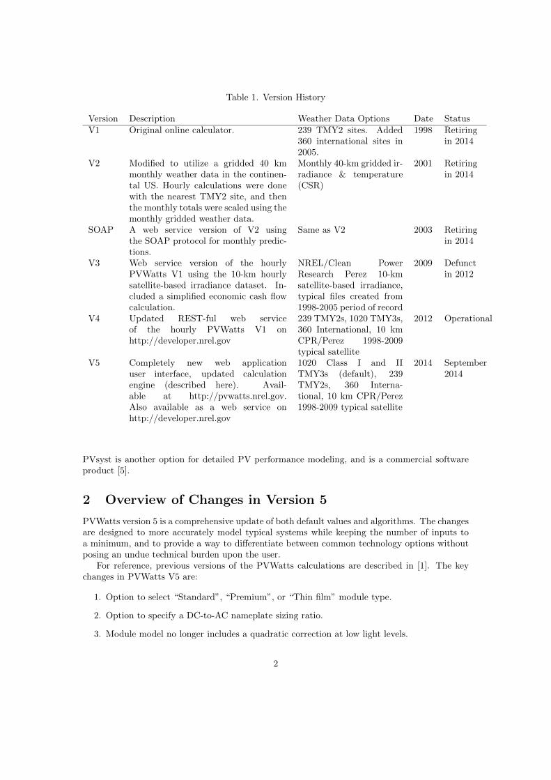
Table 1. Version History

Version Description Weather Data Options Date StatusV1 Original online calculator. 239 TMY2 sites. Added

360 international sites in2005.

1998 Retiringin 2014

V2 Modified to utilize a gridded 40 kmmonthly weather data in the continen-tal US. Hourly calculations were donewith the nearest TMY2 site, and thenthe monthly totals were scaled using themonthly gridded weather data.

Monthly 40-km gridded ir-radiance & temperature(CSR)

2001 Retiringin 2014

SOAP A web service version of V2 usingthe SOAP protocol for monthly predic-tions.

Same as V2 2003 Retiringin 2014

V3 Web service version of the hourlyPVWatts V1 using the 10-km hourlysatellite-based irradiance dataset. In-cluded a simplified economic cash flowcalculation.

NREL/Clean PowerResearch Perez 10-kmsatellite-based irradiance,typical files created from1998-2005 period of record

2009 Defunctin 2012

V4 Updated REST-ful web serviceof the hourly PVWatts V1 onhttp://developer.nrel.gov

239 TMY2s, 1020 TMY3s,360 International, 10 kmCPR/Perez 1998-2009typical satellite

2012 Operational

V5 Completely new web applicationuser interface, updated calculationengine (described here). Avail-able at http://pvwatts.nrel.gov.Also available as a web service onhttp://developer.nrel.gov

1020 Class I and IITMY3s (default), 239TMY2s, 360 Interna-tional, 10 km CPR/Perez1998-2009 typical satellite

2014 September2014

PVsyst is another option for detailed PV performance modeling, and is a commercial softwareproduct [5].

2 Overview of Changes in Version 5

PVWatts version 5 is a comprehensive update of both default values and algorithms. The changesare designed to more accurately model typical systems while keeping the number of inputs toa minimum, and to provide a way to differentiate between common technology options withoutposing an undue technical burden upon the user.

For reference, previous versions of the PVWatts calculations are described in [1]. The keychanges in PVWatts V5 are:

1. Option to select “Standard”, “Premium”, or “Thin film” module type.

2. Option to specify a DC-to-AC nameplate sizing ratio.

3. Module model no longer includes a quadratic correction at low light levels.

2

4. Total system losses are specified as a percentage, with a default value of 14 %. This replacesthe former DC-to-AC derate factor in PVWatts V1.

5. Inverter efficiency curve is derived from statistical analysis of data on inverters manufac-tured since 2010. The nominal inverter efficiency can be entered by the user.

6. One-axis tracking systems either estimate linear beam+diffuse self-shading losses based onrow spacing, or use backtracking.

7. Albedo is fixed at 0.2 unless explicitly specified at each hour in a TMY3, EPW, orSAM/CSV weather file.

3 Model Inputs

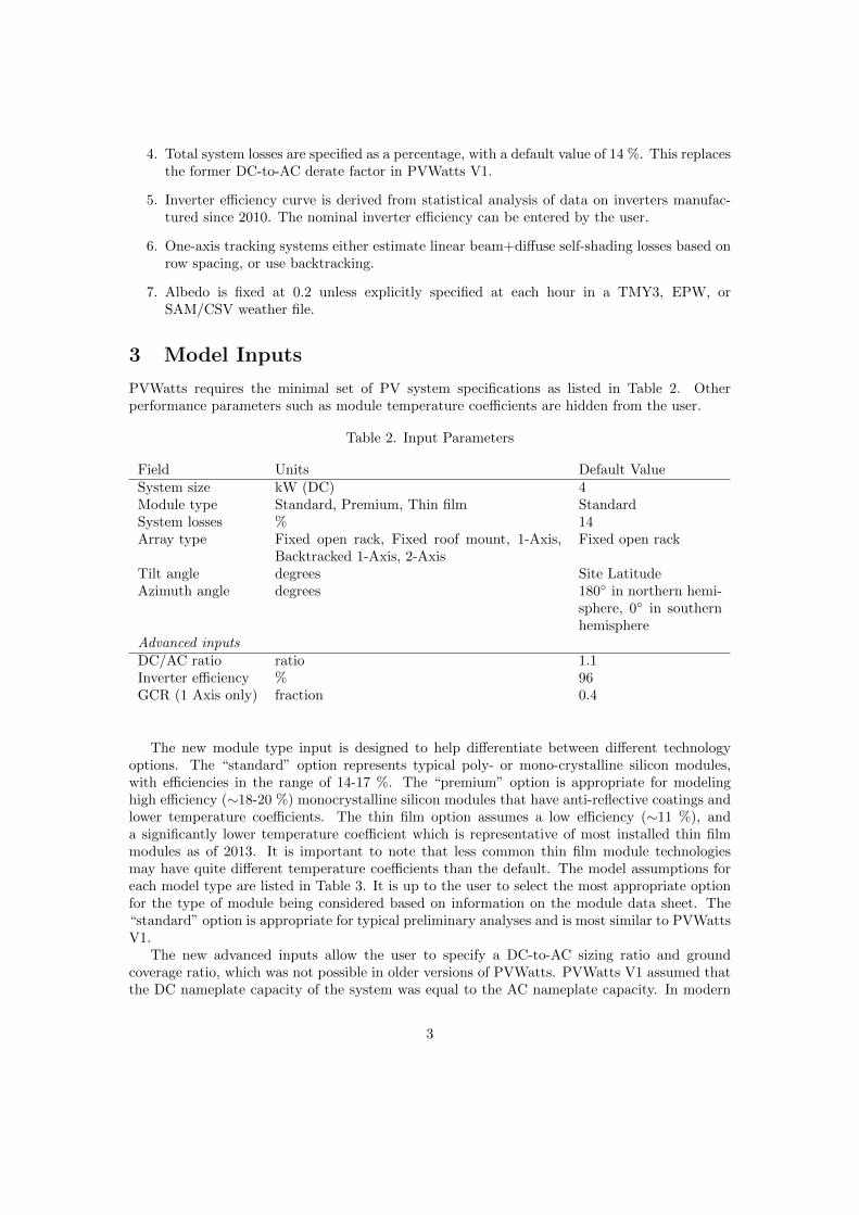
PVWatts requires the minimal set of PV system specifications as listed in Table 2. Otherperformance parameters such as module temperature coefficients are hidden from the user.

Table 2. Input Parameters

Field Units Default ValueSystem size kW (DC) 4Module type Standard, Premium, Thin film StandardSystem losses % 14Array type Fixed open rack, Fixed roof mount, 1-Axis,

Backtracked 1-Axis, 2-AxisFixed open rack

Tilt angle degrees Site LatitudeAzimuth angle degrees 180◦ in northern hemi-

sphere, 0◦ in southernhemisphere

Advanced inputsDC/AC ratio ratio 1.1Inverter efficiency % 96GCR (1 Axis only) fraction 0.4

The new module type input is designed to help differentiate between different technologyoptions. The “standard” option represents typical poly- or mono-crystalline silicon modules,with efficiencies in the range of 14-17 %. The “premium” option is appropriate for modelinghigh efficiency (∼18-20 %) monocrystalline silicon modules that have anti-reflective coatings andlower temperature coefficients. The thin film option assumes a low efficiency (∼11 %), anda significantly lower temperature coefficient which is representative of most installed thin filmmodules as of 2013. It is important to note that less common thin film module technologiesmay have quite different temperature coefficients than the default. The model assumptions foreach model type are listed in Table 3. It is up to the user to select the most appropriate optionfor the type of module being considered based on information on the module data sheet. The“standard” option is appropriate for typical preliminary analyses and is most similar to PVWattsV1.

The new advanced inputs allow the user to specify a DC-to-AC sizing ratio and groundcoverage ratio, which was not possible in older versions of PVWatts. PVWatts V1 assumed thatthe DC nameplate capacity of the system was equal to the AC nameplate capacity. In modern

3

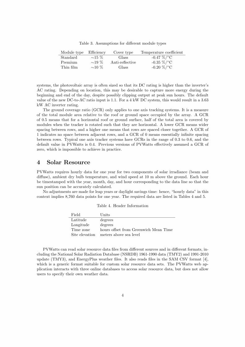
Table 3. Assumptions for different module types

Module type Efficiency Cover type Temperature coefficientStandard ∼15 % Glass -0.47 %/◦CPremium ∼19 % Anti-reflective -0.35 %/◦CThin film ∼10 % Glass -0.20 %/◦C

systems, the photovoltaic array is often sized so that its DC rating is higher than the inverter’sAC rating. Depending on location, this may be desirable to capture more energy during thebeginning and end of the day, despite possibly clipping output at peak sun hours. The defaultvalue of the new DC-to-AC ratio input is 1.1. For a 4 kW DC system, this would result in a 3.63kW AC inverter rating.

The ground coverage ratio (GCR) only applies to one axis tracking systems. It is a measureof the total module area relative to the roof or ground space occupied by the array. A GCRof 0.5 means that for a horizontal roof or ground surface, half of the total area is covered bymodules when the tracker is rotated such that they are horizontal. A lower GCR means widerspacing between rows, and a higher one means that rows are spaced closer together. A GCR of1 indicates no space between adjacent rows, and a GCR of 0 means essentially infinite spacingbetween rows. Typical one axis tracker systems have GCRs in the range of 0.3 to 0.6, and thedefault value in PVWatts is 0.4. Previous versions of PVWatts effectively assumed a GCR ofzero, which is impossible to achieve in practice.

4 Solar Resource

PVWatts requires hourly data for one year for two components of solar irradiance (beam anddiffuse), ambient dry bulb temperature, and wind speed at 10 m above the ground. Each hourbe timestamped with the year, month, day, and hour corresponding to the data line so that thesun position can be accurately calculated.

No adjustments are made for leap years or daylight savings time: hence, “hourly data” in thiscontext implies 8,760 data points for one year. The required data are listed in Tables 4 and 5.

Table 4. Header Information

Field UnitsLatitude degreesLongitude degreesTime zone hours offset from Greenwich Mean TimeSite elevation meters above sea level

PVWatts can read solar resource data files from different sources and in different formats, in-cluding the National Solar Radiation Database (NSRDB) 1961-1990 data (TMY2) and 1991-2010update (TMY3), and EnergyPlus weather files. It also reads files in the SAM CSV format [4],which is a generic format suitable for custom solar resource data sets. The PVWatts web ap-plication interacts with three online databases to access solar resource data, but does not allowusers to specify their own weather data.

4

Table 5. Hourly Input Data Fields

Field Units/ValuesYear 1950-2050Month 1-12Day 1-31Hour 0-23Direct normal irradiance (DNI) W/m2

Diffuse horizontal irradiance (DHI) W/m2

Ambient dry bulb temperature CelsiusWind speed at 10 m m/sAlbedo (optional, typically in TMY3 files) [0..1]

Change from PVWatts V1 In PVWatts V1, the albedo was changed to 0.6 forhours with a positive snow depth when using a TMY2 file. This increased systemoutput, assuming the modules were cleaned regularly of any snow cover. Now,PVWatts assumes an albedo of 0.2 for all hours of the year for TMY2 files, and usesthe hourly value provided in TMY3 files.

5 Sun Position

At each hour, PVWatts calculates the sun position using the algorithm described in [6]. The sunposition is calculated at the midpoint of the hour: for example, from 2 p.m. to 3 p.m., the sunposition is calculated at 2:30 p.m. to determine the solar zenith and azimuth angles. This is thecase for normal daytime hours during which the sun is above the horizon for the whole hour.

For the sunrise hour, the midpoint between the sunrise time and the end of the timestepis used for the sun position calculation. Similarly, the midpoint between the beginning of thetimestep and sunset time is used for the sunset hour.

6 Tracking

PVWatts performs angle of incidence (AOI) (α) calculations for fixed, one-axis, or two-axistracking systems.

Fixed systems implement standard geometrical calculations for the angle of incidence givensurface tilt β, surface azimuth γ, solar azimuth γsun, and solar zenith θsun angles, as listed inEqn. 1.

αfixed = cos−1 [sin(θsun) cos(γ − γsun) sin(β) + cos(θsun) cos(β)] (1)

For one axis trackers, the algorithm documented in [10] is used. It assumes ideal trackingand does not account for any shading. The one-axis tracking algorithm assumes a hard-codedrotation limit of ± 45 degrees from the horizontal. PVWatts uses a separate algorithm tocalculate the fraction of each row that is shaded by adjacent rows based on the ground coverageratio (GCR), and reduces the beam and diffuse irradiance incident on each row accordingly.When the backtracking option is enabled, PVWatts uses the SAM backtracking algorithm toavoid self-shading of adjacent rows. For details on these algorithms, consult [25].

5

Change from PVWatts V1 In PVWatts V1, one axis tracking assumed no self-shading or backtracking. This is an unrealistic assumption for most installed sys-tems, as tracking rows cannot be spaced infinitely apart. Consequently, the pro-duction estimates for one axis tracked systems will be reduced relative to PVWattsV1.

For two axis tracking systems, the PV surface tilt and azimuth are set equal to the sun zenithangle and the sun azimuth angle, respectively, and the incidence angle is zero. The two axistracking algorithm assumes no shading.

7 Plane-of-Array Irradiance

The plane-of-array (POA) beam, sky diffuse, and ground-reflected diffuse irradiance componentsare calculated using the Perez 1990 algorithm [7]. The POA beam component Ib is simply thebeam normal input multiplied by the cosine of the angle of incidence. The isotropic, circumsolar,and horizon brightening diffuse terms are calculated from the beam and diffuse input given twoempirical functions F1 and F2 as defined and are summed to yield the total sky diffuse on thesurface Id,sky. A slight modification from the standard Perez model treats the diffuse irradiance asisotropic for zenith angles between 87.5 and 90 degrees. The ground reflected irradiance Id,groundis treated as isotropic diffuse with a view factor calculated from the ground with respect to thetilted surface. The total POA incident on the module cover is the sum of the three components(Eqn. 2).

Ipoa = Ib + Id,sky + Id,ground (2)

The albedo, or ground reflectance, is by default fixed at 0.2. When using TMY3 data asinput, and valid data is found in the albedo column, the hourly albedo from the data file is used.

8 Module Cover

Given the total POA irradiance incident on the module cover, PVWatts applies an AOI correctionto adjust the direct beam irradiance to account for reflection losses. The correction uses amodified version of the physical model of transmittance through a module cover used in [19].

PVWatts V5 gives users the option of “Standard”, “Premium”, or “Thin film” modules.For standard and thin film modules, PVWatts uses a single slab, calculating the transmittancethrough glass with index of refraction of 1.526. This follows the treatment in [19], with thesimplification of removing the absorptance term which is determined (see below) to have anegligible effect.

For the premium module option, a two slab approach is used to model both the glass andthe thin anti-reflective (AR) coating that is designed to improve the angular response. The twoslab model involves predicting the transmittance of irradiance through two materials. The modelapplies the physical representation for unpolarized radiation described in [19] twice: once for theanti-reflective (AR) coating, and subsequently for the glass cover.

First, the angle of refraction θ2 into the AR coating is calculated with Snell’s law given angleof incidence θ1:

θ2 = arcsin

(nairnAR

sin(θ1)

)(3)

6

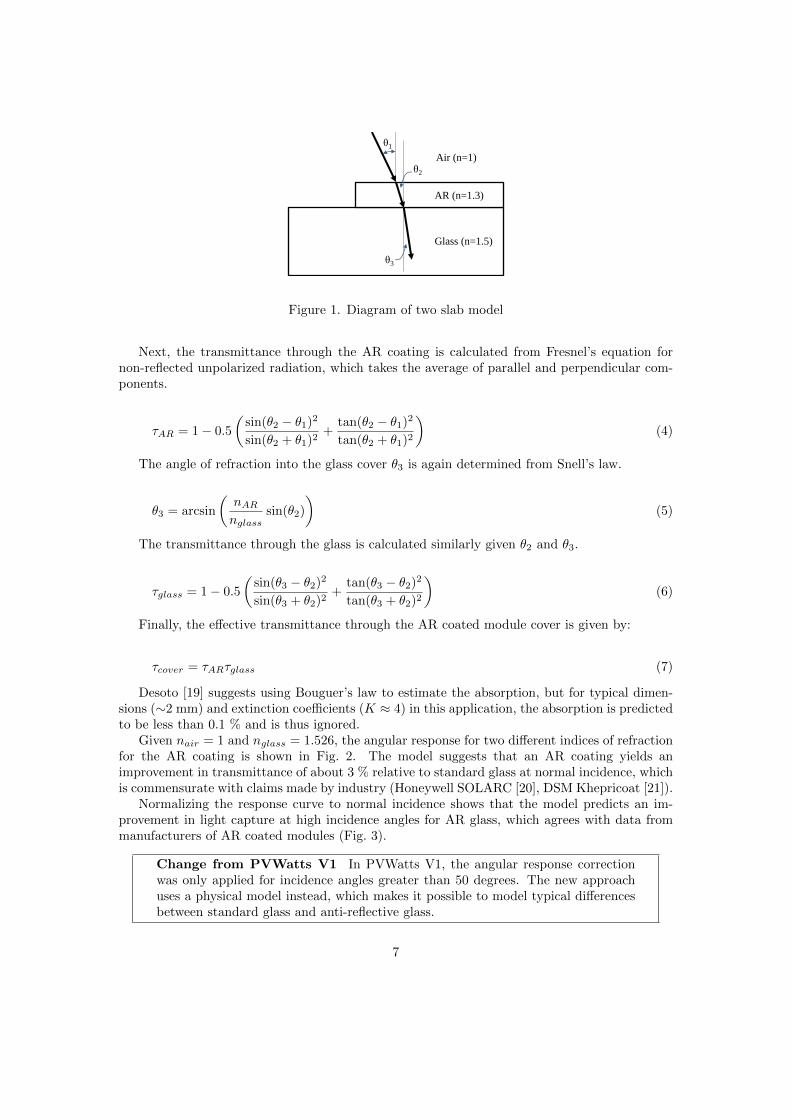
θ1

θ2

θ3

AR (n=1.3)

Glass (n=1.5)

Air (n=1)

Figure 1. Diagram of two slab model

Next, the transmittance through the AR coating is calculated from Fresnel’s equation fornon-reflected unpolarized radiation, which takes the average of parallel and perpendicular com-ponents.

τAR = 1 − 0.5

(sin(θ2 − θ1)2

sin(θ2 + θ1)2+

tan(θ2 − θ1)2

tan(θ2 + θ1)2

)(4)

The angle of refraction into the glass cover θ3 is again determined from Snell’s law.

θ3 = arcsin

(nAR

nglasssin(θ2)

)(5)

The transmittance through the glass is calculated similarly given θ2 and θ3.

τglass = 1 − 0.5

(sin(θ3 − θ2)2

sin(θ3 + θ2)2+

tan(θ3 − θ2)2

tan(θ3 + θ2)2

)(6)

Finally, the effective transmittance through the AR coated module cover is given by:

τcover = τARτglass (7)

Desoto [19] suggests using Bouguer’s law to estimate the absorption, but for typical dimen-sions (∼2 mm) and extinction coefficients (K ≈ 4) in this application, the absorption is predictedto be less than 0.1 % and is thus ignored.

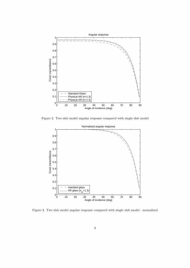
Given nair = 1 and nglass = 1.526, the angular response for two different indices of refractionfor the AR coating is shown in Fig. 2. The model suggests that an AR coating yields animprovement in transmittance of about 3 % relative to standard glass at normal incidence, whichis commensurate with claims made by industry (Honeywell SOLARC [20], DSM Khepricoat [21]).

Normalizing the response curve to normal incidence shows that the model predicts an im-provement in light capture at high incidence angles for AR glass, which agrees with data frommanufacturers of AR coated modules (Fig. 3).

Change from PVWatts V1 In PVWatts V1, the angular response correctionwas only applied for incidence angles greater than 50 degrees. The new approachuses a physical model instead, which makes it possible to model typical differencesbetween standard glass and anti-reflective glass.

7

0 10 20 30 40 50 60 70 80 900

0.1

0.2

0.3

0.4

0.5

0.6

0.7

0.8

0.9

1

Angle of incidence (deg)

Cov

er tr

ansm

ittan

ce

Angular response

Standard GlassPhysical AR (n=1.3)Physical AR (n=1.4)

Figure 2. Two slab model angular response compared with single slab model

0 10 20 30 40 50 60 70 80 900

0.1

0.2

0.3

0.4

0.5

0.6

0.7

0.8

0.9

1

Angle of incidence (deg)

Cov

er tr

ansm

ittan

ce

Normalized angular response

standard glassAR glass (n

ar=1.3)

Figure 3. Two slab model angular response compared with single slab model - normalized

8

The AR glass option will predict slightly higher output compared with the standard optiondue to the improved angular response. The normal incidence transmittance of the module coveris assumed to be captured in the nameplate rating of the system. The additional energy outputdue to the better angular response for AR glass is slight: for a fixed south-facing system in Texas,the anti-reflective coating yielded about ∼0.5 % more energy on an annual basis. This will varydepending on location and system parameters.

9 Thermal Model

PVWatts implements a thermal model to calculate the operating cell temperature Tcell using afirst-principles heat transfer energy balance model developed by Fuentes [15]. The Fuentes modelincludes effects of the thermal capacitance of the module and performs a numerical integrationbetween timesteps to account for the thermal lag transient behavior. The thermal model uses thetotal incident POA irradiance, wind speed, and dry bulb temperature to calculate the operatingcell temperature. PVWatts assumes a height of 5 m above the ground when correcting the windspeed in the weather data, and that the installed nominal operating cell temperature (INOCT)of the module is 45 ◦C.

Change from PVWatts V1 In PVWatts V5, fixed systems may be mounted onan open rack or a roof mount. The selection changes the assumed INOCT based onthe reduced air flow and thus higher operating temperature of a roof mount system.

The Fuentes paper discusses translation of the nominal operating cell temperature (NOCT)measured at standard conditions (800 W/m2, 20◦C ambient) to INOCT based on mountingconfiguration. For a roof mount system, air flow around the modules more restricted than on anopen rack, and the installed nominal operating temperature will be higher. The estimate is forINOCT to be roughly 49 ◦C for 4 inch standoffs. For fixed open rack and tracking systems, theoriginal PVWatts V1 assumption of 45 ◦C INOCT is retained.

10 Module Model

The PVWatts module computes the DC power from the array with a specified nameplate DCrating of Pdc0 given a computed cell temperature Tcell and transmitted POA irradiance Itr.The array efficiency is assumed to decrease at a linear rate as a function of temperature rise,governed by temperature coefficient γ. The reference cell temperature Tref is 25◦C, and referenceirradiance is 1000 W/m2.

Pdc =Itr

1000Pdc0(1 + γ(Tcell − Tref )) (8)

Change from PVWatts V1 In PVWatts V1, a quadratic correction was used toreduce the output for irradiance less than 125 W/m2. In comparison with operatingdata from many systems, this behavior was not observed in modern systems, andthus the correction was removed.

The temperature coefficent depends on the module type selected. The values used weredetermined from a statistical analysis of over 11000 modules in the CEC module database, andare listed in Table 3.

Change from PVWatts V1 PVWatts V1 used a fixed temperature coefficient of-0.5%/◦C . The new values indicate improved performance of newer modules.

9

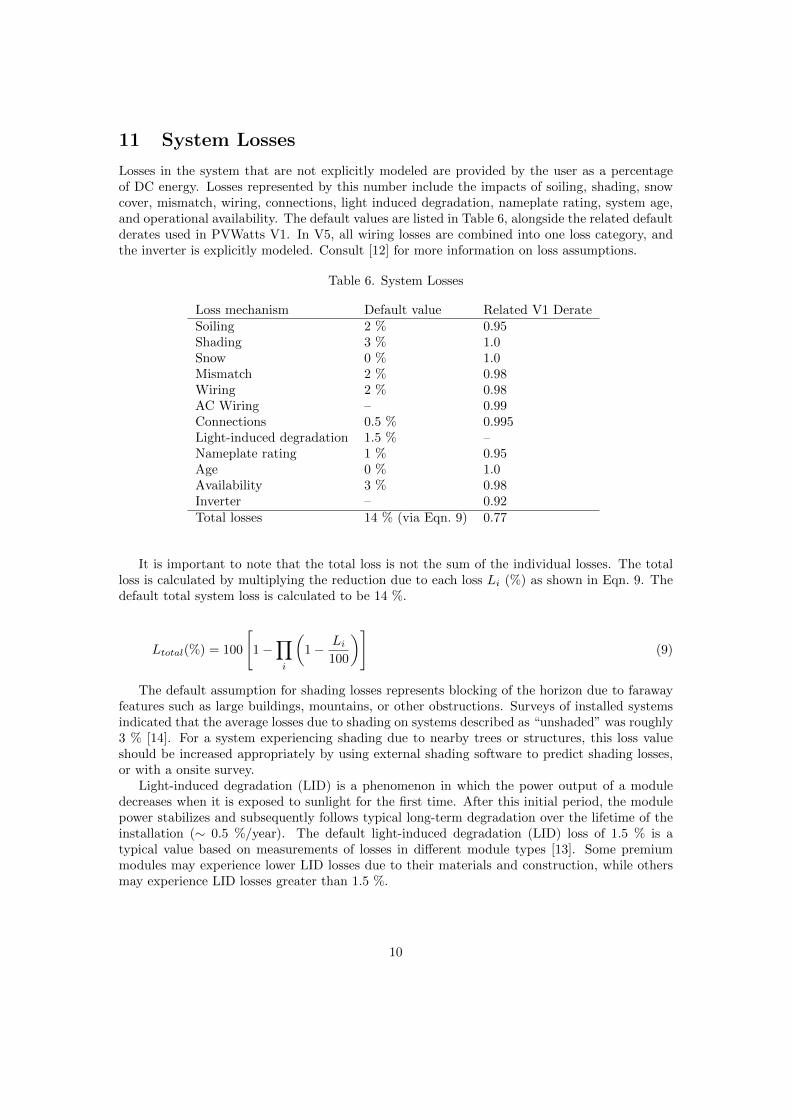
11 System Losses

Losses in the system that are not explicitly modeled are provided by the user as a percentageof DC energy. Losses represented by this number include the impacts of soiling, shading, snowcover, mismatch, wiring, connections, light induced degradation, nameplate rating, system age,and operational availability. The default values are listed in Table 6, alongside the related defaultderates used in PVWatts V1. In V5, all wiring losses are combined into one loss category, andthe inverter is explicitly modeled. Consult [12] for more information on loss assumptions.

Table 6. System Losses

Loss mechanism Default value Related V1 DerateSoiling 2 % 0.95Shading 3 % 1.0Snow 0 % 1.0Mismatch 2 % 0.98Wiring 2 % 0.98AC Wiring – 0.99Connections 0.5 % 0.995Light-induced degradation 1.5 % –Nameplate rating 1 % 0.95Age 0 % 1.0Availability 3 % 0.98Inverter – 0.92Total losses 14 % (via Eqn. 9) 0.77

It is important to note that the total loss is not the sum of the individual losses. The totalloss is calculated by multiplying the reduction due to each loss Li (%) as shown in Eqn. 9. Thedefault total system loss is calculated to be 14 %.

Ltotal(%) = 100

[1 −

∏i

(1 − Li

100

)](9)

The default assumption for shading losses represents blocking of the horizon due to farawayfeatures such as large buildings, mountains, or other obstructions. Surveys of installed systemsindicated that the average losses due to shading on systems described as “unshaded” was roughly3 % [14]. For a system experiencing shading due to nearby trees or structures, this loss valueshould be increased appropriately by using external shading software to predict shading losses,or with a onsite survey.

Light-induced degradation (LID) is a phenomenon in which the power output of a moduledecreases when it is exposed to sunlight for the first time. After this initial period, the modulepower stabilizes and subsequently follows typical long-term degradation over the lifetime of theinstallation (∼ 0.5 %/year). The default light-induced degradation (LID) loss of 1.5 % is atypical value based on measurements of losses in different module types [13]. Some premiummodules may experience lower LID losses due to their materials and construction, while othersmay experience LID losses greater than 1.5 %.

10

Change from PVWatts V1 PVWatts V1 used a DC-to-AC derate factor with adefault value of 0.77. The decision to switch to a system loss percentage input wasmade to bring PVWatts in line with common practice in the industry, and to makethe inputs easier to understand for people not familiar with the concept of a deratefactor. The inverter efficiency is not included in the system loss, and is a separateinput parameter.

To approximately convert PVWatts V5 system loss to a PVWatts V1 DC-to-AC derate factor:

1. Convert the system loss to a derate: 1 − 14/100 = 0.86.

2. Multiply this value by the nominal inverter efficiency: 0.86 × 0.96 = 0.825

This suggests that the default PVWatts V5 system loss represents roughly a 7 % increasein system performance relative to PVWatts V1 due solely to updated input assumptions. Theimpact of the revised inverter efficiency curve in version 5 (described in next section) places therealized performance gain relative to V1 closer to 8-9 % on an annual energy basis. This behavioris commensurate with hundreds of reports from PVWatts users, an expert survey solicitation,and calibration to numerous measured datasets that suggested that the old PVWatts derate wastwo conservative and underpredicted modern system performance by at least 8-9 % on average.

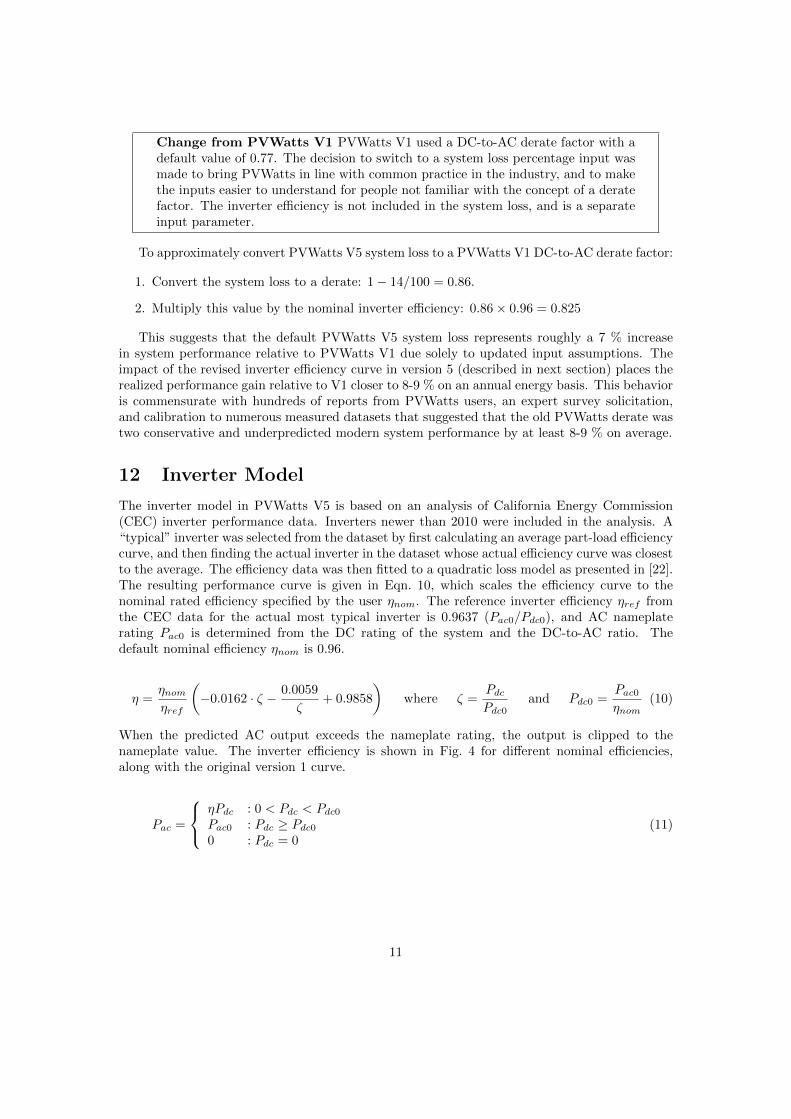
12 Inverter Model

The inverter model in PVWatts V5 is based on an analysis of California Energy Commission(CEC) inverter performance data. Inverters newer than 2010 were included in the analysis. A“typical” inverter was selected from the dataset by first calculating an average part-load efficiencycurve, and then finding the actual inverter in the dataset whose actual efficiency curve was closestto the average. The efficiency data was then fitted to a quadratic loss model as presented in [22].The resulting performance curve is given in Eqn. 10, which scales the efficiency curve to thenominal rated efficiency specified by the user ηnom. The reference inverter efficiency ηref fromthe CEC data for the actual most typical inverter is 0.9637 (Pac0/Pdc0), and AC nameplaterating Pac0 is determined from the DC rating of the system and the DC-to-AC ratio. Thedefault nominal efficiency ηnom is 0.96.

η =ηnomηref

(−0.0162 · ζ − 0.0059

ζ+ 0.9858

)where ζ =

Pdc

Pdc0and Pdc0 =

Pac0

ηnom(10)

When the predicted AC output exceeds the nameplate rating, the output is clipped to thenameplate value. The inverter efficiency is shown in Fig. 4 for different nominal efficiencies,along with the original version 1 curve.

Pac =

ηPdc : 0 < Pdc < Pdc0

Pac0 : Pdc ≥ Pdc0

0 : Pdc = 0(11)

11

0 0.2 0.4 0.6 0.8 10

0.1

0.2

0.3

0.4

0.5

0.6

0.7

0.8

0.9

1Inverter Part−Load Efficiency

Load fraction

Effi

cien

cy

η=99%η=98%η=96% (default)η=94%η=92%PVWatts V1

Figure 4. Inverter part-load efficiency curve

Table 7. Hourly Calculated Outputs

Field UnitsIncident POA irradiance W/m2

Transmitted POA irradiance W/m2

DC power WAC power W

13 Model Outputs

PVWatts reports several hourly outputs based on the system specifications and hourly irradiance,temperature, and wind speed data. They are summarized in Table 7.

In addition, the average incident POA irradiance per day in each month is reported to theuser. For each month m, the average POA in (kW/m2/day) is given by Eqn. 12.

POAm =0.001 ·

∑m POAh

number of days in month m(12)

The hourly outputs DC and AC power are also aggregated into monthly and annual energy totalsthat are reported to the user.

12

14 Comparison with Version 1 Results

Energy predictions of PVWatts V5 were compared to PVWatts V1 for several TMY2 locations.Several scenarios were considered:

1. Fixed : Fixed 20 degree tilt, south facing, standard module

2. Fixed+Premium: Fixed 20 degree tilt, south facing, premium module in PVWatts V5

3. 1 Axis: Self-shaded one axis tracking, GCR 0.4, standard module

4. Backtracking : Backtracked one axis tracking, GCR 0.4, standard module

5. 2 Axis: Two axis tracking, standard module

The number for each scenario reported in Table 8 is the percent difference between PVWattsV5 and V1 annual AC energy production estimates. The results show that PVWatts V5 predictson average 8 % percent more annual energy across all system configurations and locations. Theone axis tracking cases show a lower increase - this is because PVWatts V1 overpredicts one axistracking by assuming no self shading of rows. The greater relative improvement for fixed systemsis due to the fact that fixed arrays operate more frequently at part-load since they do not trackthe sun, and so the effect of the improved part-load inverter efficiency is more pronounced.

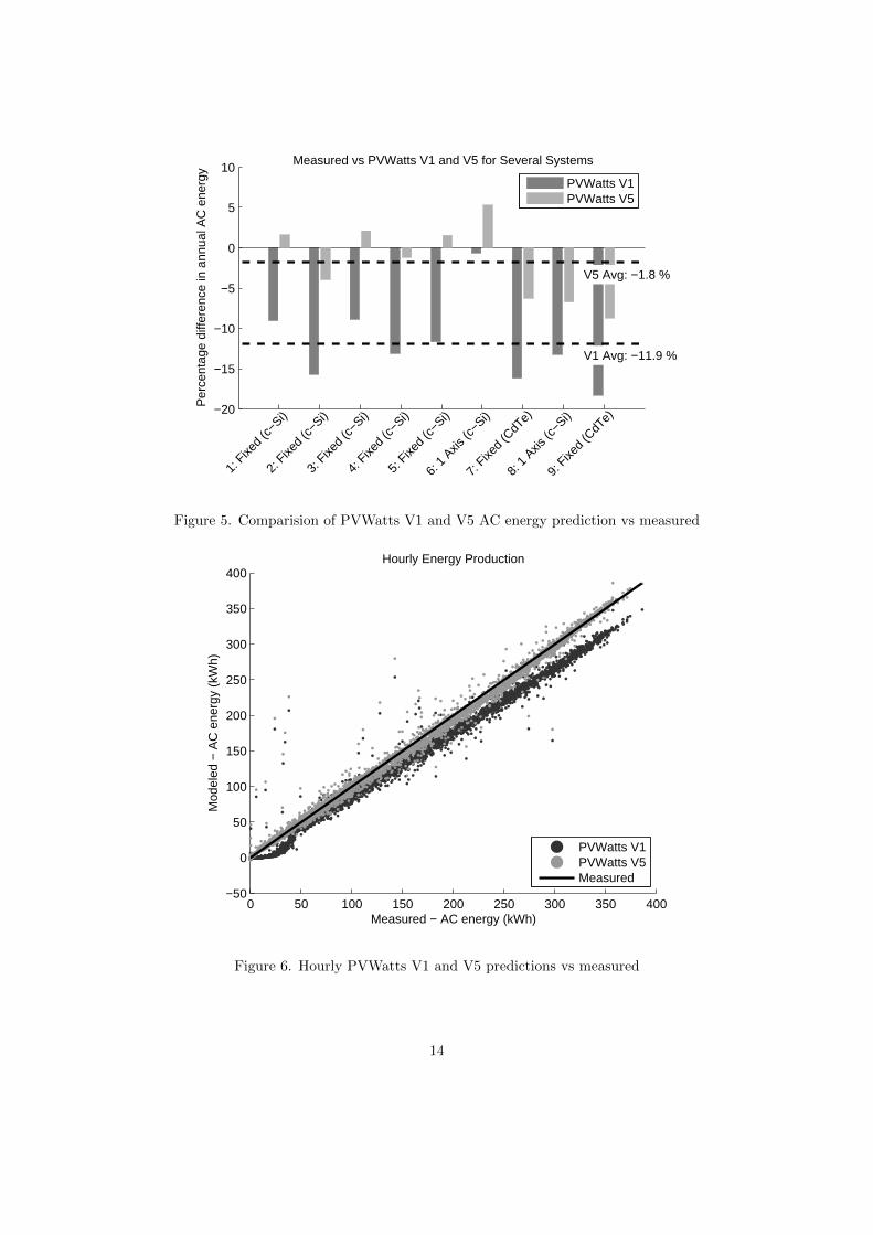
15 Comparison with Measured Data

In this section, PVWatts predictions are shown for several systems. The nine systems consideredare detailed in [23], and consist of 8 fixed tilt systems and one 1-axis tracked system. PVWatts V1underpredicts system performance by 11.9 % when comparing annual AC energy, while PVWattsV5 is low by only 1.8 %. All of the systems considered were unshaded, and the periods duringwhich the system was unavailable were removed from the comparison. Consequently, the lossmechanisms for shading and availability were set to zero for both models. Systems with non-standard module types were configured appropriately in PVWatts V5: system 2 (premium),system 7 (thin-film), and system 9 (thin-film).

In Figure 6, PVWatts V1 hourly results are shown for a fixed crystalline silicon system inColorado. The data does not support the quadratic behavior at low power levels predicted byV1. PVWatts V5 does not include the module performance adjustment below 125 W/m2, andthus matches the measured system data better. The PVWatts V1 low irradiance assumptionsare not supported by any of the modern systems considered. In addition, the updated inverterperformance curve in V5 tracks the measured system output more closely at high power outputs.

16 Summary

A comprehensive update to the popular PVWatts photovoltaic performance model was pre-sented. The improved model formulation and updated default assumptions in V5 largely cor-rect the underprediction of V1 relative to actual system performance. The updated PVWattswill be deployed to the NREL PVWatts Online Calculator in the fall of 2014, available athttp://pvwatts.nrel.gov.

13

−20

−15

−10

−5

0

5

10

Per

cent

age

diffe

renc

e in

ann

ual A

C e

nerg

y

Measured vs PVWatts V1 and V5 for Several Systems

1: F

ixed

(c−S

i)

2: F

ixed

(c−S

i)

3: F

ixed

(c−S

i)

4: F

ixed

(c−S

i)

5: F

ixed

(c−S

i)

6: 1

Axis

(c−S

i)

7: F

ixed

(CdT

e)

8: 1

Axis

(c−S

i)

9: F

ixed

(CdT

e)

V1 Avg: −11.9 %

V5 Avg: −1.8 %

PVWatts V1PVWatts V5

Figure 5. Comparision of PVWatts V1 and V5 AC energy prediction vs measured

0 50 100 150 200 250 300 350 400−50

0

50

100

150

200

250

300

350

400

Measured − AC energy (kWh)

Mod

eled

− A

C e

nerg

y (k

Wh)

Hourly Energy Production

PVWatts V1PVWatts V5Measured

Figure 6. Hourly PVWatts V1 and V5 predictions vs measured

14

References

[1] Dobos, A.; PVWatts Version 1 Technical Reference. . NREL/TP-6A20-60272. 2013.

[2] Marion, W.; Urban, K. (2012). User’s Manual for TMY2. Accessed September 3, 2013:http://rredc.nrel.gov/solar/pubs/tmy2/.

[3] Wilcox, S.; Marion, W. (2008). User’s Manual for TMY3 Data Sets. NREL/TP-581-43156.Golden, CO: National Renewable Energy Laboratory.

[4] NREL. System Advisor Model (SAM). http://sam.nrel.gov. 2014.

[5] PVsyst SA. PVsyst Photovoltaic Software Version 6.1. http://www.pvsyst.com. 2014.

[6] Michalsky, J. (1988). “The Astronomical Almanac’s Algorithm for Approximate Solar Posi-tion (1950-2050).” Solar Energy (40).

[7] Perez, R.; Ineichen, P.; Seals, R.; Michalsky, J.; Stewart, R. (1990). “Modeling DaylightAvailability and Irradiance Components for Direct and Global Irradiance.” Solar Energy(44:5), pp. 271-289.

[8] Marion, W.; Anderberg, M. (2000). PVWATTS - An Online Performance Calculator forGrid-Connected PV Systems. Proceedings of the ASES Solar Conference, June 15-21, 2000,Madison, Wisconsin.

[9] Marion, W.; Anderberg, M.; George, R.; Gray-Hann, P.; Heimiller, D.; (2001) PVWATTSVersion 2 - Enhanced Spatial Resolution for Calculating Grid-Connected PV Performance.CP-560-30941. Golden CO: National Renewable Energy Laboratory.

[10] Marion, W.; Dobos, A. P. (2013). Rotation Angle for the Optimum Tracking of One-AxisTrackers. TP-6A20-58891. Golden, CO: National Renewable Energy Laboratory.

[11] Marion, W. (2010). Overview of the PV Module Model in PVWatts. Presentation at theSandia National Laboratories PV Performance Modeling Workshop, September 22, 2010,Albuquerque, New Mexico.

[12] Marion, W.; Adelstein, J.; Boyle, K.; Hayden, H.; Hammond, B.; Fletcher, T.; Canada, B.;Narang, D.; Shugar, D.; Wenger, H.; Kimber, A.; Mitchell, L.; Rich, G.; Townsend, T. (2005).Performance Parameters for Grid-Connected PV Systems. Proc. of 31st IEEE PhotovoltaicsSpecialists Conference, January 2005, Lake Buena Vista, Florida.

[13] Pingel, S., Koshnicharov, D., Frank, O., Geipel, T., Zemen, Y., Striner, B., Berghold, J.Initial degradation of industrial silicon solar cells in solar panels. 25th EU PVSEC, 2010.

[14] Deline, C.; Meydbray, J.; Donovan, M.; Forrest, J.; Photovoltaic Shading Testbed forModule-level Power Electronics. NREL Technical Report NREL/TP-5200-54876, May 2012.http://www.nrel.gov/docs/fy12osti/54876.pdf

[15] Fuentes, M. K. (1987). A Simplified Thermal Model for Flat-Plate Photovoltaic Arrays.SAND85-0330. Albuquerque, NM: Sandia National Laboratories. Accessed September 3,2013: http://prod.sandia.gov/techlib/access-control.cgi/1985/850330.pdf.

[16] California Energy Commission. (2013). “CEC PV Calculator Version 4.0.” Accessed Septem-ber 3, 2013: http://gosolarcalifornia.org/tools/nshpcalculator/index.php.

15

[17] Menicucci, D. F.; Fernandez, J. P. (1988). User’s Manual for PVFORM: A Photo-voltaic System Simulation Program For Stand-Alone and Grid-Interactive Applications.SAND85-0376. Albuquerque, NM: Sandia National Laboratories. Accessed September 3,2013: http://prod.sandia.gov/techlib/access-control.cgi/1985/850376.pdf.

[18] Menicucci, D. F. (1986). Photovoltaic Array Performance Simulation Models. Solar Cells(18).

[19] DeSoto, W.; Klein, S.; Beckman, W.; Improvement and Validation of a Model for Photo-voltaic Array Performance. Solar Energy, vol.80, pp.78-88, 2006.

[20] Honeywell SOLARC. http://www.honeywell-pmt.com/sm/em/common/documents/SOLARC anti-reflective coating.pdf.

[21] DSM Khepricoat. https://www.dsm.com/content/dam/dsm/cworld/en US/documents/khepricoat-boosting-module-performance-with-a-durable-ar-coating.pdf

[22] Dreisse, A.; Jain, P.; Harrison, S.; Beyond the Curves: Modeling the Electrical Efficiency ofPhotovoltaic Inverters. Proc. IEEE Photovoltaic Specialists Conf., 2008.

[23] Freeman, J.; Whitmore, J.; Kaffine, L.; Blair, N.; Dobos, A.; System Advisor Model: FlatPlat Photovolatic Performance Modeling Validation Report. NREL/TP-6A20-60204, 2013.

[24] Freeman, J.; Whitmore, J.; Blair, N.; Dobos, A.; Validation of Multiple Tools for Flat PlatePhotovoltaic Modeling Against Measured Data. NREL/TP-6A20-61497, 2014.

[25] Gilman, P.; SAM Photovoltaic Model Technical Reference. NREL/TP-6A20-xxxxx, forth-coming, 2014.

16

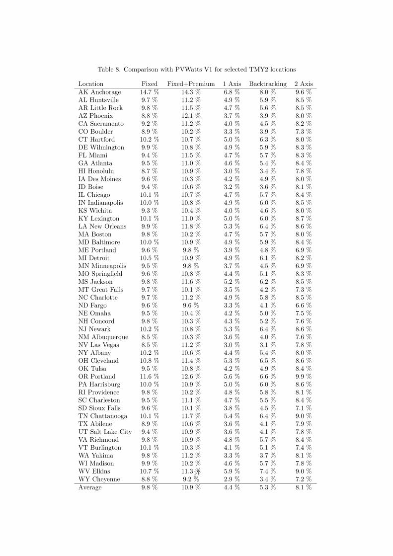
Table 8. Comparison with PVWatts V1 for selected TMY2 locations

Location Fixed Fixed+Premium 1 Axis Backtracking 2 AxisAK Anchorage 14.7 % 14.3 % 6.8 % 8.0 % 9.6 %AL Huntsville 9.7 % 11.2 % 4.9 % 5.9 % 8.5 %AR Little Rock 9.8 % 11.5 % 4.7 % 5.6 % 8.5 %AZ Phoenix 8.8 % 12.1 % 3.7 % 3.9 % 8.0 %CA Sacramento 9.2 % 11.2 % 4.0 % 4.5 % 8.2 %CO Boulder 8.9 % 10.2 % 3.3 % 3.9 % 7.3 %CT Hartford 10.2 % 10.7 % 5.0 % 6.3 % 8.0 %DE Wilmington 9.9 % 10.8 % 4.9 % 5.9 % 8.3 %FL Miami 9.4 % 11.5 % 4.7 % 5.7 % 8.3 %GA Atlanta 9.5 % 11.0 % 4.6 % 5.4 % 8.4 %HI Honolulu 8.7 % 10.9 % 3.0 % 3.4 % 7.8 %IA Des Moines 9.6 % 10.3 % 4.2 % 4.9 % 8.0 %ID Boise 9.4 % 10.6 % 3.2 % 3.6 % 8.1 %IL Chicago 10.1 % 10.7 % 4.7 % 5.7 % 8.4 %IN Indianapolis 10.0 % 10.8 % 4.9 % 6.0 % 8.5 %KS Wichita 9.3 % 10.4 % 4.0 % 4.6 % 8.0 %KY Lexington 10.1 % 11.0 % 5.0 % 6.0 % 8.7 %LA New Orleans 9.9 % 11.8 % 5.3 % 6.4 % 8.6 %MA Boston 9.8 % 10.2 % 4.7 % 5.7 % 8.0 %MD Baltimore 10.0 % 10.9 % 4.9 % 5.9 % 8.4 %ME Portland 9.6 % 9.8 % 3.9 % 4.8 % 6.9 %MI Detroit 10.5 % 10.9 % 4.9 % 6.1 % 8.2 %MN Minneapolis 9.5 % 9.8 % 3.7 % 4.5 % 6.9 %MO Springfield 9.6 % 10.8 % 4.4 % 5.1 % 8.3 %MS Jackson 9.8 % 11.6 % 5.2 % 6.2 % 8.5 %MT Great Falls 9.7 % 10.1 % 3.5 % 4.2 % 7.3 %NC Charlotte 9.7 % 11.2 % 4.9 % 5.8 % 8.5 %ND Fargo 9.6 % 9.6 % 3.3 % 4.1 % 6.6 %NE Omaha 9.5 % 10.4 % 4.2 % 5.0 % 7.5 %NH Concord 9.8 % 10.3 % 4.3 % 5.2 % 7.6 %NJ Newark 10.2 % 10.8 % 5.3 % 6.4 % 8.6 %NM Albuquerque 8.5 % 10.3 % 3.6 % 4.0 % 7.6 %NV Las Vegas 8.5 % 11.2 % 3.0 % 3.1 % 7.8 %NY Albany 10.2 % 10.6 % 4.4 % 5.4 % 8.0 %OH Cleveland 10.8 % 11.4 % 5.3 % 6.5 % 8.6 %OK Tulsa 9.5 % 10.8 % 4.2 % 4.9 % 8.4 %OR Portland 11.6 % 12.6 % 5.6 % 6.6 % 9.9 %PA Harrisburg 10.0 % 10.9 % 5.0 % 6.0 % 8.6 %RI Providence 9.8 % 10.2 % 4.8 % 5.8 % 8.1 %SC Charleston 9.5 % 11.1 % 4.7 % 5.5 % 8.4 %SD Sioux Falls 9.6 % 10.1 % 3.8 % 4.5 % 7.1 %TN Chattanooga 10.1 % 11.7 % 5.4 % 6.4 % 9.0 %TX Abilene 8.9 % 10.6 % 3.6 % 4.1 % 7.9 %UT Salt Lake City 9.4 % 10.9 % 3.6 % 4.1 % 7.8 %VA Richmond 9.8 % 10.9 % 4.8 % 5.7 % 8.4 %VT Burlington 10.1 % 10.3 % 4.1 % 5.1 % 7.4 %WA Yakima 9.8 % 11.2 % 3.3 % 3.7 % 8.1 %WI Madison 9.9 % 10.2 % 4.6 % 5.7 % 7.8 %WV Elkins 10.7 % 11.3 % 5.9 % 7.4 % 9.0 %WY Cheyenne 8.8 % 9.2 % 2.9 % 3.4 % 7.2 %Average 9.8 % 10.9 % 4.4 % 5.3 % 8.1 %

17