“Putting a price on infrastructure”Aspects of pricing third-party access to

infrastructure

University of Piraeus

Graduate Program - ENERGY: Strategy, Law & Economics

Academic year: 2018-2019

Course A4

G. Avlonitis

Chemical Engineer

MSc Petroleum Engineering

Introduction

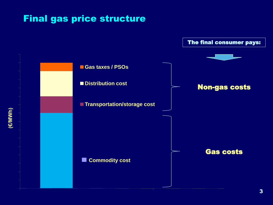
Final gas price structure

3

(€/M

Wh

)

Gas taxes / PSOs

Distribution cost

Transportation/storage cost

Commodity cost

The final consumer pays:

Non-gas costs

Gas costs

Final gas price structure II

• In a liberalized and competitive gas market:

− Non gas costs: Are known in advance (transparency) and

are common to all market participants (non-discrimination)

− Gas costs: Are formed by the market, through the interaction

of supply and demand, in conditions of competition between

different suppliers

4

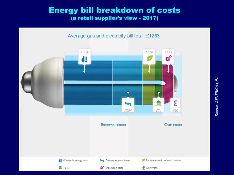
Energy bill breakdown of costs(a retail supplier’s view - 2017)

So

urc

e: C

EN

TR

ICA

(U

K)

5

Final gas price structure III

• Cost of gas (commodity)

− Derived through competition (market value)

• Taxes, levies, Public Service Obligations (PSO)

− Imposed by the government as a means to achieve public

and energy policy objectives

• Cost of using the infrastructure (e.g. transmission,

storage, LNG regasification, distribution)

− Approved by the energy regulator, so that it is transparent

and non-discriminatory for the users of the infrastructure

“third-party access (TPA) tariff”

6

Final gas price structure IV

• Setting a discreet TPA tariff which is known in

advance and is common to every interested party is a

fundamental pre-condition for proper market

functioning:

• The competition not to be distorted and being focused on the

supply activities

• Setting the TPA tariff at a fair level is fundamental for

efficiency reasons:

• The consumer should not pay unjustified/inefficient costs

• The TSO should be able to perform its duties and being able

to finance the further expansion/development of the

infrastructure

7

TSO activities

• Regulated:

− Operation, maintenance and development of the system

− Services related to third-party access to the transmission system

• Non-regulated:

− Related to the transmission system (e.g. certification of metering

equipment of industrial installations, gas odorization services etc)

− Not related to the transmission system (e.g. real estate!)

• Strict accounting unbundling rules prevent cross-subsidization

between regulated and non-regulated activities

8

TSO revenues

• Regulated:

− Sourced from provision of TPA services, through TPA tariffs

− Approved by the National Regulatory Authority

− Recorded (along with relevant costs) in a separate account

• Non-regulated

− Sourced from provision of non-regulated services

− Relevant tariffs are defined by the TSO based on the competition in

the relevant market, generally without any regulatory intervention

− Recorded (along with relevant costs) in a separate account

• Usually, the non-regulated revenue is a small fraction of the

regulated revenue9

Financing infrastructure development in a

regulated regime

• Gas transmission system:

− Natural monopoly (inefficient to duplicate, unless capacity exhausted)

− Subject to regulation and unbundling rules

• Financing sources:

− Equity (own money – TSO’s shareholders):

• Sourced from provision of TPA services, through TPA tariffs

− Debt:

• From banks/international financial institutions

− Grants:

• From EU [through the Projects of Common Interest (PCI) and Connecting

Europe Facility (CEF) process] and/or banks/international financial institutions

10

Third-party access tariffs

12

TPA tariffs in general

• Approving of the TPA tariffs is one of the most important regulatory

competences (*)

• TPA tariffs are not related to the gas (commodity) cost transmitted

through the infrastructure

• TPA tariffs defines the amount of money paid to the TSO by a User of

the infrastructure for:

– Connection of Uses facilities with the infrastructure and/or

– Use of the infrastructure to transmit gas

• A prerequisite for setting TPA tariffs for a piece of infrastructure is the

accounting unbundling of the activity associated with the relevant

infrastructure

(*) For simplicity reasons, discussion will be limited on transmission system tariffs,

since the logic for TPA tariff setting is the same for all gas infrastructures

(transmission, distribution, LNG terminals, storage facilities) (in fact, transportation

presents more complex issues like locational pricing and transit flows).

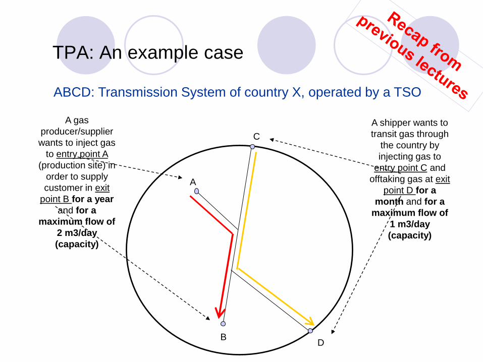
ABCD: Transmission System of country X, operated by a TSO

A

C

DB

A gas

producer/supplier

wants to inject gas

to entry point A

(production site) in

order to supply

customer in exit

point B for a year

and for a

maximum flow of

2 m3/day

(capacity)

A shipper wants to

transit gas through

the country by

injecting gas to

entry point C and

offtaking gas at exit

point D for a

month and for a

maximum flow of

1 m3/day

(capacity)

TPA: An example case

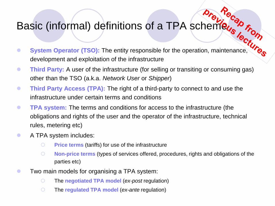
Basic (informal) definitions of a TPA scheme

⚫ System Operator (TSO): The entity responsible for the operation, maintenance,

development and exploitation of the infrastructure

⚫ Third Party: A user of the infrastructure (for selling or transiting or consuming gas)

other than the TSO (a.k.a. Network User or Shipper)

⚫ Third Party Access (TPA): The right of a third-party to connect to and use the

infrastructure under certain terms and conditions

⚫ TPA system: The terms and conditions for access to the infrastructure (the

obligations and rights of the user and the operator of the infrastructure, technical

rules, metering etc)

⚫ A TPA system includes:

Price terms (tariffs) for use of the infrastructure

Non-price terms (types of services offered, procedures, rights and obligations of the

parties etc)

⚫ Two main models for organising a TPA system:

The negotiated TPA model (ex-post regulation)

The regulated TPA model (ex-ante regulation)

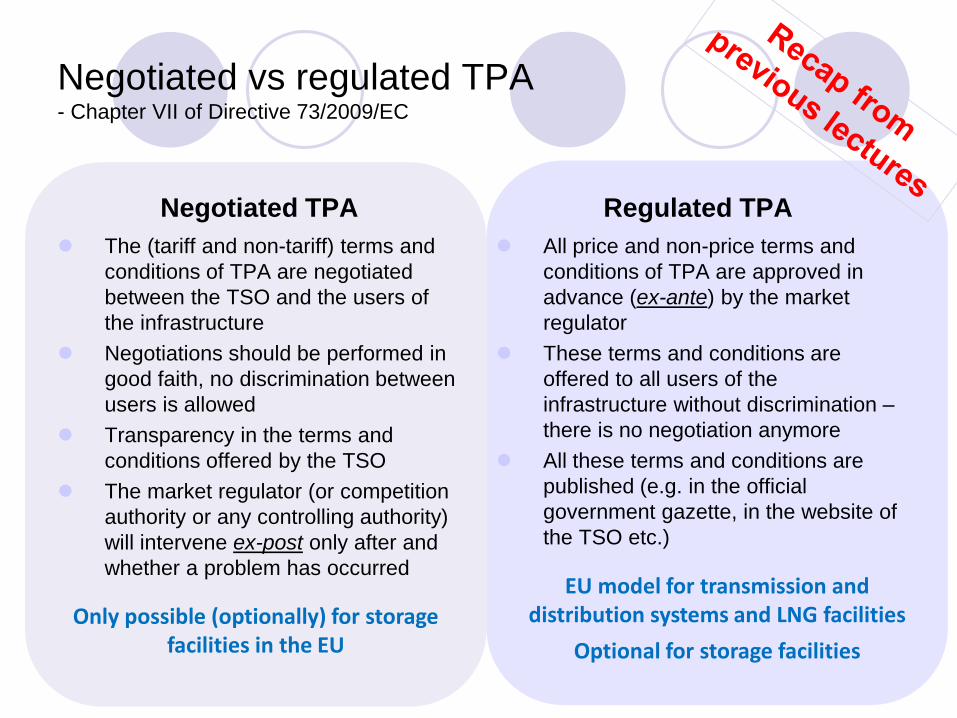
Only possible (optionally) for storage facilities in the EU

EU model for transmission and distribution systems and LNG facilities

Optional for storage facilities

Negotiated vs regulated TPA- Chapter VII of Directive 73/2009/EC

Negotiated TPA

⚫ The (tariff and non-tariff) terms and

conditions of TPA are negotiated

between the TSO and the users of

the infrastructure

⚫ Negotiations should be performed in

good faith, no discrimination between

users is allowed

⚫ Transparency in the terms and

conditions offered by the TSO

⚫ The market regulator (or competition

authority or any controlling authority)

will intervene ex-post only after and

whether a problem has occurred

Regulated TPA

⚫ All price and non-price terms and

conditions of TPA are approved in

advance (ex-ante) by the market

regulator

⚫ These terms and conditions are

offered to all users of the

infrastructure without discrimination –

there is no negotiation anymore

⚫ All these terms and conditions are

published (e.g. in the official

government gazette, in the website of

the TSO etc.)

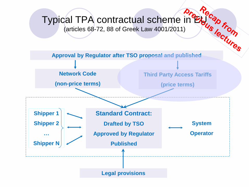
Typical TPA contractual scheme in EU(articles 68-72, 88 of Greek Law 4001/2011)

Approval by Regulator after TSO proposal and published

Shipper 1

Shipper 2

…

Shipper N

Network Code

(non-price terms)

Third Party Access Tariffs

(price terms)

Standard Contract:

Drafted by TSO

Approved by Regulator

Published

Legal provisions

System

Operator

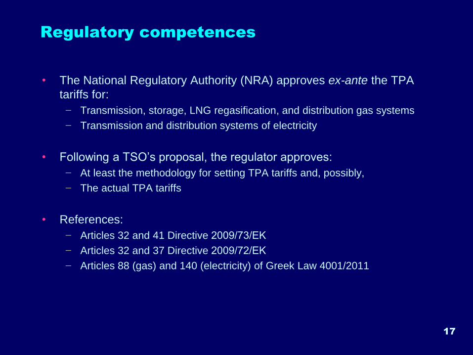
Regulatory competences

• The National Regulatory Authority (NRA) approves ex-ante the TPA

tariffs for:

− Transmission, storage, LNG regasification, and distribution gas systems

− Transmission and distribution systems of electricity

• Following a TSO’s proposal, the regulator approves:

− At least the methodology for setting TPA tariffs and, possibly,

− The actual TPA tariffs

• References:

− Articles 32 and 41 Directive 2009/73/ΕΚ

− Articles 32 and 37 Directive 2009/72/ΕΚ

− Articles 88 (gas) and 140 (electricity) of Greek Law 4001/2011

17

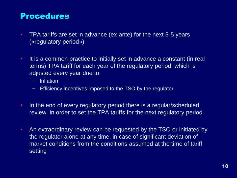
Procedures

• TPA tariffs are set in advance (ex-ante) for the next 3-5 years

(«regulatory period»)

• It is a common practice to initially set in advance a constant (in real

terms) TPA tariff for each year of the regulatory period, which is

adjusted every year due to:

− Inflation

− Efficiency incentives imposed to the TSO by the regulator

• In the end of every regulatory period there is a regular/scheduled

review, in order to set the TPA tariffs for the next regulatory period

• An extraordinary review can be requested by the TSO or initiated by

the regulator alone at any time, in case of significant deviation of

market conditions from the conditions assumed at the time of tariff

setting

18

19

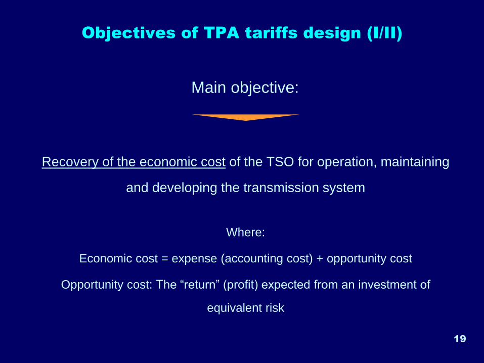
Objectives of TPA tariffs design (I/II)

Recovery of the economic cost of the TSO for operation, maintaining

and developing the transmission system

Where:

Economic cost = expense (accounting cost) + opportunity cost

Opportunity cost: The “return” (profit) expected from an investment of

equivalent risk

Main objective:

20

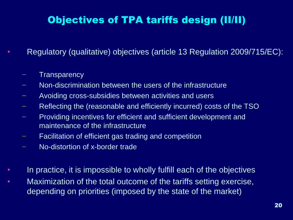
Objectives of TPA tariffs design (II/II)

• Regulatory (qualitative) objectives (article 13 Regulation 2009/715/EC):

− Transparency

− Non-discrimination between the users of the infrastructure

− Avoiding cross-subsidies between activities and users

− Reflecting the (reasonable and efficiently incurred) costs of the TSO

− Providing incentives for efficient and sufficient development and

maintenance of the infrastructure

− Facilitation of efficient gas trading and competition

− No-distortion of x-border trade

• In practice, it is impossible to wholly fulfill each of the objectives

• Maximization of the total outcome of the tariffs setting exercise,

depending on priorities (imposed by the state of the market)

21

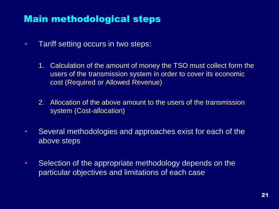
Main methodological steps

• Tariff setting occurs in two steps:

1. Calculation of the amount of money the TSO must collect form the

users of the transmission system in order to cover its economic

cost (Required or Allowed Revenue)

2. Allocation of the above amount to the users of the transmission

system (Cost-allocation)

• Several methodologies and approaches exist for each of the

above steps

• Selection of the appropriate methodology depends on the

particular objectives and limitations of each case

22

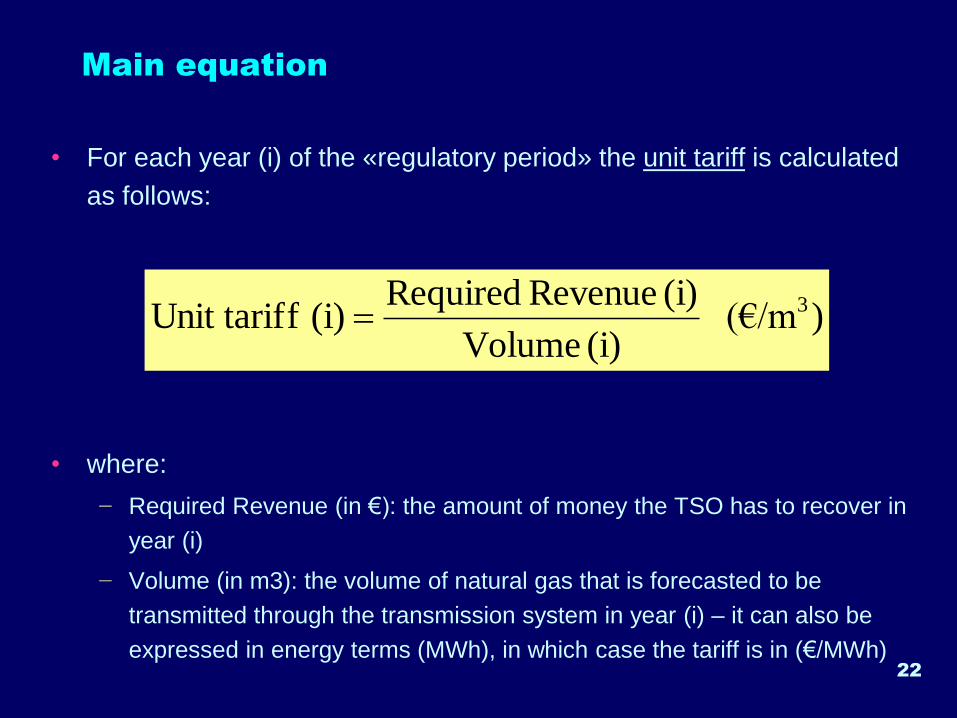
Main equation

• For each year (i) of the «regulatory period» the unit tariff is calculated

as follows:

• where:

− Required Revenue (in €): the amount of money the TSO has to recover in

year (i)

− Volume (in m3): the volume of natural gas that is forecasted to be

transmitted through the transmission system in year (i) – it can also be

expressed in energy terms (MWh), in which case the tariff is in (€/MWh)

)(€/m (i) Volume

(i) Revenue Required(i) fUnit tarif 3=

Notes

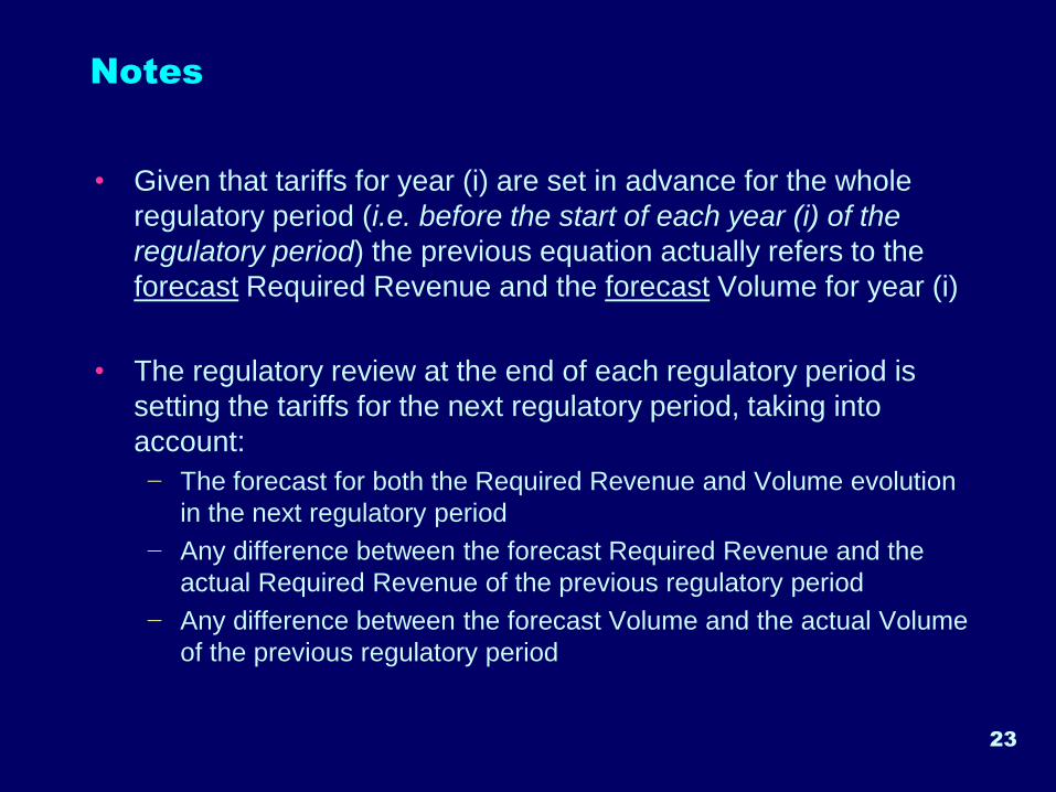
• Given that tariffs for year (i) are set in advance for the whole

regulatory period (i.e. before the start of each year (i) of the

regulatory period) the previous equation actually refers to the

forecast Required Revenue and the forecast Volume for year (i)

• The regulatory review at the end of each regulatory period is

setting the tariffs for the next regulatory period, taking into

account:

− The forecast for both the Required Revenue and Volume evolution

in the next regulatory period

− Any difference between the forecast Required Revenue and the

actual Required Revenue of the previous regulatory period

− Any difference between the forecast Volume and the actual Volume

of the previous regulatory period

23

Calculation of Required Revenue

Required Revenue - RR

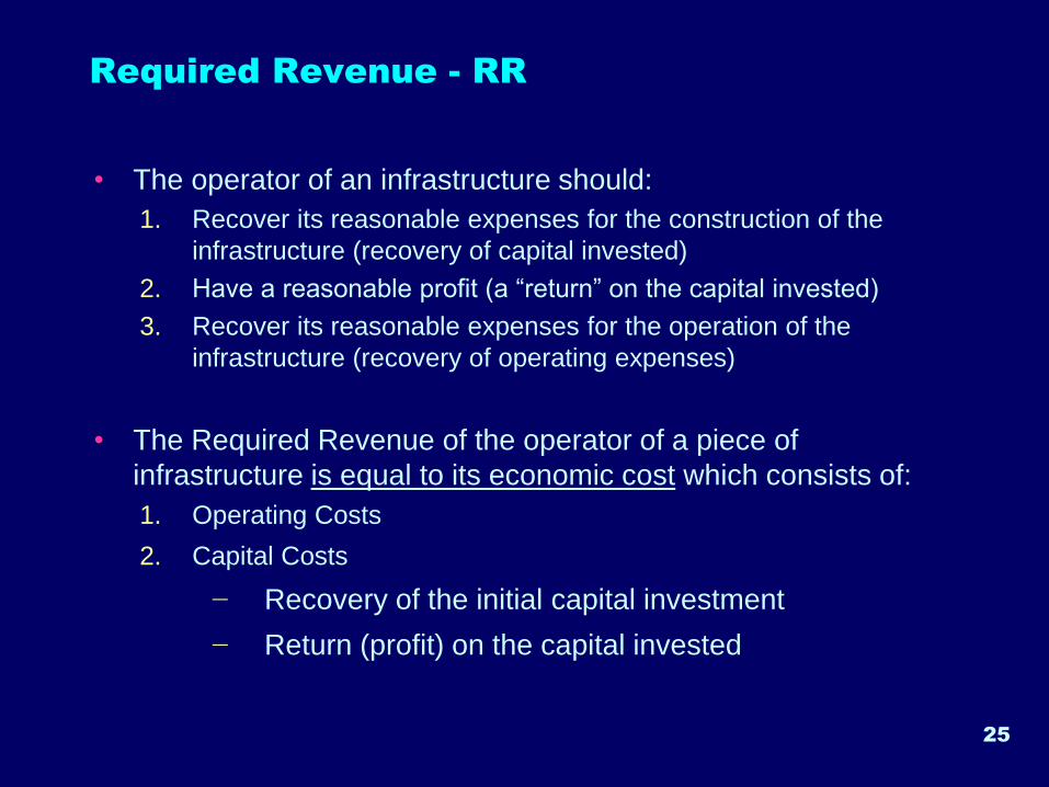
• The operator of an infrastructure should:

1. Recover its reasonable expenses for the construction of the

infrastructure (recovery of capital invested)

2. Have a reasonable profit (a “return” on the capital invested)

3. Recover its reasonable expenses for the operation of the

infrastructure (recovery of operating expenses)

• The Required Revenue of the operator of a piece of

infrastructure is equal to its economic cost which consists of:

1. Operating Costs

2. Capital Costs

− Recovery of the initial capital investment

− Return (profit) on the capital invested

25

26

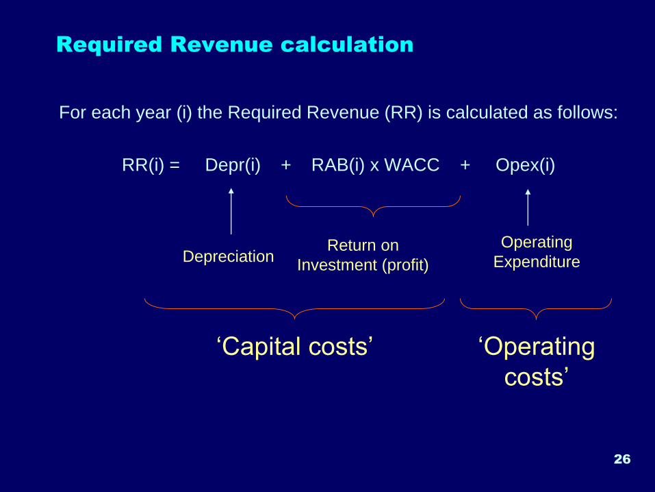
Required Revenue calculation

For each year (i) the Required Revenue (RR) is calculated as follows:

RR(i) = Depr(i) + RAB(i) x WACC + Opex(i)

DepreciationReturn on

Investment (profit)

Operating

Expenditure

‘Capital costs’ ‘Operating

costs’

27

Regulatory Asset Base (RAB)

• RAB: All assets used in the activity for which tariffs are designed

− For example, in a transmission system, it consists of the all pipelines, valve

stations, metering/stations, compressors etc

• For setting the tariffs, the value of the RAB at the time of calculation

of the tariffs is necessary to be defined

− If tariffs are designed today but are to be applied also in future years, the value

of the RAB should also include future assets (new investments)

• The RAB is really the basis of tariff calculation. It affects both

aspects of the “capital cost” part of the Required Revenue:

− Depreciation

− Return on capital invested

• For that matter, the selection of the appropriate RAB methodology

and calculation is a matter of serious negotiations between the

owner/operator of the transmission system and the regulator

28

Methodologies for defining RAB value

• Two main categories:

− Cost-based methodologies

• Historic Cost (book value)

• Indexed Historic Cost

• Replacement Cost

• Optimised Replacement Cost

− Value-based methodologies

• Fair market value

• Deprival value

• Optimised deprival value

Difference between “Asset Base” and

“Regulatory Asset Base”

• The “Asset Base” usually refers to all the assets owned by the TSO

• When setting the third-party access tariffs, it is possible for the regulator -at

its justified discretion- not to take into account the value of some parts of the

Asset Base of the TSO, such as:

− The value of assets owned by the TSO, but paid directly by the consumers (e.g.

the connection between of a final consumer’s facilities and the transmission

system)

− The value of any grants issued to the TSO by national/international authorities

during the construction of the transmission system

− The value of any assets considered by the TSO as “inefficient investments”

− The value of any assets of the TSO not used for the regulated activity for which

tariffs are designed (e.g. assets related to non-regulated activities)

• The remaining assets form the RAB 29

30

Depreciation

• A schedule of payments during the life of an asset, for the purpose of

recovery of the initial RAB of that asset (e.g. pipelines, compressor

stations etc

• The duration of the asset’s “life” and the rate of recovery of the initial

RAB (e.g. constant rate - equal annual payments or accelerated rate as

we approach the end of the life of the asset) is a basic regulatory

choice

• Accounting life:

− The accounting life of the asset is defined by the tax legislation of each

country and is expressed by the annual depreciation rate. For example, in

the case of pipelines, the usual accounting life is 40 years (constant annual

depreciation rate of 2,5%)

• Economic life:

− The real useful (economic) life of the asset can be very different than the

accounting life. For example, the useful life of pipelines is no less than 50

years with reasonable maintenance

31

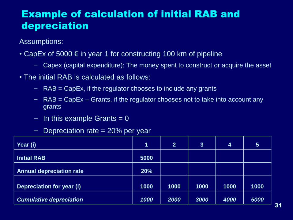
Example of calculation of initial RAB and

depreciation

Year (i) 1 2 3 4 5

Initial RAB 5000

Annual depreciation rate 20%

Depreciation for year (i) 1000 1000 1000 1000 1000

Cumulative depreciation 1000 2000 3000 4000 5000

Assumptions:

• CapEx of 5000 € in year 1 for constructing 100 km of pipeline

− Capex (capital expenditure): The money spent to construct or acquire the asset

• The initial RAB is calculated as follows:

− RAB = CapEx, if the regulator chooses to include any grants

− RAB = CapEx – Grants, if the regulator chooses not to take into account any grants

− In this example Grants = 0

− Depreciation rate = 20% per year

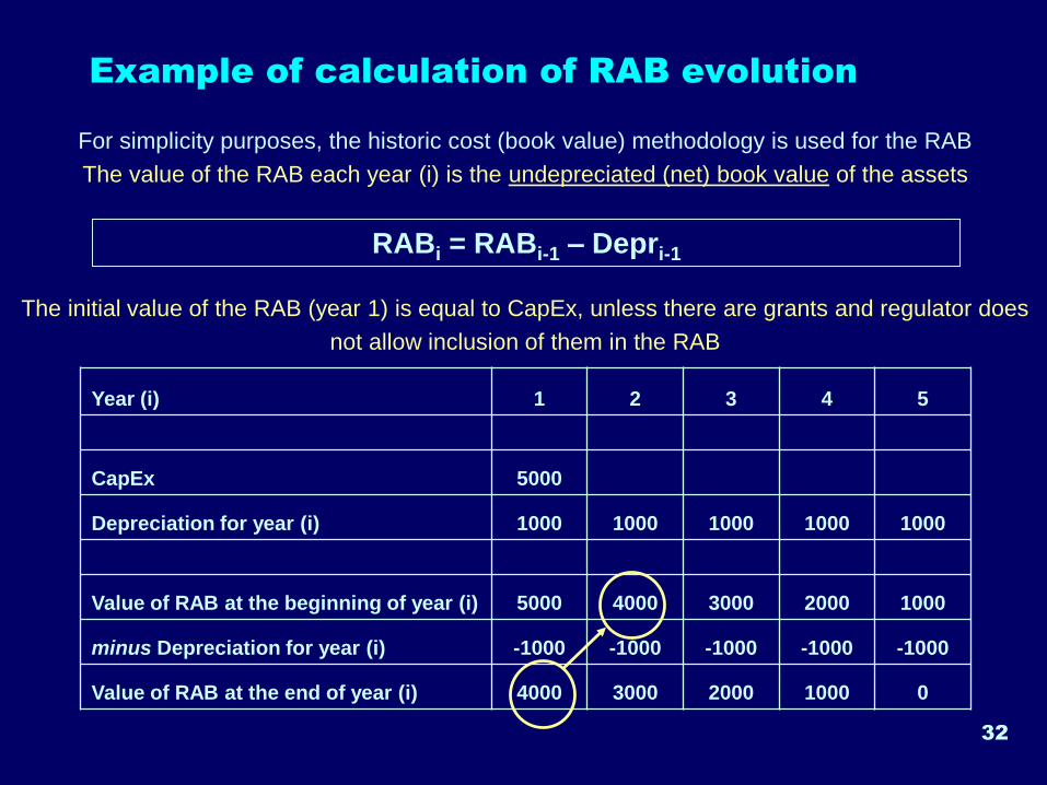
Example of calculation of RAB evolution

Year (i) 1 2 3 4 5

CapEx 5000

Depreciation for year (i) 1000 1000 1000 1000 1000

Value of RAB at the beginning of year (i) 5000 4000 3000 2000 1000

minus Depreciation for year (i) -1000 -1000 -1000 -1000 -1000

Value of RAB at the end of year (i) 4000 3000 2000 1000 0

32

RABi = RABi-1 – Depri-1

For simplicity purposes, the historic cost (book value) methodology is used for the RAB

The value of the RAB each year (i) is the undepreciated (net) book value of the assets

The initial value of the RAB (year 1) is equal to CapEx, unless there are grants and regulator does

not allow inclusion of them in the RAB

Cost of capital

• Capital for the construction of an asset (e.g. the transmission system)

is usually provided by:

1. Equity i.e. money from the owner of the pipeline/private investors

2. Debt i.e. money provided by banks or other financial institutions

3. Grants i.e. money offered by national or international organisations to

support development activities

• Cost of Capital: The opportunity cost of the capital invested i.e. the

return that one would have from the best alternative investment of

equivalent risk

• Each one of the financing sources has each own cost in providing

capital, because the level of risk for each one is different

• The cost of capital for the whole asset should take into account the

cost of capital of each financing source (equity, debt, grants)

• Grants are usually considered not to have a cost of capital33

Weighted Average Cost of Capital

34

Weighted Average Cost of Capital (WACC):

WACC =

(% equity in RAB) x Cost of capital of equity +

(% of debt in RAB) x Cost of capital of debt

35

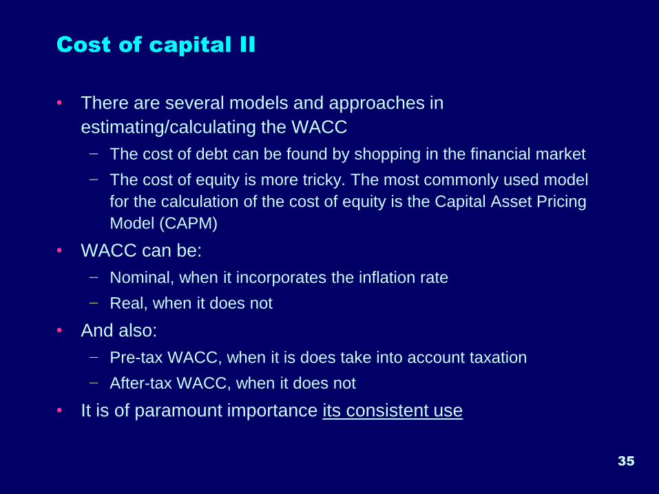
Cost of capital II

• There are several models and approaches in

estimating/calculating the WACC

− The cost of debt can be found by shopping in the financial market

− The cost of equity is more tricky. The most commonly used model

for the calculation of the cost of equity is the Capital Asset Pricing

Model (CAPM)

• WACC can be:

− Nominal, when it incorporates the inflation rate

− Real, when it does not

• And also:

− Pre-tax WACC, when it is does take into account taxation

− After-tax WACC, when it does not

• It is of paramount importance its consistent use

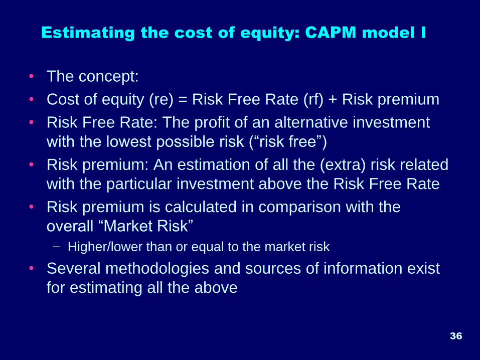
Estimating the cost of equity: CAPM model I

• The concept:

• Cost of equity (re) = Risk Free Rate (rf) + Risk premium

• Risk Free Rate: The profit of an alternative investment

with the lowest possible risk (“risk free”)

• Risk premium: An estimation of all the (extra) risk related

with the particular investment above the Risk Free Rate

• Risk premium is calculated in comparison with the

overall “Market Risk”

− Higher/lower than or equal to the market risk

• Several methodologies and sources of information exist

for estimating all the above

36

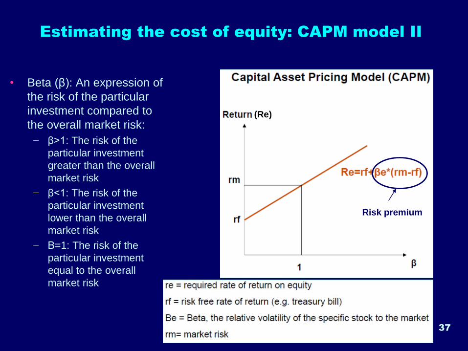
Estimating the cost of equity: CAPM model II

• Beta (β): An expression of

the risk of the particular

investment compared to

the overall market risk:

− β>1: The risk of the

particular investment

greater than the overall

market risk

− β<1: The risk of the

particular investment

lower than the overall

market risk

− Β=1: The risk of the

particular investment

equal to the overall

market risk

37

(Re)

Risk premium

38

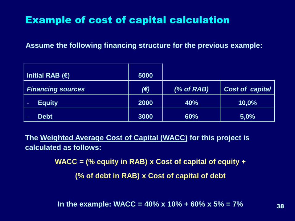
Example of cost of capital calculation

Assume the following financing structure for the previous example:

Initial RAB (€) 5000

Financing sources (€) (% of RAB) Cost of capital

- Equity 2000 40% 10,0%

- Debt 3000 60% 5,0%

The Weighted Average Cost of Capital (WACC) for this project is

calculated as follows:

WACC = (% equity in RAB) x Cost of capital of equity +

(% of debt in RAB) x Cost of capital of debt

In the example: WACC = 40% x 10% + 60% x 5% = 7%

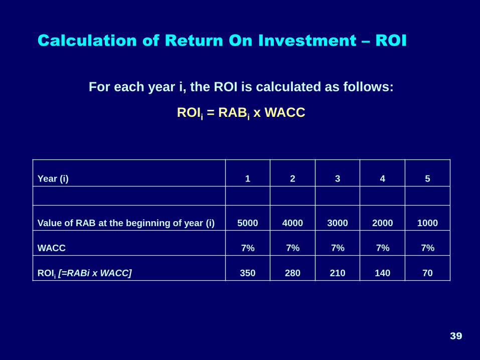
Year (i) 1 2 3 4 5

Value of RAB at the beginning of year (i) 5000 4000 3000 2000 1000

WACC 7% 7% 7% 7% 7%

ROIi [=RABi x WACC] 350 280 210 140 70

39

For each year i, the ROI is calculated as follows:

ROIi = RABi x WACC

Calculation of Return On Investment – ROI

40

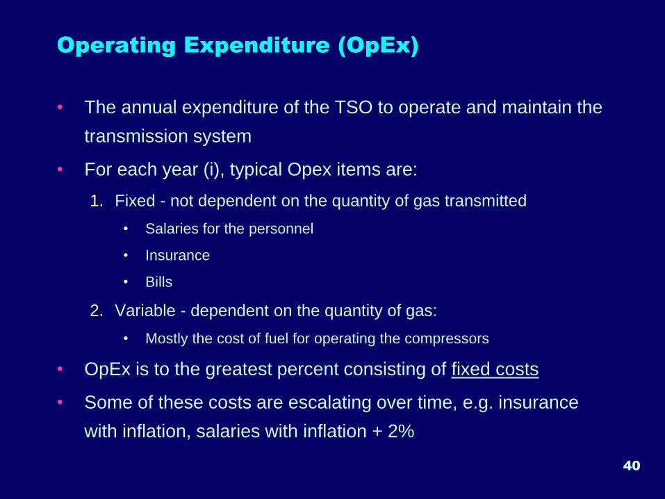
Operating Expenditure (OpEx)

• The annual expenditure of the TSO to operate and maintain the

transmission system

• For each year (i), typical Opex items are:

1. Fixed - not dependent on the quantity of gas transmitted

• Salaries for the personnel

• Insurance

• Bills

2. Variable - dependent on the quantity of gas:

• Mostly the cost of fuel for operating the compressors

• OpEx is to the greatest percent consisting of fixed costs

• Some of these costs are escalating over time, e.g. insurance

with inflation, salaries with inflation + 2%

41

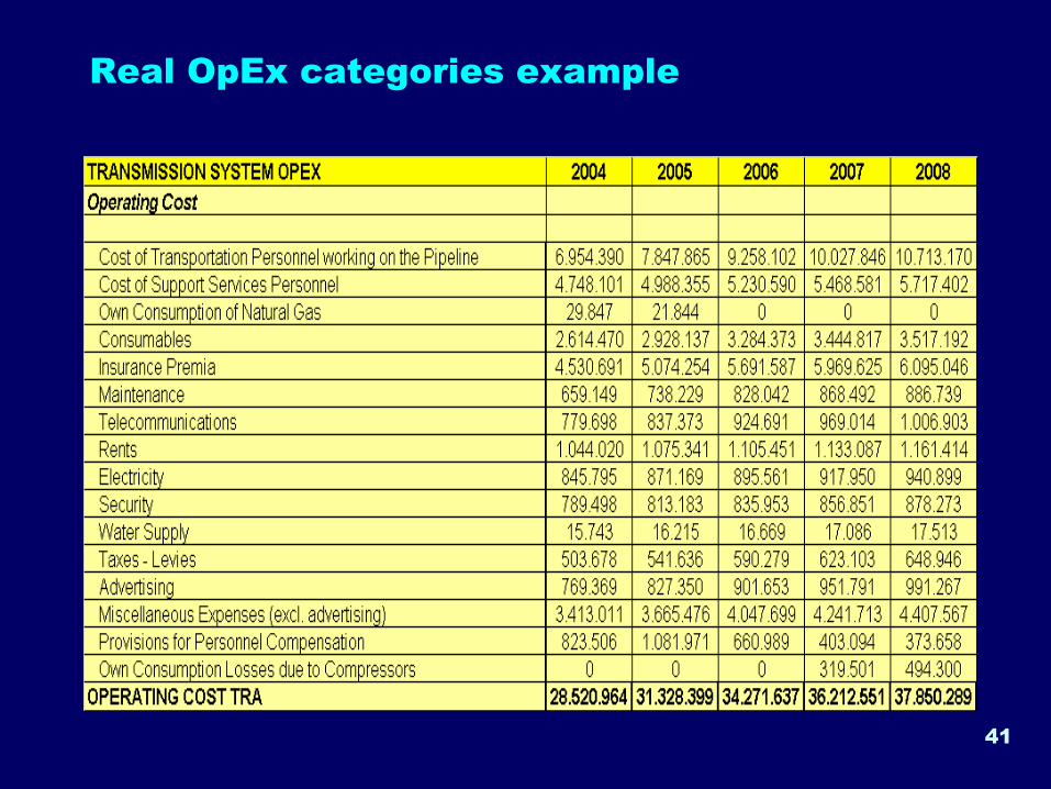
Real OpEx categories example

42

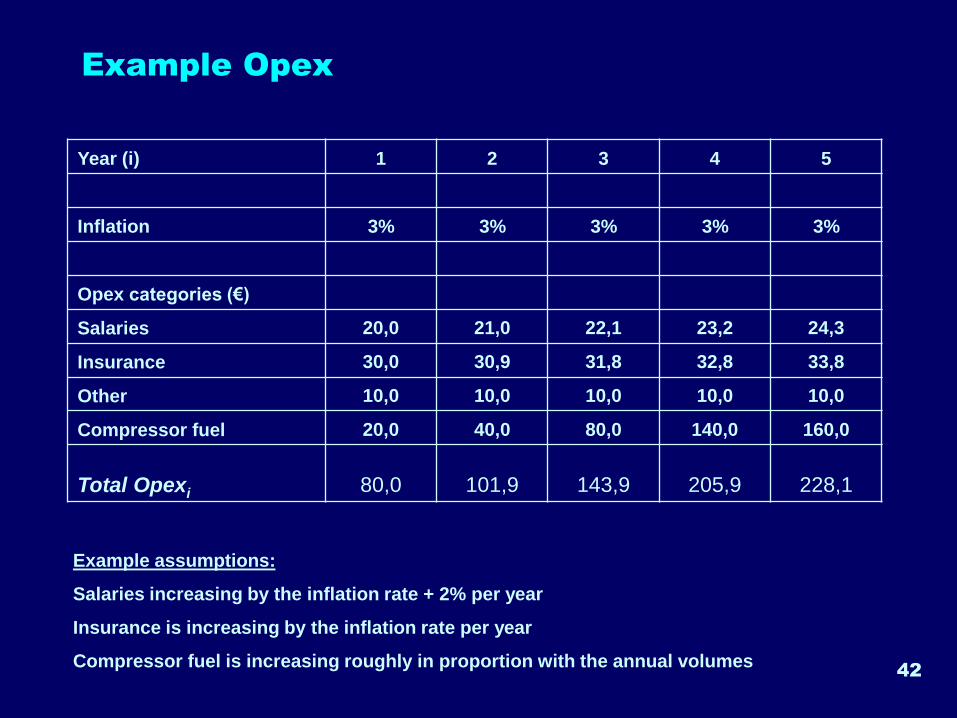
Example Opex

Year (i) 1 2 3 4 5

Inflation 3% 3% 3% 3% 3%

Opex categories (€)

Salaries 20,0 21,0 22,1 23,2 24,3

Insurance 30,0 30,9 31,8 32,8 33,8

Other 10,0 10,0 10,0 10,0 10,0

Compressor fuel 20,0 40,0 80,0 140,0 160,0

Total Opexi 80,0 101,9 143,9 205,9 228,1

Example assumptions:

Salaries increasing by the inflation rate + 2% per year

Insurance is increasing by the inflation rate per year

Compressor fuel is increasing roughly in proportion with the annual volumes

43

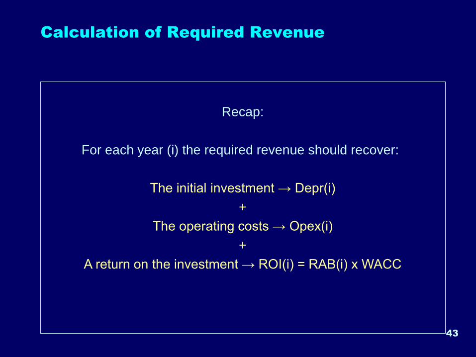
Calculation of Required Revenue

Recap:

For each year (i) the required revenue should recover:

The initial investment → Depr(i)

+

The operating costs → Opex(i)

+

A return on the investment → ROI(i) = RAB(i) x WACC

44

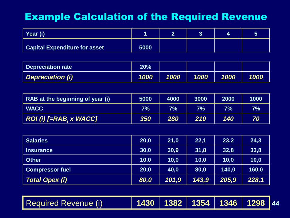
Example Calculation of the Required Revenue

Year (i) 1 2 3 4 5

Capital Expenditure for asset 5000

Depreciation rate 20%

Depreciation (i) 1000 1000 1000 1000 1000

RAB at the beginning of year (i) 5000 4000 3000 2000 1000

WACC 7% 7% 7% 7% 7%

ROI (i) [=RABi x WACC] 350 280 210 140 70

Salaries 20,0 21,0 22,1 23,2 24,3

Insurance 30,0 30,9 31,8 32,8 33,8

Other 10,0 10,0 10,0 10,0 10,0

Compressor fuel 20,0 40,0 80,0 140,0 160,0

Total Opex (i) 80,0 101,9 143,9 205,9 228,1

Required Revenue (i) 1430 1382 1354 1346 1298

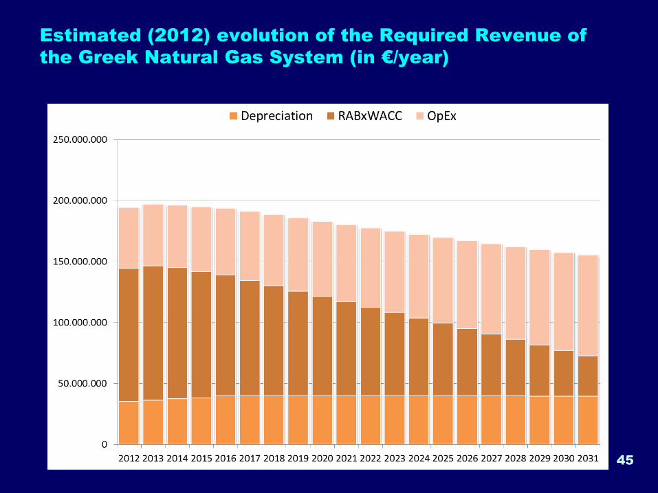
Estimated (2012) evolution of the Required Revenue of

the Greek Natural Gas System (in €/year)

45

Calculation of the unit tariff

47

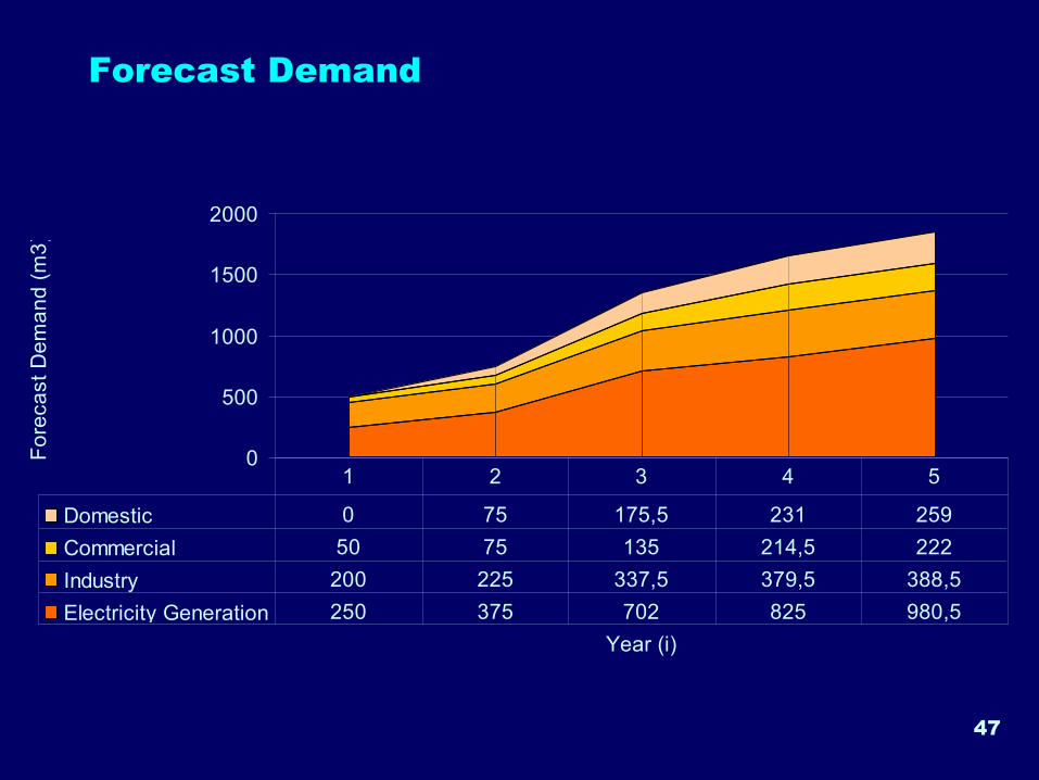
Forecast Demand

0

500

1000

1500

2000

Year (i)

Fo

reca

st

De

ma

nd

(m

3)

Domestic 0 75 175,5 231 259

Commercial 50 75 135 214,5 222

Industry 200 225 337,5 379,5 388,5

Electricity Generation 250 375 702 825 980,5

1 2 3 4 5

48

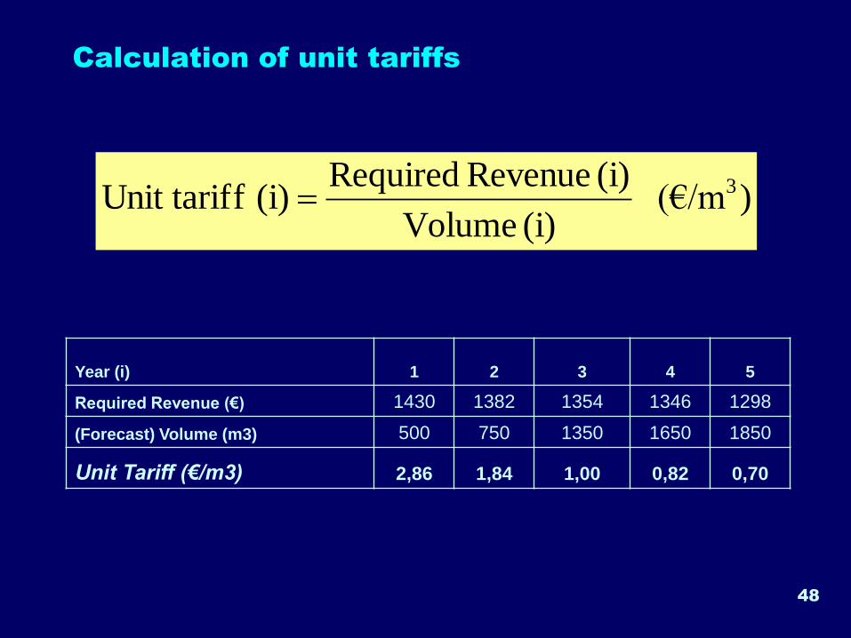
Calculation of unit tariffs

)(€/m (i) Volume

(i) Revenue Required(i) fUnit tarif 3=

Year (i) 1 2 3 4 5

Required Revenue (€) 1430 1382 1354 1346 1298

(Forecast) Volume (m3) 500 750 1350 1650 1850

Unit Tariff (€/m3) 2,86 1,84 1,00 0,82 0,70

49

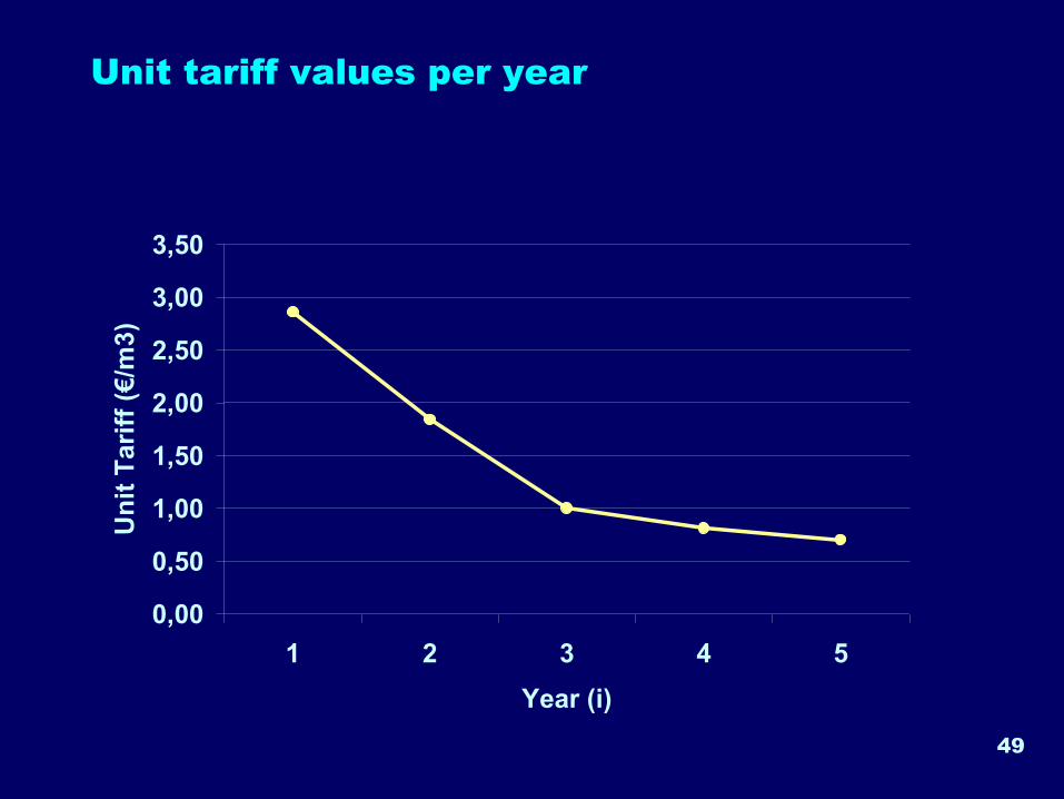
Unit tariff values per year

0,00

0,50

1,00

1,50

2,00

2,50

3,00

3,50

1 2 3 4 5

Year (i)

Un

it T

ari

ff (

€/m

3)

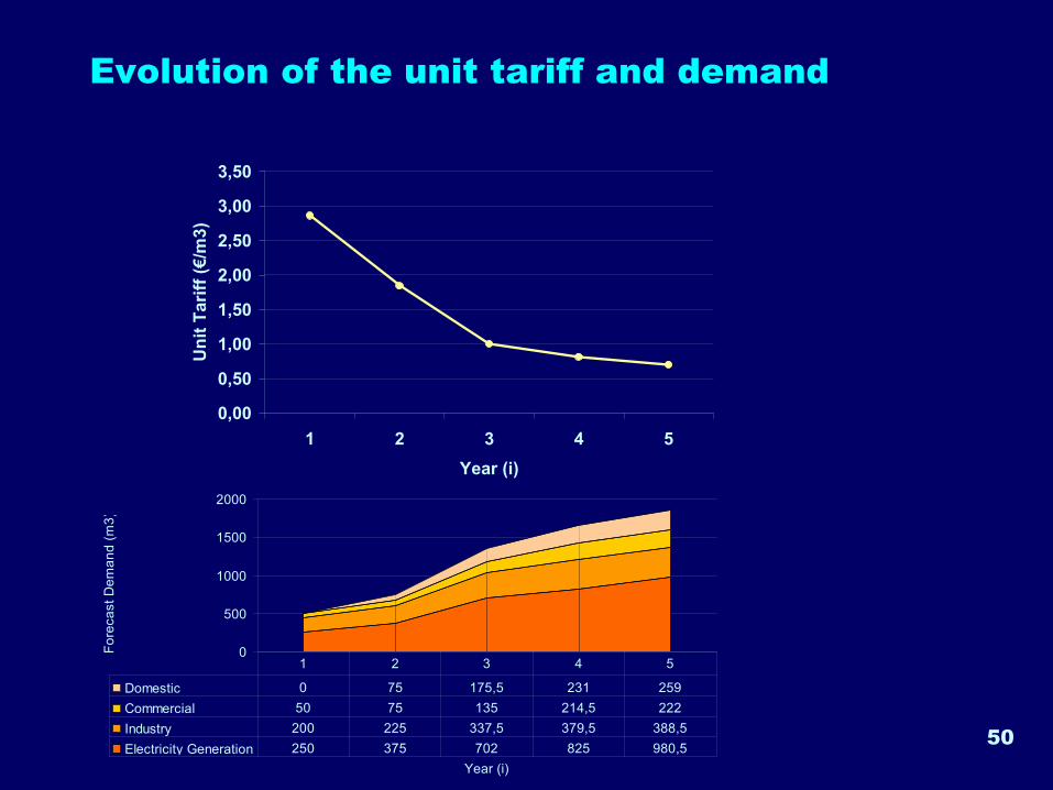
Evolution of the unit tariff and demand

0,00

0,50

1,00

1,50

2,00

2,50

3,00

3,50

1 2 3 4 5

Year (i)

Un

it T

ari

ff (

€/m

3)

50

0

500

1000

1500

2000

Year (i)

Fo

reca

st

De

ma

nd

(m

3)

Domestic 0 75 175,5 231 259

Commercial 50 75 135 214,5 222

Industry 200 225 337,5 379,5 388,5

Electricity Generation 250 375 702 825 980,5

1 2 3 4 5

51

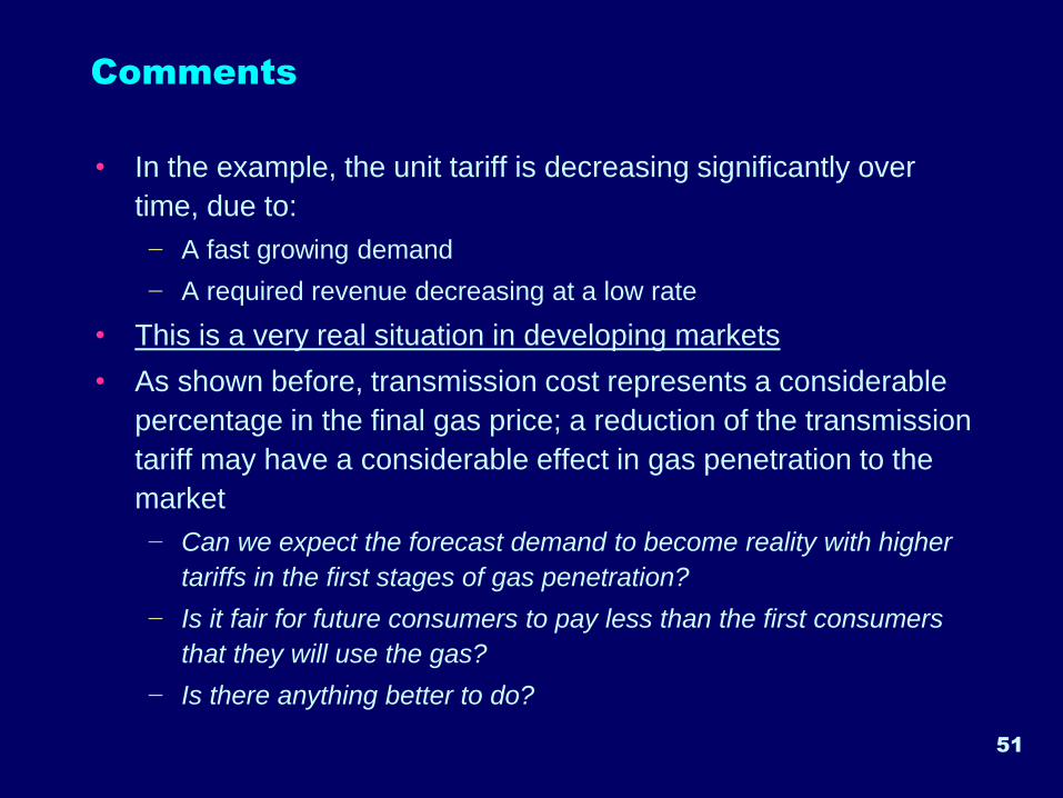
Comments

• In the example, the unit tariff is decreasing significantly over

time, due to:

− A fast growing demand

− A required revenue decreasing at a low rate

• This is a very real situation in developing markets

• As shown before, transmission cost represents a considerable

percentage in the final gas price; a reduction of the transmission

tariff may have a considerable effect in gas penetration to the

market

− Can we expect the forecast demand to become reality with higher

tariffs in the first stages of gas penetration?

− Is it fair for future consumers to pay less than the first consumers

that they will use the gas?

− Is there anything better to do?

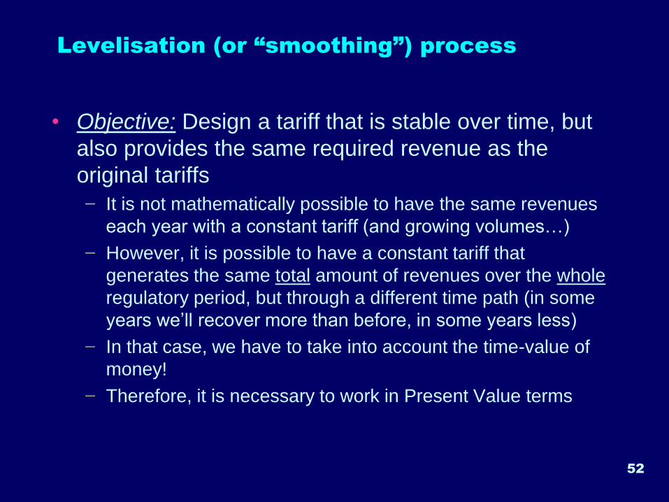
Levelisation (or “smoothing”) process

• Objective: Design a tariff that is stable over time, but

also provides the same required revenue as the

original tariffs

− It is not mathematically possible to have the same revenues

each year with a constant tariff (and growing volumes…)

− However, it is possible to have a constant tariff that

generates the same total amount of revenues over the whole

regulatory period, but through a different time path (in some

years we’ll recover more than before, in some years less)

− In that case, we have to take into account the time-value of

money!

− Therefore, it is necessary to work in Present Value terms

52

53

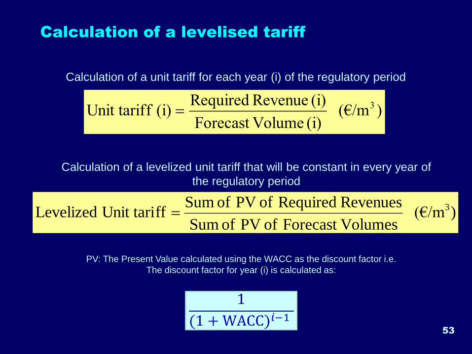
Calculation of a levelised tariff

)(€/m (i) VolumeForecast

(i) Revenue Required(i) fUnit tarif 3=

)(€/m Volumes Forecast of PVof Sum

Revenues Requiredof PVof Sum ff Unit tariLevelized 3=

Calculation of a unit tariff for each year (i) of the regulatory period

Calculation of a levelized unit tariff that will be constant in every year of

the regulatory period

PV: The Present Value calculated using the WACC as the discount factor i.e.

The discount factor for year (i) is calculated as:

54

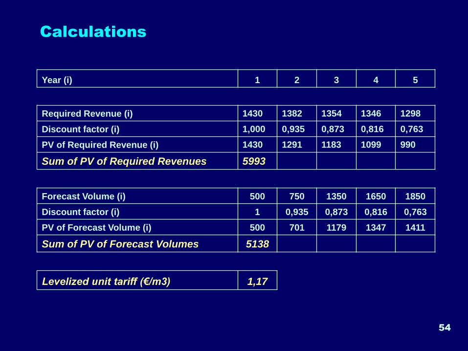
Calculations

Year (i) 1 2 3 4 5

Required Revenue (i) 1430 1382 1354 1346 1298

Discount factor (i) 1,000 0,935 0,873 0,816 0,763

PV of Required Revenue (i) 1430 1291 1183 1099 990

Sum of PV of Required Revenues 5993

Forecast Volume (i) 500 750 1350 1650 1850

Discount factor (i) 1 0,935 0,873 0,816 0,763

PV of Forecast Volume (i) 500 701 1179 1347 1411

Sum of PV of Forecast Volumes 5138

Levelized unit tariff (€/m3) 1,17

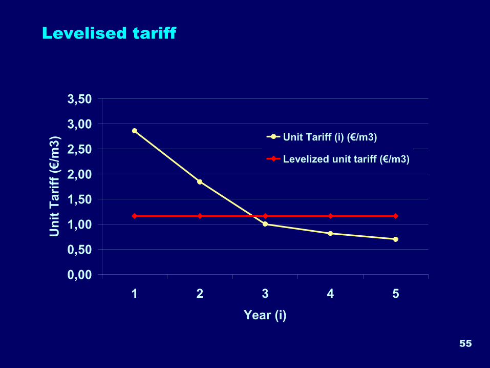
55

Levelised tariff

0,00

0,50

1,00

1,50

2,00

2,50

3,00

3,50

1 2 3 4 5

Year (i)

Un

it T

ari

ff (

€/m

3) Unit Tariff (i) (€/m3)

Levelized unit tariff (€/m3)

56

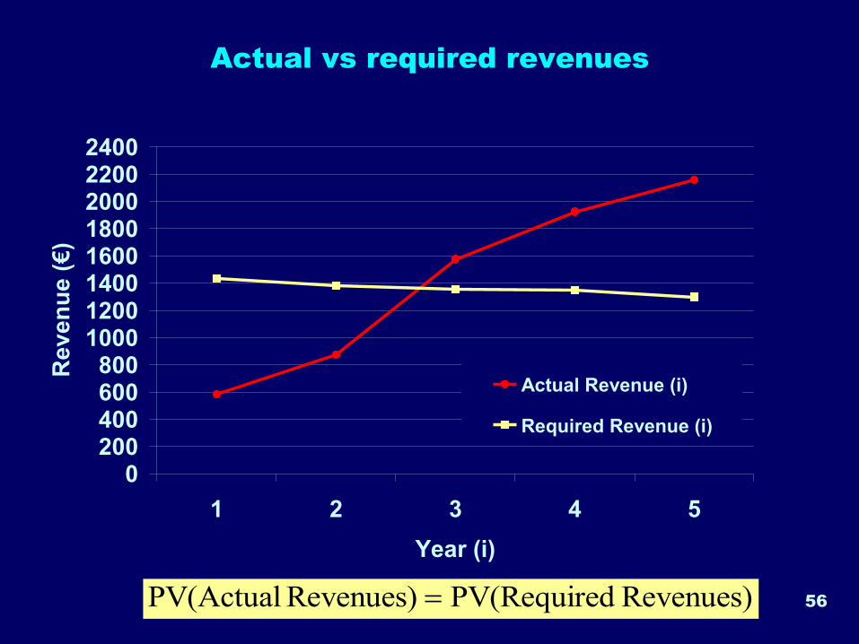
Actual vs required revenues

)Revenues dPV(RequireRevenues) PV(Actual =

0200400600800

10001200140016001800200022002400

1 2 3 4 5

Year (i)

Re

ve

nu

e (

€)

Actual Revenue (i)

Required Revenue (i)

57

Actual Revenue (i)

0

400

800

1200

1600

2000

2400

1 2 3 4 5

Year (i)

Reven

ue (

€)

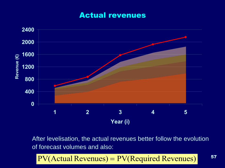
Actual revenues

After levelisation, the actual revenues better follow the evolution

of forecast volumes and also:

)Revenues dPV(RequireRevenues) PV(Actual =

Models of regulation of the TSO’s

Required Revenue

Overview

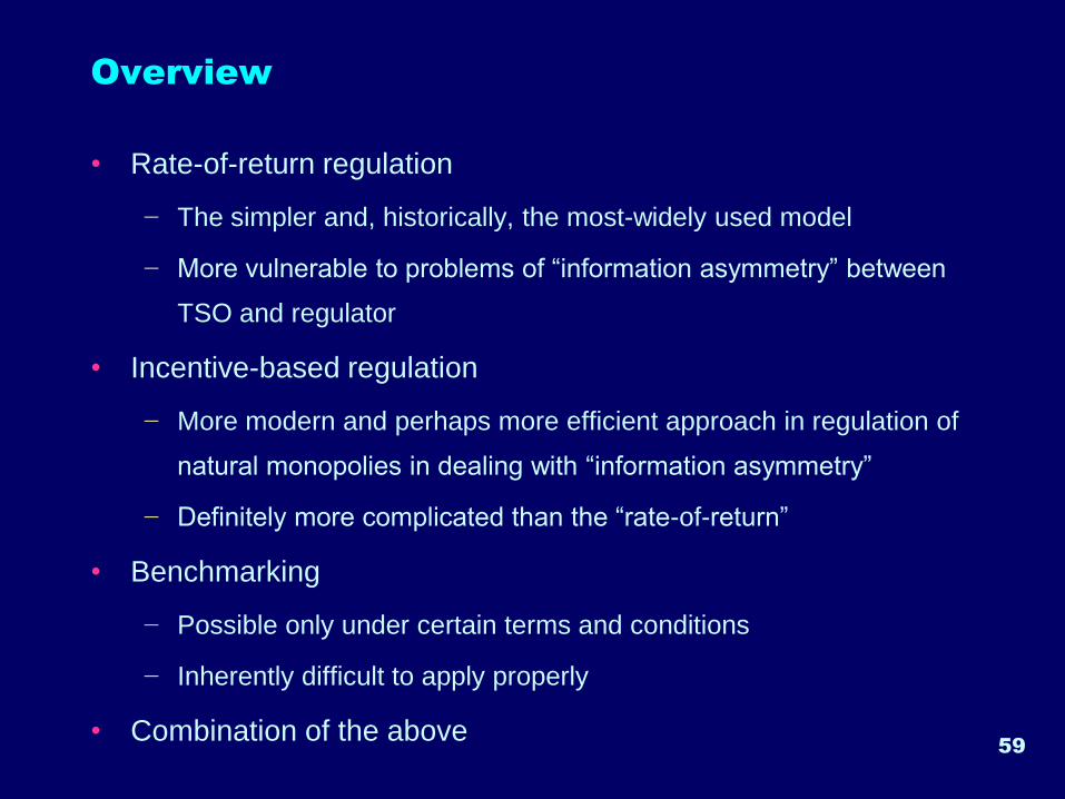
• Rate-of-return regulation

− The simpler and, historically, the most-widely used model

− More vulnerable to problems of “information asymmetry” between

TSO and regulator

• Incentive-based regulation

− More modern and perhaps more efficient approach in regulation of

natural monopolies in dealing with “information asymmetry”

− Definitely more complicated than the “rate-of-return”

• Benchmarking

− Possible only under certain terms and conditions

− Inherently difficult to apply properly

• Combination of the above59

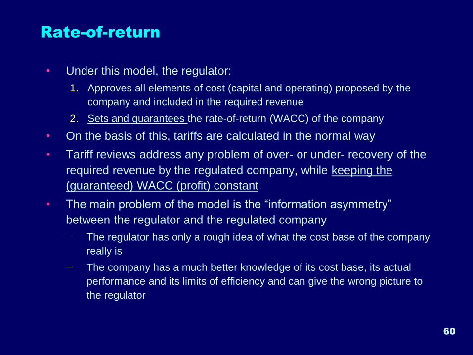
Rate-of-return

• Under this model, the regulator:

1. Approves all elements of cost (capital and operating) proposed by the

company and included in the required revenue

2. Sets and guarantees the rate-of-return (WACC) of the company

• On the basis of this, tariffs are calculated in the normal way

• Tariff reviews address any problem of over- or under- recovery of the

required revenue by the regulated company, while keeping the

(guaranteed) WACC (profit) constant

• The main problem of the model is the “information asymmetry”

between the regulator and the regulated company

− The regulator has only a rough idea of what the cost base of the company

really is

− The company has a much better knowledge of its cost base, its actual

performance and its limits of efficiency and can give the wrong picture to

the regulator

60

61

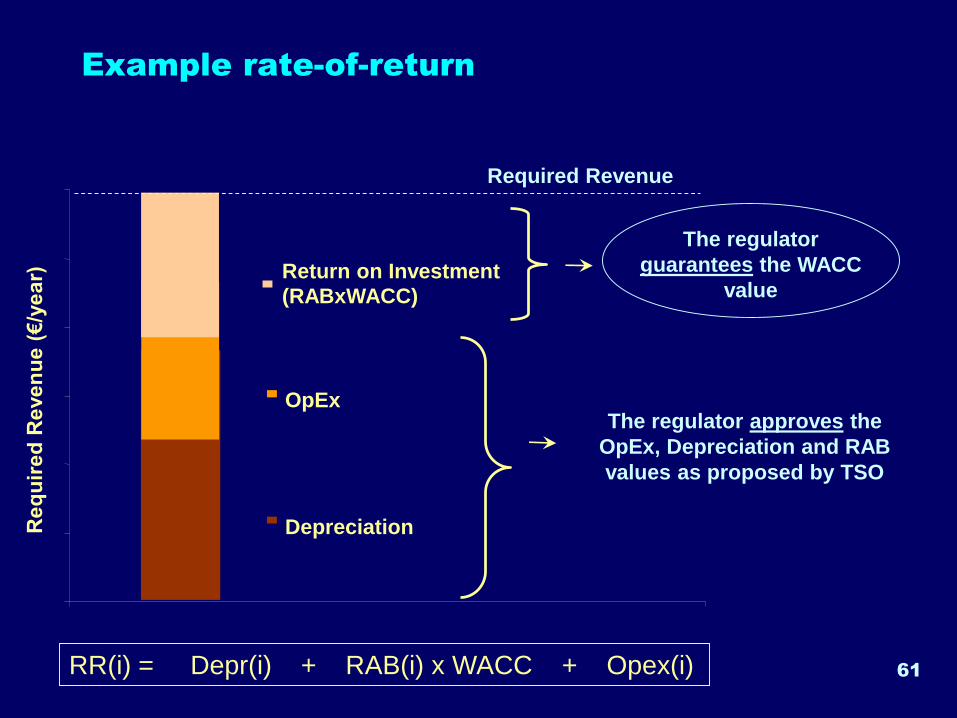
Example rate-of-returnR

eq

uir

ed

Reven

ue (

€/y

ear) Return on Investment

(RABxWACC)

OpEx

Depreciation

Required Revenue

The regulator approves the

OpEx, Depreciation and RAB

values as proposed by TSO

The regulator

guarantees the WACC

value

RR(i) = Depr(i) + RAB(i) x WACC + Opex(i)

62

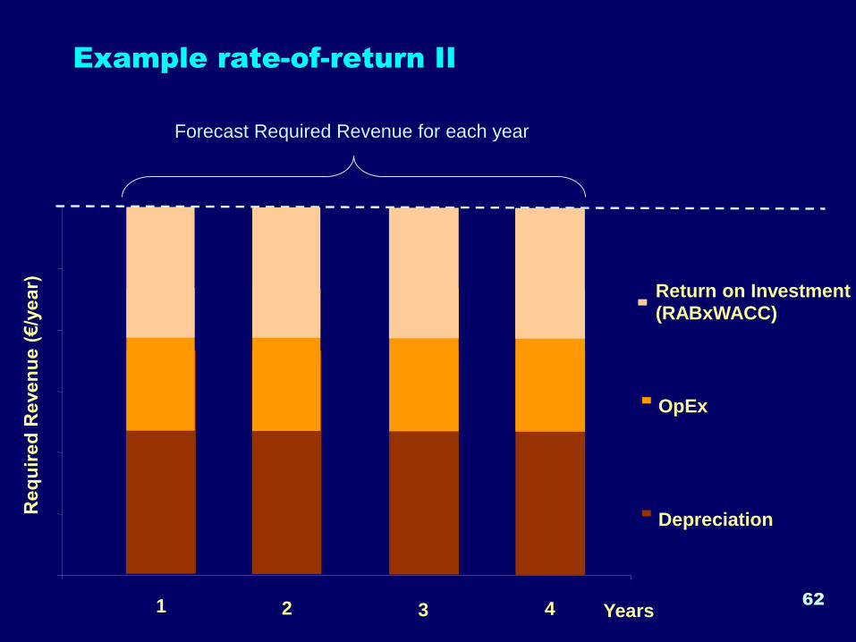
Example rate-of-return IIR

eq

uir

ed

Reven

ue (

€/y

ear) Return on Investment

(RABxWACC)

OpEx

Depreciation

Years1 432

Forecast Required Revenue for each year

63

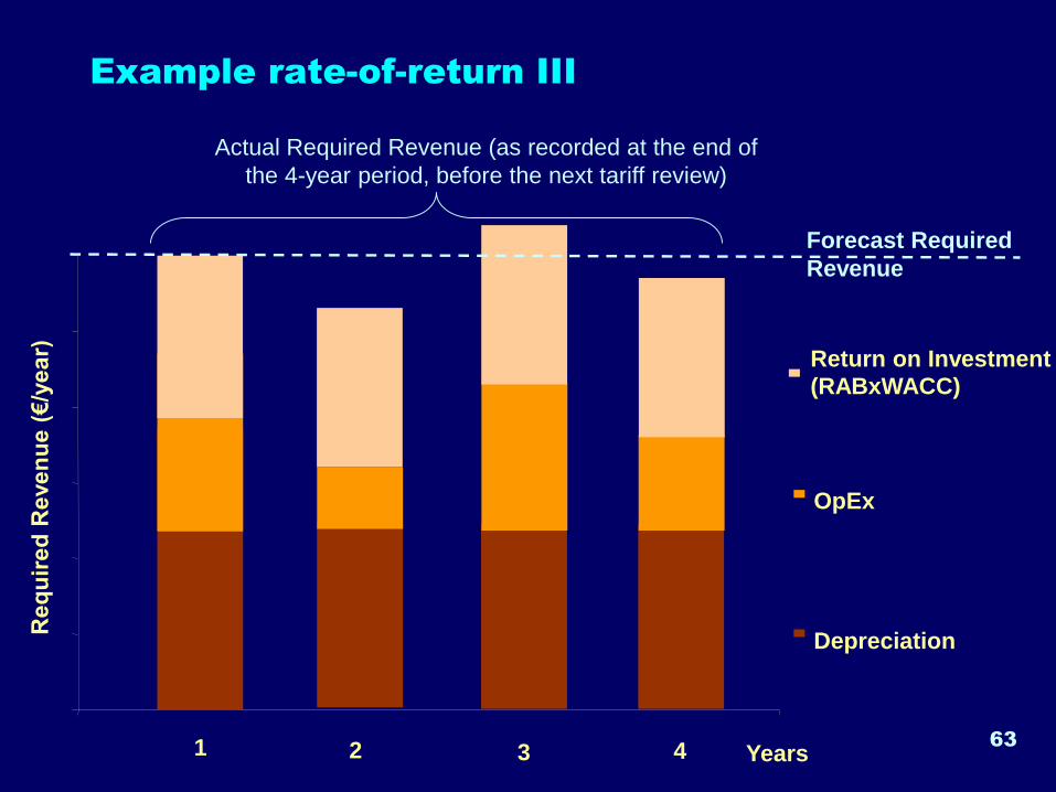
Example rate-of-return IIIR

eq

uir

ed

Reven

ue (

€/y

ear) Return on Investment

(RABxWACC)

OpEx

Depreciation

Years1 432

Forecast Required

Revenue

Actual Required Revenue (as recorded at the end of

the 4-year period, before the next tariff review)

64

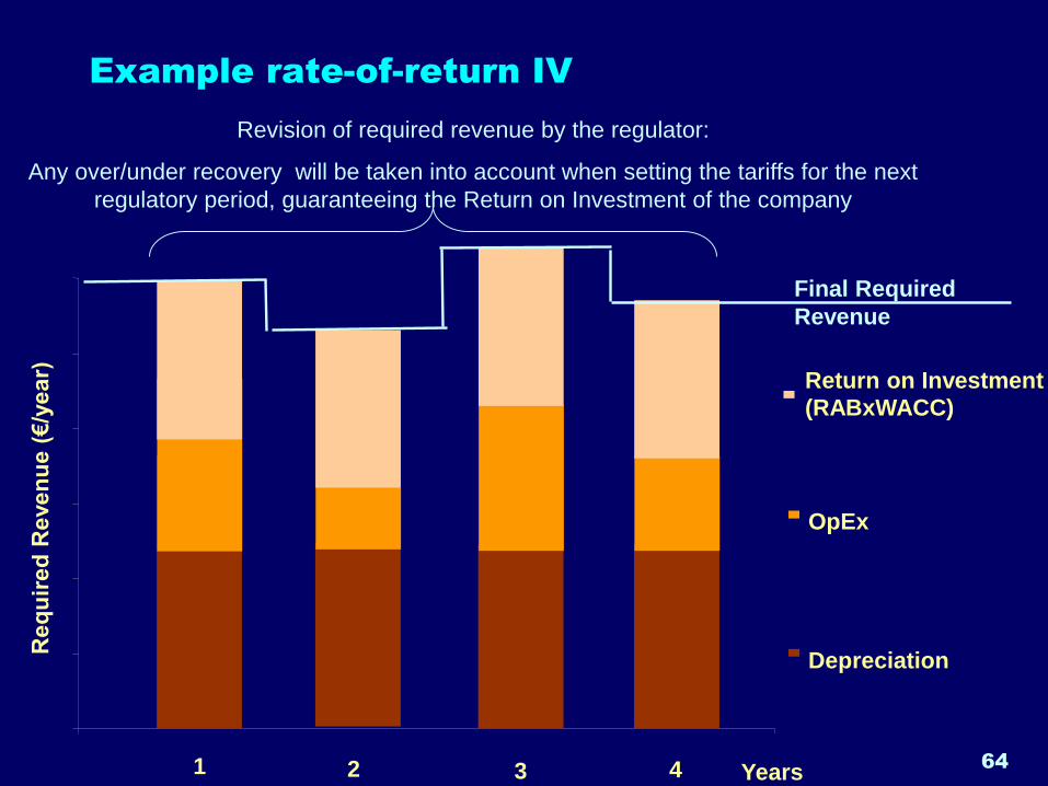
Example rate-of-return IVR

eq

uir

ed

Re

ve

nu

e (

€/y

ea

r) Return on Investment

(RABxWACC)

OpEx

Depreciation

Final Required

Revenue

Years1 432

Revision of required revenue by the regulator:

Any over/under recovery will be taken into account when setting the tariffs for the next

regulatory period, guaranteeing the Return on Investment of the company

65

Rate-of-return II

• The consequences of this information asymmetry are:

1. The TSO tends to “over-invest”: Since the revenue of the TSO

depends heavily on the RAB x WACC factor, and the WACC is set by

the regulator, the TSO tends to increase the RAB by:

− Investing in new infrastructure that may not be necessary at all or may be

not necessary yet

− Increasing the cost of the new infrastructure (e.g. by putting unnecessarily

strict safety rules or “custom” specifications)

2. The TSO has no incentive to reduce operating costs

• If the regulator cannot control this costs the TSO has no reason to put

effort in reducing its operating costs, because it will be compensated for

them anyway

3. There are high costs of monitoring the performance of the TSO

• The regulator, in order to estimate accurately the cost base of the TSO is

trying to “simulate” the way the TSO is run

• This has a cost in the resources used by the regulator (personnel etc)

66

Incentive based regulation I

• Incentive (or performance) based regulation is trying to address the

“information asymmetry” problem by incentivising directly the regulated

company to be more efficient

• The most common schemes work like this:

− The regulator sets for the each year of the “regulatory period” the maximum

prices that the company may be allowed to charge (price-cap regulation) or the

maximum revenue that the company is allowed to recover (revenue cap

regulation) for this period (Allowed Revenue)

− It then allows the company to set the actual tariffs as it wishes

− At the end of the period, there is a tariff review to examine the performance of

the company

− If during this period the company manages to be more efficient (has less actual

costs than forecasted) the company retains (whole or part of) the gains

− If the company did not manage to be efficient it will be responsible for the

losses

67

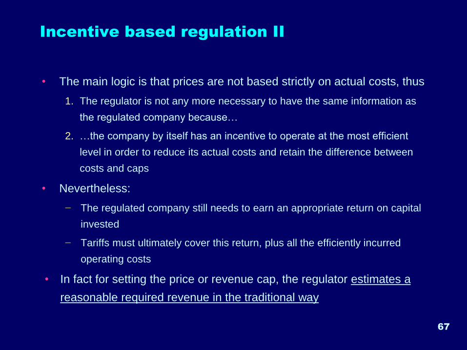
Incentive based regulation II

• The main logic is that prices are not based strictly on actual costs, thus

1. The regulator is not any more necessary to have the same information as

the regulated company because…

2. …the company by itself has an incentive to operate at the most efficient

level in order to reduce its actual costs and retain the difference between

costs and caps

• Nevertheless:

− The regulated company still needs to earn an appropriate return on capital

invested

− Tariffs must ultimately cover this return, plus all the efficiently incurred

operating costs

• In fact for setting the price or revenue cap, the regulator estimates a

reasonable required revenue in the traditional way

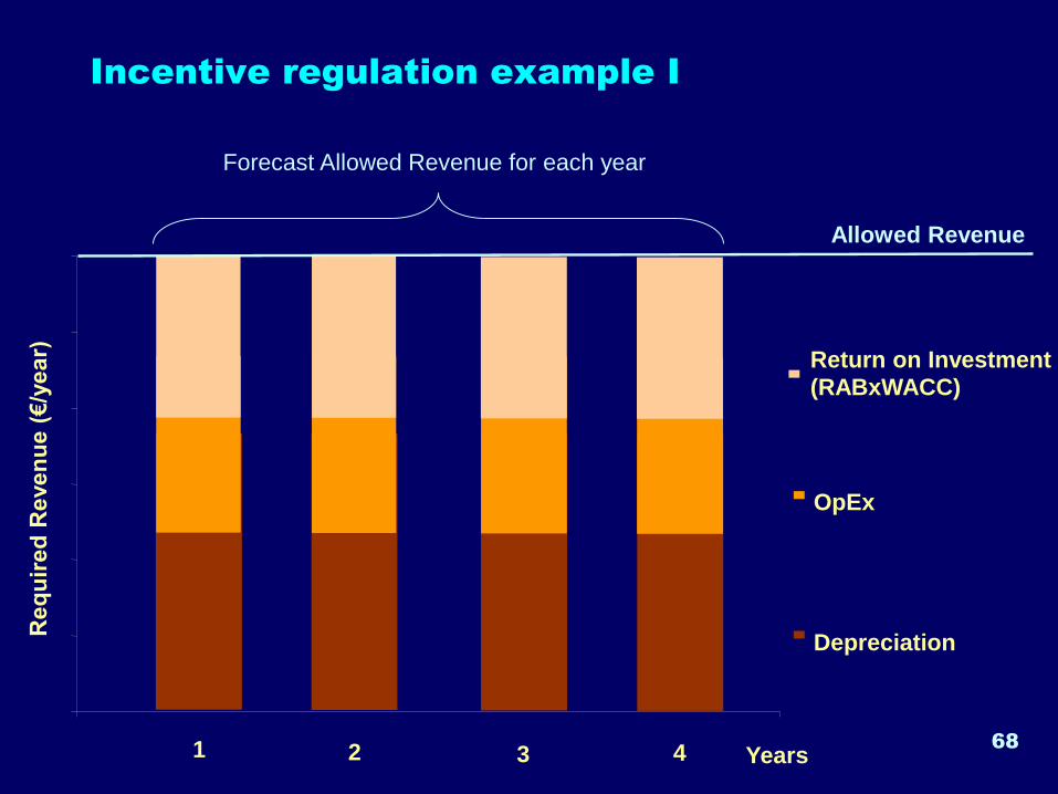
Incentive regulation example I

68

Req

uir

ed

Reven

ue (

€/y

ear) Return on Investment

(RABxWACC)

OpEx

Depreciation

Years1 432

Allowed Revenue

Forecast Allowed Revenue for each year

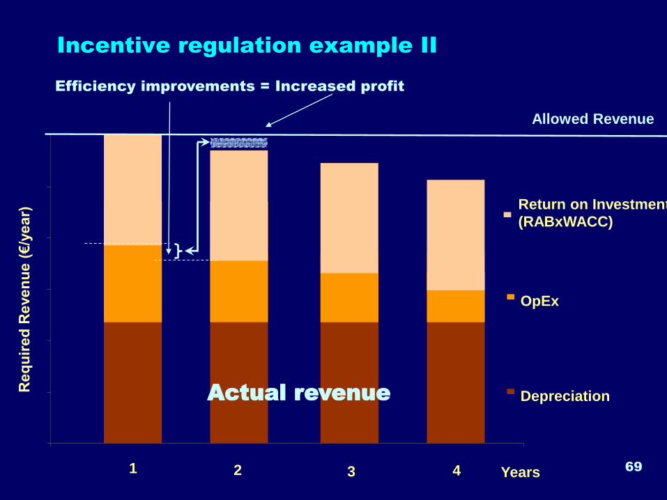
Incentive regulation example II

69

Efficiency improvements = Increased profit

Req

uir

ed

Reven

ue (

€/y

ear)

Return on Investment

(RABxWACC)

OpEx

Depreciation

Years1 432

Allowed Revenue

Actual revenue

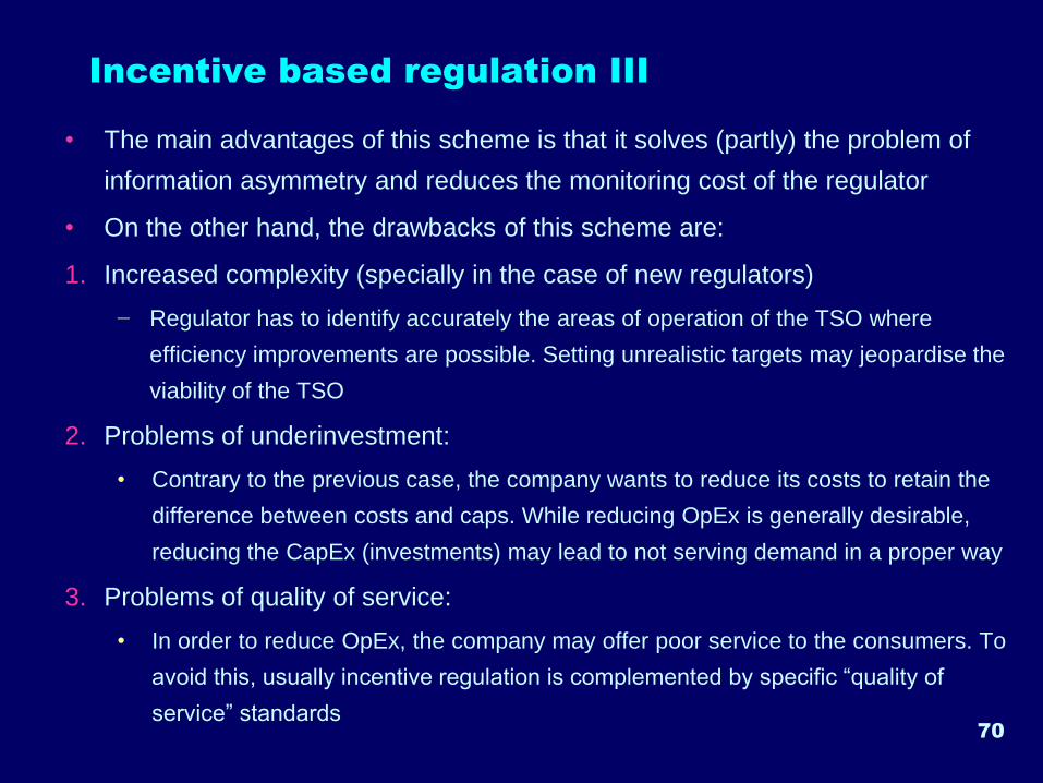
Incentive based regulation III

• The main advantages of this scheme is that it solves (partly) the problem of

information asymmetry and reduces the monitoring cost of the regulator

• On the other hand, the drawbacks of this scheme are:

1. Increased complexity (specially in the case of new regulators)

− Regulator has to identify accurately the areas of operation of the TSO where

efficiency improvements are possible. Setting unrealistic targets may jeopardise the

viability of the TSO

2. Problems of underinvestment:

• Contrary to the previous case, the company wants to reduce its costs to retain the

difference between costs and caps. While reducing OpEx is generally desirable,

reducing the CapEx (investments) may lead to not serving demand in a proper way

3. Problems of quality of service:

• In order to reduce OpEx, the company may offer poor service to the consumers. To

avoid this, usually incentive regulation is complemented by specific “quality of

service” standards70

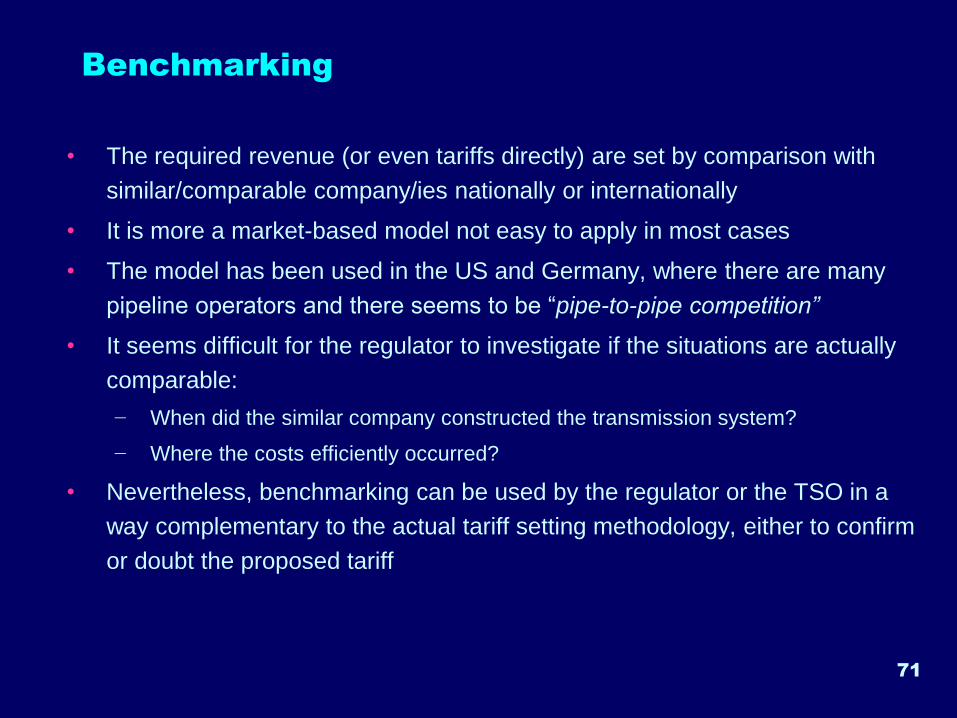
Benchmarking

• The required revenue (or even tariffs directly) are set by comparison with

similar/comparable company/ies nationally or internationally

• It is more a market-based model not easy to apply in most cases

• The model has been used in the US and Germany, where there are many

pipeline operators and there seems to be “pipe-to-pipe competition”

• It seems difficult for the regulator to investigate if the situations are actually

comparable:

− When did the similar company constructed the transmission system?

− Where the costs efficiently occurred?

• Nevertheless, benchmarking can be used by the regulator or the TSO in a

way complementary to the actual tariff setting methodology, either to confirm

or doubt the proposed tariff

71

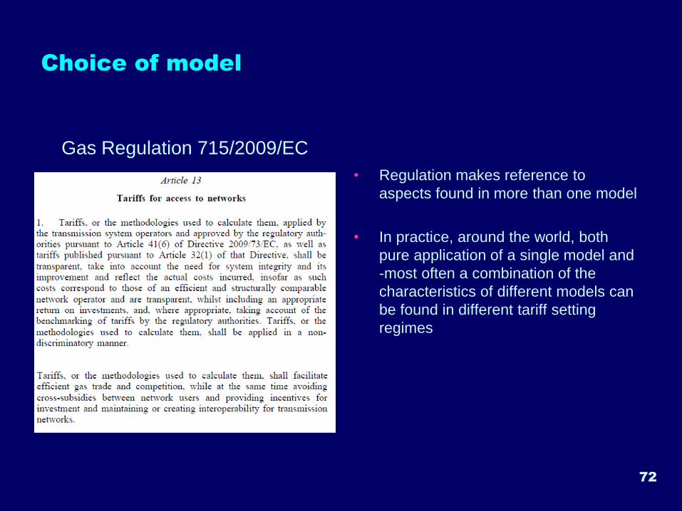
Choice of model

Gas Regulation 715/2009/EC

• Regulation makes reference to

aspects found in more than one model

• In practice, around the world, both

pure application of a single model and

-most often a combination of the

characteristics of different models can

be found in different tariff setting

regimes

72

Cost-allocation to users

74

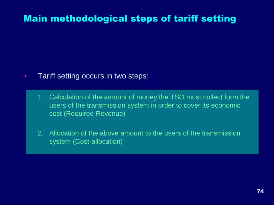
Main methodological steps of tariff setting

• Tariff setting occurs in two steps:

1. Calculation of the amount of money the TSO must collect form the

users of the transmission system in order to cover its economic

cost (Required Revenue)

2. Allocation of the above amount to the users of the transmission

system (Cost-allocation)

75

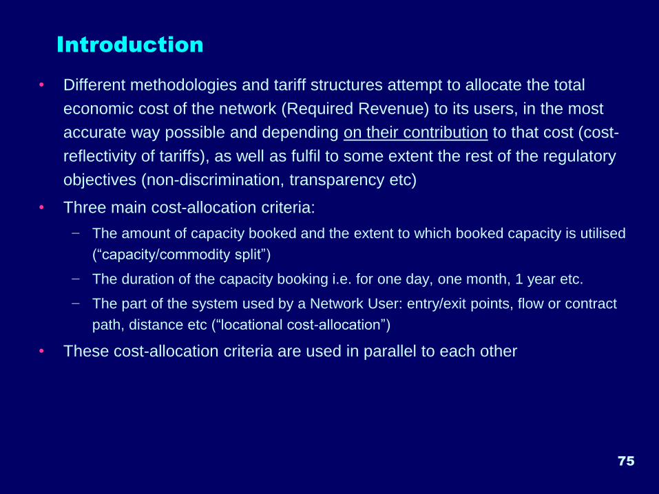
Introduction

• Different methodologies and tariff structures attempt to allocate the total

economic cost of the network (Required Revenue) to its users, in the most

accurate way possible and depending on their contribution to that cost (cost-

reflectivity of tariffs), as well as fulfil to some extent the rest of the regulatory

objectives (non-discrimination, transparency etc)

• Three main cost-allocation criteria:

− The amount of capacity booked and the extent to which booked capacity is utilised

(“capacity/commodity split”)

− The duration of the capacity booking i.e. for one day, one month, 1 year etc.

− The part of the system used by a Network User: entry/exit points, flow or contract

path, distance etc (“locational cost-allocation”)

• These cost-allocation criteria are used in parallel to each other

76

Capacity/commodity split(two-part tariffs)

77

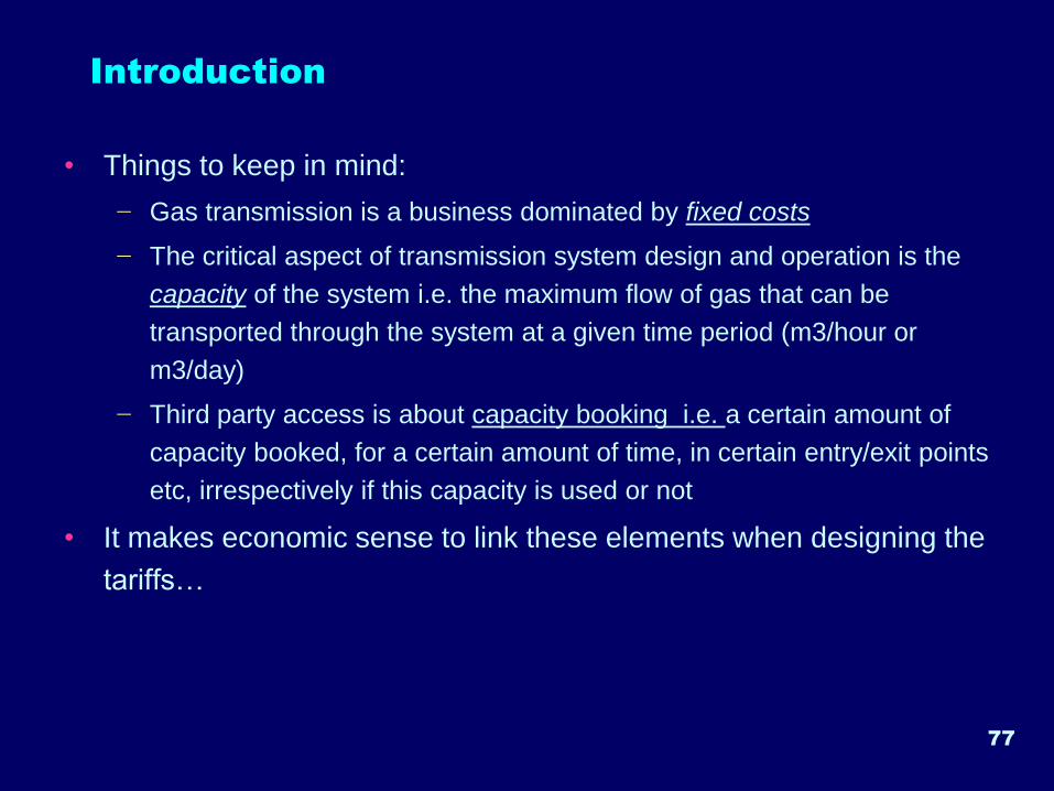
Introduction

• Things to keep in mind:

− Gas transmission is a business dominated by fixed costs

− The critical aspect of transmission system design and operation is the

capacity of the system i.e. the maximum flow of gas that can be

transported through the system at a given time period (m3/hour or

m3/day)

− Third party access is about capacity booking i.e. a certain amount of

capacity booked, for a certain amount of time, in certain entry/exit points

etc, irrespectively if this capacity is used or not

• It makes economic sense to link these elements when designing the

tariffs…

78

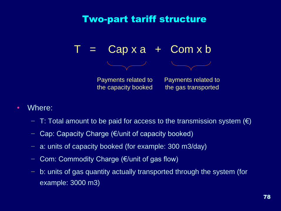
Two-part tariff structure

T = Cap x a + Com x b

• Where:

− T: Total amount to be paid for access to the transmission system (€)

− Cap: Capacity Charge (€/unit of capacity booked)

− a: units of capacity booked (for example: 300 m3/day)

− Com: Commodity Charge (€/unit of gas flow)

− b: units of gas quantity actually transported through the system (for

example: 3000 m3)

Payments related to

the capacity booked

Payments related to

the gas transported

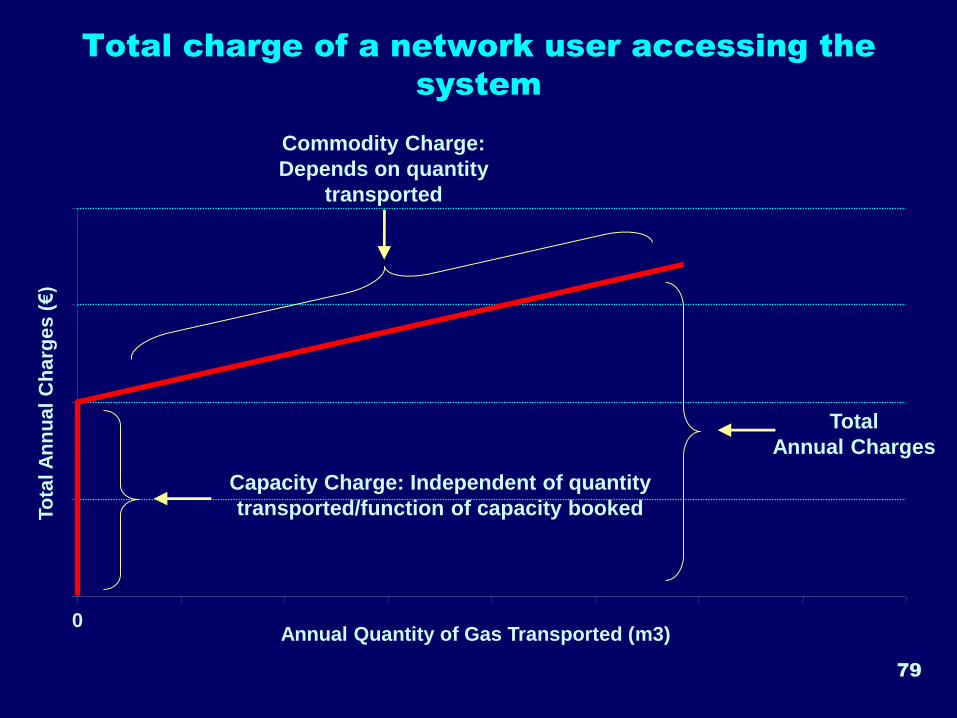
79

Total charge of a network user accessing the

system

Annual Quantity of Gas Transported (m3)

To

tal A

nn

ua

l C

ha

rge

s (

€)

0

Total

Annual Charges

Capacity Charge: Independent of quantity

transported/function of capacity booked

Commodity Charge:

Depends on quantity

transported

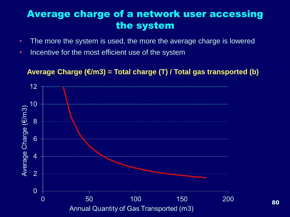
80

• The more the system is used, the more the average charge is lowered

• Incentive for the most efficient use of the system

Average charge of a network user accessing

the system

Average Charge (€/m3) = Total charge (T) / Total gas transported (b)

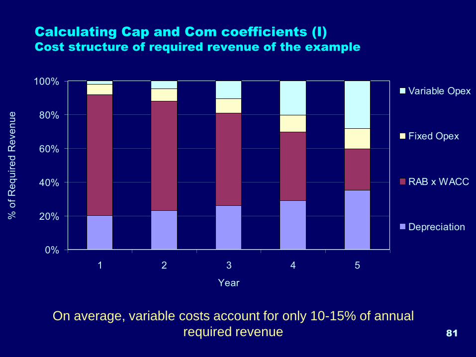
81

Calculating Cap and Com coefficients (I) Cost structure of required revenue of the example

0%

20%

40%

60%

80%

100%

1 2 3 4 5

Year

% o

f R

eq

uir

ed

Re

ve

nu

e

Variable Opex

Fixed Opex

RAB x WACC

Depreciation

On average, variable costs account for only 10-15% of annual

required revenue

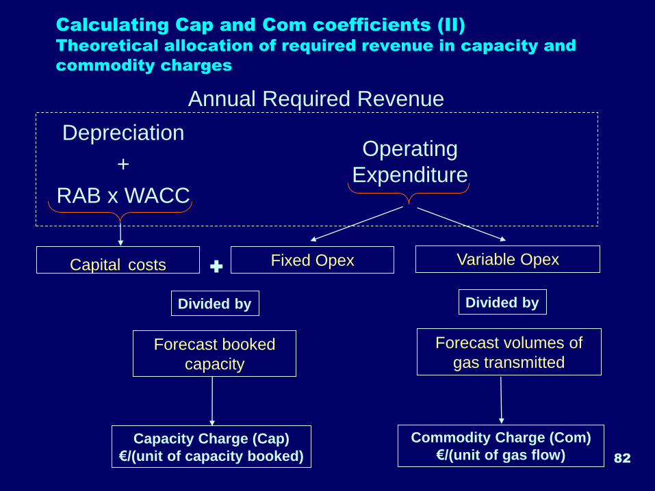
82

Calculating Cap and Com coefficients (II) Theoretical allocation of required revenue in capacity and

commodity charges

Annual Required Revenue

Variable Opex

Forecast volumes of

gas transmitted

Divided by

Commodity Charge (Com)

€/(unit of gas flow)

Fixed OpexCapital costs +

Divided by

Forecast booked

capacity

Capacity Charge (Cap)

€/(unit of capacity booked)

Operating

Expenditure

Depreciation

+

RAB x WACC

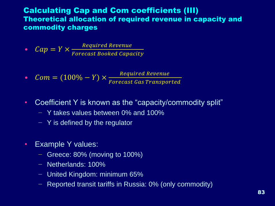
Calculating Cap and Com coefficients (III) Theoretical allocation of required revenue in capacity and

commodity charges

• 𝐶𝑎𝑝 = 𝑌 ×𝑅𝑒𝑞𝑢𝑖𝑟𝑒𝑑 𝑅𝑒𝑣𝑒𝑛𝑢𝑒

𝐹𝑜𝑟𝑒𝑐𝑎𝑠𝑡 𝐵𝑜𝑜𝑘𝑒𝑑 𝐶𝑎𝑝𝑎𝑐𝑖𝑡𝑦

• 𝐶𝑜𝑚 = (100% − 𝑌) ×𝑅𝑒𝑞𝑢𝑖𝑟𝑒𝑑 𝑅𝑒𝑣𝑒𝑛𝑢𝑒

𝐹𝑜𝑟𝑒𝑐𝑎𝑠𝑡 𝐺𝑎𝑠 𝑇𝑟𝑎𝑛𝑠𝑝𝑜𝑟𝑡𝑒𝑑

• Coefficient Y is known as the “capacity/commodity split”

− Y takes values between 0% and 100%

− Y is defined by the regulator

• Example Y values:

− Greece: 80% (moving to 100%)

− Netherlands: 100%

− United Kingdom: minimum 65%

− Reported transit tariffs in Russia: 0% (only commodity)83

84

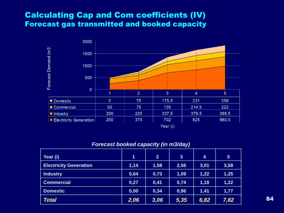
Calculating Cap and Com coefficients (IV) Forecast gas transmitted and booked capacity

Forecast booked capacity (in m3/day)

Year (i) 1 2 3 4 5

Electricity Generation 1,14 1,58 2,56 3,01 3,58

Industry 0,64 0,73 1,09 1,22 1,25

Commercial 0,27 0,41 0,74 1,18 1,22

Domestic 0,00 0,34 0,96 1,41 1,77

Total 2,06 3,06 5,35 6,82 7,82

85

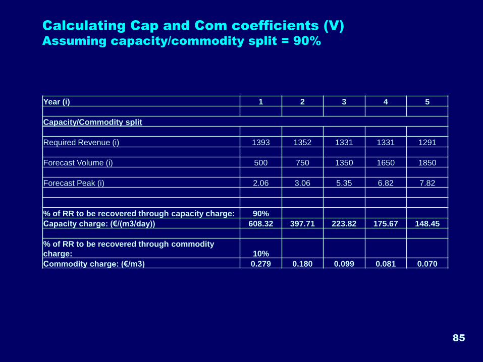
Calculating Cap and Com coefficients (V) Assuming capacity/commodity split = 90%

Year (i) 1 2 3 4 5

Capacity/Commodity split

Required Revenue (i) 1393 1352 1331 1331 1291

Forecast Volume (i) 500 750 1350 1650 1850

Forecast Peak (i) 2.06 3.06 5.35 6.82 7.82

% of RR to be recovered through capacity charge: 90%

Capacity charge: (€/(m3/day)) 608.32 397.71 223.82 175.67 148.45

% of RR to be recovered through commodity

charge: 10%

Commodity charge: (€/m3) 0.279 0.180 0.099 0.081 0.070

86

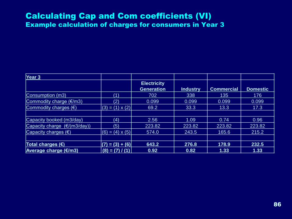
Calculating Cap and Com coefficients (VI) Example calculation of charges for consumers in Year 3

Year 3

Electricity

Generation Industry Commercial Domestic

Consumption (m3) (1) 702 338 135 176

Commodity charge (€/m3) (2) 0.099 0.099 0.099 0.099

Commodity charges (€) (3) = (1) x (2) 69.2 33.3 13.3 17.3

Capacity booked (m3/day) (4) 2.56 1.09 0.74 0.96

Capacity charge (€/(m3/day)) (5) 223.82 223.82 223.82 223.82

Capacity charges (€) (6) = (4) x (5) 574.0 243.5 165.6 215.2

Total charges (€) (7) = (3) + (6) 643.2 276.8 178.9 232.5

Average charge (€/m3) (8) = (7) / (1) 0.92 0.82 1.33 1.33

87

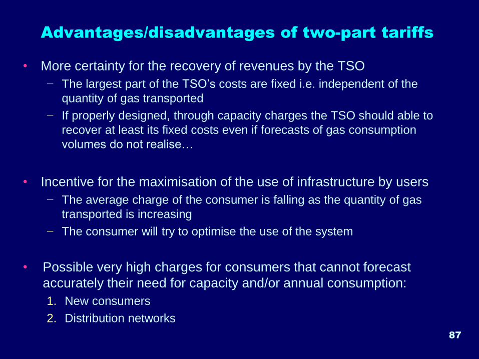
Advantages/disadvantages of two-part tariffs

• More certainty for the recovery of revenues by the TSO

− The largest part of the TSO’s costs are fixed i.e. independent of the

quantity of gas transported

− If properly designed, through capacity charges the TSO should able to

recover at least its fixed costs even if forecasts of gas consumption

volumes do not realise…

• Incentive for the maximisation of the use of infrastructure by users

− The average charge of the consumer is falling as the quantity of gas

transported is increasing

− The consumer will try to optimise the use of the system

• Possible very high charges for consumers that cannot forecast

accurately their need for capacity and/or annual consumption:

1. New consumers

2. Distribution networks

Duration of capacity booking

Short-term capacity tariff coefficients

88

89

Introduction

• Capacity coefficients are initially calculated assuming booking of certain

amount of capacity for 1 year (365 or 366 days)

• TSO also develops the transmission system based on the forecast

maximum capacity to serve demand (“peak demand”) on a long term

basis e.g.:

− Maximum capacity needed (m3/hour or m3/day) for the next 20 years

• Short duration bookings (also booked at short-notice) are allowed by

the EU regulations:

− From a single hour within a day, to daily, monthly and quarterly (3-month)

• Short-term capacity bookings:

− Facilitate gas trading, specially for capacity between two markets (cross-

border)

− Pose a great uncertainty in the TSO revenues and the planning of system

expansion

90

The case

• What would be the tariff for a capacity booking of e.g. 1 day?

• Possibilities:

− Cap_(1 day) = 1/365 of Cap_(1 year)

− Cap_(1 day) < 1/365 of Cap_(1 year)

− Cap_(1 day) > 1/365 of Cap_(1 year)

• Strong debate between TSOs – suppliers – traders - regulators

• Current status in accordance with EU regulation:

− Short-term capacity is allowed to be more expensive than annual capacity

bookings

− There is a cap imposed to the “short-term coefficients”

− The issue is under further consideration

91

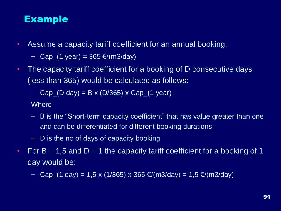
Example

• Assume a capacity tariff coefficient for an annual booking:

− Cap_(1 year) = 365 €/(m3/day)

• The capacity tariff coefficient for a booking of D consecutive days

(less than 365) would be calculated as follows:

− Cap_(D day) = B x (D/365) x Cap_(1 year)

Where

− B is the “Short-term capacity coefficient” that has value greater than one

and can be differentiated for different booking durations

− D is the no of days of capacity booking

• For B = 1,5 and D = 1 the capacity tariff coefficient for a booking of 1

day would be:

− Cap_(1 day) = 1,5 x (1/365) x 365 €/(m3/day) = 1,5 €/(m3/day)

Locational cost-allocation

92

93

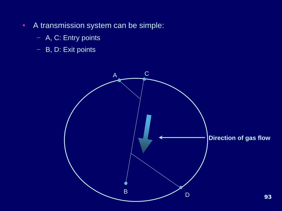
• A transmission system can be simple:

− A, C: Entry points

− B, D: Exit points

A C

DB

Direction of gas flow

94

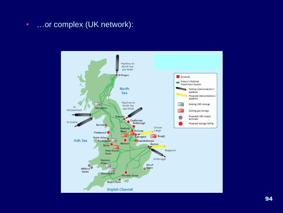
• …or complex (UK network):

95

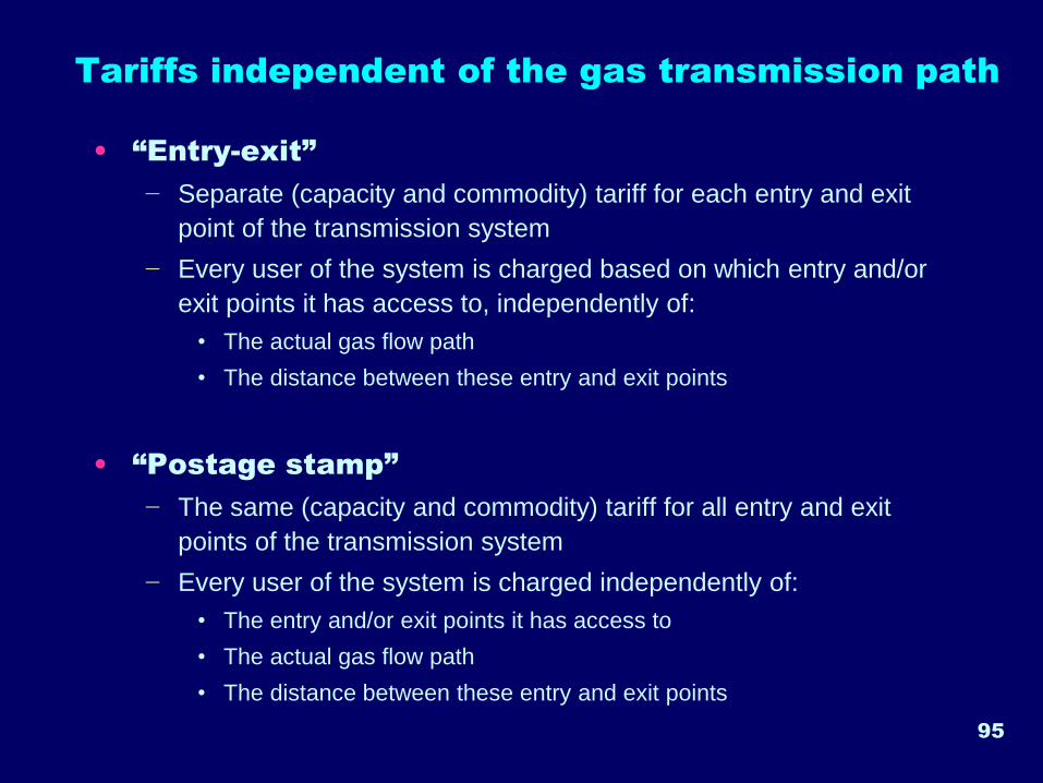
Tariffs independent of the gas transmission path

• “Entry-exit”

− Separate (capacity and commodity) tariff for each entry and exit

point of the transmission system

− Every user of the system is charged based on which entry and/or

exit points it has access to, independently of:

• The actual gas flow path

• The distance between these entry and exit points

• “Postage stamp”

− The same (capacity and commodity) tariff for all entry and exit

points of the transmission system

− Every user of the system is charged independently of:

• The entry and/or exit points it has access to

• The actual gas flow path

• The distance between these entry and exit points

96

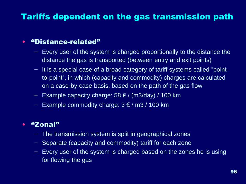
Tariffs dependent on the gas transmission path

• “Distance-related”

− Every user of the system is charged proportionally to the distance the

distance the gas is transported (between entry and exit points)

− It is a special case of a broad category of tariff systems called “point-

to-point”, in which (capacity and commodity) charges are calculated

on a case-by-case basis, based on the path of the gas flow

− Example capacity charge: 58 € / (m3/day) / 100 km

− Example commodity charge: 3 € / m3 / 100 km

• “Zonal”

− The transmission system is split in geographical zones

− Separate (capacity and commodity) tariff for each zone

− Every user of the system is charged based on the zones he is using

for flowing the gas

Final remarks

97

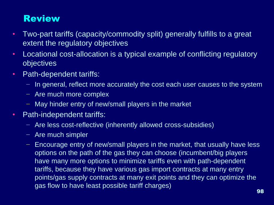
Review

• Two-part tariffs (capacity/commodity split) generally fulfills to a great

extent the regulatory objectives

• Locational cost-allocation is a typical example of conflicting regulatory

objectives

• Path-dependent tariffs:

− In general, reflect more accurately the cost each user causes to the system

− Are much more complex

− May hinder entry of new/small players in the market

• Path-independent tariffs:

− Are less cost-reflective (inherently allowed cross-subsidies)

− Are much simpler

− Encourage entry of new/small players in the market, that usually have less

options on the path of the gas they can choose (incumbent/big players

have many more options to minimize tariffs even with path-dependent

tariffs, because they have various gas import contracts at many entry

points/gas supply contracts at many exit points and they can optimize the

gas flow to have least possible tariff charges)98

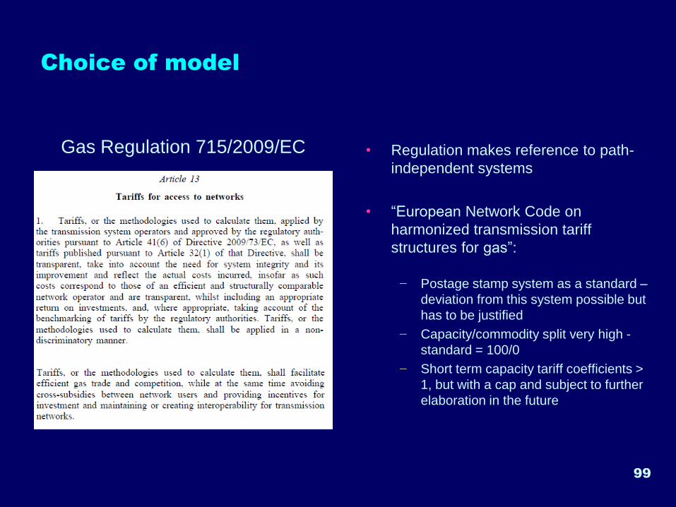
Choice of model

Gas Regulation 715/2009/EC • Regulation makes reference to path-

independent systems

• “European Network Code on

harmonized transmission tariff

structures for gas”:

− Postage stamp system as a standard –

deviation from this system possible but

has to be justified

− Capacity/commodity split very high -

standard = 100/0

− Short term capacity tariff coefficients >

1, but with a cap and subject to further

elaboration in the future

99

100

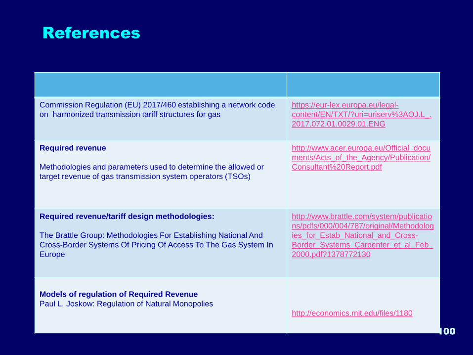
Commission Regulation (EU) 2017/460 establishing a network code

on harmonized transmission tariff structures for gas

https://eur-lex.europa.eu/legal-

content/EN/TXT/?uri=uriserv%3AOJ.L_.

2017.072.01.0029.01.ENG

Required revenue

Methodologies and parameters used to determine the allowed or

target revenue of gas transmission system operators (TSOs)

http://www.acer.europa.eu/Official_docu

ments/Acts_of_the_Agency/Publication/

Consultant%20Report.pdf

Required revenue/tariff design methodologies:

The Brattle Group: Methodologies For Establishing National And

Cross-Border Systems Of Pricing Of Access To The Gas System In

Europe

http://www.brattle.com/system/publicatio

ns/pdfs/000/004/787/original/Methodolog

ies_for_Estab_National_and_Cross-

Border_Systems_Carpenter_et_al_Feb_

2000.pdf?1378772130

Models of regulation of Required Revenue

Paul L. Joskow: Regulation of Natural Monopolies

http://economics.mit.edu/files/1180

References