Embed Size (px)
Citation preview
Putting the New Keynesian Model to a Test: An SVAR
Analysis with DSGE Priors∗
Gert Peersman
Ghent University
Roland Straub
International Monetary Fund
June 2005
Preliminary version
Abstract
This paper shows how the popular New Keynesian DSGE model can be used to
derive sign restrictions for the identification of several shocks in a structural vector
autoregression (SVAR) for the Euro Area. The impact is first estimated for respec-
tively monetary policy, preferences, government spending, investment, price mark-up,
technology and labor supply shocks. In a second step, the restrictions from the DSGE
model are significantly relaxed and the SVAR is re-estimated with a minimum set
of more general constraints. The data can then provide more information about the
validity of the DSGE model. It is shown that most of the responses remain consis-
tent with the New Keynesian model, including the controversial negative effects of a
government spending shock on private consumption and investment. Some interesting
differences, however, emerge. In contrast to the theoretical model, a positive effect
of a technology shock on employment, and a positive impact of a preferences and
investment shock on respectively investment and consumption are found.
JEL classification: C32, C51, E32, E52
Keywords: Sticky price models; vector autoregressions; sign restrictions
∗The views expressed are solely our own and do not necessarily reflect those of the International Mon-
etary Fund. All remaining errors are ours.
1
1 Introduction
The workhorse in today’s theoretical macroeconomics is a dynamic stochastic general equi-
librium (DSGE) model with sticky prices, habit formation, capital adjustment costs, vari-
able capacity utilization and other frictions introduced to capture empirical fluctuations in
macroeconomic data.1 In addition, these type of models are also used for policy purposes
in practise2. On the other hand, since the seminal work of Sims (1980), structural vector
autoregressions (SVARs) are frequently used as a tool in empirical macroeconomic analy-
sis. This technique is convenient to implement and can provide clear answers to policy
relevant questions such as: "What are the effects of monetary and fiscal policy shocks?",
"What shocks drive the business cycle?" and "Which underlying disturbances caused re-
cent output and inflation fluctuations?" using respectively impulse response functions,
variance decompositions and historical decompositions. The results of a VAR analysis are
also frequently used to evaluate the outcome of theoretical models. Gali (1992) checks
whether the IS-LM model is able to fit postwar US data. Blanchard and Perotti (2002)
and Fatás and Mihov (2001) use the outcome of a government spending shock from an
SVAR model to assess New Keynesian (NK) and Real Business Cycle (RBC) models. Gali
(1999) estimates the effects of technology shocks on hours worked to discriminate between
both theoretical models. Canova (2002) compares a limited participation monetary model
and a sticky price monopolistic competition model with a VAR analysis. In this study,
we first show how the popular NK DSGE model can be used to derive restrictions for the
identification of a large set of shocks in a structural vector autoregression (SVAR) for the
Euro Area. In a second step, we significantly relax the restrictions from the DSGE model
and re-estimate the SVAR in order to evaluate the outcome of the theoretical model. So
to say, we put the conditional properties of the large scale NK model to a test.
A crucial aspect in the SVAR literature is the identification of structural shocks. In
order to identify these shocks, a number of zero restrictions on the immediate or long-
1Examples are Christiano, Eichenbaum and Evans (2005) for the US and Smets and Wouters (2003)
for the Euro Area.2See for example the GEM model of the IMF, the SIGMA model of the FED and the TOTEM model
of the Bank of Canada.
2
run impact of the shocks are typically introduced.3 A problem, however, is that the
implementation of zero restrictions could be very arbitrary and misleading if a lot of
variables are included in the system. That is why a majority of the empirical papers only
focus on one type of shock, such as monetary or fiscal policy shocks. In that case it is
only necessary to make assumptions to estimate the monetary or fiscal policy rule. Even
if additional shocks are identified, this is still at a relative aggregate level. Examples are
aggregate supply or aggregate spending shocks. Identifying more shocks at a disaggregated
level is not possible because it involves using economic theory to introduce additional
zero restrictions in the short or long-run to disentangle the shocks from each other.4
Unfortunately, these restrictions are not always available or are very stringent, which can
significantly affect the results.
In this paper, we consider many shocks simultaneously at a more disaggregate level
which is a first contribution of the paper. We identify monetary policy, preferences, gov-
ernment spending, investment, price mark-up, technology and labor supply shocks in the
Euro Area economy. In order to identify the shocks, we use sign restrictions. The lat-
ter are used by Faust (1998), Uhlig (1999) and Canova and de Nicoló (2003) to identify
monetary policy shocks and extended by Peersman (2005) to oil price, aggregate supply
and aggregate demand shocks. The advantage of this procedure is that no zero constraints
have to be imposed. The restrictions are much more general and easier to implement when
economic theory only provides qualitative rather than quantitative information about the
effects of shocks. As a consequence, it is possible to identify more shocks. In this paper
we use a standard DSGE model to derive the sign restrictions for our empirical analy-
sis. Specifically, we first calibrate a NK DSGE model with sticky prices, habit formation,
capital adjustment costs and variable capacity utilization which provides us theoretical
3Several alternative strategies are used to do this. For instance, Christiano et. al. (1998) and Sims
(1990) assume a short-run recursive ordering of the variables in the system. This means that the shocks
are orthogonal to the variables ordered before the shock. Bernanke (1986), Sims (1986) and Bernanke and
Mihov (1998) abandon the recursiveness assumption and introduce a broader set of short-run relations
based on economic theory. Blanchard and Quah (1989), King et al. (1989) and Gali (1992) also use
long-run restrictions to identify the shocks.4Blanchard (1993) estimates a VAR on the components of GDP, but does not identify structural dis-
turbances.
3

impulse response functions for a number of macroeconomic variables. From these impulse
response functions, we select a set of sign conditions which are robust with respect to
the parameterization of the model. We then estimate a seven-variables VAR for output,
prices, employment, real wages, consumption, investment and the short-run interest rate
for the Euro Area. The data can then determine the magnitudes of the responses, the
contribution to the variances of the variables and the historical contribution of the shocks
to all variables.
When we consider the theoretical DSGE model into more detail, some of the constraints
and responses are however not consistent with existing empirical evidence or other alter-
native theoretical models. For instance, Blanchard and Perotti (2002), Fatás and Mihov
(2001) and Gali et. al. (2003) find a rise in private consumption after a government
spending shock which is ad odds with the DSGE model.5 On the other hand, standard
RBC models predict a positive impact of technology shocks on employment whilst this
effect is always negative in a NK model. As a result, restricting the latter two responses
to be negative with sign conditions can be questioned. We therefore significantly relax the
imposed conditions in a second step. The SVAR is re-estimated with a minimum set of less
stringent more general constraints from the NK model that are consistent with a broader
class of models and less controversial. Accordingly, it is possible to evaluate the DSGE
model and compare it with other empirical evidence which is the second contribution of
the paper. We show that most of the responses remain consistent with the NK DSGE
model, including the negative impact of government spending shocks on private consump-
tion and investment. Some interesting differences, however, emerge. We find a positive
effect of a technology shock on employment, and a positive impact of a preferences and
investment shock on respectively investment and consumption, which was not predicted
by the model.
This methodology implies that we use the outcome of a DSGE model as a prior for
SVARs. There are also other papers using DSGE priors. DeJong et al. (1993) and Ingram
and Whiteman (1994) use a DSGE model as a prior to estimate a bayesian VAR used for
5Gali et. al. (2003) extend the standard New Keynesian model with rule-of-thumb consumers and
show that the interaction of the latter with sticky prices and deficit financing can account for the existing
evidence on the effects of government spending in specific circumstances.
4
forecasting purposes. However, they do not identify structural shocks in their analysis. Del
Negro and Schorfheide (2003), in contrast, utilize the priors from the theoretical model to
estimate a three-variables bayesian VAR and to do the identification of a monetary policy
shock, which seems to be a very promising method. The disadvantage of these approaches
is that the modelling of the dynamics of the DSGE model is relative important, which can
have a substantial impact on the results. Misspecification can lead to biased results and
wrong conclusions. In contrast to these studies, our VAR is more extended and includes
much more shocks. In addition, we only use the DSGE model to derive the sign constraints
to do the identification of the structural shocks. Moreover, these conditions are robust for
several parameterizations of the model. This implies that the construction of the dynamics
of the theoretical model is rather limited for the estimation results.6
The rest of the paper is structured as follows. In Section 2, we develop a New Keynesian
DSGE model for the Euro Area and show the theoretical impulse response functions. The
sign conditions for the identification are derived from this model. Section 3 shows the
estimation results of the SVAR-model for the Euro Area with the DSGE priors for the
sign restrictions. In Section 4, we substantially relax the imposed restrictions in order to
evaluate the NK results. Finally, Section 5 concludes.
2 The DSGE Priors
The DSGE model and the corresponding discussion in this section draws heavily on Smets
and Wouters (2003) and Coenen and Straub (2005).7 The paper by Smets and Wouters
has garnered much attention because it demonstrates that large scale DSGE models are
able to fit data as well as a conventional atheoretical VAR. The empirical success lies
in the introduction of numerous dynamic extensions into the ‘workhorse’ New Keynesian
6This approach is somewhat similar to Canova (2002). He evaluates two DSGE models of money, i.e.
a limited participation economy and a sticky price monopolistic competitive economy against the data.
Specifically, he derives robust restrictions for the cross correlations of some macroeconomic variables from
both models and implement them in a VAR. In contrast, we only restrict the sign of the responses and
we analyse a large set of structural shocks while Canova (2002) only focuses on monetary and technology
shocks.7See also Christiano et. al. (2005), the GEM and Sigma model.
5
model to capture the persistence in the macro data. Large scale DSGE models exhibit
both sticky prices and wages, partial indexation, external habit formation in consumption,
capital adjustment costs and variable capital utilization. Additionally, several structural
shocks are identified and can be estimated within the model framework. These features
make them sufficiently rich to capture the stochastics and dynamics in the data and
a valuable tool for policy analysis in an empirically plausible set-up. In the following
we will focus on the log-linearized version of the model. For the description of the full
non-linear model and derivation of the equilibrium conditions, the interested reader is
referred to the papers cited above. We first briefly describe the model in Section 2.1. The
sign restrictions obtained from this model and implemented in our empirical analysis are
discussed in Section 2.2.
2.1 Description of the model
The model consists of a continuum of households who value consumption and leisure and
are subject to habit persistence. The preferences are subject to two type of preference
shocks. Households supply a differentiated labor in a imperfectly competitive labor market
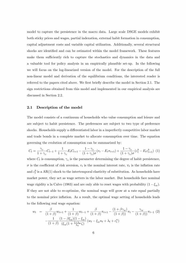
and trade bonds in a complete market to allocate consumption over time. The equation
governing the evolution of consumption can be summarized by:
Ct =γc
1 + γcCt−1 +
1
1 + γcEtCt+1 −
1− γc(1 + γc)σ
(rt −Etπt+1) +1− γc(1 + γc)σ
(εbt −Etεbt+1) (1)
where Ct is consumption, γc is the parameter determining the degree of habit persistence,
σ is the coefficient of risk aversion, rt is the nominal interest rate, πt is the inflation rate
and εbt is a AR(1) shock to the intertemporal elasticity of substitution. As households have
market power, they act as wage setters in the labor market. But households face nominal
wage rigidity a la Calvo (1983) and are only able to reset wages with probability (1− ξw).
If they are not able to re-optimize, the nominal wage will grow at a rate equal partially
to the nominal price inflation. As a result, the optimal wage setting of households leads
to the following real wage equation:
wt =β
(1 + β)wt+1 +
1
(1 + β)wt−1 +
β
(1 + β)πt+1 −
(1 + βγw)
(1 + β))πt −
γw(1 + β))
πt−1 (2)
− 1
(1 + β)
(1− βξw)(1− ξw)
(ξw(1 +1+λwλw
ζ)(wt − ξwnt + λt + εnt )
6
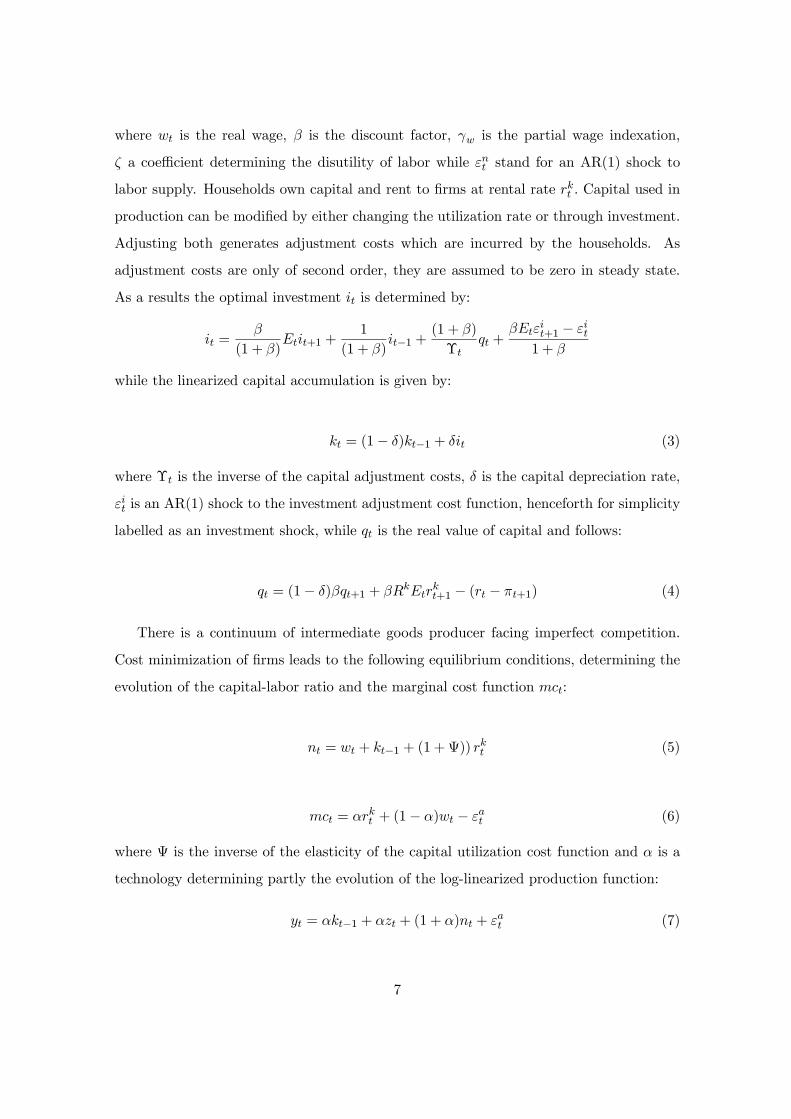
where wt is the real wage, β is the discount factor, γw is the partial wage indexation,
ζ a coefficient determining the disutility of labor while εnt stand for an AR(1) shock to
labor supply. Households own capital and rent to firms at rental rate rkt . Capital used in
production can be modified by either changing the utilization rate or through investment.
Adjusting both generates adjustment costs which are incurred by the households. As
adjustment costs are only of second order, they are assumed to be zero in steady state.
As a results the optimal investment it is determined by:
it =β
(1 + β)Etit+1 +
1
(1 + β)it−1 +
(1 + β)
Υtqt +
βEtεit+1 − εit1 + β
while the linearized capital accumulation is given by:
kt = (1− δ)kt−1 + δit (3)
where Υt is the inverse of the capital adjustment costs, δ is the capital depreciation rate,
εit is an AR(1) shock to the investment adjustment cost function, henceforth for simplicity
labelled as an investment shock, while qt is the real value of capital and follows:
qt = (1− δ)βqt+1 + βRkEtrkt+1 − (rt − πt+1) (4)
There is a continuum of intermediate goods producer facing imperfect competition.
Cost minimization of firms leads to the following equilibrium conditions, determining the
evolution of the capital-labor ratio and the marginal cost function mct:
nt = wt + kt−1 + (1 +Ψ)) rkt (5)
mct = αrkt + (1− α)wt − εat (6)
where Ψ is the inverse of the elasticity of the capital utilization cost function and α is a
technology determining partly the evolution of the log-linearized production function:
yt = αkt−1 + αzt + (1 + α)nt + εat (7)
7
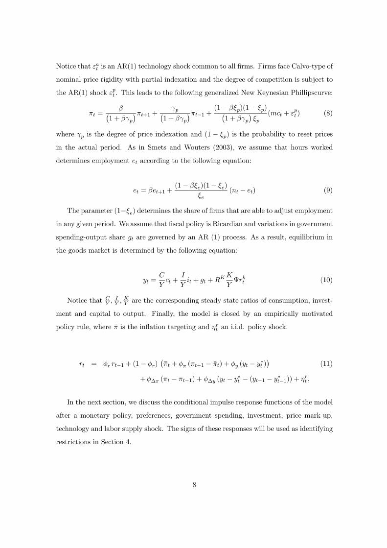
Notice that εat is an AR(1) technology shock common to all firms. Firms face Calvo-type of
nominal price rigidity with partial indexation and the degree of competition is subject to
the AR(1) shock εpt . This leads to the following generalized New Keynesian Phillipscurve:
πt =β¡
1 + βγp¢πt+1 + γp¡
1 + βγp¢πt−1 + (1− βξp)(1− ξp)¡
1 + βγp¢ξp
(mct + εpt ) (8)
where γp is the degree of price indexation and (1 − ξp) is the probability to reset prices
in the actual period. As in Smets and Wouters (2003), we assume that hours worked
determines employment et according to the following equation:
et = βet+1 +(1− βξe)(1− ξe)
ξe(nt − et) (9)
The parameter (1−ξe) determines the share of firms that are able to adjust employment
in any given period. We assume that fiscal policy is Ricardian and variations in government
spending-output share gt are governed by an AR (1) process. As a result, equilibrium in
the goods market is determined by the following equation:
yt =C
Yct +
I
Yit + gt +RKK
YΨrkt (10)
Notice that CY ,
IY ,
KY are the corresponding steady state ratios of consumption, invest-
ment and capital to output. Finally, the model is closed by an empirically motivated
policy rule, where π̄ is the inflation targeting and ηrt an i.i.d. policy shock.
rt = φr rt−1 + (1− φr)¡π̄t + φπ (πt−1 − π̄t) + φy (yt − y∗t )
¢(11)
+φ∆π (πt − πt−1) + φ∆y (yt − y∗t − (yt−1 − y∗t−1)) + ηrt ,
In the next section, we discuss the conditional impulse response functions of the model
after a monetary policy, preferences, government spending, investment, price mark-up,
technology and labor supply shock. The signs of these responses will be used as identifying
restrictions in Section 4.
8
2.2 Sign restrictions
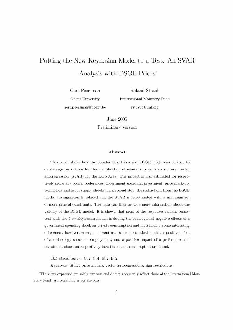
In order to derive the sign restrictions utilized later in the VAR analysis, we calculate the
impulse response functions from the DSGE model. We focus on the conditional responses
of output, prices, interest rate, employment, real wages, consumption and investment fol-
lowing a monetary policy, preferences, government spending, investment, price mark-up,
technology and labor supply shock because these will be used in our empirical estima-
tions. To do so, we first calibrate the DSGE model for a range of sensible values for the
parameters that are frequently used in the literature. For some of these values, we also
borrow estimation results for Euro Area structural parameters from the recently developed
literature such as Smets and Wouters (2003). More specifically, for each parameter, we
draw a value from an interval and generate the corresponding impulse response functions.
The intervals for the parameter values are reported in Table 1.8 This exercise is repeated
for 10000 simulations. The 20th and 80th percentiles of all these conditional simulations
are shown in Figure 1 for our 7 variables (dotted lines). In this figure, we also include
the median of the posterior (full line) for the Smets and Wouters (2003) model to check
consistency of these two exercises. Except for the real wage reaction to an investment
shock, the sign of all responses are the same for both exercises.9 The corresponding sign
restrictions for our empirical analysis are presented in Table 2.
Consider first demand and policy shocks. A temporary expansionary monetary policy
shock reflected by a fall in the nominal interest rate implies a rise in consumption, invest-
ment and output respectively. Also prices, employment and real wages rise. Preferences,
government spending and investment shocks all have a positive effect on output, prices,
the nominal interest rate, employment and real wages. A shock in preferences, while in-
creasing consumption and output, has a negative effect on investment. In contrast, an
investment boom generated by a temporary reduction in the cost of installing capital,
crowds out consumption on impact. A government spending shock generates the expected
negative wealth effect that has a negative impact on consumption and investment while
8Notice that ρshock is the AR(1) coefficient for the corresponding shocks and g/y is the share of gov-
ernment spending to output.9Note that for some shocks, the scaling is somewhat different for both exercises. Since we are only
interested in the signs of the responses, this is irrelevant for our analysis.
9
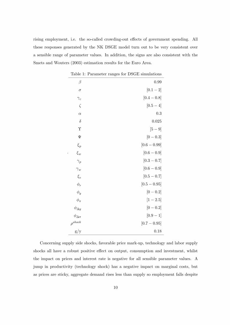
rising employment, i.e. the so-called crowding-out effects of government spending. All
these responses generated by the NK DSGE model turn out to be very consistent over
a sensible range of parameter values. In addition, the signs are also consistent with the
Smets and Wouters (2003) estimation results for the Euro Area.
.
Table 1: Parameter ranges for DSGE simulations
β 0.99
σ [0.1− 2]
γc [0.4− 0.8]
ζ [0.5− 4]
α 0.3
δ 0.025
Υ [5− 9]
Ψ [0− 0.3]
ξp [0.6− 0.99]
ξw [0.6− 0.9]
γp [0.3− 0.7]
γw [0.6− 0.9]
ξe [0.5− 0.7]
φr [0.5− 0.95]
φy [0− 0.2]
φπ [1− 2.5]
φ∆y [0− 0.2]
φ∆π [0.9− 1]
ρshock [0.7− 0.95]
g/y 0.18
Concerning supply side shocks, favorable price mark-up, technology and labor supply
shocks all have a robust positive effect on output, consumption and investment, whilst
the impact on prices and interest rate is negative for all sensible parameter values. A
jump in productivity (technology shock) has a negative impact on marginal costs, but
as prices are sticky, aggregate demand rises less than supply so employment falls despite
10
the positive response of output and there is a rise in real wages. Notice that if monetary
policy is accommodative enough, the NK model is also able to generate a positive response
of employment. On the other hand, a positive labor supply shock leads unambigiously
to an increase in employment and a fall in the equilibrium real wage. As discussed in
detailed in Peersman and Straub (2004), the fall in real wages along with the positive
correlation between output and employment is the most significant and robust qualitative
difference between the conditional responses following a technology and labor supply shock.
The impact of price-mark up shocks on output, consumption, investment and inflation
are similar to the previous shocks, but the model predicts different impact responses
of real wages and employment compared to labor supply shocks and technology shocks
respectively.
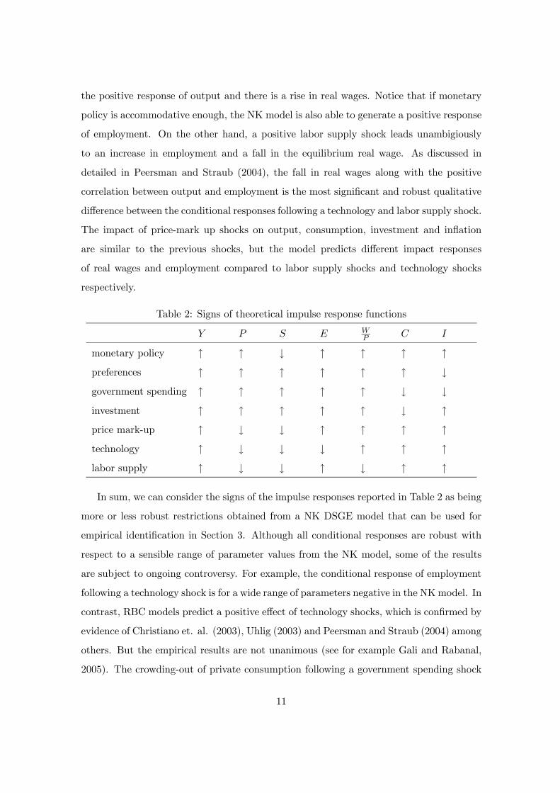
Table 2: Signs of theoretical impulse response functions
Y P S E WP C I
monetary policy ↑ ↑ ↓ ↑ ↑ ↑ ↑
preferences ↑ ↑ ↑ ↑ ↑ ↑ ↓
government spending ↑ ↑ ↑ ↑ ↑ ↓ ↓
investment ↑ ↑ ↑ ↑ ↑ ↓ ↑
price mark-up ↑ ↓ ↓ ↑ ↑ ↑ ↑
technology ↑ ↓ ↓ ↓ ↑ ↑ ↑
labor supply ↑ ↓ ↓ ↑ ↓ ↑ ↑
In sum, we can consider the signs of the impulse responses reported in Table 2 as being
more or less robust restrictions obtained from a NK DSGE model that can be used for
empirical identification in Section 3. Although all conditional responses are robust with
respect to a sensible range of parameter values from the NK model, some of the results
are subject to ongoing controversy. For example, the conditional response of employment
following a technology shock is for a wide range of parameters negative in the NKmodel. In
contrast, RBC models predict a positive effect of technology shocks, which is confirmed by
evidence of Christiano et. al. (2003), Uhlig (2003) and Peersman and Straub (2004) among
others. But the empirical results are not unanimous (see for example Gali and Rabanal,
2005). The crowding-out of private consumption following a government spending shock
11
is similarly controversial. The majority of the empirical literature predicts a positive or
insignificant impact of government spending on private consumption. See the empirical
work by Blanchard and Perotti (2002), Fatás and Mihov (2001) among others. On the basis
of this evidence, Gali, López-Salido and Vallés (2004) extend the standard New Keynesian
model to allow for the presence of non-Ricardian, rule-of-thumb households and show that
the interaction of the latter with sticky prices and deficit financing can account for the
existing empirical evidence. However, as argued in Bilbiie and Straub (2004), the result
relies on a sharp response of real wages following government spending shocks which stands
in contrast with the observed a-cyclical pattern of real wages in the data. Coenen and
Straub (2005) argue utilizing an estimated DSGE model with non-Ricardian agents for the
Euro Area that, although the presence of non-Ricardian households is in general conducive
to raising the level of private aggregate consumption in response to government spending
shocks; as a practical matter, however, there is only a fairly low probability for this to
happen. The results show that the estimated share of non-Ricardian households is quite
low, but also that the large negative wealth effect induced by the highly persistent nature
of the estimated government spending shocks crowds out consumption of the Ricardian
agents significantly. Finally the lack of empirical evidence on the responses of preference
and investment shocks give rise to caution in implementing the full set of conditional
responses for identification.
Despite the lack of agreement in the empirical and theoretical literature with respect
to some of the impact responses, we first estimate our VAR using the complete set of
restrictions depicted in Table 2 to provide a benchmark for our later results. Using the
estimation results, we can check whether there exist decompositions in the data that
are consistent with all restrictions from the theoretical DSGE model in the first place.
Moreover, it provides us information how easy it is to find these decompositions in the
data. If one fully believes the derived restrictions from the New Keynesian model, the
results of the estimations can also be used to evaluate the magnitudes of the impulse
responses and analyze variance and historical decompositions. In Section 4, we will then
significantly reduce the number of restrictions by utilizing only a minimum set of robust
sign restrictions that are more general and less controversial. Accordingly, it is possible
12
to check the robustness of the conditional responses and accompanying contributions to
variances and historical fluctuations. So to say: we put the conditional properties of the
large scale New Keynesian model to a test.
3 An SVAR-model for the Euro Area with DSGE priors
In this section we present the results of the standard SVAR-model using Euro Area quar-
terly data for the sample period 1980-2003. All data are taken from the area-wide model
of the ECB (Fagan et. al., 2001). We first describe the specification and identification
strategy of the SVAR in Section 3.1. Results for impulse response analysis and variance
decompositions are presented in Section 3.2.
3.1 Methodology
Consider the following specification for a vector of endogenous variables Yt:
Yt = c+nXi=1
AiYt−i +Bεt (12)
where c is an (n × 2) matrix of constants and linear trends, Ai is an (n × n) matrix of
autoregressive coefficients and εt is a vector of structural disturbances. The endogenous
variables, Yt, that we include in the VAR are real GDP (yt), the GDP deflator (pt), short-
term nominal interest rate (st), employment (et), real wages (wtpt ), consumption (ct) and
investment (it). All variables are logs, except the interest rate which is in percentages. We
estimate this VAR-model in levels with three lags. By doing the analysis in levels we allow
for implicit cointegration relationships in the data, and still have consistent estimates of
the parameters (Sims et. al., 1990).
Within this VAR, the seven types of shocks from the NK model are identified: a
monetary policy, preferences, government spending, investment, price mark-up, technology
and labor supply shock respectively. In order to identify these shocks, we use the sign
restrictions as shown in Table 2. The restrictions are sufficient to uniquely disentangle all
seven shocks. Specifically, for each shock the sign of the response of at least one variable
is different from the sign of the response to another shock. For the implementation of
13
these restrictions, we refer to Peersman (2005). All restrictions are imposed as 6 or >.
For all variables, the time period over which the sign constraints are binding is set equal
to four quarters, except for the interest rate where this time period is two quarters.10
Following Uhlig (1999) and Peersman (2005), we use a Bayesian approach for estimation
and inference. Our prior and posterior belong to the Normal-Wishart family used in the
RATS manual for drawing error bands. Because there are an infinite number of admissible
decompositions for each draw from the posterior when using sign restrictions, we use the
following procedure. To draw the "candidate truths" from the posterior, we take a joint
draw from the posterior for the usual unrestricted Normal-Wishart posterior for the VAR
parameters as well as a uniform distribution for the rotation matrices. We then construct
impulse response functions. If all the imposed conditions on the responses are satisfied, we
keep the draw. If the decomposition does not match the criteria, the draw is rejected. This
means that these draws receive zero prior weight. Based on the draws left, we calculate
statistics and report the median responses, together with 84th and 16th percentiles error
bands. We do not require the restrictions of all shocks to hold simultaneously. Specifically,
if the impulse responses to an individual shock are consistent with the imposed conditions
for this shock, the results for the specific shock are accepted. This implies that even if
some restrictions for a certain shock are debatable, this has no effect on the estimation of
the other shocks.11 Impulse responses and error bands are computed with a minimum of
1000 solutions for each shock.
3.2 Results
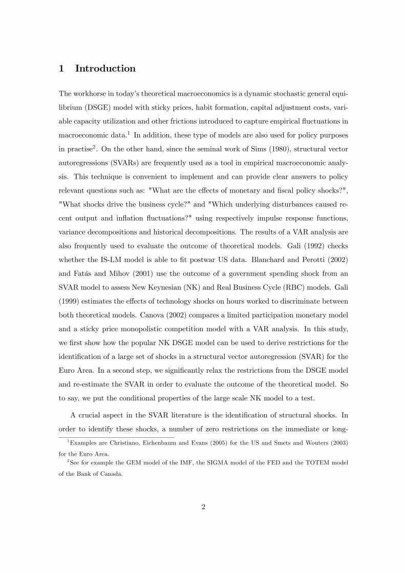
Figure 2 shows the results for the impulse response analysis. By construction, the signs of
all responses are consistent with the theoretical model. The fact that we do find empirical
results for all shocks, however, already indicates that the DSGE model conditions exist in
the data. The monetary policy effects in the Euro Area are comparable to the results of
Peersman and Smets (2001), although we also find a considerable contemporaneous impact
10Note that since the response of the interest rate to an investment shock is only significant at lag 2 in
our theoretical analysis, we only introduce this restriction for the second lag after the investment shock.11This enables us also to evaluate for all individual shocks how easy it is to find an admissible decom-
position in the data, i.e. an acceptance rate of each shock.
14
on output, which is restricted to be zero in Peersman and Smets (2001). Output returns to
baseline after five years whilst the effect on prices is permanent. In addition, we also find
a hump-shaped effect on employment, real wages, consumption and investment. A shock
in preferences also has a temporary effect on output and more persistent price effects. As
discussed in Section 2, the DSGE model predicts a negative impact on investment as a
result of crowding-out effects. This assumption will be abandoned in the next section.
The data can then determine the exact response of this variable. It is already interesting
to note that it is very hard to find solutions for the preferences shock that match all
the restrictions. On average only 1 solution out of 140000 draws is consistent with all
conditions of a preferences shock. All other draws from the posterior are rejected for this
shock. For comparison, the acceptance is 1 out of 8 draws for a monetary policy shock.
This might already be an indication that the restrictions from the NK DSGE model are
too stringent for a preferences shock. The same is true for a government spending and
investment shock. For these shocks we find a solution consistent with the NK priors for
respectively each 23000 and 70000 draws. On the other hand, noticeable is that a few
quarters after a technology shock, the impact on employment becomes insignificant and
highly uncertain. The imposed negative effect on this variable is seriously questioned by
standard RBC-models and will also be tested in the next section. Also for this shock we
only accept on average one solution out of each 168 draws. In contrast, the responses to
a price mark-up and labor supply shock are more accepted by the data. The acceptance
rate is 1/9 for the former and 1/17 for the latter.
If one believes the theoretical DSGE model presented in Section 2 its accompanying
restrictions for the responses, the empirical results can also be used to do variance and his-
torical decompositions. The former decomposes the forecast error variance of the variables
into the part due to each of the innovation processes, the latter decomposes the historical
values of these variables into a deterministic component and the accumulated effects of
15
current and past innovations.
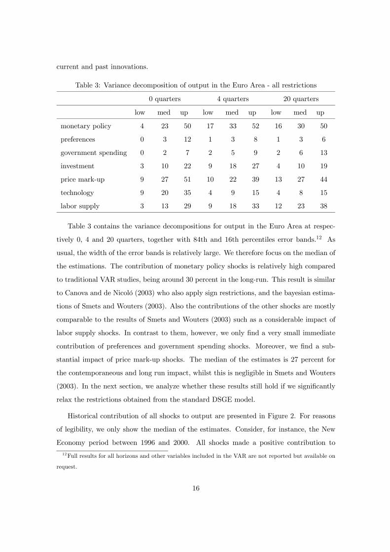
Table 3: Variance decomposition of output in the Euro Area - all restrictions
0 quarters 4 quarters 20 quarters
low med up low med up low med up
monetary policy 4 23 50 17 33 52 16 30 50
preferences 0 3 12 1 3 8 1 3 6
government spending 0 2 7 2 5 9 2 6 13
investment 3 10 22 9 18 27 4 10 19
price mark-up 9 27 51 10 22 39 13 27 44
technology 9 20 35 4 9 15 4 8 15
labor supply 3 13 29 9 18 33 12 23 38
Table 3 contains the variance decompositions for output in the Euro Area at respec-
tively 0, 4 and 20 quarters, together with 84th and 16th percentiles error bands.12 As
usual, the width of the error bands is relatively large. We therefore focus on the median of
the estimations. The contribution of monetary policy shocks is relatively high compared
to traditional VAR studies, being around 30 percent in the long-run. This result is similar
to Canova and de Nicoló (2003) who also apply sign restrictions, and the bayesian estima-
tions of Smets and Wouters (2003). Also the contributions of the other shocks are mostly
comparable to the results of Smets and Wouters (2003) such as a considerable impact of
labor supply shocks. In contrast to them, however, we only find a very small immediate
contribution of preferences and government spending shocks. Moreover, we find a sub-
stantial impact of price mark-up shocks. The median of the estimates is 27 percent for
the contemporaneous and long run impact, whilst this is negligible in Smets and Wouters
(2003). In the next section, we analyze whether these results still hold if we significantly
relax the restrictions obtained from the standard DSGE model.
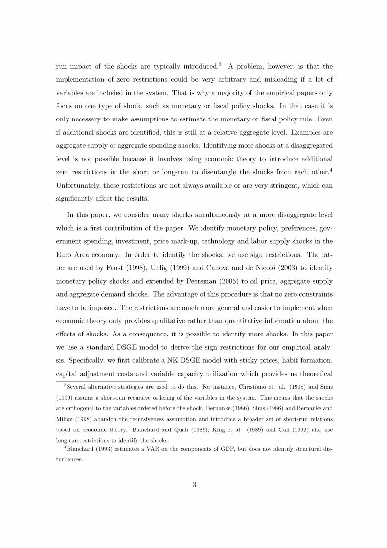
Historical contribution of all shocks to output are presented in Figure 2. For reasons
of legibility, we only show the median of the estimates. Consider, for instance, the New
Economy period between 1996 and 2000. All shocks made a positive contribution to
12Full results for all horizons and other variables included in the VAR are not reported but available on
request.
16
this period of high growth. The two most important shocks, however, turn out to be
labor supply and price mark-up shocks. The former is also found by Smets and Wouters
(2003) and Peersman and Straub (2004), the latter is rather surprising. Also investment,
monetary and fiscal policy shocks made a favorable contribution, whilst the positive effects
of preferences and technology shocks were much more limited. On the other hand, the
slowdown at the beginning of the century was mainly caused by negative labor supply
and price mark-up shocks and too restrictive monetary policy. This result is more or less
consistent with the findings of Peersman (2005).
4 A more general SVAR-model with DSGE priors
If one fully believes that the restrictions of the NK DSGE model of Section 2 are a true
representation of reality, the results presented above should be accepted. Some constraints
and responses are, however, not consistent with other theoretical and empirical evidence.
The theoretical DSGE model predicts a negative effect of government spending shocks
on private consumption and investment whilst Blanchard and Perotti (2002), Fatás and
Mihov (2001) and Gali et. al. (2003) among others find evidence in favour of a rise in
private consumption; and Mountford and Uhlig (2004) find an insignificant reaction of
consumption. Also the reaction of investment to a shock in government spending is not
robust across empirical studies. For instance Blanchard and Perotti (2002) find a fall in
investment while Edelberg et. al. (1999) find the opposite. Only the former is consistent
with our sign restriction from the DSGE model. In addition, the reaction of employment
to technology shocks is restricted to be negative in the above presented empirical analysis.
In contrast, RBC models predict a positive effect of technology shocks, which is confirmed
by evidence of Christiano et. al. (2003), Uhlig (2003) and Peersman and Straub (2004).
As a result, some of the restrictions we have imposed are questionable. In this section, we
further evaluate and test the NK DSGE model. Specifically, we significantly relax the sign
restrictions obtained from the theoretical model and make them more general in order to
check whether the responses are still consistent with the model and, as such, test the NK
model. We first discuss the more general restrictions in Section 4.1. New empirical results
are presented in Section 4.2.
17
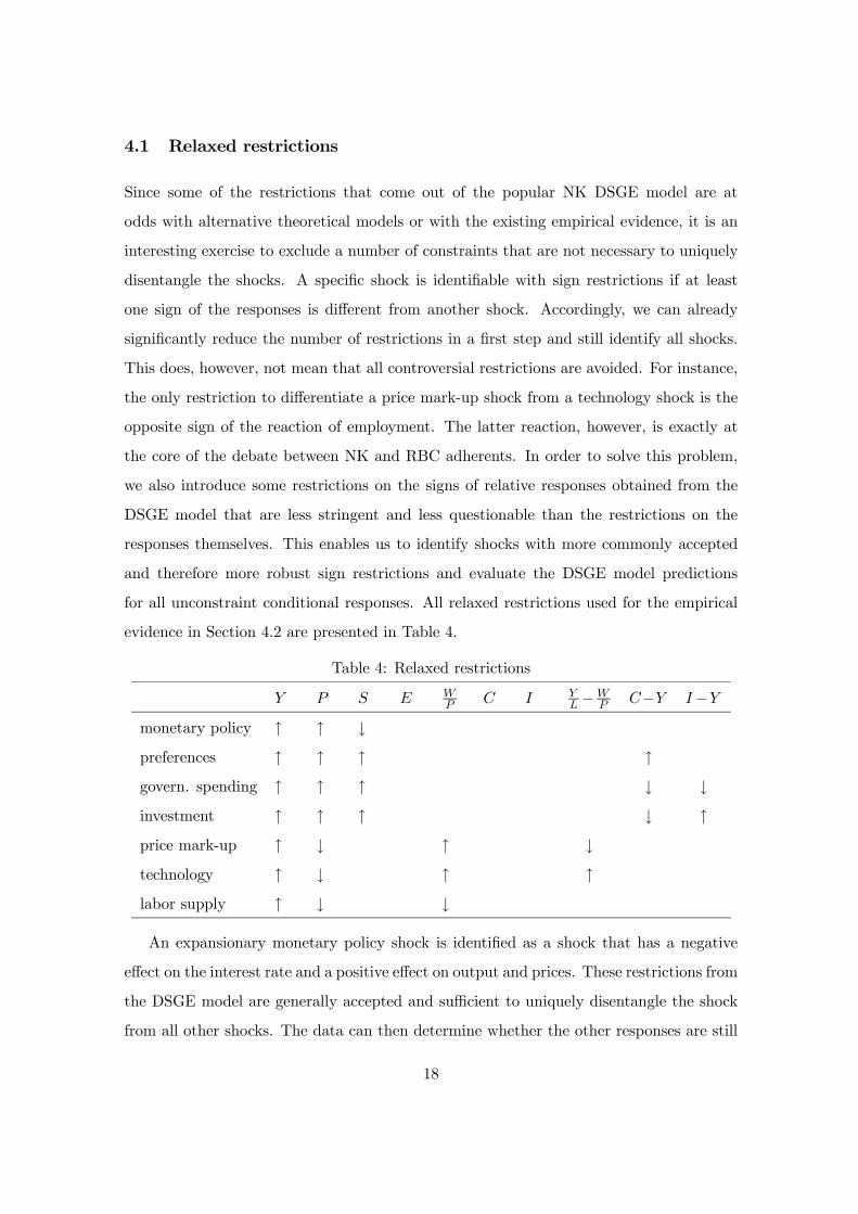
4.1 Relaxed restrictions
Since some of the restrictions that come out of the popular NK DSGE model are at
odds with alternative theoretical models or with the existing empirical evidence, it is an
interesting exercise to exclude a number of constraints that are not necessary to uniquely
disentangle the shocks. A specific shock is identifiable with sign restrictions if at least
one sign of the responses is different from another shock. Accordingly, we can already
significantly reduce the number of restrictions in a first step and still identify all shocks.
This does, however, not mean that all controversial restrictions are avoided. For instance,
the only restriction to differentiate a price mark-up shock from a technology shock is the
opposite sign of the reaction of employment. The latter reaction, however, is exactly at
the core of the debate between NK and RBC adherents. In order to solve this problem,
we also introduce some restrictions on the signs of relative responses obtained from the
DSGE model that are less stringent and less questionable than the restrictions on the
responses themselves. This enables us to identify shocks with more commonly accepted
and therefore more robust sign restrictions and evaluate the DSGE model predictions
for all unconstraint conditional responses. All relaxed restrictions used for the empirical
evidence in Section 4.2 are presented in Table 4.
Table 4: Relaxed restrictions
Y P S E WP C I Y
L −WP C−Y I−Y
monetary policy ↑ ↑ ↓
preferences ↑ ↑ ↑ ↑
govern. spending ↑ ↑ ↑ ↓ ↓
investment ↑ ↑ ↑ ↓ ↑
price mark-up ↑ ↓ ↑ ↓
technology ↑ ↓ ↑ ↑
labor supply ↑ ↓ ↓
An expansionary monetary policy shock is identified as a shock that has a negative
effect on the interest rate and a positive effect on output and prices. These restrictions from
the DSGE model are generally accepted and sufficient to uniquely disentangle the shock
from all other shocks. The data can then determine whether the other responses are still
18
consistent with the DSGE model. All other shocks at the demand side of the economy, i.e.
a preferences, government spending and investment cost shock are still assumed to have a
positive impact on output, prices and the nominal interest rate. If we want to differentiate
them from each other using the NK DSGE model and the standard responses of the
variables, some restrictions on consumption and investment are required. Specifically,
consumption increases and investment decreases following a shock in preferences. The
opposite is true for an investment shock. On the other hand, both variables fall after
a government spending shock. These responses derived from the DSGE model are the
result of capacity constraints or so-called crowding-out effects. If one of the variables
significantly rises, this is only possible if there is a fall in the other variables. There is,
however, disagreement about these responses in the literature, in particular for government
spending shocks.13 Although also RBC models predict a fall in private consumption and
investment after a positive government spending shock, this is mostly rejected in empirical
evidence. Blanchard and Perotti (2002), Fatás and Mihov (2001) and Gali et. al. (2003)
find an increase in private consumption after a favorable government spending shock. On
the other hand, they do find crowding-out effects on investment. However, Edelberg et. al.
(1999) find the opposite effects on investment and Perotti (2002) shows that the responses
of both variables are often insignificant in many countries and even negative in the post-
1980 period for the US. Gali et. al. (2003) even show that an extended NK DSGE model
with rule-of-thumb consumers can account for a positive effect of government spending
on consumption in specific circumstances. To avoid these controversial restrictions, we
introduce some less stringent constraints on the responses of consumption and investment
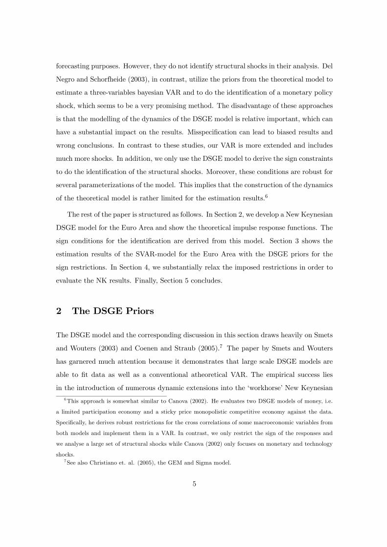
relative to output. The responses obtained from the DSGE model for consumption-output
ratio and investment-output ratio are shown in respectively the second and third column of
Figure 4. Consider a positive shock in preferences. Since the DSGE model predicts a rise in
consumption and a fall in all other components of output, the reaction of the consumption-
output ratio is obviously positive. On the other hand, for the same reason, the reaction
13We are not aware of theoretical or empirical papers questioning the mentioned effects of preferences
and investment shocks because we are the first to evaluate these specific responses empirically. Smets and
Wouters (2003, p 1156) do, however, describe the negative conditional responses as a potential problem in
their underlying model.
19
of this ratio to a government spending and investment shock is negative (not surprisingly
because the model predict for both shocks a rise in output and fall in consumption). More
generally, preferences shocks, e.g. a shift in preferences towards consumption today, will
cause in most of the generally accepted models a stronger response of consumption than
output. We therefore introduce a positive restriction on the consumption-output ratio
after a preferences shock and a negative restriction after a shock in government spending
and investment costs. As a result, it is perfectly possible to have a rise in investment after
a shock in preferences and a positive effect on private consumption after a government
spending and investment shock, as long as this effect is smaller than the effect on total
GDP.14 We use the same reasoning to discriminate between the investment and government
spending shock, i.e. the investment-output ratio rises after the former and falls after the
latter in the short-run. These restrictions are much more general and less stringent. The
data can now determine the exact sign of consumption, investment and all other responses.
At the supply side (shocks with a negative correlation between output and prices),
a labor supply shock is identified as a shock with a negative effect on real wages whilst
this effect is positive for a technology and price mark-up shock. Also this restriction is
generally accepted in the theoretical and empirical literature. Peersman and Straub (2004)
illustrate this for a large class of DSGE models, including RBC models. Moreover, Francis
and Ramey (2002) and Fleischmann (1999) find a positive effect of technology shocks and
a negative effect of labor supply shocks on employment using an identification strategy in
the spirit of Gali (1999). To differentiate between a price mark-up and technology shock
is much more difficult. Only one sign of the response functions in the DSGE model is
different between these two shocks, i.e. employment rises after a price mark-up shock and
falls after a technology shock. This restriction, however, is the well known controversy
between RBC and New Keynesian sticky price models. The former expects a positive
impact whilst the latter predicts a negative effect. Also the empirical evidence is mixed.
Gali (1999), Shea (1998), Basu et. al. (1999), Francis and Ramey (2002), and Francis,
Owyand and Theodorou (2003) find a negative effect and Christiano, Eichenbaum and
Vigfusson (2003), Peersman and Straub (2004), Uhlig (2004), Dedola and Neri (2004) and,
14Note that these restrictions are only introduced the first four lags after a shock. Accordingly, it is
perfectly possible to have a different sign in the long run.
20
Canova and Gambetti (2005) find a positive impact. We follow Dedola and Neri (2004)
to discriminate between both shocks. The first column of Figure 4 shows the responses of
the difference between labor productivity and real wages after both shocks obtained from
our theoretical DSGE model. This difference is clearly negative following a price mark-up
shock and positive after a technology shock for different parameterizations of the model,
i.e. we assume that the impact of technology shocks on labor productivity is stronger than
the one on real wages; a result again in line with both NK and RBC models. In contrast
and again independent from the existence of nominal rigidities, a negative shock to the
price mark-up will have, through the corresponding fall in prices, a stronger effect on the
real wage than on labor productivity.15 As a result, we use this restriction to disentangle
both shocks. No additional restrictions are required and the empirical results, discussed in
next section, can determine the signs of all unconstrained responses to evaluate the DSGE
model.
4.2 Results
Impulse response functions for the SVAR with relaxed restrictions are shown in Figure 5.
Due to the limited number of constraints, it was much easier to find solutions that match
all the restrictions for each shock. The acceptance rate for a monetary policy, preferences,
government spending, investment, price mark-up, technology and labor supply shock is
respectively 1/4, 1/21, 1/42, 1/4, 1/11, 1/102 and 1/4 whilst this was only 1/8, 1/140000,
1/23000, 1/70000, 1/9, 1/168 and 1/17 for the SVAR with all DSGE restrictions. The
results are nevertheless still very consistent with the theoretical DSGE model. Some
interesting differences, however, emerge.
After a monetary policy shock, all conditional responses still have the same sign in
line with the DSGE model. Restrictive monetary policy has a significant negative effect
on output, prices, employment, real wages, consumption and investment. The responses
to a government spending shock are also very comparable with the results of Section 3
and the theoretical DSGE model, although the impact on employment and real wages
are insignificant now in the short-run. Remarkably is that we still find the crowding-out
15Dedola and Neri (2004) show that this restriction holds in a pure RBC model with flexible prices.
21
effects of fiscal policy, i.e. there is a fall in investment and private consumption after
an expansionary government spending shock. The impact on the latter is, however, only
significant during one quarter. This empirical finding is in contrast to many other studies
using VAR-methods such as Blanchard and Perotti (2002), Fatás and Mihov (2001) and
Gali et. al. (2003).
The conditional responses to preferences and investment shocks are also qualitatively
similar to our previous results for respectively output, prices, interest rates, employment
and real wages, although we now find a somewhat stronger quantitative effect on output.
We do notice, however, a substantial difference with respect to the responses of investment
and consumption after a preferences and investment cost shock respectively. A shift in
preferences towards consumption today, i.e. a positive preferences shock, has a significant
positive impact on investment. Similarly, a fall in investment costs has an upward effect
on private consumption. Both effects are ad odds with theoretical New Keynesian DSGE
models discussed in Section 2. We notice also the sharp increase in the acceptance rate
of possible decompositions for both shocks. Only 21 and 4 draws are necessary to find a
solution that match all imposed sign conditions for respectively a preferences and invest-
ment shock, while this was respectively 140000 and 70000 using all DSGE restrictions.
Crowding-in effects of both shocks seems to be more accepted by the data.
Concerning supply side shocks, responses to price mark-up and labor supply shocks
do also not change much when we impose only a limited number of restrictions. Notice
that this is not the case for the conditional responses to a technology shock. From a
quantitative point of view, we find a much larger impact of a rise in productivity on
output being almost double the first years after the shock. This difference is mainly the
result of a stronger impact on investment using less stringent restrictions. In addition, we
now find a positive effect on employment whilst this response is restricted to be negative
when we impose all constraints obtained from the NK model. The conditional response
of employment to technology shocks is at the core of the debate between NK and RBC
adherents. The former expect a negative effect while the latter expect the opposite. Our
evidence is in favour of the RBC model. This positive effect on employment is also found
by Christiano et. al. (2003), Uhlig (2003), Peersman and Straub (2004) and Canova and
22
Gambetti (2005).
Table 5: Variance decomposition of output in the Euro Area - relaxed restrictions
0 quarters 4 quarters 20 quarters
low med up low med up low med up
monetary policy 0 4 19 6 13 27 4 12 31
preferences 1 12 29 4 11 22 4 10 23
government spending 1 8 18 5 10 18 4 8 15
investment 8 29 56 16 31 52 6 14 27
price mark-up 0 8 24 3 8 17 4 12 29
technology 23 42 63 14 31 50 8 23 43
labor supply 2 11 28 4 12 26 4 11 27
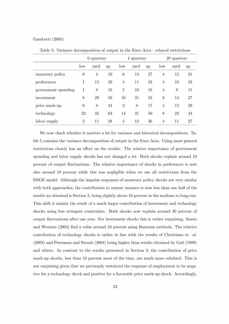
We now check whether it matters a lot for variance and historical decompositions. Ta-
ble 5 contains the variance decomposition of output in the Euro Area. Using more general
restrictions clearly has an effect on the results. The relative importance of government
spending and labor supply shocks has not changed a lot. Both shocks explain around 10
percent of output fluctuations. The relative importance of shocks in preferences is now
also around 10 percent while this was negligible when we use all restrictions from the
DSGE model. Although the impulse responses of monetary policy shocks are very similar
with both approaches, the contribution to output variance is now less than one half of the
results we obtained is Section 3, being slightly above 10 percent in the medium to long-run.
This shift is mainly the result of a much larger contribution of investment and technology
shocks using less stringent constraints. Both shocks now explain around 30 percent of
output fluctuations after one year. For investment shocks this is rather surprising. Smets
and Wouters (2003) find a value around 10 percent using Bayesian methods. The relative
contribution of technology shocks is rather in line with the results of Christiano et. al.
(2003) and Peersman and Straub (2004) being higher than results obtained by Gali (1999)
and others. In contrast to the results presented in Section 3, the contribution of price
mark-up shocks, less than 10 percent most of the time, are much more subdued. This is
not surprising given that we previously restricted the response of employment to be nega-
tive for a technology shock and positive for a favorable price mark-up shock. Accordingly,
23
part of the technology shocks were identified as price mark-up shocks.
These findings are also reflected in the historical decomposition of output fluctuations
as shown in Figure 6. When we use less controversial restrictions, the impact of price
mark-up shocks in explaining the long-lasting boom of the second half of the nineties,
also often called the New Economy period, and the succeeding recession is much less. In
contrast, we now find a substantial impact of positive and negative technology shocks in
explaining both periods. Moreover, we now also find an important role for positive shocks
in preferences between 1998 and 2001, turning negative afterwards which is in line with
shifts in consumer confidence around that period following September 11. Finally, the more
general approach also finds a role for unfavorable investment cost shocks in explaining the
slowdown after the millennium shift. In sum, these results are not inconsistent with the
general believe about the causes of the boom in the second half of the nineties and the
early millennium slowdown.
5 Conclusions
In this paper we have shown how the popular New Keynesian DSGE model can be used
to derive sign restrictions for the identification of a large set of structural shocks in the
Euro Area economy using an SVAR methodology. For a sensible range of underlying
parameter values, the DSGE model can deliver us sufficient restrictions to uniquely identify
respectively monetary policy, preferences, government spending, investment, price mark-
up, technology and labor supply shocks. Many of these shocks have not been identified
before in SVARs and can be considered as a first contribution of the paper.
Some of the imposed conditions of the New Keynesian DSGE model are, however,
not consistent with alternative theoretical models and existing empirical evidence. In a
second step, we therefore significantly relax the restrictions from the DSGE model and
re-estimate the VAR with a minimum set of more general constraints. The data can then
provide more information about the validity of the DSGE model, in particular about the
conditional responses of the model. As such, we put the New Keynesian model to a test.
The empirical evidence shows that most of the responses remain consistent with the
24
New Keynesian DSGE model, including the controversial negative effects of a government
spending shock on private consumption and investment, i.e. crowding-out effects of fiscal
policy. We do find, however, some interesting differences. In contrast to the theoretical
model, we find a positive impact of technology shocks on employment whilst New Keyne-
sian models predict a negative effect. Our finding is more consistent with an RBC model
in which technology shocks are the driving force of business cycles. In addition, we find a
positive impact of shocks in preferences on investment and also private consumption rises
after a negative shock in investment costs. The latter two conditional responses are not
predicted by a theoretical New Keynesian DSGE model. Specifically, a standard feature
of New Keynesian DSGE models is the so-called crowding-out effect. Empirical evidence,
however, suggests that this is not consistent with the data, a finding which should be tried
to be incorporated in future theoretical DSGE modelling.
References
Sims, C. (1980): “Macroeconomics and Reality,” Econometrica, 48(1), 1—48.
25
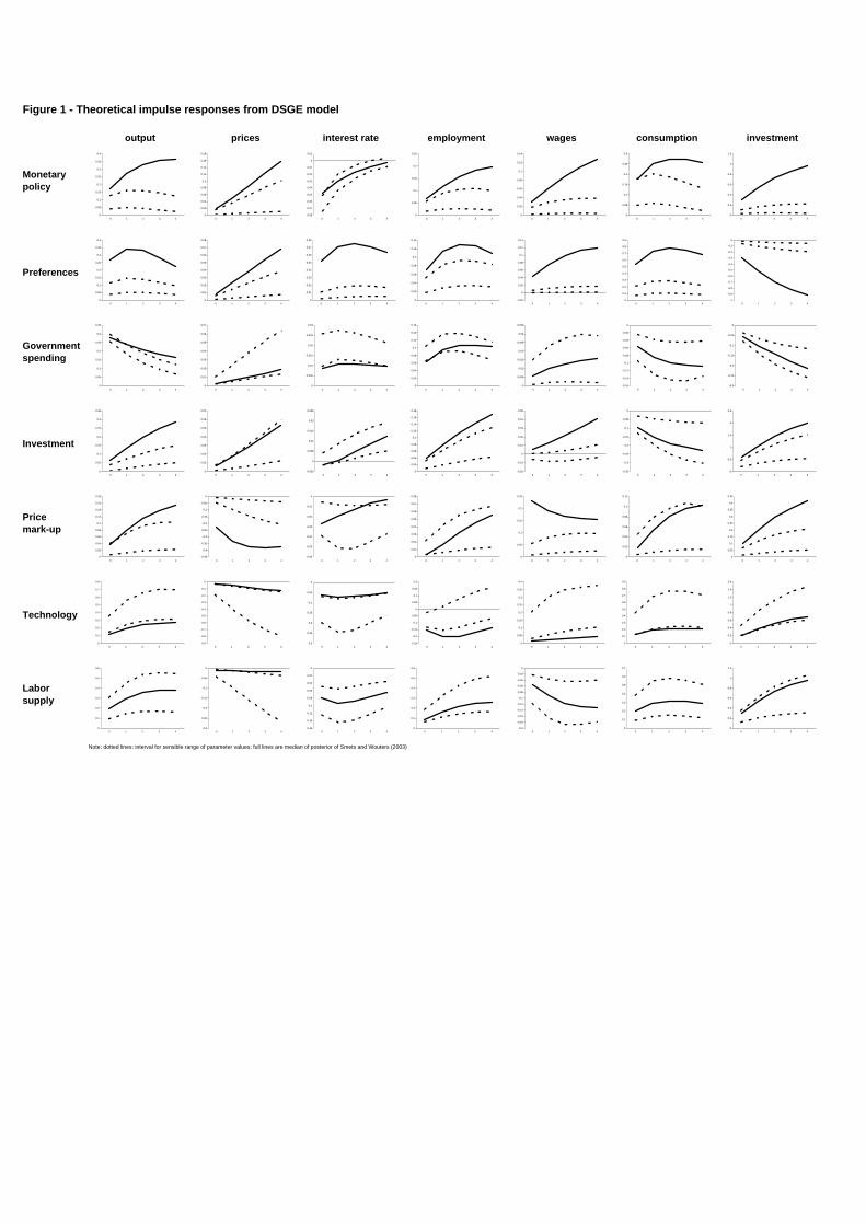
Figure 1 - Theoretical impulse responses from DSGE model
output prices interest rate employment wages consumption investment
Monetary policy
Preferences
Governmentspending
Investment
Pricemark-up
Technology
Laborsupply
Note: dotted lines: interval for sensible range of parameter values; full lines are median of posterior of Smets and Wouters (2003)
0
0.05
0.1
0.15
0.2
0.25
0.3
0.35
0.4
0 1 2 3 40
0.02
0.04
0.06
0.08
0.1
0.12
0.14
0.16
0.18
0 1 2 3 4-0.08
-0.07
-0.06
-0.05
-0.04
-0.03
-0.02
-0.01
0
0.01
0 1 2 3 40
0.05
0.1
0.15
0.2
0.25
0 1 2 3 40
0.02
0.04
0.06
0.08
0.1
0.12
0.14
0 1 2 3 40
0.05
0.1
0.15
0.2
0.25
0.3
0 1 2 3 40
0.2
0.4
0.6
0.8
1
1.2
0 1 2 3 4
0
0.05
0.1
0.15
0.2
0.25
0.3
0.35
0.4
0 1 2 3 40
0.01
0.02
0.03
0.04
0.05
0.06
0.07
0.08
0 1 2 3 40
0.01
0.02
0.03
0.04
0.05
0.06
0.07
0.08
0 1 2 3 40
0.02
0.04
0.06
0.08
0.1
0.12
0.14
0 1 2 3 4-0.02
0
0.02
0.04
0.06
0.08
0.1
0.12
0.14
0 1 2 3 40
0.1
0.2
0.3
0.4
0.5
0.6
0.7
0.8
0.9
0 1 2 3 4-1
-0.9
-0.8
-0.7
-0.6
-0.5
-0.4
-0.3
-0.2
-0.1
0
0 1 2 3 4
0
0.05
0.1
0.15
0.2
0.25
0.3
0.35
0 1 2 3 40
0.01
0.02
0.03
0.04
0.05
0.06
0.07
0 1 2 3 40
0.005
0.01
0.015
0.02
0.025
0.03
0 1 2 3 40
0.02
0.04
0.06
0.08
0.1
0.12
0.14
0.16
0 1 2 3 40
0.005
0.01
0.015
0.02
0.025
0.03
0.035
0 1 2 3 4-0.16
-0.14
-0.12
-0.1
-0.08
-0.06
-0.04
-0.02
0
0 1 2 3 4-0.3
-0.25
-0.2
-0.15
-0.1
-0.05
0
0 1 2 3 4
0
0.05
0.1
0.15
0.2
0.25
0.3
0.35
0 1 2 3 40
0.01
0.02
0.03
0.04
0.05
0.06
0.07
0 1 2 3 4-0.005
0
0.005
0.01
0.015
0.02
0.025
0 1 2 3 40
0.02
0.04
0.06
0.08
0.1
0.12
0.14
0.16
0.18
0 1 2 3 4-0.02
-0.01
0
0.01
0.02
0.03
0.04
0.05
0 1 2 3 4-0.35
-0.3
-0.25
-0.2
-0.15
-0.1
-0.05
0
0 1 2 3 40
0.5
1
1.5
2
2.5
0 1 2 3 4
0
0.02
0.04
0.06
0.08
0.1
0.12
0.14
0.16
0.18
0 1 2 3 4-0.45
-0.4
-0.35
-0.3
-0.25
-0.2
-0.15
-0.1
-0.05
0
0 1 2 3 4-0.06
-0.05
-0.04
-0.03
-0.02
-0.01
0
0 1 2 3 40
0.01
0.02
0.03
0.04
0.05
0.06
0.07
0.08
0 1 2 3 40
0.05
0.1
0.15
0.2
0.25
0 1 2 3 40
0.02
0.04
0.06
0.08
0.1
0.12
0 1 2 3 40
0.05
0.1
0.15
0.2
0.25
0.3
0.35
0.4
0.45
0 1 2 3 4
0
0.1
0.2
0.3
0.4
0.5
0.6
0.7
0.8
0 1 2 3 4-0.9
-0.8
-0.7
-0.6
-0.5
-0.4
-0.3
-0.2
-0.1
0
0 1 2 3 4-0.3
-0.25
-0.2
-0.15
-0.1
-0.05
0
0 1 2 3 4-0.25
-0.2
-0.15
-0.1
-0.05
0
0.05
0.1
0.15
0.2
0 1 2 3 40
0.05
0.1
0.15
0.2
0.25
0.3
0.35
0.4
0 1 2 3 40
0.1
0.2
0.3
0.4
0.5
0.6
0.7
0.8
0.9
0 1 2 3 40
0.2
0.4
0.6
0.8
1
1.2
1.4
1.6
0 1 2 3 4
0
0.1
0.2
0.3
0.4
0.5
0.6
0 1 2 3 4-0.3
-0.25
-0.2
-0.15
-0.1
-0.05
0
0 1 2 3 4-0.16
-0.14
-0.12
-0.1
-0.08
-0.06
-0.04
-0.02
0
0 1 2 3 40
0.1
0.2
0.3
0.4
0.5
0.6
0 1 2 3 4-0.2
-0.18
-0.16
-0.14
-0.12
-0.1
-0.08
-0.06
-0.04
-0.02
0
0 1 2 3 40
0.1
0.2
0.3
0.4
0.5
0.6
0.7
0 1 2 3 40
0.2
0.4
0.6
0.8
1
1.2
0 1 2 3 4
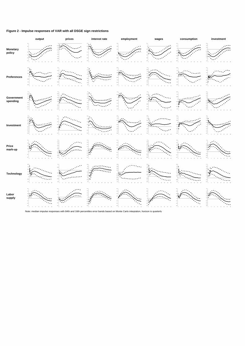
Figure 2 - Impulse responses of VAR with all DSGE sign restrictions
output prices interest rate employment wages consumption investment
Monetary policy
Preferences
Governmentspending
Investment
Pricemark-up
Technology
Laborsupply
Note: median impulse responses with 84th and 16th percentiles error bands based on Monte Carlo integration, horizon is quarterly
-0.4
-0.3
-0.2
-0.1
0
0.1
0.2
0 4 8 12 16 20 24 28-0.4
-0.35
-0.3
-0.25
-0.2
-0.15
-0.1
-0.05
0
0 4 8 12 16 20 24 28-0.4
-0.3
-0.2
-0.1
0
0.1
0.2
0 4 8 12 16 20 24 28-0.3
-0.2
-0.1
0
0.1
0.2
0.3
0 4 8 12 16 20 24 28-0.5
-0.4
-0.3
-0.2
-0.1
0
0.1
0 4 8 12 16 20 24 28-0.5
-0.4
-0.3
-0.2
-0.1
0
0.1
0.2
0 4 8 12 16 20 24 28-1.2
-1
-0.8
-0.6
-0.4
-0.2
0
0.2
0.4
0.6
0 4 8 12 16 20 24 28
-0.15
-0.1
-0.05
0
0.05
0.1
0.15
0 4 8 12 16 20 24 28-0.1
-0.05
0
0.05
0.1
0.15
0.2
0 4 8 12 16 20 24 28-0.2
-0.15
-0.1
-0.05
0
0.05
0.1
0.15
0.2
0 4 8 12 16 20 24 28-0.2
-0.15
-0.1
-0.05
0
0.05
0.1
0.15
0 4 8 12 16 20 24 28-0.15
-0.1
-0.05
0
0.05
0.1
0.15
0.2
0.25
0.3
0 4 8 12 16 20 24 28-0.15
-0.1
-0.05
0
0.05
0.1
0.15
0 4 8 12 16 20 24 28-0.4
-0.3
-0.2
-0.1
0
0.1
0.2
0.3
0 4 8 12 16 20 24 28
-0.2
-0.15
-0.1
-0.05
0
0.05
0.1
0.15
0.2
0 4 8 12 16 20 24 28-0.15
-0.1
-0.05
0
0.05
0.1
0.15
0.2
0.25
0.3
0 4 8 12 16 20 24 28-0.2
-0.15
-0.1
-0.05
0
0.05
0.1
0.15
0.2
0 4 8 12 16 20 24 28-0.2
-0.15
-0.1
-0.05
0
0.05
0.1
0 4 8 12 16 20 24 28-0.15
-0.1
-0.05
0
0.05
0.1
0.15
0.2
0 4 8 12 16 20 24 28-0.2
-0.15
-0.1
-0.05
0
0.05
0.1
0.15
0 4 8 12 16 20 24 28-0.6
-0.5
-0.4
-0.3
-0.2
-0.1
0
0.1
0.2
0.3
0.4
0 4 8 12 16 20 24 28
-0.25
-0.2
-0.15
-0.1
-0.05
0
0.05
0.1
0.15
0.2
0.25
0.3
0 4 8 12 16 20 24 28-0.1
0
0.1
0.2
0.3
0.4
0.5
0 4 8 12 16 20 24 28-0.2
-0.1
0
0.1
0.2
0.3
0.4
0 4 8 12 16 20 24 28-0.25
-0.2
-0.15
-0.1
-0.05
0
0.05
0.1
0.15
0 4 8 12 16 20 24 28-0.15
-0.1
-0.05
0
0.05
0.1
0.15
0.2
0.25
0 4 8 12 16 20 24 28-0.25
-0.2
-0.15
-0.1
-0.05
0
0.05
0.1
0.15
0 4 8 12 16 20 24 28-0.8
-0.6
-0.4
-0.2
0
0.2
0.4
0.6
0.8
0 4 8 12 16 20 24 28
-0.2
-0.1
0
0.1
0.2
0.3
0.4
0 4 8 12 16 20 24 28-0.2
-0.15
-0.1
-0.05
0
0.05
0.1
0.15
0.2
0.25
0.3
0 4 8 12 16 20 24 28-0.4
-0.3
-0.2
-0.1
0
0.1
0.2
0.3
0.4
0 4 8 12 16 20 24 28-0.3
-0.2
-0.1
0
0.1
0.2
0.3
0.4
0 4 8 12 16 20 24 28-0.15
-0.1
-0.05
0
0.05
0.1
0.15
0.2
0.25
0.3
0.35
0.4
0 4 8 12 16 20 24 28-0.2
-0.1
0
0.1
0.2
0.3
0.4
0.5
0 4 8 12 16 20 24 28-0.6
-0.4
-0.2
0
0.2
0.4
0.6
0.8
1
1.2
0 4 8 12 16 20 24 28
-0.1
-0.05
0
0.05
0.1
0.15
0.2
0.25
0 4 8 12 16 20 24 28-0.2
-0.15
-0.1
-0.05
0
0.05
0.1
0 4 8 12 16 20 24 28-0.3
-0.25
-0.2
-0.15
-0.1
-0.05
0
0.05
0.1
0.15
0 4 8 12 16 20 24 28-0.1
-0.08
-0.06
-0.04
-0.02
0
0.02
0.04
0.06
0.08
0 4 8 12 16 20 24 28-0.15
-0.1
-0.05
0
0.05
0.1
0.15
0.2
0.25
0.3
0.35
0 4 8 12 16 20 24 28-0.1
-0.05
0
0.05
0.1
0.15
0.2
0.25
0.3
0.35
0 4 8 12 16 20 24 28-0.2
-0.1
0
0.1
0.2
0.3
0.4
0.5
0.6
0.7
0 4 8 12 16 20 24 28
-0.3
-0.2
-0.1
0
0.1
0.2
0.3
0.4
0 4 8 12 16 20 24 28-0.3
-0.2
-0.1
0
0.1
0.2
0.3
0 4 8 12 16 20 24 28-0.4
-0.3
-0.2
-0.1
0
0.1
0.2
0.3
0.4
0 4 8 12 16 20 24 28-0.3
-0.2
-0.1
0
0.1
0.2
0.3
0.4
0 4 8 12 16 20 24 28-0.3
-0.2
-0.1
0
0.1
0.2
0.3
0.4
0 4 8 12 16 20 24 28-0.3
-0.2
-0.1
0
0.1
0.2
0.3
0.4
0 4 8 12 16 20 24 28-0.8
-0.6
-0.4
-0.2
0
0.2
0.4
0.6
0.8
1
1.2
0 4 8 12 16 20 24 28
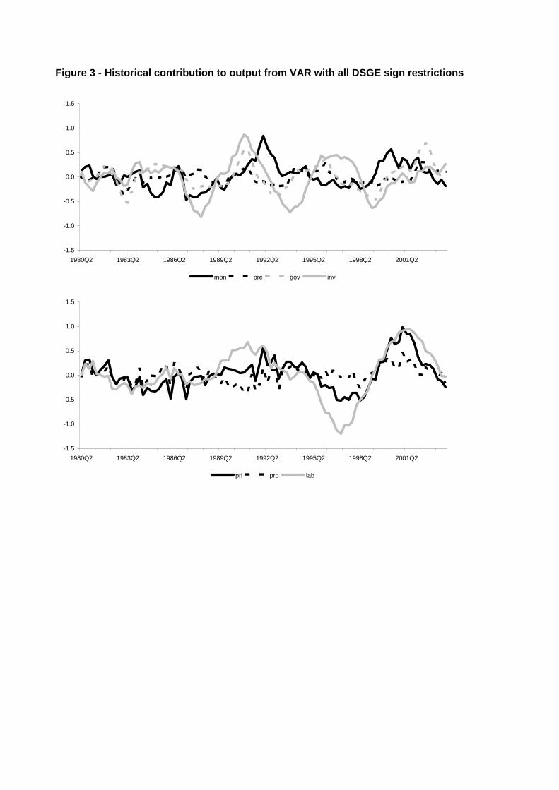
Figure 3 - Historical contribution to output from VAR with all DSGE sign restrictions
-1.5
-1.0
-0.5
0.0
0.5
1.0
1.5
1980Q2 1983Q2 1986Q2 1989Q2 1992Q2 1995Q2 1998Q2 2001Q2
mon pre gov inv
-1.5
-1.0
-0.5
0.0
0.5
1.0
1.5
1980Q2 1983Q2 1986Q2 1989Q2 1992Q2 1995Q2 1998Q2 2001Q2
pri pro lab
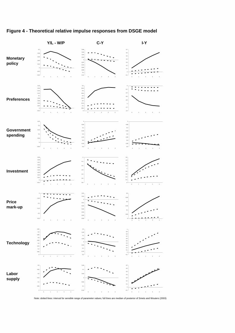
Figure 4 - Theoretical relative impulse responses from DSGE model
Y/L - W/P C-Y I-Y
Monetary policy
Preferences
Governmentspending
Investment
Pricemark-up
Technology
Laborsupply
Note: dotted lines: interval for sensible range of parameter values; full lines are median of posterior of Smets and Wouters (2003)
-0.04
-0.02
0
0.02
0.04
0.06
0.08
0.1
0 1 2 3 4-0.12
-0.1
-0.08
-0.06
-0.04
-0.02
0
0.02
0.04
0.06
0.08
0 1 2 3 4-0.1
0
0.1
0.2
0.3
0.4
0.5
0.6
0.7
0 1 2 3 4
-0.02
0
0.02
0.04
0.06
0.08
0.1
0.12
0.14
0.16
0.18
0 1 2 3 40
0.05
0.1
0.15
0.2
0.25
0.3
0.35
0.4
0.45
0.5
0 1 2 3 4-1.4
-1.2
-1
-0.8
-0.6
-0.4
-0.2
0
0 1 2 3 4
-0.05
0
0.05
0.1
0.15
0.2
0.25
0 1 2 3 4-0.4
-0.35
-0.3
-0.25
-0.2
-0.15
-0.1
-0.05
0
0 1 2 3 4-0.4
-0.35
-0.3
-0.25
-0.2
-0.15
-0.1
-0.05
0
0 1 2 3 4
-0.01
0
0.01
0.02
0.03
0.04
0.05
0.06
0.07
0.08
0.09
0 1 2 3 4-0.6
-0.5
-0.4
-0.3
-0.2
-0.1
0
0 1 2 3 40
0.2
0.4
0.6
0.8
1
1.2
1.4
1.6
1.8
0 1 2 3 4
-0.25
-0.2
-0.15
-0.1
-0.05
0
0 1 2 3 4-0.06
-0.05
-0.04
-0.03
-0.02
-0.01
0
0.01
0.02
0 1 2 3 40
0.05
0.1
0.15
0.2
0.25
0.3
0 1 2 3 4
0
0.05
0.1
0.15
0.2
0.25
0.3
0.35
0.4
0.45
0 1 2 3 4-0.2
-0.15
-0.1
-0.05
0
0.05
0.1
0.15
0.2
0 1 2 3 4-0.1
0
0.1
0.2
0.3
0.4
0.5
0.6
0.7
0.8
0.9
1
0 1 2 3 4
0
0.05
0.1
0.15
0.2
0.25
0.3
0 1 2 3 4-0.15
-0.1
-0.05
0
0.05
0.1
0.15
0 1 2 3 4-0.1
0
0.1
0.2
0.3
0.4
0.5
0.6
0.7
0 1 2 3 4
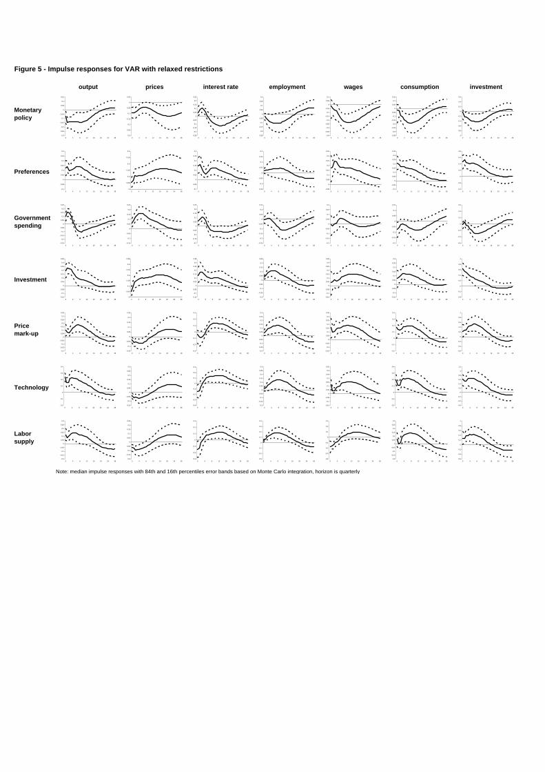
Figure 5 - Impulse responses for VAR with relaxed restrictions
output prices interest rate employment wages consumption investment
Monetary policy
Preferences
Governmentspending
Investment
Pricemark-up
Technology
Laborsupply
Note: median impulse responses with 84th and 16th percentiles error bands based on Monte Carlo integration, horizon is quarterly
-0.3
-0.25
-0.2
-0.15
-0.1
-0.05
0
0.05
0.1
0.15
0 4 8 12 16 20 24 28-0.3
-0.25
-0.2
-0.15
-0.1
-0.05
0
0.05
0 4 8 12 16 20 24 28-0.25
-0.2
-0.15
-0.1
-0.05
0
0.05
0.1
0.15
0.2
0.25
0 4 8 12 16 20 24 28-0.25
-0.2
-0.15
-0.1
-0.05
0
0.05
0.1
0.15
0.2
0 4 8 12 16 20 24 28-0.4
-0.35
-0.3
-0.25
-0.2
-0.15
-0.1
-0.05
0
0.05
0.1
0 4 8 12 16 20 24 28-0.35
-0.3
-0.25
-0.2
-0.15
-0.1
-0.05
0
0.05
0.1
0.15
0 4 8 12 16 20 24 28-1
-0.8
-0.6
-0.4
-0.2
0
0.2
0.4
0.6
0 4 8 12 16 20 24 28
-0.1
-0.05
0
0.05
0.1
0.15
0.2
0.25
0.3
0 4 8 12 16 20 24 280
0.05
0.1
0.15
0.2
0.25
0.3
0 4 8 12 16 20 24 28-0.1
-0.05
0
0.05
0.1
0.15
0.2
0.25
0.3
0 4 8 12 16 20 24 28-0.15
-0.1
-0.05
0
0.05
0.1
0.15
0.2
0 4 8 12 16 20 24 28-0.05
0
0.05
0.1
0.15
0.2
0.25
0.3
0.35
0 4 8 12 16 20 24 28-0.1
-0.05
0
0.05
0.1
0.15
0.2
0.25
0.3
0.35
0 4 8 12 16 20 24 28-0.4
-0.2
0
0.2
0.4
0.6
0.8
0 4 8 12 16 20 24 28
-0.25
-0.2
-0.15
-0.1
-0.05
0
0.05
0.1
0.15
0.2
0.25
0 4 8 12 16 20 24 28-0.15
-0.1
-0.05
0
0.05
0.1
0.15
0.2
0.25
0 4 8 12 16 20 24 28-0.2
-0.15
-0.1
-0.05
0
0.05
0.1
0.15
0.2
0.25
0 4 8 12 16 20 24 28-0.25
-0.2
-0.15
-0.1
-0.05
0
0.05
0.1
0.15
0 4 8 12 16 20 24 28-0.2
-0.15
-0.1
-0.05
0
0.05
0.1
0.15
0.2
0 4 8 12 16 20 24 28-0.2
-0.15
-0.1
-0.05
0
0.05
0.1
0.15
0 4 8 12 16 20 24 28-0.6
-0.4
-0.2
0
0.2
0.4
0.6
0 4 8 12 16 20 24 28
-0.15
-0.1
-0.05
0
0.05
0.1
0.15
0.2
0.25
0.3
0.35
0 4 8 12 16 20 24 280
0.05
0.1
0.15
0.2
0.25
0.3
0.35
0 4 8 12 16 20 24 28-0.15
-0.1
-0.05
0
0.05
0.1
0.15
0.2
0.25
0.3
0.35
0 4 8 12 16 20 24 28-0.2
-0.15
-0.1
-0.05
0
0.05
0.1
0.15
0.2
0.25
0 4 8 12 16 20 24 28-0.15
-0.1
-0.05
0
0.05
0.1
0.15
0.2
0.25
0.3
0.35
0 4 8 12 16 20 24 28-0.15
-0.1
-0.05
0
0.05
0.1
0.15
0.2
0.25
0.3
0 4 8 12 16 20 24 28-0.4
-0.2
0
0.2
0.4
0.6
0.8
1
0 4 8 12 16 20 24 28
-0.2
-0.15
-0.1
-0.05
0
0.05
0.1
0.15
0.2
0.25
0.3
0.35
0 4 8 12 16 20 24 28-0.15
-0.1
-0.05
0
0.05
0.1
0.15
0.2
0.25
0 4 8 12 16 20 24 28-0.3
-0.2
-0.1
0
0.1
0.2
0.3
0 4 8 12 16 20 24 28-0.2
-0.15
-0.1
-0.05
0
0.05
0.1
0.15
0.2
0.25
0.3
0 4 8 12 16 20 24 28-0.15
-0.1
-0.05
0
0.05
0.1
0.15
0.2
0.25
0.3
0.35
0 4 8 12 16 20 24 28-0.2
-0.1
0
0.1
0.2
0.3
0.4
0 4 8 12 16 20 24 28-0.6
-0.4
-0.2
0
0.2
0.4
0.6
0.8
1
0 4 8 12 16 20 24 28
-0.2
-0.1
0
0.1
0.2
0.3
0.4
0 4 8 12 16 20 24 28-0.15
-0.1
-0.05
0
0.05
0.1
0.15
0.2
0.25
0.3
0 4 8 12 16 20 24 28-0.4
-0.3
-0.2
-0.1
0
0.1
0.2
0.3
0 4 8 12 16 20 24 28-0.2
-0.15
-0.1
-0.05
0
0.05
0.1
0.15
0.2
0.25
0.3
0 4 8 12 16 20 24 28-0.15
-0.1
-0.05
0
0.05
0.1
0.15
0.2
0.25
0.3
0.35
0 4 8 12 16 20 24 28-0.2
-0.1
0
0.1
0.2
0.3
0.4
0 4 8 12 16 20 24 28-0.6
-0.4
-0.2
0
0.2
0.4
0.6
0.8
1
1.2
0 4 8 12 16 20 24 28
-0.2
-0.15
-0.1
-0.05
0
0.05
0.1
0.15
0.2
0.25
0.3
0 4 8 12 16 20 24 28-0.2
-0.15
-0.1
-0.05
0
0.05
0.1
0.15
0.2
0.25
0 4 8 12 16 20 24 28-0.3
-0.2
-0.1
0
0.1
0.2
0.3
0 4 8 12 16 20 24 28-0.3
-0.2
-0.1
0
0.1
0.2
0.3
0.4
0 4 8 12 16 20 24 28-0.4
-0.3
-0.2
-0.1
0
0.1
0.2
0.3
0 4 8 12 16 20 24 28-0.2
-0.15
-0.1
-0.05
0
0.05
0.1
0.15
0.2
0.25
0.3
0 4 8 12 16 20 24 28-0.6
-0.4
-0.2
0
0.2
0.4
0.6
0.8
1
0 4 8 12 16 20 24 28
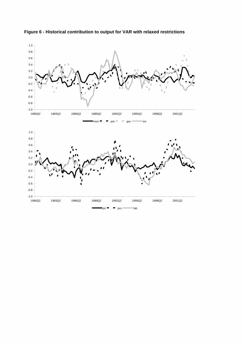
Figure 6 - Historical contribution to output for VAR with relaxed restrictions
-1.0
-0.8
-0.6
-0.4
-0.2
0.0
0.2
0.4
0.6
0.8
1.0
1980Q2 1983Q2 1986Q2 1989Q2 1992Q2 1995Q2 1998Q2 2001Q2
mon pre gov inv
-1.0
-0.8
-0.6
-0.4
-0.2
0.0
0.2
0.4
0.6
0.8
1.0
1980Q2 1983Q2 1986Q2 1989Q2 1992Q2 1995Q2 1998Q2 2001Q2
pri pro lab