■ The value proposition of advice is changing. The nature of what investors expect from advisors is changing. And fortunately, the tools available to advisors are evolving as well.

■ In creating the Vanguard Advisor’s Alpha™ concept in 2001, we outlined how advisors could add value, or alpha, through relationship-oriented services such as providing cogent wealth management via financial planning, discipline, and guidance, rather than by trying to outperform the market.

■ Since then, our work in support of the concept has continued. This paper takes the Advisor’s Alpha framework further by attempting to quantify the benefits that advisors can add relative to others who are not using such strategies. Each of these can be used individually or in combination, depending on the strategy.

■ We believe implementing the Vanguard Advisor’s Alpha framework can add “about 3%” in net returns for your clients and also allow you to differentiate your skills and practice.

Francis M. Kinniry Jr., CFA, Colleen M. Jaconetti, CPA, CFP ®, Michael A. DiJoseph, CFA, and Yan Zilbering

The buck stops here: Vanguard money market funds

Vanguard research March 2014

Putting a value on your value: Quantifying Vanguard Advisor’s Alpha

The value proposition for advisors has always been easier to describe than to define. In a sense, that is how it should be, as value is a subjective assessment and necessarily varies from individual to individual. However, some aspects of investment advice lend themselves to an objective quantification of their potential added value, albeit with a meaningful degree of conditionality. At best, we can only estimate the “value-add” of each tool, because each is affected by the unique client and market environments to which it is applied.

As the financial advice industry continues to gravitate toward fee-based advice, there is a great temptation to define an advisor’s value-add as an annualized number. Again, this may seem appropriate, as fees deducted annually for the advisory relationship could be justified by the “annual value-add.” However, although some of the strategies we describe here could be expected to yield an annual benefit—such as reducing expected investment costs or taxes—the most significant opportunities to add value do not present themselves consistently, but intermittently over the years, and often during periods of either market duress or euphoria. These opportunities can pique an investor’s fear or greed, tempting him or her to abandon a well-thought-out investment plan. In such circumstances, the advisor may have the opportunity to add tens of percentage points of value-add, rather than mere basis points,1 and may more than offset years of advisory fees. And while the value of this wealth creation is certainly real, the difference in your clients’ performance if they stay invested according to your plan, as opposed to abandoning it, does not show up on any client statement. An infinite number of alternate histories might have happened had we made different decisions; yet, we only measure and/or monitor the implemented decision and outcome, even though the other histories were real alternatives. For instance, most client statements don’t keep track of the benefits of talking your clients into “staying the course” in the midst of a bear market or convincing them to rebalance when it doesn’t “feel” like the right thing to do at the time. We don’t measure and show these other outcomes, but their value and impact on clients’ wealth creation is very real, nonetheless.

The quantifications in this paper compare the projected results of a portfolio that is managed using well-known and accepted best practices for wealth management with those that are not. Obviously, the way assets are actually managed versus how they could have been managed will introduce significant variance in the results.

Believing is seeing

What makes one car with four doors and wheels worth $300,000 and another $30,000? Although we might all have an answer, that answer likely differs from person to person. Vanguard Advisor’s Alpha is similarly difficult to define consistently. For some investors without the time, willingness, or ability to confidently handle their financial matters, working with an advisor may be a matter of peace of mind: They may simply prefer to spend their time doing something—anything—else. Maybe they feel overwhelmed by product proliferation in the fund industry, where even the number of choices for the new product on the block—ETFs—exceeds 1,000. While virtually impossible to quantify, in this context the value of an advisor is very real to clients, and this aspect of an advisor’s value proposition, and our efforts here to measure it, should not be negatively affected by the inability to objectively quantify it. By virtue of the fact that the overwhelming majority of mutual fund assets are advised, investors have already indicated that they strongly value professional investment advice. We don’t need to see oxygen to feel its benefits.

Investors who prepare their own tax returns have probably wondered whether an expert like a CPA might do a better job. Are you really saving money by doing your own tax return, or might a CPA save you from paying more tax than necessary? Would you not use a CPA just because he or she couldn’t tell you in advance how much you would save in taxes? If you believe an expert can add value, you see value, even if the value can’t be well quantified in advance. The same reasoning applies to other household services that we pay for—such as painting, house cleaning, or landscaping; these can be considered “negative carry” services, in that we expect to recoup the fees we pay largely through

1 One basis point equals 1/100 of a percentage point.

2

emotional, rather than financial, means. You may well be able to wield a paint brush, but you might want to spend your limited free time doing something else. Or, maybe like many of us, you suspect that a professional painter will do a better job. Value is in the eye of the beholder.

It is understandable that advisors would want a less abstract or less subjective basis for their value proposition. Investment performance thus seems the obvious, quantifiable value-add to focus on. For advisors who promise better returns, the question is: Better returns than what? Better returns than those of a benchmark or “the market”? Not likely, as evidenced by the historical track record of active fund managers, who tend to have experience and resources well in excess of those of most advisors, yet have regularly failed to consistently outperform versus benchmarks in pursuit of excess returns (see Philips, Kinniry, and Schlanger, 2013). Better returns than those provided by an advisor or investor who doesn’t use the value-added practices described here? Probably, as we discuss in the sections following.

Indeed, investors have already hinted at their thoughts on the value of market-beating returns: Over the ten years ended 2013, cash flows into mutual funds have heavily favored broad-based index funds and ETFs, rather than higher-cost actively managed funds (Kinniry, Bennyhoff, and Zilbering, 2013). In essence, investors have chosen investments that are generally structured

to match their benchmark’s return, less management fees. In other words, investors seem to feel there is great value in investing in funds whose expected returns trail, rather than outperform, their benchmarks’ returns.

Why would they do this? Ironically, their approach is sensible, even if “better performance” is the overall goal. Better performance compared to what? Better than the average mutual fund investor in comparable investment strategies. Although index funds should not be expected to beat their benchmark, over the long term they can be expected to better the return of the average mutual fund investor in their benchmark category, because of their lower average cost (Philips et al., 2013). A similar logic can be applied to the value of advice: Paying a fee for advice and guidance to a professional who uses the tools and tactics described here can add meaningful value compared to the average investor experience, currently advised or not. We are in no way suggesting that every advisor—charging any fee—can add value, but merely that advisors can add value if they understand how they can best help investors. Similarly, we cannot hope to define here every avenue for adding value. For example, charitable-giving strategies, key-person insurance, or business-continuation planning can all add tremendous value given the right circumstances, but they certainly do not accurately reflect the “typical” investor experience. The framework for advice that we describe in this paper can serve as the foundation upon which an Advisor’s Alpha can be constructed.

3

Important: The projections or other information generated by the Vanguard Capital Markets Model® regarding the likelihood of various investment outcomes are hypothetical in nature, do not reflect actual investment results, and are not guarantees of future results. VCMM results will vary with each use and over time. These hypothetical data do not respresent the returns on any particular investment. (See also Appendix 2.)

Notes on risk and performance data: All investments, including a portfolio’s current and future holdings, are subject to risk, including the possible loss of the money you invest. Past performance is no guarantee of future returns. The performance of an index is not an exact representation of any particular investment, as you cannot invest directly in an index. Diversification does not ensure a profit or protect against a loss in a declining market. There is no guarantee that any particular asset allocation or mix of funds will meet your investment objectives or provide you with a given level of income. Be aware that fluctuations in the financial markets and other factors may cause declines in the value of your account. Bond funds are subject to the risk that an issuer will fail to make payments on time, and that bond prices will decline because of rising interest rates or negative perceptions of an issuer’s ability to make payments. While U.S. Treasury or government-agency securities provide substantial protection against credit risk, they do not protect investors against price changes due to changing interest rates. U.S. government backing of Treasury or agency securities applies only to the underlying securities and does not prevent share-price fluctuations.

Figure 1 is a high-level summary of tools (organized into seven modules as detailed in the “Vanguard Advisor’s Alpha Quantification Modules” section, see page 9) covering the range of value we believe advisors can add by incorporating wealth-management best practices. Based on our analysis, advisors can potentially add “about 3%” in net returns by using the Vanguard Advisor’s Alpha framework. Because clients only get to keep, spend, or bequest net returns, the focus of wealth management should always be on maximizing net returns. It is important to note that we do not believe this potential 3% improvement can be expected annually; rather, it is likely to be very lumpy. Further, although every advisor has the ability to add this value, the extent of the value will vary based on each client’s unique circumstances and the way the assets are actually managed, versus how they could have been managed. Obviously, although our suggested strategies are universally available to advisors, they are not universally applicable to every client circumstance. Thus, our aim is to motivate advisors to adopt and embrace these best practices and to provide advisors with a reasonable framework for describing and differentiating their value proposition. With these considerations in mind, this paper

focuses on the most common tools for adding value, encompassing both investment-oriented and relationship-oriented strategies and services.

As stated, we provide a more comprehensive description of our analysis in the modules in the latter part of this paper (see page 9). While quantifying the value you can add for your clients is certainly important, it’s equally crucial to understand how following a set of best practices for wealth management such as Vanguard Advisor’s Alpha can influence the success of your advisory practice.

Vanguard Advisor’s Alpha: Good for your clients and your practice

For many clients, entrusting their future to an advisor is not only a financial commitment but also an emotional commitment. Similar to finding a new doctor or other professional service provider, you typically enter the relationship based on a referral or other due diligence. You put your trust in someone and assume he or she will keep your best interests in mind—you trust that person until you have reason not to. The same is true

4

Figure 1. Vanguard quantifies the value-add of best practices in wealth management

Vanguard Advisor’s Alpha strategy modules Module numberValue-add relative to “average” client

experience (in basis points of return)

Suitable asset allocation using broadly diversified funds/ETFs I > 0 bps

Cost-effective implementation (expense ratios) II 45 bps

Rebalancing III 35 bps

Behavioral coaching IV 150 bps

Asset location V 0 to 75 bps

Spending strategy (withdrawal order) VI 0 to 70 bps

Total-return versus income investing VII > 0 bps

Potential value added “About 3%”

Notes: Return value-add for Modules I and VI was deemed significant but too unique for each investor to quantify. See page 9 for detailed descriptions of each module. Also, for “Potential value added,” we did not sum the values because there can be interactions between the strategies. Bps = basis points.Source: Vanguard.

with an advisor. Most investors in search of an advisor are looking for someone they can trust. Yet, trust can be fragile. Typically, trust is established as part of the “courting” process, in which your clients are getting to know you and you are getting to know them. Once the relationship has been established, and the investment policy has been implemented, we believe the key to asset retention is keeping that trust.

So how best can you keep the trust? First and foremost, clients want to be treated as people, not just as portfolios. This is why beginning the client relationship with a financial plan is so essential. Yes, a financial plan promotes more complete disclosure about clients’ investments, but more important, it provides a perfect way for clients to share with the advisor what is of most concern to them: their goals, feelings about risk, their family, and charitable interests. All of these topics are emotionally based, and a client’s willingness to share this information is crucial in building trust and deepening the relationship.

Another important aspect of trust is delivering on your promises—which begs another question: How much control do you actually have over the services promised? At the start of the client relationship, expectations are set regarding the services, strategies, and performance that the client should anticipate from you. Some aspects, such as client contact and meetings, are entirely within your control, which is a good thing: Recent surveys suggest that clients want more contact and responsiveness from their advisors (Spectrem Group, 2012). Not being proactive in contacting clients and not returning phone calls or e-mails in a timely fashion were cited by Spectrem as among the top reasons for changing financial advisors. Consider that in a fee-based practice, an advisor is paid the same whether he or she makes a point of calling clients just to ask how they’re doing or calls only when suggesting a change in their portfolio. That said, a client’s perceived value-add from the “hey, how are you doing?” call is likely to be far greater.

This is not to say that performance is unimportant to clients. Here, advisors have some control, but not total control. Although advisors choose the strategies upon which to build their practices, they cannot control performance. For example, advisors decide how strategic or tactical they want to be with their investments, or how far they are willing to deviate from the broad-market portfolio. As part of this decision process, it’s important to consider how committed you are to a strategy; why a

counterparty may be willing to commit to the other side of the strategy and which party has more knowledge or information, as well as the holding period necessary to see the strategy through. For example, opting for an investment process that deviates significantly from the broad market may work extremely well when you are “right,” but could be disastrous to your clients and practice if your clients lack the patience to stick with the strategy during difficult times.

Human behavior is such that many individuals do not like change. They tend to have an affinity for inertia and, absent a compelling reason not to, are inclined to stick with the status quo. What would it take for a long-time client to leave your practice? The return distribution in Figure 2 illustrates where, in our opinion, the risk of losing clients increases. Although outperformance of the market is possible, history suggests that underperformance is more probable. Thus, significantly tilting your clients’ portfolios away from a market-capitalization-weighted portfolio or engaging in large tactical moves can result in meaningful deviations from the market benchmark return. The farther a client’s portfolio return moves to the left (in Figure 2)—that is, the amount by which the client’s return underperforms his or her benchmark return—the greater the likelihood that a client will remove assets from the advisory relationship.

5

Figure 2. Hypothetical return distribution for portfolios that significantly deviate from a market- cap-weighted portfolio

Ben

chm

ark

retu

rn

Risk of losing clients

1. Client asks questions

2. Client pulls some assets

3. Client pulls most assets

4. Client pulls all assets

Portfolio’s periodic returns

1234

Source: Vanguard.

Do you really want the performance of your client base (and your revenue stream) to be moving in and out of favor all at the same time? The markets are uncertain and cyclical—but your practice doesn’t have to be. To take one example, an advisor may believe that a value-tilted stock portfolio will outperform over the long run; however, he or she will need to keep clients invested over the long run for this belief to even have the possibility of paying off. Historically, there have been periods—sometimes protracted ones—in which value has significantly underperformed the broad market

(see Figure 3). Looking forward, it’s reasonable to expect this type of cyclicality in some way. Recall, however: Your clients’ trust is fragile, and even if you have a deep client relationship with well-established trust, periods of significant underperformance—such as the 12- and 60-month return differentials shown in Figure 3—can undermine this trust. The same holds true for other areas of the market such as sectors, countries, size, duration, and credit, to name a few. (Appendix 1 highlights performance differentials for some of these other market areas.)

6

Figure 3. Relative performance of value versus broad U.S. equity

60-m

on

th r

elat

ive

per

form

ance

d

iffe

ren

tial

–80

–60

–40

–20

0

20

40

60%

201320112009200720052003200119991997199519931991198919871985

Value outperforms

Value underperforms

100% value50% value/50% broad market10% value/90% broad market

Largest performance differentials

Outperform12 months

Underperform

Outperform60 months

Underperform

100% value 28.3% –18.7% 44.4% –66.6%

50% value/50% broad market 13.4% –9.6% 22.0% –34.7%

10% value/90% broad market 2.6% –1.9% 4.4% –7.2%

Notes: Broad U.S. equity is represented by Dow Jones Wilshire 5000 Index through April 22, 2005, MSCI US Broad Market Index through June 2, 2013, and CRSP US Total Market Index through December 31, 2013. Value U.S. equity is represented by Standard & Poor’s 500/Barra Value Index.Sources: Vanguard calculations, based on data from Thompson Reuters Datastream.

7

We are not suggesting that market deviations are unacceptable, but rather that you should carefully consider the size of those deviations, given markets’ cyclicality and investor behavior. As Figure 3 shows, there is a significant performance differential between allocating 50% of a broad-market U.S. equity portfolio to value versus allocating 10% of it to value. As expected, the smaller the deviation from the broad market, the tighter the tracking error and performance differential versus the market. With this in mind, consider allocating a significant portion of your clients’ portfolios to the “core,” which we define as broadly diversified, low-cost, market-cap-weighted investments (see Figure 4)—limiting the deviations to a level that aligns with average investor behavior and your comfort as an advisory practice.

For advisors in a fee-based practice, substantial deviations from a core approach to portfolio construction can have major practice-management implications and can result in an asymmetric payoff when significant deviations from the market portfolio are employed. Because investors commonly report that they hold the majority of their investable assets with a primary advisor (2013 Cogent Wealth Reports, 2013), even if their hoped-for outperformance is realized, the advisor has less to

gain than lose if the portfolio underperforms instead. Although the advisor might gain a little more in assets from the client with a success, the advisor might lose some or even all of the client’s assets in the event of a failure. So when considering significant deviations from the market, make sure your clients and practice are prepared for all the possible implications.

‘Annuitizing’ your practice to ‘infinity and beyond’

In a world of fee-based advice, assets reign. Why? Acquiring clients is expensive, requiring significant investment of your time, energy, and money. Developing a financial plan for a client can take many hours and require multiple meetings, before any investments are implemented. Figure 5 demonstrates that these client costs tend to be concentrated at the beginning of the relationship, if not actually before (in terms of advisor’s overhead and preparation), then moderate significantly over time. In a transaction-fee world, this is where most client-relationship revenues occur, more or less as a “lump sum.” However, in a fee-based practice, the same assets would need to remain with an advisor for several years to generate the same revenue. Hence, assets—and asset retention—are paramount.

Figure 4. Hypothetical return distribution for portfolios that closely resemble a market-cap-weighted portfolio

Ben

chm

ark

retu

rn

1. Client asks questions

2. Client pulls some assets

3. Client pulls most assets

4. Client pulls all assets

Less risk of losing clients

Portfolio’s periodic returns

1234

Source: Vanguard.

Figure 5. Advisor’s alpha “J” curve

Per

-clie

nt

pro

�ta

bili

ty

–5

0

5

10

15%

2 3 5 7 98 100 1 4 6

Years

To “in�nity and beyond”

Trying to get here

Source: Vanguard.

8

Conclusion

“Putting a value on your value” is as subjective and unique as each individual investor. For some investors, the value of working with an advisor is peace of mind. Although this value does not lend itself to objective quantification, it is very real nonetheless. For others, we found that working with an advisor can add “about 3%” in net returns when following the Vanguard Advisor’s Alpha framework for wealth management, particularly for taxable investors. This 3% increase in potential net returns should not be viewed as an annual value-add, but is likely to be intermittent, as some of the most significant opportunities to add value occur during periods of market duress or euphoria when clients are tempted to abandon their well-thought-out investment plan.

It is important to note that the strategies discussed in this paper are available to every advisor; however, the applicability—and resulting value added—will vary by client circumstance (based on each client’s

time horizon, risk tolerance, financial goals, portfolio composition, and marginal tax bracket, to name a few) as well as implementation on the part of the advisor. Our analysis and conclusions are meant to motivate you as an advisor to adopt and embrace these best practices as a reasonable framework for describing and differentiating your value proposition.

The Vanguard’s Advisor’s Alpha framework is not only good for your clients but also good for your practice. With the compensation structure for advisors evolving from a commission- and transaction-based system to a fee-based asset management framework, assets— and asset retention—are paramount. Following this framework can provide you with additional time to spend communicating with your clients and can increase client retention by avoiding significant deviations from the broad-market performance—thus taking your practice to “infinity and beyond.”

9

Module I. Asset allocation ...............................................................................................................................................10

Module II. Cost-effective implementation ..................................................................................................................12

Module III. Rebalancing ....................................................................................................................................................13

Module IV. Behavioral coaching ....................................................................................................................................16

Module V. Asset location ................................................................................................................................................18

Module VI. Withdrawal order for client spending from portfolios .......................................................................20

Module VII. Total-return versus income investing....................................................................................................22

Vanguard Advisor’s Alpha™ Quantification ModulesFor accessibility, our supporting analysis is included here as a separate section. Also for easy reference, we have reproduced below our chart providing a high-level summary of wealth-management best-practice tools and their corresponding modules, together with the range of potential value we believe can be added by following these practices.

Vanguard quantifies the value-add of best practices in wealth management

Vanguard Advisor’s Alpha strategy modules Module number

(see details on pages following)

Value-add relative to “average” client experience

(in basis points of return)

Suitable asset allocation using broadly diversified funds/ETFs I > 0 bps

Cost-effective implementation (expense ratios) II 45 bps

Rebalancing III 35 bps

Behavioral coaching IV 150 bps

Asset location V 0 to 75 bps

Spending strategy (withdrawal order) VI 0 to 70 bps

Total-return versus income investing VII > 0 bps

Potential value added “About 3%”

Notes: Return value-add for Modules I and VI was deemed significant but too unique for each investor to quantify. See Appendix 1 for detailed descriptions of each module. Also for “Potential value-added,” we did not sum the values because there can be interactions between the strategies. Source: Vanguard.

10

It is widely accepted that a portfolio’s asset allocation— the percentage of a portfolio invested in various asset classes such as stocks, bonds, and cash investments, according to the investor’s financial situation, risk tolerance, and time horizon—is the most important determinant of the return variability and long-term performance of a broadly diversified portfolio that engages in limited market-timing (Davis, Kinniry, and Sheay, 2007).

We believe a sound investment plan begins with an individual’s investment policy statement, which outlines the financial objectives for the portfolio as well as any other pertinent information such as the investor’s asset allocation, annual contributions to the portfolio, planned expenditures, and time horizon. Unfortunately, many ignore this critical effort, in part, because like our previous painting analogy, it can be very time-consuming, detail-oriented, and tedious. But unlike house painting, which is primarily decorative, the financial plan is integral to a client’s investment success; it’s the blueprint for a client’s entire financial house and, done well, provides a firm foundation on which all else rests.

Starting your client relationships with a well-thought-out plan can not only ensure that clients will be in the best position possible to meet their long-term financial goals but can also form the basis for future behavioral coaching

conversations. Whether the markets have been performing well or poorly, you can help your clients cut through the noise they hear on a regular basis, noise that often suggests to them that if they’re not making changes in their investments, they’re doing something wrong. The problem is, almost none of what investors are hearing pertains to their specific objectives: Market performance and headlines change far more often than do clients’ objectives. Thus, not reacting to the ever-present noise and sticking to the plan can add tremendous value over the course of your relationship. The process sounds simple, but adhering to an investment plan, given the wide cyclicality in the market and its segments, has proven to be very difficult for investors and advisors alike.

Asset allocation and diversification are two of the most powerful tools advisors can use to help their clients achieve their financial goals and manage investment risk in the process. Since the bear market in the United States from 2000 to 2002, many investors have embraced more complicated portfolios, with more asset classes, than in the past. This is often attributed to equities having two significant bear markets and a “lost decade,” as well as very low yields on traditional high-grade bonds. What is often missed in this is that forward-return expectations should be proportional to forward-risk expectations. It is rare to expect higher returns without a commensurate

Potential value-add: Value is deemed significant but too unique to each investor to quantify, based on each investor’s varying time horizon, risk tolerance, and financial goals.

Module I. Asset allocation

11

increase in risk. Perhaps a way to demonstrate that a traditional long-only, highly liquid, investable portfolio can be competitive is to compare a portfolio of 60% stocks/ 40% bonds to the NACUBO-Commonfund (2014) study on the performance of endowment portfolios, as shown in Figure I-1. The institutions studied have incredibly talented professional staffs as well as unique access, so the expectation of replicating or even coming close to their performance would be considered a tough task. And yet, a portfolio constructed using traditional asset classes—domestic and nondomestic stocks and bonds—held up quite well, outperforming the vast majority (90%) of these endowment portfolios.

Although the traditional 60% stock/40% bond portfolio may not hold as many asset classes as the endowment portfolio, it should not be viewed as unsophisticated. More often than not, these asset classes and the investable index funds and ETFs that track them are perfectly suitable for the investor’s situation. For example, a diversified portfolio using broad-market index funds gives an investor exposure to more than 9,000 individual stocks and 7,500 individual bonds—representing more than 99% and 83% of market-cap coverage for stocks and bonds, respectively. It would be difficult to argue that a portfolio such as this is undiversified, lacking in sophistication, or inadequate. Better yet, the tools for

implementation, such as mutual funds and ETFs, can be very efficient—that is, broadly diversified, low-cost, tax-efficient, and readily available. Taking advantage of these strengths, an asset allocation can be implemented using only a small number of funds. Too simple to charge a fee for, some advisors say, but simple isn’t simplistic. For many, if not most, investors, a portfolio that provides the simplicity of broad asset-class diversification, low-costs, and return transparency can enable the investor to comfortably adopt the investment strategy, embrace it with confidence, and better endure the inevitable ups and downs in the markets. Complexity is not necessarily sophisticated, it’s just complex.

Simple is thus a strength, not a weakness, and can be used to promote better client understanding of the asset allocation and of how returns are derived. When incorporating index funds or ETFs as the portfolio’s “core,” the simplicity and transparency are enhanced, as the risk of portfolio tilts (a source of substantial return uncertainty) is minimized. These features can be used to anchor expectations and to help keep clients invested when headlines and emotions tempt them to abandon the investment plan. The value-add from asset allocation and diversification may be difficult to quantify, but is real and important, nonetheless.

Figure I-1. Comparing performance of endowments and a traditional 60% stock/40% bond portfolio

Large endowments (10% of endowments)

Medium endowments (39% of endowments)

Small endowments (51% of endowments)

60% stock/ 40% bond portfolio

1 year 11.70% 11.92% 11.57% 11.28%

3 years 10.58% 10.01% 9.70% 11.10%

5 years 3.82% 3.63% 3.89% 5.79%

10 years 8.50% 7.22% 6.09% 7.37%

15 years 8.14% 5.97% 4.89% 5.67%

Since July 1, 1985 10.86% 9.28% 8.28% 9.42%

Notes: Data are as of June 30 for each year. Data through June 30, 2013. For the 60% stock/40% bond portfolio: Domestic equity (42%) is represented by Dow Jones Wilshire 5000 Index through April 22, 2005, and MSCI US Broad Market Index thereafter. Non-U.S. equity (18%) is represented by MSCI World ex USA through December 31, 1987 and MSCI All Country World Index ex USA thereafter. Bonds (40%) are represented by Barclays U.S. Aggregate Bond Index. Past performance is no guarantee of future returns. The performance of an index is not an exact representation of any particular investment, as you cannot invest directly in an index.Sources: Vanguard and 2013 NACUBO-Commonfund Study of Endowments (2014).

12

Cost-effective implementation is a critical component of every advisor’s tool kit and is based on simple math: Gross return minus costs (expense ratios, trading or frictional costs, and taxes) equals net return. Every dollar paid for management fees, trading costs, and taxes is a dollar less of potential return for clients. And, for fee-based advisors, this equates to lower growth for their assets under management, the base from which their fee revenues are calculated. As a result, cost-effective implementation is a “win-win” for clients and advisors alike.

If low costs are associated with better investment performance (and research has repeatedly shown this to be true), then costs should play a role in an advisor’s investment selection process. With the recent expansion of the ETF marketplace, advisors now have many more investments to choose from—and ETF costs tend to be among the lowest in the mutual fund industry.

Expanding on Vanguard’s previous research,2 which examines the link between net expense ratios and net cash inflows over the past decade through 2013, we found that an investor could save from 35 bps to 46 bps

annually by moving to low-cost funds, as shown in Figure II-1. By measuring the asset-weighted expense ratio of the entire mutual fund and ETF industry, we found that, depending on the asset allocation, the average investor pays between 47 bps annually for an all-bond portfolio and 61 bps annually for an all-stock portfolio, while the average investor in the lowest quartile of the lowest-cost funds can expect annually to pay between 12 bps (all-bond portfolio) and 15 bps (all-stock portfolio). This includes only the explicit carrying cost (ER) and is extremely conservative when taking into account total investment costs, which often include sales commissions and 12b-1 fees.

It’s important to note, too, that this value-add has nothing to do with market performance. When you pay less, you keep more, regardless of whether the markets are up or down. In fact, in a low-return environment, costs are even more important because the lower the returns, the higher the proportion that is assumed by fund expenses. If you are using higher-cost funds than the asset-weighted average shown in Figure II-1 (47 bps to 61bps), the increase in value could be even higher than stated here.

Figure II-1. Asset-weighted expense ratios versus “low-cost” investing

Stocks/Bonds 100%/0% 80%/20% 60%/40% 50%/50% 40%/60% 20%/80% 0%/100%

Asset-weighted expense ratio 0.61% 0.58% 0.55% 0.54% 0.53% 0.50% 0.47%

“Lowest of the low” 0.15 0.14 0.14 0.14 0.13 0.13 0.12

Cost-effective implementation (expense ratio bps) 0.46 0.44 0.42 0.41 0.39 0.37 0.35

Note: “Lowest of the low” category is the funds whose expense ratios ranked in approximately the lowest 7% of funds in our universe by fund count.Sources: Vanguard calculations, based on data from Morningstar, Inc., as of December 30, 2013.

2 See the Vanguard research paper Costs Matter: Are Fund Investors Voting With Their Feet? (Kinniry, Bennyhoff, and Zilbering, 2013).

Potential value-add: 45 bps annually, by moving to low-cost funds. This value-add is the difference between the average investor experience, measured by the asset-weighted expense ratio of the entire mutual fund and ETF industry, and the lowest-cost funds within the universe. This value could be larger if using higher-cost funds than the asset-weighted averages.

Module II. Cost-effective implementation

13

Given the importance of selecting an asset allocation, it’s also vital to maintain that allocation through time. As a portfolio’s investments produce different returns over time, the portfolio likely drifts from its target allocation, acquiring new risk-and-return characteristics that may be inconsistent with your client’s original preferences. Note that the goal of a rebalancing strategy is to minimize risk, rather than maximize return. An investor wishing to maximize returns, with no concern for the inherent risks, should allocate his or her portfolio to 100% equity to best capitalize on the equity risk premium. The bottom line is that an investment strategy that does not rebalance, but drifts with the markets, has experienced higher volatility. An investor should expect a risk premium for any investment or strategy that has higher volatility.

In a portfolio that is more evenly balanced between stocks and bonds, this equity risk premium tends to result in stocks becoming overweighted relative to a lower risk–return asset class such as bonds; thus, the need to rebalance. Although failing to rebalance may help the expected long-term returns of portfolios (due to the higher weighting of equities than the original allocation), the true benefit of rebalancing is realized in the form of controlling risk. If the portfolio is not rebalanced, the likely result is a portfolio that is overweighted to equities and therefore more vulnerable to equity-market corrections, putting a client’s portfolio at risk of larger losses compared with the 60% stock/40% bond target portfolio, as shown in Figure III-1.

Figure III-1. Equity allocation of 60% stock/40% bond portfolio: Rebalanced and non-rebalanced, 1960 through 2013

Eq

uit

y al

loca

tio

n

60%/40% Equity allocation (rebalanced)60%/40% Equity allocation (non-rebalanced)

40

50

60

70

80

90

100%

198219781974197019641960 1986 1990 1994 1998 2002 2006 2010 2013

Notes: Stocks are represented by Standard & Poor’s 500 Index from 1960 through 1974, Wilshire 5000 Index from 1975 through April 22, 2005, and MSCI US Broad Market Index thereafter. Bonds are represented by S&P High Grade Corporate Index from 1960 through 1968; Citigroup High Grade Index from 1969 through 1972; Barclays U.S. Long Credit AA Bond Index from 1973 through 1975; and Barclays U.S. Aggregate Bond Index thereafter. Sources: Vanguard calculations, based on data from Thompson Reuters Datastream.

Potential value-add: Up to 35 bps when risk-adjusting a 60% stock/40% bond portfolio that is rebalanced annually versus the same portfolio that is not rebalanced (and thus drifts).

Module III. Rebalancing

14

Figure III-2. Portfolio returns and risk: Rebalanced and non-rebalanced, 1960 through 2013

60% stocks/40% bonds 60% stocks/40% bonds (drift) 80% stocks/20% bonds

Average annualized return 9.12% 9.36% 9.71%

Average annual standard deviation 11.41% 14.15% 14.19%

Notes: Stocks are represented by Standard & Poor’s 500 Index from 1960 through 1974, Wilshire 5000 Index from 1975 through April 22, 2005, and MSCI US Broad Market Index thereafter. Bonds are represented by S&P High Grade Corporate Index from 1960 through 1968; Citigroup High Grade Index from 1969 through 1972; Barclays U.S. Long Credit AA Bond Index from 1973 through 1975; and Barclays U.S. Aggregate Bond Index thereafter. Source: Vanguard calculations, based on data from Thompson Reuters Datastream.

Figure III-3. Looking backward, the non-rebalanced (drift) portfolio exhibited risk similar to that of a rebalanced 80% stock/20% bond portfolio

10-y

ear

rolli

ng

an

nu

al

po

rtfo

lio v

ola

tilit

y

198219851981197719731969 1989 1993 1997 2001 2005 2009 2013

20%

0

5

10

15

60%/40% Rebalanced60%/40% Non-rebalanced (drift)80%/20% Rebalanced

Notes: Stocks are represented by Standard & Poor’s 500 Index from 1960 through 1974, Wilshire 5000 Index from 1975 through April 22, 2005, and MSCI US Broad Market Index thereafter. Bonds are represented by S&P High Grade Corporate Index from 1960 through 1968; Citigroup High Grade Index from 1969 through 1972; Barclays U.S. Long Credit AA Bond Index from 1973 through 1975; and Barclays U.S. Aggregate Bond Index thereafter. Sources: Vanguard calculations, based on data from Thompson Reuters Datastream.

During this period (1960–2013), a 60% stock/40% bond portfolio that was rebalanced annually provided a marginally lower return (9.12% versus 9.36%) with significantly lower risk (11.41% versus 14.15%) than a 60% stock/40% bond portfolio that was not rebalanced (drift), as shown in Figure III-2.

Vanguard believes that the goal of rebalancing is to minimize risk, not maximize return. That said, for the sole purpose of assigning a return value for this

quantification exercise, we searched over the same time period for a rebalanced portfolio that exhibited similar risk as the non-rebalanced portfolio. We found that an 80% stock/20% bond portfolio provided similar risk as measured by standard deviation (14.19% versus 14.15%) with a higher average annualized return (9.71% versus 9.36%), as shown in Figures III-2 and III-3.

15

Looking forward, we would not expect the risk of a 60% stock/40% bond portfolio that drifts to match the risk of an 80% stock/20% bond portfolio; however, we believe the equity risk premium will persist, and that investors who do not rebalance over long time periods will have higher returns than the target portfolio, and as such, higher risk. One could argue that if an investor is comfortable with the higher risk of the non-rebalanced portfolio, he or she should simply select the higher equity allocation from inception and rebalance to that allocation through time.

Helping investors to stay committed to their asset allocation strategy and remain invested in the markets increases the probability of their meeting their goals, but the task of rebalancing is often an emotional challenge. Historically, rebalancing opportunities have occurred when there has been a wide dispersion between the returns of different asset classes (such as stocks and bonds). Whether in bull or bear markets, reallocating assets from the better-performing asset classes to the worse-performing ones feels counterintuitive to the “average” investor. An advisor can provide the discipline to rebalance when rebalancing is needed most, which is often when the thought of rebalancing is a very uncomfortable leap of faith.

Keep in mind, too, that rebalancing is not necessarily free: There are costs associated with any rebalancing strategy, including taxes and transaction costs, as well as time and labor on the part of advisors. These costs could all potentially reduce your client’s return. An advisor can add value for clients by balancing these trade-offs, thus potentially minimizing the associated costs. For example, a portfolio can be rebalanced with cash flows by directing dividends, interest payments, realized capital gains, and/or new contributions to the most underweight asset class. This not only can keep the client’s asset allocation closer to its target but can also trim the costs of rebalancing. An advisor can furthermore determine whether to rebalance to the target asset allocation or to an intermediate allocation, based on the type of rebalancing costs. When trading costs are mainly fixed and independent of the size of the trade—the cost of time, for example—rebalancing to the target allocation is optimal because it reduces the need for further transactions. When trading costs are mainly proportional to the size of the trade—as with commissions or taxes, for example—rebalancing to the closest rebalancing boundary is optimal, minimizing the size of the transaction.3 Advisors who can systematically direct investor cash flows into the most underweighted asset class and/or rebalance to the “most appropriate” boundary are likely to reduce their clients’ rebalancing costs and thereby increase the returns their clients keep.

3 See the Vanguard research paper Best Practices for Portfolio Rebalancing (Jaconetti, Kinniry, and Zilbering, 2010).

16

Because investing evokes emotion, advisors need to help their clients maintain a long-term perspective and a disciplined approach—the amount of potential value an advisor can add here is large. Most investors are aware of these time-tested principles, but the hard part of investing is sticking to them in the best and worst of times—that is where you, as a behavioral coach to your clients, can earn your fees and then some. Abandoning a planned investment strategy can be costly, and research has shown that some of the most significant derailers are behavioral: the allure of market-timing and the temptation to chase performance.

Persuading investors not to abandon the markets when performance has been poor or dissuading them from chasing the next “hot” investment—this is where you need to remind your clients of the plan you created before emotions were involved. This is where the faith and trust that clients have in an advisor is key: Strong relationships need to be established before the bull- and bear-market periods that challenge investors’ confidence in the plan detailed for them. Thankfully, as stated earlier, these potentially disruptive markets tend to occur only sporadically. Advisors, as behavioral coaches, can act as emotional circuit breakers by circumventing clients’ tendencies to chase returns or run for cover in emotionally charged markets. In the process, advisors may save their clients from significant wealth destruction and also add percentage points—rather than basis points—of value. A single client intervention, such as we’ve just described, could more than offset years of advisory fees. The following example from the most recent period of “fear and greed” can provide context in quantifying this point.

In a recent Vanguard study, we analyzed the personal performance of 58,168 self-directed Vanguard IRA® investors over the five years ended December 31, 2012,

an extremely tumultuous period in the global markets. These investors’ returns were compared to the returns of the applicable Vanguard Target Retirement Funds for the same five-year period. For the purpose of our example, we are assuming that Vanguard target-date funds provide some of the structure and guidance that an advisor might have provided. The result was that a majority of investor returns trailed their target-date fund benchmark slightly, which might be expected based on the funds’ expense ratios alone. However, investors who exchanged money between funds or into other funds fared considerably worse.

In Figure IV-1, which highlights results of this Vanguard study, the purple-shaded area illustrates the degree of underperformance of accounts with exchanges relative

Figure IV-1. Vanguard target-date fund benchmark comparison: 2008–2012

Per

cen

tag

e o

f ac

cou

nts

0

3

6

9

12

15%

–10 –8 –4 0 4 8 12 162 6 10 14–14 –12 –6 –2

Accounts with an exchangeNo exchange

Excess return (percentage points)

Notes: Average value with exchange, −1.50%; average value with no exchange, −0.19%.Source: Vanguard.

Note: Investments in Target Retirement Funds are subject to the risks of their underlying funds. The year in the Fund name refers to the approximate year (the target date) when an investor in the Fund would retire and leave the workforce. The Fund will gradually shift its emphasis from more aggressive investments to more conservative ones based on its target date. An investment in the Target Retirement Fund is not guaranteed at any time, including on or after the target date.

Potential value-add: Based on a Vanguard study of actual client behavior, we found that investors who deviated from their initial retirement fund investment trailed the target-date fund benchmark by 150 bps. This suggests that the discipline and guidance that an advisor might provide through behavioral coaching could be the largest potential value-add of the tools available to advisors. In addition, Vanguard research and other academic studies have concluded that behavioral coaching can add 1% to 2% in net return.

Module IV. Behavioral coaching

17

to those that did not make an exchange. The “average” investor who made even one exchange over the entire five-year period through 2012 trailed the applicable Vanguard target-date fund benchmark by 150 bps. Investors who refrained from such activity lagged the benchmark by only 19 bps.

Another common method of analyzing mutual fund investor behavior is to compare investor returns (internal rates of return, IRRs) to fund returns (time-weighted returns, TWRs) over time. Although all mandates should expect a return drag versus the benchmark over longer periods due to more money continually coming into a growing mutual fund market and a rising market, larger differences can be a sign of performance-chasing. Using the IRR–TWR method, we note that history suggests that investors commonly receive much lower returns from the

funds they invest in, since cash flows tend to be attracted by, rather than precede, higher returns (see Figure IV-2). History also shows that, on average, the drag is significantly more pronounced in funds that are more concentrated, narrow, or different from the overall market (see the nine style boxes grouped on the left in Figure IV-2) and is much less pronounced for broad index funds, especially balanced index funds (see Figure IV-2). The Vanguard Advisor’s Alpha framework was constructed with a firm awareness of these behavioral tendencies. Its foundation is built upon having a significant allocation to the “core” portfolio, which is broadly diversified, low-cost, and market-cap-weighted, while limiting the satellite allocation to a level that is appropriate for each investor and practice.

Figure IV-2. Investor returns versus fund returns: Ten years ended December 31, 2013

Notes: The time-weighted returns in this figure represent the average fund return in each category. Morningstar Investor Return™ assumes that the growth of a fund’s total net assets for a given period is driven by market returns and investor cash flow. To calculate investor return, a fund’s change in assets for the period is discounted by the return of the fund, to isolate how much of the asset growth was driven by cash flow. A proprietary model, similar to an internal rate-of-return calculation, is then used to calculate a constant growth rate that links the beginning total net assets and periodic cash flows to the ending total net assets. Discrepancies in the return “difference” are due to rounding.Sources: Vanguard calculations, based on data from Morningstar, Inc.

Value Blend GrowthConservative

allocationModerate allocation

Larg

e

6.97% 6.93% 7.60% 5.06% 6.06%

5.14 5.54 6.21 4.24 4.96

–1.83 –1.39 –1.39 –0.82 –1.10

Mid

8.95 8.58 9.01

6.69 6.73 7.80

–2.26 –1.85 –1.21

Sm

all

9.25 9.04 9.15

8.11 7.70 6.83

–1.14 –1.34 –2.32

Time-weighted returnInvestor returnDifferential

18

Asset location, the allocation of assets between taxable and tax-advantaged accounts, is one tool an advisor can use that can add value each year, with an expectation that the benefits will compound through time.4 From a tax perspective, optimal portfolio construction minimizes the impact of taxes by holding tax-efficient broad-market equity investments in taxable accounts and by holding taxable bonds within tax-advantaged accounts. This arrangement takes maximum advantage of the yield spread between taxable and municipal bonds, which can generate a higher and more certain return premium. And those incremental differences have a powerful compounding effect over the long run. Our research

has shown that constructing the portfolio in this manner can add up to 75 bps of additional return in the first year, without increasing risk (see Figure V-1).

For investors or advisors who want to include active strategies—such as actively managed equity funds (or ETFs), REITs, or commodities—these investments should be purchased within tax-advantaged accounts before taxable bonds because of their tax-inefficiency; however, this likely means giving up space within tax-advantaged accounts that would otherwise have been devoted to taxable bonds—thereby giving up the extra return generated by the taxable–municipal spread.5

Figure V-1. Asset location can add up to 75 bps of value annually to a portfolio

Taxable accounts Tax-deferred accountsPre-tax return

After-tax return

Relative to optimal (Row A)

A. Index equity (50%) Taxable bonds (40%) and equity (10%) 6.60% 6.38% N.A.

B. Taxable bonds (40%) and index equity (10%) Equity (50%) 6.60% 6.08% (0.30%)

C. Municipal bonds (40%) and index equity (10%) Equity (50%) 6.24% 6.19% (0.19%)

D. Active equity (50%) Taxable bonds (40%) and equity (10%) 6.60% 5.61% (0.77%)

Notes: Pre-tax and after-tax returns are based on the following assumptions: Taxable bond return, 3.00%; municipal bond return, 2.40%; index equity, 9.00% (1.80% for dividends, 0.45% for long-term capital gains, and 6.75% for unrealized gains); active equity, 9.00% (1.80% for dividends, 1.80% for short-term capital gains, 4.50% for long-term capital gains, and 0.90% for unrealized gains). This analysis uses a marginal U.S. income tax rate of 39.6% for income and short-term capital gains and 20% for long-term capital gains. These values do not assume liquidation. See Jaconetti (2007) for more details.Source: Vanguard.

4 Absent liquidity constraints, wealth-management best practices would dictate maximizing tax-advantaged savings opportunities.5 The taxable–municipal spread is the difference between the yields on taxable bonds and municipal bonds.

Potential value-add: 0 to 75 bps, depending on the investor’s asset allocation and “bucket” size (the breakdown of assets between taxable and tax-advantaged accounts). The majority of the benefits occur when the taxable and tax-advantaged accounts are roughly equal in size, the target allocation is in a balanced portfolio, and the investor is in a high marginal tax bracket. If an investor has all of his or her assets in one account type (that is, all taxable or all tax-advantaged), the value of asset location is 0 bps.

Module V. Asset location

19

This is because purchasing actively managed equities or taxable bonds in taxable accounts frequently results in higher taxes because your client will be subject to:

1. Paying a federal marginal income tax rate on taxable bond income. This could be as high as 39.6%. One could, of course, purchase municipal bonds, but the result would be to forgo the taxable–municipal income spread.

2. Paying a long-term capital gains tax rate as high as 15% or 20%, depending on income, on long-term capital gains/distributions and the client’s marginal income tax rate on short-term gains. (To the extent the portfolio includes actively managed equity funds, capital gains distributions are more likely.)

3. Paying a tax rate on qualified dividend income also as high as 15% or 20% from equities, depending on income.

By contrast, purchasing tax-efficient broad-market equity funds or ETFs in taxable accounts will still be subject to the preceding points 2 and 3; however, the amount of income or capital gains distributions will likely be significantly lower.

Advisors may decide to incorporate active strategies in tax-advantaged accounts before fulfilling a client’s strategic allocation to bonds, for several reasons. First, the advisor may believe that the alternate investment can potentially generate an excess return large enough to not only offset the yield spread but also the higher costs associated with these investments.6 Or, second, the advisor may decide that the alternate investments bring sufficient benefits in other ways, such as risk reduction as a result of additional diversification within the portfolio. Although these beneficial outcomes are both possible, they are not highly probable and are certainly less probable compared to capturing the return premium offered by taxable bonds when held in tax-advantaged registrations.

In addition, estate-planning benefits may result from placing broad-market equity index funds or ETFs in taxable accounts; because broad-market equity investments usually provide more deferred capital appreciation than bonds over the long term, the taxable assets have the added advantage of a potentially larger step-up in cost basis for heirs.

6 See the Vanguard research paper The Case for Index-Fund Investing (Philips et al., 2013).

20

Potential value-add: Up to 70 bps, depending on the investor’s “bucket” size (the breakdown of assets between taxable and tax-advantaged accounts) and marginal tax bracket. The greatest benefits occur when the taxable and tax-advantaged accounts are roughly equal in size and the investor is in a high marginal tax bracket. If an investor has all of his or her assets in one account type (that is, all taxable or all tax-advantaged), or an investor is not currently spending from the portfolio, the value of the withdrawal order is 0 bps.

Module VI. Withdrawal order for client spending from portfolios

Figure VI-1a. Average internal rate of return of different withdrawal-order strategies

Inte

rnal

rat

e o

f re

turn

Spend taxableassets before

tax-advantaged

0

1

2

3

4

5%

Spend from tax-deferred assets

before taxable

Spend from tax-free assetsbefore taxable

3.7% 3.6%

4.4%

Important note: These hypothetical data do not represent the returns on any particular investment. Each internal rate of return (IRR) is calculated by running the same 10,000 VCMM simulations through three separate models, each designed to replicate the stated withdrawal order strategy listed.Source: Vanguard.

Assumptions for our analysis

Portfolio 60% stocks/40% bonds

Equity allocation 70% U.S./30% international

Fixed income allocation 80% U.S./20% international

Time horizon 30 years

Marginal U.S. income tax rate 39.6%

Long-term capital gains tax rate 20%

With the retiree population on the rise, an increasing number of clients are facing important decisions about how to spend from their portfolios. Complicating matters is the fact that many clients hold multiple account types, including taxable, tax-deferred (such as a traditional 401(k) or IRA), and/or tax-free (such as a Roth 401(k) or IRA) accounts. Advisors who implement informed withdrawal-order strategies can minimize the total taxes paid over the course of their clients’ retirement, thereby increasing their clients’ wealth and the longevity of their portfolios. This process alone could represent the entire value proposition for the fee-based advisor.

The primary determinant of whether one should spend from taxable assets or tax-advantaged assets7 is taxes. Absent taxes, the order of which account to draw from would yield identical results (assuming accounts earned the same rates of return). Advisors can minimize the impact of taxes on their clients’ portfolios by spending in the following order: Required minimum distributions (RMDs), if applicable, followed by cash flows on assets held in taxable accounts, taxable assets, and finally tax-advantaged assets8 (see Figure VI-1 and the accompanying explanation on the next page). Our research has shown that spending from the portfolio in this manner can add up to 70 bps of average annualized value without any additional risk.

To calculate this value, we compared the internal rate of return (IRR) of this spending order to that of two alternate spending orders in which tax-advantaged assets were tapped before taxable assets. The orders are as follows: (1) spending from tax-deferred assets before taxable assets and (2) spending from tax-free assets before taxable assets. In both cases, accelerating spending from tax-advantaged accounts resulted in lower terminal wealth.

7 Tax-advantaged assets include both tax-deferred and tax-free (Roth accounts).8 Clearly, an investor’s specific financial plan may warrant a different spending order, but this framework can serve as a prudent guideline for most investors.

See Spending From a Portfolio: Implications of Withdrawal Order for Taxable Investors (Jaconetti and Bruno, 2008), for a more detailed analysis.

21

• RMDs are the first assets to be used for spending, because they are required to be taken by law for retired investors more than 70½ years old who own assets in tax-deferred accounts. For investors who are not subject to RMDs or who need monies in excess of their RMDs, the next source of spending should be cash flows from assets held in taxable accounts, including interest, dividends, and capital gains distributions, followed by assets held in taxable accounts.

• Investors should deplete their taxable assets before spending from their tax-deferred accounts, because swapping the order would accelerate the payment of income taxes. Taxes on tax-deferred accounts will likely be higher than taxes on withdrawals from taxable accounts, for two reasons. First, the investor will pay ordinary income taxes on the entire withdrawal (assuming the contributions were made with pre-tax dollars), rather than just paying capital gains taxes on the capital appreciation. Second, ordinary income tax rates are currently higher than the respective capital gains tax rates, so the investor would have to pay a higher tax rate on a larger withdrawal amount if he or she spends from the tax-deferred accounts first. Over time, the acceleration of income taxes and the resulting loss of tax-deferred growth can negatively affect the portfolio, resulting in lower terminal wealth values and success rates.

• Investors should likewise consider spending from their taxable accounts before spending from their tax-free accounts, to maximize the long-term growth of their overall portfolio. Reducing the amount of assets that have tax-free growth potential can result in lower terminal wealth values and success rates.

• Once the order of withdrawals between taxable and tax-advantaged accounts has been determined, the next step is to specifically identify which asset or assets to sell to meet spending needs. Within the taxable portfolio, an investor should first spend his or her portfolio cash flows. This is because these monies are taxed regardless of whether they are spent or reinvested into the portfolio. Reinvesting these monies and then selling the assets later to meet spending needs could result in short-term capital gains, which are currently taxed at ordinary income tax rates. Next the investor should consider selling the asset or assets that would produce the lowest taxable gain, or would even realize a loss. This should continue until the spending need has been met or the taxable portfolio has been exhausted.

• Once an investor’s taxable accounts have been depleted, he or she must decide whether to spend first from tax-deferred or tax-free (Roth) accounts. The primary driver of this decision is the investor’s expectations for future tax rates relative to his or her current tax rate. If an investor anticipates that his or her future tax rate will be higher than the current tax rate, then spending from tax-deferred accounts should take priority over spending from tax-free accounts. This allows the investor to lock in taxes on the tax-deferred withdrawals today at the lower rate, rather than allowing the tax-deferred account to continue to grow and be subject to a higher tax rate on future withdrawals. Conversely, if an investor anticipates his or her future tax rate will be lower than the current tax rate, spending from the tax-free assets should take priority over spending from the tax-deferred assets. Taking distributions from the tax-deferred account at the future lower tax rate will result in lower taxes over the entire investment horizon.

Taxable portfolio

RMDs (if applicable)

Taxable �ows

Tax-free

Higher expected marginaltax bracket in the future

Tax-deferred

Tax-deferred

Lower expected marginaltax bracket in the future

Tax-free

BA

Figure VI-1b. Detailed spending order and explanation

22

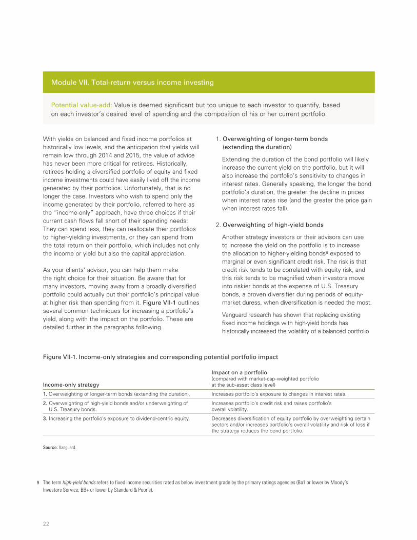
Figure VII-1. Income-only strategies and corresponding potential portfolio impact

Income-only strategy

Impact on a portfolio (compared with market-cap-weighted portfolio at the sub-asset class level)

1. Overweighting of longer-term bonds (extending the duration). Increases portfolio’s exposure to changes in interest rates.

2. Overweighting of high-yield bonds and/or underweighting of U.S. Treasury bonds.

Increases portfolio’s credit risk and raises portfolio’s overall volatility.

3. Increasing the portfolio’s exposure to dividend-centric equity. Decreases diversification of equity portfolio by overweighting certain sectors and/or increases portfolio’s overall volatility and risk of loss if the strategy reduces the bond portfolio.

Source: Vanguard.

With yields on balanced and fixed income portfolios at historically low levels, and the anticipation that yields will remain low through 2014 and 2015, the value of advice has never been more critical for retirees. Historically, retirees holding a diversified portfolio of equity and fixed income investments could have easily lived off the income generated by their portfolios. Unfortunately, that is no longer the case. Investors who wish to spend only the income generated by their portfolio, referred to here as the “income-only” approach, have three choices if their current cash flows fall short of their spending needs: They can spend less, they can reallocate their portfolios to higher-yielding investments, or they can spend from the total return on their portfolio, which includes not only the income or yield but also the capital appreciation.

As your clients’ advisor, you can help them make the right choice for their situation. Be aware that for many investors, moving away from a broadly diversified portfolio could actually put their portfolio’s principal value at higher risk than spending from it. Figure VII-1 outlines several common techniques for increasing a portfolio’s yield, along with the impact on the portfolio. These are detailed further in the paragraphs following.

1. Overweighting of longer-term bonds (extending the duration)

Extending the duration of the bond portfolio will likely increase the current yield on the portfolio, but it will also increase the portfolio’s sensitivity to changes in interest rates. Generally speaking, the longer the bond portfolio’s duration, the greater the decline in prices when interest rates rise (and the greater the price gain when interest rates fall).

2. Overweighting of high-yield bonds

Another strategy investors or their advisors can use to increase the yield on the portfolio is to increase the allocation to higher-yielding bonds9 exposed to marginal or even significant credit risk. The risk is that credit risk tends to be correlated with equity risk, and this risk tends to be magnified when investors move into riskier bonds at the expense of U.S. Treasury bonds, a proven diversifier during periods of equity-market duress, when diversification is needed the most.

Vanguard research has shown that replacing existing fixed income holdings with high-yield bonds has historically increased the volatility of a balanced portfolio

Potential value-add: Value is deemed significant but too unique to each investor to quantify, based on each investor’s desired level of spending and the composition of his or her current portfolio.

Module VII. Total-return versus income investing

9 The term high-yield bonds refers to fixed income securities rated as below investment grade by the primary ratings agencies (Ba1 or lower by Moody’s Investors Service; BB+ or lower by Standard & Poor’s).

23

by an average of 78 basis points annually.10 This is because high-yield bonds are more highly correlated with the equity markets and are more volatile than investment-grade bonds. Investors who employ such a strategy are certainly sacrificing diversification benefits in hopes of receiving higher current income from the portfolio.

3. Increasing the portfolio’s exposure to dividend-centric equity

An often-advocated equity approach to increase income is to shift some or all of a fixed income allocation into higher-yielding dividend-paying stocks. But, stocks are not bonds. At the end of the day, stocks will perform like stocks—that is, they have higher volatility and the potential for greater losses. Moreover, dividend stocks are correlated with stocks in general, whereas bonds show little to no correlation to either stocks in general or dividend-paying stocks. If you view fixed income as not just providing yield but also diversification, dividend-paying stocks fall well short as a substitute.

A second approach investors may take is to shift from broad-market equity to dividend- or income-focused equity. However, these investors may be inadvertently changing the risk profile of their portfolio, because dividend-focused equities tend to display a significant bias toward “value stocks.”11 Although value stocks are generally considered to be a less risky subset of the broader equity market,12 the risks nevertheless can be substantial, owing to the fact that portfolios focused on dividend-paying stocks tend to be overly concentrated in certain individual stocks and sectors.

In addition, when employing an income-only approach, asset location is typically driven by accessing the income at the expense of tax-efficiency. As a result, investors/advisors are more likely to purchase taxable bond funds and/or income-oriented stock funds in taxable accounts so that investors can gain access to the income (yield) from these investments. Following this approach will most likely increase taxes on the portfolio, resulting in a direct reduction in spending.

Benefits of a total-return approach to investing

In pursuing the preceding income strategies, some may feel they will be rewarded with a more certain return and therefore less risk. But in reality, this is increasing the

portfolio’s risk as it becomes too concentrated in certain sectors, with less tax-efficiency and with a higher chance of retirees falling short of their long-term financial goals.

As a result, Vanguard believes in a total-return approach, which considers both components of total return: income plus capital appreciation. The total-return approach has the following potential advantages over an income-only method:

• Less risk. A total-return approach allows better diversification, instead of concentrating on certain securities, market segments, or industry sectors to increase yield.

• Better tax-efficiency. A total-return approach allows more tax-efficient asset locations (for clients who have both taxable and tax-advantaged accounts). An income approach focuses on access to income, resulting in the need to keep tax-inefficient assets in taxable accounts.

• Potentially longer lifespan for the portfolio, stemming from the previous factors.

Certainly, to employ a tax-efficient, total-return strategy in which the investor requires specific cash flows to meet his or her spending needs involves substantial analysis, experience, and transactions. To do this well is not easy, and this alone could also represent the entire value proposition of an advisory relationship.

10 See the Vanguard research paper Worth the Risk? The Appeal and Challenge of High-Yield Bonds (Philips, 2012).11 See the Vanguard research paper Total-Return Investing: An Enduring Solution for Low Yields (Jaconetti, Kinniry, and Zilbering, 2012). 12 “Less risky” should not be taken to mean “better.” Going forward, value stocks should have a risk-adjusted return similar to that of the broad equity market,

unless there are risks that are not recognized in traditional volatility metrics.

So where should you begin? We believe you should focus on those areas in which you have control, at least to some extent, such as:

• Helping your clients select the asset allocation that is most appropriate to meeting their goals and objectives, given their time horizon and risk tolerance.

• Implementing the asset allocation using low-cost investments and, to the extent possible, using asset-location guidelines.

• Limiting the deviations from the market portfolio, which will benefit your clients and your practice.

• Concentrating on behavioral coaching and spending time communicating with your clients.

Modules conclusion

24

References

Bennyhoff, Donald G., and Yan Zilbering, 2009. Market-Timing: A Two-Sided Coin. Valley Forge, Pa.: The Vanguard Group.

Bennyhoff, Donald G., and Colleen M. Jaconetti, 2013. Required or Desired Returns? That Is the Question. Valley Forge, Pa.: The Vanguard Group.

Bennyhoff, Donald G., and Francis M. Kinniry Jr., 2013 (rev. ed). Advisor’s Alpha. Valley Forge, Pa.: The Vanguard Group.

Bruno, Maria A., Colleen M. Jaconetti, and Yan Zilbering, 2013. Revisiting the ‘4% Spending Rule.’ Valley Forge, Pa.: The Vanguard Group.

Davis, Joseph H., Francis M. Kinniry Jr., and Glenn Sheay, 2007. The Asset Allocation Debate: Provocative Questions, Enduring Realities. Valley Forge, Pa.: The Vanguard Group.

Davis, Joseph, Roger Aliaga-Díaz, Charles J. Thomas, and Andrew J. Patterson, 2014. Vanguard’s Economic and Investment Outlook. Valley Forge, Pa.: The Vanguard Group.

Jaconetti, Colleen M., 2007. Asset Location for Taxable Investors. Valley Forge, Pa.: The Vanguard Group.

Jaconetti, Colleen M., and Maria A. Bruno, 2008. Spending From a Portfolio: Implications of Withdrawal Order for Taxable Investors. Valley Forge, Pa.: The Vanguard Group.

Jaconetti, Colleen M., Francis M. Kinniry Jr., and Yan Zilbering, 2010. Best Practices for Portfolio Rebalancing. Valley Forge, Pa.: The Vanguard Group.

Jaconetti, Colleen M., Francis M. Kinniry Jr., and Yan Zilbering, 2012. Total-Return Investing: An Enduring Solution for Low Yields. Valley Forge, Pa.: The Vanguard Group.

Kinniry, Francis M., Jr., Donald G. Bennyhoff, and Yan Zilbering, 2013. Costs Matter: Are Fund Investors Voting With Their Feet? Valley Forge, Pa.: The Vanguard Group.

Philips, Christopher B., 2012. Worth the Risk? The Appeal and Challenge of High-Yield Bonds. Valley Forge, Pa.: The Vanguard Group.

Philips, Christopher B., Francis M. Kinniry Jr., and Todd Schlanger, 2013. The Case for Index-Fund Investing. Valley Forge, Pa.: The Vanguard Group.

Spectrem Group, 2012. Ultra High Net Worth Investor Attitudes and Behaviors: Relationships with Advisors. Chicago: Spectrem Group, 20.

2013 Cogent Wealth Reports: Investor Brandscape, 2013. The Investor-Advisor Relationship. Livonia, Mich.: Market Strategies International, 23.

2013 NACUBO-Commonfund Study of Endowments, 2014. National Association of College and University Business Officers. Washington, D.C.: NACUBO.

Weber, Stephen M., 2013, Most Vanguard IRA® Investors Shot Par by Staying the Course: 2008–2012, Valley Forge, Pa.: The Vanguard Group.

25

Figure A-1. Relative performance of U.S. equity and U.S. bonds

Per

form

ance

dif

fere

nti

al

12-month return differential36-month return differential60-month return differential

–100

–50

0

50

100

150

200%

201320102007200420011998199519921989198619831980

U.S. equity underperforms

U.S. equity outperforms

Largest performance differentials

1 month

12 months

36 months

60 months

U.S. equity outperforms 12.1% 47.1% 95.4% 186.0%

U.S. equity underperforms –25.1% –45.3% –73.8% –61.7%

Notes: U.S. bonds are represented by Barclays U.S. Aggregate Bond Index; U.S. equity is represented by Dow Jones Wilshire 5000 Index through April 22, 2005, MSCI US Broad Market Index through June 2, 2013, and CRSP US Total Market Index through December 31, 2013. Sources: Vanguard calculations, based on data from Thompson Reuters Datastream.

Appendix 1. Relative performance charts

26

Figure A-2. Relative performance of U.S. equity and non-U.S. equity

Per

form

ance

dif

fere

nti

al

12-month return differential36-month return differential60-month return differential

201320102007200420011998199519921989198619831980

U.S. equity underperforms

U.S. equity outperforms

–200

–150

–100

–50

0

50

100

150

200%

Largest performance differentials

1 month

12 months

36 months

60 months

U.S. outperforms 12.6% 31.5% 98.0% 167.1%

U.S. underperforms –15.7% –32.6% –96.6% –136.9%

Notes: U.S. equity is represented by Dow Jones Wilshire 5000 Index through April 22, 2005, MSCI US Broad Market Index through June 2, 2013, and CRSP US Total Market Index thereafter; non-U.S. equity is represented by MSCI World Index through December 31, 1987, and MSCI All Country World Index ex US through December 31, 2013.Sources: Vanguard calculations, based on data from Thompson Reuters Datastream.

Figure A-3. Relative performance of large and small U.S. equity

Per

form

ance

dif

fere

nti

al

12-month return differential36-month return differential60-month return differential

–100

–50

0

50

100

150

200%

201320102007200420011998199519921989198619831980

Large underperforms

Large outperforms

Largest performance differentials

1 month

12 months

36 months

60 months

Large outperforms 16.4% 34.7% 85.8% 150.5%

Large underperforms –18.4% –37.5% –66.9% –64.4%

Notes: Large-cap U.S. equity is represented by S&P 500 Index through December 31, 1983, MSCI US Prime Market 750 Index through January 30, 2013, and CRSP US Large Cap Index thereafter; small-cap U.S. equity is represented by Russell 2000 Index through May 16, 2003, MSCI US Small Cap 1750 Index through January 30, 2013, and CRSP US Small Cap Index thereafter.Sources: Vanguard calculations, based on data from Thompson Reuters Datastream.

27

Figure A-4. Relative performance of developed and emerging-markets equity

Per

form

ance

dif

fere

nti

al

12-month return differential36-month return differential60-month return differential

–400

–300

–200

–100

0

100

200%

201320102007200420011998199519921989198619831980

Developed underperforms

Developed outperforms

Largest performance differentials

1 month

12 months

36 months

60 months

Developed outperforms 15.6% 56.5% 101.7% 150.3%

Developed underperforms –16.7% –64.7% –171.8% –333.4%

Notes: Developed equity is represented by MSCI World Index; emerging equity is represented by MSCI Emerging Markets Index. Performance differential begins in 1989 because of a lack of emerging market equity data before 1988.Sources: Vanguard calculations, based on data from Thompson Reuters Datastream.

Figure A-5. Relative performance of value and growth: U.S. equity

Per

form

ance

dif

fere

nti

al

12-month return differential36-month return differential60-month return differential

201320102007200420011998199519921989198619831980

Value underperforms

Value outperforms

–200

–150

–100

–50

0

50

100

150

200%

Largest performance differentials

1 month

12 months

36 months

60 months

Value outperforms 9.7% 40.4% 35.0% 58.7%

Value underperforms –12.0% –27.5% –84.7% –147.3%

Notes: Value U.S. equity is represented by S&P 500/Barra Value Index through May 16, 2003, MSCI US Prime Market Value Index through April 16, 2013, and CRSP US Large Cap Value Index through December 31, 2013; growth U.S. equity is represented by S&P 500/Barra Growth Index through May 16, 2003, MSCI US Prime Market Growth Index through April 16, 2013, and CRSP US Large Cap Growth Index thereafter. Sources: Vanguard calculations, based on data from Thompson Reuters Datastream.

© 2014 The Vanguard Group, Inc. All rights reserved. Vanguard Marketing Corporation, Distributor.

ISGQVAA 032014

Vanguard Research

P.O. Box 2600 Valley Forge, PA 19482-2600

Connect with Vanguard® > vanguard.com > research@vanguard.com

For more information about Vanguard funds, visit vanguard.com, or call 800-662-2739, to obtain a prospectus. Investment objectives, risks, charges, expenses, and other important information about a fund are contained in the prospectus; read and consider it carefully before investing.

Morningstar data: ©2014 Morningstar, Inc. All Rights Reserved. The information contained herein: (1) is proprietary to Morningstar and/or its content providers; (2) may not be copied or distributed; (3) does not constitute investment advice offered by Morningstar; and (4) is not warranted to be accurate, complete, or timely. Neither Morningstar nor its content providers are responsible for any damages or losses arising from any use of this information. Past performance is no guarantee of future results.

CFA® is a trademark owned by CFA Institute.

Appendix 2. About the Vanguard Capital Markets Model

The Vanguard Capital Markets Model (VCMM) is a proprietary financial simulation tool developed and maintained by Vanguard’s Investment Strategy Group. Part of the tool is a dynamic module that employs vector autoregressive methods to simulate forward-looking return distributions on a wide array of broad asset classes, including stocks, taxable bonds, and cash. For the VCMM simulations in Figure V-1, we used market data available through June 30, 2013, for the U.S. Treasury spot yield curves. The VCMM then created projections based on historical relationships of past realizations among the interactions of several macroeconomic and financial variables, including the expectations for future conditions reflected in the U.S. term structure of interest rates. The projections were applied to the following Barclays U.S. bond indexes: 1–5 Year Treasury Index, 1–5 Year Credit Index, 5–10 Year Treasury Index, and 5–10 Year Credit Index. Important note: Taxes are not factored into the analysis.

Limitations: The projections are based on a statistical analysis of June 30, 2013, yield curves in the context of relationships observed in historical data for both yields and index returns, among other factors. Future returns may behave differently from the historical patterns captured in the distribution of returns generated by the VCMM. It is important to note that our model may be underestimating extreme scenarios that were unobserved in the historical data on which the model is based.

These hypothetical data do not represent the returns on any particular investment. The projections or other information generated by Vanguard Capital Markets Model® simulations regarding the likelihood of various investment outcomes are hypothetical in nature, do not reflect actual investment results, and are not guarantees of future results. Results from the model may vary with each use and over time.