Embed Size (px)
Citation preview

Purifying contaminated water by eutectic freezing
Ami Karlsson
Degree Project in Engineering Chemistry, 30 hp
Report passed: January 2014
Supervisors:
Johan Hansson, Boliden
Jan-Eric Sundkvist, Boliden
Tomas Hedlund, Umeå Universitet


I
Abstract
The water treatment plant in Maurliden struggles to keep up with the constant flow of
ARD water from the open pit mine. The major problem is the high concentrations of
SO4, Fe and Zn.
The main idea for this project was to use eutectic freezing to purify the contaminated
water, produce pure ice and precipitate using the cold outdoors. The ARD water in this
project had high concentrations of ions with over 27 detected elements which made the
results difficult to predict.
The experiment procedure was made to resemble an outdoor environment with
temperatures between -5 and -10 ˚C.
The goal was to get really low concentration in the ice fraction. To do that a multistep
freezing procedure was developed to reduce the ion concentration as much as possible.
Low temperature usually increases the precipitation, but in this brine it ceased to
precipitate below 4˚C. Both temperatures above 22˚C and dilution helps to get
maximum precipitation, even though some solid product precipitated during the
freezing.
Using the freezing method decreased the concentrations of a few different ions, but with
the dilution only Fe concentration decreased. The refrozen ice got lower concentrations
than the diluted one but the diluted brine got a much larger amount of precipitate.
Two different large scale suggestions were designed; one much based on the tests in
this project and the other was more based on articles.

II

III
List of abbreviations
AFS Atomic fluorescence spectroscopy
ALS ALS Scandinavia AB, External laboratory used for the analysis of
G11B, I1C and V3B
AMD Acid mine drainage
ARD Acid rock drainage
G11B Analysis with XRD, determining what minerals is included in the
sample, results are listed in Appendix 3
I1C Analysis with ICP-SFMS on a specific group of ions listed in
Appendix 3 and on ALS:s web page
ICP-AES Inductively coupled plasma Atomic emission spectroscopy
ICP-SFMS Inductively coupled plasma Mass spectroscopy with the lowest
detection limit of all ICP-MS
Pt-100 Temperature sensor, uses Pt in the sensor, and has the resistance
100 Ω at 0 ˚C
SEM Scanning electron microscope
Slaked lime Ca(OH)2
V3B Analysis with ICP-AES, AFS and ICP-SFMS on a specific group of
ions listed in Appendix 3 and on ALS:s web page
XRD X-ray diffraction
IV
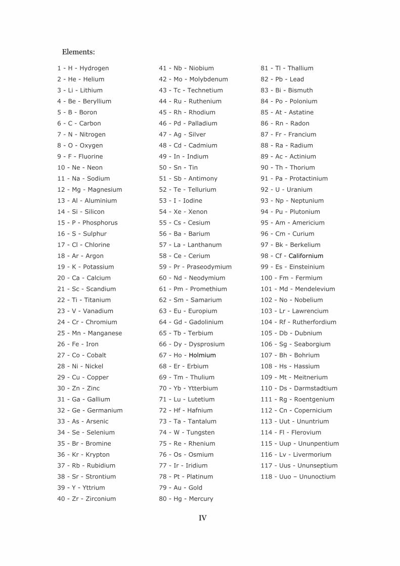
Elements:
1 - H - Hydrogen
2 - He - Helium
3 - Li - Lithium
4 - Be - Beryllium
5 - B - Boron
6 - C - Carbon
7 - N - Nitrogen
8 - O - Oxygen
9 - F - Fluorine
10 - Ne - Neon
11 - Na - Sodium
12 - Mg - Magnesium
13 - Al - Aluminium
14 - Si - Silicon
15 - P - Phosphorus
16 - S - Sulphur
17 - Cl - Chlorine
18 - Ar - Argon
19 - K - Potassium
20 - Ca - Calcium
21 - Sc - Scandium
22 - Ti - Titanium
23 - V - Vanadium
24 - Cr - Chromium
25 - Mn - Manganese
26 - Fe - Iron
27 - Co - Cobalt
28 - Ni - Nickel
29 - Cu - Copper
30 - Zn - Zinc
31 - Ga - Gallium
32 - Ge - Germanium
33 - As - Arsenic
34 - Se - Selenium
35 - Br - Bromine
36 - Kr - Krypton
37 - Rb - Rubidium
38 - Sr - Strontium
39 - Y - Yttrium
40 - Zr - Zirconium
41 - Nb - Niobium
42 - Mo - Molybdenum
43 - Tc - Technetium
44 - Ru - Ruthenium
45 - Rh - Rhodium
46 - Pd - Palladium
47 - Ag - Silver
48 - Cd - Cadmium
49 - In - Indium
50 - Sn - Tin
51 - Sb - Antimony
52 - Te - Tellurium
53 - I - Iodine
54 - Xe - Xenon
55 - Cs - Cesium
56 - Ba - Barium
57 - La - Lanthanum
58 - Ce - Cerium
59 - Pr - Praseodymium
60 - Nd - Neodymium
61 - Pm - Promethium
62 - Sm - Samarium
63 - Eu - Europium
64 - Gd - Gadolinium
65 - Tb - Terbium
66 - Dy - Dysprosium
67 - Ho - Holmium
68 - Er - Erbium
69 - Tm - Thulium
70 - Yb - Ytterbium
71 - Lu - Lutetium
72 - Hf - Hafnium
73 - Ta - Tantalum
74 - W - Tungsten
75 - Re - Rhenium
76 - Os - Osmium
77 - Ir - Iridium
78 - Pt - Platinum
79 - Au - Gold
80 - Hg - Mercury
81 - Tl - Thallium
82 - Pb - Lead
83 - Bi - Bismuth
84 - Po - Polonium
85 - At - Astatine
86 - Rn - Radon
87 - Fr - Francium
88 - Ra - Radium
89 - Ac - Actinium
90 - Th - Thorium
91 - Pa - Protactinium
92 - U - Uranium
93 - Np - Neptunium
94 - Pu - Plutonium
95 - Am - Americium
96 - Cm - Curium
97 - Bk - Berkelium
98 - Cf - Californium
99 - Es - Einsteinium
100 - Fm - Fermium
101 - Md - Mendelevium
102 - No - Nobelium
103 - Lr - Lawrencium
104 - Rf - Rutherfordium
105 - Db - Dubnium
106 - Sg - Seaborgium
107 - Bh - Bohrium
108 - Hs - Hassium
109 - Mt - Meitnerium
110 - Ds - Darmstadtium
111 - Rg - Roentgenium
112 - Cn - Copernicium
113 - Uut - Ununtrium
114 - Fl - Flerovium
115 - Uup - Ununpentium
116 - Lv - Livermorium
117 - Uus - Ununseptium
118 - Uuo – Ununoctium
V
Table of contents
1 Introduction ............................................................................................................ 1
2 Materials and Supplies .......................................................................................... 4
2.1 Preparation ....................................................................................................... 4
2.2 Analysis tests: .................................................................................................. 5
2.3 Content of starting sample ............................................................................... 6
3 Method ................................................................................................................... 7
3.1 Main test 1 ....................................................................................................... 7
3.1.1 General procedure for Main test 1: .......................................................... 7
3.2 Main tests 2 and 3: ........................................................................................... 9
3.3 Iron and sulphate analysis ............................................................................. 10
3.3.1 Iron analysis ........................................................................................... 10
3.3.2 Sulphate analysis .................................................................................... 11
3.4 Post-tests ........................................................................................................ 12
3.4.1 Test 6 - pH: ............................................................................................. 12
3.4.2 Test 7 - Temperature: ............................................................................. 12
3.4.3 Test 8 - Titration: ................................................................................... 12
3.4.4 Test 9 - Diluting: .................................................................................... 12
3.4.5 Test 10 - Analyses: ................................................................................. 13
4 Results and Discussion ......................................................................................... 14
4.1 Main test 1 ..................................................................................................... 14
4.1.1 Loss of ions ............................................................................................ 14
4.1.2 Precipitate increases after time in room temperature ............................. 14
4.1.3 Crystalline content of precipitate ........................................................... 14
4.1.4 Amorphous content of precipitate .......................................................... 15
4.2 Main test 2 and 3 ........................................................................................... 15

VI
4.2.1 Produced amount of precipitate of Main test 3 ...................................... 15
4.2.2 Difference in concentration and precipitate of Main test 2 and 3 .......... 15
4.3 Iron and sulphate analyses ............................................................................. 17
4.3.1 Statistical differences between Di and L ................................................ 17
4.3.2 General pattern of iron and sulphate analyses ........................................ 17
4.3.3 Uncertainties in the results in iron and sulphate analyses ...................... 18
4.3.4 Main test 1 – iron and sulphate results ................................................... 18
4.3.5 Main test 2 and 3 – iron and sulphate results ......................................... 18
4.4 Post-tests ........................................................................................................ 20
4.4.1 Test 6 - pH: ............................................................................................. 20
4.4.2 Test 7 - Temperature: ............................................................................. 21
4.4.3 Test 8 - Titration: ................................................................................... 21
4.4.4 Test 9 - Diluting ..................................................................................... 22
4.4.5 Test 10 – SEM ........................................................................................ 23
4.5 Possible large scale application ..................................................................... 26
4.5.1 Natural .................................................................................................... 26
4.5.2 Artificial ................................................................................................. 29
4.5.3 Comparisons: natural vs. artificial ......................................................... 30
4.6 Other points ................................................................................................... 30
5 Conclusions .......................................................................................................... 31
6 Outlook ................................................................................................................. 32
7 Acknowledgement ................................................................................................ 32
References .................................................................................................................... 33
Appendix 1: Pre-tests – Method
Collecting the brine
Test 1 - Quick analysis
VII
Test 2 - Total freezing:
Test 3 - No stirring:
Test 4 - Stirring:
Test 5 - Cleaning ice:
Material for the Main tests
Appendix 2: Pre-tests – Results
Test 1 - Quick analysis:
Test 2 - Total freezing:
Test 3 and 4 - Stirring or No stirring:
Test 5 - Cleaning ice:
Results from Main test materials
Other results from Main test 1
Appendix 3 – ALS results
Appendix 4 - Sample points Main test 1
Appendix 5: Sample points for Main test 2 and 3
Appendix 6: Fe, SO4 and pH
Appendix 7: Difference between ALS and laboratory results
Appendix 8: Mass balance for Main test 3
Appendix 9: Diagrams from SEM
Appendix 10: Mass balance for large scale application

VIII

1
1 Introduction
Maurliden is one of the mining sites in the Skellefte field and Boliden have operated
about 30 mines in this field since 1920. There are currently two active open pit mines,
Maurliden and Maurliden Östra. The ore in the area is rich of Cu, Zn, Au and Ag but it
has also high amounts of sulphide minerals, mainly pyrite.
The waste rock from the mines is being deposited in heaps while the mines are in
production, after that it will be backfilled into the pits. During this time the sulphides
oxidizes to sulphate that together with metal ions like Fe, Zn and Al drains from the
heaps with water down through ditches to a collecting pond (pond 11) in Maurliden, the
polluted water is called acidic rock drainage (ARD).
The water treatment plant in Maurliden uses slaked lime to precipitate metals
hydroxide from the ARD. To increase the settling rate of the precipitate, Zetag 9014 is
added as flocculent.
To treat the brine in pond 11 more than 70 kg lime/m3 is needed, compared the
optimum for the plant which is around 3 kg/m3 makes it obvious that the ARD water
needs to be diluted.
The ARD water is diluted with other contaminated waters from the mine site that also
need treatment, these water qualities contains much lower concentration of ions. There
is a higher ratio of the less contaminated water but the concentrated brine from pond
11 is the limiting factor for the plant.
Keeping the levels in the pond constant reduces the total water flow through the plant
which means that not enough less contaminated water can pass through it. This led to
a temporary mining stop in Maurliden a few years ago because of the high water levels
that had to remain in the mine pit.
Eutectic freezing is a principle based on freezing brine slowly to create pure ice and
through that increase the concentration of ions together with the cold atmosphere
should help the ions to precipitate. By using the density differences between the salt,
water and ice a natural separation occurs. The main goal is to precipitate different salts
at different times to use the method both for separation of minerals and cleaning the
water [1,2].
It is called eutectic freezing because it takes advantage of the eutectic points to separate
the salts from the water and ice. The principle of the general binary phase diagram in
figure 1 [1] shows when and how the salt and liquid will separate in an arbitrary case. 1
shows the starting point with the concentration and temperature of brine with one type
of dissolved salt. By reducing the temperature down to point 2, nothing will happen to
the concentrations but when the temperature goes below point 2 solid A starts to

2
crystallize. Only solid A will crystallise until point 3, where both solid A and solid B
(salt) precipitate until there’s no more liquid. After the liquid is gone the temperature
can decrease more.
Figure 1: A general binary phase diagram [1]
There is not much research done in this area and the published articles almost all use
high tech equipment such as cooled disk column crystalliser (CDCC) or fluidized bed
heat exchanger (FBHE) compared to the “bucket and freezer method” that will be used
here. The reason for not using any of the advanced methods was due to lack of time and
resources together with Bolidens wish for an easily upscaled freezing method which
could take advantage of the outside cold.
There are two other points that make it difficult to use or compare this report with
earlier results: the ions in articles are usually alkali metals and alkaline earth metals
like Na, K, Mg and Ca, usually together with SO4 in the brine [1-3] but in the brine from
Maurliden it is mostly Fe, Cu, Zn and Al; most researchers also make their own brine
with one [2,4] or a few salts [5] compared to this project when the brine comes from a
mine site with a lot more variety of ions.
The research from earlier work does have good result but the large differences between
the methods and the starting materials make it questionable if the results will be
comparable.
Jarosite is a sulphate mineral common in ore deposits where sulphide has oxidized to
sulphate and there is a presence of Fe3+. The mineral precipitates below pH 3 [6] and
can be used to remove Fe and SO4 from solutions if the pH and concentrations are
correct. In the article of G.A. Norton [7] it states the optimum pH is between 1.5 and
2.3 and to remove Na as well the pH need to be between 1.4 and 1.6. These experiments
were performed at high temperatures, 80 – 95 °C, and the low solubility of jarosite in

3
water makes it easy to remove after it has precipitated. Schwertmannite precipitates at
a higher pH [6], between 3 – 4, but it also needs Fe3+ and SO4 and is common in
ARD/AMD (acidic rock/mine drainage).
The objective of this project was to improve the treatment of the ARD water with as
environmentally friendly method as possible by using the cold in Maurliden to execute
the freezing. The specific goals were to:
- Find out if it is possible to selectively precipitate metal salts with this method.
- Find out what it takes to totally freeze this water from Maurliden.
- Investigate if there is any value in the precipitated product.
- Design two full-scale plant solutions using both “natural” and “artificial”
freezing.

4
2 Materials and Supplies
2.1 Preparation
Collect sample:
Pump – Watson Marlow 620U (Picture 1A)
Stirrer on a stand – IKA - Labortechnik RW 20.n (Picture 1B and D)
60 L barrels with sample from Maurliden (Picture 1C)
Litre measure
A B C D
Picture 1 A-D: Materials used when collecting sample, A the pump, C the 60L barrel, B and D the stirrer
Freezing sample:
Freezer - Cylinda Frysbox FB1350A (Picture 2A)
Six stirrers on a stand - IKA - Labortechnik RW 20.n (Picture 2A)
Stirrers for the freezer (Picture 2F)
Stand for stirrers (Picture 2A)
Modified lid (Picture 2A)
Rubber stoppers for the sensor holes
Temperature sensors - Endress + Hauser pt100 (Picture 2A)
Labview program (Picture 7A and B)
3 L buckets with lids
Bucket stand in freezer (Picture 2B)
Bucket isolation (Picture 2C and D)
Nets (Picture 3C), bought at Clas Ohlson, article number 34-1113
100 ml sample cups with lids (Picture 2E)
A B F C D E
Picture 2 A-F: Materials used during the freezing of samples: A shows the freezer, the lid, stirrers, the stand for the stirrers and temperature sensors, B the stand for the buckets, C and D the isolation for the buckets and E the sample cups with three different samples. F displays
the type of stirrers used in the freezer.

5
Filtration of brine:
Filter paper – Whatman GF/B, circles, diameter 150 mm, pore size 1 µm
Büchner funnel – 150 mm
Filtration flask– 1 L
Scale – Mettler AE 160
Total freeze:
Filter paper – Whatman GF/B, circles, diameter 150 mm, pore size 1 µm
2.2 Analysis tests: LCK 360 for zinc from Hach Lange
LCK 529 for copper from Hach Lange
LCK 301 for aluminium from Hach Lange
Filter paper Munktell 1F, circles, 110 mm (preparation for iron and sulphate tests)
Adjustable volume pipette – VWR ergonomic high performance, 100-1000 μL
Adjustable volume pipette – Eppendorf research 5000, 500-5000 μL
20 ml syringe - Braun Omnifix, 20 ml
Cuvettes – Sample cell, 25 mm round Glass
Spectrophotometer – Hach Lange DR 2800
100 ml volumetric flasks
Deionised water
Total iron ions test:
SSA – 5-Sulfosalicylic acid dehydrate, Merck Schuchardt, 254.22 g/mol
NH3 – Ammonia, 28 %, VWR
HCl – Hydrochloric acid, AnalaR Normapur, 37 %, VWR, 36.46 g/mol, 1.18 kg/L
SO4 test:
BaCl2 – Barium Chloride, Merck Schuchardt, 208.25 g/mol, 99,995 % pure
H2SO4 – Sulphuric acid, GDR Rectapur, 95 %, 98.07 g/mol, 1.84 kg/L
SO4 buffer:
MgCl2 – Magnesium Chloride Hexahydrate, GR for analysis, Merck KGaA,
203.30 g/mol
NaAc – Sodium Acetate, anhydrous GR for analysis, Merck KGaA, 82.03 g/mol
KNO3 – Potassium Nitrate, extra pure, Merck KGaA, 101.10 g/mol
CH3CO2H - Acetic Acid, 99.5 % pure, 60.05 g/mol, Acros Organics
pH-measurements
pH-meter – calibrated for pH 4-7, WTW pH 340i with a Sentix 41-3 pH electrode
Titration:
NaOH – Sodium Hydroxide, Ph.Eur., pellets, VWR, 99.5 % pure
pH-meter calibrated for pH 4-7, WTW pH 340i with a Sentix 41-3 pH electrode
Filter paper – glass microfiber, 55 mm, grade MGA
Dilution test:
Volumetric flasks – 100, 500 and 1000 ml
Filter paper – glass microfiber, 55 mm, grade MGA
6
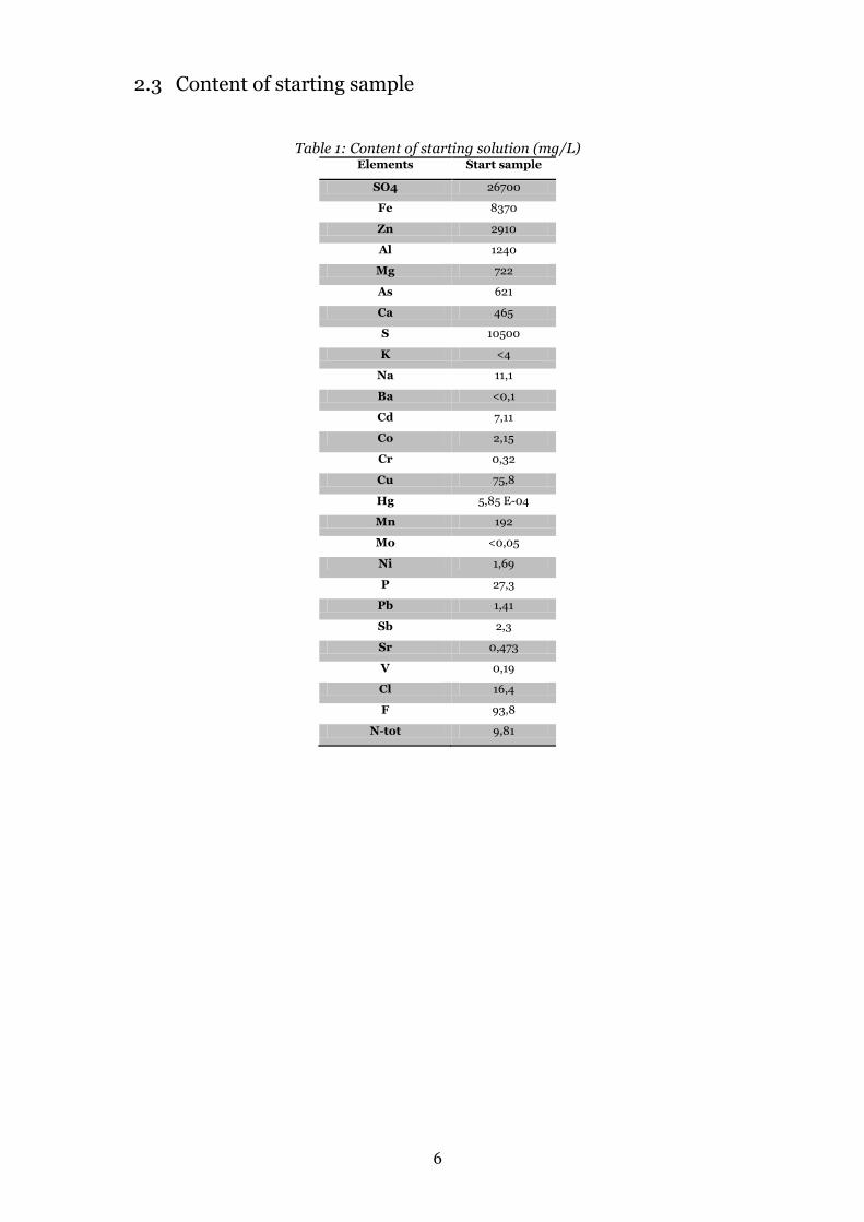
2.3 Content of starting sample
Table 1: Content of starting solution (mg/L) Elements Start sample
SO4 26700
Fe 8370
Zn 2910
Al 1240
Mg 722
As 621
Ca 465
S 10500
K <4
Na 11,1
Ba <0,1
Cd 7,11
Co 2,15
Cr 0,32
Cu 75,8
Hg 5,85 E-04
Mn 192
Mo <0,05
Ni 1,69
P 27,3
Pb 1,41
Sb 2,3
Sr 0,473
V 0,19
Cl 16,4
F 93,8
N-tot 9,81

7
3 Method
In this project three extensive tests, below called Main test 1-3, were executed. While
waiting for the equipment to be finished some smaller tests, called pre-tests, were made
to find a god starting point. Some extra experiments were made during and after the
Main tests to try some ideas that surfaced during the project, called post-tests.
The pre-tests and information on the material used in the Main tests can be seen in
appendix 1.
3.1 Main test 1
Main test 1 was used to get an idea on how to proceed and the main goal was to
investigate at what temperatures highly concentrated samples froze. Main test 1 has the
letter N before the number of all its samples to easily identify from which test the
sample came.
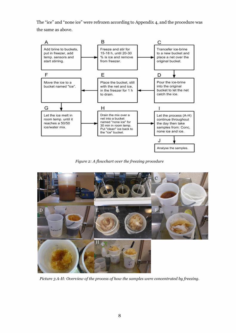
3.1.1 General procedure for Main test 1:
An overview of the procedure can be seen in figure 2.
A. Add 2 L of sample to clean and dry 3 L buckets, place them in the freezer and
start stirring. Usually two temperature sensors were used, one in the air and one
in one of the samples (see appendix 1).
B. Freeze the water for 15-18 h to get enough ice, about 20-30 % of the total
volume, and take them out of the freezer.
C. Pour the semi-frozen water into a “transfer bucket”, then placing a net over the
original bucket.
D. Pour the liquid back into the original bucket and let the net catch the ice.
E. Place the bucket back into the freezer for an hour to drain.
F. Take the buckets out of the freezer again and transfer the ice in the net to a
bucket named “ice”.
G. Let the ice melt to about a 50/50 ice/water mix. Stir the ice a few times to help
it melt.
H. Drain the 50/50 ice mixture into a bucket named “none ice”. Leave the ice in
room temperature to drain.
a. When the ice and liquid had been separated the second time, three
fractions of the starting material had now been acquired: “Conc”
(concentrated sample), “none ice” (the water from the ice when it had
melted a bit) and “ice” (the remaining ice after draining it twice).
I. A 100 ml sample was collected from each fraction.
J. The iron and sulphate analysis were performed after the tests were done.
8
The “ice” and “none ice” were refrozen according to Appendix 4, and the procedure was
the same as above.
Figure 2: A flowchart over the freezing procedure
A B C
D E F
G H
Picture 3 A-H: Overview of the process of how the samples were concentrated by freezing.

9
3.2 Main tests 2 and 3:
These two tests were based on the procedure from Main test 1 but with some
improvements and additions (listed below). All the samples from these tests were
named with a letter and number, Main test 2 had the letter V (vanlig/ordinary) and
Main test 3 had the letter F (filtrerad/filtered).
1. A flow chart was constructed to give a clearer view of the path that each fraction
took (Figure 4); the exact flow chart and the names of the fractions are listed in
Appendix 5.
2. The principle of the numbers from the flow chart are (Figure 3):
a. 1 is the starting product.
b. 2 is the “conc” from 1.
c. 3 is the “none ice” from 1.
d. 4 is the “ice” from 1, the same principle applies for the rest of the
segments.
e. Number 50, 51, 52 and 53 (Figure 4) are mixed samples from the
fractions that the arrows come from.
f. The area in parentheses were supposed to be done but there were not
enough liquid for it.
Figure 3: A segment in the flow chart
3. The two tests started with 6 L of liquid each, divided into three buckets per test.
4. The tests were done simultaneously with one difference, Main test 3 was filtered
before the test started and all fractions were filtered throughout the test to
record the amount of precipitate and liquid.
5. All times were noted: how many hours the liquid was in the freezer, how long it
drained in the freezer, how long the ice melted and how long the ice drained for
the second time.
6. The iron and sulphate analyses were generally made the day after they were
frozen.

10
Figure 4: Flow chart of the freezing sequence for each sample batch.
3.3 Iron and sulphate analysis
The 100 ml samples were analysed to follow the changes in Fe and SO4 throughout the
freezing tests. In all these samples solid particles had precipitated in various amounts.
30 ml of liquid were taken from the samples and divided into: L (liquid) and two types
of Di (dissolved): Dissolved sulphate (DS) and Dissolved iron (DF). The preparation
procedures were:
1. Each sample needed tree 50 ml cups (Picture 4A).
2. 10 ml was added to each cup, one cup had a filter paper to remove all precipitate.
3. To the two unfiltered cups concentrated acid were added, in one (DF) H2SO4
and the other (DS) with HCl, until the precipitate dissolved.
4. The three cups were used in the the iron and sulphate analysis.
3.3.1 Iron analysis
This analysis was based on an article [13] about how to rapidly measure both Fe3+ ions
and the total amount of Fe ions in drainage water samples. The method is especially
considered for mine drainage water analyses and was tested for interference with Mg2+,
Cu2+, Mn2+ and H2SO4 but without any changes to the results except for H2SO4 that
changed the result after 167 g/g Fe. The measuring range for this analysis was between
0-2 mg Fe/L.
The procedure was modified a little from the original but the principle should be the
same, this is the modified version:
1. Start with diluting 1 ml of the sample a 100 times with deionised water (Picture
4B) and shake well. (Most of the samples needed diluting before the analysis.)

11
2. Add about 40 ml of deionised water into a 100 ml flask.
3. Add 3 ml of 10 wt% SSA, and then 3 ml of ammonia.
4. Add diluted sample to the flask until it gets a yellow colour.
5. Fill the flask with water and shake well.
6. Pour the liquid into a sample cell and measure the absorbance at 425 nm.
The problem with the original method was to know how much sample was enough, or
the larger issue: if too much was added in the beginning then all had to be redone. The
method was altered to make it easier to see when a sufficient amount of sample was
added which reduced the extra work. Another alteration was that the ammonia was
included in the 100 ml total.
3.3.2 Sulphate analysis
The concentration of sulphate in the liquid was analysed using a turbidimetric method
based on principles presented in ref. [14].
A buffer solution was prepared by mixing 30 g MgCl2, 5 g NaAc, 1.0 g KNO3, 20 ml
acetic acid and deionised water in a 1 L volumetric flask.
The analysis procedure used was:
1. A known volume of sample was added to a 100 ml volumetric flask.
2. 5 ml of buffer was added.
3. Deionised water was added up to the start of the neck.
4. ~0.5 g of BaCl2 was added.
5. After addition of water to the mark the flask was vigorously shaken.
6. A volume of the suspension was transferred to a sample cell and the turbidity
was measured using a spectrophotometer at 450 nm.
A B
Picture 4 A-B: A - sample cups with 10 ml sample, the top row is Dissolved Sulphate (DS), the next is Liquid (L) and at the bottom is Dissolved Iron (DF). B - the darker liquids (1st, 3rd, and
5th flask) is diluted sample from the middle row (L) in A. The lighter liquids (2nd, 4th and 6th flask) represents diluted liquids from the bottom row (DF) in A.

12
3.4 Post-tests
Some different minor testes were made to support different findings during the Main
tests.
3.4.1 Test 6 - pH:
To test a theory that the pH could be a factor linked to the amount of solid particles that
precipitates, all the collected samples were measured with a pH-meter.
3.4.2 Test 7 - Temperature:
The normal behaviour of salts is that the solubility increases with temperature but some
salts have reversed solubility. To analyse if the salts in these tests had reversed
solubility, four bottles were filled with 250 ml newly filtered liquid each, two with F11
(D4 conc) and two with V11 (D4 conc). One of each was placed in a refrigerator (~5 °C)
and the others in room temperature. After a week the samples were filtered to
investigate if there was any difference between the temperatures and between the
filtered and unfiltered (F and V) liquids.
3.4.3 Test 8 - Titration:
Titration with 0.1 M NaOH was made to investigate the difference between some of the
samples.
The titration was made by first preparing the NaOH solution, and then filtering the
three samples F 22 (ice), V1 (starting solution) and N50 (concentrated sample) in the
same way as in the iron and sulphate analysis.
The filtrated samples were diluted with deionized water according to Table 2. The pH
level and amount of NaOH added were registered a few times during the titration to
construct a titration curve, the pH needed to be increased above 9.5.
Table 2: Starting point of titration, the amount of sample and how much it was diluted. F 22 V1 N50
Amount of sample (ml) 3 2,5 2
Diluted to (ml) 30 25 40
3.4.4 Test 9 - Diluting:
After an observation that diluted samples from the iron analyses got turbid after a while
made it interesting to study if there were anything to learn by diluting samples. The
first test was with a newly collected sample that was diluted 10, 20, 50, 100, 133, 200,
400, 1 000, 2 000 and 10 000 times.
These flasks were left to equilibrate for five days and then filtrated to get an idea of the
amount of precipitate produced during the dilution. The pH was measured after the
filtration and two of the liquid samples were sent for element analysis (V3B).

13
To investigate if it was possible to do the same thing with the most concentrated liquid
(N50), four dilutions were prepared based on the increase in concentration and the
optimum from the ten earlier tests. Because of the precipitate in the N50 water, it was
filtered before it was used in the test. The dilutions were 200, 400, 1 000 and 2 000.
These flasks got to equilibrate for 24 h, after that they were filtrated and pH was
measured.
3.4.5 Test 10 - Analyses:
The external analyses made by ALS were by SEM, XRD, ICP-AES, AFS and ICP-SFMS.
The SEM analysis was made by Boliden’s own machine (QEMSCAN 650) and from that,
three pictures with seven areas were analysed. The XRD analyses were made to reveal
what type of solid products that were produced during the freezing- and dilution tests.
The three other analysis methods were used to analyse the elements in the water
samples. ICP-SFMS was also used on the solid products after they were dissolved.
14
4 Results and Discussion
In this section are the results from the main and post-tests together with discussion.
The pre-tests and results about the materials used can be found in appendix 1 and 2.
4.1 Main test 1
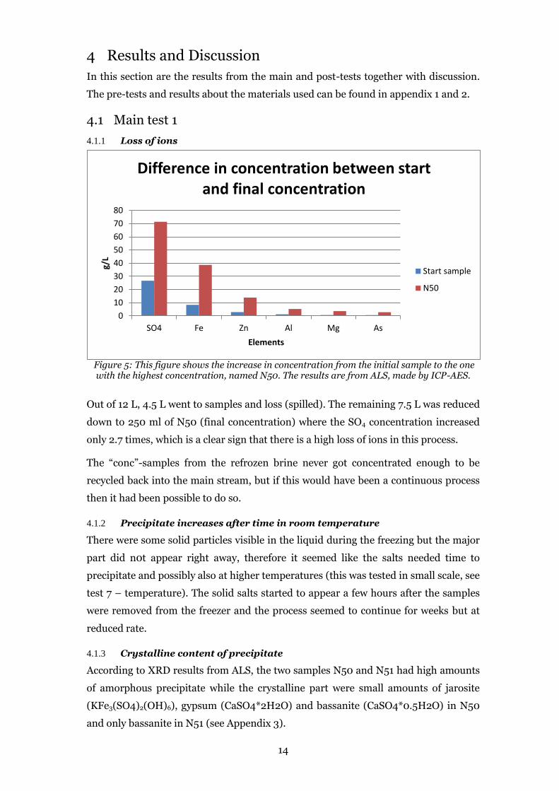
4.1.1 Loss of ions
Figure 5: This figure shows the increase in concentration from the initial sample to the one with the highest concentration, named N50. The results are from ALS, made by ICP-AES.
Out of 12 L, 4.5 L went to samples and loss (spilled). The remaining 7.5 L was reduced
down to 250 ml of N50 (final concentration) where the SO4 concentration increased
only 2.7 times, which is a clear sign that there is a high loss of ions in this process.
The “conc”-samples from the refrozen brine never got concentrated enough to be
recycled back into the main stream, but if this would have been a continuous process
then it had been possible to do so.
4.1.2 Precipitate increases after time in room temperature
There were some solid particles visible in the liquid during the freezing but the major
part did n0t appear right away, therefore it seemed like the salts needed time to
precipitate and possibly also at higher temperatures (this was tested in small scale, see
test 7 – temperature). The solid salts started to appear a few hours after the samples
were removed from the freezer and the process seemed to continue for weeks but at
reduced rate.
4.1.3 Crystalline content of precipitate
According to XRD results from ALS, the two samples N50 and N51 had high amounts
of amorphous precipitate while the crystalline part were small amounts of jarosite
(KFe3(SO4)2(OH)6), gypsum (CaSO4*2H2O) and bassanite (CaSO4*0.5H2O) in N50
and only bassanite in N51 (see Appendix 3).
0
10
20
30
40
50
60
70
80
SO4 Fe Zn Al Mg As
g/L
Elements
Difference in concentration between start and final concentration
Start sample
N50
15
4.1.4 Amorphous content of precipitate
The amorphous precipitate was dissolved and analysed. The main elements detected
were As, Fe and Zn, also high amount of S was assumed (based on the results from other
samples where S was included). The detected elements only contributed to around 25
% of the total weight (see Appendix 3). If S was included the estimation would be
around 35-40 % of the weight. The content of the remaining weight is unknown,
including the amount of Ca and water.
4.2 Main test 2 and 3
4.2.1 Produced amount of precipitate of Main test 3
The total amount of precipitate produced during Main test 3 was 8.5 g total. A simple
approximation estimates the amount of precipitate, assuming no losses (see Appendix
8 for calculations), to 10.4 g which can be recalculated to about 1.7 g/L of ARD water.
This was the amount precipitate recovered after 12-24 h, more solids precipitated later
which again indicates that this process needs time to equilibrate.
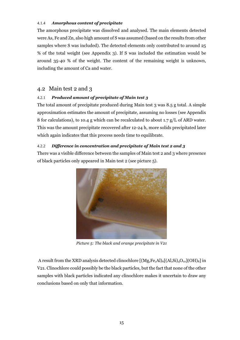
4.2.2 Difference in concentration and precipitate of Main test 2 and 3
There was a visible difference between the samples of Main test 2 and 3 where presence
of black particles only appeared in Main test 2 (see picture 5).
Picture 5: The black and orange precipitate in V21
A result from the XRD analysis detected clinochlore [(Mg,Fe,Al)6[(Al,Si)4O10](OH)8] in
V21. Clinochlore could possibly be the black particles, but the fact that none of the other
samples with black particles indicated any clinochlore makes it uncertain to draw any
conclusions based on only that information.

16
Figure 6: The concentrations in the samples, V3B analyses from ALS. Main test 2 (V) and 3 (F) with samples: 1 (start solution), 11 (highest concentrated), 50 (mixed sample of all “none
ice”), 51 (mixed sample of all “ice”) and 21 (refreeze ice none ice).
Figure 7: The content of the samples precipitate, I1c analyses from ALS. Main test 2 (V) and 3 (F) with samples: 1 (start solution), 11 (highest concentrated), 50 (mixed sample of all “none
ice”), 51 (mixed sample of all “ice”) and 21 (refreeze ice none ice).
The ALS results in figure 6 and 7 show the concentrations and different elements in the
most important samples that represents the different fraction in the Main tests. Except
for some deviation in the SO4 (figure 6) and Fe (figure 7) the concentrations seemed
consistent between the two tests. This pattern is also comparable to the Fe and SO4
analyses below.
0
5
10
15
20
25
30
35
40
V1 V11 V50 V51 V21 F1 F11 F50 F51 F21
g/L
Samples
Concentrations of SO4, Fe and Zn
SO4 Fe Zn
0
50
100
150
200
250
300
V1 V11 V50 V51 V21 F1 F11 F50 F51 F21
g/kg
Samples
Content of precipitate: As, Fe & Zn
As* Fe* Zn*

17
4.3 Iron and sulphate analyses
4.3.1 Statistical differences between Di and L
Samples were prepared in two ways (filtering and dissolving) to compare the total
amount of ions between the dissolved- and filtered sample. This was to get an idea of
how much hade precipitated, all the results can be seen in Appendix 6.
The results from Main test 1 and 2 (both Di- and L results) were not as easily interpreted
as expected and after all analyses were executed, statistical f-tests and t-tests were
performed to validate the results, calculated on website [17,18]. The conclusion was that
neither their variances nor their medians were different from each other. This indicates
that both Di- and L results are statistically equal and because of this the plots below will
only have the results from the filtrated (L) preparation method.
4.3.2 General pattern of iron and sulphate analyses
Figure 8: The concentrations in each sample from Main test 2.
The results in Figure 8 shows a pattern with decreasing concentrations between the
fractions: “conc”, “none ice” and “ice”. A small increase in concentration can be
observed in the “conc” fraction over time and that the concentration decreases after one
refreezing. These patterns can also be seen in figure 9 and the consistency of these
patterns makes it believable that it is accurate.
0.00
5.00
10.00
15.00
20.00
25.00
30.00
35.00
40.00
45.00
Star
t p
rod
uct
D1
co
nc
D1
no
ne
ice
D1
ice
D2
co
nc
D2
no
ne
ice
D2
ice
D3
co
nc
D3
no
ne
ice
D3
ice
D4
co
nc
D4
no
ne
ice
D4
ice
Mix
ed
sam
ple
no
ne
ice
Re
fre
eze
no
ne
ice
con
c
Re
fre
eze
no
ne
ice
no
ne
…
Re
fre
eze
no
ne
ice
ice
Mix
ed
sam
ple
ice
Re
fre
eze
ice
con
c
Re
fre
eze
ice
no
ne
ice
Re
fre
eze
ice
ice
Mix
ed
sam
ple
17
,18
,20
Re
fre
eze
17
,18
,20
co
nc
Re
fre
eze
17
,18
,20
no
ne…
Re
fre
eze
17
,18
,20
ice
g/L
Samples
Fe and SO4 Main test 2
Fe tot V Sulphate V

18
4.3.3 Uncertainties in the results in iron and sulphate analyses
The problem with the analyses done in the lab compared to the results from ALS
(authorized lab) is that some are really consistent and some are significantly different,
especially SO4 (Appendix 7). This could be due to the time delay between the lab
analysis and ALS’s analysis, which could be up to several weeks for some samples.
Another possibility for the inconsistency could be that several batches of solutions had
prepared to analyse all 105 samples. The fact that different batches of solutions were
used and that few tests with Fe and SO4 standards were made makes the lab results a
bit unreliable. Despite this, the overall pattern (figure 8 and 9) seems reasonable.
4.3.4 Main test 1 – iron and sulphate results
The results from the Fe and SO4 analyses indicated that the method was sufficient and
that the ice got less contaminated. The improvement from second drainage can be
viewed by comparing “none ice” and “ice” (figure 9).
Figure 9: Changes in concentration for Fe and SO4 over time and between “conc”, “none ice” and “ice”. The “D” in the sample names stands for day and the number for how many days
that had past. This displays only the concentrated liquid and not the attempts on refreezing.
The results in figure 9 are from the Fe and SO4 analyses made in the lab except for four
sulphate analyses and which were disproportionally high. “D10 conc” and “D10 none
ice” were replaced by results from ALS and “D9 conc” and “D9 none ice” got
approximated values.
4.3.5 Main test 2 and 3 – iron and sulphate results
The reason for filtering all liquids in Main test 3 was to study if Le Châtelier’s principle
could help to increase the amount of precipitate produced and reduce the concentration
0.00
10.00
20.00
30.00
40.00
50.00
60.00
70.00
80.00
Star
t p
rod
uct
D1
-2 ic
e +
no
ne
ice
D3
co
nc
D3
no
ne
ice
D3
ice
D4
co
nc
D4
par
t 1
no
ne
ice
D4
par
t 1
ice
D4
par
t 2
no
ne
ice
D4
par
t 2
ice
D5
co
nc
D5
no
ne
ice
D5
ice
D6
co
nc
D6
no
ne
ice
D6
ice
D7
co
nc
D7
no
ne
ice
D7
ice
D8
co
nc
D8
no
ne
ice
D8
ice
D9
co
nc
D9
no
ne
ice
D9
ice
D1
0 c
on
c
D1
0 n
on
e ic
e
D1
0 ic
e
g/L
Samples
Concentration changes from start to day 10 (D10)
Fe tot L Sulphate L

19
in the liquids [19]. A practical interpretation of this is that if the precipitate is removed
the equilibrium would shift to restore it and more precipitate would be produced. On
the other hand, taking away precipitate makes the need for producing new nuclei larger
which instead could inhibit the precipitation.
Figure 10: The Fe concentrations in Main test 2 and 3
Figure 11: The SO4 concentrations in Main test 2 and 3
Le Châtelier’s principle with filtered and non-filtered samples did not work out as
planned. The results of Main test 2 (non-filtered, V/L) and 3 (filtered, F) seemed
random, except for the final ice and none ice in Main test 2 (“refreeze ice ice” and
0.00
2.00
4.00
6.00
8.00
10.00
12.00
14.00
16.00
g/L
Samples
Fe concentration differences between Main test 2 and 3
Fe tot V Fe tot F
0.005.00
10.0015.0020.0025.0030.0035.0040.0045.0050.00
g/L
Sample
SO4 concentration differences between Main test 2 and 3
Sulphate L Sulphate F

20
“refreeze ice none ice”). They had definitely the lowest concentrations for both iron and
sulphate compared to Main test 3 which showed the complete opposite to the expected
results. This could be because of the removal of nucleuses that the precipitate grew on,
but the used buckets were never washed so a bit of starting crystals should have existed.
Concentration differences between Main test 2 and 3 were tested according to the
statistical methods, which showed no significant difference. I.e. it should not matter if
the precipitate was removed often or not at all.
4.4 Post-tests
4.4.1 Test 6 - pH:
The pH-meter used for these tests were calibrated at pH 4 and 7.
The samples had a pH in the range of 1.8 to 2.5.
A pattern can be detected in the pH distribution where it increases from “conc” to “none
ice” to “ice” (Figure 12). The opposite pattern was observed in the Fe and SO4 results
for the same samples (Figure 8). A negative correlation between pH and concentrations
of Fe and SO4 can be noticed if figure 8 and 12 are compared.
Figure 12:The pH measured in each sample from Main test 2.
From the knowledge that there were high amounts of iron and sulphate in the samples
together with a pH level between 1.5 and 3 made it likely that the precipitate in the
samples was jarosite. This conclusion was drawn before the XRD analyses confirming
it. Considering the Norton article [7], that precipitation of jarosite takes a few hours at
80-95 ˚C makes it likely that it has reversed solubility and need higher temperatures to
2.20
2.25
2.30
2.35
2.40
2.45
2.50
2.55
2.60
2.65
pH
Samples
pH Main test 2
pH

21
precipitate. These results were later confirmed with XRD which detected jarosite in
samples V1, V18, N50 and F21.
4.4.2 Test 7 - Temperature:
The results in Figure 13 show that the room temperature sample from Main test 2 (V11)
had almost four times as much precipitate than the one from the fridge. The same
indications can be observed in Main test 3’s samples (F11). This result supports the
jarosite theory and the fact that cold temperatures are not optimal for precipitating it.
Figure 13: The amount of precipitate per litre of “D4 conc” after one week.
4.4.3 Test 8 - Titration:
The titrations were performed with NaOH instead of slaked lime, which is used in the
plant. The results were recalculated with the assumptions: two moles of NaOH
corresponds to one mole of Ca(OH)2 (slaked lime), the efficiency of NaOH was 100 %
while it may be expected that the efficiency of the lime would have been ~ 90 %. The
molar weight for the lime was 74.09 g/mol.
Table 3: Results from titration F22 V1 N50
Final pH 10,2 9,7 10,1
ml NaOH/ ml sample 1,5 5,6 28,0
Recalculated to kg lime/m3 sample 6,17 23,1 115,3
The analysed samples were F22 (Main test 3, “refreeze ice ice”), V1 (Main test 2, start
material) and N50 (Main test 1, D10 “conc”). The results, listed in table 3, were initially
convincing; if the ice was as pure as F22 then the water would not have to be diluted
before entering the plant.
There was a large problem with the results. The fact that V1 got such a low value
compared to earlier titrations made by Boliden on the same kind of ARD water; 23
kg/m3 vs 70 kg/m3 [lime/water]. A possible reason could be that the concentrations
had changed due to the time the sample had precipitated and that it was filtered off
before the titration. Another explanation could be that the efficiency is lower than 90
050
100150200250300
V11 roomtemp
V11 frigde F11 roomtemp
F11 frigde
mg/
L
Samples
Amount of precipitate after temp test
mg precipitate/L sample

22
% (Boliden use lime for titration). The large difference in the results makes these results
very questionable, and no conclusions were drawn from these tests.
4.4.4 Test 9 - Diluting
After the mixtures had equilibrated, the amount of solid particles were filtered off, dried
and weighed. The pH was measured in the filtrated water and the amount of g
precipitate per L starting sample were calculated (results in figure 14 and table 4).
Figure 14: The amount of precipitate per L sample from each starting material vs. pH.
Table 4: The starting material, how much they were diluted, their pH and how many g precipitate/L sample it produced. The red sample is the excluded one and the green and bold
samples are the best ones. Starting material Dilution pH g precipitate /L sample
The start 10000.00 3.96 32.00
The start 2000.00 3.66 10.80
The start 1000.00 3.54 9.00
The start 400.00 3.29 13.60
The start 200.00 3.07 15.60
The start 133.33 2.97 14.80
The start 100.00 2.91 13.20
The start 50.00 2.79 12.80
The start 20.00 2.69 9.14
The start 10.00 2.67 6.54
N50 200.00 2.75 49.80
N50 400.00 2.90 61.36
N50 1000.00 3.17 70.80
N50 2000.00 3.37 73.40
Six water samples were sent for ALS analysis: the start sample, the start sample diluted
10 and 200 times, N50 and the N50 samples diluted 1000 and 2000 times. The results
are shown in figure 15, included the best ice from Main test 2 (V21).
Start 15,6 g/L
N50 73,4 g/L
0
10
20
30
40
50
60
70
80
2.5 2.75 3 3.25 3.5 3.75
g/L
pH
Amount of precipitate/L sample at differen pH:s
Start
N50

23
Figure 15: Shows how much cleaner the water gets after diluting compared to the best ice,
the diluted concentrations are multiplied with how much they are diluted to be able to compare the results. Results from ALS, V3B.
Figure 15 shows that the iron decreases a lot after dilution, but not as much as after the
freezing test. The other elements did not decrease at all after the dilution but they did
after freezing. Considering that the pH results were around or above pH 3 (Table 4) for
most of the dilutions makes it is possible that the precipitation could be
schwertmannite. Filter papers with precipitate from S10 and S200 were sent for XRD
analysis but all precipitate was amorphous and could not be identified. The
concentrations of Fe and SO4, together with the pH levels, support this theory but
without confirmation form XRD.
4.4.5 Test 10 – SEM
The SEM analysis was made on precipitate from V21. There were two types of solids
that were visibly detected; orange and black solid particles. The orange particles were
very small and the black were large crystals (picture 5). A small amount of solids were
taken and dried, including a large black crystal, which were then added to a type of
adhesive tape used for SEM analysis.
The samples were scanned seven times at different locations (picture 6), scan 1 and 4
was believed to be on a black crystal. Also scan 7 is thought to be the same type of
particle as 1 and 4. Scan 2 and 3 are believed to been taken on orange precipitate and
scan 5 and 6 were taken on an unknown crystal with a different ratio than the rest. The
analyses results are listed in table 5. No real conclusions have been drawn from these
analyses.
0
20
40
60
80
100
120
Startsample
S 200 S 10 N50 N50 2000 N50 1000 V21
g/L
Samples
Start samples, diluted samples and ice
SO4 Fe Zn

24
Table 5: The analysis results from the SEM. (Point 5 and 6 are identical in the table but their SEM diagram differ, see Appendix 9)
1 2 3 4 5 6 7
Fe 38,03 34,71 44,63 52,40 23,39 23,39 38,93
O 36,82 41,52 34,01 33,14 45,78 45,78 42,91
N 11,82 11,62 10,28 8,69 11,40 11,40 10,27
C 6,09 3,73
Rb 3,71
Pb 2,86 5,99
S 0,67 4,82 6,20 3,79 12,58 12,58 1,25
As 3,59 4,88 1,53 1,53
Mg 1,97 0,64
Zn 4,32 4,32
Al 1,00 1,00

25
Picture 6: Displays the areas were the SEM analysed the sample

26
4.5 Possible large scale application
There has not been much time to consider the large scale production of this method
because of the time it took for the Main tests to begin and the time it has taken to do all
the analyses.
There are two different big scale plans, one artificial and one natural.
4.5.1 Natural
The plan for the natural freezing method is to use the same method during the
laboratory test work, but in a larger scale. Using the outdoor temperature to freeze the
water and precipitate the ions making it into valuable product instead of a problem.
This principle will use large tanks made of some type of none isolating material to get a
good heat exchange. It will also need to have as large cooling area per volume unit as
possible which means a high and narrow tank (compared to a shallow and wide).
The basic principle (see figure 16) is to feed the starting material into tank 1. There will
be a need for stirring to make the ice into small crystals instead of a large block. One
stirring alternative is cold air.
Starting material will probably be added in batches. When about 30 % of the mass in
the tank has been converted to ice, the stirring stops which will let the ice go to the top
of the tank. The density could be measured to know when the correct amount of ice
produced.
The content is pumped from the bottom of the tank; first the water comes and is
directed to tank 2; when the ice comes the direction shifts and it is pumped to process
4.
In tank 2 the same procedure continues; the water is frozen again, the liquid is pumped
to tank 3 and the ice is pumped to process 4. The same procedure is done once more
and the liquid goes to tank 6 and the remaining ice is pumped to process 4.
Tank 6 is the most highly concentrated liquid and will be left until summer to
precipitate. After that, the liquid will be filtered of and the precipitate will be collected.
The remaining liquid will then be diluted to a pH around 3 to precipitate the last iron
in the water.
The aim is to use less slaked lime and sell the precipitate to make the water treatment
less costly compared to treating with the current method. After the iron has precipitated
the mix will be filtered of again to collect the precipitate. After that the brine will go
through the water treatment plant.
To lose as little amount of ions as possible and to get the cleanest ice possible, the ice
needs to be treated. Doing this in a somewhat similar way as in the laboratory; the ice
is transported to a wire cloth with vacuum underneath, were the water is pulled through

27
the wire cloth and the ice remain on the top. After the wire cloth the ice is collected in
the “ice pond” and left to melt until the summer.
The reject, from process 4, goes through the wire cloth, recycles back and is mixed with
feed 1 to become feed 2, which goes into tank 1.
In the summer time the ice pond, pond 5, will be drained by pumping the liquid through
a filter where the precipitate is collected, after that the brine goes to the water treatment
plant.
Figure 16: A simple overview of the natural freezing process
There is some major problem with this method. The first is that the average water flow
is 15 000 kg/h, which is 360 000 kg/day. It will be virtually impossible to freeze that
much water in this way, since it takes 3-6 h to get a few dl of ice in controlled conditions.
A more reasonable flow would be 5 000 kg/h with the help of cold air for the freezing.
A mass balance was constructed using the data about the flows and weights of
precipitate (from Main test 3) together with the ALS results. The calculations are based
on the flows in figure 16 and are named after them. A detailed description and the mass
balance table can be found in Appendix 10. An overview of the flows in the system based
on mass (kg/h), SO4 (kg/h) and metal (Fe + Zn, kg/h) can be seen in figure 17. A
problem with this method is that it has not considered the fact that Fe minerals need
temperatures above 22 ˚C to precipitate.
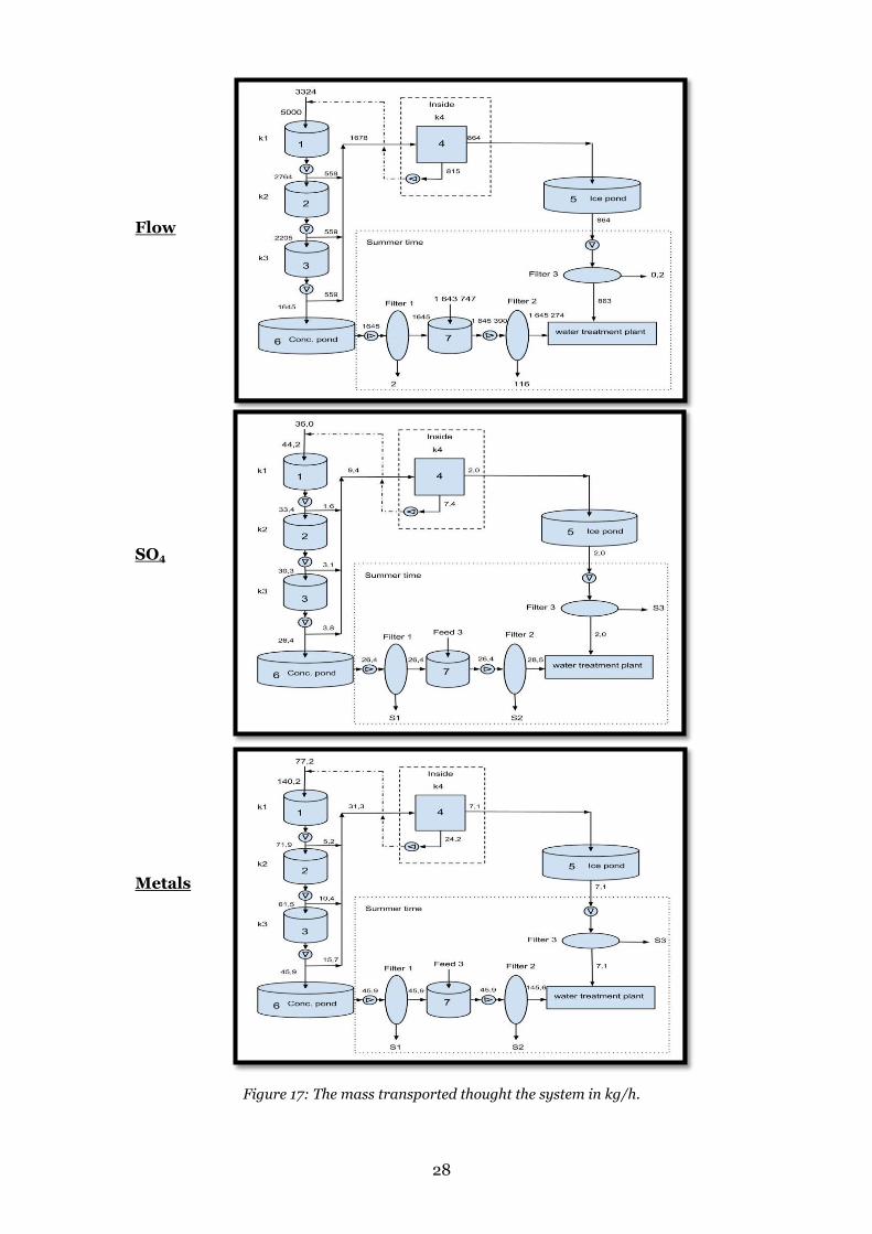
28
Flow
SO4
Metals
Figure 17: The mass transported thought the system in kg/h.

29
4.5.2 Artificial
The artificial freezing large scale method is based on some ideas from articles [2,4,20]
that uses cooled disc column crystallizer. In these articles the procedure worked really
well but they did not have the same amount of difficult ions that do not precipitate in
cold atmospheres.
This crystalliser is basically an extraction column with the cold coming from the walls
that will be scraped continuously to remove ice.
The principle (figure 18) of this process is that the feed first goes through a heat
exchanger to reduce the temperature difference between feed and column. The feed is
than entered into the column at the lower end of it; the temperature in the column will
probably be around -20 ˚C at the bottom and possibly a higher temperature at the top.
The temperature depends on the double jacketed walls with a cooling agent and the
efficiency of the scraping of the inner walls driven by an engine.
Even though the separation is not easy, the ice will go to the top of the column and the
liquid with the highest concentration will be lower in the column.
The ice at the top will be pumped away to the heat exchanger cool the feed and melt the
ice. After that some of the water will be recirculated to the top of the column to wash
the ice. The rest of the ice will go to the water treatment plant. If there will be precipitate
in this phase, it will be collected before the treatment plant.
At the bottom the most concentrated liquid will be taken out, this brine will go through
a heat exchanger to increase the temperature, helping the ions to precipitate. The
temperature in the lower column will be at least 20 ˚C, but increasing it more would
probably be even better. The precipitate in the bottom of the column will be pumped
out and collected. The concentrated brine will go to a pond and wait to be diluted
(during the summer) to help with precipitating the Fe left in the solution. Before the
dilution the new precipitate is collected by pumping it through a filter and after that the
solution is diluted. The diluted solution will then go thru another filter to collect the
new precipitate and after that the brine will go to the treatment plant.

30
Figure 18: A simple overview of the artificial freezing process
4.5.3 Comparisons: natural vs. artificial
The difference between this and the natural one is that this will have double jacketed
walls with a cooling agent to reduce the temperature more efficiently than the natural
one. This cooling agent will take advantage of the cold temperatures. This could make
it possible to purify a higher quantity of ARD water/h and it will be less weather
dependent. This step is to separate the feed into pourer ice and higher concentrated
brine.
The major amount of solid product precipitates from the concentrated brine at a
temperature around and above 20 ˚C. This process is better adjusted to the precipitate
allowing it a higher temperature to make the precipitate process more efficient.
In either of these processes more tests need to be made, but the alternative most likely
to work is the artificial, but it is not certain that any of them will.
4.6 Other points
Some of the more important things to consider in this project is the time it takes for the
precipitation to start to occur and the amount of time it needs to reach maximum
precipitation. Here is also temperature an important factor.
The value of the precipitate per L starting solution was estimated on data from Main
test 3 but the problem is that it was filtrated within 24 h. What the total should be if the

31
fractions had the time to precipitate properly is unknown but the amount of solids
produced would increase.
The value of the precipitate is calculated using the Zn value listed on Boliden’s home
page 2013-07-15, 1895 USD/Ton Zn. The amount of Zn per Ton precipitate will be an
average of the 13 samples results from ALS (the cost of purifying the precipitate is not
included in the value). The average is rounded to 38000 mg/kg or 38 kg/Ton
precipitate. The precipitate is worth about 72 USD/Ton precipitate. The solid products
produced in Main test 3 were 1.7 g of precipitate per L starting solution or 1.7 kg/m3
starting solution (appendix 8). If this number is used, a ton of precipitate will be
produced from about 590 m3 starting solution.
5 Conclusions
This eutectic freezing method works, but not as well as we expected, mainly because of
the complexity of the ARD water from Maurliden.
The water seemed to totally freeze at -20 ˚C.
There is some precipitate formed during the freezing process but most of it precipitates
at higher temperatures and needs time to precipitate.
The majority of precipitate per volume unit is produced in the “none ice” and there is
no real explanation for this. One possibility could be that some of this precipitate would
have been in the ice fraction if another separation method were used.
XRD analyses of the precipitates show that samples had some jarosite, gypsum and/or
bassanite. The rest is amorphous and could not be detected. In element analyses, the
highest concentrations were of As, Zn, Fe and S.
It does not seem possible to selectively precipitate metal salts from this starting
solution. Jarosite is the only mineral detected by XRD and is certain to be in some of
the precipitate. The composition of the rest of the ions detected in the dissolved
precipitate are unknown which makes it hard to detect any variation in the actual
minerals.
Two plants were designed; one natural and one artificial, the two proposals need more
tests, but could work. The largest problem with the method is the fact that the majority
of the ions will precipitate at room temperature or higher, at least the ones producing
jarosite, which makes the freezing method a bit contradictive.
The approximated value of the precipitate was 72 USD/Ton minus possible
purification, investments and running costs. A ton of precipitate takes about 590 m3
starting solution according to assumptions and calculations.

32
6 Outlook
The main thing to follow up is the large scale plant. If one or both of these suggestions
are possible to use, cost estimation for implementation is needed.
To get a more efficient method, is it possible to combine the two proposed methods to
get a more efficient?
There is a need to more accurately measure the temperature changes in Maurliden to
get a better idea of the conditions than the general one that SMHI provided.
Would cool air improve the rate of the freezing, and could the purity of the ice be altered
because of this method of mixing?
7 Acknowledgement
I would like to acknowledge: The construction division at Boliden for building the
bucket stand and the lids and Bergteamet MEC for constructing the stirrers stand.
The workers at the concentrator plant for the use of the two temperature sensors and
for help with the installation, and Torbjörn Viklund for the help with the Labview
program.
Amang Saleh for teaching me the analyses and generally helping me in the laboratory.
Rolf Danielsson and the others at Pilotverket for support.
Johan Hansson, Jan-Eric Sundkvist and Tomas Hedlund for help, support and ideas
through this project.
Andreas Berggren for letting me come and do this project and also show much interest
and support during this time.
Lars Lövgren for taking the time and accepting to be the examiner on this project.
Manne Alstergren for the help with some of the figures and pictures.
Martin and Agneta Karlsson for support, help and ideas.

33
References
[1] D.G. Randall, J. Nathoo, A.E. Lewis, Desalination 266 (2011) 256.
[2] F.E. Genceli, R. Gartner, G.J. Witkamp, Journal of Crystal Growth 275 (2005) E1369.
[3] B. Habib, M. Farid, Chemical Engineering and Processing 45 (2006) 698.
[4] F. van der Ham, M.M. Seckler, G.J. Witkamp, Chemical Engineering and Processing 43 (2004) 161.
[5] F. van der Ham, G.J. Witkamp, J. de Graauw, G.M. van Rosmalen, Journal of Crystal Growth 198 (1999) 744.
[6] J. Jonsson, P. Persson, S. Sjoberg, L. Lovgren, Applied Geochemistry 20 (2005) 179.
[7] G.A. Norton, R.G. Richardson, R. Markuszewski, A.D. Levine, Environmental Science & Technology 25 (1991) 449.
[8] A. Lundkvist, Environment, G1ZM.
[9] A. Global, http://www.alsglobal.se/.
[10] H. Lange, Zinc LCK 360.
[11] H. Lange, Copper LCK 529.
[12] H. Lange, Aluminium LCK 301.
[13] D.G. Karamanev, L.N. Nikolov, V. Mamatarkova, Minerals Engineering 15 (2002) 341.
[14] A.E. Greenberg, Standard Methods for the examination of water and wastewater, sixteenth edition, American public health assosiation, Warshington DC, 1985.
[15] SMHI, Temperature in Maurliden, Average 1961-1990, 1961-1990.
[16] N. Instuments, What is LabView?, 2013.
[17] T-test, http://easycalculation.com/statistics/critical-t-test.php.
[18] F-test, http://www.danielsoper.com/statcalc3/calc.aspx?id=4.
[19] S.S. Zumdahl, Zumdahl, Susan A., Chemistry, 2006.
[20] F. van der Ham, G.J. Witkamp, J. de Graauw, G.M. van Rosmalen, Chemical Engineering and Processing 37 (1998) 207.

34

Appendix 1: Pre-tests – Method
Here are some of the methods for the more marginal experiments that can be read to
get a bigger picture of the total project.
Collecting the brine:
The first thing done in the lab part was to collect about 100 litres of ARD water from
well 11 in pond 11 [8] in Maurliden, the 14 of February. This was made by pumping it
into two 60 litre barrels, and from that a 100 ml sample was taken and sent to the
certified lab ALS in Luleå [9] for an element analysis called V3B. The elements included
in the analysis are listed in Appendix 3.
Test 1 - Quick analysis:
To be able to observe the concentration changes in the samples without sending every
sample to ALS, some quick analyses that were possible to do in the lab were carried out.
The quick analyses were performed on an ARD water sample. The choices of elements
for the quick tests were based on the results that had arrived from ALS (Appendix 3).
Six substances were of interest: iron, aluminium, zinc, copper, sulphate and fluorine.
Fluorine was eliminated because the method for measuring it was an old fluoride
selective electrode that could not be trusted, so it was never tested. Aluminium, zinc
and copper were tested with quick analyses from Hach Lange with the tests: LCK 360
for zinc [10], LCK 529 for copper [11] and LCK 301 for aluminium [12]. Iron was tested
according to a modified method based on the article of D.G. Karamanev [13] and
sulphate were tested with the turbidimetric method [14]. The preparation for these two
methods will be listed under the heading “iron and sulphate analyses”.
Test 2 - Total freezing:
Four minor test was made with the freezer during the time spent waiting for the rest of
the equipment to arrive. The only parts that were ready at this time were the freezer
and the lid. Because of that, there were no automatic stirring in the buckets and the
temperature was not recorded but estimated to about -20˚C.
There had been three different total freeze experiments, two in the beginning and one
at the end. This first test was to see if the water froze at all, about 2 litres of brine was
added to a 3 litre bucket and left in the freezer overnight. It was left there for 24 hours.
The second one was not very well documented so it is not totally clear if the starting
material had been concentrated through test 3 and 4 or if it was taken directly from the
barrel, either way it was placed in the freezer for about two weeks. After that it was
melted and the solids were filtered off.

The third freezing was with a 2 L sample from the barrel and it was left in the freezer
for five days. After that is was left to melt and equilibrate for a few days and then filtered
in a Büchner funnel.
Test 3 - No stirring:
To find out if stirring was needed or not, two simple tests were made. The test without
stirring started with a bucket containing about 2 litres of brine that was placed in the
freezer for a few hours to let some ice form. When the bucket was taken out of the
freezer, the ice had formed a shell around the liquid and two holes were made in the ice
to be able to pour it out. The liquid was filtered in a Büchner funnel with a Whatman
GF/B filter paper to see the amount of solid particles. The concentrated liquid was then
returned to the freezer to produce more ice, this cycle were repeated a few times to
investigate if it was possible to concentrate the liquid with this method.
Test 4 - Stirring:
The second test was done in the same way, but with hourly intervals the ice was broken
and the liquid was stirred to make sure no ice remained on the bottom or on the sides
of the bucket. After the sample had been in the freezer for the same time as the previous
test, it was filtered to separate the two phases. This test was also repeated a few times
to make the starting material more concentrated.
Test 5 - Cleaning ice:
The work proceeded with manual stirring (as in test 4) and the focus was now set on
the ice. The ice crystals seemed to be pure ice but the problem was the water between
the crystals (Picture 3D). Some different methods were tested to get rid of this water.
The first two methods of the ice tests were performed in a Büchner funnel for filtration.
The first test was made by pouring cold (~0 C) deionised water over the ice. The second
was to spray the ice with cold water from both a squeeze bottle and with a spray. The
final test was to drain the ice using nets (Picture 3C and D). The principle was to drain
most of the liquid from the ice, then move it to a bucket where it was left to melt to
about 50/50 ice/water mixture and then it was drained again in the net.
The last method gave the best results. Considering that the first methods needed
vacuum and filter paper. The last method was refined a little and used in the Main tests
later.
Material for the Main tests
The necessary starting equipment was a freezer, some stirrers, a modified lid with holes
for the stirrers and temperature sensors, but to make everything work some extra
material was needed.

To be able to take a representative sample from the barrels (Picture 1C) a stirrer on a
stand (Picture 1B) was needed to get adequate stirring during the time it took to collect
the sample. To collect the sample, a pump (Picture 1A) was used to extract the liquid
from the bottom of the barrel. About 15 L were taken and divided into the sample
buckets.
The minimum temperature in the freezer was about - 20 ˚C which would be too cold
considering that the temperature should to be in the same range as the outdoor
temperature in Maurliden during the winter months, which approximately is between
five and ten degrees below zero [15].
To be able to regulate the temperature around the buckets to between -5 to -10 °C; a
stand (Picture 2B) was constructed and the buckets were insulated (picture 2C and 2D).
When the freezer was set to medium effect the correct temperature was established.
Stirrers are needed to make the ice form many crystals instead of big blocks and the
point of this was to get automatic separation of ice and salt crystals when the stirring
stopped. The principle of this is that ice floats on the surface and salt descends to the
bottom [1].
To keep track of the temperature in the freezer and the water, two Pt-100 sensors were
used (Picture 2A), they were connected to a Labview program [16] (Picture 1A and B)
designed to log the last three hours with measurements every 10 seconds. The sensors
were calibrated between -50 and 50 °C, and they were placed in either the solution or
the air in the freezer.

A B
Picture 1A-B: A – Shows a schematic view of the Labview program. B - Shows the temperature variations in registered in Labview when the freezer has not been opened for 24
hours, it alternates between -7.5 and -9.5 °C.

Appendix 2: Pre-tests – Results
Test 1 - Quick analysis:
Based on the results from ALS (Appendix 3) some quick analyses on Al, Zn, Cu, Fe and
SO42- were performed and the results were compared.
The analyses for Al, Zn and Cu were quick analyses from Hach Lange, with the
instruction manual came a list with different ions that would influence the results
negatively. The Al test was very sensitive to F- but by diluting the starting material to
the point where F- and the other ions were below their limit, the test produced adequate
results. In the Zn test, Pb2+ was the most interfering ion according to the list but the low
content of it made the results adequate. The main problem for the Cu analysis was Fe
ions, and even though it was possible to dilute the sample enough to get the Fe
concentration below the limit, it still did not give a sufficiently good result compared to
ALS.
The total Fe ion concentration was analysed with the original method, this produced a
good result and was easy to use. The method for the sulphate analysis was also
previously addressed and produced acceptable result.
There was a need to restrict the variety of analyses to two types, considering the amount
of analysis needed. The possible analyses were: Al, Zn, Fe and SO42-. Taking into
account that a lot of samples would be prepared and analysed simultaneously would
have made it difficult to get the timing right that are needed for Al [12] and Zn [10]
analyses. The fact that Fe and SO42- have the highest concentrations in the samples and
it was possible to analyse a lot of samples simultaneously made the decision apparent
that Fe and SO42- would be the best elements to pursue.
Test 2 - Total freezing:
The first freezing test used about 2 L of brine that was placed in a freezer for 24 hours.
The temperature was estimated to about -20 °C and the sample seemed totally frozen.
An interesting discovery was that the ice had colour shiftings. It was darker at the
bottom and got lighter on the top, except for a really light layer at the bottom (Picture
8A) and a dark circle at the top (Picture 1B).
The second test was performed in the same way but this time it was placed in the freezer
for about 2 weeks. During this time the colour changes grew more and more apparent
as the time went by. The colour change remained also after melting and when filtrating,
three filter papers were needed to collect the precipitate. The bucket was not stirred
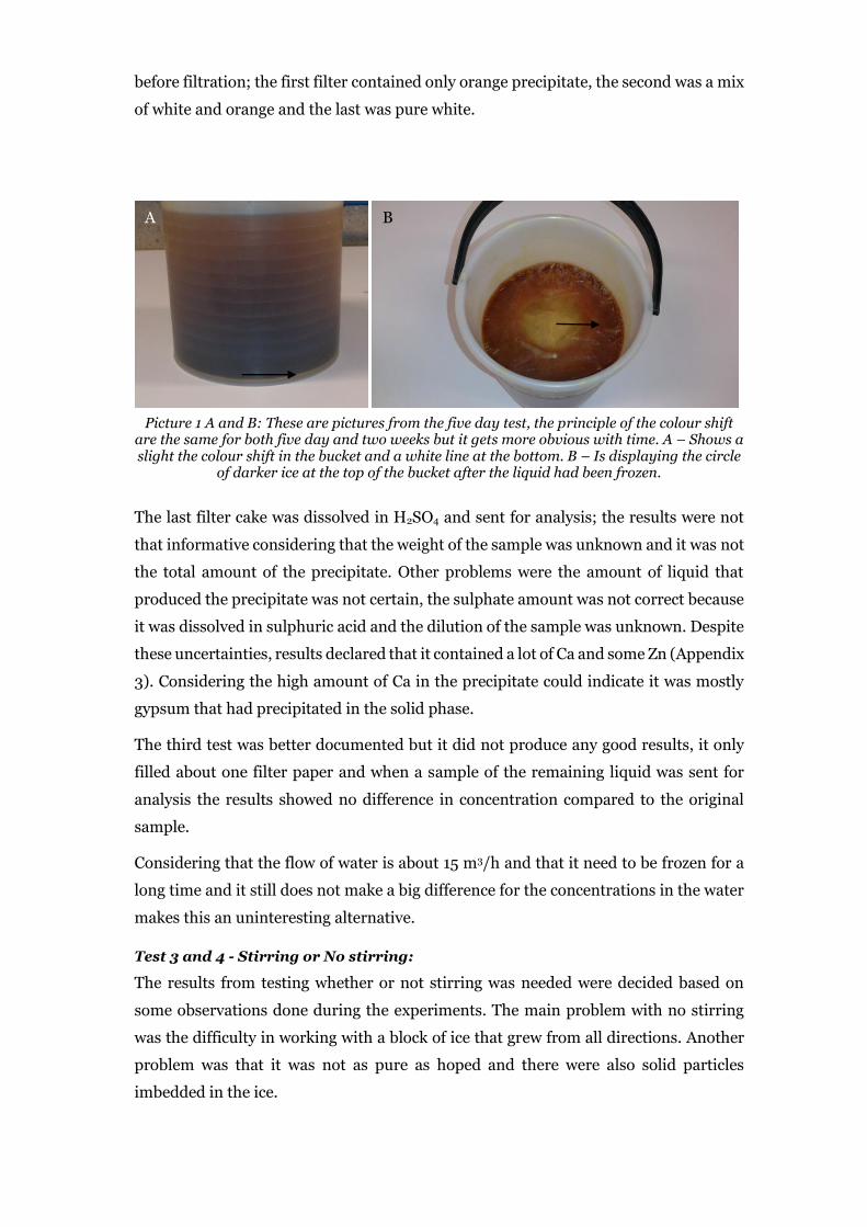
before filtration; the first filter contained only orange precipitate, the second was a mix
of white and orange and the last was pure white.
A B
Picture 1 A and B: These are pictures from the five day test, the principle of the colour shift are the same for both five day and two weeks but it gets more obvious with time. A – Shows a slight the colour shift in the bucket and a white line at the bottom. B – Is displaying the circle
of darker ice at the top of the bucket after the liquid had been frozen.
The last filter cake was dissolved in H2SO4 and sent for analysis; the results were not
that informative considering that the weight of the sample was unknown and it was not
the total amount of the precipitate. Other problems were the amount of liquid that
produced the precipitate was not certain, the sulphate amount was not correct because
it was dissolved in sulphuric acid and the dilution of the sample was unknown. Despite
these uncertainties, results declared that it contained a lot of Ca and some Zn (Appendix
3). Considering the high amount of Ca in the precipitate could indicate it was mostly
gypsum that had precipitated in the solid phase.
The third test was better documented but it did not produce any good results, it only
filled about one filter paper and when a sample of the remaining liquid was sent for
analysis the results showed no difference in concentration compared to the original
sample.
Considering that the flow of water is about 15 m3/h and that it need to be frozen for a
long time and it still does not make a big difference for the concentrations in the water
makes this an uninteresting alternative.
Test 3 and 4 - Stirring or No stirring:
The results from testing whether or not stirring was needed were decided based on
some observations done during the experiments. The main problem with no stirring
was the difficulty in working with a block of ice that grew from all directions. Another
problem was that it was not as pure as hoped and there were also solid particles
imbedded in the ice.

The stirring made the ice easier to control, the crystals seemed cleaner and no solid
particles were observed in the ice. There were two drawbacks with the stirring and that
was the concentrated water between ice crystals and the increased time for freezing the
sample. Stirring was the preferred method but the remaining problem was how to clean
the ice from the contaminated water.
Test 5 - Cleaning ice:
Two different methods were tested to clean the ice with deionised water, but it always
seemed to take equal or more water to rinse the ice than the amount of ice produced,
no matter the technique. By using any of the two methods, larger volumes of water
would get contaminated instead of the opposite. Instead a new approach was needed.
This approach was to let the ice clean itself by draining it twice: first to get off the
concentrated liquid and the second to take away the melted water when there was a
50/50 ice/water mix, this time there was less concentrated water between the crystals
and the ice got cleaner. Theoretically contaminated ice has a lower melting point than
pure ice. This method were improved and used in the Main tests.
Results from Main test materials
The isolation done to make the cooling come from above worked quit good, but there
were some ice formation on the walls despite the stirring.
The laboratory stirrers used in the tests had different minimum speeds and it was not
possible to get an exact speed from any of them and the stirrers in the buckets needed
modified to fit the holes in the lid.
The mosquito net worked really well and all the ice got caught, but it is hard to say how
the original distribution of salts was with this technique.
The temperature data from Main test 1 are not as extensive as it was hoped to be
because the short sensors did not reach the brine in buckets if the buckets contained
less than 1.5 L, this made it into an ineffective tool to measure the temperatures in the
liquids.
One of the aims of using the sensors was to be able to see at what temperatures the ice
and salts starts to crystallize, but it was only possible to see the start of the ice
crystallisation through temperature changes. The ice crystallisation point was never
seen below –1 °C which tells that the concentration in the liquid was not high enough
to cause any severe changes of the freezing point, but the freezing point could be lower
in the brines that could not be measured.
The main use of the sensors was to keep track of the temperature in the freezer to make
sure that it stays within the limits. The freezer temperature was between -4 and -9 ˚C.

Other results from Main test 1
After all practical things were finished, a large scale test was able to start with 12 L of
brine to test how concentrated it could be. The procedure of how to divide the three
fractions (“conc”, ”none ice” and ”ice”) and what to do with the “conc” were roughly
clear before the test but what to do with the two other fractions were unconsidered.
This part was decided during the test and was not as well documented or thought out
as it should have been, mostly because it was unclear what would be relevant. A list over
the approximated stream of liquid is displayed in Appendix 4.
The ice fraction did not become as clean as expected and desired after the first freezing
[1] despite the second drainage. A thought about refreezing the other two fractions were
considered. There were two reasons for the refreezing test and they were to recover lost
ions and get cleaner ice. The basic principle was to mix “ice” with “ice” and “none ice”
with “none ice”, making them into two new starting points, freeze them in the same way
as the concentrated ones and test if that could make the “ice” and “none ice” even
cleaner.
The problem with the refreezing was that it was started somewhere in the middle of the
test and it keep forming more ice both from the concentrated liquid and from a much
purer refrozen “ice” and everything was mixed without any real control. Considering
that the refreezing part got so inconsistent, the only thing that was really interesting
about it was that there were improvements in the ice quality. Based on the experience
from this test a thought out flow chart could be made for the following Main tests.
The concentration was increased about three times for sulphate and 4.5 times for Fe
and Zn compared to the starting sample (as displayed in Figure 5) and it was still
possible to freeze out ice at -10 °C. When it was possible the water temperature was
measured to study if the freezing temperature had decreased, but in none of these
experiments did the temperature go below -1 ˚C.

Appendix 3 – ALS results
Table 1: V3B results (mg/L) Elements Start
sample V1 V11 V50 V51 V21 V18 White
dissolved precipitate
SO4 26700 22400 36000 28300 6780 2880 17000 22300
Fe 8370 7840 11300 6540 1130 534 5190 56,2
Zn 2910 2930 4200 2590 542 319 2100 17,3
Al 1240 1070 1550 1080 230 128 758 9,88
Mg 722 766 1090 659 144 88,5 560 5,6
As 621 500 788 456 46,8 11,6 344 4,3
Ca 465 481 650 391 89,1 66,2 363 557
S 10500 9510 13900 8510 1760 1050 6770 6310
K <4 <4 <4 <4 <4 <20 <4 3,28
Na 11,1 11,3 16,4 10,4 <5 <30 8,16 6,93
Ba <0,1 <0,2 <0,2 <0,1 <0,1 <0,2 <0,2 0,0701
Cd 7,11 8,52 11,2 7,22 1,52 0,898 6 0,275
Co 2,15 2,15 3,06 2,07 0,47 0,218 1,54 0,0145
Cr 0,32 0,394 0,475 0,301 <0,09 <0,2 0,226 0,0121
Cu 75,8 84,6 121 81,2 20,1 12,8 61 0,956
Hg 5,85 E-04 5,35E-04 2,82E-04 2,1E-04 3,68E-05 5,03E-05 1,84E-04 1,17E-04
Mn 192 175 249 160 35,4 20,1 125 1,22
Mo <0,05 <0,1 <0,1 <0,05 <0,05 <0,1 <0,1 0,00373
Ni 1,69 1,69 2,56 1,51 0,375 0,181 1,23 0,0347
P 27,3
Pb 1,41 1,04 1,21 0,581 0,211 0,118 0,615 0,456
Sb 2,3 2,17 3,61 1,71 0,156 0,0436 1,27 0,0966
Sr 0,473 0,453 0,624 0,486 0,112 <0,1 0,341 0,578
V 0,19 0,06 0,121 0,0457 <0,02 <0,04 <0,04 0,0104
Cl 16,4 19,4 29,2 18,9 9,94 2,27 16 22
F 93,8 95,8 137 58,1 31,7 10,3 59 <2,00
N-tot 9,81 <2,00 <2,00 12,4 2,1 0,46 <2,00 0,51
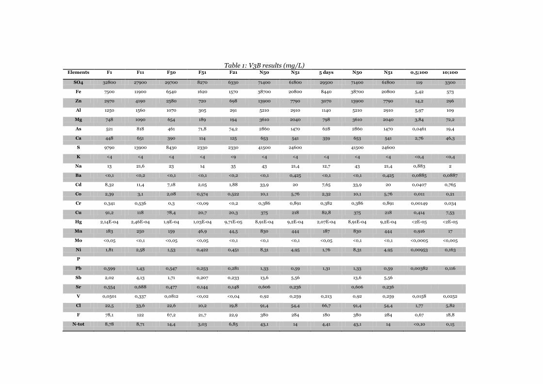
Table 1: V3B results (mg/L) Elements F1 F11 F50 F51 F21 N50 N51 5 days N50 N51 0,5;100 10;100
SO4 32800 27900 29700 8270 6330 71400 61800 29500 71400 61800 119 3300
Fe 7500 11900 6540 1620 1570 38700 20800 8440 38700 20800 5,42 573
Zn 2970 4190 2580 720 698 13900 7790 3070 13900 7790 14,2 296
Al 1250 1560 1070 305 291 5210 2910 1140 5210 2910 5,97 109
Mg 748 1090 654 189 194 3610 2040 798 3610 2040 3,84 72,2
As 521 818 461 71,8 74,2 2860 1470 628 2860 1470 0,0461 19,4
Ca 448 651 390 114 125 653 541 359 653 541 2,76 46,3
S 9790 13900 8430 2330 2330 41500 24600 41500 24600
K <4 <4 <4 <4 <9 <4 <4 <4 <4 <4 <0,4 <0,4
Na 13 21,6 23 14 35 43 21,4 12,7 43 21,4 0,883 2
Ba <0,1 <0,2 <0,1 <0,1 <0,2 <0,1 0,425 <0,1 <0,1 0,425 0,0885 0,0887
Cd 8,32 11,4 7,18 2,05 1,88 33,9 20 7,65 33,9 20 0,0407 0,765
Co 2,39 3,1 2,08 0,574 0,522 10,1 5,76 2,32 10,1 5,76 0,011 0,21
Cr 0,341 0,536 0,3 <0,09 <0,2 0,386 0,891 0,382 0,386 0,891 0,00149 0,034
Cu 91,2 118 78,4 20,7 20,3 375 218 82,8 375 218 0,414 7,53
Hg 2,14E-04 2,46E-04 1,9E-04 1,03E-04 9,71E-05 8,91E-04 9,2E-04 2,07E-04 8,91E-04 9,2E-04 <2E-05 <2E-05
Mn 183 250 159 46,9 44,5 830 444 187 830 444 0,916 17
Mo <0,05 <0,1 <0,05 <0,05 <0,1 <0,1 <0,1 <0,05 <0,1 <0,1 <0,0005 <0,005
Ni 1,81 2,58 1,53 0,422 0,451 8,31 4,95 1,76 8,31 4,95 0,00953 0,163
P
Pb 0,599 1,43 0,547 0,253 0,281 1,33 0,59 1,31 1,33 0,59 0,00382 0,116
Sb 2,02 4,13 1,71 0,207 0,233 13,6 5,56 13,6 5,56
Sr 0,554 0,688 0,477 0,144 0,148 0,606 0,236 0,606 0,236
V 0,0501 0,337 0,0812 <0,02 <0,04 0,92 0,259 0,213 0,92 0,259 0,0158 0,0252
Cl 22,5 33,6 22,6 10,2 19,8 91,4 54,4 66,7 91,4 54,4 1,77 5,82
F 78,1 122 67,2 21,7 22,9 380 284 180 380 284 0,67 18,8
N-tot 8,78 8,71 14,4 3,03 6,85 43,1 14 4,41 43,1 14 <0,10 0,15

Table 2: I1c results (mg/kg) Elements V1 V11 V50 V51 V21 F1 F11
As* 9790 20200 18700 45800 45600 18100 11400
Fe* 119000 184000 168000 286000 297000 166000 131000
Zn* 40600 40500 42000 23000 18000 43900 44500
S* 133000 102000 135000
Ba* 0,831 11,8 2,83 20,3 52,4 30,8 14
Be* 0,517 0,492 0,526 <0,3 0,271 0,537 0,586
Cd* 110 111 116 64,6 60,9 121 126
Co* 29,8 30,3 32,2 19,4 14,3 32,3 33,5
Cr* 4,95 6,91 6,11 6,59 9,51 6,05 5,5
Cu* 1130 1280 1200 909 1080 1230 1310
Hg* <0,9 <1 <1 <3 <3 <1 <1
Mn* 2410 2430 2370 1420 1110 2550 2700
Mo* 0,37 2,78 1,4 4,27 8,22 1,16 0,594
Ni* 25,5 27,6 25,4 18,7 18,9 27,1 27,5
P* 769 1250 1250 3170 3190 1190 890
Pb* 70,2 304 146 305 437 71,8 48,2
Sr* 19,9 13,3 8,91 10,3 14,2 8,15 8,17
V* 7,39 19,1 18,8 26,7 28,5 18,6 12,2
Table 2: I1c results (mg/kg) Elements F50 F51 F21 V18 N50 N51
As* 22300 36600 8790 16000 24300 16400
Fe* 188000 248000 122000 156000 197000 158000
Zn* 38800 29600 44000 42800 40700 44100
S* 130000 110000
Ba* 121 286 1,39 1,08 871 1,94
Be* 0,541 0,344 0,579 0,561 0,497 0,574
Cd* 110 81,8 120 119 119 125
Co* 31,1 23,2 32,2 31,3 31,1 32,4
Cr* 6,1 5,84 5,28 5,74 5,26 5,7
Cu* 1130 828 1270 1240 1190 1290
Hg* <2 <2 <1 <1 <1 <1
Mn* 2360 1710 2590 2480 2450 2600
Mo* 1,52 1,44 <0,4 1,2 1,06 1,28
Ni* 24,5 18,1 28,6 24,7 24,6 26,5
P* 1440 2650 779 1020 1780 1080
Pb* 160 99,2 186 126 73 107
Sr* 9,32 6,79 50,8 9,58 9,58 8,81
V* 41 61 3,28 18,2 35,7 15,7

Table 3: XRD results Amorphous Bassanite Gypsum Jarosite Clinochlore Quartz
F11 very high very low
F21 high high low
N50 high low low very low
N51 very high low
V1 high high low
V11 very high very low
V18 very high very low
V21 high low
0,1 in 100 all
10 in 100 all
5 days frozen very low high low low

Appendix 4 - Sample points Main test 1
1. Start product 2. D1-2 ice = D1 ice, D1 none ice, D2 ice, D2 none ice 3. D3 conc 4. D3 none ice Origin: 1 5. D3 ice 6. D4 conc 7. D4 part 1 none ice 8. D4 part 2 none ice Origin: 3 9. D4 part 1 ice 10. D4 part 2 ice 11. Refreeze none ice: D1-D4 part 1 conc 12. Refreeze none ice: D1-D4 part 1 none ice Origin: 2, 4, 7. Made in day 5 13. Refreeze none ice: D1-D4 part 1 ice 14. D5 conc 15. D5 none ice Origin: 6 16. D5 ice 17. Aggregate sample of refreeze none ice D4 part 2 and D5. Origin: 8, 15 18. Aggregate sample of refreeze ice D3-D5. Origin: 5, 9, 10, 16 19. D6 conc 20. D6 none ice Origin: 14 21. D6 ice 22. All none ice refreeze D1-D6. Origin: 11, 12, 17, 20 23. All ice refreezes 1 day D3-D5. Origin: 13, 18 24. All ice from D6 except ‘D6 ice’. Origin: 22 ice, 23 ice 25. Filtered and refreeze ice, conc 26. Filtered and refreeze ice, none ice Origin: 24 27. Filtered and refreeze ice, ice 28. D7 conc 29. D7 none ice Origin: 19 30. D7 ice 31. Refreeze all ice + none ice, conc 32. Refreeze all ice + none ice, none ice Origin: 20, 21, 22 conc + none ice, 33. Refreeze all ice + none ice, ice 23 conc + none ice, 26, 27 34. D8 conc 35. D8 none ice Origin: 28 36. D8 ice 37. Filtered ice refreeze 2 days conc Origin: 25 38. Filtered ice refreeze 2 days ice + none ice 39. All ice + none ice refreeze conc 40. All ice + none ice refreeze none ice Origin: 29, 30, 31 41. All ice + none ice refreeze ice 42. D9 conc 43. D9 none ice Origin: 34 44. D9 ice 45. All ice + none ice refreeze conc 46. All ice + none ice refreeze none ice Origin: 35, 36, 37, 39, 40 47. All ice + none ice refreeze ice 48. Ice from day 8 refreeze conc Origin: 32, 33, 38, 41 49. Ice from day 8 refreeze none ice + ice 50. D10 conc 51. D10 none ice Origin: 42 52. D10 ice 53. All ice + none ice conc 54. All ice + none ice none ice Origin: 48 55. All ice + none ice ice
All normal numbers are certain and the cursives are uncertain.
There were some of the fractions that ran out of brine after the sample were taken, these are some of the uncertain numbers the others were not documented at the time they were mixed and are part of a reconstruction it is therefore not clear if they are placed correctly.
There are some samples missing which are the reason for writing conc, none ice and ice after some of the numbers instead of the their own numbers.


Appendix 5: Sample points for Main test 2 and 3
1. Start product 2. D1 conc 3. D1 none ice Origin: 1 4. D1 ice 5. D2 conc 6. D2 none ice Origin: 2 7. D2 ice 8. D3 conc 9. D3 none ice Origin: 5 10. D3 ice 11. D4 conc 12. D4 none ice Origin: 8 13. D4 ice 14. D5 conc 15. D5 none ice Origin: 11 16. D5 ice
50. Mixed sample 3, 6, 9, 12 17. Refreeze none ice: D1-D4 conc 18. Refreeze none ice: D1-D4 none ice Origin: 3, 6, 9, 12. Made on day 5 19. Refreeze none ice: D1-D4 ice
51. Mixed sample 4, 7, 10, 13 20. Refreeze ice: D1-D4 conc 21. Refreeze ice: D1-D4 none ice Origin: 4, 7, 10, (Main test 3, 12 added 22. Refreeze ice: D1-D4 ice to the wrong batch), 13. Made on day 5 23. D6 conc 24. D6 none ice Origin: 14 25. D6 ice
52. Mixed sample 17, 18, 20 26. Refreeze ice + none ice D1-D4 conc 27. Refreeze ice + none ice D1-D4 none ice Origin: 17, 18, 20. Made on day 6 28. Refreeze ice + none ice D1-D4 ice
53. Mixed sample 19, 21, 22 29. Refreeze ice + none ice D1-D4 conc 30. Refreeze ice + none ice D1-D4 none ice Origin: 19, 21, 22. Never made, to 31. Refreeze ice + none ice D1-D4 ice small amount of liquid to do 32. D7 conc 33. D7 none ice Origin: 23 34. D7 ice 35. D8 conc 36. D8 none ice Origin: 32 37. D8 ice
54. Mixed sample 15, 24, 33, 36 38. Refreeze none ice: D5-D8 conc 39. Refreeze none ice: D5-D8 none ice Origin: 15, 24, 33, 36. Made on day 9 40. Refreeze none ice: D5-D8 ice
55. Mixed sample 16, 25, 34, 37 41. Refreeze ice: D5-D8 conc 42. Refreeze ice: D5-D8 none ice Origin: 16, 25, 34, 37. Made on day 9 43. Refreeze ice: D5-D8 ice
56. Mixed sample 38, 39, 41 44. Refreeze ice + none ice D5-D8 conc 45. Refreeze ice + none ice D5-D8 none ice Origin: 38, 39, 41. Made on day 10 46. Refreeze ice + none ice D5-D8 ice
57. Mixed sample 40, 42, 43 47. Refreeze ice + none ice D5-D8 conc 48. Refreeze ice + none ice D5-D8 none ice Origin: 40, 42, 43. Made on day 10 49. Refreeze ice + none ice D5-D8 ice
The blue text points out a difference between the two Main tests, the nr 12 brine in filtrated Main test 3 were added to the wrong bucket, 12 should be with 3, 6 and 9.
The red texts are samples that would have been made if there were enough brine to execute them.
The cursive text shows how the tests would have proceeded if there were enough time and brine.


Appendix 6: Fe, SO4 and pH
Table 1: Results from Fe, SO4 and pH analyses Fe tot Sulphate
Nr Sample point L pH Dilution Machine (mg/l)
Result (mg/l)
Note Dilution Machine (mg/l)
Result (mg/l)
Note
1 Start product L 2,23 5150,00 1,456 7498,40
a 1000,00
32,14 32140,00 a
1 Start product Di 2,23 10300,00 0,898 9249,40
a,4 1000,00
28,31 28310,00 a,7
2 D1-2 ice + non ice L 2,31 2060,00 1,040 2142,40
a 500,00 19,70 9850,00 a
2 D1-2 ice + non ice Di 2,31 2060,00 1,682 3464,92
a,4 500,00 27,64 13820,00 a,7
3 D3 conc L 2,20 5150,00 1,931 9944,65
b 1000,00
37,33 37330,00 b
3 D3 conc Di 2,20 5150,00 1,899 9779,85
b,3,6 1000,00
42,90 42900,00 b,5
4 D3 not ice L 2,30 5150,00 0,983 5062,45
b 500,00 36,20 18100,00 b
4 D3 not ice Di 2,30 5150,00 1,079 5556,85
b,3,6 500,00 44,37 22185,00 b,5
5 D3 ice L 2,34 2060,00 1,196 2463,76
b 500,00 22,17 11085,00 b
5 D3 ice Di 2,34 3433,33 0,817 2805,03
b,3,6 500,00 26,95 13475,00 b,5
6 D4 conc L 2,16 10300,00 1,235 12720,5
c 1000,00
40,14 40140,00 c
6 D4 conc Di 2,16 10300,00 1,394 14358,2
c,6 1000,00
42,56 42560,00 c,5
7 D4 part 1 non ice L 2,25 5150,00 1,320 6798,00
c 500,00 40,20 20100,00 c
7 D4 part 1 non ice Di 2,25 5150,00 1,322 6808,30
c,6 500,00 43,74 21870,00 c,5
9 D4 part 1 ice L 2,21 2060,00 1,774 3654,44
c 500,00 30,18 15090,00 c
9 D4 part 1 ice Di 2,21 3433,33 1,049 3601,57
c,6 500,00 20,18 10090,00 c,5
8 D4 part 2 non ice L 2,26 10000,00 0,592 5920,00
c 500,00 35,10 17550,00 c
8 D4 part 2 non ice Di 2,26 10000,00 0,890 8900,00
c,6 1000,00
20,84 20840,00 c,7
10 D4 part 2 ice L 2,04 2000,00 1,091 2182,00
c 500,00 23,42 11710,00 c
10 D4 part 2 ice Di 2,04 5000,00 0,696 3480,00
c,6 1000,00
10,16 10160,00 c,7
11 Refreeze non ice conc L 2,03 5000,00 0,931 4655,00
c 500,00 33,01 16505,00 c
11 Refreeze non ice conc Di 2,03 10000,00 0,678 6780,00
c,6 1000,00
26,84 26840,00 c,7
12 Refreeze non ice non ice
L 2,08 5000,00 0,616 3080,00
c 500,00 29,85 14925,00 c
12 Refreeze non ice non ice
Di 2,08 5000,00 0,712 3560,00
c,6 1000,00
17,33 17330,00 c,7
13 Refreeze non ice ice L 2,16 666,67 1,471 980,67 c 500,00 12,84 6420,00 c
13 Refreeze non ice ice Di 2,16 3333,33 0,344 1146,67
c,6 500,00 9,84 4920,00 c,7
14 D5 conc L 1,98 10000,00 1,263 12630,0
c 1000,00
49,54 49540,00 c
14 D5 conc Di 1,98 10000,00 1,270 12700,0
c,8 1000,00
51,13 51130,00 c,7
15 D5 not ice L 2,11 10000,00 0,838 8380,00
c 1000,00
36,91 36910,00 c
15 D5 not ice Di 2,11 10000,00 0,935 9350,00
c,8 1000,00
33,27 33270,00 c,7
16 D5 ice L 2,25 2500,00 0,841 2102,50
c 500,00 18,94 9470,00 c
16 D5 ice Di 2,25 3333,33 0,688 2293,33
c,6 500,00 21,19 10595,00 c,7
17 D4-5 non ice L 2,18 5000,00 1,274 6370,00
c 500,00 39,84 19920,00 c
17 D4-5 non ice Di 2,18 10000,00 0,634 6340,00
c, 6 1000,00
29,16 29160,00 c,7
18 All ice to D5 L 2,27 2000,00 0,924 1848,00
c 500,00 20,59 10295,00 c
18 All ice to D5 Di 2,27 5000,00 0,467 2335,00
c, 6 500,00 15,93 7965,00 c,7
19 D6 conc L 2,06 10000,00 1,427 14270,0
c 1000,00
39,47 39470,00 c
19 D6 conc Di 2,06 10000,00 1,374 13740,0
c, 8, 3
1000,00
37,56 37560,00 c,7,3

20 D6 non ice L 2,15 10000,00 0,814 8140,00
c 1000,00
32,90 32900,00 c
20 D6 non ice Di 2,15 10000,00 0,856 8560,00
c, 8 1000,00
24,60 24600,00 c,7
21 D6 ice L 2,25 2500,00 1,163 2907,50
c 500,00 33,78 16890,00 c
21 D6 ice Di 2,25 10000,00 0,436 4360,00
c,6 1000,00
15,40 15400,00 c,7
22 Refreeze non ice ice L 2,17 5000,00 1,321 6605,00
c 1000,00
26,22 26220,00 c
22 Refreeze non ice ice Di 2,17 10000,00 0,685 6850,00
c, 6 1000,00
27,48 27480,00 c,7
23 Refreeze ice ice L 2,25 1428,57 1,346 1922,86
c 500,00 21,63 10815,00 C
Fe tot Sulphate
Nr Sample point L pH Dilution Machine (mg/l)
Result (mg/l)
Note Dilution Machine (mg/l)
Result (mg/l)
Note
24 All ice from D6 filtered, not D6 ice
L 2,27 1428,57 1,139 1627,14
c 500,00 26,38 13190,00 c
24 All ice from D6 filtered, not D6 ice
Di 2,27 10000,00 0,340 3400,00
c, 6 1000,00
8,44 8440,00 c,7
25 Filtered ice conc L 2,26 1666,67 1,261 2101,67
c 333,33 44,07 14690,00 c
25 Filtered ice conc Di 2,26 5000,00 0,556 2780,00
c,6 333,33 40,12 13373,33 c,7
26 Filtered ice non ice L 2,33 1666,67 0,288 480,00 c 333,33 13,74 4580,00 c
26 Filtered ice non ice Di 2,33 5000,00 0,481 2405,00
c, 6 333,33 13,79 4596,67 c,7
27 Filtered ice ice L 2,34 500,00 0,714 357,00 c 333,33 3,88 1293,33 c
27 Filtered ice ice Di 2,34 1000,00 0,641 641,00 c,6 333,33 6,50 2166,67 c,7
28 D7 conc L 2,05 10000,00 1,706 17060,0
c 1000,00
53,58 53580,00 c
28 D7 conc Di 2,05 10000,00 1,654 16540,0
c, 6, 2
1000,00
58,08 58080,00 c,9,2
29 D7 non ice L 2,14 10000,00 0,870 8700,00
c 1000,00
29,36 29360,00 c
29 D7 non ice Di 2,14 10000,00 0,929 9290,00
c,6, 3 1000,00
30,58 30580,00 c,7
30 D7 ice L 2,23 10000,00 0,396 3960,00
c 1000,00
18,21 18210,00 c
30 D7 ice Di 2,23 10000,00 0,468 4680,00
c, 6 1000,00
20,35 20350,00 c,7
31 Refreeze ice + non ice conc
L 2,20 5000,00 1,196 5980,00
c 1000,00
24,62 24620,00 c
31 Refreeze ice + non ice conc
Di 2,20 10000,00 0,705 7050,00
c,8,3 1000,00
22,83 22830,00 c,7,3
32 Refreeze ice + non ice non ice
L 2,24 5000,00 0,875 4375,00
c 1000,00
21,45 21450,00 c
32 Refreeze ice + non ice non ice
Di 2,24 10000,00 0,421 4210,00
c, 6 1000,00
14,24 14240,00 c,7
33 Refreeze ice + non ice ice
L 2,32 2500,00 0,536 1340,00
c 1000,00
5,83 5830,00 c
33 Refreeze ice + non ice ice
Di 2,32 5000,00 0,464 2320,00
c,6 1000,00
6,27 6270,00 c,7
34 D8 conc L 2,04 10000,00 1,672 16720,0
c 3333,33
19,53 65100,00 c
34 D8 conc Di 2,04 10000,00 1,718 17180,0
c, 4,2 3333,33
15,57 51900,00 c,9,2
35 D8 non ice L 2,10 10000,00 1,157 11570,0
c 1000,00
37,16 37160,00 c
35 D8 non ice Di 2,10 10000,00 1,257 12570,0
c,8,2 1000,00
40,99 40990,00 c,7,3
36 D8 ice L 2,23 5000,00 0,998 4990,00
c 1000,00
22,20 22200,00 c
36 D8 ice Di 2,23 10000,00 0,523 5230,00
c, 6 1000,00
23,03 23030,00 c,7
37 Filtered ice conc L 2,20 5000,00 1,007 5035,00
c 1000,00
25,22 25220,00 c
37 Filtered ice conc Di 2,20 10000,00 0,500 5000,00
c,6 1000,00
14,97 14970,00 c,7
38 Filtered ice ice + non ice
L 2,35 1428,57 0,842 1202,86
c 1000,00
6,24 6240,00 c
38 Filtered ice ice + non ice
Di 2,35 5000,00 0,229 1145,00
c,6 1000,00
4,62 4620,00 c,7
39 Refreeze ice conc L 2,21 5000,00 1,348 6740,00
c 1000,00
22,61 22610,00 c
39 Refreeze ice conc Di 2,21 10000,00 0,828 8280,00
c, 8,3 1000,00
22,64 22640,00 c,7
40 Refreeze ice non ice L 2,08 5000,00 0,690 3450,00
c 1000,00
18,32 18320,00 c
40 Refreeze ice non ice Di 2,08 10000,00 0,376 3760,00
c,6 1000,00
18,50 18500,00 c,7
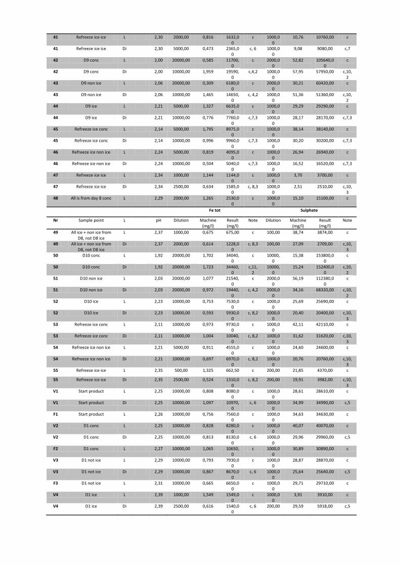
41 Refreeze ice ice L 2,30 2000,00 0,816 1632,00
c 1000,00
10,76 10760,00 c
41 Refreeze ice ice Di 2,30 5000,00 0,473 2365,00
c, 6 1000,00
9,08 9080,00 c,7
42 D9 conc L 2,00 20000,00 0,585 11700,0
c 2000,00
52,82 105640,00
c
42 D9 conc Di 2,00 10000,00 1,959 19590,0
c,4,2 1000,00
57,95 57950,00 c,10,2
43 D9 non ice L 2,06 20000,00 0,309 6180,00
c 2000,00
30,21 60420,00 c
43 D9 non ice Di 2,06 10000,00 1,465 14650,0
c, 4,2 1000,00
51,36 51360,00 c,10,2
44 D9 ice L 2,21 5000,00 1,327 6635,00
c 1000,00
29,29 29290,00 c
44 D9 ice Di 2,21 10000,00 0,776 7760,00
c,7,3 1000,00
28,17 28170,00 c,7,3
45 Refreeze ice conc L 2,14 5000,00 1,795 8975,00
c 1000,00
38,14 38140,00 c
45 Refreeze ice conc Di 2,14 10000,00 0,996 9960,00
c,7,3 1000,00
30,20 30200,00 c,7,3
46 Refreeze ice non ice L 2,24 5000,00 0,819 4095,00
c 1000,00
26,94 26940,00 c
46 Refreeze ice non ice Di 2,24 10000,00 0,504 5040,00
c,7,3 1000,00
16,52 16520,00 c,7,3
47 Refreeze ice ice L 2,34 1000,00 1,144 1144,00
c 1000,00
3,70 3700,00 c
47 Refreeze ice ice Di 2,34 2500,00 0,634 1585,00
c, 8,3 1000,00
2,51 2510,00 c,10,3
48 All is from day 8 conc L 2,29 2000,00 1,265 2530,00
c 1000,00
15,10 15100,00 c
Fe tot Sulphate
Nr Sample point L pH Dilution Machine (mg/l)
Result (mg/l)
Note Dilution Machine (mg/l)
Result (mg/l)
Note
49 All ice + non ice from D8, not D8 ice
L 2,37 1000,00 0,675 675,00 c 100,00 38,74 3874,00 c
49 All ice + non ice from D8, not D8 ice
Di 2,37 2000,00 0,614 1228,00
c, 8,3 100,00 27,09 2709,00 c,10,3
50 D10 conc L 1,92 20000,00 1,702 34040,0
c 10000,0
15,38 153800,00
c
50 D10 conc Di 1,92 20000,00 1,723 34460,0
c,11,2
10000,0
15,24 152400,00
c,10,2
51 D10 non ice L 2,03 20000,00 1,077 21540,0
c 2000,00
56,19 112380,00
c
51 D10 non ice Di 2,03 20000,00 0,972 19440,0
c, 4,2 2000,00
34,16 68320,00 c,10,2
52 D10 ice L 2,23 10000,00 0,753 7530,00
c 1000,00
25,69 25690,00 c
52 D10 ice Di 2,23 10000,00 0,593 5930,00
c, 8,2 1000,00
20,40 20400,00 c,10,3
53 Refreeze ice conc L 2,11 10000,00 0,973 9730,00
c 1000,00
42,11 42110,00 c
53 Refreeze ice conc Di 2,11 10000,00 1,004 10040,0
c, 8,2 1000,00
31,62 31620,00 c,10,3
54 Refreeze ice non ice L 2,21 5000,00 0,911 4555,00
c 1000,00
24,60 24600,00 c
54 Refreeze ice non ice Di 2,21 10000,00 0,697 6970,00
c, 8,2 1000,00
20,76 20760,00 c,10,3
55 Refreeze ice ice L 2,35 500,00 1,325 662,50 c 200,00 21,85 4370,00 c
55 Refreeze ice ice Di 2,35 2500,00 0,524 1310,00
c, 8,2 200,00 19,91 3982,00 c,10,3
V1 Start product L 2,25 10000,00 0,808 8080,00
c 1000,00
28,61 28610,00 c
V1 Start product Di 2,25 10000,00 1,097 10970,0
c, 6 1000,00
34,99 34990,00 c,5
F1 Start product L 2,26 10000,00 0,756 7560,00
c 1000,00
34,63 34630,00 c
V2 D1 conc L 2,25 10000,00 0,828 8280,00
c 1000,00
40,07 40070,00 c
V2 D1 conc Di 2,25 10000,00 0,813 8130,00
c, 6 1000,00
29,96 29960,00 c,5
F2 D1 conc L 2,27 10000,00 1,065 10650,0
c 1000,00
30,89 30890,00 c
V3 D1 not ice L 2,29 10000,00 0,793 7930,00
c 1000,00
28,87 28870,00 c
V3 D1 not ice Di 2,29 10000,00 0,867 8670,00
c, 6 1000,00
25,64 25640,00 c,5
F3 D1 not ice L 2,31 10000,00 0,665 6650,00
c 1000,00
29,71 29710,00 c
V4 D1 ice L 2,39 1000,00 1,549 1549,00
c 1000,00
3,91 3910,00 c
V4 D1 ice Di 2,39 2500,00 0,616 1540,00
c, 6 200,00 29,59 5918,00 c,5

F4 D1 ice L 2,40 1000,00 1,996 1996,00
c 1000,00
6,50 6500,00 c
V5 D2 conc L 2,28 5000,00 1,849 9245,00
c 1000,00
36,00 36000,00 c
V5 D2 conc Di 2,28 10000,00 0,895 8950,00
c, 6 1000,00
23,78 23780,00 c,5
F5 D2 conc L 2,29 10000,00 0,917 9170,00
c 1000,00
35,34 35340,00 c
V6 D2 non ice L 2,32 5000,00 1,318 6590,00
c 1000,00
22,31 22310,00 c
V6 D2 non ice Di 2,32 10000,00 0,777 7770,00
c, 6 1000,00
25,23 25230,00 c,5
F6 D2 non ice L 2,35 5000,00 1,395 6975,00
c 1000,00
20,59 20590,00 c
V7 D2 ice L 2,41 1000,00 1,917 1917,00
c 200,00 26,72 5344,00 c
V7 D2 ice Di 2,41 1000,00 1,985 1985,00
c, 8 200,00 31,14 6228,00 c,12,3
F7 D2 ice L 2,47 1000,00 1,148 1148,00
c 200,00 20,61 4122,00 c
V8 D3 conc L 2,28 10000,00 1,049 10490,0
c 1000,00
36,12 36120,00 c
V8 D3 conc Di 2,28 10000,00 0,793 7930,00
c, 6 1000,00
38,62 38620,00 c,5
F8 D3 conc L 2,27 10000,00 0,972 9720,00
c 1000,00
42,17 42170,00 c
V9 D3 not ice L 2,32 5000,00 1,219 6095,00
c 1000,00
27,72 27720,00 c
V9 D3 not ice Di 2,32 10000,00 0,566 5660,00
c, 6 1000,00
24,23 24230,00 c,5
F9 D3 not ice L 2,31 10000,00 0,587 5870,00
c 1000,00
30,29 30290,00 c
V10 D3 ice L 2,39 1428,57 1,150 1642,86
c 333,33 27,84 9280,00 c
V10 D3 ice Di 2,39 3333,33 0,586 1953,33
c, 6,3 333,33 26,22 8740,00 c,5,3
F10 D3 ice L 2,41 2000,00 0,952 1904,00
c 333,33 30,40 10133,33 c
V11 D4 conc L 2,33 10000,00 1,495 14950,0
c 1000,00
36,90 36900,00 c
V11 D4 conc Di 2,33 10000,00 1,062 10620,0
c, 8,3 1000,00
37,51 37510,00 c,7
F11 D4 conc L 2,32 10000,00 1,216 12160,0
C 1000,00
46,79 46790,00 c
V12 D4 non ice L 2,38 10000,00 0,790 7900,00
C 1000,00
29,39 29390,00 c
V12 D4 non ice Di 2,38 10000,00 0,650 6500,00
c, 8,3 1000,00
20,00 20000,00 c,7,3
F12 D4 non ice L 2,37 10000,00 0,680 6800,00
C 1000,00
28,06 28060,00 c
Fe tot Sulphate
Nr Sample point L pH Dilution Machine (mg/l)
Result (mg/l)
Note Dilution Machine (mg/l)
Result (mg/l)
Note
V13 D4 ice Di 2,48 3333,33 0,400 1333,33
c, 8,3 500,00 8,18 4090,00 c,7,3
F13 D4 ice L 2,49 2000,00 0,790 1580,00
c 2 500,00 12,65 6325,00 c
V17 Refreeze non ice conc L 2,31 10000,00 0,522 5220,00
C 1000,00
32,25 32250,00 c
V17 Refreeze non ice conc Di 2,31 10000,00 0,763 7630,00
c, 8 1000,00
30,68 30680,00 c,13
F17 Refreeze non ice conc L 2,29 10000,00 0,580 5800,00
C 1000,00
33,59 33590,00 c
V18 Refreeze non ice non ice
L 2,34 10000,00 0,305 3050,00
c 1000,00
16,86 16860,00 c
V18 Refreeze non ice non ice
Di 2,34 10000,00 0,483 4830,00
c, 8,3 1000,00
18,16 18160,00 c,13, 3
F18 Refreeze non ice non ice
L 2,37 10000,00 0,449 4490,00
c 1000,00
21,88 21880,00 c
V19 Refreeze non ice ice L 2,43 3333,33 0,254 846,67 c 500,00 14,23 7115,00 c
V19 Refreeze non ice ice Di 2,43 3333,33 0,645 2150,00
c, 8,3 500,00 15,70 7850,00 c,13, 3
F19 Refreeze non ice ice L 2,41 2000,00 0,393 786,00 c 2 500,00 11,04 5520,00 c 2
V20 Refreeze ice conc L 2,39 2000,00 0,526 1052,00
c 500,00 16,91 8455,00 c
V20 Refreeze ice conc Di 2,39 5000,00 0,421 2105,00
c, 8,3 500,00 14,17 7085,00 c,13, 3
F20 Refreeze ice conc L 2,41 3333,33 0,310 1033,33
c 500,00 16,21 8105,00 c
V21 Refreeze ice non ice L 2,43 2000,00 0,168 336,00 c 200,00 15,96 3192,00 c
V21 Refreeze ice non ice Di 2,43 3333,33 0,232 773,33 c, 8,3 200,00 10,20 2040,00 c,13, 3

F21 Refreeze ice non ice L 2,43 3333,33 0,310 1033,33
c 2 200,00 33,67 6734,00 c 2
V22 Refreeze ice ice L 2,61 142,86 0,341 48,71 c 33,33 14,40 480,00 c
V22 Refreeze ice ice Di 2,61 200,00 1,139 227,80 c, 8 33,33 18,59 619,67 c,13
F22 Refreeze ice ice L 2,52 500,00 0,976 488,00 c 2 100,00 33,79 3379,00 c 2
V26 Refreeze 17,18,20 conc L 2,35 5000,00 0,435 2175,00
C 1000,00
24,05 24050,00 c
V26 Refreeze 17,18,20 conc Di 2,35 5000,00 0,837 4185,00
c,8 1000,00
17,74 17740,00 c,10
F26 Refreeze 17,18,20 conc L 2,34 5000,00 0,532 2660,00
C 1000,00
21,66 21660,00 c
V27 Refreeze 17,18,20 non ice
L 2,38 2500,00 0,518 1295,00
C 1000,00
13,88 13880,00 c
V27 Refreeze 17,18,20 non ice
Di 2,38 5000,00 0,650 3250,00
c,8 500,00 22,33 11165,00 c,10
F27 Refreeze 17,18,20 non ice
L 2,40 3333,33 0,351 1170,00
C 500,00 18,50 9250,00 c
V28 Refreeze 17,18,20 ice L 2,46 666,67 0,989 659,33 C 200,00 21,11 4222,00 c
V28 Refreeze 17,18,20 ice Di 2,46 1000,00 1,044 1044,00
c,8 200,00 15,74 3148,00 c,10
F28 Refreeze 17,18,20 ice L 2,51 1000,00 0,668 668,00 C 200,00 18,50 3700,00 c
V50 Mixed sample non ice L 2,36 10000,00 0,914 9140,00
C 1000,00
23,67 23670,00 c
V50 Mixed sample non ice Di 2,36 10000,00 0,640 6400,00
c, 8,3 1000,00
25,60 25600,00 c,7,3
F50 Mixed sample non ice L 2,35 10000,00 0,600 6000,00
C 1000,00
23,31 23310,00 c
V51 Mixed sample ice L 2,44 1428,57 0,983 1404,29
C 500,00 13,00 6500,00 c
V51 Mixed sample ice Di 2,44 3333,33 0,416 1386,67
c, 8,3 500,00 10,55 5275,00 c,7,3
F51 Mixed sample ice L 2,46 2000,00 0,812 1624,00
C 500,00 16,78 8390,00 c
V52 Mixed sample 17,18,20 L 2,35 5000,00 0,621 3105,00
c 1000,00
14,14 14140,00 c
V52 Mixed sample 17,18,21 Di 2,35 10000,00 0,493 4930,00
c, 8 1000,00
15,64 15640,00 c,13,3
F52 Mixed sample 17,18,21 L 2,35 5000,00 0,373 1865,00
c 1000,00
26,77 26770,00 c
Notes:
L = Liquid, left after filtration 5 = dissolved in conc HCl, 0,1 ml
Di = Dissolved, solids dissolved in acid 6 = dissolved in conc H2SO4, 0,1 ml
a = about 20 ml sample to S+L and to Di 8 = dissolved in conc H2SO4, 0,2 ml
b = exact 20 ml sample to S+L and to Di 9 = dissolved in conc HCl, 0,7 ml
c = exact 10 ml sample to S+L and to Di 11 = dissolved in conc H2SO4, 0,4 ml
2 = some not dissolved solid left 12 = dissolved in conc HCl, 0,2 ml
3 = little not dissolved solid left


Appendix 7: Difference between ALS and laboratory results
Table 1: Difference between laboratory analyses and ALS Lab results ALS results Diff. Lab - ALS
Fe SO4 Fe SO4 Fe SO4
1 7498,40 32140,00 8 370,00 26 700,00 -871,60 5 440,00
50 34 040,00 153 800,00 38 700,00 71 400,00 -4 660,00 82 400,00
51 21 540,00 112 380,00 20 800,00 61 800,00 740,00 50 580,00
V1 8 080,00 28 610,00 7 840,00 22 400,00 240,00 6 210,00
V11 14 950,00 36 900,00 11 300,00 36 000,00 3 650,00 900,00
V18 3 050,00 16 860,00 5 190,00 17 000,00 -2 140,00 -140,00
V21 336,00 3 192,00 534,00 2 880,00 -198,00 312,00
F11 12 160,00 46 790,00 11 900,00 27 900,00 260,00 18 890,00
F21 1 033,33 6 734,00 1 570,00 6 330,00 -536,67 404,00


Appendix 8: Mass balance for Main test 3
Table 1: Mass balance for Main test 3 volume
(L) Tot (L)
Diff. (L)
Prod. (g)
Prod (g/L)
Average prod (g/L)
Amount of lost prod (g)
Start product 6,000 6,000 0,000 1,822 0,304
D1 conc 5,000 0,965 0,193
D1 none ice 0,400 5,800 0,200 0,708 1,770 0,784 0,157
D1 ice 0,400 0,156 0,390
D2 conc 4,450 1,003 0,225
D2 none ice 0,250 4,900 0,100 0,656 2,624 1,140 0,342
D2 ice 0,200 0,114 0,570
D3 conc 3,500 0,337 0,096
D3 none ice 0,350 4,250 0,200 0,261 0,746 0,367 0,183
D3 ice 0,400 0,103 0,258
D4 conc 2,750 0,557 0,203
D4 none ice 0,250 3,350 0,150 0,246 0,984 0,456 0,297
D4 ice 0,350 0,064 0,183
Refreeze none ice conc 0,400 0,349 0,873
Refreeze none ice none ice 0,125 0,625 0,175 0,154 1,232 0,845 0,317
Refreeze none ice ice 0,100 0,043 0,430
Refreeze ice conc 0,650 0,067 0,103
Refreeze ice none ice 0,175 0,900 0,050 0,056 0,320 0,230 0,161
Refreeze ice ice 0,075 0,020 0,267
Refreeze 17,18,20 conc 0,600 0,190 0,317
Refreeze 17,18,20 none ice 0,100 0,800 0,125 0,110 1,100 0,662 0,248
Refreeze 17,18,20 ice 0,100 0,057 0,570
Mixed sample none ice 0,800 0,800 0,200 0,263 0,329 0,329 0,066
Mixed sample ice 0,950 0,950 0,650 0,192 0,202 0,202 0,131
Mixed sample 17,18,20 0,925 0,925 0,250 - -
The estimated lost product was based on the diff. in liquid times the average amount of
produced precipitate;
D1: 0.2*0.784=0.157, D2: (0.2+0.1)*1.140=0.342, and so on.
The mixed samples are calculated by taking the loss in liquid times produced
precipitate.
The calculations for combining “Refreeze none ice together” with “mixed sample none
ice”: (0.625+0.800)*0.845=0.317, “Refreeze ice” together with “mixed sample ice”,
“Refreeze 17, 18, 20” together with “mixed sample 17, 18, 20”.
The columns were summed to:
Table 2: summation of table 1 Actual prod (g) Liquid loss (L) Estimated loss of prod (g) Estimated tot of prod. (g)
8,493 2,100 1,902 10,395


Appendix 9: Diagrams from SEM
Diagrams from SEM


Appendix 10: Mass balance for large scale application
Explanations of the flows in Figure 16 and table 1:
- S3 would be the precipitate of the ice, W6 would be the liquid from the ice and an estimation the
liquid concentration before anything had precipitate is W5.
- I4 is the ice of W5 and is therefore estimated to be the same.
- W4 (s) and W4 (l) are the ALS results from the non ice analysis and are recalculated to be only
dissolved ions in W4, the separation between W4 and I4 should be about 50/50.
- I1+I2+I3 are before ice and none ice is separated and is therefore the sum of I4 and W4.
- I1, I2 and I3 are expected to produce equal amounts of ice and therefore are I1+I2+I3 divided into
three equal parts. The concentration of ions should increase as the brine concentration increases
and therefore are the ions divided to give I1 a sixth of the ion, I2 got a third of them and I3 got
half of them.
- S1 would be the precipitate of the concentrated brine and together with the concentrated liquid,
called W8, the sum would be the content the “conc” fraction called W7. W7 and W3 should have
the same concentrations.
- W2 is the sum of W3 and I3, the same goes for W1 that is the sum of W2 and I2.
- Feed 1 is the sum Feed 1 (s) and Feed 1 (l) that are results from ALS. The green Feed 1 is the
calculated sum of W1 and I1 that should be comparable to the ALS results.
- Feed 2 is supposed to be used in the larger scale and in this mass balance the flow is adapted to
be 5000 kg for this feed. The flow is increased 553.5 times.
Table 1: Mass balance for Main test 3 and the natural large scale process Flow name Flow kg/h SO4 g/kg Fe g/kg Zn g/kg As g/kg SO4 kg/h metal kg/h
S3 0,2 0,07 0,01 0,01 0,0
W6 863 8,27 1,62 0,72 7,1 2,0
W5 864 8,27 1,62 0,72 0,00 7,1 2,0
I4 864 8,27 1,62 0,72 0,00 7,1 2,0
W4 (s) 1 0,24 0,05 0,03 0,0
W4 (l) 814 29,70 6,54 2,58 24,2 7,4
W4 815 29,66 6,53 2,58 0,00 24,2 7,4
I1+I2+I3 1 678 18,65 4,00 1,62 0,00 31,3 9,4
I1 559 9,33 2,00 0,81 0,00 5,2 1,6
I2 559 18,65 4,00 1,62 0,00 10,4 3,1
I3 559 27,98 6,01 0,81 0,00 15,7 3,8
S1 2 0,13 0,04 0,01 0,0
W8 1 644 27,90 11,90 4,19 45,9 26,4
W3 ≈ W7 1 645 27,87 11,89 4,19 0,00 45,9 26,4
W2 2 205 27,90 10,40 3,33 0,00 61,5 30,3
W1 2 764 26,03 9,10 2,98 0,00 71,9 33,4
Feed1 (s) 1 0,05 0,01 0,01 0,0
Feed1 (l) 3 321 32,80 7,50 2,97 108,9 34,8
Feed 1 3 322 32,79 7,50 2,97 0,00 108,9 34,8
Feed 3 1 643 747
W9 1 645 390 0,03 0,01 0,00 45,9 26,4
S2 116
W10 1 645 274 0,09 0,00 0,01 0,00 145,6 28,5
Feed 1 3 324 23,22 7,91 2,62 0,00 77,2 35,0
Feed 2 5 000 28,04 6,33 2,52 0,00 140,2 44,2